Regional data refine local predictions: modeling the distribution of plant species abundance on a...

Regional data refine local predictions: modelingthe distribution of plant species abundance on a portionof the central plains

Nicholas E. Young & Thomas J. Stohlgren &

Paul H. Evangelista & Sunil Kumar &

Jim Graham & Greg Newman

Received: 26 April 2011 /Accepted: 30 August 2011 /Published online: 13 September 2011# Springer Science+Business Media B.V. 2011

Abstract Species distribution models are frequentlyused to predict species occurrences in novel con-ditions, yet few studies have examined the conse-quences of extrapolating locally collected data toregional landscapes. Similarly, the process of usingregional data to inform local prediction for speciesdistribution models has not been adequately evaluat-ed. Using boosted regression trees, we examinederrors associated with extrapolating models developedwith locally collected abundance data to regional-scale spatial extents and associated with usingregional data for predictions at a local extent for anative and non-native plant species across thenortheastern central plains of Colorado. Our objec-tives were to compare model results and accuracybetween those developed locally and extrapolatedregionally, those developed regionally and extrapolat-ed locally, and to evaluate extending species distribu-tion modeling from predicting the probability ofpresence to predicting abundance. We developed

models to predict the spatial distribution of plantspecies abundance using topographic, remotelysensed, land cover and soil taxonomic predictorvariables. We compared model predicted mean andrange abundance values to observed values betweenlocal and regional. We also evaluated model predic-tion performance based on Pearson’s correlationcoefficient. We show that: (1) extrapolating localmodels to regional extents may restrict predictions,(2) regional data can help refine and improve localpredictions, and (3) boosted regression trees can beuseful to model and predict plant species abundance.Regional sampling designed in concert with largesampling frameworks such as the National EcologicalObservatory Network may improve our ability tomonitor changes in local species abundance.

Keywords Boosted regression trees . Speciesdistribution models . Spatial scale . Extrapolation .

National EcologicalObservatoryNetwork . Abundance

Introduction

Scaling ecological patterns and processes is a linger-ing challenge for ecologists (Levin 1992). Using theappropriate scale can have impacts on the ability tonot only identify ecological patterns but also tounderstand the processes driving those patterns (Scottet al. 2002). For example, the drivers of change at alocal scale are often influenced by past disturbances

Environ Monit Assess (2012) 184:5439–5451DOI 10.1007/s10661-011-2351-9

N. E. Young (*) : P. H. Evangelista : S. Kumar :J. Graham :G. NewmanNatural Resource Ecology Laboratory,Colorado State University,Fort Collins, CO, USAe-mail: [email protected]

T. J. StohlgrenUSGS, Fort Collins Science Center,2150 Centre Ave,Fort Collins, CO, USA

while drivers at a continental scale are primarilyclimatic (Brown et al. 2008). One area where scalehas been especially challenging is predicting speciesdistributions; often with the use of species distributionmodels (SDM).

Species distribution models relate species responsedata (either occurrence or abundance) with environ-mental characteristics (Elith and Leathwick 2009).These models have met many management objectivesincluding identifying previously unknown popula-tions of endangered species (Evangelista et al.2008b), predicting vulnerable habitats to speciesinvasions (Stohlgren et al. 2002), estimating speciesrichness (Graham and Hijmans 2006), and manyothers (Elith and Leathwick 2009). The breadth andapplication of SDMs has rapidly increased in the pastdecade. Advances in computer capabilities, availabil-ity of geospatial environmental data, and powerfulgeographic information systems facilitate modelingcomplex ecological interactions to predict speciesdistributions (Guisan and Thuiller 2005; Elith andLeathwick 2009). Some of the most common SDMsinclude Maxent (Phillips et al. 2006), boostedregression trees (BRT; Friedman et al. 2000), multi-variate adaptive regression splines (Friedman 1991),and Random Forests (Breiman 2001). Each algorithmoffers strengths and weaknesses for modeling speciesdistributions; multiple studies compare these methods(Araujo and New 2007; Elith and Graham 2009;Kumar et al. 2009; Parisien and Moritz 2009).Although these models are often compared using thesame data set, environmental predictors, and spatialscale, it is important to consider that SDMs aredesigned to handle different types of data sets andperform best under specific circumstances. For exam-ple, some models are designed for datasets with onlypresence locations like Biomapper (Hirzel et al. 2002)or Maxent while other models such as BRT orRandom forests require presence and absence data.

Although SDMs were developed to model specieswithin the environment from which the data werecollected (Guisan and Zimmermann 2000), thesemodels are now being used to predict species distribu-tions in space and/or time to novel conditions notrepresentative of the modeled environment (Elith et al.2010). This has been referred to as model projection,generalization, transfer, and extrapolation (Fielding andHaworth 1995; Randin et al. 2006), hereafter referredto as extrapolation. Model extrapolation has been

used to predict the distribution of a species underclimate change (Penman et al. 2010), in hypothe-sized susceptible regions of invasion (Medley 2010),and over large extents (Mateo-Tomas and Olea2010). While insights may be gained throughextrapolation, recent studies have suggested that thismay not always be the best approach to modelspecies distributions in novel environments (Pearsonet al. 2006). Thuiller et al. (2004) demonstrated thatextrapolating SDMs to regions not representing thecomplete range of environmental conditions maylead to highly liberal predictions of species occur-rence. On the other hand, regional data are moredifficult to collect and require more resources.Therefore, valuable resources (e.g., personnel, time,and money) will be saved if local data can beextrapolated to make accurate regional predictions.

While there have been some studies looking atextrapolating local prediction to regional extents, toour knowledge there have not been any studies that havelooked at the impact of using regional data to makepredictions at a local extent. In most cases, the extent ofinterest (e.g., national park, watershed, political bound-ary, etc.) is modeled using data collected at that extent (e.g., Stohlgren et al. 2010). This makes sense whenmodeling the global distribution of a species, butbecomes questionable when modeling a portion of aspecies distribution. Here, we explore this concept andhypothesize that using regional data to make predic-tions at a local extent can help capture largerenvironmental and response variation which has beenshown to improve model results (Elith and Graham2009) and improve local predictions.

Most SDMs are designed exclusively for presence-only or presence–absence data and are not compatiblewith abundance data. Under this framework, thesemodels predict the probability of presence or proba-bility of suitable habitat rather than a prediction of thenumber of species. Estimates of abundance allowmanagers to prioritize management actions that maynot be possible with predicted presence alone. Beforethe advent of powerful computers and geographicinformation systems, previous studies predictingspecies abundance primarily used regression methods(Evangelista et al. 2004; Crall et al. 2006). Thesemethods still serve as a foundation to many recentlydeveloped models (e.g., random forests and boostedregression trees). Identifying and predicting thespatial pattern of species abundance has advanced

5440 Environ Monit Assess (2012) 184:5439–5451

through the increased use of geographic informationsystems and spatial models (Sagarin et al. 2006). Partof the issue surrounding the lack of distributionmodels predicting abundance in the ecological com-munity is the fact that modeling abundance datarequires more robust statistical models than presence–absence data (Austin 2002) and abundance data areinherently rarer than presence/absence or presence-only data. Still, there are some recent examples whereSDM were used to model predicted abundance on alandscape (e.g., Strubbe et al. 2010). The accuracyand predictive capabilities of models that extrapolatethe distribution of species abundance from local toregional extents using only locally collected data arelargely unknown.

From management perspective, non-native speciescontinue to be an economic burden for organizationsresponsible for maintaining ecosystem integrity andprocesses (Mack et al. 2000). In most cases, the task ofsurveying an entire area for non-native species isunrealistic. Providing spatial abundances models ofnon-native species can help managers spatially priori-tize detection, control and prevention efforts. Thepurpose of this study was to examine the issue ofscale (in terms of spatial extent) and abundancepredictions associated with extrapolating SDMs devel-oped using locally collected data to regional extentsand predictions associated with using regional data tomake predictions at the local extent. Specifically, ourobjectives were to: (1) investigate how extrapolatingfrom local to regional scales impacts model results andaccuracy (2) compare local extent model results andaccuracy from models developed using data inside thelocal extent and to those developed with data insideand outside the local extent, (3) evaluate extendingSDM from predicting probability of presences topredicting abundance using boosted regression trees.We used abundance data (i.e., percent foliar cover) of anative and non-native species on a portion of thecentral plains and boosted regression trees.

Methods

Study area

We examined data at two extents on the central plainsof eastern Colorado (Fig. 1). We chose these extentsbecause they represent two of the four strategic

designs the National Ecological Observatory Network(NEON) has identified in their continental-scaleresearch platform for discovering and understandingthe impacts of climate change, land-use change, andnon-native species on ecosystem processes (NEON2010). There are 20 ecoclimatic domains establishedby NEON across the USA, and the local and regionalextents in this study represent the core wildland siteand the approximate footprint of aerial observations(airborne observatory platform), respectively, withinthe Central Plains domain (domain 10).

The core wildland site for domain 10 is at theCentral Plains Experimental Range, which is locatedin the Colorado Piedmont section of the Great Plains(40°49′ N and 104°46′ W). Covering 6,798 ha, thesite represents the local extent of our study area andfocal point of our research. This area is a semi-arid, C4-dominated native shortgrass steppe ecosystem. Mostof the precipitation occurs during the growing seasonfrom April to September. Grazing by domestic cattleis the dominant land use in conjunction with researchand monitoring projects including prescribed fire(Shortgrass Steppe Long Term Ecological Research;http://www.sgslter.colostate.edu).

The regional extent of our study area covers anarea of 40,000 ha, which represents the 20×20 kmfootprint of aerial observations defined by NEON forthis domain. This area was defined by NEON tocollect detailed aerial data about land-use and vege-tation structure (NEON). The regional extent encom-passes the local extent and is similar in terms ofclimate and ecological characteristics; however, landuse is more diverse. Much of the regional extent is amosaic of shortgrass steppe, agricultural land, range-land, and human development. Highway 85 runsnorth–south down the middle of the regional extentand the large developed area surrounding the town ofNunn is located in the southern portion.

Species

We chose to model common native and non-nativespecies to the central plains. Bouteloua gracilis (bluegrama), a warm season perennial bunchgrass, is nativeto the shortgrass steppe and considered a dominantspecies throughout the Colorado Piedmont. Although ithas evolved on the shortgrass steppe, Marilyn and Hart(1994) found that B. gracilis recovered poorly ondisturbed sites. Sisymbrium altissimum (tall tumble-

Environ Monit Assess (2012) 184:5439–5451 5441

http://www.sgslter.colostate.edu

mustard) is a non-native annual or biannual speciesfound in disturbed sites with other non-native andnative annuals (Allen and Knight 1984). S. altissimumcan be found on many different soil types (Patman andHugh 1961). Although both species are commonlyfound in the shortgrass steppe ecosystem, B. gracilis isgenerally a dominant species, while S. altissimum israrely dominant.

Field data

Local and regional abundance data were combined fromtwo separate studies. Data for the local extent werecollected in 2008 as a part of a NEON preliminaryassessment for the Central Plains Experimental Range(Evangelista et al. 2009a) that consisted of 20 sampledplots. Vegetation cover abundance data were recorded byestimating the percent cover within a 168-m2 circular,

multi-scale vegetation plot modified from the NationalForest Service Inventory and Analysis Program (Barnettet al. 2007); (Frayer and Furnival 1999). Regionalabundance data were collected with 72 Braun-Blanquetplots (Braun-Blanquet 1932). This relatively quickmethod of sampling is suited for species–environmentrelationships (Wikum and Shanholtzer 1978). Thesedata were collected at the regional extent with theexception of two locations which were sampled insidethe local extent. These two samples were added to thelocal extent dataset. This provided a dataset of 92samples for the regional models and 22 samples for thelocal models.

Environmental variables

We included soil, land cover, topographic and remote-ly sensed environmental data as our predictor varia-

Fig. 1 Study area showing sampled plots at the local and regional extents. The local and regional extents are within the larger centralplains domain (National Ecological Observatory Network domain 10)


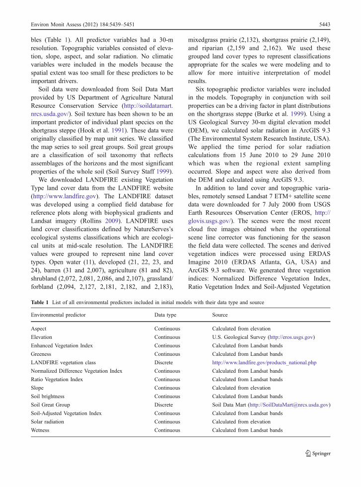
bles (Table 1). All predictor variables had a 30-mresolution. Topographic variables consisted of eleva-tion, slope, aspect, and solar radiation. No climaticvariables were included in the models because thespatial extent was too small for these predictors to beimportant drivers.

Soil data were downloaded from Soil Data Martprovided by US Department of Agriculture NaturalResource Conservation Service (http://soildatamart.nrcs.usda.gov/). Soil texture has been shown to be animportant predictor of individual plant species on theshortgrass steppe (Hook et al. 1991). These data wereoriginally classified by map unit series. We classifiedthe map series to soil great groups. Soil great groupsare a classification of soil taxonomy that reflectsassemblages of the horizons and the most significantproperties of the whole soil (Soil Survey Staff 1999).

We downloaded LANDFIRE existing VegetationType land cover data from the LANDFIRE website(http://www.landfire.gov). The LANDFIRE datasetwas developed using a complied field database forreference plots along with biophysical gradients andLandsat imagery (Rollins 2009). LANDFIRE usesland cover classifications defined by NatureServes’secological systems classifications which are ecologi-cal units at mid-scale resolution. The LANDFIREvalues were grouped to represent nine land covertypes. Open water (11), developed (21, 22, 23, and24), barren (31 and 2,007), agriculture (81 and 82),shrubland (2,072, 2,081, 2,086, and 2,107), grassland/forbland (2,094, 2,127, 2,181, 2,182, and 2,183),

mixedgrass prairie (2,132), shortgrass prairie (2,149),and riparian (2,159 and 2,162). We used thesegrouped land cover types to represent classificationsappropriate for the scales we were modeling and toallow for more intuitive interpretation of modelresults.

Six topographic predictor variables were includedin the models. Topography in conjunction with soilproperties can be a driving factor in plant distributionson the shortgrass steppe (Burke et al. 1999). Using aUS Geological Survey 30-m digital elevation model(DEM), we calculated solar radiation in ArcGIS 9.3(The Environmental System Research Institute, USA).We applied the time period for solar radiationcalculations from 15 June 2010 to 29 June 2010which was when the regional extent samplingoccurred. Slope and aspect were also derived fromthe DEM and calculated using ArcGIS 9.3.

In addition to land cover and topographic varia-bles, remotely sensed Landsat 7 ETM+ satellite scenedata were downloaded for 7 July 2000 from USGSEarth Resources Observation Center (EROS, http://glovis.usgs.gov/). The scenes were the most recentcloud free images obtained when the operationalscene line corrector was functioning for the seasonthe field data were collected. The scenes and derivedvegetation indices were processed using ERDASImagine 2010 (ERDAS Atlanta, GA, USA) andArcGIS 9.3 software. We generated three vegetationindices: Normalized Difference Vegetation Index,Ratio Vegetation Index and Soil-Adjusted Vegetation

Table 1 List of all environmental predictors included in initial models with their data type and source

Environmental predictor Data type Source

Aspect Continuous Calculated from elevation

Elevation Continuous U.S. Geological Survey (http://eros.usgs.gov)

Enhanced Vegetation Index Continuous Calculated from Landsat bands

Greeness Continuous Calculated from Landsat bands

LANDFIRE vegetation class Discrete http://www.landfire.gov/products_national.php

Normalized Difference Vegetation Index Continuous Calculated from Landsat bands

Ratio Vegetation Index Continuous Calculated from Landsat bands

Slope Continuous Calculated from elevation

Soil brightness Continuous Calculated from Landsat bands

Soil Great Group Discrete Soil Data Mart (http://[email protected])

Soil-Adjusted Vegetation Index Continuous Calculated from Landsat bands

Solar radiation Continuous Calculated from elevation

Wetness Continuous Calculated from Landsat bands


http://soildatamart.nrcs.usda.gov/

http://soildatamart.nrcs.usda.gov/

http://www.landfire.gov

http://glovis.usgs.gov/

http://glovis.usgs.gov/

http://eros.usgs.gov

http://www.landfire.gov/products_national.php

http://[email protected]

Index (Li and Weng 2005). These indices are forvegetation and land cover feature estimations. Tas-seled cap transformations were also conducted for theLandsat 7 scenes. Tasseled cap transformationsprovide measurements of soil brightness (tasseledcap, band 1), vegetation greenness (tasseled cap, band2) and soil/vegetation wetness (tasseled cap, band 3)(Huang et al. 2002). Tasseled cap bands and vegeta-tion indices have been shown to be effectivepredictors of plant occurrences when combined withSDMs (Evangelista et al. 2009b).

Analyses

For spatial analyses, we chose BRTs to model B. gracilisand S. altissimum at local and regional extents.Modeling species abundances using BRTs is a relativelynew method in ecology (Elith et al. 2008). In additionto being able to model abundance data, we chose BRTsbecause they have been shown to perform well withsmall sample sizes compared with other SDMs (Wisz etal. 2008) and because they can incorporate categoricalpredictor variables. Boosted regression trees attempt tominimize the loss function by generalizing many simpleclassification and regression trees. Tree-based models,such as BRTs, accomplish this by applying rules to thepredictors that partition the data into rectangles with themost homogeneous response (Elith et al. 2008).Boosting is a form of re-sampling that, unlike othermethods such as bagging or sub-sampling, applies aweighted probability of a response to be re-sampledbased on previous classifications (Franklin 2009). Therelative importance of the predictor variables is calcu-lated based on the number of times a predictor variablewas chosen as a splitting node and weighted based onthe improvement to the model based on each split(Friedman and Meulman 2003). BRTs are able todecrease over-fitting data by averaging the predictionsof many trees created using subsets of the data(Franklin 2009).

We used the generalized boosted models packagein R (R Development Core Team 2010) for our BRTanalyses (Friedman et al. 2000). There are a fewsettings that can be adjusted when running BRTs. Alow-learning rate decreases the model over learningbut requires more iterations (De’ath 2007). Optimiz-ing both the learning rate in conjunction with thenumber of trees is similar to model regularization.Regularization prevents models from over-fitting

training data. Interaction depth or tree complexity isthe number of nodes in each tree created. By addingmore nodes to the tree, more variable interactions areadded. With smaller datasets, larger tree complexityprovides no advantage (De’ath 2007). We performed5,000 iterations and ensured that at least 1,000 treeswere generated for each model (Elith et al. 2008)accomplished by a learning rate of 0.001 and a treecomplexity of 2.

Preliminarymodels for each species for both the localand regional extent were constructed using all 13predictor variables to identify those with the greatestpredictive contributions and reduce the overall numberof variables in our analyses. From these results, we keptonly the top 3 predictors and removed the remainingvariables due to the limited sample size for local models(Maxwell 2000). From those, we performed a Pear-son’s cross-correlation test using SYSTAT (version 12;SYSTAT Software, Port Richmond, California, USA)to remove highly correlated variables (Pearson’scorrelation coefficient, >0.8 or ≤0.8) keeping thevariable that had the highest contribution and thenselected the next predictor variable with the highestrelative influence to include in the final model. Thevariables remaining were used to develop final modelsfor each extent. Regional models for both species weredeveloped with data at both the local and regionalextent (n=92) while local models were developedusing only local data (n=22). To evaluate modelperformance, we used cross-validation during modeldevelopment and fit a linear regression betweenpredicted values and observed values to calculateadjusted r2 and also calculated Pearson’s correlationcoefficient (Potts and Elith 2006).

Finally, we compared the mean, minimum andmaximum across the extents for the predicted models.We also evaluated the difference between predictedabundance and observed abundance to comparemodels developed with local data and models devel-oped using regional data. The summary statistics werecalculated using SYSTAT.

Results

Predictor variables

Both the local model and the regional model for B.gracilis had similar predictor variables (Table 2). S.


altissimum final models for local and regional extentsalso had similar predictor variables (Table 3). Soil andslope proved to be key predictors for both species atboth extents. Soil great group was a key contributor atthe local extent models (>40% relative influence) forboth species, while slope was the important contrib-utor for the regional extent models (>40% relativeinfluence).

Model performance

Local and regional models showed significant predic-tive ability for both B. gracilis and S. altissimum (p<0.001). The local model for B. gracilis had a slightlyhigher explained variance (adjusted R2=0.65) than theregional model (adjusted R2=0.52). The same wastrue for S. altissimum local (adjusted R2=0.45) andregional (adjusted R2=0.44) models. Local modelsalso had a stronger association than regional modelswhen model predictions were compared with ob-served values (Pearson’s r for local and regionalmodels for B. gracilis=0.82, 0.72, respectively, and S.altissimum=0.69, 0.67, respectively).

Predictive map descriptions

For B. gracilis predictions at the local extent, the localmodel predicted more uniform abundance with higherabundance in the east closely aligned with soiltaxonomy (Fig. 2a). The regional model for the localextent showed much more variation in abundancepredictions than the local model, but showed similar

areas of high abundance (Fig. 2b). At the regionalextent, predictions for the local model of B. graciliswere highest in the southern portion and extendednorthward in bands following suitable soil types(Fig. 2c). The lowest abundance predictions werefound in the northern portion of the regional extentwhere the land cover is more barren and includes aportion of the Pawnee Buttes National Grassland. Theregional model predictions at the regional extentdiffers from the local model in that the highestpredicted abundance values are found in a swathrunning from the east to the northwest (Fig. 2d) withrelatively lower abundance predictions in the southand southwestern portions where there is more humandevelopment.

At the local extent, the mean abundance predic-tions for the local model (mean=27.4% cover, SE±6.9) and regional model (mean=22.1% cover, SE±7.5) for B. gracilis were similar, but the range ofabundance for the local model (33.8% cover) wasnarrower than the regional model (39.0% cover;Table 4). The regional model predicted a maximumabundance of 44.4% cover which was similar to thelocal model maximum abundance predictions (44.8%;Table 4). Furthermore, the minimum predicted abun-dance for the regional model was 5.4% while the localmodel minimum prediction was 11.0% (Table 4).

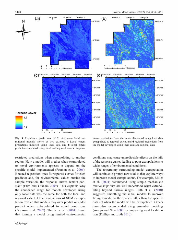
For S. altissimum predictions at the local extent,the local model predicted relatively low abundanceand little variation (Fig. 3a). In contrast, the regionalmodel had greater prediction variation and predictedrelatively higher abundance at the local extent

Local Regional

Predictor Relative influence Predictor Relative influence

Soil great group 41 Slope 43

Solar radiation 37 Soil great group 30

Slope 22 Solar radiation 27

Table 2 Relative influenceof environmental predictorsfor B. gracilis for the localand regional models

Local Regional

Predictor Relative influence Predictor Relative influence

Soil great group 57 Slope 66

Soil brightness 24 Soil brightness 26

Slope 19 Soil great group 9

Table 3 Relative influenceof environmental predictorsfor S. altissimum for thelocal and regional models


(Fig. 3b). At the regional extent, the local modelagain predicted relatively low abundance and littlevariation with lower abundance predictions in thesouthwest and southeast corners of the regionalextent and higher abundance predictions in swathsthat follow soil great groups (Fig. 3c). Conversely,the regional model had more variation in predictionsand predicted high abundance in the south-centralarea of the regional extent that extended northwest(Fig. 3d). These predictions coincide with the high-est observed abundance where the land use isprimarily agricultural.

At the local extent, S. altissimum regional andlocal models had a large difference in predictedabundance ranges (local=0.8% cover, regional=

4.1% cover). The difference in the range of predictedabundance can be attributed to the predicted maxi-mum abundance for each model (local=1.0% cover,regional=4.7% cover) even though the predictedminimum for the local model (local=0.2% cover)was less than the regional model (regional=0.6%cover). The predicted mean of the local model was0.5% cover (SE±0.2) and the regional model meanwas 1.1% cover (SE±0.5).

Difference comparison between observe and predictedvalues

For B. gracilis, models developed using local datapredicted an average 12% cover (SE±2.1, n=92)

Fig. 2 Abundance predictions of B. gracilis local and regionalmodels shown at two extents. a Local extent predictionsmodeled using local data and b local extent predictionsmodeled using local and regional data. c Regional extent

predictions from the model developed using local dataextrapolated to regional extent and d regional predictions fromthe model developed using local data and regional data


lower than observed values and 0.4% lower (SE±0.4,n=92) for S. altissimum. Conversely, the regionalmodels were off by an average 7% cover (SE±2.1,n=92) for B. gracilis and 0.1% cover (SE±0.3, n=92)for S. altissimum. For both species, the regional modelspredicted abundance values closer to the observedvalues than the local models.

Discussion

Using regional data can refine local predictions

Incorporating regional data improved the model rangeof predictions at local and regional extents. For bothspecies, the models developed using regional data tomodel the local geographical extent showed a largerrange of predicted abundances (Figs. 2d and 3d). Thiswas especially true for S. altissimum where themaximum predicted abundance for the regional modelwas more than four times that of the local model. Theimproved predictions may be attributed to theadditional landscape elements included by increasingthe extent sampled (Wiens 1989).

A larger range of predicted abundance can providemore detail and easier interpretations of predictions.Our results suggest the importance of collecting dataoutside the local area to not only capture environ-mental variation, but also species response variation.For example, locations with higher abundance of a

species of interest might exist just outside the area ofinterest being modeled; excluding data outside thearea increases the possibility of an invasion goingunnoticed. Modeling the potential distribution ofinvaders in the local area is essential to non-nativespecies risk characterization (Stohlgren and Schnase2006), and only possible by sampling outside thelocal area. Collecting additional regional samples mayimprove model predictions and reveal patterns missedby local models.

Extrapolation may restrict predictions

Using BRTs to extrapolate models using local datato regional extents may constrict the range ofpredicted values. Our results show that whenextrapolating local models to regional extents,predictions in the regional extent will not exceedthe range of predictions within the local extent. Forboth S. altissimum and B. gracilis, the modelsdeveloped using data collected at the local extentdid not predict abundance values below the mini-mum or above the maximum predicted within thelocal extent (Figs. 2 and 3). Our results are similar tothose of Menke et al. (2009) who looked atextrapolation of an Argentine ant in southernCalifornia and found if predictions are to be madefor larger un-sampled regions, additional sampling isneeded to capture the environmental variation inthose regions. Similarly, Randin et al. (2006) found

Bouteloua gracilis Sisymbrium altissimum

Local modelpredicted %cover

Regional modelpredicted %cover

Local modelpredicted %cover

Regional modelpredicted %cover

Regional extent

Maximum 44.8 44.4 1.0 4.7

Minimum 11.0 5.4 0.2 0.6

Mean 28.5 25.2 0.6 1.1

Mean standard error 7.2 7.5 0.2 0.6

Range 33.8 39.0 0.7 4.0

Local extent

Maximum 44.8 44.4 1.0 4.7

Minimum 11.0 5.5 0.2 0.7

Mean 27.4 22.1 0.5 1.1

Mean standard error 6.9 7.5 0.2 0.5

Range 33.8 39.0 0.8 4.1

Table 4 Local and regionalmodel predicted maxima,minima, means, mean stan-dard errors, and rangesacross the local and regionalextents


restricted predictions when extrapolating to anotherregion. How a model will predict when extrapolatedto novel environments appears to depend on thespecific model implemented (Pearson et al. 2006).Boosted regression trees fit response curves for eachpredictor and, for environmental values outside thesample variation, the response curves remain con-stant (Elith and Graham 2009). This explains whythe abundance range for models developed usingonly local data was the same for both the local andregional extent. Other evaluations of SDM extrapo-lation reveled that models may over predict or underpredict when extrapolated to novel conditions(Peterson et al. 2007). Thuiller et al. (2004) foundthat training a model using limited environmental

conditions may cause unpredictable effects on the tailsof the response curves leading to poor extrapolations towider ranges of environmental conditions.

The uncertainty surrounding model extrapolationwill continue to prompt new studies that explore waysto improve model extrapolations. For example, Milleret al. (2004) recommend using simple mechanisticrelationships that are well understood when extrapo-lating beyond narrow ranges. Elith et al. (2010)suggested smoothing the initial models to improvefitting a model to the species rather than the specificdata set when the model will be extrapolated. Othershave also recommended using ensemble modeling(Araujo and New 2007) or improving model calibra-tion (Phillips and Elith 2010).

Fig. 3 Abundance predictions of S. altissimum local andregional models shown at two extents. a Local extentpredictions modeled using local data and b local extentpredictions modeled using local and regional data. c Regional

extent predictions from the model developed using local dataextrapolated to regional extent and d regional predictions fromthe model developed using local data and regional data


Modeling abundance using boosted regression trees

Our results show BRTs can be an effective method tomodel plant species abundance. We generated accuratespatial distribution models for plant species abundanceat both local and regional extents.While the use of BRTsto predict abundance appears promising, uncertainty isinherent to all models and results should be carefullyinterpreted (Elith and Leathwick 2009). More specifi-cally, decision trees are sensitive to the response dataand environmental predictors being modeled (Berk2008). Modifying either of these can result in verydifferent models that have similar measured predictiveabilities (Scull et al. 2005). Interestingly, the S.altissimum regional model preformed the poorest ofall four models. This may be because S. altissimum is ageneralist species which tend to be more difficult topredict (Evangelista et al. 2008a) or because of therelatively low abundance of S. altissimum (often onlyobserved at 1% cover). While S. altissimum wasgenerally observed at low abundance values, a fewlocations were observed to have over 25% cover. Thesehigh abundances are not common but are important torecognize for non-native species management, and ourresults suggest that BRTs may not predict abundancesthat are unusually high. Also of note, none of themodels predicted abundance at 0% while there weremany sampled plots that had 0% cover. This mayindicate the predications should be interpreted as moreof a relative abundance than absolute. Therefore,modeled abundance predictions may be best appliedin conjunction with model probability of presence. Theprobability of presence models can be used to identifylocations of interest from which the abundancepredictions can provide a measure of the biomass atthose locations.

The ability to predict abundance rather than justprobability of presence may provide more than justwhere a species may occur but also information onthe quality of habitat (Pearce and Ferrier 2001). Interms of non-native species, this information mayhelp managers identify possible susceptible life stagesto control and prevent invasion (Brown et al. 2008).When managing and monitoring non-native species,abundance predictions can help prioritize control andprevention efforts in addition to early detection. ManySDMs are limited to presence–absence or presence-only data. This is most likely due to the costsassociated with obtaining abundance data compared

with presence–absences or presence-only data. Thishas prompted comparison studies that investigatedpossible correlations between probability of presenceand abundance. Unfortunately, these studies foundlittle correlation, and if so, only between highprobability of occurrence and high abundance (Pearceand Ferrier 2001; but see Vanderwal et al. 2009).

Conclusions

Extrapolating local models to regional extents islikely to predict abundance further from observedvalues when compared with models that includedregional data. Model extrapolation in time or space isprone to violating assumptions of SDMs (Wiens et al.2009). This is especially true for non-native speciesbecause they are rarely at equilibrium with theenvironment. When possible, additional samplesshould be collected in the regional extent to improvepredictions. These additional data can provideinsights into populations that may be just outside thelocal extent and would otherwise go unnoticed. Thisinformation can be important for regional and localconservation planning in prioritizing managementefforts. Future work may investigate the number ofadditional regional samples required and their optimallocation to provide the best predictions. Boostedregression trees can be a useful tool for modeling,and while BRTs are still largely unused in ecology(De’ath 2007), the recent increase of BRTs in theliterature is promising. The ability to take advantageof BRT capabilities will depend on abundance dataavailable with the development of large databasescollecting and disseminating ecological data (Grahamet al. 2007). An iterative approach to surveys andmodeling may gain a more comprehensive under-standing of modeling abundances and possible errorsstemming from model extrapolation. More researchinto the use and extrapolation of species distributionmodels to predict species abundance is needed to fullyunderstand the errors and benefits of this approach.

Acknowledgments The research for this study was funded byThe US Geological Survey (USGS), the National Science Founda-tion and the National Ecological Observatory Network, Inc. Wewould like to thank the Natural Resource Ecology Laboratory at theColorado State University for facility use and expertise. In addition,wewould like to thank the Colorado State University herbarium andstaff for access to their collection and for their expertise.


References

Allen, E. B., & Knight, D. H. (1984). The effects of introducedannuals on secondary succession in sagebrush-grassland,wyoming. The Southwestern Naturalist, 29, 407–421.

Araujo,M. B., &New,M. (2007). Ensemble forecasting of speciesdistributions. Trends in Ecology & Evolution, 22, 42–47.

Austin, M. P. (2002). Spatial prediction of species distribution:an interface between ecological theory and statisticalmodelling. Ecological Modelling, 157, 101–118.

Barnett, D., Stohlgren, T., Jarnevich, C., Chong, G., Ericson, J.,Davern, T., et al. (2007). The art and science of weedmapping. Environmental Monitoring and Assessment, 132,235–252.

Berk, R. A. (2008). Statistical learning from a regressionperspective. New York: Springer.

Braun-Blanquet, J. (1932). Plant sociology. The study of plantcommunities. New York: McGraw-Hill.

Breiman, L. (2001). Random forests. Technical report 567,University of California Berkeley, CA.

Brown, K. A., Spector, S., & Wu, W. (2008). Multi-scaleanalysis of species introductions: combining landscapeand demographic models to improve management deci-sions about non-native species. Journal of AppliedEcology, 45, 1639–1648.

Burke, I. C., Lauenroth, W. K., Riggle, R., Brannen, P., Madigan,B., & Beard, S. (1999). Spatial variability of soil properties inthe shortgrass steppe: the relative importance of topography,grazing, microsite, and plant species in controlling spatialpatterns. Ecosystems, 2, 422–438.

Crall, A. W., Newman, G. J., Stohlgren, T. J., Jarnevich, C. S.,Evangelista, P., & Guenther, D. (2006). Evaluatingdominance as a component of non-native species inva-sions. Diversity and Distributions, 12, 195–204.

De’ath, G. (2007). Boosted trees for ecological modeling andprediction. Ecology, 88, 243–251.

Elith, J., & Graham, C. H. (2009). Do they? How do they?Why dothey differ? On finding reasons for differing performances ofspecies distribution models. Ecography, 32, 66–77.

Elith, J., & Leathwick, J. R. (2009). Species distributionmodels: ecological explanation and prediction acrossspace and time. Annual Review of Ecology, Evolution,and Systematics, 40, 677–697.

Elith, J., Leathwick, J. R., & Hastie, T. (2008). Aworking guideto boosted regression trees. Journal of Animal Ecology, 77,802–813.

Elith, J., Kearney, M., & Phillips, S. (2010). The art ofmodelling range-shifting species. Methods in Ecologyand Evolution, 1, 330–342.

Evangelista, P., Stohlgren, T. J., Guenther, D., & Stewart, S. (2004).Vegetation response to fire and postburn seeding treatments injuniper woodlands of the grand staircase-Escalante nationalmonument, Utah. Western North American Naturalist, 64,293–305.

Evangelista, P. H., Kumar, S., Stohlgren, T. J., Jarnevich, C. S.,Crall, A. W., Norman, J. B., et al. (2008). Modellinginvasion for a habitat generalist and a specialist plantspecies. Diversity and Distributions, 14, 808–817.

Evangelista, P. H., Norman, J., Berhanu, L., Kumar, S., & Alley,N. (2008). Predicting habitat suitability for the endemic

mountain nyala (Tragelaphus buxtoni) in Ethiopia. WildlifeResearch, 35, 409–416.

Evangelista, P., Barnett, D., Stohlgren, T.J., Stapp, P.,Jarnevich, C., Kumar, S. & Rauth, S. (2009a). Fieldand costs assessment for the fundamental sentinel unit(FSU) at the central plains experimental range, Colorado.Technical Report for National Ecological ObservatoryNetwork, Inc., Boulder

Evangelista, P., Stohlgren, T., Morisette, J., & Kumar, S. (2009).Mapping invasive tamarisk (Tamarix): a comparison ofsingle-scene and time-series analyses of remotely senseddata. Remote Sensing, 1, 519–533.

Fielding, A. H., & Haworth, P. F. (1995). Testing the generalityof bird-habitat models. Conservation Biology, 9, 1466–1481.

Franklin, J. (2009). Mapping species distributions. Cambridge:Cambridge University Press.

Frayer, W. E., & Furnival, G. M. (1999). Forest surveysampling designs: a history. Journal of Forestry, 97, 4–10.

Friedman, J. H. (1991). Multivariate adaptive regressionsplines. The Annals of Statistics, 19, 1–67.

Friedman, J. H., & Meulman, J. J. (2003). Multiple additiveregression trees with application in epidemiology. Statisticsin Medicine, 22, 1365–1381.

Friedman, J., Hastie, T., & Tibshirani, R. (2000). Additivelogistic regression: a statistical view of boosting. TheAnnals of Statistics, 28, 337–374.

Graham, C. H., & Hijmans, R. J. (2006). A comparison ofmethods for mapping species ranges and species richness.Global Ecology and Biogeography, 15, 578–587.

Graham, J., Newman, G., Jarnevich, C., Shory, R., & Stohlgren,T. J. (2007). A global organism detection and monitoringsystem for non-native species. Ecological Informatics, 2,177–183.

Guisan, A., & Thuiller, W. (2005). Predicting species distribu-tion: offering more than simple habitat models. EcologyLetters, 8, 993–1009.

Guisan, A., & Zimmermann, N. E. (2000). Predictive habitatdistribution models in ecology. Ecological Modelling, 135,147–186.

Hirzel, A. H., Hausser, J., Chessel, D., & Perrin, N. (2002).Ecological-niche factor analysis: how to compute habitat-suitability maps without absence data? Ecology, 83, 2027–2036.

Hook, P. B., Burke, I. C., & Lauenroth, W. K. (1991).Heterogeneity of soil and plant N and C associated withindividual plants and openings in north american short-grass steppe. Plant and Soil, 138, 247–256.

Huang, C., Wylie, B., Yang, L., Homer, C., & Zylstra, G. (2002).Derivation of a tasselled cap transformation based on landsat7 at-satellite reflectance. International Journal of RemoteSensing, 23, 1741–1748

Kumar, S., Spaulding, S. A., Stohlgren, T. J., Hermann, K. A.,Schmidt, T. S., & Bahls, L. L. (2009). Potential habitatdistribution for the freshwater diatom Didymospheniageminata in the continental US. Frontiers in Ecology andEnvironment, 7, 415–420.

Levin, S. A. (1992). The problem of pattern and scale inecology. Ecology, 73, 1943–1967.

Li, G. Y., & Weng, Q. H. (2005). Using landsat ETM plusimagery to measure population density in Indianapolis,


Indiana, USA. Phoyogrammetric Engineering and RemoteSensing, 71, 947–958.

Mack, R. N., Simberloff, D., Lonsdale, W. M., Evans, H.,Clout, M., & Bazzaz, F. A. (2000). Biotic invasions:causes, epidemiology, global consequences, and control.Ecological Applications, 10, 689–710.

Marilyn, S. J., & Hart, R. H. (1994). 61 years of secondarysuccession on rangelands of the wyoming high-plains.Journal of Range Management, 47, 184–191.

Mateo-Tomas, P. & Olea, P.P. (2010). Anticipating knowledge toinform species management: predicting spatially explicithabitat suitability of a colonial vulture spreading its range.Plos One, 5:e12374

Maxwell, S. E. (2000). Sample size and multiple regressionanalysis. Psychological Methods, 5, 434–458.

Medley, K. A. (2010). Niche shifts during the global invasionof the asian tiger mosquito, aedes albopictus skuse(culicidae), revealed by reciprocal distribution models.Global Ecology and Biogeography, 19, 122–133.

Menke, S. B., Holway, D. A., Fisher, R. N., & Jetz, W. (2009).Characterizing and predicting species distributions acrossenvironments and scales: Argentine ant occurrences in theeye of the beholder. Global Ecology and Biogeography,18, 50–63.

Miller, J. R., Turner, M. G., Smithwick, E. A. H., Dent, C. L., &Stanley, E. H. (2004). Spatial extrapolation: the science ofpredicting ecological patterns and processes. Bioscience,54, 310–320.

NEON (2010). National Ecological Observatory Network Inc.Available at: http://www.neoninc.org/

Parisien, M. A., & Moritz, M. A. (2009). Environmentalcontrols on the distribution of wildfire at multiple spatialscales. Ecological Monographs, 79, 127–154.

Patman, J. P., & Hugh, I. H. (1961). Preliminary reports on theflora of wisconsin. No. 44. Cruciferae–mustard family.WisconsinAcademy of Science.Arts and Letters, 50, 17–73.

Pearce, J., & Ferrier, S. (2001). The practical value ofmodelling relative abundance of species for regionalconservation planning: a case study. Biological Conserva-tion, 98, 33–43.

Pearson, R. G., Thuiller, W., Araujo, M. B., Martinez-Meyer, E.,Brotons, L., Mcclean, C., et al. (2006). Model-based uncer-tainty in species range prediction. Journal of Biogeography,33, 1704–1711.

Penman, T. D., Pike, D. A., Webb, J. K., & Shine, R. (2010).Predicting the impact of climate change on australia’s mostendangered snake, hoplocephalus bungaroides. Diversityand Distributions, 16, 109–118.

Peterson, A. T., Papes, M., & Eaton, M. (2007). Transferabilityand model evaluation in ecological niche modeling: acomparison of garp and maxent. Ecography, 30, 550–560.

Phillips, S. J., & Elith, J. (2010). POC plots: calibrating speciesdistribution models with presence-only data. Ecology, 91,2476–2484.

Phillips, S. J., Anderson, R. P., & Schapire, R. E. (2006).Maximum entropy modeling of species geographic dis-tributions. Ecological Modelling, 190, 231–259.

Potts, J. M., & Elith, J. (2006). Comparing species abundancemodels. Ecological Modelling, 199, 153–163.

Randin, C. F., Dirnbock, T., Dullinger, S., Zimmermann, N. E.,Zappa, M., & Guisan, A. (2006). Are niche-based species

distribution models transferable in space? Journal ofBiogeography, 33, 1689–1703.

R Development Core Team (2010). R: a language andenvironment for statistical computing. R Foundation forStatistical Computing, Vienna, Austria.

Rollins, M. G. (2009). Landfire: a nationally consistentvegetation, wildland fire, and fuel assessment. Interna-tional Journal of Wildland Fire, 18, 235–249.

Sagarin, R. D., Gaines, S. D., & Gaylord, B. (2006). Movingbeyond assumptions to understand abundance distributionsacross the ranges of species. Trends in Ecology &Evolution, 21, 524–530.

Scott, M. J., Heglund, P. J., & Morrison, M. L. (2002).Predicting species occurrences: issues of accuracy andscale. Washington: Island Press.

Scull, P., Franklin, J., & Chadwick, O. A. (2005). The applicationof classification tree analysis to soil type prediction in a desertlandscape. Ecological Modelling, 181, 1–15.

Soil Survey Staff (1999). Soil taxonomy: a basic system of soilclassification for making and interpreting soil surveys (2ndedn). Washington, DC: US Department of Agriculture SoilConservation Service

Stohlgren, T. J., & Schnase, J. L. (2006). Risk analysis forbiological hazards: what we need to know about invasivespecies. Risk Analysis, 26, 163–173.

Stohlgren, T. J., Chong, G. W., Schell, L. D., Rimar, K. A.,Otsuki, Y., Lee, M., et al. (2002). Assessing vulnerabilityto invasion by nonnative plant species at multiple spatialscales. Environmental Management, 29, 566–577.

Stohlgren, T. J., Ma, P., Kumar, S., Rocca, M., Morisette, J.T., Jarnevich, C. S., et al. (2010). Ensemble habitatmapping of invasive plant species. Risk Analysis, 30,224–235.

Strubbe, D., Matthysen, E., & Graham, C. H. (2010). Assessingthe potential impact of invasive ring-necked parakeetsPsittacula krameri on native nuthatches Sitta europeae inBelgium. Journal of Applied Ecology, 47, 549–557.

Thuiller, W., Brotons, L., Araujo, M. B., & Lavorel, S. (2004).Effects of restricting environmental range of data toproject current and future species distributions. Ecography,27, 165–172.

Vanderwal, J., Shoo, L. P., Johnson, C. N., & Williams, S. E.(2009). Abundance and the environmental niche: environ-mental suitability estimated from niche models predicts theupper limit of local abundance. The American Naturalist,174, 282–291.

Wiens, J. A. (1989). Spatial scaling in ecology. BritishEcological Society, 3, 385–397.

Wiens, J. A., Stralberg, D., Jongsomjit, D., Howell, C. A., &Snyder, M. A. (2009). Niches, models, and climatechange: assessing the assumptions and uncertainties.Proceedings of the National Academy of Sciences of theUnited States of America, 106, 19729–19736.

Wikum, D. A., & Shanholtzer, G. F. (1978). Application ofbraun-blanquet cover-abundance scale for vegetation anal-ysis in land-development studies. Environmental Manage-ment, 2, 323–329.

Wisz, M. S., Hijmans, R. J., Li, J., Peterson, A. T., Graham, C.H., Guisan, A., et al. (2008). Effects of sample size on theperformance of species distribution models. Diversity andDistributions, 14, 763–773.


http://www.neoninc.org/

Regional data refine local predictions: modeling the distribution of plant species abundance on a...

Documents

Transcript of Regional data refine local predictions: modeling the distribution of plant species abundance on a...