1

(Don’t) try this at home!

The effects of recording devices and software on phonetic analysis

Chelsea Sanker, Sarah Babinski, Roslyn Burns, Marisha Evans, Jeremy Johns, Juhyae Kim,

Slater Smith, Natalie Weber, Claire Bowern

Yale University

Abstract

Because of restrictions on in-person research due to Covid-19, researchers are now relying on

remotely recorded data to a much greater extent than in the past. Given the change in

methodology, it is important to know how remote recording might affect acoustic measurements,

either because of different recording devices used by participants and consultants recording

themselves or because of video-conferencing software used to make interactive recordings. This

study investigates audio signal fidelity across different in-person recording equipment and

remote recording software when compared to a solid-state digital audio recording device that is

representative of the standard used in-person for elicitation and fieldwork. We show that the

choice of equipment and software can have a large effect on acoustic measurements, including

measurements of frequency, duration, and noise. The issues do not just reflect decreased

reliability of measurements; some measurements are systematically shifted in particular

recording conditions. These results show the importance of carefully considering and

documenting equipment choices. In particular, any cross-linguistic or cross-speaker comparison

needs to account for possible effects of differences in which devices or software platforms were

used. We close with a framework for researchers to use in deciding what types of recording may

be most appropriate.

2

1 Introduction1

1.1 Overview: fieldwork in a pandemic

Human subjects compliance boards across various institutions restricted approval of protocols

for in-person research for much of 2020, and at the time of writing many of these restrictions are

still in place. For this reason, and also for the safety of research participants, many researchers

have decided to either postpone phonetic elicitation or turn to alternative methods involving the

use of remote recordings. This has led to a rapid and dramatic shift in the types of technologies

used for phonetic elicitation both in fieldwork and other linguistic research, as well as language

documentation more broadly. In order to use the data collected online, it is necessary to know

how the recording device and recording software might impact acoustic measurements, both as

the last year’s recordings continue to be used, and as such methods become integrated in the

repertoire of recording techniques in language documentation and sociolinguistics.

While in-person linguistic fieldwork has primarily used digital recording equipment for 15 years

or more (cf. Bird and Simons 2003; Maddieson 2001; Podesva and Zsiga 2013), the use of video-

conferencing or social media software applications for primary fieldwork has not been

widespread until this year, a result of restrictions on travel and in-person interactions in response

to COVID-19 pandemic. Remote recording technology is readily accessible and many different

methods can be used. Prior to the pandemic, the types of technology used for linguistic

documentation and archiving had already started to shift away from dedicated solid-state audio

recorders such as those made by Edirol and Marantz, in favor of more easily accessible multi-use

technologies, such as smartphones (cf. Bird et al 2014; Goldman et al 2014).

With these new devices, however, come new issues around how audio is recorded. It has long

been noted that compression (van Son 2005), technical differences (e.g. transmission over

telephone lines; Künzel 2001; Rathcke et al 2017, and cell phones; Gold 2009, Hughes et al

2019) all affect measurements of the speech signal in more or less predictable ways. However, to

1 Division of work: CS, CB, RB and NW planned the project, with input from all authors. CS, CB, JK and NW made

the recordings. CS and CB analyzed the data. CS, CB, and RB led the paper writing, with extensive input from all

authors. Apart from the first and last authors, all names are ordered alphabetically.

3

our knowledge, there is no study which systematically tests the acoustic impact of recent

internet-based video conferencing programs in order to establish new best practices for language

documentation and sociolinguistic research (cf. Leemann et al 2020). Furthermore, though these

considerations have been discussed in technical phonetics venues, this knowledge appears to be

less commonly discussed among endangered language researchers. Our aim here is both to make

these issues more transparent and to suggest some best practices for researchers suddenly faced

with the shift to online recording.2

Without testing of this type, we do not know how the data that we record and archive today

encodes artefacts from these different technologies, and how comparable contemporary datasets

are to materials digitized from analog collections. In particular, the rapid shift to online fieldwork

raises questions, including whether this remotely recorded data is comparable to data collected

in-person, as well as what differences are likely to be present. While some acoustic signals may

be less affected by differences in recording method (e.g. F0, or possibly segment duration), other

types of measurements are likely to be more sensitive to differences between methods and

devices. For example, because the center of gravity (COG) in fricatives measures aperiodic

noise, differences in background noise based on the sensitivity of the microphone can influence

these measurements, particularly in spectrally diffuse fricatives like [f]. A high degree of

background noise could thus substantially alter the COG of [f], while fricatives with denser

spectral peaks exhibit less of an influence from background noise. There are many possible

sources for differences in acoustic signal recording, and therefore in the measurements that

might be impacted. Measurement issues that disproportionately impact certain sounds could thus

not only alter findings from the raw data but also the relative measurements that are necessary

for measuring production of phonological contrasts.

2 We therefore hope that the audience for this paper will include any linguists who engage with empirical data

collection that records speech, whether or not their primary aim is acoustic phonetic measurements. Given the

number of languages which are now endangered, one must assume that data collected now will be used in future for

projects well beyond their original purpose; therefore it is important to make sure that recordings are done as well as

possible. That is, in our view, even recordings made for research questions that do not rely on high quality audio

recordings should nonetheless make the best quality recordings possible, especially if the language is endangered.

4

In this paper, we report the results of a two-phase experimental data gathering study which tests

the impact of recording equipment and software applications on the recording output for

linguistic data. In the first phase, we gathered a single acoustic sample on six commonly

available technological devices. In the second phase, we recorded speech transmitted over

popular video conferencing applications in order to test the effects of that software on the audio.3

These methods were devised to highlight possible interactions between signal intake through a

device, signal transmission, and signal processing through different software. We compared

these recordings against a digitally recorded “gold standard” solid state recording. All recordings

were analyzed with the same methods. We found that some remote recording methods produce

acoustic measurements that statistically resemble the solid-state audio, whereas other remote

recording methods produce measurements that significantly differ from the solid-state audio

recordings. While identification of the acoustic correlates of phonological contrasts remains clear

in the majority of cases, the raw measurements are substantially altered for many characteristics,

including duration and spectral measurements. This raises potential issues for work on

comparative phonetic typologies or sociolinguistic or forensic research which relies on the

comparisons of acoustic data from different sources.

We begin with an overview of digital speech recording (Section 1.2). The design for our tests is

described in Section 2. We briefly summarize the results of tests in Section 3. Finally, in Section

4 we discuss the implications of our results for remote fieldwork, both during the pandemic and

in the future. The supplementary materials provide fuller discussion and analysis of the statistical

results.

1.2 Digital speech recording

When speech is recorded digitally, the air vibrations that comprise the speech signal are encoded

as a set of binary data that can be read by the computer, reconverted to audio and played through

speakers, and otherwise manipulated.4 The raw acoustic signal can be frequently sampled,

3 There are several factors which fall beyond the scope of this study such as the effects of technology on inter-

speaker, genre (see Hall-Lew and Boyd 2017), and formality differences (see Sneller 2021). As a result, we do not

make any claims about these results in comparison to other studies. 4 For more information about this process, see Zölzer (2008), Lyons (2011), and Lyons & Fugal (2014).

5

producing accurate reproductions. However, doing so creates large files. There is a tradeoff

between obtaining high fidelity and requiring excessive bandwidth when sending large amounts

of audio and video traffic over the internet. Many software programs thus compress recordings,

in order to reduce the amount of data that must be transmitted. To maximize comprehensibility

while reducing file size, certain parts of the signal may be compressed more than others , which

we discuss below.

Turning to the effects of digital (particularly online) recording on speech, there are several types

of acoustic signal manipulation which are likely to introduce variation: (1) different types of

compression; (2) artefacts introduced by filters of echoes and non-speech noise; and (3) different

sampling rates. These are in addition to variation produced from different types of recording

devices, including (4) shielding, (5) ambient noise, and (6) microphone placement. We describe

each of these below.

Audio compression can be lossless (that is, encoded in such a way that recorded information is

fully recoverable) or lossy, where parts of the signal are irretrievably compressed. The programs

or functions which convert audio signals into digital signals and back are known as codecs. Both

lossless and lossy codecs are in common use (cf. Drude et al 2011; Bowern 2015:18–36).

Compression may be vertical (compressing parts of the sound spectrum but not affecting timing),

or horizontal, where, for example, a timespan of silence is compressed. Any alterations in timing

can cause issues in frequency measurements (e.g. F0, formants), because frequency is defined by

the timing of the recurring wave. Compression can cause large jumps in frequency measurements

like f0, formants, and center of gravity, as well as smaller shifts in these measurements (van Son

2005; de Decker & Nycz 2015; Nash 2001).

Compression is often not uniform across the entire signal, but identifies repeating wave patterns;

a repeating cycle is mostly redundant information that can be reconstructed from more reduced

information. Compression systems often include some assumptions about the signal, such as

using this type of frequency-based compression (Sun et al. 2013). While selective compression

can result in a perceptually clearer output than uniform compression, it does not necessarily

preserve all of the acoustic cues that are relevant for phonetic analysis. Non-uniform

6

compression like this can exaggerate or eliminate spectral valleys, altering formants, f0, and

spectral tilt (Liu, Hsu, & Lee 2008). Although codecs usually have anti-aliasing filters, which

prevent conversion of frequencies that are higher than the sampling rate can measure, this does

not prevent the system from misidentifying the frequency and altering the signal based on the

assumed frequency. Compression can thus alter the signal, either by adding noise because some

parts of the signal are better preserved than others, or by building in assumptions made by a

codec in compression.

Digital audio may also include other non-speech artefacts. Some recording programs filter out

background noise and feedback (e.g. echos from the microphone picking up signal from the

device’s speakers5), which also decreases the amount of information that needs to be sent and

may improve the listening experience for individuals. However, manipulations to reduce noise

may also alter acoustic measurements depending on how the algorithm identifies noise and what

frequencies are attenuated or amplified. This kind of audio manipulation may also come from the

device itself. For example, some sound cards now include audio manipulation (e.g. boosting or

depressing certain frequencies). Finally, while not specific to the online transmission of speech,

digital audio recordings may also be contaminated by other types of noise, which will affect the

signal. Some artefacts in the signal might be introduced from equipment noise, or interference

from poor shielding, for example.6 These artefacts can alter measurements either because they

have directly altered the components of the signal that are being measured (e.g. boosting low

frequencies will alter spectral tilt) or because of more indirect effects in how acoustic

characteristics are measured (e.g. background noise in a similar frequency range as a formant

might shift measurements of that formant).

Digital audio can be sampled at different rates. The sampling rate may be constrained by a

variety of factors, such as the type of microphone that is used or the recording device itself.

5 For example, https://support.zoom.us/hc/en-us/articles/360046244692-Background-noise-suppression describes

some of Zoom’s background noise suppression techniques. 6 Shielding is what prevents devices from picking up other electrical signals, such as the hum from mains power

(electric network frequency) or transmissions between cell phones and phone towers. See Hua et al. (2020) for

discussion and exploitation of the incidental recording of electric network frequency.

7

Historically, different linguistic subfields have established different standards of recorded signal

fidelity. Within sociolinguistics, major documentation projects such as the Atlas of North

American English (Labov, Ash, & Boberg 2006) have made use of telephone-quality recordings

which have a sampling rate around 8kHz/s.7 It has long been considered best practice in language

documentation to use a sampling rate around 44.1 kHz/s, in order to create high-quality

recordings, even if lower quality would be adequate for the goals of the project (cf.

recommendations in field linguistics textbooks such as Bowern 2015). This is because

researchers cannot anticipate how future language records might be used; subsequent research

questions might require recordings with a high sampling rate. Projects which do not require high

sampling rates can employ a technique called downsampling.

Downsampling refers to reducing the frequency at which the audio spectrum is sampled. Keep in

mind that downsampling and compression are two separate transformations of digital data.

Downsampling changes the sampling rate so that samples are less frequent; this reduces how

much information is retained, but sampling rate is consistent across the signal. This does not alter

the information that is retained, so downsampling does not impact measurements that only

depend on low frequencies. Compression is more variable; as discussed above, compression

codecs may involve a range of processes that have a different impact on different frequencies

and may alter the signal, e.g. by identifying repeating or redundant information in the signal.

Lower sampling rates limit what frequencies can be measured, thus leading to less information at

higher frequencies (Johnson 2012). Most speech information, such as vowel formant structure, is

at lower frequencies (below 4000 Hz), and will not be obscured by lower sampling rates. Other

information, such as fricative frequency structure, is encoded in higher frequencies and can be

sensitive to sampling rate (Johnson 2012:51–53). In particular, fricatives often make use of a

measurement called the center of gravity (COG) (Gordon, Barthmaier, and Sands 2002). To get a

sense of how sampling rate can affect fricatives, we will revisit the point made above about

sampling rate standards used in different fields of linguistics. The standard sampling rate over

telephone lines, as sometimes used in sociolinguistic studies, is around 8kHz/s, whereas the

standard audio recording sample rate from a dedicated solid-state recorder is usually 44.1kHz/s.

7 See Leemann et al. (2020) for a discussion of cellphone data collection and best practices for online interviewing

in a sociolinguistic context.

8

Fricatives like [s] have spectral energy which exceeds 8kHz, meaning that some of the energy of

the [s] is cut off over the phone, but these frequencies are retained in recordings with higher

sampling rates. Sociolinguistic studies that use telephone recordings generally do not focus on

fricative contrasts, but rather on vowel contrasts (Labov, Ash, & Boberg 2006:4), which are not

as affected by the lower sampling rate. Even if a sound remains perceptually clear at lower

sampling rates, cutting off higher frequencies will result in lower COG measurements. If two

recordings have different sampling rates, it is important to downsample the one with the higher

sampling rate in order to make them comparable.

Finally, it is important to remember that the recording setup is important for recording clarity, as

fieldwork manuals have long noted. A poorly placed microphone (for example, one that is too far

from the speaker) or excessive ambient noise will lead to lower signal intensity. Further, as

mentioned above, excessive electrical equipment may also lead to distortion if the devices are

poorly shielded.8

To summarize, variation in the quality of the online recording can arise either from the software

program used or from the device used. The variation may arise via (1) compression, which may

preserve data optimized for human perception of speech but at the expense of manipulating the

signal irrecoverably; (2) artefacts in the signal introduced through equipment noise, poor

shielding, frequency limitations of devices, or through the background filters introduced by

software programs; or (3) different sampling rates. This, of course, is in addition to all the issues

about audio recording that fieldworkers are familiar with based on the circumstances of

recording, such as background noise, microphone placement, and the recording environment

(see, for example, Barwick 2006; Bowern 2015; Seyfeddinipur and Rau 2020).

8 In earlier analog recording equipment, poor shielding would often result in electrical hum if the device was

plugged into mains power, to the extent that early models of cell phones would also interfere with recordings when

they contacted the cell tower. We saw no evidence of such interference in our files, despite recording with multiple

devices in close proximity.

9

2 Methods

In this section we describe methods used to record and compare speech across multiple recording

devices and software programs. Given the number of ways one can record audio and share it

through social media, there are potentially limitless combinations of apps, software, and devices

to test. Our aim was not to produce a comprehensive set of comparisons; that would not be

feasible. Instead, we chose software applications and recording equipment that are already

commonly used, and we focused tests on those choices most likely to impact the audio signal.

For example, we made sure to test solid state recording equipment (the “gold standard” of in-

field recording) versus cellular telephones, but we did not test different brands of solid state

recorder. On the software side, we tested local recordings versus remote recording, but did not

additionally test files which were locally recorded through a device and then uploaded remotely.

Language users cannot repeat language utterances identically from production event to

production event, and background noise may differ across production events. Therefore, we

could not simply record the same speakers sequentially on different devices, because each

recording could introduce new variation. Instead, we constructed a two-phase setup so that all

comparisons occur between multiple recordings of the same production event. In Phase 1, each

speaker produced a set of stimuli while all devices recorded simultaneously. In Phase 2, the

recording from the solid-state recorder was used as the input to each software. Figure 1

summarizes the different recording conditions and the setup is described in more detail in

Sections 2.2 and 2.3 below.

Figure 1: Setup of recording phases.

10

In the remainder of this section, we discuss the stimuli we used (Section 2.1), the device setup in

Phase 1 and the software selection in Phase 2 (Sections 2.2 and 2.3), the types of acoustic

measurements we made (Section 2.4), and the statistical analyses (Section 2.5).

2.1 Stimuli

Stimuli were designed to test some parameters of acoustic interest (cf. Whalen et al 2020), in

particular using contexts where those parameters are part of the realization of distinctions made

in English (e.g. f0 as related to stress and onset voicing). The stimuli allowed us to construct a

vowel space for speakers, and also test f0, jitter, peak timing, duration, spectral tilt, Harmonics-

to-Noise Ratio (HNR), and the center of gravity (COG) of fricatives. The stimuli are given in the

Supplementary materials. Stimuli were 94 target words embedded in the carrier sentence “we say

[word] again” and delivered through PsychoPy (Pierce 2007) on the computer that was running

the internal microphone condition in Phase 1 (described in Section 2.2). The recordings were

made by three native speakers of English.9 One speaker (NW) was excluded from the statistical

tests of the by-device comparisons (Phase 1) due to a recording error with one device.

2.2 Device setup (Phase 1)

As briefly discussed above, we used a sample of convenience for recording equipment, and did

not attempt to include all possible configurations of internal and external microphones and types

of devices. We tested an array of commonly used devices, including two Macs, a tablet, two

cellular phones, and a handheld recorder. All devices were in airplane mode and running on

battery power. Table S1 in the supplementary materials gives the specifications of the items that

were tested. The recording took place in a quiet room in an otherwise empty building, but with

some street noise. Three speakers of English with different regional dialects recorded the stimuli

analyzed in this phase.10 The following picture illustrates the setup:

9 The three speakers are female, with ages between early 30s and early 40s. All three speak different English dialects

(two North American, one Australian). 10 Due to COVID-19 campus restrictions on who is permitted within university buildings, external participants were

not recruited. Social distancing measures were implemented during all recordings.

11

Figure 2: Phase 1 recording setup. (1) Zoom H4n; (2) ipad; (3) computer with internal

microphone; (4) computer with external headset microphone; (5) android phone; (6) iphone. See

supplementary materials for specifications

2.3 Software selection (Phase 2)

The second phase was carried out remotely to test recordings made over the internet. This

involved two researchers, mimicking the combination of the “local” and “remote” recordings of

a fieldwork consultant. In each case, the recordings made with the Handy Zoom H4n (“H4n”11)

solid state recorder in the first phase were played through the sound card of a 2012 Macbook Air

(where the H4n was recognized by the computer as an external microphone). The H4n was

connected to the computer using a TRRS connector cable attached to the headphone/line-out jack

of the H4n and the microphone/headphone combined jack in the Macbook Air. While this is not

equivalent to recording live speech, it does ensure that identical signals were transmitted across

each remote recording condition. The input from the H4n was recorded uncompressed at 44,100

Hz through the H4n’s internal microphones. The output was governed by the settings of the

software programs being used.

11 While these devices are typically referred to as “Zoom” recorders, we call this the H4n recorder to distinguish it

from the video conferencing software Zoom, which has no relationship to the solid state recorder.

12

The software programs which were tested were: Zoom, Skype, Facebook Messenger (using the

free program Audacity to make the recording, since Messenger does not have built-in recording

capabilities), and Cleanfeed, a commonly used podcast interview platform. Details of the remote

recordings conditions are given in the supplementary materials. Note that all software programs

here involve direct streaming of speech over the internet, as opposed to files which are recorded

locally and then transmitted asynchronously.12

2.4 Acoustic measurements

The software and devices used to make these recordings produce audio files in several different

formats. All audio files were converted to 16,000 Hz uncompressed mono wav files, because this

is the format required for forced alignment through p2fa. See Section 1.2 above for a discussion

of sampling rate; recall that downsampling is not the same thing as compression. Given that

some of the recording devices produced recordings with different sampling rates, downsampling

would be necessary anyway in order to avoid measurement differences due to sampling rate;

Center of Gravity measurements are higher with higher sampling rates, so work on fricatives

often downsamples in order to ensure comparable measurements across different studies (e.g.

Stuart-Smith et al 2019; Busso, Lee, & Narayanan 2007).

The audio files were then trimmed so that only the speech of the experiment was kept. These

recordings were force-aligned to the segmental level using the p2fa forced alignment scripts

described by Evanini et al (2009), which aligns at a resolution of 10ms.13 These recordings were

inspected for gross alignment errors (of which there were none) but were not further corrected.

We only used the data from the target words (not the carrier phrases) in these analyses.

Testing how the results of forced alignment compares to manual alignment is outside the scope

of this paper. Previous work has demonstrated a high level of agreement between manual

12 Programs which use the latter method -- local recording and upload -- include WhatsApp (voice messaging) and

Zencastr. 13 Because all files used the same speech input, it would be, in theory, possible to manually correct a single set of

“gold standard” alignments from the H4n recording and use the correctly aligned version in all experiment

conditions. However, in practice this is impossible, because the different lossy compression algorithms introduced

by different recorders leads in practice to non-identical file lengths. This is further discussed in Section 3.

13

alignment and manual segmentation when a large corpus is available for the language,

particularly when the word-by-word transcription is included and the recording contains read lab

speech (e.g. Hosom 2009). MacKenzie and Turton (2020), using FAVE (which is based on

p2fa), found that the mean disagreement with manual segmentation was in the range of 7.5-19.6

ms when applying to recordings that were not the training language variety; there is some

disagreement between manual coding and automatic coding, but the disagreement overall is

small, even in conditions that pose more segmentation challenges than ours. They used running

speech, largely from interviews. Agreement in alignment across human transcribers is not

substantially higher than forced aligner performance on the training language variety. For

example, Leung and Zue (1984), testing continuous speech in English, found 80% agreement

within 10 ms and 93% agreement within 20 ms. Wesenick and Kipp (1996), testing read speech

in German, found 87% within 10 ms and 96% within 20 ms.

The acoustic characteristics measured were: Duration, F1, F2, Center of Gravity (COG), jitter, f0

mean, f0 peak timing, spectral tilt (H1-H2), Harmonics-to-Noise ratio (HNR), and intensity.

Measurements were extracted using scripts in Praat (Boersma & Weenink 2017); references for

these scripts are provided in the supplementary materials All measurements are means taken

across the whole interval, except characteristics that are a single point by definition (e.g. time of

the f0 peak). Phonation measurements were calculated using Voice Report with the following

parameters: start, end, 65, 350, 1.3, 1.6, 0.03, 0.45. For COG, fricatives were extracted with

Hanning windows to create the spectral objects for analysis. Formants were analyzed with a

maximum frequency setting of 5500 Hz for 5 formants.

Signal to noise ratio was calculated by comparing the intervals labeled as “silence” in the forced

alignment versus those labelling the target words that were analyzed for the acoustic

characteristics described above. These were then averaged across each recording condition.

2.5 Statistical analyses

All statistical results are from mixed effects models calculated with the lme4 package in R (Bates

et al 2015). The p-values were calculated by the lmerTest package (Kuznetsova et al 2015). The

reference condition, which the other conditions were compared against, was always the H4n

recorder.

14

3 Results

Here we summarize the main results. For reasons of space and legibility, only an overview is

presented, and more thorough discussion of each condition is provided in the supplementary

materials. Section 3.1 provides a general overview of the key findings about variation between

devices and software programs and presumes minimal familiarity with phonetic measures.

Section 3.2 discusses the results of individual acoustic measurements, while Section 3.3. presents

an overview of findings with respect to recovery of data for the acoustic correlates of

phonological contrasts.

When reading the results, the size of the effects and the significance must be interpreted with

respect to the somewhat small amount of data. Lack of significance cannot be interpreted as

indicating that there is no real effect, and some of the estimates are large despite not being

significant, suggesting a high degree of variability. It is thus important to keep in mind that our

tests are, if anything, underestimating how many measurements are affected by the recording

program or device; some of the differences that do not reach significance in our data are likely to

be significant in a larger sample. A larger dataset would not eliminate the issues that we find; it

would just make it possible to identify effects with smaller effect sizes.

This overview should be read in conjunction with the supplementary materials, which provides

further discussion of all of these points (Supplementary Materials). We concentrate here on a

description of the results that will be accessible to linguists who do not use quantitative methods

extensively in their work but whose work is affected by recording choices.

3.1 Summary of results

While our set of measurements is not exhaustive, we cover several types of measurements that

exhibit effects of recording condition. These can broadly be grouped into measurements of

duration, measurements of intensity in aperiodic noise, and measurements of frequency.

First, as seen in more detail in Section 3.2, duration measurements seem to be affected by the

compression algorithms used in m4a formats. The effects on duration are likely influenced both

directly by lossy compression effects on timing and also indirectly when boundary assignment is

obscured by noise and lowered intensity of the signal. While manual segmentation might reduce

15

the latter effects, they would not be fully eliminated; see the supplementary materials for a

discussion of segmentation issues and how human segmenters are susceptible to the same

difficulties. The compression-based effects could not be improved at all.

Second, there are also differences in levels of background noise, efficacy in capturing the speech

signal, and filtering meant to remove background noise or boost the speech signal. Lowered

signal-to-noise ratios, either due to higher intensity of noise or lowered intensity of the signal,

directly impact measurements like the Harmonics-to-Noise ratio (HNR) and center of gravity

(COG). Changes in noise and intensity also have indirect effects in identification of segment

boundaries and measurement of other characteristics that depend on being able to isolate the

target characteristic of the speech signal.

Lastly, there are changes in measurements of frequency, observed in f0 and formants. These are

likely the result of lossy compression; depending on how the compression system handles

repeating waves, these could be over-regularized or obscured. Compression that alters the file’s

duration will also produce changes in spectral measurements. Some of the spectral issues may

also be caused by changes in intensity, as some recording conditions are less sensitive to certain

frequency ranges, which can subsequently change how formants and f0 are identified. Of course,

changes in intensity of different frequencies is also directly reflected in spectral tilt effects. Such

differences are also likely to affect perceptual clarity, making fieldwork using remote recordings

more difficult and making transcription less reliable.

There were a larger number of significant differences between software programs than between

devices. Signal to noise ratio measures differed significantly among devices, but most other

measures are not significantly different. As noted above, however, though the differences were

not all statistically significant, we did find measurement differences, that is, raw differences in

the measurements of variables beyond what one might expect. The software choices also led to

differences in signal to noise ratio and duration measurements.

Finally, we found that we were, in almost all cases, able to recover evidence for the phonemic

distinctions which were tracked (such as stressed versus unstressed vowels, voicing differences,

16

and vowel space measurements to capture vowel differences). However, the raw measurements

of the distinctions varied, in some cases substantially.

3.2 Individual Acoustic Metrics

For each measure, the results come from a linear mixed effects model with that characteristic as

the dependent variable. For Phase 1, device was the one fixed effect, and for Phase 2, program

was the one fixed effect. All models included a random intercept for speaker. The models for

formants and for COG also included a random intercept for segment.

3.2.1 Device comparisons

Table 2 below summarizes the different measures in the Phase 1 recordings, testing differences

based on recording device. Asterisks indicate significance levels at < 0.05 (*), < 0.01 (**), or <

0.001 (***). When a test was significant, then the direction of significance is also indicated in

that table cell. For readability, only significant results are included in the table; for the full

results, see the Supplementary Materials. Keep in mind that a lack of significant difference

doesn’t guarantee that the measurement is measured equivalently across different devices; lack

of significance just indicates that the effect was not large enough to be detected within our data.

Table 2: Effects of device on acoustic measures. The given value in each cell is the estimate for

that factor in the model predicting the given acoustic measure; stars indicate significance. Empty

cells indicate that the condition did not differ significantly from the Zoom H4n solid state

recording in the given characteristic. The supplementary materials contain full results.

Device: Android

(m4a)

External Mic

(wav)

Internal Mic

(wav)

iPad (m4a,

compressed)

iPhone (m4a,

uncompresse

d)

Consonant

Duration (ms)

-9.6** -9.0*

Vowel

Duration (ms)

15.5*

17

Mean Vowel

f0 (Hz)

Peak f0

timing (ms)

Jitter

Spectral tilt -1.5*

Harmonics-

to-noise ratio

-1.5***

F1 (Hz) -19.8** -15.2* -25.7***

F2 (Hz) 56.8* -77.4** 145.0*** 70.6**

Center of

Gravity

(frics)

440.3*** 1172.5*** 1115.2***

Signal to

noise ratio

10.2*** 19.2*** -11.5*** -13.7*** -15.5***

In addition to those tests reported here, we also tested whether devices differed in capturing the

acoustic correlates of English phonological contrasts. The measurements included: stress

reflected in vowel duration, and F0 maximum; coda voicing reflected in vowel duration and

HNR; onset voicing indicated in HNR, spectral tilt, and F0 maximum; and sibilant identity

indicated in COG.

Few measurements of these contrasts are significantly altered by device, though both the internal

computer mic and external computer mic conditions overestimated the difference between the

COG of /s/ and /ʃ/. However, most contrasts were captured by the recordings, as further

discussed below.

18

Consonant duration was significantly shorter than the baseline standard in the

InternalComputerMic condition and the iPad condition. The existence of differences in duration

might suggest that other factors are impacting how the forced aligner determines boundaries;

most of the overall estimates as well as the estimates for individual segments are within about 10

ms, which is close to the margin of error of the forced aligner (Evanini et al 2009; see

supplementary materials). It is important to keep in mind that human segmenters are also

sensitive to differences in intensity and noise that change how visible cues to segment boundaries

are. See the supplementary materials for an illustration of such errors.

It is also possible that some effects on duration reflect actual differences in duration

measurements within the file, through lossy compression warping the signal in different ways.

This is, however, unlikely. The Android and iPad were recorded with compressed audio, while

the iPhone condition was not. However, the iPad results are almost identical to the Internal

Computer Microphone, which (like the external computer mic) used Audacity to record the

audio. Therefore it is unlikely that compression algorithms alone are responsible for the

differences. The differences in consonant duration seen in the table above appear to be largely

offset by the differences in vowel duration. That is, those conditions where the vowels are

shorter are the same ones where the consonants are longer. This implies that the issue is

primarily a difference in boundary placement identification rather than compression. Note,

moreover, that the magnitude of the effects is overall quite small (as detailed in the

supplementary materials).

Our gold standard recording did not have a particularly high signal to noise ratio, compared to

some of the other recording devices used in the live recording condition. This is probably due in

part to the sensitivity of the H4n’s microphone and picking up background noise from the air

conditioning system and external traffic noise. The SNR can also be influenced by the distance

of each recording device from the speaker. SNR values varied by speaker in the gold standard

recording. They also varied by both device and software program, implying that software adjusts

internal volume levels.

19

3.2.2 Software comparisons

Table 3 below summarizes the different measures in the Phase 2 recordings, testing differences

based on the software application used. For readability, only significant results are included in

the table; for the full results, see the Supplementary Materials. As for Phase 1, the results come

from a linear mixed effects model for each characteristic as the dependent variable. Program was

the one fixed effect. All models included a random intercept for speaker. The models for

formants and for COG also included a random intercept for segment.

The models comparing these conditions used only one of the conditions that we recorded with

Zoom software, because there were no large differences between using different settings in

Zoom (compressed or ‘original’ sound, or audio channel extracted from the video vs separate

audio channel), and no differences that were significant after correcting for multiple

comparisons. See the supplementary materials for the full comparisons across Zoom conditions

The lack of substantial differences between Zoom conditions suggests that the observed effects

of Zoom are inherent to the program, rather than an effect of certain settings or the process of

transmission in remote recordings. The Zoom condition reported here was recorded locally with

the default audio settings.

Table 3: Effects of program on acoustic measures. The given value in each cell is the estimate

for that factor in the model predicting the given acoustic measure; stars indicate significance.

Empty cells indicate that the condition did not differ significantly from the H4n solid state

recording in the given characteristic.

Application Audacity

(wav)

Cleanfeed

(wav)

Messenger

(wav)

Skype (.mp4) Zoom (.wav)

Consonant

Duration (ms)

-11.6*** -8.5** -11.2***

Vowel

Duration (ms)

17.5** 19.8** 31.5***

20

Mean Vowel

f0 (Hz)

Peak f0

timing (ms)

14.2**

Jitter

Spectral tilt -1.4** -1.3** 4.6*** -1.7*** -2.0***

Harmonics-

to-noise ratio

1.2***

F1 (Hz) -29.7***

F2 (Hz) 46.0* 91.0*** 42.0*

Center of

Gravity

(frics)

-653.3*** -904.1***

Signal to

noise ratio

7.4*** 8.5*** 17.4*** 21.7*** 41.9***

Duration measures were often affected, even in cases where the recording signal is supposedly

uncompressed, as in the Zoom condition where audio compression options were unchecked. This

could be the result of the background noise and highpass filters leading p2fa to identify CV

transitions in different places. Most of the programs do not record a significant difference

between software conditions when it comes to f0 and many do not differ significantly in formant

measurements. However, lack of significant difference is not because these measurements were

unaffected. Across different vowels, frequency was sometimes overestimated and sometimes

underestimated; the lack of significant overall differences is due to the effects not being

systematic across different vowels. Section 3.3 provides a discussion of how formant

measurements for different vowels were impacted differently by the software conditions.

21

Contrasts were generally still captured, even for characteristics that were influenced by the

recording condition. Just as in Phase 1, there was some variation across conditions that did not

reach significance. Additionally, Messenger failed to capture the difference in COG between /s/

and /ʃ/.

The gold standard H4n recorder did not have the highest signal to noise ratio; it was actually

lower than any of the software program conditions. The highest signal to noise ratio comes from

the Zoom condition, presumably as an effect of the Zoom software suppressing background

noise. While filtering background noise or amplifying frequencies that are typical of speech

increases the signal to noise ratio, this filtering alters the acoustic signal and could potentially

influence the results in misleading ways. Having a higher SNR is not necessarily indicative of a

higher fidelity recording, even if the suppression of certain frequencies increases perceptual

clarity for listeners.14

3.3 Combined Acoustic Metrics

While the previous section discussed absolute measurements of a range of acoustic phenomena,

in this section we examine another facet of the data: how clearly the acoustic correlates of

phonological contrasts are separated in each condition. That is, are features of the speech signal

that mark phonological contrasts sufficiently recoverable to allow linguists to do phonological

documentation? In these cases, a known acoustic difference exists and should be observable in

the measurements (e.g. longer vowels in stressed syllables). A few English contrasts are

presented here as examples; the full results testing the measurement of contrasts are given in the

Supplementary Materials.15

14 A reviewer wondered whether the signal to noise ratio differences was an artefact of microphones being placed at

different distances from the speaker. This is not the case, as the signal to noise ratio is not clearly related to the

distance between the device and the speaker. Moreover, there are signal to noise ratio differences between software

conditions; as these were recorded from identical input, signal to noise ratio differences in software conditions are

purely the result of the software. 15 Note that this set of contrasts is limited to Englishbased on the language of the experiment. We did aim to include

examples of contrasts that have a range of acoustic correlates, including duration, frequency of periodic waves, and

22

For these models, as before, the results come from a linear mixed effects model for each acoustic

measure with that characteristic as the dependent variable. For Phase 1, device was a fixed

effect, and for Phase 2, program was a fixed effect. There was additionally a fixed effect of the

phonological contrast of interest (e.g. stress as a predictor of vowel duration) and an interaction

between the device/program and the phonological contrast of interest. All models included a

random intercept for speaker.

Figure 3 illustrates vowel duration differences between stressed and unstressed vowels across

Phase 1 devices, while Figure 4 illustrates vowel duration differences between stressed and

unstressed vowels across Phase 2 recording software. In all cases, the contrast is recovered,

though note that the category separation differs among conditions in both Phase 1 and Phase 2.

As discussed in Section 3.2, vowel duration measurements are lengthened (though not always

significantly) and that can be seen from these results as well. The device results have a higher

variance than the software conditions.

intensity of periodic and aperiodic components of the signal. However, it is possible that contrasts other than the

particular ones we measured here might behave differently.

23

Figure 3: Aggregated stressed vs unstressed vowel duration across Phase 1 devices. Measured

vowel duration as predicted by device and stress. Pooled raw data, not the model results.

Whiskers indicate the standard error and the dot is the average.

Figure 4: Aggregated stressed vs unstressed vowel duration across Phase 2 applications. The

dots represent the average duration and the whiskers the standard error.

Figure 5 gives the vowel spaces for each speaker as measured in Phase 1 (by-Device). Since the

speakers come from different regions of the English-speaking world, we separate the vowel

spaces by speaker. The diphthong /ɑi/ is omitted. All speakers have different phonological

systems for the low back vowels; these have all been labelled as /ɑ/, for ease of comparisons.

24

Figure 5: Vowel spaces for each of the three speakers as measured in Phase 1 (comparisons by

Device). Values are given in Hz.16

The device conditions in Phase 1 all clearly pick out a recognizable vowel space. However, some

of the vowels are shifted enough that they would likely cause problems for analysis. In

particular, F2 measurements for /u/ and /ou/ were very high in many of the conditions. While

other vowels did not exhibit systematic effects, there are several vowels that have strikingly

variable measurements across conditions. Including the interaction between device and vowel

significantly improved the model for F2, indicating that the differences in F2 between vowels

were measured differently by different devices. There was less evidence for an interaction with

F1. See the supplementary materials for what might underlie the differences in formant

measurements.

Vowel spaces from Phase 2 exhibit considerable variation across different software applications.

Figure 6 gives vowel spaces for each speaker as measured in Phase 2 (by-Program). Including

the interaction between device and vowel significantly improved the model for both F1 and F2,

indicating that the differences in formants between vowels were measured differently by

different devices.

16 Lobanov normalization does not change any of these results.

25

Figure 6: Vowel spaces for each of the three speakers as measured in Phase 2 (comparisons by

Program). Values are given in Hz.

Many of the conditions produce measurements that substantially shift a vowel far into the region

of a different vowel. While clusters for measurements of each vowel are mostly apparent,

Messenger is a clear outlier for most of the vowels for most of the speakers.

It is important to note that the lack of overall effect of Device or Program in a measurement does

not indicate that each individual data point is reliable. Formant measurements have no main

effect for many devices and programs because different vowels are impacted in different ways.

These inconsistent effects across vowels are in fact likely to cause more issues than consistent

effects, because they could obscure or exaggerate phonological contrasts, while a consistent shift

would be more likely to preserve evidence for contrasts.

4 Discussion, Implications, and Recommendations

4.1 Implications of the results

As seen from the previous section, both device and software altered the recording in ways that

affected the retrieval of measurements and the instantiation of contrasts (though not, by and

large, the contrasts themselves). Some of the effects of different devices and recording programs

were very large and could produce misleading phonetic results. The acoustic correlates of

contrasts generally remained clear, because effects were largely consistent across different items,

26

but some contrasts were exaggerated or underestimated. The main – and important – implication

of the results is that it will be difficult to directly combine or compare data gathered “in person”

in the field with data gathered remotely, even if recorded from the same speaker. Even the

relatively reliable conditions produced measurement differences that will need to be taken into

account in any analyses.

The variation across recording conditions problematizes research that, for example, asks

participants to record themselves and upload recordings, if that recording is done on different

devices. It also means that the findings of cross-linguistic phonetic comparisons, such as Salesky

et al (2020), should be evaluated in the context of possibly substantial interference from

differences in measurements resulting from the circumstances of recording. This is particularly

an issue for work on endangered languages, where a small number of speakers may be taken as

“representative” of the language, further confounding differences between speakers, languages,

and devices.

Secondly, fieldworkers should be wary about combining measurements from recordings from the

same speaker that were made in person and remotely at different times. That is, recordings made

from the same person but with different devices are likely to show differences that are not

features of the person’s speech.

Thirdly, this work raises questions for any work that requires stable identification of features

across devices or programs. While our discussion focuses on implications for fieldwork and

language documentation, these effects are similarly relevant for sociophonetics research, online

phonetic production experiments, and (perhaps most importantly) forensic phonetics, where the

variation identified here (based on device and software) should be taken into consideration in

voice comparisons.

In the following sections we make some recommendations for field linguists looking to minimize

the impact of device or software bias on their recordings.

27

4.2 Documenting recording set-up

Documenting the recording set-up is crucial: what microphone was used, what program was

used, and any settings for programs that allow multiple settings. Even if effects of these

conditions do not have a large impact on comparisons within a recording, documenting the

recording conditions will facilitate interpretation of results and comparisons across recordings,

both for fieldworkers themselves and for others using their data in the future. The recordings

being made now are the archival data for the future, so it is important to provide as much

information as possible to make these recordings interpretable. The more we know about the

effects of particular recording conditions, the better our ability to make comparisons across

different recordings.

One should always be cautious about comparing measurements from one set of recordings to

measurements from another set of recordings, particularly if there is no documentation of what

recording set-up was used to create a set of recordings. Our results suggest that the recording set-

up should generally not have a substantial impact on being able to identify contrasts; most of

these methods will recover most phonological contrasts, so comparisons within a recording are

likely to be usable. However, the magnitude of the effects may be estimated differently, and the

precise measurements will vary across devices and software programs. The raw measurements

are unreliable for a range of factors across many conditions.

For language documentation, online recording can be used to recover phonemic contrasts and for

broad description of linguistic processes, though the data might not reliably demonstrate the

specific acoustic phonetic realization of each category. Researchers making comparisons across

individual speakers (for example, in sociolinguistics or in comparative phonetics) or comparisons

across languages need to be particularly aware of these issues. It is important to consider

potential effects of the recording set-up, particularly if it varies across speakers. If information

about the recording set-up is not available, it will be very difficult to distinguish between effects

of the set-up and effects of the speaker or the speaker’s language.

28

4.3 General recommendations

Based on the conditions we tested, we have a few specific recommendations for fieldworkers,

sociolinguists, and anyone else conducting phonetic research.

Because of the substantial differences across different recording conditions, it is important to

make comparisons within the same recording whenever possible, and to use the same set-up

when making multiple recordings that will be compared with one another, e.g. when recording

multiple speakers in documentary and sociolinguistic tasks. When making long-distance

recordings, ensure that the setup is the same on both ends (their set-up and yours) for all speakers

being recorded.

If using different devices or programs is unavoidable, this will, most likely, limit possibilities for

making comparisons across different individuals, because individual differences will be

confounded with differences due to the recording conditions. It will nonetheless be particularly

important to include participant/recording as a factor in analyses. Given that linguistic fieldwork,

particularly for endangered languages, is often conducted with few individuals, “pandemic

recordings” from different speakers using different platforms may mean that in the future we will

be unable to distinguish between individual speaker differences and individual software

differences in much of this data. This risk is especially problematic for endangered languages,

which are already severely phonetically underdocumented (Whalen et al 2020).

Researchers doing virtual recordings should consider testing their own setup for which effects

are likely to be present, by comparing a field recorder to the setup the linguistic consultants are

using. The stimuli used here are available for download as part of the supplementary materials if

readers would like to directly compare their setup with the results here.

4.4 Recommendations about devices and local settings

For recording devices, an external computer microphone is preferable to the internal microphone,

even for a relatively new computer with a high quality microphone. Avoid compression if

possible, and use lossless formats; this difference is reflected by the difference between our iPad

29

and iPhone conditions. This will mean that recording file size may become an issue and external

storage may be necessary.

Our device recording tests suggest relatively little overall difference between devices, which

could simply be due to the different distances each device had from the speaker. This is good

news for making recordings in the field, and suggests that if possible, the best way to record

remotely is to have research participants make recordings on their own devices (including

phones or tablets) and transfer those recording files via file upload. Another option (though one

not investigated here) is to use a service which records locally and uploads as internet speeds

allow.17 We understand, however, that such a recommendation may not be feasible in many

areas, given the costs of data plans, or the technical knowledge needed to transfer recordings.

Furthermore, although most differences in recording devices were not significant, that does not

mean that there were no differences in measurements.

4.5 Recommendations about software programs

For online recording, Cleanfeed performed overall the closest to the gold standard solid state

recordings. However, this program does not make video recordings. We understand that using

audio recording alone is problematic for general language documentation, and that there are

many advantages to being able to see one’s interlocutor, as well as the screen-sharing and other

features that programs like Zoom and Skype bring. However, if the primary goal is comparable

acoustic phonetic measurements, Cleanfeed is preferable. Other video-based services (that we

did not test) may also be preferable to Zoom or Skype. Facebook Messenger should be avoided;

it consistently produced measurements that substantially differed from our solid state recorder

and which were often very different from the measurements produced by other programs and

devices. These issues seem to be traceable to Messenger and not to Audacity, given the more

limited effects of using Audacity alone.

If video is necessary, Skype and Zoom are similar to each other in reliability. Both produce some

artefacts, so it is very important to document what software was used. The two programs handle

17 Zencastr is one such program.

30

noise differently, in a way that produces divergent COG effects and might also produce

differences in other measurements. If a single speaker is being recorded, it might be possible to

record locally using Audacity -- that is, capturing the audio from the external microphone

locally, while using Zoom for video interaction.

In order to facilitate comparisons across different recordings, it is important to use the same

software program across speakers and across recording sessions. While the absolute

measurements are altered to some degree by all of these applications, using the same application

for all recordings will at least ensure that artefacts do not produce apparent variability across

speakers, across tasks, or based on other factors that also vary between recordings.

4.6 Additional factors

There are additional factors which were not investigated here but which we expect, given these

results, to be significant. Perhaps the most significant is internet connection speed. Our remote

tests were run on stable, high-speed internet connections with high upload/download speeds.18

However, unstable or slow internet connections would affect recordings in several ways.

Software programs such as Zoom dynamically adjust the bitrate of audio and video transmission

if upload speeds are slow. Internet Service Providers may also limit upload speeds to regulate the

amount of internet traffic in an area. Unstable connections may also produce 'dropped packets'

(that is, data transmission failures which lead to speech that sounds 'choppy'). Thus, it is

preferable to record locally whenever possible and subsequently share those recordings, rather

than making the recording over an internet connection.

Another factor not tested here is algorithmic bias. As an anonymous reviewer pointed out,

background noise reduction algorithms are trained overwhelmingly on English speech (see, for

example, Reddy et al 2021). It is therefore quite possible that speech sounds of other languages,

particularly languages with speech sounds not present in the language(s) used for training, may

be more adversely affected by noise cancelation algorithms than the English speech recorded

here; for example, they could be subject to more distortion, the noise filters could be less

18 Broad-band cable internet at one end, fiber-optic-to-curb at the other.

31

effective, or the speech itself could be more likely to be treated as ‘noise’. This is yet another

way in which a bias towards English training data increases the digital divide.

5 Conclusions

The ubiquity and relative auditory fidelity of online voice platforms and portable devices have

led linguists to be more comfortable using such systems in field research. Covid-related

restrictions and lockdowns have made it difficult or impossible to conduct in-person field

research. We tested the feasibility of using these online solutions in a remote recording situation,

by comparing a recording made on a solid-state recorder against the same recording after being

fed through various software programs and recorded on different devices. We found that all

options distort the signal in some fashion, and give recommendations for best practices: local

recordings are best when possible, and the recording set-up should be consistent across recording

sessions. For all recordings, both in-person and remote, researchers should document all aspects

of the recording setup, including devices and software programs, in order to facilitate future

interpretation of the data.

References

Barwick, L. (2006). A musicologist’s wishlist: some issues, practices and practicalities in

musical aspects of language documentation. Language documentation and description, 3(2005),

53–62.

Bates, Douglas, Martin Mächler, Ben Bolker & Steve Walker. 2015. Fitting linear mixed-effects

models using lme4. Journal of Statistical Software, 67(1), 1–48.

Bird, Steven, & Gary Simons. 2003. Seven dimensions of portability for language documentation

and description. Language, 79(3), 557–582.

Bird, Steven, Florian R. Hanke, Oliver Adams, & Haejoong Lee. 2014. Aikuma: A Mobile App

for Collaborative Language Documentation. Proceedings of the 2014 Workshop on the Use of

Computational Methods in the Study of Endangered Languages, 1–5. Association for

Computational Linguistics. (http://dx.doi.org/10.3115/v1/W14-2201)

32

Boersma, Paul & David Weenink. 2017. Praat: Doing phonetics by computer (Version 6.0.30)

[Computer program]. Retrieved September 29, 2017, from /http://www.praat.org/.

Bowern, Claire. 2015. Linguistic fieldwork: A practical guide. 2nd edition. Springer.

Busso, Carlos, Sungbok Lee, and Shrikanth S. Narayanan. 2007. Using neutral speech models

for emotional speech analysis. Proceedings of the 8th Annual Conference of the International

Speech Communication Association, Antwerp, Belgium, August 27-31, 2007.

de Decker, Paul & Jennifer Nycz. 2015. For the record: Which digital media can be used for

sociophonetic analysis? University of Pennsylvania Working Papers in Linguistics, 17(2), Article

7.

Drude, Sebastian, Trilsbeek, Paul, & Broeder, Daan. (2011). The ‘Language Archiving

Technology’ solutions for sustainable data from digital research. Sustainable data from digital

research: Humanities perspectives on digital scholarship. Proceedings of the conference held at

the University of Melbourne, 12–14th December 2011. (http://hdl.handle.net/2123/7935)

Evanini, Keelan, Stephen Isard and Mark Liberman. 2009. Automatic formant extraction for

sociolinguistic analysis of large corpora. Tenth Annual Conference of the International

Speech Communication Association. http://languagelog.ldc.upenn.edu/myl/

BayesianFormants.pdf.

Goldman, Jean-Philippe, Adrian Leemann, Marie-José Kolly, Ingrid Hove, Ibrahim Almajai,

Volker Dellwo & Steven Moran. 2014. A Crowdsourcing Smartphone Application for Swiss

German: Putting Language Documentation in the Hands of the Users. European Language

Resources Association (ELRA). https://doi.org/10.5167/UZH-103791.

https://www.zora.uzh.ch/id/eprint/103791 (21 January, 2021).

33

Gordon, Matthew, Paul Barthmaier & Kathy Sands. 2002. A cross-linguistic acoustic study of

voiceless fricatives. Journal of the International Phonetic Association, 32(2), 141–174.

Hall-Lew, Lauren & Zac Boyd. 2017. Phonetic Variation and Self-Recorded Data. University of

Pennsylvania Working Papers in Linguistics 23(2).

https://repository.upenn.edu/pwpl/vol23/iss2/11.

Hosom, John-Paul. 2009. Speaker-independent phoneme alignment using transition-dependent

states. Speech Communication, 51, 352–368.

Hou, Lynn, Ryan Lepic & Erin Wilkinson. 2020. Working with ASL Internet Data. Sign

Language Studies. Gallaudet University Press, 21(1). 32–67. https://doi.org/10/ghmbkz.

Hua, G., H. Liao, Q. Wang, H. Zhang and D. Ye, "Detection of Electric Network Frequency in

Audio Recordings–From Theory to Practical Detectors," in IEEE Transactions on Information

Forensics and Security, vol. 16, pp. 236-248, 2021, doi: 10.1109/TIFS.2020.3009579.

Hughes, Vincent, Phillip Harrison, Paul Foulkes, Peter French, and Amelia J. Gully. (2019).

Effects of Formant analysis settings and channel mismatch on semi-automatic forensic voice

comparison. ICPhS2019, 3080-3084.

Johnson, Keith. (2012). Acoustic and auditory phonetics. 3rd ed.. Oxford: Wiley-Blackwell..

Johnson, Lisa M., Marianna Di Paolo & Adrian Bell. 2018. Forced Alignment for Understudied

Language Varieties: Testing Prosodylab-Aligner with Tongan Data. Language Documentation &

Conservation, 12. 80–123.

Künzel, H. J. 2001. Beware of the ‘telephone effect’: The influence of telephone transmission on

the measurement of formant frequencies. Forensic Linguistics 8. 80–99.

34

Kuznetsova, Alexandra, Per Bruun Brockhoff & Rune Haubo Bojesen Christensen. 2015.

lmerTest: Tests in Linear Mixed Effects Models. https://CRAN.R-project.org/

package=lmerTest. R package version 2.0-29.

Labov, William, Sharon Ash, & Charles Boberg. 2006. The Atlas of North American English:

Phonetics, phonology and sound change. Berlin: Walter de Gruyter.

Leemann, Adrian, Péter Jeszenszky, Carina Steiner, Melanie Studerus & Jan Messerli. 2020.

Linguistic fieldwork in a pandemic: Supervised data collection combining smartphone

recordings and videoconferencing. Linguistics Vanguard. De Gruyter Mouton 6(s3).

https://doi.org/10/ghk9xw. https://www.degruyter.com/view/journals/lingvan/6/s3/article-

20200061.xml (21 January, 2021).

Leung, Hong, & V. Zue. 1984. A procedure for automatic alignment of phonetic transcriptions

with continuous speech. Proceedings of the IEEE International Conference on Acoustics,

Speech, and Signal Processing, March 19-21 1984, San Diego, CA (pp. 73-76).

Liu, Chi-Min, Hsu, Han-Wen & Lee, Wen-Chieh. 2008. Compression artifacts in perceptual

audio coding. IEEE Transactions on Audio, Speech, and Language Processing, 16(4), 681–695.

Lucas, Ceil, Gene Mirus, Jeffrey L. Palmer, Nicholas J. Roessler & Adam Frost. 2013. The

effect of new technologies on sign language research. Sign Language Studies, 13(4), 541–564.

Lyons, Richard. 2011. Understanding digital signal processing, 3rd edn. Upper Saddle River,

NJ: Prentice Hall.

Lyons, Richard & D. Lee Fugal. 2014. The essential guide to digital signal processing. Upper

Saddle River, NJ: Prentice Hall.

MacKenzie, Lauden & Danielle Turton. 2020. Assessing the accuracy of existing forced

alignment software on varieties of British English. Linguistic Vanguard, Article 20180061.

35

Maddieson, Ian. 2001. Phonetic fieldwork. In Paul Newman and Martha Ratliff (eds.), Linguistic

Fieldwork, 211–229. Cambridge: Cambridge University Press.

Mihas, E. 2012. Subcontracting native speakers in linguistic fieldwork: A case study of the

Ashéninka Perené (Arawak) research community from the Peruvian Amazon. Language

Documentation and Conservation, 6, 1–21.

Nash, Carlos Marcelo. (2001) "Evaluating the use of adaptive transform acoustic coding

(ATRAC) data compression in acoustic phonetics." Master’s Thesis, Rice University.

https://hdl.handle.net/1911/17453.

Pierce, Jonathan W. 2007. PsychoPy – Psychophysics software in Python. Journal of Neuro-

science Methods, 162(1-2), 8–13.

Podesva, Robert & Elizabeth Zsiga. 2013. Sound recordings: Acoustic and articulatory data. In

Robert Podesva & Devyani Sharma (Eds.), Research methods in linguistics (169-194).

Cambridge: Cambridge University Press.

Purnell, Thomas, Eric Raimy & Joseph Salmons. 2013. Making linguistics matter: Building on

the public's interest in language. Language and Linguistics Compass, 7(7), 398–407.

Rathcke, Tamara, Jane Stuart-Smith, Bernard Torsney & Jonathan Harrington. 2017. The beauty

in a beast: Minimising the effects of diverse recording quality on vowel formant measurements

in sociophonetic real-time studies. Speech Communication, 86. 24-41.

Reddy, C. K., Dubey, H., Gopal, V., Cutler, R., Braun, S., Gamper, H., ... & Srinivasan, S.

(2021, June). Icassp 2021 deep noise suppression challenge. In ICASSP 2021-2021 IEEE

International Conference on Acoustics, Speech and Signal Processing (ICASSP) (pp. 6623-

6627). IEEE.

36

Salesky, Elizabeth, Eleanor Chodroff, Tiago Pimentel, Matthew Wiesner, Ryan Cotterell, Alan

W. Black & Jason Eisner. 2020. A Corpus for Large-Scale Phonetic Typology.

arXiv:2005.13962 [cs]. http://arxiv.org/abs/2005.13962 (21 January, 2021).

Seyfeddinipur, Mandana, & Rau, Felix. 2020. Keeping it real: Video data in language

documentation and language archiving. Language Documentation & Conservation, 14, 503–519.

Sneller, Betsy. 2021. Workshop: Sociolinguistic research in the time of COVID: Methods,

Ethics, Theory Workshop at the Annual Meeting of the Linguistic Society of America.

van Son, R.J.J.H. 2005. A study of pitch, formant, and spectral estimation errors introduced by

three lossy speech compression algorithms. Acta Acustica United with Acustica, 91, 771–778.

Stuart-Smith, Jane, Morgan Sonderegger, Rachel Macdonald, Jeff Mielke, Michael McAuliffe, &

Erik Thomas. 2019. Large-scale acoustic analysis of dialectal and social factors in English/s/-

retraction. In Sasha Calhoun, Paola Escudero, Marija Tabain & Paul Warren (eds.) Proceedings

of the 19th International Congress of Phonetic Sciences, Melbourne, Australia 2019 (pp. 1273-

1277).

Sun Lingfen, Mkwawa, Is-Haka, Jammeh Emmanuel, & Ifeachor Emmanuel. 2013. Speech

Compression. In: Guide to Voice and Video over IP. Computer Communications and Networks.

Springer, London.

Wesenick, Maria-Barbara & Andreas Kipp. 1996. Estimating the quality of phonetic

transcriptions and segmentations of speech signals. In Proceeding of Fourth International

Conference on Spoken Language Processing. (pp. 129-132).

Whalen, Douglas H., Christian DiCanio & Rikker Dockum. 2020. Phonetic documentation in

three collections: Topics and evolution. Journal of the International Phonetic Association.

FirstView Online, 1–27.

37

Zölzer, Udo. 2008. Digital audio signal processing, 2nd edn. UK: Wiley.

1

Supplementary Materials These supplementary materials contain further information about the statistical models used to test each effect and further discussion of the results from individual measurements, including effects which did not reach significance. See the main text (section 3) for an overview of the results. Some of the points that are included in the main text are also presented in the supplementary materials, in order to provide a complete presentation of the results here.

1 Further information about recording devices and software Table S1 below provides further information about the devices used in Phase 1 of the recording. The numbers refer to the photograph of the setup in Figure 1 of the main text. Table S1. Specifications for recorders used.

Number Device Specifications Output

1 Zoom H4n

uncompressed, 44,100 Hz sampling rate, internal microphone; recorder is c. 3 years old

wav

2 iPad 8th generation, iOS 14, on airplane mode, using VoiceMemos, internal microphone, “compressed” setting

m4a

3 Macbook Pro

running OS 10.15 (Catalina), using internal microphone recording to Audacity, running Psychopy to present the stimuli

wav

4 Macbook Pro

running OS 10.15 (Catalina), using external microphone recording to Audacity, recording with mid 2015 Audio Technica headset microphone using iXr external sound card

wav

5 Android phone

model LM-X320TA, running Android version 9, recording with the built-in application Audio Recorder (the settings do not give options for compression)

m4a

6 iPhone iPhone 6s, iOS 14, recording with internal microphone using VoiceMemos, uncompressed format

m4a

For the software conditions (Phase 2 of the recording), we chose to test video conferencing software that, we believe, are commonly being used in remote field recordings. These included

2

Zoom, Skype, Facebook Messenger (recorded through Audacity, because it does not have an in-app recording option), the web-based podcast program Cleanfeed,1 and Audacity (without any virtual transmission, to distinguish between effects of Messenger and effects of Audacity). We chose only free recording programs. Since the settings of some of these software programs can vary results substantially, we specify our recording setup below. All settings and program versions were up to date as of November 2020. Zoom (v 5.3.1): We tested three configurations: remote recording vs locally recorded; and in the remote condition, compressed vs “original sound”2 (without echo cancellation), and extracted from video vs audio only. The two remote recordings were done on a Mac and a Windows PC, with the former being set to “original sound” and the latter recording with the default, compressed settings. The local recording was also done on a Mac. Files were output as wav (audio only) or mp4 (audio and video) Skype: We recorded the call using Skype’s built-in recording feature that captures audio and video. The local recording was done on a Mac running 10.14, and the remote recording on a PC with Windows 10 (Skype v 8.65.0.78.). Files are saved as mp4. Messenger/Audacity: Facebook Messenger is a widely used application for linguistic fieldwork. Although there is no built-in recording system, we used Audacity (version 2.4.2) running in the background of the remote recorder’s PC to record the call's audio. Audacity is widely used by fieldworkers as a way to record audio directly from a computer sound card (cf. Mihas 2012; Johnson et al 2018; Purnell et al 2013) . Files were saved in Audacity as uncompressed 16bit wav. To distinguish between effects of Messenger and effects of Audacity, a second condition used Audacity alone; as in the other condition, the sound card was treated as audio input to the Audacity program. CleanFeed: This is an online platform (https://cleanfeed.net/) that allows the user who initiates the call to manage the settings and make audio recordings. In our case, the “remote” recorder (in the role of fieldworker) initiated and recorded the call, and this was done on a PC running Windows 10. Cleanfeed also has options of muting speakers and selecting which channel to record. Our settings were such that the remote recorder was muted and only the audio stream playing the stimuli was recorded. Files are saved as wav.

1 Since consultants may use their phones during remote elicitation sessions, we also considered the inclusion of phone apps in our remote recording conditions (that is, where the audio signal is played through the cellphone or tablet and recorded remotely). However, logistical issues with recording and the already ballooning number of testing configurations led us to exclude this condition from Phase 2. For example, Messenger’s mobile app also does not seem to allow recording apps to run in the background and record the call. Some other apps on iOS devices are allowed to run in the background while recording, but they use the Voice memo app, which was already tested in our “device” condition in Phase 1. Most crucially, our method of using the H4n to play our recordings was unreliable on phones and tablets, where the external source did not reliably select the device as the microphone input. An external sound card would have perhaps allowed this, at the expense of testing the device audio itself. 2 According to Zoom’s settings, the “original sound” option “disables noise suppression, removes high pass filtering, and automatic gain control.“

3

The recordings from CleanFeed and Messenger (through Audacity) did not include videos. Software such as Zoom and Skype provide the option to extract audio tracks, but given that a) the quality of the audio file is not altered by the presence or absence of video and b) remote fieldworkers may find videos useful to see certain articulatory features (such as rounding), facilitate general communication with the linguistic consultant, or for sign language research, we included video recording where possible. However, we did not further analyze the video recordings except to extract the audio signal. Similar issues raised in this paper for audio fieldwork probably also apply to fieldwork with sign languages, particularly the horizontal compression identified in Section 3 below. See Lucas et al (2013) for further discussions of sign language fieldwork, and Hou et al (2020) on strategies for web-based sign language data collection and annotation. Some additional comments about the file processing pipeline are in order. As briefly discussed in the main text, we converted all files to wav format and downsampled them to 16kHz for processing with the p2fa forced alignment algorithm. The effects of downsampling on digital audio files are well-known (cf. Johnson 2008). The only measurement for which downsampling may affect our results is CoG (Center of Gravity, a measurement used to characterize fricatives). We did find measurement differences in CoG,but note that they are not due to the downsampling method (we would probably find differences if we compared the downsampled files to non-downsampled ones, and also would find differences between different non-downsampled recordings due to their sampling rates). Note that our aim in this experiment is not to compare recorded speech to live speech; rather, we are primarily comparing different forms of recorded speech to one another. Therefore, while for a research project where the aim is to represent speech as accurately as possible, we would probably use a higher sampling rate (as permitted by the recording device) and not downsample, in our case, we wish to treat the sound files as similarly to one another as possible, to be sure that any differences we see are due to the type of recording.

2 Results

2.1 Effects of Device Because of a technical issue, one of the recordings for one of the speakers was lost, so the analyses of effects by device only include two speakers instead of three.

2.1.1 Overall device effects Table S1 presents the summary of a linear mixed effects model for consonant duration (in ms) as predicted by the device. There was a random intercept for speaker. Several of the conditions found significantly different consonant duration than the baseline H4n recorder, as is discussed in the main text.

4

Table S1. Linear mixed effects model for consonant duration (in milliseconds) Estimate SE t-value p

(Intercept) 116.6 2.5 45.8 < 0.001

Device Android -2.8 3.6 -0.79 0.43

Device ExternalComputerMic 4.7 3.6 1.3 0.19

Device InternalComputerMic -9.6 3.6 -2.7 0.008

Device iPad -9.0 3.6 -2.5 0.012

Device iPhone -4.9 3.6 -1.4 0.18 Reference level Program = zoomH4n Table S2 presents the summary of a linear mixed effects model for vowel duration (in ms) as predicted by the device. There was a random intercept for speaker. Vowels were significantly longer than the baseline standard in the iPad condition. The differences in consonant duration seen above appear to be largely offset by the differences in vowel duration. That is, those conditions where the vowels are shorter are the same ones where the consonants are longer. Note, however, that the magnitude of the effects is overall quite small; less than 10 ms for most cases (which is the level of resolution of the forced aligner). Table S2. Linear mixed effects model for vowel duration (in milliseconds) Estimate SE t-value p

(Intercept) 164.3 12.8 12.9 0.025

Device Android 4.3 7.0 0.61 0.54

Device ExternalComputerMic -4.9 7.0 -0.7 0.48

Device InternalComputerMic 8.6 7.0 1.2 0.24

Device iPad 15.5 7.0 2.2 0.027

Device iPhone 6.1 7.0 0.87 0.39 Reference level Program = zoomH4n There are two possible (not mutually exclusive) causes of segment differences. One is differences in boundary identification. In this case, properties of the digitization affect the performance of the forced aligner, such that segment boundaries are placed in different positions. A second source of difference is variation in the timing of segments which is introduced by compression. In this case, the segments do actually have different durations in the recording file (though not, of course, in the original speech). To illustrate the problem, consider the sets of alignments in Figure S1 below. The figure shows the waveform, spectrogram, and two sets of alignments. The file is CS’s speech recorded by Skype. The upper set (tiers 1 and 2) are the alignments as run on the actual file. The bottom set (tiers 3 and 4) are the timings for the alignments as run on the ‘gold standard’ recording. They begin close to identical (compare differences for the first phrase ‘we say latch again’). However, the second phrase (‘we say sheep again’) shows a fairly consistent offset, starting from "we". This is most

5

readily explained by compression affecting the length of the silence in the pause (marked by "sp").

Figure S1. Comparison of alignments from the Skype condition and the gold standard (Handy Zoom H4). It is likely that differences in measured duration by device mostly reflect differences in boundary identification rather than alterations to the actual timing of segments. However, as we discuss in Section 2.5, the timing is directly influenced in some conditions, particularly in comparisons across programs. A lower signal-to-noise ratio makes boundaries more difficult to identify. This issue is not specific to the forced aligner. Humans also depend on segmentation cues that are obscured by low intensity or high background noise; indeed, automatic segmentation in such cases is likely to be preferable for comparisons, because segmentation biases will be consistent, while manual segmentation is likely to be more variable. Figure S2 and S3 illustrate an item for which segmentation is variable, tug as produced by speaker CS. The final consonant has formant structure due to incomplete closure, which is segmented differently in the two conditions. In the baseline condition, the drop in intensity and lack of clear higher formants results in a relatively early boundary between the vowel and the final consonant. In the iPad condition, the divide is not so sharp, due to background noise, and the boundary between the vowel and final consonant is put much later.

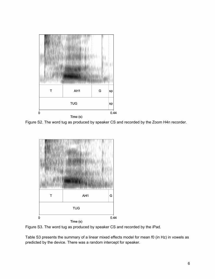
6

Figure S2. The word tug as produced by speaker CS and recorded by the Zoom H4n recorder.

Figure S3. The word tug as produced by speaker CS and recorded by the iPad. Table S3 presents the summary of a linear mixed effects model for mean f0 (in Hz) in vowels as predicted by the device. There was a random intercept for speaker.

7

There were no significant effects of Device on mean f0, though f0 was marginally lower in the iPad and iPhone conditions. In a larger dataset, the effect might reach significance. However, it is worth noting that the differences in measured f0 are small relative to the expected size of phonological f0 patterns. Figure S3 presents the distribution of f0 measurements for each speaker. Given the similar distributions across conditions, the different results are unlikely to be the result of pitch tracking errors. None of the conditions excluded more than 5 tokens as unmeasurable, so the results are also not the result of different exclusions. The differences might be related to the differing boundary assignments in each condition, as also reflected in the duration differences. Different boundaries could reduce extrinsic f0 effects of voicing of the neighboring consonants. Table S3. Linear mixed effects model for mean f0 (in Hz) in vowels Estimate SE t-value p

(Intercept) 180.4 5.1 35.1 0.011

Device Android 1.0 2.2 0.47 0.63

Device ExternalComputerMic 0.98 2.2 0.45 0.65

Device InternalComputerMic -0.98 2.2 -0.45 0.65

Device iPad -3.3 2.2 -1.5 0.13

Device iPhone -3.6 2.2 -1.7 0.098 Reference level Program = zoomH4n

Figure S4. Density plots for the mean f0 Table S4 presents the summary of a linear mixed effects model for peak timing (in ms) -- the position of the maximum f0 relative to the beginning of the vowel, as predicted by the recording program. There was a random intercept for speaker.

There were no significant effects of Device on peak timing, but there were suggestive trends for Android and ExternalComputerMic which could be expected as a side effect of

8

differences in vowel duration, because when the beginning of the vowel is put earlier, then the peak occurs later relative to that boundary. The size of the differences are small, though they are large enough relative to the size of actual peak timing effects that they could alter results. Many of the differences are due to how many items identify the peak f0 as occurring at the beginning of the vowel, which could be a result of the differences in the boundary identified for the beginning of the vowel. Table S4. Linear mixed effects model for f0 peak timing (in milliseconds) Estimate SE t-value p

(Intercept) 27.5 3.2 8.6 < 0.001

Device Android 6.6 4.5 1.5 0.15

Device ExternalComputerMic 7.4 4.5 1.6 0.1

Device InternalComputerMic -2.9 4.5 -0.64 0.53

Device iPad -0.6 4.5 -0.13 0.9

Device iPhone -4.4 4.5 -0.98 0.33 Reference level Program = zoomH4n Table S5 presents the summary of a linear mixed effects model for jitter in vowels as predicted by the device, i.e. the cycle-to-cycle variation in f0. There was a random intercept for speaker.

There were no significant effects of Device on jitter measurements, which is consistent with generally reliable f0 measurements. Table S5. Linear mixed effects model for jitter in vowels Estimate SE t-value p

(Intercept) 0.021 0.0017 12.3 0.0025

Device Android 0.00031 0.0016 0.19 0.85

Device ExternalComputerMic -0.0012 0.0016 -0.72 0.47

Device InternalComputerMic -0.0009 0.0016 -0.56 0.58

Device iPad 0.0022 0.0016 1.3 0.18

Device iPhone 0.0019 0.0016 1.2 0.24 Reference level Program = zoomH4n Table S6 presents the summary of a linear mixed effects model for spectral tilt (H1-H2) in vowels as predicted by the device. There was a random intercept for speaker.

Spectral tilt was significantly lower in the Android condition, and marginally higher in the iPhone condition. Even the differences that were not significant are rather large relative to the size of meaningful spectral tilt differences. The differences might indicate variation in how well the devices record higher and lower frequencies. The differences do not seem to be the result of distance from the speaker; the phones and the baseline H4n device were similarly close to the speaker, and the phones have opposite effects.

9

Table S6. Linear mixed effects model for spectral tilt in vowels Estimate SE t-value p

(Intercept) -2.0 2.0 -1.0 0.48

Device Android -1.5 0.59 -2.5 0.013

Device ExternalComputerMic -0.93 0.59 -1.6 0.11

Device InternalComputerMic -0.57 0.59 -0.97 0.33

Device iPad 0.41 0.59 0.69 0.49

Device iPhone 1.0 0.59 1.7 0.084 Reference level Program = zoomH4n Table S7 presents the summary of a linear mixed effects model for Harmonics-to-Noise Ratio (HNR) in vowels as predicted by the device. There was a random intercept for speaker. HNR was significantly lower in the InternalComputerMic condition, indicating more noise in this condition than the baseline condition. This might be due to distance from the speaker; this microphone was the furthest from the speaker (see the setup diagram in Figure 1 of the main text). Impressionistically, internal computer microphones also pick up more noise from computer fans. Table S7. Linear mixed effects model for HNR in vowels Estimate SE t-value p

(Intercept) 6.4 1.3 4.9 0.12

Device Android 0.59 0.37 1.6 0.11

Device ExternalComputerMic 0.039 0.37 0.11 0.92

Device InternalComputerMic -1.5 0.37 -4.2 <0.001

Device iPad -0.34 0.37 -0.92 0.36

Device iPhone -0.23 0.37 -0.63 0.53 Reference level Program = zoomH4n Table S8 presents the summary of a linear mixed effects model for F1 in vowels as predicted by the device. There was a random intercept for speaker and for vowel.

F1 was significantly lower in the InternalComputerMic, iPad, and iPhone conditions. These results might be related to the trend also found in spectral tilt; formant measurements are influenced by how the formants align with the harmonics (Chen, Whalen & Shadle 2019). Differences in how each vowel is impacted by condition are presented at the end of Section 1.1.2.

Table S8. Linear mixed effects model for F1 in vowels Estimate SE t-value p

(Intercept) 613.5 55.1 11.1 < 0.001

Device Android -7.3 7.5 -0.98 0.33

10

Device ExternalComputerMic -8.7 7.5 -1.2 0.24

Device InternalComputerMic -19.8 7.5 -2.7 0.008

Device iPad -15.2 7.5 -2.0 0.042

Device iPhone -25.7 7.5 -3.4 < 0.001 Reference level Program = zoomH4n Table S9 presents the summary of a linear mixed effects model for F2 in vowels as predicted by the device. There was a random intercept for speaker and for vowel.

F2 was significantly lower than the baseline measurement in the InternalComputerMic condition, and significantly higher in the iPad and iPhone conditions. The results vary substantially for different vowels, as is presented at the end of Section 1.1.2 below. One of the major effects seems to be attributable to diphthongization of high and mid-high tense vowels, so failure to capture the trajectory of the formants within the vowel results in altered estimation of the mean F2. Table S9. Linear mixed effects model for F2 in vowels Estimate SE t-value p

(Intercept) 1897.5 115.7 16.4 < 0.001

Device Android 56.8 25.7 2.2 0.027

Device ExternalComputerMic -33.5 25.7 -1.3 0.19

Device InternalComputerMic -77.4 25.7 -3.0 0.0026

Device iPad 145.0 25.7 5.7 < 0.001

Device iPhone 70.6 25.7 2.7 0.0061 Reference level Program = zoomH4n All formant analyses used the measurements in Hz. Lobanov normalization did not substantially change the results, so those analyses are not included here. Table S10 presents the summary of a linear mixed effects model for Center of Gravity (COG) in fricatives as predicted by the device. There was a random intercept for speaker and for segment.

The overall measurements were far higher in the ExternalComputerMic and InternalComputerMic conditions than in the baseline condition; this was largely due to the sibilants, as will be addressed subsequently. Measurements were also significantly higher in the Android condition. COG measurements by fricative are addressed in 1.1.2. Table S10. Linear mixed effects model for COG for fricatives Estimate SE t-value p

(Intercept) 2078.6 892.1 2.3 0.058

Device Android 440.3 132.5 3.3 0.00095

11

Device ExternalComputerMic 1172.5 132.5 8.9 < 0.001

Device InternalComputerMic 1115.2 132.5 8.4 < 0.001

Device iPad -196.7 132.5 -1.5 0.14

Device iPhone 125.3 132.5 0.95 0.34 Reference level Program = zoomH4n

2.1.2 Impact on contrasts Effects in these characteristics are primarily a concern if they alter our ability to find contrasts. In this section, we test whether contrasts depending on these characteristics are altered by the recording device. These contrasts were selected as contrasts that are known to exist in English and which should be reflected by the measurements that we are using. When the regression models found no significant interaction between Device and the phonological categories, the results are illustrated just with a figure. Stress in vowels Figure S5 illustrates vowel duration as influenced by stress. The device did not have any substantial impact on these measurements, even though the overall vowel duration measurements were influenced by device. The effect of stress is significant or marginally significant in all conditions, and of a similar size.

Figure S5. Measured vowel duration as predicted by device and stress. Pooled raw data, not the model results. Whiskers indicate the standard error.

12

Figure S6 illustrates maximum f0 in vowels as influenced by stress. There are no substantial effects; all of the conditions find a significant effect, of a similar size.

Figure S6. Measured F0 maximum as predicted by device and stress. Pooled raw data, not the model results. Whiskers indicate the standard error. Coda voicing Figure S7 illustrates vowel duration as influenced by coda voicing. There are no substantial effects, although overall vowel duration differs across devices; all of the conditions find a significant effect, though some of them seem to be overestimating the effect, which could be a concern.

13

Figure S7. Measured vowel duration as predicted by device and coda voicing. Pooled raw data, not the model results. Whiskers indicate the standard error. Table S11 presents the summary of a linear mixed effects model for HNR in vowels as predicted by the device and the coda voicing. There was a random intercept for speaker. Vowels followed by voiceless codas generally have a lower HNR than vowels before voiced codas. None of the interactions reach significance, though several of the conditions seem to be underestimating the size of the effect, which is consistent with those conditions overall having more noise and thus lower HNR. Figure S8 illustrates HNR in vowels as influenced by coda voicing.

Table S11. Linear mixed effects model for HNR in vowels, including coda voicing as a factor Estimate SE t-value p

(Intercept) 8.7 1.2 7.5 0.047

Device Android 0.55 0.61 0.89 0.37

Device ExternalComputerMic 0.38 0.61 0.62 0.54

Device InternalComputerMic -2.0 0.61 -3.3 0.0012

Device iPad -0.9 0.61 -1.5 0.14

Device iPhone -0.55 0.61 -0.9 0.37

FollowingVoicing Voiceless -4.1 0.53 -7.8 < 0.001

Device Android:FollowingVoicing Voiceless

0.034 0.75 0.046 0.96

Device ExternalComputerMic:FollowingVoicing Voiceless

-0.66 0.75 -0.89 0.38

Device InternalComputerMic:FollowingVoici

0.61 0.75 0.82 0.41

14

ng Voiceless

Device iPad:FollowingVoicing Voiceless

0.83 0.75 1.1 0.27

Device iPhone:FollowingVoicing Voiceless

0.43 0.75 0.58 0.56

Reference level Program = zoomH4n, FollowingVoicing = voiced

Figure S8. Measured HNR as predicted by device and coda voicing. Pooled raw data, not the model results. Whiskers indicate the standard error. Onset voicing Table S12 presents the summary of a linear mixed effects model for HNR in vowels as predicted by the device and the onset voicing. There was a random intercept for speaker.

As with coda voicing, the HNR differences between voiced and voiceless onsets are decreased for the InternalComputerMic, iPad and iPhone devices, but the difference was only marginally significant even in the baseline condition. The issue here might be about boundary assignment, if vowels are only considered to begin when there is clear modal voicing. Figure S9 illustrates HNR in vowels as influenced by onset voicing.

Table S12. Linear mixed effects model for HNR in vowels, including onset voicing as a factor Estimate SE t-value p

(Intercept) 6.9 1.38 5.0 0.086

Device Android 0.7 0.68 1.0 0.3

Device ExternalComputerMic 0.18 0.68 0.27 0.79

Device InternalComputerMic -1.8 0.68 -2.6 0.0096

Device iPad -0.54 0.68 -0.79 0.43

15

Device iPhone -0.47 0.68 -0.69 0.49

PrecedingVoicing Voiceless -1.3 0.62 -2.2 0.033

Device Android:PrecedingVoicing Voiceless

-0.2 0.88 -0.23 0.82

Device ExternalComputerMic:PrecedingVoicing Voiceless

-0.35 0.88 -0.4 0.69

Device InternalComputerMic:PrecedingVoicing Voiceless

0.53 0.88 0.6 0.55

Device iPad:PrecedingVoicing Voiceless

0.35 0.88 0.4 0.69

Device iPhone:PrecedingVoicing Voiceless

0.41 0.88 0.47 0.64

Reference level Program = zoomH4n, PrecedingVoicing = voiced

Figure S9. Measured HNR as predicted by device and onset voicing. Pooled raw data, not the model results. Whiskers indicate the standard error. Table S13 presents the summary of a linear mixed effects model for spectral tilt in vowels as predicted by the device and the onset voicing. There was a random intercept for speaker.

The effect is only marginally significant in the baseline condition; it is only a small effect, but has been established elsewhere (e.g. Kong, Beckman & Edwards 2012). Though most of the differences are not significant, it is important to note that they are large relative to the size of the actual effect; there are clear distortions of spectral tilt, which are likely to obscure measurements. Figure S10 illustrates spectral tilt in vowels as influenced by onset voicing.

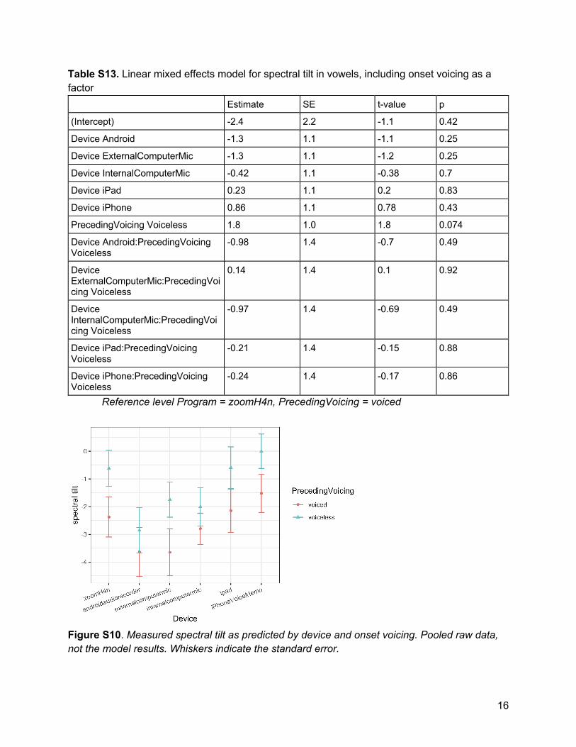
16

Table S13. Linear mixed effects model for spectral tilt in vowels, including onset voicing as a factor Estimate SE t-value p

(Intercept) -2.4 2.2 -1.1 0.42

Device Android -1.3 1.1 -1.1 0.25

Device ExternalComputerMic -1.3 1.1 -1.2 0.25

Device InternalComputerMic -0.42 1.1 -0.38 0.7

Device iPad 0.23 1.1 0.2 0.83

Device iPhone 0.86 1.1 0.78 0.43

PrecedingVoicing Voiceless 1.8 1.0 1.8 0.074

Device Android:PrecedingVoicing Voiceless

-0.98 1.4 -0.7 0.49

Device ExternalComputerMic:PrecedingVoicing Voiceless

0.14 1.4 0.1 0.92

Device InternalComputerMic:PrecedingVoicing Voiceless

-0.97 1.4 -0.69 0.49

Device iPad:PrecedingVoicing Voiceless

-0.21 1.4 -0.15 0.88

Device iPhone:PrecedingVoicing Voiceless

-0.24 1.4 -0.17 0.86

Reference level Program = zoomH4n, PrecedingVoicing = voiced

Figure S10. Measured spectral tilt as predicted by device and onset voicing. Pooled raw data, not the model results. Whiskers indicate the standard error.

17

Figure S11 illustrates maximum f0 in vowels as influenced by onset voicing. None of the effects are significant, but there is variation in how large the effect is estimated to be.

Figure S11. Measured f0 maximum as predicted by device and onset voicing. Pooled raw data, not the model results. Whiskers indicate the standard error. Consonant manner Table S14 presents the summary of a linear mixed effects model for COG in /s/ vs. /ʃ/ as predicted by the device. There was a random intercept for speaker. The model finds the same effect noted above for overall COG measurements: The COG for /s/ is overestimated in the ExternalComputerMic condition and the InternalComputerMic condition. The interactions show that /ʃ/ isn’t as affected. Figure S12 illustrates COG by fricative. These results seem to be a combination of how well the microphones pick up low-frequency noise and how much background noise they pick up. The effects of this problem would likely be smaller for recordings with a higher sampling rate.

Table S14. Linear mixed effects model for COG in sibilant fricatives, including particular fricative as a factor Estimate SE t-value p

(Intercept) 5053.7 559.0 9.0 0.058

Device Android 632.7 181.6 3.5 0.00058

Device ExternalComputerMic 1723.1 181.6 9.5 < 0.001

Device InternalComputerMic 1359.7 181.6 7.5 < 0.001

Device iPad -460.4 181.6 -2.5 0.011810

Device iPhone 226.6 181.6 1.2 0.21

Segment /ʃ/ -1689.3 254.2 -6.6 < 0.001

Device Android:Segment /ʃ/ -496.5 359.4 -1.4 0.17

18

Device ExternalComputerMic:Segment /ʃ/

-1587.6 359.4 -4.4 < 0.001

Device InternalComputerMic:Segment /ʃ/

-763.1 359.4 -2.1 0.035

Device iPad:Segment /ʃ/ 301.0 359.4 0.84 0.4

Device iPhone:Segment /ʃ/ -253.8 359.4 -0.71 0.48 Reference level Program = zoomH4n, Segment = /s/

Figure S12. Measured center of gravity as predicted by device and segment, among fricatives. Pooled raw data, not the model results. Whiskers indicate the standard error. Vowel quality Figure S13 illustrates F1 and F2 as influenced by vowel quality and device. Adding the interaction between vowel quality and device marginally improves the model for F1 (χ2 = 105.0, df = 84, p = 0.06). The interaction between vowel quality and device significantly improves the model for F2 (χ2 = 186.4, df = 84, p < 0.0001); the measured F2 varies considerably across conditions for some vowels. The device conditions in phase 1 all clearly pick out a recognizable vowel space. However, some of the vowels are shifted enough that they would be likely to cause problems for analysis. In particular, F2 measurements for /u/ and /ou/ were very high in many of the conditions; this is in part due to issues in identifying boundaries or tracking low-intensity formants, which altered which part of the diphthong were measured. Many of the words with /u/ lacked codas, so failure to capture the back portion of the offglide of the vowel resulted in only measuring the fronter beginning portion. While other vowels didn’t exhibit systematic effects, there are several vowels that have strikingly variable measurements across conditions.

19

Figure S13. Vowel spaces for each speaker as measured in Phase 1 (by-Device).

2.2 Effects of Program There were five software conditions compared to the H4n reference condition: Zoom, Skype, Cleanfeed, Facebook Messenger (recorded through Audacity, because it does not have an in-app recording option), and AudacityAlone. Note that four of these are testing applications for online transmission, while AudacityAlone is present to test whether the Audacity program causes effects in itself, to clarify how to interpret the results of the Messenger condition. For these comparisons, we used a single Zoom condition, recording locally with the default audio settings. Although we tested several different Zoom conditions, there were no differences between any of them: Local vs. remote, operating system, conversion from mp4, or the “Original Audio” setting. None of the characteristics measured exhibited significant effects of recording condition. The models comparing Zoom conditions to each other are presented in Section 1.3 below.

2.2.1 Overall effects Table S15 presents the summary of a linear mixed effects model for consonant duration as predicted by the recording program. There was a random intercept for speaker.

There were no significant consonant duration differences between the baseline recording and the recording made through Cleanfeed or Audacity alone. However, consonant durations were significantly shorter in all of the other conditions. Some of the effects on duration may be due to differences in intensity or background noise, which could alter the boundaries identified by forced alignment and would also be likely to produce similar effects in manual alignment, as discussed in 1.1.1 above. Some of the differences in duration might also reflect actual duration differences created by compression algorithms; see Section 2.5

20

Table S15. Linear mixed effects model for consonant duration (in milliseconds) Estimate SE t-value p

(Intercept) 106.8 10.3 10.4 0.0072

Program AudacityAlone

1.1 2.9 0.38 0.7

Program Cleanfeed -0.44 2.9 -0.15 0.88

Program Messenger

-11.6 2.9 -4.0 < 0.001

Program Skype -8.5 2.9 -3.0 0.003

Program Zoom -11.2 2.9 -3.9 < 0.001 Reference level Program = zoomH4n Table S16 presents the summary of a linear mixed effects model for vowel duration as predicted by the recording program. There was a random intercept for speaker. As for consonant duration, there were no significant vowel duration differences between the baseline recording and the recording made through Cleanfeed or AudacityAlone. However, vowel durations were significantly longer in all of the other conditions. Table S16. Linear mixed effects model for vowel duration (in milliseconds) Estimate SE t-value p

(Intercept) 157.2 12.3 12.8 0.0025

Program AudacityAlone

-0.84 6.0 -0.14 0.89

Program Cleanfeed 0.37 6.0 0.061 0.95

Program Messenger

17.5 6.0 2.9 0.0039

Program Skype 19.8 6.0 3.3 0.0011

Program Zoom 31.5 6.0 5.2 < 0.001 Reference level Program = zoomH4n Table S17 presents the summary of a linear mixed effects model for the mean f0 in vowels, as predicted by the recording program. There was a random intercept for speaker. There was no significant effect on mean f0 in any of the conditions. Table S17. Linear mixed effects model for mean f0 (in Hz) in vowels Estimate SE t-value p

(Intercept) 181.1 3.8 48.2 < 0.001

Program AudacityAlone

0.17 1.5 0.12 0.91

Program Cleanfeed -0.14 1.5 -0.095 0.92

21

Program Messenger

-1.3 1.5 -0.87 0.38

Program Skype 0.33 1.5 0.23 0.82

Program Zoom 0.63 1.5 0.43 0.67 Reference level Program = zoomH4n Table S18 presents the summary of a linear mixed effects model for peak timing -- the position of the maximum f0 relative to the beginning of the vowel, as predicted by the recording program. There was a random intercept for speaker. The peak timing was significantly later for Zoom than the baseline condition. This is probably due to the overestimated vowel duration, described above. Because the beginnings of the vowels were placed earlier, the peak f0 was later relative to that starting point. However, it is worth considering why none of the other conditions have effects on peak timing, when several of them did have duration effects. The different results might be due to the size of the effect; MessengerThroughAudacity and Skype had smaller effects on duration than Zoom did, so the corresponding differences in peak timing are smaller and don’t reach significance. Table S18. Linear mixed effects model for f0 peak timing (in milliseconds) Estimate SE t-value p

(Intercept) 33.7 6.5 5.2 0.014

Program AudacityAlone

-0.93 4.3 -0.21 0.83

Program Cleanfeed -0.073 4.3 -0.017 0.99

Program Messenger

6.5 4.3 1.5 0.13

Program Skype 5.0 4.3 1.1 0.25

Program Zoom 14.2 4.3 3.3 0.001 Reference level Program = zoomH4n Table S19 presents the summary of a linear mixed effects model for jitter in vowels, as predicted by the recording program. There was a random intercept for speaker. There was no significant effect of jitter, though there was a marginal effect of the Zoom condition, finding more jitter than the H4n recorder. Table S19. Linear mixed effects model for jitter in vowels Estimate SE t-value p

(Intercept) 0.019 0.0033 5.6 0.023

Program AudacityAlone

0.00075 0.0012 0.63 0.53

Program Cleanfeed 0.0011 0.0012 0.92 0.36

Program 0.0008 0.0012 0.67 0.5

22

Messenger

Program Skype 0.00039 0.0012 0.32 0.75

Program Zoom 0.0023 0.0012 1.9 0.059 Reference level Program = zoomH4n Table S20 presents the summary of a linear mixed effects model for spectral tilt (H1-H2) in vowels, as predicted by the recording program. There was a random intercept for speaker. All of the programs exhibited effects of spectral tilt. Most of them underestimated spectral tilt, while MessengerThroughAudacity overestimated it. The effects suggest that transmission for many of these programs is worse for lower frequencies. Notably, this effect is even present in the AudacityAlone condition. On the other hand, the higher spectral tilt in the MessengerThrough Audacity condition might suggest that Messenger is amplifying low frequencies. Table S20. Linear mixed effects model for spectral tilt in vowels Estimate SE t-value p

(Intercept) -1.6 1.6 -1.0 0.4

Program AudacityAlone

-1.4 0.5 -2.9 0.0041

Program Cleanfeed -1.3 0.5 -2.6 0.009

Program Messenger

4.6 0.5 9.1 < 0.001

Program Skype -1.7 0.5 -3.3 < 0.001

Program Zoom -2.0 0.5 -3.9 < 0.001 Reference level Program = zoomH4n Table S21 presents the summary of a linear mixed effects model for the Harmonics-to-Noise Ratio (HNR) in vowels, as predicted by the recording program. There was a random intercept for speaker. MessengerThroughAudacity exhibited a much higher HNR than the baseline condition. None of the other effects were significant, but they all have the trend towards being somewhat lower than the baseline, indicating more noise. The higher value for the MessengerThroughAudacity condition must have a different explanation. It isn’t the result of excluding unmeasurable items; none of the conditions excluded more than 3 tokens. The result might come from amplification of low frequencies, like the spectral tilt effect; low frequencies include the clearest harmonics, so if these frequencies are amplified, the HNR would appear to be higher. Table S21. Linear mixed effects model for HNR in vowels Estimate SE t-value p

(Intercept) 7.3 1.0 7.0 0.016

23

Program AudacityAlone

-0.34 0.29 -1.2 0.24

Program Cleanfeed -0.24 0.29 -0.84 0.4

Program Messenger

1.2 0.29 4.2 < 0.001

Program Skype -0.3 0.29 -1.0 0.3

Program Zoom -0.4 0.29 -1.4 0.17 Reference level Program = zoomH4n Table S22 presents the summary of a linear mixed effects model for F1, as predicted by the recording program. There was a random intercept for speaker and for vowel. F1 was significantly lower in the MessengerThroughAudacity condition. The cause of the effect is somewhat unclear. This is addressed in more detail at the end of section 1.2.2, where formant effects are separated by vowel. Table S22. Linear mixed effects model for F1 in vowels Estimate SE t-value p

(Intercept) 613.7 48.4 12.7 < 0.001

Program AudacityAlone

1.5 8.8 0.17 0.87

Program Cleanfeed 10.8 7.9 1.4 0.17

Program Messenger

-29.7 7.9 -3.8 0.00018

Program Skype -3.5 7.9 -0.45 0.66

Program Zoom -11.1 7.9 -1.4 0.16 Reference level Program = zoomH4n Table S23 presents the summary of a linear mixed effects model for F2, as predicted by the recording program. There was a random intercept for speaker and for vowel. F2 was overestimated in all of the conditions, to varying degrees; by far the largest difference was in the Messenger condition. Section 1.2.2 addresses formant effects in more detail, separated by vowel. Table S23. Linear mixed effects model for F2 in vowels Estimate SE t-value p

(Intercept) 1898.4 119.6 15.9 < 0.001

Program AudacityAlone

36.1 21.2 1.7 0.088

Program Cleanfeed 46.0 19.0 2.4 0.016

Program Messenger

91.0 19.0 4.8 < 0.001

24

Program Skype 42.0 19.0 2.2 0.027

Program Zoom 31.4 19.0 1.7 0.099 Reference level Program = zoomH4n All formant analyses used the measurements in Hz. Lobanov normalization did not substantially change the results, so those analyses are not included here. Table S24 presents the summary of a linear mixed effects model for center of gravity (COG) in fricatives, as predicted by the recording program. There was a random intercept for speaker and for segment. COG was significantly lower in the Cleanfeed and MessengerThroughAudacity conditions, and marginally higher in the Zoom condition. As in the Device comparisons, the largest effects are on /s/ and /z/. Further analysis of differences between fricatives are presented in section 1.2.2. Table S24. Linear mixed effects model for COG for fricatives Estimate SE t-value p

(Intercept) 1923.9 549.3 3.5 0.0094

Program AudacityAlone

220.6 140.6 1.6 0.12

Program Cleanfeed -653.3 126.1 -5.2 < 0.001

Program Messenger

-904.1 126.1 -7.2 < 0.001

Program Skype -196.3 126.1 -1.6 0.12

Program Zoom 220.7 126.1 1.7 0.08 Reference level Program = zoomH4n

2.2.2 Impact on contrasts As for the comparisons by device, effects in these characteristics are primarily a concern if they alter our ability to find contrasts. In this section, we test whether contrasts depending on these characteristics are altered by the recording device. Stress in vowels Figure S14 illustrates vowel duration as influenced by stress. The program did not have any substantial impact on these measurements, even though the overall vowel duration measurements were influenced by device. The effect of stress is significant or marginally significant in all conditions, and of a similar size.

25

Figure S14. Measured vowel duration as predicted by program and stress. Pooled raw data, not the model results. Whiskers indicate the standard error. Figure S15 illustrates F0 in vowels as influenced by stress. The program did not have any substantial impact on these measurements; there was a clear separation between stressed and unstressed vowels in all conditions, though there is some variation in the size of the effect.

Figure S15. Measured f0 maximum as predicted by program and stress. Pooled raw data, not the model results. Whiskers indicate the standard error. Coda voicing

26

Figure S16 illustrates vowel duration as influenced by coda voicing. The program did not have any substantial impact on these measurements, though there was variation in the size of the effect, and some conditions were substantially overestimating overall vowel duration.

Figure S16. Measured vowel duration as predicted by program and coda voicing. Pooled raw data, not the model results. Whiskers indicate the standard error. Figure S17 illustrates HNR in vowels as influenced by coda voicing. The program did not have any substantial impact on these measurements; the effect was a similar size in all conditions.

Figure S17. Measured HNR as predicted by program and coda voicing. Pooled raw data, not the model results. Whiskers indicate the standard error.

27

Onset voicing Figure S18 illustrates HNR in vowels as influenced by onset voicing. The program did not have any substantial impact on these measurements; the effect was a similar size in all conditions, even though MessengerThroughAudacity substantially overestimated HNR for vowels in both environments.

Figure S18. Measured HNR as predicted by program and onset voicing. Pooled raw data, not the model results. Whiskers indicate the standard error. Figure S19 illustrates spectral tilt in vowels as influenced by onset voicing. The program did not have any substantial impact on these measurements; the effect was a similar size in all conditions, even though MessengerThroughAudacity substantially overestimated spectral tilt for vowels in both environments.

28

Figure S19. Measured spectral tilt as predicted by program and onset voicing. Pooled raw data, not the model results. Whiskers indicate the standard error. Figure S20 illustrates maximum F0 as influenced by onset voicing. The program did not have any substantial impact on these measurements; the effect was a similar size in all conditions.

Figure S20. Measured f0 maximum as predicted by program and onset voicing. Pooled raw data, not the model results. Whiskers indicate the standard error. Consonant manner Table S25 presents the summary of a linear mixed effects model for COG in /s/ and /ʃ/, as predicted by the recording program and segment. There was a random intercept for speaker.

29

MessengerThroughAudacity was substantially underestimating /s/, to the point where it has a slightly lower cog than /ʃ/, and they don’t substantially differ. Figure S21 illustrates COG across all fricatives. Zoom, Skype, and MessengerThrough Audacity were also substantially overestimating the COG for /f/. Because the frication for /f/ is rather diffuse, this could be the result of amplifying lower frequencies, or filtering out higher frequency aperiodic noise as “background noise.” Table S25. Linear mixed effects model for COG in sibilant fricatives, including particular fricative as a factor Estimate SE t-value p

(Intercept) 4735.9 224.2 21.1 < 0.001

Program AudacityAlone

194.4 197.7 0.98 0.33

Program Cleanfeed -301.3 197.7 -1.5 0.13

Program Messenger

-1676.7 197.7 -8.5 < 0.001

Program Skype -380.4 197.7 -1.9 0.055

Program Zoom 509.3 197.7 2.6 0.01

Segment /ʃ/ -1544.7 279.5 -5.5 < 0.001

Program AudacityAlone:Segment /ʃ/

73.2 395.3 0.19 0.85

Program Cleanfeed:Segment /ʃ/

465.0 395.3 1.2 0.24

Program Messenger:Segment /ʃ/

1744.0 395.3 4.4 < 0.001

Program Skype:Segment /ʃ/

510.4 395.3 1.3 0.2

Program Zoom:Segment /ʃ/

-206.3 395.3 -0.52 0.6

Reference level Program = zoomH4n, Segment = /s/

30

Figure S21. Measured center of gravity as predicted by program and segment, among fricatives. Pooled raw data, not the model results. Whiskers indicate the standard error. Vowel quality Figure S22 illustrates F1 and F2 as influenced by vowel quality and device. Adding the interaction between vowel quality and device significantly improves the model for F1 (χ2 = 208.3, df = 85, p = < 0.0001). The interaction between vowel quality and device also marginally improves the model for F2 (χ2 = 102.3, df = 85, p = 0.097). There is substantial variation in the measurement of both formants in recordings made by different programs. These effects vary by vowel, which is why they did not show up as clearly in the some of the overall models for F1 and F2 above. Many of the conditions produce measurements that substantially shift a vowel far into the region of a different vowel, which is likely to cause major problems in phonetic analysis and even in phonological categorization of tokens. While clusters for measurements of each vowel are mostly apparent, Messenger Through Audacity is a clear outlier for most of the vowels. The differences in formant measurements are likely to reflect a combination of factors. Some differences are directly due to compression algorithms changing spectral information. Other differences are indirect effects of differences caused by the recording program; background noise and filtering or amplifying certain frequencies can change the apparent center of a frequency band and might also lead to the wrong formants being identified.

31

Figure S22. Vowel spaces for each speaker as measured in Phase 2 (by-Program).

2.3 Comparing Zoom Conditions This section provides the models comparing measurements across the Zoom conditions -- this varied based on whether the recording was local or remote, whether the computer was mac or windows, whether the files were converted from mp4 or not, and whether the recording used the “Original Audio” setting in Zoom or not. In most of these measures, there were clearly no effects; the variation between conditions is very small. For duration, two comparisons were marginally significant, but would not withstand correction for multiple comparisons. Table S26 presents the summary of a linear mixed effects model for consonant duration as predicted by the recording condition. There was a random intercept for speaker.

There were no significant consonant duration differences between the different conditions. Table S26. Linear mixed effects model for consonant duration Estimate SE t-value p

(Intercept) 95.6 9.4 10.2 0.0064

Condition Mac Local mp4 -0.73 3.4 -0.21 0.83

Condition Mac Remote mp4 2.4 3.4 0.7 0.49

Condition Mac Remote wav 5.4 3.4 1.6 0.11

Condition Windows Remote wav 4.4 3.4 1.3 0.19

Condition Mac Remote mp4 OriginalAudio 1.5 3.4 0.44 0.66

Condition Mac Remote wav OriginalAudio 1.4 3.4 0.41 0.68 Reference level Condition = Local, macOSX, not “original audio”, not from mp4

32

Table S27 presents the summary of a linear mixed effects model for vowel duration as predicted by the recording condition. There was a random intercept for speaker.

Vowel duration in the Mac Remote mp4 condition was below the threshold of significance; however, it is important to keep in mind the large number of tests being conducted. When correcting for multiple comparisons, this effect is no longer significant. Table S27. Linear mixed effects model for vowel duration Estimate SE t-value p

(Intercept) 188.6 11.8 15.9 < 0.001

Condition Mac Local mp4 -3.2 7.0 -0.45 0.65

Condition Mac Remote mp4 -13.9 7.0 -2.0 0.047

Condition Mac Remote wav -13.4 7.0 -1.9 0.057

Condition Windows Remote wav -11.2 7.0 -1.6 0.11

Condition Mac Remote mp4 OriginalAudio 0.28 7.0 0.04 0.97

Condition Mac Remote wav OriginalAudio -0.68 7.0 -0.097 0.92 Reference level Condition = Local, macOSX, not “original audio”, not from mp4 Table S28 presents the summary of a linear mixed effects model for mean f0 in vowels as predicted by the recording condition. There was a random intercept for speaker.

There was no effect of recording condition on f0 mean. Table S28. Linear mixed effects model for mean f0 in vowels Estimate SE t-value p

(Intercept) 181.7 3.8 48.1 < 0.001

Condition Mac Local mp4 -0.35 1.6 -0.21 0.83

Condition Mac Remote mp4 -0.46 1.6 -0.28 0.78

Condition Mac Remote wav -0.19 1.6 -0.12 0.91

Condition Windows Remote wav -0.51 1.6 -0.31 0.75

Condition Mac Remote mp4 OriginalAudio 0.1 1.6 0.061 0.95

Condition Mac Remote wav OriginalAudio 0.69 1.6 0.42 0.68 Reference level Condition = Local, macOSX, not “original audio”, not from mp4 Table S29 presents the summary of a linear mixed effects model for peak timing -- the position of the maximum f0 relative to the beginning of the vowel, as predicted by the recording condition. There was a random intercept for speaker.

There was no effect of recording condition on peak timing Table S29. Linear mixed effects model for f0 peak timing in vowels Estimate SE t-value p

33

(Intercept) 0.048 0.0072 6.6 0.0056

Condition Mac Local mp4 0.00022 0.005 0.044 0.96

Condition Mac Remote mp4 -0.0073 0.005 -1.4 0.15

Condition Mac Remote wav -0.0071 0.005 -1.4 0.16

Condition Windows Remote wav -0.0047 0.005 -0.94 0.35

Condition Mac Remote mp4 OriginalAudio 0.0001 0.005 0.02 0.98

Condition Mac Remote wav OriginalAudio 0.0012 0.005 0.23 0.81 Reference level Condition = Local, macOSX, not “original audio”, not from mp4 Table S30 presents the summary of a linear mixed effects model for jitter in vowels as predicted by the recording condition. There was a random intercept for speaker.

There was no effect of recording condition on jitter. Table S30. Linear mixed effects model for jitter in vowels Estimate SE t-value p

(Intercept) 0.021 0.0035 6.0 0.02

Condition Mac Local mp4 -0.000048 0.0013 -0.038 0.97

Condition Mac Remote mp4 0.000044 0.0013 0.034 0.97

Condition Mac Remote wav 0.0006 0.0013 0.47 0.64

Condition Windows Remote wav -0.00083 0.0013 -0.65 0.52

Condition Mac Remote mp4 OriginalAudio -0.00019 0.0013 -0.15 0.88

Condition Mac Remote wav OriginalAudio 0.00032 0.0013 0.25 0.8 Reference level Condition = Local, macOSX, not “original audio”, not from mp4 Table S31 presents the summary of a linear mixed effects model for spectral tilt (H1-H2) in vowels as predicted by the recording condition. There was a random intercept for speaker.

There was no effect of recording condition on spectral tilt. Table S31. Linear mixed effects model for spectral tilt in vowels Estimate SE t-value p

(Intercept) -3.6 1.9 -1.9 0.18

Condition Mac Local mp4 0.16 0.54 0.29 0.77

Condition Mac Remote mp4 -0.091 0.54 -0.17 0.87

Condition Mac Remote wav -0.02 0.54 -0.036 0.97

Condition Windows Remote wav -0.26 0.54 -0.47 0.64

Condition Mac Remote mp4 OriginalAudio -0.31 0.54 -0.56 0.58

Condition Mac Remote wav OriginalAudio -0.034 0.54 -0.063 0.95 Reference level Condition = Local, macOSX, not “original audio”, not from mp4

34

Table S32 presents the summary of a linear mixed effects model for Harmonics-to-Noise Ratio (HNR) in vowels as predicted by the recording condition. There was a random intercept for speaker.

There was no effect of recording condition on HNR. Table S32. Linear mixed effects model for HNR in vowels Estimate SE t-value p

(Intercept) 6.9 0.96 7.2 0.016

Condition Mac Local mp4 -0.0046 0.28 -0.017 0.99

Condition Mac Remote mp4 0.16 0.28 0.56 0.57

Condition Mac Remote wav 0.19 0.28 0.66 0.51

Condition Windows Remote wav 0.31 0.28 1.1 0.27

Condition Mac Remote mp4 OriginalAudio 0.0017 0.28 0.006 0.99

Condition Mac Remote wav OriginalAudio 0.00078 0.28 0.003 0.99 Reference level Condition = Local, macOSX, not “original audio”, not from mp4 Table S33 presents the summary of a linear mixed effects model for F1 in vowels as predicted by the recording condition. There was a random intercept for speaker and for vowel.

There was no effect of recording condition on F1. Table S33. Linear mixed effects model for F1 in vowels Estimate SE t-value p

(Intercept) 605.7 48.4 12.5 < 0.001

Condition Mac Local mp4 1.6 5.0 0.33 0.74

Condition Mac Remote mp4 2.9 5.0 0.57 0.57

Condition Mac Remote wav 4.1 5.0 0.81 0.42

Condition Windows Remote wav 2.8 5.0 0.55 0.58

Condition Mac Remote mp4 OriginalAudio 2.7 5.0 0.53 0.59

Condition Mac Remote wav OriginalAudio 8.9 5.0 1.8 0.079 Reference level Condition = Local, macOSX, not “original audio”, not from mp4 Table S34 presents the summary of a linear mixed effects model for F2 in vowels as predicted by the recording condition. There was a random intercept for speaker and for vowel.

There was no effect of recording condition on F2. Table S34. Linear mixed effects model for F2 in vowels Estimate SE t-value p

(Intercept) 1934.0 128.0 15.1 < 0.001

35

Condition Mac Local mp4 6.3 18.0 0.35 0.73

Condition Mac Remote mp4 -2.1 18.0 -0.12 0.91

Condition Mac Remote wav -1.1 18.0 -0.062 0.95

Condition Windows Remote wav 4.3 18.0 0.24 0.81

Condition Mac Remote mp4 OriginalAudio 10.0 18.0 0.56 0.58

Condition Mac Remote wav OriginalAudio 25.2 18.0 1.4 0.16 Reference level Condition = Local, macOSX, not “original audio”, not from mp4 Table S35 presents the summary of a linear mixed effects model for Center of Gravity (COG) in fricatives as predicted by the recording condition. There was a random intercept for speaker and for segment.

Most of the conditions had a slightly higher COG than in the recording made locally on a Mac, not using the “original audio” setting and without conversion from mp4. The comparisons do not remain significant when adjusting for multiple comparisons. Table S35. Linear mixed effects model for COG in fricatives Estimate SE t-value p

(Intercept) 1902.8 660.8 2.9 0.024

Condition Mac Local mp4 282.0 110.0 2.6 0.011

Condition Mac Remote mp4 244.1 110.0 2.2 0.027

Condition Mac Remote wav 196.9 110.0 1.8 0.074

Condition Windows Remote wav 256.8 110.0 2.3 0.02

Condition Mac Remote mp4 OriginalAudio 267.329 110.0 2.4 0.015

Condition Mac Remote wav OriginalAudio 242.739 110.0 2.2 0.028 Reference level Condition = Local, macOSX, not “original audio”, not from mp4

2.4 Signal to noise ratio Figure S22 plots the average signal to noise ratio across each condition. It was calculated by measuring the mean energy in the “signal” (that is, from the words used in the analysis) compared to the background noise, as measured in intervals labeled as silence, using the following formula. (1) SNR = 20log(Psignal/Pnoise)

36

Figure S23. Signal to noise ratio by condition, across all devices and programs Signal to noise ratio should be above 50 DH for adequate recordings. Here the highest signal to noise ratios come from the zoom recordings, presumably as an effect of the zoom software suppressing background noise. Our gold standard recording did not have a particularly high signal to noise ratio, compared to some of the other recording devices used in the live recording condition. This is probably due in part to the sensitivity of the H4n’s microphone and picking up background noise from the air conditioning system and external traffic noise.3 Some of the software programs include filters to amplify what is identified as speech or suppress sounds that are identified as background noise; while this may improve perceptual clarity, it is altering the acoustic signal and could potentially influence the results in misleading ways, so having a higher SNR is not necessarily indicative of a better recording. Table S36 presents the summary of a linear mixed effects model for SNR as predicted by device. SNR was calculated for each sentence, using the maximum amplitude of the target word and of the silence following the sentence. As in previous models, there was a random intercept for speaker. Table S36. Linear mixed effects model for SNR

3 As mentioned in the main article, we attempted to mimic a reasonable field situation in that we recorded in a “quiet” room but did not attempt to remove all background noise. While the building was quiet, there was both noise from the building’s air conditioning system and traffic noise from the street outside.

37

Estimate SE t-value p

(Intercept) 57.0 4.4 12.8 0.045

Device Android 10.2 1.0 10.1 < 0.001

Device ExternalComputerMic 19.2 1.0 19.0 < 0.001

Device InternalComputerMic -11.5 1.0 -11.4 < 0.001

Device iPad -13.7 1.0 -13.5 < 0.001

Device iPhone -15.5 1.0 -15.3 < 0.001 Reference level Program = zoomH4n Table S37 presents the summary of a linear mixed effects model for SNR as predicted by program. SNR was calculated for each sentence, using the maximum amplitude of the target word and of the silence following the sentence. As in previous models, there was a random intercept for speaker. Table S37. Linear mixed effects model for SNR Estimate SE t-value p

(Intercept) 57.9 1.8 31.6 < 0.001

Program AudacityAlone 7.4 1.4 5.5 < 0.001

Program Cleanfeed 8.5 1.4 6.3 < 0.001

Program Messenger 17.4 1.4 12.9 < 0.001

Program Skype 21.7 1.4 16.1 < 0.001

Program Zoom 41.9 1.4 31.0 < 0.001 Reference level Program = zoomH4n As can be seen from Figure S24 below, which presents the mean intensity for words recorded by each device, the Hn4 had the highest mean intensity measurements out of all the device conditions, implying that the issue is not with low microphone levels (compared to, for example, the external microphone). Reduction of noise when there is no speech does not necessarily mean that Zoom was equally effective at reducing background noise during speech, or that it removed noise in a way that will leave crucial acoustic characteristics of the speech signal intact.

38

Figure S24. Mean intensity by device and speaker Figure S25 presents the mean intensity measurements for all words in each version of the recording, based on the software program and the speaker. While input to all conditions was the same (the H4n playing the recordings that were made through its internal microphones), the mean intensity differs, implying either that Cleanfeed does a signal boost, or that other programs are autolimiting the microphone input.

Figure S25. Mean intensity by program and speaker Further indication that programs are playing a role in limiting mic input comes from the mean amplitude according to the program condition, where it can be seen that the amplitude measurements for the four main conditions vary extensively:

Differences in the amplitude of the signal and the background noise could directly impact

some acoustic measures, including intensity, center of gravity, and the harmonics-to-noise ratio,

39

which are each discussed above. Differences in amplitude are also likely to be part of the explanation for differences in identification of segment boundaries.

2.5 Timing issues To account for whether duration differences and other measurement differences were due to how the forced aligner was placing boundaries or if they were the result of actual duration differences caused by the condition, we combined these recordings with the textgrids produced for the baseline conditions. Because the recordings were made under identical conditions (either because they were made at the same time or recorded from the H4n recorder’s output), the intervals should be identical; if they indeed are the same, the boundaries identified in the solid state recording condition should be transferable across all recording conditions. However, the textgrids from the baseline condition do not align with the other conditions. Because of the substantial timing differences, it was impossible to use the textgrids from the baseline condition to make measurements in the other recording conditions. This lack of alignment makes clear that the compression/decompression systems of these programs created some differences in timing. While the changes for any individual word are somewhat small (about 10 ms at most), these small mis-alignments can combine to produce substantial misalignment between recordings, when the recordings are long. (Note that for analytical purposes all files were aligned individually, so these offsets are not driving the differences between results). The following figures plot the difference between the interval timestamps for the gold standard versus three of the recording conditions (Messenger, Cleanfeed, and Zoom), to illustrate the extent of the timing issues that were present within the data. Because the order in which the stimuli were presented was randomized between speakers, measurements are done separately for individual speakers. As can be seen from Figures S26 and S27, the Zoom condition (in black) is very close to the boundaries in recordings from the “gold standard” H4n recorder. The Messenger and Cleanfeed conditions, however, can be off by several hundred milliseconds.

40

Figure S26. Difference in alignment between the H4n and three Program conditions (Messenger, Cleanfeed, and Zoom) for Speaker 1 (CS)

41

Figure S27. Difference in alignment between the H4n and three Program conditions (Messenger, Cleanfeed, and Zoom) for Speaker 2 (CB) To see an example together with waveforms, consider Figure 1 above.

2.6 Additional comments on software Here we offer some additional impressionistic summary comments about the software options and their relative reliability and ease of use, for researchers who are intending to make online recordings. Cleanfeed was very user-friendly and performed well overall. It is probably the least well known of the set of software options tested here (but is used in podcasting interviews). It was straightforward to set up. The software allows the user to choose which speakers to record and how to record them (separate tracks, together, etc). Individual participants can be muted. Muting individual participants was not particularly important for our tests but using this would allow a way to have multiple remote participants while avoiding possible interference. However, it has a big drawback that video is not present, which limits its effectiveness. Skype and Zoom are well known to participants; they are easy to set up and use. However, they exhibit extensive digital artefacts, so it is important to be careful when using these programs. Information about the conditions of recording (including any settings) should be included with recording metadata. Facebook Messenger performed poorly in our tests, frequently giving outputs that differ from all the other conditions. Because Audacity alone behaves like the gold standard for almost all tests, the effects of Messenger recorded through Audacity, the effects cannot be attributed to Audacity itself. However, the effects might be due to how Messenger compresses the audio or in how Audacity interacts with audio input from Messenger. Messenger is widely available, but provides little control over recordings and produces unreliable results.

3 List of stimuli

bad cheap fade leave rib ten insult (n.)

badge chest fan mace rich tick insult (v.)

base chew file match ridge tongue permit (n.)

bat chip fuss maze rim tug permit (v.)

batch choke fuzz mob rip van survey (n.)

42

batch chug gap mop roam vase survey (v.)

bead clock half neck robe vote suspect (n.)

bean clog have paid sap wash suspect (v.)

bet deck jest pet sheep watch torment (n.)

bid den joke pick ship wish torment (v.)

bit dip jug pig shoe witch

boat do lash pile sick zap

cab edge latch plod sue zip

cap etch leaf plot tap zoo The order of items was randomized for each speaker. Words occurred within the frame sentence “We say ____ again.”

4 Scripts and recordings Scripts, stimuli, audio files, text grids, and raw result files have been uploaded to osf, at the following address: https://osf.io/yf9k8/?view_only=9458f75d3fdd4dadb98164e7d9f07560. In addition, the following scripts were used. Duration, jitter, mean f0, HNR: The script is included with the supplementary materials, DurationVoiceReportExtractor. Peak timing: The script was modified from McCloy, Daniel. 2012. PRAAT SCRIPT "SEMI-AUTO PITCH EXTRACTOR". GitHub repository. https://github.com/drammock/praat-semiauto/blob/master/SemiAutoPitchAnalysis.praat Spectral tilt: Vicenik, Chad. n.d. PraatVoiceSauceImitator. Praat Script Resources. http://phonetics.linguistics.ucla.edu/facilities/acoustic/PraatVoiceSauceImitator.txt Formants: McCloy, Daniel & August McGrath. 2012. PRAAT SCRIPT "SEMI-AUTO FORMANT EXTRACTOR". GitHub repository. https://github.com/drammock/praat-semiauto/blob/master/SemiAutoFormantExtractor.praat COG: DiCanio, Christian. 2013. Spectral moments of fricative spectra script in Praat. Scripts. https://www.acsu.buffalo.edu/~cdicanio/scripts/Time_averaging_for_fricatives_2.0.praat

43

Additional References Chen, Wei-Rong, Douglas H. Whalen, & Christine Shadle. 2019. F0-induced formant measurement errors result in biased variabilities. Journal of the Acoustical Society of America, 145(5), EL360-366. Kong, Eun Jong, Mary E. Beckman & Jan Edwards. 2012. Voice onset time is necessary but not always sufficient to describe acquisition of voiced stops: The cases of Greek and Japanese. Journal of Phonetics, 40, 725-744.