Recommendations on grocery shopping: customer or product ...

Recommendations on grocery shopping:

customer or product similarities?

K.Y.M. de Kruiff

444677

Supervisor: F.J.L. van Maasakkers

Second assessor: S.I. Birbil

Bachelor Thesis: Econometrics and Operational Research

Erasmus School of Economics, ERASMUS UNIVERSITY ROTTERDAM

5th July 2019

Abstract

Online grocery shopping becomes more popular every day and benefits both customer and gro-

cery store. To increase revenue, grocery stores recommend products to customers to add to their

online baskets. Such recommendations can be either item- or consumer-based. In this research

I investigate recommender systems based on the Collaborative Filtering algorithm. First, I rep-

licate part of the paper of Li, Dias, Jarman, El-Deredy and Lisboa (2009), which investigates

different standard item-based Collaborative Filtering models and introduces a new personal-

ised recommender system, which outperforms the standard methods. Second, I investigate a

user-based Collaborative Filtering model and compare these results to results of the item-based

models. The results of the replication do not entirely agree with the results found by Li et al.

(2009), which is mainly due to the higher number of items used in the replication. Despite the

challenges of the user-based Collaborative Filtering model, the performance of the user-based

model is similar to the performance of some of the item-based models, but does not outperform

the item-based models. To generate all the results I have used a real-world dataset from the

grocery store Ta-Feng.

The views stated in this thesis are those of the author and not necessarily those of Erasmus School of

Economics or Erasmus University Rotterdam.

1

Contents

1 Introduction 3

2 Literature review 4

3 Data 6

4 Methodology 7

4.1 Random Walk model . . . . . . . . . . . . . . . . . . . . . . . . . . . . . . . . . . . . 7

4.2 Basket-Sensitive Random Walk on bipartite network . . . . . . . . . . . . . . . . . . 8

4.2.1 First-Order Transition Probability Matrix . . . . . . . . . . . . . . . . . . . . 8

4.2.2 Basket-Sensitive Random Walk . . . . . . . . . . . . . . . . . . . . . . . . . . 9

4.3 Performance metrics and evaluation protocols . . . . . . . . . . . . . . . . . . . . . . 10

4.4 User-based Collaborative Algorithm . . . . . . . . . . . . . . . . . . . . . . . . . . . 12

5 Results 13

5.1 Results replication . . . . . . . . . . . . . . . . . . . . . . . . . . . . . . . . . . . . . 14

5.2 Results user-based CF algorithm . . . . . . . . . . . . . . . . . . . . . . . . . . . . . 17

6 Conclusion 18

7 Discussion 19

A Matlab code 24

2

1 Introduction

Grocery shopping becomes easier every day. Nowadays a lot of brick-and-mortar grocery stores,

i.e. Albert Heijn, Jumbo and Coop, have an online shopping website where you can order your

groceries and have them delivered on your doorstep. While ordering groceries online, a grocery shop

recommends products which are not yet in your shopping basket, by highlighting other products:

‘You might also like...’ or ‘Did you forget...’. For example, if you have cake mix in your shopping

basket but no butter or eggs, you probably get a recommendation for butter and eggs as these

products are often sold with the cake mix. These recommendations are generated by recommender

systems.

A good recommender system is beneficial for both customer and grocery store. A customer

benefits from accurate recommendations, thereby diminishing the chance that crucial groceries do

not get ordered. At the same time, accurate recommendations lead to more revenue for the grocery

store as they will sell more products1. Therefore, a grocery store wants to optimise the recommender

system used by its online webshop.

The main part of a recommender system is the personalisation algorithm that models consumer2

shopping behaviour. This algorithm is used to search for items that are likely of interest to the

individual customer. In general, the algorithm generates a rank-ordered list of items, which are not

already present in the individual’s basket. It is expected that a customer is more likely to accept

recommendations on top of the list than items on the bottom of that list.

Several frameworks are used for item recommendations. For example, the Collaborative Filtering

(CF) framework and the Random Walk model. These algorithms are used in a many papers (e.g.

Breese, Heckerman & Kadie, 1998; Brin & Page, 1998; Sarwar, Karypis, Konstan, Riedl et al.,

2001) that focus on recommendations for leisure products (e.g. movies, books and music). In

contrast to products in the grocery shopping domain, leisure products are mostly purchased just

once. In the domain of grocery shopping, customers buy products repeatedly. In addition, movies,

books and music are often rated by their users, which is again not applicable to grocery shopping

products. Many existing recommendation techniques are based on these user ratings. Hence, these

techniques cannot simply be applied to grocery shopping data. Therefore, this research focuses on1In this research, the terms products and items are used interchangeably when talking about recommender systems.2In this research, the terms consumer and customer are used interchangeably.

3

the application of recommender systems for online grocery shopping. I investigate an algorithm

introduced by Li et al. (2009) that appears to suit the characteristics of grocery shopping data

better than the currently applied algorithms developed for leisure products. My research question

is: How does the item-based algorithm introduced by Li et al. (2009) perform on grocery shopping

data compared to a user-based CF algorithm? To answer my research question I first replicate part

of the research of Li et al. (2009). Second, I investigate the user-based algorithm as described in

Breese, Heckerman and Kadie (1998) for the same dataset as used in the replication and compare

these results to the results of the replication.

The remainder of this research paper is organised as follows. Section 2 gives an overview of the

empirical literature. A description of the retrospective data is given in Section 3. Section 4 describes

the recommender systems used for the replication and the extension and the performance measures

used to evaluate the recommender systems. The results of the replication and the extension are

presented in Section 5. Finally, Section 6 provides the overall conclusion based on the results and

Section 7 lists suggestions for improvement to this research and possibilities for future research.

2 Literature review

Previous research has demonstrated that CF is an effective framework to generate item recommend-

ations (Breese et al., 1998; Konstan et al., 1997; Liu & Yang, 2008; Sarwar, Karypis, Konstan, Riedl

et al., 2001; Yildirim & Krishnamoorthy, 2008). Researchers invented a number of CF algorithms

that can be split into two categories: user-based and item-based algorithms (Breese et al., 1998).

User-based algorithms use the entire user-item database to generate a recommendation. These

algorithms find a set of users, also called neighbours, that have the same preference (i.e. they either

tend to buy a similar set of items or rate different products the same way) as the target user. The

preferences of the neighbours are then used to generate one or more recommendations for the target

user. This technique, known as nearest-neighbour or user-based CF, is very popular and widely used

in practice. However, sparsity of the data and scalability of the process are challenges in user-based

CF algorithms (Sarwar et al., 2001).

Item-based CF is a very simple method and has a relatively good performance. Therefore, it

is one of the most popular recommendation algorithms. The item-based CF is a similarity-based

algorithm, which assumes that consumers are likely to accept an item recommendation that is

4

similar to an item bought previously. In this research, similarity is defined as how well a product

supplements the products already present in the basket. Hence, the success of the item-based CF

depends on the quality of the similarity measure. There are two types of similarity measures that

are widely used in empirical literature (Li et al., 2009). First, the cosine-based measure, which is

symmetric and determines the similarity between two products as the normalised inner product of

two feature vectors of a user-item matrix. The feature vectors contain the number of times a user

bought a certain product. To reduce the problem of overestimating the relevance of items that have

an extremely high purchase frequency, the raw purchase frequency is converted to a log scale with

log(frequency + 1). Afterwards the n ×m user-item matrix is normalised, where n is the number

of users and m is the number of items. The cosine similarity is computed as:

sim(i, j) =M∗,i ·M∗,j∣∣M∗,i∣∣∣∣M∗,j∣∣ , (1)

where M reflects the n×m normalised user-item matrix and M∗,i is the ith column of M .

Another similarity measure is the conditional probability-based similarity measure, which reflects

the ratio between the number of users who have bought both items and the number of users who

bought just one of the two items. This measure is asymmetric. A challenge of an asymmetric measure

is that items often have high conditional probabilities with respect to very popular products caused

by customers who purchase many items (Deshpande & Karypis, 2004). Therefore, Deshpande and

Karypis (2004) propose a similarity measure that puts more emphasis on customers who have bought

fewer items as these customers are more reliable indicators when determining the similarity. The

measure is defined as:

sim(i, j) =

∑∀q:Mq,i>0Mq,j

Freq(i)× (Freq(j))α, (2)

where α ∈ [0, 1] and is used to penalise very popular products, Freq(i) the number of users that

have purchased item i, and M the same normalised n × m user-item matrix as used in (1). As

(2) uses the non-zero entries of the normalised user-item matrix M , customers contribute less to

the total similarity if they purchased more items. Hence, more emphasis is put on the purchasing

decisions of the customers who bought fewer items (Deshpande & Karypis, 2004).

After determining the similarity matrices, the recommendations are determined based on the

products already in the customer’s basket. The rows of the similarity matrix belonging to the

products already in the customer’s basket are added together, which results in a single row matrix

containing the total similarity of each possible item. Then, the items with the highest values in the

resulting row matrix form a list of recommendations for the user.

5

Previous research has shown that item-based CF is able to achieve recommendation accuracies

similar to, or better than, the user-based approach (Sarwar et al., 2001). However, a challenge of the

item-based CF is that it is not able to recommend an item that has never been co-purchased with

the other items before. A solution to this deficiency is to use a Random Walk based recommendation

algorithm, which randomly jumps from product to product.

Besides the different CF algorithms, recommender systems can be based on a Random Walk

which will be described in Section 4. Further, there are several machine learning techniques that

can also be applied to generate recommendations for customers, i.e. the nearest-neighbour technique

and the Random-Forest framework. The machine learning techniques are beyond the scope of this

research.

3 Data

In this research I use a basket dataset from the grocery store Ta-Feng.3 Ta-Feng is a Chinese

membership retailer warehouse that sells a wide variety of goods (Hsu, Chung & Huang, 2004). The

dataset consists of shopping records of different customers from November 2000 until February 2001

and contains, among other data, the shopping date, customer ID, type of product and the amount

of the product bought. If several shopping records have the same shopping date and the same

customer ID, they are seen as one transaction. To determine the number of transactions, I order

the data on shopping date and afterwards on customer ID. For evaluation purposes I exclude the

records from customers that only ordered products from Ta-Feng once in the four month period. The

resulting dataset consists of 20,388 customers, 107,700 transactions and 2,000 product sub-classes.

The sparsity, which represents the ratio of empty entries in the co-occurrence matrix, is 0.625. The

other descriptive statistics of the resulting dataset are given in Table 1.

After deleting all customers with only one transaction during the four month period, I split the

data into two parts: a training and a test set. The test set consists of the last transaction of each

customer and the training set consists of all other transactions aggregated per customer into one

basket to maximise the information content. Some of the product sub-classes are never purchased

in the training set and are therefore excluded, which results in 1,973 remaining sub-classes. From

the test set, I delete the transactions containing less than four items for evaluation purposes. This3https://www.kaggle.com/chiranjivdas09/ta-feng-grocery-dataset

6

https://www.kaggle.com/chiranjivdas09/ta-feng-grocery-dataset

results in a training set of 87,312 transactions and a test set of 11,813 transactions.

Table 1: Descriptive statistics adjusted Ta-Feng dataset

Min. Median Mean Max.# products per basket 1 6 9.24 1,200# products per sublcass 1 57 497.81 21,744# baskets per customer 2 4 5.28 86

4 Methodology

In this section, I describe the methods that I apply to answer my research question stated in the

introduction. Section 4.1 describes the basic Random Walk model and Section 4.2 describes the

personalised Basket-Sensitive Random Walk introduced by Li et al. (2009). The performance meas-

ures used for evaluation of the recommender systems are explained in Section 4.3 and Section 4.4

describes the user-based CF model.

4.1 Random Walk model

Many researchers have used a Random Walk model to generate recommendations for movies (Liu

& Yang, 2008; Yildirim & Krishnamoorthy, 2008; Wijaya & Bressan, 2008; Huang, Zeng & Chen,

2004). The Random Walk model is very similar to Google’s PageRank algorithm, which is a link

analysis algorithm that assigns an importance rank to each page. The importance rank of a page

reflects the probability of visiting that page in a Random Walk (Brin & Page, 1998). Yildirim

and Krishnamoorthy (2008) use this idea to develop an item graph where the nodes are items and

the edges reflect the similarities between the items. The algorithm introduced by Yildirim and

Krishnamoorthy (2008) generates a user-item matrix, Rbasket, which contains the ratings of the

items for each user and is computed as follows:

Rbasket = MdP (I − dP )−1, (3)

where M is the same user-item matrix as in (1) and (2), P is the transition probability matrix and

d ∈ (0, 1) is the damping factor used to define the stopping probability of the Random Walk. There

are two possibilities for the transition matrix P , namely the normalised cosine and the normalised

conditional probability-based similarity matrix. The normalisation of the matrices is needed to

7

derive a transition probability matrix from the similarity matrices. The products with the highest

rating in Rbasket that are not yet contained in a customer’s basket, are recommended to the customer.

Thus, the Random Walk model is personalised but does not compute the product ratings based on

the products already in the basket.

4.2 Basket-Sensitive Random Walk on bipartite network

As described in Section 4.1, the Random Walk model does not take the current basket into ac-

count when recommending new products. Therefore, Li et al. (2009) introduce the Basket-Sensitive

Random Walk algorithm. This approach computes the transaction probabilities between products

(not users) from a bipartite network as described in Section 4.2.1. Further, the model computes the

ratings of the products while taking into account the products already in the basket. In this way,

relevant products are given a higher rating on the list of recommendations, with less bias to the

most popular products.

4.2.1 First-Order Transition Probability Matrix

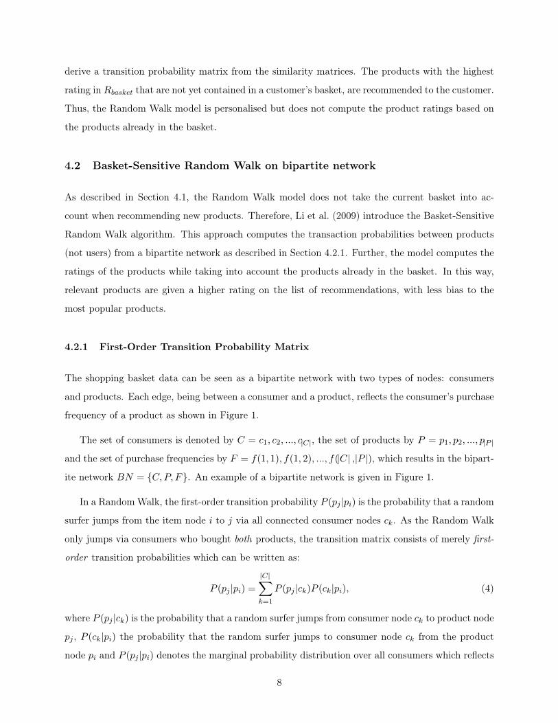
The shopping basket data can be seen as a bipartite network with two types of nodes: consumers

and products. Each edge, being between a consumer and a product, reflects the consumer’s purchase

frequency of a product as shown in Figure 1.

The set of consumers is denoted by C = c1, c2, ..., c|C|, the set of products by P = p1, p2, ..., p|P |

and the set of purchase frequencies by F = f(1, 1), f(1, 2), ..., f(|C| ,|P |), which results in the bipart-

ite network BN = {C,P, F}. An example of a bipartite network is given in Figure 1.

In a RandomWalk, the first-order transition probability P (pj |pi) is the probability that a random

surfer jumps from the item node i to j via all connected consumer nodes ck. As the Random Walk

only jumps via consumers who bought both products, the transition matrix consists of merely first-

order transition probabilities which can be written as:

P (pj |pi) =

|C|∑k=1

P (pj |ck)P (ck|pi), (4)

where P (pj |ck) is the probability that a random surfer jumps from consumer node ck to product node

pj , P (ck|pi) the probability that the random surfer jumps to consumer node ck from the product

node pi and P (pj |pi) denotes the marginal probability distribution over all consumers which reflects

8

the similarity between products i and j. The intuition behind probability P (pj |pi) is that it can

be seen as the preference for product pj from all customers C who have already bought product

pi. Every preference P (pj |ck) from the kth customer is weighed proportionally to the number of

times the customer bought product pi, namely P (ck|pi). The conditional probabilities used in (4)

are calculated as:

P (pj |ck) =f(ck, pj)

(∑f(ck, ·))α1

, (5) P (ck|pi) =f(ck, pi)

(∑f(·, pi))α2

. (6)

where α1, α2 ∈ [0, 1] correct for products that have high purchases frequencies. For convenience

reasons this research applies α1 = α2. As in (2), the parameter α corrects for the fact that people

who buy a lot of different products are less informative than people who bought just a few products.

Also, more popular products are less informative for the personal preferences of the shoppers than

unpopular products. However, the first-order similarity measure does not capture the possible

similarity between products which are never bought together, like newly launched products (Li et

al., 2009). Hence, when data is sparse, the first-order similarity measure suffers and results in less

effective recommendation.

Figure 1: Bipartite network for shopping basket data where f(i, j) is the amount of product j bought

by customer i (Li et al., 2009)

4.2.2 Basket-Sensitive Random Walk

As described in Section 4.2.1, the transition probability matrix has a disadvantage when data is

sparse. This limitation can be solved by combining the similarities of all orders as:

P ∗ =

∞∑t=1

(dP )t∣∣(dP )t∣∣ , (7)

where P is either the cosine or conditional probability matrix described in ?? or the first-order

transition probability matrix explained in 4.2.1. Again, the parameter d ∈ (0, 1) is the damping

9

factor which determines the length of the Random Walk. When t, the number of purchases of a

product, goes to infinity, P ∗ converges to dP (I − dP )−1 (Yildirim & Krishnamoorthy, 2008).

As the Random Walk P ∗ is not based on the current shopping behaviour, the model has to be

biased towards the items already in the shopping basket in order to get more accurate results. To

do so, an additional rating can be assigned to items currently in the shopper’s basket during each

iteration of the Random Walk computation. Therefore, Li et al. (2009) introduce a non-uniform

personalisation vector Ubasket to compute the importance score during each iteration as follows:

Rbasket = d · P ·Rbasket + (1− d) · Ubasket, (8)

where Rbasket contains the ratings for all products derived from the basket-based importance scores

and U ibasket = 1m if the ith product is in the basket and zero otherwise, where m is the number of

products in the current basket. The matrix P can be the normalised cosine or conditional probability-

based similarity matrix or the first-order transition probability matrix as described in Section 4.2.1.

The first term of (8), d · P · Rbasket, can be interpreted as the probability that the Random Walk

stops and that the customer is done shopping. The second term of the equation, (1 − d) · Ubasket,

can be seen as the probability that the Random Walk proceeds, meaning that the customer is still

adding items to the basket. However, applying (8) in practice would be too time consuming due to

the re-computations of the ratings in each iteration of the Random Walk. Therefore, Li et al. (2009)

also proposed an approximation, Rbasket defined as:

Rbasket =∑

pi∈basketRitemi , (9) Ritemi = d · P ·Ritemi + (1− d) · Uitemi (10)

where Ritem is the item-based importance score and Uitemi is the personalisation vector with the ith

entry set to one, and the rest set to zero. The computation of Ritemi can be simplified to

Ritemi = (1− d)(I − dP )−1Uitemi , (11)

which also simplifies the computation of (9). The products with the highest rating in Rbasket, which

are not already present in the basket, are recommended to the consumer.

4.3 Performance metrics and evaluation protocols

There are several ways to evaluate the accuracy of a recommender system. It is important that the

performance evaluation results are representative of live, interactive behaviour. Sordo-Garcia, Dias,

10

Li, El-Deredy and Lisboa (2007) looked into three evaluation strategies which differed in how to

split the retrospective basket into evidence and target components, where the evidence products are

used to predict the target products. The three approaches were to split the data randomly, based

on popularity and via the leave-n-out approach (Breese et al., 1998). According to the results the

popularity-based approach was the only one that ranked the recommender systems consistently with

their live performance (Sordo-Garcia et al., 2007).

To evaluate the accuracy of the recommender systems, this research uses the popularity-based

binary hit rate, bHR(pop), and the weighed hit rate, wHR(loo), introduced by Li et al. (2009). The

popularity based binary hit rate is based on a leave-three-out principle; the least three popular

products of the test basket, based on the training set, are the targets, the rest of the test basket is

used as evidence. When testing the recommender systems, the evidence items are used to predict

the target items. The binary hit rate is computed as the proportion of test baskets having at least

one out of three correctly predicted target items (Li et al., 2009). Besides leaving out the three least

popular items, I also evaluate the performance of the recommender system when using a random

leave-three-out approach (bHR(rnd)), where three target items are randomly selected from the test

basket. However, bHR(rnd) favors items which occur with a high frequency and therefore tends

to overestimate the model performance. Moreover, previous research has shown that when using a

leave-one-out cross validation the hit rates also over-emphasize the performance of popular products

(Sordo-Garcia et al., 2007; Li, Dias, El-Deredy & Lisboa, 2007).

To solve the issue of over-estimation for a leave-one-out cross validation, Li et al. (2009) propose

a new performance measure, which weighs the hit of items inversely to their popularity. The weighed

hit rate based on a leave-one-out approach, wHR(loo), is computed as:

wHR(loo) =

∑i(1− p(xi))HIT (xi)∑

i(1− p(xi))with HIT (xi) =

{1, if xi is predicted correctly0, otherwise

, (12)

where xi is the target item and p(xi) is its prior probability based on the popularity of the product.

The popularity and hence the prior probability p(xi) is based on the converted user-item matrix and

is computed as the ratio between the number of times an item was bought and the total number

of items bought by all customers. When all items are predicted correctly, the basket will achieve a

hit rate of one. The final hit rate is computed by averaging over all test baskets. Another measure

based on a leave-one-out cross validation that biases the results towards the performance of small

classes, is the macro-average hit rate, macroHR(loo). The macroHR(loo) measure computes the hit

11

rate for each product in a basket, which results in a vector of zeros, reflecting no hit, and ones,

reflecting a hit. The final hit rate is averaged over all products, which is the length of the vector,

instead of all baskets as for the wHR(loo).

In total I evaluate three types of standard item-based CF models, the cosine (1), the conditional

probability (2) and the bipartite network (4) based similarities, referred to as cf(cos), cf(cp) and

cf(bn) respectively. I also evaluate the standard Random Walk item-based CF model (rw) described

in Section 4.1 and the Basket-Sensitive Random Walk model (bsrw) described in Section 4.2. All

these methods are item-based models and are compared to a baseline method, pop, which merely

recommends the most popular items not contained in the basket.

4.4 User-based Collaborative Algorithm

Besides the item-based CF algorithm, I investigate the user-based CF algorithm for the same Ta-

Feng dataset, which is not yet done by Li et al. (2009). The idea of the user-based algorithm is to

predict the ratings of the products for a particular user, also referred to as active user, based on

the user-ratings of similar users from the training set, where ratings are based on the number of

purchases of a product. The user database for the Ta-Feng dataset is not too big, namely 20,388

customers. Hence, the scalability problem, which was mentioned in Section 2, of the user-based

CF algorithm might be avoided. Therefore, it is interesting to investigate whether for the size of

this user database a user-based CF approach could also work, despite its ‘cold start’ problem and

scalability issues (Konstan et al., 1997; Shardanand & Maes, 1995).

The user-based CF algorithm makes use of the cosine similarity matrix containing the similarities

between users instead of items. Again, the normalised n×m user-item matrix M is constructed as

described in Section 2 and can be used to compute the cosine similarity matrix for the users as:

sim(i, j) =Mi,∗ ·Mj,∗∣∣Mi,∗

∣∣∣∣Mj,∗∣∣ , (13)

where Mi,∗ is the ith row of the n ×m user-item matrix M representing the quantity of the items

bought by customer i (Deshpande & Karypis, 2004).

Before predicting ratings for the active user for the test set, the k most similar users are determ-

ined from the cosine similarity matrix. Then, the predicted ratings of the active user for item j,

12

ra,j , are computed as a weighed sum of the ratings of the k most similar users as:

ra,j = va +k∑i=1

w(a, i)(vi,j − vi), (14)

where vi is the mean of all the ratings of the products in the basket of customer i for the training

set, vi,j is the rating from user i for item j and w(a, i) is the normalised cosine similarity between

user a and i (Breese et al., 1998). The mean of all ratings is computed as:

vi =1

|Ii|∑j∈Ii

vi,j , (15)

where Ii is the set of items of user i for which there exists a rating in the training set. As for the

item-based algorithm, the user-based algorithm is evaluated with the test set which is split into

targets and evidence. With the targets and evidence products, the performance metrics bHR(pop),

bHR(rnd) and wHR(loo) can be computed based on the exact same training and test set as used to

generate the replication results. In this way an accurate comparison can be made to the results of

the item-based CF models. However, this also makes it hard to compare the results of the user-based

CF model to the results of Li et al. (2009) as this research makes use of a different composition of

the Ta-Feng dataset.

Besides evaluating the performance of the user-based CF algorithm compared to the item-based

CF algorithm and the baseline method pop, I intend to find an optimal level for k. To determine the

optimal level for k I investigate a trade-off between the values of the performance metrics and the

computation time of the user-based CF algorithm. For the computation time I focus on the time

needed to compute (14) as this will differ most between the different values for k. Suggestions for

an optimal value for k are widely varying in empirical literature (Mobasher, Dai, Luo & Nakagawa,

2001; Sarwar et al., 2001; Al Mamunur Rashid, Karypis & Riedl, 2006). Therefore, I consider values

going from three to 1000.

5 Results

This section gives an overview of the results of the replication of Li et al. (2009) in paragraph 5.1

and paragraph 5.2 gives the results of the user-based CF algorithm and a comparison to the results

of the replication.

13

5.1 Results replication

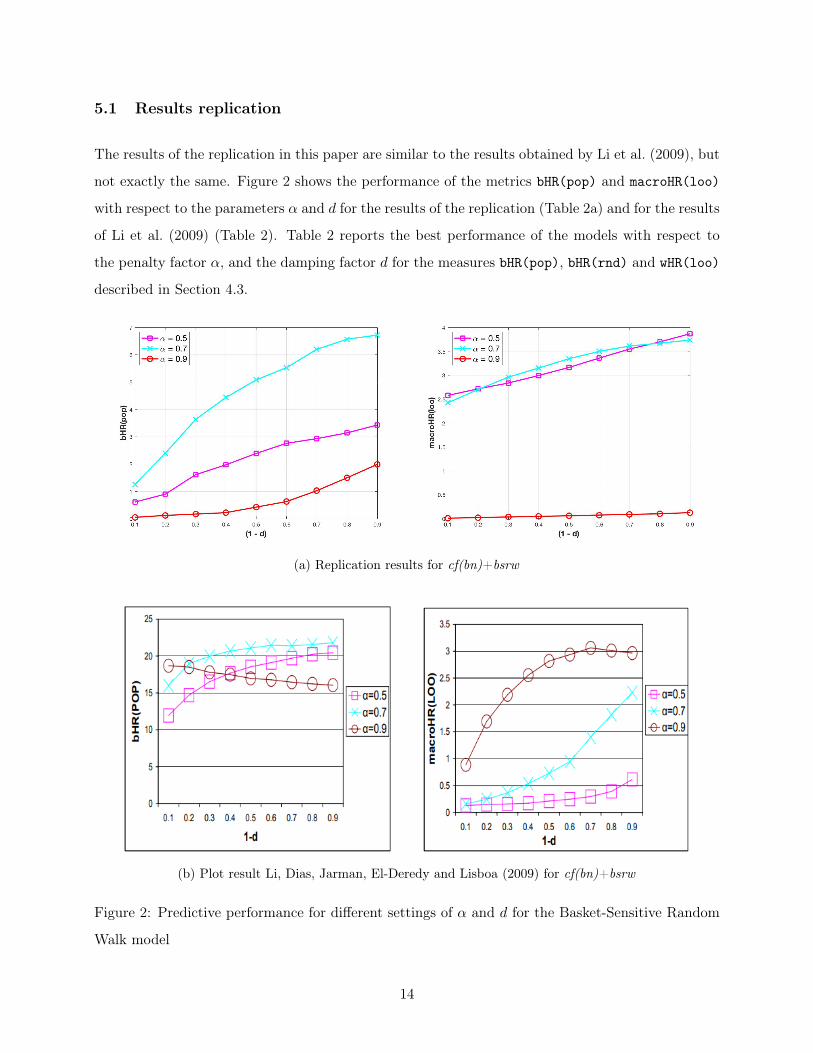
The results of the replication in this paper are similar to the results obtained by Li et al. (2009), but

not exactly the same. Figure 2 shows the performance of the metrics bHR(pop) and macroHR(loo)

with respect to the parameters α and d for the results of the replication (Table 2a) and for the results

of Li et al. (2009) (Table 2). Table 2 reports the best performance of the models with respect to

the penalty factor α, and the damping factor d for the measures bHR(pop), bHR(rnd) and wHR(loo)

described in Section 4.3.

(a) Replication results for cf(bn)+bsrw

(b) Plot result Li, Dias, Jarman, El-Deredy and Lisboa (2009) for cf(bn)+bsrw

Figure 2: Predictive performance for different settings of α and d for the Basket-Sensitive Random

Walk model

14

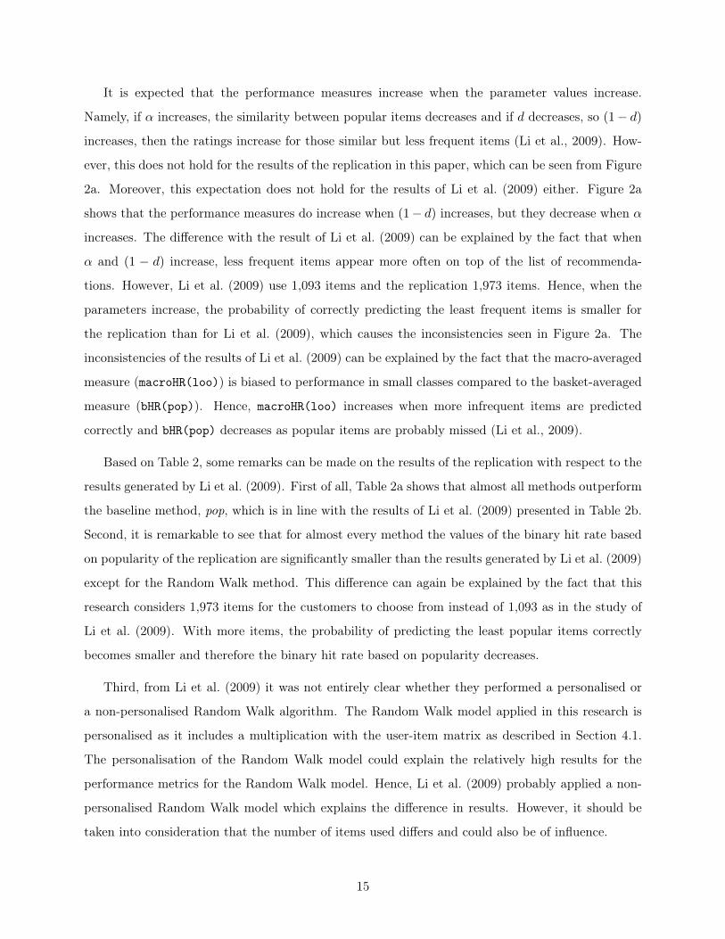
It is expected that the performance measures increase when the parameter values increase.

Namely, if α increases, the similarity between popular items decreases and if d decreases, so (1− d)

increases, then the ratings increase for those similar but less frequent items (Li et al., 2009). How-

ever, this does not hold for the results of the replication in this paper, which can be seen from Figure

2a. Moreover, this expectation does not hold for the results of Li et al. (2009) either. Figure 2a

shows that the performance measures do increase when (1− d) increases, but they decrease when α

increases. The difference with the result of Li et al. (2009) can be explained by the fact that when

α and (1 − d) increase, less frequent items appear more often on top of the list of recommenda-

tions. However, Li et al. (2009) use 1,093 items and the replication 1,973 items. Hence, when the

parameters increase, the probability of correctly predicting the least frequent items is smaller for

the replication than for Li et al. (2009), which causes the inconsistencies seen in Figure 2a. The

inconsistencies of the results of Li et al. (2009) can be explained by the fact that the macro-averaged

measure (macroHR(loo)) is biased to performance in small classes compared to the basket-averaged

measure (bHR(pop)). Hence, macroHR(loo) increases when more infrequent items are predicted

correctly and bHR(pop) decreases as popular items are probably missed (Li et al., 2009).

Based on Table 2, some remarks can be made on the results of the replication with respect to the

results generated by Li et al. (2009). First of all, Table 2a shows that almost all methods outperform

the baseline method, pop, which is in line with the results of Li et al. (2009) presented in Table 2b.

Second, it is remarkable to see that for almost every method the values of the binary hit rate based

on popularity of the replication are significantly smaller than the results generated by Li et al. (2009)

except for the Random Walk method. This difference can again be explained by the fact that this

research considers 1,973 items for the customers to choose from instead of 1,093 as in the study of

Li et al. (2009). With more items, the probability of predicting the least popular items correctly

becomes smaller and therefore the binary hit rate based on popularity decreases.

Third, from Li et al. (2009) it was not entirely clear whether they performed a personalised or

a non-personalised Random Walk algorithm. The Random Walk model applied in this research is

personalised as it includes a multiplication with the user-item matrix as described in Section 4.1.

The personalisation of the Random Walk model could explain the relatively high results for the

performance metrics for the Random Walk model. Hence, Li et al. (2009) probably applied a non-

personalised Random Walk model which explains the difference in results. However, it should be

taken into consideration that the number of items used differs and could also be of influence.

15

Further, as mentioned in Section 4.3, bHR(rnd) favors very popular items and therefore tends

to overestimate the model performance. This is in line with the results of the replication and the

results of Li et al. (2009) as the values for the bHR(rnd) metric are higher than for the bHR(pop)

metric.

Finally, the results for the Basket-Sensitive Random Walk of the replication are lower than the

results generated by Li et al. (2009) for the bHR(pop)measure, which is already explained above. The

rest of the evaluation measures generate more or less the same results as Li et al. (2009) do. However,

the results for the Basket-Sensitive Random Walk model based on the bipartite network transition

probability matrix for the replication are not as outstanding as the results of Li et al. (2009). This

could again be due to the number of items used in the replication or a misinterpretation of the

method as described in Li et al. (2009). When only comparing the results of the Basket-Sensitive

Random Walk model to the results of the standard CF model, the cf(bn) + bsrw method is always

among the top two performers. Also, the bipartite network-based Basket-Sensitive Random Walk

model has the highest hit rates compared with the cosine and conditional probability-based Basket-

Sensitive Random Walk model, which is in line with the results of Li et al. (2009). This can be

explained by the fact that the transition probability of the bipartite network is directly structured

from the graph and hence is more effective than the transition probability indirectly derived by

normalising the similarity matrices (Li et al., 2009).

Table 2: Predictive performance comparison of different models

(a) Results replication (%)

L-3-O L-1-O CVMethod bHR(pop) bHR(rnd) wHR(loo)

cf(cos) 6.2728 20.7483 4.3438cf(cp) 4.7067 21.0023 4.1406cf(bn) 5.4770 24.1260 2.4651

cf(cos) + bsrw 6.7891 18.6405 3.2600cf(cp) + bsrw 4.5374 20.7822 4.1205cf(bn) + bsrw 6.7214 24.0159 4.3078

cf(cos) + rw 11.1149 23.8551 3.9529cf(cp) + rw 12.6132 19.9611 2.9326pop 0.5418 18.3357 2.4944

(b) Results Li et al. (2009) (%)

L-3-O L-1-O CVMethod bHR(pop) bHR(rnd) wHR(loo)

cf(cos) 18.1945 22.0730 3.9281cf(cp) 14.6064 19.9129 3.3541cf(bn) 21.7341 25.2556 4.6646

cf(cos) + bsrw 18.2429 22.6599 3.9652cf(cp) + bsrw 16.7605 20.6571 3.4367cf(bn) + bsrw 21.7886 26.1814 4.8151

cf(cos) + rw 7.7994 5.4880 0.7289cf(cp) + rw 14.0679 19.1807 3.1493pop 7.9900 16.5700 2.2800

Note: For the results of the replication the metric based on random selection of targets is evaluated just once as it

did not differ much per run and spared computation time.

16

5.2 Results user-based CF algorithm

Table 3 shows the results for the user-based CF model for different values of k, which reflects the

number of users used to determine the ratings of the active user. Further, Table 3 shows that

the user-based CF outperforms the baseline method, pop, denoted in Table 2a for all values of k.

The user-based CF also outperforms the standard item-based CF model based on the leave-three-out

metrics for almost every k. However, the best methods for the bHR(pop) metric of the Random Walk

model and Basket-Sensitive Random Walk model shown in Table 2a outperform the user-based CF

model, but for the bHR(rnd) metric the user-based CF model is better for k ≥ 20. The above results

are based on the results for different values of k for the test set. However, for a more accurate

comparison between the results of the item- and user-based CF model, a validation set should be

used to determine the optimal level for k first and afterwards the results of the performance metrics

should be determined for the test set for the optimal value of k. These latter results should then be

used for comparison with the results of the item-based CF model.

Besides comparing the user-based CF model to the item-based CF models, it is interesting to

see what the optimal value for k is. The evaluation of the performance metrics with respect to k is

shown in Figure 3. The exact values of the performance metrics displayed in Figure 3 correspond to

the results denoted in Table 3. Table 3 and Figure 3 show that the macro-averaged metric does not

differ much amongst different values of k. This could be explained by the fact that macroHR(loo)

is based on a leave-one-out cross validation and hence that the recommended item with the highest

rating does not differ much when taking more customers into consideration. The basket-averaged

binary hit rate based on popularity decreases once k increases. This can be due to the number of

items taken into consideration determining the ratings. When k increases, more and more users are

used who are not very similar to the active user. This leads to less accurate rating prediction as a

lot of irrelevant information is used and more products are probably considered, which causes the

bHR(pop) to decrease. Furthermore, the random basket-averaged binary hit rate and the elapsed

time both increase when k increases. As seen before, the bHR(rnd) tends to overestimate the model

performance as it favors very popular products. When using more information as k increases, the

very popular products will probably appear more often, which causes overestimation of the metric.

Depending on what metric is important for a research, one could determine the optimal value for

k. However, I believe that k = 10 can be seen as the most appropriate value for k for this dataset as

17

Table 3: Predictive performance user-based CF algorithm for different sizes of neighbourhood

L-3-O (%) L-1-O CV (%)Method bHR(pop) bHR(rnd) macroHR(loo) Elapsed time (sec)

k = 3 10.5223 22.6191 3.5400 32.4475k = 5 10.1840 23.3472 3.6800 38.8772k = 10 9.7858 23.9228 3.7500 47.8670k = 20 9.5149 24.3799 3.8700 53.1561k = 50 9.1425 25.1926 3.9800 87.7133k = 100 8.6346 24.5916 4.0200 146.1390k = 500 7.4410 25.6328 3.9700 728.6756k = 1000 6.8315 26.4708 3.9300 1083.4911

Note: The metric based on random selection of targets is evaluated just once as it did

not differ much per run and spared computation time.

Figure 3: Evaluation of different metrics for different sizes of neighbourhood

the computation time for the ratings is less than one minute, the metric bHR(pop) is still relatively

high and the measure macroHR(loo) does not increase much when increasing the value of k. As

the bHR(rnd) is probably overestimated even more for a higher value of k, a lower value of k is also

preferable for bHR(rnd).

6 Conclusion

Grocery stores implement a variety of recommender systems to recommend products that are not

already present in a customer’s basket. As it benefits both customer and grocery store to have the

18

best possible working recommender system, this research investigates a basket-sensitive recommender

system introduced by Li et al. (2009). I replicate the paper from Li et al. (2009) for the Ta-Feng

dataset and apply a user-based CF model to the same dataset. The results of the user-based CF

model are compared to the results of the item-based models. Furthermore, I assess into the optimal

number of users used to determine the ratings for the active user.

The results of the replication of Li et al. (2009) in this paper approach the results of Li et al. (2009)

to a large extent. However, with a different set of items used in this paper for the replication, the

replication does not yield the exact same conclusion as Li et al. (2009). Li et al. (2009) conclude that

the Basket-Sensitive Random Walk model performs better than all other models they investigated.

However, this paper finds that the Basket-Sensitive Random Walk model can be outperformed by

some of the other models. The results of the replication show that every performance metric has a

different optimal method, but that overall cf(bn) + bsrw performs well on all measures.

The user-based CF model outperforms the standard item-based CF model, but in turn outper-

formed by some of the Random Walk and Basket-Sensitive Random Walk models. This can be

explained by the fact that the user-based CF model does not take into account the items already

in the customer’s basket, whereas the Random Walk and Basket-Sensitive Random Walk model do.

Overall, the Basket-Sensitive Random Walk is the most appropriate recommender system in the

domain of grocery shopping as the difference with the best performing models per metric is very

small and the model is among the top two performers for every metric, which is not the case for the

other models.

Finally, the optimal number of neighbours used to determine the ratings of the active user is

determined by examining the three different hit rates, bHR(pop), bHR(rnd) and macroHR(loo), and

by elapsed time for computing the ratings of the active user. For this research the optimal number

of neighbours used is ten, based on a trade-off between the decrease of bHR(pop) and an increase in

bHR(rnd) and the computation time.

7 Discussion

As some of the results of the replication do not agree with the results generated by Li et al. (2009)

there is room for improvement to this research. One of the big differences between the replication

and Li et al. (2009) is the number of items used as it was not clear from Li et al. (2009) how

19

they determined the number of items used in their research. Therefore, it would be interesting to

determine whether the results are more alike when taking the 1,093 most popular items and base the

replication on only those 1,093 items. From Li et al. (2009) it is not clear if they took the 1,093 most

popular items. However, with further investigation of the results, this might become clear. Further,

the results for the popularity based binary hit rate based on 1,093 items will show whether the low

hit rates for bHR(pop) are due to the number of items or whether there is a different underlying

reason.

There are several other limitations to this research. First of all, in this research the items

are all organised in sub-classes. This is probably done to overcome the sparsity and scalability

problem, but it also causes a loss of information. However, a sub-class item recommendation is not

as precise as a specific product recommendation and could therefore not be optimal. Second, people

are price-sensitive and this research does not take the price of products into consideration while

generating recommendations. Not everyone has the same income, and therefore the same budget, to

do groceries. The price of a product is a really important factor and by including the price factor in

the recommender system, recommendations can be more accurate. Furthermore, it is also of interest

for the grocery stores to recommend products with a high profit margin. Hence, including this in

the recommender system benefits the grocery store. Third, there are a lot of other factors that

may also be of interest when generating recommendations for grocery shoppers, which are not yet

included in this paper, i.e. age of the customer, location of product in the store, and whether it is

a seasonal product yes or no. Hence, future research needs to point out how including more details

in the recommender system benefits the performance of recommender systems.

Besides the ideas for future research proposed by Li et al. (2009), I think it is interesting to

investigate the user-based approach in more detail. There are several other methods that can be

applied to determine similarity between customers. For example, it can be interesting to cluster

customers by age, average price of the basket and average size of the basket and provide recom-

mendations based on the cluster to which a customer belongs. Furthermore, it is also interesting

to examine how machine learning techniques like Random-Forest and nearest-neighbour perform

on grocery recommendations. These machine learning techniques are, just like the CF algorithm,

widely explored in the field of movie recommendation, but have not yet been applied on the domain

of grocery shopping. Besides, it might even be possible to apply an item-based machine learning

approach to the dataset. One of the main advantages of machine learning techniques is that they

20

learn from their ‘mistakes’. By applying the machine learning technique on a greater amount of

data, the machine learning technique is able to recognise patterns and provide even more accurate

recommendations.

21

References

Al Mamunur Rashid, S. K. L., Karypis, G. & Riedl, J. (2006). Clustknn: A highly scalable hybrid

model-& memory-based cf algorithm. Proceeding of webKDD, 2006.

Breese, J. S., Heckerman, D. & Kadie, C. (1998). Empirical analysis of predictive algorithms for

collaborative filtering. In Proceedings of the fourteenth conference on uncertainty in artificial

intelligence (pp. 43–52). Morgan Kaufmann Publishers Inc.

Brin, S. & Page, L. (1998). The anatomy of a large-scale hypertextual web search engine. Computer

networks and ISDN systems, 30 (1-7), 107–117.

Deshpande, M. & Karypis, G. (2004). Item-based top-n recommendation algorithms. ACM Trans-

actions on Information Systems (TOIS), 22 (1), 143–177.

Hsu, C.-N., Chung, H.-H. & Huang, H.-S. (2004). Mining skewed and sparse transaction data for

personalized shopping recommendation. Machine Learning, 57 (1-2), 35–59.

Huang, Z., Zeng, D. & Chen, H. (2004). A link analysis approach to recommendation under sparse

data. AMCIS 2004 Proceedings, 239.

Konstan, J. A., Miller, B. N., Maltz, D., Herlocker, J. L., Gordon, L. R. & Riedl, J. (1997). Grouplens:

Applying collaborative filtering to usenet news. Communications of the ACM, 40 (3), 77–87.

Li, M., Dias, B. M., Jarman, I., El-Deredy, W. & Lisboa, P. J. (2009). Grocery shopping recom-

mendations based on basket-sensitive random walk. In Proceedings of the 15th acm sigkdd

international conference on knowledge discovery and data mining (pp. 1215–1224). ACM.

Li, M., Dias, B., El-Deredy, W. & Lisboa, P. J. (2007). A probabilistic model for item-based recom-

mender systems. In Proceedings of the 2007 acm conference on recommender systems (pp. 129–

132). ACM.

Liu, N. N. & Yang, Q. (2008). Eigenrank: A ranking-oriented approach to collaborative filtering. In

Proceedings of the 31st annual international acm sigir conference on research and development

in information retrieval (pp. 83–90). ACM.

Mobasher, B., Dai, H., Luo, T. & Nakagawa, M. (2001). Effective personalization based on association

rule discovery from web usage data. In Proceedings of the 3rd international workshop on web

information and data management (pp. 9–15). ACM.

Sarwar, B. M., Karypis, G., Konstan, J. A., Riedl, J. et al. (2001). Item-based collaborative filtering

recommendation algorithms. Www, 1, 285–295.

Shardanand, U. & Maes, P. (1995). Social information filtering: Algorithms for automating

22

. In Chi (Vol. 95, pp. 210–217). Citeseer.

Sordo-Garcia, C. M., Dias, M. B., Li, M., El-Deredy, W. & Lisboa, P. J. (2007). Evaluating retail

recommender systems via retrospective data: Lessons learnt from a live-intervention study. In

Dmin (Vol. 95, pp. 197–206). Citeseer.

Wijaya, D. T. & Bressan, S. (2008). A random walk on the red carpet: Rating movies with user

reviews and pagerank. In Proceedings of the 17th acm conference on information and knowledge

management (Vol. 95, pp. 951–960). ACM.

Yildirim, H. & Krishnamoorthy, M. S. (2008). A random walk method for alleviating the sparsity

problem in collaborative filtering. In Proceedings of the 2008 acm conference on recommender

systems (Vol. 95, pp. 131–138). ACM.

23

A Matlab code

Listing 1: Code to generate the descriptive statistics for the Ta-Feng dataset1 transactions2 = 1;2 baskets2 = [];3 transDate2 = [];4 customerTransaction2 = [];5 subclassPerBasket = zeros(107700,2000);6 indexNewBasket = [];7 %amount of baskets8 for i = 1:7201649 if i == 110 baskets2(transactions2) = newAmount(i);11 transDate2(transactions2) = newTransactionDate(i);12 customerTransaction2(transactions2) = newCustomerID(i);13 indexNewBasket = [indexNewBasket; i];14 else if newTransactionDate(i+1) == newTransactionDate(i) && newCustomerID(i+1)

== newCustomerID(i)15 baskets2(transactions2) = baskets2(transactions2) + newAmount(i+1);16 else17 indexNewBasket = [indexNewBasket; i+1];18 transactions2 = transactions2 + 1;19 baskets2(transactions2) = newAmount(i+1);20 transDate2(transactions2) = newTransactionDate(i+1);21 customerTransaction2(transactions2) = newCustomerID(i+1);22 end23 end24 end25 meanBasket = mean(baskets2);26 medianBasket = median(baskets2);27 minBasket = min(baskets2);28 maxBasket = max(baskets2);29 %amount of customers30 [sortedCustomers2, ia, indexSortedCustomers2] = unique(customerTransaction2);31 %amount of subclasses32 [sortedSubClasses2, is, indexSortedSubclasses2] = unique(newSubClasses);33 %amount of products per subclass34 amountPerSubclass = zeros(2000, 1);35 for j=1:200036 for i = 1:size(newAmount,2)37 if indexSortedSubclasses2(i) == j38 amountPerSubclass(j) = amountPerSubclass(j) +newAmount(i);39 end40 end41 end42 meanAmountSC = mean(amountPerSubclass);43 medianAmountSC = median(amountPerSubclass);44 maxAmountSC = max(amountPerSubclass);45 minAmountSC = min(amountPerSubclass);46 %amount of baskets per customer47 basketsPerCustomer = zeros(20388,1);

24

48 for j=1:2038849 for i = 1:transactions250 if indexSortedCustomers2(i) == j51 basketsPerCustomer(j) = basketsPerCustomer(j) + 1;52 end53 end54 end55 minbasketsPC = min(basketsPerCustomer);56 maxbasketsPC = max(basketsPerCustomer);57 meanbasketsPC = mean(basketsPerCustomer);58 medianbasketsPC = median(basketsPerCustomer);59 %aggregated baskets (only necessary for trainingset)60 aggregatedBaskets = zeros(20388, 1);6162 for j = 1:2038863 for i= 1:size(baskets2,1)64 if sortedCustomers2(j) == customerTransaction2(i)65 aggregatedBaskets(j) = aggregatedBaskets(j) + baskets2(i);66 end67 end68 end69 subclassesInBasket = zeros(20388, 2000);70 for i = 1:2038871 i72 newIndexSubClass = find(newCustomerID == sortedCustomers2(i));73 for j = 1:size(newIndexSubClass)74 subclassesInBasket(i,j) = newSubClasses(newIndexSubClass(j));75 end76 end77 %co occurence matrix78 coOccurenceMatrix = zeros(2000, 2000);79 for i = 1:2038880 uniqueSubClassesPerBasket = unique(subclassesInBasket(i,:));81 for j = 2:size(uniqueSubClassesPerBasket, 2)−182 for k = j+1:size(uniqueSubClassesPerBasket,2)83 coOccurenceMatrix(indexMatrix, indexMatrix2) = 1;84 end85 end86 end87 %generate test set88 [sortedCustomersLast, iaLast, indexSortedCustomersLast] = unique(

customerTransaction2, 'last');89 newCustomerIDtest = customerTransaction2(iaLast)';90 newIndexNewBasketTest = indexNewBasket(iaLast);91 newBasketsTest = baskets2(iaLast)';92 newTransDateTest = transDate2(iaLast)';93 subclassPerBasketTest = subclassPerBasket(iaLast,:);94 newAmountTest = newAmount(iaLast,:);95 %remove removed subclasses from baskets96 removedSubclasses = uniqueSubClasses(indexZero);97 adjustments = 0;98 for i = 1:2038899 for j = 1:2000

25

100 for k = 1:27101 if removedSubclasses(k) == subclassPerBasketTest(i,j)102 subclassPerBasketTest(i,j) = 0;103 adjustments = adjustments + 1;104 end105106 end107 end108 end

Listing 2: Code to generate the training and test set and the similarity matrices1 indexNewCustomerTrain = [];2 for i = 1:203883 if i == 14 indexNewCustomerTrain = [indexNewCustomerTrain; i];5 else if sortedCustomerIDtrain(i+1) == sortedCustomerIDtrain(i)6 %do nothing7 else8 indexNewCustomerTrain = [indexNewCustomerTrain; i+1];9 end10 end11 end12 %determine baskets13 userItemMatrix = zeros(20388, 2000);14 for i=1:size(indexNewCustomer,1)15 if i == 116 for j = 1:indexNewCustomer(i+1)−117 for k = 1:nnz(sortedSubclassPerBasket(indexIDtrain(j),:))18 indexSubClass = find(subclassPerBasketTrain(indexIDtrain(j),k) ==

uniqueSubClasses);19 userItemMatrix(i,indexSubClass) = userItemMatrix(i,indexSubClass) +

size(indexSubClass,2);20 end21 end22 else if i == size(indexNewCustomer,1)23 for j = indexNewCustomer(i):8731224 for k = 1:nnz(sortedSubclassPerBasket(indexIDtrain(j),:))25 indexSubClass = find(subclassPerBasketTrain(indexIDtrain(j),k)

== uniqueSubClasses);26 userItemMatrix(i,indexSubClass) = userItemMatrix(i,indexSubClass

) + size(indexSubClass,2);27 end28 end29 else30 for j = indexNewCustomer(i):indexNewCustomer(i+1) − 131 for k = 1:nnz(sortedSubclassPerBasket(indexIDtrain(j),:))32 indexSubClass = find(subclassPerBasketTrain(indexIDtrain(j),k)

== uniqueSubClasses);33 userItemMatrix(i,indexSubClass) = userItemMatrix(i,indexSubClass

) + size(indexSubClass,2);34 end35 end36 end

26

37 end38 end39 %delete subclasses which are never bought40 SUM = sum(userItemMatrix,1);41 indexZero = [];42 for i=1:200043 if SUM(i) == 044 indexZero = [indexZero;i];45 end46 end47 userItemMatrix2 = userItemMatrix;48 userItemMatrix2(:,indexZero)=[];49 %delete subclasses which are never bought in the training set50 uniqueSubClasses2 = uniqueSubClasses;51 uniqueSubClasses2(indexZero) = [];52 %define training baskets53 trainingBaskets = zeros(20388, 1973);54 for i = 1:2038855 for j = 1:197356 if userItemMatrix2(i,j) > 057 trainingBaskets(i,j) = uniqueSubClasses2(j);58 end59 end60 end61 trainingBaskets = sort(trainingBaskets,2, 'descend');62 %normalize user−item matrix63 logUserItemMatrix = log(userItemMatrix2 + 1);64 sumUser = sum(logUserItemMatrix,2);65 for i = 1:2038866 for j = 1:197367 normUserItemMatrix(i,j) = logUserItemMatrix(i,j)/sumUser(i);68 end69 end70 %cosine based similarity71 cosineSim = eye(1973);72 for i = 1:197273 for j=i+1:197374 cosineSim(i,j) = dot(normUserItemMatrix(:,i), normUserItemMatrix(:,j))/( (

sqrt(sum(abs(normUserItemMatrix(:,i)).^2))) * (sqrt(sum(abs(normUserItemMatrix(:,j)).^2))) );

75 cosineSim(j,i) = cosineSim(i,j);76 end77 end78 %conditional prob. based similarity79 for i=1:197380 freq(i) = nnz(userItemMatrix2(:,i));81 end82 totAmountOfBoughtProducts = 0;83 for i = 1:2038884 totAmountOfBoughtProducts = totAmountOfBoughtProducts + sum(logUserItemMatrix(i

,:));85 end86 for i = 1:1973

27

87 popularity(i) = sum(logUserItemMatrix(:,i))/totAmountOfBoughtProducts;88 end89 condProbSimAlpha5 = eye(1973);90 condProbSimAlpha7 = eye(1973);91 condProbSimAlpha9 = eye(1973);92 for i = 1:197293 for j = i+1:197394 sumPosEntries = 0;95 for c = 1:2038896 if normUserItemMatrix(c,i)>097 sumPosEntries = sumPosEntries + normUserItemMatrix(c,j);98 end99 end100 sumPosEntries2 = 0;101 for c = 1:20388102 if normUserItemMatrix(c,j)>0103 sumPosEntries2 = sumPosEntries2 + normUserItemMatrix(c,i);104 end105 end106 condProbSimAlpha5(i,j) = sumPosEntries / (freq(i) * freq(j)^0.5);107 condProbSimAlpha5(j,i) = sumPosEntries2 / (freq(j) * freq(i)^0.5);108 condProbSimAlpha7(i,j) = sumPosEntries / (freq(i) * freq(j)^0.7);109 condProbSimAlpha7(j,i) = sumPosEntries2 / (freq(j) * freq(i)^0.7);110 condProbSimAlpha9(i,j) = sumPosEntries / (freq(i) * freq(j)^0.9);111 condProbSimAlpha9(j,i) = sumPosEntries2 / (freq(j) * freq(i)^0.9);112 end113 end

Listing 3: Code to determine the transition probability matrix based on a bipartite network forthree values of α

1 totProductsPerUser = sum(logUserItemMatrix,2);2 totAmountProduct = sum(logUserItemMatrix, 1);3 for i = 1:203884 for j = 1:19735 probCustToProd5(i,j) = logUserItemMatrix(i,j)/( (totProductsPerUser(i))^0.5

);6 probProdToCust5(i,j) = logUserItemMatrix(i,j)/( (totAmountProduct(j))^0.5 );7 probCustToProd7(i,j) = logUserItemMatrix(i,j)/( (totProductsPerUser(i))^0.7

);8 probProdToCust7(i,j) = logUserItemMatrix(i,j)/( (totAmountProduct(j))^0.7 );9 probCustToProd9(i,j) = logUserItemMatrix(i,j)/( (totProductsPerUser(i))^0.9

);10 probProdToCust9(i,j) = logUserItemMatrix(i,j)/( (totAmountProduct(j))^0.9 );11 end12 end13 %determine transition probability matrix of bipartite network14 bnMatrix5 = zeros(1973, 1973);15 bnMatrix7 = zeros(1973, 1973);16 bnMatrix9 = zeros(1973, 1973);17 for j = 1:197318 for k=1:197319 for i = 1:20388

28

20 bnMatrix5(j,k) = bnMatrix5(j,k) + probCustToProd5(i,j)*probProdToCust5(i,k);

21 bnMatrix5(k,j) = bnMatrix5(k,j) + probCustToProd5(i,k)*probProdToCust5(i,j);





26 end27 end28 end

Listing 4: Code to determine the ratings for products based on the Random Walk model1 %determine personalization vector U2 Uitem = eye(1973);3 %rating CS4 RitemCS = inv(eye(1973) − .1*normCS) * (1 − .1) * Uitem;5 RitemCS = inv(eye(1973) − .2*normCS) * (1 − .2) * Uitem;6 RitemCS = inv(eye(1973) − .3*normCS) * (1 − .3) * Uitem;7 RitemCS = inv(eye(1973) − .4*normCS) * (1 − .4) * Uitem;8 RitemCS = inv(eye(1973) − .5*normCS) * (1 − .5) * Uitem;9 RitemCS = inv(eye(1973) − .6*normCS) * (1 − .6) * Uitem;10 RitemCS = inv(eye(1973) − .7*normCS) * (1 − .7) * Uitem;11 RitemCS = inv(eye(1973) − .8*normCS) * (1 − .8) * Uitem;12 RitemCS = inv(eye(1973) − .9*normCS) * (1 − .9) * Uitem;13 %rating CP alpha 0.514 RitemCP5_1 = inv(eye(1973) − .1*normCP5) * (1 − .1) * Uitem;15 RitemCP5_2 = inv(eye(1973) − .2*normCP5) * (1 − .2) * Uitem;16 RitemCP5_3 = inv(eye(1973) − .3*normCP5) * (1 − .3) * Uitem;17 RitemCP5_4 = inv(eye(1973) − .4*normCP5) * (1 − .4) * Uitem;18 RitemCP5_5 = inv(eye(1973) − .5*normCP5) * (1 − .5) * Uitem;19 RitemCP5_6 = inv(eye(1973) − .6*normCP5) * (1 − .6) * Uitem;20 RitemCP5_7 = inv(eye(1973) − .7*normCP5) * (1 − .7) * Uitem;21 RitemCP5_8 = inv(eye(1973) − .8*normCP5) * (1 − .8) * Uitem;22 RitemCP5_9 = inv(eye(1973) − .9*normCP5) * (1 − .9) * Uitem;23 %rating CP alpha 0.724 RitemCP7_1 = inv(eye(1973) − .1*normCP7) * (1 − .1) * Uitem;25 RitemCP7_2 = inv(eye(1973) − .2*normCP7) * (1 − .2) * Uitem;26 RitemCP7_3 = inv(eye(1973) − .3*normCP7) * (1 − .3) * Uitem;27 RitemCP7_4 = inv(eye(1973) − .4*normCP7) * (1 − .4) * Uitem;28 RitemCP7_5 = inv(eye(1973) − .5*normCP7) * (1 − .5) * Uitem;29 RitemCP7_6 = inv(eye(1973) − .6*normCP7) * (1 − .6) * Uitem;30 RitemCP7_7 = inv(eye(1973) − .7*normCP7) * (1 − .7) * Uitem;31 RitemCP7_8 = inv(eye(1973) − .8*normCP7) * (1 − .8) * Uitem;32 RitemCP7_9 = inv(eye(1973) − .9*normCP7) * (1 − .9) * Uitem;33 %rating CP alpha 0.934 RitemCP9_1 = inv(eye(1973) − .1*normCP9) * (1 − .1) * Uitem;35 RitemCP9_2 = inv(eye(1973) − .2*normCP9) * (1 − .2) * Uitem;36 RitemCP9_3 = inv(eye(1973) − .3*normCP9) * (1 − .3) * Uitem;

29

37 RitemCP9_4 = inv(eye(1973) − .4*normCP9) * (1 − .4) * Uitem;38 RitemCP9_5 = inv(eye(1973) − .5*normCP9) * (1 − .5) * Uitem;39 RitemCP9_6 = inv(eye(1973) − .6*normCP9) * (1 − .6) * Uitem;40 RitemCP9_7 = inv(eye(1973) − .7*normCP9) * (1 − .7) * Uitem;41 RitemCP9_8 = inv(eye(1973) − .8*normCP9) * (1 − .8) * Uitem;42 RitemCP9_9 = inv(eye(1973) − .9*normCP9) * (1 − .9) * Uitem;43 %rating BN alpha 0.544 RitemBN5_1 = inv(eye(1973) − .1*normBnMatrix5) * (1 − .1) * Uitem;45 RitemBN5_2 = inv(eye(1973) − .2*normBnMatrix5) * (1 − .2) * Uitem;46 RitemBN5_3 = inv(eye(1973) − .3*normBnMatrix5) * (1 − .3) * Uitem;47 RitemBN5_4 = inv(eye(1973) − .4*normBnMatrix5) * (1 − .4) * Uitem;48 RitemBN5_5 = inv(eye(1973) − .5*normBnMatrix5) * (1 − .5) * Uitem;49 RitemBN5_6 = inv(eye(1973) − .6*normBnMatrix5) * (1 − .6) * Uitem;50 RitemBN5_7 = inv(eye(1973) − .7*normBnMatrix5) * (1 − .7) * Uitem;51 RitemBN5_8 = inv(eye(1973) − .8*normBnMatrix5) * (1 − .8) * Uitem;52 RitemBN5_9 = inv(eye(1973) − .9*normBnMatrix5) * (1 − .9) * Uitem;53 %rating BN alpha 0.754 RitemBN7_1 = inv(eye(1973) − .1*normBnMatrix7) * (1 − .1) * Uitem;55 RitemBN7_2 = inv(eye(1973) − .2*normBnMatrix7) * (1 − .2) * Uitem;56 RitemBN7_3 = inv(eye(1973) − .3*normBnMatrix7) * (1 − .3) * Uitem;57 RitemBN7_4 = inv(eye(1973) − .4*normBnMatrix7) * (1 − .4) * Uitem;58 RitemBN7_5 = inv(eye(1973) − .5*normBnMatrix7) * (1 − .5) * Uitem;59 RitemBN7_6 = inv(eye(1973) − .6*normBnMatrix7) * (1 − .6) * Uitem;60 RitemBN7_7 = inv(eye(1973) − .7*normBnMatrix7) * (1 − .7) * Uitem;61 RitemBN7_8 = inv(eye(1973) − .8*normBnMatrix7) * (1 − .8) * Uitem;62 RitemBN7_9 = inv(eye(1973) − .9*normBnMatrix7) * (1 − .9) * Uitem;63 %rating BN alpha 0.964 RitemBN9_1 = inv(eye(1973) − .1*normBnMatrix9) * (1 − .1) * Uitem;65 RitemBN9_2 = inv(eye(1973) − .2*normBnMatrix9) * (1 − .2) * Uitem;66 RitemBN9_3 = inv(eye(1973) − .3*normBnMatrix9) * (1 − .3) * Uitem;67 RitemBN9_4 = inv(eye(1973) − .4*normBnMatrix9) * (1 − .4) * Uitem;68 RitemBN9_5 = inv(eye(1973) − .5*normBnMatrix9) * (1 − .5) * Uitem;69 RitemBN9_6 = inv(eye(1973) − .6*normBnMatrix9) * (1 − .6) * Uitem;70 RitemBN9_7 = inv(eye(1973) − .7*normBnMatrix9) * (1 − .7) * Uitem;71 RitemBN9_8 = inv(eye(1973) − .8*normBnMatrix9) * (1 − .8) * Uitem;72 RitemBN9_9 = inv(eye(1973) − .9*normBnMatrix9) * (1 − .9) * Uitem;

Listing 5: Code to determine the ratings of the products based on the evidence products with helpof the similarity matrices. The code also contains the computation of the binary hit rate based ona popularity selection of targets. The code for the hit rate based on a random selection of targets issimilar to the code based on a popularity selection.

1 %determine targets test basket based on popularity2 for i = 1:118133 for j = 1:nnz(testBaskets(i,:))4 indexSubClassTest = find(testBaskets(i,j) == uniqueSubClasses2);5 freqSubclass(i,j) = popularity(indexSubClassTest);6 end7 end8 freqSubclass( freqSubclass == 0 ) = Inf;9 [sortedFreqSubclass, indexFreqSubclass] = sort(freqSubclass,2,'ascend');10 freqSubclass( isinf(freqSubclass) ) = 0;11 sortedFreqSubclass( isinf(sortedFreqSubclass) ) = 0;

30

12 for i = 1:1181313 for j = 1:314 targetSubclass(i,j) = testBaskets(i,indexFreqSubclass(i,j));15 end16 for j = 4:nnz(testBaskets(i,:))17 evidenceSubclass(i,j) = testBaskets(i,indexFreqSubclass(i,j));18 end19 end20 %determine recommendations21 csRows1=zeros(11813,1973);csRows2=zeros(11813,1973);csRows3=zeros(11813,1973);

csRows4=zeros(11813,1973);csRows5=zeros(11813,1973);csRows6=zeros(11813,1973);csRows7=zeros(11813,1973);csRows8=zeros(11813,1973);csRows9=zeros(11813,1973);

22 cp5Rows1=zeros(11813,1973);cp5Rows2=zeros(11813,1973);cp5Rows3=zeros(11813,1973);cp5Rows4=zeros(11813,1973);cp5Rows5=zeros(11813,1973);cp5Rows6=zeros(11813,1973);cp5Rows7=zeros(11813,1973);cp5Rows8=zeros(11813,1973);cp5Rows9=zeros(11813,1973);



25 bn5Rows1=zeros(11813,1973);bn5Rows2=zeros(11813,1973);bn5Rows3=zeros(11813,1973);bn5Rows4=zeros(11813,1973);bn5Rows5=zeros(11813,1973);bn5Rows6=zeros(11813,1973);bn5Rows7=zeros(11813,1973);bn5Rows8=zeros(11813,1973);bn5Rows9=zeros(11813,1973);



28 for i = 1:1181329 for j = 4:nnz(testBaskets(i,:))30 indexSubClassTest = find(testBaskets(i,indexFreqSubclass(i,j)) ==

uniqueSubClasses2);31 csRows1(i,:) = csRows1(i,:) + RitemCS1(indexSubClassTest,:);32 csRows2(i,:) = csRows2(i,:) + RitemCS2(indexSubClassTest,:);33 csRows3(i,:) = csRows3(i,:) + RitemCS3(indexSubClassTest,:);34 csRows4(i,:) = csRows4(i,:) + RitemCS4(indexSubClassTest,:);35 csRows5(i,:) = csRows5(i,:) + RitemCS5(indexSubClassTest,:);36 csRows6(i,:) = csRows6(i,:) + RitemCS6(indexSubClassTest,:);37 csRows7(i,:) = csRows7(i,:) + RitemCS7(indexSubClassTest,:);38 csRows8(i,:) = csRows8(i,:) + RitemCS8(indexSubClassTest,:);39 csRows9(i,:) = csRows9(i,:) + RitemCS9(indexSubClassTest,:);40 cp5Rows1(i,:) = cp5Rows1(i,:) + RitemCP5_1(indexSubClassTest,:);41 cp5Rows2(i,:) = cp5Rows2(i,:) + RitemCP5_2(indexSubClassTest,:);42 cp5Rows3(i,:) = cp5Rows3(i,:) + RitemCP5_3(indexSubClassTest,:);43 cp5Rows4(i,:) = cp5Rows4(i,:) + RitemCP5_4(indexSubClassTest,:);

31

44 cp5Rows5(i,:) = cp5Rows5(i,:) + RitemCP5_5(indexSubClassTest,:);45 cp5Rows6(i,:) = cp5Rows6(i,:) + RitemCP5_6(indexSubClassTest,:);46 cp5Rows7(i,:) = cp5Rows7(i,:) + RitemCP5_7(indexSubClassTest,:);47 cp5Rows8(i,:) = cp5Rows8(i,:) + RitemCP5_8(indexSubClassTest,:);48 cp5Rows9(i,:) = cp5Rows9(i,:) + RitemCP5_9(indexSubClassTest,:);49 cp7Rows1(i,:) = cp7Rows1(i,:) + RitemCP7_1(indexSubClassTest,:);50 cp7Rows2(i,:) = cp7Rows2(i,:) + RitemCP7_2(indexSubClassTest,:);51 cp7Rows3(i,:) = cp7Rows3(i,:) + RitemCP7_3(indexSubClassTest,:);52 cp7Rows4(i,:) = cp7Rows4(i,:) + RitemCP7_4(indexSubClassTest,:);53 cp7Rows5(i,:) = cp7Rows5(i,:) + RitemCP7_5(indexSubClassTest,:);54 cp7Rows6(i,:) = cp7Rows6(i,:) + RitemCP7_6(indexSubClassTest,:);55 cp7Rows7(i,:) = cp7Rows7(i,:) + RitemCP7_7(indexSubClassTest,:);56 cp7Rows8(i,:) = cp7Rows8(i,:) + RitemCP7_8(indexSubClassTest,:);57 cp7Rows9(i,:) = cp7Rows9(i,:) + RitemCP7_9(indexSubClassTest,:);58 cp9Rows1(i,:) = cp9Rows1(i,:) + RitemCP9_1(indexSubClassTest,:);59 cp9Rows2(i,:) = cp9Rows2(i,:) + RitemCP9_2(indexSubClassTest,:);60 cp9Rows3(i,:) = cp9Rows3(i,:) + RitemCP9_3(indexSubClassTest,:);61 cp9Rows4(i,:) = cp9Rows4(i,:) + RitemCP9_4(indexSubClassTest,:);62 cp9Rows5(i,:) = cp9Rows5(i,:) + RitemCP9_5(indexSubClassTest,:);63 cp9Rows6(i,:) = cp9Rows6(i,:) + RitemCP9_6(indexSubClassTest,:);64 cp9Rows7(i,:) = cp9Rows7(i,:) + RitemCP9_7(indexSubClassTest,:);65 cp9Rows8(i,:) = cp9Rows8(i,:) + RitemCP9_8(indexSubClassTest,:);66 cp9Rows9(i,:) = cp9Rows9(i,:) + RitemCP9_9(indexSubClassTest,:);67 bn5Rows1(i,:) = bn5Rows1(i,:) + RitemBN5_1(indexSubClassTest,:);68 bn5Rows2(i,:) = bn5Rows2(i,:) + RitemBN5_2(indexSubClassTest,:);69 bn5Rows3(i,:) = bn5Rows3(i,:) + RitemBN5_3(indexSubClassTest,:);70 bn5Rows4(i,:) = bn5Rows4(i,:) + RitemBN5_4(indexSubClassTest,:);71 bn5Rows5(i,:) = bn5Rows5(i,:) + RitemBN5_5(indexSubClassTest,:);72 bn5Rows6(i,:) = bn5Rows6(i,:) + RitemBN5_6(indexSubClassTest,:);73 bn5Rows7(i,:) = bn5Rows7(i,:) + RitemBN5_7(indexSubClassTest,:);74 bn5Rows8(i,:) = bn5Rows8(i,:) + RitemBN5_8(indexSubClassTest,:);75 bn5Rows9(i,:) = bn5Rows9(i,:) + RitemBN5_9(indexSubClassTest,:);76 bn7Rows1(i,:) = bn7Rows1(i,:) + RitemBN7_1(indexSubClassTest,:);77 bn7Rows2(i,:) = bn7Rows2(i,:) + RitemBN7_2(indexSubClassTest,:);78 bn7Rows3(i,:) = bn7Rows3(i,:) + RitemBN7_3(indexSubClassTest,:);79 bn7Rows4(i,:) = bn7Rows4(i,:) + RitemBN7_4(indexSubClassTest,:);80 bn7Rows5(i,:) = bn7Rows5(i,:) + RitemBN7_5(indexSubClassTest,:);81 bn7Rows6(i,:) = bn7Rows6(i,:) + RitemBN7_6(indexSubClassTest,:);82 bn7Rows7(i,:) = bn7Rows7(i,:) + RitemBN7_7(indexSubClassTest,:);83 bn7Rows8(i,:) = bn7Rows8(i,:) + RitemBN7_8(indexSubClassTest,:);84 bn7Rows9(i,:) = bn7Rows9(i,:) + RitemBN7_9(indexSubClassTest,:);85 bn9Rows1(i,:) = bn9Rows1(i,:) + RitemBN9_1(indexSubClassTest,:);86 bn9Rows2(i,:) = bn9Rows2(i,:) + RitemBN9_2(indexSubClassTest,:);87 bn9Rows3(i,:) = bn9Rows3(i,:) + RitemBN9_3(indexSubClassTest,:);88 bn9Rows4(i,:) = bn9Rows4(i,:) + RitemBN9_4(indexSubClassTest,:);89 bn9Rows5(i,:) = bn9Rows5(i,:) + RitemBN9_5(indexSubClassTest,:);90 bn9Rows6(i,:) = bn9Rows6(i,:) + RitemBN9_6(indexSubClassTest,:);91 bn9Rows7(i,:) = bn9Rows7(i,:) + RitemBN9_7(indexSubClassTest,:);92 bn9Rows8(i,:) = bn9Rows8(i,:) + RitemBN9_8(indexSubClassTest,:);93 bn9Rows9(i,:) = bn9Rows9(i,:) + RitemBN9_9(indexSubClassTest,:);94 end95 end96 %determine place ratings

32

97 [maxCS1, indexMaxCS1] = sort(csRows1, 2, 'descend');98 [maxCS2, indexMaxCS2] = sort(csRows2, 2, 'descend');99 [maxCS3, indexMaxCS3] = sort(csRows3, 2, 'descend');100 [maxCS4, indexMaxCS4] = sort(csRows4, 2, 'descend');101 [maxCS5, indexMaxCS5] = sort(csRows5, 2, 'descend');102 [maxCS6, indexMaxCS6] = sort(csRows6, 2, 'descend');103 [maxCS7, indexMaxCS7] = sort(csRows7, 2, 'descend');104 [maxCS8, indexMaxCS8] = sort(csRows8, 2, 'descend');105 [maxCS9, indexMaxCS9] = sort(csRows9, 2, 'descend');106 [indexCP5_1, indexMaxCP5_1] = sort(cp5Rows1, 2, 'descend');107 [indexCP5_2, indexMaxCP5_2] = sort(cp5Rows2, 2, 'descend');108 [indexCP5_3, indexMaxCP5_3] = sort(cp5Rows3, 2, 'descend');109 [indexCP5_4, indexMaxCP5_4] = sort(cp5Rows4, 2, 'descend');110 [indexCP5_5, indexMaxCP5_5] = sort(cp5Rows5, 2, 'descend');111 [indexCP5_6, indexMaxCP5_6] = sort(cp5Rows6, 2, 'descend');112 [indexCP5_7, indexMaxCP5_7] = sort(cp5Rows7, 2, 'descend');113 [indexCP5_8, indexMaxCP5_8] = sort(cp5Rows8, 2, 'descend');114 [indexCP5_9, indexMaxCP5_9] = sort(cp5Rows9, 2, 'descend');115 [indexCP7_1, indexMaxCP7_1] = sort(cp7Rows1, 2, 'descend');116 [indexCP7_2, indexMaxCP7_2] = sort(cp7Rows2, 2, 'descend');117 [indexCP7_3, indexMaxCP7_3] = sort(cp7Rows3, 2, 'descend');118 [indexCP7_4, indexMaxCP7_4] = sort(cp7Rows4, 2, 'descend');119 [indexCP7_5, indexMaxCP7_5] = sort(cp7Rows5, 2, 'descend');120 [indexCP7_6, indexMaxCP7_6] = sort(cp7Rows6, 2, 'descend');121 [indexCP7_7, indexMaxCP7_7] = sort(cp7Rows7, 2, 'descend');122 [indexCP7_8, indexMaxCP7_8] = sort(cp7Rows8, 2, 'descend');123 [indexCP7_9, indexMaxCP7_9] = sort(cp7Rows9, 2, 'descend');124 [indexCP9_1, indexMaxCP9_1] = sort(cp9Rows1, 2, 'descend');125 [indexCP9_2, indexMaxCP9_2] = sort(cp9Rows2, 2, 'descend');126 [indexCP9_3, indexMaxCP9_3] = sort(cp9Rows3, 2, 'descend');127 [indexCP9_4, indexMaxCP9_4] = sort(cp9Rows4, 2, 'descend');128 [indexCP9_5, indexMaxCP9_5] = sort(cp9Rows5, 2, 'descend');129 [indexCP9_6, indexMaxCP9_6] = sort(cp9Rows6, 2, 'descend');130 [indexCP9_7, indexMaxCP9_7] = sort(cp9Rows7, 2, 'descend');131 [indexCP9_8, indexMaxCP9_8] = sort(cp9Rows8, 2, 'descend');132 [indexCP9_9, indexMaxCP9_9] = sort(cp9Rows9, 2, 'descend');133 [indexBN5_1, indexMaxBN5_1] = sort(bn5Rows1, 2, 'descend');134 [indexBN5_2, indexMaxBN5_2] = sort(bn5Rows2, 2, 'descend');135 [indexBN5_3, indexMaxBN5_3] = sort(bn5Rows3, 2, 'descend');136 [indexBN5_4, indexMaxBN5_4] = sort(bn5Rows4, 2, 'descend');137 [indexBN5_5, indexMaxBN5_5] = sort(bn5Rows5, 2, 'descend');138 [indexBN5_6, indexMaxBN5_6] = sort(bn5Rows6, 2, 'descend');139 [indexBN5_7, indexMaxBN5_7] = sort(bn5Rows7, 2, 'descend');140 [indexBN5_8, indexMaxBN5_8] = sort(bn5Rows8, 2, 'descend');141 [indexBN5_9, indexMaxBN5_9] = sort(bn5Rows9, 2, 'descend');142 [indexBN7_1, indexMaxBN7_1] = sort(bn7Rows1, 2, 'descend');143 [indexBN7_2, indexMaxBN7_2] = sort(bn7Rows2, 2, 'descend');144 [indexBN7_3, indexMaxBN7_3] = sort(bn7Rows3, 2, 'descend');145 [indexBN7_4, indexMaxBN7_4] = sort(bn7Rows4, 2, 'descend');146 [indexBN7_5, indexMaxBN7_5] = sort(bn7Rows5, 2, 'descend');147 [indexBN7_6, indexMaxBN7_6] = sort(bn7Rows6, 2, 'descend');148 [indexBN7_7, indexMaxBN7_7] = sort(bn7Rows7, 2, 'descend');149 [indexBN7_8, indexMaxBN7_8] = sort(bn7Rows8, 2, 'descend');

33

150 [indexBN7_9, indexMaxBN7_9] = sort(bn7Rows9, 2, 'descend');151 [indexBN9_1, indexMaxBN9_1] = sort(bn9Rows1, 2, 'descend');152 [indexBN9_2, indexMaxBN9_2] = sort(bn9Rows2, 2, 'descend');153 [indexBN9_3, indexMaxBN9_3] = sort(bn9Rows3, 2, 'descend');154 [indexBN9_4, indexMaxBN9_4] = sort(bn9Rows4, 2, 'descend');155 [indexBN9_5, indexMaxBN9_5] = sort(bn9Rows5, 2, 'descend');156 [indexBN9_6, indexMaxBN9_6] = sort(bn9Rows6, 2, 'descend');157 [indexBN9_7, indexMaxBN9_7] = sort(bn9Rows7, 2, 'descend');158 [indexBN9_8, indexMaxBN9_8] = sort(bn9Rows8, 2, 'descend');159 [indexBN9_9, indexMaxBN9_9] = sort(bn9Rows9, 2, 'descend');160 %determine recommendations and hitrates161 for i = 1:11813162 a = 0;163 b = 0;164 c = 0;165 d = 0;166 e = 0;167 f = 0;168 g = 0;169 h = 0;170 z = 0;171 for j = 4:1973172 if a < 3173 if ismember(uniqueSubClasses2(indexMaxCS1(i,j−3)),evidenceSubclass(i,:))

> 0174 %do nothing175 else176 a = a+1;177 recCS1(i,a) = uniqueSubClasses2(indexMaxCS1(i,j−3));178 end179 end180 if b < 3181 if ismember(uniqueSubClasses2(indexMaxCS2(i,j−3)),evidenceSubclass(i,:))

> 0182 %do nothing183 else184 b = b+1;185 recCS2(i,b) = uniqueSubClasses2(indexMaxCS2(i,j−3));186 end187 end188 if c < 3189 if ismember(uniqueSubClasses2(indexMaxCS3(i,j−3)),evidenceSubclass(i,:))

> 0190 %do nothing191 else192 c = c+1;193 recCS3(i,c) = uniqueSubClasses2(indexMaxCS3(i,j−3));194 end195 end196 if d < 3197 if ismember(uniqueSubClasses2(indexMaxCS4(i,j−3)),evidenceSubclass(i,:))

> 0198 %do nothing

34

199 else200 d = d+1;201 recCS4(i,d) = uniqueSubClasses2(indexMaxCS4(i,j−3));202 end203 end204 if e < 3205 if ismember(uniqueSubClasses2(indexMaxCS5(i,j−3)),evidenceSubclass(i,:))

> 0206 %do nothing207 else208 e = e+1;209 recCS5(i,e) = uniqueSubClasses2(indexMaxCS5(i,j−3));210 end211 end212 if f < 3213 if ismember(uniqueSubClasses2(indexMaxCS6(i,j−3)),evidenceSubclass(i,:))

> 0214 %do nothing215 else216 f = f+1;217 recCS6(i,f) = uniqueSubClasses2(indexMaxCS6(i,j−3));218 end219 end220 if g < 3221 if ismember(uniqueSubClasses2(indexMaxCS7(i,j−3)),evidenceSubclass(i,:))

> 0222 %do nothing223 else224 g = g+1;225 recCS7(i,g) = uniqueSubClasses2(indexMaxCS7(i,j−3));226 end227 end228 if h < 3229 if ismember(uniqueSubClasses2(indexMaxCS8(i,j−3)),evidenceSubclass(i,:))

> 0230 %do nothing231 else232 h = h+1;233 recCS8(i,h) = uniqueSubClasses2(indexMaxCS8(i,j−3));234 end235 end236 if z < 3237 if ismember(uniqueSubClasses2(indexMaxCS9(i,j−3)),evidenceSubclass(i,:))

> 0238 %do nothing239 else240 z = z+1;241 recCS9(i,z) = uniqueSubClasses2(indexMaxCS9(i,j−3));242 end243 end244 end245 end246 %determine hit rate similarities

35

247 bHR_CS1 = zeros(11813,3);bHR_CS2 = zeros(11813,3);bHR_CS3 = zeros(11813,3);bHR_CS4 =zeros(11813,3);bHR_CS5 = zeros(11813,3);bHR_CS6 = zeros(11813,3);bHR_CS7 =zeros(11813,3);bHR_CS8 = zeros(11813,3);bHR_CS9 = zeros(11813,3);

248 for i = 1:11813249 for j = 1:3250 for z= 1:3251 if targetSubclass(i,j) == recCS1(i,z)252 bHR_CS1(i,j) = 1;253 end254 if targetSubclass(i,j) == recCS2(i,z)255 bHR_CS2(i,j) = 1;256 end257 if targetSubclass(i,j) == recCS3(i,z)258 bHR_CS3(i,j) = 1;259 end260 if targetSubclass(i,j) == recCS4(i,z)261 bHR_CS4(i,j) = 1;262 end263 if targetSubclass(i,j) == recCS5(i,z)264 bHR_CS5(i,j) = 1;265 end266 if targetSubclass(i,j) == recCS6(i,z)267 bHR_CS6(i,j) = 1;268 end269 if targetSubclass(i,j) == recCS7(i,z)270 bHR_CS7(i,j) = 1;271 end272 if targetSubclass(i,j) == recCS8(i,z)273 bHR_CS8(i,j) = 1;274 end275 if targetSubclass(i,j) == recCS9(i,z)276 bHR_CS9(i,j) = 1;277 end278 end279 end280 end281 hitCS1=0;hitCS2= 0;hitCS3=0;hitCS4=0;hitCS5=0;hitCS6=0;hitCS7=0;hitCS8=0;hitCS9=0;282 for i = 1:11813283 if nnz(bHR_CS1(i,:))>0284 hitCS1 = hitCS1 + 1;285 end286 if nnz(bHR_CS2(i,:))>0287 hitCS2 = hitCS2 + 1;288 end289 if nnz(bHR_CS3(i,:))>0290 hitCS3 = hitCS3 + 1;291 end292 if nnz(bHR_CS4(i,:))>0293 hitCS4 = hitCS4 + 1;294 end295 if nnz(bHR_CS5(i,:))>0296 hitCS5 = hitCS5 + 1;297 end

36

298 if nnz(bHR_CS6(i,:))>0299 hitCS6 = hitCS6 + 1;300 end301 if nnz(bHR_CS7(i,:))>0302 hitCS7 = hitCS7 + 1;303 end304 if nnz(bHR_CS8(i,:))>0305 hitCS8 = hitCS8 + 1;306 end307 if nnz(bHR_CS9(i,:))>0308 hitCS9 = hitCS9 + 1;309 end310 end311 percentageHitCS(1) = (hitCS1/11813);312 percentageHitCS(2) = (hitCS2/11813);313 percentageHitCS(3) = (hitCS3/11813);314 percentageHitCS(4) = (hitCS4/11813);315 percentageHitCS(5) = (hitCS5/11813);316 percentageHitCS(6) = (hitCS6/11813);317 percentageHitCS(7) = (hitCS7/11813);318 percentageHitCS(8) = (hitCS8/11813);319 percentageHitCS(9) = (hitCS9/11813);

Listing 6: Code for weighed hit rate based on conditional probability similarity matrix for α = 0.5.Same approach can be applied for α = 0.7 and α = 0.9

1 sumPreviousProb = zeros(11813,1);2 sumHitCP5_1 = zeros(11813,1);sumHitCP5_2 = zeros(11813,1);3 sumHitCP5_3 = zeros(11813,1);sumHitCP5_4 = zeros(11813,1);4 sumHitCP5_5 = zeros(11813,1);sumHitCP5_6 = zeros(11813,1);5 sumHitCP5_7 = zeros(11813,1);sumHitCP5_8 = zeros(11813,1);6 sumHitCP5_9 = zeros(11813,1);7 for i=1:118138 for j = 1:nnz(testBaskets(i,:))9 %determine target and evidence10 target = testBaskets(i,j);11 evidence = testBaskets(i,:);12 evidence(j) = 0;13 evidence = sort(evidence, 'descend');14 % %determine similarity evidence cosine based15 cp5RowsL1O_1 = zeros(1,1973);cp5RowsL1O_2 = zeros(1,1973);16 cp5RowsL1O_3 = zeros(1,1973);cp5RowsL1O_4 = zeros(1,1973);17 cp5RowsL1O_5 = zeros(1,1973);cp5RowsL1O_6 = zeros(1,1973);18 cp5RowsL1O_7 = zeros(1,1973);cp5RowsL1O_8 = zeros(1,1973);19 cp5RowsL1O_9 = zeros(1,1973);20 for m = 1:nnz(evidence)21 indexSubClassTest = find(evidence(m) == uniqueSubClasses2);22 cp5RowsL1O_1(1,:) = cp5RowsL1O_1(1,:) + RitemCP5_1(indexSubClassTest,:);23 cp5RowsL1O_2(1,:) = cp5RowsL1O_2(1,:) + RitemCP5_2(indexSubClassTest,:);24 cp5RowsL1O_3(1,:) = cp5RowsL1O_3(1,:) + RitemCP5_3(indexSubClassTest,:);25 cp5RowsL1O_4(1,:) = cp5RowsL1O_4(1,:) + RitemCP5_4(indexSubClassTest,:);26 cp5RowsL1O_5(1,:) = cp5RowsL1O_5(1,:) + RitemCP5_5(indexSubClassTest,:);27 cp5RowsL1O_6(1,:) = cp5RowsL1O_6(1,:) + RitemCP5_6(indexSubClassTest,:);

37

28 cp5RowsL1O_7(1,:) = cp5RowsL1O_7(1,:) + RitemCP5_7(indexSubClassTest,:);29 cp5RowsL1O_8(1,:) = cp5RowsL1O_8(1,:) + RitemCP5_8(indexSubClassTest,:);30 cp5RowsL1O_9(1,:) = cp5RowsL1O_9(1,:) + RitemCP5_9(indexSubClassTest,:);31 end32 [maxCP5_1, indexMaxCP5_L1O_1] = sort(cp5RowsL1O_1, 2, 'descend');33 [maxCP5_2, indexMaxCP5_L1O_2] = sort(cp5RowsL1O_2, 2, 'descend');34 [maxCP5_3, indexMaxCP5_L1O_3] = sort(cp5RowsL1O_3, 2, 'descend');35 [maxCP5_4, indexMaxCP5_L1O_4] = sort(cp5RowsL1O_4, 2, 'descend');36 [maxCP5_5, indexMaxCP5_L1O_5] = sort(cp5RowsL1O_5, 2, 'descend');37 [maxCP5_6, indexMaxCP5_L1O_6] = sort(cp5RowsL1O_6, 2, 'descend');38 [maxCP5_7, indexMaxCP5_L1O_7] = sort(cp5RowsL1O_7, 2, 'descend');39 [maxCP5_8, indexMaxCP5_L1O_8] = sort(cp5RowsL1O_8, 2, 'descend');40 [maxCP5_9, indexMaxCP5_L1O_9] = sort(cp5RowsL1O_9, 2, 'descend');41 hitCP5_L1O_1 = 0;hitCP5_L1O_2 = 0;hitCP5_L1O_3 = 0;hitCP5_L1O_4 = 0;42 hitCP5_L1O_5 = 0;hitCP5_L1O_6 = 0;hitCP5_L1O_7 = 0;hitCP5_L1O_8 = 0;43 hitCP5_L1O_9 = 0;44 %determine recommendations cosine sim45 k = 0;46 a = 0;47 b = 0;48 c = 0;49 d = 0;50 e = 0;51 f = 0;52 g = 0;53 h = 0;54 for z = 1:197355 if k<156 if ismember(uniqueSubClasses2(indexMaxCP5_L1O_1(1,z)),evidence)>057 %do nothing58 else59 k = k+1;60 recCP5_L1O_1 = uniqueSubClasses2(indexMaxCP5_L1O_1(1,z));61 if target == recCP5_L1O_162 hitCP5_L1O_1= 1;63 end64 end65 end66 end67 for z = 1:197368 if a < 169 if ismember(uniqueSubClasses2(indexMaxCP5_L1O_2(1,z)),evidence)>070 %do nothing71 else72 a = a+1;73 recCP5_L1O_2 = uniqueSubClasses2(indexMaxCP5_L1O_2(1,z));74 if target == recCP5_L1O_275 hitCP5_L1O_2 = 1;76 end77 end78 end79 end80 for z = 1:1973

38

81 if b < 182 if ismember(uniqueSubClasses2(indexMaxCP5_L1O_3(1,z)),evidence)>083 %do nothing84 else85 b = b+1;86 recCP5_L1O_3 = uniqueSubClasses2(indexMaxCP5_L1O_3(1,z));87 if target == recCP5_L1O_388 hitCP5_L1O_3= 1;89 end90 end91 end92 end93 for z = 1:197394 if c < 195 if ismember(uniqueSubClasses2(indexMaxCP5_L1O_4(1,z)),evidence)>096 %do nothing97 else98 c = c+1;99 recCP5_L1O_4 = uniqueSubClasses2(indexMaxCP5_L1O_4(1,z));100 if target == recCP5_L1O_4101 hitCP5_L1O_4= 1;102 end103 end104 end105 end106 for z = 1:1973107 if d < 1108 if ismember(uniqueSubClasses2(indexMaxCP5_L1O_5(1,z)),evidence)>0109 %do nothing110 else111 d = d+1;112 recCP5_L1O_5 = uniqueSubClasses2(indexMaxCP5_L1O_5(1,z));113 if target == recCP5_L1O_5114 hitCP5_L1O_5= 1;115 end116 end117 end118 end119 for z = 1:1973120 if e < 1121 if ismember(uniqueSubClasses2(indexMaxCP5_L1O_6(1,z)),evidence)>0122 %do nothing123 else124 e = e+1;125 recCP5_L1O_6 = uniqueSubClasses2(indexMaxCP5_L1O_6(1,z));126 if target == recCP5_L1O_6127 hitCP5_L1O_6= 1;128 end129 end130 end131 end132 for z = 1:1973133 if f < 1

39

134 if ismember(uniqueSubClasses2(indexMaxCP5_L1O_7(1,z)),evidence)>0135 %do nothing136 else137 f = f+1;138 recCP5_L1O_7 = uniqueSubClasses2(indexMaxCP5_L1O_7(1,z));139 if target == recCP5_L1O_7140 hitCP5_L1O_7= 1;141 end142 end143 end144 end145 for z = 1:1973146 if g < 1147 if ismember(uniqueSubClasses2(indexMaxCP5_L1O_8(1,z)),evidence)>0148 %do nothing149 else150 g = g+1;151 recCP5_L1O_8 = uniqueSubClasses2(indexMaxCP5_L1O_8(1,z));152 if target == recCP5_L1O_8153 hitCP5_L1O_8= 1;154 end155 end156 end157 end158 for z = 1:1973159 if h < 1160 if ismember(uniqueSubClasses2(indexMaxCP5_L1O_9(1,z)),evidence)>0161 %do nothing162 else163 h = h+1;164 recCP5_L1O_9 = uniqueSubClasses2(indexMaxCP5_L1O_9(1,z));165 if target == recCP5_L1O_9166 hitCP5_L1O_9= 1;167 end168 end169 end170 end171 %previous probability target172 indexTarget = find(target == uniqueSubClasses2);173 sumPreviousProb(i) = sumPreviousProb(i) + (1 − popularity(indexTarget));174 sumHitCP5_1(i) = sumHitCP5_1(i) + (1 − popularity(indexTarget))*hitCP5_L1O_1

;175 sumHitCP5_2(i) = sumHitCP5_2(i) + (1 − popularity(indexTarget))*hitCP5_L1O_2






40



;183 end184 %determine weighted hit rate basket185 wHR_L1O_CP5_1(i) = sumHitCP5_1(i)/sumPreviousProb(i);186 wHR_L1O_CP5_2(i) = sumHitCP5_2(i)/sumPreviousProb(i);187 wHR_L1O_CP5_3(i) = sumHitCP5_3(i)/sumPreviousProb(i);188 wHR_L1O_CP5_4(i) = sumHitCP5_4(i)/sumPreviousProb(i);189 wHR_L1O_CP5_5(i) = sumHitCP5_5(i)/sumPreviousProb(i);190 wHR_L1O_CP5_6(i) = sumHitCP5_6(i)/sumPreviousProb(i);191 wHR_L1O_CP5_7(i) = sumHitCP5_7(i)/sumPreviousProb(i);192 wHR_L1O_CP5_8(i) = sumHitCP5_8(i)/sumPreviousProb(i);193 wHR_L1O_CP5_9(i) = sumHitCP5_9(i)/sumPreviousProb(i);194 end195 perCP5(1) = sum(wHR_L1O_CP5_1)/11813;196 perCP5(2) = sum(wHR_L1O_CP5_2)/11813;197 perCP5(3) = sum(wHR_L1O_CP5_3)/11813;198 perCP5(4) = sum(wHR_L1O_CP5_4)/11813;199 perCP5(5) = sum(wHR_L1O_CP5_5)/11813;200 perCP5(6) = sum(wHR_L1O_CP5_6)/11813;201 perCP5(7) = sum(wHR_L1O_CP5_7)/11813;202 perCP5(8) = sum(wHR_L1O_CP5_8)/11813;203 perCP5(9) = sum(wHR_L1O_CP5_9)/11813;

Listing 7: Code for macro-averaged hit rate based on the bipartite network transition probabilitymatrix for α = 0.5. The same approach can be applied for α = 0.7 and α = 0.9

1 hitBN5_L1O_1 = [];hitBN5_L1O_2 = [];hitBN5_L1O_3 = [];hitBN5_L1O_4 = [];2 hitBN5_L1O_5 = [];hitBN5_L1O_6 = [];hitBN5_L1O_7 = [];hitBN5_L1O_8 = [];3 hitBN5_L1O_9 = [];4 for i=1:118135 for j = 1:nnz(testBaskets(i,:))6 %determine target and evidence7 target = testBaskets(i,j);8 evidence = testBaskets(i,:);9 evidence(j) = 0;10 evidence = sort(evidence, 'descend');11 %determine similarity evidence cosine based12 bn5RowsL1O_1 = zeros(1,1973);bn5RowsL1O_2 = zeros(1,1973);13 bn5RowsL1O_3 = zeros(1,1973);bn5RowsL1O_4 = zeros(1,1973);14 bn5RowsL1O_5 = zeros(1,1973);bn5RowsL1O_6 = zeros(1,1973);15 bn5RowsL1O_7 = zeros(1,1973);bn5RowsL1O_8 = zeros(1,1973);16 bn5RowsL1O_9 = zeros(1,1973);17 for m = 1:nnz(evidence)18 indexSubClassTest = find(evidence(m) == uniqueSubClasses2);19 bn5RowsL1O_1(1,:) = bn5RowsL1O_1(1,:) + RitemBN5_1(indexSubClassTest,:);20 bn5RowsL1O_2(1,:) = bn5RowsL1O_2(1,:) + RitemBN5_2(indexSubClassTest,:);21 bn5RowsL1O_3(1,:) = bn5RowsL1O_3(1,:) + RitemBN5_3(indexSubClassTest,:);22 bn5RowsL1O_4(1,:) = bn5RowsL1O_4(1,:) + RitemBN5_4(indexSubClassTest,:);23 bn5RowsL1O_5(1,:) = bn5RowsL1O_5(1,:) + RitemBN5_5(indexSubClassTest,:);

41

24 bn5RowsL1O_6(1,:) = bn5RowsL1O_6(1,:) + RitemBN5_6(indexSubClassTest,:);25 bn5RowsL1O_7(1,:) = bn5RowsL1O_7(1,:) + RitemBN5_7(indexSubClassTest,:);26 bn5RowsL1O_8(1,:) = bn5RowsL1O_8(1,:) + RitemBN5_8(indexSubClassTest,:);27 bn5RowsL1O_9(1,:) = bn5RowsL1O_9(1,:) + RitemBN5_9(indexSubClassTest,:);28 end29 [maxBN5_1, indexMaxBN5_L1O_1] = sort(bn5RowsL1O_1, 2, 'descend');30 [maxBN5_2, indexMaxBN5_L1O_2] = sort(bn5RowsL1O_2, 2, 'descend');31 [maxBN5_3, indexMaxBN5_L1O_3] = sort(bn5RowsL1O_3, 2, 'descend');32 [maxBN5_4, indexMaxBN5_L1O_4] = sort(bn5RowsL1O_4, 2, 'descend');33 [maxBN5_5, indexMaxBN5_L1O_5] = sort(bn5RowsL1O_5, 2, 'descend');34 [maxBN5_6, indexMaxBN5_L1O_6] = sort(bn5RowsL1O_6, 2, 'descend');35 [maxBN5_7, indexMaxBN5_L1O_7] = sort(bn5RowsL1O_7, 2, 'descend');36 [maxBN5_8, indexMaxBN5_L1O_8] = sort(bn5RowsL1O_8, 2, 'descend');37 [maxBN5_9, indexMaxBN5_L1O_9] = sort(bn5RowsL1O_9, 2, 'descend');38 %determine recommendations cosine sim39 k = 0;40 a = 0;41 b = 0;42 c = 0;43 d = 0;44 e = 0;45 f = 0;46 g = 0;47 h = 0;48 for z = 1:197349 if k<150 if ismember(uniqueSubClasses2(indexMaxBN5_L1O_1(1,z)),evidence)>051 %do nothing52 else53 k = k+1;54 recBN5_L1O_1 = uniqueSubClasses2(indexMaxBN5_L1O_1(1,z));55 if target == recBN5_L1O_156 hitBN5_L1O_1 = [hitBN5_L1O_1; 1];57 else58 hitBN5_L1O_1 = [hitBN5_L1O_1; 0];59 end60 end61 end62 end63 for z = 1:197364 if a < 165 if ismember(uniqueSubClasses2(indexMaxBN5_L1O_2(1,z)),evidence)>066 %do nothing67 else68 a = a+1;69 recBN5_L1O_2 = uniqueSubClasses2(indexMaxBN5_L1O_2(1,z));70 if target == recBN5_L1O_271 hitBN5_L1O_2 = [hitBN5_L1O_2; 1];72 else73 hitBN5_L1O_2 = [hitBN5_L1O_2; 0];74 end75 end76 end

42

77 end78 for z = 1:197379 if b < 180 if ismember(uniqueSubClasses2(indexMaxBN5_L1O_3(1,z)),evidence)>081 %do nothing82 else83 b = b+1;84 recBN5_L1O_3 = uniqueSubClasses2(indexMaxBN5_L1O_3(1,z));85 if target == recBN5_L1O_386 hitBN5_L1O_3 = [hitBN5_L1O_3; 1];87 else88 hitBN5_L1O_3 = [hitBN5_L1O_3; 0];89 end90 end91 end92 end93 for z = 1:197394 if c < 195 if ismember(uniqueSubClasses2(indexMaxBN5_L1O_4(1,z)),evidence)>096 %do nothing97 else98 c = c+1;99 recBN5_L1O_4 = uniqueSubClasses2(indexMaxBN5_L1O_4(1,z));100 if target == recBN5_L1O_4101 hitBN5_L1O_4 = [hitBN5_L1O_4; 1];102 else103 hitBN5_L1O_4 = [hitBN5_L1O_4; 0];104 end105 end106 end107 end108 for z = 1:1973109 if d < 1110 if ismember(uniqueSubClasses2(indexMaxBN5_L1O_5(1,z)),evidence)>0111 %do nothing112 else113 d = d+1;114 recBN5_L1O_5 = uniqueSubClasses2(indexMaxBN5_L1O_5(1,z));115 if target == recBN5_L1O_5116 hitBN5_L1O_5 = [hitBN5_L1O_5; 1];117 else118 hitBN5_L1O_5 = [hitBN5_L1O_5; 0];119 end120 end121 end122 end123 for z = 1:1973124 if e < 1125 if ismember(uniqueSubClasses2(indexMaxBN5_L1O_6(1,z)),evidence)>0126 %do nothing127 else128 e = e+1;129 recBN5_L1O_6 = uniqueSubClasses2(indexMaxBN5_L1O_6(1,z));

43

130 if target == recBN5_L1O_6131 hitBN5_L1O_6 = [hitBN5_L1O_6; 1];132 else133 hitBN5_L1O_6 = [hitBN5_L1O_6; 0];134 end135 end136 end137 end138 for z = 1:1973139 if f < 1140 if ismember(uniqueSubClasses2(indexMaxBN5_L1O_7(1,z)),evidence)>0141 %do nothing142 else143 f = f+1;144 recBN5_L1O_7 = uniqueSubClasses2(indexMaxBN5_L1O_7(1,z));145 if target == recBN5_L1O_7146 hitBN5_L1O_7 = [hitBN5_L1O_7; 1];147 else148 hitBN5_L1O_7 = [hitBN5_L1O_7; 0];149 end150 end151 end152 end153 for z = 1:1973154 if g < 1155 if ismember(uniqueSubClasses2(indexMaxBN5_L1O_8(1,z)),evidence)>0156 %do nothing157 else158 g = g+1;159 recBN5_L1O_8 = uniqueSubClasses2(indexMaxBN5_L1O_8(1,z));160 if target == recBN5_L1O_8161 hitBN5_L1O_8 = [hitBN5_L1O_8; 1];162 else163 hitBN5_L1O_8 = [hitBN5_L1O_8; 0];164 end165 end166 end167 end168 for z = 1:1973169 if h < 1170 if ismember(uniqueSubClasses2(indexMaxBN5_L1O_9(1,z)),evidence)>0171 %do nothing172 else173 h = h+1;174 recBN5_L1O_9 = uniqueSubClasses2(indexMaxBN5_L1O_9(1,z));175 if target == recBN5_L1O_9176 hitBN5_L1O_9 = [hitBN5_L1O_9; 1];177 else178 hitBN5_L1O_9 = [hitBN5_L1O_9; 0];179 end180 end181 end182 end

44

183 end184 end185 perBN5(1) = sum(hitBN5_L1O_1)/size(hitBN5_L1O_1,1);186 perBN5(2) = sum(hitBN5_L1O_2)/size(hitBN5_L1O_2,1);187 perBN5(3) = sum(hitBN5_L1O_3)/size(hitBN5_L1O_3,1);188 perBN5(4) = sum(hitBN5_L1O_4)/size(hitBN5_L1O_4,1);189 perBN5(5) = sum(hitBN5_L1O_5)/size(hitBN5_L1O_5,1);190 perBN5(6) = sum(hitBN5_L1O_6)/size(hitBN5_L1O_6,1);191 perBN5(7) = sum(hitBN5_L1O_7)/size(hitBN5_L1O_7,1);192 perBN5(8) = sum(hitBN5_L1O_8)/size(hitBN5_L1O_8,1);193 perBN5(9) = sum(hitBN5_L1O_9)/size(hitBN5_L1O_9,1);

Listing 8: Code for user-based Collaborative Filtering model1 %normalize user user sim matrix2 sumUser = sum(userCosineSim, 2);3 for i=1:203884 for j = 1:203885 normUserCosineSim(i,j) = userCosineSim(i,j)/sumUser(i);6 end7 end89 %determine mean of the ratings10 mean_ratings = zeros(20388,1);11 for i = 1:2038812 mean_ratings(i,1) = sum(normUserItemMatrix(i,:))/nnz(normUserItemMatrix(i,:));13 end1415 %determine mean ratings test customers/active user16 mean_ratings_test = mean_ratings(indexCustomersTestSet);17 tic18 %determine k most similar customers19 ratings = zeros(11813, 1973);20 for i = 1:1181321 indexCustomer = indexCustomersTestSet(i);2223 [maxUCS, indexMaxUserCS] = sort(userCosineSim(indexCustomer,:), 'descend');2425 for j = 1:197326 sumRatings = 0;27 for k = 1:3 %nog bepalen tm hoe veel28 sumRatings = sumRatings + normUserCosineSim(indexCustomer,

indexMaxUserCS(k)) * (normUserItemMatrix(indexMaxUserCS(k),j) −mean_ratings(indexMaxUserCS(k)));

29 end3031 ratings(i,j) = mean_ratings_test(i) + sumRatings;32 end33 end34 toc35 %POPULARITY BASED HIT RATE36 %determine targets test basket37 for i = 1:1181338 for j = 1:nnz(testBaskets(i,:))

45

39 indexSubClassTest = find(testBaskets(i,j) == uniqueSubClasses2);40 freqSubclass(i,j) = popularity(indexSubClassTest);41 end42 end43 freqSubclass( freqSubclass == 0 ) = Inf;44 [sortedFreqSubclass, indexFreqSubclass] = sort(freqSubclass,2,'ascend');45 freqSubclass( isinf(freqSubclass) ) = 0;46 sortedFreqSubclass( isinf(sortedFreqSubclass) ) = 0;47 for i = 1:1181348 for j = 1:349 targetSubclass(i,j) = testBaskets(i,indexFreqSubclass(i,j));50 end51 for j = 4:nnz(testBaskets(i,:))52 evidenceSubclass(i,j) = testBaskets(i,indexFreqSubclass(i,j));53 end54 end55 %determine recommendations56 [maxRating, indexMaxRating] = sort(ratings, 2, 'descend');57 for i = 1:1181358 k = 0;59 for j = 4:197360 if k<361 if ismember(uniqueSubClasses2(indexMaxRating(i,j−3)),evidenceSubclass(i

,:)) > 062 %do nothing63 else64 k = k+1;65 recExtension_POP(i,k) = uniqueSubClasses2(indexMaxRating(i,j−3));66 end67 end68 end69 end70 %determine hit rate similarities71 binaryHitExtension = zeros(11813,3);7273 for i = 1:1181374 for j = 1:375 for k= 1:376 if targetSubclass(i,j) == recExtension_POP(i,k)77 binaryHitExtension(i,j) = 1;78 end79 end80 end81 end82 hitPopExtension = 0;83 for i = 1:1181384 if nnz(binaryHitExtension(i,:))>085 hitPopExtension = hitPopExtension + 1;86 end87 end88 percentageHitPop = hitPopExtension/11813;89 %RANDOM BASED HIT RATE90 %determine targets test basket

46

91 for i = 1:1181392 randomIndices = randperm(nnz(testBaskets(i,:)),3);93 for j = 1:394 targetSubclassRandom(i,j) = testBaskets(i,randomIndices(j));95 end96 evidenceSubclassRandom(i,:) = testBaskets(i,:);97 evidenceSubclassRandom(i,randomIndices) = 0;98 end99 evidenceSubclassRandom = sort(evidenceSubclassRandom,2, 'descend');100 %determine recommendations101 recExtension_RND = [];102 [maxRatingRND, indexMaxRating_RND] = sort(ratings, 2, 'descend');103 for i = 1:11813104 k = 0;105 for j = 1:1973106 if k<3107 if ismember(uniqueSubClasses2(indexMaxRating_RND(i,j)),

evidenceSubclassRandom(i,:)) > 0108 %do nothing109 else110 k = k+1;111 recExtension_RND(i,k) = uniqueSubClasses2(indexMaxRating_RND(i,j));112 end113 end114 end115 end116 %determine hit rate similarities117 binaryHitRandom_EX = zeros(11813,3);118119 for i = 1:11813120 for j = 1:3121 for k= 1:3122 if targetSubclassRandom(i,j) == recExtension_RND(i,k)123 binaryHitRandom_EX(i,j) = 1;124 end125 end126 end127 end128 hitRandom_EX = 0;129 for i = 1:11813130 if nnz(binaryHitRandom_EX(i,:))>0131 hitRandom_EX = hitRandom_EX + 1;132 end133 end134 percentageHitRnd = hitRandom_EX/11813;135 %WEIGHED HIT RATE136 hitExtension = [];137 [maxRating_loo, indexMaxRating_loo] = sort(ratings, 2, 'descend');138 for i = 1:11813139 for j = 1:nnz(testBaskets(i,:))140 %determine target and evidence141 target = testBaskets(i,j);142 evidence = testBaskets(i,:);

47

143 evidence(j) = 0;144 evidence = sort(evidence, 'descend');145 %determine recommendation146 k = 0;147 for m = 1:1973148 if k<1149 if ismember(uniqueSubClasses2(indexMaxRating_loo(i,m)),evidence)>0150 %do nothing151 else152 k = k+1;153 recEx_loo = uniqueSubClasses2(indexMaxRating_loo(i,m));154 if target == recEx_loo155 hitExtension = [hitExtension; 1];156 else157 hitExtension = [hitExtension; 0];158 end159 end160 end161 end162 end163 end164 %determine total amount of hits165 percentageHitEx = sum(hitExtension)/size(hitExtension,1);

Listing 9: Code to generate plots of the performance of the metrics1 d = [0.1;0.2;0.3;0.4;0.5;0.6;0.7;0.8;0.9];2 %plot basket−sensitive random walk based on bipartite network3 plot(d,bsrw_bn_5,'−s','Color','magenta','Markersize',10,'LineWidth',2)4 hold on5 plot(d,bsrw_bn_7,'−x','Color','cyan','Markersize',10,'LineWidth',2)6 hold on7 plot(d,bsrw_bn_9,'−o','Color','red','Markersize',10,'LineWidth',2)8 hold off9 grid on10 x = xlabel('(1 − d)','fontweight','bold');11 x.FontSize = 14;12 y = ylabel('bHR(pop)','fontweight','bold');13 y.FontSize = 14;14 lgd = legend({'\alpha = 0.5','\alpha = 0.7', '\alpha = 0.9'},'Location','northwest')

;15 lgd.FontSize = 15;16 %plot macro−averaged hit rate17 plot(d,macroBN5,'−s','Color','magenta','Markersize',10,'LineWidth',2)18 hold on19 plot(d,macroBN7,'−X','Color','cyan','Markersize',10,'LineWidth',2)20 hold on21 plot(d,macroBN9,'−o','Color','red','Markersize',10,'LineWidth',2)22 hold off23 grid on24 x = xlabel('(1 − d)','fontweight','bold');25 x.FontSize = 14;26 y = ylabel('macroHR(loo)','fontweight','bold');27 y.FontSize = 14;

48

28 lgd = legend({'\alpha = 0.5','\alpha = 0.7', '\alpha = 0.9'},'Location','northwest');

29 lgd.FontSize = 15;

49

Recommendations on grocery shopping: customer or product ...

Documents

Transcript of Recommendations on grocery shopping: customer or product ...