How Does Assortment Affect Grocery Store Choice?

How Does Assortment Affect Grocery Store Choice?†

Richard A. Briesch (Southern Methodist University)*

Pradeep K. Chintagunta (University of Chicago)**

Edward J. Fox (Southern Methodist University)***

September 2004

Revised July 2005 Revised July 2006

Revised September 2007 Revised January 2008

* Assistant Professor of Marketing, Edwin L. Cox School of Business, Southern Methodist University, Dallas, TX; phone: 214-768 3180; [email protected] UT ** Robert Law Professor of Marketing, Graduate School of Business, University of Chicago, Chicago, IL; phone 773 702-8015; [email protected] *** Associate Professor of Marketing, Edwin L. Cox School of Business, Southern Methodist University, Dallas, TX; phone: 214-768 3943; [email protected] UT † The authors would like to thank David Bell and John Slocum for their comments and suggestions. The second author also thanks the Kilts Center for Marketing at the Chicago GSB for financial support. Any mistakes or omissions are the sole responsibility of the authors.

2

How Does Assortment Affect Grocery Store Choice?

We investigate the impact of product assortments, along with convenience, prices and feature advertising, on consumers’ grocery store choice decisions. Extending recent research on store choice, we add assortments as a predictor, specify a very general structure for heterogeneity, and estimate store choice and category needs models simultaneously. Using household-level market basket data, we find that assortments are generally more important than retail prices in store choice decisions. We find that the number of brands offered in retail assortments has a positive effect on store choice for most households, while the number of stock-keeping-units [SKUs] per brand, sizes per brand and proportion of SKUs sold at a store that are unique to that store (a proxy for presence of private labels) have a negative effect on store choice for most households. We also find more heterogeneity in response to assortment than to either convenience or price. Optimal assortments therefore depend on the particular preferences of a retailer’s shoppers. Finally, we find a correlation in household-level responses to assortment and travel distance (r=0.43), suggesting that the less important assortment is to a consumer’s store choices, the more the consumer values convenience and vice versa.

(keywords: assortment, store choice, shopping behavior, retail, random effects)

Introduction

“Why do consumers shop at the stores they do?” Marketing academics and

practitioners have long recognized the importance of this question because it affects not only

where consumers buy, but what and how much they buy. Shoppers consistently say that

retail assortments affect their store choice decisions, ranking it third in importance behind

convenient locations and low prices as a choice criterion (Arnold, Ma and Tigert 1978;

Arnold and Tigert 1981; Arnold, Roth and Tigert 1981; Arnold, Oum and Tigert 1983).

The most widely-used theory implies that shoppers prefer larger assortments. The

“law of retail gravitation,” the foundational theory of store choice, suggests that the

probability of choosing a retail outlet is positively related to its size but inversely related to its

distance from the shopper’s home (Reilly 1931; Huff 1964; see Hubbard 1978 and Brown

1989 for reviews of this work; Baumol and Ide 1956 makes a similar argument). The size of

the outlet, a proxy for product selection, is the product of the number of categories offered

and the number of items within each category (Levy and Weitz 2004 p. 370). Because most

grocery stores carry the same categories, differences in product selection across stores depend

almost entirely on variation in category assortments. Retail gravitation models have been

used extensively in the analysis of retail competition and for retail site selection decisions.

In contrast, recent studies have failed to find a positive relationship between

assortment size and category sales in grocery stores (IRI and Bishop 1993; Dreze, Hoch and

Purk 1994; Broniarczk, Hoyer and McAlister 1998). In fact, one study of an internet grocer

found a significant negative relationship between assortment size and category sales

(Boatwright and Nunes 2001) implying that grocery stores are over-assorted. However, Fox,

Montgomery and Lodish (2004) calculated assortment elasticities for grocery (and non-

grocery) retailers and found that assortment size positively affects the probability that

shoppers patronize their stores. Using the data from Boatwright and Nunes (2001), Borle, et

2

al. (2005) also found that the assortment reductions which increase category sales negatively

affect long-term patronage.

In this study, we propose and estimate a model of grocery store choice with

assortment variables as predictors, along with convenience (defined as travel distance to the

store), price (defined as cost of the basket) and feature advertising. Our research objectives

are to understand how product assortments affect grocery store choice decisions, to determine

how important assortments are in those decisions and to address conflicting findings about

assortment size in the extant literature. Drawing on that literature (e.g., Broniarczyk, Hoyer

and McAlister 1998, Boatwright and Nunes 2001, and Corstjens and Lal 2000), we

characterize assortments based on the (i) number of brands, (ii) number of stock keeping

units (SKUs) per brand, (iii) number of sizes per brand, (iv) proportion of SKUs that are

unique to the retailer (a proxy for private label) and (v) availability of a household’s favorite

brands.

Our key findings:

• In general, the number of brands in an assortment and the presence of a household’s

favorite brands increase that household’s probability of choosing a store; the number of

SKUs per brand, the number of sizes per brand and the number of unique SKUs do not.

These results suggest that the effect of assortment on store choice is more nuanced than

previously known and that the effect of adding or deleting an SKU depends upon how it

fits in the category assortment—Does it increase/decrease the number of brands or sizes

offered? Is it unique to that retailer? Is it a favorite of many households? The conflicting

findings in the literature may be a result of more limited characterizations of assortment.

• Unobserved heterogeneity, reflected in the distribution of household-level response

parameters, was found to be much greater for assortment than for other determinants of

store choice. While shoppers uniformly prefer lower prices and shorter travel distances,

3

our analysis suggests that shoppers prefer different assortment characteristics.

Specifically, a substantial minority prefer stores that offer more SKUs per brand, more

sizes per brand, and more unique SKUs but fewer different brands. Our analysis of

consumer heterogeneity reveals that response to assortment is correlated with response to

travel distance (r=0.43). Thus, the less importance a household ascribes to assortment,

the more it values convenience and vice versa. This finding is consistent with the tradeoff

suggested by Baumol and Ide (1956) and Brown (1978).

• Contrary to shoppers’ self reports, we find that store choice decisions are generally more

responsive to changes in assortment than to changes in price.

Beyond these key findings, our study contributes to the literature on store choice in

two additional ways. First, it extends the approach of Bell, Ho and Tang (1998) to include

product assortment and demonstrates its effect on store choice decisions. Incorporating

assortment, along with travel distance, price and feature advertising in our store choice model

results in (i) better model fit and prediction, (ii) insights that are relevant to retail managers

and (iii) a more complete characterization of retail competition. Second, the study identifies

important differences between shoppers’ response to assortments and to the other key

determinants of store choice—convenience and prices.

The remainder of the paper is organized as follows. The next section provides a

review of related literature. Next, we develop the econometric model of store choice and

introduce the panel dataset. This is followed by a description of the data used in the analysis.

The penultimate section discusses the model fit and presents the empirical results. Finally,

we discuss the results and their implications, along with topics for future research.

4

Related Literature

Store choice has been modeled extensively at the aggregate level (assuming that all

shoppers share the same preference parameters) since Hotelling’s (1929) landmark analysis

of spatial competition. More recently, disaggregate analysis of shopping decisions (assuming

that preference parameters vary by shopper) has become possible due to market basket data

from household scanner panels, advances in choice modeling, and increases in computing

power (e.g., Bell and Lattin 1998; Bell, Ho, and Tang 1998; Rhee and Bell 2002, Fox,

Montgomery and Lodish 2004). Disaggregate analysis has focused primarily on differences

between retail everyday low price (EDLP) and promotional (HiLo) pricing formats.

The benchmark disaggregate store choice model comes from Bell, Ho and Tang

(1998), hereafter BHT, which investigated the effect of retail price format on patronage

across consumer segments. BHT observed that consumers incur lower variable costs (i.e.,

pay lower prices) but higher fixed costs (i.e., less convenient locations) with EDLP stores as

compared to HiLo stores. The implied tradeoff between price and convenience led them to

frame the competition between stores with different pricing formats in terms of the size of

consumers’ shopping lists; i.e., consumers choose EDLP stores if their shopping lists exceed

a household-specific threshold; they choose HiLo stores when they intend to buy less.

Yet previous research showed that consumers make a different tradeoff when

choosing a store. Baumol and Ide (1956) and Brown (1978) observed that shoppers may be

willing to travel farther to stores that offer more products in their assortments than to stores

which offer fewer products. They also found that, unlike lower prices and more convenience

locations, larger assortments are not always preferred.

The following stylized facts guide our modeling approach.

More assortment ≠ better – Broniarczyk and Hoyer (2006) chose this title for their review of

the growing body of evidence that shoppers may prefer smaller grocery store assortments.

5

Assortment is fundamentally different from price and convenience in that lower prices and

more convenience are uniformly preferred, but larger assortments are not. For this reason,

we will neither restrict nor expect the effect of assortment on store choice to be positive.

Assortment is multidimensional – Broniarczyk, Hoyer and McAlister (1998) determined that

three factors affect consumers’ perceptions of assortment in a category—the number of

SKUs, the amount of shelf space devoted to the category and the availability of the

consumer’s favorite item (note that the terms “item,” “product” and “SKUs” will be used

interchangeably). Hoch, Bradlow and Wansink (1999) determined that product attributes

affect consumers’ perceptions of an assortment. In practice, these attributes are largely

category-specific (e.g., Hardie, Johnson, and Fader 1996). However, the number of brands

and sizes are attributes that can be applied parsimoniously across categories (Boatwright and

Nunes 2001). The availability of private label items in assortments can also have an effect on

store loyalty (Corstjens and Lal 2000). We require a parsimonious model using variables that

can be measured in our panel dataset, so we have chosen the following measures of category

assortments: (i) number of brands offered, (ii) number of SKUs per brand, (iii) number of

sizes per brand, (iv) proportion of SKUs that are unique to the retailer (a proxy for private

label) and (v) availability of a household’s favorite brands.

Assortment preferences are heterogeneous – Broniarczyk, Hoyer and McAlister (1998)

showed that shoppers’ perceptions of a retail assortment depend on the availability of their

favorite items. Clearly, favorite items vary by individual. In addition, the ideal size of an

assortment depends on shopping costs (Baumol and Ide 1956). Because shopping costs are a

function of wage rates, education, expertise, etc., the ideal assortment size also varies by

individual. We model heterogeneity in assortment response in two ways. First, we include

the availability of the consumer’s preferred brands in our definition of assortment. Second,

we capture unobserved heterogeneity in assortment response by specifying a random effects

6

model. Unobserved heterogeneity in assortment response is also allowed to covary with

response to prices and travel distance.

Model

We specify a model that exploits two sources of variation in panel data – between-

household retailer preferences and within-household needs over time. Our approach is

similar to that of BHT but extends their framework to incorporate product assortment.

Our model assumes that, after deciding to make a shopping trip, the process by which

the shopper chooses a store can be summarized in the following three steps:

1) Determine which categories the household needs.

2) Calculate the utility of shopping for those household needs at each competing store chain.

The utility depends on travel distances to the nearest store of the chain as well as

demonstrated preference for that store (fixed component). The utility also depends on

expected prices, feature advertising and assortments for categories that the household

needs at the time of the visit (variable component).

3) Choose the store chain that offers the highest utility.

The primary difference between our approach and that of BHT is how within-

household variation (step 1 above) is modeled. BHT assumes that the shopper constructs a

list of planned purchases that is not observed by the researcher prior to choosing a store.

BHT models the probability that purchased items were on this shopping list as a function of

household inventories, consumption rates, and retailer price discounts.

We assume instead that, when choosing a store, consumers pay attention to the

categories they need. This assumption results in a model of time-varying attention that, while

similar to BHT’s shopping list model, is different in three important ways. First, we model

selective attention at the category rather than SKU-level. This aggregation makes our model

internally consistent because product assortment is defined at the category level (Levy and

Weitz 2004 p. 370) and consistent with the extant literature showing that needs are realized at

7

the category-level (e.g., Spiggle 1987, Chib, Seetharaman, and Strijnev 2004). Second, needs

are independent of the store while the shopping list may not be. Consider a shopper whose

household needs apples. That shopper might know of an advertised discount on apples at a

particular store or prefer the quality of its apples strongly enough that s/he would plan to buy

apples only if that store were chosen. Modeling a store-specific shopping list would greatly

complicate our analysis and so is left for future research. Third, modeling household needs

allows for the possibility that categories not purchased may have been needed a priori. After

all, the shopper may encounter prices in the store that exceed her/his reservation price or

products that are out-of-stock. Note that our approach does not preclude the possibility that

shoppers purchase categories that are not needed, i.e., impulse purchases. Impulse purchase

decisions are made in-store—after the store choice decision. Impulse purchasing is therefore

more relevant to category incidence models and so is left for future research in this area.

A final difference between our model and that of BHT is that we assume unobserved

heterogeneity is continuously distributed while BHT specified a discrete mixture model.

While there is no consensus about the relative virtues of continuous versus discrete

specifications of heterogeneity (Allenby and Rossi 1999; Wedel, et al 1999; Andrews,

Ainslie, and Currim 2002), our continuous heterogeneity assumption enables us to investigate

covariation in response to assortment, price and travel distance, a key objective of our paper.

Category Needs

Modeling within-household variation in store choice requires that we determine the

probability that household h (h=1, …, H) needs category ch (ch=1, …, Ch indexes the

categories consumed by household h; the h subscript will be suppressed hereafter) on store

visit vh (vh=1, …, Vh; again the h subscript will be suppressed hereafter). Ihvc is an indicator

variable that is set to one when household h purchases in category c on visit v. Note that Ihvc

8

does not contain an “s” subscript and so is not specific to a store. This is based on our

assumption that category purchases are a reflection of household needs (Chib, Seetharaman

and Strijnev 2004) with households paying attention to the prices, assortments and feature

advertising of products in those categories that they need. We also assume that the needs of

household h for category c on store visit v can be represented by Pr(Ihvc), the probability that

Ihvc = 1. Further, the drivers of category need, i.e., Pr(Ihvc), are a household’s intrinsic

preference to purchase that category, the household’s inventory in the category and the rate at

which that inventory is consumed. Note that Pr(Ihvc) > 0 even for categories that are not

subsequently purchased, indicating a non-zero probability that consumers need and so pay

attention to those categories as well.

Since category needs, Pr(Ihvc), depend on the household’s inventory and the rate at

which that inventory is consumed, we need to operationalize these variables. Following the

arguments of Erdem, Imai and Keane (2003) and Nevo and Hendel (2002), we do not

construct an inventory variable. Instead, we reason that inventory is always increased by the

amount of the most recent category purchase and then consumed at a non-negative rate.

Because the probability of category purchase is negatively related to inventory level (Chib,

Seetharaman, and Strijnev 2004), we expect that: (i) as the quantity of the most recent

category purchase increases, the probability that the category will be purchased decreases;

and (ii) as time since the most recent category purchase increases, the probability that the

category will be purchased also increases. Note that both time since the most recent category

purchase and quantity of that purchase are observed in the data. We specify a threshold

crossing model of category need with the systematic component of “indirect utility” specified

in equation (2.1) (note that the total indirect utility includes this systematic component and a

random component).

))(()()( 3210 hchvchchvchchchvchchchvchchchvc QQTTQQTTW −−+−+−+= γγγγ (2.1)

9

where Thvc is the time (in days) since household h’s most recent purchase in category c, hcT is

the average time between household h’s purchases in category c, QhvcB is the quantity that

household h bought on the most recent purchase in category c and hcQ is the average quantity

of household h’s purchases in category c. ThvcB and Qhvc are mean centered by household to

control for differences in average consumption rates. The interaction between time since the

most recent category purchase and quantity purchased on that occasion is also included in

equation (2.1); this allows consumption rates to vary over time. Assuncao and Meyer (1993)

showed that the consumption rate should be highest immediately after a purchase, then

decrease as inventory is depleted. Thus, we expect the interaction parameter γ3hc to be

negative. Assuming that the random component of the indirect utility, hvcξ , follows an

extreme value distribution, we specify Pr(Ihvc) in equation (2.2).

Pr(Ihvc) = (1+exp(-Whvc))-1 (2.2)

Store Choice

Borrowing BHT’s general framework, we specify the utility of household h choosing store

chain s (s=1, …, S) on store visit v in equation (2.3) as a function of fixed and variable

components plus an error term.

Uhsv = Fixedhs+Variablehsv+εhsv (2.3)

Note that we are modeling the choice of a store chain rather than an individual store. This

permits a more parsimonious characterization of the shopping alternatives captured in multi-

outlet panel data.

Fixed Component - The fixed component of utility depends on the factors shown in equation

(2.4).

Fixedhs = β0hs+β1hLhs+β2hln(Dhs+1) (2.4)

10

where β0hs is a household-specific intercept for store chain s, Lhs is a store loyalty variable,

and DBhsB is the distance from household h’s home to the closest store of chain s (in miles).

The household subscript on all parameters will be addressed in our discussion of unobserved

heterogeneity later in this section. Store loyalty is defined in equation (2.5).

Lhs = (Nhs+1/S)/(Nh+1) (2.5)

where Nhs is the number of visits made by household h to store chain s during the

initialization period and Nh is the total number of store visits by household h during that

period. Thus, it is approximately the proportion of visits made to store chain s during the

initialization period. We expect loyalty to be a positive predictor of store choice. Travel

distance is log-transformed so that, consistent with retail gravitation models, it has a

decreasing marginal effect.

Variable Component – The variable component of utility is specified in equation (2.6) as a

linear combination of three factors.

Variablehsv = Pricehsv+Feathsv+Assorthsv (2.6)

where Pricehsv captures the effect of prices, Feathsv captures the effect of feature advertising,

and Assorthsv captures the effect of assortment on household h’s utility of shopping at store

chain s on visit v. The variable component of utility is computed by summing category price,

feature, and assortment measures, each weighted by the probability that the household needs

the category at the time of the visit.

Price - Pricehsv is specified in equation (2.7) as the probability that the category is

needed, multiplied by both the expected price at store chain s and the expected quantity.

( ) ( ) ( )∑=

=hC

csvchvchvchcshsv PEQEIPrce

13Pri β (2.7)

11

where E(Qhvc) is quantity of category c that household h would be expected to purchase on

visit v and E(Psvc) is the expected price-per-unit in category c at store chain s during visit v.

E(Qhvc) is operationalized as the average quantity purchased by household h over the entire

period of our dataset in equation (2.8).

( ) hchtc QQE = (2.8)

Note that using average household purchase quantity over time in the expected spending

variable does not introduce endogeneity because it is not correlated with visit-level prices,

promotions or other causal variables (Ainslie and Rossi 1998 p.97 made a similar argument

for using average category expenditure over time as a covariate for their brand choice model).

E(Psvc) is operationalized as the average price-per-unit of products in category c at

store chain s during visit v as shown in equation (2.9).

( ) svcsvc PPE = (2.9)

Using actual prices as a proxy for expected prices during visit v implies rational expectations.

We could have operationalized expected prices in other ways, such as exponentially

smoothing previous prices. However, we find empirical support for the rational expectations

assumption in the data (see the web-based appendix). We leave it to future research to

determine how category-level price expectations are formed.

Feature Advertising – Feathsv is specified in equation (2.10) as the probability that the

category is needed, multiplied by an indicator variable of feature advertising in the category.

∑

∑

=

== C

1chvc

C

1csvchvchsc4

hsv

)I(Pr

F)I(PrFeat

β (2.10)

12

where Fsvc is a binary variable indicating whether at least one SKU in category c was feature

advertised by store chain s during visit v. The need-weighted advertising variable,

Pr(Ihvc)FsvcB, is divided by the sum of those weights (i.e., the sum of probabilities that

individual categories are needed) to ensure that the effect of feature advertising does not

depend on basket size. This avoids collinearity with Pricehsv which does depend on basket

size. Feature advertising activity should increase the probability of choosing a store so we

expect β4hsc to be positive.

Assortment – Assorthsv is specified in equation (2.11) as the average of category-level

assortment variables weighted by the probability that the household needs the category.

∑

∑

=

== C

chvc

C

chsvchvch

hsv

IPr

AIPrAssort

1

15

)(

)(β (2.11)

where Ahsvc is a household-specific assortment variable for category c at store chain s during

visit v. Again, that the need-weighted assortment variable, Pr(Ihvc)AhsvcB, is divided by the sum

of those weights (i.e., the sum of probabilities that individual categories are needed) so that

the effect of assortment does not depend on basket size.

Previous research has determined that assortment is multidimensional (Broniarczyk,

Hoyer, and McAlister 1998; Hoch, Bradlow and Wansink 1999; Boatwright and Nunes

2001). Accordingly, the assortment variable Ahsvc is specified in equation (2.12) to

incorporate the number of SKUs, brands, and sizes that the retailer offers, availability of the

household’s preferred brands, as well as the proportion of items that are unique to the retailer

(a proxy for private label items).

Ahsvc = SKUsvc+β6hSizesvc+β7hBrandsvc+β8hFavBrandhsvc+β9hUniquesvc (2.12)

where

13

• SKUsvc is the number of SKUs/brand in category c scanned by the store chain during

the week of visit v divided by the average number of SKUs/brand in category c across

all store chains and all weeks; the parameter is set to one for model identification,

• Sizesvc is the number of different sizes/brand in category c scanned by the store chain

during the week of visit v divided by the average number of sizes/brand in category c

across all store chains and all weeks.

• Brandsvc is the number of brands in category c scanned by the retailer during the week

of visit v divided by the average number of brands in category c across all store chains

and all weeks.

• FavBrandhsvc is the average of (0,1) variables indicating whether household h’s three

most frequently purchased brands in category c are carried in the retailer’s assortment

(weighted by the number of previous purchases the household made of each brand).

The measure is effectively the proportion of the household’s favorite brands that are

carried by the retailer.

• Uniquesvc is the proportion of SKUs in category c scanned during the week of visit v

that are unique to the store chain divided by the proportion of SKUs in category c that

are unique across all store chains and all weeks.

Together, these five variables capture the dimensions of assortment that were found to

be significant in previous research, are available in our panel dataset and can be

parsimoniously applied across categories. Each of these variables except FavBrand is

normalized by the market average so it comparable across categories (see the web-based

appendix). The parameters in equation (2.12) vary across households, as indicated by the h

subscripts. They are modeled as random effects, assuming that the parameters share a

common variance component which is set to unity for identification (see Erdem 1996 for a

discussion of identification conditions).

Within-household variation in Assorthsv comes from two sources: changes in which

categories the household needs and changes in retailer assortments over time. To determine

how much variation comes from each source, we estimated one-way analyses of variance for

weekly brand, SKU/brand, and size/brand counts in ten categories at four grocery retailers

14

(see Table 4 in the next section for details about the data). We found that between-category

differences explain the vast majority of variation (more than 88%) in assortment compared to

within-category differences over time. This analysis suggests that we do not have to assume

that shoppers correctly anticipate changing assortments through time in order to form

accurate expectations. We need only assume that shoppers know the relative assortments

levels in categories that they purchase.

BHT showed that the effect of price on store choice is moderated by consumers’

preference to purchase categories at specific stores. We incorporate this preference, which

they called category-specific store loyalty, into price, feature advertising and assortment

response using the hierarchical equations (2.13).

βkhcs = βkh+ βk+7Lhcs, k = 3,4,5 (2.13)

Thus, price, feature advertising and assortment response parameters are linear combinations

of an intercept and category-specific store loyalty term. Category-specific store loyalty, Lhcs,

is defined in equation (2.14) much as store loyalty, Lhs, was defined previously.

Lhcs = (Nhcs+1/S)/(Nhc+1) (2.14)

where Nhcs is the number of purchases that household h made at store chain s in category c

during the initialization period, and Nhc is the number of purchases that household h made in

category c across all stores during the initialization period.

Assuming that the random error term in equation (2.3) follows an extreme value

distribution, the probability that household h chooses store s on visit v, Pr(yhsv =1), is

specified in equation (2.15).

( ) ⎟⎠

⎞⎜⎝

⎛++== ∑

=

S

ihivhihsvhshsv VariableFixedVariableFixedy

1)exp(/)exp(1Pr (2.15)

A summary of predictors can be found in Table 1.

<Put Table 1 about here>

15

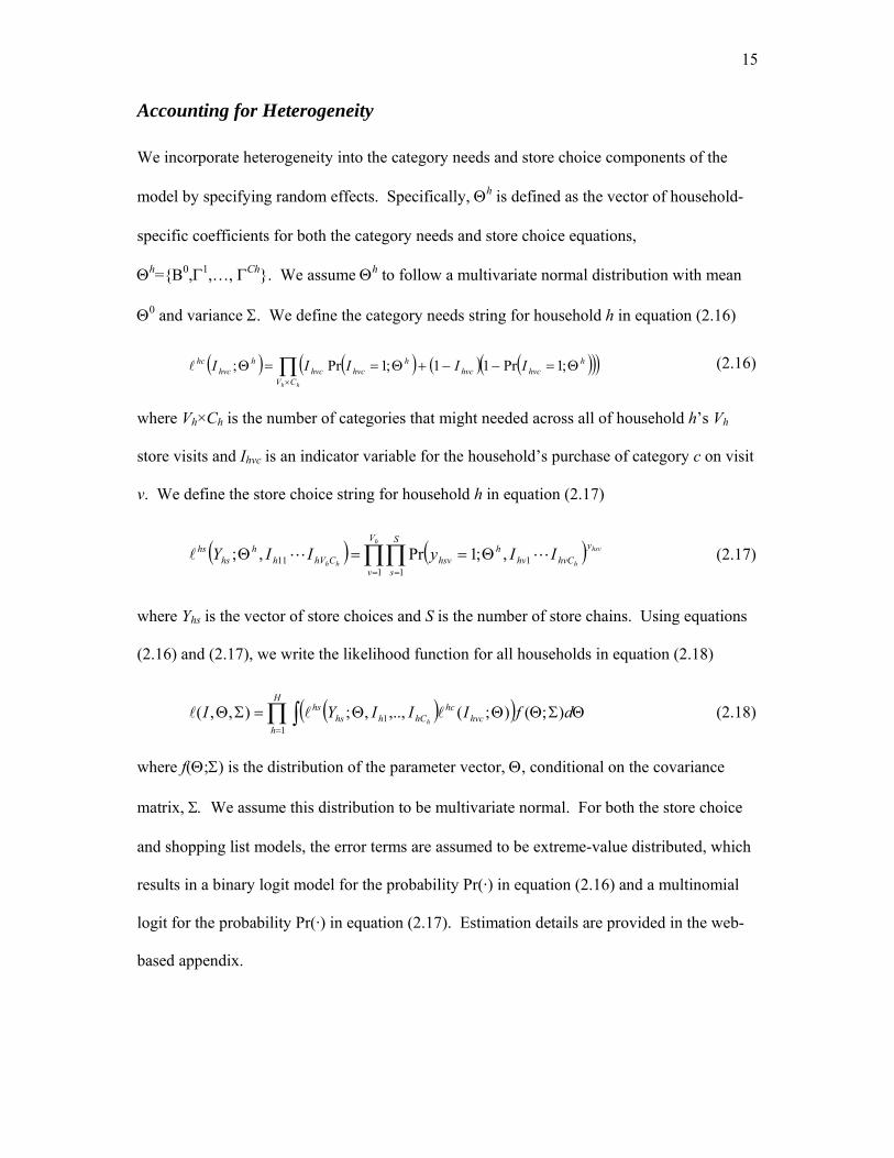
Accounting for Heterogeneity

We incorporate heterogeneity into the category needs and store choice components of the

model by specifying random effects. Specifically, Θh is defined as the vector of household-

specific coefficients for both the category needs and store choice equations,

Θh={Β0,Γ1,…, ΓCh}. We assume Θh to follow a multivariate normal distribution with mean

Θ0 and variance Σ. We define the category needs string for household h in equation (2.16)

( ) ( ) ( ) ( )( )( )∏×

Θ=−−+Θ==Θhh CV

hhvchvc

hhvchvc

hhvc

hc IIIII ;1Pr11;1Pr;l (2.16)

where Vh×Ch is the number of categories that might needed across all of household h’s Vh

store visits and Ihvc is an indicator variable for the household’s purchase of category c on visit

v. We define the store choice string for household h in equation (2.17)

( ) ( )∏∏= =

Θ==Θh

hsv

hhh

V

v

yhvChv

hhsv

S

sChVh

hhs

hs IIyIIY1

11

11 ,;1Pr,; LLl (2.17)

where Yhs is the vector of store choices and S is the number of store chains. Using equations

(2.16) and (2.17), we write the likelihood function for all households in equation (2.18)

( )( ) ΘΣΘΘΘ=ΣΘ ∏∫=

dfIIIYIH

hhvc

hchChhs

hsh

);();(,..,,;),,(1

1 lll (2.18)

where f(Θ;Σ) is the distribution of the parameter vector, Θ, conditional on the covariance

matrix, Σ. We assume this distribution to be multivariate normal. For both the store choice

and shopping list models, the error terms are assumed to be extreme-value distributed, which

results in a binary logit model for the probability Pr(·) in equation (2.16) and a multinomial

logit for the probability Pr(·) in equation (2.17). Estimation details are provided in the web-

based appendix.

16

Data

Our dataset is an enhanced multi-outlet panel from Chicago covering a 104-week period

between October 1995 and October 1997. This panel dataset is different from those

commonly used by marketing researchers because panelists recorded all of their packaged

goods purchases using in-home scanning equipment. Thus, purchase records are not limited

to a small sample of grocery stores. Because purchases made at grocery and non-grocery

(e.g., drug, warehouse club and mass merchandise) stores are recorded, we are able to

accurately determine the timing and quantity of the last purchase in every category prior to

each store visit.

The category needs models are estimated using ten product categories: chocolate

candy, carbonated beverages, coffee, diapers, dog food, household cleaners, laundry

detergent, salty snacks, sanitary napkins, and shampoo. These ten categories offer a broad

representation of high and low frequency, high and low penetration, as well as food and non-

food (including health and beauty care) categories. Together, these categories comprise

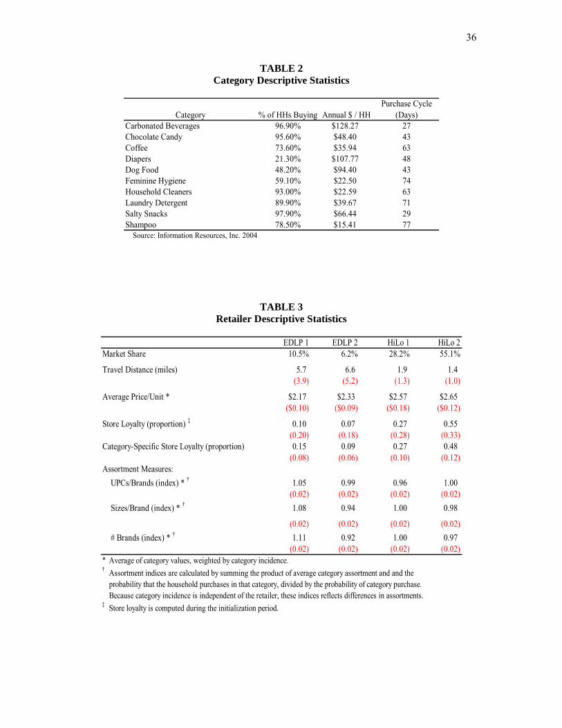
roughly 10% of the average market basket. Descriptive statistics for these categories are

reported in Table 2.


As noted previously, panelists recorded purchases at all grocery stores. We model

choices at the four largest store chains which together account for 91% of store visits and

92% of spending at known grocery outlets in the market. Following BHT, we identify these

retailers based on their advertised pricing strategy: EDLP1, EDLP2, HiLo1, and HiLo2.

More purchases were made at HiLo (77% of trips; 76% of spending) than EDLP (14% of

trips; 16% of spending) stores.

Initial testing suggested that many panel households had not faithfully recorded all of

their purchases. To avoid bias from underreported purchases, we limited our dataset to

17

households that recorded at least one grocery shopping trip in every month and spent an

average of at least $20 per week in grocery stores. We included only visits with spending of

at least $8; i.e., during which substantial purchases were made (as opposed to, for example,

buying a pack of gum or a single-serve drink). We further required that seventy-five percent

of the household’s grocery purchases were made at the four largest store chains to ensure that

we captured the household’s preferred outlet.

The resulting dataset contains 169 households (392 of the 581 available households

were excluded because they might not have faithfully recorded all purchases). The first third

of the panel duration (35 out of 104 weeks) was used to initialize category purchases. After

the initialization period, households made an average of 66 visits to the four largest grocery

store chains (std dev=39) and spent an average of $79 per trip (std dev=$31). We randomly

selected 25% of these store visits for out-of-sample testing. The other 75% were used for

estimation. The estimation sample contains 69 weeks of data, 11,005 store visits, and 52,489

binary category purchase observations. Binary category purchase observations were used

only if a household bought that category at least five times during the two-year duration of

the data and at least twice after the initialization period. Our dataset was augmented with

locations of the panel households and grocery stores. These locations allowed us to compute

travel distances from a shopper’s home (defined as the centroid of the panelist’s zip+4; actual

street addresses were unavailable due to privacy concerns) to the closest store of each chain,

the standard operationalization of spatial convenience. Note that travel distances are actual

road distances, not Euclidean distances.


The market positions and strategies of the four retailers are evident from the

descriptive data in Table 3. HiLo stores were visited far more frequently, with HiLo 2 visited

nearly twice as often as HiLo 1 (55.1% vs. 28.2%). Together, the two EDLP retailers

18

accounted for fewer than 20% of store visits. This disparity is consistent with the high

penetration of the two HiLo retailers, whose stores are within 1.6 (HiLo 1) and 1.2 (HiLo 2)

miles of panelists’ homes on average. There are far fewer EDLP stores in the market as

reflected in average travel distances from panelists’ homes of 4.9 (EDLP 1) and 5.8 (EDLP 2)

miles. Across the ten categories for which we have detailed merchandise files, HiLo retailers

charged higher prices on average than EDLP retailers. This is consistent with descriptive

data from BHT and Bell and Lattin (1998). On the other hand, the HiLo/EDLP distinction

does not explain the indexed measures of the average number of brands, SKUs/brand or

sizes/brand for each category. Moreover, the ranges of these three indices of assortment

reflect substantial differences among retailers.

Because of our focus on assortments, we report “raw” category assortment numbers—

the number of SKUs, unique SKUs, brands, SKUs/brand, and sizes/brand scanned weekly at

each retailer—in Table 4. Across retailers, the largest numbers of SKUs are found in

carbonated beverages and salty snacks; the smallest number in diapers. There are no

consistent patterns in the number of unique SKUs, suggesting substantial variation in private

label penetration across categories. The largest number of brands is offered in salty snacks,

the smallest number in diapers. More SKUs/brand are offered in feminine hygiene products

than in any other category; the fewest SKUs/brand are found in shampoo and household

cleaners. The most sizes/brand are offered in diapers; the fewest sizes/brand are offered in

the shampoo category.

<Put Table 4 about Here>

Results

In this section, we test three alternative models to determine which fits best. We then report

the parameter estimates and associated inferences for the best-fitting model. Next, we report

elasticity estimates and conduct a sensitivity analysis to put our findings in context.

19

Model Fit

Fit statistics for three different model specifications are shown in Table 5. The baseline

specification “(a)” is BHT with the modifications described in the previous section but no

assortment variables. Specification “(b)” is the full model detailed in the previous section. It

includes assortment variables and a category-specific store loyalty parameter for assortment

response. Specification “(c)” is a restricted version of the full model in which the category-

specific loyalty parameter for assortment response is constrained to zero (this was suggested

by an anonymous reviewer).

The table includes both in and out-of-sample fit tests. In sample, we use the

Consistent Akaike’s Information Criterion (CAIC) and Bayesian Information Criterion (BIC)

to assess the three specifications. For all three, we evaluate the full likelihood as well as the

partial likelihood of store choice (i.e., conditioned on category needs). Information criteria

for both full and partial likelihoods indicate that specification (c), which includes assortment

variables but no category-specific store loyalty in assortment response, is preferred.

Specification (c) also offers a higher store choice hit rate in sample than the other

specifications do. In the holdout sample, we assess model fit by comparing log likelihoods

(again both full and partial likelihoods) and store choice hit rates. Out-of-sample log

likelihoods also indicate that specification (c) is preferred to both the baseline specification

(a) and specification (b) with both assortment variables and category-specific store loyalty in

assortment response. While specification (b) offers a higher store choice hit rate out-of-

sample than specification (c), the difference is small. Consistent with these model fit test

results, the remaining analyses will focus on specification (c).


20

Parameters

Parameter estimates for the store choice component of the model are shown in Table 6.

Focusing first on the mean parameter estimates in the center of the table, we find that the

store loyalty parameter is positive (p-value=0.000) which suggests inertial behavior in store

choice. This is consistent with Rhee and Bell’s (2002) finding that persistence in store choice

is a strong negative predictor of future store switching. The distance parameter is negative

(p-value=0.000), demonstrating shoppers’ disutility for travel to and from the store.


Recall that hierarchical equations for price and feature response (2.13) incorporate

category-specific store loyalty. The intercepts of these hierarchical equations implicitly

assume category-specific store loyalty to be zero. The intercept of the hierarchical equation

for price response is negative but not significantly different from zero (p-value=0.167). In

contrast, category-specific store loyalty has a significant negative effect on price response (p-

value=0.048). Taken together, the parameter estimates of the hierarchical equation for price

response imply that, the more category purchases a household makes at a store, the more that

category’s prices affect the household’s preference for that store. This finding is consistent

with selective attention to prices and can be explained by bounded rationality arguments.

Neither the intercept nor the category-specific store loyalty term in the hierarchical

equation for feature response is significantly different from zero (p-value=0.792 and p-

value=0.264, respectively). Thus, after controlling for price, shoppers are not significantly

more likely to choose a store which advertises items in the categories they need. This finding

is consistent with Bodapati and Srinivasan (2006), who determined that feature advertising is

not important to most shoppers. We further investigated this result by estimating two

alternative specifications: (i) one in which the binary feature advertising variable is

household-specific; i.e., it reflects whether or not the household’s favorite brands were

21

advertised, and (ii) another in which feature advertising is a predictor in the category needs

equation rather than in the store choice equation (it is not clear in which equation feature

advertising belongs). Both of these alternative specifications were rejected based on CAIC

and BIC criteria.

The assortment parameter is negative and significant (p-value=0.000), though the sign

of this parameter is an artifact of how the assortment variable is constructed. The assortment

variable is a positive function of the number of SKUs/brand (by construction), a positive

function of the number of sizes/brand (p-value=0.007), a negative function of the number of

brands offered (p-value=0.000), a negative function of the availability of the household’s

favorite brands (p-value=0.000), and a positive function of the proportion of unique SKUs

offered (p-value=0.000). Multiplying the assortment parameter by the five measures of

assortment, we find that the probability of choosing a store is positively affected by the

number of brands offered and the availability of the household’s favorite brands, but

negatively affected by the number of SKUs/brand and sizes/brand as well as the number of

unique SKUs offered. To ensure that these results are not driven by collinearity among the

assortment measures, we estimated the model without EDLP 1 as a choice alternative (EDLP

1 offers substantially more brands, SKUs/brand, and sizes/brand than any other store chain).

We found that, except for sizes/brand which became negative and non-significant, the signs

of the assortment variable parameters did not change and the parameters remained significant

when EDLP 1 was dropped from the analysis. We conclude that collinearity induced by the

extensive assortments at EDLP 1 is not driving our results.

Turning to the heterogeneity standard deviations in the right-most panel of Table 6,

we observe that all are significant except the heterogeneity in price response. It appears that

household-level differences in price response cannot be reliably estimated because they are

driven by category-specific store loyalty and/or covariation with other predictors of store

22

choice. Interestingly, we find significant heterogeneity in feature advertising response

despite a despite a non-significant parameter mean. This suggests that feature advertising can

be important in the store choice decisions of some households. Note that heterogeneity

standard deviations for the five measures of assortment are set to one to identify

heterogeneity in assortment response.

Using the heterogeneity standard deviations, we can compare the relative variability

in distance and assortment response. The standardized beta for distance is -1.97/0.97=-2.03;

the standardized beta for assortment –0.25/0.58=-0.42. Thus, there is far more heterogeneity

among households in assortment response than in distance response. Mindful of the

heterogeneity in assortment response, we consider the implications of the parameter estimates

for how the average shopper evaluates assortments. All else equal, the average shopper

prefers stores which offer more brands, particularly his/her favorite brands. All else equal,

the average shopper is not attracted to stores which offer more SKUs/brand or sizes/brand.

Private labels, for which the number of unique SKUs is a proxy, also fail to attract the

average shopper to the store. Thus, offering a higher proportion of national brands would

seem to make a store more attractive to the average shopper.

To gain insight into the tradeoffs that shoppers make when choosing a store, we now

consider heterogeneity covariances between the key determinants of store choice. We

compute correlations between the household-specific distance, price and assortment

parameters for ease of interpretation. The only significant correlation is between distance and

assortment (r=-0.43; p-value=0.000); neither of the other correlations (between price and

distance and between price and assortment) has a p-value below 0.493. Thus, shoppers

appear willing to trade off travel distances for more attractive assortments and vice versa.

The specification of category needs is not the focus of this investigation, so parameter

estimates for equation (2.1) are not reported here but are available from the authors. We

23

note, however, that these parameter estimates support the validity of our results. Across the

ten category models, all statistically significant parameter estimates have the expected sign.

Further, although the none of the interaction parameters in category needs models are

significant, some of the parameter heterogeneity standard deviations are significant. This

implies that consumers may not consume certain categories (e.g., carbonated beverages) at

constant rates.

Elasticities

Narrowing our focus to the key determinants of store choice, we compute market

share elasticities from the parameter estimates. Table 7 reports these elasticities at three

points in the parameter heterogeneity distribution: at the mean parameter estimate (in the

upper panel), plus and minus one heterogeneity standard deviation (in the middle and lower

panels, respectively). Representing heterogeneity in this way (as opposed to integrating over

the heterogeneity distribution) shows the extent to which distance, price, and assortment

response vary across households. In each case only the variable of interest is evaluated at

different points in the heterogeneity distribution; others are evaluated at the mean parameter

estimate. Beginning with the top panel, we find that the distance elasticities have greater

magnitudes than do price and assortment elasticities for all store chains. This supports the

conventional wisdom that convenience is the most important determinant of store choice.

Price and assortment elasticities in the upper panel are of similar magnitudes to one another

and are all below unity. The small magnitude of price elasticities is consistent with empirical

evidence of inelastic category prices (Neslin and Shoemaker 1983; Bolton 1989). EDLP

store shares are more sensitive than HiLo store shares to changes in all three determinants of

store choice—distance, price and assortment. EDLP 1’s share is most sensitive; HiLo 2’s

share is least sensitive.


24

Turning to the two lower panels in the table, we find that computing distance and

price elasticities at different points in the heterogeneity distribution does not cause their signs

to change—lower prices and less travel are uniformly preferred. In contrast, the sign of

assortment elasticities changes when the elasticities are computed at minus one heterogeneity

standard deviation. Recalling that assortment is the weighted sum of five different measures,

the changing sign suggests that not all customers are attracted to stores that offer more

brands, more of their favorite brands, fewer SKUs/brand, fewer sizes/brand, and fewer unique

(i.e., private label) SKUs. In other words, different shoppers are attracted to stores with

assortments that differ in terms of these characteristics. In addition, the magnitudes of

assortment elasticities computed at plus and minus one heterogeneity standard deviation are

considerably larger than those computed at the mean parameter estimate. Comparing

assortment and price elasticities computed at +1 and -1 heterogeneity standard deviations

reveals that the magnitudes of assortment elasticities are higher in all cases. Thus, across

households, changes in assortments appear to affect store choices more than the same

proportional changes in prices.

Sensitivity Analyses

To determine the joint implications of response parameters, heterogeneity variances

and covariances, we compute expected changes in market share (integrating over the entire

heterogeneity distribution) if each retailer were to modify its prices or assortments. We

report this sensitivity analysis in Table 8 using switching matrices that show how market

shares of all store chains (presented by row) would change if a particular store chain

(presented by column) increased either its (i) prices, (ii) number of brands, (iii) SKUs/brand,

(iv) sizes/brand, (v) proportion of favorite brands or (vi) proportion of unique SKUs by three

percent in all categories. Clearly, the predictive validity of our estimates for three-percent

increases in these variables depends on the range of the data used for estimation, but the

25

results in Table 8 nonetheless illustrate the competitive implications. Note that this table

reports integrated probabilities which may vary slightly from the point elasticities reported in

Table 7 at +1, 0 and -1 heterogeneity standard deviations.


First, we consider a hypothetical three-percent increase in prices. If EDLP 1 or EDLP

2 were to raise its prices, it would lose 0.7% market share. The HiLo retailers would lose

somewhat less market share if they were to increase prices. Note that the shares of all

retailers are price inelastic, consistent with empirical studies of category prices (Neslin and

Shoemaker 1983; Bolton 1989). Price changes at HiLo 2 would have the biggest impact on

the shares of other retailers because of the retailer’s high baseline sales.

Next, we consider hypothetical increases in the five components of assortment. Note

that changing one variable (SKUs/brand, for example) assumes that the other assortment

variables (number of brands, for example) remain fixed; we acknowledge that this is a strong

assumption. Nevertheless, we find that EDLP 1, the lowest-share retailer, is most sensitive to

changes in assortment while HiLo 2, the highest-share retailer, is least sensitive. Across

retailers, we find that own market shares are most affected by changing in the number of

brands that retailers offer. Share gains from increasing the number of brands ranges from

0.4% for HiLo 2 to 2.4% for EDLP 1. Retailers would also benefit by offering more of

shoppers’ favorite brands, with share gains ranging from 0.3% for HiLo 2 to 1.4% for EDLP

1. Retailers are less sensitive to increases in the number of SKUs/brand and the number of

sizes/brand, both of which would result in small market share losses for the retailer. Finally,

retailers’ shares are not at all sensitive to changes in the proportion of unique items offered.

Thus, changing the proportion of private label items does not seem to affect store choice

substantially. Note that cross effects are smaller than own effects (except if HiLo 2 were to

change its assortments) and nearly always have the expected sign.

26

Discussion

Our investigation of store choice has focused on retail assortments, with prices,

feature advertising and shoppers’ travel distances also considered. We now discuss our key

findings and consider their implications.

We find that convenience (operationalized as travel distance) has a larger effect on

store choice size than do price and product assortment, consistent with shoppers’ self reports

(Arnold, Ma and Tigert 1978; Arnold and Tigert 1981; Arnold, Roth and Tigert 1981;

Arnold, Oum and Tigert 1983). In fact, the effect of price on store choice is much smaller

than that of convenience. However, our elasticities contradict shoppers’ self reports in that,

regardless of what assortment characteristics a shopper prefers, his/her store choice decisions

are generally more sensitive to assortments than to prices.

A second key finding relates to feature advertising. We find that, on average, the

frequency of feature advertising does not seem to affect store choice. On the other hand, the

significant heterogeneity term suggests that some consumers do consider feature advertising

into their store choice decisions. This result is consistent with some previous findings

(Bodapati and Srinivasan 2006), but not others (e.g., Blattberg, et al 1995). We believe our

null finding this is due to limited variation in feature advertising at the category level and

correlations in feature advertising within and across categories. Key categories such as

carbonated beverages are advertised almost every week, resulting in little variation in

featuring over time. On the other hand, retailers advertise many categories each week to

communicate the breadth of their product offerings. Across categories, this causes positive

correlations because categories appear together in feature advertising so often. Within

category, this causes a negative correlation because competing brands are advertised in

sequence, not in parallel. For example, a retailer would rather advertise Coca-Cola one week

and Pepsi the next (or vice versa) than advertise both Coca-Cola and Pepsi during one week

27

and neither brand during the other week. A key limitation of our approach is that we did not

look at the interaction between price and feature advertising, which may influence store

choice. That is, if the discount is large enough, more consumers may alter their store choice

decisions.

The remainder of our findings relate to assortment response. Our analysis of product

assortment focused on five measures. All five of these measures—the number of brands,

SKUs/brand, sizes/brand, proportion of unique SKUs, and presence of the household’s

favorite brands in the assortment—were found to significantly affect store choice. The signs

of the estimated parameters show that, by carrying more brands (particularly households’

favorite brands), retailers increase the probability that the average household will choose their

stores. On the other hand, retailers that offer fewer SKUs/brand, fewer sizes/brand, and

proportionally fewer unique items (a proxy for the private label penetration in the category)

in the assortment also increase the probability that the average household will choose their

stores. These findings are consistent with the recent literature on assortment perceptions and

suggest that shoppers want SKUs in grocery store assortments only if they add meaningful

variety to those assortments (Broniarczk, Hoyer and McAlister 1998; Hoch, Bradlow and

Wansink 1999; Broniarcyzk and Hoyer 2006).

Our research has implications for both retail managers and academic researchers.

Along with recent findings that category sales are unresponsive to assortment (IRI and

Bishop 1993; Dreze, Hoch and Purk 1994; Boatwright and Nunes 2001), our results provide

qualified support for the argument in favor of SKU reduction (as prescribed by the grocery

industry’s ECR and category management initiatives). If retail assortments can be reduced

without eliminating brands, particularly consumers’ favorite brands, then the associated

reductions in operating costs and out-of-stocks could make SKU reduction an effective and

profitable strategy. Yet our results must be interpreted carefully. They suggest that

28

assortment response is nuanced and that the effect of assortment changes depends upon the

characteristics of the items being added or removed. For example, if an item being added or

removed changes the number of brands in the category, then response is affected not only by

that change but also changes in the number of SKUs per brand and the number of sizes per

brand, as well as the proportion of unique SKUs and whether or not the brand is a favorite in

shoppers’ households. Our results seem to imply the existence of optimal assortment levels

although we leave this investigation for future research.

Consumer heterogeneity was also found to influence the effect of assortment on

shoppers’ store choice Unobserved heterogeneity, reflected in the distribution of household-

level response parameters, was much greater for assortment than for the other determinants of

store choice. While shoppers uniformly prefer lower prices and shorter travel distances, our

analyses of parameter heterogeneity and assortment elasticities suggest that shoppers prefer

different assortment characteristics. Specifically, unlike most consumers, a substantial

minority prefer stores that offer more SKUs/brand, more sizes/brand, and more unique SKUs

but fewer different brands. Our analysis of heterogeneity covariances reveals that response to

assortment is correlated to response to travel distance (r=0.43). Thus, the less importance a

household assigns to assortment, the more it values convenience and vice versa. This finding

is consistent with the tradeoff promulgated by Baumol and Ide (1956) and Brown (1978).

The heterogeneity in assortment response suggests that retailers should not necessarily match

each others’ assortment levels. Ideal assortment levels could differ substantially between

retailers depending on the preferences of their customers.

Retailers should also be mindful that heterogeneity in assortment preferences across

households means that even a well-considered SKU reduction strategy could result in some

customer losses. Heterogeneity in assortment response also results in asymmetric assortment

competition. Assortment may be a competitive weapon, with own- and cross-effects

29

dictating which retailers can exploit assortments and how they may do so. For example, if

EDLP 1 were to increase the number of brands in its assortments, its share would be

substantially increased while HiLo 1 would lose little. However, if HiLo 1 were to increase

the number of brands in its assortments, it would gain less market share than EDLP 1 would

lose. Asymmetric switching patterns underscore the importance of assortment in retail

strategy and retail competition.

Concluding Remarks

Our results provide a foundation for future research on store choice and retail

assortments. Our finding that assortments are more important than prices in store choice

decisions suggests the need for deeper understanding of the roles of prices and assortments on

shopping behavior and how price and assortment expectations play a role in store choice.

A second issue for future research is why feature advertising does not, on average,

affect store choice. Though our finding could be dependent on the fact that discount depth

was not modeled, it is also quite probably dependent on the type of shopping trip (e.g., cherry

picking, fill-in, or stock up) undertaken. Feature advertising may well affect different types

of shopping trips differentially.

Another remaining issue involves heterogeneity in assortment response: Why do most

consumers prefer more brands but fewer SKUs/brand while many other consumers prefer

fewer brands but more SKUs/brand? Analyses that relate demographics, attitudes, or other

characteristics to assortment response might help address these questions.

Yet another subject for future research concerns how other store characteristics such

as service level, quality of perishables, and out-of-stocks affect store choice. Our findings

about the effect of product assortment suggest that shoppers’ self-reports might not contain

sufficient detail for retailers to allocate their resources and formulate effective strategies.

However, modeling store choice as a function of these additional factors would require

30

augmenting panel data with measures of the factors gathered from other sources. Such an

investigation would present econometric challenges beyond those addressed in this paper.

A final area for future research is the dynamic effects of assortment, price and

convenience on store choice. Changes in assortment and price influence future, as well as

current patronage decisions. Thus, these changes are likely to have a substantial impact on

the lifetime value of retail customers, and consequently on optimal retailer assortment and

price levels.

31

References

Ainslie, Andrew and Peter E. Rossi (1998), “Similarities in Choice Behavior Across Product

Categories,” Marketing Science, 17 (2), 91-106.

Allenby, Greg M., and Peter E. Rossi (1999), Marketing Models of Consumer Heterogeneity,”

Journal of Econometrics, 89 (March/April), 57-78.

Andrews, Rick L., Andrew Ainslie and Imran S. Currim (2002), “An Empirical Comparison of

Logit Choice Models with Discrete Versus Continuous Representations of

Heterogeneity,” Journal of Marketing Research, 39 (November), 479-87.

Arnold, Stephen J., Sylvia Ma and Douglas J. Tigert (1978), “A Comparative Analysis of

Determinant Attributes in Retail Store Selection,” in H. K. Hunt (ed.), Advances in

Consumer Research, Vol. 5, Ann Arbor, MI: Association for Consumer Research, 663-7.

Arnold, Stephen J., Victor Roth and Douglas J. Tigert (1981), “Conditional Logit Versus MDA in

the Prediction of Store Choice,” in K. B. Monroe (ed.), Advances in Consumer Research,

Vol. 9, Washington: Association for Consumer Research, 665-70.

Arnold, Stephen J., Tae H. Oum and Douglas J. Tigert (1983), “Determinant Attributes in Retail

Patronage: Seasonal, Temporal, Regional and International Comparisons,” Journal of

Marketing Research, 20 (May) 149-57.

Arnold, Stephen J., and Douglas J. Tigert (1982), “Comparative Analysis of Determinants of

Patronage,” in R. F. Lusch and W. R. Darden (eds.), Retail Patronage Theory: 1981

Workshop Proceedings, University of Oklahoma: Center for Management and Economic

Research.

Assuncao, Joao L., and Robert J. Meyer (1993), “The Rational Effect of Price Promotions on

Sales and Consumption,” Management Science, 39 (5) 517-35.

Baumol, William J., and Edward A. Ide (1956), “Variety in Retailing,” Management Science, 3

(1), 93-101.

Bell, David R., Teck Hua Ho and Christopher S. Tang (1998), “Determining Where to Shop:

Fixed and Variable Costs of Shopping,” Journal of Marketing Research, 35 (August),

352-69.

Bell, David R., and James M. Lattin (1998), “Grocery Shopping Behavior and Consumer

Response to Retailer Price Format: Why ‘Large Basket’ Shoppers Prefer EDLP,”

Marketing Science, 17 (1), 66-88.

32

Blattberg, Robert C., Richard Briesch, and Edward J. Fox (1995), "How Promotions Work,"

Marketing Science, 14, 3(Part 2 of 2), G122-G132.

Boatwright, Peter and Joseph C. Nunes (2001), “Reducing Assortment: An Attribute-Based

Approach,” Journal of Marketing, 65 (3), 50-63.

Bodapati, Anand, and V. Srinivasan (2006), “The Impact of Feature Advertising on Customer

Store Choice,” Working Paper, Stanford University, Palo Alto, California.

Bolton, Ruth N. (1989), “The Robustness of Retail-Level Price Elasticity Estimates,” Journal of

Retailing, 65 (2), 193-219.

Borle, Sharad, Peter Boatwright, Joseph B. Kadane, Joseph C. Nunes and Galit Shmueli (2005),

“Effect of Product Assortment on Changes in Customer Retention,” Marketing Science,

forthcoming.

Broniarczyk, Susan M., Wayne D. Hoyer and Leigh McAlister (1998), “Consumers’ Perceptions

of the Assrotment Offered in a Grocery Category: The Impact of Item Reduction,”

Journal of Marketing Research, 35 (May), 166-76.

Broniarczyk, Susan M. and Wayne D. Hoyer and Leigh McAlister (2006), “Retail Assortment:

More ≠ Better,” in M. Krafft and M. K. Mantrala (eds.), Retailing in the 21st Century,

Springer: Berlin.

Brown, Stephen (1989), “Retail Location Theory: The Legacy of Harold Hotelling,” Journal of

Retailing, 65 (4), 450-70.

Brown, Daniel J., (1978), “An Examination of Consumer Grocery Store Choice: Considering the

Attraction of Size and the Friction of Travel Time,” Advances in Consumer Research, 5,

243-246.

Chib, Siddhartha, P.B. Seetharaman and Andrei Strijnev (2004), "Model of Brand Choice with a

No-Purchase Option Calibrated to Scanner Panel Data," Journal of Marketing Research,

41 (May), 184-196.

Corstjens, Marcel and Rajiv Lal (2000) “Building Store Loyalty through Store Brands,” Journal

of Marketing Research, 37 (August), 281-291.

Dreze, Xavier, Stephen J. Hoch and Mary E. Purk (1994), “Shelf Management and Space

Elasticity,” Journal of Retailing, 70 (4), 301-26.

Erdem, Tulin (1996), “A Dynamic Analysis of Market Sctructure Based on Panel Data”.

Marketing Science, 15(4), 359-378.

33

Erdem, Tulin, Susumu Imai and Michael P. Keane (2003), “Brand and Quantity Choice

Dynamics Under Price Uncertainty,” Quantitative Marketing and Economics, (1) 5-64.

Fox, Edward J., Alan L. Montgomery and Leonard M. Lodish (2004), “Consumer Shopping and

Spending Across Retail Formats,” Journal of Business, 77 (2), S25-S60.

Fox, Edward J., and Raj Sethuraman (2006), “Retail Competition,” in M. Krafft and M. K.

Mantrala (eds.), Retailing in the 21st Century, Springer: Berlin.

Hajivassiliou, Vassilis A., and Paul A. Ruud (1994), “Classical Estimation Methods for LDV

Models Using Simulation, in D. McFadden and R. Engle (eds.), The Handbook of

Econometrics, Volume 4, North Holland: Amsterdam, 2383-441.

Fader Peter S., and Bruce G. S. Hardie (1996), “Modeling Consumer Choice Among SKUs,”

Journal of Marketing Research, 33 (Nov), 1-21.

Hoch, Stephen J., Eric T. Bradlow and Brian Wansink (1999), “The Variety of an Assortment,”

Marketing Science, 18 (4) 527-546.

Hotelling, Harold (1929), “Stability in Competition,” The Economic Journal, 39 (March), 41-57.

Hubbard, Raymond (1978), “A Review of Selected Factors Conditioning Consumer Travel

Behavior,” Journal of Consumer Research, 5 (June), 1-21.

Huff, David (1964), “Redefining and Estimating a Trading Area,” Journal of Marketing, 28

(February), 34-8.

Information Resources, Inc. and Willard Bishop Consulting (1993), Variety or Duplication: A

Process to Know Where You Stand, Washington, DC: Food Marketing Institute.

Levy, Michael and Barton A. Weitz (2004), Retailing Management (5th Edition), New York, NY:

McGraw-Hill Irwin.

Lindquist, Jay D. (1974-1975), “Meaning of Image: A Survey of Hypothetical Evidence,”

Journal of Retailing, 50 (Winter), 29-38, 116.

Neslin, Scott, A., and Robert W. Shoemaker (1983), “Using a Natural Experiment to Estimate

Price Elasticity: The 1974 Sugar Shortage and the Ready-to-Eat Cereal Market,” Journal

of Marketing, 47 (Winter) 44-57.

Nevo, Aviv and Igal Hendel (2002), “Measuring the Implications of Sales and Consumer

Stockpiling Behavior,” Mimeo, Berkeley, CA: University of California.

Reilly, William J. (1931), The Law of Retail Gravitation, Pillsbury: New York.

34

Rhee, Hong, and David R. Bell (2002), “The Inter-store Mobility of Supermarket Shoppers.”

Journal of Retailing, 78 (4) 225-237.

Spiggle, Susan (1987), “Grocery Shopping Lists: What Do Consumers Write?” in M. Wallendorf

and P.F. Anderson (eds.), Advances in Consumer Research, Vol 14, Provo, UT:

Association for Consumer Research, 241-5.

Wedel, Michel, Wagner Kamakura, Neeraj Arora, Albert Bemmaor, Jeongwen Chiang, Terry

Elrod, Rich Johnson, Peter Lenk, Scott Neslin andd Carsten Stig Poulsen (1999),

“Discrete and Continuous Representations of Unobserved Heterogeneity in Choice

Modeling,” Marketing Letters, 10 (3), 219-32.

35

TABLE 1 Notation

Name Description Notation

Store Choice Specification Store Loyalty Proportion of hh’s store visits

made to the retailer’s stores during the initialization period

hsL

Distance Distance between the shopper’s home and the retailer’s closest store

hsvD

Feature Advertising

Indicator variable that the retailer feature advertised at least one SKU in the category, weighted by the probability of purchasing in the category

∑

∑

=

== C

1chvc

C

1csvchvchsc4

hsv

)I(Pr

F)I(PrFeat

β

Price Category price weighted by probability of purchasing in the category × average purchase quantity

( ) ( ) ( )∑=

=hC

csvchvchvchcshsv PEQEIPrce

13Pri β

Assortment Category assortment weighted by the probability of purchasing in the category

∑

∑

=

== C

1chvc

C

1chsvchvchs5

hsv

)I(Pr

A)I(PrAssort

β

Category-Specific Store Loyalty

Percentage of the household’s previous category purchases made at the retailer

hscL

Category Need Specification

Time Since Last Category Purchase

Elapsed time since the most recent category purchase centered on the household’s average inter-purchase time

hchvc TT −

Quantity of Last Category Purchase

Volumetric quantity of the most recent category purchase centered on the household’s average category purchase quantity

hchvc QQ −

36

TABLE 2 Category Descriptive Statistics

Category % of HHs Buying Annual $ / HHPurchase Cycle

(Days)Carbonated Beverages 96.90% $128.27 27Chocolate Candy 95.60% $48.40 43Coffee 73.60% $35.94 63Diapers 21.30% $107.77 48Dog Food 48.20% $94.40 43Feminine Hygiene 59.10% $22.50 74Household Cleaners 93.00% $22.59 63Laundry Detergent 89.90% $39.67 71Salty Snacks 97.90% $66.44 29Shampoo 78.50% $15.41 77 Source: Information Resources, Inc. 2004

TABLE 3 Retailer Descriptive Statistics

EDLP 1 EDLP 2 HiLo 1 HiLo 2

Market Share 10.5% 6.2% 28.2% 55.1%

Travel Distance (miles) 5.7 6.6 1.9 1.4(3.9) (5.2) (1.3) (1.0)

Average Price/Unit * $2.17 $2.33 $2.57 $2.65($0.10) ($0.09) ($0.18) ($0.12)

Store Loyalty (proportion) ‡ 0.10 0.07 0.27 0.55(0.20) (0.18) (0.28) (0.33)

Category-Specific Store Loyalty (proportion) 0.15 0.09 0.27 0.48(0.08) (0.06) (0.10) (0.12)

Assortment Measures: UPCs/Brands (index) * † 1.05 0.99 0.96 1.00

(0.02) (0.02) (0.02) (0.02) Sizes/Brand (index) * † 1.08 0.94 1.00 0.98

(0.02) (0.02) (0.02) (0.02) # Brands (index) * † 1.11 0.92 1.00 0.97

(0.02) (0.02) (0.02) (0.02)* Average of category values, weighted by category incidence.† Assortment indices are calculated by summing the product of average category assortment and and the

probability that the household purchases in that category, divided by the probability of category purchase. Because category incidence is independent of the retailer, these indices reflects differences in assortments.

‡ Store loyalty is computed during the initialization period.

37

TABLE 4 Raw Category Assortment Variables

Category

Chocolate Candy 247.1 (16.6) 164.8 (13.7) 215.5 (14.9) 204.1 (10.9)Carbonated Beverage 635.3 (15.2) 487.6 (24.3) 491.4 (9.5) 522.7 (26.8)Salty Snacks 546.0 (24.4) 441.7 (19.5) 464.5 (25.8) 557.9 (19.9)Coffee 271.2 (20.8) 211.6 (12.4) 245.0 (11.1) 240.3 (10.4)Feminine Hygiene 182.1 (5.3) 137.1 (8.6) 126.2 (10.7) 104.3 (4.0)Shampoo 292.3 (15.3) 238.7 (10.2) 225.5 (12.4) 84.3 (10.3)Diapers 113.9 (8.1) 78.3 (4.5) 89.0 (9.6) 48.8 (5.8)Dog Food 325.4 (7.4) 258.7 (13.5) 291.4 (7.9) 280.1 (6.5)HH Cleaners 251.7 (7.1) 211.9 (6.6) 214.1 (6.4) 187.0 (5.0)Laundry Detergent 129.9 (14.6) 114.9 (6.8) 120.8 (13.2) 98.8 (10.6)


Chocolate Candy 25.4 (3.1) 15.0 (2.5) 21.6 (4.3) 28.4 (2.3)Carbonated Beverage 40.3 (1.6) 39.2 (2.6) 40.0 (1.4) 37.5 (1.6)Salty Snacks 75.5 (4.9) 56.6 (2.0) 64.9 (4.5) 60.1 (2.7)Coffee 19.0 (1.1) 17.4 (1.2) 20.2 (1.0) 22.5 (1.8)Feminine Hygiene 8.7 (0.5) 7.9 (0.7) 7.0 . 7.0 .Shampoo 45.0 (2.5) 36.0 (1.6) 33.2 (1.8) 20.1 (2.2)Diapers 7.3 (0.6) 4.9 (0.7) 5.1 (0.5) 3.7 (0.6)Dog Food 26.4 (2.6) 21.0 (1.0) 23.5 (1.4) 23.8 (1.7)HH Cleaners 38.3 (2.4) 32.9 (0.9) 31.4 (2.1) 36.6 (1.4)Laundry Detergent 10.6 (0.6) 8.4 (0.5) 9.4 (0.6) 10.1 (0.6)



HiLo 1 HiLo 2EDLP 1 EDLP 2

Number of Sizes/Brand

Number of SKUs/Brand

Number of SKUs

Number of Unique SKUs

Number of Brands

(Standard errors in parentheses)

38

TABLE 5 Model Fit Statistics

(a) Baseline (b) Baseline + Assortment + Category-Specific Store Loyalty (c) Baseline + Assortment

Parameters 136 146 145Households 169 169 169In Sample # Store Choices 11044 11044 11044 # Category Needs 54053 54053 54053 LL -25813 -25714 -25715 CAIC 53028 52933 52925 BIC 52892 52787 52780 LL (Partial - Store Choice Only) -6964 -6861 -6864 CAIC (Partial - Store Choice Only) 15330 15227 15222 BIC (Partial - Store Choice Only) 15194 15081 15077 Store Chice Hit Rate 67.8% 68.8% 69.0%Out of Sample # Store Choices 3810 3810 3810 # Category Needs 18494 18494 18494 LL -8888 -8875 -8873 LL (Partial - Store Choice Only) -2619 -2603 -2602 Store Chice Hit Rate 66.5% 67.4% 67.2%

TABLE 6 Store Choice Model Parameters

Value Std Err P-value Value Std Err P-valueEDLP 1* 0.00 . . . . .

β 0h 2 EDLP 2 -0.17 0.14 0.227 2.80 0.16 0.000β 0h 3 HiLo 1 0.78 0.14 0.000 1.36 0.11 0.000β 0h 4 HiLo 2 1.03 0.16 0.000 0.61 0.07 0.000β 1h Store Loyalty 3.61 0.23 0.000 2.51 0.15 0.000β 2h Ln (Distance + 1) -1.97 0.12 0.000 0.97 0.13 0.000β 3h Price (÷10) Intercept -9.66 6.99 0.167 4.49 6.67 0.501

β 10,h Price (÷10) x Category-Specific Store Loyalty -9.84 4.97 0.048 . . .β 4h Feature Intercept -0.06 0.21 0.792 0.65 0.18 0.000

β 11,h Feature x Category-Specific Store Loyalty 0.35 0.31 0.264 . . .β 5h Assortment -0.25 0.06 0.000 0.58 0.05 0.000

# SKUs/Brand** 1.00 . . 1.00 . .β 6h # Sizes/Brand 1.87 0.69 0.007 1.00 . .β 7h # Brands -2.99 0.61 0.000 1.00 . .β 8h Favorite Brands Available -2.60 0.39 0.000 1.00 . .β 9h Unique SKUs 0.28 0.05 0.000 1.00 . .

* Intercept for EDLP 1 is set to zero for identification** Parameter for # SKUs/Brand is set to one for identification

Mean Heterogeneity Standard DeviationVariable

39

TABLE 7 Market Share Elasticities at -1, 0 and 1 Heterogeneity Standard Deviations

Distance Price AssortmentEDLP 1 -1.31 -0.33 0.38EDLP 2 -1.22 -0.26 0.30HiLo 1 -0.76 -0.19 0.23HiLo 2 -0.37 -0.10 0.09

Distance Price AssortmentEDLP 1 -0.68 -0.23 1.24EDLP 2 -0.65 -0.17 1.04HiLo 1 -0.41 -0.13 0.72HiLo 2 -0.21 -0.06 0.32

Distance Price AssortmentEDLP 1 -1.93 -0.42 -0.54EDLP 2 -1.78 -0.35 -0.41HiLo 1 -1.07 -0.26 -0.33HiLo 2 -0.51 -0.13 -0.12

Elasticity at Mean Parameter Estimate

Elasticity at Mean Parameter Estimate + 1 Heteogeneity Std Dev

Elasticity at Mean Parameter Estimate - 1 Heteogeneity Std Dev

40

TABLE 8 Sensitivity Analysis of Market Share to Changes in Price and Assortment

EDLP 1 EDLP 2 HiLo 1 HiLo 2EDLP 1 -0.7% 0.0% 0.3% 0.5%EDLP 2 0.0% -0.7% 0.4% 0.5%HiLo 1 0.1% 0.1% -0.6% 0.5%HiLo 2 0.1% 0.0% 0.2% -0.4%

EDLP 1 EDLP 2 HiLo 1 HiLo 2EDLP 1 2.4% -0.1% -0.8% -1.1%EDLP 2 -0.1% 0.6% -0.3% -0.1%HiLo 1 -0.2% -0.1% 0.7% -0.5%HiLo 2 -0.2% 0.0% -0.3% 0.4%



EDLP 1 EDLP 2 HiLo 1 HiLo 2EDLP 1 1.4% -0.1% -0.6% -0.7%EDLP 2 -0.1% 0.6% -0.3% -0.1%HiLo 1 -0.2% -0.1% 0.6% -0.3%HiLo 2 -0.1% 0.0% -0.2% 0.3%

EDLP 1 EDLP 2 HiLo 1 HiLo 2EDLP 1 -0.1% 0.0% 0.1% -0.2%EDLP 2 0.0% 0.1% 0.0% -0.3%HiLo 1 0.1% 0.0% -0.1% 0.2%HiLo 2 0.0% 0.0% 0.0% -0.1%

Store Chain Increasing # Sizes/Brand by 3%

Store Chain Increasing Proportion of Favorite Brands Carried by 3%

Store Chain Increasing # Unique SKUs by 3%

Store Chain Increasing Price by 3%

Store Chain Increasing # Brands by 3%

Store Chain Increasing # SKUs/Brand by 3%

41

Technical, Web-Based Appendices for How Does Assortment Affect Grocery Store Choice?†

Richard A. Briesch (Southern Methodist University)*

Pradeep K. Chintagunta (University of Chicago)**

Edward J. Fox (Southern Methodist University)***

* Assistant Professor of Marketing, Edwin L. Cox School of Business, Southern Methodist University, Dallas, TX; phone: 214-768 3180; [email protected] UT ** Robert Law Professor of Marketing, Graduate School of Business, University of Chicago, Chicago, IL; phone 773 702-8015; [email protected] *** Associate Professor of Marketing, Edwin L. Cox School of Business, Southern Methodist University, Dallas, TX; phone: 214-768 3943; [email protected] UT † The authors would like to thank David Bell and John Slocum for their comments and suggestions. The second author also thanks the Kilts Center for Marketing at the Chicago GSB for financial support. Any mistakes or omissions are the sole responsibility of the authors.

42

Appendix A. Simulated Maximum Likelihood Details

We use simulated maximum likelihood estimation, or SMLE, to estimate the parameters

given our assumptions about the errors (e.g., Hajivassiliou and Ruud 1994). SMLE employs

a structured lower-triangular Cholesky matrix, C, by which relationships in the parameter

covariance matrix, Σ, are estimated. The Cholesky matrix, C, is defined as CP

TPC = Σ so it can

be interpreted as the square root of the covariance matrix Σ. Because estimating the full

Cholesky matrix is infeasible (there are (57x56)/2 = 1,596 elements in the matrix), we must

restrict most off-diagonal elements of the matrix to be zero while still estimating relationships

of interest.

We allow for the store intercepts to co-vary with one another ((S-1)×(S-2)/2 terms)

and to co-vary with the category intercepts from the category needs model ((S-1)×C terms).

By allowing the store intercepts to co-vary with the category intercepts, we control for any

correlation in the error terms between the equations. This result is straight-forward to see as

the error terms can be written as having an unique component and a component which is

correlated between the equations. This last component is not separately identified from

correlation in preferences.

We also allow parameters of four predictor variables in the store choice model—store

loyalty, distance, spending and assortment—to covary with one another (6 terms). Finally,

we allow the feature advertising parameter in the category needs model, γ1, to covary with the

category intercepts, γ0 (C terms). With S=4 and C=10, we are estimating a total of 36

heterogeneity terms in addition to the 57 main diagonal elements of the Cholesky matrix,

which capture unique heterogeneity in the parameters. It is important to note that restricting

elements of the lower-diagonal Cholesky matrix to be zero does not imply that the

corresponding off-diagonal elements in the parameter covariance matrix, Σ, are zero.

43

Equation (2.18) implies that each household’s likelihood is integrated separately and

that the likelihood across households is the product of each household’s integrated likelihood.

We will therefore focus our discussion on the integration of a single household’s likelihood

function. The numerical integration is done as follows. Prior to beginning the optimization,

a fixed number of draws (ND) is made for each household from K independent random

variates where K is the dimension of ΘP

0. This results in a K×ND matrix of random draws

(DRAWS) for each household. Deviations from the mean vector Θ0 with the distribution

described by Σ is then created by multiplying the lower Cholesky Matrix by the matrix of

draws; i.e., DEVIATIONS = C×DRAWS, where the Cholesky matrix is populated by the terms

described above.

The integral in equation (2.18) is computed by evaluating the household’s likelihood

function ND times using the mean vector plus the vector of deviations for that draw, then

averaging the likelihood over the ND draws. Because of the high dimensionality of the

integrals in equation (2.18), numerical integration using normal random variates can result in

computational problems. For more computational efficiency, we make draws from a quasi-

random sequence. Specifically we use 100 draws from a Halton sequence (e.g., Train 1999;

Bhat 2001). Bhat argued that 100 draws from a Halton sequence is roughly equal to 1000-

1500 draws from a random normal distribution.

The simultaneous estimation of the store choice and category needs models helps us

in two ways. First, compared to a two-stage estimation where the category needs model is

estimated first and the resulting values “plugged into” the store choice model in a second

stage, the joint approach avoids the measurement error associated with the fitted planned

purchase probabilities in the first stage. Hence, the standard errors for the estimates that we

obtain are the true standard errors for the model parameters. Second, it allows us to specify a

joint heterogeneity distribution over parameters across the category needs and store choice

44

models, if we believe that is the true representation of heterogeneity in the marketplace. This

represents an extension of previous research, which addressed these distributions separately.

Appendix B. Additional Details of Modeling Assortment.

In this section, we provide additional detail about the modeling of assortment. First,

we note that we estimated a very simple version of the model presented in the paper (which

exploits only cross-sectional variation) to determine whether our findings are entirely

dependent on within-household variation over time. They are not. Cross-sectional variation

alone is sufficient to find significant effects of product assortment similar to those found in

our more general model.

B.1 Single Variance Term for All Assortment Factors

We thank an anonymous reviewer for suggesting that parameters of the assortment

measures not be deterministic. We therefore modeled the assortment measures as random

effects using the parsimonious approach of Erdem (1996, p 365). An artifact of this

approach, however, is that the random effects are perfectly correlated. We tested the validity

of this approach by estimating a more general specification of heterogeneity with separate

random effects for all measures of assortment (recall that the variance of one measure had to

be set to one for identification). We also had to set the assortment parameter β5h to unity and

add covariance terms. The more general specification had a modestly higher likelihood but

14 more variance/covariance terms than the specification detailed in this section, and so was

rejected on the basis of CAIC and BIC. We note, however, that this result was for only one

dataset and so may not be a general result.

45

B.2 Normalizing Assortment Measures

In the paper, we normalize four of the five assortment measures by market averages

(all except the FavBrand measure). The number of brands, SKUs/brand, sizes/brand and

unique SKUs can only be interpreted in the context of a particular category. For example, is

ten brands a large or small number? Clearly the answer depends upon the category. Ten

brands is not very many for carbonated beverages but is above average for diapers. Because

they are normalized, these assortment measures can be compared across categories.

FavBrand is a proportion and is independent of the number of brands in the category. It

simply captures the concentration of a household’s preferences.. As such, it can be compared

across the categories without being normalized.

B.3 Effects of Stockouts

We thank the Associate Editor for pointing out that stockouts could also cause

variation in assortments over time. We contend that, while stockouts could substantially

affect the assortment in a particular category in any given week, stockouts would have a

limited impact on assortment expectations across categories. In terms of materiality, reported

stockout rates are small compared to the range of brand, SKUs/brand and sizes/brand indices

across retailers. Moreover, it is unclear how past stockouts would affect shoppers’

expectations of category assortments for an upcoming shopping trip. It is quite possible that

consumers would expect a product or brand to be available, even if it was out-of-stock on a

previous visit. It is also important to note that stockouts cannot be measured using our

syndicated data.

Appendix C. Rational Price Expectations

The assumption of rational price expectations requires (i) that shoppers know relative

category prices in different stores and (ii) that relative category prices do not change much

46

from week to week. BHT (1998 p. 354) asserted that “consumers develop some prior

knowledge about the pricing environment in different stores.” We find empirical support for

this assertion in our data; shoppers made frequent grocery store visits and switched often

among stores. In the “Data” section of the paper, we report that consumers switch stores on

39% of their visits. We also find that households in our dataset shop with frequently, making

1.28 grocery store visits per week. Alba, et al. (1994) showed that, when shoppers compare

the prices of many products across stores, their impressions of relative price levels (i.e.,

higher or lower) are very consistent with actual prices. Thus, in support of requirement (i),

frequent grocery shopping and store switching would be expected to result in accurate beliefs

about relative category price levels at competing stores. We also find empirical support for

requirement (ii) in our data. Using the same dataset, Fox, Metters and Semple (2003, pp. 22-

3) conducted pairwise signed-rank tests of weekly category prices across retailers and found

that prices at both EDLP retailers were consistently below those at both HiLo retailers (all p-

values < 0.0001) in all categories. Thus, relative category prices were consistent over time.

References

Alba, Joseph W., Susan M. Broniarczyk, Terence A. Shimp, and Joel E. Urbany (1994), “The

Influence of Prior Beliefs, Frequency Cues, and Magnitude Cues on Consumers’

Perceptions of Comparative Price Data,” Journal of Consumer Research, 21 (December),

219-235.

Bell, David R., Teck Hua Ho and Christopher S. Tang (1998), “Determining Where to Shop:

Fixed and Variable Costs of Shopping,” Journal of Marketing Research, 35 (August),

352-69.

Bhat, C.R. (2001), “Quasi-Random Maximum Simulated Likelihood Estimation of the Mixed

Multinomial Logit Model,” Transportation Research Part B, Vol. 35, pp. 677-693,

August.

Erdem, Tulin (1996), “A Dynamic Analysis of Market Sctructure Based on Panel Data”.

Marketing Science, 15(4), 359-378.

47

Fox, Edward J., Richard Metters, and John Semple (2003), “Every House a Warehouse: An

Inventory Model of Retail Shopping Behavior,” Working paper, Dallas, TX: Southern

Methodist University.

Train, Kenneth (1999), “Halton Sequences for Mixed Logit,” Mimeo, Berkeley, CA: University

of California.

How Does Assortment Affect Grocery Store Choice?

Documents

Transcript of How Does Assortment Affect Grocery Store Choice?