REAL-TIME TIME IMPACT CONTROL OF A SOLID ROCKET MOTOR STAGE DURING LAUNCHER ASCENT

5TH EUROPEAN CONFERENCE FOR AERONAUTICS AND SPACE SCIENCES (EUCASS)

Copyright 2013 by Solenn Hervouet and Loïc Perrot. Published by the EUCASS association with permission.

REAL-TIME TIME IMPACT CONTROL OF A SOLID

ROCKET MOTOR STAGE DURING LAUNCHER

ASCENT

Solenn Hervouet * and Loïc Perrot

**

* SCILOC Ingénierie, [email protected]

**

SCILOC Ingénierie, [email protected]

Abstract In this study, a method to control the fall-down area of a solid stage during launcher ascent is presented. The

strategy is based firstly on the real-time estimation of the propulsive dispersions using a non-linear method.

The impact control is included in a more general launcher guidance. The algorithm is based on an analytical

prediction-correction of the launcher trajectory and is sufficiently accurate after estimation of the propulsive

dispersions to allow an effective limitation of the stage fall-down area. Finally the impact control efficiency

and the launcher performance losses are evaluated statistically on a test case by large Monte-Carlo

simulations. The results show that the re-entry conditions and the stage impact zone are controlled without

excessive reduction of the launcher performance.

1. Introduction

Classically, to control the impact zone of a liquid stage, the powered flight phase of the stage is aimed at a

predetermined orbit established in relation to safety requirements. The motor is shut down when the characteristics of

the orbit, as estimated by the calculations of the on-board computer, are those of the target orbit. The impact zone

area is thus defined by the guidance errors at stage separation and the debris dispersions after breakup at re-entry in

the high atmosphere. Unlike liquid propulsion, a solid rocket motor cannot be switched off on request, so specific

conditions cannot be reached precisely at burn out in order to limit the stage fall-down area. Despite this drawback,

solid motors may bring certain benefits: a better long-term storage capability, a cheaper and simpler propulsion

system, more compactness, a higher reliability.

Various launch vehicles use stages with solid rocket motors: ASLV and PSLV (India), MINOTAUR and PEGASUS

(OSC, United States), ATHENA (Lockheed Martin, United States), SHAVIT (Israel), VLS 4 (Brazil), START 1

(Russia), VEGA (Europe). They are small and medium size launchers, but heavy launchers projects are underway as

the future European Launcher Ariane 6 with the version “PPH” whose the two first stages using solid propulsion

offer better cost competitiveness than a cryogenic core design.

By using solid upper stages, technical difficulties can arise as the limitation of the stage impact area after burn out.

To mitigate this disadvantage an active control of the stage impact zone can be considered. To reach this objective, a

guidance algorithm based on a prediction-correction scheme of the stage impact location combined with an estimator

of the propulsive dispersions is proposed.

This preliminary study is a proof of concept, exploring the capabilities of a guidance method to limit the impact zone

of a solid upper stage while preserving the launcher performance. In particular, this guidance method has to meet the

following requirements:

- The guidance should be autonomous for on-board application

- The impact zone should stay within bounds, given propulsive, mass, atmospheric and aerodynamic dispersions,

- The launcher performance should be preserved,

- The guidance and control method should be simple and robust enough, as it would need to be implemented

aboard a launcher.

2. The propulsive dispersions estimator

The control of the solid stage impact zone is based on the stage trajectory prediction until burnout. This prediction

depends at first order on the velocity impulse remaining to deliver which is linked to the specific impulse (Isp) and

the mass dispersions. So the estimation of the propulsive and mass dispersions is required for an accurate trajectory

Solenn Hervouet, Loïc Perrot

2

prediction. As the classical extended Kalman filter fails on this problem due to its high non linearity, we propose a

new estimation approach based on a non linear identification method using only the longitudinal acceleration or the

recorded Vs to estimate at each instant the propulsive parameters (flow rate (q), specific impulse (Isp) and

incidentally the mass). It should be noted that to determine the dispersions on the specific impulse and mass from

acceleration measures, an accurate estimation of the flow rate is needed first (see the thrust equation T = qg0Isp and

= T/m).

Thereafter, we define the following notation: index 0 refers to the propulsion model (or “nominal”); index 1 refers to

real propulsion.

2.1. Flow rate estimation

Let q0(t) be the model flow rate function and q1(t) the dispersed flow rate function. We introduce a “time scaling”

function g(t) which reflects a shift of time relative to the “nominal” time due to the flow rate dispersion. We assume

that this function is strictly increasing, positive, continuous and differentiable.

t : (real time) t0 = g(t) ( nominal time)

We assume that g(t) follows the principle of mass conservation. Thus, at any given time, we must have:

ttgt

dvvgqvgduuqdvvq

0

0

)(

0

0

0

1 )()()()(

So, for v>0, the necessary condition must be verified:

vgqvgvq 01 (1)

2.2. Specific impulse estimation

The specific impulse scattering is modelled using an additional function l(t):

)()(1)( 01 tgIsptltIsp (2)

Using the relations above, the relation between the real and nominal accelerations is given by:

)()())(1()( 01 tgtgtlt (3)

2.3. Estimation principle

For given ordered measurement points (t1, t2 ... ti ...tm+1), the propulsive velocity measurements V1(ti) are provided

by an inertial navigation system (INS). The following relationship which expresses the link between the

measurements (V1(ti)) and the thrust dynamic must be verified:

For i = 2, m+1:

))(())(())(1)((

)()()())(1)((

1001

)(

)(001

1

111

tgVtgVduulu

dvvduugugduulu

i

t

t

tg

tg

t

t

t

t

i

iii

(4)

The function l(u) will be considered as linear on the interval [t1, tm+1]:

l(u) = l1 + l2 u (u=t-t1)

So, for each measurement V1(ti) at ti, using (4) we obtain:

(5)

))((0 itgV is the nominal non gravitational velocity delivered until the reference time g(ti). 0V is a known function

and can be tabulated. We suppose that an approximation of g(u) is known as a second degree polynomial on the

measurement interval [t1, tm+1]:

))1((0))((0)(12))1(1)(1()(1

1

tgVitgVdu

t

t

uVltVitVitli

Real-time time impact control of a solid rocket motor stage during launcher ascent

3

2

3210)( uauaaugug 1ttu (6)

We propose to compute a correction of g given by:

Δg(u)= Δa1 + Δa2 u +Δa3 u2 (6 b)

By developing the right side of the equation (5) at first order with respect to (a1, a2, a3) and rearranging we obtain a

linear system:

bAx (7)

Where A is a (m x 3) matrix and x = (Δa1, Δa2, Δa3).

2.4. Computation process

If m > 3 the linear system (7) is overdetermined, a least mean square solution is computed by solving AT A x = A

T b

Then we can improve g(u) given by (6) with Δg(u) (6 b) on the interval [t1, tm+1]:

iii aaa (i=1,3) (8)

Equation (5) is non linear wrt the parameters (ai ), so the solution of the linear system (7) must be used iteratively

until the condition:

Δa1= Δa2 = Δa3 = 0. The accuracy of the estimation is then given by:

xbbbxE TT )( (9)

which reflects the estimation error on Vis (in (m/s)2). Finally a robust two-steps process is used to determine g(u)

and l(u):

1. Resolution of (5) using the solution given by (7) and (8) with l(u) fixed

2. E(x) minimization by moving l1 et l2 while g(u) is fixed in the opposite direction of the gradient: (21

)(,

)(

l

xE

l

xE

).

If the two steps of the above process are iterated, we have verified that this process converges always to the

minimum of E(x) in few iterations with weak hypothesis on the initial conditions (for instance with g(u)=g0+u,

l(u)=0).

When E(x) reaches its minimum, the g(u) and l(u) functions are considered known, the real flow rate and specific

impulse can be determined by (1) and (2) and are used for time-extrapolation and trajectory prediction. The predicted

burnout time is given simply by the positive solution of a 2nd

degree equation:

tf1 = g-1

(tf0)

where tf0 is the nominal burnout time.

2.5. Simulation and tests

The test case concerns the estimation of the propulsive dispersions of the third stage of the VEGA launcher (Z9).The

Zefiro 9 (Z9) is a solid-fuel rocket motor (SRM), which equips the Vega launch vehicle’s third stage. The nominal

thrust profile (reference R6) is presented figure 1.

Figure 1: Z9 nominal vacuum thrust (from reference [R6])


4

The thrust envelope specification for the Z9 SRM is shown below (source ESA reference [R7]): upper and lower

envelope (in red), nominal thrust prediction (in blue) and thrust reconstruction from SRM tests (in black). From the

figure below, the maximum allowed dispersions with respect to the nominal case are estimated: ±3% for the burn

time (or the flow rate), ±3.5%.for the thrust.

Figure 2 Z9 thrust envelope (from reference [R7])

To generate the real data recordings, INS errors (magnitude of the acceleration measurements errors: 1.5 10-4

g) are

simulated with an INS velocity quantization effect. The non gravitational velocity measures (Vi) are used. The Vi

measures are generated every 0.04s and the vector sampling length is fixed to 14s (m=350). The tests have shown

that the flow rate and the specific impulse scatterings are observable and separable and can be identified in real time

thanks to the computation process given at §2.4. Moreover any dispersion on the initial mass is identified and the

burnout time can be predicted.

The accuracy is generally better than 0.5 % of the real flow rate and specific impulse. The CPU time is quite short:

(single estimation) ~ 1 10-3

s (Intel Core 2 Duo T5870 2. GHz). The algorithm is simple and robust enough to allow

onboard applications.

The figure 3 presents a result of the dispersions estimation. For this test case, the real dispersions are: dq= +3%

varying to +3.8%, dIsp= -2% (dotted lines). The method converges after an observation period of 10 s. The

estimation error E(x) remains close to zero until the beginning of the thrust tail-off (110s).

-0.5

-0.4

-0.3

-0.2

-0.1

0

0.1

0.2

0.3

0.4

0.5

-3

-2

-1

0

1

2

3

4

5

6

20 40 60 80 100

E(x)

0.5

(m/s

)

dis

pe

rsio

n e

stim

atio

n (%

)

time (s)

Flow rate

ISP

Error E(x)

Figure 3 : Estimation of flow rate and Isp dispersions

3. The impact zone limitation strategy

3.1. Overview

As stated before, the strategy is in closed-loop. At each call of the guidance (typically every 2s), the control (written

as the thrust orientation angles) is computed in four phases:

Phase 1: Dispersed flow mass / Isp estimation with and V measurements from INS

Phase 2: Ballistic impact point prediction, with (q, Isp) estimation and position-velocity measurements from INS. To

estimate the real impact, a fixed distance is considered between an impact point taking into account the drag

and the predicted ballistic impact.

Phase 3: Analytic derivatives of the range wrt the control parameters computation.

Phase 4: Control correction by solving analytically a minimization problem with constraints.


5

Figure 4 : Schematic diagram of the control of the stage fall-down area

3.2. Control frame and parameterization

Guidance frame

The control is the thrust orientation during the powered stage flight. The thrust orientation is defined by two angles

(,) in the guidance frame. The guidance frame is inertial and is fixed at motor ignition. It axes ( , , ) are defined

by the aimed transfer orbit radius direction at nominal end position on the transfer orbit, opposite to the

angular momentum, x

Figure 5 : Thrust attitude in the control frame

The angles and determine the orientation of the thrust respectively in the trajectory plane and in the out-of-plane

direction. This choice allows decoupling the equations of dynamics in the plane and out of the orbital plane. The

angles are expressed as linear functions of time:

tt 0 Pitch (in-plane orientation) (10)

tt 0)( Yaw (out-of-plane orientation)

This parameterization is near optimal for short boosts (see [R4]).

3.3. Simple Launcher guidance for upper stages

The first stages are flying in atmosphere. During this phase the angle of attack must remain close to zero to avoid

high structural loads. For these stages, the guidance law is reduced to a pre-programmed attitude law based on

gravity-turn (thrust attitude along the nominal trajectory). For the next stages flying out of the atmosphere, the thrust

orientation is free, we will assume:

- A solid stage providing a major part of the necessary V and for which the fall-down zone must be controlled.

Thrust

Orbital plane

X,V from INS

i, Vi from INS

Attitude

Control System


6

- A reignitable stage (last stage using liquid propulsion) in charge firstly to reach a transfer orbit, and, after a

ballistic phase and a second boost, to deliver the payload on the final orbit.

For this classical orbital maneuver strategy, particularly if the final orbit is circular, the transfer and final orbits need

to be defined by only four orbital parameters (semi-major axis, eccentricity, inclination, ascending node (a, e, i, ) ).

We will suppose also that the orbital transfer requires only small corrections of the orbital plane (defined by i and ),

then the control attitude during the boosts can be decoupled inside and outside the orbital plane.

The guidance is based on a prediction – correction of the orbital parameters reached at the end of each boost of the

final stage.

Orbit prediction

The prediction is carried out using the control parameterization (10). Writing second order Taylor developments of

the control (considering the variations t and (t) as small) gives the following equations written in matrix form:

U

Q

S

MIdtgttVtXtX fff ,2

1 200

P

I

L

MIdtgtVtV ff ,0

(11)

t0: current guidance time

tb: time-to-go until burnout

tf : final time (boost end of the final stage)

X: position vector

V: velocity vector

Id: identity vector

g : mean gravity 1st order integral (with J2 and a third degree polynomial approximation)

g : mean gravity 2nd

order integral (with J2 and a third degree polynomial approximation)

M: (33) matrix with coefficients computed from a second order Taylor development wrt (θ, ψ); the matrix M can be

written like:

222

210

210

cba

BBB

AAA

M with coefficients depending only on ( ,0,,0 ).

L, I, P, S, Q, U: 1st and 2

nd order acceleration integrals of terms (0, 0.t, 0.t

2) computed with tabulated data and

corrected with propulsive dispersions and mass estimations. The gravity integrals are written as third order

polynomial approximations on the thrust arc.

Note: the prediction accuracy is increased if the relation (11) is cut in several segments of time.

Orbit correction

- Thrust direction in the out-of-plane direction

0 and are determined explicitly at each guidance call by writing the condition in the guidance frame using (11)

(the components of the final state vector ),( VX

must be equal to zero in the direction of the angular momentum of

the target orbit):

- Thrust direction in the orbital plane

The derivatives: 0

)(

ftX

,

)( ftX,

0

)(

ftV

,

)( ftV are computed using the relation (11) :

)0,0().,.( ff tVtX


7

000

100

100

;

000

210

210

0AA

BBiM

AAA

BBBiM

Using (11) and the derivatives of M above, the derivatives computation of ),( VX

wrt ( ,0 ) is straightforward.

f

f

t

tX

)(

, f

f

t

tV

)(

are also computed easily as M is time-independent.

Using the derivatives of the state vector we can compute the derivatives of the apogee and perigee altitudes with

respect to ( ,0 , tf).

Pitch and time-to-go corrections

By using the more practical parameter V instead tf (equivalence is given by bdtftVd )( ), the control corrections

at each guidance call are solution of the system:

hperiVdV

hperid

hperid

hperi

hapoVdV

hapod

hapod

hapo

00

00

(12)

Where hapo , hperi1 are the corrections required on the apogee and perigee altitudes.

The system (12) is overdetermined. Therefore, we solve this system first considering d =0 and, to stay in the linear

validity domain of the parameters variation, with the constraints (fixed by a pre-analysis):

maxmax,00 VdVddd

(13)

(Note: Values of hapo and hperi are automatically reduced if the system (12) with the constraints (13) has no

solution)

Optimisation of the Launcher performance by V minimization

After correction of (V, 0) with dV and d0 solutions of (12) with the constraints (13), V can be minimized by

moving the solution ( V,,0 ) in the plane tangent to the constraints (12) and by varying firstly the additional

parameter . Thus, the problem depends only on d and can be stated as:

dV

min

The following constraints must be verified with any variation of :

00

0

000

VdV

hperid

hperid

hperi

VdV

hapod

hapod

hapo

Where:

dddV

Vd

0

0; and

max

max

max00

0

dd

VddV

Vd

ddd

1 For circular orbits, the variations of the semi-major axis and eccentricity (a, e) will be preferably used in the

system (12) instead ( hapo , hperi ).


8

The derivatives

0 ,

V, with the condition of constraints verification (equation (12) with a second member equal

to zero), verify the relations (condition to move in the tangent plan to the constraints):

)(10

hperi

V

hapohapo

V

hperi

)00

(1

hperihapohapohperiV

V

hapohperi

V

hperihapo

00

Guidance initialisation

The efficiency of this very simple guidance algorithm depends nevertheless on the control initialization. The

initialisation of the guidance control (V, (t), (t)) can be based on the open-loop control of the optimized nominal

trajectory given during the mission preparation.

Nevertheless, for orbital transfer between near-circular orbits (say eccentricity less than 0.1), the V can be

approximated by the classical Hohman transfer and the thrust attitude by the hypothesis of tangential thrust. In this

case, using this initial control, tests have shown a good convergence to the solution.

3.4. Ballistic impact prevision

We express the range as an angle between the current position and the position of the impact (=1+2).

Figure 6 : Parameters of the Ballistic range prevision

The control strategy is built from an analytic prediction of this range. We have to predict first the position/velocity of

the launcher at stage burn-out, and the ballistic impact given this position/velocity. The prediction of the state vector

at burn-out is performed thanks to the equations (11).

Keplerian impact prediction

The range 2 can be explicitly expressed as a function of the radius (Rb), the velocity (Vb), the path angle (b) at

burnout and the orbit parameters (a, e) using classical conics formulas (see reference [R3] for details).

3.5. Analytic derivatives

The derivatives are computed in two phases. The parameters (Rb, Vb, b) at stage burnout are found using (11). Then,

we can express first the derivative of 2 wrt (Rb, Vb, b) (see [R3] ). Using (11) and the derivatives of M wrt the

control parameters, the derivatives of (Rb,Vb,b) wrt the control parameters are computed. Using both sets of

derivatives, we can then write the total derivatives of the range angle () wrt the control parameters.

120

Rb

Current position

Burnout b

Vb

2 1

Rd


9

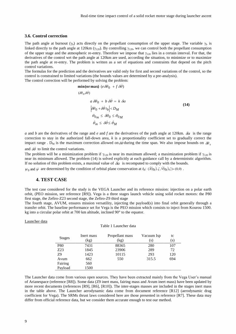
3.6. Control correction

The path angle at burnout (b) acts directly on the propellant consumption of the upper stage. The variable b is

linked directly to the path angle at 120km (120). By controlling 120, we can control both the propellant consumption

of the upper stage and the atmospheric re-entry. Therefore we impose that 120 lies in a certain interval. For that, the

derivatives of the control wrt the path angle at 120km are used, according the situation, to minimize or to maximize

the path angle at re-entry. The problem is written as a set of equations and constraints that depend on the pitch

control variations.

The formulas for the prediction and the derivatives are valid only for first and second variations of the control, so the

control is constrained to limited variations (the bounds values are determined by a pre-analysis).

The control correction will be performed by solving the problem:

Mm

Mm

Mb Dt

k b a

fe

000

0

0

),(

0

0

)(max)(or min

(14)

a and b are the derivatives of the range and e and f are the derivatives of the path angle at 120km. is the range

correction to stay in the authorized fall-down area, k is a proportionality coefficient set to gradually correct the

impact range . DM is the maximum correction allowed on during the time span. We also impose bounds on 0

and to limit the control variations.

The problem will be a minimization problem if 120 is near its maximum allowed; a maximization problem if 120 is

near its minimum allowed. The problem (14) is solved explicitly at each guidance call by a deterministic algorithm.

If no solution of this problem exists, a maximal value of is recomputed to comply with the bounds.

and0 are determined by the condition of orbital plane conservation at tb: )0,0().,.( btVbtX

.

4. TEST CASE

The test case considered for the study is the VEGA Launcher and its reference mission: injection on a polar earth

orbit, (PEO mission, see reference [R9]). Vega is a three stages launch vehicle using solid rocket motors: the P80

first stage, the Zefiro-Z23 second stage, the Zefiro-Z9 third stage

The fourth stage, AVUM, ensures mission versatility, injecting the payload(s) into final orbit generally through a

transfer orbit. The baseline performance set for Vega is the PEO mission which consists to inject from Kourou 1500.

kg into a circular polar orbit at 700 km altitude, inclined 90° to the equator.

Launcher data

Table 1 Launcher data

Stages Inert mass

(kg)

Propellant mass

(kg)

Vacuum Isp

(s)

tc

(s)

P80 7431 88365 280 107 Z23 1845 23906 289 72

Z9 1423 10115 293 120 Avum 662 550 315.5 694

Fairing 560 Payload 1500

The Launcher data come from various open sources. They have been extracted mainly from the Vega User’s manual

of Arianespace (reference [R8]). Some data (Z9 inert mass, fairing mass and Avum inert mass) have been updated by

more recent documents (references [R9], [R6], [R10]). The inter-stages masses are included in the stages inert mass

in the table above. The Launcher aerodynamic data come from document reference [R12] (aerodynamic drag

coefficient for Vega). The SRMs thrust laws considered here are those presented in reference [R7]. These data may

differ from official reference data, but we consider them accurate enough to test our method.


10

Figure 7 Nominal trajectory of VEGA (PEO mission)

Mission scenario for the PEO mission

During the flight of the two first stages (P80, Z23) in atmosphere, the angle of attack is kept near zero. After Z9-Z23

separation and a short ballistic phase, the 3rd

stage is ignited and the fairing is jettisoned when the conventional heat

flux comes below a certain threshold (conventionally 1135 w/m2). After fairing jettisoning, the launcher attitude is

free and the launcher guidance aims at a transfer orbit reached at the end of the first boost of the last stage (Avum).

Then the final stage follows a ballistic trajectory before a re-ignition near the apogee of the transfer orbit and a 2nd

boost to circularise the orbit.

For the test case, the parameters of the transfer orbit resulting of a pre-optimisation are:

Table 2: Transfer orbit parameters

Apogee

Altitude

Perigee

Altitude Inclination

Argument

of perigee

Ascending

node

692.5 km 163 km 89.95 d° 20.5 d° 0.83°

For the VEGA reference mission (PEO orbit) and in nominal conditions (without dispersions), considering a drag

coefficient of 6.510-3

(2), the Z9 stage falls in the Arctic Ocean a thousand km beyond Greenland. The ballistic

impact is located forward at approximately 1200 km from the impact point with drag (see figure 7).

Note: According to our model assumptions (launcher data, flight sequential, guidance), we cannot certify that our

results are representative of a real trajectory of the VEGA Launcher.

4.1. The Monte-Carlo computation process

To compute the statistical Z9 impact zone, we use a Monte-Carlo method based on a quasi-random process more

accurate than the standard Monte-Carlo method (Sobol quasi-random generator; reference [R1]). We suppose that the

dispersions which affect the Launcher follow a Gaussian Law. The following table lists the dispersed parameters and

their standard deviations3:

Table 3: Monte-Carlo parameters

Propulsive dispersions

Stage Flow rate Std. Dev. Isp Std. Dev.

P80

2 % 0.5%

Z23

2% 0.5%

Z9 1% 0.5%

Avum (1st boost)

2.5% 0.3%

Avum (2nd

boost)

2.5% 0.3%

2 See references [R2] and [R5] for estimation of the drag coefficient of stage debris

3 The standard deviations of the propulsive laws are estimated from the documents in references ([R7] and [R13])

Transfer Orbit

Z9 ballistic

impact

Z9 impact Z9 re-entry trajectory

1st

boost Avum

boost Z9

Transfer Orbit


11

Other dispersions

Drag coefficient (Std. Dev.) Dispersion profile wrt mach

Atmospheric density Dispersion profile wrt altitude

We consider a dispersed atmosphere (model GRAM10 reference [R11]) for which a standard deviation of the

atmospheric density is given wrt altitude.

Figure 8: Density perturbation model (reference [R11])

4.2. Debris footprint model

This study is not aimed at modelling precisely the Z9 debris re-entry. We have chosen to simplify the computations

by integrating the re-entry trajectory taking into account the drag force with a constant drag coefficient (SCx/m) and

the earth J2 effect (see references [[R2]] and [[R5]] for drag coefficient values of the pieces of a space vehicle after

breakup). No lift was modelled nor any breakup phenomenon.

The correction strategy is based on analytic derivatives of the ballistic impact wrt control parameters. Obviously, the

real impact location differs from the ballistic impact since the drag effect must be added. Monte-Carlo results will

show that for a given test case, there is a more or less constant offset between the two, the path angle and the relative

velocity at 120km being the most influent parameters. A “virtual” ballistic target has been accordingly assigned to

the range correction algorithm.

5. Computation results

To obtain a sufficiently accurate statistical fall down zone, 100 000 Monte-Carlo runs have been computed. This big

size Monte-Carlo allows also testing the robustness of the algorithms (dispersions estimator, launcher guidance,

control of the impact zone).

5.1. Monte-Carlo results without impact control

As a reference, we computed first a full Monte-Carlo without activating the control of the Z9 impact zone. The

Launcher thrust attitude is computed with the guidance algorithm defined in § 3.3. For all the simulations, the final

orbit has been reached accurately without any propellant depletion (the final accuracy is better than 0.5 km for the

semi-major axis (a), less than 0.004° for i and ), thus demonstrating the efficiency and the robustness of the

guidance algorithm.


12

Results

Table 4: impact zone characteristics and propellant consumption (nominal guidance without impact control)

Parameter Value

Max. Undershoot distance 4

-2458 km

Undershoot distance at probability 10-3

-2017 km


-2300 km

Max Overshoot Distance 5 4619 km

Overshoot distance at probability 10-3

2985 km


3641 km

Statistical Avum propellant

consumption (probability 10-2

)

470.5 kg

0

0.01

0.02

0.03

0.04

0.05

0.06

0.07

0.08

0.09

323 339 355 371 387 403 419 435 451 467 483 499 515

pro

bab

ility

Propellant consumption (kg)

Avum propellant consumption

HISTOGRAM (100K runs)

Probability10-2

Figure 9 Avum propellant consumption (Histogram)

The figure 10 shows the distribution of Avum propellant consumption. The statistical propellant consumption is

moderate and leaves enough propellant reserve to compensate the dispersions and to proceed to Avum de-orbit.

0

0.01

0.02

0.03

0.04

0.05

0.06

0.07

0.08

0.09

pro

bab

ility

distance wrt nominal impact (km)

Z9 distance impact wrt nominal impactHISTOGRAM (100K runs)

Probability10-4

Figure 10 Distance impact wrt nominal (Histogram)

4 Undershoot distance : distance from nominal impact, the impact is behind the nominal impact (negative value by

convention) 5 Overshoot distance : distance from nominal impact, the impact is beyond the nominal impact (positive value)


13

The figure 11 shows the impact distribution of the Z9 stage. For this large Monte-Carlo simulation (100 000 runs),

the fall-down zone stretches over 7100 km; the forward part of the distribution presents a very flat tail suggesting

possible important overshoot impact distances for low probability.

Figure 11 Z9 statistical Z9 fall-down zone over the Arctic Ocean (100 000 runs)

The figure 12 visualizes the statistical fall down zone, an important part of the fall down zone lies beyond the coasts.

5.2. Monte-Carlo results with impact control

The same full Monte-Carlo simulation (100 000 runs) is performed now with impact control ( see § 3.6). The

authorized Z9 fall-down area is defined with respect to a maximum distance between the Z9 ballistic impact point

which results from the simulation with dispersions and a fictitious impact (close to the ballistic impact point of the

nominal trajectory (without dispersions)). The maximum distance depends on the nature of the impact (undershoot,

overshoot):

Maximum undershoot ballistic impact point: 700 km

Maximum overshoot ballistic impact point: 500 km

Impact control strategy

If the ballistic impact is outside the above limits, the nominal launcher guidance is interrupted and the impact control

is activated. The range impact is corrected thanks to the algorithm defined at §3.6. According to the discussion at §

3.6, to control both the propellant consumption of the upper stage and the atmospheric re-entry, the following

strategy is applied (§ 3.6):

- if 120 > -2°, 120 is minimized and the ballistic range impact corrected

- if -4° < 120 -2°, the Z9 ballistic range impact is corrected only

- if 120 < -4°, 120 is maximized and the ballistic range impact corrected

Results

For all the simulations, the final orbit has been reached accurately: the errors on the orbit parameters of the final orbit

are less than 0.7 km for the semi-major axis, less than 0.005° for i and .

Table 5: impact zone characteristics and propellant consumption with impact control

Parameter Value

Max. Undershoot distance

-690 km


-553 km


-608 km

Max Overshoot Distance 867 km


651 km


740 km

Statistical Avum propellant

consumption (probability 10-2

)

477.8 kg


14

0

0.02

0.04

0.06

0.08

0.1

0.12

0.14

359 373 388 402 417 432 446 461 475 490 504 519

pro

bab

ility

Propellant consumption (kg)

Avum propellant consumption

HISTOGRAM (100K runs)

Probability10-2

Figure 12 Avum propellant consumption with impact control

The figure 13 shows the distribution of the Avum propellant consumption. The fuel consumption increases slightly

(+7.3 kg at a probability of 0.01), the histogram shows a flatter distribution.

0

0.01

0.02

0.03

0.04

0.05

0.06

0.07

pro

bab

ility

distance wrt nominal impact (km)

Z9 distance impact wrt nominal impactHISTOGRAM (100K runs)

Probability10-4

Figure 13 Distance impact distribution with impact control

The negative distances in figure 14 are for undershoot impacts. We can check on the figure 14 that the impact control

is effective: the length of the Z9 fall-down zone is now reduced to 1500 km. The ballistic impact zone was

constrained to [-700 km, 500 km]. Taking into account the drag, the impact zone is found here to [-690 km, 828 km].

Because the method manages only the ballistic impact zone, a great part of this difference can be explained by a non

constant deviation between the ballistic impact and the real impact with drag, and also by the error of the propulsive

dispersions estimation leading to a threshold violation, especially for the extreme overshoot cases. The tail

distribution is quite short for the overshoot or undershoot impact zones. So, it can be expected than that the extreme

impact points at very low probability lie at a reasonable distance of the nominal impact point.

Figure 14 Z9 statistical fall-down zone with impact control (100 000 runs)


15

0

0.02

0.04

0.06

0.08

0.1

0.12

0.14

0.16

0.18

0.2

Pro

bab

ilit

y

Flightpath angle (d°)

Flight path angle at reentry (H=120 km)

Histogram (100K runs)

with impact control

without impact control

Figure 15 Flight path angle at re-entry with and without impact control

On the figure above, we can see that the impact control strategy decreases the path angle at re-entry and generally

shifts the values of the path angle to lowest values.

Table 6: Probability comparison for low path angle at re-entry

Probability [ 120 > -1.3°]

Without impact control With impact control

4% 0.7%

6. Conclusion

The ability of our method to limit the fall-down zone of a solid stage during the Launcher ascent is demonstrated.

The solid dispersion estimator is also proven efficient and can have application for other space vehicle guidance. In

addition, the impact control method increases only slightly the propellant consumption of the final stage in charge to

deliver the payload while reducing significantly the fall-down zone and ensuring a direct re-entry by lowering the

flight path angle at re-entry. Therefore the impact control method presented here does not penalize the Launcher

performance (at least for the study case presented here).

We can conclude also that the simplicity of the impact control method for solid stages coupled with a robust

Launcher guidance allows envisaging an onboard application in real time. However, this is still a preliminary work

and following issues need to be addressed:

- Tests on others missions and launchers,

- Global strategy accuracy and Launcher performance optimisation,

- Quantification and effect of the dispersions of a solid motor at tail-off

7. References

[R1] Bratley P. and Fox B.L. (1988). Implementing Sobol’s quasirandom sequence generator, ACM Transactions

on Math. Software 14, 88-100

[R2] Mrozinski R. B. (2003). NASA Pre-event Debris Footprint Estimates for the Deorbit of Space Station MIR,

Nasa Johnson Space Center, USA.

[R3] Siouris G. M., 2004. Missile Guidance and Control Systems, Springer.

[R4] “Autonomous Optimal Deorbit Targeting”, Donald J. Jezewski, AAS/AIAA 1991

[R5] Trajectory design and control for the Compton gamma ray observatory re-entry. Hoge, Vaughn Flight

Mechanics symposium 2001

[R6] Vega Launch system- Final Preparation for qualification flight A. Neri VEGA-IPT ESRIN Vega Program

Status JPC 11 for STTC.ppt

[R7] Vega Launcher F. Serraglia VEGA-IPT ESRIN November 2008

[R8] VEGA User’s Manual Arianespace (2006)

[R9] VEGA satellite Launcher AVIO VEGA quartino_new_m.indd - zefiro_9_77.pdf

[R10] VEGA status and qualification flight preparation S. Bianchi, R. Lafranconi, M. Bonnet ESRIN

[R11] The NASA MSFC Earth Global Reference Atmospheric Model – 2010 Version NASA/TM – 2011 -216467

[R12] Global and Local Multidisciplinary Design Optimization of Expendable Launch Vehicles. F Castellini, A

Riccardi, M Lavagna Report 11-09 Bremen Universität Zentrum für Technomathematik December 2011

[R13] The (successful) experience of The Maiden Flight of Vega, in parallel to the worth mission to lift Lares PG

Lasagni, P Bellomi ELV Fiat Avio PPT presentation (Post-flight analyses, SRM thrust laws envelopes)

REAL-TIME TIME IMPACT CONTROL OF A SOLID ROCKET MOTOR STAGE DURING LAUNCHER ASCENT

Documents

Transcript of REAL-TIME TIME IMPACT CONTROL OF A SOLID ROCKET MOTOR STAGE DURING LAUNCHER ASCENT