Ranked k-medoids: A fast and accurate rank-based partitioning algorithm for clustering large...

Knowledge-Based Systems 39 (2013) 133–143

Contents lists available at SciVerse ScienceDirect

Knowledge-Based Systems

journal homepage: www.elsevier .com/ locate /knosys

Ranked k-medoids: A fast and accurate rank-based partitioning algorithmfor clustering large datasets

Seyed Mohammad Razavi Zadegan a, Mehdi Mirzaie b,c, Farahnaz Sadoughi a,⇑a Department of Health Information Management, School of Health Management and Information Sciences, Tehran University of Medical Sciences, Tehran, Iranb Proteomics Research Center, Faculty of Paramedical Sciences, Shahid Beheshti University of Medical Sciences, Tehran, Iranc Department of Bioinformatics, School of Computer Science, Institute for Research in Fundamental Sciences (IPM), Tehran, Iran

a r t i c l e i n f o a b s t r a c t

Article history:Received 13 May 2012Received in revised form 6 October 2012Accepted 14 October 2012Available online 23 November 2012

Keywords:Clustering analysisPartitioning clusteringk-Medoids clusteringk-Harmonic meansExternal validation measures

0950-7051/$ - see front matter � 2012 Elsevier B.V. Ahttp://dx.doi.org/10.1016/j.knosys.2012.10.012

⇑ Corresponding author. Tel.: +98 2188794300.E-mail addresses: [email protected], sadoughi

Clustering analysis is the process of dividing a set of objects into none-overlapping subsets. Each subset isa cluster, such that objects in the cluster are similar to one another and dissimilar to the objects in theother clusters. Most of the algorithms in partitioning approach of clustering suffer from trapping in localoptimum and the sensitivity to initialization and outliers. In this paper, we introduce a novel partitioningalgorithm that its initialization does not lead the algorithm to local optimum and can find all theGaussian-shaped clusters if it has the right number of them. In this algorithm, the similarity betweenpairs of objects are computed once and updating the medoids in each iteration costs O(k �m) where kis the number of clusters and m is the number of objects needed to update medoids of the clusters. Com-parison between our algorithm and two other partitioning algorithms is performed by using four well-known external validation measures over seven standard datasets. The results for the larger datasetsshow the superiority of the proposed algorithm over two other algorithms in terms of speed andaccuracy.

� 2012 Elsevier B.V. All rights reserved.

1. Introduction

Clustering analysis is the process of dividing a set of objects intonone-overlapping subsets. Each subset is a cluster, such that ob-jects in the cluster are similar to one another (intra-similarity)and dissimilar to objects in other clusters (inter-dissimilarity) [1].Clustering analysis has been widely used in many applicationssuch as business intelligence [2,3], image processing [4,5], Websearch [6], biology [7–9], and security [10].

There are several approaches of clustering such as hierarchical[11,12], partitioning [13], density-based [14], model-based[15,16] and grid-based [17]. Xu and Wunsch [18] provided a goodsurvey on the clustering algorithms. In this paper our particularinterest is in the partitioning approach that divides a dataset intok < N clusters (N is size of dataset) such that every cluster has acenter by which other members are determined according to theirsimilarities. By using an iterative manner and re-computing thecenters, algorithms of this approach attempt to find the bestpartitioning which has a high degree of intra-similarity andinter-dissimilarity. They mostly report the circle-shaped or Gauss-ian-shaped clusters because of assigning an object in the dataset tothe most similar center.

ll rights reserved.

[email protected] (F. Sadoughi).

One of the most well-known algorithms of partitioning ap-proach is k-means that re-computes each of the new centers byaveraging the dissimilarities (distances) of the assigned objects tothe old centers [19]. Although, k-mean is simple and efficient algo-rithm, but it is sensitive to outliers and also its greedy naturemakes it sensitive to initialization which may cause trapping in lo-cal optimum [20]. Other methods were designed based on k-meanssuch as Fuzzy C-Mean (FCM), a fuzzy version of k-means [21], andK-Harmonic Means (KHMs) that uses a harmonic means forre-computing centers [22]. FCM is useful for datasets that theboundaries among clusters are not well-separated. However, ithas problems with outliers and local optimum [18]. KHM solvesthe problems with initialization and outliers, but, it still suffersfrom local optimum [20].

To overcome local optimum problem, optimization algorithmslike genetic algorithm [23], particle swarm optimization [24], antcolony [25], firefly algorithm [26] and artificial bee colony [27]were employed. They mostly use the cost function of k-means orK-Harmonic Means and by using their stochastic manner, attemptto escape from local optimum and find the best centers. However,they have brought their problems to the clustering analysis. As anexample, PSO algorithm has two important phases which areexploration and exploitation. If these two phases perform incor-rectly, for any reason, such as setting inappropriate parameters,PSO will not work out and cannot find the global optimum [28].

134 S.M. Razavi Zadegan et al. / Knowledge-Based Systems 39 (2013) 133–143

Another series of attempt to reduce sensitivity to outliers aredeveloped by k-medoids algorithms. In these algorithms the centerof cluster or medoid is always one of the objects in the dataset andthrough iterations the most centrally located objects are supposedto be found. One of the first algorithms of k-medoids clustering isPartitioned Around Medians (PAM) which deals with pairs ofobjects in the dataset [13]. The high computational time of PAMhas impeded using this algorithm for large dataset [29]. Based onPAM another algorithm named CLARA was designed to deal withlarger dataset [13]. This new algorithm selects multiple samplesfrom the dataset and applies PAM over them. CLARA can handlelarger datasets in contrast to PAM. However, some new problemshave been appeared. If the samples do not involve the real centrallylocated objects, CLARA cannot find the pattern in dataset [30].Therefore, determining the best sampling method and the size ofthe samples are new challenge for the algorithm. Moreover thecomputational time did not improve. CLARANS [31] is aimed atimproving CLARA. It uses randomize policy in choosing pairs andmakes use of the neighborhood to update the medoids. CLARANSand other algorithms based on PAM have considerable difficultyin computational time [30].

Newly designed algorithm by Park and Jun [29] is much effi-cient than PAM-based algorithms. In this paper, their algorithmis referred to as ‘Simple and Fast k-medoids’. A new medoid in thisalgorithm is selected by examining all the assigned members tothe old medoid, and choosing one who increases intra-similaritymore than others. Therefore, in each iteration the new set of med-oids is selected with running time O(N), where N is the number ofobjects in the dataset. Simple and Fast k-medoids is so sensitive toinitialization which increases the possibility of trapping in localoptimum. As Park and Jun [29] showed, the results vary consider-ably according to the methods of initialization.

In this paper we introduce a novel k-medoids algorithm whichthe initialization does not lead the algorithm to local optimum andcan find all the Gaussian-shaped clusters. The remaining of the pa-per is organized as follows: Section 2 describes the partitioning ap-proach and the local optimum definition. A rank-based similarityamong objects in the datasets is introduced; it helps us to findthe medoids faster. The hostility relation in human society isemployed to explain the new concept. At the end of Section 2our proposed algorithm is described and its behavior is analyzedin theory. Section 3 presents the experiments. Two algorithms of

Fig. 1. A dataset of 2-dimensional points with six clusters. Algor

the partitioning approach of clustering which are K-HarmonicMeans (KHM) and Simple and Fast k-medoids, are selected forcomparison. Two challenging artificial datasets and five real data-sets are used and in order to evaluate the results, four well-knownexternal validation measures are explained in this section. The re-sults are discussed in Section 4 and Section 5 makes conclusion.

2. Ranked k-medoids

2.1. Partitioning approach

Suppose a dataset D = {X1,X2, . . . ,XN} in which every object is ad-dimensional vector like Xi = (xi1,xi2, . . . ,xid). In the partitioningapproach of clustering, D is divided into k < N clusters. Every clus-ter has a center which can be a hypothetical (centroid) or a real ob-ject (medoid) in D, and a similarity between objects and thecenters determines the members of clusters. The similarity amongobjects can be defined using the Euclidean distance, correlation,cosine similarity, etc. In this paper the Euclidean distance in Eq.(1) is used to express the dissimilarity between objects like Xi

and Xj.

kXi � Xjk ¼

ffiffiffiffiffiffiffiffiffiffiffiffiffiffiffiffiffiffiffiffiffiffiffiffiffiffiffiffiffiXp

k¼1

ðxik � xjkÞ2vuut ð1Þ

The definition of local optimum is relative to the approaches ofclustering. For example, if we are analyzing a dataset, e.g. Fig. 1,that its clusters are spiral-shaped, ring-shaped or moon-shaped,we should not expect that an algorithm in the partitioning ap-proach finds the clusters. Therefore, claiming that the algorithmwas trapped in local optimum is not acceptable because the algo-rithms in the partitioning approach are not designed to find thesekinds of clusters and they intrinsically report Gaussian-shapedclusters. Here the problem arising from selecting wrong approach,not trapping in local optimum. The meaning of the local optimumfor partitioning approach is made clear by Definition 1.

Definition 1. Local optimum is a partitioning of a dataset thatcombined some real clusters and divide at least one cluster intoseveral estimated clusters, in a situation that all the clusters areGaussian-shaped and the right number of them is given.

ithms of the partitioning approach cannot find the clusters.

S.M. Razavi Zadegan et al. / Knowledge-Based Systems 39 (2013) 133–143 135

Definition 1 is the appropriate definition for local optimum inthe partitioning approach of clustering. It is essential for analgorithm of the partitioning approach to find the clusters of adataset like what we mentioned in Definition 1. However, most ofthe well-known algorithms like KM, KHM and FCM have problemin finding the pattern of these suitable dataset [18,32].

2.2. Ranking and hostility relation

In our method the values of similarity between the objects arenot directly used and we introduce new function that ranks objectsaccording to their similarities. By this function, the more similarobject gets lower rank. In other words, rank(Xi, Xj) = l shows thatXj is the lth similar object to Xi among N objects in the dataset.The ranks of other objects according to an object like Xi can becomputed by sorting the similarity values between Xi and other ob-jects in the dataset. The rank function also expresses a rank matrixas follows:

R ¼ ½rij�; rankðXi;XjÞ ¼ rij; 8 Xi; Xj 2 D ð2Þ

Since two objects are not always at the same rank of each other,R is not necessarily a symmetric matrix, in other words, it mayhappen that rank(Xi, Xj) – rank(Xj, Xi).

R is similar to the hostility relation in human society. As weknow, in human society each person ranks others according totheir common interests or ideas and based on this system of rank-ing finds some persons friendly and others unfriendly. But, thesefeelings are not always symmetry, in other words, a person maybe deeply hostile to somebody, but, he/she may not be that muchhostile toward the first person. In our algorithm two objects arefiguratively hostile toward each other according to their ranks,and the more similar objects have less hostile feelings toward eachother. Thus, R is a matrix that shows the hostility relationshipamong objects in the dataset, and also, it contains the strength ofthese relations through numbers, from 1 (for the least hostility)to N (for the extreme hostility).

Similarly, from rij < rji which is a case of asymmetric relation inR, can be understood that the rank of xi is higher, according to thesimilarities of xj to other objects (rji), than the rank of xj accordingto the similarities of xi to other objects (rij). Thus, it can be consid-ered that xj are much hostile or unfriendly toward xi. Consequently,it reveals the existence of some other objects more similar to xj thatmake xi looks more unfriendly. We utilize this information inupdating the medoids.

In order to find the medoids we introduce another quantitywhich is the hostility value (hv) of an object in a group of objects.

Fig. 2. Two clusters of objects in 2-dimensional space, and the Euclidean distancedetermined their dissimilarity. Groups of objects are enclosed by ellipses. Leftcluster: The lowest object in the group (Xi) are more similar to the objects from theoutside of the group, therefore, the ranks of the objects in the group increase andconsequently the hostility value of Xi becomes maximum. Right cluster: All theobjects in the group are approximately at the same rank of each other; therefore,their hostility values are nearly equal.

The hostility value of an object like Xi in a set of objects like G isdefined as follows:

hv i ¼XXj2G

rij ð3Þ

As an example, we compute the hostility value of two objects(Xi, Xj) in Fig. 2 in which the members of the group are enclosedby an ellipse and the Euclidean distance determines the dissimilar-ity among them. According to the similarity of Xi to the other ob-jects (Right cluster is ignored), we can visually find out that theinner objects in the group are 13th to 16th similar objects to Xi

(the numbers are distinguishable by label (i)). Thus, the hostilityvalue of Xi is computed as follows:

hv i ¼ 1þ 13þ 14þ 15þ 16 ¼ 59

Similarly, from the similarity between Xj and other objects canbe understood that the inner objects in the group are 2nd, 3rd, 4thand 6th similar objects to Xj (the numbers are distinguishable bylabel (j)), therefore, the hostility value of Xj is computed as follows:

hv j ¼ 1þ 2þ 3þ 4þ 6 ¼ 16

hv shows figuratively, how much an object is unfriendly with othersin a group. For example, Xi in Fig. 2 is much hostile to the othersrather than any other members. Moreover, the hostility values ofa group provide clues about how objects in the group or even outof the group are scattered in the input space. The distribution ofhvs in the group involves two possible cases. In the first case, thehostility values of data objects in a group are not nearly equal.Therefore, we can conclude that some objects are more hostile thanothers to the members of group. We see this heterogeneity in hvsbecause the objects which have greater hv are more similar to someobjects from the outside of the group. Therefore, the outer objectsare placed in lower rank and the inner ones place in higher rank,as left cluster in Fig. 2 shows. In the second case, the hostility valuesof objects in a group are approximately equal. It shows that themost of the similar objects are part of the group; thus, there arenot many other similar objects from the outside of the group, asright cluster in Fig. 2 shows. Therefore, by using hvs of a groupwe can slightly discover how objects in the group or those aroundthe group are scattered.

2.3. Proposed algorithm

Our proposed algorithm consists of the following steps:

Step 1. (Initialization)1.1. Calculate the similarities among pairs of objects

based on the similarity metric (e.g. Euclidean,correlation).

1.2. Calculate R matrix by sorting the similarity valuesand store the indexes of similar objects from themost similar to the least similar in sorted indexmatrix.

1.3. Select k medoids randomly.Step 2. (Update medoids)

2.1. Do the following steps for each medoid:2.1.1. Select the group of the most similar objects to

each medoid, using sorted index matrix.(The number of members of the group isdetermined by an input parameter m).

2.1.2. Calculate the hostility values of every object inthose groups using Eq. (3).

2.1.3. Choose object with the maximum hostilityvalue as the new medoid.

Fig. 3. Six two-dimensional points. X1, X2 and X3 are in the group indicated by G.


2.2. Relocate one of the medoids placed in the samegroup.

2.3. Go to step 2.1. until the maximum iteration will bereached.

Step 3. (Labeling objects)3.1. Assign each object to the most similar medoid.

In each iteration, calculating k new medoids costs O(k �m)where shows the number of members in the group. The parameterm has a direct effect on the speed of the algorithm. By having asmaller group, the medoids approach the centers with the smallersteps. The medoids may also jump between clusters easily, if thegroup is too large. But, selecting m between 5 and 15 will be effi-cient for small and large datasets.

In the step 1.2. a matrix called sortedIndex matrix is returnedfrom calculating the ranks of objects. It keeps the indexes of similarobjects in the dataset. sortedIndexij = t, shows that the jth similarobjects to Xi is Xt. By using sortedIndex matrix, the computationaltime of forming group G will be O(m). To understand thoroughlythis matrix, suppose a dataset D with one-dimensional points asfollows:

D ¼ fX1;X2;X3;X4g ¼ f1;3;4;6g

The matrix R and sortedIndex for D are as follows (closenessshows the similarity):

R ¼

1 2 3 43 1 2 44 2 1 34 3 2 1

26664

37775; sortedIndex ¼

1 2 3 42 3 1 43 2 4 14 3 2 1

26664

37775

In the matrix R, R21 = 3 means that X1 is the third similar objectto X2 and sortedIndex34 = 1 means that X1 is the fourth similar ob-ject to X3.

In order to understand how the algorithm escapes from localoptimum, we will show how it moves the medoids through itera-tions and afterwards, analyzing the behavior of the algorithm indealing with a dataset will be described.

2.3.1. Seeking the centerSuppose a cluster like C that its objects are scattered in input

space by a Gaussian distribution with the average l and the stan-dard deviation r. For selecting a new medoid, a group of the closestobjects to the old medoid like G is needed. Imagine that G containstwo object Xi and Xj such that Xi is closer to l or the center ofcluster, therefore we have:

Xi;Xj 2 G; kXi � lk < kXj � lk ð4Þ

We can also rewrite Eq. (3) as follows:

hv i ¼mðmþ 1Þ

2

� �þX8Xj2G

jSijj ð5Þ

m is the number of objects in G and jSijj is the number of objects inSij which is defined as follows:

Sij ¼ fXk R GjkXk � Xik < kXi � Xjkg ð6Þ

By using Eq. (3), the calculated ranks of every objects in thegroup (according to their similarities to Xi) are added to obtainhvi. However in Eq. (5), at first the objects in the group are sup-posed to be the first m ranks of Xi, and afterwards the number ofmore similar objects to Xi, from the outside of the group are added.Now, an example is served to illustrate this new form of calculatinghv. There are six points in Fig. 3 in which three of them are in thegroup G (m = 3). To calculating the hv1 according to Eq. (3), theranks of X2 and X3 are needed. The ranks of the objects in Fig. 3 con-sidering their distances to X1 are as follows:

Objects
X1 X2 X3 X4 X5 X6
Rank
1 4 6 5 3 2
Therefore, the hostility value of X1 according to Eq. (3) is asfollows:

hv1 ¼ 1þ 4þ 6 ¼ 11

In order to calculate the hv1 according to Eq. (5), the sets S12 andS13 should be identified. S12 is the set of objects from outside of thegroup which are closer than X2 to X1. Therefore, the set S12 is asfollows:

S12 ¼ fX5;X6g

Similarly, the members of S13 are:

S13 ¼ fX4;X5;X6g

According to Eq. (5) the hv1 is calculated as follows:

hv1 ¼3 � 4

2

� �þ ðjS12j þ jS13jÞ ¼ ð1þ 2þ 3Þ þ ð2þ 3Þ ¼ 11

The distribution of C is Gaussian; therefore, the probability ofobjects closer to average is greater than those farther from average.It means that the probability of objects in Sij (which is a subset ofobjects in the cluster) increases as Xi becomes closer to the average.Therefore, it reveals that Sij is larger for Xi which is closer to theaverage than Sij, for Xj which is farther than the average. Conse-quently, hvs in G increase as the objects approach the average.

In each iteration, our algorithm selects the maximum hv in G asthe next medoid. We showed that the maximum hv in G occurredamong those objects which are closer to the average or the centerof cluster. Therefore, through iteration, the medoid distances fromthe edge of cluster and comes near the center. When the medoid islocated in the center of cluster it never returns to the edge of clus-ter, because, the hvs in G decreases as the object comes near to theedge of the clusters. Therefore, the objects from the edge cannothave maximum hv and be the next possible medoid, in the pres-ence of some objects near the center.

Fig. 4 shows the behavior of the algorithm in selecting the med-oid, through four iterations. The only cluster in the figure is Gauss-ian-shaped and the current and the previous medoids aredistinguishable by filled square and circle. The number of membersin G is equal to 15, and the circles around these points make themrecognizable. It can be seen how medoid approaches the centerfrom the edge of the cluster. Finally, by locating at the center in


the fourth iteration, the medoid and the group G will not leavethere.

The behavior of the algorithm in leading medoid to the center ofcluster can be illustrated from theoretical point of view. Therefore,suppose that the objects of cluster C follow one-dimensional (forthe sake of simplicity) Gaussian distribution with parameters land r. The density function of this distribution is as follows:

FðXÞ ¼ 1rffiffiffiffiffiffiffi2pp e�

ðX�lÞ2

2r2 ð7Þ

Fig. 5 shows the curve of a Gaussian distribution with the aver-age l. It can be seen that the probability of an objects closer to l isgreater than the farther one (F(Xi) > F(Xj)). The hachured area inFig. 5A is the probability of objects which are in the cluster and clo-ser than Xj to Xi. Uij is a set of these objects:

Uij ¼ fXt 2 CjkXt � Xik 6 kXj � Xikg ð8Þ

This probability is directly related to the probability of an objectbelonged to the set Sij, because Sij is a subset of Uij. Therefore, as Xi

moves towards l, the probability of objects like Xk 2 Sij increases.Consequently, for two objects like Xi and Xj in the group G, thehvi is greater than hvj, if Xi is closer to l than Xj.

2.3.2. Escaping from local optimumAfter describing the movements of medoids, it is time to look at

the behavior of the algorithm in dealing with a dataset containing kGaussian-shaped clusters. The algorithm chooses k objects as themedoids of the clusters. Regarding to Definition 1, we will showthat the algorithm can escape from local optimum.

Suppose a state at the early iterations of the running algorithmthat most of the medoids share some clusters. As we have the rightnumber of clusters, there are also some of them without medoid.We call the clusters with at least one medoid ‘‘discovered cluster’’

Fig. 4. Four iterations of RKM algorithm. The current and previous medoid with the meplaced at the edge of cluster, but, in the fourth iteration it has found the center.

and those without medoid ‘‘undiscovered cluster’’ (Fig. 6). Weshowed that in a finite number of iterations medoids will be placedat the center of discovered clusters. In that moment, the medoidsof a discovered cluster are so close that they are placed in theirsimilar groups (a group which is needed to compute the hvs andfind the new medoid). Then, the algorithm relocates all the med-oids except one of them (step 2.2). Fig. 7 shows a situation thattwo medoids are the parts of their similar groups; therefore, oneof them should be relocated. Afterwards, the relocated medoidmight be placed inside an undiscovered cluster or even in anotherdiscovered cluster. In the first case, the medoid reaches the centerin a finite number of iteration and possesses the undiscovered clus-ter. In the second case that there is a cluster with more than onemedoid, a new relocation will happen. Obviously, the algorithmcan be implemented such that these relocations of misplaced ob-jects end, in a finite number of iterations (at the worst case it testsall the objects except the members of the undiscovered cluster).Therefore in a finite number of iterations, the algorithm can findall the clusters regardless of how the medoids were locatedinitially.

Video 1 shows how our algorithm finds the clusters. In this vi-deo the medoids (big black circles) are plotted in each iteration,with the rest of the objects in the dataset. At early iterations (1–30) most of the medoids are placed in the same clusters and theirseparations are visible. As iteration continues, each medoid pos-sesses a cluster of objects. In 41th iteration all the medoids areplaced at the centers of clusters, therefore, nothing will happen ex-cept the little movements of medoids in the centers.

To expedite the process of finding real medoids, we can alsodouble the size of similar groups and select half of them randomlyto find next medoids. By this policy we enlarge the groups and con-sequently the steps to the centers of clusters as we keep the num-ber of members unchanged.

mbers of group G have been indicated at the end of each iteration. Initial medoid is

Fig. 5. The curve of Gaussian distribution with the average (l). (A) Hachured area shows the probability of a point belonging to Uij and kX0j � Xik ¼ kXj � Xik and (B) hachuredarea shows the probability of a point belonging to Uji and kX0i � Xjk ¼ kXj � Xik.

Fig. 6. Five clusters and the initial location of five medoids are shown. Three clusters have at least one medoid (discovered clusters), and two of them are without any medoid(undiscovered clusters).

Fig. 7. Two clusters of objects. The diamond-shaped cluster has two medoids which are the members of their similar groups and one of them should leave the cluster.


3. Experiments

3.1. Algorithms

Our proposed algorithm was compared with two other parti-tioning algorithms, K-Harmonic Means (KHMs) and Simple and

Fast k-medoids. KHM is one of the most well-known algorithmsin this family that unlike k-means is not sensitive to initializationand outliers. Updating k centers, in each iteration, costsO(k � N � D) in a situation that the Euclidean distance shows dis-similarity among objects of the dataset which are D-dimensional.

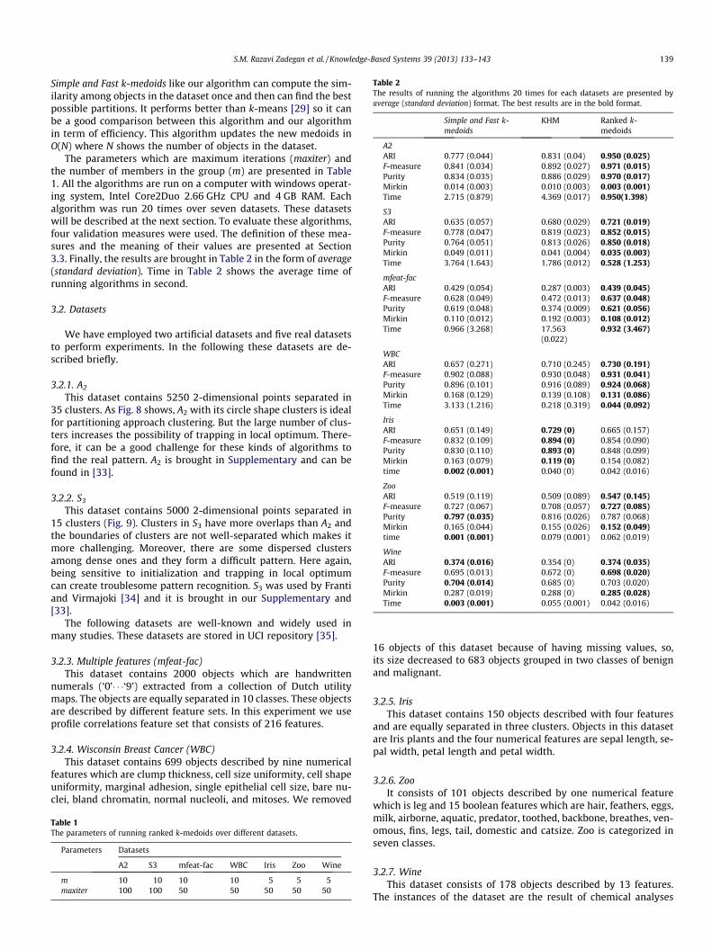
Table 2The results of running the algorithms 20 times for each datasets are presented byaverage (standard deviation) format. The best results are in the bold format.

Simple and Fast k-medoids

KHM Ranked k-medoids

A2ARI 0.777 (0.044) 0.831 (0.04) 0.950 (0.025)F-measure 0.841 (0.034) 0.892 (0.027) 0.971 (0.015)Purity 0.834 (0.035) 0.886 (0.029) 0.970 (0.017)Mirkin 0.014 (0.003) 0.010 (0.003) 0.003 (0.001)Time 2.715 (0.879) 4.369 (0.017) 0.950(1.398)

S3ARI 0.635 (0.057) 0.680 (0.029) 0.721 (0.019)F-measure 0.778 (0.047) 0.819 (0.023) 0.852 (0.015)Purity 0.764 (0.051) 0.813 (0.026) 0.850 (0.018)Mirkin 0.049 (0.011) 0.041 (0.004) 0.035 (0.003)Time 3.764 (1.643) 1.786 (0.012) 0.528 (1.253)

mfeat-facARI 0.429 (0.054) 0.287 (0.003) 0.439 (0.045)F-measure 0.628 (0.049) 0.472 (0.013) 0.637 (0.048)Purity 0.619 (0.048) 0.374 (0.009) 0.621 (0.056)Mirkin 0.110 (0.012) 0.192 (0.003) 0.108 (0.012)Time 0.966 (3.268) 17.563

(0.022)0.932 (3.467)

WBCARI 0.657 (0.271) 0.710 (0.245) 0.730 (0.191)F-measure 0.902 (0.088) 0.930 (0.048) 0.931 (0.041)Purity 0.896 (0.101) 0.916 (0.089) 0.924 (0.068)Mirkin 0.168 (0.129) 0.139 (0.108) 0.131 (0.086)Time 3.133 (1.216) 0.218 (0.319) 0.044 (0.092)

IrisARI 0.651 (0.149) 0.729 (0) 0.665 (0.157)F-measure 0.832 (0.109) 0.894 (0) 0.854 (0.090)Purity 0.830 (0.110) 0.893 (0) 0.848 (0.099)Mirkin 0.163 (0.079) 0.119 (0) 0.154 (0.082)time 0.002 (0.001) 0.040 (0) 0.042 (0.016)

ZooARI 0.519 (0.119) 0.509 (0.089) 0.547 (0.145)F-measure 0.727 (0.067) 0.708 (0.057) 0.727 (0.085)Purity 0.797 (0.035) 0.816 (0.026) 0.787 (0.068)Mirkin 0.165 (0.044) 0.155 (0.026) 0.152 (0.049)time 0.001 (0.001) 0.079 (0.001) 0.062 (0.019)

WineARI 0.374 (0.016) 0.354 (0) 0.374 (0.035)F-measure 0.695 (0.013) 0.672 (0) 0.698 (0.020)Purity 0.704 (0.014) 0.685 (0) 0.703 (0.020)Mirkin 0.287 (0.019) 0.288 (0) 0.285 (0.028)Time 0.003 (0.001) 0.055 (0.001) 0.042 (0.016)


Simple and Fast k-medoids like our algorithm can compute the sim-ilarity among objects in the dataset once and then can find the bestpossible partitions. It performs better than k-means [29] so it canbe a good comparison between this algorithm and our algorithmin term of efficiency. This algorithm updates the new medoids inO(N) where N shows the number of objects in the dataset.

The parameters which are maximum iterations (maxiter) andthe number of members in the group (m) are presented in Table1. All the algorithms are run on a computer with windows operat-ing system, Intel Core2Duo 2.66 GHz CPU and 4 GB RAM. Eachalgorithm was run 20 times over seven datasets. These datasetswill be described at the next section. To evaluate these algorithms,four validation measures were used. The definition of these mea-sures and the meaning of their values are presented at Section3.3. Finally, the results are brought in Table 2 in the form of average(standard deviation). Time in Table 2 shows the average time ofrunning algorithms in second.

3.2. Datasets

We have employed two artificial datasets and five real datasetsto perform experiments. In the following these datasets are de-scribed briefly.

3.2.1. A2

This dataset contains 5250 2-dimensional points separated in35 clusters. As Fig. 8 shows, A2 with its circle shape clusters is idealfor partitioning approach clustering. But the large number of clus-ters increases the possibility of trapping in local optimum. There-fore, it can be a good challenge for these kinds of algorithms tofind the real pattern. A2 is brought in Supplementary and can befound in [33].

3.2.2. S3

This dataset contains 5000 2-dimensional points separated in15 clusters (Fig. 9). Clusters in S3 have more overlaps than A2 andthe boundaries of clusters are not well-separated which makes itmore challenging. Moreover, there are some dispersed clustersamong dense ones and they form a difficult pattern. Here again,being sensitive to initialization and trapping in local optimumcan create troublesome pattern recognition. S3 was used by Frantiand Virmajoki [34] and it is brought in our Supplementary and[33].

The following datasets are well-known and widely used inmany studies. These datasets are stored in UCI repository [35].

3.2.3. Multiple features (mfeat-fac)This dataset contains 2000 objects which are handwritten

numerals (‘0’� � �‘9’) extracted from a collection of Dutch utilitymaps. The objects are equally separated in 10 classes. These objectsare described by different feature sets. In this experiment we useprofile correlations feature set that consists of 216 features.

3.2.4. Wisconsin Breast Cancer (WBC)This dataset contains 699 objects described by nine numerical

features which are clump thickness, cell size uniformity, cell shapeuniformity, marginal adhesion, single epithelial cell size, bare nu-clei, bland chromatin, normal nucleoli, and mitoses. We removed

Table 1The parameters of running ranked k-medoids over different datasets.

Parameters Datasets

A2 S3 mfeat-fac WBC Iris Zoo Wine

m 10 10 10 10 5 5 5maxiter 100 100 50 50 50 50 50

16 objects of this dataset because of having missing values, so,its size decreased to 683 objects grouped in two classes of benignand malignant.

3.2.5. IrisThis dataset contains 150 objects described with four features

and are equally separated in three clusters. Objects in this datasetare Iris plants and the four numerical features are sepal length, se-pal width, petal length and petal width.

3.2.6. ZooIt consists of 101 objects described by one numerical feature

which is leg and 15 boolean features which are hair, feathers, eggs,milk, airborne, aquatic, predator, toothed, backbone, breathes, ven-omous, fins, legs, tail, domestic and catsize. Zoo is categorized inseven classes.

3.2.7. WineThis dataset consists of 178 objects described by 13 features.

The instances of the dataset are the result of chemical analyses

Fig. 8. A2.

Fig. 9. S3.


of wine in Italy. The numerical feature are alcohol, malic acid, ash,alcalinity of ash, magnesium, total phenols, flavanoids, nonflava-noid phenols, proanthocyanins, color intensity, hue, OD280/OD315 of diluted wines and proline. Wine is classified in threeclasses.

3.3. Evaluation functions

To evaluate the results of clustering methods, two types of clus-ter validation techniques are using: internal validation measuresand external validation measures. Internal validation measuresevaluate clusters based on the structure of the dataset; therefore,

intra-clusters similarity (cohesion) and inter-cluster dissimilarity(separation) are the main factors for these measures. On the otherhand, external validation measures evaluate clusters by comparingcomputed labels of objects with their real label [36]. In our exper-iments, the clusters were evaluated by four external validationmeasures which are Mirkin [37], Purity [38], F-measure [36] andAdjusted RandIndex (ARI) [39]. In the following these measuresare described briefly.

To explain the external validation measures we need a matrixcalled association matrix. Suppose that a dataset with N objectsis partitioned into C = {c1,c2, . . . ,cI} classes and the algorithm findsK = {k1,k2, . . . ,kJ} clusters, then matrix A = [aij]I�J is association


matrix where aij indicates number of ci’s members which belong toki. Moreover, ai and aj as marginal numbers is defined by:

a:j ¼X

i

aij ð9Þ

a:i ¼X

j

aij ð10Þ

3.3.1. MirkinThe Mirkin metric is defined by Eq. (11) and related to the num-

ber of disagreed pairs in the sets K and C. Mirkin metric is scaled inthe interval [0,1] which is 0 for identical sets of labels or completefinding of the pattern and positive otherwise.

MirkinðC;KÞ ¼ 1N2

XI

i¼1

a2i: þ

XJ

j¼1

a2:j � 2�

XJ

j¼1

XI

i¼1

a2ij

!ð11Þ

3.3.2. PurityThe purity of a cluster is defined as follows:

PurityðkpÞ ¼1

a:pðmaxðaipÞÞ; i ¼ 1; . . . ; I ð12Þ

The above purity determines the class that was predicted by kp.The larger value of Eq. (12) shows more common objects in clusterkp and the predicted class. The purity of whole solution can be de-fined by using a weighted mean of the individual cluster purities.

purityðKÞ ¼XJ

p¼1

a:pN� PurityðkpÞ

� �ð13Þ

3.3.3. F-measureIt is widely used in information retrieval and is based on two

concepts of precision and recall which indicate accuracy and cover-age of retrieved information correspondingly, and are defined by:

precisionðki; cjÞ ¼aij

a:jð14Þ

recallðki; cjÞ ¼aij

ai:ð15Þ

F-measure of cluster ki regards to class cj is the harmonic meanof its precision and recall. It has a low value for a situation in whichrecall and precision are unbalanced. This value is defined by:

Fkcðki; cjÞ ¼2

1=precisionðki; cjÞ þ 1=recallðki; cjÞð16Þ

Consequently, F-measure of a cluster is defined by:

FkðkpÞ ¼ maxj¼1;2;...;I

Fðkp; cjÞ ð17Þ

Therefore the F-measure of whole clustering solution can be definedas Eq. (18) and the greater its value, the better clustering solution.

FðKÞ ¼XJ

p¼1

a:pN

FðkpÞ ð18Þ

3.3.4. Adjusted Rand Index (ARI)It is one of the most popular external validation measures rang-

ing from 0 to 1. Higher value of ARI shows better quality of clusters.To explain ARI four quantities based on pairs of objects are defined:

‘a’ is the number of pairs which are in the same class in C and in thesame cluster in K, ‘b’ is the number of pairs which are in the sameclass in C but not in the same cluster in K, ‘c’ is the number of pairswhich are in the different classes of C but in the same cluster in Kand ‘d’ is the number of pairs placed on different classes and clus-ters in C and K. According to these quantities rand index (RI) is de-fined by:

RIðC;KÞ ¼ aþ daþ bþ c þ d

¼ aþ dN

2

� �ð19Þ

RI is not uniformly distributed in the interval [0,1] and cannot showproperly the differences between random partitioning and real par-titioning [40]. ARI is an adjustment of RI that solves this problemand is defined by:

ARIðC;KÞ ¼ RIðC;KÞ � EðRIÞ1� EðRIÞ ð20Þ

E(RI) is the expected value of rand index under the generalizedhypergeometric assumption. ARI can be simplified and rewrittenas follows:

ARIðC;KÞ ¼

PIi¼1

PJj¼1

aij

2

� ��PI

i¼1

ai:

2

� �PJj¼1

a:j2

� �� N

2

� �

1=2PI

i¼1

ai:

2

� �þPJ

j¼1

a:j2

� �� PI

i¼1

ai:

2

� �PJj¼1

a:j2

� �� N

2

� �ð21Þ

Some simple examples and comparison between RI and ARI arebrought in [40].

4. Discussion

There is a striking contrast between the results of our methodand the other algorithms for datasets A2, S3, mfeat-fac and WBC.Worse values of external validation measures for KHM and Simpleand Fast k-medoids reveal that they have combined some classes ordivide one class into several clusters and trapped in local optimum.For the smaller datasets including Iris, zoo and wine, our algorithmdoes not outperform the two other algorithms. However, the closevalues of external validation measures for these datasets show thatRKM has not lost the pattern, and some misplaced objects in theedge of the clusters make RKM slightly worse than other algorithm.

To understand why these results emerged from experiments,the behavior of the algorithms should be considered. Algorithmslike KHM or Simple and Fast k-medoids have tendency to be station-ary. By the stationary, we mean that the algorithm updates thecentroid of a cluster, if a more centrally located point can be found,such that, it decreases the cost function of the algorithm. This gree-dy behavior is one of the main reasons of trapping in the local opti-mum. Therefore, as the number of clusters and objects increase,the local optimum situations and the probability of trapping inthe local optimum raise too (as we have seen in the result of data-set A2 and S3). But, in the smaller datasets with the decreased num-ber of local optimum, they can be placed at the optimum point bythe help of a suitable initialization, and can keep the point till theend. Therefore, their weakness in the lager datasets can be benefi-cial in the smaller datasets.

In contrast, our algorithm is dynamic, meaning that, a medoid isupdated in each iteration. After finding a way into the center ofcluster, the medoid may not stand still and some movements inits similar group of objects are predictable, therefore, slight devia-tion from the center is resulted. This deviation from the centershows its downsides on the results of the smaller datasets morethan the larger datasets. Therefore, RKM did not entirely outper-form in the datasets Iris, zoo and wine. But, in the datasets S3, A2,


mfeat-fac and WBC, our algorithms has the merit of being both fastand accurate, and the increased number of the local optimum can-not hinder RKM in finding clusters as much as the two otheralgorithms.

The running time of our algorithm is significantly smaller forthe larger datasets like S3, A2, WBC and mfeat-fac. To understandthe running time of these algorithms we should consider somefacts. First, the running time of the algorithm is related to the num-ber of clusters, therefore, the increase in the number of clusters,derives the running times up. Second, KHM should compute thesimilarity between new centers and the objects in the dataset,through iterations continuously. Therefore, its computational timeis dependent to the computational time of the used similarity met-ric. In the case of the Euclidean distance that the running time hasa linear dependency to dimension of the objects, the computationaltime of KHM, in each iteration is O(k � N � D) as we have seen be-fore. Thus, 216-dimension objects of mfeat-fac are the main reasonfor the long computational time of KHM. Third, Simple and Fastk-medoids selects a new medoid from a set of candidates whichare the members of the same cluster. It updates the medoids ineach iteration at the cost of O(N) and therefore it finds the clustersfaster than KHM. But, in our implementation the increase in thenumber of members of clusters makes the Simple and Fast k-medoidsslower than KHM as we can see in the results of datasets S3 andWBC. Our proposed algorithm updates the medoids in eachiteration at the cost of O(k �m) where m is the number of mem-bers in G. It is much faster than the two other algorithms for largerdatasets but in our implementation the overheads of relocating themedoids in step 2.2 makes it slower than Simple and Fast k-medoidsfor the smaller datasets.

As we mentioned before, the real dataset was widely used inmany research and comparing the result with other algorithms ispossible by using external measures. For example, the superiorityof our results is revealed by reviewing the results of other algo-rithms like K-means, PSOKHM, ant clustering with KHM, ant col-ony clustering, data swarm clustering [20,25,41].

5. Conclusion

In this paper we introduced a novel k-medoids algorithm thatuses a useful ranking function for finding the centrally located ob-jects. We clarified the definition of local optimum for partitioningapproach of clustering and showed that the algorithm can findall the Gaussian-shaped clusters if the right number of them is gi-ven. The initialization does not lead the algorithm into the localoptimum. The similarity among objects in dataset is computedonce and updating the medoids costs O(k �m) per iteration, wherek is the number of clusters and m shows the number of members ina group needed to select the next medoids. To evaluate our algo-rithm, two artificial datasets and five real datasets were employed.K-Harmonic Means (KHM), our algorithm and Simple and Fastk-medoids compared with the help of four well-known externalvalidation measures. The results revealed that KHM and Simpleand Fast k-medoids suffer from local optimum. Our algorithm foundthe clusters in larger datasets faster and more accurate than thetwo other algorithms and it seems that ranked k-medoid clusteringis a suitable algorithm for large dataset.

Acknowledgement

This study was part of a M.S. thesis supported by TehranUniversity of Medical Sciences (Grant No.: 541).

Appendix A. Supplementary material

Supplementary data associated with this article can be found, inthe online version, at http://dx.doi.org/10.1016/j.knosys.2012.10.012.

References

[1] J. Han, M. Kamber, J. Pei, Data Mining: Concepts and Techniques, MorganKaufmann, 2006.

[2] P.C. Chang, C.H. Liu, C.Y. Fan, Data clustering and fuzzy neural network for salesforecasting: a case study in printed circuit board industry, Knowledge-BasedSystems 22 (5) (2009) 344–355.

[3] E. Hadavandi, H. Shavandi, A. Ghanbari, Integration of genetic fuzzy systemsand artificial neural networks for stock price forecasting, Knowledge-BasedSystems 23 (8) (2010) 800–808.

[4] V. Subramanyam Rallabandi, S. Sett, Knowledge-based image retrieval system,Knowledge-Based Systems 21 (2) (2008) 89–100.

[5] M. ElAlami, Supporting image retrieval framework with rule base system,Knowledge-Based Systems 24 (2) (2011) 331–340.

[6] J.D. Martin-Guerrero, A. Palomares, E. Balaguer-Ballester, E. Soria-Olivas, J.Gomez-Sanchis, A. Soriano-Asensi, Studying the feasibility of a recommenderin a citizen web portal based on user modeling and clustering algorithms,Expert Systems with Applications 30 (2) (2006) 299–312.

[7] J. Ponomarenko, T. Merkulova, G. Orlova, O. Fokin, E. Gorshkov, M.Ponomarenko, Mining DNA sequences to predict sites which mutationscause genetic diseases, Knowledge-Based Systems 15 (4) (2002) 225–233.

[8] J. Shi, Z. Luo, Nonlinear dimensionality reduction of gene expression data forvisualization and clustering analysis of cancer tissue samples, Computers inBiology and Medicine 40 (8) (2010) 723–732.

[9] D. Sebiskveradze, V. Vrabie, C. Gobinet, A. Durlach, P. Bernard, E. Ly, M. Manfait,P. Jeannesson, O. Piot, Automation of an algorithm based on fuzzy clusteringfor analyzing tumoral heterogeneity in human skin carcinoma tissue sections,Laboratory Investigation 91 (5) (2011) 799–811.

[10] S. Kalyani, K. Swarup, Particle swarm optimization based K-means clusteringapproach for security assessment in power systems, Expert Systems withApplications 38 (9) (2011) 10839–10846.

[11] T. Zhang, R. Ramakrishnan, M. Livny, BIRCH: an efficient data clusteringmethod for very large databases, in: ACM SIGMOD Conf. Management of Data,1996.

[12] G. Karypis, E.H. Han, V. Kumar, Chameleon: hierarchical clustering usingdynamic modeling, Computer 32 (8) (1999) 68–75.

[13] L. Kaufman, P.J. Rousseeuw, Finding Groups in Data: An Introduction to ClusterAnalysis, vol. 39, Wiley Online Library, 1990.

[14] J. Sander, M. Ester, H.P. Kriegel, X. Xu, Density-based clustering in spatialdatabases: the algorithm GDBSCAN and its applications, Data Mining andKnowledge Discovery 2 (2) (1998) 169–194.

[15] C. Fraley, A.E. Raftery, Model-based clustering, discriminant analysis, anddensity estimation, Journal of the American Statistical Association 97 (458)(2002) 611–631.

[16] J. Vesanto, E. Alhoniemi, Clustering of the self-organizing map, IEEETransactions on Neural Networks 11 (3) (2000) 586–600.

[17] W. Wang, J. Yang, R. Muntz, STING: a statistical information grid approach tospatial data mining, in: The International Conference on Very Large Databases,1997.

[18] R. Xu, D. Wunsch, Survey of clustering algorithms, IEEE Transactions on NeuralNetworks 16 (3) (2005) 645–678.

[19] J. MacQueen, Some methods for classification and analysis of multivariateobservations, in: The 5th Berkeley Symposium Math, Statistic and Probability,Berkeley, CA, 1967.

[20] F. Yang, T. Sun, C. Zhang, An efficient hybrid data clustering method based onK-harmonic means and particle swarm optimization, Expert Systems withApplications 36 (6) (2009) 9847–9852.

[21] J.C. Bezdek, R. Ehrlich, FCM: the fuzzy c-means clustering algorithm,Computers and Geosciences 10 (2–3) (1984) 191–203.

[22] B. Zhang, M. Hsu, U. Dayal, K-harmonic means – a data clustering algorithm,Hewllet-Packard Research Laboratory Technical Report HPL-1999-124, 1999.

[23] U. Maulik, S. Bandyopadhyay, Genetic algorithm-based clustering technique,Pattern recognition 33 (9) (2000) 1455–1465.

[24] Y.T. Kao, E. Zahara, I. Kao, A hybridized approach to data clustering, ExpertSystems with Applications 34 (3) (2008) 1754–1762.

[25] H. Jiang, S. Yi, J. Li, F. Yang, X. Hu, Ant clustering algorithm with K-harmonicmeans clustering, Expert Systems with Applications 37 (12) (2010) 8679–8684.

[26] J. Senthilnath, S. Omkar, V. Mani, Clustering using firefly algorithm:performance study, Swarm and Evolutionary Computation 1 (3) (2011) 164–171.

[27] C. Zhang, D. Ouyang, J. Ning, An artificial bee colony approach for clustering,Expert Systems with Applications 37 (7) (2010) 4761–4767.

[28] K.E. Parsopoulos, M.N. Vrahatis, Particle Swarm Optimization and Intelligence:Advances and Applications, Information Science Reference, New York, 2010.


[29] H.S. Park, C.H. Jun, A simple and fast algorithm for K-medoids clustering,Expert Systems with Applications 36 (2) (2009) 3336–3341.

[30] Q. Zhang, I. Couloigner, A new and efficient K-medoid algorithm for spatialclustering, Computational Science and Its Applications_ICCSA 2005 (2005)207–224.

[31] R.T. Ng, J. Han, Clarans: a method for clustering objects for spatial data mining,IEEE Transactions on Knowledge and Data Engineering 14 (5) (2002) 1003–1016.

[32] Y. Tian, D. Liu, H. Qi, K-harmonic means data clustering with differentialevolution, in: International Conference on Future BioMedical InformationEngineering, 2009.

[33] Clustering Datasets. <http://cs.joensuu.fi/sipu/datasets> (retrieved 01.08.12).[34] P. Franti, O. Virmajoki, Iterative shrinking method for clustering problems,

Pattern Recognition 39 (5) (2006) 761–775.[35] UCI Machine Learning Repository, 2010. <http://archive.ics.uci.edu/ml/

datasets.html> (retrieved 01.08.12).

[36] R.M. Aliguliyev, Performance evaluation of density-based clustering methods,Information Sciences 179 (20) (2009) 3583–3602.

[37] B.G. Mirkin, Mathematical Classification and Clustering, vol. 11, Springer,1996.

[38] J. Wu, J. Chen, H. Xiong, M. Xie, External validation measures for K-meansclustering: a data distribution perspective, Expert Systems with Applications36 (3) (2009) 6050–6061.

[39] D. Steinley, Properties of the Hubert–Arable adjusted rand index, PsychologicalMethods 9 (3) (2004) 386.

[40] K.Y. Yeung, W.L. Ruzzo, Details of the adjusted rand index and clusteringalgorithms, supplement to the paper ‘‘An empirical study on principalcomponent analysis for clustering gene expression data’’, Bioinformatics 17(9) (2001) 763–774.

[41] C. Veenhuis, M. Köppen, Data swarm clustering, Swarm Intelligence in DataMining 34 (2006) 221–241.

Ranked k-medoids: A fast and accurate rank-based partitioning algorithm for clustering large...

Documents

Transcript of Ranked k-medoids: A fast and accurate rank-based partitioning algorithm for clustering large...