
Quantum Field Theory I UC Berkeley Fall 2012/2013 Semesters
148
Physics 232A: Quantum Field Theory I U.C. Berkeley Fall 2012/2013 Semesters Professor: Petr Hoˇ rava GSI: Kevin Grosvenor September 3, 2017
-
Upload
khangminh22 -
Category
Documents
-
view
4 -
download
0
Transcript of Quantum Field Theory I UC Berkeley Fall 2012/2013 Semesters

Physics 232A: Quantum Field Theory IU.C. Berkeley Fall 2012/2013 Semesters
Professor: Petr HoravaGSI: Kevin Grosvenor
September 3, 2017

b
Contents
1 Problem Set 1 1
1.1 QM Path Integral with Potential, Zee I.2.1 p.16 . . . . . . . . . . . . . . . . . . . . . . . . . . . . 1
1.2 Wick’s Theorem, Zee I.2.2 p.16 . . . . . . . . . . . . . . . . . . . . . . . . . . . . . . . . . . . . . 2
1.3 Discussion: Free Particle on a Circle . . . . . . . . . . . . . . . . . . . . . . . . . . . . . . . . . . 4
2 Problem Set 2 7
2.1 E&M Field Theory, Peskin & Schroeder 2.1, p.33 . . . . . . . . . . . . . . . . . . . . . . . . . . . 7
2.2 The Complex Scalar Field, P&S 2.2 p.33 . . . . . . . . . . . . . . . . . . . . . . . . . . . . . . . . 9
2.3 Discussion 1: Alternative Current Derivation . . . . . . . . . . . . . . . . . . . . . . . . . . . . . 19
2.4 Discussion 2: Energy-Momentum Tensor by Coupling to Gravity . . . . . . . . . . . . . . . . . . 20
3 Problem Set 3 21
3.1 Lorentz Group, P&S 3.1, p.71 . . . . . . . . . . . . . . . . . . . . . . . . . . . . . . . . . . . . . . 21
3.2 Lorentz-Invariant Measure, Zee I.8.1 p.69 . . . . . . . . . . . . . . . . . . . . . . . . . . . . . . . 24
3.3 Gordon Identity, P&S 3.2 p.72 . . . . . . . . . . . . . . . . . . . . . . . . . . . . . . . . . . . . . 26
3.4 Quadratic Shift Symmetry . . . . . . . . . . . . . . . . . . . . . . . . . . . . . . . . . . . . . . . . 26
3.5 Discussion 1: Cubic Shift Symmetry . . . . . . . . . . . . . . . . . . . . . . . . . . . . . . . . . . 28
3.6 Discussion 2: Alternative Method . . . . . . . . . . . . . . . . . . . . . . . . . . . . . . . . . . . . 28
4 Problem Set 4 31
4.1 Advanced and Retarded Propagators, Zee I.3.3, p.24 . . . . . . . . . . . . . . . . . . . . . . . . . 31
4.2 Force Law in Arbitrary Dimension, Zee I.4.1 p.31 . . . . . . . . . . . . . . . . . . . . . . . . . . . 32
4.3 Graviton Propagator, Zee I.5.1 p.39 . . . . . . . . . . . . . . . . . . . . . . . . . . . . . . . . . . 34
4.4 Discussion 1: Grassmann Variables . . . . . . . . . . . . . . . . . . . . . . . . . . . . . . . . . . . 36
5 Problem Set 5 41
5.1 Majorana Fermions, P&S 3.4, p.73 . . . . . . . . . . . . . . . . . . . . . . . . . . . . . . . . . . . 41
5.2 Supersymmetry, P&S 3.5 p.74 . . . . . . . . . . . . . . . . . . . . . . . . . . . . . . . . . . . . . . 49
5.3 Discussion 1: Majorana Basis . . . . . . . . . . . . . . . . . . . . . . . . . . . . . . . . . . . . . . 53
5.4 Discussion 2: SUSY . . . . . . . . . . . . . . . . . . . . . . . . . . . . . . . . . . . . . . . . . . . 55
6 Problem Set 6 59
6.1 Amplitude of Figure I.7.11 p.58, Zee I.7.1, p.60 . . . . . . . . . . . . . . . . . . . . . . . . . . . . 59
6.2 Amplitude of Figure I.7.10 p.57, Zee I.7.2 p.60 . . . . . . . . . . . . . . . . . . . . . . . . . . . . 60
6.3 Two-to-Four Meson Processes, Zee I.7.3 p.60 . . . . . . . . . . . . . . . . . . . . . . . . . . . . . 61
6.4 Decay of a Scalar Particle, P&S 4.2 p.127 . . . . . . . . . . . . . . . . . . . . . . . . . . . . . . . 62
7 Problem Set 7 65
7.1 Linear Sigma Model, P&S 4.3 p.127 . . . . . . . . . . . . . . . . . . . . . . . . . . . . . . . . . . 65
7.2 Rutherford Scattering, P&S 4.4 p.129 . . . . . . . . . . . . . . . . . . . . . . . . . . . . . . . . . 71
7.3 Discussion: Goldstone Bosons (being eaten up) . . . . . . . . . . . . . . . . . . . . . . . . . . . . 75
i
ii CONTENTS
8 Problem Set 8 798.1 Massless Tree Diagrams, P&S 5.3 p.170 . . . . . . . . . . . . . . . . . . . . . . . . . . . . . . . . 798.2 Physical Amplitude, Zee III.1.1 p.168 . . . . . . . . . . . . . . . . . . . . . . . . . . . . . . . . . . 848.3 Sliding Cut-off, Zee III.1.3 p.168 . . . . . . . . . . . . . . . . . . . . . . . . . . . . . . . . . . . . 858.4 Discussion: Naturalness and Renormalizability . . . . . . . . . . . . . . . . . . . . . . . . . . . . 86
9 Problem Set 9 899.1 Fermion Field Dimension, Zee III.3.1 p.181 . . . . . . . . . . . . . . . . . . . . . . . . . . . . . . 899.2 Degree of Divergence, Zee III.3.2 p.181 . . . . . . . . . . . . . . . . . . . . . . . . . . . . . . . . . 899.3 Massless Weisskopf Phenomenon, Zee III.3.3 p.181 . . . . . . . . . . . . . . . . . . . . . . . . . . 909.4 Form of Anomalous Magnetic Moment, Zee III.6.3 p.198 . . . . . . . . . . . . . . . . . . . . . . . 929.5 Discussion 1: Phi-Fourth Dimensional Analysis . . . . . . . . . . . . . . . . . . . . . . . . . . . . 929.6 Discussion 2: Phi-Cubed Dimensional Analysis . . . . . . . . . . . . . . . . . . . . . . . . . . . . 93
10 Problem Set 10 9510.1 Exotic Contributions to g – 2, P&S 6.3 p.210 . . . . . . . . . . . . . . . . . . . . . . . . . . . . . 9510.2 Diagramatics of Effective Potential, Zee IV.3.4 p.244 . . . . . . . . . . . . . . . . . . . . . . . . . 10010.3 Discussion 1: Coleman-Weinberg Effective Potential . . . . . . . . . . . . . . . . . . . . . . . . . 10110.4 Discussion 2: A Lower Bound on the Higgs Mass . . . . . . . . . . . . . . . . . . . . . . . . . . . 105
11 Problem Set 11 10911.1 The Gross-Neveu Model, P&S 11.3 p.390 . . . . . . . . . . . . . . . . . . . . . . . . . . . . . . . 10911.2 Discussion 1: Clarification Regarding the Effective Potential . . . . . . . . . . . . . . . . . . . . . 11611.3 Discussion 2: More on Gross-Neveu . . . . . . . . . . . . . . . . . . . . . . . . . . . . . . . . . . . 117
12 Problem Set 12 11912.1 QED plus Yukawa, P&S 7.3 p.257 . . . . . . . . . . . . . . . . . . . . . . . . . . . . . . . . . . . 11912.2 Massive Axial Anomaly, Zee IV.7.4 p.279 . . . . . . . . . . . . . . . . . . . . . . . . . . . . . . . 131
13 Final Exam 13513.1 Scalar Electrodynamics . . . . . . . . . . . . . . . . . . . . . . . . . . . . . . . . . . . . . . . . . 13513.2 Non-relativistic Lifshitz Scalar Field Theory . . . . . . . . . . . . . . . . . . . . . . . . . . . . . . 13813.3 Asymptotic Freedom in 5+1 Dimensions . . . . . . . . . . . . . . . . . . . . . . . . . . . . . . . . 139
Chapter 1
Problem Set 1
1.1 QM Path Integral with Potential, Zee I.2.1 p.16
Verify (5) p.11 Zee: with H = p2/2m+ V (q),
〈qF |e−iHT |qI〉 =
∫Dq(t) ei
∫ T0dt[ 1
2mq2−V (q)].
SOLUTION: (Thanks to Lenny (’12) and Brian S. (’13) for presenting their solutions.)
We must eventually calculate
〈qj+1|e−iδtH |qj〉 =⟨qj+1
∣∣exp[−iδt
(p2
2m + V (q))]∣∣qj⟩.
In circumstances like these, involving exponentials of sums of operators, the Zassenhaus formula is often useful.This formula is related to the Baker-Campbell-Hausdorff formula and says
eε(X+Y ) = eεXeεY e−12 ε
2[X,Y ]e16 ε
3(2[Y,[X,Y ]]+[X,[X,Y ]]) · · · . (1.1.1)
Let us apply this with ε = −iδt, X = p2/2m and Y = V (q). Since we are interested in the continuum limit,δt→ 0, we drop all of the terms on the right side of Eqn. (1.1.1) except for the first two terms. Technically weshould rewrite eεX ≈ 1 + εX. But, these are equivalent to first order.
〈qj+1|e−iδtH |qj〉 =⟨qj+1
∣∣e−iδt p2/2me−iδt V (q)∣∣qj⟩.
Once the exponential of the potential operator acts on |qj〉 it simply produces the factor e−iδt V (qj). This is nolonger an operator, merely a number, and can be pulled out of the expectation value:
〈qj+1|e−iδtH |qj〉 =⟨qj+1
∣∣e−iδt p2/2m∣∣qj⟩e−iδt V (qj).
We already know the result of the remaining expectation value
〈qj+1|e−iδtH |qj〉 =
(−im2πδt
)1/2
eiδt12m(qj+1−qj
δt
)2
e−iδt V (qj). (1.1.2)
The total propagator is then
〈qF |e−iHT |qI〉 =
(−im2πδt
)N2(N−1∏k=1
∫dqk
)eiδt
∑N−1j=0
[12m(qj+1−qj
δt
)2−V (qj)
]. (1.1.3)
In the continuum limit, this becomes
〈qF |e−iHT |qI〉 =
∫Dq(t) ei
∫ T0dt[ 1
2mq2−V (q)] . (1.1.4)
1
2 CHAPTER 1. PROBLEM SET 1
The boundary conditions, q(0) = qI and q(T ) = qF , are taken for granted.
Note: We could have taken X = V (q) and Y = p2/2m in (1.1.1) instead. In this case e−iδt V (q) would act on〈qj+1| instead of |qj〉. The result is that everywhere we had V (qj) before is now changed to V (qj+1). However,the difference between V (qj+1) and V (qj) can be approximated as V (qj+1)− V (qj) ≈ V ′(qj)(qj+1 − qj). Recallthat the paths picked out in the path integral are those with Hausdorff dimension 2, for which qj+1−qj ∼ (δt)1/2.Therefore, exp
−iδt
[V (qj+1) − V (qj)
]∼ exp
[−iV ′(qj) (δt)3/2
], which gives corrections of order larger than 1
and thus irrelevant.
1.2 Wick’s Theorem, Zee I.2.2 p.16
Derive (24) p.15 Zee:
〈xixj · · ·xkxl〉 =∑Wick
(A−1
)ab· · ·(A−1
)cd, (1.2.1)
where
〈xixj · · ·xkxl〉 =
∫dx e−
12x·A·xxixj · · ·xkxl∫dx e−
12x·A·x
. (1.2.2)
Note that a, b, . . . , c, d is a permutation of the set i, j, . . . , k, l.
SOLUTION: (Thanks to Jackie (’12) and Eric D. (’13) for presenting their solutions.)
I will take to heart the quotation in the preface to the second edition of Zee: “It is often deper to know whysomething is true rather than to have a proof that it is true.” With regards to this problem, a calculation of〈xixj〉 and 〈xixjxkx`〉 is sufficient to give one a sense of how Wick’s theorem works. It is actually relativelyeasy to extend the first two methods to a rigorous inductive proof; the third is trickier. However, for the thirdmethod, one can recognize that half of the J derivatives have to act on the exponential and half have to act onthe J ’s that are pulled down, as suggested by Ken.
The point is that we need to figure out a way to pull down factors of x by taking various derivatives. I can thinkof three ways to do this: (1) Take derivatives of the unsourced partition function, Z, (i.e. J = 0) with respectto x; (2) Take derivatives of the unsourced partition function with respect to A; and (3) Take derivatives of thesourced partition function with respect to J and then take the J = 0 limit.
Method 1: Taking derivatives with respect to x.
Note that, given implicit summation over repeated indices, and using the fact that A is a symmetric matrix,
∂
∂xa
(−1
2x ·A · x
)= −1
2Aabxb −
1
2Acaxc = −Aabxb, (1.2.3)
From this, it follows that
∂
∂xae−
12x·A·x = −Aabxbe−
12x·A·x. (1.2.4)
Left-multiplying this by −A−1ia (and summing over the repeated index a, of course) yields
−∑a
A−1ia
∂
∂xae−
12x·A·x = xie
− 12x·A·x. (1.2.5)
1.2. WICK’S THEOREM, ZEE I.2.2 P.16 3
Now, everywhere we see the RHS of the above equation, we will replace it with the LHS. For instance,
〈xixj〉 =1
Z
∫dx e−
12x·A·xxixj
= − 1
Z
∑a
A−1ia
∫dxxj
∂
∂xae−
12x·A·x
=1
Z
∑a
A−1ia
∫dx
∂xj∂xa
e−12x·A·x
=1
ZA−1ij
∫dx e−
12x·A·x
= A−1ij . (1.2.6)
We integrated by parts to the get the third line. We dropped the boundary term because it vanishes by virtueof the Gaussian form of the integrand.
The extension of this argument to the case of four x’s is straightforward. In this case, after the integrationby parts step, ∂
∂xanow acts on xjxkx` instead of only xj . That produces exactly the three terms that you want
depending on which x factor the derivative acts.
Method 2: Taking derivatives with respect to A.
Recall that the sourced partition function is given by
Z[J ] ≡∫dNx e−
12x·A·x+J·x =
((2π)N
detA
)1/2
e12J·A
−1·J . (1.2.7)
With Z ≡ Z[0], as before, observe that taking a derivative with respect to Aij pulls down a factor of xixj :
〈xixj〉 =1
Z
(− ∂
∂Aij
)Z. (1.2.8)
We will need to know how to take the derivatives of detA and A−1. These are given by
∂ detA
∂Aij= A−1
ab
∂Aba∂Aij
detA = (A−1ji +A−1
ij ) detA = 2A−1ij detA, (1.2.9a)
∂A−1ab
∂Aij= −A−1
ac
∂Acd∂Aij
A−1db = −A−1
ai A−1jb −A
−1aj A
−1ib . (1.2.9b)
Then, Eqn. (1.2.8) becomes
〈xixj〉 =1
Z
[−1
2
(2π)N/2
(detA)3/2
(−∂ detA
∂Aij
)]=
1
Z
((2π)N
detA
)1/2
A−1ij
= A−1ij . (1.2.10)
Now, we can work out the next level up:
〈xixjxkx`〉 =1
Z
(− ∂
∂Ak`
)(− ∂
∂Aij
)Z
=1
Z
(− ∂
∂Ak`
)(A−1ij Z
)=
1
Z
(A−1ij A
−1k` −
∂A−1ij
∂Ak`
)Z
= A−1ij A
−1k` +A−1
ik A−1j` +A−1
i` A−1jk . (1.2.11)
4 CHAPTER 1. PROBLEM SET 1
I’ll leave it up to you to consider what happens when two of the indices are equal. One must be a little morecareful, as pointed out by Han Han. However, the result is unchanged.
Method 3: Taking derivatives with respect to J .
Taking a derivative with respect to J will pull down one factor of x at a time. Thus,
〈xixj〉 =1
Z[J ]
∂2Z[J ]
∂Ji∂Jj
=Z
Z[J ]
∂
∂Ji
(JaA
−1aj e
12J·A
−1·J)= JaA
−1ai JbA
−1bj +A−1
ij
J=0−−−→ A−1ij . (1.2.12)
Now for the four-point correlation function:
〈xixjxkx`〉 =1
Z[J ]
∂4Z[J ]
∂Ji∂Jj∂Jk∂J`
=Z
Z[J ]
∂2
∂Ji∂Jj
[(JaA
−1ak JbA
−1b` +A−1
k`
)e
12J·A
−1·J]. (1.2.13)
At this point, note that to get terms that survive in the J = 0 limit, we have two options: (1) ∂2
∂Ji∂Jjacts on
JaJb; or (2) we drop the term with JaJb and one of the derivatives acts on the exponential and the other on theJ that is dropped down as a result. Thus, with · · · denoting the terms that vanish when J = 0,
〈xixjxkx`〉 =Z
Z[J ]
∂
∂Ji
[(A−1jk JbA
−1b` + JaA
−1akA
−1j` +A−1
k` JaA−1aj
)e
12J·A
−1·J]+ · · ·
=Z
Z[J ]
(A−1i` A
−1jk +A−1
ik A−1j` +A−1
ij A−1k`
)e
12J·A
−1·J + · · ·
J=0−−−→ A−1ij A
−1k` +A−1
ik A−1j` +A−1
i` A−1jk . (1.2.14)
1.3 Discussion: Free Particle on a Circle
Before we discuss the free particle on a circle, let us review the free particle on a line. We would like to knowthe probability amplitude that a free particle of mass M is at some final position xf at some final time tf giventhat it was initially at position xi at some initial time ti. This is a straightforward quantum mechanics problem.In the Schrodinger picture, the initial state is |xi〉 and the final state is |xf 〉. The initial state is evolved through
time using the time evolution operator, e−iH∆t, where ∆t = tf − ti and H = p2/2M . Therefore, the desiredamplitude is
〈xf , tf |xi, ti〉 = 〈xf |e−iH∆t|xi〉. (1.3.1)
We would like to express the states in the momentum eigenbasis since the Hamiltonian is a function of p and notof q. We write
|xi〉 =
∫dp
2π|p〉 〈p|xi〉 =
∫dp
2πe−ipxi |p〉 , 〈xf | =
∫dk
2π〈xf |k〉 〈k| =
∫dk
2πeikxf 〈k| . (1.3.2)
Then,
〈xf , tf |xi, ti〉 =
∫∫dk
2π
dp
2πei(kxf−pxi) 〈k|e−iH∆t|p〉︸ ︷︷ ︸
e−ip2∆t/2M2πδ(k−p)
=
∫dp
2πexp
(−ip
2∆t
2M+ ip∆x
). (1.3.3)
We have done this integral before when ∆t and ∆x were “infinitesimal”. There is no need to break up theevolution into many steps because the Hamiltonian is just quadratic. The result of the above Gaussian integralis thus
〈xf , tf |xi, ti〉 =
√M
2πi∆texp
(i1
2M
(∆x)2
∆t
). (1.3.4)
1.3. DISCUSSION: FREE PARTICLE ON A CIRCLE 5
When we compactify the line to a circle, let us call the coordinate along the circle θ instead of x. The onlydifference now is that not all plane waves are allowed momentum states: only those with integer momentum areallowed by the periodic boundary conditions, θ ∼ θ + 2π. Customarily, these plane wavefunctions are denotedeimθ where m ∈ Z (hence the use of M for the mass). Therefore, instead of Eqn. (2.1.6), we get
〈θf , tf |θi, ti〉 =1
2π
∑m∈Z
exp
(−im
2∆t
2M+ im∆θ
). (1.3.5)
The Gaussian integral was relatively straightforward to perform. This sum is much harder. We will rewrite itin terms of a slightly different sum, which will be easier to interpret. First, let us perform the following trivial(admittedly rather unmotivated) manipulation:
〈θf , tf |θi, ti〉 =
∫dp
2π
∑m∈Z
exp
(−ip
2∆t
2M+ ip∆θ
)δ(p−m). (1.3.6)
The point of this is that we can now replace the sum over m using Poisson’s summation formula:∑m∈Z
δ(p−m) =∑n∈Z
e2πinp. (1.3.7)
Then, the result is
〈θf , tf |θi, ti〉 =∑n∈Z
∫dp
2πexp
(−ip
2∆t
2M+ ip(∆θ + 2πn)
). (1.3.8)
The p integral here is the same as in Eqn. (2.1.6) with the replacement ∆x→ ∆θ + 2πn. Therefore,
〈θf , tf |θi, ti〉 =
√M
2πi∆t
∑n∈Z
exp
(i1
2M
(∆θ + 2πn)2
∆t
). (1.3.9)
Okay, now we have calculated the appropriate amplitudes just using quantum mechanics. If you want, you canperform the standard discretization of the path integral. It is good practice and you should get the same results.However, we can at least determine the exponential parts of the transition amplitudes using the saddle-pointapproximation. Since the Hamiltonian is purely Gaussian in this case, the saddle-point approximation is actuallyexact. Therefore, the result of the path integral of eiS over all paths should be the same as
∑eiS |c, where the
sum is over all classical paths (solutions to the equations of motion) and eiS is evaluated on the classical paths.For the free particle, on the line or the circle, the equation of motion is simply that the acceleration is zero.
The classical paths are those that have constant velocity. In other words,
xc(t) = x0 + vt, θc(t) = θ0 + vt, (1.3.10)
where x0, θ0, and v are some constants. We only actually care about v, which is determined by the boundaryconditions (e.g. xc(ti) = xi, etc.) For the line, there is only one solution:
line: v =∆x
∆t. (1.3.11)
However, for the circle, there are many constant velocity paths, depending on how many times the path windsaround the circle:
circle: vn =∆θ + 2πn
∆t. (1.3.12)
Now, note that the exponential part of Eqn. (2.1.7) is simply eiS evaluated on the constant-velocity path, wherethe velocity is given by Eqn. (1.3.11). Similarly, the exponential part of Eqn. (1.3.9) is eiS evaluated and summedover all of the constant-velocity paths on the circle with velocities given by Eqn. (1.3.12).
Consider ∆θ very small and zoom in on the region near θi and θf . Sufficiently close, this region will simplylook like a line. The “perturbative” path would be the shortest one between θi and θf . Because you have zoomedin on this small region, you can imagine that you might be ignorant of the fact that the space eventually curvesback on itself in the shape of a circle and you might miss the other possible paths. They are “non-perturbative”paths since they go well beyond any small neighborhood of the start and end point. In fact, they explore largeregions of the space and tell you about the global topology of the space rather than just local geometry. Inquantum field theory, the analogous thing would be “non-perturbative” field configurations, which are solutionsto the classical equations of motion. These are also called instantons.

6 CHAPTER 1. PROBLEM SET 1
Chapter 2
Problem Set 2
2.1 E&M Field Theory, Peskin & Schroeder 2.1, p.33
Classical electromagnetism (with no sources) follows from the action
S = −1
4
∫d4xFµνF
µν , where Fµν = ∂µAν − ∂νAµ. (2.1.1)
(a) Derive Maxwell’s equations as the Euler-Lagrange equations of this action, treating the components Aµ(x) asthe dynamical variables. Write the equations in standard form by identifying Ei = −F 0i and εijkBk = −F ij .
(b) Construct the energy-momentum tensor for this theory. Note that the usual procedure does not resultin a symmetric tensor. To remedy that, we can add to Tµν a term of the form ∂λK
λµν , where Kλµν isantisymmetric in its first two indices. Such an object is automatically divergenceless, so
Tµν = Tµν + ∂λKλµν (2.1.2)
is an equally good energy-momentum tensor with the same globally conserved energy and momentum. Showthat this construction, with
Kλµν = FµλAν , (2.1.3)
leads to an energy-momentum tensor T that is symmetric and yields the standard formulae for the electro-magnetic energy and momentum densities:
E = 12 (E2 +B2), S = E×B. (2.1.4)
SOLUTION: (Thanks to Eric H. (’13) and Haoyu (’13) for presenting parts (a) and (b) respectively.)
(a) Let us first calculate
∂Fµν∂(∂αAβ)
= δαµδβν − δαν δβµ . (2.1.5)
Next, we write the Lagrangian as L = − 14ηµρηνσFµνFρσ. Thus,
∂L∂(∂αAβ)
= − 14ηµρηνσ
[(δαµδ
βν − δαν δβµ
)Fρσ + Fµν
(δαρ δ
βσ − δασ δβρ
)]= − 1
4
(Fαβ − F βα + Fαβ − F βα
)= −Fαβ . (2.1.6)
The Euler-Lagrange equation of motion reads
0 = ∂α
(∂L
∂(∂αAβ)
)−∂L
∂Aβ= −∂αFαβ . (2.1.7)
7
8 CHAPTER 2. PROBLEM SET 2
The β = 0 component of this equation reads
0 = −∂iF i0 = −∂iEi = −∇ ·E , (2.1.8)
which is Gauss’ law without sources (charges, in this case).
The β = i component of Eqn. (2.1.7) is
0 = −∂0F0i − ∂jF ji = Ei − εijk∂jBk = E−∇×B , (2.1.9)
which is Ampere’s law without sources (currents, in this case).
The two remaining Maxwell equations automatically follow from writing the theory in terms of the 4-vector potential, Aµ. The fact that B = ∇×A implies ∇ ·B = 0 and the fact that E = −∇φ − A implies∇×E = −B, which is Faraday’s law.
(b) Under an infinitesimal translation, xµ → xµ − aµ, the field transforms as
δAν = aµ∂µAν . (2.1.10)
Being a scalar, the Lagrangian transforms as
δL = aµ∂µL = aν∂µ(δµνL). (2.1.11)
On the other hand, actually plugging in the field transformation, Eqn. (2.1.10), gives
δL =∂L∂Aν
δAν +
(∂L
∂(∂µAν)
)∂µδAν
= ∂µ
(∂L
∂(∂µAν)δAν
)+
[∂L∂Aν
− ∂µ(
∂L∂(∂µAν)
)]δAν
= aν∂µ(−Fµλ∂νAλ
). (2.1.12)
The canonical energy-momentum tensor is
Tµν = −Fµλ∂νAλ − Lδµν . (2.1.13)
We may rewrite this as
Tµν = −ηνσFµλ∂σAλ + 14ηµνFλσFλσ . (2.1.14)
The first term is not symmetric in (µν). However, let us add ∂λKλµν , where Kλµν = FµλAν = ηνσFµλAσ,
as stated in the problem. Then, using the equation of motion,
Tµν = ηνσ
∂λFµλAσ + ηνσFµλ(∂λAσ − ∂σAλ) + 1
4ηµνFλσFλσ
Tµν = ηλσFµλFσν + 1
4ηµνFλσF
λσ . (2.1.15)
The second term is obviously symmetric. The first term is also symmetric because µ ↔ ν is equivalent toλ↔ σ and ηλσ is symmetric.
Recall that the energy is precisely the conserved charge associated with time translation symmetry. Thissymmetry is the µ = 0 component of Tµν since the µ index is associated with the symmetry xµ → xµ − aµ.Since the energy is the charge, it would be the integral over space of the ν = 0 component of T 0ν . Therefore,the energy density is T 00:
T 00 = ηλσF0λFσ0 + 1
4FλσFλσ
= −F 0iF i0 + 14F
0iF0i + 14F
i0Fi0 + 14F
ijFij
= −(−Ei)Ei + 14 (−Ei)Ei + 1
4Ei(−Ei) + 1
4εijkεij`BkB`
= 12E
2 + 14 · 2δ
k`BkB`
E = T 00 = 12 (E2 +B2) . (2.1.16)
2.2. THE COMPLEX SCALAR FIELD, P&S 2.2 P.33 9
Now, recall that the Poynting vector can be interpreted as energy flux density or momentum density (these
two things have the same units when c = 1). The former is given by T 0i (the spacial components of the time-
translation current), while the latter is given by T i0 (the charge density associated with spatial translations).
Since T is symmetric, it makes no difference which one we calculate. We will calculate the (i0) component:
T i0 = ηλσFiλFσ0 = −F ijF j0 = −(−εijkBk)Ej = εijkEjBk. (2.1.17)
Thus, the Poynting vector is given by Si = T i0 and we get the desired result:
S = E×B . (2.1.18)
2.2 The Complex Scalar Field, P&S 2.2 p.33
Consider the field theory of a complex-valued scalar field obeying the Klein-Gordon equation. The action of thistheory is
S =
∫d4x(∂µφ
∗∂µφ−m2φ∗φ). (2.2.1)
It is easiest to analyze this theory by considering φ(x) and φ∗(x), rather than the real and imaginary parts ofφ(x), as the basic dynamical variables.
(a) Find the conjugate momentum to φ(x) and φ∗(x) and the canonical commutation relations. Show that theHamiltonian is
H =
∫d3x(π∗π +∇φ∗ · ∇φ+m2φ∗φ
). (2.2.2)
Compute the Heisenberg equation of motion for φ(x) and show that it is indeed the Klein-Gordon equation.
(b) Diagonalize H by introducing creation and annihilation operators. Show that the theory contains two setsof particles of mass m.
(c) Rewrite the conserved charge
Q =
∫d3x
i
2
(φ∗π∗ − πφ
)(2.2.3)
in terms of creation and annihilation operators, and evaluate the charge of the particles of each type.
(d) Consider the case of two complex Klein-Gordon fields with the same mass. Label the fields as φa(x), wherea = 1, 2. Show that there are now four conserved charges, one given by the generalization of part (c), andthe other three given by
Qi =
∫d3x
i
2
[φ∗a(σi)abπ
∗b − πa(σi)abφb
], (2.2.4)
where σi are the Pauli sigma matrices. Show that these three charges have the commutation relations ofangular momentum (SU(2)). Generalize these results to the case of n identical complex scalar fields.
SOLUTION: (Thanks to Tess, Richard and Chien-I (’12) and Mudassir, Brad and Adrian (’13) for parts (a),(b) and (d) respectively.)
(a) First, we rewrite the action as
S =
∫d4x(φ∗φ−∇φ∗ · ∇φ−m2φ∗φ
). (2.2.5)
Then, the canonical momenta are
π =∂L∂φ
= φ∗ , π∗ =∂L∂φ∗
= φ . (2.2.6)

10 CHAPTER 2. PROBLEM SET 2
The canonical equal-time commutation relations are
[φ(x, t), π(y, t)] = [φ(x, t), φ∗(y, t)] = iδ(x− y),
[φ∗(x, t), π∗(y, t)] = [φ∗(x, t), φ(y, t)] = iδ(x− y).(2.2.7)
The Hamiltonian density is
H = πφ+ π∗φ∗ − L = ππ∗ + π∗π − ππ∗ +∇φ∗ · ∇φ+m2φ∗φ
= π∗π +∇φ∗ · ∇φ+m2φ∗φ. (2.2.8)
Therefore, the Hamiltonian is
H =
∫d3xH =
∫d3x(π∗π +∇φ∗ · ∇φ+m2φ∗φ
). (2.2.9)
The Heisenberg equation of motion for φ is
φ(x, t) = −i[φ(x, t), H(t)] = −i∫d3y [φ(x, t),H(y, t)]
= −i∫d3y π∗(y, t)[φ(x, t), π(y, t)]
= −i∫d3y π∗(y, t) iδ(x− y)
φ(x, t) = π∗(x, t) , (2.2.10)
which is precisely the second equation in (2.2.6). This agrees with the classical equation, φ = ∂H/∂π.
To calculate the Heisenberg equation of motion for π∗, let us first rewrite H by integrating the middleterm by parts and assuming that the corresponding boundary term vanishes:
H =
∫d3x[π∗π + φ∗(m2 −∇2)φ
]. (2.2.11)
Then, we find
π∗(x, t) = i[H(t), π∗(x, t)]
= i
∫d3y [φ∗(y, t), π∗(x, t)](m2 −∇2
y)φ(y, t)
= i
∫d3y iδ(y− x)(m2 −∇2
y)φ(y, t)
π∗(x, t) = (∇2 −m2)φ(x, t) . (2.2.12)
Note that this agrees with the classical equation π∗ = −∂H/∂φ∗.Combining Eqns. (2.2.10) and (2.2.12) yields the Klein-Gordon equation:
φ = π∗ = (∇2 −m2)φ =⇒ ( +m2)φ = 0 , (2.2.13)
where = ∂µ∂µ = ∂2
t −∇2.
(b) Split φ up into its real and imaginary pieces:
φ = 1√2(A+ iB). (2.2.14)
2.2. THE COMPLEX SCALAR FIELD, P&S 2.2 P.33 11
Since φ satisfies the KG equation, so do A and B. Being real scalar fields they are expanded as
A(x) =
∫d 3p√2Ep
(αpe
−ipx + α†peipx), (1.15a)
B(x) =
∫d 3p√2Ep
(βpe−ipx + β†pe
ipx), (1.15b)
where d 3p = d3p/(2π)3 and αp and βp satisfy the usual commutation relations of creation and annihilationoperators. Therefore,
φ(x) =
∫d 3p√2Ep
(ape−ipx + b†pe
ipx), (2.2.16)
where
ap = 1√2(αp + iβp), b†p = 1√
2(α†p + iβ†p). (2.2.17)
Note that a and b also satisfy the usual commutation relations. For example,
[ap, a†q] = 1
2
([αp, α
†q]− i
: 0
[αp, β†q] + i
: 0
[βp, α†q] + [βp, β
†q])
= 12
[(2π)3δ(p− q) + (2π)3δ(p− q)
]= (2π)3δ(p− q). (2.2.18)
We will verify these commutation relationships again in a moment directly from the assumption of the com-mutation relationships between φ and π (i.e. ab initio from the basic assumption of canonical quantization).
Below are the expansions of the fields:
φ(x) =
∫d3p
(2π)3√
2Ep
(ape−ipx + b†pe
ipx), (1.19a)
φ∗(x) =
∫d3p
(2π)3√
2Ep
(a†pe
ipx + bpe−ipx), (1.19b)
π(x) = φ∗(x) = i
∫d3p
(2π)3
√Ep
2
(a†pe
ipx − bpe−ipx), (1.19c)
π∗(x) = φ(x) = −i∫
d3p
(2π)3
√Ep
2
(ape−ipx − b†peipx
). (1.19d)
To solve for the creation and annihilation operators in terms of the fields, we must inverse-Fourier-transform:∫d3x eipxφ(x) =
∫d3x eipx
∫d3q
(2π)3√
2Eq
(aqe−iqx + b†qe
iqx)
=
∫d3q√2Eq
∫d3x
(2π)3
(aqe
i(p−q)·x + b†qei(p+q)·x)
=
∫d3q√2Eq
[aqe
i(Ep−Eq)tδ(p− q) + b†qei(Ep+Eq)tδ(p + q)
]= (2Ep)−1/2
(ap + b†−pe
2iEpt). (2.2.20)
Similarly, we find all the following relations:
ap + b†−pe2iEpt =
√2Ep
∫d3x eipxφ(x), (1.21a)
a−pe−2iEpt + b†p =
√2Ep
∫d3x e−ipxφ(x), (1.21b)
ap − b†−pe2iEpt = i
√2
Ep
∫d3x eipxπ∗(x), (1.21c)
a−pe−2iEpt − b†p = i
√2
Ep
∫d3x e−ipxπ∗(x). (1.21d)
12 CHAPTER 2. PROBLEM SET 2
From these relations, we may solve for ap and b†p and thus their adjoints:
ap = i
∫d3x√2Ep
eipx[π∗(x)− iEpφ(x)
], (1.22a)
a†p = −i∫
d3x√2Ep
e−ipx[π(x) + iEpφ
∗(x)], (1.22b)
b†p = −i∫
d3x√2Ep
e−ipx[π∗(x) + iEpφ(x)
], (1.22c)
bp = i
∫d3x√2Ep
eipx[π(x)− iEpφ
∗(x)]. (1.22d)
Now, we may use the canonical commutation relations, Eqn. (2.2.7), to calculate the commutation relationsof the above operators. For example,
[ap, a†q] =
∫d3x d3y
2√EpEq
ei(px−qy)(−iEq[φ∗(y), π∗(x)]− iEp[φ(x), π(y)]
)=
Ep + Eq
2√EpEq
∫d3x d3y ei(px−qy)δ(y− x)
=Ep + Eq
2√EpEq
∫d3x ei(p−q)·x
=Ep + Eq
2√EpEq
ei(Ep−Eq)t(2π)3δ(p− q)
[ap, a†q] = (2π)3δ(p− q) . (2.2.23)
A prefactor was dropped in going from the penultimate to the final line because this factor equals 1 whenp = q, which is the only support of the delta function anyway. This reproduces Eqn. 2.29 p.21 of P&S. It iseasy to see that the two terms, which have the same sign, in the above commutator will have opposite signsin the commutator of a with itself, or of a† with itself. Hence, these latter commutators vanish.
Next, we calculate the Hamiltonian. We work with the form (2.2.11). The first term is
∫d3xπ∗π =
∫d3x
[−i∫
d3p
(2π)3
√Ep
2
(ape−ipx − b†peipx
)]×[i
∫d3q
(2π)3
√Eq
2
(a†qe
iqx − bqe−iqx)]
=
∫d3p d3q
(2π)3
√EpEq
2
∫d3x
(2π)3
[apa
†qe−i(p−q)·x − apbqe−i(p+q)·x
− b†pa†qei(p+q)·x + b†pbqei(p−q)·x
]=
∫d3p d3q
(2π)3
√EpEq
2
[(apa
†qe−i(Ep−Eq)t + b†pbqe
i(Ep−Eq)t)δ(p− q)
−(apbqe
−i(Ep+Eq)t + b†pa†qei(Ep+Eq)t
)δ(p + q)
]=
∫d3p
(2π)3
Ep
2
[apa
†p + b†pbp − b†pa
†−pe
2iEpt − apb−pe−2iEpt]. (2.2.24)
2.2. THE COMPLEX SCALAR FIELD, P&S 2.2 P.33 13
The second term is∫d3xφ∗(m2 −∇2)φ =
∫d3p d3q (m2 + |q|2)
(2π)32√EpEq
∫d3x
(2π)3
[a†paqe
i(p−q)·x + a†pb†qei(p+q)·x
+ bpaqe−i(p+q)·x + bpb
†qe−i(p−q)·x
]=
∫d3p d3q (m2 + |q|2)
(2π)32√EpEq
[(a†paqe
i(Ep−Eq)t + bpb†qe−i(Ep−Eq)t
)δ(p− q)
+(a†pb†qei(Ep+Eq)t + bpaqe
−i(Ep+Eq)t)δ(p + q)
]=
∫d3p
(2π)3
m2 + |p|2
2Ep
[a†pap + bpb
†p + a†pb
†−pe
2iEpt + bpa−pe−2iEpt
]=
∫d3p
(2π)3
Ep
2
[a†pap + bpb
†p + b†pa
†−pe
2iEpt + apb−pe−2iEpt
]. (2.2.25)
To get the final line, we transformed p → −p for the last two terms and used the fact that a’s and b’scommute with each other. The point of this is that, in this form, it is clear that the last two terms of Eqns.(2.2.24) and (2.2.25) cancel leaving just
H =
∫d3p
(2π)3
Ep
2
[apa
†p + a†pap + bpb
†p + b†pbp
]. (2.2.26)
We may rewrite this as
H =
∫d3p
(2π)3Ep
(a†pap + b†pbp
)+
∫d3pEpδ
(3)(0) . (2.2.27)
The last piece may be dropped as usual by normal ordering.
The exact same procedure gives the physical momentum (the integral of T i0):
P = −∫d3x(π∇φ+ π∗∇φ∗
)=
∫d3p
(2π)3p(a†pap + b†pbp
). (2.2.28)
Thus, we may interpret the two sets of creation operators as each creating its own particle of momentum p
and energy Ep =(|p|2 +m2
)1/2.
(c) In preparation for part (d), let us show that this charge is indeed conserved.
Conservation proof 1: Take a time derivative:
Q =i
2
∫d3x
(φ∗π∗ + φ∗π∗ − πφ− πφ
)=i
2
∫d3x
(ππ∗ + φ∗φ− φ∗φ−ππ∗
). (2.2.29)
From Eqns. (1.19a) and (1.19b), we see that φ = −E2Pφ and φ∗ = −E2
pφ∗. Thus,
Q =i
2E2
p
∫d3x
(φ∗φ− φ∗φ) = 0. (2.2.30)
Conservation proof 2: Use the Heisenberg equation of motion for Q:
Q = −i[Q,H]
= −i i2
∫∫d3x d3y [φ∗xπ
∗x − πxφx, π∗yπy +∇yφ∗y · ∇yφy +m2φ∗yφy]. (2.2.31)
14 CHAPTER 2. PROBLEM SET 2
The subscripts remind us of the argument of the various fields.
Note the following commutation identities:
[A,CD] = ACD − CDA = ACD − CAD + CAD − CDA = [A,C]D + C[A,D], (1.32a)
[AB,C] = ABC − CAB = ABC −ACB +ACB − CAB = A[B,C] + [A,C]B. (1.32b)
Using these, we can derive a third identity:
[AB,CD] = A[B,C]D +AC[B,D] + [A,C]DB + C[A,D]B. (1.32c)
We can use this to calculate the various commutators in Eqn. (2.2.26). For example,
[φ∗xπ∗x, π∗yπy] = [φ∗x, π
∗y ]πyπ
∗x = iδ(x− y)πyπ
∗x. (2.2.33)
All in all, Eqn. (2.2.31) gives
Q =1
2
∫∫d3x d3y
iδ(x− y)πyπ
∗x − i[∇yδ(x− y)]φ∗x∇yφy − iδ(x− y)φ∗xφy
− iδ(x− y)πxπ∗y + i[∇yδ(x− y)](∇yφ∗y)φx + iδ(x− y)φ∗yφx
=i
2
∫d3x
[ππ∗ + φ∗∇2φ−φ∗φ−ππ∗ − (∇2φ∗)φ+φ
∗φ]
=i
2
∫d3x
(−∇φ∗ · ∇φ+∇φ∗ · ∇φ)
= 0. (2.2.34)
Note that we used integration by parts at various points in the derivation.
Conservation proof 3: We can derive Q using the Noether procedure. Note, however, that if you are justgiven the charge, it might be quite difficult to work out the symmetry from which it derives even though youmay be able to prove conservation using the previous two methods.
The conserved charge, (2.2.3), is associated with the symmetry of the action under the simultaneous phasetransformations
φ→ e−iα/2φ ≈(1− iα2
)φ, φ∗ → eiα/2φ∗ ≈
(1 + iα2
)φ∗. (2.2.35)
In other words,
∆φ = − i2φ, ∆φ∗ = i
2φ∗. (2.2.36)
The conserved current, given by Eqn. 2.12 p.18 of P&S, is
jµ = ∆φ∂L
∂(∂µφ)+
∂L∂(∂µφ∗)
∆φ∗ −J µ =i
2
[(∂µφ)φ∗ − (∂µφ∗)φ
]. (2.2.37)
Note that 0 = ∆L = ∂µJ µ, so we may drop J µ since it is divergenceless and jµ is well-defined only up to adivergenceless quantity. This gives the charge
Q =i
2
∫d3x(φφ∗ − φ∗φ
)=i
2
∫d3x(φ∗π∗ − πφ
)≡ Q† − Q. (2.2.38)
We switched the order of multiplication of φ = π∗ and φ∗ in the first term. This does not matter here sincethe difference is infinite and vanishes after normal ordering. In part (d), however, the order of multiplicationis important and only one way makes sense. Then, Q is conserved by construction.
2.2. THE COMPLEX SCALAR FIELD, P&S 2.2 P.33 15
Finally, let us actually answer the question and write Q in terms of creation and annihilation operators:
Q† =i
2
∫d3x
∫d3p
(2π)3√
2Ep
(a†pe
ipx + bpe−ipx)[−i ∫ d3q
(2π)3
√Eq
2
(aqe−iqx − b†qeiqx
)]
=1
4
∫d3p d3q
(2π)3
√Eq
Ep
∫d3x
(2π)3
(a†paqe
i(p−q)x + bpaqe−i(p+q)x − a†pb†qei(p+q)x − bpb†qe−i(p−q)x
)=
1
4
∫d3p d3q
(2π)3
√Ep
Eq
[(a†paqe
i(Ep−Eq)t − bpb†qe−i(Ep−Eq)t)δ(p− q)
+(bpaqe
−i(Ep+Eq)t − a†pb†qei(Ep+Eq)t)δ(p + q)
]=
1
4
∫d3p
(2π)3
(a†pap − bpb†p + bpa−pe
−2iEpt − a†pb†−pe
2iEpt). (2.2.39)
Similarly, one finds
Q = −1
4
∫d3p
(2π)3
(a†pap − bpb†p + a†pb
†−pe
2iEpt − bpa−pe−2iEpt). (2.2.40)
The last two terms in Eqns. (2.2.39) and (2.2.40) cancel after a p→ −p switch. The result is
Q =1
4
∫d3p
(2π)3
(apa
†p + a†pap − b†pbp − bpb†p
). (2.2.41)
The a’s can be put into normal ordered form leaving an infinite constant. The same can be done for the b’s.However, since the a’s and b’s come with opposite sign, the infinite constants cancel! We find
Q =1
2
∫d3p
(2π)3
(a†pap − b†pbp
). (2.2.42)
Thus, a and b particles have charge + 12 and − 1
2 , respectively.
(d) Suppose we have n complex scalar fields, φ1, . . . , φn. Combine these into an n× 1 matrix. Define
φ =
φ1
...φn
, π∗ = φ =
φ1
...
φn
,
φ† = (φ∗1, . . . , φ∗n), π = φ† = (φ∗1, . . . , φ
∗n).
(2.2.43)
Defineσµ = (1, σi), (2.2.44)
where 1 here is the 2× 2 identity matrix, and σi are the Pauli matrices
σ1 =
(0 11 0
), σ2 =
(0 −ii 0
), σ3 =
(1 00 −1
). (2.2.45)
We can unify the notation and write (suppressing the matrix indices)
Qµ =
∫d3x
i
2
(φ†σµπ∗ − πσµφ
). (2.2.46)
Here is an example where it might be more difficult to imagine the symmetry from which this charge derives.Nevertheless, we are able to prove that it is conserved using the methods in used in part (c):

16 CHAPTER 2. PROBLEM SET 2
Conservation proof 1: The only change from part (c) is that φ∗ is replaced with φ† and σµ is put in themiddle of each field binomial. Otherwise, the calculation is exactly identical and we find Qµ = 0.
Conservation proof 2: Again, this follows through as in part (c) with factors of σµab and various indicesflying around.
Conservation proof 3: In this case, the Lagrangian is
L = ∂µφ†∂µφ−m2φ†φ. (2.2.47)
Clearly, this is invariant under the transformation φ → Uφ and φ† → φ†U†, where U is a unitary matrix(i.e. U†U = 1). Any unitary n × n matrix, U ∈ U(n), may be written as U = e−iαATA , where TA forms abasis for the space of n × n Hermitian matrices. First, let us count how many TA’s there are. Before anyconstraints, a Hermitian matrix, H, is an n×n complex matrix and thus has 2n2 free parameters. Hermiticityrequires H = H†. This implies that the diagonal elements are real and thus cuts the numbers of degrees offreedom by n. The lower-triangular elements are determined to be the complex conjugates of their mirrorupper-triangular elements, which are otherwise arbitrary. This cuts down the number of parameters by twice
the number of lower-triangular slots (the factor of 2 is due to complexity). This is 2 · n(n−1)2 = n2−n. All in
all, we have 2n2−n−(n2−n) = n2 free parameters. Thus, there are n2 matrices, TA. That is, A = 1, . . . , n2.
Infinitesimally, we have
∆Aφ = −iTAφ, ∆Aφ† = iφ†T †A = iφ†TA, (2.2.48)
where the final equality follows from the fact that TA is Hermitian.
This gives us n2 conserved currents (the order really does matter now):
jµA = ∆Aφ† ∂L∂(∂µφ†)
+∂L
∂(∂µφ)∆Aφ = i
[φ†TA∂
µφ− (∂µφ†)TAφ], (2.2.49)
and n2 conserved charges:
QA =
∫d3x j0
A = i
∫d3x (φ†TAφ− φ†TAφ) = i
∫d3x (φ†TAπ
∗ − πTAφ). (2.2.50)
For n = 2, we are supposed to have 22 = 4 matrices TA. This aligns with the fact that any 2× 2 Hermitianmatrix can be written as a linear combination of 12×2 and the three Pauli matrices. The standard conventionis to let T1 = 1
21, T2 = 12σ
1, T3 = 12σ
2 and T4 = 12σ
3. Therefore, it makes more sense to use a spacetimeindex instead of the A index. Recalling the definition, σµ = (1, σi), we can write Eqn. (2.2.50) instead as
Qµ =i
2
∫d3x (φ†σµπ∗ − πσµφ) . (2.2.51)
This is precisely the generalization of (2.2.3) and (2.2.4) with matrix indices suppressed.
Now, we will calculate the commutation relations of the charges QA:
[QA, QB ] = −∫d3x d3y
[(φ†TAπ
∗ − πTAφ)(x), (φ†TBπ∗ − πTBφ)(y)]
= −∫d3x d3y
([φ†TAπ
∗(x), φ†TBπ∗(y)] +
[πTAφ(x), πTBφ(y)]
).
2.2. THE COMPLEX SCALAR FIELD, P&S 2.2 P.33 17
Let A(x) = φ†TAπ∗(x) and B(y) = φ†TBπ
∗(y). Then,
B(y)A(x) = φ∗c(y)TBcdπ∗d(y)φ∗a(x)TAabπ
∗b (x)
= TBcdTAabφ∗c(y)
[φ∗a(x)π∗d(y)− iδadδ(x− y)
]π∗b (x)
= TBcdTAab
[φ∗a(x)φ∗c(y)π∗b (x)π∗d(y)− iδadδ(x− y)φ∗c(x)π∗b (x)
]= TBcdTAab
φ∗a(x)
[π∗b (x)φ∗c(y) + iδbcδ(x− y)
]π∗d(y)− iδadδ(x− y)φ∗c(x)π∗b (x)
= A(x)B(y) + iδ(x− y)
[φ∗a(x)TAabTBbdπ
∗d(x)− φ∗c(x)TBcaTAabπ
∗b (x)
]= A(x)B(y) + iδ(x− y)φ∗a(x)[TA, TB ]abπ
∗b (x)
= A(x)B(y) + iδ(x− y)φ†[TA, TB ]π∗.
We find a similar result if we define C(x) = πTAabφ(x) and D(y) = πTBcdφ(y). We organize the results here:
[A(x), B(y)] = −iδ(x− y)φ†[TA, TB ]π∗,
[C(x), D(y)] = iδ(x− y)π[TA, TB ]φ.
Therefore,
[QA, QB ] = −∫d3x d3y
([A(x), B(y)] + [C(x), D(y)]
)= i
∫d3x(φ†[TA, TB ]π∗ − π[TA, TB ]φ
). (2.2.52)
A Lie algebra is defined by its commutation relations:
[TA, TB ] = ifABCTC , (2.2.53)
where fABC are constants, called the structure constants. This encodes the fact that the Lie group (i.e. theexponentials) must be closed under multiplication. Therefore,
[QA, QB ] = ifABC i
∫d3x(φ†TCπ
∗ − πTCφ)
= ifABCQC . (2.2.54)
In other words, the charges have the same algebra as the generators of the symmetry Lie algebra.
In the case of n = 2 excluding the time component, the SU(2) algebra reads
[Qi, Qj ] = iεijkQk . (2.2.55)
It should be clear that Q0 commutes with Qi and so the group is SU(2)× U(1) = U(2).
Actually, U(n) is not the full symmetry group. n complex scalars is the same as 2n real scalars. Wecan define 1√
2Φ1 = Reφ1, 1√
2Φ2 = Imφ1, 1√
2Φ3 = Reφ2, 1√
2Φ4 = Imφ2, . . . , 1√
2Φ2n−1 = Reφn and
1√2Φ2n = Imφn. Define
Φ =
Φ1
...Φ2n
. (2.2.56)
The Lagrangian may be written asL = 1
2∂µΦᵀ∂µΦ− 12m
2ΦᵀΦ. (2.2.57)
Clearly, this is invariant under the transformation Φ→ OΦ, where O is an orthogonal matrix (i.e. OᵀO = 1).Since detOᵀ detO = det(OᵀO) = det1 = 1 and detOᵀ = detO, an orthogonal matrix has detO = ±1. Theelements in the orthogonal group with determinant −1 are reached from those that have determinant +1 via
18 CHAPTER 2. PROBLEM SET 2
a parity transformation, which is not a continuous transformation and thus excluded from the calculation ofconserved currents. In other words, we only consider SO(2n), those real orthogonal 2n × 2n matrices thathave determinant +1.
One basis for SO(2n) consists of all the plane rotations. That is, pick two orthogonal directions in R2n
and rotate in the plane containing those two directions. In terms of the fields, this simply rotates two ofthe fields into each other and leaves the rest unchanged. The number of pairs of orthogonal directions (notcounting the order, of course) is
(2n2
)= n(2n − 1). This is therefore the dimension of SO(2n) and thus the
number of conserved currents.
To write down the currents, we must pass to the Lie algebra. Consider the rotation in the (1, 2) direction:
O =
cosα sinα 0− sinα cosα 0
0 0 1
.
We can write this as an exponential:
O = e−αT where T =
0 −11 0
0
.
It should be clear how to generalize this to a rotation in any other pair of directions. This gives us n(2n− 1)generators, TA. The infinitesimal transformations are thus
∆AΦ = −TAΦ, ∆AΦᵀ = −ΦᵀTᵀA = ΦᵀTA, (2.2.58)
where we used the fact that TᵀA = −TA.
The corresponding currents are
µA = ∆AΦᵀ ∂L∂(∂µΦᵀ)
+∂L
∂(∂µΦ)∆AΦ = 1
2ΦᵀTA∂µΦ− 1
2 (∂µΦᵀ)TAΦ. (2.2.59)
In principle, we should be able to write the currents (2.2.49) in terms of (2.2.59). Let us see how this worksin the case of n = 2. In this case, we write Eqn. (2.2.48) as
∆µφ = − i2σ
µφ, ∆µφ† = i2φ†σµ. (2.2.60)
Let us consider µ = 0. Then,
∆0
(Φ1 + iΦ2
Φ3 + iΦ4
)= − i
2
(Φ1 + iΦ2
Φ3 + iΦ4
)=
1
2
(Φ2 − iΦ1
Φ4 − iΦ3
). (2.2.61)
In the four-component form, this reads
∆0
Φ1
Φ2
Φ3
Φ4
= −1
2
−Φ2
Φ1
−Φ4
Φ3
= −1
2
0 −11 0
0 −11 0
Φ1
Φ2
Φ3
Φ4
. (2.2.62)
Organize the generators of the Lie algebra of SO(4) so that T 1 generates rotations in the (1, 2) direction, T 2
in the (1, 3) direction, T 3 in the (1, 4) direction, up to T 6 in the (3, 4) direction. Then, it is clear that
∆0 = 12 (∆1 + ∆6). (2.2.63)
Consequently,j0µ = 1
2 (µ1 + µ6 ) and Q0 = 12 (Q1 +Q6), (2.2.64)
where QA are the SO(4) charges while Qµ are the U(2) charges. The remaining three U(2) charges, Qi, maybe expressed in terms of the SO(4) charges via a similar procedure.
2.3. DISCUSSION 1: ALTERNATIVE CURRENT DERIVATION 19
Note: The notation often used to express the Lie algebra associated with a Lie group is the name of the Liegroup but in lower-case Fraktur font. For example, the Lie group SO(4) consists of all real orthogonal 4 × 4matrices with unit determinant whereas the Lie algebra so(4) consists of real skew-symmetric 4× 4 matrices. Asanother example, the Lie group U(2) consists of all unitary 2× 2 matrices whereas the Lie algebra u(2) consistsof all Hermitian 2×2 matrices. Also, the Lie group SU(2) is the subgroup of U(2) containing only those matriceswith unit determinant while the Lie algebra su(2) is the subgroup of u(2) containing only those matrices that aretraceless. This final fact derives from the identity det eX = etrX , which is obviously crucial to the study of Liealgebras
2.3 Discussion 1: Alternative Current Derivation
For more on the method we are about to describe, see Zee Ed. 1 exercise I.9.1 or Zee Ed. 2 exercise I.10.1.As is described therein, in the case of a global symmetry, one can promote the infinitesimal field transformationparameter (called α in P&S) to a spacetime-dependent one (i.e. promote the global transformation to a localone). Of course, the action will no longer be invariant (i.e. δS 6= 0). However, since δS = 0 when this parameter,α, is constant, δS must have the form
δS =
∫d4xJµ(x) ∂µα(x). (2.3.1)
More precisely,
δS =
∫d4x (E(x)α(x) + Jµ(x) ∂µα(x)), (2.3.2)
where E is proportional to the Euler-Lagrange equation of motion and vanishes on-shell. In this formalism, thecurrent is simply the coefficient in δS of the derivative of α. Note that to get δS into the above form may involvevarious judicious integration by parts.
Let us derive the (un-symmetrized) energy-momentum tensor in Eqn. (2.1.18) using this formalism. In thiscase, Eqn. (2.1.15) is promoted to
δAν = aµ(x) ∂µAν . (2.3.3)
Let us find the transformation of the field strength:
Fαβ → ∂α(Aβ + aν∂νAβ)− ∂β(Aα + aν∂νAα)
= Fαβ + aν∂νFαβ + (∂αaν)∂νAβ − (∂βa
ν)∂νAα. (2.3.4)
Let us plug this into the action:
S → −1
4
∫d4x
[Fαβ + aν∂νFαβ + (∂αa
ν)∂νAβ − (∂βaν)∂νAα
][Fαβ + aσ∂σF
αβ + (∂αaσ)∂σAβ − (∂βaσ)∂σA
α]
= S − 1
4
∫d4x
[aν∂ν(FαβF
αβ) + 4(∂µaν)Fµλ∂νAλ
]+O(a2). (2.3.5)
Everything on the right hand side of Eqn. (2.3.5) that is not S is δS. Note my comment about possibly havingto integrate by parts in order to get the form Eqn. (2.3.2). If one were being careless, one might think that whatmultiplies aν above is not included in the current. However, we would have to massage δS into a form such thatwhat multiplies aν is proportional to the equation of motion. Well, the thing that multiplies aν is ∂ν(FαβF
αβ),which is not proportional to the equation of motion, ∂µF
µν = 0. Therefore, we must integrate this term by partsto get
δS = −1
4
∫d4x (∂µa
ν)(−δµνFαβFαβ + 4Fµλ∂νAλ). (2.3.6)
Therefore, the current, or energy-momentum tensor is
Tµν = −Fµλ∂νAλ + 14δµνFαβF
αβ , (2.3.7)
which agrees with the result of Problem 2.1.
20 CHAPTER 2. PROBLEM SET 2
2.4 Discussion 2: Energy-Momentum Tensor by Coupling to Gravity
As mentioned in lecture, there is an alternative definition for the energy-momentum tensor, which makes useof the fact that in gravity, the energy-momentum tensor acts as a source for the gravitational field, namely thespacetime metric. Unfortunately, gravity is very much nonlinear and so the source term is not simply L = gµνT
µν ,which would be the thing analogous to the source term for a scalar field, for example, L = φJ . However, thereis still a procedure to get the energy-momentum tensor. One starts with the usual action in flat spacetime ofthe system that one wants to couple to gravity. Then, one “covariantizes” this action and asserts the result tobe the action in non-flat spacetime. In practice, one simply replaces
∫d4x with
∫d4x√−g, where g = det gµν .
The minus sign in the square root is just there because of the signature of the metric; you can replace it withabsolute value if you want. In addition, one replaces derivatives, ∂µ, with covariant derivatives, ∇µ. For ourpresent purpose, we will not need to know exactly what ∇µ means because it actually does not make a differencein our case: ∇µAν − ∇νAµ = ∂µAν − ∂νAµ. This procedure derives from the “minimal-coupling principle” ingeneral relativity. For more details, see the beginning of chapter 4 of Sean Carroll’s GR textbook.
Therefore, our minimally-coupled action is
S = −1
4
∫d4x√−ggαγ gβδFαβF γδ. (2.4.1)
To vary S with respect to gµν we need to vary the√−g term. We can use Eqn. 2.9a of Problem Set 1 to get
δ√−g =
1
2
√−g gµνδgµν . (2.4.2)
One can now calculate δS and retrieve the energy-momentum tensor via the formula
Tµν = − 2√−g
δS
δgµν. (2.4.3)
Chapter 3
Problem Set 3
3.1 Lorentz Group, P&S 3.1, p.71
Recall from Eqn. 3.17 p.39 P&S the Lorentz commutation relations,
[Jµν , Jρσ] = i(gνρJµσ − gµρJνσ − gνσJµρ + gµσJνρ). (3.1.1)
(a) Define the generators of rotations and boosts as
Li = 12εijkJjk, Ki = J0i, (3.1.2)
where i, j, k = 1, 2, 3. An infinitesimal Lorentz transformation can then be written
Φ→ (1− iθ · L− iβ ·K)Φ. (3.1.3)
Write the commutation relations of these vector operators explicitly. (For example, [Li, Lj ] = iεijkLk.) Showthat the combinations
J± = 12 (L± iK) (3.1.4)
commute with one another and separately satisfy the commutation relations of angular momentum.
(b) The finite-dimensional representations of the rotation group correspond precisely to the allowed values forangular momentum: integers or half-integers. The results of part (a) implies that all finite-dimensionalrepresentations of the Lorentz group correspond to pairs of integers or half-integers, (j+, j−), correspondingto pairs of representations of the rotation group. Using the fact that J = σ/2 in the spin-1/2 representationof angular momentum, write explicitly the transformation laws of the 2-component objects transformingaccording to the
(12 , 0)
and(0, 1
2
)representations of the Lorentz group. Show that these correspond precisely
to the transformations of ψL and ψR given in Eqn. 3.37 p.44 P&S:
ψL →(1− iθ · σ2 − β · σ2
)ψL, ψR →
(1− iθ · σ2 + β · σ2
)ψR. (3.1.5)
(c) The identity σᵀ = −σ2σσ2 allows us to rewrite the ψL transformation in the unitarily equivalent form
ψ′ → ψ′(1 + iθ · σ2 + β · σ2
), (3.1.6)
where ψ′ = ψTLσ2. Using this law, we can represent the object that transforms as
(12 ,
12
)as a 2 × 2 matrix
that has the ψR transformation law on the left and, simultaneously, the transposed ψL transformation onthe right. Parametrize this matrix as (
V 0 + V 3 V 1 − iV 2
V 1 + iV 2 V 0 − V 3
). (3.1.7)
Show that the object V µ transforms as a 4-vector.
21
22 CHAPTER 3. PROBLEM SET 3
SOLUTION:
(a) We will use the following identity regarding the multiplication of two Levi-Civita symbols:
εijkε`mn =
∣∣∣∣∣∣δi` δim δin
δj` δjm δjn
δk` δkm δkn
∣∣∣∣∣∣= δi`(δjmδkn − δjnδkm)− δim(δj`δkn − δjnδk`) + δin(δj`δkm − δjmδk`). (3.1.8)
In particular, this implies the singly-contracted result
εijkεi`m = δj`δkm − δjmδk`. (3.1.9)
We first calculate the commutator of two L’s:
[Li, Lj ] = 14εiabεjcd[Jab, Jcd]
= i4εiabεjcd
(gbcJad − gacJbd − gbdJac + gadJbc
)= i
4εiab(−εjbdJad + εjadJbd + εjcbJac − εjcaJbc
)= i
4 (δijδad − δidδja)Jad + i4 (δijδbd − δidδjb)Jbd
+ i4 (δijδac − δicδja)Jac + i
4 (δijδbc − δicδjb)Jbc
= iJ ij . (3.1.10)
Note that all four terms at the fourth equality are equal to each other and the first term in each vanishessince it involves the trace of J , which vanishes since J is antisymmetric. From the definition of Li, we get
εijkLk = 12εijkεk`mJ`m = 1
2 (δi`δjm − δimδj`)J`m = J ij . (3.1.11)
Hence, we may write Eqn. (3.1.10) as
[Li, Lj ] = iεijkLk . (3.1.12)
Next, we calculate the commutator of L with K:
[Li,Kj ] = 12εik`[Jk`, J0j ]
= i2εik`(g`0Jkj −gk0J`j − g`jJk0 + gkjJ`0
)= i
2εikjJk0 − i
2εij`J`0
= iεijkJ0k.
Therefore, we have
[Li,Kj ] = iεijkKk . (3.1.13)
Next, we calculate the commutator of K with itself:
[Ki,Kj ] = [J0i, J0j ]
= igi0J0j − ig00J ij − igijJ00 + i
g0jJ i0
= −iJ ij .
Using Eqn. (3.1.11), we may write this as
[Ki,Kj ] = −iεijkLk . (3.1.14)
3.1. LORENTZ GROUP, P&S 3.1, P.71 23
Let us compute the commutator of J+ with J−:
[J i+, Jj−] = 1
4 [Li + iKi, Lj − iKj ]
= 14
([Li, Lj ] + [Ki,Kj ]− i[Li,Kj ]− i[Lj ,Ki]
)= 1
4
(iεijkLk − iεijkLk + εijkKk + εjikKk
)[J i+, J
j−] = 0 . (3.1.15)
Now, we compute the commutator of J± with itself:
[J i±, Jj±] = 1
4 [Li ± iKi, Lj ± iKj ]
= 14
([Li, Lj ]− [Ki,Kj ]± i[Li,Kj ]∓ i[Lj ,Ki]
)= 1
4
(iεijkLk + iεijkLk ± i · iεijkKk ∓ i · iεjikKk
)= i
2εijk(Lk ± iKk)
[J i±, Jj±] = iεijkJk± , (3.1.16)
which is indeed the same commutation relation as that satisfied by angular momentum.
(b) We can solve for L and K in terms of J± as follows:
L = J+ + J−, K = −i(J+ − J−). (3.1.17)
In the(
12 , 0)
representation, J+ = σ/2 and J− = 02×2. Thus,
L = σ2 , K = − iσ2 . (3.1.18)
The transformation, Eqn. (3.1.3) then reads(12 , 0)
: Φ→(1− iθ · σ2 − β · σ2
)Φ , (3.1.19)
which is precisely the transformation of ψL.
In the(0, 1
2
)representation, J− = σ/2 and J+ = 02×2. Thus,
L = σ2 , K = iσ
2 . (3.1.20)
The transformation, Eqn. (3.1.3) then reads(0, 1
2
): Φ→
(1− iθ · σ2 + β · σ2
)Φ , (3.1.21)
which is precisely the transformation of ψR.
(c) We simply use the identities given to us and (σ2)2 = 1 to calculate the transformation of ψ′:
ψ′ = ψLᵀσ2 → ψL
ᵀ(1− iθ · σᵀ
2 − β · σᵀ
2
)σ2
= ψLᵀ(1 + iθ · σ
2σσ2
2 + β · σ2σσ2
2
)σ2
= ψLᵀσ2(1 + iθ · σ2 + β · σ2
)ψ′ → ψ′
(1 + iθ · σ2 + β · σ2
). (3.1.22)
(d) We write the matrix (3.1.7) as (V 0 + V 3 V 1 − iV 2
V 1 + iV 2 V 0 − V 3
)= ηµνV
µσν , (3.1.23)
24 CHAPTER 3. PROBLEM SET 3
where σµ = (1,−σ). Note that the extra minus sign is necessary given the convention for the metric, whichhas the mostly-negative signature.
We are told in the problem that the transformation of this matrix is
ηµνVµσν →
(1− i
2θ · σ + 12β · σ
)ηµνV
µσν(1 + i
2θ · σ + 12β · σ
)= ηµνV
µσν − i2δijθ
i
[σj , σ0]V 0 + i2δijθ
i[σj , σk]V k + 12δijβ
iσj , σ0V 0
− 12δijβ
iσj , σkV k
= ηµνVµσν − i
2δijθi[σj , σk]V k + βiV
0σi + 12βiσ
i, σjV j
= ηµνVµσν + δijθ
iεjk`σ`V k + βiV0σi + βiδ
ijV j
= ηµνVµσν + εijkθ
kV iσj + βiV0σi + βiV
i
= ηµνVµσν − εijkθkV iσj − βiV 0σi + βiV
iσ0. (3.1.24)
Define the antisymmetric tensor ωµν via
ω0i = βi, ωij = εijkθk, (3.1.25)
so that we may write Eqn. (3.1.24) as
ηµνVµσν → ηµνV
µσν − ωijV iσj − ω0iV0σi − ωi0V iσ0
= ηµνVµσν − ωµνV µσν
= ηµν(δµρVρ)σν − ηµνω µ
ρ V ρσν
= ηµν(δµρ + ωµρ)Vρσν . (3.1.26)
This gives the transformation for V µ as
V µ → (δµν + ωµν)V ν =[δµν − i
2ωρσ(Jρσ)µν]V ν , (3.1.27)
where (Jρσ)µν = i(δρµδ
σν − δρνδσµ
)is the matrix in Eqn. 3.18 p.39 P&S. This is indeed the transformation of
a 4-vector, as given in Eqn. 3.19 p.40 P&S.
3.2 Lorentz-Invariant Measure, Zee I.8.1 p.69
Derive Eqn. 14 (Zee, p.63): ∫dD+1k δ(k2 −m2) θ(k0) f(k0,k) =
∫dDk
2ωkf(ωk,k). (3.2.1)
Then verify explicitly that dDk/(2ωk) is indeed Lorentz invariant. Some authors prefer to replace√
2ωk in Eqn.11 (Zee p.63):
ϕ(x, t) =
∫dDk√
(2π)D2ωk
[a(k)e−i(ωkt−k·x) + a†(k)ei(ωkt−k·x)
](3.2.2)
by 2ωk when relating the scalar field to the creation and annihilation operators. Show that the operators definedby these authors are Lorentz covariant. Work out their commutation relation.
SOLUTION: (Thanks to Di (’13) for presenting his solution.)
Rewrite the left hand side of Eqn. (3.2.1) as∫dDk
∫ ∞−∞
dk0 δ[(k0)2 − ω2k] θ(k0) f(k0,k). (3.2.3)
Write
δ[(k0)2 − ω2k] =
δ(k0 − ωk) + δ(k0 + ωk)
2ωk. (3.2.4)

3.2. LORENTZ-INVARIANT MEASURE, ZEE I.8.1 P.69 25
Only the first term in Eqn. (3.2.4) contributes to Eqn. (3.2.3) because of the θ(k0) factor. What remains is theright hand side of Eqn. (3.2.1), as desired.
The measure is obviously invariant under space-time translations and spatial rotations. The only transfor-mations left are boosts, which we can check explicitly. Consider, for example a boost in the x direction:
ω′k = cωk + sk1, k′1 = sωk + ck1, (3.2.5)
with k2, k3, . . . , kD unchanged, where
c ≡ coshφ, s ≡ sinhφ, (3.2.6)
and φ is the rapidity parameter related to the familiar γ parameter of relativity via coshφ = γ.Then,
dk′1 =
(c+ s
∂ωk∂k1
)dk1 + s
∂ωk∂ki
dki
=
(c+
sk1
ωk
)dk1 +
skidki
ωk
=ω′kωkdk1 +
skidki
ωk. (3.2.7)
Therefore,
dDk′ =ω′kωkdDk , (3.2.8)
which proves invariance of the measure.Note that the scalar field has not changed. The only thing that has changed is the definition of the creation
and annihilation operators. Write the new creation and annihilation operators with a tilde:
ϕ(x, t) =
∫dDk
(2π)D/2 2ωk
[a(k)e−i(ωkt−k·x) + a†(k)ei(ωkt−k·x)
]. (3.2.9)
Lorentz transform the 4-vector x to Λ−1x = Λµνxν and k to Λk = Λ ν
µ kν . By definition, the scalar field iscontravariant:
U(Λ)ϕ(x)U(Λ)−1 = ϕ(Λ−1x). (3.2.10)
The left hand side expands to
U(Λ)ϕ(x)U(Λ)−1 =
∫dDk
(2π)D/2 2ωk
[U(Λ)a(k)U(Λ)−1e−ikx + h.c.
]∣∣∣k0=ωk
, (3.2.11)
where h.c. stands for Hermitian conjugate.The right hand side of Eqn. (3.2.10) expands to
ϕ(Λ−1x) =
∫dDΛk
(2π)D/2 2ωΛk
[a(Λk)e−iΛkΛ−1x + h.c.
]∣∣∣(Λk)0=ωΛk
=
∫dDk
(2π)D/2 2ωk
[a(Λk)e−ikx + h.c.
]∣∣∣k0=ωk
, (3.2.12)
where we used the fact that the measure and the inner product kµxµ are Lorentz invariant.
Since Eqns. (3.2.11) and (3.2.12) are equal, we find that a is Lorentz covariant:
U(Λ)a(k)U(Λ)−1 = a(Λk) . (3.2.13)
We can relate a to a, the old definition of the operator:
a(k) =√
2ωk a(k). (3.2.14)
Eqn. I.8.12 p.63 of Zee gives the commutation relations of the old operators. Those of the new ones followimmediately from the above identification:
[a(k), a†(k′)] = (2ωk) δ(k− k′) . (3.2.15)
26 CHAPTER 3. PROBLEM SET 3
3.3 Gordon Identity, P&S 3.2 p.72
Derive the Gordon identity,
u(p′)γµu(p) = u(p′)
[p′µ + pµ
2m+iσµνqν
2m
]u(p), (3.3.1)
where q = (p′ − p). We will put this formula to use in Chapter 6.
SOLUTION:
We will need to use the Dirac equation satisfied by u. To get this, we will first take the adjoint of the Diracequation satisfied by u, Eqn. 3.46 p.45 P&S, then right-multiply by γ0:
u†(p)(㵆pµ −m)γ0 = 0. (3.3.2)
We must pass γ0 accross 㵆. Note that
σµ† = σµ, σµ† = σµ. (3.3.3)
Therefore,
㵆 =
(0 σµ†
σµ† 0
)=
(0 σµ
σµ 0
). (3.3.4)
Left and right-multiplying this by γ0 gives
γ0㵆γ0 =
(0 σµ
σµ 0
)= γµ =⇒ 㵆γ0 = γ0γµ. (3.3.5)
Therefore, we may write Eqn. (3.3.2) asu(p)(γµpµ −m) = 0. (3.3.6)
Next, we multiply the left side of Eqn. (3.3.1) by 2m and rewrite it using the Dirac equations:
2mu(p′)γµu(p) = u(p′)(γνγµp′ν + γµγνpν
)u(p). (3.3.7)
We can rewrite the central bracketed term on the right side of the above equation as
γνγµp′ν + γµγνpν = 12 (γµγν + γνγµ)(p′ν + pν)− 1
2 (γµγν − γνγµ)(p′ν − pν)
= 12γ
µ, γν(p′ν + pν)− 12 [γµ, γν ]qν
= p′µ + pµ + iσµνqν , (3.3.8)
where use was made of the defining characteristic of the γ matrics: γµ, γν = 2gµν , Eqn. 3.22 p.40 P&S. Wealso used the definition of σµν on p.49 of P&S: −iσµν = 1
2 [γµ, γν ].Plugging this into Eqn. (3.3.7) and dividing by 2m yields the desired result:
u(p′)γµu(p) = u(p′)
[p′µ + pµ
2m+iσµνqν
2m
]u(p) . (3.3.9)
3.4 Quadratic Shift Symmetry
Consider the following nonrelativistic scalar field theory (known as the “Lifshitz scalar”) in D + 1 dimensions(which we will parametrize by Cartesian coordinates t and xi, i = 1, . . . , D):
S =1
2
∫dt dDx
(∂tφ)2 − (∂i∂iφ)2
. (3.4.1)
This theory is invariant under the following “quadratic shift” symmetry,
φ→ φ+ aijxixj + aix
i + a, (3.4.2)
where aij , ai and a are real, spacetime-independent constants.
3.4. QUADRATIC SHIFT SYMMETRY 27
Derive the Noether current for this symmetry (following the strategry outlined in Chapter 2.2 of [PS]), andprove that it is conserved.
Reference: This symmetry has played a central role in our recent paper, arXiv:1308.5967, Multicritical Symme-try Breaking and Naturalness of Slow Nambu-Goldstone Bosons (by T. Griffin, K. Grosvenor, Z. Yan & P.H.).
SOLUTION: (Thanks to Ryan J. (’13) for presenting his solution.)
Define
φ ≡ ∂tφ, ∂2φ ≡ ∂i∂iφ. (3.4.3)
Let us consider the pieces of the transformation separately.
Constant shift: Plugging δφ = a into δL directly clearly gives δL = 0 and so Jt = 0 and Ji = 0. But
δL =∂L∂φ
δφ+∂L∂φ
δφ+∂L
∂(∂iφ)δ(∂iφ) +
∂L∂(∂2φ)
δ(∂2φ) + · · ·
=∂L
∂φδφ+
∂
∂t
(∂L∂φ
δφ
)−
∂
∂t
(∂L∂φ
)δφ+ ∂i
(∂L
∂(∂iφ)δφ
)−
∂i
(∂L
∂(∂iφ)
)δφ
+ ∂i
(∂L
∂(∂2φ)∂iδφ
)− ∂i
[∂i
(∂L
∂(∂2φ)
)δφ
]+
∂2
(∂L
∂(∂2φ)
)δφ+ · · · . (3.4.4)
where · · · stands for derivatives with respect to higher and higher derivatives of φ.By definition, the terms proportional to δφ combine to give the equation of motion and thus we can drop
them. For the action, Eqn. (3.4.1), we have∂L
∂(∂iφ)= 0. (3.4.5)
In addition, all higher derivatives vanish as well. Therefore, we get
δL =∂
∂t
(∂L∂φ
δφ
)− ∂i
[∂i
(∂L
∂(∂2φ)
)δφ− ∂L
∂(∂2φ)∂iδφ
]. (3.4.6)
When δφ = a, this readsδL = a∂tφ− a∂i(−∂i∂2φ). (3.4.7)
Therefore, after peeling off the infinitesimal constant parameter, a, the currents are
Jt = φ , Ji = −∂i∂2φ . (3.4.8)
Current conservation in this case is identical to the equation of motion:
∂tJt − ∂iJi = φ+ ∂4φ = 0 , (3.4.9)
where ∂4 ≡ (∂2)2.
Linear shift: Again, direct calculation gives δL = 0 and so (J j)t = 0 and (J j)i = 0. Substitution of δφ = aixi
into Eqn. (3.4.6) givesδL = aj∂t(φx
j)− aj∂i[−(∂i∂
2φ)xj + (∂2φ)δji]. (3.4.10)
Therefore,
(Jj)t = xj φ , (Jj)i = (−xj∂i + δji )∂2φ . (3.4.11)
Indeed, this is conserved:
∂t(Jj)t − ∂i(Jj)i = xj
(φ+ ∂4φ) + δji ∂i∂
2φ− ∂j∂2φ = 0 , (3.4.12)
where the first term vanishes again by the equation of motion, and the last two terms cancel each other.
28 CHAPTER 3. PROBLEM SET 3
Note the notation here: upper indices inside the parentheses enumerate the different currents (one per in-finitesimal parameter) while the lower indices are just the space and time components.
Quadratic shift: In this case,
δL = −2(∂2φ)ajkδjk = −2ajk∂i(δ
jk∂iφ). (3.4.13)
Therefore,
(J jk)t = 0, (J jk)i = 2δjk∂iφ. (3.4.14)
Plugging δφ = ajkxjxk into Eqn. (3.4.6) yields
δL = ajk∂t(φxjxk)− ajk∂i
[−(∂i∂
2φ)xjxk + (∂2φ)(xjδki + xkδji )]. (3.4.15)
Therefore,
(Jjk)t = xjxkφ , (Jjk)i = (−xjxk∂i + xjδki + xkδji )∂2φ− 2δjk∂iφ . (3.4.16)
Indeed, this is conserved:
∂t(Jjk)t − ∂i(Jjk)i = xjxk
(φ+ ∂4φ) + (xjδki + xkδji )∂i∂
2φ− (xjδki + xkδji )∂i∂2φ
− 2δji δki ∂
2φ+ 2δjk∂2φ
= 0.
(3.4.17)
3.5 Discussion 1: Cubic Shift Symmetry
Let δφ = ajk`xjxkx`, then
δL = −2ajk`(∂2φ)∂i(x
jδk` + xkδj` + x`δjk)
= −2ajk`∂i[(xjδk` + xkδj` + x`δjk)∂iφ− (δji δ
k` + δki δj` + δ`i δ
jk)φ]. (3.5.1)
However, using Eqn. (3.4.6) gives
δL = ajk`∂t(xjxkx`φ)− ajk`∂i
[−xjxkx`∂i∂2φ+ (δji x
kx` + δki xjx` + δ`ix
jxk)∂2φ]. (3.5.2)
Therefore,
(Jjk`)t = xjxkx`φ,
(Jjk`)i = (−xjxkx`∂i + δji xkx` + δki x
jx` + δ`ixjxk)∂2φ
− 2(xjδk` + xkδj` + x`δjk)∂iφ+ 2(δji δk` + δki δ
j` + δ`i δjk)φ
. (3.5.3)
3.6 Discussion 2: Alternative Method
Constant shift: Promote δφ = a to a spacetime-dependent transformation a→ a(t, x). Then,
δS =
∫dt d3x
[φ a− (∂2φ)∂2a
]=
∫dt d3x
[φ a+ (∂i∂
2φ)∂ia]. (3.6.1)
Note that we have performed an integration by parts on the second term to get it into the desired form. Then,J t is the coefficient of a and J i is the coefficient of −∂ia. This derives the same currents as in Eqn.(3.4.8).
3.6. DISCUSSION 2: ALTERNATIVE METHOD 29
Linear shift: Now, δφ = aj(t, x)xj . Then,
δS =
∫dt d3x
[φ ajx
j − (∂2φ)∂2(ajxj)]
=
∫dt d3x
[xj φ aj − (∂2φ)(xj∂2aj + 2δji ∂iaj)
]=
∫dt d3x
[xj φ aj − (−xj∂i∂2φ− δji ∂
2φ+ 2δji ∂2φ)∂ia
j]
=
∫dt d3x
[xj φ aj − (−xj∂i∂2φ+ δji ∂
2φ)∂iaj]. (3.6.2)
Again, we read off the same currents as in Eqn. (3.4.11).
Quadratic shift: Now, δφ = ajk(t, x)xjxk. Then,
δS =
∫dt d3x
[φ ajkx
jxk − (∂2φ)∂2(ajkxjxk)
]=
∫dt d3x
xjxkφ ajk − (∂2φ)[xjxk∂2ajk + 2(xjδki + xkδji )∂iajk + 2δjkajk]
=
∫dt d3x
xjxkφ ajk − [−xjxk∂i∂2φ− (xjδki + xkδji )∂
2φ+ 2(xjδki + xkδji )∂2φ− 2δjk∂iφ]∂iajk
=
∫dt d3x
xjxkφ ajk − [−xjxk∂i∂2φ+ (xjδki + xkδji )∂
2φ− 2δjk∂iφ]∂iajk. (3.6.3)
This gives the same currents as in Eqn. (3.4.16).
Cubic shift: Now, δφ = ajk`(t, x)xjxkx`. Then,
δS =
∫dt d3x
[φ ajk`x
jxkx` − (∂2φ)∂2(ajk`xjxkx`)
]=
∫dt d3x
xjxkx`φ ajk` − (∂2φ)[xjxkx`∂2ajk` + 2(xjxkδ`i + xjx`δki + xkx`δji )∂iajk`
+ 2(xjδk` + xkδj` + x`δj`)ajk`]
=
∫dt d3x
xjxkx`φ ajk` − [−xjxkx`∂i∂2φ− (xjxkδ`i + xjx`δki + xkx`δji )∂
2φ
+ 2(xjxkδ`i + xjx`δki + xkx`δji )∂2φ− 2(xjδk` + xkδj` + x`δj`)∂iφ]∂iajk`
+ 2(δji δk` + δki δ
j` + δ`i δjk)(∂iφ)ajk`
=
∫dt d3x
xjxkx`φ ajk` − [−xjxkx`∂i∂2φ+ (xjxkδ`i + xjx`δki + xkx`δji )∂
2φ
− 2(xjδk` + xkδj` + x`δj`)∂iφ+ 2(δji δk` + δki δ
j` + δ`i δjk)φ]∂iajk`
. (3.6.4)
This gives the same currents as in Eqn. (3.5.3).

30 CHAPTER 3. PROBLEM SET 3
Chapter 4
Problem Set 4
4.1 Advanced and Retarded Propagators, Zee I.3.3, p.24
Show that the advanced propagator defined by
DA(x− y) =
∫d4k
(2π)4
eik(x−y)
k2 −m2 − i sgn(k0)ε, (4.1.1)
(where the sign function is defined by sgn(k0) = +1 if k0 > 0 and sgn(k0) = −1 if k0 < 0) is nonzero onlyif x0 > y0. In other words, it only propagates into the future. [Hint: both poles of the integrand are nowin the upper half of the k0-plane.] Incidentally, some authors prefer to write (k0 − iε)2 − |k|2 −m2 instead ofk2 −m2 − isgn(k0)ε in the integrand. Similarly, show that the retarded propagator,
DR(x− y) =
∫d4k
(2π)4
eik(x−y)
k2 −m2 + i sgn(k0)ε, (4.1.2)
propagates into the past.
SOLUTION:
For the advanced propagator, the roots are located at
k0 = ±√|k|2 +m2 + i sgn(k0)ε = ±
√|k|2 +m2 ± iε. (4.1.3)
Note that the two ± signs are correlated. ε is just an infinitesimal parameter. We are free to redefine it via, forexample, ε→ 2
√|k|2 +m2 ε. Doing so allows us to expand to linear order in ε:
k0 ≈ ±(√|k|2 +m2 ± iε
)= ±
√|k|2 +m2 + iε. (4.1.4)
As stated in the hint, both roots have a small positive imaginary part and are thus both in the upper half ofthe k0-plane. If x0 < y0, then the exponential in k0 reads e−ik0(y0−x0). We must complete the countour inthe lower half k0-plane so that, along the contour at a large radial distance from the origin, the exponential ise−positive and huge and thus vanishing. This contour does not enclose the roots, which are both in the upper halfk0-plane. Thus, the residue, the whole integral and the propagator vanish.
This argument is repeated wholesale for the retarded propagator except that the roots are now in the lowerhalf k0-plane and, when x0 > y0, we must complete the contour in the upper half k0-plane, once again missingthe roots.
31
32 CHAPTER 4. PROBLEM SET 4
4.2 Force Law in Arbitrary Dimension, Zee I.4.1 p.31
Calculate the analog of the inverse square law in a (2 + 1)-dimensional universe, and more generally in a (D+ 1)-dimensional universe.
SOLUTION:
We want to calculate the integral in Eqn. 6 of Zee p.28 in D spatial dimensions:
E = −∫
dDk
(2π)Deik·(x1−x2)
|k|2 +m2. (4.2.1)
Take the spatial Laplacian of E in the m→ 0 limit:
∇2E =
∫dDk
(2π)D|k|2 eik·(x1−x2)
|k|2 +m2
m→0−−−→∫
dDk
(2π)Deik·(x1−x2) = δ(x1 − x2). (4.2.2)
This is Poisson’s equation for a point source. In E&M, this would be Poisson’s equation for a point charge withcharge 1/4π in Gaussian units. Since the force is defined via F = −∇E, the equation for the force is
∇ · F = −δ(x1 − x2). (4.2.3)
By spherical symmetry about the point x1 − x2 = 0, we know that the energy, E, and the force, F, can only bea function of r = |r|, where r = x1 − x2, and that F must point radially: F = F (r)r (radially away if F (r) > 0and towards the origin if F (r) < 0). By Gauss’ law, or the divergence theorem, we know that the flux of Fover a sphere of radius r centered at the origin must be equal to −1, which is the volume integral of its source,−δ(r), inside the region enclosed by the sphere. Since F has constant magnitude over this sphere and pointspurely radially, the flux is simply F (r) multiplied by the surface area of the sphere (circumference for a 1-sphereor a circle, usual area for a 2-sphere, and so on). In D dimensions, this sphere is a (D − 1)-sphere. So, intwo dimensions, it is a circle, S1, in three it is a usual sphere, S2, in four it is a 3-sphere, S3, and so on. Thecircumference of S1 is 2πr, the area of S2 is 4πr2. The generalization of area to SD−1 is
A(SD−1) =2π
D2 rD−1
Γ(D2 ). (4.2.4)
By the argument above, it follows that
F = −Γ(D2 )
2πD2 rD−1
r . (4.2.5)
Note that this is always attractive.Let us write down the two most familiar lower-dimensional cases:
D = 2 : F = − r
2πr, D = 3 : F = − r
4πr2. (4.2.6)
For D = 2, the corresponding energy is
D = 2 : E =1
2πln r . (4.2.7)
Of course, r is dimensionfull, so ln r is technically nonsensical. This is the usual problem that appears in E&M(e.g. electric potential due to a uniformly charged infinite line) where a “boundary” condition, where the potentialvanishes, has to be chosen at some arbitrary finite distance, r0, and not r →∞. Then, E ∼ ln(r/r0).
For D > 2, the corresponding energy is
E = −Γ(D2 )
2πD2 (D − 2)rD−2
= −Γ(D2 )
4πD2 (D2 − 1)rD−2
. (4.2.8)
Using the property of the Gamma function: Γ(x) = (x− 1)Γ(x− 1), we can write E as
D > 2 : E = −Γ(D2 − 1)
4πD2 rD−2
. (4.2.9)
4.2. FORCE LAW IN ARBITRARY DIMENSION, ZEE I.4.1 P.31 33
We can also just calculate the integral (4.2.1). Write the denominator as an integral:
1
|k|2 +m2=
∫ ∞0
e−(|k|2+m2)sds. (4.2.10)
Doing so allows us to write the energy as
E = −∫ ∞
0
ds
∫dDk
(2π)De−s|k|
2+ik·(x1−x2)−sm2
. (4.2.11)
Let r = x1 − x2, r = |r| and k = |k|. We can complete the square in the exponential:
− sk2 + ik · r− sm2 = −s(k2 − i
sk · r−r2
4s2
)− r2
4s − sm2 = −s
∣∣k− i2sr∣∣2 − r2
4s − sm2. (4.2.12)
Define q =√s(k− i
2sr) and q = |q|. Then, dDk = s−D2 dDq and the energy is
E = −∫ ∞
0
s−D2 e−
r2
4s−sm2
ds
∫dDq
(2π)De−q
2
. (4.2.13)
Note that we have been cavalier about the region of integration over q. Relative to k, q has an imaginary part.However, the integrand is simply Gaussian, which is analytic. Therefore, we can deform the contour of integrationover the q coordinates towards the real line with impunity. The q integral is∫
dDq
(2π)De−q
2
=
(∫ ∞−∞
dq
2πe−q
2
)D=
(√π
2π
)D= 2−Dπ−
D2 . (4.2.14)
Define t = sm2 so that
E = −2−Dπ−D2 mD−2
∫ ∞0
t−D2 e−
(mr)2
4t −tdt. (4.2.15)
An integral expression for the modified Bessel function of the second kind is
Kν(z) =zν
2ν+1
∫ ∞0
t−ν−1e−z2
4t−tdt. (4.2.16)
Therefore, we can write E using Kν(z) with ν = D2 − 1 and z = mr:
E = −2−Dπ−D2 mD−22
D2 (mr)1−D2 KD
2 −1(mr) = − 1
(2π)D2
(mr
)D2 −1
KD2 −1(mr). (4.2.17)
We are interested in taking the m→ 0 limit. Wikipedia gives the small argument limit of K:
Kν(z)z→0−−−→
− ln
(z2
)− γ if ν = 0,
Γ(ν)2
(2z
)νif ν > 0.
(4.2.18)
Here γ is the Euler-Mascheroni constant, which will be irrelevant for our purposes anyway.
Therefore, when D = 2, or in 2 + 1 spacetime dimensions,
D = 2 : E = − 1
2πK0(mr)
m→0−−−→ 1
2πln r , (4.2.19)
where we have dropped the constant 12π (γ − ln 2) since the energy is only well-defined up to an overall constant
anyway. For D > 2,
D > 2 : Em→0−−−→ − 1
(2π)D2
(mr
)D2 −1 Γ
(D2 − 1
)2
( 2
mr
)D2 −1
= −Γ(D2 − 1
)4π
D2 rD−2
. (4.2.20)
34 CHAPTER 4. PROBLEM SET 4
4.3 Graviton Propagator, Zee I.5.1 p.39
Write down the most general form for∑a ε
(a)µν (k)ε
(a)λσ (k) using symmetry repeatedly. For example, it must be
invariant under the exchange µν ↔ λσ. You might end up with something like
AGµνGλσ +B(GµλGνσ +GµσGνλ) + C(Gµνkλkσ + kµkνGλσ)
+D(kµkλGνσkµkσGνλ + kνkσGµλ + kνkλGµσ) + Ekµkνkλkσ, (4.3.1)
with various unknown A, . . . , E. Apply kµ∑a ε
(a)µν (k)ε
(a)λσ (k) = 0 and find out what that implies for the constants.
Proceeding in this way, derive Eqn. 13 p.35:∑a
ε(a)µν (k)ε
(a)λσ (k) = (GµλGνσ +GµσGνλ)− 2
3GµνGλσ. (4.3.2)
SOLUTION: (Thanks to Byungmin (’12) and Yixing (’13) for presenting their solutions.)
Denote the sum over products of polarizations by Iµνλσ. This is comprised of terms with four indices. To buildit out of Gµν and kµ we either have the product of two G’s, one G and two k’s, or four k’s. The symmetries ofIµνλσ that we use are that it is invariant under the switches
(a) µ↔ ν, (b) λ↔ σ, (c) µ↔ λ and ν ↔ σ.
All other symmetries are compositions of these three.Let us consider first the case of two G’s. There are only three independent possibilities (noting that Gµν is
symmetric): GµνGλσ or GµλGνσ or GµσGνλ. The first is its own orbit under all the symmetries above and theircompositions whereas the last two form a single orbit. Therefore, these give an expansion term
AGµνGλσ +B (GµλGνσ +GµσGνλ). (4.3.3)
Now, let us consider the case of one G and two k’s. There are six possibilities:
(1) Gµνkλkσ (3) kµkλGνσ, (5) kνkσGµλ,
(2) kµkνGλσ, (4) kµkσGνλ, (6) kνkλGµσ.
(1) and (2) form a single orbit excluding the other four which can only be reached from (1) by switches such asµ↔ λ, which are not valid symmetries. (4) is reached from (3) by by (b); (5) is reached from (4) by (a); and (6)is reached from (5) by (b). Thus, the last four form a single orbit.
Therefore, we have an expansion term of the form
C (Gµνkλkσ + kµkνGλσ) +D (kµkλGνσ + kµkσGνλ + kνkσGµλ + kνkλGµσ). (4.3.4)
Finally, the only possible term with four k’s gives an expansion term
E kµkνkλkσ. (4.3.5)
Thus, we have derived Eqn. (4.3.1).Since Gµν = gµν − 1
m2 kµkν , we have kµGµν = 0. Thus, all terms in Iµνρσ where the µ index is in a G vanishonce we multiply with kµ. The remainder is
0 = kµIµνλσ = Cm2kνGλσ +Dm2(kλGνσ + kσGνλ) + Em2kνkλkσ. (4.3.6)
Left multiplying (4.3.6) by gνλ gets rid of the first and second terms. Note that the trace of G is 3: gµνGµν =gµνgµν − kµkµ/m2 = 4− 1 = 3. Thus, we get
0 = kµkσgνλIµνλσ = 3Dm4 + Em6. (4.3.7)
Left multiplying (4.3.6) by gλσ gets rid of the second and third terms and yields the equation
0 = kµkνgλσIµνλσ = 3Cm4 + Em6. (4.3.8)
4.3. GRAVITON PROPAGATOR, ZEE I.5.1 P.39 35
The only solution is that C, D and E all vanish:
C = D = E = 0 . (4.3.9)
At this point, we are left with only the A and B terms in (4.3.3). Now note that
gµνGµλGνσ = gλµgµνgνσ − gλµgµν
kνkσm2
− kλkµm2
gµνgνσ +kλkµm2
gµνkνkσm2
= gλσ −kλkσm2
= Gλσ. (4.3.10)
By symmetry, Eqn. (4.3.10) is also equal to gµνGµσGνλ. So, left multiplying (4.3.2) by gµν gives
0 = gµνIµνλσ = (3A+ 2B)Gλσ, (4.3.11)
where the first equality follows from the traceless condition gµνε(a)µν = 0. Thus, A = −2B/3 and we may write
Iµνλσ = B(GµλGνσ +GµσGνλ −
2
3GµνGλσ
)(4.3.12)
Let us evaluate this at µ = λ = 1 and ν = σ = 2 and in the rest frame, kµ = (m, 0, 0, 0), where Zee gives us thenormalization condition
1 = I1212 = B(g11g22 +g12g21 −2
3g12g12
)= B. (4.3.13)
Therefore, ∑a
ε(a)µν (k)ε
(a)λσ (k) = (GµλGνσ +GµσGνλ)− 2
3GµνGλσ . (4.3.14)
Discussion: Let us clarify why we care about the sum of products of polarizations. The point is in the expansionof the field in creation and annihilation operators. For a scalar field we simply have
φ ∼∫· · · ae··· + h.c. (4.3.15)
Here, h.c. stands for Hermitian conjugate. Really, there is a polarization, but there is only one and it is a scalar:ε = 1. It couldn’t be simpler. We can write
φ ∼∫· · · εae··· + h.c. (4.3.16)
That is, there is one annihilation operator and it kills a particle with polarization ε = 1. Propagation of a particlefrom x to y is encoded in the expectation value 〈0|φ(y)φ(x)|0〉. Indeed, the only nonvanishing term is the oneinvolving the creation operator in φ(x) and the annihilation operator in φ(y) and describes the creation of aparticle at x and its destruction at y (i.e. propagation of a particle from x to y). Since a and a† are multipliedby the polarization, ε, this expectation value also involves the sum over products εε. This is seems like a sillystatement since there is only one such product and it is just equal to 1. However, it is less trivial for fields withmore components. For example, for the photon, the field is the vector potential. By analogy with Eqn. (4.3.16),we have
Aµ ∼∫· · ·∑a
ε(a)µ a(a)e··· + h.c. (4.3.17)
Now, there are three polarizations, one for each value of the superscript a = 1, 2, 3. Each polarization is a 4-vector having the same spacetime index structure as the field itself. There is one set of creation and annihilationoperators for each polarization since you can create or destroy each type separately. In this case, we would like
to calculate 〈0|Aµ(y)Aν(x)|0〉. The only surviving term involves∑ab ε
(a)µ ε
(b)ν a(a)a(b)†. After commutation the
creation operator past the annhiliation operator, we pick up a factor of δ(a)(b), which is the reason why we pick
up a factor of∑a ε
(a)µ ε
(a)ν .
You can generalize this to gravity. In that case, we write the metric as a perturbation about flat spacetime,gµν = ηµν + hµν , and then we expand hµν in creation and annihilation operators. In this case, there are fivepolarizations and they are 2-tensors since they have the same spacetime index structure as hµν .

36 CHAPTER 4. PROBLEM SET 4
Now, let us discuss the conditions imposed on these polarizations. For polarizations with at least one spacetime
index, it is customary to impose the transversality condition, kµε(a)µ··· = 0. Usually, this can be arranged in the
rest frame, but since the inner product is Lorentz invariant, it must hold in any inertial frame. However, it ispossible to be silly and write down polarizations in the rest frame, which do not satisfy these conditions. Thisfreedom for “silliness” is due to gauge invariance. The massive vector field is described by a 4-vector even thoughthere are only three degrees of freedom: the theory is over-complete. We have to somehow eliminate one would-bedegree of freedom. This process is called fixing the gauge. A standard gauge for the vector field is the Lorenzgauge, which imposes ∂µAµ = 0. Since Aµ is written as in Eqn. (4.3.17), this immediately implies kµεµ = 0.
For gravity, a priori hµν has ten degrees of freedom, but there are only supposed to be five! The analog of theLorenz gauge, ∂µhµν = 0, gives four constraints (one per value of the ν index). We need one more condition to getus from ten to five degrees of freedom. The usual choice is the tracelessness condition, gµνhµν = 0 (customarilywe keep only the leading term, which is ηµνhµν = 0). Unsurprisingly, this set of gauge fixing conditions is calledthe “transverse-traceless” gauge.
4.4 Discussion 1: Grassmann Variables
References:
Steven Weinberg, The Quantum Theory of Fields Vol. 1 Section 4.2 p.173.
A. Zee, Quantum Field Theory in a Nutshell Ed. 2 Section II.5 p.123.
Jean Zinn-Justin, Quantum Field Theory and Critical Phenomena Ed. 4 Sections I.4-7 pp.6-16.
Mikio Nakahara, Geometry, Topology and Physics Ed. 2 Section 1.5 pp.38-51.
Let Gn be the Grassmann algebra of dimension n defined to be the algebra (either real or complex) generatedby η1, · · · , ηn, which satisfy the anticommutation relations
ηi, ηj = 0. (4.4.1)
An element f of Gn can be written as
f =
n∑k=0
1
k!
n∑i1,...,ik=1
fi1···ikηi1 · · · ηik , (4.4.2)
where fi1···ik are real or complex and fully antisymmetric. Of course, the k = 0 term is just a number (real orcomplex).
A function of Grassmann numbers is defined to be the Taylor expansion. Note that this Taylor expansionmust end at order n at most. A famous example is the exponential for n = 1:
eη = 1 + η. (4.4.3)
All the higher order terms vanish because η, η = 0 implies η2 = 0.Differentiation is defined fairly intuitively:
∂
∂ηjηi = δij . (4.4.4)
However, because of the anticommutation relations, the derivative is forced to behave like a Grassmann number(i.e. it anticommutes with the generators):
∂
∂ηi(ηjηk) = δijηk − δikηj . (4.4.5)
You can check that this is consistent with the anticommutation relations among the generators by considering∂∂η (η2). Since η2 = 0, this derivative had better vanish. If the derivative were to commute with the generatorsand hence give the usual Leibniz rule instead of the modified one above, then we would get 2η instead of 0.

4.4. DISCUSSION 1: GRASSMANN VARIABLES 37
One can use these relations to prove that the derivative operators anticommute (as an operator equation):∂
∂ηi,∂
∂ηj
= 0, (4.4.6)
which automatically implies that differentiation is nilpotent:
∂2
∂η2i
= 0. (4.4.7)
Integration is much weirder. It is defined operationally in terms of the derivative. Firstly, we want the integralof a derivative to be zero (ignore boundary terms). Secondly, we want the derivative of an integral to be zero.Thirdly, we want to be able to pull real or complex constants out of an integral. The modified Leibniz ruleand nilpotency of the derivative gives us a natural candidate that satisfies these conditions: the derivative itself!Thus, we define integration to be differentiation:∫
dη1 · · · dηn f(η1, . . . , ηn) =∂
∂η1· · · ∂
∂ηnf(η1, . . . , ηn). (4.4.8)
Note that the order of integrations and differentiations matters: they have the same order. You do the ηn integrafirst by doing the ηn derivative first, and so on all the way to η1.
For n = 1, this gives the same results “derived” differently in Zee:∫dη =
∂
∂η1 = 0,
∫dη η =
∂
∂ηη = 1. (4.4.9)
Let n = 1 and consider the integral∫dη f(η) under a change of variables, which is necessarily of the form aη′ = η
for some real or complex number a. Then,∫dη f(η) =
∂
∂ηf(η) =
∂
∂(aη′)f(aη′) = a−1 ∂
∂η′f(aη′) = a−1
∫dη′ f(aη′). (4.4.10)
This is quite strange. Usually, if η = aη′, we would expect∫dη = a
∫dη′ not a−1
∫dη′, but we get the latter
because the integral is defined to be the derivative!More generally,
dη1 · · · dηn = dη′1 · · · dη′n J(η′), (4.4.11)
with
J−1 = det∂
∂η′jηi. (4.4.12)
Again, this is the inverse of what you would expect for normal commuting variables.We can now compute Gaussian Grassmann integrals:
Z =
∫dη1 dη1 · · · dηn dηn eηiAijηj
= detA
∫ ( n∏i=1
dη′i dηi
)eηjη
′j
= detA
∫ ( n∏i=1
dη′i dηi eηiη′i
)(4.4.13)
In the second line, we have changed variables to η′i = Aijηj . Note that repeated indices are summed over exceptwhen they are explicitly in a product. To get the third line, we first split up the exponential and then redistributedit among the integration measures. For example, for n = 2:∫
dη′1 dη1 dη′2 dη2 e
η1η′1+η2η
′2 =
∫dη′1 dη1 dη
′2 dη2 e
η1η′1eη2η
′2
=
∫ (dη′1 dη1 e
η1η′1)(dη′2 dη2 e
η2η′2). (4.4.14)
38 CHAPTER 4. PROBLEM SET 4
The reason why we can do this is that the exponential is a function of products of two Grassmann variables.Products of an even number of Grassmann variables commute with everything by the obvious fact that an evenpower of −1 is +1. Thus, we can split the exponential (first line above) and move it freely around (second lineabove). Now, we simply expand the exponential adn integrate:
Z = detA
∫ ( n∏i=1
dη′i dηi(1 + ηiη
′i
))= detA. (4.4.15)
We used the fact that of 1 is 0 and∫dη η = 1. Note that the order in which the variables are written is important.
It is important that the η integral is rightmost (done first) and that the η factor in the exponential is writtenon the left. If we switch some of these, we pick up corresponding minus signs. This result is contrasted with theresult for a bosonic integral, which yields ∼ (detA)−1/2.
A source term for η would have to be Grassmann as well and of the same dimension. Therefore, consider asecond copy of the Grassmann algebra with generators θi and θi and consider
Z[θ, θ] =
∫dη1 · · · dηn eηiAijηj+θiηi+ηiθi . (4.4.16)
Note that the only reason why we insist on writing half of the Grassmann variables with bars is to make contactwith the notation of spinor fields where tersm in the free action contain one copy of ψ and one copy of ψ. Also,the reason why we insist on writing barred variables on the left of unbarred ones and the reverse order in theintegration measure is because that is the order in which they appear in the path integral for spinor fields. Indeed,a source term for a spinor field would have to be a spinor and would enter in the Lagrangian as Jψ + ψJ .
Change variables to η′ and η′ defined via
ηi = η′i − (A−1)ijθj , ηi = η′i − θj(A−1)ji. (4.4.17)
This serves to “complete the square” after which the integral is straightforward and yields
Z[θ, θ] = (detA) e−θi(A−1)ijθj . (4.4.18)
From our experience in the Bosonic case, we know that we simply take various derivatives with respect to thesource to pull down factors of the field and get expectation values of products of fields. In fact, we derivedWick’s theorem in this way. We can do the same thing here. We just have to be very very careful about movingderivatives past Grassmann variables and taking care of signs. In the case of the spin-1/2 field, we might beinterested in the propagator, which would be
⟨ψψ⟩. Note that for spinors, the order is really important: ψψ is a
scalar; ψψ is a matrix! Let us take a derivative to pull down a barred field:
∂
∂θiZ =
∂
∂θi
∫dη1 · · · dηn eηkAk`η`+θkηk+ηkθk
= (−1)2n
∫dη1 · · · dηn
∂
∂θieηkAk`η`+θkηk+ηkθk . (4.4.19)
I wrote (−1)2n explicitly to remind you to not take anything for granted. You cannot just move the derivativepast a dη willy-nilly; you pick up a minus sign. However, since there is an even number in the integration measure,we can actually move the derivative past the whole measure because it produces an even number of minus signs.
As discussed earlier, since the exponential is a function of products of even numbers of Grassmann variables,we can separate the exponential factors and move them around freely. In the following expression, repeated iindices are NOT summed over:
∂
∂θiZ =
∫dη1 · · · dηn
(∂
∂θieηiθi
)eηkAk`η`+θkηk+ηkθk−ηiθi . (4.4.20)
Now, we can evaluate the derivative (again, repeated i indices are not summed over):
∂
∂θieηiθi =
∂
∂θi(1 + ηiθi) = −ηi. (4.4.21)
We can do something seemingly dumb, but quite useful: we can multiply this by the exponential and it wouldnot change:
− ηieηiθi = −ηi(1 + ηiθi) = −ηi − η2i θi = −ηi. (4.4.22)
4.4. DISCUSSION 1: GRASSMANN VARIABLES 39
Therefore, we can write∂
∂θjeθjηj = ηje
θjηj , (4.4.23)
which is more remeniscent of standard differentiation in Bosonic variables.Altogether then, we get
∂
∂θiZ =
∫dη1 · · · dηn (−ηi) eηkAk`η`+θkηk+ηkθk . (4.4.24)
On the other hand, using Eqn. (4.4.18), we find
∂
∂θiZ = (detA) θj(A
−1)ji e−θk(A−1)k`θ` . (4.4.25)
Note that there is a cancellation of two minus signs in the above equation. One minus sign comes from the minussign already in the exponential and the other comes from the fact that we have to move ∂
∂θipast θk first before
it can act on θ`.It follows that
〈ηi〉 = − 1
detA
∂
∂θiZ
∣∣∣∣θ=θ=0
= −θj(A−1)ji e−θk(A−1)k`θ`
∣∣θ=θ=0
= 0. (4.4.26)
The expectation value of ηi similarly vanishes:
〈ηj〉 =1
detA
∂
∂θjZ
∣∣∣∣θ=θ=0
= −(A−1)jiθi e−θk(A−1)k`θ`
∣∣θ=θ=0
= 0. (4.4.27)
Please make sure you understand the signs in the above equations.Let us calculate 〈ηiηj〉, which in the case of the spinor field represents the propagator. Consider
∂
∂θj
∂
∂θiZ =
∫dη1 · · · dηn
∂
∂θj
[(−ηi) eηkAk`η`+θkηk+ηkθk ]
=
∫dη1 · · · dηn ηi
∂
∂θjeηkAk`η`+θkηk+ηkθk
=
∫dη1 · · · dηn ηiηj eηkAk`η`+θkηk+ηkθk ] (4.4.28)
On the other hand, using Eqn. (4.4.25), we get
∂
∂θj
∂
∂θiZ = (detA)
∂
∂θj
[θa(A−1)ai e
−θk(A−1)k`θ`]
= (detA)[(A−1)ji + θa(A−1)ai(A
−1)jbθb]e−θk(A−1)k`θ` . (4.4.29)
Note that the + sign between the two terms in the square brackets is actually two minus signs cancelling: onefrom moving ∂
∂θjpast θa and one from the minus sign in the exponential.
From Eqns. (4.4.28) and (4.4.29), we find
〈ηiηj〉 =1
detA
∂
∂θj
∂
∂θiZ
∣∣∣∣θ=θ=0
= (A−1)ji. (4.4.30)
Note that the order of the subscripts on A−1 is important because A (and therefore A−1) is antisymmetric.Lest we lose sight of the point of all this, when applied to the Dirac field, the above equation implies that
the Dirac propagator is simply the inverse of the operator that sits between ψ and ψ in the Dirac Lagrangian,namely, i/∂ −m. Well, we have already seen that (i/∂ −m)(i/∂ +m) = −∂2 −m2 and so, up to a proportionalityfactor, the propagator is
S(p) ∝ /p+m
p2 −m2. (4.4.31)
The Feynman iε prescription picks out the Feynman propagator form and then it is conventional to put in afactor of i. Hence,
SF (x− y) =
∫d4p
(2π)4
i(/p+m)
p2 −m2 + iεe−ip(x−y). (4.4.32)
40 CHAPTER 4. PROBLEM SET 4
Thus, we have shown that by introducing Grassmann variables, we can derive the propagator from the pathintegral just as we did for the case of the scalar field. In fact, we can derive higher-point correlation functions aswell by deriving a Fermionic version of Wick’s theorem:
〈ηi1ηj1 · · · ηinηjn〉 =∑
P of j’s
(−1)P (A−1)jP1i1 · · · (A−1)jPnin , (4.4.33)
where P is a permutation of the j indices and (−1)P is its signature.For example, for four fields:
〈ηi1ηj1 ηi2ηj2〉 = (A−1)j1i1(A−1)j2i2 − (A−1)j2i1(A−1)j1i2 . (4.4.34)
It would be a very good exercise for you to derive this.
Chapter 5
Problem Set 5
5.1 Majorana Fermions, P&S 3.4, p.73
Denote the two-component spinor, ψL, by χa (a = 1, 2).
(a) Show that it is possible to write an equation for χ(x) as a massive field in the following way:
iσ · ∂χ− imσ2χ∗ = 0 (5.1.1)
That is, first show that (5.1.1) is relativistically invariant and that it implies the Klein-Gordon equation,(∂2 +m2)χ = 0.
(b) Treat χ(x) as a Grassman field and define the action
S =
∫d4x
[χ†iσ · ∂χ+
im
2
(χTσ2χ− χ†σ2χ∗
)](5.1.2)
Show that S is real and that varying S with respect to χ and χ∗ yields the Majorana equation (5.1.1).
(c) We may write the four-component Dirac field in terms of two 2-component spinors
ψL(x) = χ1(x) ψR(x) = iσ2χ∗2(x) (5.1.3)
Rewrite the Dirac Lagrangian in terms of χ1 and χ2.
(d) Show that the action of part (c) has a global symmetry. Define χ = (χ1, χ2)T. Compute the divergences ofthe currents
Jµb = χ†σµχ Jµc = χ†1σµχ1 − χ†2σµχ2 (5.1.4)
for the theories of part (b) and (c), respectively. Relate your results to the symmetries of these theories.Construct a theory of N free massive two-component fermion fields with O(N) symmetry.
(e) Quantize the Majorana theory of parts (a) and (b). That is, promote χ(x) to a quantum field satisfying thecanonical anticommutation relation
χa(x), χ†b(y) = δab δ(3)(x− y) (5.1.5)
Then, construct a Hermitian Hamiltonian and find a representation of the canonical commutation relationsthat diagonalizes the Hamiltonian in terms of a set of creation and annihilation operators.
41
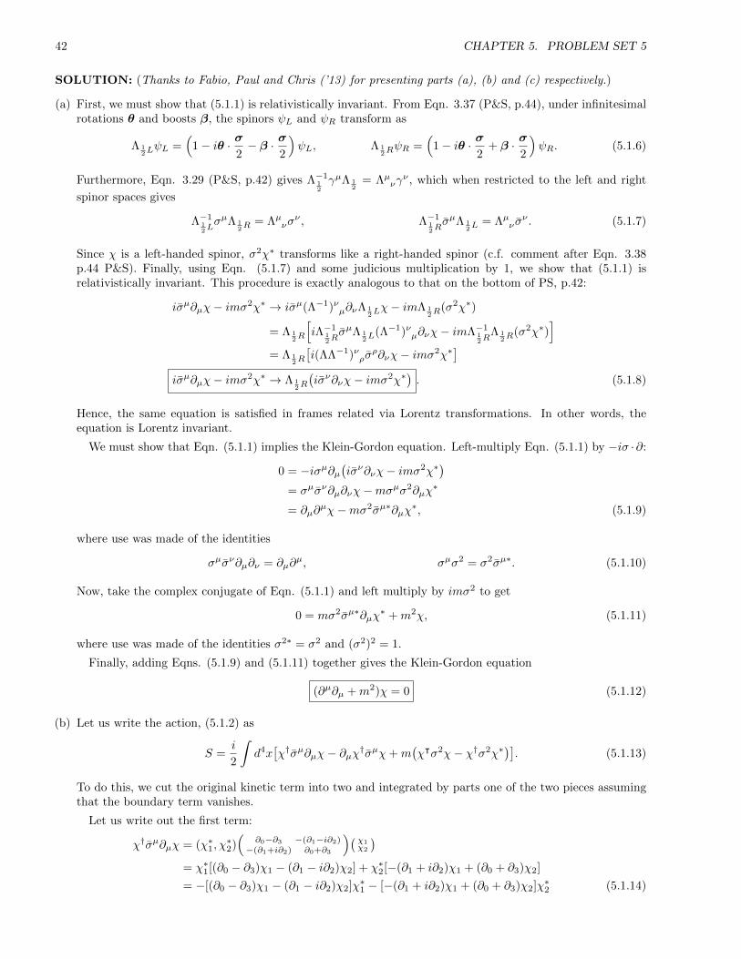
42 CHAPTER 5. PROBLEM SET 5
SOLUTION: (Thanks to Fabio, Paul and Chris (’13) for presenting parts (a), (b) and (c) respectively.)
(a) First, we must show that (5.1.1) is relativistically invariant. From Eqn. 3.37 (P&S, p.44), under infinitesimalrotations θ and boosts β, the spinors ψL and ψR transform as
Λ 12LψL =
(1− iθ · σ
2− β · σ
2
)ψL, Λ 1
2RψR =
(1− iθ · σ
2+ β · σ
2
)ψR. (5.1.6)
Furthermore, Eqn. 3.29 (P&S, p.42) gives Λ−112
γµΛ 12
= Λµνγν , which when restricted to the left and right
spinor spaces gives
Λ−112LσµΛ 1
2R= Λµνσ
ν , Λ−112RσµΛ 1
2L= Λµν σ
ν . (5.1.7)
Since χ is a left-handed spinor, σ2χ∗ transforms like a right-handed spinor (c.f. comment after Eqn. 3.38p.44 P&S). Finally, using Eqn. (5.1.7) and some judicious multiplication by 1, we show that (5.1.1) isrelativistically invariant. This procedure is exactly analogous to that on the bottom of PS, p.42:
iσµ∂µχ− imσ2χ∗ → iσµ(Λ−1)νµ∂νΛ 12Lχ− imΛ 1
2R(σ2χ∗)
= Λ 12R
[iΛ−1
12RσµΛ 1
2L(Λ−1)νµ∂νχ− imΛ−1
12R
Λ 12R
(σ2χ∗)]
= Λ 12R
[i(ΛΛ−1)νρσ
ρ∂νχ− imσ2χ∗]
iσµ∂µχ− imσ2χ∗ → Λ 12R
(iσν∂νχ− imσ2χ∗
). (5.1.8)
Hence, the same equation is satisfied in frames related via Lorentz transformations. In other words, theequation is Lorentz invariant.
We must show that Eqn. (5.1.1) implies the Klein-Gordon equation. Left-multiply Eqn. (5.1.1) by −iσ ·∂:
0 = −iσµ∂µ(iσν∂νχ− imσ2χ∗
)= σµσν∂µ∂νχ−mσµσ2∂µχ
∗
= ∂µ∂µχ−mσ2σµ∗∂µχ
∗, (5.1.9)
where use was made of the identities
σµσν∂µ∂ν = ∂µ∂µ, σµσ2 = σ2σµ∗. (5.1.10)
Now, take the complex conjugate of Eqn. (5.1.1) and left multiply by imσ2 to get
0 = mσ2σµ∗∂µχ∗ +m2χ, (5.1.11)
where use was made of the identities σ2∗ = σ2 and (σ2)2 = 1.
Finally, adding Eqns. (5.1.9) and (5.1.11) together gives the Klein-Gordon equation
(∂µ∂µ +m2)χ = 0 (5.1.12)
(b) Let us write the action, (5.1.2) as
S =i
2
∫d4x[χ†σµ∂µχ− ∂µχ†σµχ+m
(χᵀσ2χ− χ†σ2χ∗
)]. (5.1.13)
To do this, we cut the original kinetic term into two and integrated by parts one of the two pieces assumingthat the boundary term vanishes.
Let us write out the first term:
χ†σµ∂µχ = (χ∗1, χ∗2)(
∂0−∂3 −(∂1−i∂2)−(∂1+i∂2) ∂0+∂3
)( χ1χ2
)= χ∗1[(∂0 − ∂3)χ1 − (∂1 − i∂2)χ2] + χ∗2[−(∂1 + i∂2)χ1 + (∂0 + ∂3)χ2]
= −[(∂0 − ∂3)χ1 − (∂1 − i∂2)χ2]χ∗1 − [−(∂1 + i∂2)χ1 + (∂0 + ∂3)χ2]χ∗2 (5.1.14)

5.1. MAJORANA FERMIONS, P&S 3.4, P.73 43
Now, let us take the complex conjugate of this:
(χ†σµ∂µχ)∗ = −χ1[(∂0 − ∂3)χ∗1 − (∂1 + i∂2)χ∗2] + χ2[−(∂1 − i∂2)χ∗1 + (∂0 + ∂3)χ∗2]
= −(χ1, χ2)(
∂0−∂3 −(∂1+i∂2)−(∂1−i∂2) ∂0+∂3
)( χ∗1χ∗2
)= −χᵀσµ∗∂µχ
∗
= ∂µχ†σµχ, (5.1.15)
where use was made of the identity ηᵀσµ∗ε∗ = −ε†σµη. Notice that this term, ∂µχ†σµχ, is precisely negative
of the second term in the action, (5.1.13).
Now, we write out the third term in the action (dropping the m):
χᵀσ2χ = (χ∗1, χ∗2)(
0 −ii 0
)( χ1χ2
)= −i(χ1χ2 − χ2χ1) = 2iχ2χ1. (5.1.16)
The complex conjugate of this is
(χᵀσ2χ)∗ = −2iχ∗1χ∗2 = −i(χ∗1χ∗2 − χ∗2χ∗1) = χ†σ2χ∗. (5.1.17)
Again, we recognize this as negative of the last term in the action. Hence, we have shown that
S =i
2
∫d4x(χ†σµ∂µχ+mχᵀσ2χ− c.c.
)=
1
2
∫d4x[i(χ†σµ∂µχ+mχᵀσ2χ) + c.c.
]. (5.1.18)
This is real since it is the sum of complex conjugate terms.
To vary the action with respect to χ†, we revert back to the form of the action in Eqn. (5.1.2) and writeout the mass term explicitly using Eqns. (5.1.16) and (5.1.17):
S =
∫d4x
[χ†iσµ∂µχ+
im
2(2iχ2χ1 + 2iχ∗1χ
∗2)
]=
∫d4x[χ†iσµ∂µχ−m(χ2χ1 + χ∗1χ
∗2)]. (5.1.19)
The variation of the first term with respect to χ† just gives iσµ∂µχ. The variation of the last term withrespect to χ∗1 is −mχ∗2 and with respect to χ∗2 is mχ∗1. Thus,
0 =δS
δχ†= iσµ∂µχ+m
(−χ∗2χ∗1
)= iσµ∂µχ− imσ2χ∗ , (5.1.20)
which is precisely Eqn. (5.1.1).
To take the variation with respect to χ, we first integrate the kinetic term by parts:
S =
∫d4x[−∂µχ†iσµχ−m(χ2χ1 + χ∗1χ
∗2)]. (5.1.21)
Now, χ is on the right, and so when we take variations, we do so on the right. This means that taking thevariation of −mχ2χ1 with respect to χ1 gives −mχ2 and with respect to χ2 gives mχ1. Thus,
0 =δS
δχ= −i∂µχ†σµ +m(−χ2, χ1) = −i∂µχ†σµ + imχᵀσ2 , (5.1.22)
which we note is exactly the adjoint of Eqn. (5.1.20).
(c) Let us first write the Dirac Lagrangian in terms of ψL and ψR:
ψ(i/∂ −m)ψ = (ψ†L, ψ†R)(
0 11 0
)[i(
0 σµ
σµ 0
)∂µ −m
]( ψLψR
)= (ψ†R, ψ
†L)[i( σµ∂µψRσµ∂µψL
)−m
( ψLψR
)]= i(ψ†Rσ
µ∂µψR + ψ†Lσµ∂µψL)−m(ψ†RψL + ψ†LψR). (5.1.23)

44 CHAPTER 5. PROBLEM SET 5
Now, let us plug in the forms for ψL and ψR in Eqn. (5.1.3):
ψ(i/∂ −m)ψ = i[(−iχᵀ2σ
2)σµ∂µ(iσ2χ∗2) + χ†1σµ∂µ∂µχ1]−m[(−iχᵀ
2σ2)χ1 + χ†1iσ
2χ∗2]. (5.1.24)
Using the identities σ2σµσ2 = σµ∗, ηᵀσµ∗ε = −ε†σµη and εᵀσ2η = ηᵀσ2ε, we get
ψ(i/∂ −m)ψ = i(χ†1σµ∂µχ1 − ∂µχ†2σµχ2) + im(χᵀ
1σ2χ2 − χ†1σ2χ∗2). (5.1.25)
Note that the second term can be integrated by parts to yield the Dirac action (up to total derivative):
SDirac =
∫d4x[χ†1iσ
µ∂µχ1 + χ†2iσµ∂µχ2 + im(χᵀ
1σ2χ2 − χ†1σ2χ∗2)
]. (5.1.26)
(d) The Lagrangian in Eqn. (5.1.26) is invariant under the transformations
χ1 → e−iαχ1, χ2 → eiαχ2. (5.1.27)
Infinitesimally, this reads
∆χ1 = 1αδχ1 = −iχ1, ∆χ2 = 1
αδχ2 = iχ2. (5.1.28)
The associated current is
Jµ =∂L
∂(∂µχ1)∆χ1 +
∂L∂(∂µχ2)
∆χ2 = χ†1iσµ(−iχ1) + χ†2iσ
µ(iχ2) = χ†1σµχ1 − χ†2σµχ2, (5.1.29)
which is the current called Jµc in (5.1.4).
The equations of motion that follow from Eqn. (5.1.26) are
σµ∂µχ1 = mσ2χ∗2, ∂µχ†1σµ = mχᵀ
2σ2,
σµ∂µχ2 = mσ2χ∗1, ∂µχ†2σµ = mχᵀ
1σ2.
(5.1.30)
Therefore, the divergence of the current Jµc is
∂µJµc = ∂µχ
†1σµχ1 + χ†1σ
µ∂µχ1 + ∂µχ†2σµχ2 + χ†2σ
µ∂µχ2
= mχᵀ2σ
2χ1 + χ†1mσ2χ∗2 −mχ
ᵀ1σ
2χ2 − χ†2mσ2χ∗1
∂µJµc = 0 . (5.1.31)
Before calculating the divergence of Jµb = χ†σµχ, first note that it would be the current associated with thetransformation χ → e−iαχ. However, this is only a symmetry of the action (5.1.2) when m = 0. Therefore,we expect that ∂µJ
µb ought to be proportional to the mass and only vanishes when m = 0. The exact same
procedure as used above yields
∂µJµb = m(χᵀσ2χ+ χ†σ2χ∗) . (5.1.32)
The theory of N free massive spinors with O(N) symmetry is
S =
N∑i=1
∫d4x
[χ†i iσ
µ∂µχi +im
2
(χᵀi σ
2χi − χ†iσ2χ∗i)]
. (5.1.33)
Clearly, we can rotate the fields arbitrarily. Define the quantities
χ =
χ1
...χN
, Σµ
=
σµ
. . .
σµ
, Σ2 =
σ2
. . .
σ2
. (5.1.34)

5.1. MAJORANA FERMIONS, P&S 3.4, P.73 45
Then, the action (5.1.33) may be written
S =
∫d4x
[χ†iΣ
µ∂µχ+
im
2
(χᵀΣ2χ− χ†Σ2χ∗
)]. (5.1.35)
The symmetry is χ→ Rχ where R ∈ O(N) is a real orthogonal matrix, so RᵀR = 1. This is clear because,in the N × N space enumerating the spinors but not the two components of each spinor, the matrices Σ
µ
and Σ2 are both proportional to 1. Therefore, RᵀΣµR = Σ
µand RᵀΣ2R = Σ2.
(e) Looking back at the action we found in part (c), Eqn. (5.1.26), we see that we get exactly twice the Majoranaaction if we make the identification χ = χ1 = χ2. According to the definitions in (5.1.3), this means that ψLand ψR are related via
χ = ψL = iσ2ψ∗R. (5.1.36)
From the quantized Dirac field in P&S Eqn. 3.99 p.58, we write the quantized ψL and ψR:
ψL(x) =
∫d3p
(2π)3
1√2Ep
√p · σ
(aspξ
se−ip·x + bspηseip·x
), (4.3.37a)
ψR(x) =
∫d3p
(2π)3
1√2Ep
√p · σ
(aspξ
se−ip·x − bspηseip·x). (4.3.37b)
We have left the sum over the repeated index, s, implicit. One should be mindful of the fact that theanticommutativity (Grassmann nature) of the fields is due solely to the anticommutativity of the creationand annihilation operators. The spinors, ξ and η, are NOT Grassmann-valued! Indeed, a basis for them isfurnished by
(10
)and
(01
).
The expressions√p · σ and
√p · σ just come from a boost applied to the rest frame solution of the Dirac
equation. This boost was done along the z-direction in Eqns. 3.48 to 3.50 on P&S p.46 with the result thatthe boost matrix was
e−i2 (2η)S03
=
(cosh(η2 )− σ3 sinh(η2 ) 0
0 cosh(η2 ) + σ3 sinh(η2 )
),
where η is the rapidity defined by the relations in P&S Eqn. 3.48 p.46: E = m cosh η and p3 = m sinh η.
The generalization to an arbitrary boost is straightforward. The rapidity is replaced by a vector, η, whosemagnitude is what was formerly called η. Then,
e−i2 (2ηi)S
0i
=
(cosh(η2 )− σ · η sinh(η2 ) 0
0 cosh(η2 ) + σ · η sinh(η2 )
), (5.1.38)
The relationships between the energy, mass, momentum and rapidity are
E = m cosh η, p = ηm sinh η. (5.1.39)
Using half-angle formulae, we write
coshη
2=
√cosh η + 1
2=
√Em + 1
2=
√E +m
2m, (4.3.40a)
sinhη
2=
√cosh η − 1
2=
√Em − 1
2=
√E −m
2m. (4.3.40b)
Then, tanh η2 is given by
tanhη
2=
√E −mE +m
=
√E2 −m2
E +m=
|p|E +m
. (4.3.40c)
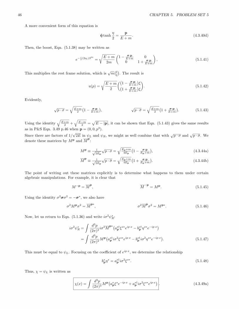
46 CHAPTER 5. PROBLEM SET 5
A more convenient form of this equation is
η tanhη
2=
p
E +m. (4.3.40d)
Then, the boost, Eqn. (5.1.38) may be written as
e−i2 (2ηi)S
0i
=
√E +m
2m
(1− σ·p
E+m 0
0 1 + σ·pE+m
), (5.1.41)
This multiplies the rest frame solution, which is√m(ξξ
). The result is
u(p) =
√E +m
2
((1− σ·p
E+m
)ξ(
1 + σ·pE+m
)ξ
). (5.1.42)
Evidently,
√p · σ =
√E+m
2
(1− σ·p
E+m
),
√p · σ =
√E+m
2
(1 + σ·p
E+m
). (5.1.43)
Using the identity√
E+m2 +
√E−m
2 =√E − |p|, it can be shown that Eqn. (5.1.43) gives the same results
as in P&S Eqn. 3.49 p.46 when p = (0, 0, p3).
Since there are factors of 1/√
2E in ψL and ψR, we might as well combine that with√p · σ and
√p · σ. We
denote these matrices by Mp and Mp:
Mp ≡ 1√2Ep
√p · σ =
√Ep+m
4Ep
(1− σ·p
Ep+m
), (4.3.44a)
Mp ≡ 1√
2Ep
√p · σ =
√Ep+m
4Ep
(1 + σ·p
Ep+m
). (4.3.44b)
The point of writing out these matrices explicitly is to determine what happens to them under certainalgebraic manipulations. For example, it is clear that
M−p = Mp, M
−p= Mp. (5.1.45)
Using the identity σ2σσ2 = −σ∗, we also have
σ2Mpσ2 = Mp∗, σ2M
pσ2 = Mp∗. (5.1.46)
Now, let us return to Eqn. (5.1.36) and write iσ2ψ∗R:
iσ2ψ∗R =
∫d3p
(2π)3iσ2M
p∗(as†p ξ
s∗eip·x − bs†p ηs∗e−ip·x)
=
∫d3p
(2π)3Mp
(as†p iσ
2ξs∗eip·x − bs†p iσ2ηs∗e−ip·x). (5.1.47)
This must be equal to ψL. Focusing on the coefficient of eip·x, we determine the relationship
bspηs = as†p iσ
2ξs∗. (5.1.48)
Thus, χ = ψL is written as
χ(x) =
∫d3p
(2π)3Mp
(aspξ
se−ip·x + as†p iσ2ξs∗eip·x
). (4.3.49a)
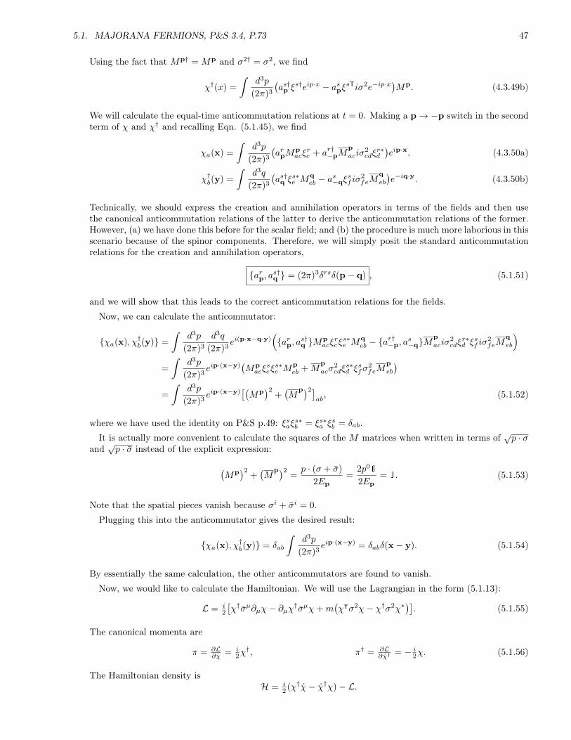
5.1. MAJORANA FERMIONS, P&S 3.4, P.73 47
Using the fact that Mp† = Mp and σ2† = σ2, we find
χ†(x) =
∫d3p
(2π)3
(as†p ξ
s†eip·x − aspξsTiσ2e−ip·x)Mp. (4.3.49b)
We will calculate the equal-time anticommutation relations at t = 0. Making a p→ −p switch in the secondterm of χ and χ† and recalling Eqn. (5.1.45), we find
χa(x) =
∫d3p
(2π)3
(arpM
pacξ
rc + ar†−pM
p
aciσ2cdξ
r∗d
)eip·x, (4.3.50a)
χ†b(y) =
∫d3q
(2π)3
(as†q ξ
s∗e M
qeb − a
s−qξ
sf iσ
2feM
q
eb
)e−iq·y. (4.3.50b)
Technically, we should express the creation and annihilation operators in terms of the fields and then usethe canonical anticommutation relations of the latter to derive the anticommutation relations of the former.However, (a) we have done this before for the scalar field; and (b) the procedure is much more laborious in thisscenario because of the spinor components. Therefore, we will simply posit the standard anticommutationrelations for the creation and annihilation operators,
arp, as†q = (2π)3δrsδ(p− q) , (5.1.51)
and we will show that this leads to the correct anticommutation relations for the fields.
Now, we can calculate the anticommutator:
χa(x), χ†b(y) =
∫d3p
(2π)3
d3q
(2π)3ei(p·x−q·y)
(arp, as†q Mp
acξrc ξs∗e M
qeb − a
r†−p, a
s−qM
p
aciσ2cdξ
r∗d ξ
sf iσ
2feM
q
eb
)=
∫d3p
(2π)3eip·(x−y)
(Mpacξ
scξs∗e M
peb +M
p
acσ2cdξ
s∗d ξ
sfσ
2feM
p
eb
)=
∫d3p
(2π)3eip·(x−y)
[(Mp
)2+(M
p)2]ab, (5.1.52)
where we have used the identity on P&S p.49: ξsaξs∗b = ξs∗a ξ
sb = δab.
It is actually more convenient to calculate the squares of the M matrices when written in terms of√p · σ
and√p · σ instead of the explicit expression:
(Mp
)2+(M
p)2=p · (σ + σ)
2Ep=
2p01
2Ep= 1. (5.1.53)
Note that the spatial pieces vanish because σi + σi = 0.
Plugging this into the anticommutator gives the desired result:
χa(x), χ†b(y) = δab
∫d3p
(2π)3eip·(x−y) = δabδ(x− y). (5.1.54)
By essentially the same calculation, the other anticommutators are found to vanish.
Now, we would like to calculate the Hamiltonian. We will use the Lagrangian in the form (5.1.13):
L = i2
[χ†σµ∂µχ− ∂µχ†σµχ+m
(χᵀσ2χ− χ†σ2χ∗
)]. (5.1.55)
The canonical momenta are
π = ∂L∂χ = i
2χ†, π† = ∂L
∂χ†= − i
2χ. (5.1.56)
The Hamiltonian density isH = i
2 (χ†χ− χ†χ)− L.
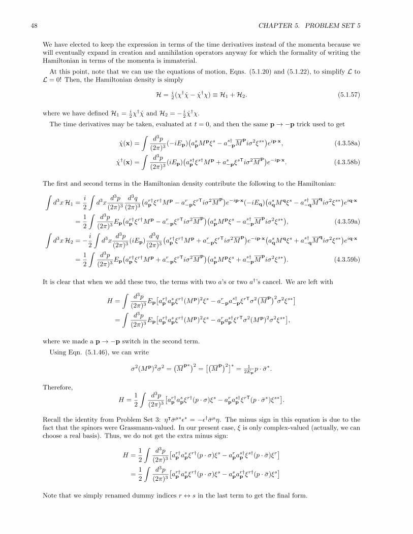
48 CHAPTER 5. PROBLEM SET 5
We have elected to keep the expression in terms of the time derivatives instead of the momenta because wewill eventually expand in creation and annihilation operators anyway for which the formality of writing theHamiltonian in terms of the momenta is immaterial.
At this point, note that we can use the equations of motion, Eqns. (5.1.20) and (5.1.22), to simplify L toL = 0! Then, the Hamiltonian density is simply
H = i2 (χ†χ− χ†χ) ≡ H1 +H2. (5.1.57)
where we have defined H1 = i2χ†χ and H2 = − i
2 χ†χ.
The time derivatives may be taken, evaluated at t = 0, and then the same p→ −p trick used to get
χ(x) =
∫d3p
(2π)3(−iEp)
(aspM
pξs − as†−pMpiσ2ξs∗
)eip·x, (4.3.58a)
χ†(x) =
∫d3p
(2π)3(iEp)
(as†p ξ
s†Mp + as−pξsTiσ2M
p)e−ip·x. (4.3.58b)
The first and second terms in the Hamiltonian density contribute the following to the Hamiltonian:∫d3xH1 =
i
2
∫d3x
d3p
(2π)3
d3q
(2π)3
(ar†p ξ
r†Mp − ar−pξrTiσ2Mp)e−ip·x(−iEq)
(asqM
qξs − as†−qMqiσ2ξs∗
)eiq·x
=1
2
∫d3p
(2π)3Ep
(ar†p ξ
r†Mp − ar−pξrTiσ2Mp)(
aspMpξs − as†−pM
piσ2ξs∗
), (4.3.59a)∫
d3xH2 = − i2
∫d3x
d3p
(2π)3(iEp)
d3q
(2π)3
(ar†p ξ
r†Mp + ar−pξrTiσ2M
p)e−ip·x
(asqM
qξs + as†−qMqiσ2ξs∗
)eiq·x
=1
2
∫d3p
(2π)3Ep
(ar†p ξ
r†Mp + ar−pξrTiσ2M
p)(aspM
pξs + as†−pMpiσ2ξs∗
). (4.3.59b)
It is clear that when we add these two, the terms with two a’s or two a†’s cancel. We are left with
H =
∫d3p
(2π)3Ep
[ar†p a
spξr†(Mp)2ξs − ar−pa
s†−pξ
rTσ2(M
p)2σ2ξs∗
]=
∫d3p
(2π)3Ep
[ar†p a
spξr†(Mp)2ξs − arpas†p ξrTσ2(Mp)2σ2ξs∗
],
where we made a p→ −p switch in the second term.
Using Eqn. (5.1.46), we can write
σ2(Mp)2σ2 =(M
p∗)2=[(M
p)2]∗= 1
2Epp · σ∗.
Therefore,
H =1
2
∫d3p
(2π)3
[ar†p a
spξr†(p · σ)ξs − arpas†p ξrT(p · σ∗)ξs∗
].
Recall the identity from Problem Set 3: ηᵀσµ∗ε∗ = −ε†σµη. The minus sign in this equation is due to thefact that the spinors were Grassmann-valued. In our present case, ξ is only complex-valued (actually, we canchoose a real basis). Thus, we do not get the extra minus sign:
H =1
2
∫d3p
(2π)3
[ar†p a
spξr†(p · σ)ξs − arpas†p ξs†(p · σ)ξr
]=
1
2
∫d3p
(2π)3
[ar†p a
spξr†(p · σ)ξs − aspar†p ξr†(p · σ)ξs
]Note that we simply renamed dummy indices r ↔ s in the last term to get the final form.
5.2. SUPERSYMMETRY, P&S 3.5 P.74 49
We use the anticommutation relations of the creation and annihilation operators to put the second termin normal-ordered form:
H =1
2
∫d3p
(2π)3ar†p a
spξr†[p · (σ + σ)]ξs − 1
2
∫d3p δ(0)ξs†(p · σ)ξs.
As before, only the energy component of p · (σ+ σ) survives and gives 2Ep1. Then, we use the explicit basisfor ξ, namely ξ1 =
(10
)and ξ2 =
(01
)to derive ξr†ξs = δrs. Finally, we drop the formally divergent second
piece in the Hamiltonian and write the normal-ordered Hamiltonian as
: H : =
∫d3p
(2π)3
∑s
Epas†p a
sp . (5.1.60)
We have reintroduced the sum over s, which has been implicit throughout.
Note: Please take a moment to read the small section on the Majorana neutrino on p.102 of Zee.
5.2 Supersymmetry, P&S 3.5 p.74
It is possible to write field theories with continuous symmetries linking fermions and bosons; such transformationsare called supersymmetries.
(a) The simplest example of a supersymmetric field theory is the theory of a free complex boson and a free Weylfermion, written in the form
L = ∂µφ∗∂µφ+ χ†iσ · ∂χ+ F ∗F. (5.2.1)
Here F is an auxiliary complex scalar field whose field equation is F = 0. Show that this Lagrangian isinvariant (up to a total divergence) under the infinitesimal transformation
δφ = −iεᵀσ2χ,
δχ = εF + σ · ∂φσ2ε∗, (5.2.2)
δF = −iε†σ · ∂χ,
where the parameter εa is a 2-component spinor of Grassmann numbers.
(b) Show that the term
∆L = [mφF + 12 imχ
ᵀσ2χ] + (c.c.) (5.2.3)
is also left invariant by the transformation, (5.2.2). Eliminate F from the complete Lagrangian L + ∆L bysolving its field equation, and show that the fermion and boson fields φ and χ are given the same mass.
(c) It is possible to write supersymmetric nonlinear field equations by adding cubic and higher-order terms tothe Lagrangian. Show that the following rather general field theory, containing the field (φi, χi) i = 1, . . . , n,is supersymmetric:
L = ∂µφ∗i ∂µφi + χ†i iσ · ∂χi + F ∗i Fi +
(Fi∂W [φ]
∂φi+i
2
∂2W [φ]
∂φi∂φjχᵀi σ
2χj + c.c.
), (5.2.4)
where W [φ] is an arbitrary function of the φi, called the superpotential. For the simple case n = 1 andW = gφ3/3, write out the field equations for φ and χ (after elimination of F ).
SOLUTION:
(a) Let us start off with a bunch of identities that will be useful later on. The first is
σ2σµσ2 = σµ∗. (5.2.5)
50 CHAPTER 5. PROBLEM SET 5
This is easily proven using the fact that σ0 = 1 and σiσj = iεijkσk. Thus,
σ2σ0σ2 = (σ2)2 = 1 = σ0,
σ2σ1σ2 = σ2iσ3 = i · iσ1 = −σ1,
σ2σ2σ2 = 1σ2 = σ2,
σ2σ3σ2 = iσ1σ2 = i · iσ3 = −σ3.
The right hand sides of the above four equations may be summarized as σµ∗.
Next, for two Weyl spinors, η and ε,
ηᵀσµ∗ε∗ = −ε†σµη. (5.2.6)
This has the important corollary
εᵀσ2η = ηᵀσ2ε. (5.2.7)
We prove Eqn. (5.2.6) by brute force:
ηᵀσ0∗ε∗ = (η1, η2)(
1 00 1
)( ε∗1ε∗2
)= η1ε
∗1 + η2ε
∗2 = −ε∗1η1 − ε∗2η2 = −(ε∗1, ε
∗2)(
1 00 1
)( η1η2
)= −ε†σ0η,
ηᵀσ1∗ε∗ = −(η1, η2)(
0 11 0
)( ε∗1ε∗2
)= −η1ε
∗2 − η2ε
∗1 = ε∗1η2 + ε∗2η1 = (ε∗1, ε
∗2)(
0 11 0
)( η1η2
)= ε†σ2η,
ηᵀσ2∗ε∗ = −(η1, η2)(
0 i−i 0
)( ε∗1ε∗2
)= −i(η1ε
∗2 − η2ε
∗1) = −i(ε∗1η2 − ε∗2η1) = (ε∗1, ε
∗2)(
0 −ii 0
)( η1η2
)= ε†σ2η,
ηᵀσ3∗ε∗ = −(η1, η2)(
1 00 −1
)( ε∗1ε∗2
)= −η1ε
∗1 + η2ε
∗2 = ε∗1η1 − ε∗2η2 = (ε∗1, ε
∗2)(
1 00 −1
)( η1η2
)= ε†σ3η.
Indeed, the right hand sides of the above four equations may be summarized as −ε†σµη.
Finally, we will use the identity
σµσν∂µ∂ν = ∂µ∂µ. (5.2.8)
This can be proved as follows:
σµσν∂µ∂ν = (∂0 − σi∂i)(∂0 + σj∂j) = ∂20 − σiσj∂i∂j = ∂2
0 − 12σ
i, σ2∂i∂j = ∂20 − ∂i∂i = ∂µ∂
µ.
Note that we symmetrized the product σiσj because it is multiplying ∂i∂j , which is symmetric.
These identities allow us to write δφ and δF in two ways. In components, δφ, looks like
δφ = χ2ε1 − χ1ε2.
We can complex conjugate this, remembering that the order of multiplication switches under conjugation:
δφ∗ = ε∗1χ∗2 − ε∗2χ∗1 = (ε∗1, ε
∗2)(
0 1−1 0
)( χ∗1χ∗2
)= iε†σ2χ∗ = iχ†σ2ε∗,
where the final equality is just identity (5.2.7) with ε→ ε∗ and η → χ∗.
Since there is only one spinor on the right side of δχ, it is actually straightforward to take its dagger. Wesimply observe that σµ† = σµ. Then,
δχ† = F ∗ε† + ε†σ2σµ∂µφ∗.
The hardest one to write out is δF :
δF = −i(ε∗1, ε∗2)(
∂0−∂3 −(∂1−i∂2)−(∂1+i∂2) ∂0+∂3
)( χ1χ2
)= −i
(ε∗1[(∂0 − ∂3)χ1 − (∂1 − i∂2)χ2] + ε∗2[−(∂1 + i∂2)χ1 + (∂0 + ∂3)χ2]
)= i([(∂0 − ∂3)χ1 − (∂1 − i∂2)χ2]ε∗1 + [−(∂1 + i∂2)χ1 + (∂0 + ∂3)χ2]ε∗2
).

5.2. SUPERSYMMETRY, P&S 3.5 P.74 51
Now, we can complex conjugate this:
δF ∗ +−i(ε1[(∂0 − ∂3)χ∗1 − (∂1 + i∂2)χ∗2] + ε2[−(∂1 − i∂2)χ∗1 + (∂0 + ∂3)χ∗2]
)= −i(ε1, ε2)
(∂0−∂3 −(∂1+i∂2)−(∂1−i∂2) ∂0+∂3
)( χ∗1χ∗2
)= −iεᵀσµ∗∂µχ∗
= i∂µχ†σµε,
where use was made of identity (5.2.6).
Let us collect these transformations below
δφ = −iεᵀσ2χ = −iχᵀσ2ε, (3.3.9a)
δφ∗ = iε†σ2χ∗ = iχ†σ2ε∗, (3.3.9b)
δχ = εF + σµσ2ε∗∂µφ, (3.3.9c)
δχ† = F ∗ε† + εᵀσ2σµ∂µφ∗, (3.9d)
δF = −iε†σµ∂µχ = i∂µχᵀσµ∗ε∗, (3.3.9e)
δF ∗ = −iεᵀσµ∗∂µχ∗ = i∂µχ†σµε. (3.3.9f)
Now, we plug these into δL:
δL = ∂µ(iε†σ2χ∗)∂µφ+ ∂µ(−iεᵀσ2χ)∂µφ∗ + (F ∗ε† + εᵀσ2σν∂νφ
∗)iσµ∂µχ+ χ†iσµ∂µ(εF + σνσ2ε∗∂νφ)
+ (−iεᵀσµ∗∂µχ∗)F +((((((((F ∗(−iε†σµ∂µχ)
= iε†σ2∂µχ∗∂µφ− iεᵀσ2∂µχ∂
µφ∗ + iεᵀσ2σν σµ∂µχ∂νφ∗ − iεᵀσµ∗χ∗∂µF + iε†σ2χ∗∂µ∂
µφ− iεᵀσµ∗∂µχ∗F
= ∂µ(iε†σ2χ∗∂µφ)− ∂µ(iεᵀσµ∗χ∗F )− ∂µ(iεᵀσ2χ∂µφ∗) +(((((((iεᵀσ2χ∂µ∂µφ∗
+ ∂µ(iεᵀσ2σν σµχ∂νφ∗)−(((((
((((iεᵀσ2σν σµχ∂µ∂νφ∗
= i∂µ[ε†σ2χ∗∂µφ+ εᵀσ2[(σν σµ − ηµν)χ∂νφ
∗ − σµσ2χ∗F ]]
Note that the aforementioned identities were all used. Therefore,
δL = ∂µJ µ where J µ = i[ε†σ2χ∗∂µφ+ εᵀσ2[(σν σµ − ηµν)χ∂νφ
∗ − σµσ2χ∗F ]]. (5.2.10)
It follows that L is supersymmetric.
(b) The fact that ∆L is supersymmetric follows from part (c) using W (φ) = 12mφ
2. The F -dependent terms inL+ ∆L are F ∗F +mφF +mφ∗F ∗. The F and F ∗ equations of motion amount to the identities
F ∗ = −mφ , F = −mφ∗ . (3.3.11a)
Plugging these back into the Lagrangian L+ ∆L gives
L+ ∆L = ∂µφ∗∂µφ−mφ∗φ+ χ†iσµ∂µχ+ im
2 (χᵀσ2χ− χ†σ2χ∗) (3.3.11b)
Note that −iχ†σ2χ∗ is the complex conjugate of iχᵀσ2χ. Indeed, this is the Lagrangian of a massive spin-0boson and massive Majorana fermion both with the same mass, m.
(c) Using σ2T = −σ2 and σµT = σµ∗, the transformation of χᵀ is
δχᵀ = Fεᵀ − ε†σ2σµ∗∂µφ. (5.2.12)
52 CHAPTER 5. PROBLEM SET 5
Let L be the free action and ∆L the interaction containing the superpotential. By trivial extension of theargument in part (a), L is supersymmetric. The transformation of ∆L is
δ∆L = (−iε†σµ∂µχi)∂W
∂φi+ Fi
∂2W
∂φi∂φj(−iεᵀσ2χj) +
i
2
∂3W
∂φi∂φj∂φk(−iεᵀσ2χk)(χᵀ
i σ2χj)
+i
2
∂2W
∂φi∂φj(Fiε
ᵀ − ε†σ2σµ∗∂µφi)σ2χj +
i
2
∂2W
∂φi∂φjχᵀi σ
2(εFj + σµσ2ε∗∂µφj) + c.c.
The dashed terms cancel after we rewrite the third one using χᵀi σ
2ε = εᵀσ2χi. We can use the identityσ2σµ∗σ2 = σµ, which is simply the complex conjugate of Eqn. (5.2.5), to rewrite the second underlined term:
2nd underlined term = − i2ε†σµχi
∂2W
∂φi∂φj∂µφj = − i
2ε†σµχi∂µ
∂W
∂φi.
Note that we also switched i and j indices.
The third underlined term can be simplified by first using σ2σµσ2 = σµ∗, which is Eqn. (5.2.5), and thenusing χᵀσµ∗ε∗ = −ε†σµχ, which is Eqn. (5.2.6). The result is that the third underlined term is actuallyidentical to the second one. This combines with the first underlined term to give a total derivative:
δ∆L = −i∂µ(ε†σµχi
∂W
∂φi
)+i
2
∂3W
∂φi∂φj∂φk(−iεᵀσ2χk)(χᵀ
i σ2χj) + c.c.
Clearly, the triple derivative term is not a total derivative. Therefore, it must somehow vanish due tosymmetry in the indices. The triple derivative is symmetric in the ijk indices. Let us write this term as
i
2
∂3W
∂φi∂φj∂φkεᵀσ2χkχ
ᵀi (−iσ2)χj ≡
i
2
∂3W
∂φi∂φj∂φkεᵀσ2(kij),
where we have introduced the notation (kij) for the appropriate terms on the left. By symmetry in the ijkindices,
i
2
∂3W
∂φi∂φj∂φkεᵀσ2(kij) =
i
6
∂3W
∂φi∂φj∂φkεᵀσ2[(kij) + (ijk) + (jki)].
It must be the case that the symmetric combination of the (ijk)’s vanishes. The proof of this is just by bruteforce calculation:
(ijk) =( χi1χi2
)(χj1, χj2)
(0 −11 0
)( χk1χk2
)=( χi1χj2χk1−χi1χj1χk1
χi2χj2χk1−χi2χj1χk2
). (3.3.13a)
Similarly, we can calculate the other two orders. In so doing, we will always reorder the χ factors in the endin the order ijk and thus we must remember that a switch of two of the χ’s generates a minus sign. Theresults are
(jki) =( χi1χj1χk2−χi2χj1χk1
χi1χj2χk2−χi2χj2χk1
), (3.3.13b)
(kij) =( χi2χj1χk1−χi1χj2χk1
χi2χj1χk2−χi1χj2χk2
). (3.3.13c)
Now, we can just observe that all the terms pairwise cancel in the sum:
(ijk) + (jki) + (kij) =(
00
). (5.2.14)
Therefore, we finally have
δ∆L = −i∂µ(ε†σµχi
∂W
∂φi
)+ c.c. (5.2.15)
This proves that the total Lagrangian is supersymmetric.
When W = gφ3/3, the F -dependent terms in the Lagrangian are F ∗F + gFφ2 + gF ∗φ∗2, where we haveassumed g to be real out of convenience, not necessity. Thus, the F and F ∗ equations of motion amount to
F ∗ = −gφ2 F = −gφ∗2. (5.2.16)
5.3. DISCUSSION 1: MAJORANA BASIS 53
Plugging this back into L yields
L = ∂µφ∗∂µφ− g2φ∗2φ2 + χ†iσµ∂µχ+ ig(φχᵀσ2χ− φ∗χ†σ2χ∗). (5.2.17)
The φ∗ and φ equations of motion read
φ = −2g2φ∗φ2 − igχ†σ2χ∗,
φ∗ = −2g2φφ∗2 + igχᵀσ2χ.(5.2.18)
To calculate the equation of the fermionic field, we may treat χ1, χ∗1, χ2 and χ∗2 as the independent fields.Taking the variation of the third term in Eqn. (5.2.17) with respect to χ† gives the two component term iσ ·∂χwhose first component is a term in ∂L/∂χ∗1 and whose second component is a term in ∂L/∂χ∗2. The fourthterm does not contain factors of χ∗1 or χ∗2. We may write the last term as −gφ∗(χ∗1χ∗2−χ∗2χ∗1). When taking thevariation with respect to χ∗1, we write this term as −2gφ∗χ∗1χ
∗2 and the variation is ∂L/∂χ∗1 3 −2gφ∗χ∗2. When
taking the variation with respect to χ∗2, we write this term as 2gφ∗χ∗2χ∗1 and the variation is ∂L/∂χ∗2 3 2gφ∗χ∗1.
All in all, we have
0 =∂L∂χ†
= iσµ∂µχ+ 2gφ∗(−χ∗2χ∗1
)= iσ · ∂χ− 2igφ∗σ2χ∗ . (5.2.19)
Similarly, one finds the variation with respect to χ:
0 =∂L∂χ
= −i∂µχ†σµ + 2gφ∗(−χ2 χ1
)= −i∂χ† · σ + 2igφχᵀσ2 . (5.2.20)
5.3 Discussion 1: Majorana Basis
Note: Please take a moment to read the small section on the Majorana neutrino on p.102 of Zee.
For me, the take-away message of P&S Problem 3.4 parts (a)-(c) is that if you start off with the Dirac spinorwith the Dirac Lagrangian and impose the strange-looking condition
ψR = iσ2ψ∗L, (5.3.1)
then you end up with the Majorana Lagrangian up to a factor of 2, which you can always just absorb into aredefinition of the fields (e.g. by absorbing a factor of
√2 into the spinor).
We have to remember that we have written all our spinors, γ matrices and the representation Λ 12
of theLorentz group all in the so-called Weyl basis. Of course, we could conjugate all of the γ matrices by someunitary matrix, U , and we would have an equivalent, but different-looking basis and the condition (5.3.1) maylook very different. You have heard in lecture that a Majorana spinor in 3 + 1 dimensions is just the same as thefour-component Dirac spinor, but where each component is now real rather than complex. It is not clear howcondition (5.3.1) achieves this. However, we will find a basis in which this reality condition is made manifest.We will call this the Majorana basis (more precisely, one possible Majorana basis).
Consider the matrix
U =1
2
(σ2 + σ3 i− σ1
−i− σ1 σ2 − σ3
). (5.3.2)
This is a 4× 4 matrix written in terms of four 2× 2 blocks. Note also that i in a 2× 2 block means i multipliedby the 2× 2 identity matrix. Right now I’m just pulling this matrix out of thin air, but after you see what I dowith it, you may want to entertain yourself by trying to work out how I came up with it. You may even try tothink of other examples that will do just as well.
You may check that U is unitary: U†U = 1. Therefore, I can consider a set of γ matrices that are related tothe ones we have used so far (Weyl basis) by conjugation with U . Since we will call this the Majorana basis, wewill put a subscript M on these new matrices:
γµM = UγµU†. (5.3.3)
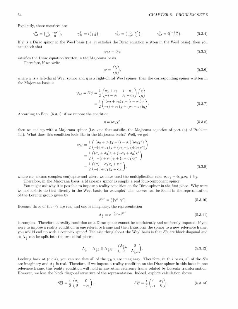
54 CHAPTER 5. PROBLEM SET 5
Explicitly, these matrices are
γ0M =
(0 −iσ1
iσ1 0
), γ1
M = i(
0 11 0
), γ2
M =(
0 σ2
−σ2 0
), γ3
M = i(−1 0
0 1
). (5.3.4)
If ψ is a Dirac spinor in the Weyl basis (i.e. it satisfies the Dirac equation written in the Weyl basis), then youcan check that
ψM = Uψ (5.3.5)
satisfies the Dirac equation written in the Majorana basis.Therefore, if we write
ψ =
(χ
η
), (5.3.6)
where χ is a left-chiral Weyl spinor and η is a right-chiral Weyl spinor, then the corresponding spinor written inthe Majorana basis is
ψM = Uψ =1
2
(σ2 + σ3 i− σ1
−i− σ1 σ2 − σ3
)(χ
η
)=
1
2
((σ2 + σ3)χ+ (i− σ1)η
−(i+ σ1)χ+ (σ2 − σ3)η
). (5.3.7)
According to Eqn. (5.3.1), if we impose the condition
η = iσ2χ∗, (5.3.8)
then we end up with a Majorana spinor (i.e. one that satisfies the Majorana equation of part (a) of Problem3.4). What does this condition look like in the Majorana basis? Well, we get
ψM =1
2
((σ2 + σ3)χ+ (i− σ1)(iσ2χ
∗)
−(i+ σ1)χ+ (σ2 − σ3)(iσ2χ∗)
)=
1
2
((σ2 + σ3)χ+ (−σ2 + σ3)χ∗
−(i+ σ1)χ+ (i− σ1)χ∗
)=
1
2
((σ2 + σ3)χ+ c.c.
−(i+ σ1)χ+ c.c.
), (5.3.9)
where c.c. means complex conjugate and where we have used the multiplication rule: σiσj = iεijkσk + δij .Therefore, in the Majorana basis, a Majorana spinor is simply a real four-component spinor.You might ask why it is possible to impose a reality condition on the Dirac spinor in the first place. Why were
we not able to do that directly in the Weyl basis, for example? The answer can be found in the representationof the Lorentz group given by
Sµν = i4 [γµ, γν ]. (5.3.10)
Because three of the γ’s are real and one is imaginary, the representation
Λ 12
= e−i2ωµνS
µν
(5.3.11)
is complex. Therefore, a reality condition on a Dirac spinor cannot be consistently and uniformly imposed: if youwere to impose a reality condition in one reference frame and then transform the spinor to a new reference frame,you would end up with a complex spinor! The nice thing about the Weyl basis is that S’s are block diagonal andso Λ 1
2can be split into the two chiral pieces:
Λ 12
= Λ 12L⊕ Λ 1
2R=
(Λ 1
2L0
0 Λ 12R
). (5.3.12)
Looking back at (5.3.4), you can see that all of the γM ’s are imaginary. Therefore, in this basis, all of the S’sare imaginary and Λ 1
2is real. Therefore, if we impose a reality condition on the Dirac spinor in this basis in one
reference frame, this reality condition will hold in any other reference frame related by Lorentz transformation.However, we lose the block diagonal structure of the representation. Indeed, explicit calculation shows
S01M =
i
2
(σ1 00 −σ1
), S03
M =i
2
(0 σ1
σ1 0
). (5.3.13)

5.4. DISCUSSION 2: SUSY 55
Thus, while S01M is block diagonal, S03
M is not. Furthermore, you can check that S0iM is anti-Hermitian while SijM
is Hermitian, for i, j = 1, 2, 3. Therefore, the representation is still not unitary.What we are seeing here is actually a manifestation of an important point that Petr made during his lecture
on spinors in arbitrary dimension. In 3+1 dimensions, you can have a Weyl spinor (2 complex components) or aMajorana spinor (4 real components), but you cannot have a Majorana-Weyl spinor (2 real components). Thatwould imply the existence of a basis in which the S’s are both block diagonal and purely imaginary so that Λ 1
2is
simultaneously block diagonal and real. Of course, we have not proven that no such basis exists here. But, whatwe have done confirms this fact: we now have two bases, the Weyl and the Majorana bases. In the Weyl basisΛ 1
2is block diagonal, but not purely real, and in the Majorana basis it is purely real but not block diagonal.
5.4 Discussion 2: SUSY
The following is a discussion on the topic of the example of supersymmetry in this problem. Recall that thekinetic term for a Dirac spinor is iΨ/∂Ψ. Let us write Ψ as
Ψ =
(χ
ξ
), (5.4.1)
where χ is a left-chirality (chirality −1) spinor and ξ is a right-chirality (chirality +1) spinor, as suggested byP&S Eqn. 3.36 p.43. Then, the kinetic term may be written
iΨ/∂Ψ = i(χ†, ξ†)(
0 11 0
)(0 σµ·∂σ·∂ 0
)( χξ
)= i(χ†σ · ∂χ+ ξ†σ · ∂ξ). (5.4.2)
The kinetic term for χ in the Lagrangian of this problem, (5.2.1), is precisely the same as the kinetic term for χcontained in the Dirac kinetic term above. Apparently, the χ in this problem has been chosen to be a chirality-leftspinor. Presumably, the construction could equally well have been done using a right-chirality spinor, ξ. We areallowed to use only one of the Weyl spinors and not both in the form of a Dirac spinor because we have notincluded a Dirac mass term −mΨΨ, which is the only thing that mixes the two.
But, eventually, χ will have a mass, as we found in part (b). The point here is that the only way to geta Lorentz-invariant product of two spinors is to have one be chirality-left and the other chirality-right. Forexample, the Dirac mass term is −mΨΨ = −m(χ†ξ + ξ†χ) and χ and ξ have opposite chirality. Part (c) ofProblem 3.4 shows that a chirality-right spinor can be built out of a chirality-left spinor by transposing and thenright-multiplying by σ2: namely, if χ is left-chirality, then χᵀσ2 is right-chirality. Therefore, χᵀσ2χ is Lorentz-invariant. Since σ2 is imaginary, we make it real by multiplying by i and then we must add the Hermitianconjugate, which is −iχ†σ2χ∗, to make the whole mass term real. The factor of 1/2 just gets the normalizationsright. This gives the mass term im
2 (χᵀσ2χ− χ†σ2χ∗).By the way, another way to motivate the combination χᵀσ2χ is that it equals −χ1χ2 +χ2χ1, which is like the
anti-symmetric combination of a spin-up and spin-down state if we make the analogy χ1 ∼↑ and χ2 ∼↓. This isprecisely the spin-0 combination, which is rotationally-invariant.
One complex two-component spinor contains four real fields off-shell and two real fields on-shell (the Diracequation kills off two of the modes). Thus, a theory containing this spinor has a chance of being supersymmetricon-shell if we pair it with one complex scalar field since this gives a total of two bosonic and two fermionic degreesof freedom. However, we usually want symmetries to hold even off-shell because intermediate virtual particleswill be off-shell. The simplest way to make the counting work is to introduce an auxiliary complex scalar field,which in the problem was called F . This gives a total of four bosonic and four fermionic degrees of freedom.
The Lagrangian, (5.2.1), must have dimension +4 so that the action is dimensionless. This implies thefollowing dimensions for the fields
[φ] = 1, [χ] = 32 , [F ] = 2. (5.4.3)
Supersymmetry should turn bosonic fields into fermionic ones and vice versa. The simplest scenario would beif the transformation is linear in the fields. This implies δφ ∼ χ. But the right hand side must be a scalar andso we must take the inner product with some infinitesimal spinor, ε, but in a way that is Lorentz invariant. Wehave already discussed how to produce Lorentz invariant combinations of left-chirality spinors:
δφ = −iεᵀσ2χ. (5.4.4)
This is certainly not unique: χ could have appeared complex-conjugated, the factor of −i is certainly not unique,etc. But, this choice presumably more or less fixes the form of the other transformation by requiring that the

56 CHAPTER 5. PROBLEM SET 5
action be invariant. A different choice would alter the other transformations as well, but should nevertheless betenable. No matter the choice, dimensional analysis requires
[ε] = − 12 . (5.4.5)
We must also have δF ∼ εχ. However, [δF ] = 2 whereas [εχ] = 1. We don’t want to add any more fields and sothe only thing we can add with dimension 1 is a derivative. We are then forced to contract ∂µ with something.We already know how to construct a Lorentz-invariant “kinetic” term out of two left-chirality spinors. Recallthat we need to contract ∂µ with σµ. Thus,
δF = −iε†σ · ∂χ. (5.4.6)
δχ is much more difficult, but one can at least partially motivate it by observing that it is linear in the scalarfields and ε, and has the correct dimension. Ultimately, the point is that it is what it is in order to keep theaction invariant.
Now, let us calculate the commutator of two supersymmetry transformations:
δηδεφ = −iεᵀσ2(ηF + σµσ2η∗∂µφ) = −iεᵀσ2ηF − iεᵀσµ∗η∗∂µφ = −iεᵀσ2ηF + iη†σµε∂µφ. (5.4.7)
Therefore,[δη, δε]φ = i(ηᵀσ2ε− εᵀσ2η)F + i(η†σµε− ε†σµη)∂µφ. (5.4.8)
The first term on the right vanishes by virtue of identity (5.2.7). By writing out the components, one finds that−iε†σµη is in fact the complex conjugate of iη†σµε. Therefore,
[δη, δε]φ = aµ∂µφ where aµ = iη†σµε+ c.c. (5.4.9)
This is the result of a translation xµ → xµ − aµ.Let us repeat this for F :
δηδεF = −iε†σµ∂µ(ηF + σνσ2η∗∂νφ) = −iε†σµη∂µF − iε†σ2η∗∂µ∂µφ. (5.4.10)
Therefore,[δη, δε]F = i(η†σµε− ε†σµη)∂µF + i(η†σ2ε∗ − ε†σ2η∗)∂µ∂
µφ. (5.4.11)
Once again, the second term vanishes and we get the same translation:
[δη, δε]F = aµ∂µF where aµ = iη†σµε+ c.c. (5.4.12)
Finally, let us repeat this for χ:
δηδεχ = ε(−iη†σµ∂µχ) + σµσ2ε∗∂µ(−iηᵀσ2χ) = −iεη†σµ∂µχ+ i∂µ[σµ(−iσ2)ε∗ηᵀ(−iσ2)χ]. (5.4.13)
For the moment, define
χi ≡ σµ(−iσ2)ε∗, χj ≡ η, χk ≡ χ. (5.4.14)
Then, using the notation of Eqn. (3.3.13a), we may write
δηδεχ = −iεη†σµ∂µχ+ i∂µ(ijk). (5.4.15)
Using the identity (5.2.14) and σµT = σµ∗, the second term above may be written
i∂µ(ijk) = −i∂µ[(jki) + (kij)]
= −i∂µ[ηχᵀ(−iσ2)σµ(−iσ2)ε∗ + χε†(iσ2)σµ∗(−iσ2)η]
= i∂µ[ηχᵀσµ∗ε∗ − χε†σµη]
= −iηε†σµ∂µχ− i∂µχ ε†σµη. (5.4.16)
In the last term, we can pass ∂µχ through the scalar ε†σµη without any change in sign because it has to passthrough two Grassmanns. Hence,
δηδεχ = −i(εη† + ηε†)σµ∂µχ− iε†σµη∂µχ. (5.4.17)

5.4. DISCUSSION 2: SUSY 57
The opposite order givesδεδηχ = −i(ηε† + εη†)σµ∂µχ− iη†σµε∂µχ. (5.4.18)
Notice that the first term cancels in the commutator and we get the same translation result:
[δη, δε]χ = aµ∂µχ where aµ = iη†σµε+ c.c. (5.4.19)
We see that if we did not have the auxiliary field, F , then we would have gotten
[δη, δε]χ = aµ∂µχ+ i(εη† − ηε†)σµ∂µχ. (5.4.20)
The algebra would only close on-shell, when χ satisfies the massless Dirac equation σµ∂µχ = 0. By countingdegrees of freedom, we should have known this would have to be true from the beginning.

58 CHAPTER 5. PROBLEM SET 5
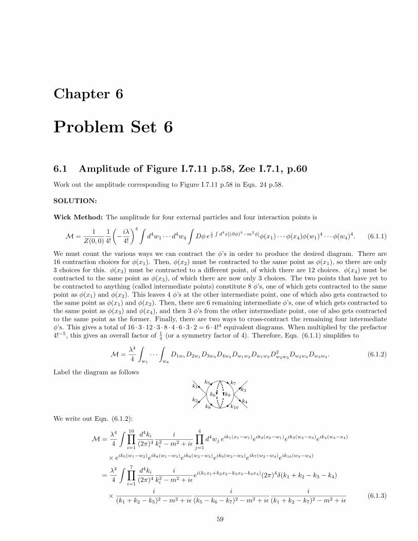
Chapter 6
Problem Set 6
6.1 Amplitude of Figure I.7.11 p.58, Zee I.7.1, p.60
Work out the amplitude corresponding to Figure I.7.11 p.58 in Eqn. 24 p.58.
SOLUTION:
Wick Method: The amplitude for four external particles and four interaction points is
M =1
Z(0, 0)
1
4!
(− iλ
4!
)4 ∫d4w1 · · · d4w4
∫Dφe
i2
∫d4x[(∂φ)4−m2φ]φ(x1) · · ·φ(x4)φ(w1)4 · · ·φ(w4)4. (6.1.1)
We must count the various ways we can contract the φ’s in order to produce the desired diagram. There are16 contraction choices for φ(x1). Then, φ(x2) must be contracted to the same point as φ(x1), so there are only3 choices for this. φ(x3) must be contracted to a different point, of which there are 12 choices. φ(x4) must becontracted to the same point as φ(x3), of which there are now only 3 choices. The two points that have yet tobe contracted to anything (called intermediate points) constitute 8 φ’s, one of which gets contracted to the samepoint as φ(x1) and φ(x2). This leaves 4 φ’s at the other intermediate point, one of which also gets contracted tothe same point as φ(x1) and φ(x2). Then, there are 6 remaining intermediate φ’s, one of which gets contracted tothe same point as φ(x3) and φ(x4), and then 3 φ’s from the other intermediate point, one of also gets contractedto the same point as the former. Finally, there are two ways to cross-contract the remaining four intermediateφ’s. This gives a total of 16 · 3 · 12 · 3 · 8 · 4 · 6 · 3 · 2 = 6 · 4!4 equivalent diagrams. When multiplied by the prefactor4!−5, this gives an overall factor of 1
4 (or a symmetry factor of 4). Therefore, Eqn. (6.1.1) simplifies to
M =λ4
4
∫w1
· · ·∫w4
D1w1D2w1D3w4D4w4Dw1w2Dw1w3D2w2w3
Dw2w4Dw3w4 . (6.1.2)
Label the diagram as follows
@@
&%'$
@@
R
R
R
??R
k1
k2
k3
k4
k5
k6
k7
k8
k9
k10
We write out Eqn. (6.1.2):
M =λ4
4
∫ 10∏i=1
d4ki(2π)4
i
k2i −m2 + iε
4∏j=1
d4wj eik1(x1−w1)eik2(x2−w1)eik3(w4−x3)eik4(w4−x4)
× eik5(w1−w2)eik8(w1−w3)eik6(w2−w3)eik9(w2−w3)eik7(w2−w4)eik10(w3−w4)
=λ4
4
∫ 7∏i=1
d4ki(2π)4
i
k2i −m2 + iε
ei(k1x1+k2x2−k3x3−k4x4)(2π)4δ(k1 + k2 − k3 − k4)
× i
(k1 + k2 − k5)2 −m2 + iε
i
(k5 − k6 − k7)2 −m2 + iε
i
(k1 + k2 − k7)2 −m2 + iε(6.1.3)
59

60 CHAPTER 6. PROBLEM SET 6
After amputating the external legs and the overall delta function, what remains is
M =λ4
4
∫d4k5
(2π)4
d4k6
(2π)4
d4k7
(2π)4
i
k25 −m2 + iε
i
k26 −m2 + iε
i
k27 −m2 + iε
× i
(k1 + k2 − k5)2 −m2 + iε
i
(k5 − k6 − k7)2 −m2 + iε
i
(k1 + k2 − k7)2 −m2 + iε. (6.1.4)
Up to the symmetry factor, this is the same as Eqn. 24 of Zee p.58 with the identifications p = k5, q = k6 andr = k7.
Schwinger Method: The amplitude may be written as
M =1
4!
(− iλ
4!
)4 ∫ ( 4∏i=1
d4wi
[δ
iδJ(wi)
]4)1
10!
[− i
2
∫∫d4x d4y J(x)D(x− y)J(y)
]10
. (6.1.5)
Now, we must count the number of ways to act the derivatives on the J ’s. In the language of Zee, there are10 strings with J ’s on each end and D’s connecting the two endpoints. There are 20 choices for string ends toplace at x1, then 18 for x2, then 16 for x3, then 14 for x4. The other ends of the strings placed at x1 and x2
are attached to each other at, say, a, as are the free ends of the strings placed at x3 and x4 at, say, b. Next,there are 12, then 10 choices of two string ends to place at a and 8, then 6 choices of two strings to place at b.At this point, we have two crosses. There are 4 ways to attach the remaining two free strings at the free endsof one of the crosses and then 2 ways to attached the remaining two components together. This alone accountsfor a factor of 20!! = 21010!, which nicely cancels the same factor in the denominator from the expansion term inexp[− i
2
∫∫d4x d4y J(x)D(x− y)J(y)
].
We have not accounted for the fact that the vertices could have any order of labeling from w1 to w4. Thisgives a factor of 4!. We must also account for the fact that the four derivatives at each vertex may be acted onthe string ends in any order, which gives a factor of 4! per vertex, or 4!4. Overall, we have 4!5, which neatlycancels the same factor in the denominator out front in Eqn. (6.1.5).
However, we must be careful because we have overcounted the number of diagrams. The following switchesof the internal lines leave the diagram unchanged: (1) k5 ↔ k8 and k7 ↔ k10; or (2) k6 ↔ k9. This gives aninternal symmetry structure of dimension 4 (i.e. a symmetry factor of 4). Note that this is the same factor aswas found using the Wick method.
At this point, the result is actually exactly the same as Eqn. (6.1.2) since the derivatives simply collapse tothe same product of propagators. The only possible difference is a sign, which is immaterial since M is squaredin any physically sensible quantity.
Symmetry factors formula: For φ4 theory, there is a formula for the symmetry factor:
S = g
∞∏n=2
2β(n!)αn , (6.1.6)
where g is the number of permutations of vertices that leave unchanged the diagram with fixed external lines,αn is the number of vertex pairs connected by n identical lines, and β is the number of lines connecting a vertexwith itself. For the diagram in this problem, g = 2 since we have the identity permutation (in other words, nopermutation at all), which is always obviously allowed, and the permutation that switches the two intermediatevertices. No vertex is connected to itself, and so β = 0. Finally, the two intermedate vertices are connected toeach other with 2 identical lines, and so α2 = 1 (and αn = 0 for n > 2). This gives the same symmetry factor ofS = 4 as we found using the previous two methods.
6.2 Amplitude of Figure I.7.10 p.57, Zee I.7.2 p.60
Work out the amplitude corresponding to Figure I.7.10 p.57 in Eqn. 23 p.57.
SOLUTION: (Thanks to Kate and Melanie (’12) for presenting their solutions.)

6.3. TWO-TO-FOUR MESON PROCESSES, ZEE I.7.3 P.60 61
Wick Method: The amplitude for four external particles and four interaction points is
M =1
Z(0, 0)
1
2!
(− iλ
4!
)2 ∫d4w1 d
4w2
∫Dφe
i2
∫d4x[(∂φ)4−m2φ]φ(x1) · · ·φ(x4)φ(w1)4φ(w2)4. (6.2.1)
We must count the various ways we can contract the φ’s in order to produce the desired diagram. There are8 contraction choices for φ(x1). Then, φ(x2) must be contracted to the same point as φ(x1), so there are only3 choices for this. φ(x3) must be contracted to a different point, of which there are 4 choices. φ(x4) must becontracted to the same point as φ(x3), of which there are now only 3 choices. Now, we just have two more φ(w1)’sand two φ(w2)′s, which can be cross-contracted with each other in 2 ways. This gives a total of 8 ·3 ·4 ·3 ·2 = 4!2
equivalent diagrams. When multiplied by the prefactor 2!−14!−2, this gives an overall factor of 12 (or a symmetry
factor of 2). Therefore, Eqn. (6.2.1) simplifies to
M = −λ2
2
∫w1
∫w2
D1w1D2w1
D3w2D4w2
D2w1w2
. (6.2.2)
Plugging in the expressions for the propagators, integrating over w1 and w2 and amputating the external legsand an overall momentum delta function, as in the previous problem, exactly reproduces Eqn. 23 of Zee p.57:
M = −λ2
2
∫d4k
(2π)4
i
k2 −m2 + iε
i
(k1 + k2 − k)2 −m2 + iε, (6.2.3)
where k is the momentum along one of the internal lines.
Schwinger Method: The amplitude may be written as
M =1
2!
(− iλ
4!
)2 ∫ ( 2∏i=1
d4wi
[δ
iδJ(wi)
]4)1
6!
[− i
2
∫∫d4x d4y J(x)D(x− y)J(y)
]6
. (6.2.4)
Now, we must count the number of ways to act the derivatives on the J ’s. In the language of Zee, there are 6strings with J ’s on each end and D’s connecting the two endpoints. There are 12 choices for string ends to placeat x1, then 10 for x2, then 8 for x3, then 6 for x4. The other ends of the strings placed at x1 and x2 are attachedto each other at, say, a, as are the free ends of the strings placed at x3 and x4 at, say, b. Next, there are 4, then2 choices of two string ends to place at a, at which point the other ends are attached to b. This alone accountsfor a factor of 12!! = 266!, which nicely cancels the same factor in the denominator from the expansion term inexp[− i
2
∫∫d4x d4y J(x)D(x− y)J(y)
].
We have not accounted for the fact that the vertices could have any order of labeling from w1 to w2. Thisgives a factor of 2!. We must also account for the fact that the four derivatives at each vertex may be acted onthe string ends in any order, which gives a factor of 4! per vertex, or 4!2. Overall, we have 2! · 4!2, which neatlycancels the same factor in the denominator out front in Eqn. (6.2.4).
However, we must be careful because we have overcounted the number of diagrams. Switching the two internallines leaves the diagram unchanged. This gives an internal symmetry structure of dimension 2 (i.e. a symmetryfactor of 2). Note that this is the same factor as was found using the Wick method.
As in the previous problem, this procedure is identical to the first henceforth.
Symmetry factors formula: In this case, g = 1, β = 0 and α2 = 1, which gives S = 2, as previously found.
6.3 Two-to-Four Meson Processes, Zee I.7.3 p.60
Draw all the diagrams describing two mesons producing four mesons up to and including order λ2. Write downthe corresponding Feynman amplitudes.
SOLUTION: (Thanks to Ken (’12) for presenting his solution.)
There is only one diagram at order λ and seven at order λ2:We will not treat (b) separately from (a). There is no point in calculating the contribution of the vacuum bubblebecause when one includes the contributions of all possible vacuum bubbles, one eventually divides out by thatcontribution anyway.
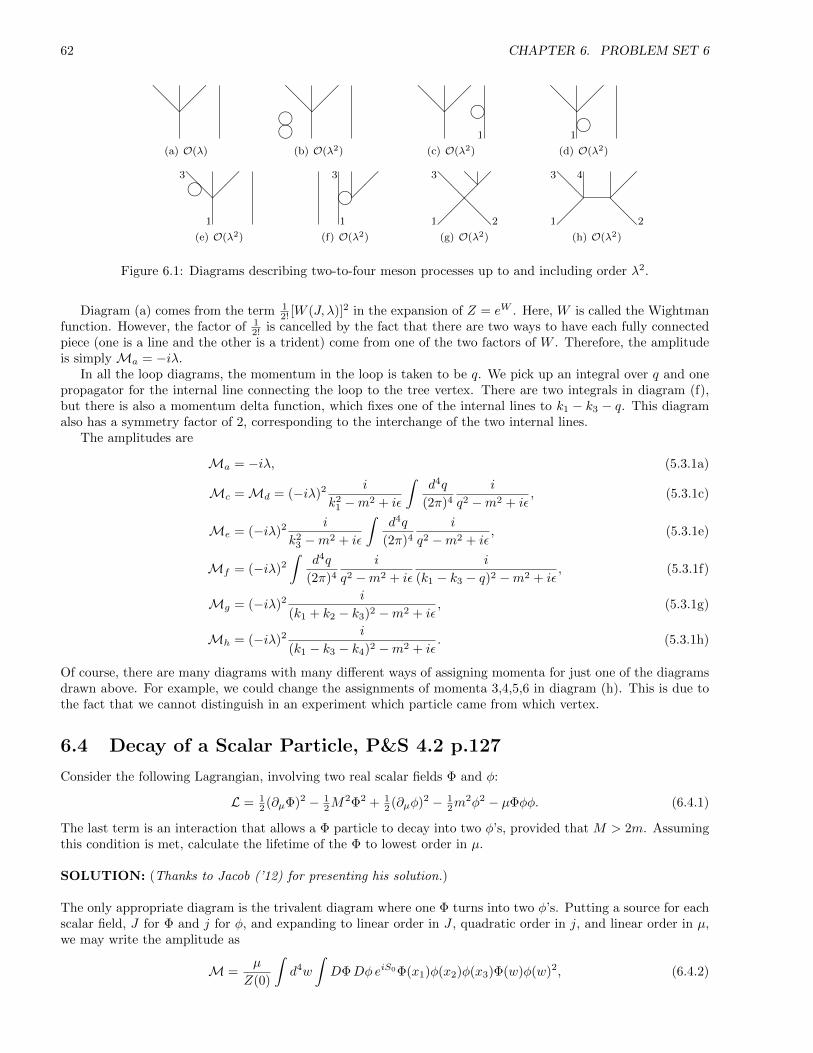
62 CHAPTER 6. PROBLEM SET 6
@@
(a) O(λ)
@@
ii(b) O(λ2)
@@ i
1
(c) O(λ2)
@@i
1
(d) O(λ2)
@@
i
1
3
(e) O(λ2)
i1
3
(f) O(λ2)
@
@@@
@
1 2
3
(g) O(λ2)
@
@@@1 2
3 4
(h) O(λ2)
Figure 6.1: Diagrams describing two-to-four meson processes up to and including order λ2.
Diagram (a) comes from the term 12! [W (J, λ)]2 in the expansion of Z = eW . Here, W is called the Wightman
function. However, the factor of 12! is cancelled by the fact that there are two ways to have each fully connected
piece (one is a line and the other is a trident) come from one of the two factors of W . Therefore, the amplitudeis simply Ma = −iλ.
In all the loop diagrams, the momentum in the loop is taken to be q. We pick up an integral over q and onepropagator for the internal line connecting the loop to the tree vertex. There are two integrals in diagram (f),but there is also a momentum delta function, which fixes one of the internal lines to k1 − k3 − q. This diagramalso has a symmetry factor of 2, corresponding to the interchange of the two internal lines.
The amplitudes are
Ma = −iλ, (5.3.1a)
Mc =Md = (−iλ)2 i
k21 −m2 + iε
∫d4q
(2π)4
i
q2 −m2 + iε, (5.3.1c)
Me = (−iλ)2 i
k23 −m2 + iε
∫d4q
(2π)4
i
q2 −m2 + iε, (5.3.1e)
Mf = (−iλ)2
∫d4q
(2π)4
i
q2 −m2 + iε
i
(k1 − k3 − q)2 −m2 + iε, (5.3.1f)
Mg = (−iλ)2 i
(k1 + k2 − k3)2 −m2 + iε, (5.3.1g)
Mh = (−iλ)2 i
(k1 − k3 − k4)2 −m2 + iε. (5.3.1h)
Of course, there are many diagrams with many different ways of assigning momenta for just one of the diagramsdrawn above. For example, we could change the assignments of momenta 3,4,5,6 in diagram (h). This is due tothe fact that we cannot distinguish in an experiment which particle came from which vertex.
6.4 Decay of a Scalar Particle, P&S 4.2 p.127
Consider the following Lagrangian, involving two real scalar fields Φ and φ:
L = 12 (∂µΦ)2 − 1
2M2Φ2 + 1
2 (∂µφ)2 − 12m
2φ2 − µΦφφ. (6.4.1)
The last term is an interaction that allows a Φ particle to decay into two φ’s, provided that M > 2m. Assumingthis condition is met, calculate the lifetime of the Φ to lowest order in µ.
SOLUTION: (Thanks to Jacob (’12) for presenting his solution.)
The only appropriate diagram is the trivalent diagram where one Φ turns into two φ’s. Putting a source for eachscalar field, J for Φ and j for φ, and expanding to linear order in J , quadratic order in j, and linear order in µ,we may write the amplitude as
M =µ
Z(0)
∫d4w
∫DΦDφeiS0Φ(x1)φ(x2)φ(x3)Φ(w)φ(w)2, (6.4.2)
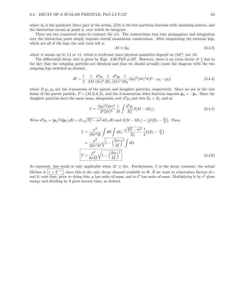
6.4. DECAY OF A SCALAR PARTICLE, P&S 4.2 P.127 63
where S0 is the quadratic (free) part of the action, Z(0) is the free partition function with vanishing sources, andthe interaction occurs at point w, over which we integrate.
There are two connected ways to contract the φ’s. The contractions turn into propagators and integrationover the interaction point simply imposes overall momentum conservation. After amputating the external legs,which are all of the legs, the only term left is
M≈ 2µ, (6.4.3)
where ≈ means up to ±1 or ±i, which is irrelevant since physical quantities depend on |M|2, not M.The differential decay rate is given by Eqn. 4.86 P&S p.107. However, there is an extra factor of 1
2 due tothe fact that the outgoing particles are identical and thus we should actually count the diagram with the twooutgoing legs switched as distinct.
dΓ =1
2· 1
2M
d3p1
(2π)3
1
2E1
d3p2
(2π)3
1
2E2(2µ)2(2π)4δ(P − p1 − p2), (6.4.4)
where P, p1, p2 are the 4-momenta of the parent and daughter particles, respectively. Since we are in the restframe of the parent particle, P = (M, 0, 0, 0), and the 3-momentum delta function imposes p2 = −p1. Since thedaughter particles have the same mass, integration over d3p2 just sets E2 = E1 and so
Γ =(2µ)2(2π)4
24(2π)6
1
M
∫d3p1
E21
δ(M − 2E1). (6.4.5)
Write d3p1 = |p1|2d|p1| dΩ = E1
√E2
1 −m2 dE1 dΩ and δ(M − 2E1) = 12δ(E1 − M
2
). Then,
Γ =µ2
16π2M
∫dΩ
∫dE1
√E2
1 −m2
E1
1
2δ(E1 − M
2
)=
µ2
32π2M
√1−
(2m
M
)2∫dΩ
Γ =µ2
8πM
√1−
(2m
M
)2
. (6.4.6)
As expected, this result is only applicable when M ≥ 2m. Furthermore, Γ is the decay constant; the actual
lifetime is τ = Γ−1 , since this is the only decay channel available to Φ. If we want to reintroduce factors of cand ~, note that, prior to doing this, µ has units of mass, and so Γ has units of mass. Multiplying it by c2 givesenergy and dividing by ~ gives inverse time, as desired.

64 CHAPTER 6. PROBLEM SET 6
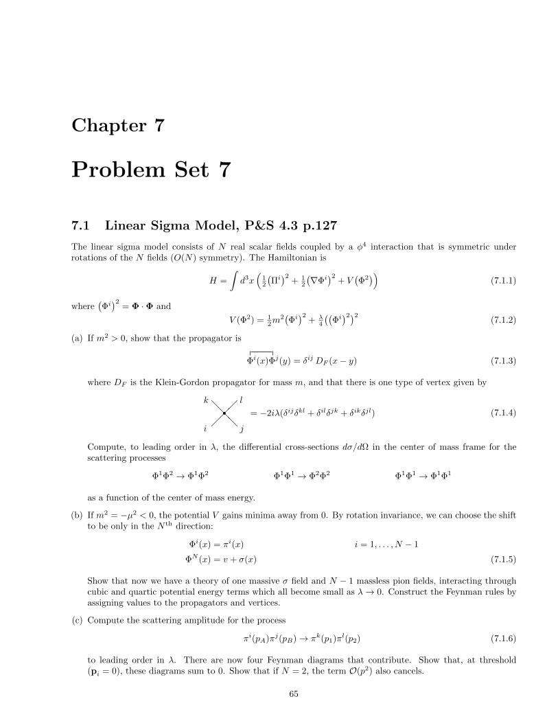
Chapter 7
Problem Set 7
7.1 Linear Sigma Model, P&S 4.3 p.127
The linear sigma model consists of N real scalar fields coupled by a φ4 interaction that is symmetric underrotations of the N fields (O(N) symmetry). The Hamiltonian is
H =
∫d3x
(12
(Πi)2
+ 12
(∇Φi
)2+ V
(Φ2))
(7.1.1)
where(Φi)2
= Φ ·Φ and
V (Φ2) = 12m
2(Φi)2
+ λ4
((Φi)2)2
(7.1.2)
(a) If m2 > 0, show that the propagator is
Φi(x)Φj(y) = δij DF (x− y) (7.1.3)
where DF is the Klein-Gordon propagator for mass m, and that there is one type of vertex given by
@@@
ri j
k l
= −2iλ(δijδkl + δilδjk + δikδjl) (7.1.4)
Compute, to leading order in λ, the differential cross-sections dσ/dΩ in the center of mass frame for thescattering processes
Φ1Φ2 → Φ1Φ2 Φ1Φ1 → Φ2Φ2 Φ1Φ1 → Φ1Φ1
as a function of the center of mass energy.
(b) If m2 = −µ2 < 0, the potential V gains minima away from 0. By rotation invariance, we can choose the shiftto be only in the N th direction:
Φi(x) = πi(x) i = 1, . . . , N − 1
ΦN (x) = v + σ(x) (7.1.5)
Show that now we have a theory of one massive σ field and N − 1 massless pion fields, interacting throughcubic and quartic potential energy terms which all become small as λ→ 0. Construct the Feynman rules byassigning values to the propagators and vertices.
(c) Compute the scattering amplitude for the process
πi(pA)πj(pB)→ πk(p1)πl(p2) (7.1.6)
to leading order in λ. There are now four Feynman diagrams that contribute. Show that, at threshold(pi = 0), these diagrams sum to 0. Show that if N = 2, the term O(p2) also cancels.
65

66 CHAPTER 7. PROBLEM SET 7
(d) Add to V a symmetry-breaking term ∆V = −aΦN where a is a small constant. Find the new value of v thatminimizes V , and work out the content of the theory about that point. Show that the pion acquires a masssuch that m2
π ∼ a, and show that the pion scattering amplitude at threshold is now nonvanishing and alsoproportional to a.
SOLUTION: (Thanks to Lenny (’12) for presenting his solution.)
(a) Notice that for λ = 0, the Hamiltonian (7.1.1) is exactly N copies of the Klein-Gordon Hamiltonian. Recallthat propagators are given by contractions of interaction fields. Thus, if the masses are all the same, thenthe propagators are the same as the Klein-Gordon propagators except that we must make sure to distinguishbetween the field species (hence, the Kronecker delta):
Φi(x)Φj(y) = δijDF (x− y) . (7.1.7)
In momentum space, this would be given by
Φi Φj =iδij
p2 −m2 + iε. (7.1.8)
Vertices follow from the perturbation term
Hpert =
∫d3x
(λ
4
(Φ2)2)
=∑i
∫d3x
λ
4
(Φi)4
+∑i<j
∫d3x
λ
2
(Φi)2(
Φj)2. (7.1.9)
Thus, there are two vertex types:
(1) 4 lines of same field type with factor −iλ4 × 4! = −6iλ
(2) 2 lines of Φi and two of Φj 6=i with factor −iλ2 × (2!)2 = −2iλ
This is indeed equivalent to the vertex factor (7.1.4) which would give −6iλ if i = j = k = l and −2iλ if
two pairs of the indices are separately equal.
To lowest order, we only have the one vertex diagram (7.1.4) for the scattering process ΦiΦj → ΦkΦl,which we notationally simplify to ij → kl. The scattering amplitudes are thus
M(12→ 12) =M(11→ 22) = −2λ, M(11→ 11) = −6λ. (7.1.10)
Now, we can use Equation 4.85 (PS p.107):(dσ
dΩ
)CM
=|M|2
64π2E2CM
, (4 identical masses). (7.1.11)
However, we must divide by 2 in the case when the final particles are of the same type:
( dσdΩ
)12→12
CM=( λ
4πECM
)2
,( dσdΩ
)11→22
CM=( λ
4πECM
)2
,( dσdΩ
)11→11
CM=( 3λ
4πECM
)2
.
(7.1.12)
(b) We rewrite our potential in terms of the fields (7.1.5):
V (πi, σ) = −1
2µ2
(N−1∑i=1
(πi)2 + (v + σ)2
)+λ
4
N−1∑i,j=1
(πi)2(πj)2 +λ
2
N−1∑i=1
(πi)2(v + σ)2 +λ
4(v + σ)4.
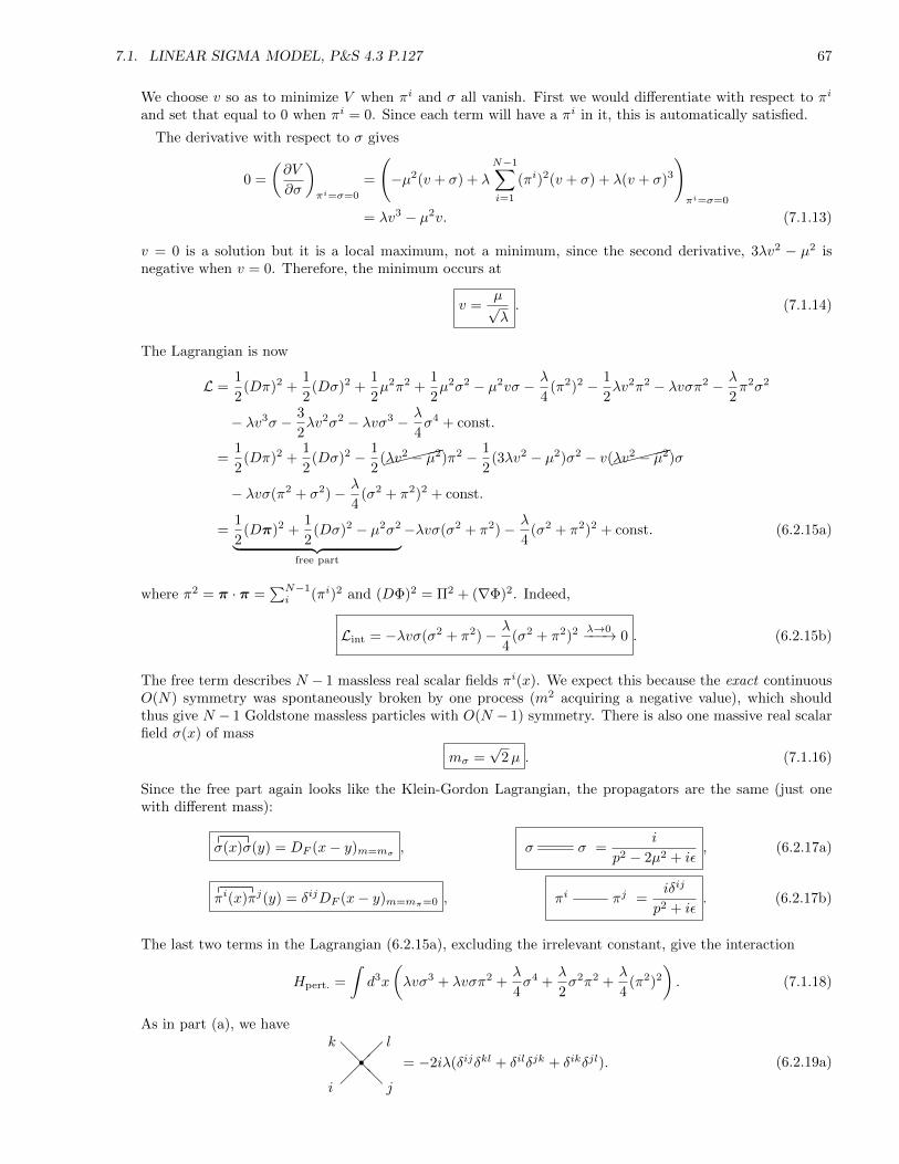
7.1. LINEAR SIGMA MODEL, P&S 4.3 P.127 67
We choose v so as to minimize V when πi and σ all vanish. First we would differentiate with respect to πi
and set that equal to 0 when πi = 0. Since each term will have a πi in it, this is automatically satisfied.
The derivative with respect to σ gives
0 =
(∂V
∂σ
)πi=σ=0
=
(−µ2(v + σ) + λ
N−1∑i=1
(πi)2(v + σ) + λ(v + σ)3
)πi=σ=0
= λv3 − µ2v. (7.1.13)
v = 0 is a solution but it is a local maximum, not a minimum, since the second derivative, 3λv2 − µ2 isnegative when v = 0. Therefore, the minimum occurs at
v =µ√λ. (7.1.14)
The Lagrangian is now
L =1
2(Dπ)2 +
1
2(Dσ)2 +
1
2µ2π2 +
1
2µ2σ2 − µ2vσ − λ
4(π2)2 − 1
2λv2π2 − λvσπ2 − λ
2π2σ2
− λv3σ − 3
2λv2σ2 − λvσ3 − λ
4σ4 + const.
=1
2(Dπ)2 +
1
2(Dσ)2 − 1
2(
λv2 − µ2)π2 − 1
2(3λv2 − µ2)σ2 − v(
λv2 − µ2)σ
− λvσ(π2 + σ2)− λ
4(σ2 + π2)2 + const.
=1
2(Dπ)2 +
1
2(Dσ)2 − µ2σ2︸ ︷︷ ︸
free part
−λvσ(σ2 + π2)− λ
4(σ2 + π2)2 + const. (6.2.15a)
where π2 = π · π =∑N−1i (πi)2 and (DΦ)2 = Π2 + (∇Φ)2. Indeed,
Lint = −λvσ(σ2 + π2)− λ
4(σ2 + π2)2 λ→0−−−→ 0 . (6.2.15b)
The free term describes N − 1 massless real scalar fields πi(x). We expect this because the exact continuousO(N) symmetry was spontaneously broken by one process (m2 acquiring a negative value), which shouldthus give N − 1 Goldstone massless particles with O(N − 1) symmetry. There is also one massive real scalarfield σ(x) of mass
mσ =√
2µ . (7.1.16)
Since the free part again looks like the Klein-Gordon Lagrangian, the propagators are the same (just onewith different mass):
σ(x)σ(y) = DF (x− y)m=mσ , σ σ =i
p2 − 2µ2 + iε, (6.2.17a)
πi(x)πj(y) = δijDF (x− y)m=mπ=0 , πi πj =iδij
p2 + iε. (6.2.17b)
The last two terms in the Lagrangian (6.2.15a), excluding the irrelevant constant, give the interaction
Hpert. =
∫d3x
(λvσ3 + λvσπ2 +
λ
4σ4 +
λ
2σ2π2 +
λ
4(π2)2
). (7.1.18)
As in part (a), we have
@@@
ri j
k l
= −2iλ(δijδkl + δilδjk + δikδjl). (6.2.19a)
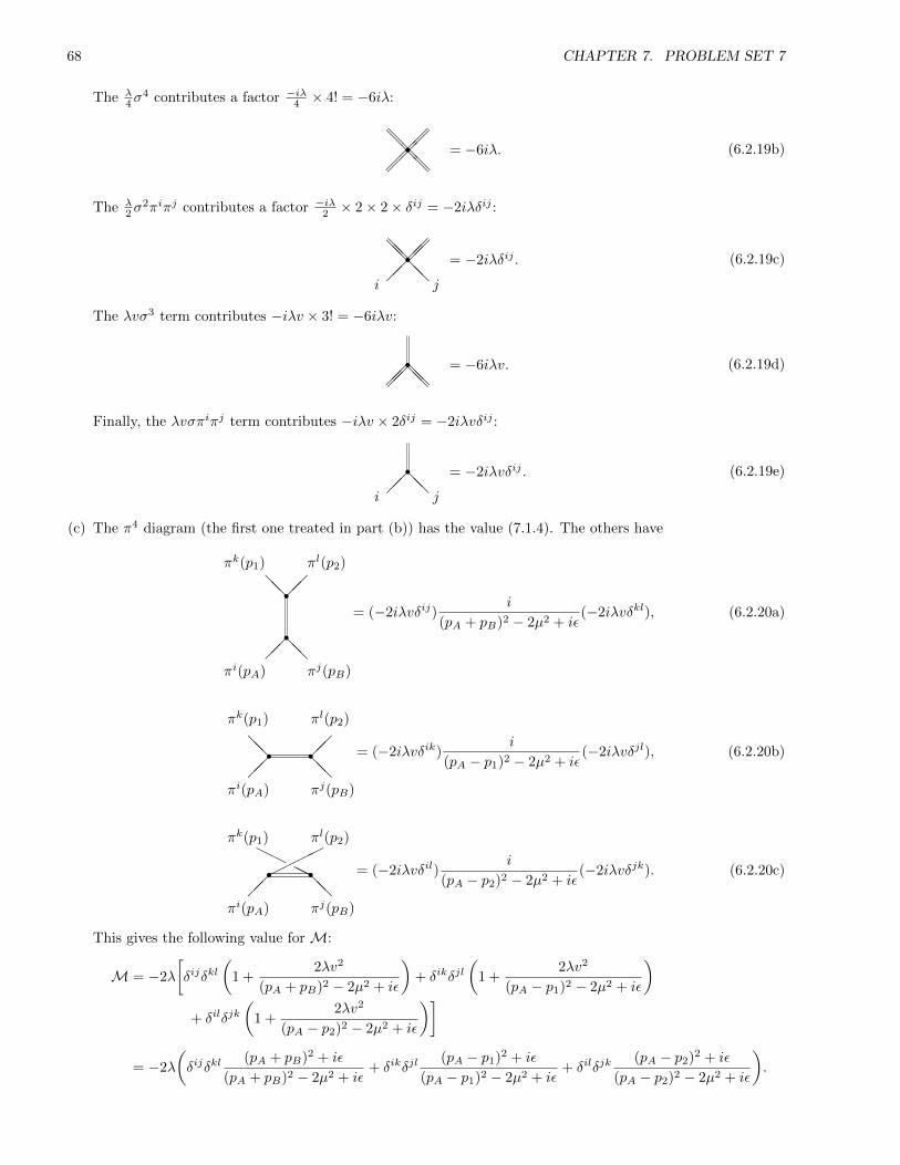
68 CHAPTER 7. PROBLEM SET 7
The λ4σ
4 contributes a factor −iλ4 × 4! = −6iλ:
@@@
@@@
r = −6iλ. (6.2.19b)
The λ2σ
2πiπj contributes a factor −iλ2 × 2× 2× δij = −2iλδij :
@@@@
@@ri j
= −2iλδij . (6.2.19c)
The λvσ3 term contributes −iλv × 3! = −6iλv:
@@@@r = −6iλv. (6.2.19d)
Finally, the λvσπiπj term contributes −iλv × 2δij = −2iλvδij :
@@r
i j
= −2iλvδij . (6.2.19e)
(c) The π4 diagram (the first one treated in part (b)) has the value (7.1.4). The others have
@@
@@
rr
πi(pA) πj(pB)
πk(p1) πl(p2)
= (−2iλvδij)i
(pA + pB)2 − 2µ2 + iε(−2iλvδkl), (6.2.20a)
@@
@@ r rπi(pA) πj(pB)
πk(p1) πl(p2)
= (−2iλvδik)i
(pA − p1)2 − 2µ2 + iε(−2iλvδjl), (6.2.20b)
@@
HHHHr r
πi(pA) πj(pB)
πk(p1) πl(p2)
= (−2iλvδil)i
(pA − p2)2 − 2µ2 + iε(−2iλvδjk). (6.2.20c)
This gives the following value for M:
M = −2λ
[δijδkl
(1 +
2λv2
(pA + pB)2 − 2µ2 + iε
)+ δikδjl
(1 +
2λv2
(pA − p1)2 − 2µ2 + iε
)+ δilδjk
(1 +
2λv2
(pA − p2)2 − 2µ2 + iε
)]
= −2λ
(δijδkl
(pA + pB)2 + iε
(pA + pB)2 − 2µ2 + iε+ δikδjl
(pA − p1)2 + iε
(pA − p1)2 − 2µ2 + iε+ δilδjk
(pA − p2)2 + iε
(pA − p2)2 − 2µ2 + iε
).
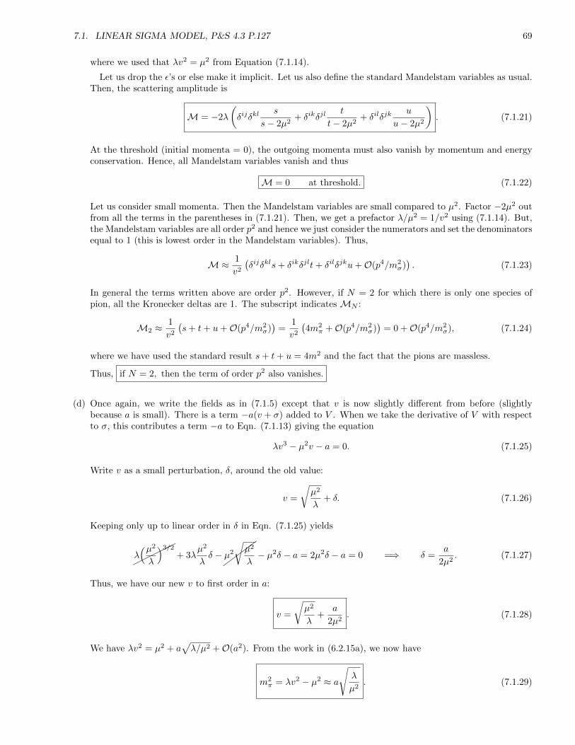
7.1. LINEAR SIGMA MODEL, P&S 4.3 P.127 69
where we used that λv2 = µ2 from Equation (7.1.14).
Let us drop the ε’s or else make it implicit. Let us also define the standard Mandelstam variables as usual.Then, the scattering amplitude is
M = −2λ
(δijδkl
s
s− 2µ2+ δikδjl
t
t− 2µ2+ δilδjk
u
u− 2µ2
). (7.1.21)
At the threshold (initial momenta = 0), the outgoing momenta must also vanish by momentum and energyconservation. Hence, all Mandelstam variables vanish and thus
M = 0 at threshold. (7.1.22)
Let us consider small momenta. Then the Mandelstam variables are small compared to µ2. Factor −2µ2 outfrom all the terms in the parentheses in (7.1.21). Then, we get a prefactor λ/µ2 = 1/v2 using (7.1.14). But,the Mandelstam variables are all order p2 and hence we just consider the numerators and set the denominatorsequal to 1 (this is lowest order in the Mandelstam variables). Thus,
M≈ 1
v2
(δijδkls+ δikδjlt+ δilδjku+O(p4/m2
σ)). (7.1.23)
In general the terms written above are order p2. However, if N = 2 for which there is only one species ofpion, all the Kronecker deltas are 1. The subscript indicates MN :
M2 ≈1
v2
(s+ t+ u+O(p4/m2
σ))
=1
v2
(4m2
π +O(p4/m2σ))
= 0 +O(p4/m2σ), (7.1.24)
where we have used the standard result s+ t+ u = 4m2 and the fact that the pions are massless.
Thus, if N = 2, then the term of order p2 also vanishes.
(d) Once again, we write the fields as in (7.1.5) except that v is now slightly different from before (slightlybecause a is small). There is a term −a(v + σ) added to V . When we take the derivative of V with respectto σ, this contributes a term −a to Eqn. (7.1.13) giving the equation
λv3 − µ2v − a = 0. (7.1.25)
Write v as a small perturbation, δ, around the old value:
v =
õ2
λ+ δ. (7.1.26)
Keeping only up to linear order in δ in Eqn. (7.1.25) yields
λ(µ2
λ
)3/2
+ 3λµ2
λδ −
µ2
õ2
λ− µ2δ − a = 2µ2δ − a = 0 =⇒ δ =
a
2µ2. (7.1.27)
Thus, we have our new v to first order in a:
v =
õ2
λ+
a
2µ2. (7.1.28)
We have λv2 = µ2 + a√λ/µ2 +O(a2). From the work in (6.2.15a), we now have
m2π = λv2 − µ2 ≈ a
√λ
µ2. (7.1.29)
70 CHAPTER 7. PROBLEM SET 7
Again, from the work of (6.2.15a), we have the mass of the σ:
m2σ = 3λv2 − µ2 = 2µ2 + 3(λv2 − µ2) = 2µ2 + 3m2
π. (7.1.30)
But, the free part of the theory still looks like massive Klein-Gordon fields. Hence,
σ(x)σ(y) = DF (x− y)m=mσ , σ σ =i
p2 −m2σ + iε
, (6.2.31a)
πi(x)πj(y) = δijDF (x− y)m=mπ , πi πj =iδij
p2 −m2π + iε
. (6.2.31b)
In complete analogy to the work of part (c), M will be given by
M = −2λ
[δijδkl
(1 +
2λv2
(pA + pB)2 −m2σ
)+ δikδjl
(1 +
2λv2
(pA − p1)2 −m2σ
)+ δilδjk
(1 +
2λv2
(pA − p2)2 −m2σ
)].
Then, using (7.1.28), this simplifies to
M = −2λ
(δijδkl
s−m2π
s−m2σ
+ δikδjlt−m2
π
t−m2σ
+ δilδjku−m2
π
u−m2σ
). (7.1.32)
As we did in part (c), we factor our −m2σ from the denominator and set the denominator to 1 just to see the
order p2 terms:
M =
(2λ
m2σ
≈ 1
v2
)(δijδkl (s−m2
π) + δikδjl (t−m2π) + δilδjk (u−m2
π) +O(p4/m2σ)). (7.1.33)
Again, at threshold, t = u = 0 and s = 4m2π and we have
M =m2π
v2=
a
v3= a
( λµ2
)3/2
+O(a2) . (7.1.34)
As an aside, we can actually solve the cubic equation, Eqn. (7.1.25), with some neat tricks and it is a bitsimpler than solving a general cubic equation because the first step is usually to shift the variable by aconstant in order to eliminate the quadratic term; well, our cubic equation already has vanishing quadraticterm! Let us rewrite the equation as
v3 − 3pv − 2q = 0, p =µ2
3λ, q =
a
2λ. (7.1.35)
Then we perform a Vieta substitution:
v = w +p
w. (7.1.36)
After a bit of algebra, we can rewrite the cubic equation in v in terms of w as follows:
w3 +( pw
)3
− 2q = 0. (7.1.37)
Multiplying by w3 turns this equation into a simple quadratic equation for w3, which I choose to divide by2 for convenience:
1
2w6 − qw3 +
1
2p3 = 0. (7.1.38)
7.2. RUTHERFORD SCATTERING, P&S 4.4 P.129 71
The quadratic equation gives the solution
w3 = q ±√q2 − p3. (7.1.39)
The solution is therefore,
v =3
√q ±
√q2 − p3 +
p
3
√q ±
√q2 − p3
. (7.1.40)
This is not particularly illuminating. Also, we have a rather large degeneracy of possible solutions here
depending on the ± sign and how we take the cube-root. We want the solution such that vq→0−−−→
√3p = µ/
√λ.
It turns out that the correct choice for the ± is +. If q = 0, then, our expression reads
vq=0−−→ (−p3)1/6 +
p
(−p3)1/6= (e±iπ/6 − e±5iπ/6)
√p =
√3p, (7.1.41)
where we used the expressions
(−1)1/6 = e±iπ/6 =
√3
2± i
2, (−1)−1/6 = −(−1)5/6 = −e±5iπ/6 =
√3
2∓ i
2.
We can see why the choice of − for ± in Eqn. (7.1.40) fails. It multiplies the first term in Eqn. (7.1.41) by(−1)1/3 = e±iπ/3 and the second by (−1)−1/3 = −(−1)2/3 = −e±2iπ/3. None of the possible combinations ofsigns give
√3p; they either give 0 or else something complex.
Now, we look for the lowest order term in q. The q2 term in the square-root in w3 (Eqn. (7.1.39)) isirrelevant to this order. Thus, we find
w ≈(q + (−p3)1/2
)1/3 ≈ (−p3)1/6(
1 +q
3(−p3)1/2
)= (−p3)1/6 +
q
3(−p3)1/3.
We can use this to write 1/w as well. Below are the simplified expressions for w and 1/w:
w = e±iπ/6√p− 1
3e±2iπ/3 q
p,
1
w= −e
±5iπ/6
√p
+1
3e±iπ/3
q
p2. (7.1.42)
Plugging these into v (Eqn. (7.1.36)) gives precisely the same result as Eqn. (7.1.28):
v = (e±iπ/6 − e±5iπ/6)√p+
1
3(e±iπ/3 − e±2iπ/3)
q
p=√
3p+q
3p=
µ√λ
+a
2µ2. (7.1.43)
The next term in the expansion can be computed with some effort:
v =µ√λ
+a
2µ2− 3√λ a2
8µ5. (7.1.44)
In turn, this can be used to work out the quadratic correction to the pion mass:
mπ =a√λ
µ− a2λ
2µ4. (7.1.45)
The σ mass is still related to the π mass according to Eqn. (7.1.30).
7.2 Rutherford Scattering, P&S 4.4 p.129
The cross section for scattering of an electron by the Coulomb field of a nucleus can be computed, to lowestorder, without quanitizing the electromagnetic field. Instead, treat the field as a given, classical potential Aµ(x).The interaction Hamiltonian is
HI =
∫d3x eψγµψAµ, (7.2.1)
where ψ(x) is the usual quantized Dirac field.
72 CHAPTER 7. PROBLEM SET 7
(a) Show that the T -matrix element for electron scattering off a localized classical potential is, to lowest order,
〈p′|iT |p〉 = −ieu(p′)γµu(p) · Aµ(p′ − p), (7.2.2)
where Aµ(q) is the four-dimensional Fourier transform of Aµ(x).
(b) If Aµ(x) is time independent, its Fourier transform contains a delta function of energy. It is then natural todefine
〈p′|iT |p〉 ≡ iM · (2π)δ(Ef − Ei), (7.2.3)
where Ei and Ef are the initial and final energies of the particle, and to adopt a new Feynman rule forcomputing M:
JJJ] h = −ieγµAµ(q), (7.2.4)
where Aµ(q) is the three-dimensional Fourier transform of Aµ(x). Given this definition ofM, show that thecross section for scattering off a time-independent, localized potential is
dσ =1
vi
1
2Ei
d3pf(2π)3
1
2Ef|M(pi → pf )|2(2π)δ(Ef − Ei), (7.2.5)
where vi is the particle’s initial velocity. This formula is a natural modiciation of Eqn. 4.79 P&S p.106.Integrate over |pf | to find a simple expression for dσ/dΩ.
(c) Specialize to the case of electron scattering from a Coulomb potential (A0 = Ze/4πr). Working in thenonrelativistic limit, derive the Rutherford formula,
dσ
dΩ=
α2Z2
4m2v4 sin4(θ/2). (7.2.6)
(With a few calculational tricks from Section 5.1, you will have no difficulty evaluating the general crosssection in the relativistic case; see Problem 5.1.)
SOLUTION: (Thanks to Melanie for presenting her solution to this problem.)
(a) The transition amplitude in general is
〈p′|Te−i∫H dt|p〉 = 〈p′|Te−ie
∫d4xψγµψAµ |p〉.
The zeroth order term is obviously just 〈p′|p〉 = (2π)4δ(p′ − p). We do not care about this term since itcontains no interactions. The first order term is
〈p′|iT |p〉 = −ie∫d4xAµ(x)
⟨p′∣∣ψ(x)γµψ(x)
∣∣p⟩= −ie
∫d4xAµ(x) u(p′)γµu(p)eix(p′−p)
〈p′|iT |p〉 = −ieu(p′)γµu(p)Aµ(p′ − p) . (7.2.7)
Contracting p′ with ψ and p with ψ would instead describe a positron interacting with the classical field.
(b) As in Eqn. 4.68 P&S p.103, we set the “in” state to be a superposition of plane wave states with somedistribution, ψ(k) e−ik·b over momenta and impact parameters
|ψ〉in =
∫d3k
(2π)3
1√2Ek
ψ(k) e−ik·b |k〉in . (7.2.8)
7.2. RUTHERFORD SCATTERING, P&S 4.4 P.129 73
So that in〈ψ|ψ〉in = 1, the distribution must be normalized to 1, as in Eqn. 4.66 P&S p.102:∫d3k
(2π)3|ψ(k)|2 = 1. (7.2.9)
The probability for the initial state to scatter to a final state containing one electron with momentum pf is
P(b) =d3pf(2π)3
1
2Ef
∣∣out〈pf |ψ〉in
∣∣2=
d3pf(2π)3
1
2Ef
∫d3k
(2π)3
ψ(k)√2Ek
d3q
(2π)3
ψ∗(q)√2Eq
e−i(k−q)·b(out〈pf |k〉in)(out〈pf |q〉in)∗. (7.2.10)
As instructed, we write
out〈pf |k〉in = iM(k → pf )2πδ(Ef − Ek). (7.2.11)
Consider first the q|| integral: ∫dq||
2π
ψ∗(q)√2Eq
M∗(q → pf )2πδ(Ef − Eq). (7.2.12)
Using the rule for delta functions of functions, we write
δ(Ef − Eq) =∣∣∣ q||Eq
∣∣∣−1
δ(q|| −
√|pf |2 − |q⊥|2︸ ︷︷ ︸
q0||
)=
1
v(q)δ(q|| − q0
||), (7.2.13)
where v(q) is the speed of the incident particles with momentum q.
The cross-section is given by the integral over all impact parameters of P(b), as in Eqn. 4.75 P&S p.105.The only part of the integrand that depends on b is the exponential whose integral yields a delta functionover the transverse components of the momenta:∫
d2b e−i(k−q)·b = (2π)2δ(k⊥ − q⊥). (7.2.14)
Now consider the q⊥ integral:∫d2q⊥(2π)2
(2π)2δ(k⊥ − q⊥)1
v(q)
ψ∗(q)√2Eq
M∗(q → pf )∣∣∣q||=q
0||
. (7.2.15)
Taken together, the delta functions δ(Ef −Ek), δ(k⊥− q⊥), and δ(q||− q0||) impose the equality q = k. This
collapses the integral, Eqn. (7.2.15), via evaluation at q = k. Therefore, the k integral is∫d3k
(2π)3
1
v(k)
|ψ(k)|2
2Ek|M(k → pf )|22πδ(Ef − Ek). (7.2.16)
As per the discussion on P&S p.106 around Eqns. 4.78 and 4.79, we can pull all the factors except ψ out ofthe integral and evaluate them at the peak of the distrubution at k = pi. After doing so, the k integral justbecomes 1 by the normalization condition, Eqn. (7.2.9). What remains is exactly what we want:
dσ =d3pf(2π)3
1
2Ef
1
vi
1
2Ei|M(pi → pf )|2(2π)δ(Ef − Ei) . (7.2.17)
To integrate over pf , we change variables to Ef =√|pf |2 +m2. The relationship between the differentials
is |pf |2d|pf | = Ef√E2f −m2 dEf . Thus,
σ =
∫dΩ dEfEf
√E2f −m2
1
16π2viEiEf|M|2δ(Ef − Ei)
=
∫dΩ
√E2i −m2
16π2viEi|M|2. (7.2.18)

74 CHAPTER 7. PROBLEM SET 7
Note that 1Ei
√E2i −m2 = |pi|
Ei= vi, which cancels the vi in the denominator. Therefore,
dσ
dΩ=|M|2
16π2. (7.2.19)
(c) We must Fourier transform the Coulomb potential:
A0(k) =
∫d4x eik·x
Ze
4πr=
∫dt eik
0t
∫d3x e−ik·x
Ze
4πr= 2πδ(k0) A0(k). (7.2.20)
We have done this already when we considered the generalization of the inverse square law in arbitrarydimension in problem set 4:
limm→0
Ze
∫d3k
(2π)3
eik·x
|k|2 +m2= limm→0
Zee−mr
4πr=
Ze
4πr= A0. (7.2.21)
Therefore,
A0(k) = limm→0
Ze
|k|2 +m2=
Ze
|k|2, (7.2.22)
and the four-dimensional Fourier transform is
A0(k) =Ze
|k|22πδ(k0). (7.2.23)
Combining Eqns. (7.2.2), (7.2.3) and (7.2.23) gives the amplitude:
Mrs = −eur(pf )γ0us(pi)Ze
|pf − pi|2. (7.2.24)
Note that, until now, we have kept the spinor indices implicit. The spinor product may be simplified in thenon-relativistic limit to
ur(pf )γ0us(pi) = ur†(pf )us(pi)
=(√
(pf · σ∗)(pi · σ) +√
(pf · σ∗)(pi · σ))ξr†ξs
E>>|p|−−−−−→ 2√EiEf δ
rs. (7.2.25)
In the non-relativistic limit, the energy is much greater than the momentum and thus only the terms inthe square roots involving energy will matter; these are just the dot products with σ0 = 1 and its barand complex conjugates, which are obviously all still equal to the identity. Since there is an overall energyconserving delta function, we might as well set Ei = Ef = E, in which case
Mrs = − 2Ze2Eδrs
|pf − pi|2. (7.2.26)
In order for the amplitude to be non-vanishing, the incoming and outgoing electrons must have the samespin state. There are two such spin states, giving a factor of 2. Then, we average over these states, whichmeans we divide by 2. These two factors of 2 cancel. Finally, since Ei = Ef = E, the scattering is elasticand |p|f = |pi| = P . Thus, the differential scattering cross section, given by Eqn. (7.2.19), is
dσ
dΩ=
4Z2e4E2
16π2|pf − pi|4=
4Z2e4E2
16π2[2P 2(1− cos θ)]2=
Z2e4E2
16π2P 4(1− cos θ)2. (7.2.27)
Note that we used the fact that |pf − pi|2 = |pf |2 + |pi|2 − 2pf · pi = 2P 2(1 − cos θ). Here, θ is the anglebetween pf and pi. We write P 4 = E4v4. Two factors of E cancel between the numerator and denominatorleaving a factor of E2 in the denominator, which we replace by m2 in the non-relativistic limit:
dσ
dΩ=
Z2e4
16π2m2v4(1− cos θ)2. (7.2.28)
7.3. DISCUSSION: GOLDSTONE BOSONS (BEING EATEN UP) 75
Next, we use the trigonometric identity sin θ2 = 1
2 (1− cos θ) and the definition of the fine structure constant,α = e2/4π, to write
dσ
dΩ=
α2Z2
4m2v4 sin4(θ/2). (7.2.29)
As an aside, let us try to complete this calculation in the fully relativistic case. As before, |pf − p1|2 =
2P 2(1− cos θ) = 4P 2 sin2 θ2 . The amplitude is
Mrs = − Ze2
4P 2 sin2 θ2
ur(pf )γ0us(pi). (7.2.30)
Therefore, the unpolarized amplitude squared is
A ≡ 1
2
∑s
∑r
|M|2 =e4Z2
32P 4 sin4 θ2
us(pi)γ0ur(pf )ur(pf )γ0us(pi) =
e4Z2
32P 4 sin4 θ2
tr[(/pi +m)γ0(/pf +m)γ0].
(7.2.31)Let us expand out the trace:
tr[(/pi +m)γ0(/pf +m)γ0] = tr[/piγ0/pfγ
0] +m tr[/pi + /pf ] +m2 tr1. (7.2.32)
The middle terms vanish because they involve traces of just one γ matrix. The last term is simply 4m2. For thefirst term, we move the γ0 past one of the slashed momenta to combine the two γ0’s together to 1:
tr[/piγ0/pfγ
0] = tr[/pipfν(2g0ν − γνγ0)γ0]
= 2Ef tr[/piγ0]− tr[/pi/pf ]
= 8EiEf − 4pi · pf= 4(E2 + P 2 cos θ), (7.2.33)
where Ef = Ei = E and |pf | = |pi| = P by energy conservation.Therefore, we find
A =e4Z2
8P 4 sin4 θ2
(E2 + P 2 cos θ +m2) =e4Z2
8P 4 sin4 θ2
[2E2 − P 2(1− cos θ)] =e4Z2E2
4P 4 sin4 θ2
(1− P 2
E2sin2 θ
2
). (7.2.34)
If we replace P/E with v and E2 with m2/(1− v2), we find
dσ
dΩ=A
16π2=
α2Z2
4m2v4 sin4 θ2
(1− v2)(1− v2 sin2 θ
2
). (7.2.35)
7.3 Discussion: Goldstone Bosons (being eaten up)
Whenever a symmetry holds for the Hamiltonian, but not for the ground state, the symmetry is said to havebeen spontaneously broken. Each spontaneously broken continuous symmetry produces a massless excitation(particle) called a Goldstone boson. In the example of the previous problem, prior to symmetry breaking, thefields enjoyed an O(N) rotation symmetry. Afterwards, only the π fields enjoy rotation symmetry and there areonly N − 1 of them, giving an O(N − 1) symmetry group. We worked out the dimension of O(N) in problem set2 and found |O(N)| = 1
2N(N − 1). Therefore, the number of symmetry generators that have been broken is
|O(N)| − |O(N − 1)| = 12N(N − 1)− 1
2 (N − 1)(N − 2) = N − 1. (7.3.1)
As expected, there should be N − 1 massless Goldstone bosons (i.e. the π fields).An interesting phenomenon occurs when the symmetry is a gauge symmetry (local symmetry), meaning that
the symmetry parameter depends on spacetime. In the previous problem, if the O(N) rotation symmetry weregauge, then it would mean that we could perform different rotations at different points in spacetime (varyingsmoothly over spacetime, of course). This is NOT a symmetry of the previous problem; for that problem, the
76 CHAPTER 7. PROBLEM SET 7
rotation had to be constant and so the symmetry is called a global one. Sometimes, we can gauge a globalsymmetry (i.e. make it local) by introducing extra fields to compensate. The complex scalar is an example ofthis. Recall from problem set 2 that the free Lagrangian for a massive complex scalar is
L = ∂µφ∗∂µφ−m2φ∗φ. (7.3.2)
Again, recall from problem set 2 that this has a global symmetry with corresponding current given by
φ→ eiαφ, jµ = i(φ∂µφ∗ − φ∗∂µφ). (7.3.3)
We can turn this into a gauge symmetry if we simultaneously add a vector field, Aµ, which has a compensatingtransformation. This is the analog of Eqn. 4.6 P&S p.78 in the case of a complex scalar field:
φ(x)→ eiα(x)φ(x), Aµ(x)→ Aµ(x)− 1e∂µα(x), (7.3.4)
as long as we also alter the Lagrangian by turning the derivatives into covariant derivatives as in Eqn. 4.5 P&Sp.78, i.e. ∂µ → Dµ = ∂µ + ieAµ. Of course, we take the complex conjugate when this derivative acts on φ∗:
L = D∗µφ∗Dµφ−m2φ∗φ. (7.3.5)
This turns out to be equivalent to adding an interaction term to the original Lagrangian of the form Aµjµ, where
jµ is the same as in Eqn. (7.3.3) with the derivatives turned into covariant ones. This suggests including theusual Yang-Mills term for Aµ:
L = − 14FµνF
µν +D∗µφ∗Dµφ−m2φ∗φ, (7.3.6)
where Fµν = ∂µAν − ∂νAµ, so that the Euler-Lagrange equation of motion for Aµ is
∂νFµν = jµ, (7.3.7)
which is simply the statement that the current associated with the scalar field sources the electromagnetic field(we can now associate the vector field with the massless Maxwell (photon) field).
Finally, we add a quartic φ interaction potential just as in the previous problem:
L = − 14FµνF
µν +D∗µφ∗Dµφ−m2φ∗φ− λ
2 (φ∗φ)2. (7.3.8)
Then, we consider the situation when m2 = −µ2 < 0. For convenience, we add a constant µ4/2λ to L in orderto write it in the form
L = − 14FµνF
µν +D∗µφ∗Dµφ− λ
2
(φ∗φ− µ2
λ
)2. (7.3.9)
As usual, the potential is minimized at |φ|2 = µ2/λ ≡ v2/2. Write
φ = 1√2(φ1 + iφ2).
By rotation symmetry in (φ1, φ2) space, we can choose to expand φ1 around√
2µ2/λ = v and φ2 around 0:
φ1 = v + h, φ2 = h. (7.3.10)
Plugging this in gives the Lagrangian
L = − 14 (Fµν)2 + 1
2 (∂µh)2 + 12 (∂µh)2 − ehAµ∂µh+ e(v + h)Aµ∂
µh+ 12e
2AµAµ[(v + h)2 + h2]
− µ2h2 − 2λvh(h2 + h2)− λ8 (h2 + h2)2. (7.3.11)
This is a rather complicated Lagrangian with many interactions and even derivative interactions between thevarious fields. Nevertheless, we see that h is a Klein-Gordon field with mass mh =
√2µ and h has zero mass.
However, we note that the gauge symmetry, φ(x)→ eiα(x)φ(x) allows us to fix the gauge (i.e. choose a specificα(x)) in order to force φ to be real. If we write φ = ϕeiθ, then this is accomplished by setting α(x) = −θ(x).Note that it is important that the symmetry be gauge. If the symmetry is global, we can always make φ real atat least one spacetime point, x0, by setting α = −θ(x0). However, φ cannot be made real throughout spacetime.When α can vary locally, this can be done. Fixing the gauge in this way allows us to get rid of h altogetherleaving only
L = − 14 (Fµν)2 + 1
2 (∂µh)2 + 12e
2AµAµ(v + h)2 − µ2h2 − 2λvh3 − λ
8h4. (7.3.12)
7.3. DISCUSSION: GOLDSTONE BOSONS (BEING EATEN UP) 77
Note that the vector field now has a mass, mA = ev. What has happened here? We started off with 2 degrees offreedom in the complex scalar field and 2 degrees of freedom in the massless vector field (massless vectors haveonly the two transverse polarization states and no longitudinal one since there is no rest frame). However, we haveended up with one massive scalar degree of freedom and one massive vector field with three degrees of freedomsince now it must have a longitudinal polarization state. The language often used to describe this phenomenon isthat the vector field has eaten the would-be Goldstone boson, h, which then becomes the longitudinal polarizationof the resulting massive vector field.
In principle, this is the story of the Ginzburg-Landau theory of superconductivity. In that case, the phe-nomenon of magnetic flux exclusion in the superconductor (Meissner effect) is a manifestation of the photongaining a large effective mass in the bulk of the superconductor. Nambu took this story as his inspiration behindelectroweak symmetry breaking. In this case, the weak interactions enjoy an SU(2) symmetry with the corre-sponding massless vector fields being the weak force carriers, the W± and Z0 bosons. One adds a Higgs scalarfield into the mix in a way very similar to what we did above. The difference is that there are actually 4 realHiggs degrees of freedom: the Higgs field is an SU(2) doublet the two components of which are complex, andthe covariant derivatives now include all three vector fields corresponding to the W± and Z0 instead of just theone Aµ in our example above. Again, one adds a quartic interaction for the Higgs and flips the sign of the masssquared. Rotation symmetry in the components of the Higgs field allows us to choose one to expand around theminimum of the potential and the other three to expand around 0. This should produce one massive Higgs scalarand three massless Goldstone modes. However, just as in our example above, the SU(2) symmetry is gauge andone can fix the gauge so as to get rid of the three would-be Goldstone bosons altogether. What remains is onemassive Higgs scalar and the three vector fields, W± and Z0, which are now massive. Thus, we say that the W±
and Z0 bosons ate three of the massless Higgs modes, which become the longitudinal modes of the now-massiveW± and Z0.
The fact that the SU(2) symmetry is broken but the U(1) symmetry of electromagnetism is not means thatthe W± and Z0 become massive, but the photon remains massless. Of course, as a result, the Coulomb forceremains a long-range force, but the weak force becomes a short-range force with a range roughly equal to theinverse mass of the W± and Z0.

78 CHAPTER 7. PROBLEM SET 7
Chapter 8
Problem Set 8
8.1 Massless Tree Diagrams, P&S 5.3 p.170
The spinor product formalism introduced in Problem 3.3 provides an efficient way to compute tree diagramsinvolving massless particles. Recall that in Problem 3.3 we defined spinor products as follows: Let uL0, uR0 bethe left- and right-handed spinors at some fixed lightlike momentum k0. These satisfy
uL0uL0 =(1− γ5
2
)/k0, uR0uR0 =
(1 + γ5
2
)/k0. (8.1.1)
(These relations are just the projections onto definite helicity of the more standard formula∑u0u0 = /k0.) Then
define spinors for any other lightlike momentum p by
uL(p) =1√
2p · k0/puR0, uR(p) =
1√2p · k0
/puL0. (8.1.2)
We showed that these spinors satisfy /pu(p) = 0; because there is no m around, they can be used as spinors foreither fermions or antifermions. We defined
s(p1, p2) = uR(p1)uL(p2), t(p1, p2) = uL(p1)uR(p2), (8.1.3)
and, in a special frame, we proved the properties
t(p1, p2) = s(p2, p1)∗, s(p1, p2) = −s(p2, p1), |s(p1, p2)|2 = 2p1 · p2. (8.1.4)
Now let us apply these result.
(a) To warm up, give another proof of the last relation in Eqn. (8.1.4) by using Eqn. (8.1.1) to rewrite |s(p1, p2)|2as a trace of Dirac matrices, and then applying the trace calculus.
(b) Show that, for any string of Dirac matrices,
tr[γµγνγρ · · · ] = tr[· · · γργνγµ], (8.1.5)
where µ, ν, ρ . . . = 0, 1, 2, 3, or 5. Use this identity to show that
uL(p1)γµuL(p2) = uR(p2)γµuR(p1). (8.1.6)
(c) Prove the Fierz identity
uL(p1)γµuL(p2)[γµ]ab = 2[uL(p2)uL(p1) + uR(p1)uR(p2)]ab, (8.1.7)
where a, b = 1, 2, 3, 4 are Dirac indices. This can be done by justifying the following statements: The right-handed side of this equation is a Dirac matrix; thus, it can be written as a linear combination of the 16 Γmatrices discussed in Section 3.4. It satisfies
γ5[M ] = −[M ]γ5, (8.1.8)
79
80 CHAPTER 8. PROBLEM SET 8
thus, it must have the form
[M ] =(1− γ5
2
)γµV
µ +(1 + γ5
2
)γµW
µ, (8.1.9)
where V µ and Wµ are 4-vectors. These 4-vectors can be computed by trace technology; for example,
V ν =1
2tr[γν(1− γ5
2
)M]. (8.1.10)
(d) Consider the process e+e− → µ+µ−, to the leading order in α, ignoring the masses of both the electron andthe muon. Consider first the case in which the electron and the final muon are both right-handed and thepositron and the final antimuon are both left-handed. (Use the spinor vR for the antimuon and uR for thepositron.) Apply the Fierz identity to show that the amplitude can be evaluated directly in terms of spinorproducts. Square the amplitude and reproduce the result for
dσ
d cos θ(e−Re
+L → µ−Rµ
+L) (8.1.11)
given in Eqn. 5.22 p.143. Compute the other helicity cross sections for this process and show that they alsoreproduce the results found in Section 5.2.
SOLUTION: (Thanks to Tess, Richard, Ken and Edgar (’12) for parts (a), (b), (c) and (d) respectively.)
(a) Define the left- and right-projection operators
PL =1− γ5
2, PR =
1 + γ5
2. (8.1.12)
From the definitions, ∣∣s(p1, p2)∣∣2 = 1
4(p1·k0)(p2·k0) uL0/p1/p2uR0uR0/p2/p1
uL0
= 14(p1·k0)(p2·k0) tr
(uL0uL0/p1/p2
uR0uR0/p2/p1
)= 1
4(p1·k0)(p2·k0) tr(PL/k0/p1/p2
PR/k0/p2/p1
). (8.1.13)
Since γ5 anticommutes with γµ, each time we pass γ5 past anything that is slashed, it picks up a minus sign.This means that PL turns into PR and vice versa when they are moved past slashed objects. Thus,∣∣s(p1, p2)
∣∣2 = 14(p1·k0)(p2·k0) tr
(/k0/p1/p2
/k0/p2P 2R/p1
)= 1
4(p1·k0)(p2·k0) tr(/p1/k0/p1/p2
/k0/p2PR), (8.1.14)
where the last step uses the cylic property of the trace and the fact that PR is a projection operator and istherefore idempotent: P 2
R = PR.
Slashed objects inherit a contracted version of the Clifford algebra:
/p, /k = 2p · k. (8.1.15)
A special case of this is /p2 = p2. The momenta involved in this problem are all light-like, or null, and thus
all satisfy /p2 = p2 = 0. Therefore, we can write
/p/k/p = 2(p · k)/p− /k/p2 = 2(p · k)/p. (8.1.16)
Therefore, we can write Eqn. (8.1.14) as
∣∣s(p1, p2)∣∣2 =
tr[2(p1 · k0)/p1
2(p2 · k0)/p2PR]
4(p1 · k0)(p2 · k0)= tr
(/p1/p2
PR). (8.1.17)
Eqn. 5.5 P&S p.134, namely, tr(γµγν) = 4gµν and tr(γµγνγ5) = 0, imply tr(γµγνPR
)= 2gµν . Thus, we
derive the desired result: ∣∣s(p1, p2)∣∣2 = 2p1 · p2 . (8.1.18)

8.1. MASSLESS TREE DIAGRAMS, P&S 5.3 P.170 81
(b) Let us follow the hint on P&S p.135. Define C = γ0γ2 and notice that C2 = γ0γ2γ0γ2 = −(γ0)2(γ2)2 =−1(−1) = 1. By explicit calculation, we find that
CγµC = −γµT, Cγ5C = γ5T. (8.1.19)
Let n be the number of γ’s in the trace that are NOT γ5. Then,
tr[γµγνγρ · · · ] = tr[CγµCCγνCCγρC · · · ]= (−1)n tr
[γµTγνTγρT · · · ]
= (−1)n tr[(· · · γργνγµ)T
]= (−1)n tr[· · · γργνγµ]. (8.1.20)
The last equality follows from the fact that the trace is invariant under transposition. As stated on P&Sp.134, the trace of γ5 times an odd number of γµ’s vanishes. Also, the trace of an odd number of γµ’svanishes. Therefore, n must be even. This continues to hold even if there is more than one γ5 in the productbecause we can simply move the γ5’s until they are all side-by-side, at which point, if there is an even numberof them, their product is identity, and if there is an odd number of them, their product is γ5. Both cases,still require n to be even. This derives the desired result,
tr[γµγνγρ · · · ] = tr[· · · γργνγµ] . (8.1.21)
Let us write out the desired products:
uL(p1)γµuL(p2) =uR0/p1√2p1 · k0
γµ/p2uR0√
2p2 · k0
=tr[uR0uR0/p1
γµ/p2]
2√
(p1 · k0)(p2 · k0)=
tr[PR/k0/p1γµ/p2
]
2√
(p1 · k0)(p2 · k0), (8.1.22a)
uR(p2)γµuR(p1) =uL0/p2√2p2 · k0
γµ/p1uL0√
2p1 · k0
=tr[/p2
γµ/p1uL0uL0]
2√
(p1 · k0)(p2 · k0)=
tr[/p2γµ/p1
PL/k0]
2√
(p1 · k0)(p2 · k0). (8.1.22b)
We chose to combine the uL0’s at the back of the trace rather than the front for convenience. In Eqn.(8.1.22a), move PR past /k0, which turns it into a PL. Then, use Eqn. (8.1.21) to derive the equality
tr[PR/k0/p1γµ/p2
] = tr[/k0PL/p1γµ/p2
] = tr[/p2γµ/p1
PL/k0]. (8.1.23)
This establishes the desired identity,
uL(p1)γµuL(p2) = uR(p2)γµuR(p1) . (8.1.24)
(c) As in the hint, defineM = 2[uL(p2)uL(p1) + uR(p1)uR(p2)]. (8.1.25)
This is a product of Dirac matrices and is thus a Dirac matrix itself. Therefore, we can expand it in termsof the 16 Γ’s (P&S p.49). Since there is an odd number of slashed quantities in each term of M (i.e. /p1
, /p2
and /k0),γ5M = −Mγ5. (8.1.26)
The only Γ’s that anticommute with γ5 are γµ and γµγ5. Therefore,
M = γµAµ + γµγ
5Bµ, (8.1.27)
for some sets of constants, Aµ and Bµ. Instead, define
V µ = Aµ +Bµ, Wµ = Aµ −Bµ, (8.1.28)
in terms of which, M is written
M =(1− γ5
2
)γµV
µ +(1 + γ5
2
)γµW
µ = PLγµVµ + PRγµW
µ. (8.1.29)
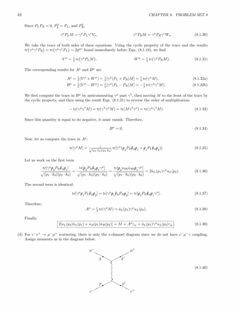
82 CHAPTER 8. PROBLEM SET 8
Since PLPR = 0, P 2L = PL, and P 2
R,
γµPLM = γµPLγνVν , γµPRM = γµPRγ
νWν . (8.1.30)
We take the trace of both sides of these equations. Using the cyclic property of the trace and the resultstr(γµγνPR
)= tr
(γµγνPL
)= 2gµν found immediately before Eqn. (8.1.18), we find
V µ = 12 tr(γµPLM
), Wµ = 1
2 tr(γµPRM
). (8.1.31)
The corresponding results for Aµ and Bµ are
Aµ = 12 (V µ +Wµ) = 1
4 [γµ(PL + PR)M ] = 14 tr(γµM), (8.1.32a)
Bµ = 12 (V µ −Wµ) = 1
4 [γµ(PL − PR)M ] = − 14 tr(γµγ5M). (8.1.32b)
We first compute the trace in Bµ by anticommuting γµ past γ5, then moving M to the front of the trace bythe cyclic property, and then using the result Eqn. (8.1.21) to reverse the order of multiplication:
− tr(γµγ5M) = tr(γ5γµM) = tr(Mγ5γµ) = tr(γµγ5M). (8.1.33)
Since this quantity is equal to its negative, it must vanish. Therefore,
Bµ = 0. (8.1.34)
Now, let us compute the trace in Aµ:
tr[γµM ] = 1√(p1·k0)(p2·k0)
tr[γµ(/p2PR/k0/p1
+ /p1PL/k0/p2
)]. (8.1.35)
Let us work on the first term
tr[γµ/p2PR/k0/p1
]√(p1 · k0)(p2 · k0)
=tr[/p2
PR/k0/p1γµ]√
(p1 · k0)(p2 · k0)=
tr[/p2uR0uR0/p1
γµ]√(p1 · k0)(p2 · k0)
= 2uL(p1)γµuL(p2). (8.1.36)
The second term is identical:
tr[γµ/p1PL/k0/p2
] = tr[γµ/p1/k0PR/p2
] = tr[/p2PR/k0/p1
γµ]. (8.1.37)
Therefore,
Aµ = 14 tr(γµM) = uL(p1)γµuL(p2). (8.1.38)
Finally,
2[uL(p2)uL(p1) + uR(p1)uR(p2)] = M = Aµγµ = uL(p1)γµuL(p2)γµ . (8.1.39)
(d) For e−e+ → µ−µ+ scattering, there is only the s-channel diagram since we do not have e−µ−γ coupling.Assign momenta as in the diagram below.
HHHHH
HHH
HH
* Y
Y *
e− e+
µ− µ+
p p′
k k′
(8.1.40)
8.1. MASSLESS TREE DIAGRAMS, P&S 5.3 P.170 83
Now, consider e−Re+L → µ−Rµ
+L scattering. A subtlety here is that for antiparticles, uL is right-chirality and
vice versa! Then, the amplitude is given by
MRL→RL = e2
s uR(k)γµuR(k′)uR(p′)γµuR(p)
= 4παs uL(k′)γµuL(k)[γµ]ab[uR(p′)]a[uR(p)]b
= 8παs [uL(k)uL(k′) + uR(k′)uR(k)]ab[uR(p′)]a[uR(p)]b
= 8παs uR(p′)
[uL(k)uL(k′) + uR(k′)uR(k)
]uR(p) (8.1.41)
We used Eqn. (8.1.24) to get the second line and the Fierz identity in the form Eqn. (8.1.39) to get thethird.
The second term in Eqn. (8.1.41) vanishes because it involves two factors of PL separated by an oddnumber of slashed objects:
uR(p′)uR(k′)uR(k)uR(p) ∝ tr[/pPL/k0/p′/k′PL/k0/k] = tr[/p/k0/p
′/k′PRPL/k0/k] = 0. (8.1.42)
The first term in Eqn. (8.1.41) can be simplified using s and t defined in Eqn. (8.1.3):
MRL→RL = 8παs s(p′, k)t(k′, p) = 8πα
s s(p′, k)s(p, k′)∗. (8.1.43)
Using Eqn. (8.1.18) for the square of s, we get∣∣MRL→RL∣∣2 =(
8παs
)22(p′ · k)2(p · k′). (8.1.44)
Since we neglect mass, p2 = p′2 = k2 = k′2 = 0. Thus, the Mandelstam variables are given by
s = (p+ p′)2 = (k + k′)2 = 2p · p′ = 2k · k′, (8.1.45a)
t = (k − p)2 = (p′ − k)2 = −2p · k = −2p′ · k′, (8.1.45b)
u = (k′ − p)2 = (p′ − k)2 = −2p · k′ = −2p′ · k, (8.1.45c)
where we also used conservation of momentum, p+ p′ = k + k′.
In the center of momentum frame, let θ be the angle between the muons and the electrons. Then,
p = Ecm2 (1, 0, 0, 1), k = Ecm
2 (1, 0, sin θ, cos θ), (8.1.46a)
p′ = Ecm2 (1, 0, 0,−1), k′ = Ecm
2 (1, 0,− sin θ,− cos θ). (8.1.46b)
Therefore,
s = 2(Ecm
2
)2[(1)(1)− (1)(−1)] = E2
cm, (8.1.47a)
t = −2(Ecm
2
)2[(1)(1)− (1)(cos θ)] = − s2 (1− cos θ), (8.1.47b)
u = −2(Ecm
2
)2[(1)(1)− (1)(− cos θ)] = − s2 (1 + cos θ). (8.1.47c)
Thus, we can write Eqn. (8.1.44) as∣∣MRL→RL∣∣2 =(
8παus
)2= [4πα(1 + cos θ)]2. (8.1.48)
Therefore, the differential cross-section is
( dσdΩ
)RL→RL=|MRL→RL|2
64π2s=α2
4s(1 + cos θ)2 . (8.1.49)
Indeed, this agrees with Eqn. 5.22 P&S p.143.
Consider the LR → LR case. This simply changes all the R subscripts to L subscripts in the first line ofEqn. (8.1.41). Using Eqn. (8.1.24), we can change these back to R’s while also switching the momenta in
84 CHAPTER 8. PROBLEM SET 8
each coupled pair. Thus, MLR→LR = MRL→RL except with p′ and k switched in the first s and p and k′
switched in the second. However, using Eqn. (8.1.4), we can switch them back, incurring two minus signs,which cancel. Therefore, the cross-section is the same:
( dσdΩ
)LR→LR=α2
4s(1 + cos θ)2 . (8.1.50)
Consider the RL→ LR case. As just described, the only difference in this case is that∣∣MRL→LR∣∣2 =(
8παs
)2|s(p′, k′)|2|s(p, k)|2 =(
8παs
)22(p′ · k′)2(p · k) =
(8παts
)2= [4πα(1− cos θ)]2. (8.1.51)
Therefore, ( dσdΩ
)RL→LR=( dσdΩ
)LR→RL=α2
4s(1− cos θ)2 . (8.1.52)
This agrees with Eqn. 5.23 P&S p.143. Finally, dσd cos θ = 2π dσdΩ .
8.2 Physical Amplitude, Zee III.1.1 p.168
Work through the manipulations leading to Eqn. 9 without referring to the text:
M = −iλP + iCλ2P log
s0t0u0
stu+O(λ3
P ). (8.2.1)
SOLUTION:
We have written down the the one-loop fully connected diagram at order λ2 before (problem set 5). The resultin the s-channel is
Ms =(−iλ)2
2
∫d4k
(2π)4
i
k2 −m2 + iε
i
(K − k)2 −m2 + iε, (8.2.2)
where K is the total momentum, that is, K2 = s.We write
1
k2 −m2 + iε
1
(K − k)2 −m2 + iε=
∫ 1
0
dx
x(k2 −m2 + iε) + (1− x)[(K − k)2 −m2 + iε]2
=
∫ 1
0
dx
[k2 − 2(1− x)k ·K + (1− x)2K2 − (1− x)2K2 + (1− x)K2 −m2 + iε]2
=
∫ 1
0
dx
[k − (1− x)K]2 + x(1− x)K2 −m2 + iε2. (8.2.3)
Define
` = k − (1− x)K, ∆ = m2 − x(1− x)K2, D = `2 −∆ + iε. (8.2.4)
Then, we write the amplitude as
Ms =λ2
2
∫ 1
0
dx
∫d4`
(2π)4
1
D2=
λ2
16π2
∫ 1
0
dx
∫ ∞0
`3d`
(`2 −∆)2. (8.2.5)
By integration by parts, we find∫ ∞0
`3d`
(`2 −∆)2= − `2
2(`2 −∆)
∣∣∣∞0
+
∫ ∞0
` d`
`2 −∆= −1
2+
1
2log(`2 −∆)
∣∣∣∞0. (8.2.6)
Unfortunately, the final integral is divergent. Let us regularize it by imposing a cut-off, Λ:∫ Λ
0
`3d`
(`2 −∆)2= −1
2+
1
2log
Λ2 −∆
−∆. (8.2.7)

8.3. SLIDING CUT-OFF, ZEE III.1.3 P.168 85
In the limit Λ→∞ and s = K2 >> m2, we have ∆ ≈ −x(1− x)s and Λ2 >> ∆. Thus,∫ ∞0
`3d`
(`2 −∆)2≈ −1
2+
1
2log
Λ2
x(1− x)s≈ 1
2
(log
Λ2
s− 1− log x− log(1− x)
). (8.2.8)
Integration over x yields
Ms =λ2
32π2
(log
Λ2
s− 3)≈ λ2
32π2log
Λ2
s. (8.2.9)
The most important part is Ms ∼ λ2 log Λ2
s since it is the divergent piece. We could also extract this divergentpiece by observing that the divergence is a UV divergence and thus is dominated by the large k region of theintegrand in Eqn. (8.2.2), that is, k2 >> K2,m2. This justifies dropping K and m from the integrand andrestricting the integral to the region k >> K. To do this, let the lower bound of the integral be ξK, where ξ issome sufficiently large, but finite number. Then,
Ms ≈(−iλ)2
2
1
(2π)42π2
∫ Λ
ξK
k3dk
k4∼ log
Λ
K−log ξ ∼ log
Λ2
s. (8.2.10)
Note: Even though we introduced the large number ξ to parametrize the fact that lower bound of the integralshould be much greater than K, it ends up not mattering because it does not contribute to the divergence (i.e. issubleading in the Λ→∞ limit). Also, we can square the argument of the log because that just incurs an overallfactor of 2 and we are not keeping track of the exact proportionality constant anyway.
To get the t- and u-channel results, we simply change s to t and u. This derives the result
M = −iλ+ iCλ2 logΛ6
stu. (8.2.11)
At (s, t, u) = (s0, t0, u0), the physical coupling constant is λp = λp(s0, t0, u0), and by definition, M(s0, t0, u0) =−iλp. Hence,
λp = λ− Cλ2 logΛ6
s0t0u0. (8.2.12)
We can invert this to order λ3p:
λ = λp + Cλ2p log
Λ6
s0t0u0. (8.2.13)
Therefore,
M = −iλp − iCλ2p log
Λ6
s0t0u0+ iCλ2
p logΛ6
stu= −iλp + iCλ2
p logs0t0u0
stu. (8.2.14)
8.3 Sliding Cut-off, Zee III.1.3 p.168
Change Λ to eεΛ. Show that forM not to change to the order indicated λ must change by δλ = 6εCλ2 +O(λ3),that is,
Λdλ
dΛ= 6Cλ2 +O(λ3). (8.3.1)
SOLUTION:
With Λ→ eεΛ and λ→ λ+ δλ,
M→M+ iδλ(
2Cλ logΛ6
stu+ 12εCλ− 1
)+ 6iεCλ2. (8.3.2)
At this order, there is nothing that can cancel the extra log term if it indeed exists to order λ2. The only way toget rid of it is to force it to be of higher order by having δλ = Aλ2 +O(λ3). This gives
M→M+ (6εC −A)iλ2 +O(λ3). (8.3.3)
Therefore, in order that M not change to this order, we must have A = 6εC. Thus,
δλ = 6εCλ2 +O(λ3) . (8.3.4)
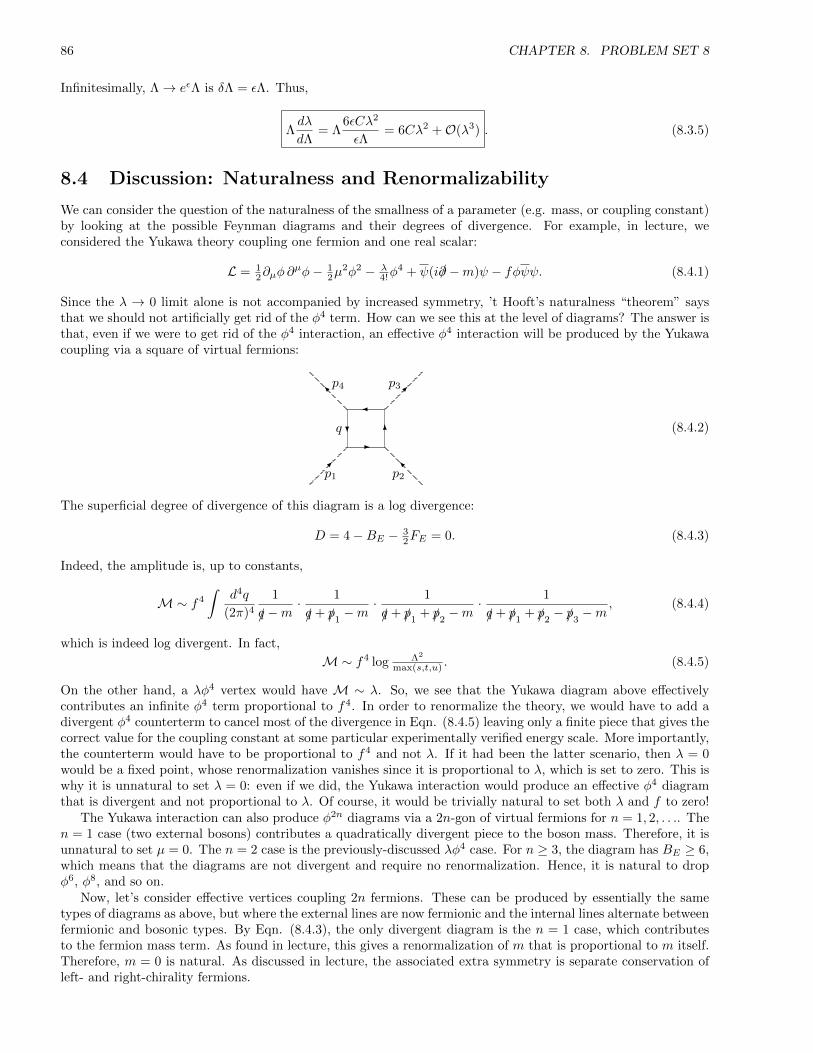
86 CHAPTER 8. PROBLEM SET 8
Infinitesimally, Λ→ eεΛ is δΛ = εΛ. Thus,
Λdλ
dΛ= Λ
6εCλ2
εΛ= 6Cλ2 +O(λ3) . (8.3.5)
8.4 Discussion: Naturalness and Renormalizability
We can consider the question of the naturalness of the smallness of a parameter (e.g. mass, or coupling constant)by looking at the possible Feynman diagrams and their degrees of divergence. For example, in lecture, weconsidered the Yukawa theory coupling one fermion and one real scalar:
L = 12∂µφ∂
µφ− 12µ
2φ2 − λ4!φ
4 + ψ(i/∂ −m)ψ − fφψψ. (8.4.1)
Since the λ → 0 limit alone is not accompanied by increased symmetry, ’t Hooft’s naturalness “theorem” saysthat we should not artificially get rid of the φ4 term. How can we see this at the level of diagrams? The answer isthat, even if we were to get rid of the φ4 interaction, an effective φ4 interaction will be produced by the Yukawacoupling via a square of virtual fermions:
I
I
-6
?
p1 p2
p3p4
q (8.4.2)
The superficial degree of divergence of this diagram is a log divergence:
D = 4−BE − 32FE = 0. (8.4.3)
Indeed, the amplitude is, up to constants,
M∼ f4
∫d4q
(2π)4
1
/q −m· 1
/q + /p1−m
· 1
/q + /p1+ /p2
−m· 1
/q + /p1+ /p2
− /p3−m
, (8.4.4)
which is indeed log divergent. In fact,
M∼ f4 log Λ2
max(s,t,u) . (8.4.5)
On the other hand, a λφ4 vertex would have M ∼ λ. So, we see that the Yukawa diagram above effectivelycontributes an infinite φ4 term proportional to f4. In order to renormalize the theory, we would have to add adivergent φ4 counterterm to cancel most of the divergence in Eqn. (8.4.5) leaving only a finite piece that gives thecorrect value for the coupling constant at some particular experimentally verified energy scale. More importantly,the counterterm would have to be proportional to f4 and not λ. If it had been the latter scenario, then λ = 0would be a fixed point, whose renormalization vanishes since it is proportional to λ, which is set to zero. This iswhy it is unnatural to set λ = 0: even if we did, the Yukawa interaction would produce an effective φ4 diagramthat is divergent and not proportional to λ. Of course, it would be trivially natural to set both λ and f to zero!
The Yukawa interaction can also produce φ2n diagrams via a 2n-gon of virtual fermions for n = 1, 2, . . .. Then = 1 case (two external bosons) contributes a quadratically divergent piece to the boson mass. Therefore, it isunnatural to set µ = 0. The n = 2 case is the previously-discussed λφ4 case. For n ≥ 3, the diagram has BE ≥ 6,which means that the diagrams are not divergent and require no renormalization. Hence, it is natural to dropφ6, φ8, and so on.
Now, let’s consider effective vertices coupling 2n fermions. These can be produced by essentially the sametypes of diagrams as above, but where the external lines are now fermionic and the internal lines alternate betweenfermionic and bosonic types. By Eqn. (8.4.3), the only divergent diagram is the n = 1 case, which contributesto the fermion mass term. As found in lecture, this gives a renormalization of m that is proportional to m itself.Therefore, m = 0 is natural. As discussed in lecture, the associated extra symmetry is separate conservation ofleft- and right-chirality fermions.

8.4. DISCUSSION: NATURALNESS AND RENORMALIZABILITY 87
You can keep playing this game, determining all of the types of effective vertices you can produce that mix φand ψ. However, all of them, except for the Yukawa term are convergent and require no renormalization. Hence,this theory requires only a finite number of divergent counterterms and is therefore renormalizable.
Contrast this with the case of the four-Fermi theory: Lint = −GF (ψψ)2. We can ask the question, is itnatural to drop the (ψψ)n term for n ≥ 3? Below, on the left, is a diagram involving only quartic interactionsthat nevertheless produces an effective sextic interaction, proportional to G2
F . By the superficial degree ofdivergence formula, D = 4 − 3
2FE + 2V , this diagram is not divergent and so we might rejoice in thinking thatit is natural to drop the sextic interaction term. However, since we can add any number of vertices withoutchanging the number of external lines, it turns out that we can make arbitrarily divergent diagrams that wouldcontribute to an effective sextic interaction, such as the one on the right below.
@
@@
@@@
@
@@
@@@
(8.4.6)
Therefore, it is not natural to set the sextic term to zero. Indeed, we pick up no extra symmetry from doingso. We would need a divergent sextic counterterm in order to renormalize the theory. The problem is, we wouldneed a counterterm for (ψψ)n for all n = 1, 2, . . ., and therefore the theory is not renormalizable.
However, we can think of the theory as an effective theory, which is only sensible at low energies. The (ψψ)n
counterterm must be proportional to Gn−1F . Note that GF has mass dimensions −2 in 4D and so the counterterms
have coupling constants with dimension −2(n− 1) = 2− 2n. For n ≥ 3, this is quite a large negative dimension.Therefore, if we set GF ∼ M−2, where M is the scale at which the theory breaks down, then the contributionsof such vertices would be suppressed by factors of (µ/M)n−1, where µ is the scale at which we are observing thesystem (the experimental scale). As long as µ << M , the theory should be well-behaved.

88 CHAPTER 8. PROBLEM SET 8
Chapter 9
Problem Set 9
9.1 Fermion Field Dimension, Zee III.3.1 p.181
Show that in (1+1)-dimensional spacetime the Dirac field ψ has mass dimension 12 , and hence the Fermi coupling
is dimensionless.
SOLUTION: (Thanks to Tova (’12) for presenting her solution.)
The dimensional analysis determining the dimension of ψ proceeds as follows:
0 = [d2xψi/∂ψ] = 2[x] + [∂] + 2[ψ] = −2 + 1 + 2[ψ] =⇒ [ψ] = 12 . (9.1.1)
The dimensional analysis determining the dimension of GF proceeds as follows:
0 = [d2xGF (ψψ)2] = 2[x] + 4[ψ] + [GF ] = −2 + 4(
12
)+ [GF ] =⇒ [GF ] = 0 . (9.1.2)
9.2 Degree of Divergence, Zee III.3.2 p.181
Derive Eqn. 11 p.178 and Eqn. 13 p.179. The first says that the degree of divergence in Yukawa theory in 3 + 1dimensions is D = 4−BE − 3
2FE , where BE and FE are the numbers of external bosonic and fermionic legs, re-spectively. The second says that the degree of divergence in Four-Fermi theory in 1+1 dimensions is D = 2− 1
2FE .
SOLUTION: (Thanks to Diana and Shreyas (’12) for presenting their solutions.)
Yukawa: Let L be the total number of loops, Vf and Vλ be the numbers of f -vertices and λ-vertices, respectively,V ≡ Vλ + Vf be the total number of vertices, and BE , BI , FE and FI be the numbers of external and internalbosonic and fermionic lines, respectively. The superficial degree of divergence is
D = 4L− 2BI − FI , (9.2.1)
since each loop contributes∫d4q for some unspecifiied momentum, q, each internal bosonic line contributes
a factor of the bosonic propagator ∼ q−2, and each internal fermionic contributes a factor of the fermionicpropagator ∼ /qq−2 ∼ q−1.
The number of loops is equal to the number of internal lines minus the number of internal lines whosemomenta are fixed by momentum conservation. The latter are due to momentum-conserving delta functions atevery vertex. However, some combination of these delta functions just gives an overall momentum-conservingdelta function, which does not constrain any of the internal momenta. Hence, the number of internal momentathat are constrained by momentum conservation is V − 1. Hence,
L = BI + FI − (V − 1) =⇒ D = 4− 4V + 2BI + 3FI . (9.2.2)
Conservation of bosonic and fermionic ends yields
Vf + 4Vλ = BE + 2BI , 2Vf = FE + 2FI . (9.2.3)
89
90 CHAPTER 9. PROBLEM SET 9
The first follows from the fact that each external bosonic line has only one of its endpoints attached to a vertexwhile both ends of an internal line must be attached, and each f -vertex accommodates only one bosonic endwhile each λ-vertex accommodates four. The same argument pertains to the second equation for fermionic ends.
These two equations combine to the following useful form:
4V = 4(Vλ + Vf ) = BE + 2BI + 32FE + 3FI . (9.2.4)
Putting this all together, we get
D = 4−BE − 32FE . (9.2.5)
4-Fermi: In 1 + 1 dimensions, each loop contributes two powers of momentum while each fermion propagatorstill contributes one inverse power of momentum. Therefore,
D = 2L− FI . (9.2.6)
The same argument that gave Eqn. (9.2.2) gives
L = FI − (V − 1) =⇒ D = 2− 2V + FI . (9.2.7)
Conservation of ends reads
4V = FE + 2FI . (9.2.8)
Combining this with Eqn. (9.2.7) yields
D = 2− 12FE . (9.2.9)
9.3 Massless Weisskopf Phenomenon, Zee III.3.3 p.181
Show that B(p2) in Eqn. 14 p.180, reproduced below, vanishes when we set m = 0. Show that the same behaviorholds in quantum electrodynamics.
(if)2i2∫
d4k
(2π)4
1
k2 − µ2
/p+ /k +m
(p+ k)2 −m2≡ A(p2)/p+B(p2). (9.3.1)
SOLUTION: (Thanks to Jonathan (’12) for presenting his solution.)
The term in the left hand side that does not involve gamma matrices (i.e. slashed objects) is proportional to m.Hence, the same must be true for the right hand side. Hence,
B(p2) ∝ m m→0−−−→ 0 . (9.3.2)
If the virtual scalar is replaced by a virtual photon (of fiducial mass µ), then the amplitude becomes
(ie)2i2∫
d4k
(2π)4
−gµνk2 − µ2
u(p)γν/p+ /k +m
(p+ k)2 −m2γµu(p). (9.3.3)
Recall that we can safely drop the piece of the photon propagator involvingkµkνµ2 by the appropriate Ward
identity, which encodes gauge invariance. Let us simplify the numerator:
−gµνγν(/p+ /k +m)γµ = −gµνγν [2(p+ k)µ − γµ(/p+ /k −m)]
= −2(/p+ /k) + 4(/p+ /k −m)
= 2(/p+ /k − 2m). (9.3.4)
Here, we used the identity γµγµ = 4. Therefore, up to numerical factors, Eqn. (9.3.3) is the same as Eqn. (9.3.1).
By the way, you can actually keep the massive term in the photon propagator. It can only possibly contributeto A and not to B.
9.3. MASSLESS WEISSKOPF PHENOMENON, ZEE III.3.3 P.181 91
Aside: It might seem peculiar that the integral involving /k end up being proportional to /p. However, it mustdo because it must be proportional to a relativistic-invariant matrix and since it contains γ matrices, the onlypossibility is /p. This is a non-constructive proof of this fact.
We can also prove it by brute force calculation using the Feynman trick. Define the integral
I =
∫d4k
(2π)4
/k
(k2 − µ2)[(p+ k)2 −m2]. (9.3.5)
Then, using the Feynman trick, we have
I =
∫ 1
0
dx
∫d4k
(2π)4
/kx[(p+ k)2 −m2] + (1− x)(k2 − µ2)
2
=
∫ 1
0
dx
∫d4k
(2π)4
/k[k2 + 2xpk + x2p2 − x2p2 + xp2 − xm2 − (1− x)µ2
]2=
∫ 1
0
dx
∫d4k
(2π)4
/k[(k + xp)2 + x(1− x)p2 − xm2 − (1− x)µ2
]2 . (9.3.6)
Define`µ = kµ + xpµ, (9.3.7)
in terms of which, we may write the integral as
I =
∫ 1
0
dx
∫d4`
(2π)4
/− x/pD2
, (9.3.8)
whereD = `2 −∆, (9.3.9)
and∆ = xm2 + (1− x)µ2 − x(1− x)p2. (9.3.10)
The integral of the / term vanishes because it is the integral of an odd function of `µ. The only term left isindeed proportional to /p and is a function only of p2 (since ∆ is a function only of p2).
Another aside: It was suggested that we write the intermediate fermion propagator in the m = 0 limit as
/p+ /k
(p+ k)2=
1
/p+ /k· /p− /k/p− /k
?=
/p− /kp2 − k2
. (9.3.11)
The reason for the question mark above the final equality is that it is not actually correct. In fact,
(/p+ /k)(/p− /k) = /p2 − /k2
+ /k/p− /p/k = p2 − k2 + [/k, /p] 6= p2 − k2. (9.3.12)
This spoils our ability to use this method to massage the denominator into a form that depends only on p2 andk2. The point of the p2 is that the result is supposed to be a function only of p2 and the point of k2 is that it iseven and so if it is multiplied by an odd function of k, such as /k in the numerator, then that integral vanishesidentically. Even though this doesn’t work, the idea is spot on. The method of Feynman parameters achievesthis goal.
92 CHAPTER 9. PROBLEM SET 9
9.4 Form of Anomalous Magnetic Moment, Zee III.6.3 p.198
By Lorentz invariance, the right hand side of Eqn. 7 p.196, reproduced below, has to be a vector. The onlypossibilities are uγµu, (p+p′)µuu, and (p−p′)µuu. The last term is ruled out because it would not be consistentwith current conservation. Show that the form given below is in fact the most general allowed.
〈p′, s′|Jµ(0)|p, s〉 = u(p′, s′)
[γµF1(q2) +
iσµνqν2m
F2(q2)
]u(p, s), (9.4.1)
where q ≡ p′ − p.
SOLUTION:
Current conservation reads qµJµ = 0, which means that the only terms that can show up on the right hand side
of Eqn. (9.4.1) are vectors with vanishing dot product with q. Since q2 6= 0 for the virtual photon, we cannothave a term proportional to uqµu. On the other hand, q · (p+p′) = p2−p′2 = m2−m2 = 0 and uqµγ
µu = 0 since
/pu(p) = mu(p) and u(p′)/p′ = mu(p′) and so u/qu = u(/p
′− /p)u = u(m−m)u = 0. Therefore, current conservationcannot get rid of the other two terms. Thus,
〈p′, s′|Jµ(0)|p, s〉 = u(p′, s′)[γµA+ (p+ p′)µB
]u(p, s), (9.4.2)
where, A and B are Lorentz scalars, but could be proportional to slashed momenta, /p and /p′. Since the latter are
equivalent to m when acting on u(p) or u(p′), we may assume A and B to just be functions and be proportionalto the identity in spinor space. A and B must be functions of Lorentz invariants (and constants, of course).Certainly, q2 is an invariant, and since p2 = p′2 = m2 and 2p ·p′ = 2m2− q2, there is no other independent choicefor a variable on which A and B may depend. Hence,
〈p′, s′|Jµ(0)|p, s〉 = u(p′, s′)[γµA(q2) + (p+ p′)µB(q2)
]u(p, s). (9.4.3)
Finally, recall the Gordon identity from problem set 3:
u(p′)γµu(p) = u(p′)
[p′µ + pµ
2m+iσµνqν
2m
]u(p). (9.4.4)
Then, define
F1(q2) = A(q2) + 2mB(q2), F2(q2) = −2mB(q2), (9.4.5)
in terms of which, Eqn. (9.4.3) may be written as
〈p′, s′|Jµ(0)|p, s〉 = u(p′, s′)
[γµF1(q2) +
iσµνqν2m
F2(q2)
]u(p, s) . (9.4.6)
9.5 Discussion 1: Phi-Fourth Dimensional Analysis
Recall that a theory with a coupling constant of negative mass dimension is non-renormalizable (see Zee p.170for a heuristic argument). Thus, we can find out in which dimensions φ4 theory is renormalizable. In d spacetimedimensions, the Lagrangian density must have mass dimension [L] = d so that the action
∫ddxL be dimensionless.
Since [∂] = +1,d =
[12∂µφ∂
µφ]
= 2[∂] + 2[φ] = 2 + 2[φ] =⇒ [φ] = d−22 . (9.5.1)
Therefore, the dimension of λ is
d =[− λ
4!φ4]
= [λ] + 4[φ] = [λ] + 4(d−2
2
)=⇒ [λ] = 4− d. (9.5.2)
Therefore, φ4 theory is renormalizable for d ≤ 4 and non-renormalizable for d > 4.We know another method for determining renormalizability: calculating the superficial degree of divergence.
Recall that in d = 4, for φ4 theory, this is given by D = 4 − BE . The only difference in the equations used toderive this is in the number of momenta contributed by each loop: it is now d instead of 4. Thus,
D = dL− 2BI , L = BI − (V − 1), 4V = 2BI +BE . (9.5.3)
9.6. DISCUSSION 2: PHI-CUBED DIMENSIONAL ANALYSIS 93
Together, these giveD = d− d
4BE + 2(d4 − 1
)BI . (9.5.4)
This indeed gives D = 4−BE when d = 4. Note that the BI term exactly vanishes in this dimension. This is nicebecause it means that we can enumerate the divergent diagrams by the number of external lines and only finitelymany cases are divergent and require renormalization. Hence, the theory is renormalizable. This continues tohold when the coefficient of BI is negative since adding more and more internal lines just makes diagrams moreand more convergent. On the other hand, if the coefficient of BI is positive, then we can make diagrams withany number of external lines arbitrarily divergent by adding sufficiently many internal lines. In this case, thetheory is non-renormalizable. Note that this exactly reproduces the result from dimensional analysis because thecoefficient of BI is zero or negative exactly when d ≤ 4 and it is positive when d > 4.
In principle, the secret agent behind all of this is Weinberg’s theorem, which has to do with the behavior ofcorrelators under dilations of momenta. You can look it up if you like, but we probably won’t get to it in class.
9.6 Discussion 2: Phi-Cubed Dimensional Analysis
If we repeat the dimensional analysis for a theory with Lin = − λ3!φ
3, instead, we find
[φ] = d−22 , [λ] = 6−d
2 . (9.6.1)
Therefore, the theory is renormalizable for d ≤ 6 and non-renormalizable for d > 6.We also find the superficial degree of divergence
D = d− d3BE + 2
(d6 − 1
)BI . (9.6.2)
As before, the coefficient of BI vanishes when d = 6, is negative when d < 6 and is positive when d > 6. Thisconfirms the fact that the theory is renormalizable when d ≤ 6 and non-renormalizable when d > 6.
In accordance with the discussion last week, we can see this break-down at the diagramatic level. Forsimplicity, consider diagrams that are divergent at the one-loop level. Thus, L = 1 and the middle equation in(9.5.3) implies that BI = V . The third equation is replaced with 3V = 2BI + BE and so this also implies thatBE = BI = V when L = 1. In this case, D simplifies to
D|L=1 = d− 2BE . (9.6.3)
In d = 2 dimensions, the only divergent diagram has BE = BI = V = 1. This diagram is the tadpole diagram:
(9.6.4)
This contributes a source term to φ and therefore a divergent constant vacuum expectation value, 〈φ〉. This islike an infinite zero-point energy and is simply subtracted out since an overall constant value in φ is irrelevant.Therefore, this is not actually of any interest.
In d = 4 dimensions, the tadpole diagram is still divergent, but now BE = BI = V = 2 is also divergent. Thisdiagram is
(9.6.5)
This gives the wavefunction renormalization (of φ) and the mass renormalization. Since these are already in theaction, the theory is certainly one-loop renormalizable.
In d = 6 dimensions, we get a new divergent diagram when BE = BI = V = 3:
(9.6.6)
This renormalizes the vertex. That is, it renormalizes λ. Again, nothing other than the terms originally in theLagrangian get renormalized. Thus, the theory is one-loop renormalizable.

94 CHAPTER 9. PROBLEM SET 9
Finally, this must break down in d = 8 dimensions. BE = BI = V = 4 is divergent. This diagram is
@@
@@
(9.6.7)
This would renormalize a φ4 interaction, but there is no such thing in the original Lagrangian. Thus, it generatesan infinite φ4 interaction proportional to λ4. This signals one-loop non-renormalizability. The φ4 interactiontogether with the φ3 interaction will now generate further divergent one-loop diagrams involving higher andhigher numbers of external particles.
Renormalizability must break down when d = 7 as well. However, it must do so at the two-loop level.
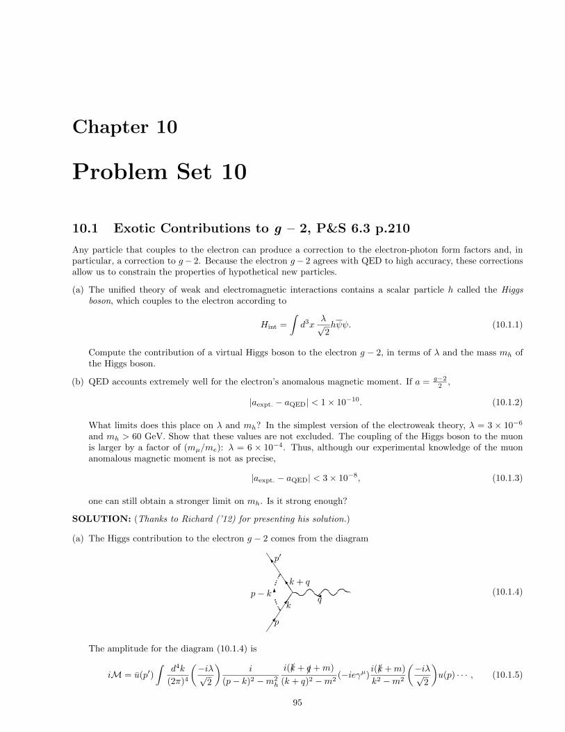
Chapter 10
Problem Set 10
10.1 Exotic Contributions to g – 2, P&S 6.3 p.210
Any particle that couples to the electron can produce a correction to the electron-photon form factors and, inparticular, a correction to g− 2. Because the electron g− 2 agrees with QED to high accuracy, these correctionsallow us to constrain the properties of hypothetical new particles.
(a) The unified theory of weak and electromagnetic interactions contains a scalar particle h called the Higgsboson, which couples to the electron according to
Hint =
∫d3x
λ√2hψψ. (10.1.1)
Compute the contribution of a virtual Higgs boson to the electron g − 2, in terms of λ and the mass mh ofthe Higgs boson.
(b) QED accounts extremely well for the electron’s anomalous magnetic moment. If a = g−22 ,
|aexpt. − aQED| < 1× 10⁻¹⁰. (10.1.2)
What limits does this place on λ and mh? In the simplest version of the electroweak theory, λ = 3 × 10⁻⁶
and mh > 60 GeV. Show that these values are not excluded. The coupling of the Higgs boson to the muonis larger by a factor of (mµ/me): λ = 6 × 10⁻⁴. Thus, although our experimental knowledge of the muonanomalous magnetic moment is not as precise,
|aexpt. − aQED| < 3× 10⁻⁸, (10.1.3)
one can still obtain a stronger limit on mh. Is it strong enough?
SOLUTION: (Thanks to Richard (’12) for presenting his solution.)
(a) The Higgs contribution to the electron g − 2 comes from the diagram
JJJJJ
]
]6
p
kq
k + q
p− k
p′
(10.1.4)
The amplitude for the diagram (10.1.4) is
iM = u(p′)
∫d4k
(2π)4
(−iλ√
2
)i
(p− k)2 −m2h
i(/k + /q +m)
(k + q)2 −m2(−ieγµ)
i(/k +m)
k2 −m2
(−iλ√
2
)u(p) · · · , (10.1.5)
95
96 CHAPTER 10. PROBLEM SET 10
where the · · · involves the rest of the diagram to which the vertex is attached, including the photon propa-gator, or the photon polarization state if it is external. The iε is taken for granted.
Let us clean this up a little bit:
iM = (−ie) iλ2
2
∫d4k
(2π)4
u(p′)(/k + /q +m)γµ(/k +m)u(p)
[(p− k)2 −m2h][(k + q)2 −m2](k2 −m2)
= (−ie)iλ2
∫F
∫d4k
(2π)4
u(p′)(/k + /q +m)γµ(/k +m)u(p)x(k2 −m2) + y[(k + q)2 −m2] + z[(p− k)2 −m2
h]3 , (10.1.6)
where∫F
stands for the integral over the Feynman parameters. In this case,∫F
=
∫∫∫ 1
0
dx dy dz δ(x+ y + z − 1). (10.1.7)
Before we embark on complicated and tedious mathematics, let us pause for a moment to think about thegoal. We want the correction to g − 2, which depends only on the F2(q2) term. Thus, we can neglect all theterms in Eqn. (10.1.7) that do not contribute to F2 (such as terms proportional to γµ).
Now, let us first work on the denominator:
D ≡ x(k2 −m2) + y(k2 + 2q · k + q2 −m2) + z(k2 − 2p · k + p2 −m2h)
= (x+ y + z)k2 + 2(yq − zp) · k + yq2 + zp2 − (x+ y)m2 − zm2h
= k2 + 2(yq − zp) · k + (yq − zp)2 − (yq − zp)2 + yq2 + zp2 − (x+ y)m2 − zm2h
= (k + yq − zp)2︸ ︷︷ ︸`2
−[(x+ y)m2 + zm2
h − y(1− y)q2 − z(1− z)p2 − 2yzp · q]︸ ︷︷ ︸
∆
. (10.1.8)
Replace p′2 and p2 with m2. Then, note that m2 = p′2 = (p+ q)2 = m2 + 2p · q + q2. Thus, we may write
p2 = m2, 2p · q = −q2. (10.1.9)
Using these identities, we simplify ∆ to
∆ = (x+ y)m2 + zm2h + y(1− y)q2 − z(1− z)m2 + yzq2. (10.1.10)
Since x+ y + z = 1, we may write the coefficients of m2 and q2 as
x+ y − z(1− z) = (1− z)− z(1− z) = (1− z)2, (10.1.11a)
−y(1− y) + yz = −y(x+ z) + yz = −xy. (10.1.11b)
Therefore, this leaves us with∆ = (1− z)2m2 + zm2
h − xyq2. (10.1.12)
This is exactly the same as Eqn. 6.44 P&S p.191 except for an extra factor of zm2h. Therefore, the same
argument that showed that Eqn. 6.44 P&S p.191 is positive, namely that q2 < 0 for a scattering process,implies that Eqn. (10.1.12) is positive as well.
We want to express the numerator of the integrand in Eqn. (10.1.6) in terms of `, which is related to k via
`µ = kµ + yqµ − zpµ. (10.1.13)
The numerator is
num = u(p′)[/+ z/p+ (1− y)/q +m
]γµ[/+ z/p− y/q +m
]u(p)
= u(p′)[/+
(z − (1− y)
)/p+ (1− y)/p
′ +m]γµ[/+ (y + z)/p− y/p′ +m
]u(p)
= u(p′)[/− x/p+ (2− y)m
]γµ[/− y/p′ + (2− x)m
]u(p). (10.1.14)
10.1. EXOTIC CONTRIBUTIONS TO G – 2, P&S 6.3 P.210 97
We have turned any /p on the right and /p′ on the left into m because they act on u(p) and u(p′), respectively.
We also used the identity x = 1− y− z twice, to turn the coefficients of /p on the left and m on the right into−x and (2− x), respectively.
The following identities (Eqns. 6.45 and 6.46 P&S p.191) will help us simplify this:∫d4`
(2π)4
`µ
D3= 0,
∫d4`
(2π)4
`µ`ν
D3=
∫d4`
(2π)4
14gµν`2
D3. (10.1.15)
The first identity implies that we can discard all terms in the numerator that are linear in `. The secondidentity implies that we can replace `µ`ν in the numerator with 1
4`2gµν . In the sequel, we will take the u(p′)
and u(p) factors for granted. The quadratic term in num is
num(2) = /γµ/ = 2`µ/− γµ/2= 2 1
4`2gµνγν − γµ`2 = − 1
2`2γµ. (10.1.16)
As we mentioned earlier, we only care about terms that contribute to F2. This quadratic piece is proportionalto γµ and thus only contributes to F1. We keep it here only for the sake of completeness.
The terms of zeroth order in ` are
num(0) =[−x/p+ (2− y)m
]γµ[−y/p′ + (2− x)m
]= xy/pγ
µ/p′︸ ︷︷ ︸
num(0)3
−x(2− x)m/pγµ − y(2− y)mγµ/p
′︸ ︷︷ ︸num
(0)2
+(2− x)(2− y)m2γµ. (10.1.17)
Now, let us massage this into a convenient form by moving /p′ to the left and /p to the right and then replacing
each with m since they act on u(p′) and u(p), respectively:
num(0)2 = −x(2− x)m(2pµ − γµ/p)− y(2− y)m(2p′µ − /p′γµ)
= −2x(2− x)mpµ + x(2− x)m2γµ − 2y(2− y)mp′µ + y(2− y)m2γµ. (10.1.18)
Define
qµ = (p′ − p)µ, q′µ = (p′ + p)µ. (10.1.19)
Inverting this yields
p′µ = 12 (q′ + q)µ, pµ = 1
2 (q′ − q)µ. (10.1.20)
Write Eqn. (10.1.18) in terms of q′ and q:
num(0)2 = [x(2− x) + y(2− y)]m2γµ − x(2− x)m(q′ − q)µ − y(2− y)m(q′ + q)µ
= [x(2− x) + y(2− y)]m2γµ − [x(2− x) + y(2− y)]mq′µ + [x(2− x)− y(2− y)]mqµ. (10.1.21)
Now, let us work on num(0)3 :
num(0)3 = xy(2pµ − γµ/p)/p′
= 2xympµ − xyγµ(2p′ · p− /p′/p)= 2xympµ − 2xyp′ · pγµ + xym(2p′µ − /p′γµ)
= 2xympµ − 2xyp′ · pγµ + 2xymp′µ − xym2γµ
= 2xymq′µ − xy(2p′ · p+m2)γµ. (10.1.22)
Let us rewrite the dot product using the following identity:
q2 = (p′ − p)2 = p′2 + p2 − 2p′ · p = 2m2 − 2p′ · p. (10.1.23)
98 CHAPTER 10. PROBLEM SET 10
This gives
num(0)3 = xy(q2 − 3m2)γµ + 2xymq′µ. (10.1.24)
Putting Eqns. (10.1.16) (10.1.17), (10.1.21) and (10.1.24) together, Eqn. (10.1.14) becomes
num =
A︷ ︸︸ ︷− 1
2`2 + xy(q2 − 3m2) + [x(2− x) + y(2− y)]m2 + (2− x)(2− y)m2
γµ
+
2xy − [x(2− x) + y(2− y)]m︸ ︷︷ ︸
B
q′µ + [x(2− x)− y(2− y)]m︸ ︷︷ ︸C
qµ. (10.1.25)
Let us simplify some of these coefficients. First, we simplify A.
A = − 12`
2 + xyq2 +[−
2
3xy +2x− x2 +2y − y2 + 4−2x−2y +xy
]m2
= − 12`
2 + xyq2 + [4− (x+ y)2]m2
= − 12`
2 + xyq2 + [2− (1− z)][2 + (1− z)]m2
= − 12`
2 + xyq2 + (1 + z)(3− z)m2. (10.1.26)
Next, we simplify B.
Bm
= 2xy−2x+x2−2y+y2 = (x+y)2−2(x+y) = −(x+y)(2−x−y) = −(1−z)(1+z) = −(1−z2). (10.1.27)
Finally, we can write the amplitude as
iM = (−ie)iλ2u(p′)
∫F
∫d4`
(2π)4
Aγµ + Bq′µ + Cqµ
D3u(p) · · · . (10.1.28)
Note that ∆ in Eqn. (10.1.12), and therefore D, is even under the interchange x↔ y. Meanwhile, C is odd.Therefore, after integration over the Feynman parameters, the term proportional to qµ vanishes. We provedthis in problem set 9 using current conservation (the Ward identity).
Recall the Gordon identity, which we proved in problem set 3. We will write it in the form
u(p′)q′µu(p) = u(p′)[2mγµ − iσµνqν
]u(p). (10.1.29)
Then, already dropping the C term, we get
iM = (−ie)iλ2u(p′)
∫F
∫d4`
(2π)4
(A+ 2mB)γµ − BiσµνqνD3
u(p) · · · . (10.1.30)
Define
F1 = A+ 2mB, F2 = −2mB, Fi = iλ2
∫F
∫d4`
(2π)4
FiD3
. (10.1.31)
Then, we can write the amplitude as
iM = u(p′)(−ie)(γµF1 +
iσµνqν2m
F2
)u(p) · · · . (10.1.32)
Compare this to the vertex at tree level:
iM = u(p′)(−ieγµ)u(p) · · · . (10.1.33)
Therefore, we recognize that the correction to the vertex due to the Higgs is
δΓµ = γµF1 +iσµνqν
2mF2. (10.1.34)
10.1. EXOTIC CONTRIBUTIONS TO G – 2, P&S 6.3 P.210 99
Only F2 affects g. It is given by
F2 = iλ2
∫F
∫d4`
(2π)4
−2m[−m(1− z2)]
D3. (10.1.35)
We can use Eqn. 6.49 P&S p.193 to compute the ` integral:∫d4`
(2π)4
1
D3=i(−1)3
(4π)2
1
(3− 1)(3− 2)
1
∆3−2= − i
2(4π)2
1
∆. (10.1.36)
Therefore,
F2 =
(λm
4π
)2 ∫F
1− z2
∆. (10.1.37)
Anticipating the fact that mh >> m, write ∆ as
∆ = m2h
[z + (1− z)2
(mmh
)2 − xy( qm)2]. (10.1.38)
As expected, since ∆ is a function just of q2, so is F2. Define
ε ≡(mmh
)2. (10.1.39)
Then, the correction to a = g−22 due to the higgs is
ah = F2(0) =
(λ
4π
)2
ε
∫∫∫ 1
0
dx dy dz δ(x+ y + z − 1)1− z2
z + (1− z)2ε. (10.1.40)
Change the x and y variables to
u = x+ y, v = y − x. (10.1.41)
We can invert these relations:
x = 12 (u− v), y = 1
2 (u+ v). (10.1.42)
Therefore, the Jacobian matrix and determinant are
J =
(∂x∂u
∂x∂v
∂y∂u
∂y∂v
)=
1
2
(1 −11 1
), det J =
1
2. (10.1.43)
Therefore, dx dy = 12du dv. The u integral goes from 0 (minimum of x + y) to 2 (maximum of x + y). The
v limits depend on u. When 0 ≤ u ≤ 1, the v limits are −u ≤ v ≤ u. When 1 ≤ u ≤ 2, the v limits areu− 2 ≤ v ≤ 2− u. Therefore,
ah =
(λ
4π
)2ε
2
∫ 1
0
dz
(∫ 1
0
du
∫ u
−udv +
∫ 2
1
du
∫ 2−u
u−2
dv
)δ(u+ z − 1)
1− z2
z + (1− z)2ε. (10.1.44)
The delta function sets u = 1− z. Since 0 ≤ z ≤ 1, we have 0 ≤ 1− z ≤ 1 and so the u integral in the range[1, 2] vanishes. Thus,
ah =
(λ
4π
)2ε
2
∫ 1
0
dz
∫ 1−z
−(1−z)dv
1− z2
z + (1− z)2ε=
(λ
4π
)2
ε
∫ 1
0
dz(1− z)(1− z2)
z + (1− z)2ε︸ ︷︷ ︸I
. (10.1.45)
Note that the integrand behaves like 1z near z = 0 when ε = 0, which signals a logarithmic divergence in ε.
Therefore, we peal off a piece from the integral which will give a logarithm:
I =
∫ 1
0
dz
(1− 2(1− z)εz + (1− z)2ε
+2(1− z)ε− z(1 + z − z2)
z + (1− z)2ε
). (10.1.46)
100 CHAPTER 10. PROBLEM SET 10
The first piece can be integrated exactly and just gives∫ 1
0
dz1− 2(1− z)εz + (1− z)2ε
= ln[z + (1− z)2ε]∣∣10
= ln 1− ln ε = − ln ε. (10.1.47)
The integrand in the remaining piece is a much better behaved function. Its limit as z → 0 is just 2 andit has no poles. Thus, we can simply set ε = 0 in that term. The integrand becomes −1 − z + z2 and theintegral is easy to compute:∫ 1
0
dz2(1− z)ε− z(1 + z − z2)
z + (1− z)2ε≈ −
(z +
z2
2− z3
3
)∣∣∣10
= −7
6. (10.1.48)
Therefore, we finally have
ah ≈ −(λ
4π
)2
ε
(7
6+ ln ε
)= −
(λm
4πmh
)2(7
6+ 2 ln
m
mh
). (10.1.49)
Since ε << 1, its logarithm is large and negative. Therefore, it makes more sense to write
ah =
(λm
4πmh
)2(2 ln
mh
m− 7
6
). (10.1.50)
(b) Well, all we can say is
|ah| < 10−10 . (10.1.51)
ahε→0−−−→ 0 and ah
ε→∞−−−→ −∞. Meanwhile, there is one point where dah
dε = 0, namely ε = e−19/12 ≈ 0.2, andd2ah
dε2 < 0 and so there is one maximum. Therefore ah must increase from 0, reach a maximum, then decreaseforever beyond that point. Clearly, ε << 0.2 since m ≈ 0.5 MeV and mh > 60 GeV. Therefore, in the regionmh > 60 GeV, a bigger and bigger mh just makes ah smaller and smaller. Therefore, if mh = 60 GeV is notexcluded when λ = 3× 10⁻⁶, then the whole region mh ≥ 60 GeV is not excluded. Indeed, plugging in thesevalues gives
ah ≈ 9× 10⁻²³ . (10.1.52)
This is indeed much smaller than the upper bound in Eqn. (10.1.51) and thus is not excluded.
If we plug in λ = 6× 10⁻⁴ instead, for the muon, and the same mh, we get
ah ≈ 4× 10⁻¹⁸ . (10.1.53)
This is still not excluded.
10.2 Diagramatics of Effective Potential, Zee IV.3.4 p.244
Understand Eqn. 14, Zee p.240, reproduced below, using Feynman diagrams. Show that Veff is generated by aninfinite number of diagrams. [Hint: Expand the logarithm in Eqn. 14, Zee p.240, as a series in V ′′(ϕ)/k2 andtry to associate a Feynman diagram with each term in the series.]
Veff(ϕ) = V (ϕ)− i~2
∫d4k
(2π)4log
[k2 − V ′′(ϕ)
k2
]+O(~2). (10.2.1)
SOLUTION: (Thanks to Melanie (’12) for presenting her solution.)
Let us expand the quantum corrections to the potential in powers of V ′′:
Veff(ϕ)− V (ϕ) =i~2
∞∑n=1
1
n
∫d4k
(2π)4
(V ′′(ϕ)
k2
)n. (10.2.2)
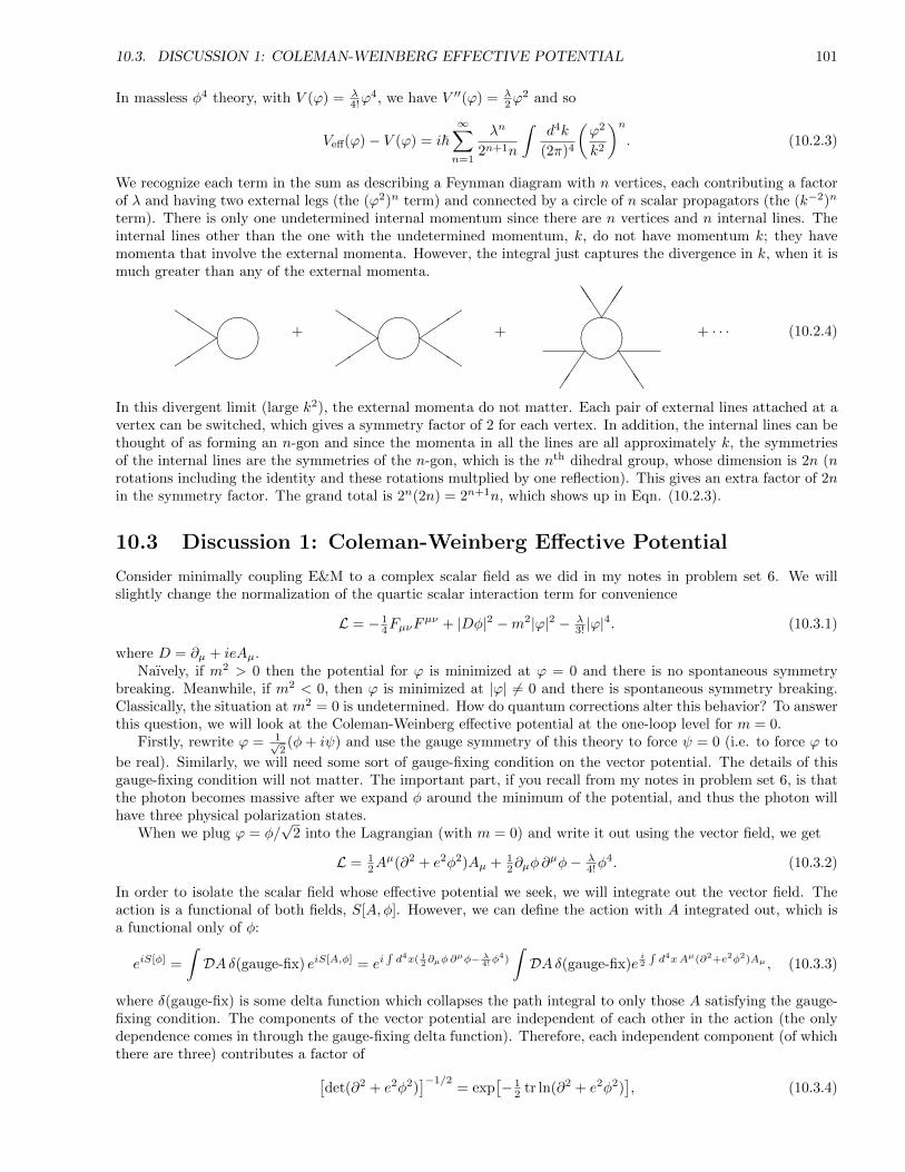
10.3. DISCUSSION 1: COLEMAN-WEINBERG EFFECTIVE POTENTIAL 101
In massless φ4 theory, with V (ϕ) = λ4!ϕ
4, we have V ′′(ϕ) = λ2ϕ
2 and so
Veff(ϕ)− V (ϕ) = i~∞∑n=1
λn
2n+1n
∫d4k
(2π)4
(ϕ2
k2
)n. (10.2.3)
We recognize each term in the sum as describing a Feynman diagram with n vertices, each contributing a factorof λ and having two external legs (the (ϕ2)n term) and connected by a circle of n scalar propagators (the (k−2)n
term). There is only one undetermined internal momentum since there are n vertices and n internal lines. Theinternal lines other than the one with the undetermined momentum, k, do not have momentum k; they havemomenta that involve the external momenta. However, the integral just captures the divergence in k, when it ismuch greater than any of the external momenta.
QQQ
+
QQQ
QQQ
+
JJJ
JJJ
+ · · · (10.2.4)
In this divergent limit (large k2), the external momenta do not matter. Each pair of external lines attached at avertex can be switched, which gives a symmetry factor of 2 for each vertex. In addition, the internal lines can bethought of as forming an n-gon and since the momenta in all the lines are all approximately k, the symmetriesof the internal lines are the symmetries of the n-gon, which is the nth dihedral group, whose dimension is 2n (nrotations including the identity and these rotations multplied by one reflection). This gives an extra factor of 2nin the symmetry factor. The grand total is 2n(2n) = 2n+1n, which shows up in Eqn. (10.2.3).
10.3 Discussion 1: Coleman-Weinberg Effective Potential
Consider minimally coupling E&M to a complex scalar field as we did in my notes in problem set 6. We willslightly change the normalization of the quartic scalar interaction term for convenience
L = − 14FµνF
µν + |Dφ|2 −m2|ϕ|2 − λ3! |ϕ|
4. (10.3.1)
where D = ∂µ + ieAµ.Naıvely, if m2 > 0 then the potential for ϕ is minimized at ϕ = 0 and there is no spontaneous symmetry
breaking. Meanwhile, if m2 < 0, then ϕ is minimized at |ϕ| 6= 0 and there is spontaneous symmetry breaking.Classically, the situation at m2 = 0 is undetermined. How do quantum corrections alter this behavior? To answerthis question, we will look at the Coleman-Weinberg effective potential at the one-loop level for m = 0.
Firstly, rewrite ϕ = 1√2(φ+ iψ) and use the gauge symmetry of this theory to force ψ = 0 (i.e. to force ϕ to
be real). Similarly, we will need some sort of gauge-fixing condition on the vector potential. The details of thisgauge-fixing condition will not matter. The important part, if you recall from my notes in problem set 6, is thatthe photon becomes massive after we expand φ around the minimum of the potential, and thus the photon willhave three physical polarization states.
When we plug ϕ = φ/√
2 into the Lagrangian (with m = 0) and write it out using the vector field, we get
L = 12A
µ(∂2 + e2φ2)Aµ + 12∂µφ∂
µφ− λ4!φ
4. (10.3.2)
In order to isolate the scalar field whose effective potential we seek, we will integrate out the vector field. Theaction is a functional of both fields, S[A, φ]. However, we can define the action with A integrated out, which isa functional only of φ:
eiS[φ] =
∫DAδ(gauge-fix) eiS[A,φ] = ei
∫d4x( 1
2∂µφ ∂µφ− λ
4!φ4)
∫DAδ(gauge-fix)e
i2
∫d4xAµ(∂2+e2φ2)Aµ , (10.3.3)
where δ(gauge-fix) is some delta function which collapses the path integral to only those A satisfying the gauge-fixing condition. The components of the vector potential are independent of each other in the action (the onlydependence comes in through the gauge-fixing delta function). Therefore, each independent component (of whichthere are three) contributes a factor of[
det(∂2 + e2φ2)]−1/2
= exp[− 1
2 tr ln(∂2 + e2φ2)], (10.3.4)
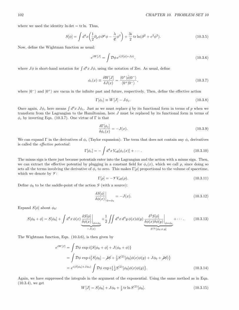
102 CHAPTER 10. PROBLEM SET 10
where we used the identity ln det = tr ln. Thus,
S[φ] =
∫d4x
(1
2∂µφ∂
µφ− λ
4!φ4
)+
3i
2tr ln(∂2 + e2φ2). (10.3.5)
Now, define the Wightman function as usual:
eiW [J] =
∫Dφ ei(S[φ]+Jφ), (10.3.6)
where Jφ is short-hand notation for∫d4xJφ, using the notation of Zee. As usual, define
φc(x) ≡ δW [J ]
δJ(x)=〈0+|φ|0−〉〈0+|0−〉
, (10.3.7)
where |0−〉 and |0+〉 are vacua in the infinite past and future, respectively. Then, define the effective action
Γ[φc] ≡W [J ]− Jφc. (10.3.8)
Once again, Jφc here means∫d4xJφc. Just as we must replace q by its functional form in terms of p when we
transform from the Lagrangian to the Hamiltonian, here J must be replaced by its functional form in terms ofφc by inverting Eqn. (10.3.7). One virtue of Γ is that
δΓ[φc]
δφc(x)= −J(x). (10.3.9)
We can expand Γ in the derivatives of φc (Taylor expansion). The term that does not contain any φc derivativesis called the effective potential :
Γ[φc] = −∫d4xVeff[φc(x)] + · · · . (10.3.10)
The minus sign is there just because potentials enter into the Lagrangian and the action with a minus sign. Then,we can extract the effective potential by plugging in a constant field for φc(x), which we call ρ, since doing sosets all the terms involving the derivative of φc to zero. This makes Γ[ρ] proportional to the volume of spacetime,which we denote by V :
Γ[ρ] = −V Veff(ρ). (10.3.11)
Define φ0 to be the saddle-point of the action S (with a source):
δS[φ]
δφ(x)
∣∣∣∣φ=φ0
= −J(x). (10.3.12)
Expand S[φ] about φ0:
S[φ0 + φ] = S[φ0] +
∫d4xφ(x)
δS[φ]
δφ(x)
∣∣∣∣φ=φ0︸ ︷︷ ︸
−J(x)
+1
2
∫∫d4x d4y φ(x)φ(y)
δ2S[φ]
δφ(x)δφ(y)
∣∣∣∣φ=φ0︸ ︷︷ ︸
S(2)[φ0;x,y]
+ · · · . (10.3.13)
The Wightman function, Eqn. (10.3.6), is then given by
eiW [J] =
∫Dφ exp iS[φ0 + φ] + J(φ0 + φ)
=
∫Dφ exp i
S[φ0]−Jφ+ 1
2S(2)[φ0]φ(x)φ(y) + Jφ0 +Jφ)
= ei(S[φ0]+Jφ0)
∫Dφ exp i
12S
(2)[φ0]φ(x)φ(y). (10.3.14)
Again, we have suppressed the integrals in the argument of the exponential. Using the same method as in Eqn.(10.3.4), we get
W [J ] = S[φ0] + Jφ0 + i2 tr lnS(2)[φ0]. (10.3.15)
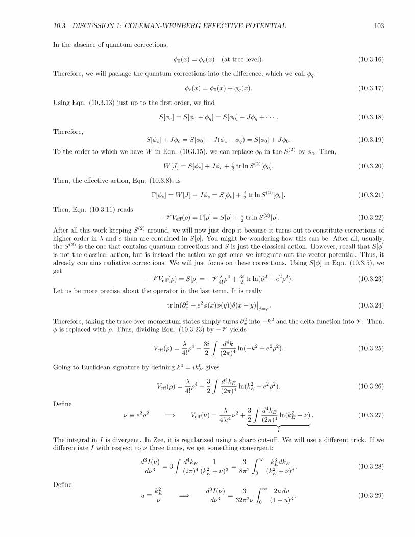
10.3. DISCUSSION 1: COLEMAN-WEINBERG EFFECTIVE POTENTIAL 103
In the absence of quantum corrections,
φ0(x) = φc(x) (at tree level). (10.3.16)
Therefore, we will package the quantum corrections into the difference, which we call φq:
φc(x) = φ0(x) + φq(x). (10.3.17)
Using Eqn. (10.3.13) just up to the first order, we find
S[φc] = S[φ0 + φq] = S[φ0]− Jφq + · · · . (10.3.18)
Therefore,S[φc] + Jφc = S[φ0] + J(φc − φq) = S[φ0] + Jφ0. (10.3.19)
To the order to which we have W in Eqn. (10.3.15), we can replace φ0 in the S(2) by φc. Then,
W [J ] = S[φc] + Jφc + i2 tr lnS(2)[φc]. (10.3.20)
Then, the effective action, Eqn. (10.3.8), is
Γ[φc] = W [J ]− Jφc = S[φc] + i2 tr lnS(2)[φc]. (10.3.21)
Then, Eqn. (10.3.11) reads− V Veff(ρ) = Γ[ρ] = S[ρ] + i
2 tr lnS(2)[ρ]. (10.3.22)
After all this work keeping S(2) around, we will now just drop it because it turns out to constitute corrections ofhigher order in λ and e than are contained in S[ρ]. You might be wondering how this can be. After all, usually,the S(2) is the one that contains quantum corrections and S is just the classical action. However, recall that S[φ]is not the classical action, but is instead the action we get once we integrate out the vector potential. Thus, italready contains radiative corrections. We will just focus on these corrections. Using S[φ] in Eqn. (10.3.5), weget
− V Veff(ρ) = S[ρ] = −V λ4!ρ
4 + 3i2 tr ln(∂2 + e2ρ2). (10.3.23)
Let us be more precise about the operator in the last term. It is really
tr ln(∂2x + e2φ(x)φ(y))δ(x− y)
∣∣φ=ρ
. (10.3.24)
Therefore, taking the trace over momentum states simply turns ∂2x into −k2 and the delta function into V . Then,
φ is replaced with ρ. Thus, dividing Eqn. (10.3.23) by −V yields
Veff(ρ) =λ
4!ρ4 − 3i
2
∫d4k
(2π)4ln(−k2 + e2ρ2). (10.3.25)
Going to Euclidean signature by defining k0 = ik0E gives
Veff(ρ) =λ
4!ρ4 +
3
2
∫d4kE(2π)4
ln(k2E + e2ρ2). (10.3.26)
Define
ν ≡ e2ρ2 =⇒ Veff(ν) =λ
4!e4ν2 +
3
2
∫d4kE(2π)4
ln(k2E + ν)︸ ︷︷ ︸
I
. (10.3.27)
The integral in I is divergent. In Zee, it is regularized using a sharp cut-off. We will use a different trick. If wedifferentiate I with respect to ν three times, we get something convergent:
d3I(ν)
dν3= 3
∫d4kE(2π)4
1
(k2E + ν)3
=3
8π2
∫ ∞0
k3EdkE
(k2E + ν)3
. (10.3.28)
Define
u ≡ k2E
ν=⇒ d3I(ν)
dν3=
3
32π2ν
∫ ∞0
2u du
(1 + u)3. (10.3.29)
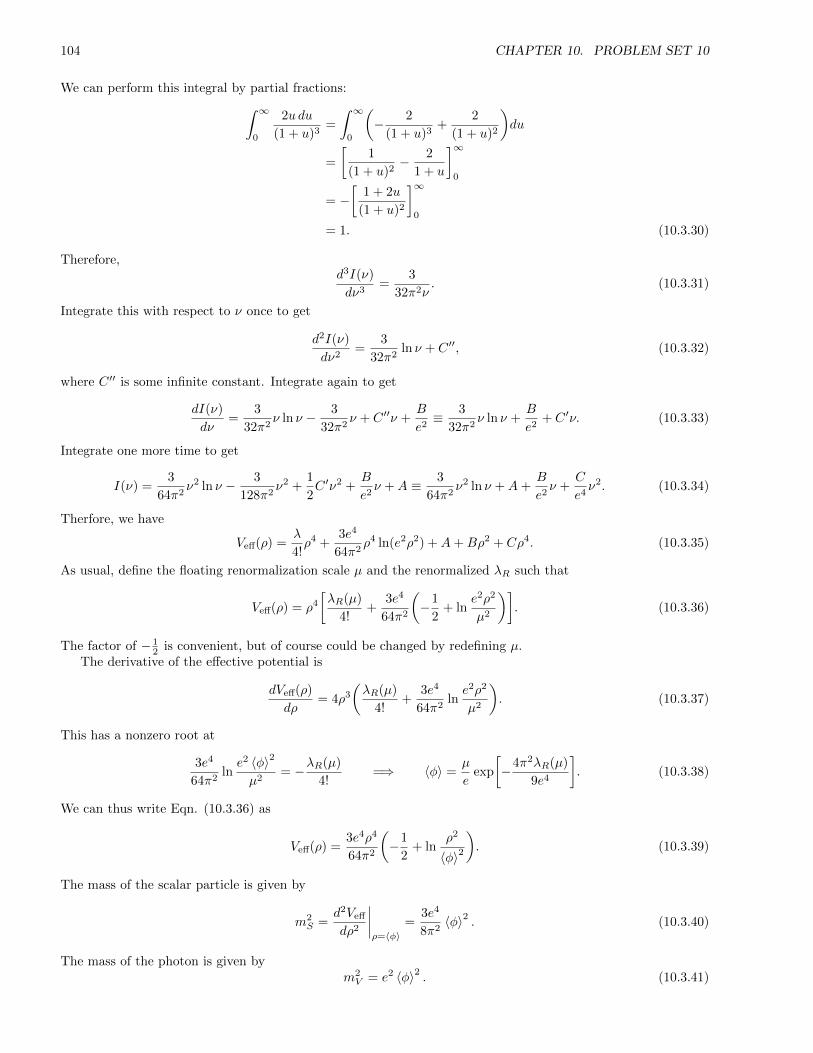
104 CHAPTER 10. PROBLEM SET 10
We can perform this integral by partial fractions:∫ ∞0
2u du
(1 + u)3=
∫ ∞0
(− 2
(1 + u)3+
2
(1 + u)2
)du
=
[1
(1 + u)2− 2
1 + u
]∞0
= −[
1 + 2u
(1 + u)2
]∞0
= 1. (10.3.30)
Therefore,d3I(ν)
dν3=
3
32π2ν. (10.3.31)
Integrate this with respect to ν once to get
d2I(ν)
dν2=
3
32π2ln ν + C ′′, (10.3.32)
where C ′′ is some infinite constant. Integrate again to get
dI(ν)
dν=
3
32π2ν ln ν − 3
32π2ν + C ′′ν +
B
e2≡ 3
32π2ν ln ν +
B
e2+ C ′ν. (10.3.33)
Integrate one more time to get
I(ν) =3
64π2ν2 ln ν − 3
128π2ν2 +
1
2C ′ν2 +
B
e2ν +A ≡ 3
64π2ν2 ln ν +A+
B
e2ν +
C
e4ν2. (10.3.34)
Therfore, we have
Veff(ρ) =λ
4!ρ4 +
3e4
64π2ρ4 ln(e2ρ2) +A+Bρ2 + Cρ4. (10.3.35)
As usual, define the floating renormalization scale µ and the renormalized λR such that
Veff(ρ) = ρ4
[λR(µ)
4!+
3e4
64π2
(−1
2+ ln
e2ρ2
µ2
)]. (10.3.36)
The factor of − 12 is convenient, but of course could be changed by redefining µ.
The derivative of the effective potential is
dVeff(ρ)
dρ= 4ρ3
(λR(µ)
4!+
3e4
64π2lne2ρ2
µ2
). (10.3.37)
This has a nonzero root at
3e4
64π2lne2 〈φ〉2
µ2= −λR(µ)
4!=⇒ 〈φ〉 =
µ
eexp
[−4π2λR(µ)
9e4
]. (10.3.38)
We can thus write Eqn. (10.3.36) as
Veff(ρ) =3e4ρ4
64π2
(−1
2+ ln
ρ2
〈φ〉2
). (10.3.39)
The mass of the scalar particle is given by
m2S =
d2Veff
dρ2
∣∣∣∣ρ=〈φ〉
=3e4
8π2〈φ〉2 . (10.3.40)
The mass of the photon is given bym2V = e2 〈φ〉2 . (10.3.41)
10.4. DISCUSSION 2: A LOWER BOUND ON THE HIGGS MASS 105
Let us be clear about the logic here. Without experimental input, all we can say is that both the scalar andvector particles gain mass. But these masses are theoretically arbitrary since they are proportional to the as-yet-undetermined vev 〈φ〉. However, if we can perform an experiment in an energy scale where the value of e isknown and that can be sensitive only to something like the ratio of the masses, then this could really make orbreak the theory because the mass ratio is independent of the unknown 〈φ〉.
Even though there is no natural mass scale to begin with, since we started with a massless theory, we wereforced to introduce a floating renormalization scale, µ. If the theory is really scale-free, then we should expectthat all renormalization points be equivalent. However, we find that this is not the case. Instead, the scale µrelated to 〈φ〉 is singled out. This singling out of a mass scale from a theory that originally has no preferred massscale is called dimensional transmutation. The name is apt because the cut-off or renormalization scale has beentransmuted into a physical mass.
Something of this sort happens in QCD. We start off with massless u and d quarks and end up with themassive spectrum of hadrons as bound states. The story there is a fair bit more complicated, however.
Finally, before we move on to the Higgs, we should motivate, in hindsight, introducing the photon to beginwith. In the regular massless scalar theory, we get a very similar form for the effective potential roughly via theidentification λ ∼ e2. Looking at Eqn. (10.3.38), we see that this would force us to equate a term of order λwith one of order λ2 thereby taking us outside the regime of validity of perturbation theory. By coupling to thephoton, we introduce the second coupling constant, e, such that e4 is basically able to play the role of λ2 andthis problem vanishes since these two coupling constants are independent.
Alternative derivation:
In the pure massless scalar case, the one-loop effective action was found to be (Eqn. 12 Zee p.239)
Γ[φc] =
∫d4x
(1
2∂µφc∂
µφc −λ
4!φ4c
)+i
2tr ln
(∂2 +
λ
2φ2c
). (10.3.42)
If we drop the S(2) term, Eqn. (10.3.21) reads
Γ[φc] = S[φc] =
∫d4x
(1
2∂µφc∂
µφc −λ
4!φ4c
)+
3i
2tr ln
(∂2 + e2φ2
c
). (10.3.43)
Recall that Eqn. (10.3.42) leads to a solution to V ′eff = 0 that requires equating a tree level result (order λ) witha quantum correction (order λ2). The equation at some appropriately chosen renormalization scale, µ, can bewritten as
λ = − 3
32π2λ2 ln
λ 〈φ〉2
2µ2. (10.3.44)
The λ on the left comes directly from the action and the λ2 on the right comes from the quantum correction inEqn. (10.3.42) (i.e. the tr ln term). We see how coupling to the photon avoids this problem: the λ on the rightis replaced by ∼ e2. Since λ and e are independent coupling constants, the equation can be solved within theregime of validity of perturbation theory. That is, both λ and e can be small while producing a solution for 〈φ〉2.To get the equation in the photon-coupled case, we replace λ with 2e on the right hand side of Eqn. (10.3.44) andmultiply by 3 due to the extra factor of 3 in the trace term of Eqn. (10.3.43). Then, we multiply the numeratorand denominator by 2 for convenience:
λ = −2
2· 3 · 3
32π2(2e2)2 ln
e2 〈φ〉2
µ2=⇒ λ
4!= − 3e4
64π2lne2 〈φ〉2
µ2. (10.3.45)
This reproduces Eqn. (10.3.38).
10.4 Discussion 2: A Lower Bound on the Higgs Mass
Letus now think of the scalar field in the previous section as the one component of the SU(2) doublet Higgs fieldthat cannot be gauged away. This time, we have three vector fields corresponding to the W± and Z0 bosons. Ifwe start of with a “mass” term for the Higgs, the the generalization of the effective potential in Eqn. (10.3.36)would be
Veff(ρ) =λ
4!ρ4 +
1
2m2ρ2 +
3ρ4
64π2
3∑i=1
e2i
(−1
2+ ln
e2i ρ
2
µ2
), (10.4.1)
106 CHAPTER 10. PROBLEM SET 10
where ei is the coupling appropriate to the three vector bosons. Since we are not starting from scratch, let usconsider these parameters to already be renormalized.
If the Higgs develops a nonzero vev, 〈φ〉, then the vector masses are
m2i = e2
i 〈φ〉2. (10.4.2)
Redefine µ′ to be the scale at which
λ
4!= − 3
64π2
3∑i=1
e4i ln
e2i ρ
2
µ′2. (10.4.3)
Then,
Veff(ρ) =1
2m2ρ2 +
3ρ4
64π2
3∑i=1
e4i
(−1
2+ ln
µ′2ρ2
µ2
). (10.4.4)
Redefine µ first to be µ/µ′ and then to absorb the − 12 factor. Then,
Veff(ρ) =1
2m2ρ2 +
3ρ4
64π2 〈φ〉43∑i=1
m4i ln
ρ2
µ2. (10.4.5)
It is convenient to define
α ≡ 3
64π2 〈φ〉43∑i=1
m4i =
3
64π2 〈φ〉4(2m4
W +m4Z). (10.4.6)
Then,
Veff(ρ) =1
2m2ρ2 + αρ4 ln
ρ2
µ2. (10.4.7)
The first and second derivatives are
dVeff(ρ)
dρ= m2ρ+ 4αρ3
(1
2+ ln
ρ2
µ2
), (10.4.8a)
d2Veff(ρ)
dρ2= m2 + 12αρ2
(7
6+ ln
ρ2
µ2
).
Vanishing of the first derivative yields the equation
m2 = −4α 〈φ〉2(
1
2+ ln
〈φ〉2
µ2
), (10.4.9)
which, when plugged into the potential and its second derivative gives
Veff(〈φ〉) = −α 〈φ〉4(
1 + ln〈φ〉2
µ2
), (10.4.10a)
d2Veff(ρ)
dρ2
∣∣∣∣ρ=〈φ〉
= 8α 〈φ〉2(
3
2+ ln
〈φ〉2
µ2
). (10.4.10b)
Veff(0) = 0 implies that if Eqn. (10.4.10a) is positive then it is a local minimum, but higher than the minimumat ρ = 0. It is at best a metastable state. Therefore, in order to have spontaneous symmetry breaking, we musthave
ln〈φ〉2
µ2≥ −1. (10.4.11)
Eqn. (10.4.10b) gives the physical Higgs mass on which we therefore get a lower bound:
m2H ≥ 4α 〈φ〉2 =
3
16π2 〈φ〉2(2m4
W +m4Z). (10.4.12)
Often, 〈φ〉 is called v when it pertains to the Higgs. This is called the electroweak scale. It is related to the Fermicoupling constant via
v = 2−1/4G−1/2F . (10.4.13)
10.4. DISCUSSION 2: A LOWER BOUND ON THE HIGGS MASS 107
We have experimental values for GF (e.g. via neutron beta decay), and thus for v. We also have experimentalvalues for the W and Z masses (e.g. leptonic decays and the neutral K decay). The accepted values are
v = 246 GeV, mW = 80.4 GeV, mZ = 91.2 GeV. (10.4.14)
Plugging these numbers into Eqn. (10.4.12) gives
mH ≥ 6.92 GeV. (10.4.15)

108 CHAPTER 10. PROBLEM SET 10
Chapter 11
Problem Set 11
11.1 The Gross-Neveu Model, P&S 11.3 p.390
The Gross-Neveu model is a model in two spacetime dimensions of fermions with a discrete chiral symmetry:
L = ψii/∂ψi + 12g
2(ψiψi
)2, (11.1.1)
with i = 1, . . . , N . The kinetic term of two-dimensional fermions is built from matrices γµ taht satisfy thetwo-dimensional Dirac algebra. These matrices can be 2× 2:
γ0 = σ2, γ1 = iσ1, (11.1.2)
where σi are Pauli sigma matrices. Defineγ5 = γ0γ1 = σ3; (11.1.3)
this matrix anticommutes with the γµ.
(a) Show that this theory is invariant with respect to
ψi → γ5ψi, (11.1.4)
and that this symmetry forbids the appearance of a fermion mass.
(b) Show that this theory is renormalizable in 2 dimensions (at the level of dimensional analysis).
(c) Show that the functional integral for this theory can be represented in the following form:∫DψDψ ei
∫d2xL =
∫DψDψDσ exp
[i
∫d2x
(ψii/∂ψi − σψiψi −
1
2g2σ2
)], (11.1.5)
where σ(x) (not to be confused with a Pauli matrix) is a new scalar field with no kinematic energy terms.
(d) Compute the leading correction to the effective potential for σ by integrating over the fermion fields ψi. Youwill encounter the determinant of a Dirac operator; to evaluate this determinant, diagonalize the operator byfirst going to Fourier components and then diagonalizing the 2× 2 Pauli matrix associated with each Fouriermode. (Alternatively, you might just take the determinant of this 2 × 2 matrix.) This 1-loop contributionrequires a renormalization proportional to σ2 (that is, a renormalization of g2). Renormalize by minimalsubtraction.
(e) Ignoring two-loop and higher-order contributions, minimize this potential. Show that the σ field acquires avacuum expectation value which breaks the symmetry of part (a). Convince yourself that this result doesnot depend on the particular renormalization condition chosen.
(f) Note that the effective potential derived in part (e) depends on g and N according to the form
Veff(σcl) = N · f(g2N). (11.1.6)
(The overall factor of N is expected in a theory with N fields.) Construct a few of the higher-order contri-butions to the effective potential and show that they contain additional factors of N−1 which suppress themif we take the limit N →∞, with g2N fixed. In this limit, the result of part (e) is unambiguous.
109
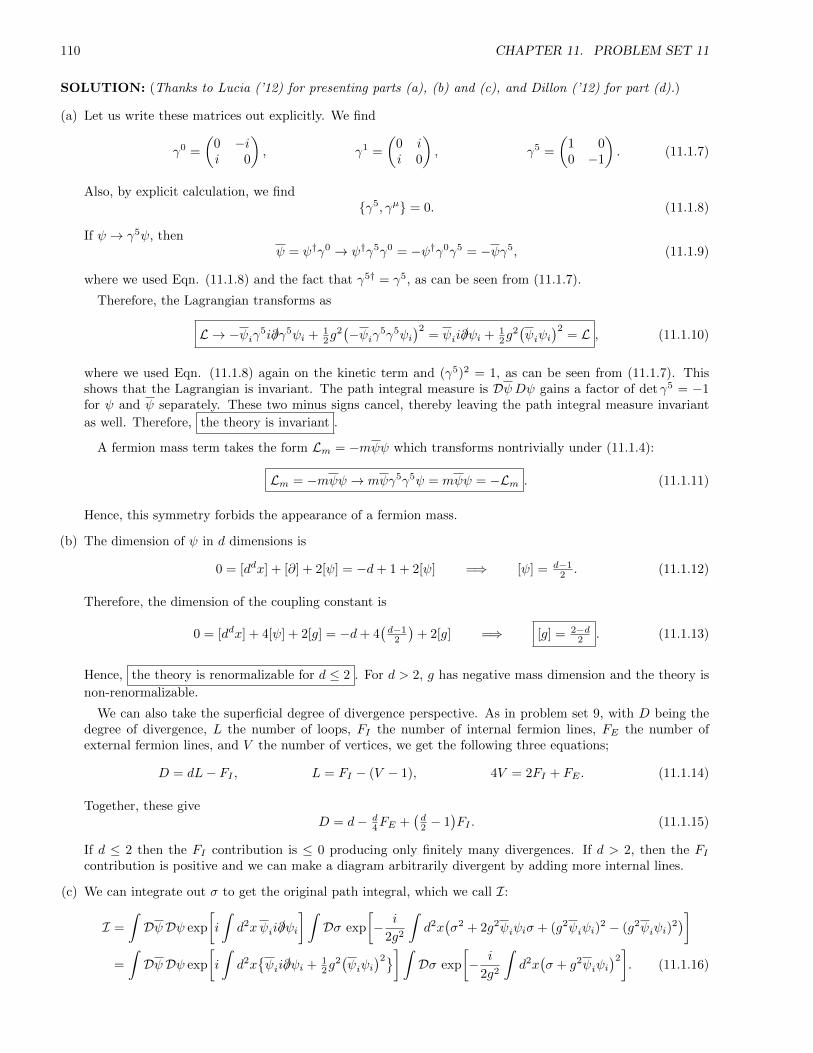
110 CHAPTER 11. PROBLEM SET 11
SOLUTION: (Thanks to Lucia (’12) for presenting parts (a), (b) and (c), and Dillon (’12) for part (d).)
(a) Let us write these matrices out explicitly. We find
γ0 =
(0 −ii 0
), γ1 =
(0 ii 0
), γ5 =
(1 00 −1
). (11.1.7)
Also, by explicit calculation, we findγ5, γµ = 0. (11.1.8)
If ψ → γ5ψ, thenψ = ψ†γ0 → ψ†γ5γ0 = −ψ†γ0γ5 = −ψγ5, (11.1.9)
where we used Eqn. (11.1.8) and the fact that γ5† = γ5, as can be seen from (11.1.7).
Therefore, the Lagrangian transforms as
L → −ψiγ5i/∂γ5ψi + 12g
2(−ψiγ5γ5ψi
)2= ψii/∂ψi + 1
2g2(ψiψi
)2= L , (11.1.10)
where we used Eqn. (11.1.8) again on the kinetic term and (γ5)2 = 1, as can be seen from (11.1.7). Thisshows that the Lagrangian is invariant. The path integral measure is DψDψ gains a factor of det γ5 = −1for ψ and ψ separately. These two minus signs cancel, thereby leaving the path integral measure invariant
as well. Therefore, the theory is invariant .
A fermion mass term takes the form Lm = −mψψ which transforms nontrivially under (11.1.4):
Lm = −mψψ → mψγ5γ5ψ = mψψ = −Lm . (11.1.11)
Hence, this symmetry forbids the appearance of a fermion mass.
(b) The dimension of ψ in d dimensions is
0 = [ddx] + [∂] + 2[ψ] = −d+ 1 + 2[ψ] =⇒ [ψ] = d−12 . (11.1.12)
Therefore, the dimension of the coupling constant is
0 = [ddx] + 4[ψ] + 2[g] = −d+ 4(d−1
2
)+ 2[g] =⇒ [g] = 2−d
2 . (11.1.13)
Hence, the theory is renormalizable for d ≤ 2 . For d > 2, g has negative mass dimension and the theory is
non-renormalizable.
We can also take the superficial degree of divergence perspective. As in problem set 9, with D being thedegree of divergence, L the number of loops, FI the number of internal fermion lines, FE the number ofexternal fermion lines, and V the number of vertices, we get the following three equations;
D = dL− FI , L = FI − (V − 1), 4V = 2FI + FE . (11.1.14)
Together, these giveD = d− d
4FE +(d2 − 1
)FI . (11.1.15)
If d ≤ 2 then the FI contribution is ≤ 0 producing only finitely many divergences. If d > 2, then the FIcontribution is positive and we can make a diagram arbitrarily divergent by adding more internal lines.
(c) We can integrate out σ to get the original path integral, which we call I:
I =
∫DψDψ exp
[i
∫d2xψii/∂ψi
] ∫Dσ exp
[− i
2g2
∫d2x(σ2 + 2g2ψiψiσ + (g2ψiψi)
2 − (g2ψiψi)2)]
=
∫DψDψ exp
[i
∫d2xψii/∂ψi + 1
2g2(ψiψi
)2]∫ Dσ exp
[− i
2g2
∫d2x(σ + g2ψiψi
)2]. (11.1.16)

11.1. THE GROSS-NEVEU MODEL, P&S 11.3 P.390 111
One can shift and rescale σ and since the shift and rescaling is independent of σ, the path integral measurechanges by at most an overall constant, which we can simply absorb into the fermion integral measure orneglect since it drops out when taking expectation values.
I =
∫DψDψ eiS . (11.1.17)
(d) Denote the action containing fermions and σ by S[ψi, ψi, σ]. Let S[σ] be the action for σ when the ψi areintegrated out. Let I now denote the integration over the fermion fields:
I =
∫DψDψ exp
[i
∫d2xψi(i/∂ − σ)ψi
]= DetN (i/∂ − σ) = exp
[N Tr ln(i/∂ − σ)
], (11.1.18)
where we used the identity ln Det = Tr ln. The trace involves integration over phase space as well as a traceover the spinor indices, which we denote by tr. Analogously, we use Det to mean the total determinant andwe reserve det for the determinant over spinor space:
Tr ln(i/∂ − σ) =
∫d2x d2p
(2π)2tr ln(/p− σ) =
∫d2x d2p
(2π)2ln det(/p− σ). (11.1.19)
The latter determinant is
det(/p− σ) = det
(−σ −i(p0 + p1)
i(p0 − p1) −σ
)= σ2 − (p0)2 + (p1)2 = −p2 + σ2. (11.1.20)
Therefore,
I = exp
[N
∫d2x d2p
(2π)2ln(−p2 + σ2)
]. (11.1.21)
Wick-rotate the p0 integral by defining p0 = ip0E so that
I = exp
[iN
∫d2x d2pE
(2π)2ln(p2
E + σ2)
]. (11.1.22)
Therefore, we have the action just in terms of σ:
S[σ] =
∫d2x
(− 1
2g2σ2 +N
∫d2pE(2π)2
ln(p2E + σ2)︸ ︷︷ ︸
L(1)
). (11.1.23)
We can use several different methods to calculate L(1):
Method 1 (Sharp cut-off): As in Zee, we will subtract a constant (infinite, but constant and thusirrelevant) to make the argument of the logarithm unitless.
ln(p2E + σ2)→ ln(p2
E + σ2)− ln p2E . (11.1.24)
Then, we write this in a convenient form as an integral:
ln(p2E + σ2)− ln p2
E =
∫ σ2
0
du
p2E + u
. (11.1.25)
Then, we can switch the order of integration (between u and pE):
L(1) =
∫d2pE(2π)2
ln
(p2E + σ2
p2E
)=
1
2π
∫ Λ
0
dpE pE
∫ σ2
0
du
p2E + u
=1
4π
∫ σ2
0
du
∫ Λ
0
2pE dpEp2E + u
. (11.1.26)
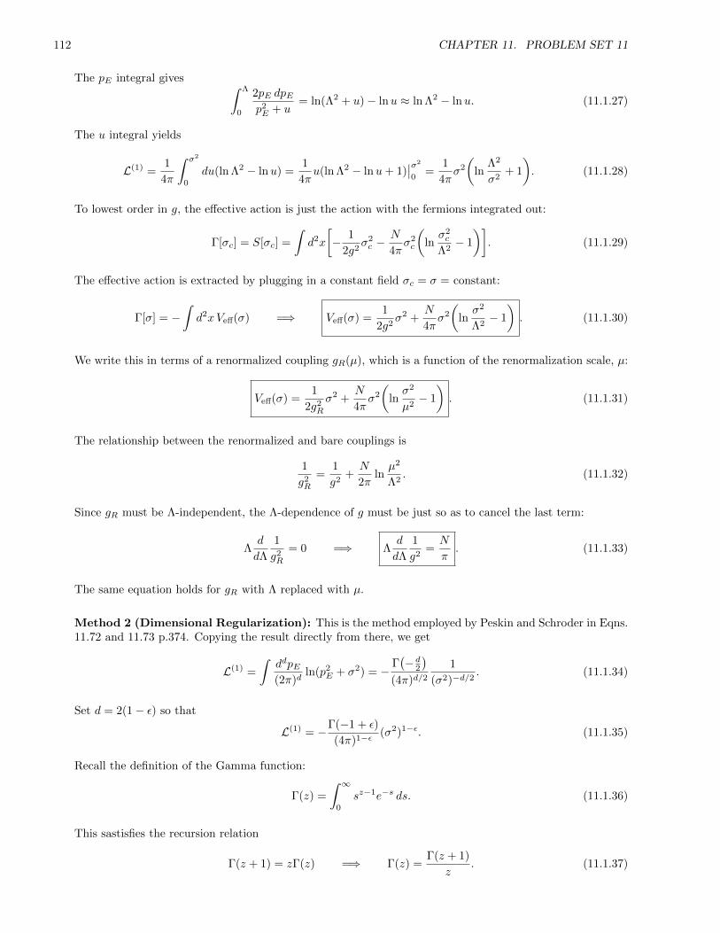
112 CHAPTER 11. PROBLEM SET 11
The pE integral gives ∫ Λ
0
2pE dpEp2E + u
= ln(Λ2 + u)− lnu ≈ ln Λ2 − lnu. (11.1.27)
The u integral yields
L(1) =1
4π
∫ σ2
0
du(ln Λ2 − lnu) =1
4πu(ln Λ2 − lnu+ 1)
∣∣σ2
0=
1
4πσ2
(ln
Λ2
σ2+ 1
). (11.1.28)
To lowest order in g, the effective action is just the action with the fermions integrated out:
Γ[σc] = S[σc] =
∫d2x
[− 1
2g2σ2c −
N
4πσ2c
(lnσ2c
Λ2− 1
)]. (11.1.29)
The effective action is extracted by plugging in a constant field σc = σ = constant:
Γ[σ] = −∫d2xVeff(σ) =⇒ Veff(σ) =
1
2g2σ2 +
N
4πσ2
(lnσ2
Λ2− 1
). (11.1.30)
We write this in terms of a renormalized coupling gR(µ), which is a function of the renormalization scale, µ:
Veff(σ) =1
2g2R
σ2 +N
4πσ2
(lnσ2
µ2− 1
). (11.1.31)
The relationship between the renormalized and bare couplings is
1
g2R
=1
g2+N
2πlnµ2
Λ2. (11.1.32)
Since gR must be Λ-independent, the Λ-dependence of g must be just so as to cancel the last term:
Λd
dΛ
1
g2R
= 0 =⇒ Λd
dΛ
1
g2=N
π. (11.1.33)
The same equation holds for gR with Λ replaced with µ.
Method 2 (Dimensional Regularization): This is the method employed by Peskin and Schroder in Eqns.11.72 and 11.73 p.374. Copying the result directly from there, we get
L(1) =
∫ddpE(2π)d
ln(p2E + σ2) = −
Γ(−d2)
(4π)d/21
(σ2)−d/2. (11.1.34)
Set d = 2(1− ε) so that
L(1) = −Γ(−1 + ε)
(4π)1−ε (σ2)1−ε. (11.1.35)
Recall the definition of the Gamma function:
Γ(z) =
∫ ∞0
sz−1e−s ds. (11.1.36)
This sastisfies the recursion relation
Γ(z + 1) = zΓ(z) =⇒ Γ(z) =Γ(z + 1)
z. (11.1.37)
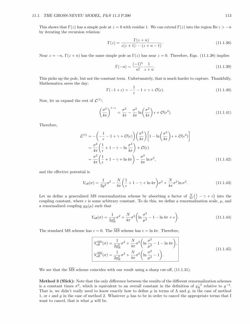
11.1. THE GROSS-NEVEU MODEL, P&S 11.3 P.390 113
This shows that Γ(z) has a simple pole at z = 0 with residue 1. We can extend Γ(z) into the region Re z > −nby iterating the recursion relation:
Γ(z) =Γ(z + n)
z(z + 1) · · · (z + n− 1). (11.1.38)
Near z = −n, Γ(z + n) has the same simple pole as Γ(z) has near z = 0. Therefore, Eqn. (11.1.38) implies
Γ(−n) ∼ (−1)n
n!
1
z + n. (11.1.39)
This picks up the pole, but not the constant term. Unfortunately, that is much harder to capture. Thankfully,Mathematica saves the day:
Γ(−1 + ε) = −1
ε− 1 + γ +O(ε). (11.1.40)
Now, let us expand the rest of L(1):(σ2
4π
)1−ε
=σ2
4π− σ2
4πln
(σ2
4π
)ε+O(ε2). (11.1.41)
Therefore,
L(1) = −(−1
ε− 1 + γ +O(ε)
)(σ2
4π
)[1− ln
(σ2
4π
)ε+O(ε2)
]=σ2
4π
(1
ε+ 1− γ − ln
σ2
4π
)+O(ε)
=σ2
4π
(1
ε+ 1− γ + ln 4π
)− σ2
4πlnσ2, (11.1.42)
and the effective potential is
Veff(σ) =1
2g2σ2 − N
4π
(1
ε+ 1− γ + ln 4π
)σ2 +
N
4πσ2 lnσ2. (11.1.43)
Let us define a generalized MS renormalization scheme by absorbing a factor of N4π
(1ε − γ + c
)into the
coupling constant, where c is some arbitrary constant. To do this, we define a renormalization scale, µ, anda renormalized coupling gR(µ) such that
Veff(σ) =1
2g2R
σ2 +N
4πσ2
(lnσ2
µ2− 1− ln 4π + c
). (11.1.44)
The standard MS scheme has c = 0. The MS scheme has c = ln 4π. Therefore,
V MSeff (σ) =
1
2g2R
σ2 +N
4πσ2
(lnσ2
µ2− 1− ln 4π
),
V MSeff (σ) =
1
2g2R
σ2 +N
4πσ2
(lnσ2
µ2− 1
).
(11.1.45)
We see that the MS scheme coincides with our result using a sharp cut-off, (11.1.31).
Method 3 (Slick): Note that the only difference between the results of the different renormalization schemesis a constant times σ2, which is equivalent to an overall constant in the definition of g−2
R relative to g−2.That is, we didn’t really need to know exactly how to define µ in terms of Λ and g, in the case of method1, or ε and g in the case of method 2. Whatever µ has to be in order to cancel the appropriate terms that Iwant to cancel, that is what µ will be.
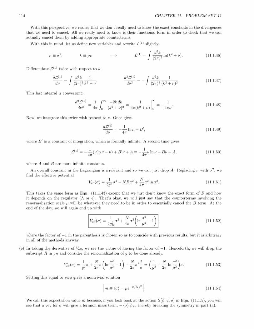
114 CHAPTER 11. PROBLEM SET 11
With this perspective, we realize that we don’t really need to know the exact constants in the divergencesthat we need to cancel. All we really need to know is their functional form in order to check that we canactually cancel them by adding appropriate counterterms.
With this in mind, let us define new variables and rewrite L(1) slightly:
ν ≡ σ2, k ≡ pE =⇒ L(1) =
∫d2k
(2π)2ln(k2 + ν). (11.1.46)
Differentiate L(1) twice with respect to ν:
dL(1)
dν=
∫d2k
(2π)2
1
k2 + ν,
d2L(1)
dν2= −
∫d2k
(2π)2
1
(k2 + ν)2. (11.1.47)
This last integral is convergent:
d2L(1)
dν2=
1
4π
∫ ∞0
−2k dk
(k2 + ν)2=
1
4π(k2 + ν)
∣∣∣∣∞0
= − 1
4πν. (11.1.48)
Now, we integrate this twice with respect to ν. Once gives
dL(1)
dν= − 1
4πln ν +B′, (11.1.49)
where B′ is a constant of integration, which is formally infinite. A second time gives
L(1) = − 1
4π(ν ln ν − ν) +B′ν +A ≡ − 1
4πν ln ν +Bν +A, (11.1.50)
where A and B are more infinite constants.
An overall constant in the Lagrangian is irrelevant and so we can just drop A. Replacing ν with σ2, wefind the effective potential
Veff(σ) =1
2g2σ2 −NBσ2 +
N
4πσ2 lnσ2. (11.1.51)
This takes the same form as Eqn. (11.1.43) except that we just don’t know the exact form of B and howit depends on the regulator (Λ or ε). That’s okay, we will just say that the counterterms involving therenormalization scale µ will be whatever they need to be in order to essentially cancel the B term. At theend of the day, we will again end up with
Veff(σ) =1
2g2R
σ2 +N
4πσ2
(lnσ2
µ2− 1
), (11.1.52)
where the factor of −1 in the parenthesis is chosen so as to coincide with previous results, but it is arbitraryin all of the methods anyway.
(e) In taking the derivative of Veff, we see the virtue of having the factor of −1. Henceforth, we will drop thesubscript R in gR and consider the renormalization of g to be done already.
V ′eff(σ) =1
g2σ +
N
2πσ
(lnσ2
µ2− 1
)+N
2πσ2 2
σ=
(1
g2+N
2πlnσ2
µ2
)σ. (11.1.53)
Setting this equal to zero gives a nontrivial solution
m ≡ 〈σ〉 = µe−π/Ng2
. (11.1.54)
We call this expectation value m because, if you look back at the action S[ψ,ψ, σ] in Eqn. (11.1.5), you willsee that a vev for σ will give a fermion mass term, −〈σ〉ψψ, thereby breaking the symmetry in part (a).
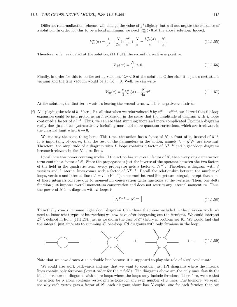
11.1. THE GROSS-NEVEU MODEL, P&S 11.3 P.390 115
Different renormalization schemes will change the value of g2 slightly, but will not negate the existence ofa solution. In order for this to be a local minimum, we need V ′′eff > 0 at the above solution. Indeed,
V ′′eff(σ) =1
g2+N
2πlnσ2
µ2+N
π=V ′eff(σ)
σ+N
π. (11.1.55)
Therefore, when evaluated at the solution, (11.1.54), the second derivative is positive:
V ′′eff(m) =N
π> 0. (11.1.56)
Finally, in order for this to be the actual vacuum, Veff < 0 at the solution. Otherwise, it is just a metastablevacuum and the true vacuum would be at 〈σ〉 = 0. Well, we can write
Veff(σ) =σ
2V ′eff(σ)− N
4πσ2. (11.1.57)
At the solution, the first term vanishes leaving the second term, which is negative as desired.
(f) N is playing the role of ~−1 here. Recall that when we reintroduced ~ by eiS → eiS/~, we showed that the loopexpansion could be interpreted as an ~ expansion in the sense that the amplitude of diagram with L loopscontained a factor of ~L−1. Thus, we can see that summing more and more complicated Feynman diagramsreally does just mean systematically including more and more quantum corrections, which are irrelevant inthe classical limit when ~→ 0.
We can say the same thing here. This time, the action has a factor of N in front of it, instead of ~−1.It is important, of course, that the rest of the parameters in the action, namely λ = g2N , are constant.Therefore, the amplitude of a diagram with L loops contains a factor of N1−L and higher-loop diagramsbecome irrelevant in the N →∞ limit.
Recall how this power counting works. If the action has an overall factor of N , then every single interactionterm contains a factor of N . Since the propagator is just the inverse of the operator between the two factorsof the field in the quadratic term, every propagator gets a factor of N−1. Therefore, a diagram with Vvertices and I internal lines comes with a factor of NV−I . Recall the relationship between the number ofloops, vertices and internal lines: L = I − (V − 1), since each internal line gets an integral, except that someof these integrals collapse due to momentum conservation delta functions at the vertices. Then, one deltafunction just imposes overall momentum conservation and does not restrict any internal momentum. Thus,the power of N in a diagram with L loops is
NV−I = N1−L . (11.1.58)
To actually construct some higher-loop diagrams than those that were included in the previous work, weneed to know what types of interactions we now have after integrating out the fermions. We could interpretL(1), defined in Eqn. (11.1.23), just as we did in the case of φ4 theory in problem set 10. We would find thatthe integral just amounts to summing all one-loop 1PI diagrams with only fermions in the loop:
+
@@@@
@@@@
+
TTT
TTT
TTT
TTT
+ · · · (11.1.59)
Note that we have drawn σ as a double line because it is supposed to play the role of a ψψ condensate.
We could also work backwards and say that we want to consider just 1PI diagrams where the internallines contain only fermions (lowest order for the σ field). The diagrams above are the only ones that fit thebill! There are no diagrams with more loops where the loops only include fermions. Therefore, we see thatthe action for σ alone contains vertex interactions for any even number of σ lines. Furthermore, we easilysee why each vertex gets a factor of N : each diagram above has N copies, one for each fermion that can

116 CHAPTER 11. PROBLEM SET 11
run around the loop. Therefore, the one-loop diagrams in the σ theory would be the following. Since thefermions are gone now, we will just use single lines to denote σ.
QQQ
+
QQQ
QQQ
+ · · ·
@@aa
a!!!
+ · · · (11.1.60)
Three examples of two-loop diagrams are
QQQ
QQQ
QQQ
(11.1.61)
11.2 Discussion 1: Clarification Regarding the Effective Potential
Before we move on to discuss the Gross-Neveu model specifically, I want to correct (or qualify) something I saidduring last discussion section with regards to the Zee problem. We were supposed to interpret the one-loopeffective potential for φ4 theory as a sum over one-loop 1PI diagrams. We saw that the internal propagators allhad momentum k and the external lines could be interchanged in pairs and swapped within each pair that isattached to the same point on the loop. This makes the diagram considerably more symmetric than it usuallyis and gave us the symmetry factor 2n(2n). I said that we only care about the divergence of the diagram, as faras renormalization is concerned, and in this limit, we can neglect all momenta except the internal momentum,k. While this is true, it happens that when we calculate the effective potential, we are actually supposed to setall the external momenta to zero. Therefore, the statement about only caring about the large k divergence isactually superfluous. Let us see how this works.
The point is to compare the two ways we can expand the effective action: (a) in powers of the field; and (b)in powers of derivatives of the field. It will be more convenient to consider the expansion in powers of the Fouriertransform of the field instead:
Γ[φc] =
∞∑n=0
1
n!
∫Γn(k1, . . . , kn) (2π)4δ(k1 + · · ·+ kn)
n∏i=1
φc(ki)d4ki(2π)4
, (11.2.1a)
Γ[φc] =
∫d4x[−Veff(φc) + higher-derivatives
]. (11.2.1b)
To isolate the effective potential, we plug in a constant value for φc, which we call ρ. In this case,
φc(k) =
∫d4x eikxρ = (2π)4ρ δ(k). (11.2.2)
Therefore,
Γ[ρ] =
∞∑n=0
1
n!
∫Γn(k1, . . . , kn) (2π)4δ(k1 + · · ·+ kn)
n∏i=1
ρ δ(ki) d4ki
=
∞∑n=0
ρn
n!Γn(0) (2π)4δ(0). (11.2.3)
Using (2π)4δ(0) =∫d4x, and the fact that everything in Eqn. (11.2.3) is independent of spacetime, we can write
the effective action with constant field as
Γ[ρ] =
∫d4x
∞∑n=0
ρn
n!Γn(0) = −
∫d4xVeff(ρ), (11.2.4)
where we have used the fact that the higher derivative terms in Eqn. (11.2.1b) vanish when φc = ρ is constant.Therefore, when calculating the effective potential, the external lines are supposed have zero 4-momentum.
11.3. DISCUSSION 2: MORE ON GROSS-NEVEU 117
11.3 Discussion 2: More on Gross-Neveu
The Gross-Neveu model is actually just the 2D version of a theory of dynamical symmetry breaking proposed byNambu and Jona-Lasinio to explain spontaneous chiral symmetry breaking. The virtue of the 2D version is thatthe 4-Fermi interaction is renormalizable in 2D whereas it is non-renormalizable in 4D.
The difference between this type of symmetry breaking and the Higgs mechanism is that the latter requiresthe introduction of a separate scalar field to explain the symmetry breaking and, as often happens, the massesthat result. On the other hand, dynamical symmetry breaking does not require coupling to a separate field.Instead, interactions in the field(s) that is already present in the description of the system force composite“particles”, built out of the pre-existing particles, to form a condensate (i.e. a non-vanishing vev). This isexactly what happens in the BCS theory of superconductivity in which pairs of electrons of opposite spin formbound Cooper pairs. Therefore, the Higgs mechanism in particle physics is analogous to the Ginzburg-Landautheory of superconductivity while the Gross-Neveu model and other theories exhibiting dynamical symmetrybreaking are analogous to the BCS theory of superconductivity.
Since σ is supposed to play the role of the bound state of ψψ that gains a vev, and since this mechanism givesa mass to the fermions, m, we would expect the σ bound state to have mass as well. The difference between mσ
and 2m ought to be interpreted as a binding energy. We will find that this binding energy is a ≥ 2-loop effectand vanishes even at one-loop.
We learned in part (e) of the problem that σ gains a vev, which we called m. Then, when we shift σ → m+σ,the Lagrangian becomes
L = ψ(i/∂ −m)ψ − σψψ − m2
2g2 − mg2σ − 1
2g2σ2. (11.3.1)
The constant and linear term in σ are unimportant and we neglect them. We would like to see the effect of thepresence of the fermions on the σ propagator. Thus, we want to integrate out the fermions, but only focus onthe term that contributes to the σ propagator, which is the first diagram in (11.1.59).
At tree level, the amplitude for the two-point function in σ (inverse propagator) is
Γ(0)2 = − i
g2 . (11.3.2)
The amplitude for the first diagram in (11.1.59) is
iM = −i∫
d2k
(2π)2tr
(i(/k + /p+m)
(k + p)2 −m2· i(
/k +m)
k2 −m2
)= −
∫ 1
0
dx
∫d2k
(2π)2
tr[(/k + /p+m)(/k +m)]x[(k + p)2 −m2] + (1− x)(k2 −m2)
2 . (11.3.3)
The denominator is written as D2 where
D = k2 + 2xp · k + x2p2 − x2p2 + xp2 −m2 = (k + xp)2 + x(1− x)p2 −m2 = `2 −∆, (11.3.4)
where
` = k + xp, ∆ = m2 − x(1− x)p2. (11.3.5)
In simplifying the numerator, we will automatically drop terms linear in ` since they vanish upon integrating over`. Furthermore, we will drop traces of a single slashed object since the gamma matrices are traceless. Finally,we use the identity /p
2 = p2, which is a result of the defining relation γµ, γν = 2gµν . Thus,
num = tr[`2 − x(1− x)p2 +m2] = tr(`2 + ∆) = 2(`2 + ∆). (11.3.6)
Therefore, altogether, we have
iM = −2
∫ 1
0
dx
∫d2`
(2π)2
`2 + ∆
(`2 −∆)2= −2
∫ 1
0
dx
∫d2`
(2π)2
(1
`2 −∆+
2∆
(`2 −∆)2
). (11.3.7)
Wick rotate to
iM = −2i
∫ 1
0
dx
∫d2`E(2π)2
(2∆
(`2E + ∆)2− 1
`2E + ∆
). (11.3.8)
118 CHAPTER 11. PROBLEM SET 11
Let us calculate each ` integral one at a time:∫d2`E(2π)2
2∆
(`2E + ∆)2=
∆
2π
∫ ∞0
2`E d`E(`2E + ∆)2
= − ∆
2π
1
`2E + ∆
∣∣∣∣∞0
= − ∆
2π
(0− 1
∆
)=
1
2π. (11.3.9)
The next integral is log divergent and requires regularization:
−∫
d2`E(2π)2
1
`2E + ∆= − 1
4π
∫ Λ
0
2`E d`E`2E + ∆
= − 1
4πln(`2E + ∆)
∣∣Λ0
= − 1
4πln
Λ2
∆=
1
4πln
∆
Λ2. (11.3.10)
Therefore,
iM = − i
2π
∫ 1
0
dx
(2 + ln
∆
Λ2
)= − i
π− i
2π
∫ 1
0
dx lnm2 − x(1− x)p2
Λ2. (11.3.11)
Remember that there are N diagrams: one per fermion. Thus, adding this one-loop term to Eqn. (11.3.2) gives
Γ(1)2 = − i
g2− iN
π− iN
2π
∫ 1
0
dx lnm2 − x(1− x)p2
Λ2. (11.3.12)
Using Eqn. (11.1.32), we write this using the renormalized coupling constant:
Γ(1)2 = − i
g2R
− iN
π− iN
2π
∫ 1
0
dx lnm2 − x(1− x)p2
µ2. (11.3.13)
This is a strange equation because gR is a function of the arbitrary scale µ and m is naıvely a function of bothµ and g, as in Eqn. (11.1.54). However, m is actually independent of µ:
µdm
dµ= m
(1− π
Nµd
dµ
1
g2R
)= m
(1− π
N· Nπ
)= 0, (11.3.14)
where we made use of Eqn. (11.1.33) with g and Λ replaced with gR and µ.Thus, the µ-dependence must fall out of Eqn. (11.3.13). This happens because of the definition of m in Eqn.
(11.1.54), or more simply as the root of Eqn. (11.1.53):
1
g2R
+N
2πlnm2
µ2= 0. (11.3.15)
Using this, we can write Eqn. (11.3.13) as
Γ(1)2 = − iN
π− iN
2π
∫ 1
0
dx lnm2 − x(1− x)p2
m2. (11.3.16)
Setp2 = αm2, (11.3.17)
so that2πi
NΓ
(1)2 = 2 +
∫ 1
0
dx ln[1− αx(1− x)
]. (11.3.18)
Using Mathematica, we find
2πi
NΓ
(1)2 = 2
(4
α− 1
)1/2
tan−1
(4
α− 1
)−1/2α→4−−−→ 0. (11.3.19)
Therefore, to one loop, the inverse propagator has a zero at p2 = 4m2. A zero for the inverse propagator isequivalent to a pole for the propagator, which occurs at the physical mass. Hence, the physical mass of the σparticle is twice the mass of the fermion:
mσ = 2m . (11.3.20)
As we said earlier, σ is a bound state of ψ and ψ. Therefore, mσ ≤ 2m. What we have found is that the energythat binds this state is a ≥ 2-loop effect!
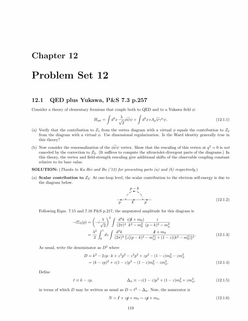
Chapter 12
Problem Set 12
12.1 QED plus Yukawa, P&S 7.3 p.257
Consider a theory of elementary fermions that couple both to QED and to a Yukawa field φ:
Hint =
∫d3x
λ√2φψψ +
∫d3x eAµψγ
µψ. (12.1.1)
(a) Verify that the contribution to Z1 from the vertex diagram with a virtual φ equals the contribution to Z2
from the diagram with a virtual φ. Use dimensional regularization. Is the Ward identity generally true inthis theory?
(b) Now consider the renormalization of the φψψ vertex. Show that the rescaling of this vertex at q2 = 0 is notcanceled by the correction to Z2. (It suffices to compute the ultraviolet-divergent parts of the diagrams.) Inthis theory, the vertex and field-strength rescaling give additional shifts of the observable coupling constantrelative to its bare value.
SOLUTION: (Thanks to Ka Hei and Bo (’12) for presenting parts (a) and (b) respectively.)
(a) Scalar contribution to Z2: At one-loop level, the scalar contribution to the electron self-energy is due tothe diagram below.
- - -
-
p k p
p− k
(12.1.2)
Following Eqns. 7.15 and 7.16 P&S p.217, the amputated amplitude for this diagram is
−iΣ2(p) =
(−i λ√
2
)2 ∫d4k
(2π)4
i(/k +m0)
k2 −m20
i
(p− k)2 −m2φ
=λ2
2
∫ 1
0
dz
∫d4k
(2π)4
/k +m0
z[(p− k)2 −m2φ] + (1− z)(k2 −m2
0)2. (12.1.3)
As usual, write the denominator as D2 where
D = k2 − 2zp · k + z2p2 − z2p2 + zp2 − (1− z)m20 − zm2
φ
= (k − zp)2 + z(1− z)p2 − (1− z)m20 − zm2
φ. (12.1.4)
Define
` ≡ k − zp, ∆φ ≡ −z(1− z)p2 + (1− z)m20 + zm2
φ, (12.1.5)
in terms of which D may be written as usual as D = `2 −∆φ. Now, the numerator is
N = /+ z/p+m0 ∼ z/p+m0, (12.1.6)
119
120 CHAPTER 12. PROBLEM SET 12
where we drop the linear term in ` since, being odd in `, its integral vanishes. Thus,
− iΣ2(p) =λ2
2
∫ 1
0
dz(z/p+m0)
∫d4`
(2π)4
1
(`2 −∆φ)2. (12.1.7)
Wick rotate and multiply both sides by i to get
Σ2(p) = −λ2
2
∫ 1
0
dz(z/p+m0)
∫d4`E(2π)4
1
(`2E + ∆φ)2. (12.1.8)
Method 1 (Pauli-Villars): First, perform the angular integral to get
Σ2(p) = − λ2
16π2
∫ 1
0
dz(z/p+m0)
∫ ∞0
`3Ed`E(`2E + ∆φ)2
. (12.1.9)
Next, defineν ≡ `2E , (12.1.10)
so that
Σ2(p) = − λ2
32π2
∫ 1
0
dz(z/p+m0)
∫ ∞0
ν dν
(ν + ∆φ)2. (12.1.11)
We can perform the divergent integral:∫ ∞0
ν dν
(ν + ∆φ)2= − ν
ν + ∆φ
∣∣∣∣∞0
+
∫ ∞0
dν
ν + ∆φ=
[ln(ν + ∆φ)− ν
ν + ∆φ
]∞0
. (12.1.12)
Replace the scalar propagator by
1
(p− k)2 −m2φ
→ 1
(p− k)2 −m2φ
− 1
(p− k)2 − Λ2. (12.1.13)
The effect of this is ∫d4`E(2π)4
1
(`2E + ∆φ)2→∫
d4`E(2π)4
(1
(`2E + ∆φ)2− 1
(`2E + ∆Λ)2
), (12.1.14)
where∆Λ = −z(1− z)p2 + (1− z)m2
0 + zΛ2 Λ→∞−−−−→ zΛ2. (12.1.15)
Therefore,∫ ∞0
ν dν
(ν + ∆φ)2→[lnν + ∆φ
ν + ∆Λ− ν
ν + ∆φ+
ν
ν + ∆Λ
]∞0
= − ln∆φ
∆Λ
Λ→∞−−−−→ − ln∆φ
zΛ2. (12.1.16)
Then, Eqn. (12.1.11) reads
Σ2(p) =λ2
32π2
∫ 1
0
dz(z/p+m0) ln∆φ
zΛ2. (12.1.17)
We can now take the derivative:
dΣ2
d/p=
λ2
32π2
∫ 1
0
dz
(z ln
∆φ
zΛ2+z/p+m0
∆φ
d∆φ
d/p
). (12.1.18)
Using /p2 = p2, we have
d∆φ
d/p= −2z(1− z)/p. (12.1.19)
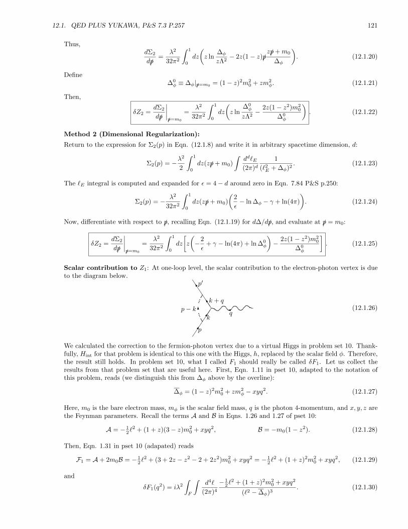
12.1. QED PLUS YUKAWA, P&S 7.3 P.257 121
Thus,dΣ2
d/p=
λ2
32π2
∫ 1
0
dz
(z ln
∆φ
zΛ2− 2z(1− z)/p
z/p+m0
∆φ
). (12.1.20)
Define∆0φ ≡ ∆φ|/p=m0
= (1− z)2m20 + zm2
φ. (12.1.21)
Then,
δZ2 =dΣ2
d/p
∣∣∣∣/p=m0
=λ2
32π2
∫ 1
0
dz
(z ln
∆0φ
zΛ2− 2z(1− z2)m2
0
∆0φ
). (12.1.22)
Method 2 (Dimensional Regularization):
Return to the expression for Σ2(p) in Eqn. (12.1.8) and write it in arbitrary spacetime dimension, d:
Σ2(p) = −λ2
2
∫ 1
0
dz(z/p+m0)
∫dd`E(2π)d
1
(`2E + ∆φ)2. (12.1.23)
The `E integral is computed and expanded for ε = 4− d around zero in Eqn. 7.84 P&S p.250:
Σ2(p) = − λ2
32π2
∫ 1
0
dz(z/p+m0)
(2
ε− ln ∆φ − γ + ln(4π)
). (12.1.24)
Now, differentiate with respect to /p, recalling Eqn. (12.1.19) for d∆/d/p, and evaluate at /p = m0:
δZ2 =dΣ2
d/p
∣∣∣∣/p=m0
=λ2
32π2
∫ 1
0
dz
[z
(−2
ε+ γ − ln(4π) + ln ∆0
φ
)− 2z(1− z2)m2
0
∆0φ
]. (12.1.25)
Scalar contribution to Z1: At one-loop level, the scalar contribution to the electron-photon vertex is dueto the diagram below.
JJJJJ
]
]6
p
kq
k + q
p− k
p′
(12.1.26)
We calculated the correction to the fermion-photon vertex due to a virtual Higgs in problem set 10. Thank-fully, Hint for that problem is identical to this one with the Higgs, h, replaced by the scalar field φ. Therefore,the result still holds. In problem set 10, what I called F1 should really be called δF1. Let us collect theresults from that problem set that are useful here. First, Eqn. 1.11 in pset 10, adapted to the notation ofthis problem, reads (we distinguish this from ∆φ above by the overline):
∆φ = (1− z)2m20 + zm2
φ − xyq2. (12.1.27)
Here, m0 is the bare electron mass, mφ is the scalar field mass, q is the photon 4-momentum, and x, y, z arethe Feynman parameters. Recall the terms A and B in Eqns. 1.26 and 1.27 of pset 10:
A = − 12`
2 + (1 + z)(3− z)m20 + xyq2, B = −m0(1− z2). (12.1.28)
Then, Eqn. 1.31 in pset 10 (adapated) reads
F1 = A+ 2m0B = − 12`
2 + (3 + 2z − z2 − 2 + 2z2)m20 + xyq2 = − 1
2`2 + (1 + z)2m2
0 + xyq2, (12.1.29)
and
δF1(q2) = iλ2
∫F
∫d4`
(2π)4
− 12`
2 + (1 + z)2m20 + xyq2
(`2 −∆φ)3. (12.1.30)

122 CHAPTER 12. PROBLEM SET 12
Wick rotating yields
δF1(q2) = λ2
∫F
∫d4`E(2π)4
12`
2E + (1 + z)2m2
0 + xyq2
(`2E + ∆φ)3. (12.1.31)
∆φ evaluated at q2 = 0 is the same as ∆φ evaluated at /p = m0, which we called ∆0φ in Eqn. (12.1.21):
∆φ|q2=0 = (1− z)2m20 + zm2
φ = ∆0φ. (12.1.32)
Let us now evaluate δF1 at q2 = 0. In this case, the integrand in Eqn. (12.1.31) is independent of x and y.Therefore, the x integral just gives 1. After this, y is constrained to be y = 1− z − x whose minimum value,−z, occurs at x = 1. However, since y is also constrained to be between 0 and 1, the actual lower bound forthe y integral is 0. On the other hand, the upper bound is 1− z, occuring when x = 0. Thus, the y integralgives a factor of (1− z):
δF1(0) = λ2
∫ 1
0
dz (1− z)∫
d4`E(2π)4
12`
2E + (1 + z)2m2
0
(`2E + ∆0φ)3
. (12.1.33)
Method 1 (Pauli-Villars): Changing variables to ν = `2E yields
δF1(0) =λ2
16π2
∫ 1
0
dz (1− z)∫ ∞
0
dν12ν
2 + (1 + z)2m20ν
(ν + ∆0φ)3
. (12.1.34)
Only the first term in the ν integral requires regularization since the second term is convergent. Let ussimplify the first term:∫ ∞
0
12ν
2dν
(ν + ∆0φ)3
= − ν2
(ν + ∆0φ)2
∣∣∣∣∞0
+1
2
∫ ∞0
ν dν
(ν + ∆0φ)2
= −[
ν2
(ν + ∆0φ)2
+ν
2(ν + ∆0φ)
]∞0
+1
2
∫ ∞0
dν
ν + ∆0φ
=
[1
2ln(ν + ∆0
φ)− ν2
(ν + ∆0φ)2− ν
2(ν + ∆0φ)
]∞0
. (12.1.35)
Pauli-Villars regularization amounts to∫ ∞0
12ν
2dν
(ν + ∆0)3→∫ ∞
0
( 12ν
2dν
(ν + ∆0φ)3−
12ν
2dν
(ν + ∆Λ)3
)=
[1
2lnν + ∆0
φ
ν + ∆Λ− ν2
(ν + ∆0φ)2− ν
2(ν + ∆0φ)
+ν2
(ν + ∆Λ)2+
ν
2(ν + ∆Λ)
]∞0
= −1
2ln
∆0φ
zΛ2. (12.1.36)
Now, let us compute the convergent integral:∫ ∞0
ν dν
(ν + ∆0φ)3
= −
ν
2(ν + ∆0φ)2
∣∣∣∣∞0
+1
2
∫ ∞0
dν
(ν + ∆0φ)2
= − 1
2(ν + ∆0φ)
∣∣∣∣∞0
=1
2∆0φ
. (12.1.37)
Thus, we get
δF1(0) =λ2
16π2
∫ 1
0
dz (1− z)(−1
2ln
∆0φ
zΛ2+
(1 + z)2m20
2∆0φ
). (12.1.38)
Rewrite this as
δF1(0) =λ2
32π2
∫ 1
0
dz
(−(1− z) ln
∆0φ
zΛ2+
(1 + z)(1− z2)m20
∆0φ
). (12.1.39)
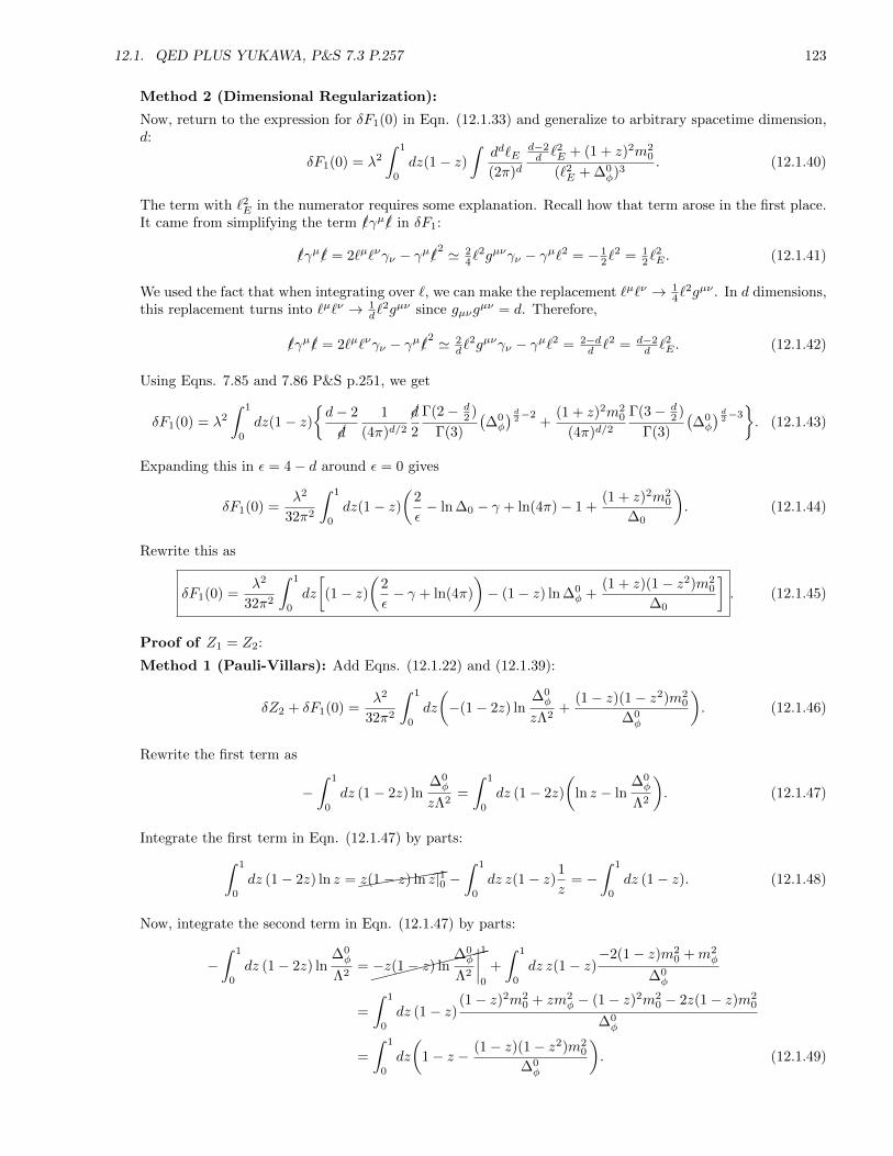
12.1. QED PLUS YUKAWA, P&S 7.3 P.257 123
Method 2 (Dimensional Regularization):
Now, return to the expression for δF1(0) in Eqn. (12.1.33) and generalize to arbitrary spacetime dimension,d:
δF1(0) = λ2
∫ 1
0
dz(1− z)∫
dd`E(2π)d
d−2d `2E + (1 + z)2m2
0
(`2E + ∆0φ)3
. (12.1.40)
The term with `2E in the numerator requires some explanation. Recall how that term arose in the first place.It came from simplifying the term /γµ/ in δF1:
/γµ/ = 2`µ`νγν − γµ/2 ' 2
4`2gµνγν − γµ`2 = − 1
2`2 = 1
2`2E . (12.1.41)
We used the fact that when integrating over `, we can make the replacement `µ`ν → 14`
2gµν . In d dimensions,this replacement turns into `µ`ν → 1
d`2gµν since gµνg
µν = d. Therefore,
/γµ/ = 2`µ`νγν − γµ/2 ' 2
d`2gµνγν − γµ`2 = 2−d
d `2 = d−2d `2E . (12.1.42)
Using Eqns. 7.85 and 7.86 P&S p.251, we get
δF1(0) = λ2
∫ 1
0
dz(1− z)d− 2
d
1
(4π)d/2d
2
Γ(2− d2 )
Γ(3)
(∆0φ
) d2−2
+(1 + z)2m2
0
(4π)d/2Γ(3− d
2 )
Γ(3)
(∆0φ
) d2−3. (12.1.43)
Expanding this in ε = 4− d around ε = 0 gives
δF1(0) =λ2
32π2
∫ 1
0
dz(1− z)(
2
ε− ln ∆0 − γ + ln(4π)− 1 +
(1 + z)2m20
∆0
). (12.1.44)
Rewrite this as
δF1(0) =λ2
32π2
∫ 1
0
dz
[(1− z)
(2
ε− γ + ln(4π)
)− (1− z) ln ∆0
φ +(1 + z)(1− z2)m2
0
∆0
]. (12.1.45)
Proof of Z1 = Z2:
Method 1 (Pauli-Villars): Add Eqns. (12.1.22) and (12.1.39):
δZ2 + δF1(0) =λ2
32π2
∫ 1
0
dz
(−(1− 2z) ln
∆0φ
zΛ2+
(1− z)(1− z2)m20
∆0φ
). (12.1.46)
Rewrite the first term as
−∫ 1
0
dz (1− 2z) ln∆0φ
zΛ2=
∫ 1
0
dz (1− 2z)
(ln z − ln
∆0φ
Λ2
). (12.1.47)
Integrate the first term in Eqn. (12.1.47) by parts:∫ 1
0
dz (1− 2z) ln z =(((((((z(1− z) ln z|10 −
∫ 1
0
dz z(1− z)1
z= −
∫ 1
0
dz (1− z). (12.1.48)
Now, integrate the second term in Eqn. (12.1.47) by parts:
−∫ 1
0
dz (1− 2z) ln∆0φ
Λ2=
−z(1− z) ln∆0φ
Λ2
∣∣∣∣10
+
∫ 1
0
dz z(1− z)−2(1− z)m2
0 +m2φ
∆0φ
=
∫ 1
0
dz (1− z)(1− z)2m2
0 + zm2φ − (1− z)2m2
0 − 2z(1− z)m20
∆0φ
=
∫ 1
0
dz
(1− z − (1− z)(1− z2)m2
0
∆0φ
). (12.1.49)
124 CHAPTER 12. PROBLEM SET 12
The first term above, (1− z), cancels Eqn. (12.1.48) simplifying Eqn. (12.1.47) into
−∫ 1
0
dz (1− 2z) ln∆0φ
zΛ2= −
∫ 1
0
dz(1− z)(1− z2)m2
0
∆0φ
, (12.1.50)
which indeed cancels the last term in Eqn. (12.1.46) leaving
δZ2 + δF1(0) = 0 . (12.1.51)
Since Γµ = Z−11 γµ, we have δZ1 = −δF1(0) and so Eqn. (12.1.51) implies δZ1 = δZ2. Since both Z1 and Z2
are 1 at tree level, we have
Z1 = Z2 . (12.1.52)
Method 2 (Dimensional Regularization): Add Eqns. (12.1.25) and (12.1.45):
δZ2 + δF1(0) =λ2
32π2
∫ 1
0
dz
[
(1− 2z)
(2
ε− γ + ln(4π)
)− (1− z)− (1− 2z) ln ∆0
φ +(1− z)(1− z2)m2
0
∆0φ
]=
λ2
32π2
∫ 1
0
dz
(−(1− z)− (1− 2z) ln ∆0
φ +(1− z)(1− z2)m2
0
∆0φ
). (12.1.53)
Note that the first term, containing the divergence, vanishes because the integrand is proportional to (1−2z),whose integral vanishes. Meanwhile, the integral of (1− 2z) ln ∆0
φ does not vanish because ∆0φ depends on z.
As in the previous method, integrating the log term by parts shows that Eqn. (12.1.53) vanishes.
Ward-Takahashi identity:
The proof of the Ward-Takahashi identity will work as long as each vertex involves a ψ and a ψ. We are stillattaching a photon line to a fermion line or loop but now the lines that are already attached to the fermioncan be either photons are scalars. All this does is get rid of some γµ’s and some minus signs, which does notinvalidate the proof. This certainly ensures gauge invariance classically, but since the proof goes through,gauge invariance holds to all orders of quantum correction.
(b) We must compare the one-loop corrections to the fermion self-energy and the fermion-scalar vertex due tothe photon and the scalar. At tree level, the fermion-scalar vertex comes with the factor, −iλ/
√2. Write the
exact vertex as
V ≡ fermion-scalar vertex =1
Z ′1
(−i λ√
2
), (12.1.54)
so that Z ′1 is 1 at tree level and
δZ ′1 = −δV. (12.1.55)
We are trying to show that
Z ′1 6= Z2. (12.1.56)
Photon contribution to Z2: The one-loop photon contribution to the fermion self-energy is
- - -
-
p k p
p− k
(12.1.57)
Define the two quantities,
∆γ = −z(1− z)p2 + (1− z)m20 + zm2
γ , (12.1.58a)
∆0γ = (1− z)2m2
0 + zm2γ . (12.1.58b)
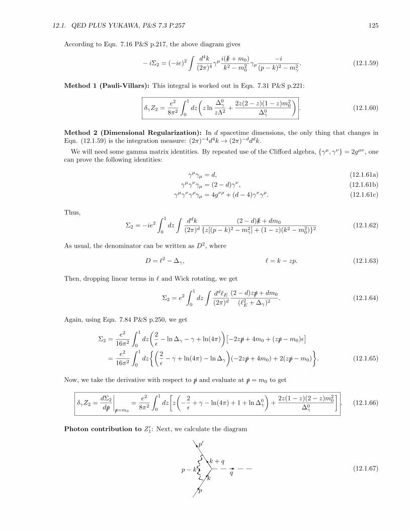
12.1. QED PLUS YUKAWA, P&S 7.3 P.257 125
According to Eqn. 7.16 P&S p.217, the above diagram gives
− iΣ2 = (−ie)2
∫d4k
(2π)4γµi(/k +m0)
k2 −m20
γµ−i
(p− k)2 −m2γ
. (12.1.59)
Method 1 (Pauli-Villars): This integral is worked out in Eqn. 7.31 P&S p.221:
δγZ2 =e2
8π2
∫ 1
0
dz
(z ln
∆0γ
zΛ2+
2z(2− z)(1− z)m20
∆0γ
). (12.1.60)
Method 2 (Dimensional Regularization): In d spacetime dimensions, the only thing that changes inEqn. (12.1.59) is the integration measure: (2π)−4d4k → (2π)−dddk.
We will need some gamma matrix identities. By repeated use of the Clifford algebra, γµ, γν = 2gµν , onecan prove the following identities:
γµγµ = d, (12.1.61a)
γµγνγµ = (2− d)γν , (12.1.61b)
γµγνγργµ = 4gνρ + (d− 4)γνγρ. (12.1.61c)
Thus,
Σ2 = −ie2
∫ 1
0
dz
∫ddk
(2π)d(2− d)/k + dm0
z[(p− k)2 −m2γ ] + (1− z)(k2 −m2
0)2(12.1.62)
As usual, the denominator can be written as D2, where
D = `2 −∆γ , ` = k − zp. (12.1.63)
Then, dropping linear terms in ` and Wick rotating, we get
Σ2 = e2
∫ 1
0
dz
∫dd`E(2π)d
(2− d)z/p+ dm0
(`2E + ∆γ)2. (12.1.64)
Again, using Eqn. 7.84 P&S p.250, we get
Σ2 =e2
16π2
∫ 1
0
dz
(2
ε− ln ∆γ − γ + ln(4π)
)[−2z/p+ 4m0 + (z/p−m0)ε
]=
e2
16π2
∫ 1
0
dz
(2
ε− γ + ln(4π)− ln ∆γ
)(−2z/p+ 4m0) + 2(z/p−m0)
. (12.1.65)
Now, we take the derivative with respect to /p and evaluate at /p = m0 to get
δγZ2 =dΣ2
d/p
∣∣∣∣/p=m0
=e2
8π2
∫ 1
0
dz
[z
(−2
ε+ γ − ln(4π) + 1 + ln ∆0
γ
)+
2z(1− z)(2− z)m20
∆0γ
]. (12.1.66)
Photon contribution to Z ′1: Next, we calculate the diagram
JJJJJ
]
] 6
p
kq
k + q
p− k
p′
(12.1.67)

126 CHAPTER 12. PROBLEM SET 12
Now, we calculate the electron-scalar vertex. The diagram is the same as for the electron-photon vertex (e.g.P&S p.189), but with the photon with momentum q replaced by a scalar or both photons replaced by ascalar. Let us first calculate the more difficult case where the loop includes a photon. The amplitude, Mγ ,of this diagram is
iMγ =
∫d4k
(2π)4u(p′)(−ieγµ)
−igµν(p− k)2 −m2
γ
i(/k′+m0)
k′2 −m20
(−i λ√
2
)i(/k +m0)
k2 −m20
(−ieγν)u(p)
=
(−i λ√
2
)(−2ie2)
∫F
∫d4k
(2π)4
u(p′)γµ(/k′+m0)(/k +m0)γµu(p)
x(k2 −m20) + y[(k + q)2 −m2
0] + z[(p− k)2 −m2γ ]3
. (12.1.68)
Let us first simplify the denominator by writing it as D3, where
D = k2 + 2(yq − zp) · k + (yq − zp)2 − (yq − zp)2 + yq2 + zp2 − (x+ y)m20 − zm2
γ
= (k + yq − zp)2 + y(1− y)q2 + 2yzp · q + z(1− z)p2 − (1− z)m20 − zm2
γ . (12.1.69)
Using the identities p2 = m2 and 2p · q = −q2 (Eqn 1.9 of problem set 10),
D = `2 −∆γ , (12.1.70)
where
` ≡ k + yq − zp, ∆γ ≡ (1− z)2m20 + zm2
γ − xyq2. (12.1.71)
When d = 4, the identities (12.1.61a), (12.1.61b) and (12.1.61c) read
γµγµ = 4, (12.1.72a)
γµγνγµ = −2γν , (12.1.72b)
γµγνγργµ = 4gνρ, (12.1.72c)
Using these identities, we may simplify the numerator to
N = u(p′)[4k′ · k − 2m0(/k′+ /k) + 4m2
0]u(p). (12.1.73)
Let us simplify this one term at a time:
4k′ · k = 4[`+ (1− y)p′ − xp] · [`− yp′ + (1− x)p]
= 4`2 + 4(1− x− y + 2xy)p′ · p− 4(y − y2 + x− x2)m20
= 4`2 + 4(1− x− y + 2xy − y + y2 − x+ x2)m20 − 2(1− x− y + 2xy)q2
= 4`2 + 4[(1− z)2 − 1 + 2z]m20 − 2(z + 2xy)q2
= 4`2 + 4z2m20 − 2(z + 2xy)q2. (12.1.74)
Note that we dropped linear terms in ` and made use of the identity
2p′ · p = 2m20 − q2. (12.1.75)
Using the Dirac equations and taking the spinors for granted, the middle term in Eqn. (12.1.59) gives
−2m0(/k′+ /k) = −2m0[2/+ (1− 2y)/p
′ + (1− 2x)/p]
= −2m0(1− 2y + 1− 2x)m0
= −4zm20. (12.1.76)
Putting these pieces together and taking the spinors for granted, Eqn. (12.1.73) simplifies to
N = 4`2 + 4(1− z + z2)m20 − 2(z + 2xy)q2. (12.1.77)
Everything in iMγ except the usual tree level value −iλ/√
2 gives δV . Hence, evaluating at q2 = 0, we have
δγZ′1 = −δγV (0) = 8ie2
∫F
∫d4`
(2π)4
`2 + (1− z + z2)m20
(`2 −∆0γ)3
= 8e2
∫ 1
0
dz (1− z)∫
d4`E(2π)4
−`2E + (1− z + z2)m20
(`2E + ∆0γ)3
. (12.1.78)
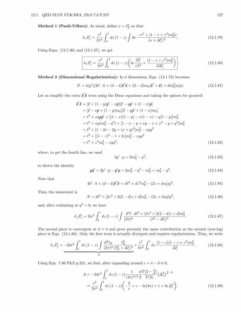
12.1. QED PLUS YUKAWA, P&S 7.3 P.257 127
Method 1 (Pauli-Villars): As usual, define ν = `2E so that
δγZ′1 =
e2
2π2
∫ 1
0
dz (1− z)∫dν−ν2 + (1− z + z2)m2
0ν
(ν + ∆0γ)3
. (12.1.79)
Using Eqns. (12.1.36) and (12.1.37), we get
δγZ′1 =
e2
2π2
∫ 1
0
dz (1− z)(
ln∆0γ
zΛ2+
(1− z + z2)m20
2∆0γ
). (12.1.80)
Method 2 (Dimensional Regularization): In d dimensions, Eqn. (12.1.73) becomes
N = u(p′)[4k′ · k + (d− 4)/k′/k + (2− d)m0(/k
′+ /k) + dm2
0]u(p). (12.1.81)
Let us simplify the extra /k′/k term using the Dirac equations and taking the spinors for granted:
/k′/k = [/+ (1− y)/p
′ − x/p][/− y/p′ + (1− x)/p]
= [/− x/p+ (1− y)m0][/− y/p′ + (1− x)m0]
= `2 + xy/p/p′ + [(1− x)(1− y)− x(1− x)− y(1− y)]m2
0
= `2 + xy(m20 − q2) + [1− x− y + xy − x+ x2 − y + y2]m2
0
= `2 + [1− 2x− 2y + (x+ y)2]m20 − xyq2
= `2 + [(1− z)2 − 1 + 2z]m20 − xyq2
= `2 + z2m20 − xyq2, (12.1.82)
where, to get the fourth line, we used2p′ · p = 2m2
0 − q2, (12.1.83)
to derive the identity
/p/p′ = 2p′ · p− /p′/p = 2m2
0 − q2 −m20 = m2
0 − q2. (12.1.84)
Note that4k′ · k + (d− 4)/k
′/k = d`2 + dz2m2
0 − (2z + dxy)q2. (12.1.85)
Thus, the numerator isN = d`2 + [dz2 + 2(2− d)z + d]m2
0 − (2z + dxy)q2, (12.1.86)
and, after evaluating at q2 = 0, we have
δγZ′1 = 2ie2
∫ 1
0
dz (1− z)∫
dd`
(2π)dd`2 + [dz2 + 2(2− d)z + d]m2
0
(`2 −∆0γ)3
. (12.1.87)
The second piece is convergent at d = 4 and gives precisely the same contribution as the second (non-log)piece in Eqn. (12.1.80). Only the first term is actually divergent and requires regularization. Thus, we write
δγZ′1 = −2de2
∫ 1
0
dz (1− z)∫
dd`E(2π)d
`2E(`2E + ∆0
γ)3︸ ︷︷ ︸A
+e2
4π2
∫ 1
0
dz(1− z)(1− z + z2)m2
0
∆0γ
. (12.1.88)
Using Eqn. 7.86 P&S p.251, we find, after expanding around ε = 4− d ≈ 0,
A = −2de2
∫ 1
0
dz (1− z) 1
(4π)d/2d
2
Γ(2− d2 )
Γ(3)
(∆0γ
) d2−2
=e2
2π2
∫ 1
0
dz (1− z)(−2
ε+ γ − ln(4π) + 1 + ln ∆0
γ
). (12.1.89)
128 CHAPTER 12. PROBLEM SET 12
Therefore, we have
δγZ′1 =
e2
2π2
∫ 1
0
dz (1− z)[(−2
ε+ γ − ln(4π) + 1 + ln ∆0
γ
)+
(1− z + z2)m20
∆0γ
]. (12.1.90)
Scalar contribution to Z ′1: Next, we calculate the diagram
JJJJJ
]
] 6
p
kq
k + q
p− k
p′
(12.1.91)
Compared to Eqn. (12.1.68), the factor (−ie)2 is replaced with(−i λ√
2
)2and there is an extra minus sign
because the scalar propagator’s numerator is i whereas that of the photon is −igµν . We drop the two factorsof γ associated with the fermion-photon vertices. Also, mγ is replaced with mφ, or ∆γ with ∆φ. Finally, wesimplify the numerator:
N = (/k′+m0)(/k +m0)
= [/+ (1− y)/p′ − x/p+m0][/− y/p′ + (1− x)/p+m0]
= [/− x/p+ (2− y)m0][/− y/p′ + (2− x)m0]
= `2 + xy/p/p′ − x(2− x)m2
0 − y(2− y)m20 + (2− x)(2− y)m2
0
= `2 + xy(2p · p′ −m20) + (−2x+ x2 − 2y + y2 + 4− 2x− 2y + xy)m2
0
= `2 + xy(m20 − q2) + (x2 + xy + y2 + 4− 4x− 4y)m2
0
= `2 + [(x+ y)2 + 4(1− x− y)]m20 − xyq2
= `2 + [(1− z)2 + 4z]m20 − xyq2
= `2 + (1 + z)2m20 − xyq2. (12.1.92)
Therefore,
iMφ =
(−i λ√
2
)(iλ2)
∫F
∫d4`
(2π)4
u(p′)[`2 + (1 + z)2m20 − xyq2]u(p)
(`2 −∆φ)3. (12.1.93)
Then,
δφZ′1 = λ2
∫ 1
0
dz (1− z)∫
d4`E(2π)4
`2E − (1 + z)2m20
(`2E + ∆0φ)3
. (12.1.94)
Method 1 (Pauli-Villars): As usual, define ν = `2E so that
δγZ′1 =
λ2
16π2
∫ 1
0
dz (1− z)∫ ∞
0
dνν2 − (1 + z)2m2
0ν
(ν + ∆0φ)3
. (12.1.95)
Again, using Eqns. (12.1.35) and (12.1.36), we get
δφZ′1 = − λ2
16π2
∫ 1
0
dz (1− z)(
ln∆
(φ)0
zΛ2+
(1 + z)2m20
2∆0φ
). (12.1.96)
Rewrite this as
δφZ′1 = − λ2
16π2
∫ 1
0
dz
((1− z) ln
∆0φ
zΛ2+
(1 + z)(1− z2)m20
2∆0φ
). (12.1.97)
12.1. QED PLUS YUKAWA, P&S 7.3 P.257 129
Method 2 (Dimensional Regularization): Again, only the first term in Eqn. (12.1.94) is divergent andneeds regularization:
δφZ′1 = λ2
∫ 1
0
dz (1− z)∫
dd`E(2π)d
`2E(`2E + ∆0
φ)3− λ2
32π2
∫ 1
0
dz(1 + z)(1− z2)m2
0
∆0φ
. (12.1.98)
Again, using Eqn. 7.86 P&S p.251 and expanding around ε = 4− d ≈ 0, we get
δφZ′1 = − λ2
16π2
∫ 1
0
dz
[(1− z)
(−2
ε+ γ − ln(4π) +
1
2− ln ∆0
φ
)+
(1 + z)(1− z2)m20
2∆0φ
]. (12.1.99)
Proof that Z ′1 6= Z2:
Method 1 (Pauli-Villars): Subtract Eqn. (12.1.60) from (12.1.80):
δγZ′1 − δγZ2 =
e2
8π2
∫ 1
0
dz
((4− 5z) ln
∆0γ
zΛ2+
2(1− z)2(1− 2z)m20
∆0γ
). (12.1.100)
The usual trick would be to integrate the first term by parts. Separating out a ln z term, we get
−∫ 1
0
dz(4− 5z) ln z =((((((((
(− 1
2z(8− 5z) ln z∣∣10
+1
2
∫ 1
0
dz z(8− 5z)1
z=
1
2
∫ 1
0
dz(8− 5z). (12.1.101)
The rest of the first term of Eqn. (12.1.100) gives∫ 1
0
dz (4− 5z) ln∆0γ
Λ2=
1
2z(8− 5z) ln
∆0γ
Λ2
∣∣∣∣10
− 1
2
∫ 1
0
dz z(8− 5z)−2(1− z)m2
0 +m2φ
∆0γ
=3
2lnm2γ
Λ2− 1
2
∫ 1
0
dz(8− 5z)
(1− (1− z2)m2
0
∆0γ
), (12.1.102)
where the same trick was used here as in Eqn. (12.1.38). As usual, the first term above cancels Eqn. (12.1.73).The rest is finite. The remainder is
δγZ′1 − δγZ2 =
3e2
16π2
(lnm2γ
Λ2+
∫ 1
0
dz(4 + z)(1− z)2m2
0
∆0γ
)6= 0 . (12.1.103)
The scalar contribution also does not cancel. Subtract Eqn. (12.1.22) from Eqn. (12.1.97):
δφZ′1 − δφZ2 = − λ2
32π2
∫ 1
0
dz
((2− z) ln
∆0φ
zΛ2+
(1− z)(1− z2)m20
∆0φ
). (12.1.104)
The analog of Eqn. (12.1.102) in this case is∫ 1
0
dz(2− z) ln∆0φ
Λ2=
3
2lnm2φ
Λ2− 1
2
∫ 1
0
dz(4− z)(
1− (1− z2)m20
∆0φ
). (12.1.105)
The final result is
δφZ′1 − δφZ2 = − 3λ2
64π2
(lnm2φ
Λ2+
∫ 1
0
dz(2− z)(1− z2)m2
0
∆0φ
)6= 0 . (12.1.106)
As stated in the problem, these non-cancellations imply extra contributions to the renormalization of λ ande. One might worry about whether or not the cancellations that occurred for the fermion-photon vertex, dueto gauge-invariance, still hold after renormalization. There is no need to worry because those cancellationsdid not depend on the specific value of the coupling constants.
130 CHAPTER 12. PROBLEM SET 12
Method 2 (Dimensional regularization):
The finite pieces in the differences are precisely the same as were found in Eqns. (12.1.103) and (12.1.106).Therefore, we will not bother to calculate those. We will just focus on the divergent pieces. From Eqns.(12.1.25), (12.1.66), (12.1.90) and (12.1.99), we find
δγZ′1 = − e2
2π2ε, δγZ2 = − e2
4π2ε, (12.1.107a)
δφZ′1 =
λ2
16π2ε, δφZ2 = − λ2
32π2ε. (12.1.107b)
Therefore,
δγZ′1 − δγZ2 = − e2
4π2ε6= 0 , (12.1.108)
and
δφZ′1 − δφZ2 =
3λ2
32π2ε6= 0 . (12.1.109)
Aside: In part (a), we found that δφZ1−δφZ2 = 0. This is true regardless of the regularization procedure. Eventhough both integrals are divergent, and therefore ill-defined, one can still prove that they are equal withoutactually evaluating the integrals and therefore without recourse to a regularization procedure. Reproduced beloware the integral expressions for δφZ1 and δφZ2:
δφZ1 = −λ2
2
∫ 1
0
dz
∫d 4`E
(1− z)`2E
(`2E + ∆0φ)3
+2(1 + z)(1− z2)m2
0
(`2E + ∆0φ)3
,
δφZ2 = −λ2
2
∫ 1
0
dz
∫d 4`E
z
(`2E + ∆0φ)2
+4z(1− z2)m2
0
(`2E + ∆0φ)3
.
Note that the expression for δφZ2 is found by differentiating the integral expression for Σ2 in Eqn. (12.1.8) beforeactually evaluating the integral explicitly. One procedure for showing the equality of these two expressions is tointegrate the first term in δφZ1 by parts with respect to `E , and use the integral∫
d 4`E1
(`2E + ∆0φ)3
=1
32π2∆0φ
, (12.1.110)
to write ∫d 4`E
`2E(`2E + ∆0
φ)3=
∫d 4`E
1
(`2E + ∆0φ)2−∫d 4`E
∆0φ
(`2E + ∆0φ)3
. (12.1.111)
Finally, in δφZ1 − δφZ2, integrate the term involving (`2E + ∆0φ)−2 by parts with respect to z. Using the same
sort of trick as was used in the derivation of Eqn. (12.1.49), for example, one can show that the result vanishes.
12.2 Massive Axial Anomaly, Zee IV.7.4 p.279
Take the Pauli-Villars regulated ∆λµν(k1, k2) and contract it with qλ. The analog of the trick in chapter II.7 is towrite /qγ5 in the second term as [2M + (/p−M)− (/p− /q +M)]γ5. Now you can freely shift integration variables.Show that
qλ∆λµν(k1, k2) = −2M∆µν(k1, k2), (12.2.1)
where
∆µν(k1, k2) = (−1)i3∫
d4p
(2π)4tr
(γ5 1
/p− /q −Mγν
1
/p− /k1 −Mγµ
1
/p−M
)+ µ, k1 ↔ ν, k2. (12.2.2)
Evaluate ∆µν and show that ∆µν goes as 1/M in the limit M →∞ and so the right hand side of Eqn. (12.2.1)goes to a finite limit. The anomaly is what the regulator leaves behind as it disappears from the low energyspectrum: It is like the smile of the Cheshire cat. [We can actually argue that ∆µν goes as 1/M without doing
12.2. MASSIVE AXIAL ANOMALY, ZEE IV.7.4 P.279 131
a detailed calculation. By Lorentz invariance and because of the presence of γ5, ∆µν must be proportional toεµνλρk1λk2ρ, but by dimensional analysis, ∆µν must be some constant times εµνλρk1λk2ρ/M . You might ask whywe can’t use something like 1/(k2
1)1/2 instead of 1/M to make the dimension come out right. The answer isthat from your experience in evaluating Feynman diagrams in (3 + 1)-dimensional spacetime you can never geta factor like 1/(k2
1)1/2.]
SOLUTION:
We take µ, k1 ↔ ν, k2 for granted. We have
qλ∆λµν = (−1)i3∫
d4p
(2π)4tr
[/qγ
5 1
/p− /qγν
1
/p− /k1
γµ1
/p− /qγ5 1
/p− /q −Mγν
1
/p− /k1 −Mγµ
1
/p−M
]. (12.2.3)
Let A and B be the first and second terms, respectively. Rewrite the first term as
A = i
∫d4p
(2π)4tr
[[/p− (/p− /q)
]γ5 1
/p− /qγν
1
/p− /k1
γµ1
/p
]= i
∫d4p
(2π)4tr
[γ5 1
/p− /qγν
1
/p− /k1
γµ + γ5γν1
/p− /k1
γµ1
/p
]. (12.2.4)
Rrewrite the second term as
B = −i∫
d4p
(2π)4tr
[[2M + (/p−M)− (/p− /q +M)
]γ5 1
/p− /q −Mγν
1
/p− /k1 −Mγµ
1
/p−M
]= −i
∫d4p
(2π)4tr
[2Mγ5 1
/p− /q −Mγν
1
/p− /k1 −Mγµ
1
/p−M+ γ5 1
/p− /q −Mγν
1
/p− /k1 −Mγµ
+ γ5γν1
/p− /k1 −Mγµ
1
/p−M
]. (12.2.5)
Note that the first term in Eqn. (12.2.5) is precisely −2M∆µν . Therefore, reintroducing the terms implied byµ, k1 ↔ ν, k2, we get
qλ∆λµν + 2M∆µν = i
∫d4p
(2π)4tr
[γ5 1
/p− /qγν
1
/p− /k1
γµ − γ5 1
/p− /q −Mγν
1
/p− /k1 −Mγµ
+ γ5γν1
/p− /k1
γµ1
/p− γ5γν
1
/p− /k1 −Mγµ
1
/p−M
+ γ5 1
/p− /qγµ
1
/p− /k2
γν − γ5 1
/p− /q −Mγµ
1
/p− /k2 −Mγν
+ γ5γµ1
/p− /k2
γν1
/p− γ5γµ
1
/p− /k2 −Mγν
1
/p−M
]. (12.2.6)
These terms cancel in pairs after we shift the integration variable. We will have to justify this shift, but let usfirst show that it produces the appropriate cancellations. For example, define
C ≡ i∫
d4p
(2π)4tr
[γ5 1
/p− /qγν
1
/p− /k1
γµ + γ5γν1
/p− /k2
γν1
/p
]= i
∫d4p
(2π)4tr
[γ5 1
/p− /qγν
1
/p− /k1
γµ − γ5 1
/p− /k2
γν1
/pγµ]. (12.2.7)
Then, making the shift p→ p+ k1 in the first integral will turn it into the second integral, but with a plus sign.Hence, the two terms cancel and C = 0. This can be done with all the appropriate pairs in Eqn. (12.2.6). Theexample above was the cancellation of the first and seventh terms. The second and eighth terms cancel, the thirdand fifth, and the fourth and sixth.
Now, we just need to justify our ability to shift the integration variable. Note that the first and secondterms are shifted in the same way in order to cancel the seventh and eighth terms, respectively. This means that

132 CHAPTER 12. PROBLEM SET 12
Pauli-Villars regulated terms cancel in pairs. The reason why we are allowed to shift the integration variable isbecause Pauli-Villars regularization makes the integrand decay faster at large p than it would otherwise do.
However, we do still have to make sure that the integrand decays sufficiently quickly as to justify the shift.How fast would it have to decay? Well, it would have to decay faster than the rate at which the surface areaof the 3-sphere in four spacetime dimensions grows, which is ∼ p3. Therefore, the integrand must decay fasterthan p−3. This is really not that obvious because, as written, each term in the integrand decays as p−2. Naıvely,Pauli-Villars regularization might make this decay faster, say as p−3, but even that would be insufficient. It turnsout that the O(p−3) term vanishes! Let us see how this works with the first line of Eqn. (12.2.6). Define
Iµν = γ5 1
/p− /qγν
1
/p− /k1
γµ − γ5 1
/p− /q −Mγν
1
/p− /k1 −Mγµ. (12.2.8)
Let us expand this for large p:
Iµν = γ5 1
/p
1
1− /q
/p
γν1
/p
1
1− /k1
/p
γµ − γ5 1
/p
1
1− /q+M
/p
γν1
/p
1
1− /k1+M
/p
γµ
= γ5 1
/p
(1 +
q
p
)γν
1
/p
(1 +
k1
p
)γµ − γ5 1
/p
(1 +
q
p+M
/p
)γν
1
/p
(1 +
k1
p+M
/p
)γµ
= −γ5 1
/pγν
1
/p
M
/pγµ − γ5 1
/p
M
/pγν
1
/pγµ +O(p−4)
= −Mp2γ5
(1
/pγνγµ + γν
1
/pγµ)
+O(p−4)
= −2Mpν
p4γ5, γµ+O(p−4)
= 0 +O(p−4). (12.2.9)
We used the fact that /p−1, γν = p−2/p, γν = 2p−2pν and γ5, γµ = 0. We conclude that the integrand ofEqn. (12.2.6) decays at least as fast as p−4 and hence we need not worry about any boundary terms incurred byshifting the variable of integration.
Therefore, we have finally proven that
qλ∆λµν(k1, k2) = −2M∆µν(k1, k2) . (12.2.10)
Once again, taking µ, k1 ↔ ν, k2 for granted, we write ∆µν as
∆µν = 2i
∫F
∫d4p
(2π)4
tr[γ5(/p− /q +M)γν(/p− /k1 +M)γµ(/p+M)]
x(p2 −M2) + y[(p− k1)2 −M2] + z[(p− q)2 −M2]3. (12.2.11)
The denominator is written D3 where
D = p2 − 2(yk1 + zq) · p+ (yk1 + zq)2 − (yk1 + zq)2 + yk21 + zq2 −M2
= (p− yk1 − zq)2 + y(1− y)k21 − 2yzk1 · q + z(1− z)q2 −M2. (12.2.12)
Define
` ≡ p− yk1 − zq, ∆ ≡M2 − y(1− y)k21 − z(1− z)q2 + 2yzk1 · q, (12.2.13)
so that we can write
D = `2 −∆. (12.2.14)
Let us simplify the numerator. This is simpler than it seems. Because of the presence of the γ5, all combinationsof the successive γ matrices containing an odd number of gamma matrices or just two gamma matrices vanish!Therefore, only the terms containing four gamma matrices matter:
Nµν = M tr γ5[(/p− /q)γν(/p− /k1)γµ + (/p− /q)γνγµ/p+ γν(/p− /k1)γµ/p]. (12.2.15)
12.2. MASSIVE AXIAL ANOMALY, ZEE IV.7.4 P.279 133
Again, because of the γ5, we are free to anticommute all of the gamma matrices. The anti-commutator terms,being proportional to the metric leaves γ5 and two gamma matrices whose trace vanishes. Thus,
Nµν = M tr γ5γµγν [(/p− /q)(/p− /k1)− (/p− /q)/p+ (/p− /k1)/p]
= M tr γ5γµγν [p2 − /p/k1 − /q/p+ /q/k1 − p2 + /q/p+ p2 − /k1/p] (12.2.16)
The /q/p terms obviously cancel. The p2 terms, being proportional to identity just leave the trace of γ5γµγν , whichvanishes. Similarly, the term involving /p/k1 + /k1/p = 2p · k1 also vanishes. This leaves only
Nµν = 4iMεµνρσqρk1σ. (12.2.17)
Thus, since we are allowed to freely shift the integration variable from p to `,
∆µν = −8Mεµνρσqρk1σ
∫F
∫d4`
(2π)4
1
(`2 −∆)3=iM
4π2εµνρσqρk1σ
∫F
1
∆. (12.2.18)
In the large M limit, ∆ ≈M2. Then,
∆µν =i
4π2Mεµνρσqρk1σ
∫F
=i
8π2Mεµνρσqρk1σ. (12.2.19)
Plug in q = k1 + k2 and discard the term k1ρk1σ, which is symmetric in ρ↔ σ whereas εµνρσ is anti-symmetric.Do not forget the extra µ, k1 ↔ ν, k2 term:
∆µν =i
8π2M(εµνρσk2ρk1σ + ενµρσk1ρk2σ) = − i
4π2Mεµνρσk1ρk2σ . (12.2.20)
Finally,
qλ∆λµν = −2M∆µν =i
2π2εµνρσk1ρk2σ , (12.2.21)
which agrees with Eqn. 9 Zee p.275.

134 CHAPTER 12. PROBLEM SET 12
Chapter 13
Final Exam
13.1 Scalar Electrodynamics
Consider minimally coupled scalar electrodynamics in 3 + 1 spacetime dimensions, whose action is given by
S1 =
∫d4x
[(Dµφ
)†Dµφ−
1
4FµνF
µν −m2φ†φ− g(φ†φ)2
], (13.1.1)
where Dµφ = (∂µ + ieAµ)φ.
(a) Derive and explain momentum-space Feynman rules for this theory.
(b) Draw all superficially divergent diagrams, and indicate their degree of divergence.
(c) Set g = 0 in the classical theory, and demonstrate conclusively using Feynman diagrams whether or not theself-interaction term (φ†φ)2 will be generated by quantum corrections anyway.
(d) Which regularization procedure would you use to show that the Ward identity associated with the gaugesymmetry in this theory is respected by quantum corrections?
SOLUTION:
(a) Let us expand out the action:
S1 =
∫d4x
[∂µφ
† ∂µφ−m2φ†φ− 1
4FµνF
µν + ieAµ[(∂µφ†)φ−φ†∂µφ
]+e2gµνAµAνφ
†φ− λ4
(φ†φ)2
]. (13.1.2)
After canonical quantization, we have
φ(x) =
∫d 3p√2Ep
(ape−ip·x + b†pe
ip·x), (13.1.3a)
φ†(x) =
∫d 3p√2Ep
(a†pe
ip·x + bpe−ip·x). (13.1.3b)
a†p creates the scalar particles and b†p the scalar antiparticles. In this theory, these are the scalar versions ofthe electron and positron in regular QED (i.e. the superpartners). Therefore, we will call them selectronsand spositrons, respectively.
The first things we will consider are the propagators. These depend only on the free part of the action.Therefore, these propagators are the same as in regular scalar field theory and regular QED. These are inP&S p.118 and p.123.
135
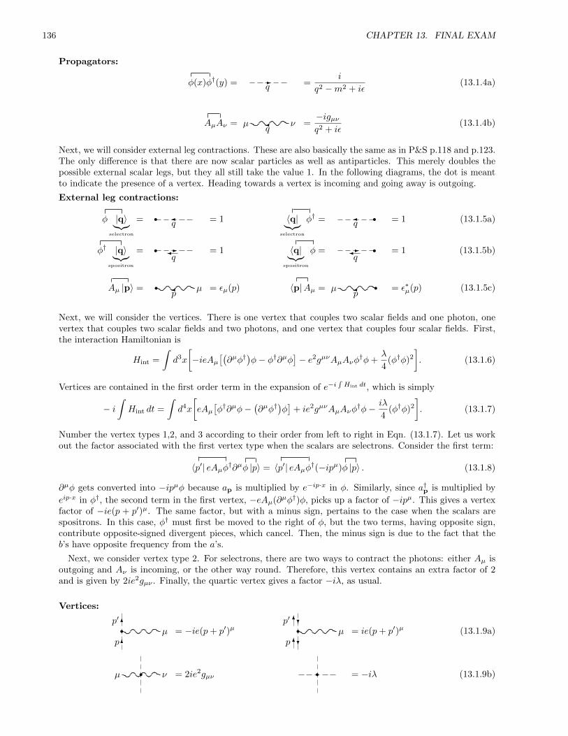
136 CHAPTER 13. FINAL EXAM
Propagators:
φ(x)φ†(y) = -q =
i
q2 −m2 + iε(13.1.4a)
AµAν = q
µ ν =−igµνq2 + iε
(13.1.4b)
Next, we will consider external leg contractions. These are also basically the same as in P&S p.118 and p.123.The only difference is that there are now scalar particles as well as antiparticles. This merely doubles thepossible external scalar legs, but they all still take the value 1. In the following diagrams, the dot is meantto indicate the presence of a vertex. Heading towards a vertex is incoming and going away is outgoing.
External leg contractions:
φ |q〉︸︷︷︸selectron
= qr = 1 〈q|︸︷︷︸
selectron
φ† = qr = 1 (13.1.5a)
φ† |q〉︸︷︷︸spositron
= -qr = 1 〈q|︸︷︷︸
spositron
φ = -qr = 1 (13.1.5b)
Aµ |p〉 = p
µr = εµ(p) 〈p|Aµ = p
µ r = ε∗µ(p) (13.1.5c)
Next, we will consider the vertices. There is one vertex that couples two scalar fields and one photon, onevertex that couples two scalar fields and two photons, and one vertex that couples four scalar fields. First,the interaction Hamiltonian is
Hint =
∫d3x
[−ieAµ
[(∂µφ†
)φ− φ†∂µφ
]− e2gµνAµAνφ
†φ+λ
4(φ†φ)2
]. (13.1.6)
Vertices are contained in the first order term in the expansion of e−i∫Hint dt, which is simply
− i∫Hint dt =
∫d4x
[eAµ
[φ†∂µφ−
(∂µφ†
)φ]
+ ie2gµνAµAνφ†φ− iλ
4(φ†φ)2
]. (13.1.7)
Number the vertex types 1,2, and 3 according to their order from left to right in Eqn. (13.1.7). Let us workout the factor associated with the first vertex type when the scalars are selectrons. Consider the first term:
〈p′| eAµφ†∂µφ |p〉 = 〈p′| eAµφ†(−ipµ)φ |p〉 . (13.1.8)
∂µφ gets converted into −ipµφ because ap is multiplied by e−ip·x in φ. Similarly, since a†p is multiplied by
eip·x in φ†, the second term in the first vertex, −eAµ(∂µφ†)φ, picks up a factor of −ipµ. This gives a vertexfactor of −ie(p + p′)µ. The same factor, but with a minus sign, pertains to the case when the scalars arespositrons. In this case, φ† must first be moved to the right of φ, but the two terms, having opposite sign,contribute opposite-signed divergent pieces, which cancel. Then, the minus sign is due to the fact that theb’s have opposite frequency from the a’s.
Next, we consider vertex type 2. For selectrons, there are two ways to contract the photons: either Aµ isoutgoing and Aν is incoming, or the other way round. Therefore, this vertex contains an extra factor of 2and is given by 2ie2gµν . Finally, the quartic vertex gives a factor −iλ, as usual.
Vertices:
µr6
6
p
p′
= −ie(p+ p′)µ µr?
?
6
6
p
p′
= ie(p+ p′)µ (13.1.9a)
r νµ = 2ie2gµν r = −iλ (13.1.9b)
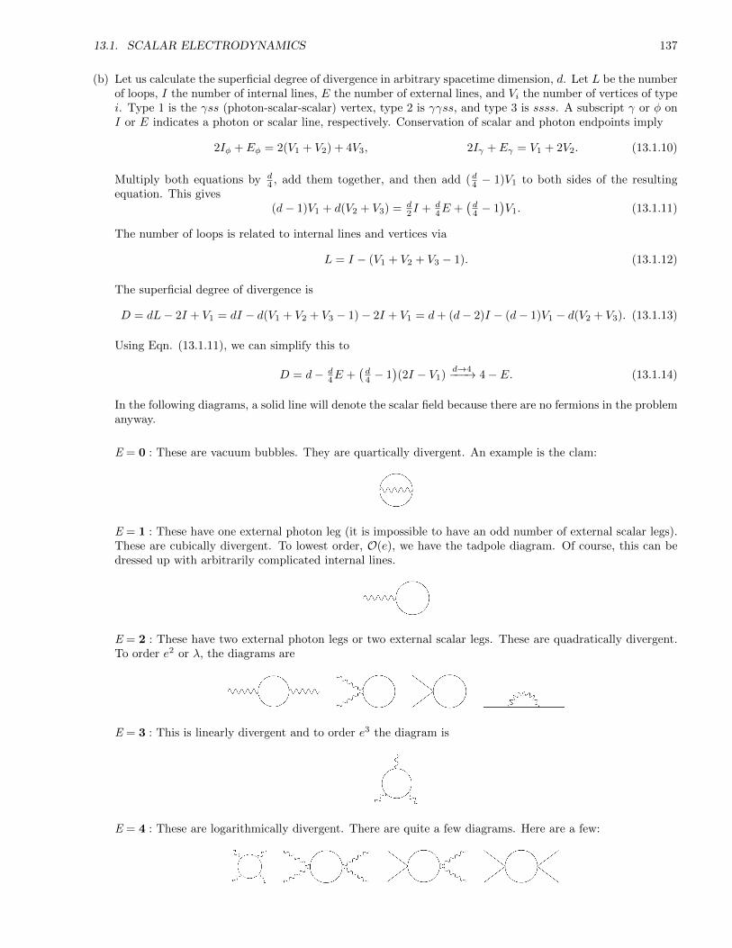
13.1. SCALAR ELECTRODYNAMICS 137
(b) Let us calculate the superficial degree of divergence in arbitrary spacetime dimension, d. Let L be the numberof loops, I the number of internal lines, E the number of external lines, and Vi the number of vertices of typei. Type 1 is the γss (photon-scalar-scalar) vertex, type 2 is γγss, and type 3 is ssss. A subscript γ or φ onI or E indicates a photon or scalar line, respectively. Conservation of scalar and photon endpoints imply
2Iφ + Eφ = 2(V1 + V2) + 4V3, 2Iγ + Eγ = V1 + 2V2. (13.1.10)
Multiply both equations by d4 , add them together, and then add (d4 − 1)V1 to both sides of the resulting
equation. This gives(d− 1)V1 + d(V2 + V3) = d
2I + d4E +
(d4 − 1
)V1. (13.1.11)
The number of loops is related to internal lines and vertices via
L = I − (V1 + V2 + V3 − 1). (13.1.12)
The superficial degree of divergence is
D = dL− 2I + V1 = dI − d(V1 + V2 + V3 − 1)− 2I + V1 = d+ (d− 2)I − (d− 1)V1 − d(V2 + V3). (13.1.13)
Using Eqn. (13.1.11), we can simplify this to
D = d− d4E +
(d4 − 1
)(2I − V1)
d→4−−−→ 4− E. (13.1.14)
In the following diagrams, a solid line will denote the scalar field because there are no fermions in the problemanyway.
E = 0 : These are vacuum bubbles. They are quartically divergent. An example is the clam:
E = 1 : These have one external photon leg (it is impossible to have an odd number of external scalar legs).These are cubically divergent. To lowest order, O(e), we have the tadpole diagram. Of course, this can bedressed up with arbitrarily complicated internal lines.
E = 2 : These have two external photon legs or two external scalar legs. These are quadratically divergent.To order e2 or λ, the diagrams are
E = 3 : This is linearly divergent and to order e3 the diagram is
E = 4 : These are logarithmically divergent. There are quite a few diagrams. Here are a few:

138 CHAPTER 13. FINAL EXAM
(c) It is technically unnatural for g to be small because there is no enhancement of symmetry in the g → 0 limit.Therefore, we should expect that the quartic term would be generated dynamically anyway by quantum cor-rections. The one loop diagram below is an example of a diagram that contributes a quartic vertex correction,and would produce such a vertex even if one did not exist to begin with. This diagram is logarithmicallydivergent since it has E = 4 or D = 0.
(13.1.15)
(d) I would use dimensional regularization because, unlike Pauli-Villars or the sharp cut-off method, dimensionalregularization never breaks gauge-invariance.
13.2 Non-relativistic Lifshitz Scalar Field Theory
Consider the simplest theory of a Lifshitz scalar, whose action is given in D spatial dimensions by
S2 =1
2
∫dt dDx
(∂tΦ)2 − (∆Φ)2
, (13.2.1)
where ∆ ≡∑Di=1 ∂i∂i is the spatial Laplacian. This defines a free field theory with anisotropic scalaing, charac-
terized by dynamical exponent z = 2.
(a) Determine the classical scaling dimension of Φ in this theory, as a function of D.
(b) List all independent classically relevant and classically marginal terms that can be added to the action ofthis theory in the special case of D = 3 spatial dimensions.
SOLUTION:
(a) Spatial coordinates have dimension −1 and time has dimension −z = −2. Therefore, in order to make S2
dimensionless, we must have
[Φ] =D − 2
2. (13.2.2)
(b) To maintain spatial isotropy, ∂i must appear in like pairs, ∆. Let λabc be the coefficient of a term containinga time derivatives, b spatial Laplacians or 2b spatial derivatives, and c scalar fields. The dimension of λabc is
[λabc] = 5− 2(a+ b)− c2 . (13.2.3)
λabc is irrelevent if its dimension is negative. Therefore, there are three cases: (1) a = b = 0 and c = 0, . . . , 10;(2) (a, b) = (1, 0) or (0, 1) and c = 0, . . . , 6; or (3) (a, b) = (2, 0) or (0, 2) or (1, 1) and c = 0, 1, 2. If we wantto maintain the φ→ −φ symmetry, then c must be even.

13.3. ASYMPTOTIC FREEDOM IN 5+1 DIMENSIONS 139
13.3 Asymptotic Freedom in 5+1 Dimensions
Consider the relativistic scalar field theory with the λφ3 interaction,
S3 =1
2
∫ddx
∂µφ∂µφ−m2φ2 − λ
3φ3
. (13.3.1)
Even though this theory does not have energy bounded from below and therefore no non-perturbatively stableground state, it still makes sense to study it to all orders in perturbation theory using Feynman diagrams. Peoplesay that this theory is asymptotically free in d = 5 + 1 dimensions.
(a) What quantity would you calculate to convince yourself that this theory is asymptotically free at one loop?
(b) Draw all Feynman diagrams that you would need in order to show asymptotic freedom at one loop. Whatdegree of divergence do you expect from those diagrams?
(c) (Bonus) Using dimensional regularization, complete the one-loop calculation in the λφ3 theory to the pointwhere you prove its asymptotic freedom in d = 5 + 1 at one loop. (You must show all intermediate steps,not just the final result.)
SOLUTION:
(a) The sign of the beta function for λ. Asymptotic freedom would be implied by β(λ) < 0.
(b) The number of loops in a diagram is related to the number of internal lines, I, and vertices, V via L =I−(V −1). Conservation of endpoints implies 3V = 2I+E, where E is the number of external lines. Finally,the superficial degree of divergence is related to the number of loops and internal lines via D = dL − 2I.Combining these three equations gives
D = dL− d3E + 2
(d6 − 1
)I. (13.3.2)
At the one-loop level, L = 1. The loop and endpoint-conservation equations imply V = I = E in this caseand Eqn. (13.3.2) simplifies to
D|L=1 = d− 2E. (13.3.3)
When d = 6, there are four types of divergent diagrams: (1) E = 0 vacuum bubbles, which are unimportant;(2) E = 1 tadpole diagram, which is also unimportant since it just gives a source term for φ; (3) E = 2self-energy diagram, which gives the wavefunction and mass renormalizations and which is quadraticallydivergent; and (4) E = 3, which gives the vertex renormalization and is logarithmically divergent.
(c) Rewrite the action in Eqn. (13.3.1) with 0 subscripts on φ, m and λ to indicate that they are bare quantities.Quantities with no subscripts are taken to be renormalized. Then,
S3 =1
2
∫ddx
∂µφ∂µφ−m2φ2 − λ
3µ
6−d2 φ3 −A∂µφ∂µφ+Bm2φ2 − Cλ
3µ
6−d2 φ3 + Jφ
. (13.3.4)
The first two terms are the free action, the third is the interaction term, and the last four are the counterterms.We have added a φ counterterm to cancel the tadpole diagram in principle, but we will not actually calculateit since it does not affect the rest of the renormalization or whether or not the theory is asymptotically free.
The term µ6−d
2 requires some explanation. The dimension of φ is [φ] = d−22 . Therefore, without this µ
term, the dimension of λ would depend on the dimension of spacetime as [λ] = 6−d2 . We must absorb this
dimension into an arbitrary scale, µ, in order to keep λ dimensionless.
A and B introduce a new quadratic vertex with vertex factor −i(Ap2 − Bm2), where p is the incomingand outgoing momentum. C introduces a new cubic vertex with vertex factor −iCλ. These new vertices aredenoted by a cross:
- -p p = −i(Ap2 −Bm2), = −iCλ. (13.3.5)

140 CHAPTER 13. FINAL EXAM
The exact propagator, De, may be expanded in terms of the free propagator, Df , and successive 1PI inter-mediates as
De = Df +Df (−iΣ)Df +Df (−iΣ)Df (−iΣ)Df + · · ·= Df
[1 + (−iΣDf ) + (−iΣDf )2 + · · ·
]=
Df
1 + iΣDf
=i
p2 −m2 − Σ, (13.3.6)
where we recall that Df = ip2−m2 . To one-loop order, or quadratic order in λ,
− iΣ = −iΣ2 +O(λ4) = m + (13.3.7)
Denote the first term by −iΣint2 and the second by −iΣct
2 . The superscripts stand for “interaction” and“counterterm”. The counterterm contribution is simply its vertex factor in Eqn. (13.3.5). The interactioncontribution is
−iΣint2 =
1
2
(−iλµ
6−d2
)2 ∫d dk
i
k2 −m2
i
(k − p)2 −m2
=1
2λ2µ6−d
∫ 1
0
dz
∫d dk
1
z[(k − p)2 −m2] + (1− z)(k2 −m2)2. (13.3.8)
Note that the factor of 12 out front is due to the symmetry factor of the diagram, which is 2. Write the
denominator as D2 where
D = k2 − 2zp+ z2p2 − z2p2 + zp2 −m2 = `2 −∆, (13.3.9)
where
` ≡ k − zp, ∆ ≡ m2 − z(1− z)p2. (13.3.10)
After Wick-rotating, we have
−iΣint2 =
i
2λ2µ6−d
∫ 1
0
dz
∫d d`E
1
(`2E + ∆)2
=i
2λ2µ6−d
∫ 1
0
dz1
(4π)d2
Γ(2− d2 )
Γ(2)∆
d2−2, (13.3.11)
where use was made of Eqn. 7.85 P&S p.251. Now substitute in ε = 6−d2 :
− iΣint2 =
i
2λ2µ2εΓ(−1 + ε)
(4π)3−ε
∫ 1
0
dz∆1−ε. (13.3.12)
Expand around ε = 0 using
Γ(−n+ ε) =(−1)n
n!
(1
ε− γ +
n∑k=1
1
k+O(ε)
), aε = 1 + ε ln a+O(ε2). (13.3.13)
The result is
− iΣint2 = − iλ2
2(4π)3
∫ 1
0
dz∆
(1
ε− γ + 1 + ln
4πµ2
∆
). (13.3.14)
Let us follow the MS renormalization scheme and absorb the factor of γ and ln 4π into a redefinition of theRG scale by defining
µ2 =4πµ2
eγ. (13.3.15)
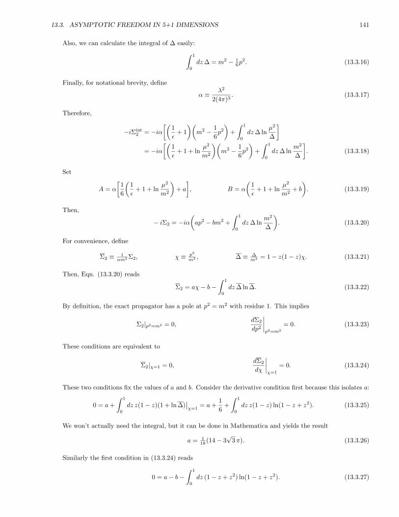
13.3. ASYMPTOTIC FREEDOM IN 5+1 DIMENSIONS 141
Also, we can calculate the integral of ∆ easily:∫ 1
0
dz∆ = m2 − 16p
2. (13.3.16)
Finally, for notational brevity, define
α ≡ λ2
2(4π)3. (13.3.17)
Therefore,
−iΣint2 = −iα
[(1
ε+ 1
)(m2 − 1
6p2
)+
∫ 1
0
dz∆ lnµ2
∆
]= −iα
[(1
ε+ 1 + ln
µ2
m2
)(m2 − 1
6p2
)+
∫ 1
0
dz∆ lnm2
∆
]. (13.3.18)
Set
A = α
[1
6
(1
ε+ 1 + ln
µ2
m2
)+ a
], B = α
(1
ε+ 1 + ln
µ2
m2+ b
). (13.3.19)
Then,
− iΣ2 = −iα(ap2 − bm2 +
∫ 1
0
dz∆ lnm2
∆
). (13.3.20)
For convenience, define
Σ2 ≡ 1αm2 Σ2, χ ≡ p2
m2 , ∆ ≡ ∆m2 = 1− z(1− z)χ. (13.3.21)
Then, Eqn. (13.3.20) reads
Σ2 = aχ− b−∫ 1
0
dz∆ ln ∆. (13.3.22)
By definition, the exact propagator has a pole at p2 = m2 with residue 1. This implies
Σ2|p2=m2 = 0,dΣ2
dp2
∣∣∣∣p2=m2
= 0. (13.3.23)
These conditions are equivalent to
Σ2|χ=1 = 0,dΣ2
dχ
∣∣∣∣χ=1
= 0. (13.3.24)
These two conditions fix the values of a and b. Consider the derivative condition first because this isolates a:
0 = a+
∫ 1
0
dz z(1− z)(1 + ln ∆)∣∣χ=1
= a+1
6+
∫ 1
0
dz z(1− z) ln(1− z + z2). (13.3.25)
We won’t actually need the integral, but it can be done in Mathematica and yields the result
a = 118 (14− 3
√3π). (13.3.26)
Similarly the first condition in (13.3.24) reads
0 = a− b−∫ 1
0
dz (1− z + z2) ln(1− z + z2). (13.3.27)
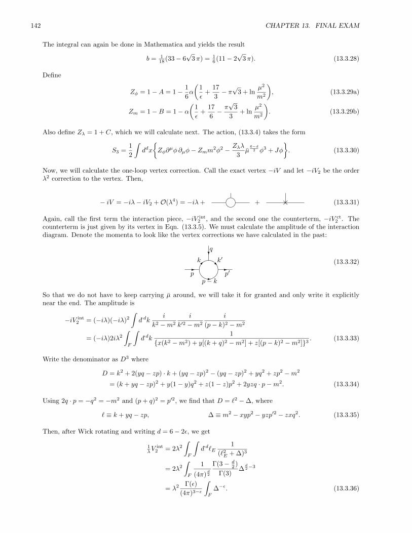
142 CHAPTER 13. FINAL EXAM
The integral can again be done in Mathematica and yields the result
b = 118 (33− 6
√3π) = 1
6 (11− 2√
3π). (13.3.28)
Define
Zφ = 1−A = 1− 1
6α
(1
ε+
17
3− π√
3 + lnµ2
m2
), (13.3.29a)
Zm = 1−B = 1− α(
1
ε+
17
6− π√
3
3+ ln
µ2
m2
). (13.3.29b)
Also define Zλ = 1 + C, which we will calculate next. The action, (13.3.4) takes the form
S3 =1
2
∫ddx
Zφ∂
µφ∂µφ− Zmm2φ2 − Zλλ
3µ
6−d2 φ3 + Jφ
. (13.3.30)
Now, we will calculate the one-loop vertex correction. Call the exact vertex −iV and let −iV2 be the orderλ2 correction to the vertex. Then,
− iV = −iλ− iV2 +O(λ4) = −iλ+ m + (13.3.31)
Again, call the first term the interaction piece, −iV int2 , and the second one the counterterm, −iV ct
2 . Thecounterterm is just given by its vertex in Eqn. (13.3.5). We must calculate the amplitude of the interactiondiagram. Denote the momenta to look like the vertex corrections we have calculated in the past:
- -
?
R
-p p′
q
k k′
p− k
(13.3.32)
So that we do not have to keep carrying µ around, we will take it for granted and only write it explicitlynear the end. The amplitude is
−iV int2 = (−iλ)(−iλ)2
∫d dk
i
k2 −m2
i
k′2 −m2
i
(p− k)2 −m2
= (−iλ)2iλ2
∫F
∫d dk
1
x(k2 −m2) + y[(k + q)2 −m2] + z[(p− k)2 −m2]3. (13.3.33)
Write the denominator as D3 where
D = k2 + 2(yq − zp) · k + (yq − zp)2 − (yq − zp)2 + yq2 + zp2 −m2
= (k + yq − zp)2 + y(1− y)q2 + z(1− z)p2 + 2yzq · p−m2. (13.3.34)
Using 2q · p = −q2 = −m2 and (p+ q)2 = p′2, we find that D = `2 −∆, where
` ≡ k + yq − zp, ∆ ≡ m2 − xyp2 − yzp′2 − zxq2. (13.3.35)
Then, after Wick rotating and writing d = 6− 2ε, we get
1λV
int2 = 2λ2
∫F
∫d d`E
1
(`2E + ∆)3
= 2λ2
∫F
1
(4π)d2
Γ(3− d2 )
Γ(3)∆
d2−3
= λ2 Γ(ε)
(4π)3−ε
∫F
∆−ε. (13.3.36)
13.3. ASYMPTOTIC FREEDOM IN 5+1 DIMENSIONS 143
We reintroduce µ on the right (there is no point in writing it on the left) by inserting a factor µ6−d = µ2ε.Then, we expand around ε = 0 to get
1λV
int2 =
λ2
(4π)3
∫F
(1
ε− γ + ln
4πµ2
∆
)MS−−→ 2α
∫F
(1
ε+ ln
µ2
∆
). (13.3.37)
Using∫F
=∫ 1
0dz∫ 1−z
0dy = 1
2 , we get
1λV
int2 = α
(1
ε+ ln
µ2
m2− 2
∫F
ln ∆
), (13.3.38)
where we recall that ∆ = ∆/m2.
Set
C = −α(
1
ε+ ln
µ2
m2+ c
). (13.3.39)
Then, since 1λV
ct2 = C, we get
1λV = 1− α
(c+ 2
∫F
ln ∆
). (13.3.40)
We must simply choose a value for c because there is no analog of the conditions in Eqn. (13.3.23). Wewill fix c such that V = λ when the external legs are at zero momentum. This is somewhat unphysicalsince the scalar is massive and thus cannot be physical at zero 4-momentum. In this case, ∆ = 1 and thus,V = (1− αc)λ. Therefore, we must set c = 0. Finally, recalling that Zλ = 1 + C, we have
Zλ = 1− α(
1
ε+ ln
µ2
m2
). (13.3.41)
Compare the expression of S3 in terms of renormalized and bare quantities:
S3 =1
2
∫ddx
Zφ∂
µφ∂µφ− Zmm2φ2 − Zλλ
3µεφ3 + Jφ
, (13.3.42a)
S3 =1
2
∫ddx
∂µφ0∂µφ0 −m2
0φ20 −
λ0
3φ3
0 − J0φ0
. (13.3.42b)
Therefore, λ0 is related to λ via
λ0 = Z−3/2φ Zλµ
ελ =⇒ α0 =λ2
0
2(4π)3= Z−3
φ Z2λµ
2εα. (13.3.43)
Let us focus only on the divergent pieces in the Z’s because it turns out that the non-divergent pieces onlycontribute terms of order ε or higher, which vanish in the ε→ 0 limit. Thus,
Zφ = 1− α
6ε, Zλ = 1− α
ε, (13.3.44)
and
α0 ≈(
1− α
2ε
)(1− 2α
ε
)(4πe−γ)εµ2εα = α
(1− 3α
2ε
)(4πe−γ)εµ2ε +O(α3). (13.3.45)
Take the log of this:
lnα0 = lnα+ ln(
1− 3α
2ε
)+ 2ε lnµ+ ε ln 4π − εγ ≈ lnα− 3α
2ε+ 2ε lnµ+ ε ln 4π − εγ. (13.3.46)
Recall what happens in Pauli-Villars regularization or the sharp cut-off method: the bare parameters arefunctions of the cut-off, but not of the RG scale. Instead, the renormalized parameters are functions of the
144 CHAPTER 13. FINAL EXAM
RG scale, but not of the cut-off. Roughly speaking, the ε parameter in dimensional regularization plays therole of the cut-off, Λ. Therefore, we must have
0 =d lnα0
d lnµ=( 1
α− 3
2ε
) dα
d lnµ+ 2ε. (13.3.47)
Therefore, (1− 3α
2ε
) dα
d lnµ= −2εα. (13.3.48)
Then, the β function is taken in the ε→ 0 limit:
β(α) =dα
d lnµ≈ −2εα
(1 +
3α
2ε
)= −2εα− 3α2 ε→0−−−→ −3α2 . (13.3.49)
Since the sign of the beta function is negative, the theory is asymptotically free . It is easy to solve for α:
α(µ) =α
1 + 3α ln(µ/µ), (13.3.50)
where α = α when µ = µ. Indeed, αµ→∞−−−−→ 0.
Aside: Note that the calculation of a, b and c is immaterial insofar as asymptotic freedom is concerned since weended up caring only about the ε poles. However, just in case you dislike the unphysical limit that we took toset c = 0, let us consider the more physical limit of on-shell external particles for which p′2 = p2 = q2 = m2.Looking back at the expression for ∆ in Eqn. (13.3.35) and recalling that ∆ = ∆/m2, in this case
∆ = 1− xy − yz − zx. (13.3.51)
You can check for yourself that this quantity is always positive in the integration domain taking on its minimumvalue of 2
3 when x = y = z = 13 . The required integral can be calculated numerically and yields∫
F
ln ∆ ≈ −0.1456. (13.3.52)
Therefore, Eqn. (13.3.40) reads
1λV = 1− α(c− 0.2912) =⇒ c = 0.2912. (13.3.53)
This means that we have chosen V = λ to coincide with the external particles being on-shell.