
Quantum Electrodynamic Bound–State Calculations and ...
124
arXiv:hep-ph/0306153 v1 17 Jun 2003 Quantum Electrodynamic Bound–State Calculations and Large–Order Perturbation Theory based on a Habilitation Thesis Dresden University of Technology by Ulrich Jentschura 1 st Edition June 2002 2 nd Edition April 2003 [with hypertext references and updates] E–Mail: [email protected] [email protected] [email protected] 1
-
Upload
khangminh22 -
Category
Documents
-
view
3 -
download
0
Transcript of Quantum Electrodynamic Bound–State Calculations and ...

arX
iv:h
ep-p
h/03
0615
3 v1
17
Jun
200
3
Quantum Electrodynamic
Bound–State Calculations
and Large–Order Perturbation
Theory
based on a
Habilitation Thesis
Dresden University of Technology
by
Ulrich Jentschura
1st Edition June 2002
2nd Edition April 2003
[with hypertext references and updates]
E–Mail:
1

This manuscript is also available – in the form of a book – from
Shaker Verlag GmbH, Postfach 101818, 52018 Aachen, Germany,ISBN: 3-8322-1686-3,
world-wide web address: http://www.shaker.de,electronic-mail address: [email protected].
It has been posted in the online archives with permission of the publisher.
2

Contents
I Quantum Electrodynamic Bound–State Calculations 7
1 Numerical Calculation of the One–Loop Self Energy (Excited States) 8
1.1 Orientation . . . . . . . . . . . . . . . . . . . . . . . . . . . . . . . . . . . . . . . . . . . . 8
1.2 Introduction to the Numerical Calculation of Radiative Corrections . . . . . . . . . . . . . 8
1.3 Method of Evaluation . . . . . . . . . . . . . . . . . . . . . . . . . . . . . . . . . . . . . . 9
1.3.1 Status of Analytic Calculations . . . . . . . . . . . . . . . . . . . . . . . . . . . . . 9
1.3.2 Formulation of the Numerical Problem . . . . . . . . . . . . . . . . . . . . . . . . . 12
1.3.3 Treatment of the divergent terms . . . . . . . . . . . . . . . . . . . . . . . . . . . . 15
1.4 The Low-Energy Part . . . . . . . . . . . . . . . . . . . . . . . . . . . . . . . . . . . . . . 17
1.4.1 The Infrared Part . . . . . . . . . . . . . . . . . . . . . . . . . . . . . . . . . . . . 17
1.4.2 The Middle-Energy Subtraction Term . . . . . . . . . . . . . . . . . . . . . . . . . 21
1.4.3 The Middle-Energy Remainder . . . . . . . . . . . . . . . . . . . . . . . . . . . . . 22
1.5 The High-Energy Part . . . . . . . . . . . . . . . . . . . . . . . . . . . . . . . . . . . . . . 25
1.5.1 The High-Energy Subtraction Term . . . . . . . . . . . . . . . . . . . . . . . . . . 25
1.5.2 The High-Energy Remainder . . . . . . . . . . . . . . . . . . . . . . . . . . . . . . 27
1.5.3 Results for the High-Energy Part . . . . . . . . . . . . . . . . . . . . . . . . . . . . 29
1.6 Comparison to Analytic Calculations . . . . . . . . . . . . . . . . . . . . . . . . . . . . . . 29
2 Analytic Self–Energy Calculations for Excited States 34
2.1 Orientation . . . . . . . . . . . . . . . . . . . . . . . . . . . . . . . . . . . . . . . . . . . . 34
2.2 The epsilon-Method . . . . . . . . . . . . . . . . . . . . . . . . . . . . . . . . . . . . . . . 35
2.3 Results for High– and Low–Energy Contributions . . . . . . . . . . . . . . . . . . . . . . . 37
2.3.1 P 1/2 states (kappa = 1) . . . . . . . . . . . . . . . . . . . . . . . . . . . . . . . . 37
2.3.2 P 3/2 states (kappa = -2) . . . . . . . . . . . . . . . . . . . . . . . . . . . . . . . . 38
2.3.3 D 3/2 states (kappa = 2) . . . . . . . . . . . . . . . . . . . . . . . . . . . . . . . . 39
2.3.4 D 5/2 states (kappa = -3) . . . . . . . . . . . . . . . . . . . . . . . . . . . . . . . . 39
2.3.5 F 5/2 states (kappa = 3) . . . . . . . . . . . . . . . . . . . . . . . . . . . . . . . . 40
2.3.6 F 7/2 states (kappa = -4) . . . . . . . . . . . . . . . . . . . . . . . . . . . . . . . . 40
2.3.7 G 7/2 states (kappa = 4) . . . . . . . . . . . . . . . . . . . . . . . . . . . . . . . . 41
2.3.8 G 9/2 states (kappa = -5) . . . . . . . . . . . . . . . . . . . . . . . . . . . . . . . . 41
2.4 Summary of Results . . . . . . . . . . . . . . . . . . . . . . . . . . . . . . . . . . . . . . . 41
2.5 Typical Cancellations . . . . . . . . . . . . . . . . . . . . . . . . . . . . . . . . . . . . . . 41
2.6 Observations . . . . . . . . . . . . . . . . . . . . . . . . . . . . . . . . . . . . . . . . . . . 42
3

3 The Two–Loop Self–Energy 45
3.1 Orientation . . . . . . . . . . . . . . . . . . . . . . . . . . . . . . . . . . . . . . . . . . . . 45
3.2 Introduction to the Two–Loop Self–Energy . . . . . . . . . . . . . . . . . . . . . . . . . . 45
3.3 Two-loop Form Factors . . . . . . . . . . . . . . . . . . . . . . . . . . . . . . . . . . . . . 47
3.4 High–Energy Part . . . . . . . . . . . . . . . . . . . . . . . . . . . . . . . . . . . . . . . . 50
3.5 Low–Energy Part . . . . . . . . . . . . . . . . . . . . . . . . . . . . . . . . . . . . . . . . . 52
3.6 Results for the Two–Loop Corrections . . . . . . . . . . . . . . . . . . . . . . . . . . . . . 55
4 Spinless Particles in Bound–State Quantum Electrodynamics 56
4.1 Orientation . . . . . . . . . . . . . . . . . . . . . . . . . . . . . . . . . . . . . . . . . . . . 56
4.2 Introduction to Spinless QED and Pionium . . . . . . . . . . . . . . . . . . . . . . . . . . 56
4.3 Breit hamiltonian for Spinless Particles . . . . . . . . . . . . . . . . . . . . . . . . . . . . . 56
4.4 Vacuum Polarization Effects . . . . . . . . . . . . . . . . . . . . . . . . . . . . . . . . . . . 60
4.5 Effects due to Scalar QED . . . . . . . . . . . . . . . . . . . . . . . . . . . . . . . . . . . . 60
5 QED Calculations: A Summary 63
II Convergence Acceleration and Divergent Series 67
6 Introduction to Convergence Acceleration and Divergent Series in Physics 68
7 Convergence Acceleration 71
7.1 The Concept of Convergence Acceleration . . . . . . . . . . . . . . . . . . . . . . . . . . . 71
7.1.1 A Brief Survey . . . . . . . . . . . . . . . . . . . . . . . . . . . . . . . . . . . . . . 71
7.1.2 The Forward Difference Operator . . . . . . . . . . . . . . . . . . . . . . . . . . . . 72
7.1.3 Linear and Logarithmic Convergence . . . . . . . . . . . . . . . . . . . . . . . . . . 72
7.1.4 The Standard Tool: Pade Approximants . . . . . . . . . . . . . . . . . . . . . . . . 73
7.1.5 Nonlinear Sequence Transformations . . . . . . . . . . . . . . . . . . . . . . . . . . 74
7.1.6 The Combined Nonlinear–Condensation Transformation (CNCT) . . . . . . . . . . 77
7.2 Applications of Convergence Acceleration Methods . . . . . . . . . . . . . . . . . . . . . . 79
7.2.1 Applications in Statistics and Applied Biophysics . . . . . . . . . . . . . . . . . . . 79
7.2.2 An Application in Experimental Mathematics . . . . . . . . . . . . . . . . . . . . . 80
7.2.3 Other Applications of the CNCT . . . . . . . . . . . . . . . . . . . . . . . . . . . . 84
7.3 Conclusions and Outlook for Convergence Acceleration . . . . . . . . . . . . . . . . . . . . 84
8 Divergent Series 86
8.1 Introduction to Divergent Series in Physics . . . . . . . . . . . . . . . . . . . . . . . . . . 86
8.2 The Stark Effect: A Paradigmatic Example . . . . . . . . . . . . . . . . . . . . . . . . . . 87
8.2.1 Perturbation Series for the Stark Effect . . . . . . . . . . . . . . . . . . . . . . . . 87
8.2.2 Borel–Pade Resummation . . . . . . . . . . . . . . . . . . . . . . . . . . . . . . . . 88
8.2.3 Doubly–Cut Borel Plane . . . . . . . . . . . . . . . . . . . . . . . . . . . . . . . . . 90
8.2.4 Numerical Calculations for the Stark Effect . . . . . . . . . . . . . . . . . . . . . . 92
8.3 Further Applications of Resummation Methods . . . . . . . . . . . . . . . . . . . . . . . . 95
8.3.1 Zero–Dimensional Theories with Degenerate Minima . . . . . . . . . . . . . . . . . 95
8.3.2 The Effective Action as a Divergent Series . . . . . . . . . . . . . . . . . . . . . . . 98
8.3.3 The Double–Well Problem . . . . . . . . . . . . . . . . . . . . . . . . . . . . . . . . 103
8.4 Divergent Series: Some Conclusions . . . . . . . . . . . . . . . . . . . . . . . . . . . . . . . 108
9 Conclusions 111
4

Abstract
This Thesis is based on quantum electrodynamic (QED) bound-state calculations [1, 2, 3, 4, 5, 6, 7, 8, 9,10, 11, 12, 13, 14, 15, 16, 17, 18, 19, 20, 21, 22], as well as on investigations related to divergent series,convergence acceleration and applications of these concepts to physical problems [23, 24, 25, 26, 27, 28,29, 30, 31].
The subjects which are discussed in this Thesis include: the self energy of a bound electron and thespin-dependence of QED corrections in bound systems (Chs. 1 – 5), convergence acceleration techniques(Chs. 6 and 7), and resummation methods for divergent series with an emphasis on physical applications(Ch. 8).
In Chapter 1, we present numerical results [12], accurate to the level of 1 Hz for atomic hydrogen, for theenergy correction to the K and L shell states due to the one-loop self energy. We investigate hydrogenlikesystems with low nuclear charge number Z = 1–5. Calculations are carried out using on-mass shellrenormalization, which guarantees that the final result is written in terms of the physical electron charge.The purpose of the calculation is twofold: first, we provide accurate theoretical predictions for the one-loopself energy of K and L shell states. Second, the comparison of the analytic and numerical approaches tothe Lamb shift calculations, which have followed separate paths for the past few decades, is demonstratedby comparing the numerical values with analytic data obtained using the Zα-expansion [1, 2, 32]. Ourcalculation essentially eliminates the uncertainty due to the truncation of the Zα-expansion, and itdemonstrates the consistency of the numerical and analytic approaches which have attracted attentionfor more than five decades, beginning with the seminal paper [33]. The most important numerical resultsare summarized in Table 1.5.
In Chapter 2, we investigate higher-order analytic calculations of the one-photon self energy for excitedatomic states. These calculations rely on mathematical methods described in Sec. 2.2 which, in physicalterms, lead to a separation of the calculation into a high- and a low-energy part for the virtual photon.This separation does not only permit adequate simplifications for the two energy regions [1, 2], but alsoan adequate treatment of the infrared divergences which plague all bound-state calculations (see alsoCh. 7 of [34]). The investigation represents a continuation of previous work on the subject [1, 2, 32]. Thecalculations are relevant for transitions to highly excited states, which are relevant for the extractionof fundamental constants from the high-precision measurements in atomic hydrogen [35], and for theestimation of QED effects in more complex atomic systems where some of the electrons occupy highlyexcited states.
Chapter 3. We investigate the two-loop self energy. The calculation is based on a generalization of themethods introduced in Sec. 2.2. Historically, the two-loop self energy for bound states has represented amajor task for theoretical evaluations. We present an analytic calculation [16] of the fine-structure differ-ence of the two-loop self energy for P states in atomic hydrogen in the order α2 (Zα)6me c
2. This energydifference can be parameterized by two analytic coefficients, known as B61 and B60 (see Sec. 3.2). Thesecoefficients describe the two-loop self energy in the sixth order in Zα, with an additional enhancementdue to a large logarithm ln[(Zα)−2] (in the case of the B61-coefficient). The calculations are relevant foran improved theoretical understanding of the fine-structure in hydrogenlike systems. They are also in partrelevant for current experiments on atomic helium [36, 37, 38, 39], whose motivation is the determinationof the fine-structure constant with improved accuracy. Finally, it is hoped that numerical calculations ofthe two-loop effect will be carried out in the near future for which the current analytic evaluation will bean important consistency check. The calculation of the analytic corrections discussed in Sec. 3 representsa solution for the most problematic set of diagrams on the way to advance our understanding of thefine-structure in atomic hydrogen to the few-Hz level. Explicit results for the fine-structure difference of
5

the B61- and B60-coefficients can be found in Eqs. (3.59) – (3.64).
In Chapter 4, We investigate the spin-dependence of the Breit hamiltonian and quantum electrodynamiceffects in general. Specifically, we consider a bound system of two spinless particles. The calculation ismotivated in part by current experiments (DIRAC at CERN) whose aim is the experimental study ofpionium, which is the bound system of two (spinless) oppositely charged pions. The evaluation of thetwo-body relativistic corrections of order (Zα)4 leads to a different result [17] than expected for a systemof two spin-1/2 particles of equal mass, e.g. positronium. In particular, we conclude in Sec. 4.3 thatthe so-called zitterbewegung term is absent for a system of two spinless particles (the absence of thezitterbewegung term in a bound system consisting of a spinless and a spin-1/2 particle was previouslypointed out in [40]). Final results for the relativistic correction, the vacuum polarization, and the selfenergy of a system of two scalar particles can be found in Eqs. (4.15), (4.21) and (4.31). A summary ofthe QED calculations is provided in Chapter 5.
In the second part of this Thesis, we discuss methods for accelerating the convergence of series, and forthe resummation of divergent series. As discussed in Chapter 6 and Sec. 7.1.1, convergence accelerationis essentially based on the idea that information hidden in trailing digits of elements of the sequencecan be used in order to make “educated guesses” regarding the remainder term, which can be usedfor the construction of powerful sequence transformations (see Sec. 7.1.5). In Chapter 7, we discussconvergence acceleration in detail. After a short overview of relevant mathematical methods (Sec. 7.1),we discuss applications in applied biophysics (Sec. 7.2.1), in experimental mathematics (Sec. 7.2.2), andother applications, mainly in the evaluation of special functions (Sec. 7.2.3). In particular, Secs. 7.2.1 –7.2.3 illustrate how the combined nonlinear-condensation transformation (CNCT) described in Sec. 7.1.6can be used for the accelerated evaluation of nonalternating series, with an emphasis to applications ofpractical significance (Sec. 7.2.1).
The discussion on convergence acceleration in Ch. 7 is complemented in Chapter 8 by an overview of re-summation techniques and relevant applications. Using the Stark effect and the associated autoionizationwidth as a paradigmatic example, we discuss basic concepts like the Borel resummation method and itsgeneralizations (Sec. 8.2.2), and the conformal mapping of the complex plane (Sec. 8.4). We then proceedto discuss further applications of resummation methods like zero-dimensional model theories (Sec. 8.3.1),the QED effective action (expressed as a perturbation series in the fine structure constant, see Sec. 8.3.2),and the quantum-mechanical double-well problem (Sec. 8.3.3). Within the context of the double-wellproblem, we perform an analytic evaluation of higher-order corrections to the two-instanton effect anddemonstrate the consistency of numerically determined energy levels with the instanton expansion.
We conclude with a summary of the results in Chapter 9, where we also explain the interrelations andconnections between the different subjects treated in this Thesis.
6

Part I
Quantum ElectrodynamicBound–State Calculations
7

Chapter 1
Numerical Calculation of theOne–Loop Self Energy (ExcitedStates)
1.1 Orientation
A nonperturbative numerical evaluation of the one-photon electron self energy for the K- and L-shellstates of hydrogenlike ions with nuclear charge numbers Z = 1 to 5 is described. Our calculation for the1S1/2 state has a numerical uncertainty of 0.8 Hz in atomic hydrogen, and for the L-shell states (2S1/2,2P1/2, and 2P3/2) the numerical uncertainty is 1.0 Hz. The method of evaluation for the ground stateand for the excited states is described in detail. The numerical results are compared to results based onknown terms in the expansion of the self energy in powers of Zα.
1.2 Introduction to the Numerical Calculation of Radiative Cor-
rections
The nonperturbative numerical evaluation of radiative corrections to bound-state energy levels is inter-esting for two reasons. First, the recent dramatic increase in the accuracy of experiments that measurethe transition frequencies in hydrogen and deuterium [35, 41, 42] necessitates a numerical evaluation(nonperturbative in the binding Coulomb field) of the radiative corrections to the spectrum of atomicsystems with low nuclear charge Z. Second, the numerical calculation serves as an independent test ofanalytic evaluations which are based on an expansion in the binding field with an expansion parameterZα.
In order to address both issues, a high-precision numerical evaluation of the self energy of an electronin the ground state in hydrogenlike ions has been performed [9, 12, 43]. The approach outlined in [9] isgeneralized here to the L shell, and numerical results are obtained for the (n = 2) states 2S1/2, 2P1/2 and
2P3/2. Results are provided for atomic hydrogen, He+, Li2+, Be3+, and B4+.
It has been pointed out in [9, 43] that the nonperturbative effects (in Zα) can be large even for lownuclear charge and exceed the current experimental accuracy for atomic transitions. For example, thedifference between the sum of the analytically evaluated terms up to the order of α (Zα)6 and the finalnumerical result for the ground state is roughly 27 kHz for atomic hydrogen and about 3200 kHz for He+.For the 2S state the difference is 3.5 kHz for atomic hydrogen and 412 kHz for He+. The large differencebetween the result obtained by an expansion in Zα persists even after the inclusion of a result recentlyobtained in [44] for the logarithmic term of order α (Zα)7 ln(Zα)−2. For the ground state, the differencebetween the all-order numerical result and the sum of the perturbative terms is still 13 kHz for atomichydrogen and 1600 kHz for He+. For the 2 S state, the difference amounts to 1.6 kHz for atomic hydrogenand to 213 kHz for He+.
8
These figures should be compared to the current experimental precision. The most accurately measuredtransition to date is the 1S–2S frequency in hydrogen; it has been measured with to a relative accuracyof 1.8 parts in 1014 or 46 Hz [42]. This experimental progress is due in part to the use of frequencychains that bridge the range between optical frequencies and the microwave cesium time standard. Theaccuracy of the measurement is likely to be improved by an order of magnitude in the near future [42, 45].With trapped hydrogen atoms, it should be feasible to observe the 1S–2S frequency with an experimentallinewidth that approaches the 1.3 Hz natural width of the 2S level [46, 47].
The apparent convergence of the perturbation series in Zα is slow. Our all-order numerical calculationpresented here essentially eliminates the uncertainty from unevaluated higher-order analytic terms, andwe obtain results for the self energy remainder function GSE with a precision of roughly 0.8 × Z4 Hz forthe ground state of atomic hydrogen and 1.0 × Z4 Hz for the 2S state.
In the evaluation, we take advantage of resummation and convergence acceleration techniques. The re-summation techniques provide an efficient method of evaluation of the Dirac-Coulomb Green function toa relative accuracy of 10−24 over a wide parameter range [43]. The convergence acceleration techniquesremove the principal numerical difficulties associated with the singularity of the relativistic propagatorsfor nearly equal radial arguments [23].
The one-photon self energy is about two orders of magnitude larger than the other contributions tothe Lamb shift in atomic hydrogen. Comprehensive reviews of the various contributions to the Lambshift in hydrogenlike atoms in the full range of nuclear charge numbers Z = 1–110 have been given inRefs. [48, 49, 50, 51].
1.3 Method of Evaluation
1.3.1 Status of Analytic Calculations
The (real part of the) energy shift ∆ESE due to the electron self energy radiative correction is usuallywritten as
∆ESE =α
π
(Zα)4
n3F (nlj , Zα)me c
2 (1.1)
where F is a dimensionless quantity. In the following, the natural unit system with ~ = c = me = 1 ande2 = 4πα is employed. Note that F (nlj, Zα) is a dimensionless function which depends for a given atomicstate with quantum numbers n, l and j on only one argument (the coupling Zα). For excited states,the (nonvanishing) imaginary part of the self energy is proportional to the (spontaneous) decay width ofthe state. We will denote here the real part of the self energy by ∆ESE, exclusively. The semi-analyticexpansion of F (nlj , Zα) about Zα = 0 for a general atomic state with quantum numbers n, l and j givesrise to the expression,
F (nlj , Zα) = A41(nlj) ln(Zα)−2
+A40(nlj) + (Zα)A50(nlj)
+ (Zα)2[
A62(nlj) ln2(Zα)−2
+A61(nlj) ln(Zα)−2 +GSE(nlj , Zα)]
. (1.2)
For particular states, some of the coefficients may vanish. Notably, this is the case for P states, which areless singular than S states at the origin [see Eq. (1.4) below]. For the nS1/2 state (l = 0, j = 1/2), none
9

of the terms in Eq. (1.2) vanishes, and we have,
F (nS1/2, Zα) = A41(nS1/2) ln(Zα)−2
+A40(nS1/2) + (Zα)A50(nS1/2)
+ (Zα)2[
A62(nS1/2) ln2(Zα)−2
+A61(nS1/2) ln(Zα)−2 +GSE(nS1/2, Zα)]
. (1.3)
The A coefficients have two indices, the first of which denotes the power of Zα [including those powersimplicitly contained in Eq. (1.1)], while the second index denotes the power of the logarithm ln(Zα)−2.For P states, the coefficients A41, A50 and A62 vanish, and we have
F (nPj, Zα) = A40(nPj) + (Zα)2[
A61(nPj) ln(Zα)−2 +GSE(nPj, Zα)]
. (1.4)
For S states, the self energy remainder function GSE can be expanded semi-analytically as
GSE(nS1/2, Zα) = A60(nS1/2) + (Zα)[
A71(nS1/2) ln(Zα)−2 +A70(nS1/2) + o(Zα)]
. (1.5)
For the “order” symbols o and O we follow a nonstandard convention (cf. [52, 53]): the requirement isO(x)/x→ const. as x→ 0, whereas o(x) fulfills the weaker requirement o(x) → 0 as x→ 0. For example,the expression [(Zα) ln(Zα)] is o(Zα) but not O(Zα). Because logarithmic terms corresponding to anonvanishing A83-coefficient must be expected in Eq. (1.5), the symbol o(Zα) is used to characterize theremainder, not O(Zα).
For P states, the semi-analytic expansion of GSE reads
GSE(nPj , Zα) = A60(nPj)(Zα) [A70(nPj) + o(Zα)] . (1.6)
The fact that A71(nPj) vanishes has been pointed out in [44]. We list below the analytic coefficientsand the Bethe logarithms relevant to the atomic states under investigation. For the ground state, thecoefficients A41 and A40 were obtained in [33, 54, 55, 56, 57, 58, 59], the correction term A50 was foundin [60, 61, 62], and the higher-order binding corrections A62 and A61 were evaluated in [32, 63, 64, 65,66, 67, 68, 69, 70, 71]. The results are,
A41(1S1/2) =4
3,
A40(1S1/2) =10
9− 4
3ln k0(1S) ,
A50(1S1/2) = 4π
[
139
128− 1
2ln 2
]
,
A62(1S1/2) = −1 ,
A61(1S1/2) =28
3ln 2 − 21
20. (1.7)
The Bethe logarithm ln k0(1S) has been evaluated in [72] and [73, 74, 75, 76, 77] as
ln k0(1S) = 2.984 128 555 8(3). (1.8)
10

For the 2S state, we have
A41(2S1/2) =4
3,
A40(2S1/2) =10
9− 4
3ln k0(2S) ,
A50(2S1/2) = 4π
[
139
128− 1
2ln 2
]
,
A62(2S1/2) = −1 ,
A61(2S1/2) =16
3ln 2 +
67
30. (1.9)
The Bethe logarithm ln k0(2S) has been evaluated (see [72, 73, 74, 75, 76, 77], the results exhibit varyingaccuracy) as
ln k0(2S) = 2.811 769 893(3). (1.10)
It might be worth noting that the value for ln k0(2S) given in [78] evidently contains a typographical error.Our independent re-evaluation confirms the result given in Eq. (1.10), which was originally obtained in [72]to the required precision. For the 2P1/2 state we have
A40(2P1/2) = −1
6− 4
3ln k0(2P) ,
A61(2P1/2) =103
108. (1.11)
Note that a general analytic result for the logarithmic correction A61 as a function of the bound statequantum numbers n, l and j can be inferred from Eq. (4.4a) of [68, 69] upon subtraction of the vacuumpolarization contribution implicitly contained in the quoted equation. The Bethe logarithm for the 2Pstates reads [72, 79]
ln k0(2P) = −0.030 016 708 9(3) . (1.12)
Because the Bethe logarithm is an inherently nonrelativistic quantity, it is spin-independent and thereforeindependent of the total angular momentum j for a given orbital angular momentum l. For the 2P3/2
state the analytic coefficients are
A40(2P3/2) =1
12− 4
3ln k0(2P) ,
A61(2P3/2) =29
90. (1.13)
We now consider the limit of the function GSE(Zα) as Zα→ 0. The higher-order terms in the potentialexpansion (see Fig. 1.3 below) and relativistic corrections to the wavefunction both generate terms ofhigher order in Zα which are manifest in Eq. (1.2) in the form of the nonvanishing function GSE(Zα)which summarizes the effects of the relativistic corrections to the bound electron wave function and ofhigher-order terms in the potential expansion. For very soft virtual photons, the potential expansion failsand generates an infrared divergence which is cut off by the atomic momentum scale, Zα. This cut-offfor the infrared divergence is one of the mechanisms which lead to the logarithmic terms in Eq. (1.2).Some of the nonlogarithmic terms in relative order (Zα)2 in Eq. (1.2) are generated by the relativisticcorrections to the wave function. The function GSE does not vanish, but approaches a constant in thelimit Zα → 0. This constant can be determined by analytic or semi-analytic calculations; it is referredto as the A60 coefficient, i.e.
A60(nlj) = GSE(nlj , 0) . (1.14)
11

The evaluation of the coefficient A60(1S1/2) has drawn a lot of attention for a long time [32, 68, 69, 70, 71].For the 2S state, there is currently only one accurate analytic result available,
A60(2S1/2) = −31.840 47(1) (see Ref. [32]). (1.15)
For the 2P1/2 state, the analytically obtained result is
A60(2P1/2) = −0.998 91(1) (see Ref. [1]), (1.16)
and for the 2P3/2 state, we have
A60(2P3/2) = −0.503 37(1) (see Ref. [1]), (1.17)
The analytic evaluations essentially rely on an expansion of the relativistic Dirac-Coulomb propagatorin powers of the binding field, i.e. in powers of Coulomb interactions of the electron with the nucleus. Innumerical evaluations, the binding field is treated nonperturbatively, and no expansion is performed.
1.3.2 Formulation of the Numerical Problem
Numerical cancellations are severe for small nuclear charges. In order to understand the origin of thenumerical cancellations it is necessary to consider the renormalization of the self energy. The renormal-ization procedure postulates that the self energy is essentially the effect on the bound electron due to theself interaction with its own radiation field, minus the same effect on a free electron which is absorbedin the mass of the electron and therefore not observable. The self energy of the bound electron is theresidual effect obtained after the subtraction of two large quantities. Terms associated with renormaliza-tion counterterms are of order 1 in the Zα-expansion, whereas the residual effect is of order (Zα)4 [seeEq. (1.1)]. This corresponds to a loss of roughly 9 significant digits at Z = 1. Consequently, even theprecise evaluation of the one-photon self energy in a Coulomb field presented in [80] extends only downto Z = 5. Among the self energy corrections in one-loop and higher-loop order, numerical cancellationsin absolute terms are most severe for the one-loop problem because of the large size of the effect of theone-loop self energy correction on the spectrum.
For our high-precision numerical evaluation, we start from the regularized and renormalized expressionfor the one-loop self energy of a bound electron,
∆ESE = limΛ→∞
{
i e2 Re
∫
CF
dω
2π
∫
d3k
(2π)3Dµν(k2,Λ)
×⟨
ψ
∣
∣
∣
∣
γµ1
6p− 6k − 1 − γ0Vγν∣
∣
∣
∣
ψ
⟩
− ∆m
}
= limΛ→∞
{
−i e2 Re
∫
C
dω
2π
∫
d3k
(2π)3Dµν(k2,Λ)
×⟨
ψ∣
∣αµ eik·x G(En − ω)αν e−ik·x∣
∣ψ⟩
− ∆m
}
, (1.18)
where G denotes the Dirac-Coulomb propagator,
G(z) =1
α · p + β + V − z, (1.19)
and ∆m is the Λ-dependent (cutoff-dependent) one-loop mass-counter term,
∆m =α
π
(
3
4ln Λ2 +
3
8
)
〈β〉 . (1.20)
12

�
�
�� �� ��
�
��
��
�
�
����� �����
�����
Figure 1.1: Integration contour C for the integration over the energy ω = En − z of thevirtual photon. The contour C consists of the low-energy contour CL and the high-energycontour CH. Lines shown displaced directly below and above the real axis denote branchcuts from the photon and electron propagator. Crosses denote poles originating from thediscrete spectrum of the electron propagator. The contour used in this work corresponds tothe one used in [81].
The photon propagator Dµν(k2,Λ) in Eq. (1.18) in Feynman gauge reads
Dµν(k2,Λ) = −(
gµνk2 + i ε
− gµνk2 − Λ2 + i ε
)
. (1.21)
The contour CF in Eq. (1.18) is the Feynman contour, whereas the contour C is depicted in Fig. 1.1. Thecontour C is employed for the ω-integration in the current evaluation [see the last line of Eq. (1.18)]. Theenergy variable z in Eq. (1.19) therefore assumes the value
z = En − ω , (1.22)
where En is the Dirac energy of the atomic state, and ω denotes the complex-valued energy of the virtualphoton. It is understood that the limit Λ → ∞ is taken after all integrals in Eq. (1.18) are evaluated.
The integration contour for the complex-valued energy of the virtual photon ω in this calculation isthe contour C employed in [80, 81, 82, 83] and depicted in Fig. 1.1. The integrations along the low-energy contour CL and the high-energy contour CH in Fig. 1.1 give rise to the low- and the high-energycontributions ∆EL and ∆EH to the self energy, respectively. Here, we employ a further separation of thelow-energy integration contour CL into an infrared contour CIR and a middle-energy contour CM shownin Fig. 1.2. This separation gives rise to a separation of the low-energy part ∆EL into the infrared part∆EIR and the middle-energy part ∆EM,
∆EL = ∆EIR + ∆EM . (1.23)
For the low-Z systems discussed here, all complications which arise for excited states due to the decayinto the ground state are relevant only for the infrared part. Except for the further separation into theinfrared and the middle-energy part, the same basic formulation of the self energy problem as in [81] is
13

�
�
�� �� ��
�
�
� �
� �
�
�
����� � �� �
� � �� �
Figure 1.2: Separation of the low-energy contour CL into the infrared part CIR and the middle-energy part CM. As in Fig. 1.1, the lines directly above and below the real axis denote branch cutsfrom the photon and electron propagator. Strictly speaking, the figure is valid only for the groundstate. For excited states, some of the crosses, which denote poles originating from the discretespectrum of the electron propagator, are positioned to the right of the line Reω = 0. These polesare subtracted in the numerical evaluation.
used. This leads to the following separation,
ω ∈ (0, 1/10En) ± i ε : infrared part ∆EIR,
ω ∈ (1/10En, En) ± i ε : middle-energy part ∆EM,
ω ∈ En + i (−∞,+∞) : high-energy part ∆EH.
Integration along these contours gives rise to the infrared, the middle-energy, and the high-energy con-tributions to the energy shift. For all of these contributions, lower-order terms are subtracted in order toobtain the contribution to the self energy of order (Zα)4. We obtain for the infrared part,
∆EIR =α
π
[
21
200〈β〉 +
43
600〈V 〉 +
(Zα)4
n3FIR(nlj , Zα)
]
, (1.24)
where FIR(nlj , Zα) is a dimensionless function of order one. The middle-energy part is recovered as
∆EM =α
π
[
279
200〈β〉 +
219
200〈V 〉 +
(Zα)4
n3FM(nlj , Zα)
]
, (1.25)
and the high-energy part reads [81, 82]
∆EH = ∆m+α
π
[
−3
2〈β〉 − 7
6〈V 〉 +
(Zα)4
n3FH(nlj , Zα)
]
. (1.26)
The infrared part is discussed in Sec. 1.4.1. The middle-energy part is divided into a middle-energysubtraction term FMA and a middle-energy remainder FMB. The subtraction term FMA is discussed inSec. 1.4.2, the remainder term FMB is treated in Sec. 1.4.3. We recover the middle-energy term as thesum
FM(nlj , Zα) = FMA(nlj , Zα) + FMB(nlj, Zα) . (1.27)
A similar separation is employed for the high-energy part. The high-energy part is divided into a subtrac-tion term FHA, which is evaluated in Sec. 1.5.1, and the high-energy remainder FHB, which is discussed
14

in Sec. 1.5.2. The sum of the subtraction term and the remainder is
FH(nlj, Zα) = FHA(nlj , Zα) + FHB(nlj, Zα) . (1.28)
The total energy shift is given as
∆ESE = ∆EIR + ∆EM + EH − ∆m
=α
π
(Zα)4
n3[FIR(nlj , Zα) + FM(nlj , Zα) + FH(nlj , Zα)] . (1.29)
The scaled self energy function F defined in Eq. (1.1) is therefore obtained as
F (nlj , Zα) = FIR(nlj , Zα) + FM(nlj , Zα) + FH(nlj , Zα) . (1.30)
In analogy to the approach described in [80, 81, 83], we define the low-energy part as the sum of theinfrared part and the middle-energy part,
∆EL = ∆EIR + ∆EM
=α
π
[
3
2〈β〉 +
7
6〈V 〉 +
(Zα)4
n3FL(nlj , Zα)
]
, (1.31)
whereFL(nlj , Zα) = FIR(nlj , Zα) + FM(nlj , Zα) . (1.32)
The limits for the functions FL(nlj , Zα) and FH(nlj , Zα) as Zα→ 0 were obtained in [43, 82, 84].
1.3.3 Treatment of the divergent terms
The free electron propagator,
F =1
α · p + β − z, (1.33)
and the full electron propagator G defined in Eq. (1.19), fulfill the following identity which is of particularimportance for the validity of the method used in the numerical evaluation of the all-order bindingcorrection to the Lamb shift,
G = F − F V F + F V GV F . (1.34)
This identity leads naturally to a separation of the one-photon self energy into a zero-vertex, a single-vertex and a many-vertex term. This is represented diagrammatically in Fig. 1.3.
All ultraviolet divergences which occur in the one-photon problem (mass counter term and vertex diver-gence) are generated by the zero-vertex and the single-vertex terms. The many-vertex term is ultravioletsafe. Of crucial importance is the observation that one may additionally simplify the problem by replac-ing the one-potential term with an approximate expression in which the potential is “commuted to theoutside”. The approximate expression generates all divergences and all terms of lower order than α (Zα)4
present in the one-vertex term. Unlike the raw one-potential term, it is amenable to significant furthersimplification and can be reduced to one-dimensional numerical integrals which can be evaluated easily(a straightforward formulation of the self energy problem requires a three-dimensional numerical integra-tion). Without this significant improvement, an all-order calculation would be much more difficult at lownuclear charge, because the lower-order terms would introduce significant further numerical cancellations.
Furthermore, the special approximate resolvent can be used effectively for an efficient subtraction schemein the middle-energy part of the calculation. In the infrared part, such a subtraction is not used becauseit would introduce infrared divergences.
We now turn to the construction of the special approximate resolvent, which will be referred to as GA
and will be used in this calculation to isolate the ultraviolet divergences in the high-energy part (andto provide subtraction terms in the middle-energy part). It is based on an approximation to the first
15

�
� �
Figure 1.3: The exact expansion of the bound electron propagator in powers of the bindingfield leads to a zero-potential, a one-potential and a many-potential term. The dashed linesdenote Coulomb photons, the crosses denote the interaction with the (external) bindingfield.
two terms on the right-hand side of Eq. (1.34). The so-called one-potential term FV F in Eq. (1.34) isapproximated by an expression in which the potential terms V are commuted to the outside,
−FV F ≈ −1
2
{
V, F 2}
. (1.35)
Furthermore, the following identity is used,
F 2 =
(
1
α · p + β − z
)2
=1
p2 + 1 − z2+
2 z (β + z)
(p2 + 1 − z2)2
+2 z (α · p)
(p2 + 1 − z2)2 . (1.36)
In 2 × 2 spinor space, this expression may be divided into a diagonal and a non-diagonal part. Thediagonal part is
diag(F 2) =1
p2 + 1 − z2+
2 z (β + z)
(p2 + 1 − z2)2. (1.37)
The off-diagonal part is given by
F 2 − diag(F 2) =2 z (α · p)
(p2 + 1 − z2)2 .
We define the resolvent GA as
GA = F − 1
2
{
V, diag(
F 2)}
. (1.38)
All divergences which occur in the self energy are generated by the simplified propagator GA. We define
16
the propagator GB as the difference of G and GA,
GB = G−GA
=1
2
{
V, diag(F 2)}
− F V F + F V G V F . (1.39)
GB does not generate any divergences and leads to the middle-energy remainder discussed in Sec. 1.4.3and the high-energy remainder (Sec. 1.5.2).
1.4 The Low-Energy Part
1.4.1 The Infrared Part
The infrared part is given by
∆EIR = −i e2 Re
∫
CIR
dω
2π
∫
d3k
(2π)3Dµν(k2)
×⟨
ψ∣
∣αµ eik·x G(En − ω)αν e−ik·x∣
∣ψ⟩
, (1.40)
where relevant definitions of the symbols can be found in Eqs. (1.18–1.21), the contour CIR is as shownin Fig. 1.2, and the unregularized version of the photon propagator
Dµν(k2) = − gµν
k2 + i ε(1.41)
may be used. The infrared part comprises the following integration region for the virtual photon (contourCIR in Fig. 1.2),
ω ∈(
0, 1/10En)
± i ε
z ∈(
9/10En, En)
± i ε
infrared part ∆EIR . (1.42)
Following Secs. 2 and 3 of [81], we write ∆EIR as a three-dimensional integral [see, e.g., Eqs. (3.4), (3.11)and (3.14) ibid.]
∆EIR =α
π
En10
− α
π(P.V.)
∫ En
9/10 En
dz
∫ ∞
0
dx1 x21
∫ ∞
0
dx2 x22 MIR(x2, x1, z) , (1.43)
where
MIR(x2, x1, z) =∑
κ
2∑
i,j=1
fı(x2)Gijκ (x2, x1, z) f(x1)Aijκ (x2, x1) . (1.44)
Here, the quantum number κ is the Dirac angular quantum number of the intermediate state,
κ = 2 (l− j) (j + 1/2) , (1.45)
where l is the orbital angular momentum quantum number and j is the total angular momentum ofthe bound electron. The functions fi(x2) (i = 1, 2) are the radial wave functions defined in Eq. (A.4)in [81] for an arbitrary bound state (and in Eq. (A.8) in [81] for the 1S state). We define ı = 3 − i. Thefunctions Gijκ (x2, x1, z) (i, j = 1, 2) are the radial Green functions, which result from a decomposition ofthe electron Green function defined in Eq. (1.19) into partial waves. The explicit formulas are given inEq. (A.16) in [81], and we do not discuss them in any further detail, here.
The photon angular functions Aijκ (i, j = 1, 2) are defined in Eq. (3.15) of Ref. [81] for an arbitrarybound state. In Eq. (3.17) in [81], specific formulas are given for the 1S state. In Eqs. (2.2), (2.3) and(2.4) of [83], the special cases of S1/2, P1/2 and P3/2 states are considered. Further relevant formulas for
17
excited states can be found in [85]. The photon angular functions depend on the energy argument z, butthis dependence is usually suppressed. The summation over κ in Eq. (1.44) extends over all negative andall positive integers, excluding zero. We observe that the integral is symmetric under the interchange ofthe radial coordinates x2 and x1, so that
∆EIR =α
π
En10
− 2α
π(P.V.)
∫ En
9/10 En
dz
∫ ∞
0
dx1 x21
∫ x1
0
dx2 x22 MIR(x2, x1, z) . (1.46)
The following variable substitution,r = x2/x1 , y = a x1 , (1.47)
is made, so that r ∈ (0, 1) and y ∈ (0,∞). The scaling variable a is defined as
a = 2√
1 − E2n . (1.48)
The Jacobian is∣
∣
∣
∣
∂(x2, x1)
∂(r, y)
∣
∣
∣
∣
=
∣
∣
∣
∣
∣
∣
∣
∂x2∂r
∂x1∂r
∂x2∂y
∂x1∂y
∣
∣
∣
∣
∣
∣
∣
=y
a2. (1.49)
The function SIR is given by,
SIR(r, y, z) = −2 r2 y5
a6MIR
(r y
a,y
a, z)
= −2 r2 y5
a6
∞∑
|κ|=1
∑
κ=±|κ|
2∑
i,j=1
fı
(r y
a
)
× Gijκ
(r y
a,y
a, z)
f
(y
a
)
Aijκ
(r y
a,y
a
)
= −2 r2 y5
a6
∞∑
|κ|=1
TIR,|κ|(r, y, z) , (1.50)
where in the last line we define implicitly the terms TIR,|κ| for |κ| = 1, . . . ,∞ as
TIR,|κ|(r, y, z) =∑
κ=±|κ|
2∑
i,j=1
fı
(r y
a
)
Gijκ
(r y
a,y
a, z)
f
(y
a
)
Aijκ
(r y
a,y
a
)
. (1.51)
Using the definition (1.50), we obtain for ∆EIR,
∆EIR =α
π
En10
+α
π(P.V.)
∫ En
9/10 En
dz
∫ 1
0
dr
∫ ∞
0
dy SIR(r, y, z) . (1.52)
The specification of the principal value (P.V.) is necessary for the excited states of the L shell, becauseof the poles along the integration contour which correspond to the spontaneous decay into the groundstate. Here we are exclusively concerned with the real part of the energy shift, as specified in Eq. (1.40),which is equivalent to the specification of the principal value in (1.52). Evaluation of the integral over
18

z is facilitated by the subtraction of those terms which generate the singularities along the integrationcontour (for higher excited states, there can be numerous bound state poles, as pointed out in [2, 85]).For the 2S and 2P1/2 states, only the pole contribution from the ground state must be subtracted. For the2P3/2 state, pole contributions originating from the 1S, the 2S and the 2P1/2 states must be taken intoaccount. The numerical evaluation of the subtracted integrand proceeds along ideas outlined in [83, 85]and is not discussed here in any further detail.
The scaling parameter a for the integration over y is chosen to simplify the exponential dependence ofthe function S defined in Eq. (1.50). The main exponential dependence is given by the relativistic radialwave functions (upper and lower components). Both components [f1(x) and f2(x)] vary approximatelyas (neglecting relatively slowly varying factors)
exp (−a x/2) (for large x) .
The scaling variable a, expanded in powers of Zα, is
a = 2√
1 − E2n
= 2
√
1 −(
1 − (Zα)2
2n2+ O [(Zα)4]
)2
= 2Zα
n+ O
[
(Zα)3]
. (1.53)
Therefore, a is just twice the inverse of the Bohr radius n/(Zα) in the nonrelativistic limit. The product
fı
(ry
a
)
× f
(y
a
)
for arbitrary ı, ∈ {1, 2}
[which occurs in Eq. (1.50)] depends on the radial arguments approximately as
e−y × exp[
1/2 (1 − r) y]
(for large y) .
Note that the main dependence as given by the term exp(−y) is exactly the weight factor of the Gauß-Laguerre integration quadrature formula. The deviation from the exact exp(−y)–type behavior becomessmaller as r → 1. This is favorable because the region near r = 1 gives a large contribution to the integralin (1.52).
Z FIR(1S1/2, Zα) FIR(2S1/2, Zα) FIR(2P1/2, Zα) FIR(2P3/2, Zα)
1 7.236 623 736 8(1) 7.479 764 180(1) 0.085 327 852(1) 0.082 736 497(1)
2 5.539 002 119 1(1) 5.782 025 637(1) 0.086 073 669(1) 0.083 279 461(1)
3 4.598 155 821 8(1) 4.840 923 962(1) 0.087 162 510(1) 0.084 091 830(1)
4 3.963 124 140 6(1) 4.205 501 798(1) 0.088 543 188(1) 0.085 140 788(1)
5 3.493 253 319 4(1) 3.735 114 958(1) 0.090 180 835(1) 0.086 403 178(1)
Table 1.1: Infrared part for the K and L shell states, FIR(1S1/2, Zα), FIR(2S1/2, Zα), FIR(2P1/2, Zα),and FIR(2P3/2, Zα), evaluated for low-Z hydrogen(-like) ions. The calculations are performed with thenumerical value of α−1 = 137.036 for the fine structure constant.
The sum over |κ| in Eq. (1.50) is carried out locally, i.e. for each set of arguments r, y, z. The sum over|κ| is absolutely convergent. For |κ| → ∞, the convergence of the sum is governed by the asymptoticbehavior of the Bessel functions which occur in the photon functions Aijκ (i, j = 1, 2) [see Eqs. (3.15) and(3.16) in [81]]. The photon functions contain products of two Bessel functions of the form Jl(ρ2/1) where
19

Jl stands for either jl or j′l , the index l is in the range l ∈ {|κ| − 1, |κ|, |κ| + 1}. The argument is eitherρ2 = (En − z)x2 or ρ1 = (En − z)x1. The asymptotic behavior of the two relevant Bessel functions forlarge l (and therefore large |κ|) is
j′l(x) =l
x
xl
(2l+ 1)!!
[
1 + O
(
1
l
)]
and (1.54)
jl(x) =xl
(2l + 1)!!
[
1 + O
(
1
l
)]
. (1.55)
This implies that when min{ρ2, ρ1} = ρ2 < l, the function Jl(ρ2) vanishes with increasing l approximatelyas (e ρ2/2l)
l. This rapidly converging asymptotic behavior sets in as soon as l ≈ |κ| > ρ2 = r ω y/a [seeEqs. (1.22) and (1.51)]. Due to the rapid convergence for |κ| > ρ2, the maximum angular momentumquantum number |κ| in the numerical calculation of the infrared part is less than 3 000. Note that becausez ∈ (9/10En, En) in the infrared part, ω < 1/10En.
The integration scheme is based on a crude estimate of the dependence of the integrand SIR(r, y, z) definedin Eq. (1.50) on the integration variables r, y and z. The main contribution to the integral is given bythe region where the arguments of the Whittaker functions as they occur in the Green function [seeEq. (A.16) in [81]] are much larger than the Dirac angular momentum,
2 cy
a� |κ|
(see also p. 56 of [82]). We assume the asymptotic form of the Green function given in Eq. (A.3) in [82]applies and attribute a factor
exp[−(1 − r) c y/a]
to the radial Green functions Gijκ as they occur in Eq. (1.50). Note that relatively slowly varying factorsare replaced by unity. The products of the radial wave functions fı and f, according to the discussionfollowing Eq. (1.53), behave as
e−y exp[
1/2 (1 − r) y]
for large y. The photon functions Aijκ in Eq. (1.50) give rise to an approximate factor
sin[(1 − r) (En − z) y/a]
(1 − r). (1.56)
Therefore [see also Eq. (2.12) in [82]], we base our choice of the integration routine on the approximation
e−y exp
[
−(
c
a− 1
2
)
(1 − r) y
]
× sin [(1 − r) {(En − z) y/a}]
(1 − r)(1.57)
for SIR. The three-dimensional integral in (1.52) is evaluated by successive Gaussian quadrature. Detailsof the integration procedure can be found in [43].
In order to check the numerical stability of the results, the calculations are repeated with three differentvalues of the fine structure constant α,
α< = 1/137.036 000 5 ,
α0 = 1/137.036 000 0 and
α> = 1/137.035 999 5 .
(1.58)
These values of the fine-structure constant are close to the 1998 CODATA recommended value of α−1 =137.035 999 76(50) [86]. The calculation was parallelized using the Message Passing Interface (MPI)and carried out on a cluster of Silicon Graphics workstations and on an IBM 9276 SP/2 multiprocessorsystem. The results for the infrared part, FIR defined in Eq. (1.24), are given in Table 1.1 for a value ofα−1 = α−1
0 = 137.036. This value of α will be used exclusively in the numerical evaluations presentedhere. For numerical results obtained by employing the values of α< and α> [see Eq. (1.58)] we referto [43].
20
1.4.2 The Middle-Energy Subtraction Term
The middle-energy part is given by
∆EM = −i e2∫
CM
dω
2π
∫
d3k
(2π)3Dµν(k2)
×⟨
ψ∣
∣αµ eik·x G(En − ω)αν e−ik·x∣
∣ψ⟩
, (1.59)
where relevant definitions of the symbols can be found in Eqs. (1.18)–(1.21) and in Eq. (1.41). The middle-energy part comprises the following integration region for the virtual photon (contour CM in Fig. 1.2),
ω ∈(
1/10En, En)
± i ε
z ∈(
0, 9/10En)
± i ε
middle-energy part ∆EM . (1.60)
The numerical evaluation of the middle-energy part is simplified considerably by the decomposition ofthe relativistic Dirac-Coulomb Green function G as
G = GA + GB , (1.61)
where GA is defined in (1.38) and represents the sum of an approximation to the so-called zero- andone-potential terms generated by the expansion of the Dirac-Coulomb Green function G in powers ofthe binding field V . We define the middle-energy subtraction term FMA as the expression obtained uponsubstitution of the propagator GA for G in Eq. (1.59). The propagator GB is simply calculated as thedifference of G and GA [see Eq. (1.39)]. A substitution of the propagator GB for G in Eq. (1.59) leads tothe middle-energy remainder FMB which is discussed in Sec. 1.4.3. We provide here the explicit expressions
∆EMA = −i e2∫
CM
dω
2π
∫
d3k
(2π)3Dµν(k2)
×⟨
ψ∣
∣αµ eik·x GA(En − ω)αν e−ik·x∣
∣ψ⟩
(1.62)
and
∆EMB = −i e2∫
CM
dω
2π
∫
d3k
(2π)3Dµν(k2)
×⟨
ψ∣
∣αµ eik·x GB(En − ω)αν e−ik·x∣
∣ψ⟩
. (1.63)
Note that the decomposition of the Dirac-Coulomb Green function as in (1.61) is not applicable in theinfrared part, because of numerical problems for ultra-soft photons (infrared divergences). Rewriting(1.62) appropriately into a three-dimensional integral [43, 81, 82], we have
∆EMA =α
π
9
10En − 2α
π
∫ 9/10 En
0
dz
∫ ∞
0
dx1 x21
∫ x1
0
dx2 x22 MMA(x2, x1, z) . (1.64)
The function MMA(x2, x1, z) is defined in analogy to the function MIR(x2, x1, z) defined in Eq. (1.44)for the infrared part. Also, we define a function SMA(x2, x1, z) in analogy to the function SIR(x2, x1, z)
21
given in Eq. (1.50) for the infrared part, which will be used in Eq. (1.67) below. We have,
SMA(r, y, z) = −2 r2 y5
a6MMA
(r y
a,y
a, z)
= −2 r2 y5
a6
∞∑
|κ|=1
∑
κ=±|κ|
2∑
i,j=1
fı
(r y
a
)
× GijA,κ
(r y
a,y
a, z)
f
(y
a
)
Aijκ
(r y
a,y
a
)
= −2 r2 y5
a6
∞∑
|κ|=1
TMA,|κ|(r, y, z) . (1.65)
The expansion of the propagator GA into partial waves is given in Eqs. (5.4) and (A.20) in [81] and inEqs. (D.37) and (D.42) in [43]. This expansion leads to the component functions GijA,κ. The terms TMA,|κ|
in the last line of Eq. (1.65) read
TMA,|κ|(r, y, z) =∑
κ=±|κ|
2∑
i,j=1
fı
(r y
a
)
GijA,κ
(r y
a,y
a, z)
f
(y
a
)
Aijκ
(r y
a,y
a
)
. (1.66)
With these definitions, the middle-energy subtraction term ∆EMA can be written as
∆EMA =α
π
9
10En +
α
π
∫ 9/10 En
0
dz
∫ ∞
0
dy
∫ 1
0
dr SMA(r, y, z) . (1.67)
The subtracted lower-order terms yield,
∆EMA =α
π
[
279
200〈β〉 +
219
200〈V 〉 +
(Zα)4
n3FMA(nlj , Zα)
]
. (1.68)
The three-dimensional integral (1.67) is evaluated by successive Gaussian quadrature. Details of theintegration procedure can be found in [43]. The numerical results are summarized in the Table 1.2.
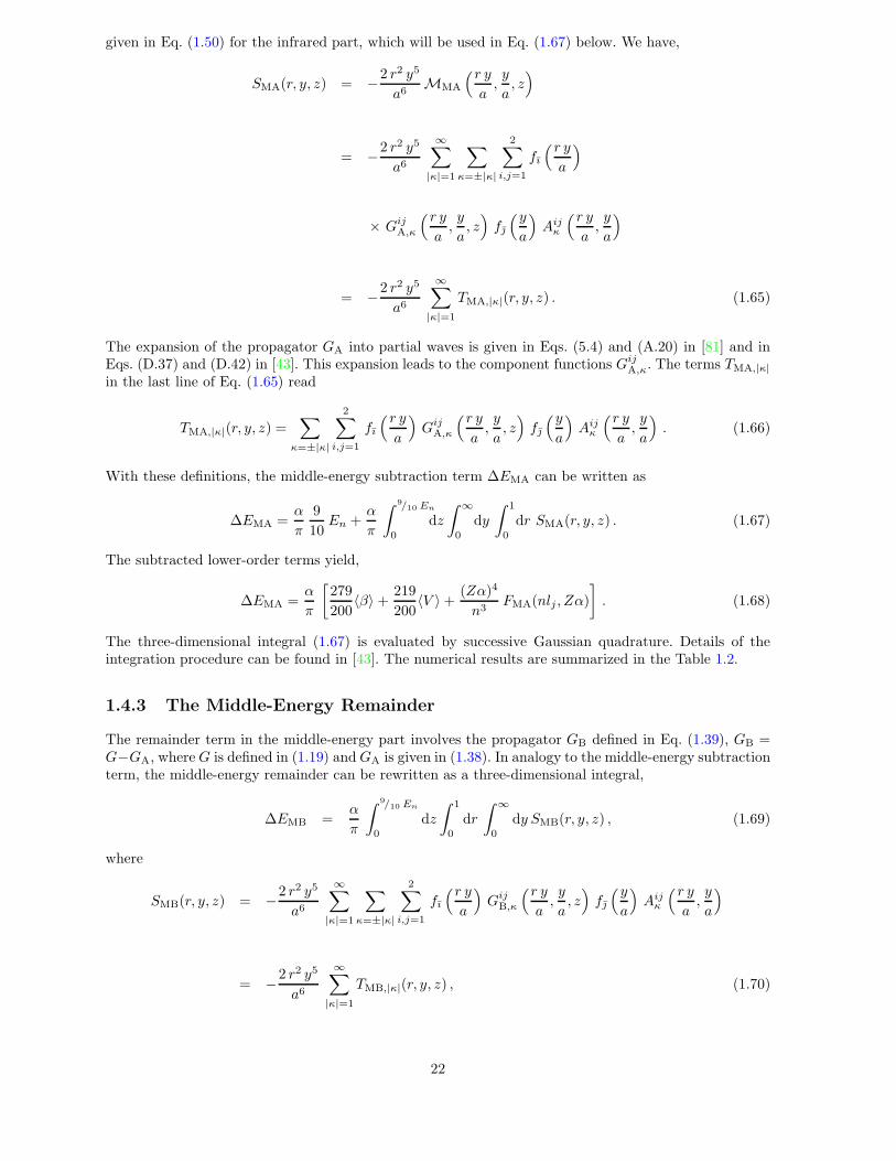
1.4.3 The Middle-Energy Remainder
The remainder term in the middle-energy part involves the propagator GB defined in Eq. (1.39), GB =G−GA, whereG is defined in (1.19) andGA is given in (1.38). In analogy to the middle-energy subtractionterm, the middle-energy remainder can be rewritten as a three-dimensional integral,
∆EMB =α
π
∫ 9/10 En
0
dz
∫ 1
0
dr
∫ ∞
0
dy SMB(r, y, z) , (1.69)
where
SMB(r, y, z) = −2 r2 y5
a6
∞∑
|κ|=1
∑
κ=±|κ|
2∑
i,j=1
fı
(r y
a
)
GijB,κ
(r y
a,y
a, z)
f
(y
a
)
Aijκ
(r y
a,y
a
)
= −2 r2 y5
a6
∞∑
|κ|=1
TMB,|κ|(r, y, z) , (1.70)
22

Z FMA(1S1/2, Zα) FMA(2S1/2, Zα) FMA(2P1/2, Zα) FMA(2P3/2, Zα)
1 2.699 379 904 5(1) 2.720 878 318(1) 0.083 207 314(1) 0.701 705 240(1)
2 2.659 561 381 1(1) 2.681 820 660(1) 0.084 208 832(1) 0.701 850 024(1)
3 2.623 779 453 0(1) 2.647 262 568(1) 0.085 831 658(1) 0.702 091 147(1)
4 2.591 151 010 1(1) 2.616 290 432(1) 0.088 040 763(1) 0.702 426 850(1)
5 2.561 096 522 1(1) 2.588 297 638(1) 0.090 803 408(1) 0.702 854 461(1)
Z FMB(1S1/2, Zα) FMB(2S1/2, Zα) FMB(2P1/2, Zα) FMB(2P3/2, Zα)
1 1.685 993 923 2(1) 1.784 756 705(2) 0.771 787 771(2) −0.094 272 681(2)
2 1.626 842 294 5(1) 1.725 583 798(2) 0.770 778 394(2) −0.094 612 071(2)
3 1.571 406 090 7(1) 1.670 086 996(2) 0.769 153 314(2) −0.095 165 248(2)
4 1.519 082 768 6(1) 1.617 650 004(2) 0.766 954 435(2) −0.095 922 506(2)
5 1.469 482 409 0(1) 1.567 873 140(2) 0.764 220 149(2) −0.096 874 556(2)
Z FM(1S1/2, Zα) FM(2S1/2, Zα) FM(2P1/2, Zα) FM(2P3/2, Zα)
1 4.385 373 827 7(1) 4.505 635 023(2) 0.854 995 085(2) 0.607 432 559(2)
2 4.286 403 675 7(1) 4.407 404 458(2) 0.854 987 226(2) 0.607 237 953(2)
3 4.195 185 543 6(1) 4.317 349 564(2) 0.854 984 972(2) 0.606 925 899(2)
4 4.110 233 778 8(1) 4.233 940 436(2) 0.854 995 198(2) 0.606 504 344(2)
5 4.030 578 931 1(1) 4.156 170 778(2) 0.855 023 557(2) 0.605 979 905(2)
Table 1.2: Numerical results for the middle-energy subtraction term FMA, the middle-energy re-mainder term FMB and the middle-energy term FM. The middle-energy term FM is given as thesum FM(nlj , Zα) = FMA(nlj , Zα) + FMB(nlj , Zα) [see also Eqs.(1.25), (1.68) and (1.72)].
where we implicitly define the terms TMB,|κ|(r, y, z) in analogy with the infrared part Eq. (1.50). The
functions GijB,κ are obtained as the difference of the expansion of the full propagator G and the simplifiedpropagator GA into angular momenta,
GijB,κ = Gijκ −GijA,κ (1.71)
where the Gijκ are listed in Eq. (A.16) in [81] and in Eq. (D.43) in [43], and the GijA,κ have already beendefined in Eqs. (5.4) and (A.20) in [81] and in Eqs. (D.37) and (D.42) in [43]. There are no lower-orderterms to subtract, and therefore
∆EMB =α
π
(Zα)4
n3FMB(nlj , Zα) . (1.72)
The three-dimensional integral (1.69) is evaluated by successive Gaussian quadrature. Details of theintegration procedure are provided in [43]. Numerical results for the middle-energy remainder FMB, aresummarized in Table 1.2 for the K- and L-shell states.
For the middle-energy part, the separation into a subtraction and a remainder term has considerablecomputational advantages which become obvious upon inspection of Eqs. (1.68) and (1.72). The sub-traction involves a propagator whose angular components can be evaluated by recursion [43, 82], whichis computationally time-consuming. Because the subtraction term involves lower-order components [seeEq. (1.25)], it has to be evaluated to high precision numerically (in a typical case, a relative accuracyof 10−19 is required). This high precision requires in turn a large number of integration points for theGaussian quadratures, which is possible only if the numerical evaluation of the integrand is not compu-tationally time-consuming. For the remainder term, no lower-order terms have to be subtracted, and therelative accuracy required of the integrals is in the range of 10−11 . . . 10−9. A numerical evaluation to this
23

smaller level of precision is feasible although the calculation of the Green function GB is computationallymore expensive than that of GA [43, 81, 82]. The separation of the high-energy part into a subtractionterm and a remainder term, which is discussed in Sec. 1.5, is motivated by analogous considerations asfor the middle-energy part. In the high-energy part, this separation is even more important than in themiddle-energy part, because of the occurrence of infinite terms which need to be subtracted analyticallybefore a numerical evaluation can proceed [see Eq. (1.82) below].
We now summarize the results for the middle-energy part. The middle-energy part is the sum of themiddle-energy subtraction term FMA and the middle-energy remainder FMB [see also Eq. (1.27)]. Numer-ical results are summarized in Table 1.2 for the K- and L-shell states. The low-energy part FL is definedas the sum of the infrared contribution FIR and the middle-energy contribution FM [see Eq. (1.32)]. Theresults for FL are provided in the Table 1.3 for the K- and L-shell states. The limits for the low-energypart as a function of the bound state quantum numbers can be found in Eq. (7.80) of [43],
FL(nlj , Zα) =4
3δl,0 ln(Zα)−2 − 4
3ln k0(n, l) +
(
ln 2 − 11
10
)
1
n
+
(
2 ln 2 − 16
15
)
1
2 l + 1+
(
3
2ln 2 − 7
4
)
1
κ (2 l+ 1)
+
(
−3
2ln 2 +
9
4
)
1
|κ| +
(
4
3ln 2 − 1
3
)
δl,0
+
(
ln 2 − 5
6
)
n− 2 l− 1
n (2 l+ 1)+ O(Zα) . (1.73)
The leadings asymptotics for the states under investigation are,
FL(1S1/2, Zα) = (4/3) ln(Zα)−2 − 1.554 642 + O(Zα) ,
FL(2S1/2, Zα) = (4/3) ln(Zα)−2 − 1.191 497 + O(Zα) ,
FL(2P1/2, Zα) = 0.940 023 + O(Zα) ,
FL(2P3/2, Zα) = 0.690 023 + O(Zα) . (1.74)
These asymptotics are consistent with the numerical data in Table 1.3. For S states, the low-energycontribution FL diverges logarithmically as Zα → 0, whereas for P states, FL approaches a constantas Zα → 0. The leading logarithm is a consequence of an infrared divergence cut off by the atomic
Z FL(1S1/2, Zα) FL(2S1/2, Zα) FL(2P1/2, Zα) FL(2P3/2, Zα)
1 11.621 997 564 5(1) 11.985 399 203(2) 0.940 322 937(2) 0.690 169 056(2)
2 9.825 405 794 7(1) 10.189 430 095(2) 0.941 060 895(2) 0.690 517 414(2)
3 8.793 341 365 4(1) 9.158 273 526(2) 0.942 147 482(2) 0.691 017 729(2)
4 8.073 357 919 4(1) 8.439 442 234(2) 0.943 538 386(2) 0.691 645 132(2)
5 7.523 832 250 6(1) 7.891 285 736(2) 0.945 204 392(2) 0.692 383 083(2)
Table 1.3: Low-energy part FL for the K- and L-shell states FL(1S1/2, Zα), FL(2S1/2, Zα), FL(2P1/2, Zα),and FL(2P3/2, Zα), evaluated for low-Z hydrogenlike ions.
24

momentum scale. It is a nonrelativistic effect which is generated by the nonvanishing probability densityof S waves at the origin in the nonrelativistic limit. The presence of the logarithmic behavior for Sstates [nonvanishing A41-coefficient, see Eqs. (1.2) and (1.3)] and its absence for P states is reproducedconsistently by the data in Table 1.3.
1.5 The High-Energy Part
1.5.1 The High-Energy Subtraction Term
The high-energy part is given by
∆EH = − limΛ→∞
i e2∫
CH
dω
2π
∫
d3k
(2π)3Dµν(k2,Λ)
×⟨
ψ∣
∣αµ eik·x G(En − ω)αν e−ik·x∣
∣ψ⟩
, (1.75)
where relevant definitions of the symbols can be found in Eqs. (1.18)–(1.21), and the contour CH is asshown in Fig. 1.1. The high-energy part comprises the following integration region for the virtual photon,
ω ∈ (En − i∞, En + i∞)
z ∈ (−i∞, i∞)
high-energy part ∆EH . (1.76)
The separation of the high-energy part into a subtraction term and a remainder is accomplished as inthe middle-energy part [see Eq. (1.61)] by writing the full Dirac-Coulomb Green function G [Eq. (1.19)]as G = GA + GB. We define the high-energy subtraction term FHA as the expression obtained uponsubstitution of the propagator GA for G in Eq. (1.75), and a substitution of the propagator GB for G inEq. (1.75) leads to the high-energy remainder FHB which is discussed in Sec. 1.5.2. The subtraction term(including all divergent contributions) is generated by GA, the high-energy remainder term correspondsto GB. We have
∆EHA = − limΛ→∞
i e2∫
CH
dω
2π
∫
d3k
(2π)3Dµν(k2,Λ)
×⟨
ψ∣
∣αµ eik·x GA(En − ω)αν e−ik·x∣
∣ψ⟩
(1.77)
and
∆EHB = −i e2∫
CH
dω
2π
∫
d3k
(2π)3Dµν(k2)
×⟨
ψ∣
∣αµ eik·x GB(En − ω)αν e−ik·x∣
∣ψ⟩
. (1.78)
The contribution ∆EHA corresponding to GA can be separated further into a term ∆E(1)HA, which contains
all divergent contributions, and a term ∆E(2)HA, which comprises contributions of lower order than (Zα)4,
but is convergent as Λ → ∞. This separation is described in detail in [81, 84]. We have
∆EHA = ∆E(1)HA + ∆E
(2)HA . (1.79)
We obtain for ∆E(1)HA, which contains a logarithmic divergence as Λ → ∞,
∆E(1)HA =
α
π
[(
3
4ln Λ2 − 9
8
)
〈β〉 +
(
1
2ln 2 − 17
12
)
〈V 〉 +(Zα)4
n3F
(1)HA(nlj , Zα)
]
. (1.80)
25

For the contribution F(1)HA, an explicit analytic result is obtained in Eq. (4.15) in [81]. This contribution
is therefore not discussed in any further detail, here. The contribution ∆E(2)HA contains lower-order terms,
∆E(2)HA =
α
π
[(
−1
2ln 2 +
1
4
)
〈V 〉 +(Zα)4
n3F
(2)HA(nlj, Zα)
]
. (1.81)
Altogether we have
∆EHA = ∆E(1)HA + ∆E
(2)HA
=α
π
[(
3
4ln Λ2 − 9
8
)
〈β〉 − 7
6〈V 〉 +
(Zα)4
n3FHA(nlj , Zα)
]
. (1.82)
The scaled function FHA(nlj , Zα) is given as
FHA(nlj , Zα) = F(1)HA(nlj , Zα) + F
(2)HA(nlj , Zα) . (1.83)
The term ∆E(2)HA falls naturally into a sum of four contributions [81],
∆E(2)HA = T1 + T2 + T3 + T4 (1.84)
where
T1 = − 1
10〈V 〉 +
(Zα)4
n3h1(nlj , Zα) ,
T2 =
(
7
20− 1
2ln 2
)
〈V 〉 +(Zα)4
n3h2(nlj , Zα) ,
T3 =(Zα)4
n3h3(nlj , Zα) ,
T4 =(Zα)4
n3h4(nlj , Zα) . (1.85)
The functions hi (i = 1, 2, 3, 4) are defined in Eqs. (4.18), (4.19) and (4.21) in [81] (see also Eq. (3.6)in [83]). The evaluation of the high-energy subtraction term proceeds as outlined in [81, 82, 83], albeitwith an increased accuracy and improved calculational methods in intermediate steps of the calculation
in order to overcome the severe numerical cancellations in the low-Z region. We recover F(2)HA as the sum
F(2)HA(nlj , Zα) = h1(nlj, Zα) + h2(nlj , Zα) + h3(nlj , Zα) + h4(nlj , Zα) . (1.86)
The scaled function FHA(nlj , Zα) [see also Eqs. (1.26) and (1.28)] is obtained as
FHA(nlj , Zα) = F(1)HA(nlj , Zα) + F
(2)HA(nlj , Zα) . (1.87)
The limits of the contributions F(1)HA(nlj , Zα) and F
(2)HA(nlj , Zα) as (Zα) → 0 have been investigated
in [81, 83, 84]. For the contribution F(1)HA(nlj , 0), the result can be found in Eq. (3.5) in [83]. The limits of
the functions hi(nlj , Zα) (i = 1, 2, 3, 4) as Zα → 0 are given as a function of the atomic state quantumnumbers in Eq. (3.8) in [83]. For the scaled high-energy subtraction term FHA, the limits read (seeEq. (3.9) in [83])
FHA(nlj , Zα) =
(
11
10− ln 2
)
1
n+
(
16
15− 2 ln 2
)
1
2 l+ 1
+
(
1
2ln 2 − 1
4
)
1
κ (2 l+ 1)+
(
3
2ln 2 − 9
4
)
1
|κ| + O(Zα) . (1.88)
26

Therefore, the explicit forms of the limits for the states under investigation are,
FHA(1S1/2, Zα) = −1.219 627 + O(Zα) ,
FHA(2S1/2, Zα) = −1.423 054 + O(Zα) ,
FHA(2P1/2, Zα) = −1.081 204 + O(Zα) ,
FHA(2P3/2, Zα) = −0.524 351 + O(Zα) . (1.89)
Numerical results for FHA, which are presented in Table 1.4, exhibit consistency with the limits inEq. (1.89).
Z FHA(1S1/2, Zα) FHA(2S1/2, Zα) FHA(2P1/2, Zα) FHA(2P3/2, Zα)
1 −1.216 846 660 6(1) −1.420 293 291(1) −1.081 265 954(1) −0.524 359 802(1)
2 −1.214 322 536 9(1) −1.417 829 864(1) −1.081 451 269(1) −0.524 385 053(1)
3 −1.212 026 714 1(1) −1.415 635 310(1) −1.081 760 224(1) −0.524 427 051(1)
4 −1.209 942 847 4(1) −1.413 693 422(1) −1.082 192 995(1) −0.524 485 727(1)
5 −1.208 059 033 6(1) −1.411 992 480(1) −1.082 749 845(1) −0.524 561 017(1)
Z FHB(1S1/2, Zα) FHB(2S1/2, Zα) FHB(2P1/2, Zα) FHB(2P3/2, Zα)
1 −0.088 357 254(1) −0.018 280 727(5) 0.014 546 64(1) −0.042 310 69(1)
2 −0.082 758 206(1) −0.012 729 99(1) 0.014 574 21(1) −0.042 296 81(1)
3 −0.076 811 229(1) −0.006 861 02(1) 0.014 620 51(1) −0.042 273 58(1)
4 −0.070 590 991(1) −0.000 746 40(1) 0.014 685 82(1) −0.042 240 92(1)
5 −0.064 146 139(1) 0.005 567 16(1) 0.014 770 52(1) −0.042 198 76(1)
Z FH(1S1/2, Zα) FH(2S1/2, Zα) FH(2P1/2, Zα) FH(2P3/2, Zα)
1 −1.305 203 915(1) −1.438 574 018(5) −1.066 719 31(1) −0.566 670 50(1)
2 −1.297 080 743(1) −1.430 559 85(1) −1.066 877 06(1) −0.566 681 86(1)
3 −1.288 837 943(1) −1.422 496 33(1) −1.067 139 72(1) −0.566 700 63(1)
4 −1.280 533 839(1) −1.414 439 82(1) −1.067 507 18(1) −0.566 726 65(1)
5 −1.272 205 173(1) −1.406 425 32(1) −1.067 979 33(1) −0.566 759 78(1)
Table 1.4: Numerical results for the high-energy subtraction term FHA and the high-energy remainderterm FHB. The high-energy term FH is given as the sum FH(nlj , Zα) = FHA(nlj , Zα) + FHB(nlj , Zα).
1.5.2 The High-Energy Remainder
The remainder term in the high-energy part involves the propagator GB defined in Eq. (1.39), GB =G − GA, where G is defined in (1.19) and GA is given in (1.38). The evaluation proceeds in completeanalogy to the calculation of the middle-energy remainder term (Sec. 1.4.3). The only difference lies inthe different integration region for the photon energy, which is given – for the high-energy part – in
27

Eq. (1.76). The photon energy integration variable z is conveniently expressed as
z → iu where u =1
2
(
1
t− t
)
. (1.90)
The method of integration is described in [12, 43], and we do not discuss any further details, here. Wefocus instead on the convergence acceleration technique used in the evaluation.
In analogy with the middle-energy remainder, we may write the integrand SHB which is defined incomplete analogy to (1.70) as a sum over angular momenta (“partial waves”)
SHB ∝∞∑
|κ|=1
THB,|κ| , (1.91)
where the THB,|κ| are defined in analogy to Eq. (1.70). Here, |κ| represents the modulus of the Diracangular momentum quantum number of the virtual intermediate state. The asymptotic behaviour of theTHB,|κ| for large |κ| is [see Eq. (4.7) in [82]]
THB,|κ| =r2 |κ|
|κ|
[
const.+ O
(
1
|κ|
)]
, (1.92)
where “const.” is independent of |κ|. The series in Eq. (1.91) is slowly convergent for r close to one, andthe region near r = 1 is known to be problematic in numerical evaluations.
It is found that the convergence of the series (1.92) series near r = 1 can be accelerated very efficientlyusing the combined nonlinear-condensation transformation (see [23] and Sec. 7.1.6) applied to the series∑∞
k=0 tk where tk = THB,k+1 [see Eqs. (1.91) and (1.92)]. The combined transformation (combination ofthe condensation transformation and the Weniger transformation) was found to be applicable to a widerange of slowly convergent monotone series (series whose terms have the same sign), and many examplesfor its application were given in Ref. [23, 31]. For the numerical treatment of radiative corrections in low-Zsystems, the transformation has the advantage of removing the principal numerical difficulties associatedwith the slow convergence of angular momentum decompositions of the propagators near their singularityfor equal radial arguments.
All that remains to be discussed in the current section is the low-Z limit of the energy shift
∆EHB =α
π
(Zα)4
n3FHB(nlj , Zα) . (1.93)
For the high-energy remainder FHB, the limits as Zα→ 0 read [see Eq. (4.15) in [83]]
FHB(nlj , Zα) =1
2 l + 1
[(
17
18− 4
3ln 2
)
δl,0 +
(
3
2− 2 ln 2
)
1
κ
+
(
5
6− ln 2
)
n− 2 l− 1
n
]
+ O(Zα) . (1.94)
For the atomic states under investigation, this leads to
FHB(1S1/2, Zα) = −0.093 457 + O(Zα) ,
FHB(2S1/2, Zα) = −0.023 364 + O(Zα) ,
FHB(2P1/2, Zα) = 0.014 538 + O(Zα) ,
FHB(2P3/2, Zα) = −0.042 315 + O(Zα) . (1.95)
28

1.5.3 Results for the High-Energy Part
The limit of the function FH as Zα→ 0 can be derived easily from the Eqs. (1.88), (1.94) as a functionof the bound state quantum numbers. It reads
FH(nlj , Zα) =
(
11
10− ln 2
)
1
n+
(
16
15− 2 ln 2
)
1
2 l+ 1
+
(
−3
2ln 2 +
5
4
)
1
κ (2 l+ 1)+
(
3
2ln 2 − 9
4
)
1
|κ|
+
(
17
18− 4
3ln 2
)
δl,0 +
(
5
6− ln 2
)
n− 2 l− 1
n (2 l+ 1)+ O(Zα) . (1.96)
For the atomic states investigated here, this expression yields the numerical values,
FH(1S1/2, Zα) = −1.313 085 + O(Zα) ,
FH(2S1/2, Zα) = −1.446 418 + O(Zα) ,
FH(2P1/2, Zα) = −1.066 667 + O(Zα) ,
FH(2P3/2, Zα) = −0.566 667 + O(Zα) . (1.97)
Numerical results for the high-energy part
FH(nlj , Zα) = FHA(nlj , Zα) + FHB(nlj , Zα) (1.98)
are summarized in Table 1.4. Note the apparent consistency of the numerical results in Table 1.4 withtheir analytically obtained low-Z limits in Eq. (1.97).
1.6 Comparison to Analytic Calculations
The numerical results for the scaled function F (nlj , Zα) describing the self energy defined in Eq. (1.1)are given in Table 1.5, together with the results for the nonperturbative function GSE(nlj , Zα), which isimplicitly defined in Eq. (1.2). Results are provided for K and L shell states. The numerical results forthe remainder GSE are obtained by subtracting the analytic lower-order terms listed in Eq. (1.2) fromthe complete numerical result for the scaled function F (nlj , Zα). No additional fitting is performed.
Analytic and numerical results at low Z can be compared by considering the remainder functionGSE. Notethat an inconsistency in any of the analytically obtained lower-order terms would be likely to manifestitself in a grossly inconsistent dependence of GSE(nlj , Zα) on its argument Zα; this is not observed.For S states, the following analytic model for GSE is commonly assumed, which is motivated in partby a renormalization-group analysis [87] and is constructed in analogy with the pattern of the analyticcoefficients Aij in Eq. (1.2) and (1.3),
GSE(nS1/2, Zα) = A60(nS1/2) + (Zα)[
A71(nS1/2) ln(Zα)−2 +A70(nS1/2)]
+(Zα)2[
A83(nS1/2) ln3(Zα)−2 + A82(nS1/2) ln2(Zα)−2
+A81(nS1/2) ln(Zα)−2 +A80(nS1/2)]
. (1.99)
29

The (probably nonvanishing) A83 coefficient, which introduces a triple logarithmic singularity at Zα = 0,hinders an accurate comparison of numerical and analytic data for GSE. A somewhat less singular behavioris expected of the difference
∆GSE(Zα) = GSE(2S1/2, Zα) −GSE(1S1/2, Zα) , (1.100)
because the leading logarithmic coefficients in any given order of Zα are generally assumed to be equalfor all S states, which would mean in particular
A71(1S1/2) = A71(2S1/2) (1.101)
andA83(1S1/2) = A83(2S1/2) . (1.102)
Now we define ∆Akl as the difference of the values of the analytic coefficients for the two lowest S states,
∆Akl = Akl(2S1/2) −Akl(1S1/2) . (1.103)
The function ∆GSE defined in Eq. (1.100) can be assumed to have the following semi-analytic expansionaround Zα = 0,
∆GSE(Zα) = ∆A60 + (Zα) ∆A70 + (Zα)2[
∆A82 ln2(Zα)−2
+∆A81 ln(Zα)−2 + ∆A80 + o(Zα)]
. (1.104)
In order to detect possible inconsistencies in the numerical and analytic data for GSE, we difference thedata for ∆GSE, i.e., we consider the following finite difference approximation to the derivative of thefunction ∆GSE,
g(Z) = ∆GSE((Z + 1)α) − ∆GSE(Zα) . (1.105)
It is perhaps not a priori obvious why this combination leads to a sensible comparison of numerical andanalytic data. This will be explained in the sequel.
We denote the analytic and numerical limits of ∆GSE(Zα) as Zα→ 0 as ∆Aana60 and ∆Anum
60 , respectively.Of course, we hope that these will turn out to be equal. However, we temporarily leave open the possibilityof an inconsistency between numerical and analytic data by keeping ∆Anum
60 and ∆Aana60 as distinct
variables. In order to illustrate how a discrepancy could be detected by investigating the function g(Z),we consider special cases of the function ∆GSE(Zα) and g(Z). For Z = 0, the exact result can be inferredexclusively and uniquely using the analytic approach of Ref. [32], and we have
∆GSE(0) = ∆Aana60 , (1.106)
whereas for Z = 1, which is determined by numerical data,
∆GSE(α) ≈ ∆Anum60 + α∆A70 , (1.107)
with a possibly different limit ∆Anum60 as Z → 0, and for Z = 2,
∆GSE(2α) ≈ ∆Anum60 + 2α∆A70 , (1.108)
where we ignore higher-order analytic terms. Hence, for Z = 0, we have
g(0) = ∆GSE(α) − ∆GSE(0) = ∆Anum60 − ∆Aana
60 + α [∆A70 + o(Zα)] . (1.109)
A possible inconsistency (nonvanishing ∆Anum60 − ∆Aana
60 ) would influence the value of g(0). For Z = 1,the value of g is determined solely by numerical data,
g(1) = ∆GSE(2α) − ∆GSE(α) = α [∆A70 + o(Zα)] , (1.110)
and for Z = 2, we have
g(2) = ∆GSE(3α) − ∆GSE(2α) = α [∆A70 + o(Zα)] . (1.111)
30

Of course, analogous relations hold for Z > 2. This means that a meaningful comparison of the analyticand numerical approaches can be made by comparing the value g(0), which is influenced by the term∆Anum
60 −∆Aana60 , to the other values g(1), . . . , g(4), which are independent of the difference ∆Anum
60 −∆Aana60 .
We recall that the numerical data from Table 1.5 lead to the evaluation of the five values g(0), g(1), g(2),g(3) and g(4). A plot of the function g(Z) serves two purposes: (i) the values g(1), . . . , g(4) should exhibitapparent convergence to some limiting value α∆A70 as Z → 0, and this can be verified by inspectionof the plot, and (ii) a discrepancy between the analytic and numerical approaches – as explained above– would result in a nonvanishing value for ∆Anum
60 − ∆Aana60 , and it would introduce an inconsistency
between the trend in the values of g(1), . . . , g(4), and the value of g(0) [see Eq. (1.109)].
Z F (1S1/2, Zα) F (2S1/2, Zα) F (2P1/2, Zα) F (2P3/2, Zα)
1 10.316 793 650(1) 10.546 825 185(5) −0.126 396 37(1) 0.123 498 56(1)
2 8.528 325 052(1) 8.758 870 25(1) −0.125 816 16(1) 0.123 835 55(1)
3 7.504 503 422(1) 7.735 777 20(1) −0.124 992 24(1) 0.124 317 10(1)
4 6.792 824 081(1) 7.025 002 41(1) −0.123 968 79(1) 0.124 918 48(1)
5 6.251 627 078(1) 6.484 860 42(1) −0.122 774 94(1) 0.125 623 30(1)
Z GSE(1S1/2, Zα) GSE(2S1/2, Zα) GSE(2P1/2, Zα) GSE(2P3/2, Zα)
1 −30.290 24(2) −31.185 15(9) −0.973 5(2) −0.486 5(2)
2 −29.770 967(5) −30.644 66(5) −0.949 40(5) −0.470 94(5)
3 −29.299 170(2) −30.151 93(2) −0.926 37(2) −0.456 65(2)
4 −28.859 222(1) −29.691 27(1) −0.904 12(1) −0.443 13(1)
5 −28.443 372 3(8) −29.255 033(8) −0.882 478(8) −0.430 244(8)
Table 1.5: Numerical results for the scaled function F [defined in Eq. (1.1)] and the remainder functionGSE implicitly defined in Eq. (1.2).
0 1 2 3 40
Z
0.0200
0.0205
0.0210
0.0215
0.0220
g(Z
)
Figure 1.4: Plot of the function g(Z) defined in Eq. (1.105) in the region oflow nuclear charge. For the evaluation of the data point at Z = 0, a value ofA60(1S1/2) = −30.92415(1) is employed [9, 32, 88].
31

Among the different evaluations of A60 for the ground state, the result in [32] has the smallest quoteduncertainty. In Fig. 1.4 we display a plot of g(Z) for low nuclear charge Z. A value of A60(1S1/2) =Aana
60 (1S1/2) = −30.92415(1) [9, 32, 88] is used in Fig. 1.4. The results indicate very good agreementbetween the numerical and analytic approaches to the Lamb shift in the low-Z region up to the level ofa few Hz in frequency units for the low-lying atomic states (where n is the principal quantum number).The error bars represent the numerical uncertainty of the values in Table 1.5, which correspond to anuncertainty on the level of 1.0 × Z4 Hz in frequency units.
Analytic work on the correction A60 has extended over three decades [32, 68, 69, 70, 71]. The complicationarises that although the calculations are in general analytic, some remaining one-dimensional integrationscould not be evaluated analytically because of the nature of the integrals [see e.g. Eq. (6.96) in [32]].Therefore a step-by-step comparison of the analytic calculations is difficult. An additional difficulty is theisolation of those analytic terms which contribute in a given order in Zα, i.e. the isolation of only thoseterms which contribute to A60. The apparent consistency of the numerical and analytic data in Fig. 1.4represents an independent consistency check on the rather involved analytic calculations.
0 1 2 3 40
Z
0.020
0.021
0.022
0.023
0.024
0.025
0.026
0.027
0.028
g1/2(Z
)
Figure 1.5: Comparison of numerical data and analytically evaluated higher-order binding corrections for the 2P1/2 state. We plot the function g1/2(Z)defined in Eq. (1.114) in the region of low Z. The numerical data appear tobe consistent with the analytic result of A60(2P1/2) = −0.99891(1) obtainedin [1].
Our numerical results are not inconsistent with the analytic result [44] for a higher-order logarithm,
A71 = π
(
139
64− ln 2
)
= 4.65, (1.112)
although they do not necessarily confirm it. As in [9], we obtain as an estimate A71 = 5.5(1.0) (from the fitto the numerical data for both S states). Logarithmic terms corresponding to the probably nonvanishingA83 coefficient should be taken into account for a consistent fit of the corrections to GSE. These highlysingular terms are difficult to handle with a numerical fitting procedure. The terms A83, A82 and A81
furnish three more free parameters for the numerical fit, where only five data points are available (inaddition to the quantities A60, A71 and A70, which may also be regarded as free parameters for thefitting procedure). The determination of A60 by a fit from the numerical data is much more stablethan the determination of the logarithmic correction A71. We briefly note that our all-order evaluationessentially eliminates the uncertainty due to the unknown higher-order analytic terms. It is interestingto note that the same numerical methods are employed for both the S and P states in our all-order (inZα) calculation, whereas the analytic treatment of S and P states differs [1, 32].
The comparison of numerical and analytic result is much less problematic for P states, because thefunction GSE is less singular [see Eqs. (1.4) and (1.6)]. For the 2P states, we observe that the function
32

GSE(2Pj, Zα) has the same semi-analytic expansion about Zα = 0 as the function ∆GSE(Zα) definedfor S states in Eq. (1.100). We have
GSE(2Pj, Zα) = A60(2Pj) + (Zα)A70(2Pj) + (Zα)2[
A82(2Pj) ln2(Zα)−2
+A81(2Pj) ln(Zα)−2 +A80(2Pj) + o(Zα)]
. (1.113)
Hence, we plot the function
gj(Z) = GSE(2Pj, (Z + 1)α)−GSE(2Pj, Zα) (1.114)
for j = 1/2 in the region of low Z, with the notion that an inconsistent analytic result for A60(2Pj) wouldlead to irregularity at Z = 0, in analogy with the S states. The numerical data shown in Fig. 1.5 appearsto be consistent with the analytic results of
A60(2P1/2) = −0.998 91(1) . (1.115)
obtained in [1]. For the 2P3/2 state, see Fig. 6 of Ref. [12]. In this context it may be interesting to notethat analytic results obtained in [1, 2] for the higher-order binding corrections to 2P, 3P and 4P stateshave recently been confirmed indirectly [89].
33
Chapter 2
Analytic Self–Energy Calculationsfor Excited States
2.1 Orientation
Analytic calculations of the one-loop self energy in bound systems have a long history, starting fromBethe’s seminal paper [33], and have meanwhile extended over more than five decades. The calculationsare based on an expansion of the effect into powers of the parameter Zα, where Z is the nuclear chargeand α is the fine-structure constant (see e.g. [1, 2, 32, 43]). The expansion is semi-analytic, i.e. it involvespowers of Zα and ln[(Zα)−2]. Terms which are of higher than leading order in Zα are commonly referredto as the binding corrections (see also Ch. 3). A certain nonlogarithmic binding correction, known as theA60-coefficient, has been of particular interest. For relevant formulas and definitions regarding A60, werefer to Ch. 1, especially to Eqs. (1.1) – (1.6).
In this chapter, we present results of an analytic evaluation of higher-order binding corrections to theone-loop self energy for excited bound states of hydrogenlike systems. We focus on states with principalquantum numbers n = 2 . . . 5 and Dirac angular quantum numbers κ = 1,−2, 2, . . . , 4,−5. The currentcalculation represents a continuation of previous investigations on the subject [1, 2].
The improved results for A60 coefficients rely essentially on a more compact code for the analytic cal-culations, written in the computer-algebra package Mathematica [90], which enables the corrections tobe evaluated semi-automatically. Intermediate expressions with some 10,000 terms are encountered, andthe complexity of the calculations sharply increases with the principal quantum number n, and, as faras the complexity of the angular momentum algebra is concerned, with the orbital angular momen-tum l = |κ+ 1/2|− 1/2 of the bound electron. Calculations were performed, in part, on IBM RISC/6000workstations, both at the National Institute of Standards and Technology and at the Laboratoire Kastler–Brossel, and profited from the availability of 2 GigaBytes of Random Access Memory.
Of crucial importance was the development of convergence acceleration methods which were used ex-tensively for the evaluation of remaining one-dimensional integrals which could not be done analytically.These integrals are analogous to expressions encountered in previous work [1, 2]. The numerically eval-uated contributions involve slowly convergent hypergeometric series, and – in more extreme cases –infinite series over partial derivatives of hypergeometric functions, and generalizations of Lerch’s Φ tran-scendent [91, 92]. We have found the Combined Nonlinear–Condensation Transformation [23] to be aversatile method for the efficient numerical evaluation of the slowly convergent series encountered in theevaluation of the A60-coefficients.
Results are given below for the A60-coefficients with an absolute precision of 10−9. As explained indetail in [1, 2, 32], the calculation of the one-loop self energy falls naturally into a high- and a low-energy part (FH and FL, respectively). In turn, the low-energy part can be separated naturally intothe nonrelativistic dipole and the nonrelativistic quadrupole part, and into relativistic corrections tothe current, to the hamiltonian, to the wavefunction, and to the energy of the bound state. For somestates, severe numerical cancellations are observed between these (low-energy) contributions to the low-energy part of the self energy. In the final step of the calculation, we observe additional numerical
34

cancellations between the high- and the low-energy part for the finite contributions to A60, beyond thenecessary cancellation of the divergent contributions which depend on the scale-separation parameter ε;this parameter and the mathematical method which is employed in the expansion of the self energy aredescribed and explained in Sec. 2.2. For some of the investigated atomic states, the absolute magnitudeof the A60-coefficients is as small as 10−3, although the largest single contribution is always on the orderof 10−2. This illustrates the cancellations between the finite contributions to A60.
2.2 The epsilon-Method
We discuss here, by way of example, the ε method employed in the analytic calculation of the self energyin bound systems. This method is very suitable [1, 2, 32] for the separation of the two different energyscales for virtual photons: the nonrelativistic domain, in which the virtual photon assumes values of theorder of the atomic binding energy, and the relativistic domain, in which the virtual photon assumesvalues of the order of the electron rest mass. Different approximation schemes and different asymptoticexpansions are adequate for the two different domains. Without these approximations and expansions,the analytic evaluation of either the high- or the low-energy part would not be feasible. Therefore, theε method is also used for the treatment of the highly excited atomic states which are the subject of(this part) of the thesis. At the same time, the model example discussed here is meant to illustrate theusefulness of the “ε method” in a more general context.
We will consider here a model problem with one “virtual photon”. The separation into high-and low-energy photons necessitates the temporary introduction of a parameter ε; the dependence on ε cancelswhen the high- and the low-energy parts are added together. We have,
nonrelativistic domain � ε� electron rest mass (2.1)
(Zα)2me � ε� me , (2.2)
where α is the fine structure constant, and Z is the nuclear charge. The high-energy part is associatedwith photon energies ω > ε, and the low-energy part is associated with photon energies ω < ε.
In order to illustrate the procedure, we discuss a simple, one-dimensional example: the evaluation of
I(β) =
∫ 1
0
√
ω2 + β2
1 − ω2dω . (2.3)
where the integration variable ω might be interpreted as the “energy” of a “virtual photon”. The integralI can be expressed in terms of special functions,
I(β) = β E
(
− 1
β2
)
= βπ
22F1
(
−1
2,
1
2; 1;− 1
β2
)
, (2.4)
where E is the complete elliptic integral of the second kind, and 2F1 denotes a hypergeometric function.
An alternative integral representation reads I(β) =∫ π/2
0
√
β2 + sin2(ω) dω.
The purpose of the calculation is to derive a semi-analytic expansion of I(β) in powers of β and lnβ.The fine structure constant α takes the role of the expansion parameter β in actual calculations of theself energy. We discuss first the “high-energy part” of the calculation. It is given by the expression
IH(β) =
∫ 1
ε
√
ω2 + β2
1 − ω2dω . (2.5)
For ω > ε, we may expand√
ω2 + β2 = ω +β2
2ω+
β4
8ω3+ O(β6) , (2.6)
but this expansion is not applicable in higher orders to the domain 0 < ω < ε because of the appearanceof inverse powers of ω (analogous to an “infrared divergence” in QED).
The separation parameter ε acts an infrared regulator. After expanding in β [see Eq. (2.6)], the resultingintegrals in each order of β can be evaluated analytically. Subsequently, we expand every term in the
35

β-expansion in powers of ε up to the order ε0, i.e. we keep only the divergent and constant terms in ε.The result is
IH(β, ε) = 1 + β2
{
1
2ln
(
2
ε
)
+ O(ε)
}
+β4
{
− 1
16 ε2− 1
16ln
(
2
ε
)
+1
32+ O(ε)
}
+β6
{
1
64 ε4+
1
64 ε2+
3
128ln
(
2
ε
)
− 7
512+ O(ε)
}
+O(β8) . (2.7)
Here, the “O”-symbol identifies a contribution for which O(x)/x → const. as x → 0, whereas the “o”-symbol identifies the weaker requirement o(x) → 0 as x→ 0; this is a nonstandard convention (cf. [53]).
The contribution IH(β) corresponds to the “high-energy part” in an analytic calculation of the self energy,where the propagator of the bound electron is explicitly expanded in powers of the fine structure constantα. Now we turn to the “low-energy part”. The expression for the low-energy part (0 < ω < ε) reads
IL(β) =
∫ ε
0
√
ω2 + β2
1 − ω2dω . (2.8)
The expansion (2.6) is not applicable in this energy domain; we therefore have to keep the numerator of
the integrand√
ω2 + β2 in unexpanded form. However, we can expand the denominator√
1 − ω2 of theintegrand in powers of ω; because 0 < ω < ε (with ε small), this expansion in ω is in fact an expansionin β – although the situation is somewhat problematic in the sense that every term in the ω-expansiongives rise to terms of arbitrarily high order in the β-expansion [see also Eq. (2.10) below].
The term√
ω2 + β2 is analogous to the Schrodinger–Coulomb propagator in the evaluation of the selfenergy – it has to be kept in an unexpanded form –, whereas the expansion
1√1 − ω2
= 1 +ω2
2+
3
8ω4 + O(ω6) (2.9)
corresponds to the expansion into the (Zα)-expansion in the low-energy part.
Every term in the expansion (2.9) gives rise to arbitrarily high-order corrections in β, but it starts withthe power ωn → βn+2. For example, we have for the leading term of order ω0 = 1 from Eq. (2.9),
∫ ε
0
√
ω2 + β2 dω = β2
{
1
2ln
(
2
βε
)
+1
4+ O(ε)
}
+β4
{
1
16 ε2+ O(ε)
}
+ β6
{
− 1
64 ε4+ O(ε)
}
+ O(β8) . (2.10)
Note that the terms generated in the orders β4 and β6 are needed to cancel divergent contributions inrespective orders of β from the high-energy part given in Eq. (2.6). The term of order ω2 from (2.9)results in
1
2
∫ ε
0
ω2√
ω2 + β2 dω = β4
{
− 1
16ln
(
2
βε
)
+1
64+ O(ε)
}
+β6
{
− 1
64 ε2+ O(ε)
}
+ O(β8) . (2.11)
36

Altogether, we obtain for the low-energy part,
IL(β, ε) = β2
{
1
2ln
(
2
βε
)
+1
4+ O(ε)
}
+β4
{
1
16 ε2− 1
16ln
(
2
βε
)
+1
64+ O(ε)
}
+β6
{
− 1
64 ε4− 1
64 ε2+
3
128ln
(
2
βε
)
− 5
512+ O(ε)
}
+O(β8 ln β) . (2.12)
When the high-energy part (2.7) and the low-energy part (2.12) are added, the dependence on ε cancels,and we have
I(β) = IH(β, ε) + IL(β, ε)
= 1 + β2
{
1
2ln
(
4
β
)
+1
4
}
+ β4
{
− 1
16ln
(
4
β
)
+3
64
}
+β6
{
3
128ln
(
4
β
)
− 3
128
}
+ O(β8 lnβ) . (2.13)
In order to illustrate the analogy with the self energy calculation presented here, we would like to pointout that the dependence on ε cancels out in the final result which is the sum of the high-energy part EH
given in Eq. (2.14) [for the two-loop case see Eq. (3.42)] and the low-energy part EL in Eq. (2.15) [forthe two-loop case see Eq. (3.58)].
2.3 Results for High– and Low–Energy Contributions
2.3.1 P 1/2 states (kappa = 1)
Here and in the following subsections, we present results which have been obtained for the high- andlow-energy energy parts of the self energy or all states with principal quantum number n = 2 . . . 5and orbital angular quantum number l > 0. These results, combined with numerical calculations forlow-, intermediate and high nuclear charge, allow to reliably estimate quantum electrodynamic (QED)radiative corrections for any atomic state with principal quantum number n ≤ 5. For the definition ofthe scaled self energy function F and of the analytic A-coefficients, see Eqs. (1.1) – (1.6). The results aregiven in terms of the expansion parameter Zα and the scale-separation parameter ε, whose role in thecalculation is explained in Sec. 2.2.
For P1/2 states, we obtain for the following results for the high- and low-energy parts. The 2P1/2 high-energy part is:
FH(2P1/2) = −1
6+ (Zα)2
[
4177
21600− 2
9 ε− 103
180ln(2ε)
]
, (2.14)
2P1/2 low-energy part:
FL(2P1/2) = −4
3ln k0(2P) + (Zα)2
[
−0.795 649 812(1) +2
9 ε+
103
180ln
(
ε
(Zα)2
)]
, (2.15)
37

3P1/2 high-energy part:
FH(3P1/2) = −1
6+ (Zα)2
[
6191
24300− 20
81 ε− 268
405ln(2ε)
]
, (2.16)
3P1/2 low-energy part:
FL(3P1/2) = −4
3ln k0(3P) + (Zα)2
[
−0.944 288 447(1) +20
81 ε+
268
405ln
(
ε
(Zα)2
)]
, (2.17)
4P1/2 high-energy part:
FH(4P1/2) = −1
6+ (Zα)2
[
24409
86400− 23
90 ε− 499
720ln(2ε)
]
, (2.18)
4P1/2 low-energy part:
FL(4P1/2) = −4
3ln k0(4P) + (Zα)2
[
−0.997 810 211(1) +23
90 ε+
499
720ln
(
ε
(Zα)2
)]
, (2.19)
5P1/2 high-energy part:
FH(5P1/2) = −1
6+ (Zα)2
[
20129
67500− 292
1125 ε− 796
1125ln(2ε)
]
, (2.20)
5P1/2 low-energy part:
FL(5P1/2) = −4
3ln k0(5P) + (Zα)2
[
−1.023 991 781(1) +292
1125 ε+
796
1125ln
(
ε
(Zα)2
)]
, (2.21)
Here and in the following, ln k0 is the Bethe logarithm for which very accurate values are available [72,73, 74, 75, 76, 77, 79].
2.3.2 P 3/2 states (kappa = -2)
The obtained results read as follows. The 2P3/2 high-energy part reads:
FH(2P3/2) =1
12+ (Zα)2
[
6577
21600− 2
9 ε− 29
90ln(2ε)
]
, (2.22)
2P3/2 low-energy part:
FL(2P3/2) = −4
3ln k0(2P) + (Zα)2
[
−0.584 516 780(1) +2
9 ε+
29
90ln
(
ε
(Zα)2
)]
, (2.23)
3P3/2 high-energy part:
FH(3P3/2) =1
12+ (Zα)2
[
67903
194400− 20
81 ε− 148
405ln(2ε)
]
, (2.24)
3P3/2 low-energy part:
FL(3P3/2) = −4
3ln k0(3P) + (Zα)2
[
−0.693 566 427(1) +20
81 ε+
148
405ln
(
ε
(Zα)2
)]
, (2.25)
4P3/2 high-energy part:
FH(4P3/2) =1
12+ (Zα)2
[
31399
86400− 23
90 ε− 137
360ln(2ε)
]
, (2.26)
38
4P3/2 low-energy part:
FL(4P3/2) = −4
3ln k0(4P) + (Zα)2
[
−0.730 579 137(1) +23
90 ε+
137
360ln
(
ε
(Zα)2
)]
, (2.27)
5P3/2 high-energy part:
FH(5P3/2) =1
12+ (Zα)2
[
199387
540000− 292
1125 ε− 436
1125ln(2ε)
]
, (2.28)
5P3/2 low-energy part:
FL(5P3/2) = −4
3ln k0(5P) + (Zα)2
[
−0.747 615 653(1) +292
1125 ε+
436
1125ln
(
ε
(Zα)2
)]
. (2.29)
2.3.3 D 3/2 states (kappa = 2)
The results obtained for states with κ = 2 read as follows. 3D3/2 high-energy part:
FH(3D3/2) = − 1
20+ (Zα)2
[
− 1721
194400− 4
405 ε− 4
405ln(2ε)
]
, (2.30)
3D3/2 low-energy part:
FL(3D3/2) = −4
3ln k0(3D) + (Zα)2
[
0.021 250 354(1) +4
405 ε+
4
405ln
(
ε
(Zα)2
)]
, (2.31)
4D3/2 high-energy part:
FH(4D3/2) = − 1
20+ (Zα)2
[
− 829
86400− 1
90 ε− 1
90ln(2ε)
]
, (2.32)
4D3/2 low-energy part:
FL(4D3/2) = −4
3ln k0(4D) + (Zα)2
[
0.022 882 528(1) +1
90 ε+
1
90ln
(
ε
(Zα)2
)]
, (2.33)
5D3/2 high-energy part:
FH(5D3/2) = − 1
20+ (Zα)2
[
− 35947
3780000− 92
7875 ε− 92
7875ln(2ε)
]
, (2.34)
5D3/2 low-energy part:
FL(5D3/2) = −4
3ln k0(5D) + (Zα)2
[
0.023 759 683(1) +92
7875 ε+
92
7875ln
(
ε
(Zα)2
)]
. (2.35)
2.3.4 D 5/2 states (kappa = -3)
For D5/2 states with Dirac quantum number κ = −3, the results read as follows. For the 3D5/2 high-energypart, we have:
FH(3D5/2) =1
30+ (Zα)2
[
371
24300− 4
405 ε− 4
405ln(2ε)
]
, (2.36)
3D5/2 low-energy part:
FL(3D5/2) = −4
3ln k0(3D) + (Zα)2
[
0.019 188 397(1) +4
405 ε+
4
405ln
(
ε
(Zα)2
)]
, (2.37)
39

4D5/2 high-energy part:
FH(4D5/2) =1
30+ (Zα)2
[
53
2880− 1
90 ε− 1
90ln(2ε)
]
, (2.38)
4D5/2 low-energy part:
FL(4D5/2) = −4
3ln k0(4D) + (Zα)2
[
0.020 710 720(1) +1
90 ε+
1
90ln
(
ε
(Zα)2
)]
, (2.39)
5D5/2 high-energy part:
FH(5D5/2) =1
30+ (Zα)2
[
3097
157500− 92
7875 ε− 92
7875ln(2ε)
]
, (2.40)
5D5/2 low-energy part:
FL(5D5/2) = −4
3ln k0(5D) + (Zα)2
[
0.021 511 798(1) +92
7875 ε+
92
7875ln
(
ε
(Zα)2
)]
. (2.41)
2.3.5 F 5/2 states (kappa = 3)
Now we turn our attention to F5/2 states. We have for the 4F5/2 high-energy part:
FH(4F5/2) = − 1
42+ (Zα)2
[
− 493
235200− 1
630 ε− 1
630ln(2ε)
]
, (2.42)
4F5/2 low-energy part:
FL(4F5/2) = −4
3ln k0(4F) + (Zα)2
[
0.005 523 310(1) +1
630 ε+
1
630ln
(
ε
(Zα)2
)]
, (2.43)
5F5/2 high-energy part:
FH(5F5/2) = − 1
42+ (Zα)2
[
− 2657
1102500− 2
1125 ε− 2
1125ln(2ε)
]
, (2.44)
5F5/2 low-energy part:
FL(5F5/2) = −4
3ln k0(5F) + (Zα)2
[
0.006 045 398(1) +2
1125 ε+
2
1125ln
(
ε
(Zα)2
)]
, (2.45)
2.3.6 F 7/2 states (kappa = -4)
States with κ = −4 yield the following results. We obtain for the 4F7/2 state (high-energy part):
FH(4F7/2) =1
56+ (Zα)2
[
25357
8467200− 1
630 ε− 1
630ln(2ε)
]
, (2.46)
4F7/2 low-energy part:
FL(4F7/2) = −4
3ln k0(4F) + (Zα)2
[
0.005 180 461(1) +1
630 ε+
1
630ln
(
ε
(Zα)2
)]
, (2.47)
5F7/2 high-energy part:
FH(5F7/2) =1
56+ (Zα)2
[
774121
211680000− 2
1125 ε− 2
1125ln(2ε)
]
, (2.48)
5F7/2 low-energy part:
FL(5F7/2) = −4
3ln k0(5F) +
2 (Zα)2
1125 ε+ (Zα)2
[
0.005 662 248(1) +2
1125ln
(
ε
(Zα)2
)]
. (2.49)
40
2.3.7 G 7/2 states (kappa = 4)
G7/2 and G9/2 states involve the most problematic angular momentum algebra of all atomic statesconsidered here. We obtain,
FH(5G7/2) = − 1
72+ (Zα)2
[
− 4397
6048000− 2
4725 ε− 2
4725ln(2ε)
]
, (2.50)
and for the low-energy part,
FL(5G7/2) = −4
3ln k0(5G) + (Zα)2
[
0.001 834 827(1) +2
4725 ε+
2
4725ln
(
ε
(Zα)2
)]
. (2.51)
2.3.8 G 9/2 states (kappa = -5)
We conclude by investigating G9/2 states, where the high-energy part reads (n = 5)
FH(5G9/2) =1
90+ (Zα)2
[
269
283500− 2
4725 ε− 2
4725ln(2ε)
]
, (2.52)
and the low-energy part reads,
FL(5G9/2) = −4
3ln k0(5G) + (Zα)2
[
0.001 757 471(1) +2
4725 ε+
2
4725ln
(
ε
(Zα)2
)]
. (2.53)
2.4 Summary of Results
By adding the high- and low-energy parts given in Secs. 2.3.1 – 2.3.8, we obtain the following resultsfor the self energy. For all atomic states, the dependence on the scale-separating parameter ε cancelswhen the low- and the high-energy parts are added, in agreement with the principal idea of the ε-methoddescribed in Sec. 2.2. The coefficients A40, A61 and A60 can then be read off according to the definitionscontained in Eqs. (1.1) – (1.6).
P1/2 state (κ = 1)
n A40 A40 (num) A61 A61 (num) A60 (num)
2 − 16 − 4
3 ln k0(2P ) -0.126644 103108 0.572 222 -0.998 904 402(1)
3 − 16 − 4
3 ln k0(3P ) -0.115746 268405 0.661 728 -1.148 189 956(1)
4 − 16 − 4
3 ln k0(4P ) -0.110727 499720 0.693 056 -1.195 688 142(1)
5 − 16 − 4
3 ln k0(5P ) -0.107954 7961125 0.707 556 -1.216 224 512(1)
Table 2.1: Results for P1/2 states. The coefficients A40 and A61 are rational numbers; in thecolumns entitled “(num)”, we give the numerical values to six decimals. The A60-coefficientsin the last column constitute the main result of the investigation presented in the currentchapter. As explained in Sec. 2.1, these coefficients involve numerical integrals which cannotbe done analytically.
2.5 Typical Cancellations
As already emphasized in Sec. 2.1, severe numerical cancellations are encountered in the calculation ofthe A60-coefficients. These cancellations will be illustrated here in Tables 2.8 and 2.9 for the 5G7/2 state.
41
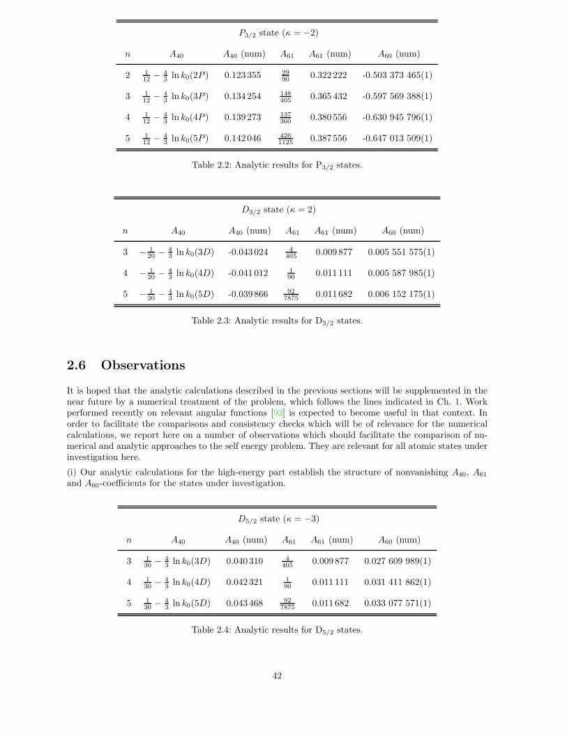
P3/2 state (κ = −2)
n A40 A40 (num) A61 A61 (num) A60 (num)
2 112 − 4
3 ln k0(2P ) 0.123 355 2990 0.322 222 -0.503 373 465(1)
3 112 − 4
3 ln k0(3P ) 0.134 254 148405 0.365 432 -0.597 569 388(1)
4 112 − 4
3 ln k0(4P ) 0.139 273 137360 0.380 556 -0.630 945 796(1)
5 112 − 4
3 ln k0(5P ) 0.142 046 4261125 0.387 556 -0.647 013 509(1)
Table 2.2: Analytic results for P3/2 states.
D3/2 state (κ = 2)
n A40 A40 (num) A61 A61 (num) A60 (num)
3 − 120 − 4
3 ln k0(3D) -0.043 024 4405 0.009 877 0.005 551 575(1)
4 − 120 − 4
3 ln k0(4D) -0.041 012 190 0.011 111 0.005 587 985(1)
5 − 120 − 4
3 ln k0(5D) -0.039 866 927875 0.011 682 0.006 152 175(1)
Table 2.3: Analytic results for D3/2 states.
2.6 Observations
It is hoped that the analytic calculations described in the previous sections will be supplemented in thenear future by a numerical treatment of the problem, which follows the lines indicated in Ch. 1. Workperformed recently on relevant angular functions [93] is expected to become useful in that context. Inorder to facilitate the comparisons and consistency checks which will be of relevance for the numericalcalculations, we report here on a number of observations which should facilitate the comparison of nu-merical and analytic approaches to the self energy problem. They are relevant for all atomic states underinvestigation here.
(i) Our analytic calculations for the high-energy part establish the structure of nonvanishing A40, A61
and A60-coefficients for the states under investigation.
D5/2 state (κ = −3)
n A40 A40 (num) A61 A61 (num) A60 (num)
3 130 − 4
3 ln k0(3D) 0.040 310 4405 0.009 877 0.027 609 989(1)
4 130 − 4
3 ln k0(4D) 0.042 321 190 0.011 111 0.031 411 862(1)
5 130 − 4
3 ln k0(5D) 0.043 468 927875 0.011 682 0.033 077 571(1)
Table 2.4: Analytic results for D5/2 states.
42

F5/2 state (κ = 3)
n A40 A40 (num) A61 A61 (num) A60 (num)
4 − 142 − 4
3 ln k0(4F ) -0.021 498 1630 0.001 587 0.002 326 988(1)
5 − 142 − 4
3 ln k0(5F ) -0.020 873 21125 0.001 778 0.002 403 159(1)
Table 2.5: Analytic results for F5/2 states.
F7/2 state (κ = −4)
n A40 A40 (num) A61 A61 (num) A60 (num)
4 156 − 4
3 ln k0(4F ) 0.020 169 1630 0.001 587 0.007 074 960(1)
5 156 − 4
3 ln k0(5F ) 0.020 793 21125 0.001 778 0.008 087 021(1)
Table 2.6: Analytic results for F7/2 states.
(ii) For a given κ quantum number, the coefficients increase in absolute magnitude with increasingprincipal quantum number n. This is the case for Bethe logarithms, for A61 coefficients and also forA60 coefficients. This behavior is consistent with the phenomenon that relativistic corrections to the selfenergy become more important as n increases.
(iii) For a given principal quantum number n, the coefficients decrease in absolute magnitude with in-creasing κ. As a function of the nuclear charge number Z, the plots of F (Zα) against Z should become“more flat” as κ increases for a given n [94].
(iv) The A61 coefficients, which represent the dominant relativistic correction to F (Zα), all have thesame (positive) sign for states with κ quantum numbers κ = 2,−3, 3,−4, 4,−5. This “same-sign” patternis also true of the A60 coefficients. Because A61 is the dominant correction in the order (Zα)6 due to theenhancement by the large logarithm, this observation explains why, in general, the qualitative dependence(on the nuclear charge number Z) of the self energy correction for the highly excited states is the samefor the states with κ = 2,−3, 3,−4, 4,−5 (see [94]).
(v) A61-coefficients are different for P1/2 and P3/2 states, but the spin dependence vanishes for higher
G7/2 state (κ = 4)
n A40 A40 (num) A61 A61 (num) A60 (num)
5 − 172 − 4
3 ln k0(5G) -0.012 860 24725 0.000 423 0.000 814 414(1)
G9/2 state (κ = −5)
n A40 A40 (num) A61 A61 (num) A60 (num)
5 190 − 4
3 ln k0(5G) 0.012 141 24725 0.000 423 0.002 412 929(1)
Table 2.7: Analytic results for G7/2 and G9/2 states.
43

Contributions to the Low-Energy Part (5G7/2)
A60-contribution due to Fnq 0.002 875 830 9(5).
A60-contribution due to Fδy -0.001 083 109 4(5).
A60-contribution due to FδH -0.008 917 782 1(5).
A60-contribution due to FδE 0.004 920 556 0(5).
A60-contribution due to Fδφ 0.004 039 332 1(5).
A60 [from low-energy, cf. Eq. (2.51)] 0.001 834 827(1)
Table 2.8: As explained in Refs. [1, 2], the low-energy part of the self energy can be separatednaturally into the nonrelativistic dipole term (which does not contribute to A60), and into thefollowing contributions: the nonrelativistic quadrupole part Fnq, the relativistic correctionsto the current Fδy, and relativistic corrections to the hamiltonian FδH, to the bound-stateenergy FδE and to the wavefunction Fδφ. Observe that the total contribution to A60 to thelow-energy part which read 0.001 834 827(1) is almost an order-of-magnitude smaller thanthe biggest individual contribution (from FδH), due to mutual cancellations.
A60(FH) −0.001 020 413
A60(FL) 0.001 834 827(1)
A60 0.000 814 415(1)
Table 2.9: An additional numerical cancellation occurs when the finite contributions toA60 originating from the low-energy part [A60(FL), see Eq. (2.51)] and the high-energypart [A60(FH), see Eq. (2.50)] are added. The result for the total A60 is also contained inTable 2.7.
orbital angular momentum L. Consequently, A61-coefficients are the same e.g. for D3/2 and D5/2 states,or for F5/2 and F7/2 states etc. This can be easily checked against numerical results.
Preliminary results indicate satisfactory consistency between the analytic and numerical approaches tothe self energy problem for highly excited states [95].
44

Chapter 3
The Two–Loop Self–Energy
3.1 Orientation
In the current Chapter, we investigate two-loop higher-order binding corrections to the fine structure,which contribute to the spin-dependent part of the Lamb shift. Our calculation focuses on the so-called“two-loop self energy” involving two virtual closed photon loops. For bound states, this correction hasproven to be notoriously difficult to evaluate. The calculation of the binding corrections to the bound-state two-loop self energy is simplified by a separate treatment of hard and soft virtual photons. The twophoton-energy scales are matched at the end of the calculation. We present results for the fine-structuredifference of the two-loop self energy through the order of α8.
3.2 Introduction to the Two–Loop Self–Energy
As already discussed in Secs. 1.3.1 and 2.1 – 2.3, radiative corrections can be described – for atomicsystems with low nuclear charge number – by a nonanalytic expansion in powers of the three parameters(i) α (the fine-structure constant), (ii) the product Zα (Z is the nuclear charge number), and (iii) thelogarithm ln[(Zα)−2]. The expansion in powers of α, which is the perturbation theory parameter inquantum electrodynamics (QED), corresponds to the number of loops in the diagrams. The bound-stateeffects are taken into account by the expansions in the two latter parameters (see also Ch. 2). Higher-orderterms in the expansions in powers of Zα and ln[(Zα)−2] are referred to as the “binding corrections”. Oneof the historically most problematic sets of Feynman diagrams in the treatment of the Lamb shift foratomic systems has been the radiative correction due to two closed virtual-photon loops shown in Fig. 3.1.
Let us recall at this point that even the evaluation of higher-order binding corrections to the one-loopself energy – see also Ch. 2 –, which a priori should represent a less involved calculational challenge,has represented a problem for analytic evaluations for over three decades [1, 2, 9, 32, 70, 71, 96]. Theenergy shifts of the bound states due to the radiative corrections are conveniently expressed by expansioncoefficients corresponding to the powers of Zα and ln[(Zα)−2]; the naming convention is that the power ofZα and the power of the logarithm are indicated as indices to the analytic coefficients [see also Eq. (3.1)]below. Because the expansion in both the one-loop and the two-loop case starts with the fourth power ofZα, the non-vanishing coefficients carry indices Akl and Bkl for the one- and two-loop cases, respectively(with k ≥ 4 – see [49, 97] for comprehensive reviews).
Logarithmic corrections with l ≥ 1 can sometimes be inferred separately in a much simplified approach,e.g. by considering infrared divergent contributions to electron form factors. By contrast, the higher-order non-logarithmic coefficients represent a considerable calculational challenge. Realistically, i.e. withthe help of current computer algebra systems [90], one can hope to evaluate non-logarithmic coefficientsof sixth order in Zα. Complete results for the one-loop higher-order correction A60 for S and P stateshave only been available recently [1, 2, 32]. Calculational difficulties have by now precluded a successfulevaluation of the corresponding coefficient B60 for the two-loop effect. Ground-work for the evaluation ofB60 was laid in [98]. Here, we are concerned with the evaluation of the fine-structure differences of the
45

Figure 3.1: Feynman diagrams representing the two-photon elec-tron self energy. The double line denotes the bound electron prop-agator. The arrow of time is from left to right.
logarithmic and non-logarithmic coefficients B6L (where L = 0, 1, 2), i.e. with the nP3/2–nP1/2 differenceof these coefficients.
Using natural Gaussian units (~ = c = ε0 = 1), as it is customary for the current type of calculation, wewrite the two-photon self energy in the Zα-expansion for P states in terms of B-coefficients as
∆ESE =(α
π
)2
(Zα)4m
n3
[
B40 + (Zα)2[
B62 ln2(Zα)−2 +B61 ln(Zα)−2 +B60
]
+ R]
, (3.1)
where the remainder R is of order O(Zα)3. Relevant Feynman diagrams are shown in Fig. 3.1.
Here, m denotes the electron mass (we write Eq. (3.1) in the non-recoil limit, i.e. for an infinite nuclearmass). The double logarithmic B62-coefficient is spin-independent, so that we have ∆fsB62 = 0. Here, weevaluate the fine-structure differences
∆fsB61 = B61(nP3/2) −B61(nP1/2) ,
∆fsB60 = B60(nP3/2) −B60(nP1/2) . (3.2)
We follow the convention that ∆fsX ≡ X(nP3/2) − X(nP1/2) denotes the “fine-structure part” of agiven quantity X . For ∆fsB61 and ∆fsB60, we provide complete results. It is perhaps worth notingthat the two-loop self energy for bound states has represented a considerable challenge for theoreticalevaluations. Our investigation represents a continuation of previous work on the two-loop problem (seee.g. [98, 99, 100, 101]). It is probably a triviality to express that technical difficulties in the calculationand its description in the following Sections cannot be avoided.
For the description of the self energy radiative effects – mediated by hard virtual photons –, we use themodified Dirac hamiltonian
H(m)D = α · [p − eF1(∆) A] + β m+ eF1(∆)φ+ F2(∆)
e
2m(i γ · E − β σ · B) , (3.3)
which approximately describes an electron subject to an external scalar potential φ ≡ φ(r) and anexternal vector potential A ≡ A(r). This modified hamiltonian is still local in coordinate space. TheDirac matrices in (3.3) are to be understood in the standard (Dirac) representation [34] (in the sequel,we will also use the non-covariant notation β ≡ γ0 and αi ≡ γ0γi).
46

The argument ∆ of the electron form factors F1 and F2 in Eq. (3.3) is to be interpreted as a Laplacianoperator acting on all quantities to the right (but not on the wave function of the bound electron in
evaluating H(m)D |ψ〉). In momentum space, the action of the hamiltonian H
(m)D is described by the convo-
lution[
H(m)D ψ
]
(p′) =∫
d3p/(2π)3H(m)D (p′ − p)ψ(p). The form factors – in momentum space – assume
arguments according to the replacement ∆ → −q2 ≡ −(p′ − p)2. In Eq. (3.3), radiative corrections aretaken into account in the sense of an effective theory via the inclusion of the on-shell form factors F1
and F2. Although the bound electron is not an on-shell particle, the modified hamiltonian (3.3) can stillapproximately account for significant radiative systems with low nuclear charge number Z. Of course,the hamiltonian (3.3) cannot offer a complete description of the bound electron. Recoil effects cannot bedescribed by a one-particle equation in principle, and vacuum-polarization effects are not contained inEq. (3.3). However, the effective description of self energy radiative corrections mediated by hard virtualphotons given by Eq. (3.3) will turn out to be useful in the context of the current investigation of thetwo-loop self energy.
Both of the form factors F1 and F2 entering in Eq. (3.3) are infrared divergent, but this divergence iscut off in a natural way at the atomic binding energy scale (Zα)2m. The fact that on-shell form factorscan describe radiative corrections to the fine structure – mediated by high-energy virtual photons – hasbeen demonstrated explicitly in [89]. The modified Dirac hamiltonian (3.3) and the associated modifiedDirac equation have been introduced – in the one-loop approximation – in Ch. 7 of [34] [see for exampleEqs. (7-77) and (7-103) ibid.]. The low-energy part of the calculation is carried out using nonrelativisticapproximations in the spirit of the simplified treatment introduced in the previous one- and two-loopcalculations [1, 2, 32, 98, 102]. This approach was inspired, in part, by various attempts to formulatesimplified low-energy (“nonrelativistic”) approximations to quantum electrodynamics (“NRQED”), seee.g. [103, 104]. Both the high-energy and the low-energy contributions are matched at the separation scaleε whose role in the calculation is illustrated by the mathematical model example discussed in Sec. 2.2.
In a two-loop calculation, either of the two virtual photons may have a high or low energy as compared tothe separation scale ε. A priori, this necessitates [98] a separation of the calculation into three differentcontributions: (i) both photon energies large, (ii) one photon with a large and one with a small energy, and(iii) both photons with small energies. For the particular problem at hand (the fine-structure differencesof B61 and B60), we are in the fortunate position that effects caused by hard virtual photons (i) aredescribed by the modified Dirac hamiltonian (3.3), whereas the low-energy part discussed in Sec. 3.5below comprises both remaining contributions (ii) and (iii).
We will continue by analyzing the two-loop form factors which enter into Eq. (3.3); these will be treatedin Sec. 3.3. The calculation will be split into two parts: the high-energy part discussed in Sec. 3.4 andthe low-energy part, which is treated along ideas introduced in [104] in Sec. 3.5.
3.3 Two-loop Form Factors
In order to analyze the modified Dirac hamiltonian (3.3) through two-loop order, we first have to in-vestigate certain expansion coefficients of the electronic F1 and F2 form factors which are thoroughlydiscussed in the seminal papers [105, 106]. For the momentum transfer q2 which is the argument of thetwo functions F1 ≡ F1(q2) and F2 ≡ F2(q2), we use the convention q2 = qµq
µ = (q0)2−q2. The variable tin [105, 106] is given as t = q2. When we evaluate radiative corrections to the binding Coulomb field whichis mediated by space-like virtual photons, we have q2 = −q2 because for q0 = 0. We use the conventions(see Eq. (1.2) in [105]):
F1(t) = 1 +
∞∑
n=1
(α
π
)n
F(2n)1 (t) , F2(t) =
∞∑
n=1
(α
π
)n
F(2n)2 (t) . (3.4)
One and two-loop effects are denoted by upper indices 2 and 4, respectively. This notation is motivatedby the observation that two-loop effects are of forth order in the quantum electrodynamic interactionLagrangian −e ψ γµAµ ψ (in the Furry picture, which is used for the description of bound states, theCoulomb interaction is taken out of the interaction Lagrangian).
There are two different points of view regarding the choice of diagrams to be included in the two-loopform factors, depending on whether the self energy vacuum polarization diagram Fig. 3.2 is included in
47

the calculation or not. We will discuss both cases and give results with and without the diagram shownin Fig. 3.2 taken into account.
���
Figure 3.2: Combined self energy vacuum-polarization diagram (denoted “V ”in the text).
First, we discuss results obtained for F1 including the combined self energy vacuum polarization diagram.In this case, the known results for the slope F ′
1(0) and for F2(0), through two-loop order, read as follows.From Eq. (1.11) of [105], we have:
m2F ′1(0) =
α
π
[
−1
3ln
(
λ
m
)
− 1
8
]
+(α
π
)2[
−4819
5184− 49
72ζ(2) + 3 ζ(2) ln 2 − 3
4ζ(3)
]
, (3.5)
where the forth-order coefficient has the numerical value
m2F′(4)1 (0) = 0.469 941 487 460 . (3.6)
According to Eq. (1.7) in [105], the value of F2(0), through two-loop order, reads
F2(0) =1
2
α
π+(α
π
)2[
197
144+
1
2ζ(2) − 3 ζ(2) ln 2 +
3
4ζ(3)
]
, (3.7)
where the two-loop coefficient has the numerical value
F(4)2 (0) = −0.328 478 965 579 . (3.8)
We now turn to the discussion of the slope F′(4)2 (0). In view of Eq. (1.20) of [105] (see also [107]), we have
(up to two-loop order)
F2(t) =α
πF (2)
2 (t) +(α
π
)2[
lnλ
mB(t)F (2)
2 (t) + F (4)2 (t)
]
, (3.9)
where the coefficients F are by definition infrared safe and
F (2)2 (0) =
1
2, B(t) = − t
3m2− t2
20m2+ O(t3) . (3.10)
48

Equations (3.9) and (3.10) uniquely determine the infrared divergent contribution to F′(4)2 (0). An ana-
lytic expressions for F (4)2 (t), t spacelike, has recently been obtained [108] in terms of harmonic polylog-
arithms [109, 110]. As a byproduct, an analytic expression for the slope F ′(4)2 (0) was found. The result
reads
m2 F′(4)2 (0) = −1
6ln
(
λ
m
)
+m2 F ′(4)2 (0) ,
m2 F ′(4)2 (0) =
1751
2160+
13
20ζ(2) − 23
10ζ(2) ln 2 +
23
40ζ(3) . (3.11)
A numerical result for F ′(4)2 (0), complementing the above analytic expression, can easily be derived in
combining Eq. (1.20), Eq. (1.30), and Eq. (3.2) in [105], as will be explained in the sequel. The dispersionrelation (1.30) in [105] reads,
ReF2(t) = − 4m2
t− 4m2F2(0) +
1
π
t
t− 4m2P
∞∫
4m2
dt′
t′ − t
t′ − 4m2
t′ImF2(t′) , (3.12)
where P denotes the Cauchy principal value. Equation (3.12) applies also if we single out the two-loop
effect and differentiate at zero momentum transfer, and we obtain for the slope F′(4)2 (0) the relation
m2 F′(4)2 (0) =
1
4F
(4)2 (0) +
1
4 πP
∞∫
4m2
dt′4m2 − t′
t′2ImF
′(4)2 (t′) =
1
4F
(4)2 (0) + T , (3.13)
where F(4)2 (0) is given in Eq. (3.8). The second term on the right-hand side, denoted by T , can be
evaluated using the result for ImF(4)2 (x) presented in Eq. (3.2) in [105]; it reads
T = −1∫
0
dx(1 − x)3
x (1 + x)ImF
(4)2 (x) = −1
6ln
(
λ
m
)
+ 0.030 740 507 833(1) . (3.14)
Here, the last error is due to numerical integration, and use is made of the natural variable [105]
x =1 −
√
1 − 4m2/t
1 +√
1 − 4m2/t. (3.15)
In combining the result of Eq. (3.8) with Eqs. (3.13) and (3.14), the result m2 F ′(4)2 (0) =
−0.051 379 233 561(1) is obtained which is in agreement with (3.11).
Now we will provide results for the form factors obtained excluding the self energy vacuum-polarizationgraph V shown in Fig. 3.2. These results refer to the pure two-photon self energy diagrams shown inFig. 3.1. The two-loop self energy diagrams independently form a gauge-invariant set. They representa historically problematic correction, and are the main subject of our investigation. The combined selfenergy vacuum-polarization diagram, according to Eqs. (1.9) and (1.10) in [106] – taking into accountthe subtracted dispersion relation (1.30) of [105] – leads to the following corrections:
F′(4),V1 (0) = −1099
1296+
77
144ζ(2) = 0.031 588 972 474 ,
F(4),V2 (0) =
119
36− 2 ζ(2) = 0.015 687 421 859 ,
F′(4),V2 (0) =
311
216− 7
8ζ(2) = 0.000 497 506 323 . (3.16)
49

For the pure self energy graphs, which we would like to denote by the symbol S, we therefore obtain thefollowing results,
m2 F′(4),S1 (0) = − 47
576− 175
144ζ(2) + 3 ζ(2) ln 2 − 3
4ζ(3) = 0.438 352 514 986 , (3.17)
F(4),S2 (0) = −31
16+
5
2ζ(2) − 3 ζ(2) ln 2 +
3
4ζ(3) = −0.344 166 387 438 , (3.18)
m2 F′(4),S2 (0) = −1
6ln
(
λ
m
)
− 151
240+
61
40ζ(2) − 23
10ζ(2) ln 2 +
23
40ζ(3)
= −1
6ln
(
λ
m
)
− 0.051 876 739 885 ≡ −1
6ln
(
λ
m
)
+ F ′(4),S2 (0) . (3.19)
where the latter equality defines F ′(4),S2 (0) in analogy with Eqs. (3.9) and (3.11).
3.4 High–Energy Part
Based on the modified Dirac hamiltonian (3.3), corrections to the energy of the bound Dirac particle canbe inferred. We will refer to the energy corrections attributable to the F1 and F2 form factors as E1 andE2, respectively. For E1, we have
E1 =⟨[
F1(−q2) − 1]
e φ⟩
fs, (3.20)
where the index fs refers to the fine-structure terms, i.e. to the result obtained by subtracting the valueof the matrix element for a nP3/2 state from the value of the same matrix element evaluated on a nP1/2
state. A matrix element 〈A〉fs of a given operator A is evaluated as
〈A〉fs ≡⟨
ψnP3/2
∣
∣
∣
∣
A
∣
∣
∣
∣
ψnP3/2
⟩
−⟨
ψnP1/2
∣
∣
∣
∣
A
∣
∣
∣
∣
ψnP1/2
⟩
.
Note that in evaluating these matrix elements, ψ+ (the hermitian conjugate of the Dirac wave functionψ) should be used (not the Dirac adjoint ψ = ψ+γ0). The Dirac wave functions ψ are expanded in powersof (Zα) up to the order relevant for the current investigation of two-loop effects. This expansion avoidspotential problems associated with the logarithmic divergence of the Dirac wave function at the origin.
For E1, up to the order of (Zα)6, we have
E1 = 4πZαF′(4)1 (0)
⟨
δ(3)(r)⟩
fs. (3.21)
For P states, the nonrelativistic (Schrodinger) wave function – the leading term in the Zα-expansion ofthe Dirac wave function – vanishes at r = 0, but the first relativistic correction gives a finite contribution,resulting in
〈δ(3)(r)〉fs = −n2 − 1
4n5(Zα)5m3 . (3.22)
This leads – again up to the order of (Zα)6 – to the following result for E1,
E1 =(α
π
)2 (Zα)6
n3
[
−F ′(4)1 (0)
n2 − 1
n2
]
m3 . (3.23)
Observe that the derivative of the F1 form factor has a physical dimension of 1/m2 in natural units,giving the correct physical dimension for E1. The correction due to F2 in (3.3) reads,
E2 = 〈F2(−q2)e
2mi γ · E〉fs . (3.24)
50
A particle in an external binding Coulomb field feels an electric field E = i (Ze) q/q2 – in momentum space– or E = −(Ze) r/(4πr3) in coordinate space. Vacuum polarization corrections to E = −(Ze) r/(4πr3)lead to higher-order effects. The correction E2 splits up in a natural way into two contributions E2a andE2b which are associated with F2(0) and the slope F ′
2(0), respectively. E2a reads
E2a =Zα
2mF
(4)2 (0)
⟨
−iγ · rr3
⟩
fs. (3.25)
The evaluation of the matrix element leads to
⟨
−iγ · rr3
⟩
fs=
{
(Zα)3
n3+
[
487
360+
5
4n− 23
10n2
]
(Zα)5
n3
}
m2 . (3.26)
For the purpose of the current investigation, the (Zα)6-component of E2a is selected only:
E2a =(α
π
)2 (Zα)6
n3
[
F(4)2 (0)
(
487
720+
5
8n− 23
20n2
)]
m. (3.27)
The matrix element E2b can be expressed as
E2b =4πZα
2mF
′(4)2 (0) 〈γ · q〉fs . (3.28)
A transformation into coordinate space leads to
〈γ · q〉fs = i
[
∂
∂x
(
ψ+(x)γψ(x))
]
x=0,fs
= −n2 − 1
n5(Zα)5m4 . (3.29)
As a function of the principal quantum number n, the result for E2b reads:
E2b =(α
π
)2 (Zα)6
n3
[
−2F′(4)2 (0)
n2 − 1
n2
]
m3 . (3.30)
This result involves the infrared divergent slope of the F2 form factor [see Eqs. (3.11) and (3.19)]. Weare thus faced with the problem of matching the infrared divergence of the slope of the F2 form factor,expressed in terms of the fictitious photon mass λ, with the usual (energy matching parameter) ε intro-duced originally in [32]. This can be done in two ways: (i) by matching the infrared divergence of the rateof soft bremsstrahlung, calculated with a fictitious photon mass λ, to a result of the same calculation,carried out with an explicit infrared cut-off ε for the photon energy. This way of calculation is describedon pp. 361–362 of [34]. It leads to the result
lnλ
2 ε= −5
6. (3.31)
The matching procedure (ii) consists in a comparison of the result of the application of the formalismconsidered above, and its application to the high-energy part of the ground state Lamb shift, which is inleading order given by the infrared divergence of the F1 form factor, and the result obtained by directcalculation of this high-energy part in a non-covariant formalism with an explicit energy cut-off ε, as ithas been carried out in [32]. This second matching procedure leads to the following result – in agreementwith (3.31) –,
lnm
λ− 3
8= ln
m
2ε+
11
24. (3.32)
So, we are led to the replacement
− lnλ
m→ ln
m
2ε+
5
6(3.33)
A comparison with the results in Eqs. (3.11), (3.19), and (3.36) reveals that the logarithmic divergencefor the fine-structure difference is given by a term
−n2 − 1
3n2lnm
2ε, (3.34)
51

so that we may anticipate at this stage the result for ∆fsB61,
∆fsB61 = −n2 − 1
3n2. (3.35)
Based on (3.30) and (3.33), we can express E2b in terms of ε and F ′(4)2 (0),
E2b =(α
π
)2 (Zα)6
n3
[
−1
3
n2 − 1
n2lnm
2ε−(
5
18+ 2F ′(4)
2 (0)m2
)
n2 − 1
n2
]
m. (3.36)
There is a third correction due to the effect of two one-loop corrections on the electron vertices. Becausewe are only interested in the fine structure, we isolate the terms which are proportional to the spin-orbitcoupling, and we obtain
E3 =
⟨
[2F2(0)] Hfs
(
1
E −H
)′
[2F2(0)] Hfs
⟩
fs
, (3.37)
where
Hfs =Zα
4m2r3σ · L , (3.38)
and 1/(E − H)′ is the nonrelativistic, spin-independent reduced Schrodinger–Coulomb Green func-tion [111, 112]. The only spin-dependence in (3.37) occurs in the coupling σ · L, and it can be takeninto account by an overall factor,
⟨
(σ · L)2⟩
fs= −3 . (3.39)
We are therefore led to consider the “spin-independent version” of the matrix element which occurs inEq. (3.37) and obtain the following result,
⟨
Zα
4m2r3
(
1
E −H
)′Zα
4m2r3
⟩
nP
=
(
− 227
8640− 1
96n+
1
80n2
)
(Zα)6m
n3. (3.40)
The spin-dependence can be easily restored by considering Eq. (3.39). The index “nP” in Eq. (3.40)means that the matrix element is evaluated with the nonrelativistic, spin-independent (Schrodinger)wave function. Alternatively, on may evaluate with either the nP1/2 or the nP3/2 Dirac wave functionand expand up to the leading order in (Zα).
The evaluation of (3.40) can proceed e.g. by solving the differential equation which defines the correctionto the wave function induced by Hfs, and subsequent direct evaluation of the resulting standard integralsusing computer algebra [90]. The final result for E3 reads,
E3 =(α
π
)2 (Zα)6
n3
[
227
2880+
1
32n− 3
80n2
]
m. (3.41)
This concludes the discussion of the high-energy part. The final result for the high-energy part is
EH = E1 + E2a + E2b + E3 , (3.42)
where E1, E2a, E2b, E3 are given in Eqs. (3.23), (3.27), (3.36), (3.41), respectively.
3.5 Low–Energy Part
The low-energy part consists essentially of two contributions. Both effects, denoted here E4 and E5, canbe obtained by a suitable variation of the low-energy part of the one-loop self energy, by considering thespin-dependent effects introduced by a further one-loop electron anomalous magnetic moment interaction.The first of the two terms, E4, is caused by spin-dependent higher-order effects in the one-loop self energy,which receive additional corrections due to the anomalous magnetic moment of the electron. The secondterm, E5, is due to an anomalous magnetic moment correction to the electron transition current, which
52

can also be seen as a correction to the radiation field of the electron due to its anomalous magneticmoment.
The leading-order low-energy part (see [32]) reads
EL = − 2α
3πm
∫ ε
0
dω ω
⟨
φ
∣
∣
∣
∣
p1
H − (E − ω)p
∣
∣
∣
∣
φ
⟩
. (3.43)
In order to isolate the fine-structure effects, we should now consider corrections to the wave function, tothe current, to the hamiltonian and to the energy of the bound state due to the spin-dependent relativistic(spin-orbit) hamiltonian
H = F2(0)e
2mi γ · E =
α(Zα)
4πm
−i γ · rr3
. (3.44)
The above hamiltonian H is the last term in the modified Dirac hamiltonian [right-hand side of Eq. (3.3)],approximated for a particle bound in a Coulomb field with the F2 form factor evaluated at zero momen-tum. The electric field E in (3.44) corresponds to the binding Coulomb interaction. The hamiltonian(3.44) describes the modification of the spin-orbit interaction due to the anomalous magnetic moment ofthe electron.
The nonrelativistic limit of H is the spin-orbit coupling Hfs given in Eq. (3.38), multiplied by a factor
2F(2)2 (0) = α/π (the additional factor 2 finds an explanation in [113]). The resulting hamiltonian
Heff =α
πHfs =
α
π
Zα
4m2r3σ · L (3.45)
takes into account magnetic vertex corrections in the framework of an effective theory. Denoting thevariation of the expression (3.43) mediated by Heff with the symbol δeff – in the spirit of the notationintroduced in [98] –, we obtain the contribution
E4a = δeff
{
− 2α
3πm
∫ ε
0
dω ω
⟨
φ
∣
∣
∣
∣
p1
H − (E − ω)p
∣
∣
∣
∣
φ
⟩}
. (3.46)
Following the notation introduced in [1, 2], the contribution E4a is the sum of the fine-structure effectscreated by the wave-function-correction Fδφ, the first relativistic correction to the energy FδE , and thecorrection due to the relativistic hamiltonian FδH , each multiplied by a factor α/π. The final result forE4 is
E4a =(α
π
)2
(Zα)4m
n3(∆fsFδφ + ∆fsFδE + ∆fsFδH) . (3.47)
There is a further correction to the nonrelativistic effective coupling to the radiation field due to the“anomalous spin-orbit hamiltonian” (3.44). The correction, in the nonrelativistic limit, can be derived byconsidering a Foldy–Wouthuysen transformation which by definition diagonalizes the hamiltonian (3.44)in spinor space and also leads to corrections to the current according to
αi → U αiU−1 , U = exp
(
−iβH2m
)
. (3.48)
Here, β and αi are standard Dirac matrices [34], i is a spatial index, and H is given in (3.44). Thecalculation is carried out along ideas introduced in [1] and leads to the result
δj4b =α
π
Zα
2mr3σ × r , (3.49)
as a relativistic correction to the electron current which is simply αi in the relativistic formalism andpi/m in the leading nonrelativistic approximation. Again, following the notation introduced in [1, 2], theresulting additional contribution is
E4b =(α
π
)2
(Zα)4m
n3∆fsFδy . (3.50)
The sum of (3.47) and (3.50) is just the (Zα)6–component of the fine-structure difference of the one-loopself energy from [1, 2], multiplied by an additional factor α/π. It can also be written as
E4 = E4a + E4b =(α
π
)2 (Zα)6m
n3
[
−n2 − 1
3n2ln
2ε
(Zα)2m+n2 − 1
n2∆fs`4(n)
]
, (3.51)
53

where ∆fs`4(n) could be interpreted as a relativistic generalization of a Bethe logarithm, which is n-dependent. However, a significant numerical fraction of the n-dependence can be eliminated if the factor(n2−1)/n2 is taken out of the final result. The evaluation of ∆fs`4(n) has recently been performed in [114]with improved numerical methods (see e.g. [23]), and the following results have been obtained:
∆fs`4(2) = 0.512 559 768(1) ,
∆fs`4(3) = 0.511 978 815(1) ,
∆fs`4(4) = 0.516 095 539(1) ,
∆fs`4(5) = 0.519 976 941(1) , (3.52)
where the uncertainty is due to numerical integration.
There is, as stated above, a further correction due to the explicit modification of the transition currentdue to the anomalous magnetic moment; it can be obtained through the replacement
αi → αi + F2(0)iβ σiν
2mqν (3.53)
and must be considered in addition to the correction (3.48). A careful consideration of the nonrelativisticlimit of this correction to the current, including retardation effects, leads to the result
δj5 =α
2π
Zα
2mr3σ × r . (3.54)
Consequently, we find that the correction is effectively F2(0) times the retardation corrections to thetransition current Fδy found in [1, 2]. We obtain
E5 =(α
π
)2
(Zα)4m
n3
∆fsFδy2
. (3.55)
In analogy with E4, this correction can favorably be rewritten as
E5 =(α
π
)2 (Zα)6m
n3
[
n2 − 1
n2∆fs`5(n)
]
, (3.56)
On the basis of [1, 2, 114], we obtain
∆fs`5(2) = −0.173 344 868(1) ,
∆fs`5(3) = −0.164 776 514(1) ,
∆fs`5(4) = −0.162 263 216(1) ,
∆fs`5(5) = −0.161 165 602(1) . (3.57)
The final result for the low-energy part is
EL = E4 + E5 , (3.58)
with E4 and E5 being given in Eqs. (3.51) and (3.56), respectively.
We can now understand why it was possible to join the two contributions with “mixed” and “low-and-low” energy virtual photons (ii) and (iii), which were discussed in Sec. 3.2, into a joint “low-energy part”.The reason is simple: The effective hamiltonian (3.45) has no infrared divergence, because it involves thelow-energy limit of the magnetic form factor F2, which is infrared safe in one-loop order according toEq. (3.9). Because the main contribution to the quantity F2(0) is caused by hard virtual photons, it isalso justified to say that the contribution of “low-and-low” energy virtual photons vanishes at the orderof interest for the current calculation (fine-structure difference). In higher-loop order, the further infrareddivergence acquired by F2 would lead to an infrared divergence in the effective hamiltonian constructed inanalogy with Eq. (3.45); this infrared divergence would have to be attributed to a “mixed” contribution.
54

3.6 Results for the Two–Loop Corrections
We have obtained analytic results for higher-order correction to the two-loop self energy of P states inhydrogen-like systems. In our calculation, we have analyzed the electron form factors through two-looporder in Sec. 3.3, and we have split the calculation into a high-energy part with two hard virtual photonsdiscussed in Sec. 3.4, and a low-energy part with at least one soft virtual photon analyzed in Sec. 3.5.The final result for the contribution to the fine-structure energy difference is obtained by adding thehigh-energy contributions E1 – E3 given in Eqs. (3.23), (3.27), (3.36), (3.41), and the low-energy effectsE4 and E5 from Eqs. (3.51) and (3.56). The dependence on ε cancels out in the final result which is thesum of the high-energy part EH given in Eq. (3.42) and the low-energy part EL defined in Eq. (3.58). Thisis also evident when considering explicitly the Eqs. (3.36) and (3.51). The final results for the analyticcoefficients of order α2(Zα)6 read
∆fsB61 = −n2 − 1
3n2. (3.59)
[see also Eq. (3.35)] and
∆fsB60 =
(
227
2880+
1
32n− 3
80n2
)
+ F(4),S2 (0)
(
487
720+
5
8n− 23
20n2
)
+n2 − 1
n2
[
−(
F′(4),S1 (0) + 2F ′(4),S
2 (0))
m2 − 5
18+ ∆fs`4(n) + ∆fs`5(n)
]
, (3.60)
where explicit numerical results for F′(4),S1 (0), F
(4),S2 (0) and F ′(4),S
2 (0) can be found in Eqs. (3.17), (3.18)and (3.19), respectively. This result refers to the pure self energy diagrams in Fig. 3.1. The result readsnumerically for the principal quantum numbers n = 2–5,
∆fsB60(2) = −0.361 196 470(1) , (3.61)
∆fsB60(3) = −0.411 156 068(1) , (3.62)
∆fsB60(4) = −0.419 926 624(1) , (3.63)
∆fsB60(5) = −0.419 832 876(1) . (3.64)
If it is desired to add in the combined self energy vacuum-polarization diagram from Fig. 3.2, thenthe form-factor results from Eqs. (3.6), (3.8) and (3.11) instead of the pure self energy results given inEqs. (3.17), (3.18) and (3.19) have to be used in evaluating (3.60). When including the combined selfenergy vacuum-polarization diagram from Fig. 3.2, there is no further low-energy contribution, so thatthe alternative set of numerical values for the form factors from Eqs. (3.6), (3.8) and (3.11) fully takesinto account the additional effect of the diagram in Fig. 3.1 on the fine-structure in the order of α2 (Zα)6.
55

Chapter 4
Spinless Particles in Bound–StateQuantum Electrodynamics
4.1 Orientation
We describe in this Chapter a simplified derivation of the relativistic corrections of order α4 for a boundsystem consisting of two spinless particles. We devote special attention to pionium, the bound system oftwo oppositely charged pions. The leading quantum electrodynamic (QED) correction to the energy levelsis of the order of α3 and due to electronic vacuum polarization. We analyze further corrections due to theself energy of the pions, and due to recoil effects, and we give a complete result for the scalar-QED leadinglogarithmic corrections which are due to virtual loops involving only the scalar constituent particles (thepions); these corrections are of order α5 lnα for S states.
4.2 Introduction to Spinless QED and Pionium
Exotic bound systems like pionium [115, 116] (the bound system of two oppositely charged pions) offerinteresting possibilities for studies of fundamental properties of quantum mechanical bound states: theinterplay between strong-interaction corrections and quantum electrodynamic corrections is of primeinterest, and the small length scales characteristic of the heavy particles make it possible to explore effectsof the virtual excitations of the quantum fields in previously unexplored kinematical regimes [3, 4, 6].We do not wish to hide the fact that any potential high-precision experiments in this area are faced withvarious experimental difficulties. Our calculations address QED corrections to the spectrum of boundsystems whose constituent particles are spinless; relativistic corrections to the decay lifetime of pioniumhave recently been discussed in [117] in the context of the DIRAC experiment at CERN.
Here, we report on results regarding the spectrum of a bound system consisting of two spinless particles.We apply the simplified calculational scheme employed in [40] for the relativistic and recoil corrections toa bound system of two “non-Dirac” particles to the case of two interacting spinless particles (see Sec. 4.3).We then recall known results on leading-order vacuum polarization corrections in Sec. 4.4 and clarify therelative order-of-magnitude of the one- and two-loop electronic vacuum polarization, the relativistic andrecoil corrections and the self energies in pionium (also in Sec. 4.4). We then provide an estimate for theself energy in Sec. 4.5, and we analyze the leading recoil correction of order α5 (the Salpeter correction)which leads us to complete results for the scalar-QED logarithmic corrections of order α5 lnα.
4.3 Breit hamiltonian for Spinless Particles
We start from the Lagrangian for a charged spinless field coupled to the electromagnetic field [see equa-tions (6-50) – (6-51b) of [34]],
L(x) = [(∂µ − ieAµ)φ∗(x)] (∂µ + ieAµ)φ(x) −m2φ∗(x)φ(x) − 1
4Fµν(x)Fµν(x) , (4.1)
56

where the field strength tensor Fµν reads Fµν(x) = ∂µAν(x) − ∂νAµ(x). We use natural Gaussian unitswith ~ = c = ε0 = 1. The transition current for a free spinless particle (Aµ = 0) can be inferred from(4.1); it reads in momentum space
jµ(p′, p) = φ∗(p′) (p′µ + pµ)φ(p) . (4.2)
This current now has to be expressed in terms of nonrelativistic wave functions. Specifically, the j0-component has to reproduce the normalization of the nonrelativistic (Schrodinger) wave function. Bycontrast, according to Eq. (4.2) the zero-component of the current reads 2mφ∗φ in the nonrelativisticlimit p′0 → m, p0 → m. The nonrelativistic wave functions are normalized according to
∫
d3xφ∗S(x)φS(x) = 1 . (4.3)
It is therefore evident that we cannot simply associate the relativistic wave function φ with φS; rather,we should define according to Eqs. (13) – (14) of [40]
φ(p) =φS(p0,p)√
2p0, (4.4)
where p0 =√
p2 +m2 ≈ m is the energy of the free nonrelativistic particle (in deriving low-energyeffective interactions, one always expands about free-particle amplitudes; all interactions are treated asperturbations; note the analogy to nonrelativistic QED – NRQED – for spinor particles [104]). TheKlein–Gordon current, in the presence of external fields, reads in contrast to (4.2)
jµ(p′, p) = φ∗(p′) (p′µ + pµ − 2 eAµ)φ(p) . (4.5)
The zero-component of this current can be interpreted as a charge density, which is not necessarilypositive definite. Questions related to the normalization of the Klein–Gordon wave functions in this caseare discussed in detail in [118, 119, 120, 121].
In terms of the Schrodinger wave function, the current is given as
j0(p′,p) = φ∗S(p′)φS(p) , (4.6)
ji(p′,p) = φ∗S(p′)pi + p′i
2mφS(p) , (4.7)
where m is the mass of the particle. The atomic momenta pi and p′i in Eq. (4.7) are of order Zα.As shown below, interactions involving the spatial components ji of the transition current give rise torelativistic contributions of order (Zα)4 to the spectrum. This is exactly the order of magnitude thatis the subject of the current investigation. Therefore, although Eq. (4.7) is only valid up to correctionsof relative order (Zα)2, these can be neglected because the further corrections contribute to the energylevels at the order of (Zα)6. Specifically, we can expect corrections proportional to (pi p2) to the currentji when a systematic expansion of the nonrelativistic current is performed; these terms are analogous tothose obtained for relativistic corrections to the current of spinor particles which can be obtained via aFoldy–Wouthuysen transformation [1, 122].
In the following, the index S on the wave function will be dropped, and the nonrelativistic amplitudesdescribing the two interacting particles (with electric charges e1 and e2) will be denoted as φ1 and φ2,respectively. Following [40], the Breit hamiltonian U(p1,p2, q) in momentum space is related to theinvariant scattering amplitude M and to the photon propagator Dµν(q) in the following way [see alsoequation (83,8) in [123]]:
M = e1 e2 jµ1 (p′
1,p1)Dµν(q) jν2 (p′2,p2)
= −φ∗1(p′1)φ∗2(p′
2)
[
e1 e2q2
+ U(p1,p2, q)
]
φ1(p1)φ2(p2) (4.8)
57

where q = p′2 − p2 = −(p1 − p′
1). We employ a Coulomb-gauge photon propagator,
D00(q) = − 1
q2, Dij(q) = − 1
q2 − ω2
[
δij − qi qj
q2
]
≈ − 1
q2
[
δij − qi qj
q2
]
, (4.9)
where we can neglect the energy of the virtual photon in Dij for the derivation of next-to-leading orderrelativistic corrections. The invariant scattering amplitude M then reads
M
e1 e2= −φ∗1(p′
1)φ∗2(p′2)
1
q2φ1(p1)φ2(p2)
+φ∗1(p′1)φ∗2(p′
2)
[
pi1 + p′i12m1
pj2 + p′j22m2
1
q2
[
δij − qi qj
q2
]
]
φ1(p1)φ2(p2) . (4.10)
We therefore identify
U(p1,p2, q) = − e1 e24m1m2
(2pi1 − qi) (2pj2 + qj)
q2
[
δij − qi qj
q2
]
= − e1 e24m1m2
{
(2p1 − q) · (2p2 + q)
q2
− (2p1 · q − q2) (2p2 · q + q2)
q4
}
.
= − e1 e2m1m2
[
p1 · p2
q2− (p1 · q) (p2 · q)
q4
]
. (4.11)
We now transform to the center-of-mass frame in which p1 = −p2 = p, so that the expression forU(p1,p2, q) becomes even simpler,
U(p,−p, q) =e1 e2m1m2
[
p2
q2− (p · q)2
q4
]
. (4.12)
The formula (83,13) of [123] can now be employed in evaluating the Fourier transform,
∫
d3q
(2π)3exp (i q · r)
4π(a · q) (b · q)
q4=
1
2r
[
a · b − (a · r)(b · r)
r2
]
. (4.13)
The Breit hamiltonian, which we would like to denote by HB, is obtained by adding to the Fouriertransform of (4.12) the relativistic correction to the kinetic energy. Denoting with p = −i ∂/∂x themomentum operator in the coordinate-space representation, we obtain
HB(r, p) = − p4
8m31
− p4
8m32
+e1 e28πr
p2
m1m2+e1 e28πr3
r · (r · p) p
m1m2. (4.14)
In the order of (Zα)4, there is no contribution due to virtual annihilation for spinless particles; correctionsof this type would enter only for positronium and dimuonium [6] because they are caused by the spin-dependent part of the transition current [see Eqs. (83,20) and (82,22) of [123]], which is absent for spinlessparticles. For S states, virtual annihilation is altogether prohibited by angular momentum conservation.
The matrix elements of the Breit hamiltonian (4.14) for spinless particles can be evaluated on nonrela-tivistic bound states via computational techniques outlined in Sec. A3 of Ch. 1 of [113]. For m1 = m2 = mand e1 e2 = −4πZα, we obtain
EB = − (Zα)2m
4n2− (Zα)4m
2n3
[
1
2l+ 1− 1
4δl0 −
11
32n
]
(4.15)
58

as the Breit energy for the energy levels of the bound system of two spinless particles, including relativisticcorrections of order (Zα)4. Here, we keep Z as a parameter which denotes the nuclear charge number ina bound system. Of course, for two particles each carrying an elementary charge, Z has to be set to unity.The fine-structure constant is denoted by α. The result (4.15) agrees with previous calculations [40, 124,125, 126, 127, 128], notably with Eq. (38) of [126].
It is instructive to compare the result (4.15) with the known result for a single-particle system of massm/2 satisfying the Klein–Gordon equation, bound to a nucleus with charge Ze. According to Eq. (2-86)of [34], we obtain the “Klein–Gordon energy” (KG)
EKG = − (Zα)2m
4n2− (Zα)4m
2n3
[
1
2l + 1− 3
8n
]
. (4.16)
The two results (4.15) and (4.16) are manifestly different in the order of (Zα)4.
From (4.14) we conclude that the zitterbewegung term is absent for spinless particles. However, thisstatement is in need of further explanation because a considerable variety of physical interpretationsexists in the literature with regard to the zitterbewegung term. We briefly expand: The Dirac α-matricesfulfill α = i[HD, x] (HD is the Dirac hamiltonian) as the relativistic generalization of the velocity operator.By contrast, in the nonrelativistic formalism, we have the analogous relation p/m = i[HS, x] where HS isthe Schrodinger hamiltonian. Since the α–matrices have eigenvalues ±1, the magnitude of the velocityof the electron – at face value – is equal to the velocity of light at any given instant. On p. 106 of [129],it is argued that “the explanation for this fact is that the electron carries out a fast irregular motion(“zitterbewegung”) – which is responsible for the spin – whereas the mean velocity is given by themomentum p/m”. Note that the introduction of the Dirac matrix formalism is necessitated by the needto describe the internal degrees of freedom of the particle – the spin. On p. 71 of [34], it is shown that thezitterbewegung term can be traced back to the positional fluctuations 〈δr2〉 ∼ 1/m2 of the electron, and aconnection is drawn to the Darwin term which results naturally in the context of the Foldy–Wouthuysentransformed Dirac hamiltonian. On pp. 117–118 of [130] and p. 62 of [34], it is argued that the momentump of a Dirac wave packet can be associated in a natural way with the group velocity, but that in addition tothe group velocity term, there exist highly oscillatory terms which represent the zitterbewegung. Similarly,on pp. 139–140 of [130], it is shown that the zitterbewegung term can also be interpreted as arising fromthe interaction of the atomic electron with virtual electron-positron pairs created in the Coulomb field ofthe nucleus. This virtual electron-positron pair-creation is subject to the uncertainty principle and canoccur only for time intervals of the order of ∆t ∼ ~/(2mc2) (where we temporarily restore the factor ~).At the time the original atomic electron fills up the vacated negative-energy state (the bound-electronwave-function has negative-energy components), the escalated electron (which forms part of the virtualpair) is at most a distance c∆t ∼ 1/m away from the original electron. This distance is precisely of theorder of magnitude of the fluctuations of the electron coordinate and consistent with the discussion onp. 71 of [34]. All these interpretations elucidate different aspects of the same problem.
In the context of the Breit hamiltonian, we would like to adhere to the definition that the zitterbewegungterm is the term of order (Zα)4 in the Breit hamiltonian generated by a contribution which is manifestlyproportional of δ(r) in coordinate space (or a constant in momentum space). Such a term is absent inthe result (4.14). For spin-1/2 particles, such a term is generated by the multiplication of the photonpropagator (proportional to 1/q2) with the zero-component of the transition current which is given for aspin-1/2 particle as [see equation (4) of [40]]
u′γ0u = w∗
(
1 − q2
8m2+
i σ · p′ × p
4m2
)
w . (4.17)
Here, u is the bispinor amplitude for the bound particle, and w is the bound-state Schrodinger wavefunction related by
u =
(
1 − p2
8m2
)
w
σ · p2m w
(4.18)
according to equation (3) of [40]. One might wonder why a term proportional to δl0, apparently generatedby a δ-function in coordinate space, prevails in the Breit energy (4.15). This term arises naturally when
59

evaluating a matrix element of the structure 〈φS|(r · (r · p) p)/r3|φS〉 (last term of equation (4.14)) onthe nonrelativistic wave function φS and should not be associated with the zitterbewegung.
Vacuum polarization corrections and the self energy, as well as corrections due to the strong interaction,are not included in (4.15). These corrections will be discussed in the two following sections.
4.4 Vacuum Polarization Effects
As pointed out by various authors (e.g. [5, 7, 131, 132, 133, 134, 135]), the electronic vacuum polarizationenters already at the order of α3 [more precisely, α (Zα)2] in bound systems with spinless particles,because the spinless particles are much heavier than the electron, which means that the Bohr radius ofthe bound system is roughly of the same order of magnitude as the Compton wavelength of the electron.The Compton wavelength of the electron, however, is the fundamental length scale at which the chargeof any bound particle is screened by the electronic vacuum polarization.
The vacuum polarization (VP) correction to energy levels has been evaluated [5, 6, 131, 133, 134, 135]with nonrelativistic wave functions. We recall that the leading-order VP correction (due to the Uehlingpotential) can be expressed as
∆E = 〈ψ|VU |ψ〉 =α
πCE Eψ , (4.19)
where
Eψ = − (Z α)2m
4n2(4.20)
is the Schrodinger binding energy for a two-body system with two particles each of mass m [first term onthe right-hand side of (4.15)]. For the CE coefficients, we recall the following known results [6, 133, 134],
CE(1S) = 0.22 , CE(2S) = 0.10 . (4.21)
Two-loop vacuum polarization effects enter at a relative order α2 in pionium and are therefore of thesame order of magnitude as the relativistic corrections mediated by the Breit interaction (discussed inSec. 4.3). The self energy correction which is discussed in the following section is even smaller, but ofconsiderable theoretical interest.
4.5 Effects due to Scalar QED
As shown in [102], the leading logarithmic correction to the self energy can be obtained, in nonrelativisticapproximation, from second-order perturbation theory based on nonrelativistic quantum electrodynam-ics [104] (see also [103]). We will investigate here, in a systematic way, the leading logarithms generatedfor S states by self energy and relativistic-recoil effects (the so-called Salpeter correction), and show thatthese are spin-independent.
The quantized electromagnetic field is [see Eq. (5) of [102]],
A(r) =∑
λ=1,2
∫
d3k√
(2π)3 2kελ(k)
[
a+
k,λexp(−ik · r) + ak,λ exp(ik · r)
]
, (4.22)
and the nonrelativistic interaction hamiltonian for an atomic system with two spinless particles (chargese1 and e2 and masses m1 and m2) reads
HI = − e1m1
p1 · A(r1) +e21
2m1A(r1)2 − e2
m2p2 · A(r2) +
e222m2
A(r2)2 . (4.23)
For two spin-1/2 particles, the terms
− e1m1
σ1 · B(r1) − e2m2
σ2 · B(r2) (4.24)
have to be added to HI [see Eq. (7) of [102]]. We will carry out the calculations for the general case ofone particle of charge e1 = e and the other having a charge e2 = −Ze (we follow the convention of [34]
60

that for hydrogen, e is the physical charge of the electron, i.e. e = −|e|). The unperturbed hamiltonianof the system of the two particles and the electromagnetic field reads [see e.g. Eq. (6) of [102]],
H0 =p2
1
2m1+
p22
2m2− Zα
r+∑
λ=1,2
∫
d3k k a+k,λ ak,λ . (4.25)
where r = r1 − r2. The eigenstates of the “atomic part” HA0 of this hamiltonian in the center-of-
mass system p1 + p2 = 0 are the nonrelativistic Schrodinger–Coulomb wave functions for a reducedmass mr = m1m2/(m1 + m2) [here, the “atomic part” HA
0 excludes the photon field, i.e. the last termof (4.25)]. We denote p ≡ p1 = −p2.
Given that the first-order perturbation 〈φS|HI|φS〉 vanishes, the second-order perturbation yields thedominant nonvanishing perturbation. When evaluated on an atomic state, it is given by
δESE = 〈φS|HI1
H0 − ESHI|φS〉 . (4.26)
The interaction hamiltonian (4.23) gives rise to QED corrections that involve both particles (in thecurrent context, these are recoil corrections involving the product e1 e2), and also to terms which involveonly a single particle and are proportional to e21 or e22. The latter effects correspond to the self-energiesof the two particles.
The low-energy part of the self energy in leading order [32] can be inferred directly from (4.26), and it canbe seen that the spin-dependent parts from (4.24) vanish in leading order in the (Zα)-expansion [102]:
EL = − e216 π2
∫ ε
0
dk k
⟨
φ
∣
∣
∣
∣
p
m1
1
HA0 − (ES − k)
p
m1
∣
∣
∣
∣
φ
⟩
+ (e1 ↔ e2,m1 ↔ m2) . (4.27)
where
ES = − (Zα)2mr
2n2(4.28)
is the Schrodinger energy (mr in the reduced mass of the atomic system under investigation). Startingfrom the spin-independent expression (4.27), it is now relatively straightforward to show that the leading“self energy logarithm” for S states is given by
δESE ≈ 4 ln(Zα)−2
3 π n3δl0
[
α (Zα)4m3
r
m21
+ Z (Zα)5m3
r
m22
]
. (4.29)
This result is by consequence spin-independent. The derivation is simplified when using the ε-methoddeveloped and used in various bound-state calculations [1, 2, 32]. The two terms in square bracketsin (4.29) correspond to the two self-energies of the two constituent particles with charges e1 = e ande2 = −Ze and masses m1 and m2, respectively. It has been pointed out [97] that in contrast to the selfenergy corrections, the vacuum polarization corrections given in Eq. (4.21) must not be double-counted.The “double-counting” of self energy corrections (and lack of it in the vacuum-polarization case) findsa natural explanation in our formalism: whereas the vacuum-polarization correction mainly leads to amodification of the 1/r-type Coulomb attraction in (4.25) within a nonrelativistic effective theory, thestructure of the interaction hamiltonian (4.23) implies the existence of the two self-energies of the twoconstituent particles of the atomic system.
It might be instructive to point out that the formula (4.29) is consistent with Welton’s argument forestimating the self energy of a bound particle which is based on analyzing the influence of the fluctuatingelectromagnetic field [a detailed discussion is given on pp. 80–82 of [34]]. For a system with two particlesof equal mass m1 = m2 = m, we have mr = m/2.
The leading-order recoil correction (Salpeter correction) can also be inferred from the interaction hamil-tonian (4.23) via second-order perturbation theory, by “picking up” terms that involve products e1 e2.It has been shown in [102] that the leading logarithm (for S states) of the Salpeter correction is spin-independent (just like the leading logarithm of the self energy correction). The Salpeter correction isusually referred to as a relativistic recoil (RR) correction. By following [102], we obtain for the leadinglogarithm of this effect
δERR ≈ 2 (Zα)5
3 π n3δl0 ln
(
1
Zα
)
m3r
m1m2. (4.30)
61
This correction involves only the products e1 e2 = −4πZα and can therefore be written as a function ofZα alone.
For pionium, we have Z = 1, m1 = m2 = m = mπ, mr = mπ/2. The leading logarithmic correction fromscalar QED for pionium in the order of α5 lnα is obtained by adding the corrections (4.29) and (4.30),
δElog = δESE + δERR =3
4
α5
π n3ln
(
1
α
)
mπ . (4.31)
The non-logarithmic term of order α5 is spin-dependent, and its evaluation requires a relativistic treatmentof the self energy of a bound spinless particle; such a calculation would be of considerable theoreticalinterest, but the size of the effect for pionium, which is roughly two orders of α smaller than the leadingvacuum polarization correction, precludes experimental verification in the near future. However, we wouldlike to point out here that a fully relativistic treatment of this problem, including a detailed discussionof the renormalization of the self energy of the spinless particle, has not yet been accomplished. ScalarQED is a renormalizable theory [34].
The dominance of vacuum polarization over the self energy in pionium is expressed, in particular, bythe fact that even two-loop vacuum polarization of order α4 has a stronger effect on the spectrum ofpionium than the leading logarithm from Eq. (4.31) according to Ref. [17], and that the strong-interactioncorrection of order α3 [136] has to be well understood before any experimental verification of (4.31) appearsfeasible. Finally, we remark that for a manifestly non-elementary particle like the pion which has a finitecharge radius, form-factor corrections have to be taken into account.
62

Chapter 5
QED Calculations: A Summary
Calculations in the area of bound-state quantum electrodynamics have a long history, starting with HansBethe’s first evaluation of the hydrogen Lamb shift [33]. Since then, the field has developed considerably,and the immense progress in high-resolution spectroscopy (for a recent culmination of the activities,see [42]) has necessitated the inclusion of higher- and higher-order corrections into the theoretical frame-work, leading to increased complexity of the theoretical calculations. Why should such an effort be carriedout? A more accurate understanding of the QED corrections is of crucial importance for the determi-nation of the fundamental constants and the test of quantum electrodynamics. The theory of the QEDbound states can, at little risk to over-statement, be described as one the most developed theories in allof physics. It combines the intricacies of quantum field theory (divergences, renormalization) with theexperimental possibilities implied by the accuracy of high-resolution spectroscopy.
For decades, there has been a tremendous amount of work on analytic self-energy calculations, notablyon the coefficient A60 for S states. However, an accurate comparison of the analytic results to numericaldata was impossible, simply because no numerical data were available in the region of low nuclear charge.The semi-analytic expansion in Zα is in part problematic because there is evidence that it may representa divergent series. This argument may be based in part on the analogy between Figs. 5.1 and 5.2, andon the observed rapid growth of the analytic self energy coefficients (A40 is of order one for S states,A50 is about 10, and the magnitude of A60 is as large as 30). The QED effective action gives rise to adivergent asymptotic expansion in appropriately defined effective coupling parameters. It is therefore apriori difficult to associate a finite remainder to a truncated series that involves all known (but disregardsthe unknown) analytic coefficients.
The results reported here in Ch. 1 answer this conceptual question in the following way: the semi-analyticexpansion in powers of Zα is in full agreement with the obtained numerical results. We may thereforeconclude that the semi-analytic expansion probably gives rise to a generalized asymptotic series whoseremainder is of the order of the first neglected semi-analytic term as Zα→ 0. Therefore, we may assumethat a truncated semi-analytic expansion in powers of Zα leads to reliable theoretical predictions in therealm of low nuclear charge numbers Z. However, although the numerical results confirm the validityof the semi-analytic expansion in this Z-region, they also show the limitations of this approach: muchmore accurate results are obtainable by numerical calculations. The accuracy on the level of 1 Hz foratomic hydrogen reported in Ch. 1 would have involved analytic terms of an excessively high order in Zα[approximately α (Zα)9)], and the multitude and complexity of terms would have been a severe obstaclefor analytic calculations in this order of Zα. In general, the related activities have recently sparked arather broad interest in the numerical calculation of relativistic, QED self energy and two-body correctionsat low Z and the comparison of analytic and numerical results [87, 137, 138, 139, 140, 141, 142, 143, 144,145, 146, 147, 148].
We have described in Ch. 1 a nonperturbative evaluation of the one-photon self energy in hydrogenlike ionswith low nuclear charge numbers Z = 1 to 5. The general outline of our approach is discussed in Sec. 1.3.In Sec. 1.4, the numerical evaluation of the low-energy part (generated by virtual photons of low energy)is described. In Sec. 1.5, we discuss the numerical evaluation of the high-energy part, which is generatedby high-energy virtual photons and contains the formally infinite contributions, which are removed bythe renormalization. Sec. 1.5 also contains a brief discussion of the convergence acceleration methods
63

� � �
� � � ���
Figure 5.1: Expansion of the bound electron self energy in powers of the binding Coulomb field.The dashed lines denote Coulomb photons, the crosses denote the interaction with the (external)binding field. Each interaction with the binding Coulomb field gives rise to a higher-order term inthe Zα-expansion.
as employed in the current evaluation. We discuss in Sec. 1.6 the comparison of analytic and numericaldata for K- and L-shell states in the region of low Z. The main results of the current investigation arecontained in Table 1.5: numerical data, nonperturbative in Zα, for the scaled function F and the selfenergy remainder function GSE for K- and L-shell states at low nuclear charge. The numerical accuracyof our data is 1 Hz or better in frequency units for 1S, 2S and both 2P states in atomic hydrogen.
Still, calculations within the semi-analytic expansion in addition to the numerical calculations (a kind of“dual strategy”) remain important. They serve as a confirmation and check for currently available andfuture numerical approaches. In general, in view of the complexity of the calculations, an independentcheck is always highly desirable. For the two-loop effect, the (Zα)-expansion converges more rapidly thanfor the one-loop effect in absolute frequency units because of the additional radiative factor α/π whichdecreases the overall size of the effect (see Ch. 3).
It is hoped that the analytic calculations reported in Ch. 3 for low nuclear charge number Z will be sup-plemented in the future by an accurate numerical treatment of the two-loop self energy problem (see alsorelated recent work in the high-Z region, Refs. [13, 148, 149]). This presupposes that the considerable nu-merical problems in the domain of small nuclear charge could be solved by adequate numerical methods,and that the further problem of the increased computational demand of the two-loop effect in comparisonto the one-loop problem [9, 12] can be tackled – possibly by massively parallel computer architectures.Note, however, that the most accurate theoretical predictions could only be reached in combining nu-merical and analytic results. The reason is the following: All numerical calculations are performed in thenon-recoil limit which is the limit of infinite nuclear mass. This is not quite sufficient for an accuratetheoretical treatment because the self energy of a bound-state depends genuinely on the ratio of the or-biting particle to the nuclear mass – an effect beyond the recoil correction. For example, the argument ofthe logarithms in Eqs. (1.2) and (3.1) should be replaced according to ln[(Zα)−2] → ln[σ (Zα)−2], whereσ = m/mr and mr is the reduced mass [97]. The possibility to include these tiny, but important effects
64
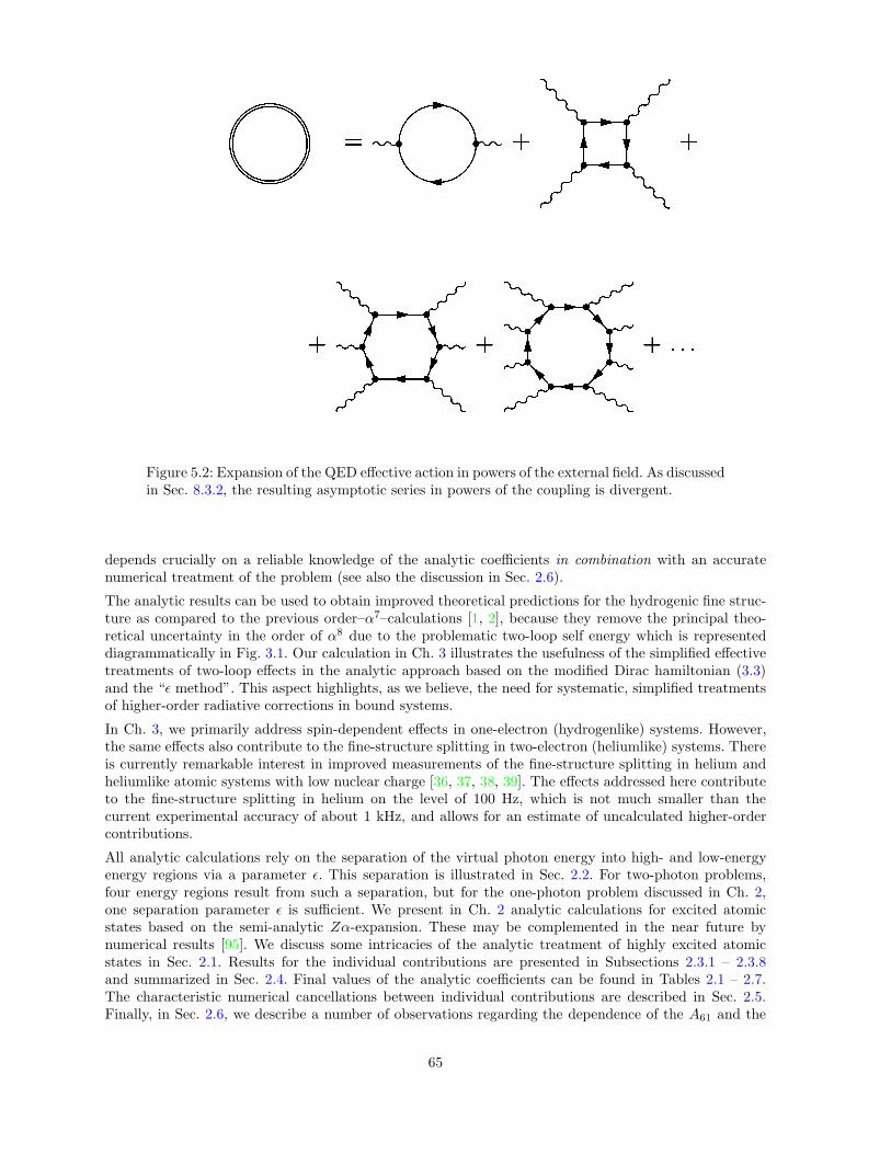
� � �
� � � � � �
Figure 5.2: Expansion of the QED effective action in powers of the external field. As discussedin Sec. 8.3.2, the resulting asymptotic series in powers of the coupling is divergent.
depends crucially on a reliable knowledge of the analytic coefficients in combination with an accuratenumerical treatment of the problem (see also the discussion in Sec. 2.6).
The analytic results can be used to obtain improved theoretical predictions for the hydrogenic fine struc-ture as compared to the previous order–α7–calculations [1, 2], because they remove the principal theo-retical uncertainty in the order of α8 due to the problematic two-loop self energy which is representeddiagrammatically in Fig. 3.1. Our calculation in Ch. 3 illustrates the usefulness of the simplified effectivetreatments of two-loop effects in the analytic approach based on the modified Dirac hamiltonian (3.3)and the “ε method”. This aspect highlights, as we believe, the need for systematic, simplified treatmentsof higher-order radiative corrections in bound systems.
In Ch. 3, we primarily address spin-dependent effects in one-electron (hydrogenlike) systems. However,the same effects also contribute to the fine-structure splitting in two-electron (heliumlike) systems. Thereis currently remarkable interest in improved measurements of the fine-structure splitting in helium andheliumlike atomic systems with low nuclear charge [36, 37, 38, 39]. The effects addressed here contributeto the fine-structure splitting in helium on the level of 100 Hz, which is not much smaller than thecurrent experimental accuracy of about 1 kHz, and allows for an estimate of uncalculated higher-ordercontributions.
All analytic calculations rely on the separation of the virtual photon energy into high- and low-energyenergy regions via a parameter ε. This separation is illustrated in Sec. 2.2. For two-photon problems,four energy regions result from such a separation, but for the one-photon problem discussed in Ch. 2,one separation parameter ε is sufficient. We present in Ch. 2 analytic calculations for excited atomicstates based on the semi-analytic Zα-expansion. These may be complemented in the near future bynumerical results [95]. We discuss some intricacies of the analytic treatment of highly excited atomicstates in Sec. 2.1. Results for the individual contributions are presented in Subsections 2.3.1 – 2.3.8and summarized in Sec. 2.4. Final values of the analytic coefficients can be found in Tables 2.1 – 2.7.The characteristic numerical cancellations between individual contributions are described in Sec. 2.5.Finally, in Sec. 2.6, we describe a number of observations regarding the dependence of the A61 and the
65

A60-coefficients on the quantum numbers of the atomic state.
All of the above calculations are related to the bound electron, which is a spin-1/2 particle. In nature,particles with different spin quantum numbers exist, and these, too, can form bound systems. The spin-dependence of the corrections is a conceptually interesting issue that forms the subject of Ch. 4. Thisinterest is sparked by the projected DIRAC experiment at CERN where the bound system of two oppo-sitely charged pions (“pionium”) will be studied. Notably, even the relativistic corrections for a boundtwo-body system consisting of spinless particles are different for spinless particles than for particles withnonvanishing spin. They are given by a generalized Breit hamiltonian that we discuss in Sec. 4.3. There,we present a simplified derivation for the relativistic and recoil corrections of order α4 to a bound state oftwo spinless particles. The results agree with previous calculations [126]. As evident from equation (4.14),the zitterbewegung term is absent in a bound system of two spinless particles.
The self energy is suppressed in systems with spinless particles in comparison to the vacuum polarizationeffect as discussed in Secs. 4.4 and 4.5, because the lightest known spinless particle is much heavier thanthe electron, which implies that the vacuum polarization effect is larger by two orders of Zα than the selfenergy in bound systems of spinless particles. We provide a complete result for the leading scalar-QEDcorrection of order α5 lnα in Sec. 4.5. A list of further QED corrections to the 1S level of pionium,including two-loop vacuum polarization, finite-size corrections and other effects, can be found in [17].
To conclude this Chapter, we would like to mention the complementarity of the high-precision calculationsand experiments at low nuclear charge and the strong-field calculations and related experiments at highnuclear charge numbers. While an accuracy [42] of one part in 1014 currently appears to be out of reach forhydrogenlike Uranium [150], the experiments on highly charged ions have meanwhile attained a precisionwhere a detailed understanding of the nuclear structure and shape is necessary in order to describe QEDeffects rigorously [151].
Bound systems described by quantum electrodynamics belong to the most accurately understood physicalsystems today. They convey a certain esthetic appeal because the apparent simplicity of the two- andthree-particle systems gives rise to a large number of conceptual as well as calculational difficulties whena thorough understanding is sought in higher orders of perturbation theory.
66

Part II
Convergence Acceleration andDivergent Series
67

Chapter 6
Introduction to ConvergenceAcceleration and Divergent Series inPhysics
The second part of this thesis will be concerned with convergence acceleration methods and with thesummation of divergent series. In theoretical physics, we often encounter sequences of numbers, either asa result of perturbation theory or as partial sums of an infinite series defining a physical quantity, whosenumerical properties are disfavourable: in many cases, the sequences converge so slowly that they arenumerically useless. In other cases, the sequences do not converge at all, and yet we know – or assume –that the sequences are associated, nevertheless, to the physical quantity in question, for example in theform of a divergent asymptotic expansion.
Let us consider the case where the sequence {sn}∞n=0 under investigation is given by partial sums of aninfinite series,
sn =
n∑
k=0
ak . (6.1)
We assume, furthermore, that the ak are real (this condition will be relaxed in the sequel).
(i) Let us assume that the sequence {sn}∞n=0 is convergent. The purpose of convergence acceleration is toconvert {sn}∞n=0 into a new sequence {s′n}∞n=0 with hopefully better numerical properties. If we denotethe limit of the sequence by s, that is s ≡ limn→∞ sn, then the rate of convergence is obviously increasedif
limn→∞
s′n − s
sn − s= 0 . (6.2)
(ii) Alternatively, let us assume that the sequence {sn}∞n=0 is divergent. The purpose of the resummationis to determine the generalized limit (or antilimit) of the sequence. The following question immediatelyarises: how is it possible to associate a finite generalized limit with a divergent series. L. Euler wrote in aletter to Goldbach (1745): “Summa cuiusque seriei est valor expressionis illius finitae, ex cuius evolutioneilla series oritur.”, which means: the generalized limit of any divergent series is the value of the particularcharacteristic finite expression, whose expansion gives rise to the divergent series. This is still the mainnotion of resummation today: Given a divergent series, to “reconstruct” a posteriori the function whoseexpansion gave rise to the divergent series, with a suitable mathematical resummation method.
We illustrate this idea with a trivial example: A divergent series can be generated, e.g., by expandingthe function f(z) = 1/(1 + z) ∼ ∑∞
j=0(−z)j at z = 1 in powers of z. The partial sums of the resultingdivergent series read
sn =
n∑
j=0
(−1)j =
1 for n even
0 for n odd. (6.3)
The resulting sequence, which is 1, 0, 1, 0, . . . , can be identified as originating from the discussed functionby expansion at unit argument, and its antilimit is therefore 1/2. Since this argument may not sound
68

convincing, let us briefly indicate that the result may also be obtained by imposing the postulate thatthe antilimit of the sum of two divergent series should be the sum of the two antilimits each. Then, itis easy to derive (by inspection) that the antilimit a of the series
∑∞j=0(−1)j should fulfill 1 − a = a,
and thus a = 1/2 (again). A more formal investigation of this series and its resummation can be foundin [152] [see Eq. (1.1.1) and the instructive discussion on the p. 6 ibid.]. It is probably a triviality toexpress that the most familiar resummation methods like the Euler transformation, Pade approximantsand recently developed nonlinear sequence transformations of the Levin–Weniger type all convert thedivergent sequence 1, 0, 1, 0, . . . to the convergent sequence 1/2,
1/2,1/2,
1/2, . . . , in mutual agreement.Some of these resummation methods are discussed in the sequel, and we also refer the reader to theseminal review [153]. It has been stressed in J. E. Littlewood’s introduction to [152] that the subject ofdivergent series is in no way “mystical or unrigorous”.
Fundamental differences exist between nonalternating series (without loss of generality we can assumeak > 0 ∀k in that case), and strictly alternating series ak = (−1)k bk where bk > 0 ∀k (mixed forms willalso be discussed in the sequel). The acceleration of the convergence and the summation of divergentnonalternating series has been historically problematic.
For example, it has been known for a long time that the acceleration of nonalternating slowly convergentseries can be highly unstable numerically (see [153] and references therein). Likewise, the summation ofnonalternating factorially divergent series has represented a considerable problem, because the series aretypically non–Borel summable (see [154, 155, 156, 157] for suitable generalizations of the concept of Borelsummability which provide solutions for large classes of problems of practical interest).
Recently, considerable progress has been achieved for the nonalternating case, and we will describe someof the relevant applications. For the acceleration of convergence of nonalternating series, new power-ful algorithms have been devised [23], and generalizations of the Borel summation process have led topromising results in the case of nonalternating factorially divergent series [25, 27, 28].
One would intuitively assume that the perturbation series, even if it is divergent, should be associated tothe physical quantity of interest in a more or less unique way. Unfortunately, many divergent series andthe associated physical observables (e.g., energy levels as a function of the coupling strength) fail to fulfillthe Carleman criterion [158] which guarantees that an asymptotic series can be uniquely associated to agiven mathematical function. It appears that some ambiguity has to accepted as far as the connectionbetween perturbation theory and physical quantities is concerned, although some attempts have beenmade to resolve ambiguities in particular cases (see e.g. [159]).
For completeness, we give here the Carleman criterion which guarantees that there is a one-to-one cor-respondence between a function and its associated asymptotic series (see for example [160], TheoremsXII.17 – XII.19 and the definition on p. 43 in [161], p. 410 in [162], or the comprehensive and elucidatingreview [163]):
Carleman Criterion. Let f(z) be a function which is analytic in the interiorand continuous on a sectorial region S = {z|| arg(z)| ≤ k π/2 + ε, 0 < |z| < R}of the complex plane for some ε > 0. Let the function f have an asymptoticexpansion f(z) ∼ ∑∞
n=0 cn zn (for z → 0). The function f obeys a strong
asymptotic condition (of order k) if there are suitable positive constants C andσ such that |f(z) − ∑m
n=0 cn zn| ≤ C σm+1 [k (m+ 1)]! |z|m+1 holds for all m
and for all z ∈ S. The validity of such a condition implies that the functionf(z) is uniquely determined by its asymptotic series.
Typically, nonalternating factorially divergent series which entail nonperturbative (imaginary) contribu-tions do not fulfill the Carleman condition. This failure gives rise to the inevitable ambiguities.
Even the generalized Borel resummation methods introduced in [154, 155, 156, 157] cannot provideconclusive answers for all possible physical scenarios. One highly problematic application is given by thequantum-mechanical double-well oscillator. The perturbation series for the ground state (as well as forany other unperturbed state) is divergent. Yet it is known that the ground state splits into two states ofopposite parity when the second minimum of the potential approaches the first from infinity [164, 165].The interesting observation is that two distinct quantum states are described by one and the sameperturbation series. The energy difference is nonperturbative in the coupling and cannot be inferred in
69
principle from perturbation theory. The problem has been the subject of intensive discussion [166, 167,168, 169, 170, 171]. The resulting multi-instanton expansion has recently found a more mathematicallymotivated explanation in the theory of resurgent functions [172, 173, 174].
We conclude this introduction by expressing that convergence acceleration and resummation methodscannot be separated. The connection can be seen as follows. We consider the remainders rn ≡ sn − s,i.e. the difference of the element sn of the sequence and the limit s. The acceleration of convergence isachieved by eliminating, as far as possible, the remainders rn from a necessarily finite set of input data{sn}mn=0, in order to obtain a better estimate s′m to s than the obvious estimate which would be providedby sm. Clearly, the “elimination of remainders” is a concept which can be transported to the case of adivergent series. The only difference is that for a convergent series, rn → 0 as n → ∞, whereas for adivergent series, limn→∞ rn does not exist. Otherwise, the concept of the elimination of remainders is thesame for both cases.
Returning to our (simple) example, it is intuitively obvious that a method which helps to eliminate theremainders
rn =
∞∑
j=n+1
(−z)j =(−z)n+1
1 + z(6.4)
inside the circle of convergence |z| < 1, could be suitable to accomplish an analogous elimination ofthe rn if z assumes values outside of the domain of convergence of the series
∑∞j=0(−z)j because the
mathematical structure of the expression which defines rn does not change. These entirely heuristicconsiderations will be illustrated and explained in the sequel.
70

Chapter 7
Convergence Acceleration
7.1 The Concept of Convergence Acceleration
7.1.1 A Brief Survey
We intend to give a brief overview of the convergence acceleration methods used in this Thesis, withoutany claim for completeness or comprehensiveness with regard to currently known convergence accelerationtechniques. Indeed, excellent textbooks (e.g. [175, 176, 177]) and review articles [153, 178, 179, 180, 181]on the subject are available. Here, we focus on aspects of the methods which will become useful for theapplications discussed in later Chapters of the Thesis.
This brief introduction is structured as follows: After a discussion of basic concepts (Secs. 7.1.2 and 7.1.3),we introduce Pade approximants (one of the standard mathematical tools for extrapolation and conver-gence acceleration) in Sec. 7.1.4. Next, we discuss nonlinear sequence transformations in Sec. 7.1.5. Bothof these convergence acceleration methods are much more powerful and much more numerically stablein the case of alternating input series than in the case of input series whose terms have the same sign(nonalternating series). We conclude in Sec. 7.1.6 with a discussion of the recently proposed [23] combinednonlinear-condensation transformation (CNCT) which provides an efficient algorithm in the historicallyproblematic case of nonalternating input series.
Before we start the discussion of Pade approximants and nonlinear sequence transformations, we wouldlike to mention that a large number of other convergence acceleration methods exist which have all beendocumented in the literature: examples include the Euler transformation, Aitken’s ∆2 process, the iterated∆2 process, and Richardson extrapolation which can be implemented using Wynn’s rho algorithm, andits iterations. Last, but not least, we mention the Euler–Maclaurin sum formula. The interested readerwill find related information e.g. in Chs. 5 and 6 of [153], App. E.2 of [43], and in Eq. (3.6.28) ff. of [182].
Concerning the mutual differences between the Pade method (Sec. 7.1.4 and nonlinear sequence trans-formations (Sec. 7.1.5), we would like to expand: Given a formal series
P(z) =
∞∑
j=0
cj zj (7.1)
as input, the Pade method produces rational approximants which depend exclusively on a finite subset ofthe coefficients {cj}∞j=0, which in turn determine the partial sums of (7.1). Nonlinear sequence transfor-mations require, in addition to the partial sums of (7.1), also explicit remainder estimates, i.e. estimatesfor the remainder
∑∞j=n+1 cj z
j which remains after the summation of the first n terms of (7.1).
Thus, the remainder estimates introduce additional degrees of freedom in the construction of sequencetransformations as compared to Pade approximants. As pointed out in [26], one may draw an analogybetween sequence transformations and Pade approximants on the one hand and the Gaussian integrationand the Simpson rule on the other hand; the variable integration nodes and weight factors of the Gaussianintegration yield additional degrees of freedom which may be used in order to construct a potentiallymuch more powerful algorithm for numerical integration.
71

Except for the additional degrees of freedom, nonlinear sequence transformations have additional advan-tages. For example, the delta transformation to be discussed in Sec. 7.1.5 gave very good results in thecase of the sextic anharmonic oscillator, and there is strong numerical evidence that it is able to sum theextremely violently divergent perturbation series for the octic anharmonic oscillator [183]. By contrast, asdiscussed in [183], Pade approximants are apparently not powerful enough to sum divergent series whosecoefficients diverge like (2n)! or even (3n)!. These observations stimulated research on sequence transfor-mations considerably. The rapid progress in this field is convincingly demonstrated by the large numberof monographs [177, 184, 185, 186, 187, 188, 189, 190, 191, 192] and review articles [153, 193, 194, 195]which appeared in recent years.
7.1.2 The Forward Difference Operator
An essential ingredient in the construction of sequence transformations, both for convergence accelerationand for the resummation of divergent series, is the (forward) difference operator. We define the differenceoperator ∆ acting on the sequence {sn}∞n=0:
∆ : {sn}∞n=0 → {(∆s)n}∞n=0 , (∆s)n ≡ sn+1 − sn , (7.2)
The nth element of the sequence {(∆s)n}∞n=0 is given by (∆s)n = sn+1 − sn. This way of writing the nthelement of the transformed sequence stresses the fact that (∆s)n is to be regarded as an element of somenew sequence. However, the brackets are often left out, and we write
∆sn ≡ sn+1 − sn = (∆s)n . (7.3)
An important relation is,
(∆ks)n = (−1)kk∑
j=0
(−1)j(
k
j
)
sn+j . (7.4)
Again, we identify∆ksn ≡ (∆ks)n . (7.5)
The kth power of the difference operator plays a crucial rule in constructing sequence transformations.
7.1.3 Linear and Logarithmic Convergence
As already stressed in Ch. 6, the main notion of convergence acceleration is to extract information “hiddenin trailing digits” from a necessarily finite number of sequence elements, in order to convert a sequence{sn}∞n=0 into a new sequence {s′n}∞n=0 with hopefully better numerical properties.
We briefly recall the notion of logarithmic convergence and the difficulties associated with the accelerationof the convergence of nonalternating series. Let a sequence {sn}∞n=0 fulfill the asymptotic condition
limn→∞
sn+1 − s
sn − s= ρ , (7.6)
where s = s∞ is the limit of the sequence as n → ∞. If ρ > 1, then the sequence {sn}∞n=0 is divergent.For ρ = 1, the sequence may either be convergent or divergent. A convergent sequence with ρ = 1 iscalled logarithmically convergent (if ρ < 1, the series is called linearly convergent). Let us further assumethat the elements of the sequence {sn}∞n=0 in Eq. (7.6) represent partial sums
sn =
n∑
k=0
a(k) (7.7)
of an infinite series. Here, we will almost exclusively investigate slowly convergent nonalternating se-quences {sn}∞n=0 whose elements are all real and positive (for these sequences, 0 < ρ ≤ 1). In the case ofslow convergence, ρ is either very close or equal to unity.
As observed by many authors (e.g. [153]), the acceleration of the convergence of nonalternating sequencesis a potentially unstable numerical process. The reason is the following: A sequence transformation can
72

only accelerate convergence if it succeeds in extracting additional information about the index-dependenceof the truncation errors
rn = sn − s (7.8)
from a necessarily finite set of partial sums {sn}kn=0 of the input series. Normally, this is done by formingarithmetic expressions involving higher weighted differences of the sn. The calculation of higher weighteddifferences is a potentially unstable process which can easily lead to a serious loss of numerical significancedue to cancellation if the input data all have the same sign.
We had mentioned in Ch. 6 that the rate of convergence can be said to be increased if the transformedsequence elements {s′n}∞n=0 and the input data {sn}∞n=0 fulfill [see also Eq. (6.2)]
limn→∞
τn ≡ limn→∞
s′n − s
sn − s= 0 , (7.9)
where we implicitly define the τn. Let us assume that the input sequence {sn}∞n=0 is logarithmicallyconvergent and that the transformed sequence {s′n}∞n=0 is linearly convergent with limn→∞(s′n+1−s)/(s′n−s) = ρ′ < 1 [see Eq. (7.6) and the definition of logarithmic convergence]. Then
limn→∞
τn+1
τn≡ limn→∞
s′n+1 − s
s′n − s
sn − s
sn+1 − s= ρ′ < 1 , (7.10)
so that limn→∞ τn = 0, and the rate of convergence is increased [according to the definition of convergenceacceleration in Eq. (7.9)].
7.1.4 The Standard Tool: Pade Approximants
The Pade approximation produces a rational approximation to the original input series; this approxima-tion is given by the ratio of two polynomials. The [l/m] Pade approximant to a series P(z),
P(z) =
∞∑
j=0
cj zj , (7.11)
is given by the ratio of two polynomials Pl(z) and Qm(z) of degree l and m, respectively:
[l/m]P(z) =Pl(z)
Qm(z)=
p0 + p1 z + . . .+ pl zl
q0 + q1 z + . . .+ qm zm. (7.12)
The polynomials Pl(z) andQm(z) are constructed so that the Taylor expansion of the Pade approximationEq. (7.12) agrees with the original input series Eq. (7.11) up to the order of l +m
P(z) − [l/m]P(z) = O(zl+m+1) . (7.13)
In other words, the Pade approximant [l/m]P(z) reproduces upon re-expansion the first l + m + 1(c0, . . . , cl+m) coefficients of the input series.
Usually the normalization condition is choosen such as q0 is one. Hence there are l+m+ 1 equations todetermine the coefficients of Pl(z) and Qm(z). In most cases it is quite unattractive to solve this systemof equations. A more attractive recursive prescription for the evaluation of Pade approximants is theε-algorithm given by the formulas [196]
ε(n)−1 = 0 , ε
(n)0 = sn ,
ε(n)k+1 = ε
(n+1)k−1 + 1/[ε
(n+1)k − ε
(n)k ] (7.14)
for k and n integer. The ε-algorithm is discussed in [196], and a detailed discussion of its implementation
can be found in [153]. If the input data ε(n)0 = sn are the partial sums
sn =n∑
j=0
cj zj (7.15)
73

of the power series Eq. (7.11), then the elements ε(n)2k of the two-dimensional table of transformations
produce Pade approximants according to
ε(n)2k = [n+ k/k]P (z) . (7.16)
The elements with odd lower subscripts ε(n)2k+1 of the table of transformations are only auxiliary quantities.
In practical applications (see e.g. Tables 1 – 3 of [24]), the epsilon algorithm can be used for evaluationof the following staircase sequence in the Pade table:
[0/0], [1/0], [1/1], [2/1], . . . , [ν/ν], [ν + 1/ν], [ν + 1/ν + 1], . . . . (7.17)
Because of Eq. (7.16) this corresponds to the sequence
ε(0)0 , ε
(1)0 , ε
(0)2 , ε
(1)2 , ε
(0)4 , ε
(1)4 , ε
(0)6 , . . . ε
(0)2ν , ε
(1)2ν , ε
(0)2ν+2, . . . , (7.18)
which can be written as {ε(ν−2[[ν/2]])2[[ν/2]] }∞ν=0. Here [[ν/2]] denotes the integral part of ν/2, which is the largest
integer µ satisfying µ ≤ ν/2. With this notation the Pade sequence in Eq. (7.17) can also be written as{[ν − [[ν/2]]/[[ν/2]]]P (z)}∞ν=0.
Modern computer algebra packages [90] contain built-in routines for the evaluation of Pade approximants.While these are computationally less effective than the epsilon algorithm, they are more flexible with re-gard to the degree of the numerator and denominator polynomials. In particular, the sequence allow for theevaluation of the sequence of lower-diagonal Pade approximants of the form {[[[ν/2]]/ν− [[ν/2]]]P (z)}∞ν=0.
As already mentioned in Sec. 7.1.1, it is a typical feature of all algorithms for Pade approximants that thecoefficients c0, c1, . . . , cl+m of the formal power series (7.11) suffice to determine [l/m]P(g) completely.No additional information is needed. At first sight, this seems to be very advantageous. However, there aresituations in which this apparent advantage becomes a disadvantage. For instance, the truncation errorof an asymptotic power series which has the Stieltjes property is for real argument bounded in magnitudeby the first term not included in the partial sum (see Example 9.3 on p. 92 of [91]). Accordingly, thetruncation error of a strictly alternating divergent hypergeometric series 2F0(α, β;−x) with α, β, x > 0,which provides a good mathematical model for many divergent perturbation expansions, is bounded inmagnitude by the first term not included in the partial sum. In addition, the truncation error and thefirst term not included in the partial sum have the same sign (see Theorem 5.12-5 of [197]). In principle,this information should be very helpful in summation processes. Unfortunately, Pade approximants arenot able to profit from it. This greatly reduces their efficiency if a divergent hypergeometric series 2F0 ofthat kind or a divergent perturbation series of a similar type is to be summed.
7.1.5 Nonlinear Sequence Transformations
A sequence transformation T is a rule which converts a slowly convergent or divergent sequence {sn}∞n=0
whose elements may be the partial sums sn =∑n
k=0 ak [see Eq. (6.1)] of an infinite series, into a newsequence {s′n}∞n=0 with hopefully better numerical properties. Pade approximants, which were discussedin Section 7.1.4, are special sequence transformations since they transform the partial sums of a formalpower series (7.11) into a doubly indexed sequence of rational approximants (7.17). In the current Section,alternative transformations will be discussed.
Let us now assume that the sequence {sn}∞n=0 of partial sums of an infinite series diverges but can besummed to its generalized limit s. Then the sequence elements sn can for all integers n ≥ 0 be partitionedinto the generalized limit s and remainders rn:
sn = s + rn . (7.19)
If {sn}∞n=0 diverges, then the remainders rn do not vanish as n → ∞. A divergent sequence would besummed to its generalized limit s if the remainders rn could somehow be eliminated from the sequenceelements sn. For a slowly convergent sequence, one can hope to accelerate convergence by eliminatingapproximations to the rn obtained from a finite set of sequence elements which are used as input datafor the transformation.
74

The sequence {sn}∞n=0 is transformed into a new sequence {s′n}∞n=0, whose elements can for all n ≥ 0 bepartitioned into the generalized limit s of the original sequence and a transformed remainder r′n:
s′n = s + r′n . (7.20)
This approximative elimination process can be termed successful if the transformed remainders r′n eithervanish as n→ ∞ (in the case of a divergent input sequence where the rn do not vanish at all as n→ ∞), orif the r′n vanish faster than the original remainders rn as n→ ∞ [in the case of a slowly convergent inputsequence, see also Eq. (7.9)]. A sequence transformation is a rule which transforms a slowly convergentor divergent sequence {sn}∞n=0 into a new sequence {s′n}∞n=0 with hopefully better numerical properties.
However, the truncation errors of a divergent series can depend on n in a very complicated way. Con-sequently, the direct elimination of approximations to rn from sn can be very difficult. A considerablesimplification can often be achieved by means of a suitable reformulation. Let us consider the followingmodel sequence (see Section 3.2 of [153]):
sn = s + ωn zn . (7.21)
Here, ωn is a remainder estimate, which has to be chosen according to some rule and which may dependon n in a very complicated way, and zn is a correction term, which should be chosen in such a way thatit depends on n in a relatively smooth way. Moreover, the products ωnzn should be capable of producingsufficiently accurate approximations to the actual remainders rn of the sequence to be transformed.
The principal advantage of this approach is that now only the correction terms {zn}∞n=0 have to bedetermined. The subsequent elimination of ωnzn from sn is often much easier than the direct eliminationof approximations to rn from sn. The use of remainder estimates {ωn}∞n=0 is also an efficient way ofincorporating additional information about the remainders into the summation scheme.
The model sequence (7.21) has another undisputable advantage: There is a systematic way of constructinga sequence transformation which is exact for this model sequence. Let us assume that a linear operator Tcan be found which annihilates the correction term zn. Then, a sequence transformation, which is exactfor the model sequence (7.21), can be constructed quite easily. Just apply T to [sn − s]/ωn = zn. SinceT annihilates zn according to T (zn) = 0 and is by assumption linear, we find that the following sequencetransformation T is exact for the model sequence (7.21) (see Eq. (3.2-11) of [153]):
T (sn, ωn) =T (sn/ωn)
T (1/ωn)= s . (7.22)
Simple and yet very powerful sequence transformations are obtained if the annihilation operators arebased upon the finite difference operator ∆ defined in Sec. 7.1.2. A polynomial Pk−1(n) of degree k − 1in n is annihilated by the k-th power of ∆. Thus, we now assume that the correction terms {zn}∞n=0 canbe chosen in such a way that multiplication of zn by some suitable quantity wk(n) yields a polynomialPk−1(n) of degree k − 1 in n:
wk(n) zn = Pk−1(n) . (7.23)
Since ∆kPk−1(n) = 0, the weighted difference operator T = ∆kwk(n) annihilates zn, and the correspond-ing sequence transformation (7.22) is given by the ratio
T (n)k
(
wk(n)∣
∣sn, ωn)
=∆k{wk(n)sn/ωn}∆k{wk(n)/ωn}
. (7.24)
A number of sequence transformations can be obtained by specializing wk(n). For instance, wk(n) =(n+ β)k−1 with β > 0 yields Levin’s sequence transformation [198]:
L(n)k (β, sn, ωn) =
∆k {(n+ β)k−1 sn/ωn}∆k {(n+ β)k−1/ωn}
=
k∑
j=0
(−1)j(
k
j
)
(β + n+ j)k−1
(β + n+ k)k−1
sn+j
ωn+j
k∑
j=0
(−1)j(
k
j
)
(β + n+ j)k−1
(β + n+ k)k−1
1
ωn+j
. (7.25)
75
We follow the notation of [153]. The subscript k denotes the order of the transformation, and n denotes thestarting index (the initial element) of the input data. Observe that the k+1 sequence elements sn, . . . sn+k
and the k+1 remainder estimates ωn . . .ωn+k are needed for the computation of the transformation L(n)k .
The shift parameter β has to be positive in order to admit n = 0 in (7.25). In most practical applications,it is observed that any choice other than β = 1 does not lead to a significant improvement of the rate ofconvergence, and therefore the choice β = 1 is standard [153].
The notation L(n)k (β, sn, ωn) is in need of a certain further explanation. As explained above, n represents
the initial element of the sequence {sn}∞n=0 used in the evaluation of the transform. The specification of
sn as the second argument of L(n)k (β, sn, ωn) is therefore redundant as far as the index n is concerned,
because n already appears as an upper index in L(n)k . The arguments sn (and ωn) are to be interpreted
as follows: they rather specify the initial element sn and the initial remainder estimate ωn which have
to be used in the calculation of the right-hand side of (7.25). Of course, the evaluation of L(n)k (β, sn, ωn)
requires the k + 1 sequence elements {sn, . . . , sn+k, sn+k} as input. The knowledge of the “post-initial”elements {sn+1, . . . , sn+k} is implicitly assumed in writing the definition (7.25).
According to Smith and Ford, who had investigated the performance of sequence transformations fora wide range of test problems [199, 200], Levin’s transformation is among the most powerful and mostversatile sequence transformations that are currently known.
We can also assume that the unspecified weights wk(n) in (7.24) are Pochhammer symbols according towk(n) = (n+ β)k−1 = Γ(n+ β + k − 1)/Γ(n+ β) with β > 0. This yields the delta transformation (seeEq. (8.2-7) of [153]):
S(n)k (β, sn, ωn) =
∆k {(n+ β)k−1 sn/ωn}∆k {(n+ β)k−1/ωn}
=
k∑
j=0
(−1)j(
k
j
)
(β + n+ j)k−1
(β + n+ k)k−1
sn+j
ωn+j
k∑
j=0
(−1)j(
k
j
)
(β + n+ j)k−1
(β + n+ k)k−1
1
ωn+j
. (7.26)
As in the case of Levin’s transformation, the most obvious choice for the shift parameter is β = 1.
The numerator and denominator sums in (7.25) and (7.26) can be computed more effectively with thehelp of the three-term recursions [see Eq. (7.2-8) of [153]]:
L(n)k+1(β) = L
(n+1)(β)k − (β + n+ k)(β + n+ k)k−1
(β + n+ k + 1)kL
(n)k (β) , (7.27)
and (see Eq. (8.3-7) of [153])
S(n)k+1(β) = S
(n+1)k (β) − (β + n+ k)(β + n+ k − 1)
(β + n+ 2k)(β + n+ 2k − 1)S
(n)k (β) . (7.28)
The initial values L(n)0 (β) = S
(n)0 (β) = sn/ωn and L
(n)0 (β) = S
(n)0 (β) = 1/ωn produce the numerator and
denominator sums, respectively, of L(n)k (β, sn, ωn) and S(n)
k (β, sn, ωn).
Let us assume that the terms ak in (6.1) are strictly alternating, i.e. ak = (−1)kbk with bk > 0. In thiscase, the first term (−1)n+1bn+1 not included in the partial sum sn =
∑nk=0(−1)kbk is the best simple
estimate for the truncation error. This corresponds to the remainder estimate
ωn = (−1)n+1bn+1 = ∆sn , (7.29)
which was proposed by Smith and Ford [199]. The use of this remainder estimate in (7.25) and (7.26)
76
yields the following sequence transformations [Eqs. (7.3-9) and (8.4-4) of [153]]:
d(n)k (β, sn) = L(n)
k (β, sn,∆sn)
=
k∑
j=0
(−1)j(
k
j
)
(β + n+ j)k−1
(β + n+ k)k−1
sn+j
∆sn+j
k∑
j=0
(−1)j(
k
j
)
(β + n+ j)k−1
(β + n+ k)k−1
1
∆sn+j
, (7.30)
δ(n)k (β, sn) = S(n)
k (β, sn,∆sn)
=
k∑
j=0
(−1)j(
k
j
)
(β + n+ j)k−1
(β + n+ k)k−1
sn+j
∆sn+j
k∑
j=0
(−1)j(
k
j
)
(β + n+ j)k−1
(β + n+ k)k−1
1
∆sn+j
. (7.31)
Alternative remainder estimates for the sequence transformations (7.25) and (7.26) were discussed inSections 7 and 8 of [153] or in [201, 202].
A final word on sequence transformations: It is observed that sequence transformations constructedaccording to (7.31) often lead to much better numerical results than better known convergence ac-celerators like the Euler transformation, Wynn’s epsilon or rho algorithms, or Aitken’s ∆2 pro-
cess [153]. In particular, there is overwhelming empirical evidence that d(n)k and δ
(n)k work very
well in the case of convergent or divergent alternating series for instance as they occur in spe-cial function theory [23, 153, 177, 198, 199, 200, 203, 204, 205, 206, 207] or in perturbation theory[183, 204, 205, 208, 209, 210, 211, 212, 213, 214]. Only for some special model problems could rigorousconvergence proofs be obtained (see [215] or Sections 13 and 14 of [153]). No general convergence proof
is known for delta transformation δ(n)k as well as their parent transformations L(n)
k and S(n)k . In view of
the partially unsatisfactory situation concerning the availability of mathematical proof, we have carriedout high-precision studies of the convergence of sequence transformations of the type (7.31), in part usingmulti-precision arithmetic (see Sec. 7.2.2). In the absence of a rigorous proof, one of the concerns whichmay be raised against the convergence of the transforms (7.31) is a plausible asymptotic nature of thesequence of transforms. In our numerical experiments, we found no indication of asymptotic behaviour.The rate of convergence of the transforms remained constant, and we observed apparent convergenceup to 430 decimal figures (see Sec. 7.2.2 below). In the absence of rigorous proof and the presence ofconsiderable numerical evidence for the computational usefulness of sequence transformations of the type(7.31), we believe that experimental mathematics may give some hints at the theoretical soundness ofthe concepts involved.
7.1.6 The Combined Nonlinear–Condensation Transformation (CNCT)
We assume the series∑∞
k=0 ak is slowly convergent and nonalternating, i.e. ak > 0 ∀k. In order tomake the notation of involved subscripts more clear, we temporarily identify ak ≡ a(k). Following VanWijngaarden [216], we transform the nonalternating input series
∞∑
k=0
a(k) , a(k) ≥ 0 , (7.32)
whose partial sums are given by (7.7), into an alternating series∑∞j=0(−1)jAj . After the first step of the
transformation, the limit of the input series is recovered according to
∞∑
k=0
a(k) =∞∑
j=0
(−1)j Aj . (7.33)
77
The quantities Aj are defined according to
Aj =∞∑
k=0
b(j)k , (7.34)
whereb
(j)k = 2k a(2k (j + 1) − 1) . (7.35)
Obviously, the terms Aj defined in Eq. (7.34) are all positive if the terms a(k) of the original series areall positive. The Aj are referred to as the condensed series [23], and the series
∑∞j=0(−1)jAj is referred
to as the transformed alternating series, or alternatively as the Van Wijngaarden transformed series.
The construction of the condensed series reminds one of Cauchy’s condensation theorem (see e.g. p. 28of Ref. [217] or p. 121 of Ref. [218]). Given a nonalternating series
∑∞k=0 a(k) with terms that satisfy
|a(k + 1)| < |a(k)|, Cauchy’s condensation theorem states that∑∞
k=0 a(k) converges if and only if thefirst condensed sum A0 defined according to Eq. (7.34) converges.
The summation over k in Eq. (7.34) dose not pose numerical problems. Specifically, it can be easily
shown in many cases of practical importance that the convergence of∑∞k=0 b
(j)k (in k) is linear even
if the convergence of∑∞
k=0 a(k) is only logarithmic. We will illustrate this statement by way of twoexamples.
Example 1: a logarithmically convergent input series whose terms behave asymptotically as a(k) ∼ k−1−ε
with ε > 0. In this case, the partial sums
A(n)j =
n∑
k=0
b(j)k (7.36)
converge linearly with
limn→∞
A(n+1)j − Aj
A(n)j − Aj
=1
2ε (j + 1)1+ε< 1 , a(k) ∼ k−1−ε , k → ∞. (7.37)
Example 2: a series with a(k) ∼ kβrk where 0 < r < 1 and β real. Here, we have ρ = r < 1, and theseries is (formally) linearly convergent. However, slow convergence may result if ρ is close to one. In thiscase, the condensed series are very rapidly convergent,
limn→∞
A(n+1)j − Aj
A(n)j − Aj
= 0 , a(k) ∼ kβrk , k → ∞. (7.38)
Therefore, when summing over k in evaluating the condensed series according to Eq. (7.34), it is inmany cases sufficient to evaluate the condensed series by adding the terms successively, and no furtheracceleration of the convergence is required.
As shown in [23, 219], the condensation transformation defined according to Eqs (7.33)– (7.35) is essen-tially a reordering of the terms of the input series
∑∞k=0 a(k). Furthermore, Daniel was able to show (see
the Corollary on p. 92 of Ref. [219]) that for nonalternating convergent series whose terms decrease inmagnitude (|a(k)| > |a(k + 1)|), the equality (7.33) holds. This formally justifies the correctness of thecondensation transformation defined according to Eqs. (7.33) – (7.35).
Note that the property
A2 j−1 =1
2[Aj−1 − aj−1] , (j = 1, 2, . . . ) , (7.39)
derived in [219], facilitates the numerical evaluation of a set of condensed series, by reducing the evaluationof condensed series of odd index to a trivial computation.
In the second step of the CNCT, the convergence of the Van Wijngaarden transformed series∑∞
j=0 (−1)j Aj on the right-hand side of Eq. (7.33) is accelerated by a suitable nonlinear sequence trans-formation. We start from the partial sums
Sn =n∑
j=0
(−1)j Aj (7.40)
78

of the Van Wijngaarden transformed series.
We use the partial sums Sn defined in Eq. (7.40) as input data for the delta transformation (7.31). Thisleads to the CNC transforms
TCNC(n) = δ(0)n (1,S0) . (7.41)
which require as input the elements {S0, . . . ,Sn,Sn+1} of the Van Wijngaarden transformed series.
7.2 Applications of Convergence Acceleration Methods
7.2.1 Applications in Statistics and Applied Biophysics
Several slowly convergent series of the type considered in this Section of the Thesis define special functionsthat have important uses in statistics, namely the Riemann zeta, generalized zeta, Jonquiere functions andLerch’s transcendent (see [92] for definitions and some properties of these functions). Discrete distributionsare related to these functions by associating probability mass functions (p.m.f.s) with the terms of theparticular infinite series defining the special functions. In turn, the normalization constants of the p.m.f.sare associated with the sums of the series.
Consider a discrete distribution with the p.m.f.
Pr[X = n] = c p(n; θ) (7.42)
and with support of all nonnegative integers n = 0, 1, . . . , where θ is a (vector of) parameter(s) and c isa constant. The probability over the set of all outcomes is unity:
∞∑
n=0
Pr[X = n] = 1 , (7.43)
from which we obtain the normalization constant
c−1 =∞∑
n=0
p(n; θ) (7.44)
(in statistics, the random variable is usually denoted by the symbol n, whether continuous or discrete,but we will denote it here by the symbol n in order to follow the usual notation used in the treatment ofspecial functions). Thus we expect the sum in Eq. (7.44) to exist and to converge to a finite value. In thesequel, we consider several related discrete distributions. The Zipf distribution has the p.m.f.
px = c1
ns(7.45)
with support of all positive integers n = 1, 2, . . . . The normalization constant (7.44) is then
c−1 = ζ(s) =
∞∑
n=1
1
ns, (7.46)
where s > 1, which is immediately recognized as the Dirichlet series for the Riemann zeta function [Eq. (1)on p. 32 of Ref. [92]]. Basic properties of the Zipf distribution can be found in [220].
The Zipf–Mandelbrot distribution [221] is the generalization of the Zipf distribution that adds a constantto the ranks n and has the p.m.f.
px = c1
(n+ v)s(7.47)
with the support of all nonnegative integers n = 0, 1, . . . . The normalization constant (7.44) is then
c−1 = ζ(s, v) =
∞∑
n=0
1
(n+ v)s, (7.48)
79

where v 6= 0,−1, . . . . The sum (7.48) is recognized as the generalized zeta function [Eq. (1) on p. 24 ofRef. [92]].
Further, the p.m.f.
px = czn
ns(7.49)
with the support of all positive integers n = 1, 2, . . . defines the Good distribution [222]. The con-stant (7.44) is then
c−1 = F (z, s) =
∞∑
n=1
zn
ns, (7.50)
where |z| < 1, which is recognized as the Jonquiere’s function [Eq. (14) on p. 30 of Ref. [92]; see also [223]].Important properties of the Good distribution were derived in [224, 225].
In biophysics, one is interested in establishing the statistical structure of DNA and RNA sequences.Indeed, an interest in statistical compositions of DNA and protein sequences originated shortly afterthe discovery that the nucleotide sequences of RNA uniquely determines the amino-acid sequence of theproteins. An early analysis was performed in [226], where it was observed that the distributions of relativeabundances of amino-acids and nucleotides were nonrandom, i.e. deviated from models assuming uniformdistribution of different words in any given text. Zipf distributions and related generalizations proved tobe very useful in further studies [227, 228, 229].
A formal generalization of the Zipf, the Zipf–Mandelbrot and the Good distributions is possible uponrealizing that the Riemann zeta, the generalized zeta and the Jonquiere functions constitute special casesof the Lerch transcendent which is defined by the following series
Φ(z, s, v) =
∞∑
n=0
zn
(n+ v)s, (7.51)
where |z| < 1 and v 6= 0,−1, . . . [Eq. (1) on p. 27 of Ref. [92]]. We use here the the nonstandard notationof a dummy index n in order to highlight the connection with statistical theory. The relations betweenΦ(z, s, v) and ζ(s), ζ(s, v) and F (z, s) can be obtained by considering appropriate limits if Φ(z, s, v) (e.g.,by letting z and/or v to 0 and/or 1), and by making use of the following functional relation [Eq. (2) onp. 27 of Ref. [92]]
Φ(z, s, v) = zmΦ(z, s,m+ v) +
m−1∑
n=0
zn
(n+ v)s. (7.52)
In particular, Eq. (7.52) with m = 1 can be used to evaluate sums that start from n = 1 rather thanfrom n = 0:
∞∑
n=1
zn
(n+ v)s= zΦ(z, s, 1 + v) (7.53)
In Tab. 7.1, we have summarized the relations between the different statistical distributions and theirdefining special functions. The table illustrates the fact that the three distributions, Zipf (Zeta), Zipf–Mandelbrot (Generalized zeta) and Good (Jonquiere), are special cases of the Lerch distribution, andthat their properties can be expressed in terms of Lerch’s transcendent with special values of parameters.
We have found that the application of the combined nonlinear-condensation transformation (CNCT)described in detail in Sec. 7.1.6 is very suitable for the accelerated evaluation of the Lerch transcendent(7.51) in the nonalternating case (z > 0). Details of the implementation, both in C and Mathematica [90],are discussed in [30, 31]. For z < 0, the series (7.51) is alternating. In this case, the direct applicationof the delta transformation (7.31) leads to an efficient calculational scheme [31]. A C code for the Lerchtranscendent is available [230, 231].
7.2.2 An Application in Experimental Mathematics
We would like to begin this section by quoting [232]: “In April 1993, Enrico Au–Yeung, an undergraduateat the University of Waterloo, brought to the attention of the author’s [David Bailey’s] colleague Jonathan
80

Distribution Support p.m.f. c−1
(related function)
Zipf 1, 2, . . . c n−s ζ(s) = Φ(1, s, 1)
(zeta function)
Zipf–Mandelbrot 0, 1, . . . c (n+ v)−s ζ(s, v) = Φ(1, s, v)
(generalized zeta)
Good 1, 2, . . . c zn n−s F (z, s) = zΦ(z, s, 1)
(Jonquiere function)
Lerch 0, 1, . . . c zn (n+ v)−s Φ(z, s, v)
(Lerch’s transcendent)
Table 7.1: Interrelationships between distributions defined by Riemann zeta, generalizedzeta, Jonquiere and Lerch functions.
Borwein the curious fact that
∞∑
k=1
(
1 +1
2+ · · · +
1
k
)2
k−2 = 4.59987 · · · ≈ 17
4ζ(4) =
17π2
360, (7.54)
based on a computation of 500,000 terms. Borwein’s reaction was to compute the value of this constantto a higher level of precision in order to dispel this conjecture. Surprisingly, his computation to 30 digitsaffirmed it. [David Bailey] then computed this constant to 100 decimal digits, and the above equality wasstill affirmed.” Many formulas similar to (7.54) have subsequently been established by rigorous proof [233].
With the help of a multiprecision system [232, 234, 235] and the CNCT, we have verified (7.54) “experi-mentally” to a couple of hundred decimals. The calculation will be sketched in the following. Using thedefinition
b(k) =
(
1 +1
2+ . . .+
1
k
)2
k−2 , (7.55)
we rewrite (7.54) as follows,
∞∑
k=0
b(k) =
∞∑
k=0
k∑
j=0
1
j + 1
2
(k + 1)−2
=∞∑
k=0
(
ψ(k + 2) + C
k + 1
)2
, (7.56)
where C is the Euler-Mascheroni constant C = 0.577 215 . . ., and ψ(z) is the logarithmic derivative ofthe Gamma function [91, 92] ,
ψ(z) =d
dzln Γ(z) . (7.57)
81

With the help of the relation∞∑
k=0
ψ(k + 2)
(k + 1)2= 2 ζ(3) − C ζ(2) , (7.58)
the conjecture (7.54) can be rewritten as
∞∑
k=0
(
ψ(k + 2)
k + 1
)2
=17
4ζ(4) − 4C ζ(3) + C2 ζ(2) . (7.59)
We proceed to calculate numerically, to high precision, the infinite sum
∞∑
k=0
a(k) , a(k) =
(
ψ(k + 2)
k + 1
)2
, (7.60)
using the CNC transformation.
In order to establish the rate of convergence of (7.60), we investigate the asymptotic behaviour of thea(k) as k → ∞. The logarithm of the Gamma function can be expanded into an asymptotic series [seeEq. (4.03) on p. 294 of [91]]:
ln Γ(z) =
(
z − 1
2
)
ln z − z +1
2ln(2π) +
m−1∑
s=1
B2s
2s(2s− 1)z2s−1+ Rm(z) , (7.61)
where
Rm(z) =
∫ ∞
0
B2m − B2m(x − [[x]])
2m(x+ z)2mdx . (7.62)
Here, [[x]] is the integral part of x, i.e., the largest integer m satisfying m ≤ x, Bk(x) is a Bernoullipolynomial defined by the generating function [see Eq. (1.06) on p. 281 of Ref. [91]]:
t exp(xt)
exp(t) − 1=
∞∑
m=0
Bm(x)tm
m!, |t| < 2π , (7.63)
andBm = Bm(0) (7.64)
is a Bernoulli number (p. 281 of Ref. [91]). The following asymptotic relation for ψ(z) follows:
ψ(z) = ln z − 1
2z−
m−1∑
s=1
B2s
2sz2s+ O
(
1
z2m
)
. (7.65)
The leading asymptotics of the remainder of the sum (7.60) after adding N −1 terms can thus be derivedeasily. We have for large k,
a(k) ∼ ln(k + 2)2
(k + 1)2− ln(k + 2)
(k + 1)2 (k + 2)− ln(k + 2)
6 (k + 1)2 (k + 2)2+ O
(
1
k4
)
, k → ∞ . (7.66)
Based on these formulas, the remainder of the sum (7.60), for large N , can be written as
∞∑
k=N
a(k) ∼ ln2N
N+
lnN
N+
1
N+ O
(
ln2N
N2
)
. (7.67)
Here, the Euler-Maclaurin formula [Eqs. (2.01) and (2.02) on p. 285 of Ref. [91]] has been used in orderto convert the sum over the a(k) in the asymptotic regime of large k [see Eq. (7.66)] into an integralplus correction terms. In order to calculate (7.59) to an accuracy of 200 decimals, Eq. (7.67) says thatwe would be required to add on the order of 10205 terms. Without the use of convergence accelerationmethods, this would represent a formidable computational task.
82

Using the CNCT, it is easy to calculate the sum (7.59) to 200 digits, based on multiprecision arith-metic [232] and a Linux personal computer, within a few hours. We obtain for the 246th and the 247thCNC transform defined according to Eq. (7.41),
TCNC(246) = 2.37254 51620 38445 67035 68130 69148 85258 25756 18499 54254
97013 57806 20011 72404 62937 46020 32218 23862 67095 00004
69194 36541 28946 10390 15116 52595 90270 23975 58737 74256
23420 48480 95165 00802 19816 35378 76591 98589 60393 32103, (7.68)
and
TCNC(247) = 2.37254 51620 38445 67035 68130 69148 85258 25756 18499 54254
97013 57806 20011 72404 62937 46020 32218 23862 67095 00004
69194 36541 28946 10390 15116 52595 90270 23975 58737 74256
23420 48480 95165 00802 19816 35378 76591 98589 60393 32112. (7.69)
The apparent convergence to 200 decimals can be verified against the right-hand side of Eq. (7.59). Ofcourse, the right-hand side of Eq. (7.59), which involves only rationals, zeta functions and the Euler–Mascheroni constant,
17
4ζ(4) − 4C ζ(3) + C2 ζ(2) ,
can be easily evaluated to 200 decimals using known algorithms which are included in computer algebrasystems [90].
The evaluation of the terms a(k) proceeds as follows. For small index k, it is easy to write a recursionrelation relating a(k) and a(k + 1) based on the (trivial) recursion for the ψ function,
ψ(k + 1) = ψ(k) +1
k. (7.70)
For large index k, the asymptotic formula (7.65) can be used in order to calculate the ψ function to highprecision. The point at which index one may switch from the recursion to the asymptotic method dependson how many explicit values for Bernoulli numbers are available to the machine. We use the first valuesfor the first 60 Bernoulli numbers, to 250 decimals, for our calculation. We switch from one method tothe other when the index k of a(k) has reached a value of 500.
With 84 308 a(k) terms evaluated (out of which 1364 by recursion and 82944 by the asymptotic method),we evaluate the first 247 transforms with the results presented above in Eqs. (7.68) and (7.69). If theterms of the series (7.54) were added on a term-by-term basis, then about 10205 would be required for anaccuracy of 200 decimals in the final result. The reduction of this number to roughly 84 000 correspondsto an acceleration of the convergence by roughly 200 orders of magnitude. We have also carried out,using enhanced precision, a calculation to 430 decimals, involving about 500 CNC transformations andarithmetic with 600 decimal figures. These evaluations not only confirm the conjecture (7.59) to highprecision, but they also represent one of the most accurate experimental verifications of the convergenceproperties of the delta transformation (7.31) today. Moreover, it is observed that the rate of convergenceof the CNC transforms, which is approximately one decimal figure per transformation, remains constantover a wide range of transformation orders. This observed behaviour is consistent with linear convergence[ρ ≈ 0.1 in Eq. (7.6)] in higher transformation orders. By contrast, the series (7.59) is only logarithmicallyconvergent. This corresponds to convergence acceleration according to the definition (7.9).
83

7.2.3 Other Applications of the CNCT
We would like to mention the existing applications in the domain of quantum electrodynamic bound-statecalculations (see [9, 12, 43] and Ch. 1 of this Thesis). Another existing application concerns the quantumelectrodynamic effective action (see Ref. [20]).
J. Becher [236] has investigated the applicability of the combined nonlinear-condensation transformationto series of the form
Rp(x) =
∞∑
k=0
x2k+1
(2k + 1)p, (7.71)
as well as
Tp(x, b) =
∞∑
k=0
1
(2k + 1)pcosh(2k + 1)x
cosh(2k + 1)b, (7.72)
and
Up(x, b) =
∞∑
k=0
1
(2k + 1)pcosh(2k + 1)x
sinh(2k + 1)b. (7.73)
Series of this type occur naturally in the context of plate contact problems with periodic boundaryconditions [237]. The arguments p, x and b are real and positive for cases of practical relevance. For x ≈ band p ≈ 1, the series Tp and Up are very slowly convergent. In App. A.2 of [236], it is demonstrated byway of numerical example that the CNCT is able to efficiently accelerate the convergence of these seriesin problematic parameter regions.
In the numerical calculations, it is necessary to evaluate terms with large index k. This can lead tonumerical overflow because of the large arguments of the hyperbolic functions. Clearly, representationslike
Tp(x, b) =∞∑
k=0
e(2k+1)(x−b)
(2k + 1)p1 + e−2x(2k+1)
1 + e−2b(2k+1)(7.74)
provide a solution for this problem.
Let us recall that considerable effort has been invested in the development of efficient numerical methodsfor the evaluation of the series (7.71) – (7.73) [238, 239, 240, 241, 242]. These alternative methods makeintensive use of special properties of the series. They involve integral transformations and infinite seriesover numerical integral [241], and they make use of special properties of Legendre’s chi-function [240]which is related to the functions (7.71) – (7.73).
A further application of convergence acceleration methods discussed by J. Becher [236] is the calculationof the incomplete Gamma function Γ(0, x) whose asymptotic expansion for large argument reads
Γ(0, x) ∼ e−x
x
∞∑
n=0
(−1)nn!
xn, x→ ∞ . . (7.75)
It is observed (see App. A.3 ibid.) that the divergent asymptotic series of this function for large positiveargument can be resummed effectively using the delta transformation, without any recourse to the CNCT.
7.3 Conclusions and Outlook for Convergence Acceleration
We have discussed several applications of the convergence acceleration methods introduced in Sec. 7.1: instatistical physics (Sec. 7.2.1), in experimental mathematics (Sec. 7.2.2), and other applications, mainlyin the evaluation of special functions (Sec. 7.2.3). Specifically, it is observed that a combination of themethods introduced in Secs. 7.1.5 and 7.1.6 leads to an efficient calculational scheme for the Lerchtranscendent Φ defined in Eq. (7.51). This special function provides a generalization of several kinds ofprobability density functions which are of significance for the statistical analysis of DNA sequences (seeTable 7.1).
Other applications can be envisaged: For example, the evaluation of generalized hypergeometric functions– notably of two-variable hypergeometric functions (Appell functions) F1 and F2 [243] – has been histor-ically problematic. In the recent investigation [244], the evaluation of F1(α, β1, β2, γ;x, y) is considered:
84

The algorithm consists in two steps: (i) the sophisticated use of analytic continuations to map the point(x, y) into the convergence region of the defining hypergeometric series of the Appell function, and (ii)the computation of the Appell function within the region of convergence. The analytic continuations giverise – in addition to F1 functions of transformed argument – to the G2 function, which can in turn bewritten in terms of Appell’s F2 function. This implies that numerical methods also have to be devised forthe F2 function. The second step of the algorithm described in [244] is the actual numerical calculation ofthe Appell function(s) (F1 and F2) within the region of convergence. This calculation proceeds by inves-tigating the criterion t0 = max(|x|, |y|) < 0.5. If the criterion is fulfilled, then both the F1 and the F2 areevaluated by single-index series expansions in terms of 2F1’s, for example employing the formula [245, 246]
F1(α, β1, β2, γ;x, y) =∞∑
r=0
(α)r (β1)r (β2)r (γ − α)r(γ + r − 1)r (γ)2r r!
× 2F1(α+ r, β1 + r, γ + 2r, x) 2F1(α+ r, β2 + r, γ + 2r, y) . (7.76)
If the criterion is not fulfilled, the authors resort to the solution of a third-order differential equationfor the evaluation of the Appell function [starting from the point (x, y) = (0, 0) where F1 vanishes]. Itappears possible that an application of convergence acceleration algorithms to the series (7.76) could leadto an efficient calculational scheme in the problematic case t0 > 0.5 where the authors of [244] had toresort to an integration of a third-order differential equation.
Possible improvements over existing algorithms concern “multi-stage transformations”. For example, itwas observed in [26] that the rate of convergence of the output data resulting from Borel summation(see Sec. 8.2.2) of a specific divergent series describing the quantum electrodynamic effective action couldbe further accelerated by using two iterations of the epsilon algorithm [defined in Eq. 7.14)], i.e. byevaluating Pade approximants to the Pade approximants of the Borel transforms (in this sequence).Iterated forms of a number of convergence accelerators have been discussed in [153]. In general, theiteration of suitable convergence accelerators depends on a thorough analysis of the remainder structureresulting from previous “stages” of the transformation, and it is not a priori guaranteed that a “multi-stagetransformation” with only one iterated algorithm will help. In principle, the use of iterated algorithms canonly be helpful when the evaluation of the sequence transforms or Pade approximants is computationallycheap in comparison to the evaluation of further terms of the input sequence which could potentially beused to calculate higher-order terms in a single-stage transformation process.
85
Chapter 8
Divergent Series
8.1 Introduction to Divergent Series in Physics
The observation that many perturbation series encountered in quantum mechanics and quantum fieldtheory are divergent, sparked the development of large-order perturbation theory [247]. This subject isinherently connected to the resummation of divergent series, and with the development of appropriatenumerical methods which exploit all available information contained in a necessarily finite number ofperturbative coefficients. Of prime importance in this context is the Borel method to be discussed inSec. 8.2.2.
As already stressed in Ch. 8, there are connections between the convergence acceleration methods dis-cussed in Ch. 7 and the resummation methods discussed in the current Chapter. Specifically, the methodsintroduced in Secs. 7.1.4 and 7.1.5 will be used below in Sec. 8.3.2 in the context of the resummation ofthe divergent perturbation series for the QED effective action.
Essentially, we will consider four physical applications of resummation methods: (i) the energy displace-ment of a hydrogen atom in a background electric field, including the autoionization width (Sec. 8.2),(ii) zero-dimensional field theories (Sec. 8.3.1), (iii) the QED effective Lagrangian for background mag-netic and electric fields (Sec. 8.3.2), and (iv) the energy levels of the double-well potential which receivenonperturbative contributions from multi-instanton effects (Sec. 8.3.3).
Several important aspects and basic concepts connected with divergent series and the large-order behaviorof perturbation theory can be illustrated by investigating the (divergent) perturbation series of the Starkeffect [248]. This effect, which is also known as the LoSurdo–Stark effect in view of the existence of theinvestigation [249]), describes the energy displacement of a hydrogen atom in a static external electricfield and can be expressed as a perturbation series (power series) in the electric field strength.
The first nonvanishing perturbation (in atomic units) is the second-order effect
F 2∑
m 6=1S
〈φ1S|z|φm〉 〈φm|z|φ1S〉E1S − Em
,
where the sum overm runs over the entire spectrum, including the continuum, but excluding the 1S groundstate, and Em is the nonrelativistic (Schrodinger) energy of the mth state. A well known, but perhapssurprising result says that the coefficients of the terms of order F 4, F 6, F 8, . . . grow so rapidly that theseries in F ultimately diverges, irrespective of how small the field strength is. The convergence radius ofthe factorially divergent perturbation series is zero. The perturbation series for the Stark effect [248, 249]can be formulated to arbitrarily high order [250]. The perturbative coefficients grow factorially in absolutemagnitude [251]. The perturbation series is a divergent, asymptotic expansion in the electric field strengthF , i.e. about zero electric field. This means that the perturbative terms at small coupling first decrease inabsolute magnitude up to some minimal term. After passing through the minimal term, the perturbativeterms increase again in magnitude, and the series ultimately diverges.
By the use of a resummation method, it is possible to assign a finite value to an otherwise divergentseries, and various applications of resummation methods in mathematics and physics have been given,
86

e.g., in [24, 153, 162, 176, 252]. When a divergent series is resummed (cf. Ch. 6), the superficial precisionlimit set by the minimal term can be overcome, and more accurate results can be obtained as comparedto the optimal truncation of the perturbation series. However, the resummation of the relevant divergentseries is problematic in the considered case, because the Borel transform, from which the physicallycorrect, finite result is obtained by evaluating a generalized Borel integral – see Eq. (8.11) in Sec. 8.2.2below –, exhibits a rich singularity structure in the complex plane. The perturbation series is formallynot Borel summable.
The Stark effect and its associated divergent perturbative expansion including the nonperturbative, non-analytic imaginary contributions have attracted considerable attention, both theoretically and experi-mentally [154, 250, 251, 253, 254, 255, 256, 257, 258, 259, 260, 261, 262, 263, 264, 265, 266, 267, 268, 269,270, 271, 272, 273, 274, 275, 276, 277, 278, 279, 280, 281, 282, 283]. Experiments have been performed infield strengths up to a couple of MV/cm [284, 285, 286, 287].
Rather mathematically motivated investigations regarding the Borel summability of the divergent per-turbation series for the Stark effect were performed in [262] and [156], and it was established that theperturbation series of the Stark effect is Borel summable in the distributional sense (for the definition of“distributional Borel summability” we refer to [155]).
In comparison to the previous investigation [154], we use here an optimized resummation method thatcombines an analytic continuation of the Borel transform with Pade approximants in the conformalvariable and the explicit use of the “leading renormalon pole”. All of these methods will be describedin Secs. 8.2.2 and 8.2.3. These optimized Borel transforms represent an alternative to so-called order-dependent mappings which have been discussed intensively in the literature [288, 289, 290, 291].
After the discussion of the Stark effect (Secs. 8.2.2 – 8.2.4), we turn our attention to the resummationof the divergent perturbation series for zero-dimensional field theories (Sec. 8.3.1), to the QED effectiveaction (Sec. 8.3.2), and to the double-well potential (Sec. 8.3.3).
8.2 The Stark Effect: A Paradigmatic Example
8.2.1 Perturbation Series for the Stark Effect
In the presence of an electric field, the SO(4) symmetry of the hydrogen atom is broken, and parabolicquantum numbers n1, n2 and m are used for the classification of the atomic states [165]. For the Starkeffect, the perturbative expansion of the energy eigenvalue E(n1, n2,m, F ) reads [see Eq. (59) of [250]],
E(n1, n2,m, F ) ∼∞∑
N=0
E(N)n1n2m F
N , (8.1)
where F is the electric field strength. For N → ∞, the leading large-order factorial asymptotics of theperturbative coefficients have been derived in [266] as
E(N)n1n2m ∼ A(N)
n1n2m + (−1)N A(N)n2n1m , N → ∞ , (8.2)
where A(N)ninjm is given as an asymptotic series,
A(N)ninjm ∼ K(ni, nj ,m,N)
∞∑
k=0
aninjmk (2nj +m+ N − k)! . (8.3)
The quantities aninjmk are constants. The K-coefficients in Eq. (8.3) are given by
K(ni, nj ,m,N) = −[
2πn3nj ! (nj +m)!]−1
exp {3 (ni − nj)} 62nj+m+1 (3n3/2)N . (8.4)
Here, the principal quantum number n as a function of the parabolic quantum numbers n1, n2 and m isgiven by [see Eq. (65) in [250]]
n = n1 + n2 + |m| + 1 . (8.5)
According to Eq. (8.2), the perturbative coefficients E(N)n1n2m, for large order N → ∞ of perturbation
theory, can be written as a sum of a nonalternating factorially divergent series [first term in Eq. (8.2)]
87

and of an alternating factorially divergent series [second term in Eq. (8.2)]. Because the aninjmk in Eq. (8.3)
are multiplied by the factorial (2ni +m+ N − k)!, we infer that for large perturbation theory order N ,the term related to the a
ninjm0 coefficient (k = 0) dominates. Terms with k ≥ 1 are suppressed in relation
to the leading term by a relative factor of 1/Nk according to the asymptotics
(2nj +m+N − k)!
(2nj +m+N)!∼ 1
Nk
[
1 + O(
1
N
)]
(8.6)
for N → ∞. The leading (k = 0)–coefficient has been evaluated in [251] as
aninjm0 = 1 . (8.7)
According to Eqs. (8.2), (8.3) and (8.7), for states with n1 < n2, the nonalternating component of theperturbation series dominates in large order of perturbation theory, whereas for states with n1 > n2,the alternating component is dominant as N → ∞. For states with n1 = n2, the odd-N perturbativecoefficients vanish [266], and the even-N coefficients necessarily have the same sign in large order [seeEq. (8.2)]. According to Eq. (8.2), there are subleading divergent nonalternating contributions for stateswith n1 > n2, and there exist subleading divergent alternating contributions for states with n1 < n2.This complicates the resummation of the perturbation series.
�
� ���� � ��
�� ��
�� ��
����� ��������� ���� ��� ���� ����
� � �
����� �!�"� �" ��� ���� ����
Figure 8.1: Integration contour C+1 for the evaluation of the generalized Borel integraldefined in Eq. (8.11). Poles displaced from the real axis are evaluated as full poles, whereasthose poles which lie on the real axis are treated as half poles.
8.2.2 Borel–Pade Resummation
The resummation of the perturbation series (8.1) by a combination of the Borel transformation and Padeapproximants proceeds as follows. First we define the parameter
λ = 2 max(n1, n2) +m+ 1 . (8.8)
88

The large-order growth of the perturbative coefficients [see Eqs. (8.2) and (8.3)] suggests the definitionof the (generalized) Borel transform [see Eq. (4) in [26]]
EB(z) ≡ EB(n1, n2,m, z)
= B(1,λ) [E(n1, n2,m); z]
=
∞∑
N=0
E(N)n1n2m
Γ(N + λ)zN , (8.9)
where we consider the argument z of EB(z) as a complex variable and λ is defined in Eq. (8.8). Theadditive constant (in this case λ) in the argument of the Gamma function is chosen in accordance withthe notion of an “asymptotically improved” resummation (see also [26]). It is observed that the additiveconstant λ can be shifted by a small integer without affecting the convergence of the Borel resummed
series. Because the perturbative coefficients E(N)n1n2m diverge factorially in absolute magnitude, the Borel
transform EB(z) has a finite radius of convergence about the origin. The evaluation of the (generalized)Laplace–Borel integral [see Eq. (8.11) below] therefore requires an analytic continuation of EB(z) beyondthe radius of convergence. The “classical” Borel integral is performed in the z-range z ∈ (0,∞), i.e. alongthe positive real axis [see e.g. Eqs. (8.2.3) and (8.2.4) of [162]]. It has been suggested in [292] that theanalytic continuation of (8.9) into regions where F retains a nonvanishing, albeit infinitesimal, imaginarypart can be achieved by evaluating Pade approximants. Using the first M+1 terms in the power expansionof the Borel transform EB(z), we construct the Pade approximant [we follow the notation of [176], seealso Eq. (7.12)]
PM (z) =
[
[[M/2]]
/
[[(M + 1)/2]]
]
EB
(z) , (8.10)
where [[x]] denotes the largest positive integer smaller than x. We then evaluate the (modified) Borelintegral along the integration contour C+1 shown in Fig. 8.1 in order to construct the transform TEM (F )where
TEM (F ) =
∫
C+1
dt tλ−1 exp(−t)PM (F t) . (8.11)
The successive evaluation of transforms TEM (F ) in increasing transformation order M is performed, andthe apparent convergence of the transforms is examined. This procedure is illustrated in Tables I and IIof [25].
The contour C+1 is supposed to encircle all poles at t = zi in the upper right quadrant of the complexplane with arg zi < π/4 in the mathematically negative sense. That is to say, the contribution of all poleszi with Re zi > 0, Im zi > 0 and Re zi > Im zi,
−2 π i∑
i
Rest=zi
tλ−1 exp(−t)PM (F t) ,
is added to the principal value (P.V.) of the integral (8.11) carried out in the range t ∈ (0,∞). We have,
TEM (F ) = (P.V.)
∫ ∞
0
dt tλ−1 exp(−t)PM (F t)
−2 π i∑
i
Rest=zi
tλ−1 exp(−t)PM (F t) . (8.12)
The principal-value prescription [first term in Eq. (8.12)] for the evaluation of the Laplace–Borel integralhas been recommended in [292, 293]. This prescription leads to a real (rather than complex) resultfor the energy shift and cannot account for the width of the quasistationary state. The additional polecontributions [second term in Eq. (8.12)] are responsible for complex-valued (imaginary) corrections whichlead, in particular, to the decay width.
89

By contour integration (Cauchy Theorem) and Jordan’s Lemma, one can show that the result obtainedalong C+1 is equivalent to an integration along the straight line with arg z = π/4,
TEM (F ) = cλ∫ ∞
0
dt tλ−1 exp(−c t)PM (F c t) (8.13)
where c = exp(i π/4). This contour has been used in [154] (see also p. 815 in [294]). The exponentialfactor exp(−c t) and the asymptotic behavior of the Pade approximant PM (F c t) as t → ∞ togetherensure that the integrand falls off sufficiently rapidly so that the Cauchy Theorem and Jordan’s Lemmacan be applied to show the equivalence of the representations (8.12) and (8.13).
The representation (8.13) illustrates the fact that the integration in the complex plane along C+1 analyt-ically continues the resummed result in those cases where the evaluation of the standard Laplace–Borelintegral is not feasible due to poles on the real axis. The representations (8.11) and (8.12) serve to clarifythe role of the additional terms which have to be added to the result obtained by the principal-valueprescription in order to obtain the full physical result, including the nonperturbative, nonanalytic contri-butions. Note that, as stressed in [25], the pole contributions in general do not only modify the imaginary,but also the real part of the resummed value for the perturbation series.
Formally, the limit of the sequence of the TEM (F ) as M → ∞, provided it exists, yields the nonpertur-bative result inferred from the perturbative expansion (8.1),
limM→∞
TEM (F ) = E(F ) ≡ E(n1, n2,m, F ) . (8.14)
Because the contour C+1 shown in Fig. 8.1 extends into the complex plane, the transforms TEM (F )acquire an imaginary part even though the perturbative coefficients in Eq. (8.1) are real.
In the context of numerical analysis, the concept of incredulity [295] may be used for the analysis of theconvergence of the transforms TEM (F ) of increasing order M . If a certain number of subsequent trans-forms exhibit apparent numerical convergence within a specified relative accuracy, then the calculationof transforms is stopped, and the result of the last calculated transformation is taken as the numericallimit of the series under investigation. It has been observed in [25, 292] that for a number of physicallyrelevant perturbation series, the apparent numerical convergence of the transforms (8.11), with increasingtransformation order, leads to the physically correct results.
It is observed that the rate of convergence of the transforms (8.11) can be enhanced if instead of theunmodified Pade approximants (8.10) leading “renormalon” poles are explicit used for the constructionof modified approximants. For the ground state, this entails the following replacement in Eq. (8.11):
PM (z) → P ′M (z) ,
where
P ′M (z) =
1
1 − z2
[
[[M + 4
2]]
/
[[M − 3
2]]
]
E′
B(ζ)
(z) , (8.15)
where E′B(ζ) = (1 − ζ2)EB(ζ). For the excited state with quantum numbers n1 = 3, n2 = 0 and m = 1,
we replacePM (z) → P ′′
M (z) ,
where
P ′′M (z) =
1
1 − z
[
[[M + 2
2]]
/
[[M − 1
2]]
]
E′′
B
(z) , (8.16)
where E′′B(ζ) = (1− ζ2)EB(ζ). The resummation method by a combination of Borel and Pade techniques
– current Section – will be referred to as “method I” in the sequel.
8.2.3 Doubly–Cut Borel Plane
According to Eqs. (8.2) and (8.3), the perturbative coefficient E(N)n1n2m, for large N , can be written as
the sum of an alternating and of a nonalternating divergent series. In view of Eqs. (8.4) and (8.7), weconclude that the series defined in Eq. (8.9),
EB(z) =∞∑
N=0
E(N)n1n2m
Γ(N + λ)zN ,
90

has a radius of convergence
s =2
3n3(8.17)
about the origin, where n is the principal quantum number [see Eq. (8.5)]. Therefore, the function
EB(w) =∞∑
N=0
E(N)n1n2m sN
Γ(N + λ)wN , (8.18)
has a unit radius of convergence about the origin. It is not a priori obvious if the points w = −1 andw = +1 represent isolated singularities or branch points. The asymptotic properties (8.2) and (8.3)together with Eq. (8.6) suggest that the points w = −1 and w = +1 do not constitute poles of finiteorder. We observe that the leading factorial growth of the perturbative coefficients in large perturbationorder N is divided out in the Borel transform (8.18), which is a sum over N . The perturbative coefficient
E(N)n1n2m can be written as an asymptotic series over k [see Eq. (8.3)]. We interchange the order of the
summations over N and k, we use Eq. (8.6) and take advantage of the identity
∞∑
N=0
wN
Nk= Lik(w) . (8.19)
The Borel transform EB(w) can then be written as a sum over terms of the form Tk(w) where for k → ∞,
Tk(w) ∼ C(ni, nj ,m) aninjmk Lik(w) . (8.20)
The coefficient C(ni, nj ,m) is given by
C(ni, nj ,m) = −[
2πn3nj ! (nj +m)!]−1
exp {3 (ni − nj)} 62nj+m+1 . (8.21)
These considerations suggest that the points w = −1 and w = +1 represent essential singularities (in thiscase, branch points) of the Borel transform EB(w) defined in Eq. (8.18). For the analytic continuation ofEB(w) by conformal mapping, we write w as
w =2 y
1 + y2(8.22)
(this conformal mapping preserves the origin of the complex plane). Here, we refer to w as the Borelvariable, and we call y the conformal variable. We then express the Mth partial sum of (8.18) as
EMB (w) =
M∑
N=0
E(N)n1n2m s
N
Γ(N + λ)wN
=
M∑
N=0
CN yN + O(yM+1) , (8.23)
where the coefficients CN are uniquely determined [see, e.g., Eqs. (36) and (37) of [296]]. We define thepartial sum of the Borel transform, re-expanded in terms of the conformal variable y, as
E ′MB (y) =
M∑
N=0
CN yN . (8.24)
We then evaluate (lower-diagonal) Pade approximants to the function E ′MB (y),
E ′′MB (y) =
[
[[M/2]]
/
[[(M + 1)/2]]
]
E′MB
(y) . (8.25)
We define the following transforms,
T ′′EM (F ) = sλ∫
C+1
dwwλ−1 exp(
−w)
E ′′MB
(
y(w))
. (8.26)
91
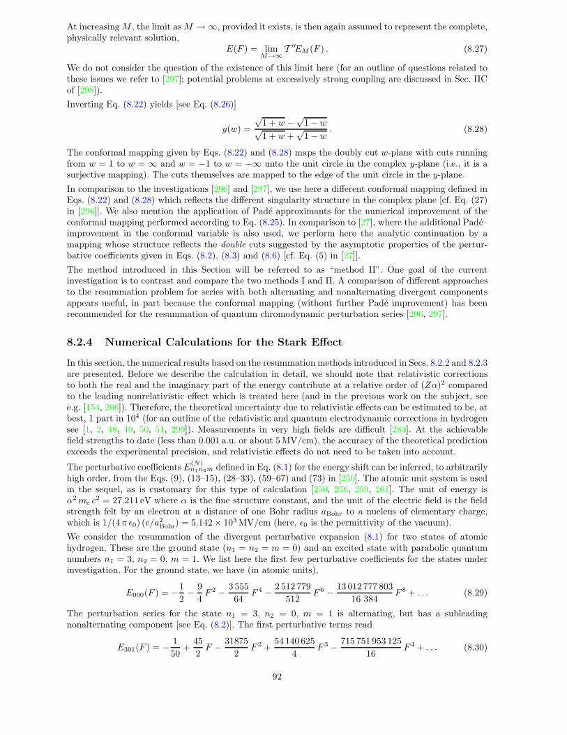
At increasing M , the limit as M → ∞, provided it exists, is then again assumed to represent the complete,physically relevant solution,
E(F ) = limM→∞
T ′′EM (F ) . (8.27)
We do not consider the question of the existence of this limit here (for an outline of questions related tothese issues we refer to [297]; potential problems at excessively strong coupling are discussed in Sec. IICof [298]).
Inverting Eq. (8.22) yields [see Eq. (8.26)]
y(w) =
√1 + w −
√1 − w√
1 + w +√
1 − w. (8.28)
The conformal mapping given by Eqs. (8.22) and (8.28) maps the doubly cut w-plane with cuts runningfrom w = 1 to w = ∞ and w = −1 to w = −∞ unto the unit circle in the complex y-plane (i.e., it is asurjective mapping). The cuts themselves are mapped to the edge of the unit circle in the y-plane.
In comparison to the investigations [296] and [297], we use here a different conformal mapping defined inEqs. (8.22) and (8.28) which reflects the different singularity structure in the complex plane [cf. Eq. (27)in [296]]. We also mention the application of Pade approximants for the numerical improvement of theconformal mapping performed according to Eq. (8.25). In comparison to [27], where the additional Pade–improvement in the conformal variable is also used, we perform here the analytic continuation by amapping whose structure reflects the double cuts suggested by the asymptotic properties of the pertur-bative coefficients given in Eqs. (8.2), (8.3) and (8.6) [cf. Eq. (5) in [27]].
The method introduced in this Section will be referred to as “method II”. One goal of the currentinvestigation is to contrast and compare the two methods I and II. A comparison of different approachesto the resummation problem for series with both alternating and nonalternating divergent componentsappears useful, in part because the conformal mapping (without further Pade improvement) has beenrecommended for the resummation of quantum chromodynamic perturbation series [296, 297].
8.2.4 Numerical Calculations for the Stark Effect
In this section, the numerical results based on the resummation methods introduced in Secs. 8.2.2 and 8.2.3are presented. Before we describe the calculation in detail, we should note that relativistic correctionsto both the real and the imaginary part of the energy contribute at a relative order of (Zα)2 comparedto the leading nonrelativistic effect which is treated here (and in the previous work on the subject, seee.g. [154, 266]). Therefore, the theoretical uncertainty due to relativistic effects can be estimated to be, atbest, 1 part in 104 (for an outline of the relativistic and quantum electrodynamic corrections in hydrogensee [1, 2, 48, 49, 50, 51, 299]). Measurements in very high fields are difficult [284]. At the achievablefield strengths to date (less than 0.001 a.u. or about 5 MV/cm), the accuracy of the theoretical predictionexceeds the experimental precision, and relativistic effects do not need to be taken into account.
The perturbative coefficients E(N)n1n2m defined in Eq. (8.1) for the energy shift can be inferred, to arbitrarily
high order, from the Eqs. (9), (13–15), (28–33), (59–67) and (73) in [250]. The atomic unit system is usedin the sequel, as is customary for this type of calculation [250, 256, 259, 261]. The unit of energy isα2me c
2 = 27.211 eV where α is the fine structure constant, and the unit of the electric field is the fieldstrength felt by an electron at a distance of one Bohr radius aBohr to a nucleus of elementary charge,which is 1/(4 π ε0) (e/a2
Bohr) = 5.142 × 10³ MV/cm (here, ε0 is the permittivity of the vacuum).
We consider the resummation of the divergent perturbative expansion (8.1) for two states of atomichydrogen. These are the ground state (n1 = n2 = m = 0) and an excited state with parabolic quantumnumbers n1 = 3, n2 = 0, m = 1. We list here the first few perturbative coefficients for the states underinvestigation. For the ground state, we have (in atomic units),
E000(F ) = −1
2− 9
4F 2 − 3 555
64F 4 − 2 512 779
512F 6 − 13 012 777 803
16 384F 8 + . . . (8.29)
The perturbation series for the state n1 = 3, n2 = 0, m = 1 is alternating, but has a subleadingnonalternating component [see Eq. (8.2)]. The first perturbative terms read
E301(F ) = − 1
50+
45
2F − 31875
2F 2 +
54 140 625
4F 3 − 715 751 953 125
16F 4 + . . . (8.30)
92
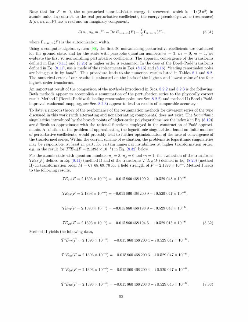
Note that for F = 0, the unperturbed nonrelativistic energy is recovered, which is −1/(2n2) inatomic units. In contrast to the real perturbative coefficients, the energy pseudoeigenvalue (resonance)E(n1, n2,m, F ) has a real and an imaginary component,
E(n1, n2,m, F ) = ReEn1n2m(F ) − i
2Γn1n2m(F ) , (8.31)
where Γn1n2m(F ) is the autoionization width.
Using a computer algebra system [90], the first 50 nonvanishing perturbative coefficients are evaluatedfor the ground state, and for the state with parabolic quantum numbers n1 = 3, n2 = 0, m = 1, weevaluate the first 70 nonvanishing perturbative coefficients. The apparent convergence of the transformsdefined in Eqs. (8.11) and (8.26) in higher order is examined. In the case of the Borel–Pade transformsdefined in Eq. (8.11), use is made of the replacements in Eqs. (8.15) and (8.16) [“leading renormalon polesare being put in by hand”]. This procedure leads to the numerical results listed in Tables 8.1 and 8.2.The numerical error of our results is estimated on the basis of the highest and lowest value of the fourhighest-order transforms.
An important result of the comparison of the methods introduced in Secs. 8.2.2 and 8.2.3 is the following:Both methods appear to accomplish a resummation of the perturbation series to the physically correctresult. Method I (Borel+Pade with leading renormalon poles, see Sec. 8.2.2) and method II (Borel+Pade-improved conformal mapping, see Sec. 8.2.3) appear to lead to results of comparable accuracy.
To date, a rigorous theory of the performance of the resummation methods for divergent series of the typediscussed in this work (with alternating and nonalternating components) does not exist. The logarithmicsingularities introduced by the branch points of higher-order polylogarithms [see the index k in Eq. (8.19)]are difficult to approximate with the rational functions employed in the construction of Pade approxi-mants. A solution to the problem of approximating the logarithmic singularities, based on finite numberof perturbative coefficients, would probably lead to further optimizimation of the rate of convergence ofthe transformed series. Within the current scheme of evaluation, the problematic logarithmic singularitiesmay be responsible, at least in part, for certain numerical instabilities at higher transformation order,e.g. in the result for T ′′E70(F = 2.1393 × 10⁻⁴) in Eq. (8.32) below.
For the atomic state with quantum numbers n1 = 3, n2 = 0 and m = 1, the evaluation of the transformsTEM (F ) defined in Eq. (8.11) (method I) and of the transforms T ′′EM (F ) defined in Eq. (8.26) (methodII) in transformation order M = 67, 68, 69, 70 for a field strength of F = 2.1393 × 10⁻⁴. Method I leadsto the following results,
TE67(F = 2.1393 × 10⁻⁴) = −0.015 860 468 199 2 − i 0.529 048 × 10−6 ,
TE68(F = 2.1393 × 10⁻⁴) = −0.015 860 468 200 9 − i 0.529 047 × 10−6 ,
TE69(F = 2.1393 × 10⁻⁴) = −0.015 860 468 198 9 − i 0.529 048 × 10−6 ,
TE70(F = 2.1393 × 10⁻⁴) = −0.015 860 468 194 5 − i 0.529 015 × 10−6 . (8.32)
Method II yields the following data,
T ′′E67(F = 2.1393 × 10⁻⁴) = −0.015 860 468 200 4 − i 0.529 047 × 10−6 ,
T ′′E68(F = 2.1393 × 10⁻⁴) = −0.015 860 468 200 3 − i 0.529 047 × 10−6 ,
T ′′E69(F = 2.1393 × 10⁻⁴) = −0.015 860 468 200 4 − i 0.529 047 × 10−6 ,
T ′′E70(F = 2.1393 × 10⁻⁴) = −0.015 860 468 203 3 − i 0.529 046 × 10−6 . (8.33)
93

Numerical results obtained by resummation are presented in Tables 8.1 and 8.2 for a variety of fieldstrengths and for the two atomic states under investigation here.
F (a.u.) ReE000(F ) Γ000(F )
0.04 −0.503 771 591 013 654 2(5) 3.892 699 990(1) × 10−6
0.06 −0.509 203 451 088(2) 5.150 775 0(5) × 10−4
0.08 −0.517 560 50(5) 4.539 63(5) × 10−3
0.10 −0.527 419 3(5) 1.453 8(5) × 10−2
0.12 −0.537 334(5) 2.992 7(5) × 10−2
0.16 −0.555 24(5) 7.131(5)× 10−2
0.20 −0.570 3(5) 1.212(5)× 10−1
0.24 −0.582 6(1) 1.767(5)× 10−1
0.28 −0.591 7(5) 2.32(3) × 10−1
0.32 −0.600(5) 2.92(3) × 10−1
0.36 −0.604(5) 3.46(3) × 10−1
0.40 −0.608(5) 4.00(5) × 10−1
Table 8.1: Real and imaginary part of the energy pseudoeigenvalue E000(F ) for the groundstate of atomic hydrogen (parabolic quantum numbers n1 = 0, n2 = 0,m = 0).
F (a.u.) ReE301(F ) Γ301(F )
1.5560 × 10⁻⁴ −0.016 855 237 140 761 7(5) 0.421 683(5) × 10−9
1.9448 × 10⁻⁴ −0.016 179 388 257 0(5) 0.143 773(5) × 10−6
2.1393 × 10⁻⁴ −0.015 860 468 20(1) 0.105 09(5) × 10−5
2.5282 × 10⁻⁴ −0.015 269 293(1) 0.176 39(5) × 10−4
2.9172 × 10⁻⁴ −0.014 742 60(3) 0.999 96(9) × 10−4
3.3061 × 10⁻⁴ −0.014 260 2(3) 0.295 4(2) × 10−3
Table 8.2: Real part and imaginary part of the energy pseudoeigenvalue E301(F ) for the excited statewith parabolic quantum numbers n1 = 3, n2 = 0,m = 1. The field strength F is given in atomic units.
94

n sn [ν − [[ν/2]]/[[ν/2]]] δ(0)n
(
1, s0)
1 −2 −0.455 882 352 941 0.837 837 837 838
2 50.5 0.011 324 180 660 0.652 631 578 947
3 −1 682 0.225 195 251 591 0.613 275 696 169
4 82 777.375 343 344 968 231 0.609 400 007 774
5 −5.373 298 × 106 0.416 165 471 150 0.612 698 290 875
. . . . . . . . . . . .
60 5.492 129 × 10151 0.619 816 798 266 0.620 282 559 592
61 −5.272 807 × 10154 0.619 846 730 800 0.620 282 559 593
62 5.146 602 × 10157 0.619 874 504 158 0.620 282 559 594
63 −5.105 759 × 10160 0.619 900 292 634 0.620 282 559 594
64 5.146 926 × 10163 0.619 924 254 847 0.620 282 559 595
65 −5.270 772 × 10166 0.619 946 535 301 0.620 282 559 595
66 5.481 925 × 10169 0.619 967 265 778 0.620 282 559 595
67 −5.789 242 × 10172 0.619 986 566 577 0.620 282 559 595
68 6.206 411 × 10175 0.620 004 547 622 0.620 282 559 595
69 −6.752 937 × 10178 0.620 004 547 622 0.620 282 559 595
70 7.455 631 × 10181 0.619 986 566 577 0.620 282 559 595
exact 0.620 282 559 595 0.620 282 559 595 0.620 282 559 595
Table 8.3: Evaluation of the perturbation series for Z(Φ) [zero-dimensional φ4-theory, seeEq. (8.34)] for g = 1. The sn are the partial sums of the divergent asymptotic series (8.35),the Pade approximants [ν − [[ν/2]]/[[ν/2]]] are calculated according to Eq. (7.13), and thedelta transforms are evaluated according to Eq. (7.31).
8.3 Further Applications of Resummation Methods
8.3.1 Zero–Dimensional Theories with Degenerate Minima
We consider the generating functional in a zero-dimensional theory (in this case, the usual path integralreduces to an ordinary integral). First, we briefly consider the Φ4-theory in zero dimensions [see Eq. (9-177) ff. in [34]]; the generating functional reads
Z(Φ) =
∞∫
−∞
dΦ√2π
exp
[
−1
2Φ2 − gΦ4
]
. (8.34)
The strictly alternating divergent asymptotic expansion in powers of g for g → 0 reads,
Z(Φ) ∼∞∑
N=0
4N Γ(2N + 1/2)√π Γ(N + 1)
(−g)N . (8.35)
On using the known asymptotics valid for N → ∞, which in this case yield the “large-order” asymptoticsof the perturbative coefficients,
Γ(2N + 1/2)
Γ(N + 1)∼ 4N√
2πΓ(N)
[
1 + O(
1
N
)]
(8.36)
95

it is easy to explicitly establish the factorial divergence of the series (see also p. 888 of [294]). The gen-erating functional in zero dimensions has been proposed as a paradigmatic example for the divergence ofperturbation theory in higher order. It can be resummed easily to the nonperturbative result; in particularit is manifestly Borel summable, and no singularities are present on the positive real axis. Specifically,in Table 8.2.4, we consider the resummation of the series (8.35) by Pade approximants (Sec. 7.1.4) anddelta transformations (Sec. 7.1.5). The rapid rate of convergence due to the delta transformations incomparison to the Pade approximants is obvious; this finding is consistent with the results of Ref. [24].
Complications are introduced by degenerate minima. As a second example, we consider the modifiedgenerating functional [compare with Eq. (2.6) on p. 15 of [247] and with Eq. (40.1) on p. 854 of [294]]:
Z ′(Φ) =
∞∫
−∞
dΦ√2π
exp
[
−1
2Φ2 (1 −√
gΦ)2]
=
∞∫
−∞
dΦ√2π
exp
[
−1
2Φ2 +
√gΦ3 − 1
2gΦ4
]
. (8.37)
The expansion of the exponential in powers of the coupling g leads to a divergent asymptotic series,
Z ′(Φ) =∞∑
N=0
1
N !
∞∫
−∞
dΦ√2π
e−1/2Φ2
(√gΦ3 − 1
2gΦ4
)N
=∞∑
N=0
∞∫
−∞
dΦ√2π
e−1/2 Φ2N∑
j=0
(−1)j
Γ(2N − j + 1)
×(
2N − j
j
)
(√g φ3
)2(N−j)(
g φ4
2
)j
=
∞∑
N=0
2√π
(−1)N CN+1/22N (1)
Γ(N − 1/2)gN
=
∞∑
N=0
8N Γ(2N + 1/2)√π Γ(N + 1)
gN , (8.38)
where CNM (x) denotes a Gegenbauer (ultraspherical) polynomial. Note that terms of half-integer powerof g entail an odd power of the field and vanish after integration. The first few terms of the asymptoticexpansion read,
Z ′(Φ) = 1 + 6 g + 210 g2 + 13860 g3
+1351350 g4 + 174594420 g5
+28109701620 g6 + 5421156741000 g7
+1218404977539750 g8 + O(g9) . (8.39)
96
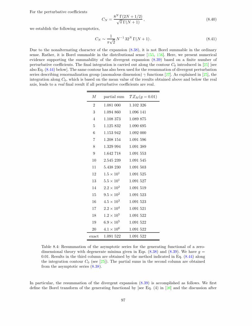
For the perturbative coefficients
CN =8N Γ(2N + 1/2)√
π Γ(N + 1), (8.40)
we establish the following asymptotics,
CN ∼ 1
π√
2N−1 32N Γ(N + 1) . (8.41)
Due to the nonalternating character of the expansion (8.38), it is not Borel summable in the ordinarysense. Rather, it is Borel summable in the distributional sense [155, 156]. Here, we present numericalevidence supporting the summability of the divergent expansion (8.39) based on a finite number ofperturbative coefficients. The final integration is carried out along the contour C0 introduced in [25] [seealso Eq. (8.44) below]. The same contour has also been used for the resummation of divergent perturbationseries describing renormalization group (anomalous dimension) γ functions [27]. As explained in [25], theintegration along C0, which is based on the mean value of the results obtained above and below the realaxis, leads to a real final result if all perturbative coefficients are real.
M partial sum T ZM (g = 0.01)
2 1.081 000 1.102 326
3 1.094 860 1.096 141
4 1.108 373 1.089 875
5 1.125 832 1.090 695
6 1.153 942 1.092 000
7 1.208 154 1.091 596
8 1.329 994 1.091 389
9 1.642 718 1.091 553
10 2.545 239 1.091 545
11 5.438 230 1.091 503
12 1.5 × 101 1.091 525
13 5.5 × 101 1.091 527
14 2.2 × 10² 1.091 519
15 9.5 × 10² 1.091 523
16 4.5 × 10³ 1.091 523
17 2.2 × 10⁴ 1.091 521
18 1.2 × 10⁵ 1.091 522
19 6.9 × 10⁵ 1.091 522
20 4.1 × 10⁶ 1.091 522
exact 1.091 522 1.091 522
Table 8.4: Resummation of the asymptotic series for the generating functional of a zero-dimensional theory with degenerate minima given in Eqs. (8.38) and (8.39). We have g =0.01. Results in the third column are obtained by the method indicated in Eq. (8.44) alongthe integration contour C0 (see [25]). The partial sums in the second column are obtainedfrom the asymptotic series (8.38).
In particular, the resummation of the divergent expansion (8.39) is accomplished as follows. We firstdefine the Borel transform of the generating functional by [see Eq. (4) in [26] and the discussion after
97
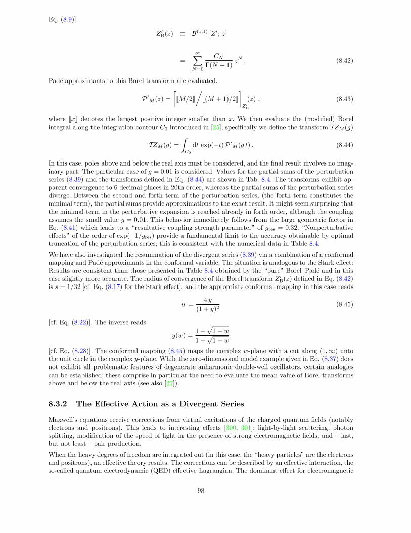
Eq. (8.9)]
Z ′B(z) ≡ B(1,1) [Z ′; z]
=
∞∑
N=0
CNΓ(N + 1)
zN . (8.42)
Pade approximants to this Borel transform are evaluated,
P ′M (z) =
[
[[M/2]]
/
[[(M + 1)/2]]
]
Z′
B
(z) , (8.43)
where [[x]] denotes the largest positive integer smaller than x. We then evaluate the (modified) Borelintegral along the integration contour C0 introduced in [25]; specifically we define the transform TZM (g)
TZM (g) =
∫
C0
dt exp(−t)P ′M (g t) . (8.44)
In this case, poles above and below the real axis must be considered, and the final result involves no imag-inary part. The particular case of g = 0.01 is considered. Values for the partial sums of the perturbationseries (8.39) and the transforms defined in Eq. (8.44) are shown in Tab. 8.4. The transforms exhibit ap-parent convergence to 6 decimal places in 20th order, whereas the partial sums of the perturbation seriesdiverge. Between the second and forth term of the perturbation series, (the forth term constitutes theminimal term), the partial sums provide approximations to the exact result. It might seem surprising thatthe minimal term in the perturbative expansion is reached already in forth order, although the couplingassumes the small value g = 0.01. This behavior immediately follows from the large geometric factor inEq. (8.41) which leads to a “resultative coupling strength parameter” of gres = 0.32. “Nonperturbativeeffects” of the order of exp(−1/gres) provide a fundamental limit to the accuracy obtainable by optimaltruncation of the perturbation series; this is consistent with the numerical data in Table 8.4.
We have also investigated the resummation of the divergent series (8.39) via a combination of a conformalmapping and Pade approximants in the conformal variable. The situation is analogous to the Stark effect:Results are consistent than those presented in Table 8.4 obtained by the “pure” Borel–Pade and in thiscase slightly more accurate. The radius of convergence of the Borel transform Z ′
B(z) defined in Eq. (8.42)is s = 1/32 [cf. Eq. (8.17) for the Stark effect], and the appropriate conformal mapping in this case reads
w =4 y
(1 + y)2(8.45)
[cf. Eq. (8.22)]. The inverse reads
y(w) =1 −
√1 − w
1 +√
1 − w
[cf. Eq. (8.28)]. The conformal mapping (8.45) maps the complex w-plane with a cut along (1,∞) untothe unit circle in the complex y-plane. While the zero-dimensional model example given in Eq. (8.37) doesnot exhibit all problematic features of degenerate anharmonic double-well oscillators, certain analogiescan be established; these comprise in particular the need to evaluate the mean value of Borel transformsabove and below the real axis (see also [27]).
8.3.2 The Effective Action as a Divergent Series
Maxwell’s equations receive corrections from virtual excitations of the charged quantum fields (notablyelectrons and positrons). This leads to interesting effects [300, 301]: light-by-light scattering, photonsplitting, modification of the speed of light in the presence of strong electromagnetic fields, and – last,but not least – pair production.
When the heavy degrees of freedom are integrated out (in this case, the “heavy particles” are the electronsand positrons), an effective theory results. The corrections can be described by an effective interaction, theso-called quantum electrodynamic (QED) effective Lagrangian. The dominant effect for electromagnetic
98

fields that vary slowly with respect to the Compton wavelength (frequencies ω � 2mc2/~) is describedby the one–loop quantum electrodynamic effective (so-called “Heisenberg–Euler”) Lagrangian which isknown to all orders in the electromagnetic field [301, 302, 303, 304, 305, 306].
The Heisenberg–Euler Lagrangian ∆L, which constitutes a quantum correction to the Maxwell La-grangian, is usually expressed as a one-dimensional proper-time integral [see e.g. Eq. (3.43) in [301],
∆L = − e2
8π2lim
ε,η→0+
∫ ∞+i η
i η
ds
se−(m2−iε) s
[
ab coth(eas) cot(ebs) − a2 − b2
3− 1
(es)2
]
. (8.46)
To clarify the notation, we introduce the well-known Lorentz invariants F and G which are given by
F = 1/4 Fµν Fµν = 1/2
(
B2 − E2)
= 1/2
(
a2 − b2)
, (8.47)
G = 1/4 Fµν (∗F )µν = −E · B = ±ab , (8.48)
where E and B are the electric and magnetic field strengths, Fµν is the field strength tensor, and(∗F )µν denotes the dual field strength tensor (∗F )µν = (1/2) εµνρσ Fρσ. By a and b we denote the secularinvariants,
a =
√
√
F2 + G2 + F ,
b =
√
√
F2 + G2 −F . (8.49)
These Lorentz invariants are referred to as secular invariants because they emerge naturally as eigenvaluesof the field strength tensor; these eigenvalues are conserved under proper Lorentz transformations of thefield strength tensor. There are connections between the different representations [301]: If the relativis-tic invariant G is positive, then it is possible to transform to a Lorentz frame in which E and B areantiparallel. In the case G < 0, it is possible to choose a Lorentz frame in which E and B are parallel.Irrespective of the sign of G we have in the specified frame
a = |B| and b = |E| if and only if B is (anti-)parallel to E . (8.50)
In any case, because a and b are positive definite, we have
a b = |E · B| > 0 for any Lorentz frame and G 6= 0 , (8.51)
which clarifies the sign ambiguity in (8.48). We give in (8.47) and (8.48) seemingly redundant definitions,but it will soon become apparent that each of the alternative “points of view” has its applications. TheMaxwell Lagrangian is given by
Lcl = −F = −1/4 Fµν Fµν = 1/2
(
E2 − B2)
= 1/2
(
b2 − a2)
. (8.52)
As it is obvious from Eq. (8.46), the correction ∆L to the Maxwell Lagrangian is conveniently written interms of the secular invariants a and b.
It was observed as early as 1956 [307] that the quantum correction (8.46), when expressed as a per-turbation series in the usual QED perturbation theory parameter α = e2/(4π), constitutes a divergentseries. This divergent character of the QED perturbative expansion is supported by Lipatov’s argumentbased on a saddle-point expansion of the generating functional [308, 309, 310], and explicit estimates forthe large-order (factorially divergent) behaviour of the QED perturbative coefficients have been obtainedin [311, 312]. Recently, the divergent character of the large-order behaviour of perturbative expansionsin quantum field theory has found an exquisite confirmation in explicit 30-loop calculations of renormal-ization group γ functions in a six-dimensional φ3 theory, and in a Yukawa theory [313, 314].
Here, we will study the divergent series generated by expanding the effective action (8.46) in powers of e2.We will distinguish the cases of a magnetic and an electric background fields. We start with a magneticfield of strength B in which case the effective action reads
SB ≡ ∆L(E = 0, B) = −e2B2
8π2
∫ ∞
0
ds
s2
{
coth s− 1
s− s
3
}
exp
(
−m2e
eBs
)
(8.53)
99

[put a = B, b = 0 in Eq. (8.46)]. The nonperturbative results in Eq. (8.53) can be expanded in powers ofthe effective coupling
gB =e2B2
m4e
. (8.54)
This results in the divergent asymptotic series
SB ∼ −2e2B2
π2gB
∞∑
n=0
(−1)n+14n |B2n+4|(2n+ 4)(2n+ 3)(2n+ 2)
gnB
= −2e2B2
π2gB
[
− 1
720+
1
1260gB − 1
630g2B
+ . . .− 2.33 × 10107 g50B + . . .
]
(8.55)
for gB → 0. Here, |B2n+4| denotes the modulus of the (2n+4)th Bernoulli number. The Bernoulli numbersalternate in sign,
sign (B2n+4) = (−1)n+1 . (8.56)
The expansion coefficients
cn =(−1)n+1 4n |B2n+4|
(2n+ 4)(2n+ 3)(2n+ 2)(8.57)
obviously display an alternating sign pattern and grow factorially in absolute magnitude,
cn ∼ (−1)n+1
8
Γ(2n+ 2)
π2n+4
(
1 + O(2−(2n+4)))
(8.58)
for n→ ∞.
The series (8.55) is an alternating series. In [160, 252, 307], it was shown that the series (8.55) is Borelsummable. A further expansion of the perturbative coefficients cn for large n is carried out in [252] inorder to perform the Borel summation; this analysis follows the asymptotic expansion in Eq. (8.58) above,and higher-order terms in the asymptotics of the coefficients for large n are also used. Here we considerthe resummation of the divergent series (8.55) with the help of rational approximants which use as inputdata only a finite number of perturbation theory coefficients in numerical form. Specifically, we use Padeapproximants defined in Eq. (7.12) and discussed in Sec. 7.1.4 and the nonlinear sequence transformationsd and δ defined in Eqs. (7.30) and (7.31), respectively. The nonlinear transformations were discussed inSec. 7.1.5.
The transformations are applied to the divergent perturbation series Eq. (8.55), the transforms are calcu-lated with the help of the recurrence relations (7.27) and (7.28). The evaluations presented in Tables 8.5and 8.6 are carried out for values gB = 1/10, gB = 1 and gB = 10 of the expansion parameter gB definedin Eq. (8.54). The first column in the tables contains the index n, the second column contains the partialsums of the input series and in the last three columns are the results of the Pade Approximation, thed-transformation and the delta-transformation.
The data in the tables is presented to a numerical accuracy of 10−9. The convergence of the transformsis indicated by underlining those decimal places which appear to have converged to the nonperturbativeresult. The numerical data in the Tables 8.5 and 8.6 indicate that the most favourable numerical results areobtained with the Weniger delta-transformation. For the numerical calculations, exact rational arithmeticswas used [90]. Numerical experiments for gB larger than 1 (not shown) and data presented in [24] indicatethat the Weniger delta transformation appears to resum the divergent series (8.55) at least up to gB = 200,and to arbitrary precision. The other resummation prescriptions – Pade, and the Levin d-transformation– fail in this domain of strong coupling.
In the case of a background electric field, Eq. (8.46) yields the following expression
SE ≡ ∆L(E,B = 0) =e2E2
8π2
∫ ∞
0
ds
s2
{
coth s− 1
s− s
3
}
exp
(
−i(me − iε)2
eEs
)
. (8.59)
100

n sn [ν − [[ν/2]]/[[ν/2]]] d(0)n
(
1, s0)
δ(0)n
(
1, s0)
1 −0.209 523 809 −0.209 523 809 −0.211 640 211 −0.211 640 211
2 −0.212 063 492 −0.211 640 211 −0.211 342 466 −0.211 342 466
3 −0.210 986 050 −0.211 306 990 −0.211 403 608 −0.211 400 530
4 −0.211 771 470 −0.211 415 931 −0.211 392 250 −0.211 393 488
5 −0.210 896 256 −0.211 382 773 −0.211 393 652 −0.211 393 513
6 −0.212 279 564 −0.211 397 516 −0.211 393 776 −0.211 393 695
7 −0.209 336 271 −0.211 391 398 −0.211 393 631 −0.211 393 675
8 −0.217 447 776 −0.211 394 638 −0.211 393 677 −0.211 393 670
9 −0.189 339 933 −0.211 393 026 −0.211 393 673 −0.211 393 671
10 −0.308 952 549 −0.211 393 982 −0.211 393 670 −0.211 393 671
exact −0.211 393 671 −0.211 393 671 −0.211 393 671 −0.211 393 671
Table 8.5: Evaluation of the perturbation series for SB given in Eq. (8.53) for gB = 1/10. Results aregiven in terms of the scaled function SB given by SB = 10−2× (−e2B2)/(8 π2)× SB. The performance ofthree different resummation methods is compared: in the second column, Pade approximants are used. Inthe third column, we list results obtained using the Levin transformation defined in Eq. (7.30), whereasin the last column, the delta transformation (7.31) is employed. The apparent convergence is indicatedby underlining the decimal figures that have stabilized in increasing transformation order.
In analogy to the expansion parameter for the magnetic case from Eq. (8.54), we can define the effectivecoupling as
gE =e2E2
m4e
. (8.60)
The expansion of the effective action in powers of gE leads to the formal power series
SE ∼ −2e2E2
π2gE
∞∑
n=0
4n |B2n+4|(2n+ 4)(2n+ 3)(2n+ 2)
gnE
= −2e2E2
π2gE
[
1
720+
1
1260gE +
1
630g2E
+ . . .+ 2.33 × 10107g50E + . . .
]
. (8.61)
The perturbation series is nonalternating. Because the remainder estimate ωn = an+1 [see Eq. (7.29)]is in general not valid for nonalternating series, we cannot assume that any of the previously discussedresummation methods (Pade, or the delta or d-transformation) are able to resum the perturbation seriesEq. (8.61). This is confirmed by the explicit numerical data presented in Table 8.3.2.
There exists a “nonperturbative” imaginary part for the uniform background electric field which is apriori not contained in the perturbation series whose coefficients are all real and positive [see Eq. (8.61)].The imaginary part can be directly inferred from Eq. (8.59) by residue calculus, the result is [34, 252]
ImSE =e2E2
8 π3
∞∑
n=1
1
n2exp
(
−nπm2e
eE
)
. (8.62)
The characteristic factor
exp
(
− 1
gE
)
(8.63)
101

n sn [ν − [[ν/2]]/[[ν/2]]] d(0)n
(
1, s0)
δ(0)n
(
1, s0)
1 −0.095 238 095 −0.095 238 095 −0.179 894 179 −0.179 894 179
2 −0.349 206 349 −0.179 894 179 −0.159 879 642 −0.159 879 642
3 −0.728 234 728 −0.143 682 906 −0.164 402 059 −0.163 671 330
4 −7.125 955 525 −0.171 471 152 −0.165 580 804 −0.164 993 772
5 80.395 411 995 −0.154 744 471 −0.164 224 936 −0.164 738 292
. . . . . . . . . . . . . . .
15 2.034 128 × 1018 −0.163 152 747 −0.164 599 332 −0.164 598 912
16 − 2.179 139 × 1020 −0.165 362 567 −0.164 598 614 −0.164 598 919
17 2.630 171 × 1022 −0.163 457 086 −0.164 599 763 −0.164 598 928
18 − 3.552 782 × 1024 −0.165 217 014 −0.164 599 218 −0.164 598 935
19 5.338 753 × 1026 −0.163 675 239 −0.164 599 045 −0.164 598 938
20 − 8.876 881 × 1028 −0.165 109 383 −0.164 598 656 −0.164 598 939
21 1.625 237 × 1031 −0.163 836 808 −0.164 598 854 −0.164 598 939
22 −3.262 042 × 1033 −0.165 027 568 −0.164 599 254 −0.164 598 939
23 7.148 693 × 1035 −0.163 959 721 −0.164 599 016 −0.164 598 939
24 −1.704 211 × 1038 −0.164 963 933 −0.164 598 550 −0.164 598 939
25 4.404 583 × 1040 −0.164 055 347 −0.164 598 862 −0.164 598 939
exact −0.164 598 939 −0.164 598 939 −0.164 598 939 −0.164 598 939
Table 8.6: Evaluation of the perturbation series for SB given in Eq. (8.53) for gB = 1. Results are given interms of the scaled function SB given by SB = 10−1 × (−e2B2)/(8 π2) × SB. The apparent convergenceis indicated by underlining the decimal figures that have stabilized in increasing transformation order.
is nonperturbative since Eq. (8.62) has an essential singularity in the limit gE → 0, and it is reminiscentof characteristic expressions occurring in the description of quantum mechanical tunneling processes (seep. 195 in [34]). In our context, the imaginary part (8.62) describes the pair production in an electricbackground field. As is well known, the vacuum in very strong electric fields becomes unstable withregard to particle-antiparticle pair production (see also the elucidating discussion in [300]).
Spontaneous pair production becomes considerable only in strong external electric fields. Ordinary fieldstrengths are much smaller than the critical field Ecrit for which
eEcrit
m2e
= 1 . (8.64)
The critical field strength Ecrit can be written (including ~ and c) as the ratio of the rest mass of theelectron to the characteristic length scale which is set by the Compton wavelength of the electron:
Ecrit =mec
2
e~/mec=
m2ec
3
e~∼ 1016 V
cm. (8.65)
This critical field strengths are comparable to those felt by an electron in a hydrogenlike atom whosenucleus has the charge Z ≈ 137.
Nonalternating divergent perturbation series require considerable effort in their resummation. It has beenshown in [25] that a generalized Borel-Pade method can be used to reconstruct the imaginary part ofthe full nonperturbative result. This method depends on the special integration contours in the complexplane, introduced in Secs. 8.2.2 and 8.2.3. In Table 8.8, we present results for the generalized Boreltransforms constructed according to Eqs. (1) – (6) of [25]).
102

n sn [ν − [[ν/2]]/[[ν/2]]] d(0)n
(
1, s0)
δ(0)n
(
1, s0)
1 −0.349 206 349 −0.349 206 349 −0.095 238 095 −0.095 238 095
2 −0.603 174 603 −0.095 238 095 −0.406 735 069 −0.406 735 069
3 −1.680 615 680 −0.270 879 691 −0.187 029 818 −0.221 607 947
4 −9.534 805 934 0.130 519 638 −6.833 824 219 −0.003 699 447
5 −97.056 173 456 −0.227 975 543 −0.305 826 743 −0.718 038 750
. . . . . . . . . . . . . . .
20 −8.984 372 007 × 1028 −0.345 709 493 −0.214 873 519 −0.213 414 911
21 −1.643 099 018 × 1031 0.132 431 882 −0.045 964 685 −0.148 354 420
22 −3.294 725 508 × 1033 −0.328 142 128 −1.274 287 822 −0.037 304 526
23 −7.214 261 175 × 1035 0.248 593 926 −0.358 736 820 −0.367 757 660
24 −1.718 574 682 × 1038 −0.313 562 944 −0.237 543 483 −1.233 623 635
25 −4.438 810 865 × 1040 0.434 092 399 −0.109 659 997 −0.499 971 155
Table 8.7: Failure of the evaluation of the perturbation series for SE (electric background field) givenin Eq. (8.59) for gE = 1. Results are given in terms of the scaled function SE given by SE = 10−1 ×(−e2E2)/(8 π2) × SE. Observe the apparent lack of convergence.
As for the complex resonances of the Stark effect (see the numerical results in Sec. 8.2.4), it is possible toreconstruct the nonperturbative imaginary part (pair production rate) from the purely real perturbativecoefficients in Eq. (8.61).
8.3.3 The Double–Well Problem
We discuss in the current section specific results, recently obtained in [29], for the quantum-mechanicaldouble-well problem and the related multi-instanton expansion. The energy levels of the double-well po-tential receive, beyond perturbation theory, contributions which are non-analytic in the coupling strength;these are related to instanton effects. For example, the separation between the energies of odd- andeven-parity states is given at leading order by the one-instanton contribution, which, in the path integralformalism, corresponds to a tunneling of the particle from one minimum of the potential to the other min-imum. In order to determine the energies (of individual levels as well as the separations) more accurately,multi-instanton configurations have also to be taken into account. The multi-instanton configurationsdescribe a particle that tunnels between the minima more than once. For even instantons, the particlereturns to the minimum from which it started the motion.
For the double-well problem, the energy eigenvalues of the states at nonvanishing coupling g 6= 0 cannotin principle be obtained by analytic continuation from the unperturbed situation at vanishing couplingg = 0 because a potential with degenerate minima introduces a degeneracy in the spectrum: for anyone unperturbed state, two states emerge when the perturbation is switched on. These two states areseparated by an energy shift which is nonperturbative and nonanalytic in the coupling, i.e. vanishingto any order in perturbation theory. Therefore, the two states are described by the same perturbationseries and yet differ in their energy by instanton contributions. Specifically, we consider the case of thedouble-well potential with the hamiltonian
H = −g2
∂2
∂q2+
1
gV (q) , V (q) =
1
2q2 (1 − q)2 . (8.66)
Of course, the alternative formulation H = −∂2/∂q2 + 12 q
2 (1 − √gq)2 gives rise to the same energy
levels, but the form (8.66) illustrates that the coupling plays the formal role of ~. The hamiltonian(8.66) can be obtained from H = −∂2/∂q2 + 1
2 q2 (1 − √
gq)2 by the scaling q → q/√g. It has been
103
n partial sum T Sn(gE)
2 0.001 146 032 0.001 144 848 + i 7.70 × 10⁻¹⁷
3 0.001 146 705 0.001 146 639 + i 8.22 × 10⁻¹¹
4 0.001 146 951 0.001 147 113 + i 3.54 × 10⁻⁸
5 0.001 147 087 0.001 147 264 + i 1.93 × 10⁻⁸
6 0.001 147 195 0.001 147 173 + i 3.15 × 10⁻⁷
7 0.001 147 310 0.001 147 113 + i 2.58 × 10⁻⁷
8 0.001 147 469 0.001 147 162 + i 2.30 × 10⁻⁷
9 0.001 147 743 0.001 147 165 + i 2.63 × 10⁻⁷
10 0.001 148 327 0.001 147 144 + i 2.53 × 10⁻⁷
11 0.001 149 825 0.001 147 157 + i 2.46 × 10⁻⁷
12 0.001 154 375 0.001 147 155 + i 2.56 × 10⁻⁷
13 0.001 170 560 0.001 147 151 + i 2.51 × 10⁻⁷
14 0.001 237 137 0.001 147 156 + i 2.51 × 10⁻⁷
15 0.001 550 809 0.001 147 153 + i 2.53 × 10⁻⁷
16 0.003 228 880 0.001 147 154 + i 2.51 × 10⁻⁷
17 0.013 345 316 0.001 147 154 + i 2.52 × 10⁻⁷
18 0.081 610 937 0.001 147 153 + i 2.52 × 10⁻⁷
19 0.594 142 371 0.001 147 154 + i 2.52 × 10⁻⁷
20 4.852 426 276 0.001 147 154 + i 2.52 × 10⁻⁷
exact 0.001 147 154 0.001 147 154 + i 2.52 × 10⁻⁷
Table 8.8: Resummation of the asymptotic series for the QED effective action (8.61) in a constant back-ground electric field for gE = 0.05. Results in the third column are obtained by the method discussedin Secs. 8.2.2 and 8.2.3 along the integration contour C+1 (see Fig. 8.1). The partial sums in the secondcolumn are obtained from the asymptotic series (8.61).
conjectured [168, 169, 170, 171] that an asymptotic expansion for the energy eigenvalue can be obtainedby finding a solution to the equation
1√2π
Γ
(
1
2−D(E, g)
) (
−2
g
)D(E,g)
exp[−A(E, g)/2] = ±i , (8.67)
which can be understood as a modified Bohr-Sommerfeld quantization condition. The plus and minus signsapply to even- and odd-parity states, respectively. The conjecture (8.67), whose validity has been provenin [173], has found a natural explanation in the framework of Ecalle’s theory of resurgent functions [172,174, 315]. The functions D(E, g), A(E, g) constitute power series in both variables. The function D(E, g)describes the perturbative expansion; its evaluation is discussed in [168, 171]. The first terms read
D(E, g) = E + g
(
3E2 +1
4
)
+ g2
(
35E3 +25
4E
)
+ O(g2) . (8.68)
The ground and the first excited state are both described by the same perturbation series which canbe found by inverting the equation D(E, g) = 1/2. When the energy is expressed in terms of the naiveperturbation series in g, the function [D(E, g) − N − 1/2] then vanishes in any order of perturbationtheory, i.e. in all orders in g. Here, N is the quantum number of the unperturbed state which is a
104

harmonic oscillator eigenstate. The function A(E, g) essentially describes instanton contributions [171];its first terms read
A(E, g) =1
3 g+ g
(
17E2 +19
12
)
+ g2
(
227E3 +187
4E
)
+ O(g2) . (8.69)
A solution to the equation (8.67) can be found by systematically expanding the energy eigenvalue E(g)in powers of g and in the two quantities
λ(g) = ln
(
−2
g
)
and ξ(g) =exp[−1/(6g)]√
πg. (8.70)
Terms of order ξ(g)n belong to the n-instanton contribution. The energy eigenvalue for nonvanishingperturbation g 6= 0 can be described by two quantum numbers: the unperturbed quantum number N andthe positive or negative parity of the state. We have (the upper index denotes the instanton order)
EN,±(g) =
∞∑
n=0
E(n)N,±(g) (8.71)
where the perturbation series (zero-instanton contribution) is given as
E(0)N,±(g) =
∞∑
K=0
E(0)N,K g
K , (8.72)
where the right-hand side is parity independent. For n > 0, the instanton contribution reads
E(n)N,±(g) =
(
2
g
)Nn
ξ(g)nn−1∑
k=0
λ(g)k∑
l=0
ε(N,±)nkl gl . (8.73)
The lower indices n, k and l of the ε coefficients denote the instanton order, the power of the logarithmand the power of g, respectively. Some of the results that will be used in the sequel read,
ε(0,+)100 = −ε(0,−)
100 = −1 , ε(0,+)101 = −ε(0,−)
101 =71
12,
ε(0,+)101 = −ε(0,−)
101 =6299
288, ε
(0,+)210 = ε
(0,−)210 = 1 ,
ε(0,+)211 = ε
(0,−)211 = −53
6, ε
(0,+)212 = ε
(0,−)212 = −1277
72,
ε(0,+)200 = ε
(0,−)200 = γ , ε
(0,+)201 = ε
(0,−)201 = −23
2− 53
6γ ,
ε(0,+)202 = ε
(0,−)202 =
13
12− 1277
72γ , (8.74)
where γ = 0.57221 . . . is Euler’s constant. Odd-instanton contributions have opposite sign for opposite-parity states and are responsible, in particular, for the energy difference of the ground state with quantumnumbers (0,+) and the first excited state with quantum numbers (0,−). The dominant contribution tothe separation of the two lowest energy levels is given by the one-instanton contribution:
E0,−(g) − E0,+(g) ∼ 2 ξ(g)
(
1 − 71
12g − 6299
288g2 + O(g3)
)
+ O(ξ(g)3) . (8.75)
By contrast, even-instanton contributions have like sign for opposite-parity states and are responsible, inparticular, for the displacement of the mean value (1/2) [E0,−(g)+E0,+(g)] from the value of the general-
ized Borel sum of the perturbation series B(
∑∞K=0E
(0)0,K g
K)
(for the evaluation of the generalized Borel
105

sum of a nonalternating divergent series, see Sec. 8.3.1). The dominant contribution to the displacementcomes from the two-instanton effect, and we have
1
2[E0,−(g) + E0,+(g)] − Re
{
B(
∞∑
K=0
E(0)0,K g
K
)}
∼
ξ(g)2{
ln
(
2eγ
g
)
+g
[
−53
6ln
(
2eγ
g
)
− 23
2
]
+g2
[
−1277
72ln
(
2eγ
g
)
+13
12
]
+O(g3 ln(g))
}
+O(ξ(g)4) . (8.76)
The function [169]
∆(g) = 4
12 [E0,−(g) + E0,+(g)] − Re
{
B(
∑∞K=0E
(0)0,K g
K)}
[E0,−(g) − E0,+(g)]2 ln(
2eγg
) (8.77)
relates the multi-instanton contributions to the energy eigenvalues, which can be evaluated numerically,and to the (generalized) Borel sum of the perturbation series which is evaluated by analytic continuationof the integration path into the complex plane (see [294]). The calculation of ∆(g) at small coupling isproblematic because of severe numerical cancellations. From the equations (8.75), (8.76) and (8.77), weobtain the following asymptotics for ∆(g),
∆(g) ∼ 1 + g
[
71
6+
(
−53
6ln
(
2eγ
g
)
− 23
2
)/
ln
(
2eγ
g
)]
+g2
[
10711
72+
(
1277
72ln
(
2eγ
g
)
− 13
12
)/
ln
(
2eγ
g
)]
+ O(g3) . (8.78)
If we additionally perform an expansion in inverse powers of ln(2/g) and keep only the first few terms in{1/ ln(2/g)} in each term in the g-expansion, the result reads
∆(g) ∼ 1 + 3g − 23
2
g
ln(2/g)
[
1 − γ
ln(2/g)+
γ2
ln2(2/g)+ O
(
1
ln3(2/g)
)]
+53
2g2
−135g2
ln(2/g)
[
1 − γ
ln(2/g)+
γ2
ln2(2/g)+ O
(
1
ln3(2/g)
)]
+ O(
g3)
. (8.79)
The higher-order corrections, which are only logarithmically suppressed with respect to the leading terms1 + 3g, change the numerical values quite significantly, even at small coupling. In Table 8.9 we presentnumerical results for the function ∆(g) at small coupling; these are in agreement with the first fewasymptotic terms listed in equation (8.78) up to numerical accuracy. Of course, for strong coupling,significant deviations from the leading asymptotics must be expected due to higher-order effects; theseare indeed observed. For example, at g = 0.1 the numerically determined value reads ∆(0.1) = 0.87684(1)whereas the first asymptotic terms given in equation (8.78) sum up to a numerical value of 0.86029.
The higher-order corrections to the two-instanton effect are related to the corrections to the leadingfactorial growth of the perturbative coefficients. This can be seen by expressing that the imaginary partof the perturbation series, when continued analytically from negative to positive coupling, has to cancelwith the imaginary part of the two-instanton contribution which is generated by the logarithms ln(−2/g).The corrections of order g ln(−2/g) and g2 ln(−2/g) yield the 1/K– and 1/K2–corrections to the leading
factorial growth of the perturbative coefficients. From the results for ε(0,±)21j (j = 0, 1, 2) given in equation
(8.74), we obtain
E00,K ∼ −3K+1K!
π
[
1 − 53
18
1
K− 1277
648
1
K2+ O
(
1
K3
)]
. (8.80)
106

Table 8.9: Comparison of numerical values for the function ∆(g) defined in equation (8.77) in theregion of small coupling to values obtained by calculating the first few terms in its asymptoticexpansion given in (8.78).
coupling g 0.005 0.006 0.007 0.008 0.009
∆(g) num. 1.0063(5) 1.0075(5) 1.00832(5) 1.00919(5) 1.00998(5)
∆(g) asymp. 1.00640 1.00739 1.00832 1.00919 1.01001
The analytic results should be checked against explicit values of the perturbative coefficients. We have
determined the first 200 perturbative coefficients E(0)0,K (K = 0, . . . , 200) of the perturbation in the form
of rational numbers, i.e. to formally infinite numerical accuracy. This allows to verify the 1/K– and1/K2–corrections to the leading factorial growth in equation (8.80) to high accuracy, for example byemploying Richardson extrapolation [316]. Using the 160th through the 200th perturbation coefficient asinput data for the Richardson algorithm, the coefficients of the leading, of the 1/K-subleading and of the1/K2 suppressed corrections are found to be consistent with the analytic results given in equation (8.80)up to a relative numerical accuracy of 10−26, 10−23 and 10−20, respectively. For completeness, we givehere the numerical values of the 198th through the 200th perturbative coefficients, to 30 decimals. Theseread:
E(0)0,198 = −5.50117 76962 88587 93527 75694 38632× 10464 ,
E(0)0,199 = −3.28445 39841 65780 00616 21912 32835× 10467 ,
E(0)0,200 = −1.97082 14193 09543 76979 53006 07410× 10470 . (8.81)
Values for all 200 coefficients are available [231].
It is an interesting consequence of the expansion (8.71) that the energy difference (E0,−−E0,+), at smallcoupling, is described to high accuracy by the one-instanton contribution (n = 1 in equation (8.73)). Forg = 0.001, we obtain to 180 decimals,
E0,+(0.001) = 0. 49899 54548 62109 17168 91308 39481 92163 68209 47240
20809 66532 93278 69722 01391 15135 28505 38294 45798
45759 95999 06739 55175 84722 67802 81306 96906 01325
25943 77289 94365 88255 24440 17437 12789 27978 99793 , (8.82)
whereas
E0,−(0.001) = 0. 49899 54548 62109 17168 91308 39481 92163 68209 47240
20809 66532 93278 69722 01391 29839 92959 55803 70812
27749 92448 48259 36743 64757 68328 84835 35511 34663
06309 82331 51885 23308 08622 84780 52722 10103 67282 . (8.83)
Decimals which differ in the two energy levels are underlined. The results have been obtained by latticeextrapolation using a modified Richardson algorithm which is constructed according to ideas outlined
107

in [153]. Calculations were performed on IBM RISC/6000 workstations while making extensive use ofmultiprecision libraries [232, 234, 235]. We define PM (g) as the Mth partial sum of the one-instanton
contribution E(1)0,−(g) − E
(1)0,+(g),
PM (g) = 2 ξ(g)
M∑
j=0
ε(0,−)10j gj . (8.84)
Using exact rational expressions for the coefficients ε(0,−)10j (j ≤ 141), we obtain
P140(0.001) × 1071 =
1.47046 44541 75092 50138 19899 64494 15198 15678 00350 05260 35283
86053 33378 03660 50415 75193 50528 41826 73433 99328 21246 74888 , (8.85)
P141(0.001) × 1071 =
1.47046 44541 75092 50138 19899 64494 15198 15678 00350 05260 35283
86053 33378 03660 50415 75193 50528 41826 73433 99328 21246 74887 . (8.86)
These values are in excellent agreement with the numerically determined energy difference (see the resultspresented above in equations (8.82) and (8.83))
[E0,−(0.001) − E0,+(0.001)] × 1071 =
1.47046 44541 75092 50138 19899 64494 15198 15678 00350 05260 35283
86053 33378 03660 50415 75193 50528 41826 73433 99328 21246 74887 . (8.87)
The first 70 decimals in equations (8.82) and (8.83) are the same because the one-instanton contributionis of the order of 1.4× 10−71. The accuracy to which the one-instanton contribution describes the energydifference E0,−(0.001) − E0,+(0.001) is limited by the three-instanton effect which for g = 0.001 is ofthe order of 8 × 10−212. Note that the two-instanton effect (which for g = 0.001 is of the order of4 × 10−142) does not limit the accuracy to which the one-instanton contribution describes the energydifference because it has the same sign for opposite-parity states.
We have demonstrated that the behavior of the characteristic function ∆(g) defined in equation (8.77)at small coupling is consistent with higher-order corrections to the one- and two-instanton contributions,specifically with the instanton expansion of the energy levels governed by the equations (8.71) and (8.73),with the assumption that the instanton contributions given by equation (8.73) should be Borel summed,with the explicit results for the higher-order coefficients listed in (8.74) and the analytically derivedasymptotics for the function ∆(g) given in equation (8.78). The corrections of relative order 1/Km
to the leading factorial growth of the perturbative coefficients – see equation (8.80) – are consistentwith the analytically evaluated gm ln(−2/g)–corrections to the two-instanton effect and with the explicitvalues for the first 200 terms in the perturbation series (8.72). The nonperturbative energy differenceE0,−(g) − E0,+(g) at small coupling g is described, to high accuracy, by the one-instanton contributiononly.
8.4 Divergent Series: Some Conclusions
A priori, it may seem rather unattractive to assume that the quantum electrodynamic perturbation seriesmay be divergent even after the regularization and the renormalization. However, as shown by explicit
108

nontrivial 30-loop calculations of renormalization group γ functions in a six-dimensional φ3 theory, andin a Yukawa theory (presented recently in [313, 314]), we believe that the ultimate divergence of theperturbative expansion can be regarded as a matter-of-fact, clearly demonstrated by explicit high-ordercalculations. Therefore, it appears meaningful to explore the physical implications of this divergence.
We have discussed four physical applications of resummation methods for divergent series: (i) the energydisplacement of a hydrogen atom in a background electric field (Sec. 8.2.4), (ii) zero-dimensional (model)field theories (Sec. 8.3.1), (iii) the QED effective Lagrangian (Sec. 8.3.2), and (iv) the energy levels of thedouble-well potential (Sec. 8.3.3). The mathematical structure of these problems can be characterized asfollows, in the order of increasing complexity:
• The QED effective Lagrangian for a background magnetic field, expressed as a perturbation seriesin α, is manifestly Borel summable [160, 252, 307], and the nonperturbative result can be inferredby a number of different resummation methods, as discussed in Sec. 8.3.2.
• The QED effective Lagrangian for a background electric field, as well as the perturbation series fora hydrogen atom in an electric field, is not Borel summable. The same applies to the perturbationseries for a zero-dimensional field theory with degenerate minima. However, these three problemsadmit a treatment according to the concept of generalized (distributional) Borel summability [155].Numerical results (see [25, 28] and Secs. 8.2.4 and 8.3.2) confirm the distributional Borel summabil-ity, and the use of additional asymptotic information about the perturbative coefficients [“leadingrenormalon poles”, see Eqs. (8.15) and (8.16) in Sec. 8.2.2] accelerates the convergence of the Borel-transformed perturbation series.
• The double-well potential represent a very problematic case: the full nonperturbative solution tothe eigenvalue problem cannot be obtained in principle from perturbation theory. The reason is thefollowing: the perturbation introduces an additional degeneracy in the spectrum: each unperturbedlevel splits into two energy levels when the perturbation is nonvanishing. Both of these levels aredescribed by one and the same naive perturbation series (see Sec. 8.3.3). The energy difference isnonperturbative and nonanalytic in the coupling strength, and finds an explanation in the theoryof instantons.
For the Stark effect and the QED effective Lagrangian (electric field), the existence of nonperturbativecontributions is intimately linked with the failure of the Carleman criterion (see for example [160], The-orems XII.17 and XII.18 and the definition on p. 43 in [161], p. 410 in [162], Ch. 6 of this Thesis or theelucidating discussion in Ref. [163]). The Carleman criterion determines, roughly speaking, if nonanalyticcontributions exist for a given effect which is described by a specified perturbation series. In this sense, thedivergence of the perturbative expansion is physically important: for the QED effective action, it allowsfor the existence of nonanalytic, nonperturbative contributions like the pair-production amplitude whichis not contained in the real perturbation series (8.61) and cannot be obtained on the basis of perturbationtheory alone.
Also, we would like to illustrate here the utility of resummation methods in those cases where perturbationtheory breaks down at large coupling. As explained in Secs. 8.2.4, 8.3.1 and 8.3.2, even in situations wherethe perturbation series diverges strongly, it can still be used to obtain meaningful physical results if it iscombined with a suitable resummation method. In a relatively weak field, it is possible to obtain moreaccurate numerical results by resummation than by optimal truncation of the perturbation series (seealso [25]). In a strong field, it is possible to obtain physically correct results by resummation even thoughthe perturbation series diverges strongly (see the discussion in Sec. 8.2.4 and the data in Tables 8.1, 8.2and 8.4). By resummation, the perturbation series which is inherently a weak-coupling expansion can begiven a physical interpretation even in situations where the coupling is large. Returning to the analogyto quantum field theory, one might be tempted to suggest that physically complete results can in manycases be obtained after regularization, renormalization and resummation.
Can the full nonperturbative result (for energy levels etc.) be inferred in all cases by a resummation ofthe divergent perturbation series? The answer is, unfortunately, no. This is demonstrated in Sec. 8.3.3by way of example. In theories with degenerate minima (such as the double-well problem), correctionsto energy levels are caused by so-called instanton contributions that follow naturally by an expansionof the path integral around nontrivial saddle points. The n-instanton contribution is characterized by anonperturbative factor ξ(g)n where [see Eq. (8.70)] ξ(g) = exp[−1/(6g)]/
√πg, and g is the coupling. The
109

expansion of ξ(g) in powers of g vanishes in all orders of g. The nonperturbative energy splitting betweeneven- and odd-parity states is investigated by considering the function ∆(g) defined in Eq. (8.77). Thisfunction would vanish if the generalized Borel sum of the perturbation series could reproduce energylevels exactly. However, it does not vanish, as demonstrated by the data in Tab. 8.9 (the numerical datacan be interpreted naturally by considering so-called two-instanton effects). At the same time, in a zero-dimensional theory with degenerate minima (considered in Sec. 8.3.1), resummation is successful despitethe existence of a nontrivial saddle point. The reason for the success of the resummation in this modelproblem appears to lie in the fact that no degeneraces are introduced by the additional saddle point. Theperturbation series determines the generating functional uniquely, which is not the case in the double-wellpotential where two distinct energy levels (of opposite parity) share the same perturbation series. Thisintriguing situation will warrant further investigation in the near future.
110

Chapter 9
Conclusions
We proceed to the interpretation of the results obtained in this Thesis, which has a dual subject: “quantumelectrodynamic bound-state calculations and large-order perturbation theory”.
The significance of quantum electrodynamics as one of the most appealing physical theories (a “jewel” oftheoretical physics according to Richard Feynman) does not require any further explanation. The estheticappeal of bound-state quantum electrodynamics stems from the accuracy of the experimental verifications,the significance of the theory for the determination of the fundamental constants, and the conceptualcomplexity of the calculations which derives from the apparent simplicity of the physical systems understudy, when an accurate understanding is required in higher orders of perturbation theory. However,the divergence of the perturbative expansion in large orders, which persists even after the regularizationand renormalization, raises fundamental questions regarding the internal consistency of the theoreticalpredictions. The problems associated with the divergence of the perturbative expansion do not onlyplague quantum electrodynamics, but even occur in ordinary quantum mechanical perturbation theory.This Thesis is divided into two Parts, which represent two attempts to advance our understanding of thehigher-order corrections as well as of the conceptual questions raised by the divergence of the perturbativeexpansion.
In the first Part, we discussed aspects of certain quantum electrodynamic bound–state calculations, whichhave been carried out over the past years. Not all of these calculations [1, 2, 3, 4, 5, 6, 7, 8, 9, 10, 11, 12, 13,14, 15, 16, 17, 18] could be described in full detail. Both the experimental accuracy as well as the accuracyof the theoretical calculations have improved dramatically in recent years [42]. On the theoretical side, thecalculations at low nuclear charge number may be based on either of two methods: the analytic approachthat is based on the Zα-expansion and the numerical approach in which all electron propagators arekept in exact relativistic form. Progress has been achieved due to advances in the analytic approach thatprofit from an adequate formulation of the problem, and due to the development of numerical techniqueswhich have led to the highly accurate numerical evaluation of QED corrections in the realm of low nuclearcharge number. This has led to the favourable situation where analytic and numerical calculations canbe checked against each other. In view of the complexity of the calculations and their importance forthe determination of the fundamental constants [86], the existence of independent cross-checks for thecalculations is highly desirable.
Numerical calculations at low Z have been made possible by convergence acceleration methods describedin the second Part of this Thesis (notably by the combined nonlinear-condensation transformation). Thesetechniques have led to the solution of the severe numerical difficulties associated with the singularity ofthe propagators for equal radial arguments, and to a reduction in computing time by three orders ofmagnitude. Results obtained for the one-photon self energy are several orders of magnitude more accuratethan previous calculations of the effect. They represent the first direct evaluations of the one-loop selfenergy at the nuclear charge numbers Z = 1 and Z = 2, which are of crucial importance for precisionspectroscopy (atomic hydrogen and hydrogenlike helium).
The analytic calculations of the one-loop self energy for higher excited states will be complemented in thenear future by numerical calculations based on the new techniques [95], leading to a cross-check of thetype mentioned above. Severe difficulties associated with the multitude of analytic terms due to the morecomplicated wavefunctions of the highly excited states and the associated angular momentum algebrahave been a problem for self energy calculations in this area.
111

The calculations for the bound-state two-loop self energy report on the first evaluation of the highlyproblematic nonlogarithmic higher-order two-loop binding correction B60. Let us recall that analyticwork on the corresponding A60 correction for the less involved one-loop problem has extended over threedecades [32, 68, 69, 70, 71]. The development of analytic methods for the evaluation of B60 leads toan improved understanding of the scaling of the two-loop effect at low Z and will enable a detailedcomparison of analytic and possibly available numerical results for the two-loop effect in the future. Atthe same time, these results lead to improved predictions for the hydrogen and helium fine structure.
The spin-dependence of quantum electrodynamic corrections is a conceptually important issue. We focuson spinless particles and present a simplified derivation of the generalized Breit hamiltonian for a systemof two spinless particles. Although scalar QED is a renormalizable theory, we found the issue of bound-state calculations within this theory insufficiently addressed in the literature. Our calculations for theleading-order self energy and the relativistic recoil correction are the first corrections of the “self energytype” to be evaluated within bound-state QED involving only scalar particles.
As a further application, we would like to mention the recent investigation [18].
In the second Part of the Thesis, we investigate convergence acceleration and resummation methodsfor divergent series. The convergence acceleration techniques address the fundamental problem of theacceleration of a slowly convergent, nonalternating series. Severe numerical instabilities associated withthe formation of higher-order weighted differences for nonalternating series have been a major obstaclefor algorithms that try to accomplish this task. The methods find applications in areas as diverse as DNAsequence analysis and experimental mathematics.
Recent highly nontrivial 30-loop calculations [313, 314] have convincingly demonstrated the divergenceof the perturbative expansions in quantum field theory originally conjectured by Dyson [317]. We discussnonlinear sequence transformations as an alternative to the “usual” Borel method for the resummation ofdivergent series that result from perturbative expansions in quantum field theory. These transformationshave favourable asymptotic properties and lead in many cases to better numerical results than Padeapproximants. We also discuss generalizations of the Borel method which lead to consistent results evenif the full, nonperturbative physical energy level or vacuum-to-vacuum amplitude acquires an imaginarypart due to quantum mechanical tunneling. This imaginary part, which represents the autoionizationdecay width (Stark effect) and the electron-positron pair-production amplitude (in the case of the QEDeffective action), can be derived starting only from the real (not complex!) perturbative coefficients.In the double-well problem, the situation is different. Even- and odd-parity states acquire an energyseparation which is nonperturbative and nonanalytic in the coupling strength and is an effect which inprinciple cannot be derived from perturbation theory alone. The energy separation is given by so-calledmulti-instantons which follow naturally from a path integral representation of the partition functionand correspond to configurations where the particle tunnels repeatedly between the two minima of thedouble-well potential. The results lead to a better understanding of the energy shifts due to multi-instanton effects, by evaluating higher-order corrections to the two-instanton effect, and they also lead toan accurate verification of the instanton expansion via a comparison to numerically determined energylevels.
The common theme of all investigations discussed in is to to explore the predictive limits of quantumtheory. It has been the aim of this Thesis to present results for some of the essential QED correctionswhich influence the spectrum of bound systems and are of current experimental interest, as well asto work towards a solution of the questions regarding the predictive limits of field theories set by theultimate divergence of the perturbative expansion. Certain methods developed along this endeavour havemeanwhile found applications in other areas (applied biophysics and mathematics).
112

Bibliography
[1] U. D. Jentschura and K. Pachucki, Phys. Rev. A 54, 1853 (1996).
[2] U. D. Jentschura, G. Soff, and P. J. Mohr, Phys. Rev. A 56, 1739 (1997).
[3] U. D. Jentschura, G. Soff, V. G. Ivanov, and S. G. Karshenboım, Phys. Rev. A 56, 4483 (1997).
[4] S. G. Karshenboım, U. D. Jentschura, V. G. Ivanov, and G. Soff, Phys. Lett. B 424, 397 (1998).
[5] U. D. Jentschura, G. Soff, V. Ivanov, and S. G. Karshenboım, Phys. Lett. A 241, 351 (1998).
[6] S. G. Karshenboım, V. G. Ivanov, U. D. Jentschura, and G. Soff, Zh. Eksp. Teor. Fiz. 113, 409(1998), [JETP 86, 226 (1998)].
[7] S. G. Karshenboım, U. D. Jentschura, V. G. Ivanov, and G. Soff, Eur. Phys. J. D 2, 209 (1998).
[8] I. F. Ginzburg, U. D. Jentschura, S. G. Karshenboım, F. Krauss, V. G. Serbo, and G. Soff, Phys.Rev. C 58, 3565 (1998).
[9] U. D. Jentschura, P. J. Mohr, and G. Soff, Phys. Rev. Lett. 82, 53 (1999).
[10] U. D. Jentschura, P. J. Mohr, and G. Soff, in AIP Conf. Proc. 457, edited by D. H. E. Dubin andD. Schneider (A. I. P., Woodbury, NY, 1999), p. 40.
[11] U. D. Jentschura, P. J. Mohr, and G. Soff, IEEE Trans. Instrum. Meas. 48, 186 (1999).
[12] U. D. Jentschura, P. J. Mohr, and G. Soff, Phys. Rev. A 64, 042512 (2001).
[13] I. A. Goidenko, L. N. Labzowsky, A. V. Nefiodov, U. D. Jentschura, G. Plunien, S. Zschocke, andG. Soff, Phys. Scr. T 92, 426 (2001).
[14] G. Soff, I. Bednyakov, T. Beier, F. Erler, I. A. Goidenko, U. D. Jentschura, L. N. Labzowsky, A. V.Nefiodov, G. Plunien, R. Schutzhold, and S. Zschocke, Hyp. Int. 132, 75 (2001).
[15] U. D. Jentschura, P. J. Mohr, and G. Soff, Hyp. Int. 132, 373 (2001).
[16] U. D. Jentschura and K. Pachucki, J. Phys. A 35, 1927 (2002).
[17] U. D. Jentschura, G. Soff, and P. J. Indelicato, J. Phys. B 35, 2459 (2002).
[18] U. D. Jentschura and I. Nandori, Phys. Rev. A 66, 022114 (2002).
[19] J. Urban, F. Krauss, U. Jentschura, and G. Soff, Nucl. Phys. B 523, 40 (1998).
[20] U. D. Jentschura, H. Gies, S. R. Valluri, D. R. Lamm, and E. J. Weniger, Can. J. Phys. 80, 267(2002).
[21] I. Nandori, K. Sailer, U. D. Jentschura, and G. Soff, J. Phys. G 28, 607 (2002).
[22] D. R. Lamm, S. R. Valluri, U. D. Jentschura, and E. J. Weniger, Phys. Rev. Lett. 88, 089101(2002).
[23] U. D. Jentschura, P. J. Mohr, G. Soff, and E. J. Weniger, Comput. Phys. Commun. 116, 28 (1999).
113

[24] U. D. Jentschura, J. Becher, E. J. Weniger, and G. Soff, Phys. Rev. Lett. 85, 2446 (2000).
[25] U. D. Jentschura, Phys. Rev. D 62, 076001 (2000).
[26] U. D. Jentschura, E. J. Weniger, and G. Soff, J. Phys. G 26, 1545 (2000).
[27] U. D. Jentschura and G. Soff, J. Phys. A 34, 1451 (2001).
[28] U. D. Jentschura, Phys. Rev. A 64, 013403 (2001).
[29] U. D. Jentschura and J. Zinn-Justin, J. Phys. A 34, L253 (2001).
[30] U. D. Jentschura, S. V. Aksenov, P. J. Mohr, M. A. Savageau, and G. Soff, in Proceedings of theNanotech 2003 Conference (Vol. 2), see also e-print math.NA/0202009 (Computational Publica-tions, Boston, 2003), pp. 535–537.
[31] S. V. Aksenov, M. A. Savageau, U. D. Jentschura, J. Becher, G. Soff, and P. J. Mohr, Comput.Phys. Commun. 150, 1 (2003).
[32] K. Pachucki, Ann. Phys. (N. Y.) 226, 1 (1993).
[33] H. A. Bethe, Phys. Rev. 72, 339 (1947).
[34] C. Itzykson and J. B. Zuber, Quantum Field Theory (McGraw-Hill, New York, NY, 1980).
[35] B. de Beauvoir, F. Nez, L. Julien, B. Cagnac, F. Biraben, D. Touahri, L. Hilico, O. Acef, A. Clairon,and J. J. Zondy, Phys. Rev. Lett. 78, 440 (1997).
[36] E. G. Myers and M. R. Tabutt, Phys. Rev. A 61, 010501 (1999).
[37] E. G. Myers, H. S. Margolis, J. K. Thompson, M. A. Farmer, J. D. Silver, and M. R. Tabutt, Phys.Rev. Lett. 82, 4200 (1999).
[38] C. H. Storry, M. C. George, and E. A. Hessels, Phys. Rev. Lett. 84, 3274 (2000).
[39] M. C. George, L. D. Lombardi, and E. A. Hessels, Phys. Rev. Lett. 87, 173002 (2001).
[40] K. Pachucki and S. G. Karshenboım, J. Phys. B 28, L221 (1995).
[41] T. Udem, A. Huber, B. Gross, J. Reichert, M. Prevedelli, M. Weitz, and T. W. Hansch, Phys. Rev.Lett. 79, 2646 (1997).
[42] M. Niering, R. Holzwarth, J. Reichert, P. Pokasov, T. Udem, M. Weitz, T. W. Hansch, P. Lemonde,G. Santarelli, M. Abgrall, P. Laurent, C. Salomon, and A. Clairon, Phys. Rev. Lett. 84, 5496 (2000).
[43] U. D. Jentschura, Ph. D. thesis, Dresden Unversity of Technology; published as “Quantum Electro-dynamic Radiative Corrections in Bound Systems”, Dresdner Forschungen: Theoretische Physik,Band 2 (w.e.b. Universitatsverlag, Dresden, 1999). Copies are available from w.e.b. Publishers:Bergstraße 78, 01069 Dresden, Germany (ISBN: 3-933592-65-8, 225 pages).
[44] S. G. Karshenboim, Z. Phys. D 39, 109 (1997).
[45] T. W. Hansch, private communication (2000).
[46] C. L. Cesar, D. G. Fried, T. C. Killian, A. D. Polcyn, J. C. Sandberg, I. A. Yu, T. J. Greytak, D.Kleppner, and J. M. Doyle, Phys. Rev. Lett. 77, 255 (1996).
[47] T. C. Killian, D. G. Fried, L. Willmann, D. Landhuis, S. C. Moss, T. J. Greytak, and D. Kleppner,Phys. Rev. Lett. 81, 3807 (1998).
[48] W. R. Johnson and G. Soff, At. Data Nucl. Data Tables 33, 405 (1985).
[49] P. J. Mohr, G. Plunien, and G. Soff, Phys. Rep. 293, 227 (1998).
[50] P. J. Mohr, in Atomic, Molecular, and Optical Physics Handbook, edited by G. W. F. Drake (A. I.P., Woodbury, NY, 1996), pp. 341–351.
114

[51] M. I. Eides, H. Grotch, and V. A. Shelyuto, Phys. Rep. 342, 63 (2001).
[52] E. T. Whittaker and G. N. Watson, A course of modern analysis (Cambridge University Press,Cambridge, UK, 1944).
[53] H. Erdelyi, Asymptotic Expansions (Dover, New York, NY, 1987).
[54] R. P. Feynman, Phys. Rev. 74, 1430 (1948).
[55] R. P. Feynman, Phys. Rev. 76, 769 (1949).
[56] J. B. French and V. F. Weisskopf, Phys. Rev. 75, 1240 (1949).
[57] N. M. Kroll and W. E. Lamb, Phys. Rev. 75, 388 (1949).
[58] J. Schwinger, Phys. Rev. 75, 898 (1949).
[59] H. Fukuda, Y. Miyamoto, and S. Tomonaga, Prog. Theor. Phys. (Kyoto) 4, 47 (1949).
[60] M. Baranger, Phys. Rev. 84, 866 (1951).
[61] R. Karplus, A. Klein, and J. Schwinger, Phys. Rev. 86, 288 (1952).
[62] M. Baranger, H. A. Bethe, and R. P. Feynman, Phys. Rev. 92, 482 (1953).
[63] H. M. Fried and D. R. Yennie, Phys. Rev. 112, 1391 (1958).
[64] H. M. Fried and D. R. Yennie, Phys. Rev. Lett. 4, 583 (1960).
[65] A. J. Layzer, Phys. Rev. Lett. 4, 580 (1960).
[66] A. J. Layzer, J. Math. Phys. 2, 292 (1961).
[67] A. J. Layzer, J. Math. Phys. 2, 308 (1961).
[68] G. W. Erickson and D. R. Yennie, Ann. Phys. (N. Y.) 35, 271 (1965).
[69] G. W. Erickson and D. R. Yennie, Ann. Phys. (N. Y.) 35, 447 (1965).
[70] G. W. Erickson, Phys. Rev. Lett. 27, 780 (1971).
[71] J. Sapirstein, Phys. Rev. Lett. 47, 1723 (1981).
[72] S. Klarsfeld and A. Maquet, Phys. Lett. B 43, 201 (1973).
[73] H. A. Bethe, L. M. Brown, and J. R. Stehn, Phys. Rev. 77, 370 (1950).
[74] J. M. Harriman, Phys. Rev. 101, 594 (1956).
[75] C. Schwartz and J. J. Tieman, Ann. Phys. (N. Y.) 6, 178 (1959).
[76] M. Lieber, Phys. Rev. 174, 2037 (1968).
[77] R. W. Huff, Phys. Rev. 186, 1367 (1969).
[78] G. W. Erickson, J. Phys. Chem. Ref. Data 6, 831 (1977).
[79] G. W. F. Drake and R. A. Swainson, Phys. Rev. A 41, 1243 (1990).
[80] P. J. Mohr, Phys. Rev. A 46, 4421 (1992).
[81] P. J. Mohr, Ann. Phys. (N. Y.) 88, 26 (1974).
[82] P. J. Mohr, Ann. Phys. (N. Y.) 88, 52 (1974).
[83] P. J. Mohr, Phys. Rev. A 26, 2338 (1982).
[84] P. J. Mohr, Radiative Corrections in Hydrogen-like Systems, PhD thesis, University of California,Berkeley (1973).
115
[85] P. J. Mohr and Y. K. Kim, Phys. Rev. A 45, 2727 (1992).
[86] P. J. Mohr and B. N. Taylor, Rev. Mod. Phys. 72, 351 (2000).
[87] A. V. Manohar and I. W. Stewart, Phys. Rev. Lett. 85, 2248 (2000).
[88] The numerical value of A60 = −30.924 15(1) has been obtained by K. Pachucki after reevaluationof certain poorly convergent one-dimensional numerical integrals in his calculation [32].
[89] K. Pachucki, J. Phys. B 32, 137 (1999).
[90] S. Wolfram, Mathematica-A System for Doing Mathematics by Computer (Addison-Wesley, Read-ing, MA, 1988).
[91] F. W. J. Olver, Asymptotics and Special Functions (Academic Press, New York, NY, 1974).
[92] H. Bateman, Higher Transcendental Functions (McGraw-Hill, New York, NY, 1953), Vol. 1.
[93] E.-O. Le Bigot, P. Indelicato, and P. J. Mohr, Phys. Rev. A 64, 052508 (2001).
[94] P. Indelicato and P. J. Mohr, Hyp. Int. 114, 147 (1998).
[95] E.-O. Le Bigot and P. Indelicato, private communication (2002).
[96] G. W. Erickson and D. R. Yennie, Ann. Phys. (N. Y.) 35, 271, 447 (1965).
[97] J. Sapirstein and D. R. Yennie, in Quantum Electrodynamics, edited by T. Kinoshita (World Sci-entific, Singapore, 1990), pp. 560–672.
[98] K. Pachucki, Phys. Rev. A 63, 042503 (2001).
[99] T. Appelquist and S. J. Brodsky, Phys. Rev. A 2, 2293 (1970).
[100] K. Pachucki, Phys. Rev. Lett. 72, 3154 (1994).
[101] M. I. Eides and V. A. Shelyuto, Phys. Rev. A 52, 954 (1995).
[102] K. Pachucki, J. Phys. B 31, 5123 (1998).
[103] I. Bia lynicki-Birula, in Quantum Electrodynamics and Quantum Optics, edited by A. O. Barut(Plenum, New York, 1984), pp. 41–61.
[104] W. E. Caswell and G. P. Lepage, Phys. Lett. B 167, 437 (1986).
[105] E. Remiddi, Nuovo Cim. A 11, 825 (1972).
[106] E. Remiddi, Nuovo Cim. A 11, 865 (1972).
[107] D. R. Yennie, S. C. Frautschi, and H. Suura, Ann. Phys. (N. Y.) 13, 379 (1961).
[108] P. Mastrolia and E. Remiddi, private communication (2001).
[109] E. Remiddi and J. A. M. Vermaseren, Int. J. Mod. Phys. A 15, 725 (2000).
[110] T. Gehrmann and E. Remiddi, Comput. Phys. Commun. 141, 296 (2001).
[111] R. A. Swainson and G. W. F. Drake, J. Phys. A 24, 79 (1991).
[112] R. A. Swainson and G. W. F. Drake, J. Phys. A 24, 95 (1991).
[113] H. A. Bethe and E. E. Salpeter, Quantum Mechanics of One- and Two-Electron Atoms (Springer,Berlin, 1957).
[114] U. D. Jentschura, E.-O. Le Bigot, P. Indelicato, P. J. Mohr, and G. Soff, Phys. Rev. Lett. 90,163001 (2003).
116

[115] L. G. Afanasyev, A. S. Chvyrov, O. E. Gorchakov, M. A. Ivanov, V. V. Karpukhin, A. V.Kolomyichenko, V. I. Komarov, V. V. Kruglov, A. V. Kuptsov, L. L. Nemenov, M. V. Nikitin,Z. P. Pustylnik, A. V. Kulikov, S. V. Trusov, V. V. Yazkov, G. G. Mkrtchyan, and A. P. Kurov,Phys. Lett. B 308, 200 (1993).
[116] L. G. Afanasyev, A. S. Chvyrov, O. E. Gorchakov, V. V. Karpukhin, A. V. Kolomyichenko, V. I.Komarov, V. V. Kruglov, A. V. Kuptsov, L. L. Nemenov, M. V. Nikitin, Z. P. Pustylnik, A. V.Kulikov, S. V. Trusov, and V. V. Yazkov, Phys. Lett. B 308, 478 (1994).
[117] A. Heim, K. Hencken, D. Trautmann, and G. Baur, J. Phys. B 34, 3763 (2001).
[118] A. Klein and J. Rafelski, Phys. Rev. D 11, 300 (1975).
[119] M. Bawin and J. P. Lavine, Phys. Rev. D 12, 1192 (1975).
[120] A. Klein and J. Rafelski, Phys. Rev. D 12, 1194 (1975).
[121] W. Fleischer and G. Soff, Z. Naturforschung 101, 703 (1984).
[122] G. Lach and K. Pachucki, Phys. Rev. A 64, 042510 (2001).
[123] V. B. Berestetskii, E. M. Lifshitz, and L. P. Pitaevskii, Quantenelektrodynamik (Band IV derLehrbuchreihe uber Theoretische Physik von L. D. Landau und E. M. Lifshitz), 7 ed. (Akademie-Verlag, Berlin, 1991).
[124] W. A. Barker and F. N. Glover, Phys. Rev. 99, 317 (1955).
[125] E. Brezin, C. Itzykson, and J. Zinn-Justin, Phys. Rev. D 1, 2349 (1969).
[126] A. Nandy, Phys. Rev. D 5, 1531 (1972).
[127] D. A. Owen, Found. Phys. 24, 273 (1994).
[128] M. Halpert and D. A. Owen, J. Phys. G 20, 51 (1994).
[129] W. Heitler, Quantum Theory of Radiation (Oxford University Press, New York, 1950).
[130] J. J. Sakurai, Advanced Quantum Mechanics (Addison-Wesley, Reading, MA, 1967).
[131] G. Pustovalov, Zh. Eksp. Teor. Fiz. 32, 1519 (1957), [JETP 5, 1234 (1957)].
[132] E. Borie and G. A. Rinker, Rev. Mod. Phys. 54, 67 (1982).
[133] D. Eiras and J. Soto, Phys. Rev. Lett. 491, 101 (2000).
[134] D. Eiras and J. Soto, Phys. Rev. D 61, 114027 (2000).
[135] P. Labelle and K. Buckley, e-print hep-ph/9804201.
[136] J. Gasser, V. E. Lyubovitskij, A. Rusetzky, and A. Gall, Phys. Rev. D 64, 016008 (2001).
[137] A. N. Artemyev, V. M. Shabaev, and V. A. Yerokhin, Phys. Rev. A 52, 1884 (1995).
[138] A. N. Artemyev, V. M. Shabaev, and V. A. Yerokhin, J. Phys. B 28, 5201 (1995).
[139] V. M. Shabaev, A. N. Artemyev, T. Beier, and G. Soff, J. Phys. B 31, L337 (1998).
[140] V. M. Shabaev, A. N. Artemyev, T. Beier, G. Plunien, V. A. Yerokhin, and G. Soff, Phys. Rev. A57, 4235 (1998).
[141] K. Pachucki and H. Grotch, Phys. Rev. A 51, 1854 (1995).
[142] A. S. Yelkhovsky, JETP 86, 472 (1998).
[143] T. Beier and G. Soff, Z. Phys. D 8, 129 (1988).
[144] S. M. Schneider, W. Greiner, and G. Soff, J. Phys. B 26, L529 (1993).
117

[145] S. G. Karshenboim, JETP 76, 541 (1993), [ZhETF 103, 1105 (1993)].
[146] I. Goidenko, L. Labzowsky, A. Nefiodov, G. Plunien, and G. Soff, Phys. Rev. Lett. 83, 2312 (1999).
[147] S. Mallampalli and J. Sapirstein, Phys. Rev. Lett. 80, 5297 (1998).
[148] V. A. Yerokhin, Phys. Rev. A 62, 012508 (2000).
[149] V. A. Yerokhin and V. M. Shabaev, Phys. Rev. A 64, 062507 (2001).
[150] T. Stohlker, P. H. Mokler, F. Bosch, R. W. Dunford, F. Franzke, O. Klepper, C. Kozhuharov, T.Ludziejewski, F. Nolden, H. Reich, P. Rymuza, Z. Stachura, M. Steck, P. Swiat, and A. Warczak,Phys. Rev. Lett. 85, 3109 (2000).
[151] P. J. Mohr and G. Soff, Phys. Rev. Lett. 70, 158 (1993).
[152] G. H. Hardy, Divergent Series (Clarendon Press, Oxford, UK, 1949).
[153] E. J. Weniger, Comput. Phys. Rep. 10, 189 (1989).
[154] V. Franceschini, V. Grecchi, and H. J. Silverstone, Phys. Rev. A 32, 1338 (1985).
[155] E. Caliceti, V. Grecchi, and M. Maioli, Commun. Math. Phys. 104, 163 (1986).
[156] E. Caliceti, V. Grecchi, and M. Maioli, Commun. Math. Phys. 157, 347 (1993).
[157] E. Caliceti, J. Phys. A 33, 3753 (2000).
[158] T. Carleman, Les Fonctions Quasi-Analytiques (Gauthiers-Villars, Paris, 1926).
[159] J. L. Kneur and D. Reynaud, e-print hep-th/0111120.
[160] S. Graffi, V. Grecchi, and B. Simon, Phys. Lett. B 32, 631 (1970).
[161] M. Reed and B. Simon, Methods of Modern Mathematical Physics IV: Analysis of Operators (Aca-demic Press, New York, 1978).
[162] C. M. Bender and S. A. Orszag, Advanced Mathematical Methods for Scientists and Engineers(McGraw-Hill, New York, NY, 1978).
[163] J. Fischer, Int. J. Mod. Phys. A 12, 3625 (1997).
[164] L. D. Landau and E. M. Lifshitz, Quantum Mechanics (Volume 3 of the Course of TheoreticalPhysics) (Pergamon Press, London, 1958).
[165] L. D. Landau and E. M. Lifshitz, Quantenmechanik (Band III der Lehrbuchreihe uber TheoretischePhysik von L. D. Landau und E. M. Lifshitz) (Akademie-Verlag, Berlin, 1979).
[166] E. Caliceti, V. Grecchi, and M. Maioli, Commun. Math. Phys. 113, 625 (1988).
[167] E. Caliceti, V. Grecchi, and M. Maioli, Commun. Math. Phys. 176, 1 (1996).
[168] J. Zinn-Justin, J. Math. Phys. 22, 511 (1981).
[169] J. Zinn-Justin, Nucl. Phys. B 192, 125 (1981).
[170] J. Zinn-Justin, Nucl. Phys. B 218, 333 (1983).
[171] J. Zinn-Justin, J. Math. Phys. 25, 549 (1984).
[172] F. Pham, Resurgence, Quantized Canonical Transformation and Multi-Instanton, Algebraic Anal-ysis, vol. II (1988); C. R. Acad. Sci. Paris 309, 999 (1989).
[173] E. Delabaere and H. Dillinger, Ph.D. thesis, University of Nice, Nice, 1991 (unpublished).
[174] B. Candelpergher, J. C. Nosmas, and F. Pham, Approche de la Resurgence (Hermann, Paris, 1993).
118
[175] G. A. Baker, Essentials of Pade approximants (Academic Press, New York, 1975).
[176] G. A. Baker and P. Graves-Morris, Pade Approximants, 2nd ed. (Cambridge University Press,Cambridge, 1996).
[177] C. Brezinski and M. Redivo-Zaglia, Extrapolation Methods (North-Holland, Amsterdam, 1991).
[178] G. A. Baker, Adv. Theor. Phys. 1, 1 (1965).
[179] The Pade Approximant in Theoretical Physics, edited by G. A. Baker and J. L. Gammel (AcademicPress, New York, 1970).
[180] J. L. Basdevant, Fortschr. Physik 20, 283 (1972).
[181] G. A. Baker, Quantitative theory of critical phenomena (Academic Press, San Diego, 1990).
[182] M. Abramowitz and I. A. Stegun, Handbook of Mathematical Functions, 10 ed. (National Bureauof Standards, Washington, D. C., 1972).
[183] E. J. Weniger, J. Cızek, and F. Vinette, J. Math. Phys. 34, 571 (1993).
[184] C. Brezinski, Pade-type Approximation and General Orthogonal Polynomials (Birkhauser, Basel,1980).
[185] C. Brezinski, Acceleration de la Convergence en Analyse Numerique (Springer, Berlin, 1977).
[186] C. Brezinski, Algorithmes d’Acceleration de la Convergence – Etude Numerique (Editions Technip,Paris, 1978).
[187] C. Brezinski, Projection Methods for Systems of Equations (Elsevier, Amsterdam, 1997).
[188] J.-P. Delahaye, Sequence Transformations (Springer, Berlin, 1988).
[189] C. B. Liem, T. Lu, and T. M. Shih, The Splitting Extrapolation Method (World Scientific, Singapore,1995).
[190] G. I. Marchuk and V. V. Shaidurov, Difference Methods and Their Extrapolations (Springer, NewYork, 1983).
[191] G. Walz, Asymptotics and Extrapolation (Akademie-Verlag, Berlin, 1996).
[192] J. Wimp, Sequence Transformations and Their Applications (Academic Press, New York, NY, 1981).
[193] C. Brezinski, J. Comput. Appl. Math. 12–13, 19 (1985).
[194] D. S. Gaunt and A. J. Guttmann, in Phase Transitions and Critical Phenomena 3, edited by C.Domb and M. S. Green (Academic Press, London, 1974), p. 181.
[195] A. J. Guttmann, in Phase Transitions and Critical Phenomena 13, edited by C. Domb and J. L.Lebowitz (Academic Press, London, 1989), p. 3.
[196] P. Wynn, Math. Tables Aids Comput. 10, 91 (1956).
[197] B. C. Carlson, Special Functions of Applied Mathematics (Academic Press, New York, 1977).
[198] D. Levin, Int. J. Comput. Math. B 3, 371 (1973).
[199] D. A. Smith and W. F. Ford, SIAM J. Numer. Anal. 16, 223 (1979).
[200] D. A. Smith and W. F. Ford, Math. Comput. 38, 481 (1982).
[201] E. J. Weniger, in Nonlinear Numerical Methods and Rational Approximation II, edited by A. Cuyt(Kluwer, Doordrecht, 1994).
[202] H. H. H. Homeier and E. J. Weinger, Comput. Phys. Commun. 92, 1 (1995).
[203] E. J. Weniger, Comput. Phys. 10, 496 (1996).
119

[204] E. J. Weniger, J. Comput. Appl. Math. 32, 291 (1990).
[205] E. J. Weniger and J. Cızek, Comput. Phys. Commun. 59, 471 (1990).
[206] D. Roy, R. Bhattacharya, and S. Bhowmick, Comput. Phys. Commun. 93, 159 (1996).
[207] R. Bhattacharya, D. Roy, and S. Bhowmick, Comput. Phys. Commun. 101, 213 (1997).
[208] E. J. Weniger, Phys. Rev. A 56, 5165 (1997).
[209] E. J. Weniger, Numer. Algor. 3, 477 (1992).
[210] E. J. Weniger, J. Cızek, and F. Vinette, Phys. Lett. A 156, 169 (1991).
[211] E. J. Weniger, Int. J. Quantum Chem. 57, 265 (1996).
[212] E. J. Weniger, Ann. Phys. (N. Y.) 246, 133 (1996).
[213] E. J. Weniger, Phys. Rev. Lett. 77, 2859 (1996).
[214] D. Roy, R. Bhattacharya, and S. Bhowmick, Comput. Phys. Commun. 113, 131 (1998).
[215] A. Sidi, J. Comput. Appl. Math. 7, 37 (1981).
[216] A. van Wijngaarden, in Cursus: Wetenschappelijk Rekenen B, Process Analyse (Stichting Mathe-matisch Centrum, Amsterdam, 1965), pp. 51–60.
[217] T. J. Bromwich, An Introduction to the Theory of Infinite Series, 3 ed. (Chelsea, New York, NY,1991).
[218] K. Knopp, Theorie und Anwendung der unendlichen Reihen (Springer, Berlin, 1964).
[219] J. W. Daniel, Math. Comput. 23, 91 (1969).
[220] N. L. Johnson, S. Kotz, and A. W. Kemp, Univariate discrete distributions, Wiley series in proba-bility and mathematical statistics (J. Wiley & Sons, New York, 1992).
[221] B. B. Mandelbrot, The fractal geometry of nature (W. H. Freeman, San Francisco, 1983).
[222] I. J. Good, Biometrika 40, 237 (1953).
[223] C. Truesdell, Ann. Math. 46, 144 (1945).
[224] K. B. Kulasekera and D. W. Tonkyn, Commun. Stat. Sim. 21, 499 (1992).
[225] L. G. Doray and A. Luong, Commun. Stat. Sim. 26, 1075 (1997).
[226] G. Gamow and M. Ycas, Proc. Natl. Acad. Sci. USA 41, 1011 (1955).
[227] R. N. Mantegna, S. V. Buldyrev, A. L. Goldberger, S. Havlin, C. K. Peng, M. Simons, and H. E.Stanley, Phys. Rev. Lett. 73, 3169 (1994).
[228] A. K. Konopka and C. Martindale, Science 268, 789 (1995).
[229] C. Martindale and A. K. Konopka, Computers Chem. 20, 35 (1996).
[230] S. V. Aksenov, internet homepage:http://aksenov.freeshell.org/.
[231] U. D. Jentschura, internet homepage:tqd1.physik.uni-freiburg.de/~ulj.
[232] D. H. Bailey, A Fortran-90 based multiprecision system, NASA Ames RNR Tech. Rep. RNR-94-013.
[233] D. H. Bailey, J. M. Borwein, and R. Girgensohn, Exp. Math. 3, 17 (1994).
[234] D. H. Bailey, A portable high performance multiprecision package, NASA Ames RNR Tech. Rep.RNR-90-022.
120

[235] D. H. Bailey, ACM Trans. Math. Soft. 19, 288 (1993).
[236] J. Becher, Master Thesis: Numerical Convergence Acceleration Techniques and Their Applicationin Theoretical Physics (in German).Available at http://www.physik.tu-dresden.de/publik/diplom.htm#Dipl ITP
(Technische Universitat Dresden, 1999, unpublished).
[237] J. P. Dempsey, L. M. Keer, N. B. Patel, and M. L. Glasser, ASME J. Appl. Mech. 51, 324 (1984).
[238] D. A. Macdonald, Math. Comput. 66, 1619 (1997).
[239] P. Baratella and R. Gabutti, J. Comput. Appl. Math. 62, 181 (1995).
[240] J. Boersma and J. P. Dempsey, Math. Comput. 59, 157 (1992).
[241] W. Gautschi, Math. Comput. 57, 325 (1991).
[242] K. M. Dempsey, D. Liu, and J. P. Dempsey, Math. Comput. 55, 693 (1990).
[243] P. Appell and J. K. de Feriet, Fonctions Hypergeometriques et Hyperspheriques Polynomesd’Hermite (Gauthiers-Villars, Paris, 1926).
[244] F. D. Colavecchia, G. Gasaneo, and J. E. Miraglia, Comput. Phys. Commun. 138, 29 (2001).
[245] J. L. Burchnall and T. W. Chaundy, Quart. J. Math. (Oxford) 11, 248 (1940).
[246] J. L. Burchnall and T. W. Chaundy, Quart. J. Math. (Oxford) 12, 112 (1941).
[247] J. C. LeGuillou and J. Zinn-Justin, Large-Order Behaviour of Perturbation Theory (North-Holland,Amsterdam, 1990).
[248] J. Stark, Berl. Ber. 1913, 932 (1913).
[249] A. LoSurdo, Atti R. Accad. Lincei 22, 664 (1913).
[250] H. Silverstone, Phys. Rev. A 18, 1853 (1978).
[251] L. Benassi, V. Grecchi, E. Harrell, and B. Simon, Phys. Rev. Lett. 42, 704 (1979).
[252] G. V. Dunne and T. M. Hall, Phys. Rev. D 60, 065002 (1999).
[253] H. S. Silverstone and P. M. Koch, J. Phys. B 12, L537 (1979).
[254] J. R. Oppenheimer, Phys. Rev. 31, 66 (1928).
[255] M. H. Alexander, Phys. Rev. 178, 34 (1969).
[256] M. Hehenberger, H. V. McIntosh, and E. Brandas, Phys. Rev. A 10, 1494 (1974).
[257] N. A. Gushina and V. K. Nikulin, Chem. Phys. 10, 23 (1975).
[258] P. Froelich and E. Brandas, Phys. Rev. A 12, 1 (1975).
[259] R. J. Damburg and V. V. Kolosov, J. Phys. B 9, 3149 (1976).
[260] T. Yamabe, A. Tachibana, and H. J. Silverstone, Phys. Rev. A 16, 877 (1977).
[261] R. J. Damburg and V. V. Kolosov, J. Phys. B 11, 1921 (1978).
[262] S. Graffi and V. Grecchi, Commun. Math. Phys. 62, 83 (1978).
[263] I. W. Herbst and B. Simon, Phys. Rev. Lett. 41, 67 (1978).
[264] L. Benassi, V. Grecchi, E. Harrell, and B. Simon, Phys. Rev. Lett. 42, 1430 (Erratum) (1979).
[265] R. J. Damburg and V. V. Kolosov, J. Phys. B 12, 2637 (1979).
[266] H. Silverstone, B. G. Adams, J. Cizek, and P. Otto, Phys. Rev. Lett. 43, 1498 (1979).
121

[267] J. E. Avron, B. G. Adams, J. Cizek, M. Clay, M. L. Glasser, P. Otto, J. Paldus, and E. Vrscay,Phys. Rev. Lett. 43, 691 (1979).
[268] B. G. Adams, J. E. Avron, J. Cizek, P. Otto, J. Paldus, R. K. Moats, and H. J. Silverstone, Phys.Rev. A 21, 1914 (1980).
[269] L. Benassi and V. Grecchi, J. Phys. B 13, 911 (1980).
[270] E. Luc-Koenig and A. Bachelier, J. Phys. B 13, 1743 (1980).
[271] E. Luc-Koenig and A. Bachelier, J. Phys. B 13, 1769 (1980).
[272] H. J. Silverstone, E. Harrell, and C. Grot, Phys. Rev. A 24, 1925 (1981).
[273] A. Maquet, S. I. Chu, and W. P. Reinhardt, Phys. Rev. A 27, 2946 (1983).
[274] D. Farrelly and W. P. Reinhardt, J. Phys. B 16, 2103 (1983).
[275] W. L. Glab, K. Ng, D. Yao, and M. H. Nayfeh, Phys. Rev. A 31, 3677 (1985).
[276] V. V. Kolosov, J. Phys. B 20, 2359 (1987).
[277] V. V. Kolosov, J. Phys. B 22, 833 (1989).
[278] G. Alvarez and H. J. Silverstone, Phys. Rev. Lett. 63, 1364 (1989).
[279] G. Alvarez, R. J. Damburg, and H. J. Silverstone, Phys. Rev. A 44, 3060 (1991).
[280] F. M. Fernandez, J. Phys. A 25, 495 (1992).
[281] C. A. Nicolaides and S. I. Themelis, Phys. Rev. A 45, 349 (1992).
[282] G. Alvarez and H. J. Silverstone, Phys. Rev. A 50, 4679 (1994).
[283] J. Zamastil, J. Cizek, and L. Skala, Phys. Rev. Lett. 84, 5683 (2000).
[284] P. M. Koch, Phys. Rev. Lett. 41, 99 (1978).
[285] T. Bergeman, C. Harvey, K. B. Butterfield, H. C. Bryant, D. A. Clark, P. A. M. Gram, D.MacArthur, M. Davis, J. B. Donahue, J. Dayton, and W. W. Smith, Phys. Rev. Lett. 53, 775(1984).
[286] W. L. Glab and M. N. Nayfeh, Phys. Rev. A 31, 530 (1985).
[287] H. Rottke and K. H. Welge, Phys. Rev. A 33, 301 (1986).
[288] R. Seznec and J. Zinn-Justin, J. Math. Phys. 20, 1398 (1979).
[289] J. C. LeGuillou and J. Zinn-Justin, Ann. Phys. (N. Y.) 147, 57 (1983).
[290] R. Guida, K. Konishi, and H. Suzuki, Ann. Phys. (N. Y.) 241, 152 (1995).
[291] R. Guida, K. Konishi, and H. Suzuki, Ann. Phys. (N. Y.) 249, 109 (1996).
[292] M. Pindor, e-print hep-th/9903151.
[293] P. A. Raczka, Phys. Rev. D 43, R9 (1991).
[294] J. Zinn-Justin, Quantum Field Theory and Critical Phenomena, 3rd ed. (Clarendon Press, Oxford,1996).
[295] A. van Wijngaarden, B.I.T. 6, 66 (1966).
[296] I. Caprini and J. Fischer, Phys. Rev. D 60, 054014 (1999).
[297] I. Caprini and J. Fischer, Phys. Rev. D 62, 054007 (2000).
[298] J. C. LeGuillou and J. Zinn-Justin, Phys. Rev. B 21, 3976 (1980).
122

[299] V. B. Berestetskii, E. M. Lifshitz, and L. P. Pitaevskii, Quantenelektrodynamik (Band IVb derLehrbuchreihe uber Theoretische Physik von L. D. Landau und E. M. Lifshitz), 1 ed. (Akademie-Verlag, Berlin, 1973).
[300] W. Greiner and J. Reinhardt, Quantum Electrodynamics (Springer, New York, 1992).
[301] W. Dittrich and H. Gies, Probing the Quantum Vacuum – Tracts in Physics Vol. 166 (Springer,Berlin, Heidelberg, New York, 2000).
[302] W. Heisenberg and H. Euler, Z. Phys. 98, 714 (1936).
[303] V. Weisskopf, Dan. Mat. Fys. Medd. 14, 1 (1936).
[304] J. Schwinger, Phys. Rev. 82, 664 (1951).
[305] Z. Bia lynicka-Birula and I. Bia lynicki-Birula, Phys. Rev. D 2, 2341 (1970).
[306] W. Dittrich and M. Reuter, Effective Lagrangians in Quantum Electrodynamics – Lecture Notes inPhysics Vol. 220 (Springer, Berlin, Heidelberg, New York, 1985).
[307] V. I. Ogievetsky, Proc. Acad. Sci. USSR 109, 919 (1956), [in Russian].
[308] L. N. Lipatov, Zh. Eksp. Teor. Fiz. Pis’ma 24, 179 (1976), [JETP Lett. 24, 157 (1976)].
[309] L. N. Lipatov, Zh. Eksp. Teor. Fiz. 71, 2010 (1976), [JETP 44, No. 6 (1977)].
[310] L. N. Lipatov, Zh. Eksp. Teor. Fiz. 72, 411 (1977), [JETP 45, 216 (1977)].
[311] C. Itzykson, G. Parisi, and J. B. Zuber, Phys. Rev. D 16, 996 (1977).
[312] R. Balian, C. Itzykson, J. B. Zuber, and G. Parisi, Phys. Rev. D 17, 1041 (1978).
[313] D. Broadhurst and D. Kreimer, Phys. Lett. B 475, 63 (2000).
[314] D. Broadhurst and D. Kreimer, Nucl. Phys. B 600, 403 (2001).
[315] L. Boutet de Monvel (Ed.), Methodes Resurgentes (Hermann, Paris, 1994).
[316] L. F. Richardson, Phil. Trans. Roy. Soc. London A 226, 229 (1927).
[317] F. J. Dyson, Phys. Rev. 85, 631 (1952).
123

Danksagung
Herrn Prof. Dr. Gerhard Soff mochte ich sehr herzlich fur die immerwahrende Unterstutzung meinerArbeit danken und dabei die vielen hilfreichen Diskussionen nicht unerwahnt lassen. Sein nie nach-lassendes Interesse an den zu untersuchenden Fragestellungen, seine Hilfsbereitschaft sowie die vielfacheUnterstutzung meiner Forschungsaktivitaten in Rat und Tat haben wesentlich zum Gelingen dieser Arbeitbeigetragen.
Weiterhin gilt mein Dank allen Kollegen aus der Arbeitsgruppe “Theorie der Hadronen und Kerne” amInstitut fur Theoretische Physik der Technischen Universitat Dresden. Die freundliche Atmosphare amInstitut hat sich sehr positiv auf das Gelingen der vielfaltigen Forschungsprojekte ausgewirkt. In diesemZusammenhang mochte ich besonders den Institutssekretarinnen G. Schadlich, G. Latus und U. Wachtleran dieser Stelle recht herzlich danken.
Es ist mir eine besondere Freude, die wissenschaftlichen Kooperations–Partner an dieser Stelle zuerwahnen, mit denen ich das Vergnugen und das Gluck hatte, im Laufe der Arbeiten zusammenzukom-men. Die Diskussionen waren Anlaß zu hochster intellektueller Freude und trugen wesentlich zum Genußder wissenschaftlichen Arbeit bei. Man konnte behaupten, ein wichtiger Aspekt Wissenschaft werde inguter Naherung gerade durch die Diskussion und den sozialen Prozeß des Austauschs der Gedankendefiniert, und/oder der Austausch der Gedanken sei die Wissenschaft. Erwahnt seien an dieser Stelle FrauProf. Dr. Emanuela Caliceti, Herr Prof. Dr. Victor Elias, Herr Dr. Holger Gies, Herr Prof. Dr. VincenzoGrecchi, Herr Prof. Dr. Barry R. Holstein, Herr Prof. Dr. Paul J. Indelicato, Herr Dr. F. Krauss, HerrProf. Dr. Darrell R. Lamm, Herr Dr. Michael Meyer–Hermann, Herr Dr. Peter J. Mohr, Herr Priv.–Doz.Dr. Krzysztof Pachucki, Herr Priv.–Doz. Dr. Gunter Plunien, Herr Prof. Dr. Vladimir M. Shabaev, HerrProf. Dr. Sreeram Valluri, Herr Priv.–Doz. Dr. Ernst Joachim Weniger, Herr Dr. Vladimir A. Yerokhin,sowie in besonderem Maße Herr Prof. Dr. Jean Zinn–Justin.
Herrn Dr. J. Sims vom National Institute of Standards and Technology sei herzlich gedankt fur seine Hilfebei der Entwicklung von parallelen Rechenprogrammen mit Hilfe des MPI Message Passing Interface.
Besonderer Dank gilt auch meinen Eltern fur wichtige Unterstutzung und Hilfe. Schließlich gilt Sabinemein ganz besonderer Dank fur Ihre immerwahrende Unterstutzung, ihre Geduld und ihre Hingabe.
This work is based on a Habilitation Thesis which was submitted to the University of Technology, Dresden,on 26 June 2002. It was defended on 14 April 2003. The current version is not identical to the habili-tation thesis submitted to Dresden University of Technology; it contains hyperreferences and updates,and in addition a number of typographical errors present in the original Thesis have been eliminated.Numerical results in Eqs. (2.14)—(2.53) are in agreement with recently available data as reported in [U.D. Jentschura, E.-O. Le Bigot, P. Indelicato, P. J. Mohr and G. Soff, Asymptotic Properties of Self–Energy Coefficients, e-print physics/0304042, Phys. Rev. Lett. 90, 163001 (2003), and E.-O. Le Bigot, U.D. Jentschura, P. Indelicato, P. J. Mohr and G. Soff, e-print physics/0304068]. A number of biographicreferences (e.g. [30, 31, 114]) have been updated, and some section headings have been edited in order tobe conformal with the hypertext standard for electronic documents (mathematical expressions cannot beused within pdf-bookmarks).
This thesis is the third in the traditional threefold sequence “diploma(master)–dissertation(PhD)–habilitation” that is being followed in Continental Europe. Copies of the author’s PhD thesis are avail-able as U. D. Jentschura, “Quantum Electrodynamic Radiative Corrections in Bound Systems (DresdnerForschungen: Theoretische Physik, Band 2)”, w.e.b. Universitatsverlag, Dresden, 1999 (ISBN: 3-933592-65-8), 225 pages (address of w.e.b. Publishers: Bergstraße 78, 01069 Dresden, Germany, world-wide webaddress: http://www.web-univerlag.de, electronic-mail address: [email protected]). This ha-bilitation thesis is also available – in the form of a book – from Shaker Verlag GmbH, Postfach 101818,52018 Aachen, Germany (world-wide web address: http://www.shaker.de, electronic-mail address:[email protected]). Further inquiries and questions are always wellcome (email: [email protected] or U. D. Jentschura, Physikalisches Institut, Universitat Freiburg, Hermann–Herder–Straße3, 79104 Freiburg im Breisgau, Germany).
124