Quantifying and predicting success in show business

Oliver E. Williams,1 Lucas Lacasa,1 Vito Latora1,2,3,4

1School of Mathematical Sciences, Queen Mary University of London, London, E1 4NS, United Kingdom.2The Alan Turing Institute, The British Library, London NW1 2DB, UK,

3Dipartimento di Fisica ed Astronomia, Universita di Catania and INFN, I-95123 Catania, Italy.4Complexity Science Hub Vienna (CSHV), Vienna, Austria.

∗

Abstract. Recent studies in the science of success have shown that the highest-impactworks of scientists or artists happen randomly and uniformly over the individual’s ca-reer. Yet in certain artistic endeavours, such as acting in films and TV, having a job isperhaps the most important achievement: success is simply making a living. By analysinga large online database of information related to films and television we are able to studythe success of those working in the entertainment industry. We first support our initialclaim, finding that two in three actors are “one-hit wonders”. In addition we find that,in agreement with previous works, activity is clustered in hot streaks, and the percentageof careers where individuals are active is unpredictable. However, we also discover thatproductivity in show business has a range of distinctive features, which are predictable.We unveil the presence of a rich-get-richer mechanism underlying the assignment of jobs,with a Zipf law emerging for total productivity. We find that productivity tends to be high-est at the beginning of a career and that the location of the “annus mirabilis” – the mostproductive year of an actor – can indeed be predicted. Based on these stylized signatureswe then develop a machine learning method which predicts, with up to 85% accuracy,whether the annus mirabilis of an actor has yet passed or if better days are still to come.Finally, our analysis is performed on both actors and actresses separately, and we re-veal measurable and statistically significant differences between these two groups acrossdifferent metrics, thereby providing compelling evidence of gender bias in show business.

∗E-mails: o.e.williams@qmul.ac.uk — l.lacasa@qmul.ac.uk — v.latora@qmul.ac.uk

1

arX

iv:1

901.

0139

2v1

[ph

ysic

s.so

c-ph

] 5

Jan

201

9

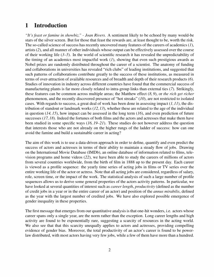
1 Introduction“It’s feast or famine in showbiz.” - Joan Rivers. A sentiment likely to be echoed by many would-bestars of the silver screen. But for those that feast the rewards are, at least thought to be, worth the risk.The so-called science of success has recently uncovered many features of the careers of academics (1),artists (2), and all manner of other individuals whose output can be effectively assessed over the courseof their working life (3–5). In the world of scientific research it has revealed the unpredictability ofthe timing of an academics most impactful work (1), showing that even such prestigious awards asNobel prizes are randomly distributed throughout the career of a scientist. The anatomy of fundingand collaborations in universities has revealed “rich clubs” of leading institutions, and suggested thatsuch patterns of collaborations contribute greatly to the success of these institutions, as measured interms of over-attraction of available resources and of breadth and depth of their research products (6).Studies of innovation in industry across different countries have found that the commercial success ofmanufacturing plants is far more closely related to intra-group links than external ties (7). Strikingly,these features can be common across multiple areas; the Matthew effect (8, 9), or the rich get richerphenomenon, and the recently discovered presence of “hot streaks” (10), are not restricted to isolatedcases. With regards to success, a great deal of work has been done in assessing impact (1,11), the dis-tribution of standout or landmark works (12,13), whether these are related to the age of the individualin question (14, 15), how impact can be assessed in the long term (16), and even prediction of futuresuccesses (17,18). Indeed the fortunes of both films and the actors and actresses that make them havebeen studied in some specific ways (16, 19–21). These studies do not however address the questionthat interests those who are not already on the higher rungs of the ladder of success: how can oneavoid the famine and build a sustainable career in acting?

The aim of this work is to use a data-driven approach in order to define, quantify and even predict thesuccess of actors and actresses in terms of their ability to maintain a steady flow of jobs. Drawingon the International Movie Database (IMDb), an online database of information related to films, tele-vision programs and home videos (22), we have been able to study the careers of millions of actorsfrom several countries worldwide, from the birth of film in 1888 up to the present day. Each careeris viewed as a profile sequence: the yearly time series of acting jobs in films or TV series over theentire working life of the actor or actress. Note that all acting jobs are considered, regardless of salary,role, screen time, or the impact of the work. The statistical analysis of such a large number of profilesequences allows us to derive some general properties of the actors activity patterns. In particular, wehave looked at several quantities of interest such as career length, productivity (defined as the numberof credit jobs in a year or in the entire career of an actor) and position of the annus mirabilis, definedas the year with the largest number of credited jobs. We have also explored possible emergence ofgender inequality in these properties.

The first message that emerges from our quantitative analysis is that one-hit wonders, i.e. actors whosecareer spans only a single year, are the norm rather than the exception. Long career lengths and highactivity are found to be exponentially rare, suggesting a scarcity of resources in the acting world.We also see that that this scarcity unequally applies to actors and actresses, providing compellingevidence of gender bias. Moreover, the total productivity of an actor’s career is found to be power-law distributed, with most actors having very few jobs, while a few of them have more than a hundred.

2

This indicates a rich-get-richer mechanism underlying the dynamics of job assignation, with alreadyscarce resources being allocated in a heterogeneous way. All of this suggests that it is activity thatis truly important when measuring success in show business. Only a select few will ever be awardedan Oscar, or have their hands on the walk of fame, but this is not important to the majority of actorsand actresses who simply want to make a living. It is the continued ability to work, as opposed toprestige which is most likely to ensure a stable career. For these reasons we propose that predictionsof success in show business should be focused on activity and productivity.Motivated by these results, we then address the questions that interest the majority of working actorsand actresses. Questions such as “am I going to get another paid job?” or “is this year going tobe my best?”. We first show that efficiency, defined as the ratio between the total number of activeyears and the career length, is unpredictable, as there is no evident correlation between these twothings. This is in line with recent studies (1, 10) pointing out that the most impactful pieces of workacross artistic and scientific disciplines usually happen randomly and uniformly over an individual’scareer, and accordingly such achievements are unpredictable. Nevertheless, we here, surprisingly,find distinctive features in their temporal arrangement. In particular, we find that actor careers areclustered in periods of high activity (hot streaks) combined with periods of latency (cold streaks).Moreover, we discover that the most productive year (annus mirabilis) for both actors and actresses islocated towards the beginning of their career, and that there are clear signals preceding and followingthe location of the annus mirabilis of an individual. Altogether, these unexpected results lead usto conclude that prediction is possible in theory. Finally, we validate this hypothesis by building astatistical learning model which predicts the location of the most productive year, finding that we can,with up to 85% accuracy, tell whether an actor’s career has reached its most productive year yet ornot.

2 ResultsWe study the careers of 1, 512, 472 actors and 896, 029 actresses as recorded on IMDb as of January16th, 2016, including careers stretching back to the first recorded movie in 1888. The career of eachactor a is characterised by his/her track record, which consists of a set of pairs of numbers representingrespectively each year when actor a was credited in IMDb, and the number of different credits in thatyear. As credits we count the number of acting jobs in films and/or TV series. A sketch of the typicalactivity pattern of an actor is reported in Figure 1, showing the yearly credits from the first to thelast year of thir career. Notice that there are not only active years, where the actor has credited jobsin IMDb, but also latent years with no recorded jobs. We therefore fill the latent years with zerosand construct the profile sequence {wk}Lk=1 of each actor a as depicted in the top part of Figure 1.The quantity wk denotes the actor’s local productivity in year k, i.e. the number of credited jobs inthat year. The length of an actor’s career is defined as the number of years between the first and thelast active year (inclusive), and is denoted as L. The total number of active years s is from now onreferred to as the activity of an actor. Since a career can have latent years intertwined with active oneswe must have s ≤ L, moreover L− s is the number of latent years. By definition we have: (i) L ≥ 1,(ii) s ≥ 1 and (iii) s = 1⇔ L = 1.Finally, we define the total productivity n of an actor, as the cumulated number of credited jobs,n =

∑Lk=1wk. The annus mirabilis (AM) of a given actor is defined as the year where the actor

was credited with the largest number of works in IMDb: AM = m, where m is such that wm =

3

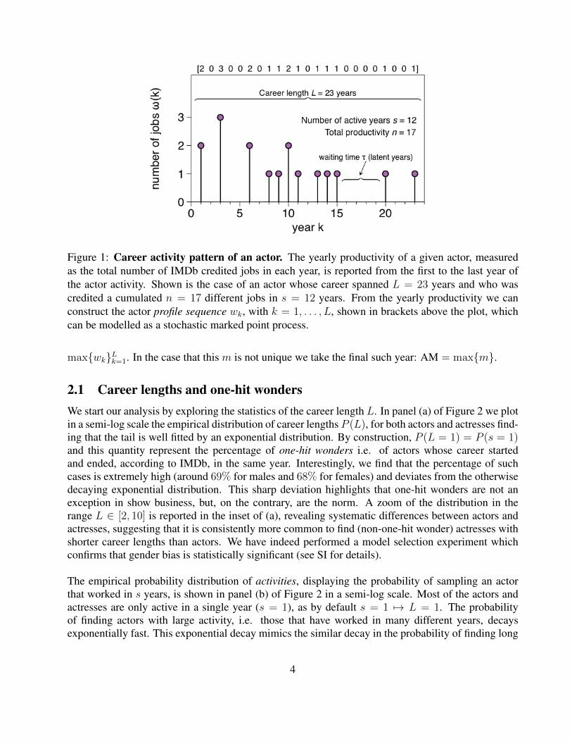
Figure 1: Career activity pattern of an actor. The yearly productivity of a given actor, measuredas the total number of IMDb credited jobs in each year, is reported from the first to the last year ofthe actor activity. Shown is the case of an actor whose career spanned L = 23 years and who wascredited a cumulated n = 17 different jobs in s = 12 years. From the yearly productivity we canconstruct the actor profile sequence wk, with k = 1, . . . , L, shown in brackets above the plot, whichcan be modelled as a stochastic marked point process.

max{wk}Lk=1. In the case that this m is not unique we take the final such year: AM = max{m}.

2.1 Career lengths and one-hit wondersWe start our analysis by exploring the statistics of the career length L. In panel (a) of Figure 2 we plotin a semi-log scale the empirical distribution of career lengths P (L), for both actors and actresses find-ing that the tail is well fitted by an exponential distribution. By construction, P (L = 1) = P (s = 1)and this quantity represent the percentage of one-hit wonders i.e. of actors whose career startedand ended, according to IMDb, in the same year. Interestingly, we find that the percentage of suchcases is extremely high (around 69% for males and 68% for females) and deviates from the otherwisedecaying exponential distribution. This sharp deviation highlights that one-hit wonders are not anexception in show business, but, on the contrary, are the norm. A zoom of the distribution in therange L ∈ [2, 10] is reported in the inset of (a), revealing systematic differences between actors andactresses, suggesting that it is consistently more common to find (non-one-hit wonder) actresses withshorter career lengths than actors. We have indeed performed a model selection experiment whichconfirms that gender bias is statistically significant (see SI for details).

The empirical probability distribution of activities, displaying the probability of sampling an actorthat worked in s years, is shown in panel (b) of Figure 2 in a semi-log scale. Most of the actors andactresses are only active in a single year (s = 1), as by default s = 1 7→ L = 1. The probabilityof finding actors with large activity, i.e. those that have worked in many different years, decaysexponentially fast. This exponential decay mimics the similar decay in the probability of finding long

4

Figure 2: Career length, activity and productivity distributions. (a) The probability P (L) that anactor or an actress has a career of length L, estimated by computing the frequency histogram of thenumber of years between the first and the last recorded entry on IMDb. P (1) measures the abundanceof “one-hit wonders”, namely the actors or actresses with IMDB records in a single year. A zoom forL ∈ [2, 10] in the inset shows that careers extending between 2 and 10 years are proportionally morefrequent in women than in men. (b) Activity distribution P (s) estimated by computing the frequencyhistogram of the number of working years within each career (s ≤ L). Curves for actors and actressesare very similar and both exhibit a clear exponential tail, implying a ‘scarcity of resources’. (c) Log-log plot of the total productivity distributions P (n) for actors (black) and actresses (blue). Both curvesdecay as a power law P (n) ∼ n−γ , where γ ≈ 2, revealing a Zipf law for the total number of actingjobs.

career lengths and altogether are the basis for claiming a scarcity of resources in show business, i.e.there are many more actors/actresses than job offers (23). This lack of resources naturally leads to aquestion: how are they allocated? We address this question in the next section.

2.2 Productivity and the rich gets richer phenomenonThe right panel of figure 2 shows the empirical distributions of total productivity P (n), reportingthe normalized numbers of actors or actresses with n appearances in movies or TV series over theircareers. While the career length distribution P (L) and the activity distributions P (s) are well fittedin their tails by an exponential law, P (n) decays more slowly and can be fitted by a power lawP (n) ∼ n−γ with exponent γ ≈ 2. This emergence of a power law shape in the distribution of totalproductivity implies that another scaling function emerges when the statistics are computed in a rank-frequency plot. It is indeed well known (24) that observing a power law distribution with exponent γfor the abundance of some variable is equivalent to obtaining a power law scaling for the frequencyof the variable that appears with rank r: f(r) ∼ r−α, where both scaling laws are mathematicallyrelated via α = 1/(γ − 1). The celebrated Zipf law refers to the particular case α ≈ 1, which isindeed the case here. The fact that a Zipf law emerges for the rank-frequency distribution of the totalproductivity of an actor may suggest a mechanistic explanation for our observations. Many differentproposals for the mechanism underpinning the emergence of a Zipf law, and several names for thephenomenon itself, have been put forward in various contexts, including the Simon-Yule process, themechanism of preferential attachment, the Matthew effect, the Gibrat principle, rich-get-richer, etc.In this context, inspired by the renowned preferential attachment paradigm as a generative model

5

to produce scale-free networks, we can easily explain the onset of a power law distribution for thetotal productivity in terms of a rich-get-richer heuristic: consider a generative model of an actor’snetwork, where nodes are actors and two actors are linked if they act in the same film. Initiallyonly a few actors are working, but as time goes on new actors come into play. In this a way thenew individuals work in films together with other actors with a probability which is proportionalto the total productivity (i.e. the total number of links) of the older actor-node. This preferentialattachment clearly expresses the rich-get-richer phenomenon by which actors that work a lot willhave a higher chance of working even more than actors with low productivity. It is well known thatsuch models generate networks with power law degree distributions (25–28), i.e. power laws for thetotal productivity. This result is not at all unexpected, after all, the more well-known someone is, themore likely producers will be to put him or her in their next film, if only for commercial purposes.What is perhaps dramatic about this observation is that it is well known that rich-get-richer effects arerather arbitrary and unpredictable, as large hubs can evolve out of unpredictable and random initialfluctuations which have been amplified, and not based on any particular intrinsic fitness (28) (such asacting skills). Quoting Easly and Kleinberg: “if we could roll time back 15 years, and then run historyforward again, would the Harry Potter books again sell hundreds of millions of copies, or would theylanguish in obscurity while some other works of children’s fiction achieved major success?”. Asa matter of fact, it seems likely that across different parallel universes popularity would still havea power law distribution, but it is far from clear that the most popular actors would always be thesame. Interestingly, this hypothesis has recently been validated in an online social experiment for thecase of musical popularity (29). In summary, productivity is probably the variable every actor aimsto maximise, but these results suggest that boosting this is more of a network effect (30, 31) than aconsequence of ‘acting skills’.

2.3 Efficiency is unpredictableIn figure 2 we observed that career length and activity are variables which are both exponentiallydistributed, indicating a scarcity of resources. In this section we further explore whether the twoquantities L and s are correlated. We first define an actor’s efficiency as the ratio s/L of active yearsover the entire career, and we investigate how this efficiency is distributed. By construction, we haves ≤ L and L = 1 → s = 1, and thus in this case s/L = 1. As roughly 68% of actors are one-hit-wonders, we expect that the probability that an actor has optimal efficiency P (s/L = 1) ≈ P (L = 1).However it is clear that these are ‘pathological’ cases as efficiency is not really well defined for one-hit wonders. In what follows, we therefore assume that the case (s = 1, L = 1) is an outlier withregards to the analysis of efficiency.

In Figure 3 we plot P (s/L) on semi-log axes for actors (top panel) and actresses (bottom panel). Asmight be expected, the distribution decreases rapidly as s/L approaches either zero or one, suggestingthat most actors and actresses have intermediate values of efficiency (see SI for a discussion and aheuristic explanation of this phenomenon). The shape of P (s/L) in the intermediate range is fractal-like, which is due to the fact that s and L are (small) integers and thus s/L cannot take arbitraryvalues in [0, 1]. The fractal shape can actually be related to the density of irreducible fractions overthe integers, as depicted in the bottom panel of Figure 3, and is not a property linked to the relationbetween s and L. In other words, when this effect is factored out, then P (s/L) is essentially flat in the

6

intermediate range. Accordingly, correlations that emerge between the activity s and the career length

Figure 3: Distribution of actor efficiency. The probabilities of finding actors (top panel) and ac-tresses (middle panel) with a given value of the ratio s/L are shown as a function of s/L. The curveshave been computed after homogeneously binning the support [0,1] into 500 bins. The fractal shapeof the curve is reminiscent of the binned density of irreducible fractions a/b, b > a, shown in thebottom panel. No obvious differences emerge here between actors and actresses.

L of an actor at intermediate ranges seem to be related only to the fact that s ≤ L. To further validatethis hypothesis, we performed a scatter plot of s versus L for all actors and actresses, and computedthe Pearson correlation coefficient. This was then compared to the correlation coefficient of a nullmodel generated by randomly extracting values of L and s from the pool of career profiles, ensuringthat L ≥ s. For actors, we found that s and L correlate with a Pearson coefficient r ≈ 0.67, whereas inthe null model we obtained rnull ≈ 0.54 (in the case of actresses r ≈ 0.67, to be compared with rnull ≈0.56). As expected, s and L are indeed correlated but almost all of those correlations can be explainedby a null model, concluding that for intermediate ranges there are in practice not strongly influentialadditional correlations between length and activity: the activity of an actor cannot be predicted bytheir career length and therefore we can conclude that the efficiency is an unpredictable quantity.

2.4 Actors careers are clustered in hot and cold streaksTo understand the temporal arrangement of active years within the profile sequence of a given actor,we now consider the statistics of waiting times. A waiting time τ is defined as the time elapsed (in

7

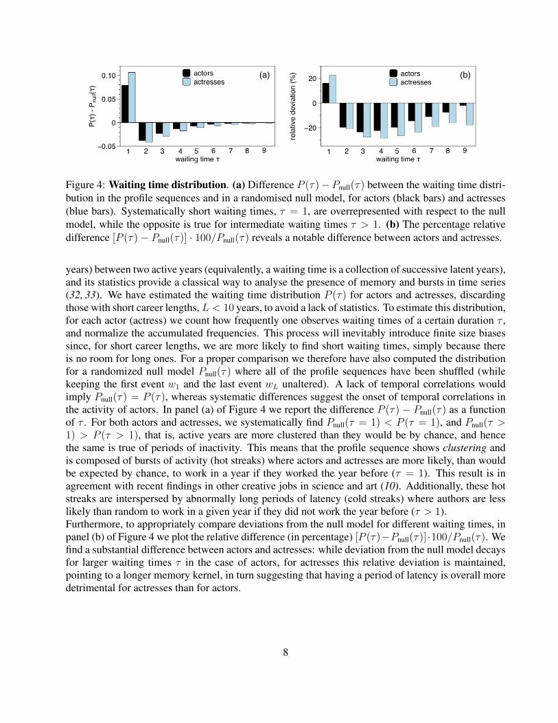
Figure 4: Waiting time distribution. (a) Difference P (τ)−Pnull(τ) between the waiting time distri-bution in the profile sequences and in a randomised null model, for actors (black bars) and actresses(blue bars). Systematically short waiting times, τ = 1, are overrepresented with respect to the nullmodel, while the opposite is true for intermediate waiting times τ > 1. (b) The percentage relativedifference [P (τ)− Pnull(τ)] · 100/Pnull(τ) reveals a notable difference between actors and actresses.

years) between two active years (equivalently, a waiting time is a collection of successive latent years),and its statistics provide a classical way to analyse the presence of memory and bursts in time series(32, 33). We have estimated the waiting time distribution P (τ) for actors and actresses, discardingthose with short career lengths, L < 10 years, to avoid a lack of statistics. To estimate this distribution,for each actor (actress) we count how frequently one observes waiting times of a certain duration τ ,and normalize the accumulated frequencies. This process will inevitably introduce finite size biasessince, for short career lengths, we are more likely to find short waiting times, simply because thereis no room for long ones. For a proper comparison we therefore have also computed the distributionfor a randomized null model Pnull(τ) where all of the profile sequences have been shuffled (whilekeeping the first event w1 and the last event wL unaltered). A lack of temporal correlations wouldimply Pnull(τ) = P (τ), whereas systematic differences suggest the onset of temporal correlations inthe activity of actors. In panel (a) of Figure 4 we report the difference P (τ) − Pnull(τ) as a functionof τ . For both actors and actresses, we systematically find Pnull(τ = 1) < P (τ = 1), and Pnull(τ >1) > P (τ > 1), that is, active years are more clustered than they would be by chance, and hencethe same is true of periods of inactivity. This means that the profile sequence shows clustering andis composed of bursts of activity (hot streaks) where actors and actresses are more likely, than wouldbe expected by chance, to work in a year if they worked the year before (τ = 1). This result is inagreement with recent findings in other creative jobs in science and art (10). Additionally, these hotstreaks are interspersed by abnormally long periods of latency (cold streaks) where authors are lesslikely than random to work in a given year if they did not work the year before (τ > 1).Furthermore, to appropriately compare deviations from the null model for different waiting times, inpanel (b) of Figure 4 we plot the relative difference (in percentage) [P (τ)−Pnull(τ)]·100/Pnull(τ). Wefind a substantial difference between actors and actresses: while deviation from the null model decaysfor larger waiting times τ in the case of actors, for actresses this relative deviation is maintained,pointing to a longer memory kernel, in turn suggesting that having a period of latency is overall moredetrimental for actresses than for actors.

8

Figure 5: Annus mirabilis tends to occur sooner rather than later. Position of AM within anactor or actress’s career, where the career length is binned into 5 bins in every case, to be able tocompare profiles of different career lengths. We systematically find that the most probable locationof the annus mirabilis is towards the beginning of a career.

2.5 Predicting the annus mirabilisIt has recently been found that the most impactful publication that a scientist will produce is equallylikely to occur at any stage of their career (1). Here we explore a related question in the contextof actors and actresses. Instead of impact, the indicator of success under study is productivity, asmeasured by the number of credited works in IMDb. We concentrate on actors and actresses withworking lives extending beyond L = 20 years, and define the annus mirabilis (AM) of a given actoras the year k = y∗ when the actor worked in the largest number of credited movies or TV series.We restrict our reported results to those cases where there were at least 5 credited jobs in the AM,although other thresholds do produce qualitatively similar results. The subset of actors with L > 20and more than 5 acting jobs in the AM consists of 15357 actors (1.02%) and 5904 actresses (0.65%).The large gender difference indicates that actors tend to have more acting jobs than actresses.In Figure 5 we plot the probability with which the AM will occur at each point within an actor oractress’s career. To be able to compare these probabilities over careers of varying lengths, we havebroken up each actor’s time series of L years respectively into 5 bins (other segmentations producequalitatively similar results). The plots consistently indicate that the most probable location of theannus mirabilis is towards the beginning of a career. Although the results are qualitatively similar formale and female actors, this bias is much more pronounced in the case of actresses, further confirmingthe gender difference previously observed.

To study whether one can detect the imminent appearance of an actor’s annus mirabilis we haveanalysed, for both actors and actresses, the average number of acting jobs before and after the AM. Inorder to do this consistently, we initially perform a translation k 7→ κ that aligns all profile sequences,so that the annus mirabilis k = y∗ all occur at κ = 0. We then define:

ξ(κ) =1

|A|

|A|∑i=1

w(i)y∗+κ,

where κ is the offset from the annus mirabilis and |A| is the size of the set of actors/actresses forwhich there exists a profile sequence with an input at offset κ. In Figure 6 we plot ξ(κ), showing that,

9

on average, there is a clear increase in the number of jobs preceding the AM and a clear decrease im-mediately afterward. This pattern is absent in the corresponding null models obtained by shuffling theprofile sequences (red bars). Such observed patterns can indeed be exploited for an early predictionof the annus mirabilis.

Figure 6: The annus mirabilis is predictable. The total number of acting jobs, ξ(κ), averaged overall actors (left panel) and actresses (right panel), is reported as a function of the number of years κafter or before the annus mirabilis. Only actors and actresses with a career lasting more than L = 20years and annus mirabilis withw > 5 acting jobs have been selected. In both cases, we observe a clearnon-monotonic pattern, indicating that the annus mirabilis is either approaching or has just passed.For comparison, we report in red the results obtained for a null model where the profile sequences ofall actors and actresses have been shuffled. No pattern emerges in that case.

Based on our observed distribution of jobs surrounding the annus mirabilis we propose a naiveearly-warning criterion: if the career sequence is non-monotonic around a value of k, i.e. if wk >wk−1 andwk+1 < wk, then the year k is a good candidate for the annus mirabilis. With this criterion inmind, one could ask the following question: given a sample of an actor or actress’s profile sequence,can we tell whether the annus mirabilis has already passed or not? Mathematically, the question abovecan be formalised as follows: given a career sequence (wk)

Lk=1 such that the maximal total productivity

occurs at time k = y∗, consider a truncated sequence wk = (wk)T≤Lk=1 . We now wish to know if we can

accurately asses whether y∗ ∈ {1, ..., T} using only wk. This forms a binary classification problem,in which wk ∈ C1 if y∗ /∈ {1, ..., T} and wk ∈ C2 otherwise. Our naive criterion, as illustrated above,readily provides the heuristic: wk ∈ C1 if wk is monotonic, and wk ∈ C2 if not. When this methodis tested on an appropriately generated setW of truncated sequences (see SI for details) we find thatit is correct ∼ 69.2% of the times for actors, and ∼ 75.0% of the times for actresses. This modelnow forms a benchmark against which we will test a more refined approach. The idea is to relaxour classification method by introducing some parameters which allow for deviation from the rigidheuristic, then train those parameters on some subset T (W , and subsequently test the trained modelon the test setW \ T . To do this let us first define the function

D (wk) = −T−1∑y=1

min (0, wy+1 − wy) . (1)

At each year k the contribution to D from that year is zero if the total productivity in the subse-quent year is larger. This means that for a monotonically increasing sequence wk, D (wk) = 0. Ifproductivity decreases from year k to k + 1, then D will increase by a corresponding amount.

10

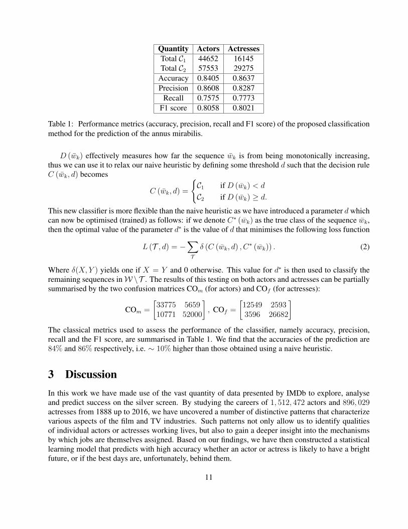
Quantity Actors ActressesTotal C1 44652 16145Total C2 57553 29275

Accuracy 0.8405 0.8637Precision 0.8608 0.8287

Recall 0.7575 0.7773F1 score 0.8058 0.8021

Table 1: Performance metrics (accuracy, precision, recall and F1 score) of the proposed classificationmethod for the prediction of the annus mirabilis.

D (wk) effectively measures how far the sequence wk is from being monotonically increasing,thus we can use it to relax our naive heuristic by defining some threshold d such that the decision ruleC (wk, d) becomes

C (wk, d) =

{C1 if D (wk) < d

C2 if D (wk) ≥ d.

This new classifier is more flexible than the naive heuristic as we have introduced a parameter dwhichcan now be optimised (trained) as follows: if we denote C∗ (wk) as the true class of the sequence wk,then the optimal value of the parameter d∗ is the value of d that minimises the following loss function

L (T , d) = −∑T

δ (C (wk, d) , C∗ (wk)) . (2)

Where δ(X, Y ) yields one if X = Y and 0 otherwise. This value for d∗ is then used to classify theremaining sequences inW\T . The results of this testing on both actors and actresses can be partiallysummarised by the two confusion matrices COm (for actors) and COf (for actresses):

COm =

[33775 565910771 52000

], COf =

[12549 25933596 26682

]The classical metrics used to assess the performance of the classifier, namely accuracy, precision,recall and the F1 score, are summarised in Table 1. We find that the accuracies of the prediction are84% and 86% respectively, i.e. ∼ 10% higher than those obtained using a naive heuristic.

3 DiscussionIn this work we have made use of the vast quantity of data presented by IMDb to explore, analyseand predict success on the silver screen. By studying the careers of 1, 512, 472 actors and 896, 029actresses from 1888 up to 2016, we have uncovered a number of distinctive patterns that characterizevarious aspects of the film and TV industries. Such patterns not only allow us to identify qualitiesof individual actors or actresses working lives, but also to gain a deeper insight into the mechanismsby which jobs are themselves assigned. Based on our findings, we have then constructed a statisticallearning model that predicts with high accuracy whether an actor or actress is likely to have a brightfuture, or if the best days are, unfortunately, behind them.

11

The analysis performed in the first part of our work supports the following eight key observations: (i)One-hit wonders are the norm, rather than the exception. This implies that productivity is probably avariable more closely related to success, rather than the importance or impact of particular jobs. (ii)Resources are scarce: long careers and higher activities are exponentially rare, implying that there arefar fewer jobs available than there are applicants. (iii) A rich-get-richer mechanism underlies the wayjobs are assigned, as evidenced by the emergence of Zipf’s law in the distribution of both actors andactresses total number of credited works. This fact suggests (29) that high productivity is likely tobe a network effect (30, 31) rather than purely based on merit, i.e. productivity does not necessarilycorrelate with acting skills. (iv) The efficiency of an actor (the ratio between active years and lengthcareer) is unpredictable, a finding reminiscent of the randomness discovered in (1). (v) Careers areclustered in periods of high activity or “hot-streaks” (again in agreement with recent findings (10))interspersed with periods of latency (cold streaks), an effect which is more pronounced for actresses.(vi) The most productive years for both actors and actresses tend to be towards the start of their careersthough, again, this is more evident for actresses. Again, we see here evidence for gender bias: olderactresses are far less likely to maintain their status in the acting world than men. (vii) There areclear signals both preceding and following the most productive years of an actor or actresses career.(viii) Including the aforementioned points, we have found statistically significant differences betweenactors and actresses across a wide range of metrics, providing credible and convincing evidence ofgender bias.The second part of our work deals with the prediction of an actors productivity. By utilising theobserved patterns present across the careers of both actors and actresses we have produced a statisti-cal learning model which, given a sample of a career, is able to predict with roughly 85% accuracywhether that career has peaked, or whether there are better things in store for our budding star.

To conclude, a life in show business appears to be very different to those of artists or scientists.Where recent works have found an inherent unpredictability and randomness in the careers of aca-demics and creatives we have found predictability and patterns. It is now natural to ask why thesedifferences occur; why were we able predict the fortunes of individuals in one area while it has beenshown to be impossible to do so elsewhere? Another natural and intriguing problem to investigatemight be the following: suppose we have predicted that a certain actors annus mirabilis has passed.What then can the actor do to change their fortunes and bring about even greater success? We hopethat our methodology and the results that we have obtained will contribute to the ongoing debatesurrounding the science of success (30). Given the scope of our findings across the industry, we alsowish that our work will be of interest to those working within it.

References1. R. Sinatra, D. Wang, P. Deville, C. Song, and A-L Barabasi, Quantifying the evolution of indi-

vidual scientific impact, Science 354, 3612 (2016).

2. David W. Galenson. Quantifying artistic success: Ranking french painters and paintings fromimpressionism to cubism. Historical Methods: A Journal of Quantitative and InterdisciplinaryHistory, 35(1):5–19, 2002.

12

3. Simone Brands, Stephen J. Brown, and David R. Gallagher. Portfolio concentration and invest-ment manager performance*. International Review of Finance, 5(3?4):149–174, 2006.

4. Thomas Gilovich, Robert Vallone, and Amos Tversky. The hot hand in basketball: On the mis-perception of random sequences. Cognitive Psychology, 17(3):295 – 314, 1985.

5. Matthew Rabin and Dimitri Vayanos. The gambler’s and hot-hand fallacies: Theory and applica-tions. The Review of Economic Studies, 77(2):730–778, 2010.

6. Athen Ma, Raul J. Mondragon, and Vito Latora. Anatomy of funded research in science. Pro-ceedings of the National Academy of Sciences, 112(48):14760–14765, 2015.

7. James H Love and Stephen Roper. Location and network effects on innovation success: evidencefor uk, german and irish manufacturing plants. Research policy, 30(4):643–661, 2001.

8. Robert K. Merton. The Matthew effect in science. Science, 159(3810):56–63 (1968).

9. Alexander M. Petersen, Woo-Sung Jung, Jae-Suk Yang, and H. Eugene Stanley. Quantitative andempirical demonstration of the Matthew effect in a study of career longevity. Proceedings of theNational Academy of Sciences, 108(1):18–23, 2011.

10. L. Liu, Y. Wang, R. Sinatra, C. Lee Giles, C. Song and D. Wang, Hot streaks in artistic, cultural,and scientific careers, Nature 559, 396-399 (2018).

11. J. E. Hirsch. An index to quantify an individual’s scientific research output. Proceedings of theNational Academy of Sciences, 102(46):16569–16572, 2005.

12. Aaron Kozbelt. One-hit wonders in classical music: Evidence and (partial) explanations for anearly career peak. Creativity Research Journal, 20(2):179–195, 2008.

13. Dean Keith Simonton. Creative productivity: A predictive and explanatory model of careertrajectories and landmarks. Psychological review, 104(1):66, 1997.

14. Harvey Christian Lehman. Age and achievement, volume 4970. Princeton University Press, 1953.

15. Dean K Simonton. Age and outstanding achievement: What do we know after a century ofresearch? Psychological bulletin, 104(2):251, 1988.

16. Andreas Spitz and Emoke-Agnes Horvat. Measuring long-term impact based on network cen-trality: Unraveling cinematic citations. PloS one, 9(10):e108857, 2014.

17. Daniel E Acuna, Stefano Allesina, and Konrad P Kording. Future impact: Predicting scientificsuccess. Nature, 489(7415):201, 2012.

18. Orion Penner, Raj K Pan, Alexander M Petersen, Kimmo Kaski, and Santo Fortunato. On thepredictability of future impact in science. Scientific reports, 3:3052, 2013.

19. Gerda Gemser, Martine Van Oostrum, and Mark AAM Leenders. The impact of film reviews onthe box office performance of art house versus mainstream motion pictures. Journal of CulturalEconomics, 31(1):43–63, 2007.

13

20. Marton Mestyan, Taha Yasseri, and Janos Kertesz. Early prediction of movie box office successbased on wikipedia activity big data. PloS one, 8(8):e71226, 2013.

21. Iain Pardoe and Dean K Simonton. Applying discrete choice models to predict academy awardwinners. Journal of the Royal Statistical Society: Series A (Statistics in Society), 171(2):375–394,2008.

22. www.imdb.com

23. Dale T. Mortensen. Chapter 15 job search and labor market analysis. volume 2 of Handbook ofLabor Economics, pages 849 – 919. Elsevier, 1986.

24. L.A. Adamic and B.A. Huberman, Zipf’s law and the Internet’, Glottometrics 3 (2002) pp.143–150

25. A-L Barabasi and R. Albert. Emergence of scaling in random networks, Science 286 (1999),pp.509–512.

26. Bela Bollobas and Oliver Riordan. Mathematical results on scale-free random graphs. In StefanBornholdt and Hans Georg Schuster, editors, Handbook of Graphs and Networks, pages 1–34.John Wiley & Sons, 2005.

27. V. Latora, V. Nicosia, G. Russo, Complex networks: principles, methods and applications (Cam-bridge University Press 2017)

28. D. Easley and J. Kleinberg, Networks, Crowds, and Markets: Reasoning About a Highly Con-nected World Chapter 18 (Cambridge University Press, 2010)

29. M. Salganik, P. Dodds, and D. Watts. Experimental study of inequality and unpredictability in anartificial cultural market, Science 311 (2006), pp.854–856.

30. A.L. Barabasi, The Formula: The Universal Laws of Success (Little Brown and Company, NewYork, 2018)

31. Fraiberger, S. P., Sinatra, R., Resch, M., Riedl, C., and Barabasi, A. L. (2018). Quantifyingreputation and success in art. Science, 362, 6416 (2018), 825-829.

32. P. Bak, K. Christensen, L. Danon, T. Scanlon, Unified scaling law for earthquakes, Phys. Rev.Lett. 88, 178501 (2002).

33. A. Corral, Long-Term Clustering, Scaling, and Universality in the Temporal Occurrence of Earth-quakes, Phys. Rev. Lett. 92, 108501 (2004).

34. K.P. Burnham, D.R. Anderson, Model Selection and Multimodel Inference: A practicalinformation-theoretic approach (2nd ed.) (Springer-Verlag, 2002).

14

AcknowledgmentsLL acknowledges support from EPSRC grant EP/P01660X/1. VL acknowledges support from EP-SRC Grant EP/N013492/1.

Author contributionsLL, VL and OW designed the study. OW and LL performed the data analysis. All authors interpretedresults and wrote the paper.

Author declarationThe authors declare no conflicts of interest.

Supplementary materialsSupplementary TextReference 34

15