QtoNum, from Qualitative values to NUMbers witharbitrary precision

Eric J.Fimbel

.

AbstractQtoNum is a calculator for qualitative values, intervals and numbers with arbitrary precision. QtoNum handlesinfinitesimals and infinites. All these types can be mixed in expressions and conversions are automatic. QtoNumcan be used as an interactive calculator (command line) as well as a software library. QtoNum provides a broaderrange of precision and orders of magnitude than classical numerical representations. In a classical scheme ofexperimental science, QtoNum allows selecting the adequate representation all along the chain, measurements, processing and interpretation without falling in over-precision (inaccuracy due to an excess of precision) or under-precision (loss of information due to a lack of precision). In general terms, QtoNum allows to be as preciseas possible while remaining accurate.

ContentThe genesis of QtoNumOverview of QtoNum

Hierarchy of typesInfinitesimals and infinites, for incommensurabilityQualitative values, for ignorance or simplicityIntervals with infinitesimals and infinites, to compute at any level of precisionQsequences, to encode at any level of precision

Types, arithmetic and conversionsSummary of typesReal numbers R( )Real numbers with infinitesimal regions and infinites Rii( )Qualitative values Q( )Qualitative values with infinitesimals and infinites Qii( )Closed intervals I( )General intervals with infinites and infinitesimals Iii( )Q-sequences Qs( )QtoNum arithmeticConversion algorithm

Implementation and PerformanceImplementationPerformanceInterpretation

Concluding notesBe precise or imprecise, but always accurateThe contribution of QtoNumApparent precision is more important than Accuracy in contemporaneous science

References

The genesis of QtoNumQtoNum stems from a failed attempt to use qualitative computer modeling to produce imprecise but accuratestatements about the brain (2001, 2002). The challenge was double: 1) multiple levels of organization at almost incommensurable scales of time and space (Churchland & Sejnovsky, 1992), and 2) remain accurate (compliant with reality) at any cost, and never produce over-precise results (i.e., diverging from reality because they are tooprecise). The incommensurable levels of organization could effectively be represented by means ofinfinitesimals and infinites, accurate qualitative (toy) models could be produced but simulations werenon-informative because after a few steps, they generated an excessive imprecision.

Years later (2010) I worked on a signal encoding controlled by the precision. Instead of using a fixed amountof bits (information capacity), the idea was to adapt the number of bits to the precision, which could be changedat any time. The Qsequences were born as a generalization of a qualitative algebra (Fimbel 2002). Qsequencescould represent any level of precision from qualitative values to arbitrary precision numbers. The qsequenceswere memory- and time-efficient thus suitable for the initial objective. However, they had no simple arithmeticoperations.

The next idea was to use two equivalent representations, qsequences for storage and transmission, and a generalinterval arithmetic for calculations (i.e., intervals extended to infinitesimal and infinite intervals and arbitraryprecision numbers). The last step was to introduce multiple, simple representations that provided a clearerhuman interface and faster computations (qualitative values, numbers, classical intervals...). The glue betweenthese multiple representations was an automatic conversion algorithm. Here is QtoNum

Overview of QtoNumHierarchy of types

QtoNUM contains qualitative values, intervals and crisp numbers, in order of increasing precision. In order ofcomputational efficiency, qualitative values are the fastest (because the operations can be implemented bitwise),followed by crisp numbers, and the interval arithmetic is the slowest.

Each of these types exists in two versions, finite and infinite. The finite qualitative values (noted Q) are3-valued, -, 0, +. (-) and (+) represent respectively the negative and positive real numbers, i.e., two sets that areunbounded but contain no infinites. The finite real numbers (noted R) are implemented as rational numbers witharbitrary precision. Rational are as good an approximation of real numbers as any other digital representation(there exist no exact digital representation of irrationals). The set R is unbounded, but each number per-se isfinite. The finite intervals (noted I) are closed intervals of finite real numbers.

The infinite qualitative values (noted Qii for qualitative-infinitesimal-infinite) contain infinites (-INF, +INF)and infinitesimals (0-, 0+), and also the inverse of the infinitesimals (--, ++) which are larger than any realnumber. The real numbers with infinites and infinitesimal regions (noted Rii) contain real numbers and theinfinites, eventually surrounded by a neighborhood (infinitesimal for the real numbers, unbounded for theinfinites). The infinite intervals (noted Iii) contains intervals with infinite and/or infinitesimal boundaries.

These six types, Q, Qii, R, Rii, I, Iii form a hierarchy, in which the values and operations of a specific type canbe represented in any more general type. The most general type is the intervals with infinitesimals and infinites.The Qsequences are equivalent in term of representation of values, but they have no proper algebra.

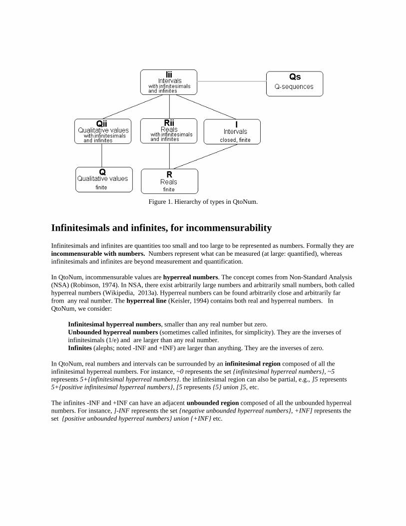
Figure 1. Hierarchy of types in QtoNum.

Infinitesimals and infinites, for incommensurability

Infinitesimals and infinites are quantities too small and too large to be represented as numbers. Formally they areincommensurable with numbers. Numbers represent what can be measured (at large: quantified), whereasinfinitesimals and infinites are beyond measurement and quantification.

In QtoNum, incommensurable values are hyperreal numbers. The concept comes from Non-Standard Analysis(NSA) (Robinson, 1974). In NSA, there exist arbitrarily large numbers and arbitrarily small numbers, both calledhyperreal numbers (Wikipedia, 2013a). Hyperreal numbers can be found arbitrarily close and arbitrarily farfrom any real number. The hyperreal line (Keisler, 1994) contains both real and hyperreal numbers. InQtoNum, we consider:

Infinitesimal hyperreal numbers, smaller than any real number but zero.Unbounded hyperreal numbers (sometimes called infinites, for simplicity). They are the inverses ofinfinitesimals (1/e) and are larger than any real number.Infinites (alephs; noted -INF and +INF) are larger than anything. They are the inverses of zero.

In QtoNum, real numbers and intervals can be surrounded by an infinitesimal region composed of all theinfinitesimal hyperreal numbers. For instance, ~0 represents the set {infinitesimal hyperreal numbers}, ~5represents 5+{infinitesimal hyperreal numbers}. the infinitesimal region can also be partial, e.g., ]5 represents 5+{positive infinitesimal hyperreal numbers}, [5 represents {5} union ]5, etc.

The infinites -INF and +INF can have an adjacent unbounded region composed of all the unbounded hyperrealnumbers. For instance, ]-INF represents the set {negative unbounded hyperreal numbers}, +INF] represents theset {positive unbounded hyperreal numbers} union {+INF} etc.

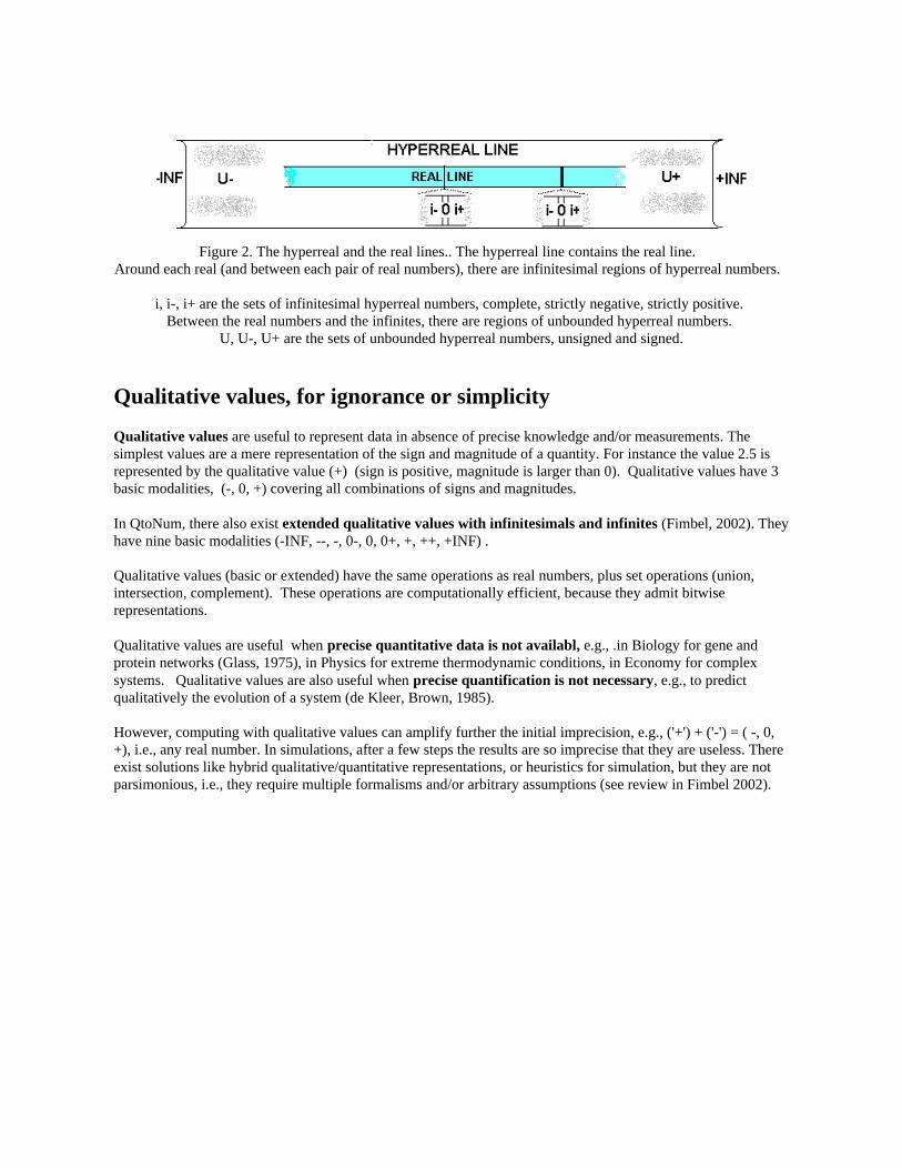
Figure 2. The hyperreal and the real lines.. The hyperreal line contains the real line. Around each real (and between each pair of real numbers), there are infinitesimal regions of hyperreal numbers.

i, i-, i+ are the sets of infinitesimal hyperreal numbers, complete, strictly negative, strictly positive. Between the real numbers and the infinites, there are regions of unbounded hyperreal numbers.

U, U-, U+ are the sets of unbounded hyperreal numbers, unsigned and signed.

Qualitative values, for ignorance or simplicity

Qualitative values are useful to represent data in absence of precise knowledge and/or measurements. Thesimplest values are a mere representation of the sign and magnitude of a quantity. For instance the value 2.5 isrepresented by the qualitative value (+) (sign is positive, magnitude is larger than 0). Qualitative values have 3basic modalities, (-, 0, +) covering all combinations of signs and magnitudes.

In QtoNum, there also exist extended qualitative values with infinitesimals and infinites (Fimbel, 2002). Theyhave nine basic modalities (-INF, --, -, 0-, 0, 0+, +, ++, +INF) .

Qualitative values (basic or extended) have the same operations as real numbers, plus set operations (union,intersection, complement). These operations are computationally efficient, because they admit bitwiserepresentations.

Qualitative values are useful when precise quantitative data is not availabl, e.g., .in Biology for gene andprotein networks (Glass, 1975), in Physics for extreme thermodynamic conditions, in Economy for complexsystems. Qualitative values are also useful when precise quantification is not necessary, e.g., to predictqualitatively the evolution of a system (de Kleer, Brown, 1985).

However, computing with qualitative values can amplify further the initial imprecision, e.g., ('+') + ('-') = ( -, 0,+), i.e., any real number. In simulations, after a few steps the results are so imprecise that they are useless. Thereexist solutions like hybrid qualitative/quantitative representations, or heuristics for simulation, but they are notparsimonious, i.e., they require multiple formalisms and/or arbitrary assumptions (see review in Fimbel 2002).

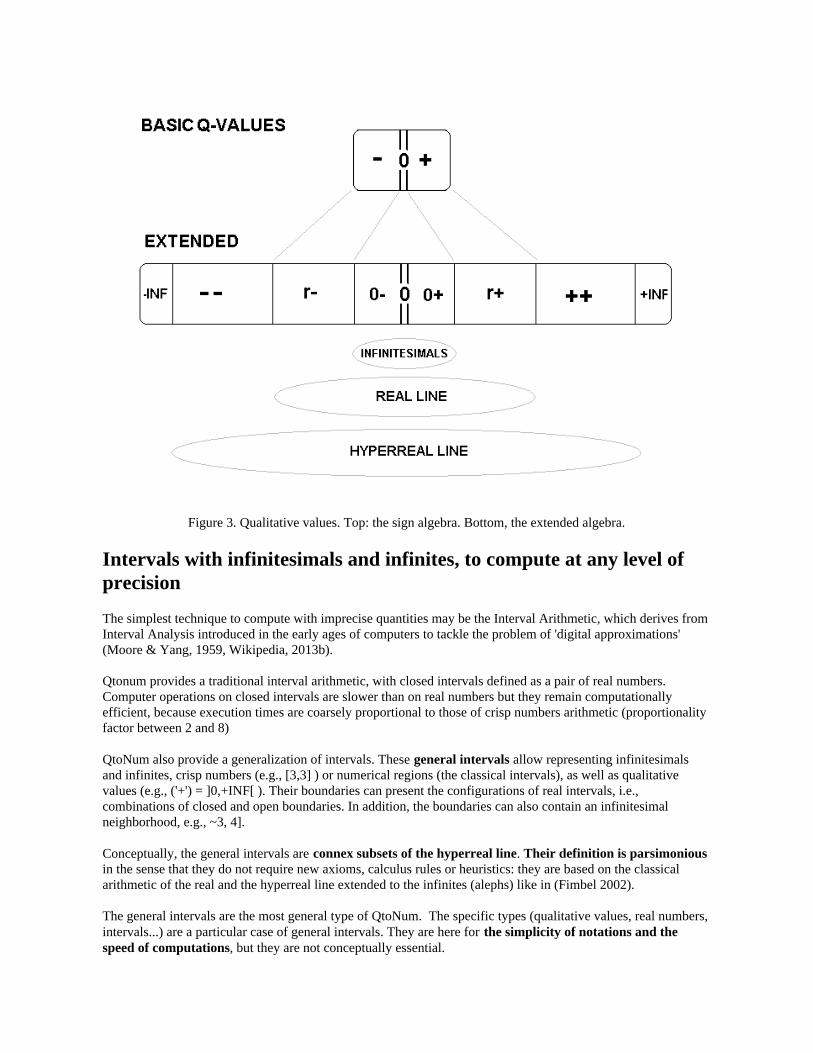
Figure 3. Qualitative values. Top: the sign algebra. Bottom, the extended algebra.

Intervals with infinitesimals and infinites, to compute at any level ofprecision

The simplest technique to compute with imprecise quantities may be the Interval Arithmetic, which derives fromInterval Analysis introduced in the early ages of computers to tackle the problem of 'digital approximations'(Moore & Yang, 1959, Wikipedia, 2013b).

Qtonum provides a traditional interval arithmetic, with closed intervals defined as a pair of real numbers.Computer operations on closed intervals are slower than on real numbers but they remain computationallyefficient, because execution times are coarsely proportional to those of crisp numbers arithmetic (proportionalityfactor between 2 and 8)

QtoNum also provide a generalization of intervals. These general intervals allow representing infinitesimalsand infinites, crisp numbers (e.g., [3,3] ) or numerical regions (the classical intervals), as well as qualitativevalues (e.g., ('+') = ]0,+INF[ ). Their boundaries can present the configurations of real intervals, i.e.,combinations of closed and open boundaries. In addition, the boundaries can also contain an infinitesimalneighborhood, e.g., ~3, 4].

Conceptually, the general intervals are connex subsets of the hyperreal line. Their definition is parsimoniousin the sense that they do not require new axioms, calculus rules or heuristics: they are based on the classicalarithmetic of the real and the hyperreal line extended to the infinites (alephs) like in (Fimbel 2002).

The general intervals are the most general type of QtoNum. The specific types (qualitative values, real numbers,intervals...) are a particular case of general intervals. They are here for the simplicity of notations and thespeed of computations, but they are not conceptually essential.

Qsequences, to encode at any level of precision

QtoNum provides a binary encoding called qSequences for all the types, intervals, qualitative values and realnumbers. Qsequences are used exclusively for data encoding, storage and transmission. In this context, theybring four benefits:

The encoding is precision-controlled and the precision is arbitrary. There are no overflows or underflowsand no limits on the range of amplitudes. The encoding is memory-efficient the number of bits is proportional to the amplitude of the quantity andthe precision (on a logarithmic scale). The encoding and the decoding are time-efficient: both take a time proportional to the number of bits.Direct comparisons of qsequences are efficient (equal, lower than, included in...), thus they allow fastreal time classification and histograms.

Qsequences are equivalent to general intervals, i.e., the two sets are isomorphic. However, qsequences have nosimple arithmetic (except for qualitative values, i.e., qsequences of length 1). Qsequences are thereforeconverted into general intervals for computations, and the results are converted back into qsequences. Also,qsequences are not suitable for human understanding. They are converted into specific notations (qualitativevalues, numbers, intervals) for clarity.

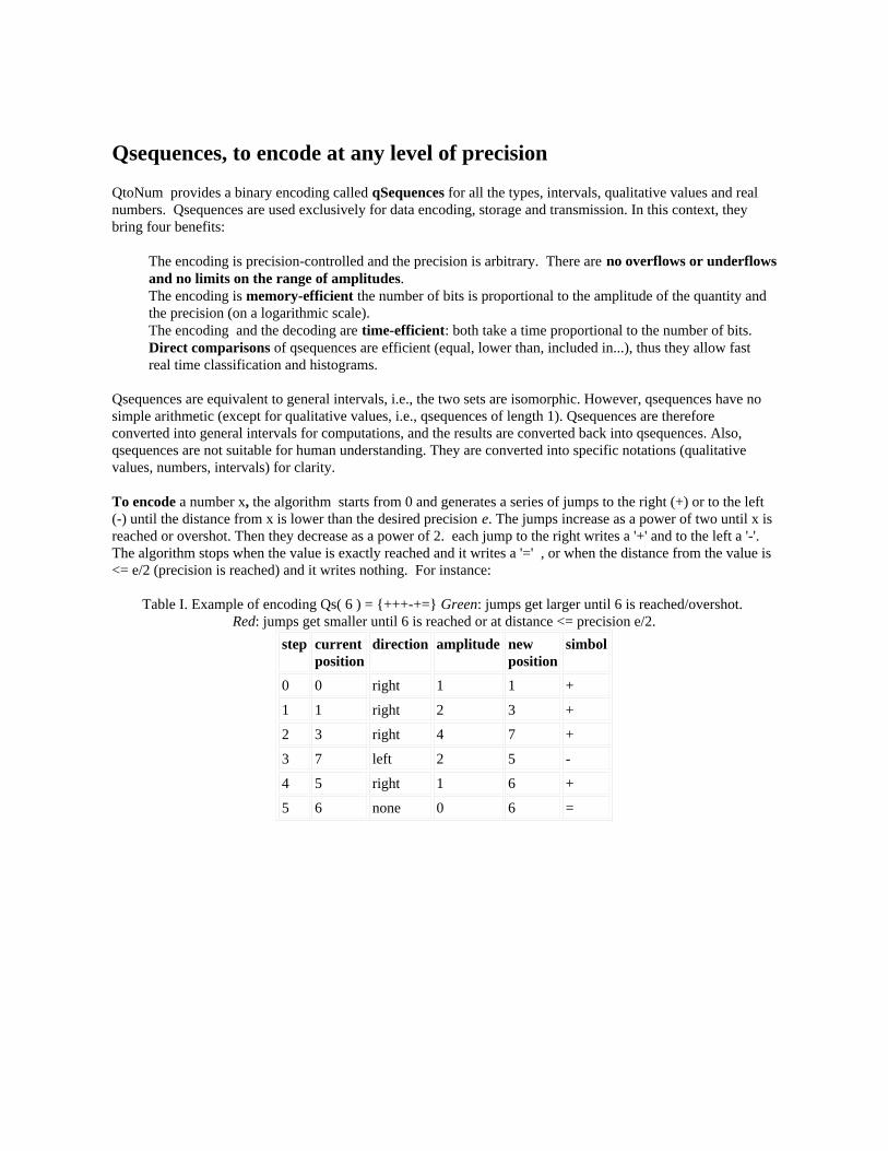
To encode a number x, the algorithm starts from 0 and generates a series of jumps to the right (+) or to the left(-) until the distance from x is lower than the desired precision e. The jumps increase as a power of two until x isreached or overshot. Then they decrease as a power of 2. each jump to the right writes a '+' and to the left a '-'. The algorithm stops when the value is exactly reached and it writes a '=' , or when the distance from the value is<= e/2 (precision is reached) and it writes nothing. For instance:

Table I. Example of encoding Qs( 6 ) = {+++-+=} Green: jumps get larger until 6 is reached/overshot. Red: jumps get smaller until 6 is reached or at distance <= precision e/2.

step currentposition

direction amplitude new position

simbol

0 0 right 1 1 +

1 1 right 2 3 +

2 3 right 4 7 +

3 7 left 2 5 -

4 5 right 1 6 +

5 6 none 0 6 =

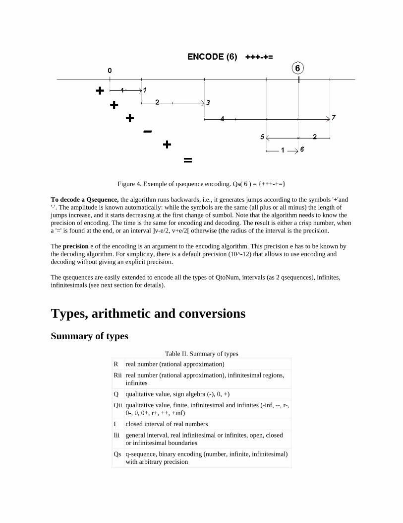
Figure 4. Exemple of qsequence encoding. Qs( 6 ) = {+++-+=}

To decode a Qsequence, the algorithm runs backwards, i.e., it generates jumps according to the symbols '+'and'-'. The amplitude is known automatically: while the symbols are the same (all plus or all minus) the length ofjumps increase, and it starts decreasing at the first change of sumbol. Note that the algorithm needs to know theprecision of encoding. The time is the same for encoding and decoding. The result is either a crisp number, whena '=' is found at the end, or an interval ]v-e/2, v+e/2[ otherwise (the radius of the interval is the precision.

The precision e of the encoding is an argument to the encoding algorithm. This precision e has to be known bythe decoding algorithm. For simplicity, there is a default precision (10^-12) that allows to use encoding anddecoding without giving an explicit precision.

The qsequences are easily extended to encode all the types of QtoNum, intervals (as 2 qsequences), infinites,infinitesimals (see next section for details).

Types, arithmetic and conversions Summary of types

Table II. Summary of typesR real number (rational approximation)

Rii real number (rational approximation), infinitesimal regions,infinites

Q qualitative value, sign algebra (-), 0, +)

Qii qualitative value, finite, infinitesimal and infinites (-inf, --, r-,0-, 0, 0+, r+, ++, +inf)

I closed interval of real numbers

Iii general interval, real infinitesimal or infinites, open, closedor infinitesimal boundaries

Qs q-sequence, binary encoding (number, infinite, infinitesimal)with arbitrary precision

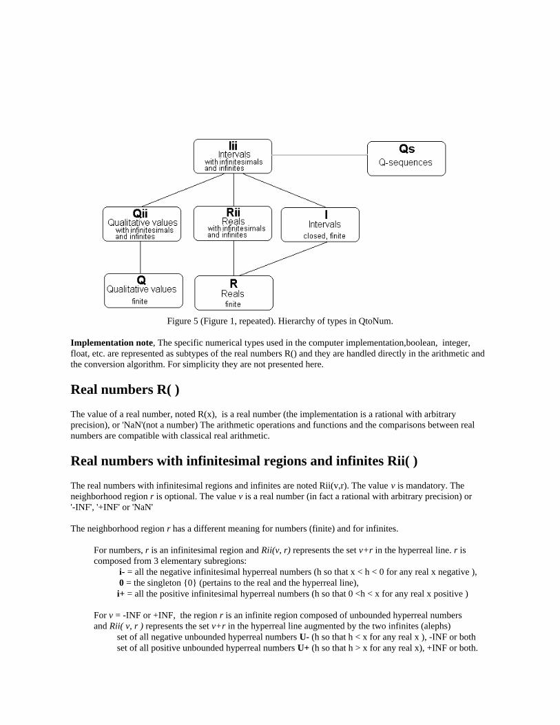
Figure 5 (Figure 1, repeated). Hierarchy of types in QtoNum.

Implementation note, The specific numerical types used in the computer implementation,boolean, integer,float, etc. are represented as subtypes of the real numbers R() and they are handled directly in the arithmetic andthe conversion algorithm. For simplicity they are not presented here.

Real numbers R( )

The value of a real number, noted R(x), is a real number (the implementation is a rational with arbitraryprecision), or 'NaN'(not a number) The arithmetic operations and functions and the comparisons between realnumbers are compatible with classical real arithmetic.

Real numbers with infinitesimal regions and infinites Rii( )

The real numbers with infinitesimal regions and infinites are noted Rii(v,r). The value v is mandatory. Theneighborhood region r is optional. The value v is a real number (in fact a rational with arbitrary precision) or'-INF', '+INF' or 'NaN'

The neighborhood region r has a different meaning for numbers (finite) and for infinites.

For numbers, r is an infinitesimal region and Rii(v, r) represents the set v+r in the hyperreal line. r is composed from 3 elementary subregions:

i- = all the negative infinitesimal hyperreal numbers (h so that x < h < 0 for any real x negative ), 0 = the singleton {0} (pertains to the real and the hyperreal line), i+ = all the positive infinitesimal hyperreal numbers (h so that 0 <h < x for any real x positive )

For v = -INF or +INF, the region r is an infinite region composed of unbounded hyperreal numbersand Rii( v, r ) represents the set v+r in the hyperreal line augmented by the two infinites (alephs)

set of all negative unbounded hyperreal numbers U- (h so that h < x for any real x ), -INF or bothset of all positive unbounded hyperreal numbers U+ (h so that h > x for any real x), +INF or both.

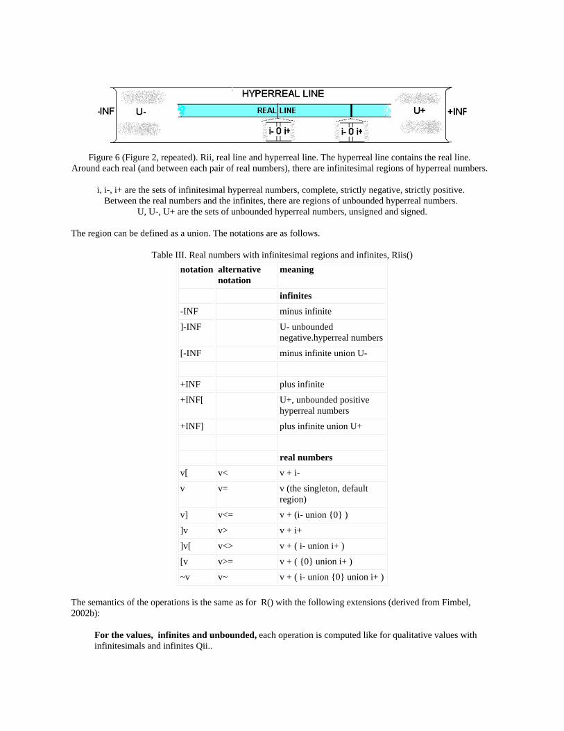
Figure 6 (Figure 2, repeated). Rii, real line and hyperreal line. The hyperreal line contains the real line. Around each real (and between each pair of real numbers), there are infinitesimal regions of hyperreal numbers.

i, i-, i+ are the sets of infinitesimal hyperreal numbers, complete, strictly negative, strictly positive. Between the real numbers and the infinites, there are regions of unbounded hyperreal numbers.

U, U-, U+ are the sets of unbounded hyperreal numbers, unsigned and signed.

The region can be defined as a union. The notations are as follows.

Table III. Real numbers with infinitesimal regions and infinites, Riis()notation alternative

notationmeaning

infinites

-INF minus infinite

]-INF U- unbounded negative.hyperreal numbers

[-INF minus infinite union U-

+INF plus infinite

+INF[ U+, unbounded positive hyperreal numbers

+INF] plus infinite union U+

real numbers

v[ v< v + i-

v v= v (the singleton, default region)

v] v<= v + (i- union {0} )

]v v> v + i+

]v[ v<> v + ( i- union i+ )

[v v>= v + ( {0} union i+ )

~v v~ v + ( i- union {0} union i+ )

The semantics of the operations is the same as for R() with the following extensions (derived from Fimbel,2002b):

For the values, infinites and unbounded, each operation is computed like for qualitative values withinfinitesimals and infinites Qii..

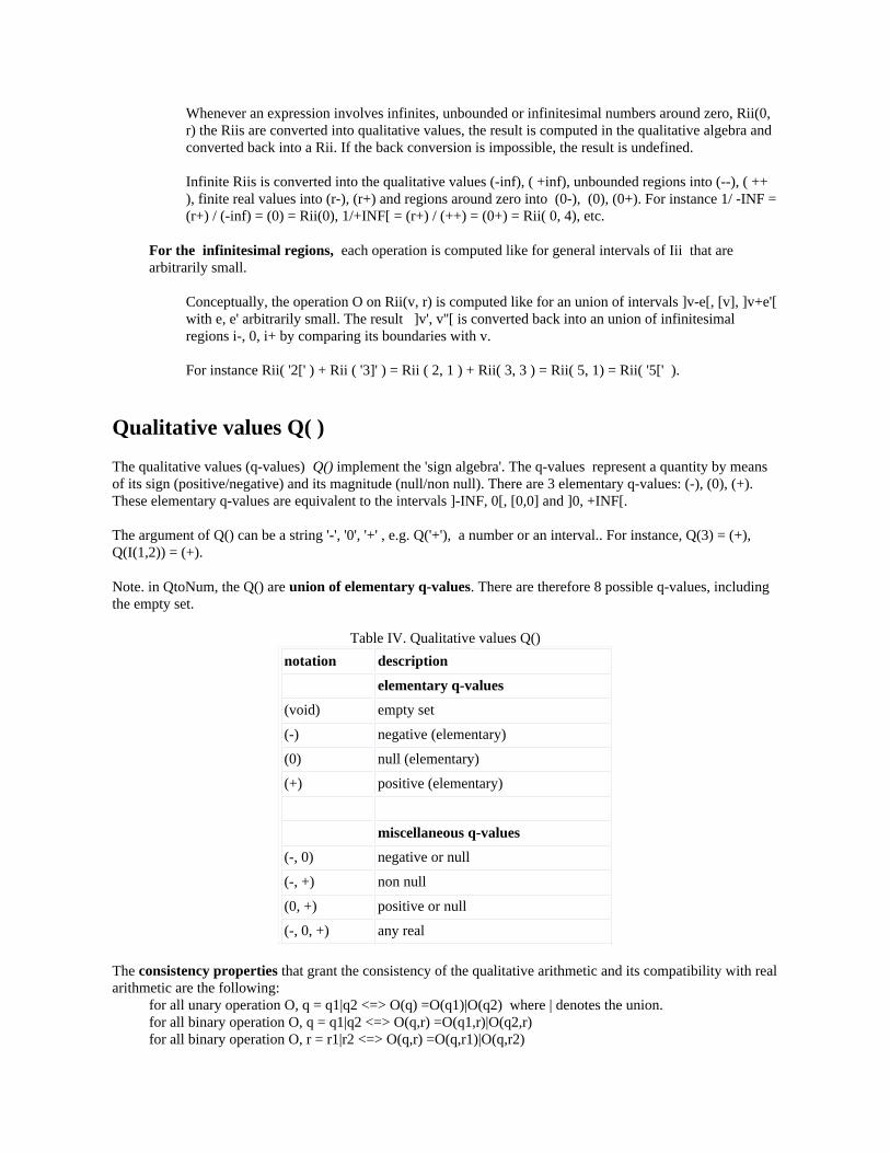
Whenever an expression involves infinites, unbounded or infinitesimal numbers around zero, Rii(0,r) the Riis are converted into qualitative values, the result is computed in the qualitative algebra andconverted back into a Rii. If the back conversion is impossible, the result is undefined.

Infinite Riis is converted into the qualitative values (-inf), ( +inf), unbounded regions into (--), ( ++), finite real values into (r-), (r+) and regions around zero into (0-), (0), (0+). For instance 1/ -INF =(r+) / (-inf) = (0) = Rii(0), 1/+INF[ = (r+) / (++) = (0+) = Rii( 0, 4), etc.

For the infinitesimal regions, each operation is computed like for general intervals of Iii that arearbitrarily small.

Conceptually, the operation O on Rii(v, r) is computed like for an union of intervals ]v-e[, [v], ]v+e'[with e, e' arbitrarily small. The result ]v', v''[ is converted back into an union of infinitesimalregions i-, 0, i+ by comparing its boundaries with v.

For instance Rii( '2[' ) + Rii ( '3]' ) = Rii ( 2, 1 ) + Rii( 3, 3 ) = Rii( 5, 1) = Rii( '5[' ).

Qualitative values Q( )

The qualitative values (q-values) Q() implement the 'sign algebra'. The q-values represent a quantity by meansof its sign (positive/negative) and its magnitude (null/non null). There are 3 elementary q-values: (-), (0), (+).These elementary q-values are equivalent to the intervals ]-INF, 0[, [0,0] and ]0, +INF[.

The argument of Q() can be a string '-', '0', '+' , e.g. Q('+'), a number or an interval.. For instance, Q(3) = (+),Q(I(1,2)) = (+).

Note. in QtoNum, the Q() are union of elementary q-values. There are therefore 8 possible q-values, includingthe empty set.

Table IV. Qualitative values Q()notation description

elementary q-values

(void) empty set

(-) negative (elementary)

(0) null (elementary)

(+) positive (elementary)

miscellaneous q-values

(-, 0) negative or null

(-, +) non null

(0, +) positive or null

(-, 0, +) any real

The consistency properties that grant the consistency of the qualitative arithmetic and its compatibility with realarithmetic are the following:

for all unary operation O, q = q1|q2 <=> O(q) =O(q1)|O(q2) where | denotes the union.for all binary operation O, q = q1|q2 <=> O(q,r) =O(q1,r)|O(q2,r)for all binary operation O, r = r1|r2 <=> O(q,r) =O(q,r1)|O(q,r2)

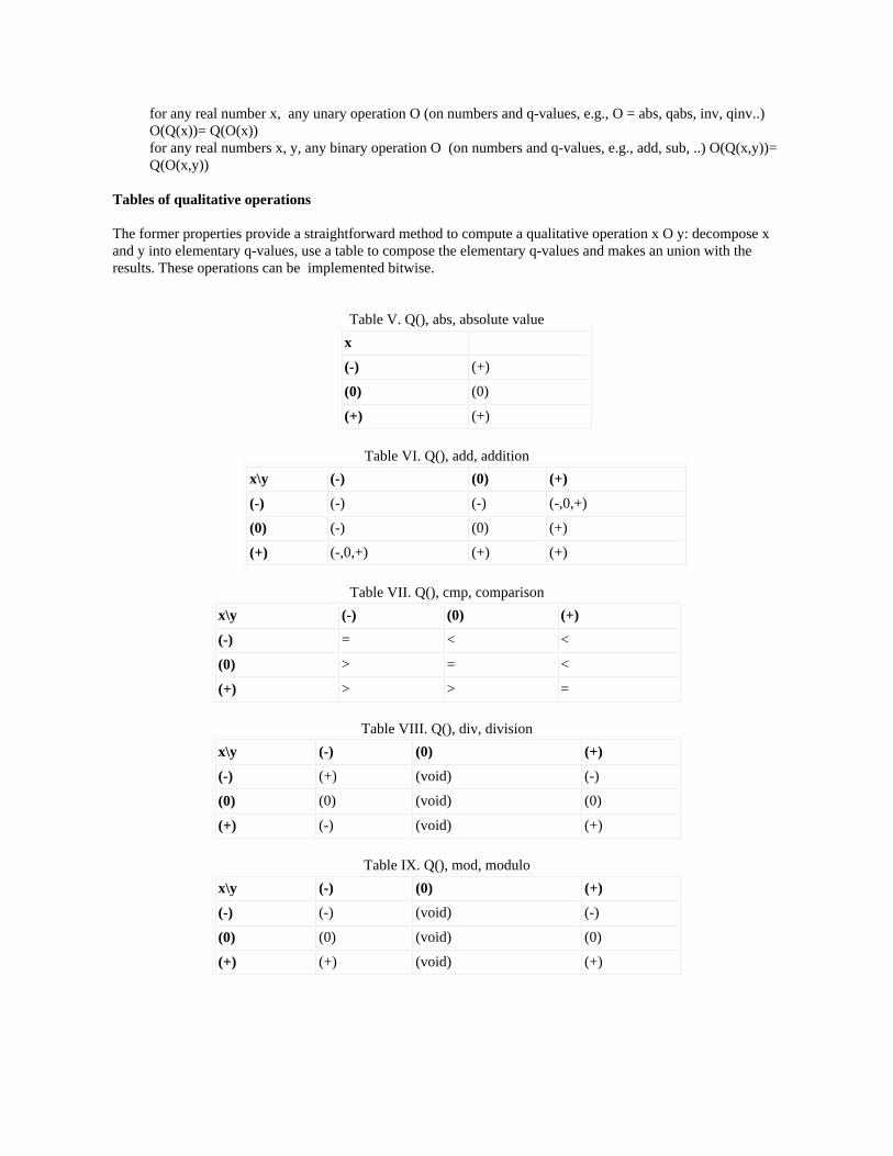
for any real number x, any unary operation O (on numbers and q-values, e.g., O = abs, qabs, inv, qinv..)O(Q(x))= Q(O(x))for any real numbers x, y, any binary operation O (on numbers and q-values, e.g., add, sub, ..) O(Q(x,y))=Q(O(x,y))

Tables of qualitative operations

The former properties provide a straightforward method to compute a qualitative operation x O y: decompose xand y into elementary q-values, use a table to compose the elementary q-values and makes an union with theresults. These operations can be implemented bitwise.

Table V. Q(), abs, absolute valuex

(-) (+)

(0) (0)

(+) (+)

Table VI. Q(), add, additionx\y (-) (0) (+)

(-) (-) (-) (-,0,+)

(0) (-) (0) (+)

(+) (-,0,+) (+) (+)

Table VII. Q(), cmp, comparisonx\y (-) (0) (+)

(-) = < <

(0) > = <

(+) > > =

Table VIII. Q(), div, divisionx\y (-) (0) (+)

(-) (+) (void) (-)

(0) (0) (void) (0)

(+) (-) (void) (+)

Table IX. Q(), mod, modulox\y (-) (0) (+)

(-) (-) (void) (-)

(0) (0) (void) (0)

(+) (+) (void) (+)

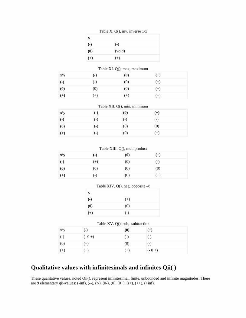
Table X. Q(), inv, inverse 1/xx

(-) (-)

(0) (void)

(+) (+)

Table XI. Q(), max, maximumx\y (-) (0) (+)

(-) (-) (0) (+)

(0) (0) (0) (+)

(+) (+) (+) (+)

Table XII. Q(), min, minimumx\y (-) (0) (+)

(-) (-) (-) (-)

(0) (-) (0) (0)

(+) (-) (0) (+)

Table XIII. Q(), mul, productx\y (-) (0) (+)

(-) (+) (0) (-)

(0) (0) (0) (0)

(+) (-) (0) (+)

Table XIV. Q(), neg, opposite -xx

(-) (+)

(0) (0)

(+) (-)

Table XV. Q(), sub, subtractionx\y (-) (0) (+)

(-) (- 0 +) (-) (-)

(0) (+) (0) (-)

(+) (+) (+) (- 0 +)

Qualitative values with infinitesimals and infinites Qii( )

These qualitative values, noted Qii(), represent infinitesimal, finite, unbounded and infinite magnitudes. Thereare 9 elementary qii-values: (-inf), (--), (r-), (0-), (0), (0+), (r+), (++), (+inf).

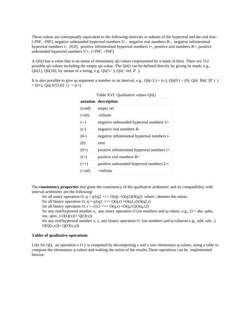
These values are conceptually equivalent to the following intervals or subsets of the hyperreal and the real line:[-INF, -INF], negative unbounded hyperreal numbers U-, negative real numbers R-, negative infinitesimalhyperreal numbers i-, [0,0], positive infinitesimal hyperreal numbers i+, positive real numbers R+, positiveunbounded hyperreal numbers U+, [+INF, +INF]

A Qii() has a value that is an union of elementary qii-values (represented by a mask of bits). There are 512possible qii-values including the empty qii-value. The Qii() can be defined directly by giving its mask, e.g.,Qii(1), Qii(16), by means of a string, e.g. Qii('r-' ), Qii( '-inf, 0' ).

It is also possible to give as argument a number or an interval, e.g., Qii(-3.) = (r-), Qii(0.) = (0), Qii( Rii( ']0' ) )= (0+), Qii( I('[5,6]' ) ) = (r+)

Table XVI. Qualitative values Qii()notation description

(void) empty set

(-inf) -infinite

(--) negative unbounded hyperreal numbers U-

(r-) negative real numbers R-

(0-) negative infinitesimal hyperreal numbers i-

(0) zero

(0+) positive infinitesimal hyperreal numbers i+

(r+) positive real numbers R+

(++) positive unbounded hyperreal numbers U+

(+inf) +infinite

The consistency properties that grant the consistency of the qualitative arithmetic and its compatibility withinterval arithmetic are the following:

for all unary operation O, q = q1|q2 <=> O(q) =O(q1)|O(q2) where | denotes the union.for all binary operation O, q = q1|q2 <=> O(q,r) =O(q1,r)|O(q2,r)for all binary operation O, r = r1|r2 <=> O(q,r) =O(q,r1)|O(q,r2)for any real/hyperreal number x, any unary operation O (on numbers and q-values, e.g., O = abs, qabs,inv, qinv..) O(Q(x))= Q(O(x))for any real/hyperreal number x, y, any binary operation O (on numbers and q-valuesm e.g., add, sub...)O(Q(x,y))= Q(O(x,y))

Tables of qualitative operations

Like for Q(), an operation x O y is computed by decomposing x and y into elementary q-values, using a table tocompose the elementary q-values and making the union of the results.These operations can be implementedbitwise.

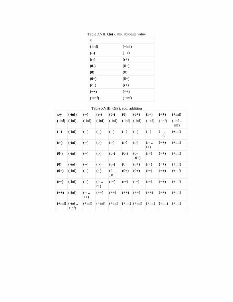
Table XVII. Qii(), abs, absolute valuex

(-inf) (+inf)

(--) (++)

(r-) (r+)

(0-) (0+)

(0) (0)

(0+) (0+)

(r+) (r+)

(++) (++)

(+inf) (+inf)

Table XVIII. Qii(), add, additionx\y (-inf) (--) (r-) (0-) (0) (0+) (r+) (++) (+inf)

(-inf) (-inf) (-inf) (-inf) (-inf) (-inf) (-inf) (-inf) (-inf) (-inf .. +inf)

(--) (-inf) (--) (--) (--) (--) (--) (--) (-- .. ++)

(+inf)

(r-) (-inf) (--) (r-) (r-) (r-) (r-) (r- .. r+)

(++) (+inf)

(0-) (-inf) (--) (r-) (0-) (0-) (0- ..0+)

(r+) (++) (+inf)

(0) (-inf) (--) (r-) (0-) (0) (0+) (r+) (++) (+inf)

(0+) (-inf) (--) (r-) (0- ..0+)

(0+) (0+) (r+) (++) (+inf)

(r+) (-inf) (--) (r- .. r+)

(r+) (r+) (r+) (r+) (++) (+inf)

(++) (-inf) (-- .. ++)

(++) (++) (++) (++) (++) (++) (+inf)

(+inf) (-inf .. +inf)

(+inf) (+inf) (+inf) (+inf) (+inf) (+inf) (+inf) (+inf)

Table XIX. Qii(), cmp,comparisonx\y (-inf) (--) (r-) (0-) (0) (0+) (r+) (++) (+inf)

(-inf) = < < < < < < < <

(--) > = < < < < < < <

(r-) > > = < < < < < <

(0-) > > > = < < < < <

(0) > > > > = < < < <

(0+) > > > > > = < < <

(r+) > > > > > > = < <

(++) > > > > > > > = <

(+inf) > > > > > > > > =

Table XX. Qii(), div, divisionx\y (-inf) (--) (r-) (0-) (0) (0+) (r+) (++) (+inf)

(-inf) (-inf .. +inf)

(+inf) (+inf) (+inf) (-inf,+inf) (-inf) (-inf) (-inf) (-inf .. +inf)

(--) (0) (0+..++) (++) (++) (-inf,+inf) (--) (--) (-- .. 0-)

(0)

(r-) (0) (0+) (r+) (++) (-inf,+inf) (--) (r-) (0-) (0)

(0-) (0) (0+) (0+) (0+ .. ++)

(-inf,+inf) (-- .. 0-)

(0-) (0-) (0)

(0) (0) (0) (0) (0) (-inf .. +inf)

(0) (0) (0) (0)

(0+) (0) (0-) (0-) (-- .. 0-)

(-inf,+inf) (0+ .. ++)

(0+) (0+) (0)

(r+) (0) (0-) (r-) (--) (-inf,+inf) (++) (r+) (0+) (0)

(++) (0) (-- .. 0-) (--) (--) (-inf,+inf) (++) (++) (0+ .. ++)

(0)

(+inf) (-inf .. +inf)

(-inf) (-inf) (-inf) (-inf,+inf) (+inf) (+inf) (+inf) (-inf ..+inf)

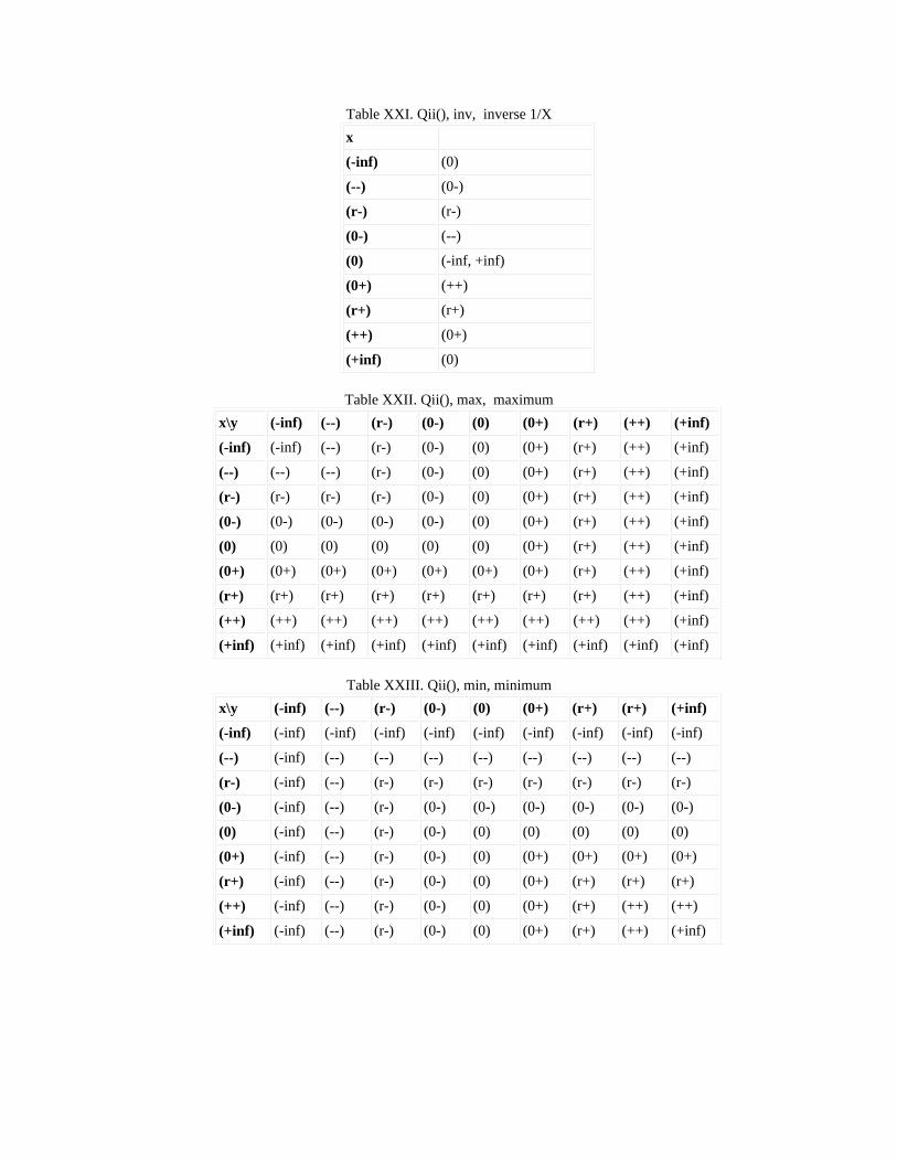
Table XXI. Qii(), inv, inverse 1/Xx

(-inf) (0)

(--) (0-)

(r-) (r-)

(0-) (--)

(0) (-inf, +inf)

(0+) (++)

(r+) (r+)

(++) (0+)

(+inf) (0)

Table XXII. Qii(), max, maximumx\y (-inf) (--) (r-) (0-) (0) (0+) (r+) (++) (+inf)

(-inf) (-inf) (--) (r-) (0-) (0) (0+) (r+) (++) (+inf)

(--) (--) (--) (r-) (0-) (0) (0+) (r+) (++) (+inf)

(r-) (r-) (r-) (r-) (0-) (0) (0+) (r+) (++) (+inf)

(0-) (0-) (0-) (0-) (0-) (0) (0+) (r+) (++) (+inf)

(0) (0) (0) (0) (0) (0) (0+) (r+) (++) (+inf)

(0+) (0+) (0+) (0+) (0+) (0+) (0+) (r+) (++) (+inf)

(r+) (r+) (r+) (r+) (r+) (r+) (r+) (r+) (++) (+inf)

(++) (++) (++) (++) (++) (++) (++) (++) (++) (+inf)

(+inf) (+inf) (+inf) (+inf) (+inf) (+inf) (+inf) (+inf) (+inf) (+inf)

Table XXIII. Qii(), min, minimumx\y (-inf) (--) (r-) (0-) (0) (0+) (r+) (r+) (+inf)

(-inf) (-inf) (-inf) (-inf) (-inf) (-inf) (-inf) (-inf) (-inf) (-inf)

(--) (-inf) (--) (--) (--) (--) (--) (--) (--) (--)

(r-) (-inf) (--) (r-) (r-) (r-) (r-) (r-) (r-) (r-)

(0-) (-inf) (--) (r-) (0-) (0-) (0-) (0-) (0-) (0-)

(0) (-inf) (--) (r-) (0-) (0) (0) (0) (0) (0)

(0+) (-inf) (--) (r-) (0-) (0) (0+) (0+) (0+) (0+)

(r+) (-inf) (--) (r-) (0-) (0) (0+) (r+) (r+) (r+)

(++) (-inf) (--) (r-) (0-) (0) (0+) (r+) (++) (++)

(+inf) (-inf) (--) (r-) (0-) (0) (0+) (r+) (++) (+inf)

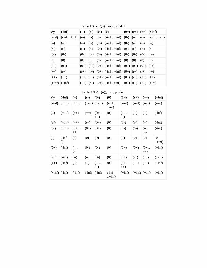
Table XXIV. Qii(), mod, modulox\y (-inf) (--) (r-) (0-) (0) (0+) (r+) (++) (+inf)

(-inf) (-inf .. +inf) (--) (r-) 0-) (-inf .. +inf) (0-) (r-) (--) (-inf .. +inf)

(--) (--) (--) (r-) (0-) (-inf .. +inf) (0-) (r-) (--) (--)

(r-) (r-) (r-) (r-) (0-) (-inf .. +inf) (0-) (r-) (r-) (r-)

(0-) (0-) (0-) (0-) (0-) (-inf .. +inf) (0-) (0-) (0-) (0-)

(0) (0) (0) (0) (0) (-inf .. +inf) (0) (0) (0) (0)

(0+) (0+) (0+) (0+) (0+) (-inf .. +inf) (0+) (0+) (0+) (0+)

(r+) (r+) (r+) (r+) (0+) (-inf .. +inf) (0+) (r+) (r+) (r+)

(++) (++) (++) (r+) (0+) (-inf .. +inf) (0+) (r+) (++) (++)

(+inf) (+inf) (++) (r+) (0+) (-inf ..+inf) (0+) (r+) (++) (+inf)

Table XXV. Qii(), mul, productx\y (-inf) (--) (r-) (0-) (0) (0+) (r+) (++) (+inf)

(-inf) (+inf) (+inf) (+inf) (+inf) (-inf .. +inf)

(-inf) (-inf) (-inf) (-inf)

(--) (+inf) (++) (++) (0+ .. ++)

(0) (-- .. 0-)

(--) (--) (-inf)

(r-) (+inf) (++) (r+) (0+) (0) (0-) (r-) (--) (-inf)

(0-) (+inf) (0+ .. ++)

(0+) (0+) (0) (0-) (0-) (-- .. 0-)

(-inf)

(0) (-inf .. 0)

(0) (0) (0) (0) (0) (0) (0) (0 ..+inf)

(0+) (-inf) (-- .. 0-)

(0-) (0-) (0) (0+) (0+) (0+ .. ++)

(+inf)

(r+) (-inf) (--) (r-) (0-) (0) (0+) (r+) (++) (+inf)

(++) (-inf) (--) (--) (-- .. 0-)

(0) (0+ .. ++)

(++) (++) (+inf)

(+inf) (-inf) (-inf) (-inf) (-inf) (-inf ..+inf)

(+inf) (+inf) (+inf) (+inf)

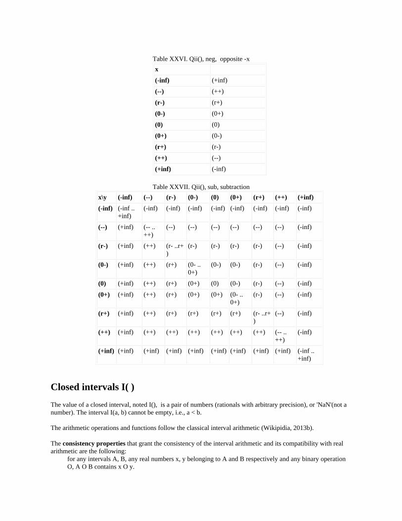
Table XXVI. Qii(), neg, opposite -xx

(-inf) (+inf)

(--) (++)

(r-) (r+)

(0-) (0+)

(0) (0)

(0+) (0-)

(r+) (r-)

(++) (--)

(+inf) (-inf)

Table XXVII. Qii(), sub, subtractionx\y (-inf) (--) (r-) (0-) (0) (0+) (r+) (++) (+inf)

(-inf) (-inf .. +inf)

(-inf) (-inf) (-inf) (-inf) (-inf) (-inf) (-inf) (-inf)

(--) (+inf) (-- .. ++)

(--) (--) (--) (--) (--) (--) (-inf)

(r-) (+inf) (++) (r- ..r+ )

(r-) (r-) (r-) (r-) (--) (-inf)

(0-) (+inf) (++) (r+) (0- .. 0+)

(0-) (0-) (r-) (--) (-inf)

(0) (+inf) (++) (r+) (0+) (0) (0-) (r-) (--) (-inf)

(0+) (+inf) (++) (r+) (0+) (0+) (0- .. 0+)

(r-) (--) (-inf)

(r+) (+inf) (++) (r+) (r+) (r+) (r+) (r- ..r+ )

(--) (-inf)

(++) (+inf) (++) (++) (++) (++) (++) (++) (-- .. ++)

(-inf)

(+inf) (+inf) (+inf) (+inf) (+inf) (+inf) (+inf) (+inf) (+inf) (-inf .. +inf)

Closed intervals I( )

The value of a closed interval, noted I(), is a pair of numbers (rationals with arbitrary precision), or 'NaN'(not anumber). The interval I(a, b) cannot be empty, i.e., a < b.

The arithmetic operations and functions follow the classical interval arithmetic (Wikipidia, 2013b).

The consistency properties that grant the consistency of the interval arithmetic and its compatibility with realarithmetic are the following:

for any intervals A, B, any real numbers x, y belonging to A and B respectively and any binary operationO, A O B contains x O y.

for any interval A, any real x belonging to A and any unary operation O, O(B) contains O(x)

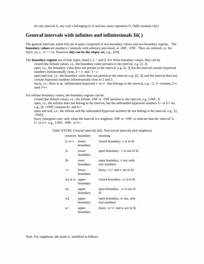
General intervals with infinites and infinitesimals Iii( )

The general intervals, noted Iii() are 4-uples composed of two boundary values and two boundary regions. Theboundary values are numbers ( rationals with arbitrary precision), or -INF, +INF. They are ordered, i.e. for Iii(vl, vu..), vl <= vu. However Iii() can be the empty set, e.g., ]0,0[.

The boundary regions are of four types, noted ], [, ~ and |]. For finite boundary values, they can be closed (the default value), i.e., the boundary value pertains to the interval, e.g. [2, 3]open, i.e., the boundary value does not pertain to the interval ,e.g. ]2, 3[ but the interval contain hyperrealnumbers infinitesimally close, 2 + i+ and 3 + i-open and real, i.e., the boundary value does not pertain to the interval ,e.g. ]|2, 3|[ and the interval does notcontain hyperreal numbers infinitesimally close to 2 and 3.fuzzy, i.e., there is an infinitesimal hyperreal i- or i+ that belongs to the interval, e.g. ~2, 3~ contains 2+i-amd 3+i+.

For infinite boundary values, the boundary regions can be:closed (the default value), i.e., the infinite -INF or +INF pertains to the interval, e.g. [-INF, 3]open, i.e., the infinite does not belong to the interval, but the unbounded hyperreal numbers U- or U+ do,e.g., [0, +INF[ contains R+ and U+open and real, i.e., the infinite and the unbounded hyperreal numbers do not belong to the interval, e.g., [2,+INF|[.fuzzy (marginal case: only when the interval is a singleton -INF or +INF, to indicate that the 'interval' isU- or U+, e.g., ]-INF, -INF~ is U+.

Table XXVIII. General intervals Iii(). Non-trivial intervals (not singleton)notation boundary meaning

[v or v lower boundary

closed boundary. v is in Iii

]v lower boundary

open boundary. v is out of Iii

]|v ower boundary

open boundary, v out, only real numbers

~v lower boundary

fuzzy. v-i+ and v are in Iii

w] or w upper boundary

closed boundary. w is in Iii

w[ upper boundary

open boundary. w is out ofIii

w|[ upper boundary

open boundary, w out, only real numbers

w~ upper boundary

fuzzy. w+i+ and w are in Iii

Note. For singletons, the mask is modified as follows

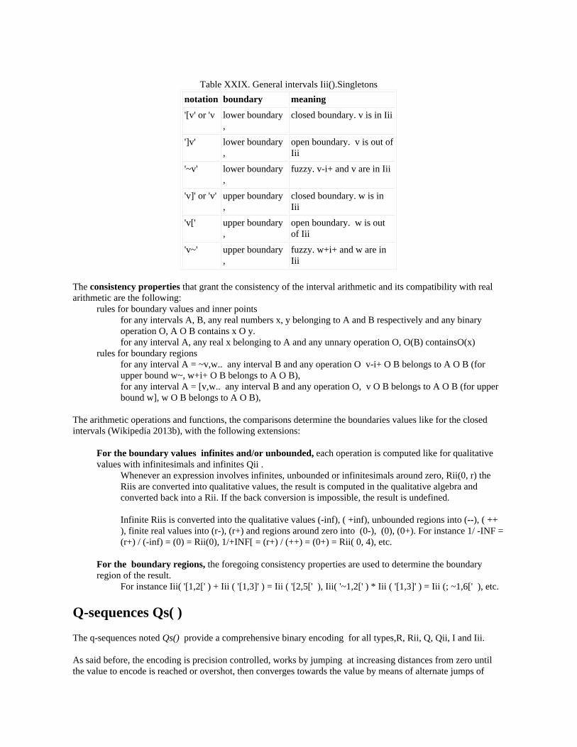
Table XXIX. General intervals Iii().Singletonsnotation boundary meaning

'[v' or 'v lower boundary ,

closed boundary. v is in Iii

']v' lower boundary ,

open boundary. v is out ofIii

'~v' lower boundary ,

fuzzy. v-i+ and v are in Iii

'v]' or 'v' upper boundary ,

closed boundary. w is in Iii

'v[' upper boundary ,

open boundary. w is outof Iii

'v~' upper boundary ,

fuzzy. w+i+ and w are in Iii

The consistency properties that grant the consistency of the interval arithmetic and its compatibility with realarithmetic are the following:

rules for boundary values and inner pointsfor any intervals A, B, any real numbers x, y belonging to A and B respectively and any binaryoperation O, A O B contains x O y.for any interval A, any real x belonging to A and any unnary operation O, O(B) containsO(x)

rules for boundary regionsfor any interval A = ~v,w.. any interval B and any operation O v-i+ O B belongs to A O B (forupper bound w~, w+i+ O B belongs to A O B), for any interval A = [v,w.. any interval B and any operation O, v O B belongs to A O B (for upperbound w], w O B belongs to A O B),

The arithmetic operations and functions, the comparisons determine the boundaries values like for the closedintervals (Wikipedia 2013b), with the following extensions:

For the boundary values infinites and/or unbounded, each operation is computed like for qualitativevalues with infinitesimals and infinites Qii .

Whenever an expression involves infinites, unbounded or infinitesimals around zero, Rii(0, r) theRiis are converted into qualitative values, the result is computed in the qualitative algebra andconverted back into a Rii. If the back conversion is impossible, the result is undefined.

Infinite Riis is converted into the qualitative values (-inf), ( +inf), unbounded regions into (--), ( ++), finite real values into (r-), (r+) and regions around zero into (0-), (0), (0+). For instance 1/ -INF =(r+) / (-inf) = (0) = Rii(0), 1/+INF[ = (r+) / (++) = (0+) = Rii( 0, 4), etc.

For the boundary regions, the foregoing consistency properties are used to determine the boundaryregion of the result.

For instance Iii( '[1,2[' ) + Iii ( '[1,3]' ) = Iii ( '[2,5[' ), Iii( '~1,2[' ) * Iii ( '[1,3]' ) = Iii (; ~1,6[' ), etc.

Q-sequences Qs( )

The q-sequences noted Qs() provide a comprehensive binary encoding for all types,R, Rii, Q, Qii, I and Iii.

As said before, the encoding is precision controlled, works by jumping at increasing distances from zero untilthe value to encode is reached or overshot, then converges towards the value by means of alternate jumps of

decreasing amplitude. The decoding works by reading the qsequence and executing the jumps that are encoded.

The length of the qsequence increases with the precision of encoding, and on average the qsequences areinformation efficient (length ~amount of information necessary to encode a value X at a precision p; proof notgiven). However, the length does not vary continuously as a function of the value and precision. For instance:

Qs(15, 0.1) = {++++=} Qs(15.1, 0.1) = {+++++-------}Qs(15, 0.001) = {++++=} Qs(15.1, 0.001) = {+++++--------++--+}

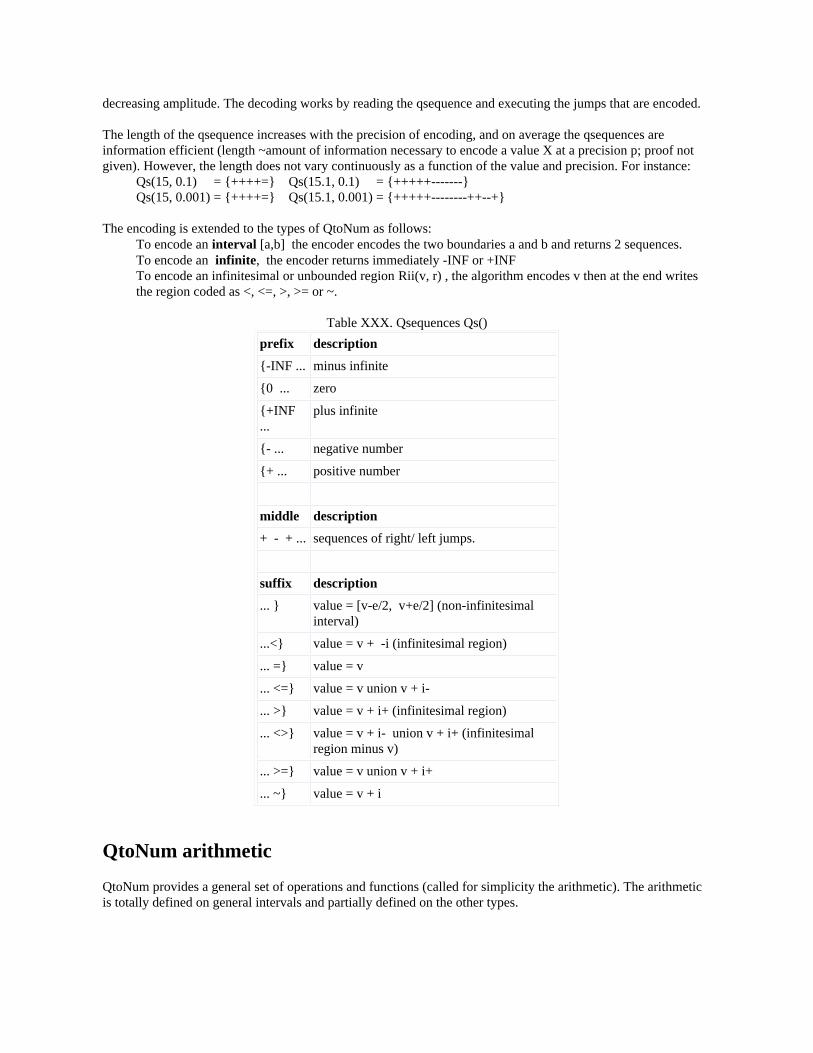
The encoding is extended to the types of QtoNum as follows:To encode an interval [a,b] the encoder encodes the two boundaries a and b and returns 2 sequences.To encode an infinite, the encoder returns immediately -INF or +INFTo encode an infinitesimal or unbounded region Rii(v, r) , the algorithm encodes v then at the end writes the region coded as <, <=, >, >= or ~.

Table XXX. Qsequences Qs()prefix description

{-INF ... minus infinite

{0 ... zero

{+INF ...

plus infinite

{- ... negative number

{+ ... positive number

middle description

+ - + ... sequences of right/ left jumps.

suffix description

... } value = [v-e/2, v+e/2] (non-infinitesimalinterval)

...<} value = v + -i (infinitesimal region)

... =} value = v

... <=} value = v union v + i-

... >} value = v + i+ (infinitesimal region)

... <>} value = v + i- union v + i+ (infinitesimalregion minus v)

... >=} value = v union v + i+

... ~} value = v + i

QtoNum arithmetic

QtoNum provides a general set of operations and functions (called for simplicity the arithmetic). The arithmeticis totally defined on general intervals and partially defined on the other types.

Table XXXI. Operations and functionsextendedoperation

common equivalentnotation

description

abs ( x ) absolute value

add( x, y ) x + y sum

and( x, y ) intersection (set operation)

ceil( x ) ceil integer, i.e. integer immediately larger

dif( x, y ) x - y difference (set operation)

div( x, y ) x / y division (real division)

fdiv( x, y ) x div y floor division (returns integer immediately below x/y)

floor( x ) floor integer, i.e., integer immediately lower

xinv( x ) 1 / x inverse

max( x, y ) maximum

min( x, y ) minimum

mod( x, y ) x % y modulo

mul( x, y ) x * y product

neg( x ) - x opposite

not( x ) complement (set operation).

or( x ) union (set operation)

pos( x ) + x positive x (x itself)

xor( x, y ) exclusive or, i.e. union minus intersection

miscellaneous equivalent inexpressions

description

rand( x ) returns a random real number in x

span( x ) len( ) span (length) of a set (real number, or zero, 0+, r+ ++, +inf)

str( x, format=..) returns a string representing number x. To override default format, use argument, e.g., format="%.2f"

type( x ) returns the type identifier (string). For builtin: 'int', 'mpq' etc. ForQtoNum: calculus module, 'qc', 'rc'....

extendedcomparison

equivalent inexpressions

description

eq( x, y ) x == y

ge( x, y ) x >= y

gt ( x, y ) x > y

in( x, y ) true iff x included in y.

le( x, y ) x <= y

lt( x, y ) x < y

nz( x ) true iff x does not contain zero

ok( x ) true iff x is defined

Connexity

The arithmetic can be executed in two modes, connex or not. In the connex mode, the result of some operation isreplaced by the smallest set that contains it. Connexity is necessary to grant completeness (see below).

Connexity is meaningless for numbers, but of interest for qualitative values and intervals. For instance Q( -1 or 1) = (-,0,+) because the exact result is ('-', '+') which would not be connex. 1/[0,0] is ] is the general interval[-INF, +INF] because the exact result is (-INF or +INF) which would not be connex.

Consistency and completeness

Indeed, the result of some operations is undefined in some specific types, e.g., 1/0 is undefined for realnumbers, qualitative values. However, QtoNum is complete and consistent, i.e., all the operations are defined atleast in one representation (the general intervals) and whenever it is defined the result of an operation is the samein any representation.

The consistency and completeness of QtoNum are immediate consequences of the connexity and of the foregoing propertiesof mappings an operations (presented here without proof).

Representations and mappings

The quantities to represent are (isomorphic to) sets of real and hyperreal numbers. Let X be their domain.

Let T = {T1..Tk} be the types of QtoNum, each type is a set of digital values (digital representations of realnumbers, qualitative values, intervals, etc.). Each type is provided with an inclusion relationship that is a partialorder (for instance for real numbers, it is degenerated: a real r included only in itself) We assume that:

there exist mappings called representations (total or partial, N x M ) between X and each Ti, and betweeneach pair of Tj, Tj . the uniqueness of the minimal representations, i.e., each non-empty ti*(x) contains one single minimalelement for the inclusion.the idempotence of the representations, i.e., ti(ti(x) ) = x (a value of type Ti represents itself).the embedding of the representations . tj( ti(x ) ) = tj( x ) whenever these quantities are defined.

We assume without formal proof the existence of the hierarchy (partial order) of types

Ti <= Tj iff 1) whenever ti(x) is defined, tj(ti(x)) = tj(x) (in other terms, any quantity that can berepresented as ti can be represented as tj and there is no loss of information in conversion from ti to tj)

Operations

The operations O (binary) and the functions F (unary) are defined separately on each set Ti (as oi and firespectively), and we assume that the operations, functions and the representations verify:

the inclusion of the operations and functionstj( ti( x ) oi ti ( y ) ) is contained in tj(ti(x) ) oj tj(ti(y) ) tj( fi( ti(x) ) ) is contained in fj( tj(ti(x) ) ) whenever these quantities are defined

the definition of the operations for any x and y and o there exist a type Ti so that ti(x) oi ti( y ) is defined.for any x and f there exist a type Ti so that fi( ti( x ) ) is defined

Conversion algorithm

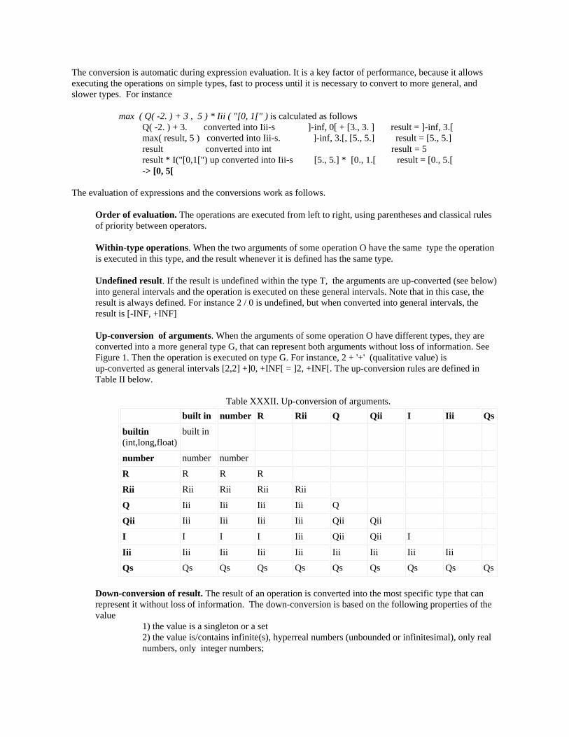
The conversion is automatic during expression evaluation. It is a key factor of performance, because it allowsexecuting the operations on simple types, fast to process until it is necessary to convert to more general, andslower types. For instance

max ( Q( -2. ) + 3 , 5 ) * Iii ( "[0, 1[" ) is calculated as followsQ( -2. ) + 3. converted into Iii-s ]-inf, 0[ + [3., 3. ] result = ]-inf, 3.[max( result, 5 ) converted into Iii-s. ]-inf, 3.[, [5., 5.] result = [5., 5.]result converted into int result = 5result * I("[0,1[") up converted into Iii-s [5., 5.] * [0., 1.[ result = [0., 5.[-> [0, 5[

The evaluation of expressions and the conversions work as follows.

Order of evaluation. The operations are executed from left to right, using parentheses and classical rulesof priority between operators.

Within-type operations. When the two arguments of some operation O have the same type the operationis executed in this type, and the result whenever it is defined has the same type.

Undefined result. If the result is undefined within the type T, the arguments are up-converted (see below)into general intervals and the operation is executed on these general intervals. Note that in this case, theresult is always defined. For instance 2 / 0 is undefined, but when converted into general intervals, theresult is [-INF, +INF]

Up-conversion of arguments. When the arguments of some operation O have different types, they areconverted into a more general type G, that can represent both arguments without loss of information. SeeFigure 1. Then the operation is executed on type G. For instance, 2 + '+' (qualitative value) isup-converted as general intervals [2,2] +]0, +INF[ = ]2, +INF[. The up-conversion rules are defined inTable II below.

Table XXXII. Up-conversion of arguments.built in number R Rii Q Qii I Iii Qs

builtin (int,long,float)

built in

number number number

R R R R

Rii Rii Rii Rii Rii

Q Iii Iii Iii Iii Q

Qii Iii Iii Iii Iii Qii Qii

I I I I Iii Qii Qii I

Iii Iii Iii Iii Iii Iii Iii Iii Iii

Qs Qs Qs Qs Qs Qs Qs Qs Qs Qs

Down-conversion of result. The result of an operation is converted into the most specific type that canrepresent it without loss of information. The down-conversion is based on the following properties of thevalue

1) the value is a singleton or a set2) the value is/contains infinite(s), hyperreal numbers (unbounded or infinitesimal), only realnumbers, only integer numbers;

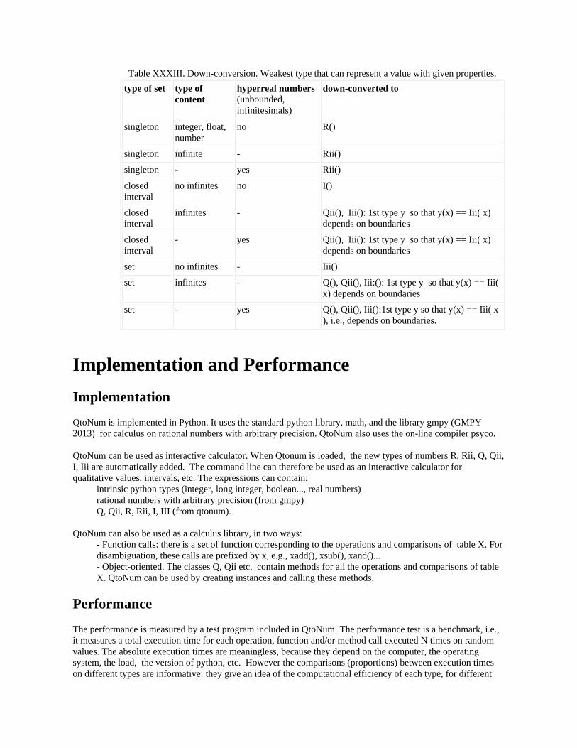
Table XXXIII. Down-conversion. Weakest type that can represent a value with given properties.type of set type of

contenthyperreal numbers (unbounded, infinitesimals)

down-converted to

singleton integer, float, number

no R()

singleton infinite - Rii()

singleton - yes Rii()

closed interval

no infinites no I()

closed interval

infinites - Qii(), Iii(): 1st type y so that y(x) == Iii( x)depends on boundaries

closed interval

- yes Qii(), Iii(): 1st type y so that y(x) == Iii( x)depends on boundaries

set no infinites - Iii()

set infinites - Q(), Qii(), Iii:(): 1st type y so that y(x) == Iii(x) depends on boundaries

set - yes Q(), Qii(), Iii():1st type y so that y(x) == Iii( x), i.e., depends on boundaries.

Implementation and PerformanceImplementation

QtoNum is implemented in Python. It uses the standard python library, math, and the library gmpy (GMPY2013) for calculus on rational numbers with arbitrary precision. QtoNum also uses the on-line compiler psyco.

QtoNum can be used as interactive calculator. When Qtonum is loaded, the new types of numbers R, Rii, Q, Qii,I, Iii are automatically added. The command line can therefore be used as an interactive calculator forqualitative values, intervals, etc. The expressions can contain:

intrinsic python types (integer, long integer, boolean..., real numbers) rational numbers with arbitrary precision (from gmpy)Q, Qii, R, Rii, I, III (from qtonum).

QtoNum can also be used as a calculus library, in two ways:- Function calls: there is a set of function corresponding to the operations and comparisons of table X. Fordisambiguation, these calls are prefixed by x, e.g., xadd(), xsub(), xand()... - Object-oriented. The classes Q, Qii etc. contain methods for all the operations and comparisons of tableX. QtoNum can be used by creating instances and calling these methods.

Performance

The performance is measured by a test program included in QtoNum. The performance test is a benchmark, i.e.,it measures a total execution time for each operation, function and/or method call executed N times on randomvalues. The absolute execution times are meaningless, because they depend on the computer, the operatingsystem, the load, the version of python, etc. However the comparisons (proportions) between execution timeson different types are informative: they give an idea of the computational efficiency of each type, for different

categories of operations.

Implementation note. The benchmark test is part of the complete test suite used to check each new versionof QtoNum. The test program is part of the library and can be executed by the user at any time.

The measurements are executed without the psyco on-line compiler (which falsifies the results by compiling thebits of code that are repeated), then with psyco (closer to performance in normal conditions).

Types of numbers. The measurements are executed on the following typesfloating point numbers (float, python type), rational numbers with arbitrary precision (mpq, type of the library gmpy), qualitative values q and qii, real numbers r and rii, intervals i and iii (from QtoNum). qsequences qs (converted into/from general intervals)under the form of object-oriented calls, Q Qii, R, Rii, I Iii

Operations. The measurements are executed for each type on the following operationsarithmetic (unary and binary) operations, boolean operations (see table X).comparisons, grouped together (table X).encoding/ decoding into qsequencescasting, up-conversion (automatic, and forced) and down-conversion (automatic)void operations (pass); indicative of the time to transfer the arguments and results between memory andprocessor.

Repetitions. For each combination of operation-type, there are 1000 repetitions on random values (5000 for thecombinations too fast to be measured precisely, e.g., sum of floating points).

Average. For each combination type-operation, the execution time is obtained by dividing the measuredexecution time by the number of repetitions. This average includes the Then the average overhead (executiontime of the test program) is removed.

Undefined operations. The proportion of undefined operations (exceptions) on the repetitions is also noted (e.g.,5.9% for division and modulo; 100% of exceptions for boolean operations on python floating point numbers).The undefined combinations operation-type (100% of exceptions) are removed from the table.

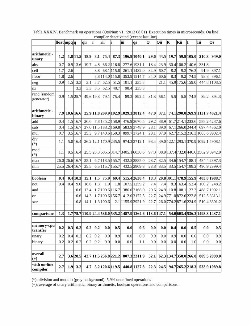
Table XXXIV. Benchmark on operations (QtoNum v1, r2013 08 01) Execution times in microseconds. On linecompiler deactivated (except last line)

float mpq q qii r rii i iii qs Q Qii R Rii I Iii Qs

arithmetic - unary 1.2 1.8 11.5 18.9 8.1 75.4 87.3 196.9 1040.1 29.6 44.5 19.7 59.9 105.0 210.3 949.0

abs 0.7 0.9 13.6 19.7 4.8 66.2 116.8 277.6 1931.1 18.4 23.9 30.4 100.2 140.6 331.8ceil 1.7 2.6 8.8 68.1 115.8 261.1 1432.0 34.9 60.7 8.2 9.2 76.3 91.9 897.1floor 1.8 2.6 8.8 114.0 115.8 353.9 1514.7 34.0 60.6 8.3 9.2 74.5 93.8 896.1neg 0.9 1.5 3.3 3.1 3.7 62.5 51.5 101.1 235.3 21.1 45.9 175.6 159.0 444.8 1108.5nz 3.3 3.3 3.5 62.5 48.7 98.4 235.3rand (random generator) 0.9 1.5 25.7 49.6 19.3 79.1 75.4 89.2 892.4 31.3 56.1 5.5 5.5 74.5 89.2 894.3

arithmetic - binary 7.9 10.6 16.6 25.9 11.8 209.9 192.9 1029.3 3812.4 47.0 37.1 74.1 290.0 269.9 1131.7 4021.4

add 0.4 1.5 16.7 26.6 7.8 135.2 158.9 476.9 3676.5 29.2 38.9 61.7 214.1 233.6 588.2 4237.6sub 0.4 1.5 16.7 27.0 11.5 188.2 169.8 583.9 3748.9 28.1 39.0 67.1 266.0 244.4 697.4 4362.0mul 0.7 3.5 16.7 25.3 9.7 140.6 150.3 899.7 3724.1 28.1 37.9 62.7 215.2 216.3 1005.6 3902.4div (*) 1.1 5.0 16.4 26.2 12.1 170.9 245.5 974.3 3712.1 98.4 39.0 122.1 293.1 370.9 1092.1 4908.1

mod (*) 1.1 9.5 16.4 25.5 28.3 605.5 314.7 3405.1 6030.5 97.3 38.9 137.4 732.0 446.6 3562.9 5942.9

max 26.0 26.6 16.7 25.1 6.7 113.5 155.7 432.5 2885.0 23.7 32.5 34.6 154.7 188.1 484.4 2397.3min 25.5 26.4 16.7 25.5 6.5 115.7 155.7 432.5 2909.8 23.8 33.5 33.5 154.7 189.2 490.9 2399.4

boolean 0.4 0.4 10.3 15.1 1.5 75.9 69.4 515.4 2630.4 18.3 20.8 391.1 478.9 155.9 403.0 1988.7not 0.4 0.4 9.0 18.6 1.3 1.9 1.8 107.5 1259.2 7.4 7.4 8.3 63.4 52.4 100.2 248.2and 10.6 13.4 1.7 100.6 116.7 386.0 2168.0 20.6 24.9 10.8 108.1 123.3 488.7 1092.1or 10.6 14.3 1.7 100.6 156.7 412.0 3172.5 22.7 24.9 771.0 872.6 222.8 512.5 3313.1xor 10.8 14.1 1.3 100.6 2.1 1155.9 3921.9 22.7 26.0 774.2 871.6 224.9 510.4 3301.2

comparisons 1.3 1.7 75.7 110.9 24.4 586.0 535.2 1487.9 1364.6 113.6 147.1 54.0 603.4 536.3 1493.3 1437.1

memory-cputransfer 0.2 0.3 0.2 0.2 0.2 0.0 0.5 0.0 0.6 0.0 0.0 0.4 0.0 0.5 0.0 0.5

unary 0.2 0.4 0.2 0.2 0.2 0.0 0.9 0.0 0.0 0.0 0.0 0.9 0.0 0.0 0.0 0.9binary 0.2 0.2 0.2 0.2 0.2 0.0 0.0 0.0 1.1 0.0 0.0 0.0 0.0 1.0 0.0 0.0

overall (+) 2.7 3.6 28.5 42.7 11.5 236.8 221.2 807.3 2211.9 52.1 62.3 134.7 358.0 266.8 809.5 2099.0

with on-line compiler 2.7 1.9 3.2 4.7 5.2 120.6 119.5 440.8 1127.8 22.3 24.5 94.7 265.2 218.3 533.9 1089.8

(*): division and modulo (grey background): 5.9% undefined operations(+): average of unary arithmetic, binary arithmetic, boolean operations and comparisons.

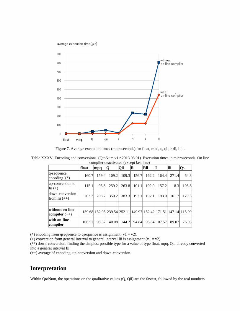
Figure 7. Average execution times (microseconds) for float, mpq, q, qii, r rii, i iii.

Table XXXV. Encoding and conversions. (QtoNum v1 r 2013 08 01) Execution times in microseconds. On linecompiler deactivated (except last line)

float mpq Q Qii R Rii I Iii Qsq-sequenceencoding (*) 160.7 159.4 109.2 109.3 156.7 162.2 164.4 271.4 64.8

up-conversion to Iii (+) 115.1 95.8 259.2 263.8 101.1 102.9 157.2 8.3 103.8

down-conversion from Iii (++) 203.3 203.7 350.2 383.3 192.1 192.1 193.0 161.7 179.3

without on-line compiler (++) 159.68 152.95 239.54 252.11 149.97 152.42 171.51 147.14 115.99

with on-line compiler 106.57 98.37 140.08 144.2 94.84 95.84 107.57 89.07 76.03

(*) encoding from qsequence to qsequence is assignment (v1 = v2).(+) conversion from general interval to general interval Iii is assignment (v1 = v2)(**) down-conversion: finding the simplest possible type for a value of type float, mpq, Q... already convertedinto a general interval Iii.(++) average of encoding, up-conversion and down-conversion.

Interpretation

Within QtoNum, the operations on the qualitative values (Q, Qii) are the fastest, followed by the real numbers

(R). Real numbers with infinites and infinitesimal regions (Rii)and closed intervals (I) present similar executiontimes. The general intervals (Iii) are the slowest. This is compatible with a coarse algorithm analysis of theoperations in each type (not presented here).

As expected computations are faster for intrinsic float type and for the rationals with arbitrary precision mpq(library gmpy) than for QtoNum types. However it is noteworthy that the differences are markedly reduced withthe on-line computer, at least for the fast QtoNum types (qualitative values and real numbers).

Conversions (up-conversions and down-conversions) are on average close from the execution time of singleoperations in the 'slow' QtoNum types (Rii, intervals). This tends to support the principle of automaticconversion, which keeps working on the fast types as long as possible and converts into stronger, slower typesonly when this is necessary.

Finally, when using QtoNum as a calculus library, it is noteworthy that the command line operations (and thedirect function calls), i.e., the procedural calls are markedly faster than the object-oriented (methods) calls.

Concluding notesBe precise or imprecise, but always accurate

This is the rationale of QtoNum. In general, the more precise the representation of some quantity is, the moreinformation it brings. However, precision has a cost in terms of measurement, memory storage, transmissiontime and computation time.

In addition, in complex systems, accuracy and precision are mutually exclusive as stated by the Principle ofIncompatibility (Zadeh, 1973). In other terms, the excess of precision introduces inaccuracy. Over-precisiondestroys information because inaccurate representations tell little about the original quantity. Besides,over-precision is a form of deception: precise data look trustable but they are not.

For practical reasons, or simply for honesty, it is important to select adequately the level of precision of therepresentation. The precision should be maximal within the cost constraints, but over-precision should beavoided at any price.

The contribution of QtoNum

Publishing QtoNum is the end of a personal cycle. It may be a useful tool for you, reader, and so I wish. For me,it is a modest contribution to the decontamination of scientific communication, namely a mean to avoid numerical lies.

When I started to study Neuroscience, I realized how relevant Zadeh's Principle of Incompatibility was (Zadeh, 1973, p.28): "As the complexity of a system increases our ability to make precise yet relevantstatements about its behaviour diminishes until a threshold is reached beyond which precision and significance(or relevance) become almost mutually exclusive characteristics". The brain and its multiple levels oforganization, their interactions and their bidirectional relation with the behavior are complex , and this is anunderstatement.

Nonetheless, I was bemused by the ubiquitous use of precise numbers in behavioral and brain sciences. A typicalresearch article presents 1) experimental data as numbers, 2) numerical data processing (statistics, quantitativemodelling), 3) qualitative interpretations and conclusions, as statements in natural language. Even if theconclusions are voluntarily imprecise (compliant with the Principle of Incompatibility), they are too often drawnfrom over-precise results (too precise, therefore inaccurate) and the chain of scientific evidence is broken.Worse, some scientific papers were numerical propaganda, presenting dogmas and opinions as logical

consequences of over-precise results.

Between qualitative simulations, doomed to imprecision by their accuracy, and over-precise results doomed tospuriousness, QtoNum may provide a compromise. Note that QtoNum is by no means unique, intervalarithmetic, fuzzy models and in general soft computing tools are aimed at the same objective. In moral terms,QtoNum and other soft computing tools may help scientists and engineers to remain honest.

Apparent precision is more important than Accuracy incontemporaneous science

I have no illusions about the use of QtoNum and other imprecise tools among researchers. QtoNum is only acalculus library whereas researchers need complete analysis tools. Using QtoNum beyond toy models andpreliminary data exploration requires programming analysis tools with the QtoNum library. This requires time,computer skills and effort. This is justified only if the results are qualitatively better with QtoNum than withoutit.

However, beyond practical barriers, the main problem is that sacrificing precision to gain accuracy is not apopular idea among researchers. In contemporaneous science, the pressure is set to produce precise quantitativeresults. There exist handy and powerful computer tools that offer increasingly subtle and complex dataprocessing methods, far beyond the understanding of the average researcher. What if these complex methods arerunning on inaccurate data? Answer: over-precise results, no expertise to detect over-precision and no sufficientbackground to interpret correctly the results. In other terms, spurious results.

However, the researcher that wants to be published can generally 'forget' this issue, because the reviewers aremore interested in positive results than in negative, methodological limitations. From times to times amethodological paper, serious and/or provocative, e.g., the "dead salmon brain activity" (Bennett, et al. 2009)rocks the boat, but this does not affect the general trend towards precise quantitative results. The accuracy is lostsomewhere on the path.

This scientific trend lead to spuriousness, over-interpretation (exceeding the validity and scope of the results)and in the worst case scientific propaganda and false science, in which the 'researchers' and/or their sponsorssupport beliefs, dogma and manipulations by means of 'scientific evidence'. The only barrier against are thepersonal scientific values, namely the seriousness, cautiousness and honesty of the researchers.

ReferencesBennett, C.M., Baird, A.A., Miller, M.B., Wolford, G.L. (2009) Neural correlates of interspecies perspectivetaking in the post-mortem Atlantic Salmon: An argument for multiple comparisons correction. Neuromage 47.1:S125.

Churchland, P. Sejnovsky, T. (1992). The Computational Brain. Bradford Books..

de Kleer, J., Brown, S. (1984) "A Qualitative Physics Based on Confluences". Artificial Intelligence 24 pp.7-83.

Fimbel, E. (2002). An algebra for qualitative modeling. Technical report RT020205, Département de génieélectrique, École de Technologie Supérieure. 19 p.

Fimbel, E. (2002b). Qualitative comparisons. Technical report RT020206, Département de génie électrique,École de Technologie Supérieure. 19 p.

GMPY (2013). Multiple precision arithmetic for Python at https://code.google.com/p/gmpy/. Last consulted2013 08 05.

Glass, L. (1975) Classification of Biological Networks by their Qualitative Dynamics. J. Theoretical Biol. 54pp.85-107.

Keisler, H.J. (1994) The hyppereal line. In Real Numbers, Generalizations of the Reals, and Theories ofContinua, ed. by P. Erlich, Kluwer Academic Publishers, pp. 207-237.

Moore, R.E. & Yang, C.T. (1959) Interval Analysis 1 - technical document LMSD-285875. Lookheed AircraftCorporation, Missiles and Space Division.

Robinson, A. (1974) Non Standard Analysis. Princeton Univ. Press (Reissued paperback 1996, ISBN0-691-04490-2

Wikipedia (2013a). Hyperreal Numbers at http://en.wikipedia.org/wiki/Hyperreal_number. Last consulted 201308 05.

Wikipedia (2013b). Interval Arithmetic at http://en.wikipedia.org/wiki/Interval_arithmetic. Last consulted 201308 05.

Zadeh, L.A. (1973) Outline of a New Approach to the Analysis of Complex Systems and Decision Processes.IEEE Transactions on Systems, man and Cybernetics, SMC 3(1), 28:44.