Python for Control purposes

Requirements• Linux machine. For better performances in RT a kernel with preempt-rt patch can be useful, but

not mandatory (better latencies in RT!)

• Python 2.7

◦ numpy

◦ scipy

◦ slycot

◦ control toolbox (R. Murray)

◦ python-qt4 and python-qt4-dev

• pyControlDistro.tgz

Install the SUPSI control packagesOpen a shell and then run

• tar xvfz pyControlDistro.tgz

• Follow the README file to install all the SUPSI packages

Install gEDAschemgEDA schem is a open source tool which can be used to draw electronics schemes. It has been modified my adding some blocks required for control purposes (input, output, linear systems, non linear blocks etc.

The followin ackages are required for gEDA package:

• geda

• geda-doc

• geda-gattrib

• geda-gnetlist

• geda-gschem

• geda-gsymcheck

• geda-symbols

• geda-utils

HardwareIn SUPSI we made the choice to use the CAN bus as general system for our plants in laboratory. In

particular we have different plants based on Maxon motors. COMEDI clock are also provided to accessa great number of acquisition cards.

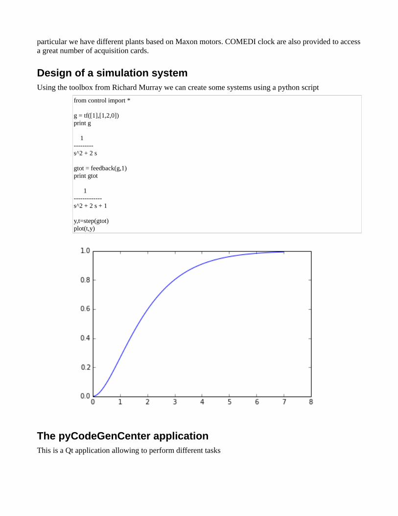
Design of a simulation systemUsing the toolbox from Richard Murray we can create some systems using a python script

from control import *

g = tf([1],[1,2,0])print g

1---------s^2 + 2 s

gtot = feedback(g,1)print gtot

1-------------s^2 + 2 s + 1

y,t=step(gtot)plot(t,y)

The pyCodeGenCenter applicationThis is a Qt application allowing to perform different tasks

Under the menu “SCH → PY” we have the following choices

1. open geda schem: open the gEDA schem application (if a sch is defined it will be open)2. open geda attrib: allows changing the parameters of the block diagram using the pyAttrib

application3. Code generation: generate the code starting from the schematic and the python initialisation

script4. run: launch the generated executable (using the pySim application)5. stop: stop the “run” and if possible, plot the results

Under the menu “File” we have the following choices1. Open CGF file: Open a predefined configuration for the pyCodegen application (extension

“.cgf”)2. Save CGF file: Save the defined configuration3. Open python script: Open a python script into the editor window4. Save python script: Save the editor window as python script

Creating a block diagraOpen the gEDA editor using the menu “gEDA schem”. It is possible to use the control blocks to create a block diagram as shown in the next figure

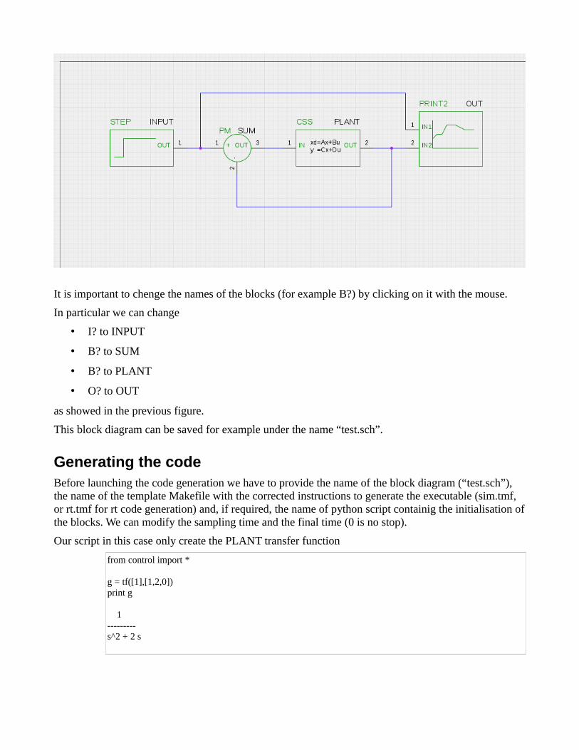
It is important to chenge the names of the blocks (for example B?) by clicking on it with the mouse.

In particular we can change

• I? to INPUT

• B? to SUM

• B? to PLANT

• O? to OUT

as showed in the previous figure.

This block diagram can be saved for example under the name “test.sch”.

Generating the codeBefore launching the code generation we have to provide the name of the block diagram (“test.sch”), the name of the template Makefile with the corrected instructions to generate the executable (sim.tmf, or rt.tmf for rt code generation) and, if required, the name of python script containig the initialisation ofthe blocks. We can modify the sampling time and the final time (0 is no stop).

Our script in this case only create the PLANT transfer function

from control import *

g = tf([1],[1,2,0])print g

1---------s^2 + 2 s

Now we are ready to launch the command “Code Generation” (translate the block diagram first into RCPBlocks, and then generate C-code from the block sequence). This command fills the editor windowwith a python script performing the initialisation and the required commands for code generation.

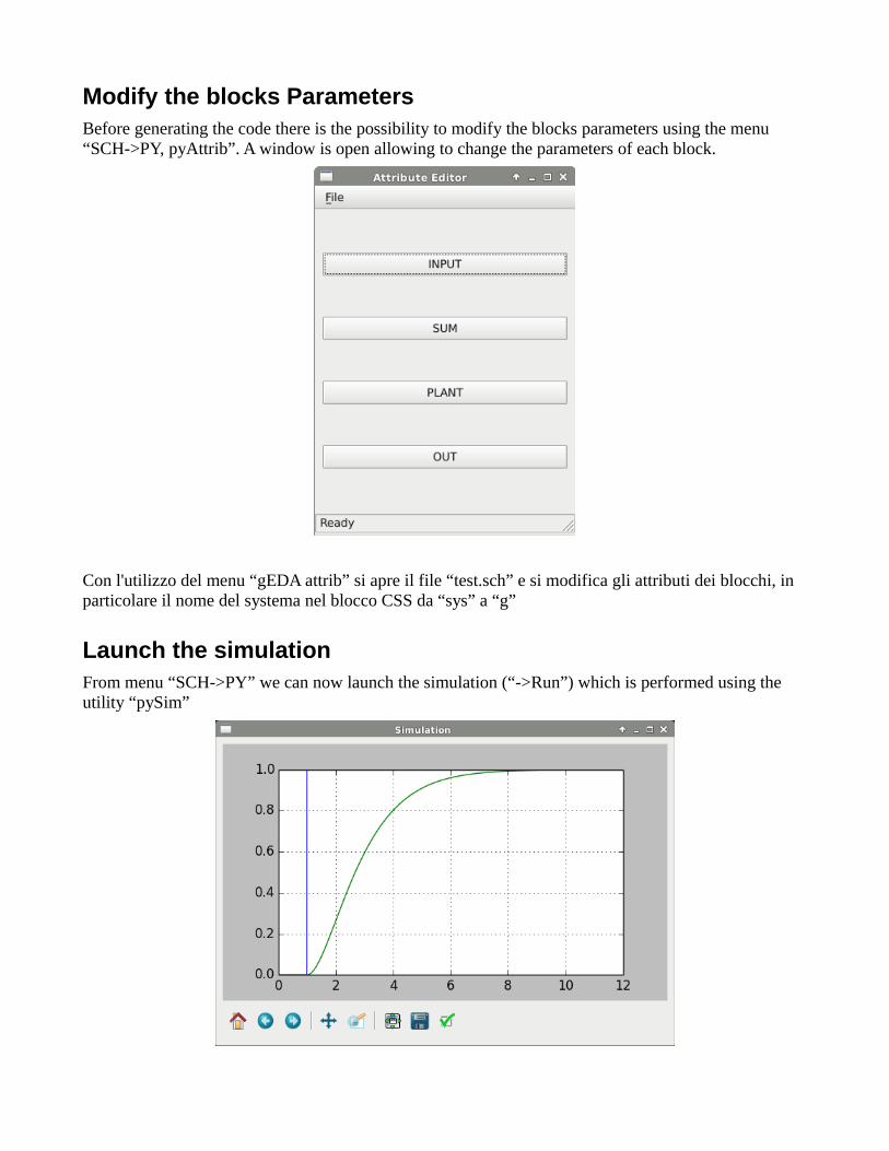
Modify the blocks ParametersBefore generating the code there is the possibility to modify the blocks parameters using the menu “SCH->PY, pyAttrib”. A window is open allowing to change the parameters of each block.

Con l'utilizzo del menu “gEDA attrib” si apre il file “test.sch” e si modifica gli attributi dei blocchi, in particolare il nome del systema nel blocco CSS da “sys” a “g”

Launch the simulationFrom menu “SCH->PY” we can now launch the simulation (“->Run”) which is performed using the utility “pySim”

A RT system

The plant

This plant is used in SUPSI to teach State feedback control of MIMO systems. The idea is to move the disk on the right using the motor on the left. The two disks are connected through a spring.

Control of the plant

The design of the controller is perfomed using the Control System Toolbox from Richard Murray and additional functions developed at SUPSI (saved as “disks.py”).

from supsictrl.yottalab import *

from scipy import zeros

import numpy as np

import scipy as sp

import matplotlib.pyplot as plt

import matplotlib.image as mpimg

from control import *

from control.matlab import *

# Plant

img = mpimg.imread('disks.jpg')

plt.imshow(img)

show()

# Motore 1

jm1 = 0.0000085 # inerzia [kg*m2]

kt1 = 0.0000382 # constante di coppia [Nm/mA] per la centralina al posto di [Nm/A]

# Volano motore 1

rho_ac = 7900 # densita alluminio [g/m3]

rv1 = 0.065 # raggio [m]

hv1 = 0.01 # spessore [m]

mv1 = ((rho_ac*(rv1**2))*np.pi)*hv1 # massa [kg]

jv1 = (mv1*(rv1**2))/2 # inerzia [kg*m2]

theta1 = jv1+jm1 # inerzia totale [kg*m2]

# Motore 2

jm2 = 0.000003 # inerzia [kg*m2]

kt2 = 0.0000205 # constante di coppia [Nm/mA] per la centralina al posto di [Nm/A]

# Volano motore 2

rho_ac = 7900 # densita acciao [kg/m3]

rv2 = 0.065 # raggio [m]

hv2 = 0.01 # spessore [m]

mv2 = ((rho_ac*(rv2**2))*np.pi)*hv2 # massa [kg]

jv2 = (mv2*(rv2**2))/2 # inerzia [kg*m2]

theta2 = jv2+jm2 # inerzia totale [km*m2]

# Molla (frequenza d''oscillazione di 2 Hz)

d = 0.0027836 # attrito molla (smorzamento)

c = 0.4797954

d1 = 0.0002953

d2 = 0.0004001

# Plant in SS form

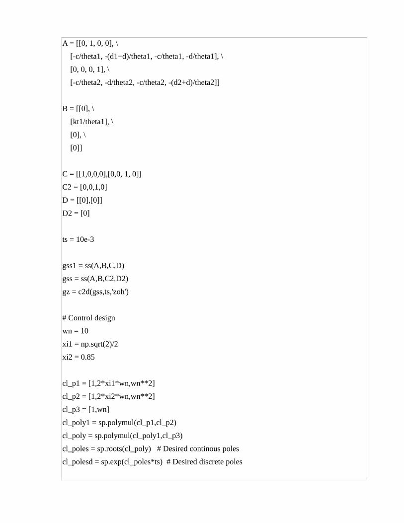
A = [[0, 1, 0, 0], \

[-c/theta1, -(d1+d)/theta1, -c/theta1, -d/theta1], \

[0, 0, 0, 1], \

[-c/theta2, -d/theta2, -c/theta2, -(d2+d)/theta2]]

B = [[0], \

[kt1/theta1], \

[0], \

[0]]

C = [[1,0,0,0],[0,0, 1, 0]]

C2 = [0,0,1,0]

D = [[0],[0]]

D2 = [0]

ts = 10e-3

gss1 = ss(A,B,C,D)

gss = ss(A,B,C2,D2)

gz = c2d(gss,ts,'zoh')

# Control design

wn = 10

xi1 = np.sqrt(2)/2

xi2 = 0.85

cl_p1 = [1,2*xi1*wn,wn**2]

cl_p2 = [1,2*xi2*wn,wn**2]

cl_p3 = [1,wn]

cl_poly1 = sp.polymul(cl_p1,cl_p2)

cl_poly = sp.polymul(cl_poly1,cl_p3)

cl_poles = sp.roots(cl_poly) # Desired continous poles

cl_polesd = sp.exp(cl_poles*ts) # Desired discrete poles

# Add discrete integrator for steady state zero error

Phi_f = np.vstack((gz.A,-gz.C*ts))

Phi_f = np.hstack((Phi_f,[[0],[0],[0],[0],[1]]))

G_f = np.vstack((gz.B,zeros((1,1))))

# Pole placement

k = placep(Phi_f,G_f,cl_polesd)

# Observer design - reduced order observer

poli_o = 5*cl_poles[0:2]

poli_oz = sp.exp(poli_o*ts)

disks = ss(A,B,C,D)

disksz = StateSpace(gz.A,gz.B,C,D,ts)

T = [[0,1,0,0],[0,0,0,1]]

r_obs = red_obs(disksz ,T, poli_oz)

# Controller and observer in the same matrix - Compact form

contr_I = comp_form_i(disksz,r_obs,k,ts,[0,1])

# Implement anti windup

[gss_in,gss_out] = set_aw(contr_I,[0.1,0.1,0.1])

Simulation

This is the gEDA block diagram for simulation

and this is the pyCodegenCenter window for the simulation

The next figure shows the result of the simulation

RT executable

In order to obtain the RT executable we have to change the block diagram and the template makefile (“rt.tmf”).

About code generationThe translation of the gEDA schematic into C-code is performed in two steps:

1. The gEDA schem is translated into a pspice netlist using the provide gEDA netlist application.

2. The netlist is translated into a RCPblk block, a python class provided by supsictrl.RCPblk usinga a function defined in the same library

The RCPblk class is described as following

class RCPblk:

def __init__(self, *args):

if len(args) == 8:

(fcn,pin,pout,nx,uy,realPar,intPar,str) = args

elif len(args) == 7:

(fcn,pin,pout,nx,uy,realPar,intPar) = args

str=''

else:

raise ValueError("Needs 6 or 7 arguments; received %i." % len(args))

self.fcn = fcn

self.pin = mat(pin)

self.pout = mat(pout)

self.nx = array(nx)

self.uy = array(uy)

self.realPar = array(realPar)

self.intPar = array(intPar)

self.str = str

def __str__(self):

"""String representation of the Block"""

str = "Function : " + self.fcn.__str__() + "\n"

str += "Input ports : " + self.pin.__str__() + "\n"

str += "Outputs ports : " + self.pout.__str__() + "\n"

str += "Nr. of states : " + self.nx.__str__() + "\n"

str += "Relation u->y : " + self.uy.__str__() + "\n"

str += "Real parameters : " + self.realPar.__str__() + "\n"

str += "Integer parameters : " + self.intPar.__str__() + "\n"

str += "String Parameter : " + self.str.__str__() + "\n"

return str

The fields contain all the information nedded to generate the C-Code

• fcn is the name of the function to be called to execute the code associated with the block

• pin is a vector containing the input port identifiers

• pout is a vector containing the output port identifiers

• nx is a vector containg the number of continous and discrete states of the block

• uy is a int value (0 or 1) definig if there is a direct feedforward between input and output

• realPar is a vector containing the real parameters of the block

• intPar is a vector containing the integer parameters of the block

• str is a string parameters

Starting from the blocks list, the function “genCode” first analyze the topology of the schema tin order to find the right sequence of blocks. This first operation fails if algebric loops are found. Otherwise the function continues defining 3 functions:

• Initialization function

• ISR functions

• Terminating function

The generated code can be easily integrated into a RT environment. A “main” for the Linux preempt-rt system is provided. The compiling and link operations are handled by the Template Makefile (provided are “sim.tmf” and “rt.tmf”). For each block, a function is programmed under “Codegen/devices” and the object code is stored into the “libpyblk.a” library.