Proper orthogonal decomposition closure models for fluid flows: Burgers equation

INTERNATIONAL JOURNAL OF c© 2014 Institute for ScientificNUMERICAL ANALYSIS AND MODELING, SERIES B Computing and InformationVolume 5, Number 3, Pages 217–237

PROPER ORTHOGONAL DECOMPOSITION CLOSURE MODELS

FOR FLUID FLOWS: BURGERS EQUATION

OMER SAN AND TRAIAN ILIESCU

Abstract. This paper puts forth several closure models for the proper orthogonal decomposition(POD) reduced order modeling of fluid flows. These new closure models, together with other

standard closure models, are investigated in the numerical simulation of the Burgers equation.

This simplified setting represents just the first step in the investigation of the new closure models.It allows a thorough assessment of the performance of the new models, including a parameter

sensitivity study. Two challenging test problems displaying moving shock waves are chosen in the

numerical investigation. The closure models and a standard Galerkin POD reduced order modelare benchmarked against the fine resolution numerical simulation. Both numerical accuracy and

computational efficiency are used to assess the performance of the models.

Key words. Proper orthogonal decomposition (POD), reduced order models (ROMs), closure

models for POD, Burgers equation, moving shock wave.

1. Introduction

Proper orthogonal decomposition (POD) is one of the most successful reducedorder modeling techniques in dynamical systems. POD has been used to gener-ate reduced order models (ROMs) for the simulation and control of many forced-dissipative nonlinear systems in science and engineering applications [1, 11, 16, 17,23, 27, 31, 34, 36, 47]. POD extracts the most energetic modes in the system, whichare expected to contain the dominant characteristics. The globally supported PODmodes are often constructed from high-fidelity numerical solutions (e.g., using fi-nite difference/element/volume methods) and are problem dependent. For manysystems, it is possible to obtain a good approximation of their dynamics with fewPOD modes. The systems built with these POD modes, called POD reduced or-der models (POD-ROMs) in what follows, are low dimensional and can provide anefficient framework for many applications.

The Galerkin POD-ROM (POD-ROM-G) is the simplest POD-ROM, which re-sults from a Galerkin truncation followed by a projection of the truncated equationonto the space spanned by the POD modes. The POD-ROM-G is an efficient tool formany applications of interest. For fluid flows (see, e.g, [37] and the exquisite surveyin [29]), the POD-ROM-G works well for laminar fluid flows. For turbulent flows,however, the POD-ROM-G yields inaccurate results. As carefully explained in [51],for realistic turbulent flows, the high index POD modes that are not included in thePOD-ROM-G do have a significant effect on the dynamics of the POD-ROM-G. Sev-eral numerical stabilization strategies have been used to address this issue [6,24,44].Building on the analogy with large eddy simulation (LES) [7,42] (see [39] for alter-native approaches), several closure modeling strategies for POD-ROMs of turbulentflows have been proposed over the years [2,3,6,9,13,14,41,50,52,53], starting withthe pioneering work in [1]. The main goal of this report is to propose and nu-merically investigate several closure models for POD-ROMs of fluid flows. Threedifferent classes of closure modeling strategies are considered.

Received by the editors March 3, 2014.

2000 Mathematics Subject Classification. 35R35, 49J40, 60G40.

217

218 O. SAN AND T. ILIESCU

The first strategy provides additional dissipation to the POD-ROM-G to accountfor the small scale dissipation effect of the discarded POD modes. The main ad-vantage of this strategy is that it has a negligibly small computational overhead.Different viscosity kernels for POD-ROMs have been suggested in literature (see,e.g., [6, 44]). In this study, these closure models together with three new closuremodels are presented in a unified framework and their performance is investigated.

The second closure modeling strategy is also of eddy viscosity type. The subgrid-scale operator used to account for the the effects of smaller scales is, however, differ-ent from that employed in the first closure modeling strategy. This closure model-ing approach is inspired from state-of-the-art LES models, such as the Smagorinksymodel [46] or its dynamic counterparts (see, e.g., [19]). The Smagorinsky POD-ROM (POD-ROM-S) has been used in several studies [9,38,49,52,53]. To the bestof our knowledge, the dynamic subgrid-scale POD-ROM was first used in [53]. Inthis study, we investigate the POD-ROM-S together with one new closure model.In general, these nonlinear closure models have a significant computational over-head (as explained in [52]). For the one-dimensional Burgers equation consideredin this study, however, the computational overhead of these two closure models isnegligible.

The third closure modeling strategy that we consider is based on the energyconservation concept. This POD-ROM closure modeling approach was introducedby Cazemier [13] (see also [14]). One of the main advantages of this closure modelis that it does not require the specification of any free parameter, which is in starkcontrast with the closure modeling strategies outlined above. This closure model,however, has a higher computational overhead since it requires the computationof a penalty/drag term. We note, however, that for the one-dimensional Burgersequation considered in this study this computational overhead is negligible.

Overall, there are 10 closure models, both new and current, in the three classesdescribed above. There are numerous other closure modeling strategies for POD-ROM of complex systems (see, e.g., [29, 37, 51]). In general, when these closuremodels are introduced, they are deemed successful if they satisfy the following twocriteria when compared with the fine resolution numerical simulation: (i) the newPOD-ROM is relatively accurate; and (ii) the new POD-ROM has a significant-ly lower computational cost. Given the number of competing closure modelingapproaches, a natural practical question is which closure model should be used.These intercomparison studies are scarce (see, e.g., [53] for an exception). Thisstudy aims at answering the above practical question for the 10 closure modelsconsidered herein.

All the 10 POD-ROM closure models considered in this study are investigatedin the numerical simulation of the Burgers equation. We emphasize again thatthese closure models are developed for POD-ROMs of realistic turbulent flows. Inorder to thoroughly assess their performance, however, as a first step, we considerthe one-dimensional Burgers equation displaying challenging moving shock waves.This simplified setting allows us to carefully assess the performance of the 10 closuremodels considered in this study and also carry out a parameter sensitivity study.Of course, once we get a better understanding of the performance and limitationsof these closure models, we will investigate them in realistic turbulent flow settings,such as those considered in [53]. We also note that this progressive evaluation iscommon in the POD-ROM literature [9,28] or in the turbulence modeling literature[4, 5, 10,18,20,26,33].

PROPER ORTHOGONAL DECOMPOSITION CLOSURE MODELS 219

The paper is organized as follows: The mathematical model and the numericalmethods for both spatial and temporal discretiations are summarized in Section2. The POD-ROM closure models are presented in Section 3. These closure mod-els are tested in Section 4 for two challenging examples displaying moving shockwaves. Finally, Section 5 consists of some concluding remarks and future researchdirections.

2. Mathematical models

2.1. Model equations. All 10 POD-ROM closure models investigated in thisreport are tested on the Burgers equation:

(1)∂u

∂t+ u

∂u

∂x= ν

∂2u

∂x2,

where ν is the viscosity parameter. In this report, we consider two examples withdifferent initial conditions:

Experiment 1: u(x, 0) =

1, if x ∈ [0, 1/2];0, if x ∈ (1/2, 1]

(2)

Experiment 2: u(x, 0) = u0 exp

(−(x− xc)2

σ

), with x ∈ [0, 1] ,(3)

where u0 = 1, xc = 0.3, and σ = 0.005. The homogeneous Drichlet boundaryconditions are applied for all the examples (i.e., u(0, t) = u(1, t) = 0 for t > 0).Similar examples are considered in [9].

2.2. Numerical methods. We provide a brief description of the numerical meth-ods employed in the investigation of the POD-ROM closure models. As benchmarkfor all these closure models we use a direct numerical simulation (DNS) of theBurgers equation given in Eq. (1). In order to minimize the spatial and temporaldiscretization errors in Eq. (1), a sixth-order compact difference and a third-orderRunge-Kutta schemes are used for the spatial and temporal discretizations, respec-tively. This will help to decouple the numerical effects from the POD modelingeffects. In the compact difference scheme, the first derivatives can be computed asfollows [30]:

(4) αf ′i−1 + f ′i + αf ′i+1 = afi+1 − fi−1

2h+ b

fi+2 − fi−2

4h,

which gives rise to an α-family of tridiagonal schemes with a = 23 (α + 2), and

b = 13 (4α − 1). The subscript i represents the spatial index of an arbitrary grid

point in the domain. Here, α = 0 leads to the explicit non-compact fourth-orderscheme for the first derivative. A classical compact fourth-order scheme, which isalso known as the Pade scheme, is obtained by setting α = 1/4. The truncationerror in the Eq. (4) is 4

5! (3α− 1)h4f (5). A sixth-order compact scheme is obtainedby choosing α = 1/3.

The second derivative compact centered scheme is given by

αf ′′i−1 + f ′′i + αf ′′i+1 = afi+1 − 2fi + fi−1

h2+ b

fi+2 − 2fi + fi−2

4h2,(5)

where a = 43 (1 − α), and b = 1

3 (10α − 1). For α = 1/10 the classical fourth-

order Pade scheme is obtained. The truncation error in the Eq. (5) is − 46! (11α −

2)h4f (6). A sixth-order compact scheme is also obtained by choosing α = 2/11. Thehigh-order sided derivative formulas are used for the Drichlet boundary conditions


in order to complete the tridiagonal system of equations for both the first orderderivative and the second order derivative formulas [12,30,43].

A system of semi-discrete ordinary differential equations (ODEs) is obtained afterthe spatial discretization of the Burgers equation. To implement the Runge-Kuttaschemes, we cast the model equation in the following form:

(6)du

dt= £(u) ,

where £(u) is the discrete operator of spatial derivatives including nonlinear convec-tive terms and linear diffusive terms. We assume that the numerical approximationfor time level ` is known, and we seek the numerical approximation for time level` + 1, after the time step ∆t. The optimal third-order accurate total variationdiminishing Runge-Kutta (TVDRK3) scheme [21] is then given as follows:

u(1) = u` + ∆t£(u`)

u(2) =3

4u` +

1

4u(1) +

1

4∆t£(u(1))

u`+1 =1

3u` +

2

3u(2) +

2

3∆t£(u(2)).(7)

We emphasize that we are not using any numerical stabilization to capture theshock in the DNS of the Burgers equation. The dissipation mechanism in DNSis only obtained through the physical viscosity specified in the Burgers equation.Therefore, in order to avoid numerical oscillations near the shock, a high resolutioncomputation (DNS) is performed.

3. Proper orthogonal decomposition (POD) reduced order models

3.1. Computing POD basis functions. A POD can be constructed from thefield variable u at different times (snapshots). In this paper, these snapshots areobtained by solving Eq. (1) using the high-order compact difference scheme outlinedin Section 2.2. In the time marching process, the ith record of the field is denoted byui(x) for i = 1, 2, ..., N , where N is the number of the snapshots used to constructthe POD basis. First, the flow field data are decomposed into the mean part andthe fluctuating part:

(8) u(x, t) = u(x) + u(x, t), u(x) =1

N

N∑i=1

u(x, ti) ,

where u is the mean part (a function of space) and u is the fluctuating part (afunction of space and time). In order to obtain the POD bases functions, we firstbuild a correlation matrix from the snapshots as follows:

(9) Cij =

∫Ω

ui(x)uj(x)dx ,

where Ω is the entire spatial domain and i and j refer to the ith and jth snapshots.The correlation matrix C is a non-negative symmetric N ×N matrix. Defining theinner product of any two fields f and g as

(10) (f, g) =

∫Ω

f(x)g(x)dx ,

Eq. (9) can also be written as Cij = (ui, uj). In this study, we use the well-knowntrapezoidal integration rule for computing the inner products numerically. Solvingthe eigenvalue problem for this C matrix provides the optimal POD basis functions.


This has been shown in detail in the POD literature (see, e.g., [22, 40, 45]). Theeigenvalue problem can be written in the following form:

(11) CW = WΛ ,

where Λ = diag[λ1, λ2, ..., λN ], W = [w1, w2, ..., wN ], λi is the ith eigenvalue andwi is the corresponding ith eigenvector. The eigenvalues are stored in descendingorder, λ1 ≥ λ2 ≥ ... ≥ λN . The POD basis functions can be written as

(12) φ1(x) =N∑i=1

w1i ui(x), φ2(x) =

N∑i=1

w2i ui(x), ..., φN (x) =

N∑i=1

wNi ui(x) ,

where wji is the ith component of eigenvector wj . The eigenvectors must be nor-malized in such a way that the basis functions satisfy the following orthogonalitycondition:

(13) (φk, φl) =

1, k = l0, k 6= l .

It can be shown that, for Eq. (13) to be true, the eigenvector wj must satisfy thefollowing equation [16]:

(14)N∑i=1

wjiwji =

1

λj.

In practice, most of the subroutines for solving the eigensystem given in Eq. (11)return the eigenvector matrix W having all the eigenvectors normalized to unity.In that case, the orthogonal POD bases can be obtained as

(15) φj(x) =1√λj

N∑i=1

wji ui(x)

where φj(x) is the jth POD basis function.

3.2. Galerkin projection for reduced order models. These POD basis func-tions account for the essential dynamics of the system. To build a ROM, we truncatethe system by considering the first R POD basis functions with R N . These firstR POD modes correspond to the R largest eigenvalues, λ1, λ2, ..., λR. Using thesefirst R POD basis functions the field variables can be approximated as follows:

(16) u(x, t) =R∑k=1

ak(t)φk(x) ,

where ak are the time dependent coefficients, and φk are the space dependent modes.To derive the POD-ROM, we first rewrite the Burgers equation (i.e., Eq. (1)) as

(17)∂u

∂t= νL[u] +N [u;u] ,

where for f and g arbitrary functions L[f ] = ∂2f∂x2 is the linear operator andN [f ; g] =

−f ∂g∂x is the nonlinear operator. By applying the Galerkin projection to the system(i.e., multiplying Eq. (1) with the basis function and integrating over the domain),we obtain the Galerkin POD-ROM, denoted POD-ROM-G:

(18)

(∂u

∂t, φk

)= (νL[u], φk) + (N [u;u], φk), for k = 1, 2, ..., R .


Substituting Eq. (8) into Eq. (15), and simplifying the resulting equation by usingthe orthogonality condition given in Eq. (13), the POD-ROM-G in Eq. (18) can bewritten as follows:

(19)dakdt

= b1k + b2k +R∑i=1

(L1ik + L2

ik)ai +R∑i=1

R∑j=1

Nijkaiaj , for k = 1, 2, ..., R ,

where

b1k = (νL[u], φk)(20)

b2k = (N [u; u], φk)(21)

L1ik = (νL[φi], φk)(22)

L2ik = (N [u;φi] +N [φi; u], φk)(23)

Nijk = (N [φi;φj ], φk).(24)

The POD-ROM-G given by Eq. (19) consists of R coupled ordinary differentialequations and can be solved by a standard numerical method (such as the third-order Runge-Kutta scheme that was used in this study). We emphasize that thenumber of degrees of freedom of the system has been substantially decreased. Thevectors, matrices and tensors in Eqs. (20)-(24) are generally precomputed, whichresults in a dynamical system that can be solved very efficiently. To complete thedynamical system given by Eq. (19), the initial condition is given by using thefollowing projection:

(25) ak(t = 0) = (u(x, t = 0)− u(x), φk) ,

where u(x, t = 0) is the physical initial condition of the problem.

3.3. Closure models. In this study, we consider three classes of POD-ROM clo-sure models. To the authors’ best knowledge, some of these closure models arenew.

To unify the notation, we rewrite the POD-ROM given by Eq. (19) in the fol-lowing form:(26)

dakdt

= b1k+b2k+ b3k+R∑i=1

(L1ik+L2

ik+L3ik)ai+

R∑i=1

R∑j=1

Nijkaiaj , for k = 1, 2, ..., R ,

where b3k and L3ik are the constraint and linear coefficient terms related to the closure

models. Eq. (26), with various choices for b3k and L3ik, represents the POD-ROM

considered in this manuscript. We emphasize that the coefficients b3k = L3ik = 0 for

the POD-ROM-G.

3.3.1. Constant eddy viscosity models. The viscosity kernel closure modelsaccount for the effect of the truncated POD modes by using an eddy viscosityansatz. In these closure models, the coefficient of the diffusion operator is constantin space and time, but can be POD mode dependent. To simplify the notation, thecoefficient of the diffusion operator is written as the product of two factors thatare constant in space and time: νe, which represents the eddy viscosity amplitudeand does not depend on the POD mode; and ψk, which represents the viscositycoefficient and can depend on the POD mode. With this notation, the POD-ROMcoefficients can be written as follows:

b3k = (νeψkL[u], φk)(27)

L3ik = (νeψkL[φi], φk) .(28)


By adjusting the eddy viscosity amplitude νe in the POD-ROM, a better accuracycan be obtained.

The first and simplest model in this category is the Heisenberg POD-ROM(POD-ROM-H). This closure model, which was introduced in [1], uses the followingviscosity kernel:

(29) ψPOD−ROM−Hk = 1 .

We note that, since in LES of turbulent flows this closure model is called the mixinglength model, the POD-ROM-H is also called the mixing length POD-ROM in theliterature [53].

An improvement of the POD-ROM-H was proposed by Rempfer [41]. In thisclosure model (denoted POD-ROM-R), a linear viscosity kernel is considered:

(30) ψPOD−ROM−Rk =k

R.

We emphasize that the viscosity kernel in Eq. (30) is POD mode dependent.In this study, we propose two new POD-ROM closure models, which are vari-

ants of the POD-ROM-R. The first closure model (denoted POD-ROM-RQ) usesa quadratic viscosity kernel:

(31) ψPOD−ROM−RQk =

(k

R

)2

.

The second closure model (denoted POD-ROM-RS) uses a square-root viscositykernel:

(32) ψPOD−ROM−RSk =

(k

R

)1/2

.

Although we present two variants of the linear closure model using the quadraticand square-root functions, other functions can be easily utilized in the POD-ROM.The structural differences among POD-ROM-R, POD-ROM-RQ, and POD-ROM-RS are obvious, since we have normalized the viscosity kernels ψk between 0 to 1:For the POD modes with the highest energy content, the POD-ROM-RQ dissipatesmost energy, followed by the POD-ROM-R and POD-ROM-RS (in this order). Forthe POD modes with the lowest energy content, the POD-ROM-RS dissipates mostenergy, followed by the POD-ROM-R and POD-ROM-RQ (in this order). We alsonote that the POD-ROM-RS is limiting the amount of eddy viscosity introducedby the closure model. In this sense, the POD-ROM-RS is similar in spirit with theconcept of “clipping” used in LES models of eddy viscosity type [8, 42].

The spectral vanishing viscosity POD-ROMs, which were introduced in [25,44],are also viscosity kernel closure models. The spectral vanishing viscosity conceptwas introduced by Tadmor [48] using the inviscid Burgers equation. The extensionof this closure model to the POD setting yields the following POD-ROM (denotedPOD-ROM-T):

(33) ψPOD−ROM−Tk =

0, k ≤M1, k > M ,

where M ≤ R is another free parameter in this model. The POD-ROM-T is similarto the POD-ROM-R (and its variants) in that it adds a POD mode dependentamount of artificial viscosity. We note that, to the best of our knowledge, thePOD-ROM-T has not been used in the POD setting before.

Sirisup and Karniadakis [44] extended the spectral vanishing viscosity conceptput forth in [48] and [35] to the POD setting. The resulting model, which we call


the Maday-Karniadakis POD-ROM (denoted POD-ROM-MK) uses the followingviscosity kernel function:

(34) ψPOD−ROM−MKk =

e−(k−R)2/(k−M)2 , k ≤M0, k > M .

The last closure model in this class is an extension to the POD setting of themodel introduced by Chollet and Lesieur [15, 32] and employed in a spectral van-ishing viscosity framework in [25]. The resulting POD-ROM, which we call theChollet-Lesieur POD-ROM (denoted by POD-ROM-CL) employs the viscositykernel function

(35) ψPOD−ROM−CLk = κ−3/20 [κ1 + κ2e

−κ3/(k/R)] ,

where the coefficients have the following values [25]: κ0 = 1.1135, κ1 = 0.441,κ2 = 15.2, and κ3 = 3.03. We note that, to the best of our knowledge, the POD-ROM-CL is new.

3.3.2. Smagorinsky type models. This section outlines two closure models thatare significantly different from the viscosity kernel models presented in Section 3.3.1:The closure models considered in this section introduce an artificial viscosity thatis variable in both space and time, whereas the models in Section 3.3.1 use anartificial viscosity that is constant in space and time.

The Smagorinsky model (and its improvements) is by far the most popular clo-sure model in LES of turbulent flows. It is thus natural that this model has beenextended to the POD setting [9,38,49,52,53]. To present the resulting POD-ROM,we consider the following nonlinear operator:

(36) S[f, g] =

∣∣∣∣∂f∂x∣∣∣∣∂2g

∂x2.

The Smagorinsky POD-ROM (denoted POD-ROM-S) uses the following coefficientsin the generic POD-ROM given in Eq. (26):

b3k = (νeS[u; u], φk)(37)

L3ik = (νeS[u;φi] + νeS[φi; u], φk) ,(38)

where νe is the constant eddy viscosity amplitude.By incorporating Rempfer’s idea of using a POD mode dependent eddy viscosity

coefficient, we propose the Smagorinsky-Rempfer POD-ROM (denoted POD-ROM-SR):

b3k = (νeψPOD−ROM−Rk S[u; u], φk)(39)

L3ik = (νeψ

POD−ROM−Rk S[u;φi] + νeψ

POD−ROM−Rk S[φi; u], φk) .(40)

We note that, to the best of our knowledge, the POD-ROM-SR is new.We emphasize that, for general three-dimensional flows, the POD-ROM-S and

POD-ROM-SR are significantly more expensive than the closure models in Sec-tion 3.3.1. The reason is that the nonlinear Smagorinsky term in the POD-ROMrequires the evaluation of its associated tensor at each time step. (See, e.g., [52]for efficient algorithms for this type of POD-ROM closure models.) In the one-dimensional setting of the Burgers equation that we consider in this report, thenonlinear Smagorinsky term can be precomputed. Thus, the resulting POD-ROMsare practically as efficient as those in Section 3.3.1.


3.3.3. Cazemier’s penalty model. A closure model that is different from thosein Sections 3.3.1 and 3.3.2 was proposed in [13, 14]. This POD-ROM, which wecall the Cazemier POD-ROM (denoted POD-ROM-C), is based on the concept ofenergy conservation and adds the following penalty term to the generic POD-ROMgiven by Eq. (19):(41)

dakdt

= b1k + b2k +R∑i=1

(L1ik +L2

ik)ai +R∑i=1

R∑j=1

Nijkaiaj +Hkak, for k = 1, 2, ..., R .

The linear damping coefficient is given by

Hk = − 1

Nλk

R∑i=1

R∑j=1

Nijk〈aiajak〉 − (L1ik + L2

ik) ,(42)

where ank are computed as

ank = (u(x, tn)− u(x), φk)(43)

and 〈aiajak〉 can be precomputed from the snapshots using the following ensembleaverage:

〈aiajak〉 =1

N

N∑n=1

ani anj a

nk .(44)

One of the main advantages of the POD-ROM-C is that it does not require any freeparameter. A potential drawback, however, is that the POD-ROM-C has a highercomputational overhead.

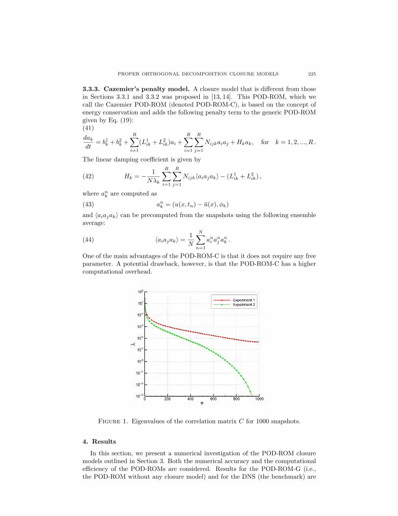
Figure 1. Eigenvalues of the correlation matrix C for 1000 snapshots.

4. Results

In this section, we present a numerical investigation of the POD-ROM closuremodels outlined in Section 3. Both the numerical accuracy and the computationalefficiency of the POD-ROMs are considered. Results for the POD-ROM-G (i.e.,the POD-ROM without any closure model) and for the DNS (the benchmark) are


(a) Experiment 1 (b) Experiment 2

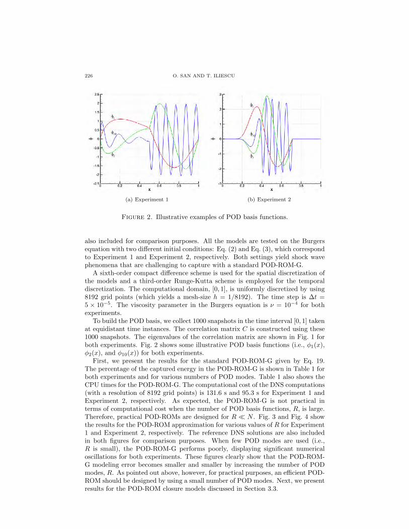
Figure 2. Illustrative examples of POD basis functions.

also included for comparison purposes. All the models are tested on the Burgersequation with two different initial conditions: Eq. (2) and Eq. (3), which correspondto Experiment 1 and Experiment 2, respectively. Both settings yield shock wavephenomena that are challenging to capture with a standard POD-ROM-G.

A sixth-order compact difference scheme is used for the spatial discretization ofthe models and a third-order Runge-Kutta scheme is employed for the temporaldiscretization. The computational domain, [0, 1], is uniformly discretized by using8192 grid points (which yields a mesh-size h = 1/8192). The time step is ∆t =5 × 10−5. The viscosity parameter in the Burgers equation is ν = 10−4 for bothexperiments.

To build the POD basis, we collect 1000 snapshots in the time interval [0, 1] takenat equidistant time instances. The correlation matrix C is constructed using these1000 snapshots. The eigenvalues of the correlation matrix are shown in Fig. 1 forboth experiments. Fig. 2 shows some illustrative POD basis functions (i.e., φ1(x),φ2(x), and φ10(x)) for both experiments.

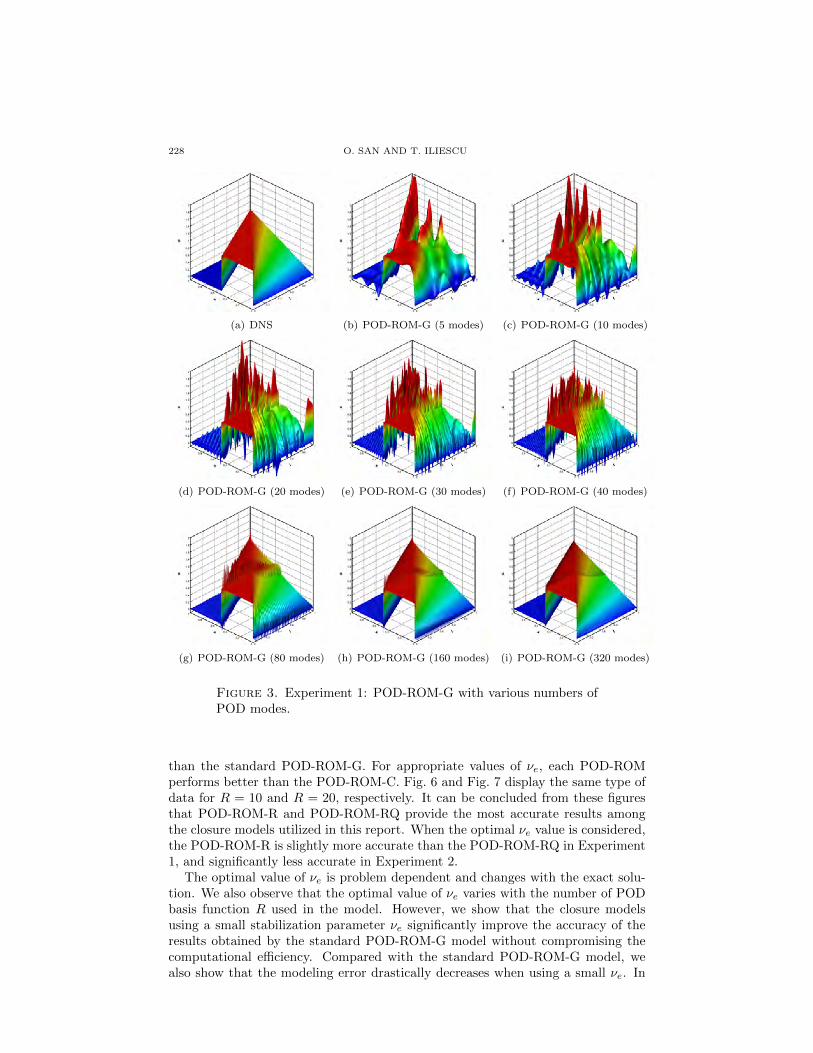
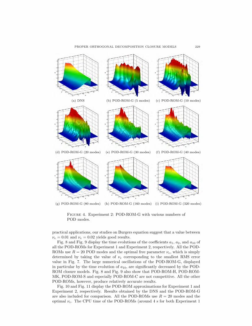
First, we present the results for the standard POD-ROM-G given by Eq. 19.The percentage of the captured energy in the POD-ROM-G is shown in Table 1 forboth experiments and for various numbers of POD modes. Table 1 also shows theCPU times for the POD-ROM-G. The computational cost of the DNS computations(with a resolution of 8192 grid points) is 131.6 s and 95.3 s for Experiment 1 andExperiment 2, respectively. As expected, the POD-ROM-G is not practical interms of computational cost when the number of POD basis functions, R, is large.Therefore, practical POD-ROMs are designed for R N . Fig. 3 and Fig. 4 showthe results for the POD-ROM approximation for various values of R for Experiment1 and Experiment 2, respectively. The reference DNS solutions are also includedin both figures for comparison purposes. When few POD modes are used (i.e.,R is small), the POD-ROM-G performs poorly, displaying significant numericaloscillations for both experiments. These figures clearly show that the POD-ROM-G modeling error becomes smaller and smaller by increasing the number of PODmodes, R. As pointed out above, however, for practical purposes, an efficient POD-ROM should be designed by using a small number of POD modes. Next, we presentresults for the POD-ROM closure models discussed in Section 3.3.


Table 1. The computational efficiency and the percentage of cap-tured energy for the POD-ROM-G for various number of PODmodes. The computational cost of the DNS is 131.6 s and 95.3 sfor Experiment 1 and Experiment 2, respectively.

Number of modesExperiment 1 Experiment 2

(R)∑R

i=1 λi∑Ni=1 λi

× 100 CPU time (s)∑R

i=1∑Ni=1

× 100 CPU time (s)

5 91.250726 0.1239 86.541659 0.142910 95.615358 0.7109 93.611926 0.663820 97.867613 4.5643 97.170311 4.667230 98.629576 15.0837 98.317899 15.121740 99.011706 40.2829 98.871930 35.046680 99.581931 293.9203 99.641204 301.1842160 99.854665 2328.0041 99.933295 2299.7983320 99.967961 18217.3255 99.996588 19875.0094

Table 2. The error between the closure model approximationsand the DNS results for various R values.

Number of modesExperiment 1 Experiment 2

(R) POD-ROM-G POD-ROM-R POD-ROM-G POD-ROM-R

5 3.7641E-1 3.8487E-2 3.4848E-1 3.3267E-210 5.5197E-1 1.1796E-2 2.4383E-1 2.1690E-220 3.6551E-1 5.6315E-3 1.7606E-1 1.0610E-230 2.6755E-1 4.2930E-3 7.0371E-2 7.0259E-340 1.8371E-1 3.6121E-3 4.6022E-2 5.7158E-380 8.3464E-2 2.4414E-3 1.0130E-2 4.0387E-3

Table 2 displays the error between the closure model approximations for POD-ROM-R model and the DNS results for various R values. We also include similarresults for the standard POD-ROM-G model for comparison purposes. Here, POD-ROM-R uses a fixed stabilization parameter νe = 0.02 in both experiments. First,it is clear that the difference between the closure model approximations and theDNS results converges to zero when R increases up to the rank of the snapshotmatrix. Second, Table 2 shows that the modeling errors on the order of 10−2 canbe obtained by the standard POD-ROM-G by using approximately 10 times morePOD modes, which also requires around 1000 times more CPU time. This tableclearly shows that we can effectively obtain accurate results by using a closuremodel to account for the discarded POD modes.

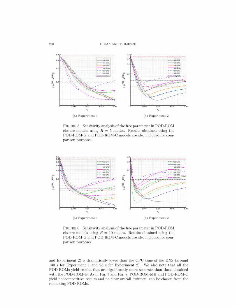
We emphasize that the closure models presented in Section 3.3 have a free mod-eling parameter νe. Exceptions are the POD-ROM-G, which has no closure term atall, and the POD-ROM-C. First, for all the closure models, we perform a sensitivitystudy on the modeling parameter νe. The discrete root mean squared (RMS) errors(with respect to the DNS results) are computed at the final time t = 1.

Fig. 5 shows the RMS errors with respect to the modeling parameter νe for allthe closure models with R = 5 for both experiments. The two straight lines inFig. 5 show the RMS errors of the POD-ROM-G and the POD-ROM-C, whichhave no dependence on νe. As expected, all the closure models perform better


(a) DNS (b) POD-ROM-G (5 modes) (c) POD-ROM-G (10 modes)

(d) POD-ROM-G (20 modes) (e) POD-ROM-G (30 modes) (f) POD-ROM-G (40 modes)

(g) POD-ROM-G (80 modes) (h) POD-ROM-G (160 modes) (i) POD-ROM-G (320 modes)

Figure 3. Experiment 1: POD-ROM-G with various numbers ofPOD modes.

than the standard POD-ROM-G. For appropriate values of νe, each POD-ROMperforms better than the POD-ROM-C. Fig. 6 and Fig. 7 display the same type ofdata for R = 10 and R = 20, respectively. It can be concluded from these figuresthat POD-ROM-R and POD-ROM-RQ provide the most accurate results amongthe closure models utilized in this report. When the optimal νe value is considered,the POD-ROM-R is slightly more accurate than the POD-ROM-RQ in Experiment1, and significantly less accurate in Experiment 2.

The optimal value of νe is problem dependent and changes with the exact solu-tion. We also observe that the optimal value of νe varies with the number of PODbasis function R used in the model. However, we show that the closure modelsusing a small stabilization parameter νe significantly improve the accuracy of theresults obtained by the standard POD-ROM-G model without compromising thecomputational efficiency. Compared with the standard POD-ROM-G model, wealso show that the modeling error drastically decreases when using a small νe. In


(a) DNS (b) POD-ROM-G (5 modes) (c) POD-ROM-G (10 modes)

(d) POD-ROM-G (20 modes) (e) POD-ROM-G (30 modes) (f) POD-ROM-G (40 modes)

(g) POD-ROM-G (80 modes) (h) POD-ROM-G (160 modes) (i) POD-ROM-G (320 modes)

Figure 4. Experiment 2: POD-ROM-G with various numbers ofPOD modes.

practical applications, our studies on Burgers equation suggest that a value betweenνe = 0.01 and νe = 0.02 yields good results.

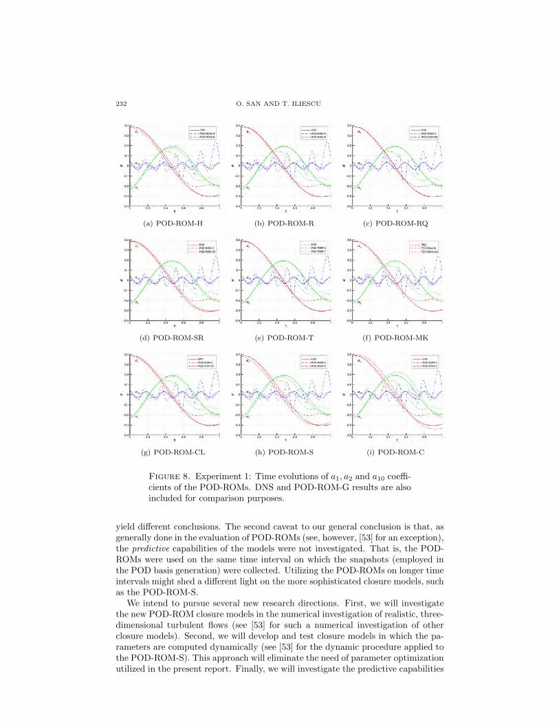
Fig. 8 and Fig. 9 display the time evolutions of the coefficients a1, a2, and a10 ofall the POD-ROMs for Experiment 1 and Experiment 2, respectively. All the POD-ROMs use R = 20 POD modes and the optimal free parameter νe, which is simplydetermined by taking the value of νe corresponding to the smallest RMS errorvalue in Fig. 7. The large numerical oscillations of the POD-ROM-G, displayedin particular by the time evolution of a10, are significantly decreased by the POD-ROM closure models. Fig. 8 and Fig. 9 also show that POD-ROM-H, POD-ROM-MK, POD-ROM-S and especially POD-ROM-C are not competitive. All the otherPOD-ROMs, however, produce relatively accurate results.

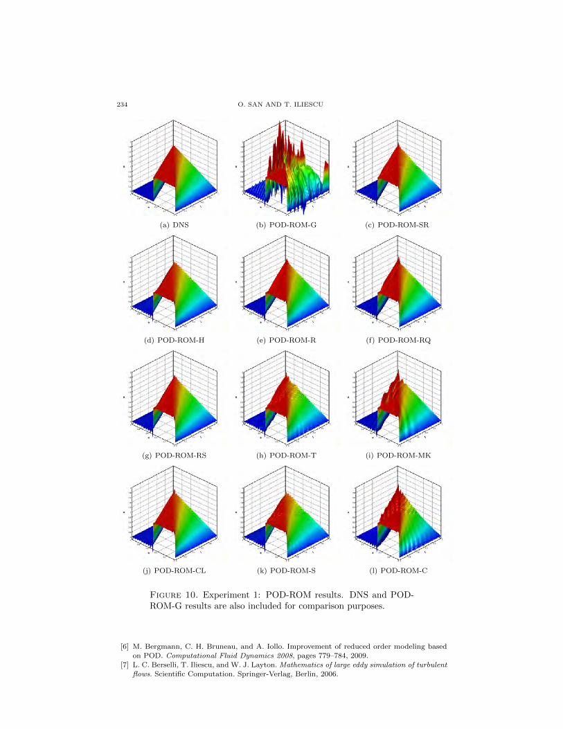
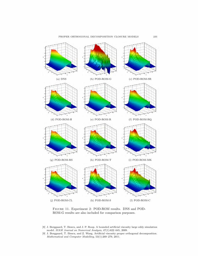
Fig. 10 and Fig. 11 display the POD-ROM approximations for Experiment 1 andExperiment 2, respectively. Results obtained by the DNS and the POD-ROM-Gare also included for comparison. All the POD-ROMs use R = 20 modes and theoptimal νe. The CPU time of the POD-ROMs (around 4 s for both Experiment 1



Figure 5. Sensitivity analysis of the free parameter in POD-ROMclosure models using R = 5 modes. Results obtained using thePOD-ROM-G and POD-ROM-C models are also included for com-parison purposes.



and Experiment 2) is dramatically lower than the CPU time of the DNS (around130 s for Experiment 1 and 95 s for Experiment 2). We also note that all thePOD-ROMs yield results that are significantly more accurate than those obtainedwith the POD-ROM-G. As in Fig. 7 and Fig. 8, POD-ROM-MK and POD-ROM-Cyield noncompetitive results and no clear overall “winner” can be chosen from theremaining POD-ROMs.




5. Conclusions

Several new closure models for the POD-ROM of fluid flows were proposed.These and other standard closure models were investigated in the numerical simu-lation of the Burgers equation. DNS and POD-ROM-G results were also includedfor comparison purposes. A detailed sensitivity analysis with respect to the model-ing free parameters was also performed. Two challenging test problems displayingmoving shock waves were chosen as numerical tests. Both numerical accuracy andcomputational efficiency were used to assess the performance of the POD-ROMs.

Two main conclusions can be drawn from the numerical investigation: First, allthe POD-ROMs showed a clear improvement in solution accuracy over the standardPOD-ROM-G. The POD-ROM-R and the POD-ROM-RQ outperformed the otherPOD-ROMs when the norm of the error was considered. When the time evolutionof the POD-ROM coefficients was considered, the POD-ROM-R and the POD-ROM-RQ performed well again, but other POD-ROMs were also competitive. Thesecond conclusion yielded by the numerical investigation is that all the POD-ROMswere computationally efficient, having a computational cost of the same order asthat of the standard POD-ROM-G and much lower than that of the DNS.

From a practical point of view, the main conclusion of this study is that, when themodel parameters are carefully chosen, closure models based on eddy viscosity termsthat are constant in space and time, but POD mode dependent, are appropriate forPOD-ROM of the Burgers equation. More sophisticated closure models, such asPOD-ROM-S and POD-ROM-C, which have a higher computational overhead, donot yield more accurate results. Two caveats to this general conclusion should beincluded. First, our numerical investigation has been centered exclusively aroundthe one-dimensional Burgers equation. This simplified setting was chosen as afirst step in the investigation of the new closure models. It allowed a thoroughassessment of the performance of the new models, including a parameter sensitivitystudy. We emphasize, however, that a similar investigation for realistic three-dimensional turbulent flows (which is the subject of a future study) could possibly


(a) POD-ROM-H (b) POD-ROM-R (c) POD-ROM-RQ

(d) POD-ROM-SR (e) POD-ROM-T (f) POD-ROM-MK

(g) POD-ROM-CL (h) POD-ROM-S (i) POD-ROM-C

Figure 8. Experiment 1: Time evolutions of a1, a2 and a10 coeffi-cients of the POD-ROMs. DNS and POD-ROM-G results are alsoincluded for comparison purposes.

yield different conclusions. The second caveat to our general conclusion is that, asgenerally done in the evaluation of POD-ROMs (see, however, [53] for an exception),the predictive capabilities of the models were not investigated. That is, the POD-ROMs were used on the same time interval on which the snapshots (employed inthe POD basis generation) were collected. Utilizing the POD-ROMs on longer timeintervals might shed a different light on the more sophisticated closure models, suchas the POD-ROM-S.

We intend to pursue several new research directions. First, we will investigatethe new POD-ROM closure models in the numerical investigation of realistic, three-dimensional turbulent flows (see [53] for such a numerical investigation of otherclosure models). Second, we will develop and test closure models in which the pa-rameters are computed dynamically (see [53] for the dynamic procedure applied tothe POD-ROM-S). This approach will eliminate the need of parameter optimizationutilized in the present report. Finally, we will investigate the predictive capabilities


(a) POD-ROM-H (b) POD-ROM-R (c) POD-ROM-RQ

(d) POD-ROM-SR (e) POD-ROM-T (f) POD-ROM-MK

(g) POD-ROM-CL (h) POD-ROM-S (i) POD-ROM-C

Figure 9. Experiment 2: Time evolutions of a1, a2 and a10 coeffi-cients of the POD-ROMs. DNS and POD-ROM-G results are alsoincluded for comparison purposes.

of the new POD-ROMs, by testing them on time intervals that are longer than thatover which the snapshots were collected.

References

[1] N. Aubry, P. Holmes, J. L. Lumley, and E. Stone. The dynamics of coherent structures in

the wall region of a turbulent boundary layer. Journal of Fluid Mechanics, 192(1):115–173,1988.

[2] M. Balajewicz and E. H. Dowell. Stabilization of projection-based reduced order models of

the Navier–Stokes. Nonlinear Dynamics, 70(2):1619–1632, 2012.[3] M. J. Balajewicz, E. H. Dowell, and B. R. Noack. Low-dimensional modelling of high-

Reynolds-number shear flows incorporating constraints from the Navier–Stokes equation.

Journal of Fluid Mechanics, 729:285–308, 2013.[4] E. Balkovsky, G. Falkovich, I. Kolokolov, and V. Lebedev. Intermittency of Burgers’ turbu-

lence. Physical Review Letters, 78(8):1452–1455, 1997.[5] J. Bec and K. Khanin. Burgers turbulence. Physics Reports, 447(1):1–66, 2007.


(a) DNS (b) POD-ROM-G (c) POD-ROM-SR

(d) POD-ROM-H (e) POD-ROM-R (f) POD-ROM-RQ

(g) POD-ROM-RS (h) POD-ROM-T (i) POD-ROM-MK

(j) POD-ROM-CL (k) POD-ROM-S (l) POD-ROM-C

Figure 10. Experiment 1: POD-ROM results. DNS and POD-ROM-G results are also included for comparison purposes.

[6] M. Bergmann, C. H. Bruneau, and A. Iollo. Improvement of reduced order modeling based

on POD. Computational Fluid Dynamics 2008, pages 779–784, 2009.

[7] L. C. Berselli, T. Iliescu, and W. J. Layton. Mathematics of large eddy simulation of turbulentflows. Scientific Computation. Springer-Verlag, Berlin, 2006.


(a) DNS (b) POD-ROM-G (c) POD-ROM-SR

(d) POD-ROM-H (e) POD-ROM-R (f) POD-ROM-RQ

(g) POD-ROM-RS (h) POD-ROM-T (i) POD-ROM-MK

(j) POD-ROM-CL (k) POD-ROM-S (l) POD-ROM-C

Figure 11. Experiment 2: POD-ROM results. DNS and POD-ROM-G results are also included for comparison purposes.

[8] J. Borggaard, T. Iliescu, and J. P. Roop. A bounded artificial viscosity large eddy simulation

model. SIAM Journal on Numerical Analysis, 47(1):622–645, 2009.

[9] J. Borggaard, T. Iliescu, and Z. Wang. Artificial viscosity proper orthogonal decomposition.Mathematical and Computer Modelling, 53(1):269–279, 2011.


[10] J. P. Bouchaud, M. Mezard, and G. Parisi. Scaling and intermittency in Burgers turbulence.

Physical Review E, 52(4):3656, 1995.

[11] M. Buffoni, S. Camarri, A. Iollo, and M. V. Salvetti. Low-dimensional modelling of a confinedthree-dimensional wake flow. Journal of Fluid Mechanics, 569:141–150, 2006.

[12] M. H. Carpenter, D. Gottlieb, and S. Abarbanel. Stable and accurate boundary treatments for

compact, high-order finite-difference schemes. Applied Numerical Mathematics, 12(1):55–87,1993.

[13] W. Cazemier. Proper orthogonal decomposition and low dimensional models for turbulent

flows. PhD thesis, Rijksuniversiteit Groningen, 1997.[14] W. Cazemier, R. Verstappen, and A. E. P. Veldman. Proper orthogonal decomposition and

low-dimensional models for driven cavity flows. Physics of Fluids, 10:1685, 1998.

[15] J. P. Chollet. Two-point closure used for a sub-grid scale model in large eddy simulations. InTurbulent Shear Flows, pages 62–72. Springer, 1985.

[16] V. Esfahanian and K. Ashrafi. Equation-Free/Galerkin-Free reduced-order modeling of theshallow water equations based on proper orthogonal decomposition. Journal of Fluids Engi-

neering, 131(7), 2009.

[17] F. Fang, C. C. Pain, I. M. Navon, G. J. Gorman, M. D. Piggott, P. A. Allison, P. E. Farrell,and A. J. H. Goddard. A POD reduced order unstructured mesh ocean modelling method

for moderate Reynolds number flows. Ocean Modelling, 28(1-3):127–136, 2009.

[18] D. Fauconnier, C. De Langhe, and E. Dick. A family of dynamic finite difference schemes forlarge-eddy simulation. Journal of Computational Physics, 228(6):1830–1861, 2009.

[19] M. Germano, U. Piomelli, P. Moin, and W. H. Cabot. A dynamic subgrid-scale eddy viscosity

model. Physics of Fluids, 3:1760, 1991.[20] T. Gotoh and R. H. Kraichnan. Statistics of decaying Burgers turbulence. Physics of Fluids,

5:445, 1993.

[21] S. Gottlieb and C. W. Shu. Total variation diminishing Runge-Kutta schemes. Mathematicsof Computation, 67(221):73–85, 1998.

[22] P. Holmes, J. L. Lumley, and G. Berkooz. Turbulence, coherent structures, dynamical systemsand symmetry. Cambridge University Press, 1998.

[23] K. Ito and S. S. Ravindran. A reduced-order method for simulation and control of fluid flows.

Journal of Computational Physics, 143(2):403–425, 1998.[24] V. L. Kalb and A. E. Deane. An intrinsic stabilization scheme for proper orthogonal decom-

position based low-dimensional models. Physics of Fluids, 19:054106, 2007.

[25] G. S. Karamanos and G. E. Karniadakis. A spectral vanishing viscosity method for large-eddysimulations. Journal of Computational Physics, 163(1):22–50, 2000.

[26] S. Kida. Asymptotic properties of Burgers turbulence. Journal of Fluid Mechanics,

93(02):337–377, 1979.[27] K. Kunisch and S. Volkwein. Control of the Burgers equation by a reduced-order approach

using proper orthogonal decomposition. Journal of Optimization Theory and Applications,

102(2):345–371, 1999.[28] K. Kunisch and S. Volkwein. Galerkin proper orthogonal decomposition methods for parabolic

problems. Numerische Mathematik, 90(1):117–148, 2001.[29] T. Lassila, A. Manzoni, A. Quarteroni, and G. Rozza. Model order reduction in fluid dy-

namics: challenges and perspectives. In A. Quarteroni and G. Rozza, editors, Reduced order

methods for modeling and computational reduction, Milano, 2013. Springer.[30] S. K. Lele. Compact finite difference schemes with spectral-like resolution. Journal of Com-

putational Physics, 103(1):16–42, 1992.[31] M. Lentine, W. Zheng, and R. Fedkiw. A novel algorithm for incompressible flow using only

a coarse grid projection. ACM Transactions on Graphics (TOG), 29(4):114, 2010.[32] M. Lesieur and O. Metais. New trends in large-eddy simulations of turbulence. Annual Review

of Fluid Mechanics, 28(1):45–82, 1996.[33] M. D. Love. Subgrid modelling studies with Burgers’ equation. Journal of Fluid Mechanics,

100:87–110, 1980.[34] H. V. Ly and H. T. Tran. Modeling and control of physical processes using proper orthogonal

decomposition. Mathematical and Computer Modelling, 33(1):223–236, 2001.[35] Y. Maday, S. M. O. Kaber, and E. Tadmor. Legendre pseudospectral viscosity method for

nonlinear conservation laws. SIAM Journal on Numerical Analysis, 30(2):321–342, 1993.[36] B. R. Noack, K. Afanasiev, M. Morzynski, G. Tadmor, and F. Thiele. A hierarchy of low-

dimensional models for the transient and post-transient cylinder wake. Journal of Fluid Me-chanics, 497(1):335–363, 2003.


[37] B. R. Noack, M. Morzynski, and G. Tadmor. Reduced-order modelling for flow control.

Springer Verlag, 2011.

[38] B. R. Noack, P. Papas, and P. A. Monkewitz. Low-dimensional Galerkin model of a laminar

shear-layer. Technical Report 2002-01, Ecole Polytechnique Federale de Lausanne, 2002.

[39] B. R. Noack, M. Schlegel, B. Ahlborn, G. Mutschke, M. Morzynski, P. Comte, and G. Tadmor.A finite-time thermodynamics of unsteady fluid flows. Journal of Non-Equilibrium Thermo-

dynamics, 33(2):103–148, 2008.

[40] S. S. Ravindran. A reduced-order approach for optimal control of fluids using proper orthog-onal decomposition. International Journal for Numerical Methods in Fluids, 34(5):425–448,

2000.

[41] D. Rempfer. Koharente Strukturen und Chaos beim laminar-turbulenten Grenzschichtum-schlag. PhD thesis, University of Stuttgart, 1997.

[42] P. Sagaut. Large eddy simulation for incompressible flows. Springer, 2006.[43] M. Sari and G. Gurarslan. A sixth-order compact finite difference scheme to the numerical

solutions of Burgers?equation. Applied Mathematics and Computation, 208(2):475–483, 2009.

[44] S. Sirisup and G. E. Karniadakis. A spectral viscosity method for correcting the long-termbehavior of POD models. Journal of Computational Physics, 194(1):92–116, 2004.

[45] L. Sirovich. Turbulence and the dynamics of coherent structures. I-Coherent structures. II-

Symmetries and transformations. III-Dynamics and scaling. Quarterly of Applied Mathemat-ics, 45:561–571, 1987.

[46] J. Smagorinsky. General circulation experiments with the primitive equations. Monthly

Weather Review, 91(3):99–164, 1963.[47] R. Stefanescu and I. M. Navon. POD/DEIM nonlinear model order reduction of an ADI

implicit shallow water equations model. Journal of Computational Physics, 237:95–114, 2013.

[48] E. Tadmor. Convergence of spectral methods for nonlinear conservation laws. SIAM Journalon Numerical Analysis, 26(1):30–44, 1989.

[49] S. Ullmann and J. Lang. A POD-Galerkin reduced model with updated coefficients for S-magorinsky LES. In J. C. F. Pereira and A. Sequeira, editors, V European Conference on

Computational Fluid Dynamics, ECCOMAS CFD 2010, Lisbon, Portugal, June 2010.

[50] S. Ullmann and J. Lang. POD and CVT Galerkin reduced-order modeling of the flow arounda cylinder. Proceedings in Applied Mathematics and Mechanics, 12(1):697–698, 2012.

[51] Z. Wang. Reduced-order modeling of complex engineering and geophysical flows: analysis and

computations. PhD thesis, Virginia Tech, 2012.[52] Z. Wang, I. Akhtar, J. Borggaard, and T. Iliescu. Two-level discretizations of nonlinear closure

models for proper orthogonal decomposition. Journal of Computational Physics, 230(1):126–

146, 2011.[53] Z. Wang, I. Akhtar, J. Borggaard, and T. Iliescu. Proper orthogonal decomposition closure

models for turbulent flows: A numerical comparison. Computer Methods in Applied Mechan-

ics and Engineering, 2012.

Department of Mathematics and Interdisciplinary Center for Applied Mathematics, VirginiaTech, Blacksburg, VA 24061, USA

E-mail : [email protected] and [email protected]

Proper orthogonal decomposition closure models for fluid flows: Burgers equation

Documents

Transcript of Proper orthogonal decomposition closure models for fluid flows: Burgers equation