Proceedings of the 1st NSE Minna Branch Engineering ...

| P a g e :

2021

Proceedings of the 1st NSE Minna

Branch Engineering Conference

1st NSE Minna Branch Engineering Conference

2021

i | P a g e :

1 s t N S E M i n n a B r a n c h E n g i n e e r i n g C o n f e r e n c e 2 0 2 1

Conference Overview

Primarily, Engineering innovations are concerned with improving human living standards,

protecting and restoring the environment. To this end, sustainable Engineering strives to design

or operate systems for efficient usage of resources. As a major stakeholder in sustainable

development, the NSE Minna Branch, in partnership with COREN, NITDA, NASENI and

SEDI-Minna, is organizing the 1st National Conference. The theme focuses on the roles of

Engineering in attaining the 17 sustainable development goals within and outside Nigeria.

Local Organizing Committee

Engr. Prof. Abdulkarim Ambali Saka, MNSE Chairman

Engr. Prof. Abdulsalami Sanni Kovo, MNSE Co-Chairman

Engr. Dr. Abubakar Sadiq Ahmad, MNSE Secretary

Engr. Prof. Abdulrahman Salawu Asipita, MNSE Member

Engr. Dr. Caroline Alenoghena, MNSE Member

Engr. Dr. Elizaberth J. Eterigho, FNSE Member

Engr. Dr. Muhammadu M. Masin, MNSE Member

Engr. Dr. Mohammed Liman Yerima, MNSE Member

Engr. David Bala Jiya, MNSE Member

Engr. Muhammad N. Abdullahi, MNSE Member

Engr. Abubakar Takuma, MNSE Member

Engr. Solomon Joseph Ibrahim, MNSE Member

Executive Committee Members NSE Minna Branch

Engr. Dr. Elizaberth J. Eterigho, FNSE Chairman

Engr. Dr. Muhammadu M. Masin, MNSE Vice Chairman

Engr. Dr. Mohammed Liman Yerima, MNSE General Secretary

Engr. Muhammad N. Abdullahi, MNSE Asst. Gen Sec.

Engr. Mohammed Danjuma Abubakar, MNSE Treasurer

Engr. Hadiza Danyaya, MNSE Financial Secretary

Engr. Dr. Abubakar Sadiq Ahmad, MNSE Tech. Secretary

Engr. Omotoso Oladipo, MNSE Asst. Tech. Secretary

Engr. Solomon Joseph Ibrahim, MNSE Publicity Secretary

Engr. Prof. Mohammed Baba Ndaliman, MNSE Ex-offcio I

Engr. Hauwa Abubakar Gimba, MNSE Ex-offcio II

ii | P a g e :


Conference Editorial Committee Engr. Dr. Abubakar Sadiq Ahmad, MNSE

Department of Electrical and Electronics Engineering, FUT Minna, Nigeria.

Chief Editor/

Tech. Sec

Engr. Prof. Abdulkarim Ambali Saka, MNSE

Department of Chemical Engineering, FUT Minna, Nigeria.

Chief Editor

SIPET

Engr. Prof. Abdulsalami Sanni Kovo, MNSE

Department of Chemical Engineering, FUT Minna, Nigeria.

Co-Chief Editor

SIPET

Engr. Dr. Caroline Alenoghena, MNSE

Department of Telecomunication Engineering, FUT Minna, Nigeria.

Chief Editor

SEET

Engr. Dr. Bala A. Salihu, MNSE

Department of Telecomunication Engineering, FUT Minna, Nigeria.

Co-Chief Editor

SEET

Engr. Prof. Abdulrahman Salawu Asipita, MNSE

Department of Materials and Metallurgy Engineering, FUT Minna, Nigeria. Member

Engr. Prof. Oluwafemi Ayodeji Olugboji, MNSE

Department of Mechanical Engineering, FUT Minna, Nigeria. Member

Engr. Prof. Abdulkarim Nasir, MNSE


Engr. Dr. Musa Alhassan, MNSE

Department of Civil Engineering, FUT Minna, Nigeria. Member

Engr. Dr. Abraham U. Usman, MNSE

Department of Telecomunication Engineering, FUT Minna, Nigeria. Member

Engr. Dr. Sunday Albert Lawal, MNSE


Engr. Dr. Olatomiwa Lanre, MNSE

Department of Electrical and Electronics Engineering, FUT Minna, Nigeria. Member

Engr. Dr. David Micheal, MNSE

Department of Telecomunication Engineering, FUT Minna, Nigeria. Member

Engr. Dr. Henry Ohize


Engr. Dr. Umar Suleiman Dauda, MNSE


Engr. Dr. Adedipe Oyewole, MNSE


Engr. Dr. Elizaberth J. Eterigho, FNSE

Department of Chemical Engineering, FUT Minna, Nigeria. Member

Engr. Dr. Taiye Adejumo, MNSE


Engr. Dr. Solomon Dauda, MNSE

Deparment of Agricultural and Bioresources Engineering FUT Minna, Nigeria Member

Engr. Dr. Alkali Babawuya, MNSE

Department of Mechatronics Engineering, FUT Minna, Nigeria. Member

Engr. Dr. Muhammadu Muhammadu Masin, MNSE Member

iii | P a g e :


Department of Mechanical Engineering, FUT Minna, Nigeria.

Engr. Dr. Mohammed Liman Yerima, MNSE

Department of Materials and Metallurgy Engineering, FUT Minna, Nigeria. Member

Engr. Abdullazeez Yusuf, MNSE


Engr. Mahmud Abubakar, MNSE


Engr. Jibril Abdullahi Bala, MNSE

Department of Mechatronics Engineering, FUT Minna, Nigeria. Member

iv | P a g e :


TABLE OF CONTENT

Paper

ID Paper Title and Authors

Page

No

Lead

Paper

University Research and Innovation for Regional Economic Development:

Panacea for Eradication of Extreme Poverty in Nigeria. OKOPI ALEX

MOMOH

01-12

1

A Topsis-based Methodology for Prioritizing Maintenance Activities Suitable

for A Municipal Water Works. Case Study: Chanchaga Water Works, Minna.

Musa Kotsu, U. G Okoro and I. A. Shehu

13-22

2

The Effectiveness of Flood Early Warning by Nigerian Meteorological

Agency for Sustainable Development in Nigeria. Abdullahi Hussaini and

Mansur Bako Matazu

23-29

3

Evaluation of Hydraulic Model for Water Allocation in a Large Rice

Irrigation Scheme, Malaysia Habibu Ismail, Md Rowshon Kamal, N.J.

Shanono and S.A. Amin

30-35

4

Ultrasonic Motion Detector, A Panacea for Theft Related Security Challenges

in the 21st Century. Adebisi J.A. and Abdulsalam K. A.

36-44

5

A Brief Review of Proposed Models for Jamming Detection in Wireless

Sensor Network Grace Audu, Michael David and Abraham U. Usman

45-49

6

Design and Implementation of a Fire/Gas Safety System with SMS and Call

Notification

M. A. Kolade, K.A. Abu-bilal, U.F. Abdu-Aguye, Z.Z Muhammad, and Kassim

A. Y

50-59

7

Non-linear Scaling in Global Optimisation. Part I: Implementation and

Validation Abubakar, H. A., Misener, R. and Adjiman, C. S.

60-68

8

An Automatic Bus Route Monitoring System for the Federal University of

Technology, Minna Hamza Farouk, Michael David, Nathaniel Salawu, Ebune

Emmanuel Opaluwa, Mamud Michael Oluwasegun, and Akabuike Kingsley

Ikenna

69-75

9 Reformation of Engineering Education for Health, Wealth and Sustainable

Development in Nigeria. Oluwadare Joshua Oyebode 76-83

v | P a g e :


10

A Review of the Different Biomass Materoals Used to Produce Activated

Carbon for Water Treatment. Korie C.I, Afolabi E.A, Kovo A.S., Muktar A.

84-94

11

Risk Analysis of Power Transmission Infrastructure for Sustainable

Development: A Case Study of the Nigerian 330 kV- 41 Bus Network. Jethro

Shola, Emmanuel Sunday Akoji, UmbugalaKigbu F., Yusuf Isah, & A. A. Sadiq

95-103

12

Non-linear Scaling in Global Optimisation. Part II: Performance Evaluation.

Abubakar, H. A., Misener, R. and Adjiman, C. S.

104-112

13

A Review of Different Proposed Image Detection Techniques for Road

Anomalies Detection.

A. M. Oyinbo, A. S. Mohammad, S. Zubair, and E. Michael

113-119

14

A Review on Leach: An Energy Efficient Protocol in Wireless Sensor

Networks P. O. Odeh, S. Zubair, A. U. Usman, and S. Bala

120-127

15

Finite Element Modelling and Analysis of a 4-Span T-Beam Bridge

Nyam, J. P. & Sadiku, S. A.

128-138

16

Automatic Radio Selection for Data Transfer in Device to Device

C. E. Igbokwe, S. Bala, M. David, and E. Michael

139-149

17

Sustainable Development in Construction Industry Using Palm Kernel Shell

Ash as Partial Replacement for Cement. S.O. Atuluku and T.E. Adejumo

150-157

18

Effect of Strengthening Vertical Circular Openings with Various Materials

on the Behaviour of Reinforced Concrete Beams Paul Peter Maiyamba and

S.M Auta

158-166

19

Opportunities for Engineers in the Solar Energy Value Chain

Mahmud, J. O., Mustapha, S. A.

167-174

20

Development of an Electric Tricycle with Adjustable Wheel Camber

Jamilu Shehu Musawa and ikechukwu C. Ugwuoke

175-183

21

Development and Characterisation of Briquettes from Biomass Wastes: A

Review Medashe, Michael Oluwasey and Abolarin, Mathew Sunda

184-193

vi | P a g e :


22

Treatment of Industrial Waste Water to Remove Heavy Metal (Zinc) Using

Palm Flower Activated Carbon as Adsorbent. Samson Adeiza Okeji, Patience

Oshuare Sedemogun

194-201

23

Irrigation with Unsafe Industrial Wastewater and Associated Health Risks:

An Emerging Technology for Heavy Metals Removal. A. S. Mohammeda, c,

E. Danso-Boatengb, G. Sandac, A.D. Wheatleyc, M.I. Animashaund, I.A.

Kutic, H.I. Mustaphad, M.Y. Otache, J.J. Musad.

202-214

24

Formulation of Cutting Oil Using Green Base Extract (Soya-Bean and

Groundnut) Oketa A.J and Okoro U. G

215-223

25

Friction Stir Welding of Some Selected High Strength Aluminium Alloys- A

Review B. I. Attah, S. A Lawal, E.T Akinlabi, K. C Bala, O. Adedikpe1 O. M

Ikumapayi

224-229

26

The Failure Analysis in Steel Reinforced Beams with different Reinforcement

Ratio Ayandokun W. A1, Balogun B. T, and Abdulrahman A. S

230-237

27

Oxidative Stability and Cold Flow Properties of Non-Edible Vegetable Oil for

Industrial Biolubricant Applications Timothy Yakubu Woma, Sunday Albert

Lawal, Asipita Salawu Abdulrahman, M.A. Olutoye, and A.A. Abdullahi,

238-243

28

Effect of Turning Process Parameters on Surface Roughness of AISI 1045

Medium Carbon Steel Using Aluminum Coated Carbide Tool Salawu Morufu

Ajibola and Sunday Albert Lawal

244-248

29

Thermal and Physicochemical Characterization of Locally Sourced Lignite

Coal C. O. Emenike, P. E. Dim and J. O. Okafor

249-254

30

Thermal and Physicochemical Characterization of Biochar Produced from

Waste Bamboo. E. Daniel, P.E. Dim and J.O. Okafor

255-258

31

Synthesis of Ni-Al2O3 Nanocatalyst for Low Temperature Production of

Carbon Nanotubes (CNTs) Yerima, M. L., Abdulkareem A. S., Abubakre, O.

K, Ndaliman, M. B. Khan, R. H., and Muriana, R.A.

259-266

32

Evaluation of Strength Properties of Lateritic Soil Stabilized with Cement

Kiln Dust T.E. Adejumo and F.A. Okeshola

267-272

33 Development of A Low-Cost Briquette Making Machine Abdullahi A.,

Abolarin. M. S., Olugboji. O. A 273-276

vii | P a g e :


1 | P a g e :


University Research and Innovation for Regional Economic

Development: Panacea for Eradication of Extreme Poverty in

Nigeria OKOPI ALEX MOMOH

Executive Secretary,

Nigerian Society of Engineers, National Engineering Centre, Abuja

[email protected] +2348037196213

ABSTRACT The natural and human resources endowment of Nigeria is enormous. Paradoxically, the nation remains largely

poor due to inadequate exploitation of these resources. Every region of the country is richly endowed with

resources for sustainable economic development. However, there has not been a sustained and collective

advocacy for collaboration and synergy for sustainable regional development in Nigeria. This paper studied

and recommended the Triple Helix Collaboration Model among Government, Industry and the Academia where

Government provides the necessary infrastructure and enabling environment for investment by Industry while

the Academia provides the intellectual properties for enterprise development through licensing of patents. This

will lead to focused applied research by our tertiary institutions for regional economic development, open more

opportunities for Nigerian Engineers to be actively involved in regional economic development activities

through job and employment creation and create more visibility for Nigerian Engineers. The proposed model

will also lead to establishment of Innovation hubs and Industrial parks to stimulate manufacturing contribution

to the nation’s Gross Domestic Product (GDP) which is currently only at 6%.

KEYWORDS: Regional development, Research, Entrepreneurial University, Triple Helix Model,

Intellectual Property, Innovation, Commercialization, Manufacturing

1. INTRODUCTION Every region of Nigeria is endowed with enormous

human and natural resources. Paradoxically the

country is regarded as the poverty capital of the

world. The national focus on resource utilization has

only been on sale of crude oil as the main source of

national revenue. Most of the county’s other exports

are raw materials without value addition. The

country exports crude oil and imports refined

petroleum products. Similarly, jewelries are

imported from exported raw gold and many other

such commodities because of lack of in-country

processing capabilities. With technology advancing

rapidly towards clean energy globally, emergence of

electric cars and huge global investments in

renewable energy systems, the future of crude oil as

a national revenue source is becoming very bleak.

The need to develop other resources has become

very paramount.

The global economy has become a knowledge -

driven economy. Internationally, regional economic

development has been founded on innovation and

research activities. The Regional Innovation System

(RIS) has become popular among academics,

political decision makers and regional stakeholders

of innovation. Academic institutions conduct

substantial volumes of research that are funded by

government, industry, and philanthropic

organizations. In Nigeria, the Tertiary Education

Trust Fund (TETFUND) spends a lot of money on

Institution Based Research both in Universities and

Polytechnics. For Nigeria to utilize the potentials of

university research, there is a need for universities to

conduct scholarly activities that translate both basic

and applied research into commercially viable

processes and technologies (Sanberg et al 2014). In

developed and newly industrializing nations, there is

pressure on university-based research by way of

increased emphasis on the commercialization of

research (Ogbogu & Caulfield 2015, Hand et al

2013, Caulfield 2012, Rasmussen 2008, Downie &

Herder 2007).

Commercialization of research which is a primary

means through which research results are utilized to

generate products and services, should also be a key

component of the research mission such that novel

ideas, techniques and products can be generated for

the marketplace for the benefit of relevant

stakeholders and society in general. Societal

expectations of tertiary institutions now go beyond

mailto:[email protected]

2 | P a g e :


just teaching and research. The missions of higher

education institutions are expanding to include

economic development, of which translation of

research is a major part ((Hand et al, 2013). The

greatness of a university is not just in its ability to

attract research grants and contracts but also in how

the university impacts and changes the world and

society at large (Caulfield, 2012).

The United States of America former President

Obama’s enthusiastic endorsement of the use of

academic research to drive economic growth in his

State of the Union Addresses (Obama 2014, Obama

2015a,) and in other speeches (Macilwain 2010,

Obama 2011, Obama 2015b) is one high profile

example of government policy commitment to

commercialization of research outputs. President

Obama’s remark that “Twenty-first century

businesses will rely on American science and

technology, research and development” (Obama

2015a) is a propelling policy commitment to the use

of research for industrialization. According to

Claulfield and Ogbogu (2015), other world leaders

who have made similar policy commitments include

the former Prime Minister of Canada, Stephen

Harper who was of the view that scientific research

should be used to power commerce. In the

industrialized countries of America, Canada and

Europe, there is a growing political view that

universities ought to play a central role in the growth

of economies (Petersen & Krisjansen 2015, Philpott

et al 2010) or to accord with national or regional

economic priorities (Claulfield & Ogbogu 2015,

Simons 2015, Caulfield 2010). In these countries, if

researchers want funding, they must frame their

work in line with the commercialization ethos

(Claulfield & Ogbogu 2015).

The paper discusses the research and innovation

commercialization lessons from some developed

and newly industrializing nations as classical

examples of how the application of technologies

drives economic and industrial development of

nations. It typically highlights a rich variety of

policy initiatives at the State and Regional levels in

America as best practice examples to foster

knowledge-based growth and development.

According to Vanderford and Marcinkowski (2015),

United States-based institutions generated over

24,000 disclosures, obtained over 5,000 new

patents, executed over 5,000 licensing agreements,

formed over 800 start-up companies, and generated

$2.75 billion in license income in 2013. The Bayh-

Dole Act in America has stimulated a substantial

acceleration in the patenting and licensing of

university-developed technologies. The Canadian

government in its 2006 to 2008 budgets provided

additional $2.2 billion in new funding for science

and technology initiatives with commercialization

efforts at Canadian universities developing into an

integral part of research and innovation activities.

According to Dodd (2017) the Hebrew University of

Jerusalem, an institution which boasts of Albert

Einstein as one of its founders, has earned over $20

billion in commercialization revenue over the years.

The reasons for the Hebrew University of

Jerusalem's success in research and

commercialization include incentives to its

researchers to commercialize and counting of

patents for promotion. Patents are counted as part of

the portfolio of a professor to be promoted in

addition to publications. Researchers, departments

and faculties, are also rewarded when technology is

commercialized. Since the establishment of Hebrew

University of Jerusalem in 1964 the university's

technology transfer arm, the Yissum Research

Development Company, has registered over 9300

patents covering 2600 inventions, licensed 800

technologies and spun off 110 companies.

According to Leichman (2018), “Universities are

reinventing themselves as microenvironments for

innovation and entrepreneurship. A university that

can’t demonstrate its impact on industry and the

marketplace will become less relevant in the future,”

Comparatively, Nigerian tertiary institutions and

research institutes do not make significant

contributions to the socio-economic development of

the nation through commercialization of research

results despite the high number of students’ research

projects and relatively huge sums of money spent on

research annually.

2. UNIVERSITIES AS INNOVATION

AND ENTREPRENEURSHIP

DRIVERS FOR REGIONAL

ECONOMIC DEVELOPMENT

3 | P a g e :


A major factor in the rise of the United States as a

technological power has been attributed to a long

tradition of close ties and frequent collaboration

between companies and universities. Underlying the

success of regional innovation clusters such as

Silicon Valley, Route 128, and the Research

Triangle of North Carolina are local universities

with a longstanding mission of spurring economic

development by developing and transferring

technology to local industries and stimulating the

creation of new businesses in university-centered

incubators and science parks. Technology-intensive

companies commonly locate their operations near

the best universities in particular fields of science

and Engineering to enable their internal research

departments to work with “star” scientists and to

recruit promising students.

Start-up companies spinning off from universities

most commonly establish operations near those

institutions. The Association of University

Technology Managers (AUTM) reported in 2002

that in the fiscal year 2000, at least 368 new

companies were formed based on university

research and that most of them settled “near the

institution where the technology was born (AUTM,

2002). “The presence of research universities is now

widely viewed as a necessary condition to bring

about innovation-based economic development of

regions.” (Wessner,2013). Illustrating the impact, a

single research university can have on a region, in

2004 alone MIT produced 133 patents, launched 20

startup companies, and spent $1.2 billion in

sponsored research. Data from 1994 showed that, at

that time, MIT graduates had founded over 4,000

companies employing 1.1 million people generating

$232 billion in sales worldwide (Daniel, 2011). In

the Boston area, MIT is flanked by other great

research universities, including Harvard, Tufts, the

University of Massachusetts, Boston University,

and others. Since the early 1970s, spinoffs from

these institutions have created a thriving

pharmaceutical industry where virtually none had

previously existed (Stevens, 2011).

According to San Diego (2017), the licensing of

university research has made significant

contributions to US gross domestic product (GDP),

industry gross output, and jobs over the last two

decades. The report, “The Economic Contribution of

University/Nonprofit Inventions in the United

States: 1996- 2015,” documents the sizeable return

that US taxpayers receive on their investment in

federally funded research. It shows that, during a 20-

year period, academic patents and the subsequent

licensing to industry bolstered US industry gross

output by up to $1.33 trillion, US GDP by up to $591

billion, and supported up to 4,272,000 jobs.

3. THE EMERGENCE OF THE

ENTREPRENEURIAL

UNIVERSITY With a knowledge-based economy in a

globalization-governed world, higher education

institutions bear the responsibility of producing

graduates with a long list of technical and

professional skills (Nasr, 2014). These graduates

must be equipped with fundamental knowledge and

skills to solve problems never seen before in a world

that is open and competitive.

According to O’Connor et al (2012), the traditional

higher education paradigm has evolved and is now

characterized by a strong focus on the development

of academic entrepreneurship through the

commercialization of higher education research with

campus and graduate enterprise development.

Higher education encompasses several roles from

teaching to scientific research and translation of

research results into economic development through

knowledge transfer (Etzkowitz et al, 2000). This is

referred to as an Entrepreneurial University

Education, whose purpose is to transform academic

knowledge into economic and social utility (Clark,

1998). With a focus on effective knowledge transfer

and the creation of new campus businesses, the

Entrepreneurial University also enhances the

competitive advantage of existing enterprise entities

both in and outside the institution. Entrepreneurial

Universities include teaching and research activities

as core to their mission whilst also focusing on

academic entrepreneurship as a key contributor to

economic development. Essentially, an

Entrepreneurial University should comprise (i) spin-

offs and spin-ins; (ii) Entrepreneurial Education;

(iii) links with SMEs and industry; (iv) the

development of diverse income streams; and (v)

campus incubators.

Van der Sijde and Ridder (1999) argued that the best

guarantee for sustainability of entrepreneurship

within a higher education institution is to change it

4 | P a g e :


into an entrepreneurial organization; that is, what

holds for the integration of entrepreneurship in the

academic curricula also holds for the

commercialization of research via spin-off

companies.

4. COMMERCIALIZATION OF

UNIVERSITY RESEARCH AND

INNOVATION FOR ECONOMIC

DEVELOPMENT

Most research universities in the developed

countries establish Technology Transfer Offices to

commercialize their research results in the form of

patents, licenses, and start-ups of new companies.

Some examples of university innovation statistics

are given below.

4.1 University Innovation Statistics

4.1.1 University of Minnesota Key Performance

Indicators

Table 1. University of Minnesota Key Performance Indicators: 2016–2020

Dollar amounts in millions

Technology Commercialization, Wellspring Sophia; UMN Enterprise Financial System

*New Patent Filing Rate is number of new patents filed during the fiscal year divided by number of new

disclosures in the same time period

Source: The University has spun out 170 companies since 2006, with operations across a diversity of fields and

74 percent being Minnesota-based.

University of Minnesota

5 | P a g e :


4.1.2 Harvard University Key Performance Indicators

Table 2: Harvard University Key Performance Indicators: 2014–2018

S/N Description 2014 2015 2016 2017 2018

1 New Patent Applications Filed 246 243 294 274 234

2 U.S. Patents Issued 87 125 122 151 181

3 Licenses 43 50 51 46 51

4 Total Commercialization Revenue (MM) $17.3 $16.1 $37.8 $35.4 $54.1

5 Startup Companies 10 14 14 14 21

6 Industry-Sponsored Research Agreements 98 75 71 81 77

7 Industry-Sponsored Research (MM) $48.6 $42.9 $48.4 $51.0 $53.0

8 Material Transfer Agreements 2,243 2,332 2,240 2,285 2,640

The Harvard University fiscal year runs from July 1 to June 30; hence, Fiscal Year 2018 includes July 1, 2017 -

June 30, 2018.

4.1.3 North Carolina State University

Table 3: North Carolina State University Key Performance Indicators: 2014–2018

S/N DESCRIPTION 2014 2015 2016 2017 2018

1 DISCLOSURES

2 Inventions 204 196 225 217 210

3 Software 22 41 36 18 18

4 Plant Variety 13 20 17 20 25

5 Copyright 14 29 13 14 19

6 Trademark 5 4 0 0 0

7 Tangible Research Materials 0 1 0 6 3

8 Total 258 291 290 275 275

9 PATENT ACTIVITY

10 New Patents Filed 186 181 229 241 264

11 U.S. Patents Issued 40 20 53 43 44

12 Foreign Patents Issued 42 24 12 16 28

13 Total Patents Issued 82 43 65 59 72

14 COMMERCIALIZATION AGREEMENTS

15 Patent License 40 27 42 46 39

16 Software License 1 4 3 3 6

17 Plant License 27 37 45 38 49

18 Copyright License 0 7 10 2 1

19 Tangible Research Materials License 2 3 1 2 3

20 Options 75 61 63 78 43

21 Total 145 139 164 169 141

22 MISCELLANEOUS AGREEMENTS

23 MTA 165 201 203 241 258

24 CDA 395 377 404 367 362

25 Other 184 233 306 297 272

26 Total 744 811 913 905 892

27 REVENUE

28 Royalties ($ millions) $7.5 $7.6 $3.8 $4.4 $5.3

29 NEW VENTURE DEVELOPMENT

30 Startup Companies 10 12 12 15 20

Source : https://otd.harvard.edu/about/productivity-highlights/

https://research.ncsu.edu/otcnv-dashboard/otcnv-dashboard.htm?tab=Patent%20Activity

https://research.ncsu.edu/otcnv-dashboard/otcnv-dashboard.htm?tab=Agreement%20Activity

https://research.ncsu.edu/otcnv-dashboard/otcnv-dashboard.htm?tab=Agreement%20Activity&tab2=Miscellaneous%20Agreements

https://research.ncsu.edu/otcnv-dashboard/otcnv-dashboard.htm?tab=Financial%20Activity

https://research.ncsu.edu/otcnv-dashboard/otcnv-dashboard.htm?tab=Venture%20Development

https://otd.harvard.edu/about/productivity-highlights/

6 | P a g e :


5. UNIVERSITY INNOVATION FOR

REGIONAL ECONOMIC

DEVELOPMENT

5.1 Stanford University and Silicon Valley

California’s Silicon Valley is an important point of

reference in State and regional initiatives to develop

innovation clusters. Stanford University played a

historic role in the establishment of Silicon Valley

and in sustaining the survival and flourishing of high

technology industries in the surrounding region. The

university is credited with creating firms that

accounted for half the revenues generated in the

Valley between 1988 and 1996 and with an

exemplary contribution to local labor market needs

(Moore & Davis, 2001). Stanford is known for its

startup culture in a region in which most successful

firms began as start-ups. It is almost an unwritten

rule in Stanford University that you must start a

company to be a successful professor (Upstarts and

Rabble Rousers, 2006). As of 2011 nearly 5,000

companies existed which could trace their roots to

Stanford, including Hewlett-Packard, Cisco

Systems, Sun Microsystems, Yahoo, and Google

(Wessner, 2013c). “Stanford and MIT were both

committed to an endogenous strategy of

encouraging firm formation from academic

knowledge.” “The examples of Massachusetts

Institute of Technology and Stanford University in

stimulating regional high-technology development

are often highlighted for emulation (Wessner, 2013).

Stanford’s Office of Technology Licensing opened

in 1970, and in four subsequent decades disclosed

roughly 8300 cumulative inventions and executed

over 3500 licenses. Notable inventions licensed by

the office include FM sound synthesis (created by a

small Yamaha music chip developed by the music

department), recombinant DNA technology,

functional antibodies, and digital subscriber line

(DSL) technology commercialized by Texas

Instruments (Katherine, 2011). The University’s

very well-known licensee is Google, which was

created by two Stanford graduate students (Larry

Page and Sergey Brin) over a four-year period.

Stanford’s experience is an example of what a

university can do to make technology transfer

effective (Katherine, 2011).

5.2 University of Akron The University of Akron Research Foundation

(UARF), a not-for-profit organization to facilitate

the transfer of research results from the university to

public and commercial use was established by

University of Akron in 2001. Between 2001 and

2012, the Foundation created fifty (50) start-up

companies from university-based patents with

annual research activity of $50 million. The “Akron

Model” for the remaking of University of Akron as

a major stakeholder in the turnaround of Ohio’s

economy was anchored on the mission:

The university through its research foundation and

other avenues is leveraging its talent for local

companies and entrepreneurs, serving as

something of a research arm or problem-solver in

the regional economy (Wessner, 2013e)

5.3 THE NEW YORK

NANOTECHNOLOGY INITIATIVE The New York State’s nanotechnology R&D

initiative offers a classical example of how the

initiative of a single U.S. State can transform the

global competitive map in a strategic economic area.

New York has been able to alter the competitive

landscape in the semiconductor industry through

large-scale investments, particularly in university

research infrastructure, and collaborative

arrangements with the private sector and regional

development organizations, leading to offshore flow

of U.S. investment and jobs in the sector (Zimpher,

2013). The epicenter of New York’s semiconductor

effort is the State University of New York at Albany

with SUNY Albany as one of six “NY Innovation

Hubs” established to link university-based research

to regional innovation, and sustained investments in

the university’s research infrastructure. It is one of

the foremost centers of nanotechnology research in

the world and a regional economic driver (Zimpher,

2013)

6. MANAGEMENT OF UNIVERSITY

RESEARCH AND INNOVATION FOR

REGIONAL ECONOMIC

DEVELOPMENT IN NIGERIA

According to (Uche 2017), the lack of attention to

commercialization of research outputs explains the

dearth of local solutions to the nation’s economic

problems and the country’s over dependence on

imported products. According to Ahaneka (2016),

“Considerable research findings abound in Nigerian

universities serving no further purpose for society at

7 | P a g e :


large because of lack of linkage with industry. This

raises the urgent necessity of moving beyond basic

research to applied research and innovation, which

in addition to creating knowledge/technology would

lead to discovering solution and promote global

competitiveness of our industries”. Zaku (2011)

charged Nigerian scientists to embark on demand

driven research which would facilitate the speedy

commercialization of Research and Development

outputs through industry linkages.

Nigerian universities and other research institutes do

not make significant contributions to the socio-

economic development of the nation despite the high

number of students and academic staff who engage

in research projects because of lack of attention to

commercialization of research outputs and

innovation. Another factor hindering

commercialization of research output is irrelevant

research carried out that do not reflect the needs of

the nation. Most research work in Nigerian tertiary

institutions are not formulated and carried out with

commercialization focus. The Tertiary Education

Trust Fund (TETFUND) spends a lot of money to

fund research in tertiary institutions but there has

been no defined national focus on

commercialization of research projects.

Number of Universities in Nigeria

S/N REGION STATE NUMBER OF UNIVERSITIES TOTAL

FEDERAL STATE PRIVATE

1 NORTH

CENTRAL

Benue 2 1 1 4

2 Kogi 1 2 1 4

3 Kwara 1 1 7 9

4 Plateau 1 1 2 4

5 Nasarawa 1 1 3 5

6 Niger 1 1 1 3

7 SUBTOTAL 7 7 15 29

8 NORTHEAST Adamawa 1 1 1 3

9 Bauchi 1 1 - 2

10 Borno 2 1 - 3

11 Gombe 1 2 - 3

12 Taraba 1 1 1 3

13 Yobe 1 1 - 2

14 SUBTOTAL 7 7 2 16

NORTHWEST KADUNA 3 1 2 6

KANO 2 2 2 6

KATSINA 1 1 1 3

KEBBI 1 1 - 2

JIGAWA 1 1 1 3

SOKOTO 1 1 - 2

ZAMFARA 1 1 - 2

SUBTOTAL 10 8 6 24

SOUTHEAST ABIA 1 1 3 5

ANAMBRA 1 1 4 6

EBONYI 1 1 1 3

ENUGU 1 1 4 6

IMO 1 2 3 6

SUBTOTAL 5 6 15 26

SOUTHSOUTH AKWA IBOM 1 1 3 5

8 | P a g e :


BAYELSA 1 3 - 4

CROSS RIVER 1 1 1 3

DELTA 2 1 5 8

EDO 1 2 5 8

RIVERS 1 2 3 6

SUBTOTAL 7 10 17 34

SOUTHWEST EKITI 1 1 1 3

LAGOS 2 1 6 9

OGUN 1 3 12 16

ONDO 1 3 3 7

OSUN 1 1 8 10

OYO 1 2 7 10

SUBTOTAL 7 11 37 55

FCT FCT 1 - 6 7

GRAND TOTAL 44 49 98 191

Summary of Number of Universities in each

Region:

North Central: 29

Northeast 16

Northwest 24

Southeast 26

South south 34

Southwest 55

FCT 7

Total 191

7. NIGERIAN SOCIETY OF ENGINEERS

ADVOCACY FOR REGIONAL

ECONOMIC DEVELOPMENT USING

THE TRIPLE HELIX MODEL OF

UNIVERSITY – INDUSTRY –

GOVERNMENT COLLABORATION

The Nigerian Society of Engineers is leading a

strong advocacy for regional economic development

in Nigeria. NSE is worried that with the enormous

human and natural resources in all the regions of the

country, the nation remains poor and is classified as

the poverty capital of the world. Engineers must rise

and begin to harness their creativity and innovation

for economic and social development of the nation.

NSE is convinced that Nigeria can develop rapidly

if the innovation potentials of her tertiary education

research are properly harnessed by focusing on

research that translates rural area endowments into

commercially viable enterprises and adopting

deliberate policies for commercialization of research

results and innovation. NSE has therefore proposed

to lead the advocacy for sustainable regional

economic development through regional resources

documentation and conferences, summits, or town

hall meetings. Under the advocacy plan, there is a

Study/Planning Team for each region to document

its natural resources endowment, identify

investment potentials, appropriate technologies for

exploitation, collaboration/partnership models and

plan the engagement with stakeholders (Conference,

Summit, Town Hall Meetings).

The advocacy plan will focus on the Triple Helix

Collaboration Model among Government, Industry,

and the Academia for Government to provide

necessary infrastructure and enabling environment

for investment by the private sector while the

academia provides the intellectual properties for

enterprise development through licensing of patents.

The group studies on regional development will also

consider potentials for establishment of Innovation

hubs and Industrial parks to stimulate manufacturing

contribution to the nation’s Gross Domestic Product

(GDP) which is currently only at 6%. NSE will use

its network of eighty-one (81) Branches and twenty

- five (25) Professional Institutions across the

country for the advocacy programme.

Expected Outcome of the Advocacy Programme

9 | P a g e :


1. Our universities and other tertiary institutions

will begin to cultivate a new culture of creating

businesses from intellectual properties and

research works through licensing of patents or

establishing start-up companies, thus becoming

entrepreneurial institutions instead of

conducting research for mere academic

promotions. They will become key architects

and drivers of regional development.

2. Tertiary institutions will begin to focus research

on developing appropriate technologies for

exploitation of local resources and engage in

contract research for industries and government.

3. Students in tertiary institutions will focus on

generating ideas that create businesses for them

instead of seeking for employment after

graduation.

4. Tertiary institutions will start to generate more

internal revenues from licensing of patents and

creation of spin-off industries to make them less

dependent on government and prevent incessant

strikes over funding.

5. Enhanced quality of education and training

6. The Organized Private Sector will get

opportunities to access intellectual properties for

business development to create more jobs and

employment.

7. A more stable regional and national economies

will emerge.

8. There will be drastic reduction in crime and

criminality.

9. Gross Domestic Product (GDP) will be enhanced

with significant increase in manufacturing

contribution.

10. National earnings will improve with country-

wide improvement in standard of living over

time.

11. States will be made to focus on providing

relevant infrastructures and creating enabling

environments for investment. There will be

enhancement of innovation infrastructure and

opening of public and community space for

accelerated development.

12. State governments will earn more revenue from

taxes and have leaner civil service as more

people will be employed by the private sector.

13. There will be less dependence on foreign goods

thereby preserving the scarce foreign reserve for

more critical transactions.

14. Promotion of regional attractiveness for foreign

direct investment.

8. DISCUSSION

The study has shown the immense contributions of

focused research and commercialization of

innovations to economic and industrial

development. America’s Silicon Valley, Route 128,

and the Research Triangle with strong collaboration

with universities as innovation drivers is a major

lesson for Nigeria on how university research and

innovation drive economic development.

The development of State and regional innovation

clusters in America around top rate universities in

specific economic sectors with high impacts on

enterprise development and employment generation

is a classic example of the kind of initiatives State

governments in Nigeria should be taking.

Government policies, regulatory frameworks, and

commitment to commercialization of research and

innovation are essential for accelerated growth and

development. The self – sustenance of the university

system has been exemplified by the

entrepreneurship and enterprise development

culture of Stanford University, MIT, University of

Akron, University of Minnesota, Harvard, North

Carolina State University and Hebrew University of

Jerusalem. Our universities can also become top rate

universities and achieve these results if they follow

the examples.

9. CONCLUSION

The Key Performance Indicators of university of

Minnesota, North Carolina University, Harvard

University and U.S.A National Institutes of Health

provide great lessons for Nigerian Universities on

intellectual property generation and

commercialization. Regional universities have

contributed immensely to the economic and

industrial development of America and other

developed countries. States in collaboration with

universities and other research organizations and the

organized private sector are the prime drivers of

innovation clusters for sustainable economic

development. University research is often business

focused with commercialization as the third primary

function of universities in addition to teaching and

research. Many universities in developed countries

are self-sustaining through the force of

commercialization of intellectual properties.

Nigerian tertiary institutions can use collaborative

research to harness States’ and regional comparative

10 | P a g e :


advantages to create industries and jobs for the

Nigerian economy. In comparative terms, Nigerian

Universities and research organizations are not

doing enough in intellectual property generation and

commercialization of innovations. Rural

development in Nigeria can be significantly

influenced by commercialization of research and

innovation based on rural area resource endowment

with active collaboration among Government,

research organizations and the private sector.

10. RECOMMENDATIONS

The Nigerian Society of Engineers advocacy plan

for regional economic development through the

adoption of the Triple Helix collaboration model

among Universities, Industries and Government in

each region of Nigeria to drive sustainable economic

development of the regions, should be aggressively

pursued.

The Research and Development (R & D) mandates

of our tertiary institutions should focus on creating

productive and innovative enterprises from their

regional resource endowments. Virtually every State

in the country has a university and a Polytechnic.

Research in these institutions should focus on

problem solving and business development for the

growth of regional economies.

Commercialization of research should be made an

explicit role of our tertiary institutions in addition to

teaching and research. Our Universities,

Polytechnics and Research Institutes must become

drivers of regional economic growth and

development.

The National Universities Commission (NUC)

should develop a template for the establishment of

research and innovation commercialization unit in

every university to coordinate intellectual property

generation, patenting and licensing for start-up

companies and create the essential linkage with the

private sector and government on the Triple Helix

for commercialization of research results.

Regional Universities should facilitate the creation

of regional innovation centres to exploit

endowments of common regional interest for

accelerated development.

REFERENCES

Ahaneka J (2016), Commercialization of Research

is Key to Nigeria’s Development.

http://247ureports.com/commercialization-of-

research-is-key-to-nigerias-development/.

247ureports.com

Caulfield T, Ogbogu U (2015). The

commercialization of university-based research:

Balancing risks and benefits. BMC Med Ethics

V.16; 2015. Published online 2015 Oct 14.

Accessed November 15, 2017

Caulfield T (2012). Talking science -

commercialization creep. Policy Options. 20–23

Caulfield T (2010). Stem cell research and economic

promises. J Law Med Ethics. 38:303–313.

Daniel, D. (2011). University of Texas at Dallas,

“Making the State bigger: Current Texas

University Initiatives,” National Research

Council. Clustering for 21st Century Prosperity:

Summary of a Symposium. Wessner C, editor.

Washington, DC: The National Academies

Press; 2011.

Dodd (2017). Hebrew University of Jerusalem

Earned $US20b Revenue from Commercializing

its Research. http://www.cfhu.org/news/hebrew-

university-of-jerusalem-earned-us20b-revenue-

from-commercialising-its-research

Downie J, Herder M (2007). Reflections on the

commercialization of research conducted in

public institutions in Canada. McGill Health

Law Publication.1:23–44.

Hand E, Mole B, Morello L, Tollefson J, Wadman

M, Witze A (2013). A back seat for basic

science. Nature. 2013; 496:277–279.

Katherine, K (2011). Office of Technology

Licensing,Stanford University. 40 Years of

Experience with Technology Licensing;

Building Hawaii’s Innovation Economy:

Summary of a Symposium; January 13–14,

2011. National Research Council;

Leichman, A. K (2018). Why Israel rocks at

commercializing academic innovations -

Universities worldwide are looking to emulate

Israel’s tech-transfer magic.

https://www.israel21c.org/why-israel-rocks-at-

commercializing-academic-innovations/

Macilwain C (2010). Science economics: what

science is really worth. Nature. 2010;465:682–

684.

http://247ureports.com/commercialization-of-research-is-key-to-nigerias-development/

http://247ureports.com/commercialization-of-research-is-key-to-nigerias-development/

https://www.israel21c.org/why-israel-rocks-at-commercializing-academic-innovations/

https://www.israel21c.org/why-israel-rocks-at-commercializing-academic-innovations/

11 | P a g e :


Moore, G. & Davis, K. (2001).SIEPR Discussion

Paper No. 00-45. Stanford Institute for

Economic Policy Research; Jul 15, 2001.

Learning the Silicon Valley Way; p. 11.

Obama (2015a). Remarks by the President in State

of the Union Address, Jan 20, 2015

[https://www.whitehouse.gov/the-press-

office/2015/01/20/remarks-president-state-

union-address-january-20-2015]. Access date:

November 15, 2017.

Obama (2015b). Remarks by the President on

Precision Medicine, Jan 30, 2015


office/2015/01/30/remarks-president-precision-

medicine]. Access date: November 15, 2015.

Obama (2014). President Barack Obama’s State of

the Union Address, Jan 28, 2014


office/2014/01/28/president-barack-obamas-

state-union-address]. Access date: November

15, 2017.

Obama (2011). Remarks by the President in State of

the Union Address, Jan 25, 2011

[http://www.whitehouse.gov/the-press-


union-address]. Access date: November 15,

2017.

Ogbogu U, Caulfield T.(2015) “Science powers

commerce”: mapping the language,

justifications, and perceptions of the drive to

commercialize in the context of Canadian

research. Canadian Journal of Comparative and

Contemporary Law. 2015;1:137–158.

Ohio’s Third Frontier (2012). Rebuilding Ohio’s

Innovation Economy;” Annual Report

Petersen A, Krisjansen I (2015). Assembling “the

bioeconomy”: exploiting the power of the

promissory life sciences. Journal of Sociology.

2015;51:28–46.

Philpott K, Dooley L, O’Reilly C, Lupton G (2011).

The entrepreneurial university: examining the

underlying academic tensions. Technovation.

2011;31:161–170. doi:

10.1016/j.technovation.2010.12.003.]

Rasmussen E (2008). Government instruments to

support the commercialization of university

research: lessons from Canada. Technovation.

2008;28:506–517.

Remarks by the President on Precision Medicine,

Jan 30, 2015 [https://www.whitehouse.gov/the-

press-office/2015/01/30/remarks-president-

precision-medicine]. Access date: October 8,

2015.

Remarks by the President in State of the Union

Address, Jan 25, 2011

[http://www.whitehouse.gov/the-press-


union-address]. Access date: October 8, 2015.

Sanberg P R, Garib M, Harker P T, Kaler E W,

Marchase R B, Sands T D, Arshadi N,

Uche O (2017), How university research can

transform from paper to products

https://techpoint.ng/2017/07/06/university-

research-commercialization/

Upstarts and Rabble Rousers (2006). Stanford Fetes

4 Decades of Computer Science. San Francisco

Chronicle. Mar 20, 2006.

Vanderford N.L & Marcinkowski E (2015). A case

study of the impediments to the

commercialization of research at the University

of Kentucky

Wessner, C. W (2013) Committee on Competing in

the 21st Century: Best Practice in State and

Regional Innovation Initiatives. National

Research Council (US), Washington (DC)

Wessner, C. W (2013a). The University City

Science Center: An Engine of Growth for

Greater Philadelphia. Sep, 2009. pp. 6pp. 23–28.

Wessner, C. W (2013b). “Arkansas Workforce and

Wind power”. Committee on Competing in the

21st Century: Best Practice in State and Regional

Innovation Initiatives. National Research

Council (US), Washington (DC) (http://www

.tekes.fi/en),

Wessner, C. W (2013c). Sowing the Seeds of a

Startup: StartX Seeks to Propel Young

Entrepreneurs to Forefront of their Field. San

Jose Mercury News. Dec 29, 2011.

Wessner, C. W (2013d). P&G Floats Idea for Soap.

Committee on Competing in the 21st Century:

Best Practice in State and Regional Innovation

Initiatives. National Research Council (US),

Washington (DC)

Zaku A B (2011). Commercialization of Research

Findings Key to VISION 20-20. The Nigerian

Voice online. Access date: November 15, 2017

https://www.whitehouse.gov/the-press-office/2015/01/20/remarks-president-state-union-address-january-20-2015



https://www.whitehouse.gov/the-press-office/2015/01/30/remarks-president-precision-medicine



https://www.whitehouse.gov/the-press-office/2014/01/28/president-barack-obamas-state-union-address



http://www.whitehouse.gov/the-press-office/2011/01/25/remarks-president-state-union-address









https://techpoint.ng/2017/07/06/university-research-commercialization/

https://techpoint.ng/2017/07/06/university-research-commercialization/

http://www.tekes.fi/en

http://www.tekes.fi/en

12 | P a g e :


Zimpher, N. L (2013). “The Power of SUNY,”

National Research Council Symposium, “New

York’s Nanotechnology Model: Building the

Innovation Economy” Troy, New York, April 4,

2013

13 | P a g e :


A Topsis-Based Methodology for Prioritizing Maintenance

Activities Suitable for A Municipal Water Works Case Study: Chanchaga Water Works, Minna

Musa Kotsu, U. G Okoro and I. A. Shehu

Mechanical Engineering Department,

Federal University of Technology, PMB 65 Minna, Niger State, Nigeria

Corresponding author email: [email protected], +2347053965955

ABSTRACT Maintenance is performed in the industry to ensure that physical assets continue to function to designed

capacity. In most instances, scheduled maintenances are hardly fully implemented owing to maintenance

budget fluctuations/constraints. Budget shortage has negative impact on maintenance strategies and results in

the undesirable deterioration of production plant’s components and increasing risk of accidents and downtimes.

In most traditional practices, the choice, of which maintenance location that should be addressed urgently and

which to delay, to the subjective discretion of the maintenance manager. One of the dangers of such discretional

judgment in maintenance is that the risk of delayed maintenance is different for different components even for

the same plant: a low-risk component could be chosen ahead of a high-risk one which jeopardized the

overarching objectives of conducting the maintenance activities. The paper developed and implemented a

methodology to minimize the impact of budget fluctuation by quantifying the risk of not performing a

maintenance activity and identifying the priority of maintenance activities based on the quantified risk. TOPSIS

algorithm uses a value system to estimate the risks that are not only relevant to failure of the system but also

concern with the repair of the various sub- system of the plant under various criteria and to integrate the scores

to arrive at a prioritization metric as an alternative to risk priority number of the traditional failure mode and

effect analysis (FMEA). The framework is implemented on a real case study of Municipal water works and the

conclusions proved well for wider applications in varied and allied industrial settings. Last, From the result

obtained, the alternative A4 (reservoir) has the highest relative coefficient of 0.904049 which shows that it

suffers most criticality than the other Alternatives, this occur as a result of abandonment of this component

over dedicates because it has not been develop any fault and for that reason much attention were been diverted

to those components like; pumping machine and others, since they always develop faults. The Alternative

A5which is fire hydrant with relative closeness of 0.704793 becomes the second component that suffers high

criticality due to the unavailability of this component across the metropolis; there is a need for the management

to build more of it across the metropolis that will help reduce the loads on this existing one. Follow by valve

with closeness coefficient of 0.483325, pipe with 0.47755 and finally pumping machine with 0.061847.

KEYWORDS: Maintenance, TOPSIS, Delayed Maintenance, Water Supply and Decision

Making

1. INTRODUCTION Water is life: adequate supply of water is central to

life and civilization. The five basic human needs

namely air, water, food, light, and heat. Water is

common factor to other four. It is therefore not an

understatement to say water is life, because it forms

an appreciable proportion of all living things

including man. In fact, water is very critical to

human life. Water constitutes about 80% of animal

cells. The human body by weight consists of about

70% water and several body functions depend on

water (United Nations report, 2006).According to

the popular Nigerian musician Fela Kuti who in his

song “water no get enemy” reiterated that all human

activities cling on water and that man will go to any

length to search for water in times of scarcity and

this has proven the slogan “water is life” right. In the

third world countries of the world with Nigeria

inclusive, the problem of portable water supply in

Minna metropolis have poised a lot of challenges

with task of collecting water falling largely on

women and children and their journey to collect

14 | P a g e :


water is long, tiring and often dangerous, it prevents

millions of mothers from working and lifting their

families out of poverty. It keeps millions of children

out school and from playing, depriving them of the

wellbeing and education necessary to become

healthy adults.

According to United Nations Report, (2012), 783

million people, or 11% of the global population,

remain without access to an improved source of

portable water supply. Water is fundamental to our

way of life at whatever point in the socio-economic

spectrum a community may be situated. The

essential paradox of water supply in developing

countries is that, in one sense, everyone has a water

supply, in another sense, most people have not.

Water is essential for life and all human

communities must have some kind of water source.

It may be dirty, it may be in adequate in volume and

it may be several hours walk away but, nevertheless

some water must be available. However, if

reasonable criterion of adequacy in term of the

quantity, quality and availability of water then most

people in developing countries do not have an

adequate supply (Cairncross and Feachem,1988)

More so, delivery of safe reliable supply of drinking

water to consumers tap depends on the integrity of

the distribution system. The pipe networks,

extending over large areas encompasses multiple

connections and points of access typically

constituting the bulk of water utility assets. Proper

management of water system is crucial for ensuring

sustainability of a given water resource, maintaining

high quality water resources, and maximizing the

utility’s ability to respond to profound operating

conditions (punmia et al, 2001). To survive in the

modern economy, water production companies must

be careful in making decisions. Improper decisions

increase companies’ costs in terms of resource

wastage as well affect the consumers’ satisfaction.

Modern water production companies are now facing

some great problems like budget deficient as a result

of modern economy, time consumption and lack of

advanced knowledge as well experience. The

difficulty of the component’s evaluation problem

has driven the researcher to develop a model for

helping decision makers/maintenance managers.

The specific objective of this research model is to

help decision maker in dealing with difficulty

arising from maintenance significant in components

criticality problem. The strategic decision, backed

by the company is to be implemented effectively to

increase water production capacity and safety as a

whole. The identification of most critical component

among eligible alternatives is a very powerful

decision. As decisions regarding components are

crucial elements in a company’s quality success or

failure. In order to identify the most critical

component among the various alternatives the

decision maker must consider meaningful criteria

and possess special knowledge of the components

properties. But those criteria should be considered

those maximize the water production capacity. A

thorough evaluation and identification of the

component that suffers the must criticality among

the existing components will be carried out and the

most critical component would be suggested to the

Niger State Water works which will help the

management to find a lasting solution to the problem

of inadequate water supply in Minna metropolis. In

this study, the evaluation criteria for the

identification of component’s criticality decision

ware selected from the studies and the discussions

with the company’s workers in deferent areas. To

evaluate the component criticality, deferent methods

have been widely applied in the literature: Simple

Additive Weighting Method (SAW), Simple Multi-

Attribute Rating Technique (SMART), Elimination

and Choice Translation Reality (ELECTHRE) and

The Analytical Hierarchy Process (AHP) are some

of these methods.

In this research work a prototype frame work using

TOPSIS method has been employed to evaluate the

component criticality to prompt the water

production capacity.

2.0 METHODOLOGY

TOPSIS: Means Technique for order of preference

by similarity to ideal solution. This is one of the

multiple – criteria decision making technique that

deals with the selection of the best alternative

usually have the closest distance to the ideal solution

and farthest distance from the negative ideal

solution.

15 | P a g e :


TOPSIS allows trade-offs between criterions, where

a poor result in one criterion can be negated by good

result in another criterion. This provides a more

realistic form of modeling than non-compensatory

methods. TOPSIS Technique has been commonly

used to solve decision making problems. This

technique is based on the comparison between all the

alternatives included in the problem. This proposed

technique is highly useful in large-scale decision-

making problems found in water quality assessment,

disaster risk assessment, real estate management,

sustainability assessment, environmental risk

assessment, supplier selection.

TOPSIS also has the following advantages:

i. Simplicity

ii. Rationality

iii. Good computational efficiency and has

ability to measure relative performance for each

alternative in a simple mathematical form

(Chen and Hwang,1992).

2.1. ANALYSIS PROCEDURES BY THE

USES OF THE TOPSIS METHOD

In the TOPSIS method, the process of rating

particular alternatives and comparing them with

others, there is a distance expressed in the n-

dimensional, Euclidean distance (n- number of

criteria) between the value vectors describing

particular alternatives and vectors responding to

ideal and negative-ideal variants. The most

reasonable alternative is the one with the value

vector of simultaneously the shortest distance from

the vector of negative-ideal solution.

The decisive steps, covered by the analysis of

TOPSIS method are followed:

i. Creation of a decision matrix,

ii. Creation of normalized decision matrix

iii. Creation of weight, normalized decision

matrix

iv. Indication of the ideal and negative-ideal

solution

v. Calculation of the distance of each alternative

for ideal and negative ideal solution.

vi. Calculation of the similarity indicators of

particular alternatives for the ideal solution

vii. Creation of the final alternatives, ranking in

the decreasing order of the similarity value

indicator (Jahanshahloo et al ,2006 ).

2.2 CLASSICAL VERSION OF THE

TOPSIS METHOD

As it was mentioned in the previous part of the

paper, the foundations of the TOPSIS method were

presented in the work of (Hwang andYoon, 1981).

The basis of the analysis is the decision matrix Qm,

n including ratings of considered alternatives i = 1,

2, ..., m in the context of the accepted criteria j = 1,

2, ..., n: On the basis of which there have been

calculated normalized ratings of particular

alternatives.

In the phase of normalized rating, it is possible to use

the formulas (Ishizaka, Nemery, 2013):

----- for the criterion

Then, there is an identification of the ideal solution

conducted (V+) and negative-ideal solution (V–)

with the use of corrected assessments. The ideal

solution is defined as:

16 | P a g e :


In the above equations

j v+ and j v− are the values defining ideal and

negative ideal solutions in the context of criterion(j),

however, Cbenefits, Ccosts are respectively benefits

and costs criteria subsets.After indication of the

ideal and negative ideal solution there are the

distances calculated di + and di − between them and

consecutive alternatives:

On the basis of di+ and di − there is a ranking the

coefficient of the particular alternatives indicated:

The procedure ends with the establishment of the

alternatives ranking in the decreasing order of the Ri

value rating (Hwang and Yoon, 1981).

2.3 ENTROPY METHOD

The entropy method is the method used for assessing

the weight in a given problem because with this

method, the decision matrix for a set of candidate

materials contains a certain amount of information.

The entropy works based on a predefined decision

matrix. Entropy in information theory is a criterion

for the amount of uncertainty represented by a

discrete probability distribution, in which there is

agreement that a broad distribution represents more

uncertainty than does a sharply packed one (Dong et

al. 2005). The entropy method for assessing the

relative importance of criteria is calculated using

material data for each criterion, the entropy of the set

of normalized outcomes of the jth criterion is given

by

....n and i=1,2 ...m (11)

The pij form the normalized decision matrix and is

given by

2,. . . , n (12)

Where rij is an element of the decision matrix, k is

a constant of the entropy equation and j E as the

information entropy value for jth criteria. Hence, the

criteria weights, j w is obtained using the following

expression

J=1,2,………….. (13)

17 | P a g e :


Whereby (1-Ej) is the degree of diversity of the

information involved in the outcomes of the Jth

criterion (Dong et all.2005)

2.4 FIGURES AND TABLES

The following components are to be consider in this

research work

i. Pumping machines

ii. Pipes lines

iii. Valves

iv. Power source

v. Reservoir

(i) PUMPING MACHINE

Pumps are used to increase the energy in a water

distribution system (Mays, 2006). There are many

different types of pumps. They include positive

displacement pumps, kinetic pumps, turbine pumps,

horizontal centrifugal pumps, vertical centrifugal

pumps. However, the most commonly used type of

pumps in water distribution system is the centrifugal

pumps. This is because of their low cost, system

piping consists of the transmission system which are

the raising mains and the distribution system which

are the distribution mains. The transmission system

consists of components that are designed to convey

large quantity of water over a great distance from

water works to the service reservoirs. simplicity, and

reliability in the range of flows and head

encountered.

Plate I A centrifugal pump of 355kw

(ii) PIPE LINES

The water system piping consists of the transmission

system which are the raising mains and the

distribution system which are the distribution mains.

The transmission system consists of components

that are designed to convey large quantity of water

over a great distance from water works to the service

reservoirs.

Plate II an asbestos cement pipe

(iii) VALVES

Valves are used for various purposes in water

distribution systems, including isolation, air release,

drainage, and checking and pressure reduction.

The valves were air release valves, sluice valve and

butterfly valves. Sluice and gate valves are

extensively used in the distribution to shut off the

supplies whenever desired.

Plate III. A Butterfly valve

(vi). STORAGE AND DISTRIBUTION

RESERVOIRS

Punmia et al., (2001) described storage and

distribution reservoirs as important units in a

modern distribution system. Clear water storage is

required for storage of filtered water until it is

pumped into the service reservoirs or distribution

reservoirs. Bhargava and Gupta (2004) gave the

18 | P a g e :


functions and economic benefits of service reservoir

to include:

The service reservoirs absorb the hourly fluctuation

in and allow the pumps to operate at a constant rate.

This improves the efficiency and reduces the cost of

operation;

Plate IV. A clear water storage reservoir

(iv) Hydrants

There is only one functional hydrant throughout the

distribution system. A fire hydrant which is an active

protection measure and a source of water provided

in most urban, suburban and rural areas with

municipal water service to enable fire-fighters to tap

into the municipal water supply to assist in

extinguishing a fire. Looking at the importance of

fire hydrant, there is the need for the Water Board to

install more fire hydrants at strategic positions in the

water distribution system.

Plate V: fire Hydrant

2.5 THE EXISTING CRITERIA FOR THIS

RESEARCH WORK

Scoring Scheme for Maintenance Significant

Factors

A number of issues are related to the failure of an

item, its repair and subsequent use. The factors

linked to failure of an item are identified as

occurrence of failure, Severity, and reliability

respectively. The issue of repair can be identified to

have closer association with service time and the

ability to organize the resources for repair, which are

classified as maintainability and lead time to get

spares. When the equipment is put to use, a measure

of safety and economic loss can be relevant. This

concern can be taken care of by measures like

economic safety factor. Thus, the five factors that

are to be considered in this research work are as

follows: chance of failure (occurrence), reliability

importance measure, maintainability, lead time for

spare parts, economic safety factor.

The evaluation of each attribute is obtained in

different ways by defining a rational method to

quantify the single criterion for each cause of fault,

based on a series of tables. In particular, every factor

is divided into several classes that are assigned a

different score (in the range from 1 to 9) to take into

account the different criticality levels. The scores

have then been defined in accordance with the

experiences of the maintenance personnel. A

technical data used to assign the different scores is

discussed below (marivappan, 2004).

a. CHANCE OF FAILURE (O)

It is concerned with the frequency with which a

failure mode occurs; higher value indicates higher

criticality of the item. Probability of occurrence of

failure was evaluated as a function of Mean Time

Between Failures (MTBF).

TABLE 1: CHANCE OF FAILURE (O

Occurrence MTBF Score

Almost never >2 years 1

Rare 2-3 years 2

Very few 2-3 years 3

Few 3/4- 1 years 4

Medium 6-9 months 5

Moderately

high

4-6 months 6

High 2-4 months 7

Very high 1-2 months 8

Extremely high <30 days 9

Adapted from (marivappan, 2004).

b. RELIABILITY IMPORTANCE

MEASURE (RI)

Here, the Biranbaum’s measure of Reliability

Importance (RI) is used to assess the change in top

19 | P a g e :


event occurrence for a given change in the

probability of occurrence of input event. Birnbaum’s

measure of a component represents the probability

that a system will be in a critical state due to the

failure of that component at time t. The guidelines to

assign the score for reliability importance of a

component are presented in Table 2.

Table 2: Reliability Importance Measure(RI)

Criteria % Criteria for

Reliability

importance

Score

Less than 10 Negligible 1

10-20 Slight 2

20-30 Little 3

30-40 Minor 4

40-50 Moderate 5

50-60 Significant 6

60-70 High 7

70-80 Very high 8

More than 80 Extremely high 9


c. MAINTAINABILITY (M)

Maintainability is defined as the probability that an

equipment/ component/ system can be restored back

to its original/desired condition within the specified

time interval. A low value of this index indicates

lower chance of putting the equipment back to its

original/desired condition. Thus, higher

maintenance criticality index is associated with

lower maintainability value. The scores assigned to

different levels of maintainability index are listed in

Table 3.3

Table 3: Maintainability (M)

Criteria Maintainability Score

Mt > 0.8 Almost certain 1

0.7 <Mt ≤ 0.8 Very high 2

0.6 <Mt ≤ 0.7 High 3

0.5 <Mt ≤ 0.6 Moderately high 4

0.4 <Mt ≤ 0.5 Medium 5

0.3 <Mt ≤ 0.4 Low 6

0.2 <Mt ≤ 0.3 Very low 7

0.1 <Mt ≤ 0.2 Slight 8

Mt < 0.1 Extremely low 9


d. SPARE PARTS (SP)

A large number of spare parts are required for

maintenance. Their chances of availability and

importance level for the functioning of the

equipment have substantial effect on the

maintenance criticality of that equipment. The

scoring scheme for their combinations is shown in

Table 4 below.

Table 4: Spare parts score (SP)

Criteria

Availability

Desirable 1 4 7

Essential 2 5 8

Vital 3 6 9


e. ECONOMIC SAFETY LOSS (ES)

The economics of safety also need to be considered

while defining the maintenance criticality of a

component. Table 5 below.

Table 5: Economic safety loss (ES)score

Status of the equipment/ sub system

Score

With no moving parts 3

With one moving part/critical category 6

With more than one moving parts/critical category 9


Table 6: The collected Data

Compo

nents

(Altern

atives)

Cha

nce

of

fail

ure

(O)

Reliab

ility

impor

tance

Measu

re

(RI)

Main

tain

abilit

y

(M)

Sp

are

Pa

rt

(S

P)

Econ

omy

safet

y

loss

(ES)

Pump 5 5 5 6 6

Pipe 3 4 5 6 3

Valve 4 3 5 6 3

Reservo

ir

2 1 5 3 3

Fire

Hydrant

1 1 5 5 3

Easy Difficult scarce

20 | P a g e :


The Table 6 above describes the details of five

different components data collected from Niger state

water works Minna. The components: pump, pipe,

valve, reservoir and fire Hydrant are the alternatives

and represented as A1, A2, A3, A4 and A5

respectively WHILE the criteria are: chance of

failure, Reliability importance measure,

Maintainability, spare parts and Economic loss

functions are represented as C1, C2, C3, C4 and C5

respectively. Therefore, the Table 6 will result to the

Table 7 below.

TABLE 7: DECISION MATRIX

Compo

nents

Crit

eria

Crit

eria

Crit

eria

Crit

eria

Crit

eria

Alternat

ive

C1 C2 C3 C4 C5

A1 5 5 5 6 6

A2 3 4 5 6 3

A3 4 3 5 6 3

A4 2 1 5 3 3

A5 1 1 5 6 3

TABLE 8: NORMALIZED DECISION MATRIX

C1 C2 C3 C4 C5

A

1

0.674

2

0.693

375

0.447

214

0.503

509

0.7071

0678

A

2

0.404

52

0.554

7

0.447

214

0.503

509

0.3535

5339

A

3

0.539

36

0.416

025

0.447

214

0.503

509

0.3535

5339

A

4

0.269

68

0.138

675

0.447

214

0.251

754

0.3535

5339

A

5

0.182

574

0.192

45

0.5 0.485

643

0.5

TABLE 9: ENTROPY VALUE EJ

C1 C2 C3 C4 C5

E

j

-

3.1965

1

-

3.0805

5

-

3.533

9

-

3.470

7

-

3.5013

4

TABLE 10: WEGTHS CRITERIA VALUES WJ

C1 C2 C3 C4 C5

W

j

0.192

651

0.187

327

0.208

139

0.205

238

0.206

645

Table 11: WEIGHTED NORMALIZED

DECISION MATRIX

C1 C2 C3 C4 C5

A

1

0.129

885

0.129

888

0.093

083

0.103

339

0.1461

2008

A

2

0.077

931

0.103

91

0.093

083

0.103

339

0.0730

6004

A

3

0.103

908

0.077

933

0.093

083

0.103

339

0.0730

6004

A

4

0.051

954

0.025

978

0.093

083

0.051

67

0.0730

6004

A

5

0.035

173

0.036

051

0.104

07

0.099

672

0.1033

225

TABLE 12: IDEAL SOLUTION AND

NEGATIVE IDEAL SOLUTION

A

+

0.035

173

0.025

978

0.093

083

0.051

67

0.0730

6004

A

-

0.129

885

0.129

888

0.104

07

0.103

339

0.1461

2008

TABLE 13: SEPARATION FROM POSITIVE

AND NEGATIVE IDEAL SOLUTION

S+ S-

A1 0.166659 0.010987

A2 0.102818 0.093982

A3 0.100467 0.093982

A4 0.016781 0.15811

A5 0.058671 0.140074

TABLE 14: RELATIVE CLOSENESS TO THE

IDEAL SOLUTION

CI RANK

A1 0.061847 5

A2 0.47755 4

A3 0.483325 3

A4 0.904049 1

A5 0.704793 2

3. RESULT AND DISCUSSION

This research work is a case study of Niger State

Chanchaga water works, Minna, therefore, the

company need to prioritise the existing components

in order to treat the most critical components before

those with less criticality should be treated last.

From the result obtained, the alternative A4 is the

reservoir has the highest relative coefficient of

0.904049 which shows that it suffers most criticality

than the other Alternatives, this occur as a result of

abandonment of this component over dedicates

because it has not been develop any fault and for that

21 | P a g e :


reason much attention were been diverted to those

components like; pumping machine and others,

since they always develop faults.

The Alternative A5 which is fire hydrant with

relative closeness of 0.704793 becomes the second

component that suffers high criticality due to the

unavailability of this component across the

metropolis; there is a need for the management to

build more of it across the metropolis that will help

reduce the loads on this existing one. The

Alternative A3 which is valve, it has the relative

closeness coefficient of 0.483325 and that make it to

be the third Alternative that suffers much criticality.

This incident occurs as a result of lack of proper

attention because most of the parts in this component

need repair and replacements.

The Alternative A2 which is pipe has relative

closeness coefficient of 0.47755 which has become

the fourth Alternative which shows that it has less

criticality since this particular component is a fixed

component and the leakages can easily be detected

and repaired. the Alternative which is pumping

machine has the most least relative closeness

coefficient of 0.061847 which shows that special

attention always been giving to this particular

component simply because of the awareness of its

functionality therefore, as a result of this constants

attention to pumping machine had made it to suffers

the least criticality.

Finally, the Alternatives, A4, A5 andA3 which are

reservoir, fire hydrant and valve are suffering

highest criticality which needs to be treated first

before these Alternatives, A2 and A3 which are pipe

and pump have less criticality and should be treated

last.

4. CONCLUSION

This study describes the role of maintenance as a

support function and its impact on production

efficiency with respect to the life length and

performance of production equipments which is

fundamental in achieving production profitability.

Maintenance is performed to ensure that physical

assets continue to function to the capacity for which

they were designed. The benefits of a well-

maintained plant include a lower rate of failures and

downtime, cost efficiency and higher productivity.

This proper decision paves way for the company to

deliver its service to the consumers effectively.

Several factors are considered in other to identify the

component that suffers the highest criticality. But

the consideration of this several criteria makes the

process of selecting of the most critical component

more difficult. for that reason, this paper has

presented a prototype frame work using the TOPSIS

classical interval version method as an effective tool

for supporting component’s criticality selection

decision.

In this research, the weights of the different criteria

are calculated using ENTROPY method of

determining the weighted criteria values under the

objective weighting method and for identifying the

most critical component one of the well-known

MCDM methods namely TOPSIS method has been

used. For both methods, the results are calculated by

using Microsoft office Excel.

ACKNOWLEDGEMENTS

All glory is to All Mighty, I sincerely appreciate and

grateful to the head and the entire staff of chanchaga

water works, minna for their understanding and

assistance.

REFRENCES

Carnacross, S. and Feachem, R.G. (1988)

Environmental Health Engineering in the

Tropics: An Introductory text. John Wiley &

Sons. Great Britain.

Jahanshahloo, G.R; Lotfi, F. H; Izadikhah, M.

(2006). An algorithmic method to extend

TOPSIS for decision making problems with

interval data, Applied Mathematics and

Computation 175.2: 1375-1384.

Marivappan , V. (2004) some studies on RCM, PhD

thesis, IIT, Bombay.

Mays, L.W. (2006) Water resources engineering

First edition. John Wiley & Sons, Inc

.Hobooken. 74

Chen, C.T. Extensions of the TOPSIS for group

decision-making under fuzzy environment.

Fuzzy Sets Syst. 2000, 114, 1–9.

22 | P a g e :


Jahanshahloo, G.R.; Lotfi, F.H.; Izadikhah, M.

Extension of the TOPSIS method for decision-

makingproblems with fuzzy data. Appl. Math.

Comput. 2006, 181, 1544–1551.

Yoon, K.; Hwang, C.L. Multiple Attribute Decision

Making: Methods and Applications;

Springer:Berlin/Heidelberg, Germany, 1981.

Dong, S.J; Jine, S.J; Eui, H.K. (2005). Development

of Integrated Materials Database System for

Plant Facilities Maintenance and Optimisation.

Key Engineering Materials, Switzerland: Trans

Technical Publications 297-300: 2681-2686.

Bhargava, D.S. and Gupta, P.K. (2004) Variation

effect on the economical design of service

reservoirs.Indian Journal of Engineering and

Material Sciences.Vol II, pp 107-112

www.niscair.res.in

Punmia, B.C., Jain, A.K., and Jain, A.K. (2001)

Water supply engineering, second edition

Laxima Publications (P) Limited. New Delhi,

India.

United Nations. (2012). Millennium Development

Goals (MDGs) Report. New York: United

Nations. Retrieved October 8, 2012, from

http://www.undp.org/content/dam/undp/library/

MDG/english/The_MDG_Report_2012.pdf

United Nations, (2006) Development programmed

UN PLZA, NEW YORK,10017, USA

23 | P a g e :


The Effectiveness of Flood Early Warning by Nigerian

Meteorological Agency for Sustainable Econimic Development Abdullahi Hussaini and Mansur Bako Matazu

Nigerian Meteorological Agency, Abuja

Corresponding Author: [email protected], gsm: +2348033115536

ABSTRACT This study assessed the effectiveness of the flood early issued by Nigerian Meteorological Agency (NIMET)

for the sustainable development of the economic sectors in Nigeria. The information used in this study was

obtained from the NIMET. The flood early warning issued by NIMET prior to the 2012 devastating flood that

destroyed so many lives and properties and displaced many people was used the index for comparison. The

predicted 2012 rainfall across the country during the Seasonal Rainfall Prediction (SRP) was used to compare

with the actual rainfall using paired t- test two sample for means and the result indicated no significance

difference between the predicted rainfall by NIMET and the actual rainfall recorded in 2012. Also, the month-

to-month Standardized Precipitation Index (SPI) for Drought and Flood Monitoring of 2012 as analyzed by

NIMET was used to further affirm the effectiveness of flood early warning by NIMET. The results from this

study indicated that NIMET has indeed issued an effective early flood warning prior to the 2012 devastated

flood. This study recommended that NIMET should be adequately funded to acquire the latest state of the art

instruments, the decentralization of its SRPs which has now become Seasonal Climate Prediction (SCP) to the

various geopolitical zones, proper circulation of its climate predictions, training and retraining of staff and the

establishment of more meteorological stations.

KEYWORDS: Flood Early Warning System, Nigeria, NIMET, Socio-economic Sectors, Sustainable

Development.

1. INTRODUCTION

Having effective flood early warning systems is

widely accepted as one component of managing risk

from disasters. The Hyogo Framework for Action

(2010 – 2015) made early warning a priority for

action and the post 2015 framework for Disaster

Risk Reduction is expected to strengthen early

warning systems and tailor them to user’s needs,

including social and cultural requirements. As such,

the primary objective of a flood warning system is

to reduce exposure to flooding (Linham and

Nicholls, 2010). The SDGs are global goals for

achieving environmental and human development

by the year 2030 (Bebbington and Unerman 2018).

Nigeria has challenges to achieving them because of

the issue of recurrent flooding. Sustainable

development and the sustainable development goals

(SDGs) Sustainable Development is; “Development

that meets the needs of the present without

compromising the ability of future generations to

meet their own needs.” This is the most widespread

and accepted definition of sustainable development,

adopted from the UN Report of the World

Commission on Environment and Development:

Our Common Future, known as the Brundtland

Report after the Chair, Gro Harlem Brundtland

(Brundtland Report, 1987). The United Nation

Sustainable Development Disasters like flooding

have disproportionate impact across populations all

over the world. The differences in impact are

attributed to the fact that countries of the world are

at different levels of development and do not face

the same challenges (Mata-Lima et al. 2013;

Reckien et al. 2017). Indeed, flooding disrupts

various aspects of life.The National Emergency

Management Agency, NEMA (2013) reported that

about 7.7 million people in Nigeria had been

affected by flooding between the period July to

October, 2012 when 363 were killed and 18,282

injured. The devastating flood event occurred due to

heavy downpours in many parts of the country. The

flood of August, 2012 along Rivers Niger and Benue

that submerged most parts of Lokoja town blocked

the major road linking the Northern and South-

eastern part of the country. Also the released water

from Lagdo Dam in the Cameroun Republic affected


24 | P a g e :


parts of Adamawa State in Nigeria. The Nigerian

Meteorological Agency (NiMet), has the mandate to

provide timely and reliable weather and climate

information to all sectors of the economy, serves as

a decision support tool for Nigerians, as it provides

key information to ease decision-making processes,

especially for strategic planning, policy making, and

for operators of various sectors of the economy

which rely on climate information for their daily

operations. Some of these sectors include:

Agriculture, Telecommunication, Water resources

management, Transportation, Power, Health and

Disaster risk management among others. Over the

years, it has proven to be very resourceful as it has

helped in cutting down losses resulting from

extreme weather conditions to the barest minimum

and also improved productivity to optimal levels.

This has gone a long way in providing information

to the activities leading to a sustainable development

in all the socio-economic sectors.

1.1 Study area The country Nigeria is situated between Latitudes

4oN and 14oN and between Longitudes 30E and 150E

(see Fig 1). It is bordered on the north, east, and west

by Niger, the Cameroon, and Benin Republic,

respectively (Nigeria’s First National

Communication, 2003; Nwilo and Badejo 2006;

Oguntunde, Abiodun and Lischeid, 2011). Nigeria,

a sub-Saharan West African country, is on the Gulf

of Guinea, east of the Greenwich and north of the

equator. The country is made up of 36 states and the

Federal Capital Territory (FCT), Abuja. It maintains

a large expanse of coastline, over 853 km in

magnitude, with hydrological features which include

the Rivers Niger and Benue, both of which

confluence at Lokoja, and flows further southwards

through the Niger Delta into the Atlantic Ocean.

1.1.1 Climate and vegetation Nigeria is located within the lowland humid of the

tropics and is generally characterized by a high

temperature experienced continuously throughout

the year. Nigeria falls within the Tropical

Continental Climate. Temperatures across the

country is relatively high with a very narrow

variation in seasonal and diurnal ranges (22oC-

36oC). However, there are clear differences in

temperatures between the country’s South and

North. While the far south of the country has the

mean maximum temperature of 32oC, the North has

a mean maximum temperature of 41oC. Conversely,

the mean minimum temperature in the northern

region is under 13oC, indicating a much higher

annual range and the mean temperature for the

southern region of Nigeria is 21oC. The mean

minimum temperature for the entire country is 27oc

in the absence of altitudinal variations (Nigeria’s

First National Communication, 2003).

Figure 1: The Study Area

25 | P a g e :


Annual rainfall generally decreases from the coast

inland from an average of about 3000 mm in Warri

on the coast to less than 500 mm in Nguru in the

Sahel of the north-east. However, rainfall is mostly

seasonal- in the south, the wet season extends from

March to October, while it is May to September in

the north (Ojo, 1977; Iloeje, 1981). The southern

two thirds of the country is characterised by double

maxima rainfall regime. The period of the maximum

in the north may have shifted from August to July

and the primary rainfall peak in the south from July

to September. Also, the high intra-annual variability

of Nigeria’s rainfall is becoming more prominent

(Odekunle and Adejuwon, 2007). This comes with

long dry spells during the growing seasons causing

crop failures. Recent studies have also revealed

declining trends in rainfall (Odjubo, 2010). Also,

some northern states in Nigeria receive less than 75

per cent of their mean annual rainfall and this is

significant and calls for proactive actions (Nigeria’s

First National Communication on Climate Change,

2003). It could be argued that, this trend is most

likely than not, to get worse in the future as a result

of climate change. According to the United Nation

Development Programme (UNDP, 2011), Nigeria is

exposed to the dangers of climate change, like other

countries globally.

Vegetation: The identified vegetation zones that are

common in Nigeria are; Mangrove and Freshwater

swamps along the coast, giving way northwards to

Rain Forest, Guinea savannah, Sudan savannah, and

Sahel savannah. It has been observed also, that, the

actual vegetation cover in all the vegetation zones

have shown heavy imprint of centuries of human

activities (National Adaptation Strategy and Plan of

Action on Climate Change for Nigeria (NASPA-

CCN, 2011). This suggests that there are significant

human impacts on the environment.

2. MATERIALS AND METHODS Materials used for this research work were the

products of interview from the Director General and

Chief Executive Officer of the Nigerian

Meteorological Agency, the Directorate of Applied

Meteorological Services, the Directorate of

Engineering and Technical Services and the

Directorate of Training and Research. Content

analysis was used in getting vital information from

the interviews. Rainfall information from the Data

Management Unit (DMU) of NIMET was collected

during the interview. The 2012 SRP prediction by

NIMET was used to determine the effectiveness of

the early warning issued by NIMET on Flood. Also

information on the 2012 Flood and Drought

Bulletins using Standard Precipitation Index was

analyzed.

3. DISCUSSION OF RESULTS The results of this study are discussed in 3.1, 3.2 and

3.3.

3.1 Using the 2012 Seasonal Rainfall

Prediction to show the effectiveness of flood

the early warning system by NIMET The Seasonal Rainfall Prediction (SRP) released by

NIMET in early July 2012, clearly forecast that

excessive rainfall and flooding were very likely to

occur during July, August and September 2012 in

many parts of the country.

Table 1 presents the predicted and actual rainfall

data of 2012 by NIMET

Paired t- test two sample for means was to show if

there is any significant difference between the

predicted rainfall and the actual rainfall using these

hypotheses:

Ho: There is no significant difference between the

predicted rainfall and the actual rainfall in 2012

H1: There is significant difference between the

predicted rainfall and the actual rainfall in 2012

After running the variables on an excel package

using 0.05 level of significance the following result

was arrived as presented in Table 1

The calculation in Table 2 has clearly indicated that

t statistis (-4.31554) is lower than t critical (2.04523)

and therefore Ho (Null Hypothesis) is accepted. This

has shown that there is no significant difference

between the predicted rainfall by NIMET and the

actual rainfall and this has further shown that the

flood warning system emanating from NIMET is

effective based on the Seasonal Rainfall Prediction

and the Flood and Drought Monitoring Bulletins

3.2 The 2012 Standard Precipitation Index

(SPI) Month to Month Analysis The cumulative 12-month SPI analysis for stream-

flow and lake storage monitoring reveals apparent

wetness intensification over some stations in the

North like Bauchi, Jos and Kano in particular while

Potiskum, Sokoto and it environ experienced mild

dryness. In the same vein, most Southern parts of the

26 | P a g e :


country also witnessed normal to extreme wet

condition especially over Calabar. This was as a

result of the effect of October, 2011 to September,

2012 cumulative rainfall on the stream-flow and

lake storage in the country (Figure. 2).

Table 1: 2012 Predicted Rainfall and Actual

Rainfall

Station Predicted

Rainfall (mm)

Actual

Rainfall

(mm)

Abeokuta

Abuja

1035.0

1424.0

1364.2

1672.2

Akure

Bauchi

Benin

Bida

Calabar

Enugu

Gusau

Ibadan

Ijebu-ode

Ikeja

Ilorin

Iseyin

Jos

Kaduna

Kano

Katsina

Lokoja

Maiduguri

Minna

Nguru

1284.0

886.0

1985.0

995.0

2635.0

1693.0

811.0

1275.0

1395.0

1279.0

1095.0

1069.0

1057.0

1082.0

799.0

462.0

1040.0

430.0

1046.0

336.0

1389.3

1545.8

2464.7

1349.7

4044.9

2137.7

754.6

1377.2

1584.4

1557.0

1079.0

1299.7

1468.0

1448.2

1689.5

698.7

1343.3

868.8

1543.2

654.1

Oshogbo

Owerri

Port

Harcourt

Sokoto

Uyo

Warri

Yelwa

Yola

1227.0

2233.0

2131.0

522.0

2061.0

2649.0

883.0

742.0

1526.7

2260.7

2248.6

613.4

4627.2

2893.6

952.2

930.7

Source: Author’s field work, 2019

Table 2: Result of the t-test: Paired Two Sample for

Means

Predicted

Rainfall

(mm)

Actual

Rainfall

(mm)

Mean 1252.033 1646.243

Variance 378128.2 832734.1

Observations 30 30

Pearson Correlation 0.855876 Hypothesized Mean

Difference 0

Df 29

t Stat -4.31554

P(T<=t) one-tail 8.44E-05

t Critical one-tail 1.699127

P(T<=t) two-tail 0.000169 t Critical two-tail 2.04523

Reduced rainfall is expected in the month of October

especially over the far North; indications of

approaching end of the rainy season due to

southward movement of the Inter-Tropical

Discontinuity (ITD). Meanwhile, Central and the

Southern states may continue to experience normal

rainfall with considerable reduced intensity rate.

Increased river and stream flows which favours

positive marine and hydropower related activities is

therefore expected particularly coastal regions of the

country. Few cases of flash flood may not be ruled

out particularly in flood prone areas.

27 | P a g e :


The Nigerian Meteorological Agency has called on

the various stakeholders to make necessary

arrangements to mitigate the effect of the flood that

may occur due to the excessive rainfall expected in

2012.

Normal – to – above normal rainfall amount was

predicted for 2012. In the update released in early

July 2012, it was clearly predicted that excessive

rainfall and flooding were very likely to occur

during July, August and September 2012 in many

parts of the country as was observed. In 2012, there

was a fair agreement between the observed and the

predicted length of rainy season. However, the

observed was higher than the predicted over Borno,

Kano, Plateau, Adamawa and Taraba States in the

North and parts of the Southern States.

Figure. 2: 12-month SPI, October, 2011 – September, 2012

Source: Authors’ fieldwork (2019) (from NIMET Hydro Unit)

Figure 3: Sector of the Economy Participants

24

11

15

12

34

1

202

21

1

20

28 | P a g e :


3.3 Establishment of Scientific Mechanism

from Stakeholder’s Feedback of Seasonal

Rainfall Prediction (SRP) 2019. Figure 3 presents the feedback received from the

different sector of the economy in relation to the

2019 SRP

The Seasonal Rainfall Prediction (SRP) is a product

of the Nigerian Meteorological Agency with broad

methodology centered on Agricultural, Environment

and Disaster Management principles and it is no

doubt that a large section of those that participated

in the unveiling of the product in 2019 were from the

Agricultural sector. It is also worth saying that the

versatility of the product is seen by the cross-section

participation of most sectors in the national

economy and everyday life. The figure above shows

the percentage number of participant’s respondents’

questionnaire for the 2019 Seasonal Rainfall

Prediction. Agriculture, Disaster Management and

Environment had the highest number of

questionnaire respondents (19% and 16% each

respectively).

4. CONCLUSION It was established by this research study through the

predicted and the actual rainfall amount of 31

selected cities in 2012 obtained from NIMET using

paired t-test, that there is no significant difference

between the predicted and the actual rainfall

recorded during 2012 and this has confirmed the

effectiveness of NIMET’s flood warning in 2012.

This study has also indicated that NIMET has issued

flood early warnings prior to the 2012 flood in

Nigeria. An effective flood early warning system is

surely a way of averting disasters before they occur

and this will go a long in reducing the impact on all

the socio-economic sectors.

4.1 Recommendations i. NIMET should aggressively broaden its internal

revenue generation away from aviation and

agro meteorology to all sectors of the economy.

ii. Factory training on flood warnings equipment

should be instituted. Observers, Forecasters,

Meteorologist and Engineers should be trained

and retrained.

iii. The establishment of Meteorological Stations at

every 100km should be actualized as this will

improve NIMET Seasonal Rainfall Predictions

and Flood Monitoring.

REFERENCES Bebbington, J., and J. Unerman. (2018). “Achieving

the United Nations Sustainable Development

Goals.” Accounting, Auditing & Accountability

Journal 31: 2–24. doi:10.1108/ AAAJ-05-2017-

2929.

Brundtland, G. H. (1987). Report of the World

Commission on environment and development

''our common future.'': United Nations.

Iloeje, N.P. (1981). A New Geography of Nigeria.

New Revised Edition, Longman, Great Britain.

Linham, M. and Nicholls, R.J. (2010). Technologies

for Climate Change Adaptation: Coastal erosion

and flooding. TNA Guidebook

Series.UNEP/GEF. Available from: http://tech-

action.org/Guidebooks/TNAhandbook-

CoastalErosionFlooding.pdf

Mata-Lima, H., A. Alvino-Borba, A. Pinheiro, A.

Mata-Lima, and J. A. Almeida. (2013). “Impacts

of Natural Disasters on Environmental and Socio-

economic Systems: What Makes the Difference?”

Ambiente & Sociedade 16: 3

National Adaptation Strategy and Plan of Action on

Climate Change for Nigeria (NASPA-CCN)

(2011) Report www.naspanigeria.org/ (Accessed

02/02/2012)

Nigeria’s First National Communication (2003)

www.unfccc.int/nationa_reports/items/1408.pl

(Accessed 02/02/2018)

Nigeria’s First National Communication (2003)

www.unfccc.int/nationa_reports/items/1408.pl

(Accessed 02/02/2018)

Nigerian Emergency Management Agency (NEMA)

(2013) Report on flood disasters in Nigeria.

Abuja: Government Press.

Nwilo, P. C. and Badejo, O. T. (2006). Impacts and

Management of Oil Spill Pollution along the

Nigeria Coastal Areas FIG Publications No. 36,

119-133

Odjugo P.A.O. (2010). Regional Evidenece of

Climate Change in Nigeria, J. Geogr. Reg. Plann.,

3(6): 142-150.

Oguntunde, P.G., B.J. Abiodun and G. Lischeid,

(2011). Rainfall trends in Nigeria, 1901-

2000. J. Hydrol., (411), 207-218.

Ojo, O. (1977). The Climates of West Africa,

Heinemann, London.

Reckien, D., F. Creutzig, B. Fernandez, S. Lwasa,

M. TovarRestrepo, D. McEvoy, and D.

http://tech-action.org/Guidebooks/TNAhandbook-CoastalErosionFlooding.pdf



29 | P a g e :


Satterthwaite. (2017). “Climate Change, Equity

and the Sustainable Development Goals: An

Urban Perspective.” Environment and

Urbanization 29 (1): 159–182. doi:10.1177/

0956247816677778.

United Nations-Water (2011). Cities coping with

water uncertainties. Media Brief, UN-Water

Decade Programme on Advocacy and

Communication, 2011.

30 | P a g e :


Evaluation of Hydraulic Model for Water Allocation in a Large

Rice Irrigation Scheme, Malaysia Habibu Ismail a, *, Md Rowshon Kamal b, N.J. Shanono c and S.A. Amin d

a Department of Agricultural and Bio-Resources Engineering,

Ahmadu Bello University, Zaria Nigeria; [email protected] b Department of Biological and Agricultural Engineering, Faculty of Engineering,

Universiti Putra Malaysia, 43400 UPM Serdang, Selangor, Malaysia; [email protected]; cDepartment of Agricultural and Environmental Engineering,

Bayero University, Kano Nigeria; [email protected] d Department of Agricultural and Bioresource Engineering,

ATBU Bauchi Nigeria; [email protected]

* Correspondence: [email protected]; Tel.: +2348038758660

ABSTRACT The productivity of agro-hydrological watersheds and water availability in various irrigation schemes has been

affected by spatial and temporal variability in climate. Water shortage is a crucial issue for Tanjung Karang

Rice Irrigation Scheme Malaysia due to imbalanced water supplied to the water demand. Hydrologic

Engineering Centers River Analysis System (HEC-RAS) model was evaluated for effective water supply in the

scheme. The water schedule has been analyzed using the simulated available water for supply by the model.

Results of R2, Nash-Sutcliffe Efficiency (NSE), Percentage bias (PBIAS) and Root mean square error –

standard deviation ratio (RSR) for calibration and validation periods were 0.66, 0.64, 0.94 and 0.60; and 0.65,

0.59, 1.77 and 0.64, respectively. The simulated water supply to the scheme using the developed HEC-RAS

model was found to be improperly allocated compared to the water demand, thereby wasting excess water in

the low-demand periods and shortage supply in high-demand. This suggests for a storage facility in the area,

which could be used to store excess water and use during the high-demand periods.

KEYWORDS: adaptive water allocation; HEC-RAS; Hydraulic modelling; irrigation.

1 INTRODUCTION An appropriate water allocation in irrigation

scheme is one of the important factors considered for

improving irrigation management of the scheme

(Rowshon et al., 2011). Water scarcity has been a

significant constraint in recent decades for socio-

economic growth around the globe. The issue is

probable to be exacerbated by fast population

growth, a drier environment, and increased water

requirements (Ipcc, 2007). Globally, irrigated

agriculture as the biggest water consumer is subject

to water allocation reductions, owing to fast

development in water demand for non-agricultural

environmental industries (e.g. residential, industrial,

recreational, ecological and use) in both developed

and developing areas (Levidow et al., 2014). In

addition, ineffective use of irrigation water,

especially in many irrigated fields has created issues

with irrigation water non-uniformity, desertification

and degradation of water quality. Water

management in irrigation areas is adequately

improved with the use of tools to integrate various

resources for planning and decision-making. The

use of prediction tools is an effective alternative in

evaluating difficult tasks in a system.

It is difficult to manually estimate and regulate

flow at various parts of a canal in a big irrigation

scheme, resulting in insufficient supply and demand.

The Bernam River Basin serves as the primary

source of irrigation for Malaysia's Tanjung Karang

Rice Irrigation Scheme. The hydraulic analysis of

this river basin is very important for adequate plan

of water schedules in the scheme. There is usually

an imbalance between water supply from upstream

and water demand at the scheme's intake (Nawabs,

2018). As a result, there is either a water shortage

during periods of high demand or water waste during

periods of low demand. Various computerized

hydraulic models were applied in various irrigation

systems to address similar challenges. For instance,

DUFLOW, MODIS, CANAL and CARIMA models

were respectively evaluated by Clemmens (1993),




31 | P a g e :


Schuurmans (1993), Holly and Parish (1993) and

Rogers and Merkley (1993). MIKE 11 and MIKE

SHE models were also applied by Singh (1997). An

irrigation canal was evaluated by Kumar (2002)

using CANALMAN model. The HEC-RAS is a

hydraulic simulation tool that has the capability of

producing river geometry using spatial data via the

model's GIS component (HEC-GeoRAS), which is

particularly useful in canals with limited data.

Nevertheless, information on applying the HEC-

RAS model to model the hydraulics of an irrigation

system is sparse (Javan, 2005), with essentially no

studies on water allocation for irrigation schemes.

Therefore, this study evaluated HEC-RAS model for

adequate water allocation at the study area.

2 METHODOLOGY

2.1 STUDY AREA Tanjung Karang Rice Irrigation Scheme

(TAKRIS) is located at latitude 30 25/ to 30 45/ N

and longitude 1000 58/ to 1010 15/ E within the

State of Selangor of Peninsular Malaysia on a

coastal plain in Kuala Selangor District as shown in

Figure 1. The area being near the coast is generally

flat with minimal slope falling towards the coast

direction. The runoff of the Upper Bernam river

basin is the main source of irrigation water for the

scheme (Amin et al., 2011; Dlamini, 2017). The

diversion of water for irrigation is from the Basin at

the BRH, situated at about 130 km upstream from

the estuary of the Bernam River, and it reaches the

scheme at TRH through a feeder canal.

Figure 1: Tanjung Karang Rice Irrigation Scheme

(TAKRIS)

2.2 HYDRAULIC MODELING OF

THE RIVER HEC-RAS model is one of the most accurate and

widely applied models in river analysis system

(Harrower et al., 2012; Henry & Walton, 2008;

Khatibi et al., 2011; Sami et al., 2016) and was

adopted in the present study. HEC-RAS is a

computer program that models the hydraulics of

water flow through natural rivers and other channels.

It was developed by the US Department of Defense,

Army Corps of Engineers in order to analyze and

manage rivers (Henry & Walton, 2008). The latest

HEC-RAS 5.0 version 2016 with Geospatial

Hydrologic Modeling extension (Arc-Hydro and

HEC-GeoRAS) was used which is available for

public domain from the HEC website

www.hec.usace.army.mil (2016).

2.3 INPUT DATA AND MODEL

SETUP To create river system interconnectivity, prior to

using the HEC-RAS model, a 30 m x 30 m Digital

Elevation Model (DEM) of the river area was

employed; cross-section data reach lengths, etc.,

were obtained using HEC-GeoRAS. The total cross-

section features of the channel were obtained and

uploaded into the HEC-RAS model after pre-

32 | P a g e :


processing steps with HEC-GeoRAS. The

contraction and expansion coefficients employed in

the model were chosen based on Usace-Hec (2016).

In order to perform an unsteady flow simulation

in a river, the river system should be evaluated first

with steady flow model (Usace-Hec, 2016). Thus,

twelve multiple profiles were used, to cover the

range (10 to 120 m3/s) of flows the unsteady flow

experiences within the study location. The model

was run and adjustments were made thereafter, the

unsteady flow model was applied.

2.4 HEC-RAS CALIBRATION AND

VALIDATION The HEC-RAS model's most variable calibration

parameter is channel resistance, (i.e., Manning's n).

Its values can be derived using HEC-GeoRAS and a

land use map of the area. However, due to a lack of

land use data spanning the entire river area Chow

(1959), n values were chosen as an initial estimate

of the acceptable channel resistance. Moreover, flow

for one month was selected to run the unsteady-flow

mode using the adjusted n values. The n values were

further refined until a good fit was obtained between

the simulated and observed-values using 2001 to

2003 daily discharge data of the river, that was taken

at the downstream side located at the intake of the

scheme. Subsequently, the validation of the

calibrated model executed with the 2004 daily

discharge data.

2.5 STATISTICAL EVALUATION OF

MODEL The model’s performance was assessed using the

most widely used statistical measures as: (i)

Coefficient of Determination, R2

R2 = (∑ (Pi

obs−Pimean)(Pi

sim−Pimean)n

i=1

[∑ (Piobs−Pi

mean)ni=1

2∑ (Pi

obs−Pisim)n

i=1

2]0.5)

2

(1)

(ii) Nash-Sutcliffe Efficiency NSE

NSE = 1-

=

−n

i

ii QsQo1

2)(

=

−n

i

i oQQo1

2)(

(2)

(iii) Percentage bias PBIAS

PBIAS = ∑ (Qoi-Qsi)

Ni=1

∑ QoiNi=1

x 100 %

(3)

(iv) Root mean square error (RSME) – standard

deviation (STDEV) ratio (RSR)

RSR = RMSE

STDEV =

√∑ (𝑄𝑜𝑏𝑠−𝑄𝑠𝑖𝑚)2𝑛

𝑖=1

√∑ (𝑄𝑜𝑏𝑠−𝑄𝑜𝑏𝑠 )2𝑛𝑖=1

(4)

Where, Qo,i, Qs,i are the i th observed and

simulated discharges respectively; (Qo ) = mean

observed discharge;

Piobs and Pisim are observed and simulated

flows, respectively; Pmean is the mean of observed

flow; n is the total number of reference data points.

3 RESULTS AND DISCUSSION

3.1 HYDRAULIC MODELING OF THE RIVER

The topology of the river was generated and

extracted using a DEM of the area, originating from

the water source and ending at the scheme's intake.

As indicated in Figure 2, the river reach was

segmented into 59 cross-sections perpendicular to

the direction of flow.

(a)

020

019

018

017

016

015

014

013012

011

010

009

008

007

006005

004003

002

001

33 | P a g e :


(b)

Figure 2: River geometry traits at the study

location: (a) Cross-sections at Tengi river; (b)

Cross-sections at Bernam river/feeder canal

The estimated coefficients of Manning's

roughness for the main channel and both left and

right overbanks are 0.045 and 0.05, respectively.

The contraction coefficient was set at 0.1, while the

expansion coefficient was set to 0.3. (Figure 3).

(a)

(b)

Figure 3: River cross-section data: (a) TRH; (b)

BRH

3.1 CALIBRATION AND VALIDATION OF

HEC-RAS MODEL The results of R2, NSE, PBIAS and RSR during

the calibration and validation periods were 0.66,

0.64, 0.94 and 0.60; and 0.65, 0.59, 1.77 and 0.64,

respectively as shown in Figure 4. Since the results

are more than 0.5, it indicates that the model

simulation is satisfactory (Moriasi et al., 2007).

Main reach

059

057055

053

051

049

047

046

045

044043

041

040

039

038

036

035034033

032

031

030

029

028

027

026

025

024

023

022

021

Be

rna

m R

iv

er

34 | P a g e :


(a)

(b)

Figure 4: Simulated and observed daily

streamflow for HEC-RAS model: (a) calibration; (b)

validation

3.2 DEMAND AND SUPPLY The daily water demand was compared with the

available water for supply simulated using the

developed HEC-RAS model for the Scheme as

shown in Figure 5. The upstream water supply to the

scheme is not managed relative to the amount of

water required. As a result, the simulated supply to

the scheme fluctuates over the seasons, with over-

supply in certain periods and under-supply in others

in relation to the project's required supply. A

balanced water supply-demand should always be

attained for effective water management. Such

balancing is attained with the operational actions,

most of which necessitate the use of prediction tools

(De Souza Groppo et al., 2019). This strongly

suggests that a developed hydraulic model for the

scheme could improve water allocation by ensuring

the right supply of the desired needed water in the

scheme, avoiding over-supply in low-demand

periods and under-supply in high-demand periods.

Figure 5: Water Demand and Supply in

Tanjung Karang Rice Irrigation Scheme for 2001-

2002

4 CONCLUSION

The runoff of the Upper Bernam river basin is

the main source of irrigation water for the Tanjung

Karang Rice Irrigation Scheme, which is the fourth

largest rice producing schemes in Malaysia. The

flow estimation in the area is using a rating curve,

which is not reliable and irregular. HEC-RAS Model

evaluation for effective water allocation in the

scheme was satisfactory. Results of R2, Nash-

Sutcliffe Efficiency (NSE), Percentage bias

(PBIAS) and Root mean square error – standard

0

5

10

15

20

25

300

1-0

1-0

1

01

-03

-01

01

-05

-01

01

-07

-01

01

-09

-01

01

-11

-01

01

-01

-02

01

-03

-02

01

-05

-02

01

-07

-02

01

-09

-02

01

-11

-02

Dai

ly D

eman

d &

Su

pp

ly (

m3/s

)

Date

Needed supply

Actual supply

35 | P a g e :


deviation ratio (RSR) for calibration and validation

are 0.66, 0.64, 0.94 and 0.60; and 0.65, 0.59, 1.77

and 0.64, respectively. Water supplied to the scheme

as simulated using the developed HEC-RAS was

found to be improperly allocated compared to the

needed supply, thereby wasting excess water in the

period of low-demand and shortage supply in the

period of high-demand. This suggests for a storage

facility in the area, which could be used to store

water at low-demand period and use during high-

demand. A proper water allocation of the scheme

should be scheduled based on the actual scheme

water demand using the developed HEC-RAS

model.

REFERENCES

de Souza Groppo, G., Costa, M.A., & Libânio, M.

(2019). Predicting water demand: a review of the

methods employed and future possibilities.

Water Supply.

Clemmens A.J. (1993). Description and evaluation

of program: DUFLOW (ASCE). Journal of

Irrigation and Drainage Engineering, 119, 724–

734.

GP, R.D.C.M. (1993). Description and evaluation of

program USM (ASCE). Journal of Irrigation

and Drainage Engineering, 119, 693–702.

IPCC. (2007). Climate Change 2007: Sysnthesis

Report. . Contribution of Working Groups I, II

and III to the Fourth Assessment Report of the

Intergovernmental Panel on Climate Change.

IPCC, Geneva, Switzerland,, 104pp.

JB., H.F.M.P. (1993). Description and evaluation of

program CARIMA (ASCE). Journal of

Irrigation and Drainage Engineering, 119, 703–

713.

JAVAN, M.A.S.M. (2005). Performance

assessment of Doroodzan irrigation network by

steady state hydraulic modeling. Irrigation and

drainage systems, 19, 189–206.

Kumar, P., M. A., Raghuwanshi N.S. & Singh R.

(2002). Application of unsteady flowhydraulic-

model to a large and complex irrigation system

(Elsevier). Agricultural WaterManagement, 54

49–66.

Levidow, L., Zaccaria, D., Maia, R., Vivas, E.,

Todorovic, M., & Scardigno, A. (2014).

Improving water-efficient irrigation: Prospects

and difficulties of innovative practices.

Agricultural water management, 146, 84-94.

NAWABS. (2018). National Water Balance

Management System (Nawabs) Bagi

Lembangan Sungai Bernam. Progress report, II.

Rowshon, M., Amin, M., & Shariff, A. M. (2011).

GIS user-interface based irrigation delivery

performance assessment: a case study for

Tanjung Karang rice irrigation scheme in

Malaysia. Irrigation and drainage systems,

25(2), 97-120.

Singh R., R. J. C., Yde L., Jorgensen G.H. &

Thorsen M. . (1997). Hydraulic-

hydrologicalsimulations of canal-command for

irrigation water management. Irrigation and

DrainageSystems, 11, 185–213.

W., S. (1993). Description and evaluation of

program MODIS (ASCE). Journal ofIrrigation

and Drainage Engineering, 119, 735–742.

36 | P a g e :


Ultrasonic Motion Detector, A Panacea For

Theft Related Security Challenges in the 21st Century ADEBISI J.A.* and ABDULSALAM K. A.

Electrical Electronics and Computer Engineering, University of Lagos

[email protected]; [email protected]

ABSTRACT The rate of theft, following various prison break and escape of bandits in police custody across the nation is

alarming. Most of escapees have been found wanting in various theft scenes in recent times hence this study.

This work considers using an Ultrasonic motion detector as a technique for addressing security challenges,

especially in Nigeria. This monitoring approach emits sound energy and react to changes based on frequency

shift in reflected energy. This design uses signal interference methodology by a moving body such that the

presence of an intruder is being monitored in real time. Wide range of components such as power supply, sensor

unit, control and alarm units, Display units were used for the design. The receiver feedback is fed to a

conditioning circuit of the signal, which consists of an Amplifier, Schmitt trigger and a phase locked loop

(PLL). The signal level is raised by an amplifier, the Schmitt trigger converts the output from the amplifier into

a square wave form which equally eliminates the noise. The PLL was used to detect forty (40) kHz bursts in

the signal received. The designed circuit was simulated on PROTEUS to ensure its effectiveness before the

model construction. Results shows that the 40 kHz signal burst released from the transmitter and the receiver

converts the reflected ultrasounds to electrical signals of the same 40 kHz frequency, which is effective up to a

distance of 30 centimetres based on the test result.

KEYWORDS: Amplifier, Motion-detector, Security, Ultrasonic.

1 BACKGROUND OF STUDY

Today motion sensor technologies are fast

becoming popular. It is required to measure the

distance at which detection is made within specified

range without any physical contact. This study

discussed the development of a system based on a

microcontroller device as a receiver, processor and

transmitter of information due to the incessant

security challenges especially in small

neighbourhood and rural communities Nigeria. This

challenge requires a 21st century approach beyond

community policing and other security measures. It

aimed at designing and constructing a simple and

cheap ultrasonic motion detector such that unwanted

theft related movement can be detected within a

given range, perform distance calculation and raise

an alarm on intruder. Motion is the movement of a

body from one point to another David and Cheeke

(2002). Geisheimer, (2002); further described

motion as a change in position of an object over

time. There are basically four major types of motion

Random Motion (motion with no pattern),

Oscillatory Motion (movement synonymous

swinging pendulum), Rotational Motion (motion in

a circular path or along a fixed point) and

Translational Motion: (rigid objects). Walking

people generate unique footstep acoustic Ekimov,

(2006) and doppler signatures that can be used in

security systems for human detection and

recognition to differentiate them from other moving

objects.

Vibrations can be generated from human

footsteps and sound by interaction of the foot on a

supporting surface. Human footstep acoustic

signatures have broadband frequency response from

a few Hertz up to ultrasonic frequencies (Adebisi, et

al, 2018). These frequencies are band by a force

normal to the supporting surface and is concentrated

in a low-frequency range below 500 Hz. They can

be used for seismic security detectors. Different

walking styles (regular, soft and stealth) (Houston

K.M. and McGaffigan, 2003) The maximum ranges

for this kind of footstep recognition are determined

by varied vibration signatures in the low-frequency

band. Ultrasonic sensors can also detect, sounds of

man, animal or any kind of moving objects which

have a sound and can result to slow or fast

movement. Ultrasonic waves have a frequency of

roughly 20 KHz and are sound waves that are above

37 | P a g e :


the range of human hearing. Ultrasonic frequencies

are those that exceed 20 kHz. Ultrasonic frequency

are mostly the ones above 20 KHz. Mostly they

comprise of one or more transducer which

transforms sound energy into electrical and vice-

versa, a covering which, protects the transducer,

connectors, and if possible, some electronic circuit

for signal processing.

When a noticeable shift is observed from a moving

person in the case of human motion, which is the

target of this work; a frequency of sound is

experienced (Ekimov A. S., 2006) Any unusual shift

in frequency, which is generally recognized owing

to predetermined frequency, is detected by a circuit

in the device. A minor frequency shift, such as that

caused by an insect or rat, is overlooked. Although

application of motion detectors can also be found in

complex security situations such as banks, offices

and shopping malls however this study concentrates

more on neighbourhood and private property

protection measures as a form of intruder alarm in

such situation. The prevailing motion detectors can

stop serious accidents by sensing the persons who

are in close proximity to the detector. The main

element in the motion detector circuit is the dual

infrared reflective sensor or any other detecting

sensor.

1.2 THE JOURNEY OF ULTRASONIC

MOTION DETECTOR The first motion detector was invented in the

early 1950s by Samuel Bango’s which was a burglar

alarm. He applied the fundamentals of a radar to

ultrasonic waves at a frequency to detect fire or thief

and that which human beings cannot hear. The

motion detector that he developed was based on the

principle of Doppler Effect. When James Prescott

Joule in 1886 investigated that a ferromagnetic bar

expands when it is weakly magnetized but contracts

when magnetic saturation is reached as such

mechanical changes that arise due to changes that

occur in the magnetic field are referred to as

magneto static effects (this phenomenon was later

widely investigated by George Washington

Pierce).When these changes are linear in nature they

are known as Joule effect which is of great necessity

in the production of oscillation for commercial

application. The piezo electric or pressure electrical

was first discovered and studied by Pierre Curie a

French scientist in the early 1880's of which he was

able to discover that asymmetrical crystals such as

Rochelle salt and quartz generate an electric charge

on their surfaces when mechanical stress is applied.

When pressure is applied to such its crystal surfaces

becomes electrically charged (i.e., one side become

positive and the other becomes negative).

During World War II ("Radar During World War

II., 2007) the use of ultrasonic pulses for detection

of energy vessels came to maturity. Ultrasonic

waves have also been used for purposes other than

echo-elation. Strong and rapid vibrations can shake

grime loose and therefore they have been used in

industries to clean parts and assemblies. It has also

been used to penetrate steel girders in search of gas

bubbles and other flaws just as it is customary to

regard light and heat as radiation, invisible, ultra-

violet and infrared sections of the electromagnetic

spectrum. Sound

can also be regarded as mechanical vibrations

having frequencies from few cycles to ultrasonic

vibrations. This fascinating word of silent sounds

that are not audible by human ear starts from 20 kHz

and extends to about 500 KHz.

1.3 THEORETICAL FRAMEWORK A typical security system which uses sensing

ability is otherwise known as a motion detector, it

has the ability to detect movements through sensors

and usually triggers alarm or sometimes stimulate

other circuits for additional operations. Albeit the

application of motion detectors are common for

indoor protections which scope has gradually been

expanded to cater for outdoor security concerns and

large communities. one major advantage identified

with indoor applications is the effective close

control. When used in homes for security purposes,

movements are being detected in a locked space with

an area of little distance. Detectors for large range

silos can protect areas with dimensions as large as

24mx37m (80ft by120ft) (Dorp, 2003). Places like

museums where long time and historical assets are

being kept is a critical area of application when it

comes to motion detectors. They can guide against

break-in at defenseless points. Some of these areas

include the brick partitions, entrance frames,

windows to mention a few among other openings.

Further efforts could also be put in place as special

detectors to handle inner exhibits such as gold and

diamonds or where similar items are kept. Narrow

38 | P a g e :


area coverage becomes very important such that; in

a slightest touch motions can be detected, and such

intrusion could be captured accurately. There are

two major categories of motion related detectors as

captured by (Ekimov A. S., 2006) they are namely,

no outgoing signals (Passive detectors) and sending

of energy waves (Active detectors). Human, animal

or moving object produces sound.

Depending on the ways sounds are being created,

they can trigger physical movement which might be

slow movement or fast one. They can be detected by

an ultrasonic sound detector or an equivalent device.

Most of these sound waves are above the range of

human hearing thus having a frequency of about 20

kHz. It is worthy to note that frequencies above

20kHz are regarded as (Geisheimer, 2002) (Theraja,

2002). In general, an ultrasonic sensor naturally

encompasses of one or more ultrasonic transducer

which converts sound energy into electrical and

vice-versa.

1.4 TYPES OF MOTION DETECTORS Common motion detectors are: Passive Infrared

[PIR], and Microwave, Video motion detector,

Radar motion detector and Photo electric motion

detectors. Passive infrared motion detectors are

electronic devices which are sensitive to infrared

wavelengths of energy. They facilitate the detector

to recognise the level of heat that is always present

in the area based on impostor entry. On the other

hand, Microwave motion detectors transmit electric

signal within a designated area in an electronic field.

The video Motion Detectors [VMD] use Closed

Circuit Television (CCTV) systems which are very

common as a form of capturing images in sequence

to be watched at later time. It has wide motion

capacity and its highly effective in surveillance and

alarm signal.

Furthermore, an active sensor RADAR (Radio

Detector and Ranging) which has passed through

considerable enhancement and uses ultrahigh

frequency radio waves to notice intrusion within an

area under watch. RADAR is frequently used to

conceal openings such as wall cracks doorways or

hallways related to as basic outlines or a trip wire;

an alarm is triggered once the ray is interrupted.

Photoelectric motion detectors, which consist of two

machineries (the transmitter and the receiver) is the

last: the former uses a Light Emitting Diode (LED)

as a source of light while the later uses Photoelectric

cell. LED transmits a steady infrared beam of light

to the later. The photoelectric cell is responsible for

sensing the points when beam is present. An alarm

signal is generated if at least 90% of the signal being

transmitted by the photo electric cell is not received

for as brief as 75 milliseconds (time of intruder

crossing the beam). When there is a change of up to

1,000 times per second in a manner that is similar to

that of the receiver’s anticipation for the prevention

of a bypass attempt using an alternative light source;

then the sensor can be bypassed at the angle of beam

and a perfect match of the modulation frequency is

obtained. This occurs when the beam is modulated

at a very high frequency.

1.5 ULTRASONIC MOTION DETECTOR This is a key concept of this work. It is a detector

that uses ultra-sound with a very high frequency to

detect motion. In this case a transmitter sends out

sound waves of a frequency that is too high for the

human ear to hear, a receiver picks up the sound

waves reflected from the area under protection. The

motion of someone or something in the space

between the receiver and transmitter will cause a

change or shift in the frequency of sound (the

"Doppler Effect" also known as the frequency shift

is a reaction of the sound waves behaviour when

compacted by a moving object) a circuit in the

device detect any unusual shift in frequency. A small

shift in frequency such as that produced by an insect

or rodent is ignored but when a larger shift such as

one produced by a moving person is detected the

device triggers the alarm. (Adebisi et al., 2021)

2.0 EMPIRICAL REVIEW James M. Sabatier et al., (2006) discussed a

method for the detection of human movement using

passive and active ultrasonic methods. They work on

the probability of human presence detection to

reduce false alarms. They used footstep acoustic

signatures for regular, soft and stealthy walking

styles of a man and was measured as shown in figure

2.1.

A digital data acquisition boards (DAQ) has a

specimen rate of 32 kHz and a 64 KHz distortion

minimization and filter acquired signals from the

accelerometer and the ultrasonic ceramic sensor

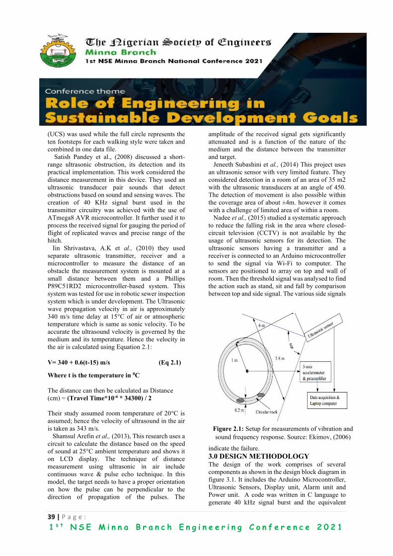
39 | P a g e :


(UCS) was used while the full circle represents the

ten footsteps for each walking style were taken and

combined in one data file.

Satish Pandey et al., (2008) discussed a short-

range ultrasonic obstruction, its detection and its

practical implementation. This work considered the

distance measurement in this device. They used an

ultrasonic transducer pair sounds that detect

obstructions based on sound and sensing waves. The

creation of 40 KHz signal burst used in the

transmitter circuitry was achieved with the use of

ATmega8 AVR microcontroller. It further used it to

process the received signal for gauging the period of

flight of replicated waves and precise range of the

hitch.

Iin Shrivastava, A.K et al., (2010) they used

separate ultrasonic transmitter, receiver and a

microcontroller to measure the distance of an

obstacle the measurement system is mounted at a

small distance between them and a Phillips

P89C51RD2 microcontroller-based system. This

system was tested for use in robotic sewer inspection

system which is under development. The Ultrasonic

wave propagation velocity in air is approximately

340 m/s time delay at 15°C of air or atmospheric

temperature which is same as sonic velocity. To be

accurate the ultrasound velocity is governed by the

medium and its temperature. Hence the velocity in

the air is calculated using Equation 2.1:

V= 340 + 0.6(t-15) m/s (Eq 2.1)

Where t is the temperature in 0C

The distance can then be calculated as Distance

(cm) = (Travel Time*10-6 * 34300) / 2

Their study assumed room temperature of 20°C is

assumed; hence the velocity of ultrasound in the air

is taken as 343 m/s.

Shamsul Arefin et al., (2013), This research uses a

circuit to calculate the distance based on the speed

of sound at 25°C ambient temperature and shows it

on LCD display. The technique of distance

measurement using ultrasonic in air include

continuous wave & pulse echo technique. In this

model, the target needs to have a proper orientation

on how the pulse can be perpendicular to the

direction of propagation of the pulses. The

amplitude of the received signal gets significantly

attenuated and is a function of the nature of the

medium and the distance between the transmitter

and target.

Jeneeth Subashini et al., (2014) This project uses

an ultrasonic sensor with very limited feature. They

considered detection in a room of an area of 35 m2

with the ultrasonic transducers at an angle of 450.

The detection of movement is also possible within

the coverage area of about ±4m. however it comes

with a challenge of limited area of within a room.

Nadee et al., (2015) studied a systematic approach

to reduce the falling risk in the area where closed-

circuit television (CCTV) is not available by the

usage of ultrasonic sensors for its detection. The

ultrasonic sensors having a transmitter and a

receiver is connected to an Arduino microcontroller

to send the signal via Wi-Fi to computer. The

sensors are positioned to array on top and wall of

room. Then the threshold signal was analysed to find

the action such as stand, sit and fall by comparison

between top and side signal. The various side signals

indicate the failure.

3.0 DESIGN METHODOLOGY The design of the work comprises of several

components as shown in the design block diagram in

figure 3.1. It includes the Arduino Microcontroller,

Ultrasonic Sensors, Display unit, Alarm unit and

Power unit. A code was written in C language to

generate 40 kHz signal burst and the equivalent

Figure 2.1: Setup for measurements of vibration and

sound frequency response. Source: Ekimov, (2006)

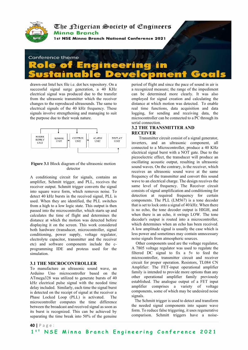
40 | P a g e :


drawn-out Intel hex file i.e. dot hex repository. On a

successful signal surge generation, a 40 KHz

electrical signal was produced due to the transfer

from the ultrasonic transmitter which the receiver

changes to the reproduced ultrasounds. The same to

electrical signals of the 40 kHz frequency. These

signals involve strengthening and managing to suit

the purpose due to their weak nature.

Figure 3.1 Block diagram of the ultrasonic motion

detector

A conditioning circuit for signals, contains an

amplifier, Schmitt trigger, and PLL, receives the

receiver output. Schmitt trigger converts the signal

into square wave form, which removes noise. To

detect 40 kHz bursts in the received signal, PLL is

used. When they are identified, the PLL switches

from a high to a low logic state. This output is then

passed into the microcontroller, which starts up and

calculates the time of flight and determines the

distance at which the motion was detected before

displaying it on the screen. This work considered

both hardware (transducer, microcontroller, signal

conditioning, power supply, voltage regulator,

electrolyte capacitor, transmitter and the receiver

etc) and software components include the c-

programming IDE and proteus used for the

simulation.

3.1 THE MICROCONTROLLER To manufacture an ultrasonic sound wave, an

Arduino Uno microcontroller based on the

ATmega328 was utilized to generate bursts of 40

kHz electrical pulse signal with the needed time

delay included. Similarly, each time the signal burst

is detected on the receipt of signal at the receiver a

Phase Locked Loop (PLL) is activated. The

microcontroller computes the time difference

between the broadcast and received signal as soon as

its burst is recognized. This can be achieved by

separating the time break into 50% of the genuine

period of flight and since the pace of sound in air is

a recognized measure; the range of the impediment

can be determined more clearly. It was also

employed for signal creation and calculating the

distance at which motion was detected. To enable

real time functions, data acquisition and data

logging, for sending and receiving data, the

microcontroller can be connected to a PC through its

serial connection.

3.2 THE TRANSMITTER AND

RECEIVER Transmitter circuit consist of a signal generator,

inverters, and an ultrasonic component, all

connected to a Microcontroller, produce a 40 KHz

electrical signal burst with a NOT gate. Due to the

piezoelectric effect, the transducer will produce an

oscillating acoustic output, resulting in ultrasonic

sound waves. On the contrary, is the receiver, which

receives an ultrasonic sound wave at the same

frequency of the transmitter and convert this sound

wave to an electrical charge. The design receives the

same level of frequency. The Receiver circuit

consists of signal amplification and conditioning for

detection at required frequency for certain

components. The PLL (LM567) is a tone decoder

that is set to lock onto a signal of 40 kHz. When there

is no echo, the tone decoder output is HIGH, and

when there is an echo, it swings LOW. The tone

decoder's output is routed into a microcontroller,

which determines when an echo has been received.

A low amplitude signal is usually the case which is

less power and sometimes may contain unnecessary

noise signals from atmospheric sources.

Other components used are the voltage regulator,

A 7805 voltage regulator was used to regulate the

filtered DC signal to fix a 5v to feed the

microcontroller, transmitter circuit and receiver

circuit for proper operation. Resistors, TL084 CN

Amplifier: The FET-input operational amplifier

family is intended to provide more options than any

other operational amplifier family previously

established. The analogue output of a FET input

amplifier comprises a variety of voltage

components, some of which may be undesired noise

signals.

The Schmitt trigger is used to detect and transform

the needed signal components into square wave

form. To reduce false triggering, it uses regenerative

comparison. Schmitt triggers have a noise-

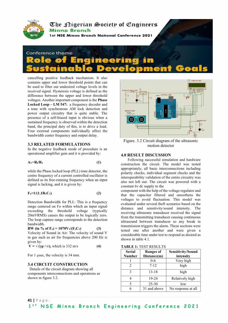
41 | P a g e :


cancelling positive feedback mechanism. It also

contains upper and lower threshold points that can

be used to filter out undesired voltage levels in the

received signal. Hysteresis voltage is defined as the

difference between the upper and lower threshold

voltages. Another important component is the Phase

Locked Loop – LM 547: a frequency decoder and

a tone with synchronous AM lock detection and

power output circuitry that is quite stable. The

presence of a self-biased input is obvious when a

sustained frequency is observed within the detection

band, the principal duty of this, is to drive a load.

Four external components individually affect the

bandwidth center frequency and output delay.

3.3 RELATED FORMULATIONS In the negative feedback mode of procedure is an

operational amplifier gain and it is provided by:

AV=Rf/R1 (1)

while the Phase locked loop (PLL) tone detector, the

centre frequency of a current controlled oscillator is

defined as its free-running frequency when an input

signal is lacking, and it is given by:

Fo=1/(1.1R1C1) (2)

Detection Bandwidth for PLL: This is a frequency

range centered on Fo within which an input signal

exceeding the threshold voltage (typically

20mVRMS) causes the output to be logically zero.

The loop capture range corresponds to the detection

bandwidth.

BW (in % of Fo) = 1070V1/(FoC1) (3)

Velocity of Sound in Air: The velocity of sound V

in gas such as air for frequencies above 200 Hz is

given by:

V = √ (γρ / ), which is 332 m/s (4)

For 1 µsec, the velocity is 34 mm.

3.4 CIRCUIT CONSTRUCTION Details of the circuit diagram showing all

components interconnections and operations as

shown in figure 3.2.

Figure. 3.2 Circuit diagram of the ultrasonic

motion detector

4.0 RESULT DISCUSSION Following successful simulation and hardware

construction the circuit. The model was tested

appropriately, all basic interconnections including

polarity checks, individual segment checks and the

interoperability validation of the entire circuitry was

also not left out. The circuit was powered with a

constant 6v dc supply to the

component with the help of the voltage regulator and

that the capacitor filtered and smoothens the

voltages to avoid fluctuation. This model was

evaluated under several theft scenarios based on the

distance and sensitivity/sound intensity. The

receiving ultrasonic transducer received the signal

from the transmitting transducer causing continuous

ultrasound between transducer so any break in

transmission triggers the alarm. These sections were

tested one after another and were given a

considerable time under test to respond as desired as

shown in table 4.1.

TABLE 1: TEST RESULTS

Serial

Number

Ranges of

Distance(m)

Sensitivity/Sound

intensity

1 0-6 Very high

2 7-12 high

3 13-18 high

4 19-24 Relatively high

5 25-30 low

6 31 and above No response at all

42 | P a g e :


Other components such as resistors and capacitors

were verified appropriately with their required

values. Figures 4.2 and 4.3 depicts graphs showing

the sensitively i.e., the degree at which this

ultrasonic detector can be used to track intruders in

case of theft or related scenarios per distance. It can

be observed that the close the range the better the

performance, a very good performance strength was

recorded up to 20 metres, beyond 20m the sound

detector and alarm system capacity reduced

drastically and fade away till 30m and beyond as

shown in figure 4.3. After extensive testing, the

system was proven to be quite effective in detecting

all motion within a range of 0-30 meters, with a

success rate of about 90%.

Table 4.2: Evaluation result showing strenght

of model

Table 4.3: Evaluation result showing the trend

of strenght

5.0 APPLICATON TO SECURITY

CHALLENGES Nowadays, solutions to security challenges

through network innovations and communication

have moved on and the multiplicity of

technologically-inclined security applications have

improved. The increase of security challenges

especially in nigeria can be addressed through the

result of this work. This motion detector has a very

high frequency to detect motion and can be deployed

to offices, prisons and other sensitive locations

where security issues has become a very serious

matter. In addition, is the high tone alert which can

awaken other security apparatus in case there is a

breach of such where they are installed. This will

quikly mobilize additional measures to abat the

challenge as may be required. In future, this work

will be improved upon to have a cloud-backup such

that location data and signal reports can be

incorporated as soon as there is an alert, this can

equally be accessed remotely even from sensitive

bush locations to track kidnappers, bandits and other

threat to the peace of a community, state and nation

at large. However, the secure design consideration

was based on a notice/awareness security principle.

6.0 CONCLUSION Conclusively, the outcome of this research and

demonstration of an ultrasonic motion sensor for

security system, human or object interference within

a space has been designed, implemented and

evaluated based on two major parameters; it can be

deduced that the use of a GSM and camera provides

better quality for any security purpose however;

considering the peculiarity of remote areas, and

basic theft activities in the face of poverty. The result

of this project becomes more viable. This system has

undergone an amount of research with different

authors presenting different methods,

implementation and design with motion detection,

obstacle detection and distance

measurements as one necessary requirements to

satisfy one requirement or the other. However, the

lacuna in the reviewed work has been considered

approprioatly to address some of the current security

issues being faced by Nigeria today. This proposed

design uses a microcontroller to generate signal that

helps to detect motion, obstacle and calculate the

43 | P a g e :


distance at which the detection was made and

intruders can be arrested for justice accordinly. The

implemenation is affordable and will in turn

contribute to security of lives and properties from

the grassroot.

REFERENCES Adebisi, J. A., Afolabi, B. S., & Akhigbe, B. I.

(2018). A

Value-based approach to modelling interoperability

in Knowledge Organization Systems. In

Challenges and Opportunities for Knowledge

Organization in the Digital Age (pp. 720-728).

Ergon-Verlag.

Adebisi, J. A., Abdulsalam, K. A., & Adams, I. O.

(2021).

Multi-Power Source and Cloud-Backup Enabled

Security Framework for Surveillance in Nigeria.

In IOP Conference Series: Earth and

Environmental Science (Vol. 730, No. 1, p.

012005). IOP Publishing.

David, J. N cheeke (2002). “Fundamentals of

Ultrasonic

Waves” CRC Press, Florida, USA.

Ekimov, A., & Sabatier, J. M. (2006). Broad

frequency

acoustic response of ground/floor to human

footsteps. In Data Mining, Intrusion Detection,

Information Assurance, and Data Networks

Security 2006 (Vol. 6241, p. 62410L).

International Society for Optics and Photonics.

Ekimov, A., & Sabatier, J. M. (2006). Vibration

and

sound signatures of human footsteps in buildings.

The Journal of the Acoustical Society of

America, 118(3), 762-768.

Geisheimer, J. L., Greneker III, E. F., & Marshall,

W. S.

(2002). High-resolution Doppler model of the

human gait. In Radar Sensor Technology and

Data Visualization (Vol. 4744, pp. 8-18).

International Society for Optics and Photonics.

He, H., & Liu, J. (2008). The design of ultrasonic

distance

measurement system based on S3C2410. In 2008

International Conference on Intelligent

Computation Technology and Automation

(ICICTA) (Vol. 2, pp. 44-47). IEEE.

Houston, K. M., & McGaffigan, D. P. (2003,

September).

Spectrum analysis techniques for personnel

detection using seismic sensors. In Unattended

Ground Sensor Technologies and Applications

V (Vol. 5090, pp. 162-173). International

Society for Optics and Photonics.

Jeneeth Subashini, b. C. (2014). Implementation,

working

and results of circuit detection of intruder(s)

movement using ultrasonic sensors.

International journal of computer science and

information technology research. 2(3), pp: (520-

526).

Nawer, A., Hossain, F., & Anwar, M. G. (2015).

Ultrasonic Navigation System for the visually

impaired & blind pedestrians. Am. J. Eng. Res.

(AJER), 4(2), 13-18.

Nadee, C., & Chamnongthai, K. (2015, June).

Ultrasonic

array sensors for monitoring of human fall detection.

In 2015 12th international conference on

electrical engineering/electronics, computer,

telecommunications and information technology

(ECTI-CON) (pp. 1-4). IEEE.

Pandey, S., Mishra, D., Srivastava, A., Srivastava,

A., &

Shukla, R. K. (2008). Ultrasonic Obstruction

Detection and Distance Measurement using

AVR Microcontroller. Sensors & Transducers

Journal, 95(8), 49-57.

Sabatier, J. M., & Ekimov, A. E. (2006). Ultrasonic

Methods for Human Motion Detection. In

Battlefield Acoustic Sensing for ISR

Applications. (pp. 9-1 – 9-12). Retrieved from

http://www.rto.nato.int/abstracts.asp.

Sharma, A., Patidar, R., Mandovara, S., & Rathod,

I. (2013). Blind Audio Guidance System.

International Journal of Emerging Technology

and Advanced Engineering, 3, 17-19.

Shamsul Arefin, T. M. (2013). Design of an

Ultrasonic

Distance Meter. International Journal of Scientific

& Engineering Research. 4(3), pp. 90-101.

Shrivastava, A. K., Verma, A., & Singh, S. P.

(2010).

Distance measurement of an object or obstacle by

ultrasound sensors using P89C51RD2.

44 | P a g e :


International Journal of Computer Theory and

Engineering, 2(1), 64-68.

Shefali Malhotra, S. B. (2016). "Blockage detection

in

seeder". World Conference on Futuristic Trends

in Research and Innovation for Social Welfare

(Startup Conclave).

Theraja, B. L., & Theraja, A. K. (2005). A textbook

of

Electrical Technology vol 1-IV. S. Chand and

Company limited: New Delhi, India 2002, pp.

1712 – 1716.

45 | P a g e :


A Brief Review of Proposed Models for Jamming Detection in

Wireless Sensor Network Grace AUDU, Michael DAVID and Abraham U. USMAN

[email protected]

ABSTRACT

Wireless sensor network (WSN) consists of a group of sensor nodes usually deployed in a hostile environment

used for sensing, processing, transmitting and receiving data from the area. Sensor Nodes are characterized

by limited memory, limited power and short transmission range, which exposes them to attacks like jamming.

In this paper, we review different jamming attacks in WSN. We also review several proposed methods for

detecting jamming. We have provided a comparative conclusion to aid researchers studying this field.

KEYWORDS: Jamming, Jamming detection, Denial of Service Attacks, Wireless Sensor Network.

I. INTRODUCTION Wireless sensor network (WSN) consists of a group of

sensor nodes usually deployed in a hostile environment

used for sensing, processing, transmitting and receiving

data where they are deployed to a base station (Osanaiye et

al 2015).

WSNs have different applications. They find application

were collecting data remotely is needed. These areas

include military, environmental monitoring, health,

controlling traffic, agriculture, and industries (Kumari et al,

2015). WSN have constrained power, storage, bandwidth

and short communication distance. These constraints in

addition to the open and shared wireless transmission

medium makes sensor nodes prone to security attacks.

Denial of Service (DoS) is one of the common attacks in

WSN. These attacks occur in physical, link and network

layer. At the physical layer, the most common DoS attack

is jamming. Jamming occurs when a rogue node

intentionally transmits a high-range signal to disrupt the

normal transmission of information between legitimate

nodes by reducing the signal to noise ratio. This attack

affects the functionality of the network as it truncates the

delivery of desired packets to the intended receiver hence

impeding network capabilities (Bhushan & Sahoo ,2018).

The major goal of jamming is to affect the long-term

availability of sensor nodes. The jammer depletes the

resources of sensor nodes by transmitting electromagnetic

signals at high power towards the communication channel

of the sensor nodes thereby prohibiting data from reaching

its destination (Upadhyaya et al.2019).

Jamming can be perpetrated by listening passively to the

communication channel in order to transmit at the same

frequency as the legitimate sensor node. Jammers have

high energy efficiency and are not easily detected

(Pelechrinis et al., 2011)

Jamming attack may be mitigated by increasing the

robustness of the legitimate signal or by implementing

frequency hopping. Due to the limited resources of WSN

applying those solution is difficult. WSN, hence the need

for detecting jamming. In this paper we describe types of

jamming attacks, metrics used for detecting jamming and

review the different proposed methods to detect jamming.

WIRELESS SENSOR NETWORK

ARCHITECTURE

The WSN architecture is made up of five layers (Akyildiz

& Vuran, 2010). These includes:

Physical layer: is responsible for transmission, modulation

and receiving techniques.

Link layer: ensures bit are transferred without errors and

it controls access to the channel.

Network layer: routes the data supplied by the transport

layer.

Transport layer: This layer is needed when the network is

going to be access by external networks; it helps to

maintain the flow of data to prevent congestion.

Application Layer: provides software for numerous

applications depending on the sensing task.

Jamming attack occurs at the physical and link layer.

II. JAMMING ATTACKS IN WIRELESS

SENSOR NETWORK

Constant Jammer: constant jammer transmits random bits

continuously on the channel to disrupt communication on

the channel. This could lead to depletion of the legitimate

node’s energy. The constant jammer does not follow any


46 | P a g e :


Medium Access Control (MAC) layer procedure before

continually transmitting series of radio signals to interrupt

legitimate signal transmission in the network. This jammer

continuously transmits random bits that occupy the

transmission path of the network, hence disrupting

legitimate data transmissions initiated by nodes (Misra et

al., 2010).

Deceptive jammer: A deceptive jammer continuously

injects legitimate bit sequences into the communication

channel without gaps in between. The sensor nodes believe

that a legitimate transmission is going on, hence they

remain in the listening state. Detecting deceptive jammers

is difficult since they are aware of the network protocol

(Misra et al., 2010).

Random Jammer: Random jammers moves from active

mode to sleep mode and vice versa to save energy. During

the active state, the attacker jams the network for a specific

time then it turns off its transmitter and goes to sleep mode.

The attacking node begins to transmit the malicious signal

again, after a while then goes back to sleep mode; the

sequence continues (Misra et al., 2010).

Reactive Jammer: Reactive jammers constantly sense the

channel to listen for when packets are being transmitted.

Once they detect a packet transmission on the channel, they

begin to transmit malicious signals to disrupt the legitimate

signal. This type of jammer reduces the rate of power

dissipation and are hard to detect (Misra et al., 2010).

a. PROPOSED METHODS FOR

DETECTING JAMMING IN WIRELESS

SENSOR NETWORK

Research on jamming detection in WSNs has been ongoing

for a while. A lot of proposed methods for detecting

jamming involves either the use of dedicated tools or

algorithms installed on the sensor nodes. Most of these

proposed methods make use of information gathered a

priori about some metrics of the node when it is jammed or

normal. Some of these metrics include received signal

strength(RSS), packet delivery ratio(PDR), packet inter

arrival time(PIAT), packet sent ratio, bad packet

ratio(BPR) signal to noise ratio(SNR), consumed energy,

clear channel assessment.

Osanaiye et al. (2015) proposed an approach for detecting

jamming attacks that uses the cluster-based topology. The

EMWA algorithm used for detecting jamming is only

installed on the cluster head and base station. The base

station detects jamming in the member nodes while base

stations detect jamming in the cluster head. In order to

minimize overhead they used only metric packet IAT to

detect jamming. In order to detect changes in traffic flow

during situations of both non-jamming and jamming, a

trace-driven experiment using EWMA was carried out.

Results obtained from their work shows that their proposed

model can detect jamming attack efficiently with little or

no overhead in WSN from the 20th jammed packet.

Bikalpa et al. (2019) in their work proposed a node-centric

approach. To reduce overhead in nodes in this detection

method, network information for detecting jamming are

passively gathered by anchor nodes placed in the network.

Using random forest algorithm, the information gathered a

prior about the network is used differentiate when the

network is jammed or not. Their work achieved 89.7% and

98.6% accuracy using RSSI from five anchor nodes for real

and simulated data respectively.

In their work, Youness et al., (2020) used four metrics

BDR, PDR, RSS and clear channel to identify the presence

of jamming attack. They generated a large set of data in a

real environment simulation and gathered measurements of

these parameters when the network was jammed and when

it was normal. They then used these data sets to train,

validate, and test the machine learning algorithms. The

simulation results showed that the proposed detects

jamming attacks with an accuracy of 97.5%.

Ganeshkumar et al. (2016) proposed a framework that also

uses cluster-based topology for jamming detection. They

used statistical tests to compute the detection metrics

normal threshold. The cluster head verifies if a packet

received is from a legitimate node. The framework

validates whether the node is a legitimate node by using the

cluster head code. Lastly, the auditing algorithm on the CH

estimates the metrics (PDR, RSSI) and makes decision

about “jammed situation” or “non-jammed situation. Their

proposed framework detects jamming with an accuracy of

99.88%.

A fuzzy logic–based algorithm was proposed by

Vijayakumar et al. (2018) for jamming detection in cluster‐

based wireless sensor networks. The detection metrics is

checked by the cluster head to check for jamming. An

accuracy of 99.89% was gotten from their simulation. The

jamming detection metrics are checked by the cluster head

at the lower level and by the base station at the higher level.

There by reducing the overhead cost on the member nodes.

Mistra et al., (2010) proposed the use of a fuzzy inference-

based system for jamming at the base stations using three

metrics. These metrics include received signal strength,

total packets received during a period and the number of

dropped packets during that period. The power received

signal is measured at the base during the jamming attack to

find the difference in value between the normal RSS.The

total packets received during a specific period and the

packet sent over the period is used at the base station to

determine the packet drop per terminal (PDPT) and signal-

47 | P a g e :


to-noise ratio (SNR). These metrics are then inputted to

obtain the jamming index from the fuzzy inference system.

The jamming index varies from 0 to 100. The system’s

true-detection rate is as high as 99.8%. In a Table 1, we

present a summarize Comparison of Proposed Methods for

Jamming detection in Wireless Sensor Network.

TABLE 1: Comparison of Proposed Methods for Detecting Jamming in Wireless Sensor Network

REFERENCE

MACHINE LEARNING

OR NON-MACHINE

LEARNING METHOD

ALGORITHM

USED Metrics

WSN

STRUCTURE ACCURACY

Osanaiye et al

(2015)

Non-Machine Learning

Method EMWA IAT Cluster

100% >20 Jammed

packets

Bikalpa et al.

(2019)

Machine Learning

method Random forest RSS Flat

89.7% for real data

and 98.6 for

simulated data

Youness et al.,

(2020)

Machine Learning

method Random forest

BPR, PDR,

RSS Flat 97.5%.

Ganeshkumar et

al., (2016)


Method

Auditing

algorithm

PDR and

RSSI Cluster 99.88 %.

Vijayakumar et

al.,(2018


Method

Fuzzy logic–

based

jamming

detection

algorithm

PDR and

RSSI Cluster 99.89 %.

Misra et al.,

2010


Method Fuzzy logic PDR, RSS Cluster 99.89 %.

48 | P a g e :


A fuzzy inference-based system to detect jamming

attacks in the base stations using three metrics

measured from each sensor node in the network was

proposed by Mistra et al., (2010). These metrics are

the total packets received during a specific period,

the number of dropped packets during that period

and the received signal strength (RSS). The base

station computes the power received during the

jamming attack to find any difference in value

between the current RSS and the normal RSS. These

values are used by the base station to compute the

packet drop per terminal (PDPT) and signal-to-noise

ratio (SNR) which is further used as inputs for the

fuzzy inference system to obtain the jamming index

The jamming index varies from 0 to 100 and is used

to determine the intensity of the jamming attack,

which can range between a situation of ‘no

jamming’ to absolute jamming’. The system with its

high robustness, ability to grade nodes with jamming

indices, and its true-detection rate as high as 99.8%,

is worthy of consideration for information warfare

defense purposes. In a Table 1, we present a

summarize Comparison of Proposed Methods for

Detecting Jamming in Wireless Sensor Network.

III. CONCLUSION

In this paper, we presented a brief survey about

jamming detection in wireless sensor networks.

Different jamming attacks occurring in WSNs are

described in detail. Different metrics used for

detecting jamming was described. The different

types of jamming are described, and detection

techniques of jamming has been is pointed out. Our

future work will focus on improving jamming

detection.

ACKNOWLEDGEMENTS

The authors sincerely thank the reviewers for

proofreading the article and providing constructive

feedback.

REFERENCES

O.A. Osanaiye, S.A. Attahiru, & Gerhard P. Hancke

(2018). A Statistical Approach to Detect

Jamming Attacks in Wireless Sensor Network.

Sensors, 1691(18) 1-15

Saru Kumari, Muhammad Khurram Khan, and

Mohammed Atiquzzaman. (2015). User

authentication schemes for wireless sensor

networks. Ad Hoc Netw. 27, C (April 2015), 159–

194.DOI:https://doi.org/10.1016/j.adhoc.2014.1

1.018

B. Upadhyaya, S. Sun and B. Sikdar (2019).

Machine Learning-based Jamming Detection in

Wireless IoT Networks. 2019 IEEE VTS Asia

Pacific Wireless Communications Symposium

(APWCS),1-5.

Bhushan, B. & Sahoo, G. (2018). Recent Advances

in Attacks, Technical Challenges, Vulnerabilities

and Their Countermeasures in Wireless Sensor

Networks. Wireless PersCommun 98, 2037–

2077. https://doi.org/10.1007/s11277-017-4962-

0

Y. Arjoune, F. Salahdine, S.Islam, E. Ghribi & N.

Kaabouch(2020). A Novel Jamming Attacks

Detection Approach Based on Machine Learning

for Wireless Communication. The 34th

International Conference on Information

Networking (ICOIN 2020) ffhal02509430f, 1-5.

Ganeshkumar, P. , Vijayakumar, K. , & Anandaraj,

M. (2016). A novel jammer detection framework

for cluster-based wireless sensor networks. J

Wireless Com Network, 2016 (1). doi:

10.1186/s13638-016-0528-1

K. P. Vijayakumar,P. Ganeshkumar, M. Anandaraj,

K. Selvaraj & P. Sivakumar(2018). Fuzzy logic–

based jamming detection algorithm for cluster

based wireless sensor network. Int Journal of

Communication Systems 31(10), 1-21.

Misra, S., Singh, R. & Mohan, S.V.R (2010).

Information Warfare-Worthy Jamming Attack

Detection Mechanism for Wireless Sensor

Networks Using a Fuzzy Inference

System. Sensors 2010, 10, 3444-3479.

https://doi.org/10.3390/s100403444

Osanaiye, O., Choo, K.K.R. & Dlodlo, M. (2016).

Distributed denial of service (DDoS) resilience

in cloud: Review and conceptual cloud DDoS

mitigation framework. J. Netw. Comput. Appl.

2016, 67, 147–165. Journal of Network and

Computer Applications 67, 147-165

https://doi.org/10.1016/j.jnca.2016.01.001

https://doi.org/10.1007/s11277-017-4962-0

https://doi.org/10.1007/s11277-017-4962-0

https://doi.org/10.3390/s100403444

https://www.sciencedirect.com/science/journal/10848045

https://www.sciencedirect.com/science/journal/10848045

https://www.sciencedirect.com/science/journal/10848045/67/supp/C

https://doi.org/10.1016/j.jnca.2016.01.001

49 | P a g e :


Pelechrinis, K.; Iliofotou, M.; Krishnamurthy, S.V.

(2011). Denial of service attacks in wireless

networks: The case of jammers. IEEE Commun.

Surv. Tutor. 2011, 13, 245–257.

Ian F. Akyildiz & Mehmet Can Vuran(2010).

WSN Architecture and Protocol Stack. Wireless

Sensor Networks 10-15

50 | P a g e :


Design and Implementation of a Fire/Gas Safety System with

SMS and Call Notification M. A. Kolade, K.A. Abu-bilal, U.F. Abdu-Aguye, Z.Z Muhammad, and Kassim A. Y

Department of Telecommunications Engineering,

Ahmadu Bello University Zaria, Nigeria

Email: [email protected]

ABSTRACT Swift and effective communication have a tremendous effect on the outcome of the safety and incidences. With

the increase in domestic use of Liquefied gas in developing country coupled with poor infrastructures and low

level of literacy, it is paramount to incorporate prompt safety measures to safeguard life and properties. The

availability and wide acceptance of mobile phones in the countries make them a suitable communication means,

for swift and effective remote monitoring and control. Design and implementation of a fire and gas detection

system with SMS and call notification was carried out in this paper. This system is divided into three units, the

control unit, sensing unit, and the alert unit. The designed system uses a micro-controller and GSM module, to

translating and relate the output from the sensors. The codes used by the micro-controller were developed in

Arduino IDE (Independent Development Environment) using Arduino language. The prototype of the system

was developed using MQ9 and KY-026 for the gas and fire sensor respectively located at specific locations in

the home. The GSM module was used to enable remote communication to the user mobile phone. It receives

the information from the micro-controller and then acts as programmed. The prototyped system was subjected

to load and no-load test in which the system was found to be working normally in accordance with the design

specifications. When the system was subjected to reliability test, an index of 0.85 was obtained based on the

failure rate of each of the component used in fabricating the system. The design system has the potential of

reducing loss of lives and property to fire outbreak and gas leakages, due to its remote and surrounding alerting

capabilities.

KEYWORDS: Mobile phone, GSM module (SIM800), Arduino UNO, Gas Sensor, Fire Sensor.

1. INTRODUCTION Gas leakages and fire incidence are common

occurrence in today’s world especially in developing

country where safety is least considered coupled

with low level of literacy. Where fire or gas leakage

is been detected early and responded to as

appropriately, probability of getting out of control

can be litigated. (1) designed a GSM based low-cost

gas Leakage, explosion, and fire alert system with

advanced security. The system is designed such that

in case fire or gas leakage occurs a buzzer is turned

on, an LCD outputs a message indicating the reason

for the alarm and an SMS is sent to the home owner.

(2) Also propose such a system, where a gas sensor

is used to detect gas leakage and subsequently, turn

the exhaust fan on. [4] Developed a similar system

with an addition to monitor rapid temperature

increase in a home. (3) Also improved on

subsequent systems with a system equipped to open

an exit windows to allow for diffusion of the

concentrated air in case of gas leakage similar to (2),

(5) in another related system, in the event of a fire,

the system is equipped with a solenoid valve

controlled water/carbon dioxide reservoir to douse

the fire, as well as an alert system.

It is evident from the reviewed literatures that a lot

of research has been done on fire and gas leakage

detection systems with some going further to control

the situation. Most of the implemented systems are

to turn on buzzer and send SMS to the homeowner,

without additional steps to ensure the sent SMS are

viewed with required urgency. Hence a need for a

system with an increase the probability of sent SMS

been read received the required urgency which is

directly related to swift response from the

homeowner.

2. MATERIALS AND METHORDS In this section, the details of the design, hardware’s

and software’s materials used in the

implementation of the system are summarized.

2.1 The Design Structure


51 | P a g e :


Figure 1 shows the block diagram of the Fire/Gas

Safety System. It consists of a power supply unit

which supplies required power to other subsystems.

The control unit consist of a programmable

microcontroller - Arduino UNO, fire sensor – KY-

026 and gas sensor – MQ-9 and the alert unit which

consist of the GSM-module and the buzzer. The

GSM module serves as the communication bridge

between the microcontroller and the user’s phone.

SMS messages and call from the system in case of

emergency are sent to the user’s phone through the

GSM module. The system is divided into two

sections: Hardware and software.

Figure 1: Block Diagram of the Fire/Gas Detection

System

2.2 Hardware Design and Selection

The hardware components used are Arduino UNO,

KY-026, MQ-9, GSM module SIM800, 240V/12V

3A transformer, four diodes 1N4001, filtering

capacitor 2000uf and 5V 2A regulator LM78S05

and buzzer.

Detailed analysis of the various hardware units is

given below.

2.2.1 Power Supply Unit

This unit is made up of several sections, the system

component’s power requirement is considered in

this design. The control unit requires a 5V 500mA

for the Arduino UNO, while SIM800 requires

between 3.4V - 4.4V and 1A current for reliable

operation. The fire and smoke sensors both require

3.5V - 5V and current of about 200mA. The power

supply should be able to provide the combine

current of 2A. Figure 2 shows the block diagram of

the power supply unit.

Figure 2: Block Diagram of the Power Supply Unit

The power supply unit consists of a stepdown

transformer that has an output of 14V AC with

output current of about 1A, a full bridge rectifier, a

voltage regulator (7805) and a filter. The power

requirement of the security system is 5V.

The transformer design and selection: The

220V AC from the mains is stepped down to 14V

AC with the help of the transformer. The peak

voltage output of the transformer is calculated using

equation (1).

𝑉𝑝𝑒𝑎𝑘 = √2 × 𝑉𝑟𝑚𝑠 (1)

Where, 𝑉𝑟𝑚𝑠 = 14𝑉

𝑉𝑝𝑒𝑎𝑘 = √2 × 14

𝑉𝑝𝑒𝑎𝑘 = 19.80𝑉

Rectifier diode design and selection: Four

1N4001 diode connected in bridge were used for the

full wave rectification of the output voltage from the

transformer. IN4001 was chosen because its PIV

(Peak Inverse Voltage) is 50V which is greater than

𝑉𝑝𝑒𝑎𝑘 which is approximately 20V.The value of the

rectified voltage is calculated as follows.

𝑉𝑑𝑐 = (2 ∕ 𝜋) × 𝑉𝑝𝑒𝑎𝑘 (2)

But 𝑉𝑝𝑒𝑎𝑘 = 19.80𝑉

𝑉𝑑𝑐 = (2/𝜋) × 19.80

𝑉𝑑𝑐 = 12.61𝑉

Voltage regulation and filter design: For the

section of the home security system which requires

a 5V power supply, a 5V regulator (LM7805) was

used. The choice is based on the IC’s ability to keep

its output voltage stable at 5V and it can provide up

to 1A load current. LM7805 also have attached heat

sink to conduct the generated heat away from it

under working condition. For the filter section it is

preferable to choose a filtering capacitor that holds

the peak-to-peak ripples (RF) at approximately 70%

- 80% of the peak voltage. The smaller the ripple

factor the better the performance of the filter.

52 | P a g e :


Therefore, using design specifications, the value of

the capacitor can be calculated as follows:

From the relations:

𝑄 = 𝐶 × 𝑉 (3)

𝑄 = 𝐼 × 𝑇 (4)

𝑓 =1

𝑇 (5)

Imin = Idc = 1A

Here, C is filtering capacitor, Q is charge in

colombs, I is current taken by the load, T is period

in seconds and f is frequency in Hz. Using, equations

(3) and (4) and substituting for T from equation (5),

yields:

𝐶 = 𝐼

𝑉𝑓 (6)

But V is the peak-to-peak voltage, and RF is the

ripple factor. To calculate its value, the relation of

equation (7) is used

𝑉 = 𝑅𝐹 × 𝑉𝑟𝑚𝑠 (7)

𝑉𝑟𝑚𝑠 is given by √2 × 𝑉𝑚 where 𝑉𝑚 is the system

required voltage 5V, the mains frequency is 50Hz

and the RF is 70%.

Therefore

𝑉 = 0.7 × √2 × 5

V = 4.949 Volts

And 𝐶 =1

4.949×50

𝐶 = 4040µf

The standard available value used is 4400µf, where

two 2200µf are connected in parallel. Figure 3

shows the circuit diagram of the power supply unit

of the fire/gas detection system.

Figure 3: Circuit Diagram of Power Supply Unit

2.2.2 Control Unit: This unit is made up of

three main components which are: Arduino

UNO, fire sensor and smoke sensor.

Arduino UNO: is a board embedded with

ATmega328 a microcontroller, ATmega328 is an

integrated circuit (IC) containing all the main parts

of a typical computer, which are: Processor,

Memories, Peripherals, Inputs, and Outputs (6). It

will provide required computing resource to achieve

the aim. All communication and controls in this

system pass through the microcontroller. The

Arduino UNO has 14 digital input/output pins (of

which 6 can be used as PWM-Pulse Width

Modulation- outputs), 6 analogue inputs, a 16 MHz

ceramic resonator, a USB connection, a power jack,

an In-Circuit Serial Programming (ICSP) header,

and a reset button. It contains everything needed to

support the microcontroller. Arduino UNO board is

shown in Figure 4.

Figure 4: The Arduino UNO Board

Fire Sensor KY-026: The KY-026 consist of a

5mm infra-red receiver LED, a LM393 dual

differential comparator a 3296W trimmer

potentiometer, six resistors and two indicator LEDs.

(7) The board features an analogue and a digital

output. Its operating voltage ranging between 3.3V

to 5V and Infrared Wavelength detection of about

760nm to 1100nm.The connected photo diode is

sensitive to the spectral range of light, which is

created by open flames. Digital Out: After detecting

a flame, a signal will be outputted. The sensor has 3

main components on its circuit board. First, the

53 | P a g e :


sensor unit at the front of the module, which

measures the area physically and sends an analogue

signal to the second unit, the amplifier. The

amplifier amplifies the signal, according to the

resistant value of the potentiometer, and sends the

signal to the analogue output of the module. The

third component is a comparator which switches the

digital out and the LED if the signal falls under a

specific value. You can control the sensitivity by

adjusting the potentiometer. A KY-026 Fire Sensor

is shown in Figure 5.

Figure 5: Fire Sensor KY-026

Gas Sensor MQ-9: (7) MQ-9 consist of a

sensitive material (SnO2), which has lower

conductivity in clean air, the sensors conductivity

increases as concentration of carbon monoxide and

hydrocarbon in the air increases. Detection is made

by method of cycle high and low temperature. It has

a working voltage of 5V, a with wide 2-20kΩ range

of resistance and able to detect concentration of

about 200ppm minimum and 10000ppm maximum.

(7) A relationship between the voltage output and

gas concentration level for various common gases is

shown in table 1.

Table 1: Output Voltage against Gas Detected

Concentration Level

2.2.3. The Alerting Unit

The alerting or output unit comprises of the GSM

module and buzzer, both are to relate information

from the controller, they are the link between the

user and the system’s control section.

GSM Module SIM800: SIM800 is a cellular

communication module that can make calls, send

email, SMS, and even connect to the internet. The

module operates like a mobile phone, but it needs

external peripherals to function properly. Figure 6

show the image of a SIM800 board.

Figure 6: SIM800 Board

The module has audio channels which include a

microphone input and a receiver output, a SIM card

interface, and it is Quad band hence can connect to

any global GSM network with any 2G SIM. The

receiver pin (RXD) of the module is connected to

transmitter pin (02) of Arduino while the transmitter

pin (TXD) of the module is connected to the receiver

pin (01) of Arduino, 𝑉𝑐𝑐 pin of the module is

connected to the LM78S05 in voltage divider circuit

and GND pin to the ground. Communication speed

(baud rate) depends on the board to be paired with,

baud rate of 115200 was chosen, this rate allows for

successful communication between SIM800 and

Arduino UNO.

Buzzer: A buzzer is an electronics component usually used

to add sound feature to systems, the buzzer is

associated with switching ON or turning OFF at

required time and adequate interval. The buzzer is

powered with 5V DC and controlled through the

Arduino. It has two terminals, the positive terminal

is identified by (+) symbol or longer terminal lead,

while the negative terminal is identified by (-)

symbol or shorter terminal lead.

54 | P a g e :


The hardware of the system unit comprises of LEDs-

which serves as indicators, resistors, GSM module

(SIM800), fire sensor, gas sensor, buzzer, and

Arduino UNO. The receiver pin Pin 0 of Arduino is

connected to the transmitter pin Pin Tx of SIM800

and the receiver pin Pin Rx of SIM800 is connected

to transmitter pin pin1 of the Arduino, the signal pin

GPIO of SIM800 is connected to pin 9 of Arduino,

analog pin (A01) of the Arduino is connected to the

signal pin SIC of MQ-9, while the analog pin (A02)

of Arduino is connected to the analog signal pin A0

of KY-026 as showed in Figure 6. Power

requirement of SIM800 is 3.3V 20mA, 3.3V for KY-

026 and 5V for MQ-9. LED1 is connected to digital

pin10, LED2 is connected to digital pin13. The

LEDs were connected in a series connection with

resistors in a simple way to stabilize the current

flowing through them. Also, the buzzer is connected

to pin4 of the microcontroller through an amplifying

transistor, which controls the switch ON and OFF

the buzzer. Figure 7 the circuit diagram of the alert

units and control unit.

Figure 7: Circuit Diagram of GSM, Fire Sensor

and Gas Sensor connected to Arduino UNO

Design and calculations: Led design

LEDs voltage drop 𝑉𝑓 is between 1.8V - 2.5V (a

worst case is used in the design, 2.5V) and operating

current I is 20mA, while 𝑉𝑠 (supply voltage) is equal

to 5V (from Arduino pin). Using these values, the

value of the current limiting resistors can be

obtained.

Ohms law, equation (8) was used to calculate the

value of the Resistors R (𝑅1and 𝑅2 ), as shown.

𝑅 =( 𝑉𝑆−𝑉 𝑓 )

𝐼 (8)

𝑅 =(5−2.5)

(20×10−3 )

𝑅 = 125Ω

From the obtained value of 125 ohms a standard

value of 150 Ω±𝟐𝟎% was chosen for 𝑅1and𝑅2.

Buzzer circuitry:

The home-based alert system (buzzer) requires an

amplifying circuit. The amplification circuit requires

a multipurpose NPN transistor (C1815) with a base

resistor 𝑅3 required to provide base current for the

transistor. The value of the resistor (𝑅3) was

calculated using equations (9):

𝑅 =( 𝑉𝑆−𝑉 𝑓 )

𝐼 (9)

Where V is the powered voltage from the Arduino

UNO 5V, 𝑉𝑏𝑒 is the base-emitter voltage 0.7V and

𝐼𝑏 is the base current (500uA)

𝑅3 = 5−0.7

0.005

𝑅3 = 860Ω

From the obtained value of 860 ohms a standard

value of 1k Ω±𝟐𝟎% was chosen. The complete

circuit diagram of the whole system with the power

supply is shown in figure 8.

Figure 8: Circuit Diagram of the Complete System

2.3 Writing Source code for the

microcontroller Arduino UNO The source code is written to satisfy the requirement

of system whose main controller is an Arduino

UNO. The program was written in the Arduino IDE.

55 | P a g e :


The flowchart of Figure 9 was used to develop the

program.

2.3.1 Software Design Methodology

The software used in this work to control and

synchronize the activities of all system parts to

function as a unit is implemented using the flowchart

in Figure 8. The software codes were written in

Arduino integrated development environment (IDE)

with Arduino programming language.

Figure 9: Flow Chart of the System Control

3. RESULTS AND DISCUSSION

3.1 Testing of the designed circuit and

components

All the components used were tested to ensure

workability before and after physical construction of

the system’s porotype to ensure that all contacts and

connections were made properly. Test was

conducted at unit levels. The tests conducted were

categories into hardware and software test.

The hardware unit was initially designed and

simulated using circuit wizard and proteus, this is to

ascertain the circuit is working properly based on

design specifications. After which the components

are put onto breadboard for further testing and

finally soldered on the Vero-board. Figure 10 shows

simulation of the power supply unit.

Figure 10: Screen Shot of the Power Supply during

Simulation

Controller Unit The controller unit comprises of the microcontroller

board, fire detector, gas detector and the GSM

module. Software was uploaded on the

microcontroller and the response to stimuli from

both the fire and gas detectors was monitor via the

communication 3 port (COM3) of the computer.

This test makes it possible to understand what is

happening inside the microcontroller. The GSM

module has in it a registered subscriber

identification module (SIM) card. Once the GSM

module is connected to power, a blinking green led

(with about 2 seconds interval) on it indicates a

successful connection to network. Software was also

written in the microcontroller to output status of

network connection. The software is presented in

appendix A. Figure 11 presents the COM3 output

during a stage of the test period.

Figure 11: Software Test Result

3.3 Fire Sensor/Gas Sensor The sensors were both tested with same situation

while connected to a DC battery, a beep from both

56 | P a g e :


sensors, indicate they are both in good condition,

their functionality is ensured.

3.4 System Test The full system test was to ensure proper response is

given by the developed system in a case of fire

outbreak or gas leakage when required by the

homeowner. The system was initially designed and

simulated in proteus environment, to ensure the

system is working perfectly based on design

specifications. The system was constructed on a

breadboard; this was to ensure proper arrangement

in other to ensure a potable system. Finally, the

system was implemented and tested on a Vero-

board.

3.4.1. Simulation Test

This simulation was carried out using Circuit

Wizard, this helped in design of the circuit and

testing it with software uploaded, to ascertain the

circuit is working properly based on design

specifications. After which the components are put

onto breadboard for further testing and finally

soldered on the Vero-board.

3.4.2. No - Load Test

This test was carried out when the circuit has been

developed on a Vero board. A state at which the

system is not faced with any control responsibility,

this is the verification stage. Physical inspection

was done to ensure all components and connections

were in place. This was done by checking all closed

tracks, jumper wires etc. for open or short circuit.

Power was fed to the circuit for a minute. Fingertip

was then used to sense the temperature of the

components if any was overheating. Also, code

inspection was carried out to ensure optimal use of

memory, by employing DRY (Don’t Repeat

Yourself) technique. DRY technique is a principle in

software development implemented to reduce

software duplication. Being satisfied with this test

result, load test then followed.

3.4.3. Load Test

At this stage, power consumption was monitored to

ensure power specifications are met, with the

voltmeter, the current consumption of the circuit was

taken note of - when a response is required and when

not. The response time to control was also

monitored. For the software aspect, the performance

of the code was scrutinized, the software was

compiled and executed, parameters such as memory

usage, CPU usage, response time and overall

performance for the software were analyzed.

Voltage test then followed. This was performed with

a digital multi-meter. Voltage and current level at

different points on the board was taken and

compared with design specification. Figure 11

shows the test diagram used during voltage and

current consumption test.

Figure 11: Test Diagram for Voltage and Current

Consumption

The current consumption test of the system was

carried out using two instances, when response is

required and when not. This test was repeated

several times and an average value computed. The

voltage at the Arduino power pin was also

monitored, to ensure conformance with design

specifications. Results of the voltage and current test

carried out are presented in Table 2 and Figure 12

shows a test instance.

Table 2: Voltage and Current Consumption

Readings.

S/N No load

current

(A)

Load

current

(A)

Voltage

(V)

1 0.234 0.45 5.12

2 0.232 0.43 4.97

3 0.201 0.46 5.09

4 0.200 0.42 5.00

5 0.221 0.41 5.05

Average 0.217 0.434 5.056

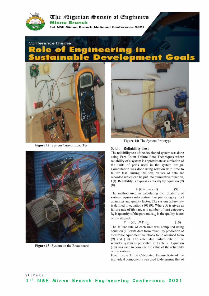
57 | P a g e :


Figure 12: System Current Load Test

Figure 13: System on the Breadboard

Figure 14: The System Prototype

3.4.4. Reliability Test The reliability test of the developed system was done

using Part Count Failure Rate Techniques where

reliability of a system is approximate as a relation of

the units of parts used in the system design.

Computation was done using relation with time to

failure test. During this test, values of data are

recorded which can be put into cumulative function,

F(t). Reliability is express explicitly by equation (9)

(8):

F (t) = 1 – R (t) (9)

The method used in calculating the reliability of

system requires information like part category, part

quantities and quality factor. The system failure rate

is defined in equation (10) (9). Where 𝐹𝑖 is given as

failure rate of ith part, n is number of part category,

𝑁𝑖 is quantity of the part and 𝜋𝑄𝑖 is the quality factor

of the ith part:

𝐹 = ∑ 𝑁𝑖𝐹𝑖𝜋𝑄𝑖𝑛𝑖=1 (10)

The failure rate of each unit was computed using

equation (10) with data from reliability prediction of

electronic equipment handbook table obtained from

(9) and (10). The calculated failure rate of the

security system is presented in Table 3. Equation

(10) was used to compute the value of the reliability

of the system.

From Table 3: the Calculated Failure Rate of the

individual components was used to determine that of

58 | P a g e :


Table 3: Calculated Failure Rate of Fire/Gas Safety System

the system. The failure rate was then used to obtain

the system reliability using equation (9) as shown

below.

𝑅(𝑡) = 1 − 0.14887504

𝑅(𝑡) = 0.85115196

𝑅(𝑡) ≈ 0.85

4. CONCLUSION The detailed procedure for the design and

implementation of a fire and gas safety system with

SMS and call notification was outline in this work.

The designed system was simulated using proteus,

the simulated system was then fabricated using

hardware components. The fabricated prototyped

system worked normally as designed. The system is

light in weight (that is portable) and has a reliability

index of 0.85 when subjected to reliability test. The

design system has the potential of reducing loss of

lives and property to fire outbreak and gas leakages,

due to its remote and surrounding alerting

capabilities.

REFERENCES P. Ghosh and P. K. Dhar, "GSM Based Low-cost

Gas Leakage, Explosion and Fire Alert System

with Advanced Security," 2019 International

Conference on Electrical, Computer and

Communication Engineering (ECCE),

Cox'sBazar, Bangladesh, 2019, pp. 1-5, doi:

10.1109/ECACE.2019.8679411.

M. A. F. Malbog, H. D. Grimaldo, L. L. Lacatan, R.

M. Dellosa and Y. D. Austria, "LPG Leakage and

Flame Detection with SMS Notification and

Alarm System: Rule-Based Method," 2020 11th

IEEE Control and System Graduate Research

Colloquium (ICSGRC), Shah Alam, Malaysia,

2020, pp. 323-327, doi:

10.1109/ICSGRC49013.2020.9232494.

A. Y. Nasir, Adoyi Boniface, A.M. Hassan, N. M.

Tahir “Development of a Gas Leakage Detector

with Temperature Control system, 2019” Journal

of Multidisciplinary Engineering Science and

Technology (JMEST) ISSN: 2458-9403 Vol. 6

Issue 12.

Rupali S. Gajare, Dr. P. M. Mahajan, “Home and

Industrial Safety System for fire and gas Leakage

detection, 2018”, International Research Journal

of Engineering and Technology (IRJET) e-ISSN:

2395-0056 www.irjet.net p-ISSN: 2395-0072

Lacatan, Luisito & Dellosa, Rhowel & Malbog, Mon

Arjay & Austria, Yolanda. (2020). LPG Leakage

and Flame Detection with SMS Notification and

Alarm System: Rule-Based Method.

10.1109/ICSGRC49013.2020.9232494

Arduino IDE available:

www.arduino.org/downloads

MQ-9 data sheet assessed 06/12/2020

https://www.mouser.com/catalog/specsheets/Se

eed_101020045.pdf

“Proteus PCB Design & Simulation Software-

Labcenter Electronics”, labcenter.com, 2017.

www.labcenter.com/ [Accessed: 26- jan-2020]

S/N Components Fi/ 106 hours N (category) Ni (units) 𝜋𝑄𝑖 F10−5/ 106 hours

1 Resistors 0.000196 1 3 0.03 1.764

2 Capacitors 0.000002 1 2 0.01 0.004

3 ICs 0.73 1 1 0.0043 313.9

4 Microcontrollers 0.015 1 1 2.4 3600

5 Semiconductors 0.0038 2 6 8.0 364.8

6 Mechanical device 0.083 1 1 0.103 854.9

7 Modules 0.028 2 3 0.26 4368

8 Inductive devices 0.0030 `1 1 0.30 90

9 Connector 0.040 1 2 0.659 5272

10 Contact/Hand

soldering

0.0064 1 27 0.0013 22.464

11 Total failure rate

of the system

14887.504

http://www.arduino.org/downloads

https://www.mouser.com/catalog/specsheets/Seeed_101020045.pdf

https://www.mouser.com/catalog/specsheets/Seeed_101020045.pdf

59 | P a g e :


Walls, L., and Quigley, J. (2000). Learning to

Enhance Relaibility of Electronic Systems

through Effective Modeling and Risk

Assessment. Available online:

http://ieeexplore.ieee.org /document/816334

Military handbook on reliability prediction of

electronic equipment (1990) (Available online:

https://snebulos.mit.edu/projects/reference/MIL-

STD/MIL-HDBK-217F-Notice2.pdf)

D. Kumar, Saurav, A. Yadav and Sharmila, "Easy to

wear child guarding gadget," 2019 4th

International Conference on Internet of Things:

Smart Innovation and Usages (IoT-SIU),

Ghaziabad, India, 2019, pp. 1-6, doi:

10.1109/IoT-SIU.2019.8777635.

Kyeongha Kwon, Seung Yun Heo, Injae Yoo,

Anthony Banks, Michelle Chan, Jong Yoon Lee,

Jun Bin Park, Jeonghyun Kim, John A Rogers

(2019). Designed an automatic door system

using a unique wireless ID by using infrared ray

or Bluetooth technology. Science Advances

eaay2462

Walls, L., and Quigley, J. (2000). Learning to

Enhance Relaibility of Electronic Systems

through Effective Modeling and Risk

Assessment. Available online:

http://ieeexplore.ieee.org/document/816334

Warrendale P.A. (1987). Electronics Reliability

Subcommittee. Automotive electronics reliability

handbook. Society of Automotive Engineers,

Inc.page169,328-9

J. Chou (2000). Hazardous Gas Monitors: A

Practical Guide to Selection, Operation and

Application. Co-published by McGraw-Hill and

SciTech Publishing

http://ieeexplore.ieee.org/

https://snebulos.mit.edu/projects/reference/MIL-STD/MIL-HDBK-217F-Notice2.pdf

https://snebulos.mit.edu/projects/reference/MIL-STD/MIL-HDBK-217F-Notice2.pdf

60 | P a g e :


Non-linear Scaling in Global Optimisation. Part I:

Implementation and Validation 1, 2*Abubakar, H. A., 2, 3Misener, R. and 2Adjiman, C. S.

1Department of Chemical Engineering, Ahmadu Bello University, Zaria 2Department of Chemical Engineering, Imperial College London

3Department of Computing, Imperial College London

*Corresponding Author: [email protected]

ABSTRACT Mathematical representation of practical optimisation problems that arise in many engineering applications in

nature are non-linear. These problems, which could comprise polynomial and signomial functions, can be

solved to absolute global optimality using global optimisation solvers. The challenge is that some of these real-

life problems can be badly scaled because they are inherently multi-scales in nature Current state of the art

approaches of solving a badly scaled problem either disregard the inherent disparity in the numerical scales of

the problem or does not take into consideration the nonlinearity in the problem. Ignoring the disparity in the

numerical scales by not scaling generates numerical instability that often results in a solution that is not the

global optimum. On the other hand, neglecting the non-linearity in the problem by applying linear scaling many

a time results in a solution that is infeasible to the original problem. We implemented a scaling algorithm that

takes into account the non-linearity in a problem and validated its suitability for global optimisation test

problems that contain polynomial and signomial functions. Analysis of the results of the test problems

considered showed that the implemented scaling technique has the potential of preventing global optimisation

solvers from developing numerical instabilities when solving badly scaled problems.

KEYWORDS: Scaling, nonlinear, global optimisation, instability, NLP.

1 INTRODUCTION Many practical engineering problems involve

choosing the best among different alternative ways of

achieving a set goal. A number of these problems

contain nonlinearity and are common in numerous

applications, such as process synthesis, molecular

products design, facility location and allocation,

facility planning and scheduling, and topology of

transportation network (Adjiman et al., 2021; Floudas,

1995; Floudas, 2000; Grant et al., 2018; Li and Yang,

2021; Misener and Floudas, 2010; Niebling and

Eichfelder, 2019; Sahinidis, 2019). For this reason,

several computational frameworks and solvers have

been developed in recent time to solve this important

group of problems to global optimum. These problems

may sometime contain terms (or functions) with

extreme coefficient and/or variables with wide

disparity in their order of magnitudes, implying that

they are badly scaled. Numerical solution of a badly-

scaled problem entails a solver dealing with numbers

of widely different order of magnitudes, which tend to

generate instability in the numerical process and could

have negative impact on the final solution.

Real numbers are represented on a computer using

floating point, in which only a fixed and finite number

of digits are used (Burden et al., 2015). This

representation introduces round-off errors that become

significant when carrying out computational

arithmetic. Significant round-off errors have very high

likelihood of resulting in wrong results, and an

instance where this occurrence is very frequent is when

carrying out arithmetic operations involving numbers

of widely different order of magnitudes (Chapra and

Canale, 2010).

One of the methods used in mitigating the numerical

difficulty that solvers encounter when solving badly

scaled problems is scaling (Neumaier, 1997; Ploskas

and Samaras, 2013; Tomlin, 1975). Scaling ensures

that the variables in a given problem are of similar

order of magnitude and eliminates wide variation in

coefficients of terms in the problem. Linear systems

scaling is a well-researched topic in the literature and

many scaling techniques and routines have been

developed and implemented in linear optimisation


61 | P a g e :


solvers (Elble and Sahinidis, 2012). For nonlinear

systems, there is paucity of study on scaling. The few

studies on scaling polynomial systems in the literature

were carried out by Watson et al (1985), Morgan

(1987) and Domes and Neumaier (2008). In Domes

and Neumaier (2008), a scaling algorithm, linear

programing (SCALELP) algorithms, for scaling

polynomial systems was presented. The algorithm was

demonstrated, using some examples, to be very stable

for problems where previously known non-linear

scalling algorithms performed poorly and are therefore

recommended to be suitable for general purpose

scaling.

Although the SCALELP algorithm was proposed to be

suitable for general purpose scaling and has been

reportedly implemented in GLoptLab (Domes, 2009),

no study has been carried out in the literature that tests

the suitability of the algorithm for scaling problems

that require the use of a global optimization solver.

Furthermore, the impacts the algorithm would have on

the performance of the solver has not been assessed.

In this study, which is the first part of a two-part paper,

the validity of the scaling algorithm for global

optimisation problem is assessed. We explored the idea

of scaling directly the non-linear system rather than the

linearised system in the solution process.

2 NONLINEAR SCALING: THEORY

AND IMPLEMENTATION The performance of a solver used in an optimisation

problem may be dependent on the formulation of the

problem, and an important issue in the formulation of

problems is scaling (Liberti, 2008; Nocedal and

Wright, 2006). To ensure numerical stability, it is

important to incorporate scaling into designing

algorithms since computer arithmetic is not scale

invariant (Gill et al, 1986; Nocedal and Wright, 2006).

Scaling involves the modification of the coefficients

matrix that characterise a system in such a way that

extreme variations that could lead to numerical

instabilities during computations is eliminated

(Morgan, 1987). By scaling, the variables and

equations in a given problem are modified using

variable and equation/constraint scaling factors,

respectively, in such a manner that the variables

become similar in their order of magnitudes and the

equations become well conditioned relative to the

variable’s perturbation and well balanced relative to

one another (Gill et al, 1986).

2.1 NONLINEAR SCALING THEORY

A general polynomial system denoted as 𝐟(𝐱) = 𝟎

can be compactly written as

𝐀𝐭(𝐱) = 0 (2.1)

where

𝐟(𝐱) = [f1(𝐱), f2(𝐱), … . fM(𝐱)]T

𝐭(𝐱) = [t1(𝐱), t2(𝐱), … . tK(𝐱)]T

with

fm(𝐱) = AM,1t1(𝐱) + AM,2t2(𝐱) +⋯AM,KtK(𝐱) = 0

(2.2)

and

tk(𝐱) = ∏ xiPk,iI

i=1 = x1Pk,1 × x2

Pk,2 ×⋯xIPk,I ∀ k =

1… . . K (2.3)

where , I, K, and M are the number of variables, terms

and equations in the polynomial systems, respectively;

x is a vector of the systems variables with component

𝐱𝐢 ∀ = 𝟏… . . 𝐈; 𝐭(𝐱) is a vector of all the terms in the

polynomial systems; P is a 𝐊 × 𝐈 matrix of power of

variables in the terms, whose coefficients are denoted

as 𝐏(𝐤,𝐢) ∀ 𝐤 = 𝟏… . . 𝐊, 𝐢 = 𝟏… . 𝐈 ; A is a 𝐌× 𝐊

matrix of coefficient of terms represented as

𝐀𝐦,𝐤 ∀ 𝐦 = 𝟏… . .𝐌, 𝐤 = 𝟏… . 𝐊.

Using (2.2) and (2.3), the system of polynomial

functions can be written as

𝐟𝐦(𝐱) = ∑ 𝐀𝐦,𝐤𝐊𝐤=𝟏 ∏ [𝐱𝐢]

𝐏𝐤,𝐢𝐈𝐢=𝟏 ∀ 𝐦 = 𝟏……𝐌

(2.4)

Performing variable and equation/constraint scaling

on (2.4) using the variables and constraints scaling

factors represented as v = [

v1v2⋮vI

] and c = [

c1c2⋮cM

],

respectively, the scaled form of (2.4) denoted as fms

becomes

fms (𝐱) = ∑ cmAm,k

Kk=1 ∏ [vixi]

Pk,iIi=1 ∀ m = 1……M

(2.5)

62 | P a g e :


Thus, the scaled coefficients of A are given as

𝐀𝐦,𝐤𝐬 = 𝐜𝐦𝐀𝐦,𝐤∏ [𝐯𝐢𝐢]

𝐏𝐤,𝐢𝐈𝐢=𝟏 ∀ 𝐦 = 𝟏……𝐌, 𝐤 =

𝟏……𝐊 (2.6)

The scalar ∏ [vi]Pk,iI

i=1 ∀ k ∈ 1, … . . K in (2.6)

could be called the column or term scaling factors.

For a particular term (function or column), it has the

same value irrespective of the equation where it

appears and is only dependent on the variable scaling

factors of the term constituent variables. This concept

of term scaling factor is the key difference between

non-linear and linear scaling techniques.

Expressing the scaling factors and the coefficient of

terms as a power of base β such that

cβm = logβ cm ∀ m ∈ 1, … . . M

vβi = logβ vi ∀ i ∈ 1, … . . I

Aβm,k = logβ |Am,k| ∀ (m, k) ∈ Q

(2.7)

it can be shown that (2.6) gives

Am,ks = βEm,k

where E is a set of exponents of non-zero scaled

coefficients given as

Em,k = cβm + A

βm,k + ∑ [vβiPk,i]

Ii=1 ∀ m ∈

1,2… . . M, k ∈ 1,2… . . K

(2.8)

Equation (2.8) is the relation that is used in the

determination of the scaling factors. Its manipulation

distinguishes between different non-linear scaling

techniques. The manipulation of (2.8) results in an

optimisation problem in which the scaling factors are

the variables. The linear program for SCALELP

together with its post-processing linear program

implemented in this study are provided in (2.9) and

(2.10), respectively. Further details on the formulation

of the optimisation problems for the nonlinear scaling

techniques, with illustrative examples, are available in

Abubakar (2014).

max objv ≔ ∑ [nmcβm]

Mm=1 ++∑ ∑ [hkv

βiPk,i]

Ii=1

Kk=1

st: cβm + Aβm,k +∑ [vβiPk,i]

Ii=1 ∀ (m, k) ∈ Q

vβiLb≤ vβi ≤ v

βiUb ∀ i ∈ 1, . . I

(2.9)

where n and h are the number of nonzero entries in

each row and column of A, respectively; cβ and vβ are

constraints and variables scaling factors expressed as

power of base β, respectively; vβiLb

and vβiUb

are

the lower and upper bounds on vβi∀ i ∈ 1, . . I and

are computed from the variable bounds as follow:

sfmin = eps ∗ min (1,1/max(|x

Lb|) ,min(|xUb|)

vβiLb= logβ (max

i(xi

Lb, sfmin))

vβiUb= logβ (min

i(xi

Ub, sfmin−1))

min objv =

∑ [cβ∗mc

βm]

Mm=1 + ∑ [vβ

∗ivβ]I

i=1

st. cβm + Aβm,k + ∑ [vβiPk,i]

Ii=1 ∀ (m, k) ∈ Q

∑ [nmcβm]

Mm=1 + +∑ ∑ [hkv

βiPk,i]

Ii=1

Kk=1 ≥ objv∗

vi

≤ 0 ∀ vβ∗i < 0

≥ 0 ∀ vβ∗i > 0

= 0 ∀ vβ∗i = 0

cβm

≤ 0 ∀ cβ∗m < 0

≥ 0 ∀ cβ∗m > 0

= 0 ∀ cβ∗m = 0

(2.10)

where sfmin is the minimum scaling factor and eps is

machine precision; xLb and xUb are the lower and

upper bounds on variables in the polynomial system;

cβ∗and vβ

∗are the solutions to the constraints and

variables scaling factors expressed as power of base β

in (2.9), respectively; objv* is the solution of objv

functon in (2.9).

2.2 SCALING CODE IMPLEMENTATION

We implemented the scaling code in MATLAB

installed on a workstation running a Microsoft

Windows 7 operating system. The implementation is

divided into two parts; generation and solution of

linear programmes (2.9) and (2.10), and computation

of scaling factors and scaled coefficient matrix using

(2.7) and (2.6), respectively. The code takes as inputs,

power of variables matrix (P), coefficient matrix (A)

and the bounds on the variables, xib ∀ i = 1, … . I,

and outputs the row scaling factors, variable scaling

factors and the scaled matrix (𝐀S).

The starting point in the code implementation is

writing the constraints, along with the objective

function, in a given optimization problem in the form

63 | P a g e :


of (2.4), from which the input data are then generated.

Figure 2.1 shows the steps taken in generating outputs

from a given inputs. It is noteworthy that constraints

(2.8) are generated only from the nonzero entries in A

which corresponds to the finite entries in Aβ. This

additional freedom differentiates the implementation

carried out in this study from that reported in Domes

and Neumaier (2008) wherein they used only the finite,

non-zero entries in matrix Aβ. In addition, we imposed

restriction on the minimum acceptable value of sf_min

to ensure that the minimal scaling factor is not less than

the precision of the machine used, eps. Following the

generation of the objective function, the constraints

and the bounds on the variable, MATLAB linear

programming solver, linprog function, is called to

solve the built (2.9) and (2.10) linear programs.

Finally, the scaling factors (v and c) and the scaled

coefficient matrix (AS) are computed, and the results

released as the outputs of the scaling code.

Figure 2.1: Algorithmic steps for the computation of scaling factors and scaled coefficient matrix from a given inputs.

3 SCALLING CODE VALIDATION AND

TESTING

We confirm the validity of the implemented code by

scaling a number of test cases, including the chemical

equilibrium problem (CEP) used as an example problem in

Domes and Neumaier (2008) and taken as test case 1 in this

study. The inputs generated from the polynomial system of

the CEP problem, and the outputs of the scaling code are

given as follow:

Test Case 1

A =

(

x1 x2 x3 x4 x5 x6 x7 x8 x9 x10 − x12 x2

2 x42 x1x3 x1x2 x1x2

2

0 1 0 0 0 2 0 0 1 2 −1. 10−5 0 0 0 0 0 00 0 1 0 0 0 0 1 0 0 −3. 10−5 0 0 0 0 0 01 0 1 0 2 0 0 2 1 1 −5. 10−5 0 0 0 0 0 00 0 0 1 0 0 2 0 0 0 −1. 10−5 0 0 0 0 0 00 0 0 0 0.5140437. 10−7 0 0 0 0 0 0 −1 0 0 0 0 00 0 0 0 0 0.1006932. 10−6 0 0 0 0 0 0 −1 0 0 0 00 0 0 0 0 0 0.7816278. 10−15 0 0 0 0 0 0 −1 0 0 00 0 0 0 0 0 0 0.1496236. 10−6 0 0 0 0 0 0 −1 0 00 0 0 0 0 0 0 0 0.6194411. 10−7 0 0 0 0 0 0 −1 00 0 0 0 0 0 0 0 0 0.2089296. 10−14 0 0 0 0 0 0 −1 )

Variable Bounds

64 | P a g e :


X0 = [0 5. 10−5; 0 10. 10−5; 0 5. 10−5; 0 10−5 ; 0 2.5. 10−5; 0 5. 10−6; 0 5. 10−6; 0 2. 5. 10−5; 0 5. 10−5; 0 5. 10−5]T

Variables’ power matrix

P =

[ X1 X2 X3 X4 X5 X6 X7 X8 X9 X101 0 0 0 0 0 0 0 0 00 1 0 0 0 0 0 0 0 00 0 1 0 0 0 0 0 0 00 0 0 1 0 0 0 0 0 00 0 0 0 1 0 0 0 0 00 0 0 0 0 1 0 0 0 00 0 0 0 0 0 1 0 0 00 0 0 0 0 0 0 1 0 00 0 0 0 0 0 0 0 1 00 0 0 0 0 0 0 0 0 10 0 0 0 0 0 0 0 0 02 0 0 0 0 0 0 0 0 00 2 0 0 0 0 0 0 0 00 0 0 2 0 0 0 0 0 01 0 1 0 0 0 0 0 0 01 1 0 0 0 0 0 0 0 01 0 2 0 0 0 0 0 0 0 ]

Outputs

Variable scaling factors

v = [1.1336. 10−6; 1.587. . 10−6; 3.0. 10−5; 2.442. 10−9; 2.5. 10−5; 2.5. 10−5; 5. 10−6; 2.5. 10−5; 5. 10−5; 2.5. 10−5]

Constraint scaling factor

c = [2. 104; 3.333. 104; 3.333. 104; 2. 104; 1. 105; 7.7814. 1011; 3.9725. 1011; 1.6769. 1017; 2.9404. 1010 ; 3.2287.1011; 3.5042. 1017]

Scaled coefficient matrix

As

=

(

x1 x2 x3 x4 x5 x6 x7 x8 x9 x10 − x12 x2

2 x42 x1x3 x1x2 x1x2

2

0 0.0317 0 0 0 1 0 0 1 1 −0.2000 0 0 0 0 0 00 0 1 0 0 0 0 0.8333 0 0 −1 0 0 0 0 0 0

0.0227 0 0.6 0 1 0 0 1 1 0.5 −1 0 0 0 0 0 00 0 0 2.442. 10−4 0 0 1 0 0 0 −1 0 0 0 0 0 00 0 0 0 1 0 0 0 0 0 0 −1 0 0 0 0 00 0 0 0 0 1 0 0 0 0 0 0 −1 0 0 0 00 0 0 0 0 0 6.554. 10−4 0 0 0 0 0 0 −1 0 0 00 0 0 0 0 0 0 0.1100 0 0 0 0 0 0 −1 0 00 0 0 0 0 0 0 0 1 0 0 0 0 0 0 −0.5807 00 0 0 0 0 0 0 0 0 0.0183 0 0 0 0 0 0 −1 )

From the output results, it is clear that there is disparity in

the magnitude of the scaled nonzero entries when

compared with the results of Domes and Neumaier (2008).

Despite the observed differences in the magnitude of the

results, we are convinced that the code outputs are correct

as the original coefficient matrix are easily recovered using

the scaling factors. In addition, as required of the scaling

code output, the scaled coefficient matrix entries are small,

bounded in absolute value by 1, and of similar order of

magnitudes. The difference in the magnitude of the entries

when compared with the results of Domes and Neumaier

(2008) could be due to the restriction imposed on the

minimum scaling factor and the finite entries (including

zeros) used in generating the constraints.

Further validations of the non-linear code were carried

using optimisation problems whose solutions are known a

priori and its suitability for scaling other nonlinear

functions different from polynomials verified. We

considered a number of test cases containing polynomial

65 | P a g e :


and signomial functions. For a given test case, the original

problem was solved in GAMS to confirm the primal

solution. The test case was then scaled using the scaling

code prior to using GAMS in solving it. From the solution

to the scaled problem in GAMS, the solution to the original

problem was recovered using the variable scaling factors

obtained from the scaling code and the recovered solution

compared with the known primal solution. The following

are the unscaled and scaled test cases solutions.

Test Case 2 Unscaled problem

1.5. 10−5X12 − 200X2 + X3 = 15.6

X1X22 − 3X3 = −9

X1 + 80X2 + X3 = 1208

solution = [1200; 0.05; 4]

Scaled problem

0.4772X12 − X2 + 0.1429X3 = 0.7432

X1X22 − X3 = −1

0.6764X1 + 0.0070X2 + 0.0025X3 = 1

v = [817.1506; 0.1105; 3]

c = [0.0476; 0.1111; 8.2781. 10−4]

solution = [1.4685; 0.4764; 1.3333]

Recovered solution ≈ [1200; 0.05; 4]

Test Case 3

Unscaled problem

X12 − 50X2 + 1.125. 10

−5X3 = 16.00275

8. 10−4X22 + 5X1

2 − 0.001X3 = 79.2

X2 − X3 + 12.5X13 = 0.000125

solution: X = [4; 1.25. 10−4; 800

Scaled problem

0.0625X12 − 0.0983X2 + 7.0300. 10

−7X3 = 1

X22 + 0.0631X1

2 − 1.2626. 10−5X3 = 1

0.0025X2 − 0.0800X3 + X13 = 1. 10−5

v = [1; 0.0315; 1] c = [0.0625; 0.0126; 0.0800]

solution: X = [4; 0.00397; 800]

Recoverd solution: X ≈ [4; 1.25. 10−4; 800]

Test Case 4

Unscaled problem

100X22 + X1 = 33

X2X12 + 200X2X1

−23⁄ + X2

−2 = 59

solution: X = [8; 0.5];

Scaled Problem

X22 + 0.1597X1 = 1

0.2705X2X12 + 0.6429X2X1

−23⁄ + 0.0295X2

−2 = 1

v = [5.2712; 0.5745] c = [0.0303; 0.0169]

solution = [1.5177; 0.8704]

Recovered solution: X ≈ [8; 0.5]

Test Case 5

Unscaled problem

MinX10bjv = X1

2 − 3X1

St. X12 + 100X1 − 525 = 0

0 ≤ X1 ≤ 100

solution: [X1; 0bjv] = [5; 10]

Scaled Problem

MinX10bjv = X1

2 − 0.75X1

St. 0.0305 X12 + 0.7619X1 − 1 = 0

0 ≤ X1 ≤ 1.3125

v = [4; 16] c = [0.0625; 0.0019]

solution: [X1; 0bjv] = [1.25; 0.625]

Recovered solution: [X1; 0bjv] ≈ [5; 10]

Test Case 6

Unscaled problem

MinX1objv = 0.25X1

2 + 500X2

St. 5X1 + X22 − 44 = 0

X1 + 2X2 ≤ 12

X2 − X1 ≤ 4

0 ≤ X1 ≤ 9; 0 ≤ X2 ≤ 6.7

solution: [X1; X2; objv] = [8; 2; 1016]

Scaled Problem

MinX10.8264objv = 0.0065X1

2 + X2

St. X1 + 0.8182X22 − 1 = 0

0.7333X1 + X2 ≤ 1

0.6818X2 − X1 ≤ 0.4545

0 ≤ X1 ≤ 1.0227; 0 ≤ X2 ≤ 1.1167

v = [8.8; 6; 2.4793. 103] c = [0.0625; 0.0019]

solution: [X1; X2; objv] = [0.9091; 0.3333; 0.4098]

Recovered solution: [X1; X2; objv] ≈ [8; 2; 1016]

Results of Test cases 2-5 confirmed the validity of the

scaling code for applications involving general signomial

functions and for global optimisation problems. In all

cases, the recovered solution to the scaled test problem is

the same as that obtained for the original unscaled problem

and the primal solution. It can be seen that scaling resulted

66 | P a g e :


in decreased search space for the variables. The bound on

the variable in test case 5 decreased by two orders of

magnitude. Similarly, for test case 6, the bound on the

variables decreased by an order of magnitude. Reduction in

search space could decrease the CPU time in arriving at the

solution of an optimisation problem. Furthermore, the

results showed that the applicability of the non-linear

scaling code is not limited to polynomial systems, but can

be applied to any nonlinear system, in so far, the system

can be written in the form of (2.4). The restriction that the

system under consideration must be written in the form of

(2.4) limits the direct applicability of the non-linear scheme

to a system containing logarithmic, trigonometric,

hyperbolic or exponential functions.

Table 3.1: Effect of Scaling Algorithm on the Condition Number And the Size (2-Norm) of the Coefficient

Matrices of the Test Cases.

Test Examples Matrix Norms Condition numbers

unscaled scaled unscaled scaled

Case 1 3.8273 2.7518 3.8273 4.9164

Case 2 8. 104 1.6212 6.3788. 103 2.5982

Case 3 1.2107. 103 2.0140 384.0625 2.2220

Case 4 208.8052 1.6709 1.9933 1.9680

Case 5 534.4402 1.6740 163.4826 1.4452

Case 6 500.0061 2.1261 2.1315. 103 3.5102

Figure 3.1: Geometric interpretation of the observed reduction in condition number of coefficient matrix using 2-norm in

ℝ2.

(a)

0

200

400

600

800

1000

1200

1400

t1 t2 t3 t4 t5 t6

F1

F2

F3

67 | P a g e :


(b)

Figure 3.2: Variations between the absolute value of nonzero entries in coefficient matrix of Test case 2 (a)

before scaling (b) after scaling. The vertical (legend) and horizontal axes represent the functions and terms in

the test case as captured by (2.5) and 2.2, respectively.

The norm and condition number of the coefficient

matrix of the test cases are shown in Table 3.1. The

norm is a measure of the size of a coefficient matrix

while the condition number measures how ‘well-

scaled’ the coefficient matrix is. Geometrically,

condition number indicates the relative maximum

stretching and shrinking impacts a matrix has on any

nonzero vector, see Figure 3.1. A high magnitude of

condition number shows that the coefficient matrix

is poorly scaled. From Figure 3.2, the scaling code

decreased the size of the coefficient matrices,

thereby improving the degree of the ‘well-

scaledness’ of the matrices. In contrast, it is seen that

scaling of test case 1 resulted in increased magnitude

of its condition number. This could be related to the

nature of the problem, wherein the observed extreme

values in the coefficient of the terms in the

polynomial system for the problem are due to

equilibrium constants used in the problem

formulation but not because the variables are of

widely different order of magnitudes. Therefore, it is

likely that the increase in condition number is due to

change in variable scales that occurred to ensure that

the scaled coefficients are bounded in absolute value

by 1.

4 CONCLUSION A general-purpose non-linear scaling algorithm

developed by Domes and Neumaier (2008) has been

implemented in MATLAB and its suitability for

scaling optimisation problems validated.

Furthermore, it was shown that the applicability of

the code is not limited to polynomial functions but

can also be used for problems containing general

signomial functions. Hence, its suitability for global

optimisation problems or solver confirmed. From

the decreased variability in the scaled coefficients,

the reduction in the scaled variable search space and

the reduced condition number of the scaled

coefficients matrix of the test cases considered, it is

evident that the implemented scaling code has the

potential of improving the performance of global

optimisation solvers.

REFERENCES

Abubakar, H. A. (2014). Managing disparate

numerical scales in global optimisations. MSc

thesis, Imperial College London.

Adjiman, C. S., Sahinidis, N. V., Vlachos, D. G.,

Bakshi, B.,.Maravelias, C. T. and Georgakis, C.

(2021). Process Systems Engineering

Perspective on the Design of Materials and

Molecules. Ind. Eng. Chem. Res. 60, 14, 5194–

5206

Burden, R.L. and Faires,

J.D.(2011). Numerical Analysis, 9th Ed., Pacific

Grove, Calif

Chapra, S.C. and Canale, R.P. (2010). Numerical

Methods for Engineers, 6th ed., International ed.,

McGraw-Hill Higher Education, Boston,

London.

Domes, F.: GloptLab (2009). A Configurable

Framework for the Rigorous Global Solution of

0

0.2

0.4

0.6

0.8

1

1.2

t1 t2 t3 t4 t5 t6

F1SCL

F2SCL

F3SCL

68 | P a g e :


Quadratic Constraint Satisfaction Problems.

Optim. Methods Softw. 24, 727–747

Domes, F. and Neumaier, A. (2008). A Scaling

Algorithm for Polynomial Constraint

Satisfaction Problems. J. Glob. Optim., 42:327–

345

Elble, J. M. and Sahinidis, N.V. (2012 ). Scaling

Linear Optimisation Problems Prior To

Application of the Simplex Method, Comput

Optim Appl., 52, 345–371

Floudas, C.A. (1995). Nonlinear and Mixed-Integer

Optimisation: Fundamentals and Application,

Oxford University Press, New York.

Floudas, C.A. (2000): Global optimisation in design

and control of chemical process systems, J.

Process Control 10, pp. 125–134

Gill, P.E., Murray, W. and Wright, M.H. (1986).

Practical Optimisation, Academic press, London,

UK.

Grant, E., Pan, Y., Richardson, J., Martinelli, J. R.,

Armstrong, A., Galindo, A. and Adjiman, C. S.

(2018). Multi-objective computer-aided solvent

design for selectivity and rate in reactions.

Computer Aided Chemical Engineering. 44,

2437-2442

Hickey, T. and Ju, Q. (2001). Interval Arithmetic:

From Principles to Implementation, Journal of

the ACM, 48 (5), 1038–1068.

Li, G. and Yang, X. (2021). Convexification Method

for Bilevel Programs with a Nonconvex

Follower’s Problem. Journal of Optimization

Theory and Applications, 188, pg. 724–743

Misener, R. and Floudas, C.A. (2010): Global

Optimisation of Large-Scale Generalized

Pooling Problems: Quadratically Constrained

MINLP Models, Ind. Eng. Chem. Res., 49, 5424–

5438

Morgan, A. (2009). Solving Polynomial Systems

Using Continuation for Engineering and

Scientific Problems,

Society for Industrial and Applied Mathematics,

Philadelphia, Prentice-Hall, chapter 5, 107-119

Neumaier, A. (1997). Scaling and Structural

Condition Number, Linear Algebra Appl., 263,

157-165

Niebling, J., Eichfelder, G. (2019). A branch-and-

bound-based algorithm for nonconvex

multiobjective optimization. SIAM J. Optim.,

29(1), 794–821

Nocedal, J. and Wright, S. J. (2006). Numerical

Opimization, 2nd edition, springer science, USA

Ploskas, N. and Samaras, N. (2013). The Impact of

Scaling on Simplex Type Algorithms, ACM

digital Library

Sahinidis, N. V (2019). .Mixed-integer nonlinear

programming 2018. Optimization and

Engineering (2019) 20:301–306

Tomlin, J. (1975). On scaling linear programing

problems, Mathematical Programing study, 4,

146-166

Watson, L.T., Billups, L.C. and Morgan, A.P.

(1985). HOMPACK: A Suite of Codes For

Globally Convergent Homotopy Algorithms.

http://deepblue.lib.umich.edu/bitstream/handle/

2027.42/8204/ban6930.0001.001.pdf;jsessionid

=4845D7244E05308ECF4988DCEBD9BEC8?s

equence=5

https://www.sciencedirect.com/science/article/pii/B9780444642417504018



https://link.springer.com/journal/10957


http://deepblue.lib.umich.edu/bitstream/handle/2027.42/8204/ban6930.0001.001.pdf;jsessionid=4845D7244E05308ECF4988DCEBD9BEC8?sequence=5




69 | P a g e :


An Automatic Bus Route Monitoring System for the Federal

University of Technology, Minna Hamza Farouk1, Michael David2, Nathaniel Salawu3, Ebune Emmanuel Opaluwa4, Mamud

Michael Oluwasegun5, and Akabuike Kingsley Ikenna6

Telecommunication Engineering Department,

Federal University of Technology, PMB 65 Minna Niger State, Nigeria.

[email protected], +2348121695567; [email protected]

ABSTRACT Transportation between both university campuses has become a tedious and tiring activity because of the

existing disconnect between the university’s transport system and the commuters due to the rapid increase in

student population. The major factor responsible for this disconnect is the information gap between the

passengers and the bus(es) en-route. This study therefore, proposes to bridge this gap by designing and

implementing a system to monitor bus route and create awareness to the waiting passengers at the bus park via

an audio system communicating remotely with the distant bus in transit via GPRS technology. Results obtained

prove the efficiency of the project, in helping commuters make better decisions.

KEYWORDS: Bus tracking, Bus route, GPRS, GPS, Latitude, Longitude

1 INTRODUCTION As cities continue to grow in size, challenges

arise in the design of urban mobility infrastructure,

and one of the key challenges of rapidly growing

cities is to provide effective public transport services

to satisfy the increasing demands for mobility

(James & Nair, 2017). The Federal University of

Technology Minna (FUTMinna) with its rapid

growth rate, is attest to the problem stated in above

(James & Nair, 2017). The university has two

campuses located approximately 20km apart. As a

result, providing an “effective” means of

transportation to cater for the entire population of

her students proves to be a herculean task.

There have been series of solutions proposed to

increase the efficiency of public transportation

around the world, ranging from systems using either

or a combination of Global System for Mobile

Communication (GSM), General Packet Radio

Service (GPRS), Global Positioning System (GPS)

technologies, and Radio Frequency Identification

(RFID) (Shyam, Kumar, Shashi, & Kumar, 2015),

(Raad, Deriche, & Sheltami, 2021), (Kumbhar,

Survase, Mastud, Salunke, & Sirdeshpande, 2016),

(Ahmed et al., 2019), (Dhende, Kaotekwar, Kokane,

& Karambelkar, 2017).

1.1 REVIEW OF RELATED WORKS

Vehicle tracking systems have been in

existence and employ various technologies to

achieve their respective aims or goals. They have

been deployed worldwide, and there is a high

possibility of having improvement on existing

methods and/or devising new methods to achieve the

goal of near-perfect transportation and traffic

management systems.

A. Developing a Smart Bus for Smart City

using IOT Technology. The proposed method in (Kadam, Patil, Kaith, &

Patil, 2018) employed a combination of GPS,

Bluetooth, GPS, and GPRS technologies to track a

bus. The bus trackers on board were equipped with

two pairs of IR sensors connected to an Arduino Uno

microcontroller via Bluetooth. The Arduino Uno

was equipped with a GSM/GPRS web module for

purpose of web connectivity. The IR sensors on the

bus were used to carryout headcount of passengers

boarding and alighting from the bus and this

information, alongside the exact (live) location of

the bus as computed by the GPS was updated to a

cloud server where processing was done and further

transmitted to an application hosted on an android

device. The estimated time of arrival (ETA) was

calculated using the Euclidean Distance Formula

and was also displayed on the android application

alongside the number of passengers aboard as at the

time of query.



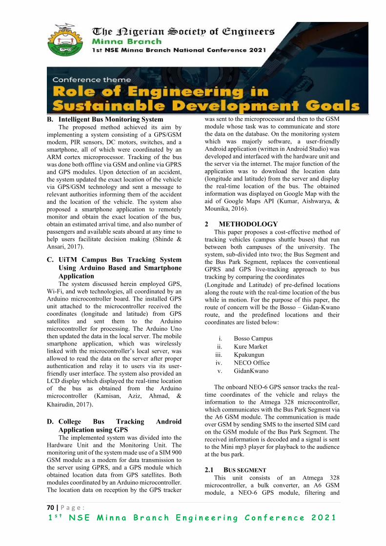
70 | P a g e :


B. Intelligent Bus Monitoring System The proposed method achieved its aim by

implementing a system consisting of a GPS/GSM

modem, PIR sensors, DC motors, switches, and a

smartphone, all of which were coordinated by an

ARM cortex microprocessor. Tracking of the bus

was done both offline via GSM and online via GPRS

and GPS modules. Upon detection of an accident,

the system updated the exact location of the vehicle

via GPS/GSM technology and sent a message to

relevant authorities informing them of the accident

and the location of the vehicle. The system also

proposed a smartphone application to remotely

monitor and obtain the exact location of the bus,

obtain an estimated arrival time, and also number of

passengers and available seats aboard at any time to

help users facilitate decision making (Shinde &

Ansari, 2017).

C. UiTM Campus Bus Tracking System

Using Arduino Based and Smartphone

Application The system discussed herein employed GPS,

Wi-Fi, and web technologies, all coordinated by an

Arduino microcontroller board. The installed GPS

unit attached to the microcontroller received the

coordinates (longitude and latitude) from GPS

satellites and sent them to the Arduino

microcontroller for processing. The Arduino Uno

then updated the data in the local server. The mobile

smartphone application, which was wirelessly

linked with the microcontroller’s local server, was

allowed to read the data on the server after proper

authentication and relay it to users via its user-

friendly user interface. The system also provided an

LCD display which displayed the real-time location

of the bus as obtained from the Arduino

microcontroller (Kamisan, Aziz, Ahmad, &

Khairudin, 2017).

D. College Bus Tracking Android

Application using GPS The implemented system was divided into the

Hardware Unit and the Monitoring Unit. The

monitoring unit of the system made use of a SIM 900

GSM module as a modem for data transmission to

the server using GPRS, and a GPS module which

obtained location data from GPS satellites. Both

modules coordinated by an Arduino microcontroller.

The location data on reception by the GPS tracker

was sent to the microprocessor and then to the GSM

module whose task was to communicate and store

the data on the database. On the monitoring system

which was majorly software, a user-friendly

Android application (written in Android Studio) was

developed and interfaced with the hardware unit and

the server via the internet. The major function of the

application was to download the location data

(longitude and latitude) from the server and display

the real-time location of the bus. The obtained

information was displayed on Google Map with the

aid of Google Maps API (Kumar, Aishwarya, &

Mounika, 2016).

2 METHODOLOGY This paper proposes a cost-effective method of

tracking vehicles (campus shuttle buses) that run

between both campuses of the university. The

system, sub-divided into two; the Bus Segment and

the Bus Park Segment, replaces the conventional

GPRS and GPS live-tracking approach to bus

tracking by comparing the coordinates

(Longitude and Latitude) of pre-defined locations

along the route with the real-time location of the bus

while in motion. For the purpose of this paper, the

route of concern will be the Bosso – Gidan-Kwano

route, and the predefined locations and their

coordinates are listed below:

i. Bosso Campus

ii. Kure Market

iii. Kpakungun

iv. NECO Office

v. GidanKwano

The onboard NEO-6 GPS sensor tracks the real-

time coordinates of the vehicle and relays the

information to the Atmega 328 microcontroller,

which communicates with the Bus Park Segment via

the A6 GSM module. The communication is made

over GSM by sending SMS to the inserted SIM card

on the GSM module of the Bus Park Segment. The

received information is decoded and a signal is sent

to the Mini mp3 player for playback to the audience

at the bus park.

2.1 BUS SEGMENT This unit consists of an Atmega 328

microcontroller, a bulk converter, an A6 GSM

module, a NEO-6 GPS module, filtering and

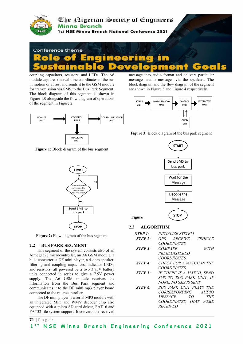
71 | P a g e :


coupling capacitors, resistors, and LEDs. The A6

module captures the real time coordinates of the bus

in motion or at rest and sends it to the GSM module

for transmission via SMS to the Bus Park Segment.

The block diagram of this segment is shown in

Figure 1.0 alongside the flow diagram of operations

of the segment in Figure 2.

Figure 1: Block diagram of the bus segment

Figure 2: Flow diagram of the bus segment

2.2 BUS PARK SEGMENT This segment of the system consists also of an

Atmega328 microcontroller, an A6 GSM module, a

bulk converter, a DF mini player, a 4-ohm speaker,

filtering and coupling capacitors, indicator LEDs,

and resistors, all powered by a two 3.75V battery

units connected in series to give a 7.5V power

supply. The A6 GSM module receives the

information from the Bus Park segment and

communicates it to the DF mini mp3 player board

connected to the microcontroller.

The DF mini player is a serial MP3 module with

an integrated MP3 and WMV decoder chip also

equipped with a micro SD card driver, FAT16 and

FAT32 file system support. It converts the received

message into audio format and delivers particular

messages audio messages via the speakers. The

block diagram and the flow diagram of the segment

are shown in Figure 3 and Figure 4 respectively.

Figure 3: Block diagram of the bus park segment

Figure 4: Flow diagram of the bus park segment

2.3 ALGORITHM

STEP 1: INITIALIZE SYSTEM

STEP 2: GPS RECEIVE VEHICLE

COORDINATES

STEP 3: COMPARE WITH

PREREGISTERED

COORDINATES

STEP 4: CHECK FOR A MATCH IN THE

COORDINATES

STEP 5: IF THERE IS A MATCH, SEND

SMS TO BUS PARK UNIT. IF

NONE, NO SMS IS SENT

STEP 6: BUS PARK UNIT PLAYS THE

CORRESPONDING AUDIO

MESSAGE TO THE

COORDINATES THAT WERE

RECEIVED

72 | P a g e :


3 RESULTS AND DISCUSSION The following images show the results obtained

when the bus arrived each of the predefined

locations. However, this is a proposed work as at the

time of writing this paper and modifications are

currently ongoing.

3.1 RESULTS FROM BUS SEGMENT

Figure 5: Final construction indicating the bus

segment is completely initialized

Figure 6: Final construction indicating the bus

segment GSM signal strength

The Bus Segment is a device that tracks the bus

location in real time. The LEDs in Figure 5 shows

the signal level of the device.

3.2 RESULTS FROM BUS PARK

SEGMENT

Figure 7: system indicating the bus is or has gone

beyond Bosso campus

Figure 8: system indicating the bus has reached

Kure Market

73 | P a g e :



Kpankungu Roundabout


NECO Office


Gidan Kwano Gate

Figures 7, 8, 9, 10, and 11 are images from the Bus

Park Segment, it houses a speaker that announce

the real time location of the bus when the system is

queried and also LEDs to show the matched

location of the bus. Figure 12 shows the result

displayed the when system was queried at

particular interval

BUS SEGMENT

The steps taken to test the operation of the bus

segment are as follows;

STEP 1: switch on the bus segment via the switch at

the side of the casing. When the system is on, the

five LEDS on the bus segment comes on in sequence

to indicate the adequate power supply is circulating

in the circuit. Four of the LEDS represent the GSM

while the last led is for the GPS.

STEP 2: the LEDS remains on until the GSM

module on-board initializes this usually takes up to

3 seconds. After its eventual initialization, the LEDS

turn off in sequence to indicate a successful

initialization.

STEP 3: the controller queries the GSM module to

know how much of signal strength is available,

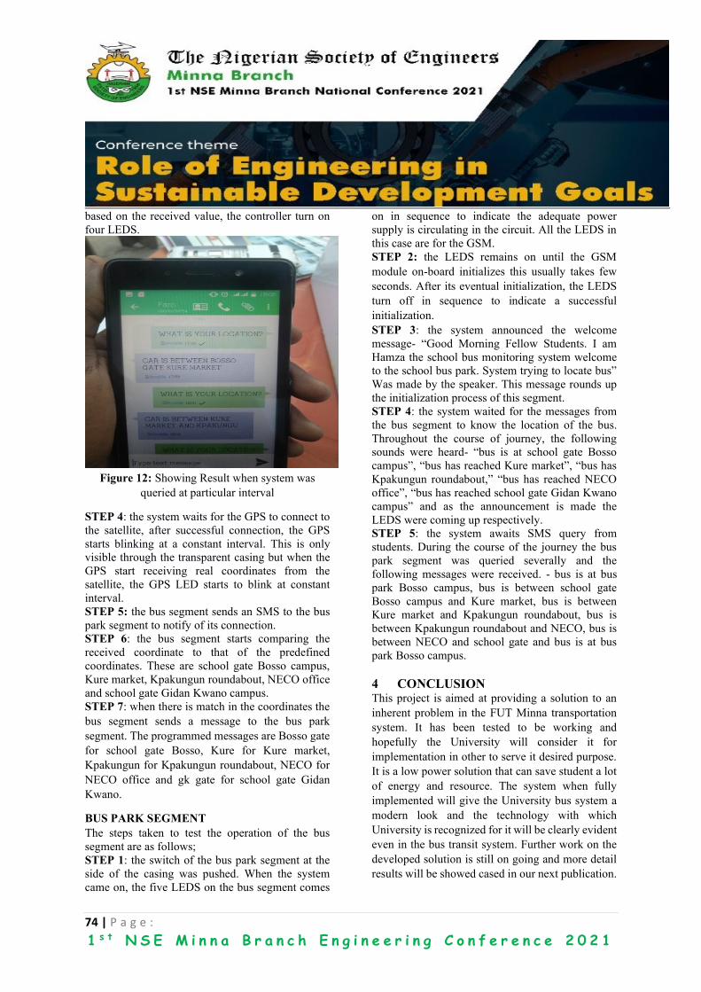
74 | P a g e :


based on the received value, the controller turn on

four LEDS.

Figure 12: Showing Result when system was

queried at particular interval

STEP 4: the system waits for the GPS to connect to

the satellite, after successful connection, the GPS

starts blinking at a constant interval. This is only

visible through the transparent casing but when the

GPS start receiving real coordinates from the

satellite, the GPS LED starts to blink at constant

interval.

STEP 5: the bus segment sends an SMS to the bus

park segment to notify of its connection.

STEP 6: the bus segment starts comparing the

received coordinate to that of the predefined

coordinates. These are school gate Bosso campus,

Kure market, Kpakungun roundabout, NECO office

and school gate Gidan Kwano campus.

STEP 7: when there is match in the coordinates the

bus segment sends a message to the bus park

segment. The programmed messages are Bosso gate

for school gate Bosso, Kure for Kure market,

Kpakungun for Kpakungun roundabout, NECO for

NECO office and gk gate for school gate Gidan

Kwano.

BUS PARK SEGMENT

The steps taken to test the operation of the bus

segment are as follows;

STEP 1: the switch of the bus park segment at the

side of the casing was pushed. When the system

came on, the five LEDS on the bus segment comes

on in sequence to indicate the adequate power

supply is circulating in the circuit. All the LEDS in

this case are for the GSM.

STEP 2: the LEDS remains on until the GSM

module on-board initializes this usually takes few

seconds. After its eventual initialization, the LEDS

turn off in sequence to indicate a successful

initialization.

STEP 3: the system announced the welcome

message- “Good Morning Fellow Students. I am

Hamza the school bus monitoring system welcome

to the school bus park. System trying to locate bus”

Was made by the speaker. This message rounds up

the initialization process of this segment.

STEP 4: the system waited for the messages from

the bus segment to know the location of the bus.

Throughout the course of journey, the following

sounds were heard- “bus is at school gate Bosso

campus”, “bus has reached Kure market”, “bus has

Kpakungun roundabout,” “bus has reached NECO

office”, “bus has reached school gate Gidan Kwano

campus” and as the announcement is made the

LEDS were coming up respectively.

STEP 5: the system awaits SMS query from

students. During the course of the journey the bus

park segment was queried severally and the

following messages were received. - bus is at bus

park Bosso campus, bus is between school gate

Bosso campus and Kure market, bus is between

Kure market and Kpakungun roundabout, bus is

between Kpakungun roundabout and NECO, bus is

between NECO and school gate and bus is at bus

park Bosso campus.

4 CONCLUSION This project is aimed at providing a solution to an

inherent problem in the FUT Minna transportation

system. It has been tested to be working and

hopefully the University will consider it for

implementation in other to serve it desired purpose.

It is a low power solution that can save student a lot

of energy and resource. The system when fully

implemented will give the University bus system a

modern look and the technology with which

University is recognized for it will be clearly evident

even in the bus transit system. Further work on the

developed solution is still on going and more detail

results will be showed cased in our next publication.

75 | P a g e :


However, an improvement is ongoing presently,

working on the limitations and shortcomings to give

a better result.

ACKNOWLEDGEMENTS

The authors of this work would like to

acknowledge the selfless and tireless contributions

of all staff of the Department of Telecommunication

Engineering Federal University of Technology,

Minna. In addition, we acknowledge the National

Information Technology Development Agency

(NITDA) IT Hub, Federal University of

Technology, Minna for granting us access to their

facilities in the course of the research.

REFERENCES

Ahmed, A., Parvez, M. R., Hasan, M. H., Nur, F. N.,

Moon, N. N., Karim, A., . . . Jonkman, M. (2019).

An intelligent and secured tracking system for

monitoring school bus. Paper presented at the

2019 International Conference on Computer

Communication and Informatics (ICCCI).

Dhende, S., Kaotekwar, V., Kokane, V., &

Karambelkar, V. (2017). Intelligent bus system

using rfid, zigbee and gprs. International

Research Journal of Engineering Technology,

4(4), 3.

James, J. G., & Nair, S. (2017). Efficient, real-time

tracking of public transport, using lorawan and

rf transceivers. Paper presented at the TENCON

2017-2017 IEEE Region 10 Conference.

Kadam, A. J., Patil, V., Kaith, K., & Patil, D. (2018).

Developing a Smart Bus for Smart City using

IOT Technology. Paper presented at the 2018

Second International Conference on Electronics,

Communication and Aerospace Technology

(ICECA).

Kamisan, M., Aziz, A., Ahmad, W., & Khairudin,

N. (2017). UiTM campus bus tracking system

using Arduino based and smartphone

application. Paper presented at the 2017 IEEE

15th Student Conference on Research and

Development (SCOReD).

Kumar, G. K., Aishwarya, C., & Mounika, A. S.

(2016). College Bus Tracking Android

Application using GPS. International Journal of

New Innovations in Engineering and

Technology, 4(4), 40-44.

Kumbhar, M., Survase, M., Mastud, P., Salunke, A.,

& Sirdeshpande, S. (2016). Real time web based

bus tracking system. International Research

Journal of Engineering and Technology, 3(2),

632-635.

Raad, M. W., Deriche, M., & Sheltami, T. (2021).

An IoT-Based School Bus and Vehicle Tracking

System Using RFID Technology and Mobile

Data Networks. Arabian Journal for Science and

Engineering, 46(4), 3087-3097.

Shinde, N., & Ansari, S. (2017). Intelligent bus

monitoring system. International Journal of

Computer Applications, 975, 8887.

Shyam, N., Kumar, N., Shashi, M., & Kumar, D.

(2015). SMS Based Kids Tracking and Safety

System by using RFID and GSM. IJISET-

International Journal of Innovative Science,

Engineering & Technology, ISSN, 2348-7968.

76 | P a g e :


Reformation of Engineering Education for Health, Wealth and

Sustainable Development in Nigeria Oluwadare Joshua OYEBODE

Civil and Environmental Engineering Department, Afe Babalola University,

Ado-Ekiti (ABUAD), Ekiti State, Nigeria

Email: [email protected]

ABSTRACT Reformation of engineering education is a principal requirement for health, wealth and sustainable development

in Nigeria and most nations of the world. This paper focuses on the reformation of engineering education in

order to attain public health, wealth creation and sustainable development in Nigeria. Methodology includes

literature review, consideration of recent trends in engineering education and clear discussion of engineering

education. Nigerian engineering teaching methods and outputs and challenges facing engineering education in

Nigeria were carefully examined. Findings revealed that there is an urgent need for the reformation of

engineering education in order to ensure adequate public health, wealth and sustainable development in Nigeria.

Engineering curriculum requires periodic review and there must be substantial linkages between academia and

engineering industry. This will enhance engineering productivity, generation of employment, increased output

through innovations, job creation, efficient utilization of available resources and the facilitation in the transfer

of technological advancement. Recommendations include enforcement of policies that will enhance

reformation of engineering education and sustainable development in Nigeria, collaboration of academia,

government, regulatory bodies, stakeholders, professionals, engineers and industries in with the curriculum

review and project implementation.

KEYWORDS: Engineering, Regulatory Bodies, Reformation of Education, Sustainable Development,

Wealth

1. INTRODUCTION Engineering education has a lot of roles to play in

the achievement of sustainable development goals.

The real problem facing humanity today in terms of

achieving sustainable development is how to

motivate people to change underlying behaviors and

activities that are problematic. Human beings are

very resentful to change. In other words, people

should be encouraged to channel their energy

towards contributing more to assist alleviate poverty

by acquiring relevant education and skills so as to

market developmental efforts that do not pollute

good ideas and wasting scarce resources to destroy

lives and edifices built over the years.

Quality education is a critical requirement for

national growth industrialization and citizens in

most nations of the world. Education is of great

importance to every nation as it is quite obvious that

the functionality of an individual in any nation is

largely dependent on the quality of education that is

imparted on that individual.

There is a general consensus among scholars that

education is the most potent instrument for the

overall development of any nation (Njoku and

Onyegbula, 2017). There is often no productive

human capital without a functional education,

countries that are at the forefront of technological

advancement equally having the most educated

population. Educated people possess more skills and

are able to perform their jobs effectively. They are

also better suited to more complex jobs, which are

often associated with high rates of pay and greater

economic benefits (Adedeji and Campbell, 2013).

The Nigerian education system has a foothold over

most of the framework adopted globally, because the

six years spent on education compared to other

countries with a 5-year secondary education.

Engineering education which is majorly taught at the

higher institution has become a key aspect of

education in Nigeria. Engineering education is based

on conceptualizing, creating and maintaining

processes or systems that are needed by humans or


77 | P a g e :


the society. This paper shall examine if this

engineering teaching trend is sustainable. Present

approaches to engineering education in Nigeria, the

factors behind the observed success, challenges and

proffer some solutions and methods to improving

engineering education should be carefully checked

in Nigeria. The present and future of engineering

education is also examined with some

recommendations for a sustainable teaching method

that would meet the future need of the nation.

2.0 OVERVIEW OF ENGINEERING

EDUCATION IN NIGERIA Engineering education was neglected among other

fields of education in Nigeria until around the

middle of the 19th century. Nigeria, however,

realized that this field is one of the major bedrocks

of any nation and established a number of Technical

Colleges, Polytechnics and Faculties of Engineering

in Universities just after the independence of the

country. As a result of the importance and

technicality of engineering education, the study of

any engineering degree in Nigeria is structured for a

five-year period, with the primary year spent

studying general sciences. To become a totally

qualified engineer, a graduate of any Engineering

degree must practice for a minimum of four years,

among other requirements before becoming a

registered engineer with the Council for the

Regulation of Engineering in Nigeria (COREN).

The Nigerian engineering education performed well

by meeting the immediate need of the early post-

independence period. The educational performance

at that point was also commended, especially giving

the very fact that the majority engineering teachers

worked with the knowledge of the industry.

However, in recent times, the standard of

engineering education in Nigeria is of major concern

more especially to the industries as it seems the

standard is falling.

Corruption is an act which deviates from the formal

rules of conduct governing the actions of someone

in a position of public authority because of private

regarding motives such as wealth, power or status

(Keeper, 2010).

There is inadequate access to spotless modern

energy services is a massive challenge facing

Nigerian because energy is fundamental for

socioeconomic development and poverty

eradication (Oyedepo, 2012).

There is urgent need for revitalization of engineering

education (Oyebode, 2020).

Drawing is very important for all engineering fields

as engineers we all know that drawing is engineering

language. This encompasses the architectural, civil,

electrical, structural, mechanical and all engineering

professions (Oyebode, 2015).

Technological advancements serve as a main key to

a nation's development. Proper engineering

knowledge (acquired through appropriate

structures) plays a major role in the attainment of a

high level of technological advancement (Akintola,

2002).

There is a worldwide campaign for efficient

teaching methods for engineering education in

Nigeria, especially with the arrival of information

and telecommunication technologies (Oloyede et al.,

2017).

Education is often seen as a prerequisite for quality

manpower development and creation of wealth, a

sure path to success in life and service to humanity

(Ogunyinka et al., 2015).

Thus, creating a barrier between the talents required

by the labor markets and what's obtainable by the

graduates. This results in the decision for

improvement of the prevailing classical course

delivery methods toward meeting the market needs.

However, over the years, extensive information

technology, vanguard technological ideas and

developmental initiative are happening within the

planet as a result of engineering innovations;

however, there are not any major changes within the

engineering education, lecturing style, and attitude

within the same time-frame in Nigeria.

3.0 SITUATION AND CHALLENGES

FACING ENGINEERING EDUCATION

IN NIGERIA Challenges facing engineering education include

curriculum issues, lack of basic knowledge by the

engineering students, an explosion in enrolled

students, difficulty in students’ recruitments,

inadequate facilities for teaching of engineering

education, lack of or inadequate university industry

78 | P a g e :


linkages, inadequate funding of education,

inadequate mentoring of engineering lecturers, lack

of special remunerations to engineers, teacher-to-

student ratio and thus the utilization of ineffective

teaching methods.

Furthermore, lack of basic infrastructure, lack of

necessary support from non-academic staff, poor

access to internet services, irregular power supply,

lack of fantastic leadership and mentoring schemes

are among other challenges facing engineering

education in Nigeria. The system of education in

Nigeria today is more of socializing with less

emphasis on diligence both on the students and

lecturers. These challenges are having a big impact

on the standard of Education in Nigeria.

However, this paper shall focus mainly on the three

areas namely: the curriculum, equipment and thus

the teaching methods utilized in Engineering

Education in Nigeria. In discussing things, this paper

shall explore a number of these situations and

suggest some solutions to sustainable engineering

education in Nigeria.

3.1 Teaching and Learning Methods Teaching is that the process of transferring

knowledge. It should be delivered during a

scientific, interactive, organized and purposive

manner. The first purpose of teaching at any level is

to bring a fundamental change in students’ learning.

it's therefore, expected that teaching will cause

desirable change within the learners’ behavior.

Learners during this context, we are pertaining to the

scholars. Therefore, teaching should be seen because

the integral a part of any educational policy

framework implementation because it would have

an immediate impact on the students’ learning.

There are many teaching methods available, and a

couple of these methods are tested in diverse

environments and proven effective in several

scenarios. These include discovery method spaced

lecture, group work, dialogue, scaffolding and

constructivism etc. The project method on the other

hand involves active participation of the scholar in

such how that a cooperative (group) study of a real-

life situation within the category is undertaken,

under the supervision of the teacher. However, the

concerned, feelings and reactions of the scholars

during this situation are taken into consideration

during the course of interacting with each other. This

might even be mentioned because the "Role-Play

Method”. Simulation method may be a more

practical oriented approach of teaching where

students are exposed to devices and equipment

physically. This method is taken into account

because the most effective in Science and

Engineering related subjects as it’s hastens and

stimulates the understanding of learners. Numerous

learning methods are identified and related to

specific teaching methods. Today, in Nigeria,

mostly, engineering lecture rooms are faced with an

identical scenario because it was in decades ago. The

teaching methodology remains the traditional

approach where an educator delivers lectures by

standing within the classroom, dictating notes or

deriving equations from the ‘old' notebook’,

recycling examples, assignments and projects. This

sort of approach does not allow skills acquisition,

critical thinking and creativity needed during a

challenging multi-disciplinary course like

engineering. Notably, some enhancements are

observed following the diffusion of ICT into the

teaching, and learning process and this creates some

quite modification on teaching methodology.

Moreover, there are quite number of methods that

might be used/or integrated in to the pedagogies.

These methods are expected to enhance students’

learning. it had been discovered that the bulk

engineering students are visual, sensing, inductive,

active, and artistic whereas the teaching methods

used are mostly passive, auditory, abstract,

deductive and sequential. Thus, resulting in

incompatibility between the teaching and therefore

the learning process, and hence, resulting to poor

performance among engineering students.

Furthermore, lack of basic infrastructure, lack of

necessary support from non-academic staff, poor

access to internet services, irregular power supply,

lack of good leadership and mentoring schemes are

among other challenges facing engineering

education in Nigeria. The system of education in

Nigeria today is more of socializing with less

emphasis on hard work both on the part of the

students and the lecturers. These challenges are

having a significant impact on the quality of

Education in Nigeria as discussed.

However, this paper shall focus mainly on the three

areas that have to do with content delivery namely:

the curriculum, equipment and the teaching methods

79 | P a g e :


used in Engineering Education in Nigeria. In

discussing the situation, this paper shall explore

some of the present situations and suggest some

solutions to sustainable engineering education in

Nigeria.

3.1 Teaching and Learning Methods Teaching is the process of transferring knowledge. It

should be delivered in a systematic, interactive,

organized and purposive manner. The primary

purpose of teaching at any level is to bring a

fundamental change in students’ learning. It is

therefore, expected that teaching will cause

desirable change in the learners’ behavior. Learners

in this context, we are referring to the students.

Therefore, teaching should be seen as the integral

part of any educational policy framework

implementation as it would have a direct impact on

the students’ learning. There are many teaching

methods available, and some of these methods have

been tested in diverse environments and proven

effective in different scenarios. These include

discovery method spaced lecture, group work,

dialogue, scaffolding and constructivism etc.

However, in Nigeria, the most widely used teaching

methods are: lecture method, discussion method,

project method, simulation method and problem-

solving method. The lecture method is also

commonly referred to as "talk chalk method" which

involves the teacher explaining the ideas with giving

examples and occasionally, writes on the chalk

board. The project method on the other hand

involves active participation of the student in such a

way that a cooperative (group) study of a real-life

situation in the class is undertaken, under the

supervision of the teacher. The drama method, may

also be classified as group method as it involves a

group-oriented approach. However, the concerned,

feelings and reactions of the students in this situation

are taken into consideration during the course of

interacting with one another. This may also be

referred to as the "Role-Play Method”. Simulation

method is a more practical oriented approach of

teaching where students are exposed to devices and

equipment physically. This method is considered as

the most efficient in Science and Engineering related

subjects as it’s hastens and stimulates the

understanding of learners. So many learning

methods have been identified and associated with

specific teaching methods. Today, in Nigeria,

mostly, engineering lecture rooms are faced with a

similar scenario as it was in decades ago. The

teaching methodology is still the conventional

approach where a teacher delivers lectures by

standing in the classroom, dictating notes or deriving

equations from the ‘old' notebook’, recycling

examples, assignments and projects. This type of

approach does not allow skills acquisition, critical

thinking and creativity needed in a challenging

multi-disciplinary course like engineering. Notably,

some enhancements have been observed following

the diffusion of ICT into the teaching, and learning

process and this creates some sort of modification on

the process. Moreover, there are quite a number of

methods that could be used/or integrated in to the

teaching method. These methods are expected to

improve students’ learning. It was discovered that

most engineering students are visual, sensing,

inductive, active, and creative whereas the teaching

methods used are mostly passive, auditory, abstract,

deductive and sequential. Thus, leading to

incompatibility between the teaching and the

learning process, and hence, resulting to poor

performance among engineering students.

3.2 ENGINEERING EDUCATION CURRICULUM Curriculum is one of the most important components

of implementing any education policy as it describes

the syllabus, teaching methods employed and

ultimately, it would determine the learning

experience. Engineering curriculum is expected to

be dynamic to reflect the change in emerging

engineering and societal problems. Curriculum is a

reflection and a product of the society and can

contribute to changing the society. Therefore, it is

important in the process of the curriculum

development and education process to reflect labor

market issues. Furthermore, for sustainable

development, engineering curriculum has to be

innovative project-based and has to be linked with

our local industries. The knowledge passed through

the modern-day engineering curriculum must be

flexible, dynamic and encompass a broad

knowledge within a specialized field of knowledge.

The traditional mode of engineering curriculum

cannot provide these and the present-day work

environment requires specialized individuals.

Therefore, there is a need to have different tracks or

specialization within the same subject area. This

method is been adopted in the United Kingdom and

80 | P a g e :


even Nigeria where the students spend three years

obtaining a specialized degree while the fourth year

is being spent in the industry. The program is

designed in such a way that critical thinking,

independent problem solving and creativity are

rewarded and encouraged which leads to creativity

and problem-solving skills. These skills are

important for independent learners to develop and

possess while overcoming challenges that are

associated with modern day engineering. Therefore,

the curriculum must allow for attitudes that can

bring out the skills and knowledge gained. Attitude

is also important because team work is an essential

feature in solving engineering challenges. The

curriculum must encourage more team work because

the reality is that most projects in the field of

engineering today and in the future require team

work from diverse range of knowledge culture,

social and religious backgrounds.

Unfortunately, lots of names have been associated

with the engineering education in Nigeria. The static

nature of Nigerian engineering curriculum has made

it to be described as obsolete. This is because there

is a huge gap between the general education

knowledge provided by the universities and

technical skills required by the industries. As such,

the graduates are not meeting the needs of the labor

markets, thus, necessitating the need for retraining

programs by the employers. The current engineering

education is also described as out of touch especially

with what is going on in the industry. This also

defeats the aim of the 21st-century engineering

education which is supposed to provide knowledge,

skills and attitude. Some authors also describe the

present-day engineering training as that of the era of

the parents of the present-day engineers. Although,

individual efforts towards realizing dynamic

engineering curriculum are acknowledged due to

recent growth in number of lecturers acquiring

higher degrees from abroad. Also, with the recent

improvements on internet access in the Nigerian

Universities, have provided access to a wider range

of information and educational resources, this has

further broadened the need and call for a review of

the system. Despite all these, there is no significant

improvement in terms of the curriculum. Based on

the findings from a survey conducted, 94% of the

lecturers who have obtained postgraduate degree

outside Nigeria and realized the need for improved

curriculum attended a conference or seminar where

improved engineering curriculum is encouraged said

they cannot implement what they have learnt. This

is because of the lack of the necessary infrastructure

and work load. Therefore, equipment and better

infrastructure is an important aspect of the improved

curriculum. Furthermore, It was also discovered that

human attitude towards making the change must

also be encouraged. Conferences are expected to

expose lecturers to latest discovery and stimulate

discussions among teachers and students about the

latest discovery in modern engineering world. The

problem of changing existing curriculum is not only

peculiar to Nigeria but across the world. This is

because the global problem with engineering

education has to do with the challenges of the 21st-

century workplace and the permeating nature of

product and services provided by engineers.

Therefore, the lack of willingness to adopt changes

in engineering curriculum as the field of engineering

is changing is a global problem. A general reason for

refusing changes in engineering education has to do

with the fact that this field is changing very fast and

before a curriculum change can be made, some more

advance changes are already recorded on the field.

However, changing this attitude must be encouraged

in Nigeria as it is been presently done around the

globe.

3.3 EQUIPMENT AND INFRASTRUCTURE Apart from the global problems, engineering

education in Nigeria is facing some peculiar

problems like lack of equipment and infrastructure.

Most engineering faculties in Nigeria complain

about the lack or inadequate availability of

necessary basic equipment and Infrastructure. This

is because of inadequate funding to our universities.

Most students and lecturers respectively complain

about the level of available equipment and

infrastructure in our engineering departments. Lack

of equipment and necessary infrastructure like

classrooms and teaching aid equipment is seen as the

major barrier to teaching and learning of engineering

in Nigeria.

4.0 THE WAY FORWARD Engineering students must be ready to learn new

skills discretely and also very quickly to satisfy up

with the ever-changing requirements of the

engineering field. Majority of the engineering

81 | P a g e :


departments in Nigerian university are not customer-

focused as a result of either lack of funds or the very

fact that the amount seeking admission year in year

out far exceeds the number of places available. a

transparent understanding of the necessity of the

customer, the scholars (who are the foremost

important customer), their parents, the society and

therefore the industry that might eventually employ

these students would go an extended way in ensuring

that some level of quality is achieved. to satisfy up

with the demand of the industry and to be ready to

still compete favorably round the world, variety of

changes need to be implemented to enhance the

standard of engineering education in Nigeria.

Consequently, some major changes that require

immediate attention and the way to travel about

these changes are discussed below:

4.1 Degree Specialization and choice to

Spend a Full Year within the industry The reality facing engineering education today is

significantly different from that of the past, and

therefore the future would be distinct from that of

today. to satisfy the longer-term need of engineering

education, significant changes are required. the

necessity of today is different, and therefore the

relevance and direction of a number of the modules

or departments in some faculty of engineering need

to be questioned. for instance, up until the first 90s,

an EE graduate in Nigeria is predicted to figure for

an electrical company or somewhere similar.

However, the truth of today is that electrical

engineers are now computer engineers,

telecommunication engineers and even biomedical

engineers where different knowledge of biology,

telecommunications computer-oriented language

and programming are all essential to having the

ability to perform well. Therefore, this five-year

engineering learning structure within the university

without specialization would not meet the necessity

of future engineers. There is a requirement to

breakdown the areas of specialization and stop the

thought of generalization.

4.2 Continuous Modification within the

Curriculum of Engineering Education To meet up with the longer-term demand, there has

got to be machinery in situ to accommodate the rapid

technological changes that are now being

experienced. Any curriculum that might meet the

necessity of the economic practice has got to change

continuously. New technology is developing at a

rate where if care is not taken before a change has

been implemented the technology would have

changed. the matter related to these changes are

often solved by providing long life learning, where

essential skills are those taught. Knowledge skills

and attitude must even be emphasized. Teamwork

must be encouraged because the processes and

systems that engineers would need to conceive,

create and operate are quite complex. Hence, it's

important that engineers must learn to unravel

problems in teams. Furthermore, the test to students

must be challenging but fair. Knowledge is that the

database of an engineer, skills are the tools to

manipulate the knowledge to satisfy a goal dictated

or strongly influenced by attitude. Presently, there's

a growing acceptance of online degrees from foreign

universities. an honest number of the undergraduate

students say they might be happy to possess a web

degree from a university outside Nigeria if going

forward for a master’s degree as an alternate to

travelling outside Nigeria. The rationale provided is

that they believe they might be recuperating

knowledge from the web degrees than attending a

standard university in Nigeria. This is often an

enormous sign that conventional universities in

Nigeria must still evolve and improve upon the

content. With technological advancement, the planet

is now a worldwide village, and giving the universal

nature of education, if care is not taken, with the way

technology is advancing, there's a likelihood that

within the near future technical course like

engineering would be taught online to incorporate

access to varied practical and this may need some

negative impacts on the enrolments of student in our

universities. This practical could be designed using

software to simulate the important environment.

4.3 Teaching what is necessary within the

world Engineering Education has been described as a

three-legged stool counting on science mathematics

and technique. Even as a stool cannot stand on two

legs, adopting a correct technique is as important

because the other two. The technique needed within

the field of engineering cannot be fully taught within

the four walls of the classroom. There is a

requirement for interaction and reinforcement of the

essential fundamentals that an engineer would wish

82 | P a g e :


when on the sector. Engineering education must

provide increased practical experience. This helps

the students’ ability to find out the abstract and

theory that forms much of the engineering

fundamentals. It also helps their ability to

understand the applicability and practical usefulness

of an honest theory. an answer to the present would

be emphasizing more on the basics of science with

integrated knowledge while longer would be spent

that specialize in the important world. Consistent

with a search which studied successful young

engineers across the sector of engineering, the study

showed that success within the field of engineering

lies within the combination of generic skills with

technical capabilities with emotional intelligence

and focused thinking. The research also showed that

less emphasis should get on assessment of

predictable skills as more of technical expertise

should be examined. This suggests that lecturers

should adopt the utilization of application-based test

such the important world capability is tested.

Furthermore, emphasis has been made on the very

fact that the important world must be taught majorly

the fundamentals, problem-solving skills,

engineering ethics, and therefore the connection

between technology and the society while reducing

the number of years spent within the class room.

Teaching what's necessary within the world requires

more equipment and infrastructures. Therefore,

government and therefore the management of our

universities must provide more in terms of kit and

infrastructure.

4.4 Use of Innovative approaches to teaching

and learning The use of innovative approaches to teaching and

learning is extremely essential. Results indicate that

96% of the scholars who have studied within the

university abroad are satisfied with the standard of

engineering education they received or obtained.

However, only 14% of the scholars were satisfied

with the standard of engineering education in

Nigeria. Additionally, 100% of the scholars agreed

that the staff outside Nigeria who are always using

teaching aids are better at explaining things, provide

better concentration, participation in school and

students were ready to retain what's being taught for

much longer compared to the normal method of

teaching utilized in the Nigeria. 100% of the

scholars also confirmed that the very fact that

teaching materials are available online before and

after lectures makes learning easier. This means that

education is global, and lecturers should be

encouraged to form their notes available online. The

utilization of technological teaching aids is long

overdue. This has got to tend proper attention by

both the management and staff of our universities.

Some lecturers are not taking adequate advantage of

the small aids like projectors and electronics boards

presently available. This might be as a result of lack

of data about the usage of that equipment. Therefore,

adequate retraining program must even be

administered to form sure that this will be put to

proper use.

5.0 CONCLUSIONS Engineering education is very critical for the

achievement of sustainable development goals.

Quality research, industrial training, effective

teaching, community development and substantial

collaboration between tertiary institutions and

industry are major requirement for realization of

sustainable development goals. Most challenges

traceable to teaching and learning can be overcome

through strategic approach and effective funding.

Employability, entrepreneurial skills and global

competitiveness are required by engineering

graduates to realize success both at under-graduate

and post-graduate levels and for effective

professional practice within industries. Engineering

curriculum requires periodic review and there must

be substantial linkages between academia and

engineering industry. This will enhance engineering

productivity, generation of employment, increased

output through innovations, job creation, efficient

utilization of available resources and the facilitation

in the transfer of technological advancement.

6.0 RECOMMENDATIONS There is need for enforcement of policies that will

enhance reformation of engineering education,

lifelong learning initiatives and sustainable

development in Nigeria, collaboration of academia,

government, regulatory bodies, stakeholders,

professionals, engineers and industries in with the

curriculum review and project implementation.

Resilient infrastructures should be provided in

engineering institutions for effective sanitation,

industrialization and innovation. Lecturers and staff

need to recommit themselves towards the

83 | P a g e :


development of sound engineers through the

provision of adequate resources for teaching as well

as well-equipped learning and training schools and

centers. Regulatory bodies should ensure that

students are trained to be more skillful and

independent as this will ensure achievement of

sustainability in the education system in Nigeria.

ACKNOWLEDGEMENTS

I appreciate Aare Afe Babalola, the Founder of

Afe Babalola University, Ado-Ekiti (ABUAD)

for his notable and philanthropic contribution to

education in Africa. I also thank the Nigerian

Society of Engineers (NSE) Minna Branch and

Council for the regulation of Engineering in

Nigeria (COREN) for the opportunity and

platform given to me to contribute my paper for

this conference.

REFERENCES

Adedeji, O., and Campbell, O. (2013). The role of

higher education in human capital

development. Available at SSRN 2380878.

Akintola, A. A., Aderounmu, G. A., and Owolarafe,

O. K. (2002). Problems of engineering

education and training in developing countries:

Nigeria as a case study. European journal of

engineering education, 27(4), 393-400.

Keeper, D. G. (2010). Systemic corruption in

Nigeria: A threat to sustainable development.

In Proceedings of the first International

Technology Education and Environment

Conference.

Njoku, J. U., and Onyegbula, J. C. (2017). Human

Capital development as a strategy for

sustainable development in the Nigerian

education system. African Research

Review, 11(2), 178-189.

Ogunyinka, E. K., Okeke, T. I., and Adedoyin, R. C.

(2015). Teacher education and development in

Nigeria: An analysis of reforms, challenges and

prospects. Education Journal, 4(3), 111-122.

Oloyede, A. A., Ajimotokan, H. A., and Faruk, N.

(2017). Embracing the future of engineering

education in Nigeria: teaching and learning

challenges. Nigerian Journal of

Technology, 36(4), 991-1001.

Oyebode, O. J. (2020). Revitalization of the Quality

Engineering Education in Nigeria: Special

attention to Funding and Implementation

Strategies. IJCEP, 38, 47.

Oyebode, O. J., Adebayo, V. B., and Olowe, K. O.

(2015). Assessment of the use of AutoCAD

package for teaching and learning engineering

drawing in Afe Babalola University Ado-

Ekiti. Assessment Of the Use Of Autocad

Package For Teaching And Learning

Engineering Drawing In Afe Babalola

University Ado-Ekiti, 4(9), 1-8.

Oyedepo, S. O. (2012). Energy and sustainable

development in Nigeria: the way

forward. Energy, Sustainability and

Society, 2(1), 1-17.

84 | P a g e :


A Review of Different Biomass Based Materials used to Produce

Activated Carbon for Water Treatment. Korie C.I, Afolabi E.A, Kovo A.S., Muktar A.

Department of Chemical Engineering, Federal University of Technology, Minna.

ABSTRACT Water treatment for industrial wastewater is very necessary, as it prevents effluents from posing hazardous

influences to the environment. Adsorption and Adsorbents are part of the techniques used to treat effluents.

Adsorbents can be developed with various materials, but it is important to focus on adsorbents that are not

expensive, do not require a lot of processing but have high adsorption capacity. Activated carbon from

agricultural waste is becoming an increasingly interesting area for research as it fits into the sphere of

inexpensive adsorbents. Activated carbon is formed through two stages; firstly, the pyrolysis or carbonization

of the precursor and secondly activation via steam or various reagents. The preparation of high-quality activated

carbon is dependent on the production process; operation parameters like time, temperature, and impregnation

ratio have influence on its quality. This article seeks to show the viability of low-cost adsorbent when activated

carbon is prepared from biomass and used as adsorbents during water treatment of heavy metal, oil spills

organic contaminants and dyes.

KEYWORDS: Activated carbon, adsorption, water treatment, biochar, biomass

1 INTRODUCTION Industrialization has its advantages, but it is

usually at costs that are environmentally

detrimental. Processes that deal with converting raw

materials to finished goods on a large scale, comes

with its share of problems. A lot of which revolves

around water effluents. As such, it has become

equally important to determine ways to implement

water treatment procedures. Textile industries

discharge colored effluents into water bodies and

battery manufactures discharge effluents consisting

of heavy metals that have an impact the quality of

the water. Other ways water might be contaminated

include oil spills that may happen at any of its

extraction, production, distribution, and

transportation stages. Contaminated water bodies do

not only affect sea life, they have the ability to affect

human life as well. Adsorption is usually the most

preferred option for treating contaminated water

because of its low cost, it needs no skill for

utilization, is flexible and highly effective.

Additionally, adsorption works to remove organic

and inorganic pollutants from effluents in a green

way; this means that bio-hazardous side products

will not be developed.

Low costs adsorbents do not need a lot of

processing before it is used. They are usually low-

cost because they are abundant whether it be natural,

a side product, or waste from industries. It is

noteworthy to add that additional processing is fine,

if it can make up for increased adsorption capacity.

There are different types of adsorbents: organic

polymers (synthetic), natural sorbents, and mineral

materials (inorganic) (Bailey, S.E. et al, 1999).

Heavy research on the area of implementing bio

adsorbents as treatment options is ongoing. It has

been discovered that bio adsorbents are lightweight,

have good adsorption selectivity, considerable

adsorption efficacy, outstanding adsorption

recyclability, and can be easily operated, plus it has

an inexpensive preparation technique. As such, it is

necessary to explore all the probable agro and

horticulturally based adsorbents in order to

determine their viability for removing contaminants.

1.1 ACTIVATED CARBON Of the many adsorbents used to treat inorganic

and organic pollutants in polluted water, plant or

lignocellulose wastes, activated carbons,

biopolymers and clays are very well known

adsorbents. Activated carbon has the higher

popularity out of all the adsorbents that researchers

use for water treatment. However, the higher the

quality, the more expensive it is. Small-scale

industries are looking for cheaper ways to prepare

activated carbon; hence, the movements towards

agricultural waste produce. Activated carbon is

formed firstly through pyrolysis or carbonization of

the precursor to get biochar and secondly activation

via an activating agent. There are two types of

85 | P a g e :


activation. For chemical activation, a catalyst is used

to speed up the process; as such, less temperature is

used. Common activators used for this process are

H3PO4, ZnCl2, KOH, K2S, H2SO4, and KCNS

(Zor et al., 1998). This process minimizes tar

formation and volatilization. Chemical activation is

one process, but two separate temperatures are used

(Smisek and Cerny, 1970). Physical activation

requires a higher temperature and more time and

ultimately might produce tar and increase

volatilization; chemical activation offers better

results and gets recommendations. Chemical

activation is also advantageous as the activation

targets the carboxyl and hydroxyl groups that are

important for adsorption to oil spills. A lot of

research on how activated carbon is prepared from

biomass and how effective this type of adsorbent is

on treating effluents form organic and inorganic

sources is ongoing

1.2 WATERMELON RIND (Jimoh et al, 2014) studied about preparing

activated carbon using watermelon peel. They

focused on activating temperature of 200°C and

varied this temperature to about 350°C. The time for

activation was also varied from 15 to 60 minutes.

The researchers discovered peak conditions at

300°C and 60 minutes. The researchers impregnated

the sample with different reagents at different molar

concentrations ranging from 0.5 to 1.5 m. HCL,

H2SO4, and zncl2 were used to get optimal

outcomes (1.0m sulphuric acid). The process was

characterized using proximate-ultimate analysis and

FTIR analysis. (Oghenejoboh, 2018) researched on

adsorbing nickel (ii) ion from wastewater with

activated carbon from watermelon rind. The

temperature and time implemented from

carbonization was 380°C for 120 minutes.

Impregnation was done using 1.0m zinc chloride.

(Mohd Azmier Ahmad, 2017) carried out research

on producing activated carbon to removal synthetic

dye. The optimal and time and temperature for the

production of char was 1 hour and 700°C. The

activated agent used was KOH. The proximate

analysis was used for characterization and a carbon

yield of 32% was discovered. Additionally, the

sample was characterized via BET and the surface

area was recorded as 776.65 m2/g. (Qiu-Feng Lu,

2018) produced activated carbon at optimal

conditions via pyrolysis. The gas used was nitrogen,

it’s heating rate at heating rate of 5 °C and optimum

temperature and time for activated carbon at 700 °C

for 1 h under nitrogen flow. The reagent used was

hydroxide with optimum impregnation ratio of 1:2.

This sample was characterized with BET and it was

discovered to have a surface area of 1303.3 m2 g-1

1.3 ORANGE PEELS (Foo, K. Y. et al, 2012) researched on preparing

activated carbon from orange peels using microwave

assisted K2CO3 activation. Optimum operation

parameters were determined from microwave

power, chemical impregnation ratio, and irradiation

time. The biomass was characterized using some

analytical methods such as zeta potential

measurement, scanning electron microscopy,

nitrogen adsorption isotherm, elemental analysis,

Fourier transform infrared spectroscopy and surface

acidity/basicity. The carbon yield for the optimal

condition of orange peel was 80.99%. (Fernandez,

M. E., 2014) also prepared activated carbon from

orange peels to be used for the adsorption of basic

dye. The parameters considered were impregnation

ratio of 2:1 in a H3PO4 acid solution, time of 2h and

temperature of 110°C. Additional preparation on

this activated carbon using furnace temperature of

475°C, heating rate of 3°C /min and time of 0.5 h

was initiated. (EdaKöseoğlu et al, 2015) produced

activated carbon via chemical activation with

reagents like zinc chloride (ZnCl2) and potassium

carbonate (K2CO3). The optimum impregnation

ratio was at 1:1 and temperature range used for this

process was from 500–1000°C. BET was used to get

the surface area for K2CO3 and ZnCl2 which were

1352 m2 g−1 and 1215 m2 g−1, respectively.

1.4 RICE HUSK (Md. Ahiduzzaman, 2016) developed biochar

and activated carbon using rice husk. The

temperature was varied from 600 to 900 °C and

heating time from 30 to 120 mins at an interval of

30min. Activation of biochar to activated carbon

happened with the reagent zinc chloride at 6500C for

2hrs. (Y.C. Sharma 2009) also prepared activated

carbon using rice husks. The precursor was activated

using a muffle furnace at 450°C For 1 hr. It was

carbonized in the absence of oxygen as such

nitrogen (99.99%) with a flow of 150ml/min was

maintained throughout the process. (Rostamian, R.,

2018) prepared biochar and activated carbon using

pyrolysis by varying temperature from 400 to 800

°C. Two activation methods were used; physical

activation with steam and chemical activation with

86 | P a g e :


potassium hydroxide (KOH). BET characterization

was used to determine the surface area, and it was

discovered that the chemical activation process

provided a higher surface area (2201 m 2 g -1) and

total pore volume (0.96 cm 3 g -1) than the physical

adsorption process. (Sobhanardakani, S. et al, 2013)

developed activated carbon from rice husk which

was used for heavy metal removal. The researchers

performed characterizations on the physical and

chemical properties of the activated carbon. It was

discovered that rice husk was an effective adsorbent

due to its reduction of particle size. The particle size

used for this process was maintained by passing the

rice husk through a 1-mm sieve.

1.5 COCONUT SHELL (M.K.B. Gratuito et al, 2008) used coconut shell

in producing activated carbon. The chemical method

of activation was used constraints like impregnation

ratio of 1 to 2 with a 0.5 interval of phosphoric acid

(H3PO4) was used. Activation time ranging from 10

to 30 min and activation temperature ranging from

400 to 500 °C was implemented.

(Tan, I et al, 2008) used coconut husk to prepare

activated carbon by combining two activation

methods; potassium hydroxide (KOH) and carbon

dioxide (CO2). The parameters temperature, CO2

activation time, impregnation ratio was used to

determine optimal conditions which were gotten at

750°C, 2.29 h and 2.91. (Anirudhan, T. S et al, 2011)

used coconut husk to prepare activated carbon to

remove heavy ions. The operational parameter for

activation using sulphuric acid was investigated

using an impregnation time of 2 hrs. The optimal

parameters for activation via steam activation were

400°C and 1 hr. Carbon yield of 40.0% was

recorded.

1.6 BAGASSE (Mohan et al, 2002) used bagasse to develop

activated carbon to remove cadmium and zinc. The

carbon was activated with chemical activation with

temperature ranging from 150–1651°C for 24 h

using sulfuric acid and physical activation using

parameters temperature at 800–8501°C for 30

minutes. The activated carbon was characterized

using an SEM photograph to determine the porosity

levels and surface texture. (Demiral, H et al, 2010),

used sugar beet bagasse to produce activated carbon

to remove nitrate from wastewater. The activated

carbon was prepared using chemical activation and

zinc chloride as the reagent. Pyrolysis was used with

nitrogen and flow

at 100 ml/min, the temperature ranged from 500

to 700°C. (Bernardo, E. C. et al, 1997) produced

activated carbon from cane bagasse to use to

decolorize of molasses' wastewater. Pyrolysis

temperature of 300°C was used with nitrogen gas to

prepare biochar and activated carbon was produced

with steam at 800°C. The authors characterized the

activated carbon using proximate analyses and this

indicated that bagasse was an adequate precursor for

activated carbon because ash content was low. BET

was sued to determine surface area of the activated

carbon and got a value greater 400 m2 g−1. (Hakan

Demiral et al, 2008) used olive bagasse to produce

activated carbon using steam as an activating agent.

This was used to remove chromium (IV) from

wastewater. The optimal parameters were

discovered at 500C and 1 h. Activation temperature

was at 850C for a time of 0.5 h. Characterization on

the sample was initiated to discover if the sample

would be perfect for adsorption. BET for surface

area was done on the sample and the value gotten

was 718 m2/g.

1.7 PALM PRODUCTS (Nor AdillaRashid et al, 2017) used palm kernel

shell to produce activated carbon via physical

activation method using carbon dioxide (CO2) using

direct activation at 850 °C for 1 h. The sample was

characterized and it was discovered that palm kernel

shell is a good adsorbent for carbon dioxide.

(Adinata, D. et al, 2007) developed activated carbon

via chemical activation, using palm shell as

precursor and potassium carbonate (K2CO3) as the

activating chemical. Parameters like activation

temperature and impregnation ratio were varied;

600–1000°C and 0.5–2.0. The results showed that

the yield reduced as impregnation ratio and

temperature increased, and CO2 adsorption

increased. The optimal conditions for producing

activated carbon using this sample was at a

temperature 800 °C, time 2 h and IR of 1.0. The

characterization at optimal conditions for BET

specific surface area gave a value of 1170 m2/g.

1.8 WOOD-BASED BIOMASS (Liu, Q. S et al, 2010) used bamboo to produce

activated carbon via chemical activation. The

researchers used microwave-induced activation and

phosphoric acid and considered how parameters like

IR, radiation time and microwave power would

87 | P a g e :


activate activation of the sample; they discovered

optimum conditions at 1:1, 20 min and 350 W

respectively. The activated had a carbon yield of

48% and BET surface area of 1432 m2/g. (Wang, T

et al, 2009) produced activated carbon from wood

using zinc chloride and microwave for activation.

The operational parameters varied to determine

influence was particle size, which was 0.3–3.3 mm,

IR of 0:1 to 3:1. The microwave radiation power was

optimized at 700 W under a nitrogen flow of 20

ml/min. (Xing et al, 2014) used steam activation to

develop activated carbon and characterized this

activated carbon to determine how these parameters

would affect adsorption capacity. The researchers

discovered that the higher the temperature the lower

the adsorption capacity because elements like pore

volume and surface area are reduced.

The optimal conditions for activation were

activation time of 120 min, temperature of 850°C,

and steam flow rate of 0.2-cm3 min−1. BET surface

area and total pore volume were 1210 m2 g−1 and

0.542 cm−3 g−1 respectively.

1.9 AGRO STALKS (IşılayOzdemir et al, 2014) used chemical

activation method to prepare activated carbon from

grape stalk with ZnCl2 in CO2 atmosphere. The

operational parameters ware temperature, time, and

impregnation ratio. These parameters were

discovered to have an outcome on surface area and

pore structure which was determined by

characterizations on BET, SEM-EDX and particle

size distribution and proximate-ultimate analysis.

The optimum parameters for this procedure were

temperature, carbonization, impregnation time and

impregnation ratio of 700°C, 120 min, 36 h and 2:1

respectively. The BET area was recorded as 1411

m2/g. (Deng, H. et al, 2009) produced activated

carbon from cotton stalk with Zinc chloride and

microware. This was used to treat methylene blue.

The parameters investigated for the development of

activated carbon from the sample was microwave

radiation time microwave power, and impregnation

ratios and the optimal values discovered for these

parameters were 9 min, 560 W, and 1.6 g/g

respectively. Characterization for activated carbon

produced a carbon yield of 37.92%.

1.10 DATE STONES (Bouchelta, C. et al, 2008) produced activated

carbon using steam activation as a method and date

stones as the precursor. Pyrolysis temperature of 700

°C and 100cm3 min−1 flow rate for nitrogen was

used for step one and step two involved steam

activation at 700 °C for 6 h. The researchers

characterized the activated carbon via scanning

electron microscopy (SEM), Fourier transform

infrared spectroscopy (FTIR) X-ray diffraction

(XRD), and nitrogen adsorption (BET). The

characterization for optimal conditions showed the

surface area and microporus volume as 635m2 g−1

and 0.716 cm3 g−1 respectively. The proximate-

ultimate analysis showed that cellulose and

hemicellulose were present in the raw material, and

that carbon and graphite were present after

pyrolysis. (FawziBanat et al, 2013) used date pits to

produce activated carbon and compared adsorption

capacity of the raw and activated date pits when

treating dye effluent waters. The researchers

considered the effect of parameters like activation

temperature; solution pH, solution salinity adsorbent

particle size, and solution temperature on the

removal of methylene blue removal. Solution PH

was an important parameter for dye removal.

Characterization using BET, FT-IR analysis, SEM-

EDX and particle size distribution shows how

elements like surface area, pore volume; pore

diameters have been modified to affect activated

carbon adsorption capacity. (Hadoun, H. et al, 2013)

used H3PO4 as an activating agent to produce

activated carbon from date stems. The parameters

varied for this process was temperature, which was

varied at 450, 550, and 650°C. Impregnation ratio of

2/1 of the activating agent was used to produce the

activated carbon. The Researchers characterized the

activated carbon to determine it met with standards

of other activated carbon being used for adsorption.

One of the characterizations was BET which was

used to find the surface area and pore volume;

surface area for the AC with these three varying

temperatures 450, 550 and 650°C respectively was

recorded at 682, 1455, 1319 m2/g and the pore

volumes were recorded at 0,343, 1,045 and 0.735

cm3/g.

1.11 OTHER BIOMASS (Selvaraju, G et al, 2017) worked on producing

activated carbon from artocarpus integer (breadfruit)

fruit processing waste. The researchers favored

steam activation with peak temperature of 750°C

and time of 60 min. BET analysis on this AC showed

that the surface area was at 1411 mg/g. Other

analysis like Fourier Transform Infrared, Scanning

88 | P a g e :


Electron Microscope (SEM), Spectroscope (FTIR),

and X-ray powder Diffraction (XRD) showed that

the AC had the functional groups needed for

adsorption purposes and a high micro-porous and

amorphous structure (P. Sugumaran et al, 2012)

used Delonix regia fruit pod and banana empty fruit

bunch as precursors when activating carbon via

chemical activation. A TGA analysis showed

maximum loss at 500 °C, as such the samples went

through pyrolysis at 400°C and 450°C respectively.

IR was used as an activation factor and BET was

implemented immediately after for analysis. The

fruit pod treated with H3PO4 had a higher surface

area than its untreated counterpart did but a lower

pore volume than its untreated counterpart.

(M.K. Rai et al, 2016) used mango seed as a

precursor of activated carbon to remove Cr (VI)

from aqueous solutions. This was a one step

chemical activation process with H3PO4 and a

temperature of 600 °C for 1 hour. The sample was

characterized BET surface area analyzer, FTIR

spectroscopy, using elemental analyzer, and SEM

analysis. (M. Benadjemia et al, 2011) produced

activated carbons via the pyrolysis of artichoke

leaves to remove of methyl blue dye from

wastewater. The activating agent used was

phosphoric acid at a temperature of 500 °C and IR

was varied at 100, 200, and 300 wt.%. (HasanSayğılı

et al, 2016) produced activated carbon from tomato

processing solid with chemical activation. The

production variables for this process were

carbonization temperature, impregnation ratio, and

carbonization time. The peak conditions determined

for the production of activated carbon for this

process were; 600 °C carbonization temperature 6:1

impregnation ratio, and 1 h carbonization time.

Characterization using proximate analysis showed

that the sample had a carbon content percentage of

53.92% and a yield of 38.20%. BET was another

analysis implemented to show surface area recorded

at 1093 m2/g/ (Syed, S. P, 2011) developed

activated carbon from kapok hull to remove

malachite green from wastewater. The sample was

treated with sulphuric acid using an impregnation

ratio 1:1 for 24hr. The sample was washed using

distilled water and kept in an air oven 383K for 12

hours. Temperature and time were varied to study

the changes in yield. The optimal temperature and

time were recorded at 823K for an hour. Particle size

was also utilized to study changes in yield using

particle sizes of 250,150 and 100 BSS mesh

numbers. XRD and SEM were the characterization

used to determine the structural and morphological

changes. (Tang et al, 2012) produced activated

carbon, using Ramulus mori as a precursor and

ammonium hydrogen phosphate as a chemical

activation agent. Investigation on operational

parameters was carried out. The optimal temperature

for carbonization was 400°C, time was 90 min,

impregnation ratio of hydrogen phosphate to

carbonized sample was 1:2, 800°C for activating

temperature, and 120 min for time. The sample was

characterized the yield of activated carbon was

recorded as 26.56%. It was discovered that hydroxyl

and carbonyl group exist on the surface of the

activated carbon. (Ceyhan, A. A. et al, 2013) used

EAS biomass to produce activated carbon using a

pyrolysis temperature of range of 150 to 350°C and

heating rate of 5oC/min. The sample was treated

with zinc chloride with impregnation ratios of 1:1,

1:2, 1:3, and 1:4 and a pre-treatment temperature

rate of 30, 50, and 80oC for 3hrs. The time for

activation was 3h. (Angın, D., et al, 2013) used

safflower seed press cake biochar to produce

activated carbon. The influence on activation

temperature and IR was determined. This was a two-

step chemical activation process using zinc chloride

and the activated carbon developed was used to treat

methylene blue dye. The activated carbon was

characterized and carbon content of 76.29% was

recorded. The BET surface area was as 801.5 m2

g−1and total pore volume 0.393 cm3 g−1.

(Ioannidou, O. A., et al, 2010) prepared activated

carbon using agricultural residues for the treatment

of pesticides. The precursors used were olive

kernels, corncobs, soya stalks and rapeseed stalks.

The influences of operational parameters were

investigated. The optimal parameters for the

pyrolysis stage at 800C for temperature and 60 min

for time with a flow rate of 15 mL /min and heating

rate of 27 oC/ min for nitrogen. The biochar was

activated using physical activation at the same

temperature for pyrolysis with a time range of 30

min under steam flow 40 g /min at 0.5 bar. (Qian, Q.

et al, 2007) used cattle-manure compost to produce

activated carbon via chemical activation using zinc

chloride as an activating agent. Operational

parameters such as IR, Temperature and time were

investigated to determine their influence on

production. The activated carbon was characterized

using BET to determine the surface area and pore

volume which were 2170 m2/g and 1.70 cm3/g. The

89 | P a g e :


sample was also characterized using

Thermogravimetric analysis (TGA). The activated

carbon was used to treat phenol. (Ahmadpour, et al,

1997) developed activated carbon from macadamia

nutshell using chemical activation. The parameters

varied were particle size variance of 212-300 pm and

500-600 pm. Two different reagents - ZnCl and

KOH – were utilized in the activation of the

carbonized precursor. The results for the experiment

depict that using a lower temperature (500°C) for

ZnCl would favor adsorption capacity. KOH on the

other hand recorded favorable conditions such as

high surface area and micropore volume when

higher temperatures were used. (Pallarés, J. et al,

2018) worked on the production of activated carbon

using barley straw as a precursor. The activation

method used was physical activation method and the

activating agents were steam and carbon dioxide.

The operational parameters were investigated to

determine influence. It was discovered that

temperature and heating rate for the carbonization

process were important factors. Additionally,

activation temperature and time were necessary

operational parameters for the process. The peak

conditions discovered for activated carbon using

barely straw was 800 °C for temperature and time

was 1 h for carbon dioxide and 700 °C and a hold

time of 1 h for steam activation. The BET surface

area was 789 m2/g and micropore volume was

0.3268 cm3/g for carbon dioxide activation and

552 m2/g and 0.2304 cm3/g for steam activation.

(Zhong, Z. Y., et al, 2012) used peanut hull to

produce activated carbon via chemical activation

using phosphoric acid for Remazol Brilliant Blue R

adsorption purposeses. The particle size was set at

2.0 mm. The sample was characterized via

proximate analysis and the results for cellulose

16.91%, moisture 10.85%, lignin 27.43%,

hemicellulose 10.11%, and ash 2.62%. The

operational time for the impregnation was set at 24

h. (Theydan, S. K. et al, 2012) developed activated

carbon from pits using FeCl3 as a chemical

activating agent. The IR for the process was 100ml

of the activating agent to 1.5 g/g. this was run for

24h at 30 C. The sample was carbonized at a

temperature 700 C for an activation time of 1 h.

(Bello, O. S. et al, 2008) produced activated carbon

from periwinkle shells for the adsorption of

methylene blue via physicochemical activation. The

activation agents used were carbon dioxide (CO2)

and potassium hydroxide (KOH) . The operational

parameters for the activation were determined at at

850 °C for 2 h. (Demirbas, E. et al, 2008) developed

activated carbon from apricot stone to use for

removal of basic dye. The operational parameters

investigated for influence were particle size, at 0.5

to 2.0 mm. The sample was activated with

concentrated H2SO4 at 250 C for 24 h. The activated

carbon sample was characterized for surface area

and this was determined at 560 m2 /g. (Baccar, R. et

al, 2013) produced activated carbon from olive-

waste cakes to use in the adsorption of tannery dye.

The operational parameters utilized to investigate

production influence were particle size ranging

between 100 and 160 μm. BET (Brunauer–Emmett

and Teller) was used to calculate the surface area,

pore volume and pore diameter as 793m2 g−1,

0.49cm3 g−1 and 4.2nm, respectively (Cafer Saka,

2012) produced activated carbons from acorn shell

using zinc chloride (ZnCl2) as an activating agent.

The precursor was carbonized at 600 °C in nitrogen

gas atmosphere and the samples were characterized.

The parameters investigated for influence were

duration time, activation temperature, IR and

impregnation time. The BET surface area was

recorded as 1289 m2/g. The sample was also

characterized by FT-IR spectroscopic method to

determine surface chemical characteristics. (Kong,

J. et al, 2013) used leather waste to produce activated

carbon via physical and chemical activation means.

The conditions investigated for activation

optimization were carbonization time, carbonization

temperature, and impregnation ratio.

The researchers characterized using thermal

gravimetric analysis of LW-H4P2O7 showed that

using H4P2O7 as the activating agent encourages

the development of carbonaceous material. Other

types of characterization on the activated carbon

were scanning electron microscopy (SEM), X-ray

diffraction (XRD), and Fourier transform infrared

spectroscopy (FT-IR).


TABLE 1: SUMMARY OF THE REVIEW ON

BIOMASS BASED ACTIVATED CARBON

Author(s) Research Work

(Jimoh et al, 2014) Study on the production of

activated carbon from

watermelon Peel. The

impregnation was done

using different reagents at

different molar

90 | P a g e :



concentrations. H2SO4,

HCL and zncl2. The best

results were gotten from

1.0m sulphuric acid.

(Oghenejoboh,

2018)

Research on adsorbing

nickel (ii) ion from

wastewater with activated

carbon from watermelon

rind. The temperature and

time implemented from

carbonization was 3800c

for 120 minutes.

Impregnation was done

using 1.0m zinc chloride.

(Mohd Azmier

Ahmad et al, 2017)

Research on producing

activated carbon for the

removal of synthetic dye.

The optimal time and

temperature for the

production of char was

700 °C and held for 1 h.

KOH was used to activate

the precursor.

(Qiu-Feng Lu et al,

2018)

Research on preparing

activated carbon at optimal

conditions of 700 °C for

temperature, 5 °C min-1

for heating rate and 1 h for

time with nitrogen flow.

The carbon was activated

with IR potassium

hydroxide of 1:2

(Foo, K. Y., 2012) Study on preparing


orange peels using

chemical agent K2CO3

and microwave. The

carbon yield for the

optimal condition of

orange peel was 80.99%.

(Fernandez, M. E.,

2014)

Study on preparation of


orange peels to be used for

the adsorption of basic

dye. The preparation

method was implemented

by mixing the precursor

with H3PO4 acid with IR

of 2:1, time at 2 h at 110°C

for temperature. This


mixture was heated in an

electric furnace at 475°C

at a heating rate of 3°C

/min and time of 0.5 h.

(EdaKöseoğlu et al,

2015)

Production of activated

carbon from orange peels

using potassium carbonate

(K2CO3) and zinc

chloride (ZnCl2). The

temperature range used for

this process was from

500–1000°C and the

impregnation ratio was at

1:1.

(Md.

Ahiduzzaman,

2016)

Research on preparing

biochar and activated

carbon with rice husk. The

parameters considered

were temperature and

time. The temperatures

range varies from 600 to

900°C; the heating time

ranged from 30 to 120 min.

Activation temperature

and time for chemical

activation with zinc

chloride was 650°C for

2hrs.

(Y. C. Sharma,

2009)

Preparation of activated

carbon using rice husks.

Rice husk was activated

using a muffle furnace at

450 C for 1 hr. It was

carbonized in the absence

of oxygen as such nitrogen

(99.99%) with a flow of

150ml/min was

maintained throughout the

process.

(Rostamian, R.,

2018)

Preparation of biochar and

activated carbon by

varying temperature at

400, 600, and 800°C.

Chemical activation was

with potassium hydroxide

(KOH) and physical

activation was with steam.

(Sobhanardakani,

S. et al, 2013)

Development of activated

carbon from rice husk to

remove heavy metals from

91 | P a g e :



wastewater. It was

discovered that rice husk

was an effective adsorbent

due to its reduction of

particle size. The particle

size used for this process

was maintained by passing

the rice husk through a 1-

mm sieve.

(M.K.B.Gratuito et

al, 2008)

Research on using coconut

shell to produce activation

via chemical activation.

Parameters like IR with

phosphoric acid (H3PO4)

were varied at 1 to 2 with a

0.5 interval. Other

parameters used were

activation temperature

from 400 to 500°C with a

50°C temperature interval

and time at 10 to 30 min.

(Tan, I et al, 2008 ) Research preparing


coconut husk using

potassium hydroxide

(KOH) as a chemical

activation method and

carbon dioxide (CO2)

gasification as a physical

activation method.

Parameters with peak

results were activation

temperature of 750 °C, and

time of 2.29 h for the

physical activation method

and IR of 2.91 for the

chemical activation

method.

(Anirudhan, T. S et

al, 2011)

Preparing activated carbon

to remove heavy metal

ions from wastewater

using coconut hull as a

precursor. The operational

parameters for activation

using sulphuric acid were

investigated using a

impregnation time of 2 hrs.

The optimal temperature

for activation via steam


activation was 400°C and

time of 1 hr.

(Mohan et al, 2002) Research on producing

bagasse-based activated

carbon to remove zinc and

cadmium via chemical

activation using sulphuric

acid. A temperature range

of 150– 165°C for a period

of 24 h is utilized and

thermal activation is used

for the product at 800–

850°C for 30 min.

(Demiral, H et al,

2010)

Research on producing


sugar beet bagasse for the

removal of nitrate from

aqueous solutions by

activated carbon. The

dried bagasse was

activated with ZnCl2 in

two stages. IR was varied

from 1 to 3 and the mixture

was passed through a

vertical furnace in the

absence of air with

temperature of 500, 600

and 700°C and flow rate of

100ml/min. (Bernardo, E. C. et al, 1997)

Production of activated

carbon from cane bagasse

to use to decolorize of

molasses' wastewater. The

sample was passed

through pyrolysis at 300°C

using nitrogen and inert

athmosphere and activated

with steam at 800°C in a

horizontal electric furnace.

2 CONCLUSIONS

It can be concluded that biomass from activated

carbon is an effective way to treat effluents from

various sources. Additionally, the carbonization

process is usually dependent on temperature and

time. Temperature is an important variable for pore

volume evolution. The process of activating carbon

can also be optimized by varying the impregnation

ratio of carbonized biomass to activating agent. It is

92 | P a g e :


necessary to characterize the activated carbon to

determine how well the resulting structures will

interact with metal ions, dyes, or organic

contaminants.

REFERENCES Ahmad, M. A., Ahmad, N., & Bello, O. S. (2017).

Statistical optimization of adsorption process for

removal of synthetic dye using watermelon rinds.

Modeling Earth Systems and Environment, 3(1),

25.

Ahiduzzaman, M., & Islam, A. S. (2016).

Preparation of porous bio-char and activated

carbon from rice husk by leaching ash and

chemical activation. SpringerPlus, 5(1), 1248.

Ahmadpour, A., & Do, D. D. (1997). The

preparation of activated carbon from macadamia

nutshell by chemical activation. Carbon, 35(12),

1723-1732.

Angın, D., Altintig, E., & Köse, T. E. (2013).

Influence of process parameters on the surface

and chemical properties of activated carbon

obtained from biochar by chemical activation.

Bioresource Technology, 148, 542-549.

Anirudhan, T. S., & Sreekumari, S. S. (2011).

Adsorptive removal of heavy metal ions from

industrial effluents using activated carbon

derived from waste coconut buttons. Journal of

Environmental Sciences, 23(12), 1989-1998.

Baccar, R., Blánquez, P., Bouzid, J., Feki, M.,

Attiya, H., & Sarrà, M. (2013). Modeling of

adsorption isotherms and kinetics of a tannery

dye onto an activated carbon prepared from an

agricultural by-product. Fuel processing

technology, 106, 408-415.

Banat, F., Al-Asheh, S., & Al-Makhadmeh, L.

(2003). Evaluation of the use of raw and

activated date pits as potential adsorbents for dye

containing waters. Process Biochemistry, 39(2),

193-202.

Bello, O. S., Adeogun, I. A., Ajaelu, J. C., &

Fehintola, E. O. (2008). Adsorption of methylene

blue onto activated carbon derived from

periwinkle shells: kinetics and equilibrium

studies. Chemistry and Ecology, 24(4), 285-295.

Bernardo, E. C., Egashira, R., & Kawasaki, J.

(1997). Decolorization of molasses' wastewater

using activated carbon prepared from cane

bagasse. Carbon, 35(9), 1217-1221.

Bailey, S.E., Olin, T.J., Bricka, R.M., and Adrian,

D.D., (1999). A Review of Pontentially Low-

Cost Sorbents for Heavy Metals. Water Res.

33(11): 2469-2479 pp

Benadjemia, M., Millière, L., Reinert, L.,

Benderdouche, N., & Duclaux, L. (2011).

Preparation, characterization, and Methylene

Blue adsorption of phosphoric acid activated

carbons from globe artichoke leaves. Fuel

Processing Technology, 92(6), 1203-1212.

Bouchelta, C., Medjram, M. S., Bertrand, O., &

Bellat, J. P. (2008). Preparation and

characterization of activated carbon from date

stones by physical activation with steam. Journal

of Analytical and Applied Pyrolysis, 82(1), 70-

77.

Ceyhan, A. A., Şahin, Ö., Baytar, O., & Saka, C.

(2013). Surface and porous characterization of

activated carbon prepared from pyrolysis of

biomass by two-stage procedure at low

activation temperature and it's the adsorption of

iodine. Journal of Analytical and Applied

Pyrolysis, 104, 378-383.

Demiral, H., & Gündüzoğlu, G. (2010). Removal of

nitrate from aqueous solutions by activated

carbon prepared from sugar beet bagasse.

Bioresource technology, 101(6), 1675-1680.

Demiral, H., Demiral, I., Tümsek, F., &

Karabacakoğlu, B. (2008). Adsorption of

chromium (VI) from aqueous solution by

activated carbon derived from olive bagasse and

applicability of different adsorption models.

Demirbas, E., Kobya, M., & Sulak, M. T. (2008).

Adsorption kinetics of a basic dye from aqueous

solutions onto apricot stone activated carbon.


Deng, H., Yang, L., Tao, G., & Dai, J. (2009).

Preparation and characterization of activated

carbon from cotton stalk by microwave assisted

chemical activation—application in methylene

blue adsorption from aqueous solution. Journal

of Hazardous Materials, 166(2-3), 1514-1521.

Fernandez, M. E., Nunell, G. V., Bonelli, P. R., &

Cukierman, A. L. (2014). Activated carbon

developed from orange peels: Batch and

dynamic competitive adsorption of basic dyes.

Industrial Crops and Products, 62, 437–445.

Foo, K. Y., & Hameed, B. H. (2009). Value-added

utilization of oil palm ash: A superior recycling

93 | P a g e :


of the industrial agricultural waste. Journal of

Hazardous Materials, 172(2-3), 523-531.

Fu, K., Yue, Q., Gao, B., Sun, Y., & Zhu, L. (2013).

Preparation, characterization and application of

lignin-based activated carbon from black liquor

lignin by steam activation. Chemical engineering

journal, 228, 1074-1082.

Gratuito, M. K. B., Panyathanmaporn, T.,

Chumnanklang, R. A., Sirinuntawittaya, N. B., &

Dutta, A. (2008). Production of activated carbon

from coconut shell: Optimization using response

surface methodology. Bioresource Technology,

99(11), 4887-4895.

Gin, W. A., Jimoh, A., Abdulkareem, A. S., & Giwa,

A. (2014). Production of activated carbon from

watermelon peel. Int. J. Scient. Eng. Res, 5, 66-

71.

Hadoun, H., Sadaoui, Z., Souami, N., Sahel, D., &

Toumert, I. (2013). Characterization of

mesoporous carbon prepared from date stems by

H3PO4 chemical activation. Applied Surface

Science, 280, 1-7.

Ioannidou, O. A., Zabaniotou, A. A., Stavropoulos,

G. G., Islam, M. A., & Albanis, T. A. (2010).

Preparation of activated carbons from

agricultural residues for pesticide adsorption.

Chemosphere, 80(11), 1328-1336.

Kong, J., Yue, Q., Huang, L., Gao, Y., Sun, Y., Gao,

B., ... & Wang, Y. (2013). Preparation,

characterization and evaluation of adsorptive

properties of leather waste based activated

carbon via physical and chemical activation.

Chemical Engineering Journal, 221, 62-71.

Köseoğlu, E., & Akmil-Başar, C. (2015).

Preparation, structural evaluation and adsorptive

properties of activated carbon from agricultural

waste biomass. Advanced Powder Technology,

26(3), 811-818.

Liu, Q. S., Zheng, T., Wang, P., & Guo, L. (2010).


carbon from bamboo by microwave-induced

phosphoric acid activation. Industrial Crops and

Products, 31(2), 233-238.

Lin, X. Q., Yang, N., Lü, Q. F., & Liu, R. (2019).

Self‐Nitrogen‐Doped Porous Biocarbon from

Watermelon Rind: A High‐Performance

Supercapacitor Electrode and Its Improved

Electrochemical Performance Using Redox

Additive Electrolyte. Energy Technology, 7(3),

1800628.

Madhumitha, S., Vanitha, B., & Balaganesh, P.

(2016). Preparation of Activated Carbon from

Watermelon peel (CITRUS LANATUS) and

preliminary studies on its characteristics.

Mohan, D., & Singh, K. P. (2002). Single-and multi-

component adsorption of cadmium and zinc

using activated carbon derived from bagasse—an

agricultural waste. Water research, 36(9), 2304-

2318.

Oghenejoboh, K. M. (2018). Biosorption of nickel

(II) ion from synthetic wastewater on

watermelon rind activated carbon using reponse

surface methodology (RSM) optimization

approach. Nigerian Journal of Technology,

37(3), 647-655.

Ozdemir, I., Şahin, M., Orhan, R., & Erdem, M.

(2014). Preparation and characterization of

activated carbon from grape stalk by zinc

chloride activation. Fuel processing technology,

125, 200-206.

Pallarés, J., González-Cencerrado, A., & Arauzo, I.

(2018). Production and characterization of

activated carbon from barley straw by physical

activation with carbon dioxide and steam.

Biomass and bioenergy, 115, 64-73.

Qian, Q., Machida, M., & Tatsumoto, H. (2007).

Preparation of activated carbons from cattle-

manure compost by zinc chloride activation.


Rashidi, N. A., & Yusup, S. (2017). Potential of

palm kernel shell as activated carbon precursors

through single stage activation technique for

carbon dioxide adsorption. Journal of cleaner

production, 168, 474-486.

Rai, M. K., Shahi, G., Meena, V., Meena, R.,

Chakraborty, S.,ingh, R. S., & Rai, B. N. (2016).

Removal of hexavalent chromium Cr (VI) using

activated carbon prepared from mango kernel

activated with H3PO4. Resource-Efficient

Technologies, 2, S63-S70.

Rostamian, R., Heidarpour, M., Afyuni, M., &

Mousavi, S. F. (2018). Characterization and

Sodium Sorption Capacity of Biochar and

Activated Carbon Prepared from Rice Hus.

Saka, C. (2012). BET, TG–DTG, FT-IR, SEM,

iodine number analysis, and preparation of

activated carbon from acorn shell by chemical

activation with ZnCl2. Journal of Analytical and

Applied Pyrolysis, 95, 21-24.

94 | P a g e :


Sayğılı, H., & Güzel, F. (2016). High surface area

mesoporous activated carbon from tomato

processing solid waste by zinc chloride

activation: process optimization,

characterization and dyes adsorption. Journal of

Cleaner Production, 113, 995-1004.

Selvaraju, G., & Bakar, N. K. A. (2017). Production

of a new industrially viable green-activated

carbon from Artocarpus integer fruit processing

waste and evaluation of its chemical,

morphological and adsorption properties. Journal

of Cleaner Production, 141, 989–999.

Smíšek, M., & Černý, S. (1970). Active carbon:

manufacture, properties and applications (Vol.

12). Elsevier Publishing Company.

Sobhanardakani, S., Parvizimosaed, H., & Olyaie, E.

(2013). Heavy metals removal from wastewaters

using organic solid waste—rice husk.

Environmental Science and Pollution Research,

20(8), 5265-5271.

Sugumaran, P., Susan, V. P., Ravichandran, P., &

Seshadri, S. (2012). Production and

characterization of activated carbon from banana

empty fruit bunch and Delonix regia fruit pod.

Journal of Sustainable Energy & Environment,

3(3), 125-13

Syed, S. P. (2011). Study of the removal of

malachite green from aqueous solution by using

solid agricultural waste. Research Journal of

Chemical Sciences Vol, 1(1).

Tan, I. A. W., Ahmad, A. L., & Hameed, B. H.

(2008). Preparation of activated carbon from

coconut husk: Optimization study on removal of

2, 4, 6-trichlorophenol using response surface

methodology. Journal of hazardous materials,

153(1-2), 709-717.

Tang, Y. B., Liu, Q., & Chen, F. Y. (2012).


carbon from waste ramulus mori. Chemical

Engineering Journal, 203, 19-24

Theydan, S. K., & Ahmed, M. J. (2012). Adsorption

of methylene blue onto biomass-based activated

carbon by FeCl3 activation: Equilibrium,

kinetics, and thermodynamic studies. Journal of

Analytical and Applied Pyrolysis, 97, 116-122.

Üner, O., Geçgel, Ü., & Bayrak, Y. (2015).

Preparation and characterization of mesoporous

activated carbons from waste watermelon rind by

using the chemical activation method with zinc

chloride. Arabian Journal of Chemistry.

Venkata Ramana, D. K., & Min, K. (2016).

Activated carbon produced from pigeon peas

hulls waste as a low-cost agro-waste adsorbent

for Cu (II) and Cd (II) removal. Desalination and

Water Treatment, 57(15), 6967-6980.

Wang, T., Tan, S., & Liang, C. (2009). Preparation

and characterization of activated carbon from

wood via microwave-induced ZnCl2 activation.

Carbon, 47(7), 1880-1883

Zhang, Y. J., Xing, Z. J., Duan, Z. K., Li, M., &

Wang, Y. (2014). Effects of steam activation on

the pore structure and surface chemistry of

activated carbon derived from bamboo waste.

Applied Surface Science, 315, 279-286.

Zhong, Z. Y., Yang, Q., Li, X. M., Luo, K., Liu, Y.,

& Zeng, G. M. (2012). Preparation of peanut

hull-based activated carbon by microwave-

induced phosphoric acid activation and its

application in Remazol Brilliant Blue R

adsorption. Industrial Crops and Products, 37(1),

178-185.

Zor, S., Yazici, B., Erbil, M., Galip, H., 1998. The

electrochemical degradation of linear

alkylbenzene sulfonate Ž . Ž. LAS on platinum

electrode. Water Res. 323, 579586.

95 | P a g e :


Risk Analysis of Power Transmission Infrastructure for

Sustainable Development: A Case Study of the Nigerian 330 kV-

41 Bus Network Jethro Shola1*, Emmanuel Sunday Akoji2, UmbugalaKigbu F.3*, Yusuf Isah4, & A. A. Sadiq5

2,4,5Department of Electrical and Electronics Engineering, Federal University of Technology, Minna 1* Transmission Company of Nigeria, PMB 193 Abuja

3*Federal Institute of Industrial Research (FIIRO) PMB 21023 Lagos

*Corresponding Authors email: [email protected]

ABSTRACT This study was aimed at risk assessment of the electrical power system network in Nigeria. The Nigeria 330kV

41-Bus network was employed in this study, sampling five transmission stations of Birnin Kebbi, Gwagwalada,

Benin, Onitsha and Ikeja. The traditional modelling risk assessment index was employed in this study, using

mathematical relationships to determine the failure rate, reliability, probability of failure and risk index of the

five transmission stations sampled. The results obtained from the analysis were presented in tabular and

graphical forms. From the analysis, it was discovered that Birnin Kebbi Transmission Station has the highest

reliability of 98% while Gwagwalada Transmission Station has the least reliability of 75%. It was also found

in the study that Ikeja Transmission Station has the highest risk index of 83.39. This shows that failure of the

transmission station will have the highest impact on the economy of the country. This is largely due to the

power delivered by the transmission station and the number of consumers the station serves. Therefore, among

other, it was recommended that since Ikeja supplies enormous power and the probability of failure of the station

is high, the equipment used for power transmission should be made adequate to forestall imminent failure,

resulting to high-risk index.

KEYWORDS: Failure Rate, Reliability, Risk Assessment, Sustainable Development, Transmission Stations,

1 INTRODUCTION The importance of electrical power in human life

cannot be overemphasized and the impact of power

outage had been demonstrated through history.

Recently, from February 13 to February 17 2021, a

large winter storm and associated cold wave caused

over 5 million inhabitants to lose power across the

United States, with Texas alone having over 4.3

million customers without power (Brian and Nauren,

2021). On 9th January. 2021 in Pakistan, power outage

occurred leaving around 200 million people without

electrical supply (Masood, 2021). In Nigeria, power

outage had led to the crippling of industries in various

sectors such as agriculture, mining and industrial

sector of the economy (Aliyu et al., 2013).

Inadvertently, the poor reliability of electrical power

supply in Nigeria has made it one of the best markets

for generator dealers across the world and the overall

effect of this anomaly is an increase in pollution,

increase in noise level, inflation, dwindling economy,

death of indigenous and small-medium scale business

among others.

Sustainable Development Goals (SDGs) number 7,

aims to ensure access to affordable, reliable,

sustainable and modern energy for all. In particular,

SDG-7 seeks to by the end of 2030, expand

transmission infrastructure and upgrade technology

for supplying modern and sustainable energy services

for all in developing countries (like Nigeria), in

particular least developed countries, small island

developing States and land locked developing

countries, in accordance with their respective

programmes of support.

Access to reliable power in Nigeria is majorly

hindered by component outage which results in

system collapse, such as the outage of transmission

line. The problem of power outage in Nigeria is

continually worsening as the day goes by. This made

Awosope (2014), to opine that unreliable power

system network in Nigeria has become a tool with

which the politicians used in their electoral campaign

to score political points. However, results are not

achieved because of the lack of experience on the side

of the politicians on how the power sector works,


96 | P a g e :

1 s t N S E M i n n a B r a n c h E n g i n e e r i n g C o n f e r e n c e

2 0 2 1

coupled with political maneuvering in the country,

leading to politicians with no competence in the field

of electrical engineering which were often times

appointed to head the sector (Airoboman et al., 2016).

The power system network in Nigeria is basically

categorized into three which are the generating

stations, the transmission network and the distribution

network. Major problem occurs in the transmission

network as it is the link between the power generating

stations and the distribution network. However, the

risk assessment of the electrical power network in

Nigeria has often focused on the voltage stability of

330kV transmission power grid in the country.

Voltage instability in the electrical power system

network is caused by contingencies; faults occurring

in the generating station or in the transmission line

leading to power outage.

Risk assessment is the procedure in which the risks

posed by inherent hazards involved in processes or

situations are estimated either quantitatively or

qualitatively. Rausand (2013) in his book, Risk

Assessment: Theory, Methods, and Applications,

opined that risk assessment is the combined effort of

identifying and analyzing potential (future) events

that may negatively impact individuals, assets, and/or

the environment (i.e., hazard analysis); and making

judgments "on the tolerability of the risk on the basis

of a risk analysis" while considering influencing

factors (i.e., risk evaluation). From the above context,

it is understood that risk assessment brings about the

likelihood of a hazard occurring which impacts

sustainable development. The cost of such hazard on

a system, can be assessed using quantitative or

qualitative approach.

Qualitative risk assessment typically means assessing

the likelihood that a risk will occur based on

subjective qualities and the impact it could have using

predefined ranking scales on sustainable

development. The impact of risks is often categorized

into three levels: low, medium or high. The

probability that a risk will occur can also be expressed

the same way or categorized as the likelihood it will

occur, ranging from 0% to 100%. Quantitative risk

assessment, on the other hand, attempts to assign a

specific financial amount (as a measure of

sustainability) to adverse events, representing the

potential cost if that event actually occurs, as well as

the likelihood that the event will occur in a given year

(Rosencrance, 2020).

Power outages and unreliability of the electrical

power system network in Nigeria had forces the

closure of many companies in the different sectors of

the Nigeria economy with others forced to relocate to

other countries with more stable and reliable power

supply. In order to mitigate the consequences of

power outage and unreliability of the power system

network in Nigeria, there is need to carry out a risks

assessment in the electrical power system. This will

help identify the factors causing outage in the power

system network, the cost of risks in the power system

network and suggest mitigation process to be pursued.

In this paper, the assessment of the risk in a Nigerian

41-bus, 330kV power grid system is studied and

discussed. Risk assessment index ranking from 0 to 1

was used in the assessment of risks occurring in the

electrical power distribution network for a year under

review. This study is aims at carrying out risk

assessment of the electrical power system network in

Nigeria through the following:

i. Determine the failure rate of randomly

chosen five transmission stations in the

Nigeria electrical power system network.

ii. Examine the reliability of randomly chosen

five transmission stations in the Nigeria

electrical power system network.

iii. Calculate the availability of randomly

chosen five transmission stations in the

Nigeria electrical power system network.

iv. Determine the risk index associated with

failure of transmission stations in the Nigeria

electrical power system network

2 METHODOLOGY In paper, the traditional component failure model will

be employed in the assessment of the risks in the case

study power system network of Nigeria. For power

transmission system risk evaluation using this model,

only failures of transmission components are

considered, whereas generating units are assumed to

be 100% reliable. Key transmission components

include overhead lines, cables, transformers,

capacitors, and reactors (Guo, 2014).

Three key parameters were used for the risk

assessment which are the failure rate of the

transmission line, the reliability of the transmission

line, probability of failure on the transmission line and

risk index of the transmission line using the Nigerian

330kV, 41-bus network shown in Figure 1(Onohaebi,

2017).

97 | P a g e :


2 0 2 1

The data for the year 2017 was obtained from five

randomly chosen transmission stations:

A. Birnin Kebbi Transmission Station,

B. Gwagwalada Transmission Station,

C. Benin Transmission Station,

D. Onitsha Transmission Station and

E. Ikeja Transmission Station

Load point indices is used to calculate the reliability,

availability as well as the failure rate.

Equations (1) to (11) were used in the risk assessment

of the power system network using five transmission

stations (Raza, 2019). The results obtained were

graphically interpreted using Microsoft Excel 2016.

Figure 1: Nigerian 330kV 41-bus Network (Source: Onohaebi, 2017).

98 | P a g e :


2.1 RELIABILITY INDICES

1. Mean Time Between Failures (MTBF): This is

the average intervals between successive failures

in a system measured in hours per year. The Mean

Time Between Failures (MTBF) is calculated

thus:

𝑀𝑇𝐵𝐹 = 8760−𝐷𝑜𝑤𝑛𝑡𝑖𝑚𝑒 (𝐷𝑇)

𝑁𝑢𝑚𝑏𝑒𝑟 𝑜𝑓 𝑂𝑢𝑡𝑎𝑔𝑒 (𝑁𝑂) (1)

Where 8760 is the total hour of operation in a year

(24 hours x 365 days).

2. Mean Time To Repair (MTTR): This is the

average time required to repair a system and bring

it back to its operational state (hours per year). The

MTTR is calculated thus:

𝑀𝑇𝑇𝑅 = 𝐷𝑜𝑤𝑛𝑡𝑖𝑚𝑒 (𝐷𝑇)

𝑁𝑢𝑚𝑏𝑒𝑟 𝑜𝑓 𝑂𝑢𝑡𝑎𝑔𝑒 (𝑁𝑂) (2)

3. Failure rate (λ): The frequency of component

failure per unit time. It is usually denoted by the

Greek letter λ (Lambda). In reliability engineering

calculations, failure rate is considered as

forecasted failure intensity given that the

component is fully operational in its initial

condition. The formula for failure rate is given as:

𝜆 =1

𝑀𝑇𝐵𝐹 (3)

4. Repair rate (μ): The frequency of successful

repair operations performed on a failed component

per unit time. It is usually denoted by the Greek

letter μ (Mu). The repair rate is determined using

the formula of equation (4).

𝜇 =1

𝑀𝑇𝑇𝑅 (4)

5. Reliability: Reliability is calculated as an

exponentially decaying probability function which

depends on the failure rate. Since failure rate may

not remain constant over the operational lifecycle

of a component, the average time-based quantities

such as MTBF can be used to calculate Reliability.

The mathematical function is specified as:

𝑅𝑒𝑙𝑖𝑎𝑏𝑖𝑙𝑖𝑡𝑦 (𝑅) = 𝑒−𝜆 (5)

Reliability (R) is complementary to probability of

failure (P), hence,

𝑅 = 1 − 𝑃𝑟𝑜𝑏𝑎𝑏𝑖𝑙𝑖𝑡𝑦 𝑜𝑓 𝐹𝑎𝑖𝑙𝑢𝑟𝑒 (𝑃) (6)

6. Probability of Failure (P): This is used in

determining the likelihood that failure will occur

in the transmission line. The probability of failure

is used for the risk index of the failure in the

transmission line. The formula for calculating the

probability of failure is given as:

𝑃𝑟𝑜𝑏𝑎𝑏𝑖𝑙𝑖𝑡𝑦 𝑜𝑓 𝐹𝑎𝑖𝑙𝑢𝑟𝑒 (𝑃) = 𝜆

𝜆+𝜇 (7)

From Equation (6), probability of failure can also be

calculated as

𝑃𝑟𝑜𝑏𝑎𝑏𝑖𝑙𝑖𝑡𝑦 𝑜𝑓 𝐹𝑎𝑖𝑙𝑢𝑟𝑒 (𝑃) = 1 – 𝑅 (8)

7. Availability (A): Availability is an important

metric used to assess the performance of

repairable systems, accounting for both the

reliability and maintainability properties of a

component or system.

While there are many types of availability, such as

Instantaneous (or Point) Availability, Average

Uptime Availability (or Mean Availability), Steady

State Availability, Inherent Availability, Achieved

Availability and Operational Availability, this article

focused on Operational Availability. Operational

availability is a measure of the "real" average

availability over a period of time and includes all

experienced sources of downtime, such as

administrative downtime, logistic downtime, etc.

The operational availability is the availability that

the consumer of electricity supplied by the

transmission stations actually experiences.

Operational availability is the ratio of the system

uptime to total time. Mathematically, it is given by:

𝐴𝑣𝑎𝑖𝑙𝑎𝑏𝑖𝑙𝑖𝑡𝑦 (𝐴) =𝑈𝑝𝑡𝑖𝑚𝑒

𝑇𝑜𝑡𝑎𝑙 𝑇𝑖𝑚𝑒 (9)

It should also be noted that uptime can be computed

using Equation (10).

𝑈𝑝𝑡𝑖𝑚𝑒 = 𝑇𝑜𝑡𝑎𝑙 𝑇𝑖𝑚𝑒 – 𝐷𝑜𝑤𝑛𝑡𝑖𝑚𝑒 (10)

Risk Index (Rindex): The risk index is a scale which

is used in determining the severalty of the risk of

failure in the transmission line. The risk index can

quantitatively capture probabilities (likelihood) of

occurrence of contingencies and their impact. In

simplified terms, risk index is the product of event

likelihood and its severity. The severity in the

transmission line is the power loss during the risk

occurrence.

99 | P a g e :


2 0 2 1

In mathematical terms

𝑅𝑖𝑠𝑘 𝐼𝑛𝑑𝑒𝑥 (𝑅𝑖𝑛𝑑𝑒𝑥) = 𝑃𝑟𝑜𝑏. 𝑜𝑓 𝐹𝑎𝑖𝑙𝑢𝑟𝑒 (𝑃) × 𝑆𝑒𝑣𝑒𝑟𝑖𝑡𝑦 (𝑆) (11)

Table 1 is the summary of data obtained for the five-

transmission station whose risk of power failure

occurrence was investigated in this study.


Equations (2) to (11) were used in the analysis of the

data obtained as shown in Table 1 and the results are

shown in Table 2.

Figure 2 shows the Failure Rate of the various

transmission stations. From the graph, it is seen that

Benin Transmission station has the highest failure

rate of 0.092 (9.2%) followed by Gwagwalada

Transmission Station with failure rate of 0.071

(7.1%) while Birnin Kebbi Transmission Station has

the least failure rate of 0.013 (1.3%).

The reliability graph of Figure 3 indicates that

Birnin Kebbi has a reliability of 0.98 (98%),

followed by Onitsha Transmission Station with

reliability of 0.95 (95%). The transmission station

with the least reliability is Gwagwalada

Transmission Station 0.75 (75%)

Table 1: Data of Selected Transmission Stations

Transmission

Station

Number of

Outages

(NO)

Downtime

(DT)

Uptime

(UT)

Power

(MW)

Birnin Kebbi 112 159.1 8600.9 276

Gwagwalada 476 2122.2 6637.8 117.4

Benin 625 1984.9 6775.1 134

Onitsha 280 398 8362 326

Ikeja 293 1045.8 7714.2 698.5

Source: (Asibeluo and Madueme, 2018)

Table 2: Result of the Risk Assessment of Power System Network in Nigeria

Trans.

Station

Num of

Outages

(NO)

Down

Time

(DT)

Severity

(S) MTBF MTTR

Failure

Rate (λ)

Repair

rate (µ)

Probability

of Failure

(P)

Reliab

(R)

Availab

(A)

Risk

Index

(Rindex)

Birnin Kebbi 112 159.1 276 76.794 1.4205 0.01302 0.70396 0.018162 0.98184 0.9818 5.01274

Gwagwalada 476 2122.2 117.4 13.945 4.4584 0.07171 0.2243 0.24226 0.75774 0.7577 28.44136

Benin 625 1984.9 134 10.84 3.1758 0.09225 0.31488 0.226587 0.77341 0.7734 30.36263

Onitsha 280 398 326 29.864 1.4214 0.03349 0.70352 0.045434 0.95457 0.9545 14.81142

Ikeja 293 1045.8 698.5 26.328 3.5693 0.03798 0.28017 0.119384 0.88062 0.8806 83.38942

Figure 2: Failure Rate of Selected Power System Network in Nigeria

0.013022

0.071711

0.09225

0.033485

0.037982

0

0.01

0.02

0.03

0.04

0.05

0.06

0.07

0.08

0.09

0.1

Birnin Kebbi Gwagwalada Benin Onitsha Ikeja

Failu

re R

ate

Stations

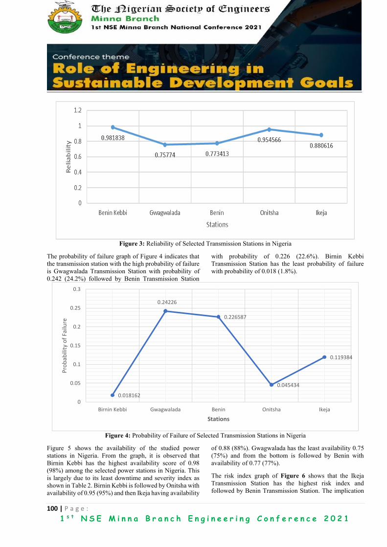
100 | P a g e :


Figure 3: Reliability of Selected Transmission Stations in Nigeria

The probability of failure graph of Figure 4 indicates that

the transmission station with the high probability of failure

is Gwagwalada Transmission Station with probability of

0.242 (24.2%) followed by Benin Transmission Station

with probability of 0.226 (22.6%). Birnin Kebbi

Transmission Station has the least probability of failure

with probability of 0.018 (1.8%).

Figure 4: Probability of Failure of Selected Transmission Stations in Nigeria

Figure 5 shows the availability of the studied power

stations in Nigeria. From the graph, it is observed that

Birnin Kebbi has the highest availability score of 0.98

(98%) among the selected power stations in Nigeria. This

is largely due to its least downtime and severity index as

shown in Table 2. Birnin Kebbi is followed by Onitsha with

availability of 0.95 (95%) and then Ikeja having availability

of 0.88 (88%). Gwagwalada has the least availability 0.75

(75%) and from the bottom is followed by Benin with

availability of 0.77 (77%).

The risk index graph of Figure 6 shows that the Ikeja

Transmission Station has the highest risk index and

followed by Benin Transmission Station. The implication

0.018162

0.24226

0.226587

0.045434

0.119384

0

0.05

0.1

0.15

0.2

0.25

0.3


Pro

bab

ility

of

Failu

re

Stations

101 | P a g e :


of this is that failure occurrence on the Ikeja Transmission

Station would have the highest impact on the economy of

the country compared to other transmission station in

Nigeria. This is largely due to the power delivered to by the

Ikeja Transmission Station and the population the station

serves.

Lagos being the economic hub of the Nigeria economy is

served by this transmission station and this accounts for the

enormous risk in the power system network serving the

state.

From Figure 2 to Figure 6, it is seen that Birnin Kebbi

Transmission Station is more stable than other transmission

stations in the study. Benin has the least failure rate (Figure

2), hence its reliability is high (98.2%) with lowest

probability of failure (1.8%). Due to the stability of Birnin

Kebbi Transmission Station, its risk index is the lowest

(5.01).

Figure 5: Availability of Selected Power System Network in Nigeria

Figure 6: Risk Index of Selected Power System Network in Nigeria

0.9818

0.75770.7734

0.9545

0.8806

0

0.2

0.4

0.6

0.8

1

1.2


Ava

ilab

ility

Stations

5.01274

28.4413630.36263

14.81142

83.38942

0

10

20

30

40

50

60

70

80

90


Ris

k In

dex

Stations

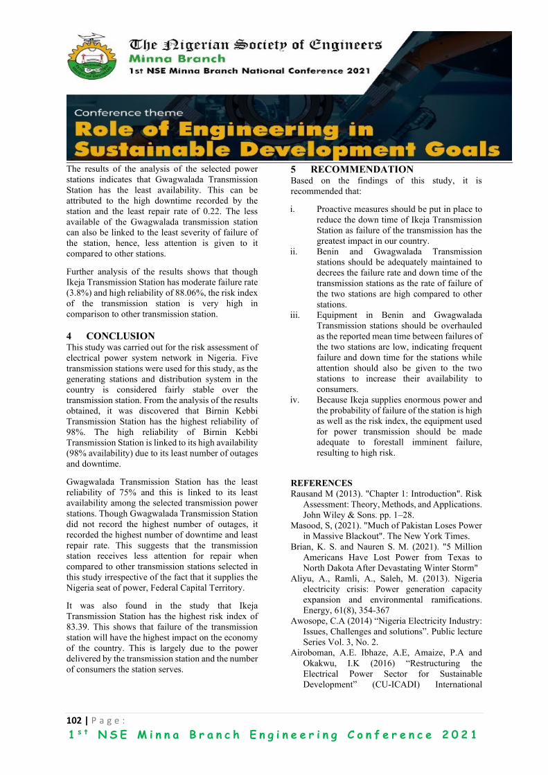
102 | P a g e :


The results of the analysis of the selected power

stations indicates that Gwagwalada Transmission

Station has the least availability. This can be

attributed to the high downtime recorded by the

station and the least repair rate of 0.22. The less

available of the Gwagwalada transmission station

can also be linked to the least severity of failure of

the station, hence, less attention is given to it

compared to other stations.

Further analysis of the results shows that though

Ikeja Transmission Station has moderate failure rate

(3.8%) and high reliability of 88.06%, the risk index

of the transmission station is very high in

comparison to other transmission station.

4 CONCLUSION This study was carried out for the risk assessment of

electrical power system network in Nigeria. Five

transmission stations were used for this study, as the

generating stations and distribution system in the

country is considered fairly stable over the

transmission station. From the analysis of the results

obtained, it was discovered that Birnin Kebbi

Transmission Station has the highest reliability of

98%. The high reliability of Birnin Kebbi

Transmission Station is linked to its high availability

(98% availability) due to its least number of outages

and downtime.

Gwagwalada Transmission Station has the least

reliability of 75% and this is linked to its least

availability among the selected transmission power

stations. Though Gwagwalada Transmission Station

did not record the highest number of outages, it

recorded the highest number of downtime and least

repair rate. This suggests that the transmission

station receives less attention for repair when

compared to other transmission stations selected in

this study irrespective of the fact that it supplies the

Nigeria seat of power, Federal Capital Territory.

It was also found in the study that Ikeja

Transmission Station has the highest risk index of

83.39. This shows that failure of the transmission

station will have the highest impact on the economy

of the country. This is largely due to the power

delivered by the transmission station and the number

of consumers the station serves.

5 RECOMMENDATION Based on the findings of this study, it is

recommended that:

i. Proactive measures should be put in place to

reduce the down time of Ikeja Transmission

Station as failure of the transmission has the

greatest impact in our country.

ii. Benin and Gwagwalada Transmission

stations should be adequately maintained to

decrees the failure rate and down time of the

transmission stations as the rate of failure of

the two stations are high compared to other

stations.

iii. Equipment in Benin and Gwagwalada

Transmission stations should be overhauled

as the reported mean time between failures of

the two stations are low, indicating frequent

failure and down time for the stations while

attention should also be given to the two

stations to increase their availability to

consumers.

iv. Because Ikeja supplies enormous power and

the probability of failure of the station is high

as well as the risk index, the equipment used

for power transmission should be made

adequate to forestall imminent failure,

resulting to high risk.

REFERENCES

Rausand M (2013). "Chapter 1: Introduction". Risk

Assessment: Theory, Methods, and Applications.

John Wiley & Sons. pp. 1–28.

Masood, S, (2021). "Much of Pakistan Loses Power

in Massive Blackout". The New York Times.

Brian, K. S. and Nauren S. M. (2021). "5 Million

Americans Have Lost Power from Texas to

North Dakota After Devastating Winter Storm"

Aliyu, A., Ramli, A., Saleh, M. (2013). Nigeria

electricity crisis: Power generation capacity

expansion and environmental ramifications.

Energy, 61(8), 354-367

Awosope, C.A (2014) “Nigeria Electricity Industry:

Issues, Challenges and solutions”. Public lecture

Series Vol. 3, No. 2.

Airoboman, A.E. Ibhaze, A.E, Amaize, P.A and

Okakwu, I.K (2016) “Restructuring the

Electrical Power Sector for Sustainable

Development” (CU-ICADI) International

103 | P a g e :


Conference on African Development Issues May

9–11 2016, Ota, Nigeria. pp.1-4

Guo, L., Qiu, Q., and Liu, J. (2014). Power

transmission risk assessment considering

component condition. J. Mod. Power Syst. Clean

Energy 2, 50–58

Onohaebi, S. O. (2017) Power Transmission

constraints and faults analysis in Nigeria Power

System

Raza, M. (2019). System Reliability and

Availability Calculations.

https://blogs.bmc.com/system-reliability-

availability-calculations/?print=pdf

Morteza, A., Habib, R. and Yaser, D. (2014).

“Reliability-Centered maintenance for circuit

breakers in transmission networks” IET

Generation, Transmission & Distribution. pp.

1583-1590.

Asibeluo, U. N. and Madueme, T. C. (2018): Risk-

Based Security Assessment of Power System

Voltage Drop: A Case Study of Nigerian 330kv

41-Bus Transmission Grid. Nigerian Journal of

Technology (NIJOTECH) Vol. 37, No. 3, July

2018, pp. 735 – 741

Rosencrance, L. (2020). risk analysis. Accessed on

15th March, 2021 from

https://searchsecurity.techtarget.com/definition/r

isk-analysis?amp=1

104 | P a g e :


Non-linear Scaling in Global Optimisation. Part II: Performance

Evaluation 1, 2*Abubakar, H. A., 2, 3Misener, R. and 2Adjiman, C. S.

1Department of Chemical Engineering, Ahmadu Bello University, Zaria 2Department of Chemical Engineering, Imperial College London

3Department of Computing, Imperial College London

*Corresponding Author: [email protected]

ABSTRACT Numerous real-life engineering problems that arise in many areas of applications such as process synthesis,

molecular products design, scheduling and planning of batch processes, among others, are non-linear and can

be solved to guarantee global optimum using global optimisation solvers. However, these solvers sometimes

develop numerical instability when solving problems that are badly scaled resulting in either no solution,

infeasible solution or a solution that is not the global optimum. One of the approaches of preventing such

numerical instability is scaling. In this study, we examined the impact of a scaling algorithm that accounts for

nonlinearity in a problem on the performance of three global optimisation solvers, SCIP, BARON and

ANTIGONE using two real life global optimisation test problems. The original and transformed forms of the

test problems, whose solutions are known a priori, are scaled using the scaling code implemented and validated

in the part I of this paper. The scaled and unscaled versions of the original and transformed problems are solved

in GAMS using the aforementioned global optimisation solvers and the solution analysed under four

performance criteria. For the test problems considered, the implemented algorithm demonstrates its

effectiveness in preventing the global optimisation solvers from developing numerical instability when solving

extremely badly-scaled forms of the problems and is therefore recommended for large scale global

optimisations applications.

KEYWORDS: Scaling, Nonlinear, Global Optimisation, Instability, NLP.

1 INTRODUCTION A great number of scientific or industrial problems

encountered in practice involve selecting the best among

different alternative decisions. These problems can be

formulated as an optimisation problem and are generally

nonlinear and nonconvex (Adjiman et al., 2021; Adjiman

et al, 1998a; Grant et al., 2018; Niebling and Eichfelder,

2019). Their nonconvex nature add complexity to the

problems as they possess two or more local optimal

solutions, and choosing the global optimum is not trivial

(Boukouvala et al., 2016; Ryoo and Sahinidis, 1995;

Sahinidis, 2019; Tawarmalani and Sahinidis, 2004).

However, global optimisation strategy can effectively

handle this type of problem.

Many important classes of problem demand the use of

global optimisation method. Typical examples are

nonconvex continuous, mixed-integer, bilevel, differential-

algebraic, and non-factorable problems (Floudas and

Gounaris, 2008; Li and Yang, 2021). For these problems, a

number of solvers have been developed to solve them to

guarantee global optimum. Commonly used deterministic

global optimisation solvers include Solving Constraint

Integer Programs (SCIP) of Bussieck and Vigerske (2012),

Branch-and-Reduce Optimisation Navigator (BARON) of

Sahinidis (1996), Convex Over and Under ENvelopes for

Nonlinear Estimation (COUENNE) of Belloti et al (2009)

and Algorithms for coNTinuous / Integer Global

Optimisation of Nonlinear Equations (ANTIGONE) of

Misener and Floudas (2013), among many others.

Despite the advancement in global optimisation theory

and the numerous numbers of solvers available, some

problems are known to be difficult to solve numerically and

are common in many application areas, such as waste

minimization and treatment, phase and chemical

equilibrium, and controller design. These problems

inherently operate on many numerical scales, hence could

be termed badly scaled problems.

One of the approaches of tackling the challenges that

solvers encounter when solving badly scaled non-linear

problems is scaling. However, the state-of-the-art

approaches of solving a badly scaled problem either

disregard the inherent disparity in the numerical scales of

the problem or does not take into consideration the

nonlinearity in the problem. Ignoring the disparity in the

105 | P a g e :


numerical scales by not scaling generates numerical

instability that often results in a solution that is not global

optimum. On the other hand, neglecting the non-linearity

in the problem by applying linear scaling many a time

results in a solution that is infeasible to the original

problem.

Other alternative approaches of preventing the

numerical difficulties that come from the solution of these

problems, such as extended precision (Chapra and Canale,

2010) and interval arithmetic (Zilinskas and Zilinskas,

2006) are computationally demanding, thereby may not be

reasonable when compared to scaling.

Scaling involves the modification of the coefficients

matrix that characterise a system in such a way that extreme

variations that could lead to numerical instabilities during

computations is eliminated (Morgan, 1987). By scaling, the

variables and equations in a given problem are modified

using variable and equation/constraint scaling factors,

respectively, in such a manner that the variables become

similar in their order of magnitudes and the equations

become well conditioned relative to the variable’s

perturbation and well balanced relative to one another.

Scaling ensures that the approaches employ in

determining and verifying the feasible points of constraint

satisfaction problems do not develop numerical challenges

(Domes, 2009). The same benefit is obtainable in

constrained optimisation problems since the former are

also optimisation problems with no given or constant

objective function. Domes and Neumaier (2011) showed

how scaling can be helpful in the calculation of interval hull

of an ill conditioned strictly convex quadratic constraint by

directed Cholesky factorization. It was demonstrated that

by scaling of the constraint symmetric matrix, the condition

number of the matrix decreased by six orders of magnitude.

Linear systems scaling is a well-researched topic in the

literature and many scaling techniques and routines have

been developed and implemented in linear optimisation

solvers (Elble and Sahinidis, 2012). In solving linear

optimization problems, scaling is widely used to reduce the

condition number of the constraint matrix (Ploskas and

Samaras, 2013). It may decrease the computational effort

in arriving at a solution and possibly improve the numerical

behaviour of the solver used (Elble and Sahinidis, 2012).

A major issue in nonlinear systems involving

multivariable polynomials is the occurrence of variables of

that operates on widely different numerical scales, which

can have negative impacts on the results of solving the

systems (Domes and Neumaier, 2008). Unlike in linear

systems, there are limited studies that have been carried out

on scaling nonlinear systems. For scaling of polynomial

systems, the few studies in the literature were carried out

by Watson et al (1985), Morgan (1987) and Domes and

Neumaier (2008). In Domes and Neumaier (2008), a

scaling algorithm, linear programing (SCALELP)

algorithms, for scaling polynomial systems was presented.

The algorithm was demonstrated, using some examples, to

be very stable for problems where previously known

nonlinear scalling algorithms performed poorly and are

therefore recommended to be suitable for general purpose

scaling. In this study, we assessed the impact of a scaling

algorithm implemented and validated in part I of this paper

on the performance of SCIP, BARON and ANTIGONE by

solving two test problems in process design under four

criteria. These criteria are the CPU time taken in arriving at

solution, number of iterations carried out in reaching the

solution, number of nodes explored and the quality of

solutions.

2 PROBLEM DESCRIPTIONS Following the validation of the suitability of the scaling

technique for optimisation problems containing signomial

and polynomial functions (see part I of this paper), the

performance of the validated scaling techniques is assessed

using practical global optimisation problems that contain

these functions. The following two test problems in

geometric programming are considered.

2.1 TEST PROBLEM 1: ALKYLATION PROCESS

DESIGN The goal in this optimisation problem is to find the optimal

operating conditions that is required to maximise a profit

function in an alkylation process, shown in Figure 2.1. The

model for this process was originally formulated by

Bracken and McCormick (1968) and then reformulated in

Dembo (1976) as a signomial problem. The reformulated

model is available in Floudas et al (1999) as a test problem.

In this study, we reintroduced the equality constraints and

the variables eliminated from the original model during the

reformulation process, and then transformed the model into

a form that is suitable for the scaling code (see (2.4) in part

I of the paper).

Figure 2.1: Alkylation process optimisation

106 | P a g e :


Cost parameters

[ Alkylate product value ∶= $0.063 per octane. barrel

Olefin feed cost: $5.04 per barrel

Isobutane recycle costs ∶= $ 0.035 per barrel

Acid addition cost ∶= $10.00 per thousand pounds

Isobutane makeup cost ≔ $ 3.36 per barrel

Process variables

[ x1: Olefin feed (barrel per day)

x2: Isobutane recycle (barrel per day) x3: Acid addition rate (thousands of pounds per day)

x4: Alkylate yield (barrel per day) x5: Isobutane makeup (barrel per day)

x6: Acid strength (wt%) x7: Octane number x8: External isobutane − to − olefin ratio x9: Acid dilution factor x10: F − 4 performance number

Optimisation problem

Objective

profit per day maximisation

[

min objv =

(

10x3 ⏟ Acid

additioncost

+ 5.04x1⏟ Olefin feed cost

+ 0.035x2⏟ Isobutanerecyclecost

+ 3.36x5⏟ Isobutanemake upcost

+ 3000⏟ fixedcost

)

⏟ Total cost

− 0.063x4x7⏟

Alkylate Value

Subject to

Mathematical model

Alkylate yield

[0.0059553571x8

2 + 0.88392857x4x1−1 − 0.1175625x8 ≤ 1

1.1088x1x4−1 + 0.1303533x1x4

−1x8 − 0.0066033x1x82x4

−1 ≤ 1

Octane number

[0.00066173269x8

2 − 0.019120592x8 − 0.0056595559x6 + 0.017239878x7 ≤ 1

56.85075x7−1 + 1.08702x8x7

−1 + 0.32175x6x7−1 − 0.03762x8

2x7−1 ≤ 1

Acid dilutionfactor

[2462.3121x3x4

−1x6−1 − 25.125634x3x4

−1 + 0.006198x10 ≤ 1

161.18996x10−1 + 5000x3x4

−1x10−1 − 489510x3x4

−1x6−1x10

−1 ≤ 1

F4 performancenumber

[44.333333x7

−1 + 0.33x10x7−1 ≤ 1

0.022255x7 − 0.00759474x10 ≤ 1

Isobutanemakeup

[0.819672131x1x4−1 + 0.819672131x5x4

−1 = 1

Acid strength

[98000x3x4−1x6

−1x9−1 − 1000x3x4

−1x9−1 = 1

External isobutane to olefin ratio

[x1x8x2−1 − x5x2

−1 = 1

Bounds

107 | P a g e :


Variablebounds

[ 1500 ≤ x1 ≤ 20001 ≤ x2 ≤ 16000 1 ≤ x3 ≤ 120 3000 ≤ x4 ≤ 35001 ≤ x5 ≤ 2000 85 ≤ x6 ≤ 93 90 ≤ x7 ≤ 95 3 ≤ x8 ≤ 12 1.2 ≤ x9 ≤ 3.6 145 ≤ x10 ≤ 162

2.2 TEST PROBLEM 2: OPTIMAL REACTOR

DESIGN The goal is to determine the optimal operating

conditions to maximise profit from a steady enzymatic

reaction process operating at fixed feed flow rate in two

continuous stirred tank reactors arranged in series, see

Figure 2.2. This entails determining the holding time and

the temperature for each reactor that maximised the final

conversion of the substrate (SS) to product (δ). The higher

the conversion of SS, the more the yield of δ, and the

greater is the total profit. The model for this process was

formulated as a geometric programming problem in

Rijckaert (1973). The model, available as a test problem in

Dembo (1976) and Floudas et al (1999), is presented here.

Rate expression

[rr =θ2(T)CEE0CSSθmk(T) + aCSS

With

[ θ2(T) = 1.7. 10

13e−1830

RT

θmk(T) = 4e−3240

RT + 2e−830

RT

a = 0.1 CEE0 = 10

−13mol/l C0 = 10mol/l

Reactor cost ≔ 0.4 per (holdup time)0.67. cost of pro

Where T, θ, CSS, CEE0 and C0 denote reactor

temperature, reaction rate constants, outlet substrate

concentration, total enzyme concentration and feed

concentration, respectively.

Figure 2.2: An enzymatic reaction process in a CSTR

cascade

Process variables

[ x1: Concentration of δ in reactor 1(mol/L) x2: Concentration of δ in reactor 2 (mol/L)

x3: Exponential function of T in reactor 1(−)

x4: Exponential function of T in reactor 2(−) x5: denominator of reaction rate in reactor 1 (mol/L. s)

x6: denominator of reaction rate in reactor 2 (mol/L. s)

x7: reaction rate in reactor 1 (mol/L. s) x8: reaction rate in reactor 2 (mol/L)

Optimisation problem

Objective

Profit per unit cost of product maximisation

[

min objv = −

[

(x1 + x2)⏟ Productvalue perunit cost

−

(

0.4 (

x1

x7)0.67

⏟ cost of reactor 1

+ 0.4 (x2

x8)0.67

⏟ cost ofreactor 2

+ 10⏟fixedcost

)

⏟ Total cost per unit cost of product ]

Subject to:

Mathematical model

108 | P a g e :


Reaction rate [0.0588x5x7 + 0.1x1 ≤ 1 reactor 1

0.0588x6x8 + 0.1x1 + 0.1x2 ≤ 1reactor 2

Denominator ofreaction rate

[4x3x5

−1 + 2x3−0.71x5

−1 + 0.0588x7x3−1.3 ≤ 1 reactor 1

4x4x6−1 + 2x4

−0.71x6−1 + 0.0588x8x4

1.3 ≤ 1 reactor 2

variablebounds

[0.1 ≤ xi ≤ 10 ∀ i ∈ 1…… .8

3 RESULTS AND DISCUSSION The impact of the nonlinear scaling code, validated in

part I of the paper, on the performance of global

optimisation solvers is analysed using a two-stage

approach. First, the scaled and unscaled versions of original

test problem described in section 2.0 are solved in GAMS

as shown in Figure 3.1. In the second stage, the original

problems are transformed such that the problems become

extremely badly scaled, and the unscaled and scaled forms

of the resulting problems solved. Global optimisations

solvers, SCIP, BARON and ANTIGONE are utilised for

solving the problems and the solutions compared under

four performance measures: numerical value or quality of

the solutions, CPU time, iteration number and number of

nodes explored. Details of the statistics of the test problems

are shown in Table 3.1.

3.1 ORIGINAL TEST PROBLEMS Tables 3.2-3.3 show optimisation results for the test

problems under the four performance measures

aforementioned. For a given test problem, we determined

if the solution quality has changed by computing the

percentage deviation between the scaled and unscaled

solution value of the variables. If at least one of the

variables deviations is greater than 10%, the solution is

considered to have unchanged. For the CPU time, iteration

number and number of nodes explored, they are considered

to have changed when the change in their values is at least

an order of magnitude.

From the results presented in Tables 3.2 and 3.3, it is

seen that in both test problems, there is no change in the

solution values of the variables. The solvers all arrived at

the same solution before and after scaling. Hence, scaling

has no impact on the solution quality. For the other three

performance criteria, the impact of scaling, though

negligibly small, is dependent on the solvers. While

ANTIGONE showed no improvement, scaling has impact

on the performance of SCIP and BARON. For SCIP,

significant reduction in the number of nodes explored

before a solution is found is noticeable. Similarly, for

BARON, improvement is observed in the number of

iterations carried out before solution is found, particularly

in test problem 1.

Figure 3.1: Performance measure assessment procedure.

TABLE 3.1: STATISTICS OF THE TEST CASES

Test

Problems

No. of

Variables

No. of

Equations

No. of Terms (Number of nonlinear

terms)

No. non-zero

entries

1 8 15 29 (20) 59

2 9 5 20 (10) 21

109 | P a g e :


TABLE 3.2: OPTIMISATION RESULTS FOR THE SCALED AND UNSCALED VERSIONS OF TEST PROBLEM 1

Measures Solvers

ANTIGONE BARON SCIP

unscaled scaled unscaled scaled unscaled scaled

Solution

𝑥1 1698.18 1698.18 1698.18 1698.18 1698.18 1698.18

𝑥2 15829.86 15829.86 15829.86 15829.86 15829.86 15829.85

𝑥3 53.67 53.67 53.67 53.67 53.67 53.67

𝑥4 3031.30 3031.30 3031.30 3031.30 3031.30 3031.30

𝑥5 2000.00 2000.00 2000.00 2000.00 2000.00 2000.00

𝑥6 90.11 90.11 90.11 90.11 90.11 90.11

𝑥7 95.00 95.00 95.00 95.00 95.00 95.00

𝑥8 10.50 10.50 10.50 10.50 10.50 10.50

𝑥9 1.55 1.55 1.55 1.55 1.55 1.55

𝑥10 153.54 153.54 153.54 153.54 153.54 153.54

𝑜𝑏𝑗𝑣 1227.23 1227.23 1227.23 1227.23 1227.23 1227.22

CPU time(s) 0.10 0.10 1000.00 0.13 0.61 0.24

No. of iterations 4 4 322056 1 2379.00 1812

No. of node explored 0 0 1 0 940 71

TABLE 3.3: OPTIMISATION RESULTS FOR THE SCALED AND UNSCALED VERSIONS OF TEST PROBLEM 2

Measures Solvers

ANTIGONE BARON SCIP


Solution

𝑥1 6.3458 6.3458 6.3458 6.3458 6.3458 6.3458

𝑥2 2.3410 2.3410 2.3410 2.3410 2.3410 2.3410

𝑥3 0.6709 0.6709 0.6709 0.6709 0.6709 0.6709

𝑥4 0.5347 0.5347 0.5347 0.5347 0.5347 0.5347

𝑥5 5.9528 5.9528 5.9528 5.9528 5.9528 5.9528

𝑥6 5.3164 5.3164 5.3164 5.3164 5.3164 5.3164

𝑥7 1.0440 1.0440 1.0440 1.0440 1.0440 1.0440

𝑥8 0.4201 0.4201 0.4201 0.4201 0.4201 0.4201

𝑜𝑏𝑗𝑣 3.9180 3.9180 3.9180 3.9180 3.9180 3.9180

CPU time(s) 0.4610 0.5410 0.9800 0.4100 1.9800 0.9600

No. iterations 4 4 25 3 26551 10968

No. nodes 3 3 1 1 1431 758

110 | P a g e :


3.1 TRANSFORMED TEST PROBLEMS Test problems in section 2 are transformed into their

badly scaled forms by modifying the units of the

variables in such a way that they become widely

different in their order of magnitudes. For the two

test problems, identified variables with units are

transformed into new units to get a scaling factor SF

that was used to scale the variables. Essentially,

(3.1) is used to substitute for old variables x in terms

of the new variables x*. Table 3.4 shows the

variables that are transformed in the test problems

and their corresponding scaling factor.

Tables 3.5 and 3.6 represent the results of the

numerical investigation performed on the modified

test problems. The results confirmed the

implemented and validated scaling technique to be

invaluable for global optimisation solvers when

solving extremely badly scaled problems as all the

solvers developed numerical instability before

scaling. The instability results in no solution

reported as seen in the results of all the solvers for

the two test problems. However, with the problems

scaled prior to being solved, the three solvers

obtained the same solution as in the original test

problems in about the same iteration number, CPU

time and number of nodes explored (see Tables 3.2

and 3.3).

𝑥 = 𝑆𝐹 𝑥∗ (3.1)

Table 3.4: Scaling factors for the transformed

variables.

TABLE 3.5: OPTIMISATION RESULTS FOR THE SCALED AND UNSCALED VERSIONS OF BADLY

SCALED TEST PROBLEM 1.

Measures Solvers

ANTIGONE BARON SCIP


Solution

𝑥1 1759.72 1698.18 0.00 1698.18 0.00 1698.18

𝑥2 16000.00 15829.86 0.00 15829.86 0.00 15829.85

𝑥3 56.59 53.67 0.00 53.67 0.00 53.67

𝑥4 3081.74 3031.30 0.00 3031.30 0.00 3031.30

𝑥5 2000.00 2000.00 0.00 2000.00 0.00 2000.00

𝑥6 90.37 90.11 0.00 90.11 0.00 90.11

𝑥7 95.00 95.00 0.00 95.00 0.00 95.00

𝑥8 10.23 10.50 0.00 10.50 0.00 10.50

𝑥9 1.55 1.55 0.00 1.55 0.00 1.55

𝑥10 153.54 153.54 0.00 153.54 0.00 153.54

𝑜𝑏𝑗𝑣 -2377.23 1227.23 0.00 1227.23 0.00 1227.22

CPU time(s) 0.11 0.12 0.13 0.14 0.01 0.62

No. of iterations NA 5 NA 1 0.00 8595

No. of node 0 0 0 1 0 291

111 | P a g e :


TABLE 3.6: OPTIMISATION RESULTS FOR THE SCALED AND UNSCALED VERSIONS OF BADLY

SCALED TEST PROBLEM 2.

Measures

Solvers

ANTIGONE BARON SCIP


Solution

𝑥1 0.0000 6.3458 0.0000 6.3458 0.0000 6.3458

𝑥2 0.0000 2.3410 0.0000 2.3410 0.0000 2.3410

𝑥3 0.0000 0.6709 0.0000 0.6709 0.0000 0.6709

𝑥4 0.0000 0.5347 0.0000 0.5347 0.0000 0.5347

𝑥5 0.0000 5.9528 0.0000 5.9528 0.0000 5.9528

𝑥6 0.0000 5.3164 0.0000 5.3164 0.0000 5.3164

𝑥7 0.0000 1.0440 0.0000 1.0440 0.0000 1.0440

𝑥8 0.0000 0.4201 0.0000 0.4201 0.0000 0.4201

𝑜𝑏𝑗𝑣 0.0000 3.9180 0.0000 3.9180 0.0000 3.9180

CPU time(s) 0.0000 0.4710 0.0100 0.3900 0.0100 0.8000

No. iterations NA 4 NA 3 0 9063

No. nodes 0 3 0 1 0 594

4 CONCLUSION

The impact of nonlinear scaling algorithm,

implemented in the part I of this paper, on the

performance of ANTIGONE, BARON and SCIP

was analysed using two real life global optimisation

problems in the area of process design. The scaling

code proved very effective in preventing the solvers

in running into numerical problem when solving the

badly scaled forms of the problems. For problems

that are not obviously badly scaled to the extent that

the solvers may developed instability problem, as

was the case of the original test problems, the scaling

technique shows potential to help a solver reduce

CPU time, number of iterations and nodes explored

in arriving at solution. It is therefore highly

recommended for large scale global

REFERENCES Adjiman, C.S., Dallwig, S., Floudas, C.A. and

Neumaier, A. (1998). A global optimisation

method, αBB, for general twice-differentiable

constrained NLPs–I: Theoretical advances.

Comput. Chem. Eng. 22, 1137-1158

Adjiman, C. S., Sahinidis, N. V., Vlachos, D. G.,

Bakshi, B., Maravelias, C. T. and Georgakis, C.

(2021). Process Systems Engineering

Perspective on the Design of Materials and

Molecules. Ind. Eng. Chem. Res. 60, 14, 5194–

5206

Bracken, J. and McCormick, G. P. (1968). Selected

Applications of Nonlinear Programming, Wiley,

New York.

Boukouvala, F., Misener, R. and Floudas, C.A

(2016). Global optimization advances in Mixed-

Integer Nonlinear Programming, MINLP, and

Constrained Derivative-Free Optimization,

CDFO. European Journal of Operational

Research, 252 (3).

Bussieck, M. R. and Vigerske, S. (2012). MINLP

Solver Software. In J. J. Cochran, L. A. Cox, P.

Keskinocak, J. P. Kharoufeh, and J. C. Smith,

editors, Wiley Encyclopedia of Operations

Research and Management Science. John Wiley

& Sons, Inc.

Chapra, S.C. and Canale, R.P. (2010). Numerical

Methods for Engineers, 6th ed., international ed.,

McGraw-Hill Higher Education, Boston,

London.

Dembo, R. S. (1976). A Set of Geometric

Programming Test Problems and Their

Solutions. Math. Prog. 10, 192-213

Domes, F.: GloptLab (2009). A Configurable

Framework for the Rigorous Global Solution of

Quadratic Constraint Satisfaction Problems.

Optim. Methods Softw. 24, 727–747

Domes, F. and Neumaier, A. (2008). A Scaling

Algorithm for Polynomial Constraint

Satisfaction Problems. J. Glob. Optim., 42:327–

345

Domes, F. and Neumaier, A. (2011). Rigorous

Enclosures of Ellipsoids and Directed Cholesky

Factorization, SIAM J. Matrix Anal. Appl. 32,

262–285

Elble, J. M. and Sahinidis, N.V. (2012). Scaling

Linear Optimisation Problems Prior To

112 | P a g e :


Application of the Simplex Method, Comput

Optim Appl., 52, 345–371

Floudas, C.A. and Gounaris, C.E. (2008). A Review

of Recent Advances in Global Optimisation. J.

Glob. Optim. 45, 3–38

Floudas, C.A., Pardalos, P.M., Adjiman, C.S.,

Esposito, W.R., Gumus, Z.H., Harding, S.T.,

Klepeis, J.L., Meyer, C.A., and Schweiger, C.A.

(1999). Handbook of Test Problems in Local and

Global Optimisation, Kluwer Academic

Publishers, Dordrecht

Grant, E., Pan, Y., Richardson, J., Martinelli, J. R.,

Armstrong, A., Galindo, A. and Adjiman, C. S.

(2018). Multi-objective computer-aided solvent

design for selectivity and rate in reactions.

Computer Aided Chemical Engineering. 44,

2437-2442

Li, G. and Yang, X. (2021). Convexification

Method for Bilevel Programs with a Nonconvex

Follower’s Problem. Journal of Optimization

Theory and Applications, 188, pg. 724–743

Misener, R. and Floudas, C. A. (2013):

ANTIGONE

:http://www.gams.com/dd/docs/solvers/antigone

, version 1.0

Morgan, A. (2009). Solving Polynomial Systems

Using Continuation for Engineering and

Scientific Problems,

Society for Industrial and Applied Mathematics,

Philadelphia, Prentice-Hall, chapter 5, 107-119

Niebling, J., Eichfelder, G. (2019). A branch-and-

bound-based algorithm for nonconvex

multiobjective optimization. SIAM J. Optim.

29(1), 794–821

Ploskas, N. and Samaras, N. (2013). The Impact of

Scaling on Simplex Type Algorithms, ACM

digital Library

Rijckaert, M.J. (1973). Engineering Applications of

Geometric Programming", in: Avriel, M.

Rijckaert, M.J. and Wilde, D.J., eds.,

Optimization and Design, Prentice-Hall,

Eaglewood Cliffs, New Jersey, 196-220

Ryoo, H. S. and Sahinidi, N. V. (1995). Global

Optimisation of Nonconvex NLPs and MINLPs

With Applications in Process Design, Computers

chem. Engng, 19, 551-566

Sahinidi, N. V. (1996). BARON: A General-Purpose

Global Optimisation Software Package, Journal

of Global Optimisation, 8, 201-205

Sahinidis, N. V (2019). Mixed-integer nonlinear

programming 2018. Optimization and

Engineering (2019) 20:301–306

Tawarmalani, M. and Sahinidis, N.V. (2004). Global

Optimisation of Mixed-Integer Nonlinear

Programs: A Theoretical and Computational

Study. Mathematical Programming, 99, 563-591.

Watson, L.T., Billups, L.C. and Morgan, A.P.

(1985). HOMPACK: A Suite of Codes for

Globally Convergent Homotopy Algorithms.

http://deepblue.lib.umich.edu/bitstream/handle/

2027.42/8204/ban6930.0001.001.pdf;jsessionid

=4845D7244E05308ECF4988DCEBD9BEC8?s

equence=5

Zilinskas, A. and Zilinskas, J. (2006). On efficiency

of tightening bounds in interval global

optimization, Lecture Notes in Computer

Science 3732: 197–205.






http://www.gams.com/dd/docs/solvers/antigone

http://www.gams.com/dd/docs/solvers/antigone





113 | P a g e :


A Review of Different Proposed Image Detection Techniques for

Road Anomalies Detection. A. M. Oyinbo1, A. S. Mohammad2, S. Zubair3, and E. MICHAEL4

1,2,3,4 Department of Telecommunication Engineering,

Federal University of Technology Minna – Nigeria. [email protected], [email protected], [email protected],

[email protected]

ABSTRACT

Road anomalies such as, potholes, speed bumps and cracks have been one of the major problems faced by road

users globally, contributing to vehicular accidents on roads, quick wear and tear of vehicles, among others.

Overtime, advancement in vehicular technology and sensors, has led to the establishment of automated

approach for detecting road anomalies. Though, these approaches can be categorized into 3D reconstruction-

based approach, 2D vision-based approach and the vibrational-based approach. These techniques are geared

towards enabling vehicles in detecting road anomalies and notifying drivers of such, thereby reducing the rate

of accidents on roads caused by these anomalies. Also, these approaches can be incorporated into vehicular

Ad-hoc network, where automated vehicles can be able to navigate through road terrains with pothole

anomalies. However, the 2D vision-based approach has received wide acceptance among the academia and the

industry due to its advantages over the 3D reconstruction-based, such as, lower cost of implementation. Also,

it has advantage over the vibrational-based approaches in terms of better detection accuracy. In this regard, this

paper presents a mini-survey of various 2D vision-based techniques proposed in the literature for road surface

condition monitoring and anomaly detection. The merits and drawbacks of these techniques are highlighted.

Furthermore, open research issues are presented. Our effort forms part of a larger goal aimed at improving and

developing robust vision-based approaches for road anomaly detection, as well as giving researchers a pathway

in similar pursuits.

KEYWORDS: Anomalies, Detection, Image, Potholes, Road and Cracks.

1. INTRODUCTION Road network plays important crucial role in any nation’s

economy (Aldagheiri, 2009), contributing to its economic

growth and development with social benefits. Road

networks provides access to employment, social, health

and educational services (Fan & Chan-Kang, 2005). Roads

open up more areas and stimulate economic and social

development. For these reasons, road infrastructure is one

of the most important of all public assets (Lemer, 1999).

This is attributed to the fact that, it is one of the major

means of transportation (Adeniyi, 2012), that allow the

vehicular movement of goods, services and human from

one location to another. However, it is important to ensure

that these roads are in good conditions at all times by

continuous monitoring of its surfaces and repairs of areas

with anomalies.

Road anomalies on asphalt road occur as a result

of the road exceeding their maximum lifespan. The use of

poor quality materials for construction, poor drainage

system (Onoyan-Usina,2013), excess road traffic and

failure to comply with the standard road construction

specification (Bello-Salau et al., 2014). These anomalies

are usually observed in form of potholes, speed bumps and

cracks (Akarsu et al., 2016). The adverse effects of these

anomalies on roads cannot be over emphasized, ranging

from discomforts experienced by drivers while plying such

roads, vehicular damages, road traffic accidents, among

others. Though, prevalent among these anomalies in

developing nations like Nigeria is the potholes anomalies,

which has contributed greatly to the rate of road traffic

accident (Ryu et al., 2015).

Pothole has been one of the major problems faced by road

users globally, and has been a contributing factor to vehicle

accidents on roads, quick wear and tear of vehicles, among

others. This is such a serious issue that several

organizations and countries always try to show the effect of

potholes on the economy at large. For example, the

American Automobile Association estimated that about 16

million drivers had suffered damage from potholes in the

last five years before the year 2016 within the United States

alone (Byun et al., 2018). Britain also made their

estimation cost of fixing potholes on their roads to amount





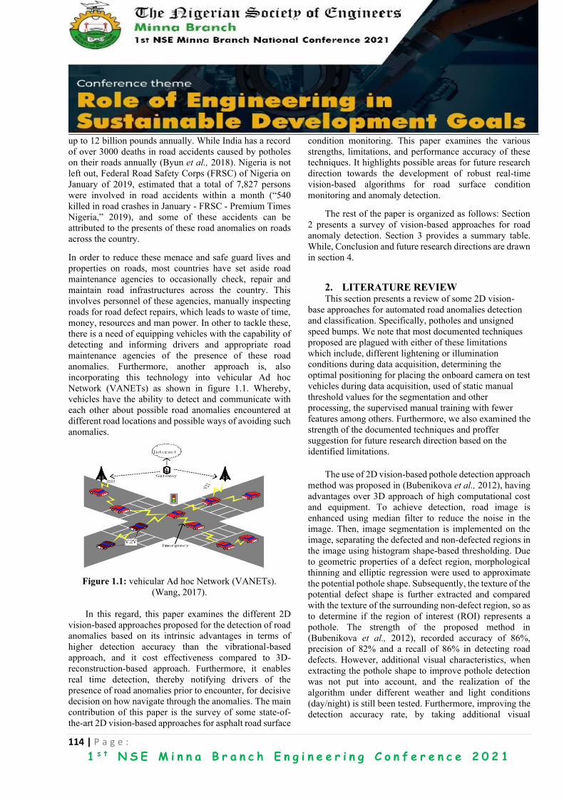
114 | P a g e :


up to 12 billion pounds annually. While India has a record

of over 3000 deaths in road accidents caused by potholes

on their roads annually (Byun et al., 2018). Nigeria is not

left out, Federal Road Safety Corps (FRSC) of Nigeria on

January of 2019, estimated that a total of 7,827 persons

were involved in road accidents within a month (“540

killed in road crashes in January - FRSC - Premium Times

Nigeria,” 2019), and some of these accidents can be

attributed to the presents of these road anomalies on roads

across the country.

In order to reduce these menace and safe guard lives and

properties on roads, most countries have set aside road

maintenance agencies to occasionally check, repair and

maintain road infrastructures across the country. This

involves personnel of these agencies, manually inspecting

roads for road defect repairs, which leads to waste of time,

money, resources and man power. In other to tackle these,

there is a need of equipping vehicles with the capability of

detecting and informing drivers and appropriate road

maintenance agencies of the presence of these road

anomalies. Furthermore, another approach is, also

incorporating this technology into vehicular Ad hoc

Network (VANETs) as shown in figure 1.1. Whereby,

vehicles have the ability to detect and communicate with

each other about possible road anomalies encountered at

different road locations and possible ways of avoiding such

anomalies.

Figure 1.1: vehicular Ad hoc Network (VANETs).

(Wang, 2017).

In this regard, this paper examines the different 2D

vision-based approaches proposed for the detection of road

anomalies based on its intrinsic advantages in terms of

higher detection accuracy than the vibrational-based

approach, and it cost effectiveness compared to 3D-

reconstruction-based approach. Furthermore, it enables

real time detection, thereby notifying drivers of the

presence of road anomalies prior to encounter, for decisive

decision on how navigate through the anomalies. The main

contribution of this paper is the survey of some state-of-

the-art 2D vision-based approaches for asphalt road surface

condition monitoring. This paper examines the various

strengths, limitations, and performance accuracy of these

techniques. It highlights possible areas for future research

direction towards the development of robust real-time

vision-based algorithms for road surface condition

monitoring and anomaly detection.

The rest of the paper is organized as follows: Section

2 presents a survey of vision-based approaches for road

anomaly detection. Section 3 provides a summary table.

While, Conclusion and future research directions are drawn

in section 4.

2. LITERATURE REVIEW This section presents a review of some 2D vision-

base approaches for automated road anomalies detection

and classification. Specifically, potholes and unsigned

speed bumps. We note that most documented techniques

proposed are plagued with either of these limitations

which include, different lightening or illumination

conditions during data acquisition, determining the

optimal positioning for placing the onboard camera on test

vehicles during data acquisition, used of static manual

threshold values for the segmentation and other

processing, the supervised manual training with fewer

features among others. Furthermore, we also examined the

strength of the documented techniques and proffer

suggestion for future research direction based on the

identified limitations.

The use of 2D vision-based pothole detection approach

method was proposed in (Bubenikova et al., 2012), having

advantages over 3D approach of high computational cost

and equipment. To achieve detection, road image is

enhanced using median filter to reduce the noise in the

image. Then, image segmentation is implemented on the

image, separating the defected and non-defected regions in

the image using histogram shape-based thresholding. Due

to geometric properties of a defect region, morphological

thinning and elliptic regression were used to approximate

the potential pothole shape. Subsequently, the texture of the

potential defect shape is further extracted and compared

with the texture of the surrounding non-defect region, so as

to determine if the region of interest (ROI) represents a

pothole. The strength of the proposed method in

(Bubenikova et al., 2012), recorded accuracy of 86%,

precision of 82% and a recall of 86% in detecting road

defects. However, additional visual characteristics, when

extracting the pothole shape to improve pothole detection

was not put into account, and the realization of the

algorithm under different weather and light conditions

(day/night) is still been tested. Furthermore, improving the

detection accuracy rate, by taking additional visual

115 | P a g e :


characteristic into account when extracting the pothole

shape, and also the use of machine learning to

automatically train and classify potholes and non-potholes

pavement textures, are all part of the future work proposed.

Morphological operations which is a tool for noise

cancellation in image processing, and better enhancement

of important information in images was adopted by

(Akarsu et al., 2016) to detect road anomalies in road

images. To this effect, a road anomalies detection method

using morphological process was proposed in (Buchinger

& Silva, 2014). Firstly, image segmentation is carried out

on the collected images using Watershed algorithm, and

morphological HMAX algorithm is then performed on the

segmented image to detect road anomalies in the image.

The result of the proposed method has a trade mark of

simplicity in implementation, and it is able to detect cracks,

but detect potholes more accurately. Out of 229 road defect

images, the proposed method detected 211 accurately and

18 wrongly, but the detection accuracy of the method is

affected by light and shadowing, the authors did not

explicitly state to what degree this affected the detection

accuracy but inferred this, because shadows of different

objects reflected on the road surface in the images could be

detected as a road defect.

Theoretically, potholes are said to be elliptical in shape

(Nienaber et al., 2018), but in reality, arbitrary shapes are

possible due to irregular wear and tear of road surfaces.

Potholes may either contain coarser (dry) or smooth (with

water) texture, but the overall surface appearance of

potholes can differ due to varying light illumination

throughout the day. Due to this limitations which can affect

detection accuracy’s, the proposed method in (Azhar et

al.,2016) makes use of Histograms of oriented gradients

(HOG) features to compute collected road images. HOG is

based on the distribution of edge directions and

cumulatively focused on the shape of an object. The

collected image features are trained and then classified

using Naïve Bayes classifier to different/label the image

either as pothole or non-pothole image. The proposed

method has a high accuracy of 90%, precision of 86.5% and

recall of 94.1%.

A novel based on fast adaptive approach for detecting

road anomalies using computer vision was proposed in

(Akarsu et al., 2016). The proposed method tries to adapt

to various type of roads and detect defects on them. In other

to achieve this, the different changes of road colors, had to

be put into concentration. To do this, the color of the

acquired roads image are been controlled through

customization, were, the mean of the RGB image value is

calculated and the image is ready for enhancement. To

enhance the image, the obtained RGB image is converted

to greyscale, and a blur version of the RGB image is also

obtained. The combination of both grey and blur image

helps to bring out the crack/ defect structure to the

forefront. Binary transform and morphological operation is

then carried out to get rid of noise in the image. After the

image is enhanced, feature extraction and classification is

carried out, and further details can be seen in (Akarsu et al.,

2016). Experimental results shows that the proposed

algorithm have high accuracy rates in different types of

roads via customization, which have an average accuracy

while running on all road types, and it has the ability to

classify errors on different road surface. However, road

color can affect the accuracy rates of the operation.

Using Wavelet Energy to separate potholes from non-

potholes regions in road was proposed by (Wang et al.,

2017). Although using wavelet energy field and

morphological process can accurately detect potholes. To

reduce the rate of false detection and increase pothole

detection accuracy in an image, two processes (Wavelet

energy field model and Markov Random field Model) were

adopted to work hand in hand in the proposed method.

After the enhancement and retriever of weak signal

(potential pothole) among noise (surrounding areas) in the

image, using Wavelet energy field by morphological

processes and geometric judgment to detect pothole in the

image. The detected pothole is then segmented using

Markov random field model, where the original image is

taken as the feature field, and the wavelet energy field is

also taken as the label field. Morphological processing and

edge extraction is performed after the pothole

segmentation, making the pothole edge to be extracted

accurately. The proposed technique is said to be better than

that of (Ryu et al., 2015) and (Koch & Brilakis, 2011),

having an accuracy of 86.7%, with 83.3% precision and

87.5% recall. It also has a good pothole segmentation

results for different kinds of potholes, where about 88.6%

of segmented potholes overlap degree is more than 0.85.

However, the proposed techniques can be said to be

complex, also having a processing time delay which is not

suitable for real time implementation. Furthermore, the

proposed technique accuracy is affected by light

illumination conditions.

Due to the fact that most vision based pothole

detection methods / algorithm are complex requiring much

data for filtering and training, (Akagic et al., 2017)

proposed an algorithm to reduce this complexity by making

use of RGB color space. Road image is been pre-processed,

followed by image segmentation, to separate the asphalt

pavement region from the rest regions in the image. The

pothole region is extracted from the pavement image using

the first, second and third level seed points, to narrow the

search of pothole regions only. The pothole is detected by

116 | P a g e :


comparing the cropped images after Otsu thresholding is

applied, and once all the linear and boundary shapes are

eliminated in the image, the remaining regions are potential

potholes. The proposed algorithm requires less data

computation and can be implemented in real time, where

the average execution time to detect a pothole from an

image is 465.71ms with an average mean error of 7%. Also

the accuracy of this method is said to be 82%, which is also

suitable as pre-processing step for other supervised

methods. However, the effectiveness of the method

depends on the extraction of ROI accuracy and it is also

affected by light illumination conditions.

The use of Fuzzy c-means clustering and

morphological operations has also showed how effective

they can be used for image processing. Due to this, a

method of detecting potholes through image processing

techniques making use of fuzzy clustering and

morphological reconstruct was proposed in (Ouma &

Hahn, 2017). First, input image is preprocessed and

enhanced with median filter to reduce background noise in

the image. To detect and recognize pothole in the image,

the image is been passed through 2-D discrete wavelet

transformation for more filtering. Adaptive soft-

thresholding is further applied for detection of candidate

defect pixels. Fuzzy c-mean clustering is used for

recognition of regions of interest (pothole and non-defect

surroundings). The proposed method have an average

accuracy of 87.5% using the Dice coefficient of similarity,

and average accuracy of 77.7% using Jac card index.

However, the method is complex and detection accuracy is

affected by lighting conditions and weather conditions.

An improved detection accuracy for the 2D vision-

based using Discrete Wavelet Transform (DWT) and

Convolution Neural Network (CNN) was proposed in

(Oyinbo et al., 2020). Median filter was first applied on the

images for denoising, while the edges in the images were

enhanced used DWT. The proposed work make use of edge

detection as a yardstick for detecting potholes in road

images. After DWT, the processed image is then passed

through canny edge extraction for segmenting the pothole

edges in the images. A resnet50 pre-trained CNN was

adopted to detect and classify the road images as either

pothole or normal road surface condition. 70% of the road

images from the dataset employed, were used for training

the algorithm, while the remaining 30% were used in

testing and validating the algorithm. The proposed

algorithm is said to be working towards a 96% accuracy,

95% precision and about 5% false alarm. However, it is

said that the algorithm falls short of real time detection, and

a dynamic threshold for segmenting edges in the road

images should be explored as future research area.

The use of histogram and closing operation of

morphology filter for image segmentation was adopted in

(Ryu et al., 2015). Candidate region extraction of potholes

are extracted using features such as, size, ellipticity,

linearity and compactness. Histogram Shaped-Based

Thresholding was also applied to separates both the pothole

region and a bright region, such as lane marking from the

background region. Finally, Ordered Histogram

Intersection (OHI) was used to decide if the image contains

a road defect or not. The proposed method, has an accuracy

of 73.5% with 80% precision and 73.3% recall in pothole

detection. It also has a processing time of average of

46.8sec in processing 10 images. However, it has varying

accuracy under different weather condition, vehicular

vibration can also affect the detection accuracy. Also,

potholes can be falsely detected according to the type of

shadow and various shapes of potholes.

The detection of road patches proposed in

(Radopoulou & Brilakis, 2015). The method, makes use of

histogram equalization for image enhancement. The

enhanced image is then converted into binary image using

histogram shape-based thresholding algorithm, which

allows the separation of darker regions of the pavement

image because, patches on pavement are usually darker

than its surroundings. Morphological operation is then

applied on the binary image. The proposed method makes

use of standard deviation of gray-level intensity values to

describe texture for both a candidate patch and the healthy

pavement around it. The method tackles the problem of

reporting the same patch multiple times in a video

sequence. It is also cost-effective and has fast processing

time. Furthermore, the detection accuracy rate of the

method is also affected by weather condition.

3. REVIEW TABLE Table 1. Gives a summary of the reviewed papers.

117 | P a g e :


Table 1. A summary of the reviewed papers.

S/

N

REFERENCE TECHNIQUES STRENGTH LIMITATION ACCURACY PRECISION RECALL

1 Bubenikova et

al., (2012)

Morphological

thinning and Elliptic regression

Simplicity. The proposed work was

not tested under different light conditions.

86%

82%

86%

2 Buchinger &

Silva. (2014).

Watershed and

Morphological HMAX algorithms.

Simplicity in

implementation. Detect both cracks and

potholes.

Light and shadowing on

the road image, affect the detection accuracy.

-

-

-

3 Azhar et al.,

(2016).

Histograms of

oriented gradients (HOG) features.

Computationally

efficient. Average processing time.

Not applicable for real

time implementation.

90%

86.5%

94.1%

4 Akarsu et al.,

(2016).

Binary transform

and Morphological

operation

Ability to classify errors

on different road surface.

Real time detection system.

Road color can affect the

accuracy rates of the

operation.

-

-

-

5 Wang et al.,

(2017).

Wavelet Energy

field model and

Markor random field model.

Good pothole

segmentation results for

different kinds of potholes.

High Processing time.

Detection accuracy is by light illumination

conditions.

86.7%

83.3%

87.5%

6. Akagic et al.,

(2017).

RGB color space

Image.

Less complex in

implementation.

Real time implementation.

Detection accuracy is

affected by light

illumination conditions.

82%

-

-

7. Ouma & Hahn,

(2017).

Fuzzy c-means

clustering and

morphological reconstruction

Cost Effective Complexity.

Detection accuracy is

affected by light illumination and weather

conditions

87.5%

-

-

8. Oyinbo et al.,

(2020).

Discrete wavelet

and Convolution

Neural Network.

Detect potholes at

different light conditions

and pothole filled water.

Not applicable for real

time detection.

96%

95%

-

9. Ryu et al., (2015) Morphological operation,

Histogram Shaped-

Based Thresholding, and

Ordered Histogram

Average processing time. Complexity. Not applicable for real

time implementation

73.5%

80%

73.3%

10 Radopoulou &

Brilakis, (2015)

Histogram

equalization for image

enhancement, and

Standard deviation of gray-level

intensity.

Fast processing time.

Low implementation cost.

Detection accuracy rate is

affected by light and weather conditions

75%

82%

86%

118 | P a g e :


4. CONCLUSION AND FUTURE

WORK This paper present a survey on various 2D vision-

based approach for road anomaly detection.

Different image processing techniques used in

achieving road anomaly detection on asphalt

pavements is highlighted. Also, the merits and

drawbacks of the various image processing

techniques examined were highlighted.

Furthermore, the complexity and detection accuracy

of various proposed image processing approaches in

the literature were analyzed and open research issues

are presented. This paper aims to provide

researchers with background knowledge required

for improving on the 2D vision-based approach for

the detection of road anomalies.

From the survey carried out, it can be stated

that, the major drawback of the various image

processing techniques for the 2D vision-based

approach is that they are often characterized by low

detection accuracy during foggy weather conditions

and at various light intensity. Also, real-time

detection of road anomalies from some of the

techniques proposed were not achieved. Hence,

future research work should explore improving on

the existing image processing and segmentation

techniques that are robust to different lightening

conditions for better detection of road anomalies.

Furthermore, real-time detection of road anomalies

should be explored.

REFERENCE Adeniyi, A. M. (2012). Impact Of Road Transport

On Agricultural Development: A Nigerian

Example Tunde.

https://doi.org/10.4314/ejesm.v5i3.3

Akagic, A., Buza, E., & Omanovic, S. (2017).

Pothole detection: An efficient vision based

method using RGB color space image

segmentation. 2017 40th International

Convention on Information and Communication

Technology, Electronics and Microelectronics,

MIPRO 2017 - Proceedings, 1104–1109.

https://doi.org/10.23919/MIPRO.2017.7973589

Akarsu, B., Karakose, M., Parlak, K., Akin, E., &

Sarimaden, A. (2016). A Fast and Adaptive Road

Defect Detection Approach Using Computer

Vision with Real Time Implementation.

International Journal of Applied Mathematics,

Electronics and Computers, 4, 290–290.

https://doi.org/10.18100/ijamec.270546

Aldagheiri, M. (2009). The role of the transport road

network in the economic development of Saudi

Arabia. WIT Transactions on the Built

Environment, 107, 275–285.

https://doi.org/10.2495/UT090251

Azhar, K., Murtaza, F., Yousaf, M. H., & Habib, H.

A. (2016). Computer vision based detection and

localization of potholes in asphalt pavement

images. Canadian Conference on Electrical and

Computer Engineering, 2016-Octob, 1–5.

https://doi.org/10.1109/CCECE.2016.7726722

Bello-Salau, H., Aibinu, A. M., Onwuka, E. N.,

Dukiya, J. J., & Onumanyi, A. J. (2014). Image

processing techniques for automated road defect

detection: A survey. Proceedings of the 11th

International Conference on Electronics,

Computer and Computation, ICECCO 2014.

https://doi.org/10.1109/ICECCO.2014.6997556

Bubenikova, E., Muzikarova, L., & Halgas, J.

(2012). Application of Image Processing in

Intelligent Transport Systems. IFAC

Proceedings Volumes, 45(7), 53–56.

https://doi.org/10.3182/20120523-3-CZ-

3015.00012

Buchinger, D., & Silva, A. G. (2014). Anomalies

detection in asphalt pavements: a morphological

image processing approach. Revista Brasileira

de Computação Aplicada, 6(1), 121–129.

https://doi.org/10.5335/rbca.2014.3661

Byun, Y., Song, H., & Baek, K. (2018). Pothole

Detection using Machine Learning System View

project Pothole Detection using Machine

Learning.

https://doi.org/10.14257/astl.2018.150.35

Fan, S., & Chan-Kang, C. (2005). Road

development, economic growth, and poverty

reduction in China. Retrieved from

https://books.google.com/books?hl=en&lr=&id

=f3c-

l4qIYtoC&oi=fnd&pg=PR5&dq=road+reducin

g+poverty&ots=nNX-

QyNmAO&sig=PnX8Gkv_eqMj9e5LRzXmWb

aSMrQ

Koch, C., & Brilakis, I. (2011). Pothole detection in

asphalt pavement images. Advanced Engineering

Informatics, 25(3), 507–515.

https://doi.org/10.1016/j.aei.2011.01.002

Lemer, A. C. (1999). Building public works

infrastructure management systems for

119 | P a g e :


achieving high return on public assets. Public

Works Management and Policy.

https://doi.org/10.1177/1087724X9933007

Nienaber, S., Booysen, M. J., & Kroon, R. S. (2018).

Detecting Potholes Using Simple Image

Processing Techniques And Real-World

Footage.

Onoyan-Usina.(2013). Bad drainage and its effects

on road pavement conditions in Nigeria.

Cabdirect.Org. Retrieved from

https://www.cabdirect.org/cabdirect/abstract/20

133422133

Ouma, Y. O., & Hahn, M. (2017). Pothole detection

on asphalt pavements from 2D-colour pothole

images using fuzzy c-means clustering and

morphological reconstruction. Automation in

Construction, 83(October 2016), 196–211.

https://doi.org/10.1016/j.autcon.2017.08.017

Oyinbo, A. M., Bello-Salau, H., Mohammed, A. S.,

Zubair, S., Adejo, A., & Abdulkarim, H. T.

(2020). Towards an Improved Potholes Anomaly

Detection Based on Discrete Wavelet Transform

and Convolution Neural Network : A Proposal.

27(2), 86–91.

Radopoulou, S. C., & Brilakis, I. (2015). Patch

detection for pavement assessment. Automation

in Construction, 53, 95–104.

https://doi.org/10.1016/j.autcon.2015.03.010

Ryu, S. K., Kim, T., & Kim, Y. R. (2015). Image-

Based Pothole Detection System for ITS Service

and Road Management System. Mathematical

Problems in Engineering, 2015.

https://doi.org/10.1155/2015/968361

Wang, P., Hu, Y., Dai, Y., & Tian, M. (2017).

Asphalt Pavement Pothole Detection and

Segmentation Based on Wavelet Energy Field.

Mathematical Problems in Engineering, 2017.

https://doi.org/10.1155/2017/1604130

540 killed in road crashes in January - FRSC -

Premium Times Nigeria. (n.d.). Retrieved March

8, 2020, from

https://www.premiumtimesng.com/news/headli

nes/328229-540-killed-in-road-crashes-in-

january-frsc.html

120 | P a g e :


A Review on Leach: An Energy Efficient Protocol in Wireless

Sensor Networks

P. O. Odeh1, S. Zubair2, A. U. Usman3, and S. Bala4 1,2,3,4 Department of Telecommunication Engineering,

Federal University of Technology Minna – Nigeria. [email protected], [email protected], [email protected],

[email protected]

ABSTRACT Wireless sensor networks (WSNs) are networks that comprise of many cheap, low power devices with sensing

capability, limited processing and wireless communication capacity. Energy saving is the essential issue in

designing efficient wireless sensor networks. The energy consumption of the sensor nodes determines the

lifespan of the network. LEACH is a clustering technique that extends a network’s lifetime by minimizing the

energy consumed and creating efficient energy distribution within the network. In this paper, we review Low

Energy Adaptive Clustering Protocol (LEACH) which is a hierarchical protocol which provides solution to

energy consumption issues of wireless sensor networks. We analyze several modifications made to LEACH to

further curb the energy consumption.

KEYWORDS: Cluster, Cluster Head, LEACH, M2M, Routing protocol

1. INTRODUCTION WSN is an inter-connection of devices that houses

sensors with capabilities to detect and respond to

some type of physical or environmental input such

as pressure, temperature, light, sound, heat etc. the

output of these sensors are usually electrical signals

that are transmitted through wireless links for

onward processing and utilization. These networks

are highly distributed and self-organized D. Estrin et

al. (2001), Mr. Ankit Gupta et al. (2012). WSN

explores different topologies for its communication,

these topologies could be star, tree or mesh and the

different types of WSN are mainly categorized

based on environmental deployment and purpose,

which are; Terrestrial, Underwater, multimedia and

mobile WSN just to mention a few. The application

of WSN technology is endless in areas such as

health, transportation, IoT, environmental

monitoring, security etc. Wireless sensors are

usually tiny in nature but fitted with sensing and

computing circuits, a radio transceiver and power

element, M. A. Matin et al. (2012). The primary

energy source for WSN is a battery with finite life

span, so for efficient utilization of the nodes there

arose the need for protocols that would ensure

efficiency energy utilization of the nodes which will

in turn extend the life span of the network.

The two major areas where strategy could be

employed to combat this energy efficiency challenge

are physical layer and MAC layer. The physical

layer technique deals with designs of circuitry for

power storage and dissipation and the quality of

materials while the MAC layer involves protocols

that coordinates the operation of the devices in the

network to achieve the intended purpose Zhihua Lin,

et al. (2020).

2. LEACH PROTOCOL

LEACH protocol is a self-organizing protocol

that aid efficient utilization of energy. It is

hierarchical in characteristics where the parent node

of one cluster could be the child node of another

cluster as shown in figure 1.1. The position of cluster

heads is rotated based on some defined parameters

such as residual energy, distance of the node from

the sink, position in the cluster etc. It distributes the

load in a network and it is assumed that each node in

the network has a transmitter with capability of

reaching the sink directly. LEACH features in both

centralized and decentralized clustering protocol

where the activities of the nodes in the network are

coordinated by the sink and the nodes respectively

Juma W. et al. (2018).





121 | P a g e :


Figure 1.1 LEACH Cluster Network. Ieryung Park.

et al. (2014).

LEACH has two phases that describe its

operation; the set up phase and the steady state

phase, Prabhat Kumar et al. (2012). The cluster is set

up and cluster head selection is done under the set

up phase whereas the sensor nodes sense their areas

and send relevant generated packets to their Cluster

Head (CH) in steady state phase. LEACH protocol

has several rounds of communication which rotates

the responsibility of CH to further balance the

energy in the network. A CH is randomly selected.

All the nodes in the network pick a number

randomly between 0 and 1. The node that select a

random number that is less than the threshold for

node n then that node becomes the CH for that

round. The value for the threshold T (n) can be

calculated using the formula.

Where; P = the desired percentage of the CH node.

r = the number indication the current round

of communication.

G = set of nodes that have not been selected

as CH node in the previous 1/P rounds.

When CH has been selected successfully, it

broadcasts a beacon message to other member

nodes. Based on the received signal strength of the

beacon message, other nodes decide to which cluster

they will join for the current round and send a

membership message to their respective CHs. After

the exchange, the cluster formation completed.

In the steady state phase, the CHs create TDMA

schedule for all the member nodes in their respective

clusters. The set of slots assigned to the nodes of a

cluster are called frames; Hicham O. et al (2019).

The duration of each frame differs according to the

number of cluster members of the cluster. When

these member nodes generate or sense data they

forward to their respective CHs based on the

assigned time slot and shut down their radio after

successful transmissions. The CHs aggregate the

data from the member nodes, compress and forward

to the sink. After a predetermined time, the network

moves to a new round. This process is repeated until

all nodes in the network are elected CH at least once

all through the previous rounds. After which the

round is reset to back to 0 then the process starts all

over again.

The transceiver consumes more of the dissipated

energy in the sensors Meenakshi S. et al. (2012). The

transceiver is made up of transmitting and receiving

circuits embedded in the nodes and the sink. The

transmitter circuit uses more energy compared to the

receiver circuit. The different power dissipated by

the receiver and transmitter is calculated by the

following formulas:

Transmitting: Divya Prabha. et al. (2018).

ETX (k,d ) = ETX – (Eelec * k) + (Emp * k * d)

(2)

ETX (k,d)= ETX – (Eelec * k) + (Efs * k * d) (3)

𝐸𝑇𝑋−(𝑘,𝑑)= 휀𝑓𝑠∗𝑑2∗𝑘 𝑖𝑓 𝑑<𝑑0

(4)

휀𝑓𝑠∗𝑑4∗𝑘 𝑖𝑓 𝑑≥𝑑0

(5)

Receiving: Divya Prabha. et al. (2018).

ERX (k) = ERX - ( Eelec + EDA ) * k (6)

122 | P a g e :


Where, Eelec = denotes amount of Energy

consumption per bit in the transmitter or receiver

circuitry.

Emp = Amount of energy consumption for multipath

fading.

Efs = Amount of energy consumption for free space.

EDA = Data aggregation energy.

Where 𝑘 is the message size and 𝑑 is the distance.

The novel LEACH has some advantages and

disadvantages. These merits and demerit have

geared different researches toward improving the

protocol’s performance in different metrics. Below

are some of these advantages and disadvantages.

Advantages: Prashant Maurya et al. (2016).

1. LEACH is a completely distributed

approach.

2. It does not require any global information

of network.

3. It is a powerful and simple routing

protocol.

4. It uses random rotation of Cluster-Head,

which provides each node to become a

cluster head node in a round.

5. It uses TDMA so that each node can

participate in rounds simultaneously.

6. Each sensor node communicates only with

associated cluster head (CH). It provides

localized co-ordination and control for

cluster setup and operation.

7. Only a cluster head node (CH) aggregates

the data collected by the nodes to minimize

the data redundancy.

Disadvantages: Prashant Maurya et al. (2016).

1. In LEACH Protocol only cluster head (CH)

is responsible for sending data to base

station (BS) directly. So, failure of CHs

leads to lack of robustness.

2. Single Hop Routing technique is used in

LEACH Protocol, which needs high energy

for data transmission from CH to BS

directly in case of large network.

3. Selection of CH in any round is random and

does not consider energy level of node,

which can lead to drainage of a particular

node.

4. Dynamic clustering technique is used in

LEACH which results in extra overhead

like selection of CHs and advertisement.

For the purpose of this paper, we review the different

modifications made on different variants of LEACH

employed to tackle energy waste due to contention

for channel access for network performance through

measured metrics such as throughput, packet loss

and energy efficiency.

3. LEACH VARIANTS There are several variants of LEACH protocol based

on deployment and node behavior in a given

network.

3.1 LEACH-C (CENTRALIZED LEACH) C-LEACH as it is famously called is a centralized

clustering algorithm. The information obtained

about the location and energy level of each node in

the setup phase is used by the sink to compute the

average energy level of the network. The sink runs a

simulated annealing algorithm for nodes whose

energy level is higher than the threshold to select the

CH nodes. The node whose ID matches the

advertised ID from sink is selected as CH

Gnanambigai J. et al. (2012). The steady state phase

is the same as for the novel LEACH. Due to the

centralized technique, the sink has the overall

knowledge of the network coverage area; hence less

energy would be consumed by the entire network. It

performs more data transfer per unit of energy. This

centralized scheme makes it not suitable for larger

network.

3.2 GRID LEACH The deployment of sensors in this variant of

LEACH is done in a grid format; Alireza Firuzbakht.

Et al. (2013). The network is separated into

independent grids with virtual grids. The node inside

the grid with zenith energy level which is also close

to the center of the cluster and sink is selected as CH.

The data is sensed by a virtual square and forwarded

to CH which is then aggregated and transmitted to

sink. In this variant, sensor energy is conserved by

making the transmitting node only to be the active

mode while other nodes will be in sleep mode.

3.3 MULTI-HOP LEACH The Multi Hop LEACH is akin to novel

LEACH protocol except the direct data transmission

123 | P a g e :


to sink. When the desired data is collected by CHs

from their cluster nodes, they will transmit them

serially through other CHs to the sink. So therefore,

the distance between the nodes gets decreased which

then conserved energy for data transmission. By

raising the number of hops, the lifetime of the

network will be improved efficiently Gnanambigai

J. et al. (2012). The main tradeoff in this technique

is the delay that occurs in the transmission.

4. MODIFICATIONS OF LEACH FOR

EFFICIENT ENERGY UTILIZATION

Enhancement of LEACH by application of Radio

Frequency through embedding active, ready and

sleep communication modes whithin the network

was done by Navdeep K. et al. (2016). The active

mode was used only to sense data, the ready mode

was used to sense and also transmit data from node

to the sink whereas the node in sleep mode reduces

the energy consumed and also balances the energy

loads of the CHs. The term RFID-LEACH was

coined as a name for their proposed method. They

experienced challenge with clock synchronization

which was one of the properties of RFID. This

problem was tackled using contention avoidance

algorithm (RTS/CTS). This technique described a

scenario where CH node send request to send (RTS)

packets containing a nonse feed to all its cluster

members (CM), the CMs would adapt their clocks to

the feed and reply with clear to send (CTS) to

achieve synchronization. The RFID-LEACH

scheme was simulated on NS2 and graphical results

showed better performance than LEACH and RFID

protocols in terms of throughput, efficient energy

utilization, less end-to-end delay and overhead in the

network.

A similar work on a variant of LEACH, where

they introduced two new techniques to the novel

protocol; the cluster head replacement scheme and

dual transmission levels to aid efficient energy

utilization Ms. Neha Bhadu, et al (2017).

MODLEACH as the protocol was termed does not

take into consideration the influence of parameter p

which defined the probability of becoming the CH;

instead, a mathematical analysis was done to select

a nominal value of p. The estimated value of p was

also varied and the impact was measured through

simulations on MATLAB. MODLEACH performed

better than LEACH in terms of network lifetime and

packets exchange with base station.

Another work which proposed network

efficiency by introduction of vice cluster head, the

algorithm allowed one node in the cluster to be

selected as VCH in case the CH dies. When this

happens, cluster nodes data will always reach base

station in an efficient way and no need to elect a new

CH for that round of transmission Sasikala S. D. et

al. (2015). K-LEACH as the technique was called

employed Kmedoids clustering algorithm for

uniform clustering, Euclidean distance and

Maximum Residual Energy (MRE) was used to

select the CH. This modification to CH selection

reduced energy consumption by 33% compared with

LEACH. This technique has advantages like

efficient transmission of data to sink, improved

network lifetime and lower energy consumption K.

Kishan et al. (2012).

Most of the modification of LEACH focused on

cluster head selection methods, inter cluster head

communications etc. An improved work on LEACH

channeled its effort towards intra-cluster

communication in a hierarchical clustering network.

The novel LEACH has two stages of operation; the

set up state and steady state. IBLEACH in a quest to

improve the performance of LEACH introduced a

new state between the set-up and steady state called

pre-steady state; Ahmed Salim et al. (2014). The

main purpose of this new state was to calculate the

cluster workload i.e., the aggregation of the sensed

data from cluster members and send to the sink in

one frame, then elect a CH that can handle the

aggregated processes through all frames in that

round; Tong M., et al. (2012). This helped to

distribute cluster load overhead over the cluster

members. This technique improved network lifetime

and balanced energy consumption.

H-LEACH described the modification of

LEACH which the cluster heads are fixed and

chosen dynamically. This protocol utilized the node

location coordinate and clusters the area on the basis

of this information; Abdul Razaque et al. (2017). It

used the maximum energy of the node to select a CH

instead of threshold utilized by LEACH. The

lifetime of a CH node could be estimated through the

number of rounds. Simulation results indicated

better performance than Hybrid Energy Efficiency

Distributed (HEED).

EEE LEACH an Energy Efficient Extended

LEACH is an energy efficient protocol that increase

124 | P a g e :


energy utilization through creation of multilevel

clusters and reducing the radio communication

distance. This multilevel clustering protocol

involves two layers of cluster formation aside

having similar one layer formation between the

nodes and the sink; Wairagu G. et al. (2009). The

formation of clusters and selection of CHs is

achieved in the first layer. Then the cluster members

transfer their sensed data to their CHs. Using the

fuse mechanism, the CHs aggregate the data

received from their cluster members. In the next

layer, Master Cluster Heads (MCHs) are selected.

The CHs locate the nearest MCHs by calculating the

distance between them then transfer their aggregate

data to the respective MCHs. Meenakshi S. et al.

(2012). In the similar fashion, the MCHs accept data

from their nearest CHs, aggregate all received data,

convert them into a compress format and forward

them to the sink.

DD-LEACH (LEACH with Distributed

Diffusion) was designed as an improved LEACH

Protocol. This technique utilizes multi-hop routing

of data from sensor nodes to sink. Nodes and CH

serve as relay nodes to forward packets from other

nodes towards the sink. In DD-LEACH Protocol

data acumulation is done at multiple levels R. K.

Kodali et al. (2016) Firstly, data aggregation is

carried out at CH level. The CH collects the data

from member nodes. While forwarding data to sink,

all the median CHs also perform data aggregation at

their different levels. In DD-LEACH energy

consumed is alleviated through multi-hop routing

communication.

LEACH-A (Advanced Low Energy Adaptive

Clustering Hierarchy); In this novel LEACH

protocol, CH is responsible for sending data directly

to sink which expends high amount of energy than

other member nodes in the network. M. Usha et al.

(2016). In advanced LEACH, a technique called

mobile agent is used to process data. This LEACH

variant protocol is defined as a heterogeneous

energy inclined protocol developed for the purpose

of energy conservation, efficient data transfer,

reducing the probability of node failure and for

improving the time interval before demise of the first

node. Hence, both the energy conservation and data

transfer reliability is improved in LEACH-A. This

scheme also uses synchronized clock, through which

each sensor node gets the beginning of each

transmission round. J. Gnanambigai1 et al. (2018).

There is an improved LEACH protocol referred

to as MG-LEACH. This modified protocol divides

the deployed nodes into sub-groups (G1…. Gk)

based on locations of the nodes; where k is a real

number. The numbers of groups in this modification

are mainly dependent on node density. The groups

formation is coordinated by the sink at the time of

deployment and after every “r” rounds. Hicham

Ouldzira et al. (2019). This is an extra step employed

in their algorithm before setup phase and steady state

phase called Set building phase. MG-LEACH has

three steps. The build phase is utilized during time

of deployment after each "r" rounds per sink, and the

remaining two are the same as those applied in

LEACH such as the set-up phase and steady state

phase. This protocol offered better performance than

LEACH in terms of energy conservation and

efficient utilization. Jong-Yong Lee et al. (2019).

In the same vein of attempt to further reduce the

energy consumed in an IoT related environment, this

variant of LEACH modified the protocol by

initiating a strict threshold for CH selection and

retaining the CH position to serve for multiple

rounds provided the node has enough residual

energy to match up with the task. Siavoshi, S. et al.

(2016). The proposed protocol also switches the

power between the nodes in a cluster. This protocol

focused on the growing demand for IoT devices

which the novel LEACH is unable to cater for in

terms of energy because of the frequent rotational

duties of the CH. This rotation consumes energy. I-

LEACH (short for IoT LEACH) maintains a node

that has serve as CH in the previous round if the

energy threshold value still meets the set criteria.

Trupti Mayee et al. (2017). This way the energy

wasted during routing information to the new CH in

each round can be minimized. The extra energy

consumed for the formation of new cluster due to

new CH selection can also be mimimized. I-LEACH

protocol outperforms LEACH by 67% increase in

throughput and extending the lifespan of the

network through successful 1750 rounds of

communication.

The table 1 summarized the different approach of

modification of LEACH, the methods, results,

strengths and weaknesses

125 | P a g e :


Table 1 THE DIFFERENT APPROACH TO MODIFICATION OF LEACH

,

5. OPEN AREAS

So many modifications have been made to

LEACH in a quest to further reduce energy

consumed and balance the load in the network but

there are still areas that are yet to be integrated to LEACH. This novel protocol has potential to last

long in the communication space, its unique way of

organizing nodes give it an edge in longevity.

One of the basic operations of LEACH is the

arrangement of clusters in layers where the child

node of one cluster would be the parent node of

another cluster, a cluster head in one cluster is a

cluster member in another cluster. These are

arranged in layers for ease of packet forwarding to

the sink and energy distribution within the network.

Contention window adjustment; a technique that

devices use to curb contention and collision in

communication could be explored in the LEACH

space, this has the potential to enable effective

Cross-layer communication especially when the

number of nodes in one cluster increase

astronomically. This would improve the

transmission time Sharma M. et al. (2012) and

throughput of LEACH protocol

6. CONCLUSION AND FUTURE WORK

In this paper, we reviewed the different

modification made on LEACH with intention to

further reduce energy consumption and improve

S/N REFERENCES PROBLEM

ADDRESSED

METHODOLOGY RESULTS LIMITATIONS OPEN AREAS

1. Navdeep K.,

Ranbir S.

(2016).

Efficient

Energy

consumption,

distributed

overhead

energy

Embedded active,

ready and sleep

modes using RFID.

The energy

consumed was

significantly less

compared with

LEACH even

when the

number of nodes

connected to the

AP increased.

Synchronization

problem with the

protocol because

of the property of

RFID.

Ways to

improve the

performance

Through clock

synchronization

of the cluster

heads and

members

2. Ms. Neha

Bhadu, Dr. Uma

Kumari (2017).

Energy

consumption on

radio

communication

by stations in

IEEE 802.11

infrastructure

WLAN.

Utilized efficient

cluster head

replacement and

dual transmission

levels as means to

utilize energy

efficiently.

Improved

energy

consumption

and longer

battery life for

sensor nodes.

Increase

network life

span.

Employed only

in homogenous

networks.

To be

implemented in

heterogeneous

networks

3. Sasikala S. D.,

Sangameswaran

N.,Aravindh P.

(2015).

Failure of

selected Cluster

Head in the

network.

Introduction of Vice

Cluster Head (VCH).

Extension of

network lifetime

in case of cluster

Head battery

being drained.

Establishment of

Vice Cluster

Head consumed

more energy in

the initial set up

phase.

Improved

technique in

selection of

Vice Cluster

head that will

consume less

energy in the set

up phase.

4.

Ahmed Salim,

Walid Osamy,

Ahmed M.

Khedr. (2014)

Evenly

distribution of

energy in the

network

between nodes

and the CH.

Used the set up

phase. Pre-steady

state and the steady

state to achieve intra

cluster

communication.

Reduced rate of

energy

consumption

and energy

distribution

between CH and

Cluster

members.

Pre-steady sate

introduced

complexity to the

LEACH process

and

implementation

problem.

Ways to execute

pre-steady state

with less

complexity.

5

Abdul Razaque,

Satwic

Mudigulam,

Kiran Gavini.

(2017)

Life time of

network and

energy

consumed per

node

Selection of CH by

considering residual

and maximum

energy of nodes,

calculation of alive

nodes after every

round.

Improved

energy

consumed by

individual nodes

and lifetime of

the network

Loss of nodes

with energy

below the

threshold even

when they are yet

to die off

completely

Ways to utilize

nodes with

energy below

the threshold

through

assigning

minimum

energy

consumption

task.

6 Meenakshi S.,

Kalpana S.

(2012)

Increased

Energy

efficiency

Used multilevel

clusters through

radio distance

reduction to form

MCH which

aggregate data from

CHs

Increased

Energy

efficiency and

network life

time.

Multiple levels of

data aggregation

that could affect

data quality and

integrity

Measuring the

QoS of data

received by the

sink efficiently

7 Hicham

Ouldzira, Hajar

Lagraini,

Energy

consumption

Division of the

clusters into sub

groups depending on

Improved

energy

conservation and

Added “set

building state” as

an extra step that

Ways for

efficient

memory

126 | P a g e :


network lifetime. We explored the different areas of

modification and techniques employed to achieve

varying results on energy efficiency, the

functionality of the modifications, area of

application and comparison of the modification to

the novel LEACH and other variants. More

parameters could be adjusted to create other

modifications that could resolve limitations of

current modifications.

7. ACKNOWLEDGMENT

I want to use this opportunity to acknowledge my

supervisors in persons of Dr. Suleiman Zubair and

Dr. Abraham Usman for the undiluted support

through the course of my program and this paper. I

want to thank Dr. S. Bala for the push and

motivation in actualizing this paper. I want to

acknowledge the moral support from my lovely wife

Mrs. Sophia Odeh. May God bless you all

REFERENCES

D. Estrin, L. Girod, G. Pottie, and M. Srivastava.

(2001) “Instrumenting the World with Wireless

Sensor Networks,” in International Conference

on Acoustics, Speech, and Signal Processing,

Salt Lake City, Utah.

M. A. Matin and M. M. Islam. (2012) Overview of

wireless sensor networks; technology and

protocol, international journal of Advanced

Research in Computer Science and Software

Engineering, DOI: 10.5772/49376.

Juma W. Raymond, Thomas O. Olwal, and Anish

M. Kuren, (2018) “Cooperative

Communications in Machine to Machine

(M2M): Solutions, Challenges and Future

Work”. DOI:10.1109/ACCESS.2018.2807583.

Prabhat Kumar, M. P. Singh and U. S. Triar, (2012)

"A Review of Routing Protocols in Wireless

Sensor Network", International Journal of

Engineering Research & Technology (UERT),

Vol. 1 Issue 4.

Gnanambigai J., Dr. Rengarajan N., Anbukkarasi K.

(2012). "LEACH and Its Descendant Protocols:

A Survey", International Journal of

Communication and Computer Technologies 01

- No.3, Issue 8.

Alireza Firuzbakht, Asgarali Bouyer. (2013) "An

optimal Algorithm based on gridding and

clustering for decrease energy consumption in

WSN", international convention on Tele

communication and information.

Navdeep K., Ranbir S. (2016) “Energy Optimization

of Leach Protocol in WSN Using NS2

Simulator” International Journal of Technology

and Computing (IJTC) ISSN-2455-099X, 2,

Issue 201.

Mr. Ankit Gupta, Ms. Sangeeta Malik, Ms. Monika

Goyal, Dr. Pankaj Gupta (2012) "Clustering

Approach for Enhancing Network Energy using

LEACH Protocol in WSN" International Journal

of Wired and Wireless Communications Vol.2,

Issue 1.

Ms. Neha Bhadu, Dr. Uma Kumari (2017)

“Performance Enhancement and Analysis of

MODLEACH Routing Protocol in WSNs”

Advances in Wireless and Mobile

Communications. ISSN 0973-6972 10, Number

5, 949-959.

Sasikala S. D., Sangameswaran N., Aravindh P.

(2015) “Improving the Energy Efficiency of

Leach Protocol Using VCH in Wireless Sensor

Network” International Journal of Engineering

Development and Research. Volume 3, Issue 2 |

ISSN: 2321-9939.

Ahmed Salim, Walid Osamy, Ahmed M. Khedr.

(2014) “IBLEACH: intra-balanced LEACH

protocol for wireless sensor networks” Springer;

Wireless Netw 20:1515–1525. DOI

10.1007/s11276-014-0691-4.

Abdul Razaque, Satwic Mudigulam, Kiran Gavini.

(2017) “H-LEACH: Hybrid-Low Energy

Adaptive Clustering Hierarchy for Wireless

Sensor Networks” International Conference on

Systems Engineering and Modeling. 62–71.

Sharma M. (2012) “Transmission Time and

Throughput analysis of EEE LEACH, LEACH

and Direct Transmission Protocol: A Simulation

Based Approach,” Advance Computer and

International Journal, vol. 3, no. 5, 97–104.

Meenakshi S., Kalpana S. (2012) “An Energy

Efficient Extended LEACH (EEE LEACH)”

International Conference on Communication

Systems and Network Technologies, Rajkot,

India. IEEE DOI 10.1109/ CSNT.2012.88.

Wairagu G. Richard, (2009) “Extending LEACH

routing algorithm for Wireless Sensor Network,”

127 | P a g e :


Data Communications Engineering, Makerere

University.

Hicham O., Hajar L., Ahmed M., Mostafa C.,

Abdelmoumen T. (2019) “MG-leach: an

enhanced leach protocol for wireless sensor

network” International Journal of Electrical and

Computer Engineering (IJECE) Vol. 9, No. 4,

pp. 3139~3145 ISSN: 2088-8708, DOI:

10.11591/ijece. v9i4.pp3139-3145.

Meenakshi S. and Anil K. (2012) “Transmission

Time and Throughput analysis of EEE LEACH,

LEACH and Direct Transmission Protocol: A

Simulation Based Approach” Advanced

Computing: An International Journal (ACIJ),

Vol.3, No.5, DOI: 10.5121/acij.2012.3511.

R. K. Kodali, and N. Sarma, "Energy efficient

routing protocols for WSN's." pp. 1-4.

M. Usha, Dr. N. Sankarram. (2016) “Analysis and

operations of variants of LEACH protocol”

International Journal of Innovative Research in

Computer and Communication Engineering Vol.

2, Special Issue 1.

J. Gnanambigai1, Dr. N. Rengarajan2, K.

Anbukkarasi3. (2018) “Leach and Its

Descendant Protocols: A Survey” International

Journal of Communication and Computer

Technologies Vol. 01, No. 3, Issue: 18.

Jong-Yong Lee. (2019) “Improvement of CH

election in three-level heterogeneous WSN”,

Indonesian Journal of Electrical Engineering and

Computer Science, Vol. 13, No. 1, pp. 272~278.

Hicham Ouldzira, Hajar Lagraini, Ahmed Mouhsen,

Mostafa Chhiba, Abdelmoumen Tabyaoui,

(2019) “MG-leach: an enhanced leach protocol

for wireless sensor network” International

Journal of Electrical and Computer Engineering

(IJECE) Vol. 9, No. 4, pp. 3139~3145 ISSN:

2088-8708, DOI: 10.11591/ijece. v9i4.pp3139-

3145.

Trupti Mayee Behera, Umesh Chandra Samal,

Sushanta Kumar Mohapatra, (2017) “Energy-

efficient modified LEACH protocol for IoT

application” The Institution of Engineering and

Technology. 2018 ISSN 2043-6386 doi:

10.1049/iet-wss.0099 www.ietdl.org.

K. Kishan Chandl, P Vijaya Bharati and B. Seetha

Ramanjaneyulu. (2012) “Optimized Energy

Efficient Routing Protocol for Life-Time

Improvement in Wireless Sensor Networks”,

IEEE-International Conference on Advances in

Engineering, Science And Management.

Tong M., & Tang. (2012) “MLEACH-B: an

improved LEACH protocol for wireless sensor

network”. In 6th international conference on

wireless communications networking and mobile

computing (WiCOM) (pp. 1–4).

Siavoshi, S., Kavian, Y.S., Sharif, H.: (2016) ‘Load-

balanced energy efficient clustering protocol for

wireless sensor networks’, IET Wirel. Sens Syst.

6, (3), pp. 67–73.

Ieryung Park, Dohyun Kim, and Dongsoo Har.

(2014) “MAC Achieving Low Latency and

Energy Efficiency in Hierarchical M2M

Networks with Clustered Nodes” IEEE Sensors.

DOI 10.1109/JSEN.2014.2364055.

Prashant Maurya, Amanpreet Kaur. (2016) “A

Survey on Descendants of LEACH Protocol” I.J.

Information Engineering and Electronic

Business, 2016, 2, 46-58 2016 in MECS

(http://www.mecs-press.org/) DOI:

10.5815/ijieeb.

Divya Prabha and Vishal Kumar Arora, (2018)

“Leach and Its Descendant Protocols in Wireless

Sensor Networks: A Survey” International

Journal of Communication and Computer

Technologies Vol. 01, No. 3, Issue: 02.

Zhihua Lin, Guang Li a, c, Jianqing Li. (2020)

“Cross-layer energy optimization in cooperative

MISO wireless sensor networks”

https://doi.org/10.1016/j.comcom.2020.04.034;

0140-3664/© 2020 Elsevier B.V.

M. Udin Harun Al Rasyid1, Bih-Hwang Lee.

(2018). “LEACH Partition Topology for

Wireless Sensor Network” IEEE International

Conference on Consumer Electronics-Taiwan

(ICCE-TW).

Dwi Widodo HK, Adit Kurniawan, M Sigit

Arifianto, (2019). “Improving Topology of

LEACH Cluster Using Reinforcement Learning

Method” IEEE International Conference on

Sensors and Nanotechnology, 978-1-5386-5619-

8/19/$31.00.

http://www.ietdl.org/

http://www.mecs-press.org/

https://doi.org/10.1016/j.comcom.2020.04.034

128 | P a g e :


Finite Element Modelling and Analysis of a 4-Span T-Beam

Bridge *Nyam, J. P.1 & Sadiku, S. A.2

1 Research Scholar, Department of Civil Engineering

Federal University of Technology, Minna 2 Professor, Department of Civil Engineering, Federal University of Technology, Minna

*Corresponding author email: [email protected]

ABSTRACT T-beam bridge is one of the principal types of cast-in place concrete bridge. T-beam bridge consists of a

concrete beam called girders and slab decks. The finite element method is a general method of structural

analysis in which the solution of a problem in continuum mechanics is approximated by the analysis of an

assemblage of smaller sub-structures called finite elements which are interconnected at a finite number of nodal

points or in the case 3-D called nodal planes and represent the solution domain of the problem. A 4-span T-

beam bridge was analyzed by using BS 5400:2 loadings as a one-dimensional structure. The same T-beam

bridge was analysed as a three- dimensional structure using finite element plate for the deck slab and beam

elements for the main beam using ANSYS 16.0 software. Both models were subjected to BS 5400:2 Loadings

to produce maximum bending moment and extreme shear. The results obtained from the finite element model

are lesser than the results obtained from one dimensional analysis, meaning that the results obtained from

manual calculations are conservative.

KEYWORDS: ANSYS, BS 5400, Finite Element Method, T-Beam.

1 INTRODUCTION An essential factor in making a sound decision

is knowledge of the strength of the bridge in its

existing form. The general characteristics of

concrete, the inelastic response, distributions of

load, and ultimate strength of multi-girder bridges

cannot be realistically assessed by use of simplified

procedures currently used in design and evaluation.

Prediction of this behaviour ultimately requires

extensive experimentation or advanced analytical

techniques (Shreedhar & Spurti, 2012). In many

cases, analytical methods are more economical and

expedient than laboratory or field testing, and a

number of researchers have extolled the potential of

using finite element analysis to predict bridge

response with reinforced-concrete deck

compositions (Ashour & Morley, 1993; Huria, 1993;

Mabsout, 1997).

The development of commercial finite element

codes, which provide a unique programme interface

with which to analyse a system, has helped

practitioners attain a better appreciation for both the

usefulness and limitations of finite element

modeling of reinforced concrete (Darwin, 1993).

Evaluation of specific applications, such as

reinforced-concrete bridge decks, can be handled

using these codes. However, to identify possible

modeling discrepancies and errors and to verify the

accuracy of these computer codes, results from

nonlinear finite element analyses need to be

compared with those from actual experiments or

simple linear methods. This may be achieved only if

the analysis can account realistically for the material

and geometric properties of the various components

of a structure and the interaction among them

(Chowdhury, 1995). A definitive technique for

analysing reinforced concrete, one of the most used

composite materials in construction, has been

difficult to develop. Researchers acknowledge that

the finite element method works very well for many

structural materials such as steel and aluminum,

which have well-defined constitutive properties.

When the constitutive behaviour is not so

straightforward, the task is more difficult. For

materials such as concrete, in which discrete

cracking occurs, this is certainly the case (Alpesh,

2016).

Linear models were used to analyse structural

systems composed of complex materials such as

concrete and reinforced concrete in recent times.


129 | P a g e :


Most methods used in the analysis of reinforced

concrete structures have not substantially described

the behaviour of the structure and load distributed

across its span. These methods of analysis are only

approximate, hence, the finite element method of

analysis which is a more promising method will be

used to analyse the T beam bridge as a three-

dimensional structure. The analysis will employ a

finite element plate for the deck slab and beam

elements using the Software Analysis and Systems,

ANSYS 16.0.

2 METHODOLOGY There are many methods available for analyzing

bridges. However, of all the available analysis

methods, the finite element method is considered to

be the most powerful, versatile and flexible method.

The 3-D finite-element method is probably the most

involved and time consuming, however, the most

general and comprehensive technique for static and

dynamic analyses, capturing all aspects affecting

structural response. The other methods proved to be

adequate but limited in scope and applicability.

2.1 FINITE ELEMENT METHOD The finite-element method is a numerical procedure

for solving problems in engineering and

mathematical physics. In structural problems, the

solution is typically concerned with determining

stresses and displacements. Finite element model

gives approximate values of unknowns at discrete

number of points in a continuum.

This numerical method of analysis starts by

discretizing a model. Discretization is the process

where a body is divided into an equivalent system of

smaller bodies or units called elements. These

elements are interconnected with each other by

means of certain points called nodes. An equation is

then formulated combining all the elements to obtain

a solution for one whole body.

In the case of small displacements and linear

material response, using a displacement

formulation, the stiffness matrix of each element is

deduced and the global stiffness matrix of the entire

structure can be formulated by assembling the

stiffness matrices of all elements using direct

stiffness method. This global stiffness matrix, along

with the given displacement boundary conditions

and applied loads is then solved, thus that the

displacements and stresses for the entire system are

determined. The global stiffness matrix represents

the nodal force-displacement relationships and can

be expressed by the following equilibrium equation

in matrix form:

[F]=[K][U] (1)

Where,

[K] = global stiffness matrix assembled from

the element stiffness matrices,

[U] = nodal displacement vector and

[F] = nodal load vector.

2.2 FINITE ELEMENT PROGRAMME: ANSYS The finite element modeling and analysis performed

in this research were carried using a general purpose,

multi-discipline finite element programme, ANSYS.

ANSYS is a commercial finite element programme

developed by Swanson Analysis Systems, Inc. (SAS

IP Inc 16th edition). The programme is available for

both PC and UNIX based systems. The analyses

presented in this paper were performed using

ANSYS version 16.0. ANSYS has an extensive

library of truss, beam, shell and solid elements. The

brief description of the elements used in the model

is presented below:

1. Shell 63 (elastic shell): A four noded element that

has both bending and membrane capabilities. The

element has six degrees of freedom at each node,

translations in the nodal X, Y, and Z directions and

rotations about the nodal X, Y, and Z axes. Large

deflection capabilities are included in the element. It

is stated in ANSYS manual that an assemblage of

this flat shell element can produce good results for

even curved shell surface provided that each flat

element does not extend over more than a 15° arc.

2. Link 8 (3-D Spar): is a two-node, three-

dimensional truss element. It is a uniaxial tension-

compression element with three degrees of freedom

at each node; translations in the nodal X, Y and Z

directions. The element is a pin-jointed structure

with no bending capabilities. Plasticity and large

deflection capabilities are included. The required

inputs for this element are the material properties

and cross-sectional area.

130 | P a g e :


3. Beam 188 (3-D Linear Finite Strain Beam): is

a linear (2-node) or quadratic beam element in 3-D.

Beam 188 has six or seven degrees of freedom at

each node. These include translations in the X, Y,

and Z directions and rotations about the X, Y and Z

directions. A seventh degree of freedom (warping

magnitude) can also be considered. This element is

well-suited for linear, large rotation, and/or large

strain nonlinear applications. The beam elements are

one-dimensional line elements in space. The cross-

section details are provided separately using the

SECTYPE and SECDATA and commands.

4. Beam 4 (3-D Elastic Beam): is a uni-axial

element with tension, compression, torsion and

bending capabilities. The element has six degrees of

freedom at each node, translations in the nodal X, Y

and Z directions and rotations about the nodal X, Y

and Z axes. Stress stiffening and large deflection

capability is included. The required inputs for this

element are the cross-sectional properties such as,

the moment of inertia, the cross-sectional area and

the torsional properties.

2.2.1 VERIFICATION STUDIES OF ANSYS

The finite element model of a concrete

beam, simply supported, and subjected to a

uniformly distributed load, was initially

investigated. The intention of this example was to do

the following:

• Analyze standard beam elements using

ordinary concrete theory

• Compare finite element results with

manual linear hand calculations.

The beam selected for analysis had a span, l of

6.1 m (20 ft), a width, w of 0.25 m (10 in), and a

depth of 0.64 m (25 in). The concrete had a strength

of 41.4 MPa (6,000 psi) and a modulus, E of 30.5

GPa (4,420 ksi). The loading was a uniform load, w

of 62.2 kN/m (4,260 lb/ft), which is close to the

ultimate load of the beam. Maximum stresses,

displacement, shear force and bending moment

attributable to the applied load were calculated in

accordance with the code of the British Standard

Institute. A finite element model of the beam,

consisting of several elements, was also developed,

and stresses and deflections were determined. The

results are presented and compared under Results

and Discussion.

Further verification of the validity of finite

element 3-D models of reinforced-concrete

components may be demonstrated by comparing the

Navier solution for a rectangular plate fixed on all

sides results obtained by evaluating a two-way

reinforced, fixed concrete slab (Timonshenko,

1959). Load deflection behaviour, stress and

distribution, two important results obtained from the

model, were compared to values deduced from the

linear hand calculation of the fixed slab.

The concrete slab tested had a length, a of 5 m

(16.4 ft), a width, b of 5 m (16.4 ft), and a thickness,

t of 250 mm (7.87 in); uniformly distributed load w

of 12 kN/m2. The properties of the concrete were the

same as those used in the previous simple beam

example. The cast-in-place test slab was fixed at its

edges.

The success of this analytical model will serve

as a precursor to subsequent research of bridge deck

analysis.

2.3 DESIGN CONSIDERATION The structure selected for this work is a four-

span continuous T beam bridge (precast) along Karu

Road, Abuja-Nigeria. The bridge has a length of 50

m spanning 10 m, 15 m, 15 m and 10 m, and a width

of 12.5 m. The doubly reinforced concrete deck is

supported by five main girders with a spacing of

2.25 m. For convenience, the girders were labelled

A through E. Figure 1 shows a plan view of the deck,

which details general dimensions and the spacing of

the girders. In order to effect better load distribution

cross girders are provided along the transverse

direction of the bridge with spacing 5.0 m. The spans

from right to left are labelled Span 1 through 4. The

cast-in-place T beam bridge deck is made of 24

kN/m3 concrete and 22 kN/m3 wearing coarse, with

the deck having longitudinal and transverse

reinforcement in both the top and bottom. Figure 2

shows the cross section of the bridge, including the

main girders, cross girders, footway, and parapets.

The main girders are supported by elastomeric

bearing resting on a coping bed carried by three piers

of equal spacing. Parapets are located on either side

of the roadway, are constructed of precast concrete

and are fastened to the reinforced concrete deck.

Footways are provided at each end of the road made

of kerbs and concrete.

Bridge Dimensions:

131 | P a g e :


Clear width of roadway = 12.5 m

Span (centre to centre of bearings) = 10 m, 15 m,

15 m, 10 m = 50 m

Average thickness of wearing coat = 100 mm

Cross section of Deck:

Five main girders are provided at 2.35 m centres.

Thickness of deck slab = 225 mm

Width of main girders = 300 mm

Depth of main girder = 1625 mm

Footway 1200 mm wide by 250 mm deep is

provided.

Cross girders are provided at every 5 m interval.

Breadth of cross girder = 300 mm.

The depth of cross girder is taken as equal to the

depth of main girder to simplify the computation.

Figure 1: Plan View of 4-Span T-Beam Bridge

Figure 2: Cross-Sectional View of 4-Span T-Beam

Bridge

The material properties of the concrete used for

the construction of the bridge by the contractors are

reproduced in Table 1 below.

TABLE 1: MATERIAL PROPERTIES, C35/45

Parameter Description Value

𝑓𝑐𝑢 Compressive strength

of concrete 45 MPa

𝐸𝐶𝑀 Modulus of Elasticity 34077 MPa

𝛾 Poisson ratio 0.2

ρ Density 2400 kg/𝑚3

2.4 LOADING AND BOUNDARY CONDITIONS The non-composite finite element beam and

slab deck bridge models are subjected to the deck

load in addition to the permanent self-weight of the

deck bridge. The beam element ANSYS models of

the bridge is analyzed with boundary conditions

using bearings modelled as simply supports at the

abutment and piers. In carrying out with the analysis

of the T beam bridge the following standards were

used for guidance.

BS 8110: Design of Reinforced Concrete Structures.

BS 5400 Part: Loadings for the Design of Bridges

BD37/01: Use of BS 5400:2

These standards laid out the specifications

for dead and live loads and their applications on the

bridge. It is important to note that Load combination

132 | P a g e :


1 is adopted for analysis of the bridge as provided by

BS 5400 and BD 37/01.

2.5 LINEAR ANALYSIS (HAND

CALCULATION) Dead Load

The dead load analysis for ultimate shear force,

maximum bending moment and their corresponding

diagrams was deduced using:

• The Moment Distribution

• Influence Line Method.

Live loads (Primary)

Standard highway loading consists of HA and

HB loading where both loading include impact

given by BD37/01.

• HA loading – loading that represent normal

traffic

• HB loading – abnormal vehicle unit

loading

Clause 6.1.1 states that the structure and its

element shall be designed to resists the more severe

effects of either:

a) design HA loading, or

b) design HB 30 or 45 units loading, or

c) design HA loading combined with design HB 30

units loading.

The HA loading consist of uniformly

distributed load UDL provided by clause 6.2.1 and

Table 13 of BD 37/01and a Knife edge load, KEL of

120kN by clause 6.2.2 along the loaded length of the

bridge.

Clause 6.3 provides the HB loading, herein 30 units

of loading.

Figure 3: HB Vehicle

Clause 6.4 of BD37/01 provides the

applications of live loads. For a carriageway width

between 7.5 m to 10.95 m the notional lane is three

as provided by clause 3.2.9.3.1 of the code.

The analysis of the bridge due to primary live

loads was done using Influence Line Diagram (ILD)

of the statically indeterminate beam due to unit load

acting along the span under consideration.

Note:

Moment for HB = γFB x 30 units load x sum of y-

coordinates of each wheel (2)

Moment for HA UDL = γFA x UDL x area under it

on ILD (3)

Moment for HA KEL = γFA x KEL x max. y-

coordinate (4)

Where design factor for HB loading, γFB = 1.3 and

design load factor for HA loading, γFA = 1.5.

3 RESULTS AND DISCUSSION The results of the analysis are presented below.

3.1 VERIFICATION OF ANSYS In order to verify the software ANSYS 16.0

as an effective tool for performing the FEM

modelling two simple members were modelled as

earlier explained in 2.2.1 and the results are

presented below.

Simply Supported Beam

133 | P a g e :


Using the description in 2.2.1, by linear methods

a) Reactions

𝑅𝐴 = 𝑅𝐵 = 𝑤𝑙

2 (5)

= 62.2 × 6.1

2= 189.71 𝑘𝑁

b) Shear Force, Fv

𝐹𝑉 = 𝑤𝑙

2 (6)

= 62.2 × 6.1

2= 189.71 𝑘𝑁

c) Maximum Bending Moment, Mmax

𝛿𝑀𝑚𝑎𝑥 = 𝑤𝑙2

8 (7)

= 62.2 × 6.12

8= 289.31 𝑘𝑁𝑚

d) Deflection, δ

𝛿𝑚𝑎𝑥 = −5𝑤𝑙4

384𝐸𝐼 (8)

= − 5 × 62.2 × 61004

384 × 30500 × 5.4613 × 109= −6.7321 𝑚𝑚

e) Maximum Bending Stress, σmax

𝜎 =𝑀𝑚𝑎𝑥

𝑍 (9)

But modulus of the section, Z = bh2/6 = (250 ×

6402)/6 = 1.7067 × 102 mm3

𝜎 = 289.31 × 106

1.7067 × 107= 16.9518 𝑁/𝑚𝑚2

Results as deduced using ANSYS are shown from

Figures 4 through 6;

Figure 4: Bending moment of simply supported

beam

Figure 5: Stress deformation of simply supported

beam

Figure 6: Sheer Force of simply supported beam

134 | P a g e :


The results of the hand calculation above are

compared with finite element analysis computed

using ANSYS presented in Table 2.

TABLE 2: VERIFICATION OF SIMPLY

SUPPORTED BEAM

Hand

Calculation

ANSYS %

Diff.

Reactions,

RA, RB (kN)

189.71 189.71 0.00

Shear Force,

Fv (kN)

189.71 188.84 0.46

Maximum

Bending

Moment,

Mmax (kNm)

289.31 289.19 0.04

Deflection, δ

(mm)

- 6.7321 -6.8954 2.43

Max.

Bending

stress, σmax

(N/mm2)

16.9518 16.9450 0.04

Fixed Slab

Using the description in 2.2.1, the slab was

manually calculated using the Navier’s solution for

thin rectangular plates fixed at all the edges.

Using the Navier’s solution

a) Maximum deflection/directional

deformation, δ

𝛿 max(𝑎𝑡 𝑐𝑒𝑛𝑡𝑟𝑒) = 0.0284𝑤𝑎4

𝐸𝑡3(1.056(𝑎

𝑏)5 +1)

(10)

= 0.0284 × 0.012 × 50004

30500 × 2503 (1.056 (50005000

)5

+ 1)

= 0.2174 𝑚𝑚

b) Maximum bending stress, σmax

𝜎𝑚𝑎𝑥 = 𝑤𝑎2

2𝑡2(0.623(𝑎

𝑏)2 +1 )

(11)

= 0.012 × 50002

2 × 2502(0.623 (50005000

)2

+ 1 )

= 1.4787 𝑁/𝑚𝑚2

Similarly, using same slab description the

results as deduced using ANSYS are shown from

Figures 7- 8;

Figure 7: ANSYS Max. Stress of Fixed Slab

Figure 8: ANSYS Max. Deflection of Fixed Slab

The results of the hand calculation above are

compared with finite element analysis computed

using ANSYS presented in Table 3 below.

TABLE 3: VERIFICATION OF FIXED SLAB

Hand

Calculation

ANSYS %

Diff.

Deflection, δ

(at centre)

(mm)

0.2174 0.1959 9.89

Max.

Bending

stress, σmax

(N/mm2)

1.4787 1.3931 5.79

3.2 DEAD LOAD OF T-BEAM BRIDGE

Using BS 5400 loadings, the dead load on the

bridge was analysed using moment distribution

135 | P a g e :


method with reference from the left support and

presented in Figures 9-12.

Figure 9: Bending Moment Diagram for Interior

Main Girder (kNm)

Figure 10: Shear Force (kN) Diagram for Interior

Main Girder

Figure 11: Bending Moment Diagram for Exterior

Main Girder (kNm)

Figure 12: Shear Force (kN) Diagram for Exterior

Main Girder

The dead load of the bridge was also analysed

using ANSYS presented from Figures 13-16 as

follows;

-600

-400

-200

0

200

400

600

800

1000

0 20 40 60

Mo

men

t

Distance from Left Hand Support

Bending Moments

-400

-300

-200

-100

0

100

200

300

400

0 20 40 60

Sh

ea

r F

orc

e

Distance From Left Hand Support

Shear Forces

-600-400-200

0200400600800

10001200

0 20 40 60M

om

en

t

Distance from Left Hand Support

Bending Moments

-600

-400

-200

0

200

400

600

0 20 40 60

Sh

ea

r F

orc

e

Distance From Left Hand Support

Shear Forces

136 | P a g e :


Figure 13: ANSYS Max. Bending Moment of

External Girder Due to Dead Load

Figure 14: ANSYS Max. Bending Moment of

Internal Girder Due to Dead Load

Figure 15: ANSYS Extreme Sheer Force of

External Girder Due to Dead Load

Figure 16: ANSYS Extreme Shear Force of

Internal Girder Due to Dead Load

The results of the linear (hand calculation) and

FEM using ANSYS are compared as shown in

Table 4 below.

TABLE 4: RESULT OF DEAD LOAD OF T-

BEAM BRIDGE

Hand

Calcula

tion

Position ANSYS

FEM

%

Diff.

External Girder

Max.

Moment

965.91

kNm

Support

3

907.39

kNm

6.06

Extreme

Shear Force

365.85

kN

Span 2 349.55

kN

4.46

Internal Girder

Max.

Moment

868.83

kNm

Support

3

853.58

kNm

1.76

Extreme

Shear Force

323.72

kN

Span 2 314.99

kN

2.70

3.3 LIVE LOAD OF T-BEAM BRIDGE Using BS 5400 loadings, the live load on the

bridge was analysed using moment distribution

method and influence line method. HB Vehicles

with standard wheel spacing (6m, 11m, 16m, 21m,

26m; see figure 1) were analysed. However,

maximum bending moment for the most severe

scenario is presented in this paper.

Span 2 (Severe Max. Sag Moment)

Using Moment Distribution method due to

unit load the live load was calculated using Influence

Line Diagram (ILD) as seen in Figure 1 below.

137 | P a g e :


Figure17: ILD for Max Sag Moment in Span 2

The critical application of HB loading with the

most severe effect is for wheel spacing 6 m apart.

Maximum sagging moment due to HB loading:

M = 1.3 x 30 x 10 x (0.0849 + 0.3987 + 2.5021 +

1.4923) = 1776 kNm (HB critical)

Support 3 (Severe Max. Hog Moment)

Using Moment Distribution method due to unit

load the live load was calculated using Influence

Line Diagram (ILD) as seen in Figure 18 below.

Figure 18: ILD for Max Hog Moment at Support 3

The critical application of HB loading with the

most severe effect is for wheel spacing 11 m apart.

Maximum hogging moment due to HB loading:

M = 1.3 x 30 x 10 x (1.148 + 1.2537 + 1.2491 +

1.1950) = 1890 kNm (HB critical)

TABLE 5: Result of live load of t-beam bridge

The live load of the bridge was analysed using

ANSYS Transient (moving) structural as shown in

Figures 19 and 20 as follows;

Figure 19: ANSYS Max. Sag Moment of Severe

Case (6m Wheel Spacing) Span 2 Due to Live

Load

Figure 20: ANSYS Max. Hog Moment of Severe

Case (11m Wheel Spacing) Support 3 Due to Live

Load

The results of the linear (hand calculation) and

FEM using ANSYS are compared as shown in

Table 5 below.

4 CONCLUSION

A 4-span T-beam bridge was analysed by using

British Standard (BS 5400; BS 8110) specifications

and Loading (dead load and live load) as a one

-2.5021

17.6375

-3

-2.5

-2

-1.5

-1

-0.5

0

0.5

1

0 10 20 30 40 50 60

Influence Line for Max Sag Moment in Span 2

1.2537

19.3875

-0.5

0

0.5

1

1.5

0 10 20 30 40 50 60

Influence Line for Hog Moment at Support 3

Hand

Calculation

Position ANSYS

FEM

%

Diff.

Max.

Sag

Moment

1776 kNm

(HB

loading)

Span 2 1698

kNm

4.39

Max.

Hog

Moment

1890 kNm

(HB

loading)

Support

3

1813

kNm

4.07

138 | P a g e :


dimensional structure. Finite Element analysis of a

three- dimensional structure was carried out using

ANSYS 16.0 software. Both models were subjected

to BS 5400:2 Loadings to produce maximum

bending moment and extreme shear force. The

results were analyzed and it was found that the

results obtained from the finite element model are

lesser than the results obtained from one

dimensional analysis, signifying that the results

obtained from linear methods of BS 5400 loading

are conservative and FEM gives economical design.

The advantage of the approach used in this

paper is time saving, economical and user safety.

Also, various material properties can easily be

defined using the FEM software, with the modal

analysis behaving like an actual bridge in three

dimensional form, giving simulation results that are

quite close to exact solution.

REFERENCES Alpesh, J. & Vyas, J. N. (2016). Modal Analysis of

Bridge Structure Using Finite Element

Analysis. IOSR Journal of Mechanical and

Civil Engineering, Volume 13, Issue 4, pp 06-

10.

Ashour, A.F., & Morley, C.T. (1993). Three-

dimensional Nonlinear Finite Element

Modeling of Reinforced-Concrete Structures.

Finite Elements in Analysis and Design, 15:

43-55.

BS 5400: Part 1, 1978. General Statement

“Steel,Concrete and Composite Bridges”.

BS 5400: Part 2: 1978. Specification for Loads

“Steel, Concrete and Composite Bridges”.

BS 5400: Part 1- 4: 1990. Code of Practice for

Design of Concrete Bridges “Steel, Concrete

and Composite Bridges”.

BS 5400: Part 5: 1979. Code of practice for design

of composite bridges “Steel, Concrete and

Composite Bridges”.

BS 5400: Part 6: 1999. Specification for material

and workmanship, “Steel, Concrete and

Composite Bridges”.

BS 5400: Part 7: 1978. “Specification for materials

and workmanship, concrete, reinforcement and

prestressing tendons”.

BS 5400: Part 8: 1995. “Recommendations for

materials and workmanship, concrete,

reinforcement and presetressing tendons”.

BS 8110: Part 2: 1985. Design of Reinforced

Concrete Structures, “Structural Use of

Concrete”.

British Design Manual (2001): BD 37/01 Volume 1,

Section 3, Part 14, Loads for Highway Bridges

“Design Manual for Roads and Bridges”.

Chowdhury, M.R. (1995). Further Considerations

for Nonlinear Finite-Element Analysis.

Journal of Structural Engineering, 121: 1377-

1379.

Darwin, D. (1993). Reinforced Concrete in Finite

Element Analysis of Reinforced-Concrete

Structures II: Proceedings of the International

Workshop. New York: American Society of

Civil Engineers, pp. 203-232.

Huria, V. (1993). Nonlinear Finite Element

Analysis of RC Slab Bridge. ASCE Journal of

Structural Engineering, 119(1): 88-107.

Onyia, M. E. (2008). A Finite Element Model for the

Analysis of Bridge Decks. Nigerian Journal of

Technology. Volume 27, No 1.

Sheedhar, R. & Spruti, M. (2012). Analysis of T-

beam Bridge Using Finite Element Method.

International Journal and Innovative

Technology. Volume 2, Issue 3.

139 | P a g e :


Automatic Radio Selection for Data Transfer in Device to Device C. E. Igbokwe1, S. Bala2, M. David3, and E. MICHAEL4

1,2,3,4 Department of Telecommunication Engineering,

Federal University of Technology Minna – Nigeria. [email protected], [email protected],

[email protected], [email protected]

ABSTRACT Over the years, as technology evolves in telecommunication, the choice of the kind of radio to be use for data

transfer in a multi radio system at a particular time still remains a challenge especially in D2D communications.

This is evident in popular user equipment’s such as phones where multiple radio systems such as Bluetooth,

WiFi and GSM are present. Despite all these radios in place, the selection of these radios has always been done

manually by users which often time, is time wasting before instantaneous data transfer and sometimes fail due

to unsimilar radio selection which leads to unsimilar channel operation of the two devices. To mitigate this and

to have a smarter system, there is need for D2D to be able to automatically select radio for data transfer based

on certain yardstick. One of such yardsticks remains area of coverage as different have different rage of

coverage area.to this end, this research presents AUTOMATIC RADIO SELECTION FOR DATA

TRANSFER FOR D2D DEVICE. This was used via the use of GPS module, Bluetooth device, Lora module

and an Arduino Nano. At the end of the research, the radio selection was possible but with error in distance

measurement.

KEYWORDS: Automated radio selection, Bluetooth, Device discovery, device to device communication,

LoRa.

1 INTRODUCTION Although, the requirements for the next

generation of communication systems referred to as

5G, are still debated by the academics and the

industry, fairly broad consensus has been reached

pertaining few key requirements such as 1

millisecond end to end round trip delay latency,

1000x bandwidth per unit area, 10-100x number of

connected devices, up to 10 years battery life for low

power/machine-type devices [1]. Apart from the

inevitable increase in bit rates, energy efficiency of

the system, the excessive increase of multimedia

applications such as High definition (HD) movies,

mobile gaming, multimedia file sharing, video

conferencing, the requirements agreed to has

triggered a rapid advancement in cellular

communication and its technology. To aid further

development, one of the emerging technologies

known as Device to device (D2D) communication,

has been proposed to bridge the gap between

communicating devices [2]. For instance, in isolated

regions, the current networks may offer some level of

Quality-of-Service (QoS), but they cannot meet the

extreme capacity demands on future wireless systems

in areas where they have to handle situations where

users are located in close proximity to one another,

such as residential environment, stadiums, shopping

malls, and even open-air-festivals. These

environments are crowded with devices that access

the Internet often simultaneously; most (if not all) of

them could interconnect and exchange data locally,

thus assisting in a better offloading. Instead, currently

this usage results in large traffic volumes impacting

both the network operation, as well as pricing models

[3]. This improves cellular coverage, increases

resource utilization and reduces latency [4]. This

technology allows devices in close proximity to

communicate using a direct link rather than having

their radio signal traveling through the base station

(BS) [5]. The benefit however, is ultra-low latency

due to its short signal traversal path. To achieve the

implementation of this D2D technology, various

short-range wireless technologies like WiFi direct,

Bluetooth and LTE (defined by the Third Generation

Partnership Project (3GPP) standardization) is often

time suggested [5],[6]. However, it is important to

note that these D2D supporting technologies differs

in device discovery mechanisms, data rates and

coverage distance. Bluetooth as observed by [4]

supports a maximum data rate of 50Mbps and a

coverage range close to 10m. WiFi direct has data rate

of 250Mbps and coverage range of 200m, while, LTE

direct has data rates of 13,5Mbps and coverage range

of 500m [4]. All these mentioned technologies are





140 | P a g e :


characterized by short-range and consumes energy.

However, this may not be applicable to scenarios with

larger coverage area. According to [7] LORA (long

range radio is characterized with capability to cover

30km surpassing the already mentioned supporting

D2D technologies. Furthermore, it is observed that

the D2D already in existence usually employ all these

supporting technologies manually. In other words,

the operator will have to select the technology he or

she wishes to use for communication. To improve

device discovery in D2D with scenarios of large

coverage area, without expending much energy and

having the ability to automatically selects the

technology to be used for data transfer based on the

area of coverage, this research presents Automatic

radio selection for data transfer in D2D.

Automated radio selection in D2D has been an

issue. In the time past people manually select which

radio to use for data transfer in their D2D. this manual

selection results to waste of time often regarded as

latency in the processes of data transfer. Furthermore,

the process involved in initiating data transfer may be

regarded as unsmart. All these ills are what

necessitated this research. The objective of these

study is to

1. Design the hardware of the D2D system

2. Implementation of hardware system

The study will look at establishing an Automatic

radio selection for data transfer in D2D device with

distance as the yard stick.

2 LITERATURE REVIEW

2.1 D2D DISCOVERY AND CONTROLS USING

BLUETOOTH Over the years D2D has been researched into to

achieve cheaper means of data transfer. Bluetooth

also known as Bluetooth Low-Energy (BLE),

because of its short-range characteristics, was one of

the earliest supporting technologies used in D2D. The

BLE which operates on the spectrum range of 2.4-

2.4835 GHz of the ISM band is designed to provide

communication at low power [8]. With this

understanding, [9] tracked device in a cooperate

building using Bluetooth indoor positioning service

(BIPS). The concept which involves the collection of

Bluetooth devices that can communicate with each

other by sharing a common channel called piconet

was used. In his presentation, every mobile BIPS user

is represented on a handheld device equipped with

Bluetooth for interacting with a static device. [10],

presented a scheme based on carrier sensing in a self-

organized BLE network in an effort to avoid

collisions during advertisement. This was done so as

to achieve lower latency and low energy consumption

during the process of discovery in crowded BLE

networks. [11] focused on a Bluetooth based

automated home using a cell phone. The model was

designed on a standalone Arduino BT board and the

home appliances are connected to the input/output

ports of this board via relays. The Bluetooth based

home automated system is designed to be a low cost

but yet scalable, allowing variety of devices to be

controlled with minimum changes to its core. [12],

presented a voice-controlled wheel chair for the

physically challenged person, where the voice

command controls the movements of the wheelchair.

The voice command is given through a cellular

device having Bluetooth and the command is

transferred and converted to string by the BT voice

control for Arduino and is transferred to the

Bluetooth Module SR-04 connected to the Arduino

board for the control of the wheelchair. [13]

developed an android application used as a remote to

control the motion of a RC car. The mobile device

harboring the android application acts as the car’s

remote control. The communication between the

android application and the controller is enabled by

Bluetooth. Another study presented by [14], focused

on Blue-Fi, a system that predicts the availability of

Wi-Fi connectivity by using a combination of

Bluetooth contact patterns and cell tower

information. This allows the device to intelligently

switch the Wi-Fi interface on only when there is Wi-

Fi connectivity available. Therefore; avoiding the

long periods in idle state and significantly reducing

the number of scans for discovery. [15], in another

study presented a water level monitoring and

controlling system using Bluetooth in agriculture. A

number of sensors were deployed for detecting the

water level from testing the soil, and report the detail

to farmer’s mobile phone. The water level was

calculated in digitally and it was displayed on the

mobile application in the smart phone. The electric

water pump is controlled by the smart phone via

Bluetooth.

141 | P a g e :


2.2 LTE D2D DISCOVERY. The last decade has experienced growth in both the

amount of mobile broadband traffic and the user

demand for faster data access [16]. Considering that

the current 4G technology cannot satisfy the present

communication demand and the forthcoming user

demand [14], Third Generation Partnership Project

(3GPP) developed an enhanced Long-Term

Evolution LTE radio interface called LTE-Advanced

[17]. [18] modelled two basic scenarios to achieving

device discovery using LTE which the first is the

broadcasting mode where the device wishing to be

discovered broadcasts a message containing its

identification information, while devices that want to

discover scan and decode the broadcast message and

can determine if the device is in its proximity. The

second scenario is the Request-Response mode where

the device trying to discover another device sends a

message containing its identity information to the

target device, after the target device is done decoding

the message it allows the device trying to be found to

discover the target device by configuration, sends a

response message to the originating device revealing

the proximity. The results of this modelling give

efficiency in energy consumption in the first scenario

and better interference management. While the

request-response mode consumes large energy on the

devices if there is no prior information from the

discovering device. [19] used LTE as a proximity

base to support the Mobile Crowd Sensing (MCS)

feature, the MCS feature is installed into smart

devices to achieve device discovery. The MCS

platform assigns task to participants who are active

and generate sensing data. Each task to be completed

may include multiple data gathering actions in a

given time span within an area of interest; these

actions are performed automatically by the MCS app

without human interaction (except for initially

accepting the task), or may require some active

response by the participant. As observed, to provide

a detailed user’s feedback about an event. The MCS

platforms include an MCS server that assigns tasks

and gather participants’ information from the MCS

client app installed on their devices. The result

showed efficient location sharing and energy

consumption. Limitations was cost of application

development and user acceptance. [20], used Timing

Advance (TA) to assist the mobile network to

determine the distance between two or more devices

and they also proposed a direct approach where each

device broadcast their discovery signal to determine

the other device’s location. The result they achieved

apart from discovery was efficiency in energy

consumption and spectrum utilization. [5] used the

parameters of LTE-Advance by introducing the Full

Duplex Amplify and Forward (FDAF) Relay Nodes

(RNs) to assist cellular network and D2D

communication. The result of this experiment was the

increase in the coverage probability for both cellular

and D2D communication with the relay nodes. [21]

proposed a network science approach for adaptive

wakeup schedule based on nodes staying asleep when

a contact is unlikely to happen and wakes up only

when the possibility of successful contact with

another node is relatively high. The result was

reduction in energy consumption without degrading

the performance of the network. In world news,

natural disasters occur frequently. [22] takes

advantage of 3GPP and D2D communication to help

save lives. D2D can be an alternative communication

in natural disaster situation with a total or partial

absence of network infrastructure. Proposed that a

receiver probes all physical resource blocs in a given

spectrum band-based LTE networks in order to be

able to detect victims. Spreading technique is used

when an SOS is transmitted and correlation is

analyzed in the receiver side in order to decide

whether a victim is using a Resource Bloc to ask for

help or not. As well, to multiply the number of

receivers in different location to exploit the user’s

diversity in order to enhance the detection accuracy

based on hard information combining. Hence,

receivers will cooperate to derive a reliable decision

about an SOS transmission. [23] introduced a

technique called ROOMMATE which Used the

Proximity Based Service (ProSe) to provide the list

of available devices and their colocation information

and uses the information to help in peering decision

process. This model was proposed for a small number

of discovery signals and reduce the collision

probability of discovery signals.

2.3 WIFI D2D DISCOVERY The IEEE 802.11 standard for Wireless Local Area

Networks (WLANs), commonly known as Wi-Fi

[24], has become a choice for short range

communication, due to the cost-effective

deployment. Its network is implemented in large

scale and available for Wi-Fi devices such as

smartphones, consumer electronics and industry

sensors [25]. In recent time, Wi-Fi direct was

released, it’ is built upon the IEEE 802.11

142 | P a g e :


infrastructure mode and offers direct, secure and

rapid device to device communication. The Wi-Fi

direct has become an interesting and suitable

technology for communication in several applications

[26]. [27], designed a smart home based on the

principles of the Wi-Fi technology, embedded the

QCA9531 wireless communication module to a

STM32F107VCT processor and provided a 5V

power for the Wi-Fi wireless module to control the

home system through an android platform. The APP

user interface contains the welcome interface, login

interface, the main interface. Where a user needs to

register an account in the APP, set a password and log

into the main interface to ensure the privacy of the

user. The main interface contains the settings

interface and the home control interface. [28],

introduced a handheld indoor directory system built

on Wi-Fi based positioning techniques. The system

consists of three modules, namely mobile phone

module, kiosks module and database module. The

mobile phone module is the main frontend module

which installed on users’ mobile devices, whereas the

Kiosks and website are to provide supports and

maintenances to the main module. User can

download maps and application from the Kiosks or

website. On the other hand, administrator uses the

website to manage the database. The system provides

a new way of providing indoor floor directory, which

offers capabilities to retrieve customizable

information, to navigate interactively, to enable

location-awareness computing and most importantly

the portability of the directory system. [29], identified

several attacks that challenge Wi-Fi Direct based

D2D communications. Since pairwise key

establishment lies in the area of securing D2D

communications, we introduce a short authentication

string (SAS) based key agreement protocol and

analyze its security performance. The SAS-based key

agreement protocol is integrated into the existing Wi-

Fi Direct protocol, and implemented in android

smartphones. The Wi-Fi Aware was used by some

researchers, which enables low power discovery over

Wi-Fi and can light up many proximities based used

cases. [30] modelled an architecture based on the

cellular networks to accommodate non cellular

Internet of Things (IoT) devices by device working as

relay devices for IoT devices and internet uses. Wi-Fi

Aware was also used as a supporting technology for

proximity services to discover relay devices. The

result of this model reduces energy consumption of

devices in IoT.

2.4 LORA D2D DISCOVERY In recent years, Low-Power Wide Area

(LPWA) technologies are becoming popular due to

the rapid growth in wireless communication.

Supporting technology such as Long Range (LoRa)

Technology which is a low-power, low bitrate and

wireless technology engaged as an infrastructure

solution for Internet of Things [31], [32]. The aim of

LoRa is to assess the “worst case” coverage of the

technology, by having an estimated number of

gateways to cover a city [33]. [34], presented a

system used on Internet of Things (IoT). A LoRa

based technological platform for the tracking and

monitoring of patients with mental disorder. The

system consists of the LoRa end device (client side)

which is a wearable device attached to the patient, and

LoRa gateways, installed in the hospital and other

public locations. The LoRa gateways are connected

to local server and cloud servers by exploiting both

mobile cellular and WiFi networks as the

communications media. [35], presented a LoRaWAN

tracking system, which is capable of exploiting

transmitted packages to calculate the current position

without using GPS. This is done using LoRa where

the geolocation is calculated applying a multiliterate

algorithm on the gateways timestamps from received

packages. The whole system consisted of an end-

node, four gateways, a server and a java application

to store the obtained data in a MySQL database. [36],

presented an object tracking system using LoRa,

which was deployed on bicycles for location tracking

and managing system. The structure is composed of

an end device, gateway, server, database and user

web and application. For the end device Waspmote is

used attached with internal acceleration sensor, GPS

sensor and SX1272 of LoRa module. For the

gateway, Meshlium is used, which is based on Linux

OS, has SX1272 of LoRa Module, and offers

Bluemix MQTT API. For the server and database, the

data provided by IBM Bluemix and database by

Mongo DB are used. IBM Bluemix that serves a role

of server, the Broker called IoTF receives data and

transfer to Bluemix server. Then the data is saved to

Mongo DB, in which data is provided in Cloud form

in Bluemix. The Waspmote installed on a bicycle

saves data in IBM Bluemix by using gateway and

offers services to the mobile APP and website to

locate the bicycles. Another study presented by [37],

used LoRa for industrial applications compared to the

traditional industrial wireless system. With light

modifications to the upper layer of LoRaWAN

143 | P a g e :


communication stack. The result of their study shows

the feasibility of the approach, which is compatible

with the requirements for soft real-time applications

in process industry.

All these contributions done by various

researchers made contributions on device discovery

on D2D with those supporting technologies, which

were manually operated. In other words, the operator

will have to select the technology he or she wishes to

use for communication. To improve device discovery

in D2D with scenarios of large coverage area, without

expending much energy by designing a sub unit that

automatically selects the technology to be used for

data transfer based on the area of coverage, this paper

presents an Automatic radio selection for data

transfer in D2D.

3 METHOD The section presents the method adopted for the

design of the system. This includes hardware and

software designs.

3.1 SOFTWARE REQUIREMENT. To achieve the design of the system, C++ is

written on Arduino IDE. The code developed was

burned on the controller. Furthermore, for the

purpose of presentation in this study, Fritzing was

used to achieve the drawing of the design

3.2 HARDWARE ARCHITECTURE The hardware of the two devices is designed with

the architecture shown in Figure 3.1. The battery

powered devices consist of a controller which is

interfaced with a LoRa radio, Bluetooth module and

a GPRS via a multiplexer. The multiplexer is used to

expand the universal asynchronous receiver

transmitter (UART) communication protocol.

Furthermore, the controller is interfaced with an

alphanumeric display and a sensor.

Figure 3.1. Architecture of the system

3.3 POWER SUPPLY The power supply used in this research consists of

two lithium batteries and voltage regulator. The

voltage regulators used as shown in Figure 3.2

depends on the voltage requirement of the different

devices in the system. According to the data sheet, the

controller used needs 3V to 12V to be powered on.

Also, the LoRa needs 3.3V which is achieved via the

use of LM317 while blue-tooth and the GPRS is

powered by 5V regulator. The resistor R1 and RV1 is

used to determine the voltage the LM317 outputs. To

determine the values of R1 and RV1, the equation (1)

is considered

1

1

1.25 1out

RVV

R

= +

(1)

From the datasheet, the voltage at the input must

be more than the output voltage by a head voltage.

The head voltage as prescribed is 2.5V. Also, the

minimum current the regulator can deliver is 10mA.

Therefore, to maintain constant reference voltage R1

will be given as

1

1.25120

10

VR ohms

mA= =

According datasheet the value of R1 can range

from 120Ω to 1kΩ. let the value of R1 in this design

be 240Ω. To calculate for RV1

1

1

1.25 1out

RVV

R

= +

144 | P a g e :


13.3 2.5 1.25 1240

RVV V

+ = +

1 840RV ohms=

To use a variable resistor one can use 1kΩ which

is a little higher than the calculated value.

Figure 3.2 Circuit diagram of the power supply

3.4 CONTROLLER: The controller used in this research is an Arduino

Nano. The controller as shown in Figure 3.3 was

chosen because of its robust nature as the controller

has on board programmer. Furthermore, it is made up

of digital input output pins. The controller also has

ADC and one UART port which is used to interface

the GPS, blue-tooth and the LoRa module.

Figure 3.3 schematic representation of the

controller

3.5 DISPLAY The display used in the research is an alpha

numeric display. The Liquid crystal display (LCD)

1602 is interfaced with the controller as shown in

Figure 3.4 such that the controller communicates with

the display via four bits. The number of characters

which the LCD displays in total is 32 characters.

Sixteen characters are displayed on the upper line and

the remaining sixteen on the lower line making 32

characters in total, hence, the name 1602. The display

is interfaced to the controller serial port.

Figure 3.5. circuit description of the display

145 | P a g e :


3.6 SENSOR The sensor used in this research is a momentary

switch (SW). The switch is connected in series with a

resistor (R2) as shown in Figure 3.6. This is done to

achieve two logics namely logic High which is 5V

and logic LOW which is 0V. The LOW logic is

achieved when the switch is closed. The reason for

the switch in the design is to send a message to the

next device.

Figure 3.6. circuit diagram of a switch

interfaced with the controller

3.7 MULTIPLEXER. The Multiplexer used is CD4052. The integrated

circuit is used to multiplex and de-multiplex signals

can be used to select different serial signal channeled

to the single serial port of the controller. This is used

to interface two devices which are GPS and Bluetooth

module which both have Universal Asynchronous

Receiver transmitter (UART) port. Figure 3.7 shows

the circuit diagram of the multiplexer interfaced with

the system.

Figure 3.7. Circuit diagram of the multiplexer

interfaced with the system

3.8 LORA RADIO The primary means of communication in this

device is the LoRa (long range) module. The module

gives the system to communicate in a range of 10km

while maintaining low power consumption. The

specific LoRa module used is SX1278 which operates

at a frequency of 433MHz. Figure 3.8 shows the

interface of the of the radio with the system which

communicates with the controller via SPI interface

146 | P a g e :


Figure 3.8. Circuit diagram of the system

interfaced with LoRa.

3.9 BLUETOOTH The Bluetooth device used is HC05. This is used

in the system so as to aid short distance

communication. The blue-tooth which is interface

with the controller via UART port is powered with

5V. Figure 3.8 illustrates the interconnection of the

device with the system

Figure 3.8 Circuit diagram of the system

interfaced with the Bluetooth radio.

3.10 DISTANCE MEASUREMENT VIA GPS

MODULE The GPS module used in the system was used to

calculate the distance between two devices. This is

achieved via the use of the longitude and the latitude

of the location where the device is. The transmitting

device will take its location and send it to the

receiving device with a request to send using the

LoRa communication. In the request to send is the

location. The receiving device will use this to

determine its distance from the transmitter. Then

advice the system to transmit using LoRa or any other

radio depending on the distance.

Here is the formula for calculating the distance:

The mean circumference of the earth is

2 x 6,371,000m x π = 40,030,170m

Δd (lat) = 40,030,170 x ΔΘ (lat) / 360

(assuming ΔΘ is small)

Δd(long) = 40,030,170 x ΔΘ(long) x cosΘm /

360

(Θm: mean latitude between two positions)

Now, the distance is √[Δd (lat)2 Δd (long)2]

147 | P a g e :


Figure 3.9 complete circuit diagram of the

device

4. RESULTS As stated earlier we designed an Automated radio

selection for data transfer in D2D and tested the

distance and which radio it selects automatically for

connectivity. Table 4.1 shows us the distance we

measured, actual distance measured and the error in

distance. Also showed which radio is selected at a

certain distance. The result shows us an 87.5%

accuracy in radio selection.

Table 4.1 Error in Distance and Error in

selection.

S

/

N

Distance

Measure

d (m)

Actual

Distanc

e (m)

Error in

Distanc

e (m)

Radio

Selecte

d

error

in

select

ion

1 1.3 1.28 0.08 BT Nil

2 3.6 3.54 0.14 BT Nil

3 5.4 5.5 -0.1 BT Nil

4 7.7 7.65 0.15 BT Nil

5 9.9 9.87 0.17 BT Nil

6 10.13 10 0.13 BT Error

7 11 10.95 0.05 LoRa nil

8 12.4 12.2 0.2 LoRa nil

4.1. CONNECTIVITY We used an Android smart phone to estimate the time

taken to for a device to connect with another from

point blank (when the user selects the radio on the

device) to when Bluetooth connectivity is achieved.

Table 4.2 shows us the time of operation establish

connectivity by Bluetooth.

Table 4.2 time of operation on a manually

controlled smart phone.

DEVICE

SPECIFICATION: RAM –

1GB

S/N Trial Time of operation

1 1 8sec

2 2 5.5sec

3 3 7sec

4 4 6sec

5 5 5.5sec

Table 4.3 shows us the time of operation of our D2D

system. We estimated the time taken for our D2D to

establish connection from the moment it requests to

send till the connection has been established. This

active D2D system will initiate a connection via the

use of LoRa, then determines the longitude and

latitude of the receiving device whose initial

reception state is also on LoRa. The receiving device

receives the packet, it then takes its longitude and

latitude and determine the distance between its device

and the Device 1. After that, it sends an

acknowledgement to connect and then based on the

distance, the radio to be used for communication.

Device 1 getting the information will turn off the

LoRa (if the distance between the two devices is less

than 10m, and if the distance between the devices is

more than 10m the Bluetooth will stay off) and use

the suggested radio. Note that receiving device has

already switch to the radio it advised. Table 4.3 in

comparison to Table 4.2 shows that the time taken for

connectivity is less in the automated D2D.

148 | P a g e :


Table 4.3 time of operation on the automated

device.

DEVICE

SPECIFICATION: Our

D2D

S/N Trial Time of operation

1 1 6sec

2 2 4sec

3 3 4.5sec

4 4 5sec

5 5 4sec

5. CONCLUSION

In conclusion, the Automated D2D system

discovered and established communication

automatically between devices in respect to the

distance and which radio is best for such

communication, i.e. If the device is within the

Bluetooth range (0-10m) it connects or as far as the

LoRa (10km) range as well, and with lesser time

taken compared to a manually controlled smart

device.

REFERENCES Ananthanarayanan, Ganesh, and Ion Stoica. 2009.

“Blue-Fi : Enhancing Wi-Fi Performance

Using Bluetooth Signals.”

Anastasi, Giuseppe et al. 2003. “Experimenting an

Indoor Bluetooth-Based Positioning Service.” :

480–83.

Asadi, Arash et al. “A Survey on Device-to-Device

Communication in Cellular Networks.” : 1–18.

Augustin, Aloÿs, Jiazi Yi, Thomas Clausen, and

William Mark Townsley. 2016. “A Study of

LoRa : Long Range & Low Power Networks

for the Internet of Things.” : 1–18.

Bellalta, Boris, Luciano Bononi, Raffaele Bruno, and

Andreas Kassler. 2015. “Current Status , Future

Directions and Open Challenges.” Computer

Communications: 1–25.

http://dx.doi.org/10.1016/j.comcom.2015.10.0

07.

Benedetto, Jacopo De, Paolo Bellavista, and Luca

Foschini. 2017. “Proximity Discovery and Data

Dissemination for Mobile Crowd Sensing

Using LTE Direct.” Computer Networks 0: 1–

12.

http://dx.doi.org/10.1016/j.comnet.2017.08.00

2.

Burghal, Daoud, Student Member, and Arash Saber

Tehrani. “Base Station Assisted Neighbor

Discovery in Device to Device Systems.”

Centenaro, Marco, Student Member, Lorenzo

Vangelista, and Senior Member. 2016. “Long-

Range Communications in Unlicensed Bands :

The Rising Stars in the IoT and Smart City

Scenarios.” (October): 1–8.

Ding, Jie, Tian-ran Li, Xue-Li Chen, and China)

(Nanjing Normal University, Nanjing. 2018.

“The Application of Wifi Technology in Smart

Home The Application of Wifi Technology in

Smart Home.” IOP Conf. Series: Journal of

Physics: Conf. Series 1061 (2018) 012010.

Fargas, Bernat Carbonés, and Martin Nordal

Petersen. 2017. “GPS-Free Geolocation Using

LoRa in Low-Power WANs.”

Firdose, Saeik. 2017. “Challenges on the Validation

of D2D Communications : Availability of

Open- Source Tools This Report Relates to

Tools and Test-Beds Available and Challenges

for Fecilities D2D Communication Within.”

(January).

Gandotra, Sheetal et al. 2016. “Bluetooth Controlled

RC Car Using Arduino.” (9): 144–47.

Guo, Jing et al. “Device-to-Device Communication

Underlaying a Finite Cellular Network

Region.” : 1–15.

Gupta, Akhil, Student Member, Rakesh Kumar Jha,

and Senior Member. 2015. “A Survey of 5G

Network : Architecture and Emerging.”

3536(c): 1–26.

Hayati, Ms Nur, and Muhammad Suryanegara. 2017.

“The IoT LoRa System Design for Tracking

and Monitoring Patient with Mental Disorder.”

(November 2018).

Ishino, Masanori, Student Member, Yuki Koizumi,

and Toru Hasegawa. 2017. “Relay Mobile

Device Discovery with Proximity Services for

User-Provided IoT Networks.” (11): 2038–48.

Jameel, Furqan et al. 2018. “A Survey of Device-to-

Device Communications: Research Issues and

Challenges.” IEEE Communications Surveys

and Tutorials 20(3): 2133–68.

Jedidi, Linda et al. 2017. “Cooperative D2D

Discovery Approach For Public Safety Based

On Spreading Technique.” : 190–95.

Kar, Udit Narayana, and Debarshi Kumar Sanyal.

2018. “An Overview of Device-to-Device

Communication in Cellular Networks.” ICT

Express 4(4): 203–8.

149 | P a g e :


https://doi.org/10.1016/j.icte.2017.08.002.

Khan, Muhammad Asif, Wael Cherif, and Fethi

Filali. 2017. “Wi-Fi Direct Research - Current

Status and Future Perspectives.” Journal of

Network and Computer Applications.

http://dx.doi.org/10.1016/j.jnca.2017.06.004.

Liu, Jia, Canfeng Chen, Yan Ma, and Ying Xu. 2013.

“Energy Analysis of Device Discovery for

Bluetooth Low Energy.” : 1–5.

Liu, Jiajia, Nei Kato, Jianfeng Ma, and Naoto

Kadowaki. 2014. “Device-to-Device

Communication in LTE-Advanced Networks :

A Survey.” (c): 1–19.

Lodhi, Deepak Kumar et al. 2016. “Smart Electronic

Wheelchair Using Arduino and Bluetooth

Module.” 5(5): 433–38.

Muthukumaran, S, M Dinesh, and V Panneer Selvam.

2017. “Water Level Monitoring and

Controlling Using Bluetooth in Agriculture.”

6(11): 22865–68.

Ngo, Thanh-hai, and Younghan Kim. 2015. “Using

Timing Advance to Support Proximity

Discovery in Network-Assisted D2D

Communication.” 125(m): 926–28.

Nguyen, Nam Tuan, Kae Won Choi, Lingyang Song,

and Zhu Han. 2018. “ROOMMATEs : An

Unsupervised Indoor Peer Discovery Approach

for LTE D2D Communications.” 9545(c).

Piyare, R, and M Tazil. 2011. “BLUETOOTH

BASED HOME AUTOMATION SYSTEM

USING CELL PHONE.” : 1–4.

Rizzi, Mattia et al. 2017. “Using LoRa for Industrial

Wireless Networks.”

Seo, Jihun et al. 2016. “Journal of Network and

Computer Applications A Discovery Scheme

Based on Carrier Sensing in Self-Organizing

Bluetooth Low Energy Networks.” Journal of

Network and Computer Applications: 1–12.

http://dx.doi.org/10.1016/j.jnca.2015.09.015.

Shen, Wenlong et al. 2016. “Secure Device-to-

Device Communications over WiFi Direct.”

(October): 4–9.

Singh, Indrasen, and Niraj Pratap Singh. 2018.

“Coverage and Capacity Analysis of Relay-

Based Device-to-Device Communications

Underlaid Cellular Networks.” Engineering

Science and Technology, an International

Journal 21(5): 834–42.

https://doi.org/10.1016/j.jestch.2018.07.011.

Sinha, Rashmi Sharan, Yiqiao Wei, and Seung-hoon

Hwang. 2017. “A Survey on LPWA

Technology : LoRa and NB-IoT.” ICT Express.

http://dx.doi.org/10.1016/j.icte.2017.03.004.

Striegel, Aaron, Shu Liu, Xueheng Hu, and Lei

Meng. 2014. “LTE and WiFi : Experiences

with Quality and Consumption.” Procedia -

Procedia Computer Science 34: 418–25.

http://dx.doi.org/10.1016/j.procs.2014.07.048.

Sun, Shaohui et al. 2015. “Recent Progress of Long-

Term Evolution Device-to-Device in Third-

Generation Partnership Project

Standardisation.” 9: 412–20.

Tehrani, Mohsen Nader, Murat Uysal, and Halim

Yanikomeroglu. 2014. “Tehrani2014.” (May).

Tsolkas, Dimitris, Nikos Passas, and Lazaros

Merakos. 2016. “Device Discovery in LTE

Networks : A Radio Access Perspective.”

Computer Networks 106: 245–59.

http://dx.doi.org/10.1016/j.comnet.2016.07.00

1.

Vangelista, Lorenzo, Andrea Zanella, and Michele

Zorzi. 2015. “Long-Range IoT Technologies :

The Dawn of LoRa.” 2: 51–58.

Wen, L E E Pieh et al. “Application of WiFi-Based

Indoor Positioning System in Handheld

Directory System 2 Literature Review.” : 21–

27.

Xiang, Wei, Kan Zheng, and Xuemin Sherman Shen.

2016. “5G Mobile Communications.” 5G

Mobile Communications: 1–691.

Zhang, Bentao, Yong Li, Depeng Jin, and Zhu Han

Fellow. 2015. “Network Science Approach for

Device Discovery in Mobile Device-to-Device

Communications.” 9545(c): 1–15.

Zhao, Wenju et al. 2018. “Design and

Implementation of Smart Irrigation System Based on LoRa.” 2017

IEEE Globecom Workshops, GC Wkshps 2017 -

Proceedings 2018-Janua: 1–6.

150 | P a g e :


Sustainable Development in Construction Industry Using Palm

Kernel Shell Ash as Partial Replacement for Cement S.O. Atuluku and T.E. Adejumo

Civil Engineering Department, Federal University of Technology, Minna, Nigeria

*Corresponding author email: [email protected] +2348137736804

ABSTRACT The construction sector, in modern times, is faced by multi-faceted challenges primarily due to the increase in

the urban population and declining natural resources that facilitates the production of construction materials.

The world in general, has turned its focus on environmental effects associated with improper disposal of waste

materials which results in excessive accumulation of dirt and pollution. Millions of tons of palm kernel shell

are constantly being dumped in the environment through careless disposal and they are mostly resistant to

degradability which makes it a problem to the environment. This study presents the sustainable development

in construction industry using palm kernel shell ash as partial replacement for cement. All the test procedures

were carried out in accordance with British Standard Institution guide. The method adopted in the preparation

of concrete was absolute volume method and concrete moulds of 150mm × 150mm × 150mm dimensions were

used. The palm kernel shell ash was obtained by burning palm kernel shell at 9000C, the cement was replaced

by palm kernel shell ash at 5, 10 and 15%. The optimum compressive strength of concrete at 28 days curing is

26.53 N/mm2, which is higher than that of 7, 14 and 21 days. The maximum compressive strength were obtained

to be 19.10 N/mm2, 20.09 N/mm2, and 22.87 N/mm2 at 7, 14 and 21 curing respectively. Therefore, the study

revealed that the use of agro-waste to develop sustainable construction materials was effective, as the developed

materials adhered to established building standards and reduced cost of cement. Therefore, this indicates that

palm kernel shell ash has the potential to replace conventional construction materials and hence achieve

economic, environmental, and social sustainability in the long run.

KEYWORDS: Cement; Construction; Palm kernel shell ash; Partial replacement; Sustainable development.

1 INTRODUCTION The adoption of new materials in today’s

construction market is the result of resource

constraint, advances in engineering techniques and

cost saving measures. There has been so much

demand in construction industries on the need for

construction materials in many countries around the

world. Efforts have equally been made by various

researchers to reduce the cost of concrete and hence

total construction cost by investigating and

ascertaining the usefulness of material which would

be classified as agricultural and industrial wastes

(Tangchirapat, 2009).

Due to the limited usage of these wastes materials,

the rate at which they are disposed as landfill

materials are expected to increase consequently

leading to potential failure, environmental problems,

accumulation, burning and landfill of solid waste

disposal which can be expensive and undesirable.

When these materials are reused in workable areas

such as in the construction industry it is considered

as an active area over the entire world which is a

current practice (Olowe and Adebayo 2015).

In the early 1960s, Nigeria was the world's largest

palm oil producer with global market share of 43%.

Today, it is the 5th largest producer with less than

2% of total global market production of 74.08

million MT. In 1966, Malaysia and Indonesia

surpassed Nigeria as the world's largest oil

producers. Since then, both countries combined

produce approximately 80% of total global output,

with Indonesia alone responsible for over half i.e.,

53.3% of global output. According to the Central

Bank of Nigeria (CBN), if Nigeria had maintained

its market dominance in the palm oil industry, the

country would have been earning approximately $20

billion annually from cultivation and processing of

palm oil as at today (PwC Analysis, 2019)

The palm kernel shell (PKS) is a waste material

obtained during the extraction of palm oil by

crushing the palm nut in the palm oil mills. They are

hard, flaky and of irregular shape. These wastes if


151 | P a g e :


properly pulverized has cementitious properties

hence making it pozzolanic (Awal and Hussin,

2011). The recycling of these waste into value added

products in construction applications will reduce

demand on non-renewable natural resources which

are fast depleting as well as scarce and costly

coupled with the energy required in processing

them. This also will further enhance local material

research, development, production, utilization and

improvement which will enhance a long-term

economy by adequately enhancing a cleaner

environment and achieving concrete performances

with physical tests (Neville, 2011).

Previous researches on the use of palm kernel shell

ash focus more on the strength properties rather than

its strength, full adoption and sustainability. The

underlying objectives of the study is to investigate

the strength properties of the palm kernel shell ash,

sustainable principles on effectiveness of palm

kernel shell ash as partial replacement for cement

and a possible reduction of cost in the construction

industry.

2 METHODOLOGY Materials

The materials (raw) required for these research work

includes: Dangote brand of Ordinary Portland

cement (OPC), fine aggregate, coarse aggregate,

palm kernel shell ash (PKSA) and clean water. The

palm kernel shells used in this research were

obtained at Umomi in Kogi State. The Ordinary

Portland cement and aggregates were obtained at

Albashiri quarry site along Bida – Minna Road. The

palm kernel shell was burnt in an incinerator using a

fabricated furnace behind the Civil Engineering

Laboratory, after which the ash was sieved using

sieve 75µm to obtain a fine powdery form. Tap

water free from contaminants was obtained from

Civil Engineering Laboratory, Federal University of

Technology, Minna, and was used for mixing and

also curing of the concrete.

Methods

The production of concrete tests was conducted in


Technology, Minna. The materials mentioned in 2.1

above were used, prescribed mix design proportion

of 1:2:4 with water cement ratio of 0.6. A total of 48

concrete cubes specimen (150mm X 150mm X

150mm) were cast according to (BS 1881: part 108,

1983), cured according to (BS1881: part 111, 1983)

and tested according to (BS 1881: part 116, 1983) at

the curing ages of 7, 14, 21, and 28 days

respectively.

Tests including sieve analysis according to (BS 812:

part 103.1, 1985), specific gravity according to (BS

812: part 107, 1995), bulk density according to (BS

812: part 108, 1995), aggregate impact value test

according to (BS 812: part 2, 1995), water

absorption test according to (BS 812: part 107,

1995), slump test according to (BS 1881: part 102,

1983) and finally the compressive strength test

according to (BS 1881: part 116, 1983) after curing

for 7, 14, 21, and 28 days were carried out.

2.1 CASTING AND CURING PROCESS Casting of concrete cubes

After concrete mixing, slump test precedes casting

of concrete cubes. The concrete mould of 150mm ×

150mm × 150mm dimensions was used. The moulds

were rubbed with black engine oil so as to allow easy

removal of the sample. The moulds were placed on

a rigid horizontal surface and filled with concrete in

such a way as to remove entrapped air as possible

and produce full compaction of the concrete with

neither segregation nor laitance. The concrete was

poured inside the mould in three layers; each layer

being given 25 strokes of the 16mm tamping rod.

Each layer is of approximately 50mm deep. The test

cube was prepared in accordance to (BS 1881: part

108, 1983).

Curing of concrete cube

Curing follows immediately after de-molding of the

cubes from the mould. The cubes will be submerged

immediately in the curing tank for the required

curing age of 7, 14, 21, and 28 days which are the

ages to be considered for the purpose of this study.

The curing of the cubes was carried out in

accordance to (BS 1881: part 111, 1983).

Compressive strength test

Curing is succeeded by crushing of the concrete.

Crushing operation was performed on concrete

cubes by applying compressive force on them

gradually until the cubes starts breaking having

attained its supposed maximum strength limit in a

compressive strength testing machine. Compressive

strength test was carried out on the concrete cubes at

152 | P a g e :


curing age 7, 14, 21, and 28 days respectively, in

accordance to (BS 116: part 116, 1963).

Figure 1: Specimen undergoing compressive

strength test


TABLE 1: PARTICLE SIZE DISTRIBUTION OF

FINE AGGREGATE

Figure 2: Particle size distribution of fine

aggregate

Table 2: SIEVE ANALYSIS OF FINE

AGGREGATE S/N

o

Siev

e

size

s

(m

m)

Weig

ht

retain

ed (g)

Cumulat

ive

weight

retained

(g)

Cumulat

ive

percenta

ge

retained

(%)

Cumulat

ive

percenta

ge

passing

(%)

1 20.0 2.50 2.50 50.00 50.00

2 14.0 1.80 4.30 86.00 14.00

3 10.0 0.60 4.90 98.00 2.00

4 6.30 0.10 5.00 100.00 0.00 5 0.00 0.00 5.00 0.00 0.00

Total

weight:5kg

Figure 3: Particle size distribution of coarse

aggregate

TABLE 3: SPECIFIC GRAVITY OF PKSA Trials 1 2 3

0102030405060708090

100110

0.01 0.1 1 10

Pe

rce

nta

ge p

assi

ng(

%)

Sieve size (mm)

Particle Size Distribution

-20

0

20

40

60

0 10 20 30

Pe

rce

nta

ge p

assi

ng(

%)

Sieve size(mm)

Particle size distribution

S/

No

Sieve

sizes

(mm)

Weight

retained

(g)

Cumulati

ve weight

retained

(g)

Cumulative

percentage

retained (%)

Cumulative

Percentage

passing (%)

1 5.00 0.21 0.21 0.042 99.96

2 3.35 8.86 9.07 1.814 98.19 3 2.36 27.75 36.82 7.364 92.64

4 2.00 13.72 50.54 10.108 89.89

5 1.18 62.68 113.22 22.644 77.36

6 0.85 57.75 170.97 34.194 65.81

7 0.60 74.93 245.9 49.180 50.82

8 0.43 93.33 339.23 67.846 32.15 9 0.30 79.08 418.31 83.662 16.34

10 0.15 66.76 485.07 97.014 2.99

11 0.08 12.01 497.08 99.416 0.58 12 0.00 2.92 500.00 100.000 0.00

Total weight:500g

153 | P a g e :


Weight of empty vessel 100.8 100.5 100.6

Weight of sample (g) 106 105 105.4

Weight of vessel + sample + water (B)(g)

216.4 214.1 215.2

Weight of vessel + water

only (C) (g)

213.2 211.6 212.6

Specific gravity Gs 2.60 2.25 2.18

Average specific gravity 2.34

TABLE 4: COMPRESSIVE STRENGTH AT

SEVEN (7) DAYS CRUSHING Replac

ement

level (%)

Cube

num

ber

Mass

of

cube (kg)

Crushi

ng

Load (kN)

Compres

sive

strength (N/mm2)

Average

compres

sive strength

(N/mm2)

0% 1 8.9 483.9 21.51

2 9.1 379.5 16.86 19.10

3 9.0 425.5 18.91

5% 1 8.8 398 17.69

2 9.1 315 14.00 16.02

3 9.0 368 16.36

10% 1 8.9 268 11.91 2 9.0 297 13.20 12.21

3 8.9 259 11.51

15% 1 9.0 230 10.22

2 8.9 249 11.07 10.95

3 9.1 260 11.56


TWENTY-EIGHT (14) DAYS CRUSHING Replacement level (%)

Cube number

Mass of

cube

(kg)

Crushing

Load

(kN)

Compressive

strength

(N/mm2)

Average compress

ive

strength (N/mm2)

0% 1 8.9 454.6 20.20 2 8.7 448 19.91 20.09

3 9.0 453.6 20.16

5% 1 8.8 386 17.16

2 9.0 432 19.20 17.81

3 8.9 384 17.07

10% 1 8.9 285 12.67

2 9.0 364 16.18 14.77

3 8.9 348 15.47

15% 1 9.0 264 11.73 2 8.7 240 10.67 11.69

3 9.1 285 12.67


TWENTY-ONE (21) DAYS CRUSHING

Replace

ment

level (%)

Cube

num

ber

Ma

ss

of cub

e

(kg

)

Crushi

ng

Load (kN)

Compres

sive

strength (N/mm2)

Average

compres

sive strength

(N/mm2)

0% 1 8.7

5

563.5 25.04

2 8.92

561 18.64 22.87

3 8.8

6

419.5 24.93

5% 1 8.6

0

415 18.44

2 8.9

1

436 19.38 19.33

3 8.73

454 20.18

10% 1 8.91

329 14.62

2 8.7

9

380 16.89 15.10

3 9.0

0

310 13.78

15% 1 9.1 280 12.44

2 8.7 281 12.48 12.29

3 9.0 269 11.96

TABLE 7: CHEMICAL COMPOSITION OF

PALM KERNEL SHELL ASH Chemical composition Concentration (%)

Na2O 4.928

MgO 8.529

Al2O3 18.991

SiO2 49.884

P2O5 4.561

K2O 15.049

CaO 3.332

TiO2 0.668

Fe2O3 6.341


TWENTY-EIGHT (28) DAYS CRUSHING Replacement

level (%) Cube

number Mass

of

cube

(kg)

Crushing Load

(kN)

Compressive strength

(N/mm2)

Average compressive

strength

(N/mm2)

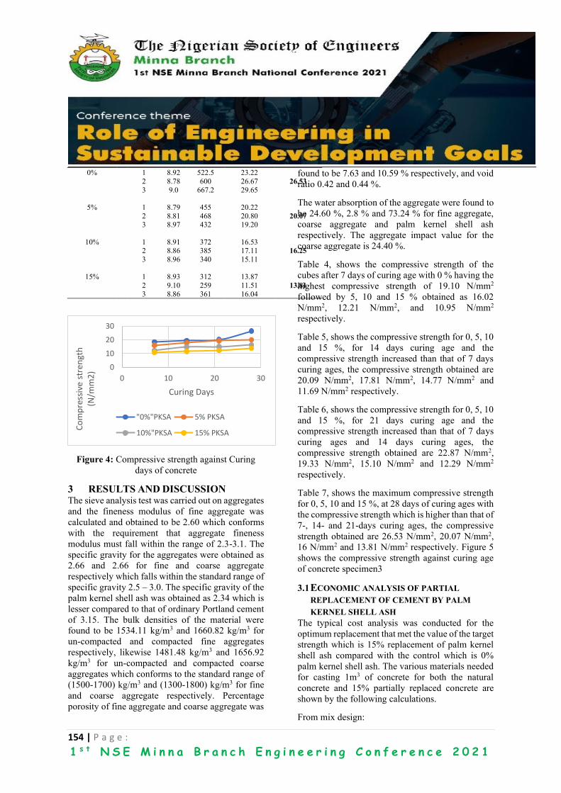
154 | P a g e :


0% 1 8.92 522.5 23.22

2 8.78 600 26.67 26.53

3 9.0 667.2 29.65

5% 1 8.79 455 20.22

2 8.81 468 20.80 20.07

3 8.97 432 19.20

10% 1 8.91 372 16.53 2 8.86 385 17.11 16.25

3 8.96 340 15.11

15% 1 8.93 312 13.87

2 9.10 259 11.51 13.81

3 8.86 361 16.04

Figure 4: Compressive strength against Curing

days of concrete

3 RESULTS AND DISCUSSION The sieve analysis test was carried out on aggregates

and the fineness modulus of fine aggregate was

calculated and obtained to be 2.60 which conforms

with the requirement that aggregate fineness

modulus must fall within the range of 2.3-3.1. The

specific gravity for the aggregates were obtained as

2.66 and 2.66 for fine and coarse aggregate

respectively which falls within the standard range of

specific gravity 2.5 – 3.0. The specific gravity of the

palm kernel shell ash was obtained as 2.34 which is

lesser compared to that of ordinary Portland cement

of 3.15. The bulk densities of the material were

found to be 1534.11 kg/m3 and 1660.82 kg/m3 for

un-compacted and compacted fine aggregates

respectively, likewise 1481.48 kg/m3 and 1656.92

kg/m3 for un-compacted and compacted coarse

aggregates which conforms to the standard range of

(1500-1700) kg/m3 and (1300-1800) kg/m3 for fine

and coarse aggregate respectively. Percentage

porosity of fine aggregate and coarse aggregate was

found to be 7.63 and 10.59 % respectively, and void

ratio 0.42 and 0.44 %.

The water absorption of the aggregate were found to

be 24.60 %, 2.8 % and 73.24 % for fine aggregate,

coarse aggregate and palm kernel shell ash

respectively. The aggregate impact value for the

coarse aggregate is 24.40 %.

Table 4, shows the compressive strength of the

cubes after 7 days of curing age with 0 % having the

highest compressive strength of 19.10 N/mm2

followed by 5, 10 and 15 % obtained as 16.02

N/mm2, 12.21 N/mm2, and 10.95 N/mm2

respectively.

Table 5, shows the compressive strength for 0, 5, 10

and 15 %, for 14 days curing age and the

compressive strength increased than that of 7 days

curing ages, the compressive strength obtained are

20.09 N/mm2, 17.81 N/mm2, 14.77 N/mm2 and

11.69 N/mm2 respectively.

Table 6, shows the compressive strength for 0, 5, 10

and 15 %, for 21 days curing age and the

compressive strength increased than that of 7 days

curing ages and 14 days curing ages, the

compressive strength obtained are 22.87 N/mm2,

19.33 N/mm2, 15.10 N/mm2 and 12.29 N/mm2

respectively.

Table 7, shows the maximum compressive strength

for 0, 5, 10 and 15 %, at 28 days of curing ages with

the compressive strength which is higher than that of

7-, 14- and 21-days curing ages, the compressive

strength obtained are 26.53 N/mm2, 20.07 N/mm2,

16 N/mm2 and 13.81 N/mm2 respectively. Figure 5

shows the compressive strength against curing age

of concrete specimen3

3.1 ECONOMIC ANALYSIS OF PARTIAL

REPLACEMENT OF CEMENT BY PALM

KERNEL SHELL ASH

The typical cost analysis was conducted for the

optimum replacement that met the value of the target

strength which is 15% replacement of palm kernel

shell ash compared with the control which is 0%

palm kernel shell ash. The various materials needed

for casting 1m3 of concrete for both the natural

concrete and 15% partially replaced concrete are

shown by the following calculations.

From mix design:

0

10

20

30

0 10 20 30

Co

mp

ress

ive

stre

ngt

h

(N/m

m2

)

Curing Days

"0%"PKSA 5% PKSA

10%"PKSA 15% PKSA

155 | P a g e :


Total material used in kg

Cement = 299.69kg per m3

Water = 179.82kg per m3

Fine aggregate = 638.34kg per m3

Coarse aggregate = 1234.72kg per m3

For Control Experiment

Volume of 1 cube mould: -0.15 × 0.15 × 0.15 =

0.003375m3

For 12 cubes: -0.003375m3 × 12 = 0.0405m3

Add 15% for compaction and wastage

100 + 15 = 115

1.15 × 0.0405m3 = 0.047m3

Calculation for the Total Materials

Cement

1m3 = 299.69kg/m3

0.047m3 = X

X = 14.09kg of cement

Sand (fine aggregate)

1m3 = 638.34kg/m3

0.047m3 = X

X = 30.00kg of sand

Gravel (coarse aggregate)

1m3 = 1234.72kg/m3

0.047m3 = X

X = 58.03kg of gravel

Water

1m3 = 179.82kg/m3

0.047m3 = X

X = 8.45kg of water

Total weight of cement needed = 299.69 × 0.047

= 14.09kg

Total weight of cement replaced by 15% PKSA = 15

100 × 14.09 =

2.11kg of PKSA

Total weight of cement - 15% PKSA = 14.09 – 2.11

= 11.98kg

Cost of 1 bag of cement 50 kg = N3700

Cost of producing 12 cubes using cement without

replacement = 14.09

50 × 3700 = N1043

Cost of producing 12 cubes using cement with 15%

PKSA replacement = 11.98

50 × 3700 = N887

Cost of saving in cost of cement = 1043 – 887

= N156

Percentage saving in cost of cement = 156

1043 × 100

= 15%.

4 CONCLUSION

From the results obtained from investigation of

sustainable development in construction industry

using palm kernel shell ash as partial replacement

for cement, the following conclusions were drawn:

1. The sustainability of this development in the

construction industry is feasible since over 70% of

the states in Nigeria cultivate and harvest oil palm

fruit so as to minimize the environmental issues

arising from the improper disposal of palm kernel

wastes.

2. The total cost required for any construction will

be greatly reduced as the use of cement with

15% PKSA replacement will reduce the cost of

cement in concrete production to 15% of the

total cost.

3. The optimum compressive strength of concrete

at 28 days curing age is 26.53 N/mm2, which is

higher than that of 7-, 14- and 21-days curing

age with their maximum compressive strength

of 19.10 N/mm2, 20.09 N/mm2, and 22.87

N/mm2 respectively.

4. Palm kernel shell ash contains all the main

constituents of cement although in varying

quantities compared to that of ordinary Portland

cement. This implies that it will be a good

replacement if the right percentage is used.

156 | P a g e :


4.1 RECOMMENDATIONS From the investigation of effect of partial

replacement of cement with palm kernel shell ash on

compressive strength of concrete, the following

recommendations are made:

1. Reduced cost of construction arising from the

use of locally available agricultural waste

materials such as palm kernel shell ash will

enhance infrastructural developments.

2. Curing of concrete with palm kernel shell ash

(PKSA) as partial replacement of cement

should reach 28 days in order to obtain

maximum compressive strength.

3. Further studies should be carried out on 0 – 50%

replacement of cement with palm kernel shell

ash in order to reveal its possibility or

otherwise.

Palm kernel shell ash (PKSA) can be used as

pozzolana in concrete production

ACKNOWLEDGEMENTS

I am totally indebted to my supervisor Engr. Dr.

T. E. Adejumo, who did not only take out time to

carry me through both in conception and the

execution process of this project work, but also

created an avenue of bringing out the hidden

potentials in me. For all the assistance, fatherly

counsels, intellectual contributions, tutoring and

constructive criticisms, I say Thank you sir, May

God Almighty reward you accordingly. I also wish

to acknowledge the contributions of other colleagues

who are not included in the authorship of this paper.

REFERENCES Adama, Y. and Jimoh, Y. A. (2011). Production and

classification of Locust Bean Pod Ash as a

pozzolana: Project Report, Civil Engineering

Portal. Retrieved from

http://www.engineeringcivil.com/production-

and-classification-of-locust-bean-pod-ash-lbpa-

as-a-pozzolana.html 23/02/2020.

American Society for Testing and Materials ASTM

C618-92a. (1994) Chemical and Physical

Specifications, 2 Parks Street, London.

American Society for Testing and Materials ASTM

C618, (2005). Specification for coal fly ash and

raw or calcined natural pozzolana for use as a

mineral admixture in Portland cement concrete.

American Society for Testing and Material,

C618-92a.

Awal, A. S. M. A., and Hussin, M. W. (2011). The

Effectiveness of Palm Oil Fuel Ash in preventing

expansion due to alkali. American Journal of

Engineering Research, pp-32-36.

Basel, N. S. and Mohammed, A. R. (2003).

Performance of Mortar and Concrete.

Construction and Building Materials, 169, pp.

800-818, 2018.

Basri, H. B., Mannan, M. A., and Zain, M. F. M.

(1999). Concrete using waste oil palm shell as

ash. Cement and Concrete Research, 29: 619-

622.

BS EN 197:1 (2000). British Standard European

Norms 197: Part 1 (2000). Cement-composition,

specifications and conformity criteria for

common cements. British Standard Institution,

London. Basri, H. B., Mannan, M. A., and Zain, M. F. M.

(1999). Concrete using waste oil palm shell as

ash. Cement and Concrete Research, 29: 619-

622.

BS 1881 Part 102 (1983). Method of determination

of slump test value of concrete, British Standard

Institute (BSI), 2 Parks Street, London.

BS 1881 Part 103 (1993). Method of determination

of compacting factor test of concrete, British

Standard Institute (BSI), 2 Parks Street, London.

BS 1881 Part 111 (1983). Method for curing of

normal concrete specimens, British Standard


BS 1881 Part 114 (1983). Method for determination

of density of hardened concrete cubes, British

Standard Institute (BSI), 2 Parks Street, London.

BS 1881 Part 116 (1983). Method for determination

of compressive strength of concrete cubes,

British Standard Institute (BSI), 2 Parks Street,

London.

BS 1881 Part 125 (1983). Method of sampling fresh

concrete in the laboratory, British Standard


BS 812 Part 103 (1985). Method of determination of

particle size distribution, British Standard



particle size distribution, British Standard



specific gravity of aggregates and absorption

test, British Standard Institute (BSI), 2 Parks

Street, London.

http://www.engineeringcivil.com/production-and-classification-of-locust-bean-pod-ash-lbpa-as-a-pozzolana.html



157 | P a g e :



moisture content of aggregates, British Standard



aggregate impact value, Construction Standard

(CS3), North Point, Hong Kong.

BS EN 197:1 (2000). British Standard European

Norms 197: Part 1 (2000). Cement-composition,

specifications and conformity criteria for

common cements. British Standard Institution,

London.

Camoes, A. and Ferreira, R. M. (2010). Structures

and Architecture. University of Mingho,

Portugal.

Chen, C., Harbert, G., Bouzidi, Y., Jullien, A.

(2010). Environmental impact of production:

Details of the different processes and cement

plant variability evaluation. Journal of cleaner

production 18, 478-485

Fadele, O. A. (2016). Compressive strength of

concrete containing palm kernel shell ash.

American Journal of Engineering Research.,

Vol-5, issue-12, pp-32-36.

Gworipalan, N., Cabrera, J., Cusens, A. R., and

Wainwright, P. J. (1992). Effect of Curing on

Durability of Concrete. ACI Compilation 24.

American Concrete Institute, Farmington Hills,

Michgan, USA, pp. 47-54.

https://www.agriculturenigeria.com/manuals/produ

ction/crop-production/general-crops/oil-palm/ >

http://www.pwc.com/ng > x-raying the Nigerian

palm oil sector.

Jackson, P. J. (1983). Building Materials and

construction. Retrieved from

https://books.google.com.ng>books 23/02/2020.

Kong, F. H. and Evans, R. H. (1994). Reinforced and

Prestressed Concrete, Chapman and Hall,

London.

Mamlouk, M. S. and Zaniewski, J. P. (2006).

Materials for Civil and Construction Engineers.

pp. 8-10.

Mannan, M. A. and Ganapathy, C. (2004). Concrete

from an Agricultural waste-oil palm shell (OPS).

Building and Environment, 39(4), pp. 441-448.

Neville, A. M and Brooks J. J (2011). Concrete

Technology, 2nd Edition, Longman.

Neville, A. M. (1996). Properties of Concrete,

ELBS 5th Edition. Pitman, London.

Neville, A. M., and Brooks, J. J. (2002). Concrete

Technology (2nd Indian reprint). Pearson

Education Limited, Singapore.

Nilson, A. H. (1980). Design of Concrete Structures.

Published by McGraw-Hill Inc. pp. 8-9

Olowe, K. O., and Adebayo, V. B. (2015).

Investigation of palm kernel ash as partial

replacement for high strength concrete.

International Journal of Civil Engineering., Vol-

2, issue-4, pp-48-50 retrieved from

www.internationaljournalssrg.org 22/02/2020.

Palm Kernel Shell p.d.f retrieved from

www.indiamart.com/impcat/pks 20/02/2020.

Price, H.W. (1951). Factors influencing concrete

strength. Journal of American Concrete institute.

Vol. 47, pp. 417-32.

Shetty, M. S. (2005). Concrete technology theory

and practice. First Multicolour Illustrative

Revised edition. Indian.

Tangchirapat, W., Jaturapitakkul, C. and

Chindaprasirt, P. (2009). Use of palm oil fuel ash

as supplementary cementitious materials for

producing high strength concrete. Construction

and Building Materials, 23(7): 2641-2646.

Tay, J. H. (1990). Ash from oil palm waste as

concrete material. Journal of Materials in Civil

Engineering, 2(2): 619-622.

Teo, D. C. L., Mannan, M. A., Kurian, V. J.,

Ganapathy, C. (2007). Light weight concrete

made from oil palm shell: Structural bond and

durability properties. Building and Environment.

42: 2614–2621.

https://www.agriculturenigeria.com/manuals/production/crop-production/general-crops/oil-palm

https://www.agriculturenigeria.com/manuals/production/crop-production/general-crops/oil-palm

http://www.pwc.com/ng

http://www.internationaljournalssrg.org/

http://www.indiamart.com/impcat/pks

158 | P a g e :


Effect of Strengthening Vertical Circular Openings with Various

Materials on the Behaviour of Reinforced Concrete Beams 1PAUL PETER MAIYAMBA and 2S.M AUTA

Department of Civil Engineering, Federal University of Technolgy,Minna.

[email protected]

ABSTRACT Opening in beam develops cracks around the region where the opening is as a result of stress concentration,

this opening causes reduction in the beam strength and load carrying capacity as well. This work presents the

effect of strengthening of vertical circular openings with various materials on the behaviour of Reinforced

rectangular Concrete beam with dimension of 200mm x230mm x700mm.The effect of strengthening of

openings was studied in terms of ultimate failure load, flexural strength and maximum deflection. It was

observed that strengthening of vertical circular opening has an increase in load capacity and strength. The solid

beam gives an average failure load of 251625N with flexural strength of 16.25N/mm2.The unstrengthen

circular opening at L/4 and L/8 distance gives an average decrease in ultimate load of 28% and 32% with

strength of 13N/mm2 and 12N/mm2 respectively. With steel plate strengthening of 4mm gauge, the ultimate

load carrying capacity of the beam increases by 15% and 17% with flexural strength of 15N/mm2 each at a

distance of L/4 and L/8 respectively as compared to beam with un strengthen opening. Using galvanize steel

pipe of 2mm thickness increases the ultimate load by 9% and 11% with flexural strength of 14N/mm2 at a

distance of L/4 and L/8 respectively. While the use of STM increases ultimate load by 3% and 5% with strength

of 13N/mm2 at a distance of L/4 and L/8 respectively.

KEYWORDS: Beam with Opening, Steel Plate, Steel Pipe, STM, Vertical Opening.

1. INTRODUCTION

Beam openings in engineering have become a daily

routine in the construction industry and this opening is

of different shapes, sizes, location and are generally

located close to the supports where shear is dominant

without considering the engineering implication as it

was not designed or planned, Lalramnghaki et, al,

(2017). In practical life beam opening is quite often use

to provide convenient passage for plumbing pipes and

ducts for water supply system, sewage and electrical

cables, but this presence of an opening in a reinforced

concrete beam leads to many problems in the beam

behaviour such as: (i) reduction in the beam stiffness;

(ii) excessive cracking; (iii) excessive deflection; and

(iv) reduction in the beam strength. Also, the presence

of openings leads to a high stress concentration at the

opening corners. The reduction in the beam stiffness as

a result of the presence of openings changes the beam

forces behaviour to a more complex one and leads to a

considerable redistribution of the internal forces,

Mansur (2006). The degree of change in the beam

cross section as a result of the presence of an opening

depends on many factors such as; shape and size of the

opening; position of the opening; and type of loading.

However, it was found that the size of opening and the

distance from the support is the most important

parameter that affects the beam behaviour, Said

(2015). With all this drawback on the beam, there is

need for solution to restore the strength of reinforced

concrete beams with openings to the original or high-

performance level. Due to this alteration of the beam

cross section caused by the presence of openings,

strengthening of such beams may be necessary.

Strengthening of beams provided with openings may

increase the ultimate load capacity of the beam, the

stiffness, and reduce deflection and cracking at the

opening corners. Those strengthening resist the

internal forces that are subjected to. The strengthened

openings were compared with their counterparts, the

un-strengthened openings. The control beam (solid)

served as a reference to assess the performance of the

test specimens with un- strengthened and the

strengthened vertical circular openings. Since in every

civil engineering work, safety is of paramount

important, Abeer (2011). Hence, this study presented a

clear understanding on the effect of various

strengthening of vertical circular openings on the

behaviour of reinforced concrete beam. The result of

this study may be beneficial to produce an efficient

strengthening of vertical circular openings. If the

concept of various strengthening of vertical circular

opening is commercially accepted, a strengthening

process can be conducted much easier with equally

satisfactory solutions.


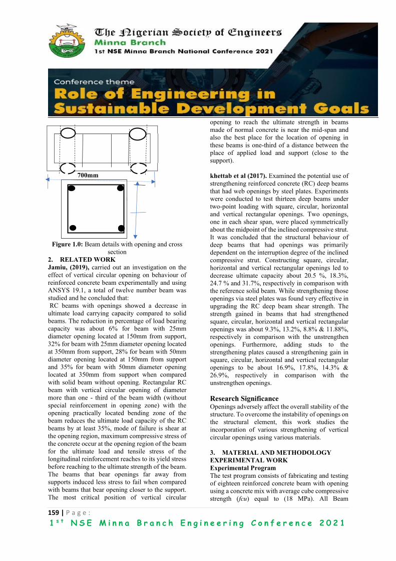
159 | P a g e :


700mm

230mm

Figure 1.0: Beam details with opening and cross

section

2. RELATED WORK

Jamiu, (2019), carried out an investigation on the

effect of vertical circular opening on behaviour of

reinforced concrete beam experimentally and using

ANSYS 19.1, a total of twelve number beam was

studied and he concluded that:

RC beams with openings showed a decrease in

ultimate load carrying capacity compared to solid

beams. The reduction in percentage of load bearing

capacity was about 6% for beam with 25mm

diameter opening located at 150mm from support,

32% for beam with 25mm diameter opening located

at 350mm from support, 28% for beam with 50mm

diameter opening located at 150mm from support

and 35% for beam with 50mm diameter opening

located at 350mm from support when compared

with solid beam without opening. Rectangular RC

beam with vertical circular opening of diameter

more than one - third of the beam width (without

special reinforcement in opening zone) with the

opening practically located bending zone of the

beam reduces the ultimate load capacity of the RC

beams by at least 35%, mode of failure is shear at

the opening region, maximum compressive stress of

the concrete occur at the opening region of the beam

for the ultimate load and tensile stress of the

longitudinal reinforcement reaches to its yield stress

before reaching to the ultimate strength of the beam.

The beams that bear openings far away from

supports induced less stress to fail when compared

with beams that bear opening closer to the support.

The most critical position of vertical circular

opening to reach the ultimate strength in beams

made of normal concrete is near the mid-span and

also the best place for the location of opening in

these beams is one-third of a distance between the

place of applied load and support (close to the

support).

khettab et al (2017). Examined the potential use of

strengthening reinforced concrete (RC) deep beams

that had web openings by steel plates. Experiments

were conducted to test thirteen deep beams under

two-point loading with square, circular, horizontal

and vertical rectangular openings. Two openings,

one in each shear span, were placed symmetrically

about the midpoint of the inclined compressive strut.

It was concluded that the structural behaviour of

deep beams that had openings was primarily

dependent on the interruption degree of the inclined

compressive strut. Constructing square, circular,

horizontal and vertical rectangular openings led to

decrease ultimate capacity about 20.5 %, 18.3%,

24.7 % and 31.7%, respectively in comparison with

the reference solid beam. While strengthening those

openings via steel plates was found very effective in

upgrading the RC deep beam shear strength. The

strength gained in beams that had strengthened

square, circular, horizontal and vertical rectangular

openings was about 9.3%, 13.2%, 8.8% & 11.88%,

respectively in comparison with the unstrengthen

openings. Furthermore, adding studs to the

strengthening plates caused a strengthening gain in

square, circular, horizontal and vertical rectangular

openings to be about 16.9%, 17.8%, 14.3% &

26.9%, respectively in comparison with the

unstrengthen openings.

Research Significance Openings adversely affect the overall stability of the

structure. To overcome the instability of openings on

the structural element, this work studies the

incorporation of various strengthening of vertical

circular openings using various materials.

3. MATERIAL AND METHODOLOGY

EXPERIMENTAL WORK

Experimental Program

The test program consists of fabricating and testing

of eighteen reinforced concrete beam with opening

using a concrete mix with average cube compressive

strength (fcu) equal to (18 MPa). All Beam

160 | P a g e :


specimens have the same dimensions (length, width

and depth) equal to (700, 200 and 230mm). The

variables investigated in this study are the type of

opening (with or without strengthening).The

specimens are divided into three groups, each of

them includes four specimens, the specimens of the

first group are with non-strengthened openings

while the specimens of second group are

strengthened, while the third are the solid with no

openings, the nineteen specimen are cast as mass

concrete without reinforcement and opening.

Materials Used Material properties

The materials used in concrete mixture were

Portland limestone cement (grade 42.5 Dangote 3x),

natural river sand, maximum aggregate size of

20mm (3/4”) with specific gravity of 2.70. The

tensile strength of concrete is typically 8%-15% of

the compressive strength and the Poisson ratio (v)

for concrete was assumed to be 0.2, (Amiri and

Masaudnia, 2011).The mix was carried out for 28

days with average cube concrete compressive

strength f (cu) =18.37N/mm2, the cubes 150mm by

150mm by 150mm were cast at the same time as the

specimen and cured alongside the concrete. The mix

design proportion of cement, fine aggregate and

coarse aggregate were (1:2:4). The water cement

ratio by weight was kept in the range of 0.50. The

longitudinal steel was high yield steel with nominal

yield strength of 400N/mm2.the stirrups was mild

steel with nominal yield strength of 240N/mm2,

Rezwana, et al (2014). The steel is assumed to be an

elastic-plastic material and identical in tension and

compression with Poisson ratio of 0.3,Timoshenko,

(1961).The main reinforcement bar was 2Ø12 at

bottom and 2Ø12 at the top with stirrups of 8mm

diameter at 200mm spacing.

Cement

Grade 42.5 Dangote Portland limestone cement

(Dangote 3x) was chosen in this work because of its

greater fineness which would have effective

hydration. The cement which conforms to BS EN,

1971 is used for making concrete. The cement was

uniform in colour, grey and was free from any hard

lumps. Table 1: Shows the properties of the cement.

Table1: Properties of Cement

S/N Characteristics Value

1 Grade cement 42.5

2 Bulk density 1507

3 Initial setting time 65mins

4 Final setting time 160mins

5 Fineness modulus 6%

Fine aggregate

Natural sand was used as fine aggregate. The sand was

sieved with sieve size 4.75mm and retained on sieve

no.0075 to get rid of coarse aggregate according to BS

EN 12620(2002). Which was free from clay or any

organic matter or chemical. It has a specific gravity of

2.57 and fineness modulus of 2.25. Moreover, sieve

analysis was also conducted on the fine aggregates, in

order to identify the gradation of the aggregates and

more so, to see if it is suitable for various civil

engineering purposes. The grading of the sand

complies with BS EN 882, zone II (1992) as shown in

Table 2: Also, physical properties of fine aggregate

are shown in Table 3:

Table 2: Grading of fine aggregate

BS Sieve

size (mm)

Passing (%)

12.7 100

9.52 100

4.75 93.8

2.36 81.1

1.18 61.1

0.60 37.6

0.30 17.1

0.15 8.7

0

20

40

60

80

100

120

0 5 10 15

% p

assi

ng

BS Sieves

161 | P a g e :


Table3: Physical properties of fine aggregate

Properties

Test

results

BS

specification

limit

Grading Zone Second ----

Fineness

Modulus

2.25 ----

Specific gravity 2.57

Materials finer

than sieve No.

200,%

2% Not greater than

5%

size Passing

4.75mm

Coarse aggregate

Coarse aggregate with 20mm nominal (3/4”) size

was used, sourced from the market, hard and clean,

free from organic impurities, free from clay and silt,

free from oil coating. The grading of the coarse

aggregate complies with the British standard. The

preliminary tests such as Aggregate Crushing Value

(ACV), Aggregate Impact Value (AIV) and particle

size distribution of aggregates were carried out prior

to concrete making specify by requirements of

British Standards Institution. The grading coarse and

particle size curve are shown in table 4 and table 5

Table 4: Grading of coarse aggregate

Sieve

size

(mm)

Passing (%)

50 100

37.5 100

19.05 90.2

9.52 9.5

4.76 1.2

Table 5: Physical properties of coarse aggregate

Properties Test

Results

BS EN

Specification

Limits

(2002)

Specific

Gravity

2.70 ----

Bulk

Density

1650

kg/m3

----

ACV 26 23-30

AIV 17 17-21

Materials

Finer

Than

Sieve No.

200,%

3% Not Greater

Than 3%

Mixing Water

Ordinary tap water was used for casting and curing

all the specimens which was obtained from the

teaching hospital construction site at Baze

University, Abuja. According to the Nigerian

Industrial Standard (NIS 87, 2004) water play a

major role in the strength and workability of

concrete when properly used as the water to cement

ratio. The water used for mixing and curing was

clean, tasteless and odourless and free from injurious

amounts of oils, acids, alkali, salts, sugar, organic

material or other substances that may be deleterious

to concrete or steel.

Materials Used for Strengthening Openings

Steel plates and steel pipe (galvanize GI Pipe) of

4mm and 2mm thickness were used for

strengthening the opening regions, these materials

were used to strengthened the concrete that was

removed due to the construction of the openings,

shear connectors were welded to the materials for

proper bonding and anchorage between the concrete,

also 8mm diameter bar was used to fabricate the

STM specimen used to strengthen the opening

region. The strengthening materials were placed in

the reinforcement cage into the formwork before

concreting the beam.

Plate 1: materials used for strengthening the

openings

Casting of Beam and Cubes specimen

The beam mould is fabricated with steel with

dimension of 200mm x 230mm x 700mm while the

mould of 150mm x 150mm x150mm size was used

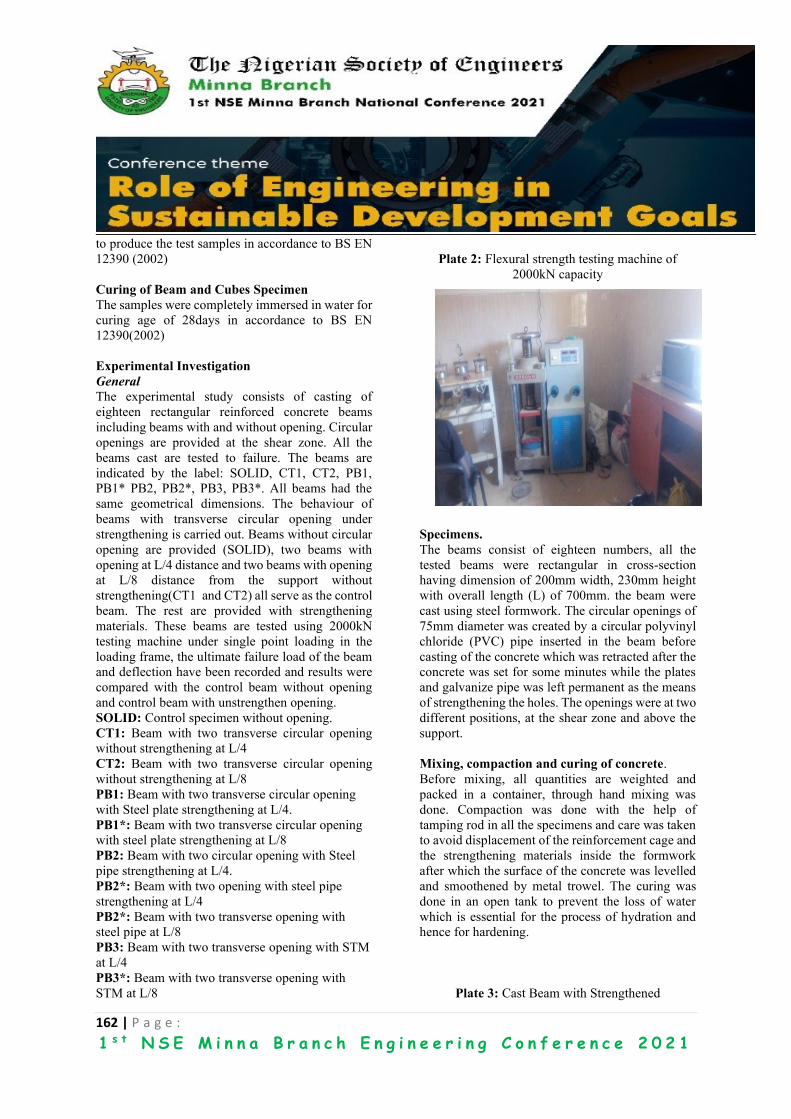
162 | P a g e :


to produce the test samples in accordance to BS EN

12390 (2002)

Curing of Beam and Cubes Specimen

The samples were completely immersed in water for

curing age of 28days in accordance to BS EN

12390(2002)

Experimental Investigation

General

The experimental study consists of casting of

eighteen rectangular reinforced concrete beams

including beams with and without opening. Circular

openings are provided at the shear zone. All the

beams cast are tested to failure. The beams are

indicated by the label: SOLID, CT1, CT2, PB1,

PB1* PB2, PB2*, PB3, PB3*. All beams had the

same geometrical dimensions. The behaviour of

beams with transverse circular opening under

strengthening is carried out. Beams without circular

opening are provided (SOLID), two beams with

opening at L/4 distance and two beams with opening

at L/8 distance from the support without

strengthening(CT1 and CT2) all serve as the control

beam. The rest are provided with strengthening

materials. These beams are tested using 2000kN

testing machine under single point loading in the

loading frame, the ultimate failure load of the beam

and deflection have been recorded and results were

compared with the control beam without opening

and control beam with unstrengthen opening.

SOLID: Control specimen without opening.

CT1: Beam with two transverse circular opening

without strengthening at L/4

CT2: Beam with two transverse circular opening

without strengthening at L/8

PB1: Beam with two transverse circular opening

with Steel plate strengthening at L/4.

PB1*: Beam with two transverse circular opening

with steel plate strengthening at L/8

PB2: Beam with two circular opening with Steel

pipe strengthening at L/4.

PB2*: Beam with two opening with steel pipe

strengthening at L/4

PB2*: Beam with two transverse opening with

steel pipe at L/8

PB3: Beam with two transverse opening with STM

at L/4

PB3*: Beam with two transverse opening with

STM at L/8

Plate 2: Flexural strength testing machine of

2000kN capacity

Specimens.

The beams consist of eighteen numbers, all the

tested beams were rectangular in cross-section

having dimension of 200mm width, 230mm height

with overall length (L) of 700mm. the beam were

cast using steel formwork. The circular openings of

75mm diameter was created by a circular polyvinyl

chloride (PVC) pipe inserted in the beam before

casting of the concrete which was retracted after the

concrete was set for some minutes while the plates

and galvanize pipe was left permanent as the means

of strengthening the holes. The openings were at two

different positions, at the shear zone and above the

support.

Mixing, compaction and curing of concrete.

Before mixing, all quantities are weighted and

packed in a container, through hand mixing was

done. Compaction was done with the help of

tamping rod in all the specimens and care was taken

to avoid displacement of the reinforcement cage and

the strengthening materials inside the formwork

after which the surface of the concrete was levelled

and smoothened by metal trowel. The curing was

done in an open tank to prevent the loss of water

which is essential for the process of hydration and

hence for hardening.

Plate 3: Cast Beam with Strengthened

163 | P a g e :


Openings

Plate 4: Curing of Beam Specimen

Test Setup

The beams were tested 28days after the casting to

investigate the effects of the strengthened openings

on the flexural behaviour of the concrete beam using

an academic Testing Machine of 2000kN maximum

capacity. All the specimens were tested for flexural

strength under single point flexural load. The

specimens were arranged with simply supported

conditions. Loads were applied digitally till the

ultimate failure of the specimens occurred.

Plate 5: Experimental Setup

4. RESULT AND DISCUSSION

Engineering Properties of the Hardened

Concrete (Compressive Strength Test)

For the purpose of determining the strength of the

concrete produced in this study, concrete cubes were

cast and compressive strength test was carried out on

the cast cubes. The tabulated result for the

compressive strength test is given in table 6. The

compressive strength test of the specimen is 18Mpa

or 18 N/mm2

Table 6: Compressive Strength Test

speci

men

weig

ht

(kg)

ultim

ate

failur

e load

(kN)

compres

sive

strength

N/mm2

average

compres

sive

strength

(N/mm2)

C1 8.01 387.2

1

17.21

C2 8.04

2

461.9

2

20.53 18.42

C3 8.21

2

389.4

1

17.37

From the sieve analysis test conducted on the fine

aggregate, the fineness modulus of the fine

aggregate which was obtained as the ratio of the sum

of the cumulative percentage retained on the

standard sieve set and an arbitrary number (in this

study 100) is 3.01. This implies that the fine

aggregate can be said to be a coarse sand and since

the fine modulus obtained in this study is lower that

the limiting value of 3.2, the fine aggregate can be

said to be fit for use in concrete production

(Mamlouk and Zaniewski 2006).

164 | P a g e :


Figure 2: Particle size distribution curve for coarse

aggregate

Figure 3: Particle size distribution for fine

aggregate

Table 7. Result of Flexural Strength Obtained

Beam

Specimen

Distance

of

Opening

from

Support

Ultimate

Failure

Load(Pu)

kN

Maximum

deflection

(mm)

Flexural

Strength

(Fs)

N/mm2

SOLID 251.625 0.443 16.25

CT1 L/4 196.96 0.347 13.03

CT2 L/8 190.84 0.336 12.62

PB1 L/4 232.31 0.409 15.37

PB1* L/8 228.92 0.403 15.15

PB2 L/4 217.21 0.383 14.37

PB2* L/8 214.74 0.378 14.18

PB3 L/4 201.86 0.336 13.36

PB3* L/8 200.17 0.352 13.24

M.C 88.06 0.155 5.83

Figure 4: Ultimate Load Graph of the Control

Beams

Testing beams CT1@L/4 and CT2@L/8 (Control)

revealed the behaviour of un-strengthened beams

with openings in comparison to that of a solid beam

without opening. Figure 4 shows the effect of

vertical circular opening on the beam load carrying

capacity, the ultimate bearing capacity of CT1@L/4

and CT2@L/8 decreases by 28% and 32% as a result

of the unstrengthen opening of diameter 75mm as

compared to the solid beam without opening which

has an average ultimate failure load of 251625N.

This openings on the beam reduces the ultimate load

capacity of the member.

0

20

40

60

80

100

120

1 10

% P

ASS

ING

PARTICLE SIZES

C.Agg

Min

Max

0

20

40

60

80

100

120

0.1 1 10

% P

ASS

ING

PARTICLE SIZES

F.Agg

Min

Max

0

50

100

150

200

250

300

SOLID CT1@L/4 CT2@L/8ULT

IMA

TE F

AIL

UR

E LO

AD

(KN

)

BEAM SPECIMEN

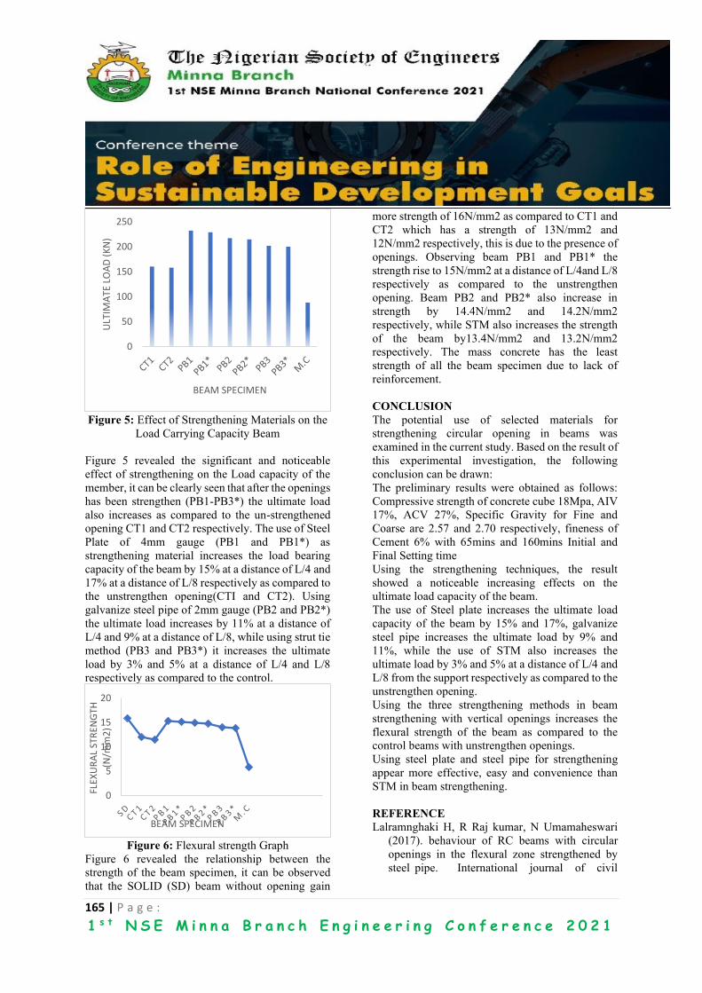
165 | P a g e :


Figure 5: Effect of Strengthening Materials on the

Load Carrying Capacity Beam

Figure 5 revealed the significant and noticeable

effect of strengthening on the Load capacity of the

member, it can be clearly seen that after the openings

has been strengthen (PB1-PB3*) the ultimate load

also increases as compared to the un-strengthened

opening CT1 and CT2 respectively. The use of Steel

Plate of 4mm gauge (PB1 and PB1*) as

strengthening material increases the load bearing

capacity of the beam by 15% at a distance of L/4 and

17% at a distance of L/8 respectively as compared to

the unstrengthen opening(CTI and CT2). Using

galvanize steel pipe of 2mm gauge (PB2 and PB2*)

the ultimate load increases by 11% at a distance of

L/4 and 9% at a distance of L/8, while using strut tie

method (PB3 and PB3*) it increases the ultimate

load by 3% and 5% at a distance of L/4 and L/8

respectively as compared to the control.

Figure 6: Flexural strength Graph

Figure 6 revealed the relationship between the

strength of the beam specimen, it can be observed

that the SOLID (SD) beam without opening gain

more strength of 16N/mm2 as compared to CT1 and

CT2 which has a strength of 13N/mm2 and

12N/mm2 respectively, this is due to the presence of

openings. Observing beam PB1 and PB1* the

strength rise to 15N/mm2 at a distance of L/4and L/8

respectively as compared to the unstrengthen

opening. Beam PB2 and PB2* also increase in

strength by 14.4N/mm2 and 14.2N/mm2

respectively, while STM also increases the strength

of the beam by13.4N/mm2 and 13.2N/mm2

respectively. The mass concrete has the least

strength of all the beam specimen due to lack of

reinforcement.

CONCLUSION

The potential use of selected materials for

strengthening circular opening in beams was

examined in the current study. Based on the result of

this experimental investigation, the following

conclusion can be drawn:

The preliminary results were obtained as follows:

Compressive strength of concrete cube 18Mpa, AIV

17%, ACV 27%, Specific Gravity for Fine and

Coarse are 2.57 and 2.70 respectively, fineness of

Cement 6% with 65mins and 160mins Initial and

Final Setting time

Using the strengthening techniques, the result

showed a noticeable increasing effects on the

ultimate load capacity of the beam.

The use of Steel plate increases the ultimate load

capacity of the beam by 15% and 17%, galvanize

steel pipe increases the ultimate load by 9% and

11%, while the use of STM also increases the

ultimate load by 3% and 5% at a distance of L/4 and

L/8 from the support respectively as compared to the

unstrengthen opening.

Using the three strengthening methods in beam

strengthening with vertical openings increases the

flexural strength of the beam as compared to the

control beams with unstrengthen openings.

Using steel plate and steel pipe for strengthening

appear more effective, easy and convenience than

STM in beam strengthening.

REFERENCE

Lalramnghaki H, R Raj kumar, N Umamaheswari

(2017). behaviour of RC beams with circular

openings in the flexural zone strengthened by

steel pipe. International journal of civil

0

50

100

150

200

250

ULT

IMA

TE L

OA

D (

KN

)

BEAM SPECIMEN

0

5

10

15

20

FLEX

UR

AL

STR

ENG

TH

(N/m

m2

)

BEAM SPECIMEN

166 | P a g e :


engineering and technology (IJCIET) 8 (5)

303-309.

M .A Mansur, (2006) “Design of reinforced concrete

beams with Web openings”, Proceeding of the

6th Asia-Pacific Structural Engineering

and Construction Conference (APSEC 2006),

Vol. A, pp.104 – 120.

Said M Allam (2015). strengthening of RC beams

with large openings in shear zone.

Alexanderia engineering journal 44(1) 59-78.

Oladipo Jamiu, (2019) ‘Effect of vertical circular

openings on the behaviour of reinforced

concrete beam, master research thesis,

Federal University of Technology,

Minna

Soroush Amiri, Reza Masoudnia (2011) effects of

openings on concrete beams without

additional reinforcement in opening region

using FEM method. Australian journal of

basic and applied science 5(5) 617-627.

Rezwana Binte Hafiz, S Ahmed, S Barua

.(2014).effects of openings on the

behaviour of RC beams.IOSR journal of

mechanical and civil engineering 2(2),

52-61.

Khattab Saleem,H Ali, M M Abdul-kareem (2017)

a new strengthening techniques for

deep beam with openings using steel

plates.International journal of applied

engineering research.12 (24) 15935- 15947.

Timoshenko, S. P.; Gere, J. M. 1997. Theory of

elastic stability. 2nd ed. McGraw-Hill.

Mamlouk, M. S. and Zaniewski, J. P. (2006).

Materials for Ciivil and Constructi Engineers.

London: Pearson Education, Inc

British Standards Institution, BS EN 1971: Cement

part 1 composition, specification

and conformity criteria for common

concretes. BS, London, UK 2002.

British Standards Institution, BS EN 12390 2002:

Testing Aggregates of hardened

concrete part 2: making and curing

specification. British Standards Institution,

London, UK 2002.

British Standards Institution, BS EN 882 1992.

Specification for aggregate from natural

sources for concrete. British Standards

Institution, London.UK 1992.

167 | P a g e :


Opportunities for Engineers in the Solar Energy Value Chain Mahmud, J. O., *Mustapha, S. A.

1NASENI Solar Energy Limited, Karshi, Abuja, *[email protected]

ABSTRACT The Nigerian electricity poverty is high due to its rising population leading to high electricity demand. Despite

evidence that Solar Energy technology is one of the most viable solutions to the electricity poverty, the

professionals have taken the back seat. Bad user experiences rife creating barriers to the adoption of technology

due to the proliferation of non-professionals in the industry. This paper therefore calls for the need for Nigerian

professionals to rise up to the occasion by taking charge of the different sectors in the solar energy value chain.

A literature review was done to establish the diverse prospects and opportunities that abound for professionals

in the industry. It is therefore established that the growing demand for energy has opened up opportunities for

Nigerian professionals in the solar energy value chain such as: manufacturing, training, research and

development some of which have been taken over by non-professionals. This work shows that when indigenous

professionals take charge of the industry, the quality of products and services delivered will significantly

improve access to quality electricity. More research works are required on ways to ensure sustainable energy

for all.

KEYWORDS: Productivity, Quality Electricity, Solar Energy, Solar PV, Value Chain.

1 INTRODUCTION At an average annual growth of 2.6%, the

Nigerian population is growing fast. As at the year

2020, the country’s population has been estimated to

be 210 million people as shown in figure 1

(Worldometer, 2020). Nigeria is adjudged as the

most populous black nation in the world with a

forecast that it will become the third most populous

nation by the year 2050 trailing India and China as

depicted in Figure 2 (Roberts, 2011; United

Nations, 2019). As there is continuous rise in

population, so are the socio-economic activities of

the citizens with attendant increase in energy

demand (Olatomiwa, Mekhilef, Huda, & Ohunakin,

2015).

Figure 1: Year 2020 estimated population for

Nigeria (Worldometer, 2020)

Figure 2: Estimated world population towards

2050 (Roberts, 2011; Mahmud, 2020)

The pervasive nature of the electricity poverty in

Nigeria has given a huge opportunity for Renewable

Energy (RE) practitioners and other stakeholders to

take advantage of its deployment in the different

sector. RE has been gaining attentions in Nigeria,

although with some barriers, in divers’ areas of

applications especially in electricity generation for

residential homes and small businesses (Akinyele, et

al., 2019). Sadly, the deployment of RE technologies

is still in its nascent stage in Nigeria despite its

abundance. Some of the RE technologies available

are: Hydro, Solar Photovoltaic (PV) and Solar


168 | P a g e :


Thermal, Wind, Tidal Energy, Geothermal,

Biomass, and Solar Hydrogen (National Renewable

Energy Laboratory, 2001; Johansson, Kelly, Reddy,

& Williams, 1993). Solar PV technology has

witnessed a great deal of worldwide acceptance and

applications in on-grid and off-grid power systems

(Yusuf, Ibikunle, Oluwatosin, & Adeyemi, 2014).

Solar PV has achieved this feat due to its continual

decline in the cost of Solar PV modules as well as

the ease at which its installation is carried as

compared to other technologies (Akinyele, Rayudu,

K., & Nair, 2015). However, numerous barriers are

affecting the effective adoption of RE in Nigeria.

The rise in solar power system failures resulting to

bad experiences of users have made many

researchers to identify some of the causes such as:

lack of adequate technical know-how and

proliferation of substandard solar PV materials

among others as some of the barriers mitigating the

adoption of solar PV technology despites its

numerous motivating factors (Habib, Idris, Ladan, &

Mohammad, 2012).

With the huge potential of the availability of

constant and sustainable electricity salvaging the

already weakened Nigerian socio-economic

activities, there is need for more research on how to

get the solar energy sector improved through

adequate knowledge sharing among professionals in

the industry. Hence, this led to the motivation for

this study.

Therefore, this paper presents an overview of

different opportunities that abound in the value

chain for indigenous professionals in order to

salvage the industry for the benefit of Nigeria and its

citizens. The rest of this paper presents the Nigeria’s

energy sector, Renewable energy sources, Solar PV

value chain and opportunities for Engineers,

Motivating features of Solar PV technology,

Barriers to the adoption of Solar PV technology and

Conclusion.

2 LITERATURE REVIEW Some related literatures were reviewed in order

to drive home the point that there are numerous

opportunities for indigenous Engineers in the solar

PV value chain.

2.1 NIGERIA’S POWER SECTOR AND

SOLAR ENERGY Electricity is a very vital component for the

development of socio-economic and technological

activity of a nation. It is a fact that the electricity

demand in Nigeria far outweighs the supply causing

it to be epileptic and consequently inhibiting the

nation’s development (Sambo, 2008). Over the

years, Nigeria has been very optimistic to solve the

electricity challenge for the country which led to the

drafting of various policies and strategies to achieve

adequate and sustainable electricity for all. In line of

this, some research-based projections were carried

out which provided analysis of possible energy

demand and supply matching by the year 2030 as

shown in Figures 3 & 4 respectively. According to

Sambo (2008), at a gross domestic product (GDP)

growth rate of 13%, the nation’s electricity demand

will increase to 297,900MW at 11,686MW/year

addition in supply. Sadly, the Nigerian economy’s

GDP grew at only 0.51% in the first quarter of 2021

following its recent way out of recession (National

Bureau of Statistics, 2021). This however has shown

the continual rise in the electricity demand with

urgent need for a corresponding supply. The

Nigerian Government has also perceived solar

energy as a key parameter to solving the economic

crisis it faces. Its economic recovery growth plan

(ERGP) policy document highlighted the strategic

adoption of the power sector to save the nation’s

economy with solar energy as a key component in

the energy mix. The objectives ERGP on the power

sector is as follows (Ministry of Budget and National

Planning, 2017; Central Bank of Nigeria, 2016):

i. Improve energy efficiency and diversify the

energy mix, including greater use of renewable

energy.

ii. Facilitate private sector investment in

generation, transmission and distribution

iii. Increase rural electrification through the use of

off-grid renewable solutions

iv. Improve access to electricity to all Nigerians

v. Implement a data-driven approach in power

sector development planning

vi. Restore financial viability in the electricity

market

169 | P a g e :


In line with the ERGP, in 2016, the Nigerian

Electricity Regulatory Commission (NERC)

approved a regulation targeted at Mini-grid aimed at

allowing private electricity companies to generate

electricity not more than 1MW to unserved and

underserved Nigerian communities (Kemabonta &

Kabalan, 2018; Nigerian Electricity Regulatory

Commission, 2016). This was aimed at achieving an

electricity generating capacity of 10GW by the year

2020 through effective utilization of renewable

energy in the energy mix (Ministry of Budget and

National Planning, 2017; Kemabonta & Kabalan,

2018; Adebayo, 2017).

Figure 3: Nigeria’s electricity demand projection

(Sambo, 2008)

Figure 3: Nigeria’s electricity supply projection

(Sambo, 2008)

2.2 SOLAR PHOTOVOLTAIC (PV) The sun is prominently the primary source of

energy in the universe. It continuously sheds its

mass through the radiation of electromagnetic waves

in the form of light and high energy spatial particles

(Cander, 2019). With Nigeria’s geographical

location, it has been opined by researchers that the

best form of alternative source of energy in terms of

RE is Solar Energy (Akuru & Animalu, 2009). Solar

PV technology converts the light from the sun

directly into electricity. This technology has found

use in many applications such as for powering rural

and urban located homes, small electronics, space

vehicles and agriculture. The market for Solar

electricity is expanding globally due the continuous

advancement in the technology which makes it to be

deployed for both on-grid and off-grid connection of

homes. Despite the various types of Solar PV

systems available, there are three basic components

they all have in common which are:

i. Solar PV module: it converts the light from

the sun directly into electricity.

ii. Inverter: this transforms the direct current

(DC) from the Solar PV module into

alternating current (AC) for easy use by

many domestic appliances.

iii. Batteries: used as a storage facility for

excess electricity by the system.

Some components that may also be included

are: charge controller, circuit breakers, wiring and

support structure.

2.3 MOTIVATING FEATURES OF SOLAR

PV TECHNOLOGY There are different features of Solar PV

technology that is making users and potential users

to adopt the technology. This is presented hereunder

(Olatomiwa, Mekhilef, Huda, & Ohunakin, 2015;

Ugulu, 2019):

i. Power Stability: the feature of Solar PV

technology is described as the most admiring for

its adoption in Nigeria. This is because the

reliability enjoyed from the solar PV technology

is lacking from the national grid.

170 | P a g e :


ii. Cost Saving: the cheapness of the technology in

the long run is another motivating feature for the

adoption of solar PV technology.

iii. Familiarity: awareness level is increasing. This

is because potential users are developing interest

in the technology as an alternative to the failing

national grid.

iv. Convenience: the comfort derived from the

usage of the technology is very inviting

compared to fossil fuel powered generators.

Unlike fossil fuel powered generators that

requires constant maintenance, noise pollution

and rigorous operation, solar PV technology is

easier to use.

2.4 BARRIERS TO THE ADOPTION OF

SOLAR PV TECHNOLOGY Despite the inviting features of the technology,

some other factors have been creating barriers for its

adoption. These are presented hereunder (Yaqoot, P.

Diwan, & Kandpal, 2016; Ozoegwu, Mgbemene, &

Ozor, 2017; Akinyele, et al., 2019; Ugulu, 2019):

i. High initial cost of installation: the

seriously high cost of installing Solar PV

power system is said to be impeding the use

of solar technology in Nigeria.

ii. Proliferation of substandard products:

the seemingly uncontrolled proliferation of

inferior Solar PV products and materials

leading to high rate of failures is causing

potential users to backtrack on their

decision of adopting the technology.

iii. Inadequate awareness: it is observed that

many intending users of the technology do

not have adequate knowledge about solar

PV technology. This creates fear for them

because they are not sure solar works.

iv. Inadequate technical know-how: another

factor that is barring intending users of

solar PV technology is the incompetence of

the system installers. This is due to the high

rate of incompetent service providers in the

industry.

3 SOLAR PV VALUE CHAIN AND

OPPORTUNITIES FOR ENGINEERS The value chain of solar PV as shown in Figure

3 depicts the different areas of possible intervention

and investment by the professionals in the solar PV

industry. The value chain comprises of the areas of

research and development which leads to the

manufacturing of different types of solar PV

materials and modules. It also covers innovative

areas where solar PV solutions can be applied.

Included in the value chain are: Power Service

provision; Operation, Maintenance and Training as

well as recycling management. These areas are

critical areas in the value chain that Engineers can

explore for Nigeria to achieve sustainable and clean

electricity for all.

Figure 3: Solar PV Value Chain (Mahmud, 2019;

Udayakumar, Anushree, & Manjunathan, 2019)

3.1 RESEARCH AND DEVELOPMENT All over the world, the solar PV technology

industry thrives as a result of intensive research

outputs. The outputs are a result of: good data

collection and analysis, discovery of available

materials for the production of solar cells, cost

analysis, efficiency improvements and

environmental impacts (Tyagi, Rahiml, Rahim, &

Selvaraj, 2013). Apart from data collection, one of

the key areas that require further research works is

in the indigenous discovery of already known solar

cell materials or technologies as in Figure 4 or

locally available materials that can be their

substitutes. The exploration the research and

development sector of the value chain by indigenous

Engineers is direly needed as there is still dearth of

Research and

Development

Manufacturing

of solar PV

materials &

modules

Areas of

Application

Power Service

providers

Operation,

Maintenance

and Training

End of Life

Management and

Decommissioning

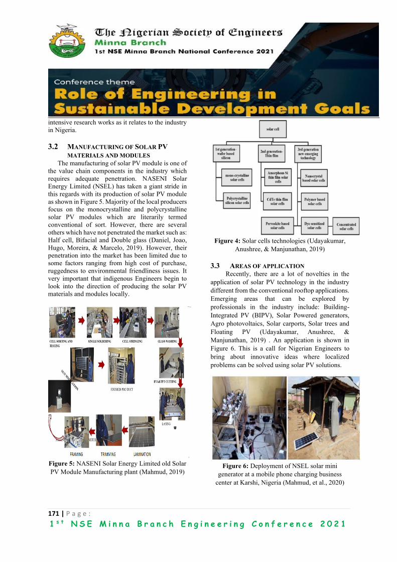
171 | P a g e :


intensive research works as it relates to the industry

in Nigeria.

3.2 MANUFACTURING OF SOLAR PV

MATERIALS AND MODULES The manufacturing of solar PV module is one of

the value chain components in the industry which

requires adequate penetration. NASENI Solar

Energy Limited (NSEL) has taken a giant stride in

this regards with its production of solar PV module

as shown in Figure 5. Majority of the local producers

focus on the monocrystalline and polycrystalline

solar PV modules which are literarily termed

conventional of sort. However, there are several

others which have not penetrated the market such as:

Half cell, Bifacial and Double glass (Daniel, Joao,

Hugo, Moreira, & Marcelo, 2019). However, their

penetration into the market has been limited due to

some factors ranging from high cost of purchase,

ruggedness to environmental friendliness issues. It

very important that indigenous Engineers begin to

look into the direction of producing the solar PV

materials and modules locally.

Figure 5: NASENI Solar Energy Limited old Solar

PV Module Manufacturing plant (Mahmud, 2019)

Figure 4: Solar cells technologies (Udayakumar,

Anushree, & Manjunathan, 2019)

3.3 AREAS OF APPLICATION Recently, there are a lot of novelties in the

application of solar PV technology in the industry

different from the conventional rooftop applications.

Emerging areas that can be explored by

professionals in the industry include: Building-

Integrated PV (BIPV), Solar Powered generators,

Agro photovoltaics, Solar carports, Solar trees and

Floating PV (Udayakumar, Anushree, &

Manjunathan, 2019) . An application is shown in

Figure 6. This is a call for Nigerian Engineers to

bring about innovative ideas where localized

problems can be solved using solar PV solutions.

Figure 6: Deployment of NSEL solar mini

generator at a mobile phone charging business

center at Karshi, Nigeria (Mahmud, et al., 2020)

172 | P a g e :


3.4 POWER SERVICE PROVIDERS The solar PV power industry has so far proven

to be real alternative to the overwhelmed centralized

national grid. This informs the need for the

professional players in the industry to take

advantage of the NERC 2016 policy to set up

independent solar power projects, solar PV power

generating companies, off grid rural electrification

to adequately compensate for the electricity shortfall

from the national grid (Mahmud, 2019).

3.5 OPERATION, MAINTENANCE AND

TRAINING As the market for solar PV is growing, more

expertise are required to continue to improve on the

life expectancy of solar PV modules and the balance

of systems (BoS) via effective operation and

maintenance (O&M). Some of the areas in the O&M

are intelligent monitoring of solar PV modules and

BoS and their outputs using smart data collection

techniques, advanced cooling techniques, drones,

output forecasting and the likes (Udayakumar,

Anushree, & Manjunathan, 2019). There is also the

continuous training component that is direly

required for personnel in the industry (Mahmud &

Mustapha, 2020).

3.6 END OF LIFE MATERIALS RECYCLING The global acceptance and usage of solar PV

modules has equally increased the potential increase

of its waste by the end of its life span. It was

projected that just by the end of the year 2030, the

cumulative waste from solar PV module will amount

to 2 million tones which is expected to be tripled by

2048 (Sica, Malandrino, Supino, Testa, & Lucchetti,

2018). It is therefore pertinent that effective ways of

disposing the solar PV module wastes as in Figure 7

be adopted while new ways be discovered in order

to save the environment. The recycling processes are

opportunities to be explored by Nigerian

Engineering professionals in the value chain.

Figure 7: End of Life process of solar PV modules

(Sukmin, Sungyeol, Jina, Bonghyun, & Hojin,

2012)

4 CONCLUSION

The solar PV industry in Nigeria is growing and

the technologies are becoming accepted. However,

non-professionals have taken a larger stake in the

industry leading to the incessant bad experiences by

unsuspecting users. In this regards, it is very

important to bring forth the numerous opportunities

and areas in the solar PV value chain that Nigerian

Engineering professionals can gain and also utilize

their expertise in order to salvage the situation. This

paper therefore highlighted the different areas in the

value chain as well as the motivating factors and

barriers to the adoption of solar PV. This work is

expected to charge up the professionals to take

charge of the Nigerian solar PV industry.

REFERENCES Adebayo, H. (2017). Nigeria launches Economic

recovery plan; targets 10GW, Food Security.

Abuja: Premium Times.

Akinyele, D. O., Rayudu, K., R., & Nair, N. K.

(2015). Development of Photovoltaic Power

Plant for Remote Residential Applications: The

Socio-Technical and Economic Perspectives.

Renewable Sustainable Energy Revolution , 112-

139.

173 | P a g e :


Akinyele, D., Babatunde, O., Monyei, C.,

Olatomiwa, L., Okediji, A., Ighraywe, D., . . .

Temikotan, K. (2019). Possibility of Solar

Thermal Power Generation Technologies in

Nigeria: Challenges and Policy Directions.

Renewable Energy, 24-41.

Akuru, U. B., & Animalu, A. O. (2009). Alternative

Means of Energy Sector Investments in Nigeria.

Proceedings of the First International Seminar

on Theoretical Physics and National

Development, (pp. 173-183).

Cander, L. R. (2019). Solar-Terrestrial Interactions

in Ionospheric Space Weather. Springer

Geophysics, 1-297.

Central Bank of Nigeria. (2016). Annual Report

2016. Abuja: Central Bank of Nigeria.

Daniel, d. B., Joao, L. d., Hugo, S., Moreira, M., &

Marcelo, G. V. (2019). A review and analysis of

technologies applied in PV modules. IEEE PES

Innovative Smart Grid Technologies.

Habib, S. L., Idris, N. A., Ladan, M. J., &

Mohammad, A. G. (2012). “Unlocking Nigeria’s

Solar PV and CSP Potentials for Sustainable

Electricity Development. International Journal

for Science & Engineering Research, 2229-5518.

Johansson, T. B., Kelly, H., Reddy, A. K., &

Williams, R. H. (1993). Renewable Energy:

Sources for Fuels and Electricity. United States.

Kemabonta, T., & Kabalan, M. (2018). Using what

you have, to get what you want – a different

approach to electricity market design for local

distribution companies (DISCOs) in Nigeria.

IEEE Global Humanitarian Technology

Conference, (pp. 1-2).

Mahmud. (2019, October 15). Renewable Energy-

Boosting Generation Capacity Towards Agro

Community Commercial Farming Sustainability.

Nigerian Alternative Energy Expo 2019. Abuja:

Nigerian Alternative Energy.

Mahmud, J. O. (2020). Improving Agro Community

Commercial Farming Sustainability through

Deployment of Renewable Energy. 11th

INTERNATIONAL CONFERENCE ON

ENERGY AND POWER SYSTEMS OPERATION

AND PLANNING (ICEPSOP 2020), (pp. 116-

119). Abuja.

Mahmud, J. O., & Mustapha, S. A. (2020).

DEVELOPING INDIGENOUS

INFRASTRUCTURE FOR LOCAL

CAPACITY IN SOLAR ENERGY. National

Solar Energy Forum (NASEF 2020) (p. 35).

Sokoto: Solar Energy Society of Nigeria.

Mahmud, J. O., A. O. Nduka, A. O., Acholoson, P.

O., Ongbabo, E., Mustapha, S. A., & Akai, Y.

(2020). Deployment of Solar Photovoltaic Mini

Generators for Small Scale Businesses. 11th

INTERNATIONAL CONFERENCE ON

ENERGY AND POWER SYSTEMS OPERATION

AND PLANNING (ICEPSOP 2020) (pp. 116-

119). Abuja: International Conference on Energy

and Power Systems Operation and Planning

(ICEPSOP).

Ministry of Budget and National Planning. (2017).

Economic Recovery and Growth Plan 2017 -

2020. Abuja: Federal Republic of Nigeria.

National Bureau of Statistics. (2021). National

Bureau of Statistics. Retrieved from

https://www.nigerianstat.gov.ng/

National Renewable Energy Laboratory. (2001).

Renewable Energy: An Overview. Energy

Efficiency and Renewable Energy Clearing

House, 1-8.

Nigerian Electricity Regulatory Commission.

(2016). Nigerian Electricity Regulatory

Commission Mini-Grid Regulation, 2016. Abuja:

NERC.

Olatomiwa, L., Mekhilef, S., Huda, A. S., &

Ohunakin, O. S. (2015). Economic Evaluation of

Hybrid Energy Systems for Rural Electrification

in Six Geo-Political Zones of Nigeria.

Renewable Energy, 435-446.

Ozoegwu, C. G., Mgbemene, C. A., & Ozor, P. A.

(2017). The Status of Solar Energy Integration

and Policy in Nigeria. Renewable and

Sustainable Energy Reviews, 457-471.

Roberts, L. (2011). 9 Billion? AAAS, 540-543.

Sambo, A. S. (2008). Matching Electricity Supply

with Demand in Nigeria. International

Association for Energy Economics.

Sica, D., Malandrino, O., Supino, S., Testa, M., &

Lucchetti, M. C. (2018). Management of endof-

life photovoltaic panels as a step towards a

174 | P a g e :


circular economy. REnew. Sustain. Energy Rev.,

2934-2945.

Sukmin, K., Sungyeol, Y., Jina, L., Bonghyun, B., &

Hojin, R. (2012). Experimental investigations for

recycling of silicon and glass from waste

photovoltaic Modules. Renewable Energy, 152-

159.

Tyagi, V. V., Rahiml, N. A., Rahim, N. A., &

Selvaraj, J. A. (2013). Progress in solar PV

technology: Research and achievement.

Renewable and Sustainable Energy Reviews,

433-461.

Udayakumar, M. D., Anushree, G., & Manjunathan,

A. (2019). The Impact of Advanced

Technological Developments on solar PV Value

Chain. Materials Today, 1-6.

Ugulu, A. I. (2019). Barriers and Motivations for

Solar Photovoltaic (PV) adoption in Urban

Nigeria. International Journal of Sustainable

Energy Planning and Management, 19-34.

United Nations. (2019). Nigeria to Pass U.S. as

World’s 3rd most Populous Country by 2050,

UN Says. Associated Press.

Worldometer. (2020). Worldometer. Retrieved from

Worldometer:

https://www.worldometers.info/world-

population/nigeria-population/

Yaqoot, M., P. Diwan, P., & Kandpal, T. C. (2016).

Review of Barriers to the Dissemination of

Decentralized Renewable Energy Systems.

Renewable and Sustainable Energy Reviews,

477-490.

Yusuf, O. A., Ibikunle, O. O., Oluwatosin, E. I., &

Adeyemi, O. A. (2014). A Descriptive Analysis

of Public Understanding and Attitudes of

Renewable Energy Resources towards Energy

Access and Development in Nigeria.

International Journal of Energy Economics and

Policy, 636-646.

175 | P a g e :


Development of an electric tricycle with adjustable wheel camber JAMILU SHEHU MUSAWA and IKECHUKWU C. UGWUOKE

Department of Mechanical Engineering,

Federal University of Technology Minna, Nigeria

E-Mail: [email protected]

ABSTRACT This research focused on enhancing the stability of tricycles used by the disabled. Tricycles are inherently

unstable at high speed and during maneuvers giving rise to safety concerns. As efforts increase to enhance the

speed of tricycles used by the disabled, through the use of electric motors, the need to investigate their stability

with increase in speed became an important safety concern. Using steady state cornering equations, tire

cornering stiffness and understeer gradient, conscious choice of geometric parameters and weight distribution

were made to enhance stability. Kinematic bicycle model was modified with application to tricycles with delta

design. A tricycle powered by an electric motor was developed having adjustable wheel camber. Quasi static

rollover model was used for rollover analyses. Rollover tests were carried out with different radii and different

camber angles. Theoretical analyses and practical test results were compared. Constant radius test was carried

out with 15m turn radius and with different wheel camber angle adjustments of 0o, 5o, 10o and 15o to determine

the handling characteristic. It was observed that at 15m radius, even with maximum camber angle of 15o, only

a maximum speed of 17km/h was achieved without the risk of tipping over. As a result, the understeer gradient

could not be established due to fewer readings of steering angle measurement and speed that were taken. Wheel

camber was seen to improve stability with maximum speed of 10km/h attained at 0o camber angle and 24km/h

maximum speed attained at 15o camber angle all tested within a 30m radius turn.

KEYWORDS: Electric tricycle, Lateral stability, Rollover threshold, Wheel camber

1 INTRODUCTION Tricycles are common means of transportation used

by people with locomotive disabilities in Nigeria.

They are used to access public places like markets,

schools, place of work, hospitals.

About 95% of children with disabilities in

developing countries are out of school while 90% of

them will never have access to education in their life

time [1]. In Nigeria, there are an estimated 25

million people living with disabilities as reported in

the 2011 world disability report by the World Health

Organisation [14]. In Kogi and Niger state alone,

32% of common disabilities involved mobility [2].

Several assistive devices (e.g., wheelchair, tricycles

etc.) are being used to enable them perform activities

of daily life thereby improving their quality of life,

maintain an increasingly independent life style and

make them more productive in society [3]. It was

reported that below 1% of wheelchair needs in

Africa are being met through local production [4].

The sustainable development goals (SDG 11,

target11.2) stated that “By 2030, provide access to

safe, affordable, accessible and sustainable transport

systems for all, improving road safety, notably by

expanding public transport, with special attention to

the needs of those in vulnerable situations, women,

children, persons with disabilities and older

persons”.

Similarly, in January 2019, the disability rights bill

was passed into law in Nigeria which forms the basis

for full social inclusion for the disabled. To fully

achieve this, development of appropriate home-

grown technologies to solve their mobility needs

should be considered.

The disabled tricycle, like other three wheeled

vehicles, is associated with stability problems as

speed increases [13]. These tricycles are very narrow

because they are designed to operate indoors and

outdoors. This brings limitations to the basic

parameters that affect stability such as wheelbase

and wheel track. As efforts are made to increase

their speed, it is important to design them for

stability and also investigate the parameters that

govern stability given their narrow configuration.


176 | P a g e :


One of the risk factors related to the use of powered

two- and three-wheel vehicles (PTW) is stability and

among the key measures and interventions to

increase PTW safety is vehicle configuration to

enhance stability [5].

The objective of this work is to develop an electric

tricycle with enhanced lateral stability. The aim is to

determine the understeer gradient as measure of

handling response of the tricycle, to evaluate

theoretical rollover speeds during lateral

acceleration in a turn and while braking in a turn, to

improve stability by adjusting wheel camber and to

compare theoretical results with field test.

2 METHODOLOGY

2.1 DESIGN CONSIDERATIONS Bicycle tire properties are insignificant at speed

below 21 km/h [6], however previous research has

shown that bicycle tire properties, specifically

cornering stiffness and camber stiffness, can

influence handling and stability [7]. It was

mentioned that light alternative vehicles stability

and handling depends strongly on tire properties

such as cornering stiffness and camber stiffness,

though very little data is available on properties of

bicycle and tricycle tires currently in the market [8].

The stability of the three wheeled vehicles, such as

the tricycle, can be enhanced through thoughtful

considerations of the centre of gravity (CG),

wheelbase and wheel track [9].

2.2 HANDLING RESPONSE Proper location of the CG ensures the vehicle is

stable by reducing excess yaw rate, reducing

weaving at high speed, resist tipping over in turns

and changes in road surfaces when sliding, swapping

ends in braking due to weight transfer.

Using established relationship between the neutral

steer point NSP, the static margin, tire cornering

stiffness, steer angle, understeer gradient and steady

state cornering equations [9], conscious choice of

geometric properties for the tricycle was made to

ensure the CG is located to enhance stability.

The Neutral Steer Point (NSP) is a point at which a

side load can be applied and not cause a yaw

response. The location of the NSP depends upon the

total cornering stiffness, C, values at each end of the

vehicle. The distance from the front axle line to the

NSP is given by:

𝐿𝑁𝑆𝑃 = [𝐶

𝐶+𝐶] 𝐿 (1)

The character of the yaw response is determined by

the location of the NSP relative to the CG. The

distance from the CG rearward to the NSP divided

by the wheelbase is termed “static margin” (SM), or

as measured from the front axle line:

𝑆𝑀 = [𝐶

𝐶+𝐶−𝑙1

𝐿] (2)

The value of SM can be positive, negative or zero

and its value is an indicator of the yaw response of

the vehicle. Consider a special case where the centre

of mass is “close” to one half of the wheelbase from

the front axle and the same types of tires are used at

each end. In that case, CF = CR and equation (3) can

be rewritten as:

𝑆𝑀 = [1

2−𝑙1

𝐿] (3)

From equation (3) above, it can be seen that when

the centre of mass is at half the wheelbase,𝑙1 =𝐿

2

then 𝑆𝑀 = 0. In this case a load at the CG will not

produce a yaw response. The slip angle of the rear

and front tires is equal and the vehicle will side slip.

This condition is known as neutral steer and is

considered stable

SM is positive when 𝑙1

𝐿 is less than one half of the

wheelbase and when the CG is ahead of the NSP.

The rear slip angle is less than the front slip and the

vehicle heads up to the direction of the applied force.

This condition is termed as understeer.

When the CG is behind the NSP, then 𝑙1

𝐿 is larger than

one half the wheelbase, the SM becomes negative,

where the rear slip angle is larger than the front and

the vehicles heads against the direction of the

applied force. This condition is known as oversteer

and is considered unstable.

The above suggests that zero or positive values of

SM are desirable for stability

177 | P a g e :


2.2.1 VEHICLE RESPONSE IN A TURN

Figure 1 Steady state handling model

During cornering, tires develop lateral force and also

experience lateral slip. The application of Newton’s

second law along with the equations describing the

geometry in turns was used to derive steady state

cornering equations [10]. The lateral force, denoted

by Fy is known as the cornering force.

𝐹𝑦 = 𝐶 ∝ (4)

Consider a vehicle travelling forward with a speed

V, the sum of forces in the lateral direction at the

tires must equal the mass times the centripetal

acceleration (Figure 1).

∑𝐹𝑦= 𝐹𝑦𝑓 + 𝐹𝑦𝑟 =𝑀𝑉2

𝑅⁄ (5)

For moment equilibrium of the vehicle about its CG,

the sum of the moment of the front and rear lateral

forces must be zero.

𝐹𝑦𝑓𝑏 − 𝐹𝑦𝑟𝑐 = 0 (6)

𝐹𝑦𝑓 =𝐹𝑦𝑟𝑐

𝑏

𝑀𝑉2𝑅⁄ = 𝐹𝑦𝑟 (

𝑐

𝑏+ 1) = 𝐹𝑦𝑟

(𝑏 + 𝑐)𝑏⁄ = 𝐹𝑦𝑟

𝐿

𝑏

𝐹𝑦𝑟 =𝑀𝑏

𝐿 (𝑉2

𝑅) (7)

Mb/L is the portion of the mass carried by the rear

axle i.e Wr/g. Equation (7) above implies that the

lateral force developed at the rear axle is Wr/g times

the lateral acceleration at that time. Solving for Fyf in

a similar manner will show that Wf/g times the lateral

acceleration at that time is the lateral force at the

front axle.

With the lateral forces known, the front and rear slip

angles from equation (4) becomes,

∝𝑓= 𝑊𝑓𝑉2

(𝐶𝑓𝑔𝑅)⁄ (8)

∝𝑟= 𝑊𝑓𝑉2

(𝐶𝑟𝑔𝑅)⁄ (9)

From the geometry of figure 1 it was established that

the steering angle, δ, becomes

𝛿 = 57.3 𝐿

𝑅+∝𝐹−∝𝑅 (10)

Substituting equations 9 and 10

𝛿 = 57.3 𝐿

𝑅[𝑊𝐹

𝐶𝐹+𝑊𝑅

𝐶𝑅]𝑉2

𝑔𝑅 (11)

The V2/gR term is the lateral acceleration in terms of

the fraction of g’s, and is abbreviated as:

𝑎𝑦 =𝑉2

𝑔𝑅⁄ (12)

Where V = velocity of CG along the path, m/s,

R = radius of the CG path, m,

g = acceleration of gravity, m/s2

The term in brackets called the “understeer

gradient”, denoted with symbol K is important to

this study.

𝐾 = [𝑊𝐹

𝐶𝐹−𝑊𝑅

𝐶𝑅], (13)

Then equation (11) can be abbreviated as:

𝛿 = 57.3𝐿

𝑅+ (𝐾)(𝑎𝑦) (14)

The steering angle can also be expressed in terms of

the static margin by combining equations (3) and (6)

to yield:

𝛿 = 57.3𝐿

𝑅+ (𝑊) [

𝐶+𝐶

𝐶𝐶] (𝑆𝑀)(𝑎𝑦) (15)

To analyse stability in a turn, it is of interest how

steering angle, δ, changes as lateral acceleration, ay,

increases. Each expression for δ is the sum of a

constant term, plus an expression involving one of

178 | P a g e :


the following terms, which could be positive, zero,

or negative.

From equation (10) αf-αr

From equations (13) & (14) 𝐾 = [𝑊𝐹

𝐶𝐹−𝑊𝑅

𝐶𝑅]

From equation (2) & (15) 𝑆𝑀 = [𝐶

𝐶+𝐶−𝑙1

𝐿]

The conditions that change the signs of these terms

are equivalent: for example, when αF>αR, then K>0

and SM>0. What determines stability and defines

the vehicles steer characteristics is the sign change

of these terms.

2.2.2 APPLICATIONS TO THREE

WHEELED VEHICLES WITH A

DELTA CONFIGURATION

For delta tricycle configuration, Equations 2 and 13

were adjusted for the expressions of SM and K

accordingly, but the K≥0 and SM≥0 condition for

stability does not change. The expressions that must

change are the cornering stiffness values. The

cornering stiffness 𝐶 value for the front wheel

remain single while the rear tire will have its

cornering stiffness value doubled denoted as 𝐶 .The

expressions for K and SM then becomes:

𝐾 = [𝑊𝐹

𝐶𝐹−𝑊𝑅

𝐶] (16)

𝑆𝑀 = [𝐶

𝐶𝐹+𝑐−𝑙1

𝐿] (17)

If the same tires were used on all three wheels and

the weight distribution is equal on all the wheels then

the threshold values of K=0 and SM=0 can be

obtained. The tires will have the same cornering

stiffness and the weight distribution is:

𝑊𝐹 =𝑊

3

𝑊𝑅 =2𝑊

3

𝑙1 =2𝐿

3

Increasing the value of WF by moving the load

forward will improve the K value. Lateral weight

transfer has significant design implications for a

tricycle with delta configuration. The rear wheels

will experience lateral load transfer consequently

reducing the 𝐶 value. From equation (16), it could

be seen that this will produce a negative K value. To

increase the value of 𝐶 rear wheel camber was

introduced.

2.3 WHEEL CAMBER CONSIDERATION TO

IMPROVE STABILITY Wheel camber has an influence on the lateral force

generated at the contact patch known as camber

thrust denoted as 𝐹𝑦𝛾 [11]. There is no available

data for camber stiffness for the 20 * 2.125 bicycle

tire. Four different camber angles, 0, 5, 10 and 15,

were used. Limiting the angle to 15 degrees is

necessary since excessive camber angle promotes

tire wear.

The tricycle was designed with a mechanism to vary

the tire camber during testing as seen in Figure 2.

Plate 1 wheel camber adjustment

2.4 DESIGN CONSIDERATION FOR

ROLLOVER STABILITY A quasi-static model was used to identify the level

of lateral acceleration, ay, that causes the inside tires

to have zero vertical loads [12]. That level of lateral

acceleration is called the rollover threshold. The

value for a three-wheeler involves the longitudinal

placement of the CG as well as its height, and the

vehicle track. The below equations were derived

from the geometry of a three-wheel vehicle with

delta configuration while negotiating a turn.

179 | P a g e :


∑𝑀𝑇𝑇 = −𝑊𝑙2𝑠𝑖𝑛𝜃 +𝑊

2. 22𝑔𝑎ℎ𝑐𝑜𝑠𝜃 < 0

(20)

The relationship can be re-written

𝑎

𝑔<

𝑙2

ℎ𝑡𝑎𝑛𝜃 (21)

Note that θ is a function of the geometry of the

vehicle; thus, it can be shown that:

𝑡𝑎𝑛𝜃 =𝑏

2𝐿 (22)

Substituting equation 22 into 21 yields:

𝑎

𝑔<

𝑏

2ℎ

𝑙1

𝐿= 𝐹𝑐 (23)

Equation (23) above is the condition required to

prevent rollover.

The lateral acceleration for a vehicle negotiating a

curve of radius R is expressed in terms of the

forward speed V, and the turning radius.

𝑎 =𝑉2

𝑅 (24)

Substituting equation (21) into (23) yields equation

for the speed at which rollover occurs.

𝑉𝑟𝑜 = √𝑔𝑅𝑏𝑙1

2ℎ𝐿 (25)

2.4.1 ROLLOVER STABILITY DURING

LATERAL ACCELERATION IN A

TURN

Longitudinal acceleration causes an inertia vector

represented with symbol A. The lateral acceleration,

resulting from the steady state turn, will cause an

inertia vector represented by the symbol E. The

symbol Z represents the resultant vector of A and E.

The magnitude of the inertia force vectors A&E can

be written as:

𝐴 = |𝐴| =𝑊

𝑔𝑎 (26)

𝐸 = || =𝑊

𝑔

𝑉2

𝑅 (27)

The resultant expression for the resultant inertia

force vector|𝑍| is:

𝑍 = |𝑍| = [𝐴2 + 𝐸2 − 2𝐴𝐸𝑠𝑖𝑛𝛾]1

2 (28)

∅ = 𝑡𝑎𝑛−1𝐸𝑠𝑖𝑛𝛾−𝐴

𝐸𝑐𝑜𝑠𝛾 (29)

𝜃 = 𝑡𝑎𝑛−1 (𝑏

2𝐿) (30)

The clockwise moment about the axis of tipping axis

TT, must be negative to ensure rollover stability

while accelerating in a turn. The rollover stability

equation governing the three wheeled vehicles with

a delta lay out is given as:

𝑍 𝑐𝑜𝑠𝛽 < 𝑊𝑏

2ℎ

𝑙1

[𝐿2+(𝑏

2)2]

12

(31)

Where 𝛽 = ∅ + 𝜃

2.4.2 ROLLOVER STABILITY WHILE

BRAKING IN A TURN

Symbol D represents the inertia force vector caused

by braking. The magnitude of the vector can be

written as:

𝐷 = || =𝑊

𝑔𝑑 (32)

The rollover stability equation when braking in a

turn is given by:

𝑍𝑐𝑜𝑠𝛽 <𝑊𝑏

2ℎ

𝑙1

[𝐿2+(𝑏

2)2]

12

(33)

Where β = ϕ – θ

To obtain the resultant vector Z and its orientation

angle, ϕ, the inertia acceleration force A in equation

(28) and (29) was replaced with the negative of the

inertia force, D, for braking in a turn.

2.5 TESTING

2.5.1 THE CONSTANT RADIUS TEST

The Constant Radius Test involves driving in a

circle of radius R at a steady speed and recording the

steering angle, δ, and speed, V. Then incrementally

increasing the speed and repeating the

measurements until a specified maximum lateral

acceleration, ay, value is attained, or the vehicle is

unable to maintain its path. The specified maximum

lateral acceleration, ay, value would be that which

corresponds to the “tipping threshold”. The velocity

180 | P a g e :


readings were taken from the speed display on the

tricycle. A rotary string encoder was used to

measure the steering angle, δ, and the readings were

displayed on the indicator. The linear displacement

was calibrated to correspond to angular

displacement of the steering.

The test is based on the equation below.

𝛿 = 57.3𝐿

𝑅+ 𝐾(𝑎𝑦)

The ay value was computed from equation (12) given

as:

𝑎𝑦 =𝑉2

𝑔𝑅

The understeer gradient K for the tricycle can then

be determined from the slope of the steer angle-

lateral acceleration curve. From Equation (14), for a

constant turning radius, the slope of the curve is

given by

𝑑𝛿𝑓

𝑑 (𝑎𝑦𝑔⁄ )= 𝐾

The K value obtained can be used to obtain motion

variable of the tricycle such as yaw velocity

response, lateral acceleration response, and

curvature response, regarded as outputs to steering

inputs from the driver.

2.5.2 ROLLOVER THRESHOLD TEST

The tricycle was tested to determine the actual

rollover velocity threshold.

The test was done on an open paved surface area of

full circles of 5m, 10m and 15m turning radii and

semi circles of 20m, 25m and 30m radii due to

space constraint. For each radii the tricycle was

driven at different camber angle and the speeds at

which the tricycle attempted to rollover were

recorded.

2.6 MATERIALS USED

TABLE I: MATERIALS USED IN THE

PROJECT.

S/N Description Quantity

1

Electric front drive hub

motor 1000W, 48V 1

2 Controller 1000W, 48V 1

3 Speed LCD Display, 48V 1

4 Brake disc and caliper 1

5

Throttle with reverse

function 1

6 Brake lever 2

7

Bicycle Tires 20*2.125, with

load rating of 70 kg each,

maximum pressure 60 psi 3

8

Lead acid Batteries, 12V, 7.2

AH 4

9

Linear String Encoder

24VDC, CALT CESI-

S1000P for steering angle

measurement; 1

10

Indicator, HB961 for

readings of steering angle;

24VDC. 1

11

25mm stainless steel round

tube

12


tube

13


tube

14

20mm stainless steel square

tube 15 Standard bicycle front fork 16 Shock Absorber, DNM 165 2

Materials used in this work were all gotten locally

except the electric bicycle kit (consisting of items 1

to 6 listed in Table I) and the bike shock absorbers.

Stainless steel was selected as the material for the

frame because of strength and weight

considerations. The batteries were selected due to

availability instead of the lithium-ion battery

commonly used with electric bicycle.

3 RESULTS AND DISCUSSION The parameters in table II were used to develop the

tricycle and also used in theoretical analyses.

181 | P a g e :


TABLE II: DESIGN PARAMETERS

Parameter Description Value

L Wheel base 1.2 m

l1

Length from wheel C.G to

front axle 0.65m

l2

Length from CG rearward

to the rear axle 0.55m

b Wheel track 0.64m

W

Weight of vehicle and

rider 120 Kg

h

Height of CG from the

ground 0.45m

δ Steering angle 3o

R Radius of turn 30 m

V Velocity 8.33 m/s

g

Acceleration due to

gravity

9.82

m/s2

a Acceleration 6.5 m/s2

d

deceleration (according to

the United States

Consumer Product Safety

Commission, the braking

requirement for a bicycle

is that it must come to

complete stop from a

speed of 25km/h within

4.57m.)

-

5.27m/s2

Plate 2 Tricycle developed during this work.

3.1 ANALYTICAL RESULT

From theoretical analysis of the rollover threshold,

it was established that:

• From equation (23) the design met the

conditions for rollover stability

• The rollover velocity from equation (25) was

evaluated to be 38.34Km/h

• From equation (31) the design failed to satisfy

the conditions for rollover stability while

accelerating in a turn

• From equation (33) the design failed to satisfy

the conditions for rollover stability while

braking in a turn

The analytical calculations do not take into

consideration the camber effect on the tricycle

wheel.

TABLE III: ROLLOVER VELOCITIES

COMPARISON BETWEEN THE CALCULATED

AND THE ACTUAL AT DIFFERENT WHEEL

CAMBER ANGLES

Rad

ius,

R

(m)

Rollover Velocity, Vro (Km/h),

Calcul

ated

Actu

al at

0o

Cam

ber

Actu

al at

5o

Cam

ber

Actu

al at

10o

Cam

ber

Actu

al at

15o

Cam

ber

5 15.66 6 8 9 9

10 22.14 9 12 13 14

15 27.11 11 14 15 17

20 31.32 14 15 18 19

25 35 17 20 22 24

30 38.34

From table III, it can be seen that wheel camber

increases the rollover velocity threshold. There is

significant difference between the actual and the

calculated rollover velocity threshold. This could, in

part, be attributed to the transient response of the

tricycle during lateral acceleration. The speed

threshold of 24km/h could not be exceeded during

testing. For this reason, no rollover velocity was

recorded for the 30m radius. All the camber angles

at the 30m radius were tested at the maximum

recorded speed of 24km/h with no corresponding

risk of rollover. It is noteworthy here to state that the

maximum speed recorded in a straight distance was

27 km/h.

182 | P a g e :


As shown in table IV, few readings were obtained

for the steering angle due to limited speed and space.

Only 15m radius full circle was obtainable. It can be

seen that at 15m radius the maximum speed reached

was 17km/h and the tricycle could no longer

maintain the circular path. Higher speed records,

beyond the maximum recorded speed of 27km/h,

were required for the constant radius test.

Consequently, the handling characteristic could not

be ascertained since the understeer gradient, K,

could not be determined.

However, the result showed that with low speed and

significantly low levels of lateral acceleration the

tricycle has tendency for oversteer characteristics

and will have poor handling characteristics at higher

speeds.

TABLE IV: VELOCITY, LATERAL

ACCELERATION AND THE

CORRESPONDING STEERING ANGLES

spee

d

Km/

h

Lateral

accelerati

on, ay (g)

Steering angle, δ

δ, at

0o

Camb

er

δ, 5o

at

Camb

er

δ, at

10o

Camb

er

δ, at

15o

Camb

er

5 0.01332 5 5 5 5

10 0.05328 5 4 4 4

13 0.09004 2 3 3 3

16 0.13639 0

20 0.21311

23 0.28185

27 0.3884

Plate 3 Constant radius test.

4 CONCLUSION An electric tricycle with variable wheel camber was

developed for use by the disabled.

Rollover tests were conducted with the different

camber angles at different turn radii. Application of

wheel camber improved the rollover stability of the

tricycles as shown by the rollover threshold test.

There was significant difference between the

calculated rollover threshold velocities and the

actual.

The understeer coefficient could not be determined

from the constant radius test due to fewer readings

obtained as a result of speed and space constraint.

Disabled tricycles, both powered and manual, are

usually operated within a shorter turn radius. The

use of speed limiting devices and use of wheel

camber and other means to enhance stability are

highly required to enhance stability.

REFERENCES

[1] Factsheet: Inclusive & Basic Education for

Children with Disabilities In Nigeria: The role of

Federal and state Ministries of Education.

Retrieved on January 15, 2019 from

www.jonapwd.org

[2] Smith, N., (2011). The Face of Disability in

Nigeria: A Disability Survey in Kogi and Niger

States. Disability, CBR & Inclusive

Development, 22(1), pp.35-47. DOI:

http://doi.org/10.5463/dcid.v22i1.11

[3] Ebrahimi A, Kazemi AR, Ebrahimi A. (2016).

Wheelchair Design and Its Influence on Physical

Activity and Quality of Life Among Disabled

Individuals. Iranian Rehabilitation Journal.;

14(2):85-92.

https://doi.org/10.18869/nrip.irj.14.2.8

[4] Winters, A., (2006). Wheelchair Design in

Developing Countries. Accessed on January 5,

2019 from www.web.mit.edu/winter/public

[5] World Health Organisation (WHO)., 2017.

Powered Two- & Three- Wheeler Safety: A

Road Safety Manual for Decision-Makers and

Practitioners. Accessed on 18 May, 2019 from

www.who.int/publications/i/item/powered-two--

and-threewheeler-safety

http://www.jonapwd.org/

http://doi.org/10.5463/dcid.v22i1.11

https://doi.org/10.18869/nrip.irj.14.2.8

http://www.who.int/publications/i/item/powered-two--and-threewheeler-safety

http://www.who.int/publications/i/item/powered-two--and-threewheeler-safety

183 | P a g e :


[6] Kooijman, J.D.G., Schwab, A.L., & Meijard,

J.P., (2008). Experimental validation of a model

of an uncontrolled bicycle. Multibody syst dyn

19, 115-132. https//doi.org/10.1007/s11044-007-

9050-x

[7] Dressel, A., & Rahman, A., (2011). Measuring

Sideslip and Camber Characteristics of Bicycle

Tyres, vehicle system dynamics, 50.8, 1365-

1378, DOI: 10.1080/00423114.615408

[8] Windes, P., Archibald, M., (2013). Experimental

Determination of Bicycle Tire Stiffness. ASEE

North central conference 2013, Retrieved on

May 16, 2019 From www.people.cst.cmich.ed

[9] Star, Patrick, J., Prof. (2006). Designing Stable

Three Wheeled Vehicles, With Application to

Solar Powered Racing Cars. Accessed February

8, 2019, from www.americansolarchallenge.org

[10] Gillespie, T.D., (1992). Fundamentals of

Vehicle Dynamics. SAE International

[11] Wong, J.Y., (1993). Theory of ground Vehicles.

New York, N.Y.: J. Wiley

[12] Huston, J., Graves, B., & Johnson, D. (1982).

Three Wheeled Vehicle Dynamics. SAE

Transactions, 91, 591-604. Retrieved May 27,

2019, from

http://www.jstor.org/stable/44631967

[13] Haynes, C. D., Stroud, S. D., Thompson, C. E.

(1986). The Three-Wheeler (Adult Tricycle): an

unstable dangerous machine. The Journal of

Trauma: Injury, Infection, and Critical Care. 26

(7) DOI: 10.1097/00005373-198607000-00009

[14] Human rights watch, Nigeria Passes Disability

Rights Law | Human Rights Watch (hrw.org).

Retrieved on July 7, 2019 from

https://www.hrw.org/news

http://www.americansolarchallenge.org/

https://doi.org/10.1097/00005373-198607000-00009

https://www.hrw.org/news/2019/01/25/nigeria-passes-disability-rights-law

https://www.hrw.org/news/2019/01/25/nigeria-passes-disability-rights-law

184 | P a g e :


Development and Characterisation of Briquettes from Biomass

Wastes: A Review Medashe, Michael Oluwasey1* and Abolarin, Mathew Sunda2

1,2Mechanical Engineering Department

Federal University of Technology, Minna, Nigeria. *Corresponding Author email: [email protected]

1 INTRODUCTION

1.1 BACKGROUND OF THE STUDY

The global trend of energy utilisation growth is on a trajectory and it is anticipated to maintain the course basically because of the population growth expectation in the population of the world and growth in the economy of developing countries. From reports 85% energy needs of the world is met by combustion of fossil fuels which is nonrenewable and the energy needs globally is predicted to grow by about 50% by 2025 with the predominant part of this increase coming from rapidly emerging countries (Agbro and Ogie, 2012). Presently the energy crisis of the world and other related environmental challenges together with increasing prices of fossil fuel has paved way for renewable energy source as an important field of research (Abdeen, 2012). The prevailing trend of energy utilisation has been characterised by huge reliance on mineral and wood fuels, which is not sustainable in the long term due to their environmental impact, global warming and susceptibility to depletion

(Agbro and Ogie, 2012). Developing nations are renowned in producing large quantities of biomass waste and agro residues. For instance, Nigeria’s total biomass potential consisting of animal and agricultural waste and wood residues was forecasted to be 1.2x10^15J in 1990 (Obioh and Fagbenle, 2009). The increase in cost of refined petroleum products and intermittent electricity supply in Nigeria makes fuel wood a major source of fuel for households and small and medium enterprises. In the course of 1989-2000, fuel wood and charcoal composed 32% and 40% of the total primary energy utilisation with 39 million tonnes estimate in national energy need in 2000 (Sambo, 2009). It forms the greatest percentage of the non-commercial energy (about 37.4% of the total energy need) and will continue to take dominance of the non-electricity energy needs for the most of the people in the country (Ohunakin, 2010). The daily average consumption of dry fuelwood for individual is estimated to be between 0.5kg to 1.0 kg utilised domestic purposes and cooking in the country (Ohunakin, 2010).

ABSTRACT The energy crisis of the world and other related environmental challenges such as climate change and global

warming has paved the way for renewable and sustainable energy sources as a significant field of research. In

Nigeria fuel wood is a predominant source of fuel for households, small and medium enterprises. Fuel wood

and its use come with inevitable disadvantages: deforestation, desertification, soil erosion and climate change.

It is imperative to provide a more efficient substitute for firewood as a source of energy. Briquetting is the

process of compression of biomass to produce high bulk density solid which can be used as fuel. Briquette

making usually requires a binder to be mixed with crushed feedstocks, a press to compress the mixture into

briquette which is then sun dried or dried in the oven. Binders used in briquette making are categorised as

organic and inorganic. Different biomasses have been used in briquettes development such as rice husks,

corncob, coconut husk, sawdust and so on. Briquette making process is initiated by first collecting the residues

followed by sorting, drying, pulverisation, and densification. Briquetting can be carried out either with or

without a binder and produced using non-carbonised or carbonised methods. Briquette performance

characteristics can be categorised basically into four; material, physical, mechanical and thermal characteristics.

One of the ways of controlling deforestation and preserving the environment is by converting biomass wastes

to briquettes which could proffer an enduring solution to the problems of waste management and disposal on

farms and Nigeria urban areas.

KEYWORDS: Binder; Biomass; Briquettes; Carbonisation; Characterisation


185 | P a g e :


Consequently, wood and its use come with inevitable disadvantages: deforestation, desertification, soil erosion, and climate change and health issues due to continual exposure to carbon emission when doing domestic cooking indoor domestic cooking. It is imperative to provide a more efficient substitute for firewood as a source of energy that will be economical and affordable to people in rural areas (Lamido, et al., 2018). The use of biomass agroresidue as alternative to fossil fuel(s) is significant considering climate change because biomass has the potential to be CO2 neutral. Raw agricultural residues have numerous disadvantages as an energy raw material. These include: relatively low heating value, difficulty in regulating the rate of burning, large space storage requirement, and transportation and distribution problems. Many of these disadvantages may be ascribed to the low bulk density of agro residues which can be converted into fuel briquettes with high density (Lamido, et al., 2018).

Briquetting sometimes called densification is the process of converting low bulk density biomass wastes into high bulk density fuel briquettes (Ajit et al., 2017). Briquetting is carried out on biomass feedstock for the improvement of density, rate of burning and other energy attributes and to turn it into a size and shape to suit its purpose (Sharma et al., 2015). Briquettes are environmentally friendly and sustainable fuel blocks produced by waste compaction. The performance evaluation of briquettes is by its thermo-physical characteristics which include calorific value, moisture content, volatile matter content, ash content, fixed carbon content and density (Sastry et al., 2013). Depending on the feedstock, the pressure of the press and the speed of compression, additional binders such as cassava starch may also be needed to bind the raw materials together. Briquettes can be produced on a small scale and large scale. Although, different types of scales of machines and equipment can be employed, the main processing procedures remain the same (Lamido, et al., 2018). Another viable opportunity is the supply of fuel to small scale industries and rural industries using raw biomass as fuel for boilers and biomass cogeneration plants (Agbro and Ogie, 2012). In industries, briquettes could be used in heating plants, boiler plants, , power stations and thermal power stations, as well as by individual customers for domestic use. It is also possible to use fuel briquettes in conventional boilers and fireplaces that are previously using fire woods (for instance local bakeries use firewood for

their oven) because of the efficient, superior and well controlled burning characteristics they offer.

1.2 AIM AND FOCUS OF THE REVIEW This review aims to holistically look at how various biomass raw materials that are otherwise been dumped indiscriminately and burnt inefficiently can be developed into briquettes that can serve as alternative renewable source of energy and the characterisation of developed briquettes that will in turn help to combat deforestation, desertification, and by extension mitigate climate change and global warming.

1.3 LIMITATIONS IDENTIFIED FROM THE REVIEW

Briquetting technology is relatively new in African countries, but well developed in Asia, America, and Europe. In such developed nations, much gain have been achieved in the production and utilisation of briquettes, but these account cannot be given in many developing countries including Nigeria. The enlargement of compaction of biomass fundamentally relies on three factors, which include biomass wastes and agro residue availability, adequate technologies, and the ready market for sales of briquettes. Developing countries in the third world, biomass availability does not constitute a problem, however the optimisation of the physicochemical and mechanical treatments needed for most of the abundant raw materials remains a challenge. Considering the rural areas where power is either inadequate or not available, a suitable method of pre-processing will be the type that requires minimum energy input. Most of the technologies that produce high-quality briquettes, as reviewed, are expensive and require a high energy input.

2 LITERATURE REVIEW

2.1 BIOMASS Biomass is ranked as the third global main source

of energy closely behind coal and fossil fuel and is set to become a critical contributor to the energy mix of the world (Sugumaran & Seshadri, 2010). Biomass are non-fossil decomposable organic material from plant, animal and microbial origin. Biomass materials are made up of products, by-products, agroresidues and wastes from forestry activities; non-fossil and decomposable fractions from municipal and industrial wastes. Typical examples are, grasses, remnant from agricultural crops, agricultural wastes, waste products from

186 | P a g e :


processing trees and wood and their derivatives, bagasse, waste paper, municipal solid waste, waste from food processing as well as aquatic plants and algae animal wastes. Biomass resources are categorised as renewable as they occur naturally and when properly handled, may be harvested without substantial depletion of their sources (Demirbas, 2010). Biomass as a typical energy feedstock may be harnessed directly as solid fuel, or converted through a variety of techniques such as pyrolysis, gasification and combustion into liquid or gaseous forms for generation of electricity, heating processes, steam generation, and mechanical or shaft power applications as well for production of biofuel. In Nigeria, the large deposits of agricultural waste been generated yearly, coupled with the dwindling availability of wood fuel has engendered cooperative efforts to seek for efficient ways to utilise this waste for sustainable and renewable energy generation (Zubairu and Gana, 2014). Combustion of agricultural waste as fuel raw materials directly comes with inevitable disadvantages among which is difficulty in regulating the rate of burning of the biomass, challenging mechanized feeding supply, low calorific value, difficulty in feedstock handling and transportation as well as large storage space problems. These problems are predominantly accompanied with the low bulk density of the agro waste. To address these drawbacks and utilise efficiently the agricultural wastes as fuel source is by their compression to produce briquettes (Zubairu and Gana, 2014).

2.2 BRIQUETTES A briquette mostly refers to a pellet of highly

flammable solid material utilised as fuel to start and

maintain a fire. The usual types of briquettes are

charcoal briquettes and biomass briquettes (Zubairu

and Gana, 2014). Briquetting sometimes called

densification is the process of developing low bulk

density biomass into high density fuel briquettes

with high energy concentration (Ajit et al., 2017).

Briquette making process is carried out on biomass

feedstocks to increase the density, rate of burning

and other energy properties and to turn it into a size

and shape to suit its purpose (Sharma et al., 2015).

Briquettes are ecofriendly and sustainable fuel

blocks developed by waste densification. The

properties of a briquette affect its performance can

be determined by its thermo-physical characteristics,

including calorific value, volatile matter content, ash

content, moisture content, fixed carbon content and

density (Sastry et al., 2013). Depending on the

feedstock, the pressure of the press and the speed of

compression, additional binders such as cassava

starch may also be needed to bind the raw materials

together. Briquettes can be made on small scale and

industrial scale. Briquettes can be produced on a

small scale and large scale. Although, different types

of scales of machines and equipment can be

employed, the main processing procedures remain

the same (Lamido, et al., 2018).

2.3 BIOMASS BRIQUETTING PROCESS

AND TECHNOLOGIES Briquetting is the process of compaction of biomass

to develop similar, uniformly sized solid pellets of

high bulk density which can be easily utilised as a

fuel. Biomass densification can be carried out by any

method from the following: (i) Carbonised

densification using a binder, (ii) Direct densification

of biomass using binders and (iii) Briquetting

without binder (Kathuria, 2012).

Briquetting technologies are processes which

develop light weight agro residues into high bulk

density solid fuels. These solid fuels can be utilised

for heating and burning purposes with improved

efficiency and pollution reduction. The primary

types of briquetting technologies are screw press,

piston press, hydraulic press, roller press, pellet

press and low pressure or manual presses (Kathuria,

2012).

2.4 BINDER Binding is the process of sticking together the

compressed feedstock. If subjected to significantly

high temperature and pressure biomass feedstocks

can bind together naturally, without the aid of

additional binding agents. High temperature can

melt a substance lignin which occurs naturally and

under pressure this can act as binder (Hamish, 2012).

Briquetting process therefore, needs binder to be

added to the mixture of crushed raw materials, a

press to compress the mixture into briquette which

is then sun dried or dried in the oven. The addition

of binder helps to strengthen the biomass particles

strongly together in place, so that the briquette is

significantly strong enough to hold desirably in the

187 | P a g e :


fire. It is desirable essentially for the binder material

to be combustible, although a binder that is non-

combustible is also suitable and effective at low

concentrations. The best binder for a given

application depends on the locality and the kind of

biomass being compressed and also the purpose the

briquette made is intended. However, there is a wide

range of reports that starch as a binder is the most

effective material (Zubairu and Gana, 2014).

2.4.1 TYPES OF BINDER USED IN

MAKING BRIQUETTES

There are numerous binding agents in use which can

be divided into two major groups: organic and

inorganic binders. Organic binders include; - starch,

molasses, and resin while inorganic binders may

include; - clay, cement, lime and sulphite liquor

(Kakooza, 2017). Binders’ addition is done to

feedstocks that cannot be densified alone to form

strong briquettes. The binder addition results in

improved bonding and more stable characteristics in

the briquettes developed (Asamoah et al., 2016). The

quantity of binder added usually depends on the

binding capabilities of the feedstocks and the

binding agent. The compacting and binding ability

of the briquette machine also shows whether a

binding agent is necessary or not. Thuis, using a

briquette making machine with high pressure would

ultimately reduce the need for a binding agent

(Asamoah et al., 2016; Okegbile et al., 2014).

2.4.2 ORGANIC BINDERS

Organic binders are naturally occurring binding

agents used in development of briquettes. Examples

of organic binders include starch, cassava starch,

wheat starch, cassava flour, wheat flour, molasses,

lignin, gum arabic, corn starch, sweet potato stems

sap, banana stem pulp, banana peel and cassava peel

gel (Aransiola et al., 2019; Kakooza, 2017;

Lubwama and Yiga, 2017; Okegbile et al., 2014;

Idah and Mopah, 2013).

2.4.3 INORGANIC BINDERS

Inorganic binders are chemical based binding agents

employed in development of briquettes. For

example, inorganic binders include; cement, lime,

clay, sulphite liquor, sodium silicate, bentonite,

magnesium chloride, iron oxides, magnesium oxides

and calcium oxides (Zhang et al., 2018 ; Das et al.,

2018; Kakooza, 2017).

3 MATERIALS AND METHODS OF

BRIQUETTES DEVELOPMENT

3.1 MATERIALS FOR BRIQUETTES In Nigeria different materials have been used in

briquettes development. Olugbade and Mohammed (2015) worked on the development of briquettes from rice bran and palm kernel shells mixtures. The rice bran was crushed to a semi pulverised form. The palm kernel shells were crushed into three different particle sizes (2 mm, 4 mm, and 6mm diameters). The three particle sizes of palm kernel shells were separately mixed with rice bran, each in ratios of 1:9, 2:8, 3:7, 4:6, and 5:5 of palm kernel shell to rice bran. The briquettes were formed by compacting the rice bran and palm kernel shells mixtures in the moulds of a briquette-making machine operated manually with sixteen moulds at the optimum pressure of 3.5 N/mm2, which produced briquettes with a density of 524 kg/m2. The higher colorific value of the briquettes was 14.25 MJ/kg. The heating value increased with a decrease in palm kernel shell grain size, and the maximum heating values was obtained in the 3:7 ratio (palm kernel shell to rice bran). The briquettes were produced with a rice bran-palm kernel shell to starch ratio of 6:1.

Oladeji (2010) developed briquette from agro residues using corncob and rice husk with a focus to determining which of the two feedstocks investigated can be utilised more effectively as fuel. Ultimate and proximate analyses of the samples were carried out to find out the average composition of their constituents. A simple prototype briquette making machine was constructed to facilitate compaction of the residues into briquettes. The results of this work show that briquettes developed from these two feedstocks would make good biomass fuels. Nonetheless, reports show that corncob briquette has more positive attributes of biomass fuel than rice husk briquette. It has an optimum moisture content of 13.47%, higher density of 650 kg/m3 and lower relaxation ratio of 1.70. Other positive characteristics of corncob briquette over rice husk are long after glow time of 370 seconds and slow propagation rate of 0.12 cm/s. It also has higher volatile matter of 86.53%, higher heating value of 20,890 kJ/kg and compressive strength of 2.34 kN/m2 compared to

188 | P a g e :


rice husk which are 67.98%, 13,389 kJ/kg, and 1.07 kN/m2, respectively.

In another work by Oyelaran (2016), he developed briquettes from groundnut shell and sugar cane bagasse. Different samples of briquettes were developed by mixing varying composition of the coal with the biomasses in the ratio of 100:0; 90:10, 80:20, 70:30, 60:40, 50:50, 40:60 and 0: 100, using calcium carbonate as a desulfurizing agent and cassava starch binder. A manually operated hydraulic briquetting making machine was employed with constant pressure of 5MPa. The results of the performance evaluation shows that biomass increases the burning efficiency of briquettes with increase in the biomass feedstocks, increasing rate of combustion, faster ignition, producing lesser ash and fewer pollutants. Results obtained shows that the heating value of briquettes developed from coal-groundnut shells and coal-sugarcane bagasse ranges from 16.94 - 20.81 and 17.31 – 21.03 MJ/kg respectively. The time taken for ignition ranges from 6.9 – 12.5 minutes for coal-groundnut shells briquettes while that of coal-sugarcane bagasse ranges from 6.5 – 11.1 minutes. The bio-coal blends with sugarcane bagasse were better than that of groundnut shells. In contrast, both sugarcane bagasse and groundnut shells produce bio-coal briquettes that are very effective, giving adequate heat as at the time necessary, generated less smoke and gases (e.g., Sulphur) that are harmful to environment, and generated less ash which all have adverse effect during cooking.

Other feedstocks that have been established as suitable for briquettes development in Nigeria include but not limited to: Saw dust of Daniellia oliveri; Palm Kernel Shell, mixture of waste paper and coconut husk; yam peels; rice husks, coconut shell, groundnut shells, and maize cobs; corncob; groundnut shell, melon shell, cassava peels and charcoal particles and sawdust agglomerates (Ugwu and Agbo, 2011; Oladeji, 2012; Idah and Mopah, 2013; Tembe et al., 2014; Ajimotokan et al., 2019; Sarpong et al., 2019).

3.2 METHODS OF BRIQUETTES

DEVELOPMENT Briquettes can broadly be categorised into two

types based on the process of briquettes development as non-carbonised briquettes and carbonised briquettes (Asamoah et al., 2016)

Briquette making process is usually initiated by first collecting the residues followed by sorting, drying,

pulverisation, and densification. Briquetting can be carried out either with or without a binder. Briquetting without a binder is relatively easy, but it needs costly and sophisticated presses and drying equipment (Sharma et al., 2015). According to the type of briquettes to be produced, that is, non-carbonised and carbonised briquettes can be developed using the following methods.

3.2.1 NON-CARBONISED BRIQUETTING METHOD In the works of (Arewa et al., 2016) using no-carbonised briquetting method, rice husk in different ratios was mixed with the binder with the total weight of the mixture kept constant at 200g. Fourteen samples of briquette were developed: one was without using binder, five using cassava starch binder and the remaining eight using cassava peels as the binder. The percentage composition of binder utiliseed was between the range to 10%. For instance, briquettes samples of rice husk was 2% binder ratio had 196 g of rice husk to 4 g of the binder: 4 g of the binder was used to prepare a solution in 15 ml cold water to form a paste; 385 ml of boiling water was then added to the paste and mixed thoroughly to obtain a gelatinous starch solution; in the hot state, 196 g of the sieved sample of rice husk was gradually added and mixed properly with the aid of a stirring rod until a homogenously thick composite was formed; the mixture was introduced into the briquette mould and compacted with a constructed hydraulic press briquette making machine at a constant pressure of 80x105N/m2 for 3 minutes before ejecting the briquette from the mould; the briquette was thereafter dried in the sun while recording the weight daily until a uniform weight was obtained. The briquettes were formed by compacting the mixture of the rice bran and palm kernel shells into the moulds of a briquette making machine operated manually designed by (Adegoke et al., 2006). The machine operated on principle of hydraulics and was made up of sixteen moulds in which the mixture of the biomass was introduced. The pressure was between the range 1.5 Nmm-2 to 7.5 Nmm-2 (with optimum pressure of 3.5 N/mm2), which produced briquettes with densities between 200 kg/mm3 and 550 kg/mm3. The piston was lowered, to compact the mixture, until the desired suitable pressure was attained. The briquettes were produced in the ratio of 6:1, rice bran-palm kernel shells to starch. The briquettes were thereafter dried in the sun for about a week. The briquette-making machine is shown in Figure 3.1.

189 | P a g e :


Figure 3.1: Manually operated briquetting

making machine Source: (Olugbade and Mohammed, 2015)

3.2.2 CARBONISED BRIQUETTING METHOD

Another method that is employed is the carbonisation of the agro residues before their compaction. In this method the agro residues are first being placed directly into a carbonising kiln before being pulverised and developed into briquettes (Chaney, 2010). To carry out charring or carbonising process on the dried raw materials, a Top-Lit Updraft (TLUD) kiln with a chimney is used. A top-lit updraft kiln is a drum used to produce charcoal, especially in biochar. At the bottom of the drum, many 2mm holes were cut at an evenly spaced distance to serve as intake vents. With this kiln, fire is set on top of the raw material to be charred – in that way forcing combustion to the bottom. The drum stood upright with the open-end up with 2/3 of its inner space filled with the prepared raw material. Fire was then started on top of the raw material in the drum. The fire burned from the top which eventually spread to the bottom gradually and the open end of the drum is covered. The cover used in this study had a chimney (Sarpong et al., 2019). The top was cut out to introduce the chimney. For evidence of carbonisation of the biomass raw materials, the black smoke coming out of chimney will fade away, the raw materials became brittle and easy to grind and were totally black (Aransiola et al., 2019). The experimental set up is shown in the figure below.

Figure 3.2: Carbonising kiln Source: (Kakooza,

2017)

4 CHARACTERISATION OF

BRIQUETTES Biomass briquette performance characteristics from various research works can be categorised basically into four namely; material characteristics, physical, mechanical and thermal (combustion) properties, depending on the parameters desired to be measured.

4.1 MATERIAL CHARACTERISTICS Material characteristics that affect the performance of briquettes include basically particle size and shape of biomass and moisture content of the biomass.

4.1.1 PARTICLE SIZE OF BIOMASS Particle size is significant for briquettes densification. Biomass feedstocks of 6-8 mm size with 10-20 %composition of powder (< 4 mesh) usually gives the best results for screw press technology. Smaller particle size produces briquettes with higher density with relatively slow rate of burning (Grover and Mishra, 1996). Finely grain particles (about 1.75mm and 2.00mm) had low heating values as the grinding briought about loss of some heat and made the sample susceptible to oxidation by air (Zakari et al., 2013). In a work by Tokan et al., (2014) to investigate the calorific value of feedstocks from sawdust, corncobs and prosopis Africana charcoal increased as the particle size increases. They observed that for all the feedstocks considered, particle size increase was accompanied by higher calorific value. Research results have

190 | P a g e :


shown that particles size <3mm although produces briquettes with higher values of physical properties but produces briquettes with lower calorific value.

4.1.2 MOISTURE CONTENT OF BIOMASS

The moisture content in biomass feedstock is a very vital characteristic. Generally, it has been discovered that when the moisture content of the material is 8-10 %, the briquettes usually have moisture range between 6-8% moisture (Grover and Mishra, 1996). This percentage moisture content produces strong briquettes that are cracks and a smooth briquetting process. However, when the moisture content exceeds 10 %, poor and weak briquettes are produced and the briquetting operation will be erratic (Ajikashile, 2017). High moisture content usually produces excessive steam thereby resulting to the blockage of incoming materials from the hopper, and can sometimes shoots the briquettes out from the die. Therefore, it is essential to ensure optimal moisture content is maintained (Grover and Mishra, 1996).

4.2 PHYSICAL CHARACTERISTICS Physical properties of briquettes include density

(compressed and relaxed), relaxation ratio, and shattered Index.

4.2.1 DENSITY The density of briquettes is determined

immediately it is removed from the mold by equation below:

ρ = mass of briquette

volume of briquette 1

The mass of the briquette can be determined by weighing the sample in digital weighing balance while the volume can be evaluated through linear measurement of the diameter and height of the briquette. The volume is then calculated. The ratio of mass to volume gives the density (Huko, 2016). Density is measured as compressed and relaxed density. Compressed density (also called maximum density) is expressed as the ratio of the mass of the briquette immediately after it is extracted to calculated volume. FAO (1990) asserted that the compressed density of a briquette depends to some degree on a wide range of factors including the nature of the original material, the machine employed and the working condition, and other factors. The maximum density of a briquette from almost all materials usually varies between 1,200 - 1,400 kg/m³ for high pressure briquetting processes (Ajikashile,

2017). Relaxed density is expressed ratio of mass of a briquette to its volume, determined 30 days after removal from the press (ASAE., 2003). Drawing from the works of Obi et al., (2013), Bamgboye and Bolufawi, (2008) relaxed density of a briquette depends large extent on the compressed density of the briquette.

4.2.2 RELAXATION RATIO Relaxation ratio is expressed as the ratio of the compressed density to the relaxed density of developed briquettes (Oyelaran et al., 2014). Relaxed density indicates how stable a briquette is when exposed to atmospheric conditions. Although there is no information on acceptable values of relaxation ratio for a quality briquette established yet but reports from research have shown that a low value of relaxation ratio suggests a more stable briquette, while higher value shows high propensity towards relaxation. Oladeji, (2012) reported the relaxation ratio of briquette from groundnut shell, corncob, melon shell, cassava and yam peel to be 2.20, 1.60, 1.95, 1.92 and 1.78, respectively.

4.2.3 SHATTERED INDEX Shattered index is used to measure the durability of briquette. It is a critical factor affecting the ability of briquettes to withstand extreme handling during transportation, storage, and adverse conditions of the locations where the products are transported, stored or exposed. Therefore, the measurement of durability is vital in describing briquette quality, considering the fact that it helps to determine aforetime briquette performance in transportation, storage and adverse conditions (Ajikashile, 2017). Shattered index is evaluated by dropping the briquette samples repeatedly from a given height of about 1.5m to a rigid base. The fraction of the briquette retained was used as an index of briquette breakability. The percentage weight loss of briquettes was expressed as a percentage of the initial mass of the material remaining on the solid base, while the shatter resistance was obtained by subtracting the percentage weight loss from 100 (Tembe et al., 2014).

4.3 MECHANICAL CHARACTERISTICS Effective densification process to produce strong

and durable bonding in densified products such as pellets, briquettes, and cubes can be achieved by testing the strength (i.e., compressive resistance, impact resistance, and water resistance), and durability (i.e., abrasion resistance) of the densified products. These tests can indicate the maximum

191 | P a g e :


force/stress that the densified products can withstand, and the amount of fines produced during handling, transportation, and storage (Kaliyan and Morey, 2009).

The mechanical property of briquette is measured in terms of the compressive strength, which expresses the strength of the briquettes. Low breaking strength briquettes are weak, crumble easily during burning and very brittle during transportation to potential end users. Also, these briquettes rate of burning is fast and produce less heat. High compressive strength shows increased volume displacement which is good for handling, storage and transportation and also it is an indication of quality briquettes because of the strong bond between the inter-particle (Kaliyan and Morey, 2009).

4.3.1 COMPRESSIVE STRENGTH Compressive resistance (or crushing resistance or hardness) gives the maximum crushing load a briquette can resist before breaking. Compressive resistance of the compressed briquettes is evaluated by diametrical compression test. Test for Compression strength simulates the compressive stress due to weight of the top blocks on the lower blocks when storing them in bins or silos and crushing of the pellets in a screw conveyor (Zafari and Kianmehr, 2014).

4.3.2 DURABILITY Durability or test for abrasive resistance simulates either mechanical or pneumatic handling. These tests can help control the compression process and the quality of pellets in the feed manufacturing industry. In the feed industry, high durability means high pellets quality. Durability is the prevalent form of measurement and expression of pellet quality in the feed pelleting industry (Kaliyan and Morey, 2009).

4.4 THERMAL CHARACTERISTICS The thermal properties that determine the performance characteristics of briquettes falls under proximate analysis and are majorly percentage volatile matter, percentage ash content, percentage fixed carbon and heating or calorific value of biomass briquettes. These characteristics also depend on the biomass feedstocks employed.

4.4.1 VOLATILE MATTER IN BIOMASS Volatile matter constitutes the composition of carbon, hydrogen and oxygen present in the biomass that usually turn to vapour when heated, usually a mixture of short and long chain hydrocarbons (Chaney, 2010). High degree of organic matter in a

biomass feedstock results in high level of volatile matter. Feedstocks with relatively high volatile matter usually ignite easily, rate of burning is fast and commensurate increase in the length of flame. Some biomass generally consists of high volatile matter of about 70 - 80% with low char content (Akowuah et al., 2012).

4.4.2 ASH CONTENT OF BIOMASS Ash is the residue of non-combustible constituent of biomass and it affects the heat transfer to the surface of briquette fuel and the permeation of oxygen through the fuel surface during char combustion. High ash content produces dust emissions which can cause air pollution and influences the combustion volume and efficiency. The higher the ash content of the fuel, the lower its heating or calorific value because ash content affects the rate of burning of the fuel because heat transfer to the internal part of the fuel and penetration of oxygen to the briquette surface during char combustion is minimised (Katimbo et al., 2014).

4.4.3 FIXED CARBON Fixed carbon of the briquette represents the percentage of carbon (solid fuel) available for char combustion after volatile matter is sublimated off or evaporated to the atmosphere. Thus, fixed carbon gives a rough approximate of the calorific value of the fuel and represents the main heat generator constituents during combustion (Akowuah et al., 2012).

4.4.4 CALORIFIC VALUE Calorific value is the measure of heat generated and released by the combustion of the biomass fuel. The calorific or heating value of briquettes largely depends on the process conditions and parameters such as particle size, temperature, and pretreatment of the feedstock. Generally, briquettes with higher calorific value also have higher density. Fuel with smaller particle sizes give more rapid and complete combustion process. This is due to the increase in surface area exposure. Fuel with large particle size requires a longer time in the combustion chamber at a specified temperature compared to the smaller particles (Obi, 2013). According to Katimbo et al., (2014) the calorific or heating value of biomass-briquette is increased by the type of binder used. It is further stated that the type of binder used is one of the essential factors to be considered in briquetting in order to achieve substantial heat generation.

192 | P a g e :


5 CONCLUSION AND RECOMMENDATION

5.1 CONCLUSION The use of wood fuel for domestic and industrial

purposes is a major contributor to our environmental problems which has resulted to desertification in the arid-climate regions and deforestation in the rainforest regions of the country. Deforestation and desertification expose the top soil to erosion, land degradation, resulting in wood fuel crisis and ecosystem instability. One of the ways of controlling deforestation and preserving the environment is by converting biomass wastes to briquettes. Biomass gives an alternative chance to reduce our continual reliance on fossil fuels. The drawback with biomass is because of its low bulk energy density, which presents challenges such as difficulty in handling, transportation, and storage. These challenges are therefore addressed by converting the biomass to briquettes, which results in improved biomass density, burning time, and the calorific or heating value. Briquettes are flammable feedstocks produced from the compaction or densification of biomass matter into solids that can be utilised as fuel for domestic and industrial purposes, which burn more efficiently than wood. This paper reviewed various studies on briquetting of biomass. From the review the type of biomass feedstock, pre-processing, process parameter in making briquettes, and technology employed affect the overall quality of briquettes that will be produced. In addition, compressing biomass wastes to briquette could proffer an enduring solution to the problems of waste management and disposal on farms and Nigeria urban areas.

5.2 RECOMMENDATION Briquettes production on an industrial scale

involves significant capital investment requirement. This poses a barrier to further expand densification of biomass. To address high capital investment requirement and high energy input in briquettes production, research efforts should be directed towards the design of more user-friendly technologies that are cost and energy effective at various scales for briquettes development.

REFERENCES

Abdeen, M. O. (2012). The Energy Crisis, the Role

of Renewable and Global Warming, Greener

Journal of Environment Management and Public

Safety ISSN: 2354-2276 Vol. 1 (1), pp. 038-070.

Agbro, E. B.. and Ogie, N. A. (2012). A

Comprehensive Review of Biomass Resources

and Biofuel Production Potential in Nigeria.

Research Journal in Engineering and Applied

Sciences 1(3) 149-155.

Ajit Kaur, Madhuka Roy, Krishnendu, Kundu.

Densification of Biomass by Briquetting: A

Review. International Journal of Recent

Scientific Research Vol. 8, Issue,10,pp.20561-

20568, DOI:10.24327/ijrsr.2017.0810.0916.

(2017).

Akowuah, J., Kemausuor F., and Mitchual, J. S.

(2012). Physiochemical characteristics and

market potential of sawdust charcoal briquettes.

International Journal of Energy and

Environmental Engineering, 3(20): 1−6.

ASAE, (2003). Cubes, pellets and crumbles –

definitions and methods for determining density,

durability and moisture content. 567 – 569. St.

Joseph, Mich.: U.S.A

Bamgboye, A. and Bolufawi, S. (2008). Physical

Characteristics of Briquettes from Guinea Corn

(sorghum bi-color) Residue. Agricultural

Engineering International: the CIGR Ejournal,

Manuscript 1364

FAO (1990). The briquetting of agricultural wastes

for fuel: environment and energy paper, vol. 11.

Rome

Hamish, F. (2012). The Potential for Briquette

Enterprises to Address the Sustainability of the

Ugandan Biomass Fuel Market. GVEP

International London.

Kaliyan, N., and Morey, R. V. (2009). Factors

Affecting Strength and Durability of Densified

Biomass Products. PhD. Dissertation. University

of Minnesota, USA.

Katimbo, A., Kiggundu, N., Kizito, S., Kivumbi,

H.B., and Tumutegyereize, T. (2014). Potential

of Densification of Mango Waste and Effect of

Binders on Produced Briquettes. Agric Eng Int:

CIGR Journal. Vol. 16, No.4.

Lamido, S.I., Lawal, M., and Salami, H., (2018).

Briquetting Business in Nigeria: A Solution to

Unemployment. International Journal of

Engineering Development and Research 6(4)

101-106

193 | P a g e :


Maninder, S. Rupinderjit, S. K., Sonia, G. (2012).

Using Agricultural Residues as a Biomass

Briquetting: An Alternative Source of Energy.

IOSR Journal of Electrical and Electronics

Engineering (IOSRJEEE). Volume 1, Issue 5.

Nordiana, J. O. (2010). Development and

Performance Evaluation of an Electrically

Operated Biomass Briquetting Machine.

International Journal of Natural and Applied

Sciences, 5(2):120-124

Obi, O. F., Akubuo, C. O. and Okonkwo, W. I.

(2013). Development of an Appropriate

Briquetting Machine for Use in Rural

Communities. International Journal of

Engineering and Advanced Technology (IJEAT)

ISSN: 2249 – 8958, Volume-2, Issue-4.

Obioh, I. and Fagbenle, R. O. (2009). Energy

Systems: Vulnerability Adaptation Resilience

(VAR). Helio International/Nigeria.

Ohunakin, S. O. (2010). Energy Utilization and

Renewable Energy Sources in Nigeria. Journal

of Engineering and Applied Sciences, Vol 5,

Issue 2, pp 171-177.

Oyedepo, S. O. (2012). Energy and sustainable

development in Nigeria: the way forward.

Energy, Sustainability and Society, Springer

Open Journal 2:15.

Oyelaran, O. A., Bolaji, B. O., Waheed, M. A. and

Adekunle, M. F. (2014). Effects of Binding

Ratios on Some Densification Characteristics of

Groundnut Shell Briquettes. Iranica Journal of

Energy & Environment 5 (2): 167-172.

Sambo, A. S. (2009). Strategic Developments in

Renewable Energy in Nigeria. International

Association for Energy Economics.

Sastry, M. K., Bridge, J., Brown, A., and Williams,

R. (2013). Biomass Briquette: A Sustainable and

Environment Friendly Energy Option for the

Caribbean. In Fifth International Symposium on

Energy, Puerto Rico Energy Center-Laccei

Puerto Rico.

Sharma, M. K., Priyank, G., and Nikita, S. (2015).

Biomass Briquette Production: A Propagation of

Non-Convention Technology and Future of

Pollution Free Thermal Energy Sources,

American Journal of Engineering Research

(AJER) e-ISSN: 2320-0847 p-ISSN: 2320-0936

Volume-04, Issue-02, pp-44-50 www.ajer.org

Sugumaran, P., and Seshadri, S. (2010). Biomass

charcoal briquetting. Technology for Alternative

Energy Based Income Generation in Rural

Areas, 4-22. Palavakkam, Chennai 600041: JR

Designing, Printing and Advertisement

Solutions.

Tokan, A., Sambo, A. S., Jatau, J. S. and Kyauta,

E. E. (2014). Effects of Particle Size on the

Thermal Properties of Sawdust, Corncobs and

Prosopis Africana Charcoal Briquettes.

American Journal of Engineering Research

(AJER). Volume-03, Issue-08, pp-369-374.

Zakari, I. Y., Ismaila, A., Sadiq, U. and Nasiru, R.

(2013). Investigation on the Effects of Addition

of Binder and Particle Size on the High Calorific

Value of Solid Biofuel Briquettes. Journal of

Natural Sciences Research.Vol.3, No.12

http://www.ajer.org/

194 | P a g e :


Treatment of Industrial Waste Water to Remove Heavy Metal

(Zinc) Using Palm Flower Activated Carbon as Adsorbent Samson Adeiza OKEJI1 , Patience Oshuare SEDEMOGUN1

1Department of Chemical Engineering,

Federal University of Technology, Minna, Nigeria

[email protected]

ABSTRACT This study was carried out to treat zinc heavy metal present in industrial wastewater (effluent from Scientific

Equipment Development Institute, Minna, Niger state, Nigeria) using activated carbon prepared from palm

flower, a low-cost agricultural material. Though zinc is useful in the body, higher concentration of zinc in the

body is a major contributing factor in kidney stones. The concentration of Zinc present in the wastewater was

shown to be 12.3mg/l. BET results for the prepared palm flower activated carbon showed a surface area of

9.55m2/s. Adsorbent dosage, contact time, and adsorption temperature were varied in a batch adsorption

process. The optimum conditions for the adsorption process were; 5g of adsorbent in 100ml of waste water

sample, temperature of 1200C and contact time of 120minutes giving 93.8% removal from 12.3mg/l to

0.76mg/l. It was noted that the adsorption increased with increase in contact time as well adsorbent dosage and

temperature. It was also observed that the adsorption of zinc metal on the adsorbent fits more to the Freundlich

adsorption isotherm. The studies reveal that the activated carbon from palm flower is effective for the removal

of Zinc ions in any industrial effluent where zinc is present.

KEYWORDS: Activated carbon, Heavy metal, Palm flower, wastewater, Zinc.

1 INTRODUCTION Recent advances in science and technology have

brought about tremendous progress in many areas of

development, but this has also contributed to the

degradation of the environment. Industrial pollution

continues to be a potential threat to fresh water

globally. Domestic and industrial wastes are mostly

channeled to seas, lakes, oceans and other large

water bodies. These wastes are either organic or

inorganic, with organic wastes mostly coming from

domestic wastes and inorganic from industries.

Accumulation of these wastes in water bodies makes

water harmful and unsafe for use by man. Inorganic

wastes, which contains heavy metals stands to be of

greater risk to cells of living organisms and hence

constitute a major ecological menace. Waste streams

containing heavy metals such as Zinc, Lead, Nickel,

Copper, Cadmium and Chromium are often

encountered in various chemical industries. The

discharge of these non-biodegradable heavy metals

into water bodies is hazardous because the

consumption of such polluted water causes various

health problems (Okeji, 2019). The major source of

these heavy metals is the effluent of industries.

Chemicals used by industries during production are

mixed with water and are later discharged into water

bodies. The major factors which distinguish other

pollutants from heavy metals are their non-

biodegradable nature and their unpropitious

inclination to accrue in living things (Abdunnasar et

al., 2014). This has made the removal of such metals

a thing of consideration. Techniques such as ion

exchange, membrane filtration, co-precipitation,

chemical precipitation and carbon adsorption have

been contrived for the deportation of these heavy

ferrous materials. These techniques have been

limited to effluents of low heavy metal

concentrations and have stood to be expensive. To

reduce costs, naturally occurring materials can be

used for this purpose.

The emergence of bio-adsorbents as potential

alternatives for the removal of heavy metals has

given a projection of these limitations being

checked. Rice husk, palm flower, palm kernel husks,

coconut husks, peanut shells, dry tree leaves and

barks as well as activated carbon has been used as

bio-adsorbents.

Adsorption of heavy metal ions occur as a result

of physicochemical interaction, mainly ion

exchange or complex formation between metal ions

and the functional groups present on the cell surface.


195 | P a g e :


Adsorption is one of the established unit operations

used for the treatment of contaminated water i.e.,

raw water and/or wastewater. Adsorption studies are

usually conducted over batch studies and column

studies (Desta, 2013).

Activated carbon is one of the most used

adsorbents. Researchers are currently turning

towards the use of alternative and non-conventional,

low-cost adsorbents for use due to the high cost of

treatment and considering the enormous quantity of

effluent produced by industries. Adsorption process

is present in many natural physical, biological, and

chemical systems, and is widely used in industrial

applications such as activated charcoal, capturing

and using waste heat to provide cold water for air

conditioning and other process requirements

(adsorption chillers), synthetic resins, increase

storage capacity of carbide-derived carbons for

tenable nonporous carbon, and water purification

(Chavan, et al., 2019).

Based on the contributions made by many

researchers who have used various materials derived

from agricultural source such as orange peel, rice

husk, sugarcane bagasse, coconut husk, palm flower

and so on to produce adsorbents, it can be said that

they are the best suitable, economical and yet

effective method for treating polluted water (Kumar

et al., 2008).

African palm flower which is a material from

agricultural source is known to be abundantly

available in Nigeria. The present study looked into

the removal of zinc heavy metal as encountered in

industrial and domestic waste water by adsorption

using a low-cost adsorbent developed from

abundantly available palm flower, a plant material.

2 METHODOLOGY

2.1 Preparation of activated carbon The palm flower used was collected from

Government Day Secondary School farm, Ihima,

Kogi State. They were then taken to the Department

of Water Aquaculture and Fishery Technology,

Federal University of Technology, Minna and was

washed using distilled water. It was then sun dried

for 5 days and later crushed using the hammer mill.

The crushed dried palm flower was then sieved to a

desired particle size and further dried in an oven at a

temperature of 1050C for 48 hours to eliminate all

the water content in the palm flower before usage.

The palm flower was calcined at a temperature

of 200oC for one hour using a furnace situated in

Step-B Bosso campus after which it was

impregnated with sulphuric acid (H2SO4) in the ratio

1:1. The pH was corrected by washing the sample

with distilled water.

2.2 Characterization of activated carbon Brunauer-Emmett-Teller (BET) characterization

was carried out on the adsorbent (PFAC) to obtain

the surface area, Pore Volume and pore width.

2.2 Preparation of the Industrial Effluent for

Adsorption The effluent used in this analysis was obtained

from Scientific Equipment Development Institutes

(SEDI), Minna, Niger state, Nigeria. Atomic

Absorption Spectrophotometric analysis was carried

out to determine the concentration of heavy metal

present in the sample. It was carried out to ascertain

the amount of selected elements in the wastewater

sample. From the results obtained, Zinc metal, Zn2+

was found to be the most dominant metal present in

the industrial effluent with a concentration of 12.3

mg/l. This necessitated and prompted the choice of

metal removal from industrial waste water.

2.3 Equilibrium adsorption studies

2.3.1 Effect of Dosage Adsorption dosage was varied during the first stage

of the adsorption process. 1g, 2g, 3g, 4g and 5g of

the adsorbent were introduced into four different

conical flasks containing 100ml of the effluent each

and then placed in a water bath with constant

agitation. A constant contact time of 30 minutes,

temperature of 30oC and effluent volume of 100ml

was used.

2.3.2 Effect of contact time Contact time between the adsorbent and the

effluent was varied to ascertain the optimum time of

contact of the system. The variation was done for a

total period of 2 hours starting from 20 minutes, 40,

60, 80 and 120minutes. This was done by

introducing 1g of the adsorbent into five different

conical flasks containing 100ml of the effluent and

they were placed in a water bath with constant

agitation. Each conical flask was removed after each

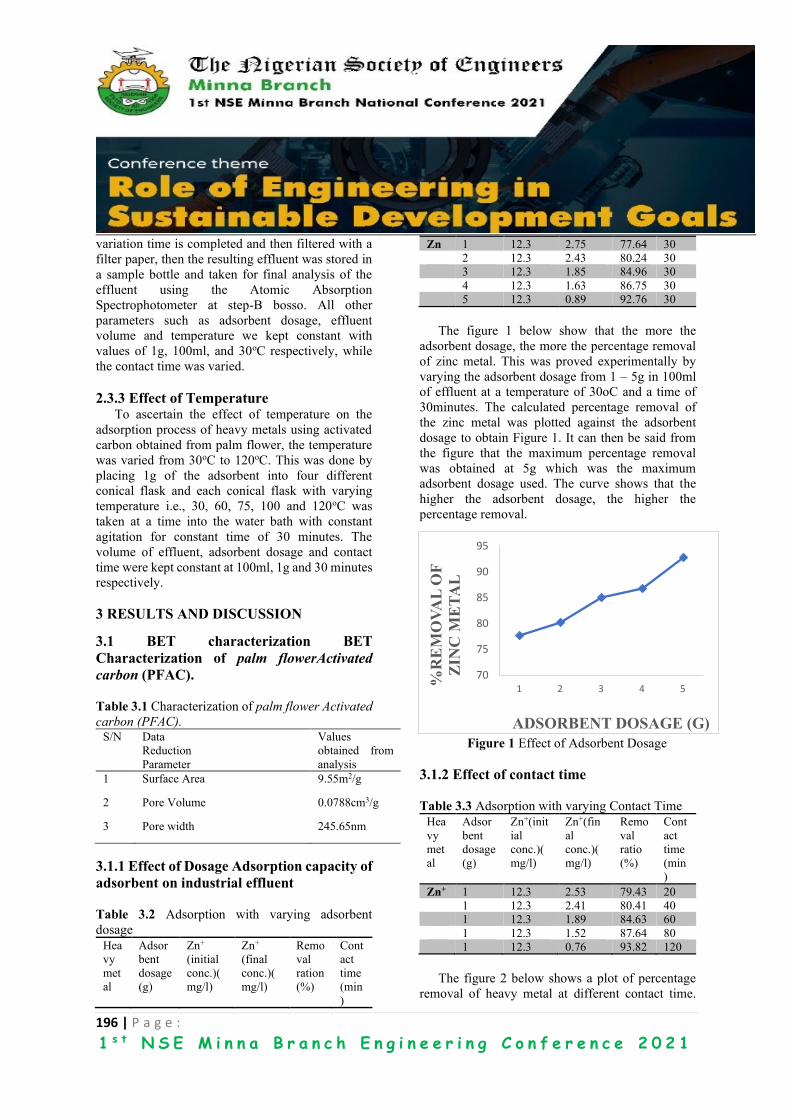
196 | P a g e :


variation time is completed and then filtered with a

filter paper, then the resulting effluent was stored in

a sample bottle and taken for final analysis of the

effluent using the Atomic Absorption

Spectrophotometer at step-B bosso. All other

parameters such as adsorbent dosage, effluent

volume and temperature we kept constant with

values of 1g, 100ml, and 30oC respectively, while

the contact time was varied.

2.3.3 Effect of Temperature To ascertain the effect of temperature on the

adsorption process of heavy metals using activated

carbon obtained from palm flower, the temperature

was varied from 30oC to 120oC. This was done by

placing 1g of the adsorbent into four different

conical flask and each conical flask with varying

temperature i.e., 30, 60, 75, 100 and 120oC was

taken at a time into the water bath with constant

agitation for constant time of 30 minutes. The

volume of effluent, adsorbent dosage and contact

time were kept constant at 100ml, 1g and 30 minutes

respectively.


3.1 BET characterization BET

Characterization of palm flowerActivated

carbon (PFAC).

Table 3.1 Characterization of palm flower Activated

carbon (PFAC). S/N Data

Reduction

Parameter

Values

obtained from

analysis

1 Surface Area 9.55m2/g

2 Pore Volume 0.0788cm3/g

3 Pore width 245.65nm

3.1.1 Effect of Dosage Adsorption capacity of

adsorbent on industrial effluent

Table 3.2 Adsorption with varying adsorbent

dosage

Hea

vy

met

al

Adsor

bent

dosage

(g)

Zn+

(initial

conc.)(

mg/l)

Zn+

(final

conc.)(

mg/l)

Remo

val

ration

(%)

Cont

act

time

(min

)

Zn 1 12.3 2.75 77.64 30

2 12.3 2.43 80.24 30

3 12.3 1.85 84.96 30

4 12.3 1.63 86.75 30

5 12.3 0.89 92.76 30

The figure 1 below show that the more the

adsorbent dosage, the more the percentage removal

of zinc metal. This was proved experimentally by

varying the adsorbent dosage from 1 – 5g in 100ml

of effluent at a temperature of 30oC and a time of

30minutes. The calculated percentage removal of

the zinc metal was plotted against the adsorbent

dosage to obtain Figure 1. It can then be said from

the figure that the maximum percentage removal

was obtained at 5g which was the maximum

adsorbent dosage used. The curve shows that the

higher the adsorbent dosage, the higher the

percentage removal.

Figure 1 Effect of Adsorbent Dosage

3.1.2 Effect of contact time

Table 3.3 Adsorption with varying Contact Time

Hea

vy

met

al

Adsor

bent

dosage

(g)

Zn+(init

ial

conc.)(

mg/l)

Zn+(fin

al

conc.)(

mg/l)

Remo

val

ratio

(%)

Cont

act

time

(min

)

Zn+ 1 12.3 2.53 79.43 20

1 12.3 2.41 80.41 40

1 12.3 1.89 84.63 60

1 12.3 1.52 87.64 80

1 12.3 0.76 93.82 120

The figure 2 below shows a plot of percentage

removal of heavy metal at different contact time.

70

75

80

85

90

95

1 2 3 4 5

%R

EM

OV

AL

OF

ZIN

C M

ET

AL

ADSORBENT DOSAGE (G)

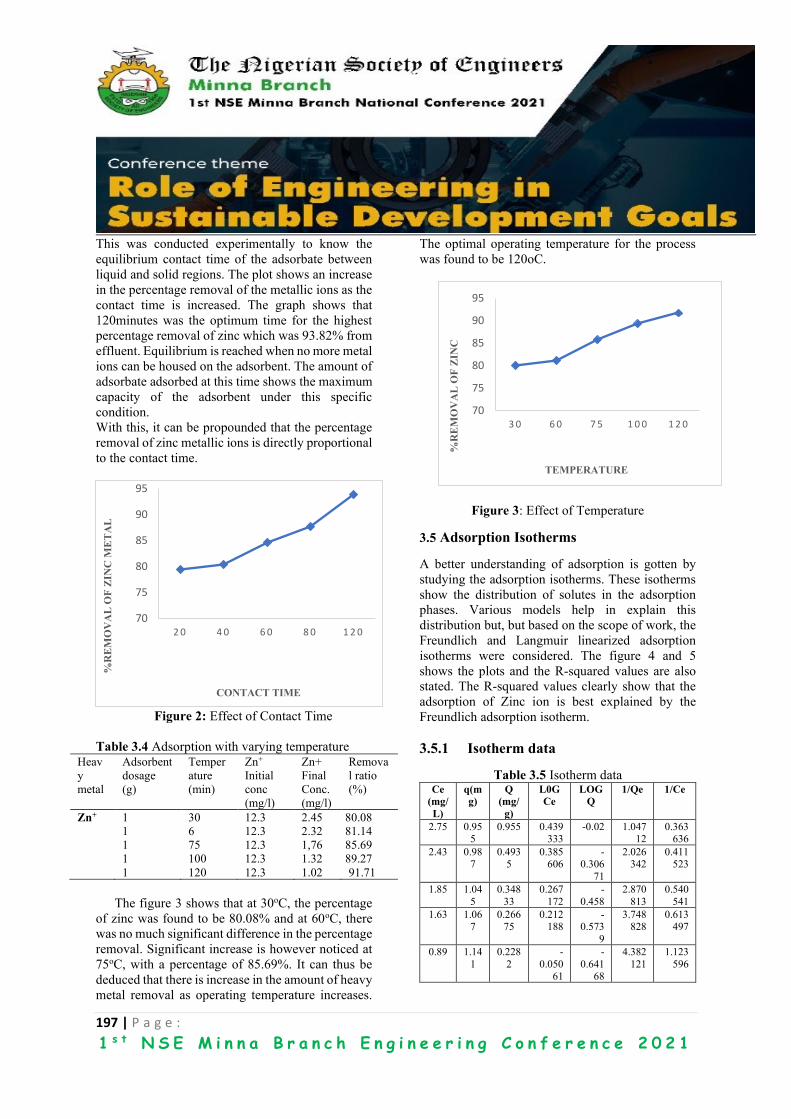
197 | P a g e :


This was conducted experimentally to know the

equilibrium contact time of the adsorbate between

liquid and solid regions. The plot shows an increase

in the percentage removal of the metallic ions as the

contact time is increased. The graph shows that

120minutes was the optimum time for the highest

percentage removal of zinc which was 93.82% from

effluent. Equilibrium is reached when no more metal

ions can be housed on the adsorbent. The amount of

adsorbate adsorbed at this time shows the maximum

capacity of the adsorbent under this specific

condition.

With this, it can be propounded that the percentage

removal of zinc metallic ions is directly proportional

to the contact time.

Figure 2: Effect of Contact Time

Table 3.4 Adsorption with varying temperature

Heav

y

metal

Adsorbent

dosage

(g)

Temper

ature

(min)

Zn+

Initial

conc

(mg/l)

Zn+

Final

Conc.

(mg/l)

Remova

l ratio

(%)

Zn+ 1 30 12.3 2.45 80.08

1 6 12.3 2.32 81.14

1 75 12.3 1,76 85.69

1 100 12.3 1.32 89.27

1 120 12.3 1.02 91.71

The figure 3 shows that at 30oC, the percentage

of zinc was found to be 80.08% and at 60oC, there

was no much significant difference in the percentage

removal. Significant increase is however noticed at

75oC, with a percentage of 85.69%. It can thus be

deduced that there is increase in the amount of heavy

metal removal as operating temperature increases.

The optimal operating temperature for the process

was found to be 120oC.

Figure 3: Effect of Temperature

3.5 Adsorption Isotherms

A better understanding of adsorption is gotten by

studying the adsorption isotherms. These isotherms

show the distribution of solutes in the adsorption

phases. Various models help in explain this

distribution but, but based on the scope of work, the

Freundlich and Langmuir linearized adsorption

isotherms were considered. The figure 4 and 5

shows the plots and the R-squared values are also

stated. The R-squared values clearly show that the

adsorption of Zinc ion is best explained by the

Freundlich adsorption isotherm.

3.5.1 Isotherm data

Table 3.5 Isotherm data Ce

(mg/

L)

q(m

g)

Q

(mg/

g)

L0G

Ce

LOG

Q

1/Qe 1/Ce

2.75 0.955

0.955 0.439333

-0.02 1.04712

0.363636

2.43 0.987

0.4935

0.385606

-0.306

71

2.026342

0.411523

1.85 1.04

5

0.348

33

0.267

172

-

0.458

2.870

813

0.540

541

1.63 1.067

0.26675

0.212188

-0.573

9

3.748828

0.613497

0.89 1.14

1

0.228

2

-

0.050

61

-

0.641

68

4.382

121

1.123

596

70

75

80

85

90

95

2 0 4 0 6 0 8 0 1 2 0

%R

EM

OV

AL

OF

ZIN

C M

ET

AL

CONTACT TIME

70

75

80

85

90

95

3 0 6 0 7 5 1 0 0 1 2 0

%R

EM

OV

AL

OF

ZIN

C

TEMPERATURE

198 | P a g e :


3.5.2 Langmuir adsorption isotherm

for Zinc (Zn) by plotting 1/Q

against 1/Ce.

3.5.3

FIGURE 4: Graph of Langmuir Adsorption

Isotherm

3.5.3 Freundlich adsorption isotherm for

Zinc (Zn) by plotting 1/Q against 1/Ce.

FIGURE 5: Graph of Freundlich Adsorption

Isotherm

3.5.4 Comparative studies between

Langmuir and Freundlich adsorption

isotherm

3.5.5 Langmuir adsorption isotherm

From the plot, Figure 2.0

y = 0.1722x + 0.094

Comparing with Langmuir’s equation, Table 1.4

was obtained.

1

𝑞𝑒=

1

aL×

1

Ce+kL

aL (1)

𝑦 = 1

𝑞𝑒 ; 𝑥 =

1

Ce (2),

TABLE 3.6: Langmuir adsorption isotherm

1/ aL aL Kl / aL

Kl R2 aL /

kl RL

0.1722 5.8072

01

0.094 0.5458

77

0.7381 10.6

383

0.1296

3

3.5.6 Freundlich adsorption isotherm

Comparing with Freundlich’s equation, Table 3

was obtained

From the plot,

y = 2.1887x - 1.0533

Comparing with Freundlich’s equation;

log 𝑞𝑒 = log𝐾𝐹 + 1

𝑛log 𝐶𝑒

(1)

𝑦 = log 𝑞𝑒 ; 𝑥 = log 𝐶𝑒 (2)

Table 3.7: Freundlich adsorption isotherm

1/n N R2 log k k

2.1887 0.456892 0.8688 -1.0533 0.348785

Kinetic studies

TABLE 3.8: Kinetic data Co t(min) Ce qt (qe –

qt) Log(qe – qt)

12.3 20 2.53 97.7 17.7 1.247973

30 2.41 98.9 16.5 1.217484

60 1.89 104.1 11.3 1.0 53078 80 1.52 107.8 7.6 0.880814

120 0.76 115.4 0 0

y = 0.1722x + 0.094R² = 0.8041

0

0.2

0.4

0.6

0.8

1

1.2

0 2 4 6

1/Ce

y = 2.1887x - 1.0533R² = 0.9131

-0.7

-0.6

-0.5

-0.4

-0.3

-0.2

-0.1

0

0 0.2 0.4 0.6

LOG Q

199 | P a g e :


First order Model for Zinc (Zn) is obtained by

plotting log (qe-qt) against t.

Figure 6: First order diffusion models.

3.5.8 Comparing with First Order Model

equation and figure 4.6, the first order

constants was obtained

From the plot,

y = -0.0125x + 1.6826

(4)

(5)

Second order Model for Zinc (Zn) is

obtained by plotting t/qt against t.

Figure 7: Second order diffusion models.

3.5.9 Comparing with second Order

Model equation and figure 4.7, the second

order constants was obtained

From the plot,

y = 0.0158x + 0.1941,

Comparing with second Order Model equations

𝑑𝑞

𝑑𝑡= 𝑘1(𝑞𝑒 − 𝑞)

2 (6)

This expression can be re-written in a linearized

form as

(7)

3.5.10 First and Second order model

constant

First order constants in relation to first order model

equation 4 and 5, while second order constants in

relation to second order model equation 6 and 7.

Table 5: First and Second order model constant

Kinetic Parameters Zinc

First Order

K1(min-1) 0.028788

qe(mg/g) 4674.122

R2 0.8838

Second Order

K2 4.850005

qe(mg/g) 63.29114

R2 0.9987

CONCLUSION

This study shows that the adsorption of zinc metal

Zn2+, onto the palm flower activated carbon treated

with sulphuric acid was effective. From the

experimental results obtained, it is noted that an

adsorbent dosage of 5g was obtained as the optimum

dosage in 100ml of the solution. The optimum

temperature was gotten to be 1200C while the

optimum time was 120 minutes.

y = -0.0125x + 1.6826R² = 0.8838

0

0.2

0.4

0.6

0.8

1

1.2

1.4

1.6

0 50 100 150

log

(q

e-q

t)

t (mins)

First order model for Zinc

y = 0.0158x + 0.1941

R² = 0.9987

0

0.5

1

1.5

2

2.5

0 50 100 150

t/q

t

t (min)

t/qt

Linear (t/qt)

200 | P a g e :


The adsorption isotherm data fitted well with the

Freundlich adsorption equilibrium models. The

separation factor of the Langmuir isotherm R1 lies

well in between 0 and 1. The Freundlich constant (n)

fell between 1 and 10 which indicated that the

process is favourable. The analysis carried out by the

Atomic Adsorption Spectrophotometer (AAS),

showed that the effluent gotten from the Scientific

Equipment development Institute (SEDI) had a

higher concentration of Zinc metal (i.e., 12.3mg/l),

hence making it a point of interest for this

experiment, while other metals such as iron,

manganese were found in lower concentrations.

These heavy metals were present beyond their

threshold values (acceptable limits) and hence,

needs treatment before being disposed into the

environment. The results obtained from the

adsorption study shows that adsorption as a process

is dependent on key factors such as adsorbent

dosage, contact time between the adsorbate and

adsorbent, and the temperature of the process. With

an encouraging removal percentage obtained from

the experiment, it can hence be concluded that palm

flower activated carbon (PFAC) is a low-cost

agricultural source material based activated carbon

and it is a recommendable and suitable adsorbent to

be sort after when it comes to carrying out a viable

adsorption study which can be employed for the

removal of heavy metals from wastewater or any

industrial effluent.

REFERENCES Abdunnasar, M. E, Mahmoud, E, Mohamed, T. M.

(2014). Removal of some heavy metals from

waste water using Fava beans. 225-226.

Alen Gabelman P. C. (2017). Adsorption Basic part

1, Gabelman process solution LLC, American

institute of chemical engineers.

Alloway B. J (2013). Source of heavy metals and

metalloids in soil. In: Alloway B (eds) Heavy

metal in soils. Environmental pollution, volume

22 Springer, Dordrecht.

Amana T., Kazi A. A., Sabir M. U., Banao Q.,

(2008). Potato peals as solid waste for the

removal of heavy metals copper II from waste

water/industrial effluent. Colloids surf. B;

Biointerfaces 63, 166-181.

Barakat M., (2011). New trends in removing heavy

metals from industrial waste water. Arabian

Journal of chemistry, 361-377.

Bharathi K. S. and Ramesh S.T. (2013). Removal of

dyes using agricultural waste as low-cost

adsorbents: A review, Applied Water Science

3(4) December 2013, DOI: 1110.1007/s13201-

013-0117-y

Chen G. H. (2004), Electrochemical technologies in

waste water treatment. Sep. purifies. Technol. 38

(1).11-41.

Crini G., Lichtfouse E., Wilson L., Nadia Morin-

Crini. (2019). Conventional and non-

conventional adsorbents for wastewater

treatment. Environmental Chemistry Letters,

Springer Verlag, 17(1),195-213.

DOI:10.1007/s10311-018-0786-8

Desta M. B., (2013). Batch Sorption Experiments:

Langmuir and Freundlich Isotherm Studies for

the Adsorption of Textile Metal Ions onto Teff

Straw (Eragrostis tef) Agricultural Waste,

Journal of Thermodynamics, vol. 2013, Article

ID 375830, 6 pages, 2013.

https://doi.org/10.1155/2013/375830

Ebuka, O. (2017). 59,000 children in Nigeria die

yearly of water related diseases, Nigerian

government. Premium times publications.

Fenglianfu, Q. W. (2010). Removal of metal ions

from waste water: A review, Journal of

environmental management.

Fu F, Wang Q. (2011). Removal of heavy metal ions

from wastewaters: a review. Journal of

Environmental Management. 92(3):407-418.

DOI: 10.1016/j.jenvman.2010.11.011.

Gulson B. L. Mahaffey K. R., Mizon K. J., Korsch

M. J., Cameron M. A., Vimpani G. (1995).

Contribution of Tissue Lead to Blood Lead in

adult female subjects based on stable lead

isotope method. [Retrieved from

http://www.ncbi.nlm.nih-

gov/pubmed/77693643]: J. lab clin med 125;

703-712.

Gupta V. K., Jain R., Saleh T., Nayak AA., Malathi

S. and Agarwal S. (2011). Equilibrium and

thermodynamic studies on the removal and

recovery of safranine-T dye from industrial

effluents. Separation science and technology, 46

(5), 839-846.

Kumar S. P., Senthamaria C., Durgadevi A. (2012).

Adsorption kinetics, mechanism, isotherm and

201 | P a g e :


thermodynamics analysis of copper ions onto the

surface modified agricultural waste. America

institute of chemical environ prog, 33: pg 28-37.

Laxmi G. S., Ahmaruzzaman M. (2014). Phenotic

waste water treatment: Development and

application of new absorbent materials”

Industrial Wastewater Treatment Recycling and

Reuse, volume 1.

Lim A.P. and Aris A.Z., (2014). A review on

economically adsorbents on heavy metals

removal in water and wastewater. Reviews in

Environmental Science and Bio/Technology,

13(2), 163-181.

Mousa W. M., Soliman S. I., El-Baily A. B. and

Hanaa A. S., (2013). Removal of some heavy

metal from aqueous solution rice straw, Journal

of Applied Science Research 9(3); 1696-1700.

Nalenthiran P., Sambandam A., and Muthu Pandian

A. (2015). Removal of heavy metals from waste

water An alternative green sonochemical process

optimization and pathway studies. Hand book of

ultrasonic and sonochemistry, Springer science

business media, Singapore.

Nimibofa A., Augustus N. E. and Donbebe W.

(2017). Modeling and interpretation of

adsorption isotherms. Journal of chemistry

department of chemical science, Niger Delta

University, 11.

Ptiha E. H., Hidayat y. and Firdaus M. (2016). The

Langmuir isotherm adsorption equation; the

monolayer approach. Iop conference series:

material science and engineering volume 107,

conference 1.

Rana S. V. S. (2006). Environmental pollution;

health and toxicology Alpha science

international technology limited U.K., 172.

Raymond A. Wuana, Felix E. Okieimen, (2011).

Heavy Metals in Contaminated Soils: A Review

of Sources, Chemistry, Risks and Best Available

Strategies for Remediation, International

Scholarly Research Notices, vol. 2011, Article

ID 402647, 20 pages, 2011.

https://doi.org/10.5402/2011/402647

Ruan C. A. Moura, Daniel A. B., Carlos A. F. Franco

D. R. Amado (2012). Study of chromium

removal by the electrodialysis of Tannery and

metal-finishing effluents. International journal

of chemical engineering, volume 2012, article ID

179312. Brazil.

Shende, A., and Main, J. S. (2014). Effect of Contact

Time on Adsorption of Nitrates and Phosphates.

International Journal of Advanced Technology

in Engineering and Science, pp 117-122.

Tchounwou, P. B., Yedjou, C. G., Patlolla, A. K., &

Sutton, D. J. (2012). Heavy metal toxicity and the

environment. Experientia supplementum, 101,

133–164. https://doi.org/10.1007/978-3-7643-

8340-4_6

UNEP (1991). Impact of lead toxicity in social

ecosystem UNEP, 1991.

Veli, S and Alyüz, B. (2007). Adsorption of copper

and zinc from aqueous solutions by using natural

clay. Journal of Hazardous Materials, 149(1),

226-233.

Wang H., and Farhang S. (2012) “Effect of particle

size on the adsorption and desorption properties

of oxide nano particles”. American Institute of

chemical engineers 59: 1502-1510.

Wang L. K., Vaccari, D. A., Li, Y., Shammas N. K..,

(2004). Chemical precipitation. In Wang L. K.,

Hung Y. J., Shammas N. K. (Eds),

Physicochemical Treatment Processes, volume

3. Humana press, New Jersey, pp. 141-198

https://doi.org/10.1007/978-3-7643-8340-4_6

https://doi.org/10.1007/978-3-7643-8340-4_6

202 | P a g e :


Irrigation with Unsafe Industrial Wastewater and Associated

Health Risks: An Emerging Technology for Heavy Metals Removal A. S. Mohammeda,c*, E. Danso-Boatengb, G. Sandac, A.D. Wheatleyc, M.I. Animashaund, I.A. Kutic, H.I.

Mustaphad, M.Y. Otache, J.J. Musad a,dDepartment of Agricultural and Bioresources Engineering, School of Infrastructure, Process Engineering and

Technology, Federal University of Technology, Minna, Nigeria bSchool of Chemical, Energy and Process Engineering, University of Leeds, Leeds, LS2 9JT, UK.

cSchool of Architecture, Building and Civil Engineering, Loughborough University, Loughb., LE11 3TU, UK. *Corresponding email: [email protected]

GRAPHICAL ABSTRACT

ABSTRACT The scarcity of freshwater resources, being currently experienced in water-stressed countries has prompted

millions of smaller farming communities to depend on wastewater for crop irrigation, drinking, bathing and

fishing. However, in this context, the treatment of wastewater from textile and tannery industries is the subject

of interest, this paper aim to address. The rule of thumb suggests, wastewater to constitute beneficial nutrients

recycling due to rich organic matter content. Inherently, the same kind of wastewater has been investigated and

analysed by several researchers and found to contain micro-pollutants such as inorganics (heavy metals, salts)

and organics (dyestuff, starch). Regrettably, the presence of these pollutants in wastewater used for irrigation

is of concern particularly as it relates human health. Although, several conventional wastewater treatment

technologies exist; their applications are now hamstrung by high procurement, operation and maintenance

costs. Recent studies on cheap and readily available biomass wastes have confirmed their high sorption

potential and can therefore, be used as adsorbents for micro-pollutants removal from industrial wastewater. In

this study, chicken eggshell, coconut peat, coconut shell, rice husk and lemon peel were all used for the

wastewater treatment. Hydrothermal carbonisation (HTC), was used to change the surface functional

characteristics of the adsorbents for enhanced adsorption. To achieve this, batch experiments using raw biomass

were carried out in triplicates at 3 different contact times and pH values. After 2 hr of contact time at pH9, the

coco-peat was proven to have Cr removal efficiency of 91.6% against 73.2% using a bonechar; and 95.0% for

Pb (II) against 91.2% for the bonechar. The outcome of this study suggests that coconut-peat and eggshell even

without been carbonised can provide a cost-effective means for metal removal from industrial wastewaters.

KEYWORDS: Adsorption, biomass waste, crop irrigation, freshwater scarcity, wastewater reuse


203 | P a g e :


1 INTRODUCTION One-third of the world's population currently

live in developing and water-deficit countries, with

overall water need is expected to rise by 2025 (Gu,

et al., 2019; Dubey and Swain 2019). As a

consequence of the resource exploitation, about two-

third of the global population would suffer from

water shortages (Mahfooz, et al., 2020). Scarcity of

freshwater resources may limit food production and

supply, as about 70% of all freshwater withdrawals

go to irrigated agriculture (≈ 2800 km3 of

freshwater/year). Scarcity of freshwater resources

may limit food production and supply, as about 70%

of all freshwater withdrawals go to irrigated

agriculture (≈ 2800 km3 of freshwater/year) (UN-

Water, 2012). Water is an essential resource for the

sustenance of life and plays a cardinal role in

agriculture and allied industries, consequently, it

also receives a variety of wastes from different

sources (Merchant and Painter, 2019; Kennedy,et

al., 2018). Studies have shown that there is global

decline in the amount of available freshwater

resources due to intensified agricultural practices

such as excessive application of fertilizers,

pesticides, insecticides and herbicides (Gu, et al.,

2019) as well as climate change and increasing

urbanization but its severity is mostly experienced in

developing and water-stressed countries (Mahfooz,

et al., 2020). The economic contributions of peasants

farmers especially in developing and water-stressed

countries are now hamstrung by freshwater scarcity,

and this is observed to affect the expansion of crop

yields and their quality. As a consequence of

artificial scarcity of freshwater resources,

wastewater stem to provide a great deal of relieve to

farmers for year-round production of crops (Dubey

and Swain, 2019). The use of wastewater for

agriculture permits the cultivation of wide range of

crops in multiple cycles, thereby promoting

potentials for high yields.

Surmise to the above, reuse of wastewater for

agriculture has become a norm and its practical

application in developing and water-stressed

countries has historical precedence which is likely to

increase in the near future (Bougnom and Piddock,

2017). Although, several benefits of wastewater

reuse, particularly in agriculture have been widely

reported; it’s practical application is most beneficial

and cost-effective in developing nations (Drechsel,

et al., 2009). However, despite the huge economic

benefits of wastewater reuse, it is apparent that this

important resource is recording varying

concentrations of heavy metals and pigments due to

uncontrolled discharge of industrial effluents into

waterways (Becerra-Castro et al., 2015; Mohammed

et al., 2020).

Regrettably, the peasant farmers along the

fringes of these waterways utilize such resource for

crop irrigation, hence compromising crop quality

and food safety (Dickson, et al., 2016). There are

several documented articles from developing

countries reporting varying concentrations of

organic and inorganic chemical substances in

agricultural soils and crops that have been receiving

perpetual wastewater (Qu, et al., 2019). Ironically,

the concentrations of these pollutants in wastewater,

agricultural soils and crops usually exceeds the

FAO/WHO recommended thresholds. Seemingly,

prolong exposure to wastewater pollutants are

impediments that hinders safe agricultural practice

and farmers’ productivity, which culminate to

pervasive health implications on humans through

food supply chain. There are several research

articles establishing the epidemiological and

carcinogenic links between the consumption of

poorly irrigated crops with individual or societal

illnesses (Qu, et al., 2019; El-Azazy et al., 2019).

Other likely ailments resulting from excessive

exposure to heavy metals and metalloids include

mutagenicity, carcinogenicity and teratogenicity.

Mutagenicity is the alteration of genetic structure,

while carcinogenicity causes damage to specific

regions of the genome, Carcinogenic substances can

get into a biological tissue through inhalation,

ingestion and contact with skin. Teratogenicity on

the other hand, is a specific mutagen that cause

damage to the genome which then causes

abnormality in the developing foetus (Tong et al.,

2000). It’s worthy to know, that humans, animals

and plants do not have good mechanisms for fixing

or excreting heavy metals; hence bio-ccumulate and

remain for life (Zhuang et al., 2009 QU, et al., 2012).

Policymaking bodies such as World Health

Organisation (WHO), Food and Agriculture

Organisation (FAO), International Commission on

204 | P a g e :


Irrigation and Drainage (ICID), among others have

been exploring modalities to safeguard humans and

environment from excessive exposure to micro-

pollutants found in wastewater used for irrigation. In

a quest to define these modalities, these international

bodies jointly issued some guidelines to regulate the

concentrations of micro-pollutants in irrigation

water worldwide. Adoption of these guidelines is

highly desirable; but in reality, their implementation

is hard to achieve practically, particularly in

developing countries (Chang et al., 2002). The

probable reasons for the unsuccessful

implementation of those guidelines may be due to

any or combination of the following: 1) high

procurement and installation costs for modern

wastewater treatment facilities; 2) non-compliance

with policy guidelines governing effluent discharge

into waterways and environment by industries; and

3) poor monitoring and enforcement strategy.

The essence of these guidelines is to safeguard

agricultural soils, plants and humans from excessive

exposure to organic and inorganic chemical

substances (Dickson, et al., 2016). Although,

application of these guidelines has recorded

tremendous success in developed nations;

regrettably, their effective implementation in

developing countries is still looming and

unsuccessful (Ensink and Van Der Hoek, 2009).

Proffering an alternative wastewater treatment

method is the purpose for which this paper is

anchored.

Over the years, chemical precipitation, ion-

exchange, electro-dialysis, reverse-osmosis,

membrane and adsorption using activated carbon

and other industrial by-products have been the most

widely treatment technique for wastewater (Geetha

and Belagali, 2013; Bhattacharjee et. al., 2020;

Ajiboye, et. al., 2021). Of all the treatment methods

mentioned, activated carbon is reported to be the

most commonly used for the removal of ions and

pigments from industrial wastewater at much lower

concentrations (Phadtare and Patil, 2015;

Bhattacharjee, et al., 2020). However, the major

limitation with the use of activated carbon is that its

procurement is quite expensive.

Furthermore, limitations of conventional

wastewater treatment methods mentioned above,

other than activated carbon include high initial

operating cost and generation of secondary toxic

wastes which may require additional cost of

treatment. The toxic wastes generated are mostly

non-environmentally friendly. Against these

backdrops, researchers are now exploring cheaper,

sustainable and more effective method for the

removal of organic and inorganic pollutants in

wastewaters (Bhattacharjee, et al., 2020).

To this end, the work herein, explores the

potentials of biomass wastes that comprise rice husk,

coconut shell, coconut peat otherwise called coir,

chicken eggshell and lemon peel. All these wastes

are readily available in Nigeria. The raw biomass

wastes are needed for the preliminary adsorption

tests. However, for column tests, the biomass wastes

were carbonised to produce hydrochar. The

technology used for the conversion of biomass

wastes into hydrochar is called hydrothermal

carbonisation (HTC). Hydrochar is mainly

composed of 40–45wt% cellulose, 25–35wt%

hemicellulose, 15–30wt% lignin and up to 10wt%

for other compounds (Sevilla and Fuertes, 2009).

Hydrothermal carbonisation is an exothermic

process that takes place in water at temperature

between 180 – 250 °C within a time period ranging

from 30–500 min to produce a carbon-rich coal-like

derivative commonly called hydrochar at saturated

pressure of 15 – 20 bar which releases CO_2 and

other volatiles (Titirici et al., 2007; Funke and

Ziegler, 2010; Libra et al., 2011). The HTC involves

dehydration and decarboxylation of biomass in order

to raise the carbon content which enhances sorption

characteristics and increases hydrochar energy

values (Libra et al., 2011). For the purpose of his

paper, only raw biomass wastes are used to

investigate the effectiveness of the metal ions

removal.

2 MATERIALS AND METHODS

2.1 RAW MATERIALS All the materials used herewith were obtained

locally; these include the following: the chicken

eggshell were gotten from the Loughborough

University kitchen; lemon from a street market in

Loughborough town, Leicestershire; the coconuts

bought from a supermarket also in Loughborough;

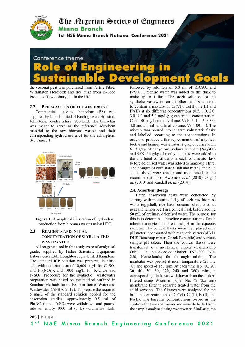
205 | P a g e :


the coconut peat was purchased from Fertile Fibre,

Withington Hereford; and rice husk from E-Coco

Products, Tewkesbury, all in the UK.

2.2 PREPARATION OF THE ADSORBENT Commercial activated bonechar (BS) was

supplied by Jaret Limited, 4 Birch groves, Houston,

Johnstone, Renfrewshire, Scotland. The bonechar

was meant to serve as the reference adsorbent

material to the raw biomass wastes and their

corresponding hydrochars used for the adsorption.

See Figure 1.

2.3 REAGENTS AND INITIAL

CONCENTRATION OF SIMULATED

WASTEWATER All reagents used in this study were of analytical

grade, supplied by Fisher Scientific Equipment

Laboratories Ltd., Loughborough, United Kingdom.

The standard ICP solution was prepared in nitric

acid with concentration of 10,000 mg/L for CuSO4

and Pb(NO3)2, and 1000 mg/L for K2CrO4 and

FeSO4. Procedure for the synthetic wastewater

preparation was based on the method outlined in

Standard Methods for the Examination of Water and

Wastewater (APHA, 2012). To prepare the required

5 mg/L of the standard solution needed for the

adsorption studies, approximately 0.5 ml of

Pb(NO3)2 and CuSO4 were withdrawn and poured

into an empty 1000 ml (1 L) volumetric flask,

followed by addition of 5.0 ml of K2CrO4 and

FeSO4. Deionise water was added to the flask to

make up to 1 litre. The stock solutions of the

synthetic wastewater on the other hand, was meant

to contain a mixture of Cr(VI), Cu(II), Fe(II) and

Pb(II) at six different concentrations (0.5, 1.0, 2.0,

3.0, 4.0 and 5.0 mg/L); given initial concentration,

C1 as 100 mg/L; initial volume, V1 (0.5, 1.0, 2.0, 3.0,

4.0 and 5.0 ml) and final volume, V2 (100 ml). The

mixture was poured into separate volumetric flasks

and labelled according to the concentrations. In

order, to produce a fair representation of a typical

textile and tannery wastewater, 2 g/kg of corn starch,

6.13 g/kg of anhydrous sodium sulphate (Na2SO4)

and 0.09466 g/kg of methylene blue were added to

the undiluted constituents in each volumetric flask

before deionised water was added to make-up 1 litre.

The dosages of corn starch, salt and methylene blue

stated above were chosen and used based on the

recommendations of Awomeso et al. (2010), Ong et

al. (2010) and Randall et. al. (2014).

2.4. Adsorbent dosage

Batch adsorption tests were conducted by

starting with measuring 1.5 g of each raw biomass

waste (eggshell, rice husk, coconut shell, coconut

peat and lemon peel) in a conical flask before adding

50 mL of ordinary deionised water. The purpose for

this is to determine a baseline concentration of each

inherent analyte of interest and pH in the aqueous

samples. The conical flasks were then placed on a

pH meter incorporated with magnetic stirrer (pH-8+

DHS Benchtop meter, Czech Republic) and various

sample pH taken. Then the conical flasks were

transferred to a mechanical shaker (Gallenkamp

Orbital Incubator-cooled Shaker, INR-200 INR-

250, Netherlands) for thorough mixing. The

incubator was pre-set at room temperature (25 ± 2 oC) and speed of 150 rpm. At each time lap (10, 20,

30, 40, 50, 60, 120, 240 and 360) mins, a

corresponding flask was withdrawn from the shaker,

filtered using Whatman paper No. 42 (2.5 µm)

membrane filter to separate treated water from the

solid sorbents. The filtrates were analysed for the

baseline concentrations of Cr(VI), Cu(II), Fe(II) and

Pb(II). The baseline concentrations served as the

controls for the experiments and were deducted from

the sample analysed using wastewater. Similarly, the

Figure 1: A graphical illustration of hydrochar

production from biomass wastes using HTC

206 | P a g e :


procedure was followed using the same adsorbent

dosage, operating conditions and volume of

wastewater.

2.5. Effect of contact time on adsorption.

At the preliminary stage of this study, the effect

of three (3) different contact times (2, 4, and 6) h on

adsorption were examined using the raw biomass

wastes. The chosen contact time were for the

purpose of optimisation in order to explore to

shortest possible time to achieve maximum

adsorption yield.

2.6 Effect of pH

A polygon F371220040 spin bar was dropped into

each volumetric flask containing ordinary water

different adsorbent and placed on magnetic stirrer to

examine the effect of solution pH on adsorption.

While the magnetic stirrer is switched ON, the

mixture begins to stir, and the initial pH taken. and

that was repeated after adjustment with 1M NaOH.

Based on typical scenarios as documented in several

literature, textile and tannery wastewaters are known

to be alkaline in nature with pH values ranging from

9 to 11. Hence, this justifies the choice of pH9 and

pH11 for alkalinity medium used in this study.

Whereas, the pH of solutions that contain hydrochar

in natural state ranges from 4 to 6, which is relatively

acidic. However, in order to adjust the acidic pH to

alkalinity, 1M of sodium hydroxide (NaOH) was

gradually added to the solution until the desired pH

for each mixture was attained.

2.7 Heavy metal removal efficiency

To determine the percentage adsorption of heavy

metals by the adsorbents, the following equation as

described by (Chen and Wang, 2008) was used.

100%

−=

i

fi

C

CCR

(1)

Where;

Ci is initial metal concentration (mg/L) and

Cf is the final metal concentration (mg/L).

2.8 CHARACTERISATION OF BIOMASS

WASTE

The analytical method used in carrying surface

characterisation are as follows: (i) Scanning

Electron Microscopy (SEM); (ii) Energy Dispersive

X-Ray Spectroscopy (EDS); (iii) Brunauer, Emmett

and Teller (BET), (vi) Fourier transformed Infrared

Ray (FTIR).

2.9 BATCH ADSORPTION TESTS

At the end of the batch adsorption tests after, the

filtrates (treated water) were all collected in 50 mL

labelled plastic bottles and stored at 4 oC to analyse

and determine the residual concentration of each

interacting heavy metals and pigment in the

synthetic textile and tannery wastewater.


3.1 CHARACTERISATION OF RAW

BIOMASS AND CORRESPONDING

HYDROCHAR

Details on surface characterization, including

morphology, pore volume, pore size and Fourier

Transform Infrared Ray (FTIR) of both raw biomass

wastes and the corresponding hydrochar can be

found in the author’s recent publication by Danso-

Boateng et al. (2021)

3.2 EFFECT OF CONTACT TIME ON

METAL ADSORPTION BY RAW

BIOMASS WASTE

The effect of contact time on adsorption of

Cr(VI), Cu(II), Fe(II) and Pb(II) ions from an

aqueous textile and tannery wastewater by various

raw biomass wastes (ES, RH, CP and LP) was

investigated. The preliminary results of the batch

tests that were carried out using only raw biomass

wastes are presented in Figure 8. To start with, a

careful study of Figure 8 (b), (c) and (e) displayed

very low uptake of Cr(VI) ions. This implies that the

surface chemistry of the raw ES, RH, LP have poor

sorption affinity for the Cr(VI) ion and even with

progressive increased in contact time, there is no

significant change on the amount of Cr(VI) ions

removed. However, Figure 8 (a) and (d) indicates

removal of about 80% and 90% of Cr(VI) by BC and

CP respectively after the first 2 h.

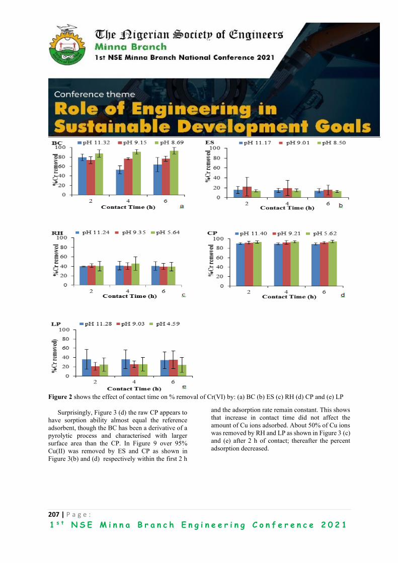
207 | P a g e :


Figure 2 shows the effect of contact time on % removal of Cr(VI) by: (a) BC (b) ES (c) RH (d) CP and (e) LP

Surprisingly, Figure 3 (d) the raw CP appears to

have sorption ability almost equal the reference

adsorbent, though the BC has been a derivative of a

pyrolytic process and characterised with larger

surface area than the CP. In Figure 9 over 95%

Cu(II) was removed by ES and CP as shown in

Figure 3(b) and (d) respectively within the first 2 h

and the adsorption rate remain constant. This shows

that increase in contact time did not affect the

amount of Cu ions adsorbed. About 50% of Cu ions

was removed by RH and LP as shown in Figure 3 (c)

and (e) after 2 h of contact; thereafter the percent

adsorption decreased.

208 | P a g e :


Figure 3 shows the effect of contact time on % removal of Cu by: (a) BC compared (b) ES (c) RH (d) CP and (e)

LP

On the other hand, Figure 4 (a) and (b) showed

that about 100% of Fe ions was removed by BC and

ES after 2 h, same with CP as illustrated in (d).

Thereafter, the adsorption rate became practically

constant through the remaining period. ES and CP

respectively after 2 h; further contact time did not

have any significant effect.

Likewise, Figures 5 (a), (b) and (d) demonstrate

that over 90% of Pb(II) was removed by BC. It can

then be concluded that the rate of metal binding with

adsorbent was more rapid during the initial stages (2

h), and this may be due to the presence of large

number of active sites for metal binding, which

became saturated with time and gradually decreased

209 | P a g e :


and remain constant. Observation on the effect of

contact time on adsorption in this study is supported

by other researchers that examined and heavy metals

removal by biomass wastes.

Figure 3 shows the effect of contact time on % removal of

Cu by: (a) BC compared (b) ES (c) RH (d) CP and (e) LP Figure 4 shows the effect of contact time on %

adsorption of Fe by (a) BC compared (b) ES (c) RH (d)

CP and (e) LP

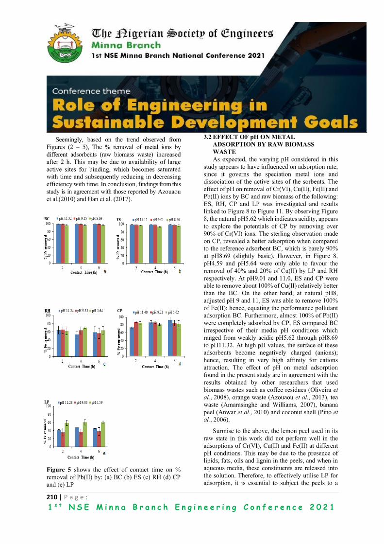
210 | P a g e :


Seemingly, based on the trend observed from

Figures (2 – 5), The % removal of metal ions by

different adsorbents (raw biomass waste) increased

after 2 h. This may be due to availability of large

active sites for binding, which becomes saturated

with time and subsequently reducing in decreasing

efficiency with time. In conclusion, findings from this

study is in agreement with those reported by Azouaou

et al.(2010) and Han et al. (2017).

Figure 5 shows the effect of contact time on %

removal of Pb(II) by: (a) BC (b) ES (c) RH (d) CP

and (e) LP

3.2 EFFECT OF pH ON METAL

ADSORPTION BY RAW BIOMASS

WASTE

As expected, the varying pH considered in this

study appears to have influenced on adsorption rate,

since it governs the speciation metal ions and

dissociation of the active sites of the sorbents. The

effect of pH on removal of Cr(VI), Cu(II), Fe(II) and

Pb(II) ions by BC and raw biomass of the following:

ES, RH, CP and LP was investigated and results

linked to Figure 8 to Figure 11. By observing Figure

8, the natural pH5.62 which indicates acidity, appears

to explore the potentials of CP by removing over

90% of Cr(VI) ions. The sterling observation made

on CP, revealed a better adsorption when compared

to the reference adsorbent BC, which is barely 90%

at pH8.69 (slightly basic). However, in Figure 8,

pH4.59 and pH5.64 were only able to favour the

removal of 40% and 20% of Cu(II) by LP and RH

respectively. At pH9.01 and 11.0, ES and CP were

able to remove about 100% of Cu(II) relatively better

than the BC. On the other hand, at natural pH8,

adjusted pH 9 and 11, ES was able to remove 100%

of Fe(II); hence, equating the performance pollutant

adsorption BC. Furthermore, almost 100% of Pb(II)

were completely adsorbed by CP, ES compared BC

irrespective of their media pH conditions which

ranged from weakly acidic pH5.62 through pH8.69

to pH11.32. At high pH values, the surface of these

adsorbents become negatively charged (anions);

hence, resulting in very high affinity for cations

attraction. The effect of pH on metal adsorption

found in the present study are in agreement with the

results obtained by other researchers that used

biomass wastes such as coffee residues (Oliveira et

al., 2008), orange waste (Azouaou et al., 2013), tea

waste (Amarasinghe and Williams, 2007), banana

peel (Anwar et al., 2010) and coconut shell (Pino et

al., 2006).

Surmise to the above, the lemon peel used in its

raw state in this work did not perform well in the

adsorptions of Cr(VI), Cu(II) and Fe(II) at different

pH conditions. This may be due to the presence of

lipids, fats, oils and lignin in the peels, and when in

aqueous media, these constituents are released into

the solution. Therefore, to effectively utilise LP for

adsorption, it is essential to subject the peels to a

211 | P a g e :


thermochemical treatment in order to denature the

organic constituents and increase its surface area for

adsorption. The thermochemical process is termed

hydrothermal carbonisation (HTC), which produces

a product called hydrochar.

4 CONCLUSIONS

Biomass wastes consisting of coco-peat (CP),

coconut shell (CS), rice husk (RH), lemon peel (LP)

and eggshell (ES) were hydrothermally treated at

200 °C for 20 h in order to investigate their sorption

ability for pollutant adsorption. The study

demonstrated that the raw biomass wastes have the

potential to be used as adsorbents. However,

hydrochar would be better due to changes in surface

characteristics of the adsorbents. The SEM images

showed that the hydrochars have more porous

structures, which resulted from denaturing of

biomass structures due to carbonisation. The surface

area of the hydrochars were significantly higher than

the corresponding raw biomass, with CS hydrochar

having the largest surface area (21.82 m2/g), whilst

ES hydrochar the smallest (0.5 m2/g). The enhanced

porosity and surface area of the hydrochars result in

more characteristics active sites for sorption of

pollutants. Therefore, the abundance of these

biomass waste materials in developing countries and

the moderate HTC temperature required make these

produced hydrochars suitable for potential practical

applications, especially in developing countries.

ACKNOWLEDGEMENTS

The authors would like to extend their profound

appreciation to the following: Jayshree Bhuptani and

Geoffrey Russell of the School of

Architecture,Building and Civil Engineering,

Logborough University,United Kingdom for their

courteous understanding in providing the enabling

environment to carry out some aspects of this

study;The authors also to thank Dr. Keith Yendall

and Monika Pietrzak, both of the School of

Chemical and Materials Engineering,

Loughborough University who assisted with

SEM/EDS, FTIR and surface area analyses. Finally,

the authors are indebted to the management of the

Petroleum Technology Development Fund (PTDF),

Abuja, Nigeria for Funding this research.

REFERENCES

Akan, J. C., Abdulrahman, F. I., Ayodele, J. T., &

Ogugbuaja, V. O. (2009). Impact of tannery and

textile effluent on the chemical characteristics of

Challawa river, Kano state, Nigeria. Electronic

Journal of Environmental, Agricultural and

Food Chemistry, 8(10), 1008–1032.

Ajiboye, Timothy O, Opeyemi A Oyewo, and

Damian C Onwudiwe. 2021. "Simultaneous

removal of organics and heavy metals from

industrial wastewater: A review." Chemosphere

262: 128379-128399.

doi:10.1016/j.chemosphere.2020.128379.

Alaoui, N. S., Laghdach, A. E., Correa, E. M.,

Stitou, M., Yousfi, F. E. and Jbari, N. (2014)

‘Preparation of bone chars by calcination in

traditional furnace’, J. Mater. and Environ.

Sci., 5(2), pp. 476–483.

Amarasinghe, B. M. W. P. K. and Williams, R. A.

(2007) ‘Tea waste as a low cost adsorbent for the

removal of Cu and Pb from wastewater’, Chem.

Eng. J., 132(1–3), pp. 299–309. doi:

10.1016/j.cej.2007.01.016.

Anwar, J., Shafique, U., Waheed-uz-Zaman,

Salman, M., Dar, A. and Anwar, S. (2010)

‘Removal of Pb(II) and Cd(II) from water by

adsorption on peels of banana.’, Bioresource

technology, 101(6), pp. 1752–5. doi:

10.1016/j.biortech.2009.10.021.

APHA. (2012). Standard Methods for the

Examination of Water and Wastewater. (E. W.

Rice, R. B. Baird, A. D. Eaton, & L. S.

Clesceri, Eds.) (22nd ed.). Washington, DC:

American Public Health Association,

American Water Works Association,Water

Environment Federation.

ASTM (2008) ‘American Standard Test Methods for

Instrumental Determination of Carbon,

Hydrogen, and Nitrogen in Laboratory

Samples of Coal: D5373-08’, A Standard -

ASTM International, West Conshohocken.

Azouaou, N., Belmedani, M., Mokaddem, H. and

Sadaoui, Z. (2013) ‘Adsorption of lead from

aqueous solution onto untreated orange barks’,

Chemical Engineering Transactions, 32, pp.

55–60. doi: 10.3303/CET1332010.

Barrett EP, Joyner LG, Halenda PP (1951) The

determination of pore volume and area

212 | P a g e :


distributions in porous substances.I.

Computations from nitrogen isotherms. J Am

Chem Soc 1896(1948):373–380

Becerra-Castro, C., Lopes, A. R., Vaz-Moreira, I.,

Silva, E. F., Manaia, C. M., & Nunes, O. C.

(2015). Wastewater reuse in irrigation: A

microbiological perspective on implications in

soil fertility and human and environmental

health. Environment International, 75, 117–

135.

https://doi.org/10.1016/j.envint.2014.11.001.

Bhattacharjee, Chiranjit, Suman Dutta, and Vinod K

Saxena. 2020. "A review on biosorptive removal

of dyes and heavy metals from wastewater using

watermelon rind as biosorbent." Environmental

Advances 2: 100007-.

doi:10.1016/j.envadv.2020.100007.

Blumenthal, U., & Peasey, A. (2002). Critical

review of epidemiological evidence of the

health effects of wastewater and excreta use in

agriculture, (December), 1–42.

Bougnom, Blaise P, and Laura J.V Piddock. 2017.

"Wastewater for Urban Agriculture: A

Significant Factor in Dissemination of Antibiotic

Resistance." Environmental Science and

Technology ( American Chemical Society) 51:

5863-5864. doi:10.1021/acs.est.7b01852.

Chen, C., & Wang, J. (2008). Removal of Pb2+, Ag+,

Cs+ and Sr2+ from aqueous solution by

brewery’s waste biomass. Journal of

Hazardous Materials, 151(1), 65–70.

https://doi.org/10.1016/j.jhazmat.2007.05.046

.

Chhikara, S., & Rana, L. (2013). Physico-chemical

Characterization of Textile Mill Effluent : A

Case Study of Haryana , India. International

Journal of Science and Technology, 8, 19–23.

Danso-Boateng, E., Holdich, R. G., Wheatley, A. D.

and Martin, S. J. (2015) ‘Hydrothermal

Carbonization of Primary Sewage Sludge and

Synthetic Faeces : Effect of Reaction

Temperature and Time on Filterability’, AlChE

Journal, 34(5), pp. 1279–1290. doi:

10.1002/ep.

Danso-Boateng, E., Mohammed, A.S., Sander,

G.C., Wheatley, A.D., Nyktari, E. and Usen,

I.C. (2021). Production and characterisation

of adsorbents synthesised by hydrothermal

carbonisation of biomass wastes. Springer

Nature (SN) Applied Sciences 3:257

https://doi.org/10.1007/s42452-021-04273-5

Dickin, S. K, C.J Schuster-Wallace, M Qadir, and K

Pizzacalla. 2016. "A Review of Health Risks

and Pathways for Exposure to Wastewater Use

in Agriculture." Environmental Health

Perspectives 124 (7): 900-909.

http://dx.doi.org/10.1289/ehp.1509995.

Drechsel, P., Scott, C. A., Raschid-Sally, L.,

Redwood, M., & BAHRI, A. (2009).

Wastewater Irrigation and Health: Assessing

and Mitigating Risk in Low-income Countries.

Retrieved from

http://www.amazon.com/Wastewater-

Irrigation-Health-Mitigating-Low-

income/dp/1844077969

Dubey, Rachana, and Subhasis Swain. 2019.

"Wastewater use in agriculture: issues and

prospects."

Dubey, Rachana, and Subhasis Swain. 2019.

"Wastewater use in agriculture: issues and

prospects." Agriclture & Food: e- Newsletter 1

(10): 254-257.

El-Azazy, M, A. S El-Shafie, A. A Issa, M Al-

Sulaiti, J Al-Yafie, B Shomar, and K Al-Saad.

2019. "Potato Peels as an Adsorbent for Heavy

Metals from Aqueous Solutions: Eco-

Structuring of a Green Adsorbent

Ensink, J. H. J., & Van Der Hoek, W. (2009).

Implementation of the WHO guidelines for

the safe use of wastewater in Pakistan:

Balancing risks and benefits. Journal of Water

and Health, 7(3), 464–468.

https://doi.org/10.2166/wh.2009.061.

Fang, J., Zhan, L., Ok, Y. S. and Gao, B. (2017)

‘Minireview of potential applications of

hydrochar derived from hydrothermal

carbonization of biomass. Available online 24

August 2017’, Journal of Industrial and

Engineering Chemistry. doi:

10.1016/j.jiec.2017.08.026

FAO/WHO. (2006). Guidelines for the Safe use of

Wastewater, Excreta and Greywater 2:

Wastewater Use in Agriculture (Vol. II).

Geneva, Switzerland

https://doi.org/10.2166/wh.2009.061

213 | P a g e :


Funke, A. and Ziegler, F. (2010b) ‘Hydrothermal

carbonization of biomass : A summary and

discussion of chemical mechanisms for process

engineering’, Biofuel, Bioproducts and

Biorefining, 4, pp. 160–177. doi:

10.1002/bbb.198.

Geetha, K. S., & Belagali, S. L. (2013). Removal of

Heavy Metals and Ss Using Low Cost

Adsorbents from Aqueous Medium- , A

Review, 4(3), 56–68..

Gu, Shiquing, Xiaonan Kang, Lan Wang, E

Lichtfouse, and Chuanyi Wang. (2019).

"Clay mineral adsorbents for heavy metal

removal from wastewater: a review."

Environmental Chemistry Letters, Springer

Verlag, ( Springer Verlag) 17 (2): 629-654.

doi:10.1007/s10311-018-0813-9.

Han, L., Sun, H., Ro, K. S., Sun, K., Libra, J. A. and

Xing, B. (2017) ‘Removal of Antimony(III)

and Cadmium(II) from Aqueous Solution

using Animal Manure-derived Hydrochars and

Pyrochars Bioresource Technology Removal

of antimony ( III ) and cadmium ( II ) from

aqueous solution using animal manure-derived

hydrochars an’, Bioresource Technology.

Elsevier Ltd, 234(March), pp. 77–85. doi:

10.1016/j.biortech.2017.02.130.

Heilmann, S. M., Davis, H. T., Jader, L. R.,

Lefebvre, P. A., Sadowsky, M. J., Schendel,

F. J., Keitz, M. G. . and Valentas, K. J. (2010)

‘Hydrothermal carbonization of microalgae’,

Biomass and Bioenergy. Elsevier Ltd, 34(6),

pp. 875–882. doi:

10.1016/j.biombioe.2010.01.032.

Hunton P (2005) Research on eggshell structure and

quality: an historical overview. Braz J Poult

Sci 7(2):67–71

Islam, S., Islam, F., Bakar, M. A., Das, S., &

Bhuiyan, H. R. (2013). Heavy Metals

Concentration at Different Tannery

Wastewater Canal of Chittagong City in

Bangladesh. International Journal of

Agriculture, Environment and Biotechnology,

6(3), 355. https://doi.org/10.5958/j.2230-

732X.6.3.003.

Ji-lu, Z. (2007) ‘Bio-oil from fast pyrolysis of rice

husk: Yields and related properties and

improvement of the pyrolysis system’, J. Anal

and Appl Pyrolsis, 80, pp. 30–35. doi:

10.1016/j.jaap.2006.12.030.

Kamsonlian, S., Suresh, S., Majumder, C. B. and

Chand, S. (2011) ‘Characterization of Banana

and Orange Peels: Biosorption Mechanism’,

Int. J. Sci Technol and Manag., 2(4).

Kennedy, K. K, K. J Maseka, and M. Mbulo. (2018).

"Selected Adsorbents for Removal of

Contaminants from Wastewater: Towards

Engineering Clay Minerals." Open Journal of

Applied Sciences 8: 355-369.

http://www.scirp.org/journal/ojapps.

Khan, K., Lu, Y., Khan, H., Ishtiaq, M., Khan, S.,

Waqas, M., Wang, T. (2013). Heavy metals in

agricultural soils and crops and their health risks

in Swat District, northern Pakistan. Food and

Chemical Toxicology, 58, 449–458.

https://doi.org/10.1016/j.fct.2013.05.014

Lima, I. M. and Marshall, W. E. (2005) ‘Granular

activated carbons from broiler manure:

physical, chemical and adsorptive properties’,

Bioresour Technol, 96, pp. 699–706. doi:

10.1016/j.biortech.2004.06.021.

Liyanage, C. D. and Pieris, M. (2015) ‘A Physico-

Chemical Analysis of Coconut Shell Powder’,

Procedia Chemistry, 16, pp. 222–228. doi:

10.1016/j.proche.2015.12.045.

Merchant, R.R, and Z. Z Painter. (2019). "Study of

Removal of Heavy Metals from Waste Water by

Adsorption." International Journal of Applied

Engineering Research (Research India

Publications.) 14 (1): 63-68.

Mumme, J., Eckervogt, L., Pielert, J., Diakité, M.,

Rupp, F. and Kern, J. (2011) ‘Bioresource

Technology Hydrothermal carbonization of

anaerobically digested maize silage’, Bioresour.

Technol. Elsevier Ltd, 102(19), pp. 9255–9260.

doi: 10.1016/j.biortech.2011.06.099.

Oliveira, W. E., Franca, A. S., Oliveira, L. S. and

Rocha, S. D. (2008) ‘Untreated coffee husks as

biosorbents for the removal of heavy metals from

aqueous solutions.’, Journal of hazardous

materials, 152(3), pp. 1073–81. doi:

10.1016/j.jhazmat.2007.07.085.

Phadtare, Madhukar J, and S. T Patil. (2015).

"Removal of Heavy Metal from Industrial Waste

water." International Journal of Advanced

Engineering Research and Studies 4 (3): 4-8.

https://doi.org/10.5958/j.2230-732X.6.3.003

https://doi.org/10.5958/j.2230-732X.6.3.003

https://doi.org/10.1016/j.fct.2013.05.014

214 | P a g e :


Pilon G, Lavoie J (2014) Biomass char production

at low severity conditions under CO2 and N2

environments. Biomass Biofuels, WIT Trans

State Art Sci Eng 83:67–78. https

://doi.org/10.2495/978-1-78466 -034-5/007

Pino, G. H., De-Mesquita, L. M., Torem, M. L. and

Pinto, G. A. (2006) ‘Biosorption of cadmium by

green coconut shell powder’, Mineral Eng., 19,

pp. 380–387. doi:

10.1016/j.mineng.2005.12.003.

Qiang, L., Xu-lai, Y. and Xi-Feng, Z. (2008)

‘Analytical and Applied Pyrolysis Analysis on

chemical and physical properties of bio-oil

pyrolyzed from rice husk’, J. Anal. and Appl

Pyrol., 82, pp. 191–198. doi:

10.1016/j.jaap.2008.03.003.

Qu, Xiaoyan, Yuanyuan Zhao, Ruoren Yu, Yuan Li,

Charles Falzone, Gregory Smith, and Keisuke

Ikehata. (2016). "Health Effects Associated with

Wastewater Treatment, Reuse, and Disposal."

Water Environment Research 88 (10): 1823-

1855.

doi:10.2175/106143016X14696400495776.

Rencoret, J., Ralph, J., Marques, G., Gutierrez, A.,

Martínez, A. T. and Del-Río, J. C. (2013)

‘Structural Characterization of Lignin Isolated

from Coconut (Cocos nucifera) Coir Fibers’,

Journal of agricultural and food chemistry,

61(10), pp. 2434–45. doi: 10.1021/jf304686x.

Robbins, R. (2013) ‘Scanning Electron Microscope

Operation Zeiss’. Texas at Dallas: The

University of Texas at Dallas.

Schneider, D., Escala, M., Supawittayayothin, K.

and Tippayawong, N. (2011) ‘Characterization

of biochar from hydrothermal carbonization of

bamboo’, Int. J. Energy and Environ., 2(4), pp.

647–652.

Titirici, M. M., Thomas, A., Yu, S. H., Muller, J. O.

and Antonietti, M. (2007) ‘A direct synthesis of

mesoporous carbons with bicontinuous pore

morphology from crude plant material by

hydrothermal carbonization’, J. Chem. of Mater.,

19(17), pp. 4205–4212. doi:

10.1021/cm0707408.

Zaman, T., Mostari, M. S., Mahmood, M. A. and

Rahman, M. S. (2018) ‘Evolution and

characterization of eggshell as a potential

candidate of raw material’, Cerâmica, 64(370),

pp. 236–241. doi: 10.1590/0366-

69132018643702349.

215 | P a g e :


Formulation of Cutting Oil Using Green Base Extract (Soya-Bean and Groundnut) Oketa A.J and Okoro U.G

Mechanical Engineering Department, Federal University of Technology PMB 65 Minna, Niger State Nigeria

Corresponding author’s email: [email protected] ABSTRACT This is an ongoing project aimed at formulating Metal Working Fluid (MWF) from green materials. The green base oil was improved by adding additives to it so as to attain the properties of commercial Metal Working Fluid (MWF). This was important because it reduces dependence on the regular cutting fluid which is mostly petroleum base, which is non-biodegradable and also has hazardous effect on machinist. All green materials used here wee Tobacco extract (antioxidants and Extreme Pressure (EP) Additives), Garlic Extract (Biocide and Extreme Pressure (EP) Additives), soya bean extract (base oil), groundnut extract (base oil), and Neem Extract (Anti corrosive agent), all oil extract went through physiochemical analysis such as Percentage yield, Refractive Index, Pour point, Flash point, PH value, Kinematic viscosity, Saponification test, Free fatty acidic, density, and Iodine value test. All values were tabulated and compared with the properties of the commercial metal Working Fluid. All parts of the analysis exhibited excellent qualities, which is an indication that the bio extract will produce a sustainable and a healthy cutting fluid.

KEYWORDS: Extreme Pressure Additive (EP), Green Material, Commercial Metal Working Fluid (CMWF), Metal working fluid (MEF) and Base oil.

1 INTRODUCTION Cutting fluid known as coolant, lubricant, metal working fluid (MWF) designed specifically for metalworking processes, such as machining, stamping etc. Cutting fluids are used to reduce the negative effects of heat and friction on both tool and work piece [1]. Taylor historically reported the use of cutting fluids in metal cutting in 1894. He observed that cutting speed could be increased up to 33% without reducing tool life by applying large amounts of water in the cutting zone [2]. Cutting fluids produce three positive effects in the process of machining, and these effects are heat evacuation, lubrication on the chip–tool interface and chip removal [3]). Higher surface finish, quality and better dimensional accuracy are also obtained from cutting fluid [4]. Cutting fluids are widely used throughout industry in machining operation such as milling, grinding, boring, and turning. Estimations shows that over 320 thousand tonnes of metalworking fluids are used annually [5]. Cutting fluid may act as coolant, lubricant or both depending on the type of machining operation. During machining heat is generated and this has adverse effect on the work piece, surface finish, dimensional accuracy, tool Wear as well as production rate [6]. The need to quickly remove heat, lubricate, reduce friction during grinding, machining, cutting process among many others justifies the use of metalworking fluids. Therefore, applying metalworking fluids in a system is crucial, especially to reduce wear of the materials employed in the system. Cutting fluid used in lubrication system can

be in different forms, such as solid, gas and liquid [7].

2 METHODOLOGY Soya bean, groundnut, garlic and tobacco seed were obtained from Nigerian markets and their oil extracted from their respective seeds using the Soxhlet extractor. Determination of some specific physiochemical properties (flash point, pour point, kinematic viscosity, PH test, iodine value, free fatty acid, refractive index Density, saponification and specific gravity) were determined.

Procedure for solvent-based extraction of vegetable oil The seeds were first cleaned by removing contaminants; common contaminants often associated with the (soya-bean) seeds are sticks, strains, leaves, sands and dirt. The seeds were crushed into fine particles, powdered materials were rolled up in a filter paper and then loaded into the Soxhlet extractor, but remember the Soxhlet extractor consist of three major parts which are the condenser, the extractor, the flask. The condenser condenses the vaporized mixture of the Solvent and oil into the extractor, the extractor basically holds the grinded material rolled up in a filtered paper, the flask contains the solvent which is being heated. Hexane was the solvent used for the extra action. Hexane was filled to more than half of the flask, water was also added to the water bath container in which the flask was placed and then stirred continuous as heat was applied to enhance the leaching process. Hexane solvent has a boiling point of 69°c. The solvent was heated until its vapor

216 | P a g e :


climbs through the outer tube and then enters the extraction chamber, the chamber then begins to be filled with the solvent, also the level of solvent rises in the inner tube too. When the extractor is full enough,the inner tube sends the solvent containing the extract back to the flask. The extraction process goes on till there was nothing left. After the extraction process has been concluded the extraction solvent (hexane) can be improved using distillation process [8].Care is taken to store vegetable oil extract in contaminant-free and air tight condition. The amount of extract obtained is calculated using the equation below :

2.1 Procedure for Solvent-Based Extraction

of Vegetable oil The seeds were first cleaned by removing contaminants; common contaminants often associated with the (soya-bean) seeds are sticks, strains, leaves, sands and dirt. The seeds were crushed into fine particles, powdered materials were rolled up in a filter paper and then loaded into the Soxhlet extractor, but remember the Soxhlet extractor consist of three major parts which are the condenser, the extractor, the flask. The condenser condenses the vaporized mixture of the Solvent and oil into the extractor, the extractor basically holds the grinded material rolled up in a filtered paper, the flask contains the solvent which is being heated.

Hexane was the solvent used for the extra action. Hexane was filled to more than half of the flask, water was also added to the water bath container in which the flask was placed and then stirred continuous as heat was applied to enhance the leaching process. Hexane solvent has a boiling point of 69°c. The solvent was heated until its vapor climbs through the outer tube and then enters the extraction chamber, the chamber then begins to be filled with the solvent, also the level of solvent rises in the inner tube too. When the extractor is full enough, the inner tube sends the solvent containing the extract back to the flask.

The extraction process goes on till there was nothing left. After the extraction process has been concluded the extraction solvent (hexane) can be improved using distillation process [8].

Care is taken to store vegetable oil extract in contaminant-free and air tight condition. The amount of extract obtained is calculated using the equation below:

(%)( )

100Weight of the oil

Oil ContentWeight g of sample

x=

The entire extraction processes were carried out at Chemical Engineering Department, Federal University of Technology Minna, Niger Stare Nigeria.

Figure 1 and Figure 2 shows Soxhlet Extractor loaded with sample and Flask containing a mixture of condensed solvent and the oil

2.2 Physiochemical Analysis of Soya-bean, Groundnut, Tobacco, and Garlic Oil

(a) Determination of Kinematic Viscosity In this work, the kinematic viscosity of the oil samples is determined using ASTM D 445 standard. The same standard has been used in the works of Didam (2016).

The determination of the kinematic viscosity of oil based on ASTM D 445 begins with determination of the velocity of flow of the oil, However the apparatus has to be prepared first to ensure the fidelity of the result. The conditions necessary for a high fidelity result stipulates; surrounding temperature of 40°c as used in [9].

The temperature of the viscometer bath was adjusted to 40oC. A calibrated thermometer was held in upright position and inserted into the bath by a holder. A clean dry calibrated viscometer was selected and carefully flushed with a dry nitrogen gas to remove the moist room air. A sample of the vegetable oil was drawn up into the working capillary of the viscometer and the timing bulb was then allowed to drain back as an additional safeguard against moisture condensing or freezing on the walls. The charged viscometer was inserted into the bath at a depth such that at no time during the measurement of the flow time was any portion of the sample in the viscometer less than 20mm below the surface of the bath as used in [10].

The viscometer together with its content was allowed to remain in the bath for 30minutes to reach the test temperature (40oC). A suction bulb was used to adjust the Head level of the vegetable oil sample to about 7mm above the first timing mark in the capillary arm of the viscometer. The vegetable oil sample is then allowed to flow freely from the first to the second marks and timing using the stop watch. The procedure was repeated to make a second measurement of flow time and the average of these determinations was used to calculate the kinematic viscosity. The procedure is repeated for the other

217 | P a g e :


samples as prescribed by ASTM D 445 [9]. The equation used is shown in Table 2

(b) Determination of Density of Oil The densities of the oils were determined using the procedure of ASTM method D-1298 The sample was brought to a specified temperature and a test portion was transferred to a hydrometer cylinder which had been brought to approximately the same temperature. The appropriate hydrometer also at a similar temperature was lowered into the test portion and allowed to settle. After which temperature equilibrium was reached. The hydrometer scale reading and temperature of test portion were taken. The observed hydrometer reading was reduced to the reference temperature by means of oil measurement table. An hydrometer correction was applied to the observed reading and the corrected hydrometer scale reading recorded to the nearest 0.1kg/m3 as density [11].

(c) Determination of Pour Point The procedure for the determination of the Pour point followed the description contained in ASTM method (ASTM D – 97).

Oil sample was poured into the test jar to the level mark. The test jar was closed with a cork carrying high – pour thermometer. Position of the cork and thermometer were adjusted for the cork to fit tightly, the thermometer and the jar were coaxial and the thermometer bulb was immersed 3mm below the surface of the sample. After this, the test jar was placed into the cooling medium. Sample was cooled at a specified rate and examined at interval of 3oC for flow characteristics until a point was reached at which the sample showed no movement when test jar was held in a horizontal position for 5seconds. Observed reading of thermometer was recorded. 3oC was added to the recorded temperature and the result was observed as the pour point. [9]

(d) Determination of Flash Point The pensky-Martens Closed Cup Test (ASTM D93) method was used to determine the flash point of oil under investigation. The test cup was filled with about 75ml of each sample of oil under investigation. It was ensured that the test flask and test sample were at least below the expected flash point of 18. The automated apparatus was started and heat was applied at a rate that temperature as indicated by temperature measuring device increased 5 oC to 6 oC. The stirring device was turn at between 100 to 110 rpm stirring downward direction. The ignition source was applied when the test sample was 23 ± 5 below the expected flash point and each time afterward at a temperature reading that was in multiple of 1. Stirring of test sample was discontinued and the ignition source was

applied by operating the mechanism on the test cover which controlled the shutter so that the ignition source was lowered into the vapor space of the test cup in 0.5 and left it in lowered position for 1sec and quickly raised again to it upward position. The observed flash point reading on the temperature measuring device was recorded accordingly [12].

(e) pH Test The pH for the test sample of the oils was measured with a pH meter. The pH meter was first calibrated with standard solution. After each reading, the electrode was cleaned with distilled water before taking another reading. This was replicated for each run. This procedure was repeated for all test samples and their pH value was read.

(f) Determination of Saponification The saponification of the oils was determined using the procedure of ASTM method D464 This method is used to determine the total acid content, both free and combined, of all oil. (Acid number only measures the free acid). The combined acids are primarily esters formed by reaction with the neutral components present in the original oil. The saponification value is therefore a measure of all oil quality. It is determined by measuring the alkali required to saponify the combined acids and neutralize the free acids.

(g) Determination of Free Fatty Acid Acid values of the vegetable oils were each determined by ASTM method (ASTM – D 974). 0.2 – 0.5g of sample were weighed into 250ml conical flask. 50ml of neutralized ethyl alcohol was added. The mixture was heated on a water bath to dissolve sample. The solution was titrated against 0.1M KOH using phenolphthalein as indicator.

(h) Determination of Iodine Value The protocol for iodine value determination usually comprises a titration procedure, such as the Wijs method. In this procedure, iodine chloride was used for double-bond saturation analysis, and the content of consumed iodine was measured by titration with 0.1 mol L− 1 sodium thiosulfate solution [14].

2.3 Selection of Extreme Pressure Additives Tobacco and Garlic were selected as additive because they are sulphur containing non-hazardous substance, though this compound is present in combined state. Sulphur is used as an extreme pressure additive in lubricant and cutting fluids [15]. The performance of MWFs was improved by adding substances that contain phosphorus, sulphur, and chlorine as EP additives [16]. Tobacco and Garlic shown good tribological properties when it was added to Neem and jatropha oil as EP additive [17]. As result shows better performance in term of tool

218 | P a g e :


wear, temperature and surface finish as quantity of tobacco.

2.4 Cutting Oil Formation Base oils are;

Groundnut oil and Soya beans oil, (petroleum base oil being replaces with the vegetable oil due to its bio degradability)

Additives

Liquid soap as an emulsifier (morning fresh), Neem as anti-corrosive agent, Tobacco seed as anti-oxidant, Garlic as biocide

pH of the base oil

The pH of Groundnut oil is between 6.59 - 6.79 (weakly acidic)

The pH of Soya beans oil is between 6.80 - 6.90 (weakly acidic)

According to [18]. Green alkaline base cutting fluid is non toxic, biodegradable and cause no harm to the environment being a sustainable product derived from renewable source. The Green alkaline base cutting fluid is cost effective, stable and with better machining properties. It promotes the healthy work environment and prevent work place injuries and illnesses compared to the ide effect of conventional mineral oil base cutting fluid.

pH of Additives

Garlic oil 6.3 (weakly acidic)

Tobacco oil 7.5 (weakly alkaline)

Neem extract 7.7 (weakly alkaline)

Emulsifier (Morning Fresh) 7.3 (weakly alkaline)

These values were all obtained using the hand-held pH meter

For typical steel/iron/cast iron, when the pH is less than about 4, protective oxide films tend to dissolve and corrosion rates increase that’s is to say a low pH promoted corrosion. However, Metals typically develop a passivation layer in moderately alkaline (high pH) solutions, which lowers the corrosion rate as compared to acidic (low pH) solution.

Note that as the pH increases from 5.5 to 7.0, corrosion rate starts to decrease before gradually gaining the momentum of growth beyond pH 7.0 and reaching the maximum rate of pH 9.5. [19].

2.5 Formulation of Cutting Oil -Base oil 100%

-Tobacco oil 5% of base oil

-Neem extract 2.5% of base oil

-Garlic oil 5% of base oil

-Emulsifier 2% of base oil.[20].

These was thoroughly agitated to ensure proper mixing, also this formulation gives good lubricity and it was in accordance with ASTM standard for cutting fluid/oil which is ASTM D7455 – 19. Standard Practice for Sample Preparation of Petroleum and Lubricant Products for Elemental Analysis.

2.6 MATERIALS The work piece to be used was a medium carbon steel. In this study, medium carbon steel was used by virtue of its availability, properties and relatively cheap cost. Soya bean, and groundnut seed were obtained from Tunga market in Minna, also some of the additives such as neem and garlic were obtained at Gidan Mangoro, the tobacco seed was obtained from Dukku village in Gombe. The extraction and analysis of oils from the two vegetable oil seeds were carried out at Chemical Engineering Department Federal University of Technology Minna Niger State.

3 FIGURES AND TABLES

The laboratory and workshop equipment used during the physiochemical analysis include the following

Figure 1: Soxhlate extractor loaded with sample

219 | P a g e :


Figure 2: Flask containing a mixture of condensed

solvent and the oil

TABLE 1: Summary of Materials

S/N Equipment

(Model)

Function

1 XL400-Excel

Lathe Machine

The machine tool that

rotates the work piece

about an axis of rotation

to perform various

operations

2 135-Surface

Roughness

Tester

Test for the surface

roughness of a material

3 IR-66Infrared

Thermometer

for the work piece and

work tool temperature

4 Pycometer: Laboratory device use

for measuring the

density or more

accurately, the volume of

solid.

5 Gas mask used to protect the

machining operator from

inhaling toxic gases and

airborne pollutant.

6 Heating mantle laboratory device used to

apply heat to containers

7 Graduated

Baker

laboratory glassware

used for measuring

volume of liquids.

8 Electronic

Weighing

Balance

device for measuring

weight or mass of a

substance

9 Bunsen Burner laboratory equipment

that produces a gas flame

which is use for heating.

10 Tri-pot Stand three-legged frame used

for supporting and

maintaining the stability

of other object.

11 Test sieve used to determine the

particle size of granular

materials

12 Hack saw hand tool used for

cutting metals to size

13 Digital Venier

Capillar

precision instrument that

can be used to measure

internal and external

distance accurately.

14 Viscometer an instrument used to

measure the viscosity of

a fluid

15 Mild steel round

bar

Work piece

16 Rotary

viscometer

For measuring the

viscosity of the oils

17 Mortar For crushing the seeds

18 Refractometer For refractive index of

oil

Table 2: Formulas and Descriptions S/N Physiochemical

Analysis

Formulae Description

1 Kinematic

Viscosity

V=C×t Where

V=

Kinematic Viscosity

(mm2/s)

C= Calibration

coolant of the

viscosity (mm2/s)/S

2 Free Fatty Acid

or Acid Value.

A×M×56.1(f)/w Where

A=ml of 0.1m of KOH

consumed by

sample

220 | P a g e :


M= Molarity

of KOH

w=weight in grams of

sample

Source:

ASTM D974

3 Saponification

Value

SV=(A-B)

×N×56.1/w

Where

A=H2SO, for

blank ml B=H2SO, for

sample ml

w=weight of sample

N=Normality

H2SO4 solution

56.1=

Equivalent weight of

Potassium

Hydroxide Source:

ASTM D464

4 Specific Gravity SG=Do/DA Where Do=Density

of oil

DA=Density of Air

3. RESULTS AND DISCUSSIONS

Table 3: Comparison of the Physiochemical

Analysis of Extract with the Commercial Metal

Working Fluid (CNC COOLANT)

Physioch

emical

Analysis

Tobac

co

Oil/Ex

tract

Soyabe

an

Oil/Ex

tract

Groun

dnut

Oil/Ex

tract

Garl

ic

Oil/

Extr

act

Comme

rcial

Metal

Workin

g Fluid

(CNC

Coolan

t)

Iodine

Value gl2

/100g of

Oil

130.2 73 38.6 100 28

Density

g/ml at

25°C

0.923 0.917 0.926 1.08

3

0.932

Specific

Gravity

1.79 0.917 0.901 0.89

4

0.932

(gram/mo

le)

Flash

Point °C

220 303 315 47 175

Free Fatty

Acid or

Acid

Value

(mg

KOH/g

oil)

15.05 0.60 4.00 12.6

9

16.92

pH 6.5-7.2 6.8-6.9 6.6-6.8 6.3-

6.7

8.5

Kinematic

Viscosity

(mm2/s)

38.21 35.00 38.00 32.1 29

Pour

Point °C

-5 -20 -23 -7 -22

Refractive

Index at

(40°C)

1.452 1.459 1.463 1.47

1

1.482

Saponific

ation

Value

(mg

KOH/g

oil)

102.5 187 184 166 142.5

Oils with iodine values higher than 115g are considered to be drying oil and also highly unsaturated in nature, this high saturation also makes it oxidative [21]. Comparing the gotten values of the base oil and addictive, it could be seen that all oil are saturated and also falls within range. This further shows that all extract has a good quality as compared with the commercial metal working fluid

Comparing the densities of the base oil with the control, it could be seen that the base oil (soya bean and ground nut oil) are fairly in the same range as the control with a value of +or – 0.006.

The specific gravity is used alternatively with the density valve., it could be seen that the base oil falls within same rage too with a value of +or- 0.02.

221 | P a g e :


The flash points of these extracts are the lowest temperature at which its vapor ignites if given an ignition source, however comparing these temperatures gotten with the control, it therefore showed that the flash point for both base oils are higher when compared with the control which makes using these set of base oil safer. But the high value of the garlic extract will have no effect with the cutting oil formulation because it is an addictive and would be added in a very low quantity therefore it will pose no hazard during Machining operation, the area of flash point concern is only on the base oil

The more the content of fatty acid in any fluid or oils the more oxidation and rancidity it will experience, therefore affecting the shell life of such fluid or oil [22] [23]. From the values of free fatty acids gotten from the table, it was observed that all values fell below the control value which then means that all extracts will have less oxidation, better shell life and also act resistance to rancidity as compared with the commercial cutting oil.

Most cutting fluids have a pH of 8.5 -9.6, but there are also products that have a lower pH during use due to contamination [24]. Although the base oil here showed weakly acidic values tending towards complete alkalinity which can be manageable, considering that all other analyses carried out showed excellent values on the use of the base oil.

Viscosity has considerable influence on the properties of a cutting fluid. Higher viscosity improves the lubrication abilities of the fluid, but decreases the cooling performance. Lower viscosity provides better cooling performance and easier removal of solid particles. On the other hand, this may lead to a lack of lubrication between tool edge and work piece, especially at higher production speed. Poor surface quality and increased tool wear can occur. So, viscosity affects the speed, at which the liquid fills the contact zone between cutting tool and work piece, and the thickness of the liquid film. Viscosity measurement helps to find a balance between fastest possible machine parameters and best possible surface quality of the work piece.[25] lubricants range from 5 to 50, the lower the number, the more readily the oil flows.[26] Comparing the gotten values of the base oil with these standards, it can be seen that all extracts are within range and suitable for use.

The pour point is the lowest temperature at which the oil will pour or flow when it is cooled, without stirring, under standard cooling conditions. Pour point represents the lowest temperature at which oil is capable of flowing under gravity. Major attention and comparison here would be the base oil against the control fluid which was observed to be in the

same range of +1or -1, which make the base oil suitable for use.

The higher the refractive index, the closer to the normal direction the light will travel. When passing into a medium with lower refractive index, the light will instead be refracted away from the normal, towards the surface. Furthermore, the more or higher the refractive index the more room it gives for the growth of microbial organisms [27]. The corresponding values of extracts compared with the control are all in the same range which is also another reason these green materials can be used.

The higher the saponification value, the lower the fatty acids, the lighter the mean molecular weight of triglycerides and vice-versa. [28][29]. Practically, oils with high saponification values are more preferable when it comes to cutting fluid, because the more the content of fatty acid in any fluid or oils the more oxidation and rancidity it will experience, thereby affecting the shell life of such fluid or oil [22] [23]. Comparing values gotten it could be seen that all extracts have higher saponification values when compared with the control which makes it veritable for use.

4. CONCLUSION All physiochemical analysis carried out in this study showed an excellent characteristic when compared with the CNC coolant, except for the pH value of the base oil which fell into the weakly acidic range but was compensated by other analysis carried out, therefore making it suitable for the formulation of a Green Metal working Fluid

ACKNOWLEDGEMENT I would like to express my special thanks of gratitude to my supervisors U.G Okoro (PhD Cranfield), and Associate Professor Sunday Albert Lawal for their unflinching support toward completion of this project. This project exposed me to new areas of knowledge and professionalism. I would also like to pay gratitude to my parents and friends who helped me a lot in finalizing this project within the limited time frame.

REFERENCES Jamiu O., and Sharafadeen k. 2013) “Performance

Evaluation of Vegetable oil based cutting fluid in Mild Steel Machining”

De Avila R.F and Abrao A.M. (2001). “The Effect of Cutting Fluid on the Machining of Hardened AISI 4340 Steel”.Journal of Material Processing Technology 119(1):21-26.

Lopez L.N, Angulo C., Lamikiz A., and Sanchez J.A (2006). “Experimental and Numerical Investigation of the Effect of Spray Cutting Fluids in High speed milling” Journal of

222 | P a g e :


Materials Processing Technology 172 (1), 11-15, 2006

Sokovic, M. and Mijanovic, K. (2001) Ecological Aspects of Cutting Fluids and Its Influence on Quantifiable Parameters of the Cutting Processes. Journal of Materials Processing Technology, 109, 181-189.

Abdalla,H.S., Baines W., McIntyre G., and Slade C (2007).Development of novel sustainable neat-oil metalworking fluids for stainless steel and titanium alloy machining. Part 1. Formulation development, J. Adv. Manuf. Technol. 34 (2007) 21–33.

Lawal S.A., Sunday A.M., Ugheoke B.I., Onche E. (2007). “Performance Evaluation of Cutting Fluids Developed from Fixed Oils”.

Leonard Electronic Journal of Practices and Technology 6(10)

Ahmad U., Azman A.H., and Maidin N.A., (2020). “ The Significant Study of Using Vegetable Oil as Lubricant on Conventional Lathe Machune.

IOP Conference Series Materials Science and Engineering 834:012014

Benedikt A., Weggler.,Frank L., Dorman. (2020). “Basis Multi Dimensional Gas Chromatography”) Separation Science and Technology

Ademoh A.N., Didam J.H,. Garba D. K (2016). “Investigation of Neem Seed oil as an Alternative Metal cutting Fluid”

American journal of Mechanical Engineering Stanchu I., (2014).”Methods of Determination of

viscosity index for sunflower”nInternational Journal of Scientific Research 3(11):55-56

Komintarachat C., Sawangkeaw R., Ngamprasertsith S., (2015). “Density Determination of Ethyl Acetate Palm oil Mixture in Super Critical Conditions” Engineering journal 19(2):29-39

Ateeq E.A. L, Ashqer I., Musameh S., (2015). “Biodiesel Viscosity and Flash Point Determination”

Conference: The Eighth Palestinian International Chemistry Conference (PICC 2015) " Chemical Sciences Towards Knowledge Based Economy " Tue - Wed 21 - 22/4/2015 At: An Najah University, Nablus Palestine

ASTM D464 "Saponification Number of Naval Stores Products Including Tall Oil and Other Related Products."

Oliveira W.S., and Ballus A.C., (2019). Mature Chemical Analysis Methods for Food Chemical Properties evaluation

Lawal S.A., Abolatin M.S., Ugheoke B. I., and Onche E.O., (2003) “Performance evaluation of cutting fluids developed from fixed oil”

Leonado electronic journal of practices and technology; Retrieved from http://www.lejpt.academicdirect.

Brinksmeier E., Meyer D., Huesmann-Cordes A.G., Hermann C. (2015). “Metal Working Fluids-Mechanism and Performance”

CIRP Annals - Manufacturing Technology 57(2) Nwadinobi C.P., and Okoli U. (2018).”

Development of Cutting Fluid from Spent Engine Oil”

Nigerian Journal of Technology Vol 37, No.4 pp 950-956

Rakesh Somashekaraiah 1), Suvin P S 2), Divya P G3), Satish V K1)*, Dipshikha C 2)*

“Eco-Friendly, Non-toxic Fluid for Sustainable Manufacturing and Machine Processes”

Department of Mechanical Engineering, Indian institute of Science CNR Rao Circle Mallaeswaram, 5600112 BANGALORA, Indian.

Center For Product Design and Manufacturing, Indian institute of Science

CNR Rao Circle Mallaeswaram, 5600112 BANGALORA,Indian.

Department of Microbiology and Cell Biology, Indian institute of Science

CNR Rao Circle Mallaeswaram, 5600112 BANGALORA,Indian.

* Corresponding authors: [email protected], [email protected]

Eliyan F.F., and Alfantazi A.,(2014). “Effect of Bicarbonate Concentration on Corrosion of Hight Strength Steel”

Corrosion Engineering Science and Technology 50(3).

The Prospects of Vegetable based Oil as Metal Working Fluids in Manufacturing Application.

International Journal of Engineering Research and Technology

ISSN 2278 -0181 Vol. 3. Naumov A.G., Latyshev V.N., and Naumoba O.A.,

(2015). “Tribological Properties of Iodine as a Cutting-Fluid Component Durinh Metal Cutting”.

Journal for Friction and Wear 36, 184-188 Christie W.W., and Han X., (2012). “Analysis of

Simple Lipid Classes Lipid Analysis Fourth Edition.

Mahesar S.A., Sherazi S.T.H., khashkheli A.R., Kandhro A. A and Udim S., (2014) “Analytical Approaches for the Assessment of Free Fatty Acids in Fats Na Oil”. From the Journal Analytical Method.

223 | P a g e :


Valaki J., (2015). “Vegetable Beased Metal cutting

fluid for sustainable marching Process” International Journal of Engineering Technologies and Applications in Engineering Technology and Sciences Volume 7.

Viscosity of Metal Working Fliud in cutting Processes Determined with SVM 3001 and SVM 4001Viscometer. Accessed date 25 May, 2021.

Curley R.,(2020). “SAE Number, Code for specifying the Viscosity of Lubricating Oil

established by the U.S. Society of Automotive Engineers.

Hecht E., (2002). Optics. Addison-Wesley. ISBN 978-0-321-18878-6.

"Saponification Value of Fats and Oils". Retrieved May 24, 2021

"Saponification value of Fat and Oil" (PDF). kyoto-kem.com. Retrieved May 24, 2021

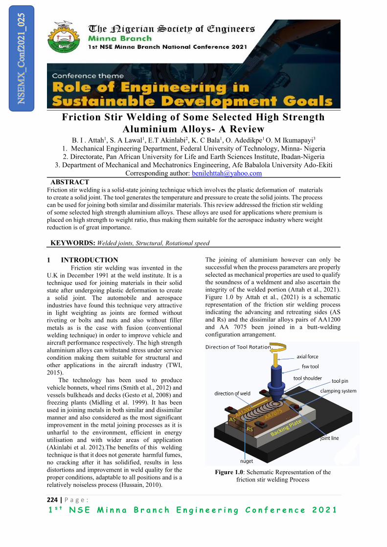
224 | P a g e :


Friction Stir Welding of Some Selected High Strength

Aluminium Alloys- A Review B. I . Attah1, S. A Lawal1, E.T Akinlabi2, K. C Bala1, O. Adedikpe1 O. M Ikumapayi3

1. Mechanical Engineering Department, Federal University of Technology, Minna- Nigeria

2. Directorate, Pan African University for Life and Earth Sciences Institute, Ibadan-Nigeria

3. Department of Mechanical and Mechatronics Engineering, Afe Babalola University Ado-Ekiti

Corresponding author: [email protected]

ABSTRACT Friction stir welding is a solid-state joining technique which involves the plastic deformation of materials

to create a solid joint. The tool generates the temperature and pressure to create the solid joints. The process

can be used for joining both similar and dissimilar materials. This review addressed the friction stir welding

of some selected high strength aluminium alloys. These alloys are used for applications where premium is

placed on high strength to weight ratio, thus making them suitable for the aerospace industry where weight

reduction is of great importance.

KEYWORDS: Welded joints, Structural, Rotational speed

1 INTRODUCTION Friction stir welding was invented in the

U.K in December 1991 at the weld institute. It is a

technique used for joining materials in their solid

state after undergoing plastic deformation to create

a solid joint. The automobile and aerospace

industries have found this technique very attractive

in light weighting as joints are formed without

riveting or bolts and nuts and also without filler

metals as is the case with fusion (conventional

welding technique) in order to improve vehicle and

aircraft performance respectively. The high strength

aluminium alloys can withstand stress under service

condition making them suitable for structural and

other applications in the aircraft industry (TWI,

2015).

The technology has been used to produce

vehicle bonnets, wheel rims (Smith et al., 2012) and

vessels bulkheads and decks (Gesto et al, 2008) and

freezing plants (Midling et al. 1999). It has been

used in joining metals in both similar and dissimilar

manner and also considered as the most significant

improvement in the metal joining processes as it is

unharful to the environment, efficient in energy

utilisation and with wider areas of application

(Akinlabi et al. 2012).The benefits of this welding

technique is that it does not generate harmful fumes,

no cracking after it has solidified, results in less

distortions and improvement in weld quality for the

proper conditions, adaptable to all positions and is a

relatively noiseless process (Hussain, 2010).

The joining of aluminium however can only be

successful when the process parameters are properly

selected as mechanical properties are used to qualify

the soundness of a weldment and also ascertain the

integrity of the welded portion (Attah et al., 2021).

Figure 1.0 by Attah et al., (2021) is a schematic

representation of the friction stir welding process

indicating the advancing and retreating sides (AS

and Rs) and the dissimilar alloys pairs of AA1200

and AA 7075 been joined in a butt-welding

configuration arrangement.

Figure 1.0: Schematic Representation of the

friction stir welding Process


225 | P a g e :


2 OPTIMISATION OF OPERATIONAL

PARAMETERS IN FRICTION STIR

WELDING OF AA7075-T6 ALUMINIUM

ALLOYS USING RESPONSE SURFACE

METHODOLOGY. The welding of AA7075 was conducted by

applying the response surface methodology

approach at five levels of three process variables

(Farazadi et al. 2017). The rotational, welding

speeds and tool diameter were varied from 350-650

rpm, 35-95 mm/min, 12-18 mm tool diameter

respectively and pin length of 4-6 mm and represents

the parameters for consideration.

It was observed that the optimal range of the

process parameters required to produce the joint

with efficiency of 85 % is 380–530 rpm, 90–95

mm/min, 14.2–17.8 and 5–6 mm. It was also

observed that the highest value of 458.9 MPa was

obtained as the UTS when the spindle speed was

varied between 350-500 rpm and at above 500 rpm

it begins to decrease. It was also observed that the

UTS is mostly affected by both the transverse and

rotational speeds as well as pin and shoulder

diameters with welding speed been the major factor

of influence.

2.1 Microstructural Features of Friction stir

Welded dissimilar Aluminium Alloys

AA2219-O - AA7475- T761

Dissimilar welding of the alloys both of plate

thickness 2.5 mm was performed by Noor et al.,

(2018) in butt configuration to examine the effect of

spindle speed on micro-hardness distribution and

microstructure of the dissimilar alloy’s joints. The

process parameters used are tool rotational speeds of

710, 900 and 1120 rpm. The dimensions of the

workpieces are 180 x 50 x 2.5 mm. Micro hardness;

microstructural analysis and optical microscopy

were done on the materials. The softer material AA

2219-O was positioned on the advancing side while

the harder material AA7475 was positioned on the

retreating side; high carbon die steel tool was used

with pin length of 2.2 mm, pin diameter of 4mm and

10mm shoulder diameter. The results showed the

highest value of microhardness of 168.8HV at the

nugget zone at a spindle speed of 1120 rpm on the

retreating side.

The results also revealed that spindle speed

significantly affects hardness due to increase in

grain size, coarsening and dissolution of

strengthening precipitates and re-precipitation. It

was observed that as a result of refined grains at the

stir zone, there was higher micro-hardness value at

the zone. There was proper mixing of the

workpieces (along the stir zone) at both advancing

and retreating sides for all set of chosen parameters.

Microhardness values at the advancing side are

reduced by increase in spindle speed due to

coarsening of grains. At high rotational speeds at

nuggets, precipitates were dissolved and re-

precipitation occurred. Hardness value increased

with increase in rotational speed on retreating side

and decreased on Advancing side.

2.2 Multiscale Electrochemical Study of Welded

Al Alloys Joined by Friction Stir Welding

Dissimilar AA7475-T651 and AA 2024-T3

were butt-joined using friction stir welding by Caio-

Palumbo et al., (2017) and the properties of the joints

were evaluated.

The corrosion behavior of the two alloys was

investigated using global and local electrochemical

methods and SEM analysis before and after

exposure to 0.1 M Na2SO4 + 0.001 M NaCl

solution. Corrosion of the system results from the

attainment of a galvanic coupling in which the

AA7475 acted as anode with regards to the AA2024.

The results of the anodic polarisation curves and of

the global EIS diagrams displayed much lower

corrosion resistance for the FSW affected zones

compared to the two aluminum alloys tested

seperatey. Local pH measurement allowed

demonstration of the location of the enhanced

reactivity for the welded system. 2.3 Effect of process parameters on the tensile

strength of friction stir welded dissimilar

Aluminium Alloy joints

The effects of tool rotational and welding

speeds on the tensile strength of dissimilar weldment

of AA2024-AA7075 joints were examined by

Padmanaban et al. (2017). The two plates each of

size 150 mm x 60 mm x 5 mm were used along with

cylindrical threaded tool, having a shoulder and pin

diameter of 17.5 mm and 5 mm respectively and

height 4.65 mm was used with the tool rotational

speed varied from 900 to 1200 rpm at10-20 mm/min

welding speed, the tensile strength of the weldment

is measured.

Mathematical model was developed for tensile

strength in terms of tool rotational and welding

speed. The results revealed higher tensile strength

226 | P a g e :


for the base metals as compared to that of the

weldment. Lower tensile strength is recorded at low

tool rotational speeds as a result of insufficient heat

required for mixing. It was observed that the tensile

strength increased when the tool spindle speed

increased from 900 rpm to around 1100 rpm. This is

because higher rotational speed generates higher

amount of heat, better material flow and good

mixing. Increasing tool rotational speed above 1100

rpm led to lower tensile strength which may be due

to increase in grain size resulting from grain growth

at higher peak temperature. However, higher tool

spindle speed (beyond 1100 rpm) produces flash and

tunnel defects probably due to stirring effect of the

pin at high speed. Elangovan and Balasubramanian

(2008) obtained a similar result. They reported flash

and tunnel defects at tool rotational speeds above

1100 rpm and can be attributed to increased

turbulence in the weld zone as reported by

Elangovan et al. (2009). It was observed that the

change in tensile strength remains constant

regardless of weld speed and that the joints made at

a tool spindle speed of around 1050 rpm gave the

peak tensile strength for a given weld speed.

It was concluded that both the tool spindle and

travel speeds affect the tensile strength of the

weldment. That tensile strength increases with

increase in tool spindle speed up to a value of 1050

rpm but reduces upon further increase. Also, that the

tensile strength increases with increase in weld

speed up to 15 mm/min and with additional

increment decreased. Surface and contour plots

revealed that when tool travel and spindle speeds are

within 1075 rpm and 1125 rpm, and weld speed are

within 13 mm/min to 15 mm/min that the tensile

strength would be very near to highest.

2.4 Influences of processing parameters on

induced energy, mechanical and corrosion

properties of friction stir welded joints of

AA 7475 Aluminium Alloys

Butt welding was done by Rajesh et al. (2011)

on the alloy plate of 9 mm thickness under the

following parameters: travel speed of 50 mm/min,

spindle speed was varied between 300-100 rpm,

plunge depth of 865 mm, tilt angle of . Tensile,

microhardness and corrosion tests were performed

The result revealed that hardness increases from

base material to a maximum at the stir zone

regardless of the rotational speed due to finer grains.

It was observed that a joint efficiency of 89.5 % can

be obtained from the welding of the alloy. It was also

observed that highest tensile strength of 355 MPa

can be attained at a tool spindle speed of 400 rpm,

and 50 mm/min travel speed. Also, corrosion

resistance from potentiostatic polarisation for both

SZ and TMAZ increase with increase in rotational

speed from 300-1000 rpm with a maximum

corrosion resistance obtained at 1000 rpm and

welding speed of 50 mm/min with the stir zone

having the highest resistance to corrosion.

3 MULTI-OBJECTIVE OPTIMISATION OF

FRICTION STIR WELDING PROCESS

PARAMETERS OF AA6061-T6 AND

AA7075-T6 USING A BIOGEOGRAPHY

BASED OPTIMISATION ALGORITHM In this study by Mehran et al. (2017), dissimilar

welding of the two alloys was conducted on the

weldment in butt configuration with dimensions 100

x 50 x 6 mm. The ultimate tensile strength and

elongation of AA 6061 and AA7075 are 310 MPa,

524 MPa and 12% and 11% respectively as

determined before welding. Experiment was

performed on UTS, % elongation and hardness of

the weldment, the result was employed in

developing a mathematical regression model which

was validated.

Analysis of the experimental data by the

developed model indicates that it can be employed

predicting the stated mechanical properties of the

weldment within 9% of their experimental values at

a 95% confidence limit. They developed a multi

objective optimization algorithm based on two

phases: generation of a Pareto set by MOBBO, and

the use of two different decision-making methods

(Shannon’s entropy and TOPSIS) to achieve the best

compromise solution from the Pareto set.

The result shows that multi-response algorithm

along with mathematical model can be used in

friction stir welding to attain maximum mechanical

properties. The optimal values for spindle and travel

speeds and tilt angle which gave the UTS value of

252.23 MPa, elongation of 8.1% and 72.11 HV were

1002.14 rpm, 149.73 mm/min and 1.92 %

respectively at -0.74 mm tool offset. Setting these

parameters closely within those of theoretical and

milling machine, the experimental values achieved

are 253 MPa, 8.2 % and 71.4 HV respectively.

227 | P a g e :


3.1 Characteristics of AA7075-T6 and

AA6061-T6 Friction Stir Welded Joints

Dissimilar AA7075-T6 and AA6061-T6 were

friction stir welded by Sathish and Vaddi (2015).

The metal is in cylindrical form with a cross section

of 23 mm diameter and 75 mm length. The process

parameter was in three levels and varied from 1000

to 1500rpm at 250rpm interval. Mechanical and

metallographic characterizations were performed on

the weldments. Taguchi method was used for

experimental design.

The result obtained from the experiment gave a

range of values for the ultimate tensile strength as

53-203MPa with the highest elongation of the strain

rate of 11.56 %. It was noticed that increasing the

upset and frictional pressure while decreasing the

spindle speed resulted in better tensile strength and

ductility.

3.2 Mechanical Strength of Dissimilar

AA7075 and AA6061 Aluminium Alloys

Using Friction Stir Welding

Sathari et, al (2015) studied the effects of

material location and tool spindle speed on the

tensile strength of the dissimilar weldment with

dimensions 100 x 50 x 2 mm. The tool rotational

speeds were varied from 800-1400 rpm while

welding speed and tilt angle were kept fixed at 100

mm/min and 3 respectively and by changing the

fixed position of the material on the advancing and

retreating sides. A total of 10 weldment were made.

From the result, a maximum value 207 MPa was

obtained as tensile strength when AA6061 alloys

were positioned on the advancing side at a spindle

speed of 1000 rpm with good surface features and

non-defective internally across the weld area, while

the least tensile strength of 160 MPa was attained

when AA6061 was located on the retreating side

with accute tunnel defects across the weld area

leading to crack propagation.

3.3 Experimental Study and Analysis of the

Wear Properties of Friction-Stir-Welded

AA7075-T6 and A384.0-T6 Dissimilar

Aluminium Alloys of Butt Joints

The workpieces with dimensions 100 x 50 x

6.35 mm were joined by Karruppannan et al.,

(2017). The ultimate tensile strengths of the joints

were tested to obtain their highest and a lowest level

of these specimens and wear analysis was conducted

on them. Their results were compared with the wear

resistance of the parent metals. Before obtaining the

results, the tool rotational speed, time and weld

speed were held constant at 500 rpm, 300s and

3.141m/s respectively while the applied load was

varied as 20, 40 and 60 N.

Wear analysis was conducted and 92 and 35.8

HRB were respectively obtained as hardness for

AA7075 and A384.0 while for wear rate, A384.0

was higher and those for the weldment were within

the wear rate values of the base metals. The hardness

of the weldment was between 35.8 and 92 HRB.

They concluded that the hardness of materials and

the level of wear are inter-related parameters.

3.4 Optimization of the friction-stir-welding

process and tool parameters to attain a

maximum tensile strength of AA7075–T6

aluminium alloy

Welding was done in a butt joint arrangement

using 300 mm x 150 mm x 5 mm thick plate to

derive a relationship empirically between the

friction stir welding process and tool variables

(spindle and travel speeds, axial load, shoulder and

pin diameters, and hardness of the tool) and the

joints tensile strength. Empirical relationship was

developed using experimental design, ANOVA, and

regression analysis. The developed model was

applied in predicting the tensile strength of the

weldment confidently at 95% limit, employing

friction stir welding process and tool variables.

Highest tensile strength of 375 MPa was

recorded by the weldment produced with the

optimised conditions of 1438 rpm, 67.64mm/min,

8.29 kN axial load, shoulder and pin diameters of

15.54 and 5.13 mm, and tool material hardness of

600 HV. It was concluded that higher sensitivity was

displayed by rotational speed compared to other

variables followed by travel speed then others.

Rajkumar et al. (2010).

3.5 Study on mechanical, macro and

microstructural characteristics of friction

stir welding of AA7075-T6 to AA6061-T6

aluminium alloys

Dissimilar joining of the alloys both of 5mm

thick plates was done in a butt arrangement by Pouya

et al. (2010). Welding was done at travel speeds of

80,100, 120 and 60 mm/min. The rotational speed

and tilt angle were fixed at 900 rpm. Temperature

readings were taken at 5mm apart and range of 10-

228 | P a g e :


30mm from the 7075 side. Harness and tensile

strength of the weldment were investigated.

The result revealed a steady increase in tensile

strength while increasing the travel speed to a level

and then starts declining. 255 MPa was obtained for

UTS at peak value at travel speed of 120 mm/min

and thereafter begins to decrease while the hardness

increased with increase in travel speed and the

highest value obtained at around 127 HV at 160

mm/min travel speed.

Conclusion In conclusion, a review of friction stir welding

of some selected high strength aluminium alloys has

been undertaken. This review has shown that

significant progress has been made in both similar

and dissimilar welding using friction stir welding

process. Most of the cited literature were directed at

understanding the appropriate process parameters,

Mechanical and microstructural properties as well as

microstructure and corrosion characteristics of the

weldment. The knowledge of friction stir welding

technology can be utilised in fabricating joints of

both similar and dissimilar materials in order to

maximize their benefits and minimize their

drawbacks. The technology is suitable for aerospace,

railway and electrical industries amongst others.

ACKNOWLEDGEMENTS

The authors’ wishes to acknowledge the assistance

given by Prof. E.T Akinlabi, Director Pan African University for Life and Earth Sciences Institute

(PAULESI) Ibadan Nigeria and Engr. Dr. Joshua

Attah of National Universities commission Abuja,

Nigeria to embark on a research visit to the Indian

Institute of Technology, Kharagpur India to conduct

experiments on dissimilar friction stir welding. The

support received from Prof. S.K Pal, Chairman and

Professor in charge of friction stir welding research

laboratory of the Indian Institute of Technology

Kharagpur is also acknowledged.

REFERENCES

Akinlabi, E.T., Annelize, E & Patrick, J. M

(2012). Effect of Travel speed on Joint Properties

of Dissimilar Metal Friction Stir Welds. Second

International Conference on Advances in

Engineering and Technology

Attah, B.I., Lawal, S.A., E.T Akinlabi & K. C Bala

(2021) Evaluation of mechanical properties of

dissimilar aluminium alloys during friction stir

welding using tapered tool. Volume 8 issue

1:1909520.

https://doi.org/10.108023311916.2021.1909520

Caio Palumbo D. A., Isolda Costa., Hercilio Gomes

D. M, Nadine, P., Bernard T. and Vincent, V.

(2017). Multiscale Electrochemical Study of

Welded Aluminium Alloys Joined by Friction

Stir Welding. HAL Achievers- ouvertes HAL Id:

hal 01611642

https://hal.sorbonneuniversite.fr/hal-01611642.

Divya, D. D., Anuj. S, & Charit, V. (2014):

Optimisation of Friction Stir Welding

Parameters for AA 6061 and AA 703 Aluminium

Alloys by

Response Surface Methodology (RSM).

International Journal of Advanced Mechanical

Engineering. ISSN 2250-3234 Volume 4,

Number5 (2014), pp. 565-571 © Research India

Publications http://www.ripublication.com

Elangovan, K.; & Balasubramanian, V. (2008).

Influences of tool pin profile and welding speed on

the formation of friction stir processing zone in

AA2219 aluminium alloy. Journal of Materials

Processing Technology, 200(1-3), 163175.

Elangovan, K.; Balasubramanian, V.; & Babu, S.

(2009). Predicting tensile strength of friction stir

welded AA6061 aluminium alloy joints by a

mathematical model. Materials & Design, 30(1),

188-193.

Farzadi1, A., Bahmani, M. & Haghshenas, D.F

(2017). Optimisation of Operational Parameters

in Friction Stir Welding of AA7075-T6

Aluminium Alloys Using Response Surface

Methodology. Arab Journal of Science and

Engineering 42:4905 4916 DOI

10.1007/s13369-0172741-6.

Gesto, D., Pintos, .V., Vazquez, .J. Rasilla J., &

Barreras, S. (2008). Application of Friction stir

welding in ship building. Proceedings of TWI,s

7th Int. Sympsium on Friction stir welding', May

4th-7th 2008, Awaji Island, Japan.

Hussain, A.K. (2000). Evaluation of parameters of

friction stir welding for aluminium

AA6351Alloy, International journal of

engineering science and technology,

2(10),59775984.

Mehran, T., Hang, B. T., Baharudin, T., Shahla, P.,

Khamirul, A. M.,Shamsuddin, S & Firouz,

https://hal.sorbonneuniversite.fr/hal-01611642

http://www.ripublication.com/

229 | P a g e :


F.(2017). Multi-Objective Optimisation of

Friction Stir Welding Process Parameters of

AA6061-T6 & AA7075-T6 Using a

Biogeography Based Optimisation Algorithm

Midling, O. T., Kvåle, J. S. & Dahl, O. (1999).

Industrialisation of the Friction Stir Welding

Technology in Panels Production for the

Maritime Sector. Proceedings of TWI 1st

International Symposium on 'Friction stir

welding', June 2nd- 5th 1999, Thousand Oaks,

CA, USA.

Noor, Z. K., Mohammed, U., Arshad, N. S., Zahid,

A. K.., Abdulrahman, A. A, Xizhang, C &

Mustufa, H. A . (2018) :Microstructural Features

Of Friction Stir Welded Dissimilar Aluminium

Alloys Aa2219 AA7475. Journal of material

research express Vol (5)

https://doi.org/10.1088/2053-1591/aac4e1.

Pouya, B., Mohammad, H., Mohammad, K. B. G &

Sahand, A. (2010). Study on mechanical, macro

and microstructural characteristics of friction stir

welding of AA7075-T6 to AA6061-T6

aluminium alloys . Proceedings of the Institution

of Mechanical Engineers part B journal of

Engineering Manufacture 1:1-12. DOI:

10.1243/09544054JEM1959

Rajkumar, S., Muralidharan, C & Balasubramanian,

V. (2010). Optimisation of the friction-stir

Welding process and tool parameters to attain a

maximum tensile strength of AA707-T6

aluminium alloy. Proceedings of the Institution

of Mechanical Engineers part B journal of

Engineering Manufacture 1:1-12. DOI:

10.1243/09544054JEM1959

Rajesh, K .G., Hrishikesh D., & Tapan K. P. (2012)

Influence of Processing Parameters on Induced

Energy, Mechanical and Corrosion Properties of

FSW Butt Joint of 7475 AA. Journal of

Materials Engineering Performance 21:1645–

1654 _ASM International. DOI:

10.1007/s11665-011-0074-21

Karruppanan, A., Subramaniam, P & Mayakrishnan,

M (2017) Experimental Study and Analysis of

the Wear Properties of Friction-Stir-Welded

AA7075-T6 and A384.0-T6 Dissimilar

Aluminium Alloys of Butt Joints. UDK

620.1:620.178.16:669.715

Sathish R & Vaddi S. R. (2014). Characteristics Of

AA7075-T6 and AA6061-T6 Friction Welded

Joints. Transactions of the Canadian Society for

Mechanical Engineering, Vol. 39, No. 4, 2015

Smith, C. B,, Hinrichs, J. F., & Ruehl, P. C. (2012).

Friction Stir and Friction Stir Spot Welding –

Lean, Mean and Green. Retrieved on October 20

2017 from:

www.frictionstirlink/Pub14AwssmcLeanMean

Geen-UnitedStates

TWI, (2015). What is welding? Definition,

processes and types of welds. Retrieved on 25th

March, 2021 from www.twi-global.com.

Padmanaban, R.V., Balusamy, V. & Nouranga, K..

N.( 2015): Effect of Process Parameters on the

tensile strength of friction stir welded dissimilar

aluminum joints. Journal of Engineering Science

and Technology Vol. 10, No. 6. 790 – 801 ©

School of Engineering, Taylor’s University

https://doi.org/10.1088/2053-1591/aac4e1

http://www.frictionstirlink/Pub14AwssmcLeanMeanGeen-UnitedStates

http://www.frictionstirlink/Pub14AwssmcLeanMeanGeen-UnitedStates

http://www.twi-global.com/

230 | P a g e :


The Failure Analysis in Steel Reinforced Beams with different

Reinforcement Ratio *Ayandokun W. A1, Balogun B. T1, and Abdulrahman A. S2

1Department of Mechanical Engineering, 2Department of Materials and Metallurgical Engineering

Federal University of Technology, Minna.

*08030999791, [email protected]

ABSTRACT This research paper presents the failure analysis in reinforced steel concrete through experimental investigation. The

experiment set-up used the flexural cracks in strainedsamples of steel reinforced beams in separate three (3) plains and three

(3) reinforced steel concretes with reinforcement ratio 0.12% and theeffects was investigated and analyzed through the

crack behaviours in fracture mode. The samples were loaded with two applied forces in one third of the length. The loading

by force displacement allowed reducing the failure and observing the development of the crack using controlled hydraulic

jacks and gauges. The compressive strength and young’s modulus were tested on reinforced concrete with cylinders of 150

mm diameter and height of 300 mm, and the average values recorded were 20.4 and 22,118 MPa respectively. The strength

(tensile)was tested on mode of cubes with length (150 mm), breadth (150 mm) and height (150 mm) at a separate test and

average value recorded was 1.64 MPa while the corresponding tensile strength (axial) was recorded as 1.48 MPa. The

average cracking moment was 5.08 kNm in plain and 5.39 kNm in reinforced steel concretes. The experimented sample

beams of differential ratio of 0.6% failed at the applied load of 44 kN and the maximum bending moment reached was 4.07

kNm. The experimental results recorded in the reinforced beam of ratio 1.5%, the shear force of cracking experienced was

recorded as 4.2 kN, but the maximum shear force reached was higher at 5.14 kN. Whereas in the sample reinforced beam

of ratio 2.1%, the shear force of cracking experienced was recorded as 5.07 kN and the maximum shear force reached was

5. 96kN.Conclusively, the inference observed that the maximum shear forces reached were numerically advantage to

cracking forces (shear). Hence, the inclined effect crack behaviours did not occur rapidly but influenced by tensile strain,

elongation, deformation mechanics, impact, and reinforcementstiffness.

KEYWORDS: Failure analysis; Flexural crack; Reinforcement ratio; Reinforced steel.

1 INTRODUCTION With a long history of technical development

behind it, the steel industry is firmly established as a

heavy reliable industrial product of great utility.

However, the diversity in today’s society and

economy leads to continuity demand for steel, better

performance, and for novel design features in

building constructions. This in turn presents new

technical research into the load capacity of building

structures supported by reinforced steels, tends to be

defected through the deformation behaviour of

reinforced beams. Most researches proved that the

compressive test (strength) of reinforced beams are

usually varies from 17 to 28 MPa and higher in

residential and commercial structures,(about 10

times)higher than its tensile strength around 2 to 5

MPa. This means, an average, the tension averages

about10% of the compressive strength (Ajagbe et

al., 2018). Though, concrete belongs to the

composite regarded as brittle but it isimperfection in

nature (quasi-brittle). Two major parameters are

required to analyze the effects of quasi-brittle nature

of concrete on cracking. These are referred to as

tensile strength and tensile toughness (Abdullahi,

2012). In a course to measure the effect of tensile

toughness in concrete, fracture energyapplication

tends to be analyzed (Akinleye and Tijani, 2017).

Moreover, the characteristics of fracture toughness

in reinforced beams application have no direct

impact tothe conventional design of structures,

while considering the British standards, (BSI, 2009).

This research paper highlights failure

investigation of reinforced steel with different

reinforcement ratio through most of the reinforced

materials formed and contributed to the initiation of

cracks in a flexure. Nonetheless, it can either be in

plain or reinforced beams which are of great

importance to analysis the effect of failure in crack

propagation.A stable propagation of several flexural

cracks is develop in moderately reinforced concrete

beams, and the load carrying capability is supported

with reaching the yield stress of reinforcing steel in


231 | P a g e :


the compression zone. In advanced set-up of

reinforced concrete beams without transverse

reinforcement, brittle failure can easily occur due to

shear forces and the development of diagonal cracks

(Alaneme et al., 2019). From structural appearance,

consideration should be given to the sampled steel

reinforced beams when investigated, brittle failure

due to occur when the martensiticrepeated bending

stress which must be stable by the reinforced beams.

It is possible for overload fractures to occur when

the excessive loads being applied (Das et al., 2014).

Since a fatigue fracture is progressive in

reinforced beams, all types of contaminants

developing over a long period of time, the fracture

surface usually shows characteristic "beach"

markings. In this case the fracture showed

discontinuity on the surface and, proceeded nearly

across the section before final separation. Fatigue

fractures initiate in shear by a mechanism involving

slip and work hardening, eventually forming

microscopic discontinuities which develop into

cracks (Hari and Moga, 2009).

Once a crack is formed, its rate of growth

depends upon the stress magnitude, stress gradient,

endurance limit of the material, notch sensitivity,

and the presence or absence of structural flaws and

inclusions. After the crack has formed, the stress is

reduced to below the value necessary to initiate it,

the crack may not propagate any further. This is

probably caused by an increase in strength due to

strain hardening at the crack tip. If the applied load

is large enough, the crack will advance

perpendicular to the maximum tensile stress. They

indicate the position of root of the advancing crack

at weakens; the crack grows faster, apart, larger, and

more distinct. Therefore, specifications and control

measures require when these markings are plenty,

they provide a means of locating the origin of

fracture (Taber et al., 2002). When reinforcing steel

bars are not designed properly, the structure

willcrack and eventually fail (Xiaoke et al., 2020).

The failure behaviour of cracks in concrete has

demonstrated the need for a better understanding of

the mechanisms of fracture in reinforced steel

concretes under flexure. Series of researchers

worked over the past decades have led to the

evolution of the field of the steel reinforcement in

concretes. This subject proved series of numerical

analysis on quantification of the relationship

between the properties of the materials such as

stress, crack-producing flaws and crack propagation

(Fernandez et al., 2016). The design engineers

should be better equipped to perform and thus

prevent structural failures (Fernandez et al., 2018).

As a result of this, failure analysis can focus on

increases in deflections, determination of the

location, type, and source of the crack-initiating

flaw. Also, reduction of bearing capacity, which is

normally a part of analysis, involvesexamining the

path of crack propagation as well as microscopic

features of the fracture surface in relation to

transverse reinforcement and, eventually cyclic

stresses such axial (tension-compression), flexural

(bending), or torsional (twisting) in nature.

2 FAILURE ANALYSIS OF PLAIN

AND REINFORCED STEEL

CONCRETES

2.1 PLAIN CONCRETE AND

REINFORCED STEEL CONCRETE A series of earlier set of the technological tests

proved that buildup to failure effect parameters

include specimen fabrication and surface

preparation, metallurgical variables, specimen

alignment, mean stress, and test frequency,

especially inslightly reinforced steel concretes.

These techniques have been developedto specify the

structures of plain and reinforced concretes in terms

of crack initiations and propagations, at a maximum

stress expecting 0.12% of the reinforcement ratio.

The sample structures wereclassified into two

categories, one is associated with plain concretes,

that produce not only elastic strain but also some

plastic strain during failure.For the other category,

reinforced steel concrete wherein deformation are

totally elastic, longer lives results in as much as

relatively large numbers of cracks were appeared to

cause failure.The loading as a result of statistical

treatment were based on fatigue life and fatigue

limits.

Consequently, sample structures set up by

aggregate composite of cement, sand, steel bars and

required water for the 40mm dimension mould

loaded with two bearing forces appliedfrom bottom

to top at about 33% of the length. The standard

methods employed to test the basic concrete

properties throughforce displacement using jacks

and gauges.

The compressive strength and young’s modulus

were tested on reinforced concrete with cylinders of

232 | P a g e :


150 mm diameter and height of 300 mm, and the

average values recorded were 20.4 and 22,118 MPa

respectively. The stress (tensile) was tested on mode

of cubes with length (150 mm), breadth (150 mm)

and height (150 mm) at a separate test and average

value recorded was 1.64 MPa while the

corresponding tensile strength (tension-

compression) was recorded as 1.48 MPa and the

yield stress was 275 MPa. The average cracking

moment was 5.08 kNm in plain and 5.39 kNm in

reinforced steel concretes. The experimented sample

beams of reinforcement ratio of 0.6% failed at the

applied load of 44 kN and the maximum bending

moment reached was 4.07 kNm. The experimental

results recorded in the reinforced beam of ratio

1.5%, the shear force of cracking experienced was

recorded as 4.2 kN, but the maximum shear force

reached was higher at 5.14 kN. Whereas in the

sample reinforced beam of ratio 2.1%, the shear

force of cracking experienced was recorded as 5.07

kN and the maximum shear force reached was 5.96

kN. Location of steel bars is presented in Figure 1.

Figure 1: Location of Reinforcement on the

reinforced steel concrete

A brittle character of failure was observed in all

tested reinforced concretes during the experiment,

but size elongation in failure process were noticed

and a higher cracking resistance was obtained in

reinforced steel concretes in comparison to that

measured in plain concrete samples. In plain

concrete sample, a brittle and sudden failure was

noticed right after the appearance of the first flexural

crack. In reinforced steel concrete sample of the

reinforcement ratio 0.12%, the failure was also

caused by the main flexural crack but the concretes’

damage was noticed at higher load level than in plain

concrete samples. The failure crack did not occur as

rapidly as in concretes, and the destructive process

in reinforced steel concretes continued developing

two or three cracks as is presented in Figure 2 and 3.

Figure 2 The location of cracks in plain concretes

Figure 3 The location of cracks in slightly

reinforced steel concretes

F

A1

F

F

A2

F

F

A3

F

F

B1

F

F

B2

F

F

B3

F

3000

2700

2700

A

2700

A

233 | P a g e :


2.2 BENDING MOMENTS Cranks in fracture behaviour of materials can be

determined using bending momenttechniques. On

the basis of the fracture surface, it is possible to

ascertain whether or not a material experiences a

ductile to brittle transition and the elongation range

over which such a transition occurs. The calculated

mean values of cracking moments were 5.08 kNm in

plain concrete and 5.39 kNm in reinforced steel

concrete samples

The need often arises for engineering fracture

energy data that are practical to collect from normal

laboratory tests to be input into the formula. This is

true for prolonged exposure tests in excess of the

requirements, for shorter time periods and at a

comparable stress level, and then making a suitable

to the service condition. Hence, the situation of

cracking moment affects the load capacity of plain

and reinforced steel concrete appeared to be higher

in both cases than the theoretical cracking moment

(BSI, 2009).

Crack’s initiation exists in micro-cracks start to

grow into nucleated coalescence. For the fracture

energy, the energy absorbed per unit crack area

during crack’s formation. Fracture energy

relationship is due to the area under the stress crack

opening curve σ – w (Slowik and Blazik-Borowa,

2011). In the process of this, the normal stress

distribution in the fracture obtained in the plain

concrete as presented in Table 2 and figure 4.

𝐺𝐹 = ∫ 𝜔l𝜎𝜕𝜔 (1)

TABLE 1: GAUGE READINGS FOR THE

PLAIN AND REINFORCED STEEL

CONCRETES

Gauge

Readings

(kN)

1 2 3 Average

Plain

concrete

(A)

5.10 5.51 4.45 5.02

Reinforced

steel

concrete

(B)

5.59 5.44 5.21 5.41

TABLE 2: THE DISTRIBUTION OF NORMAL

STRESS IN THE FRACTURE PROCESS ZONE

OF PLAIN CONCRETE Load

(kN)

Reinforcement Ratio (%)

1.0 1.9 3.1 4.0 4.96 5.19

0.03 -2650

-2300

-1800

-1400

-900 -600

0.06 -

1800

-

1700

-

1300

-

1000

-700 -

400 0.09 -

1100

-

1100

-900 -700 -450 -

300

0.12 -400 -500 -400 400 -300 -200

0.15 400 400 0 0 0 0

0.18 1400 900 500 300 200 100 0.21 1300 1500 1000 700 500 300

0.24 1100 1300 1500 1100 700 500

0.27 800 1200 1400 1400 900 600 0.30 700 1100 1300 1500 1100 700

The distribution of normal stress in the fracture

process zone was obtained in the reinforced steel

concrete with reinforcement ratio 0.12% in the

following steps of loading as shown in figure 4 and

5.

Figure 4: Normal stress distribution in concrete

in the fracture process zone in plain concrete beam

TABLE 3: THE DISTRIBUTION OF NORMAL

STRESS IN THE FRACTURE PROCESS ZONE

OF REINFORCED STEEL CONCRETE Load (kN)

Reinforcement Ratio (%)

0.9 2.15 3.95 5.15 6.65 8.45

0.03 -3800

--

2900 -2300 -1800 -1000 -500 0.06 -2800 -2100 -1600 -1300 -800 -400

0.09 -1700 -1400 -1000 -400 -500 -300

0.12 -600 -600 -500 - -400 -200 0.15 700 0 0 0 0 0

0.18 1400 1100 600 400 200 100

0.21 1200 1500 1100 900 500 400 0.24 950 1400 1300 1500 800 500

0.27 1100 1400 1300 1000 1000 600

0.30 500 1200 1000 1300 1200 700

-6000

-4000

-2000

0

2000

1 2 3 4 5 6 7 8 9 10

Stre

ss in

kN

deflection in mm

0.95 kN

2.15kN

3.95kN

5.15kN

6.65kN

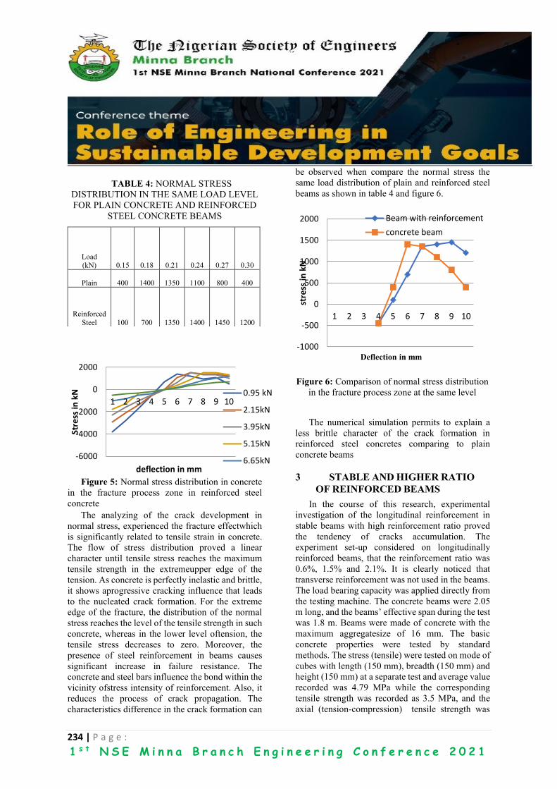
234 | P a g e :


TABLE 4: NORMAL STRESS

DISTRIBUTION IN THE SAME LOAD LEVEL

FOR PLAIN CONCRETE AND REINFORCED

STEEL CONCRETE BEAMS

Figure 5: Normal stress distribution in concrete

in the fracture process zone in reinforced steel

concrete

The analyzing of the crack development in

normal stress, experienced the fracture effectwhich

is significantly related to tensile strain in concrete.

The flow of stress distribution proved a linear

character until tensile stress reaches the maximum

tensile strength in the extremeupper edge of the

tension. As concrete is perfectly inelastic and brittle,

it shows aprogressive cracking influence that leads

to the nucleated crack formation. For the extreme

edge of the fracture, the distribution of the normal

stress reaches the level of the tensile strength in such

concrete, whereas in the lower level oftension, the

tensile stress decreases to zero. Moreover, the

presence of steel reinforcement in beams causes

significant increase in failure resistance. The

concrete and steel bars influence the bond within the

vicinity ofstress intensity of reinforcement. Also, it

reduces the process of crack propagation. The

characteristics difference in the crack formation can

be observed when compare the normal stress the

same load distribution of plain and reinforced steel

beams as shown in table 4 and figure 6.

Figure 6: Comparison of normal stress distribution

in the fracture process zone at the same level

The numerical simulation permits to explain a

less brittle character of the crack formation in

reinforced steel concretes comparing to plain

concrete beams

3 STABLE AND HIGHER RATIO

OF REINFORCED BEAMS

In the course of this research, experimental

investigation of the longitudinal reinforcement in

stable beams with high reinforcement ratio proved

the tendency of cracks accumulation. The

experiment set-up considered on longitudinally

reinforced beams, that the reinforcement ratio was

0.6%, 1.5% and 2.1%. It is clearly noticed that

transverse reinforcement was not used in the beams.

The load bearing capacity was applied directly from

the testing machine. The concrete beams were 2.05

m long, and the beams’ effective span during the test

was 1.8 m. Beams were made of concrete with the

maximum aggregatesize of 16 mm. The basic

concrete properties were tested by standard

methods. The stress (tensile) were tested on mode of

cubes with length (150 mm), breadth (150 mm) and

height (150 mm) at a separate test and average value

recorded was 4.79 MPa while the corresponding

tensile strength was recorded as 3.5 MPa, and the

axial (tension-compression) tensile strength was

-1000

-500

0

500

1000

1500

2000

1 2 3 4 5 6 7 8 9 10

stre

ss in

kN

Deflection in mm

Beam with reinforcement

concrete beam

Load (kN) 0.15 0.18 0.21 0.24 0.27 0.30

Plain 400 1400 1350 1100 800 400

Reinforced

Steel 100 700 1350 1400 1450 1200

-6000

-4000

-2000

0

2000

1 2 3 4 5 6 7 8 9 10

Stre

ss in

kN

deflection in mm

0.95 kN

2.15kN

3.95kN

5.15kN

6.65kN

235 | P a g e :


calculated as 3.15 MPa. The young’s modulus was

measured on to be 41400 MPa. As a longitudinal

reinforcement, steel bars of the diameter 12 mm

were used. The characteristic yield stress of steel

bars was 460 MPa.

From the analysis of the sample structures, the

initiation of cracks at similar load level in the mid-

span fracture, and propagated into the transverse

direction. Consequently, the increment in load

applied caused the corresponding increased in

flexural cracks within the structures. But, the effect

of the cracks was more significant toward the

supports. It can be deduced that the resulted vertical

cracks became wider and deeper. Moreover, with the

increase in applied loads, the resulted vertical cracks

also moved toward the edge of the supports and tend

to change their orientations. It finally becomes the

inclined failure cracks (Ferreira et al., 2013). The

reinforcement ratio determines the distribution,

number of cracks and their width as well as length,

which varied accordingly. The distribution cracks is

as presented in Figure 7.

Figure 7: The Failure crack distribution in the

beams

In most cases, the reinforcement ratios depend

on different levels of failures when observing the

tested beams. The procedure to be followed in the

preparation of a specimen is comparatively simple

and involves a technique which is developed only

after constant practice. The ultimate objective is to

produce a stable growth of resulted cracks from the

moderately reinforced concrete beam of

reinforcement ratio 0.6%. If a failure is to be

investigated, the sample should be close as possible

to the area of failure and compared with one taken

from the normal section, which prevented against a

sudden failure. The developments of flexural cracks

were noticed, and the failure from the flexure then

confirmed. The specimen beam failed and recorded

the value of the applied load as 9.04 kN.

Numerically, its maximum bending moment

recorded was 4.11 kNm.

In furtherance of the research, the specimen

reinforced steel beams of 1.5% and 2.1% while

reinforcement ratios were being considered, after

nucleated flexural crack formation. Also, the

resulted diagonal crack propagated in the support

area of the specimen beams. Under certain

circumstances, the resulted diagonal crack formed

from the flexural crack was due to stresses (shear)

that change its orientation and eventually become a

diagonal crack. Although in principle, the specimen

beams tend to not use the transverse reinforcement,

since the propagation of inclined cracks through the

shear, caused brittle failure. Instantly, the failures of

the specimen beams occur after the formation of the

diagonal crack. The various shear forces controlled

the failure in sample reinforced beams, with the

utmost flexural capacity due to the inability of

achieving the required longitudinal reinforcement.

When it is increased, the reinforcement ratios cause

the corresponding increase in failure cracking of

shear force. In many cases, particularly appearance

of diagonal crack and maximum shear force at

failure cracking were observed. From the

application of specimen beam of reinforcement ratio

1.5%, the cracking shear forces was 4.11 kN and the

maximum shear force was 5.14 kN. While,

considering the specimen beam of reinforcement

ratio 2.1%, the cracking shear force was 5.07 kN and

the maximum shear force recorded as 5.96 kN. The

most commonly observed from the results of this

research showed that maximum shear forces were

numerically higher to the cracking shear forces.

Therefore, the process of failure propagated by

resulted inclined cracks did not show in a rapid way.

This analysis, fortunately, is the failure process

of cracking in the beams. From the properties, this

0.9%

1.3%

1.8%

236 | P a g e :


can be concluded that the development of the

flexural cracks were somehow slow as observed to

the zone of crack failure in uniformly reinforced

steel concretes. Hence, in highly reinforced

specimen, diagonal cracks appear after the

stabilization of flexural cracking. The start up of

inclined cracks is affected by strained tensile

concrete, but in the accumulation of nucleated

diagonal cracks such procedures as an aggregate

interlock. Consider the steel bars, appearance is

predominating. From the description of this, the

increase in the capacity of shear stress results in

corresponding increase in reinforcement ratio. The

results are importantly to show that more crack

failure in shear transfer formed in highly reinforced

steel concrete beam (Abdullahi, 2012; ASTM,

1997).

4 CONCLUSIONS The effect of failure cracks of steel reinforced

concrete beams in relation to different reinforcement

ratio changes accordingly in terms of longitudinal

reinforcement ratio:

Flexural strength reached its full capacity with

the bearing capacity, and improves on steel yielding

through the axial stress in the zone.

The propagation of the failure crack with the

applied bearing capacity do follow the process of an

aggregate interlock of steels.

The analyzed results proved that transverse

reinforcement do play a major role in reducing shear

failure (brittle), when considering concrete beams

with high longitudinal reinforcement ratio.

5 ACKNOWLEDGEMENTS The authors acknowledged the support from

Engr Prof. Oguntola O..J of Osun state University,

Osogbo for the provision of materials used for the

research.

REFERENCES Abdullahi M. (2012). “The effect of aggregate type

on compressive strength of concrete”.

International Journal of civil and structural

engineering, 2(3).

Ajagbe O. W., Tijani A. M., and Agbede O. A.

(2018). “Comprehensive strength of concrete

made from aggregate of different sources”,

Journal of research information in civil

engineering, 5(1).

Akinleye M. T., and Tijani M. A. (2017).

“Assessment of quality of Asphalt concrete used

in road construction in southwest Nigeria”,

Nigeria Journal of Technological Development,

14(2).

Alaneme K. K., Fajemisin A. V., and Maledi B. N.,

(2019). “Development of Aluminum-based

composite reinforced with steel and graphite

particles, Structural, Mechanical and Wear

characterization”, Journal of material research

and technology, 8(1), 670-682.

ASTM A944-95, “Standard Test Method for

Comparing Bond Strength of Steel Reinforcing

Bars to Concrete Using Beam-End Specimens,”

1997 Annual Book of ASTM Standards, Vol.

1.04, American Society for Testing and

Materials, West Conshohocken, PA. 1997, pp.

514-517.

British Standards Institution (2009). “Testing

hardened concrete; compressive strength of test

specimens BS EN 12390 parts”, London, Uk.

Fernandez I., Herrador M. F., Mari A. R., and Bairan

J. M., (2016). “Structural effects of steel

reinforcement corrosion on statically

indeterminate reinforced concrete members”,

Journal of Materials and structures, 49(12).

Fernandez I., Herrador M. F., Mari A. R., and Bairan

J. M., (2018). “Ultimate capacity of corroded

statically indeterminate reinforced concrete

members”, International Journal of concrete,

Structures and Materials, 12(75).

Ferreira D., Bairán J., Marí A., and Faria R., (2013).

“Nonlinear analysis of RC beams using a hybrid

shear-flexural fibre beam model”. Engineering

and Computer 31:1444–1483. doi: 10.1108/EC-

04-2013-0114

Hari W., and Moga N., (2009). “Bending of

reinforcing bars testing methods and influence

on structures”. International Journal of

Structural Engineering.

MacGregor, J. (1997). “Reinforced Concrete”.

Mechanics and Design, 3rd Ed., Prentice Hall,

1997.

Malumbela G., Alexander M., and Moyo P. (2009).

“Steel corrosion on RC structures under

237 | P a g e :


sustained service loads — A critical review”.

Engineering Structures, 31:2518–2525. doi:

10.1016/j.engstruct.2009.07.016.

Shivayya M., and Bhavi I. G., (2015).

“Experimental and Finite element analysis of

bending strength of various structural cross

sections of conventional and composite”,

Material science, 4(4).

SlowikM.,andBlazik-Borowa E.,(2011).

“Numerical study of fracture process zone width

in concrete members”,Journal of Architecture,

civil engineering and environmental, 2, 73-78

Slowik M., (2014). “Shear failure mechanism in

concrete beams”, Journal of Process, and

Material sciences, 3, 1977-1982

Souvik D., Jitendra M. Tanmay B., and Sandip B.,

(2014). “Failure analysis of re-bars during

bending operations”, Case study in Engineering

Failure Analysis, 2, 51-53.

Taber L. H., Belarbi A., and Richardson D. N.,

(2002). “Effect of reforcing bar contamination on

steel-concrete bond during concrete

construction”, Journal of Performance of

constructed facilities, 24(3).

Tribune 14 May 2012, News Headline, Building

collapse, COREN proposes death penalty for

perpetrator, http//:www.tribunenews.ng

Xiaoke L., Songwie P., Kunpeng F., Habin G., and

Fenglan L., (2020). “Bending performance of

steel fibre reinforced concrete beams based on

composite-recycled aggregate and matched with

500 MPa Rebars”, Materials science, 13, 930.

238 | P a g e :


Oxidative Stability and Cold Flow Properties of Non-Edible

Vegetable Oil for Industrial Biolubricant Applications *Timothy Yakubu Woma1,2, Sunday Albert Lawal,1 Asipita Salawu Abdulrahman,3 M.A. Olutoye,4 and

A.A. Abdullahi,1

1. Department of Mechanical Engineering,

3. Department of Metallurgical and Materials Engineering,

4. Department of Chemical Engineering,

Federal University of Technology Minna P.M.B 65 Minna, Niger State, Nigeria

2. Department of Physics, Federal University Wukari, P.M.B 1020 Wukari, Taraba State, Nigeria

ABSTRACT The use of mineral oil-based lubricants is attracting increasing environmental concern. Additionally, mineral

oil is nonrenewable and subject to high price fluctuation. There is therefore a need to seek alternative

sustainable and renewable lubricant base stock. Vegetable oil are thought of as good substitute for mineral oil

-based lubricants, but their use suffers setback due to their poor cold flow characteristics and thermo-oxidative

instability. The oxidative stability, flash point and cold flow behaviour of castor oil were measured and

compared to commercially available mineral oil -based lubricant SAE 20/W50. The castor oil had peroxide

value of 8.92 meq/kg, flash point of 2820C, cloud point of -12.40C and pour point of 23.20C. The commercially

available mineral oil- based lubricant SAE 20/W50 had peroxide value of 0.99 meq/kg, flash point of 2550C,

cloud-point temperature of -18.90C and pour-point temperature of 24.10C. The castor oil has poor oxidative

stability but excellent fire safety and cold flow properties. The - castor oil is a good sustainable and renewable

alternative to petroleum oil -based lubricant, however its oxidative stability needs to be improved to increase

its shelf life and service life as a lubricant.

KEYWORDS: Biolubricant, castor oil, cold flow, flash point, Peroxide.

1 INTRODUCTION Virtually every industry consumes lubricating

solids, oils or gases. Within the last decade the

annual worldwide consumption of lubricants is over

40 billion kilograms. The final destination of 30% of

lubricants consumed is the ecosystem, the base oil

used for the formulation of most lubricants is

environmentally dangerous petroleum oil (Bartz,

2006; Ajithkumar, 2009).

However, petroleum oil reserve is finishing and the

environmental outcry about the damaging impact of

mineral oil is growing. The search for

environmentally friendly alternatives to petroleum

oils as base oils in lubricants has become a novel

area of research in the lubricant industry. Oils from

plants and animals are perceived to be alternatives to

mineral oils for lubricant base oils due to certain

their inbuilt technical behaviour and their ability to

be biodegradable. Previously, detail review of the

prospects and challenges of plant-based oils as

lubricants for industrial applications was reviewed

by Woma, et al., (2019).

Vegetable oils in general compared to petroleum oils

possess high flash point, high viscosity index, high

lubricity and low evaporative loss (Erhan and

Asadauskas, 2000; Adhvaryu and Erhan, 2002;

Mercurio, et al., 2004). During disposal or

accidental spillage, oils have been found to be less

dangerous to the soil, water, flora and fauna

compared to mineral oil (Mercurio et al. 2004;

Awoyale et al. 2011). Erhan and Asadaukas, (2000);

as well as Adhvaryu et al. (2005) reported that poor

oxidative and hydrolytic stability, high temperature

sensitivity of tribological behaviour and poor cold

flow properties are reckoned to be the limitations of

vegetable oils for their use as base oils for industrial

lubricants.

Based on findings from low temperature studies,

most vegetable oils undergo cloudiness,

precipitation, poor flow, and solidification at −10 C

upon long-term exposure to cold temperature (Rhee

et al., 1995; Kassfeldt and Goran, 1997). Not all

vegetable oils possess equivalent chemical and

performance properties (Erhan et al; 2006).

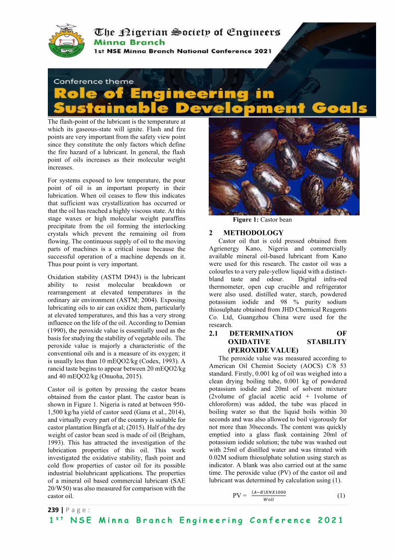
239 | P a g e :


The flash-point of the lubricant is the temperature at

which its gaseous-state will ignite. Flash and fire

points are very important from the safety view point

since they constitute the only factors which define

the fire hazard of a lubricant. In general, the flash

point of oils increases as their molecular weight

increases.

For systems exposed to low temperature, the pour

point of oil is an important property in their

lubrication. When oil ceases to flow this indicates

that sufficient wax crystallization has occurred or

that the oil has reached a highly viscous state. At this

stage waxes or high molecular weight paraffins

precipitate from the oil forming the interlocking

crystals which prevent the remaining oil from

flowing. The continuous supply of oil to the moving

parts of machines is a critical issue because the

successful operation of a machine depends on it.

Thus pour point is very important.

Oxidation stability (ASTM D943) is the lubricant

ability to resist molecular breakdown or

rearrangement at elevated temperatures in the

ordinary air environment (ASTM; 2004). Exposing

lubricating oils to air can oxidize them, particularly

at elevated temperatures, and this has a very strong

influence on the life of the oil. According to Demian

(1990), the peroxide value is essentially used as the

basis for studying the stability of vegetable oils. The

peroxide value is majorly a characteristic of the

conventional oils and is a measure of its oxygen; it

is usually less than 10 mEQO2/kg (Codex, 1993). A

rancid taste begins to appear between 20 mEQO2/kg

and 40 mEQO2/kg (Onuoha, 2015).

Castor oil is gotten by pressing the castor beans

obtained from the castor plant. The castor bean is

shown in Figure 1. Nigeria is rated at between 950-

1,500 kg/ha yield of castor seed (Gana et al., 2014),

and virtually every part of the country is suitable for

castor plantation Bingfa et al; (2015). Half of the dry

weight of castor bean seed is made of oil (Brigham,

1993). This has attracted the investigation of the

lubrication properties of this oil. This work

investigated the oxidative stability, flash point and

cold flow properties of castor oil for its possible

industrial biolubricant applications. The properties

of a mineral oil based commercial lubricant (SAE

20/W50) was also measured for comparison with the

castor oil.

Figure 1: Castor bean

2 METHODOLOGY Castor oil that is cold pressed obtained from

Agrienergy Kano, Nigeria and commercially

available mineral oil-based lubricant from Kano

were used for this research. The castor oil was a

colourles to a very pale-yellow liquid with a distinct-

bland taste and odour. Digital infra-red

thermometer, open cup crucible and refrigerator

were also used. distilled water, starch, powdered

potassium iodide and 98 % purity sodium

thiosulphate obtained from JHD Chemical Reagents

Co. Ltd, Guangzhou China were used for the

research.

2.1 DETERMINATION OF

OXIDATIVE STABILITY

(PEROXIDE VALUE) The peroxide value was measured according to

American Oil Chemist Society (AOCS) C/8 53

standard. Firstly, 0.001 kg of oil was weighed into a

clean drying boiling tube, 0.001 kg of powdered

potassium iodide and 20ml of solvent mixture

(2volume of glacial acetic acid + 1volume of

chloroform) was added, the tube was placed in

boiling water so that the liquid boils within 30

seconds and was also allowed to boil vigorously for

not more than 30seconds. The content was quickly

emptied into a glass flask containing 20ml of

potassium iodide solution; the tube was washed out

with 25ml of distilled water and was titrated with

0.02M sodium thiosulphate solution using starch as

indicator. A blank was also carried out at the same

time. The peroxide value (PV) of the castor oil and

lubricant was determined by calculation using (1).

PV = (𝐴−𝐵)𝑋𝑁𝑋1000

𝑊𝑜𝑖𝑙 (1)

240 | P a g e :


Where B= volume of sodium thiosulphate used in

blank titration. A= volume of sodium thiosulpate

used in titration with oil. N= normality of sodium

thiosulphate (which is 0.02). Woil= weight of oil

used

2.2 MEASUREMENT OF CLOUD POINT AND

POUR POINT The cloud point was measured according to the

ASTM D2500 standard using a refrigerator and

digital infra-red thermometer with measuring range

from -500C to 3800C shown in Figure 2. The oil was

first heated to 500C to ensure solution of all

ingredients and elimination of any influence of past

thermal treatment. It was then cooled at a specific

rate in the refrigerator and observed for the onset of

wax precipitation in the form of a distinctive cloud

or haze. The temperature at the onset of the

cloudiness was measured using the digital infra-red

thermometer and recorded as the cloud point.

The pour point was determined according

to the ASTM D97 standard (ASTM., 2002a). The

same procedure and equipment as that of the cloud

point was employed. The decrease in the

temperature of the oil at 30C was monitored while

the test container was tilted to check for movement.

The temperature 3°C above the point at which the oil

stopped moving was recorded as the pour point.

Figure 2: Digital infra-red thermometer

2.3 MEASUREMENT OF FLASH POINT The flash point was measured according to the

ASTM D92 standard (ASTM 2002b). 30mls of the

oil was poured into an open cup apparatus and

heated at atmospheric pressure while the

temperature was being monitored with the digital

infra-red thermometer. The set up was carried out in

a fume chamber where air was being supplied to the

heated oil until it ignited. The temperature at which

it ignited was noted and recorded as the flash point

of the oil.

3 RESULTS AND DISCUSSION The result gotten from the various tests carried

out and detail discussion of the results are presented

in subsections 3.1 -3.3.

3.1 OXIDATIVE STABILITY

CHARACTERISATION OF

CASTOR OIL AND MINERAL

BASED LUBRICANT

The peroxide value is the usual method of

assessment of primary oxidation products. Peroxide

value of any oil gives an indication of its oxidative

and thermal stability. The peroxide value of the

jatropha and castor oil is shown in Table 1. The

peroxide value of castor oil was 8.92 meq/kg, while

that of the mineral based lubricant SAE 20/W50 was

0.99 meq/kg. The peroxide value of the castor oil

was too high showing that the oil has poor oxidative

and thermal stability. The SAE 20/W50 had

desirable oxidative and thermal stability.

This result is consistent with the findings of

all other researchers that had studied the thermo-

oxidative stabilities of vegetable oils (Gunstone,

2004; Adhvaryu et al; 2005). The poor thermal and

oxidation stability of the castor oil implies that

lubricants formulated from castor oil will have a low

shelf life as degradation of the oil will take place

very fast. The poor thermo-oxidative stability of

castor oil is a major hindrance for its application as

industrial lubricant; thus, the oil must be modified

for it to be useful in the production of industrial

lubricants.

Table 1: PEROXIDE VALUE OF CASTOR OIL

AND MINERAL BASED LUBRICANT SAE

20/50

Oil/Lubricant Peroxide

value

(meq02/kg)

Oxidative

stability

Castor oil 8.92

unstable

241 | P a g e :


SAE 20/W50 0.99

Very

stable

3.2 COLD FLOW PROPERTIES OF CASTOR

OIL AND MINERAL BASED LUBRICANT

The cold flow properties (cloud point and

pour point) of the castor oil and the mineral based

oil SAE 20/W50 are shown in Figure 3. The pour

point of the castor oil was -23.20 C which is very low

and desirable. The pour point of SAE 20/W50 was -

24.10 C. the castor oil had cloud point of -12.40 C

while the SAE 20/W50 had a cloud point of -18.90

C. The pour point of the castor oil is very similar to

that of the SAE 20/W50; thus, castor oil can be used

as a lubricant in the same cold areas where SAE

20/W50 is being used.

Castor oil had good cold flow properties

(cloud point and pour point) which have been what

is lacking in most vegetable oils that hinder their

applications in systems exposed to low

temperatures. Thus, castor oil can be used for

lubrication of machines exposed to low temperatures

such as automotive engines, construction machines,

military and for space applications.

Figure 3: Cloud point and pour point of castor oil

and mineral oil- based lubricant SAE 20/W50.

3.3 FLASH POINT AND FIRE SAFETY OF

CASTOR OIL AND MINERAL BASED

LUBRICANT

The flash point of the castor oil and the

SAE 20/W50 is shown in Figure 4. The flash point

of the castor oil was 2820 C which is higher than that

of the SAE 20/W50 (2550 C). The flash point of the

castor oil might be higher than that of the SAE

20/W50 because the castor oil has a higher

molecular weight than the SAE 20/W50. Both oils

have very high flash points which is desirable for a

lubricant from the safety point of view. Castor oil is

safer to be used at high temperatures as lubricant

than most lubricanting oils with flash point of 2100

C and fire point of about 2300 C (Stachowiak, and

Batchelor, 2000). The fire hazard while using castor

oil as lubricants is lower than the fire hazard of using

commercially available mineral based oil lubricant

SAE 20/50.

Figure 4: Flash point of castor oil and mineral based

lubricant SAE 20/W50

4 CONCLUSION

The environmental issues associated with

the use of mineral based lubricants as well as the

fluctuation in price of crude coupled with the

depletion of oil reserves has made it necessary to

look for alternatives. The oxidative stability, flash

point and cold flow properties of castor oil has been

studied and compared to commercially available

mineral oil-based lubricant SAE 20/W50. The castor

-12.4

-23.2

-18.9

-24.1

-30

-25

-20

-15

-10

-5

0

cloud point(0C) Pour point (0C)

TEM

PER

ATU

RE

(^O

C)

OIL/LUBRICANT

COLD FLOW PROPERTIES

CO MNL

255282

0

50

100

150

200

250

300

350

MNL CO

FLA

SH P

OIN

T (^

0C

)

OIL/LUBRICANT

Flash point (^0C)

242 | P a g e :


oil had poor oxidative stability compared to the SAE

20/W50 which implies that its shelf and service life

as a lubricant is low

The castor oil had a higher flash point than the SAE

20/W50, thus, in applications where fire safety is of

out most consideration the castor oil will be

preferred lubricant. Both the castor oil and SAE

20/W50 had good fire safety compared to most

lubricant oil base stock. The castor oil had a pour

point similar to that of the SAE 20/W50 lubricant

and competed favourable with the mineral oil-based

lubricant in cloud point. Thus, the castor oil has

excellent cold flow property and can be used for

lubrication of machines exposed to low temperatures

such as automotive engines, construction machines,

military and for space applications. Castor oil can

be a good renewable, environmentally friendly and

sustainable substitute for mineral oil-based

lubricants.

ACKNOWLEDGEMENTS

The authors gratefully acknowledge Mr. Bulus

Musa of the Water Resources, Aquaculture and

Fisheries Laboratory, Federal University of

Technology Minna, Nigeria. and Mr. Peter Obasa of

the Central Teaching Laboratory, Federal University

of Technology Minna, Nigeria, for their assistance

with the laboratory work. The authors also

acknowledge the Petroleum Technology

Development Fund (PTDF) for partly sponsoring the

research.

REFERENCES Adhvaryu, A., & Erhan, S. Z., (2002), Epoxidized

Soybean Oil as a Potential Source of High-

Temperature Lubricants, Ind. Crops Prod., 15:

247–254.

Adhvaryu, A., Liu, Z., & Erhan, S. Z., (2005),

Synthesis of Novel Alkoxylated Triacylglycerols

and Their Lubricant Base Oil Properties, Ind.

Crops Prod., 21, 113–119.

Ajithkumar, G., (2009). Analysis, Modification and

Evaluation of the Cold Flow Poperties of Vegetable

Oils as Base Oils for Industrial Lubricants, PhD

thesis submitted to the Faculty of Engineering,

Cochin University of Science &

TechnologyKochi-22, India: 38 - 79

American Society for Testing and Materials (2004).

ASTM D943-04a, Standard Test Method for

Oxidation Characteristics of Inhibited Mineral

Oils, ASTM International, West Conshohocken,

PA, USA.

American Society for Testing and Materials,

(2002a).

ASTM D97–02, Standard Test Method

for Pour Point of Petroleum Products, ASTM

International, West Conshohocken, PA, USA.

American Society for Testing and Materials

(2002b).

ASTM D92-02b, Standard Test Method for Flash

and Fire Point by Cleveland Open Cup Tester,

ASTM International, West Conshohocken, PA,

USA.

Awoyale, A.A; Odubiyi,O. A. & Eloka-Eboka, A.

C. (2011). Production and Testing of Biodegradable

Grease from Black-Date (Canarium

schweinfurthii) Oil, Journal of Innovative

Research in Engineering and Sciences 2(4), 223-

233

Bartz, W. J., (2006). Ecotribology: Environmentally

Acceptable Tribological Practices, Tribol. Int., 39

(8), 728-733.

Binfa, B; Atabor, P.A; Barnabas, A;and

Adeoti,M.O;

(2015). Comparison of lubricant properties of Castor

oil and commercial engine oil. Jurnal Tribologi

5, 1-10.

Brigham, R.D. 1993. Castor: Return of an old crop.

New Crops, Wiley, New York, 380- 383.

Codex Alimentairus Commission (1993). Graisses

et

huiles vegetales, Division 11, version abregee

FAO/WHO, Codex Stan.

Demian, M. J., (1990). Principles of Food

Chemistry,

2nd edition, London: Van Nostrond Reinhold

International Company Limited

Erhan, S. Z., & Asadauskas, S., (2000), Lubricant

Base Stocks from Vegetable Oils,

Ind. Crops Prod., 11: 277-282.

Erhan, S.Z; Sharma, B.K. & Perez, J. M. (2006).

Oxidation and low temperature stability of

vegetableoil-based lubricants, Industrial Crops

and Products, 24: 292-299.

Gana, A., Amosun, A., Alhaji, B.B. 2014.

Determination of Number of Manual Hoe Weeding

for Optimal Yield of Castor (Ricinus communis

243 | P a g e :


L., Euphorbiaceae) in Nigeria. Global Journal of

Botanical Science, 2, 21-25.

Gunstone, F.D. 2004. Rapeseed and Canola Oil:

Production,Processing, properties and uses.

London: Blackwell Publishing Ltd

Kassfeldt, E., & Goran, D., (1997). Environmentally

Adapted Hydraulic Oils, Wear, 207:41–45.

Mercurio, P., Burns, K. A., & Negri, A., (2004),

“Testing the Ecotoxicology of Vegetable Versus

Mineral Based Lubricating Oils: 1. Degradation

Rates Using Tropical Marine Microbes”,

Environ. Pollut.,129 (2): 165-73.

Onuoha, O.J., (2015). Suitability of Vegetable

Based

Oils in Orthorgonal Machining of AISI 1330 Carbon

Steel Using Taguchi Method, PhD thesis

submitted to the Department of Mechanical

Engineering, Federal University of Technology

Minna, Niger State, Nigeria: 85 - 89

Rhee, I.S., Valez, C., & Bernewitz, K., (1995).

Evaluation of Environmentally Adapted Hydraulic

Fluids, TARDEC Tech Report 13640, US Army

Tank Automotive Command Research,

Development and Engineering Center, Warren,

MI, 1–15.

Stachowiak, G.W. & Batchelor, A. W., (2000).

Engineering Tribology, Second Edition.

Butterworth-Henemann, Boston: 3-616.

Woma, T.Y; Lawal, S.A; Abdurahman, A.S;

Olutoye, M. A; & Ojapah, M .M;(2019) .“Vegetable

Oil Based Lubricants: Challenges and

Prospects,” Tribology Online, vol. 14(2). Pp.60-

70

244 | P a g e :


Effect of Turning Process Parameters on Surface Roughness of

AISI 1045 Medium Carbon Steel Using Aluminum Coated

Carbide Tool Salawu Morufu Ajibola and Sunday Albert Lawal

Corresponding Author’s email: [email protected]

Department of Mechanical Engineering, School of Infrastructure, Process Engineering and

Technology,

Federal University of Technology, P.M.B 65, Minna, Nigeria

ABSTRACT This work investigated effects of turning process parameters on surface roughness of AISI 1045 medium carbon

steel using aluminum coated carbide tool. The experiments were conducted on CNC lathe using Duratomic,

alpha-base aluminum oxide (Al2O3) coated carbide tool. The material was turned at five different cutting speeds

and three different feed rates at a constant depth of cut, under wet condition. One variable at a time method of

analyses was used to illustrate the influence of cutting parameters on surface roughness. Cutting speed

variation between 355 m/min and 435 m/min at the feed rate of 0.15 mm/rev gave the optimum surface

roughness.

KEYWORDS: Surface roughness, depth of cut, carbide tool and feed rate.

1 INTRODUCTION Efficient manufacturing process is required for

producing parts of acceptable quality [1].

Machining, one of the most widely used

manufacturing processes is done by removing

unwanted material from a workpiece in the form of

chips such that the desired shape and size in

conformity with the specifications laid in the

relevant engineering drawings is achieved.

Machining surpassed every other manufacturing

processes in that hardly is there any product that

does not directly or indirectly involve metal cutting.

It provides dimensional accuracy and surface quality

to a pre-formed blank for it to fulfill its functional

requirements. However, investigation into the metal

cutting process appears to be very difficult due to the

complexity arising from the many variables

involved [2]. Nevertheless, the need to fulfill

increasing demand of machine parts that fit into

sensitive and sophisticated areas, requires the

principle to be well understood for it to have

economical application.

Surface roughness plays vital roles in metal

cutting and is one of the factors of great importance

in the evaluation of machining accuracy [3]. It has a

significant impact on characteristics such as fatigue

strength, corrosion resistance and aesthetics of the

finished product [4]. Not only that, it is a factor that

greatly influences manufacturing cost. Be that as it

may, so much attention is being devoted to machine

parts surface finish and dimensional accuracy.

Therefore, proper selection of process parameters

(the cutting speed, the feed and depth of cut) is very

much crucial [5] otherwise; it could result in

surfaces with high roughness and dimensional

inaccuracy. The current trend to optimize production

rate at shorter time and at minimum machining cost,

without affecting product quality has not been

achieved, because of the inability to find appropriate

parameters that influence the machining

characteristics of workpiece material.

. Machining operations often performed in

conjunction with turning are drilling, reaming,

tapping, threading and knurling. In turning, the

workpiece is rotated about its axis while cutting tool

is fed into it [6- 9]. The unwanted material is sheared

away and the desired part is created. What is

involved here are the workpiece, the tool including

the holding devises, the chips and the cutting fluid.

The tool is thus constrained to move relative to the

workpiece in such a way that it removes the metal in

the form of chips. Thus, the results of the research

245 | P a g e :


investigation will be helpful in cutting tools

selection combines with appropriate process

parameters for machining process such that

optimum production at low cost is achieved.

2 METHODOLOGY The material used in this investigation is AISI

1045, medium carbon steel rod of diameter 70 mm

× 3500 mm length. AISI 1045 medium carbon steel

is widely used for industrial applications requiring

more wear-resistance and strength such as gears,

axles, bolt, nuts, stud, connecting rods, crankshafts

and pins. Duratomic, Alpha-base aluminium oxide

(Al2O3) coated carbide insert was the cutting tool

used for this study. The cutting tool was employed

for its toughness and wear resistance which result in

stable machining. One Variable at a Time (OVAT)

method was adopted for the experimental design of

the machining operation. OVAT, ease in the analysis

of data, revealing by how much a single change

affect the results of the experiment.

2.1 Methods of Experimentation Spectrometric analysis test was conducted on

the workpiece material to determine the elemental

composition of the workpiece materials. The turning

process was conducted under wet condition on

Computer Numerically Controlled (CNC) lathe, that

is regularised by a menu-type interface on a

computer. The machine code fed into the machine

contained information on cutting speed, feed rate,

depth of cut, workpiece material and the cutting tool.

The workpiece was cut to 70 mm diameter by 232

mm length, 15 in number, using CNC band saw. One

piece at a time, the workpiece was face turned at

both ends to diameter 70 mm by 230 mm length and

predrilled at one end on the CNC lathe before the

actual machining test. Workpiece materials were

turned at five different cutting speed and three

different feed rate at a constant depth of cut, 2.0 mm.

Cutting speed was varied from 355 m/min – 435

m/min, Feed rate from 0.15 – 0.45 mm/rev in steps

of 0.15 mm/rev, while depth of cut (DoC) was fixed

at a value of 2.0 mm as presented in Table 1.

Table 1: Experimental design for the turning

operation Experimental

Run No.

Cutting Speed

(m/min)

Feed Rate

(mm/rev)

1

2

355 0.15

375 0.15

3 395 0.15

4 415 0.15

5 435 0.15

6 355 0.3

7 375 0.3

8 395 0.3

9 415 0.3

10 435 0.3

11 355 0.45

12 375 0.45

13 395 0.45

14 415 0.45

15 435 0.45

On the workpiece material, a length of

100mm length. was turned, one piece at a time.

Machining time, as captured by the machine and

gotten via the visual display unit of the computer

interface was married with the stop watch reading,

recorded and the average value was calculated. The

procedure was repeated on all the 15 workpiece

materials.

2.2 Determination of Surface Roughness

For every machined surface it was

measured surface roughness using Mitutoyo,

Portable Surface roughness tester shown in Plate I.

Along the machined surface, three readings were

taken. Average of the three Ra values measured, was

calculated and recorded for each experimental run.

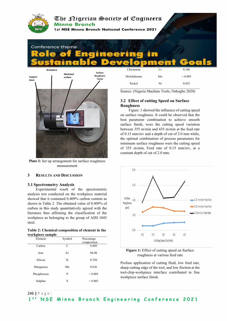
246 | P a g e :


Plate I: Set up arrangement for surface roughness

measurement


3.1 Spectrometry Analysis Experimental result of the spectrometric

analysis test conducted on the workpiece material

showed that it contained 0.409% carbon content as

shown in Table 2. The obtained value of 0.409% of

carbon in this study quantitatively agreed with the

literature thus affirming the classification of the

workpiece as belonging to the group of AISI 1045

steel.

Table 2: Chemical composition of element in the

workpiece sample Element Symbol Percentage

composition

Carbon C 0.409

Iron Fe 98.08

Silicon Si 0.350

Manganese Mn 0.636

Phosphorous P < 0.005

Sulphur S < 0.003

Chromium Cr 0.186

Molybdenum Mo < 0.005

Nickel Ni 0.025

Source: (Nigeria Machine Tools, Oshogbo 2020)

3.2 Effect of cutting Speed on Surface

Roughness Figure .1 showed the influence of cutting speed

on surface roughness. It could be observed that the

best parameter combination to achieve smooth

surface finish, were the cutting speed variation

between 355 m/min and 435 m/min at the feed rate

of 0.15 mm/rev and a depth of cut of 2.0 mm while,

the optimal combination of process parameters for

minimum surface roughness were the cutting speed

of 355 m/min, Feed rate of 0.15 mm/rev, at a

constant depth of cut of 2.0 mm.

Figure 1: Effect of cutting speed on Surface

roughness at various feed rate

Profuse application of cutting fluid, low feed rate,

sharp cutting edge of the tool, and low friction at the

tool-chip-workpiece interface contributed to fine

workpiece surface finish.

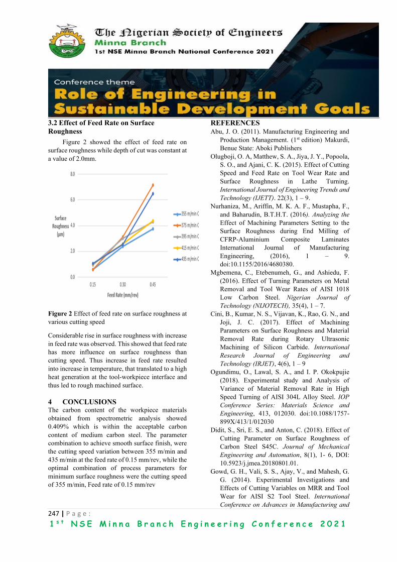
247 | P a g e :


3.2 Effect of Feed Rate on Surface

Roughness

Figure 2 showed the effect of feed rate on

surface roughness while depth of cut was constant at

a value of 2.0mm.

Figure 2 Effect of feed rate on surface roughness at

various cutting speed

Considerable rise in surface roughness with increase

in feed rate was observed. This showed that feed rate

has more influence on surface roughness than

cutting speed. Thus increase in feed rate resulted

into increase in temperature, that translated to a high

heat generation at the tool-workpiece interface and

thus led to rough machined surface.

4 CONCLUSIONS The carbon content of the workpiece materials

obtained from spectrometric analysis showed

0.409% which is within the acceptable carbon

content of medium carbon steel. The parameter

combination to achieve smooth surface finish, were

the cutting speed variation between 355 m/min and

435 m/min at the feed rate of 0.15 mm/rev, while the

optimal combination of process parameters for

minimum surface roughness were the cutting speed

of 355 m/min, Feed rate of 0.15 mm/rev

REFERENCES

Abu, J. O. (2011). Manufacturing Engineering and

Production Management. (1st edition) Makurdi,

Benue State: Aboki Publishers

Olugboji, O. A, Matthew, S. A., Jiya, J. Y., Popoola,

S. O., and Ajani, C. K. (2015). Effect of Cutting

Speed and Feed Rate on Tool Wear Rate and

Surface Roughness in Lathe Turning.

International Journal of Engineering Trends and

Technology (IJETT). 22(3), 1 – 9.

Nurhaniza, M., Ariffin, M. K. A. F., Mustapha, F.,

and Baharudin, B.T.H.T. (2016). Analyzing the

Effect of Machining Parameters Setting to the

Surface Roughness during End Milling of

CFRP-Aluminium Composite Laminates

International Journal of Manufacturing

Engineering, (2016), 1 – 9.

doi:10.1155/2016/4680380.

Mgbemena, C., Etebenumeh, G., and Ashiedu, F.

(2016). Effect of Turning Parameters on Metal

Removal and Tool Wear Rates of AISI 1018

Low Carbon Steel. Nigerian Journal of

Technology (NIJOTECH), 35(4), 1 – 7.

Cini, B., Kumar, N. S., Vijavan, K., Rao, G. N., and

Joji, J. C. (2017). Effect of Machining

Parameters on Surface Roughness and Material

Removal Rate during Rotary Ultrasonic

Machining of Silicon Carbide. International

Research Journal of Engineering and

Technology (IRJET), 4(6), 1 – 9

Ogundimu, O., Lawal, S. A., and I. P. Okokpujie

(2018). Experimental study and Analysis of

Variance of Material Removal Rate in High

Speed Turning of AISI 304L Alloy Steel. IOP

Conference Series: Materials Science and

Engineering, 413, 012030. doi:10.1088/1757-

899X/413/1/012030

Didit, S., Sri, E. S., and Anton, C. (2018). Effect of

Cutting Parameter on Surface Roughness of

Carbon Steel S45C. Journal of Mechanical

Engineering and Automation, 8(1), 1- 6, DOI:

10.5923/j.jmea.20180801.01.

Gowd, G. H., Vali, S. S., Ajay, V., and Mahesh, G.

G. (2014). Experimental Investigations and

Effects of Cutting Variables on MRR and Tool

Wear for AISI S2 Tool Steel. International

Conference on Advances in Manufacturing and

248 | P a g e :


Material Engineering, 5(2014), 1398 – 1407,

doi: 10.1016/j.mspro.2014.07.458

Vaykhinde, A. S., Bhor, U. B., Sachhe, V. V., Valte,

S. P., and Deokar, S. B. (2017). Review of Effect

of Tool Nose Radius on Cutting Force and

Surface Roughness. International Research

Journal of Engineering and Technology

(IRJET), 457- 464

249 | P a g e :


Thermal and Physicochemical Characterization of Locally

Sourced Lignite Coal C. O. Emenike, P. E. Dim and J. O. Okafor

Department of Chemical Engineering

School of Infrastructure Process Engineering and Technology

Federal University of Technology Minna Nigeria

ABSTRACT Coal as a solid mineralized substance consumed to provide was composed in ecosystems where remains of

animal or plant were conserved by wood and fine-grained sediment from oxidation and decomposition by

biological activities. The aim of this study is to examine the properties of locally sourced lignite coal. The

characterization method used were thermogravimetric analyses and physicochemical analyses. The results of

the physicochemical analyses obtained shows high carbon (C) and hydrogen (H) content of 90 % and 8.38 %;

high fixed carbon of 81.3 % with low sulphur, oxygen and nitrogen content of 0.79 %, 0.67 % and 0.16 %; low

moisture content, low ash content and low volatile matter of 1.45 %, 1.78 % and 15.84 % respectively. The low

moisture content, ash content and volatile matter shows that the lignite coal is of good quality with 16.113

MJ/kg as the high heating value, (HHV). However, this coal has nitrogen and sulphur content less than 1 %

which is an indication of the environmental friendliness of coal relative to potential NOx and SOx pollutant

emissions. This coal can be used in power generation, iron and steel making, pharmaceutical industries.

KEYWORDS: Lignite, Thermal, Ultimate, Proximate

1 INTRODUCTION Coal is a combustible form of rock made by the

deposition and compression of small particles which

contains both compounds of carbon minerals and

compounds of non-carbon materials, it is the world’s

most sufficient and commonly dispensed

mineralized energy given substance (Idris and

Ahmed, 2019). Coal and coal-derived energy given

substance have been used in residential, commercial,

and industrial applications such as generation of

electricity, iron and steel making, chemical and

pharmaceutical productions, cement production and

paper manufacturing (Bodude et al., 2018). Coal as

a solid mineralized substance consumed to provide

energy was composed in ecosystems where remains

of animal or plant were conserved by wood and fine-

grained sediment from oxidation and decomposition

by biological activities a layer of dead plants and

animals at the bottom of the wetland was covered by

layers of water and dirt, snare the energy of the dead

plants and animals for millions of years (Bizualem

and Busha, 2017). The pressure and heat from the

top layers enhanced the dead plants and animals turn

into coal, it takes millions of years to form thereby

became nonrenewable energy source. However, the

energy in coal is obtained from the energy stored by

dead plants and animals over hundreds of millions

of years ago, when the earth was not completely

covered with wetland forests. Coal is an easily

combustible black or brownish-black form of rock

made by the deposition and compression of small

particles composed mainly of carbon and

hydrocarbons, with little amount of other elements,

like oxygen, nitrogen and sulfur (Wolde-Rufael,

2010). Coal seem to possess the most entreat of all

the possible options for short-term development

suitable for the national necessity of energy

(Vasireddy et al., 2011). Coal and its products, play

an important role in satisfying the energy necessity

of the wester society. The quantity of coal deposits

estimated all over the word was approximately ten

times greater than that of other carbon yielding

resources. The availability of coal resources was a

main support to the economic expansion of many

nations like the US, China, India, and Australia

(Mehran et al., 2015). Coals can be classified into

two: hard coals (the bituminous and anthracite)

which is associated with high carbon and energy

content and soft coals (the lignite and

subbituminous) which is also associated with high

moisture content, both hard coals and soft coals can

be used in transportation, generation of electricity

and cement manufacturing because quality of coals

is not pre-requisite (Chukwu, 2015). Matsumoto et

250 | P a g e :


al., (2016), reported that researching on

physicochemical characterization of coal sample

would provide an enhanced information on the use

and application of coal samples. The aim of this

study is the thermal and physicochemical

characterization of locally sourced lignite coal.

2 METHODOLOGY The lignite coal was collected from Ogwashi

Azagba in Delta state, Nigeria.

2.1 CHARACTERIZATION Physicochemical Analyses involved ultimate and

proximate analyses. The ultimate analysis was done

using the method adopted from (Bodude et al., 2018). Proximate analysis consists of the following

parameters: moisture content, ash content, volatile

matter and fixed carbon content.

Moisture Content (MC): 0.3 g of sample was placed on a dish. Weight of dish

with sample was recorded before placing the sample

in the tray dryer. Temperature of the dryer was

adjusted to 60OC, and sample was then dried to

constant weight and final weight was recorded.

Moisture content was calculated using:

MC (%) = (𝑊𝑒𝑡 𝑊𝑒𝑖𝑔ℎ𝑡− 𝐷𝑟𝑦 𝑊𝑒𝑖𝑔ℎ𝑡

𝑊𝑒𝑡 𝑊𝑒𝑖𝑔ℎ𝑡) × 100 %

(1)

Ash Content (AC): 0.2 g of coal sample was placed into tarred crucible.

The sample was preheated to 600 OC for 3 h. The

crucibles were allowed to cool in the furnace to less

than 100 ºC and then placed into desiccators with a

vented top.

AC (%) = (𝑊𝑒𝑖𝑔ℎ𝑡 𝑜𝑓 𝑅𝑒𝑠𝑖𝑑𝑢𝑒

𝑊𝑒𝑖𝑔ℎ𝑡 𝑜𝑓 𝑆𝑎𝑚𝑝𝑙𝑒) × 100 %

(2)

Volatile Matter (VM): Volatile matter (VM) was determined by heating the

dry sample in a covered crucible in a furnace at 930

°C for 7 min. The sample was then weighed after

cooling in a desiccator. The VM was then calculated

using the equation below:

VM (%) = (𝐵−𝐶

𝐵) × 100 %

(3)

Where B is the weight of the oven dried sample and

C is the weight of the sample after heating in the

furnace at 930 °C.

Percentage Fixed Carbon:

The percentage fixed carbon (FC) was computed

by subtracting the sum of VM and AC from 100 as

shown in

the equation below:

FC = 100 % − (MC + AC + VM)

(4)

Determination of Calorific Value 1.0g of coal sample in a nickel-chromium crucible

was placed in an atmospheric environment of high-

pressure known as Combustion Vessel, surrounded

by water. The sample was then ignited. The

calorimeter jacket was held at a constant

temperature by regulating the fan speed while the

heat produced by the burning sample caused the

bomb and bucket temperature to increase. The

temperature of the water was determined by an

electronic thermometer with a resolution of 1/10000

of a degree. Any minute heat flow between the

jacket and the surrounding during the test was

continuously monitored by a microprocessor and

necessary corrections of any heat leak applied

automatically. Heat evolved is proportional to the

gross calorific value (air-dried basis) of the sample

and displayed automatically by the instrument.

Duration of each run was 10 min.

Thermogravimetric Analysis The lignite coal was heated from 25 oC to 1000 oC

in air with an an air flow rate of 50 ml/min at a

heating rate of 10 oC/min. The weight change of the

sample was recorded automatically until there was

no further weight change. The residue in the crucible

represents the ash content of the sample. Typical run

time of the test was about 3.5 h.


3.1 PHYSICOCHEMICAL ANALYSES AND

THERMOGRAVIMETRIC ANALYESS Ultimate Analyses: The data generated from

ultimate analysis, were elemental parameters (such

as carbon, hydrogen, sulphur, oxygen and nitrogen),

which are used to determine the quality of coal.

From Table 1, the coal sample possess high carbon

content followed by hydrogen content of about 90 %

and 8.38 % with low values of sulphur, oxygen and

nitrogen content of about 0.79 %, 0.67 % and 0.16

% from the elemental analysis obtained. Among

these elements, the carbon and hydrogen content of

251 | P a g e :


coals determines the maturity (rank), calorific value

and chemical reactivity during thermal conversion

of coals. From this analysis, the sulphur and nitrogen

contents of the lignite coal examined were very low,

are such, little or no NOx and SOy gases will be

released during combustion to the environment

(Bodude et al., 2018). However, this lignite coal will

be friendly to the environment and the equipment

because of the little percentage composition of

sulphur and nitrogen contents obtained from the

analysis.

Table 1: Ultimate Analyses of Lignite Coal

Parameters Values (%)

Carbon 90.00

Hydrogen 8.38

Sulphur 0.79

Oxygen 0.67

Nitrogen 0.16

Carbon and hydrogen are the main combustion

constituents of coal and these two constituents are

high in this lignite coal as compared with other

elements such sulphur, oxygen and nitrogen. The

type and ranking of coal are determined by the

amount of carbon, from lignite to anthracite.

Meanwhile, the carbon content in coal is used for

classifications of coal, the higher the carbon content,

the higher is the calorific value and the better is the

quality of the coal. Hydrogen is commonly attached

with volatile matter to determine the use to which

the coal will be engaged. (Solomon and Aliyu,

2013), also concluded, that a good coal sample

should possess high carbon content as compared

with quantity of hydrogen, nitrogen and oxygen, as

in the case of the result obtained for this lignite coal

in Table 1.

The moisture content is a useful property of coal as

all coals are mined wet. The groundwater and other

non-essential moisture which are known as external

sourced moisture is easily evolved while the

moisture held within the coal itself is inherent

moisture that is analyzed quantitatively. Most coals,

as they are dug from the ground, have some quantity

of moisture associated with them. The degree of

maturity of coal, depends on the quantity of moisture

content (Idris and Ahmed., 2019). The quality of

coal is also determined by moisture content because

it affects the calorific value, the higher the moisture

content, the lesser the calorific value which causes

reduction of the coal capacity and the lower the

moisture content, the higher calorific value. 1.5 %

moisture content is required in a good coking coal

(Solomon and Aliyu., 2013). The value recorded for

moisture content of this lignite coal in Table 2 was

very closed to the stipulated value (1.5 %) for a good

coking coal, this is an indication that the coal is a

good coking coal which can be used for different

applications where coking coal are needed. The ash

content of coal is the remains residue that will not

readily ignite left after the burning of coal, this

represent the size of mineral matter when the

Volatile Matter, moisture content, carbon, oxygen

and sulphur are burnt off during combustion, it also

indicates the rank of coal. The ash content of this

coal used in this research work is about 1.78 % from

the proximate analysis carried out (Table 2).

Table 2: Proximate Analyses on Coal Sample

Parameters Values (%)

Moisture Content 1.45

Ash Content 1.78

Volatile Matter 15.84

Fixed Carbon 81.30

HHV 16.113 MJ/kg

The high yield of ash content is usually a signed by

the mutually sufficient supply of disintegrated

materials in wetland, while the fusing materials

govern mainly with low yield ash content of coals,

whereas the part of disintegrated materials increases

and the organically bound elements concentration

decreases with increased ash yield. However, these

observations seem valid majorly for coals ranking,

lignite majorly consist of fusing mineralization,

moisture, pyrite and calcite and organically bound C

and S are common (Rasheed et al., 2015). This

observation is also in agreement with the statement

that some low yield ash content (<10%) coals

contain mainly fusing and biogenic inorganic

matter, whereas those with higher ash yield (>10%)

show simultaneous enrichment in disintegrated and

fusing inorganic matters (Sahni et al., 2013). The

volatile matter is also a coal component which are

evolved at high temperature when air is absence, at

the temperature where volatile matter is evolved, the

moisture content is as well totally liberated. Except

252 | P a g e :


for the fixed carbon and ash content which exceed

that temperature, thereby required more high

temperature. Volatile matter is mostly a combination

of short and long chain hydrocarbons, aromatic

hydrocarbons and some Sulphur. Volatile matter

ranging from 2 % to about 50 % (Rasheed et al.,

2015). in this research work, the volatile matter of

the coal sample used is found to be about 15.84 %

from the proximate analysis carried out (Table 2).

The coal that contain high volatile matter are readily

ignite, it burns fast and freqently burn with a long

smoky fire because of high percentage of a

combination of short and long chain hydrocarbons,

aromatic hydrocarbons and some Sulphur present,

the high volatile matter of coal is an indication of

low ranked coal while low volatile matter content in

a coal is more typical of higher-rank coal (Speight,

2013). In coal, the carbon found remaining after

which volatile materials are driven off is known as

fixed carbon content of coal. Fixed carbon is

determined by subtracting the mass of volatiles

material from the original mass of the coal sample,

it helps in estimating the quantity of coke that will

be produced from a coal sample. The fixed carbon

contents are different from carbon content

determined from ultimate analysis, because some

carbon is evolved in hydrocarbons with the volatiles.

The fixed carbon content of coals, excluding the ash

and moisture, ranges from 50 % to about 98 %

(Rasheed et al., 2015). However, the value of carbon

content of coal determines the fixed carbon value of

coal, in this research work, the fixed carbon of this

lignite coal used is found to be about 81.30 % from

the proximate analysis carried out (Table 2). Heating

Value indicates the extent of heat content of coal this

lignite coal is good for heating and power

generation.

Table 3 shows the comparisons between this work

and other reported work in literature. The present

work has high carbon and hydrogen content as

compared with the previous work, the more the

carbon content, the better the quality of coal.

Meanwhile, the previous work has high oxygen and

nitrogen content as compared with the present work.

Table 3: Comparative Ultimate Analyses

between this and previous work

A B C D

Parameter

s

Value

s (%)

Value

s (%)

Value

s (%)

Value

s (%)

Carbon 90.00 70.42 68.24 60.21

Hydrogen 8.38 5.42 6.48 5.89

Sulphur 0.79 0.88 0.97 0.58

Oxygen 0.67 10.48 10.43 9.46

Nitrogen 0.16 1.09 1.67 1.07

A (present study); B, C and D-(Idris and Ahmed.,

2019)

Table 4: Comparative Proximate Analysis between

this and previous works

A B

Parameters Values (%) Values (%)

Moisture Content 1.45 12.78

Ash Content 1.78 19.83

Volatile Matter 15.84 41.24

Fixed Carbon 81.30 26.15

HHV 16.113 MJ/kg 16.02 MJ/kg

A (present study) and B-(Mehran et al., 2015).

Table 4 shows the comparisons between this work

and other reported work in literature. However, the

HHV were similar, the previous work has high

volatile matter, ash content and moisture content as

compared with the present work.

Thermogravimetric Analyses

The decomposition curves of TG and DTA of the

locally sourced lignite coal from Ogwashi Azagba in

nitrogen atmosphere determined at the heating rates

of 10.00 oC /min are shown in Figures 1 and 2,

respectively. The TG curve indicates the percentage

weight loss of a coal sample at the temperature range

from 27.00 oC to 950 oC. The rate at which weight

is loss depends on temperature: the more the

temperature, the more the weight is loss because,

pyrolysis process proceeds slowly at lower

temperatures. There were three stages involved in

TG curve shown in Figure 1, the first stage

253 | P a g e :


characterized by weight loss at the temperature

range (27–266) oC was ascribed to the loss of

moisture or water vapor. The second stage

characterized by weight loss at the temperature

range (266-580) oC was typically ascribed to the

loss of volatile matter or devolatilization process.

The last stage characterized the degradation from

temperature range (580-820) oC was attributed to

the slow process of coke formation.

Figure 1: TGA properties of Lignite Coal

The DTA curve of sample at the heating rates of

10.00 oC /min is shown in Figure 2.

Figure 2: DTA properties of Lignite Coal

This DTA curve display two peaks which described

evaporation of moisture and primary breakdown,

and secondary breakdown. The small peak

represents the evaporation of moisture content

which take place at temperature between 30-183.92

oC. The second peak occurred at the temperature

between 183.92 - 576.02 oC indicating

devolatilization process in this coal sample which

involved the liberation of volatile matter content and

thermal breakdown of some covalent bond like ether

bonds and methylene group which will produce

gases like hydrogen, carbon monoxide, and lighter

hydrocarbons. This region is the most important

region to investigate since the main weight loss and

complicated chemical reaction, like release of tar

and gaseous products and semi coke formation, take

place in this temperature range (Aboyade et al.,

2013). The peak temperature (TP) from Figure 2 is

379.88 oC which is the main important point on the

DTA curve. In addition, the peak temperature

represents where the rate of weight loss is at a

maximum. This parameter is used in the assessment

of combustibility (Mehran et al., 2015).

4 CONCLUSION

The physicochemical analyses carried out shows

high carbon content of the locally sourced lignite

coal. The carbon content and HHV indicate its use

in generation of electricity, iron and steel making,

cement production and raw material for chemicals.

This analysis also shows that the coal sample

possess relatively low sulphur, oxygen and nitrogen

contents which is an indication of environmental

friendliness of coal relative to potential NOx and

SOx pollutant emissions. However, the locally

sourced lignite coal sample is easy to process, it

burns slowly and does not burn with long smoky fire

because of its low percentage of a combination of

short and long chain hydrocarbons, aromatic

hydrocarbons and some sulphur present.

REFERENCES Aboyade, A. O., Gorgens, J. F., Carrier, M., Meye,

E. L. and Knoetze, J. H. (2013).

“Thermogravmetric study of the pyrolysis

characteristics andkinetics of coal blends

with corn and sugarcane rsidues,” Fuel

Processing Technology, 106: 310–20.

Applications of Some Nigerian Coals ABUAD

Journal of Engineering Research and

Development. 2(1): 20 -25.

Bizualem, W. and Busha A (2017). Physicochemical

Characterization of Coal and its alternaas a

0

20

40

60

80

100

120

140

160

180

0 500 1000

Wei

ght

Loss

%

Temperature oC

-10

-8

-6

-4

-2

0

2

0 200 400 600 800 1000

Wei

gh

t lo

ss %

Temperature oC

254 | P a g e :


Source of Energy (in case of Yayo Coal

Mining Journal of Environmental

Science, Toxicology and Food Technolog.

11(5): 44-50.

Bodude, M. A., Ayoola, W. A., Oyetunji, A., Baba,

Y.D., Odukoya, A. L., Onifade, O. A.

and Olugbile, O. O. (2018). Proximate,

Ultimate Analysis and Industrial Application of

Some Nigerian Coals. Journal of Engineering

Research and Development. 2(1): 20-25.

Chukwu, M. (2015). Characterization of Some

Nigerian Coals for Power Generation.

M.Eng. Thesis published. Ahmadu

Bello University Zaria, Nigeria

Idris, M. N. and Ahmed, Z. D. (2019). Qualitative

Characterisation of Coal Minerals Selected

From 5 Different Locations in Nigeria

For Possible Studies on Gasification

Technology. International Journal of

Engineering and Modern Technology.

5(2): 55-69.

Matsumoto, S., Ogata, S., Shimada, H., Sasaoka, T.,

Kusuma, G. J. and Gautama, R. S. (2016).

Application of Coal Ash to Postmine

Land for Prevention of Soil Erosion in Coal

Mine in Indonesia: Utilization of Fly Ash and

Bottom Ash. Advances in Materials

Science and Engineering, 1–8.

doi:10.1155/2016/8386598.

Mehran, H., Moshfiqur, R. and Rajender, G. (2015).

Kinetic Study and Thermal

Decomposition Behavior of Lignite

Coal. International Journal of Chemical

Engineering

http://dx.doi.org/10.1155/2015/481739

Rasheed, M. A., Srinivasa Rao, P. L., Annapurna,

B., Syed, Z. H., Arpit, P. V. and Velani, K. P.

(2015). Geochemical Characterization of

Coals Using Proximate and Ultimate

Analysis of Tadkeshwar Coals, Gujarat.

Geosciences, 5(4): 113-1

DOI:10.5923/j.geo.20150504.01

Sahni, A., Saraswati, P.K., Rana, R.S., Kumar, K.,

Singh, H., Alimohammadian, H., Sahni,

N., Rose, Kd, Singh, L. And Smith, T. (2013).

Palynostratigraphy and Depositional

Environment of Vastan Lignite Mine

Gujarat, Western India. Journal of Earth

System Science. 122(1): 289-307.

Solomon, A. R. and Aliyu, J. (2013). Proximate

analysis, rheological properties and

technological applications of some Nigerian

coals. Ryemshak and Jauro International

Journal of Industrial Chemistry 4(7): 1-7.

Speight, J. G, (2013). The chemistry and technology

of coal. 3rd ed. Boca Raton: CRC Press,

2013. ISBN 978-14398-3648-4.

Vasireddy, S., Morreale, B., Cugini, A., Song, C.

and Spivey, J. J. (2011). “Clean Liquid Fuels

from Direct Coal Liquefaction: Chemistry,

Catalysis, Technological Status and

Challenges,” Journal of Energy and

Environmental Science. 4(2): 311–345.

Worde-Rufael Y. (2010). Coal Consumption and

Economic Growth Revisited. Journal of

Applied Energy 87(1): 160-167.

http://dx.doi.org/10.1155/2015/481739

255 | P a g e :


Thermal and Physicochemical Characterization of Biochar

Produced from Waste Bamboo E. Daniel, P.E. Dim and J.O. Okafor

Department of Chemical Engineering, Federal University of Technology, Minna, Nigeria.

ABSTRACT This study is aimed at the characterization of biochar produced from waste bamboo using

physicochemical and thermal analysis method. The physicochemical result shows that bamboo contains

73.8 % cellulose, 12.49 % hemicellulose, 10.50 % lignin, 0.4 % pectin and 3.20 % aqueous extracts.

Thermogravimetric analysis (TGA) was done on raw bamboo waste to determine the temperature of

decomposition of bamboo and pyrolysis was done in an inert atmosphere (pure nitrogen) at temperatures

of 400 oC, 450 oC and 500 oC to produce the biochar. Proximate and ultimate analysis of the raw bamboo

and biochar was carried out and the results showed that the physicochemical properties of the biochar

slightly changes as the pyrolysis temperature was increased.

KEYWORDS: Bamboo; Biochar; Carbon; Proximate analysis; Pyrolysis

1 INTRODUCTION Bamboo is one of the strongest and quickest growing

trees in the world and have been gaining increasing

interest due to its high strength to weight ratio,

requires less water, little or no use of pesticides or

herbicides and is harvested at its base, leaving the

root complete. Also, the tree surface is round and

smooth. It is light, harder and stronger than other

woods (Pecas et al., 2018). Bamboo has been used

in processing abundant and high-quality cellulose

fibers for a long time, and has become a major

feedstock for weaving, pulp, paper, and in the

manufacture of fiber-based composite. The main

chemical compositions of bamboo include cellulose,

hemicellulose, lignin, all kinds of extracts, a little

ash, and silicon dioxide. All of these constituents

and properties contribute to bamboo’s high strength,

bending ductility, toughness and low density (Wang

and Chen, 2017). Bamboo is mainly composed of

cellulose, hemicellulose and lignocellulose that can

be processed into higher value-added products by

pyrolysis processes. Furthermore, it possesses many

other advantages such as easy cultivation, fast

development and low ash content (Mena et al.,

2014). Biochar is a carbon-rich solid derived by

pyrolysis of biomass with little or no oxygen,

Biochar is usually produced from plant residues,

wood biomass, animal litters, and solid wastes

through various thermochemical processes,

including slow pyrolysis, fast pyrolysis,

hydrothermal carbonization, flash carbonization,

torrefaction and gasification (Tan., et al., 2016).

Biochar gotten from biomass is typically 20-40 % of

dry lignocellulose biomass. Nonetheless, the yield

and chemical properties of the pyrolysis products are

firmly impacted by operating conditions during

pyrolysis such as temperature, heating rate, holding

times, particle size, atmosphere and feedstock.

Depending on the final use of biochar, the required

properties of the material may be different (Mena et

al., 2014). Pyrolysis which is a thermochemical

decomposition process, takes place in the absence of

oxygen to produce a liquid phase (tar or hydrocarbon

liquids and water), a carbon rich solid phase

(charcoal) and non-condensable gases (CH4, CO2,

CO, H2,), (Mena et al., 2014). Thermo-chemical

conversion of biomass is one of the many methods

that can be used to convert biomass into valuable

products. Pyrolysis, a thermo-chemical process is an

effective method with less emission to produce

alternative fuels from biomass (Oyedun et al., 2012).

The objective of this study is to investigate the

thermal and physicochemical analysis of biomass

and its product of thermal treatment.

2 METHODOLOGY

2.1. BAMBOO COMPOSITION

The percentage composition of cellulose,

hemicellulose, lignocellulose, pectin and aqueous

extracts of bamboo waste was determined by acid

256 | P a g e :


digestion using a fibre Analyzer. The standard acid

digestion fibre (ADF), neutral detergent fibre (NDF)

and acid detergent lignin (ADL) analysis were

carried out using Ankom 200 Method 5, Method 6

and Method 8 respectively. 0.5 g of ground fibres

was used for each analysis. The percentage of

cellulose, hemicellulose and lignin content were

then determined.

2.2. THERMOGRAVIMETRIC

ANALYSIS (TGA)

The TGA of raw bamboo was done using a

PerkinElmer TGA 4000 thermogravimetric analyzer

and at a heating rate of 10.00 oC/min to determine

the stability temperatures of bamboo during

pyrolysis and to determine the temperatures of

transitions and reactions of raw bamboo

2.3. PREPARATION OF BIOCHAR

Bamboo was collected from a building site in

Minna, Niger state. The sample was cut into small

pieces of 6-8 cm in length and washed thoroughly

with running water followed with distilled water to

remove impurities. The sample was dried in an

electric oven at 100 oC for 24 h to reduce moisture

content. The dried Bamboo was crushed using a club

hammer, it was then reduced further into smaller

sizes of length 8-10 mm using a grinding machine.

25 g of the crushed Bamboo was weighed into a

crucible and charged into the pyrolysis reactor. The

air-lock was closed to avoid the introduction of

oxygen. The cylinder containing nitrogen gas was

then connected to the pyrolysis reactor and the valve

opened with gas flow rate set at 1cm/min. Pyrolysis

was done at temperatures of 400 oC, 450 oC and 500

oC for 2 h. The char was then removed from the

reactor, air-cooled, weighed and kept for further

analysis.

2.4. PROXIMATE AND ULTIMATE

ANALYSIS

The proximate and ultimate analysis of Bamboo

and Biochar was done to determine their physical

and chemical properties. Proximate analysis carried

out includes; moisture content (ASTM E1358-97),

ash content (ASTM E1755-01), volatile matter

(E872-82) and fixed carbon content (ASTM D1762-

84) while the elemental analysis includes;

percentage carbon, Nitrogen, Hydrogen and Oxygen

(C, N, H and O).


3.1 COMPOSITION OF BAMBOO

Analysis on the structural composition of

Bamboo was carried out on waste stem samples and

results showed that the bamboo stem has a very high

cellulose content of 73.83 %. Percentage contents of

Lignin, Hemicellulose, Pectin and aqueous extracts

are 10.50 %, 12.49 %, 0.40 % and 3.20 %

respectively as shown in table 1. These are in the

range of hard wood biomass as reported by (Amaral

and Leite., 2014). A high percentage of cellulose in

biomass suggests more volatilization during

pyrolysis as both the polysaccharide structures are

broken down at a lower temperature range of 200-

400 oc. This is in conformity with the findings of

(Sahoo et al., 2021).

3.2 THERMOGRAVIMETRIC ANALYSIS

(TGA)

Thermal analysis was carried out using 10 mg of raw

bamboo samples at a constant heating rate of 10

oC/min from room temperature up to 850 oC. The

TGA shows the thermal degradation steps, the first

TG curve corresponds to drying and dehydration

between the temperature range of 30 – 100 oC. The

second curve between the temperature range of 250-

400 oC corresponding to weight losses as a result of

Hemicellulose and cellulose degradation (Mena et

al., 2014). At temperatures higher than 400 oC,

almost all cellulose was pyrolyzed. Lignin

decomposes slowly all through the temperature

range from room temperature to 850 oC which

correlates with the findings of (Mahanim et al.,

2011). In general, pyrolysis of wood biomass takes

place in a step-wise manner with Hemicellulose

TABLE 1: COMPOSITION OF RAW

BAMBOO

CONSTITUENT COMPOSITION (%)

Cellulose 73.83

Lignin 10.50

Hemicellulose 12.49

Pectin 0.40

Aqueous extracts 3.20

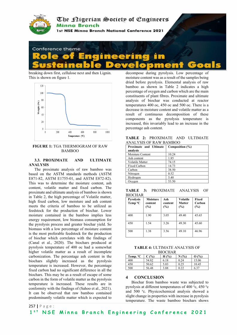
257 | P a g e :


breaking down first, cellulose next and then Lignin.

This is shown on figure 1.

FIGURE 1: TGA THERMOGRAM OF RAW

BAMBOO

3.3. PROXIMATE AND ULTIMATE

ANALYSIS

The proximate analysis of raw bamboo was

based on the ASTM standards methods (ASTM

E871-82, ASTM E1755-01, and ASTM E872-82).

This was to determine the moisture content, ash

content, volatile matter and fixed carbon. The

proximate and ultimate analysis of bamboo is shown

in Table 2, the high percentage of Volatile matter,

high fixed carbon, low moisture and ash content

meets the criteria of bamboo to be utilized as

feedstock for the production of biochar. Lower

moisture contained in the bamboo implies less

energy requirement, low biomass consumption for

the pyrolysis process and greater biochar yield. So

biomass with a low percentage of moisture content

is the most preferable feedstock for the production

of biochar which correlates with the findings of

(Canal et al., 2020). The biochars produced at

pyrolysis temperature of 400 oc had a somewhat

higher volatile matter as a result of incomplete

carbonization. The percentage ash content in the

biochars slightly increased as the pyrolysis

temperature is increased. However, the percentage

fixed carbon had no significant difference in all the

biochars. This may be as a result of escape of some

carbon in the form of volatile matter as the pyrolysis

temperature is increased. These results are in

conformity with the findings of (Sahoo et al., 2021).

It can be observed that raw bamboo contained

predominantly volatile matter which is expected to

decompose during pyrolysis. Low percentage of

moisture content was as a result of the samples being

dried before pyrolysis. Elemental analysis of raw

bamboo as shown in Table 2 indicates a high

percentage of oxygen and carbon which are the main

constituents of plant fibres. Proximate and ultimate

analysis of biochar was conducted at reactor

temperatures 400 oc, 450 oc and 500 oc. There is a

decrease in moisture content and volatile matter as a

result of continuous decomposition of these

components as the pyrolysis temperature is

increased, this invariably lead to an increase in the

percentage ash content.

TABLE 2: PROXIMATE AND ULTIMATE

ANALYSIS OF RAW BAMBOO Proximate and Ultimate

analysis

Composition (%)

Moisture Content 10.24

Ash content 1.85

Volatile Matter 74.15

Fixed Carbon 14.73

Carbon 38.50

Nitrogen 0.52

Hydrogen 5.40

Oxygen 53.50

TABLE 3: PROXIMATE ANALYSIS OF

BIOCHAR Pyrolysis

Temp oC

Moisture

content

(%)

Ash

content

(%)

Volatile

Matter

(%)

Fixed

Carbon

(%)

400 1.90 3.05 49.40 45.65

450 1.54 3.26 49.30 45.60

500 1.38 3.56 49.10 46.96

TABLE 4: ULTIMATE ANALYSIS OF

BIOCHAR Temp. oC C (%) H (%) N (%) O (%)

400 54.82 6.18 0.24 15.06

450 50.62 5.03 0.25 10.45

500 56.48 3.88 0.22 6.37

4 CONCLUSION

Biochar from bamboo waste was subjected to

pyrolysis at different temperatures of 400 oc, 450 oc

and 500 oc. Physicochemical analysis showed a

slight change in properties with increase in pyrolysis

temperature. The waste bamboo biochars shows

258 | P a g e :


suitable properties for its application in

reinforcements, as energy source and agricultural

applications.

REFERENCES Amaral, S., & Leite, L. (2014). Comparative Study

for Hardwood and Softwood forest Biomass;

Chemical Characterization, combustion phases

and gas and Particulate Matter Emissions.

Bioresource Technology, Vol. 164, pp. 55-63.

Canal, W.D., Carvalho, A.M.M., Figueiro, C.G.,

Carneiro, A.D.C.O., Fialho, L.D.F., Donato,

D.B. (2020). Impact of wood moisture in

charcoal production and quality. Florest.

Ambient. 27 http://doi.org/10.1590/2179-

8087.099917.

Mahanim, S.M.A., Asma, I.W., Rafidah, J., Puad,

E., & Shaharuddin, H. (2011). Production of

Activated carbon from Industrial bamboo

wastes. Journal of Tropical Forest Science 23(4):

417-424

Mena. L., Pecora. A., & Beraldo. A. (2014). Slow

pyrolysis of Bamboo Biomass: Analysis of

Biochar properties. Chemical Engineering

Transactions, 37, 115-120.

DOI:10.3303/CET1437020

Oyedun, A., Gebreegziabher. T., & Hui. C. (2012).

Mechanism and Modeling of bamboo pyrolysis.

Fuel processing Technology.

DOI:10.1016/j.fuproc.2012.09.031

Pecas, S., Carvalho. H., Salman. H. & Leite. M.

(2018). Natural fibre composites and their

Applications: A Review. Singh, A.P., Causin,

V., Nuryawan, A., & Park, B. (2014).

Morphological, chemical and crystalline features

of Journal of composites science 2,66.

Phuakpunk, K., Chalermsinsuwan, B., &

Assabumrungrat, S. (2020). Pyrolysis Kinetic

Analysis of Biomasses: Sugarcane Residue,

Corn Cob, Napier grass and their mixture.

ENGINEERING JOURNAL Volume 24 Issue 4.

DOI: 10.4186.

Sahoo, S., Vijay, V., Chandra, R., & Kumar, H.

(2021). Production and Characterization of

Biochar produced from slow Pyrolysis of Pigeon

pea stalk and bamboo. Cleaner Engineering and

Technology 3(2021) 100101.

Tan, x., Liu, Y., Gu, Y., Xu, Y., Zeng, G., Hu, X.,

Liu, S., Wang, X., Liu, S., & Li, J., (2016).

Biochar based nano composites for the

decontamination of wastewater: A review.

Bioresource Technology (2016),

doi:http://dx.doi.org/10.1016/j.biortech.2016.04

.093.

Wang. G. & Chen. F.(2017). Development of

Bamboo fibre-based composites. International

centre for Bamboo and Rattan, Beijing, China.

http://doi.org/10.1590/2179-8087.099917

http://doi.org/10.1590/2179-8087.099917

259 | P a g e :


Synthesis of Ni-Al2O3 Nanocatalyst for Low Temperature

Production of Carbon Nanotubes (CNTs) Yerima, M. L1., Abdulkareem A. S2., Abubakre, O. K3, Ndaliman, M. B4. Khan, R. H.5, and Muriana,

R.A.6

Material and Metallurgical Department, Federal University of Technology, Minna, Nigeria1, 6

Chemical Engineering Department, Federal University of Technology Minna, Nigeria2

Mechanical Engineering Department, Baze University, Abuja, Nigeria5

Mechanical Engineering Department, Federal University of Technology, Minna, Nigeria3, 4,

ABSTRACT This study focused on the synthesis of nickel - aluminium oxide support (Ni-Al2O3) nanocatalyst by wet

impregnation method. The catalyst yield of 86.00 % was obtained at temperature of 400 OC for 3 hours after

calcination. The catalyst was characterized to determine the thermal property, Morphology, crystalinity, pore

volume/particle size and surface area using TGA, SEM/EDX, XRD, DLS and BET respectively. Results

obtained revealed that the catalyst produced has an average particle size of 82.24 nm. It was highly crystalline

with BET surface area of 428.352 m2/g, pore size of 0.2817 Â and pore volume of 0.1779 cc/g. Analysis of the

results also shows that the catalyst developed is thermally stable with about 0.5% wt loss at 800 OC, which

makes the catalyst suitable for CNTs production. The catalyst developed was used to produce carbon nanotubes

at operating temperature of 600 OC with argon flow rate of 30ml/min, acetylene flow rate of 300 ml/min and

production time of 55 minutes. The results obtained revealed that the yield of 135 % was obtained. The CNTs

produced was characterized and the results shows that the produced CNTs is thermally stable with BET surface

area of 833.64 m2/g, pore volume of 0.3286 cc/g and pore size of 0.3148 Â. This study demonstrated that

employing Ni-Al2O3 nanocatalyst provides suitable route for efficient low temperature production of CNTs.

KEYWORDS: Nickel, Aluminium oxide, characterization, CVD, CNTs

1 INTRODUCTION Since its discovery, Carbon nanotubes (CNTs) has

continued to attract research interest worldwide.

After its discovery by Sumio Iijima in 1991, this

novel nanostructure material has gained recognition

due to its wonderful physical properties that makes

it suitable for many unique applications (Toussi et

al., 2011) in many fields of engineering. CNTs are

nanoscale carbon structure that could be described

as graphene sheets rolled up into the shape like of a

cylinder (Bondi et al., 2005) with one end covered

with hemisphere of the fullerene structure (Arranz-

Andréas and Blau, 2010). Regardless of the type of

CNTs which are single walled carbon nanotube and

multiwalled carbon nanotube (Werner and Andreas

2004); they generally have common methods of

synthesis. Owing to its many intriguing properties,

the production of CNT has turn out to be a

significant subject of worldwide research. Carbon

nanotubes (CNTs) are especially promising over

various existing materials inferable from their

interesting unique/ anisotropic extraordinary

chemical, electrical, thermal and mechanical

properties (Afolabi et al . , 2014) that have caught

creative energy of scientists globally since their

revelation by Sumio Iijima in (1991). Owing to these

remarkable electrical properties and very

extraordinary thermal conductivity, CNTs was

utilized for energy storage, functional fillers in

composites field-emission displays, some

biomedical devices and electronics (Muhammad et

al., 2011; Ajayan, 2001; Baughman et al., 2002).

Additionally, CNTs have great flexible moduli

(>1TPa), huge expandable straining length equal to

5 percent, with huge breaking strain up to 20 percent

(Esfarjani, 2013). It’s their outstanding mechanical

properties may conceivably pilot an excess of many

uses. For instance, with their noteworthy stiffness

and strength and adding to the advantage of

lightness, standpoint prospect applications of CNTs

are in progressive plane design (aerospace

engineering), biomedical engineering (virtual bio-

devices) and other disciplines.

260 | P a g e :


Different support materials such as Al2O3, zeolite,

MgO, SiO2, and CaCO3 have been applied as a

carrier in supported-catalysts for CNT (Kathyayini

et al., 2008; Willemset al., 2000; Mao-Lin et al.,

2012 and Couteauet al., 2003). Several researchers

have reported high purity multi-walled carbon

nanotubes obtained from Co-Mo supported MgO

catalyst via CVD Pelechet al., 2009; Quianet

al.,2003; Yeohet al.,2009). Awadallahet al. (2012)

demonstrated the synthesis of CNTs prepared via

CVD methods from Ni-Mo and Co-Mo supported on

Al2O3 catalyst. Studies have shown that alumina

supported catalysts for CNTs synthesis appeared

more promising due creation of a high surface areas

and mesoporous materials which promote catalysis

(Kathyayiniet al., 2008). In addition, Al2O3 has good

thermal stability and can be easily removed after the

synthesis via acid purification. In this present study,

bi-metallic Fe-Ni catalyst supported on aluminium

oxide were developed and utilised to prepare CNT

through CVD method. The choice Ni as an active

part of the catalyst is due to it availability and

cheapness (Uddin et al., 2008).

2.0 METHODOLOGY

2.1 Materials

The chemicals used in this work are of high grade

with high purity, ranging from 98.5- 99.99 %. These

chemicals include nickel nitrate hexahydrate (Ni

(NO3)2.6H2O), alumina (Al2O3), distilled water and

concentrated hydrochloric acid (H2SO4) were

supplied by Aldrich. The carbon source (acetylene)

and carrier gas (argon) are also of analytical grade

with 99.99% purity supplier by BOC Nigeria.

2.1.1 Catalyst Synthesis

The catalyst was prepared by wet impregnation

methods. A 0.22 mol/dm3 aqueous solution of Ni

(NO3)2.6H2O with IUPAC Name Nickel (II) nitrate

hexahydrate (salt solution) was made by

impregnating support material (Al2O3 powder) in the

salt solution. For single metallic Ni based catalysts,

Ni (NO3)2.6H2O/aqueous solution was used. Molar

ratio of Ni: Al2O3) 1:2 was used in preparing the

catalyst systems. The following describes the

detailed procedure for preparing a Ni/Al2O3 catalyst.

Support material (5-6 g) was suspended in 50 ml of

deionized water with stirring, followed by the

addition of 3.198 g of a green Ni (NO3)2.6H2O. The

mixture was allowed to stir for 20 min. and the

resulting slurry was dried in an oven at 120 0C – 125 0C for 5 to 7 hrs. After drying, the material was

grinded with an agate mortal to obtain fine light

green powder. It was then calcined in muffle furnace

at 400 0C for 2hr, cooled to room temperature, and

re-grinded prior to CVD growth. The calcined

material (grey) was sieved using a sieve of 150

micrometer and the desired catalyst was collected as

fine particles. The percentage yield of the catalyst

before oven drying (Yield Dried), and after

calcination (Yield Calcined) is calculated using

equation 1 and 2;

𝑌𝑖𝑒𝑙𝑑 (%)

= (𝑀𝑎𝑠𝑠 𝑜𝑓 𝑐𝑎𝑡𝑎𝑙𝑦𝑠𝑡 𝑎𝑓𝑡𝑒𝑟 𝑜𝑣𝑒𝑛 − 𝑑𝑟𝑦𝑖𝑛𝑔

𝑀𝑎𝑠𝑠 𝑎𝑓𝑡𝑒𝑟 𝑜𝑣𝑒𝑛 𝑑𝑟𝑦𝑖𝑛𝑔)

× 100 1

𝑌𝑖𝑒𝑙𝑑 (%)

= (𝑀𝑎𝑠𝑠 𝑜𝑓 𝑐𝑎𝑡𝑎𝑙𝑦𝑠𝑡 𝑎𝑓𝑡𝑒𝑟 𝑐𝑎𝑙𝑐𝑖𝑛𝑎𝑡𝑖𝑜𝑛 − 𝑑𝑟𝑦𝑖𝑛𝑔

𝑀𝑎𝑠𝑠 𝑎𝑓𝑡𝑒𝑟 𝑜𝑣𝑒𝑛 𝑑𝑟𝑦𝑖𝑛𝑔)

× 100 2

2.1.2 Synthesis of CNTs

The horizontal CVD reactor equipment shown in

Plate 1was used for the CNTs synthesis. It has a

length of 1010 mm with internal and external

diameter of 52 mm and 60 mm respectively. 1.0 g of

the supported bimetallic catalyst (Ni/Al2O3) was

weighed and spread evenly on a quartz boat placed

at the central part of the horizontal tube.

Plate 1: The horizontal CVD set up for the

synthesis of carbon nanotubes

261 | P a g e :


The heating rate, temperature, gas flow rates were

maintained at the desired rate. The entrapped gases

in the quartz tube were expelled using argon as the

carrier gas at a flow rate of 30 ml/min. At a

temperature of 600 0C, the flow of acetylene was

released into the quartz tube of catalytic reactor at

100 ml/min for 55 min with immediate increment in

the flow rate of the carrier gas (argon) to 300 ml/min.

As the residence time (45 minutes) of the reaction

was attained, the flow of acetylene was stopped and

the argon gas was left flowing at 30 ml/min until the

reactor cooled to room temperature. The sample was

removed, weighed and analysed. The yield of the

deposited carbon was therefore determined using

Equation (3) (Yeohet al., 2009; Taleshi, 2012).

𝐶𝑁𝑇𝑠 𝑌𝑖𝑒𝑙𝑑 (%) = (𝑀𝑇𝑜𝑡𝑎𝑙−𝑀𝐶𝑎𝑡𝑎𝑙𝑦𝑠𝑡

𝑀𝐶𝑎𝑡𝑎𝑙𝑦𝑠𝑡) ×

100 1

2.2 Characterization

2.2.1 Thermo Gravimetric Analysis (TGA) and

Differential Thermal Analysis (DTA)

The thermal stability, compositional and percentage

purity of materials were determined using TGA

4000 (PerkinElmer). Samples were analyzed in

nitrogen environment at a volumetric flow rate of 20

ml/min, pressure of 2.5 bars and heating rate of 10 OC/min. The thermal balance was zeroed, the sample

was recorded and placed into the equipment utilizing

pyris manager software. When constant weight was

observed utilizing the formed heating profile, the

analysis was then commenced. The test effects were

then studied using pyris manager for proximate and

compositional analysis.

2.2.2 X-Ray Diffraction Patterns (XRD)

Crystal phase identification of the catalyst and CNTs

materials were studied utilising Bruker AXS D8 X-

ray diffractometer system which was linked to Cu-

Kα radiation of 40 kV and a current of 40 mA. The

λ for Kα was 0.1541 nm, scanning rate was 1.5

º/min, The step width of 0.05° was used over 2θ

range value of 20 – 80º.

2.2.3 High Resolution Scanning Electron

Microscope (HRSEM)

The surface topology and the microstructure of the

catalyst and CNTs was studied using Zeiss Auriga

HRSEM. The HRSEM was equipped with EDS and

it was used to obtain the elemental composition of

the produced materials. A small quantity of the

materials was sprinkled on a sample holder and

sputter coated with Au-Pd using Quorum T15OT for

5 minutes before the analysis. The sputter coated

samples was firmly attached to the carbon adhesive

tape and studied using ZeissAuriga HRSEM

equipped with In-lens standard detector at 30 kV.

2.2.4 BET Surface Area

The surface area of the synthesized catalyst was

investigated by means of BET method in Nova e-

series equipment. A sample weighing 300 mg was

degassed at 150 o - 250 OC for 4 hrs in order to

remove moisture. The degassed sample was then

examined for physisorption of the adsorbate

(nitrogen) by the adsorbent in liquid nitrogen

environment.

2.2.5 Particle Size Analysis (DLS Technique)

In order to determine the particle size and the

hydrodynamic diameter, Zeta Nanosizer was used at

scattering angle of 173 O operating at 25 OC with

equilibrating time of 120 secs. 1 mg of the samples

were dispersed in 10 ml of ethanol then transferred

into a polystyrene cuvette using a syringe with 0.22

µm filter coupled to it.


The suitability of the nickel catalyst material for

CNTs growth at CVD reaction temperature of about

600 OC was investigated by thermogravimetric

analysis (TGA) and the thermal differential analysis

(DTA) presented in Figure 1. The results as

presented in Figure 1 shows that there were four

regimes of weight losses in the TGA graph of the

catalyst sample. The sample had continuous loss in

weight from the initial temperature until 400 oC.

According to the differential thermogravimetric

(DTG) curves this process is endothermic and can be

attributed to elimination of water. In the regime of

400– 550 oC the sample loss of weight was observed

to be faster. This can be ascribed to the thermal

decomposition of nickel nitrate hexahydrate as well

as the formation of metal oxides (Lobiak et al.,

2014).

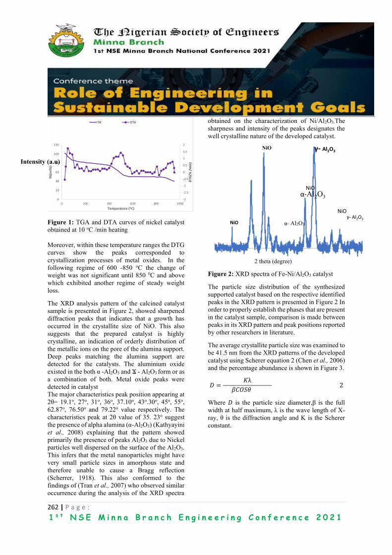
262 | P a g e :


Figure 1: TGA and DTA curves of nickel catalyst

obtained at 10 oC /min heating

Moreover, within these temperature ranges the DTG

curves show the peaks corresponded to

crystallization processes of metal oxides. In the

following regime of 600 -850 oC the change of

weight was not significant until 850 0C and above

which exhibited another regime of steady weight

loss.

The XRD analysis pattern of the calcined catalyst

sample is presented in Figure 2, showed sharpened

diffraction peaks that indicates that a growth has

occurred in the crystallite size of NiO. This also

suggests that the prepared catalyst is highly

crystalline, an indication of orderly distribution of

the metallic ions on the pore of the alumina support.

Deep peaks matching the alumina support are

detected for the catalysts. The aluminium oxide

existed in the both α -Al2O3 and Ϫ - Al2O3 form or as

a combination of both. Metal oxide peaks were

detected in catalyst

The major characteristics peak position appearing at

2θ= 19.1o, 27o, 31o, 36o, 37.10o, 43o.30o, 45o, 55o,

62.87o, 76.50o and 79.22o value respectively. The

characteristics peak at 2θ value of 35. 23o suggest

the presence of alpha alumina (α-Al2O3) (Kathyayini

et al., 2008) explaining that the pattern showed

primarily the presence of peaks Al2O3 due to Nickel

particles well dispersed on the surface of the Al2O3.

This infers that the metal nanoparticles might have

very small particle sizes in amorphous state and

therefore unable to cause a Bragg reflection

(Scherrer, 1918). This also conformed to the

findings of (Tran et al., 2007) who observed similar

occurrence during the analysis of the XRD spectra

obtained on the characterization of Ni/Al2O3.The

sharpness and intensity of the peaks designates the

well crystalline nature of the developed catalyst.

Figure 2: XRD spectra of Fe-Ni/Al2O3 catalyst

The particle size distribution of the synthesized

supported catalyst based on the respective identified

peaks in the XRD pattern is presented in Figure 2 In

order to properly establish the phases that are present

in the catalyst sample, comparison is made between

peaks in its XRD pattern and peak positions reported

by other researchers in literature.

The average crystallite particle size was examined to

be 41.5 nm from the XRD patterns of the developed

catalyst using Scherer equation 2 (Chen et al., 2006)

and the percentage abundance is shown in Figure 3.

𝐷 =𝐾λ

𝛽𝐶𝑂𝑆𝜃 2

Where 𝐷 is the particle size diameter,β is the full

width at half maximum, λ is the wave length of X-

ray, θ is the diffraction angle and K is the Scherer

constant.

NiO

α-Al2O3

γ- Al2O3

NiO

NiOγ- Al2O3

α- Al2O3

NiO

2 theta (degree)

Intensity (a.u)

263 | P a g e :


Figure 3: Percentage Crystallite Size Population

Density of Catalyst

From Figure 3 it can be seen that majority of the

particle fall within 41.50 nm which confirmed that

the size of the prepared monometallic catalyst is

nanostructure in nature and as such the catalyst is a

good template for CNTs production. The result of

the average crystalline particle obtained (82.18 nm)

shows a quite deviation from that obtained by kariim

et al. (2015) with obtained average particle size of

42.24 nm from their XRD analysis.

The HRSEM image presented in Figure 4 indicates

that the clustered solid catalyst material is near

spherical in geometry and is of high crystallinity.

The agglomerates seen in the SEM images could be

ascribed to the drying process in sample preparation.

The micropores can be recognized in the catalyst, a

property showing that there was appropriate

dispersion of Ni nanoparticles on the Al2O3 support

material with tiny spaces inside the composite. The

Al2O3 matrix sites were homogeneously occupied by

the oxides of Ni that was formed during calcination

of the catalyst sample. The SEM image of the

catalyst also indicates that the nickel nanoparticles

that were dispersed on the Al2O3 support material are

suitably less than 50 nm in size (red arrow,

concentric square). The results also show that

nitrates of nickel nitrate salts were effectively

removed by converting them to oxides during

calcination. Though, there are little clusters of

nanoparticles (red arrow, lower right-hand corner)

and lumps of catalyst (yellow arrow). These might

be responsible for the growth of CNTs of varying

diameter, which is one of the existing challenges in

producing nanotubes of uniformly distributed

diameter from catalyst prepared by wet

impregnation.

Figure 4: SEM image showing nanoparticles of Ni

dispersed on Al2O3 support

The surface area analysis was carried out on the

developed monometallic nickel catalyst (Ni/Al2O3)

by BET method. The SBET surface area of the

developed monometallic catalyst was determined to

be 428.352 m2/g using the multipoint equation under

nitrogen condition, with micropore volume of

0.1779 cc/g and micropore half pore width of 28.17

Â. This surface area is little less than those reported

by (Abassi et al., 2014). This may be due to the

presence of weak bond that exist between Ni-Al2O3

(Zhang et al., 2006).

The HRTEM micrograph of the produced CNTs is

presented in Figure 5. The micrograph shows a

densely populated strand of CNTs with high degree

of homogeneity covering the impurity present. The

morphology of the CNTs illustrates that the CNTs

formed under these conditions are entangled with

each other and possess curved, hollow, and tubular

shapes, with diameters in the range of 15 – 45 nm.

Also, some catalyst particles appear to be

encapsulated within the nanotubes hollow core.

Encapsulated metal nanoparticles are also detected

along the inside diameter of the nanotubes samples

which were introduced by the metal catalysts

utilized for CNTs growth.

0

5

10

15

20

25

30

35

30.53 31.92 41.50 59.67 62.75 84.91 116.91120.49190.90

Particle size

Abundance (%)

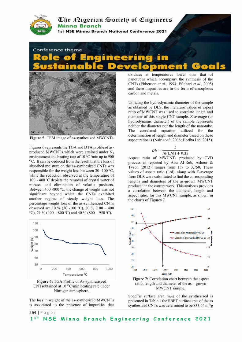
264 | P a g e :


Figure 5: TEM image of as-synthesized MWCNTs

Figures 6 represents the TGA and DTA profile of as-

produced MWCNTs which were attained under N2

environment and heating rate of 10 0C /min up to 900 OC. It can be deduced from the result that the loss of

absorbed moisture on the as-synthesized CNTs was

responsible for the weight loss between 30 -100 oC,

while the reduction observed at the temperature of

100 - 400 oC depicts the removal of crystal water of

nitrates and elimination of volatile products.

Between 400 -800 oC, the change of weight was not

significant beyond which the CNTs exhibited

another regime of steady weight loss. The

percentage weight loss of the as-synthesized CNTs

observed are 10 % (30 -100 oC), 20 % (100 – 400 oC), 21 % (400 – 800 oC) and 40 % (800 – 950 oC).

Figure 6: TGA Profile of As-synthesiseed

CNTsobtained at 10 OC/min heating rate under

Nitrogen atmosphere.

The loss in weight of the as-synthesized MWCNTs

is associated to the presence of impurities that

oxidizes at temperatures lower than that of

nanotubes which accompany the synthesis of the

CNTs (Ebbensen et al., 1994; Eftehari et al., 2005)

and these impurities are in the form of amorphous

carbon and metals.

Utilizing the hydrodynamic diameter of the sample

as obtained by DLS, the literature values of aspect

ratio of MWCNT was used to correlate length and

diameter of this single CNT sample. Z-average (or

hydrodynamic diameter) of the sample represents

neither the diameter nor the length of the nanotube.

The correlated equation utilized for the

determination of length and diameter based on these

aspect ratios is (Nair et al., 2008; Horiba Ltd, 2015).

𝐷ℎ =𝐿

𝐼𝑛(L/d) + 0.32

Aspect ratio of MWCNTs produced by CVD

process as reported by Abu Al-Rub, Ashour &

Tyson (2012), ranges from 157 to 3,750. These

values of aspect ratio (L/d), along with Z-average

from DLS were substituted to find the corresponding

lengths and diameters of the as-grown MWCNT

produced in the current work. This analyses provides

a correlation between the diameter, length and

aspect ratio, for this MWCNT sample, as shown in

the charts of Figures 7.

Figure 7: Correlation chart between the aspect

ratio, length and diameter of the as – grown

MWCNT sample.

Specific surface area m2/g of the synthesized is

presented in Table 1 the SBET surface area of the as

synthesized CNTs was determined to be 833.64 m2/g

50

60

70

80

90

100

110

0 200 400 600 800 1000

We

igh

t (%

)

Temperature oC

265 | P a g e :


using the multipoint equation under nitrogen

condition, with micro pore volume of 0.3286 m3/g

and micro pore half pore width of 31.48 Â. This

surface area is a little high than those reported by

(Abassi et al., 2014). This may be due to the

presence of weak bond that exist between Ni-Al2O3

(Zhang et al., 2006). Peigney et al. (2001) also

showed that the surface area of MWNTs decreases

with increasing walls and nanotube diameters.

However, the trend of the surface area obtained in

this work do not strictly obey the observation made

by Peigney and co-workers because the average

sizes are affected by contribution from sizes of

impurities present in varying quantities in the

samples.

Table 1: Result showing BET-Surface area Analysis

Surface area, pore volume, pore size of synthesized

CNTs and average particle size

BET surface area (m2/g)

833.641

Pore volume (m3/g)

0.3286

Pore size (Â)

0.3148

Average Particle size (DLS) nm

82.24

The SAED patterns of the CNTs sample confirmed

the graphitic nature of MWCNTs especially the

innermost ring which is due to the usual strongest

reflection plane (002) of graphite (Das et al., 2015).

As illustrated in Figure 8. The occurrence of the

sharp rings at reciprocal lattice spacing (1/d) of 2.9,

4.8, 5.7 and 8.5 nm-1 are in good agreement with

those reported for graphite. Kariim, (2015) also

collected SAED pattern of MWCNTs and observed

sharp rings attributable to the MWCNT at reciprocal

lattice spacing of 3.1, 5.0, 6.0 and 8.5 nm-1.

Figure 8: (a) EDS and (b) SAED pattern of as-

synthesized MWCNTs

Again, it can be observed from the SAED that the

CVD reaction parameters affect the crystallinity of

MWCNTs and it present a low crystallinity which as

it displayed diffuse rings in its SAED pattern, which

is typical of amorphous substances. The single

bright spots are reflections from certain individual

crystals.

4.0 CONCLUSION

In this study, multi-walled carbon nanotubes were

successfully produced from nickel supported

alumina catalyst via wet impregnation followed by

CVD technique. The CNTs was successfully

synthesized at reaction time of 45 minutes,

temperature of 600 oC, argon flow rate of 200

ml/min and acetylene flow rate 100 ml/min. The

average diameter of the as-produced multiwalled

carbon nanotubes obtained from bimetallic Ni/Al2O3

catalyst was 28.89 nm whereas; the bimetallic

catalyst had average particle size of 46.24 nm. The

correlation chart showed that the MWCNTs

produced was a long-tube multiwall carbon

nanotubes with aspect ratio of 1250. Thus, the

nickel catalyst on alumina support developed via

incipient wet impregnation method is suitable for

CNTs production by CVD method.

REFERENCE

Abbasi, N., and Mahdavifar, Z. (2014). The

influence of

Cu-doping on aluminum nitride, silicon carbide and

boron nitride nanotubes’ ability to detect carbon

dioxide; DFT study. Physica E: Low-

dimensional Systems and Nanostructures, 56,

268-276.

Abbasi, S. A., Loan, S. A., Nizamuddin, M., Bashir,

F., Shabir, H., Murshid, A. M., R., and Alamoud,

A. (2014). Design of a novel high gain carbon

266 | P a g e :


nanotube based operational transconductance

amplifier. In Proc. of the International

MultiConference of Engineers and Computer

Scientists 2014-IMECS 2014.

Afolabi, A. S., Abdulkareem, A. S., Mhlanga, S. D.

and Iyuke, S. E. (2011) “Synthesis and

purification of bimetallic catalysed carbon

nanotubes in a horizontal CVD reactor”, Journal

of Experimental Nanoscience, vol. 6(3), 248-262

Ajayan, P.M. and Zhou, O.Z. (2001), Applications

of carbon nanotubes. Carbon Nanotubes (Topics

in Applied Physics), ed Dresselhaus, M.S.,

Avouris, Ph. 80, 391-425, Berlin: Springer

Verlag.

Arranz-Andréas, J., and Blau, W. J. (2010).

Enhanced device performance using different

carbon nanotube types in polymer photovoltaic

devices. Carbon, 46(15), 2067-2075.

Awadallah, A. A., Mina, A. N., Phillips, A. H., and

Ahmed, R. R. (2012, February). Simulation of

the Band Structure of Graphene and Carbon

Nanotube. In Journal of Physics: Conference

Series (Vol. 343, No. 1, p. 012076). IOP

Publishing.

Baughman, R. H., Zakhidov, A. A., Heer, W. A.

(2002) Carbon nanotubes-the route toward

applications. Science, 297 pp.787-792.

Bondi, S. N., Lackey, W. J., Johnson, R. W., Wang,

X. and Wang, Z. L. (2005), Laser assisted

chemical vapour deposition synthesis of carbon

nanotubes and their characterization, Carbon 44

(2006) 1393–1403.

doi:10.1016/j.carbon.2005.11.023

Chen, G. Z., Shaffer, M. S., Coleby, D., Dixon, G.,

Zhou, W., Fray, D. J., and Windle, A. H. (2006).

Carbon nanotube and polypyrrole composites:

coating and doping. Advanced Materials, 12(7),

522-526.

Ebbesen, T. W., Treacy, M. J., and Gibson, J. M.

(1996). Exceptionally high Young's modulus

observed for individual carbon nanotubes.

Esfarjani S.A (2013). A Modeling Framework for

the Synthesis of Carbon Nanotubes by Plasma

Technology. Published PhD Thesis. University

of Toronto, Canada.

Horiba Scientific Ltd (2015), “Carbon nanotube

particle size”. Available online at

http//www.horiba.com/scientific/products/partic

le-characterization/applications/carbon-

nanotubes/. Retrieved May, 2015.

Kariim I, Abdulkareem, A.S., Abubakre O.K.,

Mohammed, T.A., Bankole, M.T and Jimoh T.

(2015). Suitability of Alumina (Al2O3) as

Bimetallic Catalyst Support for MWCNT

Growth. Journal of Nanotechnology, 1 - 16.

Kathyayini, H., Reddy, K. V., Nagy, J. B., and

Nagaraju, N. (2008). Synthesis of carbon

nanotubes over transition metal ions supported

on Al (OH) 3. Indian journal of chemistry.

Section A, Inorganic, bio-inorganic, physical,

theoretical & analytical chemistry, 47(5), 663.

Muhammad M. A., Javed I., (2011). Production of

Carbon Nanotubes by Different Routes— A

Review. Journal of Encapsulation and

Adsorption Sciences, 2011, 1, 29-34, 29-34

Nair, N., Kim, W., Braatz, R., and Strano, M. (2008)

Langmuir, 24, 1790 – 1795

Peigney, A., Laurent, C., Flahaut, E., Bacsa, R. R.,

& Rousset, A. (2001). Specific surface area of

carbon nanotubes and bundles of carbon

nanotubes. Carbon, 39(4), 507-514.

Qian, D., Liu, W. K., & Ruoff, R. S. (2009). Load

transfer mechanism in carbon nanotube ropes.

Composites Science and Technology, 63(11),

1561-1569.quantumdotled. html. Accessed July

10, 2006

Toussi, S. M., Fakhru’l-Razi, A., Chuah, A., and

Suraya, A. (2011). Effect of synthesis condition

on the growth of SWCNTs via catalytic chemical

vapour deposition. Sains Malaysiana, 40(3),

197-201.

Uddin, M. A., Tsuda, H., and Sasaoka, E. (2008).

“Catalytic Decomposition of Biomass Tars with

Iron oxides Catalyst”, Fuel, Vol. 87, No (4), pp.

451-459.

Yeoh, Wei-Ming; Lee, Kim-Yang; Chai, Siang-

Piao; Lee, Keat-Teong; & Mohamed, A. (2009).

Synthesis of high purity multi-walled carbon

nanotubes over Co-Mo/MgO catalyst by the

Zhang, Q., Yu, H., Zhang, Q., Wang, Q., Ning, G.,

Luo, G. and Wei, F. (2006), “Effect of the

reaction atmosphere on the diameter of single-

walled carbon nanotubes produced by chemical

vapour deposition”. Carbon, 44, pp. 1706–1712.

267 | P a g e :


Evaluation of Strength Properties of Lateritic Soil Stabilizer with

Cement Kiln Dust T.E. Adejumo and F.A. Okeshola

Civil Engineering Department, Federal University of Technology, Minna, Nigeria

*Corresponding author email: [email protected] +2348133884436

ABSTRACT In this study, the strength properties of Lapai-Gwarri lateritic soil stabilized with cement kiln dust was

evaluated. The scope includes determination of the physical composition, index properties, compaction and

strength characteristics of laterite soil-cement kiln dust mix. From the results obtained, soil sample encountered

was classified as A-7-6 corresponding to CL, it is organic silts and organic silty-clays of very low to medium

plasticity, gravelly clays, silty clays and lean clays according to AASHTO and USCS system of soil

classification respectively. There was to sharp reduction of plasticity index from 22.20% to 11.09%, with

increased in quantity of cement kiln dust, the Compaction characteristics of cement kiln dust soil mixed from

0 and 16% gives the Optimum Moisture Content (OMC) values which decreased from 19.69 - 13.02%. The

Maximum Dry Density (MDD) increase in value from 1.50 - 1.79 g/cm³. The Unconfined Compressive

Strength test at 7, 14 and 28 days of curing for Cement kiln dust of 0, 4, 8, 12 and 16% obtained average values

of 170, 369,511, 461 and 347 (kN/m2) respectively. The addition of 8% cement kiln dust to samples of laterite

soil significantly improves its compressive strength characteristics and is considered as the Optimum

percentage of cement kiln dust present and reduces construction costs.

KEYWORDS: Cement Kiln Dust; Index Properties; Lateritic Soil; Stabilization; Strength Properties.

1. INTRODUCTION In general construction, stable subgrade and base

layers are essential for engineering structure, the

need to reduce the dilemmas in geotechnical

engineering during design and construction in terms

of the variable nature of soil and rock properties and

other in-situ conditions has become a major

challenge because of the issues in reliability of

design and construction methods, and problems in

the costs and benefits of proposed designs policies.

The geotechnical properties like strength and

volume stability of the subgrade have significant

influence on the overall performance and durability

of constructions (William, 2003).

For road construction, soils encountered mostly

during construction are unable to respond to the

imposed stresses, which has become a dominant

factor responsible for the failure of road pavement

especially in Nigeria (Aigbedion,2007; Okechukwu

et al. 2011) identified inadequacy of construction

materials and poor attribute of construction as other

factors responsible for road failure. Improving the

properties of these soils by the addition of chemical

and cementitious additives becomes not only a

necessity but an important factor to make them

suitable for construction.

Chemical additives vary from waste products to the

manufactured materials which include lime,

Portland cement, proprietary chemical stabilizers,

class C fly ash, bitumen and recent technology like

NANO technology (Parson and Kneebone, 2004).

Soil stabilization is the process of improving the

engineering properties of soil and thus making it

more suitable. It is also the treatment of soil with

modifier to enable their strength and durability to

improve such that they become completely suitable

for construction beyond their original classification

(Hausmann, 1990). Lots of consideration has been

given mainly to the problems encountered in the

engineering use of laterite soils. This might give the

impression that all laterites and lateritic soils give

trouble (Christophe, 1949).

Cement kiln dust is a waste product from the

manufacturing of cement. The quantities, nature and

characteristics of CKD generated depends on the

number of operational factors and the characteristics

268 | P a g e :


of inputs to the manufacturing process, including the

raw fed, fuel used, and the design and operation of

the cement kiln. This by-product has desirable

properties that make it satisfactory for variety of

beneficial use and application including soil

improvement (Abeln et al. 1993).

The evaluation of possible change in characteristics

of lateritic soil when treated with additive such as

cement kiln dust can be an important task in the

prevention of natural disasters on our road

pavements and even buildings. Cement kiln dust

provides a cheaper alternative to Portland cement

and lime in soil improvement by stabilization. Miller

et al. (2003) showed that soil improvement by

stabilization using CKD is cheaper than lime

especially when problematic soils are encountered.

Cement kiln dust is also available in Nigeria and if

this is realized, it can find lasting solution to the

failure of road and buildings due to weak sub-grade

and foundation arising from substandard

construction materials. This work lead to

improvement without incurring excessive cost in the

construction industry.

2. METHODOLOGY

Materials

The soil used was obtained at Lapai-Gwarri area of

Minna, using the disturbed sampling technique.

Sample was obtained at 1.5m depths and classified

according to AASTHO and UCSC soil classification

system. Cement Kiln Dust which is a greyish black

material is the byproduct of cement and one of the

essential materials needed for this work. It was

obtained from Obajana Cement Plant Kogi. The

material was sieved appropriately and finally stored

in an air-tight container pending the time for sample

preparations, this is done so it maintains its value.

Methods

The production of concrete tests was conducted in


Technology, Minna. The materials mentioned in 2.1

above were used, the collected soil was air – dried

and stored. Laboratory tests were carried out on two

different samples (the natural lateritic soil and one

treated with Cement Kiln Dust). The treatment with

cement kiln dust was done at 4, 8, 12 and 16% dry

weight content in accordance to BS 1377 (1990).

Index properties of fill materials: Natural

moisture content, specific gravities, particle size

analysis and Atterberg limits tests were conducted in

accordance with tests procedures specified in BS

1377 (1990).

Compaction characteristics: Compaction of the

samples was conducted in accordance with the

guidelines specified in BS 1377 (1990) to compute

the required parameters. The Reduced British

Standard Heavy (RBSH) compactive effort was

used. The RBSH compaction is the energy resulting

from 4.5 kg rammer falling through a height of 30

cm onto three layers, each receiving 25 blows to

determine MDD and OMC of the sample according

to ASTM D-698 (1992) and ASTM D-1557 (1992).

Unconfined compressive strength (CCS): The test

was conducted in accordance with the procedure

specified in BS, 1377 (1990), to determine the

compressive strength characteristic using the values

of OMC obtained during compaction results from

Reduced British Standard Heavy compaction

method.


TABLE 1: NATURAL MOISTURE CONTENT

OF SOIL SAMPLE Trial 1 2 3

Can No M4 PQ4 A21 Weight of can (g) 34.80 38.20 38.20

Weight of can + wet soil (g) 55.30 58.60 54.80 Weight of can + dry soil (g) 51.40 54.70 51.50

Weight of dry soil (g) 16.60 16.65 13.30

Moisture Content (%) 23.50 23.63 24.80 Average Moisture Content (%) 23.97

TABLE 2: SPECIFIC GRAVITY OF SOIL

SAMPLE Trial

1 2 3

Weight of Cylinder (g) 46.0 46.0 43.6

Weight of Sample + Cylinder (g) 97.4 88.0 87.9

Weight of Sample + Cylinder + Water

(g) 170.8 168.1 167.1

Weight of Cylinder + Water (g) 144.9 145.0 142.4

Specific Gravity 2.04 2.21 2.31

Average Specific Gravity 2.2

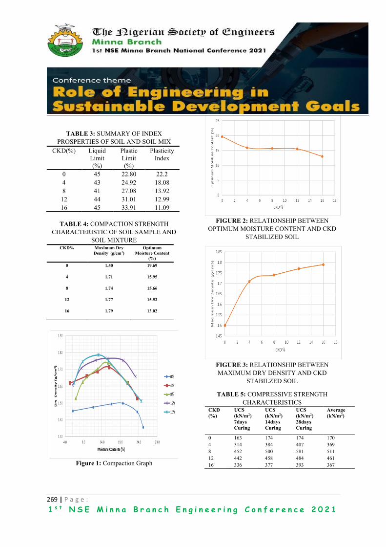
269 | P a g e :


TABLE 3: SUMMARY OF INDEX

PROSPERTIES OF SOIL AND SOIL MIX

CKD(%) Liquid

Limit

(%)

Plastic

Limit

(%)

Plasticity

Index

0 45 22.80 22.2

4 43 24.92 18.08

8 41 27.08 13.92

12 44 31.01 12.99

16 45 33.91 11.09

TABLE 4: COMPACTION STRENGTH

CHARACTERISTIC OF SOIL SAMPLE AND

SOIL MIXTURE CKD% Maximum Dry

Density (g/cm3)

Optimum

Moisture Content

(%)

0 1.50 19.69

4 1.71 15.95

8 1.74 15.66

12 1.77 15.52

16 1.79 13.02

Figure 1: Compaction Graph

FIGURE 2: RELATIONSHIP BETWEEN

OPTIMUM MOISTURE CONTENT AND CKD

STABILIZED SOIL


MAXIMUM DRY DENSITY AND CKD

STABILZED SOIL

TABLE 5: COMPRESSIVE STRENGTH

CHARACTERISTICS CKD

(%)

UCS

(kN/m2)

7days

Curing

UCS

(kN/m2)

14days

Curing

UCS

(kN/m2)

28days

Curing

Average

(kN/m2)

0 163 174 174 170

4 314 384 407 369

8 452 500 581 511

12 442 458 484 461

16 336 377 393 367

270 | P a g e :



COMPRESSIVE STRENGTH AND CKD


The natural moisture content of lateritic soil gotten

from the laboratory test after taking 3 trials was

gotten to be an average of 23.97% of NMC as shown

in Table 1.

Specific Gravity Test was carried out in accordance

to BS1377 (1990). Three trials were carried out to

get the average specific gravity of the soil, which

was gotten to be 2.2 which is satisfactory for a fine

aggregate specific gravity. Results are shown in

Table 2.

The liquid limit decreased with the addition of CKD

up to 8% and then increased slightly with further

increase in the addition of CKD. This initial

reduction in the liquid limit according to (Talal and

Awad 1998) is accredited to cementitious properties

of CKD due to high content of calcium oxide (CaO)

which aid flocculation and aggregation of soil

particles. The increased in liquid limit beyond 8%

CKD content is attributed to the extra water required

to turn the soil-CDK mix to fluid. The plastic index

increased with the addition of cement kiln dust, this

is due to the increase in cementitious property from

cement kiln dust.

Therefore, the plasticity index reduced with increase

in CKD content from 0% to 16%. This may be due

to the replacement of the finer soil particles by CKD

with consequent reduction in plasticity index (Miller

et al;1997). Summary of Index properties of soil and

soil mix is shown in Table 3.

Compaction reduces further settlement, increases

shear strength and decreases permeability by placing

soils in a denser state. Consolidation, permeability

can be exhibited if the dry density and moisture

content are controlled (Gidigasu, 1976).

The results indicate that between 0% and 16% CKD

content, the MDD increased from 1.50mg/m3 to

1.79Mg/m3 respectively while the OMC decreased

from 19.69% to 13.02, hence it is safe to say that

MDD is inversely proportional to OMC. This is as a

result of CKD occupying the void within the soil

matrix. The compaction characteristic is shown in

Table 4, Figure 1. Figure 2 and Figure 3 shows how

the OMC and MDD is affected with the addition of

CKD.

The most common and adaptive method or test

required for the evaluation of strength of stabilized

soil is Unconfined compressive strength (UCS). It is

the main test recommended for the determination of

the amount of additive required to be used in

stabilization of soil (Singh and Singh 1991).

The Unconfined Compressive Strength increased

from 0% to 8% CKD and decreased gradually from

12% to 16% CKD, the increase in the UCS is

attributed to the formation of cementitious

compound between CaOH present in the soil and the

CKD, the decrease in attributed to the slowing down

of the hydration process of Cement. A summary of

the compressive strength characteristics is shown

Table 5 and the relationship between the cement kiln

dust and compressive strength is shown in Figure 4.

4. CONCLUSION

From the Evaluation of Strength Properties of

Lateritic Soil Stabilized with Cement Kiln Dust, the

following conclusions were drawn:

1. The Lateritic Soil obtained from Lapai-Gwari

was classified as A-7-6 and CL an organic silts

and organic clay of very low to medium

plasticity according to AASHTO and USCS

respectively.

2. Atterberg Limit Test was done at percentage of

replacement method. The liquid limit decreased

with the addition of CKD up to 8% and then

increased slightly with further increase in the

addition of CKD, Plastic Limit increased with

addition of CKD ranges from 22.80% to 33.91%

271 | P a g e :


while Plasticity Index reduced progressively

from 22.2 to 11.09.

3. Compaction test was done at percentage of 0%,

4%, 8%, 12% and 16% of CKD using

replacement method having Optimum Moisture

Content between 13.02% and 19.69, also a

Maximum dry density between 1.5g/cm3 and

1.79g/cm3.

4. Unconfined Compressive Strength was done at

0%, 4%, 8%, 12% and 16%, of CKD

Compressive Strength increased with increase in

CKD from 0% to 8%, then decreased

progressively, Compressive Strength ranged

between 170 kN/m2 to 511 kN/m2 8% of CKD

replacement is gotten to be the Optimum

compressive strength because it is more

economical.

4.1 RECOMMENDATIONS

From the Evaluation carried out on the strength

properties of lateric soil stabilized with Cement

Kiln Dust, the following Recommendations were

made:

1. Due to practical work on field where

heavy weight of soil will be used, more

research should be carried out using

additional method instead of replacement

method in order to ascertain the best

percentage of CKD to add in such case.

2. The work can be furthered by

implementing other soil parameters such

as California Bearing Ration (CBR) and

consolidation.

3. Cement kiln dust (CKD) can be used to

improve Unconfined Compressive

Strength (UCS) of soils. The improvement

would make it more suitable and

economical to use as stabilizer for sub-

base and base course material in highway

construction, thereby reducing

construction cost.

4. Stabilization of other soil type in Nigeria

for improvement with Cement Kiln Dust

should be investigated.

ACKNOWLEDGEMENTS

I am totally grateful to my supervisor Engr. Dr. T. E.

Adejumo, who did not only take out time to carry

me through both in conception and the execution

process of this project work, but also created an

avenue of bringing out the hidden potentials in me.

For all the assistance, fatherly counsels, intellectual

contributions, tutoring and constructive criticisms, I

say Thank you sir, May God Almighty reward you

accordingly. I also wish to acknowledge the

contributions of other colleagues who are not

included in the authorship of this paper.

REFERENCES AASHTO (1986). American Association of State

Highway and Transport Officials. Standard

Specifications for Transport Materials and

Methods of Sampling and Testing. 14th

Edition, AASHTO, Washington, D.C.

ASTM, D - 698 (1992). American Standards Testing

Methods. Standard Proctor Compaction Test of

ASTM standards, Vol. 05.03, 1992.

Philadelphia.

ASTM, D - 1557 (1992). American Standards

Testing Methods. Modified Standard Proctor

Compaction Test of ASTM standards, Vol.

05.05, 1992. Philadelphia

Abeln, D.L., Hastings, R.J., Scxhreiber, R.J., and

Yonley, C. (1993).DetailedIllustration of

Contingent Management Practices for Cement

Kiln Dust,Researchand Development Bulletin,

SP115T, Portland cement Association, Skokie,

IL.

Aigbedion,I. (2007). Geophysical Investigation of

Road failure using ElectromagneticProfile along

Opoji-Uwenlenbo and Illeh in Ekpoma-

Nigeria,Middle –East Journalof Scientific

Research 2(3-4) pp 111-1115.

BS 1377 (1990). Methods of Testing Soils for Civil

Engineering Purpose,British

StandardInstitution, London.

Christophe, L., (1949). Les Laterites et leur

Utilization Comme Materiau de Construction

des Routes, Rev. Gen. des Routes et des

Aerodromrs, Paris, France, No.212, 38-50.

Gidigasu, M.D., (1976)Laterite soil engineering:

pedogenesis and engineering principles.

Elsevier, Amsterddam

272 | P a g e :


Hausmann, M.R.(1990). Engineering principles of

ground modification, McGraw-Hill,

Maidenheach.

Miller, G.A., Zaman M., Rahman, J., and Tan, K.N.

(2003). Laboratory and Field

Evaluation of Soil Stabilization Using Cement

Kiln Dust, Final Report, No. ORA

125-5693, Planning and Research Division,

Oklahoma Department of Transportation.

Okechukwu, P. A., and Celestine O. O., (2011): “

Geotechnical Assessment of Road Failure

in Abakalike Area, Southeastern Nigeria”.

International Journal of Civil and

Environmental Engineering, Vol. II No 2 pp 12-

24

Parson, R. L. and Kneebone E. (2004). Use of

cement kiln dust for subgrade stabilization,

Kansas Department of Transportation. Final

Report No 364.

Singh G., Singh J., (1991): “Highway Engineering”

Standard Publisher Distributions, Nai

Sarak, India, pp 608-610

Talal, O.A., and Awad A.A., (1999) Experimental

study on the utilization of cement kiln dust for

ground modification. J. King Saud Univ (JKSU)

11:218-230

William, W.H., (2003): Encyclopedia of Physical

Science and Technology (Third Edition)

273 | P a g e :


Development of A Low-Cost Briquette Making Machine 1Abdullahi A., 2Abolarin. M. S., 3Olugboji. O. A

1,2,3Mechanical Engineering Department, Federal University of Technology, Minna, Niger State

Corresponding Author: [email protected] ABSTRACT

The work focuses on the development of a low-cost briquette making machine using Rice husks and Sugarcane

baggase as selected materials. In developing this briquetting machine, mild steel was used in preference to other

available materials because of its rigidity and strength to support the weight of the component parts put together,

widely available, easily machined, improved surface finish and has low carbon content of about 0.15% -

0.25%.The developed briquette machine is based on power screw concept technique which operates in such a

way that once the electric motor is plugged into an electricity source and it is switched on, the power being

transmitted by the motor drives and rotates the screw shaft of the machine through the V-belt. As the power

from the electric motor drives the shaft, it forces the screw shaft to rotate and force the prepared material either

sugar cane baggase or Rice husks which has been properly mixed with binder to move into the briquetting die

after the compression. The moment the compressed briquette comes out of the briquetting die, it then moved

to the collection tray attached to the frame of the machine for proper collection of the briquettes to avoid being

scattered. In evaluating the performance of the designed machine, the rice husks and sugarcane baggase were

used with starch as a binder. The machine efficiency was found to be 66%. The calorific values of rice husks

briquette and sugar cane baggase briquette were found to be 18.978MJ/kg and 15.578MJ/kg respectively.

KEYWORDS: Rice husks, Sugar cane baggasse, Binder

1.0 INTRODUCTION Briquetting can be regarded as an attempt to link up

two large and complex words: that of agriculture and

that of fuel supply and use.

The realization that deforestation and wood fuel

shortages are likely to become pressing problems in

many countries has turned attention to other types of

biomass fuel. Agricultural residues are, in principle,

one of the most important of these. They arise in

large volumes and in the rural areas which are often

subject to some of the worst pressures of wood

shortage.

However, residues are often bulky and difficult to

burn so various conversion techniques have been

developed. As the population of the world continues

to grow, the demand for energy is becoming critical

challenge for the world’s energy leaders (Christoph,

2012). Global energy consumption has about

doubled in the last three decades of the past century.

In 2004, about 77.8% of the primary energy

consumption was from fossil fuels (32.8% oil,

21.1% natural gas, 24.1% coal), 5.4% from nuclear

fuels, 16.5% from renewable resources, of which the

main one was hydro (5.5%) whereas the remaining

11% consisted of non-commercial biomasses such

as wood, hay, and other types of fodder, that in rural-

economies still constitute the main resource (BP-

Amoco, 2005). With improvements in energy

efficiency, it is expected that global energy demand

doubles by 2050. This is the consequence of global

population growth, global economic growth,

continued urbanization, as well as the resulting

increased demand on mobility and other energy

dependent services (Christoph et al., 2013).

The selected materials for making briquettes from

this briquette making machine for rural areas are:

1. Rice husks

2. Sugar cane bargasse

Briquettes produced from briquetting of biomass are

good substitute for coal, lignite, fire wood with

numerous advantages. Briquetting is one of the

alternative methods to save the consumption and

dependency on fire wood, the densities of these fuels

can be easily handled, transported and stored. (Jeng

et al., 2012)

2.0 MATERIALS AND METHODS

2.1 Materials

The materials used for the development of briquette

making machine are;

(i) Mild steel (ii) Angle Iron (iii) Solid Shaft

(iv) Barrel (v) Pulley (vi) Electric Motor

(vii) Bearings (viii) Bearing house (ix) Rod

(x) V-belt (xi) Bolts and Nuts


274 | P a g e :


2.2 Methods

(i) Development of a briquette making

machine

(ii) Preparation of selected materials such as

Rice husks and Sugar cane baggase

(iii) Mixing the selected materials with binder

(iv) Production of briquette from two selected

materials

(v) Drying of the briquettes

(vi) Briquettes storage

2.3 Preparation of Selected Materials A known quantity of Sugar cane baggase and Rice

husks were sourced from Sugar cane market, Wuya,

along Mokwa road, Gbako Local Government Area,

Niger State and Rice Mill at Ciriko Junction, Bida

Niger respectively. The materials were carbonized

and sieved in order to increase the surface area and

to enhance the binding efficiency. 1 kg of each

selected materials were mixed thoroughly with

cassava starch together with 0.5 litre of water. The

cassava starch was used as a binder because of the

following reasons; it is easily accessible, it is cheap

and burns lightly without smoke when used in

required quantity. The sugarcane bagasse was

carbonized which is shown in Plate I and then mixed

with the binder prepared to put into the machine

show in Plate II. This was also done for the rice husk

which is shown in Plate III and IV.

Plate I: Carbonized sugarcane bagasse

Plate II: Carbonized sugarcane bagasse mixed

with binder

Plate III: Carbonized rice husk

Plate IV: Carbonized rice husk mixed with binder

2.4 Production process

The electric motor was connected to a power source

and it was switched on then the prepared materials

were poured into the hopper and as the electric motor

drives the rotating screw shaft or conveyor, it forced

the material into the briquetting die in which the

compression took place. The compressed briquette

being ejected from the die was cut with a knife and

the process continues for another briquette

production. After the production of the briquettes

produced, they were sundried for used, in which the

process is shown in Figure 2.4

Figure 2.4: Schematic sketch of the process

The production process shown in plate V, the

packaging process of the briquette produced shown

in plate VI and the drying process of the briquette

produced shown in plate VII.

Raw material

preparation

Briquette

storage Briquetting Drying Packaging

Carbonizing Mixing with

binder

275 | P a g e :


Plate V: Production process

Plate VI: Packing process of the briquette

produced

Plate VII: Drying process of the briquettes

produced

3.0 RESULTS AND DISCUSSIONS

3.1 Results

Table 3.1 and table 3.2 shown the Results drawn

after testing for the chemical composition of the

briquettes produced.

The proximate and ultimate analysis was employed

for the test to know the constituents and calorific

value of the briquettes produced.

Table 3.1: Proximate Analysis test

Proximate

Sample Moisture

content

Ash

content

Volatile

Matter

Fix

Carbon

Rice husks (%) 6.2 1.48 66.22 33.76

Sugar cane

baggasse (%)

4.2 0.84 72.0 22.96

Table 3.2: Ultimate Analysis test

Ultimate

Sample Carbon

Hydrogen Sulphur Nitrogen Oxygen

Rice

husks (%)

59.34 4.0 0.2 1.04 35.42

Sugar

cane

baggasse

(%)

54.92 6.0 0.3 0.86 37.92

The calorific values of Rice husks and Sugar cane

baggase briquettes produced were 18.978MJ/kg

and 15.578MJ/kg respectively using bomb

calorimeter test at Central Service Laboratory,

National Cereals Research Institute, Baddegi, Niger

State-Nigeria.

3.2 Discussions Proximate Analysis: The proximate Analysis

classifies the briquette fuel produced in terms of its

moisture content (M), volatile matter (VM), fixed

carbon (FC) and ash content.

By comparison between the two results obtained

from table 4.1 and 4.2 using proximate analysis, the

rice husks briquette produced moisture content of

about 6.2% and sugar cane baggase produced

moisture content of 4.2%. These values were low

and the effect on the calorific value were minimize.

Therefore, the rice husks briquette produced high

heating value and excessive energy not required for

drying since its moisture content falls within the

range of 5-15%.

Moisture content should be as low as possible,

generally in the range of 5-15 percent. High

moisture content will pose problems in grinding and

276 | P a g e :


excessive energy is required for drying. (FAO,

1996).

Ultimate Analysis: The ultimate analysis generally

reports the elemental Carbon (C), Hydrogen (H),

Sulphur (S), Nitrogen (N), and Oxygen (O) very

often by difference in solid fuel. From the table 3.2

of the ultimate analysis of rice husks briquette

produced and sugarcane bagasse briquette produced

validates the values stated for rice husks and sugar

cane baggasse in the literature view; Stahl et al

(2004). The values in brackets are from literature

review (Stahl et al, 2004).

Table 3.2: Ultimate Analysis of rice husks briquette

and sugarcane baggase

Rice Husks Sugar cane baggasse

C 59.34 (49) 54.92 (49)

H 4.0 (7) 6.0 (6)

O 35.42 (41) 37.92 (41)

N 1.04 (1) 0.86 (2)

S 0.2 (0-7) 0.3 (0-3)

4.0 CONCLUSION The briquette making machine developed is based

on power screw concept, and is suitable for the

briquetting of the carbonized selected materials of

rice husk and sugar cane baggase.

The machine developed is a technique which can be

easily operated by a single person and machine is

capable of producing briquettes from rice husks and

sugar cane baggase.

Therefore, with availability of this developed

machine technique, it will help in solving problems

of waste management, environmental pollution,

over dependent on fossil fuels, over dependency on

fire wood which lead to deforestation problems

through the conversion and recycling of Agricultural

wastes to solid fuel.

REFERENCES BP-Amoco, (2005). Statistical Review of World

Energy.

Christoph. F (2012). Official publication of the

World Energy Council to mark the World

Energy leaders’ Summit, Istanbul.

Christoph F. et al. World Energy Council (2013).

World Energy issues monitor report, p. 2.

FAO, (1996). Food and Agricultural Organization of

the United Nations Bangkok

FAO (2009). Biomass briquettes for Green

Electricity Production, Briquetting of

Agricultural waste for fuel: Food and

Agriculture Organisation of the United

Nations, Bangkok.

FAO (1990). The briquetting of agricultural wastes

for fuel. Food and Agriculture Organization of

the United Nations, Via delle Treme di

Caracalla, 00100 Rome, Italy, pp 2-33.

Jeng S. L., Zainuddin A. M., Sharifah R.W., and

Haslends A. (2012). A review on Utilization

of Biomass from Rice Industry as a source of

Renewable Energy, Vol. 16, Pp 3084-3094.

Stahl R., Enrich E., Gehrmann H.J., Vodegel S.,

and Coch M. (2004). Report prepared.

Proceedings of the 1st NSE Minna Branch Engineering ...

Documents

Transcript of Proceedings of the 1st NSE Minna Branch Engineering ...