Probabilistic Key Management Practical Concerns in Wireless Sensor Networks

Rui Miguel Soares Silva INESC-ID/ESTIG, Portugal

rs@estig.ipbeja.pt

Nuno Sidónio A. Pereira and Mário Serafim Nunes ESTIG, Portugal INESC-ID/IST, Portugal nsap@estig.ipbeja.pt mario.nunes@inesc-id.pt

Abstract—The subject of Key Management in Wireless Sensor Networks has gained increased attention from the security community around the world in the last years. Several proposals were made concerning the peculiarities of resource constrains inherent to sensor devices. One of the most accepted proposals is based on random distribution of keys among the sensor nodes, which was followed by some variants in order to increase its security. In this paper we introduce the mathematical concepts behind this class of proposals through a step-by-step mathematical analysis. This leads to some practical concerns about its applicability to real world applications where the technological constrains strictly compromise the mathematical theoretical models. We demonstrate that the number of communication links needed to assure near 100% network connectivity, is in fact, impractical in nowadays applications. Index Terms—Wireless Sensor Networks, Key Management, Security

I. INTRODUCTION

The use of Wireless Sensor Networks (WSN) in real world applications is gaining substantial relevance as the products available on the market became easier to deploy and use, and also more powerful in what concerns its potentialities. A good example is the set of solutions for WSN available from Crossbow [1]. Nevertheless there is yet a lot of concern on wireless communications carrying sensitive information. Besides that in WSN there are yet the natural constrains of the small size and low resource equipments, whose battery limitations strictly compromises its processing capabilities.

The security problem demands for trustable security algorithms and protocols that could be able to persuade the common user. The level of security is directly related with the trust on the Key used to protect the sensitive data. This way the Key Management algorithms and protocols are of great importance in the security of wireless environments in general, and in the WSN environments in particular. Yet concerning the energy consumption constrains of WSN equipments, the solutions based on symmetrical encryption are better

suited due to the small complexity of its algorithms. From this we can derive that a good symmetrical Key Management scheme could give a good contribution to increase the acceptance of WSN as trustable solutions.

A proposal for Key Management using symmetrical encryption was presented in [2]. This proposal is based on Random Predistribution of Keys (Key Ring) by the sensor nodes which were extracted from a big set of keys. Any two sensor nodes could establish a secure communication link if they share at least one key in them Key Rings. The calculus involved in the process assures with a good probability that the network will be connected, i.e. that all sensor nodes in the WSN will have a communication path between them. After this proposal some others appeared with some improvements, like the presented in [3] where an increase to Key Attacks resistance were done through the demand for more then one shared key in order to establish a communication link between two nodes. These two proposals share the same property of relying in probabilities to assure the network connectivity. The probabilistic property is estimated by the authors based on the great number of sensor nodes that could exist in a WSN.

In this paper we explain the mathematical concepts behind this class of systems, and through a step-by-step analysis we demonstrate that: i) The number of needed communication links for a each sensor, assure a near 100% network connectivity, is to large for nowadays real world applications; ii) The existence of a great number of nodes in a WSN could not be argue to justify the increase of communications links to each node, because that is related with the number of neighbours, whose are strictly compromised due to the small communication range of sensors, and also due to spectrum limitations.

The main contribution of this paper is to expose that this class of schemes for Key Management in Wireless Sensor Networks are not adequate to most real world applications. In the rest of the paper we present in section 2 some technological aspects of Wireless Sensor Networks, then in section 3 we present the class of solutions for Key Management that rely on probabilities,

JOURNAL OF NETWORKS, VOL. 3, NO. 2, FEBRUARY 2008 29

© 2008 ACADEMY PUBLISHER

in section 4 we expose the concerns about these class of schemes for Key Management in WSN, and in section 5 we present some final conclusions and future research directions.

II. TECHNOLOGICAL ASPECTS OF WIRELESS SENSOR

NETWORKS

Wireless Sensor Networks are a special kind of wireless networks specified in the IEEE 802.15.4 [4] as Low-Rate Wireless Personal Area Networks (LR-WPANs), whose main characteristic is the low profile and severe energy consumption constrains of its devices.

In this section we point out some technological aspects that are useful for a better understanding of the analysis in the next sections. Namely, we identify and explain some technological compromises inherent to WSNs in common present topologies. As well known there is a direct relation between energy consumption and maximum range of communications. By one side to achieve the maximum range the sensors must be set to its maximum transmission power, what increases its energy consumption. By other side to decrease the energy consumption to its minimum value the transmission power must be set to its lowest value, what compromises the communication range.

Another aspect that could lead to a low communication range is related with inter-node interference reduction. As many nodes exist in one cell, sharing the same wireless communication channel, much interference will exist between them and consequently the communication throughput will decrease.

From the last two paragraphs we get two good reasons to reduce the range of communications in WSN: minimize energy consumption and minimize inter-node interference.

Looking now to real world applications of WSN, they ranges from habitat monitoring [5] to wide areas of wild forest monitoring, for instance to observe wild animal life or fire detection [6]. In all the applications, the WSN topologies could be approximated by two classes: one that consists in the deployment of sensor nodes in linear distribution, for instance to cover a perimeter of surveillance or a side road monitoring, and we call these Linear topologies. Another topology is related to applications where the WSN needs to be spread over a wide area, like for instance to detect fire in a forest, or along the rows of a vineyard plantation equipped with sensors to collect meteorological data for intelligent agriculture. In this last class of applications the WSN topology assumes the shape of a Grid, and we call it Grid topologies.

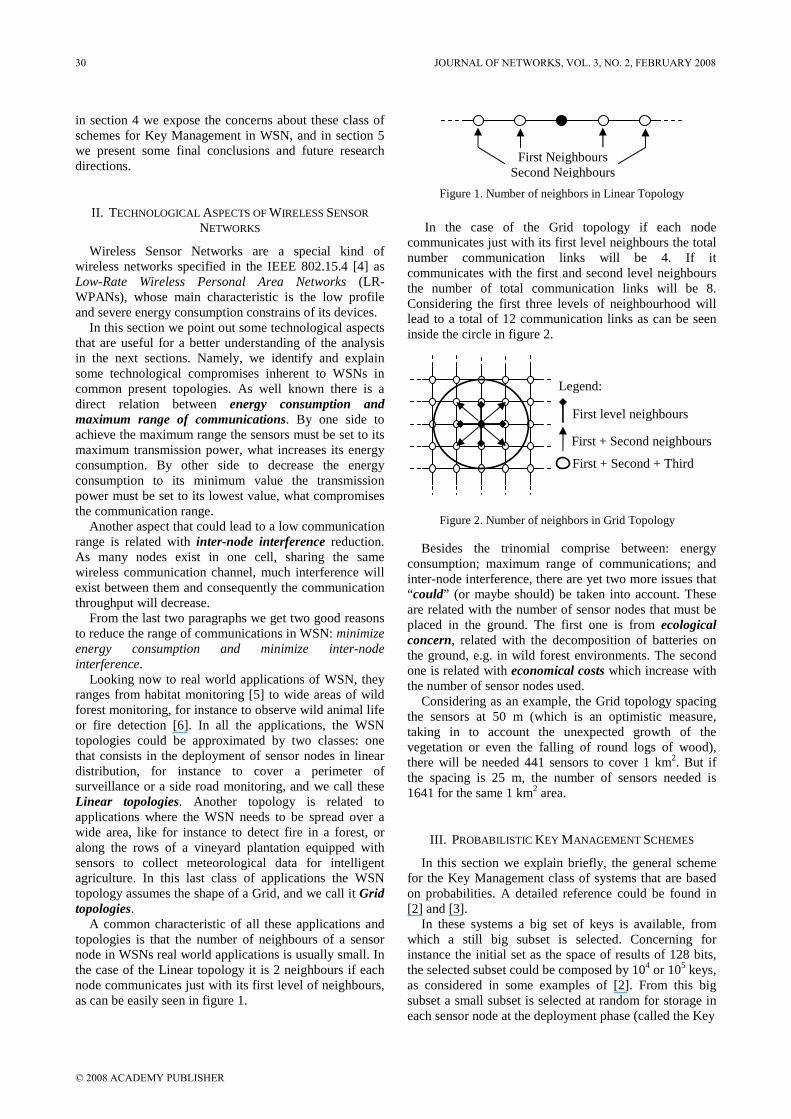
A common characteristic of all these applications and topologies is that the number of neighbours of a sensor node in WSNs real world applications is usually small. In the case of the Linear topology it is 2 neighbours if each node communicates just with its first level of neighbours, as can be easily seen in figure 1.

In the case of the Grid topology if each node

communicates just with its first level neighbours the total number communication links will be 4. If it communicates with the first and second level neighbours the number of total communication links will be 8. Considering the first three levels of neighbourhood will lead to a total of 12 communication links as can be seen inside the circle in figure 2.

Besides the trinomial comprise between: energy

consumption; maximum range of communications; and inter-node interference, there are yet two more issues that “could” (or maybe should) be taken into account. These are related with the number of sensor nodes that must be placed in the ground. The first one is from ecological concern, related with the decomposition of batteries on the ground, e.g. in wild forest environments. The second one is related with economical costs which increase with the number of sensor nodes used.

Considering as an example, the Grid topology spacing the sensors at 50 m (which is an optimistic measure, taking in to account the unexpected growth of the vegetation or even the falling of round logs of wood), there will be needed 441 sensors to cover 1 km2. But if the spacing is 25 m, the number of sensors needed is 1641 for the same 1 km2 area.

III. PROBABILISTIC KEY MANAGEMENT SCHEMES

In this section we explain briefly, the general scheme for the Key Management class of systems that are based on probabilities. A detailed reference could be found in [2] and [3].

In these systems a big set of keys is available, from which a still big subset is selected. Concerning for instance the initial set as the space of results of 128 bits, the selected subset could be composed by 104 or 105 keys, as considered in some examples of [2]. From this big subset a small subset is selected at random for storage in each sensor node at the deployment phase (called the Key

First Neighbours Second Neighbours

First level neighbours

First + Second neighbours

First + Second + Third

Legend:

Figure 1. Number of neighbors in Linear Topology

Figure 2. Number of neighbors in Grid Topology

30 JOURNAL OF NETWORKS, VOL. 3, NO. 2, FEBRUARY 2008

© 2008 ACADEMY PUBLISHER

1 2 3 4 5 6 7 8 9 10n�106

16

18

20

22

24

26

28

30

32

d

Pc=0.99

Pc=0.999

Pc=0.9999

Pc=0.99999

Pc=0.999999

Pc=0.9999999

Ring of the sensor node), using a pre-distribution based system for distribution of the keys. The number of keys that needs to be stored in each sensor node is based on the required probability that any two nodes share at least one key.

At the self-organization bootstrap phase each sensor node must try to discover other sensor nodes in its neighbourhood that shares a key with it, sending the identification of its stored keys. This can be object of a concentrated cryptanalysis effort due to the announcement of the key identification, allowing an attacker to use the identified keys with other sensor nodes.

To overcome this weak point a new proposal was presented in [7] using Merkle Puzzles, that avoids sending the complete identification of the key to the wireless communication channel, however this proposal has a drawback related with the time needed to achieve networks stability.

Another proposal also aiming to improve the security of the networks was presented in [3] as a “q-Composite Keys scheme”, in which a communication link between two sensor nodes demands for sharing q keys instead of only one. This leads to a more robust system due to a bigger number of keys that needs to be shared, but by other side it will raise store problems as will be shown further in this paper.

In the following section we expose some practical concerns about this class of schemes.

IV. PROBABILISTIC KEY MANAGEMENT PRACTICAL

CONCERNS

In this section we first explain some concepts to a better contextualization of the subject, then we will focus the storage drawbacks of this class of system, next we focus on the effect of the topology, then we show that this class of systems have network connectivity problems in real world applications, and finally we expand our analysis to the q-composite variant.

A. Node Degree, Size of the Network and Probability of Network Connectivity

In a WSN we must guarantee that the probability of establishing a link between neighbour nodes is sufficiently high so that the n-nodes network in connected. The number of available keys for distribution (key pool), and shared keys between nodes are critical parameters. On one hand, we want the number of shared keys to be large enough to guarantee a high probability of connection, and allow scalability of the system, on the other hand the memory restrictions of the physical sensor are impeditive of an arbitrary growth of the size of the key-ring within each sensor. In this sub-section we analyse the relation between these parameters and the consequences for the design of WSN where distributed key systems are used for security.

Let n be the number of sensor nodes, p the probability that a key is shared between two sensor nodes, and d the expected degree of a node, that is, the average number of

edges connecting the node with its neighbours. From [2] we get d=p(n-1). A WSN can be viewed as a random graph G(n,p), with n>>1, and we can use the results from [8] to establish that the probability Pc for graph connectivity is given by

ce

nc econnectedispnGPP

−−

∞→== )),((lim (1)

Where

n

c

n

np += )ln(

(2)

is the probability of existing a link between any two nodes, and c is a real constant. When c is given by equation (1) for a certain probability Pc, equation (2) gives the threshold value of the probability that corresponds to a connected network: the state of the network connection switches from “nonexistent” to “certainly true”. Assuming that this probability is the same as the probability of two nodes sharing a key, from equations (1) and (2), and the definition of node degree, we derive that

[ ])lnln()ln(1

),( cc Pnn

nPnd −−−= (3)

From (3), given a WSN size n, we can compute the

expected node degree. In Figure 3 we show the variation of the expected node degree as a function of the WSN size, in the range of 103 to 107 sensor nodes, for several probabilities of network connection. For large values of n, d is a O(ln (n)) and that explains the weak dependence on the size of the network. In fact, for large values of n, when we increase n by one order of magnitude we have

K30259.2)10ln(),(),10( =≈− cc PndPnd (4)

which means that de average node degree increases by 2.

Figure 3. Expected degree of node, d, as a function of WSN size, n, for six values of connectivity probability, Pc

JOURNAL OF NETWORKS, VOL. 3, NO. 2, FEBRUARY 2008 31

© 2008 ACADEMY PUBLISHER

0.2 0.4 0.6 0.8 1Pc

2.3

2.4

2.5

2.6

2.7

2.8

2.9

dHn

,Pc'L-

dHn

,PcL

0 1000 2000 3000 4000 5000m

0

0.2

0.4

0.6

0.8

1

p’

p’=0.5

p’=0.9S=10 5

S=10 6

S=10 7

1 2 3 4 5 6 7 8 9 10n�10 6

2.30259

2.30259

2.3026

2.3026

2.30261

2.30261

2.30262

dH10

n,P

cL-

dHn,

PcL

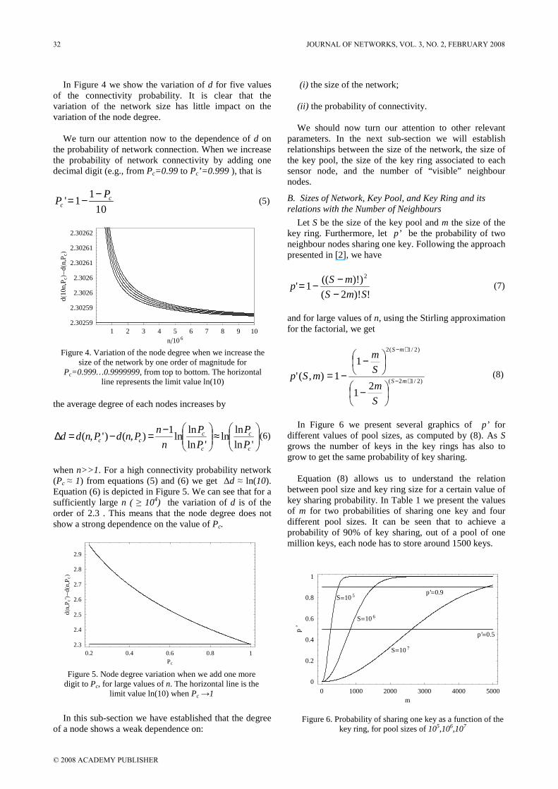
In Figure 4 we show the variation of d for five values of the connectivity probability. It is clear that the variation of the network size has little impact on the variation of the node degree.

We turn our attention now to the dependence of d on

the probability of network connection. When we increase the probability of network connectivity by adding one decimal digit (e.g., from Pc=0.99 to Pc’=0.999 ), that is

10

11' c

c

PP

−−= (5)

the average degree of each nodes increases by

≈

−=−=∆'ln

lnln

'ln

lnln

1),()',(

c

c

c

ccc P

P

P

P

n

nPndPndd (6)

when n>>1. For a high connectivity probability network (Pc ≈ 1) from equations (5) and (6) we get ∆d ≈ ln(10). Equation (6) is depicted in Figure 5. We can see that for a sufficiently large n ( ≥ 104) the variation of d is of the order of 2.3 . This means that the node degree does not show a strong dependence on the value of Pc.

In this sub-section we have established that the degree

of a node shows a weak dependence on:

(i) the size of the network; (ii) the probability of connectivity. We should now turn our attention to other relevant

parameters. In the next sub-section we will establish relationships between the size of the network, the size of the key pool, the size of the key ring associated to each sensor node, and the number of “visible” neighbour nodes.

B. Sizes of Network, Key Pool, and Key Ring and its relations with the Number of Neighbours

Let S be the size of the key pool and m the size of the key ring. Furthermore, let p’ be the probability of two neighbour nodes sharing one key. Following the approach presented in [2], we have

!)!2(

))!((1'

2

SmS

mSp

−−−= (7)

and for large values of n, using the Stirling approximation for the factorial, we get

)2/12(

)2/1(2

21

11),(' +−

+−

−

−−=

mS

mS

S

m

S

m

mSp (8)

In Figure 6 we present several graphics of p’ for

different values of pool sizes, as computed by (8). As S grows the number of keys in the key rings has also to grow to get the same probability of key sharing.

Equation (8) allows us to understand the relation

between pool size and key ring size for a certain value of key sharing probability. In Table 1 we present the values of m for two probabilities of sharing one key and four different pool sizes. It can be seen that to achieve a probability of 90% of key sharing, out of a pool of one million keys, each node has to store around 1500 keys.

Figure 5. Node degree variation when we add one more digit to Pc, for large values of n. The horizontal line is the

limit value ln(10) when Pc →1

Figure 6. Probability of sharing one key as a function of the key ring, for pool sizes of 105,106,107

Figure 4. Variation of the node degree when we increase the size of the network by one order of magnitude for

Pc=0.999…0.9999999, from top to bottom. The horizontal line represents the limit value ln(10)

32 JOURNAL OF NETWORKS, VOL. 3, NO. 2, FEBRUARY 2008

© 2008 ACADEMY PUBLISHER

20 30 40 50 60n’

200

300

400

500

600

m

n=104

n=103

S=105

25 30 35 40 45 50 55 60n’

2000

3000

4000

5000

6000

m

n=105

n=106

S=107

If, for security reasons, we need larger pool sizes, the number of stored keys in each sensor has to increase and, eventually, we must face storage capacity problems.

m S p’ 104 105 106 107

0,5 83 263 833 2633 0,9 151 479 1516 4798

From Figure 6 we can also see that larger pool sizes

will present a faster growth of m as a function of the probability p’. When we set p=p’ , with p defined by equations (1) and (2), we are assuming that each node is capable of communicating with every other node of the system. As pointed out in [2], wireless connectivity constraints impose that n’ is much smaller than n; there are few available sensor nodes within communication range. Therefore, assuming n’<<n , for a certain degree d we must have p’ >> p . Each node has a higher probability of connection with its neighbours in order to guarantee the network connectivity. Therefore, the probability p’ will, in practice, be a function of the number of neighbour nodes within reach of each sensor node. Lets examine how this relation is established for a certain pool of keys S, and a network of size n. Assuming a number of “visible” neighbours n’, and a degree d=p(n-1), we have

1'

1')1()1'('

−−=⇔−=−

n

nppnpnp

and attending to equation (3), we have

[ ])lnln()ln()1'(

1),',(' cc Pn

nn

nPnnp −−

−−= (9)

Using equation (8) we obtain

[ ] 0)lnln()ln()1´(

1

21

11 )2/12(

)2/1(2

=−−−

−−

−

−− +−

+−

cmS

mS

Pnnn

n

Sm

Sm

(10)

which implicitly DEFINES m AS A FUNCTION OF S, n, AND

n’, FOR EACH VALUE OF Pc. Let us assume that we are dealing with an “almost certainly” connected network, and set Pc=0.99999, because this is the value used in [2] as example. In Figure 7 we present the graphics for the variation of m as a function of n’ for two values of S, 105 and 107. For the first case we use networks with n=103 and 104 and for the second case we use networks with n=105 and 106. The results were obtained from numerically solving equation (10).

We can point out two important observations: (i) As expected, the number of keys in each sensor

node rapidly increases as the number of “visible” neighbours decreases, since we must increase the probability of key sharing between nodes in order to maintain network connectivity;

(ii) there is a minimum value for n’, related to the value of n.

If we want to guaranty network connectivity the

number of neighbours cannot drop bellow a certain value. In the present case we have: n’min= 20, 22, for n=103, 104, with S=105, respectively, and n’min=25, 27, for n=105, 106, with S=107, respectively. This as a consequence of the model and the mathematical reasoning is quite straightforward. We will address this problem in the next sub-section.

Observation (i) may be a problem due to the limited

storage capacity of each sensor node and presents a drawback of the key-management scheme for WSN proposed in [2], when we have a small value of n’min.

Observation (ii) imposes restrictions to the application

of this scheme when, for topological reasons, we need a number of neighbours smaller than the minimum value. We will explore this aspect in the next sub-section. It is worth noting that the situations we mentioned above are not so rare if we consider applications where a large number of nodes is distributed randomly or the distribution is dynamic.

Table 1 – Key Ring size for pool sizes of 104, 105, 106 and 107, considering a probability of sharing a key of 50 and 90%

Figure 7. Key ring size variation as a function of available neighbour nodes n’, for a pool of keys with S=105 and 107.

We assume that Pc=0.99999.

JOURNAL OF NETWORKS, VOL. 3, NO. 2, FEBRUARY 2008 33

© 2008 ACADEMY PUBLISHER

104 2x106 4x106 6x106 8x106 107

n

12

14

16

18

20

22

24

26

28

30

n’

Pc=0.5

Pc=0.9Pc=0.999

Pc=0.99999

)',,,( nnmSc eP α−=

5 10 15 20 25 30n’

0.2

0.4

0.6

0.8

1

Pc

n=104 n=107

pc=0.5

pc=0.9

C. The Effect of Network Topology

In the previous sub-section we have not considered any network topology in particular. When we set a certain value n’ for the number of neighbours nodes, we are implicitly making some assumptions on the spatial distribution of the sensors. Let us analyse, in particular, the two topologies presented in section 2 of interest in the framework of real sensor networks: the Linear and the Grid topologies.

The relevant question now is: “Can we consider Probabilistic Key Management

Schemes for key distribution under the assumption of these two topologies?”

Let’s remember that we need to keep the network

connected (with probability Pc), and the available paths are through the neighbour nodes. We can answer the former question by inspecting equation (9). Since p’ is a probability we have p’< 1, and hence

[ ] 1)lnln()ln()1'(

1 <−−−

−cPn

nn

n

From the last equation and attending to (3), we obtain

[ ] ),(1)lnln()ln(1

1'min cc PndPnn

nn +=−−−+> (11)

Equation (11) establishes a lower limit for the number

of neighbour nodes, given a certain connectivity probability Pc, which is 1 plus the average degree of each node, as defined by equation (3); in fact, we must consider the closest integer to this number. In Figure 8 we show n’min for several values of the connectivity probability.

To achieve a highly connected network (Pc>0.9) we

require at least n’=13, for a system with n=104 nodes. This is in fact an important constraint when we consider applications with linear or grid topologies.

If we use this Probabilistic Key Management schemes for key distribution with these topologies we cannot achieve acceptable connectivity for the network.

To draw our conclusions, it is more intuitive if we

solve (11) in order to Pc. From (11) we get

,)',( nnc eP α−= with 1

)1'(

)',( −−−

= n

nn

nennα (12)

Equation (12) is depicted in Figure 9. We have considered networks with sizes n=104,…,107, and n’ ranging from 2 to 30.

As we can observe, for systems with small number of

reachable neighbours, such as the ones considered in the linear and grid topologies, the connectivity probability is extremely low.

As an example for the linear topology with n’=2 and considering n=104 the probability of network connectivity is Pc≈ 10-1598. For larger systems the probabilities are even smaller. In any case, from the practical point of view, values for Pc bellow of 0.9 (meaning 90% of network connectivity) are unacceptable.

When we deduce equation (12) from (11) we are

assuming in equation (10) that p’(S,m)=1, which is the limit case that allows us to determine the minimum value of n’. However, rigorously speaking, we have to take into account equation (8) and the fact that p’ depends on the value of the pool size and of the key ring. Hence, from equations (3), (8), and (10) we obtain

),('

),(1),,,('

mSp

PndmSPnn c

c += (13)

Solving (13) in order to Pc, we get (14)

With ),('

1

)1'(

)',,,(mSp

n

nn

nennmS −−−

=α

From equation (14) we get the connectivity probability

as a function of the four relevant parameters: (i) the size of the system; (ii) the number of neighbours; (iii) the pool size; (iv) and the key ring size.

Figure 8. Minimum number of neighbours for connectivity probabilities of Pc=0.5, 0.7, 0.9, 0.999, 0.9999, 0.99999 (from

bottom to top), as a function of the size of the system.

Figure 9. Network connectivity probability as a function of the number of neighbours of each node, for n=104,…,107.

34 JOURNAL OF NETWORKS, VOL. 3, NO. 2, FEBRUARY 2008

© 2008 ACADEMY PUBLISHER

n=104, S=105

20

40

60

n’100

200

300

400

m

00.250.5

0.75

1

Pc

20

40n’

0 10 20 30 40 50 60n’

200

300

400

500

600

m

Pc=10-2

Pc=0.99999

Pc=0.5

n=106, S=107

20

40

60

n’

2000

4000

6000

m

00.250.5

0.75

1

Pc

20

40n’

20 30 40 50 60n’

2000

3000

4000

5000

6000

m

Pc=10-2

Pc=0.99999

Pc=0.5

We can now understand how the variation of the number of neighbour nodes will affect the connectivity of the network.

In Figure 10 we show two graphs for n=104 with S=105 and for n=106 with S=107, and for both we present the contour plot for seven reference values of the connectivity probability.

Some observations that are worth noting: (i) For large systems there is a well defined transition

in the connectivity probability which is a consequence of the property of random graphs stated in [11]; for certain values of (n’,m) the probability of network connectivity “jumps” from practically non-existent (Pc=10-2) to almost certain (Pc=0.9). This effect is well represented in the contour plots: the isoline Pc=10-2 is near the isoline Pc=0.9. The slope of the surface Pc(n’,m) near the transition is high;

(ii) From the contour plots we can infer a relation between m, Pc, and n’. In fact, we have

'/ nPm c∝ (15)

This equation shows the direct dependence of m with Pc, and the inverse dependence with n’, and has an important practical consequence.

D. An Example of Real World Application

Let us consider a WSN planned for forest monitoring, for instance and that we have sensors with a maximum range of communication of hmax=50 m. Our goal is to monitor an area of 10 Km2. Assuming that the sensors are distributed on a grid, for simplicity of calculation of the number of neighbours. Since we have a square of l=10 km on each side, according to the sensors range of communication we need an array of n=201x201=40401 sensors. To achieve our purposes, we need a highly connected network and we further consider Pc=0.99999. With these values, from equation (3) we get d(n,Pc)=22, meaning that on average each sensor has to be able to communicate with 22 other sensors. However, it is clear from this topology that, on the best case, the number of reachable neighbours is 8. Assuming that the communication with the neighbours is certain, which means p’(S,m)=1, from equation (14) we get Pc ≈ 10-16. The connectivity of the network is fully compromised.

Figure 10. Connectivity probability as a function of the number of neighbours and the size of the key ring, for two configurations of (n,S). For a small number of neighbours the size of the key ring increases rapidly, to achieve high values of

Pc. The contour plots show the variation of m as a function of n’ for Pc=10-2, .5, 0.9,…,0.99999.

JOURNAL OF NETWORKS, VOL. 3, NO. 2, FEBRUARY 2008 35

© 2008 ACADEMY PUBLISHER

Let us now face our real world application from other perspective. To achieve a good monitoring of the area, we want to make sure that the network is highly connected, that is, we assume Pc=0.99999. From equation (13), the number of neighbours is

'

),(1'

p

Pndn c+= (16)

where p’ is the probability of two nodes sharing at least one key. From the geometry of the topology, the number of neighbours of a node is

112'2

max −

+=h

hn

where h ≤ hmax is the distance between nodes. From the last equation we can write

11'

2 max

−+=

n

hh (17)

which implies that the total area, l x l, is covered with a grid of

2

1

+=h

ln nodes. (18)

We must solve these three equations simultaneously to

obtain a consistent solution (n, n’, h) for a certain value of p’.

In table 2 we show the results for p’=0.9, p’=0.7 and for p’=0.5. The key pool is set to S=106, which is of the order of nn’. We want to achieve a compromise between the number of keys in the key rings and the security of the communications between nodes: if S is smaller, the key ring in each node needs less keys to obtain the same probability p’ but, on the other hand, the smaller the value of S the greater the probability of having the same keys in different communications. Just as an example, we also show values of m for a pool size of S=2n.

From the general point of view of the applicability of

the key distribution scheme to this system we can point out three major concerns:

(i) we need a large quantity of neighbours for each sensor to achieve network connectivity with an

acceptable probability which, in turn, implies a large number of nodes in the network;

(ii) to decrease the size of the system we can increase the probability of sharing a key, p’ and in this case the number of keys in the sensor key ring increases and we can run into storage problems (even if we compromise security and use a smaller pool of keys);

(iii) the high density of sensors rises the problem of inter-node interference, besides the ecological and costly concerns.

To conclude, we believe by the exposed situations, that

there are practical restrictions to the applicability of this scheme to nowadays applications of sensor networks, in spite of the good mathematical results we can get when we are allowed to adjust the relevant parameters, such as the number of neighbours, the size of the system and the number of keys in each sensor key ring. As the previous example shows, real networks do not have that many degrees of freedom when concerning these parameters.

E. The q-Composite Scheme

We now turn our attention to a generalization of the key distribution scheme presented in the previous subsections. Suppose that, instead of sharing just one key from the key ring, each sensor node has to share q keys to establish a secure communication. These q keys are drawn from a key ring with m keys, extracted from a key pool of S keys. This scheme has been presented in [3]. The probability, p’, that the two nodes share q keys to form a connection is given by

( )[ ] ( )∑−

=

−

−+−

−=

1

02

2

!2!!

!1),,('

q

k mkSkmk

S

m

SqmSp (19)

When we consider the previous network, and setting

q=1, we obtain exactly the same values for m. If for security reasons we increase the value of shared keys to q=2, 3, which are the values proposed by [3] to improve the network resilience against a small number of captured nodes, we obtain the values listed in table 3. The problem with this scheme is again the requirements of the sensor storage capacity when we increase the number of shared keys between two sensors to establish a communication. For this particular application, the available memory on each sensor would have to increase by a factor of almost 2, for q=3.

m(S=106) q

p' 1 2 3

0.9 1516 1971 2305

0.7 1097 1561 1901

p’ n n’ h m(S=106) m(S=2n5) 0.9 187319 27 23 1516 479 0.7 252830 35 20 1097 346 0.5 375812 50 16 832 263

Table 2 – Relative values for the number of sensor nodes(n), number of neighbors (n’), distance between sensor nodes (h) and key ring size (m), for probabilities of 50, 70 and 90% of

network conectivity Table 3 – Size of the key ring (m), for a key pool (S) of 106, considering probabilities of 70 and 90% of network connectivity,

in the q-Composite scheme for q equal to 1, 2 and 3

(Note that q equal to 1 corresponds to the original proposal)

36 JOURNAL OF NETWORKS, VOL. 3, NO. 2, FEBRUARY 2008

© 2008 ACADEMY PUBLISHER

V. CONCLUSIONS

In this paper we expose some practical concerns about the key management schemes applicability to real world applications. In section 4 we focus five aspects and at the end of each of them we summarize the main ideas and conclusions. As a global conclusion we can say that the central problem of this class of schemes is related with the assumption that random graph theory can be applied directly to WSN and as consequence all the truth to random graph theory could be applied also directly to WSNs. In fact, considering just the main idea of WSN as big networks of self-organized sensors that sounds reasoning. The problem is related with the different concepts of communication link in WSNs and in a random graph theory.

Let’s think on a hypothetical example to make it very clear: in random graph theory we could have millions of sensors in ten square meters and consider that each of them has millions of neighbours with which it could communicate. But this theoretical conclusion for random graphs is impossible for real WSNs because those millions of sensors share the same wireless communication channel, which will completely block.

Besides that, this class of schemes are based on probability and as exposed in this paper there is a threshold value at which the network connectivity changes from null connectivity (probability near 0) to completely full connectivity (probability near 1). But this value depends on the number of neighbours as a base of communication links that could be established, and also on the number of keys stored in each sensor node. Figure 10 presents a good illustration between the number of neighbours (n’) and stored keys in each sensor node (m), as influence in the network connectivity probability.

Based on all that was previously exposed we consider that this class of schemes for key management in wireless sensor networks have some applicability concerns that must be taken in account in real world applications.

VI. RECOMMENDATION

As a final remark we point out some key ideas that should be kept in mind: i) The compromise between energy consumption and maximum range of communications leads to the reduction of this last one; ii) As many sensor nodes co-exist in the same communication cell, more inter-node interference will take place, leading again to the reduction of the communications range; iii) The present topologies point to just two neighbours in the Linear ones, and to eigth in the Grid ones; iv) As we demonstrated (see figure 10), the compromise between the number of neighbours and the near 100% of network connectivity leads to a minimum number of about 20 neighbours for each sensor node.

We conclude that with the present technological knowledge the probabilistic key management schemes should be of very concern in order of its applicability.

The conceptual idea of taking benefit from the great number of sensor nodes in a WSN could be used keeping in mind that they are low resource devices.

REFERENCES

[1] Crossbow Web Site: http://www.xbow.com/wireless_home.aspx, accessed in May, 2006.

[2] Eschenauer, L., and Gligor, V. A key-management scheme for distributed sensor networks. 9th ACM Conference on Computer and Communication Security, 2002.

[3] Chan, H., Perrig, A., and Song, D. Random Key Predistribution for Sensor Networks. IEEE Symposium on Security and Privacy, 2003.

[4] IEEE Computer Society Press. Wireless medium access control and physical layer specifications for low-rate wireless personal area networks. Standard 802.15.4-2003, May 2003.

[5] Mainwaring, A., Polastre, J., Szewczyk, R., Culler, D., and Anderson, J. WSNs for habitat monitoing. WSNA ’02, ACM, 2002.

[6] Simic, S. and Sastry, S. Distributed environmental monitoring using random sensor networks. 2nd International Workshop on Information Processing in Sensor Networks, Palo Alto, California, 2003.

[7] Merkle, R. Secure communications over insecure channels. Communications of the ACM, 1978.

[8] Spencer, J. The Strange Logic of Random Graphs. Springer-Verlag, 2000.

Rui Miguel Soares Silva, was born in Beja, Portugal, in 1971.

He got its graduation in 1996 in Computer Science Engineering from the IST at the Technical University of Lisbon in Portugal. Its Ms.C. degree was earn from the same institute in 2002. Now he’s finishing its Ph.D. also in the same institute.

He is an Associate Professor at ESTIG of the Polytechnic Institute of Beja in Portugal where he teaches Computer Networks to the graduate courses. He is also an Invited Researcher since 2000 in INESC-ID in Lisbon, Portugal. Its main research area is in Cryptography and Computer Security.

Rui Silva is Member of IEEE Computer Society and IACR (International Association for Crytologic Research).

Nuno Sodónio A. Pereira was born in Montijo, Portugal, in 1967.

He received its graduation in 1993 and its Ms.C in 2001, both in Physics from the New University of Lisbon.

He is now Associate Professor at ESTIG of the Polytechnic Institute of Beja in Portugal teaching Algebra to graduate courses.

Mário Serafim Nunes was born in Faro, Portugal, in 1952. He received the Electronics Engineer degree in 1975 and the Ph.D. degree in Electronics Engineer and Computers in 1987, both from the IST, Technical University of Lisbon, Portugal.

He is now Associated Professor at IST, where he teaches digital systems and telecommunications since 1975, in graduate and postgraduate courses. He is at INESC-ID, a research institute in Lisbon, where he is group leader, working in the areas of quality of service in IP networks and wireless sensor networks. He was responsible for the INESC participation in several European projects in networking. He is author of two books, "Digital Systems" and "Integrated Services Digital Networks".

Prof. Nunes is a Senior Member of the IEEE.

JOURNAL OF NETWORKS, VOL. 3, NO. 2, FEBRUARY 2008 37

© 2008 ACADEMY PUBLISHER