Principles of Economics

OpenStax College Rice University 6100 Main Street MS-380 Houston, Texas 77005

To learn more about OpenStax College, visit http://openstaxcollege.org. Individual print copies and bulk orders can be purchased through our website.

© 2014 Rice University. Textbook content produced by OpenStax College is licensed under a Creative Commons Attribution 4.0 License. Under this license, any user of this textbook or the textbook contents herein must provide proper attribution as follows:

- If you redistribute this textbook in a digital format (including but not limited to EPUB, PDF, and HTML), then you must retain on every page the following attribution: “Download for free at http://cnx.org/content/col11613/latest.”

- If you redistribute this textbook in a print format, then you must include on every physical page the following attribution: “Download for free at http://cnx.org/content/col11613/latest.”

- If you redistribute part of this textbook, then you must retain in every digital format page view (including but not limited to EPUB, PDF, and HTML) and on every physical printed page the following attribution:

- “Download for free at http://cnx.org/content/col11613/latest.” - If you use this textbook as a bibliographic reference, then you should cite it as follows: OpenStax College, Principles of

Economics. OpenStax College. 19 March 2014. <http://cnx.org/content/col11613/latest/>.

The OpenStax College name, OpenStax College logo, OpenStax College book covers, Connexions name, and Connexions logo are not subject to the license and may not be reproduced without the prior and express written consent of Rice University. For questions regarding this license, please contact [email protected].

Trademarks

The OpenStax College name, OpenStax College logo, OpenStax College book covers, Connexions name, and Connexions logo are registered trademarks of Rice University. All rights reserved. Any of the trademarks, service marks, collective marks, design rights, or similar rights that are mentioned, used, or cited in OpenStax College, Connexions, or Connexions’ sites are the property of their respective owners.

ISBN-10 1938168232

ISBN-13 978-1-938168-23-9

Revision PE-1-001-RS

OpenStax College

OpenStax College is a non-profit organization committed to improving student access to quality learning materials. Our free textbooks are developed and peer-reviewed by educators to ensure they are readable, accurate, and meet the scope and sequence requirements of modern college courses. Through our partnerships with companies and foundations committed to reducing costs for students, OpenStax College is working to improve access to higher education for all.

Connexions

The technology platform supporting OpenStax College is Connexions (http://cnx.org), one of the world’s first and largest open-education projects. Connexions provides students with free online and low-cost print editions of the OpenStax College library and provides instructors with tools to customize the content so that they can have the perfect book for their course.

Rice University

OpenStax College and Connexions are initiatives of Rice University. As a leading research university with a distinctive commitment to undergraduate education, Rice University aspires to path-breaking research, unsurpassed teaching, and contributions to the betterment of our world. It seeks to fulfill this mission by cultivating a diverse community of learning and discovery that produces leaders across the spectrum of human endeavor.

Foundation Support

OpenStax College is grateful for the tremendous support of our sponsors. Without their strong engagement, the goal of free access to high-quality textbooks would remain just a dream.

Laura and John Arnold Foundation (LJAF) actively seeks opportunities to invest in organizations and thought leaders that have a sincere interest in implementing fundamental changes that not only yield immediate gains, but also repair broken systems for future generations. LJAF currently focuses its strategic investments on education, criminal justice, research integrity, and public accountability.

The William and Flora Hewlett Foundation has been making grants since 1967 to help solve social and environmental problems at home and around the world. The Foundation concentrates its resources on activities in education, the environment, global development and population, performing arts, and philanthropy, and makes grants to support disadvantaged communities in the San Francisco Bay Area.

Guided by the belief that every life has equal value, the Bill & Melinda Gates Foundation works to help all people lead healthy, productive lives. In developing countries, it focuses on improving people’s health with vaccines and other life-saving tools and giving them the chance to lift themselves out of hunger and extreme poverty. In the United States, it seeks to significantly improve education so that all young people have the opportunity to reach their full potential. Based in Seattle, Washington, the foundation is led by CEO Jeff Raikes and Co-chair William H. Gates Sr., under the direction of Bill and Melinda Gates and Warren Buffett.

The Maxfield Foundation supports projects with potential for high impact in science, education, sustainability, and other areas of social importance.

Our mission at the Twenty Million Minds Foundation is to grow access and success by eliminating unnecessary hurdles to affordability. We support the creation, sharing, and proliferation of more effective, more affordable educational content by leveraging disruptive technologies, open educational resources, and new models for collaboration between for-profit, nonprofit, and public entities.

T H E C A L V I N K .

KAZANJIANECONOMICS FOUNDATION

Calvin K. Kazanjian was the founder and president of Peter Paul Inc., the maker of the Mounds and Almond Joy candy bars, located in Naugatuck, Connecticut. He firmly believed that if more people understood basic economics the world would be a better place in which to live. Accordingly, he established the Foundation in the true spirit of unselfish service. The Calvin K. Kazanjian Economics Foundation Inc. is a non-political education organization that was incorporated as a nonprofit organization under the Statue Laws of the State of Connecticut on April 4, 1947.

2

This content is available for free at http://cnx.org/content/col11613/1.10

Table of ContentsPreface . . . . . . . . . . . . . . . . . . . . . . . . . . . . . . . . . . . . . . . . . . . . . . . . . . . 6Chapter 1: Welcome to Economics! . . . . . . . . . . . . . . . . . . . . . . . . . . . . . . . . . . 13

1.1 What Is Economics, and Why Is It Important? . . . . . . . . . . . . . . . . . . . . . . . . . 141.2 Microeconomics and Macroeconomics . . . . . . . . . . . . . . . . . . . . . . . . . . . . 171.3 How Economists Use Theories and Models to Understand Economic Issues . . . . . . . . . 181.4 How Economies Can Be Organized: An Overview of Economic Systems . . . . . . . . . . . 20

Chapter 2: Choice in a World of Scarcity . . . . . . . . . . . . . . . . . . . . . . . . . . . . . . . 292.1 How Individuals Make Choices Based on Their Budget Constraint . . . . . . . . . . . . . . 302.2 The Production Possibilities Frontier and Social Choices . . . . . . . . . . . . . . . . . . . 342.3 Confronting Objections to the Economic Approach . . . . . . . . . . . . . . . . . . . . . . 38

Chapter 3: Demand and Supply . . . . . . . . . . . . . . . . . . . . . . . . . . . . . . . . . . . . 453.1 Demand, Supply, and Equilibrium in Markets for Goods and Services . . . . . . . . . . . . 463.2 Shifts in Demand and Supply for Goods and Services . . . . . . . . . . . . . . . . . . . . 513.3 Changes in Equilibrium Price and Quantity: The Four-Step Process . . . . . . . . . . . . . 593.4 Price Ceilings and Price Floors . . . . . . . . . . . . . . . . . . . . . . . . . . . . . . . . 643.5 Demand, Supply, and Efficiency . . . . . . . . . . . . . . . . . . . . . . . . . . . . . . . . 67

Chapter 4: Labor and Financial Markets . . . . . . . . . . . . . . . . . . . . . . . . . . . . . . . 774.1 Demand and Supply at Work in Labor Markets . . . . . . . . . . . . . . . . . . . . . . . . 784.2 Demand and Supply in Financial Markets . . . . . . . . . . . . . . . . . . . . . . . . . . . 854.3 The Market System as an Efficient Mechanism for Information . . . . . . . . . . . . . . . . 90

Chapter 5: Elasticity . . . . . . . . . . . . . . . . . . . . . . . . . . . . . . . . . . . . . . . . . . 995.1 Price Elasticity of Demand and Price Elasticity of Supply . . . . . . . . . . . . . . . . . . . 1005.2 Polar Cases of Elasticity and Constant Elasticity . . . . . . . . . . . . . . . . . . . . . . . 1045.3 Elasticity and Pricing . . . . . . . . . . . . . . . . . . . . . . . . . . . . . . . . . . . . . . 1065.4 Elasticity in Areas Other Than Price . . . . . . . . . . . . . . . . . . . . . . . . . . . . . . 113

Chapter 6: Consumer Choices . . . . . . . . . . . . . . . . . . . . . . . . . . . . . . . . . . . . . 1216.1 Consumption Choices . . . . . . . . . . . . . . . . . . . . . . . . . . . . . . . . . . . . . 1226.2 How Changes in Income and Prices Affect Consumption Choices . . . . . . . . . . . . . . 1286.3 Labor-Leisure Choices . . . . . . . . . . . . . . . . . . . . . . . . . . . . . . . . . . . . . 1326.4 Intertemporal Choices in Financial Capital Markets . . . . . . . . . . . . . . . . . . . . . . 136

Chapter 7: Cost and Industry Structure . . . . . . . . . . . . . . . . . . . . . . . . . . . . . . . . 1477.1 Explicit and Implicit Costs, and Accounting and Economic Profit . . . . . . . . . . . . . . . 1487.2 The Structure of Costs in the Short Run . . . . . . . . . . . . . . . . . . . . . . . . . . . . 1507.3 The Structure of Costs in the Long Run . . . . . . . . . . . . . . . . . . . . . . . . . . . . 155

Chapter 8: Perfect Competition . . . . . . . . . . . . . . . . . . . . . . . . . . . . . . . . . . . . 1678.1 Perfect Competition and Why It Matters . . . . . . . . . . . . . . . . . . . . . . . . . . . . 1688.2 How Perfectly Competitive Firms Make Output Decisions . . . . . . . . . . . . . . . . . . . 1698.3 Entry and Exit Decisions in the Long Run . . . . . . . . . . . . . . . . . . . . . . . . . . . 1818.4 Efficiency in Perfectly Competitive Markets . . . . . . . . . . . . . . . . . . . . . . . . . . 183

Chapter 9: Monopoly . . . . . . . . . . . . . . . . . . . . . . . . . . . . . . . . . . . . . . . . . . 1899.1 How Monopolies Form: Barriers to Entry . . . . . . . . . . . . . . . . . . . . . . . . . . . 1909.2 How a Profit-Maximizing Monopoly Chooses Output and Price . . . . . . . . . . . . . . . . 194

Chapter 10: Monopolistic Competition and Oligopoly . . . . . . . . . . . . . . . . . . . . . . . . 20710.1 Monopolistic Competition . . . . . . . . . . . . . . . . . . . . . . . . . . . . . . . . . . . 20810.2 Oligopoly . . . . . . . . . . . . . . . . . . . . . . . . . . . . . . . . . . . . . . . . . . . 215

Chapter 11: Monopoly and Antitrust Policy . . . . . . . . . . . . . . . . . . . . . . . . . . . . . . 22511.1 Corporate Mergers . . . . . . . . . . . . . . . . . . . . . . . . . . . . . . . . . . . . . . 22611.2 Regulating Anticompetitive Behavior . . . . . . . . . . . . . . . . . . . . . . . . . . . . . 23111.3 Regulating Natural Monopolies . . . . . . . . . . . . . . . . . . . . . . . . . . . . . . . . 23311.4 The Great Deregulation Experiment . . . . . . . . . . . . . . . . . . . . . . . . . . . . . 235

Chapter 12: Environmental Protection and Negative Externalities . . . . . . . . . . . . . . . . . 24312.1 The Economics of Pollution . . . . . . . . . . . . . . . . . . . . . . . . . . . . . . . . . . 24412.2 Command-and-Control Regulation . . . . . . . . . . . . . . . . . . . . . . . . . . . . . . 24812.3 Market-Oriented Environmental Tools . . . . . . . . . . . . . . . . . . . . . . . . . . . . 24812.4 The Benefits and Costs of U.S. Environmental Laws . . . . . . . . . . . . . . . . . . . . . 25212.5 International Environmental Issues . . . . . . . . . . . . . . . . . . . . . . . . . . . . . . 25412.6 The Tradeoff between Economic Output and Environmental Protection . . . . . . . . . . . 255

Chapter 13: Positive Externalities and Public Goods . . . . . . . . . . . . . . . . . . . . . . . . 26513.1 Why the Private Sector Under Invests in Innovation . . . . . . . . . . . . . . . . . . . . . 26613.2 How Governments Can Encourage Innovation . . . . . . . . . . . . . . . . . . . . . . . . 27013.3 Public Goods . . . . . . . . . . . . . . . . . . . . . . . . . . . . . . . . . . . . . . . . . 273

3

Chapter 14: Poverty and Economic Inequality . . . . . . . . . . . . . . . . . . . . . . . . . . . . 28114.1 Drawing the Poverty Line . . . . . . . . . . . . . . . . . . . . . . . . . . . . . . . . . . . 28214.2 The Poverty Trap . . . . . . . . . . . . . . . . . . . . . . . . . . . . . . . . . . . . . . . 28514.3 The Safety Net . . . . . . . . . . . . . . . . . . . . . . . . . . . . . . . . . . . . . . . . 28814.4 Income Inequality: Measurement and Causes . . . . . . . . . . . . . . . . . . . . . . . . 29114.5 Government Policies to Reduce Income Inequality . . . . . . . . . . . . . . . . . . . . . . 297

Chapter 15: Issues in Labor Markets: Unions, Discrimination, Immigration . . . . . . . . . . . . 30515.1 Unions . . . . . . . . . . . . . . . . . . . . . . . . . . . . . . . . . . . . . . . . . . . . 30715.2 Employment Discrimination . . . . . . . . . . . . . . . . . . . . . . . . . . . . . . . . . . 31315.3 Immigration . . . . . . . . . . . . . . . . . . . . . . . . . . . . . . . . . . . . . . . . . . 317

Chapter 16: Information, Risk, and Insurance . . . . . . . . . . . . . . . . . . . . . . . . . . . . 32516.1 The Problem of Imperfect Information and Asymmetric Information . . . . . . . . . . . . . 32616.2 Insurance and Imperfect Information . . . . . . . . . . . . . . . . . . . . . . . . . . . . . 331

Chapter 17: Financial Markets . . . . . . . . . . . . . . . . . . . . . . . . . . . . . . . . . . . . . 34117.1 How Businesses Raise Financial Capital . . . . . . . . . . . . . . . . . . . . . . . . . . . 34317.2 How Households Supply Financial Capital . . . . . . . . . . . . . . . . . . . . . . . . . . 34617.3 How to Accumulate Personal Wealth . . . . . . . . . . . . . . . . . . . . . . . . . . . . . 355

Chapter 18: Public Economy . . . . . . . . . . . . . . . . . . . . . . . . . . . . . . . . . . . . . . 36518.1 Voter Participation and Costs of Elections . . . . . . . . . . . . . . . . . . . . . . . . . . 36618.2 Special Interest Politics . . . . . . . . . . . . . . . . . . . . . . . . . . . . . . . . . . . . 36818.3 Flaws in the Democratic System of Government . . . . . . . . . . . . . . . . . . . . . . . 371

Chapter 19: The Macroeconomic Perspective . . . . . . . . . . . . . . . . . . . . . . . . . . . . 37919.1 Measuring the Size of the Economy: Gross Domestic Product . . . . . . . . . . . . . . . . 38119.2 Adjusting Nominal Values to Real Values . . . . . . . . . . . . . . . . . . . . . . . . . . . 38819.3 Tracking Real GDP over Time . . . . . . . . . . . . . . . . . . . . . . . . . . . . . . . . 39319.4 Comparing GDP among Countries . . . . . . . . . . . . . . . . . . . . . . . . . . . . . . 39519.5 How Well GDP Measures the Well-Being of Society . . . . . . . . . . . . . . . . . . . . . 398

Chapter 20: Economic Growth . . . . . . . . . . . . . . . . . . . . . . . . . . . . . . . . . . . . . 40520.1 The Relatively Recent Arrival of Economic Growth . . . . . . . . . . . . . . . . . . . . . . 40620.2 Labor Productivity and Economic Growth . . . . . . . . . . . . . . . . . . . . . . . . . . 40920.3 Components of Economic Growth . . . . . . . . . . . . . . . . . . . . . . . . . . . . . . 41420.4 Economic Convergence . . . . . . . . . . . . . . . . . . . . . . . . . . . . . . . . . . . 419

Chapter 21: Unemployment . . . . . . . . . . . . . . . . . . . . . . . . . . . . . . . . . . . . . . 42721.1 How the Unemployment Rate is Defined and Computed . . . . . . . . . . . . . . . . . . . 42821.2 Patterns of Unemployment . . . . . . . . . . . . . . . . . . . . . . . . . . . . . . . . . . 43221.3 What Causes Changes in Unemployment over the Short Run . . . . . . . . . . . . . . . . 43721.4 What Causes Changes in Unemployment over the Long Run . . . . . . . . . . . . . . . . 440

Chapter 22: Inflation . . . . . . . . . . . . . . . . . . . . . . . . . . . . . . . . . . . . . . . . . . 45122.1 Tracking Inflation . . . . . . . . . . . . . . . . . . . . . . . . . . . . . . . . . . . . . . . 45222.2 How Changes in the Cost of Living are Measured . . . . . . . . . . . . . . . . . . . . . . 45622.3 How the U.S. and Other Countries Experience Inflation . . . . . . . . . . . . . . . . . . . 46022.4 The Confusion Over Inflation . . . . . . . . . . . . . . . . . . . . . . . . . . . . . . . . . 46422.5 Indexing and Its Limitations . . . . . . . . . . . . . . . . . . . . . . . . . . . . . . . . . . 467

Chapter 23: The International Trade and Capital Flows . . . . . . . . . . . . . . . . . . . . . . . 47523.1 Measuring Trade Balances . . . . . . . . . . . . . . . . . . . . . . . . . . . . . . . . . . 47623.2 Trade Balances in Historical and International Context . . . . . . . . . . . . . . . . . . . . 47923.3 Trade Balances and Flows of Financial Capital . . . . . . . . . . . . . . . . . . . . . . . 48123.4 The National Saving and Investment Identity . . . . . . . . . . . . . . . . . . . . . . . . . 48323.5 The Pros and Cons of Trade Deficits and Surpluses . . . . . . . . . . . . . . . . . . . . . 48723.6 The Difference between Level of Trade and the Trade Balance . . . . . . . . . . . . . . . 489

Chapter 24: The Aggregate Demand/Aggregate Supply Model . . . . . . . . . . . . . . . . . . . 49524.1 Macroeconomic Perspectives on Demand and Supply . . . . . . . . . . . . . . . . . . . . 49724.2 Building a Model of Aggregate Demand and Aggregate Supply . . . . . . . . . . . . . . . 49824.3 Shifts in Aggregate Supply . . . . . . . . . . . . . . . . . . . . . . . . . . . . . . . . . . 50324.4 Shifts in Aggregate Demand . . . . . . . . . . . . . . . . . . . . . . . . . . . . . . . . . 50524.5 How the AD/AS Model Incorporates Growth, Unemployment, and Inflation . . . . . . . . . 50824.6 Keynes’ Law and Say’s Law in the AD/AS Model . . . . . . . . . . . . . . . . . . . . . . 511

Chapter 25: The Keynesian Perspective . . . . . . . . . . . . . . . . . . . . . . . . . . . . . . . 51925.1 Aggregate Demand in Keynesian Analysis . . . . . . . . . . . . . . . . . . . . . . . . . . 52025.2 The Building Blocks of Keynesian Analysis . . . . . . . . . . . . . . . . . . . . . . . . . . 52325.3 The Phillips Curve . . . . . . . . . . . . . . . . . . . . . . . . . . . . . . . . . . . . . . 52725.4 The Keynesian Perspective on Market Forces . . . . . . . . . . . . . . . . . . . . . . . . 530

Chapter 26: The Neoclassical Perspective . . . . . . . . . . . . . . . . . . . . . . . . . . . . . . 535

4


26.1 The Building Blocks of Neoclassical Analysis . . . . . . . . . . . . . . . . . . . . . . . . 53626.2 The Policy Implications of the Neoclassical Perspective . . . . . . . . . . . . . . . . . . . 54126.3 Balancing Keynesian and Neoclassical Models . . . . . . . . . . . . . . . . . . . . . . . 547

Chapter 27: Money and Banking . . . . . . . . . . . . . . . . . . . . . . . . . . . . . . . . . . . . 55127.1 Defining Money by Its Functions . . . . . . . . . . . . . . . . . . . . . . . . . . . . . . . 55227.2 Measuring Money: Currency, M1, and M2 . . . . . . . . . . . . . . . . . . . . . . . . . . 55427.3 The Role of Banks . . . . . . . . . . . . . . . . . . . . . . . . . . . . . . . . . . . . . . 55627.4 How Banks Create Money . . . . . . . . . . . . . . . . . . . . . . . . . . . . . . . . . . 560

Chapter 28: Monetary Policy and Bank Regulation . . . . . . . . . . . . . . . . . . . . . . . . . 56928.1 The Federal Reserve Banking System and Central Banks . . . . . . . . . . . . . . . . . . 57028.2 Bank Regulation . . . . . . . . . . . . . . . . . . . . . . . . . . . . . . . . . . . . . . . 57228.3 How a Central Bank Executes Monetary Policy . . . . . . . . . . . . . . . . . . . . . . . 57528.4 Monetary Policy and Economic Outcomes . . . . . . . . . . . . . . . . . . . . . . . . . . 57828.5 Pitfalls for Monetary Policy . . . . . . . . . . . . . . . . . . . . . . . . . . . . . . . . . . 582

Chapter 29: Exchange Rates and International Capital Flows . . . . . . . . . . . . . . . . . . . . 59329.1 How the Foreign Exchange Market Works . . . . . . . . . . . . . . . . . . . . . . . . . . 59429.2 Demand and Supply Shifts in Foreign Exchange Markets . . . . . . . . . . . . . . . . . . 60129.3 Macroeconomic Effects of Exchange Rates . . . . . . . . . . . . . . . . . . . . . . . . . 60429.4 Exchange Rate Policies . . . . . . . . . . . . . . . . . . . . . . . . . . . . . . . . . . . 607

Chapter 30: Government Budgets and Fiscal Policy . . . . . . . . . . . . . . . . . . . . . . . . . 61730.1 Government Spending . . . . . . . . . . . . . . . . . . . . . . . . . . . . . . . . . . . . 61830.2 Taxation . . . . . . . . . . . . . . . . . . . . . . . . . . . . . . . . . . . . . . . . . . . . 62130.3 Federal Deficits and the National Debt . . . . . . . . . . . . . . . . . . . . . . . . . . . . 62330.4 Using Fiscal Policy to Fight Recession, Unemployment, and Inflation . . . . . . . . . . . . 62630.5 Automatic Stabilizers . . . . . . . . . . . . . . . . . . . . . . . . . . . . . . . . . . . . . 62930.6 Practical Problems with Discretionary Fiscal Policy . . . . . . . . . . . . . . . . . . . . . 63130.7 The Question of a Balanced Budget . . . . . . . . . . . . . . . . . . . . . . . . . . . . . 634

Chapter 31: The Impacts of Government Borrowing . . . . . . . . . . . . . . . . . . . . . . . . . 64131.1 How Government Borrowing Affects Investment and the Trade Balance . . . . . . . . . . 64231.2 Fiscal Policy, Investment, and Economic Growth . . . . . . . . . . . . . . . . . . . . . . . 64431.3 How Government Borrowing Affects Private Saving . . . . . . . . . . . . . . . . . . . . . 64931.4 Fiscal Policy and the Trade Balance . . . . . . . . . . . . . . . . . . . . . . . . . . . . . 650

Chapter 32: Macroeconomic Policy Around the World . . . . . . . . . . . . . . . . . . . . . . . 65732.1 The Diversity of Countries and Economies across the World . . . . . . . . . . . . . . . . 65932.2 Improving Countries’ Standards of Living . . . . . . . . . . . . . . . . . . . . . . . . . . . 66232.3 Causes of Unemployment around the World . . . . . . . . . . . . . . . . . . . . . . . . . 66632.4 Causes of Inflation in Various Countries and Regions . . . . . . . . . . . . . . . . . . . . 66732.5 Balance of Trade Concerns . . . . . . . . . . . . . . . . . . . . . . . . . . . . . . . . . . 668

Chapter 33: International Trade . . . . . . . . . . . . . . . . . . . . . . . . . . . . . . . . . . . . 67533.1 Absolute and Comparative Advantage . . . . . . . . . . . . . . . . . . . . . . . . . . . . 67633.2 What Happens When a Country Has an Absolute Advantage in All Goods . . . . . . . . . 68133.3 Intra-industry Trade between Similar Economies . . . . . . . . . . . . . . . . . . . . . . . 68533.4 The Benefits of Reducing Barriers to International Trade . . . . . . . . . . . . . . . . . . 688

Chapter 34: Globalization and Protectionism . . . . . . . . . . . . . . . . . . . . . . . . . . . . . 69534.1 Protectionism: An Indirect Subsidy from Consumers to Producers . . . . . . . . . . . . . . 69634.2 International Trade and Its Effects on Jobs, Wages, and Working Conditions . . . . . . . . 70234.3 Arguments in Support of Restricting Imports . . . . . . . . . . . . . . . . . . . . . . . . . 70534.4 How Trade Policy Is Enacted: Globally, Regionally, and Nationally . . . . . . . . . . . . . 71034.5 The Tradeoffs of Trade Policy . . . . . . . . . . . . . . . . . . . . . . . . . . . . . . . . 713

A The Use of Mathematics in Principles of Economics . . . . . . . . . . . . . . . . . . . . . . . 721B Indifference Curves . . . . . . . . . . . . . . . . . . . . . . . . . . . . . . . . . . . . . . . . . . 737C Present Discounted Value . . . . . . . . . . . . . . . . . . . . . . . . . . . . . . . . . . . . . . 749D The Expenditure-Output Model . . . . . . . . . . . . . . . . . . . . . . . . . . . . . . . . . . . 751Index . . . . . . . . . . . . . . . . . . . . . . . . . . . . . . . . . . . . . . . . . . . . . . . . . . . 824

5

PREFACEWelcome to Principles of Economics, an OpenStax College resource. This textbook has been created with several goals inmind: accessibility, customization, and student engagement—all while encouraging students toward high levels of academicscholarship. Instructors and students alike will find that this textbook offers a strong foundation in economics in anaccessible format.

About OpenStax CollegeOpenStax College is a non-profit organization committed to improving student access to quality learning materials. Ourfree textbooks go through a rigorous editorial publishing process. Our texts are developed and peer-reviewed by educatorsto ensure they are readable, accurate, and meet the scope and sequence requirements of today’s college courses. Unliketraditional textbooks, OpenStax College resources live online and are owned by the community of educators using them.Through our partnerships with companies and foundations committed to reducing costs for students, OpenStax College isworking to improve access to higher education for all. OpenStax College is an initiative of Rice University and is madepossible through the generous support of several philanthropic foundations.

About OpenStax College’s ResourcesOpenStax College resources provide quality academic instruction. Three key features set our materials apart from others:they can be customized by instructors for each class, they are a "living" resource that grows online through contributionsfrom science educators, and they are available free or for minimal cost.

CustomizationOpenStax College learning resources are designed to be customized for each course. Our textbooks provide a solidfoundation on which instructors can build, and our resources are conceived and written with flexibility in mind. Instructorscan select the sections most relevant to their curricula and create a textbook that speaks directly to the needs of their classesand student body. Teachers are encouraged to expand on existing examples by adding unique context via geographicallylocalized applications and topical connections.

Principles of Economics can be easily customized using our online platform (http://cnx.org/content/col11613/). Simplyselect the content most relevant to your current semester and create a textbook that speaks directly to the needs of yourclass. Principles of Economics is organized as a collection of sections that can be rearranged, modified, and enhancedthrough localized examples or to incorporate a specific theme of your course. This customization feature will ensure thatyour textbook truly reflects the goals of your course. Principles of Economics is also available in two volumes, one coveringmicroeconomics and one covering macroeconomics principles.

CurationTo broaden access and encourage community curation, Principles of Economics is “open source” licensed under a CreativeCommons Attribution (CC-BY) license. The economics community is invited to submit examples, emerging research,and other feedback to enhance and strengthen the material and keep it current and relevant for today’s students. Submityour suggestions to [email protected], and check in on edition status, alternate versions, errata, and news on theStaxDash at http://openstaxcollege.org.

CostOur textbooks are available for free online, and in low-cost print and e-book editions.

About Principles of EconomicsPrinciples of Economics is designed for a two-semester principles of economics sequence. The text has been developed tomeet the scope and sequence of most introductory courses. At the same time, the book includes a number of innovativefeatures designed to enhance student learning. Instructors can also customize the book, adapting it to the approach thatworks best in their classroom.

Coverage and ScopeTo develop Principles of Economics, we acquired the rights to Timothy Taylor’s second edition of Principles of Economicsand solicited ideas from economics instructors at all levels of higher education, from community colleges to Ph.D.-grantinguniversities. They told us about their courses, students, challenges, resources, and how a textbook can best meet the needsof both instructors and students.

The result is a book that covers the breadth of economics topics and also provides the necessary depth to ensure the course ismanageable for instructors and students alike. And to make it more applied, we have incorporated many current topics. We

6


hope students will be interested to know just how far-reaching the recent recession was (and still is), for example, and whythere is so much controversy even among economists over the Affordable Care Act (Obamacare). The Keystone Pipeline,Occupy Wall Street, minimum wage debates, and the appointment of the United States’ first female Federal Reserve chair,Janet Yellen, are just a few of the other important topics covered.

The pedagogical choices, chapter arrangements, and learning objective fulfillment were developed and vetted with feedbackfrom educators dedicated to the project. They thoroughly read the material and offered critical and detailed commentary.The outcome is a balanced approach to micro and macro economics, to both Keynesian and classical views, and to thetheory and application of economics concepts. Current events are treated in a politically-balanced way as well.

The book is organized into eight main parts:

What is Economics? The first two chapters introduce students to the study of economics with a focus on makingchoices in a world of scarce resources.

Supply and Demand, Chapters 3 and 4, introduces and explains the first analytical model in economics: supply,demand, and equilibrium, before showing applications in the markets for labor and finance.

The Fundamentals of Microeconomic Theory, Chapters 5 through 10, begins the microeconomics portion of thetext, presenting the theories of consumer behavior, production and costs, and the different models of market structure,including some simple game theory.

Microeconomic Policy Issues, Chapters 11 through 18, cover the range of topics in applied micro, framed around theconcepts of public goods and positive and negative externalities. Students explore competition and antitrust policies,environmental problems, poverty, income inequality, and other labor market issues. The text also covers information,risk and financial markets, as well as public economy.

The Macroeconomic Perspective and Goals, Chapters 19 through 23, introduces a number of key concepts in macro:economic growth, unemployment and inflation, and international trade and capital flows.

A Framework for Macroeconomic Analysis, Chapters 24 through 26, introduces the principal analytic model inmacro, namely the Aggregate Demand/Aggregate Supply Model. The model is then applied to the Keynesian andNeoclassical perspectives. The Expenditure-Output model is fully explained in a stand-alone appendix.

Monetary and Fiscal Policy, Chapters 27 through 31, explains the role of money and the banking system, as well asmonetary policy and financial regulation. Then the discussion switches to government deficits and fiscal policy.

International Economics, Chapters 32 through 34, the final part of the text, introduces the international dimensionsof economics, including international trade and protectionism.

Chapter 1 Welcome to Economics!Chapter 2 Choice in a World of ScarcityChapter 3 Demand and SupplyChapter 4 Labor and Financial MarketsChapter 5 ElasticityChapter 6 Consumer ChoicesChapter 7 Cost and Industry StructureChapter 8 Perfect CompetitionChapter 9 MonopolyChapter 10 Monopolistic Competition and OligopolyChapter 11 Monopoly and Antitrust PolicyChapter 12 Environmental Protection and Negative ExternalitiesChapter 13 Positive Externalities and Public GoodsChapter 14 Poverty and Economic InequalityChapter 15 Issues in Labor Markets: Unions, Discrimination, ImmigrationChapter 16 Information, Risk, and InsuranceChapter 17 Financial MarketsChapter 18 Public EconomyChapter 19 The Macroeconomic PerspectiveChapter 20 Economic GrowthChapter 21 UnemploymentChapter 22 InflationChapter 23 The International Trade and Capital FlowsChapter 24 The Aggregate Demand/Aggregate Supply ModelChapter 25 The Keynesian PerspectiveChapter 26 The Neoclassical PerspectiveChapter 27 Money and BankingChapter 28 Monetary Policy and Bank RegulationChapter 29 Exchange Rates and International Capital Flows

7

Chapter 30 Government Budgets and Fiscal PolicyChapter 31 The Impacts of Government BorrowingChapter 32 Macroeconomic Policy Around the WorldChapter 33 International TradeChapter 34 Globalization and Protectionism

Appendix A The Use of Mathematics in Principles of EconomicsAppendix B Indifference CurvesAppendix C Present Discounted ValueAppendix D The Expenditure-Output Model

Alternate Sequencing

Principles of Economics was conceived and written to fit a particular topical sequence, but it can be used flexibly toaccommodate other course structures. One such potential structure, which will fit reasonably well with the textbook content,is provided. Please consider, however, that the chapters were not written to be completely independent, and that theproposed alternate sequence should be carefully considered for student preparation and textual consistency.

Chapter 1 Welcome to Economics!Chapter 2 Choice in a World of ScarcityChapter 3 Demand and SupplyChapter 4 Labor and Financial MarketsChapter 5 ElasticityChapter 6 Consumer ChoicesChapter 33 International TradeChapter 7 Cost and Industry StructureChapter 12 Environmental Protection and Negative ExternalitiesChapter 13 Positive Externalities and Public GoodsChapter 8 Perfect CompetitionChapter 9 MonopolyChapter 10 Monopolistic Competition and OligopolyChapter 11 Monopoly and Antitrust PolicyChapter 14 Poverty and Economic InequalityChapter 15 Issues in Labor Markets: Unions, Discrimination, ImmigrationChapter 16 Information, Risk, and InsuranceChapter 17 Financial MarketsChapter 18 Public EconomyChapter 19 The Macroeconomic PerspectiveChapter 20 Economic GrowthChapter 21 UnemploymentChapter 22 InflationChapter 23 The International Trade and Capital FlowsChapter 25 The Keynesian PerspectiveChapter 26 The Neoclassical PerspectiveChapter 27 Money and BankingChapter 28 Monetary Policy and Bank RegulationChapter 29 Exchange Rates and International Capital FlowsChapter 30 Government Budgets and Fiscal PolicyChapter 24 The Aggregate Demand/Aggregate Supply ModelChapter 31 The Impacts of Government BorrowingChapter 32 Macroeconomic Policy Around the WorldChapter 34 Globalization and Protectionism

Appendix A The Use of Mathematics in Principles of EconomicsAppendix B Indifference CurvesAppendix C Present Discounted ValueAppendix D The Expenditure-Output Model

Pedagogical FoundationThroughout the OpenStax version of Principles of Economics, you will find new features that engage the students ineconomic inquiry by taking selected topics a step further. Our features include:

Bring It Home: This added feature is a brief case study, specific to each chapter, which connects the chapter’s maintopic to the real word. It is broken up into two parts: the first at the beginning of the chapter (in the Intro module) and

8


the second at chapter’s end, when students have learned what’s necessary to understand the case and “bring home” thechapter’s core concepts.

Work It Out: This added feature asks students to work through a generally analytical or computational problem, andguides them step-by-step to find out how its solution is derived.

Clear It Up: This boxed feature, which includes pre-existing features from Taylor’s text, addresses common studentmisconceptions about the content. Clear It Ups are usually deeper explanations of something in the main body of thetext. Each CIU starts with a question. The rest of the feature explains the answer.

Link It Up: This added feature is a very brief introduction to a website that is pertinent to students’ understanding andenjoyment of the topic at hand.

Questions for Each Level of LearningThe OpenStax version of Principles of Economics further expands on Taylor’s original end of chapter materials by offeringfour types of end-of-module questions for students.

Self-Checks: Are analytical self-assessment questions that appear at the end of each module. They “click–to-reveal”an answer in the web view so students can check their understanding before moving on to the next module. Self-Check questions are not simple look-up questions. They push the student to think a bit beyond what is said in the text.Self-Check questions are designed for formative (rather than summative) assessment. The questions and answers areexplained so that students feel like they are being walked through the problem.

Review Questions: Have been retained from Taylor’s version, and are simple recall questions from the chapter andare in open-response format (not multiple choice or true/false). The answers can be looked up in the text.

Critical Thinking Questions: Are new higher-level, conceptual questions that ask students to demonstrate theirunderstanding by applying what they have learned in different contexts. They ask for outside-the-box thinking, forreasoning about the concepts. They push the student to places they wouldn’t have thought of going themselves.

Problems: Are exercises that give students additional practice working with the analytic and computational conceptsin the module.

Updated ArtPrinciples of Economics includes an updated art program to better inform today’s student, providing the latest data oncovered topics.

9

After adjusting for inflation, the federal minimum wage dropped more than 30 percent from 1967 to 2010, eventhough the nominal figure climbed from $1.40 to $7.25 per hour. Increases in the minimum wage in between2008 and 2010 kept the decline from being worse—as it would have been if the wage had remained the sameas it did from 1997 through 2007. (Sources: http://www.dol.gov/whd/minwage/chart.htm; http://data.bls.gov/cgi-bin/surveymost?cu)

About Our TeamSenior Contributing AuthorTimothy Taylor, Macalester CollegeTimothy Taylor has been writing and teaching about economics for 30 years, and is the Managing Editor of the Journalof Economic Perspectives, a post he’s held since 1986. He has been a lecturer for The Teaching Company, the Universityof Minnesota, and the Hubert H. Humphrey Institute of Public Affairs, where students voted him Teacher of the Year in1997. His writings include numerous pieces for journals such as the Milken Institute Review and The Public Interest, andhe has been an editor on many projects, most notably for the Brookings Institution and the World Bank, where he wasChief Outside Editor for the World Development Report 1999/2000, Entering the 21st Century: The Changing DevelopmentLandscape. He also blogs four to five times per week at http://conversableeconomist.blogspot.com. Timothy Taylor livesnear Minneapolis with his wife Kimberley and their three children.

Senior Content ExpertSteven A. Greenlaw, University of Mary WashingtonSteven Greenlaw has been teaching principles of economics for more than 30 years. In 1999, he received the Grellet C.Simpson Award for Excellence in Undergraduate Teaching at the University of Mary Washington. He is the author ofDoing Economics: A Guide to Doing and Understanding Economic Research, as well as a variety of articles on economicspedagogy and instructional technology, published in the Journal of Economic Education, the International Review ofEconomic Education, and other outlets. He wrote the module on Quantitative Writing for Starting Point: Teaching andLearning Economics, the web portal on best practices in teaching economics. Steven Greenlaw lives in Alexandria, Virginiawith his wife Kathy and their three children.

Senior Contributors

Eric Dodge Hanover College

10


Cynthia Gamez University of Texas at El Paso

Andres Jauregui Columbus State University

Diane Keenan Cerritos College

Dan MacDonald California State University San Bernardino

Amyaz Moledina The College of Wooster

Craig Richardson Winston-Salem State University

David Shapiro Pennsylvania State University

Ralph Sonenshine American University

Reviewers

Bryan Aguiar Northwest Arkansas Community College

Basil Al Hashimi Mesa Community College

Emil Berendt Mount St. Mary's University

Zena Buser Adams State University

Douglas Campbell The University of Memphis

Sanjukta Chaudhuri University of Wisconsin - Eau Claire

Xueyu Cheng Alabama State University

Robert Cunningham Alma College

Rosa Lea Danielson College of DuPage

Steven Deloach Elon University

Debbie Evercloud University of Colorado Denver

Sal Figueras Hudson County Community College

Reza Ghorashi Richard Stockton College of New Jersey

Robert Gillette University of Kentucky

Shaomin Huang Lewis-Clark State College

George Jones University of Wisconsin-Rock County

Charles Kroncke College of Mount St. Joseph

Teresa Laughlin Palomar Community College

Carlos Liard-Muriente Central Connecticut State University

Heather Luea Kansas State University

Steven Lugauer University of Notre Dame

William Mosher Nashua Community College

Michael Netta Hudson County Community College

Nick Noble Miami University

Joe Nowakowski Muskingum University

Shawn Osell University of Wisconsin, Superior

Mark Owens Middle Tennessee State University

11

Sonia Pereira Barnard College

Brian Peterson Central College

Jennifer Platania Elon University

Robert Rycroft University of Mary Washington

Adrienne Sachse Florida State College at Jacksonville

Hans Schumann Texas AM

Gina Shamshak Goucher College

Chris Warburton John Jay College of Criminal Justice, CUNY

Mark Witte Northwestern

Chiou-nan Yeh Alabama State University

AncillariesOpenStax projects offer an array of ancillaries for students and instructors. Please visit http://openstaxcollege.org and viewthe learning resources for this title.

12


1 | Welcome to Economics!

Figure 1.1 Do You Tweet? Economics is greatly impacted by how well information travels through society. Today,social media giants Twitter, Facebook, and Instagram are major forces on the information super highway. (Credit:modification of work by Manuel Iglesias/Flickr Creative Commons)

Decisions ... Decisions in the Social Media AgeTo post or not to post? To tweet or not to tweet? Every day we are faced with a myriad of decisions, fromwhat to have for breakfast, to which route to take to class, to the more complex—“Should I double majorand add possibly another semester of study to my education?” Our response to these choices dependson the information we have available at any given moment; information economists call “imperfect”because we rarely have all the data we need to make perfect decisions. Despite the lack of perfectinformation, we still make hundreds of decisions a day.

And now, we have another avenue in which to gather information—social media. Outlets like Facebookand Twitter are altering the process by which we make choices, how we spend our time, which movieswe see, which products we buy, and more. How many of you chose a university without checking out itsFacebook page or Twitter stream first for information and feedback?

As you will see in this course, what happens in economics is affected by how well and how fastinformation is disseminated through a society. “Economists love nothing better than when deep andliquid markets operate under conditions of perfect information,” says Jessica Irvine, National EconomicsEditor for News Corp Australia. “Twitter is good at this, bringing participants together to a commonmarketplace and transmitting information among them. Like the civic squares of old, Twitter is a placewhere participants come to trade information. No money changes hands, but producers and consumersof tweets can use the information available on Twitter to generate other economic benefits.”

This leads us to the topic of this chapter, an introduction to the world of making decisions, processinginformation, and understanding behavior in markets —the world of economics. Each chapter in this bookwill start with a discussion about current (or sometimes past) events and revisit it at chapter’s end—to“bring home” the concepts in play.

CHAPTER 1 | WELCOME TO ECONOMICS! 13

IntroductionIn this chapter, you will learn about:

• What Is Economics, and Why Is It Important?

• Microeconomics and Macroeconomics

• How Economists Use Theories and Models to Understand Economic Issues

• How Economies Can Be Organized: An Overview of Economic Systems

What is economics and why should you spend your time learning it? After all, there are other disciplines you could bestudying, and other ways you could be spending your time. As the Bring it Home feature just mentioned, making choicesis at the heart of what economists study, and your decision to take this course is as much as economic decision as anythingelse.

Economics is probably not what you think. It is not primarily about money or finance. It is not primarily about business. Itis not mathematics. What is it then? It is both a subject area and a way of viewing the world.

1.1 | What Is Economics, and Why Is It Important?By the end of this section, you will be able to:

• Discuss the importance of studying economics• Explain the relationship between production and division of labor• Evaluate the significance of scarcity

Economics is the study of how humans make decisions in the face of scarcity. These can be individual decisions, familydecisions, business decisions or societal decisions. If you look around carefully, you will see that scarcity is a fact of life.Scarcity means that human wants for goods, services and resources exceed what is available. Resources, such as labor,tools, land, and raw materials are necessary to produce the goods and services we want but they exist in limited supply. Ofcourse, the ultimate scarce resource is time- everyone, rich or poor, has just 24 hours in the day to try to acquire the goodsthey want. At any point in time, there is only a finite amount of resources available.

Think about it this way: In 2012 the labor force in the United States contained over 155.5 million workers, according tothe U.S. Bureau of Labor Statistics. Similarly, the total area of the United States is 3,794,101 square miles. These are largenumbers for such crucial resources, however, they are limited. Because these resources are limited, so are the numbers ofgoods and services we produce with them. Combine this with the fact that human wants seem to be virtually infinite, andyou can see why scarcity is a problem.

Figure 1.2 Scarcity of Resources Homeless people are a stark reminder that scarcity of resources is real. (Credit:“daveynin”/Flickr Creative Commons)

If you still do not believe that scarcity is a problem, consider the following: Does everyone need food to eat? Does everyoneneed a decent place to live? Does everyone have access to healthcare? In every country in the world, there are peoplewho are hungry, homeless (for example, those who call park benches their beds, as shown in Figure 1.2), and in need ofhealthcare, just to focus on a few critical goods and services. Why is this the case? It is because of scarcity. Let’s delve intothe concept of scarcity a little deeper, because it is crucial to understanding economics.

14 CHAPTER 1 | WELCOME TO ECONOMICS!


The Problem of ScarcityThink about all the things you consume: food, shelter, clothing, transportation, healthcare, and entertainment. How do youacquire those items? You do not produce them yourself. You buy them. How do you afford the things you buy? You workfor pay. Or if you do not, someone else does on your behalf. Yet most of us never have enough to buy all the things we want.This is because of scarcity. So how do we solve it?

Visit this website (http://openstaxcollege.org/l/drought) to read about how the United States is dealingwith scarcity in resources.

Every society, at every level, must make choices about how to use its resources. Families must decide whether to spendtheir money on a new car or a fancy vacation. Towns must choose whether to put more of the budget into police and fireprotection or into the school system. Nations must decide whether to devote more funds to national defense or to protectingthe environment. In most cases, there just isn’t enough money in the budget to do everything. So why do we not eachjust produce all of the things we consume? The simple answer is most of us do not know how, but that is not the mainreason. (When you study economics, you will discover that the obvious choice is not always the right answer—or at leastthe complete answer. Studying economics teaches you to think in a different of way.) Think back to pioneer days, whenindividuals knew how to do so much more than we do today, from building their homes, to growing their crops, to huntingfor food, to repairing their equipment. Most of us do not know how to do all—or any—of those things. It is not because wecould not learn. Rather, we do not have to. The reason why is something called the division and specialization of labor, aproduction innovation first put forth by Adam Smith, in his book, Figure 1.3 The Wealth of Nations.

Figure 1.3 Adam Smith Adam Smith introduced the idea of dividing labor into discrete tasks. (Credit: WikimediaCommons)

The Division of and Specialization of LaborThe formal study of economics began when Adam Smith (1723–1790) published his famous book The Wealth of Nationsin 1776. Many authors had written on economics in the centuries before Smith, but he was the first to address the subjectin a comprehensive way. In the first chapter, Smith introduces the division of labor, which means that the way a good orservice is produced is divided into a number of tasks that are performed by different workers, instead of all the tasks beingdone by the same person.


http://openstaxcollege.org/l/drought

To illustrate the division of labor, Smith counted how many tasks went into making a pin: drawing out a piece of wire,cutting it to the right length, straightening it, putting a head on one end and a point on the other, and packaging pins for sale,to name just a few. Smith counted 18 distinct tasks that were often done by different people—all for a pin, believe it or not!

Modern businesses divide tasks as well. Even a relatively simple business like a restaurant divides up the task of servingmeals into a range of jobs like top chef, sous chefs, less-skilled kitchen help, servers to wait on the tables, a greeter at thedoor, janitors to clean up, and a business manager to handle paychecks and bills—not to mention the economic connectionsa restaurant has with suppliers of food, furniture, kitchen equipment, and the building where it is located. A complexbusiness like a large manufacturing factory, such as the shoe factory shown in Figure 1.4, or a hospital can have hundredsof job classifications.

Figure 1.4 Division of Labor Workers on an assembly line are an example of the divisions of labor. (Credit: NinaHale/Flickr Creative Commons)

Why the Division of Labor Increases ProductionWhen the tasks involved with producing a good or service are divided and subdivided, workers and businesses can producea greater quantity of output. In his observations of pin factories, Smith observed that one worker alone might make 20 pinsin a day, but that a small business of 10 workers (some of whom would need to do two or three of the 18 tasks involved withpin-making), could make 48,000 pins in a day. How can a group of workers, each specializing in certain tasks, produce somuch more than the same number of workers who try to produce the entire good or service by themselves? Smith offeredthree reasons.

First, specialization in a particular small job allows workers to focus on the parts of the production process where theyhave an advantage. (In later chapters, we will develop this idea by discussing comparative advantage.) People have differentskills, talents, and interests, so they will be better at some jobs than at others. The particular advantages may be based oneducational choices, which are in turn shaped by interests and talents. Only those with medical degrees qualify to becomedoctors, for instance. For some goods, specialization will be affected by geography—it is easier to be a wheat farmer inNorth Dakota than in Florida, but easier to run a tourist hotel in Florida than in North Dakota. If you live in or near a bigcity, it is easier to attract enough customers to operate a successful dry cleaning business or movie theater than if you live ina sparsely populated rural area. Whatever the reason, if people specialize in the production of what they do best, they willbe more productive than if they produce a combination of things, some of which they are good at and some of which theyare not.

Second, workers who specialize in certain tasks often learn to produce more quickly and with higher quality. This patternholds true for many workers, including assembly line laborers who build cars, stylists who cut hair, and doctors who performheart surgery. In fact, specialized workers often know their jobs well enough to suggest innovative ways to do their workfaster and better.

A similar pattern often operates within businesses. In many cases, a business that focuses on one or a few products(sometimes called its “ core competency”) is more successful than firms that try to make a wide range of products.

Third, specialization allows businesses to take advantage of economies of scale, which means that for many goods, as thelevel of production increases, the average cost of producing each individual unit declines. For example, if a factory producesonly 100 cars per year, each car will be quite expensive to make on average. However, if a factory produces 50,000 carseach year, then it can set up an assembly line with huge machines and workers performing specialized tasks, and the averagecost of production per car will be lower. The ultimate result of workers who can focus on their preferences and talents, learnto do their specialized jobs better, and work in larger organizations is that society as a whole can produce and consume farmore than if each person tried to produce all of their own goods and services. The division and specialization of labor hasbeen a force against the problem of scarcity.



Trade and MarketsSpecialization only makes sense, though, if workers can use the pay they receive for doing their jobs to purchase the othergoods and services that they need. In short, specialization requires trade.

You do not have to know anything about electronics or sound systems to play music—you just buy an iPod or MP3 player,download the music and listen. You do not have to know anything about artificial fibers or the construction of sewingmachines if you need a jacket—you just buy the jacket and wear it. You do not need to know anything about internalcombustion engines to operate a car—you just get in and drive. Instead of trying to acquire all the knowledge and skillsinvolved in producing all of the goods and services that you wish to consume, the market allows you to learn a specializedset of skills and then use the pay you receive to buy the goods and services you need or want. This is how our modernsociety has evolved into a strong economy.

Why Study Economics?Now that we have gotten an overview on what economics studies, let’s quickly discuss why you are right to study it.Economics is not primarily a collection of facts to be memorized, though there are plenty of important concepts to belearned. Instead, economics is better thought of as a collection of questions to be answered or puzzles to be worked out.Most important, economics provides the tools to work out those puzzles. If you have yet to be been bitten by the economics“bug,” there are other reasons why you should study economics.

• Virtually every major problem facing the world today, from global warming, to world poverty, to the conflicts in Syria,Afghanistan, and Somalia, has an economic dimension. If you are going to be part of solving those problems, you needto be able to understand them. Economics is crucial.

• It is hard to overstate the importance of economics to good citizenship. You need to be able to vote intelligently onbudgets, regulations, and laws in general. When the U.S. government came close to a standstill at the end of 2012 dueto the “fiscal cliff,” what were the issues involved? Did you know?

• A basic understanding of economics makes you a well-rounded thinker. When you read articles about economic issues,you will understand and be able to evaluate the writer’s argument. When you hear classmates, co-workers, or politicalcandidates talking about economics, you will be able to distinguish between common sense and nonsense. You willfind new ways of thinking about current events and about personal and business decisions, as well as current eventsand politics.

The study of economics does not dictate the answers, but it can illuminate the different choices.

1.2 | Microeconomics and MacroeconomicsBy the end of this section, you will be able to:

• Describe microeconomics• Describe macroeconomics• Contrast monetary policy and fiscal policy

Economics is concerned with the well-being of all people, including those with jobs and those without jobs, as well as thosewith high incomes and those with low incomes. Economics acknowledges that production of useful goods and servicescan create problems of environmental pollution. It explores the question of how investing in education helps to developworkers’ skills. It probes questions like how to tell when big businesses or big labor unions are operating in a way thatbenefits society as a whole and when they are operating in a way that benefits their owners or members at the expense ofothers. It looks at how government spending, taxes, and regulations affect decisions about production and consumption.

It should be clear by now that economics covers a lot of ground. That ground can be divided into two parts:Microeconomics focuses on the actions of individual agents within the economy, like households, workers, and businesses;Macroeconomics looks at the economy as a whole. It focuses on broad issues such as growth of production, thenumber of unemployed people, the inflationary increase in prices, government deficits, and levels of exports and imports.Microeconomics and macroeconomics are not separate subjects, but rather complementary perspectives on the overallsubject of the economy.

To understand why both microeconomic and macroeconomic perspectives are useful, consider the problem of studying abiological ecosystem like a lake. One person who sets out to study the lake might focus on specific topics: certain kinds ofalgae or plant life; the characteristics of particular fish or snails; or the trees surrounding the lake. Another person mighttake an overall view and instead consider the entire ecosystem of the lake from top to bottom; what eats what, how thesystem stays in a rough balance, and what environmental stresses affect this balance. Both approaches are useful, and bothexamine the same lake, but the viewpoints are different. In a similar way, both microeconomics and macroeconomics studythe same economy, but each has a different viewpoint.


Whether you are looking at lakes or economics, the micro and the macro insights should blend with each other. In studyinga lake, the micro insights about particular plants and animals help to understand the overall food chain, while the macroinsights about the overall food chain help to explain the environment in which individual plants and animals live.

In economics, the micro decisions of individual businesses are influenced by whether the macroeconomy is healthy; forexample, firms will be more likely to hire workers if the overall economy is growing. In turn, the performance of themacroeconomy ultimately depends on the microeconomic decisions made by individual households and businesses.

MicroeconomicsWhat determines how households and individuals spend their budgets? What combination of goods and services will bestfit their needs and wants, given the budget they have to spend? How do people decide whether to work, and if so, whetherto work full time or part time? How do people decide how much to save for the future, or whether they should borrow tospend beyond their current means?

What determines the products, and how many of each, a firm will produce and sell? What determines what prices a firmwill charge? What determines how a firm will produce its products? What determines how many workers it will hire? Howwill a firm finance its business? When will a firm decide to expand, downsize, or even close? In the microeconomic part ofthis book, we will learn about the theory of consumer behavior and the theory of the firm.

MacroeconomicsWhat determines the level of economic activity in a society? In other words, what determines how many goods and servicesa nation actually produces? What determines how many jobs are available in an economy? What determines a nation’sstandard of living? What causes the economy to speed up or slow down? What causes firms to hire more workers or to layworkers off? Finally, what causes the economy to grow over the long term?

An economy's macroeconomic health can be defined by a number of goals: growth in the standard of living, lowunemployment, and low inflation, to name the most important. How can macroeconomic policy be used to pursue thesegoals? Monetary policy, which involves policies that affect bank lending, interest rates, and financial capital markets, isconducted by a nation’s central bank. For the United States, this is the Federal Reserve. Fiscal policy, which involvesgovernment spending and taxes, is determined by a nation’s legislative body. For the United States, this is the Congressand the executive branch, which originates the federal budget. These are the main tools the government has to work with.Americans tend to expect that government can fix whatever economic problems we encounter, but to what extent is thatexpectation realistic? These are just some of the issues that will be explored in the macroeconomic chapters of this book.

1.3 | How Economists Use Theories and Models toUnderstand Economic IssuesBy the end of this section, you will be able to:

• Interpret a circular flow diagram• Explain the importance of economic theories and models• Describe goods and services markets and labor markets

Figure 1.5 John Maynard Keynes One of the most influential economists in modern times was John MaynardKeynes. (Credit: Wikimedia Commons)

John Maynard Keynes (1883–1946), one of the greatest economists of the twentieth century, pointed out that economicsis not just a subject area but also a way of thinking. Keynes, shown in Figure 1.5, famously wrote in the introductionto a fellow economist’s book: “[Economics] is a method rather than a doctrine, an apparatus of the mind, a technique of



thinking, which helps its possessor to draw correct conclusions.” In other words, economics teaches you how to think, notwhat to think.

Watch this video (http://openstaxcollege.org/l/Keynes) about John Maynard Keynes and his influence oneconomics.

Economists see the world through a different lens than anthropologists, biologists, classicists, or practitioners of any otherdiscipline. They analyze issues and problems with economic theories that are based on particular assumptions about humanbehavior, that are different than the assumptions an anthropologist or psychologist might use. A theory is a simplifiedrepresentation of how two or more variables interact with each other. The purpose of a theory is to take a complex, real-world issue and simplify it down to its essentials. If done well, this enables the analyst to understand the issue and anyproblems around it. A good theory is simple enough to be understood, while complex enough to capture the key features ofthe object or situation being studied.

Sometimes economists use the term model instead of theory. Strictly speaking, a theory is a more abstract representation,while a model is more applied or empirical representation. Models are used to test theories, but for this course we will usethe terms interchangeably.

For example, an architect who is planning a major office building will often build a physical model that sits on a tabletop toshow how the entire city block will look after the new building is constructed. Companies often build models of their newproducts, which are more rough and unfinished than the final product will be, but can still demonstrate how the new productwill work.

A good model to start with in economics is the circular flow diagram, which is shown in Figure 1.6. It pictures theeconomy as consisting of two groups—households and firms—that interact in two markets: the goods and services marketin which firms sell and households buy and the labor market in which households sell labor to business firms or otheremployees.

Figure 1.6 The Circular Flow Diagram The circular flow diagram shows how households and firms interact in thegoods and services market, and in the labor market. The direction of the arrows shows that in the goods and servicesmarket, households receive goods and services and pay firms for them. In the labor market, households provide laborand receive payment from firms through wages, salaries, and benefits.

Of course, in the real world, there are many different markets for goods and services and markets for many different typesof labor. The circular flow diagram simplifies this to make the picture easier to grasp. In the diagram, firms produce goodsand services, which they sell to households in return for revenues. This is shown in the outer circle, and represents the twosides of the product market (for example, the market for goods and services) in which households demand and firms supply.


http://openstaxcollege.org/l/Keynes

Households sell their labor as workers to firms in return for wages, salaries and benefits. This is shown in the inner circleand represents the two sides of the labor market in which households supply and firms demand.

This version of the circular flow model is stripped down to the essentials, but it has enough features to explain how theproduct and labor markets work in the economy. We could easily add details to this basic model if we wanted to introducemore real-world elements, like financial markets, governments, and interactions with the rest of the globe (imports andexports).

Economists carry a set of theories in their heads like a carpenter carries around a toolkit. When they see an economic issueor problem, they go through the theories they know to see if they can find one that fits. Then they use the theory to deriveinsights about the issue or problem. In economics, theories are expressed as diagrams, graphs, or even as mathematicalequations. (Do not worry. In this course, we will mostly use graphs.) Economists do not figure out the answer to the problemfirst and then draw the graph to illustrate. Rather, they use the graph of the theory to help them figure out the answer.Although at the introductory level, you can sometimes figure out the right answer without applying a model, if you keepstudying economics, before too long you will run into issues and problems that you will need to graph to solve. Both microand macroeconomics are explained in terms of theories and models. The most well-known theories are probably those ofsupply and demand, but you will learn a number of others.

1.4 | How Economies Can Be Organized: An Overview ofEconomic SystemsBy the end of this section, you will be able to:

• Contrast traditional economies, command economies, and market economies• Explain gross domestic product (GDP)• Assess the importance and effects of globalization

Think about what a complex system a modern economy is. It includes all production of goods and services, all buying andselling, all employment. The economic life of every individual is interrelated, at least to a small extent, with the economiclives of thousands or even millions of other individuals. Who organizes and coordinates this system? Who insures that,for example, the number of televisions a society provides is the same as the amount it needs and wants? Who insures thatthe right number of employees work in the electronics industry? Who insures that televisions are produced in the best waypossible? How does it all get done?

There are at least three ways societies have found to organize an economy. The first is the traditional economy, which is theoldest economic system and can be found in parts of Asia, Africa, and South America. Traditional economies organize theireconomic affairs the way they have always done (i.e., tradition). Occupations stay in the family. Most families are farmerswho grow the crops they have always grown using traditional methods. What you produce is what you get to consume.Because things are driven by tradition, there is little economic progress or development.

Figure 1.7 A Command Economy Ancient Egypt was an example of a command economy. (Credit: Jay Bergesen/Flickr Creative Commons)

Command economies are very different. In a command economy, economic effort is devoted to goals passed down froma ruler or ruling class. Ancient Egypt was a good example: a large part of economic life was devoted to building pyramids,like those shown in Figure 1.7, for the pharaohs. Medieval manor life is another example: the lord provided the land forgrowing crops and protection in the event of war. In return, vassals provided labor and soldiers to do the lord’s bidding. Inthe last century, communism emphasized command economies.



In a command economy, the government decides what goods and services will be produced and what prices will be chargedfor them. The government decides what methods of production will be used and how much workers will be paid. Manynecessities like healthcare and education are provided for free. Currently, Cuba and North Korea have command economies.

Figure 1.8 A Market Economy Nothing says “market” more than The New York Stock Exchange. (Credit: Erik Drost/Flickr Creative Commons)

Although command economies have a very centralized structure for economic decisions, market economies have a verydecentralized structure. A market is an institution that brings together buyers and sellers of goods or services, who may beeither individuals or businesses. The New York Stock Exchange, shown in Figure 1.8, is a prime example of market inwhich buyers and sellers are brought together. In a market economy, decision-making is decentralized. Market economiesare based on private enterprise: the means of production (resources and businesses) are owned and operated by privateindividuals or groups of private individuals. Businesses supply goods and services based on demand. (In a commandeconomy, by contrast, resources and businesses are owned by the government.) What goods and services are supplieddepends on what is demanded. A person’s income is based on his or her ability to convert resources (especially labor) intosomething that society values. The more society values the person’s output, the higher the income (think Lady Gaga orLeBron James). In this scenario, economic decisions are determined by market forces, not governments.

Most economies in the real world are mixed; they combine elements of command and market (and even traditional) systems.The U.S. economy is positioned toward the market-oriented end of the spectrum. Many countries in Europe and LatinAmerica, while primarily market-oriented, have a greater degree of government involvement in economic decisions thandoes the U.S. economy. China and Russia, while they are closer to having a market-oriented system now than severaldecades ago, remain closer to the command economy end of the spectrum. A rich resource of information about countriesand their economies can be found on the Heritage Foundation’s website, as the following Clear It Up feature discusses.

What countries are considered economically free?Who is in control of economic decisions? Are people free to do what they want and to work where theywant? Are businesses free to produce when they want and what they choose, and to hire and fire asthey wish? Are banks free to choose who will receive loans? Or does the government control these kindsof choices? Each year, researchers at the Heritage Foundation and the Wall Street Journal look at 50different categories of economic freedom for countries around the world. They give each nation a scorebased on the extent of economic freedom in each category.

The 2013 Heritage Foundation’s Index of Economic Freedom report ranked 177 countries around theworld: some examples of the most free and the least free countries are listed in Table 1.1. Severalcountries were not ranked because of extreme instability that made judgments about economic freedomimpossible. These countries include Afghanistan, Iraq, Syria, and Somalia.

The assigned rankings are inevitably based on estimates, yet even these rough measures can beuseful for discerning trends. In 2013, 91 of the 177 included countries shifted toward greater economicfreedom, although 78 of the countries shifted toward less economic freedom. In recent decades, theoverall trend has been a higher level of economic freedom around the world.


Most Economic Freedom Least Economic Freedom

1. Hong Kong 168. Iran

2. Singapore 169. Turkmenistan

3. Australia 170. Equatorial Guinea

4. New Zealand 171. Democratic Republic of Congo

5. Switzerland 172. Burma

6. Canada 173. Eritrea

7. Chile 174. Venezuela

8. Mauritius 175. Zimbabwe

9. Denmark 176. Cuba

10. United States 177. North Korea

Table 1.1 Economic Freedoms, 2013 (Source: The Heritage Foundation, 2013 Index of EconomicFreedom, Country Rankings, http://www.heritage.org/index/ranking)

Regulations: The Rules of the GameMarkets and government regulations are always entangled. There is no such thing as an absolutely free market. Regulationsalways define the “rules of the game” in the economy. Economies that are primarily market-oriented have fewerregulations—ideally just enough to maintain an even playing field for participants. At a minimum, these laws governmatters like safeguarding private property against theft, protecting people from violence, enforcing legal contracts,preventing fraud, and collecting taxes. Conversely, even the most command-oriented economies operate using markets.How else would buying and selling occur? But the decisions of what will be produced and what prices will be charged areheavily regulated. Heavily regulated economies often have underground economies, which are markets where the buyersand sellers make transactions without the government’s approval.

The question of how to organize economic institutions is typically not a black-or-white choice between all market or allgovernment, but instead involves a balancing act over the appropriate combination of market freedom and governmentrules.

Figure 1.9 Globalization Cargo ships are one mode of transportation for shipping goods in the global economy.(Credit: Raul Valdez/Flickr Creative Commons)

The Rise of GlobalizationRecent decades have seen a trend toward globalization, which is the expanding cultural, political, and economicconnections between people around the world. One measure of this is the increased buying and selling of goods, services,and assets across national borders—in other words, international trade and financial capital flows.



Globalization has occurred for a number of reasons. Improvements in shipping, as illustrated by the container ship shown inFigure 1.9, and air cargo have driven down transportation costs. Innovations in computing and telecommunications havemade it easier and cheaper to manage long-distance economic connections of production and sales. Many valuable productsand services in the modern economy can take the form of information—for example: computer software; financial advice;travel planning; music, books and movies; and blueprints for designing a building. These products and many others canbe transported over telephones and computer networks at ever-lower costs. Finally, international agreements and treatiesbetween countries have encouraged greater trade.

Table 1.2 presents one measure of globalization. It shows the percentage of domestic economic production that wasexported for a selection of countries from 1970 to 2010, according to an entity known as The World Bank. Exports are thegoods and services that are produced domestically and sold in abroad. Imports are the goods and services that are producedabroad and then sold domestically. The size of total production in an economy is measured by the gross domestic product(GDP). Thus, the ratio of exports divided by GDP measures what share of a country’s total economic production is sold inother countries.

Country 1970 1980 1990 2000 2010

Some High Income Countries

United States 6% 10% 10% 11% 13%

Belgium 52% 58% 71% 86% 80%

Canada 23% 28% 26% 46% 29%

France 16% 21% 21% 29% 26%

Italy 16% 22% 20% 29% 27%

Japan 11% 14% 10% 11% 15%

Sweden 24% 29% 30% 46% 49%

Some Middle Income Countries

Brazil 7% 9% 8% 11% 11%

Mexico 8% 11% 19% 31% 30%

South Korea 14% 32% 28% 41% 52%

Some Low Income Countries

Chad 16% 17% 13% 17% 41%

China 3% 11% 19% 23% 31%

India 4% 6% 7% 6% 22%

Nigeria 8% 29% 43% 53% 35%

Table 1.2 The Extent of Globalization (exports/GDP) (Source: http://databank.worldbank.org/data/)

In recent decades, the export/GDP ratio has generally risen, both worldwide and for the U.S. economy. Interestingly, theshare of U.S. exports in proportion to the U.S. economy is well below the global average, in part because large economieslike the United States can contain more of the division of labor inside their national borders. However, smaller economieslike Belgium, Korea, and Canada need to trade across their borders with other countries to take full advantage of divisionof labor, specialization, and economies of scale. In this sense, the enormous U.S. economy is less affected by globalizationthan most other countries.

Table 1.2 also shows that many medium and low income countries around the world, like Mexico and China, have alsoexperienced a surge of globalization in recent decades. If an astronaut in orbit could put on special glasses that make alleconomic transactions visible as brightly colored lines and look down at Earth, the astronaut would see the planet coveredwith connections.

So, hopefully, you now have an idea of what economics is about. Before you move to any other chapter of study, be sure toread the very important appendix to this chapter called The Use of Mathematics in Principles of Economics. It isessential that you learn more about how to read and use models in economics.


Decisions ... Decisions in the Social Media AgeThe world we live in today provides nearly instant access to a wealth of information. Consider thatas recently as the late 1970s, the Farmer’s Almanac, along with the Weather Bureau of the U.S.Department of Agriculture, were the primary sources American farmers used to determine when to plantand harvest their crops. Today, farmers are more likely to access, online, weather forecasts from theNational Oceanic and Atmospheric Administration or watch the Weather Channel. After all, knowing theupcoming forecast could drive when to harvest crops. Consequently, knowing the upcoming weathercould change the amount of crop harvested.

Some relatively new information forums, such as Twitter, are rapidly changing how information isdistributed; hence, influencing decision making. In early July 2013, Twitter reported having more than500 million active users. Tweets range from the National Basketball Association, to celebrity singersand performers, to farmers. Twitter has even become a source of first-hand, on-the-ground, reporting ofevents.

In July 2013, Asiana Airlines flight 214 struck the seawall on its landing approach into San Francisco(SFO), California. The news media was quick to show live footage of the flaming wreckage. David Eun,an Executive Vice President of Samsung Electronics Co. Ltd. was aboard the plane. His immediatetweets were:

• "I just crash landed at SFO. Tail ripped off. Most everyone seems fine. I'm ok. Surreal ..."

• "Fire and rescue people all over the place. They're evacuating the injured. Haven't felt this waysince 9/11. Trying to help people stay calm. Deep breaths ...”

The information Eun was able to quickly disseminate via his tweets was invaluable to both the mediaand relatives of the travelers on the flight. In spite of how the accident appeared, most passengers werefine.

Information helps us make decisions. Decisions as simple as what to wear today to how many reportersshould be sent to cover a crash. Each of these decisions is an economic decision. After all, resourcesare scarce. If ten reporters are sent to cover an accident, they are not available to cover other stories orcomplete other tasks. Information provides the knowledge needed to make the best possible decisionson how to utilize scarce resources. Welcome to the world of economics!



circular flow diagram

command economy

division of labor

economics

economies of scale

exports

fiscal policy

globalization

goods and services market

gross domestic product (GDP)

imports

labor market

macroeconomics

market economy

market

microeconomics

model

monetary policy

private enterprise

scarcity

specialization

theory

traditional economy

underground economy

KEY TERMSa diagram that views the economy as consisting of households and firms interacting in a goods

and services market and a labor market

an economy where economic decisions are passed down from government authority and whereresources are owned by the government

the way in which the work required to produce a good or service is divided into tasks performed bydifferent workers

the study of how humans make choices under conditions of scarcity

when the average cost of producing each individual unit declines as total output increases

products (goods and services) made domestically and sold abroad

economic policies that involve government spending and taxes

the trend in which buying and selling in markets have increasingly crossed national borders

a market in which firms are sellers of what they produce and households are buyers

measure of the size of total production in an economy

products (goods and services) made abroad and then sold domestically

the market in which households sell their labor as workers to business firms or other employers

the branch of economics that focuses on broad issues such as growth, unemployment, inflation, andtrade balance.

an economy where economic decisions are decentralized, resources are owned by private individuals,and businesses supply goods and services based on demand

interaction between potential buyers and sellers; a combination of demand and supply

the branch of economics that focuses on actions of particular agents within the economy, likehouseholds, workers, and business firms

see theory

policy that involves altering the level of interest rates, the availability of credit in the economy, and theextent of borrowing

system where the means of production (resources and businesses) are owned and operated by privateindividuals or groups of private individuals

when human wants for goods and services exceed the available supply

when workers or firms focus on particular tasks for which they are well-suited within the overallproduction process

a representation of an object or situation that is simplified while including enough of the key features to help usunderstand the object or situation

typically an agricultural economy where things are done the same as they have always been done

a market where the buyers and sellers make transactions in violation of one or moregovernment regulations

KEY CONCEPTS AND SUMMARY

1.1 What Is Economics, and Why Is It Important?

Economics seeks to solve the problem of scarcity, which is when human wants for goods and services exceed theavailable supply. A modern economy displays a division of labor, in which people earn income by specializing in


what they produce and then use that income to purchase the products they need or want. The division of labor allowsindividuals and firms to specialize and to produce more for several reasons: a) It allows the agents to focus on areas ofadvantage due to natural factors and skill levels; b) It encourages the agents to learn and invent; c) It allows agents totake advantage of economies of scale. Division and specialization of labor only work when individuals can purchasewhat they do not produce in markets. Learning about economics helps you understand the major problems facing theworld today, prepares you to be a good citizen, and helps you become a well-rounded thinker.

1.2 Microeconomics and Macroeconomics

Microeconomics and macroeconomics are two different perspectives on the economy. The microeconomicperspective focuses on parts of the economy: individuals, firms, and industries. The macroeconomic perspective looksat the economy as a whole, focusing on goals like growth in the standard of living, unemployment, and inflation.Macroeconomics has two types of policies for pursuing these goals: monetary policy and fiscal policy.

1.3 How Economists Use Theories and Models to Understand Economic Issues

Economists analyze problems differently than do other disciplinary experts. The main tools economists use areeconomic theories or models. A theory is not an illustration of the answer to a problem. Rather, a theory is a tool fordetermining the answer.

1.4 How Economies Can Be Organized: An Overview of Economic Systems

Societies can be organized as traditional, command, or market-oriented economies. Most societies are a mix. The lastfew decades have seen globalization evolve as a result of growth in commercial and financial networks that crossnational borders, making businesses and workers from different economies increasingly interdependent.

SELF-CHECK QUESTIONS1. What is scarcity? Can you think of two causes of scarcity?

2. Residents of the town of Smithfield like to consume hams, but each ham requires 10 people to produce it andtakes a month. If the town has a total of 100 people, what is the maximum amount of ham the residents can consumein a month?

3. A consultant works for $200 per hour. She likes to eat vegetables, but is not very good at growing them. Whydoes it make more economic sense for her to spend her time at the consulting job and shop for her vegetables?

4. A computer systems engineer could paint his house, but it makes more sense for him to hire a painter to do it.Explain why.

5. What would be another example of a “system” in the real world that could serve as a metaphor for micro andmacroeconomics?

6. Suppose we extend the circular flow model to add imports and exports. Copy the circular flow diagram onto asheet of paper and then add a foreign country as a third agent. Draw a rough sketch of the flows of imports, exports,and the payments for each on your diagram.

7. What is an example of a problem in the world today, not mentioned in the chapter, that has an economicdimension?

8. The chapter defines private enterprise as a characteristic of market-oriented economies. What would publicenterprise be? Hint: It is a characteristic of command economies.

9. Why might Belgium, France, Italy, and Sweden have a higher export to GDP ratio than the United States?

REVIEW QUESTIONS10. Give the three reasons that explain why the divisionof labor increases an economy’s level of production.

11. What are three reasons to study economics?

12. What is the difference between microeconomics andmacroeconomics?

13. What are examples of individual economic agents?

14. What are the three main goals of macroeconomics?

15. How did John Maynard Keynes define economics?

16. Are households primarily buyers or sellers in thegoods and services market? In the labor market?

17. Are firms primarily buyers or sellers in the goodsand services market? In the labor market?

18. What are the three ways that societies can organizethemselves economically?



19. What is globalization? How do you think it mighthave affected the economy over the past decade?

CRITICAL THINKING QUESTIONS20. Suppose you have a team of two workers: one isa baker and one is a chef. Explain why the kitchen canproduce more meals in a given period of time if eachworker specializes in what they do best than if eachworker tries to do everything from appetizer to dessert.

21. Why would division of labor without trade notwork?

22. Can you think of any examples of free goods, that is,goods or services that are not scarce?

23. A balanced federal budget and a balance of trade areconsidered secondary goals of macroeconomics, whilegrowth in the standard of living (for example) isconsidered a primary goal. Why do you think that is so?

24. Macroeconomics is an aggregate of what happens atthe microeconomic level. Would it be possible for what

happens at the macro level to differ from how economicagents would react to some stimulus at the micro level?Hint: Think about the behavior of crowds.

25. Why is it unfair or meaningless to criticize a theoryas “unrealistic?”

26. Suppose, as an economist, you are asked to analyzean issue unlike anything you have ever done before. Also,suppose you do not have a specific model for analyzingthat issue. What should you do? Hint: What would acarpenter do in a similar situation?

27. Why do you think that most modern countries’economies are a mix of command and market types?

28. Can you think of ways that globalization has helpedyou economically? Can you think of ways that it has not?


2 | Choice in a World ofScarcity

Figure 2.1 Choices and Tradeoffs In general, the higher the degree, the higher the salary. So why aren’t morepeople pursuing higher degrees? The short answer: choices and tradeoffs. (Credit: modification of work by “Jim, thePhotographer”/Flickr Creative Commons)

Choices ... To What Degree?In 2012, the median weekly earnings for a full-time U.S. worker over 25 with a Master’s degree were$1,300. Multiply this by 52 and you get a yearly salary of $67,600. Compare that to the median weeklyearnings for a full-time worker over 25 with no higher than a bachelor’s degree: $1,066 weekly and$55,432 a year. What about those with no higher than a high school diploma? They earn just $652weekly and $ 33,904 over 12 months. In other words, says the Bureau of Labor Statistics (BLS), earninga bachelor’s degree boosted salaries 63% over what you would have earned if you had stopped youreducation after high school. A master’s degree yields a salary almost double that of a high schooldiploma.

Given these statistics, we might expect a lot of people to choose to go to college and at least earn abachelor’s degree. Assuming that people want to improve their material well-being, it seems like theywould make those choices that give them the greatest opportunity to consume goods and services. As itturns out, the analysis is not nearly as simple as this. In fact, in 2012, the BLS reported that while almost88% of the population in the United States had a high school diploma, only 31% had bachelor’s degrees,and only 8% had earned a master’s.

This brings us to the subject of this chapter: why people make the choices they make and howeconomists go about explaining those choices.

CHAPTER 2 | CHOICE IN A WORLD OF SCARCITY 29

Introduction to Choice in a World of ScarcityIn this chapter, you will learn about:

• How Individuals Make Choices Based on Their Budget Constraint

• The Production Possibilities Frontier and Social Choices

• Confronting Objections to the Economic Approach

You will learn quickly when you examine the relationship between economics and scarcity that choices involve tradeoffs.Every choice has a cost.

In 1968, the Rolling Stones recorded “You Can’t Always Get What You Want.” Economists chuckled, because they hadbeen singing a similar tune for decades. English economist Lionel Robbins (1898–1984), in his Essay on the Nature andSignificance of Economic Science in 1932, described not always getting what you want in this way:

The time at our disposal is limited. There are only twenty-four hours in the day. We have to choosebetween the different uses to which they may be put. ... Everywhere we turn, if we choose one thingwe must relinquish others which, in different circumstances, we would wish not to have relinquished.Scarcity of means to satisfy given ends is an almost ubiquitous condition of human nature.

Because people live in a world of scarcity, they cannot have all the time, money, possessions, and experiences they wish.Neither can society.

This chapter will continue our discussion of scarcity and the economic way of thinking by first introducing three criticalconcepts: opportunity cost, marginal decision making, and diminishing returns. Later, it will consider whether the economicway of thinking accurately describes either how choices are made or how they should be made.

2.1 | How Individuals Make Choices Based on TheirBudget ConstraintBy the end of this section, you will be able to:

• Calculate and graph budgets constraints• Explain opportunity sets and opportunity costs• Evaluate the law of diminishing marginal utility• Explain how marginal analysis and utility influence choices

Consider the typical consumer’s budget problem. Consumers have a limited amount of income to spend on the things theyneed and want. Suppose Alphonso has $10 in spending money each week that he can allocate between bus tickets for gettingto work and the burgers that he eats for lunch. Burgers cost $2 each, and bus tickets are 50 cents each. Figure 2.2 showsAlphonso’s budget constraint, that is, the outer boundary of his opportunity set. The opportunity set identifies all theopportunities for spending within his budget. The budget constraint indicates all the combinations of burgers and bus ticketsAlphonso can afford when he exhausts his budget, given the prices of the two goods. (There are actually many differentkinds of budget constraints. You will learn more about them in the chapter on Consumer Choices.)

Figure 2.2 The Budget Constraint: Alphonso’s Consumption Choice Opportunity Frontier Each point on thebudget constraint represents a combination of burgers and bus tickets whose total cost adds up to Alphonso’s budgetof $10. The slope of the budget constraint is determined by the relative price of burgers and bus tickets. All along thebudget set, giving up one burger means gaining four bus tickets.

The vertical axis in the figure shows burger purchases and the horizontal axis shows bus ticket purchases. If Alphonsospends all his money on burgers, he can afford five per week. ($10 per week/$2 per burger = 5 burgers per week.) But if hedoes this, he will not be able to afford any bus tickets. This choice (zero bus tickets and five burgers) is shown by point A inthe figure. Alternatively, if Alphonso spends all his money on bus tickets, he can afford 20 per week. ($10 per week/$0.50per bus ticket = 20 bus tickets per week.) Then, however, he will not be able to afford any burgers. This alternative choice(20 bus tickets and zero burgers) is shown by point F.

30 CHAPTER 2 | CHOICE IN A WORLD OF SCARCITY


If Alphonso is like most people, he will choose some combination that includes both bus tickets and burgers. That is, he willchoose some combination on the budget constraint that connects points A and F. Every point on (or inside) the constraintshows a combination of burgers and bus tickets that Alphonso can afford. Any point outside the constraint is not affordable,because it would cost more money than Alphonso has in his budget.

The budget constraint clearly shows the tradeoff Alphonso faces in choosing between burgers and bus tickets. Suppose he iscurrently at point D, where he can afford 12 bus tickets and two burgers. What would it cost Alphonso for one more burger?It would be natural to answer $2, but that’s not the way economists think. Instead they ask, how many bus tickets wouldAlphonso have to give up to get one more burger, while staying within his budget? The answer is four bus tickets. That isthe true cost to Alphonso of one more burger.

The Concept of Opportunity CostEconomists use the term opportunity cost to indicate what must be given up to obtain something that is desired. Theidea behind opportunity cost is that the cost of one item is the lost opportunity to do or consume something else; in short,opportunity cost is the value of the next best alternative. For Alphonso, the opportunity cost of a burger is the four bustickets he would have to give up. He would decide whether or not to choose the burger depending on whether the value ofthe burger exceeds the value of the forgone alternative—in this case, bus tickets. Since people must choose, they inevitablyface tradeoffs in which they have to give up things they desire to get other things they desire more.

View this website (http://openstaxcollege.org/l/linestanding) for an example of opportunity cost—payingsomeone else to wait in line for you.

A fundamental principle of economics is that every choice has an opportunity cost. If you sleep through your economicsclass (not recommended, by the way), the opportunity cost is the learning you miss from not attending class. If you spendyour income on video games, you cannot spend it on movies. If you choose to marry one person, you give up the opportunityto marry anyone else. In short, opportunity cost is all around us and part of human existence.

The following Work It Out feature shows a step-by-step analysis of a budget constraint calculation. Read through it tounderstand another important concept—slope—that is further explained in the appendix The Use of Mathematics inPrinciples of Economics.

Understanding Budget ConstraintsBudget constraints are easy to understand if you apply a little math. The appendix The Use ofMathematics in Principles of Economics explains all the math you are likely to need in this book. Soif math is not your strength, you might want to take a look at the appendix.

Step 1: The equation for any budget constraint is:

Budget = P1 × Q1 + P2 × Q2

where P and Q are the price and quantity of items purchased and Budget is the amount of income onehas to spend.

Step 2. Apply the budget constraint equation to the scenario. In Alphonso’s case, this works out to be:


http://openstaxcollege.org/l/linestanding

Budget = P1 × Q1 + P2 × Q2$10 budget = $2 per burger × quantity of burgers + $0.50 per bus ticket × quantity of bus tickets

$10 = $2 × Qburgers + $0.50 × Qbus tickets

Step 3. Using a little algebra, we can turn this into the familiar equation of a line:

y = b + mx

For Alphonso, this is:

$10 = $2 × Qburgers + $0.50 × Qbus tickets

Step 4. Simplify the equation. Begin by multiplying both sides of the equation by 2:

2 × 10 = 2 × 2 × Qburgers + 2 × 0.5 × Qbus tickets 20 = 4 × Qburgers + 1 × Qbus tickets

Step 5. Subtract four burgers from both sides to yield the answer:

20 – 4 × Qburgers = Qbus ticketsor

Qbus tickets = 20 – 4 × Qburgers

Step 6. Notice that this equation fits the budget constraint in Figure 2.2. The vertical intercept is 20 andthe slope is –4, just as the equation says. If you plug five burgers into the equation, you get zero bustickets. If you plug other numbers of bus tickets into the equation, you get the results shown in Table2.1, which are the points on Alphonso’s budget constraint.

Point Quantity of Burgers (at $2) Quantity of Bus Tickets (at 50 cents)

A 5 0

B 4 4

C 3 8

D 2 12

E 1 16

F 0 20

Table 2.1

Step 7. Notice that the slope of a budget constraint always shows the opportunity cost of the goodwhich is on the horizontal axis. For Alphonso, the slope is –4, indicating that for every burger he buys,Alphonso must give up four bus tickets.

There are two important observations here. First, the algebraic sign of the slope is negative, whichmeans that the only way to get more of one good is to give up some of the other. Second, the slope isdefined as the price of burgers (whatever is on the horizontal axis in the graph) divided by the price ofbus tickets (whatever is on the vertical axis), in this case $2/$0.50 = 4. So if you want to determine theopportunity cost quickly, just divide the two prices.

Identifying Opportunity CostIn many cases, it is reasonable to refer to the opportunity cost as the price. If your cousin buys a new bicycle for $300, then$300 measures the amount of “other consumption” that he has given up. For practical purposes, there may be no specialneed to identify the specific alternative product or products that could have been bought with that $300, but sometimes theprice as measured in dollars may not accurately capture the true opportunity cost. This problem can loom especially largewhen costs of time are involved.

For example, consider a boss who decides that all employees will attend a two-day retreat to “build team spirit.” The out-of-pocket monetary cost of the event may involve hiring an outside consulting firm to run the retreat, as well as room and



board for all participants. But an opportunity cost exists as well: during the two days of the retreat, none of the employeesare doing any other work.

Attending college is another case where the opportunity cost exceeds the monetary cost. The out-of-pocket costs ofattending college include tuition, books, room and board, and other expenses. But in addition, during the hours that you areattending class and studying, it is impossible to work at a paying job. Thus, college imposes both an out-of-pocket cost andan opportunity cost of lost earnings.

What is the opportunity cost associated with increased airportsecurity measures?After the terrorist plane hijackings on September 11, 2001, many steps were proposed to improve airtravel safety. For example, the federal government could provide armed “sky marshals” who would travelinconspicuously with the rest of the passengers. The cost of having a sky marshal on every flight wouldbe roughly $3 billion per year. Retrofitting all U.S. planes with reinforced cockpit doors to make it harderfor terrorists to take over the plane would have a price tag of $450 million. Buying more sophisticatedsecurity equipment for airports, like three-dimensional baggage scanners and cameras linked to facerecognition software, could cost another $2 billion.

But the single biggest cost of greater airline security does not involve spending money. It is theopportunity cost of additional waiting time at the airport. According to the United States Departmentof Transportation (DOT), more than 800 million passengers took plane trips in the United States in2012. Since the 9/11 hijackings, security screening has become more intensive, and consequently, theprocedure takes longer than in the past. Say that, on average, each air passenger spends an extra 30minutes in the airport per trip. Economists commonly place a value on time to convert an opportunitycost in time into a monetary figure. Because many air travelers are relatively high-paid business people,conservative estimates set the average price of time for air travelers at $20 per hour. By these back-of-the-envelope calculations, the opportunity cost of delays in airports could be as much as 800 million ×0.5 hours × $20/hour, or $8 billion per year. Clearly, the opportunity costs of waiting time can be just asimportant as costs that involve direct spending.

In some cases, realizing the opportunity cost can alter behavior. Imagine, for example, that you spend $8 on lunch every dayat work. You may know perfectly well that bringing a lunch from home would cost only $3 a day, so the opportunity cost ofbuying lunch at the restaurant is $5 each day (that is, the $8 buying lunch costs minus the $3 your lunch from home wouldcost). $5 each day does not seem to be that much. However, if you project what that adds up to in a year—250 days a year× $5 per day equals $1,250, the cost, perhaps, of a decent vacation. If the opportunity cost is described as “a nice vacation”instead of “$5 a day,” you might make different choices.

Marginal Decision-Making and Diminishing Marginal UtilityThe budget constraint framework helps to emphasize that most choices in the real world are not about getting all of onething or all of another; that is, they are not about choosing either the point at one end of the budget constraint or else thepoint all the way at the other end. Instead, most choices involve marginal analysis, which means comparing the benefitsand costs of choosing a little more or a little less of a good.

People desire goods and services for the satisfaction or utility those goods and services provide. Utility, as we will see inthe chapter on Consumer Choices, is subjective but that does not make it less real. Economists typically assume that themore of some good one consumes (for example, slices of pizza), the more utility one obtains. At the same time, the utility aperson receives from consuming the first unit of a good is typically more than the utility received from consuming the fifthor the tenth unit of that same good. When Alphonso chooses between burgers and bus tickets, for example, the first fewbus rides that he chooses might provide him with a great deal of utility—perhaps they help him get to a job interview or adoctor’s appointment. But later bus rides might provide much less utility—they may only serve to kill time on a rainy day.Similarly, the first burger that Alphonso chooses to buy may be on a day when he missed breakfast and is ravenously hungry.However, if Alphonso has a burger every single day, the last few burgers may taste pretty boring. The general pattern thatconsumption of the first few units of any good tends to bring a higher level of utility to a person than consumption of laterunits is a common pattern. Economists refer to this pattern as the law of diminishing marginal utility, which means thatas a person receives more of a good, the additional (or marginal) utility from each additional unit of the good declines. Inother words, the first slice of pizza brings more satisfaction than the sixth.


The law of diminishing marginal utility explains why people and societies rarely make all-or-nothing choices. You wouldnot say, “My favorite food is ice cream, so I will eat nothing but ice cream from now on.” Instead, even if you get a veryhigh level of utility from your favorite food, if you ate it exclusively, the additional or marginal utility from those last fewservings would not be very high. Similarly, most workers do not say: “I enjoy leisure, so I’ll never work.” Instead, workersrecognize that even though some leisure is very nice, a combination of all leisure and no income is not so attractive. Thebudget constraint framework suggests that when people make choices in a world of scarcity, they will use marginal analysisand think about whether they would prefer a little more or a little less.

Sunk CostsIn the budget constraint framework, all decisions involve what will happen next: that is, what quantities of goods will youconsume, how many hours will you work, or how much will you save. These decisions do not look back to past choices.Thus, the budget constraint framework assumes that sunk costs, which are costs that were incurred in the past and cannotbe recovered, should not affect the current decision.

Consider the case of Selena, who pays $8 to see a movie, but after watching the film for 30 minutes, she knows that it istruly terrible. Should she stay and watch the rest of the movie because she paid for the ticket, or should she leave? Themoney she spent is a sunk cost, and unless the theater manager is feeling kindly, Selena will not get a refund. But stayingin the movie still means paying an opportunity cost in time. Her choice is whether to spend the next 90 minutes sufferingthrough a cinematic disaster or to do something—anything—else. The lesson of sunk costs is to forget about the money andtime that is irretrievably gone and instead to focus on the marginal costs and benefits of current and future options.

For people and firms alike, dealing with sunk costs can be frustrating. It often means admitting an earlier error in judgment.Many firms, for example, find it hard to give up on a new product that is doing poorly because they spent so much moneyin creating and launching the product. But the lesson of sunk costs is to ignore them and make decisions based on what willhappen in the future.

From a Model with Two Goods to One of Many GoodsThe budget constraint diagram containing just two goods, like most models used in this book, is not realistic. After all,in a modern economy people choose from thousands of goods. However, thinking about a model with many goods is astraightforward extension of what we discussed here. Instead of drawing just one budget constraint, showing the tradeoffbetween two goods, you can draw multiple budget constraints, showing the possible tradeoffs between many different pairsof goods. Or in more advanced classes in economics, you would use mathematical equations that include many possiblegoods and services that can be purchased, together with their quantities and prices, and show how the total spending onall goods and services is limited to the overall budget available. The graph with two goods that was presented here clearlyillustrates that every choice has an opportunity cost, which is the point that does carry over to the real world.

2.2 | The Production Possibilities Frontier and SocialChoicesBy the end of this section, you will be able to:

• Interpret production possibilities frontier graphs• Contrast a budget constraint and a production possibilities frontier• Explain the relationship between a production possibilities frontier and the law of diminishing returns• Contrast productive efficiency and allocative efficiency• Define comparative advantage

Just as individuals cannot have everything they want and must instead make choices, society as a whole cannot haveeverything it might want, either. This section of the chapter will explain the constraints faced by society, using a modelcalled the production possibilities frontier (PPF). There are more similarities than differences between individual choiceand social choice. As you read this section, focus on the similarities.

Because society has limited resources (e.g., labor, land, capital, raw materials) at any point in time, there is a limit to thequantities of goods and services it can produce. Suppose a society desires two products, healthcare and education. Thissituation is illustrated by the production possibilities frontier in Figure 2.3.



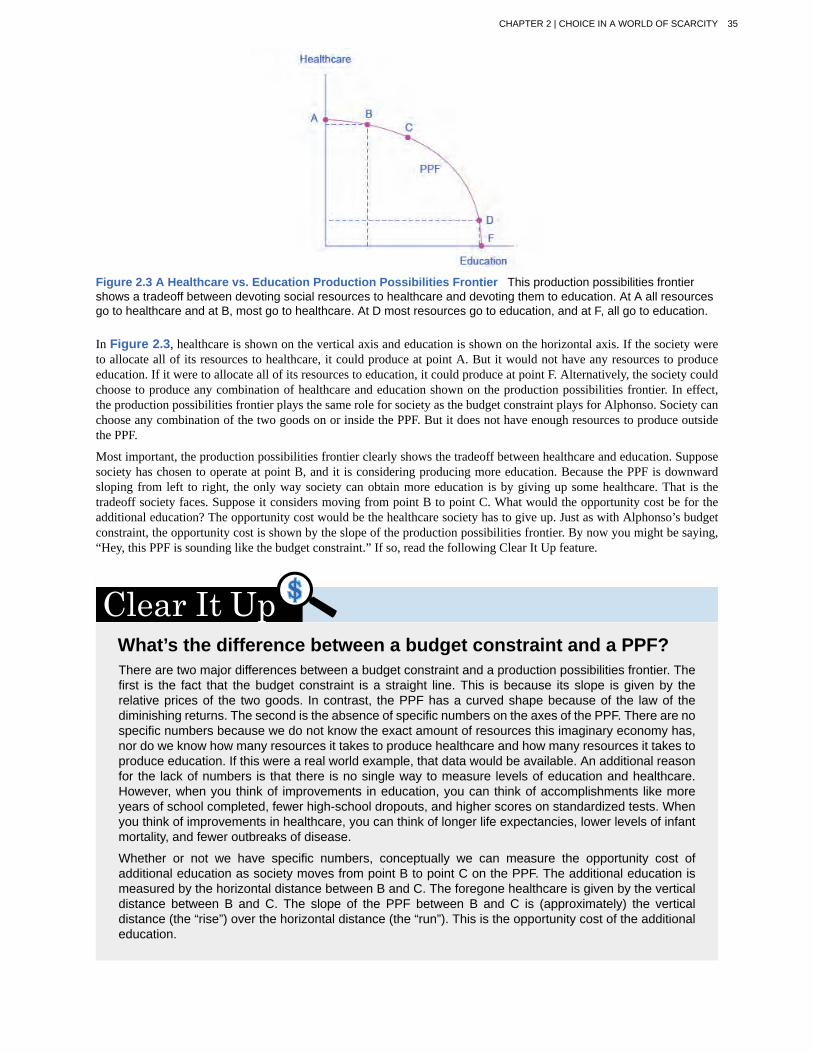
Figure 2.3 A Healthcare vs. Education Production Possibilities Frontier This production possibilities frontiershows a tradeoff between devoting social resources to healthcare and devoting them to education. At A all resourcesgo to healthcare and at B, most go to healthcare. At D most resources go to education, and at F, all go to education.

In Figure 2.3, healthcare is shown on the vertical axis and education is shown on the horizontal axis. If the society wereto allocate all of its resources to healthcare, it could produce at point A. But it would not have any resources to produceeducation. If it were to allocate all of its resources to education, it could produce at point F. Alternatively, the society couldchoose to produce any combination of healthcare and education shown on the production possibilities frontier. In effect,the production possibilities frontier plays the same role for society as the budget constraint plays for Alphonso. Society canchoose any combination of the two goods on or inside the PPF. But it does not have enough resources to produce outsidethe PPF.

Most important, the production possibilities frontier clearly shows the tradeoff between healthcare and education. Supposesociety has chosen to operate at point B, and it is considering producing more education. Because the PPF is downwardsloping from left to right, the only way society can obtain more education is by giving up some healthcare. That is thetradeoff society faces. Suppose it considers moving from point B to point C. What would the opportunity cost be for theadditional education? The opportunity cost would be the healthcare society has to give up. Just as with Alphonso’s budgetconstraint, the opportunity cost is shown by the slope of the production possibilities frontier. By now you might be saying,“Hey, this PPF is sounding like the budget constraint.” If so, read the following Clear It Up feature.

What’s the difference between a budget constraint and a PPF?There are two major differences between a budget constraint and a production possibilities frontier. Thefirst is the fact that the budget constraint is a straight line. This is because its slope is given by therelative prices of the two goods. In contrast, the PPF has a curved shape because of the law of thediminishing returns. The second is the absence of specific numbers on the axes of the PPF. There are nospecific numbers because we do not know the exact amount of resources this imaginary economy has,nor do we know how many resources it takes to produce healthcare and how many resources it takes toproduce education. If this were a real world example, that data would be available. An additional reasonfor the lack of numbers is that there is no single way to measure levels of education and healthcare.However, when you think of improvements in education, you can think of accomplishments like moreyears of school completed, fewer high-school dropouts, and higher scores on standardized tests. Whenyou think of improvements in healthcare, you can think of longer life expectancies, lower levels of infantmortality, and fewer outbreaks of disease.

Whether or not we have specific numbers, conceptually we can measure the opportunity cost ofadditional education as society moves from point B to point C on the PPF. The additional education ismeasured by the horizontal distance between B and C. The foregone healthcare is given by the verticaldistance between B and C. The slope of the PPF between B and C is (approximately) the verticaldistance (the “rise”) over the horizontal distance (the “run”). This is the opportunity cost of the additionaleducation.


The Shape of the PPF and the Law of Diminishing ReturnsThe budget constraints presented earlier in this chapter, showing individual choices about what quantities of goods toconsume, were all straight lines. The reason for these straight lines was that the slope of the budget constraint wasdetermined by relative prices of the two goods in the consumption budget constraint. However, the production possibilitiesfrontier for healthcare and education was drawn as a curved line. Why does the PPF have a different shape?

To understand why the PPF is curved, start by considering point A at the top left-hand side of the PPF. At point A, allavailable resources are devoted to healthcare and none are left for education. This situation would be extreme and evenridiculous. For example, children are seeing a doctor every day, whether they are sick or not, but not attending school.People are having cosmetic surgery on every part of their bodies, but no high school or college education exists. Nowimagine that some of these resources are diverted from healthcare to education, so that the economy is at point B instead ofpoint A. Diverting some resources away from A to B causes relatively little reduction in health because the last few marginaldollars going into healthcare services are not producing much additional gain in health. However, putting those marginaldollars into education, which is completely without resources at point A, can produce relatively large gains. For this reason,the shape of the PPF from A to B is relatively flat, representing a relatively small drop-off in health and a relatively largegain in education.

Now consider the other end, at the lower right, of the production possibilities frontier. Imagine that society starts at choice D,which is devoting nearly all resources to education and very few to healthcare, and moves to point F, which is devoting allspending to education and none to healthcare. For the sake of concreteness, you can imagine that in the movement from D toF, the last few doctors must become high school science teachers, the last few nurses must become school librarians ratherthan dispensers of vaccinations, and the last few emergency rooms are turned into kindergartens. The gains to educationfrom adding these last few resources to education are very small. However, the opportunity cost lost to health will be fairlylarge, and thus the slope of the PPF between D and F is steep, showing a large drop in health for only a small gain ineducation.

The lesson is not that society is likely to make an extreme choice like devoting no resources to education at point A orno resources to health at point F. Instead, the lesson is that the gains from committing additional marginal resources toeducation depend on how much is already being spent. If on the one hand, very few resources are currently committedto education, then an increase in resources used can bring relatively large gains. On the other hand, if a large number ofresources are already committed to education, then committing additional resources will bring relatively smaller gains.

This pattern is common enough that it has been given a name: the law of diminishing returns, which holds that asadditional increments of resources are added to a certain purpose, the marginal benefit from those additional increments willdecline. When government spends a certain amount more on reducing crime, for example, the original gains in reducingcrime could be relatively large. But additional increases typically cause relatively smaller reductions in crime, and payingfor enough police and security to reduce crime to nothing at all would be tremendously expensive.

The curvature of the production possibilities frontier shows that as additional resources are added to education, movingfrom left to right along the horizontal axis, the original gains are fairly large, but gradually diminish. Similarly, as additionalresources are added to healthcare, moving from bottom to top on the vertical axis, the original gains are fairly large, butagain gradually diminish. In this way, the law of diminishing returns produces the outward-bending shape of the productionpossibilities frontier.

Productive Efficiency and Allocative EfficiencyThe study of economics does not presume to tell a society what choice it should make along its production possibilitiesfrontier. In a market-oriented economy with a democratic government, the choice will involve a mixture of decisions byindividuals, firms, and government. However, economics can point out that some choices are unambiguously better thanothers. This observation is based on the concept of efficiency. In everyday usage, efficiency refers to lack of waste. Aninefficient machine operates at high cost, while an efficient machine operates at lower cost, because it is not wasting energyor materials. An inefficient organization operates with long delays and high costs, while an efficient organization meetsschedules, is focused, and performs within budget.

The production possibilities frontier can illustrate two kinds of efficiency: productive efficiency and allocative efficiency.Figure 2.4 illustrates these ideas using a production possibilities frontier between healthcare and education.



Figure 2.4 Productive and Allocative Efficiency Productive efficiency means it is impossible to produce more ofone good without decreasing the quantity that is produced of another good. Thus, all choices along a given PPF likeB, C, and D display productive efficiency, but R does not. Allocative efficiency means that the particular mix of goodsbeing produced—that is, the specific choice along the production possibilities frontier—represents the allocation thatsociety most desires.

Productive efficiency means that, given the available inputs and technology, it is impossible to produce more of onegood without decreasing the quantity that is produced of another good. All choices on the PPF in Figure 2.4, includingA, B, C, D, and F, display productive efficiency. As a firm moves from any one of these choices to any other, eitherhealthcare increases and education decreases or vice versa. However, any choice inside the production possibilities frontieris productively inefficient and wasteful because it is possible to produce more of one good, the other good, or somecombination of both goods.

For example, point R is productively inefficient because it is possible at choice C to have more of both goods: education onthe horizontal axis is higher at point C than point R (E2 is greater than E1), and healthcare on the vertical axis is also higherat point C than point R (H2 is great than H1).

The particular mix of goods and services being produced—that is, the specific combination of healthcare and educationchosen along the production possibilities frontier—can be shown as a ray (line) from the origin to a specific point on thePPF. Output mixes that had more healthcare (and less education) would have a steeper ray, while those with more education(and less healthcare) would have a flatter ray.

Allocative efficiency means that the particular mix of goods a society produces represents the combination that societymost desires. How to determine what a society desires can be a controversial question, and is usually discussed in politicalscience, sociology, and philosophy classes as well as in economics. At its most basic, allocative efficiency means producerssupply the quantity of each product that consumers demand. Only one of the productively efficient choices will be theallocatively efficient choice for society as a whole.

Why Society Must ChooseEvery economy faces two situations in which it may be able to expand consumption of all goods. In the first case, a societymay discover that it has been using its resources inefficiently, in which case by improving efficiency and producing on theproduction possibilities frontier, it can have more of all goods (or at least more of some and less of none). In the second case,as resources grow over a period of years (e.g., more labor and more capital), the economy grows. As it does, the productionpossibilities frontier for a society will tend to shift outward and society will be able to afford more of all goods.

But improvements in productive efficiency take time to discover and implement, and economic growth happens onlygradually. So, a society must choose between tradeoffs in the present. For government, this process often involves trying toidentify where additional spending could do the most good and where reductions in spending would do the least harm. Atthe individual and firm level, the market economy coordinates a process in which firms seek to produce goods and servicesin the quantity, quality, and price that people want. But for both the government and the market economy in the short term,increases in production of one good typically mean offsetting decreases somewhere else in the economy.

The PPF and Comparative AdvantageWhile every society must choose how much of each good it should produce, it does not need to produce every single goodit consumes. Often how much of a good a country decides to produce depends on how expensive it is to produce it versusbuying it from a different country. As we saw earlier, the curvature of a country’s PPF gives us information about thetradeoff between devoting resources to producing one good versus another. In particular, its slope gives the opportunity


cost of producing one more unit of the good in the x-axis in terms of the other good (in the y-axis). Countries tend tohave different opportunity costs of producing a specific good, either because of different climates, geography, technologyor skills.

Suppose two countries, the US and Brazil, need to decide how much they will produce of two crops: sugar cane and wheat.Due to its climatic conditions, Brazil can produce a lot of sugar cane per acre but not much wheat. Conversely, the U.S. canproduce a lot of wheat per acre, but not much sugar cane. Clearly, Brazil has a lower opportunity cost of producing sugarcane (in terms of wheat) than the U.S. The reverse is also true; the U.S. has a lower opportunity cost of producing wheatthan Brazil. This can be illustrated by the PPFs of the two countries in Figure 2.5

Figure 2.5 Production Possibility Frontier for the U.S. and Brazil The U.S. PPF is flatter than the Brazil PPFimplying that the opportunity cost of wheat in term of sugar cane is lower in the U.S. than in Brazil. Conversely, theopportunity cost of sugar cane is lower in Brazil. The U.S. has comparative advantage in wheat and brazil hascomparative advantage in sugar cane.

When a country can produce a good at a lower opportunity cost than another country, we say that this country has acomparative advantage in that good. In our example, Brazil has a comparative advantage in sugar cane and the U.S. hasa comparative advantage in wheat. One can easily see this with a simple observation of the extreme production points inthe PPFs of the two countries. If Brazil devoted all of its resources to producing wheat, it would be producing at point A. Ifhowever it had devoted all of its resources to producing sugar cane instead, it would be producing a much larger amount, atpoint B. By moving from point A to point B Brazil would give up a relatively small quantity in wheat production to obtaina large production in sugar cane. The opposite is true for the U.S. If the U.S. moved from point A to B and produced onlysugar cane, this would result in a large opportunity cost in terms of foregone wheat production.

The slope of the PPF gives the opportunity cost of producing an additional unit of wheat. While the slope is not constantthroughout the PPFs, it is quite apparent that the PPF in Brazil is much steeper than in the U.S., and therefore the opportunitycost of wheat generally higher in Brazil. In the chapter on International Trade you will learn that countries’ differencesin comparative advantage determine which goods they will choose to produce and trade. When countries engage in trade,they specialize in the production of the goods that they have comparative advantage in, and trade part of that production forgoods they do not have comparative advantage in. With trade, goods are produced where the opportunity cost is lowest, sototal production increases, benefiting both trading parties.

2.3 | Confronting Objections to the Economic ApproachBy the end of this section, you will be able to:

• Analyze arguments against economic approaches to decision-making• Interpret a tradeoff diagram• Contrast normative statements and positive statements

It is one thing to understand the economic approach to decision-making and another thing to feel comfortable applying it.The sources of discomfort typically fall into two categories: that people do not act in the way that fits the economic way ofthinking, and that even if people did act that way, they should try not to. Let’s consider these arguments in turn.



First Objection: People, Firms, and Society Do Not Act Like ThisThe economic approach to decision-making seems to require more information than most individuals possess and morecareful decision-making than most individuals actually display. After all, do you or any of your friends draw a budgetconstraint and mutter to yourself about maximizing utility before you head to the shopping mall? Do members of the U.S.Congress contemplate production possibilities frontiers before they vote on the annual budget? The messy ways in whichpeople and societies operate somehow doesn’t look much like neat budget constraints or smoothly curving productionpossibilities frontiers.

However, the economics approach can be a useful way to analyze and understand the tradeoffs of economic decisions evenso. To appreciate this point, imagine for a moment that you are playing basketball, dribbling to the right, and throwing abounce-pass to the left to a teammate who is running toward the basket. A physicist or engineer could work out the correctspeed and trajectory for the pass, given the different movements involved and the weight and bounciness of the ball. Butwhen you are playing basketball, you do not perform any of these calculations. You just pass the ball, and if you are a goodplayer, you will do so with high accuracy.

Someone might argue: “The scientist’s formula of the bounce-pass requires a far greater knowledge of physics and farmore specific information about speeds of movement and weights than the basketball player actually has, so it must be anunrealistic description of how basketball passes are actually made.” This reaction would be wrongheaded. The fact that agood player can throw the ball accurately because of practice and skill, without making a physics calculation, does not meanthat the physics calculation is wrong.

Similarly, from an economic point of view, someone who goes shopping for groceries every week has a great deal of practicewith how to purchase the combination of goods that will provide that person with utility, even if the shopper does notphrase decisions in terms of a budget constraint. Government institutions may work imperfectly and slowly, but in general,a democratic form of government feels pressure from voters and social institutions to make the choices that are most widelypreferred by people in that society. So, when thinking about the economic actions of groups of people, firms, and society,it is reasonable, as a first approximation, to analyze them with the tools of economic analysis. For more on this, read aboutbehavioral economics in the chapter on Consumer Choices.

Second Objection: People, Firms, and Society Should Not Act This WayThe economics approach portrays people as self-interested. For some critics of this approach, even if self-interest is anaccurate description of how people behave, these behaviors are not moral. Instead, the critics argue that people should betaught to care more deeply about others. Economists offer several answers to these concerns.

First, economics is not a form of moral instruction. Rather, it seeks to describe economic behavior as it actually exists.Philosophers draw a distinction between positive statements, which describe the world as it is, and normative statements,which describe how the world should be. For example, an economist could analyze a proposed subway system in a certaincity. If the expected benefits exceed the costs, he concludes that the project is worth doing—an example of positive analysis.Another economist argues for extended unemployment compensation during the Great Depression because a rich countrylike the United States should take care of its less fortunate citizens—an example of normative analysis.

Even if the line between positive and normative statements is not always crystal clear, economic analysis does try toremain rooted in the study of the actual people who inhabit the actual economy. Fortunately however, the assumption thatindividuals are purely self-interested is a simplification about human nature. In fact, we need to look no further than toAdam Smith, the very father of modern economics to find evidence of this. The opening sentence of his book, The Theoryof Moral Sentiments, puts it very clearly: “How selfish soever man may be supposed, there are evidently some principlesin his nature, which interest him in the fortune of others, and render their happiness necessary to him, though he derivesnothing from it except the pleasure of seeing it.” Clearly, individuals are both self-interested and altruistic.

Second, self-interested behavior and profit-seeking can be labeled with other names, such as personal choice and freedom.The ability to make personal choices about buying, working, and saving is an important personal freedom. Some peoplemay choose high-pressure, high-paying jobs so that they can earn and spend a lot of money on themselves. Others may earna lot of money and give it to charity or spend it on their friends and family. Others may devote themselves to a career thatcan require a great deal of time, energy, and expertise but does not offer high financial rewards, like being an elementaryschool teacher or a social worker. Still others may choose a job that does not take lots of their time or provide a high level ofincome, but still leaves time for family, friends, and contemplation. Some people may prefer to work for a large company;others might want to start their own business. People’s freedom to make their own economic choices has a moral valueworth respecting.


Is a diagram by any other name the same?When you study economics, you may feel buried under an avalanche of diagrams: diagrams in thetext, diagrams in the lectures, diagrams in the problems, and diagrams on exams. Your goal should beto recognize the common underlying logic and pattern of the diagrams, not to memorize each of theindividual diagrams.

This chapter uses only one basic diagram, although it is presented with different sets of labels. Theconsumption budget constraint and the production possibilities frontier for society, as a whole, are thesame basic diagram. Figure 2.6 shows an individual budget constraint and a production possibilitiesfrontier for two goods, Good 1 and Good 2. The tradeoff diagram always illustrates three basic themes:scarcity, tradeoffs, and economic efficiency.

The first theme is scarcity. It is not feasible to have unlimited amounts of both goods. But even ifthe budget constraint or a PPF shifts, scarcity remains—just at a different level. The second theme istradeoffs. As depicted in the budget constraint or the production possibilities frontier, it is necessary togive up some of one good to gain more of the other good. The details of this tradeoff vary. In a budgetconstraint, the tradeoff is determined by the relative prices of the goods: that is, the relative price of twogoods in the consumption choice budget constraint. These tradeoffs appear as a straight line. However,the tradeoffs in many production possibilities frontiers are represented by a curved line because the lawof diminishing returns holds that as resources are added to an area, the marginal gains tend to diminish.Regardless of the specific shape, tradeoffs remain.

The third theme is economic efficiency, or getting the most benefit from scarce resources. All choiceson the production possibilities frontier show productive efficiency because in such cases, there is noway to increase the quantity of one good without decreasing the quantity of the other. Similarly, whenan individual makes a choice along a budget constraint, there is no way to increase the quantity of onegood without decreasing the quantity of the other. The choice on a production possibilities set that issocially preferred, or the choice on an individual’s budget constraint that is personally preferred, willdisplay allocative efficiency.

The basic budget constraint/production possibilities frontier diagram will recur throughout this book.Some examples include using these tradeoff diagrams to analyze trade, labor supply versus leisure,saving versus consumption, environmental protection and economic output, equality of incomes andeconomic output, and the macroeconomic tradeoff between consumption and investment. Do not beconfused by the different labels. The budget constraint/production possibilities frontier diagram is alwaysjust a tool for thinking carefully about scarcity, tradeoffs, and efficiency in a particular situation.

Figure 2.6 The Tradeoff Diagram Both the individual opportunity set (or budget constraint) and the socialproduction possibilities frontier show the constraints under which individual consumers and society as awhole operate. Both diagrams show the tradeoff in choosing more of one good at the cost of less of theother.



Third, self-interested behavior can lead to positive social results. For example, when people work hard to make a living,they create economic output. Consumers who are looking for the best deals will encourage businesses to offer goods andservices that meet their needs. Adam Smith, writing in The Wealth of Nations, christened this property the invisible hand.In describing how consumers and producers interact in a market economy, Smith wrote:

Every. individual…generally, indeed, neither intends to promote the public interest, nor knows howmuch he is promoting it. By preferring the support of domestic to that of foreign industry, he intendsonly his own security; and by directing that industry in such a manner as its produce may be of thegreatest value, he intends only his own gain. And he is in this, as in many other cases, led by aninvisible hand to promote an end which was no part of his intention…By pursuing his own interest hefrequently promotes that of the society more effectually than when he really intends to promote it.

The metaphor of the invisible hand suggests the remarkable possibility that broader social good can emerge from selfishindividual actions.

Fourth, even people who focus on their own self-interest in the economic part of their life often set aside their own narrowself-interest in other parts of life. For example, you might focus on your own self-interest when asking your employer fora raise or negotiating to buy a car. But then you might turn around and focus on other people when you volunteer to readstories at the local library, help a friend move to a new apartment, or donate money to a charity. Self-interest is a reasonablestarting point for analyzing many economic decisions, without needing to imply that people never do anything that is not intheir own immediate self-interest.

Choices ... To What Degree?What have we learned? We know that scarcity impacts all the choices we make. So, an economist mightargue that people do not go on to get bachelor’s degrees or master’s degrees because they do not havethe resources to make those choices or because their incomes are too low and/or the price of thesedegrees is too high. A bachelor’s degree or a master’s degree may not be available in their opportunityset.

The price of these degrees may be too high not only because the actual price, college tuition (andperhaps room and board), is too high. An economist might also say that for many people, the fullopportunity cost of a bachelor’s degree or a master’s degree is too high. For these people, they areunwilling or unable to make the tradeoff of giving up years of working, and earning an income, to earn adegree.

Finally, the statistics introduced at the start of the chapter reveal information about intertemporal choices.An economist might say that people choose not to get a college degree because they may have toborrow money to go to college, and the interest they have to pay on that loan in the future will affecttheir decisions today. Also, it could be that some people have a preference for current consumption overfuture consumption, so they choose to work now at a lower salary and consume now, rather than puttingthat consumption off until after they graduate college.


allocative efficiency

budget constraint

comparative advantage

invisible hand

law of diminishing marginal utility

law of diminishing returns

marginal analysis

normative statement

opportunity cost

opportunity set

positive statement

production possibilities frontier (PPF)

productive efficiency

sunk costs

utility

KEY TERMSwhen the mix of goods being produced represents the mix that society most desires

all possible consumption combinations of goods that someone can afford, given the prices of goods,when all income is spent; the boundary of the opportunity set

when a country can produce a good at a lower cost in terms of other goods; or, when a countryhas a lower opportunity cost of production

idea that self-interested behavior by individuals can lead to positive social outcomes

as we consume more of a good or service, the utility we get from additional unitsof the good or service tend to become smaller than what we received from earlier units

as additional increments of resources are added to producing a good or service, the marginalbenefit from those additional increments will decline

examination of decisions on the margin, meaning a little more or a little less from the status quo

statement which describes how the world should be

measures cost by what is given up in exchange; opportunity cost measures the value of the forgonealternative

all possible combinations of consumption that someone can afford given the prices of goods and theindividual’s income

statement which describes the world as it is

a diagram that shows the productively efficient combinations of two productsthat an economy can produce given the resources it has available.

when it is impossible to produce more of one good (or service) without decreasing the quantityproduced of another good (or service)

costs that are made in the past and cannot be recovered

satisfaction, usefulness, or value one obtains from consuming goods and services


2.1 How Individuals Make Choices Based on Their Budget Constraint

Economists see the real world as one of scarcity: that is, a world in which people’s desires exceed what is possible.As a result, economic behavior involves tradeoffs in which individuals, firms, and society must give up somethingthat they desire to obtain things that they desire more. Individuals face the tradeoff of what quantities of goods andservices to consume. The budget constraint, which is the frontier of the opportunity set, illustrates the range of choicesavailable. The slope of the budget constraint is determined by the relative price of the choices. Choices beyond thebudget constraint are not affordable.

Opportunity cost measures cost by what is given up in exchange. Sometimes opportunity cost can be measured inmoney, but it is often useful to consider time as well, or to measure it in terms of the actual resources that must begiven up.

Most economic decisions and tradeoffs are not all-or-nothing. Instead, they involve marginal analysis, which meansthey are about decisions on the margin, involving a little more or a little less. The law of diminishing marginalutility points out that as a person receives more of something—whether it is a specific good or another resource—theadditional marginal gains tend to become smaller. Because sunk costs occurred in the past and cannot be recovered,they should be disregarded in making current decisions.

2.2 The Production Possibilities Frontier and Social Choices

A production possibilities frontier defines the set of choices society faces for the combinations of goods and servicesit can produce given the resources available. The shape of the PPF is typically curved outward, rather than straight.



Choices outside the PPF are unattainable and choices inside the PPF are wasteful. Over time, a growing economy willtend to shift the PPF outwards.

The law of diminishing returns holds that as increments of additional resources are devoted to producing something,the marginal increase in output will become smaller and smaller. All choices along a production possibilities frontierdisplay productive efficiency; that is, it is impossible to use society’s resources to produce more of one good withoutdecreasing production of the other good. The specific choice along a production possibilities frontier that reflects themix of goods society prefers is the choice with allocative efficiency. The curvature of the PPF is likely to differ bycountry, which results in different countries having comparative advantage in different goods. Total production canincrease if countries specialize in the goods they have comparative advantage in and trade some of their productionfor the remaining goods.

2.3 Confronting Objections to the Economic Approach

The economic way of thinking provides a useful approach to understanding human behavior. Economists make thecareful distinction between positive statements, which describe the world as it is, and normative statements, whichdescribe how the world should be. Even when economics analyzes the gains and losses from various events orpolicies, and thus draws normative conclusions about how the world should be, the analysis of economics is rooted ina positive analysis of how people, firms, and governments actually behave, not how they should behave.

SELF-CHECK QUESTIONS1. Suppose Alphonso’s town raised the price of bus tickets to $1 per trip (while the price of burgers stayed at $2 andhis budget remained $10 per week.) Draw Alphonso’s new budget constraint. What happens to the opportunity costof bus tickets?

2. Return to the example in Figure 2.4. Suppose there is an improvement in medical technology that enables morehealthcare to be provided with the same amount of resources. How would this affect the production possibilities curveand, in particular, how would it affect the opportunity cost of education?

3. Could a nation be producing in a way that is allocatively efficient, but productively inefficient?

4. What are the similarities between a consumer’s budget constraint and society’s production possibilities frontier,not just graphically but analytically?

5. Individuals may not act in the rational, calculating way described by the economic model of decision making,measuring utility and costs at the margin, but can you make a case that they behave approximately that way?

6. Would an op-ed piece in a newspaper urging the adoption of a particular economic policy be considered a positiveor normative statement?

7. Would a research study on the effects of soft drink consumption on children’s cognitive development beconsidered a positive or normative statement?

REVIEW QUESTIONS8. Explain why scarcity leads to tradeoffs.

9. Explain why individuals make choices that aredirectly on the budget constraint, rather than inside thebudget constraint or outside it.

10. What is comparative advantage?

11. What does a production possibilities frontierillustrate?

12. Why is a production possibilities frontier typicallydrawn as a curve, rather than a straight line?

13. Explain why societies cannot make a choice abovetheir production possibilities frontier and should notmake a choice below it.

14. What are diminishing marginal returns?

15. What is productive efficiency? Allocativeefficiency?

16. What is the difference between a positive and anormative statement?

17. Is the economic model of decision-making intendedas a literal description of how individuals, firms, and thegovernments actually make decisions?

18. What are four responses to the claim that peopleshould not behave in the way described in this chapter?

CRITICAL THINKING QUESTIONS19. Suppose Alphonso’s town raises the price of bustickets from $0.50 to $1 and the price of burgers rises

from $2 to $4. Why is the opportunity cost of bus ticketsunchanged? Suppose Alphonso’s weekly spending


money increases from $10 to $20. How is his budgetconstraint affected from all three changes? Explain.

20. During the Second World War, Germany’s factorieswere decimated. It also suffered many human casualties,both soldiers and civilians. How did the war affectGermany’s production possibilities curve?

21. It is clear that productive inefficiency is a wastesince resources are being used in a way that produces lessgoods and services than a nation is capable of. Why isallocative inefficiency also wasteful?

22. What assumptions about the economy must be truefor the invisible hand to work? To what extent are thoseassumptions valid in the real world?

23. Do economists have any particular expertise atmaking normative arguments? In other words, they haveexpertise at making positive statements (i.e., what willhappen) about some economic policy, for example, but dothey have special expertise to judge whether or not thepolicy should be undertaken?

PROBLEMSUse this information to answer the following 4 questions:Marie has a weekly budget of $24, which she likes tospend on magazines and pies.

24. If the price of a magazine is $4 each, what is themaximum number of magazines she could buy in aweek?

25. If the price of a pie is $12, what is the maximumnumber of pies she could buy in a week?

26. Draw Marie’s budget constraint with pies on thehorizontal axis and magazines on the vertical axis. Whatis the slope of the budget constraint?

27. What is Marie’s opportunity cost of purchasing apie?



3 | Demand and Supply

Figure 3.1 Farmer’s Market Organic vegetables and fruits that are grown and sold within a specific geographicalregion should, in theory, cost less than conventional produce because the transportation costs are less. That is not,however, usually the case. (Credit: modification of work by Natalie Maynor/Flickr Creative Commons)

Why Can We Not Get Enough of Organic?Organic food is increasingly popular, not just in the United States, but worldwide. At one time, consumershad to go to specialty stores or farmer’s markets to find organic produce. Now it is available in mostgrocery stores. In short, organic is part of the mainstream.

Ever wonder why organic food costs more than conventional food? Why, say, does an organic Fuji applecost $1.99 a pound, while its conventional counterpart costs $1.49 a pound? The same price relationshipis true for just about every organic product on the market. If many organic foods are locally grown, wouldthey not take less time to get to market and therefore be cheaper? What are the forces that keep thoseprices from coming down? Turns out those forces have a lot to do with this chapter’s topic: demand andsupply.

Introduction to Demand and SupplyIn this chapter, you will learn about:

• Demand, Supply, and Equilibrium in Markets for Goods and Services

• Shifts in Demand and Supply for Goods and Services

• Changes in Equilibrium Price and Quantity: The Four-Step Process

• Price Ceilings and Price Floors

An auction bidder pays thousands of dollars for a dress Whitney Houston wore. A collector spends a small fortune for afew drawings by John Lennon. People usually react to purchases like these in two ways: their jaw drops because they thinkthese are high prices to pay for such goods or they think these are rare, desirable items and the amount paid seems right.

CHAPTER 3 | DEMAND AND SUPPLY 45

Visit this website (http://openstaxcollege.org/l/celebauction) to read a list of bizarre items that have beenpurchased for their ties to celebrities. These examples represent an interesting facet of demand andsupply.

When economists talk about prices, they are less interested in making judgments than in gaining a practical understandingof what determines prices and why prices change. Consider a price most of us contend with weekly: that of a gallon ofgas. Why was the average price of gasoline in the United States $3.40 per gallon in January 2012? Why did the price forgasoline rise to $3.93 per gallon only months later, by April 2012? To explain these price movements, economists focus onthe determinants of what gasoline buyers are willing to pay and what gasoline sellers are willing to accept.

As it turns out, the price of gasoline in June of any given year is nearly always higher than the price in January of that sameyear; over recent decades, gasoline prices in midsummer have averaged about 10 cents per gallon more than their midwinterlow. The likely reason is that people drive more in the summer, and are also willing to pay more for gas. However, in 2009,gasoline prices rose by more than the average winter-to-summer rise, which suggests that other factors were at work duringthose six months.

This chapter introduces the economic model of demand and supply—one of the most powerful models in all of economics.The discussion here begins by examining how demand and supply determine the price and the quantity sold in markets forgoods and services, and how changes in demand and supply lead to changes in prices and quantities.

3.1 | Demand, Supply, and Equilibrium in Markets forGoods and ServicesBy the end of this section, you will be able to:

• Explain demand, quantity demanded, and the law of demand• Identify a demand curve and a supply curve• Explain supply, quantity supply, and the law of supply• Explain equilibrium, equilibrium price, and equilibrium quantity

First let’s first focus on what economists mean by demand, what they mean by supply, and then how demand and supplyinteract in a market.

Demand for Goods and ServicesEconomists use the term demand to refer to the amount of some good or service consumers are willing and able to purchaseat each price. Demand is based on needs and wants—a consumer may be able to differentiate between a need and a want,but from an economist’s perspective they are the same thing. Demand is also based on ability to pay. If you cannot pay forit, you have no effective demand.

What a buyer pays for a unit of the specific good or service is called price. The total number of units purchased at that priceis called the quantity demanded. A rise in price of a good or service almost always decreases the quantity demanded of thatgood or service. Conversely, a fall in price will increase the quantity demanded. When the price of a gallon of gasoline goesup, for example, people look for ways to reduce their consumption by combining several errands, commuting by carpoolor mass transit, or taking weekend or vacation trips closer to home. Economists call this inverse relationship between priceand quantity demanded the law of demand. The law of demand assumes that all other variables that affect demand (to beexplained in the next module) are held constant.

An example from the market for gasoline can be shown in the form of a table or a graph. A table that shows the quantitydemanded at each price, such as Table 3.1, is called a demand schedule. Price in this case is measured in dollars pergallon of gasoline. The quantity demanded is measured in millions of gallons over some time period (for example, per dayor per year) and over some geographic area (like a state or a country). A demand curve shows the relationship between

46 CHAPTER 3 | DEMAND AND SUPPLY


http://openstaxcollege.org/l/celebauction

price and quantity demanded on a graph like Figure 3.2, with quantity on the horizontal axis and the price per gallon onthe vertical axis. (Note that this is an exception to the normal rule in mathematics that the independent variable (x) goes onthe horizontal axis and the dependent variable (y) goes on the vertical. Economics is not math.)

The demand schedule shown by Table 3.1 and the demand curve shown by the graph in Figure 3.2 are two ways ofdescribing the same relationship between price and quantity demanded.

Figure 3.2 A Demand Curve for Gasoline The demand schedule shows that as price rises, quantity demandeddecreases, and vice versa. These points are then graphed, and the line connecting them is the demand curve (D).The downward slope of the demand curve again illustrates the law of demand—the inverse relationship betweenprices and quantity demanded.

Price (per gallon) Quantity Demanded (millions of gallons)

$1.00 800

$1.20 700

$1.40 600

$1.60 550

$1.80 500

$2.00 460

$2.20 420

Table 3.1 Price and Quantity Demanded of Gasoline

Demand curves will appear somewhat different for each product. They may appear relatively steep or flat, or they may bestraight or curved. Nearly all demand curves share the fundamental similarity that they slope down from left to right. Sodemand curves embody the law of demand: As the price increases, the quantity demanded decreases, and conversely, as theprice decreases, the quantity demanded increases.

Confused about these different types of demand? Read the next Clear It Up feature.

Is demand the same as quantity demanded?In economic terminology, demand is not the same as quantity demanded. When economists talk aboutdemand, they mean the relationship between a range of prices and the quantities demanded at thoseprices, as illustrated by a demand curve or a demand schedule. When economists talk about quantitydemanded, they mean only a certain point on the demand curve, or one quantity on the demand


schedule. In short, demand refers to the curve and quantity demanded refers to the (specific) point onthe curve.

Supply of Goods and ServicesWhen economists talk about supply, they mean the amount of some good or service a producer is willing to supply at eachprice. Price is what the producer receives for selling one unit of a good or service. A rise in price almost always leads toan increase in the quantity supplied of that good or service, while a fall in price will decrease the quantity supplied. Whenthe price of gasoline rises, for example, it encourages profit-seeking firms to take several actions: expand exploration foroil reserves; drill for more oil; invest in more pipelines and oil tankers to bring the oil to plants where it can be refined intogasoline; build new oil refineries; purchase additional pipelines and trucks to ship the gasoline to gas stations; and openmore gas stations or keep existing gas stations open longer hours. Economists call this positive relationship between priceand quantity supplied—that a higher price leads to a higher quantity supplied and a lower price leads to a lower quantitysupplied—the law of supply. The law of supply assumes that all other variables that affect supply (to be explained in thenext module) are held constant.

Still unsure about the different types of supply? See the following Clear It Up feature.

Is supply the same as quantity supplied?In economic terminology, supply is not the same as quantity supplied. When economists refer to supply,they mean the relationship between a range of prices and the quantities supplied at those prices, arelationship that can be illustrated with a supply curve or a supply schedule. When economists refer toquantity supplied, they mean only a certain point on the supply curve, or one quantity on the supplyschedule. In short, supply refers to the curve and quantity supplied refers to the (specific) point on thecurve.

Figure 3.3 illustrates the law of supply, again using the market for gasoline as an example. Like demand, supply can beillustrated using a table or a graph. A supply schedule is a table, like Table 3.2, that shows the quantity supplied at arange of different prices. Again, price is measured in dollars per gallon of gasoline and quantity demanded is measured inmillions of gallons. A supply curve is a graphic illustration of the relationship between price, shown on the vertical axis,and quantity, shown on the horizontal axis. The supply schedule and the supply curve are just two different ways of showingthe same information. Notice that the horizontal and vertical axes on the graph for the supply curve are the same as for thedemand curve.

Figure 3.3 A Supply Curve for Gasoline The supply schedule is the table that shows quantity supplied of gasolineat each price. As price rises, quantity supplied also increases, and vice versa. The supply curve (S) is created bygraphing the points from the supply schedule and then connecting them. The upward slope of the supply curveillustrates the law of supply—that a higher price leads to a higher quantity supplied, and vice versa.



Price (per gallon) Quantity Supplied (millions of gallons)

$1.00 500

$1.20 550

$1.40 600

$1.60 640

$1.80 680

$2.00 700

$2.20 720

Table 3.2 Price and Supply of Gasoline

The shape of supply curves will vary somewhat according to the product: steeper, flatter, straighter, or curved. Nearly allsupply curves, however, share a basic similarity: they slope up from left to right and illustrate the law of supply: as theprice rises, say, from $1.00 per gallon to $2.20 per gallon, the quantity supplied increases from 500 gallons to 720 gallons.Conversely, as the price falls, the quantity supplied decreases.

Equilibrium—Where Demand and Supply IntersectBecause the graphs for demand and supply curves both have price on the vertical axis and quantity on the horizontal axis,the demand curve and supply curve for a particular good or service can appear on the same graph. Together, demand andsupply determine the price and the quantity that will be bought and sold in a market.

Figure 3.4 illustrates the interaction of demand and supply in the market for gasoline. The demand curve (D) is identicalto Figure 3.2. The supply curve (S) is identical to Figure 3.3. Table 3.3 contains the same information in tabular form.

Figure 3.4 Demand and Supply for Gasoline The demand curve (D) and the supply curve (S) intersect at theequilibrium point E, with a price of $1.40 and a quantity of 600. The equilibrium is the only price where quantitydemanded is equal to quantity supplied. At a price above equilibrium like $1.80, quantity supplied exceeds thequantity demanded, so there is excess supply. At a price below equilibrium such as $1.20, quantity demandedexceeds quantity supplied, so there is excess demand.

Price (pergallon)

Quantity demanded (millions ofgallons)

Quantity supplied (millions ofgallons)

$1.00 800 500

$1.20 700 550

$1.40 600 600

$1.60 550 640

Table 3.3 Price, Quantity Demanded, and Quantity Supplied


Price (pergallon)

Quantity demanded (millions ofgallons)

Quantity supplied (millions ofgallons)

$1.80 500 680

$2.00 460 700

$2.20 420 720

Table 3.3 Price, Quantity Demanded, and Quantity Supplied

Remember this: When two lines on a diagram cross, this intersection usually means something. The point where the supplycurve (S) and the demand curve (D) cross, designated by point E in Figure 3.4, is called the equilibrium. The equilibriumprice is the only price where the plans of consumers and the plans of producers agree—that is, where the amount of theproduct consumers want to buy (quantity demanded) is equal to the amount producers want to sell (quantity supplied). Thiscommon quantity is called the equilibrium quantity. At any other price, the quantity demanded does not equal the quantitysupplied, so the market is not in equilibrium at that price.

In Figure 3.4, the equilibrium price is $1.40 per gallon of gasoline and the equilibrium quantity is 600 million gallons. Ifyou had only the demand and supply schedules, and not the graph, you could find the equilibrium by looking for the pricelevel on the tables where the quantity demanded and the quantity supplied are equal.

The word “equilibrium” means “balance.” If a market is at its equilibrium price and quantity, then it has no reason to moveaway from that point. However, if a market is not at equilibrium, then economic pressures arise to move the market towardthe equilibrium price and the equilibrium quantity.

Imagine, for example, that the price of a gallon of gasoline was above the equilibrium price—that is, instead of $1.40 pergallon, the price is $1.80 per gallon. This above-equilibrium price is illustrated by the dashed horizontal line at the price of$1.80 in Figure 3.4. At this higher price, the quantity demanded drops from 600 to 500. This decline in quantity reflectshow consumers react to the higher price by finding ways to use less gasoline.

Moreover, at this higher price of $1.80, the quantity of gasoline supplied rises from the 600 to 680, as the higher pricemakes it more profitable for gasoline producers to expand their output. Now, consider how quantity demanded and quantitysupplied are related at this above-equilibrium price. Quantity demanded has fallen to 500 gallons, while quantity suppliedhas risen to 680 gallons. In fact, at any above-equilibrium price, the quantity supplied exceeds the quantity demanded. Wecall this an excess supply or a surplus.

With a surplus, gasoline accumulates at gas stations, in tanker trucks, in pipelines, and at oil refineries. This accumulationputs pressure on gasoline sellers. If a surplus remains unsold, those firms involved in making and selling gasoline are notreceiving enough cash to pay their workers and to cover their expenses. In this situation, some producers and sellers willwant to cut prices, because it is better to sell at a lower price than not to sell at all. Once some sellers start cutting prices,others will follow to avoid losing sales. These price reductions in turn will stimulate a higher quantity demanded. So, if theprice is above the equilibrium level, incentives built into the structure of demand and supply will create pressures for theprice to fall toward the equilibrium.

Now suppose that the price is below its equilibrium level at $1.20 per gallon, as the dashed horizontal line at this price inFigure 3.4 shows. At this lower price, the quantity demanded increases from 600 to 700 as drivers take longer trips, spendmore minutes warming up the car in the driveway in wintertime, stop sharing rides to work, and buy larger cars that getfewer miles to the gallon. However, the below-equilibrium price reduces gasoline producers’ incentives to produce and sellgasoline, and the quantity supplied falls from 600 to 550.

When the price is below equilibrium, there is excess demand, or a shortage—that is, at the given price the quantitydemanded, which has been stimulated by the lower price, now exceeds the quantity supplied, which had been depressed bythe lower price. In this situation, eager gasoline buyers mob the gas stations, only to find many stations running short of fuel.Oil companies and gas stations recognize that they have an opportunity to make higher profits by selling what gasoline theyhave at a higher price. As a result, the price rises toward the equilibrium level. Read Demand, Supply, and Efficiency(http://cnx.org/content/m48832/latest/) for more discussion on the importance of the demand and supply model.



http://cnx.org/content/m48832/latest/


3.2 | Shifts in Demand and Supply for Goods andServicesBy the end of this section, you will be able to:

• Identify factors that affect demand• Graph demand curves and demand shifts• Identify factors that affect supply• Graph supply curves and supply shifts

The previous module explored how price affects the quantity demanded and the quantity supplied. The result was thedemand curve and the supply curve. Price, however, is not the only thing that influences demand. Nor is it the only thing thatinfluences supply. For example, how is demand for vegetarian food affected if, say, health concerns cause more consumersto avoid eating meat? Or how is the supply of diamonds affected if diamond producers discover several new diamondmines? What are the major factors, in addition to the price, that influence demand or supply?

Visit this website (http://openstaxcollege.org/l/toothfish) to read a brief note on how marketing strategiescan influence supply and demand of products.

What Factors Affect Demand?We defined demand as the amount of some product a consumer is willing and able to purchase at each price. That suggestsat least two factors in addition to price that affect demand. Willingness to purchase suggests a desire, based on whateconomists call tastes and preferences. If you neither need nor want something, you will not buy it. Ability to purchasesuggests that income is important. Professors are usually able to afford better housing and transportation than students,because they have more income. Prices of related goods can affect demand also. If you need a new car, the price of a Hondamay affect your demand for a Ford. Finally, the size or composition of the population can affect demand. The more childrena family has, the greater their demand for clothing. The more driving-age children a family has, the greater their demand forcar insurance, and the less for diapers and baby formula.

These factors matter both for demand by an individual and demand by the market as a whole. Exactly how do these variousfactors affect demand, and how do we show the effects graphically? To answer those questions, we need the ceteris paribusassumption.

The Ceteris Paribus AssumptionA demand curve or a supply curve is a relationship between two, and only two, variables: quantity on the horizontal axisand price on the vertical axis. The assumption behind a demand curve or a supply curve is that no relevant economic factors,other than the product’s price, are changing. Economists call this assumption ceteris paribus, a Latin phrase meaning “otherthings being equal.” Any given demand or supply curve is based on the ceteris paribus assumption that all else is held equal.A demand curve or a supply curve is a relationship between two, and only two, variables when all other variables are keptconstant. If all else is not held equal, then the laws of supply and demand will not necessarily hold, as the following ClearIt Up feature shows.


http://openstaxcollege.org/l/toothfish

When does ceteris paribus apply?Ceteris paribus is typically applied when we look at how changes in price affect demand or supply, butceteris paribus can be applied more generally. In the real world, demand and supply depend on morefactors than just price. For example, a consumer’s demand depends on income and a producer’s supplydepends on the cost of producing the product. How can we analyze the effect on demand or supply ifmultiple factors are changing at the same time—say price rises and income falls? The answer is that weexamine the changes one at a time, assuming the other factors are held constant.

For example, we can say that an increase in the price reduces the amount consumers will buy (assumingincome, and anything else that affects demand, is unchanged). Additionally, a decrease in incomereduces the amount consumers can afford to buy (assuming price, and anything else that affectsdemand, is unchanged). This is what the ceteris paribus assumption really means. In this particular case,after we analyze each factor separately, we can combine the results. The amount consumers buy fallsfor two reasons: first because of the higher price and second because of the lower income.

How Does Income Affect Demand?Let’s use income as an example of how factors other than price affect demand. Figure 3.5 shows the initial demand forautomobiles as D0. At point Q, for example, if the price is $20,000 per car, the quantity of cars demanded is 18 million. D0also shows how the quantity of cars demanded would change as a result of a higher or lower price. For example, if the priceof a car rose to $22,000, the quantity demanded would decrease to 17 million, at point R.

The original demand curve D0, like every demand curve, is based on the ceteris paribus assumption that no othereconomically relevant factors change. Now imagine that the economy expands in a way that raises the incomes of manypeople, making cars more affordable. How will this affect demand? How can we show this graphically?

Return to Figure 3.5. The price of cars is still $20,000, but with higher incomes, the quantity demanded has now increasedto 20 million cars, shown at point S. As a result of the higher income levels, the demand curve shifts to the right to the newdemand curve D1, indicating an increase in demand. Table 3.4 shows clearly that this increased demand would occur atevery price, not just the original one.

Figure 3.5 Shifts in Demand: A Car Example Increased demand means that at every given price, the quantitydemanded is higher, so that the demand curve shifts to the right from D0 to D1. Decreased demand means that atevery given price, the quantity demanded is lower, so that the demand curve shifts to the left from D0 to D2.



Price Decrease to D2 Original Quantity Demanded D0 Increase to D1

$16,000 17.6 million 22.0 million 24.0 million






Table 3.4 Price and Demand Shifts: A Car Example

Now, imagine that the economy slows down so that many people lose their jobs or work fewer hours, reducing theirincomes. In this case, the decrease in income would lead to a lower quantity of cars demanded at every given price, andthe original demand curve D0 would shift left to D2. The shift from D0 to D2 represents such a decrease in demand: At anygiven price level, the quantity demanded is now lower. In this example, a price of $20,000 means 18 million cars sold alongthe original demand curve, but only 14.4 million sold after demand fell.

When a demand curve shifts, it does not mean that the quantity demanded by every individual buyer changes by the sameamount. In this example, not everyone would have higher or lower income and not everyone would buy or not buy anadditional car. Instead, a shift in a demand curve captures an pattern for the market as a whole.

In the previous section, we argued that higher income causes greater demand at every price. This is true for most goods andservices. For some—luxury cars, vacations in Europe, and fine jewelry—the effect of a rise in income can be especiallypronounced. A product whose demand rises when income rises, and vice versa, is called a normal good. A few exceptionsto this pattern do exist. As incomes rise, many people will buy fewer generic brand groceries and more name brandgroceries. They are less likely to buy used cars and more likely to buy new cars. They will be less likely to rent an apartmentand more likely to own a home, and so on. A product whose demand falls when income rises, and vice versa, is called aninferior good. In other words, when income increases, the demand curve shifts to the left.

Other Factors That Shift Demand CurvesIncome is not the only factor that causes a shift in demand. Other things that change demand include tastes and preferences,the composition or size of the population, the prices of related goods, and even expectations. A change in any one of theunderlying factors that determine what quantity people are willing to buy at a given price will cause a shift in demand.Graphically, the new demand curve lies either to the right (an increase) or to the left (a decrease) of the original demandcurve. Let’s look at these factors.

Changing Tastes or Preferences

From 1980 to 2012, the per-person consumption of chicken by Americans rose from 33 pounds per year to 81 poundsper year, and consumption of beef fell from 77 pounds per year to 57 pounds per year, according to the U.S. Departmentof Agriculture (USDA). Changes like these are largely due to movements in taste, which change the quantity of a gooddemanded at every price: that is, they shift the demand curve for that good, rightward for chicken and leftward for beef.

Changes in the Composition of the Population

The proportion of elderly citizens in the United States population is rising. It rose from 9.8% in 1970 to 12.6% in 2000, andwill be a projected (by the U.S. Census Bureau) 20% of the population by 2030. A society with relatively more children,like the United States in the 1960s, will have greater demand for goods and services like tricycles and day care facilities.A society with relatively more elderly persons, as the United States is projected to have by 2030, has a higher demand fornursing homes and hearing aids. Similarly, changes in the size of the population can affect the demand for housing andmany other goods. Each of these changes in demand will be shown as a shift in the demand curve.

The demand for a product can also be affected by changes in the prices of related goods such as substitutes or complements.A substitute is a good or service that can be used in place of another good or service. As electronic books, like this one,become more available, you would expect to see a decrease in demand for traditional printed books. A lower price for asubstitute decreases demand for the other product. For example, in recent years as the price of tablet computers has fallen,the quantity demanded has increased (because of the law of demand). Since people are purchasing tablets, there has beena decrease in demand for laptops, which can be shown graphically as a leftward shift in the demand curve for laptops. Ahigher price for a substitute good has the reverse effect.

Other goods are complements for each other, meaning that the goods are often used together, because consumption ofone good tends to enhance consumption of the other. Examples include breakfast cereal and milk; notebooks and pens orpencils, golf balls and golf clubs; gasoline and sport utility vehicles; and the five-way combination of bacon, lettuce, tomato,


mayonnaise, and bread. If the price of golf clubs rises, since the quantity demanded of golf clubs falls (because of the lawof demand), demand for a complement good like golf balls decreases, too. Similarly, a higher price for skis would shift thedemand curve for a complement good like ski resort trips to the left, while a lower price for a complement has the reverseeffect.

Changes in Expectations about Future Prices or Other Factors that Affect Demand

While it is clear that the price of a good affects the quantity demanded, it is also true that expectations about the futureprice (or expectations about tastes and preferences, income, and so on) can affect demand. For example, if people hear thata hurricane is coming, they may rush to the store to buy flashlight batteries and bottled water. If people learn that the priceof a good like coffee is likely to rise in the future, they may head for the store to stock up on coffee now. These changesin demand are shown as shifts in the curve. Therefore, a shift in demand happens when a change in some economic factor(other than price) causes a different quantity to be demanded at every price. The following Work It Out feature shows howthis happens.

Shift in DemandA shift in demand means that at any price (and at every price), the quantity demanded will be differentthan it was before. Following is an example of a shift in demand due to an income increase.

Step 1. Draw the graph of a demand curve for a normal good like pizza. Pick a price (like P0). Identifythe corresponding Q0. An example is shown in Figure 3.6.

Figure 3.6 Demand Curve The demand curve can be used to identify how much consumers would buy atany given price.

Step 2. Suppose income increases. As a result of the change, are consumers going to buy more or lesspizza? The answer is more. Draw a dotted horizontal line from the chosen price, through the originalquantity demanded, to the new point with the new Q1. Draw a dotted vertical line down to the horizontalaxis and label the new Q1. An example is provided in Figure 3.7.

Figure 3.7 Demand Curve with Income Increase With an increase in income, consumers will purchaselarger quantities, pushing demand to the right.



Step 3. Now, shift the curve through the new point. You will see that an increase in income causes anupward (or rightward) shift in the demand curve, so that at any price the quantities demanded will behigher, as shown in Figure 3.8.

Figure 3.8 Demand Curve Shifted Right With an increase in income, consumers will purchase largerquantities, pushing demand to the right, and causing the demand curve to shift right.

Summing Up Factors That Change DemandSix factors that can shift demand curves are summarized in Figure 3.9. The direction of the arrows indicates whether thedemand curve shifts represent an increase in demand or a decrease in demand. Notice that a change in the price of the goodor service itself is not listed among the factors that can shift a demand curve. A change in the price of a good or servicecauses a movement along a specific demand curve, and it typically leads to some change in the quantity demanded, but itdoes not shift the demand curve.

Figure 3.9 Factors That Shift Demand Curves (a) A list of factors that can cause an increase in demand from D0to D1. (b) The same factors, if their direction is reversed, can cause a decrease in demand from D0 to D1.

When a demand curve shifts, it will then intersect with a given supply curve at a different equilibrium price and quantity.We are, however, getting ahead of our story. Before discussing how changes in demand can affect equilibrium price andquantity, we first need to discuss shifts in supply curves.

How Production Costs Affect SupplyA supply curve shows how quantity supplied will change as the price rises and falls, assuming ceteris paribus so that noother economically relevant factors are changing. If other factors relevant to supply do change, then the entire supply curvewill shift. Just as a shift in demand is represented by a change in the quantity demanded at every price, a shift in supplymeans a change in the quantity supplied at every price.

In thinking about the factors that affect supply, remember what motivates firms: profits, which are the difference betweenrevenues and costs. Goods and services are produced using combinations of labor, materials, and machinery, or what we callinputs or factors of production. If a firm faces lower costs of production, while the prices for the good or service the firmproduces remain unchanged, a firm’s profits go up. When a firm’s profits increase, it is more motivated to produce output,since the more it produces the more profit it will earn. So, when costs of production fall, a firm will tend to supply a largerquantity at any given price for its output. This can be shown by the supply curve shifting to the right.


Take, for example, a messenger company that delivers packages around a city. The company may find that buying gasolineis one of its main costs. If the price of gasoline falls, then the company will find it can deliver messages more cheaplythan before. Since lower costs correspond to higher profits, the messenger company may now supply more of its services atany given price. For example, given the lower gasoline prices, the company can now serve a greater area, and increase itssupply.

Conversely, if a firm faces higher costs of production, then it will earn lower profits at any given selling price for itsproducts. As a result, a higher cost of production typically causes a firm to supply a smaller quantity at any given price. Inthis case, the supply curve shifts to the left.

Consider the supply for cars, shown by curve S0 in Figure 3.10. Point J indicates that if the price is $20,000, the quantitysupplied will be 18 million cars. If the price rises to $22,000 per car, ceteris paribus, the quantity supplied will rise to 20million cars, as point K on the S0 curve shows. The same information can be shown in table form, as in Table 3.5.

Figure 3.10 Shifts in Supply: A Car Example Decreased supply means that at every given price, the quantitysupplied is lower, so that the supply curve shifts to the left, from S0 to S1. Increased supply means that at every givenprice, the quantity supplied is higher, so that the supply curve shifts to the right, from S0 to S2.

Price Decrease to S1 Original Quantity Supplied S0 Increase to S2







Table 3.5 Price and Shifts in Supply: A Car Example

Now, imagine that the price of steel, an important ingredient in manufacturing cars, rises, so that producing a car has becomemore expensive. At any given price for selling cars, car manufacturers will react by supplying a lower quantity. This can beshown graphically as a leftward shift of supply, from S0 to S1, which indicates that at any given price, the quantity supplieddecreases. In this example, at a price of $20,000, the quantity supplied decreases from 18 million on the original supplycurve (S0) to 16.5 million on the supply curve S1, which is labeled as point L.

Conversely, if the price of steel decreases, producing a car becomes less expensive. At any given price for selling cars,car manufacturers can now expect to earn higher profits, so they will supply a higher quantity. The shift of supply to theright, from S0 to S2, means that at all prices, the quantity supplied has increased. In this example, at a price of $20,000, thequantity supplied increases from 18 million on the original supply curve (S0) to 19.8 million on the supply curve S2, whichis labeled M.



Other Factors That Affect SupplyIn the example above, we saw that changes in the prices of inputs in the production process will affect the cost of productionand thus the supply. Several other things affect the cost of production, too, such as changes in weather or other naturalconditions, new technologies for production, and some government policies.

The cost of production for many agricultural products will be affected by changes in natural conditions. For example, thearea of northern China which typically grows about 60% of the country’s wheat output experienced its worst drought in atleast 50 years in the second half of 2009. A drought decreases the supply of agricultural products, which means that at anygiven price, a lower quantity will be supplied; conversely, especially good weather would shift the supply curve to the right.

When a firm discovers a new technology that allows the firm to produce at a lower cost, the supply curve will shift to theright, as well. For instance, in the 1960s a major scientific effort nicknamed the Green Revolution focused on breedingimproved seeds for basic crops like wheat and rice. By the early 1990s, more than two-thirds of the wheat and rice in low-income countries around the world was grown with these Green Revolution seeds—and the harvest was twice as high peracre. A technological improvement that reduces costs of production will shift supply to the right, so that a greater quantitywill be produced at any given price.

Government policies can affect the cost of production and the supply curve through taxes, regulations, and subsidies. Forexample, the U.S. government imposes a tax on alcoholic beverages that collects about $8 billion per year from producers.Taxes are treated as costs by businesses. Higher costs decrease supply for the reasons discussed above. Other examplesof policy that can affect cost are the wide array of government regulations that require firms to spend money to provide acleaner environment or a safer workplace; complying with regulations increases costs.

A government subsidy, on the other hand, is the opposite of a tax. A subsidy occurs when the government pays a firmdirectly or reduces the firm’s taxes if the firm carries out certain actions. From the firm’s perspective, taxes or regulationsare an additional cost of production that shifts supply to the left, leading the firm to produce a lower quantity at every givenprice. Government subsidies reduce the cost of production and increase supply at every given price, shifting supply to theright. The following Work It Out feature shows how this shift happens.

Shift in SupplyWe know that a supply curve shows the minimum price a firm will accept to produce a given quantity ofoutput. What happens to the supply curve when the cost of production goes up? Following is an exampleof a shift in supply due to a production cost increase.

Step 1. Draw a graph of a supply curve for pizza. Pick a quantity (like Q0). If you draw a vertical lineup from Q0 to the supply curve, you will see the price the firm chooses. An example is shown in Figure3.11.

Figure 3.11 Suppy Curve The supply curve can be used to show the minimum price a firm will accept toproduce a given quantity of output.

Step 2. Why did the firm choose that price and not some other? One way to think about this is that theprice is composed of two parts. The first part is the average cost of production, in this case, the costof the pizza ingredients (dough, sauce, cheese, pepperoni, and so on), the cost of the pizza oven, therent on the shop, and the wages of the workers. The second part is the firm’s desired profit, which isdetermined, among other factors, by the profit margins in that particular business. If you add these two


parts together, you get the price the firm wishes to charge. The quantity Q0 and associated price P0 giveyou one point on the firm’s supply curve, as shown in Figure 3.12.

Figure 3.12 Setting Prices The cost of production and the desired profit equal the price a firm will set fora product.

Step 3. Now, suppose that the cost of production goes up. Perhaps cheese has become more expensiveby $0.75 per pizza. If that is true, the firm will want to raise its price by the amount of the increase incost ($0.75). Draw this point on the supply curve directly above the initial point on the curve, but $0.75higher, as shown in Figure 3.13.

Figure 3.13 Increasing Costs Leads to Increasing Price Because the cost of production and thedesired profit equal the price a firm will set for a product, if the cost of production increases, the price for theproduct will also need to increase.

Step 4. Shift the supply curve through this point. You will see that an increase in cost causes an upward(or a leftward) shift of the supply curve so that at any price, the quantities supplied will be smaller, asshown in Figure 3.14.

Figure 3.14 Supply Curve Shifts When the cost of production increases, the supply curve shiftsupwardly to a new price level.



Summing Up Factors That Change SupplyChanges in the cost of inputs, natural disasters, new technologies, and the impact of government decisions all affect the costof production. In turn, these factors affect how much firms are willing to supply at any given price.

Figure 3.15 summarizes factors that change the supply of goods and services. Notice that a change in the price of theproduct itself is not among the factors that shift the supply curve. Although a change in price of a good or service typicallycauses a change in quantity supplied or a movement along the supply curve for that specific good or service, it does notcause the supply curve itself to shift.

Figure 3.15 Factors That Shift Supply Curves (a) A list of factors that can cause an increase in supply from S0 toS1. (b) The same factors, if their direction is reversed, can cause a decrease in supply from S0 to S1.

Because demand and supply curves appear on a two-dimensional diagram with only price and quantity on the axes, anunwary visitor to the land of economics might be fooled into believing that economics is about only four topics: demand,supply, price, and quantity. However, demand and supply are really “umbrella” concepts: demand covers all the factors thataffect demand, and supply covers all the factors that affect supply. Factors other than price that affect demand and supplyare included by using shifts in the demand or the supply curve. In this way, the two-dimensional demand and supply modelbecomes a powerful tool for analyzing a wide range of economic circumstances.

3.3 | Changes in Equilibrium Price and Quantity: TheFour-Step ProcessBy the end of this section, you will be able to:

• Identify equilibrium price and quantity through the four-step process• Graph equilibrium price and quantity• Contrast shifts of demand or supply and movements along a demand or supply curve• Graph demand and supply curves, including equilibrium price and quantity, based on real-world examples

Let’s begin this discussion with a single economic event. It might be an event that affects demand, like a change in income,population, tastes, prices of substitutes or complements, or expectations about future prices. It might be an event that affectssupply, like a change in natural conditions, input prices, or technology, or government policies that affect production. Howdoes this economic event affect equilibrium price and quantity? We will analyze this question using a four-step process.

Step 1. Draw a demand and supply model before the economic change took place. To establish the model requires fourstandard pieces of information: The law of demand, which tells us the slope of the demand curve; the law of supply, whichgives us the slope of the supply curve; the shift variables for demand; and the shift variables for supply. From this model,find the initial equilibrium values for price and quantity.

Step 2. Decide whether the economic change being analyzed affects demand or supply. In other words, does the event referto something in the list of demand factors or supply factors?

Step 3. Decide whether the effect on demand or supply causes the curve to shift to the right or to the left, and sketch the newdemand or supply curve on the diagram. In other words, does the event increase or decrease the amount consumers want tobuy or producers want to sell?

Step 4. Identify the new equilibrium and then compare the original equilibrium price and quantity to the new equilibriumprice and quantity.

Let’s consider one example that involves a shift in supply and one that involves a shift in demand. Then we will consider anexample where both supply and demand shift.


Good Weather for Salmon FishingIn the summer of 2000, weather conditions were excellent for commercial salmon fishing off the California coast. Heavyrains meant higher than normal levels of water in the rivers, which helps the salmon to breed. Slightly cooler oceantemperatures stimulated the growth of plankton, the microscopic organisms at the bottom of the ocean food chain, providingeverything in the ocean with a hearty food supply. The ocean stayed calm during fishing season, so commercial fishingoperations did not lose many days to bad weather. How did these climate conditions affect the quantity and price of salmon?Figure 3.16 illustrates the four-step approach, which is explained below, to work through this problem. Table 3.6 providesthe information to work the problem as well.

Figure 3.16 Good Weather for Salmon Fishing: The Four-Step Process Unusually good weather leads tochanges in the price and quantity of salmon.

Price per Pound Quantity Supplied in 1999 Quantity Supplied in 2000 Quantity Demanded

$2.00 80 400 840

$2.25 120 480 680

$2.50 160 550 550

$2.75 200 600 450

$3.00 230 640 350

$3.25 250 670 250

$3.50 270 700 200

Table 3.6 Salmon Fishing

Step 1. Draw a demand and supply model to illustrate the market for salmon in the year before the good weather conditionsbegan. The demand curve D0 and the supply curve S0 show that the original equilibrium price is $3.25 per pound and theoriginal equilibrium quantity is 250,000 fish. (This price per pound is what commercial buyers pay at the fishing docks;what consumers pay at the grocery is higher.)

Step 2. Did the economic event affect supply or demand? Good weather is an example of a natural condition that affectssupply.

Step 3. Was the effect on supply an increase or a decrease? Good weather is a change in natural conditions that increasesthe quantity supplied at any given price. The supply curve shifts to the right, moving from the original supply curve S0 tothe new supply curve S1, which is shown in both the table and the figure.

Step 4. Compare the new equilibrium price and quantity to the original equilibrium. At the new equilibrium E1, theequilibrium price falls from $3.25 to $2.50, but the equilibrium quantity increases from 250,000 to 550,000 salmon. Noticethat the equilibrium quantity demanded increased, even though the demand curve did not move.



In short, good weather conditions increased supply of the California commercial salmon. The result was a higherequilibrium quantity of salmon bought and sold in the market at a lower price.

Newspapers and the InternetAccording to the Pew Research Center for People and the Press, more and more people, especially younger people, aregetting their news from online and digital sources. The majority of U.S. adults now own smartphones or tablets, and most ofthose Americans say they use them in part to get the news. From 2004 to 2012, the share of Americans who reported gettingtheir news from digital sources increased from 24% to 39%. How has this affected consumption of print news media, andradio and television news? Figure 3.17 and the text below illustrates using the four-step analysis to answer this question.

Figure 3.17 The Print News Market: A Four-Step Analysis A change in tastes from print news sources to digitalsources results in a leftward shift in demand for the former. The result is a decrease in both equilibrium price andquantity.

Step 1. Develop a demand and supply model to think about what the market looked like before the event. The demand curveD0 and the supply curve S0 show the original relationships. In this case, the analysis is performed without specific numberson the price and quantity axis.

Step 2. Did the change described affect supply or demand? A change in tastes, from traditional news sources (print, radio,and television) to digital sources, caused a change in demand for the former.

Step 3. Was the effect on demand positive or negative? A shift to digital news sources will tend to mean a lower quantitydemanded of traditional news sources at every given price, causing the demand curve for print and other traditional newssources to shift to the left, from D0 to D1.

Step 4. Compare the new equilibrium price and quantity to the original equilibrium price. The new equilibrium (E1) occursat a lower quantity and a lower price than the original equilibrium (E0).

The decline in print news reading predates 2004. Print newspaper circulation peaked in 1973 and has declined since then dueto competition from television and radio news. In 1991, 55% of Americans indicated they got their news from print sources,while only 29% did so in 2012. Radio news has followed a similar path in recent decades, with the share of Americansgetting their news from radio declining from 54% in 1991 to 33% in 2012. Television news has held its own over the last15 years, with a market share staying in the mid to upper fifties. What does this suggest for the future, given that two-thirdsof Americans under 30 years old say they do not get their news from television at all?

The Interconnections and Speed of Adjustment in Real MarketsIn the real world, many factors that affect demand and supply can change all at once. For example, the demand forcars might increase because of rising incomes and population, and it might decrease because of rising gasoline prices (acomplementary good). Likewise, the supply of cars might increase because of innovative new technologies that reduce thecost of car production, and it might decrease as a result of new government regulations requiring the installation of costlypollution-control technology.

Moreover, rising incomes and population or changes in gasoline prices will affect many markets, not just cars. How can aneconomist sort out all these interconnected events? The answer lies in the ceteris paribus assumption. Look at how eacheconomic event affects each market, one event at a time, holding all else constant. Then combine the analyses to see the neteffect.


A Combined ExampleThe U.S. Postal Service is facing difficult challenges. Compensation for postal workers tends to increase most years dueto cost-of-living increases. At the same time, more and more people are using email, text, and other digital message formssuch as Facebook and Twitter to communicate with friends and others. What does this suggest about the continued viabilityof the Postal Service? Figure 3.18 and the text below illustrates using the four-step analysis to answer this question.

Figure 3.18 Higher Compensation for Postal Workers: A Four-Step Analysis (a) Higher labor compensationcauses a leftward shift in the supply curve, a decrease in the equilibrium quantity, and an increase in the equilibriumprice. (b) A change in tastes away from Postal Services causes a leftward shift in the demand curve, a decrease inthe equilibrium quantity, and a decrease in the equilibrium price.

Since this problem involves two disturbances, we need two four-step analyses, the first to analyze the effects of highercompensation for postal workers, the second to analyze the effects of many people switching from “snailmail” to email andother digital messages.

Figure 3.18 (a) shows the shift in supply discussed in the following steps.

Step 1. Draw a demand and supply model to illustrate what the market for the U.S. Postal Service looked like before thisscenario starts. The demand curve D0 and the supply curve S0 show the original relationships.

Step 2. Did the change described affect supply or demand? Labor compensation is a cost of production. A change inproduction costs caused a change in supply for the Postal Service.

Step 3. Was the effect on supply positive or negative? Higher labor compensation leads to a lower quantity supplied oftraditional news sources at every given price, causing the supply curve for print and other traditional news sources to shiftto the left, from S0 to S1.

Step 4. Compare the new equilibrium price and quantity to the original equilibrium price. The new equilibrium (E1) occursat a lower quantity and a higher price than the original equilibrium (E0).

Figure 3.18 (b) shows the shift in demand discussed in the following steps.

Step 1. Draw a demand and supply model to illustrate what the market for U.S. Postal Services looked like before thisscenario starts. The demand curve D0 and the supply curve S0 show the original relationships. Note that this diagram isindependent from the diagram in panel (a).

Step 2. Did the change described affect supply or demand? A change in tastes away from snailmail toward digital messageswill cause a change in demand for the Postal Service.

Step 3. Was the effect on supply positive or negative? A change in tastes away from snailmail toward digital messages leadsto a lower quantity demanded of Postal Services at every given price, causing the demand curve for Postal Services to shiftto the left, from D0 to D1.

Step 4. Compare the new equilibrium price and quantity to the original equilibrium price. The new equilibrium (E2) occursat a lower quantity and a lower price than the original equilibrium (E0).



The final step in a scenario where both supply and demand shift is to combine the two individual analyses to determinewhat happens to the equilibrium quantity and price. Graphically, we superimpose the previous two diagrams one on top ofthe other, as in Figure 3.19.

Figure 3.19 Combined Effect of Decreased Demand and Decreased Supply Supply and demand shifts causechanges in equilibrium price and quantity.

Following are the results:

Effect on Quantity: The effect of higher labor compensation on Postal Services because it raises the cost of production isto decrease the equilibrium quantity. The effect of a change in tastes away from snailmail is to decrease the equilibriumquantity. Since both shifts are to the left, the overall impact is a decrease in the equilibrium quantity of Postal Services (Q3).This is easy to see graphically, since Q3 is to the left of Q0.

Effect on Price: The overall effect on price is more complicated. The effect of higher labor compensation on PostalServices, because it raises the cost of production, is to increase the equilibrium price. The effect of a change in tastes awayfrom snailmail is to decrease the equilibrium price. Since the two effects are in opposite directions, unless we know themagnitudes of the two effects, the overall effect is unclear. This is not unusual. When both curves shift, typically we candetermine the overall effect on price or on quantity, but not on both. In this case, we determined the overall effect on theequilibrium price, but not on the equilibrium quantity. In other cases, it might be the opposite.

The next Clear It Up feature focuses on the difference between shifts of supply or demand and movements along a curve.

What is the difference between shifts of demand or supplyversus movements along a demand or supply curve?One common mistake in applying the demand and supply framework is to confuse the shift of a demandor a supply curve with movement along a demand or supply curve. As an example, consider a problemthat asks whether a drought will increase or decrease the equilibrium quantity and equilibrium price ofwheat. Lee, a student in an introductory economics class, might reason:

“Well, it is clear that a drought reduces supply, so I will shift back the supply curve, as in the shift fromthe original supply curve S0 to S1 shown on the diagram (called Shift 1). So the equilibrium moves fromE0 to E1, the equilibrium quantity is lower and the equilibrium price is higher. Then, a higher price makesfarmers more likely to supply the good, so the supply curve shifts right, as shown by the shift from S1to S2, on the diagram (shown as Shift 2), so that the equilibrium now moves from E1 to E2. The higherprice, however, also reduces demand and so causes demand to shift back, like the shift from the originaldemand curve, D0 to D1 on the diagram (labeled Shift 3), and the equilibrium moves from E2 to E3.”


Figure 3.20 Shifts of Demand or Supply versus Movements along a Demand or Supply Curve Ashift in one curve never causes a shift in the other curve. Rather, a shift in one curve causes a movementalong the second curve.

At about this point, Lee suspects that this answer is headed down the wrong path. Think about whatmight be wrong with Lee’s logic, and then read the answer that follows.

Answer: Lee’s first step is correct: that is, a drought shifts back the supply curve of wheat and leads to aprediction of a lower equilibrium quantity and a higher equilibrium price. This corresponds to a movementalong the original demand curve (D0), from E0 to E1. The rest of Lee’s argument is wrong, because itmixes up shifts in supply with quantity supplied, and shifts in demand with quantity demanded. A higheror lower price never shifts the supply curve, as suggested by the shift in supply from S1 to S2. Instead,a price change leads to a movement along a given supply curve. Similarly, a higher or lower price nevershifts a demand curve, as suggested in the shift from D0 to D1. Instead, a price change leads to amovement along a given demand curve. Remember, a change in the price of a good never causes thedemand or supply curve for that good to shift.

Think carefully about the timeline of events: What happens first, what happens next? What is cause,what is effect? If you keep the order right, you are more likely to get the analysis correct.

In the four-step analysis of how economic events affect equilibrium price and quantity, the movement from the old tothe new equilibrium seems immediate. As a practical matter, however, prices and quantities often do not zoom straight toequilibrium. More realistically, when an economic event causes demand or supply to shift, prices and quantities set off inthe general direction of equilibrium. Indeed, even as they are moving toward one new equilibrium, prices are often thenpushed by another change in demand or supply toward another equilibrium.

3.4 | Price Ceilings and Price FloorsBy the end of this section, you will be able to:

• Explain price controls, price ceilings, and price floors• Analyze demand and supply as a social adjustment mechanism

Controversy sometimes surrounds the prices and quantities established by demand and supply, especially for products thatare considered necessities. In some cases, discontent over prices turns into public pressure on politicians, who may thenpass legislation to prevent a certain price from climbing “too high” or falling “too low.”

The demand and supply model shows how people and firms will react to the incentives provided by these laws to controlprices, in ways that will often lead to undesirable consequences. Alternative policy tools can often achieve the desired goalsof price control laws, while avoiding at least some of their costs and tradeoffs.

Price CeilingsLaws that government enacts to regulate prices are called Price controls. Price controls come in two flavors. A price ceilingkeeps a price from rising above a certain level (the “ceiling”), while a price floor keeps a price from falling below a certainlevel (the “floor”). This section uses the demand and supply framework to analyze price ceilings. The next section discussesprice floors.



In many markets for goods and services, demanders outnumber suppliers. Consumers, who are also potential voters,sometimes unite behind a political proposal to hold down a certain price. In some cities, for example, renters have pressedpolitical leaders to pass rent control laws, a price ceiling that usually works by stating that rents can be raised by only acertain maximum percentage each year.

Rent control becomes a politically hot topic when rents begin to rise rapidly. Everyone needs an affordable place to live.Perhaps a change in tastes makes a certain suburb or town a more popular place to live. Perhaps locally-based businessesexpand, bringing higher incomes and more people into the area. Changes of this sort can cause a change in the demandfor rental housing, as Figure 3.21 illustrates. The original equilibrium (E0) lies at the intersection of supply curve S0 anddemand curve D0, corresponding to an equilibrium price of $500 and an equilibrium quantity of 15,000 units of rentalhousing. The effect of greater income or a change in tastes is to shift the demand curve for rental housing to the right, asshown by the data in Table 3.7 and the shift from D0 to D1 on the graph. In this market, at the new equilibrium E1, theprice of a rental unit would rise to $600 and the equilibrium quantity would increase to 17,000 units.

Figure 3.21 A Price Ceiling Example—Rent Control The original intersection of demand and supply occurs at E0.If demand shifts from D0 to D1, the new equilibrium would be at E1—unless a price ceiling prevents the price fromrising. If the price is not permitted to rise, the quantity supplied remains at 15,000. However, after the change indemand, the quantity demanded rises to 19,000, resulting in a shortage.

Price Original Quantity Supplied Original Quantity Demanded New Quantity Demanded

$400 12,000 18,000 23,000

$500 15,000 15,000 19,000

$600 17,000 13,000 17,000

$700 19,000 11,000 15,000

$800 20,000 10,000 14,000

Table 3.7 Rent Control

Suppose that a rent control law is passed to keep the price at the original equilibrium of $500 for a typical apartment. InFigure 3.21, the horizontal line at the price of $500 shows the legally fixed maximum price set by the rent control law.However, the underlying forces that shifted the demand curve to the right are still there. At that price ($500), the quantitysupplied remains at the same 15,000 rental units, but the quantity demanded is 19,000 rental units. In other words, thequantity demanded exceeds the quantity supplied, so there is a shortage of rental housing. One of the ironies of price ceilingsis that while the price ceiling was intended to help renters, there are actually fewer apartments rented out under the priceceiling (15,000 rental units) than would be the case at the market rent of $600 (17,000 rental units).

Price ceilings do not simply benefit renters at the expense of landlords. Rather, some renters (or potential renters) losetheir housing as landlords convert apartments to co-ops and condos. Even when the housing remains in the rental market,landlords tend to spend less on maintenance and on essentials like heating, cooling, hot water, and lighting. The first rule ofeconomics is you do not get something for nothing—everything has an opportunity cost. So if renters get “cheaper” housingthan the market requires, they tend to also end up with lower quality housing.

Price ceilings have been proposed for other products. For example, price ceilings to limit what producers can charge havebeen proposed in recent years for prescription drugs, doctor and hospital fees, the charges made by some automatic tellerbank machines, and auto insurance rates. Price ceilings are enacted in an attempt to keep prices low for those who demand


the product. But when the market price is not allowed to rise to the equilibrium level, quantity demanded exceeds quantitysupplied, and thus a shortage occurs. Those who manage to purchase the product at the lower price given by the price ceilingwill benefit, but sellers of the product will suffer, along with those who are not able to purchase the product at all. Qualityis also likely to deteriorate.

Price FloorsA price floor is the lowest legal price that can be paid in markets for goods and services, labor, or financial capital. Perhapsthe best-known example of a price floor is the minimum wage, which is based on the normative view that someone workingfull time ought to be able to afford a basic standard of living. The federal minimum wage at the end of 2013 was $7.25 perhour, which yields an income for a single person slightly higher than the poverty line. As the cost of living rises over time,the Congress periodically raises the federal minimum wage.

Price floors are sometimes called “price supports,” because they support a price by preventing it from falling below a certainlevel. Around the world, many countries have passed laws to create agricultural price supports. Farm prices and thus farmincomes fluctuate, sometimes widely. So even if, on average, farm incomes are adequate, some years they can be quite low.The purpose of price supports is to prevent these swings.

The most common way price supports work is that the government enters the market and buys up the product, adding todemand to keep prices higher than they otherwise would be. According to Reuters News, the European Union (EU) willspend about $60 billion per year, or roughly 38% of the EU budget, on price supports for Europe’s farmers from 2014 to2020.

Figure 3.22 illustrates the effects of a government program that assures a price above the equilibrium by focusing on themarket for wheat in Europe. In the absence of government intervention, the price would adjust so that the quantity suppliedwould equal the quantity demanded at the equilibrium point E0, with price P0 and quantity Q0. However, policies to keepprices high for farmers keeps the price above what would have been the market equilibrium level—the price Pf shown bythe dashed horizontal line in the diagram. The result is a quantity supplied in excess of the quantity demanded (Qd). Whenquantity supplied exceeds quantity demanded, a surplus exists.

The high-income areas of the world, including the United States, Europe, and Japan, are estimated to spend roughly $1billion per day in supporting their farmers. If the government is willing to purchase the excess supply (or to providepayments for others to purchase it), then farmers will benefit from the price floor, but taxpayers and consumers of foodwill pay the costs. Numerous proposals have been offered for reducing farm subsidies. In many countries, however,political support for subsidies for farmers remains strong. Either because this is viewed by the population as supporting thetraditional rural way of life or because of the lobbying power of the agro-business industry.

For more detail on the effects price ceilings and floors have on demand and supply, see the following Clear It Up feature.

Figure 3.22 European Wheat Prices: A Price Floor Example The intersection of demand (D) and supply (S)would be at the equilibrium point E0. However, a price floor set at Pf holds the price above E0 and prevents it fromfalling. The result of the price floor is that the quantity supplied Qs exceeds the quantity demanded Qd. There isexcess supply, also called a surplus.



Do price ceilings and floors change demand or supply?Neither price ceilings nor price floors cause demand or supply to change. They simply set a price thatlimits what can be legally charged in the market. Remember, changes in price do not cause demandor supply to change. Price ceilings and price floors can cause a different choice of quantity demandedalong a demand curve, but they do not move the demand curve. Price controls can cause a differentchoice of quantity supplied along a supply curve, but they do not shift the supply curve.

3.5 | Demand, Supply, and EfficiencyBy the end of this section, you will be able to:

• Contrast consumer surplus, producer surplus, and social surplus• Explain why price floors and price ceilings can be inefficient• Analyze demand and supply as a social adjustment mechanism

The familiar demand and supply diagram holds within it the concept of economic efficiency. One typical way thateconomists define efficiency is when it is impossible to improve the situation of one party without imposing a cost onanother. Conversely, if a situation is inefficient, it becomes possible to benefit at least one party without imposing costs onothers.

Efficiency in the demand and supply model has the same basic meaning: The economy is getting as much benefit as possiblefrom its scarce resources and all the possible gains from trade have been achieved. In other words, the optimal amount ofeach good and service is being produced and consumed.

Consumer Surplus, Producer Surplus, Social SurplusConsider a market for tablet computers, as shown in Figure 3.23. The equilibrium price is $80 and the equilibrium quantityis 28 million. To see the benefits to consumers, look at the segment of the demand curve above the equilibrium point andto the left. This portion of the demand curve shows that at least some demanders would have been willing to pay more than$80 for a tablet.

For example, point J shows that if the price was $90, 20 million tablets would be sold. Those consumers who would havebeen willing to pay $90 for a tablet based on the utility they expect to receive from it, but who were able to pay theequilibrium price of $80, clearly received a benefit beyond what they had to pay for. Remember, the demand curve tracesconsumers’ willingness to pay for different quantities. The amount that individuals would have been willing to pay, minusthe amount that they actually paid, is called consumer surplus. Consumer surplus is the area labeled F—that is, the areaabove the market price and below the demand curve.


Figure 3.23 Consumer and Producer Surplus The somewhat triangular area labeled by F shows the area ofconsumer surplus, which shows that the equilibrium price in the market was less than what many of the consumerswere willing to pay. Point J on the demand curve shows that, even at the price of $90, consumers would have beenwilling to purchase a quantity of 20 million. The somewhat triangular area labeled by G shows the area of producersurplus, which shows that the equilibrium price received in the market was more than what many of the producerswere willing to accept for their products. For example, point K on the supply curve shows that at a price of $45, firmswould have been willing to supply a quantity of 14 million.

The supply curve shows the quantity that firms are willing to supply at each price. For example, point K in Figure 3.23illustrates that, at $45, firms would still have been willing to supply a quantity of 14 million. Those producers who wouldhave been willing to supply the tablets at $45, but who were instead able to charge the equilibrium price of $80, clearlyreceived an extra benefit beyond what they required to supply the product. The amount that a seller is paid for a good minusthe seller’s actual cost is called producer surplus. In Figure 3.23, producer surplus is the area labeled G—that is, the areabetween the market price and the segment of the supply curve below the equilibrium.

The sum of consumer surplus and producer surplus is social surplus, also referred to as economic surplus or total surplus.In Figure 3.23, social surplus would be shown as the area F + G. Social surplus is larger at equilibrium quantity and pricethan it would be at any other quantity. This demonstrates the economic efficiency of the market equilibrium. In addition, atthe efficient level of output, it is impossible to produce greater consumer surplus without reducing producer surplus, and itis impossible to produce greater producer surplus without reducing consumer surplus.

Inefficiency of Price Floors and Price CeilingsThe imposition of a price floor or a price ceiling will prevent a market from adjusting to its equilibrium price and quantity,and thus will create an inefficient outcome. But there is an additional twist here. Along with creating inefficiency, pricefloors and ceilings will also transfer some consumer surplus to producers, or some producer surplus to consumers.

Imagine that several firms develop a promising but expensive new drug for treating back pain. If this therapy is left to themarket, the equilibrium price will be $600 per month and 20,000 people will use the drug, as shown in Figure 3.24 (a).The original level of consumer surplus is T + U and producer surplus is V + W + X. However, the government decides toimpose a price ceiling of $400 to make the drug more affordable. At this price ceiling, firms in the market now produceonly 15,000.

As a result, two changes occur. First, an inefficient outcome occurs and the total surplus of society is reduced. The loss insocial surplus that occurs when the economy produces at an inefficient quantity is called deadweight loss. In a very realsense, it is like money thrown away that benefits no one. In Figure 3.24 (a), the deadweight loss is the area U + W. Whendeadweight loss exists, it is possible for both consumer and producer surplus to be higher, in this case because the pricecontrol is blocking some suppliers and demanders from transactions they would both be willing to make.

A second change from the price ceiling is that some of the producer surplus is transferred to consumers. After the priceceiling is imposed, the new consumer surplus is T + V, while the new producer surplus is X. In other words, the priceceiling transfers the area of surplus (V) from producers to consumers. Note that the gain to consumers is less than the lossto producers, which is just another way of seeing the deadweight loss.



Figure 3.24 Efficiency and Price Floors and Ceilings (a) The original equilibrium price is $600 with a quantity of20,000. Consumer surplus is T + U, and producer surplus is V + W + X. A price ceiling is imposed at $400, so firms inthe market now produce only a quantity of 15,000. As a result, the new consumer surplus is T + V, while the newproducer surplus is X. (b) The original equilibrium is $8 at a quantity of 1,800. Consumer surplus is G + H + J, andproducer surplus is I + K. A price floor is imposed at $12, which means that quantity demanded falls to 1,400. As aresult, the new consumer surplus is G, and the new producer surplus is H + I.

Figure 3.24 (b) shows a price floor example using a string of struggling movie theaters, all in the same city. The currentequilibrium is $8 per movie ticket, with 1,800 people attending movies. The original consumer surplus is G + H + J,and producer surplus is I + K. The city government is worried that movie theaters will go out of business, reducing theentertainment options available to citizens, so it decides to impose a price floor of $12 per ticket. As a result, the quantitydemanded of movie tickets falls to 1,400. The new consumer surplus is G, and the new producer surplus is H + I. In effect,the price floor causes the area H to be transferred from consumer to producer surplus, but also causes a deadweight loss ofJ + K.

This analysis shows that a price ceiling, like a law establishing rent controls, will transfer some producer surplus toconsumers—which helps to explain why consumers often favor them. Conversely, a price floor like a guarantee that farmerswill receive a certain price for their crops will transfer some consumer surplus to producers, which explains why producersoften favor them. However, both price floors and price ceilings block some transactions that buyers and sellers would havebeen willing to make, and creates deadweight loss. Removing such barriers, so that prices and quantities can adjust to theirequilibrium level, will increase the economy’s social surplus.

Demand and Supply as a Social Adjustment MechanismThe demand and supply model emphasizes that prices are not set only by demand or only by supply, but by the interactionbetween the two. In 1890, the famous economist Alfred Marshall wrote that asking whether supply or demand determined aprice was like arguing “whether it is the upper or the under blade of a pair of scissors that cuts a piece of paper.” The answeris that both blades of the demand and supply scissors are always involved.

The adjustments of equilibrium price and quantity in a market-oriented economy often occur without much governmentdirection or oversight. If the coffee crop in Brazil suffers a terrible frost, then the supply curve of coffee shifts to the leftand the price of coffee rises. Some people—call them the coffee addicts—continue to drink coffee and pay the higher price.Others switch to tea or soft drinks. No government commission is needed to figure out how to adjust coffee prices, whichcompanies will be allowed to process the remaining supply, which supermarkets in which cities will get how much coffeeto sell, or which consumers will ultimately be allowed to drink the brew. Such adjustments in response to price changeshappen all the time in a market economy, often so smoothly and rapidly that we barely notice them.

Think for a moment of all the seasonal foods that are available and inexpensive at certain times of the year, like fresh cornin midsummer, but more expensive at other times of the year. People alter their diets and restaurants alter their menus inresponse to these fluctuations in prices without fuss or fanfare. For both the U.S. economy and the world economy as awhole, markets—that is, demand and supply—are the primary social mechanism for answering the basic questions aboutwhat is produced, how it is produced, and for whom it is produced.


Why Can We Not Get Enough of Organic?Organic food is grown without synthetic pesticides, chemical fertilizers or genetically modified seeds.In recent decades, the demand for organic products has increased dramatically. The Organic TradeAssociation reported sales increased from $1 billion in 1990 to $31.5 billion in 2011, more than 90% ofwhich were sales of food products.

Why, then, are organic foods more expensive than their conventional counterparts? The answer is aclear application of the theories of supply and demand. As people have learned more about the harmfuleffects of chemical fertilizers, growth hormones, pesticides and the like from large-scale factory farming,our tastes and preferences for safer, organic foods have increased. This change in tastes has beenreinforced by increases in income, which allow people to purchase pricier products, and has madeorganic foods more mainstream. This has led to an increased demand for organic foods. Graphically, thedemand curve has shifted right, and we have moved up the supply curve as producers have respondedto the higher prices by supplying a greater quantity.

In addition to the movement along the supply curve, we have also had an increase in the number offarmers converting to organic farming over time. This is represented by a shift to the right of the supplycurve. Since both demand and supply have shifted to the right, the resulting equilibrium quantity oforganic foods is definitely higher, but the price will only fall when the increase in supply is larger thanthe increase in demand. We may need more time before we see lower prices in organic foods. Sincethe production costs of these foods may remain higher than conventional farming, because organicfertilizers and pest management techniques are more expensive, they may never fully catch up with thelower prices of non-organic foods.

As a final, specific example: The Environmental Working Group’s “Dirty Dozen” list of fruits andvegetables, which test high for pesticide residue even after washing, was released in April 2013. Theinclusion of strawberries on the list has led to an increase in demand for organic strawberries, resultingin both a higher equilibrium price and quantity of sales.



ceteris paribus

complements

consumer surplus

deadweight loss

demand curve

demand schedule

demand

economic surplus

equilibrium price

equilibrium quantity

equilibrium

excess demand

excess supply

factors of production

inferior good

inputs

law of demand

law of supply

normal good

price ceiling

price control

price floor

price

producer surplus

quantity demanded

quantity supplied

KEY TERMSother things being equal

goods that are often used together so that consumption of one good tends to enhance consumption of theother

the extra benefit consumers receive from buying a good or service, measured by what the individualswould have been willing to pay minus the amount that they actually paid

the loss in social surplus that occurs when a market produces an inefficient quantity

a graphic representation of the relationship between price and quantity demanded of a certain good orservice, with quantity on the horizontal axis and the price on the vertical axis

a table that shows a range of prices for a certain good or service and the quantity demanded at eachprice

the relationship between price and the quantity demanded of a certain good or service

see social surplus

the price where quantity demanded is equal to quantity supplied

the quantity at which quantity demanded and quantity supplied are equal for a certain price level

the situation where quantity demanded is equal to the quantity supplied; the combination of price andquantity where there is no economic pressure from surpluses or shortages that would cause price or quantity to change

at the existing price, the quantity demanded exceeds the quantity supplied; also called a shortage

at the existing price, quantity supplied exceeds the quantity demanded; also called a surplus

the combination of labor, materials, and machinery that is used to produce goods and services;also called inputs

a good in which the quantity demanded falls as income rises, and in which quantity demanded rises andincome falls

the combination of labor, materials, and machinery that is used to produce goods and services; also called factors ofproduction

the common relationship that a higher price leads to a lower quantity demanded of a certain good orservice and a lower price leads to a higher quantity demanded, while all other variables are held constant

the common relationship that a higher price leads to a greater quantity supplied and a lower price leads to alower quantity supplied, while all other variables are held constant

a good in which the quantity demanded rises as income rises, and in which quantity demanded falls asincome falls

a legal maximum price

government laws to regulate prices instead of letting market forces determine prices

a legal minimum price

what a buyer pays for a unit of the specific good or service

the extra benefit producers receive from selling a good or service, measured by the price the produceractually received minus the price the producer would have been willing to accept

the total number of units of a good or service consumers are willing to purchase at a given price

the total number of units of a good or service producers are willing to sell at a given price


shift in demand

shift in supply

shortage

social surplus

substitute

supply curve

supply schedule

supply

surplus

total surplus

when a change in some economic factor (other than price) causes a different quantity to be demanded atevery price

when a change in some economic factor (other than price) causes a different quantity to be supplied atevery price

at the existing price, the quantity demanded exceeds the quantity supplied; also called excess demand

the sum of consumer surplus and producer surplus

a good that can replace another to some extent, so that greater consumption of one good can mean less of theother

a line that shows the relationship between price and quantity supplied on a graph, with quantity supplied onthe horizontal axis and price on the vertical axis

a table that shows a range of prices for a good or service and the quantity supplied at each price

the relationship between price and the quantity supplied of a certain good or service

at the existing price, quantity supplied exceeds the quantity demanded; also called excess supply

see social surplus


3.1 Demand, Supply, and Equilibrium in Markets for Goods and Services

A demand schedule is a table that shows the quantity demanded at different prices in the market. A demand curveshows the relationship between quantity demanded and price in a given market on a graph. The law of demand statesthat a higher price typically leads to a lower quantity demanded.

A supply schedule is a table that shows the quantity supplied at different prices in the market. A supply curve showsthe relationship between quantity supplied and price on a graph. The law of supply says that a higher price typicallyleads to a higher quantity supplied.

The equilibrium price and equilibrium quantity occur where the supply and demand curves cross. The equilibriumoccurs where the quantity demanded is equal to the quantity supplied. If the price is below the equilibrium level, thenthe quantity demanded will exceed the quantity supplied. Excess demand or a shortage will exist. If the price is abovethe equilibrium level, then the quantity supplied will exceed the quantity demanded. Excess supply or a surplus willexist. In either case, economic pressures will push the price toward the equilibrium level.

3.2 Shifts in Demand and Supply for Goods and Services

Economists often use the ceteris paribus or “other things being equal” assumption: while examining the economicimpact of one event, all other factors remain unchanged for the purpose of the analysis. Factors that can shift thedemand curve for goods and services, causing a different quantity to be demanded at any given price, include changesin tastes, population, income, prices of substitute or complement goods, and expectations about future conditions andprices. Factors that can shift the supply curve for goods and services, causing a different quantity to be supplied atany given price, include input prices, natural conditions, changes in technology, and government taxes, regulations,or subsidies.

3.3 Changes in Equilibrium Price and Quantity: The Four-Step Process

When using the supply and demand framework to think about how an event will affect the equilibrium price andquantity, proceed through four steps: (1) sketch a supply and demand diagram to think about what the market lookedlike before the event; (2) decide whether the event will affect supply or demand; (3) decide whether the effect onsupply or demand is negative or positive, and draw the appropriate shifted supply or demand curve; (4) compare thenew equilibrium price and quantity to the original ones.

3.4 Price Ceilings and Price Floors

Price ceilings prevent a price from rising above a certain level. When a price ceiling is set below the equilibrium price,quantity demanded will exceed quantity supplied, and excess demand or shortages will result. Price floors prevent a



price from falling below a certain level. When a price floor is set above the equilibrium price, quantity supplied willexceed quantity demanded, and excess supply or surpluses will result. Price floors and price ceilings often lead tounintended consequences.

3.5 Demand, Supply, and Efficiency

Consumer surplus is the gap between the price that consumers are willing to pay, based on their preferences, andthe market equilibrium price. Producer surplus is the gap between the price for which producers are willing to sella product, based on their costs, and the market equilibrium price. Social surplus is the sum of consumer surplus andproducer surplus. Total surplus is larger at the equilibrium quantity and price than it will be at any other quantity andprice. Deadweight loss is loss in total surplus that occurs when the economy produces at an inefficient quantity.

SELF-CHECK QUESTIONS1. Review Figure 3.4. Suppose the price of gasoline is $1.60 per gallon. Is the quantity demanded higher or lowerthan at the equilibrium price of $1.40 per gallon? And what about the quantity supplied? Is there a shortage or asurplus in the market? If so, of how much?

2. Why do economists use the ceteris paribus assumption?

3. In an analysis of the market for paint, an economist discovers the facts listed below. State whether each of thesechanges will affect supply or demand, and in what direction.

a. There have recently been some important cost-saving inventions in the technology for making paint.b. Paint is lasting longer, so that property owners need not repaint as often.c. Because of severe hailstorms, many people need to repaint now.d. The hailstorms damaged several factories that make paint, forcing them to close down for several months.

4. Many changes are affecting the market for oil. Predict how each of the following events will affect the equilibriumprice and quantity in the market for oil. In each case, state how the event will affect the supply and demand diagram.Create a sketch of the diagram if necessary.

a. Cars are becoming more fuel efficient, and therefore get more miles to the gallon.b. The winter is exceptionally cold.c. A major discovery of new oil is made off the coast of Norway.d. The economies of some major oil-using nations, like Japan, slow down.e. A war in the Middle East disrupts oil-pumping schedules.f. Landlords install additional insulation in buildings.g. The price of solar energy falls dramatically.h. Chemical companies invent a new, popular kind of plastic made from oil.

5. Let’s think about the market for air travel. From 2009 to 2012, the price of jet fuel increased roughly 84%. Usingthe four-step analysis, how do you think this fuel price increase affected the equilibrium price and quantity of airtravel?

6. A tariff is a tax on imported goods. Suppose the U.S. government cuts the tariff on imported flat screen televisions.Using the four-step analysis, how do you think the tariff reduction will affect the equilibrium price and quantity offlat screen TVs?

7. What is the effect of a price ceiling on the quantity demanded of the product? What is the effect of a price ceilingon the quantity supplied? Why exactly does a price ceiling cause a shortage?

8. Does a price ceiling change the equilibrium price?

9. What would be the impact of imposing a price floor below the equilibrium price?

10. Does a price ceiling increase or decrease the number of transactions in a market? Why? What about a pricefloor?

11. If a price floor benefits producers, why does a price floor reduce social surplus?

REVIEW QUESTIONS12. What determines the level of prices in a market?

13. What does a downward-sloping demand curve meanabout how buyers in a market will react to a higher price?

14. Will demand curves have the same exact shape in allmarkets? If not, how will they differ?

15. Will supply curves have the same shape in allmarkets? If not, how will they differ?


16. What is the relationship between quantity demandedand quantity supplied at equilibrium? What is therelationship when there is a shortage? What is therelationship when there is a surplus?

17. How can you locate the equilibrium point on ademand and supply graph?

18. If the price is above the equilibrium level, wouldyou predict a surplus or a shortage? If the price is belowthe equilibrium level, would you predict a surplus or ashortage? Why?

19. When the price is above the equilibrium, explainhow market forces move the market price to equilibrium.Do the same when the price is below the equilibrium.

20. What is the difference between the demand and thequantity demanded of a product, say milk? Explain inwords and show the difference on a graph with a demandcurve for milk.

21. What is the difference between the supply and thequantity supplied of a product, say milk? Explain inwords and show the difference on a graph with the supplycurve for milk.

22. When analyzing a market, how do economists dealwith the problem that many factors that affect the marketare changing at the same time?

23. Name some factors that can cause a shift in thedemand curve in markets for goods and services.

24. Name some factors that can cause a shift in thesupply curve in markets for goods and services.

25. How does one analyze a market where both demandand supply shift?

26. What causes a movement along the demand curve?What causes a movement along the supply curve?

27. Does a price ceiling attempt to make a price higheror lower?

28. How does a price ceiling set below the equilibriumlevel affect quantity demanded and quantity supplied?

29. Does a price floor attempt to make a price higher orlower?

30. How does a price floor set above the equilibriumlevel affect quantity demanded and quantity supplied?

31. What is consumer surplus? How is it illustrated on ademand and supply diagram?

32. What is producer surplus? How is it illustrated on ademand and supply diagram?

33. What is total surplus? How is it illustrated on ademand and supply diagram?

34. What is the relationship between total surplus andeconomic efficiency?

35. What is deadweight loss?

CRITICAL THINKING QUESTIONS36. Review Figure 3.4. Suppose the governmentdecided that, since gasoline is a necessity, its price shouldbe legally capped at $1.30 per gallon. What do youanticipate would be the outcome in the gasoline market?

37. Explain why the following statement is false: “In thegoods market, no buyer would be willing to pay morethan the equilibrium price.”

38. Explain why the following statement is false: “In thegoods market, no seller would be willing to sell for lessthan the equilibrium price.”

39. Consider the demand for hamburgers. If the price ofa substitute good (for example, hot dogs) increases andthe price of a complement good (for example, hamburgerbuns) increases, can you tell for sure what will happen tothe demand for hamburgers? Why or why not? Illustrateyour answer with a graph.

40. How do you suppose the demographics of an agingpopulation of “Baby Boomers” in the United States willaffect the demand for milk? Justify your answer.

41. We know that a change in the price of a productcauses a movement along the demand curve. Supposeconsumers believe that prices will be rising in the future.How will that affect demand for the product in thepresent? Can you show this graphically?

42. Suppose there is soda tax to curb obesity. Whatshould a reduction in the soda tax do to the supply ofsodas and to the equilibrium price and quantity? Can youshow this graphically? Hint: assume that the soda tax iscollected from the sellers

43. Use the four-step process to analyze the impact ofthe advent of the iPod (or other portable digital musicplayers) on the equilibrium price and quantity of the SonyWalkman (or other portable audio cassette players).

44. Use the four-step process to analyze the impact of areduction in tariffs on imports of iPods on the equilibriumprice and quantity of Sony Walkman-type products.

45. Suppose both of these events took place at the sametime. Combine your analyses of the impacts of the iPodand the tariff reduction to determine the likely impact onthe equilibrium price and quantity of Sony Walkman-typeproducts. Show your answer graphically.

46. Most government policy decisions have winners andlosers. What are the effects of raising the minimumwage? It is more complex than simply producers loseand workers gain. Who are the winners and who are thelosers, and what exactly do they win and lose? To whatextent does the policy change achieve its goals?

47. Agricultural price supports result in governmentsholding large inventories of agricultural products. Why



do you think the government cannot simply give theproducts away to poor people?

48. Can you propose a policy that would induce themarket to supply more rental housing units?

49. What term would an economist use to describe whathappens when a shopper gets a “good deal” on a product?

50. Explain why voluntary transactions improve socialwelfare.

51. Why would a free market never operate at a quantitygreater than the equilibrium quantity? Hint: What wouldbe required for a transaction to occur at that quantity?

PROBLEMS52. Review Figure 3.4 again. Suppose the price ofgasoline is $1.00. Will the quantity demanded be lower orhigher than at the equilibrium price of $1.40 per gallon?Will the quantity supplied be lower or higher? Is there ashortage or a surplus in the market? If so, of how much?

53. Table 3.8 shows information on the demand andsupply for bicycles, where the quantities of bicycles aremeasured in thousands.

Price Qd Qs

$120 50 36

$150 40 40

$180 32 48

$210 28 56

$240 24 70

Table 3.8

a. What is the quantity demanded and the quantitysupplied at a price of $210?

b. At what price is the quantity supplied equal to48,000?

c. Graph the demand and supply curve forbicycles. How can you determine theequilibrium price and quantity from the graph?How can you determine the equilibrium priceand quantity from the table? What are theequilibrium price and equilibrium quantity?

d. If the price was $120, what would the quantitiesdemanded and supplied be? Would a shortageor surplus exist? If so, how large would theshortage or surplus be?

54. The computer market in recent years has seen manymore computers sell at much lower prices. What shift indemand or supply is most likely to explain this outcome?Sketch a demand and supply diagram and explain yourreasoning for each.

a. A rise in demandb. A fall in demandc. A rise in supplyd. A fall in supply

55. Demand and supply in the market for cheddar cheeseis illustrated in Table 3.9. Graph the data and find theequilibrium. Next, create a table showing the change in

quantity demanded or quantity supplied, and a graph ofthe new equilibrium, in each of the following situations:

a. The price of milk, a key input for cheeseproduction, rises, so that the supply decreasesby 80 pounds at every price.

b. A new study says that eating cheese is good foryour health, so that demand increases by 20%at every price.

Price per Pound Qd Qs

$3.00 750 540

$3.20 700 600

$3.40 650 650

$3.60 620 700

$3.80 600 720

$4.00 590 730

Table 3.9

56. Supply and demand for movie tickets in a city areshown in Table 3.10. Graph demand and supply andidentify the equilibrium. Then calculate in a table andgraph the effect of the following two changes.

a. Three new nightclubs open. They offer decentbands and have no cover charge, but make theirmoney by selling food and drink. As a result,demand for movie tickets falls by six units atevery price.

b. The city eliminates a tax that it had beenplacing on all local entertainment businesses.The result is that the quantity supplied ofmovies at any given price increases by 10%.


$5.00 26 16

$6.00 24 18

$7.00 22 20

$8.00 21 21

Table 3.10



$9.00 20 22

Table 3.10

57. A low-income country decides to set a price ceilingon bread so it can make sure that bread is affordableto the poor. The conditions of demand and supply aregiven in Table 3.11. What are the equilibrium priceand equilibrium quantity before the price ceiling? Whatwill the excess demand or the shortage (that is, quantitydemanded minus quantity supplied) be if the price ceilingis set at $2.40? At $2.00? At $3.60?

Price Qd Qs

$1.60 9,000 5,000

$2.00 8,500 5,500

$2.40 8,000 6,400

$2.80 7,500 7,500

$3.20 7,000 9,000

$3.60 6,500 11,000

$4.00 6,000 15,000

Table 3.11



4 | Labor and FinancialMarkets

Figure 4.1 People often think of demand and supply in relation to goods, but labor markets, such as the nursingprofession, can also apply to this analysis. (Credit: modification of work by "Fotos GOVBA"/Flickr Creative Commons)

Baby Boomers Come of AgeThe Census Bureau reports that as of 2012, 19.5% of the U.S. population was over 60 years old, whichmeans that almost 61 million people are reaching an age when they will need increased medical care.

The baby boomer population, the group born between 1946 and 1964, is comprised of approximately 74million people who have just reached retirement age. As this population grows older, they will be facedwith common healthcare issues such as heart conditions, arthritis, and Alzheimer’s that may requirehospitalization, long-term, or at-home nursing care. Aging baby boomers and advances in life-savingand life-extending technologies will increase the demand for healthcare and nursing. Additionally, theAffordable Care Act, which expands access to healthcare for millions of Americans, will further increasethe demand.

According to the Bureau of Labor Statistics (BLS), nursing jobs are expected to increase by 26%between 2010 and 2020. The median wage rate of $64,690 (in 2010) for nurses is also expected toincrease. The BLS reports that in 2011, almost 300,000 jobs were created in the nursing field alone,and it forecasts that 400,000 nurses will be needed to replace the existing workforce, many of whomare members of the retiring baby boom generation. One concern is the low rate of enrollment in nursingprograms to help meet the growing demand. According to the American Association of Colleges ofNursing (AACN), enrollment in 2011 increased by only 5.1% due to a shortage of nursing educators andteaching facilities.

CHAPTER 4 | LABOR AND FINANCIAL MARKETS 77

These data tell us, as economists, that the market for healthcare professionals, and nurses in particular,will face several challenges. Our study of supply and demand will help us to analyze in the second halfof this case at chapter’s end what might happen in the labor market for nursing and other healthcareprofessionals.

Introduction to Labor and Financial MarketsIn this chapter, you will learn about:

• Demand and Supply at Work in Labor Markets

• Demand and Supply in Financial Markets

• The Market System as an Efficient Mechanism for Information

The theories of supply and demand do not apply just to markets for goods. They apply to any market, even markets forfinancial services like labor and financial investments. Labor markets are markets for employees or jobs. Financial servicesmarkets are markets for saving or borrowing.

When we think about demand and supply curves in goods and services markets, it is easy to picture who the demandersand suppliers are: businesses produce the products and households buy them. Who are the demanders and suppliers in laborand financial service markets? In labor markets job seekers (individuals) are the suppliers of labor, while firms and otheremployers who hire labor are the demanders for labor. In financial markets, any individual or firm who saves contributes tothe supply of money, and any who borrows (person, firm, or government) contributes to the demand for money.

As a college student, you most likely participate in both labor and financial markets. Employment is a fact of life for mostcollege students: In 2011, says the BLS, 52% of undergraduates worked part time and another 20% worked full time. Mostcollege students are also heavily involved in financial markets, primarily as borrowers. Among full-time students, about halftake out a loan to help finance their education each year, and those loans average about $6,000 per year. Many students alsoborrow for other expenses, like purchasing a car. As this chapter will illustrate, we can analyze labor markets and financialmarkets with the same tools we use to analyze demand and supply in the goods markets.

4.1 | Demand and Supply at Work in Labor MarketsBy the end of this section, you will be able to:

• Predict shifts in the demand and supply curves of the labor market• Explain the impact of new technology on the demand and supply curves of the labor market• Explain price floors in the labor market such as minimum wage or a living wage

Markets for labor have demand and supply curves, just like markets for goods. The law of demand applies in labor marketsthis way: A higher salary or wage—that is, a higher price in the labor market—leads to a decrease in the quantity of labordemanded by employers, while a lower salary or wage leads to an increase in the quantity of labor demanded. The law ofsupply functions in labor markets, too: A higher price for labor leads to a higher quantity of labor supplied; a lower priceleads to a lower quantity supplied.

Equilibrium in the Labor MarketIn 2008, about 35,000 nurses worked in the Minneapolis–St. Paul, Minnesota, metropolitan area, according to the MinnesotaNurses Association. They worked for a variety of employers: hospitals, doctors’ offices, schools, health clinics, and nursinghomes. Figure 4.2 illustrates how demand and supply determine equilibrium in this labor market. The demand and supplyschedules in Table 4.1 list the quantity supplied and quantity demanded of nurses at different salaries.

78 CHAPTER 4 | LABOR AND FINANCIAL MARKETS


Figure 4.2 Labor Market Example: Demand and Supply for Nurses in Minneapolis–St. Paul The demand curve(D) of those employers who want to hire nurses intersects with the supply curve (S) of those who are qualified andwilling to work as nurses at the equilibrium point (E). The equilibrium salary is $70,000 and the equilibrium quantity is35,000 nurses. At an above-equilibrium salary of $75,000, quantity supplied increases to 38,000, but the quantity ofnurses demanded at the higher pay declines to 33,000. At this above-equilibrium salary, an excess supply or surplusof nurses would exist. At a below-equilibrium salary of $60,000, quantity supplied declines to 27,000, while thequantity demanded at the lower wage increases to 40,000 nurses. At this below-equilibrium salary, excess demand ora surplus exists.

Annual Salary Quantity Demanded Quantity Supplied

$55,000 45,000 20,000

$60,000 40,000 27,000

$65,000 37,000 31,000

$70,000 35,000 35,000

$75,000 33,000 38,000

$80,000 32,000 41,000

Table 4.1 Demand and Supply of Nurses in Minneapolis-St. Paul

The horizontal axis shows the quantity of nurses hired. In this example, labor is measured by number of workers, but anothercommon way to measure the quantity of labor is by the number of hours worked. The vertical axis shows the price fornurses’ labor—that is, how much they are paid. In the real world, this “price” would be total labor compensation: salaryplus benefits. It is not obvious, but benefits are a significant part (as high as 30 percent) of labor compensation. In thisexample, the price of labor is measured by salary on an annual basis, although in other cases the price of labor could bemeasured by monthly or weekly pay, or even the wage paid per hour. As the salary for nurses rises, the quantity demandedwill fall. Some hospitals and nursing homes may cut back on the number of nurses they hire, or they may lay off someof their existing nurses, rather than pay them higher salaries. Employers who face higher nurses’ salaries may also try toreplace some nursing functions by investing in physical equipment, like computer monitoring and diagnostic systems tomonitor patients, or by using lower-paid health care aides to reduce the number of nurses they need.

As the salary for nurses rises, the quantity supplied will rise. If nurses’ salaries in Minneapolis–St. Paul are higher than inother cities, more nurses will move to Minneapolis–St. Paul to find jobs, more people will be willing to train as nurses, andthose currently trained as nurses will be more likely to pursue nursing as a full-time job. In other words, there will be morenurses looking for jobs in the Twin Cities.

At equilibrium, the quantity supplied and the quantity demanded are equal. Thus, every employer who wants to hire a nurseat this equilibrium wage can find a willing worker, and every nurse who wants to work at this equilibrium salary can finda job. In Figure 4.2, the supply curve (S) and demand curve (D) intersect at the equilibrium point (E). The equilibriumquantity of nurses in the Minneapolis–St. Paul area is 35,000, and the equilibrium salary is $70,000 per year. This examplesimplifies the nursing market by focusing on the “average” nurse. In reality, of course, the market for nurses is actually madeup of many smaller markets, like markets for nurses with varying degrees of experience and credentials. Many marketscontain closely related products that differ in quality; for instance, even a simple product like gasoline comes in regular,


premium, and super-premium, each with a different price. Even in such cases, discussing the average price of gasoline, likethe average salary for nurses, can still be useful because it reflects what is happening in most of the submarkets.

When the price of labor is not at the equilibrium, economic incentives tend to move salaries toward the equilibrium. Forexample, if salaries for nurses in Minneapolis–St. Paul were above the equilibrium at $75,000 per year, then 38,000 peoplewant to work as nurses, but employers want to hire only 33,000 nurses. At that above-equilibrium salary, excess supplyor a surplus results. In a situation of excess supply in the labor market, with many applicants for every job opening,employers will have an incentive to offer lower wages than they otherwise would have. Nurses’ salary will move downtoward equilibrium.

In contrast, if the salary is below the equilibrium at, say, $60,000 per year, then a situation of excess demand or a shortagearises. In this case, employers encouraged by the relatively lower wage want to hire 40,000 nurses, but only 27,000individuals want to work as nurses at that salary in Minneapolis–St. Paul. In response to the shortage, some employers willoffer higher pay to attract the nurses. Other employers will have to match the higher pay to keep their own employees. Thehigher salaries will encourage more nurses to train or work in Minneapolis–St. Paul. Again, price and quantity in the labormarket will move toward equilibrium.

Shifts in Labor DemandThe demand curve for labor shows the quantity of labor employers wish to hire at any given salary or wage rate, under theceteris paribus assumption. A change in the wage or salary will result in a change in the quantity demanded of labor. If thewage rate increases, employers will want to hire fewer employees. The quantity of labor demanded will decrease, and therewill be a movement upward along the demand curve. If the wages and salaries decrease, employers are more likely to hirea greater number of workers. The quantity of labor demanded will increase, resulting in a downward movement along thedemand curve.

Shifts in the demand curve for labor occur for many reasons. One key reason is that the demand for labor is based on thedemand for the good or service that is being produced. For example, the more new automobiles consumers demand, thegreater the number of workers automakers will need to hire. Therefore the demand for labor is called a “derived demand.”Here are some examples of derived demand for labor:

• The demand for chefs is dependent on the demand for restaurant meals.

• The demand for pharmacists is dependent on the demand for prescription drugs.

• The demand for attorneys is dependent on the demand for legal services.

As the demand for the goods and services increases, the demand for labor will increase, or shift to the right, to meetemployers’ production requirements. As the demand for the goods and services decreases, the demand for labor willdecrease, or shift to the left. Table 4.2 shows that in addition to the derived demand for labor, demand can also increase ordecrease (shift) in response to several factors.

Factors Results

Demand forOutput

When the demand for the good produced (output) increases, both the output price andprofitability increase. As a result, producers demand more labor to ramp up production.

EducationandTraining

A well-trained and educated workforce causes an increase in the demand for that labor byemployers. Increased levels of productivity within the workforce will cause the demand for laborto shift to the right. If the workforce is not well-trained or educated, employers will not hire fromwithin that labor pool, since they will need to spend a significant amount of time and moneytraining that workforce. Demand for such will shift to the left.

Technology

Technology changes can act as either substitutes for or complements to labor. Whentechnology acts as a substitute, it replaces the need for the number of workers an employerneeds to hire. For example, word processing decreased the number of typists needed in theworkplace. This shifted the demand curve for typists left. An increase in the availability ofcertain technologies may increase the demand for labor. Technology that acts as acomplement to labor will increase the demand for certain types of labor, resulting in a rightwardshift of the demand curve. For example, the increased use of word processing and othersoftware has increased the demand for information technology professionals who can resolvesoftware and hardware issues related to a firm’s network. More and better technology willincrease demand for skilled workers who know how to use technology to enhance workplaceproductivity. Those workers who do not adapt to changes in technology will experience adecrease in demand.

Table 4.2 Factors That Can Shift Demand



Factors Results

Number ofCompanies

An increase in the number of companies producing a given product will increase the demandfor labor resulting in a shift to the right. A decrease in the number of companies producing agiven product will decrease the demand for labor resulting in a shift to the left.

GovernmentRegulations

Complying with government regulations can increase or decrease the demand for labor at anygiven wage. In the healthcare industry, government rules may require that nurses be hired tocarry out certain medical procedures. This will increase the demand for nurses. Less-trainedhealthcare workers would be prohibited from carrying out these procedures, and the demandfor these workers will shift to the left.

Price andAvailabilityof OtherInputs

Labor is not the only input into the production process. For example, a salesperson at a callcenter needs a telephone and a computer terminal to enter data and record sales. The demandfor salespersons at the call center will increase if the number of telephones and computerterminals available increases. This will cause a rightward shift of the demand curve. As theamount of inputs increases, the demand for labor will increase. If the terminal or the telephonesmalfunction, then the demand for that labor force will decrease. As the quantity of other inputsdecreases, the demand for labor will decrease. Similarly, if prices of other inputs fall,production will become more profitable and suppliers will demand more labor to increaseproduction. The opposite is also true. Higher input prices lower demand for labor

Table 4.2 Factors That Can Shift Demand

Click here (http://openstaxcollege.org/l/Futurework) to read more about “Trends and Challenges forWork in the 21st Century.”

Shifts in Labor SupplyThe supply of labor is upward-sloping and adheres to the law of supply: The higher the price, the greater the quantitysupplied and the lower the price, the less quantity supplied. The supply curve models the tradeoff between supplying laborinto the market or using time in leisure activities at every given price level. The higher the wage, the more labor is willingto work and forego leisure activities. Table 4.3 lists some of the factors that will cause the supply to increase or decrease.

Factors Results

Number ofWorkers

An increased number of workers will cause the supply curve to shift to the right. An increasednumber of workers can be due to several factors, such as immigration, increasing population,an aging population, and changing demographics. Policies that encourage immigration willincrease the supply of labor, and vice versa. Population grows when birth rates exceed deathrates; this eventually increases supply of labor when the former reach working age. An agingand therefore retiring population will decrease the supply of labor. Another example ofchanging demographics is more women working outside of the home, which increases thesupply of labor.

Table 4.3 Factors that Can Shift Supply


http://openstaxcollege.org/l/Futurework

Factors Results

RequiredEducation

The more required education, the lower the supply. There is a lower supply of PhDmathematicians than of high school mathematics teachers; there is a lower supply ofcardiologists than of primary care physicians; and there is a lower supply of physicians than ofnurses.

GovernmentPolicies

Government policies can also affect the supply of labor for jobs. On the one hand, thegovernment may support rules that set high qualifications for certain jobs: academic training,certificates or licenses, or experience. When these qualifications are made tougher, thenumber of qualified workers will decrease at any given wage. On the other hand, thegovernment may also subsidize training or even reduce the required level of qualifications. Forexample, government might offer subsidies for nursing schools or nursing students. Suchprovisions would shift the supply curve of nurses to the right. In addition, government policiesthat change the relative desirability of working versus not working also affect the labor supply.These include unemployment benefits, maternity leave, child care benefits and welfare policy.For example, child care benefits may increase the labor supply of working mothers. Long termunemployment benefits may discourage job searching for unemployed workers. All thesepolicies must therefore be carefully designed to minimize any negative labor supply effects.

Table 4.3 Factors that Can Shift Supply

A change in salary will lead to a movement along labor demand or labor supply curves, but it will not shift those curves.However, other events like those outlined here will cause either the demand or the supply of labor to shift, and thus willmove the labor market to a new equilibrium salary and quantity.

Technology and Wage Inequality: The Four-Step ProcessEconomic events can change the equilibrium salary (or wage) and quantity of labor. Consider how the wave of newinformation technologies, like computer and telecommunications networks, has affected low-skill and high-skill workers inthe U.S. economy. From the perspective of employers who demand labor, these new technologies are often a substitute forlow-skill laborers like file clerks who used to keep file cabinets full of paper records of transactions. However, the samenew technologies are a complement to high-skill workers like managers, who benefit from the technological advances bybeing able to monitor more information, communicate more easily, and juggle a wider array of responsibilities. So, howwill the new technologies affect the wages of high-skill and low-skill workers? For this question, the four-step process ofanalyzing how shifts in supply or demand affect a market (introduced in Demand and Supply) works in this way:

Step 1. What did the markets for low-skill labor and high-skill labor look like before the arrival of the new technologies? InFigure 4.3 (a) and Figure 4.3 (b), S0 is the original supply curve for labor and D0 is the original demand curve for laborin each market. In each graph, the original point of equilibrium, E0, occurs at the price W0 and the quantity Q0.

Figure 4.3 Technology and Wages: Applying Demand and Supply (a) The demand for low-skill labor shifts to theleft when technology can do the job previously done by these workers. (b) New technologies can also increase thedemand for high-skill labor in fields such as information technology and network administration.



Step 2. Does the new technology affect the supply of labor from households or the demand for labor from firms? Thetechnology change described here affects demand for labor by firms that hire workers.

Step 3. Will the new technology increase or decrease demand? Based on the description earlier, as the substitute for low-skill labor becomes available, demand for low-skill labor will shift to the left, from D0 to D1. As the technology complementfor high-skill labor becomes cheaper, demand for high-skill labor will shift to the right, from D0 to D1.

Step 4. The new equilibrium for low-skill labor, shown as point E1 with price W1 and quantity Q1, has a lower wage andquantity hired than the original equilibrium, E0. The new equilibrium for high-skill labor, shown as point E1 with price W1and quantity Q1, has a higher wage and quantity hired than the original equilibrium (E0).

So, the demand and supply model predicts that the new computer and communications technologies will raise the pay ofhigh-skill workers but reduce the pay of low-skill workers. Indeed, from the 1970s to the mid-2000s, the wage gap widenedbetween high-skill and low-skill labor. According to the National Center for Education Statistics, in 1980, for example,a college graduate earned about 30% more than a high school graduate with comparable job experience, but by 2008, acollege graduate earned about 70% more than an otherwise comparable high school graduate. Many economists believe thatthe trend toward greater wage inequality across the U.S. economy was primarily caused by the new technologies.

Visit this website (http://openstaxcollege.org/l/oldtechjobs) to read about ten tech skills that have lostrelevance in today’s workforce.

Price Floors in the Labor Market: Living Wages and Minimum WagesIn contrast to goods and services markets, price ceilings are rare in labor markets, because rules that prevent people fromearning income are not politically popular. There is one exception: sometimes limits are proposed on the high incomes oftop business executives.

The labor market, however, presents some prominent examples of price floors, which are often used as an attempt toincrease the wages of low-paid workers. The U.S. government sets a minimum wage, a price floor that makes it illegal foran employer to pay employees less than a certain hourly rate. In mid-2009, the U.S. minimum wage was raised to $7.25 perhour. As of mid-2013, there is a bill in the U.S. Congress to raise the minimum wage to $10.15 per hour by 2015. Localpolitical movements in a number of U.S. cities have pushed for a higher minimum wage, which they call a living wage.Promoters of living wage laws maintain that the minimum wage is too low to ensure a reasonable standard of living. Theybase this conclusion on the calculation that, if you work 40 hours a week at a minimum wage of $7.25 per hour for 50weeks a year, your annual income is $14,500, which is less than the official U.S. government definition of what it meansfor a family to be in poverty. (A family with two adults earning minimum wage and two young children will find it morecost efficient for one parent to provide childcare while the other works for income. So the family income would be $14,500,which is significantly lower than the federal poverty line for a family of four, which was $22,811 in 2011.)

Supporters of the living wage argue that full-time workers should be assured a high enough wage so that they can afford theessentials of life: food, clothing, shelter, and healthcare. Since Baltimore passed the first living wage law in 1994, severaldozen cities enacted similar laws in the late 1990s and the 2000s. The living wage ordinances do not apply to all employers,but they have specified that all employees of the city or employees of firms that are hired by the city be paid at least a certainwage that is usually a few dollars per hour above the U.S. minimum wage.

Figure 4.4 illustrates the situation of a city considering a living wage law. For simplicity, we assume that there is no federalminimum wage. The wage appears on the vertical axis, because the wage is the price in the labor market. Before the passageof the living wage law, the equilibrium wage is $10 per hour and the city hires 1,200 workers at this wage. However, agroup of concerned citizens persuades the city council to enact a living wage law requiring employers to pay no less than$12 per hour. In response to the higher wage, 1,600 workers look for jobs with the city. At this higher wage, the city, as anemployer, is willing to hire only 700 workers. At the price floor, the quantity supplied exceeds the quantity demanded, anda surplus of labor exists in this market. For workers who continue to have a job at a higher salary, life has improved. For


http://openstaxcollege.org/l/oldtechjobs

those who were willing to work at the old wage rate but lost their jobs with the wage increase, life has not improved. Table4.4 shows the differences in supply and demand at different wages.

Figure 4.4 A Living Wage: Example of a Price Floor The original equilibrium in this labor market is a wage of $10/hour and a quantity of 1,200 workers, shown at point E. Imposing a wage floor at $12/hour leads to an excess supplyof labor. At that wage, the quantity of labor supplied is 1,600 and the quantity of labor demanded is only 700.

Wage Quantity Labor Demanded Quantity Labor Supplied

$8/hr 1,900 500

$9/hr 1,500 900

$10/hr 1,200 1,200

$11/hr 900 1,400

$12/hr 700 1,600

$13/hr 500 1,800

$14/hr 400 1,900

Table 4.4 Living Wage: Example of a Price Floor

The Minimum Wage as an Example of a Price FloorThe U.S. minimum wage is a price floor that is set either very close to the equilibrium wage or even slightly below it. About1% of American workers are actually paid the minimum wage. In other words, the vast majority of the U.S. labor forcehas its wages determined in the labor market, not as a result of the government price floor. But for workers with low skillsand little experience, like those without a high school diploma or teenagers, the minimum wage is quite important. In manycities, the federal minimum wage is apparently below the market price for unskilled labor, because employers offer morethan the minimum wage to checkout clerks and other low-skill workers without any government prodding.

Economists have attempted to estimate how much the minimum wage reduces the quantity demanded of low-skill labor. Atypical result of such studies is that a 10% increase in the minimum wage would decrease the hiring of unskilled workersby 1 to 2%, which seems a relatively small reduction. In fact, some studies have even found no effect of a higher minimumwage on employment at certain times and places—although these studies are controversial.

Let’s suppose that the minimum wage lies just slightly below the equilibrium wage level. Wages could fluctuate accordingto market forces above this price floor, but they would not be allowed to move beneath the floor. In this situation, the pricefloor minimum wage is said to be nonbinding —that is, the price floor is not determining the market outcome. Even if theminimum wage moves just a little higher, it will still have no effect on the quantity of employment in the economy, as longas it remains below the equilibrium wage. Even if the minimum wage is increased by enough so that it rises slightly abovethe equilibrium wage and becomes binding, there will be only a small excess supply gap between the quantity demandedand quantity supplied.

These insights help to explain why U.S. minimum wage laws have historically had only a small impact on employment.Since the minimum wage has typically been set close to the equilibrium wage for low-skill labor and sometimes evenbelow it, it has not had a large effect in creating an excess supply of labor. However, if the minimum wage were increased



dramatically—say, if it were doubled to match the living wages that some U.S. cities have considered—then its impact onreducing the quantity demanded of employment would be far greater. The following Clear It Up feature describes in greaterdetail some of the arguments for and against changes to minimum wage.

What’s the harm in raising the minimum wage?Because of the law of demand, a higher required wage will reduce the amount of low-skill employmenteither in terms of employees or in terms of work hours. Although there is controversy over the numbers,let’s say for the sake of the argument that a 10% rise in the minimum wage will reduce the employmentof low-skill workers by 2%. Does this outcome mean that raising the minimum wage by 10% is bad publicpolicy? Not necessarily.

If 98% of those receiving the minimum wage have a pay increase of 10%, but 2% of those receiving theminimum wage lose their jobs, are the gains for society as a whole greater than the losses? The answeris not clear, because job losses, even for a small group, may cause more pain than modest income gainsfor others. For one thing, we need to consider which minimum wage workers are losing their jobs. If the2% of minimum wage workers who lose their jobs are struggling to support families, that is one thing.If those who lose their job are high school students picking up spending money over summer vacation,that is something else.

Another complexity is that many minimum wage workers do not work full-time for an entire year. Imaginea minimum wage worker who holds different part-time jobs for a few months at a time, with bouts ofunemployment in between. The worker in this situation receives the 10% raise in the minimum wagewhen working, but also ends up working 2% fewer hours during the year because the higher minimumwage reduces how much employers want people to work. Overall, this worker’s income would risebecause the 10% pay raise would more than offset the 2% fewer hours worked.

Of course, these arguments do not prove that raising the minimum wage is necessarily a good ideaeither. There may well be other, better public policy options for helping low-wage workers. (The Povertyand Economic Inequality chapter discusses some possibilities.) The lesson from this maze of minimumwage arguments is that complex social problems rarely have simple answers. Even those who agree onhow a proposed economic policy affects quantity demanded and quantity supplied may still disagree onwhether the policy is a good idea.

4.2 | Demand and Supply in Financial MarketsBy the end of this section, you will be able to:

• Identify the demanders and suppliers in a financial market.• Explain how interest rates can affect supply and demand• Analyze the economic effects of U.S. debt in terms of domestic financial markets• Explain the role of price ceilings and usury laws in the U.S.

United States’ households and businesses saved almost $2.9 trillion in 2012. Where did that savings go and what was itused for? Some of the savings ended up in banks, which in turn loaned the money to individuals or businesses that wantedto borrow money. Some was invested in private companies or loaned to government agencies that wanted to borrow moneyto raise funds for purposes like building roads or mass transit. Some firms reinvested their savings in their own businesses.

In this section, we will determine how the demand and supply model links those who wish to supply financial capital (i.e.,savings) with those who demand financial capital (i.e., borrowing). Those who save money (or make financial investments,which is the same thing), whether individuals or businesses, are on the supply side of the financial market. Those whoborrow money are on the demand side of the financial market. For a more detailed treatment of the different kinds offinancial investments like bank accounts, stocks and bonds, see the Financial Markets chapter.

Who Demands and Who Supplies in Financial Markets?In any market, the price is what suppliers receive and what demanders pay. In financial markets, those who supply financialcapital through saving expect to receive a rate of return, while those who demand financial capital by receiving funds expectto pay a rate of return. This rate of return can come in a variety of forms, depending on the type of investment.


The simplest example of a rate of return is the interest rate. For example, when you supply money into a savings accountat a bank, you receive interest on your deposit. The interest paid to you as a percent of your deposits is the interest rate.Similarly, if you demand a loan to buy a car or a computer, you will need to pay interest on the money you borrow.

Let’s consider the market for borrowing money with credit cards. In 2012, more than 180 million Americans werecardholders. Credit cards allow you to borrow money from the card's issuer, and pay back the borrowed amount plusinterest, though most allow you a period of time in which you can repay the loan without paying interest. A typical creditcard interest rate ranges from 12% to 18% per year. In 2010, Americans had about $900 billion outstanding in credit carddebts. About half of U.S. families with credit cards report that they almost always pay the full balance on time, but one-quarter of U.S. families with credit cards say that they “hardly ever” pay off the card in full. In fact, as of March 2013,CreditCards.com reported that nearly two out of every five Americans (39%) carry credit card debt from one month to thenext. Let’s say that, on average, the annual interest rate for credit card borrowing is 15% per year. So, Americans pay tensof billions of dollars every year in interest on their credit cards—plus basic fees for the credit card or fees for late payments.

Figure 4.5 illustrates demand and supply in the financial market for credit cards. The horizontal axis of the financial marketshows the quantity of money that is loaned or borrowed in this market. The vertical or price axis shows the rate of return,which in the case of credit card borrowing can be measured with an interest rate. Table 4.5 shows the quantity of financialcapital that consumers demand at various interest rates and the quantity that credit card firms (often banks) are willing tosupply.

Figure 4.5 Demand and Supply for Borrowing Money with Credit Cards In this market for credit card borrowing,the demand curve (D) for borrowing financial capital intersects the supply curve (S) for lending financial capital atequilibrium €. At the equilibrium, the interest rate (the “price” in this market) is 15% and the quantity of financialcapital being loaned and borrowed is $600 billion. The equilibrium price is where the quantity demanded and thequantity supplied are equal. At an above-equilibrium interest rate like 21%, the quantity of financial capital suppliedwould increase to $750 billion, but the quantity demanded would decrease to $480 billion. At a below-equilibriuminterest rate like 13%, the quantity of financial capital demanded would increase to $700 billion, but the quantity offinancial capital supplied would decrease to $510 billion.

InterestRate (%)

Quantity of Financial Capital Demanded(Borrowing) ($ billions)

Quantity of Financial Capital Supplied(Lending) ($ billions)

11 $800 $420

13 $700 $510

15 $600 $600

17 $550 $660

19 $500 $720

21 $480 $750

Table 4.5 Demand and Supply for Borrowing Money with Credit Cards

The laws of demand and supply continue to apply in the financial markets. According to the law of demand, a higher rateof return (that is, a higher price) will decrease the quantity demanded. As the interest rate rises, consumers will reduce thequantity that they borrow. According to the law of supply, a higher price increases the quantity supplied. Consequently,



as the interest rate paid on credit card borrowing rises, more firms will be eager to issue credit cards and to encouragecustomers to use them. Conversely, if the interest rate on credit cards falls, the quantity of financial capital supplied in thecredit card market will decrease and the quantity demanded will fall.

Equilibrium in Financial MarketsIn the financial market for credit cards shown in Figure 4.5, the supply curve (S) and the demand curve (D) cross at theequilibrium point (E). The equilibrium occurs at an interest rate of 15%, where the quantity of funds demanded and thequantity supplied are equal at an equilibrium quantity of $600 billion.

If the interest rate (remember, this measures the “price” in the financial market) is above the equilibrium level, then anexcess supply, or a surplus, of financial capital will arise in this market. For example, at an interest rate of 21%, thequantity of funds supplied increases to $750 billion, while the quantity demanded decreases to $480 billion. At this above-equilibrium interest rate, firms are eager to supply loans to credit card borrowers, but relatively few people or businesseswish to borrow. As a result, some credit card firms will lower the interest rates (or other fees) they charge to attract morebusiness. This strategy will push the interest rate down toward the equilibrium level.

If the interest rate is below the equilibrium, then excess demand or a shortage of funds occurs in this market. At an interestrate of 13%, the quantity of funds credit card borrowers demand increases to $700 billion; but the quantity credit card firmsare willing to supply is only $510 billion. In this situation, credit card firms will perceive that they are overloaded with eagerborrowers and conclude that they have an opportunity to raise interest rates or fees. The interest rate will face economicpressures to creep up toward the equilibrium level.

Shifts in Demand and Supply in Financial MarketsThose who supply financial capital face two broad decisions: how much to save, and how to divide up their savings amongdifferent forms of financial investments. We will discuss each of these in turn.

Participants in financial markets must decide when they prefer to consume goods: now or in the future. Economists call thisintertemporal decision making because it involves decisions across time. Unlike a decision about what to buy from thegrocery store, decisions about investment or saving are made across a period of time, sometimes a long period.

Most workers save for retirement because their income in the present is greater than their needs, while the opposite will betrue once they retire. So they save today and supply financial markets. If their income increases, they save more. If theirperceived situation in the future changes, they change the amount of their saving. For example, there is some evidence thatSocial Security, the program that workers pay into in order to qualify for government checks after retirement, has tended toreduce the quantity of financial capital that workers save. If this is true, Social Security has shifted the supply of financialcapital at any interest rate to the left.

By contrast, many college students need money today when their income is low (or nonexistent) to pay their collegeexpenses. As a result, they borrow today and demand from financial markets. Once they graduate and become employed,they will pay back the loans. Individuals borrow money to purchase homes or cars. A business seeks financial investmentso that it has the funds to build a factory or invest in a research and development project that will not pay off for five years,ten years, or even more. So when consumers and businesses have greater confidence that they will be able to repay in thefuture, the quantity demanded of financial capital at any given interest rate will shift to the right.

For example, in the technology boom of the late 1990s, many businesses became extremely confident that investments innew technology would have a high rate of return, and their demand for financial capital shifted to the right. Conversely,during the Great Recession of 2008 and 2009, their demand for financial capital at any given interest rate shifted to the left.

To this point, we have been looking at saving in total. Now let us consider what affects saving in different types offinancial investments. In deciding between different forms of financial investments, suppliers of financial capital will haveto consider the rates of return and the risks involved. Rate of return is a positive attribute of investments, but risk is anegative. If Investment A becomes more risky, or the return diminishes, then savers will shift their funds to InvestmentB—and the supply curve of financial capital for Investment A will shift back to the left while the supply curve of capital forInvestment B shifts to the right.

The United States as a Global BorrowerIn the global economy, trillions of dollars of financial investment cross national borders every year. In the early 2000s,financial investors from foreign countries were investing several hundred billion dollars per year more in the U.S. economythan U.S. financial investors were investing abroad. The following Work It Out deals with one of the macroeconomicconcerns for the U.S. economy in recent years.


The Effect of Growing U.S. DebtImagine that the U.S. economy became viewed as a less desirable place for foreign investors to puttheir money because of fears about the growth of the U.S. public debt. Using the four-step process foranalyzing how changes in supply and demand affect equilibrium outcomes, how would increased U.S.public debt affect the equilibrium price and quantity for capital in U.S. financial markets?

Step 1. Draw a diagram showing demand and supply for financial capital that represents the originalscenario in which foreign investors are pouring money into the U.S. economy. Figure 4.6 shows ademand curve, D, and a supply curve, S, where the supply of capital includes the funds arrivingfrom foreign investors. The original equilibrium E0 occurs at interest rate R0 and quantity of financialinvestment Q0.

Figure 4.6 The United States as a Global Borrower Before U.S. Debt Uncertainty The graphshows the demand for financial capital from and supply of financial capital into the U.S. financial markets bythe foreign sector before the increase in uncertainty regarding U.S. public debt. The original equilibrium (E0)occurs at an equilibrium rate of return (R0) and the equilibrium quantity is at Q0.

Step 2. Will the diminished confidence in the U.S. economy as a place to invest affect demand or supplyof financial capital? Yes, it will affect supply. Many foreign investors look to the U.S. financial markets tostore their money in safe financial vehicles with low risk and stable returns. As the U.S. debt increases,debt servicing will increase—that is, more current income will be used to pay the interest rate on pastdebt. Increasing U.S. debt also means that businesses may have to pay higher interest rates to borrowmoney, because business is now competing with the government for financial resources.

Step 3. Will supply increase or decrease? When the enthusiasm of foreign investors’ for investing theirmoney in the U.S. economy diminishes, the supply of financial capital shifts to the left. Figure 4.7 showsthe supply curve shift from S0 to S1.



Figure 4.7 The United States as a Global Borrower Before and After U.S. Debt Uncertainty Thegraph shows the demand for financial capital and supply of financial capital into the U.S. financial markets bythe foreign sector before and after the increase in uncertainty regarding U.S. public debt. The originalequilibrium (E0) occurs at an equilibrium rate of return (R0) and the equilibrium quantity is at Q0.

Step 4. Thus, foreign investors’ diminished enthusiasm leads to a new equilibrium, E1, which occurs atthe higher interest rate, R1, and the lower quantity of financial investment, Q1.

The economy has experienced an enormous inflow of foreign capital. According to U.S. Bureau of Economic Analysis, by2012, U.S. investors had accumulated $20.1 trillion of foreign assets, but foreign investors owned a total $25.2 trillion ofU.S. assets. If foreign investors were to pull their money out of the U.S. economy and invest elsewhere in the world, theresult could be a significantly lower quantity of financial investment in the United States, available only at a higher interestrate. This reduced inflow of foreign financial investment could impose hardship on U.S. consumers and firms interested inborrowing.

In a modern, developed economy, financial capital often moves invisibly through electronic transfers between one bankaccount and another. Yet these flows of funds can be analyzed with the same tools of demand and supply as markets forgoods or labor.

Price Ceilings in Financial Markets: Usury LawsAs we noted earlier, more than 180 million Americans own credit cards, and their interest payments and fees total tensof billions of dollars each year. It is little wonder that political pressures sometimes arise for setting limits on the interestrates or fees that credit card companies charge. The firms that issue credit cards, including banks, oil companies, phonecompanies, and retail stores, respond that the higher interest rates are necessary to cover the losses created by those whoborrow on their credit cards and who do not repay on time or at all. These companies also point out that cardholders canavoid paying interest if they pay their bills on time.

Consider the credit card market as illustrated in Figure 4.8. In this financial market, the vertical axis shows the interest rate(which is the price in the financial market). Demanders in the credit card market are households and businesses; suppliersare the companies that issue credit cards. This figure does not use specific numbers, which would be hypothetical in anycase, but instead focuses on the underlying economic relationships. Imagine a law imposes a price ceiling that holds theinterest rate charged on credit cards at the rate Rc, which lies below the interest rate R0 that would otherwise have prevailedin the market. The price ceiling is shown by the horizontal dashed line in Figure 4.8. The demand and supply modelpredicts that at the lower price ceiling interest rate, the quantity demanded of credit card debt will increase from its originallevel of Q0 to Qd; however, the quantity supplied of credit card debt will decrease from the original Q0 to Qs. At the priceceiling (Rc), quantity demanded will exceed quantity supplied. Consequently, a number of people who want to have creditcards and are willing to pay the prevailing interest rate will find that companies are unwilling to issue cards to them. Theresult will be a credit shortage.


Figure 4.8 Credit Card Interest Rates: Another Price Ceiling Example The original intersection of demand D andsupply S occurs at equilibrium E0. However, a price ceiling is set at the interest rate Rc, below the equilibrium interestrate R0, and so the interest rate cannot adjust upward to the equilibrium. At the price ceiling, the quantity demanded,Qd, exceeds the quantity supplied, Qs. There is excess demand, also called a shortage.

Many states do have usury laws, which impose an upper limit on the interest rate that lenders can charge. However, in manycases these upper limits are well above the market interest rate. For example, if the interest rate is not allowed to rise above30% per year, it can still fluctuate below that level according to market forces. A price ceiling that is set at a relatively highlevel is nonbinding, and it will have no practical effect unless the equilibrium price soars high enough to exceed the priceceiling.

4.3 | The Market System as an Efficient Mechanism forInformationBy the end of this section, you will be able to:

• Apply demand and supply models to analyze prices and quantities• Explain the effects of price controls on the equilibrium of prices and quantities

Prices exist in markets for goods and services, for labor, and for financial capital. In all of these markets, prices serveas a remarkable social mechanism for collecting, combining, and transmitting information that is relevant to themarket—namely, the relationship between demand and supply—and then serving as messengers to convey that informationto buyers and sellers. In a market-oriented economy, no government agency or guiding intelligence oversees the set ofresponses and interconnections that result from a change in price. Instead, each consumer reacts according to that person’spreferences and budget set, and each profit-seeking producer reacts to the impact on its expected profits. The followingClear It Up feature examines the demand and supply models.

Why are demand and supply curves important?The demand and supply model is the second fundamental diagram for this course. (The opportunity setmodel introduced in the Choice in a World of Scarcity chapter was the first.) Just as it would be foolishto try to learn the arithmetic of long division by memorizing every possible combination of numbers thatcan be divided by each other, it would be foolish to try to memorize every specific example of demandand supply in this chapter, this textbook, or this course. Demand and supply is not primarily a list ofexamples; it is a model to analyze prices and quantities. Even though demand and supply diagramshave many labels, they are fundamentally the same in their logic. Your goal should be to understand theunderlying model so you can use it to analyze any market.

Figure 4.9 displays a generic demand and supply curve. The horizontal axis shows the differentmeasures of quantity: a quantity of a good or service, or a quantity of labor for a given job, or a quantity



of financial capital. The vertical axis shows a measure of price: the price of a good or service, the wagein the labor market, or the rate of return (like the interest rate) in the financial market.

The demand and supply model can explain the existing levels of prices, wages, and rates of return. Tocarry out such an analysis, think about the quantity that will be demanded at each price and the quantitythat will be supplied at each price—that is, think about the shape of the demand and supply curves—andhow these forces will combine to produce equilibrium.

Demand and supply can also be used to explain how economic events will cause changes in prices,wages, and rates of return. There are only four possibilities: the change in any single event may causethe demand curve to shift right or to shift left; or it may cause the supply curve to shift right or to shift left.The key to analyzing the effect of an economic event on equilibrium prices and quantities is to determinewhich of these four possibilities occurred. The way to do this correctly is to think back to the list offactors that shift the demand and supply curves. Note that if more than one variable is changing at thesame time, the overall impact will depend on the degree of the shifts; when there are multiple variables,economists isolate each change and analyze it independently.

Figure 4.9 Demand and Supply Curves The figure displays a generic demand and supply curve. Thehorizontal axis shows the different measures of quantity: a quantity of a good or service, a quantity of laborfor a given job, or a quantity of financial capital. The vertical axis shows a measure of price: the price of agood or service, the wage in the labor market, or the rate of return (like the interest rate) in the financialmarket. The demand and supply curves can be used to explain how economic events will cause changes inprices, wages, and rates of return.

An increase in the price of some product signals consumers that there is a shortage and the product should perhaps beeconomized on. For example, if you are thinking about taking a plane trip to Hawaii, but the ticket turns out to be expensiveduring the week you intend to go, you might consider other weeks when the ticket might be cheaper. The price could behigh because you were planning to travel during a holiday when demand for traveling is high. Or, maybe the cost of an inputlike jet fuel increased or the airline has raised the price temporarily to see how many people are willing to pay it. Perhapsall of these factors are present at the same time. You do not need to analyze the market and break down the price changeinto its underlying factors. You just have to look at the price of a ticket and decide whether and when to fly.

In the same way, price changes provide useful information to producers. Imagine the situation of a farmer who grows oatsand learns that the price of oats has risen. The higher price could be due to an increase in demand caused by a new scientificstudy proclaiming that eating oats is especially healthful. Or perhaps the price of a substitute grain, like corn, has risen, andpeople have responded by buying more oats. But the oat farmer does not need to know the details. The farmer only needsto know that the price of oats has risen and that it will be profitable to expand production as a result.

The actions of individual consumers and producers as they react to prices overlap and interlock in markets for goods,labor, and financial capital. A change in any single market is transmitted through these multiple interconnections to othermarkets. The vision of the role of flexible prices helping markets to reach equilibrium and linking different markets togetherhelps to explain why price controls can be so counterproductive. Price controls are government laws that serve to regulateprices rather than allow the various markets to determine prices. There is an old proverb: “Don’t kill the messenger.” Inancient times, messengers carried information between distant cities and kingdoms. When they brought bad news, therewas an emotional impulse to kill the messenger. But killing the messenger did not kill the bad news. Moreover, killing the


messenger had an undesirable side effect: Other messengers would refuse to bring news to that city or kingdom, deprivingits citizens of vital information.

Those who seek price controls are trying to kill the messenger—or at least to stifle an unwelcome message that prices arebringing about the equilibrium level of price and quantity. But price controls do nothing to affect the underlying forcesof demand and supply, and this can have serious repercussions. During China’s “Great Leap Forward” in the late 1950s,food prices were kept artificially low, with the result that 30 to 40 million people died of starvation because the low pricesdepressed farm production. Changes in demand and supply will continue to reveal themselves through consumers’ andproducers’ behavior. Immobilizing the price messenger through price controls will deprive everyone in the economy ofcritical information. Without this information, it becomes difficult for everyone—buyers and sellers alike—to react in aflexible and appropriate manner as changes occur throughout the economy.

Baby Boomers Come of AgeThe theory of supply and demand can explain what happens in the labor markets and suggests that thedemand for nurses will increase as healthcare needs of baby boomers increase, as Figure 4.10 shows.The impact of that increase will result in an average salary higher than the $64,690 earned in 2010referenced in the first part of this case. The new equilibrium (E1) will be at the new equilibrium price(Pe1).Equilibrium quantity will also increase from Qe0 to Qe1.

Figure 4.10 Impact of Increasing Demand for Nurses 2010-2020 In 2010, the median salary fornurses was $64,690. As demand for services increases, the demand curve shifts to the right (from D0 to D1)and the equilibrium quantity of nurses increases from Qe0 to Qe1. The equilibrium salary increases from Pe0to Pe1.

Suppose that as the demand for nurses increases, the supply shrinks due to an increasing number ofnurses entering retirement and increases in the tuition of nursing degrees. The impact of a decreasingsupply of nurses is captured by the leftward shift of the supply curve in Figure 4.11 The shifts in the twocurves result in higher salaries for nurses, but the overall impact in the quantity of nurses is uncertain,as it depends on the relative shifts of supply and demand.



Figure 4.11 Impact of Decreasing Supply of Nurses between 2010 and 2020 Initially, salariesincrease as demand for nursing increases to Pe1. When demand increases, so too does the equilibriumquantity, from Qe0 to Qe1. The decrease in the supply of nurses due to nurses retiring from the workforceand fewer nursing graduates (ceterus paribus), causes a leftward shift of the supply curve resulting in evenhigher salaries for nurses, at Pe2, but an uncertain outcome for the equilibrium quantity of nurses, which inthis representation is less than Qe1, but more than the initial Qe0.

While we do not know if the number of nurses will increase or decrease relative to their initialemployment, we know they will have higher salaries. The situation of the labor market for nursesdescribed in the beginning of the chapter is different from this example, because instead of a shrinkingsupply, we had the supply growing at a lower rate than the growth in demand. Since both curves wereshifting to the right, we would have an unequivocal increase in the quantity of nurses. And because theshift in the demand curve was larger than the one in the supply, we would expect higher wages as aresult.


interest rate

minimum wage

usury laws

KEY TERMSthe “price” of borrowing in the financial market; a rate of return on an investment

a price floor that makes it illegal for an employer to pay employees less than a certain hourly rate

laws that impose an upper limit on the interest rate that lenders can charge


4.1 Demand and Supply at Work in Labor Markets

In the labor market, households are on the supply side of the market and firms are on the demand side. In the marketfor financial capital, households and firms can be on either side of the market: they are suppliers of financial capitalwhen they save or make financial investments, and demanders of financial capital when they borrow or receivefinancial investments.

In the demand and supply analysis of labor markets, the price can be measured by the annual salary or hourly wagereceived. The quantity of labor can be measured in various ways, like number of workers or the number of hoursworked.

Factors that can shift the demand curve for labor include: a change in the quantity demanded of the product that thelabor produces; a change in the production process that uses more or less labor; and a change in government policythat affects the quantity of labor that firms wish to hire at a given wage. Demand can also increase or decrease (shift)in response to: workers’ level of education and training, technology, the number of companies, and availability andprice of other inputs.

The main factors that can shift the supply curve for labor are: how desirable a job appears to workers relative tothe alternatives, government policy that either restricts or encourages the quantity of workers trained for the job, thenumber of workers in the economy, and required education.

4.2 Demand and Supply in Financial Markets

In the demand and supply analysis of financial markets, the “price” is the rate of return or the interest rate received.The quantity is measured by the money that flows from those who supply financial capital to those who demand it.

Two factors can shift the supply of financial capital to a certain investment: if people want to alter their existinglevels of consumption, and if the riskiness or return on one investment changes relative to other investments. Factorsthat can shift demand for capital include business confidence and consumer confidence in the future—since financialinvestments received in the present are typically repaid in the future.

4.3 The Market System as an Efficient Mechanism for Information

The market price system provides a highly efficient mechanism for disseminating information about relative scarcitiesof goods, services, labor, and financial capital. Market participants do not need to know why prices have changed,only that the changes require them to revisit previous decisions they made about supply and demand. Price controlshide information about the true scarcity of products and thereby cause misallocation of resources.

SELF-CHECK QUESTIONS1. In the labor market, what causes a movement along the demand curve? What causes a shift in the demand curve?

2. In the labor market, what causes a movement along the supply curve? What causes a shift in the supply curve?

3. Why is a living wage considered a price floor? Does imposing a living wage have the same outcome as a minimumwage?

4. In the financial market, what causes a movement along the demand curve? What causes a shift in the demandcurve?

5. In the financial market, what causes a movement along the supply curve? What causes a shift in the supply curve?

6. If a usury law limits interest rates to no more than 35%, what would the likely impact be on the amount of loansmade and interest rates paid?

7. Which of the following changes in the financial market will lead to a decline in interest rates:a. a rise in demand



b. a fall in demandc. a rise in supplyd. a fall in supply

8. Which of the following changes in the financial market will lead to an increase in the quantity of loans made andreceived:

a. a rise in demandb. a fall in demandc. a rise in supplyd. a fall in supply

9. Identify the most accurate statement. A price floor will have the largest effect if it is set:a. substantially above the equilibrium priceb. slightly above the equilibrium pricec. slightly below the equilibrium priced. substantially below the equilibrium price

Sketch all four of these possibilities on a demand and supply diagram to illustrate your answer.

10. A price ceiling will have the largest effect:a. substantially below the equilibrium priceb. slightly below the equilibrium pricec. substantially above the equilibrium priced. slightly above the equilibrium price

Sketch all four of these possibilities on a demand and supply diagram to illustrate your answer.

11. Select the correct answer. A price floor will usually shift:a. demandb. supplyc. bothd. neither

Illustrate your answer with a diagram.

12. Select the correct answer. A price ceiling will usually shift:a. demandb. supplyc. bothd. neither

REVIEW QUESTIONS13. What is the “price” commonly called in the labormarket?

14. Are households demanders or suppliers in the goodsmarket? Are firms demanders or suppliers in the goodsmarket? What about the labor market and the financialmarket?

15. Name some factors that can cause a shift in thedemand curve in labor markets.

16. Name some factors that can cause a shift in thesupply curve in labor markets.

17. How is equilibrium defined in financial markets?

18. What would be a sign of a shortage in financialmarkets?

19. Would usury laws help or hinder resolution of ashortage in financial markets?

20. Whether the product market or the labor market,what happens to the equilibrium price and quantity foreach of the four possibilities: increase in demand,decrease in demand, increase in supply, and decrease insupply.

CRITICAL THINKING QUESTIONS21. Other than the demand for labor, what would beanother example of a “derived demand?”

22. Suppose that a 5% increase in the minimum wagecauses a 5% reduction in employment. How would thisaffect employers and how would it affect workers? Inyour opinion, would this be a good policy?

23. What assumption is made for a minimum wage to bea nonbinding price floor? What assumption is made for aliving wage price floor to be binding?

24. Suppose the U.S. economy began to grow morerapidly than other countries in the world. What would bethe likely impact on U.S. financial markets as part of theglobal economy?


25. If the government imposed a federal interest rateceiling of 20% on all loans, who would gain and whowould lose?

26. Why are the factors that shift the demand for aproduct different from the factors that shift the demandfor labor? Why are the factors that shift the supply ofa product different from those that shift the supply oflabor?

27. During a discussion several years ago on building apipeline to Alaska to carry natural gas, the U.S. Senatepassed a bill stipulating that there should be a guaranteedminimum price for the natural gas that would be carriedthrough the pipeline. The thinking behind the bill was thatif private firms had a guaranteed price for their natural

gas, they would be more willing to drill for gas and to payto build the pipeline.

a. Using the demand and supply framework,predict the effects of this price floor on theprice, quantity demanded, and quantitysupplied.

b. With the enactment of this price floor fornatural gas, what are some of the likelyunintended consequences in the market?

c. Suggest some policies other than the price floorthat the government can pursue if it wishes toencourage drilling for natural gas and for a newpipeline in Alaska.

PROBLEMS28. Identify each of the following as involving eitherdemand or supply. Draw a circular flow diagram andlabel the flows A through F. (Some choices can be onboth sides of the goods market.)

a. Households in the labor marketb. Firms in the goods marketc. Firms in the financial marketd. Households in the goods markete. Firms in the labor marketf. Households in the financial market

29. Predict how each of the following events will raiseor lower the equilibrium wage and quantity of coal minersin West Virginia. In each case, sketch a demand andsupply diagram to illustrate your answer.

a. The price of oil rises.b. New coal-mining equipment is invented that is

cheap and requires few workers to run.c. Several major companies that do not mine coal

open factories in West Virginia, offering a lot ofwell-paid jobs.

d. Government imposes costly new regulations tomake coal-mining a safer job.

30. Predict how each of the following economic changeswill affect the equilibrium price and quantity in thefinancial market for home loans. Sketch a demand andsupply diagram to support your answers.

a. The number of people at the most commonages for home-buying increases.

b. People gain confidence that the economy isgrowing and that their jobs are secure.

c. Banks that have made home loans find that alarger number of people than they expected arenot repaying those loans.

d. Because of a threat of a war, people becomeuncertain about their economic future.

e. The overall level of saving in the economydiminishes.

f. The federal government changes its bankregulations in a way that makes it cheaper andeasier for banks to make home loans.

31. Table 4.6 shows the amount of savings andborrowing in a market for loans to purchase homes,measured in millions of dollars, at various interest rates.What is the equilibrium interest rate and quantity in thecapital financial market? How can you tell? Now,imagine that because of a shift in the perceptions offoreign investors, the supply curve shifts so that therewill be $10 million less supplied at every interest rate.Calculate the new equilibrium interest rate and quantity,and explain why the direction of the interest rate shiftmakes intuitive sense.

Interest Rate Qs Qd

5% 130 170

6% 135 150

7% 140 140

8% 145 135

9% 150 125

10% 155 110

Table 4.6

32. Imagine that to preserve the traditional way of life insmall fishing villages, a government decides to impose aprice floor that will guarantee all fishermen a certain pricefor their catch.

a. Using the demand and supply framework,predict the effects on the price, quantitydemanded, and quantity supplied.

b. With the enactment of this price floor for fish,what are some of the likely unintendedconsequences in the market?

c. Suggest some policies other than the price floorto make it possible for small fishing villages tocontinue.

33. What happens to the price and the quantity boughtand sold in the cocoa market if countries producing cocoa



experience a drought and a new study is releaseddemonstrating the health benefits of cocoa? Illustrateyour answer with a demand and supply graph.


5 | Elasticity

Figure 5.1 Netflix On-Demand Media Netflix, Inc. is an American provider of on-demand Internet streaming mediato many countries around the world, including the United States, and of flat rate DVD-by-mail in the United States.(Credit: modification of work by Traci Lawson/Flickr Creative Commons)

That Will Be How Much?Imagine going to your favorite coffee shop and having the waiter inform you the pricing has changed.Instead of $3 for a cup of coffee, you will now be charged $2 for coffee, $1 for creamer, and $1 for yourchoice of sweetener. If you pay your usual $3 for a cup of coffee, you must choose between creamerand sweetener. If you want both, you now face an extra charge of $1. Sound absurd? Well, that is thesituation Netflix customers found themselves in—a 60% price hike to retain the same service.

In early 2011, Netflix consumers paid about $10 a month for a package consisting of streaming videoand DVD rentals. In July 2011, the company announced a packaging change. Customers wishing toretain both streaming video and DVD rental would be charged $15.98 per month, a price increase ofabout 60%.

How would customers of the 14-year-old firm react? Would they abandon Netflix? Would the ease ofaccess to other venues make a difference in how consumers responded to the Netflix price change?The answers to those questions will be explored in this chapter: the change in quantity with respect to achange in price, a concept economists call elasticity.

Introduction to ElasticityIn this chapter, you will learn about:

• Price Elasticity of Demand and Price Elasticity of Supply

CHAPTER 5 | ELASTICITY 99

• Polar Cases of Elasticity and Constant Elasticity

• Elasticity and Pricing

• Elasticity in Areas Other Than Price

Anyone who has studied economics knows the law of demand: a higher price will lead to a lower quantity demanded. Whatyou may not know is how much lower the quantity demanded will be. Similarly, the law of supply shows that a higher pricewill lead to a higher quantity supplied. The question is: How much higher? This chapter will explain how to answer thesequestions and why they are critically important in the real world.

To find answers to these questions, we need to understand the concept of elasticity. Elasticity is an economics concept thatmeasures responsiveness of one variable to changes in another variable. Suppose you drop two items from a second-floorbalcony. The first item is a tennis ball. The second item is a brick. Which will bounce higher? Obviously, the tennis ball.We would say that the tennis ball has greater elasticity.

Consider an economic example. Cigarette taxes are an example of a “sin tax,” a tax on something that is bad for you, likealcohol. Cigarettes are taxed at the state and national levels. State taxes range from a low of 17 cents per pack in Missourito $4.35 per pack in New York. The average state cigarette tax is $1.51 per pack. The current federal tax rate on cigarettesis $1.01 per pack, but in April 2013 the Obama Administration proposed raising the federal tax nearly a dollar to $1.95 perpack. The key question is: How much would cigarette purchases decline?

Taxes on cigarettes serve two purposes: to raise tax revenue for government and to discourage consumption of cigarettes.However, if a higher cigarette tax discourages consumption by quite a lot, meaning a greatly reduced quantity of cigarettesis sold, then the cigarette tax on each pack will not raise much revenue for the government. Alternatively, a higher cigarettetax that does not discourage consumption by much will actually raise more tax revenue for the government. Thus, when agovernment agency tries to calculate the effects of altering its cigarette tax, it must analyze how much the tax affects thequantity of cigarettes consumed. This issue reaches beyond governments and taxes; every firm faces a similar issue. Everytime a firm considers raising the price that it charges, it must consider how much a price increase will reduce the quantitydemanded of what it sells. Conversely, when a firm puts its products on sale, it must expect (or hope) that the lower pricewill lead to a significantly higher quantity demanded.

5.1 | Price Elasticity of Demand and Price Elasticity ofSupplyBy the end of this section, you will be able to:

• Calculate the price elasticity of demand• Calculate the price elasticity of supply

Both the demand and supply curve show the relationship between price and the number of units demanded or supplied.Price elasticity is the ratio between the percentage change in the quantity demanded (Qd) or supplied (Qs) and thecorresponding percent change in price. The price elasticity of demand is the percentage change in the quantity demandedof a good or service divided by the percentage change in the price. The price elasticity of supply is the percentage changein quantity supplied divided by the percentage change in price.

Elasticities can be usefully divided into three broad categories: elastic, inelastic, and unitary. An elastic demand or elasticsupply is one in which the elasticity is greater than one, indicating a high responsiveness to changes in price. Elasticitiesthat are less than one indicate low responsiveness to price changes and correspond to inelastic demand or inelastic supply.Unitary elasticities indicate proportional responsiveness of either demand or supply, as summarized in Table 5.1.

If . . . Then . . . And It Is Called . . .

% change in quantity > % change in price % change in quantity% change in price > 1 Elastic

% change in quantity = % change in price % change in quantity% change in price = 1 Unitary

% change in quantity < % change in price % change in quantity% change in price < 1 Inelastic

Table 5.1 Elastic, Inelastic, and Unitary: Three Cases of Elasticity

100 CHAPTER 5 | ELASTICITY


Before we get into the nitty gritty of elasticity, enjoy this article (http://openstaxcollege.org/l/Super_Bowl)on elasticity and ticket prices at the Super Bowl.

To calculate elasticity, instead of using simple percentage changes in quantity and price, economists use the average percentchange in both quantity and price. This is called the Midpoint Method for Elasticity, and is represented in the followingequations:

% change in quantity = Q2 – Q1⎛⎝Q2 + Q1

⎞⎠ ÷ 2

× 100

% change in price = P2 – P1⎛⎝P2 + P1

⎞⎠ ÷ 2

× 100

The advantage of the is Midpoint Method is that one obtains the same elasticity between two price points whether there is aprice increase or decrease. This is because the formula uses the same base for both cases.

Calculating Price Elasticity of DemandLet’s calculate the elasticity between points A and B and between points G and H shown in Figure 5.2.

Figure 5.2 Calculating the Price Elasticity of Demand The price elasticity of demand is calculated as thepercentage change in quantity divided by the percentage change in price.

First, apply the formula to calculate the elasticity as price decreases from $70 at point B to $60 at point A:


http://openstaxcollege.org/l/Super_Bowl

% change in quantity = 3,000 – 2,800(3,000 + 2,800) ÷ 2 × 100

= 2002,900 × 100

= 6.9% change in price = 60 – 70

(60 + 70) ÷ 2 × 100

= –1065 × 100

= –15.4Price Elasticity of Demand = 6.9%

–15.4%= 0.45

Therefore, the elasticity of demand between these two points is 6.9%–15.4% which is 0.45, an amount smaller than one,

showing that the demand is inelastic in this interval. Price elasticities of demand are always negative since price and quantitydemanded always move in opposite directions (on the demand curve). By convention, we always talk about elasticities aspositive numbers. So mathematically, we take the absolute value of the result. We will ignore this detail from now on, whileremembering to interpret elasticities as positive numbers.

This means that, along the demand curve between point B and A, if the price changes by 1%, the quantity demanded willchange by 0.45%. A change in the price will result in a smaller percentage change in the quantity demanded. For example,a 10% increase in the price will result in only a 4.5% decrease in quantity demanded. A 10% decrease in the price willresult in only a 4.5% increase in the quantity demanded. Price elasticities of demand are negative numbers indicating thatthe demand curve is downward sloping, but are read as absolute values. The following Work It Out feature will walk youthrough calculating the price elasticity of demand.

Finding the Price Elasticity of DemandCalculate the price elasticity of demand using the data in Figure 5.2 for an increase in price from G toH. Has the elasticity increased or decreased?

Step 1. We know that:

Price Elasticity of Demand = % change in quantity% change in price

Step 2. From the Midpoint Formula we know that:

% change in quantity = Q2 – Q1⎛⎝Q2 + Q1) / 2

× 100

% change in price = P2 – P1⎛⎝P2 + P1) / 2

× 100

Step 3. So we can use the values provided in the figure in each equation:

% change in quantity = 1,600 – 1,800⎛⎝1,600 + 1,800) / 2 × 100

= –2001,700 × 100

= –11.76% change in price = 130 – 120

(130 + 120) / 2 × 100

= 10125 × 100

= 8.0

Step 4. Then, those values can be used to determine the price elasticity of demand:



Price Elasticity of Demand = % change in quantity% change in price

= –11.768

= 1.47

Therefore, the elasticity of demand from G to H 1.47. The magnitude of the elasticity has increased (inabsolute value) as we moved up along the demand curve from points A to B. Recall that the elasticitybetween these two points was 0.45. Demand was inelastic between points A and B and elastic betweenpoints G and H. This shows us that price elasticity of demand changes at different points along astraight-line demand curve.

Calculating the Price Elasticity of SupplyAssume that an apartment rents for $650 per month and at that price 10,000 units are rented as shown in Figure 5.3. Whenthe price increases to $700 per month, 13,000 units are supplied into the market. By what percentage does apartment supplyincrease? What is the price sensitivity?

Figure 5.3 Price Elasticity of Supply The price elasticity of supply is calculated as the percentage change inquantity divided by the percentage change in price.

Using the Midpoint Method,

% change in quantity = 13,000 – 10,000(13,000 + 10,000) / 2 × 100

= 3,00011,500 × 100

= 26.1

% change in price = $750 – $600($750 + $600) / 2 × 100

= 50675 × 100

= 7.4Price Elasticity of Supply = 26.1%

7.4%= 3.53

Again, as with the elasticity of demand, the elasticity of supply is not followed by any units. Elasticity is a ratio of onepercentage change to another percentage change—nothing more—and is read as an absolute value. In this case, a 1% risein price causes an increase in quantity supplied of 3.5%. The greater than one elasticity of supply means that the percentagechange in quantity supplied will be greater than a one percent price change. If you're starting to wonder if the concept ofslope fits into this calculation, read the following Clear It Up box.


Is the elasticity the slope?It is a common mistake to confuse the slope of either the supply or demand curve with its elasticity. Theslope is the rate of change in units along the curve, or the rise/run (change in y over the change in x).For example, in Figure 5.2, each point shown on the demand curve, price drops by $10 and the numberof units demanded increases by 200. So the slope is –10/200 along the entire demand curve and doesnot change. The price elasticity, however, changes along the curve. Elasticity between points A and Bwas 0.45 and increased to 1.47 between points G and H. Elasticity is the percentage change, which is adifferent calculation from the slope and has a different meaning.

When we are at the upper end of a demand curve, where price is high and the quantity demanded islow, a small change in the quantity demanded, even in, say, one unit, is pretty big in percentage terms.A change in price of, say, a dollar, is going to be much less important in percentage terms than it wouldhave been at the bottom of the demand curve. Likewise, at the bottom of the demand curve, that oneunit change when the quantity demanded is high will be small as a percentage.

So, at one end of the demand curve, where we have a large percentage change in quantity demandedover a small percentage change in price, the elasticity value would be high, or demand would berelatively elastic. Even with the same change in the price and the same change in the quantitydemanded, at the other end of the demand curve the quantity is much higher, and the price is muchlower, so the percentage change in quantity demanded is smaller and the percentage change in priceis much higher. That means at the bottom of the curve we'd have a small numerator over a largedenominator, so the elasticity measure would be much lower, or inelastic.

As we move along the demand curve, the values for quantity and price go up or down, depending onwhich way we are moving, so the percentages for, say, a $1 difference in price or a one unit differencein quantity, will change as well, which means the ratios of those percentages will change.

5.2 | Polar Cases of Elasticity and Constant ElasticityBy the end of this section, you will be able to:

• Differentiate between infinite and zero elasticity• Analyze graphs in order to classify elasticity as constant unitary, infinite, or zero

There are two extreme cases of elasticity: when elasticity equals zero and when it is infinite. A third case is that of constantunitary elasticity. We will describe each case. Infinite elasticity or perfect elasticity refers to the extreme case where eitherthe quantity demanded (Qd) or supplied (Qs) changes by an infinite amount in response to any change in price at all. Inboth cases, the supply and the demand curve are horizontal as shown in Figure 5.4. While perfectly elastic supply curvesare unrealistic, goods with readily available inputs and whose production can be easily expanded will feature highly elasticsupply curves. Examples include pizza, bread, books and pencils. Similarly, perfectly elastic demand is an extreme example.But luxury goods, goods that take a large share of individuals’ income, and goods with many substitutes are likely to havehighly elastic demand curves. Examples of such goods are Caribbean cruises and sports vehicles.



Figure 5.4 Infinite Elasticity The horizontal lines show that an infinite quantity will be demanded or supplied at aspecific price. This illustrates the cases of a perfectly (or infinitely) elastic demand curve and supply curve. Thequantity supplied or demanded is extremely responsive to price changes, moving from zero for prices close to P toinfinite when price reach P.

Zero elasticity or perfect inelasticity, as depicted in Figure 5.5 refers to the extreme case in which a percentage changein price, no matter how large, results in zero change in quantity. While a perfectly inelastic supply is an extreme example,goods with limited supply of inputs are likely to feature highly inelastic supply curves. Examples include diamond ringsor housing in prime locations such as apartments facing Central Park in New York City. Similarly, while perfectly inelasticdemand is an extreme case, necessities with no close substitutes are likely to have highly inelastic demand curves. This isthe case of life-saving drugs and gasoline.

Figure 5.5 Zero Elasticity The vertical supply curve and vertical demand curve show that there will be zeropercentage change in quantity (a) supplied or (b) demanded, regardless of the price. This illustrates the case of zeroelasticity (or perfect inelasticity). The quantity supplied or demanded is not responsive to price changes.

Constant unitary elasticity, in either a supply or demand curve, occurs when a price change of one percent results in aquantity change of one percent. Figure 5.6 shows a demand curve with constant unit elasticity. As we move down thedemand curve from A to B, the price falls by 33% and quantity demanded rises by 33%; as you move from B to C, the pricefalls by 25% and the quantity demanded rises by 25%; as you move from C to D, the price falls by 16% and the quantityrises by 16%. Notice that in absolute value, the declines in price, as you step down the demand curve, are not identical.Instead, the price falls by $3 from A to B, by a smaller amount of $1.50 from B to C, and by a still smaller amount of $0.75from C to D. As a result, a demand curve with constant unitary elasticity moves from a steeper slope on the left and a flatterslope on the right—and a curved shape overall.


Figure 5.6 A Constant Unitary Elasticity Demand Curve A demand curve with constant unitary elasticity will be acurved line. Notice how price and quantity demanded change by an identical amount in each step down the demandcurve.

Unlike the demand curve with unitary elasticity, the supply curve with unitary elasticity is represented by a straight line.In moving up the supply curve from left to right, each increase in quantity of 30, from 90 to 120 to 150 to 180, is equal inabsolute value. However, in percentage value, the steps are decreasing, from 33.3% to 25% to 16.7%, because the originalquantity points in each percentage calculation are getting larger and larger, which expands the denominator in the elasticitycalculation.

Consider the price changes moving up the supply curve in Figure 5.7. From points D to E to F and to G on thesupply curve, each step of $1.50 is the same in absolute value. However, if the price changes are measured in percentagechange terms, they are also decreasing, from 33.3% to 25% to 16.7%, because the original price points in each percentagecalculation are getting larger and larger in value. Along the constant unitary elasticity supply curve, the percentage quantityincreases on the horizontal axis exactly match the percentage price increases on the vertical axis—so this supply curve hasa constant unitary elasticity at all points.

Figure 5.7 A Constant Unitary Elasticity Supply Curve A constant unitary elasticity supply curve is a straight linereaching up from the origin. Between each point, the percentage increase in quantity demanded is the same as thepercentage increase in price.

5.3 | Elasticity and PricingBy the end of this section, you will be able to:

• Analyze how price elasticities impact revenue• Evaluate how elasticity can cause shifts in demand and supply• Predict how the long-run and short-run impacts of elasticity affect equilibrium• Explain how the elasticity of demand and supply determine the incidence of a tax on buyers and sellers



Studying elasticities is useful for a number of reasons, pricing being most important. Let’s explore how elasticity relates torevenue and pricing, both in the long run and short run. But first, let’s look at the elasticities of some common goods andservices.

Table 5.2 shows a selection of demand elasticities for different goods and services drawn from a variety of different studiesby economists, listed in order of increasing elasticity.

Goods and Services Elasticity of Price

Housing 0.12

Transatlantic air travel (economy class) 0.12

Rail transit (rush hour) 0.15

Electricity 0.20

Taxi cabs 0.22

Gasoline 0.35

Transatlantic air travel (first class) 0.40

Wine 0.55

Beef 0.59

Transatlantic air travel (business class) 0.62

Kitchen and household appliances 0.63

Cable TV (basic rural) 0.69

Chicken 0.64

Soft drinks 0.70

Beer 0.80

New vehicle 0.87

Rail transit (off-peak) 1.00

Computer 1.44

Cable TV (basic urban) 1.51

Cable TV (premium) 1.77

Restaurant meals 2.27

Table 5.2 Some Selected Elasticities of Demand

Note that necessities such as housing and electricity are inelastic, while items that are not necessities such as restaurantmeals are more price-sensitive. If the price of the restaurant meal increases by 10%, the quantity demanded will decrease by22.7%. A 10% increase in the price of housing will cause a slight decrease of 1.2% in the quantity of housing demanded.

Read this article (http://openstaxcollege.org/l/Movietickets) for an example of price elasticity that mayhave affected you.


http://openstaxcollege.org/l/Movietickets

Does Raising Price Bring in More Revenue?Imagine that a band on tour is playing in an indoor arena with 15,000 seats. To keep this example simple, assume that theband keeps all the money from ticket sales. Assume further that the band pays the costs for its appearance, but that thesecosts, like travel, setting up the stage, and so on, are the same regardless of how many people are in the audience. Finally,assume that all the tickets have the same price. (The same insights apply if ticket prices are more expensive for some seatsthan for others, but the calculations become more complicated.) The band knows that it faces a downward-sloping demandcurve; that is, if the band raises the price of tickets, it will sell fewer tickets. How should the band set the price for ticketsto bring in the most total revenue, which in this example, because costs are fixed, will also mean the highest profits for theband? Should the band sell more tickets at a lower price or fewer tickets at a higher price?

The key concept in thinking about collecting the most revenue is the price elasticity of demand. Total revenue is price timesthe quantity of tickets sold. Imagine that the band starts off thinking about a certain price, which will result in the saleof a certain quantity of tickets. The three possibilities are laid out in Table 5.3. If demand is elastic at that price level,then the band should cut the price, because the percentage drop in price will result in an even larger percentage increasein the quantity sold—thus raising total revenue. However, if demand is inelastic at that original quantity level, then theband should raise the price of tickets, because a certain percentage increase in price will result in a smaller percentagedecrease in the quantity sold—and total revenue will rise. If demand has a unitary elasticity at that quantity, then a moderatepercentage change in the price will be offset by an equal percentage change in quantity—so the band will earn the samerevenue whether it (moderately) increases or decreases the price of tickets.

IfDemand

Is . . .Then . . . Therefore . . .

Elastic % change in Qd > % change in P A given % rise in P will be more than offset by a larger % fall inQ so that total revenue (P × Q) falls.

Unitary % change in Qd = % change in P A given % rise in P will be exactly offset by an equal % fall inQ so that total revenue (P × Q) is unchanged.

Inelastic % change in Qd < % change in P A given % rise in P will cause a smaller % fall in Q so that totalrevenue (P × Q) rises.

Table 5.3 Will the Band Earn More Revenue by Changing Ticket Prices?

What if the band keeps cutting price, because demand is elastic, until it reaches a level where all 15,000 seats in the availablearena are sold? If demand remains elastic at that quantity, the band might try to move to a bigger arena, so that it could cutticket prices further and see a larger percentage increase in the quantity of tickets sold. Of course, if the 15,000-seat arenais all that is available or if a larger arena would add substantially to costs, then this option may not work.

Conversely, a few bands are so famous, or have such fanatical followings, that demand for tickets may be inelastic rightup to the point where the arena is full. These bands can, if they wish, keep raising the price of tickets. Ironically, some ofthe most popular bands could make more revenue by setting prices so high that the arena is not filled—but those who buythe tickets would have to pay very high prices. However, bands sometimes choose to sell tickets for less than the absolutemaximum they might be able to charge, often in the hope that fans will feel happier and spend more on recordings, T-shirts,and other paraphernalia.

Can Costs Be Passed on to Consumers?Most businesses face a day-to-day struggle to figure out ways to produce at a lower cost, as one pathway to their goal ofearning higher profits. However, in some cases, the price of a key input over which the firm has no control may rise. Forexample, many chemical companies use petroleum as a key input, but they have no control over the world market price forcrude oil. Coffee shops use coffee as a key input, but they have no control over the world market price of coffee. If the cost



of a key input rises, can the firm pass those higher costs along to consumers in the form of higher prices? Conversely, ifnew and less expensive ways of producing are invented, can the firm keep the benefits in the form of higher profits, or willthe market pressure them to pass the gains along to consumers in the form of lower prices? The price elasticity of demandplays a key role in answering these questions.

Imagine that as a consumer of legal pharmaceutical products, you read a newspaper story that a technological breakthroughin the production of aspirin has occurred, so that every aspirin factory can now make aspirin more cheaply than it did before.What does this discovery mean to you? Figure 5.8 illustrates two possibilities. In Figure 5.8 (a), the demand curve isdrawn as highly inelastic. In this case, a technological breakthrough that shifts supply to the right, from S0 to S1, so thatthe equilibrium shifts from E0 to E1, creates a substantially lower price for the product with relatively little impact on thequantity sold. In Figure 5.8 (b), the demand curve is drawn as highly elastic. In this case, the technological breakthroughleads to a much greater quantity being sold in the market at very close to the original price. Consumers benefit more, ingeneral, when the demand curve is more inelastic because the shift in the supply results in a much lower price for consumers.

Figure 5.8 Passing along Cost Savings to Consumers Cost-saving gains cause supply to shift out to the rightfrom S0 to S1; that is, at any given price, firms will be willing to supply a greater quantity. If demand is inelastic, as in(a), the result of this cost-saving technological improvement will be substantially lower prices. If demand is elastic, asin (b), the result will be only slightly lower prices. Consumers benefit in either case, from a greater quantity at a lowerprice, but the benefit is greater when demand is inelastic, as in (a).

Producers of aspirin may find themselves in a nasty bind here. The situation shown in Figure 5.8, with extremely inelasticdemand, means that a new invention may cause the price to drop dramatically while quantity changes little. As a result,the new production technology can lead to a drop in the revenue that firms earn from sales of aspirin. However, if strongcompetition exists between producers of aspirin, each producer may have little choice but to search for and implement anybreakthrough that allows it to reduce production costs. After all, if one firm decides not to implement such a cost-savingtechnology, it can be driven out of business by other firms that do.

Since demand for food is generally inelastic, farmers may often face the situation in Figure 5.8 (a). That is, a surge inproduction leads to a severe drop in price that can actually decrease the total revenue received by farmers. Conversely, poorweather or other conditions that cause a terrible year for farm production can sharply raise prices so that the total revenuereceived increases. The Clear It Up box discusses how these issues relate to coffee.

How do coffee prices fluctuate?Coffee is an international crop. The top five coffee-exporting nations are Brazil, Vietnam, Colombia,Indonesia, and Guatemala. In these nations and others, 20 million families depend on selling coffeebeans as their main source of income. These families are exposed to enormous risk, because the worldprice of coffee bounces up and down. For example, in 1993, the world price of coffee was about 50 centsper pound; in 1995 it was four times as high, at $2 per pound. By 1997 it had fallen by half to $1.00 perpound. In 1998 it leaped back up to $2 per pound. By 2001 it had fallen back to 46 cents a pound; by


early 2011 it went back up to about $2.31 per pound. By the end of 2012, the price had fallen back toabout $1.31 per pound.

The reason for these price bounces lies in a combination of inelastic demand and shifts in supply. Theelasticity of coffee demand is only about 0.3; that is, a 10% rise in the price of coffee leads to a declineof about 3% in the quantity of coffee consumed. When a major frost hit the Brazilian coffee crop in1994, coffee supply shifted to the left with an inelastic demand curve, leading to much higher prices.Conversely, when Vietnam entered the world coffee market as a major producer in the late 1990s, thesupply curve shifted out to the right. With a highly inelastic demand curve, coffee prices fell dramatically.This situation is shown in Figure 5.8 (a).

Elasticity also reveals whether firms can pass higher costs that they incur on to consumers. Addictive substances tendto fall into this category. For example, the demand for cigarettes is relatively inelastic among regular smokers who aresomewhat addicted; economic research suggests that increasing the price of cigarettes by 10% leads to about a 3% reductionin the quantity of cigarettes smoked by adults, so the elasticity of demand for cigarettes is 0.3. If society increases taxes oncompanies that make cigarettes, the result will be, as in Figure 5.9 (a), that the supply curve shifts from S0 to S1. However,as the equilibrium moves from E0 to E1, these taxes are mainly passed along to consumers in the form of higher prices.These higher taxes on cigarettes will raise tax revenue for the government, but they will not much affect the quantity ofsmoking.

If the goal is to reduce the quantity of cigarettes demanded, it must be achieved by shifting this inelastic demand backto the left, perhaps with public programs to discourage the use of cigarettes or to help people to quit. For example, anti-smoking advertising campaigns have shown some ability to reduce smoking. However, if demand for cigarettes was moreelastic, as in Figure 5.9 (b), then an increase in taxes that shifts supply from S0 to S1 and equilibrium from E0 to E1 wouldreduce the quantity of cigarettes smoked substantially. Youth smoking seems to be more elastic than adult smoking—thatis, the quantity of youth smoking will fall by a greater percentage than the quantity of adult smoking in response to a givenpercentage increase in price.

Figure 5.9 Passing along Higher Costs to Consumers Higher costs, like a higher tax on cigarette companies forthe example given in the text, lead supply to shift to the left. This shift is identical in (a) and (b). However, in (a),where demand is inelastic, the cost increase can largely be passed along to consumers in the form of higher prices,without much of a decline in equilibrium quantity. In (b), demand is elastic, so the shift in supply results primarily in alower equilibrium quantity. Consumers suffer in either case, but in (a), they suffer from paying a higher price for thesame quantity, while in (b), they suffer from buying a lower quantity (and presumably needing to shift theirconsumption elsewhere).

Elasticity and Tax IncidenceThe example of cigarette taxes showed that because demand is inelastic, taxes are not effective at reducing the equilibriumquantity of smoking, and they are mainly passed along to consumers in the form of higher prices. The analysis, or manner,of how the burden of a tax is divided between consumers and producers is called tax incidence. Typically, the incidence, orburden, of a tax falls both on the consumers and producers of the taxed good. But if one wants to predict which group will



bear most of the burden, all one needs to do is examine the elasticity of demand and supply. In the tobacco example, the taxburden falls on the most inelastic side of the market.

If demand is more inelastic than supply, consumers bear most of the tax burden, and if supply is more inelastic than demand,sellers bear most of the tax burden.

The intuition for this is simple. When the demand is inelastic, consumers are not very responsive to price changes, and thequantity demanded remains relatively constant when the tax is introduced. In the case of smoking, the demand is inelasticbecause consumers are addicted to the product. The government can then pass the tax burden along to consumers in theform of higher prices, without much of a decline in the equilibrium quantity.

Similarly, when a tax is introduced in a market with an inelastic supply, such as, for example, beachfront hotels, and sellershave no alternative than to accept lower prices for their business, taxes do not greatly affect the equilibrium quantity. Thetax burden is now passed on to the sellers. If the supply was elastic and sellers had the possibility of reorganizing theirbusinesses to avoid supplying the taxed good, the tax burden on the sellers would be much smaller. The tax would resultin a much lower quantity sold instead of lower prices received. Figure 5.10 illustrates this relationship between the taxincidence and elasticity of demand and supply.

Figure 5.10 Elasticity and Tax Incidence An excise tax introduces a wedge between the price paid by consumers(Pc) and the price received by producers (Pp). (a) When the demand is more elastic than supply, the tax incidence onconsumers Pc – Pe is lower than the tax incidence on producers Pe – Pp. (b) When the supply is more elastic thandemand, the tax incidence on consumers Pc – Pe is larger than the tax incidence on producers Pe – Pp. The moreelastic the demand and supply curves are, the lower the tax revenue.

In Figure 5.10 (a), the supply is inelastic and the demand is elastic, such as in the example of beachfront hotels. Whileconsumers may have other vacation choices, sellers can’t easily move their businesses. By introducing a tax, the governmentessentially creates a wedge between the price paid by consumers Pc and the price received by producers Pp. In other words,of the total price paid by consumers, part is retained by the sellers and part is paid to the government in the form of a tax.The distance between Pc and Pp is the tax rate. The new market price is Pc, but sellers receive only Pp per unit sold, as theypay Pc-Pp to the government. Since a tax can be viewed as raising the costs of production, this could also be representedby a leftward shift of the supply curve, where the new supply curve would intercept the demand at the new quantity Qt. Forsimplicity, Figure 5.10 omits the shift in the supply curve.

The tax revenue is given by the shaded area, which is obtained by multiplying the tax per unit by the total quantity sold Qt.The tax incidence on the consumers is given by the difference between the price paid Pc and the initial equilibrium pricePe. The tax incidence on the sellers is given by the difference between the initial equilibrium price Pe and the price theyreceive after the tax is introduced Pp. In Figure 5.10 (a), the tax burden falls disproportionately on the sellers, and a largerproportion of the tax revenue (the shaded area) is due to the resulting lower price received by the sellers than by the resultinghigher prices paid by the buyers. The example of the tobacco excise tax could be described by Figure 5.10 (b) where thesupply is more elastic than demand. The tax incidence now falls disproportionately on consumers, as shown by the largedifference between the price they pay, Pc, and the initial equilibrium price, Pe. Sellers receive a lower price than before thetax, but this difference is much smaller than the change in consumers’ price. From this analysis one can also predict whethera tax is likely to create a large revenue or not. The more elastic the demand curve, the easier it is for consumers to reducequantity instead of paying higher prices. The more elastic the supply curve, the easier it is for sellers to reduce the quantitysold, instead of taking lower prices. In a market where both the demand and supply are very elastic, the imposition of anexcise tax generates low revenue.

Excise taxes tend to be thought to hurt mainly the specific industries they target. For example, the medical device excisetax, in effect since 2013, has been controversial for it can delay industry profitability and therefore hamper start-ups and


medical innovation. But ultimately, whether the tax burden falls mostly on the medical device industry or on the patientsdepends simply on the elasticity of demand and supply.

Long-Run vs. Short-Run ImpactElasticities are often lower in the short run than in the long run. On the demand side of the market, it can sometimes bedifficult to change Qd in the short run, but easier in the long run. Consumption of energy is a clear example. In the shortrun, it is not easy for a person to make substantial changes in the energy consumption. Maybe you can carpool to worksometimes or adjust your home thermostat by a few degrees if the cost of energy rises, but that is about all. However, in thelong-run you can purchase a car that gets more miles to the gallon, choose a job that is closer to where you live, buy moreenergy-efficient home appliances, or install more insulation in your home. As a result, the elasticity of demand for energyis somewhat inelastic in the short run, but much more elastic in the long run.

Figure 5.11 is an example, based roughly on historical experience, for the responsiveness of Qd to price changes. In 1973,the price of crude oil was $12 per barrel and total consumption in the U.S. economy was 17 million barrels per day. Thatyear, the nations who were members of the Organization of Petroleum Exporting Countries (OPEC) cut off oil exports tothe United States for six months because the Arab members of OPEC disagreed with the U.S. support for Israel. OPEC didnot bring exports back to their earlier levels until 1975—a policy that can be interpreted as a shift of the supply curve to theleft in the U.S. petroleum market. Figure 5.11 (a) and Figure 5.11 (b) show the same original equilibrium point and thesame identical shift of a supply curve to the left from S0 to S1.

Figure 5.11 How a Shift in Supply Can Affect Price or Quantity The intersection (E0) between demand curve Dand supply curve S0 is the same in both (a) and (b). The shift of supply to the left from S0 to S1 is identical in both (a)and (b). The new equilibrium (E1) has a higher price and a lower quantity than the original equilibrium (E0) in both (a)and (b). However, the shape of the demand curve D is different in (a) and (b). As a result, the shift in supply canresult either in a new equilibrium with a much higher price and an only slightly smaller quantity, as in (a), or in a newequilibrium with only a small increase in price and a relatively larger reduction in quantity, as in (b).

Figure 5.11 (a) shows inelastic demand for oil in the short run similar to that which existed for the United States in 1973.In Figure 5.11 (a), the new equilibrium (E1) occurs at a price of $25 per barrel, roughly double the price before the OPECshock, and an equilibrium quantity of 16 million barrels per day. Figure 5.11 (b) shows what the outcome would havebeen if the U.S. demand for oil had been more elastic, a result more likely over the long term. This alternative equilibrium(E1) would have resulted in a smaller price increase to $14 per barrel and larger reduction in equilibrium quantity to 13million barrels per day. In 1983, for example, U.S. petroleum consumption was 15.3 million barrels a day, which was lowerthan in 1973 or 1975. U.S. petroleum consumption was down even though the U.S. economy was about one-fourth larger in1983 than it had been in 1973. The primary reason for the lower quantity was that higher energy prices spurred conservationefforts, and after a decade of home insulation, more fuel-efficient cars, more efficient appliances and machinery, and otherfuel-conserving choices, the demand curve for energy had become more elastic.

On the supply side of markets, producers of goods and services typically find it easier to expand production in the long termof several years rather than in the short run of a few months. After all, in the short run it can be costly or difficult to build anew factory, hire many new workers, or open new stores. But over a few years, all of these are possible.

Indeed, in most markets for goods and services, prices bounce up and down more than quantities in the short run, butquantities often move more than prices in the long run. The underlying reason for this pattern is that supply and demand areoften inelastic in the short run, so that shifts in either demand or supply can cause a relatively greater change in prices. But



since supply and demand are more elastic in the long run, the long-run movements in prices are more muted, while quantityadjusts more easily in the long run.

5.4 | Elasticity in Areas Other Than PriceBy the end of this section, you will be able to:

• Calculate the income elasticity of demand and the cross-price elasticity of demand• Calculate the elasticity in labor and financial capital markets through an understanding of the elasticity of labor supply

and the elasticity of savings• Apply concepts of price elasticity to real-world situations

The basic idea of elasticity—how a percentage change in one variable causes a percentage change in another variable—doesnot just apply to the responsiveness of supply and demand to changes in the price of a product. Recall that quantitydemanded (Qd) depends on income, tastes and preferences, the prices of related goods, and so on, as well as price. Similarly,quantity supplied (Qs) depends on the cost of production, and so on, as well as price. Elasticity can be measured for anydeterminant of supply and demand, not just the price.

Income Elasticity of DemandThe income elasticity of demand is the percentage change in quantity demanded divided by the percentage change inincome.

Income elasticity of demand = % change in quantity demanded% change in income

For most products, most of the time, the income elasticity of demand is positive: that is, a rise in income will cause anincrease in the quantity demanded. This pattern is common enough that these goods are referred to as normal goods.However, for a few goods, an increase in income means that one might purchase less of the good; for example, those witha higher income might buy fewer hamburgers, because they are buying more steak instead, or those with a higher incomemight buy less cheap wine and more imported beer. When the income elasticity of demand is negative, the good is called aninferior good.

The concepts of normal and inferior goods were introduced in Demand and Supply. A higher level of income for anormal good causes a demand curve to shift to the right for a normal good, which means that the income elasticity ofdemand is positive. How far the demand shifts depends on the income elasticity of demand. A higher income elasticitymeans a larger shift. However, for an inferior good, that is, when the income elasticity of demand is negative, a higher levelof income would cause the demand curve for that good to shift to the left. Again, how much it shifts depends on how largethe (negative) income elasticity is.

Cross-Price Elasticity of DemandA change in the price of one good can shift the quantity demanded for another good. If the two goods are complements, likebread and peanut butter, then a drop in the price of one good will lead to an increase in the quantity demanded of the othergood. However, if the two goods are substitutes, like plane tickets and train tickets, then a drop in the price of one goodwill cause people to substitute toward that good, and to reduce consumption of the other good. Cheaper plane tickets leadto fewer train tickets, and vice versa.

The cross-price elasticity of demand puts some meat on the bones of these ideas. The term “cross-price” refers to the ideathat the price of one good is affecting the quantity demanded of a different good. Specifically, the cross-price elasticity ofdemand is the percentage change in the quantity of good A that is demanded as a result of a percentage change in the priceof good B.

Cross-price elasticity of demand = % change in Qd of good A% change in price of good B

Substitute goods have positive cross-price elasticities of demand: if good A is a substitute for good B, like coffee andtea, then a higher price for B will mean a greater quantity consumed of A. Complement goods have negative cross-priceelasticities: if good A is a complement for good B, like coffee and sugar, then a higher price for B will mean a lower quantityconsumed of A.

Elasticity in Labor and Financial Capital MarketsThe concept of elasticity applies to any market, not just markets for goods and services. In the labor market, for example,the wage elasticity of labor supply—that is, the percentage change in hours worked divided by the percentage change inwages—will determine the shape of the labor supply curve. Specifically:


Elasticity of labor supply = % change in quantity of labor supplied% change in wage

The wage elasticity of labor supply for teenage workers is generally thought to be fairly elastic: that is, a certain percentagechange in wages will lead to a larger percentage change in the quantity of hours worked. Conversely, the wage elasticity oflabor supply for adult workers in their thirties and forties is thought to be fairly inelastic. When wages move up or down bya certain percentage amount, the quantity of hours that adults in their prime earning years are willing to supply changes butby a lesser percentage amount.

In markets for financial capital, the elasticity of savings—that is, the percentage change in the quantity of savings dividedby the percentage change in interest rates—will describe the shape of the supply curve for financial capital. That is:

Elasticity of savings = % change in quantity of financial s vings% change in interest rate

Sometimes laws are proposed that seek to increase the quantity of savings by offering tax breaks so that the return on savingsis higher. Such a policy will increase the quantity if the supply curve for financial capital is elastic, because then a givenpercentage increase in the return to savings will cause a higher percentage increase in the quantity of savings. However, ifthe supply curve for financial capital is highly inelastic, then a percentage increase in the return to savings will cause only asmall increase in the quantity of savings. The evidence on the supply curve of financial capital is controversial but, at leastin the short run, the elasticity of savings with respect to the interest rate appears fairly inelastic.

Expanding the Concept of ElasticityThe elasticity concept does not even need to relate to a typical supply or demand curve at all. For example, imagine thatyou are studying whether the Internal Revenue Service should spend more money on auditing tax returns. The questioncan be framed in terms of the elasticity of tax collections with respect to spending on tax enforcement; that is, what is thepercentage change in tax collections derived from a percentage change in spending on tax enforcement?

With all of the elasticity concepts that have just been described, some of which are listed in Table 5.4, the possibility ofconfusion arises. When you hear the phrases “elasticity of demand” or “elasticity of supply,” they refer to the elasticitywith respect to price. Sometimes, either to be extremely clear or because a wide variety of elasticities are being discussed,the elasticity of demand or the demand elasticity will be called the price elasticity of demand or the “elasticity of demandwith respect to price.” Similarly, elasticity of supply or the supply elasticity is sometimes called, to avoid any possibility ofconfusion, the price elasticity of supply or “the elasticity of supply with respect to price.” But in whatever context elasticityis invoked, the idea always refers to percentage change in one variable, almost always a price or money variable, and howit causes a percentage change in another variable, typically a quantity variable of some kind.

Income elasticity of demand = % change in Qd% change in income

Cross-price elasticity of demand = % change in Qd of good A% change in price of good B

Wage elasticity of labor supply = % change in quantity of labor supplied% change in wage

Wage elasticity of labor demand = % change in quantity of labor demanded% change in wage

Interest rate elasticity of savings = % change in quantity of savings% change in interest rate

Interest rate elasticity of borrowing = % change in quantity of borrowing% change in interest rate

Table 5.4 Formulas for Calculating Elasticity



That Will Be How Much?How did the 60% price increase end up for Netflix? It has been a very bumpy two-year ride.

Before the price increase, there were about 24.6 million U.S. subscribers. After the price increase,810,000 infuriated U.S. consumers canceled their Netflix subscriptions, dropping the total number ofsubscribers to 23.79 million. Fast forward to June 2013, when there were 36 million streaming Netflixsubscribers in the United States. This was an increase of 11.4 million subscribers since the priceincrease—an average per quarter growth of about 1.6 million. This growth is less than the 2 million perquarter increases Netflix experienced in the fourth quarter of 2010 and the first quarter of 2011.

During the first year after the price increase, the firm’s stock price (a measure of future expectations forthe firm) fell from about $300 per share to just under $54. By June 2013, the stock price had reboundedto about $200 per share—still off by more than one-third from its high, but obviously improving.

What happened? Obviously, Netflix company officials understood the law of demand. Company officialsreported, when announcing the price increase, this could result in the loss of about 600,000 existingsubscribers. Using the elasticity of demand formula, it is easy to see company officials expected aninelastic response:

= –600,000/[(24 million + 24.6 million)/2]$6/[($10 + $16)/2]

= –600,000/24.3 million$6/$13

= –0.0250.46

= 0.05

In addition, Netflix officials had anticipated the price increase would have little impact on attracting newcustomers. Netflix anticipated adding up to 1.29 million new subscribers in the third quarter of 2011. Itis true this was slower growth than the firm had experienced over the past year—about 2 million perquarter.

Why was the estimate of customers leaving so far off? In the 14 years since Netflix had been founded,there was an increase in the number of close, but not perfect, substitutes. Consumers now had choicesranging from Vudu, Amazon Prime, Hulu, and Redbox, to retail stores. Jaime Weinman reported inMaclean’s that Redbox kiosks are “a five-minute drive for less from 68 percent of Americans, and itseems that many people still find a five-minute drive more convenient than loading up a movie online.”It seems that in 2012, many consumers still preferred a physical DVD disk over streaming video.

What missteps did the Netflix management make? In addition to misjudging the elasticity of demand, byfailing to account for close substitutes, it seems they may have also misjudged customers’ preferencesand tastes. Yet, as the population increases, the preference for streaming video may overtake physicalDVD disks. Netflix, the source of numerous late night talk show laughs and jabs in 2011, may yet havethe last laugh.


constant unitary elasticity

cross-price elasticity of demand

elastic demand

elastic supply

elasticity of savings

elasticity

inelastic demand

inelastic supply

infinite elasticity

perfect elasticity

perfect inelasticity

price elasticity of demand

price elasticity of supply

price elasticity

tax incidence

unitary elasticity

wage elasticity of labor supply

zero inelasticity

KEY TERMSwhen a given percent price change in price leads to an equal percentage change in quantity

demanded or supplied

the percentage change in the quantity of good A that is demanded as a result of apercentage change in good B

when the elasticity of demand is greater than one, indicating a high responsiveness of quantity demandedor supplied to changes in price

when the elasticity of either supply is greater than one, indicating a high responsiveness of quantitydemanded or supplied to changes in price

the percentage change in the quantity of savings divided by the percentage change in interest rates

an economics concept that measures responsiveness of one variable to changes in another variable

when the elasticity of demand is less than one, indicating that a 1 percent increase in price paid by theconsumer leads to less than a 1 percent change in purchases (and vice versa); this indicates a low responsiveness byconsumers to price changes

when the elasticity of supply is less than one, indicating that a 1 percent increase in price paid to the firmwill result in a less than 1 percent increase in production by the firm; this indicates a low responsiveness of the firm toprice increases (and vice versa if prices drop)

the extremely elastic situation of demand or supply where quantity changes by an infinite amount inresponse to any change in price; horizontal in appearance

see infinite elasticity

see zero elasticity

percentage change in the quantity demanded of a good or service divided the percentagechange in price

percentage change in the quantity supplied divided by the percentage change in price

the relationship between the percent change in price resulting in a corresponding percentage change in thequantity demanded or supplied

manner in which the tax burden is divided between buyers and sellers

when the calculated elasticity is equal to one indicating that a change in the price of the good or serviceresults in a proportional change in the quantity demanded or supplied

the percentage change in hours worked divided by the percentage change in wages

the highly inelastic case of demand or supply in which a percentage change in price, no matter howlarge, results in zero change in the quantity; vertical in appearance


5.1 Price Elasticity of Demand and Price Elasticity of Supply

Price elasticity measures the responsiveness of the quantity demanded or supplied of a good to a change in its price.It is computed as the percentage change in quantity demanded (or supplied) divided by the percentage change inprice. Elasticity can be described as elastic (or very responsive), unit elastic, or inelastic (not very responsive). Elasticdemand or supply curves indicate that quantity demanded or supplied respond to price changes in a greater thanproportional manner. An inelastic demand or supply curve is one where a given percentage change in price will causea smaller percentage change in quantity demanded or supplied. A unitary elasticity means that a given percentagechange in price leads to an equal percentage change in quantity demanded or supplied.



5.2 Polar Cases of Elasticity and Constant Elasticity

Infinite or perfect elasticity refers to the extreme case where either the quantity demanded or supplied changes byan infinite amount in response to any change in price at all. Zero elasticity refers to the extreme case in which apercentage change in price, no matter how large, results in zero change in quantity. Constant unitary elasticity in eithera supply or demand curve refers to a situation where a price change of one percent results in a quantity change of onepercent.

5.3 Elasticity and Pricing

In the market for goods and services, quantity supplied and quantity demanded are often relatively slow to react tochanges in price in the short run, but react more substantially in the long run. As a result, demand and supply often(but not always) tend to be relatively inelastic in the short run and relatively elastic in the long run. The tax incidencedepends on the relative price elasticity of supply and demand. When supply is more elastic than demand, buyers bearmost of the tax burden, and when demand is more elastic than supply, producers bear most of the cost of the tax. Taxrevenue is larger the more inelastic the demand and supply are.

5.4 Elasticity in Areas Other Than Price

Elasticity is a general term, referring to percentage change of one variable divided by percentage change of a relatedvariable that can be applied to many economic connections. For instance, the income elasticity of demand is thepercentage change in quantity demanded divided by the percentage change in income. The cross-price elasticity ofdemand is the percentage change in the quantity demanded of a good divided by the percentage change in the price ofanother good. Elasticity applies in labor markets and financial capital markets just as it does in markets for goods andservices. The wage elasticity of labor supply is the percentage change in the quantity of hours supplied divided by thepercentage change in the wage. The elasticity of savings with respect to interest rates is the percentage change in thequantity of savings divided by the percentage change in interest rates.

SELF-CHECK QUESTIONS1. From the data shown in Table 5.5 about demand for smart phones, calculate the price elasticity of demand from:point B to point C, point D to point E, and point G to point H. Classify the elasticity at each point as elastic, inelastic,or unit elastic.

Points P Q

A 60 3,000

B 70 2,800

C 80 2,600

D 90 2,400

E 100 2,200

F 110 2,000

G 120 1,800

H 130 1,600

Table 5.5

2. From the data shown in Table 5.6 about supply of alarm clocks, calculate the price elasticity of supply from:point J to point K, point L to point M, and point N to point P. Classify the elasticity at each point as elastic, inelastic,or unit elastic.

Point Price Quantity Supplied

J $8 50

Table 5.6


Point Price Quantity Supplied

K $9 70

L $10 80

M $11 88

N $12 95

P $13 100

Table 5.6

3. Why is the demand curve with constant unitary elasticity concave?

4. Why is the supply curve with constant unitary elasticity a straight line?

5. The federal government decides to require that automobile manufacturers install new anti-pollution equipmentthat costs $2,000 per car. Under what conditions can carmakers pass almost all of this cost along to car buyers? Underwhat conditions can carmakers pass very little of this cost along to car buyers?

6. Suppose you are in charge of sales at a pharmaceutical company, and your firm has a new drug that causes baldmen to grow hair. Assume that the company wants to earn as much revenue as possible from this drug. If the elasticityof demand for your company’s product at the current price is 1.4, would you advise the company to raise the price,lower the price, or to keep the price the same? What if the elasticity were 0.6? What if it were 1? Explain your answer.

7. What would the gasoline price elasticity of supply mean to UPS or FedEx?

8. The average annual income rises from $25,000 to $38,000, and the quantity of bread consumed in a year by theaverage person falls from 30 loaves to 22 loaves. What is the income elasticity of bread consumption? Is bread anormal or an inferior good?

9. Suppose the cross-price elasticity of apples with respect to the price of oranges is 0.4, and the price of orangesfalls by 3%. What will happen to the demand for apples?

REVIEW QUESTIONS10. What is the formula for calculating elasticity?

11. What is the price elasticity of demand? Can youexplain it in your own words?

12. What is the price elasticity of supply? Can youexplain it in your own words?

13. Describe the general appearance of a demand or asupply curve with zero elasticity.

14. Describe the general appearance of a demand or asupply curve with infinite elasticity.

15. If demand is elastic, will shifts in supply have alarger effect on equilibrium quantity or on price?

16. If demand is inelastic, will shifts in supply have alarger effect on equilibrium price or on quantity?

17. If supply is elastic, will shifts in demand have alarger effect on equilibrium quantity or on price?

18. If supply is inelastic, will shifts in demand have alarger effect on equilibrium price or on quantity?

19. Would you usually expect elasticity of demand orsupply to be higher in the short run or in the long run?Why?

20. Under which circumstances does the tax burden fallentirely on consumers?

21. What is the formula for the income elasticity ofdemand?

22. What is the formula for the cross-price elasticity ofdemand?

23. What is the formula for the wage elasticity of laborsupply?

24. What is the formula for elasticity of savings withrespect to interest rates?

CRITICAL THINKING QUESTIONS25. Transatlantic air travel in business class has anestimated elasticity of demand of 0.40 less thantransatlantic air travel in economy class, with anestimated price elasticity of 0.62. Why do you think thisis the case?

26. What is the relationship between price elasticityand position on the demand curve? For example, as youmove up the demand curve to higher prices and lowerquantities, what happens to the measured elasticity? Howwould you explain that?



27. Can you think of an industry (or product) with nearinfinite elasticity of supply in the short term? That is,what is an industry that could increase Qs almost withoutlimit in response to an increase in the price?

28. Would you expect supply to play a more significantrole in determining the price of a basic necessity likefood or a luxury like perfume? Explain. Hint: Think abouthow the price elasticity of demand will differ betweennecessities and luxuries.

29. A city has built a bridge over a river and it decidesto charge a toll to everyone who crosses. For one year,the city charges a variety of different tolls and recordsinformation on how many drivers cross the bridge. Thecity thus gathers information about elasticity of demand.If the city wishes to raise as much revenue as possiblefrom the tolls, where will the city decide to charge a toll:

in the inelastic portion of the demand curve, the elasticportion of the demand curve, or the unit elastic portion?Explain.

30. In a market where the supply curve is perfectlyinelastic, how does an excise tax affect the price paid byconsumers and the quantity bought and sold?

31. Normal goods are defined as having a positiveincome elasticity. We can divide normal goods into twotypes: Those whose income elasticity is less than one andthose whose income elasticity is greater than one. Thinkabout products that would fall into each category. Canyou come up with a name for each category?

32. Suppose you could buy shoes one at a time, ratherthan in pairs. What do you predict the cross-priceelasticity for left shoes and right shoes would be?

PROBLEMS33. The equation for a demand curve is P = 48 – 3Q.What is the elasticity in moving from a quantity of 5 to aquantity of 6?

34. The equation for a demand curve is P = 2/Q. What isthe elasticity of demand as price falls from 5 to 4? Whatis the elasticity of demand as the price falls from 9 to 8?Would you expect these answers to be the same?

35. The equation for a supply curve is 4P = Q. What isthe elasticity of supply as price rises from 3 to 4? Whatis the elasticity of supply as the price rises from 7 to 8?Would you expect these answers to be the same?

36. The equation for a supply curve is P = 3Q – 8. Whatis the elasticity in moving from a price of 4 to a price of7?

37. The supply of paintings by Leonardo Da Vinci, whopainted the Mona Lisa and The Last Supper and died in1519, is highly inelastic. Sketch a supply and demanddiagram, paying attention to the appropriate elasticities,to illustrate that demand for these paintings willdetermine the price.

38. Say that a certain stadium for professional footballhas 70,000 seats. What is the shape of the supply curvefor tickets to football games at that stadium? Explain.

39. When someone’s kidneys fail, the person needs tohave medical treatment with a dialysis machine (unlessor until they receive a kidney transplant) or they will die.Sketch a supply and demand diagram, paying attentionto the appropriate elasticities, to illustrate that the supplyof such dialysis machines will primarily determine theprice.

40. Assume that the supply of low-skilled workers isfairly elastic, but the employers’ demand for suchworkers is fairly inelastic. If the policy goal is to expandemployment for low-skilled workers, is it better to focuson policy tools to shift the supply of unskilled labor or ontools to shift the demand for unskilled labor? What if thepolicy goal is to raise wages for this group? Explain youranswers with supply and demand diagrams.


6 | Consumer Choices

Figure 6.1 Investment Choices Higher education is generally viewed as a good investment, if one can afford it,regardless of the state of the economy. (Credit: modification of work by Jason Bache/Flickr Creative Commons)

"Eeny, Meeny, Miney, Moe"—Making ChoicesThe Great Recession of 2008–2009 touched families around the globe. In too many countries, workersfound themselves out of a job. In developed countries, unemployment compensation provided a safetynet, but families still saw a marked decrease in disposable income and had to make tough spendingdecisions. Of course, non-essential, discretionary spending was the first to go.

Even so, there was one particular category that saw a universal increase in spending world-wide duringthat time—an 18% uptick in the United States, specifically. You might guess that consumers beganeating more meals at home, increasing spending at the grocery store. But the Bureau of Labor Statistics’Consumer Expenditure Survey, which tracks U.S. food spending over time, showed “real total foodspending by U.S. households declined five percent between 2006 and 2009.” So, it was not groceries.Just what product would people around the world demand more of during tough economic times, andmore importantly, why? (Find out at chapter’s end.)

That question leads us to this chapter’s topic—analyzing how consumers make choices. For mostconsumers, using “eeny, meeny, miney, moe” is not how they make decisions; their decision-makingprocesses have been educated far beyond a children’s rhyme.

Introduction to Consumer ChoicesIn this chapter, you will learn about:

• Consumption Choices

• How Changes in Income and Prices Affect Consumption Choices

• Labor-Leisure Choices

CHAPTER 6 | CONSUMER CHOICES 121

• Intertemporal Choices in Financial Capital Markets

Microeconomics seeks to understand the behavior of individual economic agents such as individuals and businesses.Economists believe that individuals’ decisions, such as what goods and services to buy, can be analyzed as choices madewithin certain budget constraints. Generally, consumers are trying to get the most for their limited budget. In economicterms they are trying to maximize total utility, or satisfaction, given their budget constraint.

Everyone has their own personal tastes and preferences. The French say: Chacun à son goût, or “Each to his own taste.”An old Latin saying states, De gustibus non est disputandum or “There’s no disputing about taste.” If people’s decisionsare based on their own tastes and personal preferences, however, then how can economists hope to analyze the choicesconsumers make?

An economic explanation for why people make different choices begins with accepting the proverbial wisdom that tastes area matter of personal preference. But economists also believe that the choices people make are influenced by their incomes,by the prices of goods and services they consume, and by factors like where they live. This chapter introduces the economictheory of how consumers make choices about what to buy, how much to work, and how much to save.

The analysis in this chapter will build on the three budget constraints introduced in the Choice in a World of Scarcitychapter. These were the consumption choice budget constraint, the labor-leisure budget constraint, and the intertemporalbudget constraint. This chapter will also illustrate how economic theory provides a tool to systematically look at the fullrange of possible consumption choices to predict how consumption responds to changes in prices or incomes. After readingthis chapter, consult the appendix Indifference Curves to learn more about representing utility and choice throughindifference curves.

6.1 | Consumption ChoicesBy the end of this section, you will be able to:

• Calculate total utility• Propose decisions that maximize utility• Explain marginal utility and the significance of diminishing marginal utility

Information on the consumption choices of Americans is available from the Consumer Expenditure Survey carried out bythe U.S. Bureau of Labor Statistics. Table 6.1 shows spending patterns for the average U.S. household. The first rowshows income and, after taxes and personal savings are subtracted, it shows that, in 2011, the average U.S. household spent$49,705 on consumption. The table then breaks down consumption into various categories. The average U.S. householdspent roughly one-third of its consumption on shelter and other housing expenses, another one-third on food and vehicleexpenses, and the rest on a variety of items, as shown. Of course, these patterns will vary for specific households by differinglevels of family income, by geography, and by preferences.

Average U.S. household income before taxes $63,685

Average annual expenditure $49,705

Food at home $3,838 (8%)

Food away from home $2,620 (5%)

Housing $16,803 (34%)

Apparel and services $1,740 (4%)

Transportation $8,293 (17%)

Healthcare $3,313 (7%)

Entertainment $2,572 (5%)

Education $1,051 (2%)

Personal insurance and pensions $5,424 (11%)

All else: alcohol, tobacco, reading, personal care, cash contributions, miscellaneous $4,051 (8%)

Table 6.1 U.S. Consumption Choices in 2011 (Source: http://www.bls.gov/cex/csxann11.pdf)

122 CHAPTER 6 | CONSUMER CHOICES


Total Utility and Diminishing Marginal UtilityTo understand how a household will make its choices, economists look at what consumers can afford, as shown in a budgetconstraint line, and the total utility or satisfaction derived from those choices. In a budget constraint line, the quantityof one good is measured on the horizontal axis and the quantity of the other good is measured on the vertical axis. Thebudget constraint line shows the various combinations of two goods that are affordable given consumer income. Considerthe situation of José, shown in Figure 6.2. José likes to collect T-shirts and watch movies.

In Figure 6.2, the quantity of T-shirts is shown on the horizontal axis, while the quantity of movies is shown on the verticalaxis. If José had unlimited income or goods were free, then he could consume without limit. But José, like all of us, faces abudget constraint. José has a total of $56 to spend. The price of T-shirts is $14 and the price of movies is $7. Notice that thevertical intercept of the budget constraint line is at eight movies and zero T-shirts ($56/$7=8). The horizontal intercept ofthe budget constraint is four, where José spends of all of his money on T-shirts and no movies ($56/14=4). The slope of thebudget constraint line is rise/run or –8/4=–2. The specific choices along the budget constraint line show the combinationsof T-shirts and movies that are affordable.

Figure 6.2 A Choice between Consumption Goods José has income of $56. Movies cost $7 and T-shirts cost$14. The points on the budget constraint line show the combinations of movies and T-shirts that are affordable.

José wishes to choose the combination that will provide him with the greatest utility, which is the term economists use todescribe a person’s level of satisfaction or happiness with his or her choices.

Let’s begin with an assumption, which will be discussed in more detail later, that José can measure his own utility withsomething called utils. (It is important to note that you cannot make comparisons between the utils of individuals; if oneperson gets 20 utils from a cup of coffee and another gets 10 utils, this does not mean than the first person gets moreenjoyment from the coffee than the other or that they enjoy the coffee twice as much.) Table 6.2 shows how José’s utilityis connected with his consumption of T-shirts or movies. The first column of the table shows the quantity of T-shirtsconsumed. The second column shows the total utility, or total amount of satisfaction, that José receives from consumingthat number of T-shirts. The most common pattern of total utility, as shown here, is that consuming additional goods leadsto greater total utility, but at a decreasing rate. The third column shows marginal utility, which is the additional utilityprovided by one additional unit of consumption. This equation for marginal utility is:

MU = change in total utilitychange in quantity

Notice that marginal utility diminishes as additional units are consumed, which means that each subsequent unit of a goodconsumed provides less additional utility. For example, the first T-shirt José picks is his favorite and it gives him an additionof 22 utils. The fourth T-shirt is just to something to wear when all his other clothes are in the wash and yields only 18additional utils. This is an example of the law of diminishing marginal utility, which holds that the additional utilitydecreases with each unit added.

The rest of Table 6.2 shows the quantity of movies that José attends, and his total and marginal utility from seeing eachmovie. Total utility follows the expected pattern: it increases as the number of movies seen rises. Marginal utility alsofollows the expected pattern: each additional movie brings a smaller gain in utility than the previous one. The first movieJosé attends is the one he wanted to see the most, and thus provides him with the highest level of utility or satisfaction. Thefifth movie he attends is just to kill time. Notice that total utility is also the sum of the marginal utilities. Read the next WorkIt Out feature for instructions on how to calculate total utility.


T-Shirts(Quantity)

TotalUtility

MarginalUtility

Movies(Quantity)

TotalUtility

MarginalUtility

1 22 22 1 16 16

2 43 21 2 31 15

3 63 20 3 45 14

4 81 18 4 58 13

5 97 16 5 70 12

6 111 14 6 81 11

7 123 12 7 91 10

8 133 10 8 100 9

Table 6.2 Total and Marginal Utility

Table 6.3 looks at each point on the budget constraint in Figure 6.2, and adds up José’s total utility for five possiblecombinations of T-shirts and movies.

Point T-Shirts Movies Total Utility

P 4 0 81 + 0 = 81

Q 3 2 63 + 31 = 94

R 2 4 43 + 58 = 101

S 1 6 22 + 81 = 103

T 0 8 0 + 100 = 100

Table 6.3 Finding the Choice with the Highest Utility

Calculating Total UtilityLet’s look at how José makes his decision in more detail.

Step 1. Observe that, at point Q (for example), José consumes three T-shirts and two movies.

Step 2. Look at Table 6.2. You can see from the fourth row/second column that three T-shirts are worth63 utils. Similarly, the second row/fifth column shows that two movies are worth 31 utils.

Step 3. From this information, you can calculate that point Q has a total utility of 94 (63 + 31).

Step 4. You can repeat the same calculations for each point on Table 6.3, in which the total utilitynumbers are shown in the last column.

For José, the highest total utility for all possible combinations of goods occurs at point S, with a total utility of 103 fromconsuming one T-shirt and six movies.

Choosing with Marginal UtilityMost people approach their utility-maximizing combination of choices in a step-by-step way. This step-by-step approach isbased on looking at the tradeoffs, measured in terms of marginal utility, of consuming less of one good and more of another.

For example, say that José starts off thinking about spending all his money on T-shirts and choosing point P, whichcorresponds to four T-shirts and no movies, as illustrated in Figure 6.2. José chooses this starting point randomly; he hasto start somewhere. Then he considers giving up the last T-shirt, the one that provides him the least marginal utility, andusing the money he saves to buy two movies instead. Table 6.4 tracks the step-by-step series of decisions José needs to



make (Key: T-shirts are $14, movies are $7, and income is $56). The following Work It Out feature explains how marginalutility can effect decision making.

Try WhichHas Total Utility Marginal Gain and Loss of Utility,

Compared with Previous Choice Conclusion

Choice1: P

4 T-shirtsand 0movies

81 from 4 T-shirts + 0from 0 movies = 81 – –

Choice2: Q


63 from 3 T-shirts +31 from 0 movies =94

Loss of 18 from 1 less T-shirt, but gain of 31from 2 more movies, for a net utility gain of 13

Q is preferredover P

Choice3: R



Loss of 20 from 1 less T-shirt, but gain of 27from two more movies for a net utility gain of 7

R is preferredover Q

Choice4: S

1 T-shirtand 6movies

22 from 1 T-shirt + 81from 6 movies = 103

Loss of 21 from 1 less T-shirt, but gain of 23from two more movies, for a net utility gain of 2

S is preferredover R

Choice5: T



Loss of 22 from 1 less T-shirt, but gain of 19from two more movies, for a net utility loss of 3

S is preferredover T

Table 6.4 A Step-by-Step Approach to Maximizing Utility

Decision Making by Comparing Marginal UtilityJosé could use the following thought process (if he thought in utils) to make his decision regarding howmany T-shirts and movies to purchase:

Step 1. From Table 6.2, José can see that the marginal utility of the fourth T-shirt is 18. If José gives upthe fourth T-shirt, then he loses 18 utils.

Step 2. Giving up the fourth T-shirt, however, frees up $14 (the price of a T-shirt), allowing José to buythe first two movies (at $7 each).

Step 3. José knows that the marginal utility of the first movie is 16 and the marginal utility of the secondmovie is 15. Thus, if José moves from point P to point Q, he gives up 18 utils (from the T-shirt), but gains31 utils (from the movies).

Step 4. Gaining 31 utils and losing 18 utils is a net gain of 13. This is just another way of saying that thetotal utility at Q (94 according to the last column in Table 6.3) is 13 more than the total utility at P (81).

Step 5. So, for José, it makes sense to give up the fourth T-shirt in order to buy two movies.

José clearly prefers point Q to point P. Now repeat this step-by-step process of decision making with marginal utilities.José thinks about giving up the third T-shirt and surrendering a marginal utility of 20, in exchange for purchasing two moremovies that promise a combined marginal utility of 27. José prefers point R to point Q. What if José thinks about goingbeyond R to point S? Giving up the second T-shirt means a marginal utility loss of 21, and the marginal utility gain from thefifth and sixth movies would combine to make a marginal utility gain of 23, so José prefers point S to R.

However, if José seeks to go beyond point S to point T, he finds that the loss of marginal utility from giving up the firstT-shirt is 22, while the marginal utility gain from the last two movies is only a total of 19. If José were to choose point T, hisutility would fall to 100. Through these stages of thinking about marginal tradeoffs, José again concludes that S, with oneT-shirt and six movies, is the choice that will provide him with the highest level of total utility. This step-by-step approachwill reach the same conclusion regardless of José’s starting point.

Another way to look at this is by focusing on satisfaction per dollar. Marginal utility per dollar is the amount of additionalutility José receives given the price of the product. For José’s T-shirts and movies, the marginal utility per dollar is shownin Table 6.5.


marginal utility per dollar = marginal utilityprice

José’s first purchase will be a movie. Why? Because it gives him the highest marginal utility per dollar and it is affordable.José will continue to purchase the good which gives him the highest marginal utility per dollar until he exhausts the budget.José will keep purchasing movies because they give him a greater “bang or the buck” until the sixth movie is equivalent toa T-shirt purchase. José can afford to purchase that T-shirt. So José will choose to purchase six movies and one T-shirt.

Quantityof T-Shirts

TotalUtility

MarginalUtility

MarginalUtility per

Dollar

Quantityof Movies

TotalUtility

MarginalUtility

MarginalUtility per

Dollar

1 22 22 22/$14=1.6 1 16 16 16/$7=2.3

2 43 21 21/$14=1.5 2 31 15 15/$7=2.14

3 63 20 20/$14=1.4 3 45 14 14/$7=2

4 81 18 18/$14=1.3 4 58 13 13/$7=1.9

5 97 16 16/$14=1.1 5 70 12 12/$7=1.7

6 111 14 14/$14=1 6 81 11 11/$7=1.6

7 123 12 12/$14=1.2 7 91 10 10/$7=1.4

Table 6.5 Marginal Utility per Dollar

A Rule for Maximizing UtilityThis process of decision making suggests a rule to follow when maximizing utility. Since the price of T-shirts is twice ashigh as the price of movies, to maximize utility the last T-shirt chosen needs to provide exactly twice the marginal utility(MU) of the last movie. If the last T-shirt provides less than twice the marginal utility of the last movie, then the T-shirt isproviding less “bang for the buck” (i.e., marginal utility per dollar spent) than if the same money were spent on movies. Ifthis is so, José should trade the T-shirt for more movies to increase his total utility. Marginal utility per dollar measures theadditional utility that José will enjoy given what he has to pay for the good.

If the last T-shirt provides more than twice the marginal utility of the last movie, then the T-shirt is providing more “bang forthe buck” or marginal utility per dollar, than if the money were spent on movies. As a result, José should buy more T-shirts.Notice that at José’s optimal choice of point S, the marginal utility from the first T-shirt, of 22 is exactly twice the marginalutility of the sixth movie, which is 11. At this choice, the marginal utility per dollar is the same for both goods. This is atell-tale signal that José has found the point with highest total utility.

This argument can be written as a general rule: the utility-maximizing choice between consumption goods occurs where themarginal utility per dollar is the same for both goods.

MU1P1

= MU2P2

A sensible economizer will pay twice as much for something only if, in the marginal comparison, the item confers twice asmuch utility. Notice that the formula for the table above is:

22$14 = 11

$71.6 = 1.6

The following Work It Out feature provides step by step guidance for this concept of utility-maximizing choices.



Maximizing Utility

The general rule,MU1

P1= MU2

P2, means that the last dollar spent on each good provides exactly the

same marginal utility. So:

Step 1. If we traded a dollar more of movies for a dollar more of T-shirts, the marginal utility gainedfrom T-shirts would exactly offset the marginal utility lost from fewer movies. In other words, the net gainwould be zero.

Step 2. Products, however, usually cost more than a dollar, so we cannot trade a dollar’s worth ofmovies. The best we can do is trade two movies for another T-shirt, since in this example T-shirts costtwice what a movie does.

Step 3. If we trade two movies for one T-shirt, we would end up at point R (two T-shirts and four movies).

Step 4. Choice 4 in Table 6.4 shows that if we move to point S, we would lose 21 utils from one lessT-shirt, but gain 23 utils from two more movies, so we would end up with more total utility at point S.

In short, the general rule shows us the utility-maximizing choice.

There is another, equivalent way to think about this. The general rule can also be expressed as the ratio of the prices of thetwo goods should be equal to the ratio of the marginal utilities. When the price of good 1 is divided by the price of good 2,at the utility-maximizing point this will equal the marginal utility of good 1 divided by the marginal utility of good 2. Thisrule, known as the consumer equilibrium, can be written in algebraic form:

P1P2

= MU1MU2

Along the budget constraint, the total price of the two goods remains the same, so the ratio of the prices does not change.However, the marginal utility of the two goods changes with the quantities consumed. At the optimal choice of one T-shirtand six movies, point S, the ratio of marginal utility to price for T-shirts (22:14) matches the ratio of marginal utility to pricefor movies (of 11:7).

Measuring Utility with NumbersThis discussion of utility started off with an assumption that it is possible to place numerical values on utility, an assumptionthat may seem questionable. You can buy a thermometer for measuring temperature at the hardware store, but what storesells an “utilimometer” for measuring utility? However, while measuring utility with numbers is a convenient assumption toclarify the explanation, the key assumption is not that utility can be measured by an outside party, but only that individualscan decide which of two alternatives they prefer.

To understand this point, think back to the step-by-step process of finding the choice with highest total utility by comparingthe marginal utility that is gained and lost from different choices along the budget constraint. As José compares each choicealong his budget constraint to the previous choice, what matters is not the specific numbers that he places on his utility—orwhether he uses any numbers at all—but only that he personally can identify which choices he prefers.

In this way, the step-by-step process of choosing the highest level of utility resembles rather closely how many people makeconsumption decisions. We think about what will make us the happiest; we think about what things cost; we think aboutbuying a little more of one item and giving up a little of something else; we choose what provides us with the greatest levelof satisfaction. The vocabulary of comparing the points along a budget constraint and total and marginal utility is just a setof tools for discussing this everyday process in a clear and specific manner. It is welcome news that specific utility numbersare not central to the argument, since a good utilimometer is hard to find. Do not worry—while we cannot measure utils, bythe end of the next module, we will have transformed our analysis into something we can measure—demand.


6.2 | How Changes in Income and Prices AffectConsumption ChoicesBy the end of this section, you will be able to:

• Explain how income, prices, and preferences affect consumer choices• Contrast the substitution effect and the income effect• Utilize concepts of demand to analyze consumer choices• Apply utility-maximizing choices to governments and businesses

Just as utility and marginal utility can be used to discuss making consumer choices along a budget constraint, these ideascan also be used to think about how consumer choices change when the budget constraint shifts in response to changes inincome or price. Indeed, because the budget constraint framework can be used to analyze how quantities demanded changebecause of price movements, the budget constraint model can illustrate the underlying logic behind demand curves.

How Changes in Income Affect Consumer ChoicesLet’s begin with a concrete example illustrating how changes in income level affect consumer choices. Figure 6.3 showsa budget constraint that represents Kimberly’s choice between concert tickets at $50 each and getting away overnight toa bed-and-breakfast for $200 per night. Kimberly has $1,000 per year to spend between these two choices. After thinkingabout her total utility and marginal utility and applying the decision rule that the ratio of the marginal utilities to the pricesshould be equal between the two products, Kimberly chooses point M, with eight concerts and three overnight getaways asher utility-maximizing choice.

Figure 6.3 How a Change in Income Affects Consumption Choices The utility-maximizing choice on the originalbudget constraint is M. The dashed horizontal and vertical lines extending through point M allow you to see at aglance whether the quantity consumed of goods on the new budget constraint is higher or lower than on the originalbudget constraint. On the new budget constraint, a choice like N will be made if both goods are normal goods. Ifovernight stays is an inferior good, a choice like P will be made. If concert tickets are an inferior good, a choice like Qwill be made.

Now, assume that the income Kimberly has to spend on these two items rises to $2,000 per year, causing her budgetconstraint to shift out to the right. How does this rise in income alter her utility-maximizing choice? Kimberly will againconsider the utility and marginal utility that she receives from concert tickets and overnight getaways and seek her utility-maximizing choice on the new budget line. But how will her new choice relate to her original choice?

The possible choices along the new budget constraint can be divided into three groups, which are divided up by the dashedhorizontal and vertical lines that pass through the original choice M in the figure. All choices on the upper left of the newbudget constraint that are to the left of the vertical dashed line, like choice P with two overnight stays and 32 concert tickets,involve less of the good on the horizontal axis but much more of the good on the vertical axis. All choices to the right ofthe vertical dashed line and above the horizontal dashed line—like choice N with five overnight getaways and 20 concerttickets—have more consumption of both goods. Finally, all choices that are to the right of the vertical dashed line but belowthe horizontal dashed line, like choice Q with four concerts and nine overnight getaways, involve less of the good on thevertical axis but much more of the good on the horizontal axis.

All of these choices are theoretically possible, depending on Kimberly’s personal preferences as expressed through the totaland marginal utility she would receive from consuming these two goods. When income rises, the most common reaction isto purchase more of both goods, like choice N, which is to the upper right relative to Kimberly’s original choice M, although



exactly how much more of each good will vary according to personal taste. Conversely, when income falls, the most typicalreaction is to purchase less of both goods. As defined in the chapter on Demand and Supply and again in the chapter onElasticity, goods and services are called normal goods when a rise in income leads to a rise in the quantity consumed ofthat good and a fall in income leads to a fall in quantity consumed.

However, depending on Kimberly’s preferences, a rise in income could cause consumption of one good to increase whileconsumption of the other good declines. A choice like P means that a rise in income caused her quantity consumed ofovernight stays to decline, while a choice like Q would mean that a rise in income caused her quantity of concerts to decline.Goods where demand declines as income rises (or conversely, where the demand rises as income falls) are called “inferiorgoods.” An inferior good occurs when people trim back on a good as income rises, because they can now afford the moreexpensive choices that they prefer. For example, a higher-income household might eat fewer hamburgers or be less likely tobuy a used car, and instead eat more steak and buy a new car.

How Price Changes Affect Consumer ChoicesFor analyzing the possible effect of a change in price on consumption, let’s again use a concrete example. Figure 6.4represents the consumer choice of Sergei, who chooses between purchasing baseball bats and cameras. A price increase forbaseball bats would have no effect on the ability to purchase cameras, but it would reduce the number of bats Sergei couldafford to buy. Thus a price increase for baseball bats, the good on the horizontal axis, causes the budget constraint to rotateinward, as if on a hinge, from the vertical axis. As in the previous section, the point labeled M represents the originallypreferred point on the original budget constraint, which Sergei has chosen after contemplating his total utility and marginalutility and the tradeoffs involved along the budget constraint. In this example, the units along the horizontal and verticalaxes are not numbered, so the discussion must focus on whether more or less of certain goods will be consumed, not onnumerical amounts.

Figure 6.4 How a Change in Price Affects Consumption Choices The original utility-maximizing choice is M.When the price rises, the budget constraint shifts in to the left. The dashed lines make it possible to see at a glancewhether the new consumption choice involves less of both goods, or less of one good and more of the other. The newpossible choices would be fewer baseball bats and more cameras, like point H, or less of both goods, as at point J.Choice K would mean that the higher price of bats led to exactly the same quantity of bats being consumed, but fewercameras. Choices like L are ruled out as theoretically possible but highly unlikely in the real world, because theywould mean that a higher price for baseball bats means a greater quantity consumed of baseball bats.

After the price increase, Sergei will make a choice along the new budget constraint. Again, his choices can be divided intothree segments by the dashed vertical and horizontal lines. In the upper left portion of the new budget constraint, at a choicelike H, Sergei consumes more cameras and fewer bats. In the central portion of the new budget constraint, at a choice likeJ, he consumes less of both goods. At the right-hand end, at a choice like L, he consumes more bats but fewer cameras.

The typical response to higher prices is that a person chooses to consume less of the product with the higher price. Thisoccurs for two reasons, and both effects can occur simultaneously. The substitution effect occurs when a price changesand consumers have an incentive to consume less of the good with a relatively higher price and more of the good witha relatively lower price. The income effect is that a higher price means, in effect, the buying power of income has beenreduced (even though actual income has not changed), which leads to buying less of the good (when the good is normal).In this example, the higher price for baseball bats would cause Sergei to buy a fewer bats for both reasons. Exactly howmuch will a higher price for bats cause Sergei consumption of bats to fall? Figure 6.4 suggests a range of possibilities.Sergei might react to a higher price for baseball bats by purchasing the same quantity of bats, but cutting his consumptionof cameras. This choice is the point K on the new budget constraint, straight below the original choice M. Alternatively,Sergei might react by dramatically reducing his purchases of bats and instead buy more cameras.

The key is that it would be imprudent to assume that a change in the price of baseball bats will only or primarily affectthe good whose price is changed, while the quantity consumed of other goods remains the same. Since Sergei purchases all


his products out of the same budget, a change in the price of one good can also have a range of effects, either positive ornegative, on the quantity consumed of other goods.

In short, a higher price typically causes reduced consumption of the good in question, but it can affect the consumption ofother goods as well.

Read this article (http://openstaxcollege.org/l/vending) about the potential of variable prices in vendingmachines.

The Foundations of Demand CurvesChanges in the price of a good lead the budget constraint to shift. A shift in the budget constraint means that whenindividuals are seeking their highest utility, the quantity that is demanded of that good will change. In this way, thelogical foundations of demand curves—which show a connection between prices and quantity demanded—are based on theunderlying idea of individuals seeking utility. Figure 6.5 (a) shows a budget constraint with a choice between housing and“everything else.” (Putting “everything else” on the vertical axis can be a useful approach in some cases, especially whenthe focus of the analysis is on one particular good.) The preferred choice on the original budget constraint that provides thehighest possible utility is labeled M0. The other three budget constraints represent successively higher prices for housing ofP1, P2, and P3. As the budget constraint rotates in, and in, and in again, the utility-maximizing choices are labeled M1, M2,and M3, and the quantity demanded of housing falls from Q0 to Q1 to Q2 to Q3.



http://openstaxcollege.org/l/vending

Figure 6.5 The Foundations of a Demand Curve: An Example of Housing (a) As the price increases from P0 toP1 to P2 to P3, the budget constraint on the upper part of the diagram shifts to the left. The utility-maximizing choicechanges from M0 to M1 to M2 to M3. As a result, the quantity demanded of housing shifts from Q0 to Q1 to Q2 to Q3,ceteris paribus. (b) The demand curve graphs each combination of the price of housing and the quantity of housingdemanded, ceteris paribus. Indeed, the quantities of housing are the same at the points on both (a) and (b). Thus, theoriginal price of housing (P0) and the original quantity of housing (Q0) appear on the demand curve as point E0. Thehigher price of housing (P1) and the corresponding lower quantity demanded of housing (Q1) appear on the demandcurve as point E1.

So, as the price of housing rises, the budget constraint shifts to the left, and the quantity consumed of housing falls, ceterisparibus (meaning, with all other things being the same). This relationship—the price of housing rising from P0 to P1 to P2to P3, while the quantity of housing demanded falls from Q0 to Q1 to Q2 to Q3—is graphed on the demand curve in Figure6.5 (b). Indeed, the vertical dashed lines stretching between the top and bottom of Figure 6.5 show that the quantity ofhousing demanded at each point is the same in both (a) and (b). The shape of a demand curve is ultimately determined bythe underlying choices about maximizing utility subject to a budget constraint. And while economists may not be able tomeasure “utils,” they can certainly measure price and quantity demanded.

Applications in Government and BusinessThe budget constraint framework for making utility-maximizing choices offers a reminder that people can react to a changein price or income in a range of different ways. For example, in the winter months of 2005, costs for heating homes increasedsignificantly in many parts of the country as prices for natural gas and electricity soared, due in large part to the disruptioncaused by Hurricanes Katrina and Rita. Some people reacted by reducing the quantity demanded of energy; for example, byturning down the thermostats in their homes by a few degrees and wearing a heavier sweater inside. Even so, many homeheating bills rose, so people adjusted their consumption in other ways, too. As you learned in the chapter on Elasticity, theshort run demand for home heating is generally inelastic. Each household cut back on what it valued least on the margin;for some it might have been some dinners out, or a vacation, or postponing buying a new refrigerator or a new car. Indeed,sharply higher energy prices can have effects beyond the energy market, leading to a widespread reduction in purchasingthroughout the rest of the economy.


A similar issue arises when the government imposes taxes on certain products, like it does on gasoline, cigarettes, andalcohol. Say that a tax on alcohol leads to a higher price at the liquor store, the higher price of alcohol causes the budgetconstraint to pivot left, and consumption of alcoholic beverages is likely to decrease. However, people may also react tothe higher price of alcoholic beverages by cutting back on other purchases. For example, they might cut back on snacks atrestaurants like chicken wings and nachos. It would be unwise to assume that the liquor industry is the only one affectedby the tax on alcoholic beverages. Read the next Clear It Up to learn about how buying decisions are influenced by whocontrols the household income.

Does who controls household income make a difference?In the mid-1970s, the United Kingdom made an interesting policy change in its “child allowance” policy.This program provides a fixed amount of money per child to every family, regardless of family income.Traditionally, the child allowance had been distributed to families by withholding less in taxes from thepaycheck of the family wage earner—typically the father in this time period. The new policy insteadprovided the child allowance as a cash payment to the mother. As a result of this change, householdshave the same level of income and face the same prices in the market, but the money is more likely tobe in the purse of the mother than in the wallet of the father.

Should this change in policy alter household consumption patterns? Basic models of consumptiondecisions, of the sort examined in this chapter, assume that it does not matter whether the mother or thefather receives the money, because both parents seek to maximize the utility of the family as a whole. Ineffect, this model assumes that everyone in the family has the same preferences.

In reality, the share of income controlled by the father or the mother does affect what the householdconsumes. When the mother controls a larger share of family income a number of studies, in the UnitedKingdom and in a wide variety of other countries, have found that the family tends to spend more onrestaurant meals, child care, and women’s clothing, and less on alcohol and tobacco. As the mothercontrols a larger share of household resources, children’s health improves, too. These findings suggestthat when providing assistance to poor families, in high-income countries and low-income countriesalike, the monetary amount of assistance is not all that matters: it also matters which member of thefamily actually receives the money.

The budget constraint framework serves as a constant reminder to think about the full range of effects that can arise fromchanges in income or price, not just effects on the one product that might seem most immediately affected.

6.3 | Labor-Leisure ChoicesBy the end of this section, you will be able to:

• Interpret labor-leisure budget constraint graphs• Predict consumer choices based on wages and other compensation• Explain the backward-bending supply curve of labor

People do not obtain utility just from products they purchase. They also obtain utility from leisure time. Leisure time istime not spent at work. The decision-making process of a utility-maximizing household applies to what quantity of hoursto work in much the same way that it applies to purchases of goods and services. Choices made along the labor-leisurebudget constraint, as wages shift, provide the logical underpinning for the labor supply curve. The discussion also offerssome insights about the range of possible reactions when people receive higher wages, and specifically about the claim thatif people are paid higher wages, they will work a greater quantity of hours—assuming that they have a say in the matter.

According to the Bureau of Labor Statistics, U.S. workers averaged 38.5 hours per week on the job in 2013. This averageincludes part-time workers; for full-time workers only, the average was 42.5 hours per week. Table 6.6 shows that morethan half of all workers are on the job 35 to 48 hours per week, but significant proportions work more or less than thisamount.

Table 6.7 breaks down the average hourly compensation received by private industry workers, including wages andbenefits. Wages and salaries are about three-quarters of total compensation received by workers; the rest is in the form ofhealth insurance, vacation pay, and other benefits. The compensation workers receive differs for many reasons, includingexperience, education, skill, talent, membership in a labor union, and the presence of discrimination against certain groups



in the labor market. Issues surrounding the inequality of incomes in a market-oriented economy are explored in the chapterson Poverty and Economic Inequality and Issues in Labor Markets: Unions, Discrimination, Immigration.

Hours Worked per Week Number of Workers Percentage of Workforce

1–14 hours 6.9 million 5.0%





60 hours and over 9.3 million 6.8%

Table 6.6 Persons at Work, by Average Hours Worked per Week in 2013 (Total number of workers: 137.7million) (Source: http://www.bls.gov/news.release/empsit.t18.htm)

Compensation and Benefits Hourly Amount

Wages and salaries $21.50

Vacation and holiday pay $1.72

Sick leave and other leave $0.45

Bonuses and premium pay $0.73

Employee insurance (mainly health) $2.81

Retirement plans $1.47

Employer payments to Social Security $1.39

Unemployment and worker's compensation insurance $0.67

Other benefits (Medicare) $0.35

Total compensation per hour $31.09

Table 6.7 Hourly Compensation: Wages, Benefits, and Taxes in 2013 (Source: http://www.bls.gov/news.release/ecec.nr0.htm)

The Labor-Leisure Budget ConstraintHow do workers make decisions about the number of hours to work? Again, let’s proceed with a concrete example. Theeconomic logic is precisely the same as in the case of a consumption choice budget constraint, but the labels are differenton a labor-leisure budget constraint.

Vivian has 70 hours per week that she could devote either to work or to leisure, and her wage is $10/hour. The lower budgetconstraint in Figure 6.6 shows Vivian’s possible choices. The horizontal axis of this diagram measures both leisure andlabor, by showing how Vivian’s time is divided between leisure and labor. Hours of leisure are measured from left to righton the horizontal axis, while hours of labor are measured from right to left. Vivian will compare choices along this budgetconstraint, ranging from 70 hours of leisure and no income at point S to zero hours of leisure and $700 of income at point L.She will choose the point that provides her with the highest total utility. For this example, let’s assume that Vivian’s utility-maximizing choice occurs at O, with 30 hours of leisure, 40 hours of work, and $400 in weekly income.


Figure 6.6 How a Rise in Wages Alters the Utility-Maximizing Choice Vivian’s original choice is point O on thelower opportunity set. A rise in her wage causes her opportunity set to swing upward. In response to the increase inwages, Vivian can make a range of different choices available to her: a choice like D, which involves less work; and achoice like B, which involves the same amount of work but more income; or a choice like A, which involves more workand considerably more income. Vivian’s personal preferences will determine which choice she makes.

For Vivian to discover the labor-leisure choice that will maximize her utility, she does not have to place numerical valueson the total and marginal utility that she would receive from every level of income and leisure. All that really matters is thatVivian can compare, in her own mind, whether she would prefer more leisure or more income, given the tradeoffs she faces.If Vivian can say to herself: “I’d really rather work a little less and have more leisure, even if it means less income,” or “I’dbe willing to work more hours to make some extra income,” then as she gradually moves in the direction of her preferences,she will seek out the utility-maximizing choice on her labor-leisure budget constraint.

Now imagine that Vivian’s wage level increases to $12/hour. A higher wage will mean a new budget constraint that tilts upmore steeply; conversely, a lower wage would have led to a new budget constraint that was flatter. How will a change in thewage and the corresponding shift in the budget constraint affect Vivian’s decisions about how many hours to work?

Vivian’s choices of quantity of hours to work and income along her new budget constraint can be divided into severalcategories, using the dashed horizontal and vertical lines in Figure 6.6 that go through her original choice (O). One setof choices in the upper-left portion of the new budget constraint involves more hours of work (that is, less leisure) andmore income, at a point like A with 20 hours of leisure, 50 hours of work, and $600 of income (that is, 50 hours of workmultiplied by the new wage of $12 per hour). A second choice would be to work exactly the same 40 hours, and to take thebenefits of the higher wage in the form of income that would now be $480, at choice B. A third choice would involve moreleisure and the same income at point C (that is, 33-1/3 hours of work multiplied by the new wage of $12 per hour equals$400 of total income). A fourth choice would involve less income and much more leisure at a point like D, with a choicelike 50 hours of leisure, 20 hours of work, and $240 in income.

In effect, Vivian can choose whether to receive the benefits of her wage increase in the form of more income, or moreleisure, or some mixture of these two. With this range of possibilities, it would be unwise to assume that Vivian (or anyoneelse) will necessarily react to a wage increase by working substantially more hours. Maybe they will; maybe they will not.

Applications of Utility Maximizing with the Labor-Leisure Budget ConstraintThe theoretical insight that higher wages will sometimes cause an increase in hours worked, sometimes cause hours workednot to change by much, and sometimes cause hours worked to decline, has led to labor supply curves that look like the onein Figure 6.7. The bottom-left portion of the labor supply curve slopes upward, which reflects the situation of a person whoreacts to a higher wage by supplying a greater quantity of labor. The middle, close-to-vertical portion of the labor supplycurve reflects the situation of a person who reacts to a higher wage by supplying about the same quantity of labor. The verytop portion of the labor supply curve is called a backward-bending supply curve for labor, which is the situation of high-wage people who can earn so much that they respond to a still-higher wage by working fewer hours. Read the followingClear It Up feature for more on the number of hours the average person works each year.



Figure 6.7 A Backward-Bending Supply Curve of Labor The bottom upward-sloping portion of the labor supplycurve shows that as wages increase over this range, the quantity of hours worked also increases. The middle, nearlyvertical portion of the labor supply curve shows that as wages increase over this range, the quantity of hours workedchanges very little. The backward-bending portion of the labor supply curve at the top shows that as wages increaseover this range, the quantity of hours worked actually decreases. All three of these possibilities can be derived fromhow a change in wages causes movement in the labor-leisure budget constraint, and thus different choices byindividuals.

Is America a nation of workaholics?Americans work a lot. Table 6.8 shows average hours worked per year in the United States, Canada,Japan, and several European countries, with most of the data from 2008. To get a perspective on thesenumbers, someone who works 40 hours per week for 50 weeks per year, with two weeks off, wouldwork 2,000 hours per year. The gap in hours worked is a little astonishing; the 250 to 300 hour gapbetween how much Americans work and how much Germans or the French work amounts to roughlysix to seven weeks less of work per year. Economists who study these international patterns debatethe extent to which average Americans and Japanese have a preference for working more than, say,Germans, or whether German workers and employers face particular kinds of taxes and regulations thatlead to fewer hours worked. Many countries have laws that regulate the work week and dictate holidaysand the standards of “normal” vacation time vary from country to country. It is also interesting to take theamount of time spent working in context; it is estimated that in the late nineteenth century in the UnitedStates, the average work week was over 60 hours per week—leaving little to no time for leisure.

Country Average Annual Hours Actually Worked per Employed Person

United States 1,824

Spain 1,799

Japan 1,759

Canada 1,751

United Kingdom 1,669

Sweden 1,585

Germany 1,443

France 1,441

Table 6.8 Average Hours Worked Per Year in Select Countries (Source: http://stats.oecd.org/Index.aspx?DataSetCode=ANHRS)


The different responses to a rise in wages—more hours worked, the same hours worked, or fewer hours worked—arepatterns exhibited by different groups of workers in the U.S. economy. Many full-time workers have jobs where the numberof hours is held relatively fixed, partly by their own choice and partly by their employer’s practices. These workers do notmuch change their hours worked as wages rise or fall, so their supply curve of labor is inelastic. However, part-time workersand younger workers tend to be more flexible in their hours, and more ready to increase hours worked when wages are highor cut back when wages fall.

The backward-bending supply curve for labor, when workers react to higher wages by working fewer hours and havingmore income, is not observed often in the short run. However, some well-paid professionals, like dentists or accountants,may react to higher wages by choosing to limit the number of hours, perhaps by taking especially long vacations, or takingevery other Friday off. Over a long-term perspective, the backward-bending supply curve for labor is common. Over the lastcentury, Americans have reacted to gradually rising wages by working fewer hours; for example, the length of the averagework-week has fallen from about 60 hours per week in 1900 to the present average of less than 40 hours per week.

Recognizing that workers have a range of possible reactions to a change in wages casts some fresh insight on a perennialpolitical debate: the claim that a reduction in income taxes—which would, in effect, allow people to earn more perhour—will encourage people to work more. The leisure-income budget set points out that this connection will not hold truefor all workers. Some people, especially part-timers, may react to higher wages by working more. Many will work the samenumber of hours. Some people, especially those whose incomes are already high, may react to the tax cut by working fewerhours. Of course, cutting taxes may be a good or a bad idea for a variety of reasons, not just because of its impact on workincentives, but the specific claim that tax cuts will lead people to work more hours is only likely to hold for specific groupsof workers and will depend on how and for whom taxes are cut.

6.4 | Intertemporal Choices in Financial Capital MarketsBy the end of this section, you will be able to:

• Evaluate the reasons for making intertemporal choices• Interpret an intertemporal budget constraint• Analyze why people in America tend to save such a small percentage of their income

Rates of saving in America have never been especially high, but they seem to have dipped even lower in recent years,as the data from the Bureau of Economic Analysis in Figure 6.8 show. A decision about how much to save can berepresented using an intertemporal budget constraint. Household decisions about the quantity of financial savings show thesame underlying pattern of logic as the consumption choice decision and the labor-leisure decision.

Figure 6.8 Personal Savings as a Percentage of Personal Income Personal savings were about 7 to 11% ofpersonal income for most of the years from the late 1950s up to the early 1990s. Since then, the rate of personalsavings has fallen substantially, although it seems to have bounced back a bit since 2008. (Source:http://www.bea.gov/newsreleases/national/pi/pinewsrelease.htm)

The discussion of financial saving here will not focus on the specific financial investment choices, like bank accounts,stocks, bonds, mutual funds, or owning a house or gold coins. The characteristics of these specific financial investments,along with the risks and tradeoffs they pose, are detailed in the Labor and Financial Markets chapter. Here, the focus issaving in total—that is, on how a household determines how much to consume in the present and how much to save, giventhe expected rate of return (or interest rate), and how the quantity of saving alters when the rate of return changes.



Using Marginal Utility to Make Intertemporal ChoicesSavings behavior varies considerably across households. One factor is that households with higher incomes tend to save alarger percentage of their income. This pattern makes intuitive sense; a well-to-do family has the flexibility in its budget tosave 20–25% of income, while a poor family struggling to keep food on the table will find it harder to put money aside.

Another factor that causes personal saving to vary is personal preferences. Some people may prefer to consume more now,and let the future look after itself. Others may wish to enjoy a lavish retirement, complete with expensive vacations, or topile up money that they can pass along to their grandchildren. There are savers and spendthrifts among the young, middle-aged, and old, and among those with high, middle, and low income levels.

Consider this example: Yelberton is a young man starting off at his first job. He thinks of the “present” as his working lifeand the “future” as after retirement. Yelberton’s plan is to save money from ages 30 to 60, retire at age 60, and then liveoff his retirement money from ages 60 to 85. On average, therefore, he will be saving for 30 years. If the rate of returnthat he can receive is 6% per year, then $1 saved in the present would build up to $5.74 after 30 years (using the formulafor compound interest, $1(1 + 0.06)30 = $5.74). Say that Yelberton will earn $1,000,000 over the 30 years from age 30 toage 60 (this amount is approximately an annual salary of $33,333 multiplied by 30 years). The question for Yelberton ishow much of those lifetime earnings to consume during his working life, and how much to put aside until after retirement.This example is obviously built on simplifying assumptions, but it does convey the basic life-cycle choice of saving duringworking life for future consumption after retirement.

Figure 6.9 and Table 6.9 show Yelberton’s intertemporal budget constraint. Yelberton’s choice involves comparing theutility of present consumption during his working life and future consumption after retirement. The rate of return thatdetermines the slope of the intertemporal budget line between present consumption and future consumption in this exampleis the annual interest rate that he would earn on his savings, compounded over the 30 years of his working life. (Forsimplicity, we are assuming that any savings from current income will compound for 30 years.) Thus, in the lower budgetconstraint line on the figure, future consumption grows by increments of $574,000, because each time $100,000 is saved inthe present, it compounds to $574,000 after 30 years at a 6% interest rate. If some of the numbers on the future consumptionaxis look bizarrely large, remember that this occurs because of the power of compound interest over substantial periods oftime, and because the figure is grouping together all of Yelberton’s saving for retirement over his lifetime.

Figure 6.9 Yelberton’s Choice: The Intertemporal Budget Set Yelberton will make a choice between present andfuture consumption. With an annual rate of return of 6%, he decides that his utility will be highest at point B, whichrepresents a choice of $800,000 in present consumption and $1,148,000 in future consumption. When the annualrate of return rises to 9%, the intertemporal budget constraint pivots up. Yelberton could choose to take the gainsfrom this higher rate of return in several forms: more present saving and much higher future consumption (J), thesame present saving and higher future consumption (K), more present consumption and more future consumption(L), or more present consumption and the same future consumption (M).


PresentConsumption

PresentSavings

Future Consumption (6%annual return)

Future Consumption (9%annual return)

$1,000,000 0 0 0

$900,000 $100,000 $574,000 $1,327,000

$800,000 $200,000 $1,148,000 $2,654,000

$700,000 $300,000 $1,722,000 $3,981,000

$600,000 $400,000 $2,296,000 $5,308,000

$400,000 $600,000 $3,444,000 $7,962,000

$200,000 $800,000 $4,592,000 $10,616,000

0 $1,000,000 $5,740,000 $13,270,000

Table 6.9 Yelburton’s Intertemporal Budget Constraint

Yelberton will compare the different choices along the budget constraint and choose the one that provides him with thehighest utility. For example, he will compare the utility he would receive from a choice like point A, with consumption of $1million in the present, zero savings, and zero future consumption; point B, with present consumption of $800,000, savingsof $200,000, and future consumption of $1,148,000; point C, with present consumption of $600,000, savings of $400,000,and future consumption of $2,296,000; or even choice D, with present consumption of zero, savings of $1,000,000, andfuture consumption of $5,740,000. Yelberton will also ask himself questions like these: “Would I prefer to consume a littleless in the present, save more, and have more future consumption?” or “Would I prefer to consume a little more in thepresent, save less, and have less future consumption?” By considering marginal changes toward more or less consumption,he can seek out the choice that will provide him with the highest level of utility.

Let us say that Yelberton’s preferred choice is B. Imagine that Yelberton’s annual rate of return raises from 6% to 9%. In thiscase, each time he saves $100,000 in the present, it will be worth $1,327,000 in 30 years from now (using the formula forcompound interest that $100,000 (1 + 0.09)30 = $1,327,000). A change in rate of return alters the slope of the intertemporalbudget constraint: a higher rate of return or interest rate will cause the budget line to pivot upward, while a lower rate ofreturn will cause it to pivot downward. If Yelberton were to consume nothing in the present and save all $1,000,000, with a9% rate of return, his future consumption would be $13,270,000, as shown on Figure 6.9.

As the rate of return rises, Yelberton considers a range of choices on the new intertemporal budget constraint. The dashedvertical and horizontal lines running through the original choice B help to illustrate his range of options. One choice isto reduce present consumption (that is, to save more) and to have considerably higher future consumption at a point likeJ above and to the left of his original choice B. A second choice would be to keep the level of present consumption andsavings the same, and to receive the benefits of the higher rate of return entirely in the form of higher future consumption,which would be choice K.

As a third choice Yelberton could have both more present consumption—that is, less savings—but still have higher futureconsumption because of the higher interest rate, which would be choice like L, above and to the right of his original choiceB. Thus, the higher rate of return might cause Yelberton to save more, or less, or the same amount, depending on his ownpreferences. A fourth choice would be that Yelberton could react to the higher rate of return by increasing his currentconsumption and leaving his future consumption unchanged, as at point M directly to the right of his original choice B. Theactual choice of what quantity to save and how saving will respond to changes in the rate of return will vary from person toperson, according to the choice that will maximize each person’s utility.

Applications of the Model of Intertemporal ChoiceThe theoretical model of the intertemporal budget constraint suggests that when the rate of return rises, the quantity ofsaving may rise, fall, or remain the same, depending on the preferences of individuals. For the U.S. economy as a whole,the most common pattern seems to be that the quantity of savings does not adjust much to changes in the rate of return. Asa practical matter, many households either save at a fairly steady pace, by putting regular contributions into a retirementaccount or by making regular payments as they buy a house, or they do not save much at all. Of course, some people willhave preferences that cause them to react to a higher rate of return by increasing their quantity of saving; others will reactto a higher rate of return by noticing that with a higher rate of return, they can save less in the present and still have higherfuture consumption.

One prominent example in which a higher rate of return leads to a lower savings rate occurs when firms save money becausethey have promised to pay workers a certain fixed level of pension benefits after retirement. When rates of return rise, those



companies can save less money in the present in their pension fund and still have enough to pay the promised retirementbenefits in the future.

This insight suggests some skepticism about political proposals to encourage higher savings by providing savers with ahigher rate of return. For example, Individual Retirement Accounts (IRAs) and 401(k) accounts are special savings accountswhere the money going into the account is not taxed until it is taken out many years later, after retirement. The maindifference between these accounts is that an IRA is usually set up by an individual, while a 401(k) needs to be set up throughan employer. By not taxing savings in the present, the effect of an IRA or a 401(k) is to increase the return to saving in theseaccounts.

IRA and 401(k) accounts have attracted a large quantity of savings since they became common in the late 1980s and early1990s. In fact, the amount in IRAs rose from $239 billion in 1992 to $3.7 billion in 2005 to over $5 billion in 2012, asper the Investment Company Institute, a national association of U.S investment companies. However, overall U.S. personalsavings, as discussed earlier, actually dropped from low to lower in the late 1990s and into the 2000s. Evidently, the largeramounts in these retirement accounts are being offset, in the economy as a whole, either by less savings in other kindsof accounts, or by a larger amount of borrowing (that is, negative savings). The following Clear It Up further exploresAmerica's saving rates.

A rise in interest rates makes it easier for people to enjoy higher future consumption. But it also allows them to enjoy higherpresent consumption, if that is what these individuals desire. Again, a change in prices—in this case, in interest rates—leadsto a range of possible outcomes.

How does America’s saving rates compare to other countries?By international standards, Americans do not save a high proportion of their income, as Table 6.10shows. The rate of gross national saving includes saving by individuals, businesses, and government.By this measure, U.S. national savings amount to 13% of the size of the U.S. GDP, which measures thesize of the U.S. economy. The comparable world average rate of savings is 22%.

Country Gross Domestic Savings as a Percentage of GDP (2011)

China 53%

India 32%

Russia 30%

Mexico 27%

Germany 24%

Japan 22%

Canada 20%

France 18%

Brazil 17%

United Kingdom 13%

United States 12%

World average 19%

Table 6.10 National Savings in Select Countries


The Unifying Power of the Utility-Maximizing Budget Set FrameworkThe choices of households are determined by an interaction between prices, budget constraints, and personal preferences.The flexible and powerful terminology of utility-maximizing gives economists a vocabulary for bringing these elementstogether.

Not even economists believe that people walk around mumbling about their marginal utilities before they walk into ashopping mall, accept a job, or make a deposit in a savings account. However, economists do believe that individuals seektheir own satisfaction or utility and that people often decide to try a little less of one thing and a little more of another. Ifthese assumptions are accepted, then the idea of utility-maximizing households facing budget constraints becomes highlyplausible.

Behavioral Economics: An Alternative ViewpointAs we know, people sometimes make decisions that seem “irrational” and not in their own best interest. People’s decisionscan seem inconsistent from one day to the next and they even deliberately ignore ways to save money or time. Thetraditional economic models assume rationality, which means that people take all available information and make consistentand informed decisions that are in their best interest. (In fact, economics professors often delight in pointing out so-called“irrational behavior” each semester to their new students, and present economics as a way to become more rational.)

But a new group of economists, known as behavioral economists, argue that the traditional method leaves out somethingimportant: people’s state of mind. For example, one can think differently about money if one is feeling revenge, optimism, orloss. These are not necessarily irrational states of mind, but part of a range of emotions that can affect anyone on a given day.And what’s more, actions under these conditions are indeed predictable, if the underlying environment is better understood.So, behavioral economics seeks to enrich the understanding of decision-making by integrating the insights of psychologyinto economics. It does this by investigating how given dollar amounts can mean different things to individuals dependingon the situation. This can lead to decisions that appear outwardly inconsistent, or irrational, to the outside observer.

The way the mind works, according to this view, may seem inconsistent to traditional economists but is actually far morecomplex than an unemotional cost-benefit adding machine. For example, a traditional economist would say that if you lost a$10 bill today, and also got an extra $10 in your paycheck, you should feel perfectly neutral. After all, –$10 + $10 = $0. Youare the same financially as you were before. However, behavioral economists have done research that shows many peoplewill feel some negative emotion—anger, frustration, and so forth—after those two things happen. We tend to focus moreon the loss than the gain. This is known as loss aversion, where a $1 loss pains us 2.25 times more than a $1 gain helps us,according to the economists Daniel Kahneman and Amos Tversky in a famous 1979 article in the journal Econometrica.This insight has implications for investing, as people tend to “overplay” the stock market by reacting more to losses than togains. Indeed, this behavior looks irrational to traditional economists, but is consistent once we understand better how themind works, these economists argue.

Traditional economists also assume human beings have complete self-control. But, for instance, people will buy cigarettesby the pack instead of the carton even though the carton saves them money, to keep usage down. They purchase locks fortheir refrigerators and overpay on taxes to force themselves to save. In other words, we protect ourselves from our worsttemptations but pay a price to do so. One way behavioral economists are responding to this is by setting up ways for peopleto keep themselves free of these temptations. This includes what are called “nudges” toward more rational behavior ratherthan mandatory regulations from government. For example, up to 20 percent of new employees do not enroll in retirementsavings plans immediately, because of procrastination or feeling overwhelmed by the different choices. Some companiesare now moving to a new system, where employees are automatically enrolled unless they “opt out.” Almost no-one optsout in this program and employees begin saving at the early years, which are most critical for retirement.

Another area that seems illogical is the idea of mental accounting, or putting dollars in different mental categories wherethey take different values. Economists typically consider dollars to be fungible, or having equal value to the individual,regardless of the situation.

You might, for instance, think of the $25 you found in the street differently from the $25 you earned from three hoursworking in a fast food restaurant. The street money might well be treated as “mad money” with little rational regard togetting the best value. This is in one sense strange, since it is still equivalent to three hours of hard work in the restaurant.Yet the “easy come-easy go” mentality replaces the rational economizer because of the situation, or context, in which themoney was attained.

In another example of mental accounting that seems inconsistent to a traditional economist, a person could carry a creditcard debt of $1,000 that has a 15% yearly interest cost, and simultaneously have a $2,000 savings account that pays only 2%per year. That means she pays $150 a year to the credit card company, while collecting only $40 annually in bank interest,so she loses $130 a year. That doesn’t seem wise.

The “rational” decision would be to pay off the debt, since a $1,000 savings account with $0 in debt is the equivalent networth, and she would now net $20 per year. But curiously, it is not uncommon for people to ignore this advice, since theywill treat a loss to their savings account as higher than the benefit of paying off their credit card. The dollars are not beingtreated as fungible so it looks irrational to traditional economists.



Which view is right, the behavioral economists’ or the traditional view? Both have their advantages, but behavioraleconomists have at least shed a light on trying to describe and explain behavior that has historically been dismissed asirrational. If most of us are engaged in some “irrational behavior,” perhaps there are deeper underlying reasons for thisbehavior in the first place.

"Eeny, Meeny, Miney, Moe"—Making ChoicesIn what category did consumers worldwide increase their spending during the recession? Highereducation. According to the United Nations Educational, Scientific, and Cultural Organization(UNESCO), enrollment in colleges and universities rose one-third in China and almost two-thirdsin Saudi Arabia, nearly doubled in Pakistan, tripled in Uganda, and surged by three million—18percent—in the United States. Why were consumers willing to spend on education during lean times?Both individuals and countries view higher education as the way to prosperity. Many feel that increasedearnings are a significant benefit of attending college.

Bureau of Labor Statistics data from May 2012 supports this view, as shown in Figure 6.10. They showa positive correlation between earnings and education. The data also indicate that unemployment ratesfall with higher levels of education and training.

Figure 6.10 The Impact of Education on Earnings and Unemployment Rates, 2012 Those with thehighest degrees in 2012 had substantially lower unemployment rates whereas those with the least formaleducation suffered from the highest unemployment rates. The national median average weekly income was$815, and the nation unemployment average in 2012 was 6.8%. (Source: Bureau of Labor Statistics, May 22,2013)


backward-bending supply curve for labor

behavioral economics

budget constraint line

consumer equilibrium

diminishing marginal utility

fungible

income effect

marginal utility per dollar

marginal utility

substitution effect

total utility

KEY TERMSthe situation when high-wage people can earn so much that they respond

to a still-higher wage by working fewer hours

a branch of economics that seeks to enrich the understanding of decision-making by integratingthe insights of psychology and by investigating how given dollar amounts can mean different things to individualsdepending on the situation.

shows the possible combinations of two goods that are affordable given a consumer’s limitedincome

when the ratio of the prices of goods is equal to the ratio of the marginal utilities (point at whichthe consumer can get the most satisfaction)

the common pattern that each marginal unit of a good consumed provides less of anaddition to utility than the previous unit

the idea that units of a good, such as dollars, ounces of gold, or barrels of oil are capable of mutual substitutionwith each other and carry equal value to the individual.

a higher price means that, in effect, the buying power of income has been reduced, even though actualincome has not changed; always happens simultaneously with a substitution effect

the additional satisfaction gained from purchasing a good given the price of the product;MU/Price

the additional utility provided by one additional unit of consumption

when a price changes, consumers have an incentive to consume less of the good with a relativelyhigher price and more of the good with a relatively lower price; always happens simultaneously with an income effect

satisfaction derived from consumer choices


6.1 Consumption Choices

Economic analysis of household behavior is based on the assumption that people seek the highest level of utilityor satisfaction. Individuals are the only judge of their own utility. In general, greater consumption of a good bringshigher total utility. However, the additional utility received from each unit of greater consumption tends to decline ina pattern of diminishing marginal utility.

The utility-maximizing choice on a consumption budget constraint can be found in several ways. You can add uptotal utility of each choice on the budget line and choose the highest total. You can choose a starting point at randomand compare the marginal utility gains and losses of moving to neighboring points—and thus eventually seek out thepreferred choice. Alternatively, you can compare the ratio of the marginal utility to price of good 1 with the marginalutility to price of good 2 and apply the rule that at the optimal choice, the two ratios should be equal:

MU1P1

= MU2P2

6.2 How Changes in Income and Prices Affect Consumption Choices

The budget constraint framework suggest that when income or price changes, a range of responses are possible. Whenincome rises, households will demand a higher quantity of normal goods, but a lower quantity of inferior goods. Whenthe price of a good rises, households will typically demand less of that good—but whether they will demand a muchlower quantity or only a slightly lower quantity will depend on personal preferences. Also, a higher price for one goodcan lead to more or less of the other good being demanded.

6.3 Labor-Leisure Choices

When making a choice along the labor-leisure budget constraint, a household will choose the combination of labor,leisure, and income that provides the most utility. The result of a change in wage levels can be higher work hours, thesame work hours, or lower work hours.



6.4 Intertemporal Choices in Financial Capital Markets

When making a choice along the intertemporal budget constraint, a household will choose the combination of presentconsumption, savings, and future consumption that provides the most utility. The result of a higher rate of return (orhigher interest rates) can be a higher quantity of saving, the same quantity of saving, or a lower quantity of saving,depending on preferences about present and future consumption. Behavioral economics is a branch of economics thatseeks to understand and explain the "human" factors that drive what traditional economists see as people's irrationalspending decisions.

SELF-CHECK QUESTIONS1. Jeremy is deeply in love with Jasmine. Jasmine lives where cell phone coverage is poor, so he can either call heron the land-line phone for five cents per minute or he can drive to see her, at a round-trip cost of $2 in gasoline money.He has a total of $10 per week to spend on staying in touch. To make his preferred choice, Jeremy uses a handyutilimometer that measures his total utility from personal visits and from phone minutes. Using the values given inTable 6.11, figure out the points on Jeremy’s consumption choice budget constraint (it may be helpful to do a sketch)and identify his utility-maximizing point.

Round Trips Total Utility Phone Minutes Total Utility

0 0 0 0

1 80 20 200

2 150 40 380

3 210 60 540

4 260 80 680

5 300 100 800

6 330 120 900

7 200 140 980

8 180 160 1040

9 160 180 1080

10 140 200 1100

Table 6.11

2. Take Jeremy’s total utility information in Exercise 6.1, and use the marginal utility approach to confirm thechoice of phone minutes and round trips that maximize Jeremy’s utility.

3. Explain all the reasons why a decrease in the price of a product would lead to an increase in purchases of theproduct.

4. As a college student you work at a part-time job, but your parents also send you a monthly “allowance.” Supposeone month your parents forgot to send the check. Show graphically how your budget constraint is affected. Assumingyou only buy normal goods, what would happen to your purchases of goods?

5. Siddhartha has 50 hours per week to devote to work or leisure. He has been working for $8 per hour. Based on theinformation in Table 6.12, calculate his utility-maximizing choice of labor and leisure time.

Leisure Hours Total Utility from Leisure Work Hours Income Total Utility from Income

0 0 0 0 0

10 200 10 80 500

Table 6.12


Leisure Hours Total Utility from Leisure Work Hours Income Total Utility from Income

20 350 20 160 800

30 450 30 240 1,040

40 500 40 320 1,240

50 530 50 400 1,400

Table 6.12

6. In Siddhartha’s problem, calculate marginal utility for income and for leisure. Now, start off at the choice with 50hours of leisure and zero income, and a wage of $8 per hour, and explain, in terms of marginal utility how Siddharthacould reason his way to the optimal choice, using marginal thinking only.

7. How would an increase in expected income over one’s lifetime affect one’s intertemporal budget constraint? Howwould it affect one’s consumption/saving decision?

8. How would a decrease in expected interest rates over one’s working life affect one’s intertemporal budgetconstraint? How would it affect one’s consumption/saving decision?

REVIEW QUESTIONS9. Who determines how much utility an individual willreceive from consuming a good?

10. Would you expect total utility to rise or fall withadditional consumption of a good? Why?

11. Would you expect marginal utility to rise or fall withadditional consumption of a good? Why?

12. Is it possible for total utility to increase whilemarginal utility diminishes? Explain.

13. If people do not have a complete mental picture oftotal utility for every level of consumption, how can theyfind their utility-maximizing consumption choice?

14. What is the rule relating the ratio of marginal utilityto prices of two goods at the optimal choice? Explainwhy, if this rule does not hold, the choice cannot beutility-maximizing.

15. As a general rule, is it safe to assume that a change inthe price of a good will always have its most significant

impact on the quantity demanded of that good, rather thanon the quantity demanded of other goods? Explain.

16. Why does a change in income cause a parallel shiftin the budget constraint?

17. How will a utility-maximizer find the choice ofleisure and income that provides the greatest utility?

18. As a general rule, is it safe to assume that a higherwage will encourage significantly more hours worked forall individuals? Explain.

19. According to the model of intertemporal choice,what are the major factors which determine how muchsaving an individual will do? What factors might abehavioral economist use to explain savings decisions?

20. As a general rule, is it safe to assume that a lowerinterest rate will encourage significantly lower financialsavings for all individuals? Explain.

CRITICAL THINKING QUESTIONS21. Think back to a purchase that you made recently.How would you describe your thinking before you madethat purchase?

22. The rules of politics are not always the same as therules of economics. In discussions of setting budgets forgovernment agencies, there is a strategy called “closingthe Washington monument.” When an agency faces theunwelcome prospect of a budget cut, it may decide toclose a high-visibility attraction enjoyed by many people(like the Washington monument). Explain in terms ofdiminishing marginal utility why the Washingtonmonument strategy is so misleading. Hint: If you arereally trying to make the best of a budget cut, should youcut the items in your budget with the highest marginalutility or the lowest marginal utility? Does the

Washington monument strategy cut the items with thehighest marginal utility or the lowest marginal utility?

23. Income effects depend on the income elasticity ofdemand for each good that you buy. If one of the goodsyou buy has a negative income elasticity, that is, it is aninferior good, what must be true of the income elasticityof the other good you buy?

24. In the labor-leisure choice model, what is the priceof leisure?

25. Think about the backward-bending part of the laborsupply curve. Why would someone work less as a resultof a higher wage rate?

26. What would be the substitution effect and theincome effect of a wage increase?



27. Visit the BLS website and determine if educationlevel, race/ethnicity, or gender appear to impact laborversus leisure choices.

28. What do you think accounts for the wide range ofsavings rates in different countries?

29. What assumptions does the model of intertemporalchoice make that are not likely true in the real world andwould make the model harder to use in practice?

PROBLEMS30. Praxilla, who lived in ancient Greece, derives utilityfrom reading poems and from eating cucumbers. Praxillagets 30 units of marginal utility from her first poem,27 units of marginal utility from her second poem, 24units of marginal utility from her third poem, and so on,with marginal utility declining by three units for eachadditional poem. Praxilla gets six units of marginal utilityfor each of her first three cucumbers consumed, five unitsof marginal utility for each of her next three cucumbersconsumed, four units of marginal utility for each of thefollowing three cucumbers consumed, and so on, withmarginal utility declining by one for every threecucumbers consumed. A poem costs three bronze coinsbut a cucumber costs only one bronze coin. Praxilla has18 bronze coins. Sketch Praxilla’s budget set betweenpoems and cucumbers, placing poems on the vertical axisand cucumbers on the horizontal axis. Start off with thechoice of zero poems and 18 cucumbers, and calculate thechanges in marginal utility of moving along the budgetline to the next choice of one poem and 15 cucumbers.

Using this step-by-step process based on marginal utility,create a table and identify Praxilla’s utility-maximizingchoice. Compare the marginal utility of the two goodsand the relative prices at the optimal choice to see ifthe expected relationship holds. Hint: Label the tablecolumns: 1) Choice, 2) Marginal Gain from More Poems,3) Marginal Loss from Fewer Cucumbers, 4) OverallGain or Loss, 5) Is the previous choice optimal? Labelthe table rows: 1) 0 Poems and 18 Cucumbers, 2) 1 Poemand 15 Cucumbers, 3) 2 Poems and 12 Cucumbers, 4) 3Poems and 9 Cucumbers, 5) 4 Poems and 6 Cucumbers,6) 5 Poems and 3 Cucumbers, 7) 6 Poems and 0Cucumbers.

31. If a 10% decrease in the price of one product thatyou buy causes an 8% increase in quantity demanded ofthat product, will another 10% decrease in the price causeanother 8% increase (no more and no less) in quantitydemanded?


7 | Cost and IndustryStructure

Figure 7.1 Amazon is an American international electronic commerce company that sells books, among many otherthings, shipping them directly to the consumer. There is no brick-and-mortar Amazon store. (Credit: modification ofwork by William Christiansen/Flickr Creative Commons)

AmazonIn less than two decades, Amazon.com has transformed the way books are sold, bought, and even read.Prior to Amazon, books were primarily sold through independent bookstores with limited inventories insmall retail locations. There were exceptions, of course; Borders and Barnes & Noble offered largerstores in urban areas. In the last decade, however, independent bookstores have become few andfar between, Borders has gone out of business, and Barnes & Noble is struggling. Online deliveryand purchase of books has indeed overtaken the more traditional business models. How has Amazonchanged the book selling industry? How has it managed to crush its competition?

A major reason for the giant retailer’s success is its production model and cost structure, which hasenabled Amazon to undercut the prices of its competitors even when factoring in the cost of shipping.Read on to see how firms great (like Amazon) and small (like your corner deli) determine what to sell, atwhat output and price.

Introduction to Cost and Industry StructureIn this chapter, you will learn about:

• Explicit and Implicit Costs, and Accounting and Economic Profit

• The Structure of Costs in the Short Run

• The Structure of Costs in the Long Run

CHAPTER 7 | COST AND INDUSTRY STRUCTURE 147

This chapter is the first of four chapters that explore the theory of the firm. This theory explains that firms behave inmuch the same way as consumers behave. What does that mean? Let’s define what is meant by the firm. A firm (orbusiness) combines inputs of labor, capital, land, and raw or finished component materials to produce outputs. If the firmis successful, the outputs are more valuable than the inputs. This activity of production goes beyond manufacturing (i.e.,making things). It includes any process or service that creates value, including transportation, distribution, wholesale andretail sales. Production involves a number of important decisions that define the behavior of firms. These decisions include,but are not limited to:

• What product or products should the firm produce?

• How should the products be produced (i.e., what production process should be used)?

• How much output should the firm produce?

• What price should the firm charge for its products?

• How much labor should the firm employ?

The answers to these questions depend on the production and cost conditions facing each firm. The answers also depend onthe structure of the market for the product(s) in question. Market structure is a multidimensional concept that involves howcompetitive the industry is. It is defined by questions such as these:

• How much market power does each firm in the industry possess?

• How similar is each firm’s product to the products of other firms in the industry?

• How difficult is it for new firms to enter the industry?

• Do firms compete on the basis of price, advertising, or other product differences?

Figure 7.2 illustrates the range of different market structures, which we will explore in Perfect Competition,Monopoly, and Monopolistic Competition and Oligopoly.

Figure 7.2 The Spectrum of Competition Firms face different competitive situations. At one extreme—perfectcompetition—many firms are all trying to sell identical products. At the other extreme—monopoly—only one firm isselling the product, and this firm faces no competition. Monopolistic competition and oligopoly fall between theextremes of perfect competition and monopoly. Monopolistic competition is a situation with many firms selling similar,but not identical, products. Oligopoly is a situation with few firms that sell identical or similar products.

First let’s take a look at how firms determine their costs and desired profit levels. Then we will discuss costs in the short runand long run and the factors that can influence each.

7.1 | Explicit and Implicit Costs, and Accounting andEconomic ProfitBy the end of this section, you will be able to:

• Explain the difference between explicit costs and implicit costs• Understand the relationship between cost and revenue

Private enterprise, the ownership of businesses by private individuals, is a hallmark of the U.S. economy. When people thinkof businesses, often giants like Wal-Mart, Microsoft, or General Motors come to mind. But firms come in all sizes, as shownin Table 7.1. The vast majority of American firms have fewer than 20 employees. As of 2010, the U.S. Census Bureaucounted 5.7 million firms with employees in the U.S. economy. Slightly less than half of all the workers in private firms areat the 17,000 large firms, meaning they employ more than 500 workers. Another 35% of workers in the U.S. economy are atfirms with fewer than 100 workers. These small-scale businesses include everything from dentists and lawyers to businessesthat mow lawns or clean houses. Indeed, Table 7.1 does not include a separate category for the millions of small “non-employer” businesses where a single owner or a few partners are not officially paid wages or a salary, but simply receivewhatever they can earn.

148 CHAPTER 7 | COST AND INDUSTRY STRUCTURE


Number ofEmployees

Firms (% of totalfirms)

Number of Paid Employees (% of totalemployment)

Total 5,734,538 112.0 million

0–9 4,543,315 (79.2%) 12.3 million (11.0%)

10–19 617,089 (10.8%) 8.3 million (7.4%)

20–99 475,125 (8.3%) 18.6 million (16.6%)

100–499 81,773 (1.4%) 15.9 million (14.2%)

500 or more 17,236 (0.30%) 50.9 million (49.8%)

Table 7.1 Range in Size of U.S. Firms (Source: U.S. Census, 2010 www.census.gov)

Each of these businesses, regardless of size or complexity, tries to earn a profit:

Profi = Total Revenue – Total Cost

Total revenue is the income brought into the firm from selling its products. It is calculated by multiplying the price of theproduct times the quantity of output sold:

Total Revenue = Price × Quantity

We will see in the following chapters that revenue is a function of the demand for the firm’s products.

We can distinguish between two types of cost: explicit and implicit. Explicit costs are out-of-pocket costs, that is, paymentsthat are actually made. Wages that a firm pays its employees or rent that a firm pays for its office are explicit costs. Implicitcosts are more subtle, but just as important. They represent the opportunity cost of using resources already owned by thefirm. Often for small businesses, they are resources contributed by the owners; for example, working in the business whilenot getting a formal salary, or using the ground floor of a home as a retail store. Implicit costs also allow for depreciation ofgoods, materials, and equipment that are necessary for a company to operate. (See the Work it Out feature for an extendedexample.)

These two definitions of cost are important for distinguishing between two conceptions of profit, accounting profit andeconomic profit. Accounting profit is a cash concept. It means total revenue minus explicit costs—the difference betweendollars brought in and dollars paid out. Economic profit is total revenue minus total cost, including both explicit andimplicit costs. The difference is important because even though a business pays income taxes based on its accounting profit,whether or not it is economically successful depends on its economic profit.

Calculating Implicit CostsConsider the following example. Fred currently works for a corporate law firm. He is considering openinghis own legal practice, where he expects to earn $200,000 per year once he gets established. To runhis own firm, he would need an office and a law clerk. He has found the perfect office, which rents for$50,000 per year. A law clerk could be hired for $35,000 per year. If these figures are accurate, wouldFred’s legal practice be profitable?

Step 1. First you have to calculate the costs. You can take what you know about explicit costs and totalthem:

Office ental : $50,000Law clerk's salary : +$35,000____________

Total explicit costs : $85,000

Step 2. Subtracting the explicit costs from the revenue gives you the accounting profit.

Revenues : $200,000Implicit costs : –$85,000____________

Accounting profi : $115,000


But these calculations consider only the explicit costs. To open his own practice, Fred would have toquit his current job, where he is earning an annual salary of $125,000. This would be an implicit cost ofopening his own firm.

Step 3. You need to subtract both the explicit and implicit costs to determine the true economic profit:

Economic profi = total revenues – explicit costs – implicit costs= $200,000 – $85,000 – $125,000= –$10,000 per year

Fred would be losing $10,000 per year. That does not mean he would not want to open his ownbusiness, but it does mean he would be earning $10,000 less than if he worked for the corporate firm.

Implicit costs can include other things as well. Maybe Fred values his leisure time, and starting his ownfirm would require him to put in more hours than at the corporate firm. In this case, the lost leisure wouldalso be an implicit cost that would subtract from economic profits.

Now that we have an idea about the different types of costs, let’s look at cost structures. A firm’s cost structure in the longrun may be different from that in the short run. We turn to that distinction in the next section.

7.2 | The Structure of Costs in the Short RunBy the end of this section, you will be able to:

• Analyze short-run costs as influenced by total cost, fixed cost, variable cost, marginal cost, and average cost.• Calculate average profit• Evaluate patterns of costs to determine potential profit

The cost of producing a firm’s output depends on how much labor and physical capital the firm uses. A list of the costsinvolved in producing cars will look very different from the costs involved in producing computer software or haircuts orfast-food meals. However, the cost structure of all firms can be broken down into some common underlying patterns. Whena firm looks at its total costs of production in the short run, a useful starting point is to divide total costs into two categories:fixed costs that cannot be changed in the short run and variable costs that can be changed.

Fixed and Variable CostsFixed costs are expenditures that do not change regardless of the level of production, at least not in the short term. Whetheryou produce a lot or a little, the fixed costs are the same. One example is the rent on a factory or a retail space. Once yousign the lease, the rent is the same regardless of how much you produce, at least until the lease runs out. Fixed costs cantake many other forms: for example, the cost of machinery or equipment to produce the product, research and developmentcosts to develop new products, even an expense like advertising to popularize a brand name. The level of fixed costs variesaccording to the specific line of business: for instance, manufacturing computer chips requires an expensive factory, but alocal moving and hauling business can get by with almost no fixed costs at all if it rents trucks by the day when needed.

Variable costs, on the other hand, are incurred in the act of producing—the more you produce, the greater the variable cost.Labor is treated as a variable cost, since producing a greater quantity of a good or service typically requires more workersor more work hours. Variable costs would also include raw materials.

As a concrete example of fixed and variable costs, consider the barber shop called “The Clip Joint” shown in Figure 7.3.The data for output and costs are shown in Table 7.2. The fixed costs of operating the barber shop, including the spaceand equipment, are $160 per day. The variable costs are the costs of hiring barbers, which in our example is $80 per barbereach day. The first two columns of the table show the quantity of haircuts the barbershop can produce as it hires additionalbarbers. The third column shows the fixed costs, which do not change regardless of the level of production. The fourthcolumn shows the variable costs at each level of output. These are calculated by taking the amount of labor hired andmultiplying by the wage. For example, two barbers cost: 2 × $80 = $160. Adding together the fixed costs in the third columnand the variable costs in the fourth column produces the total costs in the fifth column. So, for example, with two barbersthe total cost is: $160 + $160 = $320.

Labor Quantity Fixed Cost Variable Cost Total Cost

1 16 $160 $80 $240

Table 7.2 Output and Total Costs



Labor Quantity Fixed Cost Variable Cost Total Cost

2 40 $160 $160 $320

3 60 $160 $240 $400

4 72 $160 $320 $480

5 80 $160 $400 $560

6 84 $160 $480 $640

7 82 $160 $560 $720

Table 7.2 Output and Total Costs

Figure 7.3 How Output Affects Total Costs At zero production, the fixed costs of $160 are still present. Asproduction increases, variable costs are added to fixed costs, and the total cost is the sum of the two.

The relationship between the quantity of output being produced and the cost of producing that output is shown graphicallyin the figure. The fixed costs are always shown as the vertical intercept of the total cost curve; that is, they are the costsincurred when output is zero so there are no variable costs.

You can see from the graph that once production starts, total costs and variable costs rise. While variable costs may initiallyincrease at a decreasing rate, at some point they begin increasing at an increasing rate. This is caused by diminishingmarginal returns, discussed in the chapter on Choice in a World of Scarcity, which is easiest to see with an example.As the number of barbers increases from zero to one in the table, output increases from 0 to 16 for a marginal gain of 16; asthe number rises from one to two barbers, output increases from 16 to 40, a marginal gain of 24. From that point on, though,the marginal gain in output diminishes as each additional barber is added. For example, as the number of barbers rises fromtwo to three, the marginal output gain is only 20; and as the number rises from three to four, the marginal gain is only 12.

To understand the reason behind this pattern, consider that a one-man barber shop is a very busy operation. The singlebarber needs to do everything: say hello to people entering, answer the phone, cut hair, sweep up, and run the cash register.A second barber reduces the level of disruption from jumping back and forth between these tasks, and allows a greaterdivision of labor and specialization. The result can be greater increasing marginal returns. However, as other barbers areadded, the advantage of each additional barber is less, since the specialization of labor can only go so far. The addition of asixth or seventh or eighth barber just to greet people at the door will have less impact than the second one did. This is thepattern of diminishing marginal returns. At some point, you may even see negative returns as the additional barbers beginbumping elbows and getting in each other’s way. In this case, the addition of still more barbers would actually cause outputto decrease, as shown in the last row of Table 7.2. As a result, the total costs of production will begin to rise more rapidlyas output increases.

This pattern of diminishing marginal returns is common in production. As another example, consider the problem ofirrigating a crop on a farmer’s field. The plot of land is the fixed factor of production, while the water that can be added tothe land is the key variable cost. As the farmer adds water to the land, output increases. But adding more and more waterbrings smaller and smaller increases in output, until at some point the water floods the field and actually reduces output.Diminishing marginal returns occur because, at a given level of fixed costs, each additional input contributes less and lessto overall production.


Average Total Cost, Average Variable Cost, Marginal CostThe breakdown of total costs into fixed and variable costs can provide a basis for other insights as well. The first fivecolumns of Table 7.3 duplicate the previous table, but the last three columns show average total costs, average variablecosts, and marginal costs. These new measures analyze costs on a per-unit (rather than a total) basis and are reflected in thecurves shown in Figure 7.4.

Figure 7.4 Cost Curves at the Clip Joint The information on total costs, fixed cost, and variable cost can also bepresented on a per-unit basis. Average total cost (ATC) is calculated by dividing total cost by the total quantityproduced. The average total cost curve is typically U-shaped. Average variable cost (AVC) is calculated by dividingvariable cost by the quantity produced. The average variable cost curve lies below the average total cost curve and istypically U-shaped or upward-sloping. Marginal cost (MC) is calculated by taking the change in total cost between twolevels of output and dividing by the change in output. The marginal cost curve is upward-sloping.

Labor Quantity FixedCost

VariableCost

TotalCost

MarginalCost

AverageTotal Cost

AverageVariable Cost

1 16 $160 $80 $240 $5.00 $15.00 $5.00

2 40 $160 $160 $320 $3.30 $8.00 $4.00

3 60 $160 $240 $400 $4.00 $6.60 $4.00

4 72 $160 $320 $480 $6.60 $6.60 $4.40

5 80 $160 $400 $560 $10.00 $7.00 $5.00

6 84 $160 $480 $640 $20.00 $7.60 $5.70

Table 7.3 Different Types of Costs

Average total cost (sometimes referred to simply as average cost) is total cost divided by the quantity of output. Sincethe total cost of producing 40 haircuts is $320, the average total cost for producing each of 40 haircuts is $320/40, or $8per haircut. Average cost curves are typically U-shaped, as Figure 7.4 shows. Average total cost starts off relatively high,because at low levels of output total costs are dominated by the fixed cost; mathematically, the denominator is so smallthat average total cost is large. Average total cost then declines, as the fixed costs are spread over an increasing quantity ofoutput. In the average cost calculation, the rise in the numerator of total costs is relatively small compared to the rise in thedenominator of quantity produced. But as output expands still further, the average cost begins to rise. At the right side ofthe average cost curve, total costs begin rising more rapidly as diminishing returns kick in.

Average variable cost obtained when variable cost is divided by quantity of output. For example, the variable cost ofproducing 80 haircuts is $400, so the average variable cost is $400/80, or $5 per haircut. Note that at any level of output, theaverage variable cost curve will always lie below the curve for average total cost, as shown in Figure 7.4. The reason isthat average total cost includes average variable cost and average fixed cost. Thus, for Q = 80 haircuts, the average total costis $8 per haircut, while the average variable cost is $5 per haircut. However, as output grows, fixed costs become relativelyless important (since they do not rise with output), so average variable cost sneaks closer to average cost.

Average total and variable costs measure the average costs of producing some quantity of output. Marginal cost is somewhatdifferent. Marginal cost is the additional cost of producing one more unit of output. So it is not the cost per unit of all units



being produced, but only the next one (or next few). Marginal cost can be calculated by taking the change in total cost anddividing it by the change in quantity. For example, as quantity produced increases from 40 to 60 haircuts, total costs rise by400 – 320, or 80. Thus, the marginal cost for each of those marginal 20 units will be 80/20, or $4 per haircut. The marginalcost curve is generally upward-sloping, because diminishing marginal returns implies that additional units are more costlyto produce. A small range of increasing marginal returns can be seen in the figure as a dip in the marginal cost curve beforeit starts rising. There is a point at which marginal and average costs meet, as the following Clear it Up feature discusses.

Where do marginal and average costs meet?The marginal cost line intersects the average cost line exactly at the bottom of the average costcurve—which occurs at a quantity of 72 and cost of $6.60 in Figure 7.4. The reason why the intersectionoccurs at this point is built into the economic meaning of marginal and average costs. If the marginal costof production is below the average cost for producing previous units, as it is for the points to the left ofwhere MC crosses ATC, then producing one more additional unit will reduce average costs overall—andthe ATC curve will be downward-sloping in this zone. Conversely, if the marginal cost of productionfor producing an additional unit is above the average cost for producing the earlier units, as it is forpoints to the right of where MC crosses ATC, then producing a marginal unit will increase average costsoverall—and the ATC curve must be upward-sloping in this zone. The point of transition, between whereMC is pulling ATC down and where it is pulling it up, must occur at the minimum point of the ATC curve.

This idea of the marginal cost “pulling down” the average cost or “pulling up” the average cost may soundabstract, but think about it in terms of your own grades. If the score on the most recent quiz you takeis lower than your average score on previous quizzes, then the marginal quiz pulls down your average.If your score on the most recent quiz is higher than the average on previous quizzes, the marginal quizpulls up your average. In this same way, low marginal costs of production first pull down average costsand then higher marginal costs pull them up.

The numerical calculations behind average cost, average variable cost, and marginal cost will change from firm to firm.However, the general patterns of these curves, and the relationships and economic intuition behind them, will not change.

Lessons from Alternative Measures of CostsBreaking down total costs into fixed cost, marginal cost, average total cost, and average variable cost is useful because eachstatistic offers its own insights for the firm.

Whatever the firm’s quantity of production, total revenue must exceed total costs if it is to earn a profit. As explored inthe chapter Choice in a World of Scarcity, fixed costs are often sunk costs that cannot be recouped. In thinking aboutwhat to do next, sunk costs should typically be ignored, since this spending has already been made and cannot be changed.However, variable costs can be changed, so they convey information about the firm’s ability to cut costs in the present andthe extent to which costs will increase if production rises.

Why are total cost and average cost not on the same graph?Total cost, fixed cost, and variable cost each reflect different aspects of the cost of production over theentire quantity of output being produced. These costs are measured in dollars. In contrast, marginal cost,average cost, and average variable cost are costs per unit. In the previous example, they are measuredas cost per haircut. Thus, it would not make sense to put all of these numbers on the same graph, sincethey are measured in different units ($ versus $ per unit of output).

It would be as if the vertical axis measured two different things. In addition, as a practical matter, if theywere on the same graph, the lines for marginal cost, average cost, and average variable cost wouldappear almost flat against the horizontal axis, compared to the values for total cost, fixed cost, andvariable cost. Using the figures from the previous example, the total cost of producing 40 haircuts is


$320. But the average cost is $320/40, or $8. If you graphed both total and average cost on the sameaxes, the average cost would hardly show.

Average cost tells a firm whether it can earn profits given the current price in the market. If we divide profit by the quantityof output produced we get average profit, also known as the firm’s profit margin. Expanding the equation for profit gives:

average profi = profiquantity produced

= total revenue – total costquantity produced

= total revenuequantity produced – total cost

quantity produced= average revenue – average cost

But note that:

average revenue = price × quantity producedquantity produced

= price

Thus:

average profi = price – average cost

This is the firm’s profit margin. This definition implies that if the market price is above average cost, average profit, andthus total profit, will be positive; if price is below average cost, then profits will be negative.

The marginal cost of producing an additional unit can be compared with the marginal revenue gained by selling thatadditional unit to reveal whether the additional unit is adding to total profit—or not. Thus, marginal cost helps producersunderstand how profits would be affected by increasing or decreasing production.

A Variety of Cost PatternsThe pattern of costs varies among industries and even among firms in the same industry. Some businesses have high fixedcosts, but low marginal costs. Consider, for example, an Internet company that provides medical advice to customers. Such acompany might be paid by consumers directly, or perhaps hospitals or healthcare practices might subscribe on behalf of theirpatients. Setting up the website, collecting the information, writing the content, and buying or leasing the computer spaceto handle the web traffic are all fixed costs that must be undertaken before the site can work. However, when the website isup and running, it can provide a high quantity of service with relatively low variable costs, like the cost of monitoring thesystem and updating the information. In this case, the total cost curve might start at a high level, because of the high fixedcosts, but then might appear close to flat, up to a large quantity of output, reflecting the low variable costs of operation. Ifthe website is popular, however, a large rise in the number of visitors will overwhelm the website, and increasing outputfurther could require a purchase of additional computer space.

For other firms, fixed costs may be relatively low. For example, consider firms that rake leaves in the fall or shovel snowoff sidewalks and driveways in the winter. For fixed costs, such firms may need little more than a car to transport workersto homes of customers and some rakes and shovels. Still other firms may find that diminishing marginal returns set in quitesharply. If a manufacturing plant tried to run 24 hours a day, seven days a week, little time remains for routine maintenanceof the equipment, and marginal costs can increase dramatically as the firm struggles to repair and replace overworkedequipment.

Every firm can gain insight into its task of earning profits by dividing its total costs into fixed and variable costs, and thenusing these calculations as a basis for average total cost, average variable cost, and marginal cost. However, making a finaldecision about the profit-maximizing quantity to produce and the price to charge will require combining these perspectiveson cost with an analysis of sales and revenue, which in turn requires looking at the market structure in which the firm findsitself. Before we turn to the analysis of market structure in other chapters, we will analyze the firm’s cost structure from along-run perspective.



7.3 | The Structure of Costs in the Long RunBy the end of this section, you will be able to:

• Calculate total cost• Identify economies of scale, diseconomies of scale, and constant returns to scale• Interpret graphs of long-run average cost curves and short-run average cost curves• Analyze cost and production in the long run and short run

The long run is the period of time when all costs are variable. The long run depends on the specifics of the firm inquestion—it is not a precise period of time. If you have a one-year lease on your factory, then the long run is any periodlonger than a year, since after a year you are no longer bound by the lease. No costs are fixed in the long run. A firm canbuild new factories and purchase new machinery, or it can close existing facilities. In planning for the long run, the firmwill compare alternative production technologies (or processes).

In this context, technology refers to all alternative methods of combining inputs to produce outputs. It does not refer to aspecific new invention like the tablet computer. The firm will search for the production technology that allows it to producethe desired level of output at the lowest cost. After all, lower costs lead to higher profits—at least if total revenues remainunchanged. Moreover, each firm must fear that if it does not seek out the lowest-cost methods of production, then it maylose sales to competitor firms that find a way to produce and sell for less.

Choice of Production TechnologyMany tasks can be performed with a range of combinations of labor and physical capital. For example, a firm can havehuman beings answering phones and taking messages, or it can invest in an automated voicemail system. A firm can hire fileclerks and secretaries to manage a system of paper folders and file cabinets, or it can invest in a computerized recordkeepingsystem that will require fewer employees. A firm can hire workers to push supplies around a factory on rolling carts, itcan invest in motorized vehicles, or it can invest in robots that carry materials without a driver. Firms often face a choicebetween buying a many small machines, which need a worker to run each one, or buying one larger and more expensivemachine, which requires only one or two workers to operate it. In short, physical capital and labor can often substitute foreach other.

Consider the example of a private firm that is hired by local governments to clean up public parks. Three differentcombinations of labor and physical capital for cleaning up a single average-sized park appear in Table 7.4. The firstproduction technology is heavy on workers and light on machines, while the next two technologies substitute machines forworkers. Since all three of these production methods produce the same thing—one cleaned-up park—a profit-seeking firmwill choose the production technology that is least expensive, given the prices of labor and machines.

Production technology 1 10 workers 2 machines



Table 7.4 Three Ways to Clean a Park

Production technology 1 uses the most labor and least machinery, while production technology 3 uses the least labor andthe most machinery. Table 7.5 outlines three examples of how the total cost will change with each production technologyas the cost of labor changes. As the cost of labor rises from example A to B to C, the firm will choose to substitute awayfrom labor and use more machinery.

Example A: Workers cost $40, machines cost $80

Labor Cost Machine Cost Total Cost

Cost of technology 1 10 × $40 = $400 2 × $80 = $160 $560



Example B: Workers cost $55, machines cost $80

Table 7.5 Total Cost with Rising Labor Costs






Example C: Workers cost $90, machines cost $80


Cost of technology 1 10 × $90 = $900 2 × $80 = $160 $1,600



Table 7.5 Total Cost with Rising Labor Costs

Example A shows the firm’s cost calculation when wages are $40 and machines costs are $80. In this case, technology 1 isthe low-cost production technology. In example B, wages rise to $55, while the cost of machines does not change, in whichcase technology 2 is the low-cost production technology. If wages keep rising up to $90, while the cost of machines remainsunchanged, then technology 3 clearly becomes the low-cost form of production, as shown in example C.

This example shows that as an input becomes more expensive (in this case, the labor input), firms will attempt to conserveon using that input and will instead shift to other inputs that are relatively less expensive. This pattern helps to explain whythe demand curve for labor (or any input) slopes down; that is, as labor becomes relatively more expensive, profit-seekingfirms will seek to substitute the use of other inputs. When a multinational employer like Coca-Cola or McDonald’s sets up abottling plant or a restaurant in a high-wage economy like the United States, Canada, Japan, or Western Europe, it is likelyto use production technologies that conserve on the number of workers and focuses more on machines. However, that sameemployer is likely to use production technologies with more workers and less machinery when producing in a lower-wagecountry like Mexico, China, or South Africa.

Economies of ScaleOnce a firm has determined the least costly production technology, it can consider the optimal scale of production, orquantity of output to produce. Many industries experience economies of scale. Economies of scale refers to the situationwhere, as the quantity of output goes up, the cost per unit goes down. This is the idea behind “warehouse stores” like Costcoor Walmart. In everyday language: a larger factory can produce at a lower average cost than a smaller factory.

Figure 7.5 illustrates the idea of economies of scale, showing the average cost of producing an alarm clock falling as thequantity of output rises. For a small-sized factory like S, with an output level of 1,000, the average cost of production is $12per alarm clock. For a medium-sized factory like M, with an output level of 2,000, the average cost of production falls to$8 per alarm clock. For a large factory like L, with an output of 5,000, the average cost of production declines still furtherto $4 per alarm clock.

Figure 7.5 Economies of Scale A small factory like S produces 1,000 alarm clocks at an average cost of $12 perclock. A medium factory like M produces 2,000 alarm clocks at a cost of $8 per clock. A large factory like L produces5,000 alarm clocks at a cost of $4 per clock. Economies of scale exist because the larger scale of production leads tolower average costs.



The average cost curve in Figure 7.5 may appear similar to the average cost curves presented earlier in this chapter,although it is downward-sloping rather than U-shaped. But there is one major difference. The economies of scale curveis a long-run average cost curve, because it allows all factors of production to change. The short-run average cost curvespresented earlier in this chapter assumed the existence of fixed costs, and only variable costs were allowed to change.

One prominent example of economies of scale occurs in the chemical industry. Chemical plants have a lot of pipes. Thecost of the materials for producing a pipe is related to the circumference of the pipe and its length. However, the volumeof chemicals that can flow through a pipe is determined by the cross-section area of the pipe. The calculations in Table7.6 show that a pipe which uses twice as much material to make (as shown by the circumference of the pipe doubling) canactually carry four times the volume of chemicals because the cross-section area of the pipe rises by a factor of four (asshown in the Area column).

Circumference ( 2πr ) Area ( πr2 )

4-inch pipe 12.5 inches 12.5 square inches



Table 7.6 Comparing Pipes: Economies of Scale in the Chemical Industry

A doubling of the cost of producing the pipe allows the chemical firm to process four times as much material. This patternis a major reason for economies of scale in chemical production, which uses a large quantity of pipes. Of course, economiesof scale in a chemical plant are more complex than this simple calculation suggests. But the chemical engineers who designthese plants have long used what they call the “six-tenths rule,” a rule of thumb which holds that increasing the quantityproduced in a chemical plant by a certain percentage will increase total cost by only six-tenths as much.

Shapes of Long-Run Average Cost CurvesWhile in the short run firms are limited to operating on a single average cost curve (corresponding to the level of fixedcosts they have chosen), in the long run when all costs are variable, they can choose to operate on any average cost curve.Thus, the long-run average cost (LRAC) curve is actually based on a group of short-run average cost (SRAC) curves,each of which represents one specific level of fixed costs. More precisely, the long-run average cost curve will be the leastexpensive average cost curve for any level of output. Figure 7.6 shows how the long-run average cost curve is built froma group of short-run average cost curves. Five short-run-average cost curves appear on the diagram. Each SRAC curverepresents a different level of fixed costs. For example, you can imagine SRAC1 as a small factory, SRAC2 as a mediumfactory, SRAC3 as a large factory, and SRAC4 and SRAC5 as very large and ultra-large. Although this diagram shows onlyfive SRAC curves, presumably there are an infinite number of other SRAC curves between the ones that are shown. Thisfamily of short-run average cost curves can be thought of as representing different choices for a firm that is planning itslevel of investment in fixed cost physical capital—knowing that different choices about capital investment in the presentwill cause it to end up with different short-run average cost curves in the future.


Figure 7.6 From Short-Run Average Cost Curves to Long-Run Average Cost Curves The five different short-run average cost (SRAC) curves each represents a different level of fixed costs, from the low level of fixed costs atSRAC1 to the high level of fixed costs at SRAC5. Other SRAC curves, not shown in the diagram, lie between theones that are shown here. The long-run average cost (LRAC) curve shows the lowest cost for producing eachquantity of output when fixed costs can vary, and so it is formed by the bottom edge of the family of SRAC curves. If afirm wished to produce quantity Q3, it would choose the fixed costs associated with SRAC3.

The long-run average cost curve shows the cost of producing each quantity in the long run, when the firm can choose itslevel of fixed costs and thus choose which short-run average costs it desires. If the firm plans to produce in the long run atan output of Q3, it should make the set of investments that will lead it to locate on SRAC3, which allows producing q3 at thelowest cost. A firm that intends to produce Q3 would be foolish to choose the level of fixed costs at SRAC2 or SRAC4. AtSRAC2 the level of fixed costs is too low for producing Q3 at lowest possible cost, and producing q3 would require addinga very high level of variable costs and make the average cost very high. At SRAC4, the level of fixed costs is too high forproducing q3 at lowest possible cost, and again average costs would be very high as a result.

The shape of the long-run cost curve, as drawn in Figure 7.6, is fairly common for many industries. The left-hand portionof the long-run average cost curve, where it is downward- sloping from output levels Q1 to Q2 to Q3, illustrates the case ofeconomies of scale. In this portion of the long-run average cost curve, larger scale leads to lower average costs. This patternwas illustrated earlier in Figure 7.5.

In the middle portion of the long-run average cost curve, the flat portion of the curve around Q3, economies of scale havebeen exhausted. In this situation, allowing all inputs to expand does not much change the average cost of production, and itis called constant returns to scale. In this range of the LRAC curve, the average cost of production does not change muchas scale rises or falls. The following Clear it Up feature explains where diminishing marginal returns fit into this analysis.

How do economies of scale compare to diminishing marginalreturns?The concept of economies of scale, where average costs decline as production expands, might seem toconflict with the idea of diminishing marginal returns, where marginal costs rise as production expands.But diminishing marginal returns refers only to the short-run average cost curve, where one variableinput (like labor) is increasing, but other inputs (like capital) are fixed. Economies of scale refers to thelong-run average cost curve where all inputs are being allowed to increase together. Thus, it is quitepossible and common to have an industry that has both diminishing marginal returns when only oneinput is allowed to change, and at the same time has increasing or constant economies of scale whenall inputs change together to produce a larger-scale operation.

Finally, the right-hand portion of the long-run average cost curve, running from output level Q4 to Q5, shows a situationwhere, as the level of output and the scale rises, average costs rise as well. This situation is called diseconomies of scale.A firm or a factory can grow so large that it becomes very difficult to manage, resulting in unnecessarily high costs as



many layers of management try to communicate with workers and with each other, and as failures to communicate lead todisruptions in the flow of work and materials. Not many overly large factories exist in the real world, because with their veryhigh production costs, they are unable to compete for long against plants with lower average costs of production. However,in some planned economies, like the economy of the old Soviet Union, plants that were so large as to be grossly inefficientwere able to continue operating for a long time because government economic planners protected them from competitionand ensured that they would not make losses.

Diseconomies of scale can also be present across an entire firm, not just a large factory. The leviathan effect can hit firmsthat become too large to run efficiently, across the entirety of the enterprise. Firms that shrink their operations are oftenresponding to finding itself in the diseconomies region, thus moving back to a lower average cost at a lower output level.

Visit this website (http://openstaxcollege.org/l/Toobig) to read an article about the complexity of the beliefthat banks can be “too-big-to-fail.”

The Size and Number of Firms in an IndustryThe shape of the long-run average cost curve has implications for how many firms will compete in an industry, and whetherthe firms in an industry have many different sizes, or tend to be the same size. For example, say that one million dishwashersare sold every year at a price of $500 each and the long-run average cost curve for dishwashers is shown in Figure 7.7(a). In Figure 7.7 (a), the lowest point of the LRAC curve occurs at a quantity of 10,000 produced. Thus, the market fordishwashers will consist of 100 different manufacturing plants of this same size. If some firms built a plant that produced5,000 dishwashers per year or 25,000 dishwashers per year, the average costs of production at such plants would be wellabove $500, and the firms would not be able to compete.

Figure 7.7 The LRAC Curve and the Size and Number of Firms (a) Low-cost firms will produce at output level R.When the LRAC curve has a clear minimum point, then any firm producing a different quantity will have higher costs.In this case, a firm producing at a quantity of 10,000 will produce at a lower average cost than a firm producing, say,5,000 or 20,000 units. (b) Low-cost firms will produce between output levels R and S. When the LRAC curve has aflat bottom, then firms producing at any quantity along this flat bottom can compete. In this case, any firm producing aquantity between 5,000 and 20,000 can compete effectively, although firms producing less than 5,000 or more than20,000 would face higher average costs and be unable to compete.


http://openstaxcollege.org/l/Toobig

How can cities be viewed as examples of economies of scale?Why are people and economic activity concentrated in cities, rather than distributed evenly across acountry? The fundamental reason must be related to the idea of economies of scale—that groupingeconomic activity is more productive in many cases than spreading it out. For example, cities providea large group of nearby customers, so that businesses can produce at an efficient economy of scale.They also provide a large group of workers and suppliers, so that business can hire easily and purchasewhatever specialized inputs they need. Many of the attractions of cities, like sports stadiums andmuseums, can operate only if they can draw on a large nearby population base. Cities are big enoughto offer a wide variety of products, which is what many shoppers are looking for.

These factors are not exactly economies of scale in the narrow sense of the production function of asingle firm, but they are related to growth in the overall size of population and market in an area. Citiesare sometimes called “agglomeration economies.”

These agglomeration factors help to explain why every economy, as it develops, has an increasingproportion of its population living in urban areas. In the United States, about 80% of the population nowlives in metropolitan areas (which include the suburbs around cities), compared to just 40% in 1900.However, in poorer nations of the world, including much of Africa, the proportion of the population inurban areas is only about 30%. One of the great challenges for these countries as their economies growwill be to manage the growth of the great cities that will arise.

If cities offer economic advantages that are a form of economies of scale, then why don’t all or mostpeople live in one giant city? At some point, agglomeration economies must turn into diseconomies. Forexample, traffic congestion may reach a point where the gains from being geographically nearby arecounterbalanced by how long it takes to travel. High densities of people, cars, and factories can meanmore garbage and air and water pollution. Facilities like parks or museums may become overcrowded.There may be economies of scale for negative activities like crime, because high densities of peopleand businesses, combined with the greater impersonality of cities, make it easier for illegal activities aswell as legal ones. The future of cities, both in the United States and in other countries around the world,will be determined by their ability to benefit from the economies of agglomeration and to minimize orcounterbalance the corresponding diseconomies.

A more common case is illustrated in Figure 7.7 (b), where the LRAC curve has a flat-bottomed area of constant returns toscale. In this situation, any firm with a level of output between 5,000 and 20,000 will be able to produce at about the samelevel of average cost. Given that the market will demand one million dishwashers per year at a price of $500, this marketmight have as many as 200 producers (that is, one million dishwashers divided by firms making 5,000 each) or as few as 50producers (one million dishwashers divided by firms making 20,000 each). The producers in this market will range in sizefrom firms that make 5,000 units to firms that make 20,000 units. But firms that produce below 5,000 units or more than20,000 will be unable to compete, because their average costs will be too high. Thus, if we see an industry where almostall plants are the same size, it is likely that the long-run average cost curve has a unique bottom point as in Figure 7.7 (a).However, if the long-run average cost curve has a wide flat bottom like Figure 7.7 (b), then firms of a variety of differentsizes will be able to compete with each other.

The flat section of the long-run average cost curve in Figure 7.7 (b) can be interpreted in two different ways. Oneinterpretation is that a single manufacturing plant producing a quantity of 5,000 has the same average costs as a singlemanufacturing plant with four times as much capacity that produces a quantity of 20,000. The other interpretation is thatone firm owns a single manufacturing plant that produces a quantity of 5,000, while another firm owns four separatemanufacturing plants, which each produce a quantity of 5,000. This second explanation, based on the insight that a singlefirm may own a number of different manufacturing plants, is especially useful in explaining why the long-run average costcurve often has a large flat segment—and thus why a seemingly smaller firm may be able to compete quite well with a largerfirm. At some point, however, the task of coordinating and managing many different plants raises the cost of productionsharply, and the long-run average cost curve slopes up as a result.

In the examples to this point, the quantity demanded in the market is quite large (one million) compared with the quantityproduced at the bottom of the long-run average cost curve (5,000, 10,000 or 20,000). In such a situation, the market is setfor competition between many firms. But what if the bottom of the long-run average cost curve is at a quantity of 10,000and the total market demand at that price is only slightly higher than that quantity—or even somewhat lower?

Return to Figure 7.7 (a), where the bottom of the long-run average cost curve is at 10,000, but now imagine that thetotal quantity of dishwashers demanded in the market at that price of $500 is only 30,000. In this situation, the total



number of firms in the market would be three. A handful of firms in a market is called an “oligopoly,” and the chapteron Monopolistic Competition and Oligopoly will discuss the range of competitive strategies that can occur whenoligopolies compete.

Alternatively, consider a situation, again in the setting of Figure 7.7 (a), where the bottom of the long-run averagecost curve is 10,000, but total demand for the product is only 5,000. (For simplicity, imagine that this demand is highlyinelastic, so that it does not vary according to price.) In this situation, the market may well end up with a single firm—amonopoly—producing all 5,000 units. If any firm tried to challenge this monopoly while producing a quantity lower than5,000 units, the prospective competitor firm would have a higher average cost, and so it would not be able to compete in thelonger term without losing money. The chapter on Monopoly discusses the situation of a monopoly firm.

Thus, the shape of the long-run average cost curve reveals whether competitors in the market will be different sizes. If theLRAC curve has a single point at the bottom, then the firms in the market will be about the same size, but if the LRACcurve has a flat-bottomed segment of constant returns to scale, then firms in the market may be a variety of different sizes.

The relationship between the quantity at the minimum of the long-run average cost curve and the quantity demanded inthe market at that price will predict how much competition is likely to exist in the market. If the quantity demanded in themarket far exceeds the quantity at the minimum of the LRAC, then many firms will compete. If the quantity demanded inthe market is only slightly higher than the quantity at the minimum of the LRAC, a few firms will compete. If the quantitydemanded in the market is less than the quantity at the minimum of the LRAC, a single-producer monopoly is a likelyoutcome.

Shifting Patterns of Long-Run Average CostNew developments in production technology can shift the long-run average cost curve in ways that can alter the sizedistribution of firms in an industry.

For much of the twentieth century, the most common change has been to see alterations in technology, like the assemblyline or the large department store, where large-scale producers seemed to gain an advantage over smaller ones. In the long-run average cost curve, the downward-sloping economies of scale portion of the curve stretched over a larger quantity ofoutput.

However, new production technologies do not inevitably lead to a greater average size for firms. For example, in recentyears some new technologies for generating electricity on a smaller scale have appeared. The traditional coal-burningelectricity plants needed to produce 300 to 600 megawatts of power to exploit economies of scale fully. However, high-efficiency turbines to produce electricity from burning natural gas can produce electricity at a competitive price whileproducing a smaller quantity of 100 megawatts or less. These new technologies create the possibility for smaller companiesor plants to generate electricity as efficiently as large ones. Another example of a technology-driven shift to smaller plantsmay be taking place in the tire industry. A traditional mid-size tire plant produces about six million tires per year. However,in 2000, the Italian company Pirelli introduced a new tire factory that uses many robots. The Pirelli tire plant produced onlyabout one million tires per year, but did so at a lower average cost than a traditional mid-sized tire plant.

Controversy has simmered in recent years over whether the new information and communications technologies will leadto a larger or smaller size for firms. On one side, the new technology may make it easier for small firms to reach outbeyond their local geographic area and find customers across a state, or the nation, or even across international boundaries.This factor might seem to predict a future with a larger number of small competitors. On the other side, perhaps the newinformation and communications technology will create “winner-take-all” markets where one large company will tend tocommand a large share of total sales, as Microsoft has done in the production of software for personal computers or Amazonhas done in online bookselling. Moreover, improved information and communication technologies might make it easier tomanage many different plants and operations across the country or around the world, and thus encourage larger firms. Thisongoing battle between the forces of smallness and largeness will be of great interest to economists, businesspeople, andpolicymakers.

AmazonTraditionally, bookstores have operated in retail locations with inventories held either on the shelvesor in the back of the store. These retail locations were very pricey in terms of rent. Amazon has noretail locations; it sells online and delivers by mail. Amazon offers almost any book in print, convenientpurchasing, and prompt delivery by mail. Amazon holds its inventories in huge warehouses in low-rent locations around the world. The warehouses are highly computerized using robots and relativelylow-skilled workers, making for low average costs per sale. Amazon demonstrates the significantadvantages economies of scale can offer to a firm that exploits those economies.


accounting profit

average profit

average total cost

average variable cost

constant returns to scale

diseconomies of scale

economic profit

explicit costs

firm

fixed cost

implicit costs

long-run average cost (LRAC) curve

marginal cost

private enterprise

production technologies

production

revenue

short-run average cost (SRAC) curve

total cost

variable cost

KEY TERMStotal revenues minus explicit costs, including depreciation

profit divided by the quantity of output produced; profit margin

total cost divided by the quantity of output

variable cost divided by the quantity of output

expanding all inputs proportionately does not change the average cost of production

the long-run average cost of producing each individual unit increases as total output increases

total revenues minus total costs (explicit plus implicit costs)

out-of-pocket costs for a firm, for example, payments for wages and salaries, rent, or materials

an organization that combines inputs of labor, capital, land, and raw or finished component materials to produceoutputs.

expenditure that must be made before production starts and that does not change regardless of the level ofproduction

opportunity cost of resources already owned by the firm and used in business, for example, expanding afactory onto land already owned

shows the lowest possible average cost of production, allowing all the inputs toproduction to vary so that the firm is choosing its production technology

the additional cost of producing one more unit

the ownership of businesses by private individuals

alternative methods of combining inputs to produce output

the process of combining inputs to produce outputs, ideally of a value greater than the value of the inputs

income from selling a firm’s product; defined as price times quantity sold

the average total cost curve in the short term; shows the total of the averagefixed costs and the average variable costs

the sum of fixed and variable costs of production

cost of production that increases with the quantity produced


7.1 Explicit and Implicit Costs, and Accounting and Economic Profit

Privately owned firms are motivated to earn profits. Profit is the difference between revenues and costs. Whileaccounting profit considers only explicit costs, economic profit considers both explicit and implicit costs.

7.2 The Structure of Costs in the Short Run

In a short-run perspective, a firm’s total costs can be divided into fixed costs, which a firm must incur beforeproducing any output, and variable costs, which the firm incurs in the act of producing. Fixed costs are sunk costs;that is, because they are in the past and cannot be altered, they should play no role in economic decisions aboutfuture production or pricing. Variable costs typically show diminishing marginal returns, so that the marginal cost ofproducing higher levels of output rises.

Marginal cost is calculated by taking the change in total cost (or the change in variable cost, which will be the samething) and dividing it by the change in output, for each possible change in output. Marginal costs are typically rising.A firm can compare marginal cost to the additional revenue it gains from selling another unit to find out whether itsmarginal unit is adding to profit.



Average total cost is calculated by taking total cost and dividing by total output at each different level of output.Average costs are typically U-shaped on a graph. If a firm’s average cost of production is lower than the market price,a firm will be earning profits.

Average variable cost is calculated by taking variable cost and dividing by the total output at each level of output.Average variable costs are typically U-shaped. If a firm’s average variable cost of production is lower than the marketprice, then the firm would be earning profits if fixed costs are left out of the picture.

7.3 The Structure of Costs in the Long Run

A production technology refers to a specific combination of labor, physical capital, and technology that makes up aparticular method of production.

In the long run, firms can choose their production technology, and so all costs become variable costs. In making thischoice, firms will try to substitute relatively inexpensive inputs for relatively expensive inputs where possible, so asto produce at the lowest possible long-run average cost.

Economies of scale refers to a situation where as the level of output increases, the average cost decreases. Constantreturns to scale refers to a situation where average cost does not change as output increases. Diseconomies of scalerefers to a situation where as output increases, average costs increase also.

The long-run average cost curve shows the lowest possible average cost of production, allowing all the inputsto production to vary so that the firm is choosing its production technology. A downward-sloping LRAC showseconomies of scale; a flat LRAC shows constant returns to scale; an upward-sloping LRAC shows diseconomies ofscale. If the long-run average cost curve has only one quantity produced that results in the lowest possible averagecost, then all of the firms competing in an industry should be the same size. However, if the LRAC has a flat segmentat the bottom, so that a range of different quantities can be produced at the lowest average cost, the firms competingin the industry will display a range of sizes. The market demand in conjunction with the long-run average cost curvedetermines how many firms will exist in a given industry.

If the quantity demanded in the market of a certain product is much greater than the quantity found at the bottom ofthe long-run average cost curve, where the cost of production is lowest, the market will have many firms competing.If the quantity demanded in the market is less than the quantity at the bottom of the LRAC, there will likely be onlyone firm.

SELF-CHECK QUESTIONS1. A firm had sales revenue of $1 million last year. It spent $600,000 on labor, $150,000 on capital and $200,000 onmaterials. What was the firm’s accounting profit?

2. Continuing from Exercise 7.1, the firm’s factory sits on land owned by the firm that could be rented out for$30,000 per year. What was the firm’s economic profit last year?

3. The WipeOut Ski Company manufactures skis for beginners. Fixed costs are $30. Fill in Table 7.7 for total cost,average variable cost, average total cost, and marginal cost.

Quantity VariableCost

FixedCost

TotalCost

Average TotalCost

Average VariableCost

MarginalCost

0 0 $30

1 $10 $30

2 $25 $30

3 $45 $30

4 $70 $30

5 $100 $30

6 $135 $30

Table 7.7


4. Based on your answers to the WipeOut Ski Company in Exercise 7.3, now imagine a situation where the firmproduces a quantity of 5 units that it sells for a price of $25 each.

a. What will be the company’s profits or losses?b. How can you tell at a glance whether the company is making or losing money at this price by looking at

average cost?c. At the given quantity and price, is the marginal unit produced adding to profits?

5. Return to the problem explained in Table 7.4 and Table 7.5. If the cost of labor remains at $40, but the cost of amachine decreases to $50, what would be the total cost of each method of production? Which method should the firmuse, and why?

6. Suppose the cost of machines increases to $55, while the cost of labor stays at $40. How would that affect thetotal cost of the three methods? Which method should the firm choose now?

7. Automobile manufacturing is an industry subject to significant economies of scale. Suppose there are fourdomestic auto manufacturers, but the demand for domestic autos is no more than 2.5 times the quantity produced atthe bottom of the long-run average cost curve. What do you expect will happen to the domestic auto industry in thelong run?

REVIEW QUESTIONS8. What are explicit and implicit costs?

9. Would an interest payment on a loan to a firm beconsidered an explicit or implicit cost?

10. What is the difference between accounting andeconomic profit?

11. What is the difference between fixed costs andvariable costs?

12. Are there fixed costs in the long-run? Explainbriefly.

13. Are fixed costs also sunk costs? Explain.

14. What are diminishing marginal returns as they relateto costs?

15. Which costs are measured on per-unit basis: fixedcosts, average cost, average variable cost, variable costs,and marginal cost?

16. How is each of the following calculated: marginalcost, average total cost, average variable cost?

17. What shapes would you generally expect each of thefollowing cost curves to have: fixed costs, variable costs,marginal costs, average total costs, and average variablecosts?

18. What is a production technology?

19. In choosing a production technology, how will firmsreact if one input becomes relatively more expensive?

20. What is a long-run average cost curve?

21. What is the difference between economies of scale,constant returns to scale, and diseconomies of scale?

22. What shape of a long-run average cost curveillustrates economies of scale, constant returns to scale,and diseconomies of scale?

23. Why will firms in most markets be located at orclose to the bottom of the long-run average cost curve?

CRITICAL THINKING QUESTIONS24. Small “Mom and Pop firms,” like inner city grocerystores, sometimes exist even though they do not earneconomic profits. How can you explain this?

25. A common name for fixed cost is “overhead.” Ifyou divide fixed cost by the quantity of output produced,you get average fixed cost. Supposed fixed cost is $1,000.What does the average fixed cost curve look like? Useyour response to explain what “spreading the overhead”means.

26. How does fixed cost affect marginal cost? Why isthis relationship important?

27. Average cost curves (except for average fixed cost)tend to be U-shaped, decreasing and then increasing.Marginal cost curves have the same shape, though this

may be harder to see since most of the marginal costcurve is increasing. Why do you think that average andmarginal cost curves have the same general shape?

28. It is clear that businesses operate in the short run, butdo they ever operate in the long run? Discuss.

29. How would an improvement in technology, like thehigh-efficiency gas turbines or Pirelli tire plant, affect thelong-run average cost curve of a firm? Can you draw theold curve and the new one on the same axes? How mightsuch an improvement affect other firms in the industry?

30. Do you think that the taxicab industry in large citieswould be subject to significant economies of scale? Whyor why not?



PROBLEMS31. A firm is considering an investment that will earn a6% rate of return. If it were to borrow the money, it wouldhave to pay 8% interest on the loan, but it currently hasthe cash, so it will not need to borrow. Should the firmmake the investment? Show your work.

32. Return to Figure 7.3. What is the marginal gainin output from increasing the number of barbers from 4to 5 and from 5 to 6? Does it continue the pattern ofdiminishing marginal returns?

33. Compute the average total cost, average variablecost, and marginal cost of producing 60 and 72 haircuts.Draw the graph of the three curves between 60 and 72haircuts.

34. A small company that shovels sidewalks anddriveways has 100 homes signed up for its services this

winter. It can use various combinations of capital andlabor: lots of labor with hand shovels, less labor withsnow blowers, and still less labor with a pickup truckthat has a snowplow on front. To summarize, the methodchoices are:

Method 1: 50 units of labor, 10 units of capital



If hiring labor for the winter costs $100/unit and a unitof capital costs $400, what production method should bechosen? What method should be chosen if the cost oflabor rises to $200/unit?


8 | Perfect Competition

Figure 8.1 Depending upon the competition and prices offered, a wheat farmer may choose to grow a different crop.(Credit: modification of work by Daniel X. O'Neil/Flickr Creative Commons)

A Dime a DozenWhen you were younger did you babysit, deliver papers, or mow the lawn for money? If so, you facedstiff competition from a lot of other competitors who offered identical services. There was nothing to stopothers from offering their services too.

All of you charged the “going rate.” If you tried to charge more, your customers would simply buy fromsomeone else. These conditions are very similar to the conditions agricultural growers face.

Growing a crop may be more difficult to start than a babysitting or lawn mowing service, but growersface the same fierce competition. In the grand scale of world agriculture, farmers face competition fromthousands of others because they sell an identical product. After all, winter wheat is winter wheat. But itis relatively easy for farmers to leave the marketplace for another crop. In this case, they do not sell thefamily farm, they switch crops.

Take the case of the upper Midwest region of the United States—for many generations the area wascalled “King Wheat.” According to the United States Department of Agriculture National AgriculturalStatistics Service, statistics by state, in 1997, 11.6 million acres of wheat and 780,000 acres of cornwere planted in North Dakota. In the intervening 15 or so years has the mix of crops changed? Sinceit is relatively easy to switch crops, did farmers change what was planted as the relative crop priceschanged? We will find out at chapter’s end.

In the meantime, let's consider the topic of this chapter—the perfectly competitive market. This is amarket in which entry and exit are relatively easy and competitors are “a dime a dozen.”

CHAPTER 8 | PERFECT COMPETITION 167

Introduction to Perfect CompetitionIn this chapter, you will learn about:

• Perfect Competition and Why It Matters

• How Perfectly Competitive Firms Make Output Decisions

• Entry and Exit Decisions in the Long Run

• Efficiency in Perfectly Competitive Markets

All businesses face two realities: no one is required to buy their products, and even customers who might want thoseproducts may buy from other businesses instead. Firms that operate in perfectly competitive markets face this reality. In thischapter, you will learn how such firms make decisions about how much to produce, how much profit they make, whetherto stay in business or not, and many others. Industries differ from one another in terms of how many sellers there are in aspecific market, how easy or difficult it is for a new firm to enter, and the type of products that are sold. This is referred toas the market structure of the industry. In this chapter, we focus on perfect competition. However, in other chapters wewill examine other industry types: Monopoly and Monopolistic Competition and Oligopoly.

8.1 | Perfect Competition and Why It MattersBy the end of this section, you will be able to:

• Explain the characteristics of a perfectly competitive market• Discuss how perfectly competitive firms react in the short run and in the long run

Firms are said to be in perfect competition when the following conditions occur: (1) many firms produce identicalproducts; (2) many buyers are available to buy the product, and many sellers are available to sell the product; (3) sellers andbuyers have all relevant information to make rational decisions about the product being bought and sold; and (4) firms canenter and leave the market without any restrictions—in other words, there is free entry and exit into and out of the market.

A perfectly competitive firm is known as a price taker, because the pressure of competing firms forces them to acceptthe prevailing equilibrium price in the market. If a firm in a perfectly competitive market raises the price of its product byso much as a penny, it will lose all of its sales to competitors. When a wheat grower, as discussed in the Bring it Homefeature, wants to know what the going price of wheat is, he or she has to go to the computer or listen to the radio to check.The market price is determined solely by supply and demand in the entire market and not the individual farmer. Also, aperfectly competitive firm must be a very small player in the overall market, so that it can increase or decrease outputwithout noticeably affecting the overall quantity supplied and price in the market.

A perfectly competitive market is a hypothetical extreme; however, producers in a number of industries do face manycompetitor firms selling highly similar goods, in which case they must often act as price takers. Agricultural markets areoften used as an example. The same crops grown by different farmers are largely interchangeable. According to the UnitedStates Department of Agriculture monthly reports, in 2012, U.S. corn farmers received an average price of $6.07 per busheland wheat farmers received an average price of $7.60 per bushel. A corn farmer who attempted to sell at $7.00 per bushel,or a wheat grower who attempted to sell for $8.00 per bushel, would not have found any buyers. A perfectly competitivefirm will not sell below the equilibrium price either. Why should they when they can sell all they want at the higher price?Other examples of agricultural markets that operate in close to perfectly competitive markets are small roadside producemarkets and small organic farmers.

Visit this website (http://openstaxcollege.org/l/commodities) that reveals the current value of variouscommodities.

This chapter examines how profit-seeking firms decide how much to produce in perfectly competitive markets. Such firmswill analyze their costs as discussed in the chapter on Cost and Industry Structure. In the short run, the perfectly

168 CHAPTER 8 | PERFECT COMPETITION


http://openstaxcollege.org/l/commodities

competitive firm will seek the quantity of output where profits are highest or, if profits are not possible, where losses arelowest. In this example, the “short run” refers to a situation in which firms are producing with one fixed input and incurfixed costs of production. (In the real world, firms can have many fixed inputs.)

In the long run, perfectly competitive firms will react to profits by increasing production. They will respond to losses byreducing production or exiting the market. Ultimately, a long-run equilibrium will be attained when no new firms want toenter the market and existing firms do not want to leave the market, as economic profits have been driven down to zero.

8.2 | How Perfectly Competitive Firms Make OutputDecisionsBy the end of this section, you will be able to:

• Calculate profits by comparing total revenue and total cost• Identify profits and losses with the average cost curve• Explain the shutdown point• Determine the price at which a firm should continue producing in the short run

A perfectly competitive firm has only one major decision to make—namely, what quantity to produce. To understand whythis is so, consider a different way of writing out the basic definition of profit:

Profi = Total revenue − Total cost = (Price)(Quantity produced) − (Average cost)(Quantity produced)

Since a perfectly competitive firm must accept the price for its output as determined by the product’s market demandand supply, it cannot choose the price it charges. This is already determined in the profit equation, and so the perfectlycompetitive firm can sell any number of units at exactly the same price. It implies that the firm faces a perfectly elasticdemand curve for its product: buyers are willing to buy any number of units of output from the firm at the market price.When the perfectly competitive firm chooses what quantity to produce, then this quantity—along with the prices prevailingin the market for output and inputs—will determine the firm’s total revenue, total costs, and ultimately, level of profits.

Determining the Highest Profit by Comparing Total Revenue and Total CostA perfectly competitive firm can sell as large a quantity as it wishes, as long as it accepts the prevailing market price. Totalrevenue is going to increase as the firm sells more, depending on the price of the product and the number of units sold. If youincrease the number of units sold at a given price, then total revenue will increase. If the price of the product increases forevery unit sold, then total revenue also increases. As an example of how a perfectly competitive firm decides what quantityto produce, consider the case of a small farmer who produces raspberries and sells them frozen for $4 per pack. Sales ofone pack of raspberries will bring in $4, two packs will be $8, three packs will be $12, and so on. If, for example, the priceof frozen raspberries doubles to $8 per pack, then sales of one pack of raspberries will be $8, two packs will be $16, threepacks will be $24, and so on.

Total revenue and total costs for the raspberry farm, broken down into fixed and variable costs, are shown in Table 8.1and also appear in Figure 8.2. The horizontal axis shows the quantity of frozen raspberries produced in packs; the verticalaxis shows both total revenue and total costs, measured in dollars. The total cost curve intersects with the vertical axis at avalue that shows the level of fixed costs, and then slopes upward. All these cost curves follow the same characteristics asthe curves covered in the Cost and Industry Structure chapter.


Figure 8.2 Total Cost and Total Revenue at the Raspberry Farm Total revenue for a perfectly competitive firm is astraight line sloping up. The slope is equal to the price of the good. Total cost also slopes up, but with somecurvature. At higher levels of output, total cost begins to slope upward more steeply because of diminishing marginalreturns. The maximum profit will occur at the quantity where the gap of total revenue over total cost is largest.

Quantity(Q)

Total Cost(TC)

Fixed Cost(FC)

Variable Cost(VC)

Total Revenue(TR) Profit

0 $62 $62 - $0 −$62

10 $90 $62 $28 $40 −$50

20 $110 $62 $48 $80 −$30

30 $126 $62 $64 $120 −$6

40 $144 $62 $82 $160 $16

50 $166 $62 $104 $200 $34

60 $192 $62 $130 $240 $48

70 $224 $62 $162 $280 $56

80 $264 $62 $202 $320 $56

90 $324 $62 $262 $360 $36

100 $404 $62 $342 $400 −$4

Table 8.1 Total Cost and Total Revenue at the Raspberry Farm

Based on its total revenue and total cost curves, a perfectly competitive firm like the raspberry farm can calculate thequantity of output that will provide the highest level of profit. At any given quantity, total revenue minus total cost willequal profit. One way to determine the most profitable quantity to produce is to see at what quantity total revenue exceedstotal cost by the largest amount. On Figure 8.2, the vertical gap between total revenue and total cost represents either profit(if total revenues are greater that total costs at a certain quantity) or losses (if total costs are greater that total revenues at acertain quantity). In this example, total costs will exceed total revenues at output levels from 0 to 40, and so over this rangeof output, the firm will be making losses. At output levels from 50 to 80, total revenues exceed total costs, so the firm isearning profits. But then at an output of 90 or 100, total costs again exceed total revenues and the firm is making losses.Total profits appear in the final column of Table 8.1. The highest total profits in the table, as in the figure that is based onthe table values, occur at an output of 70–80, when profits will be $56.

A higher price would mean that total revenue would be higher for every quantity sold. A lower price would mean that totalrevenue would be lower for every quantity sold. What happens if the price drops low enough so that the total revenue lineis completely below the total cost curve; that is, at every level of output, total costs are higher than total revenues? In thisinstance, the best the firm can do is to suffer losses. But a profit-maximizing firm will prefer the quantity of output wheretotal revenues come closest to total costs and thus where the losses are smallest.



(Later we will see that sometimes it will make sense for the firm to shutdown, rather than stay in operation producingoutput.)

Comparing Marginal Revenue and Marginal CostsFirms often do not have the necessary data they need to draw a complete total cost curve for all levels of production. Theycannot be sure of what total costs would look like if they, say, doubled production or cut production in half, because theyhave not tried it. Instead, firms experiment. They produce a slightly greater or lower quantity and observe how profits areaffected. In economic terms, this practical approach to maximizing profits means looking at how changes in productionaffect marginal revenue and marginal cost.

Figure 8.3 presents the marginal revenue and marginal cost curves based on the total revenue and total cost in Table 8.1.The marginal revenue curve shows the additional revenue gained from selling one more unit. As mentioned before, a firmin perfect competition faces a perfectly elastic demand curve for its product—that is, the firm’s demand curve is a horizontalline drawn at the market price level. This also means that the firm’s marginal revenue curve is the same as the firm’s demandcurve: Every time a consumer demands one more unit, the firm sells one more unit and revenue goes up by exactly thesame amount equal to the market price. In this example, every time a pack of frozen raspberries is sold, the firm’s revenueincreases by $4. Table 8.2 shows an example of this. This condition only holds for price taking firms in perfect competitionwhere:

marginal revenue = price

The formula for marginal revenue is:

marginal revenue = change in total revenuechange in quantity

Price Quantity Total Revenue Marginal Revenue

$4 1 $4 -

$4 2 $8 $4

$4 3 $12 $4

$4 4 $16 $4

Table 8.2

Notice that marginal revenue does not change as the firm produces more output. That is because the price is determined bysupply and demand and does not change as the farmer produces more (keeping in mind that, due to the relative small sizeof each firm, increasing their supply has no impact on the total market supply where price is determined).

Since a perfectly competitive firm is a price taker, it can sell whatever quantity it wishes at the market-determined price.Marginal cost, the cost per additional unit sold, is calculated by dividing the change in total cost by the change in quantity.The formula for marginal cost is:

marginal cost = change in total costchange in quantity

Ordinarily, marginal cost changes as the firm produces a greater quantity.

In the raspberry farm example, shown in Figure 8.3, Figure 8.4 and Table 8.3, marginal cost at first declines asproduction increases from 10 to 20 to 30 packs of raspberries—which represents the area of increasing marginal returnsthat is not uncommon at low levels of production. But then marginal costs start to increase, displaying the typical patternof diminishing marginal returns. If the firm is producing at a quantity where MR > MC, like 40 or 50 packs of raspberries,then it can increase profit by increasing output because the marginal revenue is exceeding the marginal cost. If the firm isproducing at a quantity where MC > MR, like 90 or 100 packs, then it can increase profit by reducing output because thereductions in marginal cost will exceed the reductions in marginal revenue. The firm’s profit-maximizing choice of outputwill occur where MR = MC (or at a choice close to that point). You will notice that what occurs on the production side isexemplified on the cost side. This is referred to as duality.


Figure 8.3 Marginal Revenues and Marginal Costs at the Raspberry Farm: Individual Farmer For a perfectlycompetitive firm, the marginal revenue (MR) curve is a horizontal straight line because it is equal to the price of thegood, which is determined by the market, shown in Figure 8.4. The marginal cost (MC) curve is sometimes firstdownward-sloping, if there is a region of increasing marginal returns at low levels of output, but is eventually upward-sloping at higher levels of output as diminishing marginal returns kick in.

Figure 8.4 Marginal Revenues and Marginal Costs at the Raspberry Farm: Raspberry Market The equilibriumprice of raspberries is determined through the interaction of market supply and market demand at $4.00.

Quantity TotalCost

FixedCost

VariableCost

MarginalCost

TotalRevenue

MarginalRevenue

0 $62 $62 - - - -

10 $90 $62 $28 $2.80 $40 $4.00

20 $110 $62 $48 $2.00 $80 $4.00

30 $126 $62 $64 $1.60 $120 $4.00

40 $144 $62 $82 $1.80 $160 $4.00

50 $166 $62 $104 $2.20 $200 $4.00

60 $192 $62 $130 $2.60 $240 $4.00

70 $224 $62 $162 $3.20 $280 $4.00

80 $264 $62 $202 $4.00 $320 $4.00

Table 8.3 Marginal Revenues and Marginal Costs at the Raspberry Farm



Quantity TotalCost

FixedCost

VariableCost

MarginalCost

TotalRevenue

MarginalRevenue

90 $324 $62 $262 $6.00 $360 $4.00

100 $404 $62 $342 $8.00 $400 $4.00

Table 8.3 Marginal Revenues and Marginal Costs at the Raspberry Farm

In this example, the marginal revenue and marginal cost curves cross at a price of $4 and a quantity of 80 produced. If thefarmer started out producing at a level of 60, and then experimented with increasing production to 70, marginal revenuesfrom the increase in production would exceed marginal costs—and so profits would rise. The farmer has an incentive tokeep producing. From a level of 70 to 80, marginal cost and marginal revenue are equal so profit doesn’t change. If thefarmer then experimented further with increasing production from 80 to 90, he would find that marginal costs from theincrease in production are greater than marginal revenues, and so profits would decline.

The profit-maximizing choice for a perfectly competitive firm will occur where marginal revenue is equal to marginalcost—that is, where MR = MC. A profit-seeking firm should keep expanding production as long as MR > MC. But at thelevel of output where MR = MC, the firm should recognize that it has achieved the highest possible level of economicprofits. (In the example above, the profit maximizing output level is between 70 and 80 units of output, but the firm will notknow they’ve maximized profit until they reach 80, where MR = MC.) Expanding production into the zone where MR <MC will only reduce economic profits. Because the marginal revenue received by a perfectly competitive firm is equal to theprice P, so that P = MR, the profit-maximizing rule for a perfectly competitive firm can also be written as a recommendationto produce at the quantity where P = MC.

Profits and Losses with the Average Cost CurveDoes maximizing profit (producing where MR = MC) imply an actual economic profit? The answer depends on therelationship between price and average total cost. If the price that a firm charges is higher than its average cost of productionfor that quantity produced, then the firm will earn profits. Conversely, if the price that a firm charges is lower than itsaverage cost of production, the firm will suffer losses. You might think that, in this situation, the farmer may want toshut down immediately. Remember, however, that the firm has already paid for fixed costs, such as equipment, so it maycontinue to produce and incur a loss. Figure 8.5 illustrates three situations: (a) where price intersects marginal cost at alevel above the average cost curve, (b) where price intersects marginal cost at a level equal to the average cost curve, and(c) where price intersects marginal cost at a level below the average cost curve.


Figure 8.5 Price and Average Cost at the Raspberry Farm In (a), price intersects marginal cost above the averagecost curve. Since price is greater than average cost, the firm is making a profit. In (b), price intersects marginal cost atthe minimum point of the average cost curve. Since price is equal to average cost, the firm is breaking even. In (c),price intersects marginal cost below the average cost curve. Since price is less than average cost, the firm is makinga loss.

First consider a situation where the price is equal to $4 for a pack of frozen raspberries. The rule for a profit-maximizingperfectly competitive firm is to produce the level of output where Price= MR = MC, so the raspberry farmer will produce aquantity of 90, which is labeled as e in Figure 8.5 (a). Remember that the area of a rectangle is equal to its base multipliedby its height. The farm’s total revenue at this price will be shown by the large shaded rectangle from the origin over to aquantity of 90 packs (the base) up to point E (the height), over to the price of $4, and back to the origin. The average costof producing 80 packs is shown by point C or about $3.50. Total costs will be the quantity of 80 times the average cost of$3.50, which is shown by the area of the rectangle from the origin to a quantity of 90, up to point C, over to the vertical axisand down to the origin. It should be clear from examining the two rectangles that total revenue is greater than total cost.Thus, profits will be the blue shaded rectangle on top.

It can be calculated as:

profi = total revenue − total cost= (90)($5.00) − (90)($3.50)= $135

Or, it can be calculated as:



profi = (price – average cost) × quantity= ($5.00 – $3.50) × 90= $135

Now consider Figure 8.5 (b), where the price has fallen to $3.00 for a pack of frozen raspberries. Again, the perfectlycompetitive firm will choose the level of output where Price = MR = MC, but in this case, the quantity produced will be 70.At this price and output level, where the marginal cost curve is crossing the average cost curve, the price received by thefirm is exactly equal to its average cost of production.

The farm’s total revenue at this price will be shown by the large shaded rectangle from the origin over to a quantity of 70packs (the base) up to point E’ (the height), over to the price of $3, and back to the origin. The average cost of producing70 packs is shown by point C’. Total costs will be the quantity of 70 times the average cost of $3.00, which is shown by thearea of the rectangle from the origin to a quantity of 70, up to point C’, over to the vertical axis and down to the origin. Itshould be clear from that the rectangles for total revenue and total cost are the same. Thus, the firm is making zero profit.The calculations are as follows:

profit = otal revenue – total cost = (70)($3.00) – (70)($3.00) = $0

Or, it can be calculated as:

profit = (p ice – average cost) × quantity = ($3.00 – $3.00) × 70 = $0

In Figure 8.5 (c), the market price has fallen still further to $2.00 for a pack of frozen raspberries. At this price, marginalrevenue intersects marginal cost at a quantity of 50. The farm’s total revenue at this price will be shown by the large shadedrectangle from the origin over to a quantity of 50 packs (the base) up to point E” (the height), over to the price of $2, andback to the origin. The average cost of producing 50 packs is shown by point C” or about $3.30. Total costs will be thequantity of 50 times the average cost of $3.30, which is shown by the area of the rectangle from the origin to a quantity of50, up to point C”, over to the vertical axis and down to the origin. It should be clear from examining the two rectangles thattotal revenue is less than total cost. Thus, the firm is losing money and the loss (or negative profit) will be the rose-shadedrectangle.

The calculations are:

profit = ( otal revenue – total cost) = (50)($2.00) – (50)($3.30) = – $77.50

Or:

profit = (p ice – average cost) × quantity = ($1.75 – $3.30) × 50 = – $77.50

If the market price received by a perfectly competitive firm leads it to produce at a quantity where the price is greater thanaverage cost, the firm will earn profits. If the price received by the firm causes it to produce at a quantity where price equalsaverage cost, which occurs at the minimum point of the AC curve, then the firm earns zero profits. Finally, if the pricereceived by the firm leads it to produce at a quantity where the price is less than average cost, the firm will earn losses. Thisis summarized in Table 8.4.

If... Then...

Price > ATC Firm earns an economic profit

Price = ATC Firm earns zero economic profit

Price < ATC Firm earns a loss

Table 8.4


The Shutdown PointThe possibility that a firm may earn losses raises a question: Why can the firm not avoid losses by shutting down and notproducing at all? The answer is that shutting down can reduce variable costs to zero, but in the short run, the firm has alreadypaid for fixed costs. As a result, if the firm produces a quantity of zero, it would still make losses because it would still needto pay for its fixed costs. So, when a firm is experiencing losses, it must face a question: should it continue producing orshould it shut down?

As an example, consider the situation of the Yoga Center, which has signed a contract to rent space that costs $10,000per month. If the firm decides to operate, its marginal costs for hiring yoga teachers is $15,000 for the month. If the firmshuts down, it must still pay the rent, but it would not need to hire labor. Table 8.5 shows three possible scenarios. In thefirst scenario, the Yoga Center does not have any clients, and therefore does not make any revenues, in which case it faceslosses of $10,000 equal to the fixed costs. In the second scenario, the Yoga Center has clients that earn the center revenuesof $10,000 for the month, but ultimately experiences losses of $15,000 due to having to hire yoga instructors to cover theclasses. In the third scenario, the Yoga Center earns revenues of $20,000 for the month, but experiences losses of $5,000.

In all three cases, the Yoga Center loses money. In all three cases, when the rental contract expires in the long run, assumingrevenues do not improve, the firm should exit this business. In the short run, though, the decision varies depending on thelevel of losses and whether the firm can cover its variable costs. In scenario 1, the center does not have any revenues, sohiring yoga teachers would increase variable costs and losses, so it should shut down and only incur its fixed costs. Inscenario 2, the center’s losses are greater because it does not make enough revenue to offset the increased variable costsplus fixed costs, so it should shut down immediately. If price is below the minimum average variable cost, the firm mustshut down. In contrast, in scenario 3 the revenue that the center can earn is high enough that the losses diminish when itremains open, so the center should remain open in the short run.

Scenario 1

If the center shuts down now, revenues are zero but it will not incur any variable costs and would only need topay fixed costs of $10,000.

profit = otal revenue – (fi ed costs + variable cost) = 0 – $10,000 = – $10,000

Scenario 2

The center earns revenues of $10,000, and variable costs are $15,000. The center should shut down now.

profit = otal revenue – (fi ed costs + variable cost) = $10,000 – ($10,000 + $15,000) = – $15,000

Scenario 3

The center earns revenues of $20,000, and variable costs are $15,000. The center should continue inbusiness.

profit = otal revenue – (fi ed costs + variable cost) = $20,000 – ($10,000 + $15,000) = – $5,000

Table 8.5 Should the Yoga Center Shut Down Now or Later?

This example suggests that the key factor is whether a firm can earn enough revenues to cover at least its variable costs byremaining open. Let’s return now to our raspberry farm. Figure 8.6 illustrates this lesson by adding the average variablecost curve to the marginal cost and average cost curves. At a price of $2.20 per pack, as shown in Figure 8.6 (a), the farmproduces at a level of 50. It is making losses of $56 (as explained earlier), but price is above average variable cost and sothe firm continues to operate. However, if the price declined to $1.80 per pack, as shown in Figure 8.6 (b), and if the firmapplied its rule of producing where P = MR = MC, it would produce a quantity of 40. This price is below average variablecost for this level of output. If the farmer cannot pay workers (the variable costs), then it has to shut down. At this price andoutput, total revenues would be $72 (quantity of 40 times price of $1.80) and total cost would be $144, for overall losses of$72. If the farm shuts down, it must pay only its fixed costs of $62, so shutting down is preferable to selling at a price of$1.80 per pack.



Figure 8.6 The Shutdown Point for the Raspberry Farm In (a), the farm produces at a level of 50. It is makinglosses of $56, but price is above average variable cost, so it continues to operate. In (b), total revenues are $72 andtotal cost is $144, for overall losses of $72. If the farm shuts down, it must pay only its fixed costs of $62. Shuttingdown is preferable to selling at a price of $1.80 per pack.

Looking at Table 8.6, if the price falls below $2.05, the minimum average variable cost, the firm must shut down.

Quantity TotalCost

FixedCost

VariableCost

MarginalCost

AverageCost


0 $62 $62 - - - -

10 $90 $62 $28 $2.80 $9.00 $2.80

20 $110 $62 $48 $2.00 $5.50 $2.40

30 $126 $62 $64 $1.60 $4.20 $2.13

40 $144 $62 $82 $1.80 $3.60 $2.05

50 $166 $62 $104 $2.20 $3.32 $2.08

60 $192 $62 $130 $2.60 $3.20 $2.16

70 $224 $62 $162 $3.20 $3.20 $2.31

80 $264 $62 $202 $4.00 $3.30 $2.52

90 $324 $62 $262 $6.00 $3.60 $2.91

100 $404 $62 $342 $8.00 $4.04 $3.42

Table 8.6 Cost of Production for the Raspberry Farm

The intersection of the average variable cost curve and the marginal cost curve, which shows the price where the firm wouldlack enough revenue to cover its variable costs, is called the shutdown point. If the perfectly competitive firm can charge aprice above the shutdown point, then the firm is at least covering its average variable costs. It is also making enough revenueto cover at least a portion of fixed costs, so it should limp ahead even if it is making losses in the short run, since at leastthose losses will be smaller than if the firm shuts down immediately and incurs a loss equal to total fixed costs. However, ifthe firm is receiving a price below the price at the shutdown point, then the firm is not even covering its variable costs. Inthis case, staying open is making the firm’s losses larger, and it should shut down immediately. To summarize, if:

• price < minimum average variable cost, then firm shuts down

• price = minimum average variable cost, then firm stays in business


Short-Run Outcomes for Perfectly Competitive FirmsThe average cost and average variable cost curves divide the marginal cost curve into three segments, as shown in Figure8.7. At the market price, which the perfectly competitive firm accepts as given, the profit-maximizing firm chooses theoutput level where price or marginal revenue, which are the same thing for a perfectly competitive firm, is equal to marginalcost: P = MR = MC.

Figure 8.7 Profit, Loss, Shutdown The marginal cost curve can be divided into three zones, based on where it iscrossed by the average cost and average variable cost curves. The point where MC crosses AC is called the zero-profit point. If the firm is operating at a level of output where the market price is at a level higher than the zero-profitpoint, then price will be greater than average cost and the firm is earning profits. If the price is exactly at the zero-profit point, then the firm is making zero profits. If price falls in the zone between the shutdown point and the zero-profit point, then the firm is making losses but will continue to operate in the short run, since it is covering its variablecosts. However, if price falls below the price at the shutdown point, then the firm will shut down immediately, since it isnot even covering its variable costs.

First consider the upper zone, where prices are above the level where marginal cost (MC) crosses average cost (AC) at thezero profit point. At any price above that level, the firm will earn profits in the short run. If the price falls exactly on the zeroprofit point where the MC and AC curves cross, then the firm earns zero profits. If a price falls into the zone between thezero profit point, where MC crosses AC, and the shutdown point, where MC crosses AVC, the firm will be making losses inthe short run—but since the firm is more than covering its variable costs, the losses are smaller than if the firm shut downimmediately. Finally, consider a price at or below the shutdown point where MC crosses AVC. At any price like this one,the firm will shut down immediately, because it cannot even cover its variable costs.

Marginal Cost and the Firm’s Supply CurveFor a perfectly competitive firm, the marginal cost curve is identical to the firm’s supply curve starting from the minimumpoint on the average variable cost curve. To understand why this perhaps surprising insight holds true, first think aboutwhat the supply curve means. A firm checks the market price and then looks at its supply curve to decide what quantity toproduce. Now, think about what it means to say that a firm will maximize its profits by producing at the quantity where P= MC. This rule means that the firm checks the market price, and then looks at its marginal cost to determine the quantityto produce—and makes sure that the price is greater than the minimum average variable cost. In other words, the marginalcost curve above the minimum point on the average variable cost curve becomes the firm’s supply curve.

Watch this video (http://openstaxcollege.org/l/foodprice) that addresses how drought in the UnitedStates can impact food prices across the world. (Note that the story on the drought is the second one inthe news report; you need to let the video play through the first story in order to watch the story on thedrought.)



http://openstaxcollege.org/l/foodprice

As discussed in the chapter on Demand and Supply, many of the reasons that supply curves shift relate to underlyingchanges in costs. For example, a lower price of key inputs or new technologies that reduce production costs cause supply toshift to the right; in contrast, bad weather or added government regulations can add to costs of certain goods in a way thatcauses supply to shift to the left. These shifts in the firm’s supply curve can also be interpreted as shifts of the marginal costcurve. A shift in costs of production that increases marginal costs at all levels of output—and shifts MC to the left—willcause a perfectly competitive firm to produce less at any given market price. Conversely, a shift in costs of production thatdecreases marginal costs at all levels of output will shift MC to the right and as a result, a competitive firm will choose toexpand its level of output at any given price. The following Work It Out feature will walk you through an example.

At What Price Should the Firm Continue Producing in the ShortRun?To determine the short-run economic condition of a firm in perfect competition, follow the steps outlinedbelow. Use the data shown in Table 8.7.

Q P TFC TVC TC AVC ATC MC TR Profits

0 $30 $20 $0 - - - - - -

1 $30 $20 $20 - - - - - -

2 $30 $20 $25 - - - - - -

3 $30 $20 $35 - - - - - -

4 $30 $20 $52 - - - - - -

5 $30 $20 $80 - - - - - -

Table 8.7

Step 1. Determine the cost structure for the firm. For a given total fixed costs and variable costs, calculate total cost, averagevariable cost, average total cost, and marginal cost. Follow the formulas given in the Cost and Industry Structurechapter. These calculations are shown in Table 8.8.

Q P TFC TVC TC(TFC+TVC)

AVC(TVC/Q)

ATC(TC/Q)

MC(TC2−TC1)/

(Q2−Q1)

0 $30 $20 $0 $20+$0=$20 - - -

1 $30 $20 $20 $20+$20=$40 $20/1=$20.00 $40/1=$40.00 ($40−$20)/(1−0)= $20

Table 8.8


Q P TFC TVC TC(TFC+TVC)

AVC(TVC/Q)

ATC(TC/Q)

MC(TC2−TC1)/

(Q2−Q1)

2 $30 $20 $25 $20+$25=$45 $25/2=$12.50 $45/2=$22.50 ($45−$40)/(2−1)= $5

3 $30 $20 $35 $20+$35=$55 $35/3=$11.67 $55/3=$18.33 ($55−$45)/(3−2)= $10

4 $30 $20 $52 $20+$52=$72 $52/4=$13.00 $72/4=$18.00 ($72−$55)/(4−3)= $17

5 $30 $20 $80 $20+$80=$100 $80/5=$16.00 $100/5=$20.00 ($100−$72)/(5−4)= $28

Table 8.8

Step 2. Determine the market price that the firm receives for its product. This should be given information, as the firm inperfect competition is a price taker. With the given price, calculate total revenue as equal to price multiplied by quantity forall output levels produced. In this example, the given price is $30. You can see that in the second column of Table 8.9.

Quantity Price Total Revenue (P × Q)

0 $30 $30×0=$0

1 $30 $30×1=$30

2 $30 $30×2=$60

3 $30 $30×3=$90

4 $30 $30×4=$120

5 $30 $30×5=$150

Table 8.9

Step 3. Calculate profits as total cost subtracted from total revenue, as shown in Table 8.10.

Quantity Total Revenue Total Cost Profits (TR−TC)

0 $0 $20 $0−$20=−$20

1 $30 $40 $30−$40=−$10

2 $60 $45 $60−$45=$15

3 $90 $55 $90−$55=$35

4 $120 $72 $120−$72=$48

5 $150 $100 $150−$100=$50

Table 8.10

Step 4. To find the profit-maximizing output level, look at the Marginal Cost column (at every output level produced), asshown in Table 8.11, and determine where it is equal to the market price. The output level where price equals the marginalcost is the output level that maximizes profits.


0 $30 $20 $0 $20 - - - $0 −$20

Table 8.11




1 $30 $20 $20 $40 $20.00 $40.00 $20 $30 −$10

2 $30 $20 $25 $45 $12.50 $22.50 $5 $60 $15

3 $30 $20 $35 $55 $11.67 $18.33 $10 $90 $35

4 $30 $20 $52 $72 $13.00 $18.00 $17 $120 $48

5 $30 $20 $80 $100 $16.40 $20.40 $30 $150 $50

Table 8.11

Step 5. Once you have determined the profit-maximizing output level (in this case, output quantity 5), you can look at theamount of profits made (in this case, $50).

Step 6. If the firm is making economic losses, the firm needs to determine whether it produces the output level where priceequals marginal revenue and equals marginal cost or it shuts down and only incurs its fixed costs.

Step 7. For the output level where marginal revenue is equal to marginal cost, check if the market price is greater than theaverage variable cost of producing that output level.

• If P > AVC but P < ATC, then the firm continues to produce in the short-run, making economic losses.

• If P < AVC, then the firm stops producing and only incurs its fixed costs.

In this example, the price of $30 is greater than the AVC ($16.40) of producing 5 units of output, so the firm continuesproducing.

8.3 | Entry and Exit Decisions in the Long RunBy the end of this section, you will be able to:

• Explain how entry and exit lead to zero profits in the long run• Discuss the long-run adjustment process

The line between the short run and the long run cannot be defined precisely with a stopwatch, or even with a calendar. Itvaries according to the specific business. The distinction between the short run and the long run is therefore more technical:in the short run, firms cannot change the usage of fixed inputs, while in the long run, the firm can adjust all factors ofproduction.

In a competitive market, profits are a red cape that incites businesses to charge. If a business is making a profit in the shortrun, it has an incentive to expand existing factories or to build new ones. New firms may start production, as well. Whennew firms enter the industry in response to increased industry profits it is called entry.

Losses are the black thundercloud that causes businesses to flee. If a business is making losses in the short run, it will eitherkeep limping along or just shut down, depending on whether its revenues are covering its variable costs. But in the long run,firms that are facing losses will shut down at least some of their output, and some firms will cease production altogether.The long-run process of reducing production in response to a sustained pattern of losses is called exit. The following ClearIt Up feature discusses where some of these losses might come from, and the reasons why some firms go out of business.

Why do firms cease to exist?Can we say anything about what causes a firm to exit an industry? Profits are the measurement thatdetermines whether a business stays operating or not. Individuals start businesses with the purposeof making profits. They invest their money, time, effort, and many other resources to produce andsell something that they hope will give them something in return. Unfortunately, not all businesses aresuccessful, and many new startups soon realize that their “business adventure” must eventually end.

In the model of perfectly competitive firms, those that consistently cannot make money will “exit,” whichis a nice, bloodless word for a more painful process. When a business fails, after all, workers lose theirjobs, investors lose their money, and owners and managers can lose their dreams. Many businessesfail. The U.S. Small Business Administration indicates that in 2009–2010, for example, 533,945 firms


“entered” in the United States, but 593,347 firms “exited.” About 96.3% and 96.6% of these businessentries and exits, respectively, involved small firms with fewer than 20 employees.

Sometimes a business fails because of poor management or workers who are not very productive, orbecause of tough domestic or foreign competition. Businesses also fail from a variety of causes thatmight best be summarized as bad luck. For example, conditions of demand and supply in the marketshift in an unexpected way, so that the prices that can be charged for outputs fall or the prices thatneed to be paid for inputs rise. With millions of businesses in the U.S. economy, even a small fractionof them failing will affect many people—and business failures can be very hard on the workers andmanagers directly involved. But from the standpoint of the overall economic system, business exitsare sometimes a necessary evil if a market-oriented system is going to offer a flexible mechanism forsatisfying customers, keeping costs low, and inventing new products.

How Entry and Exit Lead to Zero Profits in the Long RunNo perfectly competitive firm acting alone can affect the market price. However, the combination of many firms enteringor exiting the market will affect overall supply in the market. In turn, a shift in supply for the market as a whole will affectthe market price. Entry and exit to and from the market are the driving forces behind a process that, in the long run, pushesthe price down to minimum average total costs so that all firms are earning a zero profit.

To understand how short-run profits for a perfectly competitive firm will evaporate in the long run, imagine the followingsituation. The market is in long-run equilibrium, where all firms earn zero economic profits producing the output levelwhere P = MR = MC and P = AC. No firm has the incentive to enter or leave the market. Let’s say that the product’s demandincreases, and with that, the market price goes up. The existing firms in the industry are now facing a higher price thanbefore, so they will increase production to the new output level where P = MR = MC.

This will temporarily make the market price rise above the average cost curve, and therefore, the existing firms in the marketwill now be earning economic profits. However, these economic profits attract other firms to enter the market. Entry ofmany new firms causes the market supply curve to shift to the right. As the supply curve shifts to the right, the marketprice starts decreasing, and with that, economic profits fall for new and existing firms. As long as there are still profits inthe market, entry will continue to shift supply to the right. This will stop whenever the market price is driven down to thezero-profit level, where no firm is earning economic profits.

Short-run losses will fade away by reversing this process. Say that the market is in long-run equilibrium. This time, instead,demand decreases, and with that, the market price starts falling. The existing firms in the industry are now facing a lowerprice than before, and as it will be below the average cost curve, they will now be making economic losses. Some firmswill continue producing where the new P = MR = MC, as long as they are able to cover their average variable costs. Somefirms will have to shut down immediately as they will not be able to cover their average variable costs, and will then onlyincur their fixed costs, minimizing their losses. Exit of many firms causes the market supply curve to shift to the left. Asthe supply curve shifts to the left, the market price starts rising, and economic losses start to be lower. This process endswhenever the market price rises to the zero-profit level, where the existing firms are no longer losing money and are at zeroprofits again. Thus, while a perfectly competitive firm can earn profits in the short run, in the long run the process of entrywill push down prices until they reach the zero-profit level. Conversely, while a perfectly competitive firm may earn lossesin the short run, firms will not continually lose money. In the long run, firms making losses are able to escape from theirfixed costs, and their exit from the market will push the price back up to the zero-profit level. In the long run, this processof entry and exit will drive the price in perfectly competitive markets to the zero-profit point at the bottom of the AC curve,where marginal cost crosses average cost.

The Long-Run Adjustment and Industry TypesWhenever there are expansions in an industry, costs of production for the existing and new firms could either stay thesame, increase, or even decrease. Therefore, we can categorize an industry as being (1) a constant cost industry (as demandincreases, the cost of production for firms stays the same), (2) an increasing cost industry (as demand increases, the cost ofproduction for firms increases), or (3) a decreasing cost industry (as demand increases the costs of production for the firmsdecreases).

For a constant cost industry, whenever there is an increase in market demand and price, then the supply curve shifts to theright with new firms’ entry and stops at the point where the new long-run equilibrium intersects at the same market price asbefore. But why will costs remain the same? In this type of industry, the supply curve is very elastic. Firms can easily supplyany quantity that consumers demand. In addition, there is a perfectly elastic supply of inputs—firms can easily increasetheir demand for employees, for example, with no increase to wages. Tying in to our Bring it Home discussion, an increaseddemand for ethanol in recent years has caused the demand for corn to increase. Consequently, many farmers switched fromgrowing wheat to growing corn. Agricultural markets are generally good examples of constant cost industries.



For an increasing cost industry, as the market expands, the old and new firms experience increases in their costs ofproduction, which makes the new zero-profit level intersect at a higher price than before. Here companies may have to dealwith limited inputs, such as skilled labor. As the demand for these workers rise, wages rise and this increases the cost ofproduction for all firms. The industry supply curve in this type of industry is more inelastic.

For a decreasing cost industry, as the market expands, the old and new firms experience lower costs of production, whichmakes the new zero-profit level intersect at a lower price than before. In this case, the industry and all the firms in it areexperiencing falling average total costs. This can be due to an improvement in technology in the entire industry or anincrease in the education of employees. High tech industries may be a good example of a decreasing cost market.

Figure 8.8 (a) presents the case of an adjustment process in a constant cost industry. Whenever there are output expansionsin this type of industry, the long-run outcome implies more output produced at exactly the same original price. Note thatsupply was able to increase to meet the increased demand. When we join the before and after long-run equilibriums, theresulting line is the long run supply (LRS) curve in perfectly competitive markets. In this case, it is a flat curve. Figure 8.8(b) and Figure 8.8 (c) present the cases for an increasing cost and decreasing cost industry, respectively. For an increasingcost industry, the LRS is upward sloping, while for a decreasing cost industry, the LRS is downward sloping.

Figure 8.8 Adjustment Process in a Constant-Cost Industry In (a), demand increased and supply met it. Noticethat the supply increase is equal to the demand increase. The result is that the equilibrium price stays the same asquantity sold increases. In (b), notice that sellers were not able to increase supply as much as demand. Some inputswere scarce, or wages were rising. The equilibrium price rises. In (c), sellers easily increased supply in response tothe demand increase. Here, new technology or economies of scale caused the large increase in supply, resulting indeclining equilibrium price.

8.4 | Efficiency in Perfectly Competitive MarketsBy the end of this section, you will be able to:

• Apply concepts of productive efficiency and allocative efficiency to perfectly competitive markets• Compare the model of perfect competition to real-world markets

When profit-maximizing firms in perfectly competitive markets combine with utility-maximizing consumers, somethingremarkable happens: the resulting quantities of outputs of goods and services demonstrate both productive and allocativeefficiency (terms that were first introduced in (Choice in a World of Scarcity) .

Productive efficiency means producing without waste, so that the choice is on the production possibility frontier. In thelong run in a perfectly competitive market, because of the process of entry and exit, the price in the market is equal to theminimum of the long-run average cost curve. In other words, goods are being produced and sold at the lowest possibleaverage cost.

Allocative efficiency means that among the points on the production possibility frontier, the point that is chosen is sociallypreferred—at least in a particular and specific sense. In a perfectly competitive market, price will be equal to the marginalcost of production. Think about the price that is paid for a good as a measure of the social benefit received for that good;after all, willingness to pay conveys what the good is worth to a buyer. Then think about the marginal cost of producingthe good as representing not just the cost for the firm, but more broadly as the social cost of producing that good. Whenperfectly competitive firms follow the rule that profits are maximized by producing at the quantity where price is equal tomarginal cost, they are thus ensuring that the social benefits received from producing a good are in line with the social costsof production.

To explore what is meant by allocative efficiency, it is useful to walk through an example. Begin by assuming that themarket for wholesale flowers is perfectly competitive, and so P = MC. Now, consider what it would mean if firms in thatmarket produced a lesser quantity of flowers. At a lesser quantity, marginal costs will not yet have increased as much, so thatprice will exceed marginal cost; that is, P > MC. In that situation, the benefit to society as a whole of producing additionalgoods, as measured by the willingness of consumers to pay for marginal units of a good, would be higher than the cost of


the inputs of labor and physical capital needed to produce the marginal good. In other words, the gains to society as a wholefrom producing additional marginal units will be greater than the costs.

Conversely, consider what it would mean if, compared to the level of output at the allocatively efficient choice when P =MC, firms produced a greater quantity of flowers. At a greater quantity, marginal costs of production will have increasedso that P < MC. In that case, the marginal costs of producing additional flowers is greater than the benefit to society asmeasured by what people are willing to pay. For society as a whole, since the costs are outstripping the benefits, it will makesense to produce a lower quantity of such goods.

When perfectly competitive firms maximize their profits by producing the quantity where P = MC, they also assure thatthe benefits to consumers of what they are buying, as measured by the price they are willing to pay, is equal to the coststo society of producing the marginal units, as measured by the marginal costs the firm must pay—and thus that allocativeefficiency holds.

The statements that a perfectly competitive market in the long run will feature both productive and allocative efficiencydo need to be taken with a few grains of salt. Remember, economists are using the concept of “efficiency” in a particularand specific sense, not as a synonym for “desirable in every way.” For one thing, consumers’ ability to pay reflects theincome distribution in a particular society. Thus, a homeless person may have no ability to pay for housing because theyhave insufficient income.

Perfect competition, in the long run, is a hypothetical benchmark. For market structures such as monopoly, monopolisticcompetition, and oligopoly, which are more frequently observed in the real world than perfect competition, firms will notalways produce at the minimum of average cost, nor will they always set price equal to marginal cost. Thus, these othercompetitive situations will not produce productive and allocative efficiency.

Moreover, real-world markets include many issues that are assumed away in the model of perfect competition, includingpollution, inventions of new technology, poverty which may make some people unable to pay for basic necessities of life,government programs like national defense or education, discrimination in labor markets, and buyers and sellers who mustdeal with imperfect and unclear information. These issues are explored in other chapters. However, the theoretical efficiencyof perfect competition does provide a useful benchmark for comparing the issues that arise from these real-world problems.

A Dime a DozenA quick glance at Table 8.12 reveals the dramatic increase in North Dakota corn production—more thandouble. Taking into consideration that corn typically yields two to three times as many bushels per acreas wheat, it is obvious there has been a significant increase in bushels of corn. Why the increase in cornacreage? Converging prices.

Year Corn (thousands of acres) Wheat (thousands of acres)

1997 780 11,625

2006 1,690 8,800

Table 8.12 (Source: USDA National Agricultural Statistics Service)

Historically, wheat prices have been higher than corn prices, offsetting wheat’s lower yield per acre.However, in recent years wheat and corn prices have been converging. In April 2013, Agweek reportedthe gap was just 71 cents per bushel. As the difference in price narrowed, switching to the productionof higher yield per acre of corn simply made good business sense. Erik Younggren, president of theNational Association of Wheat Growers said in the Agweek article, “I don't think we're going to see mileafter mile of waving amber fields [of wheat] anymore." (Until wheat prices rise, we will probably be seeingfield after field of tasseled corn.)



entry

exit

long-run equilibrium

marginal revenue

market structure

perfect competition

price taker

shutdown point

KEY TERMSthe long-run process of firms entering an industry in response to industry profits

the long-run process of firms reducing production and shutting down in response to industry losses

where all firms earn zero economic profits producing the output level where P = MR = MC and P =AC

the additional revenue gained from selling one more unit

the conditions in an industry, such as number of sellers, how easy or difficult it is for a new firm toenter, and the type of products that are sold

each firm faces many competitors that sell identical products

a firm in a perfectly competitive market that must take the prevailing market price as given

level of output where the marginal cost curve intersects the average variable cost curve at the minimumpoint of AVC; if the price is below this point, the firm should shut down immediately


8.1 Perfect Competition and Why It Matters

A perfectly competitive firm is a price taker, which means that it must accept the equilibrium price at which it sellsgoods. If a perfectly competitive firm attempts to charge even a tiny amount more than the market price, it will beunable to make any sales. In a perfectly competitive market there are thousands of sellers, easy entry, and identicalproducts. A short-run production period is when firms are producing with some fixed inputs. Long-run equilibriumin a perfectly competitive industry occurs after all firms have entered and exited the industry and seller profits aredriven to zero.

Perfect competition means that there are many sellers, there is easy entry and exiting of firms, products are identicalfrom one seller to another, and sellers are price takers.

8.2 How Perfectly Competitive Firms Make Output Decisions

As a perfectly competitive firm produces a greater quantity of output, its total revenue steadily increases at a constantrate determined by the given market price. Profits will be highest (or losses will be smallest) at the quantity of outputwhere total revenues exceed total costs by the greatest amount (or where total revenues fall short of total costs bythe smallest amount). Alternatively, profits will be highest where marginal revenue, which is price for a perfectlycompetitive firm, is equal to marginal cost. If the market price faced by a perfectly competitive firm is above averagecost at the profit-maximizing quantity of output, then the firm is making profits. If the market price is below averagecost at the profit-maximizing quantity of output, then the firm is making losses.

If the market price is equal to average cost at the profit-maximizing level of output, then the firm is making zeroprofits. The point where the marginal cost curve crosses the average cost curve, at the minimum of the average costcurve, is called the “zero profit point.” If the market price faced by a perfectly competitive firm is below averagevariable cost at the profit-maximizing quantity of output, then the firm should shut down operations immediately. Ifthe market price faced by a perfectly competitive firm is above average variable cost, but below average cost, thenthe firm should continue producing in the short run, but exit in the long run. The point where the marginal cost curvecrosses the average variable cost curve is called the shutdown point.

8.3 Entry and Exit Decisions in the Long Run

In the long run, firms will respond to profits through a process of entry, where existing firms expand output andnew firms enter the market. Conversely, firms will react to losses in the long run through a process of exit, in whichexisting firms reduce output or cease production altogether. Through the process of entry in response to profits andexit in response to losses, the price level in a perfectly competitive market will move toward the zero-profit point,where the marginal cost curve crosses the AC curve, at the minimum of the average cost curve.

The long-run supply curve shows the long-run output supplied by firms in three different types of industries: constantcost, increasing cost, and decreasing cost.


8.4 Efficiency in Perfectly Competitive Markets

Long-run equilibrium in perfectly competitive markets meets two important conditions: allocative efficiency andproductive efficiency. These two conditions have important implications. First, resources are allocated to their bestalternative use. Second, they provide the maximum satisfaction attainable by society.

SELF-CHECK QUESTIONS1. Firms in a perfectly competitive market are said to be “price takers”—that is, once the market determines anequilibrium price for the product, firms must accept this price. If you sell a product in a perfectly competitive market,but you are not happy with its price, would you raise the price, even by a cent?

2. Would independent trucking fit the characteristics of a perfectly competitive industry?

3. Look at Table 8.13. What would happen to the firm’s profits if the market price increases to $6 per pack ofraspberries?

Quantity Total Cost Fixed Cost Variable Cost Total Revenue Profit

0 $62 $62 - $0 −$62

10 $90 $62 $28 $60 −$30

20 $110 $62 $48 $120 $10

30 $126 $62 $64 $180 $54

40 $144 $62 $82 $240 $96

50 $166 $62 $104 $300 $134

60 $192 $62 $130 $360 $168

70 $224 $62 $162 $420 $196

80 $264 $62 $202 $480 $216

90 $324 $62 $262 $540 $216

100 $404 $62 $342 $600 $196

Table 8.13

4. Suppose that the market price increases to $6, as shown in Table 8.14. What would happen to the profit-maximizing output level?

Quantity TotalCost

FixedCost

VariableCost

MarginalCost

TotalRevenue

MarginalRevenue

0 $62 $62 - - $0 -

10 $90 $62 $28 $2.80 $60 $6.00

20 $110 $62 $48 $2.00 $120 $6.00

30 $126 $62 $64 $1.60 $180 $6.00

40 $144 $62 $82 $1.80 $240 $6.00

50 $166 $62 $104 $2.20 $300 $6.00

60 $192 $62 $130 $2.60 $360 $6.00

70 $224 $62 $162 $3.20 $420 $6.00

Table 8.14



Quantity TotalCost

FixedCost

VariableCost

MarginalCost

TotalRevenue

MarginalRevenue

80 $264 $62 $202 $4.00 $480 $6.00

90 $324 $62 $262 $6.00 $540 $6.00

100 $404 $62 $342 $8.00 $600 $6.00

Table 8.14

5. Explain in words why a profit-maximizing firm will not choose to produce at a quantity where marginal costexceeds marginal revenue.

6. A firm’s marginal cost curve above the average variable cost curve is equal to the firm’s individual supply curve.This means that every time a firm receives a price from the market it will be willing to supply the amount of outputwhere the price equals marginal cost. What happens to the firm’s individual supply curve if marginal costs increase?

7. If new technology in a perfectly competitive market brings about a substantial reduction in costs of production,how will this affect the market?

8. A market in perfect competition is in long-run equilibrium. What happens to the market if labor unions are ableto increase wages for workers?

9. Productive efficiency and allocative efficiency are two concepts achieved in the long run in a perfectly competitivemarket. These are the two reasons why we call them “perfect.” How would you use these two concepts to analyzeother market structures and label them “imperfect?”

10. Explain how the profit-maximizing rule of setting P = MC leads a perfectly competitive market to be allocativelyefficient.

REVIEW QUESTIONS11. A single firm in a perfectly competitive market isrelatively small compared to the rest of the market. Whatdoes this mean? How “small” is “small”?

12. What are the four basic assumptions of perfectcompetition? Explain in words what they imply for aperfectly competitive firm.

13. What is a “price taker” firm?

14. How does a perfectly competitive firm decide whatprice to charge?

15. What prevents a perfectly competitive firm fromseeking higher profits by increasing the price that itcharges?

16. How does a perfectly competitive firm calculatetotal revenue?

17. Briefly explain the reason for the shape of a marginalrevenue curve for a perfectly competitive firm.

18. What two rules does a perfectly competitive firmapply to determine its profit-maximizing quantity ofoutput?

19. How does the average cost curve help to showwhether a firm is making profits or losses?

20. What two lines on a cost curve diagram intersect atthe zero-profit point?

21. Should a firm shut down immediately if it is makinglosses?

22. How does the average variable cost curve help a firmknow whether it should shut down immediately?

23. What two lines on a cost curve diagram intersect atthe shutdown point?

24. Why does entry occur?

25. Why does exit occur?

26. Do entry and exit occur in the short run, the long run,both, or neither?

27. What price will a perfectly competitive firm end upcharging in the long run? Why?

28. Will a perfectly competitive market displayproductive efficiency? Why or why not?

29. Will a perfectly competitive market displayallocative efficiency? Why or why not?

CRITICAL THINKING QUESTIONS30. Finding a life partner is a complicated process thatmay take many years. It is hard to think of this processas being part of a very complex market, with a demand

and a supply for partners. Think about how this marketworks and some of its characteristics, such as search


costs. Would you consider it a perfectly competitivemarket?

31. Can you name five examples of perfectlycompetitive markets? Why or why not?

32. Your company operates in a perfectly competitivemarket. You have been told that advertising can help youincrease your sales in the short run. Would you create anaggressive advertising campaign for your product?

33. Since a perfectly competitive firm can sell as muchas it wishes at the market price, why can the firm notsimply increase its profits by selling an extremely highquantity?

34. Many firms in the United States file for bankruptcyevery year, yet they still continue operating. Why wouldthey do this instead of completely shutting down?

35. Why will profits for firms in a perfectly competitiveindustry tend to vanish in the long run?

36. Why will losses for firms in a perfectly competitiveindustry tend to vanish in the long run?

37. Assuming that the market for cigarettes is in perfectcompetition, what does allocative and productiveefficiency imply in this case? What does it not imply?

38. In the argument for why perfect competition isallocatively efficient, the price that people are willing topay represents the gains to society and the marginal costto the firm represents the costs to society. Can you thinkof some social costs or issues that are not included in themarginal cost to the firm? Or some social gains that arenot included in what people pay for a good?

PROBLEMS39. The AAA Aquarium Co. sells aquariums for $20each. Fixed costs of production are $20. The total variablecosts are $20 for one aquarium, $25 for two units, $35 forthe three units, $50 for four units, and $80 for five units.In the form of a table, calculate total revenue, marginalrevenue, total cost, and marginal cost for each outputlevel (one to five units). What is the profit-maximizingquantity of output? On one diagram, sketch the totalrevenue and total cost curves. On another diagram, sketchthe marginal revenue and marginal cost curves.

40. Perfectly competitive firm Doggies Paradise Inc.sells winter coats for dogs. Dog coats sell for $72 each.The fixed costs of production are $100. The total variablecosts are $64 for one unit, $84 for two units, $114 forthree units, $184 for four units, and $270 for five units.In the form of a table, calculate total revenue, marginalrevenue, total cost and marginal cost for each outputlevel (one to five units). On one diagram, sketch the totalrevenue and total cost curves. On another diagram, sketchthe marginal revenue and marginal cost curves. What isthe profit maximizing quantity?

41. A computer company produces affordable, easy-to-use home computer systems and has fixed costs of $250.The marginal cost of producing computers is $700 for thefirst computer, $250 for the second, $300 for the third,$350 for the fourth, $400 for the fifth, $450 for the sixth,and $500 for the seventh.

a. Create a table that shows the company’s output,total cost, marginal cost, average cost, variablecost, and average variable cost.

b. At what price is the zero-profit point? At whatprice is the shutdown point?

c. If the company sells the computers for $500,is it making a profit or a loss? How big is theprofit or loss? Sketch a graph with AC, MC,and AVC curves to illustrate your answer andshow the profit or loss.

d. If the firm sells the computers for $300, is itmaking a profit or a loss? How big is the profitor loss? Sketch a graph with AC, MC, and AVCcurves to illustrate your answer and show theprofit or loss.



9 | Monopoly

Figure 9.1 Political Power from a Cotton Monopoly In the mid-nineteenth century, the United States, specificallythe Southern states, had a near monopoly in the cotton supplied to Great Britain. These states attempted to leveragethis economic power into political power—trying to sway Great Britain to formally recognize the Confederate States ofAmerica. (Credit: modification of work by “ashleylovespizza”/Flickr Creative Commons)

The Rest is HistoryMany of the opening case studies have focused on current events. This one steps into the past toobserve how monopoly, or near monopolies, have helped shape history. In the spring of 1773, the EastIndia Company, a firm that, in its time, was designated ‘too big to fail,’ was continuing to experiencefinancial difficulties. To help shore up the failing firm, the British Parliament authorized the Tea Act. Theact continued the tax on teas and made the East India Company the sole legal supplier of tea to theAmerican colonies. By November, the citizens of Boston had had enough. They refused to permit thetea to be unloaded, citing their main complaint: “No taxation without representation.” Arriving tea-bearingships were warned via several newspapers, including The Massachusetts Gazette, “We are prepared,and shall not fail to pay them an unwelcome visit; by The Mohawks.”

Step forward in time to 1860—the eve of the American Civil War—to another near monopoly supplier ofhistorical significance: the U.S. cotton industry. At that time, the Southern states provided the majorityof the cotton Britain imported. The South, wanting to secede from the Union, hoped to leverage Britain’shigh dependency on its cotton into formal diplomatic recognition of the Confederate States of America.

This leads us to the topic of this chapter: a firm that controls all (or nearly all) of the supply of a good orservice—a monopoly. How do monopoly firms behave in the marketplace? Do they have “power?” Doesthis power potentially have unintended consequences? We’ll return to this case at the end of the chapterto see how the tea and cotton monopolies influenced U.S. history.

CHAPTER 9 | MONOPOLY 189

Introduction to a MonopolyIn this chapter, you will learn about:

• How Monopolies form: Barriers to Entry

• How a Profit-Maximizing Monopoly Chooses Output and Price

There is a widespread belief that top executives at firms are the strongest supporters of market competition, but this belief isfar from the truth. Think about it this way: If you very much wanted to win an Olympic gold medal, would you rather be farbetter than everyone else, or locked in competition with many athletes just as good as you are? Similarly, if you would liketo attain a very high level of profits, would you rather manage a business with little or no competition, or struggle againstmany tough competitors who are trying to sell to your customers? By now, you might have read the chapter on PerfectCompetition. In this chapter, we explore the opposite extreme: monopoly.

If perfect competition is a market where firms have no market power and they simply respond to the market price, monopolyis a market with no competition at all, and firms have complete market power. In the case of monopoly, one firm producesall of the output in a market. Since a monopoly faces no significant competition, it can charge any price it wishes. Whilea monopoly, by definition, refers to a single firm, in practice the term is often used to describe a market in which one firmmerely has a very high market share. This tends to be the definition that the U.S. Department of Justice uses.

Even though there are very few true monopolies in existence, we do deal with some of those few every day, often withoutrealizing it: The U.S. Postal Service, your electric and garbage collection companies are a few examples. Some new drugsare produced by only one pharmaceutical firm—and no close substitutes for that drug may exist.

From the mid-1990s until 2004, the U.S. Department of Justice prosecuted the Microsoft Corporation for including InternetExplorer as the default web browser with its operating system. The Justice Department’s argument was that, since Microsoftpossessed an extremely high market share in the industry for operating systems, the inclusion of a free web browserconstituted unfair competition to other browsers, such as Netscape Navigator. Since nearly everyone was using Windows,including Internet Explorer eliminated the incentive for consumers to explore other browsers and made it impossible forcompetitors to gain a foothold in the market. In 2013, the Windows system ran on more than 90% of the most commonlysold personal computers.

This chapter begins by describing how monopolies are protected from competition, including laws that prohibit competition,technological advantages, and certain configurations of demand and supply. It then discusses how a monopoly will chooseits profit-maximizing quantity to produce and what price to charge. While a monopoly must be concerned about whetherconsumers will purchase its products or spend their money on something altogether different, the monopolist need not worryabout the actions of other competing firms producing its products. As a result, a monopoly is not a price taker like a perfectlycompetitive firm, but instead exercises some power to choose its market price.

9.1 | How Monopolies Form: Barriers to EntryBy the end of this section, you will be able to:

• Distinguish between a natural monopoly and a legal monopoly.• Explain how economies of scale and the control of natural resources led to the necessary formation of legal monopolies• Analyze the importance of trademarks and patents in promoting innovation• Identify examples of predatory pricing

Because of the lack of competition, monopolies tend to earn significant economic profits. These profits should attractvigorous competition as described in Perfect Competition, and yet, because of one particular characteristic of monopoly,they do not. Barriers to entry are the legal, technological, or market forces that discourage or prevent potential competitorsfrom entering a market. Barriers to entry can range from the simple and easily surmountable, such as the cost of renting retailspace, to the extremely restrictive. For example, there are a finite number of radio frequencies available for broadcasting.Once the rights to all of them have been purchased, no new competitors can enter the market.

In some cases, barriers to entry may lead to monopoly. In other cases, they may limit competition to a few firms. Barriersmay block entry even if the firm or firms currently in the market are earning profits. Thus, in markets with significantbarriers to entry, it is not true that abnormally high profits will attract new firms, and that this entry of new firms willeventually cause the price to decline so that surviving firms earn only a normal level of profit in the long run.

There are two types of monopoly, based on the types of barriers to entry they exploit. One is natural monopoly, where thebarriers to entry are something other than legal prohibition. The other is legal monopoly, where laws prohibit (or severelylimit) competition.

190 CHAPTER 9 | MONOPOLY


Natural MonopolyEconomies of scale can combine with the size of the market to limit competition. (This theme was introduced in Cost andIndustry Structure). Figure 9.2 presents a long-run average cost curve for the airplane manufacturing industry. It showseconomies of scale up to an output of 8,000 planes per year and a price of P0, then constant returns to scale from 8,000 to20,000 planes per year, and diseconomies of scale at a quantity of production greater than 20,000 planes per year.

Now consider the market demand curve in the diagram, which intersects the long-run average cost (LRAC) curve at anoutput level of 6,000 planes per year and at a price P1, which is higher than P0. In this situation, the market has room foronly one producer. If a second firm attempts to enter the market at a smaller size, say by producing a quantity of 4,000planes, then its average costs will be higher than the existing firm, and it will be unable to compete. If the second firmattempts to enter the market at a larger size, like 8,000 planes per year, then it could produce at a lower average cost—but itcould not sell all 8,000 planes that it produced because of insufficient demand in the market.

Figure 9.2 Economies of Scale and Natural Monopoly In this market, the demand curve intersects the long-runaverage cost (LRAC) curve at its downward-sloping part. A natural monopoly occurs when the quantity demanded isless than the minimum quantity it takes to be at the bottom of the long-run average cost curve.

This situation, when economies of scale are large relative to the quantity demanded in the market, is called a naturalmonopoly. Natural monopolies often arise in industries where the marginal cost of adding an additional customer is verylow, once the fixed costs of the overall system are in place. Once the main water pipes are laid through a neighborhood,the marginal cost of providing water service to another home is fairly low. Once electricity lines are installed through aneighborhood, the marginal cost of providing additional electrical service to one more home is very low. It would be costlyand duplicative for a second water company to enter the market and invest in a whole second set of main water pipes, or fora second electricity company to enter the market and invest in a whole new set of electrical wires. These industries offer anexample where, because of economies of scale, one producer can serve the entire market more efficiently than a number ofsmaller producers that would need to make duplicate physical capital investments.

A natural monopoly can also arise in smaller local markets for products that are difficult to transport. For example, cementproduction exhibits economies of scale, and the quantity of cement demanded in a local area may not be much larger thanwhat a single plant can produce. Moreover, the costs of transporting cement over land are high, and so a cement plant in anarea without access to water transportation may be a natural monopoly.

Control of a Physical ResourceAnother type of natural monopoly occurs when a company has control of a scarce physical resource. In the U.S. economy,one historical example of this pattern occurred when ALCOA—the Aluminum Company of America—controlled most ofthe supply of bauxite, a key mineral used in making aluminum. Back in the 1930s, when ALCOA controlled most of thebauxite, other firms were simply unable to produce enough aluminum to compete.

As another example, the majority of global diamond production is controlled by DeBeers, a multi-national company thathas mining and production operations in South Africa, Botswana, Namibia, and Canada. It also has exploration activitieson four continents, while directing a worldwide distribution network of rough diamonds. Though in recent years they haveexperienced growing competition, their impact on the rough diamond market is still considerable.


Legal MonopolyFor some products, the government erects barriers to entry by prohibiting or limiting competition. Under U.S. law, noorganization but the U.S. Postal Service is legally allowed to deliver first-class mail. Many states or cities have laws orregulations that allow households a choice of only one electric company, one water company, and one company to pickup the garbage. Most legal monopolies are considered utilities—products necessary for everyday life—that are sociallybeneficial to have. As a consequence, the government allows producers to become regulated monopolies, to insure thatan appropriate amount of these products is provided to consumers. Additionally, legal monopolies are often subject toeconomies of scale, so it makes sense to allow only one provider.

Promoting InnovationInnovation takes time and resources to achieve. Suppose a company invests in research and development and finds the curefor the common cold. In this world of near ubiquitous information, other companies could take the formula, produce thedrug, and because they did not incur the costs of research and development (R&D), undercut the price of the companythat discovered the drug. Given this possibility, many firms would choose not to invest in research and development, andas a result, the world would have less innovation. To prevent this from happening, the Constitution of the United Statesspecifies in Article I, Section 8: “The Congress shall have Power . . . To Promote the Progress of Science and Useful Arts,by securing for limited Times to Authors and Inventors the Exclusive Right to their Writings and Discoveries.” Congressused this power to create the U.S. Patent and Trademark Office, as well as the U.S. Copyright Office. A patent gives theinventor the exclusive legal right to make, use, or sell the invention for a limited time; in the United States, exclusive patentrights last for 20 years. The idea is to provide limited monopoly power so that innovative firms can recoup their investmentin R&D, but then to allow other firms to produce the product more cheaply once the patent expires.

A trademark is an identifying symbol or name for a particular good, like Chiquita bananas, Chevrolet cars, or the Nike“swoosh” that appears on shoes and athletic gear. Roughly 1.9 million trademarks are registered with the U.S. government.A firm can renew a trademark over and over again, as long as it remains in active use.

A copyright, according to the U.S. Copyright Office, “is a form of protection provided by the laws of the United States for‘original works of authorship’ including literary, dramatic, musical, architectural, cartographic, choreographic, pantomimic,pictorial, graphic, sculptural, and audiovisual creations.” No one can reproduce, display, or perform a copyrighted workwithout permission of the author. Copyright protection ordinarily lasts for the life of the author plus 70 years.

Roughly speaking, patent law covers inventions and copyright protects books, songs, and art. But in certain areas, like theinvention of new software, it has been unclear whether patent or copyright protection should apply. There is also a body oflaw known as trade secrets. Even if a company does not have a patent on an invention, competing firms are not allowed tosteal their secrets. One famous trade secret is the formula for Coca-Cola, which is not protected under copyright or patentlaw, but is simply kept secret by the company.

Taken together, this combination of patents, trademarks, copyrights, and trade secret law is called intellectual property,because it implies ownership over an idea, concept, or image, not a physical piece of property like a house or a car. Countriesaround the world have enacted laws to protect intellectual property, although the time periods and exact provisions ofsuch laws vary across countries. There are ongoing negotiations, both through the World Intellectual Property Organization(WIPO) and through international treaties, to bring greater harmony to the intellectual property laws of different countriesto determine the extent to which patents and copyrights in one country will be respected in other countries.

Government limitations on competition used to be even more common in the United States. For most of the twentiethcentury, only one phone company—AT&T—was legally allowed to provide local and long distance service. From the 1930sto the 1970s, one set of federal regulations limited which destinations airlines could choose to fly to and what fares theycould charge; another set of regulations limited the interest rates that banks could pay to depositors; yet another specifiedwhat trucking firms could charge customers.

What products are considered utilities depends, in part, on the available technology. Fifty years ago, local and long distancetelephone service was provided over wires. It did not make much sense to have multiple companies building multiplesystems of wiring across towns and across the country. AT&T lost its monopoly on long distance service when thetechnology for providing phone service changed from wires to microwave and satellite transmission, so that multiple firmscould use the same transmission mechanism. The same thing happened to local service, especially in recent years, with thegrowth in cellular phone systems.

The combination of improvements in production technologies and a general sense that the markets could provide servicesadequately led to a wave of deregulation, starting in the late 1970s and continuing into the 1990s. This wave eliminated orreduced government restrictions on the firms that could enter, the prices that could be charged, and the quantities that couldbe produced in many industries, including telecommunications, airlines, trucking, banking, and electricity.

Around the world, from Europe to Latin America to Africa and Asia, many governments continue to control and limitcompetition in what those governments perceive to be key industries, including airlines, banks, steel companies, oilcompanies, and telephone companies.



Vist this website (http://openstaxcollege.org/l/patents) for examples of some pretty bizarre patents.

Intimidating Potential CompetitionBusinesses have developed a number of schemes for creating barriers to entry by deterring potential competitors fromentering the market. One method is known as predatory pricing, in which a firm uses the threat of sharp price cuts todiscourage competition. Predatory pricing is a violation of U.S. antitrust law, but it is difficult to prove.

Consider a large airline that provides most of the flights between two particular cities. A new, small start-up airline decidesto offer service between these two cities. The large airline immediately slashes prices on this route to the bone, so that thenew entrant cannot make any money. After the new entrant has gone out of business, the incumbent firm can raise pricesagain.

After this pattern is repeated once or twice, potential new entrants may decide that it is not wise to try to compete. Smallairlines often accuse larger airlines of predatory pricing: in the early 2000s, for example, ValuJet accused Delta of predatorypricing, Frontier accused United, and Reno Air accused Northwest. In late 2009, the American Booksellers Association,which represents independently owned and often smaller bookstores, accused Amazon, Wal-Mart, and Target of predatorypricing for selling new hardcover best-sellers at low prices.

In some cases, large advertising budgets can also act as a way of discouraging the competition. If the only way to launcha successful new national cola drink is to spend more than the promotional budgets of Coca-Cola and Pepsi Cola, not toomany companies will try. A firmly established brand name can be difficult to dislodge.

Summing Up Barriers to EntryTable 9.1 lists the barriers to entry that have been discussed here. This list is not exhaustive, since firms have proved to behighly creative in inventing business practices that discourage competition. When barriers to entry exist, perfect competitionis no longer a reasonable description of how an industry works. When barriers to entry are high enough, monopoly canresult.

Barrier to Entry Government Role? Example

Natural monopoly Government often responds with regulation(or ownership) Water and electric companies

Control of a physicalresource No DeBeers for diamonds

Legal monopoly Yes Post office, past regulation of airlinesand trucking

Patent, trademark, andcopyright

Yes, through protection of intellectualproperty New drugs or software

Intimidating potentialcompetitors Somewhat Predatory pricing; well-known brand

names

Table 9.1 Barriers to Entry


http://openstaxcollege.org/l/patents

9.2 | How a Profit-Maximizing Monopoly Chooses Outputand PriceBy the end of this section, you will be able to:

• Explain the perceived demand curve for a perfect competitor and a monopoly• Analyze a demand curve for a monopoly and determine the output that maximizes profit and revenue• Calculate marginal revenue and marginal cost• Explain allocative efficiency as it pertains to the efficiency of a monopoly

Consider a monopoly firm, comfortably surrounded by barriers to entry so that it need not fear competition from otherproducers. How will this monopoly choose its profit-maximizing quantity of output, and what price will it charge? Profitsfor the monopolist, like any firm, will be equal to total revenues minus total costs. The pattern of costs for the monopoly canbe analyzed within the same framework as the costs of a perfectly competitive firm—that is, by using total cost, fixed cost,variable cost, marginal cost, average cost, and average variable cost. However, because a monopoly faces no competition,its situation and its decision process will differ from that of a perfectly competitive firm. (The Clear it Up feature discusseshow hard it is sometimes to define “market” in a monopoly situation.)

Demand Curves Perceived by a Perfectly Competitive Firm and by aMonopolyA perfectly competitive firm acts as a price taker, so its calculation of total revenue is made by taking the given marketprice and multiplying it by the quantity of output that the firm chooses. The demand curve as it is perceived by a perfectlycompetitive firm appears in Figure 9.3 (a). The flat perceived demand curve means that, from the viewpoint of the perfectlycompetitive firm, it could sell either a relatively low quantity like Ql or a relatively high quantity like Qh at the market priceP.

Figure 9.3 The Perceived Demand Curve for a Perfect Competitor and a Monopolist (a) A perfectly competitivefirm perceives the demand curve that it faces to be flat. The flat shape means that the firm can sell either a lowquantity (Ql) or a high quantity (Qh) at exactly the same price (P). (b) A monopolist perceives the demand curve thatit faces to be the same as the market demand curve, which for most goods is downward-sloping. Thus, if themonopolist chooses a high level of output (Qh), it can charge only a relatively low price (Pl); conversely, if themonopolist chooses a low level of output (Ql), it can then charge a higher price (Ph). The challenge for the monopolistis to choose the combination of price and quantity that maximizes profits.



What defines the market?A monopoly is a firm that sells all or nearly all of the goods and services in a given market. But whatdefines the “market”?

In a famous 1947 case, the federal government accused the DuPont company of having a monopolyin the cellophane market, pointing out that DuPont produced 75% of the cellophane in the UnitedStates. DuPont countered that even though it had a 75% market share in cellophane, it had less thana 20% share of the “flexible packaging materials,” which includes all other moisture-proof papers, films,and foils. In 1956, after years of legal appeals, the U.S. Supreme Court held that the broader marketdefinition was more appropriate, and the case against DuPont was dismissed.

Questions over how to define the market continue today. True, Microsoft in the 1990s had a dominantshare of the software for computer operating systems, but in the total market for all computer softwareand services, including everything from games to scientific programs, the Microsoft share was only about16% in 2000. The Greyhound bus company may have a near-monopoly on the market for intercity bustransportation, but it is only a small share of the market for intercity transportation if that market includesprivate cars, airplanes, and railroad service. DeBeers has a monopoly in diamonds, but it is a muchsmaller share of the total market for precious gemstones and an even smaller share of the total marketfor jewelry. A small town in the country may have only one gas station: is this gas station a “monopoly,”or does it compete with gas stations that might be five, 10, or 50 miles away?

In general, if a firm produces a product without close substitutes, then the firm can be considereda monopoly producer in a single market. But if buyers have a range of similar—even if notidentical—options available from other firms, then the firm is not a monopoly. Still, arguments overwhether substitutes are close or not close can be controversial.

While a monopolist can charge any price for its product, that price is nonetheless constrained by demand for the firm’sproduct. No monopolist, even one that is thoroughly protected by high barriers to entry, can require consumers to purchaseits product. Because the monopolist is the only firm in the market, its demand curve is the same as the market demand curve,which is, unlike that for a perfectly competitive firm, downward-sloping.

Figure 9.3 illustrates this situation. The monopolist can either choose a point like R with a low price (Pl) and high quantity(Qh), or a point like S with a high price (Ph) and a low quantity (Ql), or some intermediate point. Setting the price too highwill result in a low quantity sold, and will not bring in much revenue. Conversely, setting the price too low may result in ahigh quantity sold, but because of the low price, it will not bring in much revenue either. The challenge for the monopolistis to strike a profit-maximizing balance between the price it charges and the quantity that it sells. But why isn’t the perfectlycompetitive firm’s demand curve also the market demand curve? See the following Clear it Up feature for the answer to thisquestion.

What is the difference between perceived demand and marketdemand?The demand curve as perceived by a perfectly competitive firm is not the overall market demand curvefor that product. However, the firm’s demand curve as perceived by a monopoly is the same as themarket demand curve. The reason for the difference is that each perfectly competitive firm perceivesthe demand for its products in a market that includes many other firms; in effect, the demand curveperceived by a perfectly competitive firm is a tiny slice of the entire market demand curve. In contrast, amonopoly perceives demand for its product in a market where the monopoly is the only producer.


Total Cost and Total Revenue for a MonopolistProfits for a monopolist can be illustrated with a graph of total revenues and total costs, as shown with the example of thehypothetical HealthPill firm in Figure 9.4. The total cost curve has its typical shape; that is, total costs rise and the curvegrows steeper as output increases.

Figure 9.4 Total Revenue and Total Cost for the HealthPill Monopoly Total revenue for the monopoly firm calledHealthPill first rises, then falls. Low levels of output bring in relatively little total revenue, because the quantity is low.High levels of output bring in relatively less revenue, because the high quantity pushes down the market price. Thetotal cost curve is upward-sloping. Profits will be highest at the quantity of output where total revenue is most abovetotal cost. Of the choices in Table 9.2, the highest profits happen at an output of 4. The profit-maximizing level ofoutput is not the same as the revenue-maximizing level of output, which should make sense, because profits takecosts into account and revenues do not.

Quantity Total Cost Quantity Price Total Revenue Profit = Total Revenue – Total Cost

1 1,500 1 1,200 1,200 –300

2 1,800 2 1,100 2,200 400

3 2,200 3 1,000 3,000 800

4 2,800 4 900 3,600 900

5 3,500 5 800 4,000 700

6 4,200 6 700 4,200 0

7 5,600 7 600 4,200 –1,400

8 7,400 8 500 4,000 –3,400

Table 9.2 Total Costs and Total Revenues of HealthPill

To calculate total revenue for a monopolist, start with the demand curve perceived by the monopolist. Table 9.2 showsquantities along the demand curve and the price at each quantity demanded, and then calculates total revenue by multiplyingprice times quantity at each level of output. (In this example, the output is given as 1, 2, 3, 4, and so on, for the sake ofsimplicity. If you prefer a dash of greater realism, you can imagine that these output levels and the corresponding pricesare measured per 1,000 or 10,000 pills.) As the figure illustrates, total revenue for a monopolist rises, flattens out, and thenfalls. In this example, total revenue is highest at a quantity of 6 or 7.

Clearly, the total revenue for a monopolist is not a straight upward-sloping line, in the way that total revenue wasfor a perfectly competitive firm. The different total revenue pattern for a monopolist occurs because the quantity thata monopolist chooses to produce affects the market price, which was not true for a perfectly competitive firm. If themonopolist charges a very high price, then quantity demanded drops, and so total revenue is very low. If the monopolistcharges a very low price, then, even if quantity demanded is very high, total revenue will not add up to much. At someintermediate level, total revenue will be highest.



However, the monopolist is not seeking to maximize revenue, but instead to earn the highest possible profit. Profits arecalculated in the final row of the table. In the HealthPill example in Figure 9.4, the highest profit will occur at the quantitywhere total revenue is the farthest above total cost. Of the choices given in the table, the highest profits occur at an outputof 4, where profit is 900.

Marginal Revenue and Marginal Cost for a MonopolistIn the real world, a monopolist often does not have enough information to analyze its entire total revenues or total costscurves; after all, the firm does not know exactly what would happen if it were to alter production dramatically. But amonopolist often has fairly reliable information about how changing output by small or moderate amounts will affect itsmarginal revenues and marginal costs, because it has had experience with such changes over time and because modestchanges are easier to extrapolate from current experience. A monopolist can use information on marginal revenue andmarginal cost to seek out the profit-maximizing combination of quantity and price.

The first four columns of Table 9.3 use the numbers on total cost from the HealthPill example in the previous exhibit andcalculate marginal cost and average cost. This monopoly faces a typical U-shaped average cost curve and upward-slopingmarginal cost curve, as shown in Figure 9.5. The second four columns of Table 9.3 use the total revenue informationfrom the previous exhibit and calculate marginal revenue.

Notice that marginal revenue is zero at a quantity of 7, and turns negative at quantities higher than 7. It may seemcounterintuitive that marginal revenue could ever be zero or negative: after all, does an increase in quantity sold not alwaysmean more revenue? For a perfect competitor, each additional unit sold brought a positive marginal revenue, becausemarginal revenue was equal to the given market price. But a monopolist can sell a larger quantity and see a decline in totalrevenue. When a monopolist increases sales by one unit, it gains some marginal revenue from selling that extra unit, butalso loses some marginal revenue because every other unit must now be sold at a lower price. As the quantity sold becomeshigher, the drop in price affects a greater quantity of sales, eventually causing a situation where more sales cause marginalrevenue to be negative.

Figure 9.5 Marginal Revenue and Marginal Cost for the HealthPill Monopoly For a monopoly like HealthPill,marginal revenue decreases as additional units are sold. The marginal cost curve is upward-sloping. The profit-maximizing choice for the monopoly will be to produce at the quantity where marginal revenue is equal to marginalcost: that is, MR = MC. If the monopoly produces a lower quantity, then MR > MC at those levels of output, and thefirm can make higher profits by expanding output. If the firm produces at a greater quantity, then MC > MR, and thefirm can make higher profits by reducing its quantity of output.

Cost Information Revenue Information

Quantity Total Cost Marginal Cost Average Cost Quantity Price Total Revenue Total Revenue

1 1,500 1,500 1,500 1 1,200 1,200 1,200

2 1,800 300 900 2 1,100 2,200 1,000

3 2,200 400 733 3 1,000 3,000 800

Table 9.3 Costs and Revenues of HealthPill


Cost Information Revenue Information

4 2,800 600 700 4 900 3,600 600

5 3,500 700 700 5 800 4,000 400

6 4,400 900 733 6 700 4,200 200

7 5,600 1,200 800 7 600 4,200 0

8 7,400 1,800 925 8 500 4,000 –200

Table 9.3 Costs and Revenues of HealthPill

A monopolist can determine its profit-maximizing price and quantity by analyzing the marginal revenue and marginal costsof producing an extra unit. If the marginal revenue exceeds the marginal cost, then the firm should produce the extra unit.

For example, at an output of 3 in Figure 9.5, marginal revenue is 800 and marginal cost is 400, so producing this unit willclearly add to overall profits. At an output of 4, marginal revenue is 600 and marginal cost is 600, so producing this unitstill means overall profits are unchanged. However, expanding output from 4 to 5 would involve a marginal revenue of 400and a marginal cost of 700, so that fifth unit would actually reduce profits. Thus, the monopoly can tell from the marginalrevenue and marginal cost that of the choices given in the table, the profit-maximizing level of output is 4.

Indeed, the monopoly could seek out the profit-maximizing level of output by increasing quantity by a small amount,calculating marginal revenue and marginal cost, and then either increasing output as long as marginal revenue exceedsmarginal cost or reducing output if marginal cost exceeds marginal revenue. This process works without any need tocalculate total revenue and total cost. Thus, a profit-maximizing monopoly should follow the rule of producing up to thequantity where marginal revenue is equal to marginal cost—that is, MR = MC.

Maximizing ProfitsIf you find it counterintuitive that producing where marginal revenue equals marginal cost will maximizeprofits, working through the numbers will help.

Step 1. Remember that marginal cost is defined as the change in total cost from producing a smallamount of additional output.

MC = change in total costchange in quantity produced

Step 2. Note that in Table 9.3, as output increases from 1 to 2 units, total cost increases from $1500 to$1800. As a result, the marginal cost of the second unit will be:

MC = $1800 – $15001

= $300

Step 3. Remember that, similarly, marginal revenue is the change in total revenue from selling a smallamount of additional output.

MR = change in total revenuechange in quantity sold

Step 4. Note that in Table 9.3, as output increases from 1 to 2 units, total revenue increases from $1200to $2200. As a result, the marginal revenue of the second unit will be:

MR = $2200 – $12001

= $1000



Quantity Marginal Revenue Marginal Cost Marginal Profit Total Profit

1 1,200 1,500 –300 –300

2 1,000 300 700 400

3 800 400 400 800

4 600 600 0 800

5 400 700 –300 500

6 200 900 –700 –200

7 0 1,200 –1,200 –1,400

Table 9.4 Marginal Revenue, Marginal Cost, Marginal and Total Profit

Table 9.4 repeats the marginal cost and marginal revenue data from Table 9.3, and adds two more columns: Marginalprofit is the profitability of each additional unit sold. It is defined as marginal revenue minus marginal cost. Finally, totalprofit is the sum of marginal profits. As long as marginal profit is positive, producing more output will increase total profits.When marginal profit turns negative, producing more output will decrease total profits. Total profit is maximized wheremarginal revenue equals marginal cost. In this example, maximum profit occurs at 4 units of output.

A perfectly competitive firm will also find its profit-maximizing level of output where MR = MC. The key difference witha perfectly competitive firm is that in the case of perfect competition, marginal revenue is equal to price (MR = P), whilefor a monopolist, marginal revenue is not equal to the price, because changes in quantity of output affect the price.

Illustrating Monopoly ProfitsIt is straightforward to calculate profits of given numbers for total revenue and total cost. However, the size of monopolyprofits can also be illustrated graphically with Figure 9.6, which takes the marginal cost and marginal revenue curves fromthe previous exhibit and adds an average cost curve and the monopolist’s perceived demand curve.

Figure 9.6 Illustrating Profits at the HealthPill Monopoly This figure begins with the same marginal revenue andmarginal cost curves from the HealthPill monopoly presented in Figure 9.5. It then adds an average cost curve andthe demand curve faced by the monopolist. The HealthPill firm first chooses the quantity where MR = MC; in thisexample, the quantity is 4. The monopolist then decides what price to charge by looking at the demand curve it faces.The large box, with quantity on the horizontal axis and marginal revenue on the vertical axis, shows total revenue forthe firm. Total costs for the firm are shown by the lighter-shaded box, which is quantity on the horizontal axis andmarginal cost of production on the vertical axis. The large total revenue box minus the smaller total cost box leavesthe darkly shaded box that shows total profits. Since the price charged is above average cost, the firm is earningpositive profits.

Figure 9.7 illustrates the three-step process where a monopolist: selects the profit-maximizing quantity to produce; decideswhat price to charge; determines total revenue, total cost, and profit.

Step 1: The Monopolist Determines Its Profit-Maximizing Level of Output


The firm can use the points on the demand curve D to calculate total revenue, and then, based on total revenue, calculate itsmarginal revenue curve. The profit-maximizing quantity will occur where MR = MC—or at the last possible point beforemarginal costs start exceeding marginal revenue. On Figure 9.6, MR = MC occurs at an output of 4.

Step 2: The Monopolist Decides What Price to Charge

The monopolist will charge what the market is willing to pay. A dotted line drawn straight up from the profit-maximizingquantity to the demand curve shows the profit-maximizing price. This price is above the average cost curve, which showsthat the firm is earning profits.

Step 3: Calculate Total Revenue, Total Cost, and Profit

Total revenue is the overall shaded box, where the width of the box is the quantity being sold and the height is the price.In Figure 9.6, the bottom part of the shaded box, which is shaded more lightly, shows total costs; that is, quantity on thehorizontal axis multiplied by average cost on the vertical axis. The larger box of total revenues minus the smaller box oftotal costs will equal profits, which is shown by the darkly shaded box. In a perfectly competitive market, the forces ofentry would erode this profit in the long run. But a monopolist is protected by barriers to entry. In fact, one telltale sign of apossible monopoly is when a firm earns profits year after year, while doing more or less the same thing, without ever seeingthose profits eroded by increased competition.

Figure 9.7 How a Profit-Maximizing Monopoly Decides Price In Step 1, the monopoly chooses the profit-maximizing level of output Q1, by choosing the quantity where MR = MC. In Step 2, the monopoly decides how muchto charge for output level Q1 by drawing a line straight up from Q1 to point R on its perceived demand curve. Thus,the monopoly will charge a price (P1). In Step 3, the monopoly identifies its profit. Total revenue will be Q1 multipliedby P1. Total cost will be Q1 multiplied by the average cost of producing Q1, which is shown by point S on the averagecost curve to be P2. Profits will be the total revenue rectangle minus the total cost rectangle, shown by the shadedzone in the figure.

Why is a monopolist’s marginal revenue always less than theprice?The marginal revenue curve for a monopolist always lies beneath the market demand curve. Tounderstand why, think about increasing the quantity along the demand curve by one unit, so that youtake one step down the demand curve to a slightly higher quantity but a slightly lower price. A demandcurve is not sequential: It is not that first we sell Q1 at a higher price, and then we sell Q2 at a lowerprice. Rather, a demand curve is conditional: If we charge the higher price, we would sell Q1. If, instead,we charge a lower price (on all the units that we sell), we would sell Q2.

So when we think about increasing the quantity sold by one unit, marginal revenue is affected in twoways. First, we sell one additional unit at the new market price. Second, all the previous units, whichcould have been sold at the higher price, now sell for less. Because of the lower price on all units sold,the marginal revenue of selling a unit is less than the price of that unit—and the marginal revenue curve



is below the demand curve. Tip: For a straight-line demand curve, the marginal revenue curve equalsprice at the lowest level of output. (Graphically, MR and demand have the same vertical axis.) As outputincreases, marginal revenue decreases twice as fast as demand, so that the horizontal intercept of MRis halfway to the horizontal intercept of demand. You can see this in the Figure 9.8.

Figure 9.8 The Monopolist’s Marginal Revenue Curve versus Demand Curve Because the marketdemand curve is conditional, the marginal revenue curve for a monopolist lies beneath the demand curve.

The Inefficiency of MonopolyMost people criticize monopolies because they charge too high a price, but what economists object to is that monopolies donot supply enough output to be allocatively efficient. To understand why a monopoly is inefficient, it is useful to compareit with the benchmark model of perfect competition.

Allocative efficiency is a social concept. It refers to producing the optimal quantity of some output, the quantity where themarginal benefit to society of one more unit just equals the marginal cost. The rule of profit maximization in a world ofperfect competition was for each firm to produce the quantity of output where P = MC, where the price (P) is a measure ofhow much buyers value the good and the marginal cost (MC) is a measure of what marginal units cost society to produce.Following this rule assures allocative efficiency. If P > MC, then the marginal benefit to society (as measured by P) isgreater than the marginal cost to society of producing additional units, and a greater quantity should be produced. But inthe case of monopoly, price is always greater than marginal cost at the profit-maximizing level of output, as can be seenby looking back at Figure 9.6. Thus, consumers will suffer from a monopoly because a lower quantity will be sold in themarket, at a higher price, than would have been the case in a perfectly competitive market.

The problem of inefficiency for monopolies often runs even deeper than these issues, and also involves incentives forefficiency over longer periods of time. There are counterbalancing incentives here. On one side, firms may strive for newinventions and new intellectual property because they want to become monopolies and earn high profits—at least for a fewyears until the competition catches up. In this way, monopolies may come to exist because of competitive pressures onfirms. However, once a barrier to entry is in place, a monopoly that does not need to fear competition can just produce thesame old products in the same old way—while still ringing up a healthy rate of profit. John Hicks, who won the Nobel Prizefor economics in 1972, wrote in 1935: “The best of all monopoly profits is a quiet life.” He did not mean the comment in acomplimentary way. He meant that monopolies may bank their profits and slack off on trying to please their customers.

When AT&T provided all of the local and long-distance phone service in the United States, along with manufacturing mostof the phone equipment, the payment plans and types of phones did not change much. The old joke was that you couldhave any color phone you wanted, as long as it was black. But in 1982, AT&T was split up by government litigation into anumber of local phone companies, a long-distance phone company, and a phone equipment manufacturer. An explosion ofinnovation followed. Services like call waiting, caller ID, three-way calling, voice mail though the phone company, mobilephones, and wireless connections to the Internet all became available. A wide range of payment plans was offered, as well.It was no longer true that all phones were black; instead, phones came in a wide variety of shapes and colors. The end of thetelephone monopoly brought lower prices, a greater quantity of services, and also a wave of innovation aimed at attractingand pleasing customers.


The Rest is HistoryIn the opening case, the East India Company and the Confederate States were presented as amonopoly or near monopoly provider of a good. Nearly every American schoolchild knows the result ofthe ‘unwelcome visit’ the ‘Mohawks’ bestowed upon Boston Harbor’s tea-bearing ships—the Boston TeaParty. Regarding the cotton industry, we also know Great Britain remained neutral during the Civil War,taking neither side during the conflict.

Did the monopoly nature of these business have unintended and historical consequences? Might theAmerican Revolution have been deterred, if the East India Company had sailed the tea-bearing shipsback to England? Might the southern states have made different decisions had they not been soconfident “King Cotton” would force diplomatic recognition of the Confederate States of America? Ofcourse, it is not possible to definitively answer these questions; after all we cannot roll back the clockand try a different scenario. We can, however, consider the monopoly nature of these businesses andthe roles they played and hypothesize about what might have occurred under different circumstances.

Perhaps if there had been legal free tea trade, the colonists would have seen things differently; therewas smuggled Dutch tea in the colonial market. If the colonists had been able to freely purchase Dutchtea, they would have paid lower prices and avoided the tax.

What about the cotton monopoly? With one in five jobs in Great Britain depending on Southern cottonand the Confederate States nearly the sole provider of that cotton, why did Great Britain remain neutralduring the Civil War? At the beginning of the war, Britain simply drew down massive stores of cotton.These stockpiles lasted until near the end of 1862. Why did Britain not recognize the Confederacy atthat point? Two reasons: The Emancipation Proclamation and new sources of cotton. Having outlawedslavery throughout the United Kingdom in 1833, it was politically impossible for Great Britain, emptycotton warehouses or not, to recognize, diplomatically, the Confederate States. In addition, during thetwo years it took to draw down the stockpiles, Britain expanded cotton imports from India, Egypt, andBrazil.

Monopoly sellers often see no threats to their superior marketplace position. In these examples did thepower of the monopoly blind the decision makers to other possibilities? Perhaps. But, as they say, therest is history.



allocative efficiency

barriers to entry

copyright

deregulation

intellectual property

legal monopoly

marginal profit

monopoly

natural monopoly

patent

predatory pricing

trade secrets

trademark

KEY TERMSproducing the optimal quantity of some output; the quantity where the marginal benefit to society

of one more unit just equals the marginal cost

the legal, technological, or market forces that may discourage or prevent potential competitors fromentering a market

a form of legal protection to prevent copying, for commercial purposes, original works of authorship, includingbooks and music

removing government controls over setting prices and quantities in certain industries

the body of law including patents, trademarks, copyrights, and trade secret law that protect theright of inventors to produce and sell their inventions

legal prohibitions against competition, such as regulated monopolies and intellectual property protection

profit of one more unit of output, computed as marginal revenue minus marginal cost

a situation in which one firm produces all of the output in a market

economic conditions in the industry, for example, economies of scale or control of a critical resource,that limit effective competition

a government rule that gives the inventor the exclusive legal right to make, use, or sell the invention for a limitedtime

when an existing firm uses sharp but temporary price cuts to discourage new competition

methods of production kept secret by the producing firm

an identifying symbol or name for a particular good and can only be used by the firm that registered thattrademark


9.1 How Monopolies Form: Barriers to Entry

Barriers to entry prevent or discourage competitors from entering the market. These barriers include: economies ofscale that lead to natural monopoly; control of a physical resource; legal restrictions on competition; patent, trademarkand copyright protection; and practices to intimidate the competition like predatory pricing. Intellectual propertyrefers to legally guaranteed ownership of an idea, rather than a physical item. The laws that protect intellectualproperty include patents, copyrights, trademarks, and trade secrets. A natural monopoly arises when economies ofscale persist over a large enough range of output that if one firm supplies the entire market, no other firm can enterwithout facing a cost disadvantage.

9.2 How a Profit-Maximizing Monopoly Chooses Output and Price

A monopolist is not a price taker, because when it decides what quantity to produce, it also determines the marketprice. For a monopolist, total revenue is relatively low at low quantities of output, because not much is being sold.Total revenue is also relatively low at very high quantities of output, because a very high quantity will sell only ata low price. Thus, total revenue for a monopolist will start low, rise, and then decline. The marginal revenue for amonopolist from selling additional units will decline. Each additional unit sold by a monopolist will push down theoverall market price, and as more units are sold, this lower price applies to more and more units.

The monopolist will select the profit-maximizing level of output where MR = MC, and then charge the price for thatquantity of output as determined by the market demand curve. If that price is above average cost, the monopolist earnspositive profits.

Monopolists are not productively efficient, because they do not produce at the minimum of the average cost curve.Monopolists are not allocatively efficient, because they do not produce at the quantity where P = MC. As a result,monopolists produce less, at a higher average cost, and charge a higher price than would a combination of firms in aperfectly competitive industry. Monopolists also may lack incentives for innovation, because they need not fear entry.


SELF-CHECK QUESTIONS1. Classify the following as a government-enforced barrier to entry, a barrier to entry that is not government-enforced, or a situation that does not involve a barrier to entry.

a. A patented inventionb. A popular but easily copied restaurant recipec. An industry where economies of scale are very small compared to the size of demand in the marketd. A well-established reputation for slashing prices in response to new entrye. A well-respected brand name that has been carefully built up over many years

2. Classify the following as a government-enforced barrier to entry, a barrier to entry that is not government-enforced, or a situation that does not involve a barrier to entry.

a. A city passes a law on how many licenses it will issue for taxicabsb. A city passes a law that all taxicab drivers must pass a driving safety test and have insurancec. A well-known trademarkd. Owning a spring that offers very pure watere. An industry where economies of scale are very large compared to the size of demand in the market

3. Suppose the local electrical utility, a legal monopoly based on economies of scale, was split into four firms ofequal size, with the idea that eliminating the monopoly would promote competitive pricing of electricity. What doyou anticipate would happen to prices?

4. If Congress reduced the period of patent protection from 20 years to 10 years, what would likely happen to theamount of private research and development?

5. Suppose demand for a monopoly’s product falls so that its profit-maximizing price is below average variable cost.How much output should the firm supply? Hint: Draw the graph.

6. Imagine a monopolist could charge a different price to every customer based on how much he or she were willingto pay. How would this affect monopoly profits?

REVIEW QUESTIONS7. How is monopoly different from perfectcompetition?

8. What is a barrier to entry? Give some examples.

9. What is a natural monopoly?

10. What is a legal monopoly?

11. What is predatory pricing?

12. How is intellectual property different from otherproperty?

13. By what legal mechanisms is intellectual propertyprotected?

14. In what sense is a natural monopoly “natural”?

15. How is the demand curve perceived by a perfectlycompetitive firm different from the demand curveperceived by a monopolist?

16. How does the demand curve perceived by amonopolist compare with the market demand curve?

17. Is a monopolist a price taker? Explain briefly.

18. What is the usual shape of a total revenue curve fora monopolist? Why?

19. What is the usual shape of a marginal revenue curvefor a monopolist? Why?

20. How can a monopolist identify the profit-maximizing level of output if it knows its total revenueand total cost curves?

21. How can a monopolist identify the profit-maximizing level of output if it knows its marginalrevenue and marginal costs?

22. When a monopolist identifies its profit-maximizingquantity of output, how does it decide what price tocharge?

23. Is a monopolist allocatively efficient? Why or whynot?

24. How does the quantity produced and price chargedby a monopolist compare to that of a perfectlycompetitive firm?

CRITICAL THINKING QUESTIONS25. ALCOA does not have the monopoly power it oncehad. How do you suppose their barriers to entry wereweakened?

26. Why are generic pharmaceuticals significantlycheaper than name brand ones?

27. For many years, the Justice Department has triedto break up large firms like IBM, Microsoft, and mostrecently Google, on the grounds that their large marketshare made them essentially monopolies. In a globalmarket, where U.S. firms compete with firms from other



countries, would this policy make the same sense as itmight in a purely domestic context?

28. Intellectual property laws are intended to promoteinnovation, but some economists, such as MiltonFriedman, have argued that such laws are not desirable.In the United States, there is no intellectual propertyprotection for food recipes or for fashion designs.Considering the state of these two industries, and bearingin mind the discussion of the inefficiency of monopolies,can you think of any reasons why intellectual propertylaws might hinder innovation in some cases?

29. Imagine that you are managing a small firm andthinking about entering the market of a monopolist. Themonopolist is currently charging a high price, and youhave calculated that you can make a nice profit charging10% less than the monopolist. Before you go ahead andchallenge the monopolist, what possibility should youconsider for how the monopolist might react?

30. If a monopoly firm is earning profits, how muchwould you expect these profits to be diminished by entryin the long run?

PROBLEMS31. Return to Figure 9.2. Suppose P0 is $10 and P1 is$11. Suppose a new firm with the same LRAC curve asthe incumbent tries to break into the market by selling4,000 units of output. Estimate from the graph what thenew firm’s average cost of producing output would be.If the incumbent continues to produce 6,000 units, howmuch output would be supplied to the market by the twofirms? Estimate what would happen to the market priceas a result of the supply of both the incumbent firm andthe new entrant. Approximately how much profit wouldeach firm earn?

32. Draw the demand curve, marginal revenue, andmarginal cost curves from Figure 9.6, and identify thequantity of output the monopoly wishes to supply and the

price it will charge. Suppose demand for the monopoly’sproduct increases dramatically. Draw the new demandcurve. What happens to the marginal revenue as a resultof the increase in demand? What happens to the marginalcost curve? Identify the new profit-maximizing quantityand price. Does the answer make sense to you?

33. Draw a monopolist’s demand curve, marginalrevenue, and marginal cost curves. Identify themonopolist’s profit-maximizing output level. Now, thinkabout a slightly higher level of output (say Q0 + 1).According to the graph, is there any consumer willingto pay more than the marginal cost of that new level ofoutput? If so, what does this mean?


10 | MonopolisticCompetition and Oligopoly

Figure 10.1 Competing Brands? The laundry detergent market is one that is characterized neither as perfectcompetition nor monopoly. (Credit: modification of work by Pixel Drip/Flickr Creative Commons)

The Temptation to Defy the LawLaundry detergent and bags of ice—products of industries that seem pretty mundane, maybe evenboring. Hardly! Both have been the center of clandestine meetings and secret deals worthy of a spynovel. In France, between 1997 and 2004, the top four laundry detergent producers (Proctor & Gamble,Henkel, Unilever, and Colgate-Palmolive) controlled about 90 percent of the French soap market.Officials from the soap firms were meeting secretly, in out-of-the-way, small cafés around Paris. Theirgoals: Stamp out competition and set prices.

Around the same time, the top five Midwest ice makers (Home City Ice, Lang Ice, Tinley Ice, Sisler’sDairy, and Products of Ohio) had similar goals in mind when they secretly agreed to divide up the baggedice market.

If both groups could meet their goals, it would enable each to act as though they were a single firm—inessence, a monopoly—and enjoy monopoly-size profits. The problem? In many parts of the world,including the European Union and the United States, it is illegal for firms to divide up markets and setprices collaboratively.

These two cases provide examples of markets that are characterized neither as perfect competitionnor monopoly. Instead, these firms are competing in market structures that lie between the extremes ofmonopoly and perfect competition. How do they behave? Why do they exist? We will revisit this caselater, to find out what happened.

CHAPTER 10 | MONOPOLISTIC COMPETITION AND OLIGOPOLY 207

Introduction to Monopolistic Competition andOligopolyIn this chapter, you will learn about:

• Monopolistic Competition

• Oligopoly

Perfect competition and monopoly are at opposite ends of the competition spectrum. A perfectly competitive market hasmany firms selling identical products, who all act as price takers in the face of the competition. If you recall, price takersare firms that have no market power. They simply have to take the market price as given.

Monopoly arises when a single firm sells a product for which there are no close substitutes. Microsoft, for instance, hasbeen considered a monopoly because of its domination of the operating systems market.

What about the vast majority of real world firms and organizations that fall between these extremes, firms that could bedescribed as imperfectly competitive? What determines their behavior? They have more influence over the price theycharge than perfectly competitive firms, but not as much as a monopoly would. What will they do?

One type of imperfectly competitive market is called monopolistic competition. Monopolistically competitive marketsfeature a large number of competing firms, but the products that they sell are not identical. Consider, as an example, theMall of America in Minnesota, the largest shopping mall in the United States. In 2010, the Mall of America had 24 storesthat sold women’s “ready-to-wear” clothing (like Ann Taylor and Coldwater Creek), another 50 stores that sold clothing forboth men and women (like Banana Republic, J. Crew, and Nordstrom’s), plus 14 more stores that sold women’s specialtyclothing (like Motherhood Maternity and Victoria’s Secret). Most of the markets that consumers encounter at the retail levelare monopolistically competitive.

The other type of imperfectly competitive market is oligopoly. Oligopolistic markets are those dominated by a small numberof firms. Commercial aircraft provides a good example: Boeing and Airbus each produce slightly less than 50% of thelarge commercial aircraft in the world. Another example is the U.S. soft drink industry, which is dominated by Coca-Colaand Pepsi. Oligopolies are characterized by high barriers to entry with firms choosing output, pricing, and other decisionsstrategically based on the decisions of the other firms in the market. In this chapter, we first explore how monopolisticallycompetitive firms will choose their profit-maximizing level of output. We will then discuss oligopolistic firms, which facetwo conflicting temptations: to collaborate as if they were a single monopoly, or to individually compete to gain profits byexpanding output levels and cutting prices. Oligopolistic markets and firms can also take on elements of monopoly and ofperfect competition.

10.1 | Monopolistic CompetitionBy the end of this section, you will be able to:

• Explain the significance of differentiated products• Describe how a monopolistic competitor chooses price and quantity• Discuss entry, exit, and efficiency as they pertain to monopolistic competition• Analyze how advertising can impact monopolistic competition

Monopolistic competition involves many firms competing against each other, but selling products that are distinctive insome way. Examples include stores that sell different styles of clothing; restaurants or grocery stores that sell different kindsof food; and even products like golf balls or beer that may be at least somewhat similar but differ in public perceptionbecause of advertising and brand names. When products are distinctive, each firm has a mini-monopoly on its particularstyle or flavor or brand name. However, firms producing such products must also compete with other styles and flavors andbrand names. The term “monopolistic competition” captures this mixture of mini-monopoly and tough competition, and thefollowing Clear It Up feature introduces its derivation.

Who invented the theory of imperfect competition?The theory of imperfect competition was developed by two economists independently but simultaneouslyin 1933. The first was Edward Chamberlin of Harvard University who published The Economics ofMonopolistic Competition. The second was Joan Robinson of Cambridge University who published The

208 CHAPTER 10 | MONOPOLISTIC COMPETITION AND OLIGOPOLY


Economics of Imperfect Competition. Robinson subsequently became interested in macroeconomicswhere she became a prominent Keynesian, and later a post-Keynesian economist. (See the Welcometo Economics! and The Keynesian Perspective chapters for more on Keynes.)

Differentiated ProductsA firm can try to make its products different from those of its competitors in several ways: physical aspects of the product,location from which the product is sold, intangible aspects of the product, and perceptions of the product. Products that aredistinctive in one of these ways are called differentiated products.

Physical aspects of a product include all the phrases you hear in advertisements: unbreakable bottle, nonstick surface,freezer-to-microwave, non-shrink, extra spicy, newly redesigned for your comfort. The location of a firm can also create adifference between producers. For example, a gas station located at a heavily traveled intersection can probably sell moregas, because more cars drive by that corner. A supplier to an automobile manufacturer may find that it is an advantage tolocate close to the car factory.

Intangible aspects can differentiate a product, too. Some intangible aspects may be promises like a guarantee of satisfactionor money back, a reputation for high quality, services like free delivery, or offering a loan to purchase the product. Finally,product differentiation may occur in the minds of buyers. For example, many people could not tell the difference in tastebetween common varieties of beer or cigarettes if they were blindfolded but, because of past habits and advertising, theyhave strong preferences for certain brands. Advertising can play a role in shaping these intangible preferences.

The concept of differentiated products is closely related to the degree of variety that is available. If everyone in the economywore only blue jeans, ate only white bread, and drank only tap water, then the markets for clothing, food, and drinkwould be much closer to perfectly competitive. The variety of styles, flavors, locations, and characteristics creates productdifferentiation and monopolistic competition.

Perceived Demand for a Monopolistic CompetitorA monopolistically competitive firm perceives a demand for its goods that is an intermediate case between monopoly andcompetition. Figure 10.2 offers a reminder that the demand curve as faced by a perfectly competitive firm is perfectlyelastic or flat, because the perfectly competitive firm can sell any quantity it wishes at the prevailing market price. Incontrast, the demand curve, as faced by a monopolist, is the market demand curve, since a monopolist is the only firm inthe market, and hence is downward sloping.

Figure 10.2 Perceived Demand for Firms in Different Competitive Settings The demand curve faced by aperfectly competitive firm is perfectly elastic, meaning it can sell all the output it wishes at the prevailing market price.The demand curve faced by a monopoly is the market demand. It can sell more output only by decreasing the price itcharges. The demand curve faced by a monopolistically competitive firm falls in between.

The demand curve as faced by a monopolistic competitor is not flat, but rather downward-sloping, which means that themonopolistic competitor can raise its price without losing all of its customers or lower the price and gain more customers.Since there are substitutes, the demand curve facing a monopolistically competitive firm is more elastic than that of amonopoly where there are no close substitutes. If a monopolist raises its price, some consumers will choose not to purchaseits product—but they will then need to buy a completely different product. However, when a monopolistic competitor raisesits price, some consumers will choose not to purchase the product at all, but others will choose to buy a similar productfrom another firm. If a monopolistic competitor raises its price, it will not lose as many customers as would a perfectlycompetitive firm, but it will lose more customers than would a monopoly that raised its prices.


At a glance, the demand curves faced by a monopoly and by a monopolistic competitor look similar—that is, they both slopedown. But the underlying economic meaning of these perceived demand curves is different, because a monopolist facesthe market demand curve and a monopolistic competitor does not. Rather, a monopolistically competitive firm’s demandcurve is but one of many firms that make up the “before” market demand curve. Are you following? If so, how would youcategorize the market for golf balls? Take a swing, then see the following Clear It Up feature.

Are golf balls really differentiated products?Monopolistic competition refers to an industry that has more than a few firms, each offering a productwhich, from the consumer’s perspective, is different from its competitors. The U.S. Golf Association runsa laboratory that tests 20,000 golf balls a year. There are strict rules for what makes a golf ball legal.The weight of a golf ball cannot exceed 1.620 ounces and its diameter cannot be less than 1.680 inches(which is a weight of 45.93 grams and a diameter of 42.67 millimeters, in case you were wondering).The balls are also tested by being hit at different speeds. For example, the distance test involves havinga mechanical golfer hit the ball with a titanium driver and a swing speed of 120 miles per hour. As thetesting center explains: “The USGA system then uses an array of sensors that accurately measure theflight of a golf ball during a short, indoor trajectory from a ball launcher. From this flight data, a computercalculates the lift and drag forces that are generated by the speed, spin, and dimple pattern of the ball.... The distance limit is 317 yards.”

Over 1800 golf balls made by more than 100 companies meet the USGA standards. The balls do differin various ways, like the pattern of dimples on the ball, the types of plastic used on the cover and in thecores, and so on. Since all balls need to conform to the USGA tests, they are much more alike thandifferent. In other words, golf ball manufacturers are monopolistically competitive.

However, retail sales of golf balls are about $500 million per year, which means that a lot of largecompanies have a powerful incentive to persuade players that golf balls are highly differentiated andthat it makes a huge difference which one you choose. Sure, Tiger Woods can tell the difference. For theaverage duffer (golf-speak for a “mediocre player”) who plays a few times a summer—and who losesa lot of golf balls to the woods and lake and needs to buy new ones—most golf balls are pretty muchindistinguishable.

How a Monopolistic Competitor Chooses Price and QuantityThe monopolistically competitive firm decides on its profit-maximizing quantity and price in much the same way as amonopolist. A monopolistic competitor, like a monopolist, faces a downward-sloping demand curve, and so it will choosesome combination of price and quantity along its perceived demand curve.

As an example of a profit-maximizing monopolistic competitor, consider the Authentic Chinese Pizza store, which servespizza with cheese, sweet and sour sauce, and your choice of vegetables and meats. Although Authentic Chinese Pizza mustcompete against other pizza businesses and restaurants, it has a differentiated product. The firm’s perceived demand curveis downward sloping, as shown in Figure 10.3 and the first two columns of Table 10.1.



Figure 10.3 How a Monopolistic Competitor Chooses its Profit Maximizing Output and Price To maximizeprofits, the Authentic Chinese Pizza shop would choose a quantity where marginal revenue equals marginal cost, orQ where MR = MC. Here it would choose a quantity of 40 and a price of $16.

Quantity Price TotalRevenue

MarginalRevenue

TotalCost

MarginalCost

AverageCost

10 $23 $230 - $340 - $34

20 $20 $400 $17 $400 $6 $20

30 $18 $540 $14 $480 $8 $16

40 $16 $640 $10 $580 $10 $14.50

50 $14 $700 $6 $700 $12 $14

60 $12 $720 $2 $840 $14 $14

70 $10 $700 –$2 $1,020 $18 $14.57

80 $8 $640 –$6 $1,280 $26 $16

Table 10.1 Revenue and Cost Schedule

The combinations of price and quantity at each point on the demand curve can be multiplied to calculate the total revenuethat the firm would receive, which is shown in the third column of Table 10.1. The fourth column, marginal revenue, iscalculated as the change in total revenue divided by the change in quantity. The final columns of Table 10.1 show totalcost, marginal cost, and average cost. As always, marginal cost is calculated by dividing the change in total cost by thechange in quantity, while average cost is calculated by dividing total cost by quantity. The following Work It Out featureshows how these firms calculate how much of its product to supply at what price.

How a Monopolistic Competitor Determines How Much toProduce and at What PriceThe process by which a monopolistic competitor chooses its profit-maximizing quantity and priceresembles closely how a monopoly makes these decisions process. First, the firm selects the profit-maximizing quantity to produce. Then the firm decides what price to charge for that quantity.

Step 1. The monopolistic competitor determines its profit-maximizing level of output. In this case,the Authentic Chinese Pizza company will determine the profit-maximizing quantity to produce byconsidering its marginal revenues and marginal costs. Two scenarios are possible:


• If the firm is producing at a quantity of output where marginal revenue exceeds marginal cost,then the firm should keep expanding production, because each marginal unit is adding to profit bybringing in more revenue than its cost. In this way, the firm will produce up to the quantity whereMR = MC.

• If the firm is producing at a quantity where marginal costs exceed marginal revenue, then eachmarginal unit is costing more than the revenue it brings in, and the firm will increase its profits byreducing the quantity of output until MR = MC.

In this example, MR and MC intersect at a quantity of 40, which is the profit-maximizing level of outputfor the firm.

Step 2. The monopolistic competitor decides what price to charge. When the firm has determined itsprofit-maximizing quantity of output, it can then look to its perceived demand curve to find out what it cancharge for that quantity of output. On the graph, this process can be shown as a vertical line reachingup through the profit-maximizing quantity until it hits the firm’s perceived demand curve. For AuthenticChinese Pizza, it should charge a price of $16 per pizza for a quantity of 40.

Once the firm has chosen price and quantity, it’s in a position to calculate total revenue, total cost, andprofit. At a quantity of 40, the price of $16 lies above the average cost curve, so the firm is makingeconomic profits. From Table 10.1 we can see that, at an output of 40, the firm’s total revenue is $640and its total cost is $580, so profits are $60. In Figure 10.3, the firm’s total revenues are the rectanglewith the quantity of 40 on the horizontal axis and the price of $16 on the vertical axis. The firm’s totalcosts are the light shaded rectangle with the same quantity of 40 on the horizontal axis but the averagecost of $14.50 on the vertical axis. Profits are total revenues minus total costs, which is the shaded areaabove the average cost curve.

Although the process by which a monopolistic competitor makes decisions about quantity and price is similar to the wayin which a monopolist makes such decisions, two differences are worth remembering. First, although both a monopolistand a monopolistic competitor face downward-sloping demand curves, the monopolist’s perceived demand curve is themarket demand curve, while the perceived demand curve for a monopolistic competitor is based on the extent of its productdifferentiation and how many competitors it faces. Second, a monopolist is surrounded by barriers to entry and need notfear entry, but a monopolistic competitor who earns profits must expect the entry of firms with similar, but differentiated,products.

Monopolistic Competitors and EntryIf one monopolistic competitor earns positive economic profits, other firms will be tempted to enter the market. A gasstation with a great location must worry that other gas stations might open across the street or down the road—and perhapsthe new gas stations will sell coffee or have a carwash or some other attraction to lure customers. A successful restaurantwith a unique barbecue sauce must be concerned that other restaurants will try to copy the sauce or offer their own uniquerecipes. A laundry detergent with a great reputation for quality must be concerned that other competitors may seek to buildtheir own reputations.

The entry of other firms into the same general market (like gas, restaurants, or detergent) shifts the demand curve faced by amonopolistically competitive firm. As more firms enter the market, the quantity demanded at a given price for any particularfirm will decline, and the firm’s perceived demand curve will shift to the left. As a firm’s perceived demand curve shifts tothe left, its marginal revenue curve will shift to the left, too. The shift in marginal revenue will change the profit-maximizingquantity that the firm chooses to produce, since marginal revenue will then equal marginal cost at a lower quantity.

Figure 10.4 (a) shows a situation in which a monopolistic competitor was earning a profit with its original perceiveddemand curve (D0). The intersection of the marginal revenue curve (MR0) and marginal cost curve (MC) occurs at point S,corresponding to quantity Q0, which is associated on the demand curve at point T with price P0. The combination of priceP0 and quantity Q0 lies above the average cost curve, which shows that the firm is earning positive economic profits.



Figure 10.4 Monopolistic Competition, Entry, and Exit (a) At P0 and Q0, the monopolistically competitive firmshown in this figure is making a positive economic profit. This is clear because if you follow the dotted line above Q0,you can see that price is above average cost. Positive economic profits attract competing firms to the industry, drivingthe original firm’s demand down to D1. At the new equilibrium quantity (P1, Q1), the original firm is earning zeroeconomic profits, and entry into the industry ceases. In (b) the opposite occurs. At P0 and Q0, the firm is losingmoney. If you follow the dotted line above Q0, you can see that average cost is above price. Losses induce firms toleave the industry. When they do, demand for the original firm rises to D1, where once again the firm is earning zeroeconomic profit.

Unlike a monopoly, with its high barriers to entry, a monopolistically competitive firm with positive economic profits willattract competition. When another competitor enters the market, the original firm’s perceived demand curve shifts to theleft, from D0 to D1, and the associated marginal revenue curve shifts from MR0 to MR1. The new profit-maximizing outputis Q1, because the intersection of the MR1 and MC now occurs at point U. Moving vertically up from that quantity on thenew demand curve, the optimal price is at P1.

As long as the firm is earning positive economic profits, new competitors will continue to enter the market, reducing theoriginal firm’s demand and marginal revenue curves. The long-run equilibrium is shown in the figure at point V, where thefirm’s perceived demand curve touches the average cost curve. When price is equal to average cost, economic profits arezero. Thus, although a monopolistically competitive firm may earn positive economic profits in the short term, the processof new entry will drive down economic profits to zero in the long run. Remember that zero economic profit is not equivalentto zero accounting profit. A zero economic profit means the firm’s accounting profit is equal to what its resources could earnin their next best use. Figure 10.4 (b) shows the reverse situation, where a monopolistically competitive firm is originallylosing money. The adjustment to long-run equilibrium is analogous to the previous example. The economic losses lead tofirms exiting, which will result in increased demand for this particular firm, and consequently lower losses. Firms exit up tothe point where there are no more losses in this market, for example when the demand curve touches the average cost curve,as in point Z.

Monopolistic competitors can make an economic profit or loss in the short run, but in the long run, entry and exit willdrive these firms toward a zero economic profit outcome. However, the zero economic profit outcome in monopolisticcompetition looks different from the zero economic profit outcome in perfect competition in several ways relating both toefficiency and to variety in the market.

Monopolistic Competition and EfficiencyThe long-term result of entry and exit in a perfectly competitive market is that all firms end up selling at the price leveldetermined by the lowest point on the average cost curve. This outcome is why perfect competition displays productiveefficiency: goods are being produced at the lowest possible average cost. However, in monopolistic competition, the endresult of entry and exit is that firms end up with a price that lies on the downward-sloping portion of the average cost curve,not at the very bottom of the AC curve. Thus, monopolistic competition will not be productively efficient.

In a perfectly competitive market, each firm produces at a quantity where price is set equal to marginal cost, both in theshort run and in the long run. This outcome is why perfect competition displays allocative efficiency: the social benefitsof additional production, as measured by the marginal benefit, which is the same as the price, equal the marginal costs tosociety of that production. In a monopolistically competitive market, the rule for maximizing profit is to set MR = MC—andprice is higher than marginal revenue, not equal to it because the demand curve is downward sloping. When P > MC,which is the outcome in a monopolistically competitive market, the benefits to society of providing additional quantity,as measured by the price that people are willing to pay, exceed the marginal costs to society of producing those units. Amonopolistically competitive firm does not produce more, which means that society loses the net benefit of those extra units.


This is the same argument we made about monopoly, but in this case to a lesser degree. Thus, a monopolistically competitiveindustry will produce a lower quantity of a good and charge a higher price for it than would a perfectly competitive industry.See the following Clear It Up feature for more detail on the impact of demand shifts.

Why does a shift in perceived demand cause a shift in marginalrevenue?The combinations of price and quantity at each point on a firm’s perceived demand curve are used tocalculate total revenue for each combination of price and quantity. This information on total revenue isthen used to calculate marginal revenue, which is the change in total revenue divided by the changein quantity. A change in perceived demand will change total revenue at every quantity of output and inturn, the change in total revenue will shift marginal revenue at each quantity of output. Thus, when entryoccurs in a monopolistically competitive industry, the perceived demand curve for each firm will shift tothe left, because a smaller quantity will be demanded at any given price. Another way of interpreting thisshift in demand is to notice that, for each quantity sold, a lower price will be charged. Consequently, themarginal revenue will be lower for each quantity sold—and the marginal revenue curve will shift to theleft as well. Conversely, exit causes the perceived demand curve for a monopolistically competitive firmto shift to the right and the corresponding marginal revenue curve to shift right, too.

A monopolistically competitive industry does not display productive and allocative efficiency in either the short run, whenfirms are making economic profits and losses, nor in the long run, when firms are earning zero profits.

The Benefits of Variety and Product DifferentiationEven though monopolistic competition does not provide productive efficiency or allocative efficiency, it does have benefitsof its own. Product differentiation is based on variety and innovation. Many people would prefer to live in an economywith many kinds of clothes, foods, and car styles; not in a world of perfect competition where everyone will always wearblue jeans and white shirts, eat only spaghetti with plain red sauce, and drive an identical model of car. Many people wouldprefer to live in an economy where firms are struggling to figure out ways of attracting customers by methods like friendlierservice, free delivery, guarantees of quality, variations on existing products, and a better shopping experience.

Economists have struggled, with only partial success, to address the question of whether a market-oriented economyproduces the optimal amount of variety. Critics of market-oriented economies argue that society does not really need dozensof different athletic shoes or breakfast cereals or automobiles. They argue that much of the cost of creating such a highdegree of product differentiation, and then of advertising and marketing this differentiation, is socially wasteful—that is,most people would be just as happy with a smaller range of differentiated products produced and sold at a lower price.Defenders of a market-oriented economy respond that if people do not want to buy differentiated products or highlyadvertised brand names, no one is forcing them to do so. Moreover, they argue that consumers benefit substantially whenfirms seek short-term profits by providing differentiated products. This controversy may never be fully resolved, in partbecause deciding on the optimal amount of variety is very difficult, and in part because the two sides often place differentvalues on what variety means for consumers. Read the following Clear It Up feature for a discussion on the role thatadvertising plays in monopolistic competition.

How does advertising impact monopolistic competition?The U.S. economy spent about $139.5 billion on advertising in 2012, according to Kantar Media Reports.Roughly one third of this was television advertising, and another third was divided roughly equallybetween Internet, newspapers, and radio. The remaining third was divided up between direct mail,magazines, telephone directory yellow pages, billboards, and other miscellaneous sources. More than500,000 workers held jobs in the advertising industry.

Advertising is all about explaining to people, or making people believe, that the products of one firm aredifferentiated from the products of another firm. In the framework of monopolistic competition, there are



two ways to conceive of how advertising works: either advertising causes a firm’s perceived demandcurve to become more inelastic (that is, it causes the perceived demand curve to become steeper);or advertising causes demand for the firm’s product to increase (that is, it causes the firm’s perceiveddemand curve to shift to the right). In either case, a successful advertising campaign may allow a firm tosell either a greater quantity or to charge a higher price, or both, and thus increase its profits.

However, economists and business owners have also long suspected that much of the advertising mayonly offset other advertising. Economist A. C. Pigou wrote the following back in 1920 in his book, TheEconomics of Welfare:

It may happen that expenditures on advertisement made by competing monopolists [that is,what we now call monopolistic competitors] will simply neutralise one another, and leave theindustrial position exactly as it would have been if neither had expended anything. For, clearly,if each of two rivals makes equal efforts to attract the favour of the public away from the other,the total result is the same as it would have been if neither had made any effort at all.

10.2 | OligopolyBy the end of this section, you will be able to:

• Explain why and how oligopolies exist• Contrast collusion and competition• Interpret and analyze the prisoner’s dilemma diagram• Evaluate the tradeoffs of imperfect competition

Many purchases that individuals make at the retail level are produced in markets that are neither perfectly competitive,monopolies, nor monopolistically competitive. Rather, they are oligopolies. Oligopoly arises when a small number of largefirms have all or most of the sales in an industry. Examples of oligopoly abound and include the auto industry, cabletelevision, and commercial air travel. Oligopolistic firms are like cats in a bag. They can either scratch each other to piecesor cuddle up and get comfortable with one another. If oligopolists compete hard, they may end up acting very much likeperfect competitors, driving down costs and leading to zero profits for all. If oligopolists collude with each other, they mayeffectively act like a monopoly and succeed in pushing up prices and earning consistently high levels of profit. Oligopoliesare typically characterized by mutual interdependence where various decisions such as output, price, advertising, and soon, depend on the decisions of the other firm(s). Analyzing the choices of oligopolistic firms about pricing and quantityproduced involves considering the pros and cons of competition versus collusion at a given point in time.

Why Do Oligopolies Exist?A combination of the barriers to entry that create monopolies and the product differentiation that characterizes monopolisticcompetition can create the setting for an oligopoly. For example, when a government grants a patent for an invention toone firm, it may create a monopoly. When the government grants patents to, for example, three different pharmaceuticalcompanies that each has its own drug for reducing high blood pressure, those three firms may become an oligopoly.

Similarly, a natural monopoly will arise when the quantity demanded in a market is only large enough for a single firm tooperate at the minimum of the long-run average cost curve. In such a setting, the market has room for only one firm, becauseno smaller firm can operate at a low enough average cost to compete, and no larger firm could sell what it produced giventhe quantity demanded in the market.

Quantity demanded in the market may also be two or three times the quantity needed to produce at the minimum of theaverage cost curve—which means that the market would have room for only two or three oligopoly firms (and they neednot produce differentiated products). Again, smaller firms would have higher average costs and be unable to compete, whileadditional large firms would produce such a high quantity that they would not be able to sell it at a profitable price. Thiscombination of economies of scale and market demand creates the barrier to entry, which led to the Boeing-Airbus oligopolyfor large passenger aircraft.

The product differentiation at the heart of monopolistic competition can also play a role in creating oligopoly. For example,firms may need to reach a certain minimum size before they are able to spend enough on advertising and marketing to createa recognizable brand name. The problem in competing with, say, Coca-Cola or Pepsi is not that producing fizzy drinks istechnologically difficult, but rather that creating a brand name and marketing effort to equal Coke or Pepsi is an enormoustask.

Collusion or Competition?When oligopoly firms in a certain market decide what quantity to produce and what price to charge, they face a temptationto act as if they were a monopoly. By acting together, oligopolistic firms can hold down industry output, charge a higher


price, and divide up the profit among themselves. When firms act together in this way to reduce output and keep prices high,it is called collusion. A group of firms that have a formal agreement to collude to produce the monopoly output and sell atthe monopoly price is called a cartel. See the following Clear It Up feature for a more in-depth analysis of the differencebetween the two.

Collusion versus cartels: How can I tell which is which?In the United States, as well as many other countries, it is illegal for firms to collude since collusion isanti-competitive behavior, which is a violation of antitrust law. Both the Antitrust Division of the JusticeDepartment and the Federal Trade Commission have responsibilities for preventing collusion in theUnited States.

The problem of enforcement is finding hard evidence of collusion. Cartels are formal agreements tocollude. Because cartel agreements provide evidence of collusion, they are rare in the United States.Instead, most collusion is tacit, where firms implicitly reach an understanding that competition is bad forprofits.

The desire of businesses to avoid competing so that they can instead raise the prices that they charge and earn higher profitshas been well understood by economists. Adam Smith wrote in Wealth of Nations in 1776: “People of the same trade seldommeet together, even for merriment and diversion, but the conversation ends in a conspiracy against the public, or in somecontrivance to raise prices.”

Even when oligopolists recognize that they would benefit as a group by acting like a monopoly, each individual oligopolyfaces a private temptation to produce just a slightly higher quantity and earn slightly higher profit—while still countingon the other oligopolists to hold down their production and keep prices high. If at least some oligopolists give in to thistemptation and start producing more, then the market price will fall. Indeed, a small handful of oligopoly firms may end upcompeting so fiercely that they all end up earning zero economic profits—as if they were perfect competitors.

The Prisoner’s DilemmaBecause of the complexity of oligopoly, which is the result of mutual interdependence among firms, there is no single,generally-accepted theory of how oligopolies behave, in the same way that we have theories for all the other marketstructures. Instead, economists use game theory, a branch of mathematics that analyzes situations in which players mustmake decisions and then receive payoffs based on what other players decide to do. Game theory has found widespreadapplications in the social sciences, as well as in business, law, and military strategy.

The prisoner’s dilemma is a scenario in which the gains from cooperation are larger than the rewards from pursuing self-interest. It applies well to oligopoly. The story behind the prisoner’s dilemma goes like this:

Two co-conspiratorial criminals are arrested. When they are taken to the police station, they refuseto say anything and are put in separate interrogation rooms. Eventually, a police officer enters theroom where Prisoner A is being held and says: “You know what? Your partner in the other room isconfessing. So your partner is going to get a light prison sentence of just one year, and becauseyou’re remaining silent, the judge is going to stick you with eight years in prison. Why don’t youget smart? If you confess, too, we’ll cut your jail time down to five years, and your partner will getfive years, also.” Over in the next room, another police officer is giving exactly the same speech toPrisoner B. What the police officers do not say is that if both prisoners remain silent, the evidenceagainst them is not especially strong, and the prisoners will end up with only two years in jail each.

The game theory situation facing the two prisoners is shown in Table 10.2. To understand the dilemma, first consider thechoices from Prisoner A’s point of view. If A believes that B will confess, then A ought to confess, too, so as to not getstuck with the eight years in prison. But if A believes that B will not confess, then A will be tempted to act selfishly andconfess, so as to serve only one year. The key point is that A has an incentive to confess regardless of what choice B makes!B faces the same set of choices, and thus will have an incentive to confess regardless of what choice A makes. Confess isconsidered the dominant strategy or the strategy an individual (or firm) will pursue regardless of the other individual’s (orfirm’s) decision. The result is that if prisoners pursue their own self-interest, both are likely to confess, and end up doing atotal of 10 years of jail time between them.



Prisoner B

Remain Silent (cooperate withother prisoner)

Confess (do not cooperate withother prisoner)

Remain Silent (cooperate withother prisoner) A gets 2 years, B gets 2 years A gets 1 year, B gets 8 years

PrisonerA Confess (do not cooperate with

other prisoner) A gets 8 years, B gets 1 year A gets 5 years B gets 5 years

Table 10.2 The Prisoner’s Dilemma Problem

The game is called a dilemma because if the two prisoners had cooperated by both remaining silent, they would only havehad to serve a total of four years of jail time between them. If the two prisoners can work out some way of cooperating sothat neither one will confess, they will both be better off than if they each follow their own individual self-interest, which inthis case leads straight into longer jail terms.

The Oligopoly Version of the Prisoner’s DilemmaThe members of an oligopoly can face a prisoner’s dilemma, also. If each of the oligopolists cooperates in holding downoutput, then high monopoly profits are possible. Each oligopolist, however, must worry that while it is holding down output,other firms are taking advantage of the high price by raising output and earning higher profits. Table 10.3 shows theprisoner’s dilemma for a two-firm oligopoly—known as a duopoly. If Firms A and B both agree to hold down output,they are acting together as a monopoly and will each earn $1,000 in profits. However, both firms’ dominant strategy is toincrease output, in which case each will earn $400 in profits.

Firm B

Hold Down Output (cooperatewith other firm)

Increase Output (do notcooperate with other firm)

Hold Down Output (cooperatewith other firm) A gets $1,000, B gets $1,000 A gets $200, B gets $1,500

FirmA Increase Output (do not

cooperate with other firm) A gets $1,500, B gets $200 A gets $400, B gets $400

Table 10.3 A Prisoner’s Dilemma for Oligopolists

Can the two firms trust each other? Consider the situation of Firm A:

• If A thinks that B will cheat on their agreement and increase output, then A will increase output, too, because for Athe profit of $400 when both firms increase output (the bottom right-hand choice in Table 10.3) is better than a profitof only $200 if A keeps output low and B raises output (the upper right-hand choice in the table).

• If A thinks that B will cooperate by holding down output, then A may seize the opportunity to earn higher profits byraising output. After all, if B is going to hold down output, then A can earn $1,500 in profits by expanding output (thebottom left-hand choice in the table) compared with only $1,000 by holding down output as well (the upper left-handchoice in the table).

Thus, firm A will reason that it makes sense to expand output if B holds down output and that it also makes sense to expandoutput if B raises output. Again, B faces a parallel set of decisions.

The result of this prisoner’s dilemma is often that even though A and B could make the highest combined profits bycooperating in producing a lower level of output and acting like a monopolist, the two firms may well end up in a situationwhere they each increase output and earn only $400 each in profits. The following Clear It Up feature discusses one cartelscandal in particular.


What is the Lysine cartel?Lysine, a $600 million-a-year industry, is an amino acid used by farmers as a feed additive to ensurethe proper growth of swine and poultry. The primary U.S. producer of lysine is Archer Daniels Midland(ADM), but several other large European and Japanese firms are also in this market. For a time in thefirst half of the 1990s, the world’s major lysine producers met together in hotel conference rooms anddecided exactly how much each firm would sell and what it would charge. The U.S. Federal Bureau ofInvestigation (FBI), however, had learned of the cartel and placed wire taps on a number of their phonecalls and meetings.

From FBI surveillance tapes, following is a comment that Terry Wilson, president of the corn processingdivision at ADM, made to the other lysine producers at a 1994 meeting in Mona, Hawaii:

I wanna go back and I wanna say something very simple. If we’re going to trust each other,okay, and if I’m assured that I’m gonna get 67,000 tons by the year’s end, we’re gonna sellit at the prices we agreed to . . . The only thing we need to talk about there because we aregonna get manipulated by these [expletive] buyers—they can be smarter than us if we letthem be smarter. . . . They [the customers] are not your friend. They are not my friend. Andwe gotta have ‘em, but they are not my friends. You are my friend. I wanna be closer to youthan I am to any customer. Cause you can make us ... money. ... And all I wanna tell youagain is let’s—let’s put the prices on the board. Let’s all agree that’s what we’re gonna do andthen walk out of here and do it.

The price of lysine doubled while the cartel was in effect. Confronted by the FBI tapes, Archer DanielsMidland pled guilty in 1996 and paid a fine of $100 million. A number of top executives, both at ADM andother firms, later paid fines of up to $350,000 and were sentenced to 24–30 months in prison.

In another one of the FBI recordings, the president of Archer Daniels Midland told an executive fromanother competing firm that ADM had a slogan that, in his words, had “penetrated the whole company.”The company president stated the slogan this way: “Our competitors are our friends. Our customers arethe enemy.” That slogan could stand as the motto of cartels everywhere.

How to Enforce CooperationHow can parties who find themselves in a prisoner’s dilemma situation avoid the undesired outcome and cooperate witheach other? The way out of a prisoner’s dilemma is to find a way to penalize those who do not cooperate.

Perhaps the easiest approach for colluding oligopolists, as you might imagine, would be to sign a contract with each otherthat they will hold output low and keep prices high. If a group of U.S. companies signed such a contract, however, it wouldbe illegal. Certain international organizations, like the nations that are members of the Organization of Petroleum ExportingCountries (OPEC), have signed international agreements to act like a monopoly, hold down output, and keep prices high sothat all of the countries can make high profits from oil exports. Such agreements, however, because they fall in a gray areaof international law, are not legally enforceable. If Nigeria, for example, decides to start cutting prices and selling more oil,Saudi Arabia cannot sue Nigeria in court and force it to stop.

Visit the Organization of the Petroleum Exporting Countries website (http://openstaxcollege.org/l/OPEC)and learn more about its history and how it defines itself.



http://openstaxcollege.org/l/OPEC

Because oligopolists cannot sign a legally enforceable contract to act like a monopoly, the firms may instead keep closetabs on what other firms are producing and charging. Alternatively, oligopolists may choose to act in a way that generatespressure on each firm to stick to its agreed quantity of output.

One example of the pressure these firms can exert on one another is the kinked demand curve, in which competingoligopoly firms commit to match price cuts, but not price increases. This situation is shown in Figure 10.5. Say that anoligopoly airline has agreed with the rest of a cartel to provide a quantity of 10,000 seats on the New York to Los Angelesroute, at a price of $500. This choice defines the kink in the firm’s perceived demand curve. The reason that the firm faces akink in its demand curve is because of how the other oligopolists react to changes in the firm’s price. If the oligopoly decidesto produce more and cut its price, the other members of the cartel will immediately match any price cuts—and therefore, alower price brings very little increase in quantity sold.

If one firm cuts its price to $300, it will be able to sell only 11,000 seats. However, if the airline seeks to raise prices, theother oligopolists will not raise their prices, and so the firm that raised prices will lose a considerable share of sales. Forexample, if the firm raises its price to $550, its sales drop to 5,000 seats sold. Thus, if oligopolists always match price cutsby other firms in the cartel, but do not match price increases, then none of the oligopolists will have a strong incentive tochange prices, since the potential gains are minimal. This strategy can work like a silent form of cooperation, in which thecartel successfully manages to hold down output, increase price, and share a monopoly level of profits even without anylegally enforceable agreement.

Figure 10.5 A Kinked Demand Curve Consider a member firm in an oligopoly cartel that is supposed to produce aquantity of 10,000 and sell at a price of $500. The other members of the cartel can encourage this firm to honor itscommitments by acting so that the firm faces a kinked demand curve. If the oligopolist attempts to expand output andreduce price slightly, other firms also cut prices immediately—so if the firm expands output to 11,000, the price perunit falls dramatically, to $300. On the other side, if the oligopoly attempts to raise its price, other firms will not do so,so if the firm raises its price to $550, its sales decline sharply to 5,000. Thus, the members of a cartel can disciplineeach other to stick to the pre-agreed levels of quantity and price through a strategy of matching all price cuts but notmatching any price increases.

Many real-world oligopolies, prodded by economic changes, legal and political pressures, and the egos of their topexecutives, go through episodes of cooperation and competition. If oligopolies could sustain cooperation with each otheron output and pricing, they could earn profits as if they were a single monopoly. However, each firm in an oligopoly has anincentive to produce more and grab a bigger share of the overall market; when firms start behaving in this way, the marketoutcome in terms of prices and quantity can be similar to that of a highly competitive market.

Tradeoffs of Imperfect CompetitionMonopolistic competition is probably the single most common market structure in the U.S. economy. It provides powerfulincentives for innovation, as firms seek to earn profits in the short run, while entry assures that firms do not earn economicprofits in the long run. However, monopolistically competitive firms do not produce at the lowest point on their average costcurves. In addition, the endless search to impress consumers through product differentiation may lead to excessive socialexpenses on advertising and marketing.

Oligopoly is probably the second most common market structure. When oligopolies result from patented innovations orfrom taking advantage of economies of scale to produce at low average cost, they may provide considerable benefit toconsumers. Oligopolies are often buffeted by significant barriers to entry, which enable the oligopolists to earn sustainedprofits over long periods of time. Oligopolists also do not typically produce at the minimum of their average cost curves.When they lack vibrant competition, they may lack incentives to provide innovative products and high-quality service.

The task of public policy with regard to competition is to sort through these multiple realities, attempting to encouragebehavior that is beneficial to the broader society and to discourage behavior that only adds to the profits of a few


large companies, with no corresponding benefit to consumers. Monopoly and Antitrust Policy discusses the delicatejudgments that go into this task.

The Temptation to Defy the LawOligopolistic firms have been called “cats in a bag,” as this chapter mentioned. The French detergentmakers chose to “cozy up” with each other. The result? An uneasy and tenuous relationship. Whenthe Wall Street Journal reported on the matter, it wrote: “According to a statement a Henkel managermade to the [French anti-trust] commission, the detergent makers wanted ‘to limit the intensity of thecompetition between them and clean up the market.’ Nevertheless, by the early 1990s, a price war hadbroken out among them.” During the soap executives’ meetings, which sometimes lasted more than fourhours, complex pricing structures were established. “One [soap] executive recalled ‘chaotic’ meetingsas each side tried to work out how the other had bent the rules.” Like many cartels, the soap carteldisintegrated due to the very strong temptation for each member to maximize its own individual profits.

How did this soap opera end? After an investigation, French antitrust authorities fined Colgate-Palmolive, Henkel, and Proctor & Gamble a total of €361 million ($484 million). A similar fate befell theicemakers. Bagged ice is a commodity, a perfect substitute, generally sold in 7- or 22-pound bags. Noone cares what label is on the bag. By agreeing to carve up the ice market, control broad geographicswaths of territory, and set prices, the icemakers moved from perfect competition to a monopoly model.After the agreements, each firm was the sole supplier of bagged ice to a region; there were profits inboth the long run and the short run. According to the courts: “These companies illegally conspired tomanipulate the marketplace.” Fines totaled about $600,000—a steep fine considering a bag of ice sellsfor under $3 in most parts of the United States.

Even though it is illegal in many parts of the world for firms to set prices and carve up a market, thetemptation to earn higher profits makes it extremely tempting to defy the law.



cartel

collusion

differentiated product

duopoly

game theory

imperfectly competitive

kinked demand curve

monopolistic competition

oligopoly

prisoner’s dilemma

KEY TERMSa group of firms that collude to produce the monopoly output and sell at the monopoly price

when firms act together to reduce output and keep prices high

a product that is perceived by consumers as distinctive in some way

an oligopoly with only two firms

a branch of mathematics often used by economists that analyzes situations in which players must makedecisions and then receive payoffs based on what decisions the other players make

firms and organizations that fall between the extremes of monopoly and perfect competition

a perceived demand curve that arises when competing oligopoly firms commit to match pricecuts, but not price increases

many firms competing to sell similar but differentiated products

when a few large firms have all or most of the sales in an industry

a game in which the gains from cooperation are larger than the rewards from pursuing self-interest


10.1 Monopolistic Competition

Monopolistic competition refers to a market where many firms sell differentiated products. Differentiated productscan arise from characteristics of the good or service, location from which the product is sold, intangible aspects of theproduct, and perceptions of the product.

The perceived demand curve for a monopolistically competitive firm is downward-sloping, which shows that itis a price maker and chooses a combination of price and quantity. However, the perceived demand curve for amonopolistic competitor is more elastic than the perceived demand curve for a monopolist, because the monopolisticcompetitor has direct competition, unlike the pure monopolist. A profit-maximizing monopolistic competitor willseek out the quantity where marginal revenue is equal to marginal cost. The monopolistic competitor will producethat level of output and charge the price that is indicated by the firm’s demand curve.

If the firms in a monopolistically competitive industry are earning economic profits, the industry will attract entryuntil profits are driven down to zero in the long run. If the firms in a monopolistically competitive industry aresuffering economic losses, then the industry will experience exit of firms until economic profits are driven up to zeroin the long run.

A monopolistically competitive firm is not productively efficient because it does not produce at the minimum ofits average cost curve. A monopolistically competitive firm is not allocatively efficient because it does not producewhere P = MC, but instead produces where P > MC. Thus, a monopolistically competitive firm will tend to producea lower quantity at a higher cost and to charge a higher price than a perfectly competitive firm.

Monopolistically competitive industries do offer benefits to consumers in the form of greater variety and incentivesfor improved products and services. There is some controversy over whether a market-oriented economy generatestoo much variety.

10.2 Oligopoly

An oligopoly is a situation where a few firms sell most or all of the goods in a market. Oligopolists earn theirhighest profits if they can band together as a cartel and act like a monopolist by reducing output and raising price.Since each member of the oligopoly can benefit individually from expanding output, such collusion often breaksdown—especially since explicit collusion is illegal.

The prisoner’s dilemma is an example of game theory. It shows how, in certain situations, all sides can benefit fromcooperative behavior rather than self-interested behavior. However, the challenge for the parties is to find ways toencourage cooperative behavior.


SELF-CHECK QUESTIONS1. Suppose that, due to a successful advertising campaign, a monopolistic competitor experiences an increase indemand for its product. How will that affect the price it charges and the quantity it supplies?

2. Continuing with the scenario outlined in question 1, in the long run, the positive economic profits earned by themonopolistic competitor will attract a response either from existing firms in the industry or firms outside. As thosefirms capture the original firm’s profit, what will happen to the original firm’s profit-maximizing price and outputlevels?

3. Consider the curve shown in Figure 10.6, which shows the market demand, marginal cost, and marginal revenuecurve for firms in an oligopolistic industry. In this example, we assume firms have zero fixed costs.

Figure 10.6

a. Suppose the firms collude to form a cartel. What price will the cartel charge? What quantity will the cartelsupply? How much profit will the cartel earn?

b. Suppose now that the cartel breaks up and the oligopolistic firms compete as vigorously as possible bycutting the price and increasing sales. What will the industry quantity and price be? What will the collectiveprofits be of all firms in the industry?

c. Compare the equilibrium price, quantity, and profit for the cartel and cutthroat competition outcomes.

4. Sometimes oligopolies in the same industry are very different in size. Suppose we have a duopoly where one firm(Firm A) is large and the other firm (Firm B) is small, as shown in the prisoner’s dilemma box in Table 10.4.

Firm B colludes with Firm A Firm B cheats by selling more output

Firm A colludes with Firm B A gets $1,000, B gets $100 A gets $800, B gets $200

Firm A cheats by selling more output A gets $1,050, B gets $50 A gets $500, B gets $20

Table 10.4

Assuming that the payoffs are known to both firms, what is the likely outcome in this case?

REVIEW QUESTIONS5. What is the relationship between productdifferentiation and monopolistic competition?

6. How is the perceived demand curve for amonopolistically competitive firm different from theperceived demand curve for a monopoly or a perfectlycompetitive firm?

7. How does a monopolistic competitor choose itsprofit-maximizing quantity of output and price?

8. How can a monopolistic competitor tell whether theprice it is charging will cause the firm to earn profits orexperience losses?

9. If the firms in a monopolistically competitive marketare earning economic profits or losses in the short run,would you expect them to continue doing so in the longrun? Why?

10. Is a monopolistically competitive firm productivelyefficient? Is it allocatively efficient? Why or why not?



11. Will the firms in an oligopoly act more like amonopoly or more like competitors? Briefly explain.

12. Does each individual in a prisoner’s dilemma benefitmore from cooperation or from pursuing self-interest?Explain briefly.

13. What stops oligopolists from acting together as amonopolist and earning the highest possible level ofprofits?

CRITICAL THINKING QUESTIONS14. Aside from advertising, how can monopolisticallycompetitive firms increase demand for their products?

15. Make a case for why monopolistically competitiveindustries never reach long-run equilibrium.

16. Would you rather have efficiency or variety? Thatis, one opportunity cost of the variety of products wehave is that each product costs more per unit than if therewere only one kind of product of a given type, like shoes.Perhaps a better question is, “What is the right amountof variety? Can there be too many varieties of shoes, forexample?”

17. Would you expect the kinked demand curve to bemore extreme (like a right angle) or less extreme (like a

normal demand curve) if each firm in the cartel producesa near-identical product like OPEC and petroleum? Whatif each firm produces a somewhat different product?Explain your reasoning.

18. When OPEC raised the price of oil dramaticallyin the mid-1970s, experts said it was unlikely that thecartel could stay together over the long term—that theincentives for individual members to cheat would becometoo strong. More than forty years later, OPEC still exists.Why do you think OPEC has been able to beat the oddsand continue to collude? Hint: You may wish to considernon-economic reasons.

PROBLEMS19. Andrea’s Day Spa began to offer a relaxingaromatherapy treatment. The firm asks you how much tocharge to maximize profits. The demand curve for thetreatments is given by the first two columns in Table10.5; its total costs are given in the third column. Foreach level of output, calculate total revenue, marginalrevenue, average cost, and marginal cost. What is theprofit-maximizing level of output for the treatments andhow much will the firm earn in profits?

Price Quantity TC

$25.00 0 $130

$24.00 10 $275

$23.00 20 $435

$22.50 30 $610

$22.00 40 $800

$21.60 50 $1,005

$21.20 60 $1,225

Table 10.5

20. Mary and Raj are the only two growers who provideorganically grown corn to a local grocery store. Theyknow that if they cooperated and produced less corn,they could raise the price of the corn. If they workindependently, they will each earn $100. If they decideto work together and both lower their output, they caneach earn $150. If one person lowers output and the otherdoes not, the person who lowers output will earn $0 and

the other person will capture the entire market and willearn $200. Table 10.6 represents the choices availableto Mary and Raj. What is the best choice for Raj if heis sure that Mary will cooperate? If Mary thinks Rajwill cheat, what should Mary do and why? What is theprisoner’s dilemma result? What is the preferred choice ifthey could ensure cooperation? A = Work independently;B = Cooperate and Lower Output. (Each results entry listsRaj’s earnings first, and Mary's earnings second.)

Mary

A B

A ($100, $100) ($200, $0)Raj

B ($0, $200) ($150, $150)

Table 10.6

21. Jane and Bill are apprehended for a bank robbery.They are taken into separate rooms and questioned by thepolice about their involvement in the crime. The policetell them each that if they confess and turn the otherperson in, they will receive a lighter sentence. If theyboth confess, they will be each be sentenced to 30 years.If neither confesses, they will each receive a 20-yearsentence. If only one confesses, the confessor will receive15 years and the one who stayed silent will receive 35years. Table 10.7 below represents the choices availableto Jane and Bill. If Jane trusts Bill to stay silent, whatshould she do? If Jane thinks that Bill will confess, whatshould she do? Does Jane have a dominant strategy? DoesBill have a dominant strategy? A = Confess; B = Stay


Silent. (Each results entry lists Jane’s sentence first (inyears), and Bill's sentence second.)

Jane

Table 10.7

A B

A (30, 30) (15, 35)Bill

B (35, 15) (20, 20)

Table 10.7



11 | Monopoly and AntitrustPolicy

Figure 11.1 Oligopoly versus Competitors in the Marketplace Large corporations, such as the natural gasproducer Kinder Morgan, can bring economies of scale to the marketplace. Will that benefit consumers? Or is morecompetition better for consumers? (Credit: modification of work by Derrick Coetzee/Flickr Creative Commons)

More than Cooking, Heating, and CoolingIf you live in the United States, there is a slightly better than 50–50 chance your home is heated andcooled using natural gas. You may even use natural gas for cooking. However, those uses are not theprimary uses of natural gas in the U.S. In 2012, according to the U.S. Energy Information Administration,home heating, cooling, and cooking accounted for just 18% of natural gas usage. What accounts for therest? The greatest uses for natural gas are the generation of electric power (39%) and in industry (30%).Together these three uses for natural gas touch many areas of our lives, so why would there be anyopposition to a merger of two natural gas firms? After all, a merger could mean increased efficienciesand reduced costs to people like you and me.

In October 2011, Kinder Morgan and El Paso Corporation, two natural gas firms, announced they weremerging. The announcement stated the combined firm would link “nearly every major production regionwith markets,” cut costs by “eliminating duplication in pipelines and other assets,” and that “the savingscould be passed on to consumers.”

The objection? The $21.1 billion deal would give Kinder Morgan control of more than 80,000 miles ofpipeline, making the new firm the third largest energy producer in North America. As the third largestenergy producer, policymakers and the public wondered whether the cost savings really would bepassed on to consumers, or would the merger give Kinder Morgan a strong oligopoly position in thenatural gas marketplace?

That brings us to the central question this chapter poses: What should the balance be betweencorporate size and a larger number of competitors in a marketplace? We will also consider what role thegovernment should play in this balancing act.

Introduction to Monopoly and Antitrust PolicyIn this chapter, you will learn about:

CHAPTER 11 | MONOPOLY AND ANTITRUST POLICY 225

• Corporate Mergers

• Regulating Anticompetitive Behavior

• Regulating Natural Monopolies

• The Great Deregulation Experiment

The previous chapters on the theory of the firm identified three important lessons: First, that competition, by providingconsumers with lower prices and a variety of innovative products, is a good thing; second, that large-scale productioncan dramatically lower average costs; and third, that markets in the real world are rarely perfectly competitive. As aconsequence, government policymakers must determine how much to intervene to balance the potential benefits of large-scale production against the potential loss of competition that can occur when businesses grow in size, especially throughmergers.

For example, in 2006, AT&T and BellSouth, two telecommunications companies, wished to merge into a single firm. Inthe year before the merger, AT&T was the 121st largest company in the country when ranked by sales, with $44 billion inrevenues and 190,000 employees. BellSouth was the 314th largest company in the country, with $21 billion in revenues and63,000 employees.

The two companies argued that the merger would benefit consumers, who would be able to purchase bettertelecommunications services at a cheaper price because the newly created firm would be able to produce more efficiently bytaking advantage of economies of scale and eliminating duplicate investments. However, a number of activist groups likethe Consumer Federation of America and Public Knowledge expressed fears that the merger would reduce competition andlead to higher prices for consumers for decades to come. In December 2006, the federal government allowed the mergerto proceed. By 2009, the new post-merger AT&T was the eighth largest company by revenues in the United States, and bythat measure the largest telecommunications company in the world. Economists have spent – and will still spend – yearstrying to determine whether the merger of AT&T and BellSouth, as well as other smaller mergers of telecommunicationscompanies at about this same time, helped consumers, hurt them, or did not make much difference.

This chapter discusses public policy issues about competition. How can economists and governments determine whenmergers of large companies like AT&T and BellSouth should be allowed and when they should be blocked? The governmentalso plays a role in policing anticompetitive behavior other than mergers, like prohibiting certain kinds of contracts thatmight restrict competition. In the case of natural monopoly, however, trying to preserve competition probably will not workvery well, and so government will often resort to regulation of price and/or quantity of output. In recent decades, there hasbeen a global trend toward less government intervention in the price and output decisions of businesses.

11.1 | Corporate MergersBy the end of this section, you will be able to:

• Explain antitrust law and its significance• Calculate concentration ratios• Calculate the Herfindahl-Herschman Index (HHI)• Evaluate methods of antitrust regulation

A corporate merger occurs when two formerly separate firms combine to become a single firm. When one firm purchasesanother, it is called an acquisition. An acquisition may not look just like a merger, since the newly purchased firm maycontinue to be operated under its former company name. Mergers can also be lateral, where two firms of similar sizescombine to become one. However, both mergers and acquisitions lead to two formerly separate firms being under commonownership, and so they are commonly grouped together.

Regulations for Approving MergersSince a merger combines two firms into one, it can reduce the extent of competition between firms. Therefore, when twoU.S. firms announce a merger or acquisition where at least one of the firms is above a minimum size of sales (a thresholdthat moves up gradually over time, and was at $70.9 million in 2013), or certain other conditions are met, they are requiredunder law to notify the U.S. Federal Trade Commission (FTC). The left-hand panel of Figure 11.2 (a) shows the number ofmergers submitted for review to the FTC each year from 1999 to 2012. Mergers were very high in the late 1990s, diminishedin the early 2000s, and then rebounded somewhat in a cyclical fashion. The right-hand panel of Figure 11.2 (b) showsthe distribution of those mergers submitted for review in 2012 as measured by the size of the transaction. It is important toremember that this total leaves out many small mergers under $50 million, which only need to be reported in certain limitedcircumstances. About a quarter of all reported merger and acquisition transactions in 2012 exceeded $500 million, whileabout 11 percent exceeded $1 billion.

226 CHAPTER 11 | MONOPOLY AND ANTITRUST POLICY


Figure 11.2 Number and Size of Mergers (a) The number of mergers in 1999 and 2000 were relatively highcompared to the annual numbers seen from 2001–2012. While 2001 and 2007 saw a high number of mergers, thesewere still only about half the number of mergers in 1999 and 2000. (b) In 2012, the greatest number of mergerssubmitted for review was for transactions between $100 and $150 million.

The laws that give government the power to block certain mergers, and even in some cases to break up large firms intosmaller ones, are called antitrust laws. Before a large merger happens, the antitrust regulators at the FTC and the U.S.Department of Justice can allow the merger, prohibit it, or allow it if certain conditions are met. One common conditionis that the merger will be allowed if the firm agrees to sell off certain parts. For example, in 2006, Johnson & Johnsonbought the Pfizer’s “consumer health” division, which included well-known brands like Listerine mouthwash and Sudafedcold medicine. As a condition of allowing the merger, Johnson & Johnson was required to sell off six brands to other firms,including Zantac® heartburn relief medication, Cortizone anti-itch cream, and Balmex diaper rash medication, to preservea greater degree of competition in these markets.

The U.S. government approves most proposed mergers. In a market-oriented economy, firms have the freedom to maketheir own choices. Private firms generally have the freedom to:

• expand or reduce production

• set the price they choose

• open new factories or sales facilities or close them

• hire workers or to lay them off

• start selling new products or stop selling existing ones

If the owners want to acquire a firm or be acquired, or to merge with another firm, this decision is just one of many thatfirms are free to make. In these conditions, the managers of private firms will sometimes make mistakes. They may closedown a factory which, it later turns out, would have been profitable. They may start selling a product that ends up losingmoney. A merger between two companies can sometimes lead to a clash of corporate personalities that makes both firmsworse off. But the fundamental belief behind a market-oriented economy is that firms, not governments, are in the bestposition to know if their actions will lead to attracting more customers or producing more efficiently.

Indeed, government regulators agree that most mergers are beneficial to consumers. As the Federal Trade Commission hasnoted on its website (as of November, 2013): “Most mergers actually benefit competition and consumers by allowing firmsto operate more efficiently.” At the same time, the FTC recognizes, “Some [mergers] are likely to lessen competition. That,in turn, can lead to higher prices, reduced availability of goods or services, lower quality of products, and less innovation.Indeed, some mergers create a concentrated market, while others enable a single firm to raise prices.” The challenge for theantitrust regulators at the FTC and the U.S. Department of Justice is to figure out when a merger may hinder competition.This decision involves both numerical tools and some judgments that are difficult to quantify. The following Clear it Uphelps explain how antitrust laws came about.


What is U.S. antitrust law?In the closing decades of the 1800s, many industries in the U.S. economy were dominated by a singlefirm that had most of the sales for the entire country. Supporters of these large firms argued that theycould take advantage of economies of scale and careful planning to provide consumers with productsat low prices. However, critics pointed out that when competition was reduced, these firms were free tocharge more and make permanently higher profits, and that without the goading of competition, it wasnot clear that they were as efficient or innovative as they could be.

In many cases, these large firms were organized in the legal form of a “trust,” in which a group of formerlyindependent firms were consolidated together by mergers and purchases, and a group of “trustees”then ran the companies as if they were a single firm. Thus, when the U.S. government passed theSherman Antitrust Act in 1890 to limit the power of these trusts, it was called an antitrust law. Inan early demonstration of the law’s power, the U.S. Supreme Court in 1911 upheld the government’sright to break up Standard Oil, which had controlled about 90% of the country’s oil refining, into 34independent firms, including Exxon, Mobil, Amoco, and Chevron. In 1914, the Clayton Antitrust Actoutlawed mergers and acquisitions (where the outcome would be to “substantially lessen competition”in an industry), price discrimination (where different customers are charged different prices for the sameproduct), and tied sales (where purchase of one product commits the buyer to purchase some otherproduct). Also in 1914, the Federal Trade Commission (FTC) was created to define more specificallywhat competition was unfair. In 1950, the Celler-Kefauver Act extended the Clayton Act by restrictingvertical and conglomerate mergers. In the twenty-first century, the FTC and the U.S. Department ofJustice continue to enforce antitrust laws.

The Four-Firm Concentration RatioRegulators have struggled for decades to measure the degree of monopoly power in an industry. An early tool was theconcentration ratio, which measures what share of the total sales in the industry are accounted for by the largest firms,typically the top four to eight firms. For an explanation of how high market concentrations can create inefficiencies in aneconomy, refer to Monopoly.

Say that the market for replacing broken automobile windshields in a certain city has 18 firms with the market shares shownin Table 11.1, where the market share is each firm’s proportion of total sales in that market. The four-firm concentrationratio is calculated by adding the market shares of the four largest firms: in this case, 16 + 10 + 8 + 6 = 40. This concentrationratio would not be considered especially high, because the largest four firms have less than half the market.

If the market shares in the market for replacing automobile windshields are:

Smooth as Glass Repair Company 16% of the market

The Auto Glass Doctor Company 10% of the market

Your Car Shield Company 8% of the market

Seven firms that each have 6% of the market 42% of the market, combined

Eight firms that each have 3% of the market 24% of the market, combined

Then the four-firm concentration ratio is 16 + 10 + 8 + 6 = 40.

Table 11.1 Calculating Concentration Ratios from Market Shares

The concentration ratio approach can help to clarify some of the fuzziness over deciding when a merger might affectcompetition. For instance, if two of the smallest firms in the hypothetical market for repairing automobile windshieldsmerged, the four-firm concentration ratio would not change—which implies that there is not much worry that the degree ofcompetition in the market has notably diminished. However, if the top two firms merged, then the four-firm concentrationratio would become 46 (that is, 26 + 8 + 6 + 6). While this concentration ratio is modestly higher, the four-firm concentrationratio would still be less than half, so such a proposed merger might barely raise an eyebrow among antitrust regulators.



Visit this website (http://openstaxcollege.org/l/Google_FTC) to read an article about Google’s run-in withthe FTC.

The Herfindahl-Hirshman IndexA four-firm concentration ratio is a simple tool, which may reveal only part of the story. For example, consider twoindustries that both have a four-firm concentration ratio of 80. However, in one industry five firms each control 20% of themarket, while in the other industry, the top firm holds 77% of the market and all the other firms have 1% each. Althoughthe four-firm concentration ratios are identical, it would be reasonable to worry more about the extent of competition in thesecond case—where the largest firm is nearly a monopoly—than in the first.

Another approach to measuring industry concentration that can distinguish between these two cases is called theHerfindahl-Hirschman Index (HHI). The HHI, as it is often called, is calculated by summing the squares of the marketshare of each firm in the industry, as the following Work it Out shows.

Calculating HHIStep 1. Calculate the HHI for a monopoly with a market share of 100%. Because there is only one firm,it has 100% market share. The HHI is 1002 = 10,000.

Step 2. For an extremely competitive industry, with dozens or hundreds of extremely small competitors,the value of the HHI might drop as low as 100 or even less. Calculate the HHI for an industry with 100firms that each have 1% of the market. In this case, the HHI is 100(12) = 100.

Step 3. Calculate the HHI for the industry shown in Table 11.1. In this case, the HHI is 162 + 102 + 82 +7(62) + 8(32) = 744.

Step 4. Note that the HHI gives greater weight to large firms.

Step 5. Consider the example given earlier, comparing one industry where five firms each have 20%of the market with an industry where one firm has 77% and the other 23 firms have 1% each. The twoindustries have the same four-firm concentration ratio of 80. But the HHI for the first industry is 5(202) =2,000, while the HHI for the second industry is much higher at 772 + 23(12) = 5,952.

Step 6. Note that the near-monopolist in the second industry drives up the HHI measure of industrialconcentration.

Step 7. Review Table 11.2 which gives some examples of the four-firm concentration ratio and the HHIin various U.S. industries in 2009. (You can find market share data from multiple industry sources. Datain the table are from: Verizon (for wireless), The Wall Street Journal (for automobiles), IDC Worldwide(for computers) and the U.S. Bureau of Transportation Statistics (for airlines).)

U.S. Industry Four-Firm Ratio HHI

Wireless 91 2,311

Table 11.2 Examples of Concentration Ratios and HHIs in the U.S. Economy, 2009


http://openstaxcollege.org/l/Google_FTC

U.S. Industry Four-Firm Ratio HHI

Largest five: Verizon, AT&T, Sprint Nextel, T-Mobile, MetroPCS

Automobiles 63 1,121

Largest five: GM, Toyota, Ford, Honda, Chrysler

Computers 74 1,737

Largest five: HP, Dell, Acer, Apple, Toshiba

Airlines 44 536

Largest five: Southwest, American, Delta, United, U.S. Airways

Table 11.2 Examples of Concentration Ratios and HHIs in the U.S. Economy, 2009

In the 1980s, the FTC followed these guidelines: If a merger would result in an HHI of less than 1,000, the FTC wouldprobably approve it. If a merger would result in an HHI of more than 1,800, the FTC would probably challenge it. If amerger would result in an HHI between 1,000 and 1,800, then the FTC would scrutinize the plan and make a case-by-case decision. However, in the last several decades, the antitrust enforcement authorities have moved away from relying asheavily on measures of concentration ratios and HHIs to determine whether a merger will be allowed, and instead carriedout more case-by-case analysis on the extent of competition in different industries.

New Directions for AntitrustBoth the four-firm concentration ratio and the Herfindahl-Hirschman index share some weaknesses. First, they begin fromthe assumption that the “market” under discussion is well-defined, and the only question is measuring how sales are dividedin that market. Second, they are based on an implicit assumption that competitive conditions across industries are similarenough that a broad measure of concentration in the market is enough to make a decision about the effects of a merger.These assumptions, however, are not always correct. In response to these two problems, the antitrust regulators have beenchanging their approach in the last decade or two.

Defining a market is often controversial. For example, Microsoft in the early 2000s had a dominant share of the softwarefor computer operating systems. However, in the total market for all computer software and services, including everythingfrom games to scientific programs, the Microsoft share was only about 16% in 2000. A narrowly defined market will tendto make concentration appear higher, while a broadly defined market will tend to make it appear smaller.

There are two especially important shifts affecting how markets are defined in recent decades: one centers on technologyand the other centers on globalization. In addition, these two shifts are interconnected. With the vast improvement incommunications technologies, including the development of the Internet, a consumer can order books or pet supplies fromall over the country or the world. As a result, the degree of competition many local retail businesses face has increased.The same effect may operate even more strongly in markets for business supplies, where so-called “business-to-business”websites can allow buyers and suppliers from anywhere in the world to find each other.

Globalization has changed the boundaries of markets. As recently as the 1970s, it was common for measurements ofconcentration ratios and HHIs to stop at national borders. Now, many industries find that their competition comes from theglobal market. A few decades ago, three companies, General Motors, Ford, and Chrysler, dominated the U.S. auto market.By 2007, however, these three firms were making less than half of U.S. auto sales, and facing competition from well-knowncar manufacturers such as Toyota, Honda, Nissan, Volkswagen, Mitsubishi, and Mazda. When HHIs are calculated with aglobal perspective, concentration in most major industries—including cars—is lower than in a purely domestic context.

Because attempting to define a particular market can be difficult and controversial, the Federal Trade Commission hasbegun to look less at market share and more at the data on actual competition between businesses. For example, in February2007, Whole Foods Market and Wild Oats Market announced that they wished to merge. These were the two largestcompanies in the market that the government defined as “premium natural and organic supermarket chains.” However, onecould also argue that they were two relatively small companies in the broader market for all stores that sell groceries orspecialty food products.

Rather than relying on a market definition, the government antitrust regulators looked at detailed evidence on profits andprices for specific stores in different cities, both before and after other competitive stores entered or exited. Based on thatevidence, the Federal Trade Commission decided to block the merger. After two years of legal battles, the merger waseventually allowed in 2009 under the conditions that Whole Foods sell off the Wild Oats brand name and a number of



individual stores, to preserve competition in certain local markets. For more on the difficulties of defining markets, refer toMonopoly.

This new approach to antitrust regulation involves detailed analysis of specific markets and companies, instead of defining amarket and counting up total sales. A common starting point is for antitrust regulators to use statistical tools and real-worldevidence to estimate the demand curves and supply curves faced by the firms that are proposing the merger. A second stepis to specify how competition occurs in this specific industry. Some possibilities include competing to cut prices, to raiseoutput, to build a brand name through advertising, and to build a reputation for good service or high quality. With thesepieces of the puzzle in place, it is then possible to build a statistical model that estimates the likely outcome for consumersif the two firms are allowed to merge. Of course, these models do require some degree of subjective judgment, and so theycan become the subject of legal disputes between the antitrust authorities and the companies that wish to merge.

11.2 | Regulating Anticompetitive BehaviorBy the end of this section, you will be able to:

• Analyze restrictive practices• Explain tying sales, bundling, and predatory pricing• Evaluate a real-world situation of possible anticompetitive and restrictive practices

The U.S. antitrust laws reach beyond blocking mergers that would reduce competition to include a wide array ofanticompetitive practices. For example, it is illegal for competitors to form a cartel to collude to make pricing and outputdecisions, as if they were a monopoly firm. The Federal Trade Commission and the U.S. Department of Justice prohibitfirms from agreeing to fix prices or output, rigging bids, or sharing or dividing markets by allocating customers, suppliers,territories, or lines of commerce.

In the late 1990s, for example, the antitrust regulators prosecuted an international cartel of vitamin manufacturers, includingthe Swiss firm Hoffman-La Roche, the German firm BASF, and the French firm Rhone-Poulenc. These firms reachedagreements on how much to produce, how much to charge, and which firm would sell to which customers. The high-pricedvitamins were then bought by firms like General Mills, Kellogg, Purina-Mills, and Proctor and Gamble, which pushed upthe prices more. Hoffman-La Roche pleaded guilty in May 1999 and agreed both to pay a fine of $500 million and to haveat least one top executive serve four months of jail time.

Under U.S. antitrust laws, monopoly itself is not illegal. If a firm has a monopoly because of a newly patented invention,for example, the law explicitly allows a firm to earn higher-than-normal profits for a time as a reward for innovation. If afirm achieves a large share of the market by producing a better product at a lower price, such behavior is not prohibited byantitrust law.

Restrictive PracticesAntitrust law includes rules against restrictive practices—practices that do not involve outright agreements to raise price orto reduce the quantity produced, but that might have the effect of reducing competition. Antitrust cases involving restrictivepractices are often controversial, because they delve into specific contracts or agreements between firms that are allowed insome cases but not in others.

For example, if a product manufacturer is selling to a group of dealers who then sell to the general public it is illegal forthe manufacturer to demand a minimum resale price maintenance agreement, which would require the dealers to sell forat least a certain minimum price. A minimum price contract is illegal because it would restrict competition among dealers.However, the manufacturer is legally allowed to “suggest” minimum prices and to stop selling to dealers who regularlyundercut the suggested price. If you think this rule sounds like a fairly subtle distinction, you are right.

An exclusive dealing agreement between a manufacturer and a dealer can be legal or illegal. It is legal if the purpose ofthe contract is to encourage competition between dealers. For example, it is legal for the Ford Motor Company to sell itscars to only Ford dealers, for General Motors to sell to only GM dealers, and so on. However, exclusive deals may alsolimit competition. If one large retailer obtained the exclusive rights to be the sole distributor of televisions, computers, andaudio equipment made by a number of companies, then this exclusive contract would have an anticompetitive effect onother retailers.

Tying sales happen when a customer is required to buy one product only if the customer also buys a second product. Tyingsales are controversial because they force consumers to purchase a product that they may not actually want or need. Further,the additional, required products are not necessarily advantageous to the customer. Suppose that to purchase a popular DVD,the store required that you also purchase a portable TV of a certain model. These products are only loosely related, thusthere is no reason to make the purchase of one contingent on the other. Even if a customer was interested in a portableTV, the tying to a particular model prevents the customer from having the option of selecting one from the numerous typesavailable in the market. A related, but not identical, concept is called bundling, where two or more products are sold asone. Bundling typically offers an advantage for the consumer by allowing them to acquire multiple products or services fora better price. For example, several cable companies allow customers to buy products like cable, internet, and a phone line


through a special price available through bundling. Customers are also welcome to purchase these products separately, butthe price of bundling is usually more appealing.

In some cases, tying sales and bundling can be viewed as anticompetitive. However, in other cases they may be legaland even common. It is common for people to purchase season tickets to a sports team or a set of concerts so that theycan be guaranteed tickets to the few contests or shows that are most popular and likely to sell out. Computer softwaremanufacturers may often bundle together a number of different programs, even when the buyer wants only a few of theprograms. Think about the software that is included in a new computer purchase, for example.

Recall from the chapter on Monopoly that predatory pricing occurs when the existing firm (or firms) reacts to a new firmby dropping prices very low, until the new firm is driven out of the market, at which point the existing firm raises pricesagain. This pattern of pricing is aimed at deterring the entry of new firms into the market. But in practice, it can be hardto figure out when pricing should be considered predatory. Say that American Airlines is flying between two cities, and anew airline starts flying between the same two cities, at a lower price. If American Airlines cuts its price to match the newentrant, is this predatory pricing? Or is it just market competition at work? A commonly proposed rule is that if a firm isselling for less than its average variable cost—that is, at a price where it should be shutting down—then there is evidencefor predatory pricing. But calculating in the real world what costs are variable and what costs are fixed is often not obvious,either.

The Microsoft antitrust case embodies many of these gray areas in restrictive practices, as the next Clear it Up shows.

Did Microsoft® engage in anticompetitive and restrictivepractices?The most famous restrictive practices case of recent years was a series of lawsuits by the U.S.government against Microsoft—lawsuits that were encouraged by some of Microsoft’s competitors. Allsides admitted that Microsoft’s Windows program had a near-monopoly position in the market for thesoftware used in general computer operating systems. All sides agreed that the software had manysatisfied customers. All sides agreed that the capabilities of computer software that was compatible withWindows—both software produced by Microsoft and that produced by other companies—had expandeddramatically in the 1990s. Having a monopoly or a near-monopoly is not necessarily illegal in and ofitself, but in cases where one company controls a great deal of the market, antitrust regulators look atany allegations of restrictive practices with special care.

The antitrust regulators argued that Microsoft had gone beyond profiting from its software innovationsand its dominant position in the software market for operating systems, and had tried to use its marketpower in operating systems software to take over other parts of the software industry. For example,the government argued that Microsoft had engaged in an anticompetitive form of exclusive dealingby threatening computer makers that, if they did not leave another firm’s software off their machines(specifically, Netscape’s Internet browser), then Microsoft would not sell them its operating systemsoftware. Microsoft was accused by the government antitrust regulators of tying together its Windowsoperating system software, where it had a monopoly, with its Internet Explorer browser software, whereit did not have a monopoly, and thus using this bundling as an anticompetitive tool. Microsoft was alsoaccused of a form of predatory pricing; namely, giving away certain additional software products for freeas part of Windows, as a way of driving out the competition from other makers of software.

In April 2000, a federal court held that Microsoft’s behavior had crossed the line into unfair competition,and recommended that the company be broken into two competing firms. However, that penalty wasoverturned on appeal, and in November 2002 Microsoft reached a settlement with the government thatit would end its restrictive practices.

The concept of restrictive practices is continually evolving, as firms seek new ways to earn profits and governmentregulators define what is permissible and what is not. A situation where the law is evolving and changing is alwayssomewhat troublesome, since laws are most useful and fair when firms know what they are in advance. In addition, since thelaw is open to interpretation, competitors who are losing out in the market can accuse successful firms of anticompetitiverestrictive practices, and try to win through government regulation what they have failed to accomplish in the market.Officials at the Federal Trade Commission and the Department of Justice are, of course, aware of these issues, but there isno easy way to resolve them.



11.3 | Regulating Natural MonopoliesBy the end of this section, you will be able to:

• Evaluate the appropriate competition policy for a natural monopoly• Interpret a graph of regulatory choices• Contrast cost-plus and price cap regulation

Most true monopolies today in the U.S. are regulated, natural monopolies. A natural monopoly poses a difficult challengefor competition policy, because the structure of costs and demand seems to make competition unlikely or costly. A naturalmonopoly arises when average costs are declining over the range of production that satisfies market demand. This typicallyhappens when fixed costs are large relative to variable costs. As a result, one firm is able to supply the total quantitydemanded in the market at lower cost than two or more firms—so splitting up the natural monopoly would raise the averagecost of production and force customers to pay more.

Public utilities, the companies that have traditionally provided water and electrical service across much of the United States,are leading examples of natural monopoly. It would make little sense to argue that a local water company should be brokenup into several competing companies, each with its own separate set of pipes and water supplies. Installing four or fiveidentical sets of pipes under a city, one for each water company, so that each household could choose its own water provider,would be terribly costly. The same argument applies to the idea of having many competing companies for deliveringelectricity to homes, each with its own set of wires. Before the advent of wireless phones, the argument also applied to theidea of many different phone companies, each with its own set of phone wires running through the neighborhood.

The Choices in Regulating a Natural MonopolySo what then is the appropriate competition policy for a natural monopoly? Figure 11.3 illustrates the case of naturalmonopoly, with a market demand curve that cuts through the downward-sloping portion of the average cost curve. PointsA, B, C, and F illustrate four of the main choices for regulation. Table 11.3 outlines the regulatory choices for dealing witha natural monopoly.

Figure 11.3 Regulatory Choices in Dealing with Natural Monopoly A natural monopoly will maximize profits byproducing at the quantity where marginal revenue (MR) equals marginal costs (MC) and by then looking to the marketdemand curve to see what price to charge for this quantity. This monopoly will produce at point A, with a quantity of 4and a price of 9.3. If antitrust regulators split this company exactly in half, then each half would produce at point B,with average costs of 9.75 and output of 2. The regulators might require the firm to produce where marginal costcrosses the market demand curve at point C. However, if the firm is required to produce at a quantity of 8 and sell ata price of 3.5, the firm will suffer from losses. The most likely choice is point F, where the firm is required to produce aquantity of 6 and charge a price of 6.5.

Quantity PriceTotal

Revenue*MarginalRevenue

TotalCost

MarginalCost

AverageCost

1 14.7 14.7 - 11.0 - 11.00

Table 11.3 Regulatory Choices in Dealing with Natural Monopoly (*Total Revenue is given by multiplyingprice and quantity. However, some of the price values in this table have been rounded for ease ofpresentation.)


Quantity PriceTotal

Revenue*MarginalRevenue

TotalCost

MarginalCost

AverageCost

2 12.4 24.7 10.0 19.5 8.5 9.75

3 10.6 31.7 7.0 25.5 6.0 8.50

4 9.3 37.2 5.5 31.0 5.5 7.75

5 8.0 40.0 2.8 35.0 4.0 7.00

6 6.5 39.0 –1.0 39.0 4.0 6.50

7 5.0 35.0 –4.0 42.0 3.0 6.00

8 3.5 28.0 –7.0 45.5 3.5 5.70

9 2.0 18.0 –10.0 49.5 4.0 5.5

Table 11.3 Regulatory Choices in Dealing with Natural Monopoly (*Total Revenue is given by multiplyingprice and quantity. However, some of the price values in this table have been rounded for ease ofpresentation.)

The first possibility is to leave the natural monopoly alone. In this case, the monopoly will follow its normal approach tomaximizing profits. It determines the quantity where MR = MC, which happens at point P at a quantity of 4. The firm thenlooks to point A on the demand curve to find that it can charge a price of 9.3 for that profit-maximizing quantity. Since theprice is above the average cost curve, the natural monopoly would earn economic profits.

A second outcome arises if antitrust authorities decide to divide the company, so that the new firms can compete. As asimple example, imagine that the company is cut in half. Thus, instead of one large firm producing a quantity of 4, two half-size firms each produce a quantity of 2. Because of the declining average cost curve (AC), the average cost of production foreach of the half-size companies each producing 2, as shown at point B, would be 9.75, while the average cost of productionfor a larger firm producing 4 would only be 7.75. Thus, the economy would become less productively efficient, since thegood is being produced at a higher average cost. In a situation with a downward-sloping average cost curve, two smallerfirms will always have higher average costs of production than one larger firm for any quantity of total output. In addition,the antitrust authorities must worry that splitting the natural monopoly into pieces may be only the start of their problems.If one of the two firms grows larger than the other, it will have lower average costs and may be able to drive its competitorout of the market. Alternatively, two firms in a market may discover subtle ways of coordinating their behavior and keepingprices high. Either way, the result will not be the greater competition that was desired.

A third alternative is that regulators may decide to set prices and quantities produced for this industry. The regulators willtry to choose a point along the market demand curve that benefits both consumers and the broader social interest. PointC illustrates one tempting choice: the regulator requires that the firm produce the quantity of output where marginal costcrosses the demand curve at an output of 8, and charge the price of 3.5, which is equal to marginal cost at that point.This rule is appealing because it requires price to be set equal to marginal cost, which is what would occur in a perfectlycompetitive market, and it would assure consumers a higher quantity and lower price than at the monopoly choice A. Infact, efficient allocation of resources would occur at point C, since the value to the consumers of the last unit bought andsold in this market is equal to the marginal cost of producing it.

Attempting to bring about point C through force of regulation, however, runs into a severe difficulty. At point C, with anoutput of 8, a price of 3.5 is below the average cost of production, which is 5.7, and so if the firm charges a price of 3.5,it will be suffering losses. Unless the regulators or the government offer the firm an ongoing public subsidy (and there arenumerous political problems with that option), the firm will lose money and go out of business.

Perhaps the most plausible option for the regulator is point F; that is, to set the price where AC crosses the demand curve atan output of 6 and a price of 6.5. This plan makes some sense at an intuitive level: let the natural monopoly charge enoughto cover its average costs and earn a normal rate of profit, so that it can continue operating, but prevent the firm from raisingprices and earning abnormally high monopoly profits, as it would at the monopoly choice A. Of course, determining thislevel of output and price with the political pressures, time constraints, and limited information of the real world is muchharder than identifying the point on a graph. For more on the problems that can arise from a centrally determined price, seethe discussion of price floors and price ceilings in Demand and Supply.

Cost-Plus versus Price Cap RegulationIndeed, regulators of public utilities for many decades followed the general approach of attempting to choose a point like Fin Figure 11.3. They calculated the average cost of production for the water or electricity companies, added in an amount



for the normal rate of profit the firm should expect to earn, and set the price for consumers accordingly. This method wasknown as cost-plus regulation.

Cost-plus regulation raises difficulties of its own. If producers are reimbursed for their costs, plus a bit more, then at aminimum, producers have less reason to be concerned with high costs—because they can just pass them along in higherprices. Worse, firms under cost-plus regulation even have an incentive to generate high costs by building huge factories oremploying lots of staff, because what they can charge is linked to the costs they incur.

Thus, in the 1980s and 1990s, some regulators of public utilities began to use price cap regulation, where the regulator setsa price that the firm can charge over the next few years. A common pattern was to require a price that declined slightly overtime. If the firm can find ways of reducing its costs more quickly than the price caps, it can make a high level of profits.However, if the firm cannot keep up with the price caps or suffers bad luck in the market, it may suffer losses. A few yearsdown the road, the regulators will then set a new series of price caps based on the firm’s performance.

Price cap regulation requires delicacy. It will not work if the price regulators set the price cap unrealistically low. It maynot work if the market changes dramatically so that the firm is doomed to incurring losses no matter what it does—say, ifenergy prices rise dramatically on world markets, then the company selling natural gas or heating oil to homes may not beable to meet price caps that seemed reasonable a year or two ago. But if the regulators compare the prices with producersof the same good in other areas, they can, in effect, pressure a natural monopoly in one area to compete with the pricesbeing charged in other areas. Moreover, the possibility of earning greater profits or experiencing losses—instead of havingan average rate of profit locked in every year by cost-plus regulation—can provide the natural monopoly with incentivesfor efficiency and innovation.

With natural monopoly, market competition is unlikely to take root, so if consumers are not to suffer the high prices andrestricted output of an unrestricted monopoly, government regulation will need to play a role. In attempting to design asystem of price cap regulation with flexibility and incentive, government regulators do not have an easy task.

11.4 | The Great Deregulation ExperimentBy the end of this section, you will be able to:

• Evaluate the effectiveness of price regulation and antitrust policy• Explain regulatory capture and its significance

Governments at all levels across the United States have regulated prices in a wide range of industries. In some cases, likewater and electricity that have natural monopoly characteristics, there is some room in economic theory for such regulation.But once politicians are given a basis to intervene in markets and to choose prices and quantities, it is hard to know whereto stop.

Doubts about Regulation of Prices and QuantitiesBeginning in the 1970s, it became clear to policymakers of all political leanings that the existing price regulationwas not working well. The United States carried out a great policy experiment—the deregulation discussed inMonopoly—removing government controls over prices and quantities produced in airlines, railroads, trucking, intercitybus travel, natural gas, and bank interest rates. The Clear it Up discusses the outcome of deregulation in one industry inparticular—airlines.


What are the results of airline deregulation?Why did the pendulum swing in favor of deregulation? Consider the airline industry. In the early daysof air travel, no airline could make a profit just by flying passengers. Airlines needed something elseto carry and the Postal Service provided that something with airmail. And so the first U.S. governmentregulation of the airline industry happened through the Postal Service, when in 1926 the PostmasterGeneral began giving airlines permission to fly certain routes based on the needs of mail delivery—andthe airlines took some passengers along for the ride. In 1934, the Postmaster General was chargedby the antitrust authorities with colluding with the major airlines of that day to monopolize the nation’sairways. In 1938, the Civil Aeronautics Board (CAB) was created to regulate airfares and routes instead.For 40 years, from 1938 to 1978, the CAB approved all fares, controlled all entry and exit, and specifiedwhich airlines could fly which routes. There was zero entry of new airlines on the main routes across thecountry for 40 years, because the CAB did not think it was necessary.

In 1978, the Airline Deregulation Act took the government out of the business of determining airfaresand schedules. The new law shook up the industry. Famous old airlines like Pan American, Eastern, andBraniff went bankrupt and disappeared. Some new airlines like People Express were created—and thenvanished.

The greater competition from deregulation reduced airfares by about one-third over the next twodecades, saving consumers billions of dollars a year. The average flight used to take off with just halfits seats full; now it is two-thirds full, which is far more efficient. Airlines have also developed hub-and-spoke systems, where planes all fly into a central hub city at a certain time and then depart. As a result,one can fly between any of the spoke cities with just one connection—and there is greater service tomore cities than before deregulation. With lower fares and more service, the number of air passengersdoubled from the late 1970s to the start of the 2000s—an increase that, in turn, doubled the numberof jobs in the airline industry. Meanwhile, with the watchful oversight of government safety inspectors,commercial air travel has continued to get safer over time.

The U.S. airline industry is far from perfect. For example, a string of mergers in recent years has raisedconcerns over how competition might be compromised.

One difficulty with government price regulation is what economists call regulatory capture, in which the firms supposedlybeing regulated end up playing a large role in setting the regulations that they will follow. When the airline industrywas being regulated, for example, it suggested appointees to the regulatory board, sent lobbyists to argue with the board,provided most of the information on which the board made decisions, and offered well-paid jobs to at least some of thepeople leaving the board. In this situation, consumers can easily end up being not very well represented by the regulators.The result of regulatory capture is that government price regulation can often become a way for existing competitors towork together to reduce output, keep prices high, and limit competition.

The Effects of DeregulationDeregulation, both of airlines and of other industries, has its negatives. The greater pressure of competition led to entry andexit. When firms went bankrupt or contracted substantially in size, they laid off workers who had to find other jobs. Marketcompetition is, after all, a full-contact sport.

A number of major accounting scandals involving prominent corporations such as Enron, Tyco International, andWorldCom led to the Sarbanes-Oxley Act in 2002. Sarbanes-Oxley was designed to increase confidence in financialinformation provided by public corporations to protect investors from accounting fraud.

The Great Recession which began in late 2007 and which the U.S. economy is still struggling to recover from was caused atleast in part by a global financial crisis, which began in the United States. The key component of the crisis was the creationand subsequent failure of several types of unregulated financial assets, such as collateralized mortgage obligations (CMOs,a type of mortgage-backed security), and credit default swaps (CDSs, insurance contracts on assets like CMOs that provideda payoff even if the holder of the CDS did not own the CMO). Many of these assets were rated very safe by private creditrating agencies such as Standard & Poors, Moody’s, and Fitch.

The collapse of the markets for these assets precipitated the financial crisis and led to the failure of Lehman Brothers, amajor investment bank, numerous large commercial banks, such as Wachovia, and even the Federal National MortgageCorporation (Fannie Mae), which had to be nationalized—that is, taken over by the federal government. One response to the



financial crisis was the Dodd-Frank Act, which attempted major reforms of the financial system. The legislation’s purpose,as noted on dodd-frank.com is:

To promote the financial stability of the United States by improving accountability and transparency inthe financial system, to end “too big to fail,” to protect the American taxpayer by ending bailouts, [and]to protect consumers from abusive financial services practices. . .

We will explore the financial crisis and the Great Recession in more detail in the macroeconomic chapters of this book, butfor now it should be clear that many Americans have grown disenchanted with deregulation, at least of financial markets.

All market-based economies operate against a background of laws and regulations, including laws about enforcingcontracts, collecting taxes, and protecting health and the environment. The government policies discussed in thischapter—like blocking certain anticompetitive mergers, ending restrictive practices, imposing price cap regulation onnatural monopolies, and deregulation—demonstrate the role of government to strengthen the incentives that come with agreater degree of competition.

More than Cooking, Heating, and CoolingWhat did the Federal Trade Commission (FTC) decide on the Kinder Morgan / El Paso Corporationmerger? After careful examination, federal officials decided there was only one area of significantoverlap that might provide the merged firm with strong market power. The FTC approved the merger,provided Kinder Morgan divest itself of the overlap area. Tallgrass purchased Kinder Morgan InterstateGas Transmission, Trailblazer Pipeline Co. LLC, two processing facilities in Wyoming, and KinderMorgan’s 50 percent interest in the Rockies Express Pipeline to meet the FTC requirements. The FTCwas attempting to strike a balance between potential cost reductions resulting from economies of scaleand concentration of market power.

Did the price of natural gas decrease? Yes, rather significantly. In 2010, the wellhead price of naturalgas was $4.48 per thousand cubic foot; in 2012 the price had fallen to just $2.66. Was the mergerresponsible for the large drop in price? The answer is uncertain. The larger contributor to the sharp dropin price was the overall increase in the supply of natural gas. More and more natural gas was able tobe recovered by fracturing shale deposits, a process called fracking. Fracking, which is controversialfor environmental reasons, enabled the recovery of known reserves of natural gas that previously werenot economically feasible to tap. Kinder Morgan’s control of 80,000-plus miles of pipeline likely mademoving the gas from wellheads to end users smoother and allowed for an even greater benefit from theincreased supply.


acquisition

antitrust laws

bundling

concentration ratio

cost-plus regulation

exclusive dealing

four-firm concentration ratio

Herfindahl-Hirschman Index (HHI)

market share

merger

minimum resale price maintenance agreement

price cap regulation

regulatory capture

restrictive practices

tying sales

KEY TERMSwhen one firm purchases another

laws that give government the power to block certain mergers, and even in some cases to break up largefirms into smaller ones

a situation in which multiple products are sold as one

an early tool to measure the degree of monopoly power in an industry; measures what share of thetotal sales in the industry are accounted for by the largest firms, typically the top four to eight firms

when regulators permit a regulated firm to cover its costs and to make a normal level of profit

an agreement that a dealer will sell only products from one manufacturer

the percentage of the total sales in the industry that are accounted for by the largest fourfirms

approach to measuring market concentration by adding the square of the marketshare of each firm in the industry

the percentage of total sales in the market

when two formerly separate firms combine to become a single firm

an agreement that requires a dealer who buys from a manufacturerto sell for at least a certain minimum price

when the regulator sets a price that a firm cannot exceed over the next few years

when the firms supposedly being regulated end up playing a large role in setting the regulations thatthey will follow and as a result, they “capture” the people doing the regulation, usually through the promise of a job inthat “regulated” industry once their term in government has ended.

practices that reduce competition but that do not involve outright agreements between firms to raiseprices or to reduce the quantity produced

a situation where a customer is allowed to buy one product only if the customer also buys another product


11.1 Corporate Mergers

A corporate merger involves two private firms joining together. An acquisition refers to one firm buying another firm.In either case, two formerly independent firms become one firm. Antitrust laws seek to ensure active competitionin markets, sometimes by preventing large firms from forming through mergers and acquisitions, sometimes byregulating business practices that might restrict competition, and sometimes by breaking up large firms into smallercompetitors.

A four-firm concentration ratio is one way of measuring the extent of competition in a market. It is calculated byadding the market shares—that is, the percentage of total sales—of the four largest firms in the market. A Herfindahl-Hirschman Index (HHI) is another way of measuring the extent of competition in a market. It is calculated by takingthe market shares of all firms in the market, squaring them, and then summing the total.

The forces of globalization and new communications and information technology have increased the level ofcompetition faced by many firms by increasing the amount of competition from other regions and countries.

11.2 Regulating Anticompetitive Behavior

Firms are blocked by antitrust authorities from openly colluding to form a cartel that will reduce output and raiseprices. Companies sometimes attempt to find other ways around these restrictions and, consequently, many antitrustcases involve restrictive practices that can reduce competition in certain circumstances, like tie-in sales, bundling, andpredatory pricing.



11.3 Regulating Natural Monopolies

In the case of a natural monopoly, market competition will not work well and so, rather than allowing an unregulatedmonopoly to raise price and reduce output, the government may wish to regulate price and/or output. Commonexamples of regulation are public utilities, the regulated firms that often provide electricity and water service.

Cost-plus regulation refers to government regulation of a firm which sets the price that a firm can charge over a periodof time by looking at the firm’s accounting costs and then adding a normal rate of profit. Price cap regulation refersto government regulation of a firm where the government sets a price level several years in advance. In this case, thefirm can either make high profits if it manages to produce at lower costs or sell a higher quantity than expected orsuffer low profits or losses if costs are high or it sells less than expected.

11.4 The Great Deregulation Experiment

The U.S. economy experienced a wave of deregulation in the late 1970s and early 1980s, when a number ofgovernment regulations that had set prices and quantities produced in a number of industries were eliminated. Majoraccounting scandals in the early 2000s and, more recently, the Great Recession have spurred new regulation to preventsimilar occurrences in the future. Regulatory capture occurs when the industries being regulated end up having astrong influence over what regulations exist.

SELF-CHECK QUESTIONS1. Is it true that both the four-firm concentration ratio and the Herfindahl-Hirshman Index can be affected by amerger between two firms that are not already in the top four by size? Explain briefly.

2. Is it true that the four-firm concentration ratio puts more emphasis on one or two very large firms, while theHerfindahl-Hirshman Index puts more emphasis on all the firms in the entire market? Explain briefly.

3. Some years ago, two intercity bus companies, Greyhound Lines, Inc. and Trailways Transportation System,wanted to merge. One possible definition of the market in this case was “the market for intercity bus service.” Anotherpossible definition was “the market for intercity transportation, including personal cars, car rentals, passenger trains,and commuter air flights.” Which definition do you think the bus companies preferred, and why?

4. As a result of globalization and new information and communications technology, would you expect that thedefinitions of markets used by antitrust authorities will become broader or narrower?

5. Why would a firm choose to use one or more of the anticompetitive practices described in RegulatingAnticompetitive Behavior?

6. Urban transit systems, especially those with rail systems, typically experience significant economies of scale inoperation. Consider the transit system whose data is given in the Table 11.4. Note that the quantity is in millions ofriders.

Demand: Quantity 1 2 3 4 5 6 7 8 9 10

Price 10 9 8 7 6 5 4 3 2 1

Marginal Revenue 10 8 6 4 2 0 –2 –4 –6 –8

Costs: Marginal Cost 9 6 5 3 2 3 4 5 7 10

Average Cost 9 7.5 6.7 5.8 5 4.7 4.6 4.6 4.9 5.4

Table 11.4

Draw the demand, marginal revenue, marginal cost, and average cost curves. Do they have the normal shapes?

7. From the graph you drew to answer Exercise 11.6, would you say this transit system is a natural monopoly?Justify.

Use the following information to answer the next three questions. In the years before wireless phones, when telephonetechnology required having a wire running to every home, it seemed plausible that telephone service had diminishingaverage costs and might need to be regulated like a natural monopoly. For most of the twentieth century, thenational U.S. phone company was AT&T, and the company functioned as a regulated monopoly. Think about thederegulation of the U.S. telecommunications industry that has happened over the last few decades. (This is not aresearch assignment, but a thought assignment based on what you have learned in this chapter.)


8. What real world changes made the deregulation possible?

9. What are some of the benefits of the deregulation?

10. What might some of the negatives of deregulation be?

REVIEW QUESTIONS11. What is a corporate merger? What is an acquisition?

12. What is the goal of antitrust policies?

13. How is a four-firm concentration ratio measured?What does a high measure mean about the extent ofcompetition?

14. How is a Herfindahl-Hirshman Index measured?What does a low measure mean about the extent ofcompetition?

15. Why can it be difficult to decide what a “market” isfor purposes of measuring competition?

16. What is a minimum resale price maintenanceagreement? How might it reduce competition and whenmight it be acceptable?

17. What is exclusive dealing? How might it reducecompetition and when might it be acceptable?

18. What is a tie-in sale? How might it reducecompetition and when might it be acceptable?

19. What is predatory pricing? How might it reducecompetition, and why might it be difficult to tell when itshould be illegal?

20. If public utilities are a natural monopoly, what wouldbe the danger in deregulating them?

21. If public utilities are a natural monopoly, what wouldbe the danger in splitting them up into a number ofseparate competing firms?

22. What is cost-plus regulation?

23. What is price cap regulation?

24. What is deregulation? Name some industries thathave been deregulated in the United States.

25. What is regulatory capture?

26. Why does regulatory capture reduce thepersuasiveness of the case for regulating industries for thebenefit of consumers?

CRITICAL THINKING QUESTIONS27. Does either the four-firm concentration ratio or theHHI directly measure the amount of competition in anindustry? Why or why not?

28. What would be evidence of serious competitionbetween firms in an industry? Can you identify twohighly competitive industries?

29. Can you think of any examples of successfulpredatory pricing in the real world?

30. If you were developing a product (like a webbrowser) for a market with significant barriers to entry,how would you try to get your product into the marketsuccessfully?

31. In the middle of the twentieth century, major U.S.cities had multiple competing city bus companies. Today,

there is usually only one and it runs as a subsidized,regulated monopoly. What do you suppose caused thechange?

32. Why are urban areas willing to subsidize urbantransit systems? Does the argument for subsidies makesense to you?

33. Deregulation, like all changes in government policy,always has pluses and minuses. What do you think someof the minuses might be for airline deregulation?

34. Do you think it is possible for government to outlaweverything that businesses could do wrong? If so, whydoes government not do that? If not, how can regulationstay ahead of rogue businesses that push the limits of thesystem until it breaks?

PROBLEMS35. Use Table 11.5 to calculate the four-firmconcentration ratio for the U.S. auto market. Does thisindicate a concentrated market or not?

GM 19%

Ford 17%

Table 11.5 Global Auto Manufacturers with TopFour U.S. Market Share, June 2013 (Source:http://www.zacks.com/commentary/27690/auto-industry-stock-outlook-june-2013)

Toyota 14%

Chrysler 11%

Table 11.5 Global Auto Manufacturers with TopFour U.S. Market Share, June 2013 (Source:http://www.zacks.com/commentary/27690/auto-industry-stock-outlook-june-2013)

36. Use Table 11.5 and Table 11.6 to calculate theHerfindal-Hirschman Index for the U.S. auto market.



Would the FTC approve a merger between GM andFord?

Honda 10%

Nissan 7%

Hyundai 5%

Kia 4%

Subaru 3%

Volkswagen 3%

Table 11.6 Global Auto Manufacturers withadditional U.S. Market Share, June2013 (Source: http://www.zacks.com/commentary/27690/auto-industry-stock-outlook-june-2013)

Use Table 11.4 to answer the following questions.

37. If the transit system was allowed to operate as anunregulated monopoly, what output would it supply andwhat price would it charge?

38. If the transit system was regulated to operate with nosubsidy (i.e., at zero economic profit), what approximateoutput would it supply and what approximate price wouldit charge?

39. If the transit system was regulated to provide themost allocatively efficient quantity of output, what outputwould it supply and what price would it charge? Whatsubsidy would be necessary to insure this efficientprovision of transit services?


12 | EnvironmentalProtection and NegativeExternalities

Figure 12.1 Environmental Debate Across the country, countless people have protested, even risking arrest,against the Keystone XL Pipeline. (Credit: modification of image by “NoKXL”/Flickr Creative Commons)

Keystone XLYou might have heard about Keystone XL in the news. It is a pipeline system designed to bring oilfrom Canada to the refineries near the Gulf of Mexico, as well as to boost crude oil production in theUnited States. While a private company, TransCanada, will own the pipeline, U.S. government approvalis required because of its size and location. The pipeline is being built in four phases, with the first twocurrently in operation, bringing oil from Alberta, Canada, east across Canada, south through the UnitedStates into Nebraska and Oklahoma, and northeast again to Illinois. The third and fourth phases of theproject, known as Keystone XL, would create a pipeline southeast from Alberta straight to Nebraska,and then from Oklahoma to the Gulf of Mexico.

Sounds like a great idea, right? A pipeline that would move much needed crude oil to the Gulf refinerieswould increase oil production for manufacturing needs, reduce price pressure at the gas pump, andincrease overall economic growth. Supporters argue that the pipeline is one of the safest pipelines builtyet, and would reduce America’s dependence on politically vulnerable Middle Eastern oil imports.

Not so fast, say its critics. The Keystone XL would be constructed over an enormous aquifer (oneof the largest in the world) in the Midwest, and through an environmentally fragile area in Nebraska,causing great concern among environmentalists about possible destruction to the natural surroundings.They argue that leaks could taint valuable water sources and construction of the pipeline could disruptand even harm indigenous species. Environmentalist groups have fought government approval of theproposed construction of the pipeline, and as of press time the pipeline projects remain stalled.

Of course, environmental concerns matter when discussing issues related to economic growth. But howmuch should they factor in? In the case of the pipeline, how do we know how much damage it wouldcause when we do not know how to put a value on the environment? Would the benefits of the pipeline

CHAPTER 12 | ENVIRONMENTAL PROTECTION AND NEGATIVE EXTERNALITIES 243

outweigh the opportunity cost? The issue of how to balance economic progress with unintended effectson our planet is the subject of this chapter.

Introduction to Environmental Protection andNegative ExternalitiesIn this chapter, you will learn about:

• The Economics of Pollution

• Command-and-Control Regulation

• Market-Oriented Environmental Tools

• The Benefits and Costs of U.S. Environmental Laws

• International Environmental Issues

• The Tradeoff between Economic Output and Environmental Protection

In 1969, the Cuyahoga River in Ohio was so polluted that it spontaneously burst into flame. Air pollution was so bad atthat time that Chattanooga, Tennessee was a city where, as an article from Sports Illustrated put it: “the death rate fromtuberculosis was double that of the rest of Tennessee and triple that of the rest of the United States, a city in which the filthin the air was so bad it melted nylon stockings off women’s legs, in which executives kept supplies of clean white shirts intheir offices so they could change when a shirt became too gray to be presentable, in which headlights were turned on athigh noon because the sun was eclipsed by the gunk in the sky.”

The problem of pollution arises for every economy in the world, whether high-income or low-income, and whether market-oriented or command-oriented. Every country needs to strike some balance between production and environmental quality.This chapter begins by discussing how firms may fail to take certain social costs, like pollution, into their planning if theydo not need to pay these costs. Traditionally, policies for environmental protection have focused on governmental limitson how much of each pollutant could be emitted. While this approach has had some success, economists have suggested arange of more flexible, market-oriented policies that reduce pollution at a lower cost. We will consider both approaches, butfirst let’s see how economists frame and analyze these issues.

12.1 | The Economics of PollutionBy the end of this section, you will be able to:

• Explain and give examples of positive and negative externalities• Identify equilibrium price and quantity• Evaluate how firms can contribute to market failure

From 1970 to 2012, the U.S. population increased by one-third and the size of the U.S. economy more than doubled.Since the 1970s, however, the United States, using a variety of anti-pollution policies, has made genuine progress against anumber of pollutants. Table 12.1 lists users of energy—from residential to industrial—the types of fuels each used, and theemissions from each, according to the U.S. Energy Information Administration (EIA). The table shows that emissions ofcertain key air pollutants declined substantially from 2007 to 2012; they dropped 730 million metric tons (MMT) a year—a12% reduction. This seems to indicate that progress has been made in the United States in reducing overall carbon dioxideemissions, which cause greenhouse gases.

Primary Fossil Fuels Purchased ElectricPower

Total Primary FossilFuels

End-use Sector Coal Petroleum NaturalGas

Residential (0) (14) (31) (134) (179)

Commercial (2) (2) (7) (126) (136)

Table 12.1 U.S. Carbon Dioxide (CO2) Emissions from Fossil Fuels Consumed 2007–2012, Million MetricTons (MMT) per Year (Source: EIA Monthly Energy Review)

244 CHAPTER 12 | ENVIRONMENTAL PROTECTION AND NEGATIVE EXTERNALITIES


Primary Fossil Fuels Purchased ElectricPower

Total Primary FossilFuels

Industrial (40) (62) 31 (118) (191)

Transportation 0 (228) 5 (1) (224)

Power (464) (36) (122) - -

Change2007–2012 (508) (342) 121 (378) (730)

Table 12.1 U.S. Carbon Dioxide (CO2) Emissions from Fossil Fuels Consumed 2007–2012, Million MetricTons (MMT) per Year (Source: EIA Monthly Energy Review)

Despite the gradual reduction in emissions from fossil fuels, many important environmental issues remain. Along with thestill high levels of air and water pollution, other issues include hazardous waste disposal, destruction of wetlands and otherwildlife habitats, and the impact on human health from pollution.

ExternalitiesPrivate markets, such as the cell phone industry, offer an efficient way to put buyers and sellers together and determine whatgoods are produced, how they are produced, and who gets them. The principle that voluntary exchange benefits both buyersand sellers is a fundamental building block of the economic way of thinking. But what happens when a voluntary exchangeaffects a third party who is neither the buyer nor the seller?

As an example, consider a concert producer who wants to build an outdoor arena that will host country music concerts ahalf-mile from your neighborhood. You will be able to hear these outdoor concerts while sitting on your back porch—orperhaps even in your dining room. In this case, the sellers and buyers of concert tickets may both be quite satisfied withtheir voluntary exchange, but you have no voice in their market transaction. The effect of a market exchange on a third partywho is outside or “external” to the exchange is called an externality. Because externalities that occur in market transactionsaffect other parties beyond those involved, they are sometimes called spillovers.

Externalities can be negative or positive. If you hate country music, then having it waft into your house every night wouldbe a negative externality. If you love country music, then what amounts to a series of free concerts would be a positiveexternality.

Pollution as a Negative ExternalityPollution is a negative externality. Economists illustrate the social costs of production with a demand and supply diagram.The social costs include the private costs of production incurred by the company and the external costs of pollution that arepassed on to society. Figure 12.2 shows the demand and supply for manufacturing refrigerators. The demand curve (D)shows the quantity demanded at each price. The supply curve (Sprivate) shows the quantity of refrigerators supplied by allthe firms at each price if they are taking only their private costs into account and they are allowed to emit pollution at zerocost. The market equilibrium (E0), where quantity supplied and quantity demanded are equal, is at a price of $650 and aquantity of 45,000. This information is also reflected in the first three columns of Table 12.2.


Figure 12.2 Taking Social Costs into Account: A Supply Shift If the firm takes only its own costs of productioninto account, then its supply curve will be Sprivate, and the market equilibrium will occur at E0. Accounting foradditional external costs of $100 for every unit produced, the firm’s supply curve will be Ssocial. The new equilibriumwill occur at E1.

Price QuantityDemanded

Quantity Supplied beforeConsidering Pollution Cost

Quantity Supplied afterConsidering Pollution Cost

$600 50,000 40,000 30,000

$650 45,000 45,000 35,000

$700 40,000 50,000 40,000

$750 35,000 55,000 45,000

$800 30,000 60,000 50,000

$850 25,000 65,000 55,000

$900 20,000 70,000 60,000

Table 12.2 A Supply Shift Caused by Pollution Costs

However, as a by-product of the metals, plastics, chemicals and energy that are used in manufacturing refrigerators, somepollution is created. Let’s say that, if these pollutants were emitted into the air and water, they would create costs of $100per refrigerator produced. These costs might occur because of injuries to human health, property values, wildlife habitat,reduction of recreation possibilities, or because of other negative impacts. In a market with no anti-pollution restrictions,firms can dispose of certain wastes absolutely free. Now imagine that firms which produce refrigerators must factor in theseexternal costs of pollution—that is, the firms have to consider not only the costs of labor and materials needed to make arefrigerator, but also the broader costs to society of injuries to health and other values caused by pollution. If the firm isrequired to pay $100 for the additional external costs of pollution each time it produces a refrigerator, production becomesmore costly and the entire supply curve shifts up by $100.

As illustrated in the fourth column of Table 12.2 and in Figure 12.2, the firm will need to receive a price of $700 perrefrigerator and produce a quantity of 40,000—and the firm’s new supply curve will be Ssocial. The new equilibrium willoccur at E1, taking the additional external costs of pollution into account results in a higher price, a lower quantity ofproduction, and a lower quantity of pollution. The following Work It Out feature will walk you through an example, thistime with musical accompaniment.



Identifying the Equilibrium Price and QuantityTable 12.3 shows the supply and demand conditions for a firm that will play trumpets on the streetswhen requested. Output is measured as the number of songs played.


Quantity Supplied withoutpaying the costs of the

externality

Quantity Supplied after payingthe costs of the externality

$20 0 10 8

$18 1 9 7

$15 2.5 7.5 5.5

$12 4 6 4

$10 5 5 3

$5 7.5 2.5 0.5

Table 12.3 Supply and Demand Conditions for a Trumpet-Playing Firm

Step 1. Determine the negative externality in this situation. To do this, you must think about the situationdescribed and consider all parties that might be impacted. A negative externality might be the increasein noise pollution in the area where the firm is playing.

Step 2. Identify the equilibrium price and quantity when only private costs are taken into account,and then when social costs are taken into account. Remember that equilibrium is where the quantitydemanded is equal to the quantity supplied.

Step 3. Look down the columns to where the quantity demanded (the second column) is equal to the“quantity supplied without paying the costs of the externality” (the third column). Then refer to the firstcolumn of that row to determine the equilibrium price. In this case, the equilibrium price and quantitywhen only private costs are taken into account would be at a price of $10 and a quantity of five.

Step 4. Identify the equilibrium price and quantity when the additional external costs are taken intoaccount. Look down the columns of quantity demanded (the second column) and the “quantity suppliedafter paying the costs of the externality” (the fourth column) then refer to the first column of that row todetermine the equilibrium price. In this case, the equilibrium will be at a price of $12 and a quantity offour.

Step 5. Consider how taking the externality into account affects the equilibrium price and quantity. Dothis by comparing the two equilibrium situations. If the firm is forced to pay its additional external costs,then production of trumpet songs becomes more costly, and the supply curve will shift up.

Remember that the supply curve is based on choices about production that firms make while looking at their marginalcosts, while the demand curve is based on the benefits that individuals perceive while maximizing utility. If no externalitiesexisted, private costs would be the same as the costs to society as a whole, and private benefits would be the same as thebenefits to society as a whole. Thus, if no externalities existed, the interaction of demand and supply will coordinate socialcosts and benefits.

However, when the externality of pollution exists, the supply curve no longer represents all social costs. Becauseexternalities represent a case where markets no longer consider all social costs, but only some of them, economistscommonly refer to externalities as an example of market failure. When there is market failure, the private market failsto achieve efficient output, because either firms do not account for all costs incurred in the production of output and/orconsumers do not account for all benefits obtained (a positive externality). In the case of pollution, at the market output,social costs of production exceed social benefits to consumers, and the market produces too much of the product.

We can see a general lesson here. If firms were required to pay the social costs of pollution, they would create less pollutionbut produce less of the product and charge a higher price. In the next module, we will explore how governments requirefirms to take the social costs of pollution into account.


12.2 | Command-and-Control RegulationBy the end of this section, you will be able to:

• Explain command-and-control regulation• Evaluate the effectiveness of command-and-control regulation

When the United States started passing comprehensive environmental laws in the late 1960s and early 1970s, a typicallaw specified how much pollution could be emitted out of a smokestack or a drainpipe and imposed penalties if thatlimit was exceeded. Other laws required the installation of certain equipment—for example, on automobile tailpipes or onsmokestacks—to reduce pollution. These types of laws, which specify allowable quantities of pollution and which also maydetail which pollution-control technologies must be used, fall under the category of command-and-control regulation. Ineffect, command-and-control regulation requires that firms increase their costs by installing anti-pollution equipment; firmsare thus required to take the social costs of pollution into account.

Command-and-control regulation has been highly successful in protecting and cleaning up the U.S. environment. In 1970,the Environmental Protection Agency (EPA) was created to oversee all environmental laws. In the same year, the CleanAir Act was enacted to address air pollution. Just two years later, in 1972, Congress passed and the president signed thefar-reaching Clean Water Act. These command-and-control environmental laws, and their amendments and updates, havebeen largely responsible for America’s cleaner air and water in recent decades. However, economists have pointed out threedifficulties with command-and-control environmental regulation.

First, command-and-control regulation offers no incentive to improve the quality of the environment beyond the standardset by a particular law. Once the command-and-control regulation has been satisfied, polluters have zero incentive to dobetter.

Second, command-and-control regulation is inflexible. It usually requires the same standard for all polluters, and often thesame pollution-control technology as well. This means that command-and-control regulation draws no distinctions betweenfirms that would find it easy and inexpensive to meet the pollution standard—or to reduce pollution even further—and firmsthat might find it difficult and costly to meet the standard. Firms have no reason to rethink their production methods infundamental ways that might reduce pollution even more and at lower cost.

Third, command-and-control regulations are written by legislators and the EPA, and so they are subject to compromisesin the political process. Existing firms often argue (and lobby) that stricter environmental standards should not apply tothem, only to new firms that wish to start production. Consequently, real-world environmental laws are full of fine print,loopholes, and exceptions.

Although critics accept the goal of reducing pollution, they question whether command-and-control regulation is the bestway to design policy tools for accomplishing that goal. A different approach is the use of market-oriented tools, which arediscussed in the next section.

12.3 | Market-Oriented Environmental ToolsBy the end of this section, you will be able to:

• Show how pollution charges impact firm decisions• Suggest other laws and regulations that could fall under pollution charges• Explain the significance of marketable permits and property rights• Evaluate which policies are most appropriate for various situations

Market-oriented environmental policies create incentives to allow firms some flexibility in reducing pollution. The threemain categories of market-oriented approaches to pollution control are pollution charges, marketable permits, and better-defined property rights. All of these policy tools, discussed below, address the shortcomings of command-and-controlregulation—albeit in different ways.

Pollution ChargesA pollution charge is a tax imposed on the quantity of pollution that a firm emits. A pollution charge gives a profit-maximizing firm an incentive to figure out ways to reduce its emissions—as long as the marginal cost of reducing theemissions is less than the tax.

For example, consider a small firm that emits 50 pounds per year of small particles, such as soot, into the air. Particulatematter, as it is called, causes respiratory illnesses and also imposes costs on firms and individuals.

Figure 12.3 illustrates the marginal costs that a firm faces in reducing pollution. The marginal cost of pollution reduction,like most most marginal cost curves increases with output, at least in the short run. Reducing the first 10 pounds ofparticulate emissions costs the firm $300. Reducing the second 10 pounds would cost $500; reducing the third ten pounds



would cost $900; reducing the fourth 10 pounds would cost $1,500; and the fifth 10 pounds would cost $2,500. This patternfor the costs of reducing pollution is common, because the firm can use the cheapest and easiest method to make initialreductions in pollution, but additional reductions in pollution become more expensive.

Figure 12.3 A Pollution Charge If a pollution charge is set equal to $1,000, then the firm will have an incentive toreduce pollution by 30 pounds because the $900 cost of these reductions would be less than the cost of paying thepollution charge.

Imagine the firm now faces a pollution tax of $1,000 for every 10 pounds of particulates emitted. The firm has the choiceof either polluting and paying the tax, or reducing the amount of particulates they emit and paying the cost of abatement asshown in the figure. How much will the firm pollute and how much will the firm abate? The first 10 pounds would cost thefirm $300 to abate. This is substantially less than the $1,000 tax, so they will choose to abate. The second 10 pounds wouldcost $500 to abate, which is still less than the tax, so they will choose to abate. The third 10 pounds would cost $900 toabate, which is slightly less than the $1,000 tax. The fourth 10 pounds would cost $1,500, which is much more costly thanpaying the tax. As a result, the firm will decide to reduce pollutants by 30 pounds, because the marginal cost of reducingpollution by this amount is less than the pollution tax. With a tax of $1,000, the firm has no incentive to reduce pollutionmore than 30 pounds.

A firm that has to pay a pollution tax will have an incentive to figure out the least expensive technologies for reducingpollution. Firms that can reduce pollution cheaply and easily will do so to minimize their pollution taxes, whereas firms thatwill incur high costs for reducing pollution will end up paying the pollution tax instead. If the pollution tax applies to everysource of pollution, then no special favoritism or loopholes are created for politically well-connected producers.

For an example of a pollution charge at the household level, consider two ways of charging for garbage collection. Onemethod is to have a flat fee per household, no matter how much garbage a household produces. An alternative approach isto have several levels of fees, depending on how much garbage the household produces—and to offer lower or free chargesfor recyclable materials. As of 2006 (latest statistics available), the EPA had recorded over 7,000 communities that haveimplemented “pay as you throw” programs. When people have a financial incentive to put out less garbage and to increaserecycling, they find ways of doing so.

Visit this website (http://openstaxcollege.org/l/payasyouthrow) to learn more about pay-as-you-throwprograms, including viewing a map and a table that shows the number of communities using thisprogram in each state.


http://openstaxcollege.org/l/payasyouthrow

A number of environmental policies are really pollution charges, although they often do not travel under that name. Forexample, the federal government and many state governments impose taxes on gasoline. We can view this tax as a chargeon the air pollution that cars generate as well as a source of funding for maintaining roads. Indeed, gasoline taxes are farhigher in most other countries than in the United States.

Similarly, the refundable charge of five or 10 cents that only 10 states have for returning recyclable cans and bottles workslike a pollution tax that provides an incentive to avoid littering or throwing bottles in the trash. Compared with command-and-control regulation, a pollution tax reduces pollution in a more flexible and cost-effective way.

Visit this website (http://openstaxcollege.org/l/bottlebill) to see the current U.S. states with bottle bills andthe states that have active campaigns for new bottle bills. You can also view current and proposed billsin Canada and other countries around the world.

Marketable PermitsWhen a city or state government sets up a marketable permit program (e.g. cap-and-trade), it must start by determiningthe overall quantity of pollution it will allow as it tries to meet national pollution standards. Then, a number of permitsallowing only this quantity of pollution are divided among the firms that emit that pollutant. These permits to pollute canbe sold or given to firms free.

Now, add two more conditions. Imagine that these permits are designed to reduce total emissions over time. For example,a permit may allow emission of 10 units of pollution one year, but only nine units the next year, then eight units the yearafter that, and so on down to some lower level. In addition, imagine that these are marketable permits, meaning that firmscan buy and sell them.

To see how marketable permits can work to reduce pollution, consider the four firms listed in Table 12.4. The table showscurrent emissions of lead from each firm. At the start of the marketable permit program, each firm receives permits to allowthis level of pollution. However, these permits are shrinkable, and next year the permits allow the firms to emit only half asmuch pollution. Let’s say that in a year, Firm Gamma finds it easy and cheap to reduce emissions from 600 tons of lead to200 tons, which means that it has permits that it is not using that allow emitting 100 tons of lead. Firm Beta reduces its leadpollution from 400 tons to 200 tons, so it does not need to buy any permits, and it does not have any extra permits to sell.However, although Firm Alpha can easily reduce pollution from 200 tons to 150 tons, it finds that it is cheaper to purchasepermits from Gamma rather than to reduce its own emissions to 100. Meanwhile, Firm Delta did not even exist in the firstperiod, so the only way it can start production is to purchase permits to emit 50 tons of lead.

The total quantity of pollution will decline. But the buying and selling of the marketable permits will determine exactlywhich firms reduce pollution and by how much. With a system of marketable permits, the firms that find it least expensiveto do so will reduce pollution the most.



http://openstaxcollege.org/l/bottlebill

Firm Alpha Firm Beta Firm Gamma Firm Delta

Current emissions—permitsdistributed free for this amount 200 tons 400 tons 600 tons 0 tons

How much pollution will these permitsallow in one year? 100 tons 200 tons 300 tons 0 tons

Actual emissions one year in thefuture 150 tons 200 tons 200 tons 50 tons

Buyer or seller of marketable permit? Buys permitsfor 50 tons

Doesn’t buy orsell permits

Sells permitsfor 100 tons

Buys permitsfor 50 tons

Table 12.4 How Marketable Permits Work

Another application of marketable permits occurred when the Clean Air Act was amended in 1990. The revised law soughtto reduce sulfur dioxide emissions from electric power plants to half of the 1980 levels out of concern that sulfur dioxidewas causing acid rain, which harms forests as well as buildings. In this case, the marketable permits the federal governmentissued were free of charge (no pun intended) to electricity-generating plants across the country, especially those that wereburning coal (which produces sulfur dioxide). These permits were of the “shrinkable” type; that is, the amount of pollutionallowed by a given permit declined with time.

Better-Defined Property RightsA clarified and strengthened idea of property rights can also strike a balance between economic activity and pollution.Ronald Coase (1910–2013), who won the 1991 Nobel Prize in economics, offered a vivid illustration of an externality: arailroad track running beside a farmer’s field where the railroad locomotive sometimes gives off sparks and sets the fieldablaze. Coase asked whose responsibility it was to address this spillover. Should the farmer be required to build a tallfence alongside the field to block the sparks? Or should the railroad be required to put some gadget on the locomotive’ssmokestack to reduce the number of sparks?

Coase pointed out that this issue cannot be resolved until property rights are clearly defined—that is, the legal rights ofownership on which others are not allowed to infringe without paying compensation. Does the farmer have a property rightnot to have a field burned? Does the railroad have a property right to run its own trains on its own tracks? If neither party hasa property right, then the two sides may squabble endlessly, nothing will be done, and sparks will continue to set the fieldaflame. However, if either the farmer or the railroad has a well-defined legal responsibility, then that party will seek out andpay for the least costly method of reducing the risk that sparks will hit the field. The property right determines whether thefarmer or the railroad pays the bills.

The property rights approach is highly relevant in cases involving endangered species. The U.S. government’s endangeredspecies list includes about 1,000 plants and animals, and about 90% of these species live on privately owned land. Theprotection of these endangered species requires careful thinking about incentives and property rights. The discovery of anendangered species on private land has often triggered an automatic reaction from the government to prohibit the landownerfrom using that land for any purpose that might disturb the imperiled creatures. Consider the incentives of that policy: If youadmit to the government that you have an endangered species, the government effectively prohibits you from using yourland. As a result, rumors abounded of landowners who followed a policy of “shoot, shovel, and shut up” when they foundan endangered animal on their land. Other landowners have deliberately cut trees or managed land in a way that they knewwould discourage endangered animals from locating there.

How effective are market-oriented environmental policy tools?Environmentalists sometimes fear that market-oriented environmental tools are an excuse to weakenor eliminate strict limits on pollution emissions and instead to allow more pollution. It is true that ifpollution charges are set very low or if marketable permits do not reduce pollution by very much thenmarket-oriented tools will not work well. But command-and-control environmental laws can also be fullof loopholes or have exemptions that do not reduce pollution by much, either. The advantage of market-oriented environmental tools is not that they reduce pollution by more or less, but because of theirincentives and flexibility, they can achieve any desired reduction in pollution at a lower cost to society.


A more productive policy would consider how to provide private landowners with an incentive to protect the endangeredspecies that they find and to provide a habitat for additional endangered species. For example, the government might paylandowners who provide and maintain suitable habitats for endangered species or who restrict the use of their land toprotect an endangered species. Again, an environmental law built on incentives and flexibility offers greater promise than acommand-and-control approach, which tries to oversee millions of acres of privately owned land.

Applying Market-Oriented Environmental ToolsMarket-oriented environmental policies are a tool kit. Specific policy tools will work better in some situations than in others.For example, marketable permits work best when a few dozen or a few hundred parties are highly interested in trading, as inthe cases of oil refineries that trade lead permits or electrical utilities that trade sulfur dioxide permits. However, for cases inwhich millions of users emit small amounts of pollution—such as emissions from car engines or unrecycled soda cans—andhave no strong interest in trading, pollution charges will typically offer a better choice. Market-oriented environmental toolscan also be combined. Marketable permits can be viewed as a form of improved property rights. Or the government couldcombine marketable permits with a pollution tax on any emissions not covered by a permit.

12.4 | The Benefits and Costs of U.S. Environmental LawsBy the end of this section, you will be able to:

• Evaluate the benefits and costs of environmental protection• Explain the effects of ecotourism• Apply marginal analysis to illustrate the marginal costs and marginal benefits of reducing pollution

Government economists have estimated that U.S. firms may pay more than $200 billion per year to comply with federalenvironmental laws. That is big bucks. Is the money well spent?

Benefits and Costs of Clean Air and Clean WaterThe benefits of a cleaner environment can be divided into four areas: (1) people may stay healthier and live longer; (2)certain industries that rely on clean air and water, such as farming, fishing, and tourism, may benefit; (3) property valuesmay be higher; and (4) people may simply enjoy a cleaner environment in a way that does not need to involve a markettransaction. Some of these benefits, such as gains to tourism or farming, are relatively easy to value in economic terms. It isharder to assign a monetary value to others, such as the value of clean air for someone with asthma. It seems impossible toput a clear-cut monetary value on still others, such as the satisfaction you might feel from knowing that the air is clear overthe Grand Canyon, even if you have never visited the Grand Canyon.

Although estimates of environmental benefits are not precise, they can still be revealing. For example, a study by theEnvironmental Protection Agency looked at the costs and benefits of the Clean Air Act from 1970 to 1990. It found that totalcosts over that time period were roughly $500 billion—a huge amount. However, it also found that a middle-range estimateof the health and other benefits from cleaner air was $22 trillion—about 44 times higher than the costs. A more recent studyby the EPA estimated that the environmental benefits to Americans from the Clean Air Act will exceed their costs by amargin of four to one. The EPA estimated that “in 2010 the benefits of Clean Air Act programs will total about $110 billion.This estimate represents the value of avoiding increases in illness and premature death which would have prevailed.” Sayingthat overall benefits of environmental regulation have exceeded costs in the past, however, is very different from saying thatevery environmental regulation makes sense. For example, studies suggest that when breaking down emission reductions bytype of contaminants, the benefits of air pollution control outweigh the costs primarily for particulates and lead, but whenlooking at other air pollutants, the costs of reducing them may be comparable to or greater than the benefits. Just becausesome environmental regulations have had benefits much higher than costs does not prove that every individual regulation isa sensible idea.

Ecotourism: Making Environmentalism PayThe definition of ecotourism is a little vague. Does it mean sleeping on the ground, eating roots, and getting close to wildanimals? Does it mean flying in a helicopter to shoot anesthetic darts at African wildlife? Or a little of both? The definitionmay be fuzzy, but tourists who hope to appreciate the ecology of their destination—“eco tourists”—are the impetus to a bigand growing business. The International Ecotourism Society estimates that international tourists interested in seeing natureor wildlife will take 1.56 billion trips by 2020.



Visit The International Ecotourism Society’s website (http://openstaxcollege.org/l/ecotourism) to learnmore about The International Ecotourism Society, its programs, and tourism’s role in sustainablecommunity development.

Realizing the attraction of ecotourism, the residents of low-income countries may come to see that preserving wildlifehabitats is more lucrative than, say, cutting down forests or grazing livestock to survive. In South Africa, Namibia,and Zimbabwe, for example, a substantial expansion of both rhinoceros and elephant populations is broadly credited toecotourism, which has given local communities an economic interest in protecting them. Some of the leading ecotourismdestinations include: Costa Rica and Panama in Central America; the Caribbean; Malaysia, and other South Pacificdestinations; New Zealand; the Serengeti in Tanzania; the Amazon rain forests; and the Galapagos Islands. In many ofthese countries and regions, governments have enacted policies whereby revenues from ecotourism are shared with localcommunities, to give people in those local communities a kind of property right that encourages them to conserve their localenvironment.

Ecotourism needs careful management, so that the combination of eager tourists and local entrepreneurs does not destroywhat the visitors are coming to see. But whatever one’s qualms are about certain kinds of ecotourism—such as theoccasional practice of rich tourists shooting elderly lions with high-powered rifles—it is worth remembering that thealternative is often that low-income people in poor countries will damage their local environment in their effort to survive.

Marginal Benefits and Marginal CostsWe can use the tools of marginal analysis to illustrate the marginal costs and the marginal benefits of reducing pollution.Figure 12.4 illustrates a theoretical model of this situation. When the quantity of environmental protection is low sothat pollution is extensive—for example, at quantity Qa—there are usually a lot of relatively cheap and easy ways toreduce pollution, and the marginal benefits of doing so are quite high. At Qa, it makes sense to allocate more resourcesto fight pollution. However, as the extent of environmental protection increases, the cheap and easy ways of reducingpollution begin to decrease, and more costly methods must be used. The marginal cost curve rises. Also, as environmentalprotection increases, the largest marginal benefits are achieved first, followed by reduced marginal benefits. As the quantityof environmental protection increases to, say, Qb, the gap between marginal benefits and marginal costs narrows. At pointQc the marginal costs will exceed the marginal benefits. At this level of environmental protection, society is not allocatingresources efficiently, because too many resources are being given up to reduce pollution.


http://openstaxcollege.org/l/ecotourism

Figure 12.4 Marginal Costs and Marginal Benefits of Environmental Protection Reducing pollution iscostly—resources must be sacrificed. The marginal costs of reducing pollution are generally increasing, because theleast expensive and easiest reductions can be made first, leaving the more expensive methods for later. The marginalbenefits of reducing pollution are generally declining, because the steps that provide the greatest benefit can betaken first, and steps that provide less benefit can wait until later.

As society draws closer to Qb, some might argue that it becomes more important to use market-oriented environmental toolsto hold down the costs of reducing pollution. Their objective would be to avoid environmental rules that would providethe quantity of environmental protection at Qc, where marginal costs exceed marginal benefits. The following Clear It Upfeature delves into how the EPA measures its policies – and the monetary value of our lives.

What's a life worth?The U.S. Environmental Protection Agency (EPA) must estimate the value of saving lives by reducingpollution against the additional costs. In measuring the benefits of government environmental policies,the EPA’s National Center for Environmental Economics (NCEE) values a statistical human life at $7.4million (in 2006 U.S. dollars).

Economists value a human life on the basis of studies of the value that people actually place on humanlives in their own decisions. For example, some jobs have a higher probability of death than others, andthese jobs typically pay more to compensate for the risk. Examples are ocean fishery as opposed to fishfarming, and ice trucking in Alaska as opposed to truck driving in the “lower forty-eight” states.

Government regulators use estimates such as these when deciding what proposed regulations are“reasonable,” which means deciding which proposals have high enough benefits to justify their cost.For example, when the U.S. Department of Transportation makes decisions about what safety systemsshould be required in cars or airplanes, it will approve rules only where the estimated cost per life savedis $3 million or less.

Resources spent on life-saving regulations create tradeoff. A study by W. Kip Viscusi of VanderbiltUniversity estimated that when a regulation costs $50 million, it diverts enough spending in the rest ofthe economy from health care and safety expenditures that it costs a life. This finding suggests that anyregulation that costs more than $50 million per life saved actually costs lives, rather than saving them.

12.5 | International Environmental IssuesBy the end of this section, you will be able to:

• Explain biodiversity• Analyze the partnership of high-income and low-income countries in efforts to address international externalities



Many countries around the world have become more aware of the benefits of environmental protection. Yet even if mostnations individually took steps to address their environmental issues, no nation acting alone can solve certain environmentalproblems which spill over national borders. No nation by itself can reduce emissions of carbon dioxide and other gasesby enough to solve the problem of global warming—not without the cooperation of other nations. Another issue is thechallenge of preserving biodiversity, which includes the full spectrum of animal and plant genetic material. Although anation can protect biodiversity within its own borders, no nation acting alone can protect biodiversity around the world.Global warming and biodiversity are examples of international externalities.

Bringing the nations of the world together to address environmental issues requires a difficult set of negotiations betweencountries with different income levels and different sets of priorities. If nations such as China, India, Brazil, Mexico, andothers are developing their economies by burning vast amounts of fossil fuels or by stripping their forest and wildlifehabitats, then the world’s high-income countries acting alone will not be able to reduce greenhouse gases. However, low-income countries, with some understandable exasperation, point out that high-income countries do not have much moralstanding to lecture them on the necessities of putting environmental protection ahead of economic growth. After all, high-income countries have historically been the primary contributors to greenhouse warming by burning fossil fuels—and stillare today. It is hard to tell people who are living in a low-income country, where adequate diet, health care, and educationare lacking, that they should sacrifice an improved quality of life for a cleaner environment.

Can rich and poor countries come together to address global environmental spillovers? At the initiative of the EuropeanUnion and the most vulnerable developing nations, the Durban climate conference in December 2011 launched negotiationsto develop a new international climate change agreement that covers all countries. The agreement will take the form of anagreed upon outcome with legal force applicable to all parties. According to the EU, the goal is to adopt the plan in 2015and implement it in 2020. For the agreement to work, the two biggest emitters of greenhouse gases—China and the UnitedStates—will have to sign on.

Visit this website (http://openstaxcollege.org/l/EC) to learn more about the European Commission.

If high-income countries want low-income countries to reduce their emissions of greenhouse gases, then the high-incomecountries may need to pay some of the costs. Perhaps some of these payments will happen through private markets; forexample, some tourists from rich countries will pay handsomely to vacation near the natural treasures of low-incomecountries. Perhaps some of the transfer of resources can happen through making modern pollution-control technologyavailable to poorer countries.

The practical details of what such an international system might look like and how it would operate across internationalborders are forbiddingly complex. But it seems highly unlikely that some form of world government will impose a detailedsystem of environmental command-and-control regulation around the world. As a result, a decentralized and market-oriented approach may be the only practical way to address international issues such as global warming and biodiversity.

12.6 | The Tradeoff between Economic Output andEnvironmental ProtectionBy the end of this section, you will be able to:

• Apply the production possibility frontier to evaluate the tradeoff between economic output and the environment• Interpret a graphic representation of the tradeoff between economic output and environmental protection

The tradeoff between economic output and the environment can be analyzed with a production possibility frontier (PPF)such as the one shown in Figure 12.5. At one extreme, at a choice like P, a country would be selecting a high levelof economic output but very little environmental protection. At the other extreme, at a choice like T, a country wouldbe selecting a high level of environmental protection but little economic output. According to the graph, an increasein environmental protection involves an opportunity cost of less economic output. No matter what their preferences, all


http://openstaxcollege.org/l/EC

societies should wish to avoid choices like M, which are productively inefficient. Efficiency requires that the choice shouldbe on the production possibility frontier.

Figure 12.5 The Tradeoff between Economic Output and Environmental Protection Each society will have toweigh its own values and decide whether it prefers a choice like P with more economic output and less environmentalprotection, or a choice like T with more environmental protection and less economic output.

Economists do not have a great deal to say about the choice between P, Q, R, S and T in Figure 12.5, all of which liealong the production possibility frontier. Countries with low per capita gross domestic product (GDP), such as China, placea greater emphasis on economic output—which in turn helps to produce nutrition, shelter, health, education, and desirableconsumer goods. Countries with higher income levels, where a greater share of people have access to the basic necessitiesof life, may be willing to place a relatively greater emphasis on environmental protection.

However, economists are united in their belief that an inefficient choice such as M is undesirable. Rather than choosingM, a nation could achieve either greater economic output with the same environmental protection, as at point Q, orgreater environmental protection with the same level of output, as at point S. The problem with command-and-controlenvironmental laws is that they sometimes involve a choice like M. Market-oriented environmental tools offer a mechanismeither for providing either the same environmental protection at lower cost, or providing a greater degree of environmentalprotection for the same cost.

Keystone XLSo how would an economist respond to claims of environmental damage caused by the Keystone XLproject? Clearly the environmental cost of oil spills would be considered a negative externality, but howmany external costs would arise? And are these costs “too high” when measured against any potentialfor economic benefit?

As this chapter indicates, in deciding whether construction of the pipeline is a good idea, an economistwould want to know not only about the marginal benefits resulting from the additional pipelineconstruction, but also the potential marginal costs—and especially the marginal external costs of thepipeline. Typically these come in the form of environmental impact statements, which are usuallyrequired for these kinds of projects. The most recent impact statement, released in March 2013 bythe Nebraska Department of State, considered the possibility of fewer miles of pipeline going over theaquifer system and avoiding completely environmentally fragile areas; it indicated that “most resources”would not be harmed by construction of the pipeline.

As of press time, the Obama Administration has not approved construction of the Keystone XL project.While the economic benefits of additional oil in the United States may be fairly easily quantified, thesocial costs are not. It seems that, in a period of economic expansion, people want to err on the sideof caution and estimate the marginal costs to be greater than the marginal benefits of additional oilgeneration. Those estimates may change, however, if the price of gasoline continues to rise.



additional external cost

biodiversity

command-and-control regulation

externality

international externalities

market failure

marketable permit program

negative externality

pollution charge

positive externality

property rights

social costs

spillover

KEY TERMSadditional costs incurred by third parties outside the production process when a unit of output

is produced

the full spectrum of animal and plant genetic material

laws that specify allowable quantities of pollution and that also may detail whichpollution-control technologies must be used

a market exchange that affects a third party who is outside or “external” to the exchange; sometimes called a“spillover”

externalities that cross national borders and that cannot be resolved by a single nation actingalone

When the market on its own does not allocate resources efficiently in a way that balances social costs andbenefits; externalities are one example of a market failure

a permit that allows a firm to emit a certain amount of pollution; firms with more permitsthan pollution can sell the remaining permits to other firms

a situation where a third party, outside the transaction, suffers from a market transaction by others

a tax imposed on the quantity of pollution that a firm emits; also called a pollution tax

a situation where a third party, outside the transaction, benefits from a market transaction by others

the legal rights of ownership on which others are not allowed to infringe without paying compensation

costs that include both the private costs incurred by firms and also additional costs incurred by third partiesoutside the production process, like costs of pollution

see externality


12.1 The Economics of Pollution

Economic production can cause environmental damage. This tradeoff arises for all countries, whether high-income orlow-income, and whether their economies are market-oriented or command-oriented.

An externality occurs when an exchange between a buyer and seller has an impact on a third party who is notpart of the exchange. An externality, which is sometimes also called a spillover, can have a negative or a positiveimpact on the third party. If those parties imposing a negative externality on others had to take the broader socialcost of their behavior into account, they would have an incentive to reduce the production of whatever is causingthe negative externality. In the case of a positive externality, the third party is obtaining benefits from the exchangebetween a buyer and a seller, but they are not paying for these benefits. If this is the case, then markets would tendto under produce output because suppliers are not aware of the additional demand from others. If the parties thatare generating benefits to others would be somehow compensated for these external benefits, they would have anincentive to increase production of whatever is causing the positive externality.

12.2 Command-and-Control Regulation

Command-and-control regulation sets specific limits for pollution emissions and/or specific pollution-controltechnologies that must be used. Although such regulations have helped to protect the environment, they have threeshortcomings: they provide no incentive for going beyond the limits they set; they offer limited flexibility on whereand how to reduce pollution; and they often have politically-motivated loopholes.

12.3 Market-Oriented Environmental Tools

Examples of market-oriented environmental policies include pollution charges, marketable permits, and better-defined property rights. Market-oriented environmental policies include taxes, markets, and property rights so thatthose who impose negative externalities must face the social cost.


12.4 The Benefits and Costs of U.S. Environmental Laws

We can make a strong case, taken as a whole, that the benefits of U.S. environmental regulation have outweighedthe costs. As the extent of environment regulation increases, additional expenditures on environmental protection willprobably have increasing marginal costs and decreasing marginal benefits. This pattern suggests that the flexibilityand cost savings of market-oriented environmental policies will become more important.

12.5 International Environmental Issues

Certain global environmental issues, such as global warming and biodiversity, spill over national borders and willneed to be addressed with some form of international agreement.

12.6 The Tradeoff between Economic Output and Environmental Protection

Depending on their different income levels and political preferences, countries are likely to make different choicesabout allocative efficiency—that is, the choice between economic output and environmental protection along theproduction possibility frontier. However, all countries should prefer to make a choice that shows productiveefficiency—that is, the choice is somewhere on the production possibility frontier rather than inside it. RevisitChoice in a World of Scarcity for more on these terms.

SELF-CHECK QUESTIONS1. Identify the following situations as an example of a negative or a positive externality:

a. You are a birder (bird watcher), and your neighbor has put up several birdhouses in the yard as well asplanting trees and flowers that attract birds.

b. Your neighbor paints his house a hideous color.c. Investments in private education raise your country’s standard of living.d. Trash dumped upstream flows downstream right past your home.e. Your roommate is a smoker, but you are a nonsmoker.

2. Identify whether the market supply curve will shift right or left or will stay the same for the following:a. Firms in an industry are required to pay a fine for their emissions of carbon dioxide.b. Companies are sued for polluting the water in a river.c. Power plants in a specific city are not required to address the impact of their emissions on the quality of air.d. Companies that use fracking to remove oil and gas from rock are required to clean up the damage.

3. For each of your answers to Exercise 12.2, will equilibrium price rise or fall or stay the same?

4. The supply and demand conditions for a manufacturing firm are given in Table 12.5. The third column representsa supply curve without taking the social cost of pollution into account. The fourth column represents the supply curvewhen the firm is required to take the social cost of pollution into account. Identify the equilibrium before the socialcost of production is included and after the social cost of production is included.


Quantity Supplied without payingthe cost of the pollution

Quantity Supplied after paying thecost of the pollution

$10 450 400 250

$15 440 440 290

$20 430 480 330

$25 420 520 370

$30 410 560 410

Table 12.5

5. Consider two approaches to reducing emissions of CO2 into the environment from manufacturing industries in theUnited States. In the first approach, the U.S. government makes it a policy to use only predetermined technologies. Inthe second approach, the U.S. government determines which technologies are cleaner and subsidizes their use. Of thetwo approaches, which is the command-and-control policy?

6. Classify the following pollution-control policies as command-and-control or market incentive based.



a. A state emissions tax on the quantity of carbon emitted by each firm.b. The federal government requires domestic auto companies to improve car emissions by 2020.c. The EPA sets national standards for water quality.d. A city sells permits to firms that allow them to emit a specified quantity of pollution.e. The federal government pays fishermen to preserve salmon.

7. An emissions tax on a quantity of emissions from a firm is not a command-and-control approach to reducingpollution. Why?

8. Four firms called Elm, Maple, Oak, and Cherry, produce wooden chairs. However, they also produce a great dealof garbage (a mixture of glue, varnish, sandpaper, and wood scraps). The first row of Table 12.6 shows the totalamount of garbage (in tons) currently produced by each firm. The other rows of the table show the cost of reducinggarbage produced by the first five tons, the second five tons, and so on. First, calculate the cost of requiring each firmto reduce the weight of its garbage by one-fourth. Now, imagine that marketable permits are issued for the currentlevel of garbage, but the permits will shrink the weight of allowable garbage for each firm by one-fourth. What willbe the result of this alternative approach to reducing pollution?

Elm Maple Oak Cherry

Current production of garbage (in tons) 20 40 60 80

Cost of reducing garbage by first five tons $5,500 $6,300 $7,200 $3,000

Cost of reducing garbage by second five tons $6,000 $7,200 $7,500 $4,000

Cost of reducing garbage by third five tons $6,500 $8,100 $7,800 $5,000

Cost of reducing garbage by fouth five tons $7,000 $9,000 $8,100 $6,000

Cost of reducing garbage by fifth five tons $0 $9,900 $8,400 $7,000

Table 12.6

9. The rows in Table 12.7 show three market-oriented tools for reducing pollution. The columns of the table showthree complaints about command-and-control regulation. Fill in the table by stating briefly how each market-orientedtool addresses each of the three concerns.

Incentives toGo Beyond

Flexibility about Where and HowPollution Will Be Reduced

Political Process CreatesLoopholes and Exceptions

PollutionCharges

MarketablePermits

PropertyRights

Table 12.7

10. Suppose a city releases 16 million gallons of raw sewage into a nearby lake. Table 12.8 shows the totalcosts of cleaning up the sewage to different levels, together with the total benefits of doing so. (Benefits includeenvironmental, recreational, health, and industrial benefits.)

Total Cost (in thousands of dollars) Total Benefits (in thousands of dollars)

16 million gallons Current situation Current situation

12 million gallons 50 800

Table 12.8


Total Cost (in thousands of dollars) Total Benefits (in thousands of dollars)



0 gallons 1200 2000

Table 12.8

a. Using the information in Table 12.8, calculate the marginal costs and marginal benefits of reducing sewageemissions for this city. See Cost and Industry Structure if you need a refresher on how to calculatemarginal costs.

b. What is the optimal level of sewage for this city?c. Why not just pass a law that zero sewage can be emitted? After all, the total benefits of zero emissions

exceed the total costs.

11. The state of Colorado requires oil and gas companies who use fracking techniques to return the land to its originalcondition after the oil and gas extractions. Table 12.9 shows the total cost and total benefits (in dollars) of thispolicy.

Land Restored (in acres) Total Cost Total Benefit

0 $0 $0

100 $20 $140

200 $80 $240

300 $160 $320

400 $280 $480

Table 12.9

a. Calculate the marginal cost and the marginal benefit at each quantity (acre) of land restored. See Cost andIndustry Structure if you need a refresher on how to calculate marginal costs and benefits.

b. If we apply marginal analysis, what is the optimal amount of land to be restored?

12. Consider the case of global environmental problems that spill across international borders as a prisoner’sdilemma of the sort studied in Monopolistic Competition and Oligopoly. Say that there are two countries, A andB. Each country can choose whether to protect the environment, at a cost of 10, or not to protect it, at a cost of zero. Ifone country decides to protect the environment, there is a benefit of 16, but the benefit is divided equally between thetwo countries. If both countries decide to protect the environment, there is a benefit of 32, which is divided equallybetween the two countries.

a. In Table 12.10, fill in the costs, benefits, and total payoffs to the countries of the following decisions.Explain why, without some international agreement, they are likely to end up with neither country acting toprotect the environment.

Country B

Protect Not Protect

ProtectCountry A

Not Protect

Table 12.10



13. A country called Sherwood is very heavily covered with a forest of 50,000 trees. There are proposals to clearsome of Sherwood’s forest and grow corn, but obtaining this additional economic output will have an environmentalcost from reducing the number of trees. Table 12.11 shows possible combinations of economic output andenvironmental protection.

Combos Corn Bushels (thousands) Number of Trees (thousands)

P 9 5

Q 2 30

R 7 20

S 2 40

T 6 10

Table 12.11

a. Sketch a graph of a production possibility frontier with environmental quality on the horizontal axis,measured by the number of trees, and the quantity of economic output, measured in corn, on the verticalaxis.

b. Which choices display productive efficiency? How can you tell?c. Which choices show allocative efficiency? How can you tell?d. In the choice between T and R, decide which one is better. Why?e. In the choice between T and S, can you say which one is better, and why?f. If you had to guess, which choice would you think is more likely to represent a command-and-control

environmental policy and which choice is more likely to represent a market-oriented environmental policy,choice Q or S? Why?

REVIEW QUESTIONS14. What is an externality?

15. Give an example of a positive externality and anexample of a negative externality.

16. What is the difference between private costs andsocial costs?

17. In a market without environmental regulations, willthe supply curve for a firm take into account private costs,external costs, both, or neither? Explain.

18. What is command-and-control environmentalregulation?

19. What are the three problems that economists havenoted with regard to command-and-control regulation?

20. What is a pollution charge and what incentive doesit provide for a firm to take external costs into account?

21. What is a marketable permit and what incentive doesit provide for a firm to take external costs into account?

22. What are better-defined property rights and whatincentive do they provide to take external costs intoaccount?

23. As the extent of environmental protection expands,would you expect marginal costs of environmentalprotection to rise or fall? Why or why not?

24. As the extent of environmental protection expands,would you expect the marginal benefits of environmentalprotection to rise or fall? Why or why not?

25. What are the economic tradeoffs between low-income and high-income countries in internationalconferences on global environmental damage?

26. What arguments do low-income countries make ininternational discussions of global environmental clean-up?

27. In the tradeoff between economic output andenvironmental protection, what do the combinations onthe protection possibility curve represent?

28. What does a point inside the production possibilityfrontier represent?

CRITICAL THINKING QUESTIONS29. Suppose you want to put a dollar value on theexternal costs of carbon emissions from a power plant.

What information or data would you obtain to measurethe external [not social] cost?


30. Would environmentalists favor command-and-control policies as a way to reduce pollution? Why orwhy not?

31. Consider two ways of protecting elephants frompoachers in African countries. In one approach, thegovernment sets up enormous national parks that havesufficient habitat for elephants to thrive and forbids alllocal people to enter the parks or to injure either theelephants or their habitat in any way. In a secondapproach, the government sets up national parks anddesignates 10 villages around the edges of the park asofficial tourist centers that become places where touristscan stay and bases for guided tours inside the nationalpark. Consider the different incentives of localvillagers—who often are very poor—in each of theseplans. Which plan seems more likely to help the elephantpopulation?

32. Will a system of marketable permits work withthousands of firms? Why or why not?

33. Is zero pollution possible under a marketable permitssystem? Why or why not?

34. Is zero pollution an optimal goal? Why or why not?

35. From an economic perspective, is it sound policy topursue a goal of zero pollution? Why or why not?

36. Recycling is a relatively inexpensive solution tomuch of the environmental contamination from plastics,glass, and other waste materials. Is it a sound policy tomake it mandatory for everybody to recycle?

37. Can extreme levels of pollution hurt the economicdevelopment of a high-income country? Why or whynot?

38. How can high-income countries benefit fromcovering much of the cost of reducing pollution createdby low-income countries?

39. Technological innovations shift the productionpossibility curve. Look at graph you sketched forExercise 12.13 Which types of technologies shoulda country promote? Should “clean” technologies bepromoted over other technologies? Why or why not?

PROBLEMS40. Show the market for cigarettes in equilibrium,assuming that there are no laws banning smoking inpublic. Label the equilibrium private market price andquantity as Pm and Qm. Add whatever is needed to themodel to show the impact of the negative externalityfrom second-hand smoking. (Hint: In this case it is theconsumers, not the sellers, who are creating the negativeexternality.) Label the social optimal output and price asPe and Qe. On the graph, shade in the deadweight loss atthe market output.

41. Refer to Table 12.2. The externality created by theproduction of refrigerators was $100. However, once boththe private and additional external costs were taken intoconsideration, the market price increased by only $50.If the external costs were $100 why did the price onlyincrease by $50 when all costs were taken into account?

42. Table 12.12, shows the supply and demandconditions for a firm that will play trumpets on the streetswhen requested. Qs1 is the quantity supplied withoutsocial costs. Qs2 is the quantity supplied with social costs.What is the negative externality in this situation? Identifythe equilibrium price and quantity when only privatecosts are taken into account, and then when social costsare taken into account. How does taking the externalityinto account affect the equilibrium price and quantity?

P Qd Qs1 Qs2

$20 0 10 8

$18 1 9 7

Table 12.12

P Qd Qs1 Qs2

$15 2.5 7.5 5.5

$12 4 6 4

$10 5 5 3

$5 7.5 2.5 0.5

Table 12.12

43. A city currently emits 16 million gallons (MG) ofraw sewage into a lake that is beside the city. Table12.13 shows the total costs (TC) in thousands of dollarsof cleaning up the sewage to different levels, togetherwith the total benefits (TB) of doing so. Benefits includeenvironmental, recreational, health, and industrialbenefits.

TC TB

16 MG Current Current

12 MG 50 800

8 MG 150 1300

4 MG 500 1850

0 MG 1200 2000

Table 12.13



a. Using the information in Table 12.13calculate the marginal costs and marginalbenefits of reducing sewage emissions for thiscity.

b. What is the optimal level of sewage for thiscity? How can you tell?

44. In the Land of Purity, there is only one form ofpollution, called “gunk.” Table 12.14 shows possiblecombinations of economic output and reduction of gunk,depending on what kinds of environmental regulationsare chosen.

Combos Eco Output Gunk Cleaned Up

J 800 10%

K 500 30%

L 600 40%

M 400 40%

N 100 90%

Table 12.14

a. Sketch a graph of a production possibilityfrontier with environmental quality on thehorizontal axis, measured by the percentagereduction of gunk, and with the quantity ofeconomic output on the vertical axis.

b. Which choices display productive efficiency?How can you tell?

c. Which choices show allocative efficiency?How can you tell?

d. In the choice between K and L, can you saywhich one is better and why?

e. In the choice between K and N, can you saywhich one is better, and why?

f. If you had to guess, which choice would youthink is more likely to represent a command-and-control environmental policy and whichchoice is more likely to represent a market-oriented environmental policy, choice L or M?Why?


13 | Positive Externalitiesand Public Goods

Figure 13.1 View from Voyager I Launched by NASA on September 5, 1977, Voyager 1’s primary mission was toprovide detailed images of Jupiter, Saturn, and their moons. It took this photograph of Jupiter on its journey. In Augustof 2012, Voyager I entered intersteller space—the first human-made object to do so—and it is expected to send dataand images back to earth until 2025. Such a technological feat has a lot to do with economic principles. (Credit:modification of work by NASA/JPL)

The Benefits of Voyager I Live OnThe rapid growth of technology has increased our ability to access and process data, to navigatethrough a busy city, and to communicate with friends on the other side of the globe. The research anddevelopment efforts of citizens, scientists, firms, universities, and governments have truly revolutionizedthe modern economy. To get a sense of how far we have come in a short period of time, let’s compareone of humankind’s greatest achievements to the smartphone most of us have in our coat pocket.

In 1977 the United States launched Voyager I, a spacecraft originally intended to reach Jupiter andSaturn, to send back photographs and other cosmic measurements. Voyager I, however, kept going,and going—past Jupiter and Saturn—right out of our solar system. At the time of its launch, Voyager hadsome of the most sophisticated computing processing power NASA could engineer (8,000 instructionsper second), but by the time it left the solar system (in 2012, actually) we Earthlings were using handhelddevices that could process 14 billion instructions per second.

Still, the technology of today is a spillover product of the incredible feats accomplished by NASAthirty years ago. NASA research, for instance, is responsible for the kidney dialysis and mammogrammachines that we use today. Research in new technologies not only produces private benefits to theinvesting firm, or in this case to NASA, but it also creates benefits for the broader society. In this

CHAPTER 13 | POSITIVE EXTERNALITIES AND PUBLIC GOODS 265

way, new knowledge often becomes what economists refer to as a public good. This leads us to thetopic of this chapter—technology, positive externalities, public goods, and the role of government in theencouragement of innovation and the social benefits that it provides.

Introduction to Positive Externalities and PublicGoodsIn this chapter, you will learn about:

• Why the Private Sector Under Invests in Technologies

• How Governments Can Encourage Innovation

• Public Goods

Can you imagine a world in which you did not own a cellular phone or use Wikipedia? New technology changes howpeople live and work and what they buy. Technology includes the invention of new products, new ways of producing goodsand services, and even new ways of managing a company more efficiently. Research and development of technology isthe difference between horses and automobiles, between candles and electric lights, between fetching water in buckets andindoor plumbing, and between infection and good health from antibiotics.

In December 2009, ABC News compiled a list of some of the technological breakthroughs that have revolutionizedconsumer products in the past 10 years:

• GPS tracking devices, originally developed by the defense department and available to consumers in 2000, give usersup-to-date information on location and time through satellite technology.

• In 2000, Toyota introduced the Prius hybrid car, which greatly improved fuel efficiency.

• Also in 2000, AT&T offered its customers the ability to text on a mobile phone.

• In 2001, Wikipedia launched a user-generated encyclopedia on the Web.

• Even though Napster died in 2001, the company launched music downloading and file sharing, which revolutionizedhow consumers get their music and videos.

• Friendster kicked off the social networking business in 2003, and Twitter and Facebook followed.

• In 2003, the Human Genome project was completed. It helps to fight disease and launch new pharmaceuticalinnovations.

• Also in 2003, the search engine became a way of life for obtaining information quickly. The search engine companiesalso became innovators in the digital software that dominates mobile devices.

• In 2006, Nintendo launched Wii and changed the way video games are played. Players can now be drawn into theaction and use their bodies to respond rather than a handheld device.

• Apple introduced the iPhone in 2007 and launched an entire smartphone industry.

With all new technologies, however, there are new challenges. This chapter deals with some of these issues: Will privatecompanies be willing to invest in new technology? In what ways does new technology have positive externalities? Whatmotivates inventors? Does government have a role to play in encouraging research and technology? Are there certain typesof goods that markets fail to provide efficiently, and that only government can produce? What happens when consumptionor production of a product creates positive externalities? Why is it unsurprising when a common resource, like marinefisheries, is overused?

13.1 | Why the Private Sector Under Invests in InnovationBy the end of this section, you will be able to:

• Identify the positive externalities of new technology.• Explain the difference between private benefits and social benefits and give examples of each.• Calculate and analyze rates of return

Market competition can provide an incentive for discovering new technology because a firm can earn higher profits byfinding a way to produce products more cheaply or to create products with characteristics consumers want. As Gregory Lee,CEO of Samsung said, “Relentless pursuit of new innovation is the key principle of our business and enables consumersto discover a world of possibilities with technology.” An innovative firm knows that it will usually have a temporary edgeover its competitors and thus an ability to earn above-normal profits before competitors can catch up.

266 CHAPTER 13 | POSITIVE EXTERNALITIES AND PUBLIC GOODS


In certain cases, however, competition can discourage new technology, especially when other firms can quickly copy a newidea. Consider a pharmaceutical firm deciding to develop a new drug. On average, it can cost $800 million and take morethan a decade to discover a new drug, perform the necessary safety tests, and bring the drug to market. If the research anddevelopment (R&D) effort fails—and every R&D project has some chance of failure—then the firm will suffer losses andcould even be driven out of business. If the project succeeds, then the firm’s competitors may figure out ways of adaptingand copying the underlying idea, but without having to pay the costs themselves. As a result, the innovative company willbear the much higher costs of the R&D and will enjoy at best only a small, temporary advantage over the competition.

Many inventors over the years have discovered that their inventions brought them less profit than they might havereasonably expected.

• Eli Whitney (1765–1825) invented the cotton gin, but then southern cotton planters built their own seed-separatingdevices with a few minor changes in Whitney’s design. When Whitney sued, he found that the courts in southern stateswould not uphold his patent rights.

• Thomas Edison (1847–1931) still holds the record for most patents granted to an individual. His first invention was anautomatic vote counter, and despite the social benefits, he could not find a government that wanted to buy it.

• Gordon Gould came up with the idea behind the laser in 1957. He put off applying for a patent and, by the time he didapply, other scientists had laser inventions of their own. A lengthy legal battle resulted, in which Gould spent $100,000on lawyers, before he eventually received a patent for the laser in 1977. Compared to the enormous social benefits ofthe laser, Gould received relatively little financial reward.

A variety of studies by economists have found that the original inventor receives one-third to one-half of the total economicbenefits from innovations, while other businesses and new product users receive the rest.

The Positive Externalities of New TechnologyWill private firms in a market economy under invest in research and technology? If a firm builds a factory or buys a pieceof equipment, the firm receives all the economic benefits that result from the investments. However, when a firm investsin new technology, the private benefits, or profits, that the firm receives are only a portion of the overall social benefits.The social benefits of an innovation take into account the value of all the positive externalities of the new idea or product,whether enjoyed by other companies or society as a whole, as well as the private benefits received by the firm that developedthe new technology. As you learned in Environmental Protection and Negative Externalities, positive externalitiesare beneficial spillovers to a third party, or parties.

Consider the example of the Big Drug Company, which is planning its R&D budget for the next year. Economists andscientists working for Big Drug have compiled a list of potential research and development projects and estimated rates ofreturn. (The rate of return is the estimated payoff from the project.) Figure 13.2 shows how the calculations work. Thedownward-sloping DPrivate curve represents the firm’s demand for financial capital and reflects the company’s willingnessto borrow to finance research and development projects at various interest rates. Suppose that this firm’s investment inresearch and development creates a spillover benefit to other firms and households. After all, new innovations often sparkother creative endeavors that society also values. If we add the spillover benefits society enjoys to the firm’s private demandfor financial capital, we can draw DSocial that lies above DPrivate.

If there was a way for the firm to fully monopolize those social benefits by somehow making them unavailable to the restof us, the firm’s private demand curve would be the same as society’s demand curve. According to Figure 13.2 and Table13.1, if the going rate of interest on borrowing is 8%, and the company can receive the private benefits of innovation only,then the company would finance $30 million. Society, at the same rate of 8%, would find it optimal to have $52 million ofborrowing. Unless there is a way for the company to fully enjoy the total benefits, then it will borrow less than the sociallyoptimal level of $52 million.


Figure 13.2 Positive Externalities and Technology Big Drug faces a cost of borrowing of 8%. If the firm receivesonly the private benefits of investing in R&D, then its demand curve for financial capital is shown by DPrivate, and theequilibrium will occur at $30 million. Because there are spillover benefits, society would find it optimal to have $52million of investment. If the firm could keep the social benefits of its investment for itself, its demand curve forfinancial capital would be DSocial and it would be willing to borrow $52 million.

Rate of Return DPrivate (in millions) DSocial (in millions)

2% $72 $84

4% $52 $72

6% $38 $62

8% $30 $52

10% $26 $44

Table 13.1 Return and Demand for Capital

Big Drug’s original demand for financial capital (DPrivate) is based on the profits received by the firm. However, otherpharmaceutical firms and health care companies may learn new lessons about how to treat certain medical conditions andare then able to create their own competing products. The social benefit of the drug takes into account the value of all thepositive externalities of the drug. If Big Drug were able to gain this social return instead of other companies, its demandfor financial capital would shift to the demand curve DSocial, and it would be willing to borrow and invest $52 million.However, if Big Drug is receiving only 50 cents of each dollar of social benefits, the firm will not spend as much on creatingnew products. The amount it would be willing to spend would fall somewhere in between DPrivate and DSocial.

Why Invest in Human Capital?The investment in anything, whether it is the construction of a new power plant or research in a new cancer treatment,usually requires a certain upfront cost with an uncertain future benefit. The investment in education, or human capital, isno different. Over the span of many years, a student and her family invest significant amounts of time and money into thatstudent’s education. The idea is that higher levels of educational attainment will eventually serve to increase the student’sfuture productivity and subsequent ability to earn. Once the numbers are crunched, does this investment pay off for thestudent?

Almost universally, economists have found that the answer to this question is a clear “Yes.” For example, several studiesof the return to education in the United States estimate that the rate of return to a college education is approximately10%. Data in Table 13.2, from the U.S. Bureau of Labor Statistics’ Usual Weekly Earnings of Wage and Salary Workers,Third Quarter 2013, demonstrate that median weekly earnings are higher for workers who have completed more education.While these rates of return will beat equivalent investments in Treasury bonds or savings accounts, the estimated returns toeducation go primarily to the individual worker, so these returns are private rates of return to education.



Less than a HighSchool Degree

High SchoolDegree, No College

Bachelor’sDegree

Median Weekly Earnings (full-timeworkers over the age of 25) $479 $659 $1,174

Table 13.2 Usual Weekly Earnings of Wage and Salary Workers, Third Quarter 2013 (Source:http://www.bls.gov/news.release/pdf/wkyeng.pdf)

What does society gain from investing in the education of another student? After all, if the government is spending taxpayerdollars to subsidize public education, society should expect some kind of return on that spending. Again, economists likeGeorge Psacharopoulos have found that, across a variety of nations, the social rate of return on schooling is also positive.After all, positive externalities exist from investment in education. While not always easy to measure, according to WalterMcMahon, the positive externalities to education typically include better health outcomes for the population, lower levelsof crime, a cleaner environment and a more stable, democratic government. For these reasons, many nations have chosento use taxpayer dollars to subsidize primary, secondary, and higher education. Education clearly benefits the person whoreceives it, but a society where most people have a good level of education provides positive externalities for all.

Other Examples of Positive ExternalitiesAlthough technology may be the most prominent example of a positive externality, it is not the only one. For example, beingvaccinated against disease is not only a protection for the individual, but it has the positive spillover of protecting otherswho may become infected. When a number of homes in a neighborhood are modernized, updated, and restored, not onlydoes it increase the value of those homes, but the value of other properties in the neighborhood may increase as well.

The appropriate public policy response to a positive externality, like a new technology, is to help the party creating thepositive externality receive a greater share of the social benefits. In the case of vaccines, like flu shots, an effective policymight be to provide a subsidy to those who choose to get vaccinated.

Figure 13.3 shows the market for flu shots. The market demand curve DMarket for flu shots reflects only the marginalprivate benefits (MPB) that the vaccinated individuals receive from the shots. Assuming that there are no spillover costsin the production of flu shots, the market supply curve is given by the marginal private cost (MPC) of producing thevaccinations.

The equilibrium quantity of flu shots produced in the market, where MPB is equal to MPC, is QMarket and the price offlu shots is PMarket. However, spillover benefits exist in this market because others, those who chose not to purchase a flushot, receive a positive externality in a reduced chance of contracting the flu. When we add the spillover benefits to themarginal private benefit of flu shots, the marginal social benefit (MSB) of flu shots is given by DSocial. Because the MPBis greater than MSB, we see that the socially optimal level of flu shots is greater than the market quantity (QSocial exceedsQMarket) and the corresponding price of flu shots, if the market were to produce QSocial, would be at PSocial. Unfortunately,the marketplace does not recognize the positive externality and flu shots will go under produced and under consumed.

So how can government try to move the market level of output closer to the socially desirable level of output? One policywould be to provide a subsidy, like a voucher, to any citizen who wishes to get vaccinated. This voucher would act as“income” that could be used to purchase only a flu shot and, if the voucher was exactly equal to the per-unit spilloverbenefits, would increase market equilibrium to a quantity of QSocial and a price of PSocial where MSB equals MSC.Suppliers of the flu shots would receive payment of PSocial per vaccination, while consumers of flu shots would redeem thevoucher and only pay a price of PSubsidy. When the government uses a subsidy in this way, the socially optimal quantity ofvaccinations is produced.


Figure 13.3 The Market for Flu Shots with Spillover Benefits (A Positive Externality) The market demand curvedoes not reflect the positive externality of flu vaccinations, so only QMarket will be exchanged. This outcome isinefficient because the marginal social benefit exceeds the marginal social cost. If the government provides a subsidyto consumers of flu shots, equal to the marginal social benefit minus the marginal private benefit, the level ofvaccinations can increase to the socially optimal quantity of QSocial.

13.2 | How Governments Can Encourage InnovationBy the end of this section, you will be able to:

• Explain the effects of intellectual property rights on social and private rates of return.• Identify three U.S. Government policies and explain how they encourage innovation

A number of different government policies can increase the incentives to innovate, including: guaranteeing intellectualproperty rights, government assistance with the costs of research and development, and cooperative research venturesbetween universities and companies.

Intellectual Property RightsOne way to increase new technology is to guarantee the innovator an exclusive right to that new product or process.Intellectual property rights include patents, which give the inventor the exclusive legal right to make, use, or sell theinvention for a limited time, and copyright laws, which give the author an exclusive legal right over works of literature,music, film/video, and pictures. For example, if a pharmaceutical firm has a patent on a new drug, then no other firm canmanufacture or sell that drug for twenty-one years, unless the firm with the patent grants permission. Without a patent, thepharmaceutical firm would have to face competition for any successful products, and could earn no more than a normalrate of profit. With a patent, a firm is able to earn monopoly profits on its product for a period of time—which offers anincentive for research and development. In general, how long can “a period of time” be? The Clear it Up discusses patentand copyright protection timeframes for some works you might have heard of.

How long is Mickey Mouse protected from being copied?All patents and copyrights are scheduled to end someday. In 2003, copyright protection for MickeyMouse was scheduled to run out. Once the copyright had expired, anyone would be able to copy MickeyMouse cartoons or draw and sell new ones. In 1998, however, Congress passed the Sonny BonoCopyright Term Extension Act. For copyrights owned by companies or other entities, it increased orextended the copyright from 75 years to 95 years after publication. For copyrights owned by individuals,it increased or extended the copyright coverage from 50 years to 70 years after death. Along withprotecting Mickey for another 20 years, the copyright extension affected about 400,000 books, movies,and songs.



Figure 13.4 illustrates how the total number of patent applications filed with the U.S. Patent and Trademark Office, as wellas the total number of patents granted, surged in the mid-1990s with the invention of the Internet, and is still going strongtoday.

Figure 13.4 Patents Filed and Granted, 1981–2008 The number of applications filed for patents increasedsubstantially from the mid-1990s into the first years of the 2000s, due in part to the invention of the Internet, whichhas led to many other inventions and to the 1998 Copyright Term Extension Act. (Source: http://www.uspto.gov/web/offices/ac/ido/oeip/taf/us_stat.htm)

While patents provide an incentive to innovate by protecting the innovator, they are not perfect. For example:

• In countries that already have patents, economic studies show that inventors receive only one-third to one-half of thetotal economic value of their inventions.

• In a fast-moving high-technology industry like biotechnology or semiconductor design, patents may be almostirrelevant because technology is advancing so quickly.

• Not every new idea can be protected with a patent or a copyright—for example, a new way of organizing a factory ora new way of training employees.

• Patents may sometimes cover too much or be granted too easily. In the early 1970s, Xerox had received over 1,700patents on various elements of the photocopy machine. Every time Xerox improved the photocopier, it received apatent on the improvement.

• The 21-year time period for a patent is somewhat arbitrary. Ideally, a patent should cover a long enough period oftime for the inventor to earn a good return, but not so long that it allows the inventor to charge a monopoly pricepermanently.

Because patents are imperfect and do not apply well to all situations, alternative methods of improving the rate of returnfor inventors of new technology are desirable. Some of these possible alternative policies are described in the followingsections.

Policy #1: Government Spending on Research and DevelopmentIf the private sector does not have sufficient incentive to carry out research and development, one possibility is forthe government to fund such work directly. Government spending can provide direct financial support for research anddevelopment (R&D) done at colleges and universities, nonprofit research entities, and sometimes by private firms, as wellas at government-run laboratories. While government spending on research and development produces technology that isbroadly available for firms to use, it costs taxpayers money and can sometimes be directed more for political than forscientific or economic reasons.

Visit the NASA website (http://openstaxcollege.org/l/NASA) and the USDA website(http://openstaxcollege.org/l/USDA) to read about government research that would not take place whereit left to firms due to the externalities.


http://openstaxcollege.org/l/NASA

http://openstaxcollege.org/l/USDA

http://openstaxcollege.org/l/USDA

The first column of Table 13.3 shows the sources of total U.S. spending on research and development; the second columnshows the total dollars of R&D funding by each source. The third column shows that, relative to the total amount of funding,26% comes from the federal government, about 67% of R&D is done by industry, and less than 3% is done by universitiesand colleges.

Sources of R&D Funding Amount ($ billions) Percent of the Total

Federal government $103.7 26.08%

Industry $267.8 67.35%

Universities and colleges $10.6 2.67%

Nonprofits $12 3.02%

Nonfederal government $3.5 0.88%

Total $397.6

Table 13.3 U.S. Research and Development Expenditures, 2008 (Source: http://www.nsf.gov/statistics/nsf12321/pdf/tab10.pdf)

In the 1960s the federal government paid for about two-thirds of the nation’s R&D. Over time, the U.S. economy has cometo rely much more heavily on industry-funded R&D. The federal government has tried to focus its direct R&D spendingon areas where private firms are not as active. One difficulty with direct government support of R&D is that it inevitablyinvolves political decisions about which projects are worthy. The scientific question of whether research is worthwhile caneasily become entangled with considerations like the location of the congressional district in which the research funding isbeing spent.

Policy #2: Tax Breaks for Research and DevelopmentA complementary approach to supporting R&D that does not involve the government’s close scrutiny of specific projectsis to give firms a reduction in taxes depending on how much research and development they do. The federal governmentrefers to this policy as the research and experimentation (R&E) tax credit. According to the Treasury Department: “. . . theR&E Credit is also a cost-effective policy for stimulating additional private sector investment. Most recent studies find thateach dollar of foregone tax revenue through the R&E Tax Credit causes firms to invest at least a dollar in R&D, with somestudies finding a benefit to cost ratio of 2 or 2.96.”

Visit this website (http://openstaxcollege.org/l/REtaxcredit) for more information on how the R&E TaxCredit encourages investment.



http://openstaxcollege.org/l/REtaxcredit

Policy #3 Cooperative ResearchState and federal governments support research in a variety of ways. For example, United for Medical Research, a coalitionof groups that seek funding for the National Institutes of Health, (which is supported by federal grants), states: “NIH-supported research added $69 billion to our GDP and supported seven million jobs in 2011 alone.” Other institutions,such as the National Academy of Scientists and the National Academy of Engineers, receive federal grants for innovativeprojects. The Agriculture and Food Research Initiative (AFRI) at the United States Department of Agriculture awardsfederal grants to projects that apply the best science to the most important agricultural problems, from food safety tochildhood obesity. Cooperation between government-funded universities, academies, and the private sector can spur productinnovation and create whole new industries.

13.3 | Public GoodsBy the end of this section, you will be able to:

• Identify a public good using nonexcludable and nonrivalrous as criteria• Explain the free rider problem• Identify several sources of public goods

Even though new technology creates positive externalities so that perhaps one-third or one-half of the social benefit of newinventions spills over to others, the inventor still receives some private return. What about a situation where the positiveexternalities are so extensive that private firms could not expect to receive any of the social benefit? This kind of goodis called a public good. Spending on national defense is a good example of a public good. Let’s begin by defining thecharacteristics of a public good and discussing why these characteristics make it difficult for private firms to supply publicgoods. Then we will see how government may step in to address the issue.

The Definition of a Public GoodEconomists have a strict definition of a public good, and it does not necessarily include all goods financed through taxes.To understand the defining characteristics of a public good, first consider an ordinary private good, like a piece of pizza. Apiece of pizza can be bought and sold fairly easily because it is a separate and identifiable item. However, public goods arenot separate and identifiable in this way.

Instead, public goods have two defining characteristics: they are nonexcludable and nonrivalrous. The first characteristic,that a public good is nonexcludable, means that it is costly or impossible to exclude someone from using the good. If Larrybuys a private good like a piece of pizza, then he can exclude others, like Lorna, from eating that pizza. However, if nationaldefense is being provided, then it includes everyone. Even if you strongly disagree with America’s defense policies or withthe level of defense spending, the national defense still protects you. You cannot choose to be unprotected, and nationaldefense cannot protect everyone else and exclude you.

The second main characteristic of a public good, that it is nonrivalrous, means that when one person uses the public good,another can also use it. With a private good like pizza, if Max is eating the pizza then Michelle cannot also eat it; that is,the two people are rivals in consumption. With a public good like national defense, Max’s consumption of national defensedoes not reduce the amount left for Michelle, so they are nonrivalrous in this area.

A number of government services are examples of public goods. For instance, it would not be easy to provide fire and policeservice so that some people in a neighborhood would be protected from the burning and burglary of their property, whileothers would not be protected at all. Protecting some necessarily means protecting others, too.

Positive externalities and public goods are closely related concepts. Public goods have positive externalities, like policeprotection or public health funding. Not all goods and services with positive externalities, however, are public goods.Investments in education have huge positive spillovers but can be provided by a private company. Private companies caninvest in new inventions such as the Apple iPad and reap profits that may not capture all of the social benefits. Patents canalso be described as an attempt to make new inventions into private goods, which are excludable and rivalrous, so that noone but the inventor is allowed to use them during the length of the patent.

The Free Rider Problem of Public GoodsPrivate companies find it difficult to produce public goods. If a good or service is nonexcludable, like national defense, sothat it is impossible or very costly to exclude people from using this good or service, then how can a firm charge people forit?


Visit this website (http://openstaxcollege.org/l/freerider) to read about a connection between free ridersand “bad music.”

When individuals make decisions about buying a public good, a free rider problem can arise, in which people have anincentive to let others pay for the public good and then to “free ride” on the purchases of others. The free rider problem canbe expressed in terms of the prisoner’s dilemma game, which is discussed as a representation of oligopoly in MonopolisticCompetition and Oligopoly. Say that two people are thinking about contributing to a public good: Rachel and Samuel.When either of them contributes to a public good, such as a local fire department, their personal cost of doing so is $4and the social benefit of that person’s contribution is $6. Because society’s benefit of $6 is greater than the cost of $4, theinvestment is a good idea for society as a whole. The problem is that, while Rachel and Samuel pay for the entire cost oftheir contribution to the public good, they receive only half of the benefit, because the benefit of the public good is dividedequally among the members of society. This sets up the prisoner’s dilemma illustrated in Table 13.4.

Samuel (S) Contribute Samuel (S) Do Not Contribute

Rachel (R) Contribute R pays $4, receives $6, net gain +$2S pays $4, receives $6, net gain +$2

R pays $4, receives $3, net gain –$1S pays $0, receives $3, net gain +$3

Rachel (R) Do Not Contribute R pays $0, receives $3, net gain +$3S pays $4, receives $3, net gain –$1

R pays $0, receives $0S pays $0, receives $0

Table 13.4 Contributing to a Public Good as a Prisoner’s Dilemma

If neither Rachel nor Samuel contributes to the public good, then there are no costs and no benefits of the public good.Suppose, however, that only Rachel contributes, while Samuel does not. Rachel incurs a cost of $4, but receives only $3of benefit (half of the total $6 of benefit to society), while Samuel incurs no cost, and yet he also receives $3 of benefit. Inthis outcome, Rachel actually loses $1 while Samuel gains $3. A similar outcome, albeit with roles reversed, would occurif Samuel had contributed, but Rachel had not. Finally, if both parties contribute, then each incurs a cost of $4 and eachreceives $6 of benefit (half of the total $12 benefit to society). There is a dilemma with the Prisoner’s Dilemma, though.See the Work it Out feature.

The Problem with the Prisoner’s DilemmaThe difficulty with the prisoner’s dilemma arises as each person thinks through his or her strategicchoices.

Step 1. Rachel reasons in this way: If Samuel does not contribute, then I would be a fool to contribute.However, if Samuel does contribute, then I can come out ahead by not contributing.

Step 2. Either way, I should choose not to contribute, and instead hope that I can be a free rider whouses the public good paid for by Samuel.

Step 3. Samuel reasons the same way about Rachel.

Step 4. When both people reason in that way, the public good never gets built, and there is no movementto the option where everyone cooperates—which is actually best for all parties.



http://openstaxcollege.org/l/freerider

The Role of Government in Paying for Public GoodsThe key insight in paying for public goods is to find a way of assuring that everyone will make a contribution and toprevent free riders. For example, if people come together through the political process and agree to pay taxes and makegroup decisions about the quantity of public goods, they can defeat the free rider problem by requiring, through the law, thateveryone contributes.

However, government spending and taxes are not the only way to provide public goods. In some cases, markets can producepublic goods. For example, think about radio. It is nonexcludable, since once the radio signal is being broadcast, it would bevery difficult to stop someone from receiving it. It is nonrivalrous, since one person listening to the signal does not preventothers from listening as well. Because of these features, it is practically impossible to charge listeners directly for listeningto conventional radio broadcasts.

Radio has found a way to collect revenue by selling advertising, which is an indirect way of “charging” listeners by takingup some of their time. Ultimately, consumers who purchase the goods advertised are also paying for the radio service,since the cost of advertising is built into the product cost. In a more recent development, satellite radio companies, such asSirusXM, charge a regular subscription fee for streaming music without commercials. In this case, however, the product isexcludable—only those who pay for the subscription will receive the broadcast.

Some public goods will also have a mixture of public provision at no charge along with fees for some purposes, like a publiccity park that is free to use, but the government charges a fee for parking your car, for reserving certain picnic grounds, andfor food sold at a refreshment stand.

Read this article (http://openstaxcollege.org/l/governmentpay) to find out what economists say thegovernment should pay for.

In other cases, social pressures and personal appeals can be used, rather than the force of law, to reduce the number offree riders and to collect resources for the public good. For example, neighbors sometimes form an association to carryout beautification projects or to patrol their area after dark to discourage crime. In low-income countries, where socialpressure strongly encourages all farmers to participate, farmers in a region may come together to work on a large irrigationproject that will benefit all. Many fundraising efforts, including raising money for local charities and for the endowments ofcolleges and universities, also can be viewed as an attempt to use social pressure to discourage free riding and to generatethe outcome that will produce a public benefit.

Common Resources and the “Tragedy of the Commons”There are some goods that do not fall neatly into the categories of private good or public good. While it is easy to classify apizza as a private good and a city park as a public good, what about an item that is nonexcludable and rivalrous, such as thequeen conch?

In the Caribbean, the queen conch is a large marine mollusk found in shallow waters of sea grass. These waters areso shallow, and so clear, that a single diver may harvest many conch in a single day. Not only is conch meat a localdelicacy and an important part of the local diet, but the large ornate shells are used in art and can be crafted into musicalinstruments. Because almost anyone with a small boat, snorkel, and mask, can participate in the conch harvest, it isessentially nonexcludable. At the same time, fishing for conch is rivalrous; once a diver catches one conch it cannot becaught by another diver.

Goods that are nonexcludable and rivalrous are called common resources. Because the waters of the Caribbean are open toall conch fishermen, and because any conch that you catch is conch that I cannot catch, common resources like the conchtend to be overharvested.

The problem of overharvesting common resources is not a new one, but ecologist Garret Hardin put the tag “Tragedy of theCommons” to the problem in a 1968 article in the magazine Science. Economists view this as a problem of property rights.


http://openstaxcollege.org/l/governmentpay

Since nobody owns the ocean, or the conch that crawl on the sand beneath it, no one individual has an incentive to protectthat resource and responsibly harvest it. To address the issue of overharvesting conch and other marine fisheries, economiststypically advocate simple devices like fishing licenses, harvest limits, and shorter fishing seasons. When the population ofa species drops to critically low numbers, governments have even banned the harvest until biologists determine that thepopulation has returned to sustainable levels. In fact, such is the case with the conch, the harvesting of which has beeneffectively banned in the United States since 1986.

Visit this website (http://openstaxcollege.org/l/queenconch) for more on the queen conch industry.

Positive Externalities in Public Health ProgramsOne of the most remarkable changes in the standard of living in the last several centuries is that people are living longer.Thousands of years ago, human life expectancy is believed to have been in the range of 20 to 30 years. By 1900, averagelife expectancy in the United States was 47 years. By the start of the twenty-first century, U.S. life expectancy was 77 years.Most of the gains in life expectancy in the history of the human race happened in the twentieth century.

The rise in life expectancy seems to stem from three primary factors. First, systems for providing clean water and disposingof human waste helped to prevent the transmission of many diseases. Second, changes in public behavior have advancedhealth. Early in the twentieth century, for example, people learned the importance of boiling bottles before using themfor food storage and baby’s milk, washing their hands, and protecting food from flies. More recent behavioral changesinclude reducing the number of people who smoke tobacco and precautions to limit sexually transmitted diseases. Third,medicine has played a large role. Immunizations for diphtheria, cholera, pertussis, tuberculosis, tetanus, and yellow feverwere developed between 1890 and 1930. Penicillin, discovered in 1941, led to a series of other antibiotic drugs for bringinginfectious diseases under control. In recent decades, drugs that reduce the risks of high blood pressure have had a dramaticeffect in extending lives.

These advances in public health have all been closely linked to positive externalities and public goods. Public healthofficials taught hygienic practices to mothers in the early 1900s and encouraged less smoking in the late 1900s. Many publicsanitation systems and storm sewers were funded by government because they have the key traits of public goods. In thetwentieth century, many medical discoveries came out of government or university-funded research. Patents and intellectualproperty rights provided an additional incentive for private inventors. The reason for requiring immunizations, phrased ineconomic terms, is that it prevents spillovers of illness to others—as well as helping the person immunized.

The Benefits of Voyager I Live OnWhile we applaud the technology spillovers of NASA’s space projects, we should also acknowledgethat those benefits are not shared equally. Economists like Tyler Cowen, a professor at George MasonUniversity, are seeing more and more evidence of a widening gap between those who have access torapidly improving technology, and those who do not. According to Cowen author of the recent book,Average Is Over: Powering America Beyond the Age of the Great Stagnation, this inequality in accessto technology and information is going to deepen the inequality in skills, and ultimately, in wages andglobal standards of living.



http://openstaxcollege.org/l/queenconch

free rider

intellectual property

nonexcludable

nonrivalrous

positive externalities

private benefits

private rates of return

public good

social benefits

social rate of return

KEY TERMSthose who want others to pay for the public good and then plan to use the good themselves; if many people act as

free riders, the public good may never be provided

the body of law including patents, trademarks, copyrights, and trade secret law that protect theright of inventors to produce and sell their inventions

when it is costly or impossible to exclude someone from using the good, and thus hard to charge for it

even when one person uses the good, others can also use it

beneficial spillovers to a third party or parties

the dollar value of all benefits of a new product or process invented by a company that can be capturedby the investing company

when the estimated rates of return go primarily to an individual; for example, earning interest ona savings account

good that is nonexcludable and nonrivalrous, and thus is difficult for market producers to sell to individualconsumers

the dollar value of all benefits of a new product or process invented by a company that can be captured byother firms and by society as a whole

when the estimated rates of return go primarily to society; for example, providing free education


13.1 Why the Private Sector Under Invests in Innovation

Competition creates pressure to innovate. However, if new inventions can be easily copied, then the original inventorloses the incentive to invest further in research and development. New technology often has positive externalities;that is, there are often spillovers from the invention of new technology that benefit firms other than the innovator. Thesocial benefit of an invention, once these spillovers are taken into account, typically exceeds the private benefit to theinventor. If inventors could receive a greater share of the broader social benefits for their work, they would have agreater incentive to seek out new inventions.

13.2 How Governments Can Encourage Innovation

Public policy with regard to technology must often strike a balance. For example, patents provide an incentive forinventors, but they should be limited to genuinely new inventions and not extend forever.

Government has a variety of policy tools for increasing the rate of return for new technology and encouragingits development, including: direct government funding of R&D, tax incentives for R&D, protection of intellectualproperty, and forming cooperative relationships between universities and the private sector.

13.3 Public Goods

A public good has two key characteristics: it is nonexcludable and nonrivalrous. Nonexcludable means that it iscostly or impossible for one user to exclude others from using the good. Nonrivalrous means that when one personuses the good, it does not prevent others from using it. Markets often have a difficult time producing public goodsbecause free riders will attempt to use the public good without paying for it. The free rider problem can be overcomethrough measures to assure that users of the public good pay for it. Such measures include government actions, socialpressures, and specific situations where markets have discovered a way to collect payments.

SELF-CHECK QUESTIONS1. Are positive externalities reflected in market demand curves? Why or why not?

2. Samsung’s R&D investment in digital devices has increased profits by 20%. Is this a private or social benefit?

3. The Gizmo Company is planning to develop new household gadgets. Table 13.5 shows the company’s demandfor financial capital for research and development of these gadgets, based on expected rates of return from sales. Now,


say that every investment would have an additional 5% social benefit—that is, an investment that pays at least a 6%return to the Gizmo Company will pay at least an 11% return for society as a whole; an investment that pays at least7% for the Gizmo Company will pay at least 12% for society as a whole, and so on. Answer the questions that followbased on this information.

Estimated Rate of Return Private profits of the firm from an R&D project (in $ millions)

10% $100

9% $102

8% $108

7% $118

6% $133

5% $153

4% $183

3% $223

Table 13.5

a. If the going interest rate is 9%, how much will Gizmo invest in R&D if it receives only the private benefitsof this investment?

b. Assume that the interest rate is still 9%. How much will the firm invest if it also receives the social benefitsof its investment? (Add an additional 5% return on all levels of investment.)

4. The Junkbuyers Company travels from home to home, looking for opportunities to buy items that would otherwisebe put out with the garbage, but which the company can resell or recycle. Which will be larger, the private or thesocial benefits?

5. When a neighborhood is cleaned up and kept neat, there are a number of positive spillovers: higher propertyvalues, less crime, happier residents. What types of government policies can encourage neighborhoods to clean up?

6. Education provides both private benefits to those who receive it and broader social benefits for the economyas a whole. Think about the types of policies a government can follow to address the issue of positive spilloversin technology and then suggest a parallel set of policies that governments could follow for addressing positiveexternalities in education.

7. Which of the following goods or services are nonexcludable?a. police protectionb. streaming music from satellite transmission programsc. roadsd. primary educatione. cell phone service

8. Are the following goods nonrivalrous in consumption?a. slice of pizzab. laptop computerc. public radiod. ice cream cone

REVIEW QUESTIONS9. In what ways do company investments in researchand development create positive externalities?

10. Will the demand for borrowing and investing inR&D be higher or lower if there are no external benefits?

11. Why might private markets tend to provide too fewincentives for the development of new technology?

12. What can government do to encourage thedevelopment of new technology?

13. What are the two key characteristics of publicgoods?

14. Name two public goods and explain why they arepublic goods.



15. What is the free rider problem? 16. Explain why the federal government funds nationaldefense.

CRITICAL THINKING QUESTIONS17. Can a company be guaranteed all of the socialbenefits of a new invention? Why or why not?

18. Is it inevitable that government must becomeinvolved in supporting investments in new technology?

19. How do public television stations, like PBS, try toovercome the free rider problem?

20. Why is a football game on ESPN a quasi-publicgood but a game on the NBC, CBS, or ABC is a publicgood?

21. Provide two examples of goods/services that areclassified as private goods/services even though they areprovided by a federal government.

22. Radio stations, tornado sirens, light houses, andstreet lights are all public goods in that all arenonrivalrous and nonexclusionary. Therefore why doesthe government provide tornado sirens, street lights andlight houses but not radio stations (other than PBSstations)?

PROBLEMS23. HighFlyer Airlines wants to build new airplaneswith greatly increased cabin space. This will allowHighFlyer Airlines to give passengers more comfort andsell more tickets at a higher price. However, redesigningthe cabin means rethinking many other elements of theairplane as well, like the placement of engines andluggage, and the most efficient shape of the plane formoving through the air. HighFlyer Airlines has developeda list of possible methods to increase cabin space, alongwith estimates of how these approaches would affectcosts of operating the plane and sales of airline tickets.Based on these estimates, Table 13.6 shows the value ofR&D projects that provide at least a certain private rateof return. Column 1 = Private Rate of Return. Column 2= Value of R&D Projects that Return at Least the PrivateRate of Return to HighFlyer Airlines. Use the data toanswer the following questions.

Private Rate of Return Value of R&D

12% $100

10% $200

8% $300

6% $400

4% $500

Table 13.6

a. If the opportunity cost of financial capital forHighFlyer Airlines is 6%, how much should thefirm invest in R&D?

b. Assume that the social rate of return for R&Dis an additional 2% on top of the private return;that is, an R&D investment that had a 7%

private return to HighFlyer Airlines would havea 9% social return. How much investment issocially optimal at the 6% interest rate?

24. The marginal private costs and the marginal privatebenefits of a firm producing fuel-efficient cars isrepresented in the following diagram (show theequilibrium P_market, Q_market). The governmentwould like to increase the amount of fuel-efficient carsto be produced and sold to Q_social. One way that thegovernment can try to increase production of fuel-efficient cars is by making them cheaper to produce, bysubsidizing their production. Show, on the same graph,the amount of subsidy needed to increase the equilibriumquantity of fuel-efficient cars to Q_social. Hint: thegovernment is trying to affect production through costs,not benefits.

25. Becky and Sarah are sisters who share a room. Theirroom can easily get messy, and their parents are alwaystelling them to clean it up. Here are the costs and benefitsto both Becky and Sarah, of taking the time to cleantheir room: If both Becky and Sarah clean, they eachspends two hours and get a clean room. If Becky decidesnot to clean and Sarah does all the cleaning, then Sarahspends 10 hours cleaning (Becky spends 0) but Sarahis exhausted. The same would occur for Becky if Sarahdecided not to clean—Becky spends 10 hours andbecomes exhausted. If both girls decide not to clean, theyboth have a dirty room.

a. What is the best outcome for Becky and Sarah?What is the worst outcome? (It would help youto construct a prisoner’s dilemma table.)

b. Unfortunately, we know that the optimaloutcome will most likely not happen, and thatthe worst one will probably be chosen instead.Explain what it is about Becky’s and Sarah’sreasoning that will lead them both to choose theworst outcome.


14 | Poverty and EconomicInequality

Figure 14.1 Occupying Wall Street On September 17, 2011, Occupy Wall Street began in New York City’s WallStreet financial district. (Credit: modification of work by David Shankbone/Flickr Creative Commons)

Occupy Wall StreetIn September 2011, a group of protesters gathered in Zuccotti Park in New York City to decry whatthey perceived as increasing social and economic inequality in the United States. Calling their protest“Occupy Wall Street,” they argued that the concentration of wealth among the richest 1% in the UnitedStates was both economically unsustainable and inequitable, and needed to be changed. The protestthen spread to other major cities, and the Occupy movement was born.

Why were people so upset? How much wealth is concentrated among the top 1% in our society? Howdid they acquire so much wealth? These are very real, very important questions in the United Statesnow, and this chapter on poverty and economic inequality will help us address the causes behind thissentiment.

Introduction to Poverty and Economic InequalityIn this chapter, you will learn about:

• Drawing the Poverty Line

• The Poverty Trap

• The Safety Net

• Income Inequality: Measurement and Causes

• Government Policies to Reduce Income Inequality

CHAPTER 14 | POVERTY AND ECONOMIC INEQUALITY 281

The labor markets that determine what workers are paid do not take into account how much income a family needs for food,shelter, clothing, and health care. Market forces do not worry about what happens to families when a major local employergoes out of business. Market forces do not take time to contemplate whether those who are earning higher incomes shouldpay an even higher share of taxes.

However, labor markets do create considerable inequalities of income. In 2012, the median American family income was$62,241 (the median is the level where half of all families had more than that level and half had less). According to the U.S.Census Bureau, almost nine million U.S. families were classified by the federal government as being below the poverty linein that year. Think about a family of three—perhaps a single mother with two children—attempting to pay for the basics oflife on perhaps $17,916 per year. After paying for rent, healthcare, clothing, and transportation, such a family might have$6,000 to spend on food. Spread over 365 days, the food budget for the entire family would be about $17 per day. To putthis in perspective, most cities have restaurants where $17 will buy you an appetizer for one.

This chapter explores how the U.S. government defines poverty, the balance between assisting the poor withoutdiscouraging work, and how federal antipoverty programs work. It also discusses income inequality—how economistsmeasure inequality, why inequality has changed in recent decades, the range of possible government policies to reduceinequality, and the danger of a tradeoff that too great a reduction in inequality may reduce incentives for producing output.

14.1 | Drawing the Poverty LineBy the end of this section, you will be able to:

• Explain economic inequality and how the poverty line is determined• Analyze the U.S. poverty rate over time, noting its prevalence among different groups of citizens

Comparisons of high and low incomes raise two different issues: economic inequality and poverty. Poverty is measured bythe number of people who fall below a certain level of income—called the poverty line—that defines the income needed fora basic standard of living. Income inequality compares the share of the total income (or wealth) in society that is receivedby different groups; for example, comparing the share of income received by the top 10% to the share of income receivedby the bottom 10%.

In the United States, the official definition of the poverty line traces back to a single person: Mollie Orshansky. In 1963,Orshansky, who was working for the Social Security Administration, published an article called “Children of the Poor” in ahighly useful and dry-as-dust publication called the Social Security Bulletin. Orshansky’s idea was to define a poverty linebased on the cost of a healthy diet.

Her previous job had been at the U.S. Department of Agriculture, where she had worked in an agency called the Bureau ofHome Economics and Human Nutrition. One task of this bureau had been to calculate how much it would cost to feed anutritionally adequate diet to a family. Orshansky found that the average family spent one-third of its income on food. Shethen proposed that the poverty line be the amount needed to buy a nutritionally adequate diet, given the size of the family,multiplied by three.

The current U.S. poverty line is essentially the same as the Orshansky poverty line, although the dollar amounts are adjustedeach year to represent the same buying power over time. The U.S. poverty line in 2012 ranged from $11,720 for a singleindividual to $23,492 for a household of four people.

Figure 14.2 shows the U.S. poverty rate over time; that is, the percentage of the population below the poverty line in anygiven year. The poverty rate declined through the 1960s, rose in the early 1980s and early 1990s, but seems to have beenslightly lower since the mid-1990s. However, in no year in the last four decades has the poverty rate been less than 11%of the U.S. population—that is, at best about one American in nine is below the poverty line. In recent years, the povertyrate appears to have peaked at 15.9% in 2011 before dropping to 15.0% in 2012. Table 14.1 compares poverty rates fordifferent groups in 2011. As you will see when we delve further into these numbers, poverty rates are relatively low forwhites, for the elderly, for the well-educated, and for male-headed households. Poverty rates for females, Hispanics, andAfrican Americans are much higher than for whites. While Hispanics and African Americans have a higher percentage ofindividuals living in poverty than others, most people in the United States living below the poverty line are white.

Visit this website (http://openstaxcollege.org/l/povertyprogram) for more information on U.S. poverty.

282 CHAPTER 14 | POVERTY AND ECONOMIC INEQUALITY


http://openstaxcollege.org/l/povertyprogram

Figure 14.2 The U.S. Poverty Rate since 1960 The poverty rate fell dramatically during the 1960s, rose in the early1980s and early 1990s, and, after declining in the 1990s through mid-2000s, rose to 15.9% in 2011, which is close tothe 1960 levels. In 2012, the poverty dropped slightly to 15.0%. (Source: U.S. Census Bureau)

Group Poverty Rate

Females 16.3%

Males 13.6%

White 13.0%

Black 27.6%

Hispanic 25.3%

Under age 18 21.9%

Ages 18–24 20.6%

Ages 25–34 15.9%

Ages 35–44 12.2%

Ages 45–54 10.9%

Ages 55–59 10.7%

Ages 60–64 10.8%

Ages 65 and older 8.7%

Table 14.1 Poverty Rates by Group, 2011


The concept of a poverty line raises many tricky questions. In a vast country like the United States, should there be a nationalpoverty line? After all, according to the Federal Register, the median household income for a family of four was $102,552in New Jersey and $57,132 in Mississippi in 2013, and prices of some basic goods like housing are quite different betweenstates. The poverty line is based on cash income, which means it does not take into account government programs thatprovide assistance to the poor in a non-cash form, like Medicaid (health care for low-income individuals and families) andfood aid. Also, low-income families can qualify for federal housing assistance. (These and other government aid programswill be discussed in detail later in this chapter.)

Should the poverty line be adjusted to take the value of such programs into account? Many economists and policymakerswonder whether the concept of what poverty means in the twenty-first century should be rethought. The following Clear ItUp feature explains the poverty lines set by the World Bank for low-income countries around the world.

How is poverty measured in low-income countries?The World Bank sets two poverty lines for low-income countries around the world. One poverty line isset at an income of $1.25/day per person; the other is at $2/day. By comparison, the U.S. 2011 povertyline of $17,916 annually for a family of three works out to $16.37 per person per day.

Clearly, many people around the world are far poorer than Americans, as Table 14.2 shows. China andIndia both have more than a billion people; Nigeria is the most populous country in Africa; and Egyptis the most populous country in the Middle East. In all four of those countries, in the mid-2000s, asubstantial share of the population subsisted on less than $2/day. Indeed, about half the world lives onless than $2.50 a day, and 80 percent of the world lives on less than $10 per day. (Of course, the cost offood, clothing, and shelter in those countries can be very different from those costs in the United States,so the $2 and $2.50 figures may mean greater purchasing power than they would in the United States.)

Country Share of Population below $1.25/Day

Share of Population below $2.00/Day

Brazil (in 2009) 6.1% 10.8%

China (in 2009) 11.8% 27.2%

Egypt (in 2008) 1.7% 15.4%

India (in 2010) 32.7% 68.8%

Mexico (in2010) 0.7% 4.5%

Nigeria (in2010) 68.0% 84.5%

Table 14.2 Poverty Lines for Low-Income Countries, mid-2000s (Source: http://data.worldbank.org/indicator/SI.POV.DDAY)

Any poverty line will be somewhat arbitrary, and it is useful to have a poverty line whose basic definition does not changemuch over time. If Congress voted every few years to redefine what poverty means, then it would be difficult to comparerates over time. After all, would a lower poverty rate mean that the definition had been changed, or that people were actuallybetter off? Government statisticians at the U.S. Census Bureau have ongoing research programs to address questions likethese.



14.2 | The Poverty TrapBy the end of this section, you will be able to:

• Explain the poverty trap, noting how it is impacted by government programs• Identify potential issues in government programs that seek to reduce poverty• Calculate a budget constraint line that represents the poverty trap

Can you give people too much help, or the wrong kind of help? When people are provided with food, shelter, healthcare,income, and other necessities, assistance may reduce their incentive to work. Consider a program to fight poverty that worksin this reasonable-sounding manner: the government provides assistance to the poor, but as the poor earn income to supportthemselves, the government reduces the level of assistance it provides. With such a program, every time a poor person earns$100, the person loses $100 in government support. As a result, the person experiences no net gain for working. Economistscall this problem the poverty trap.

Consider the situation faced by a single-parent family. A single mother (earning $8 an hour) with two children, as illustratedin Figure 14.3. First, consider the labor-leisure budget constraint faced by this family in a situation without governmentassistance. On the horizontal axis is hours of leisure (or time spent with family responsibilities) increasing in quantity fromright to left. Also on the horizontal axis is the number of hours at paid work, going from zero hours on the right to themaximum of 2,500 hours on the left. On the vertical axis is the amount of income per year rising from low to higher amountsof income. The budget constraint line shows that at zero hours of leisure and 2,500 hours of work, the maximum amountof income is $20,000 ($8 × 2,500 hours). At the other extreme of the budget constraint line, an individual would work zerohours, earn zero income, but enjoy 2,500 hours of leisure. At point A on the budget constraint line, by working 40 hours aweek, 50 weeks a year, the utility-maximizing choice is to work a total of 2,000 hours per year and earn $16,000.

Now suppose that a government antipoverty program guarantees every family with a single mother and two children$18,000 in income. This is represented on the graph by a horizontal line at $18,000. With this program, each time the motherearns $1,000, the government will deduct $1,000 of its support. Table 14.3 shows what will happen at each combinationof work and government support.

Figure 14.3 The Poverty Trap in Action The original choice is 500 hours of leisure, 2,000 hours of work at point A,and income of $16,000. With a guaranteed income of $18,000, this family would receive $18,000 whether it provideszero hours of work or 2,000 hours of work. Only if the family provides, say, 2,300 hours of work does its income riseabove the guaranteed level of $18,000—and even then, the marginal gain to income from working many hours issmall.

Amount Worked (hours) Total Earnings Government Support Total Income

0 0 $18,000 $18,000

500 $4,000 $14,000 $18,000

1,000 $8,000 $10,000 $18,000

1,500 $12,000 $6,000 $18,000

Table 14.3 Total Income at Various Combinations of Work and Support



2,000 $16,000 $2,000 $18,000

2,500 $20,000 0 $20,000

Table 14.3 Total Income at Various Combinations of Work and Support

The new budget line, with the antipoverty program in place, is the horizontal and heavy line that is flat at $18,000. If themother does not work at all, she receives $18,000, all from the government. If she works full time, giving up 40 hoursper week with her children, she still ends up with $18,000 at the end of the year. Only if she works 2,300 hours in theyear—which is an average of 44 hours per week for 50 weeks a year—does household income rise to $18,400. Even in thiscase, all of her year’s work means that household income rises by only $400 over the income she would receive if she didnot work at all. She would need to work 50 hours a week to reach $20,000.

Indeed, the poverty trap is even stronger than this simplified example shows, because a working mother will have extraexpenses like clothing, transportation, and child care that a nonworking mother will not face, making the economic gainsfrom working even smaller. Moreover, those who do not work fail to build up job experience and contacts, which makesworking in the future even less likely.

The bite of the poverty trap can be reduced by designing an antipoverty program so that, instead of reducing governmentpayments by $1 for every $1 earned, payments are reduced by some smaller amount instead. The bite of the poverty trap canalso be reduced by imposing requirements for work as a condition of receiving benefits and setting a time limit on benefits.

Figure 14.4 illustrates a government program that guarantees $18,000 in income, even for those who do not work at all,but then reduces this amount by 50 cents for each $1 earned. The new, higher budget line in Figure 14.4 shows that, withthis program, additional hours of work will bring some economic gain. Because of the reduction in government incomewhen an individual works, an individual earning $8.00 will really net only $4.00 per hour. The vertical intercept of thishigher budget constraint line is at $28,000 ($18,000 + 2,500 hours × $4.00 = $28,000). The horizontal intercept is at thepoint on the graph where $18,000 and 2500 hours of leisure is set. Table 14.4 shows the total income differences withvarious choices of labor and leisure.

However, this type of program raises other issues. First, even if it does not eliminate the incentive to work by reducinggovernment payments by $1 for every $1 earned, enacting such a program may still reduce the incentive to work. At leastsome people who would be working 2,000 hours each year without this program might decide to work fewer hours but stillend up with more income—that is, their choice on the new budget line would be like S, above and to the right of the originalchoice P. Of course, others may choose a point like R, which involves the same amount of work as P, or even a point to theleft of R that involves more work.

The second major issue is that when the government phases out its support payments more slowly, the antipoverty programcosts more money. Still, it may be preferable in the long run to spend more money on a program that retains a greaterincentive to work, rather than spending less money on a program that nearly eliminates any gains from working.



Figure 14.4 Loosening the Poverty Trap: Reducing Government Assistance by 50 Cents for Every $1Earned On the original labor-leisure opportunity set, the lower budget set shown by the smaller dashed line in thefigure, the preferred choice P is 500 hours of leisure and $16,000 of income. Then, the government created anantipoverty program that guarantees $18,000 in income even to those who work zero hours, shown by the largerdashed line. In addition, every $1 earned means phasing out 50 cents of benefits. This program leads to the higherbudget set shown in the diagram. The hope is that this program will provide incentives to work the same or morehours, despite receiving income assistance. However, it is possible that the recipients will choose a point on the newbudget set like S, with less work, more leisure, and greater income, or a point like R, with the same work and greaterincome.


0 0 $18,000 $18,000

500 $4,000 $16,000 $20,000

1,000 $8,000 $14,000 $22,000

1,500 $12,000 $12,000 $24,000

2,000 $16,000 $10,000 $26,000

2,500 $20,000 $8,000 $28,000

Table 14.4 The Labor-Leisure Tradeoff with Assistance Reduced by 50 Cents for Every Dollar Earned

The next module will consider a variety of government support programs focused specifically on the poor, includingwelfare, SNAP (food supplement), Medicaid, and the earned income tax credit (EITC). Although these programs vary fromstate to state, it is generally a true statement that in many states from the 1960s into the 1980s, if poor people worked, theirlevel of income barely rose—or did not rise at all—after the reduction in government support payments was factored in.The following Work It Out feature shows how this happens.


Calculating a Budget Constraint LineJason earns $9.00 an hour, and a government antipoverty program provides a floor of $10,000guaranteed income. The government reduces government support by $0.50 for each $1.00 earned.What are the horizontal and vertical intercepts of the budget constraint line? Assume the maximumhours for work or leisure is 2,500 hours.

Step 1. Determine the amount of the government guaranteed income. In this case, it is $10,000.

Step 2. Plot that guaranteed income as a horizontal line on the budget constraint line.

Step 3. Determine what Jason earns if he has no income and enjoys 2,500 hours of leisure. In this case,he will receive the guaranteed $10,000 (the horizontal intercept).

Step 4. Calculate how much Jason’s salary will be reduced by due to the reduction in governmentincome. In Jason’s case, it will be reduced by one half. He will, in effect, net only $4.50 an hour.

Step 5. If Jason works 1,000 hours, at a maximum what income will Jason receive? Jason will get thegovernment assistance of $10,000. He will net only $4.50 for every hour he chooses to work. If he works1,000 hours at $4.50, his earned income is $4,500 plus the government income of $10,000. Thus thetotal maximum income (the vertical intercept) is $10,000 + $4,500 = $14,500.

14.3 | The Safety NetBy the end of this section, you will be able to:

• Identify the antipoverty government programs that compose the safety net• Explain the primary goals of the safety net programs and how these programs have changed over time• Discuss the complexities of these safety net programs and why they can be controversial

The U.S. government has implemented a number of programs to assist those below the poverty line and those who haveincomes just above the poverty line, who are referred to as the near-poor. Such programs are called the safety net, inrecognition of the fact that they offer some protection for those who find themselves without jobs or income.

Temporary Assistance for Needy FamiliesFrom the Great Depression of the 1930s until 1996, the United States’ most visible antipoverty program was Aid to Familieswith Dependent Children (AFDC), which provided cash payments to mothers with children who were below the povertyline. This program was often just called “welfare.” In 1996, Congress passed and President Bill Clinton signed into law thePersonal Responsibility and Work Opportunity Reconciliation Act, more commonly called the “welfare reform act.” Thenew law replaced AFDC with Temporary Assistance for Needy Families (TANF).

Visit this website (http://openstaxcollege.org/l/Clinton_speech) to watch a video of President BillClinton’s Welfare Reform speech.

TANF brought several dramatic changes in how welfare operated. Under the old AFDC program, states set the level ofwelfare benefits that they would pay to the poor, and the federal government guaranteed it would chip in some of the moneyas well. The federal government’s welfare spending would rise or fall depending on the number of poor people, and on howeach state set its own welfare contribution.



http://openstaxcollege.org/l/Clinton_speech

Under TANF, however, the federal government gives a fixed amount of money to each state. The state can then use themoney for almost any program with an antipoverty component: for example, the state might use the money to give cashto poor families, or to reduce teenage pregnancy, or even to raise the high school graduation rate. However, the federalgovernment imposed two key requirements. First, if states are to keep receiving the TANF grants, they must impose workrequirements so that most of those receiving TANF benefits are working (or attending school). Second, no one can receiveTANF benefits with federal money for more than a total of five years over his or her lifetime. The old AFDC program hadno such work requirements or time limits.

TANF attempts to avoid the poverty trap by requiring that welfare recipients work and by limiting the length of time theycan receive benefits. In its first few years, the program was quite successful. The number of families receiving paymentsin 1995, the last year of AFDC, was 4.8 million. By 2012, according to the Congressional Research Service, the averagenumber of families receiving payments under TANF was 1.8 million—a decline of more than half.

TANF benefits to poor families vary considerably across states. For example, again according to the Congressional ResearchService, in 2011 the highest monthly payment in Alaska to a single mother with two children was $923, while in Mississippithe highest monthly payment to that family was $170. These payments reflect differences in states’ cost of living. Totalspending on TANF was approximately $16.6 billion in 1997. As of 2012, spending was at $12 billion, an almost 28%decrease, split about evenly between the federal and state governments. When you take into account the effects of inflation,the decline is even greater. Moreover, there seemed little evidence that poor families were suffering a reduced standardof living as a result of TANF—although, on the other side, there was not much evidence that poor families had greatlyimproved their total levels of income, either.

The Earned Income Tax Credit (EITC)The earned income tax credit (EITC), first passed in 1975, is a method of assisting the working poor through the taxsystem. The EITC is one of the largest assistance program for low-income groups, and projections for 2013 expected 26million households to take advantage of it at an estimated cost of $50 billion. In 2013, for example, a single parent with twochildren would have received a tax credit of $5,372 up to an income level of $17,530. The amount of the tax break increaseswith the amount of income earned, up to a point. The earned income tax credit has often been popular with both economistsand the general public because of the way it effectively increases the payment received for work.

What about the danger of the poverty trap that every additional $1 earned will reduce government support payments byclose to $1? To minimize this problem, the earned income tax credit is phased out slowly. According to the Tax PolicyCenter, for a single-parent family with two children in 2013, the credit is not reduced at all (but neither is it increased) asearnings rise from $13,430 to $17,530. Then, for every $1 earned above $17,530, the amount received from the credit isreduced by 21.06 cents, until the credit phases out completely at an income level of $46,227.

Figure 14.5 illustrates that the earned income tax credits, child tax credits, and the TANF program all cost the federalgovernment money—either in direct outlays or in loss of tax revenues. CTC stands for the government tax cuts for the childtax credit.

Figure 14.5 Real Federal Spending on CTC, EITC, and TANF, 1975-2013 EITC increased from more than $20billion in 2000 to over an estimated $50 billion by 2013, far exceeding estimated 2013 outlays in the CTC (Child TaxCredits) and TANF of over $20 billion and $10 billion, respectively. (Source: Office of Management and Budget)

In recent years, the EITC has become a hugely expensive government program for providing income assistance to the poorand near-poor, costing about $60 billion in 2012. In that year, the EITC provided benefits to about 27 million families andindividuals and, on average, is worth about $2,296 per family (with children), according to the Tax Policy Center. One


reason that the TANF law worked as well as it did is that the EITC was greatly expanded in the late 1980s and again in theearly 1990s, which increased the returns to work for low-income Americans.

Supplemental Nutrition Assistance Program (SNAP)Often called “food stamps,” Supplemental Nutrition Assistance Program (SNAP) is a federally funded program, startedin 1964, in which each month poor people receive a card like a debit card that they can use to buy food. The amount of foodaid for which a household is eligible varies by income, number of children, and other factors but, in general, households areexpected to spend about 30% of their own net income on food, and if 30% of their net income is not enough to purchase anutritionally adequate diet, then those households are eligible for SNAP.

SNAP can contribute to the poverty trap. For every $100 earned, the government assumes that a family can spend $30more for food, and thus reduces its eligibility for food aid by $30. This decreased benefit is not a complete disincentive towork—but combined with how other programs reduce benefits as income increases, it adds to the problem. SNAP, however,does try to address the poverty trap with its own set of work requirements and time limits.

Why give debit cards and not just cash? Part of the political support for SNAP comes from a belief that since the cards mustbe spent on food, they cannot be “wasted” on other forms of consumption. From an economic point of view, however, thebelief that cards must increase spending on food seems wrong-headed. After all, say that a poor family is spending $2,500per year on food, and then it starts receiving $1,000 per year in SNAP aid. The family might react by spending $3,500 peryear on food (income plus aid), or it might react by continuing to spend $2,500 per year on food, but use the $1,000 in foodaid to free up $1,000 that can now be spent on other goods. So it is reasonable to think of SNAP cards as an alternativemethod, along with TANF and the earned income tax credit, of transferring income to the working poor.

Indeed, anyone eligible for TANF is also eligible for SNAP, although states can expand eligibility for food aid if they wishto do so. In some states, where TANF welfare spending is relatively low, a poor family may receive more in support fromSNAP than from TANF. In 2012, about 46.6 million people received food aid at an annual cost of about $74.6 billion,with an average monthly benefit of about $287 per person per month. SNAP participation increased by 70% between 2007and 2011, from 26.6 million participants to 45 million. According to the Congressional Budget Office, this dramatic rise inparticipation was caused by the Great Recession of 2008–2009 and rising food prices.

The federal government deploys a range of income security programs that are funded through departments such as Healthand Human Services, Agriculture, and Housing and Urban Development (HUD) (see Figure 14.6). According to the Officeof Management and Budget, collectively, these three departments provided an estimated $62 billion of aid through programssuch as supplemental feeding programs for women and children, subsidized housing, and energy assistance. The federalgovernment also transfers funds to individual states through special grant programs.

Figure 14.6 Expenditure Comparison of TANF, SNAP, HUD, and Other Income Security Programs, 1988–2013(est.) Total expenditures on income security continued to rise between 1988 and 2010, while payments for TANFhave increased from $13 billion in 1998 to an estimated $17.3 billion in 2013. SNAP has seen relatively smallincrements. These two programs comprise a relatively small portion of the estimated $106 billion dedicated to incomesecurity in 2013. Note that other programs and housing programs increased dramatically during the 2008 and 2010time periods. (Source: Table 12.3 Section 600 Income Security, http://www.whitehouse.gov/sites/default/files/omb/budget/fy2013/assets/hist.pdf)



The safety net includes a number of other programs: government-subsidized school lunches and breakfasts for children fromlow-income families; the Special Supplemental Food Program for Women, Infants and Children (WIC), which providesfood assistance for pregnant women and newborns; the Low Income Home Energy Assistance Program, which provideshelp with home heating bills; housing assistance, which helps pay the rent; and Supplemental Security Income, whichprovides cash support for the disabled and the elderly poor.

MedicaidMedicaid was created by Congress in 1965 and is a joint health insurance program entered into by both the states andthe federal government. The federal government helps fund Medicaid, but each state is responsible for administering theprogram, determining the level of benefits, and determining eligibility. It provides medical insurance for certain low-incomepeople, including those below the poverty line, with a focus on families with children, the elderly, and the disabled. Aboutone-third of Medicaid spending is for low-income mothers with children. While an increasing share of the program fundingin recent years has gone to pay for nursing home costs for the elderly poor. The program ensures that a basic level of benefitsis provided to Medicaid participants, but because each state sets eligibility requirements and provides varying levels ofservice, the program differs from state to state.

In the past, a common problem has been that many low-paying jobs pay enough to a breadwinner so that a family could loseits eligibility for Medicaid, yet the job does not offer health insurance benefits. A poor parent considering such a job mightchoose not to work rather than lose health insurance for his or her children. In this way, health insurance can become a partof the poverty trap. Many states recognized this problem in the 1980s and 1990s and expanded their Medicaid coverageto include not just the poor, but the near-poor earning up to 135% or even 185% of the poverty line. Some states alsoguaranteed that children would not lose coverage if their parents worked.

These expanded guarantees cost the government money, of course, but they also helped to encourage those on welfare toenter the labor force. As of 2012, approximately 67 million people participated in Medicaid. Of those enrolled, almosthalf are children. Healthcare expenditures, however, are highest for the elderly population, which comprises approximately25% of participants. As Figure 14.7 (a) indicates, the largest number of households that enroll in Medicaid are those withchildren. Lower-income adults are the next largest group enrolled in Medicaid at 28%. The blind and disabled are 16% ofthose enrolled, and seniors are 9% of those enrolled. Figure 14.7 (b) shows how much actual Medicaid dollars are spentfor each group. Out of total Medicaid spending, more is spent on seniors (20%) and the blind and disabled (44%). So, 64%of all Medicaid spending goes to seniors, the blind, and disabled. Children receive 21% of all Medicaid spending, followedby adults at 15%.

Figure 14.7 Medicaid Enrollment and Spending Part (a) shows the Medicaid enrollment by different populations,with children comprising the largest percentage at 47%, followed by adults at 28%, and the blind and disabled at16%. Part (b) shows that Medicaid spending is principally for the blind and disabled, followed by the elderly. Althoughchildren are the largest population covered by Medicaid, expenditures on children are only at 21%.

14.4 | Income Inequality: Measurement and CausesBy the end of this section, you will be able to:

• Explain the distribution of income, and analyze the sources of income inequality in a market economy• Measure income distribution in quintiles• Calculate and graph a Lorenz curve• Show income inequality through demand and supply diagrams


Poverty levels can be subjective based on the overall income levels of a country; typically poverty is measured based on apercentage of the median income. Income inequality, however, has to do with the distribution of that income, in terms ofwhich group receives the most or the least income. Income inequality involves comparing those with high incomes, middleincomes, and low incomes—not just looking at those below or near the poverty line. In turn, measuring income inequalitymeans dividing up the population into various groups and then comparing the groups, a task that can be carried out in severalways, as the next Clear It Up feature shows.

How do you separate poverty and income inequality?Poverty can change even when inequality does not move at all. Imagine a situation in which income foreveryone in the population declines by 10%. Poverty would rise, since a greater share of the populationwould now fall below the poverty line. However, inequality would be the same, because everyonesuffered the same proportional loss. Conversely, a general rise in income levels over time would keepinequality the same, but reduce poverty.

It is also possible for income inequality to change without affecting the poverty rate. Imagine a situationin which a large number of people who already have high incomes increase their incomes by evenmore. Inequality would rise as a result—but the number of people below the poverty line would remainunchanged.

Why did inequality of household income increase in the United States in recent decades? Indeed, a trend toward greaterincome inequality has occurred in many countries around the world, although the effect has been more powerful in the U.S.economy. Economists have focused their explanations for the increasing inequality on two factors that changed more or lesscontinually from the 1970s into the 2000s. One set of explanations focuses on the changing shape of American households;the other focuses on greater inequality of wages, what some economists call “winner take all” labor markets. We will beginwith how we measure inequality, and then consider the explanations for growing inequality in the United States.

Measuring Income Distribution by QuintilesOne common way of measuring income inequality is to rank all households by income, from lowest to highest, and thento divide all households into five groups with equal numbers of people, known as quintiles. This calculation allows formeasuring the distribution of income among the five groups compared to the total. The first quintile is the lowest fifth or20%, the second quintile is the next lowest, and so on. Income inequality can be measured by comparing what share of thetotal income is earned by each quintile.

U.S. income distribution by quintile appears in Table 14.5. In 2011, for example, the bottom quintile of the incomedistribution received 3.2% of income; the second quintile received 8.4%; the third quintile, 14.3%; the fourth quintile,23.0%; and the top quintile, 51.14%. The final column of Table 14.5 shows what share of income went to households inthe top 5% of the income distribution: 22.3% in 2011. Over time, from the late 1960s to the early 1980s, the top fifth ofthe income distribution typically received between about 43% to 44% of all income. The share of income that the top fifthreceived then begins to rise. According to the Census Bureau, much of this increase in the share of income going to thetop fifth can be traced to an increase in the share of income going to the top 5%. The quintile measure shows how incomeinequality has increased in recent decades.

Year LowestQuintile

SecondQuintile

ThirdQuintile

FourthQuintile

HighestQuintile

Top5%

1967 4.0 10.8 17.3 24.2 43.6 17.2

1970 4.1 10.8 17.4 24.5 43.3 16.6

1975 4.3 10.4 17.0 24.7 43.6 16.5

1980 4.2 10.2 16.8 24.7 44.1 16.5

1985 3.9 9.8 16.2 24.4 45.6 17.6

Table 14.5 Share of Aggregate Income Received by Each Fifth and Top 5% of Households,1967–2011 (Source: U.S. Census Bureau, Table H-2)



Year LowestQuintile

SecondQuintile

ThirdQuintile

FourthQuintile

HighestQuintile

Top5%

1990 3.8 9.6 15.9 24.0 46.6 18.5

1995 3.7 9.1 15.2 23.3 48.7 21.0

2000 3.6 8.9 14.8 23.0 49.8 22.1

2005 3.4 8.6 14.6 23.0 50.4 22.2

2010 3.3 8.5 14.6 23.4 50.3 21.3

2011 3.2 8.4 14.3 23.0 51.1 22.3

Table 14.5 Share of Aggregate Income Received by Each Fifth and Top 5% of Households,1967–2011 (Source: U.S. Census Bureau, Table H-2)

It can also be useful to divide the income distribution in ways other than quintiles; for example, into tenths or even intopercentiles (that is, hundredths). A more detailed breakdown can provide additional insights. For example, the last columnof Table 14.5 shows the income received by the top 5% percent of the income distribution. Between 1980 and 2011, theshare of income going to the top 5% increased by 5.8 percentage points (from 16.5% in 1980 to 22.3% in 2011). From 1980to 2011 the share of income going to the top quintile increased by 7.0 percentage points (from 44.1% in 1980 to 51.1%in 2011). Thus, the top 20% of householders (the fifth quintile) received over half (51.1%) of all the income in the UnitedStates in 2011.

Lorenz CurveThe data on income inequality can be presented in various ways. For example, you could draw a bar graph that showedthe share of income going to each fifth of the income distribution. Figure 14.8 presents an alternative way of showinginequality data in what is called a Lorenz curve. The Lorenz curve shows the cumulative share of population on thehorizontal axis and the cumulative percentage of total income received on the vertical axis.

Figure 14.8 The Lorenz Curve A Lorenz curve graphs the cumulative shares of income received by everyone up toa certain quintile. The income distribution in 1980 was closer to the perfect equality line than the income distribution in2011—that is, the U.S. income distribution became more unequal over time.

Every Lorenz curve diagram begins with a line sloping up at a 45-degree angle, shown as a dashed line in Figure 14.8.The points along this line show what perfect equality of the income distribution looks like. It would mean, for example, thatthe bottom 20% of the income distribution receives 20% of the total income, the bottom 40% gets 40% of total income, andso on. The other lines reflect actual U.S. data on inequality for 1980 and 2011.

The trick in graphing a Lorenz curve is that you must change the shares of income for each specific quintile, which areshown in the first column of numbers in Table 14.6, into cumulative income, shown in the second column of numbers. Forexample, the bottom 40% of the cumulative income distribution will be the sum of the first and second quintiles; the bottom60% of the cumulative income distribution will be the sum of the first, second, and third quintiles, and so on. The final entryin the cumulative income column needs to be 100%, because by definition, 100% of the population receives 100% of theincome.


IncomeCategory

Share ofIncome in 1980

(%)

Cumulative Share ofIncome in 1980 (%)

Share ofIncome in 2011

(%)

Cumulative Share ofIncome in 2011 (%)

Firstquintile 4.2 4.2 3.2 3.2

Secondquintile 10.2 14.4 8.4 11.6

Thirdquintile 16.8 31.2 14.3 25.9

Fourthquintile 24.7 55.9 23.0 48.9

Fifthquintile 44.1 100.0 51.1 100.0

Table 14.6 Calculating the Lorenz Curve

In a Lorenz curve diagram, a more unequal distribution of income will loop farther down and away from the 45-degreeline, while a more equal distribution of income will move the line closer to the 45-degree line. The greater inequality of theU.S. income distribution between 1980 and 2011 is illustrated in Figure 14.8 because the Lorenz curve for 2011 is fartherfrom the 45-degree line than the Lorenz curve for 1980. The Lorenz curve is a useful way of presenting the quintile datathat provides an image of all the quintile data at once. The next Clear It Up feature shows how income inequality differs invarious countries compared to the United States.



How does economic inequality vary around the world?The U.S. economy has a relatively high degree of income inequality by global standards. As Table 14.7shows, based on a variety of national surveys done for a selection of years in the last five years ofthe 2000s (with the exception of Germany, and adjusted to make the measures more comparable), theU.S. economy has greater inequality than Germany (along with most Western European countries). Theregion of the world with the highest level of income inequality is Latin America, illustrated in the numbersfor Brazil and Mexico. The level of inequality in the United States is lower than in some of the low-income countries of the world, like China and Nigeria, or some middle-income countries like the RussianFederation. However, not all poor countries have highly unequal income distributions; India provides acounterexample.

Country SurveyYear

FirstQuintile

SecondQuintile

ThirdQuintile

FourthQuintile

FifthQuintile

UnitedStates 2011 3.2% 8.4% 14.3% 23.0% 51.1%

Germany 2000 8.5% 13.7% 17.8% 23.1% 36.9%

Brazil 2009 2.9% 7.1% 12.4% 19.0% 58.6%

Mexico 2010 4.9% 8.8% 13.3% 20.2% 52.8%

China 2009 4.7% 9.7% 15.3% 23.2% 47.1%

India 2010 8.5% 12.1% 15.7% 20.8% 42.8%

Russia 2009 6.1% 10.4% 14.8% 21.3% 47.1%

Nigeria 2010 4.4% 8.3% 13.0% 20.3% 54.0%

Table 14.7 Income Distribution in Select Countries (Source: U.S. data from U.S. Census BureauTable H-2. Other data from The World Bank Poverty and Inequality Data Base,http://databank.worldbank.org/data/views/reports/tableview.aspx#)

Visit this website (http://openstaxcollege.org/l/inequality/) to watch a video of wealth inequality acrossthe world.

Causes of Growing Inequality: The Changing Composition of AmericanHouseholdsIn 1970, 41% of married women were in the labor force, but by 2011, according to the Bureau of Labor Statistics, 60.2% ofmarried women were in the labor force. One result of this trend is that more households have two earners. Moreover, it hasbecome more common for one high earner to marry another high earner. A few decades ago, the common pattern featured


http://openstaxcollege.org/l/inequality/

a man with relatively high earnings, such as an executive or a doctor, marrying a woman who did not earn as much, like asecretary or a nurse. Often, the woman would leave paid employment, at least for a few years, to raise a family. However,now doctors are marrying doctors and executives are marrying executives, and mothers with high-powered careers are oftenreturning to work while their children are quite young. This pattern of households with two high earners tends to increasethe proportion of high-earning households.

According to data in the National Journal, even as two-earner couples have increased, so have single-parent households.Of all U.S. families, 13.1% were headed by single mothers; the poverty rate among single-parent households tends to berelatively high.

These changes in family structure, including the growth of single-parent families who tend to be at the lower end of theincome distribution, and the growth of two-career high-earner couples near the top end of the income distribution, accountfor roughly half of the rise in income inequality across households in recent decades.

Visit this website (http://openstaxcollege.org/l/US_wealth) to watch a video that illustrates the distributionof wealth in the United States.

Causes of Growing Inequality: A Shift in the Distribution of WagesAnother factor behind the rise in U.S. income inequality is that earnings have become less equal since the late 1970s. Inparticular, the earnings of high-skilled labor relative to low-skilled labor have increased. Winner-take-all labor marketsresult from changes in technology, which have increased global demand for “stars,”—whether the best CEO, doctor,basketball player, or actor. One way to measure this change is to take the earnings of workers with at least a four-year collegebachelor’s degree (including those who went on and completed an advanced degree) and divide them by the earnings ofworkers with only a high school degree. The result is that those in the 25–34 age bracket with college degrees earned about1.67 times as much as high school graduates in 2010, up from 1.59 times in 1995, according to U.S. Census data.

Economists use the demand and supply model to reason through the most likely causes of this shift. According to theNational Center for Education Statistics, in recent decades, the supply of U.S. workers with college degrees has increasedsubstantially; for example, 840,000 four-year bachelor’s degrees were conferred on Americans in 1970; in 2009–2010,1,602,480 such degrees were conferred—an increase of about 90%. In Figure 14.9, this shift in supply to the right, fromS0 to S1, should result in a lower equilibrium wage for high-skilled labor. Thus, the increase in the price of high-skilledlabor must be explained by a greater demand, like the movement from D0 to D1. Evidently, combining both the increase insupply and in demand has resulted in a shift from E0 to E1, and a resulting higher wage.



http://openstaxcollege.org/l/US_wealth

Figure 14.9 Why Would Wages Rise for High-Skilled Labor? The proportion of workers attending college hasincreased in recent decades, so the supply curve for high-skilled labor has shifted to the right, from S0 to S1. If thedemand for high-skilled labor had remained at D0, then this shift in supply would have led to lower wages for high-skilled labor. However, the wages for high-skilled labor, especially if there is a large global demand, have increasedeven with the shift in supply to the right. The explanation must lie in a shift to the right in demand for high-skilledlabor, from D0 to D1. The figure shows how a combination of the shift in supply, from S0 to S1, and the shift indemand, from D0 to D1, led to both an increase in the quantity of high-skilled labor hired and also to a rise in thewage for such labor, from W0 to W1.

What factors would cause the demand for high-skilled labor to rise? The most plausible explanation is that while theexplosion in new information and communications technologies over the last several decades has helped many workersto become more productive, the benefits have been especially great for high-skilled workers like top business managers,consultants, and design professionals. The new technologies have also helped to encourage globalization, the remarkableincrease in international trade over the last few decades, by making it more possible to learn about and coordinate economicinteractions all around the world. In turn, the rising impact of foreign trade in the U.S. economy has opened up greateropportunities for high-skilled workers to sell their services around the world.

The market for high-skilled labor can be viewed as a race between forces of supply and demand. Additional education andon-the-job training will tend to increase the supply of high-skilled labor and to hold down its relative wage. Conversely,new technology and other economic trends like globalization tend to increase the demand for high-skilled labor and pushup its relative wage. The greater inequality of wages can be viewed as a sign that demand for skilled labor is increasingfaster than supply. On the other hand, if the supply of lower skilled workers exceeds the demand, then average wages in thelower quintiles of the income distribution will decrease. The combination of forces in the high-skilled and low-skilled labormarkets leads to increased income disparity.

14.5 | Government Policies to Reduce Income InequalityBy the end of this section, you will be able to:

• Explain the arguments for and against government intervention in a market economy• Identify beneficial ways to reduce the economic inequality in a society• Show the tradeoff between incentives and income equality

No society should expect or desire complete equality of income at a given point in time, for a number of reasons. First,most workers receive relatively low earnings in their first few jobs, higher earnings as they reach middle age, and thenlower earnings after retirement. Thus, a society with people of varying ages will have a certain amount of income inequality.Second, people’s preferences and desires differ. Some are willing to work long hours to have income for large houses, fastcars and computers, luxury vacations, and the ability to support children and grandchildren.

These factors all imply that a snapshot of inequality in a given year does not provide an accurate picture of how people’sincomes rise and fall over time. Even if some degree of economic inequality is expected at any point in time, how muchinequality should there be? There is also the difference between income and wealth, as the following Clear It Up featureexplains.


How do you measure wealth versus income inequality?Income is a flow of money received, often measured on a monthly or an annual basis; wealth is thesum of the value of all assets, including money in bank accounts, financial investments, a pension fund,and the value of a home. In calculating wealth all debts must be subtracted, such as debt owed on ahome mortgage and on credit cards. A retired person, for example, may have relatively little income in agiven year, other than a pension or Social Security. However, if that person has saved and invested overtime, the person’s accumulated wealth can be quite substantial.

The wealth distribution is more unequal than the income distribution, because differences in income canaccumulate over time to make even larger differences in wealth. However, the degree of inequality inthe wealth distribution can be measured with the same tools we use to measure the inequality in theincome distribution, like quintile measurements. Data on wealth are collected once every three years inthe Survey of Consumer Finance.

Even if they cannot answer the question of how much inequality is too much, economists can still play an important rolein spelling out policy options and tradeoffs. If a society decides to reduce the level of economic inequality, it has threemain sets of tools: redistribution from those with high incomes to those with low incomes; trying to assure that a ladder ofopportunity is widely available; and a tax on inheritance.

RedistributionRedistribution means taking income from those with higher incomes and providing income to those with lower incomes.Earlier in this chapter, we considered some of the key government policies that provide support for the poor: the welfareprogram TANF, the earned income tax credit, SNAP, and Medicaid. If a reduction in inequality is desired, these programscould receive additional funding.

The programs are paid for through the federal income tax, which is a progressive tax system designed in such a way thatthe rich pay a higher percent in income taxes than the poor. Data from household income tax returns in 2009 shows thatthe top 1% of households had an average income of $1,219,700 per year in pre-tax income and paid an average federal taxrate of 28.9%. The effective income tax, which is total taxes paid divided by total income (all sources of income such aswages, profits, interest, rental income, and government transfers such as veterans’ benefits), was much lower. The effectivetax paid by the top 1% of householders was 20.4%, while the bottom two quintiles actually paid negative effective incometaxes, because of provisions like the earned income tax credit. News stories occasionally report on a high-income personwho has managed to pay very little in taxes, but while such individual cases exist, according to the Congressional BudgetOffice, the typical pattern is that people with higher incomes pay a higher average share of their income in federal incometaxes.

Of course, the fact that some degree of redistribution occurs now through the federal income tax and government antipovertyprograms does not settle the questions of how much redistribution is appropriate, and whether more redistribution shouldoccur.

The Ladder of OpportunityEconomic inequality is perhaps most troubling when it is not the result of effort or talent, but instead is determined by thecircumstances under which a child grows up. One child attends a well-run grade school and high school and heads on tocollege, while parents help out by supporting education and other interests, paying for college, a first car, and a first house,and offering work connections that lead to internships and jobs. Another child attends a poorly run grade school, barelymakes it through a low-quality high school, does not go to college, and lacks family and peer support. These two childrenmay be similar in their underlying talents and in the effort they put forth, but their economic outcomes are likely to be quitedifferent.

Public policy can attempt to build a ladder of opportunities so that, even though all children will never come from identicalfamilies and attend identical schools, each child has a reasonable opportunity to attain an economic niche in society basedon their interests, desires, talents, and efforts. Some of those initiatives include those shown in Table 14.8.



Children College Level Adults

Improved daycare

Widespread loans and grants for those infinancial need

Opportunities for retraining and acquiringnew skills

Enrichmentprograms forpreschoolers

Public support for a range of institutions fromtwo-year community colleges to largeresearch universities

Prohibiting discrimination in job marketsand housing on the basis of race, gender,age, and disability

Improved publicschools - -

After schooland communityactivities

- -

Internships andapprenticeships - -

Table 14.8 Public Policy Initiatives

The United States has often been called a land of opportunity. Although the general idea of a ladder of opportunity for allcitizens continues to exert a powerful attraction, specifics are often quite controversial. Society can experiment with a widevariety of proposals for building a ladder of opportunity, especially for those who otherwise seem likely to start their livesin a disadvantaged position. Such policy experiments need to be carried out in a spirit of open-mindedness, because somewill succeed while others will not show positive results or will cost too much to enact on a widespread basis.

Inheritance TaxesThere is always a debate about inheritance taxes. It goes like this: On the one hand, why should people who have workedhard all their lives and saved up a substantial nest egg not be able to give their money and possessions to their children andgrandchildren? In particular, it would seem un-American if children were unable to inherit a family business or a familyhome. On the other hand, many Americans are far more comfortable with inequality resulting from high-income peoplewho earned their money by starting innovative new companies than they are with inequality resulting from high-incomepeople who have inherited money from rich parents.

The United States does have an estate tax—that is, a tax imposed on the value of an inheritance—which suggests awillingness to limit how much wealth can be passed on as an inheritance. However, according to the Center on Budgetand Policy Priorities, in 2013 the estate tax applied only to those leaving inheritances of more than $5.25 million and thusapplies to only a tiny percentage of those with high levels of wealth.

The Tradeoff between Incentives and Income EqualityGovernment policies to reduce poverty or to encourage economic equality, if carried to extremes, can injure incentivesfor economic output. The poverty trap, for example, defines a situation where guaranteeing a certain level of income caneliminate or reduce the incentive to work. An extremely high degree of redistribution, with very high taxes on the rich,would be likely to discourage work and entrepreneurship. Thus, it is common to draw the tradeoff between economic outputand equality, as shown in Figure 14.10 (a). In this formulation, if society wishes a high level of economic output, likepoint A, it must also accept a high degree of inequality. Conversely, if society wants a high level of equality, like point B, itmust accept a lower level of economic output because of reduced incentives for production.

This view of the tradeoff between economic output and equality may be too pessimistic, and Figure 14.10 (b) presentsan alternate vision. Here, the tradeoff between economic output and equality first slopes up, in the vicinity of choice C,suggesting that certain programs might increase both output and economic equality. For example, the policy of providingfree public education has an element of redistribution, since the value of the public schooling received by children of low-income families is clearly higher than what low-income families pay in taxes. A well-educated population, however, is alsoan enormously powerful factor in providing the skilled workers of tomorrow and helping the economy to grow and expand.In this case, equality and economic growth may complement each other.

Moreover, policies to diminish inequality and soften the hardship of poverty may sustain political support for a marketeconomy. After all, if society does not make some effort toward reducing inequality and poverty, the alternative might bethat people would rebel against market forces. Citizens might seek economic security by demanding that their legislatorspass laws forbidding employers from ever laying off workers or reducing wages, or laws that would impose price floors andprice ceilings and shut off international trade. From this viewpoint, policies to reduce inequality may help economic outputby building social support for allowing markets to operate.


Figure 14.10 The Tradeoff between Incentives and Economic Equality (a) Society faces a trade-off where anyattempt to move toward greater equality, like moving from choice A to B, involves a reduction in economic output. (b)Situations can arise like point C, where it is possible both to increase equality and also to increase economic output,to a choice like D. It may also be possible to increase equality with little impact on economic output, like themovement from choice D to E. However, at some point, too aggressive a push for equality will tend to reduceeconomic output, as in the shift from E to F.

The tradeoff in Figure 14.10 (b) then flattens out in the area between points D and E, which reflects the pattern that anumber of countries that provide similar levels of income to their citizens—the United States, Canada, the nations of theEuropean Union, Japan, Australia—have different levels of inequality. The pattern suggests that countries in this rangecould choose a greater or a lesser degree of inequality without much impact on economic output. Only if these countriespush for a much higher level of equality, like at point F, will they experience the diminished incentives that lead to lowerlevels of economic output. In this view, while a danger always exists that an agenda to reduce poverty or inequality can bepoorly designed or pushed too far, it is also possible to discover and design policies that improve equality and do not injureincentives for economic output by very much—or even improve such incentives.

Occupy Wall StreetThe Occupy movement took on a life of its own over the last few months of 2011, bringing to light issuesfaced by many people on the lower end of the income distribution. The contents of this chapter indicatethat there is a significant amount of income inequality in the United States. The question is: What shouldbe done about it?

The Great Recession of 2008–2009 caused unemployment to rise and incomes to fall. Many peopleattribute the recession to mismanagement of the financial system by bankers and financialmanagers—those in the 1% of the income distribution—but those in lower quintiles bore the greaterburden of the recession through unemployment. This seemed to present the picture of inequality in adifferent light: the group that seemed responsible for the recession was not the group that seemed tobear the burden of the decline in output. A burden shared can bring a society closer together; a burdenpushed off onto others can polarize it.

On one level, the problem with trying to reduce income inequality comes down to whether you stillbelieve in the American Dream. If you believe that one day you will have your American Dream—a largeincome, large house, happy family, or whatever else you would like to have in life—then you do notnecessarily want to prevent anyone else from living out their dream. You certainly would not want to runthe risk that someone would want to take part of your dream away from you. So there is some reluctanceto engage in a redistributive policy to reduce inequality.

However, when those for whom the likelihood of living the American Dream is very small are considered,there are sound arguments in favor of trying to create greater balance. As the text indicated, a littlemore income equality, gained through long-term programs like increased education and job training, canincrease overall economic output. Then everyone is made better off. And the 1% will not seem like sucha small group any more.



earned income tax credit (EITC)

effective income tax

estate tax

income inequality

income

Lorenz curve

Medicaid

near-poor

poverty line

poverty rate

poverty trap

poverty

progressive tax system

quintile

redistribution

Supplemental Nutrition Assistance Program (SNAP)

safety net

wealth

KEY TERMSa method of assisting the working poor through the tax system

percentage of total taxes paid divided by total income

a tax imposed on the value of an inheritance

when one group receives a disproportionate share of total income or wealth than others

a flow of money received, often measured on a monthly or an annual basis

a graph that compares the cumulative income actually received to a perfectly equal distribution of income;it shows the share of population on the horizontal axis and the cumulative percentage of total income received on thevertical axis

a federal–state joint program enacted in 1965 that provides medical insurance for certain (not all) low-incomepeople, including the near-poor as well as those below the poverty line, and focusing on low-income families withchildren, the low-income elderly, and the disabled

those who have incomes just above the poverty line

the specific amount of income needed for a basic standard of living

percentage of the population living below the poverty line

antipoverty programs set up so that government benefits decline substantially as people earn moreincome—as a result, working provides little financial gain

the situation of being below a certain level of income needed for a basic standard of living

a tax system in which the rich pay a higher percentage of their income in taxes, rather than ahigher absolute amount

dividing a group into fifths, a method often used to look at distribution of income

taking income from those with higher incomes and providing income to those with lower incomes

a federally funded program, started in 1964, in which eachmonth poor people receive SNAP cards they can use to buy food

the group of government programs that provide assistance to the poor and the near-poor

the sum of the value of all assets, including money in bank accounts, financial investments, a pension fund, and thevalue of a home


14.1 Drawing the Poverty Line

Wages are influenced by supply and demand in labor markets, which can lead to very low incomes for some peopleand very high incomes for others. Poverty and income inequality are not the same thing. Poverty applies to thecondition of people who cannot afford the necessities of life. Income inequality refers to the disparity between thosewith higher and lower incomes. The poverty rate is what percentage of the population lives below the poverty line,which is determined by the amount of income that it takes to purchase the necessities of life. Choosing a poverty linewill always be somewhat controversial.

14.2 The Poverty Trap

A poverty trap occurs when government-support payments for the poor decline as the poor earn more income. Asa result, the poor do not end up with much more income when they work, because the loss of government supportlargely or completely offsets any income that is earned by working. The bite of the poverty trap can be reducedby phasing out government benefits more slowly, as well as by imposing requirements for work as a condition ofreceiving benefits and a time limit on benefits.


14.3 The Safety Net

The group of government programs that assist the poor are called the safety net. In the United States, prominentsafety net programs include Temporary Assistance to Needy Families (TANF), the Supplemental Nutrition AssistanceProgram (SNAP), the earned income tax credit (EITC), Medicaid, and the Special Supplemental Food Program forWomen, Infants, and Children (WIC).

14.4 Income Inequality: Measurement and Causes

Measuring inequality involves making comparisons across the entire distribution of income, not just the poor. Oneway of doing this is to divide the population into groups, like quintiles, and then calculate what share of income isreceived by each group. An alternative approach is to draw Lorenz curves, which compare the cumulative incomeactually received to a perfectly equal distribution of income. Income inequality in the United States increasedsubstantially from the late 1970s and early 1980s into the 2000s. The two most common explanations cited byeconomists are changes in the structure of households that have led to more two-earner couples and single-parentfamilies, and the effect of new information and communications technology on wages.

14.5 Government Policies to Reduce Income Inequality

Policies that can affect the level of economic inequality include redistribution between rich and poor, making iteasier for people to climb the ladder of opportunity; and estate taxes, which are taxes on inheritances. Pushing tooaggressively for economic equality can run the risk of decreasing economic incentives. However, a moderate push foreconomic equality can increase economic output, both through methods like improved education and by building abase of political support for market forces.

SELF-CHECK QUESTIONS1. Describe how each of these changes is likely to affect poverty and inequality:

a. Incomes rise for low-income and high-income workers, but rise more for the high-income earners.b. Incomes fall for low-income and high-income workers, but fall more for high-income earners.

2. Jonathon is a single father with one child. He can work as a server for $6 per hour for up to 1,500 hours peryear. He is eligible for welfare, and so if he does not earn any income, he will receive a total of $10,000 per year.He can work and still receive government benefits, but for every $1 of income, his welfare stipend is $1 less. Createa table similar to Table 14.4 that shows Jonathan’s options. Use four columns, the first showing number of hoursto work, the second showing his earnings from work, the third showing the government benefits he will receive,and the fourth column showing his total income (earnings + government support). Sketch a labor-leisure diagram ofJonathan’s opportunity set with and without government support.

3. Imagine that the government reworks the welfare policy that was affecting Jonathan in question 1, so that for eachdollar someone like Jonathan earns at work, his government benefits diminish by only 30 cents. Reconstruct the tablefrom question 1 to account for this change in policy. Draw Jonathan’s labor-leisure opportunity sets, both for beforethis welfare program is enacted and after it is enacted.

4. We have discovered that the welfare system discourages recipients from working because the more income theyearn, the less welfare benefits they receive. How does the earned income tax credit attempt to loosen the povertytrap?

5. How does the TANF attempt to loosen the poverty trap?

6. A group of 10 people have the following annual incomes: $24,000, $18,000, $50,000, $100,000, $12,000,$36,000, $80,000, $10,000, $24,000, $16,000. Calculate the share of total income received by each quintile of thisincome distribution. Do the top and bottom quintiles in this distribution have a greater or larger share of total incomethan the top and bottom quintiles of the U.S. income distribution?

7. Table 14.9 shows the share of income going to each quintile of the income distribution for the United Kingdomin 1979 and 1991. Use this data to calculate what the points on a Lorenz curve would be, and sketch the Lorenz curve.How did inequality in the United Kingdom shift over this time period? How can you see the patterns in the quintilesin the Lorenz curves?



Share of Income 1979 1991

Top quintile 39.7% 42.9%

Fourth quintile 24.8% 22.7%

Middle quintile 17.0% 16.3%

Second quintile 11.5% 11.5%

Bottom quintile 7.0% 6.6%

Table 14.9 Income Distribution in the United Kingdom, 1979 and 1991

8. Using two demand and supply diagrams, one for the low-wage labor market and one for the high-wage labormarket, explain how information technology can increase income inequality if it is a complement to high-incomeworkers like salespeople and managers, but a substitute for low-income workers like file clerks and telephonereceptionists.

9. Using two demand and supply diagrams, one for the low-wage labor market and one for the high-wage labormarket, explain how a program that increased educational levels for a substantial number of low-skill workers couldreduce income inequality.

10. Here is one hypothesis: A well-funded social safety net can increase economic equality but will reduce economicoutput. Explain why this might be so, and sketch a production possibility curve that shows this tradeoff.

11. Here is a second hypothesis: A well-funded social safety net may lead to less regulation of the market economy.Explain why this might be so, and sketch a production possibility curve that shows this tradeoff.

12. Which set of policies is more likely to cause a tradeoff between economic output and equality: policies ofredistribution or policies aimed at the ladder of opportunity? Explain how the production possibility frontier tradeoffbetween economic equality and output might look in each case.

13. Why is there reluctance on the part of some in the United States to redistribute income so that greater equalitycan be achieved?

REVIEW QUESTIONS14. How is the poverty rate calculated?

15. What is the poverty line?

16. What is the difference between poverty and incomeinequality?

17. How does the poverty trap discourage people fromworking?

18. How can the effect of the poverty trap be reduced?

19. Who are the near-poor?

20. What is the safety net?

21. Briefly explain the differences between TANF, theearned income tax credit, SNAP, and Medicaid.

22. Who is included in the top income quintile?

23. What is measured on the two axes of a Lorenzcurve?

24. If a country had perfect income equality what wouldthe Lorenz curve look like?

25. How has the inequality of income changed in theU.S. economy since the late 1970s?

26. What are some reasons why a certain degree ofinequality of income would be expected in a marketeconomy?

27. What are the main reasons economists give for theincrease in inequality of incomes?

28. Identify some public policies that can reduce thelevel of economic inequality.

29. Describe how a push for economic equality mightreduce incentives to work and produce output. Thendescribe how a push for economic inequality might nothave such effects.

CRITICAL THINKING QUESTIONS30. What goods and services would you include in anestimate of the basic necessities for a family of four?

31. If a family of three earned $20,000, would theybe able to make ends meet given the official povertythreshold?

32. Exercise 14.2 and Exercise 14.3 asked you todescribe the labor-leisure tradeoff for Jonathon. Since,in the first example, there is no monetary incentive forJonathon to work, explain why he may choose to workanyway. Explain what the opportunity costs of working


and not working might be for Jonathon in each example.Using your tables and graphs from Exercise 14.2 andExercise 14.3, analyze how the government welfaresystem affects Jonathan’s incentive to work.

33. Explain how you would create a governmentprogram that would give an incentive for labor to increasehours and keep labor from falling into the poverty trap.

34. Many critics of government programs to help low-income individuals argue that these programs create apoverty trap. Explain how programs such as TANF,EITC, SNAP, and Medicaid will affect low-incomeindividuals and whether or not you think these programswill benefit families and children.

35. Think about the business cycle: during a recession,unemployment increases; it decreases in an expansionaryphase. Explain what happens to TANF, SNAP, andMedicaid programs at each phase of the business cycle(recession, trough, expansion, and peak).

36. Explain how a country may experience greaterequality in the distribution of income, yet still experiencehigh rates of poverty Hint: Look at the Clear It Up"How is poverty measured in low-income countries?" andcompare to Table 14.5.

37. The demand for skilled workers in the United Stateshas been increasing. To increase the supply of skilled

workers, many argue that immigration reform to allowmore skilled labor into the United States is needed.Explain whether you agree or disagree.

38. Explain a situation using the supply and demand forskilled labor in which the increased number of collegegraduates leads to depressed wages. Given the rising costof going to college, explain why a college education willor will not increase income inequality.

39. What do you think is more important to focus onwhen considering inequality: income inequality or wealthinequality?

40. To reduce income inequality, should the marginal taxrates on the top 1% be increased?

41. Redistribution of income occurs through the federalincome tax and government antipoverty programs.Explain whether or not this level of redistribution isappropriate and whether more redistribution shouldoccur.

42. How does a society or a country make the decisionabout the tradeoff between equality and economicoutput? Hint: Think about the political system.

43. Explain what the long- and short-term consequencesare of not promoting equality or working to reducepoverty.

PROBLEMS44. In country A, the population is 300 million and 50million people are living below the poverty line. What isthe poverty rate?

45. In country B, the population is 900 million and 100million people are living below the poverty line. What isthe poverty rate?

46. Susan is a single mother with three children. Shecan earn $8 per hour and works up to 2,000 hours peryear. However, if she does not earn any income at all,she will receive government benefits totaling $16,000per year. For every $1 of income she earns, her level ofgovernment support will be reduced by $1. Create a table,patterned after Table 34.8. The first column should showSusan’s choices of how many hours to work per year,

up to 2,000 hours. The second column should show herearnings from work. The third column should show herlevel of government support, given her earnings. Thefinal column should show her total income, combiningearnings and government support.

47. A group of 10 people have the following annualincomes: $55,000, $30,000, $15,000, $20,000, $35,000,$80,000, $40,000, $45,000, $30,000, $50,000. Calculatethe share of total income received by each quintile of thisincome distribution. Do the top and bottom quintiles inthis distribution have a greater or larger share of totalincome than the top and bottom quintiles of the U.S.income distribution for 2005?



15 | Issues in LaborMarkets: Unions,Discrimination, Immigration

Figure 15.1 Arguing for Collective Bargaining In 2011, thousands of people in Wisconsin protested against a billthat would eliminate the right to collective bargaining over everything except wages. (Credit: modification of work byFibonacci Blue/Flickr Creative Commons)

Collective Bargaining in WisconsinIn 2011, thousands of people crowded into the Wisconsin State Capitol rotunda carrying placardsreading “Kill the Bill.” What were they protesting? The newly elected Wisconsin governor, Scott Walker,supported a bill proposed by Republican state legislators that would have effectively eliminated mostcollective bargaining rights of public sector union employees.

Collective bargaining laws require employers to sit down and negotiate with the representative unionof their employees. The governor argued that the state needed to close a multi-billion-dollar deficit, solegislators proposed a Budget Repair Act that would eliminate collective bargaining over everything butwages. The bill passed and was signed into law after a significant level of drama that saw Democraticlegislators leaving the state so that there would not be enough legislators in house to continue thedebate or bring the bill to a vote. The law proved so unpopular that Governor Walker faced a recall votein 2012. The recall attempt was defeated, but the law has been subjected to numerous court reviews.The discussion about the role of collective bargaining is not over.

Why was a bill like this proposed? Are collective bargaining rights necessary for public sectoremployees? How would an economist respond to such a bill? This chapter lays out the changing role ofunions in U.S. labor markets.

CHAPTER 15 | ISSUES IN LABOR MARKETS: UNIONS, DISCRIMINATION, IMMIGRATION 305

Introduction to Issues in Labor Markets: Unions,Discrimination, ImmigrationIn this chapter, you will learn about:

• Labor Unions

• Employment Discrimination

• Immigration

When a job applicant is bargaining with an employer for a position, the applicant is often at a disadvantage—needing thejob more than the employer needs that particular applicant. John Bates Clark (1847–1938), often named as the first greatAmerican economist, wrote in 1907: “In the making of the wages contract the individual laborer is always at a disadvantage.He has something which he is obliged to sell and which his employer is not obliged to take, since he [that is, the employer]can reject single men with impunity.”

To give workers more power, the U.S. government has passed a number of laws to create a more equal balance of powerbetween workers and employers. These laws include some of the following:

• Setting minimum hourly wages

• Setting maximum hours of work (at least before employers pay overtime rates)

• Prohibiting child labor

• Regulating health and safety conditions in the workplace

• Preventing discrimination on the basis of race, ethnicity, gender, sexual orientation, and age

• Requiring employers to provide family leave

• Requiring employers to give advance notice of layoffs

• Covering workers with unemployment insurance

• Setting a limit on the number of immigrant workers from other countries

Table 15.1 lists some prominent U.S. workplace protection laws. Many of the laws listed in the table were only the startof labor market regulations in these areas and have been followed, over time, by other related laws, regulations, and courtrulings.

Law Protection

National Labor-ManagementRelations Act of 1935(the “Wagner Act”)

Establishes procedures for establishing a union that firms are obligated to follow;sets up the National Labor Relations Board for deciding disputes

Social Security Act of1935

Under Title III, establishes a state-run system of unemployment insurance, in whichworkers pay into a state fund when they are employed and received benefits for atime when they are unemployed

Fair Labor StandardsAct of 1938

Establishes the minimum wage, limits on child labor, and rules requiring payment ofovertime pay for those in jobs that are paid by the hour and exceed 40 hours perweek

Taft-Hartley Act of1947

Allows states to decide whether all workers at a firm can be required to join a unionas a condition of employment; in the case of a disruptive union strike, permits thepresident to declare a “cooling-off period” during which workers have to return towork

Civil Rights Act of1964

Title VII of the Act prohibits discrimination in employment on the basis of race,gender, national origin, religion, or sexual orientation

Occupational Healthand Safety Act of1970

Creates the Occupational Safety and Health Administration (OSHA), which protectsworkers from physical harm in the workplace

Table 15.1 Prominent U.S. Workplace Protection Laws

306 CHAPTER 15 | ISSUES IN LABOR MARKETS: UNIONS, DISCRIMINATION, IMMIGRATION


Law Protection

Employee Retirementand Income SecurityAct of 1974

Regulates employee pension rules and benefits

PregnancyDiscrimination Act of1978

Prohibits discrimination against women in the workplace who are planning to getpregnant or who are returning to work after pregnancy

Immigration Reformand Control Act of1986

Prohibits hiring of illegal immigrants; requires employers to ask for proof ofcitizenship; protects rights of legal immigrants

Worker Adjustmentand RetrainingNotification Act of1988

Requires employers with more than 100 employees to provide written notice 60 daysbefore plant closings or large layoffs

Americans withDisabilities Act of1990

Prohibits discrimination against those with disabilities and requires reasonableaccommodations for them on the job

Family and MedicalLeave Act of 1993

Allows employees to take up to 12 weeks of unpaid leave per year for familyreasons, including birth or family illness

Pension ProtectionAct of 2006

Penalizes firms for underfunding their pension plans and gives employees moreinformation about their pension accounts

Lilly Ledbetter FairPay Act of 2009

Restores protection for pay discrimination claims on the basis of sex, race, nationalorigin, age, religion, or disability

Table 15.1 Prominent U.S. Workplace Protection Laws

This chapter covers three issues in the labor markets: labor unions, discrimination against women or minority groups, andimmigration and U.S. labor market issues.

15.1 | UnionsBy the end of this section, you will be able to:

• Explain the concept of labor unions, including membership levels and wages• Evaluate arguments for and against labor unions• Analyze reasons for the decline in U.S. union membership

A labor union is an organization of workers that negotiates with employers over wages and working conditions. A laborunion seeks to change the balance of power between employers and workers by requiring employers to deal with workerscollectively, rather than as individuals. Thus, negotiations between unions and firms are sometimes called collectivebargaining.

The subject of labor unions can be controversial. Supporters of labor unions view them as the workers’ primary line ofdefense against efforts by profit-seeking firms to hold down wages. Critics of labor unions view them as having a tendencyto grab as much as they can in the short term, even if it means injuring workers in the long run by driving firms intobankruptcy or by blocking the new technologies and production methods that lead to economic growth. We will start withsome facts about union membership in the United States.

Facts about Union Membership and PayAccording to the U.S. Bureau of Labor and Statistics, about 11.3% of all U.S. workers belong to unions. Following are someof the facts provided by the bureau for 2013:

• 12.0% of U.S. male workers belong to unions; 10.5% of female workers do

• 11.1% of white workers, 13.4 % of black workers, and 9.8 % of Hispanic workers belong to unions

• 12.5% of full-time workers and 6.0% of part-time workers are union members

• 4.2% of workers ages 16–24 belong to unions, as do 14% of workers ages 45-54


• Occupations in which relatively high percentages of workers belong to unions are the federal government (26.9%belong to a union), state government (31.3%), local government (41.7%); transportation and utilities (20.6%); naturalresources, construction, and maintenance (16.3%); and production, transportation, and material moving (14.7%)

• Occupations that have relatively low percentages of unionized workers are agricultural workers (1.4%), financialservices (1.1%), professional and business services (2.4%), leisure and hospitality (2.7%), and wholesale and retailtrade (4.7%)

In summary, the percentage of workers belonging to a union is higher for men than women; higher for blacks than for whitesor Hispanics; higher for the 45–64 age range; and higher among workers in government and manufacturing than workers inagriculture or service-oriented jobs. Table 15.2 lists the largest U.S. labor unions and their membership.

Union Membership

National Education Association (NEA) 3.2 million

Service Employees International Union (SEIU) 2.1 million

American Federation of Teachers (AFT) 1.5 million

International Brotherhood of Teamsters (IBT) 1.4 million

The American Federation of State, County, and Municipal Workers (AFSCME) 1.3 million

United Food and Commercial Workers International Union 1.3 million

United Steelworkers 1.2 million

International Union, United Automobile, Aerospace and Agricultural Implement Workers ofAmerica (UAW) 990,000

International Association of Machinists and Aerospace Workers 720,000

International Brotherhood of Electrical Workers (IBEW) 675,000

Table 15.2 The Largest American Unions in 2013 (Source: U.S. Department of Labor, Bureau of LaborStatistics)

In terms of pay, benefits, and hiring, U.S. unions offer a good news/bad news story. The good news for unions and theirmembers is that their members earn about 20% more than nonunion workers, even after adjusting for factors such as yearsof work experience and education level. The bad news for unions is that the share of U.S. workers who belong to a laborunion has been steadily declining for 50 years, as shown in Figure 15.2. About one-quarter of all U.S. workers belongedto a union in the mid-1950s, but only 11.3% of U.S. workers are union members today. If you leave out workers employedby the government (which includes teachers in public schools), only 6.6% of the workers employed by private firms nowwork for a union.

Figure 15.2 Percentage of Wage and Salary Workers Who Are Union Members The share of wage and salaryworkers who belong to unions rose sharply in the 1930s and 1940s, but has tailed off since then to 11.3% of allworkers in 2012.



The following section analyzes the higher pay union workers receive compared the pay rates for nonunion workers. Thefollowing section analyzes declining union membership levels. An overview of these two issues will allow us to discussmany aspects of how unions work.

Higher Wages for Union WorkersWhy might union workers receive higher pay? What are the limits on how much higher pay they can receive? To analyzethese questions, let’s consider a situation where all firms in an industry must negotiate with a single union, and no firm isallowed to hire nonunion labor. If no labor union existed in this market, then equilibrium (E) in the labor market wouldoccur at the intersection of the demand for labor (D) and the supply of labor (S) in Figure 15.3. The union can, however,threaten that, unless firms agree to the wages they demand, the workers will strike. As a result, the labor union manages toachieve, through negotiations with the firms, a union wage of Wu for its members, above what the equilibrium wage wouldotherwise have been.

Figure 15.3 Union Wage Negotiations Without a union, the equilibrium at E would have involved the wage We andthe quantity of labor Qe. However, the union is able to use its bargaining power to raise the wage to Wu. The result isan excess supply of labor for union jobs. That is, a quantity of labor supplied, Qs is greater than firms’ quantitydemanded for labor, Qd.

This labor market situation resembles what a monopoly firm does in selling a product, but in this case a union is a monopolyselling labor to firms. At the higher union wage Wu, the firms in this industry will hire less labor than they would have hiredin equilibrium. Moreover, an excess supply of workers want union jobs, but firms will not be hiring for such jobs.

From the union point of view, workers who receive higher wages are better off. However, notice that the quantity of workers(Qd) hired at the union wage Wu is smaller than the quantity Qe that would have been hired at the original equilibrium wage.A sensible union must recognize that when it pushes up the wage, it also reduces the incentive of firms to hire. This situationdoes not necessarily mean that union workers are fired. Instead, it may be that when union workers move on to other jobsor retire, they are not always replaced. Or perhaps when a firm expands production, it expands employment somewhat lesswith a higher union wage than it would have done with the lower equilibrium wage. Or perhaps a firm decides to purchaseinputs from nonunion producers, rather than producing them with its own highly paid unionized workers. Or perhaps thefirm moves or opens a new facility in a state or country where unions are less powerful.

From the firm’s point of view, the key question is whether the higher wage of union workers is matched by higherproductivity. If so, then the firm can afford to pay the higher union wages and, indeed, the demand curve for “unionized”labor could actually shift to the right. This could reduce the job losses as the equilibrium employment level shifts to theright and the difference between the equilibrium and the union wages will have been reduced. If worker unionization doesnot increase productivity, then the higher union wage will cause lower profits or losses for the firm.

Union workers might have higher productivity than nonunion workers for a number of reasons. First, higher wages mayelicit higher productivity. Second, union workers tend to stay longer at a given job, a trend that reduces the employer’scosts for training and hiring and results in workers with more years of experience. Many unions also offer job training andapprenticeship programs.

In addition, firms that are confronted with union demands for higher wages may choose production methods that involvemore physical capital and less labor, resulting in increased labor productivity. Table 15.3 provides an example. Assumethat a firm can produce a home exercise cycle with three different combinations of labor and manufacturing equipment.Say that labor is paid $16 an hour (including benefits) and the machines for manufacturing cost $200 each. Under thesecircumstances, the total cost of producing a home exercise cycle will be lowest if the firm adopts the plan of 50 hours of


labor and one machine, as the table shows. Now, suppose that a union negotiates a wage of $20 an hour including benefits.In this case, it makes no difference to the firm whether it uses more hours of labor and fewer machines or less labor andmore machines, though it might prefer to use more machines and to hire fewer union workers. (After all, machines neverthreaten to strike—but they do not buy the final product or service either.) In the final column of the table, the wage has risento $24 an hour. In this case, the firm clearly has an incentive for using the plan that involves paying for fewer hours of laborand using three machines. If management responds to union demands for higher wages by investing more in machinery,then union workers can be more productive because they are working with more or better physical capital equipment thanthe typical nonunion worker. However, the firm will need to hire fewer workers.

Hoursof

Labor

Number ofMachines

Cost of Labor + Costof Machine $16/hour

Cost of Labor + Costof Machine $20/hour

Cost of Labor + Costof Machine $24/hr

30 3 $480 + $600 = $1,080 $600 + $600 = $1,200 $720 + $600 = $1,320

40 2 $640 + $400 = $1,040 $800 + $400 = $1,200 $960 + $400 = $1,360

50 1 $800 + $200 = $1,000 $1,000 + $200 = $1,200 $1,200 + $200 = $1,400

Table 15.3 Three Production Choices to Manufacture a Home Exercise Cycle

In some cases, unions have discouraged the use of labor-saving physical capital equipment—out of the reasonable fearthat new machinery will reduce the number of union jobs. For example, in 2002, the union representing longshoremenwho unload ships and the firms that operate shipping companies and port facilities staged a work stoppage that shut downthe ports on the western coast of the United States. A key issue in the dispute was the desire of the shipping companiesand port operators to use handheld scanners for record-keeping and computer-operated cabs for loading and unloadingships—changes which the union opposed. President George W. Bush invoked the Labor Management Relations Act of1947—commonly known as the Taft-Hartley Act—and asked a court to impose an 80-day “cooling-off period” in orderto allow time for negotiations to proceed without the threat of a work stoppage. Federal mediators were called in, and thetwo sides agreed to a deal in November 2002. The ultimate agreement allowed the new technologies, but also kept wages,health, and pension benefits high for workers. In the past, presidential use of the Taft-Hartley Act sometimes has made labornegotiations more bitter and argumentative but, in this case, it seems to have smoothed the road to an agreement.

In other instances, unions have proved quite willing to adopt new technologies. In one prominent example, during the 1950sand 1960s, the United Mineworkers union demanded that mining companies install labor-saving machinery in the mines.The mineworkers’ union realized that over time, the new machines would reduce the number of jobs in the mines, but theunion leaders also knew that the mine owners would have to pay higher wages if the workers became more productive, andmechanization was a necessary step toward greater productivity.

In fact, in some cases union workers may be more willing to accept new technology than nonunion workers, because theunion workers believe that the union will negotiate to protect their jobs and wages, whereas nonunion workers may bemore concerned that the new technology will replace their jobs. In addition, union workers, who typically have higher jobmarket experience and training, are likely to suffer less and benefit more than non-union workers from the introduction ofnew technology. Overall, it is hard to make a definitive case that union workers as a group are always either more or lesswelcoming to new technology than are nonunion workers.

The Decline in U.S. Union MembershipThe proportion of U.S. workers belonging to unions has declined dramatically since the early 1950s. Economists haveoffered a number of possible explanations:

• The shift from manufacturing to service industries

• The force of globalization and increased competition from foreign producers

• A reduced desire for unions because of the workplace protection laws now in place

• U.S. legal environment that makes it relatively more difficult for unions to organize workers and expand theirmembership

Let’s discuss each of these four explanations in more detail.

A first possible explanation for the decline in the share of U.S. workers belonging to unions involves the patterns of jobgrowth in the manufacturing and service sectors of the economy shown in Figure 15.4. The U.S. economy had about 15million manufacturing jobs in 1960. This total rose to 19 million by the late 1970s and then declined to 17 million in 2013.Meanwhile, the number of jobs in service industries and in government combined rose from 35 million in 1960 to over 118million by 2013, according to the Bureau of Labor Statistics. Because over time unions were stronger in manufacturing thanin service industries, the growth in jobs was not happening where the unions were. It is interesting to note that several of the



biggest unions in the country are made up of government workers, including the American Federation of State, County andMunicipal Employees (AFSCME); the Service Employees International Union; and the National Education Association.The membership of each of these unions is listed in Table 15.2. Outside of government employees, however, unions havenot had great success in organizing the service sector.

Figure 15.4 The Growth of Service Jobs Jobs in services have increased dramatically in the last few decades.Jobs in government have increased modestly. Jobs in manufacturing have not changed much, although they havetrended down in recent years. Source: U.S. Department of Labor, Bureau of Labor Statistics.

A second explanation for the decline in the share of unionized workers looks at import competition. Starting in the 1960s,U.S. carmakers and steelmakers faced increasing competition from Japanese and European manufacturers. As sales ofimported cars and steel rose, the number of jobs in U.S. auto manufacturing fell. This industry is heavily unionized. Notsurprisingly, membership in the United Auto Workers, which was 975,000 in 1985, had fallen to roughly 390,000 by 2013.Import competition not only decreases the employment in sectors where unions were once strong, but also decreases thebargaining power of unions in those sectors. However, as we have seen, unions that organize public-sector workers, whoare not threatened by import competition, have continued to see growth.

A third possible reason for the decline in the number of union workers is that citizens often call on their electedrepresentatives to pass laws concerning work conditions, overtime, parental leave, regulation of pensions, and other issues.Unions offered strong political support for these laws aimed at protecting workers but, in an ironic twist, the passage ofthose laws then made many workers feel less need for unions.

These first three possible reasons for the decline of unions are all somewhat plausible, but they have a common problem.Most other developed economies have experienced similar economic and political trends, such as the shift frommanufacturing to services, globalization, and increasing government social benefits and regulation of the workplace. Clearlythere are cultural differences between countries as to their acceptance of unions in the workplace. The share of thepopulation belonging to unions in other countries is very high compared with the share in the United States. Table 15.4shows the proportion of workers in a number of the world’s high-income economies who belong to unions. The UnitedStates is near the bottom, along with France and Spain. The last column shows union coverage, defined as including thoseworkers whose wages are determined by a union negotiation even if the workers do not officially belong to the union. Inthe United States, union membership is almost identical to union coverage. However, in many countries, the wages of manyworkers who do not officially belong to a union are still determined by collective bargaining between unions and firms.


Country Union Density: Percentage ofWorkers Belonging to a Union

Union Coverage: Percentage of Workers WhoseWages Are Determined by Union Bargaining

Austria 37% 99%

France 9% 95%

Germany 26% 63%

Japan 22% 23%

Netherlands 25% 82%

Spain 11.3% 81%

Sweden 82% 92%

UnitedKingdom 29% 35%

UnitedStates 11.3% 12.5%

Table 15.4 International Comparisons of Union Membership and Coverage in 2012 (Source, CIA WorldFactbook, retrieved from www.cia.gov)

These international differences in union membership suggest a fourth reason for the decline of union membership in theUnited States: perhaps U.S. laws are less friendly to the formation of unions than such laws in other countries. The closeconnection between union membership and a friendly legal environment is apparent in the history of U.S. unions. The greatrise in union membership in the 1930s followed the passage of the National Labor-Management Relations Act of 1935,which specified that workers had a right to organize unions and that management had to give them a fair chance to do so.The U.S. government strongly encouraged the formation of unions during the early 1940s in the belief that unions wouldhelp to coordinate the all-out production efforts needed during World War II. However, after World War II came the passageof the Taft-Hartley Act of 1947, which gave states the power to allow workers to opt out of the union in their workplace ifthey so desired. This law made the legal climate less encouraging to those seeking to form unions, and union membershiplevels soon started declining.

The procedures for forming a union differ substantially from country to country. For example, the procedures in the UnitedStates and those in Canada are strikingly different. When a group of workers wish to form a union in the United States, theyannounce this fact and an election date is set when the employees at a firm will vote in a secret ballot on whether to forma union. Supporters of the union lobby for a “yes” vote, and the management of the firm lobbies for a “no” vote—ofteneven hiring outside consultants for assistance in swaying workers to vote “no.” In Canada, by contrast, a union is formedwhen a sufficient proportion of workers (usually about 60%) sign an official card saying that they want a union. There is noseparate “election date.” The management of Canadian firms is limited by law in its ability to lobby against the union. Inaddition, though it is illegal to discriminate and fire workers based on their union activity in the United States, the penaltiesare slight, making this a not so costly way of deterring union activity. In short, forming unions is easier in Canada—and inmany other countries—than in the United States.

In summary, union membership in the United States is lower than in many other high-income countries, a difference thatmay be due to different legal environments and cultural attitudes toward unions.

Visit this website (http://openstaxcollege.org/l/fastfoodwages) to read about recent protests regardingminimum wage for fast food employees.



http://openstaxcollege.org/l/fastfoodwages

15.2 | Employment DiscriminationBy the end of this section, you will be able to:

• Analyze earnings gaps based on race and gender• Explain the impact of discrimination in a competitive market• Identify U.S. public policies designed to reduce discrimination

Discrimination involves acting on the belief that members of a certain group are inferior solely because of a factor suchas race, gender, or religion. There are many types of discrimination but the focus here will be on discrimination in labormarkets, which arises if workers with the same skill levels—as measured by education, experience, and expertise—receivedifferent pay receive different pay or have different job opportunities because of their race or gender.

Earnings Gaps by Race and GenderA possible signal of labor market discrimination is when one group is paid less than another. Figure 15.5 shows theaverage wage of black workers as a ratio of the average wage of white workers and the average wage of female workers asa ratio of the average wage of male workers. Research by the economists Francine Blau and Laurence Kahn shows that thegap between the earnings of women and men did not move much in the 1970s, but has declined since the 1980s. Accordingto the U.S. Census, the gap between the earnings of blacks and whites diminished in the 1970s, but has not changed in 50years. In both gender and race, an earnings gap remains.

Figure 15.5 Wage Ratios by Sex and Race The ratio of wages for black workers to white workers rosesubstantially in the late 1960s and through the 1970s, but has not changed much since then. The ratio of wages forfemale to male workers changed little through the 1970s, but has risen substantially since the 1980s. In both cases, agap remains between the average wages of black and white workers and between the average wages of female andmale workers. Source: U.S. Department of Labor, Bureau of Labor Statistics.

An earnings gap between average wages, in and of itself, does not prove that discrimination is occurring in the labor market.We need to apply the same productivity characteristics to all parties (employees) involved. Gender discrimination in thelabor market occurs when women are paid less than men despite having comparable levels of education, experience, andexpertise. (Read the Clear It Up about the sex-discrimination suit brought against Wal-Mart.) Similarly, racial discriminationin the labor market exists when racially diverse employees are paid less than their coworkers of the majority race despitehaving comparable levels of education, experience, and expertise. To bring a successful gender discrimination lawsuit, afemale employee must prove that she is paid less than a male employee who holds a similar job, with similar educationalattainment, and with similar expertise. Likewise, someone who wants to sue on the grounds of racial discrimination mustprove that he or she is paid less than an employee of another race who holds a similar job, with similar educationalattainment, and with similar expertise.


What was the sex-discrimination case against Wal-Mart?In one of the largest class-action sex-discrimination cases in U.S. history, 1.2 million female employeesof Wal-Mart claimed that the company engaged in wage and promotion discrimination. In 2011, theSupreme Court threw out the case on the grounds that the group was too large and too diverse forthe case to be considered a class action suit. Lawyers for the women regrouped and are now suingin smaller groups. Part of the difficulty for the female employees is that the court said that pay andpromotion decisions were made by local managers and were not necessarily policies of the companyas a whole. Consequently, female Wal-Mart employees in Texas are arguing that their new suit willchallenge the management of a “discrete group of regional district and store managers.” They claimthese managers made biased pay and promotion decisions. However, in 2013, a smaller California classaction suit against the company was again rejected by a federal district court.

On other issues, Wal-Mart made the news again in 2013 when the National Labor Relations Board foundWal-Mart guilty of illegally penalizing and firing workers who took part in labor protests and strikes. Wal-Mart has already paid $11.7 million in back wages and compensation damages to women in Kentuckywho were denied jobs due to their sex.

Investigating the Female/Male Earnings GapAs a result of changes in law and culture, women began to enter the paid workforce in substantial numbers in the mid-to late-twentieth century. By 2013, 58.6% of adult women held jobs while 71.2% of adult men did. Moreover, along withentering the workforce, women began to ratchet up their education levels. In 1971, 44% of undergraduate college degreeswent to women; by 2013, women received 56% of bachelor’s degrees. In 1970, women received 5.4% of the degrees fromlaw schools and 8.4% of the degrees from medical schools. By 2013, women were receiving 47.2% of the law degrees and48.3% of the medical degrees. These gains in education and experience have reduced the female/male wage gap over time.However, concerns remain about the extent to which women have not yet assumed a substantial share of the positions at thetop of the largest companies or in the U.S. Congress.

There are factors that can lower women’s average wages. Women are likely to bear a disproportionately large share ofhousehold responsibilities. A mother of young children is more likely to drop out of the labor force for several years orwork on a reduced schedule than is the father. As a result, women in their 30s and 40s are likely, on average, to have lessjob experience than men. In the United States, childless women with the same education and experience levels as men aretypically paid comparably. However, women with families and children are typically paid about 7% to 14% less than otherwomen of similar education and work experience. (Meanwhile, married men earn about 10% to 15% more than single menwith comparable education and work experience.)

The different patterns of family responsibilities possibly could be called discrimination, but it is primarily rooted inAmerica’s social patterns of discrimination, which involve the roles that fathers and mothers play in child-rearing, ratherthan discrimination by employers in hiring and salary decisions.

Visit this website (http://openstaxcollege.org/l/catalyst) to read more about the persistently low numbersof women in executive roles in business and in the U.S. Congress.



http://openstaxcollege.org/l/catalyst

Investigating the Black/White Earnings GapBlacks experienced blatant labor market discrimination during much of the twentieth century. Until the passage of the CivilRights Act of 1964, it was legal in many states to refuse to hire a black worker, regardless of the credentials or experienceof that worker. Moreover, blacks were often denied access to educational opportunities, which in turn meant that theyhad lower levels of qualifications for many jobs. At least one economic study has shown that the 1964 law is partiallyresponsible for the narrowing of the gap in black–white earnings in the late 1960s and into the 1970s; for example, the ratioof total earnings of black male workers to white male workers rose from 62% in 1964 to 75.3% in 2013, according to theBureau of Labor Statistics.

However, the earnings gap between black and white workers has not changed as much as the earnings gap between menand women has in the last half century. The remaining racial gap seems related both to continuing differences in educationlevels and to the presence of discrimination. Table 15.5 shows that the percentage of blacks who complete a four-yearcollege degree remains substantially lower than the percentage of whites who complete college. According to the U.S.Census, both whites and blacks have higher levels of educational attainment than Hispanics and lower levels than Asians.The lower average levels of education for black workers surely explain part of the earnings gap. In fact, black women whohave the same levels of education and experience as white women receive, on average, about the same level of pay. Onestudy shows that white and black college graduates have identical salaries immediately after college; however, the racialwage gap widens over time, an outcome that suggests the possibility of continuing discrimination. Another study conducteda field experiment by responding to job advertisements with fictitious resumes with either very African American soundingnames or very white sounding names and found out that white names received 50 percent more callbacks for interviews.This is suggestive of discrimination in job opportunities. Further, as the following Clear It Up feature explains, there isevidence to support that discrimination in the housing market is connected to employment discrimination.

White Hispanic Black Asian

Completed four years of high school or more 87.6% 62.9% 84.2% 88.9%

Completed four years of college or more 30.3% 13.9% 19.8% 52.4%

Table 15.5 Educational Attainment by Race and Ethnicity in 2011 (Source: www.census.gov)

How is discrimination in the housing market connected toemployment discrimination?In a recent study by the Housing and Urban Development (HUD) department, black homebuyers whoask to look at homes for sale are shown 18 percent fewer homes compared to white homebuyers. Asiansare shown 19 percent fewer properties. Additionally, Hispanics experience more discrimination in rentingapartments and undergo stiffer credit checks than white renters. In a 2012 study conducted by the U.S.Department of Housing and Urban Development and the nonprofit Urban Institute, Hispanic testers whocontacted agents about advertised rental units were given information about 12 percent fewer unitsavailable and were shown seven percent fewer units than white renters. The $9 million study, basedon research in 28 metropolitan areas, concluded that blatant “door slamming” forms of discriminationare on the decline but that the discrimination that does exist is harder to detect, and as a result, moredifficult to remedy. According to the Chicago Tribune, HUD Secretary Shaun Donovan told reporters,“Just because it’s taken on a hidden form doesn’t make it any less harmful. You might not be able tomove into that community with the good schools.”

The lower levels of education for black workers can also be a result of discrimination—although itmay be pre-labor market discrimination, rather than direct discrimination by employers in the labormarket. For example, if discrimination in housing markets causes black families to live clusteredtogether in certain poorer neighborhoods, then the black children will continue to have lower educationalattainment then their white counterparts and, consequently, not be able to obtain the higher paying jobsthat require higher levels of education. Another element to consider is that in the past, when blackswere effectively barred from many high-paying jobs, getting additional education could have seemedsomewhat pointless, because the educational degrees would not pay off. Even though labor marketdiscrimination has been legally abolished, it can take some time to establish a culture and a traditionof valuing education highly. Additionally, a legacy of past discrimination may contribute to an attitude


that blacks will have a difficult time succeeding in academic subjects. In any case, the impact of socialdiscrimination in labor markets is more complicated than seeking to punish a few bigoted employers.

Competitive Markets and DiscriminationGary Becker (b. 1930), who won the Nobel Prize in economics in 1992, was one of the first to analyze discrimination ineconomic terms. Becker pointed out that while competitive markets can allow some employers to practice discrimination,it can also provide profit-seeking firms with incentives not to discriminate. Given these incentives, Becker explored thequestion of why discrimination persists.

If a business is located in an area with a large minority population and refuses to sell to minorities, it will cut into itsown profits. If some businesses run by bigoted employers refuse to pay women and/or minorities a wage based on theirproductivity, then other profit-seeking employers can hire these workers. In a competitive market, if the owners of a businesscare more about the color of money than about the color of skin, they will have an incentive to make buying, selling, hiring,and promotion decisions strictly based on economic factors.

The power of markets to offer at least a degree of freedom to oppressed groups should not be underestimated. In manycountries, cohesive minority groups like Jews and emigrant Chinese have managed to carve out a space for themselvesthrough their economic activities, despite legal and social discrimination against them. Many immigrants, including thosewho come to the United States, have taken advantage of economic freedom to make new lives for themselves. However,history teaches that market forces alone are unlikely to eliminate discrimination. After all, discrimination against AfricanAmericans persisted in the market-oriented U.S. economy during the century between President Abraham Lincoln’sEmancipation Proclamation, which freed the slaves in 1863, and the passage of the Civil Rights Act of 1964—and hascontinued since then, too.

So why does discrimination persist in competitive markets? Gary Becker sought to explain this persistence. Discriminatoryimpulses can emerge at a number of levels: among managers, among workers, and among customers. Consider the situationof a manager who is not personally prejudiced, but who has many workers or customers who are prejudiced. If that managertreats minority groups or women fairly, the manager may find it hurts the morale of prejudiced co-workers or drives awayprejudiced customers. In such a situation, a policy of nondiscrimination could reduce the firm’s profits. After all, a businessfirm is part of society, and a firm that does not follow the societal norms is likely to suffer. Market forces alone are unlikelyto overwhelm strong social attitudes about discrimination.

Visit this website (http://openstaxcollege.org/l/censusincome) to read more about wage discrimination.

Public Policies to Reduce DiscriminationA first public policy step against discrimination in the labor market is to make it illegal. For example, the Equal Pay Actof 1963 said that men and women who do equal work at a company must be paid the same. The Civil Rights Act of1964 prohibits employment discrimination based on race, color, religion, sex, or national origin. The Age Discriminationin Employment Act of 1967 prohibited discrimination on the basis of age against individuals who are 40 years of age orolder. The Civil Rights Act of 1991 provides monetary damages in cases of intentional employment discrimination. ThePregnancy Discrimination Act of 1978 was aimed at prohibiting discrimination against women in the workplace who areplanning to get pregnant, are pregnant, or are returning after pregnancy. Passing a law, however, is only part of the answer,since discrimination by prejudiced employers may be less important than broader social patterns.

These laws against discrimination have reduced the gender wage gap. A study by the Department of Labor in 2007compared salaries of men and women who have similar educational achievement, work experience, and occupation andfound that the gender wage gap is only 5%.



http://openstaxcollege.org/l/censusincome

In the case of the earnings gap between blacks and whites (and also between Hispanics and whites), probably the singlelargest step that could be taken at this point in U.S. history to close the earnings gap would be to reduce the gap ineducational achievement. Part of the answer to this issue involves finding ways to improve the performance of schools,which is a highly controversial topic in itself. In addition, the education gap is unlikely to close unless black and Hispanicfamilies and peer groups strengthen their culture of support for educational achievement.

Affirmative action is the name given to active efforts by government or businesses that give special rights to minorities inhiring and promotion to make up for past discrimination. Affirmative action, in its limited and not especially controversialform, means making an effort to reach out to a broader range of minority candidates for jobs. In its more aggressiveand controversial form, affirmative action required government and companies to hire a specific number or percentage ofminority employees. However, the U.S. Supreme Court has ruled against state affirmative action laws. Today, affirmativeaction policies are applied only to federal contractors who have lost a discrimination lawsuit. This type of redress is enforcedby the federal Equal Employment Opportunity Commission (EEOC).

An Increasingly Diverse WorkforceRacial and ethnic diversity is on the rise in the U.S. population and work force. As Figure 15.6 shows, while the whiteAmericans composed 78% of the population in 2012, the U.S. Bureau of the Census projects that whites will be 69% of theU.S. population by 2060. The proportion of U.S. citizens who are of Hispanic background is predicted to rise substantially.Moreover, in addition to expected changes in the population, diversity is being increased in the workforce as the womenwho entered the workforce in the 1970s and 1980s are now moving up the promotion ladders within their organizations.

Figure 15.6 Projected Changes in America’s Racial and Ethnic Diversity This figure shows projected changes inthe ethnic makeup of the U.S. population by 2060. Note that “NHPI” stands for Native Hawaiian and Other PacificIslander. “AIAN” stands for American Indian and Alaska Native. Source: US Department of Commerce

Fortune-telling is not economics, but it still can be clarifying to speculate about the future. Optimists argue that thegrowing proportions of minority workers will knock over remaining discriminatory barriers. The economy will benefit as anincreasing proportion of workers from traditionally disadvantaged groups have a greater opportunity to fulfill their potential.Pessimists worry that the social tensions between men and women and between ethnic groups will rise and that workers willbe less productive as a result. Anti-discrimination policy, at its best, seeks to help society move toward the more optimisticoutcome.

15.3 | ImmigrationBy the end of this section, you will be able to:

• Analyze historical patterns of immigration• Explain economic effects of immigration• Evaluate notable proposals for immigration reform

Most Americans would be outraged if a law prevented them from moving to another city or another state. However, whenthe conversation turns to crossing national borders and are about other people arriving in the United States, laws preventingsuch movement often seem more reasonable. Some of the tensions over immigration stem from worries over how it mightaffect a country’s culture, including differences in language, and patterns of family, authority, or gender relationships.Economics does not have much to say about such cultural issues. Some of the worries about immigration do, however,


have to do with its effects on wages and income levels, and how it affects government taxes and spending. On those topics,economists have insights and research to offer.

Historical Patterns of ImmigrationSupporters and opponents of immigration look at the same data and see different patterns. Those who express concern aboutimmigration levels to the United States point to graphics like Figure 15.7 which shows total inflows of immigrants decadeby decade through the twentieth century. Clearly, the level of immigration has been high and rising in recent years, reachingand exceeding the towering levels of the early twentieth century. However, those who are less worried about immigrationpoint out that the high immigration levels of the early twentieth century happened when total population was much lower.Since the U.S. population roughly tripled during the twentieth century, the seemingly high levels in immigration in the1990s and 2000s look relatively smaller when they are divided by the population.

Figure 15.7 Immigration Since 1900 The number of immigrants in each decade declined between 1900 and the1940s, but has risen sharply in recent decades. (Source: U.S. Department of Homeland Security, Yearbook ofImmigration Statistics: 2011, Table 1)

Where have the immigrants come from? Immigrants from Europe were more than 90% of the total in the first decade of thetwentieth century, but less than 20% of the total by the end of the century. By the 2000s, about half of U.S. immigrationcame from the rest of the Americas, especially Mexico, and about a quarter came from various countries in Asia.

Economic Effects of ImmigrationA surge of immigration can affect the economy in a number of different ways. In this section, we will consider howimmigrants might benefit the rest of the economy, how they might affect wage levels, and how they might affect governmentspending at the federal and local level.

To understand the economic consequences of immigration, consider the following scenario. Imagine that the immigrantsentering the United States matched the existing U.S. population in age range, education, skill levels, family size,occupations, and so on. How would immigration of this type affect the rest of the U.S. economy? Immigrants themselveswould be much better off, because their standard of living would be higher in the United States. Immigrants wouldcontribute to both increased production and increased consumption. Given enough time for adjustment, the range of jobsperformed, income earned, taxes paid, and public services needed would not be much affected by this kind of immigration.It would be as if the population simply increased a little.

Now, consider the reality of recent immigration to the United States. Immigrants are not identical to the rest of the U.S.population. About one-third of immigrants over the age of 25 lack a high school diploma. As a result, many of the recentimmigrants end up in jobs like restaurant and hotel work, lawn care, and janitorial work. This kind of immigration representsa shift to the right in the supply of unskilled labor for a number of jobs, which will lead to lower wages for these jobs. Themiddle- and upper-income households that purchase the services of these unskilled workers will benefit from these lowerwages. However, low-skilled U.S. workers who must compete with low-skilled immigrants for jobs will tend to suffer fromimmigration.

The difficult policy questions about immigration are not so much about the overall gains to the rest of the economy, whichseem to be real but small in the context of the U.S. economy, as they are about the disruptive effects of immigration inspecific labor markets. One disruptive effect, as just noted, is that immigration weighted toward low-skill workers tendsto reduce wages for domestic low-skill workers. A study by Michael S. Clune found that for each 10% rise in the numberof employed immigrants with no more than a high school diploma in the labor market, high school students reduced theirannual number of hours worked by 3%. The effects on wages of low-skill workers are not large—perhaps in the range of



decline of about 1%. These effects are likely kept low, in part, because of the legal floor of federal and state minimum wagelaws. In addition, immigrants are also thought to contribute to increased demand for local goods and services which canstimulate the local low skilled labor market. It is also possible that employers, in face of abundant low-skill workers maychoose production processes which are more labor intensive than otherwise would have been. These various factors wouldexplain the small negative wage effect observed among the native low-skill workers as a result of immigration.

Another potential disruptive effect is the impact on the budgets of state and local government. Many of the costs imposedby immigrants are costs that arise in state-run programs, like the cost of public schooling and of welfare benefits. However,many of the taxes that immigrants pay are federal taxes like income taxes and Social Security taxes. Many immigrants donot own property (such as homes and cars), so they do not pay property taxes, which are one of the main sources of stateand local tax revenue. Though they do pay sales taxes, which are state and local, and the landlords of property they rent payproperty taxes. According to the nonprofit Rand Corporation, the effects of immigration on taxes are generally positive atthe federal level, but they are negative at the state and local levels in places where there are many low-skilled immigrants.

Visit this website (http://openstaxcollege.org/l/nber) to obtain more context regarding immigration.

Proposals for Immigration ReformThe Congressional Jordan Commission of the 1990s proposed reducing overall levels of immigration and refocusing U.S.immigration policy to give priority to immigrants with a higher level of skills. In the labor market, focusing on high-skilled immigrants would help prevent any negative effects on the wages of low-skilled workers. For government budgets,higher-skilled workers find jobs more quickly, earn higher wages, and pay more in taxes. Several other immigration-friendlycountries, notably Canada and Australia, have immigration systems where those with high levels of education or job skillshave a much better chance of obtaining permission to immigrate. For the United States, high tech companies regularlyask for a more lenient immigration policy to admit a greater quantity of highly skilled workers. In addition, a currentimmigration issue deals with the so-called “DREAM Act” legislation not yet passed by Congress, which would offer a pathto citizenship for illegal immigrants brought to the United States before the age of 16.

If the United States decided to reduce immigration substantially, the economic losses would likely be small relative to theoverall economy. If the United States decided to increase immigration substantially, the U.S. economy certainly is largeenough to afford some additional assistance to low-wage workers or to local governments that might be adversely affectedby immigration. Whether immigration levels are increased, decreased, or left the same, the quality of the debate overimmigration policy would be improved by an explicit recognition of who receives economic benefits from immigration andwho bears its costs.

Collective Bargaining in WisconsinShould we end collective bargaining rights for government employees? In an effort to reduce the budgetdeficit, a contentious Wisconsin law prohibited most public employees from collectively bargaining onanything except wages. Legislators in Wisconsin argued that public safety is so important that publicsafety workers should be exempted from this. They could not risk firefighters and police going onstrike. All firms and employees know that pensions and benefits are expensive; and there was a $3.6billion budget deficit in Wisconsin that Governor Walker and legislators wanted to decrease. A lingeringquestion is: should the unions have been more willing to shoulder a greater burden of the cost of thosebenefits? That question suggests that it is the cost, not necessarily the role of the union itself, which isthe problem. After all, unions were founded to reduce the disadvantage that single employees face when


http://openstaxcollege.org/l/nber

bargaining with employers. Because so many government employees are union members, collectivebargaining is even more important for them.

Ultimately, the benefit of unions is in the impact they have on economic productivity and output. Themore productive the union workers become as a result of collective bargaining, the better off theeconomy will be.

The long-term repercussions of the Wisconsin law have yet to be realized. As a result of this bill, wageincreases higher than the rate of inflation for Wisconsin public sector employees must be voted upon.Imagine if you are working for the Wisconsin government, and are able to find a higher-paying job inthe private sector. What will you do? If you decide to leave because your options are better elsewhere,then the government must replace you. How will the government find workers to replace you? For somesectors of the government, reduced numbers of workers may mean greater efficiency. For other sectors,though, reduced numbers of government workers may mean reduced services.



affirmative action

collective bargaining

discrimination

labor union

KEY TERMSactive efforts by government or businesses that give special rights to minorities in hiring, promotion,

or access to education to make up for past discrimination

negotiations between unions and a firm or firms

actions based on the belief that members of a certain group or groups are in some way inferior solelybecause of a factor such as race, gender, or religion

an organization of workers that negotiates with employers over wages and working conditions


15.1 Unions

A labor union is an organization of workers that negotiates as a group with employers over compensation andwork conditions. Union workers in the United States are paid more on average than other workers with comparableeducation and experience. Thus, either union workers must be more productive to match this higher pay or the higherpay will lead employers to find ways of hiring fewer union workers than they otherwise would. American unionmembership has been falling for decades. Some possible reasons include the shift of jobs to service industries; greatercompetition from globalization; the passage of worker-friendly legislation; and U.S. laws that are less favorable toorganizing unions.

15.2 Employment Discrimination

Discrimination occurs in a labor market when workers with the same economic characteristics, such as education,experience, and skill, are paid different amounts because of race, gender, religion, age, or disability status. In theUnited States, female workers on average earn less than male workers, and black workers on average earn less thanwhite workers. There is controversy over the extent to which these earnings gaps can be explained by discriminationor by differences in factors like education and job experience. Free markets can allow discrimination to occur; butthe threat of a loss of sales or a loss of productive workers can also create incentives for a firm not to discriminate.A range of public policies can be used to reduce earnings gaps between men and women or between white and otherracial/ethnic groups: requiring equal pay for equal work, and attaining more equal educational outcomes.

15.3 Immigration

The recent level of U.S. immigration is at a historically high level if measured in absolute numbers, but not ifmeasured as a share of population. The overall gains to the U.S. economy from immigration are real but relativelysmall. However, immigration also causes effects like slightly lower wages for low-skill workers and budget problemsfor certain state and local governments.

SELF-CHECK QUESTIONS1. Table 15.6 shows the quantity demanded and supplied in the labor market for driving city buses in the town ofUnionville, where all the bus drivers belong to a union.

Wage Per Hour Quantity of Workers Demanded Quantity of Workers Supplied

$14 12,000 6,000

$16 10,000 7,000

$18 8,000 8,000

$20 6,000 9,000

$22 4,000 10,000

$24 2,000 11,000

Table 15.6


a. What would the equilibrium wage and quantity be in this market if no union existed?b. Assume that the union has enough negotiating power to raise the wage to $4 per hour higher than it would

otherwise be. Is there now excess demand or excess supply of labor?

2. Do unions typically oppose new technology out of a fear that it will reduce the number of union jobs? Why orwhy not?

3. Compared with the share of workers in most other high-income countries, is the share of U.S. workers whosewages are determined by union bargaining higher or lower? Why or why not?

4. Are firms with a high percentage of union employees more likely to go bankrupt because of the higher wages thatthey pay? Why or why not?

5. Do countries with a higher percentage of unionized workers usually have less growth in productivity because ofstrikes and other disruptions caused by the unions? Why or why not?

6. Explain in each of the following situations how market forces might give a business an incentive to act in a lessdiscriminatory fashion.

a. A local flower delivery business run by a bigoted white owner notices that many of its local customers areblack.

b. An assembly line has traditionally only hired men, but it is having a hard time hiring sufficiently qualifiedworkers.

c. A biased owner of a firm that provides home health care services would like to pay lower wages to Hispanicworkers than to other employees.

7. Does the earnings gap between the average wages of females and the average wages of males prove labor marketdiscrimination? Why or why not?

8. If immigration is reduced, what is the impact on the wage for low-skilled labor? Explain.

REVIEW QUESTIONS9. What is a labor union?

10. Why do employers have a natural advantage inbargaining with employees?

11. What are some of the most important laws thatprotect employee rights?

12. How does the presence of a labor union changenegotiations between employers and workers?

13. What is the long-term trend in American unionmembership?

14. Would you expect the presence of labor unions tolead to higher or lower pay for worker-members? Wouldyou expect a higher or lower quantity of workers hired bythose employers? Explain briefly.

15. What are the main causes for the recent trends inunion membership rates in the United States? Why areunion rates lower in the United States than in many otherdeveloped countries?

16. Describe how the earnings gap between men andwomen has evolved in recent decades.

17. Describe how the earnings gap between blacks andwhites has evolved in recent decades.

18. Does a gap between the average earnings of menand women, or between whites and blacks, prove thatemployers are discriminating in the labor market?Explain briefly.

19. Will a free market tend to encourage or discouragediscrimination? Explain briefly.

20. What policies, when used together withantidiscrimination laws, might help to reduce the earningsgap between men and women or between white and blackworkers?

21. Describe how affirmative action is applied in thelabor market.

22. Have levels of immigration to the United States beenrelatively high or low in recent years? Explain.

23. How would you expect immigration by primarilylow-skill workers to affect American low-skilledworkers?

24. What factors can explain the relatively small effectof low-skilled immigration on the wages of low-skilledworkers?

CRITICAL THINKING QUESTIONS25. Are unions and technological improvementscomplementary? Why or why not?

26. Will union membership continue to decline? Why orwhy not?



27. If it is not profitable to discriminate, why doesdiscrimination persist?

28. If a company has discriminated against minorities inthe past, should it be required to give priority to minorityapplicants today? Why or why not?

29. If the United States allows a greater quantity ofhighly skilled workers, what will be the impact on theaverage wages of highly skilled employees?

30. If all countries eliminated all barriers toimmigration, would global economic growth increase?Why or why not?


16 | Information, Risk, andInsurance

Figure 16.1 President Obama’s Health Care Reform The Patient Protection and Affordable Care Act has becomea controversial topic—one which relates strongly to the topic of this chapter. (Credit: modification of work by DanielBorman/Flickr Creative Commons)

What’s the Big Deal with Obamacare?In August 2009, many members of the U.S. Congress used their summer recess to return to theirhome districts and hold town hall-style meetings to discuss President Obama’s proposed changes tothe U.S. healthcare system. This was officially known as the Patient Protection and Affordable Care Act(PPACA) or as the Affordable Care Act (ACA), but was more popularly known as Obamacare. The bill’sopponents’ claims ranged from the charge that the changes were unconstitutional and would add $750billion to the deficit, to extreme claims about the inclusion of things like the implantation of microchipsand so-called “death panels” that decide which critically-ill patients receive care and which do not.

Why did people react so strongly? After all, the intent of the law is to make healthcare insurance moreaffordable, to allow more people to get insurance, and to reduce the costs of healthcare. For each yearfrom 2000 to 2011, these costs grew at least double the rate of inflation. In 2012, healthcare spendingaccounted for around 24% of all federal government spending. In the United States, we spend morefor our healthcare than any other high-income nation. Yet in 2013, over 48 million people in the UnitedStates, about 15.4%, were without insurance. Even today, however, several years after the Act wassigned into law and after it was mostly upheld by the Supreme Court, a 2013 Rasmussen poll found that55% of likely voters viewed it unfavorably. Why is this?

CHAPTER 16 | INFORMATION, RISK, AND INSURANCE 325

The debate over the ACA and healthcare reform could take an entire textbook, but what this chapterwill do is introduce the basics of insurance and the problems insurance companies face. It is theseproblems, and how insurance companies respond to them that, in part, explain the ACA.

Introduction to Information, Risk, and InsuranceIn this chapter, you will learn about:

• The Problem of Imperfect Information and Asymmetric Information

• Insurance and Imperfect Information

Every purchase is based on a belief about the satisfaction that the good or service will provide. In turn, these beliefs arebased on the information that the buyer has available. For many products, the information available to the buyer or the selleris imperfect or unclear, which can either make buyers regret past purchases or avoid making future ones.

This chapter discusses how imperfect and asymmetric information affect markets. The first module of the chapter discusseshow asymmetric information affects markets for goods, labor, and financial capital. When buyers have less informationabout the quality of the good (for example, a gemstone) than sellers do, sellers may be tempted to mislead buyers. If a buyercannot have at least some confidence in the quality of what is being purchased, then he will be reluctant or unwilling topurchase the products. Thus, mechanisms are needed to bridge this information gap, so buyers and sellers can engage in atransaction.

The second module of the chapter discusses insurance markets, which also face similar problems of imperfect information.For example, a car insurance company would prefer to sell insurance only to those who are unlikely to have autoaccidents—but it is hard for the firm to identify those perfectly safe drivers. Conversely, buyers of car insurance wouldlike to persuade the auto insurance company that they are safe drivers and should pay only a low price for insurance. Ifinsurance markets cannot find ways to grapple with these problems of imperfect information, then even people who havelow or average risks of making claims may not be able to purchase insurance. The chapter on financial markets (markets forstocks and bonds) will show that the problems of imperfect information can be especially poignant. Imperfect informationcannot be eliminated, but it can often be managed.

16.1 | The Problem of Imperfect Information andAsymmetric InformationBy the end of this section, you will be able to:

• Analyze the impact of both imperfect information and asymmetric information• Evaluate the role of advertisements in creating imperfect information• Identify ways to reduce the risk of imperfect information• Explain how imperfect information can affect price, quantity, and quality

Consider a purchase that many people make at important times in their lives: buying expensive jewelry. In May 1994, DoreeLynn bought an expensive ring from a jeweler in Washington, D.C., which included an emerald that cost $14,500. Severalyears later, the emerald fractured. Lynn took it to another jeweler who found that cracks in the emerald had been filled withan epoxy resin. Lynn sued the original jeweler in 1997 for selling her a treated emerald without telling her, and won. Thecase publicized a number of little-known facts about precious stones. Most emeralds have internal flaws, and so they aresoaked in clear oil or an epoxy resin to hide the flaws and make the color more deep and clear. Clear oil can leak out overtime, and epoxy resin can discolor with age or heat. However, using clear oil or epoxy to “fill” emeralds is completely legal,as long as it is disclosed.

After Doree Lynn’s lawsuit, the NBC news show “Dateline” bought emeralds at four prominent jewelry stores in New YorkCity in 1997. All the sales clerks at these stores, unaware that they were being recorded on a hidden camera, said the stoneswere untreated. When the emeralds were tested at a laboratory, however, it was discovered they had all been treated with oilor epoxy. Emeralds are not the only gemstones that are treated. Diamonds, topaz, and tourmaline are also often irradiated toenhance colors. The general rule is that all treatments to gemstones should be revealed, but often disclosure is not made. Assuch, many buyers face a situation of asymmetric information, where the both parties involved in an economic transactionhave an unequal amount of information (one party knows much more than the other).

Many economic transactions are made in a situation of imperfect information, where either the buyer, the seller, or both,are less than 100% certain about the qualities of what is being bought and sold. Also, the transaction may be characterizedby asymmetric information, in which one party has more information than the other regarding the economic transaction.Let’s begin with some examples of how imperfect information complicates transactions in goods, labor, and financial capital

326 CHAPTER 16 | INFORMATION, RISK, AND INSURANCE


markets. The presence of imperfect information can easily cause a decline in prices or quantities of products sold. However,buyers and sellers also have incentives to create mechanisms that will allow them to make mutually beneficial transactionseven in the face of imperfect information.

If you are unclear about the difference between asymmetric information and imperfect information, read the following ClearIt Up feature.

What is the difference between imperfect and asymmetricinformation?For a market to reach equilibrium sellers and buyers must have full information about the product’s priceand quality. If there is limited information, then buyers and sellers may not be able to transact or willpossibly make poor decisions.

Imperfect information refers to the situation where buyers and/or sellers do not have all of the necessaryinformation to make an informed decision about the price or quality of a product. The term imperfectinformation simply means that not all the information necessary to make an informed decision is knownto the buyers and/or sellers. Asymmetric information is the condition where one party, either the buyeror the seller, has more information about the quality or price of the product than the other party. In eithercase (imperfect or asymmetric information) buyers or sellers need remedies to make more informeddecisions.

“Lemons” and Other Examples of Imperfect InformationConsider Marvin, who is trying to decide whether to buy a used car. Let’s assume that Marvin is truly clueless about whathappens inside a car’s engine. He is willing to do some background research, like reading Consumer Reports or checkingwebsites that offer information about makes and models of used cars and what they should cost. He might pay a mechanic toinspect the car. Even after devoting some money and time collecting information, however, Marvin still cannot be absolutelysure that he is buying a high-quality used car. He knows that he might buy the car, drive it home, and use it for a few weeksbefore discovering that car is a “lemon,” which is slang for a defective product (especially a car).

Imagine that Marvin shops for a used car and finds two that look very similar in terms of mileage, exterior appearances, andage. One car costs $4,000, while the other car costs $4,600. Which car should Marvin buy?

If Marvin was choosing in a world of perfect information, the answer would be simple: he should buy the cheaper car. ButMarvin is operating in a world of imperfect information, where the sellers likely know more about the car’s problems thanhe does, and have an incentive to hide the information. After all, the more problems that are disclosed, the lower the car’sselling price.

What should Marvin do? First, he needs to understand that even with imperfect information, prices still reflect information.Typically, used cars are more expensive on some dealer lots because the dealers have a trustworthy reputation to uphold.Those dealers try to fix problems that may not be obvious to their customers, in order to create good word of mouth abouttheir vehicles’ long term reliability. The short term benefits of selling their customers a “lemon” could cause a quick collapsein the dealer’s reputation and a loss of long term profits. On other lots that are less well-established, one can find cheaperused cars, but the buyer takes on more risk when a dealer’s reputation has little at stake. The cheapest cars of all often appearon Craigslist, where the individual seller has no reputation to defend. In sum, cheaper prices do carry more risk, so Marvinshould balance his appetite for risk versus the potential headaches of many more unanticipated trips to the repair shop.

Similar problems with imperfect information arise in labor and financial capital markets. Consider Greta, who is applyingfor a job. Her potential employer, like the used car buyer, is concerned about ending up with a “lemon”—in this case a poorquality employee. The employer will collect information about Greta’s academic and work history. In the end, however,a degree of uncertainty will inevitably remain regarding Greta’s abilities, which are hard to demonstrate without actuallyobserving her on the job. How can a potential employer screen for certain attributes, such as motivation, timeliness, abilityto get along with others, and so on? Employers often look to trade schools and colleges to pre-screen candidates. Employersmay not even interview a candidate unless he has a degree and, sometimes, a degree from a particular school. Employersmay also view awards, a high grade point average, and other accolades as a signal of hard work, perseverance, and ability.Employers may also seek references for insights into key attributes such as energy level, work ethic, and so on.


How Imperfect Information Can Affect Equilibrium Price and QuantityThe presence of imperfect information can discourage both buyers and sellers from participating in the market. Buyers maybecome reluctant to participate because they cannot determine the quality of a product. Sellers of high-quality or medium-quality goods may be reluctant to participate, because it is difficult to demonstrate the quality of their goods to buyers—andsince buyers cannot determine which goods have higher quality, they are likely to be unwilling to pay a higher price forsuch goods.

A market with few buyers and few sellers is sometimes referred to as a thin market. By contrast, a market with many buyersand sellers is called a thick market. When imperfect information is severe and buyers and sellers are discouraged fromparticipating, markets may become extremely thin as a relatively small number of buyer and sellers attempt to communicateenough information that they can agree on a price.

When Price Mixes with Imperfect Information about QualityA buyer confronted with imperfect information will often believe that the price being charged reveals something about thequality of the product. For example, a buyer may assume that a gemstone or a used car that costs more must be of higherquality, even though the buyer is not an expert on gemstones. Think of the expensive restaurant where the food must be goodbecause it is so expensive or the shop where the clothes must be stylish because they cost so much, or the gallery where theart must be great, because it costs so much. If you are hiring a lawyer, you might assume that a lawyer who charges $400per hour must be better than a lawyer who charges $150 per hour. In these cases, price can act as a signal of quality.

When buyers use the market price to draw inferences about the quality of products, then markets may have trouble reachingan equilibrium price and quantity. Imagine a situation where a used car dealer has a lot full of used cars that do not seemto be selling, and so the dealer decides to cut the prices of the cars to sell a greater quantity. In a market with imperfectinformation, many buyers may assume that the lower price implies low-quality cars. As a result, the lower price may notattract more customers. Conversely, a dealer who raises prices may find that customers assume that the higher price meansthat cars are of higher quality; as a result of raising prices, the dealer might sell more cars. (Whether or not consumersalways behave rationally, as an economist would see it, is the subject of the following Clear It Up feature.)

The idea that higher prices might cause a greater quantity demanded and that lower prices might cause a lower quantitydemanded runs exactly counter to the basic model of demand and supply (as outlined in the Demand and Supplychapter). These contrary effects, however, will reach natural limits. At some point, if the price is high enough, the quantitydemanded will decline. Conversely, when the price declines far enough, buyers will increasingly find value even if thequality is lower. In addition, information eventually becomes more widely known. An overpriced restaurant that chargesmore than the quality of its food is worth to many buyers will not last forever.

Is consumer behavior rational?There is a lot of human behavior out there that mainstream economists have tended to call “irrational”since it is consistently at odds with economists’ utility maximizing models. The typical response is foreconomists to brush these behaviors aside and call them “anomalies” or unexplained quirks.

“If only you knew more economics, you would not be so irrational,” is what many mainstream economistsseem to be saying. A group known as behavioral economists has challenged this notion, because somuch of this so-called “quirky” behavior is extremely common among us. For example, a conventionaleconomist would say that if you lost a $10 bill today, and also got an extra $10 in your paycheck, youshould feel perfectly neutral. After all, –$10 + $10 = $0. You are the same financially as you were before.However, behavioral economists have done research that shows many people will feel some negativeemotion—anger, frustration, and so forth—after those two things happen. We tend to focus more on theloss than the gain. This is known as “loss aversion,” where a $1 loss pains us 2.25 times more than a$1 gain helps us, according to the economists Daniel Kahneman and Amos Tversky in a famous 1979Econometrica paper. This has implications for investing, as people tend to “overplay” the stock marketby reacting more to losses than to gains.

Behavioral economics also tries to explain why people make seemingly irrational decisions in thepresence of different situations, or how the decision is “framed.” A popular example is outlined here:Imagine you have the opportunity to buy an alarm clock for $20 in Store A. Across the street, you learn,is the exact same clock at Store B for $10. You might say it is worth your time—a five minute walk—tosave $10. Now, take a different example: You are in Store A buying a $300 phone. Five minutes away,at Store B, the same phone is $290. You again save $10 by taking a five minute walk. Do you do it?



Surprisingly, it is likely that you would not. Mainstream economists would say “$10 is $10” and that itwould be irrational to make a five minute walk for $10 in one case and not the other. However, behavioraleconomists have pointed out that most of us evaluate outcomes relative to a reference point—here thecost of the product—and think of gains and losses as percentages rather than using actual savings.

Which view is right? Both have their advantages, but behavioral economists have at least shed a lighton trying to describe and explain systematic behavior which previously has been dismissed as irrational.If most of us are engaged in some “irrational behavior,” perhaps there are deeper underlying reasons forthis behavior in the first place.

Mechanisms to Reduce the Risk of Imperfect InformationIf you were selling a good like emeralds or used cars where imperfect information is likely to be a problem, how couldyou reassure possible buyers? If you were buying a good where imperfect information is a problem, what would ittake to reassure you? Buyers and sellers in the goods market rely on reputation as well as guarantees, warrantees, andservice contracts to assure product quality; in the labor market, occupational licenses and certifications are used to assurecompetency, while in financial capital market cosigners and collateral are used as insurance against unforeseen, detrimentalevents.

In the goods market, the seller of a good might offer a money-back guarantee, an agreement that functions as a promiseof quality. This strategy may be especially important for a company that sells goods through mail-order catalogs or over theweb, whose customers cannot see the actual products, because it encourages people to buy something even if they are notcertain they want to keep it.

L.L. Bean started using money-back-guarantees in 1911, when the founder stitched waterproof shoe rubbers together withleather shoe tops, and sold them as hunting shoes. He guaranteed satisfaction. However, the stitching came apart and, out ofthe first batch of 100 pairs that were sold, 90 pairs were returned. L.L. Bean took out a bank loan, repaired all of the shoes,and replaced them. The L.L. Bean reputation for customer satisfaction began to spread. Many firms today offer money-back-guarantees for a few weeks or months, but L.L. Bean offers a complete money-back guarantee. Anything you havebought from L.L. Bean can always be returned, no matter how many years later or what condition the product is in, for afull money-back guarantee.

L.L. Bean has very few stores. Instead, most of its sales are made by mail, telephone, or, now, through their website. Forthis kind of firm, imperfect information may be an especially difficult problem, because customers cannot see and touchwhat they are buying. A combination of a money-back guarantee and a reputation for quality can help for a mail-order firmto flourish.

Visit this website (http://openstaxcollege.org/l/guarantee) to read about the origin of Eddie Bauer’s 100%customer satisfaction guarantee.

Sellers may offer a warranty, which is a promise to fix or replace the good, at least for a certain period of time. The sellermay also offer a buyer a chance to buy a service contract, where the buyer pays an extra amount and the seller agrees to fixanything that goes wrong for a set time period. Service contracts are often used with large purchases such as cars, appliancesand even houses.

Guarantees, warranties, and service contracts are examples of explicit reassurance that sellers provide. In many cases, firmsalso offer unstated guarantees. For example, some movie theaters might refund the cost of a ticket to a customer whowalks out complaining about the show. Likewise, while restaurants do not generally advertise a money-back guarantee orexchange policies, many restaurants allow customers to exchange one dish for another or reduce the price of the bill if thecustomer is not satisfied.


http://openstaxcollege.org/l/guarantee

The rationale for these policies is that firms want repeat customers, who in turn will recommend the business to others;as such, establishing a good reputation is of paramount importance. When buyers know that a firm is concerned about itsreputation, they are less likely to worry about receiving a poor-quality product. For example, a well-established grocerystore with a good reputation can often charge a higher price than a temporary stand at a local farmer’s market, where thebuyer may never see the seller again.

Sellers of labor provide information through resumes, recommendations, school transcripts, and examples of their work.Occupational licenses are also used to establish quality in the labor market. Occupational licenses, which are typicallyissued by government agencies, show that a worker has completed a certain type of education or passed a certain test.Some of the professionals who must hold a license are doctors, teachers, nurses, engineers, accountants, and lawyers. Inaddition, most states require a license to work as a barber, an embalmer, a dietitian, a massage therapist, a hearing aid dealer,a counselor, an insurance agent, and a real estate broker. Some other jobs require a license in only one state. Minnesotarequires a state license to be a field archeologist. North Dakota has a state license for bait retailers. In Louisiana, a statelicense is needed to be a “stress analyst” and California requires a state license to be a furniture upholsterer. According to a2013 study from the University of Chicago, about 29% of U.S. workers have jobs that require occupational licenses.

Occupational licenses have their downside as well, as they represent a barrier to entry to certain industries. This makes itmore difficult for new entrants to compete with incumbents, which can lead to higher prices and less consumer choice. Inindustries that require licenses, the government has decided that the additional information provided by licenses outweighsthe negative effect on competition.

Are advertisers allowed to benefit from imperfect information?Many advertisements seem full of imperfect information—at least by what they imply. Driving a certaincar, drinking a particular soda, or wearing a certain shoe are all unlikely to bring fashionable friendsand fun automatically, if at all. The government rules on advertising, enforced by the Federal TradeCommission (FTC), allow advertising to contain a certain amount of exaggeration about the generaldelight of using a product. They, however, also demand that if a claim is presented as a fact, it must betrue.

Legally, deceptive advertising dates back to the 1950s when Colgate-Palmolive created a televisionadvertisement that seemed to show Rapid Shave shaving cream being spread on sandpaper and thenthe sand was shaved off the sandpaper. What the television advertisement actually showed was sandsprinkled on Plexiglas—without glue—and then scraped aside by the razor.

In the 1960s, in magazine advertisements for Campbell’s vegetable soup, the company was havingproblems getting an appetizing picture of the soup, because the vegetables kept sinking. So they filleda bowl with marbles and poured the soup over the top, so that the bowl appeared to be crammed withvegetables.

In the late 1980s, the Volvo Company filmed a television advertisement that showed a monster truckdriving over cars, crunching their roofs—all except for the Volvo, which did not crush. However, the FTCfound in 1991 that the roof of the Volvo used in the filming had been reinforced with an extra steelframework, while the roof supports on the other car brands had been cut.

The Wonder Bread Company ran television advertisements featuring “Professor Wonder,” who said thatbecause Wonder Bread contained extra calcium, it would help children’s minds work better and improvetheir memory. The FTC objected, and in 2002 the company agreed to stop running the advertisements.

As can be seen in each of these cases, factual claims about the product’s performance are oftenchecked, at least to some extent, by the Federal Trade Commission. Language and images that areexaggerated or ambiguous, but not actually false, are allowed in advertising. Untrue “facts” are notallowed. In any case, an old Latin saying applies when watching advertisements: Caveat emptor—thatis, “let the buyer beware.”

On the buyer’s side of the labor market, a standard precaution against hiring a “lemon” of an employee is to specify that thefirst few months of employment are officially a trial or probationary period, and that the worker can be let go for any reasonor no reason after that time. Sometimes workers also receive lower pay during this trial period.

In the financial capital market, before a bank makes a loan, it requires a prospective borrower fill out forms regarding thesources of income; in addition, the bank conducts a credit check on the individual’s past borrowing. Another approach is torequire a cosigner on a loan; that is, another person or firm who legally pledges to repay some or all of the money if the



original borrower does not do so. Yet another approach is to require collateral, often property or equipment that the bankwould have a right to seize and sell if the loan is not repaid.

Buyers of goods and services cannot possibly become experts in evaluating the quality of gemstones, used cars, lawyers,and everything else they buy. Employers and lenders cannot be perfectly omniscient about whether possible workers willturn out well or potential borrowers will repay loans on time. But the mechanisms mentioned above can reduce the risksassociated with imperfect information so that the buyer and seller are willing to proceed.

16.2 | Insurance and Imperfect InformationBy the end of this section, you will be able to:

• Explain how insurance works• Identify and evaluate various forms of government and social insurance• Discuss the problems caused by moral hazard and adverse selection• Analyze the impact of government regulation of insurance

Insurance is a method that households and firms use to prevent any single event from having a significant detrimentalfinancial effect. Generally, households or firms with insurance make regular payments, called premiums. The insurancecompany prices these premiums based on the probability of certain events occurring among a pool of people. Members ofthe group who then suffer a specified bad experience receive payments from this pool of money.

Many people have several kinds of insurance: health insurance that pays when they receive medical care; car insurancethat pays if they are the driver in an automobile accident; house or renter’s insurance that pays if possessions are stolenor damaged by fire; and life insurance, which pays for the family if the principal dies. Table 16.1 lists a set of insurancemarkets.

Type of Insurance Who Pays for It? It Pays Out When . . .

Health insurance Employers and individuals Medical expenses are incurred

Life insurance Employers and individuals Policyholder dies

Automobile insurance Individuals Car is damaged, stolen, or causes damage toothers

Property and homeowner’sinsurance Homeowners and renters Dwelling is damaged or burglarized

Liability insurance Firms and individuals An injury occurs for which you are partlyresponsible

Malpractice insurance Doctors, lawyers, and otherprofessionals

A poor quality of service is provided thatcauses harm to others

Table 16.1 Some Insurance Markets

All insurance involves imperfect information in both an obvious way and in a deeper way. At an obvious level, future eventscannot be predicted with certainty. For example, it cannot be known with certainty who will have a car accident, become ill,die, or have his home robbed in the next year. Imperfect information also applies to estimating the risk that something willhappen to any individual. It is difficult for an insurance company to estimate the risk that, say, a particular 20-year-old maledriver from New York City will have an accident, because even within that group, some drivers will drive more safely thanothers. Thus, adverse events occur out of a combination of people’s characteristics and choices that make the risks higheror lower and then the good or bad luck of what actually happens.

How Insurance WorksA simplified example of automobile insurance might work this way. Suppose that a group of 100 drivers can be dividedinto three groups. In a given year, 60 of those people have only a few door dings or chipped paint, which costs $100 each.Another 30 of the drivers have medium-sized accidents that cost an average of $1,000 in damages, and 10 of the drivershave large accidents that cost $15,000 in damages. For the moment, let’s imagine that at the beginning of any year, there isno way of identifying the drivers who are low-risk, medium-risk, or high-risk. The total damage incurred by car accidentsin this group of 100 drivers will be $186,000, that is:


Total damage = (60 × $100) + (30 × $1,000) + (10 × $15,000) = $600 + $30,000 + $150,000 = $186,000

If each of the 100 drivers pays a premium of $1,860 each year, the insurance company will collect the $186,000 that isneeded to cover the costs of the accidents that occur.

Since insurance companies have such a large number of clients, they are able to negotiate with providers of health care andother services for lower rates than the individual would be able to get, thus increasing the benefit to consumers of becominginsured and saving the insurance company itself money when it pays out claims.

Insurance companies receive income, as shown in Figure 16.2, from insurance premiums and investment income.Investment income is derived from investing the funds that insurance companies received in the past but did not pay outas insurance claims in prior years. The insurance company receives a rate of return from investing these funds or reserves.The investments are typically made in fairly safe, liquid (easy to convert into cash) investments, as the insurance companiesneeds to be able to readily access these funds when a major disaster strikes.

Figure 16.2 An Insurance Company: What Comes In, What Goes Out Money flows into an insurance companythrough premiums and investments and out through the payment of claims and operating expenses.

Government and Social InsuranceFederal and state governments run a number of insurance programs. Some of the programs look much like private insurance,in the sense that the members of a group makes steady payments into a fund, and those in the group who suffer an adverseexperience receive payments. Other programs protect against risk, but without an explicit fund being set up. Following aresome examples.

• Unemployment insurance: Employers in every state pay a small amount for unemployment insurance, which goes intoa fund that is used to pay benefits to workers for a period of time, usually six months, after they lose their jobs.

• Pension insurance: Employers that offer pensions to their retired employees are required by law to pay a small fractionof what they are setting aside for pensions to the Pension Benefit Guarantee Corporation, which is used to pay at leastsome pension benefits to workers if a company goes bankrupt and cannot pay the pensions it has promised.

• Deposit insurance: Banks are required by law to pay a small fraction of their deposits to the Federal Deposit InsuranceCorporation, which goes into a fund that is used to pay depositors the value of their bank deposits up to $250,000 (theamount was raised from $100,000 to $250,000 in 2008) if the bank should go bankrupt.

• Workman’s compensation insurance: Employers are required by law to pay a small percentage of the salaries that theypay into funds, typically run at the state level, that are used to pay benefits to workers who suffer an injury on the job.

• Retirement insurance: All workers pay a percentage of their income into Social Security and into Medicare, whichthen provides income and health care benefits to the elderly. Social Security and Medicare are not literally “insurance”in the sense that those currently contributing to the fund are not eligible for benefits. They function like insurance,however, in the sense that regular payments are made into the programs today in exchange for benefits to be receivedin the case of a later event—either becoming old or becoming sick when old. Such programs are sometimes called“social insurance.”

The major additional costs to insurance companies, other than the payment of claims, are the costs of running a business:the administrative costs of hiring workers, administering accounts, and processing insurance claims. For most insurancecompanies, the insurance premiums coming in and the claims payments going out are much larger than the amounts earnedby investing money or the administrative costs.

Thus, while factors like investment income earned on reserves, administrative costs, and groups with different riskscomplicate the overall picture, a fundamental law of insurance must hold true: The average person’s payments intoinsurance over time must cover 1) the average person’s claims, 2) the costs of running the company, and 3) leave room forthe firm’s profits. This law can be boiled down to the idea that average premiums and average insurance payouts must beapproximately equal.



Risk Groups and Actuarial FairnessNot all of those who purchase insurance face the same risks. Some people may be more likely, because of genetics orpersonal habits, to fall sick with certain diseases. Some people may live in an area where car theft or home robbery is morelikely than others. Some drivers are safer than others. A risk group can be defined as a group that shares roughly the samerisks of an adverse event occurring.

Insurance companies often classify people into risk groups, and charge lower premiums to those with lower risks. If peopleare not separated into risk groups, then those with low-risk must pay for those with high risks. In the simple example of howcar insurance works, given earlier, 60 drivers had very low damage of $100 each, 30 drivers had medium-sized accidentsthat cost $1,000 each, and 10 of the drivers had large accidents that cost $15,000. If all 100 of these drivers pay the same$1,860, then those with low damages are in effect paying for those with high damages.

If it is possible to classify drivers according to risk group, then each group can be charged according to its expected losses.For example, the insurance company might charge the 60 drivers who seem safest of all $100 apiece, which is the averagevalue of the damages they cause. Then the intermediate group could pay $1,000 apiece and the high-cost group $15,000each. When the level of insurance premiums that someone pays is equal to the amount that an average person in that riskgroup would collect in insurance payments, the level of insurance is said to be “actuarially fair.”

Classifying people into risk groups can be controversial. For example, if someone had a major automobile accident last year,should that person be classified as a high-risk driver who is likely to have similar accidents in the future, or as a low-riskdriver who was just extremely unlucky? The driver is likely to claim to be low-risk, and thus someone who should be in arisk group with those who pay low insurance premiums in the future. The insurance company is likely to believe that, onaverage, having a major accident is a signal of being a high-risk driver, and thus try to charge this driver higher insurancepremiums. The next two sections discuss the two major problems of imperfect information in insurance markets—calledmoral hazard and adverse selection. Both problems arise from attempts to categorize those purchasing insurance into riskgroups.

The Moral Hazard ProblemMoral hazard refers to the case when people engage in riskier behavior with insurance than they would if they did not haveinsurance. For example, if you have health insurance that covers the cost of visiting the doctor, you may be less likely totake precautions against catching an illness that might require a doctor’s visit. If you have car insurance, you will worry lessabout driving or parking your car in ways that make it more likely to get dented. In another example, a business withoutinsurance might install absolute top-level security and fire sprinkler systems to guard against theft and fire. If it is insured,that same business might only install a minimum level of security and fire sprinkler systems.

Moral hazard cannot be eliminated, but insurance companies have some ways of reducing its effect. Investigations toprevent insurance fraud are one way of reducing the extreme cases of moral hazard. Insurance companies can also monitorcertain kinds of behavior; to return to the example from above, they might offer a business a lower rate on property insuranceif the business installs a top-level security and fire sprinkler system and has those systems inspected once a year.

Another method to reduce moral hazard is to require the injured party to pay a share of the costs. For example, insurancepolicies often have deductibles, which is an amount that the insurance policyholder must pay out of their own pocketbefore the insurance coverage starts paying. For example, auto insurance might pay for all losses greater than $500. Healthinsurance policies often have a copayment, in which the policyholder must pay a small amount; for example, a person mighthave to pay $20 for each doctor visit, and the insurance company would cover the rest. Another method of cost-sharingis coinsurance, which means that the insurance company covers a certain percentage of the cost. For example, insurancemight pay for 80% of the costs of repairing a home after a fire, but the homeowner would pay the other 20%.

All of these forms of cost-sharing discourage moral hazard, because people know that they will have to pay something outof their own pocket when they make an insurance claim. The effect can be powerful. One prominent study found that whenpeople face moderate deductibles and copayments for their health insurance, they consume about one-third less in medicalcare than people who have complete insurance and do not pay anything out of pocket, presumably because deductibles andcopayments reduce the level of moral hazard. However, those who consumed less health care did not seem to have anydifference in health status.

A final way of reducing moral hazard, which is especially applicable to health care, is to focus on the incentives of providersof health care, rather than consumers. Traditionally, most health care in the United States has been provided on a fee-for-service basis, which means that medical care providers are paid for the services they provide and are paid more ifthey provide additional services. However, in the last decade or so, the structure of healthcare provision has shifted to anemphasis on health maintenance organizations (HMOs). A health maintenance organization (HMO) provides healthcarethat receives a fixed amount per person enrolled in the plan—regardless of how many services are provided. In this case,a patient with insurance has an incentive to demand more care, but the healthcare provider, which is receiving only a fixedpayment, has an incentive to reduce the moral hazard problem by limiting the quantity of care provided—as long as it willnot lead to worse health problems and higher costs later. Today, many doctors are paid with some combination of managed


care and fee-for-service; that is, a flat amount per patient, but with additional payments for the treatment of certain healthconditions.

Imperfect information is the cause of the moral hazard problem. If an insurance company had perfect information on risk,it could simply raise its premiums every time an insured party engages in riskier behavior. However, an insurance companycannot monitor all the risks that people take all the time and so, even with various checks and cost-sharing, moral hazardwill remain a problem.

Visit this website (http://openstaxcollege.org/l/healtheconomics) to read about the relationship betweenhealth care and behavioral economics.

The Adverse Selection ProblemAdverse selection refers to the problem in which the buyers of insurance have more information about whether they arehigh-risk or low-risk than the insurance company does. This creates an asymmetric information problem for the insurancecompany because buyers who are high-risk tend to want to buy more insurance, without letting the insurance company knowabout their higher risk. For example, someone purchasing health insurance or life insurance probably knows more abouttheir family’s health history than an insurer can reasonably find out even with a costly investigation; someone purchasing carinsurance may know that they are a high-risk driver who has not yet had a major accident—but it is hard for the insurancecompany to collect information about how people actually drive.

To understand how adverse selection can strangle an insurance market, recall the situation of 100 drivers who are buyingautomobile insurance, where 60 drivers had very low damages of $100 each, 30 drivers had medium-sized accidents thatcost $1,000 each, and 10 of the drivers had large accidents that cost $15,000. That would equal $186,000 in total payouts bythe insurance company. Imagine that, while the insurance company knows the overall size of the losses, it cannot identifythe high-risk, medium-risk, and low-risk drivers. However, the drivers themselves know their risk groups. Since there isasymmetric information between the insurance company and the drivers, the insurance company would likely set the priceof insurance at $1,860 per year, to cover the average loss (not including the cost of overhead and profit). The result is thatthose with low risks of only $100 will likely decide not to buy insurance; after all, it makes no sense for them to pay $1,860per year when they are likely only to experience losses of $100. Those with medium risks of a $1,000 accident will not buyinsurance either. So the insurance company ends up only selling insurance for $1,860 to high-risk drivers who will average$15,000 in claims apiece. So the insurance company ends up losing a lot of money. If the insurance company tries to raise itspremiums to cover the losses of those with high risks, then those with low or medium risks will be even more discouragedfrom buying insurance.

Rather than face such a situation of adverse selection, the insurance company may decide not to sell insurance in this marketat all. If an insurance market is to exist, then one of two things must happen. First, the insurance company might find someway of separating insurance buyers into risk groups with some degree of accuracy and charging them accordingly, whichin practice often means that the insurance company tries not to sell insurance to those who may pose high risks. Or second,those with low risks must be required to buy insurance, even if they have to pay more than the actuarially fair amountfor their risk group. The notion that people can be required to purchase insurance raises the issue of government laws andregulations that influence the insurance industry.

U.S. Health Care in an International ContextThe United States is the only high-income country in the world where most health insurance is paid for and provided byprivate firms. Greater government involvement in the provision of health insurance is one possible way of addressing moralhazard and adverse selection problems.

The moral hazard problem with health insurance is that when people have insurance, they will demand higher quantitiesof health care. In the United States, private healthcare insurance tends to encourage an ever-greater demand for healthcareservices, which healthcare providers are happy to fulfill. Table 16.2 shows that on a per-person basis, U.S. healthcare



http://openstaxcollege.org/l/healtheconomics

spending towers above other countries. It should be noted that while healthcare expenditures in the United States arefar higher than healthcare expenditures in other countries, the health outcomes in the United States, as measured by lifeexpectancy and lower rates of childhood mortality, tend to be lower. Health outcomes, however, may not be significantlyaffected by healthcare expenditures. Many studies have shown that a country’s health is more closely related to diet,exercise, and genetic factors than to healthcare expenditure. This fact further emphasizes that the United States is spendingvery large amounts on medical care with little obvious health gain.

In the U.S. health insurance market, the main way of solving this adverse selection problem is that health insurance isoften sold through groups based on place of employment. From an insurance company’s point of view, selling insurancethrough an employer mixes together a group of people—some with high risks of future health problems and some withlower risks—and thus reduces the insurance firm’s fear of attracting only those who have high risks. However, many smallcompanies do not provide health insurance to their employees, and many lower-paying jobs do not include health insurance.Even after all U.S. government programs that provide health insurance for the elderly and the poor are taken into account,approximately 48 million Americans were without health insurance in 2011. A government-controlled system can avoid theadverse selection problem by providing at least basic health insurance for all.

Country

Health CareSpending

per Person(in 2008)

Male LifeExpectancyat Birth, inYears (in

2012)

Female LifeExpectancy atBirth, in Years

(in 2012)

Male Chance ofDying before

Age 5, per 1,000(in 2012)

Female Chanceof Dying beforeAge 5, per 1,000

(in 2012)

UnitedStates $7,538 76 81 8 7

Germany $3,737 78 83 4 4

France $3,696 78 85 4 4

Canada $4,079 79 84 6 5

UnitedKingdom $3,129 78 83 5 4

Table 16.2 A Comparison of Healthcare Spending Across Select Countries (Source: 2010 OECD studyand World Fact Book)

At its best, the largely private U.S. system of health insurance and healthcare delivery provides an extraordinarily highquality of care, along with generating a seemingly endless parade of life-saving innovations. But the system also strugglesto control its high costs and to provide basic medical care to all. Other countries have lower costs and more equal access,but they often struggle to provide rapid access to health care and to offer the near-miracles of the most up-to-date medicalcare. The challenge is a healthcare system that strikes the right balance between quality, access, and cost.

Government Regulation of InsuranceThe U.S. insurance industry is primarily regulated at the state level; indeed, since 1871 there has been a NationalAssociation of Insurance Commissioners that brings together these state regulators to exchange information and strategies.The state insurance regulators typically attempt to accomplish two things: to keep the price of insurance low and to makesure that everyone has insurance. These goals, however, can conflict with each other and also become easily entangled inpolitics.

If insurance premiums are set at actuarially fair levels, so that people end up paying an amount that accurately reflects theirrisk group, certain people will end up paying a lot. For example, if health insurance companies were trying to cover peoplewho already have a chronic disease like AIDS, or who were elderly, they would charge these groups very high premiumsfor health insurance, because their expected health care costs are quite high. Women in the age bracket 18–44 consume, onaverage, about 65% more in health care spending than men. Young male drivers have more car accidents than young femaledrivers. Thus, actuarially fair insurance would tend to charge young men much more for car insurance than young women.Because people in high-risk groups would find themselves charged so heavily for insurance, they might choose not to buyinsurance at all.

State insurance regulators have sometimes reacted by passing rules that attempt to set low premiums for insurance. Overtime, however, the fundamental law of insurance must hold: the average amount received by individuals must equal theaverage amount paid in premiums. When rules are passed to keep premiums low, insurance companies try to avoid insuringany high-risk or even medium-risk parties. If a state legislature passes strict rules requiring insurance companies to sellto everyone at low prices, the insurance companies always have the option of withdrawing from doing business in that


state. For example, the insurance regulators in New Jersey are well-known for attempting to keep auto insurance premiumslow, and more than 20 different insurance companies stopped doing business in the state in the late 1990s and early 2000s.Similarly, in 2009, State Farm announced that it was withdrawing from selling property insurance in Florida.

In short, government regulators cannot force companies to charge low prices and provide high levels of insurancecoverage—and thus take losses—for a sustained period of time. If insurance premiums are going to be set below theactuarially fair level for a certain group, some other group will have to make up the difference. There are two other groupswho can make up the difference: taxpayers or other buyers of insurance.

In some industries, the U.S. government has decided free markets will not provide insurance at an affordable price, andso the government pays for it directly. For example, private health insurance is too expensive for many people whoseincomes are too low. To combat this, the U.S. government, together with the states, runs the Medicaid program, whichprovides health care to those with low incomes. Private health insurance also does not work well for the elderly, becausetheir average health care costs can be very high. Thus, the U.S. government started the Medicare program, which provideshealth insurance to all those over age 65. Other government-funded health-care programs are aimed at military veterans, asan added benefit, and children in families with relatively low incomes.

Another common government intervention in insurance markets is to require that everyone buy certain kinds of insurance.For example, most states legally require car owners to buy auto insurance. Likewise, when a bank loans someone moneyto buy a home, the person is typically required to have homeowner’s insurance, which protects against fire and otherphysical damage (like hailstorms) to the home. A legal requirement that everyone must buy insurance means that insurancecompanies do not need to worry that those with low risks will avoid buying insurance. Since insurance companies do notneed to fear adverse selection, they can set their prices based on an average for the market, and those with lower riskswill, to some extent, end up subsidizing those with higher risks. However, even when laws are passed requiring people topurchase insurance, insurance companies cannot be compelled to sell insurance to everyone who asks—at least not at lowcost. Thus, insurance companies will still try to avoid selling insurance to those with high risks whenever possible.

The government cannot pass laws that make the problems of moral hazard and adverse selection disappear, but thegovernment can make political decisions that certain groups should have insurance, even though the private market wouldnot otherwise provide that insurance. Also, the government can impose the costs of that decision on taxpayers or on otherbuyers of insurance.

The Patient Protection and Affordable Care ActIn March of 2010, President Obama signed into law the Patient Protection and Affordable Care Act (PPACA). This highlycontentious law began to be phased in over time starting in October of 2013. The goal of the act is to bring the United Statescloser to universal coverage. Some of the key features of the plan include:

• Individual mandate: All individuals, who do not receive health care through their employer or through a governmentprogram (for example, Medicare), are required to have health insurance or pay a fine.

• Each state is required to have health insurance exchanges whereby insurance companies compete for business. Thegoal of the exchanges is to improve competition in the market for health insurance.

• Employer mandate: All employers with more than 50 employees must offer health insurance to their employees.

The Affordable Care Act (ACA) will be funded through additional taxes to include:

• Increase the Medicare tax by 0.9 percent and add a 3.8 percent tax on unearned income for high income taxpayers.

• Charge an annual fee on health insurance providers.

• Impose other taxes such as a 2.3% tax on manufacturers and importers of certain medical devices.

Many people and politicians have sought to overturn the bill. Those that oppose the bill believe it violates an individual’sright to choose whether to have insurance or not. In 2012, a number of states challenged the law on the basis that theindividual mandate provision is unconstitutional. In June of 2012, the U.S. Supreme Court ruled in a 5–4 decision that theindividual mandate is actually a tax, so it is constitutional as the federal government has the right to tax the populace.



What’s the Big Deal with Obamacare?What is it that the Affordable Care Act (ACA) will actually do? To begin with, we should note that it isa massively complex law, with a large number of parts, some of which were implemented immediately,and others that will start every year from 2013 through 2020.

As noted in the chapter, people face ever-increasing healthcare costs in the United States. Those withhealth insurance demand more health care, pushing up the cost. This is one of the problems the ACAis attempting to fix, in part by introducing regulations designed to control increases in healthcare costs.One example is the regulation that caps the amount healthcare providers can spend on administrativecosts. Another is a requirement that healthcare providers switch to electronic medical records (EMRs),which will reduce administrative costs.

Another component of the ACA is the requirement that states establish health insurance exchanges,or markets, where people without health insurance, and businesses that do not provide it for theiremployees, can shop for different insurance plans. Setting up these exchanges reduces theimperfections in the market for insurance and, by adding to the supply of insurance plans, may leadto lower prices if the supply increases more than demand. Also, people who are uninsured tend touse emergency rooms for treatment—the most expensive form of healthcare. Given that there areover 40 million uninsured citizens in the United States, this has contributed significantly to rising costs.Capping administrative costs, requiring the use of EMRs, and establishing health insurance markets forthose currently uninsured, are all components of the ACA that are intended to help control increases inhealthcare costs.

Over the years, the ranks of the uninsured in the United States have grown as rising prices, designed tooffset the problem of distinguishing the high-risk from the low-risk person, have pushed employers andindividuals out of the market. Also, insurance companies have increasingly used pre-existing conditionsto determine if someone is high risk, and thus they either charge prices based on average costs, or theychoose not to insure these groups. This has also contributed to the over 40 million uninsured. The ACAaddresses this problem by providing that people with preexisting conditions cannot be denied healthinsurance.

This presents another selection problem because those with pre-existing conditions are a high-riskgroup. Taken as a separate group, the law of insurance says they should pay higher prices for insurance.Since they cannot be singled out, prices go up for everyone, and low-risk people leave the group. As thehigh-risk group gets sicker and more risky, prices go up again, and still more people leave the group,creating an upward spiral in prices. To offset this selection problem, the ACA includes an employer andindividual mandate requirement. All businesses and individuals must purchase health insurance.

At the time of this writing, the actual impact of the Patient Protection and Affordable Care Act is stillunknown. Due to political opposition and some difficulties with meeting deadlines, several parts of thelaw have been delayed, and it will be some time before economists are able to collect enough data todetermine whether the law has, in fact, increased coverage and lowered costs as was its intent.


adverse selection

asymmetric information

coinsurance

collateral

copayment

cosigner

deductible

fee-for-service

health maintenance organization (HMO)

imperfect information

insurance

money-back guarantee

moral hazard

occupational license

premium

risk group

service contract

warranty

KEY TERMSwhen groups with inherently higher risks than the average person seek out insurance, thus straining

the insurance system

a situation where the seller or the buyer has more information than the other regarding thequality of the item being sold

when an insurance policyholder pays a percentage of a loss, and the insurance company pays the remainingcost

something valuable—often property or equipment—that a lender would have a right to seize and sell if the loanis not repaid

when an insurance policyholder must pay a small amount for each service, before insurance covers the rest

another person or firm who legally pledges to repay some or all of the money on a loan if the original borrowerdoes not do so

an amount that the insurance policyholders must pay out of their own pocket before the insurance coveragepays anything

when medical care providers are paid according to the services they provide

an organization that provides health care and is paid a fixed amount perperson enrolled in the plan—regardless of how many services are provided

a situation where either the buyer or the seller, or both, are uncertain about the qualities of what isbeing bought and sold

method of protecting a person from financial loss, whereby policy holders make regular payments to aninsurance entity; the insurance firm then remunerates a group member who suffers significant financial damage froman event covered by the policy

a promise that the buyer’s money will be refunded under certain conditions

when people have insurance against a certain event, they are less likely to guard against that eventoccurring

licenses issued by government agencies, which indicate that a worker has completed a certain typeof education or passed a certain test

payment made to an insurance company

a group that shares roughly the same risks of an adverse event occurring

the buyer pays an extra amount and the seller agrees to fix anything specified in the contract that goeswrong for a set time period

a promise to fix or replace the good for a certain period of time


16.1 The Problem of Imperfect Information and Asymmetric Information

Many economic transactions are made in a situation of imperfect information, where either the buyer, the seller, orboth are less than 100% certain about the qualities of what is being bought and sold. When information about thequality of products is highly imperfect, it may be difficult for a market to exist.

A “lemon” is the name given to a product that turns out, after the purchase, to have low quality. When the seller hasmore accurate information about the quality of the product than the buyer, the buyer will be hesitant to buy, out offear of purchasing a “lemon.”

Markets have many ways to deal with imperfect information. In goods markets, buyers facing imperfect informationabout products may depend upon money-back guarantees, warranties, service contracts, and reputation. In labormarkets, employers facing imperfect information about potential employees may turn to resumes, recommendations,



occupational licenses for certain jobs, and employment for trial periods. In capital markets, lenders facing imperfectinformation about borrowers may require detailed loan applications and credit checks, cosigners, and collateral.

16.2 Insurance and Imperfect Information

Insurance is a way of sharing risk. A group of people pay premiums for insurance against some unpleasant event, andthose in the group who actually experience the unpleasant event then receive some compensation. The fundamentallaw of insurance is that what the average person pays in over time must be very similar to what the average persongets out. In an actuarially fair insurance policy, the premiums that a person pays to the insurance company are thesame as the average amount of benefits for a person in that risk group. Moral hazard arises in insurance marketsbecause those who are insured against a risk will have less reason to take steps to avoid the costs from that risk.

Many insurance policies have deductibles, copayments, or coinsurance. A deductible is the maximum amount that thepolicyholder must pay out-of-pocket before the insurance company pays the rest of the bill. A copayment is a flat feethat an insurance policy-holder must pay before receiving services. Coinsurance requires the policyholder to pay acertain percentage of costs. Deductibles, copayments, and coinsurance reduce moral hazard by requiring the insuredparty to bear some of the costs before collecting insurance benefits.

In a fee-for-service health financing system, medical care providers are reimbursed according to the cost of servicesthey provide. An alternative method of organizing health care is through health maintenance organizations (HMOs),where medical care providers are reimbursed according to the number of patients they handle, and it is up to theproviders to allocate resources between patients who receive more or fewer health care services. Adverse selectionarises in insurance markets when insurance buyers know more about the risks they face than does the insurancecompany. As a result, the insurance company runs the risk that low-risk parties will avoid its insurance because it istoo costly for them, while high-risk parties will embrace it because it looks like a good deal to them.

SELF-CHECK QUESTIONS1. For each of the following purchases, say whether you would expect the degree of imperfect information to berelatively high or relatively low:

a. Buying apples at a roadside standb. Buying dinner at the neighborhood restaurant around the cornerc. Buying a used laptop computer at a garage saled. Ordering flowers over the Internet for your friend in a different city

2. Why is there asymmetric information in the labor market? What signals can an employer look for that mightindicate the traits they are seeking in a new employee?

3. Why is it difficult to measure health outcomes?

REVIEW QUESTIONS4. Why might it be difficult for a buyer and seller toagree on a price when imperfect information exists?

5. What do economists (and used-car dealers) mean by a“lemon”?

6. What are some of the ways a seller of goods mightreassure a possible buyer who is faced with imperfectinformation?

7. What are some of the ways a seller of labor (thatis, someone looking for a job) might reassure a possibleemployer who is faced with imperfect information?

8. What are some of the ways that someone looking fora loan might reassure a bank that is faced with imperfectinformation about whether the loan will be repaid?

9. What is an insurance premium?

10. In an insurance system, would you expect eachperson to receive in benefits pretty much what they pay in

premiums? Or is it just that the average benefits paid willequal the average premiums paid?

11. What is an actuarially fair insurance policy?

12. What is the problem of moral hazard?

13. How can moral hazard lead to insurance being morecostly than was expected?

14. Define deductibles, copayments, and coinsurance.

15. How can deductibles, copayments, and coinsurancereduce moral hazard?

16. What is the key difference between a fee-for-servicehealthcare system and a system based on healthmaintenance organizations?

17. How might adverse selection make it difficult for aninsurance market to operate?

18. What are some of the metrics used to measure healthoutcomes?


CRITICAL THINKING QUESTIONS19. You are on the board of directors of a private highschool, which is hiring new tenth-grade science teachers.As you think about hiring someone for a job, what aresome mechanisms you might use to overcome theproblem of imperfect information?

20. A website offers a place for people to buy and sellemeralds, but information about emeralds can be quiteimperfect. The website then enacts a rule that all sellersin the market must pay for two independent examinationsof their emerald, which are available to the customer forinspection.

a. How would you expect this improvedinformation to affect demand for emeralds onthis website?

b. How would you expect this improvedinformation to affect the quantity of high-quality emeralds sold on the website?

21. How do you think the problem of moral hazardmight have affected the safety of sports such as footballand boxing when safety regulations started requiring thatplayers wear more padding?

22. To what sorts of customers would an insurancecompany offer a policy with a high copay? What about ahigh premium with a lower copay?

PROBLEMS23. Using Exercise 16.20, sketch the effects in parts(a) and (b) on a single supply and demand diagram. Whatprediction would you make about how the improvedinformation alters the equilibrium quantity and price?

24. Imagine that 50-year-old men can be divided intotwo groups: those who have a family history of cancerand those who do not. For the purposes of this example,say that 20% of a group of 1,000 men have a familyhistory of cancer, and these men have one chance in 50 ofdying in the next year, while the other 80% of men haveone chance in 200 of dying in the next year. The insurancecompany is selling a policy that will pay $100,000 to theestate of anyone who dies in the next year.

a. If the insurance company were selling lifeinsurance separately to each group, what wouldbe the actuarially fair premium for each group?

b. If an insurance company were offering lifeinsurance to the entire group, but could not findout about family cancer histories, what wouldbe the actuarially fair premium for the group asa whole?

c. What will happen to the insurance company ifit tries to charge the actuarially fair premium tothe group as a whole rather than to each groupseparately?



17 | Financial Markets

Figure 17.1 Building Home Equity Many people choose to purchase their home rather than rent. This chapterexplores how the global financial crisis has influenced home ownership. (Credit: modification of work by DianaParkhouse/Flickr Creative Commones)

The Housing Bubble and the Financial Crisis of 2007In 2006, housing equity in the United States peaked at $13 trillion. That means that the market pricesof homes, less what was still owed on the loans used to buy these houses, equaled $13 trillion. Thiswas a very good number, since the equity represented the value of the financial asset most U.S. citizensowned.

However, by 2008 this number had gone down to $8.8 trillion, and it declined further still in 2009.Combined with the decline in value of other financial assets held by U.S. citizens, by 2010, U.S.homeowners’ wealth had declined by $14 trillion! This is a staggering result, and it affected millions oflives: people had to alter their retirement decisions, housing decisions, and other important consumptiondecisions. Just about every other large economy in the world suffered a decline in the market value offinancial assets, as a result of the global financial crisis of 2008–2009.

This chapter will explain why people buy houses (other than as a place to live), why they buy other typesof financial assets, and why businesses sell those financial assets in the first place. The chapter willalso give us insight into why financial markets and assets go through boom and bust cycles like the onedescribed here.

Introduction to Financial MarketsIn this chapter, you will learn about:

• How Businesses Raise Financial Capital

• How Households Supply Financial Capital

• How to Accumulate Personal Wealth

CHAPTER 17 | FINANCIAL MARKETS 341

When a firm needs to buy new equipment or build a new facility, it often must go to the financial market to raise funds.Usually firms will add capacity during an economic expansion when profits are on the rise and consumer demand is high.Business investment is one of the critical ingredients needed to sustain economic growth. Even in the sluggish economy of2009, U.S. firms invested $1.4 trillion in new equipment and structures, in the hope that these investments would generateprofits in the years ahead.

Between the end of the recession in 2009 through the second quarter 2013, profits for the S&P 500 companies grew to 9.7% despite the weak economy, with much of that amount driven by cost cutting and reductions in input costs, according tothe Wall Street Journal. Figure 17.2 shows corporate profits after taxes (adjusted for inventory and capital consumption).Despite the steep decline in quarterly net profit in 2008, profits have recovered and surpassed pre-Recession levels.

Figure 17.2 Corporate Profits After Tax (Adjusted for Inventory and Capital Consumption) Since 2000,corporate profits after tax have mostly continued to increase each year save for a substantial decrease between 2008and 2009. (Source: http://research.stlouisfed.org/fred2)

Many firms, from huge companies like General Motors to startup firms writing computer software, do not have the financialresources within the firm to make all the desired investments. These firms need financial capital from outside investors, andthey are willing to pay interest for the opportunity to get a rate of return on the investment for that financial capital.

On the other side of the financial capital market, suppliers of financial capital, like households, wish to use their savings ina way that will provide a return. Individuals cannot, however, take the few thousand dollars that they save in any given year,write a letter to General Motors or some other firm, and negotiate to invest their money with that firm. Financial capitalmarkets bridge this gap: that is, they find ways to take the inflow of funds from many separate suppliers of financial capitaland transform it into the funds desired by demanders of financial capital. Such financial markets include stocks, bonds, bankloans, and other financial investments.

Visit this website (http://openstaxcollege.org/l/marketoverview) to read more about financial markets.

Our perspective then shifts to consider how these financial investments appear to suppliers of capital such as the householdsthat are saving funds. Households have a range of investment options: bank accounts, certificates of deposit, money marketmutual funds, bonds, stocks, stock and bond mutual funds, housing, and even tangible assets like gold. Finally, the chapterinvestigates two methods for becoming rich: a quick and easy method that does not work very well at all, and a slow, reliablemethod that can work very well indeed over a lifetime.

342 CHAPTER 17 | FINANCIAL MARKETS


http://openstaxcollege.org/l/marketoverview

17.1 | How Businesses Raise Financial CapitalBy the end of this section, you will be able to:

• Describe financial capital and how it relates to profits• Discuss the purpose and process of borrowing, bonds, and corporate stock• Explain how firms choose between sources of financial capital

Firms often make decisions that involve spending money in the present and expecting to earn profits in the future. Examplesinclude when a firm buys a machine that will last 10 years, or builds a new plant that will last for 30 years, or starts aresearch and development project. Firms can raise the financial capital they need to pay for such projects in four main ways:(1) from early-stage investors; (2) by reinvesting profits; (3) by borrowing through banks or bonds; and (4) by selling stock.When owners of a business choose sources of financial capital, they also choose how to pay for them.

Early Stage Financial CapitalFirms that are just beginning often have an idea or a prototype for a product or service to sell, but few customers, or evenno customers at all, and thus are not earning profits. Such firms face a difficult problem when it comes to raising financialcapital: How can a firm that has not yet demonstrated any ability to earn profits pay a rate of return to financial investors?

For many small businesses, the original source of money is the owner of the business. Someone who decides to start arestaurant or a gas station, for instance, might cover the startup costs by dipping into his or her own bank account, or byborrowing money (perhaps using a home as collateral). Alternatively, many cities have a network of well-to-do individuals,known as “angel investors,” who will put their own money into small new companies at an early stage of development, inexchange for owning some portion of the firm.

Venture capital firms make financial investments in new companies that are still relatively small in size, but that havepotential to grow substantially. These firms gather money from a variety of individual or institutional investors, includingbanks, institutions like college endowments, insurance companies that hold financial reserves, and corporate pension funds.Venture capital firms do more than just supply money to small startups. They also provide advice on potential products,customers, and key employees. Typically, a venture capital fund invests in a number of firms, and then investors in that fundreceive returns according to how the fund as a whole performs.

The amount of money invested in venture capital fluctuates substantially from year to year: as one example, venturecapital firms invested more than $27 billion in 2012, according to the National Venture Capital Association. All early-stageinvestors realize that the majority of small startup businesses will never hit it big; indeed, many of them will go out ofbusiness within a few months or years. They also know that getting in on the ground floor of a few huge successes like aNetflix or an Amazon.com can make up for a lot of failures. Early-stage investors are therefore willing to take large risks inorder to be in a position to gain substantial returns on their investment.

Profits as a Source of Financial CapitalIf firms are earning profits (their revenues are greater than costs), they can choose to reinvest some of these profits inequipment, structures, and research and development. For many established companies, reinvesting their own profits isone primary source of financial capital. Companies and firms just getting started may have numerous attractive investmentopportunities, but few current profits to invest. Even large firms can experience a year or two of earning low profits oreven suffering losses, but unless the firm can find a steady and reliable source of financial capital so that it can continuemaking real investments in tough times, the firm may not survive until better times arrive. Firms often need to find sourcesof financial capital other than profits.

Borrowing: Banks and BondsWhen a firm has a record of at least earning significant revenues, and better still of earning profits, the firm can make acredible promise to pay interest, and so it becomes possible for the firm to borrow money. Firms have two main methods ofborrowing: banks and bonds.

A bank loan for a firm works in much the same way as a loan for an individual who is buying a car or a house. The firmborrows an amount of money and then promises to repay it, including some rate of interest, over a predetermined period oftime. If the firm fails to make its loan payments, the bank (or banks) can often take the firm to court and require it to sell itsbuildings or equipment to make the loan payments.

Another source of financial capital is a bond. A bond is a financial contract: a borrower agrees to repay the amount that wasborrowed and also a rate of interest over a period of time in the future. A corporate bond is issued by firms, but bonds arealso issued by various levels of government. For example, a municipal bond is issued by cities, a state bond by U.S. states,and a Treasury bond by the federal government through the U.S. Department of the Treasury. A bond specifies an amountthat will be borrowed, the interest rate that will be paid, and the time until repayment.


A large company, for example, might issue bonds for $10 million; the firm promises to make interest payments at an annualrate of 8%, or $800,000 per year and then, after 10 years, will repay the $10 million it originally borrowed. When a firmissues bonds, the total amount that is borrowed is divided up. A firm seeks to borrow $50 million by issuing bonds, mightactually issue 10,000 bonds of $5,000 each. In this way, an individual investor could, in effect, loan the firm $5,000, or anymultiple of that amount. Anyone who owns a bond and receives the interest payments is called a bondholder. If a firmissues bonds and fails to make the promised interest payments, the bondholders can take the firm to court and require it topay, even if the firm needs to raise the money by selling buildings or equipment. However, there is no guarantee the firmwill have sufficient assets to pay off the bonds. The bondholders may get back only a portion of what they loaned the firm.

Bank borrowing is more customized than issuing bonds, so it often works better for relatively small firms. The bank canget to know the firm extremely well—often because the bank can monitor sales and expenses quite accurately by lookingat deposits and withdrawals. Relatively large and well-known firms often issue bonds instead. They use bonds to raise newfinancial capital that pays for investments, or to raise capital to pay off old bonds, or to buy other firms. However, the ideathat banks are usually used for relatively smaller loans and bonds for larger loans is not an ironclad rule: sometimes groupsof banks make large loans and sometimes relatively small and lesser-known firms issue bonds.

Corporate Stock and Public FirmsA corporation is a business that “incorporates”—that is owned by shareholders that have limited liability for the debt ofthe company but share in its profits (and losses). Corporations may be private or public, and may or may not have stock thatis publicly traded. They may raise funds to finance their operations or new investments by raising capital through the saleof stock or the issuance of bonds.

Those who buy the stock become the owners, or shareholders, of the firm. Stock represents ownership of a firm; that is, aperson who owns 100% of a company’s stock, by definition, owns the entire company. The stock of a company is dividedinto shares. Corporate giants like IBM, AT&T, Ford, General Electric, Microsoft, Merck, and Exxon all have millions ofshares of stock. In most large and well-known firms, no individual owns a majority of the shares of the stock. Instead, largenumbers of shareholders—even those who hold thousands of shares—each have only a small slice of the overall ownershipof the firm.

When a company is owned by a large number of shareholders, there are three questions to ask:

1. How and when does the company get money from the sale of its stock?

2. What rate of return does the company promise to pay when it sells stock?

3. Who makes decisions in a company owned by a large number of shareholders?

First, a firm receives money from the sale of its stock only when the company sells its own stock to the public (the publicincludes individuals, mutual funds, insurance companies, and pension funds). A firm’s first sale of stock to the public iscalled an initial public offering (IPO). The IPO is important for two reasons. For one, the IPO, and any stock issuedthereafter, such as stock held as treasury stock (shares that a company keeps in their own treasury) or new stock issued lateras a secondary offering, provides the funds to repay the early-stage investors, like the angel investors and the venture capitalfirms. A venture capital firm may have a 40% ownership in the firm. When the firm sells stock, the venture capital firm sellsits part ownership of the firm to the public. A second reason for the importance of the IPO is that it provides the establishedcompany with financial capital for a substantial expansion of its operations.

Most of the time when corporate stock is bought and sold, however, the firm receives no financial return at all. If you buyshares of stock in General Motors, you almost certainly buy them from the current owner of those shares, and GeneralMotors does not receive any of your money. This pattern should not seem particularly odd. After all, if you buy a house,the current owner gets your money, not the original builder of the house. Similarly, when you buy shares of stock, you arebuying a small slice of ownership of the firm from the existing owner—and the firm that originally issued the stock is not apart of this transaction.

Second, when a firm decides to issue stock, it must recognize that investors will expect to receive a rate of return. That rateof return can come in two forms. A firm can make a direct payment to its shareholders, called a dividend. Alternatively, afinancial investor might buy a share of stock in Wal-Mart for $45 and then later sell that share of stock to someone else for$60, for a gain of $15. The increase in the value of the stock (or of any asset) between when it is bought and when it is soldis called a capital gain.

Third: Who makes the decisions about when a firm will issue stock, or pay dividends, or re-invest profits? To understandthe answers to these questions, it is useful to separate firms into two groups: private and public.

A private company is owned by the people who run it on a day-to-day basis. A private company can be run by individuals,in which case it is called a sole proprietorship, or it can be run by a group, in which case it is a partnership. A privatecompany can also be a corporation, but with no publicly issued stock. A small law firm run by one person, even if it employssome other lawyers, would be a sole proprietorship. A larger law firm may be owned jointly by its partners. Most privatecompanies are relatively small, but there are some large private corporations, with tens of billions of dollars in annual sales,



that do not have publicly issued stock, such as farm products dealer Cargill, the Mars candy company, and the Bechtelengineering and construction firm.

When a firm decides to sell stock, which in turn can be bought and sold by financial investors, it is called a public company.Shareholders own a public company. Since the shareholders are a very broad group, often consisting of thousands or evenmillions of investors, the shareholders vote for a board of directors, who in turn hire top executives to run the firm on aday-to-day basis. The more shares of stock a shareholder owns, the more votes that shareholder is entitled to cast for thecompany’s board of directors.

In theory, the board of directors helps to ensure that the firm is run in the interests of the true owners—the shareholders.However, the top executives who run the firm have a strong voice in choosing the candidates who will be on their boardof directors. After all, few shareholders are knowledgeable enough or have enough of a personal incentive to spend energyand money nominating alternative members of the board.

How Firms Choose between Sources of Financial CapitalThere are clear patterns in how businesses raise financial capital. These patterns can be explained in terms of imperfectinformation, which as discussed in Information, Risk, and Insurance, is a situation where buyers and sellers in amarket do not both have full and equal information. Those who are actually running a firm will almost always have moreinformation about whether the firm is likely to earn profits in the future than outside investors who provide financial capital.

Any young startup firm is a risk; indeed, some startup firms are only a little more than an idea on paper. The firm’s foundersinevitably have better information about how hard they are willing to work, and whether the firm is likely to succeed, thananyone else. When the founders put their own money into the firm, they demonstrate a belief in its prospects. At this earlystage, angel investors and venture capitalists try to overcome the imperfect information, at least in part, by knowing themanagers and their business plan personally and by giving them advice.

Accurate information is sometimes not available because corporate governance, the name economists give to theinstitutions that are supposed to watch over top executives, fails, as the following Clear It Up feature on Lehman Brothersshows.

How did lack of corporate governance lead to the LehmanBrothers failure?In 2008, Lehman Brothers was the fourth largest U.S. investment bank, with 25,000 employees. Thefirm had been in business for 164 years. On September 15, 2008, Lehman Brothers filed for Chapter11 bankruptcy protection. There are many causes of the Lehman Brothers failure. One area of apparentfailure was the lack of oversight by the Board of Directors to keep managers from undertaking excessiverisk. Part of the oversight failure, according to Tim Geithner’s April 10, 2010, testimony to Congress, canbe attributed to the Executive Compensation Committee’s emphasis on short-term gains without enoughconsideration of the risks. In addition, according to the court examiner’s report, the Lehman Brother’sBoard of Directors paid too little attention to the details of the operations of Lehman Brothers and alsohad limited financial service experience.

The board of directors, elected by the shareholders, is supposed to be the first line of corporategovernance and oversight for top executives. A second institution of corporate governance is theauditing firm hired to go over the financial records of the company and certify that everything looksreasonable. A third institution of corporate governance is outside investors, especially largeshareholders like those who invest large mutual funds or pension funds. In the case of Lehman Brothers,corporate governance failed to provide investors with accurate financial information about the firm’soperations.

As a firm becomes at least somewhat established and its strategy appears likely to lead to profits in the near future, knowingthe individual managers and their business plans on a personal basis becomes less important, because information hasbecome more widely available regarding the company’s products, revenues, costs, and profits. As a result, other outsideinvestors who do not know the managers personally, like bondholders and shareholders, are more willing to providefinancial capital to the firm.

At this point, a firm must often choose how to access financial capital. It may choose to borrow from a bank, issue bonds,or issue stock. The great disadvantage of borrowing money from a bank or issuing bonds is that the firm commits toscheduled interest payments, whether or not it has sufficient income. The great advantage of borrowing money is that the


firm maintains control of its operations and is not subject to shareholders. Issuing stock involves selling off ownership ofthe company to the public and becoming responsible to a board of directors and the shareholders.

The benefit of issuing stock is that a small and growing firm increases its visibility in the financial markets and can accesslarge amounts of financial capital for expansion, without worrying about paying this money back. If the firm is successfuland profitable, the board of directors will need to decide upon a dividend payout or how to reinvest profits to furthergrow the company. Issuing and placing stock is expensive, requires the expertise of investment bankers and attorneys, andentails compliance with reporting requirements to shareholders and government agencies, such as the federal Securities andExchange Commission.

17.2 | How Households Supply Financial CapitalBy the end of this section, you will be able to:

• Show the relationship between savers, banks, and borrowers• Calculate bond yield• Contrast bonds, stocks, mutual funds, and assets• Explain the tradeoffs between return and risk

The ways in which firms would prefer to raise funds are only half the story of financial markets. The other half is whatthose households and individuals who supply funds desire, and how they perceive the available choices. The focus of ourdiscussion now shifts from firms on the demand side of financial capital markets to households on the supply side ofthose markets. The mechanisms for saving available to households can be divided into several categories: deposits in bankaccounts; bonds; stocks; money market mutual funds; stock and bond mutual funds; and housing and other tangible assetslike owning gold. Each of these investments needs to be analyzed in terms of three factors: (1) the expected rate of returnit will pay; (2) the risk that the return will be much lower or higher than expected; and (3) the liquidity of the investment,which refers to how easily money or financial assets can be exchanged for a good or service. We will do this analysis aswe discuss each of these investments in the sections below. First, however, we need to understand the difference betweenexpected rate of return, risk, and actual rate of return.

Expected Rate of Return, Risk, and Actual Rate of ReturnThe expected rate of return refers to how much a project or an investment is expected to return to the investor, eitherin future interest payments, capital gains, or increased profitability. It is usually the average return over a period of time,usually in years or even decades. Risk measures the uncertainty of that project’s profitability. There are several types of risk,including default risk and interest rate risk. Default risk, as its name suggests, is the risk that the borrower fails to pay backthe bond. Interest rate risk is the danger that you might buy a long term bond at a 6% interest rate right before market ratessuddenly raise, so had you waited, you could have gotten a similar bond that paid 9%. A high-risk investment is one forwhich a wide range of potential payoffs is reasonably probable. A low-risk investment will have actual returns that are fairlyclose to its expected rate of return year after year. A high-risk investment will have actual returns that are much higher thanthe expected rate of return in some months or years and much lower in other months or years. The actual rate of returnrefers to the total rate of return, including capital gains and interest paid on an investment at the end of a period of time.

Bank AccountsAn intermediary is one who stands between two other parties; for example, a person who arranges a blind date betweentwo other people is one kind of intermediary. In financial capital markets, banks are an example of a financialintermediary—that is, an institution that operates between a saver who deposits funds in a bank and a borrower whoreceives a loan from that bank. When a bank serves as a financial intermediary, unlike the situation with a couple on a blinddate, the saver and the borrower never meet. In fact, it is not even possible to make direct connections between those whodeposit funds in banks and those who borrow from banks, because all funds deposited end up in one big pool, which is thenloaned out.

Figure 17.3 illustrates the position of banks as a financial intermediary, with a pattern of deposits flowing into a bank andloans flowing out, and then repayment of the loans flowing back to the bank, with interest payments for the original savers.



Figure 17.3 Banks as Financial Intermediaries Banks are a financial intermediary because they stand betweensavers and borrowers. Savers place deposits with banks, and then receive interest payments and withdraw money.Borrowers receive loans from banks, and repay the loans with interest.

Banks offer a range of accounts to serve different needs. A checking account typically pays little or no interest, but itfacilitates transactions by giving you easy access to your money, either by writing a check or by using a debit card (that is, acard which works like a credit card, except that purchases are immediately deducted from your checking account rather thanbeing billed separately through a credit card company). A savings account typically pays some interest rate, but gettingthe money typically requires you to make a trip to the bank or an automatic teller machine (or you can access the fundselectronically). The lines between checking and savings accounts have blurred in the last couple of decades, as many banksoffer checking accounts that will pay an interest rate similar to a savings account if you keep a certain minimum amount inthe account, or conversely, offer savings accounts that allow you to write at least a few checks per month.

Another way to deposit savings at a bank is to use a certificate of deposit (CD). With a CD, as it is commonly called, youagree to deposit a certain amount of money, often measured in thousands of dollars, in the account for a stated period oftime, typically ranging from a few months to several years. In exchange, the bank agrees to pay a higher interest rate thanfor a regular savings account. While you can withdraw the money before the allotted time, as the advertisements for CDsalways warn, there is “a substantial penalty for early withdrawal.”

Figure 17.4 shows the annual rate of interest paid on a six-month, one-year, and five-year CD since 1984, as reported byBankrate.com. The interest rates paid by savings accounts are typically a little lower than the CD rate, because financialinvestors need to receive a slightly higher rate of interest as compensation for promising to leave deposits untouched for aperiod of time in a CD, and thus giving up some liquidity.

Figure 17.4 Interest Rates on Six-Month, One-Year, and Five-Year Certificates of Deposit The interest rates oncertificates of deposit have fluctuated over time. The high interest rates of the early 1980s are indicative of therelatively high inflation rate in the United States at that time. Interest rates fluctuate with the business cycle, typicallyincreasing during expansions and decreasing during a recession. Note the steep decline in CD rates since 2008, thebeginning of the Great Recession.

The great advantages of bank accounts are that financial investors have very easy access to their money, and also moneyin bank accounts is extremely safe. In part, this safety arises because a bank account offers more security than keeping a


few thousand dollars in the toe of a sock in your underwear drawer. In addition, the Federal Deposit Insurance Corporation(FDIC) protects the savings of the average person. Every bank is required by law to pay a fee to the FDIC, based on the sizeof its deposits. Then, if a bank should happen to go bankrupt and not be able to repay depositors, the FDIC guarantees thatall customers will receive their deposits back up to $250,000.

The bottom line on bank accounts looks like this: low risk means low rate of return but high liquidity.

BondsAn investor who buys a bond expects to receive a rate of return. However, bonds vary in the rates of return that they offer,according to the riskiness of the borrower. An interest rate can always be divided up into three components (as explained inChoice in a World of Scarcity): compensation for delaying consumption, an adjustment for an inflationary rise in theoverall level of prices, and a risk premium that takes the borrower’s riskiness into account.

The U.S. government is considered to be an extremely safe borrower, so when the U.S. government issues Treasury bonds,it can pay a relatively low rate of interest. Firms that appear to be safe borrowers, perhaps because of their sheer size orbecause they have consistently earned profits over time, will still pay a higher interest rate than the U.S. government. Firmsthat appear to be riskier borrowers, perhaps because they are still growing or their businesses appear shaky, will pay thehighest interest rates when they issue bonds. Bonds that offer high interest rates to compensate for their relatively highchance of default are called high yield bonds or junk bonds. A number of today’s well-known firms issued junk bonds inthe 1980s when they were starting to grow, including Turner Broadcasting and Microsoft.

Visit this website (http://openstaxcollege.org/l/bondsecurities) to read about Treasury bonds.

A bond issued by the U.S. government or a large corporation may seem to be relatively low risk: after all, the issuer ofthe bond has promised to make certain payments over time, and except for rare cases of bankruptcy, these payments willbe made. If the issuer of a corporate bond fails to make the payments that it owes to its bondholders, the bondholders canrequire that the company declare bankruptcy, sell off its assets, and pay them as much as it can. Even in the case of junkbonds, a wise investor can reduce the risk by purchasing bonds from a wide range of different companies since, even if afew firms go broke and do not pay, they are not all likely to go bankrupt.

As we noted before, bonds carry an interest rate risk. For example, imagine you decide to buy a 10-year bond that wouldpay an annual interest rate of 8%. Soon after you buy the bond, interest rates on bonds rise, so that now similar companiesare paying an annual rate of 12%. Anyone who buys a bond now can receive annual payments of $120 per year, butsince your bond was issued at an interest rate of 8%, you have tied up $1,000 and receive payments of only $80 per year.In the meaningful sense of opportunity cost, you are missing out on the higher payments that you could have received.Furthermore, the amount you should be willing to pay now for future payments can be calculated. To place a presentdiscounted value on a future payment, decide what you would need in the present to equal a certain amount in the future.This calculation will require an interest rate. For example, if the interest rate is 25%, then a payment of $125 a year fromnow will have a present discounted value of $100—that is, you could take $100 in the present and have $125 in the future.(This is discussed further in the appendix on Present Discounted Value.)

In financial terms, a bond has several parts. A bond is basically an “I owe you” note that is given to an investor in exchangefor capital (money). The bond has a face value. This is the amount the borrower agrees to pay the investor at maturity. Thebond has a coupon rate or interest rate, which is usually semi-annual, but can be paid at different times throughout theyear. (Bonds used to be paper documents with coupons that were clipped and turned in to the bank to receive interest.) Thebond has a maturity date when the borrower will pay back its face value as well as its last interest payment. Combiningthe bond’s face value, interest rate, and maturity date, and market interest rates, allows a buyer to compute a bond’s presentvalue, which is the most that a buyer would be willing to pay for a given bond. This may or may not be the same as the facevalue.

The bond yield measures the rate of return a bond is expected to pay over time. Bonds are bought not only when they areissued; they are also bought and sold during their lifetimes. When buying a bond that has been around for a few years,



http://openstaxcollege.org/l/bondsecurities

investors should know that the interest rate printed on a bond is often not the same as the bond yield, even on new bonds.Read the next Work It Out feature to see how this happens.

Calculating the Bond YieldYou have bought a $1,000 bond whose coupon rate is 8%. To calculate your return or yield, follow thesesteps:

1. Assume the following:Face value of a bond: $1,000Coupon rate: 8 %Annual payment: $80 per year

2. Consider the risk of the bond. If this bond carries no risk, then it would be safe to assume that thebond will sell for $1,000 when it is issued and pay the purchaser $80 per year until its maturity,at which time the final interest payment will be made and the original $1,000 will be repaid. Now,assume that over time the interest rates prevailing in the economy rise to 12% and that there is nowonly one year left to this bond’s maturity. This makes the bond an unattractive investment, since aninvestor can find another bond that perhaps pays 12%. To induce the investor to buy the 8% bond,the bond seller will lower its price below its face value of $1,000.

3. Calculate the price of the bond when its interest rate is less than the market interest rate. Theexpected payments from the bond one year from now are $1,080, because in the bond’s last yearthe issuer of the bond will make the final interest payment and then also repay the original $1,000.Given that interest rates are now 12%, you know that you could invest $964 in an alternativeinvestment and receive $1,080 a year from now; that is, $964(1 + 0.12) = $1080. Therefore, youwill not pay more than $964 for the original $1,000 bond.

4. Consider that the investor will receive the $1,000 face value, plus $80 for the last year’s interestpayment. The yield on the bond will be ($1080 – $964)/$964 = 12%. The yield, or total return,means interest payments, plus capital gains. Note that the interest or coupon rate of 8% did notchange. When interest rates rise, bonds previously issued at lower interest rates will sell for lessthan face value. Conversely, when interest rates fall, bonds previously issued at higher interestrates will sell for more than face value.

Figure 17.5 shows bond yield for two kinds of bonds: 10-year Treasury bonds (which are officially called “notes”)and corporate bonds issued by firms that have been given an AAA rating as relatively safe borrowers by Moody’s, anindependent firm that publishes such ratings. Even though corporate bonds pay a higher interest rate, because firms areriskier borrowers than the federal government, the rates tend to rise and fall together. Treasury bonds typically pay morethan bank accounts, and corporate bonds typically pay a higher interest rate than Treasury bonds.

Figure 17.5 Interest Rates for Corporate Bonds and Ten-Year U.S. Treasury Bonds The interest rates forcorporate bonds and U.S. Treasury bonds (officially “notes”) rise and fall together, depending on conditions forborrowers and lenders in financial markets for borrowing. The corporate bonds always pay a higher interest rate, tomake up for the higher risk they have of defaulting compared with the U.S. government.


The bottom line for bonds: rate of return—low to moderate, depending on the risk of the borrower; risk—low to moderate,depending on whether interest rates in the economy change substantially after the bond is issued; liquidity—moderate,because the bond needs to be sold before the investor regains the cash.

StocksAs stated earlier, the rate of return on a financial investment in a share of stock can come in two forms: as dividends paidby the firm and as a capital gain achieved by selling the stock for more than you paid. The range of possible returns frombuying stock is mind-bending. Firms can decide to pay dividends or not. A stock price can rise to a multiple of its originalprice or sink all the way to zero. Even in short periods of time, well-established companies can see large movements in theprice of their stock. For example, in July 1, 2011, Netflix stock peaked at $295 per share; one year later, on July 30, 2012, itwas at $53.91 per share; a year after that, it had recovered to $264.58. When Facebook went public, its shares of stock soldfor around $40 per share, but five months later they were selling for slightly over $17.

The reasons why stock prices fall and rise so abruptly will be discussed below, but first you need to know how we measurestock market performance. There are a number of different ways of measuring the overall performance of the stock market,based on averaging the stock prices of different subsets of companies. Perhaps the best-known measure of the stock marketsis the Dow Jones Industrial Average, which is based on the stock prices of 30 large U.S. companies. Another gauge of stockmarket performance, the Standard & Poor’s 500, follows the stock prices of the 500 largest U.S. companies. The Wilshire5000 tracks the stock prices of essentially all U.S. companies that have stock the public can buy and sell.

Other measures of stock markets focus on where stocks are traded. For example, the New York Stock Exchange monitorsthe performance of stocks that are traded on that exchange in New York City. The Nasdaq stock market includes about 3,600stocks, with a concentration of technology stocks. Table 17.1 lists some of the most commonly cited measures of U.S. andinternational stock markets.

Measure of the Stock Market Comments

Dow Jones Industrial Average(DJIA):http://indexes.dowjones.com

Based on 30 large companies from a diverse set of representativeindustries, chosen by analysts at Dow Jones and Company. The indexwas started in 1896.

Standard & Poor’s 500:http://www.standardandpoors.com

Based on 500 large U.S. firms, chosen by analysts at Standard & Poor’sto represent the economy as a whole.

Wilshire 5000:http://www.wilshire.com

Includes essentially all U.S. companies with stock ownership. Despite thename, this index includes about 7,000 firms.

New York Stock Exchange:http://www.nyse.com

The oldest and largest U.S. stock market, dating back to 1792. It tradesstocks for 2,800 companies of all sizes. It is located at 18 Broad St. inNew York City.

NASDAQ: http://www.nasdaq.com Founded in 1971 as an electronic stock market, allowing people to buy orsell from many physical locations. It has about 3,600 companies.

FTSE: http://www.ftse.comIncludes the 100 largest companies on the London Stock Exchange.Pronounced “footsie.” Originally stood for Financial Times StockExchange.

Nikkei: http://www.nni.nikkei.co.jp

Nikkei stands for Nihon Keizai Shimbun, which translates as the JapanEconomic Journal, a major business newspaper in Japan. Index includesthe 225 largest and most actively traded stocks on the Tokyo StockExchange.

DAX: http://www.exchange.de Tracks 30 of the largest companies on the Frankfurt, Germany, stockexchange. DAX is an abbreviation for Deutscher Aktien Index.

Table 17.1 Some Measures of Stock Markets

The trend in the stock market is generally up over time, but with some large dips along the way. Figure 17.6 shows thepath of the Standard & Poor’s 500 index (which is measured on the left-hand vertical axis) and the Dow Jones Index (whichis measured on the right-hand vertical axis). Broad measures of the stock market, like the ones listed here, tend to movetogether. The S&P 500 Index is the weighted average market capitalization of the firms selected to be in the index. The DowJones Industrial Average is the price weighted average of 30 industrial stocks tracked on the New York Stock Exchange.



When the Dow Jones average rises from 5,000 to 10,000, you know that the average price of the stocks in that index hasroughly doubled. Figure 17.6 shows that stock prices did not rise much in the 1970s, but then started a steady climb in the1980s. From 2000 to 2013, stock prices bounced up and down, but ended up at about the same level.

Figure 17.6 The Dow Jones Industrial Index and the Standard & Poor’s 500, 1965–2013 Stock prices rosedramatically from the 1980s up to about 2000. From 2000 to 2013, stock prices bounced up and down, but ended upat about the same level.

Table 17.2 shows the total annual rate of return an investor would have received from buying the stocks in the S&P 500index over recent decades. The total return here includes both dividends paid by these companies and also capital gainsarising from increases in the value of the stock. (For technical reasons related to how the numbers are calculated, thedividends and capital gains do not add exactly to the total return.) From the 1950s to the 1980s, the average firm paid annualdividends equal to about 4% of the value of its stock. Since the 1990s, dividends have dropped and now often provide areturn closer to 1% to 2%. In the 1960s and 1970s, the gap between percent earned on capital gains and dividends was muchcloser than it has been since the 1980s. In the 1980s and 1990s, however, capital gains were far higher than dividends. In the2000s, dividends remained low and, while stock prices fluctuated, they ended the decade roughly where they had started.

Period Total Annual Return Capital Gains Dividends

1950–1959 19.25% 13.58% 4.99%

1960–1969 7.78% 4.39% 3.25%

1970–1979 5.88% 1.60% 4.20%

1980–1989 17.55% 12.59% 4.40%

1990–1999 18.21% 15.31% 2.51%

2000–2009 −1.00% −2.70% 1.70%

2010 15.06% 13.22% 1.84%

2011 2.11% 0.04% 2.07%

2012 16.00% 13.87% 2.13%

Table 17.2 Annual Returns on S&P 500 Stocks, 1950–2012

The overall pattern is that stocks as a group have provided a high rate of return over extended periods of time, but this returncomes with risks. The market value of individual companies can rise and fall substantially, both over short time periods andover the long run. During extended periods of time like the 1970s or the first decade of the 2000s, the overall return on thestock market can be quite modest. The stock market can sometimes fall sharply, as it did in 2008.

The bottom line on investing in stocks is that the rate of return over time will be high, but the risks are also high, especiallyin the short run; liquidity is also high since stock in publicly held companies can be readily sold for spendable money.


Mutual FundsBuying stocks or bonds issued by a single company is always somewhat risky. An individual firm may find itself buffetedby unfavorable supply and demand conditions or hurt by unlucky or unwise managerial decisions. Thus, a standardrecommendation from financial investors is diversification, which means buying stocks or bonds from a wide range ofcompanies. A saver who diversifies is following the old proverb: “Don’t put all your eggs in one basket.” In any broadgroup of companies, some firms will do better than expected and some will do worse—but the extremes have a tendency tocancel out extreme increases and decreases in value.

Purchasing a diversified group of the stocks or bonds has gotten easier in the Internet age, but it remains something of atask. To simplify the process, companies offer mutual funds, which are organizations that buy a range of stocks or bondsfrom different companies. The financial investor buys shares of the mutual fund, and then receives a return based on howthe fund as a whole performs. In 2012, according to the Investment Company Factbook, about 44% of U.S. householdshad a financial investment in a mutual fund—including many people who have their retirement savings or pension moneyinvested in this way.

Mutual funds can be focused in certain areas: one mutual fund might invest only in stocks of companies based in Indonesia,or only in bonds issued by large manufacturing companies, or only in stock of biotechnology companies. At the other endof the spectrum, a mutual fund might be quite broad; at the extreme, some mutual funds own a tiny share of every firm inthe stock market, and thus the value of the mutual fund will fluctuate with the average of the overall stock market. A mutualfund that seeks only to mimic the overall performance of the market is called an index fund.

Diversification can offset some of the risks of individual stocks rising or falling. Even investors who buy an indexed mutualfund designed to mimic some measure of the broad stock market, like the Standard & Poor’s 500, had better buckle theirseatbelts against some ups and downs, like those the stock market experienced in the first decade of the 2000s. In 2008average U.S. stock funds declined 38%, reducing the wealth of individuals and households. This steep drop in value hithardest those who were close to retirement and were counting on their stock funds to supplement retirement income.

The bottom line on investing in mutual funds is that the rate of return over time will be high; the risks are also high, but therisks and returns for an individual mutual fund will be lower than those for an individual stock. As with stocks, liquidity isalso high provided the mutual fund or stock index fund is readily traded.

Housing and Other Tangible AssetsHouseholds can also seek a rate of return by purchasing tangible assets, especially housing. About two-thirds of U.S.households own their own home. An owner’s equity in a house is the monetary value the owner would have after sellingthe house and repaying any outstanding bank loans used to buy the house. For example, imagine that you buy a housefor $200,000, paying 10% of the price as a down payment and taking out a bank loan for the remaining $180,000. Overtime, you pay off some of your bank loan, so that only $100,000 remains, and the value of the house on the market rises to$250,000. At that point, your equity in the home is the value of the home minus the value of the loan outstanding, whichis $150,000. For many middle-class Americans, home equity is their single greatest financial asset. The total value of allhome equity held by U.S. households was $8.8 trillion at the end of 2012, according to Federal Reserve Data.

Investment in a house is tangibly different from bank accounts, stocks, and bonds because a house offers both a financialand a nonfinancial return. If you buy a house to live in, part of the return on your investment occurs from your consumptionof “housing services”—that is, having a place to live. (Of course, if you buy a home and rent it out, you receive rentalpayments for the housing services you provide, which would offer a financial return.) Buying a house to live in also offersthe possibility of a capital gain from selling the house in the future for more than you paid for it. There can, however, bedifferent outcomes, as the Clear It Up on the housing market shows.

Housing prices have usually risen steadily over time; for example, the median sales price for an existing one-family homewas $122,900 in 1990, but $245,200 in 2013. Over these 23 years, home prices increased an average of 3.1% per year,which is an average financial return over this time. Figure 17.7 shows U.S. Census data for the median average sales priceof a house in the United States over this time period.

Go to this website (http://openstaxcollege.org/l/investopedia) to experiment with a compound annualgrowth rate calculator.



http://openstaxcollege.org/l/investopedia

However, the possible capital gains from rising housing prices are riskier than these national price averages. Certain regionsof the country or metropolitan areas have seen drops in housing prices over time. The median housing price for the UnitedStates as a whole fell almost 7% in 2008 and again in 2009, dropping the median price from $247,900 to $216,700. As of2012, home values had almost recovered to their pre-recession levels.

Visit this website (http://openstaxcollege.org/l/insidejob) to watch the trailer for Inside Job, a movie thatexplores the modern financial crisis.

Figure 17.7 The Median Average Sales Price for New Single-Family Homes, 1990–2012 The median price is theprice where half of sales prices are higher and half are lower. The median sales price for an new one-family homewas $122,900 in 1990. It rose as high as $248,000 in 2007, before falling to $232,000 in 2008. Of course, thisnational figure conceals many local differences, like the areas where housing prices are higher or lower, or howhousing prices have risen or fallen at certain times. (Source: U.S. Census)

Investors can also put money into other tangible assets such as gold, silver, and other precious metals, or in dullercommodities like sugar, cocoa, coffee, orange juice, oil, and natural gas. The return on these investments derives from thesaver’s hope of buying low, selling high, and receiving a capital gain. Investing in, say, gold or coffee offers relatively littlein the way of nonfinancial benefits to the user (unless the investor likes to caress gold or gaze upon a warehouse full ofcoffee). Indeed, typically investors in these commodities never even see the physical goods; instead, they sign a contractthat takes ownership of a certain quantity of these commodities, which are stored in a warehouse, and later they sell theownership to someone else. As one example, from 1981 to 2005, the price of gold generally fluctuated between about $300and $500 per ounce, but then rose sharply to over $1,100 per ounce by early 2010.


http://openstaxcollege.org/l/insidejob

A final area of tangible assets are “collectibles” like paintings, fine wine, jewelry, antiques, or even baseball cards. Mostcollectibles provide returns both in the form of services or of a potentially higher selling price in the future. You can usepaintings by hanging them on the wall; jewelry by wearing it; baseball cards by displaying them. You can also hope to sellthem someday for more than you paid for them. However, the evidence on prices of collectibles, while scanty, is that whilethey may go through periods where prices skyrocket for a time, you should not expect to make a higher-than-average rateof return over a sustained period of time from investing in this way.

The bottom line on investing in tangible assets: rate of return—moderate, especially if you can receive nonfinancial benefitsfrom, for example, living in the house; risk—moderate for housing or high if you buy gold or baseball cards; liquidity—low,because it often takes considerable time and energy to sell a house or a piece of fine art and turn your capital gain into cash.The next Clear It Up feature explains the issues in the recent U.S. housing market crisis.

What was all the commotion in the recent U.S. housing market?The cumulative average growth rate in housing prices from 1981 to 2000 was 5.1%. The price of anaverage U.S. home then took off from 2003 to 2005, rising at more than 10% per year. No seriousanalyst believed this rate of growth was sustainable; after all, if housing prices grew at, say, 11% peryear over time, the average price of a home would more than double every seven years. However, atthe time many serious analysts saw no reason for deep concern. After all, housing prices often changein fits and starts, like all prices, and a price surge for a few years is often followed by prices that are flator even declining a bit as local markets adjust.

The sharp rise in housing prices was driven by a high level of demand for housing. Interest rates werelow, so people were encouraged to borrow money to buy a house. Banks became much more flexible intheir lending, making what were called “subprime” loans. Banks loaned money with low, or sometimesno, down payment. They offered loans with very low payments for the first two years, but then muchhigher payments after that; the idea was that housing prices would keep rising, so the borrower wouldjust refinance the mortgage two years in the future, and thus would not ever have to make the higherpayments. Some banks even offered so-called NINJA loans, which meant a loan given even though theborrower had No Income, No Job or Assets.

In retrospect, these loans seem nearly crazy. Many borrowers figured, however, that as long as housingprices kept rising, it made sense to buy. Many lenders used a process called “securitizing,” in whichthey sold their mortgages to financial companies, which put all the mortgages into a big pool, creatinglarge financial securities, and then re-sold these mortgage-backed securities to investors. In this way,the lenders off-loaded the risks of the mortgages to investors. Investors were interested in mortgage-backed securities as they appeared to offer a steady stream of income, provided the mortgages wererepaid. Investors relied on the ratings agencies to assess the credit risk associated with the mortgagebacked securities. In hindsight, it appears that the credit agencies were far too lenient in their ratings ofmany of the securitized loans. Bank and financial regulators watched the steady rise in the market formortgage-backed securities, but saw no reason at the time to intervene.

When housing prices turned down, many households that had borrowed when prices were high foundthat what they owed the bank was more than their home was worth. Many banks believed that theyhad diversified by selling their individual loans and instead buying securities based on mortgage loansfrom all over the country. After all, banks thought back in 2005, the average price of a house had notdeclined at any time since the Great Depression of the 1930s. These securities based on mortgageloans, however, turned out to be far riskier than expected. The bust in housing prices weakened thefinances of both banks and households, and thus helped bring on the Great Recession of 2008–2009.

The Tradeoffs between Return and RiskThe discussion of financial investments has emphasized the expected rate of return, the risk, and the liquidity of eachinvestment. Table 17.3 summarizes these characteristics.



Financial Investment Return Risk Liquidity

Checking account Very low Very little Very high

Savings account Low Very little High

Certificate of deposit Low to medium Very little Medium

Stocks High Medium to high Medium

Bonds Medium Low to medium Medium

Mutual funds Medium to high Medium to high Medium to high

Housing Medium Medium Low

Gold Medium High Low

Collectibles Low to medium High Low

Table 17.3 Key Characteristics for Financial Investments

The household investment choices listed here display a tradeoff between the expected return and the degree of risk involved.Bank accounts have very low risk and very low returns; bonds have higher risk but higher returns; and stocks are riskiestof all but have the potential for still higher returns. In effect, the higher average return compensates for the higher degree ofrisk. If risky assets like stocks did not also offer a higher average return, then few investors would want them.

This tradeoff between return and risk complicates the task of any financial investor: Is it better to invest safely or to take arisk and go for the high return? Ultimately, choices about risk and return will be based on personal preferences. However, itis often useful to examine risk and return in the context of different time frames.

The high returns of stock market investments refer to a high average return that can be expected over a period of severalyears or decades. The high risk of such investments refers to the fact that in shorter time frames, from months to a few years,the rate of return may fluctuate a great deal. Thus, a person near retirement age, who already owns a house, may preferreduced risk and certainty about retirement income. For young workers, just starting to make a reasonably profitable living,it may make sense to put most of their savings for retirement in stocks. Stocks are risky in the short term, to be sure, butwhen the worker can look forward to several decades during which stock market ups and downs can even out, stocks willtypically pay a much higher return over that extended period than will bonds or bank accounts. Thus, tradeoffs between riskand return must be considered in the context of where the investor is in life.

17.3 | How to Accumulate Personal WealthBy the end of this section, you will be able to:

• Explain the random walk theory• Calculate simple and compound interest• Evaluate how capital markets transform financial capital

Getting rich may seem straightforward enough. Figure out what companies are going to grow and earn high profits in thefuture, or figure out what companies are going to become popular for everyone else to buy. Those companies are the onesthat will pay high dividends or whose stock price will climb in the future. Then, buy stock in those companies. Presto!Multiply your money!

Why is this path to riches not as easy as it sounds? This module first discusses the problems with picking stocks, and thendiscusses a more reliable but undeniably duller method of accumulating personal wealth.

Why It Is Hard to Get Rich Quick: The Random Walk TheoryThe chief problem with attempting to buy stock in companies that will have higher prices in the future is that many otherfinancial investors are trying to do the same thing. Thus, in attempting to get rich in the stock market, it is no help to identifya company that is going to earn high profits if many other investors have already reached the same conclusion, because thestock price will already be high, based on the expected high level of future profits.

The idea that stock prices are based on expectations about the future has a powerful and unexpected implication. Ifexpectations determine stock price, then shifts in expectations will determine shifts in the stock price. Thus, what mattersfor predicting whether the stock price of a company will do well is not whether the company will actually earn profits inthe future. Instead, you must find a company that is widely believed at present to have poor prospects, but that will actually


turn out to be a shining star. Brigades of stock market analysts and individual investors are carrying out such research 24hours a day.

The fundamental problem with predicting future stock winners is that, by definition, no one can predict the future news thatalters expectations about profits. Because stock prices will shift in response to unpredictable future news, these prices willtend to follow what mathematicians call a “random walk with a trend.” The “random walk” part means that, on any givenday, stock prices are just as likely to rise as to fall. “With a trend” means that over time, the upward steps tend to be largerthan the downward steps, so stocks do gradually climb.

If stocks follow a random walk, then not even financial professionals will be able to choose those that will beat the averageconsistently. While some investment advisers are better than average in any given year, and some even succeed for a numberof years in a row, the majority of financial investors do not outguess the market. If we look back over time, it is typicallytrue that half or two-thirds of the mutual funds that attempted to pick stocks which would rise more than the market averageactually ended up doing worse than the market average. For the average investor who reads the business pages of thenewspaper over a cup of coffee in the morning, the odds of doing better than full-time professionals is not very good at all.Trying to pick the stocks that will gain a great deal in the future is a risky and unlikely way to become rich.

Getting Rich the Slow, Boring WayMany U.S. citizens can accumulate a large amount of wealth during their lifetimes, if they make two key choices. The firstis to complete additional education and training. In 2011, the U.S. Census Bureau reported median earnings for householdswhere the main earner had only a high school degree of $39,420; for those with a two-year associate degree, medianearnings were $55,928, and for those with a four-year bachelor’s degree, median income was $83,985. Learning is not onlygood for you, but it pays off financially, too.

The second key choice is to start saving money early in life, and to give the power of compound interest a chance. Imaginethat at age 25, you save $3,000 and place that money into an account that you do not touch. In the long run, it is notunreasonable to assume a 7% real annual rate of return (that is, 7% above the rate of inflation) on money invested in awell-diversified stock portfolio. After 40 years, using the formula for compound interest, the original $3,000 investmentwill have multiplied nearly fifteen fold:

3, 000(1 + .07)40 = $44, 923

Having $45,000 does not make you a millionaire. Notice, however, that this tidy sum is the result of saving $3,000exactly once. Saving that amount every year for several decades—or saving more as income rises—will multiply the totalconsiderably. This type of wealth will not rival the riches of Microsoft CEO Bill Gates, but remember that only half ofAmericans have any money in mutual funds at all. Accumulating hundreds of thousands of dollars by retirement is aperfectly achievable goal for a well-educated person who starts saving early in life—and that amount of accumulated wealthwill put you at or near the top 10% of all American households. The following Work It Out feature shows the differencebetween simple and compound interest, and the power of compound interest.

Simple and Compound InterestSimple interest is an interest rate calculation only on the principal amount.

Step 1. Learn the formula for simple interest:

Principal × Rate × Time = Interest

Step 2. Practice using the simple interest formula.

Example 1: $100 Deposit at a simple interest rate of 5% held for one year is:

$100 × 0.05 × 1 = $5

Simple interest in this example is $5.

Example 2: $100 Deposit at a simple interest rate of 5% held for three years is:

$100 × 0.05 × 3 = $15

Simple interest in this example is $5.

Step 3. Calculate the total future amount using this formula:

Total future amount = principal + interest

Step 4. Put the two simple interest formulas together.



Total future amount (with simple interest) = Principal + (Principal × Rate × Time)

Step 5. Apply the simple interest formula to our three year example.

Total future amount (with simple interest) = $100 + ($100 × 0.05 × 3) = $115

Compound interest is an interest rate calculation on the principal plus the accumulated interest.

Step 6. To find the compound interest, we determine the difference between the future value and thepresent value of the principal. This is accomplished as follows:

Future Value = Principal × (1 + interest rate)time

Compound interest = Future Value – Present Valve

Step 7. Apply this formula to our three-year scenario. Follow the calculations in

Table 17.4

Year 1

Amount in Bank $100

Bank Interest Rate 5%

Total Return $105

$100 + ($100 × 0.5)

Year 2

Amount in Bank $105


Total Return $110.25

$105 + ($105 × .05)

Year 3

Amount in Bank $110.25


Total Return $115.75

$110.25 + ($110.25 × .05)

Compound interest $115.75 – $100 = $15.75

Table 17.4

Step 8. Note that, after three years, the total return is $115.75. Therefore the total compound interest is$15.75. This is $0.75 more than was obtained with simple interest. While this may not seem like much,keep in mind that we were only working with $100 and over a relatively short time period. Compoundinterest can make a huge difference with larger sums of money and over longer periods of time.

Getting additional education and saving money early in life obviously will not make you rich overnight. Additionaleducation typically means putting off earning income and living as a student for more years. Saving money often requireschoices like driving an older or less expensive car, living in a smaller apartment or buying a smaller house, and making otherday-to-day sacrifices. For most people, the tradeoffs for achieving substantial personal wealth will require effort, patience,and sacrifice.

How Capital Markets Transform Financial FlowsFinancial capital markets have the power to repackage money as it moves from those who supply financial capital tothose who demand it. Banks accept checking account deposits and turn them into long-term loans to companies. Individualfirms sell shares of stock and issue bonds to raise capital. Firms make and sell an astonishing array of goods and services,


but an investor can receive a return on the company’s decisions by buying stock in that company. Stocks and bonds aresold and resold by financial investors to one another. Venture capitalists and angel investors search for promising smallcompanies. Mutual funds combine the stocks and bonds—and thus, indirectly, the products and investments—of manydifferent companies.

Visit this website (http://openstaxcollege.org/l/austerebaltic/) to read an article about how austerity canwork.

In this chapter, we discussed the basic mechanisms of financial markets. (A more advanced course in economics or financewill consider more sophisticated tools.) The fundamentals of those financial capital markets remain the same: Firms aretrying to raise financial capital and households are looking for a desirable combination of rate of return, risk, and liquidity.Financial markets are society’s mechanisms for bringing together these forces of demand and supply.

The Housing Bubble and the Financial Crisis of 2007The housing boom and bust in the United States, and the resulting multi-trillion-dollar decline in homeequity, started with the fall of home prices starting in 2007. As home values fell, many home pricesfell below the amount owed on the mortgage and owners stopped paying and defaulted on their loan.Banks found that their assets (loans) became worthless. Many financial institutions around the world hadinvested in mortgage-backed securities, or had purchased insurance on mortgage-backed securities.When housing prices collapsed, the value of those financial assets collapsed as well. The asset side ofthe banks’ balance sheets dropped, causing bank failures and bank runs. Around the globe, financialinstitutions were bankrupted or nearly so. The result was a large decrease in lending and borrowing,referred to as a freezing up of available credit. When credit dries up, the economy is on its knees. Thecrisis was not limited to the United States. Iceland, Ireland, the United Kingdom, Spain, Portugal, andGreece all had similar housing boom and bust cycles, and similar credit freezes.

If businesses cannot access financial capital, they cannot make physical capital investments. Thoseinvestments ultimately lead to job creation. So when credit dried up, businesses invested less, and theyultimately laid off millions of workers. This caused incomes to drop, which caused demand to drop.In turn businesses sold less, so they laid off more workers. Compounding these events, as economicconditions worsened, financial institutions were even less likely to make loans.

To make matters even worse, as businesses sold less, their expected future profit decreased, and thisled to a drop in stock prices. Combining all these effects led to major decreases in incomes, demand,consumption, and employment, and to the Great Recession, which in the United States officially lastedfrom December 2007 to June 2009. During this time, the unemployment rate rose from 5% to a peak of10.1%. Four years after the recession officially ended, unemployment was still stubbornly high, at 7.6%,and 11.8 million people were still unemployed.

As the world’s leading consumer, if the United States goes into recession, it usually drags other countriesdown with it. The Great Recession was no exception. With few exceptions, U.S. trading partners alsoentered into recessions of their own, of varying lengths, or suffered slower economic growth. Like theUnited States, many European countries also gave direct financial assistance, so-called bailouts, to theinstitutions that make up their financial markets. There was good reason to do this. Financial markets



http://openstaxcollege.org/l/austerebaltic/

bridge the gap between demanders and suppliers of financial capital. These institutions and marketsneed to function in order for an economy to invest in new financial capital.

However, much of this bailout money was borrowed, and this borrowed money contributed to anothercrisis in Europe. Because of the impact on their budgets of the financial crisis and the resulting bailouts,many countries found themselves with unsustainably high deficits. They chose to undertake austeritymeasures, large decreases in government spending and large tax increases, in order to reduce theirdeficits. Greece, Ireland, Spain, and Portugal have all had to undertake relatively severe austeritymeasures. The ramifications of this crisis have spread; the viability of the euro has even been called intoquestion.


actual rate of return

bond yield

bond

bondholder

capital gain

certificate of deposit (CD)

checking account

compound interest

corporate bond

corporate governance

corporation

coupon rate

debit card

diversification

dividend

equity

expected rate of return

face value

financial intermediary

high yield bonds

index fund

initial public offering (IPO)

junk bonds

liquidity

maturity date

municipal bonds

mutual funds

partnership

KEY TERMSthe total rate of return, including capital gains and interest paid on an investment at the end of a

period of time

the rate of return a bond is expected to pay at the time of purchase

a financial contract through which a borrower like a corporation, a city or state, or the federal government agrees torepay the amount that was borrowed and also a rate of interest over a period of time in the future

someone who owns bonds and receives the interest payments

a financial gain from buying an asset, like a share of stock or a house, and later selling it at a higher price

a mechanism for a saver to deposit funds at a bank and promise to leave them at the bank fora time, in exchange for a higher rate of interest

a bank account that typically pays little or no interest, but that gives easy access to money, either bywriting a check or by using a “debit card”

an interest rate calculation on the principal plus the accumulated interest

a bond issued by firms that wish to borrow

the name economists give to the institutions that are supposed to watch over top executives incompanies owned by shareholders

a business owned by shareholders who have limited liability for the company’s debt yet a share of thecompany’s profits; may be private or public and may or may not have publicly-traded stock

the interest rate paid on a bond; can be annual or semi-annual

a card that lets the person make purchases, and the cost is immediately deducted from that person’s checkingaccount

investing in a wide range of companies to reduce the level of risk

a direct payment from a firm to its shareholders

the monetary value a homeowner would have after selling the house and repaying any outstanding bank loans usedto buy the house

how much a project or an investment is expected to return to the investor, either in futureinterest payments, capital gains, or increased profitability

the amount that the bond issuer or borrower agrees to pay the investor

an institution, like a bank, that receives money from savers and provides funds to borrowers

bonds that offer relatively high interest rates to compensate for their relatively high chance of default

a mutual fund that seeks only to mimic the overall performance of the market

the first sale of shares of stock by a firm to outside investors

see high yield bonds

refers to how easily money or financial assets can be exchanged for a good or service

the date that a bond must be repaid

a bond issued by cities that wish to borrow

funds that buy a range of stocks or bonds from different companies, thus allowing an investor an easy wayto diversify

a company run by a group as opposed to an individual



present value

private company

public company

risk

savings account

shareholders

shares

simple interest

sole proprietorship

stock

Treasury bond

venture capital

a bond’s current price at a given time

a firm owned by the people who run it on a day-to-day basis

a firm that has sold stock to the public, which in turn can be bought and sold by investors

a measure of the uncertainty of that project’s profitability

a bank account that pays an interest rate, but withdrawing money typically requires a trip to the bank oran automatic teller machine

people who own at least some shares of stock in a firm

the stock of a firm, divided into individual portions

an interest rate calculation only on the principal amount

a company run by an individual as opposed to a group

a claim on partial ownership of a specific firm

a bond issued by the federal government through the U.S. Department of the Treasury

financial investments in new companies that are still relatively small in size, but that have potential togrow substantially


17.1 How Businesses Raise Financial Capital

Companies can raise early-stage financial capital in several ways: from their owners’ or managers’ personal savings,or credit cards and from private investors like angel investors and venture capital firms.

A bond is a financial contract through which a borrower agrees to repay the amount that was borrowed. A bondspecifies an amount that will be borrowed, the amounts that will be repaid over time based on the interest rate whenthe bond is issued, and the time until repayment. Corporate bonds are issued by firms; municipal bonds are issued bycities, state bonds by U.S. states, and Treasury bonds by the federal government through the U.S. Department of theTreasury.

Stock represents ownership of a firm. The stock of a company is divided into shares. A firm receives financial capitalwhen it sells stock to the public. A company’s first sale of stock to the public is called the initial public offering (IPO).However, a firm does not receive any funds when one shareholder sells stock in the firm to another investor. The rateof return on stock is received in two forms: dividends and capital gains.

A private company is usually owned by the people who run it on a day-to-day basis, although it can be run by hiredmanagers. A private company owned and run by an individual is called a sole proprietorship, while a firm ownedrun by a group is called a partnership. When a firm decides to sell stock that can be bought and sold by financialinvestors, then the firm is owned by its shareholders—who in turn elect a board of directors to hire top day-to-daymanagement—and is called a public company. Corporate governance is the name economists give to the institutionsthat are supposed to watch over top executives, though it does not always work.

17.2 How Households Supply Financial Capital

All investments can be categorized according to three key characteristics: average expected return, degree of risk, andliquidity. To get a higher rate of return, an investor must typically accept either more risk or less liquidity. Banks arean example of a financial intermediary, an institution that operates to coordinate supply and demand in the financialcapital market. Banks offer a range of accounts, including checking accounts, savings accounts, and certificates ofdeposit. Under the federal deposit insurance program, banks purchase insurance against the risk of a bank failure.

A typical bond promises the financial investor a series of payments over time, based on the interest rate at the time thebond is issued, and then repayment of what was borrowed. Bonds that offer a high rate of return but also a relativelyhigh chance of defaulting on the payments are called high yield or junk bonds. The bond yield is the rate of return thata bond promises to pay at the time of purchase. Even when bonds make payments based on a fixed rate of interest,they are somewhat risky, because if interest rates rise for the economy as a whole, an investor who owns bonds issuedat lower interest rates is now locked into the low rate and suffers a loss.


Changes in the price of a stock depend on changes in expectations about future profits. Investing in any individualfirm is somewhat risky, so investors are wise to practice diversification, which means investing in a range ofcompanies. A mutual fund purchases an array of stocks and/or bonds. An investor in the mutual fund then receivesa return depending on the overall performance of the investments made by the fund as a whole. A mutual fund thatseeks to imitate the overall behavior of the stock market is called an index fund.

Housing and other tangible assets can also be regarded as forms of financial investment, which pay a rate of return inthe form of capital gains. Housing can also offer a nonfinancial return—specifically, you can live in it.

17.3 How to Accumulate Personal Wealth

It is extremely difficult, even for financial professionals, to predict changes in future expectations and thus to choosethe stocks whose price is going to rise in the future. Most Americans can accumulate considerable financial wealth ifthey follow two rules: complete significant additional education and training after graduating from high school andstart saving money early in life.

SELF-CHECK QUESTIONS1. Answer these three questions about early-stage corporate finance:

a. Why do very small companies tend to raise money from private investors instead of through an IPO?b. Why do small, young companies often prefer an IPO to borrowing from a bank or issuing bonds?c. Who has better information about whether a small firm is likely to earn profits, a venture capitalist or a

potential bondholder, and why?

2. From a firm’s point of view, how is a bond similar to a bank loan? How are they different?

3. Calculate the equity each of these people has in his or her home:a. Fred just bought a house for $200,000 by putting 10% as a down payment and borrowing the rest from the

bank.b. Freda bought a house for $150,000 in cash, but if she were to sell it now, it would sell for $250,000.c. Frank bought a house for $100,000. He put 20% down and borrowed the rest from the bank. However, the

value of the house has now increased to $160,000 and he has paid off $20,000 of the bank loan.

4. Which has a higher average return over time: stocks, bonds, or a savings account? Explain your answer.

5. Investors sometimes fear that a high-risk investment is especially likely to have low returns. Is this fear true? Doesa high risk mean the return must be low?

6. What is the total amount of interest collected from a $5,000 loan after three years with a simple interest rate of6%?

7. If your receive $500 in simple interest on a loan that you made for $10,000 for 5 years, what was the interest rateyou charged?

8. You open a 5-year CD for $1,000 that pays 2% interest, compounded annually. What is the value of that CD at theend of the 5 years?

REVIEW QUESTIONS9. What are the most common ways for start-up firms toraise financial capital?

10. Why can firms not just use their own profits forfinancial capital, with no need for outside investors?

11. Why are banks more willing to lend to well-established firms?

12. What is a bond?

13. What does a share of stock represent?

14. When do firms receive money from the sale of stockin their firm and when do they not receive money?

15. What is a dividend?

16. What is a capital gain?

17. What is the difference between a private companyand a public company?

18. How do the shareholders who own a companychoose the actual managers of the company?

19. Why are banks called “financial intermediaries”?

20. Name several different kinds of bank account. Howare they different?

21. Why are bonds somewhat risky to buy, even thoughthey make predetermined payments based on a fixed rateof interest?

22. Why should a financial investor care aboutdiversification?

23. What is a mutual fund?



24. What is an index fund?

25. How is buying a house to live in a type of financialinvestment?

26. Why is it hard to forecast future movements in stockprices?

27. What are the two key choices U.S. citizens need tomake that determines their relative wealth?

28. Is investing in housing always a very safeinvestment?

CRITICAL THINKING QUESTIONS29. If you owned a small firm that had becomesomewhat established, but you needed a surge offinancial capital to carry out a major expansion, wouldyou prefer to raise the funds through borrowing or byissuing stock? Explain your choice.

30. Explain how a company can fail when thesafeguards that should be in place fail.

31. What are some reasons why the investment strategyof a 30-year-old might differ from the investment strategyof a 65-year-old?

32. Explain why a financial investor in stocks cannotearn high capital gains simply by buying companies witha demonstrated record of high profits.

33. Explain what happens in an economy when thefinancial markets limit access to capital. How does thisaffect economic growth and employment?

34. You and your friend have opened an account onE-Trade and have each decided to select five similarcompanies in which to invest. You are diligent inmonitoring your selections, tracking prices, currentevents, and actions taken by the company. Your friendchooses his companies randomly, pays no attention to thefinancial news, and spends his leisure time focused oneverything besides his investments. Explain what mightbe the performance for each of your portfolios at the endof the year.

35. How do bank failures cause the economy to go intorecession?

PROBLEMS36. The Darkroom Windowshade Company has 100,000shares of stock outstanding. The investors in the firmown the following numbers of shares: investor 1 has20,000 shares; investor 2 has 18,000 shares; investor 3has 15,000 shares; investor 4 has 10,000 shares; investor5 has 7,000 shares; and investors 6 through 11 have 5,000shares each. What is the minimum number of investorsit would take to vote to change the top management ofthe company? If investors 1 and 2 agree to vote together,can they be certain of always getting their way in how thecompany will be run?

37. Imagine that a $10,000 ten-year bond was issued atan interest rate of 6%. You are thinking about buying thisbond one year before the end of the ten years, but interestrates are now 9%.

a. Given the change in interest rates, would youexpect to pay more or less than $10,000 for thebond?

b. Calculate what you would actually be willing topay for this bond.

38. Suppose Ford Motor Company issues a five yearbond with a face value of $5,000 that pays an annualcoupon payment of $150.

a. What is the interest rate Ford is paying on theborrowed funds?

b. Suppose the market interest rate rises from 3%to 4% a year after Ford issues the bonds. Willthe value of the bond increase or decrease?

39. How much money do you have to put into a bankaccount that pays 10% interest compounded annually tohave $10,000 in ten years?

40. Many retirement funds charge an administrative feeeach year equal to 0.25% on managed assets. Supposethat Alexx and Spenser each invest $5,000 in the samestock this year. Alexx invests directly and earns 5% ayear. Spenser uses a retirement fund and earns 4.75%.After 30 years, how much more will Alexx have thanSpenser?


18 | Public Economy

Figure 18.1 Domestic Tires? While these tires may all appear similar, some are made in the United States andothers are not. Those that are not could be subject to a tariff that could cause the cost of all tires to be higher. (Credit:modification of work by Jayme del Rosario/Flickr Creative Commons)

Chinese Tire TariffsDo you know where the tires on your car are made? If they were imported, they may be subject to atariff (a tax on imported goods) that could raise the price of your car. What do you think about that tariff?Would you write to your representative or your senator about it? Would you start a Facebook or Twittercampaign?

Most people are unlikely to fight this kind of tax or even inform themselves about the issue in the firstplace. In The Logic of Collective Action (1965), economist Mancur Olson challenged the popular ideathat, in a democracy, the majority view will prevail, and in doing so launched the modern study of publiceconomy, sometimes referred to as public choice, a subtopic of microeconomics. In this chapter, we willlook at the economics of government policy, why smaller, more organized groups have an incentive towork hard to get certain policies enacted, and why lawmakers ultimately make decisions that may resultin bad economic policy.

Introduction to Public EconomyIn this chapter, you will learn about:

• Voter Participation and Costs of Elections

• Special Interest Politics

• Flaws in the Democratic System of Government

CHAPTER 18 | PUBLIC ECONOMY 365

As President Abraham Lincoln famously said in his 1863 Gettysburg Address, democratic governments are supposed tobe “of the people, by the people, and for the people.” Can we rely on democratic governments to enact sensible economicpolicies? After all, they react to voters, not to analyses of demand and supply curves. The main focus of an economics courseis, naturally enough, to analyze the characteristics of markets and purely economic institutions. But political institutionsalso play a role in allocating society’s scarce resources, and economists have played an active role, along with other socialscientists, in analyzing how such political institutions work.

Other chapters of this book discuss situations in which market forces can sometimes lead to undesirable results: monopoly,imperfect competition, and antitrust policy; negative and positive externalities; poverty and inequality of incomes; failuresto provide insurance; and financial markets that may go from boom to bust. Many of these chapters suggest that governmenteconomic policies could be aimed at addressing these issues.

However, just as markets can face issues and problems that lead to undesirable outcomes, a democratic system ofgovernment can also make mistakes, either by enacting policies that do not benefit society as a whole or by failing to enactpolicies that would have benefited society as a whole. This chapter discusses some practical difficulties of democracy froman economic point of view: the actors in the political system are presumed to follow their own self-interest, which is notnecessarily the same as the public good. For example, many of those who are eligible to vote do not, which obviously raisesquestions about whether a democratic system will reflect everyone’s interests. Benefits or costs of government action aresometimes concentrated on small groups, which in some cases may organize and have a disproportionately large impact onpolitics and in other cases may fail to organize and end up neglected. A legislator who worries about support from voters inhis or her district may focus on spending projects specific to the district without sufficient concern for whether this spendingis in the interest of the nation.

When more than two choices exist, the principle that the majority of voters should decide may not always make logicalsense, because situations can arise where it becomes literally impossible to decide what the “majority” prefers. Governmentmay also be slower than private firms to correct its mistakes, because government agencies do not face competition or thethreat of new entry.

18.1 | Voter Participation and Costs of ElectionsBy the end of this section, you will be able to:

• Explain the significance of rational ignorance• Evaluate the impact of election expenses

In U.S. presidential elections over the last few decades, about 55% to 65% of voting-age citizens actually voted, accordingto the U.S. Census. In congressional elections when there is no presidential race, or in local elections, the turnout is typicallylower, often less than half the eligible voters. In other countries, the share of adults who vote is often higher. For example,in national elections since the 1980s in Germany, Spain, and France, about 75% to 80% of those of voting age cast ballots.Even this total falls well short of 100%. Some countries have laws that require voting, among them Australia, Belgium,Italy, Greece, Turkey, Singapore, and most Latin American nations. At the time the United States was founded, voting wasmandatory in Virginia, Maryland, Delaware, and Georgia. Even if the law can require people to vote, however, no law canrequire that each voter cast an informed or a thoughtful vote. Moreover, in the United States and in most countries aroundthe world, the freedom to vote has also typically meant the freedom not to vote.

Why do people not vote? Perhaps they do not care too much about who wins, or they are uninformed about who is running,or they do not believe their vote will matter or change their lives in any way. Indeed, these reasons are probably tied together,since people who do not believe their vote matters will not bother to become informed or care who wins. Economists havesuggested why a utility-maximizing person might rationally decide not to vote or not to become informed about the election.While a few elections in very small towns may be decided by a single vote, in most elections of any size, the marginof victory is measured in hundreds, thousands, or even millions of votes. A rational voter will recognize that one vote isextremely unlikely to make a difference. This theory of rational ignorance holds that people will not vote if the costs ofbecoming informed and voting are too high, or they feel their vote will not be decisive in the election.

In a 1957 work, An Economic Theory of Democracy, the economist Anthony Downs stated the problem this way: “Itseems probable that for a great many citizens in a democracy, rational behavior excludes any investment whatever inpolitical information per se. No matter how significant a difference between parties is revealed to the rational citizen byhis free information, or how uncertain he is about which party to support, he realizes that his vote has almost no chance ofinfluencing the outcome… He will not even utilize all the free information available, since assimilating it takes time.” In hisclassic 1948 novel Walden Two, the psychologist B. F. Skinner puts the issue even more succinctly via one of his characters,who states: “The chance that one man’s vote will decide the issue in a national election…is less than the chance that hewill be killed on his way to the polls.” The following Clear It Up feature explores another aspect of the election process:spending.

366 CHAPTER 18 | PUBLIC ECONOMY


How much is too much to spend on an election?According to a report from The New York Times, the 2012 elections for president, Congress, and stateand local offices, saw a total of about $5.8 billion spent. The money raised went to the campaigns,including advertising, fundraising, travel, and staff. Many people worry that politicians spend too muchtime raising money and end up entangled with special interest groups that make major donations. Criticswould prefer a system that restricts what candidates can spend, perhaps in exchange for limited publiccampaign financing or free television advertising time.

How much spending on campaigns is too much? Five billion dollars will buy a lot of potato chips, butin the U.S. economy, which exceeded $16 trillion in 2012, the $5.8 billion spent on political campaignswas about 1/25 of 1% of the overall economy. Here is another way to think about campaign spending.Total government spending programs in 2009, including federal and state governments, was about $5.1trillion, so the cost of choosing the people who would determine how this money would be spent wasabout 1/10 of 1% of that. In the context of the enormous U.S. economy, $5.8 billion is not as much moneyas it sounds. U.S. consumers spend about $2 billion per year on toothpaste and $7 billion on hair careproducts. In 2008, Proctor and Gamble spent $4.8 billion on advertising. It may not be sensible to believethe United States is going to decide its presidential elections for less than we spend on toothpaste orthan Proctor and Gamble spends on advertisements.

Whatever we believe about whether candidates and their parties spend too much or too little onelections, the U.S. Supreme Court has placed limits on how government can limit campaign spending.In a 1976 decision, Buckley v. Valeo, the Supreme Court emphasized that the First Amendment to theU.S. Constitution specifies freedom of speech. The federal government and states can offer candidatesa voluntary deal in which government makes some public financing available to candidates, but onlyif the candidates agree to abide by certain spending limits. Of course, candidates can also voluntarilyagree to set certain spending limits if they wish. But government cannot forbid people or organizationsto raise and spend money above these limits if they choose.

In 2002, Congress passed and President George W. Bush signed into law the Bipartisan CampaignReform Act (BCRA). The relatively noncontroversial portions of the act strengthen the rules requiring fulland speedy disclosure of who contributes money to campaigns. However, some controversial portionsof the Act limit the ability of individuals and groups to make certain kinds of political donations and theyban certain kinds of advertising in the months leading up to an election. These bans were called intoquestion after the release of two films: Michael Moore’s Fahrenheit 9/11 and Citizens United’s Hillary:The Movie. At question was whether each film sought to discredit political candidates for office tooclose to an election, in violation of the BCRA. Moore’s film was found by lower courts not to violate theAct, while Citizens United’s was. The fight reached the Supreme Court, as Citizens United v. FederalElection Commission, saying that the First Amendment protects the rights of corporations as well asindividuals to donate to political campaigns. The Court ruled, in a 5–4 decision, that the spendinglimits were unconstitutional. This controversial decision, which essentially allows unlimited contributionsby corporations to political action committees, overruled several previous decisions and will likely berevisited in the future, due to the strength of the public reaction. For now, it has resulted in a sharpincrease in election spending.

While many U.S. adults do not bother to vote in presidential elections, more than half do. What motivates them? Researchon voting behavior has shown that people who are more settled or more “connected” to society tend to vote more frequently.According to the Washington Post, more married people vote than single people. Those with a job vote more than theunemployed. Those who have lived longer in a neighborhood are more likely to vote than newcomers. Those who reportthat they know their neighbors and talk to them are more likely to vote than socially isolated people. Those with a higherincome and level of education are also more likely to vote. These factors suggest that politicians are likely to focus more onthe interests of married, employed, well-educated people with at least a middle-class level of income than on the interestsof other groups. For example, those who vote may tend to be more supportive of financial assistance for the two-year andfour-year colleges they expect their children to attend than they are of medical care or public school education aimed atfamilies of the poor and unemployed.


Visit this website (http://openstaxcollege.org/l/votergroups) to see a breakdown of how different groupsvoted in 2012.

A number of proposals have been offered to encourage greater voter turnout: making it easier to register to vote, keepingthe polls open for more hours, or even moving Election Day to the weekend, when fewer people need to worry about jobs orschool commitments. However, the changes that have been made do not seem to have caused a long-term upward trend inthe number of people voting. After all, casting an informed vote will always impose some costs of time and energy. It is notclear how to strengthen people’s feeling of connectedness to society in a way that will lead to a substantial increase in voterturnout. Without greater voter turnout, however, politicians elected by the votes of 60% or fewer of the population may notenact economic policy in the best interests of 100% of the population. Meanwhile, countering a long trend toward makingvoting easier, many states have recently erected new voting laws that critics say are actually barriers to voting. States havepassed laws reducing early voting, restricting groups who are organizing get-out-the-vote efforts, enacted strict photo IDlaws, as well as laws that require showing proof of U.S. citizenship. The ACLU argues that while these laws profess toprevent voter fraud, they are in effect making it harder for individuals to cast their vote.

18.2 | Special Interest PoliticsBy the end of this section, you will be able to:

• Explain how special interest groups and lobbyists can influence campaigns and elections• Describe pork-barrel spending and logrolling

Many political issues are of intense interest to a relatively small group, as noted above. For example, many U.S. drivers donot much care where the tires for their car were made—they just want good quality as inexpensively as they can get it. InSeptember 2009, President Obama and Congress enacted a tariff (taxes added on imported goods) on tires imported fromChina that would increase the import price of Chinese tires by 35 percent in its first year, 30 percent in its second year, and25 percent in its third year. Interestingly, the U.S. companies that make tires did not favor this step, because most of themalso import tires from China and other countries. (See Globalization and Protectionism for more on tariffs.) However,the United Steelworkers union, which had seen jobs in the tire industry fall by 5,000 over the previous five years, lobbiedfiercely for the tariff to be enacted. With this tariff, the cost of all tires increased significantly. (See the closing Bring ItHome feature at the end of this chapter for more information on the tire tariff.)

Special interest groups are groups that are small in number relative to the nation, but quite well organized and focusedon a specific issue. A special interest group can pressure legislators to enact public policies that do not benefit society as awhole. Imagine an environmental rule to reduce air pollution that will cost 10 large companies $8 million each, for a totalcost of $80 million. The social benefits from enacting this rule provide an average benefit of $10 for every person in theUnited States, for a total of about $3 trillion. Even though the benefits are far higher than the costs for society as a whole,the 10 companies are likely to lobby much more fiercely to avoid $8 million in costs than the average person is to argue for$10 worth of benefits.

As this example suggests, we can relate the problem of special interests in politics to an issue raised in EnvironmentalProtection and Negative Externalities about economic policy with respect to negative externalities and pollution—theproblem called regulatory capture (which we defined in Monopoly and Antitrust Policy). In legislative bodies andagencies that write laws and regulations about how much corporations will pay in taxes, or rules for safety in the workplace,or instructions on how to satisfy environmental regulations, you can be sure the specific industry affected has lobbyists whostudy every word and every comma. They talk with the legislators who are writing the legislation and suggest alternativewording. They contribute to the campaigns of legislators on the key committees—and may even offer those legislatorshigh-paying jobs after they have left office. As a result, it often turns out that those who are being regulated can exerciseconsiderable influence over the regulators.



http://openstaxcollege.org/l/votergroups

Visit this website (http://openstaxcollege.org/l/lobbying) to read about lobbying.

In the early 2000s, about 40 million people in the United States were eligible for Medicare, a government program thatprovides health insurance for those 65 and older. On some issues, the elderly are a powerful interest group. They donatemoney and time to political campaigns, and in the 2012 presidential election, 70% of those over age 65 voted, while just49% of those aged 18 to 24 cast a ballot, according to the U.S. Census.

In 2003, Congress passed and President George Bush signed into law a substantial expansion of Medicare that helped theelderly to pay for prescription drugs. The prescription drug benefit cost the federal government about $40 billion in 2006,and the Medicare system projects that the annual cost will rise to $121 billion by 2016. The political pressure to pass aprescription drug benefit for Medicare was apparently quite high, while the political pressure to assist the 40 million withno health insurance at all was considerably lower. One reason might be that senior citizens are represented by AARP, awell-funded and well-organized lobbying group, while there is no umbrella organization to lobby for those without healthinsurance.

In the battle over passage of the 2010 Affordable Care Act (ACA), which became known as “Obamacare,” there washeavy lobbying on all sides by insurance companies and pharmaceutical companies. However, a lobby group, Health Carefor America Now (HCAN), was financed by labor unions and community groups and was organized to offset corporatelobbying. HCAN, spending $60 million dollars, was successful in helping to get the legislation passed which added newregulations on insurance companies and a mandate that all individuals will obtain health insurance by 2014. The followingWork It Out feature further explains voter incentives and lobbyist influence.

Paying To Get Your WaySuppose Congress proposes a tax on carbon emissions for certain factories in a small town of 10,000people. The tax is estimated to reduce pollution to such an extent that it will benefit each resident by anequivalent of $300. The tax will also reduce profits to the town’s two large factories by $1 million each.How much should the factory owners be willing to spend to fight the passage of the tax, and how muchshould the townspeople be willing to pay to support it? Why is society unlikely to achieve the optimaloutcome?

Step 1. The two factory owners each stand to lose $1 million if the tax is passed, so each should bewilling to spend up to that amount to prevent the passage of the tax, a combined sum of $2 million. Ofcourse, in the real world, there is no guarantee that lobbying efforts will be successful, so the factoryowners may choose to invest an amount that is substantially lower.

Step 2. There are 10,000 townspeople, each standing to benefit by $300 if the tax passes. Theoretically,then, they should be willing to spend up to $3 million (10,000 × $300) to ensure passage. (Again, in thereal world with no guarantees of success, they may choose to spend less.)

Step 3. It is costly and difficult for 10,000 people to coordinate in such a way as to influence public policy.Since each person stands to gain only $300, many may feel lobbying is not worth the effort.

Step 4. The two factory owners, however, find it very easy and profitable to coordinate their activities, sothey have a greater incentive to do so.

Special interests may develop a close relationship with one political party, so their ability to influence legislation rises andfalls as that party moves in or out of power. A special interest may even hurt a political party if it appears to a number of


http://openstaxcollege.org/l/lobbying

voters that the relationship is too cozy. In a close election, a small group that has been under-represented in the past mayfind that it can tip the election one way or another—so that group will suddenly receive considerable attention. Democraticinstitutions produce an ebb and flow of political parties and interests and thus offer both opportunities for special interestsand ways of counterbalancing those interests over time.

Identifiable Winners, Anonymous LosersA number of economic policies produce gains whose beneficiaries are easily identifiable, but costs that are partly or entirelyshared by a large number who remain anonymous. A democratic political system probably has a bias toward those who areidentifiable.

For example, policies that impose price controls—like rent control—may look as if they benefit renters and impose costsonly on landlords. However, when landlords then decide to reduce the number of rental units available in the area, a numberof people who would have liked to rent an apartment end up living somewhere else because no units were available. Thesewould-be renters have experienced a cost of rent control, but it is hard to identify who they are.

Similarly, policies that block imports will benefit the firms that would have competed with those imports—and workers atthose firms—who are likely to be quite visible. Consumers who would have preferred to purchase the imported products,and who thus bear some costs of the protectionist policy, are much less visible.

Specific tax breaks and spending programs also have identifiable winners and impose costs on others who are hard toidentify. Special interests are more likely to arise from a group that is easily identifiable, rather than from a group wheresome of those who suffer may not even recognize they are bearing costs.

Pork Barrels and LogrollingPoliticians have an incentive to ensure that government money is spent in their home state or district, where it will benefittheir constituents in a direct and obvious way. Thus, when legislators are negotiating over whether to support a pieceof legislation, they commonly ask each other to include pork-barrel spending, legislation that benefits mainly a singlepolitical district. Pork-barrel spending is another case in which democracy is challenged by concentrated benefits and widelydispersed costs: the benefits of pork-barrel spending are obvious and direct to local voters, while the costs are spread overthe entire country. Read the following Clear It Up feature for more information on pork-barrel spending.

How much impact can pork-barrel spending have?U.S. Senator Robert C. Byrd of West Virginia, who was originally elected to the Senate in 1958 andserved until 2010, is widely regarded as one of the masters of pork-barrel politics, directing a steadystream of federal funds to his home state. A journalist once compiled a list of structures in West Virginiaat least partly funded by the government and named after Byrd: “the Robert C. Byrd Highway; the RobertC. Byrd Locks and Dam; the Robert C. Byrd Institute; the Robert C. Byrd Life Long Learning Center; theRobert C. Byrd Honors Scholarship Program; the Robert C. Byrd Green Bank Telescope; the Robert C.Byrd Institute for Advanced Flexible Manufacturing; the Robert C. Byrd Federal Courthouse; the RobertC. Byrd Health Sciences Center; the Robert C. Byrd Academic and Technology Center; the Robert C.Byrd United Technical Center; the Robert C. Byrd Federal Building; the Robert C. Byrd Drive; the RobertC. Byrd Hilltop Office Complex; the Robert C. Byrd Library; and the Robert C. Byrd Learning ResourceCenter; the Robert C. Byrd Rural Health Center.” This list does not include government-funded projectsin West Virginia that were not named after Byrd. Of course, we would have to analyze each of theseexpenditures in detail to figure out whether they should be treated as pork-barrel spending or whetherthey provide widespread benefits that reach beyond West Virginia. At least some of them, or a portion ofthem, certainly would fall into that category. Because there are currently no term limits for Congressionalrepresentatives, those who have been in office longer generally have more power to enact pork-barrelprojects.

The amount spent on individual pork-barrel projects is small, but many small projects can add up to a substantial total. Anonprofit watchdog organization, called Citizens against Government Waste, produces an annual report, the Pig Book thatattempts to quantify the amount of pork-barrel spending, focusing on items that were requested by only one member ofCongress, that were passed into law without any public hearings, or that serve only a local purpose. Whether any specificitem qualifies as pork can be controversial, of course, but at least by this measure, pork-barrel spending totaled $17 billionin 2008.



Pork-barrel spending can be encouraged by logrolling, an action in which all members of a group of legislators agree to votefor a package of otherwise unrelated laws that they individually favor. For example, if one member of the U.S. Congresssuggests building a new bridge or hospital in his or her own congressional district, the other members might oppose it.However, if 51% of the legislators come together, they can pass a bill that includes a bridge or hospital for every one oftheir districts.

As a reflection of this interest of legislators in their own districts, the U.S. government has typically spread out its spendingon military bases and weapons programs to congressional districts all across the country. In part, this is done to help createa situation that encourages members of Congress to vote in support of defense spending.

18.3 | Flaws in the Democratic System of GovernmentBy the end of this section, you will be able to:

• Assess the median voter theory• Explain the voting cycle• Analyze the interrelationship between markets and government

Most developed countries today have a democratic system of government: citizens express their opinions through votes andthose votes affect the direction of the country. The advantage of democracy over other systems is that it allows everyonein a society an equal say and therefore may reduce the possibility of oppression of the masses by a small group of wealthyoligarchs. There is no such thing as a perfect system, and democracy, for all its popularity, is not without its problems, a fewof which we will examine here.

Democracy is sometimes summed up (and oversimplified) in two words: “Majority rule.” When voters face three or morechoices, however, then voting may not always be a useful way of determining what the majority prefers.

As one example, consider an election in a state where 60% of the population is liberal and 40% is conservative. If there areonly two candidates, one from each side, and if liberals and conservatives vote in the same 60–40 proportions in which theyare represented in the population, then the liberal will win. What if the election ends up including two liberal candidatesand one conservative? It is possible that the liberal vote will split and victory will go to the minority party. In this case, theoutcome does not reflect the majority’s preference.

Does the majority view prevail in the case of sugar quotas? Clearly there are more sugar consumers in the United Statesthan sugar producers, but the U.S. domestic sugar lobby (www.sugarcane.org) has successfully argued for protection againstimports since 1789. By law, therefore, U.S. makers of cookies and candies must use 85% domestic sugar in their products.Meanwhile quotas on imported sugar restrict supply and keep the domestic price of sugar up—raising prices for companiesthat use sugar in the production of their goods and for consumers. The European Union allows sugar imports, and pricesthere are 40% lower than U.S. sugar prices. Sugar-producing countries in the Caribbean repeatedly protest the U.S. quotas atthe World Trade Organization meetings, but each bite of cookie, at present, costs you more than if there were no sugar lobby.This case goes against the theory of the “median” voter in a democracy. The median voter theory argues that politicianswill try to match policies to what pleases the median voter preferences. If we think of political positions along a spectrumfrom left to right, the median voter is in the middle of the spectrum. This theory argues that actual policy will reflect “middleof the road.” In the case of sugar lobby politics, the minority, not the median, dominates policy.

Sometimes it is not even clear how to define what the majority opinion might be. Step aside from politics for a moment andthink about a choice facing three families (the Ortegas, the Schmidts, and the Alexanders) who are planning to celebrateNew Year’s Day together. They agree to vote on the menu, choosing from three entrees, and they agree that the majorityvote wins. With three families, it seems reasonable that one choice of entree will get a 2–1 majority. What if, however, theirvote ends up looking like Table 18.1?

Clearly, the three families disagree on their first choice. But the problem goes even deeper. Instead of looking at all threechoices at once, compare them two at a time. (See Figure 18.2) In a vote of turkey versus beef, turkey wins by 2–1. Ina vote of beef versus lasagna, beef wins 2–1. If turkey beats beef, and beef beats lasagna, then it might seem only logicalthat turkey must also beat lasagna. However, with the preferences shown, lasagna is preferred to turkey by a 2–1 vote, aswell. If lasagna is preferred to turkey, and turkey beats beef, then surely it must be that lasagna also beats beef? Actually,no; beef beats lasagna. In other words, the majority view may not win. Clearly, as any car salesmen will tell you, choicesare influenced by the way they are presented.


Figure 18.2 A Voting Cycle Given these choices, voting will struggle to produce a majority outcome. Turkey isfavored over roast beef by 2–1 and roast beef is favored over lasagna by 2–1. If turkey beats roast beef and roastbeef beats lasagna, then it might seem that turkey must beat lasagna, too. But given these preferences, lasagna isfavored over turkey by 2–1.

The Ortega Family The Schmidt Family The Alexander Family

First Choice Turkey Roast beef Lasagna

Second Choice Roast beef Lasagna Turkey

Third Choice Lasagna Turkey Roast beef

Table 18.1 Circular Preferences

The situation in which Choice A is preferred by a majority over Choice B, Choice B is preferred by a majority over ChoiceC, and Choice C is preferred by a majority over Choice A is called a voting cycle. It is easy to imagine sets of governmentchoices—say, perhaps the choice between increased defense spending, increased government spending on health care, and atax cut—in which a voting cycle could occur. The result will be determined by the order in which choices are presented andvoted on, not by majority rule, because every choice is both preferred to some alternative and also not preferred to anotheralternative.

Visit this website (http://openstaxcollege.org/l/IRV) to read about instant runoff voting, a preferentialvoting system.

Where Is Government’s Self-Correcting Mechanism?When a firm produces a product no one wants to buy or produces at a higher cost than its competitors, the firm is likely tosuffer losses. If it cannot change its ways, it will go out of business. This self-correcting mechanism in the marketplace canhave harsh effects on workers or on local economies, but it also puts pressure on firms for good performance.



http://openstaxcollege.org/l/IRV

Government agencies, on the other hand, do not sell their products in a market; they receive tax dollars instead. They arenot challenged by competitors as are private-sector firms. If the U.S. Department of Education or the U.S. Department ofDefense is doing a poor job, citizens cannot purchase their services from another provider and drive the existing governmentagencies into bankruptcy. If you are upset that the Internal Revenue Service is slow in sending you a tax refund or seemsunable to answer your questions, you cannot decide to pay your income taxes through a different organization. Of course,elected politicians can assign new leaders to government agencies and instruct them to reorganize or to emphasize a differentmission. The pressure government faces, however, to change its bureaucracy, to seek greater efficiency, and to improvecustomer responsiveness is much milder than the threat of being put out of business altogether.

This insight suggests that when government provides goods or services directly, we might expect it to do so with lessefficiency than private firms—except in certain cases where the government agency may compete directly with privatefirms. At the local level, for example, services like garbage collection can be provided by government directly, by privatefirms under contract to the government, or by a mix of government employees competing with private firms.

A Balanced View of Markets and GovernmentThe British statesman Sir Winston Churchill (1874–1965) once wrote: “No one pretends that democracy is perfect or all-wise. Indeed, it has been said that democracy is the worst form of government except for all of the other forms which havebeen tried from time to time.” In that spirit, the theme of this discussion is certainly not that democratic government shouldbe abandoned. A practical student of public policy needs to recognize that in some cases, like the case of well-organizedspecial interests or pork-barrel legislation, a democratic government may seek to enact economically unwise projects orprograms. In other cases, by placing a low priority on the problems of those who are not well organized or who are lesslikely to vote, the government may fail to act when it could do some good. In these and other cases, there is no automaticreason to believe that government will necessarily make economically sensible choices.

“The true test of a first-rate mind is the ability to hold two contradictory ideas at the same time,” wrote the American authorF. Scott Fitzgerald (1896–1940). At this point in your study of microeconomics, you should be able to go one better thanFitzgerald and hold three somewhat contradictory ideas about the interrelationship between markets and government in yourmind at the same time.

First, markets are extraordinarily useful and flexible institutions through which society can allocate its scarce resources.This idea was introduced with the subjects of international trade and demand and supply in other chapters and reinforced inall the subsequent discussions of how households and firms make decisions.

Second, markets may sometimes produce unwanted results. A short list of the cases in which markets produce unwantedresults includes monopoly and other cases of imperfect competition, pollution, poverty and inequality of incomes,discrimination, and failure to provide insurance.

Third, while government may play a useful role in addressing the problems of markets, government action is also imperfectand may not reflect majority views. Economists readily admit that, in settings like monopoly or negative externalities, apotential role exists for government intervention. However, in the real world, it is not enough to point out that governmentaction might be a good idea. Instead, we must have some confidence that the government is likely to identify and carry outthe appropriate public policy. To make sensible judgments about economic policy, we must see the strengths and weaknessesof both markets and government. We must not idealize or demonize either unregulated markets or government actions.Instead, consider the actual strengths and weaknesses of real-world markets and real-world governments.

These three insights seldom lead to simple or obvious political conclusions. As the famous British economist Joan Robinsonwrote some decades ago: “[E]conomic theory, in itself, preaches no doctrines and cannot establish any universally validlaws. It is a method of ordering ideas and formulating questions.” The study of economics is neither politically conservative,nor moderate, nor liberal. There are economists who are Democrats, Republicans, libertarians, socialists, and members ofevery other political group you can name. Of course, conservatives may tend to emphasize the virtues of markets and thelimitations of government, while liberals may tend to emphasize the shortcomings of markets and the need for governmentprograms. Such differences only illustrate that the language and terminology of economics is not limited to one set ofpolitical beliefs, but can be used by all.

Chinese Tire TariffsIn April 2009, the union representing U.S. tire manufacturing workers filed a request with the U.S.International Trade Commission (ITC), asking it to investigate tire imports from China. Under U.S. tradelaw, if imports from a country increase to the point that they cause market disruption in the UnitedStates, as determined by the ITC, then it can also recommend a remedy for this market disruption.In this case, the ITC determined that from 2004 to 2008, U.S. tire manufacturers suffered declines in


production, financial health, and employment as a direct result of increases in tire imports from China.The ITC recommended that an additional tax be placed on tire imports from China. President Obamaand Congress agreed with the ITC recommendation, and in June 2009 tariffs on Chinese tires increasedfrom 4% to 39%.

Why would U.S. consumers buy imported tires from China in the first place? Most likely, becausethey are cheaper than tires produced domestically or in other countries. Therefore, this tariff increaseshould cause U.S. consumers to pay higher prices for tires, either because Chinese tires are now moreexpensive, or because U.S. consumers are pushed by the tariff to buy more expensive tires made byU.S. manufacturers or those from other countries. In the end, this tariff made U.S. consumers pay morefor tires.

Was this tariff met with outrage expressed via social media, traditional media, or mass protests? Werethere “Occupy Wall Street-type” demonstrations? The answer is a resounding “No.” Most U.S. tireconsumers were likely unaware of the tariff increase, although they may have noticed the price increase,which was between $4 and $13 depending on the type of tire. Tire consumers are also potential voters.Conceivably, a tax increase, even a small one, might make voters unhappy. However, voters probablyrealized that it was not worth their time to learn anything about this issue or cast a vote based on it. Theyprobably thought their vote would not matter in determining the outcome of an election or changing thispolicy.

Estimates of the impact of this tariff show it costs U.S. consumers around $1.11 billion annually. Of thisamount, roughly $817 million ends up in the pockets of foreign tire manufacturers other than in China,and the remaining $294 million goes to U.S. tire manufacturers. In other words, the tariff increase onChinese tires may have saved 1,200 jobs in the domestic tire sector, but it cost 3,700 jobs in othersectors, as consumers had to cut down on their spending because they were paying more for tires. Jobswere actually lost as a result of this tariff. Workers in U.S. tire manufacturing firms earned about $40,000in 2010. Given the number of jobs saved and the total cost to U.S. consumers, the cost of saving onejob amounted to $926,500!

This tariff caused a net decline in U.S. social surplus. (Total surplus is discussed in the Demand andSupply chapter, and tariffs are discussed in the The International Trade and Capital Flows chapter.)Instead of saving jobs, it cost jobs, and those jobs that it saved cost many times more than the peopleworking in them could ever hope to earn. Why would the government do this?

The chapter answers this question by discussing the influence special interest groups have on economicpolicy. The steelworkers union, whose members make tires, saw more and more of its members losetheir jobs as U.S. consumers consumed more and more cheap Chinese tires. By definition, this unionis relatively small but well organized, especially compared to tire consumers. It stands to gain much foreach of its members, compared to what each tire consumer may have to give up in terms of higherprices. So the steelworkers union (joined by domestic tire manufacturers) has not only the means but theincentive to lobby economic policymakers and lawmakers. Given that U.S. tire consumers are a largeand unorganized group, if they even are a group, it is unlikely they will lobby against higher tire tariffs.In the end, lawmakers tend to listen to those who lobby them, even though the results make for badeconomic policy.



logrolling

median voter theory

pork-barrel spending

rational ignorance

special interest groups

voting cycle

KEY TERMSthe situation in which groups of legislators all agree to vote for a package of otherwise unrelated laws that they

individually favor

theory that politicians will try to match policies to what pleases the median voter preferences

spending that benefits mainly a single political district

the theory that rational people will not vote if the costs of becoming informed and voting are too highor because they know their vote will not be decisive in the election

groups that are small in number relative to the nation, but well organized and thus exert adisproportionate effect on political outcomes

the situation in which a majority prefers A over B, B over C, and C over A


18.1 Voter Participation and Costs of Elections

The theory of rational ignorance says voters will recognize that their single vote is extremely unlikely to influencethe outcome of an election. As a consequence, they will choose to remain uninformed about issues and not vote. Thistheory helps explain why voter turnout is so low in the United States.

18.2 Special Interest Politics

Special interest politics arises when a relatively small group, called a special interest group, each of whose membershas a large interest in a political outcome, devotes a lot of time and energy to lobbying for the group’s preferredchoice. Meanwhile, the large majority, each of whose members has only a small interest in this issue, pays noattention.

Pork-barrel spending is defined as legislation whose benefits are concentrated on a single district while the costs arespread widely over the country. Logrolling refers to a situation in which two or more legislators agree to vote for eachother’s legislation, which can then encourage pork-barrel spending in many districts.

18.3 Flaws in the Democratic System of Government

Majority votes can run into difficulties when more than two choices exist. A voting cycle occurs when, in a situationwith at least three choices, choice A is preferred by a majority vote to choice B, choice B is preferred by a majorityvote to choice C, and choice C is preferred by a majority vote to choice A. In such a situation, it is impossible toidentify what the majority prefers. Another difficulty arises when the vote is so divided that no choice receives amajority.

A practical approach to microeconomic policy will need to take a realistic view of the specific strengths andweaknesses of markets and the specific strengths and weaknesses of government, rather than making the easy butwrong assumption that either the market or government is always beneficial or always harmful.

SELF-CHECK QUESTIONS1. Based on the theory of rational ignorance, what should we expect to happen to voter turnout as the Internet makesinformation easier to obtain?

2. What is the cost of voting in an election?

3. What is the main factor preventing a large community from influencing policy in the same way as a special interestgroup?

4. Why might legislators vote to impose a tariff on Egyptian cotton, when consumers in their districts would benefitfrom its availability?

5. True or false: Majority rule can fail to produce a single preferred outcome when there are more than two choices.

6. Anastasia, Emma, and Greta are deciding what to do on a weekend getaway. They each suggest a first, second,and third choice and then vote on the options. Their first choice, second choice, and third choice preferences are asshown in Table 18.2. Explain why they will have a hard time reaching a decision. Does the group prefer mountain


biking to canoeing? What about canoeing compared to the beach? What about the beach compared to the originalchoice of mountain biking?

Anastasia Emma Greta

First Choice Beach Mountain biking Canoeing

Second Choice Mountain biking Canoeing Beach

Third Choice Canoeing Beach Mountain biking

Table 18.2

7. Suppose an election is being held for Soft Drink Commissioner. The field consists of one candidate from the Pepsiparty and four from the Coca-Cola party. This would seem to indicate a strong preference for Coca-Cola among thevoting population, but the Pepsi candidate ends up winning in a landslide. Why does this happen?

REVIEW QUESTIONS8. How does rational ignorance discourage voting?

9. How can a small special interest group win in asituation of majority voting when the benefits it seeksflow only to a small group?

10. How can pork-barrel spending occur in a situation ofmajority voting when it benefits only a small group?

11. Why do legislators vote for spending projects indistricts that are not their own?

12. Why does a voting cycle make it impossible todecide on a majority-approved choice?

13. How does a government agency raise revenuedifferently from a private company, and how does thataffect the way government decisions are made, comparedto business decisions?

CRITICAL THINKING QUESTIONS14. What are some reasons people might find acquiringinformation about politics and voting rational, in contrastto rational ignorance theory?

15. What are some possible ways to encourage voterparticipation and overcome rational ignorance?

16. Given that rational ignorance discourages somepeople from becoming informed about elections, is itnecessarily a good idea to encourage greater voterturnout? Why or why not?

17. When Microsoft was founded, the company devotedvery few resources to lobbying activities. After a high-profile antitrust case against it, however, the companybegan to lobby heavily. Why does it make financial sensefor companies to invest in lobbyists?

18. Special interest groups are often made up ofrepresentatives of competing firms. Why are competitorssometimes willing to cooperate in order to form lobbyingassociations?

19. Special interests do not oppose regulations in allcases. The Marketplace Fairness Act of 2013 wouldrequire online merchants to collect sales taxes from theircustomers in other states. Why might a large onlineretailer like Amazon.com support such a measure?

20. To ensure safety and efficacy, the Food and DrugAdministration regulates the medicines that are allowedto be sold in the United States. Sometimes this meansa drug must be tested for years before it is allowed to

reach the market. The winners in this system are easilyidentifiable as those who are protected from unsafe drugsthat might otherwise harm them. Who are the moreanonymous losers who suffer from strict medicalregulations?

21. How is it possible to bear a cost without realizing it?What are some examples of policies that affect people inways they may not even be aware of?

22. Is pork-barrel spending always a bad thing? Can youthink of some examples of pork-barrel projects, perhapsfrom your own district, that have had positive results?

23. The United States currently uses a voting systemcalled “first past the post” in elections, meaning that thecandidate with the most votes wins. What are some of theproblems with a “first past the post” system?

24. What are some alternatives to a “first past the post”system that might reduce the problem of voting cycles?

25. AT&T spent some $10 million dollars lobbyingCongress to block entry of competitors into the telephonemarket in 1978. Why do you think it efforts failed?

26. Occupy Wall Street was a national (and later global)organized protest against the greed, bank profits, andfinancial corruption that led to the 2008–2009 recession.The group popularized slogans like “We are the 99%,”meaning it represented the majority against the wealth ofthe top 1%. Does the fact that the protests had little to



no effect on legislative changes support or contradict thechapter?

PROBLEMS27. Say that the government is considering a ban onsmoking in restaurants in Tobaccoville. There are 1million people living there, and each would benefit by$200 from this smoking ban. However, there are two

large tobacco companies in Tobaccoville and the banwould cost them $5 million each. What are the total costsand benefits of this proposed policy? Do you think it willbe passed?


19 | The MacroeconomicPerspective

Figure 19.1 The Great Depression At times, such as when many people are in need of government assistance, itis easy to tell how the economy is doing. This photograph shows people lined up during the Great Depression,waiting for relief checks. At other times, when some are doing well and others are not, it is more difficult to ascertainhow the economy of a country is doing. (Credit: modification of work by the U.S. Library of Congress/WikimediaCommons)

How is the Economy Doing? How Does One Tell?The 1990s were boom years for the U.S. economy. The late 2000s, from 2007 to 2013 were not. Whatcauses the economy to expand or contract? Why do businesses fail when they are making all theright decisions? Why do workers lose their jobs when they are hardworking and productive? Are badeconomic times a failure of the market system? Are they a failure of the government? These are allquestions of macroeconomics, which we will begin to address in this chapter. We will not be able toanswer all of these questions here, but we will start with the basics: How is the economy doing? Howcan we tell?

The macro economy includes all buying and selling, all production and consumption; everything thatgoes on in every market in the economy. How can we get a handle on that? The answer begins morethan 80 years ago, during the Great Depression. President Franklin D. Roosevelt and his economicadvisers knew things were bad—but how could they express and measure just how bad it was? Aneconomist named Simon Kuznets, who later won the Nobel Prize for his work, came up with a way totrack what the entire economy is producing. The result—gross domestic product (GDP)—remains ourbasic measure of macroeconomic activity. In this chapter, you will learn how GDP is constructed, how itis used, and why it is so important.

CHAPTER 19 | THE MACROECONOMIC PERSPECTIVE 379

Introduction to the Macroeconomic PerspectiveIn this chapter, you will learn about:

• Measuring the Size of the Economy: Gross Domestic Product

• Adjusting Nominal Values to Real Values

• Tracking Real GDP over Time

• Comparing GDP among Countries

• How Well GDP Measures the Well-Being of Society

Macroeconomics focuses on the economy as a whole (or on whole economies as they interact). What causes recessions?What makes unemployment stay high when recessions are supposed to be over? Why do some countries grow faster thanothers? Why do some countries have higher standards of living than others? These are all questions that macroeconomicsaddresses. Macroeconomics involves adding up the economic activity of all households and all businesses in all markets toget the overall demand and supply in the economy. However, when we do that, something curious happens. It is not unusualthat what results at the macro level is different from the sum of the microeconomic parts. Indeed, what seems sensible froma microeconomic point of view can have unexpected or counterproductive results at the macroeconomic level. Imagine thatyou are sitting at an event with a large audience, like a live concert or a basketball game. A few people decide that they wanta better view, and so they stand up. However, when these people stand up, they block the view for other people, and theothers need to stand up as well if they wish to see. Eventually, nearly everyone is standing up, and as a result, no one can seemuch better than before. The rational decision of some individuals at the micro level—to stand up for a better view—endedup being self-defeating at the macro level. This is not macroeconomics, but it is an apt analogy.

Macroeconomics is a rather massive subject. How are we going to tackle it? Figure 19.2 illustrates the structure we willuse. We will study macroeconomics from three different perspectives:

1. What are the macroeconomic goals? (Macroeconomics as a discipline does not have goals, but we do have goals forthe macro economy.)

2. What are the frameworks economists can use to analyze the macroeconomy?

3. Finally, what are the policy tools governments can use to manage the macroeconomy?

Figure 19.2 Macroeconomic Goals, Framework, and Policies This chart shows what macroeconomics is about.The box on the left indicates a consensus of what are the most important goals for the macro economy, the middlebox lists the frameworks economists use to analyze macroeconomic changes (such as inflation or recession), and thebox on the right indicates the two tools the federal government uses to influence the macro economy.

GoalsIn thinking about the overall health of the macroeconomy, it is useful to consider three primary goals: economic growth,low unemployment, and low inflation.

• Economic growth ultimately determines the prevailing standard of living in a country. Economic growth is measuredby the percentage change in real (inflation-adjusted) gross domestic product. A growth rate of more than 3% isconsidered good.

• Unemployment, as measured by the unemployment rate, is the percentage of people in the labor force who do nothave a job. When people lack jobs, the economy is wasting a precious resource-labor, and the result is lower goodsand services produced. Unemployment, however, is more than a statistic—it represents people’s livelihoods. Whilemeasured unemployment is unlikely to ever be zero, a measured unemployment rate of 5% or less is considered low(good).

• Inflation is a sustained increase in the overall level of prices, and is measured by the consumer price index. If manypeople face a situation where the prices that they pay for food, shelter, and healthcare are rising much faster than thewages they receive for their labor, there will be widespread unhappiness as their standard of living declines. For thatreason, low inflation—an inflation rate of 1–2%—is a major goal.

380 CHAPTER 19 | THE MACROECONOMIC PERSPECTIVE


FrameworksAs you learn in the micro part of this book, principal tools used by economists are theories and models (see Welcometo Economics! for more on this). In microeconomics, we used the theories of supply and demand; in macroeconomics,we use the theories of aggregate demand (AD) and aggregate supply (AS). This book presents two perspectives onmacroeconomics: the Neoclassical perspective and the Keynesian perspective, each of which has its own version of AD andAS. Between the two perspectives, you will obtain a good understanding of what drives the macroeconomy.

Policy ToolsNational governments have two tools for influencing the macroeconomy. The first is monetary policy, which involvesmanaging the money supply and interest rates. The second is fiscal policy, which involves changes in government spending/purchases and taxes.

Each of the items in Figure 19.2 will be explained in detail in one or more other chapters. As you learn these things, youwill discover that the goals and the policy tools are in the news almost every day.

19.1 | Measuring the Size of the Economy: GrossDomestic ProductBy the end of this section, you will be able to:

• Identify the components of GDP on the demand side and on the supply side• Evaluate how gross domestic product (GDP) is measured• Contrast and calculate GDP, net exports, and net national product

Macroeconomics is an empirical subject, so the first step toward understanding it is to measure the economy.

How large is the U.S. economy? The size of a nation’s overall economy is typically measured by its gross domestic product(GDP), which is the value of all final goods and services produced within a country in a given year. The measurementof GDP involves counting up the production of millions of different goods and services—smart phones, cars, musicdownloads, computers, steel, bananas, college educations, and all other new goods and services produced in the currentyear—and summing them into a total dollar value. This task is straightforward: take the quantity of everything produced,multiply it by the price at which each product sold, and add up the total. In 2012, the U.S. GDP totaled $16.2 trillion, thelargest GDP in the world.

Each of the market transactions that enter into GDP must involve both a buyer and a seller. The GDP of an economy canbe measured either by the total dollar value of what is purchased in the economy, or by the total dollar value of what isproduced. There is even a third way, as we will explain later.

GDP Measured by Components of DemandWho buys all of this production? This demand can be divided into four main parts: consumer spending (consumption),business spending (investment), government spending on goods and services, and spending on net exports. (See thefollowing Clear It Up feature to understand what is meant by investment.) Table 19.1 shows how these four componentsadded up to the GDP in 2012. Figure 19.4 (a) shows the levels of consumption, investment, and government purchasesover time, expressed as a percentage of GDP, while Figure 19.4 (b) shows the levels of exports and imports as a percentageof GDP over time. A few patterns about each of these components are worth noticing. Table 19.1 shows the componentsof GDP from the demand side. Figure 19.3 provides a visual of the percentages.

Components of GDP on the Demand Side (in trillions ofdollars)

Percentage ofTotal

Consumption $11.1 68.6%

Investment $2.5 15.2%

Government $3.2 19.5%

Exports $2.2 13.5%

Imports –$2.7 –16.9%

Table 19.1 Components of U.S. GDP in 2012: From the Demand Side (Source: http://bea.gov/iTable/iTable.cfm?ReqID=9&step=1)


Components of GDP on the Demand Side (in trillions ofdollars)

Percentage ofTotal

Total GDP $16.2 100%

Table 19.1 Components of U.S. GDP in 2012: From the Demand Side (Source: http://bea.gov/iTable/iTable.cfm?ReqID=9&step=1)

Figure 19.3 Percentage of Components of U.S. GDP on the Demand Side Consumption makes up over half ofthe demand side components of the GDP. (Source: http://bea.gov/iTable/iTable.cfm?ReqID=9&step=1)

What is meant by the word “investment”?What do economists mean by investment, or business spending? In calculating GDP, investment doesnot refer to the purchase of stocks and bonds or the trading of financial assets. It refers to the purchaseof new capital goods, that is, new commercial real estate (such as buildings, factories, and stores) andequipment, residential housing construction, and inventories. Inventories that are produced this year areincluded in this year’s GDP—even if they have not yet sold. From the accountant’s perspective, it is asif the firm invested in its own inventories. Business investment in 2012 was over $2 trillion, according tothe Bureau of Economic Analysis.



Figure 19.4 Components of GDP on the Demand Side (a) Consumption is about two-thirds of GDP, but it movesrelatively little over time. Business investment hovers around 15% of GDP, but it increases and declines more thanconsumption. Government spending on goods and services is around 20% of GDP. (b) Exports are added to totaldemand for goods and services, while imports are subtracted from total demand. If exports exceed imports, as inmost of the 1960s and 1970s in the U.S. economy, a trade surplus exists. If imports exceed exports, as in recentyears, then a trade deficit exists. (Source: http://bea.gov/iTable/iTable.cfm?ReqID=9&step=1)

Consumption expenditure by households is the largest component of GDP, accounting for about two-thirds of the GDP inany year. This tells us that consumers’ spending decisions are a major driver of the economy. However, consumer spendingis a gentle elephant: when viewed over time, it does not jump around too much.

Investment expenditure refers to purchases of physical plant and equipment, primarily by businesses. If Starbucks buildsa new store, or Amazon buys robots, these expenditures are counted under business investment. Investment demand isfar smaller than consumption demand, typically accounting for only about 15–18% of GDP, but it is very important forthe economy because this is where jobs are created. However, it fluctuates more noticeably than consumption. Businessinvestment is volatile; new technology or a new product can spur business investment, but then confidence can drop andbusiness investment can pull back sharply.

If you have noticed any of the infrastructure projects (new bridges, highways, airports) launched during the recession of2009, you have seen how important government spending can be for the economy. Government expenditure in the UnitedStates is about 20% of GDP, and includes spending by all three levels of government: federal, state, and local. The onlypart of government spending counted in demand is government purchases of goods or services produced in the economy.Examples include the government buying a new fighter jet for the Air Force (federal government spending), building a newhighway (state government spending), or a new school (local government spending). A significant portion of governmentbudgets are transfer payments, like unemployment benefits, veteran’s benefits, and Social Security payments to retirees.These payments are excluded from GDP because the government does not receive a new good or service in return orexchange. Instead they are transfers of income from taxpayers to others. If you are curious about the awesome undertakingof adding up GDP, read the following Clear It Up feature.

How do statisticians measure GDP?Government economists at the Bureau of Economic Analysis (BEA), within the U.S. Department ofCommerce, piece together estimates of GDP from a variety of sources.

Once every five years, in the second and seventh year of each decade, the Bureau of the Census carriesout a detailed census of businesses throughout the United States. In between, the Census Bureaucarries out a monthly survey of retail sales. These figures are adjusted with foreign trade data to accountfor exports that are produced in the United States and sold abroad and for imports that are producedabroad and sold here. Once every ten years, the Census Bureau conducts a comprehensive survey ofhousing and residential finance. Together, these sources provide the main basis for figuring out what isproduced for consumers.


For investment, the Census Bureau carries out a monthly survey of construction and an annual surveyof expenditures on physical capital equipment.

For what is purchased by the federal government, the statisticians rely on the U.S. Department ofthe Treasury. An annual Census of Governments gathers information on state and local governments.Because a lot of government spending at all levels involves hiring people to provide services, a largeportion of government spending is also tracked through payroll records collected by state governmentsand by the Social Security Administration.

With regard to foreign trade, the Census Bureau compiles a monthly record of all import and exportdocuments. Additional surveys cover transportation and travel, and adjustment is made for financialservices that are produced in the United States for foreign customers.

Many other sources contribute to the estimates of GDP. Information on energy comes from the U.S.Department of Transportation and Department of Energy. Information on healthcare is collected by theAgency for Health Care Research and Quality. Surveys of landlords find out about rental income. TheDepartment of Agriculture collects statistics on farming.

All of these bits and pieces of information arrive in different forms, at different time intervals. The BEAmelds them together to produce estimates of GDP on a quarterly basis (every three months). Thesenumbers are then “annualized” by multiplying by four. As more information comes in, these estimates areupdated and revised. The “advance” estimate of GDP for a certain quarter is released one month aftera quarter. The “preliminary” estimate comes out one month after that. The “final” estimate is publishedone month later, but it is not actually final. In July, roughly updated estimates for the previous calendaryear are released. Then, once every five years, after the results of the latest detailed five-year businesscensus have been processed, the BEA revises all of the past estimates of GDP according to the newestmethods and data, going all the way back to 1929.

Visit this website (http://openstaxcollege.org/l/beafaq) to read FAQs on the BEA site. You can even emailyour own questions!

When thinking about the demand for domestically produced goods in a global economy, it is important to count spendingon exports—domestically produced goods that are sold abroad. By the same token, we must also subtract spending onimports—goods produced in other countries that are purchased by residents of this country. The net export component ofGDP is equal to the dollar value of exports (X) minus the dollar value of imports (M), (X – M). The gap between exportsand imports is called the trade balance. If a country’s exports are larger than its imports, then a country is said to have atrade surplus. In the United States, exports typically exceeded imports in the 1960s and 1970s, as shown in Figure 19.4(b).

Since the early 1980s, imports have typically exceeded exports, and so the United States has experienced a trade deficitin most years. Indeed, the trade deficit grew quite large in the late 1990s and in the mid-2000s. Figure 19.4 (b) alsoshows that imports and exports have both risen substantially in recent decades, even after the declines during the GreatRecession between 2008 and 2009. As noted before, if exports and imports are equal, foreign trade has no effect on totalGDP. However, even if exports and imports are balanced overall, foreign trade might still have powerful effects on particularindustries and workers by causing nations to shift workers and physical capital investment toward one industry rather thananother.

Based on these four components of demand, GDP can be measured as:

GDP = Consumption + Investment + Government + Trade balanceGDP = C + I + G + (X – M)



http://openstaxcollege.org/l/beafaq

Understanding how to measure GDP is important for analyzing connections in the macro economy and for thinking aboutmacroeconomic policy tools.

GDP Measured by What is ProducedEverything that is purchased must be produced first. Table 19.2 breaks down what is produced into five categories:durable goods, nondurable goods, services, structures, and the change in inventories. Before going into detail aboutthese categories, notice that total GDP measured according to what is produced is exactly the same as the GDP measuredby looking at the five components of demand. Figure 19.5 provides a visual representation of this information.

Components of GDP on the Supply Side (in trillions ofdollars)

Percentage ofTotal

Goods

Durable goods $2.7 16.6%

Nondurablegoods $4.7 29.1%

Services $7.6 46.7%

Structures $1.2 7.2%

Change ininventories $0.1 0.4%

Total GDP $16.3 100%

Table 19.2 Components of U.S. GDP on the Production Side, 2012 (Source: http://bea.gov/iTable/iTable.cfm?ReqID=9&step=1)

Figure 19.5 Percentage of Components of GDP on the Production Side Services make up almost half of theproduction side components of GDP in the United States.

Since every market transaction must have both a buyer and a seller, GDP must be the same whether measured by what isdemanded or by what is produced. Figure 19.6 shows these components of what is produced, expressed as a percentage ofGDP, since 1960.


Figure 19.6 Types of Production Services are the largest single component of total supply, representing over halfof GDP. Nondurable goods used to be larger than durable goods, but in recent years, nondurable goods have beendropping closer to durable goods, which is about 20% of GDP. Structures hover around 10% of GDP. The change ininventories, the final component of aggregate supply, is not shown here; it is typically less than 1% of GDP.

In thinking about what is produced in the economy, many non-economists immediately focus on solid, long-lasting goods,like cars and computers. By far the largest part of GDP, however, is services. Moreover, services have been a growing shareof GDP over time. A detailed breakdown of the leading service industries would include healthcare, education, and legaland financial services. It has been decades since most of the U.S. economy involved making solid objects. Instead, the mostcommon jobs in a modern economy involve a worker looking at pieces of paper or a computer screen; meeting with co-workers, customers, or suppliers; or making phone calls.

Even within the overall category of goods, long-lasting durable goods like cars and refrigerators are about the same share ofthe economy as short-lived nondurable goods like food and clothing. The category of structures includes everything fromhomes, to office buildings, shopping malls, and factories. Inventories is a small category that refers to the goods that havebeen produced by one business but have not yet been sold to consumers, and are still sitting in warehouses and on shelves.The amount of inventories sitting on shelves tends to decline if business is better than expected, or to rise if business isworse than expected.

The Problem of Double CountingGDP is defined as the current value of all final goods and services produced in a nation in a year. What are final goods? Theyare goods at the furthest stage of production at the end of a year. Statisticians who calculate GDP must avoid the mistakeof double counting, in which output is counted more than once as it travels through the stages of production. For example,imagine what would happen if government statisticians first counted the value of tires produced by a tire manufacturer, andthen counted the value of a new truck sold by an automaker that contains those tires. In this example, the value of the tireswould have been counted twice-because the price of the truck includes the value of the tires.

To avoid this problem, which would overstate the size of the economy considerably, government statisticians count justthe value of final goods and services in the chain of production that are sold for consumption, investment, government,and trade purposes. Intermediate goods, which are goods that go into the production of other goods, are excluded fromGDP calculations. From the example above, only the value of the Ford truck will be counted. The value of what businessesprovide to other businesses is captured in the final products at the end of the production chain.

The concept of GDP is fairly straightforward: it is just the dollar value of all final goods and services produced in theeconomy in a year. In our decentralized, market-oriented economy, actually calculating the more than $16 trillion-dollarU.S. GDP—along with how it is changing every few months—is a full-time job for a brigade of government statisticians.



What is Counted in GDP What is not included in GDP

Consumption Intermediate goods

Business investment Transfer payments and non-market activities

Government spending on goods and services Used goods

Net exports Illegal goods

Table 19.3 Counting GDP

Notice the items that are not counted into GDP, as outlined in Table 19.3. The sales of used goods are not included becausethey were produced in a previous year and are part of that year’s GDP. The entire underground economy of services paid“under the table” and illegal sales should be counted, but is not, because it is impossible to track these sales. In a recent studyby Friedrich Schneider of shadow economies, the underground economy in the United States was estimated to be 6.6% ofGDP, or close to $2 trillion dollars in 2013 alone. Transfer payments, such as payment by the government to individuals,are not included, because they do not represent production. Also, production of some goods—such as home production aswhen you make your breakfast—is not counted because these goods are not sold in the marketplace.

Visit this website (http://openstaxcollege.org/l/undergroundecon) to read about the “New UndergroundEconomy.”

Other Ways to Measure the EconomyBesides GDP, there are several different but closely related ways of measuring the size of the economy. We mentionedabove that GDP can be thought of as total production and as total purchases. It can also be thought of as total income sinceanything produced and sold produces income.

One of the closest cousins of GDP is the gross national product (GNP). GDP includes only what is produced within acountry’s borders. GNP adds what is produced by domestic businesses and labor abroad, and subtracts out any paymentssent home to other countries by foreign labor and businesses located in the United States. In other words, GNP is basedmore on the production of citizens and firms of a country, wherever they are located, and GDP is based on what happenswithin the geographic boundaries of a certain country. For the United States, the gap between GDP and GNP is relativelysmall; in recent years, only about 0.2%. For small nations, which may have a substantial share of their population workingabroad and sending money back home, the difference can be substantial.

Net national product (NNP) is calculated by taking GNP and then subtracting the value of how much physical capital isworn out, or reduced in value because of aging, over the course of a year. The process by which capital ages and loses valueis called depreciation. The NNP can be further subdivided into national income, which includes all income to businessesand individuals, and personal income, which includes only income to people.

For practical purposes, it is not vital to memorize these definitions. However, it is important to be aware that thesedifferences exist and to know what statistic you are looking at, so that you do not accidentally compare, say, GDP in oneyear or for one country with GNP or NNP in another year or another country. To get an idea of how these calculations work,follow the steps in the following Work It Out feature.


http://openstaxcollege.org/l/undergroundecon

Calculating GDP, Net Exports, and NNPBased on the information in Table 19.4:

a. What is the value of GDP?

b. What is the value of net exports?

c. What is the value of NNP?

Government purchases $120 billion

Depreciation $40 billion

Consumption $400 billion

Business Investment $60 billion

Exports $100 billion

Imports $120 billion

Table 19.4

Step 1. To calculate GDP use the following formula:

GDP = Consumption + Investment + Government spending + (Exports – Imports) = C + I + G + (X – M) = $400 + $60 + $120 + ($100 – $120) = $560 billion

Step 2. To calculate net exports, subtract imports from exports.

Net exports = X – M = $100 – $120 = –$20 billion

Step 3. To calculate NNP, use the following formula:

NNP = GDP – Depreciation = $560 – $40 = $520 billion

19.2 | Adjusting Nominal Values to Real ValuesBy the end of this section, you will be able to:

• Contrast nominal GDP and real GDP• Explain GDP deflator• Calculate real GDP based on nominal GDP values

When examining economic statistics, there is a crucial distinction worth emphasizing. The distinction is between nominaland real measurements, which refer to whether or not inflation has distorted a given statistic. Looking at economic statisticswithout considering inflation is like looking through a pair of binoculars and trying to guess how close something is: unlessyou know how strong the lenses are, you cannot guess the distance very accurately. Similarly, if you do not know the rateof inflation, it is difficult to figure out if a rise in GDP is due mainly to a rise in the overall level of prices or to a rise inquantities of goods produced. The nominal value of any economic statistic means the statistic is measured in terms of actualprices that exist at the time. The real value refers to the same statistic after it has been adjusted for inflation. Generally, it isthe real value that is more important.



Converting Nominal to Real GDPTable 19.5 shows U.S. GDP at five-year intervals since 1960 in nominal dollars; that is, GDP measured using the actualmarket prices prevailing in each stated year. This data is also reflected in the graph shown in Figure 19.7

Year Nominal GDP (billions of dollars) GDP Deflator (2005 = 100)

1960 543.3 19.0

1965 743.7 20.3

1970 1,075.9 24.8

1975 1,688.9 34.1

1980 2,862.5 48.3

1985 4,346.7 62.3

1990 5,979.6 72.7

1995 7,664.0 81.7

2000 10,289.7 89.0

2005 13,095.4 100.0

2010 14,958.3 110.0

Table 19.5 U.S. Nominal GDP and the GDP Deflator (Source: www.bea.gov)

Figure 19.7 U.S. Nominal GDP, 1960–2010 Nominal GDP values have risen exponentially from 1960 through 2010,according to the BEA.

If an unwary analyst compared nominal GDP in 1960 to nominal GDP in 2010, it might appear that national output hadrisen by a factor of twenty-seven over this time (that is, GDP of $14,958 billion in 2010 divided by GDP of $543 billion in1960). This conclusion would be highly misleading. Recall that nominal GDP is defined as the quantity of every good orservice produced multiplied by the price at which it was sold, summed up for all goods and services. In order to see howmuch production has actually increased, we need to extract the effects of higher prices on nominal GDP. This can be easilydone, using the GDP deflator.

GDP deflator is a price index measuring the average prices of all goods and services included in the economy. We exploreprice indices in detail and how they are computed in Inflation, but this definition will do in the context of this chapter. Thedata for the GDP deflator are given in Table 19.5 and shown graphically in Figure 19.8.


Figure 19.8 U.S. GDP Deflator, 1960–2010 Much like nominal GDP, the GDP deflator has risen exponentially from1960 through 2010. (Source: BEA)

Figure 19.8 shows that the price level has risen dramatically since 1960. The price level in 2010 was almost six timeshigher than in 1960 (the deflator for 2010 was 110 versus a level of 19 in 1960). Clearly, much of the apparent growth innominal GDP was due to inflation, not an actual change in the quantity of goods and services produced, in other words, notin real GDP. Recall that nominal GDP can rise for two reasons: an increase in output, and/or an increase in prices. What isneeded is to extract the increase in prices from nominal GDP so as to measure only changes in output. After all, the dollarsused to measure nominal GDP in 1960 are worth more than the inflated dollars of 1990—and the price index tells exactlyhow much more. This adjustment is easy to do if you understand that nominal measurements are in value terms, where

Value = Price × Quantity or

Nominal GDP = GDP Defla or × Real GDP

Let’s look at an example at the micro level. Suppose the t-shirt company, Coolshirts, sells 10 t-shirts at a price of $9 each.

Coolshirt's nominal revenue from sales = Price × Quantity = $9 × 10 = $90

Then,

Coolshirt's real income = Nominal revenuePrice

= $90$9

= 10

In other words, when we compute “real” measurements we are trying to get at actual quantities, in this case, 10 t-shirts.

With GDP, it is just a tiny bit more complicated. We start with the same formula as above:

Real GDP = Nominal GDPPrice Index

For reasons that will be explained in more detail below, mathematically, a price index is a two-digit decimal number like1.00 or 0.85 or 1.25. Because some people have trouble working with decimals, when the price index is published, it hastraditionally been multiplied by 100 to get integer numbers like 100, 85, or 125. What this means is that when we “deflate”nominal figures to get real figures (by dividing the nominal by the price index). We also need to remember to divide thepublished price index by 100 to make the math work. So the formula becomes:

Real GDP = Nominal GDPPrice Index / 100

Now read the following Work It Out feature for more practice calculating real GDP.



Computing GDPIt is possible to use the data in Table 19.5 to compute real GDP.

Step 1. Look at Table 19.5, to see that, in 1960, nominal GDP was $543.3 billion and the price index(GDP deflator) was 19.0.

Step 2. To calculate the real GDP in 1960, use the formula:


= $543.3 billion19 / 100

= $2,859.5 billion

We’ll do this in two parts to make it clear. First adjust the price index: 19 divided by 100 = 0.19. Thendivide into nominal GDP: $543.3 billion / 0.19 = $2,859.5 billion.

Step 3. Use the same formula to calculate the real GDP in 1965.


= $743.7 billion20.3 / 100

= $3,663.5 billion

Step 4. Continue using this formula to calculate all of the real GDP values from 1960 through 2010. Thecalculations and the results are shown in Table 19.6.

Year Nominal GDP(billions of dollars)

GDP Deflator(2005 = 100) Calculations Real GDP (billions of

2005 dollars)

1960 543.3 19.0 543.3 / (19.0/100) 2859.5

1965 743.7 20.3 743.7 / (20.3/100) 3663.5

1970 1075.9 24.8 1,075.9 /(24.8/100) 4338.3

1975 1688.9 34.1 1,688.9 /(34.1/100) 4952.8

1980 2862.5 48.3 2,862.5 /(48.3/100) 5926.5

1985 4346.7 62.3 4,346.7 /(62.3/100) 6977.0

1990 5979.6 72.7 5,979.6 /(72.7/100) 8225.0

1995 7664.0 82.0 7,664 / (82.0/100) 9346.3

2000 10289.7 89.0 10,289.7 /(89.0/100) 11561.5

2005 13095.4 100.0 13,095.4 /(100.0/100) 13095.4

Table 19.6 Converting Nominal to Real GDP (Source: Bureau of Economic Analysis, www.bea.gov)


Year Nominal GDP(billions of dollars)

GDP Deflator(2005 = 100) Calculations Real GDP (billions of

2005 dollars)

2010 14958.3 110.0 14,958.3 /(110.0/100) 13598.5

Table 19.6 Converting Nominal to Real GDP (Source: Bureau of Economic Analysis, www.bea.gov)

There are a couple things to notice here. Whenever you compute a real statistic, one year (or period)plays a special role. It is called the base year (or base period). The base year is the year whose pricesare used to compute the real statistic. When we calculate real GDP, for example, we take the quantitiesof goods and services produced in each year (for example, 1960 or 1973) and multiply them by theirprices in the base year (in this case, 2005), so we get a measure of GDP that uses prices that do notchange from year to year. That is why real GDP is labeled “Constant Dollars” or “2005 Dollars,” whichmeans that real GDP is constructed using prices that existed in 2005. The formula used is:

GDP defla or = Nominal GDPReal GDP × 100

Rearranging the formula and using the data from 2005:


= $13,095.4 billion100 / 100

= $13,095.4 billion

Comparing real GDP and nominal GDP for 2005, you see they are the same. This is no accident. It isbecause 2005 has been chosen as the “base year” in this example. Since the price index in the baseyear always has a value of 100 (by definition), nominal and real GDP are always the same in the baseyear.

Look at the data for 2010.


= $14,958.3 billion110 / 100

= $13,598.5 billion

Use this data to make another observation: As long as inflation is positive, meaning prices increase onaverage from year to year, real GDP should be less than nominal GDP in any year after the base year.The reason for this should be clear: The value of nominal GDP is “inflated” by inflation. Similarly, as longas inflation is positive, real GDP should be greater than nominal GDP in any year before the base year.

Figure 19.9 shows the U.S. nominal and real GDP since 1960. Because 2005 is the base year, the nominal and real valuesare exactly the same in that year. However, over time, the rise in nominal GDP looks much larger than the rise in real GDP(that is, the nominal GDP line rises more steeply than the real GDP line), because the rise in nominal GDP is exaggeratedby the presence of inflation, especially in the 1970s.



Figure 19.9 U.S. Nominal and Real GDP, 1960–2012 The red line measures U.S. GDP in nominal dollars. Theblack line measures U.S. GDP in real dollars, where all dollar values have been converted to 2005 dollars. Since realGDP is expressed in 2005 dollars, the two lines cross in 2005. However, real GDP will appear higher than nominalGDP in the years before 2005, because dollars were worth less in 2005 than in previous years. Conversely, real GDPwill appear lower in the years after 2005, because dollars were worth more in 2005 than in later years.

Let’s return to the question posed originally: How much did GDP increase in real terms? What was the rate of growth ofreal GDP from 1960 to 2010? To find the real growth rate, we apply the formula for percentage change:

2010 real GDP – 1960 real GDP1960 real GDP × 100 = % change

13,598.5 – 2,859.52,859.5 × 100 = 376%

In other words, the U.S. economy has increased real production of goods and services by nearly a factor of four since 1960.Of course, that understates the material improvement since it fails to capture improvements in the quality of products andthe invention of new products.

There is a quicker way to answer this question approximately, using another math trick. Because:

Real GDP = Price × Quantity% change in real GDP = % change in price + % change in quantity

OR % change in quantity = % change in real GDP – % change in price

Therefore, the growth rate of real GDP (% change in quantity) equals the growth rate in nominal GDP (% change in value)minus the inflation rate (% change in price).

Note that using this equation provides an approximation for small changes in the levels. For more accurate measures, oneshould use the first formula shown.

19.3 | Tracking Real GDP over TimeBy the end of this section, you will be able to:

• Explain recessions, depressions, peaks, and troughs• Evaluate the importance of tracking real GDP over time• Analyze the impact of economic fluctuations on a country’s output and price level

When news reports indicate that “the economy grew 1.2% in the first quarter,” the reports are referring to the percentagechange in real GDP. By convention, GDP growth is reported at an annualized rate: Whatever the calculated growth in realGDP was for the quarter, it is multiplied by four when it is reported as if the economy were growing at that rate for a fullyear.


Figure 19.10 U.S. GDP, 1900–2012 Real GDP in the United States in 2012 was about $13 trillion. After adjusting toremove the effects of inflation, this represents a roughly 20-fold increase in the economy’s production of goods andservices since the start of the twentieth century. (Source: bea.gov)

Figure 19.10 shows the pattern of U.S. real GDP since 1900. The generally upward long-term path of GDP has beenregularly interrupted by short-term declines. A significant decline in real GDP is called a recession. An especially lengthyand deep recession is called a depression. The severe drop in GDP that occurred during the Great Depression of the 1930sis clearly visible in the figure, as is the Great Recession of 2008–2009.

Real GDP is important because it is highly correlated with other measures of economic activity, like employment andunemployment. When real GDP rises, so does employment.

The most significant human problem associated with recessions (and their larger, uglier cousins, depressions) is that aslowdown in production means that firms need to lay off or fire some of the workers they have. Losing a job imposes painfulfinancial and personal costs on workers, and often on their extended families as well. In addition, even those who keep theirjobs are likely to find that wage raises are scanty at best—or they may even be asked to take pay cuts.

Table 19.7 lists the pattern of recessions and expansions in the U.S. economy since 1900. The highest point of theeconomy, before the recession begins, is called the peak; conversely, the lowest point of a recession, before a recoverybegins, is called the trough. Thus, a recession lasts from peak to trough, and an economic upswing runs from trough topeak. The movement of the economy from peak to trough and trough to peak is called the business cycle. It is intriguing tonotice that the three longest trough-to-peak expansions of the twentieth century have happened since 1960. The most recentrecession started in December 2007 and ended formally in June 2009. This was the most severe recession since the GreatDepression of the 1930’s.

Trough Peak Months of Contraction Months of Expansion

December 1900 September 1902 18 21

August 1904 May 1907 23 33

June 1908 January 1910 13 19

January 1912 January 1913 24 12

December 1914 August 1918 23 44

March 1919 January 1920 7 10

July 1921 May 1923 18 22

July 1924 October 1926 14 27

November 1927 August 1929 23 21

March 1933 May 1937 43 50

June 1938 February 1945 13 80

Table 19.7 U.S. Business Cycles since 1900 (Source: http://www.nber.org/cycles/main.html)



Trough Peak Months of Contraction Months of Expansion

October 1945 November 1948 8 37

October 1949 July 1953 11 45

May 1954 August 1957 10 39

April 1958 April 1960 8 24

February 1961 December 1969 10 106

November 1970 November 1973 11 36

March 1975 January 1980 16 58

July 1980 July 1981 6 12

November 1982 July 1990 16 92

March 2001 November 2001 8 120

December 2007 June 2009 18 73

Table 19.7 U.S. Business Cycles since 1900 (Source: http://www.nber.org/cycles/main.html)

A private think tank, the National Bureau of Economic Research, is the official tracker of business cycles for the U.S.economy. However, the effects of a severe recession often linger on after the official ending date assigned by the NBER.

19.4 | Comparing GDP among CountriesBy the end of this section, you will be able to:

• Explain how GDP can be used to compare the economic welfare of different nations• Calculate the conversion of GDP to a common currency by using exchange rates• Calculate GDP per capita using population data

It is common to use GDP as a measure of economic welfare or standard of living in a nation. When comparing the GDP ofdifferent nations for this purpose, two issues immediately arise. First, the GDP of a country is measured in its own currency:the United States uses the U.S. dollar; Canada, the Canadian dollar; most countries of Western Europe, the euro; Japan, theyen; Mexico, the peso; and so on. Thus, comparing GDP between two countries requires converting to a common currency.A second issue is that countries have very different numbers of people. For instance, the United States has a much largereconomy than Mexico or Canada, but it also has roughly three times as many people as Mexico and nine times as manypeople as Canada. So, if we are trying to compare standards of living across countries, we need to divide GDP by population.

Converting Currencies with Exchange RatesTo compare the GDP of countries with different currencies, it is necessary to convert to a “common denominator” using anexchange rate, which is the value of one currency in terms of another currency. Exchange rates are expressed either as theunits of country A’s currency that need to be traded for a single unit of country B’s currency (for example, Japanese yen perBritish pound), or as the inverse (for example, British pounds per Japanese yen). Two types of exchange rates can be usedfor this purpose, market exchange rates and purchasing power parity (PPP) equivalent exchange rates. Market exchangerates vary on a day-to-day basis depending on supply and demand in foreign exchange markets. PPP-equivalent exchangerates provide a longer run measure of the exchange rate. For this reason, PPP-equivalent exchange rates are typicallyused for cross country comparisons of GDP. Exchange rates will be discussed in more detail in Exchange Rates andInternational Capital Flows. The following Work It Out feature explains how to convert GDP to a common currency.


Converting GDP to a Common CurrencyUsing the exchange rate to convert GDP from one currency to another is straightforward. Say that thetask is to compare Brazil’s GDP in 2012 of 4,403 billion reals with the U.S. GDP of $16,245 trillion forthe same year.

Step 1. Determine the exchange rate for the specified year. In 2012, the exchange rate was 1.869 reals= $1. (These numbers are realistic, but rounded off to simplify the calculations.)

Step 2. Convert Brazil’s GDP into U.S. dollars:

Brazil's GDP in $ U.S. = Brazil's GDP in realsExchange rate (reals/$ U.S.)

= 4,403 billion reals1.869 reals per $ U.S.

= $2,355.8 billion

Step 3. Compare this value to the GDP in the United States in the same year. The U.S. GDP was$16,245 in 2012 which is nearly seven times that of GDP in Brazil in 2012.

Step 4. View Table 19.8 which shows the size of and variety of GDPs of different countries in 2012, allexpressed in U.S. dollars. Each is calculated using the process explained above.

Country GDP in Billions ofDomestic Currency

Domestic Currency/U.S.Dollars(PPP Equivalent)

GDP (in billions ofU.S. dollars)

Brazil 4,403 reals 1.869 2,356

Canada 1,818 dollars 1.221 1,488

China 51,932 yuan 4.186 12,406

Egypt 1,542 pounds 2.856 540

Germany 2,644 euros 0.827 3,197

India 97,514 rupees 20.817 4,684

Japan 475,868 yen 102.826 4,628

Mexico 15,502 pesos 8.813 1,759

SouthKorea 1,302,128 won 806.81 1,614

UnitedKingdom 1,539 pounds 0.659 2,336

UnitedStates 16,245 dollars 1.000 16,245

Table 19.8 Comparing GDPs Across Countries, 2012 (Source: http://www.imf.org/external/pubs/ft/weo/2013/01/weodata/index.aspx)

GDP Per CapitaThe U.S. economy has the largest GDP in the world, by a considerable amount. The United States is also a populouscountry; in fact, it is the third largest country by population in the world, although well behind China and India. So is theU.S. economy larger than other countries just because the United States has more people than most other countries, orbecause the U.S. economy is actually larger on a per-person basis? This question can be answered by calculating a country’sGDP per capita; that is, the GDP divided by the population.



GDP per capita = GDP/population

The second column of Table 19.9 lists the GDP of the same selection of countries that appeared in the previous TrackingReal GDP over Time and Table 19.8, showing their GDP as converted into U.S. dollars (which is the same as the lastcolumn of the previous table). The third column gives the population for each country. The fourth column lists the GDP percapita, which is calculated by dividing the second column by the third.

Country GDP (in billions of U.S.dollars)

Population (inmillions)

Per Capita GDP ( in U.S.dollars)

Brazil $2,356 198.36 11,875

Canada $1,488 34.83 42,734

China $ 12,406 1354.04 9,162

Egypt $540 82.50 6,545

Germany $3,197 81.90 $39,028

India $4,684 1223.17 $3,830

Japan $4,628 127.61 $36,266

Mexico $1,614 50.01 $32,272

South Korea $1,759 114.87 $15,312

UnitedKingdom $2,336 63.24 $36,941

United States $16,245 314.18 $51,706

Table 19.9 GDP Per Capita, 2012 (Source: http://www.imf.org/external/pubs/ft/weo/2013/01/weodata/index.aspx)

Notice that the ranking by GDP is different from the ranking by GDP per capita. India has a somewhat larger GDP thanGermany, but on a per capita basis, Germany has more than 10 times India’s standard of living. Will China soon have abetter standard of living than the U.S.? Read the following Clear It Up feature to find out.

Is China going to surpass the United States in terms of standardof living?As shown in Table 19.9, China has the second largest GDP of the countries: $12,406 compared to theUnited States’ $16,245. Perhaps it will surpass the United States, but probably not any time soon. Chinahas a much larger population so that in per capita terms, its GDP is less than one fifth that of the UnitedStates ($9,162 compared to $51,706). The Chinese people are still quite poor relative to the UnitedStates and other developed countries. One caveat: For reasons to be discussed shortly, GDP per capitacan give us only a rough idea of the differences in living standards across countries.

The high-income nations of the world—including the United States, Canada, the Western European countries, andJapan—typically have GDP per capita in the range of $20,000 to $50,000. Middle-income countries, which include muchof Latin America, Eastern Europe, and some countries in East Asia, have GDP per capita in the range of $6,000 to $12,000.The low-income countries in the world, many of them located in Africa and Asia, often have GDP per capita of less than$2,000 per year.


19.5 | How Well GDP Measures the Well-Being of SocietyBy the end of this section, you will be able to:

• Discuss how productivity influences the standard of living• Explain the limitations of GDP as a measure of the standard of living• Analyze the relationship between GDP data and fluctuations in the standard of living

The level of GDP per capita clearly captures some of what we mean by the phrase “standard of living.” Most of themigration in the world, for example, involves people who are moving from countries with relatively low GDP per capita tocountries with relatively high GDP per capita.

“Standard of living” is a broader term than GDP. While GDP focuses on production that is bought and sold in markets,standard of living includes all elements that affect people’s well-being, whether they are bought and sold in the market ornot. To illuminate the gap between GDP and standard of living, it is useful to spell out some things that GDP does not coverthat are clearly relevant to standard of living.

Limitations of GDP as a Measure of the Standard of LivingWhile GDP includes spending on recreation and travel, it does not cover leisure time. Clearly, however, there is a substantialdifference between an economy that is large because people work long hours, and an economy that is just as large becausepeople are more productive with their time so they do not have to work as many hours. The GDP per capita of the U.S.economy is larger than the GDP per capita of Germany, as was shown in Table 19.9, but does that prove that the standardof living in the United States is higher? Not necessarily, since it is also true that the average U.S. worker works severalhundred hours more per year more than the average German worker. The calculation of GDP does not take the Germanworker’s extra weeks of vacation into account.

While GDP includes what is spent on environmental protection, healthcare, and education, it does not include actual levelsof environmental cleanliness, health, and learning. GDP includes the cost of buying pollution-control equipment, but it doesnot address whether the air and water are actually cleaner or dirtier. GDP includes spending on medical care, but does notaddress whether life expectancy or infant mortality have risen or fallen. Similarly, it counts spending on education, but doesnot address directly how much of the population can read, write, or do basic mathematics.

GDP includes production that is exchanged in the market, but it does not cover production that is not exchanged in themarket. For example, hiring someone to mow your lawn or clean your house is part of GDP, but doing these tasks yourselfis not part of GDP. One remarkable change in the U.S. economy in recent decades is that, as of 1970, only about 42% ofwomen participated in the paid labor force. By the second decade of the 2000s, nearly 60% of women participated in thepaid labor force according to the Bureau of Labor Statistics. As women are now in the labor force, many of the servicesthey used to produce in the non-market economy like food preparation and child care have shifted to some extent into themarket economy, which makes the GDP appear larger even if more services are not actually being consumed.

GDP has nothing to say about the level of inequality in society. GDP per capita is only an average. When GDP per capitarises by 5%, it could mean that GDP for everyone in the society has risen by 5%, or that of some groups has risen by morewhile that of others has risen by less—or even declined. GDP also has nothing in particular to say about the amount ofvariety available. If a family buys 100 loaves of bread in a year, GDP does not care whether they are all white bread, orwhether the family can choose from wheat, rye, pumpernickel, and many others—it just looks at whether the total amountspent on bread is the same.

Likewise, GDP has nothing much to say about what technology and products are available. The standard of living in, forexample, 1950 or 1900 was not affected only by how much money people had—it was also affected by what they couldbuy. No matter how much money you had in 1950, you could not buy an iPhone or a personal computer.

In certain cases, it is not clear that a rise in GDP is even a good thing. If a city is wrecked by a hurricane, and thenexperiences a surge of rebuilding construction activity, it would be peculiar to claim that the hurricane was thereforeeconomically beneficial. If people are led by a rising fear of crime, to pay for installation of bars and burglar alarms onall their windows, it is hard to believe that this increase in GDP has made them better off. In that same vein, some peoplewould argue that sales of certain goods, like pornography or extremely violent movies, do not represent a gain to society’sstandard of living.

Does a Rise in GDP Overstate or Understate the Rise in the Standard ofLiving?The fact that GDP per capita does not fully capture the broader idea of standard of living has led to a concern that theincreases in GDP over time are illusory. It is theoretically possible that while GDP is rising, the standard of living couldbe falling if human health, environmental cleanliness, and other factors that are not included in GDP are worsening.Fortunately, this fear appears to be overstated.



In some ways, the rise in GDP understates the actual rise in the standard of living. For example, the typical workweek for aU.S. worker has fallen over the last century from about 60 hours per week to less than 40 hours per week. Life expectancyand health have risen dramatically, and so has the average level of education. Since 1970, the air and water in the UnitedStates have generally been getting cleaner. New technologies have been developed for entertainment, travel, information,and health. A much wider variety of basic products like food and clothing is available today than several decades ago.Because GDP does not capture leisure, health, a cleaner environment, the possibilities created by new technology, or anincrease in variety, the actual rise in the standard of living for Americans in recent decades has exceeded the rise in GDP.

On the other side, rates of crime, levels of traffic congestion, and inequality of incomes are higher in the United States nowthan they were in the 1960s. Moreover, a substantial number of services that used to be provided, primarily by women,in the non-market economy are now part of the market economy that is counted by GDP. By ignoring these factors, GDPwould tend to overstate the true rise in the standard of living.

Visit this website (http://openstaxcollege.org/l/amdreamvalue) to read about the American Dream andstandards of living.

GDP is Rough, but UsefulA high level of GDP should not be the only goal of macroeconomic policy, or government policy more broadly. Eventhough GDP does not measure the broader standard of living with any precision, it does measure production well andit does indicate when a country is materially better or worse off in terms of jobs and incomes. In most countries, asignificantly higher GDP per capita occurs hand in hand with other improvements in everyday life along many dimensions,like education, health, and environmental protection.

No single number can capture all the elements of a term as broad as “standard of living.” Nonetheless, GDP per capita is areasonable, rough-and-ready measure of the standard of living.

How is the Economy Doing? How Does One Tell?To determine the state of the economy, one needs to examine economic indicators, such as GDP. Tocalculate GDP is quite an undertaking. It is the broadest measure of a nation’s economic activity and weowe a debt to Simon Kuznets, the creator of the measurement, for that.

The sheer size of the U.S. economy as measured by GDP is huge—as of the third quarter of 2013, $16.6trillion worth of goods and services were produced annually. Real GDP informed us that the recession of2008–2009 was a severe one and that the recovery from that has been slow, but is improving. GDP percapita gives a rough estimate of a nation’s standard of living. This chapter is the building block for otherchapters that explore more economic indicators such as unemployment, inflation, or interest rates, andperhaps more importantly, will explain how they are related and what causes them to rise or fall.


http://openstaxcollege.org/l/amdreamvalue

business cycle

depreciation

depression

double counting

durable good

exchange rate

final good and service

GDP per capita

gross domestic product (GDP)

gross national product (GNP)

intermediate good

inventory

national income

net national product (NNP)

nominal value

nondurable good

peak

real value

recession

service

standard of living

structure

trade balance

trade deficit

trade surplus

trough

KEY TERMSthe relatively short-term movement of the economy in and out of recession

the process by which capital ages over time and therefore loses its value

an especially lengthy and deep decline in output

a potential mistake to be avoided in measuring GDP, in which output is counted more than once as ittravels through the stages of production

long-lasting good like a car or a refrigerator

the price of one currency in terms of another currency

output used directly for consumption, investment, government, and trade purposes; contrast with“intermediate good”

GDP divided by the population

the value of the output of all goods and services produced within a country in a year

includes what is produced domestically and what is produced by domestic labor andbusiness abroad in a year

output provided to other businesses at an intermediate stage of production, not for final users;contrast with “final good and service”

good that has been produced, but not yet been sold

includes all income earned: wages, profits, rent, and profit income

GDP minus depreciation

the economic statistic actually announced at that time, not adjusted for inflation; contrast with real value

short-lived good like food and clothing

during the business cycle, the highest point of output before a recession begins

an economic statistic after it has been adjusted for inflation; contrast with nominal value

a significant decline in national output

product which is intangible (in contrast to goods) such as entertainment, healthcare, or education

all elements that affect people’s happiness, whether these elements are bought and sold in the marketor not

building used as residence, factory, office building, retail store, or for other purposes

gap between exports and imports

exists when a nation's imports exceed its exports and is calculated as imports –exports

exists when a nation's exports exceed its imports and is calculated as exports – imports

during the business cycle, the lowest point of output in a recession, before a recovery begins


19.1 Measuring the Size of the Economy: Gross Domestic Product

The size of a nation’s economy is commonly expressed as its gross domestic product (GDP), which measures thevalue of the output of all goods and services produced within the country in a year. GDP is measured by taking thequantities of all goods and services produced, multiplying them by their prices, and summing the total. Since GDP



measures what is bought and sold in the economy, it can be measured either by the sum of what is purchased in theeconomy or what is produced.

Demand can be divided into consumption, investment, government, exports, and imports. What is produced in theeconomy can be divided into durable goods, nondurable goods, services, structures, and inventories. To avoid doublecounting, GDP counts only final output of goods and services, not the production of intermediate goods or the valueof labor in the chain of production.

19.2 Adjusting Nominal Values to Real Values

The nominal value of an economic statistic is the commonly announced value. The real value is the value afteradjusting for changes in inflation. To convert nominal economic data from several different years into real, inflation-adjusted data, the starting point is to choose a base year arbitrarily and then use a price index to convert themeasurements so that they are measured in the money prevailing in the base year.

19.3 Tracking Real GDP over Time

Over the long term, U.S. real GDP have increased dramatically. At the same time, GDP has not increased the sameamount each year. The speeding up and slowing down of GDP growth represents the business cycle. When GDPdeclines significantly, a recession occurs. A longer and deeper decline is a depression. Recessions begin at the peakof the business cycle and end at the trough.

19.4 Comparing GDP among Countries

Since GDP is measured in a country’s currency, in order to compare different countries’ GDPs, we need to convertthem to a common currency. One way to do that is with the exchange rate, which is the price of one country’s currencyin terms of another. Once GDPs are expressed in a common currency, we can compare each country’s GDP per capitaby dividing GDP by population. Countries with large populations often have large GDPs, but GDP alone can be amisleading indicator of the wealth of a nation. A better measure is GDP per capita.

19.5 How Well GDP Measures the Well-Being of Society

GDP is an indicator of a society’s standard of living, but it is only a rough indicator. GDP does not directly takeaccount of leisure, environmental quality, levels of health and education, activities conducted outside the market,changes in inequality of income, increases in variety, increases in technology, or the (positive or negative) value thatsociety may place on certain types of output.

SELF-CHECK QUESTIONS1. Country A has export sales of $20 billion, government purchases of $1,000 billion, business investment is $50billion, imports are $40 billion, and consumption spending is $2,000 billion. What is the dollar value of GDP?

2. Which of the following are included in GDP, and which are not?a. The cost of hospital staysb. The rise in life expectancy over timec. Child care provided by a licensed day care centerd. Child care provided by a grandmothere. The sale of a used carf. The sale of a new carg. The greater variety of cheese available in supermarketsh. The iron that goes into the steel that goes into a refrigerator bought by a consumer.

3. Using data from Table 19.5 how much of the nominal GDP growth from 1980 to 1990 was real GDP and howmuch was inflation?

4. Without looking at Table 19.7, return to Figure 19.10. If a recession is defined as a significant decline innational output, can you identify any post-1960 recessions in addition to the recession of 2008–2009? (This requiresa judgment call.)

5. According to Table 19.7, how often have recessions occurred since the end of World War II (1945)?

6. According to Table 19.7, how long has the average recession lasted since the end of World War II?

7. According to Table 19.7, how long has the average expansion lasted since the end of World War II?


8. Is it possible for GDP to rise while at the same time per capita GDP is falling? Is it possible for GDP to fall whileper capita GDP is rising?

9. The Central African Republic has a GDP of 1,107,689 million CFA francs and a population of 4.862 million. Theexchange rate is 284.681CFA francs per dollar. Calculate the GDP per capita of Central African Republic.

10. Explain briefly whether each of the following would cause GDP to overstate or understate the degree of changein the broad standard of living.

a. The environment becomes dirtierb. The crime rate declinesc. A greater variety of goods become available to consumersd. Infant mortality declines

REVIEW QUESTIONS11. What are the main components of measuring GDPwith what is demanded?

12. What are the main components of measuring GDPwith what is produced?

13. Would you usually expect GDP as measured by whatis demanded to be greater than GDP measured by what issupplied, or the reverse?

14. Why must double counting be avoided whenmeasuring GDP?

15. What is the difference between a series of economicdata over time measured in nominal terms versus thesame data series over time measured in real terms?

16. How do you convert a series of nominal economicdata over time to real terms?

17. What are the typical patterns of GDP for a high-income economy like the United States in the long runand the short run?

18. What are the two main difficulties that arise incomparing the GDP of different countries?

19. List some of the reasons why GDP should not beconsidered an effective measure of the standard of livingin a country.

CRITICAL THINKING QUESTIONS20. U.S. macroeconomic data are thought to be amongthe best in the world. Given what you learned in theClear It Up "How do statisticians measure GDP?", doesthis surprise you? Or does this simply reflect thecomplexity of a modern economy?

21. What does GDP not tell us about the economy?

22. Should people typically pay more attention to theirreal income or their nominal income? If you choose thelatter, why would that make sense in today’s world?Would your answer be the same for the 1970s?

23. Why do you suppose that U.S. GDP is so muchhigher today than 50 or 100 years ago?

24. Why do you think that GDP does not grow at asteady rate, but rather speeds up and slows down?

25. Cross country comparisons of GDP per capitatypically use purchasing power parity equivalentexchange rates, which are a measure of the long runequilibrium value of an exchange rate. In fact, we usedPPP equivalent exchange rates in this module. Why couldusing market exchange rates, which sometimes changedramatically in a short period of time, be misleading?

26. Why might per capita GDP be only an imperfectmeasure of a country’s standard of living?

27. How might a “green” GDP be measured?

PROBLEMS28. Last year, a small nation with abundant forests cutdown $200 worth of trees. $100 worth of trees were thenturned into $150 worth of lumber. $100 worth of thatlumber was used to produce $250 worth of bookshelves.Assuming the country produces no other outputs, andthere are no other inputs used in the production of trees,lumber, and bookshelves, what is this nation's GDP? Inother words, what is the value of the final goods producedincluding trees, lumber and bookshelves?

29. The “prime” interest rate is the rate that banks chargetheir best customers. Based on the nominal interest ratesand inflation rates given in Table 19.10, in which of theyears given would it have been best to be a lender? Based

on the nominal interest rates and inflation rates given inTable 19.10, in which of the years given would it havebeen best to be a borrower?

Year Prime Interest Rate Inflation Rate

1970 7.9% 5.7%

1974 10.8% 11.0%

1978 9.1% 7.6%

Table 19.10



Year Prime Interest Rate Inflation Rate

1981 18.9% 10.3%

Table 19.10

30. A mortgage loan is a loan that a person makes topurchase a house. Table 19.11 provides a list of themortgage interest rate being charged for several differentyears and the rate of inflation for each of those years.In which years would it have been better to be a personborrowing money from a bank to buy a home? In whichyears would it have been better to be a bank lendingmoney?

Year Mortgage InterestRate

InflationRate

1984 12.4% 4.3%

1990 10% 5.4%

Table 19.11

Year Mortgage InterestRate

InflationRate

2001 7.0% 2.8%

Table 19.11

31. Ethiopia has a GDP of $8 billion (measured in U.S.dollars) and a population of 55 million. Costa Rica hasa GDP of $9 billion (measured in U.S. dollars) and apopulation of 4 million. Calculate the per capita GDP foreach country and identify which one is higher.

32. In 1980, Denmark had a GDP of $70 billion(measured in U.S. dollars) and a population of 5.1million. In 2000, Denmark had a GDP of $160 billion(measured in U.S. dollars) and a population of 5.3million. By what percentage did Denmark’s GDP percapita rise between 1980 and 2000?

33. The Czech Republic has a GDP of 1,800 billionkoruny. The exchange rate is 20 koruny/U.S. dollar. TheCzech population is 20 million. What is the GDP percapita of the Czech Republic expressed in U.S. dollars?


20 | Economic Growth

Figure 20.1 Average Daily Calorie Consumption Not only has the number of calories consumer per dayincreased, so has the amount of food calories that people are able to afford based on their working wages. (Credit:modification of work by Lauren Manning/Flickr Creative Commons)

Calories and Economic GrowthOn average, humans need about 2,500 calories a day to survive, depending on height, weight, andgender. The economist Brad DeLong estimates that the average worker in the early 1600s earnedwages that could afford him 2,500 food calories. This worker lived in Western Europe. Two hundredyears later, that same worker could afford 3,000 food calories. However, between 1800 and 1875, justa time span of just 75 years, economic growth was so rapid that western European workers couldpurchase 5,000 food calories a day. By 2012, a low skilled worker in an affluent Western European/NorthAmerican country could afford to purchase 2.4 million food calories per day.

What caused such a rapid rise in living standards between 1800 and 1875 and thereafter? Why is it thatmany countries, especially those in Western Europe, North America, and parts of East Asia, can feedtheir populations more than adequately, while others cannot? We will look at these and other questionsas we examine long-run economic growth.

Introduction to Economic GrowthIn this chapter, you will learn about:

• The Relatively Recent Arrival of Economic Growth

• Labor Productivity and Economic Growth

• Components of Economic Growth

• Economic Convergence

Every country worries about economic growth. In the United States and other high-income countries, the question iswhether economic growth continues to provide the same remarkable gains in our standard of living as it did during thetwentieth century. Meanwhile, can middle-income countries like South Korea, Brazil, Egypt, or Poland catch up to the

CHAPTER 20 | ECONOMIC GROWTH 405

higher-income countries? Or must they remain in the second tier of per capita income? Of the world’s population of roughly6.7 billion people, about 2.6 billion are scraping by on incomes that average less than $2 per day, not that different from thestandard of living 2,000 years ago. Can the world’s poor be lifted from their fearful poverty? As the 1995 Nobel laureatein economics, Robert E. Lucas Jr., once noted: “The consequences for human welfare involved in questions like these aresimply staggering: Once one starts to think about them, it is hard to think about anything else.”

Dramatic improvements in a nation’s standard of living are possible. After the Korean War in the late 1950s, the Republicof Korea, often called South Korea, was one of the poorest economies in the world. Most South Koreans worked in peasantagriculture. According to the British economist Angus Maddison, whose life’s work was the measurement of GDP andpopulation in the world economy, GDP per capita in 1990 international dollars was $854 per year. From the 1960s to theearly twenty-first century, a time period well within the lifetime and memory of many adults, the South Korean economygrew rapidly. Over these four decades, GDP per capita increased by more than 6% per year. According to the World Bank,GDP for South Korea now exceeds $30,000 in nominal terms, placing it firmly among high-income countries like Italy,New Zealand, and Israel. Measured by total GDP in 2012, South Korea is the thirteenth-largest economy in the world. Fora nation of 49 million people, this transformation is extraordinary.

South Korea is a standout example, but it is not the only case of rapid and sustained economic growth. Other nations of EastAsia, like Thailand and Indonesia, have seen very rapid growth as well. China has grown enormously since market-orientedeconomic reforms were enacted around 1980. GDP per capita in high-income economies like the United States also hasgrown dramatically albeit over a longer time frame. Since the Civil War, the U.S. economy has been transformed from aprimarily rural and agricultural economy to an economy based on services, manufacturing, and technology.

20.1 | The Relatively Recent Arrival of Economic GrowthBy the end of this section, you will be able to:

• Explain the conditions that have allowed for modern economic growth in the last two centuries• Analyze the influence of public policies on the long-run economic growth of an economy

Let’s begin with a brief overview of the spectacular patterns of economic growth around the world in the last two centuries,commonly referred to as the period of modern economic growth. (Later in the chapter we will discuss lower rates ofeconomic growth and some key ingredients for economic progress.) Rapid and sustained economic growth is a relativelyrecent experience for the human race. Before the last two centuries, although rulers, nobles, and conquerors could affordsome extravagances and although economies rose above the subsistence level, the average person’s standard of living hadnot changed much for centuries.

Progressive, powerful economic and institutional changes started to have a significant effect in the late eighteenth and earlynineteenth centuries. According to the Dutch economic historian Jan Luiten van Zanden, slavery-based societies, favorabledemographics, global trading routes, and standardized trading institutions that spread with different empires set the stage forthe Industrial Revolution to succeed. The Industrial Revolution refers to the widespread use of power-driven machineryand the economic and social changes that resulted in the first half of the 1800s. Ingenious machines—the steam engine, thepower loom, and the steam locomotive—performed tasks that otherwise would have taken vast numbers of workers to do.The Industrial Revolution began in Great Britain, and soon spread to the United States, Germany, and other countries.

The jobs for ordinary people working with these machines were often dirty and dangerous by modern standards, but thealternative jobs of that time in peasant agriculture and small-village industry were often dirty and dangerous, too. The newjobs of the Industrial Revolution typically offered higher pay and a chance for social mobility. A self-reinforcing cyclebegan: New inventions and investments generated profits, the profits provided funds for new investment and inventions,and the investments and inventions provided opportunities for further profits. Slowly, a group of national economies inEurope and North America emerged from centuries of sluggishness into a period of rapid modern growth. During the lasttwo centuries, the average rate of growth of GDP per capita in the leading industrialized countries has averaged about 2%per year. What were times like before then? Read the following Clear It Up feature for the answer.

What were economic conditions like before 1870?Angus Maddison, a quantitative economic historian, led the most systematic inquiry into nationalincomes before 1870. His methods recently have been refined and used to compile GDP per capitaestimates from year 1 C.E. to 1348. Table 20.1 is an important counterpoint to most of the narrative inthis chapter. It shows that nations can decline as well as rise. The declines in income are explained bya wide array of forces, such as epidemics, natural and weather-related disasters, the inability to govern

406 CHAPTER 20 | ECONOMIC GROWTH


large empires, and the remarkably slow pace of technological and institutional progress. Institutions arethe traditions, laws, and so on by which people in a community agree to behave and govern themselves.Such institutions include marriage, religion, education, and laws of governance. Institutional progressis the development and codification of these institutions to reinforce social order, and thus, economicgrowth.

One example of such an institution is the Magna Carta (Great Charter), which the English nobles forcedKing John to sign in 1215. The Magna Carta codified the principles of due process, whereby a free mancould not be penalized unless his peers had made a lawful judgment against him. This concept was lateradopted by the United States in its own constitution. This social order may have contributed to England’sGDP per capita in 1348, which was second to that of northern Italy.

In the study of economic growth, a country’s institutional framework plays a critical role. Table 20.1 alsoshows relative global equality for almost 1,300 years. After this, we begin to see significant divergencein income (not shown in table).

Year Northern Italy Spain England Holland Byzantium Iraq Egypt Japan

1 $800 $600 $600 $600 $700 $700 $700 -

730 - - - - - $920 $730 $402

1000 - - - - $600 $820 $600 -

1150 - - - - $580 $680 $660 $520

1280 - - - - - - $670 $527

1300 $1,588 $864 $892 - - - $610 -

1348 $1,486 $907 $919 - - - - -

Table 20.1 GDP Per Capita Estimates in Current International Dollars from AD 1 to 1348 (Source:Bolt and van Zanden. “The First Update of the Maddison Project. Re-Estimating Growth Before 1820.”2013)

Another fascinating and underreported fact is the high levels of income, compared to others at that time,attained by the Islamic Empire Abbasid Caliphate—which was founded in present-day Iraq in 730 C.E.At its height, the empire spanned large regions of the Middle East, North Africa, and Spain until itsgradual decline over 200 years.

The Industrial Revolution led to increasing inequality among nations. Some economies took off, whereas others, like manyof those in Africa or Asia, remained close to a subsistence standard of living. General calculations show that the 17 countriesof the world with the most-developed economies had, on average, 2.4 times the GDP per capita of the world’s pooresteconomies in 1870. By 1960, the most developed economies had 4.2 times the GDP per capita of the poorest economies.

However, by the middle of the twentieth century, some countries had shown that catching up was possible. Japan’s economicgrowth took off in the 1960s and 1970s, with a growth rate of real GDP per capita averaging 11% per year during thosedecades. Certain countries in Latin America experienced a boom in economic growth in the 1960s as well. In Brazil, forexample, GDP per capita expanded by an average annual rate of 11.1% from 1968 to 1973. In the 1970s, some East Asianeconomies, including South Korea, Thailand, and Taiwan, saw rapid growth. In these countries, growth rates of 11% to 12%per year in GDP per capita were not uncommon. More recently, China, with its population of 1.3 billion people, grew at aper capita rate 9% per year from 1984 into the 2000s. India, with a population of 1.1 billion, has shown promising signs ofeconomic growth, with growth in GDP per capita of about 4% per year during the 1990s and climbing toward 7% to 8% peryear in the 2000s.

Visit this website (http://openstaxcollege.org/l/asiadevbank) to read about the Asian Development Bank.


http://openstaxcollege.org/l/asiadevbank

These waves of catch-up economic growth have not reached all shores. In certain African countries like Niger, Tanzania,and Sudan, for example, GDP per capita at the start of the 2000s was still less than $300, not much higher than it was inthe nineteenth century and for centuries before that. In the context of the overall situation of low-income people aroundthe world, the good economic news from China (population: 1.3 billion) and India (population: 1.1 billion) is, nonetheless,astounding and heartening.

Economic growth in the last two centuries has made a striking change in the human condition. Richard Easterlin, aneconomist at the University of Southern California, wrote in 2000:

By many measures, a revolution in the human condition is sweeping the world. Most people todayare better fed, clothed, and housed than their predecessors two centuries ago. They are healthier,live longer, and are better educated. Women’s lives are less centered on reproduction and politicaldemocracy has gained a foothold. Although Western Europe and its offshoots have been the leadersof this advance, most of the less developed nations have joined in during the 20th century, with thenewly emerging nations of sub-Saharan Africa the latest to participate. Although the picture is not oneof universal progress, it is the greatest advance in the human condition of the world’s population everachieved in such a brief span of time.

Rule of Law and Economic GrowthEconomic growth depends on many factors. Key among those factors is adherence to the rule of law and protection ofproperty rights and contractual rights by a country’s government so that markets can work effectively and efficiently. Lawsmust be clear, public, fair, enforced, and equally applicable to all members of society. Property rights, as you might recallfrom Environmental Protection and Negative Externalities are the rights of individuals and firms to own propertyand use it as they see fit. If you have $100, you have the right to use that money, whether you spend it, lend it, or keep itin a jar. It is your property. The definition of property includes physical property as well as the right to your training andexperience, especially since your training is what determines your livelihood. The use of this property includes the right toenter into contracts with other parties with your property. Individuals or firms must own the property to enter into a contract.

Contractual rights, then, are based on property rights and they allow individuals to enter into agreements with othersregarding the use of their property providing recourse through the legal system in the event of noncompliance. One exampleis the employment agreement: a skilled surgeon operates on an ill person and expects to get paid. Failure to pay wouldconstitute a theft of property by the patient; that property being the services provided by the surgeon. In a society withstrong property rights and contractual rights, the terms of the patient–surgeon contract will be fulfilled, because the surgeonwould have recourse through the court system to extract payment from that individual. Without a legal system that enforcescontracts, people would not be likely to enter into contracts for current or future services because of the risk of non-payment.This would make it difficult to transact business and would slow economic growth.

The World Bank considers a country’s legal system effective if it upholds property rights and contractual rights. The WorldBank has developed a ranking system for countries’ legal systems based on effective protection of property rights and rule-based governance using a scale from 1 to 6, with 1 being the lowest and 6 the highest rating. In 2012, the world averageranking was 2.9. The three countries with the lowest ranking of 1.5 were Afghanistan, the Central African Republic, andZimbabwe; their GDP per capita was $1,000, $800, and $600 respectively. Afghanistan is cited by the World Bank ashaving a low standard of living, weak government structure, and lack of adherence to the rule of law, which has stymiedits economic growth. The landlocked Central African Republic has poor economic resources as well as political instabilityand is a source of children used in human trafficking. Zimbabwe has had declining growth since 1998. Land redistributionand price controls have disrupted the economy, and corruption and violence have dominated the political process. Althoughglobal economic growth has increased, those countries lacking a clear system of property rights and an independent courtsystem free from corruption have lagged far behind.



20.2 | Labor Productivity and Economic GrowthBy the end of this section, you will be able to:

• Identify the role of labor productivity in promoting economic growth• Analyze the sources of economic growth using the aggregate production function• Measure an economy’s rate of productivity growth• Evaluate the power of sustained growth

Sustained long-term economic growth comes from increases in worker productivity, which essentially means how well wedo things. In other words, how efficient is your nation with its time and workers? Labor productivity is the value thateach employed person creates per unit of his or her input. The easiest way to comprehend labor productivity is to imaginea Canadian worker who can make 10 loaves of bread in an hour versus a U.S. worker who in the same hour can make onlytwo loaves of bread. In this fictional example, the Canadians are more productive. Being more productive essentially meansyou can do more in the same amount of time. This in turn frees up resources to be used elsewhere.

What determines how productive workers are? The answer is pretty intuitive. The first determinant of labor productivity ishuman capital. Human capital is the accumulated knowledge (from education and experience), skills, and expertise thatthe average worker in an economy possesses. Typically the higher the average level of education in an economy, the higherthe accumulated human capital and the higher the labor productivity.

The second factor that determines labor productivity is technological change. Technological change is a combination ofinvention—advances in knowledge—and innovation, which is putting that advance to use in a new product or service. Forexample, the transistor was invented in 1947. It allowed us to miniaturize the footprint of electronic devices and use lesspower than the tube technology that came before it. Innovations since then have produced smaller and better transistorsthat that are ubiquitous in products as varied as smart-phones, computers, and escalators. The development of the transistorhas allowed workers to be anywhere with smaller devices. These devices can be used to communicate with other workers,measure product quality or do any other task in less time, improving worker productivity.

The third factor that determines labor productivity is economies of scale. Recall that economies of scale are the costadvantages that industries obtain due to size. (Read more about economies of scale in Cost and Industry Structure.)Consider again the case of the fictional Canadian worker who could produce 10 loaves of bread in an hour. If this differencein productivity was due only to economies of scale, it could be that Canadian workers had access to a large industrial-sizeoven while the U.S. worker was using a standard residential size oven.

Now that we have explored the determinants of worker productivity, let’s turn to how economists measure economic growthand productivity.

Sources of Economic Growth: The Aggregate Production FunctionTo analyze the sources of economic growth, it is useful to think about a production function, which is the process ofturning economic inputs like labor, machinery, and raw materials into outputs like goods and services used by consumers. Amicroeconomic production function describes the inputs and outputs of a firm, or perhaps an industry. In macroeconomics,the connection from inputs to outputs for the entire economy is called an aggregate production function.

Components of the Aggregate Production FunctionEconomists construct different production functions depending on the focus of their studies. Figure 20.2 presents twoexamples of aggregate production functions. In the first production function, shown in Figure 20.2 (a), the output is GDP.The inputs in this example are workforce, human capital, physical capital, and technology. We discuss these inputs furtherin the module, Components of Economic Growth.


Figure 20.2 Aggregate Production Functions An aggregate production function shows what goes into producingthe output for an overall economy. (a) This aggregate production function has GDP as its output. (b) This aggregateproduction function has GDP per capita as its output. Because it is calculated on a per-person basis, the labor input isalready figured into the other factors and does not need to be listed separately.

Measuring ProductivityAn economy’s rate of productivity growth is closely linked to the growth rate of its GDP per capita, although the two arenot identical. For example, if the percentage of the population who holds jobs in an economy increases, GDP per capitawill increase but the productivity of individual workers may not be affected. Over the long term, the only way that GDPper capita can grow continually is if the productivity of the average worker rises or if there are complementary increases incapital.

A common measure of U.S. productivity per worker is dollar value per hour the worker contributes to the employer’s output.This measure excludes government workers, because their output is not sold in the market and so their productivity is hardto measure. It also excludes farming, which accounts for only a relatively small share of the U.S. economy. Figure 20.3shows that the average amount produced by a U.S. worker in an hour averaged over $100 in 2011, more than twice theamount an average worker produced per hour in 1966.



Figure 20.3 Output per Hour Worked in the U.S. Economy, 1947–2011 Output per hour worked is a measure ofworker productivity. In the U.S. economy, worker productivity rose more quickly in the 1960s and the mid-1990scompared with the 1970s and 1980s. However, these growth-rate differences are only a few percentage points peryear. Look carefully to see them in the changing slope of the line. The average U.S. worker produced nearly $105 perhour in 2012. (Source: U.S. Department of Labor, Bureau of Labor Statistics.)

According to the Department of Labor, U.S. productivity growth was fairly strong in the 1950s but then declined in the1970s and 1980s before rising again in the second half of the 1990s and the first half of the 2000s. In fact, the rate ofproductivity measured by the change in output per hour worked averaged 3.2% per year from 1950 to 1970; dropped to1.9% per year from 1970 to 1990; and then climbed back to over 2.3% from 1991 to the present, with another modestslowdown after 2001. Figure 20.4 shows average annual rates of productivity growth averaged over time since 1950.

Figure 20.4 Productivity Growth Since 1950 U.S. growth in worker productivity was very high between 1950 and1970. It then declined to lower levels in the 1970s and the 1980s. The late 1990s and early 2000s saw productivityrebound, but then productivity sagged a bit in the 2000s. Some think the productivity rebound of the late 1990s andearly 2000s marks the start of a “new economy” built on higher productivity growth, but this cannot be determineduntil more time has passed. (Source: U.S. Department of Labor, Bureau of Labor Statistics.)

The “New Economy” ControversyIn recent years a controversy has been brewing among economists about the resurgence of U.S. productivity in the secondhalf of the 1990s. One school of thought argues that the United States had developed a “new economy” based on theextraordinary advances in communications and information technology of the 1990s. The most optimistic proponents argue


that it would generate higher average productivity growth for decades to come. The pessimists, on the other hand, arguethat even five or ten years of stronger productivity growth does not prove that higher productivity will last for the longterm. It is hard to infer anything about long-term productivity trends during the later part of the 2000s, because the steeprecession of 2008–2009, with its sharp but not completely synchronized declines in output and employment, complicatesany interpretation.

Productivity growth is also closely linked to the average level of wages. Over time, the amount that firms are willing topay workers will depend on the value of the output those workers produce. If a few employers tried to pay their workersless than what those workers produced, then those workers would receive offers of higher wages from other profit-seekingemployers. If a few employers mistakenly paid their workers more than what those workers produced, those employerswould soon end up with losses. In the long run, productivity per hour is the most important determinant of the average wagelevel in any economy. To learn how to compare economies in this regard, follow the steps in the following Work It Outfeature.

Comparing the Economies of Two CountriesThe Organization for Economic Co-operation and Development (OECD) tracks data on the annualgrowth rate of real GDP per hour worked. You can find these data on the OECD data webpage“Labour productivity growth in the total economy” at this (http://stats.oecd.org/Index.aspx?DataSetCode=PDYGTH) website.

Step 1. Visit the OECD website given above and select two countries to compare.

Step 2. On the drop-down menu “Variable,” select “Real GDP, Annual Growth, in percent” and record thedata for the countries you have chosen for the five most recent years.

Step 3. Go back to the drop-down menu and select “Real GDP per Hour Worked, Annual Growth Rate,in percent” and select data for the same years for which you selected GDP data.

Step 4. Compare real GDP growth for both countries. Table 20.2 provides an example of a comparisonbetween Australia and Belgium.

Australia 2008 2009 2010 2011 2012

Real GDP Growth (%) 1.6% 2.1% 2.4% 3.3% 2.8%

Real GDP Growth/Hours Worked (%) 0.6% 2.1% –0.2% 1.7% 2.4%

Belgium 2008 2009 2010 2011 2012

Real GDP Growth (%) 1 –2.8 2.4 1.8 –0.3

Real GDP Growth/Hours Worked (%) –1.2 –1.5 1.6 –1.1 –0.3

Table 20.2

Step 5. Consider the many factors can affect growth. For example, one factor that may have affectedAustralia is its isolation from Europe, which may have insulated the country from the effects of the globalrecession. In Belgium’s case, the global recession seems to have had an impact on both GDP and realGDP per hours worked between 2008 and 2012.

The Power of Sustained Economic GrowthNothing is more important for people’s standard of living than sustained economic growth. Even small changes in the rateof growth, when sustained and compounded over long periods of time, make an enormous difference in the standard ofliving. Consider Table 20.3, in which the rows of the table show several different rates of growth in GDP per capita andthe columns show different periods of time. Assume for simplicity that an economy starts with a GDP per capita of 100.The table then applies the following formula to calculate what GDP will be at the given growth rate in the future:

GDP at starting date × (1 + growth rate of GDP)years = GDP at end date



http://stats.oecd.org/Index.aspx?DataSetCode=PDYGTH

http://stats.oecd.org/Index.aspx?DataSetCode=PDYGTH

For example, an economy that starts with a GDP of 100 and grows at 3% per year will reach a GDP of 209 after 25 years;that is, 100 (1.03)25 = 209.

The slowest rate of GDP per capita growth in the table, just 1% per year, is similar to what the United States experiencedduring its weakest years of productivity growth. The second highest rate, 3% per year, is close to what the U.S. economyexperienced during the strong economy of the late 1990s and into the 2000s. Higher rates of per capita growth, such as 5%or 8% per year, represent the experience of rapid growth in economies like Japan, Korea, and China.

Table 20.3 shows that even a few percentage points of difference in economic growth rates will have a profound effectif sustained and compounded over time. For example, an economy growing at a 1% annual rate over 50 years will see itsGDP per capita rise by a total of 64%, from 100 to 164 in this example. However, a country growing at a 5% annual ratewill see (almost) the same amount of growth—from 100 to 163—over just 10 years. Rapid rates of economic growth canbring profound transformation. (See the following Clear It Up feature on the relationship between compound growth ratesand compound interest rates.) If the rate of growth is 8%, young adults starting at age 20 will see the average standard ofliving in their country more than double by the time they reach age 30, and grow nearly sevenfold by the time they reachage 45.

GrowthRate

Value of an original 100 in10 Years



1% 110 128 164

3% 134 209 438

5% 163 338 1,147

8% 216 685 4,690

Table 20.3 Growth of GDP over Different Time Horizons


How are compound growth rates and compound interest ratesrelated?The formula for growth rates of GDP over different periods of time, as shown in Figure 20.3, is exactlythe same as the formula for how a given amount of financial savings grows at a certain interest rate overtime, as presented in Choice in a World of Scarcity. Both formulas have the same ingredients:

• an original starting amount, in one case GDP and in the other case an amount of financial saving;

• a percentage increase over time, in one case the growth rate of GDP and in the other case aninterest rate;

• and an amount of time over which this effect happens.

Recall that compound interest is interest that is earned on past interest. It causes the total amount offinancial savings to grow dramatically over time. Similarly, compound rates of economic growth, or thecompound growth rate, means that the rate of growth is being multiplied by a base that includes pastGDP growth, with dramatic effects over time.

For example, in 2012, the World Fact Book, produced by the Central Intelligence Agency, reported thatSouth Korea had a GDP of $1.64 trillion with a growth rate of 2%. We can estimate that at that growthrate, South Korea’s GDP will be $1.81 trillion in five years. If we apply the growth rate to each year’sending GDP for the next five years, we will calculate that at the end of year one, GDP is $1.67 trillion. Inyear two, we start with the end-of-year one value of $1.67 and increase it by 2%. Year three starts withthe end-of-year two GDP, and we increase it by 2% and so on, as depicted in the Table 20.4.

Year Starting GDP Growth Rate 2% Year-End Amount

1 $1.64 Trillion × (1+0.02) $1.67 Trillion



4 $1.74 × (1+0.02) $1.78 Trillion

5 $1.77 × (1+0.02) $1.81 Trillion

Table 20.4

Another way to calculate the growth rate is to apply the following formula:

Future Value = Present Value × (1 + g) n

Where “future value” is the value of GDP five years hence, “present value” is the starting GDP amount of$1.64 trillion, “g” is the growth rate of 2%, and “n” is the number of periods for which we are calculatinggrowth.

Future Value = 1.64 × (1+0.02) 5 = $1.81 trillion

20.3 | Components of Economic GrowthBy the end of this section, you will be able to:

• Discuss the components of economic growth, including physical capital, human capital, and technology• Explain capital deepening and its significance• Analyze the methods employed in economic growth accounting studies• Identify factors that contribute to a healthy climate for economic growth



Over decades and generations, seemingly small differences of a few percentage points in the annual rate of economic growthmake an enormous difference in GDP per capita. In this module, we discuss some of the components of economic growth,including physical capital, human capital, and technology.

The category of physical capital includes the plant and equipment used by firms and also things like roads (also calledinfrastructure). Again, greater physical capital implies more output. Physical capital can affect productivity in two ways:(1) an increase in the quantity of physical capital (for example, more computers of the same quality); and (2) an increasein the quality of physical capital (same number of computers but the computers are faster, and so on). Human capital andphysical capital accumulation are similar: In both cases, investment now pays off in longer-term productivity in the future.

The category of technology is the “joker in the deck.” Earlier we described it as the combination of invention andinnovation. When most people think of new technology, the invention of new products like the laser, the smartphone, orsome new wonder drug come to mind. In food production, the development of more drought-resistant seeds is anotherexample of technology. Technology, as economists use the term, however, includes still more. It includes new ways oforganizing work, like the invention of the assembly line, new methods for ensuring better quality of output in factories,and innovative institutions that facilitate the process of converting inputs into output. In short, technology comprises all theadvances that make the existing machines and other inputs produce more, and at higher quality, as well as altogether newproducts.

It may not make sense to compare the GDPs of China and say, Benin, simply because of the great difference in populationsize. To understand economic growth, which is really concerned with the growth in living standards of an average person,it is often useful to focus on GDP per capita. Using GDP per capita also makes it easier to compare countries with smallernumbers of people, like Belgium, Uruguay, or Zimbabwe, with countries that have larger populations, like the United States,the Russian Federation, or Nigeria.

To obtain a per capita production function, divide each input in Figure 20.2(a) by the population. This creates a secondaggregate production function where the output is GDP per capita (that is, GDP divided by population). The inputs are theaverage level of human capital per person, the average level of physical capital per person, and the level of technology perperson—see Figure 20.2(b). The result of having population in the denominator is mathematically appealing. Increases inpopulation lower per capita income. However, increasing population is important for the average person only if the rate ofincome growth exceeds population growth. A more important reason for constructing a per capita production function is tounderstand the contribution of human and physical capital.

Capital DeepeningWhen society increases the level of capital per person, the result is called capital deepening. The idea of capital deepeningcan apply both to additional human capital per worker and to additional physical capital per worker.

Recall that one way to measure human capital is to look at the average levels of education in an economy. Figure 20.5illustrates the human capital deepening for U.S. workers by showing that the proportion of the U.S. population with a highschool and a college degree is rising. As recently as 1970, for example, only about half of U.S. adults had at least a highschool diploma; by the start of the twenty-first century, more than 80% of adults had graduated from high school. The ideaof human capital deepening also applies to the years of experience that workers have, but the average experience level ofU.S. workers has not changed much in recent decades. Thus, the key dimension for deepening human capital in the U.S.economy focuses more on additional education and training than on a higher average level of work experience.


Figure 20.5 Human Capital Deepening in the U.S. Rising levels of education for persons 25 and older show thedeepening of human capital in the U.S. economy. Even today, relatively few U.S. adults have completed a four-yearcollege degree. There is clearly room for additional deepening of human capital to occur. (Source: US Department ofEducation, National Center for Education Statistics)

Physical capital deepening in the U.S. economy is shown in Figure 20.6. The average U.S. worker in the late 2000s wasworking with physical capital worth almost three times as much as that of the average worker of the early 1950s.

Figure 20.6 Physical Capital per Worker in the United States The value of the physical capital, measured byplant and equipment, used by the average worker in the U.S. economy has risen over the decades. The increasemay have leveled off a bit in the 1970s and 1980s, which were not, coincidentally, times of slower-than-usual growthin worker productivity. We see a renewed increase in physical capital per worker in the late 1990s, followed by aflattening in the early 2000s. (Source: Center for International Comparisons of Production, Income and Prices,University of Pennsylvania)

Not only does the current U.S. economy have better-educated workers with more and improved physical capital than it didseveral decades ago, but these workers have access to more advanced technologies. Growth in technology is impossible



to measure with a simple line on a graph, but evidence that we live in an age of technological marvels is all aroundus—discoveries in genetics and in the structure of particles, the wireless Internet, and other inventions almost too numerousto count. The U.S. Patent and Trademark Office typically has issued more than 150,000 patents annually in recent years.

This recipe for economic growth—investing in labor productivity, with investments in human capital and technology, aswell as increasing physical capital—also applies to other economies. In South Korea, for example, universal enrollment inprimary school (the equivalent of kindergarten through sixth grade in the United States) had already been achieved by 1965,when Korea’s GDP per capita was still near its rock bottom low. By the late 1980s, Korea had achieved almost universalsecondary school education (the equivalent of a high school education in the United States). With regard to physical capital,Korea’s rates of investment had been about 15% of GDP at the start of the 1960s, but doubled to 30–35% of GDP by thelate 1960s and early 1970s. With regard to technology, South Korean students went to universities and colleges around theworld to get scientific and technical training, and South Korean firms reached out to study and form partnerships with firmsthat could offer them technological insights. These factors combined to foster South Korea’s high rate of economic growth.

Growth Accounting StudiesSince the late 1950s, economists have conducted growth accounting studies to determine the extent to which physical andhuman capital deepening and technology have contributed to growth. The usual approach uses an aggregate productionfunction to estimate how much of per capita economic growth can be attributed to growth in physical capital and humancapital. These two inputs can be measured, at least roughly. The part of growth that is unexplained by measured inputs,called the residual, is then attributed to growth in technology. The exact numerical estimates differ from study to study andfrom country to country, depending on how researchers measured these three main factors over what time horizons. Forstudies of the U.S. economy, three lessons commonly emerge from growth accounting studies.

First, technology is typically the most important contributor to U.S. economic growth. Growth in human capital and physicalcapital often explains only half or less than half of the economic growth that occurs. New ways of doing things aretremendously important.

Second, while investment in physical capital is essential to growth in labor productivity and GDP per capita, building humancapital is at least as important. Economic growth is not just a matter of more machines and buildings. One vivid example ofthe power of human capital and technological knowledge occurred in Europe in the years after World War II (1939–1945).During the war, a large share of Europe’s physical capital, such as factories, roads, and vehicles, was destroyed. Europealso lost an overwhelming amount of human capital in the form of millions of men, women, and children who died duringthe war. However, the powerful combination of skilled workers and technological knowledge, working within a market-oriented economic framework, rebuilt Europe’s productive capacity to an even higher level within less than two decades.

A third lesson is that these three factors of human capital, physical capital, and technology work together. Workers with ahigher level of education and skills are often better at coming up with new technological innovations. These technologicalinnovations are often ideas that cannot increase production until they become a part of new investment in physical capital.New machines that embody technological innovations often require additional training, which builds worker skills further.If the recipe for economic growth is to succeed, an economy needs all the ingredients of the aggregate production function.See the following Clear It Up feature for an example of how human capital, physical capital, and technology can combineto significantly impact lives.

How do girls’ education and economic growth relate in low-income countries?In the early 2000s, according to the World Bank, about 110 million children between the ages of 6 and 11were not in school—and about two-thirds of them were girls. In Bangladesh, for example, the illiteracyrate for those aged 15 to 24 was 78% for females, compared to 75% for males. In Egypt, for this agegroup, illiteracy was 84% for females and 91% for males. Cambodia had 86% illiteracy for females and88% for males. Nigeria had 66% illiteracy for females in the 15 to 24 age bracket and 78% for males.

Whenever any child does not receive a basic education, it is both a human and an economic loss. Inlow-income countries, wages typically increase by an average of 10 to 20% with each additional yearof education. There is, however, some intriguing evidence that helping girls in low-income countries toclose the education gap with boys may be especially important, because of the social role that many ofthe girls will play as mothers and homemakers.

Girls in low-income countries who receive more education tend to grow up to have fewer, healthier,better-educated children. Their children are more likely to be better nourished and to receive basic


health care like immunizations. Economic research on women in low-income economies backs up thesefindings. When 20 women get one additional year of schooling, as a group they will, on average, haveone less child. When 1,000 women get one additional year of schooling, on average one to two fewerwomen from that group will die in childbirth. When a woman stays in school an additional year, thatfactor alone means that, on average, each of her children will spend an additional half-year in school.Education for girls is a good investment because it is an investment in economic growth with benefitsbeyond the current generation.

A Healthy Climate for Economic GrowthWhile physical and human capital deepening and better technology are important, equally important to a nation’s well-beingis the climate or system within which these inputs are cultivated. Both the type of market economy and a legal system thatgoverns and sustains property rights and contractual rights are important contributors to a healthy economic climate.

A healthy economic climate usually involves some sort of market orientation at the microeconomic, individual, or firmdecision-making level. Markets that allow personal and business rewards and incentives for increasing human and physicalcapital encourage overall macroeconomic growth. For example, when workers participate in a competitive and well-functioning labor market, they have an incentive to acquire additional human capital, because additional education andskills will pay off in higher wages. Firms have an incentive to invest in physical capital and in training workers, becausethey expect to earn higher profits for their shareholders. Both individuals and firms look for new technologies, because evensmall inventions can make work easier or lead to product improvement. Collectively, such individual and business decisionsmade within a market structure add up to macroeconomic growth. Much of the rapid growth since the late nineteenth centuryhas come from harnessing the power of competitive markets to allocate resources. This market orientation typically reachesbeyond national borders and includes openness to international trade.

A general orientation toward markets does not rule out important roles for government. There are times when marketsfail to allocate capital or technology in a manner that provides the greatest benefit for society as a whole. The role of thegovernment is to correct these failures. In addition, government can guide or influence markets toward certain outcomes.The following examples highlight some important areas that governments around the world have chosen to invest in tofacilitate capital deepening and technology:

• Education. The Danish government requires all children under 16 to attend school. They can choose to attend a publicschool (Folkeskole) or a private school. Students do not pay tuition to attend Folkeskole. Thirteen percent of primary/secondary (elementary/high) school is private, and the government supplies vouchers to citizens who choose privateschool.

• Savings and Investment. In the United States, as in other countries, private investment is taxed. Low capital gains taxesencourage investment and so also economic growth.

• Infrastructure. The Japanese government in the mid-1990s undertook significant infrastructure projects to improveroads and public works. This in turn increased the stock of physical capital and ultimately economic growth.

• Special Economic Zones. The island of Mauritius is one of the few African nations to encourage international tradein government-supported special economic zones (SEZ). These are areas of the country, usually with access to a portwhere, among other benefits, the government does not tax trade. As a result of its SEZ, Mauritius has enjoyed above-average economic growth since the 1980s. Free trade does not have to occur in an SEZ however. Governments canencourage international trade across the board, or surrender to protectionism.

• Scientific Research. The European Union has strong programs to invest in scientific research. The researchersAbraham García and Pierre Mohnen demonstrate that firms which received support from the Austrian governmentactually increased their research intensity and had more sales. Governments can support scientific research andtechnical training that helps to create and spread new technologies. Governments can also provide a legal environmentthat protects the ability of inventors to profit from their inventions.

There are many more ways in which the government can play an active role in promoting economic growth; we explorethem in other chapters and in particular in Macroeconomic Policy Around the World. A healthy climate for growthin GDP per capita and labor productivity includes human capital deepening, physical capital deepening, and technologicalgains, operating in a market-oriented economy with supportive government policies.



20.4 | Economic ConvergenceBy the end of this section, you will be able to:

• Explain economic convergence• Analyze various arguments for and against economic convergence• Evaluate the speed of economic convergence between high-income countries and the rest of the world

Some low-income and middle-income economies around the world have shown a pattern of convergence, in which theireconomies grow faster than those of high-income countries. GDP increased by an average rate of 2.7% per year in the 1990sand 2.3% per year from 2000 to 2008 in the high-income countries of the world, which include the United States, Canada,the countries of the European Union, Japan, Australia, and New Zealand.

Table 20.5 lists 10 countries of the world that belong to an informal “fast growth club.” These countries averaged GDPgrowth (after adjusting for inflation) of at least 5% per year in both the time periods from 1990 to 2000 and from 2000to 2008. Since economic growth in these countries has exceeded the average of the world’s high-income economies, thesecountries may converge with the high-income countries. The second part of Table 20.5 lists the “slow growth club,” whichconsists of countries that averaged GDP growth of 2% per year or less (after adjusting for inflation) during the same timeperiods. The final portion of Table 20.5 shows GDP growth rates for the countries of the world divided by income.

Country Average Growth Rate of GDP1990–2000

Average Growth Rate of GDP2000–2008

Fast Growth Club (5% or more per year in both time periods)

Cambodia 7.1% 9.1%

China 10.6% 9.9%

India 6.0% 7.1%

Ireland 7.5% 5.1%

Jordan 5.0% 6.3%

Laos 6.5% 6.8 %

Mozambique 6.4% 7.3%

Sudan 5.4% 7.3%

Uganda 7.1% 7.3%

Vietnam 7.9% 7.3%

Slow Growth Club (2% or less per year in both time periods)

Central AfricanRepublic 2.0% 0.8%

France 2.0% 1.8%

Germany 1.8% 1.3%

Guinea-Bissau 1.2% 0.2%

Haiti –1.5% 0.3%

Italy 1.6% 1.2%

Jamaica 0.9% 1.4%

Japan 1.3% 1.3%

Switzerland 1.0% 2.0%

Table 20.5 Economic Growth around the World (Source: http://databank.worldbank.org/data/views/variableSelection/selectvariables.aspx?source=world-development-indicators#c_u)


Country Average Growth Rate of GDP1990–2000

Average Growth Rate of GDP2000–2008

United States 3.2% 2.2%

World Overview

High income 2.7% 2.3%

Low income 3.8% 5.6%

Middle income 4.7% 6.1%

Table 20.5 Economic Growth around the World (Source: http://databank.worldbank.org/data/views/variableSelection/selectvariables.aspx?source=world-development-indicators#c_u)

Each of the countries in Table 20.5 has its own unique story of investments in human and physical capital, technologicalgains, market forces, government policies, and even lucky events, but an overall pattern of convergence is clear. The low-income countries have GDP growth that is faster than that of the middle-income countries, which in turn have GDP growththat is faster than that of the high-income countries. Two prominent members of the fast-growth club are China and India,which between them have nearly 40% of the world’s population. Some prominent members of the slow-growth club arehigh-income countries like the United States, France, Germany, Italy, and Japan.

Will this pattern of economic convergence persist into the future? This is a controversial question among economists thatwe will consider by looking at some of the main arguments on both sides.

Arguments Favoring ConvergenceSeveral arguments suggest that low-income countries might have an advantage in achieving greater worker productivity andeconomic growth in the future.

A first argument is based on diminishing marginal returns. Even though deepening human and physical capital will tendto increase GDP per capita, the law of diminishing returns suggests that as an economy continues to increase its humanand physical capital, the marginal gains to economic growth will diminish. For example, raising the average educationlevel of the population by two years from a tenth-grade level to a high school diploma (while holding all other inputsconstant) would produce a certain increase in output. An additional two-year increase, so that the average person had atwo-year college degree, would increase output further, but the marginal gain would be smaller. Yet another additional two-year increase in the level of education, so that the average person would have a four-year-college bachelor’s degree, wouldincrease output still further, but the marginal increase would again be smaller. A similar lesson holds for physical capital. Ifthe quantity of physical capital available to the average worker increases, by, say, $5,000 to $10,000 (again, while holdingall other inputs constant), it will increase the level of output. An additional increase from $10,000 to $15,000 will increaseoutput further, but the marginal increase will be smaller.

Low-income countries like China and India tend to have lower levels of human capital and physical capital, so an investmentin capital deepening should have a larger marginal effect in these countries than in high-income countries, where levelsof human and physical capital are already relatively high. Diminishing returns implies that low-income economies couldconverge to the levels achieved by the high-income countries.

A second argument is that low-income countries may find it easier to improve their technologies than high-incomecountries. High-income countries must continually invent new technologies, whereas low-income countries can often findways of applying technology that has already been invented and is well understood. The economist Alexander Gerschenkron(1904–1978) gave this phenomenon a memorable name: “the advantages of backwardness.” Of course, he did not literallymean that it is an advantage to have a lower standard of living. He was pointing out that a country that is behind has someextra potential for catching up.

Finally, optimists argue that many countries have observed the experience of those that have grown more quickly and havelearned from it. Moreover, once the people of a country begin to enjoy the benefits of a higher standard of living, they maybe more likely to build and support the market-friendly institutions that will help provide this standard of living.

View this video (http://openstaxcollege.org/l/tedhansrosling) to learn about economic growth across theworld.



http://openstaxcollege.org/l/tedhansrosling

Arguments That Convergence Is neither Inevitable nor LikelyIf the growth of an economy depended only on the deepening of human capital and physical capital, then the growth rate ofthat economy would be expected to slow down over the long run because of diminishing marginal returns. However, thereis another crucial factor in the aggregate production function: technology.

The development of new technology can provide a way for an economy to sidestep the diminishing marginal returns ofcapital deepening. Figure 20.7 shows how. The horizontal axis of the figure measures the amount of capital deepening,which on this figure is an overall measure that includes deepening of both physical and human capital. The amount ofhuman and physical capital per worker increases as you move from left to right, from C1 to C2 to C3. The vertical axis ofthe diagram measures per capita output. Start by considering the lowest line in this diagram, labeled Technology 1. Alongthis aggregate production function, the level of technology is being held constant, so the line shows only the relationshipbetween capital deepening and output. As capital deepens from C1 to C2 to C3 and the economy moves from R to U to W,per capita output does increase—but the way in which the line starts out steeper on the left but then flattens as it moves to theright shows the diminishing marginal returns, as additional marginal amounts of capital deepening increase output by ever-smaller amounts. The shape of the aggregate production line (Technology 1) shows that the ability of capital deepening, byitself, to generate sustained economic growth is limited, since diminishing returns will eventually set in.

Figure 20.7 Capital Deepening and New Technology Imagine that the economy starts at point R, with the level ofphysical and human capital C1 and the output per capita at G1. If the economy relies only on capital deepening, whileremaining at the technology level shown by the Technology 1 line, then it would face diminishing marginal returns asit moved from point R to point U to point W. However, now imagine that capital deepening is combined withimprovements in technology. Then, as capital deepens from C1 to C2, technology improves from Technology 1 toTechnology 2, and the economy moves from R to S. Similarly, as capital deepens from C2 to C3, technologyincreases from Technology 2 to Technology 3, and the economy moves from S to T. With improvements intechnology, there is no longer any reason that economic growth must necessarily slow down.

Now, bring improvements in technology into the picture. Improved technology means that with a given set of inputs, moreoutput is possible. The production function labeled Technology 1 in the figure is based on one level of technology, butTechnology 2 is based on an improved level of technology, so for every level of capital deepening on the horizontal axis,it produces a higher level of output on the vertical axis. In turn, production function Technology 3 represents a still higherlevel of technology, so that for every level of inputs on the horizontal axis, it produces a higher level of output on the verticalaxis than either of the other two aggregate production functions.

Most healthy, growing economies are deepening their human and physical capital and increasing technology at the sametime. As a result, the economy can move from a choice like point R on the Technology 1 aggregate production line toa point like S on Technology 2 and a point like T on the still higher aggregate production line (Technology 3). With thecombination of technology and capital deepening, the rise in GDP per capita in high-income countries does not need to fadeaway because of diminishing returns. The gains from technology can offset the diminishing returns involved with capitaldeepening.


Will technological improvements themselves run into diminishing returns over time? That is, will it become continuallyharder and more costly to discover new technological improvements? Perhaps someday, but, at least over the last twocenturies since the Industrial Revolution, improvements in technology have not run into diminishing marginal returns.Modern inventions, like the Internet or discoveries in genetics or materials science, do not seem to provide smaller gains tooutput than earlier inventions like the steam engine or the railroad. One reason that technological ideas do not seem to runinto diminishing returns is that the ideas of new technology can often be widely applied at a marginal cost that is very lowor even zero. A specific additional machine, or an additional year of education, must be used by a specific worker or groupof workers. A new technology or invention can be used by many workers across the economy at very low marginal cost.

The argument that it is easier for a low-income country to copy and adapt existing technology than it is for a high-incomecountry to invent new technology is not necessarily true, either. When it comes to adapting and using new technology,a society’s performance is not necessarily guaranteed, but is the result of whether the economic, educational, and publicpolicy institutions of the country are supportive. In theory, perhaps, low-income countries have many opportunities to copyand adapt technology, but if they lack the appropriate supportive economic infrastructure and institutions, the theoreticalpossibility that backwardness might have certain advantages is of little practical relevance.

Visit this website (http://openstaxcollege.org/l/Indiapoverty) to read more about economic growth inIndia.

The Slowness of ConvergenceAlthough economic convergence between the high-income countries and the rest of the world seems possible and evenlikely, it will proceed slowly. Consider, for example, a country that starts off with a GDP per capita of $40,000, which wouldroughly represent a typical high-income country today, and another country that starts out at $4,000, which is roughly thelevel in low-income but not impoverished countries like Indonesia, Guatemala, or Egypt. Say that the rich country chugsalong at a 2% annual growth rate of GDP per capita, while the poorer country grows at the aggressive rate of 7% per year.After 30 years, GDP per capita in the rich country will be $72,450 (that is, $40,000 (1 + 0.02)30) while in the poor country itwill be $30,450 (that is, $4,000 (1 + 0.07)30). Convergence has occurred; the rich country used to be 10 times as wealthy asthe poor one, and now it is only about 2.4 times as wealthy. Even after 30 consecutive years of very rapid growth, however,people in the low-income country are still likely to feel quite poor compared to people in the rich country. Moreover, as thepoor country catches up, its opportunities for catch-up growth are reduced, and its growth rate may slow down somewhat.

The slowness of convergence illustrates again that small differences in annual rates of economic growth become hugedifferences over time. The high-income countries have been building up their advantage in standard of living overdecades—more than a century in some cases. Even in an optimistic scenario, it will take decades for the low-incomecountries of the world to catch up significantly.

Calories and Economic GrowthThe story of modern economic growth can be told by looking at calorie consumption over time. Thedramatic rise in incomes allowed the average person to eat better and consume more calories. How didthese incomes increase? The neoclassical growth consensus uses the aggregate production function tosuggest that the period of modern economic growth came about because of increases in inputs such astechnology and physical and human capital. Also important was the way in which technological progresscombined with physical and human capital deepening to create growth and convergence. The issue of



http://openstaxcollege.org/l/Indiapoverty

distribution of income notwithstanding, it is clear that the average worker can afford more calories in2014 than in 1875.

Aside from increases in income, there is another reason why the average person can afford more food.Modern agriculture has allowed many countries to produce more food than they need. Despite havingmore than enough food, however, many governments and multilateral agencies have not solved the fooddistribution problem. In fact, food shortages, famine, or general food insecurity are caused more oftenby the failure of government macroeconomic policy, according to the Nobel Prize-winning economistAmartya Sen. Sen has conducted extensive research into issues of inequality, poverty, and the role ofgovernment in improving standards of living. Macroeconomic policies that strive toward stable inflation,full employment, education of women, and preservation of property rights are more likely to eliminatestarvation and provide for a more even distribution of food.

Because we have more food per capita, global food prices have decreased since 1875. The prices ofsome foods, however, have decreased more than the prices of others. For example, researchers fromthe University of Washington have shown that in the United States, calories from zucchini and lettuce are100 times more expensive than calories from oil, butter, and sugar. Research from countries like India,China, and the United States suggests that as incomes rise, individuals want more calories from fats andprotein and fewer from carbohydrates. This has very interesting implications for global food production,obesity, and environmental consequences. Affluent urban India has an obesity problem much like manyparts of the United States. The forces of convergence are at work.


aggregate production function

capital deepening

compound growth rate

contractual rights

convergence

human capital

Industrial Revolution

infrastructure

innovation

invention

labor productivity

modern economic growth

physical capital

production function

rule of law

special economic zone (SEZ)

technological change

technology

KEY TERMSthe process whereby an economy as a whole turns economic inputs such as human

capital, physical capital, and technology into output measured as GDP per capita

an increase by society in the average level of physical and/or human capital per person

the rate of growth when multiplied by a base that includes past GDP growth

the rights of individuals to enter into agreements with others regarding the use of their propertyproviding recourse through the legal system in the event of noncompliance

pattern in which economies with low per capita incomes grow faster than economies with high per capitaincomes

the accumulated skills and education of workers

the widespread use of power-driven machinery and the economic and social changes that occurredin the first half of the 1800s

a component of physical capital such as roads, rail systems, and so on

putting advances in knowledge to use in a new product or service

advances in knowledge

the value of what is produced per worker, or per hour worked (sometimes called worker productivity)

the period of rapid economic growth from 1870 onward

the plant and equipment used by firms in production; this includes infrastructure

the process whereby a firm turns economic inputs like labor, machinery, and raw materials intooutputs like goods and services used by consumers

the process of enacting laws that protect individual and entity rights to use their property as they see fit. Lawsmust be clear, public, fair, and enforced, and applicable to all members of society

area of a country, usually with access to a port where, among other benefits, thegovernment does not tax trade

a combination of invention—advances in knowledge—and innovation

all the ways in which existing inputs produce more or higher quality, as well as different and altogether newproducts


20.1 The Relatively Recent Arrival of Economic Growth

Since the early nineteenth century, there has been a spectacular process of long-run economic growth during whichthe world’s leading economies—mostly those in Western Europe and North America—expanded GDP per capita atan average rate of about 2% per year. In the last half-century, countries like Japan, South Korea, and China haveshown the potential to catch up. The extensive process of economic growth, often referred to as modern economicgrowth, was facilitated by the Industrial Revolution, which increased worker productivity and trade, as well as thedevelopment of governance and market institutions.

20.2 Labor Productivity and Economic Growth

Productivity, the value of what is produced per worker, or per hour worked, can be measured as the level of GDP perworker or GDP per hour. The United States experienced a productivity slowdown between 1973 and 1989. Since then,U.S. productivity has rebounded (the current global recession notwithstanding). It is not clear whether the currentgrowth in productivity will be sustained. The rate of productivity growth is the primary determinant of an economy’srate of long-term economic growth and higher wages. Over decades and generations, seemingly small differences ofa few percentage points in the annual rate of economic growth make an enormous difference in GDP per capita. An



aggregate production function specifies how certain inputs in the economy, like human capital, physical capital, andtechnology, lead to the output measured as GDP per capita.

Compound interest and compound growth rates behave in the same way as productivity rates. Seemingly smallchanges in percentage points can have big impacts on income over time.

20.3 Components of Economic Growth

Over decades and generations, seemingly small differences of a few percentage points in the annual rate of economicgrowth make an enormous difference in GDP per capita. Capital deepening refers to an increase in the amount ofcapital per worker, either human capital per worker, in the form of higher education or skills, or physical capital perworker. Technology, in its economic meaning, refers broadly to all new methods of production, which includes majorscientific inventions but also small inventions and even better forms of management or other types of institutions.A healthy climate for growth in GDP per capita consists of improvements in human capital, physical capital, andtechnology, in a market-oriented environment with supportive public policies and institutions.

20.4 Economic Convergence

When countries with lower levels of GDP per capita catch up to countries with higher levels of GDP per capita,the process is called convergence. Convergence can occur even when both high- and low-income countries increaseinvestment in physical and human capital with the objective of growing GDP. This is because the impact of newinvestment in physical and human capital on a low-income country may result in huge gains as new skills orequipment are combined with the labor force. In higher-income countries, however, a level of investment equal tothat of the low income country is not likely to have as big an impact, because the more developed country mostlikely has high levels of capital investment. Therefore, the marginal gain from this additional investment tends to besuccessively less and less. Higher income countries are more likely to have diminishing returns to their investmentsand must continually invent new technologies; this allows lower-income economies to have a chance for convergentgrowth. However, many high-income economies have developed economic and political institutions that provide ahealthy economic climate for an ongoing stream of technological innovations. Continuous technological innovationcan counterbalance diminishing returns to investments in human and physical capital.

SELF-CHECK QUESTIONS1. Explain what the Industrial Revolution was and where it began.

2. Explain the difference between property rights and contractual rights. Why do they matter to economic growth?

3. Are there other ways in which we can measure productivity besides the amount produced per hour of work?

4. Assume there are two countries: South Korea and the United States. South Korea grows at 4% and the UnitedStates grows at 1%. For the sake of simplicity, assume they both start from the same fictional income level, $10,000.What will the incomes of the United States and South Korea be in 20 years? By how many multiples will eachcountry’s income grow in 20 years?

5. What do the growth accounting studies conclude are the determinants of growth? Which is more important, thedeterminants or how they are combined?

6. What policies can the government of a free-market economy implement to stimulate economic growth?

7. List the areas where government policy can help economic growth.

8. Use an example to explain why, after periods of rapid growth, a low-income country that has not caught up to ahigh-income country may feel poor.

9. Would the following events usually lead to capital deepening? Why or why not?a. A weak economy in which businesses become reluctant to make long-term investments in physical capital.b. A rise in international trade.c. A trend in which many more adults participate in continuing education courses through their employers and

at colleges and universities.

10. What are the “advantages of backwardness” for economic growth?

11. Would you expect capital deepening to result in diminished returns? Why or why not? Would you expectimprovements in technology to result in diminished returns? Why or why not?


12. Why does productivity growth in high-income economies not slow down as it runs into diminishing returnsfrom additional investments in physical capital and human capital? Does this show one area where the theory ofdiminishing returns fails to apply? Why or why not?

REVIEW QUESTIONS13. How did the Industrial Revolution increase the rateof economic growth and income levels in the UnitedStates?

14. How much should a nation be concerned if its rate ofeconomic growth is just 2% slower than other nations?

15. How is GDP per capita calculated differently fromlabor productivity?

16. How do gains in labor productivity lead to gains inGDP per capita?

17. What is an aggregate production function?

18. What is capital deepening?

19. What do economists mean when they refer toimprovements in technology?

20. For a high-income economy like the United States,what elements of the aggregate production function aremost important in bringing about growth in GDP percapita? What about a middle-income country such asBrazil? A low-income country such as Niger?

21. List some arguments for and against the likelihoodof convergence.

CRITICAL THINKING QUESTIONS22. Over the past 50 years, many countries haveexperienced an annual growth rate in real GDP per capitagreater than that of the United States. Some examples areChina, Japan, South Korea, and Taiwan. Does that meanthe United States is regressing relative to other countries?Does that mean these countries will eventually overtakethe United States in terms of rate of growth of real GDPper capita? Explain.

23. Labor Productivity and Economic Growthoutlined the logic of how increased productivity isassociated with increased wages. Detail a situation wherethis is not the case and explain why it is not.

24. Change in labor productivity is one of the mostwatched international statistics of growth. Visit the St.Louis Federal Reserve website and find the data section(http://research.stlouisfed.org). Find internationalcomparisons of labor productivity, listed under the FREDEconomic database (Growth Rate of Total LaborProductivity), and compare two countries in the recentpast. State what you think the reasons for differences inlabor productivity could be.

25. Refer back to the Work It Out about Comparing theEconomies of Two Countries and examine the data for the

two countries you chose. How are they similar? How arethey different?

26. Education seems to be important for human capitaldeepening. As people become better educated and moreknowledgeable, are there limits to how much additionalbenefit more education can provide? Why or why not?

27. Describe some of the political and social tradeoffsthat might occur when a less developed country adoptsa strategy to promote labor force participation andeconomic growth via investment in girls’ education.

28. Why is investing in girls’ education beneficial forgrowth?

29. How is the concept of technology, as defined withthe aggregate production function, different from oureveryday use of the word?

30. What sorts of policies can governments implementto encourage convergence?

31. As technological change makes us more sedentaryand food costs increase, obesity is likely. What factors doyou think may limit obesity?

PROBLEMS32. An economy starts off with a GDP per capita of$5,000. How large will the GDP per capita be if it growsat an annual rate of 2% for 20 years? 2% for 40 years?4% for 40 years? 6% for 40 years?

33. An economy starts off with a GDP per capita of12,000 euros. How large will the GDP per capita be if itgrows at an annual rate of 3% for 10 years? 3% for 30years? 6% for 30 years?

34. Say that the average worker in Canada has aproductivity level of $30 per hour while the averageworker in the United Kingdom has a productivity level of

$25 per hour (both measured in U.S. dollars). Over thenext five years, say that worker productivity in Canadagrows at 1% per year while worker productivity in theUK grows 3% per year. After five years, who will havethe higher productivity level, and by how much?

35. Say that the average worker in the U.S. economyis eight times as productive as an average worker inMexico. If the productivity of U.S. workers grows at 2%for 25 years and the productivity of Mexico’s workersgrows at 6% for 25 years, which country will have higherworker productivity at that point?



21 | Unemployment

Figure 21.1 Out of Business Borders was one of the many companies unable to recover from the economicrecession of 2008-2009. (Credit: modification of work by Luis Villa del Campo/Flickr Creative Commons)

The Mysterious Case of the Missing CandidatesNearly eight million U.S. jobs were lost during the Great Recession of 2008-2009, with unemploymentpeaking at 10% in October 2009, according to the Bureau of Labor Statistics (BLS). That is a hugenumber of positions gone. During the tepid recovery, some positions were added, but as of summer2013, unemployment had remained persistently higher than the pre-recession rate of less than 5%.Some economists and policymakers worried the recovery would be “jobless.” With the economygrowing, albeit slowly, why wasn’t the unemployment number falling? Why were firms not hiring?

Peter Cappelli, noted Wharton management professor and Director of Wharton’s Center for HumanResources, does not believe the job search process is akin to what he terms the “Home Depot” view ofhiring. According to him, this view “basically says that filling a job is like replacing a part in a washingmachine. You simply find someone who does the exact same job as that broken part, plug him or herinto the washing machine and that is it.” The job search, for both the prospective employee and theemployer, is more complex than that.

In a hiring situation, employers hold all the cards. They write the job descriptions, determine the salaries,decide when and how to advertise positions, and set the controls on employment application screeningsoftware. Advertising for positions has increased as the economic recovery progresses, yet here’s thekicker: Employers say there are no applicants out there who meet their needs. With unemployment stillover 7% (as of the first half of 2013), where are the job candidates?

That question leads us to the topic of this chapter—unemployment. What constitutes it? How is itmeasured? And if the economy is growing, why isn’t the pool of job openings growing along with it?Sounds like the economy has a case of “missing” candidates.

CHAPTER 21 | UNEMPLOYMENT 427

Introduction to UnemploymentIn this chapter, you will learn about:

• How the Unemployment Rate is Defined and Computed

• Patterns of Unemployment

• What Causes Changes in Unemployment over the Short Run

• What Causes Changes in Unemployment over the Long Run

Unemployment can be a terrible and wrenching life experience—like a serious automobile accident or a messydivorce—whose consequences can be fully understood only by someone who has gone through it. For unemployedindividuals and their families, there is the day-to-day financial stress of not knowing where the next paycheck is comingfrom. There are painful adjustments, like watching your savings account dwindle, selling a car and buying a cheaper one,or moving to a less expensive place to live. Even when the unemployed person finds a new job, it may pay less than theprevious one. For many people, their job is an important part of their self worth. When unemployment separates peoplefrom the workforce, it can affect family relationships as well as mental and physical health.

The human costs of unemployment alone would justify making a low level of unemployment an important public policypriority. But unemployment also includes economic costs to the broader society. When millions of unemployed but willingworkers cannot find jobs, an economic resource is going unused. An economy with high unemployment is like a companyoperating with a functional but unused factory. The opportunity cost of unemployment is the output that could have beenproduced by the unemployed workers.

This chapter will discuss how the unemployment rate is defined and computed. It will examine the patterns ofunemployment over time, for the U.S. economy as a whole, for different demographic groups in the U.S. economy, andfor other countries. It will then consider an economic explanation for unemployment, and how it explains the patterns ofunemployment and suggests public policies for reducing it.

21.1 | How the Unemployment Rate is Defined andComputedBy the end of this section, you will be able to:

• Calculate the labor force percentage and the unemployment rate• Explain hidden unemployment and what it means to be in or out of the labor force• Evaluate the collection and interpretation of unemployment data

Unemployment is typically described in newspaper or television reports as a percentage or a rate. A recent report mighthave said, for example, from August 2009 to November 2009, the U.S. unemployment rate rose from 9.7% to 10.0%, but byJune 2010, it had fallen to 9.5%. At a glance, the changes between the percentages may seem small. But remember that theU.S. economy has about 155 million adults who either have jobs or are looking for them. A rise or fall of just 0.1% in theunemployment rate of 155 million potential workers translates into 155,000 people, which is roughly the total populationof a city like Syracuse, New York, Brownsville, Texas, or Pasadena, California. Large rises in the unemployment rate meanlarge numbers of job losses. The increase from 5% in April 2008 to 10% by November 2009 meant an additional 7.75million people were looking for jobs but could not find them.

The Bureau of Labor Statistics (http://openstaxcollege.org/l/BLS1) tracks and reports all data related tounemployment.

428 CHAPTER 21 | UNEMPLOYMENT


http://openstaxcollege.org/l/BLS1

Who’s In or Out of the Labor Force?Should everyone without a job be counted as unemployed? Of course not. Children, for example, should not be counted asunemployed. Surely, the retired should not be counted as unemployed. Many full-time college students have only a part-time job, or no job at all, but it seems inappropriate to count them as suffering the pains of unemployment. Some people arenot working because they are rearing children, ill, on vacation, or on parental leave.

The point is that the adult population is not just divided into employed and unemployed. A third group exists: people whodo not have a job, and for some reason—retirement, looking after children, taking a voluntary break before a new job—arenot interested in having a job, either. It also includes those who do want a job but have quit looking, often due to beingdiscouraged by their inability to find suitable employment. Economists refer to this third group of those who are not workingand not looking for work as out of the labor force or not in the labor force.

The U.S. unemployment rate, which is based on a monthly survey carried out by the U.S. Bureau of the Census, asks aseries of questions to divide up the adult population into employed, unemployed, or not in the labor force. To be classifiedas unemployed, a person must be without a job, currently available to work, and actively looking for work in the previousfour weeks. Thus, a person who does not have a job but who is not currently available to work or has not actively lookedfor work in the last four weeks is counted as out of the labor force.

Employed: currently working for pay

Unemployed: Out of work and actively looking for a job

Out of the labor force: Out of paid work and not actively looking for a job

Labor force: the number of employed plus the unemployed

Calculating the Unemployment RateFigure 21.2 shows the three-way division of the over-16 adult population. In 2012, 63.7% of the adult population was “inthe labor force;” that is, either employed or without a job but looking for work. Those in the labor force can be dividedinto the employed and the unemployed. These values are also shown in Table 21.1. The unemployment rate is not thepercentage of the total adult population without jobs, but rather the percentage of adults who are in the labor force but whodo not have jobs:

Unemployment rate = Unemployed peopleTotal labor force

× 100

Figure 21.2 Employed, Unemployed, and Out of the Labor Force Distribution of Adult Population (age 16 andolder), 2012 The total adult, working-age population in 2012 was 243.2 million. Out of this total population, 142.4million were classified as employed and 12.5 million were classified as unemployed. The remaining 88.3 million wereclassified as out of the labor force. As you will learn, however, this seemingly simple chart does not tell the wholestory.

Total adult population over the age of 16 243.2 million

In the labor force 154.9 million (63.7%)

Employed 142.4 million

Table 21.1 U.S. Employment and Unemployment, 2012 (Source: www.bls.gov)


Unemployed 12.5 million

Out of the labor force 88.3 million (36.3%)

Table 21.1 U.S. Employment and Unemployment, 2012 (Source: www.bls.gov)

In this example, the unemployment rate can be calculated as 12.5 million unemployed people divided by 155.0 millionpeople in the labor force, which works out to an 8.1% rate of unemployment. The following Work It Out feature will walkyou through the steps of this calculation.

Calculating Labor Force PercentagesSo how do economists arrive at the percentages in and out of the labor force and the unemploymentrate? We will use the values in Table 21.1 to illustrate the steps.

To determine the percentage in the labor force:

Step 1. Divide the number of people in the labor force (154.9 million) by the total adult (working-age)population (243.2 million).

Step 2. Multiply by 100 to obtain the percentage.

Percentage in the labor force = 154.9243.2

= 0.6369= 63.7%

To determine the percentage out of the labor force:

Step 1. Divide the number of people out the labor force (88.3 million) by the total adult (working-age)population (243.2 million).

Step 2. Multiply by 100 to obtain the percentage.

Percentage in the labor force = 88.3243.2

= 0.3631= 36.3%

To determine the unemployment rate:

Step 1. Divide the number of unemployed people (12.5 million) by the total labor force (154.9 million).

Step 2. Multiply by 100 to obtain the rate.

Unemployment rate = 12.5154.9

= 0.0807= 8.1%

Hidden UnemploymentEven with the “out of the labor force” category, there are still some people that are mislabeled in the categorization ofemployed, unemployed, or out of the labor force. There are some people who have only part time or temporary jobs andwho are looking for full time and permanent employment that are counted as employed, though they are not employed inthe way they would like or need to be. Additionally, there are individuals who are underemployed. This includes those thatare trained or skilled for one type or level of work who are working in a lower paying job or one that does not utilize theirskills. For example, an individual with a college degree in finance who is working as a sales clerk would be consideredunderemployed. They are, however, also counted in the employed group. All of these individuals fall under the umbrella ofthe term “ hidden unemployment.” Discouraged workers, those who have stopped looking for employment and, hence, areno longer counted in the unemployed also fall into this group



Labor Force Participation RateAnother important statistic is the labor force participation rate. This is the percentage of adults in an economy who areeither employed or who are unemployed and looking for a job. So, using the data in Figure 21.2 and Table 21.1, thoseincluded in this calculation would be the 154.9 million individuals in the labor force. The rate is calculated by taking thenumber employed, divided by the total adult population and multiplying by 100 to get the percentage. For the data from2012, the labor force participation rate is 63.7%. In the United States the labor force participation rate is usually around67-68%.

The Establishment Payroll SurveyWhen the unemployment report comes out each month, the Bureau of Labor Statistics (BLS) also reports on the numberof jobs created—which comes from the establishment payroll survey. The payroll survey is based on a survey of about140,000 businesses and government agencies throughout the United States. It generates payroll employment estimates bythe following criteria: all employees, average weekly hours worked, and average hourly, weekly, and overtime earnings.One of the criticisms of this survey is that it does not count the self-employed. It also does not make a distinction betweennew, minimum wage, part time or temporary jobs and full time jobs with “decent” pay.

How Is the U.S. Unemployment Data Collected?The unemployment rate announced by the U.S. Bureau of Labor Statistics each month is based on the Current PopulationSurvey (CPS), which has been carried out every month since 1940. Great care is taken to make this survey representativeof the country as a whole. The country is first divided into 3,137 areas. The U.S. Bureau of the Census then selects 729 ofthese areas to survey. The 729 areas are then divided into districts of about 300 households each, and each district is dividedinto clusters of about four dwelling units. Every month, Census Bureau employees call about 15,000 of the four-householdclusters, for a total of 60,000 households. Households are interviewed for four consecutive months, then rotated out of thesurvey for eight months, and then interviewed again for the same four months the following year, before leaving the samplepermanently.

Based on this survey, unemployment rates are calculated by state, industry, urban and rural areas, gender, age, race orethnicity, and level of education. A wide variety of other information is available, too. For example, how long havepeople been unemployed? Did they become unemployed because they quit, or were laid off, or their employer went out ofbusiness? Is the unemployed person the only wage earner in the family? The Current Population Survey is a treasure troveof information about employment and unemployment. If you are wondering what the difference is between the CPS andEPS, read the following Clear it Up feature.

What is the difference between CPS and EPS?The Current Population Survey (CPS) conducted by the United States Census Bureau measures thepercentage of the labor force that is unemployed. The establishment payroll survey (EPS) by the Bureauof Labor Statistics is a payroll survey that measures the net change in jobs created for the month.

Criticisms of Measuring UnemploymentThere are always complications in measuring the number of unemployed. For example, what about people who do not havejobs and would be available to work, but have gotten discouraged at the lack of available jobs in their area and stoppedlooking? Such people, and their families, may be suffering the pains of unemployment. But the survey counts them as outof the labor force because they are not actively looking for work. Other people may tell the Census Bureau that they areready to work and looking for a job but, truly, they are not that eager to work and are not looking very hard at all. They arecounted as unemployed, although they might more accurately be classified as out of the labor force. Still other people mayhave a job, perhaps doing something like yard work, child care, or cleaning houses, but are not reporting the income earnedto the tax authorities. They may report being unemployed, when they actually are working.

Although the unemployment rate gets most of the public and media attention, economic researchers at the Bureau of LaborStatistics publish a wide array of surveys and reports that try to measure these kinds of issues and to develop a more nuancedand complete view of the labor market. It is not exactly a hot news flash that economic statistics are imperfect. Evenimperfect measures like the unemployment rate, however, can still be quite informative, when interpreted knowledgeablyand sensibly.


Click here (http://openstaxcollege.org/l/BLS_CPS) to learn more about the CPS to read frequently askedquestions about employment and labor.

21.2 | Patterns of UnemploymentBy the end of this section, you will be able to:

• Explain historical patterns of unemployment in the U.S.• Identify trends of unemployment based on demographics• Evaluate global unemployment rates

Let’s look at how unemployment rates have changed over time and how various groups of people are affected byunemployment differently.

The Historical U.S. Unemployment RateFigure 21.3 shows the historical pattern of U.S. unemployment since 1948.

Figure 21.3 The U.S. Unemployment Rate, 1948–2012 The U.S. unemployment rate moves up and down as theeconomy moves in and out of recessions. But over time, the unemployment rate seems to return to a range of 4% to6%. There does not seem to be a long-term trend toward the rate moving generally higher or generally lower.(Source: www.census.gov/cps)

As we look at this data, several patterns stand out:

1. Unemployment rates do fluctuate over time. During the deep recessions of the early 1980s and of 2007–2009,unemployment reached roughly 10%. For comparison, during the Great Depression of the 1930s, the unemploymentrate reached almost 25% of the labor force.

2. Unemployment rates in the late 1990s and into the mid-2000s were rather low by historical standards. Theunemployment rate was below 5% from 1997 to 2000 and near 5% during almost all of 2006–2007. The previous timeunemployment had been less than 5% for three consecutive years was three decades earlier, from 1968 to 1970.

3. The unemployment rate never falls all the way to zero. Indeed, it never seems to get below 3%—and it stays that lowonly for very short periods. (Reasons why this is the case are discussed later in this chapter.)



http://openstaxcollege.org/l/BLS_CPS

4. The timing of rises and falls in unemployment matches fairly well with the timing of upswings and downswings inthe overall economy. During periods of recession and depression, unemployment is high. During periods of economicgrowth, unemployment tends to be lower.

5. No significant upward or downward trend in unemployment rates is apparent. This point is especially worth notingbecause the U.S. population nearly quadrupled from 76 million in 1900 to over 314 million by 2012. Moreover, ahigher proportion of U.S. adults are now in the paid workforce, because women have entered the paid labor forcein significant numbers in recent decades. Women composed 18% of the paid workforce in 1900 and nearly half ofthe paid workforce in 2012. But despite the increased number of workers, as well as other economic events likeglobalization and the continuous invention of new technologies, the economy has provided jobs without causing anylong-term upward or downward trend in unemployment rates.

Unemployment Rates by GroupUnemployment is not distributed evenly across the U.S. population. Figure 21.4 shows unemployment rates broken downin various ways: by gender, age, and race/ethnicity.


Figure 21.4 Unemployment Rate by Demographic Group (a) By gender, 1972–2012. Unemployment rates formen used to be lower than unemployment rates for women, but in recent decades, the two rates have been veryclose, often with the unemployment rate for men somewhat higher. (b) By age, 1972–2012. Unemployment rates arehighest for the very young and become lower with age. (c) By race and ethnicity, 1972–2012. Althoughunemployment rates for all groups tend to rise and fall together, the unemployment rate for whites has been lowerthan the unemployment rate for blacks and Hispanics in recent decades. (Source: www.census.gov/bls)

The unemployment rate for women had historically tended to be higher than the unemployment rate for men, perhapsreflecting the historical pattern that women were seen as “secondary” earners. By about 1980, however, the unemploymentrate for women was essentially the same as that for men, as shown in Figure 21.4 (a). During the recession of 2008–2009,however, the unemployment rate climbed higher for men than for women.

Read this report (http://openstaxcollege.org/l/BLS_recession) for detailed information on the recessionof 2008–2009. It also provides some very useful information on the statistics of unemployment.



http://openstaxcollege.org/l/BLS_recession

Younger workers tend to have higher unemployment, while middle-aged workers tend to have lower unemployment,probably because the middle-aged workers feel the responsibility of needing to have a job more heavily. Younger workersmove in and out of jobs (and in and out of the labor force) more easily. Elderly workers have extremely low rates ofunemployment, because those who do not have jobs often exit the labor force by retiring, and thus are not counted in theunemployment statistics. Figure 21.4 (b) shows unemployment rates for women divided by age; the pattern for men issimilar.

The unemployment rate for African-Americans is substantially higher than the rate for other racial or ethnic groups, a factthat surely reflects, to some extent, a pattern of discrimination that has constrained blacks’ labor market opportunities.However, the gaps between unemployment rates for whites and for blacks and Hispanics diminished in the 1990s, as shownin Figure 21.4 (c). In fact, unemployment rates for blacks and Hispanics were at the lowest levels for several decades inthe mid-2000s before rising during the recent Great Recession.

Finally, those with less education typically suffer higher unemployment. In early 2013, for example, the unemployment ratefor those with a college degree was 3.7%; for those with some college but not a four-year degree, the unemployment ratewas 6.0%; for high school graduates with no additional degree, the unemployment rate was 7.6%; and for those without ahigh school diploma, the unemployment rate was 10.3%. This pattern may arise because additional education offers betterconnections to the labor market and higher demand, or it may occur because the labor market opportunities for low-skilledworkers are less attractive than the opportunities for the more highly-skilled. Because of lower pay, low-skilled workersmay be less motivated to find jobs.

Breaking Down Unemployment in Other WaysThe Bureau of Labor Statistics also gives information about the reasons for being unemployed as well as the length oftime individuals have been unemployed. Table 21.2, for example, shows the four reasons for being unemployed and thepercentages of the currently unemployed that fall into each category. Table 21.3 shows the length of unemployment. Forboth of these, the data is from May of 2013. (bls.gov)

Reason Percentage

New Entrants 10.8%

Re-entrants 28.5%

Job Leavers 8.1%

Job Losers: Temporary 8.5%

Job Losers: Non Temporary 44.1%

Table 21.2 Reasons for Being Unemployed, May 2013

Length of Time Percentage

Under 5 weeks 23.2%

5 to 14 weeks 22.8%

15 to 26 weeks 16.7%

Over 27 weeks 37.3%

Table 21.3 Length of Unemployment, May 2013


Watch this speech (http://openstaxcollege.org/l/droids) on the impact of droids on the labor market.

International Unemployment ComparisonsFrom an international perspective, the U.S. unemployment rate typically has looked a little better than average. Table21.4 compares unemployment rates for 1991, 1996, 2001, 2006 (just before the recession), and 2011 (somewhat after therecession) from several other high-income countries.

Country 1991 1996 2001 2006 2012

United States 6.8% 5.4% 4.8% 4.4% 8.1%

Canada 9.8% 8.8% 6.4% 6.2% 6.3%

Japan 2.1% 3.4% 5.1% 4.5% 3.9%

France 9.5% 12.5% 8.7% 10.1% 10.0%

Germany 5.6% 9.0% 8.9% 9.8% 5.5%

Italy 6.9% 11.7% 9.6% 7.8% 10.8%

Sweden 3.1% 9.9% 5.0% 5.2% 7.9%

United Kingdom 8.8% 8.1% 5.1% 5.5% 8.0%

Table 21.4 International Comparisons of Unemployment Rates

However, cross-country comparisons of unemployment rates need to be treated with care, because each country has slightlydifferent survey tools for measuring unemployment and also different labor markets. For example, Japan’s unemploymentrates appear quite low, but Japan’s economy has been mired in slow growth and recession since the late 1980s, and Japan’sunemployment rate probably paints too rosy a picture of its labor market. In Japan, workers who lose their jobs are oftenquick to exit the labor force and not look for a new job, in which case they are not counted as unemployed. In addition,Japanese firms are often quite reluctant to fire workers, and so firms have substantial numbers of workers who are onreduced hours or officially employed, but doing very little. This Japanese pattern is perhaps best viewed as an unusualmethod for society to provide support for the unemployed, rather than a sign of a healthy economy.

We hear about the Chinese economy in the news all the time. The value of the Chinese yuan incomparison to the U.S. dollar is likely to be part of the nightly business report. So why is the Chineseeconomy not included in this discussion of international unemployment? The lack of reliable statistics isprobably the reason. This article (http://openstaxcollege.org/l/ChinaEmployment) explains why.



http://openstaxcollege.org/l/droids

http://openstaxcollege.org/l/ChinaEmployment

Comparing unemployment rates in the United States and other high-income economies with unemployment rates in LatinAmerica, Africa, Eastern Europe, and Asia is very difficult. One reason is that the statistical agencies in many poorercountries lack the resources and technical capabilities of the U.S. Bureau of the Census. But a more difficult problem withinternational comparisons is that in many low-income countries, most workers are not involved in the labor market throughan employer who pays them regularly. Instead, workers in these countries are engaged in short-term work, subsistenceactivities, and barter. Moreover, the effect of unemployment is very different in high-income and low-income countries.Unemployed workers in the developed economies have access to various government programs like unemploymentinsurance, welfare, and food stamps; such programs may barely exist in poorer countries. Although unemployment is aserious problem in many low-income countries, it manifests itself in a different way than in high-income countries.

21.3 | What Causes Changes in Unemployment over theShort RunBy the end of this section, you will be able to:

• Analyze cyclical unemployment• Explain the relationship between sticky wages and employment using various economic arguments• Apply supply and demand models to unemployment and wages

We have seen that unemployment varies across times and places. What causes changes in unemployment? There aredifferent answers in the short run and in the long run. Let's look at the short run first.

Cyclical UnemploymentLet’s make the plausible assumption that in the short run, from a few months to a few years, the quantity of hours that theaverage person is willing to work for a given wage does not change much, so the labor supply curve does not shift much. Inaddition, make the standard ceteris paribus assumption that there is no substantial short-term change in the age structure ofthe labor force, institutions and laws affecting the labor market, or other possibly relevant factors.

One primary determinant of the demand for labor from firms is how they perceive the state of the macro economy. If firmsbelieve that business is expanding, then at any given wage they will desire to hire a greater quantity of labor, and the labordemand curve shifts to the right. Conversely, if firms perceive that the economy is slowing down or entering a recession,then they will wish to hire a lower quantity of labor at any given wage, and the labor demand curve will shift to the left. Thevariation in unemployment caused by the economy moving from expansion to recession or from recession to expansion (i.e.the business cycle) is known as cyclical unemployment.

From the standpoint of the supply-and-demand model of competitive and flexible labor markets, unemployment representssomething of a puzzle. In a supply-and-demand model of a labor market, as illustrated in Figure 21.5, the labor marketshould move toward an equilibrium wage and quantity. At the equilibrium wage (We), the equilibrium quantity (Qe) oflabor supplied by workers should be equal to the quantity of labor demanded by employers.


Figure 21.5 The Unemployment and Equilibrium in the Labor Market In a labor market with flexible wages, theequilibrium will occur at wage We and quantity Qe, where the number of people looking for jobs (shown by S) equalsthe number of jobs available (shown by D).

One possibility for unemployment is that people who are unemployed are those who are not willing to work at the currentequilibrium wage, say $10 an hour, but would be willing to work at a higher wage, like $20 per hour. The monthly CurrentPopulation Survey would count these people as unemployed, because they say they are ready and looking for work (at $20per hour). But from an economist’s point of view, these people are choosing to be unemployed.

Probably a few people are unemployed because of unrealistic expectations about wages, but they do not represent themajority of the unemployed. Instead, unemployed people often have friends or acquaintances of similar skill levels who areemployed, and the unemployed would be willing to work at the jobs and wages similar to what is being received by thosepeople. But the employers of their friends and acquaintances do not seem to be hiring. In other words, these people areinvoluntarily unemployed. What causes involuntary unemployment?

Why Wages Might Be Sticky DownwardIf a labor market model with flexible wages does not describe unemployment very well—because it predicts that anyonewilling to work at the going wage can always find a job—then it may prove useful to consider economic models in whichwages are not flexible or adjust only very slowly. In particular, even though wage increases may occur with relative ease,wage decreases are few and far between.

One set of reasons why wages may be “sticky downward,” as economists put it, involves economic laws and institutions.For low-skilled workers being paid the minimum wage, it is illegal to reduce their wages. For union workers operating undera multiyear contract with a company, wage cuts might violate the contract and create a labor dispute or a strike. However,minimum wages and union contracts are not a sufficient reason why wages would be sticky downward for the U.S. economyas a whole. After all, out of the 150 million or so workers in the U.S. economy, only about 1.4 million—less than 2% ofthe total—are paid the minimum wage. Similarly, only about 12% of American wage and salary workers are represented bya labor union. In other high-income countries, more workers may have their wages determined by unions or the minimumwage may be set at a level that applies to a larger share of workers. But for the United States, these two factors combinedaffect only about one-fifth or less of the labor force.

Economists looking for reasons why wages might be sticky downwards have focused on factors that may characterize mostlabor relationships in the economy, not just a few. A number of different theories have been proposed, but they share acommon tone.

One argument is that even employees who are not union members often work under an implicit contract, which is that theemployer will try to keep wages from falling when the economy is weak or the business is having trouble, and the employeewill not expect huge salary increases when the economy or the business is strong. This wage-setting behavior acts like aform of insurance: the employee has some protection against wage declines in bad times, but pays for that protection withlower wages in good times. Clearly, this sort of implicit contract means that firms will be hesitant to cut wages, lest workersfeel betrayed and work less hard or even leave the firm.

Efficiency wage theory argues that the productivity of workers depends on their pay, and so employers will often find itworthwhile to pay their employees somewhat more than market conditions might dictate. One reason is that employees whoare paid better than others will be more productive because they recognize that if they were to lose their current jobs, theywould suffer a decline in salary. As a result, they are motivated to work harder and to stay with the current employer. Inaddition, employers know that it is costly and time-consuming to hire and train new employees, so they would prefer to payworkers a little extra now rather than to lose them and have to hire and train new workers. Thus, by avoiding wage cuts, theemployer minimizes costs of training and hiring new workers, and reaps the benefits of well-motivated employees.



The adverse selection of wage cuts argument points out that if an employer reacts to poor business conditions by reducingwages for all workers, then the best workers, those with the best employment alternatives at other firms, are the most likelyto leave. The least attractive workers, with fewer employment alternatives, are more likely to stay. Consequently, firmsare more likely to choose which workers should depart, through layoffs and firings, rather than trimming wages across theboard. Sometimes companies that are going through tough times can persuade workers to take a pay cut for the short term,and still retain most of the firm’s workers. But these stories are notable because they are so uncommon. It is far more typicalfor companies to lay off some workers, rather than to cut wages for everyone.

The insider-outsider model of the labor force, in simple terms, argues that those already working for firms are “insiders,”while new employees, at least for a time, are “outsiders.” A firm depends on its insiders to grease the wheels of theorganization, to be familiar with routine procedures, to train new employees, and so on. However, cutting wages willalienate the insiders and damage the firm’s productivity and prospects.

Finally, the relative wage coordination argument points out that even if most workers were hypothetically willing to seea decline in their own wages in bad economic times as long as everyone else also experiences such a decline, there is noobvious way for a decentralized economy to implement such a plan. Instead, workers confronted with the possibility of awage cut will worry that other workers will not have such a wage cut, and so a wage cut means being worse off both inabsolute terms and relative to others. As a result, workers fight hard against wage cuts.

These theories of why wages tend not to move downward differ in their logic and their implications, and figuring out thestrengths and weaknesses of each theory is an ongoing subject of research and controversy among economists. All tend toimply that wages will decline only very slowly, if at all, even when the economy or a business is having tough times. Whenwages are inflexible and unlikely to fall, then either short-run or long-run unemployment can result. This can be seen inFigure 21.6.

Figure 21.6 Sticky Wages in the Labor Market Because the wage rate is stuck at W, above the equilibrium, thenumber of job seekers (Qs) is greater than the number of job openings (Qd). The result is unemployment, shown bythe bracket in the figure.

The interaction between shifts in labor demand and wages that are sticky downward are shown in Figure 21.7. Figure21.7 (a) illustrates the situation in which the demand for labor shifts to the right from D0 to D1. In this case, the equilibriumwage rises from W0 to W1 and the equilibrium quantity of labor hired increases from Q0 to Q1. It does not hurt employeemorale at all for wages to rise.

Figure 21.7 (b) shows the situation in which the demand for labor shifts to the left, from D0 to D1, as it would tend to doin a recession. Because wages are sticky downward, they do not adjust toward what would have been the new equilibriumwage (Q1), at least not in the short run. Instead, after the shift in the labor demand curve, the same quantity of workersis willing to work at that wage as before; however, the quantity of workers demanded at that wage has declined from theoriginal equilibrium (Q0) to Q2. The gap between the original equilibrium quantity (Q0) and the new quantity demanded oflabor (Q2) represents workers who would be willing to work at the going wage but cannot find jobs. The gap represents theeconomic meaning of unemployment.


Figure 21.7 Rising Wage and Low Unemployment: Where Is the Unemployment in Supply and Demand? (a)In a labor market where wages are able to rise, an increase in the demand for labor from D0 to D1 leads to anincrease in equilibrium quantity of labor hired from Q0 to Q1 and a rise in the equilibrium wage from W0 to W1. (b) In alabor market where wages do not decline, a fall in the demand for labor from D0 to D1 leads to a decline in thequantity of labor demanded at the original wage (W0) from Q0 to Q2. These workers will want to work at the prevailingwage (W0), but will not be able to find jobs.

This analysis helps to explain the connection noted earlier: that unemployment tends to rise in recessions and to declineduring expansions. The overall state of the economy shifts the labor demand curve and, combined with wages that aresticky downwards, unemployment changes. The rise in unemployment that occurs because of a recession is cyclicalunemployment.

The St. Louis Federal Reserve Bank is the best resource for macroeconomic time series data, known asthe Federal Reserve Economic Data (FRED). FRED (http://openstaxcollege.org/l/FRED_employment)provides complete data sets on various measures of the unemployment rate as well as the monthlyBureau of Labor Statistics report on the results of the household and employment surveys.

21.4 | What Causes Changes in Unemployment over theLong RunBy the end of this section, you will be able to:

• Explain frictional and structural unemployment• Assess relationships between the natural rate of employment and potential real GDP, productivity, and public policy• Identify recent patterns in the natural rate of employment• Propose ways to combat unemployment

Cyclical unemployment explains why unemployment rises during a recession and falls during an economic expansion. Butwhat explains the remaining level of unemployment even in good economic times? Why is the unemployment rate neverzero? Even when the U.S. economy is growing strongly, the unemployment rate only rarely dips as low as 4%. Moreover,



http://openstaxcollege.org/l/FRED_employment

the discussion earlier in this chapter pointed out that unemployment rates in many European countries like Italy, France, andGermany have often been remarkably high at various times in the last few decades. Why does some level of unemploymentpersist even when economies are growing strongly? Why are unemployment rates continually higher in certain economies,through good economic years and bad? Economists have a term to describe the remaining level of unemployment thatoccurs even when the economy is healthy: it is called the natural rate of unemployment.

The Long Run: The Natural Rate of UnemploymentThe natural rate of unemployment is not “natural” in the sense that water freezes at 32 degrees Fahrenheit or boils at 212degrees Fahrenheit. It is not a physical and unchanging law of nature. Instead, it is only the “natural” rate because it isthe unemployment rate that would result from the combination of economic, social, and political factors that exist at atime—assuming the economy was neither booming nor in recession. These forces include the usual pattern of companiesexpanding and contracting their workforces in a dynamic economy, social and economic forces that affect the labor market,or public policies that affect either the eagerness of people to work or the willingness of businesses to hire. Let’s discussthese factors in more detail.

Frictional UnemploymentIn a market economy, some companies are always going broke for a variety of reasons: old technology; poor management;good management that happened to make bad decisions; shifts in tastes of consumers so that less of the firm’s product isdesired; a large customer who went broke; or tough domestic or foreign competitors. Conversely, other companies will bedoing very well for just the opposite reasons and looking to hire more employees. In a perfect world, all of those who lostjobs would immediately find new ones. But in the real world, even if the number of job seekers is equal to the number ofjob vacancies, it takes time to find out about new jobs, to interview and figure out if the new job is a good match, or perhapsto sell a house and buy another in proximity to a new job. The unemployment that occurs in the meantime, as workers movebetween jobs, is called frictional unemployment. Frictional unemployment is not inherently a bad thing. It takes time onpart of both the employer and the individual to match those looking for employment with the correct job openings. Forindividuals and companies to be successful and productive, you want people to find the job for which they are best suited,not just the first job offered.

In the mid-2000s, before the recession of 2008–2009, it was true that about 7% of U.S. workers saw their jobs disappearin any three-month period. But in periods of economic growth, these destroyed jobs are counterbalanced for the economyas a whole by a larger number of jobs created. In 2005, for example, there were typically about 7.5 million unemployedpeople at any given time in the U.S. economy. Even though about two-thirds of those unemployed people found a job in14 weeks or fewer, the unemployment rate did not change much during the year, because those who found new jobs werelargely offset by others who lost jobs.

Of course, it would be preferable if people who were losing jobs could immediately and easily move into the new jobs beingcreated, but in the real world, that is not possible. Someone who is laid off by a textile mill in South Carolina cannot turnaround and immediately start working for a textile mill in California. Instead, the adjustment process happens in ripples.Some people find new jobs near their old ones, while others find that they must move to new locations. Some people can doa very similar job with a different company, while others must start new career paths. Some people may be near retirementand decide to look only for part-time work, while others want an employer that offers a long-term career path. The frictionalunemployment that results from people moving between jobs in a dynamic economy may account for one to two percentagepoints of total unemployment.

The level of frictional unemployment will depend on how easy it is for workers to learn about alternative jobs, which mayreflect the ease of communications about job prospects in the economy. The extent of frictional unemployment will alsodepend to some extent on how willing people are to move to new areas to find jobs—which in turn may depend on historyand culture.

Frictional unemployment and the natural rate of unemployment also seem to depend on the age distribution of thepopulation. Figure 21.4 (b) showed that unemployment rates are typically lower for people between 25–54 years ofage than they are for those who are either younger or older. “Prime-age workers,” as those in the 25–54 age bracket aresometimes called, are typically at a place in their lives when they want to have a job and income arriving at all times.But some proportion of those who are under 30 may still be trying out jobs and life options and some proportion of thoseover 55 are eyeing retirement. In both cases, the relatively young or old tend to worry less about unemployment than thosein-between, and their periods of frictional unemployment may be longer as a result. Thus, a society with a relatively highproportion of relatively young or old workers will tend to have a higher unemployment rate than a society with a higherproportion of its workers in middle age.

Structural UnemploymentAnother factor that influences the natural rate of unemployment is the amount of structural unemployment. Thestructurally unemployed are individuals who have no jobs because they lack skills valued by the labor market, either becausedemand has shifted away from the skills they do have, or because they never learned any skills. An example of the former


would be the unemployment among aerospace engineers after the U.S. space program downsized in the 1970s. An exampleof the latter would be high school dropouts.

Some people worry that technology causes structural unemployment. In the past, new technologies have put lower skilledemployees out of work, but at the same time they create demand for higher skilled workers to use the new technologies.Education seems to be the key in minimizing the amount of structural unemployment. Individuals who have degrees can beretrained if they become structurally unemployed. For people with no skills and little education, that option is more limited.

Natural Unemployment and Potential Real GDPThe natural unemployment rate is related to two other important concepts: full employment and potential real GDP. Theeconomy is considered to be at full employment when the actual unemployment rate is equal to the natural unemployment.When the economy is at full employment, real GPD is equal to potential real GDP. By contrast, when the economy is belowfull employment, the unemployment rate is greater than the natural unemployment rate and real GDP is less than potential.Finally, when the economy above full employment, then the unemployment rate is less than the natural unemployment rateand real GDP is greater than potential. Operating above potential is only possible for a short while, since it is analogous toall workers working overtime.

Productivity Shifts and the Natural Rate of UnemploymentUnexpected shifts in productivity can have a powerful effect on the natural rate of unemployment. Over time, the level ofwages in an economy will be determined by the productivity of workers. After all, if a business paid workers more thancould be justified by their productivity, the business will ultimately lose money and go bankrupt. Conversely, if a businesstries to pay workers less than their productivity then, in a competitive labor market, other businesses will find it worthwhileto hire away those workers and pay them more.

However, adjustments of wages to productivity levels will not happen quickly or smoothly. Wages are typically reviewedonly once or twice a year. In many modern jobs, it is difficult to measure productivity at the individual level. For example,how precisely would one measure the quantity produced by an accountant who is one of many people working in the taxdepartment of a large corporation? Because productivity is difficult to observe, wage increases are often determined basedon recent experience with productivity; if productivity has been rising at, say, 2% per year, then wages rise at that level aswell. However, when productivity changes unexpectedly, it can affect the natural rate of unemployment for a time.

The U.S. economy in the 1970s and 1990s provides two vivid examples of this process. In the 1970s, productivity growthslowed down unexpectedly (as discussed in Economic Growth). For example, output per hour of U.S. workers in thebusiness sector increased at an annual rate of 3.3% per year from 1960 to 1973, but only 0.8% from 1973 to 1982. Figure21.8 (a) illustrates the situation where the demand for labor—that is, the quantity of labor that business is willing to hire atany given wage—has been shifting out a little each year because of rising productivity, from D0 to D1 to D2. As a result,equilibrium wages have been rising each year from W0 to W1 to W2. But when productivity unexpectedly slows down, thepattern of wage increases does not adjust right away. Wages keep rising each year from W2 to W3 to W4. But the demandfor labor is no longer shifting up. A gap opens where the quantity of labor supplied at wage level W4 is greater than thequantity demanded. The natural rate of unemployment rises; indeed, in the aftermath of this unexpectedly low productivityin the 1970s, the national unemployment rate did not fall below 7% from May, 1980 until 1986. Over time, the rise in wageswill adjust to match the slower gains in productivity, and the unemployment rate will ease back down. But this process maytake years.



Figure 21.8 Unexpected Productivity Changes and Unemployment (a) Productivity is rising, increasing thedemand for labor. Employers and workers become used to the pattern of wage increases. Then productivity suddenlystops increasing. However, the expectations of employers and workers for wage increases do not shift immediately,so wages keep rising as before. But the demand for labor has not increased, so at wage W4, unemployment existswhere the quantity supplied of labor exceeds the quantity demanded. (b) The rate of productivity increase has beenzero for a time, so employers and workers have come to accept the equilibrium wage level (W). Then productivityincreases unexpectedly, shifting demand for labor from D0 to D1. At the wage (W), this means that the quantitydemanded of labor exceeds the quantity supplied, and with job offers plentiful, the unemployment rate will be low.

The late 1990s provide an opposite example: instead of the surprise decline in productivity in the 1970s, productivityunexpectedly rose in the mid-1990s. The annual growth rate of real output per hour of labor increased from 1.7% from1980–1995, to an annual rate of 2.6% from 1995–2001. Let’s simplify the situation a bit, so that the economic lesson of thestory is easier to see graphically, and say that productivity had not been increasing at all in earlier years, so the intersectionof the labor market was at point E in Figure 21.8 (b), where the demand curve for labor (D0) intersects the supply curvefor labor. As a result, real wages were not increasing. Now, productivity jumps upward, which shifts the demand for laborout to the right, from D0 to D1. At least for a time, however, wages are still being set according to the earlier expectationsof no productivity growth, so wages do not rise. The result is that at the prevailing wage level (W), the quantity of labordemanded (Qd) will for a time exceed the quantity of labor supplied (Qs), and unemployment will be very low—actuallybelow the natural level of unemployment for a time. This pattern of unexpectedly high productivity helps to explain why theunemployment rate stayed below 4.5%—quite a low level by historical standards—from 1998 until after the U.S. economyhad entered a recession in 2001.

Average levels of unemployment will tend to be somewhat higher on average when productivity is unexpectedly low, andconversely, will tend to be somewhat lower on average when productivity is unexpectedly high. But over time, wages doeventually adjust to reflect productivity levels.

Public Policy and the Natural Rate of UnemploymentPublic policy can also have a powerful effect on the natural rate of unemployment. On the supply side of the labor market,public policies to assist the unemployed can affect how eager people are to find work. For example, if a worker who loses ajob is guaranteed a generous package of unemployment insurance, welfare benefits, food stamps, and government medicalbenefits, then the opportunity cost of being unemployed is lower and that worker will be less eager to seek a new job.

What seems to matter most is not just the amount of these benefits, but how long they last. A society that provides generoushelp for the unemployed that cuts off after, say, six months, may provide less of an incentive for unemployment than asociety that provides less generous help that lasts for several years. Conversely, government assistance for job search orretraining can in some cases encourage people back to work sooner. See the Clear it Up to learn how the U.S. handlesunemployment insurance.


How does U.S. unemployment insurance work?Unemployment insurance is a joint federal–state program, established by federal law in 1935. Thefederal government sets minimum standards for the program, but most of the administration is done bystate governments.

The funding for the program is a federal tax collected from employers. The federal government requiresthat the tax be collected on the first $7,000 in wages paid to each worker; however, states can chooseto collect the tax on a higher amount if they wish, and 41 states have set a higher limit. States canchoose the length of time that benefits will be paid, although most states limit unemployment benefits to26 weeks—with extensions possible in times of especially high unemployment. The fund is then usedto pay benefits to those who become unemployed. Average unemployment benefits are equal to aboutone-third of the wage earned by the person in his or her previous job, but the level of unemploymentbenefits varies considerably across states.

Bottom 10 States that pay the LowestBenefit per Week

Top 10 States that pay the HighestBenefit per week

Georgia $330 Massachusetts $653

South Carolina $326 Washington $604

Missouri $320 New Jersey $600

South Dakota $295 Minnesota $585

Florida $275 Pennsylvania $573

Tennessee $275 Rhode Island $566

Alabama $265 Hawaii $560

Louisiana $258 Connecticut $555

Arizona $240 Ohio $524

Mississippi $235 Oregon $507

Table 21.5 Average Weekly Unemployment Benefits by State in 2013 (Source:jobsearch.about.com/od/unemployment/a/weekly-unemployment-benefits.htm)

One other interesting thing to note about the classifications of unemployment—an individual does nothave to collect unemployment benefits to be classified as unemployed. While there are statistics keptand studied relating to how many people are collecting unemployment insurance, this is not the sourceof unemployment rate information.

View this article (http://openstaxcollege.org/l/NYT_Benefits) for an explanation of exactly who is eligiblefor unemployment benefits.



http://openstaxcollege.org/l/NYT_Benefits

On the demand side of the labor market, government rules social institutions, and the presence of unions can affect thewillingness of firms to hire. For example, if a government makes it hard for businesses to start up or to expand, bywrapping new businesses in bureaucratic red tape, then businesses will become more discouraged about hiring. Governmentregulations can make it harder to start a business by requiring that a new business obtain many permits and pay many fees,or by restricting the types and quality of products that can be sold. Other government regulations, like zoning laws, maylimit where business can be done, or whether businesses are allowed to be open during evenings or on Sunday.

Whatever defenses may be offered for such laws in terms of social value—like the value some Christians place onnot working on Sunday—these kinds of restrictions impose a barrier between some willing workers and other willingemployers, and thus contribute to a higher natural rate of unemployment. Similarly, if government makes it difficult to fireor lay off workers, businesses may react by trying not to hire more workers than strictly necessary—since laying theseworkers off would be costly and difficult. High minimum wages may discourage businesses from hiring low-skill workers.Government rules may encourage and support powerful unions, which can then push up wages for union workers, but at acost of discouraging businesses from hiring those workers.

The Natural Rate of Unemployment in Recent YearsThe underlying economic, social, and political factors that determine the natural rate of unemployment can change overtime, which means that the natural rate of unemployment can change over time, too.

Estimates by economists of the natural rate of unemployment in the U.S. economy in the early 2000s run at about 4.5to 5.5%. This is a lower estimate than earlier. Three of the common reasons proposed by economists for this change areoutlined below.

1. The Internet has provided a remarkable new tool through which job seekers can find out about jobs at differentcompanies and can make contact with relative ease. An Internet search is far easier than trying to find a list of localemployers and then hunting up phone numbers for all of their human resources departments, requesting a list of jobsand application forms, and so on. Social networking sites such as LinkedIn have changed how people find work aswell.

2. The growth of the temporary worker industry has probably helped to reduce the natural rate of unemployment. In theearly 1980s, only about 0.5% of all workers held jobs through temp agencies; by the early 2000s, the figure had risenabove 2%. Temp agencies can provide jobs for workers while they are looking for permanent work. They can alsoserve as a clearinghouse, helping workers find out about jobs with certain employers and getting a tryout with theemployer. For many workers, a temp job is a stepping-stone to a permanent job that they might not have heard aboutor gotten any other way, so the growth of temp jobs will also tend to reduce frictional unemployment.

3. The aging of the “baby boom generation”—the especially large generation of Americans born between 1946 and1963—meant that the proportion of young workers in the economy was relatively high in the 1970s, as the boomersentered the labor market, but is relatively low today. As noted earlier, middle-aged workers are far more likely to keepsteady jobs than younger workers, a factor that tends to reduce the natural rate of unemployment.

The combined result of these factors is that the natural rate of unemployment was on average lower in the 1990s and theearly 2000s than in the 1980s. The Great Recession of 2008–2009 pushed monthly unemployment rates above 10% in late2009. But even at that time, the Congressional Budget Office was forecasting that by 2015, unemployment rates would fallback to about 5%.

The Natural Rate of Unemployment in EuropeBy the standards of other high-income economies, the natural rate of unemployment in the U.S. economy appears relativelylow. Through good economic years and bad, many European economies have had unemployment rates hovering near 10%,or even higher, since the 1970s. European rates of unemployment have been higher not because recessions in Europe havebeen deeper, but rather because the conditions underlying supply and demand for labor have been different in Europe, in away that has created a much higher natural rate of unemployment.

Many European countries have a combination of generous welfare and unemployment benefits, together with nests ofrules that impose additional costs on businesses when they hire. In addition, many countries have laws that require firms


to give workers months of notice before laying them off and to provide substantial severance or retraining packagesafter laying them off. The legally required notice before laying off a worker can be more than three months in Spain,Germany, Denmark, and Belgium, and the legally required severance package can be as high as a year’s salary or more inAustria, Spain, Portugal, Italy, and Greece. Such laws will surely discourage laying off or firing current workers. But whencompanies know that it will be difficult to fire or lay off workers, they also become hesitant about hiring in the first place.

The typically higher levels of unemployment in many European countries in recent years, which have prevailed even wheneconomies are growing at a solid pace, are attributable to the fact that the sorts of laws and regulations that lead to a highnatural rate of unemployment are much more prevalent in Europe than in the United States.

A Preview of Policies to Fight UnemploymentThe Government Budgets and Fiscal Policy and Macroeconomic Policy Around the World chapters providea detailed discussion of how to fight unemployment, when these policies can be discussed in the context of the full arrayof macroeconomic goals and frameworks for analysis. But even at this preliminary stage, it is useful to preview the mainissues concerning policies to fight unemployment.

The remedy for unemployment will depend on the diagnosis. Cyclical unemployment is a short-term problem, causedbecause the economy is in a recession. Thus, the preferred solution will be to avoid or minimize recessions. AsGovernment Budgets and Fiscal Policy discusses, this policy can be enacted by stimulating the overall buying powerin the economy, so that firms perceive that sales and profits are possible, which makes them eager to hire.

Dealing with the natural rate of unemployment is trickier. There is not much to be done about the fact that in a market-oriented economy, firms will hire and fire workers. Nor is there much to be done about how the evolving age structure ofthe economy, or unexpected shifts in productivity, will affect the natural rate of unemployment for a time. However, as theexample of high ongoing unemployment rates for many European countries illustrates, government policy clearly can affectthe natural rate of unemployment that will persist even when GDP is growing.

When a government enacts policies that will affect workers or employers, it must examine how these policies will affectthe information and incentives employees and employers have to seek each other out. For example, the government mayhave a role to play in helping some of the unemployed with job searches. The design of government programs that offerassistance to unemployed workers and protections to employed workers may need to be rethought so that they will notunduly discourage the supply of labor. Similarly, rules that make it difficult for businesses to begin or to expand may needto be redesigned so that they will not unduly discourage the demand for labor. The message is not that all laws affectinglabor markets should be repealed, but only that when such laws are enacted, a society that cares about unemployment willneed to consider the tradeoffs involved.

The Mysterious Case of the Missing CandidatesAfter reading the chapter you might think the current unemployment conundrum may be due to structuralunemployment. Indeed, there is a mismatch between the skills employers are seeking and the skillsthe unemployed possess. But Peter Cappelli has a slightly different view on this—it is called the purplesquirrel. The what?

In human resource parlance, a purple squirrel is a job candidate who is a perfect fit for all of the manydifferent responsibilities of a position. A purple squirrel candidate could step into a multi-faceted positionwith no training and permit the firm to higher fewer people because the worker is so versatile. During theGreat Recession, Human Resources (HR) positions were reduced. This means today’s hiring managersare drafting job descriptions and requirements without much, if any HR feedback. “It turns out it'stypically the case that employers' requirements are crazy, they're not paying enough, or their applicantscreening is so rigid that nobody gets through,” Cappelli stated in a 2012 Knowledge@Whartoninterview about the findings in his book, Why Good People Can’t Find Jobs: Chasing After the PurpleSquirrel. In short, managers are searching for “purple squirrels” when what they really need are justversatile workers. There really is not a shortage of “normal squirrels”—candidates who are versatileworkers. The managers just cannot find them because their requirements, screening processes, andcompensation will filter out all but the “purple” ones.



adverse selection of wage cuts argument

cyclical unemployment

discouraged workers

efficiency wage theory

frictional unemployment

implicit contract

insider-outsider model

labor force participation rate

natural rate of unemployment

out of the labor force

relative wage coordination argument

structural unemployment

underemployed

unemployment rate

KEY TERMSif employers reduce wages for all workers, the best will leave

unemployment closely tied to the business cycle, like higher unemployment during a recession

those who have stopped looking for employment due to the lack of suitable positions available

the theory that the productivity of workers, either individually or as a group, will increase if theyare paid more

unemployment that occurs as workers move between jobs

an unwritten agreement in the labor market that the employer will try to keep wages from falling whenthe economy is weak or the business is having trouble, and the employee will not expect huge salary increases whenthe economy or the business is strong

those already working for the firm are “insiders” who know the procedures; the other workersare “outsiders” who are recent or prospective hires

this is the percentage of adults in an economy who are either employed or who areunemployed and looking for a job

the unemployment rate that would exist in a growing and healthy economy from thecombination of economic, social, and political factors that exist at a given time

those who are not working and not looking for work—whether they want employment or not; alsotermed “not in the labor force”

across-the-board wage cuts are hard for an economy to implement, andworkers fight against them

unemployment that occurs because individuals lack skills valued by employers

individuals who are employed in a job that is below their skills

the percentage of adults who are in the labor force and thus seeking jobs, but who do not have jobs


21.1 How the Unemployment Rate is Defined and Computed

Unemployment imposes high costs. Unemployed individuals suffer from loss of income and from stress. An economywith high unemployment suffers an opportunity cost of unused resources. The adult population can be divided intothose in the labor force and those out of the labor force. In turn, those in the labor force are divided into employed andunemployed. A person without a job must be willing and able to work and actively looking for work to be countedas unemployed; otherwise, a person without a job is counted as being out of the labor force. The unemployment rateis defined as the number of unemployed persons divided by the number of persons in the labor force (not the overalladult population). The Current Population Survey (CPS) conducted by the United States Census Bureau measures thepercentage of the labor force that is unemployed. The establishment payroll survey by the Bureau of Labor Statisticsmeasures the net change in jobs created for the month.

21.2 Patterns of Unemployment

The U.S. unemployment rate rises during periods of recession and depression, but falls back to the range of 4% to6% when the economy is strong. The unemployment rate never falls to zero. Despite enormous growth in the size ofthe U.S. population and labor force in the twentieth century, along with other major trends like globalization and newtechnology, the unemployment rate shows no long-term rising trend.

Unemployment rates differ by group: higher for African-Americans and Hispanics than for whites; higher for lesseducated than more educated; higher for the young than the middle-aged. Women’s unemployment rates used to behigher than men’s, but in recent years men’s and women’s unemployment rates have been very similar. In recentyears, unemployment rates in the United States have compared favorably with unemployment rates in most otherhigh-income economies.


21.3 What Causes Changes in Unemployment over the Short Run

Cyclical unemployment rises and falls with the business cycle. In a labor market with flexible wages, wages willadjust in such a market so that quantity demanded of labor always equals the quantity supplied of labor at theequilibrium wage. Many theories have been proposed for why wages might not be flexible, but instead may adjustonly in a “sticky” way, especially when it comes to downward adjustments: implicit contracts, efficiency wage theory,adverse selection of wage cuts, insider-outsider model, and relative wage coordination.

21.4 What Causes Changes in Unemployment over the Long Run

The natural rate of unemployment is the rate of unemployment that would be caused by the economic, social, andpolitical forces in the economy even when the economy is not in a recession. These factors include the frictionalunemployment that occurs when people are put out of work for a time by the shifts of a dynamic and changingeconomy and any laws concerning conditions of hiring and firing have the undesired side effect of discouraging jobformation. They also include structural unemployment, which occurs when demand shifts permanently away from acertain type of job skill.

SELF-CHECK QUESTIONS1. Suppose the adult population over the age of 16 is 237.8 million and the labor force is 153.9 million (of whom139.1 million are employed). How many people are “not in the labor force?” What are the proportions of employed,unemployed and not in the labor force in the population? Hint: Proportions are percentages.

2. Using the above data, what is the unemployment rate? These data are U.S. statistics from 2010. How does itcompare to the 2012 unemployment rate computed earlier?

3. Over the long term, has the U.S. unemployment rate generally trended up, trended down, or remained at basicallythe same level?

4. Whose unemployment rates are commonly higher in the U.S. economy:a. Whites or nonwhites?b. The young or the middle-aged?c. College graduates or high school graduates?

5. Beginning in the 1970s and continuing for three decades, women entered the U.S. labor force in a big way. If weassume that wages are sticky in a downward direction, but that around 1970 the demand for labor equaled the supplyof labor at the current wage rate, what do you imagine happened to the wage rate, employment, and unemploymentas a result of increased labor force participation?

6. Is the increase in labor force participation rates among women better thought of as causing an increase in cyclicalunemployment or an increase in the natural rate of unemployment? Why?

7. Many college students graduate from college before they have found a job. When graduates begin to look for ajob, they are counted as what category of unemployed?

REVIEW QUESTIONS8. What is the difference between being unemployedand being out of the labor force?

9. How is the unemployment rate calculated? How is thelabor force participation rate calculated?

10. Are all adults who do not hold jobs counted asunemployed?

11. If you are out of school but working part time, areyou considered employed or unemployed in U.S. laborstatistics? If you are a full time student and working 12hours a week at the college cafeteria are you consideredemployed or not in the labor force? If you are a seniorcitizen who is collecting social security and a pensionand working as a greeter at Wal-Mart are you consideredemployed or not in the labor force?

12. What happens to the unemployment rate whenunemployed workers are reclassified as discouragedworkers?

13. What happens to the labor force participation ratewhen employed individuals are reclassified asunemployed? What happens when they are reclassified asdiscouraged workers?

14. What are some of the problems with using theunemployment rate as an accurate measure of overalljoblessness?

15. What criteria are used by the BLS to count someoneas employed? As unemployed?

16. Assess whether the following would be counted as“unemployed” in the Current Employment Statisticssurvey.



a. A husband willingly stays home with childrenwhile his wife works.

b. A manufacturing worker whose factory justclosed down.

c. A college student doing an unpaid summerinternship.

d. A retiree.e. Someone who has been out of work for two

years but keeps looking for a job.f. Someone who has been out of work for two

months but isn’t looking for a job.g. Someone who hates her present job and is

actively looking for another one.h. Someone who decides to take a part time job

because she could not find a full time position.

17. Are U.S. unemployment rates typically higher,lower, or about the same as unemployment rates in otherhigh-income countries?

18. Are U.S. unemployment rates distributed evenlyacross the population?

19. When would you expect cyclical unemployment tobe rising? Falling?

20. Why is there unemployment in a labor market withflexible wages?

21. Name and explain some of the reasons why wagesare likely to be sticky, especially in downwardadjustments.

22. What term describes the remaining level ofunemployment that occurs even when the economy ishealthy?

23. What forces create the natural rate of unemploymentfor an economy?

24. Would you expect the natural rate of unemploymentto be roughly the same in different countries?

25. Would you expect the natural rate of unemploymentto remain the same within one country over the long runof several decades?

26. What is frictional unemployment? Give examples offrictional unemployment.

27. What is structural unemployment? Give examples ofstructural unemployment.

28. After several years of economic growth, would youexpect the unemployment in an economy to be mainlycyclical or mainly due to the natural rate ofunemployment? Why?

29. What type of unemployment (cyclical, frictional, orstructural) applies to each of the following:

a. landscapers laid off in response to drop in newhousing construction during a recession.

b. coal miners laid off due to EPA regulations thatshut down coal fired power

c. a financial analyst who quits his/her job inChicago and is pursing similar work in Arizona

d. printers laid off due to drop in demand forprinted catalogues and flyers as firms go theinternet to promote an advertise their products.

e. factory workers in the U.S. laid off as the plantsshut down and move to Mexico and Ireland.

CRITICAL THINKING QUESTIONS30. Using the definition of the unemployment rate, is anincrease in the unemployment rate necessarily a bad thingfor a nation?

31. Is a decrease in the unemployment rate necessarily agood thing for a nation? Explain.

32. If many workers become discouraged from lookingfor jobs, explain how the number of jobs could declinebut the unemployment rate could fall at the same time.

33. Would you expect hidden unemployment to behigher, lower, or about the same when the unemploymentrate is high, say 10%, versus low, say 4%? Explain.

34. Is the higher unemployment rates for minorityworkers necessarily an indication of discrimination?What could be some other reasons for the higherunemployment rate?

35. While unemployment is highly negatively correlatedwith the level of economic activity, in the real worldit responds with a lag. In other words, firms do notimmediately lay off workers in response to a salesdecline. They wait a while before responding. Similarly,firms do not immediately hire workers when sales pick

up. What do you think accounts for the lag in responsetime?

36. Why do you think that unemployment rates arelower for individuals with more education?

37. Do you think it is rational for workers to prefersticky wages to wage cuts, when the consequence ofsticky wages is unemployment for some workers? Whyor why not? How do the reasons for sticky wagesexplained in this section apply to your argument?

38. Under what condition would a decrease inunemployment be bad for the economy?

39. Under what condition would an increase in theunemployment rate be a positive sign?

40. As the baby boom generation retires, the ratio ofretirees to workers will increase noticeably. How will thisaffect the Social Security program? How will this affectthe standard of living of the average American?

41. Unemployment rates have been higher in manyEuropean countries in recent decades than in the UnitedStates. Is the main reason for this long-term differencein unemployment rates more likely to be cyclical


unemployment or the natural rate of unemployment?Explain briefly.

42. Is it desirable to pursue a goal of zerounemployment? Why or why not?

43. Is it desirable to eliminate natural unemployment?Why or why not? Hint: Think about what our economywould look like today and what assumptions would haveto be met to have a zero rate of natural unemployment.

44. The U.S. unemployment rate increased from 4.6%in July 2001 to 5.9% by June 2002. Without studyingthe subject in any detail, would you expect that a changeof this kind is more likely to be due to cyclicalunemployment or a change in the natural rate ofunemployment? Why?

PROBLEMS45. A country with a population of eight million adultshas five million employed, 500,000 unemployed, and therest of the adult population is out of the labor force.What’s the unemployment rate? What share of populationis in the labor force? Sketch a pie chart that divides theadult population into these three groups.

46. A government passes a family-friendly law that nocompanies can have evening, nighttime, or weekend

hours, so that everyone can be home with their familiesduring these times. Analyze the effect of this law usinga demand and supply diagram for the labor market: firstassuming that wages are flexible, and then assuming thatwages are sticky downward.

47. As the baby boomer generation retires, what shouldhappen to wages and employment? Can you show thisgraphically?



22 | Inflation

Figure 22.1 Big Bucks in Zimbabwe This bill was worth 100 billion Zimbabwean dollars when issued in 2008.There were even bills issued with a face value of 100 trillion Zimbabwean dollars. The bills had$100,000,000,000,000 written on them. Unfortunately, they were almost worthless. At one point, 621,984,228Zimbabwean dollars were equal to one U.S. dollar. Eventually, the country abandoned its own currency and allowedforeign currency to be used for purchases. (Credit: modification of work by Samantha Marx/Flickr Creative Commons)

A $550 Million Loaf of Bread?If you were born within the last three decades in the United States, Canada, or many other countriesin the developed world, you probably have no real experience with a high rate of inflation. Inflationis when most prices in an entire economy are rising. But there is an extreme form of inflation calledhyperinflation. This occurred in Germany between 1921 and 1928, and more recently in Zimbabwebetween 2008 and 2009. In November of 2008, Zimbabwe had an inflation rate of 79.6 billion percent.In contrast, in 2012, the United States had an average annual rate of inflation of 2.1%.

Zimbabwe’s inflation rate was so high it is difficult to comprehend. So, let’s put it into context. It isequivalent to price increases of 98% per day. This means that, from one day to the next, pricesessentially double. What is life like in an economy afflicted with hyperinflation? Not like anything youare familiar with. Prices for commodities in Zimbabwean dollars were adjusted several times eachday. There was no desire to hold on to currency since it lost value by the minute. The people therespent a great deal of time getting rid of any cash they acquired by purchasing whatever food or othercommodities they could find. At one point, a loaf of bread cost 550 million Zimbabwean dollars. Teacherswere paid in the trillions a month; however this was equivalent to only one U.S. dollar a day. At its height,it took 621,984,228 Zimbabwean dollars to purchase one U.S. dollar.

Government agencies had no money to pay their workers so they started printing money to paytheir bills rather than raising taxes. Rising prices caused the government to enact price controls onprivate businesses, which led to shortages and the emergence of black markets. In 2009, the countryabandoned its currency and allowed foreign currencies to be used for purchases.

How does this happen? How can both government and the economy fail to function at the most basiclevel? Before we consider these extreme cases of hyperinflation, let’s first look at inflation itself.

CHAPTER 22 | INFLATION 451

Introduction to InflationIn this chapter, you will learn about:

• Tracking Inflation

• How Changes in the Cost of Living are Measured

• How the U.S. and Other Countries Experience Inflation

• The Confusion Over Inflation

• Indexing and Its Limitations

Inflation is a general and ongoing rise in the level of prices in an entire economy. Inflation does not refer to a change inrelative prices. A relative price change occurs when you see that the price of tuition has risen, but the price of laptops hasfallen. Inflation, on the other hand, means that there is pressure for prices to rise in most markets in the economy. In addition,price increases in the supply-and-demand model were one-time events, representing a shift from a previous equilibrium toa new one. Inflation implies an ongoing rise in prices. If inflation happened for one year and then stopped—well, then itwould not be inflation any more.

This chapter begins by showing how to combine prices of individual goods and services to create a measure of overallinflation. It discusses the historical and recent experience of inflation, both in the United States and in other countries aroundthe world. Other chapters have sometimes included a note under an exhibit or a parenthetical reminder in the text saying thatthe numbers have been adjusted for inflation. In this chapter, it is time to show how to use inflation statistics to adjust othereconomic variables, so that you can tell how much of, say, the rise in GDP over different periods of time can be attributedto an actual increase in the production of goods and services and how much should be attributed to the fact that prices formost things have risen.

Inflation has consequences for people and firms throughout the economy, in their roles as lenders and borrowers, wage-earners, taxpayers, and consumers. The chapter concludes with a discussion of some imperfections and biases in theinflation statistics, and a preview of policies for fighting inflation that will be discussed in other chapters.

22.1 | Tracking InflationBy the end of this section, you will be able to:

• Calculate the annual rate of inflation• Explain and use index numbers and base years when simplifying the total quantity spent over a year for products• Calculate inflation rates using index numbers

Dinner table conversations where you might have heard about inflation usually entail reminiscing about when “everythingseemed to cost so much less. You used to be able to buy three gallons of gasoline for a dollar and then go see an afternoonmovie for another dollar.” Table 22.1 compares some prices of common goods in 1970 and 2012. Of course, the averageprices shown in this table may not reflect the prices where you live. The cost of living in New York City is much higherthan in Houston, Texas, for example. In addition, certain products have evolved over recent decades. A new car in 2012,loaded with antipollution equipment, safety gear, computerized engine controls, and many other technological advances,is a more advanced machine (and more fuel efficient) than your typical 1970s car. However, put details like these to oneside for the moment, and look at the overall pattern. The primary reason behind the price rises in Table 22.1—and all theprice increases for the other products in the economy—is not specific to the market for housing or cars or gasoline or movietickets. Instead, it is part of a general rise in the level of all prices. In 2012, $1 had about the same purchasing power inoverall terms of goods and services as 18 cents did in 1972, because of the amount of inflation that has occurred over thattime period.

Items 1970 2012

Pound of ground beef $0.66 $3.24

Pound of butter $0.87 $2.80

Movie ticket $1.55 $7.96

Sales price of existing home $23,000 $185,283

New car $3,000 $30,303

Table 22.1 Price Comparisons, 1970 and 2012 (Sources: See chapter References at end of book.)

452 CHAPTER 22 | INFLATION


Items 1970 2012

Gallon of gasoline $0.36 $3.48

Average hourly wage for a manufacturing worker $3.23 $19.17

Per capita GDP $5,069 $43,063

Table 22.1 Price Comparisons, 1970 and 2012 (Sources: See chapter References at end of book.)

Moreover, the power of inflation does not affect just goods and services, but wages and income levels, too. The second-to-last row of Table 22.1 shows that the average hourly wage for a manufacturing worker increased nearly six-fold from 1970to 2012. Sure, the average worker in 2012 is better educated and more productive than the average worker in 1970—but notsix times more productive. Sure, per capita GDP increased substantially from 1970 to 2012, but is the average person in theU.S. economy really more than eight times better off in just 42 years? Not likely.

A modern economy has millions of goods and services whose prices are continually quivering in the breezes of supply anddemand. How can all of these shifts in price be boiled down to a single inflation rate? As with many problems in economicmeasurement, the conceptual answer is reasonably straightforward: Prices of a variety of goods and services are combinedinto a single price level; the inflation rate is simply the percentage change in the price level. Applying the concept, however,involves some practical difficulties.

The Price of a Basket of GoodsTo calculate the price level, economists begin with the concept of a basket of goods and services, consisting of the differentitems individuals, businesses, or organizations typically buy. The next step is to look at how the prices of those items changeover time. In thinking about how to combine individual prices into an overall price level, many people find that their firstimpulse is to calculate the average of the prices. Such a calculation, however, could easily be misleading because someproducts matter more than others.

Changes in the prices of goods for which people spend a larger share of their incomes will matter more than changes in theprices of goods for which people spend a smaller share of their incomes. For example, an increase of 10% in the rental rateon housing matters more to most people than whether the price of carrots rises by 10%. To construct an overall measure ofthe price level, economists compute a weighted average of the prices of the items in the basket, where the weights are basedon the actual quantities of goods and services people buy. The following Work It Out feature walks you through the steps ofcalculating the annual rate of inflation based on a few products.


Calculating an Annual Rate of InflationConsider the simple basket of goods with only three items, represented in Table 22.2. Say that in anygiven month, a college student spends money on 20 hamburgers, one bottle of aspirin, and five movies.Prices for these items over four years are given in the table through each time period (Pd). Prices ofsome goods in the basket may rise while others fall. In this example, the price of aspirin does not changeover the four years, while movies increase in price and hamburgers bounce up and down. Each year,the cost of buying the given basket of goods at the prices prevailing at that time is shown.

Items Hamburger Aspirin Movies Total Inflation Rate

Qty 20 1 bottle 5 - -

(Pd 1) Price $3.00 $10.00 $6.00 - -

(Pd 1) Amount Spent $60.00 $10.00 $30.00 $100.00 -

(Pd 2) Price $3.20 $10.00 $6.50 - -

(Pd 2) Amount Spent $64.00 $10.00 $32.50 $106.50 6.5%

(Pd 3) Price $3.10 $10.00 $7.00 - -

(Pd 3) Amount Spent $62.00 $10.00 $35.00 $107.00 0.5%

(Pd 4) Price $3.50 $10.00 $7.50 - -

(Pd 4) Amount Spent $70.00 $10.00 $37.50 $117.50 9.8%

Table 22.2 A College Student’s Basket of Goods

To calculate the annual rate of inflation in this example:

Step 1. Find the percentage change in the cost of purchasing the overall basket of goods between thetime periods. The general equation for percentage changes between two years, whether in the contextof inflation or in any other calculation, is:

⎛⎝Level in new year – Level in previous year ⎞

⎠

Level in previous year = Percentage change

Step 2. From period 1 to period 2, the total cost of purchasing the basket of goods in Table 22.2 risesfrom $100 to $106.50. Therefore, the percentage change over this time—the inflation rate—is:

(106.50 – 100)100.0 = 0.065 = 6.5%

Step 3. From period 2 to period 3, the overall change in the cost of purchasing the basket rises from$106.50 to $107. Thus, the inflation rate over this time, again calculated by the percentage change, isapproximately:

(107 – 106.50)106.50 = 0.0047 = 0.47%

Step 4. From period 3 to period 4, the overall cost rises from $107 to $117.50. The inflation rate is thus:

(117.50 – 107)107 = 0.098 = 9.8%

This calculation of the change in the total cost of purchasing a basket of goods takes into account howmuch is spent on each good. Hamburgers are the lowest-priced good in this example, and aspirin isthe highest-priced. If an individual buys a greater quantity of a low-price good, then it makes sense thatchanges in the price of that good should have a larger impact on the buying power of that person’smoney. The larger impact of hamburgers shows up in the “amount spent” row, where, in all time periods,hamburgers are the largest item within the amount spent row.



Index NumbersThe numerical results of a calculation based on a basket of goods can get a little messy. The simplified example in Table22.2 has only three goods and the prices are in even dollars, not numbers like 79 cents or $124.99. If the list of productswas much longer, and more realistic prices were used, the total quantity spent over a year might be some messy-lookingnumber like $17,147.51 or $27,654.92.

To simplify the task of interpreting the price levels for more realistic and complex baskets of goods, the price level in eachperiod is typically reported as an index number, rather than as the dollar amount for buying the basket of goods. Priceindices are created to calculate an overall average change in relative prices over time. To convert the money spent on thebasket to an index number, economists arbitrarily choose one year to be the base year, or starting point from which wemeasure changes in prices. The base year, by definition, has an index number equal to 100. This sounds complicated, butit is really a simple math trick. In the example above, say that time period 3 is chosen as the base year. Since the totalamount of spending in that year is $107, we divide that amount by itself ($107) and multiply by 100. Mathematically, thatis equivalent to dividing $107 by 100, or $1.07. Doing either will give us an index in the base year of 100. Again, this isbecause the index number in the base year always has to have a value of 100. Then, to figure out the values of the indexnumber for the other years, we divide the dollar amounts for the other years by 1.07 as well. Note also that the dollar signscancel out so that index numbers have no units.

Calculations for the other values of the index number, based on the example presented in Table 22.2 are shown in Table22.3. Because the index numbers are calculated so that they are in exactly the same proportion as the total dollar cost ofpurchasing the basket of goods, the inflation rate can be calculated based on the index numbers, using the percentage changeformula. So, the inflation rate from period 1 to period 2 would be

(99.5 – 93.4)93.4 = 0.065 = 6.5%

This is the same answer that was derived when measuring inflation based on the dollar cost of the basket of goods for thesame time period.

Total Spending Index Number Inflation Rate Since Previous Period

Period 1 $1001001.07 = 93.4

Period 2 $106.50106.501.07 = 99.5 (99.5 – 93.4)

93.4 = 0.065 = 6.5%

Period 3 $1071071.07 = 100.0 100 – 99.5

99.5 = 0.005 = 0.5%

Period 4 $117.50117.501.07 = 109.8 109.8 – 100

100 = 0.098 = 9.8%

Table 22.3 Calculating Index Numbers When Period 3 is the Base Year

If the inflation rate is the same whether it is based on dollar values or index numbers, then why bother with the indexnumbers? The advantage is that indexing allows easier eyeballing of the inflation numbers. If you glance at two indexnumbers like 107 and 110, you know automatically that the rate of inflation between the two years is about, but not quiteexactly equal to, 3%. By contrast, imagine that the price levels were expressed in absolute dollars of a large basket of goods,so that when you looked at the data, the numbers were $19,493.62 and $20,009.32. Most people find it difficult to eyeballthose kinds of numbers and say that it is a change of about 3%. However, the two numbers expressed in absolute dollars areexactly in the same proportion of 107 to 110 as the previous example. If you’re wondering why simple subtraction of theindex numbers wouldn’t work, read the following Clear It Up feature.

Why do you not just subtract index numbers?A word of warning: When a price index moves from, say, 107 to 110, the rate of inflation is not exactly3%. Remember, the inflation rate is not derived by subtracting the index numbers, but rather throughthe percentage-change calculation. The precise inflation rate as the price index moves from 107 to 110


is calculated as (110 – 107) / 107 = 0.028 = 2.8%. When the base year is fairly close to 100, a quicksubtraction is not a terrible shortcut to calculating the inflation rate—but when precision matters down totenths of a percent, subtracting will not give the right answer.

Two final points about index numbers are worth remembering. First, index numbers have no dollar signs or other unitsattached to them. Although index numbers can be used to calculate a percentage inflation rate, the index numbersthemselves do not have percentage signs. Index numbers just mirror the proportions found in other data. They transform theother data so that the data are easier to work with.

Second, the choice of a base year for the index number—that is, the year that is automatically set equal to 100—is arbitrary.It is chosen as a starting point from which changes in prices are tracked. In the official inflation statistics, it is common touse one base year for a few years, and then to update it, so that the base year of 100 is relatively close to the present. Butany base year that is chosen for the index numbers will result in exactly the same inflation rate. To see this in the previousexample, imagine that period 1, when total spending was $100, was also chosen as the base year, and given an index numberof 100. At a glance, you can see that the index numbers would now exactly match the dollar figures, the inflation rate in thefirst period would be 6.5%, and so on.

Now that we see how indexes work to track inflation, the next module will show us how the cost of living is measured.

Watch this video (http://openstaxcollege.org/l/Duck_Tales) from the cartoon Duck Tales to view a mini-lesson on inflation.

22.2 | How Changes in the Cost of Living are MeasuredBy the end of this section, you will be able to:

• Use the Consumer Price Index (CPI) to calculate U.S. inflation rates• Identify several ways the Bureau of Labor Statistics avoids baises in the Consumer Price Index (CPI)• Differentiate among the Consumer Price Index (CPI), the Producer Price Index (PPI), the International Price Index,

the Employment Cost Index, and the GDP deflator.

The most commonly cited measure of inflation in the United States is the Consumer Price Index (CPI). The CPI iscalculated by government statisticians at the U.S. Bureau of Labor Statistics based on the prices in a fixed basket ofgoods and services that represents the purchases of the average family of four. In recent years, the statisticians have paidconsiderable attention to a subtle problem: that the change in the total cost of buying a fixed basket of goods and servicesover time is conceptually not quite the same as the change in the cost of living, because the cost of living represents howmuch it costs for a person to feel that his or her consumption provides an equal level of satisfaction or utility.

To understand the distinction, imagine that over the past 10 years, the cost of purchasing a fixed basket of goods increasedby 25% and your salary also increased by 25%. Has your personal standard of living held constant? If you do not necessarilypurchase an identical fixed basket of goods every year, then an inflation calculation based on the cost of a fixed basket ofgoods may be a misleading measure of how your cost of living has changed. Two problems arise here: substitution bias andquality/new goods bias.

When the price of a good rises, consumers tend to purchase less of it and to seek out substitutes instead. Conversely, as theprice of a good falls, people will tend to purchase more of it. This pattern implies that goods with generally rising pricesshould tend over time to become less important in the overall basket of goods used to calculate inflation, while goods withfalling prices should tend to become more important. Consider, as an example, a rise in the price of peaches by $100 perpound. If consumers were utterly inflexible in their demand for peaches, this would lead to a big rise in the price of food forconsumers. Alternatively, imagine that people are utterly indifferent to whether they have peaches or other types of fruit.



http://openstaxcollege.org/l/Duck_Tales

Now, if peach prices rise, people completely switch to other fruit choices and the average price of food does not changeat all. A fixed and unchanging basket of goods assumes that consumers are locked into buying exactly the same goods,regardless of price changes—not a very likely assumption. Thus, substitution bias—the rise in the price of a fixed basketof goods over time—tends to overstate the rise in a consumer’s true cost of living, because it does not take into account thatthe person can substitute away from goods whose relative prices have risen.

The other major problem in using a fixed basket of goods as the basis for calculating inflation is how to deal with the arrivalof improved versions of older goods or altogether new goods. Consider the problem that arises if a cereal is improved byadding 12 essential vitamins and minerals—and also if a box of the cereal costs 5% more. It would clearly be misleadingto count the entire resulting higher price as inflation, because the new price is being charged for a product of higher (or atleast different) quality. Ideally, one would like to know how much of the higher price is due to the quality change, and howmuch of it is just a higher price. The Bureau of Labor Statistics, which is responsible for the computation of the ConsumerPrice Index, must deal with these difficulties in adjusting for quality changes.

Visit this website (http://openstaxcollege.org/l/Fords) to view a list of Ford car prices between 1909 and1927. Consider how these prices compare to today’s models. Is the product today of a different quality?

A new product can be thought of as an extreme improvement in quality—from something that did not exist to somethingthat does. However, the basket of goods that was fixed in the past obviously does not include new goods created since then.The basket of goods and services used in the Consumer Price Index (CPI) is revised and updated over time, and so newproducts are gradually included. But the process takes some time. For example, room air conditioners were widely sold inthe early 1950s, but were not introduced into the basket of goods behind the Consumer Price Index until 1964. The VCR andpersonal computer were available in the late 1970s and widely sold by the early 1980s, but did not enter the CPI basket ofgoods until 1987. By 1996, there were more than 40 million cellular phone subscribers in the United States—but cell phoneswere not yet part of the CPI basket of goods. The parade of inventions has continued, with the CPI inevitably lagging a fewyears behind.

The arrival of new goods creates problems with respect to the accuracy of measuring inflation. The reason people buynew goods, presumably, is that the new goods offer better value for money than existing goods. Thus, if the price indexleaves out new goods, it overlooks one of the ways in which the cost of living is improving. In addition, the price of a newgood is often higher when it is first introduced and then declines over time. If the new good is not included in the CPI forsome years, until its price is already lower, the CPI may miss counting this price decline altogether. Taking these argumentstogether, the quality/new goods bias means that the rise in the price of a fixed basket of goods over time tends to overstatethe rise in a consumer’s true cost of living, because it does not take into account how improvements in the quality of existinggoods or the invention of new goods improves the standard of living. The following Clear It Up feature is a must-read onhow the CPI is comprised and calculated.

How do U.S. government statisticians measure the ConsumerPrice Index?When the U.S. Bureau of Labor Statistics (BLS) calculates the Consumer Price Index, the first task is todecide on a basket of goods that is representative of the purchases of the average household. This isdone by using the Consumer Expenditure Survey, a national survey of about 7,000 households, whichprovides detailed information on spending habits. Consumer expenditures are broken up into eight major


http://openstaxcollege.org/l/Fords

groups, shown below, which in turn are broken up into more than 200 individual item categories. TheBLS currently uses 1982–1984 as the base period.

For each of the 200 individual expenditure items, the BLS chooses several hundred very specificexamples of that item and looks at the prices of those examples. So, in figuring out the “breakfast cereal”item under the overall category of “foods and beverages,” the BLS picks several hundred examples ofbreakfast cereal. One example might be the price of a 24-oz. box of a particular brand of cereal soldat a particular store. The specific products and sizes and stores chosen are statistically selected toreflect what people buy and where they shop. The basket of goods in the Consumer Price Index thusconsists of about 80,000 products; that is, several hundred specific products in over 200 broad-itemcategories. About one-quarter of these 80,000 specific products are rotated out of the sample each year,and replaced with a different set of products.

The next step is to collect data on prices. Data collectors visit or call about 23,000 stores in 87 urbanareas all over the United States every month to collect prices on these 80,000 specific products. Asurvey of 50,000 landlords or tenants is also carried out to collect information about rents.

The Consumer Price Index is then calculated by taking the 80,000 prices of individual products andcombining them, using weights (as shown in Figure 22.2) determined by the quantities of these productsthat people buy and allowing for factors like substitution between goods and quality improvements, intoprice indices for the 200 or so overall items. Then, the price indices for the 200 items are combinedinto an overall Consumer Price Index. According the Consumer Price Index website, there are eightcategories used by data collectors:

The Eight Major Categories in the Consumer Price Index

1. Food and beverages (breakfast cereal, milk, coffee, chicken, wine, full-service meals, and snacks)

2. Housing (renter’s cost of housing, homeowner’s cost of housing, fuel oil, bedroom furniture)

3. Apparel (men’s shirts and sweaters, women’s dresses, jewelry)

4. Transportation (new vehicles, airline fares, gasoline, motor vehicle insurance)

5. Medical care (prescription drugs and medical supplies, physicians’ services, eyeglasses and eyecare, hospital services)

6. Recreation (televisions, cable television, pets and pet products, sports equipment, admissions)

7. Education and communication (college tuition, postage, telephone services, computer software andaccessories)

8. Other goods and services (tobacco and smoking products, haircuts and other personal services,funeral expenses)

Figure 22.2 The Weighting of CPI Components Of the eight categories used to generate theConsumer Price Index, housing is the highest at 41%. The next highest category, transportation at 16.8%, isless than half the size of housing. Other goods and services, and apparel, are the lowest at 3.4% and 3.6%,respectively. (Source: www.bls.gov/cpi)



The CPI and Core Inflation IndexImagine if you were driving a company truck across the country- you probably would care about things like the prices ofavailable roadside food and motel rooms as well as the truck’s operating condition. However, the manager of the firm mighthave different priorities. He would care mostly about the truck’s on-time performance and much less so about the foodyou were eating and the places you were staying. In other words, the company manager would be paying attention to theproduction of the firm, while ignoring transitory elements that impacted you, but did not affect the company’s bottom line.

In a sense, a similar situation occurs with regard to measures of inflation. As we’ve learned, CPI measures prices as theyaffect everyday household spending. Well, a core inflation index is typically calculated by taking the CPI and excludingvolatile economic variables. In this way, economists have a better sense of the underlying trends in prices that affect the costof living.

Examples of excluded variables include energy and food prices, which can jump around from month to month because ofthe weather. According to an article by Kent Bernhard, during Hurricane Katrina in 2005, a key supply point for the nation’sgasoline was nearly knocked out. Gas prices quickly shot up across the nation, in some places up to 40 cents a gallon in oneday. This was not the cause of an economic policy but rather a short-lived event until the pumps were restored in the region.In this case, the CPI that month would register the change as a cost of living event to households, but the core inflation indexwould remain unchanged. As a result, the Federal Reserve’s decisions on interest rates would not be influenced. Similarly,droughts can cause world-wide spikes in food prices that, if temporary, do not affect the nation’s economic capability.

As former Chairman of the Federal Reserve Ben Bernanke noted in 1999 about the core inflation index, “It provide(s) abetter guide to monetary policy than the other indices, since it measures the more persistent underlying inflation rather thantransitory influences on the price level.” Bernanke also noted that it helps communicate that every inflationary shock neednot be responded to by the Federal Reserve since some price changes are transitory and not part of a structural change inthe economy.

In sum, both the CPI and the core inflation index are important, but serve different audiences. The CPI helps householdsunderstand their overall cost of living from month to month, while the core inflation index is a preferred gauge from whichto make important government policy changes.

Practical Solutions for the Substitution and the Quality/New Goods BiasesBy the early 2000s, the Bureau of Labor Statistics was using alternative mathematical methods for calculating the ConsumerPrice Index, more complicated than just adding up the cost of a fixed basket of goods, to allow for some substitution betweengoods. It was also updating the basket of goods behind the CPI more frequently, so that new and improved goods could beincluded more rapidly. For certain products, the BLS was carrying out studies to try to measure the quality improvement.For example, with computers, an economic study can try to adjust for changes in speed, memory, screen size, and othercharacteristics of the product, and then calculate the change in price after these product changes are taken into account.But these adjustments are inevitably imperfect, and exactly how to make these adjustments is often a source of controversyamong professional economists.

By the early 2000s, the substitution bias and quality/new goods bias had been somewhat reduced, so that since then therise in the CPI probably overstates the true rise in inflation by only about 0.5% per year. Over one or a few years, this isnot much; over a period of a decade or two, even half of a percent per year compounds to a more significant amount. Inaddition, the CPI tracks prices from physical locations, and not at online sites like Amazon, where prices can be lower.

When measuring inflation (and other economic statistics, too), a tradeoff arises between simplicity and interpretation. Ifthe inflation rate is calculated with a basket of goods that is fixed and unchanging, then the calculation of an inflation rateis straightforward, but the problems of substitution bias and quality/new goods bias will arise. However, when the basketof goods is allowed to shift and evolve to reflect substitution toward lower relative prices, quality improvements, and newgoods, the technical details of calculating the inflation rate grow more complex.

Additional Price Indices: PPI, GDP Deflator, and MoreThe basket of goods behind the Consumer Price Index represents an average hypothetical U.S. household, which is to saythat it does not exactly capture anyone’s personal experience. When the task is to calculate an average level of inflation, thisapproach works fine. What if, however, you are concerned about inflation experienced by a certain group, like the elderly,or the poor, or single-parent families with children, or Hispanic-Americans? In specific situations, a price index based onthe buying power of the average consumer may not feel quite right.

This problem has a straightforward solution. If the Consumer Price Index does not serve the desired purpose, then inventanother index, based on a basket of goods appropriate for the group of interest. Indeed, the Bureau of Labor Statisticspublishes a number of experimental price indices: some for particular groups like the elderly or the poor, some for differentgeographic areas, and some for certain broad categories of goods like food or housing.

The BLS also calculates several price indices that are not based on baskets of consumer goods. For example, the ProducerPrice Index (PPI) is based on prices paid for supplies and inputs by producers of goods and services. It can be broken


down into price indices for different industries, commodities, and stages of processing (like finished goods, intermediategoods, crude materials for further processing, and so on). There is an International Price Index based on the prices ofmerchandise that is exported or imported. An Employment Cost Index measures wage inflation in the labor market. TheGDP deflator, measured by the Bureau of Economic Analysis, is a price index that includes all the components of GDP(that is, consumption plus investment plus government plus exports minus imports). Unlike the CPI, its baskets are not fixedbut re-calculate what that year’s GDP would have been worth using the base-year’s prices.

What’s the best measure of inflation? If concerned with the most accurate measure of inflation, use the GDP deflator as itpicks up the prices of goods and services produced. However, it is not a good measure of cost of living as it includes pricesof many products not purchased by households (for example, aircraft, fire engines, factory buildings, office complexes, andbulldozers). If one wants the most accurate measure of inflation as it impacts households, use the CPI, as it only picks upprices of products purchased by households. That is why the CPI is sometimes referred to as the cost-of-living index. Asthe Bureau of Labor Statistics states on its website: “The ‘best’ measure of inflation for a given application depends on theintended use of the data.”

22.3 | How the U.S. and Other Countries ExperienceInflationBy the end of this section, you will be able to:

• Identify patterns of inflation for the United States using data from the Consumer Price Index• Identify patterns of inflation on an international level

In the last three decades, inflation has been relatively low in the U.S. economy, with the Consumer Price Index typicallyrising 2% to 4% per year. Looking back over the twentieth century, there have been several periods where inflation causedthe price level to rise at double-digit rates, but nothing has come close to hyperinflation.

Historical Inflation in the U.S. EconomyFigure 22.3 (a) shows the level of prices in the Consumer Price Index stretching back to 1916. In this case, the base years(when the CPI is defined as 100) are set for the average level of prices that existed from 1982 to 1984. Figure 22.3 (b)shows the annual percentage changes in the CPI over time, which is the inflation rate.



Figure 22.3 U.S. Price Level and Inflation Rates since 1913 (a) The U.S. price level rose relatively little over thefirst half of the twentieth century but has increased more substantially in recent decades. The upward slope of theprice level was especially steep in the 1970s, which reflects the high rate of inflation in that decade. (b) Inflationduring the twentieth century was highest just after World Wars I and II, and during the 1970s. Deflation—that is,negative inflation, when most prices are falling—occurred several times in the first half of the century and in 2009 aswell. Inflation rates since the 1990s have been in the low single digits. (Source: http://data.bls.gov/cgi-bin/surveymost)

The first two waves of inflation are easy to characterize in historical terms: they are right after World War I and WorldWar II. However, there are also two periods of severe negative inflation—called deflation—in the early decades of thetwentieth century: one following the deep recession of 1920–21 and the other during the Great Depression of the 1930s.(Since inflation is a time when the buying power of money in terms of goods and services is reduced, deflation will be atime when the buying power of money in terms of goods and services increases.) For the period from 1900 to about 1960,the major inflations and deflations nearly balanced each other out, so the average annual rate of inflation over these yearswas only about 1% per year. A third wave of more severe inflation arrived in the 1970s and departed in the early 1980s.

Visit this website (http://openstaxcollege.org/l/CPI_calculator) to use an inflation calculator and discoverhow prices have changed in the last 100 years.


http://openstaxcollege.org/l/CPI_calculator

Times of recession or depression often seem to be times when the inflation rate is lower, as in the recession of 1920–1921,the Great Depression, the recession of 1980–1982, and the Great Recession in 2008–2009. There were a few months in 2009that were deflationary, but not at an annual rate. Recessions are typically accompanied by higher levels of unemployment,and the total demand for goods falls, pulling the price level down. Conversely, the rate of inflation often, but not always,seems to start moving up when the economy is growing very strongly, like right after wartime or during the 1960s. Theframeworks for macroeconomic analysis, developed in other chapters, will explain why recession often accompanies higherunemployment and lower inflation, while rapid economic growth often brings lower unemployment but higher inflation.

Inflation around the WorldAround the rest of the world, the pattern of inflation has been very mixed, as can be seen in Figure 22.4 which showsinflation rates over the last several decades. Many industrialized countries, not just the United States, had relatively highinflation rates in the 1970s. For example, in 1975, Japan’s inflation rate was over 8% and the inflation rate for the UnitedKingdom was almost 25%. In the 1980s, inflation rates came down in the United States and in Europe and have largelystayed down.

Figure 22.4 Countries with Relatively Low Inflation Rates, 1960–2012 This chart shows the annual percentagechange in consumer prices compared with the previous year’s consumer prices in the United States, the UnitedKingdom, Japan, and Germany.

Countries with controlled economies in the 1970s, like the Soviet Union and China, historically had very low rates ofmeasured inflation—because prices were forbidden to rise by law, except for the cases where the government deemed aprice increase to be due to quality improvements. However, these countries also had perpetual shortages of goods, sinceforbidding prices to rise acts like a price ceiling and creates a situation where quantity demanded often exceeds quantitysupplied. As Russia and China made a transition toward more market-oriented economies, they also experienced outburstsof inflation, although the statistics for these economies should be regarded as somewhat shakier. Inflation in China averagedabout 10% per year for much of the 1980s and early 1990s, although it has dropped off since then. Russia experiencedhyperinflation—an outburst of high inflation—of 2,500% per year in the early 1990s, although by 2006 Russia’s consumerprice inflation had dipped below 10% per year, as shown in Figure 22.5. The closest the United States has ever gotten tohyperinflation was during the Civil War, 1860–1865, in the Confederate states.



Figure 22.5 Countries with Relatively High Inflation Rates, 1980–2012 These charts show the percentagechange in consumer prices compared with the previous year’s consumer prices in Argentina, Brazil, China, Nigeria,and Russia. (a) Of these, Argentina, Brazil, and Russia all experienced hyperinflation at some point between themid-1980s and mid-1990s. (b) Though not as high, China and Nigeria also had high inflation rates in the mid-1990s.Even though their inflation rates have come down over the last two decades, several of these countries continue tosee significant inflation rates. (Source: http://www.tradingeconomics.com/)

Many countries in Latin America experienced raging hyperinflation during the 1980s and early 1990s, with inflation ratesoften well above 100% per year. In 1990, for example, both Brazil and Argentina saw inflation climb above 2000%. Certaincountries in Africa experienced extremely high rates of inflation, sometimes bordering on hyperinflation, in the 1990s.Nigeria, the most populous country in Africa, had an inflation rate of 75% in 1995.

In the early 2000s, the problem of inflation appears to have diminished for most countries, at least in comparison to theworst times of recent decades. As we noted in this earlier Bring it Home feature, in recent years, the world’s worst example


of hyperinflation was in Zimbabwe, where at one point the government was issuing bills with a face value of $100 trillion(in Zimbabwean dollars)—that is, the bills had $100,000,000,000,000 written on the front, but were almost worthless. Inmany countries, the memory of double-digit, triple-digit, and even quadruple-digit inflation is not very far in the past.

22.4 | The Confusion Over InflationBy the end of this section, you will be able to:

• Explain how inflation can cause redistributions of purchasing power• Identify ways inflation can blur the perception of supply and demand• Explain the economic benefits and challenges of inflation

Economists usually oppose high inflation, but they oppose it in a milder way than many non-economists. Robert Shiller, oneof 2013’s Nobel Prize winners in economics, carried out several surveys during the 1990s about attitudes toward inflation.One of his questions asked, “Do you agree that preventing high inflation is an important national priority, as important aspreventing drug abuse or preventing deterioration in the quality of our schools?” Answers were on a scale of 1–5, where1 meant “Fully agree” and 5 meant “Completely disagree.” For the U.S. population as a whole, 52% answered “Fullyagree” that preventing high inflation was a highly important national priority and just 4% said “Completely disagree.”However, among professional economists, only 18% answered “Fully agree,” while the same percentage of 18% answered“Completely disagree.”

The Land of Funny MoneyWhat are the economic problems caused by inflation, and why do economists often regard them with less concern than thegeneral public? Consider a very short story: “ The Land of Funny Money.”

One morning, everyone in the Land of Funny Money awakened to find that everything denominated in money had increasedby 20%. The change was completely unexpected. Every price in every store was 20% higher. Paychecks were 20% higher.Interest rates were 20 % higher. The amount of money, everywhere from wallets to savings accounts, was 20% larger.This overnight inflation of prices made newspaper headlines everywhere in the Land of Funny Money. But the headlinesquickly disappeared, as people realized that in terms of what they could actually buy with their incomes, this inflation hadno economic impact. Everyone’s pay could still buy exactly the same set of goods as it did before. Everyone’s savingswere still sufficient to buy exactly the same car, vacation, or retirement that they could have bought before. Equal levels ofinflation in all wages and prices ended up not mattering much at all.

When the people in Robert Shiller’s surveys explained their concern about inflation, one typical reason was that they fearedthat as prices rose, they would not be able to afford to buy as much. In other words, people were worried because they didnot live in a place like the Land of Funny Money, where all prices and wages rose simultaneously. Instead, people live hereon Planet Earth, where prices might rise while wages do not rise at all, or where wages rise more slowly than prices.

Economists note that over most periods, the inflation level in prices is roughly similar to the inflation level in wages, andso they reason that, on average, over time, people’s economic status is not greatly changed by inflation. If all prices, wages,and interest rates adjusted automatically and immediately with inflation, as in the Land of Funny Money, then no one’spurchasing power, profits, or real loan payments would change. However, if other economic variables do not move exactlyin sync with inflation, or if they adjust for inflation only after a time lag, then inflation can cause three types of problems:unintended redistributions of purchasing power, blurred price signals, and difficulties in long-term planning.

Unintended Redistributions of Purchasing PowerInflation can cause redistributions of purchasing power that hurt some and help others. People who are hurt by inflationinclude those who are holding a lot of cash, whether it is in a safe deposit box or in a cardboard box under the bed. Wheninflation happens, the buying power of cash is diminished. But cash is only an example of a more general problem: anyonewho has financial assets invested in a way that the nominal return does not keep up with inflation will tend to suffer frominflation. For example, if a person has money in a bank account that pays 4% interest, but inflation rises to 5%, then the realrate of return for the money invested in that bank account is negative 1%.

The problem of a good-looking nominal interest rate being transformed into an ugly-looking real interest rate can beworsened by taxes. The U.S. income tax is charged on the nominal interest received in dollar terms, without an adjustmentfor inflation. So, a person who invests $10,000 and receives a 5% nominal rate of interest is taxed on the $500 received—nomatter whether the inflation rate is 0%, 5%, or 10%. If inflation is 0%, then the real interest rate is 5% and all $500 is a gainin buying power. But if inflation is 5%, then the real interest rate is zero and the person had no real gain—but owes incometax on the nominal gain anyway. If inflation is 10%, then the real interest rate is negative 5% and the person is actuallyfalling behind in buying power, but would still owe taxes on the $500 in nominal gains.

Inflation can cause unintended redistributions for wage earners, too. Wages do typically creep up with inflation over timeeventually. The last row of Table 22.1 at the start of this chapter showed that average hourly wage in the U.S. economyincreased from $3.23 in 1970 to $19.20 in 2012, which is an increase by a factor of almost six. Over that time period, the



Consumer Price Index increased by an almost identical amount. However, increases in wages may lag behind inflation fora year or two, since wage adjustments are often somewhat sticky and occur only once or twice a year. Moreover, the extentto which wages keep up with inflation creates insecurity for workers and may involve painful, prolonged conflicts betweenemployers and employees. If the minimum wage is adjusted for inflation only infrequently, minimum wage workers arelosing purchasing power from their nominal wages, as shown in Figure 22.6.

Figure 22.6 U.S. Minimum Wage and Inflation After adjusting for inflation, the federal minimum wage droppedmore than 30 percent from 1967 to 2010, even though the nominal figure climbed from $1.40 to $7.25 per hour.Increases in the minimum wage in between 2008 and 2010 kept the decline from being worse—as it would havebeen if the wage had remained the same as it did from 1997 through 2007. (Sources: http://www.dol.gov/whd/minwage/chart.htm; http://data.bls.gov/cgi-bin/surveymost?cu)

One sizable group of people has often received a large share of their income in a form that does not increase over time:retirees who receive a private company pension. Most pensions have traditionally been set as a fixed nominal dollar amountper year at retirement. For this reason, pensions are called “defined benefits” plans. Even if inflation is low, the combinationof inflation and a fixed income can create a substantial problem over time. A person who retires on a fixed income at age 65will find that losing just 1% to 2% of buying power per year to inflation compounds to a considerable loss of buying powerafter a decade or two.

Fortunately, pensions and other defined benefits retirement plans are increasingly rare, replaced instead by “definedcontribution” plans, such as 401(k)s and 403(b)s. In these plans, the employer contributes a fixed amount to the worker’sretirement account on a regular basis (usually every pay check). The employer often contributes as well. The worker investsthese funds in a wide range of investment vehicles. These plans are tax deferred, and they are portable so that if theindividual takes a job with a different employer, their 401(k) comes with them. To the extent that the investments madegenerate real rates of return, retirees do not suffer from the inflation costs of traditional pensioners.

However, ordinary people can sometimes benefit from the unintended redistributions of inflation. Consider someone whoborrows $10,000 to buy a car at a fixed interest rate of 9%. If inflation is 3% at the time the loan is made, then the loanmust be repaid at a real interest rate of 6%. But if inflation rises to 9%, then the real interest rate on the loan is zero. In thiscase, the borrower’s benefit from inflation is the lender’s loss. A borrower paying a fixed interest rate, who benefits frominflation, is just the flip side of an investor receiving a fixed interest rate, who suffers from inflation. The lesson is that wheninterest rates are fixed, rises in the rate of inflation tend to penalize suppliers of financial capital, who end up being repaidin dollars that are worth less because of inflation, while demanders of financial capital end up better off, because they canrepay their loans in dollars that are worth less than originally expected.

The unintended redistributions of buying power caused by inflation may have a broader effect on society. America’swidespread acceptance of market forces rests on a perception that people’s actions have a reasonable connection to marketoutcomes. When inflation causes a retiree who built up a pension or invested at a fixed interest rate to suffer, however, while


someone who borrowed at a fixed interest rate benefits from inflation, it is hard to believe that this outcome was deservedin any way. Similarly, when homeowners benefit from inflation because the price of their homes rises, while renters sufferbecause they are paying higher rent, it is hard to see any useful incentive effects. One of the reasons that inflation is sodisliked by the general public is a sense that it makes economic rewards and penalties more arbitrary—and therefore likelyto be perceived as unfair – even dangerous, as the next Clear It Up feature shows.

Is there a connection between German hyperinflation and Hitler’srise to power?Germany suffered an intense hyperinflation of its currency, the Mark, in the years after World War I,when the Weimar Republic in Germany resorted to printing money to pay its bills and the onset of theGreat Depression created the social turmoil that Adolf Hitler could take advantage of in his rise to power.Shiller described the connection this way in a National Bureau of Economic Research 1996 WorkingPaper:

A fact that is probably little known to young people today, even in Germany, is that thefinal collapse of the Mark in 1923, the time when the Mark’s inflation reached astronomicallevels (inflation of 35,974.9% in November 1923 alone, for an annual rate that month of4.69 × 1028%), came in the same month as did Hitler’s Beer Hall Putsch, his Nazi Party’sarmed attempt to overthrow the German government. This failed putsch resulted in Hitler’simprisonment, at which time he wrote his book Mein Kampf, setting forth an inspirational planfor Germany’s future, suggesting plans for world domination. . .

. . . Most people in Germany today probably do not clearly remember these events; thislack of attention to it may be because its memory is blurred by the more dramatic eventsthat succeeded it (the Nazi seizure of power and World War II). However, to someone livingthrough these historical events in sequence . . . [the putsch] may have been remembered asvivid evidence of the potential effects of inflation.

Blurred Price SignalsPrices are the messengers in a market economy, conveying information about conditions of demand and supply. Inflationblurs those price messages. Inflation means that price signals are perceived more vaguely, like a radio program receivedwith a lot of static. If the static becomes severe, it is hard to tell what is happening.

In Israel, when inflation accelerated to an annual rate of 500% in 1985, some stores stopped posting prices directly on items,since they would have had to put new labels on the items or shelves every few days to reflect inflation. Instead, a shopperjust took items from a shelf and went up to the checkout register to find out the price for that day. Obviously, this situationmakes comparing prices and shopping for the best deal rather difficult. When the levels and changes of prices becomeuncertain, businesses and individuals find it harder to react to economic signals. In a world where inflation is at a high rate,but bouncing up and down to some extent, does a higher price of a good mean that inflation has risen, or that supply of thatgood has decreased, or that demand for that good has increased? Should a buyer of the good take the higher prices as aneconomic hint to start substituting other products—or have the prices of the substitutes risen by an equal amount? Shoulda seller of the good take a higher price as a reason to increase production—or is the higher price only a sign of a generalinflation in which the prices of all inputs to production are rising as well? The true story will presumably become clear overtime, but at a given moment, who can say?

High and variable inflation means that the incentives in the economy to adjust in response to changes in prices are weaker.Markets will adjust toward their equilibrium prices and quantities more erratically and slowly, and many individual marketswill experience a greater chance of surpluses and shortages.

Problems of Long-Term PlanningInflation can make long-term planning difficult. In discussing unintended redistributions, we considered the case ofsomeone trying to plan for retirement with a pension that is fixed in nominal terms and a high rate of inflation. Similarproblems arise for all people trying to save for retirement, because they must consider what their money will really buyseveral decades in the future when the rate of future inflation cannot be known with certainty.

Inflation, especially at moderate or high levels, will pose substantial planning problems for businesses, too. A firm can makemoney from inflation—for example, by paying bills and wages as late as possible so that it can pay in inflated dollars, while



collecting revenues as soon as possible. A firm can also suffer losses from inflation, as in the case of a retail business thatgets stuck holding too much cash, only to see the value of that cash eroded by inflation. But when a business spends its timefocusing on how to profit by inflation, or at least how to avoid suffering from it, an inevitable tradeoff strikes: less timeis spent on improving products and services or on figuring out how to make existing products and services more cheaply.An economy with high inflation rewards businesses that have found clever ways of profiting from inflation, which are notnecessarily the businesses that excel at productivity, innovation, or quality of service.

In the short term, low or moderate levels of inflation may not pose an overwhelming difficulty for business planning,because costs of doing business and sales revenues may rise at similar rates. If, however, inflation varies substantially overthe short or medium term, then it may make sense for businesses to stick to shorter-term strategies. The evidence as towhether relatively low rates of inflation reduce productivity is controversial among economists. There is some evidencethat if inflation can be held to moderate levels of less than 3% per year, it need not prevent a nation’s real economy fromgrowing at a healthy pace. For some countries that have experienced hyperinflation of several thousand percent per year,an annual inflation rate of 20–30% may feel basically the same as zero. However, several economists have pointed to thesuggestive fact that when U.S. inflation heated up in the early 1970s—to 10%—U.S. growth in productivity slowed down,and when inflation slowed down in the 1980s, productivity edged up again not long thereafter, as shown in Figure 22.7.

Figure 22.7 U.S. Inflation Rate and U.S. Labor Productivity, 1961-2012 Over the last several decades in theUnited States, there have been times when rising inflation rates have been closely followed by lower productivityrates and lower inflation rates have corresponded to increasing productivity rates. As the graph shows, however, thiscorrelation does not always exist.

Any Benefits of Inflation?Although the economic effects of inflation are primarily negative, two countervailing points are worth noting. First, theimpact of inflation will differ considerably according to whether it is creeping up slowly at 0% to 2% per year, gallopingalong at 10% to 20% per year, or racing to the point of hyperinflation at, say, 40% per month. Hyperinflation can rip aneconomy and a society apart. An annual inflation rate of 2%, 3%, or 4%, however, is a long way from a national crisis. Lowinflation is also better than deflation which occurs with severe recessions.

Second, an argument is sometimes made that moderate inflation may help the economy by making wages in labor marketsmore flexible. The discussion in Unemployment pointed out that wages tend to be sticky in their downward movementsand that unemployment can result. A little inflation could nibble away at real wages, and thus help real wages to decline ifnecessary. In this way, even if a moderate or high rate of inflation may act as sand in the gears of the economy, perhaps a lowrate of inflation serves as oil for the gears of the labor market. This argument is controversial. A full analysis would haveto take all the effects of inflation into account. It does, however, offer another reason to believe that, all things considered,very low rates of inflation may not be especially harmful.

22.5 | Indexing and Its LimitationsBy the end of this section, you will be able to:

• Explain the relationship between indexing and inflation• Identify three ways the government can control inflation through macroeconomic policy


When a price, wage, or interest rate is adjusted automatically with inflation, it is said to be indexed. An indexed paymentincreases according to the index number that measures inflation. A wide array of indexing arrangements is observed inprivate markets and government programs. Since the negative effects of inflation depend in large part on having inflationunexpectedly affect one part of the economy but not another—say, increasing the prices that people pay but not the wagesthat workers receive—indexing will take some of the sting out of inflation.

Indexing in Private MarketsIn the 1970s and 1980s, labor unions commonly negotiated wage contracts that had cost-of-living adjustments (COLAs)which guaranteed that their wages would keep up with inflation. These contracts were sometimes written as, for example,COLA plus 3%. Thus, if inflation was 5%, the wage increase would automatically be 8%, but if inflation rose to 9%, thewage increase would automatically be 12%. COLAs are a form of indexing applied to wages.

Loans often have built-in inflation adjustments, too, so that if the inflation rate rises by two percentage points, then theinterest rate charged on the loan rises by two percentage points as well. An adjustable-rate mortgage (ARM) is a kindof loan used to purchase a home in which the interest rate varies with the rate of inflation. Often, a borrower will be ablereceive a lower interest rate if borrowing with an ARM, compared to a fixed-rate loan. The reason is that with an ARM, thelender is protected against the risk that higher inflation will reduce the real loan payments, and so the risk premium part ofthe interest rate can be correspondingly lower.

A number of ongoing or long-term business contracts also have provisions that prices will be adjusted automaticallyaccording to inflation. Sellers like such contracts because they are not locked into a low nominal selling price if inflationturns out higher than expected; buyers like such contracts because they are not locked into a high buying price if inflationturns out to be lower than expected. A contract with automatic adjustments for inflation in effect agrees on a real price to bepaid, rather than a nominal price.

Indexing in Government ProgramsMany government programs are indexed to inflation. The U.S. income tax code is designed so that as a person’s incomerises above certain levels, the tax rate on the marginal income earned rises as well; this is what is meant by the expression“move into a higher tax bracket.” For example, according to the basic tax tables from the Internal Revenue Service, in 2013a single person owed 10% of all taxable income from $0 to $8,925; 15% of all income from $8,926 to $36,250; 25% ofall income from $36,251 to $87,850; 28% of all income from $87,851 to $183,250; 33% of all income from $183,251 to$398,350; 35% of all income from $398,351 to $400,000; and 39.6% on all income from $400,001 and above.

Because of the many complex provisions in the rest of the tax code, the taxes owed by any individual cannot be exactlydetermined based on these numbers, but the numbers illustrate the basic theme that tax rates rise as the marginal dollarof income rises. Until the late 1970s, if nominal wages increased along with inflation, people were moved into higher taxbrackets and owed a higher proportion of their income in taxes, even though their real income had not risen. This “bracketcreep,” as it was called, was eliminated by law in 1981. Now, the income levels where higher tax rates kick in are indexedto rise automatically with inflation.

The Social Security program offers two examples of indexing. Since the passage of the Social Security Indexing Act of1972, the level of Social Security benefits increases each year along with the Consumer Price Index. Also, Social Securityis funded by payroll taxes, which are imposed on the income earned up to a certain amount—$113,700 in 2013. This levelof income is adjusted upward each year according to the rate of inflation, so that the indexed rise in the benefit level isaccompanied by an indexed increase in the Social Security tax base.

As yet another example of a government program affected by indexing, in 1996 the U.S., government began offeringindexed bonds. Bonds are means by which the U.S. government (and many private-sector companies as well) borrowsmoney; that is, investors buy the bonds, and then the government repays the money with interest. Traditionally, governmentbonds have paid a fixed rate of interest. This policy gave a government that had borrowed an incentive to encourageinflation, because it could then repay its past borrowing in inflated dollars at a lower real interest rate. But indexed bondspromise to pay a certain real rate of interest above whatever inflation rate occurs. In the case of a retiree trying to plan forthe long term and worried about the risk of inflation, for example, indexed bonds that guarantee a rate of return higher thaninflation—no matter the level of inflation—can be a very comforting investment.

Might Indexing Reduce Concern over Inflation?Indexing may seem like an obviously useful step. After all, when individuals, firms, and government programs are indexedagainst inflation, then people can worry less about arbitrary redistributions and other effects of inflation.

However, some of the fiercest opponents of inflation express grave concern about indexing. They point out that indexing isalways partial. Not every employer will provide COLAs for workers. Not all companies can assume that costs and revenueswill rise in lockstep with the general rates of inflation. Not all interest rates for borrowers and savers will change to matchinflation exactly. But as partial inflation indexing spreads, the political opposition to inflation may diminish. After all, olderpeople whose Social Security benefits are protected against inflation, or banks that have loaned their money with adjustable-rate loans, no longer have as much reason to care whether inflation heats up. In a world where some people are indexed



against inflation and some are not, financially savvy businesses and investors may seek out ways to be protected againstinflation, while the financially unsophisticated and small businesses may suffer from it most.

A Preview of Policy Discussions of InflationThis chapter has focused on how inflation is measured, historical experience with inflation, how to adjust nominal variablesinto real ones, how inflation affects the economy, and how indexing works. The causes of inflation have barely been hintedat, and government policies to deal with inflation have not been addressed at all. These issues will be taken up in depth inother chapters. However, it is useful to offer a preview here.

The cause of inflation can be summed up in one sentence: Too many dollars chasing too few goods. The great surges ofinflation early in the twentieth century came after wars, which are a time when government spending is very high, butconsumers have little to buy, because production is going to the war effort. Governments also commonly impose pricecontrols during wartime. After the war, the price controls end and pent-up buying power surges forth, driving up inflation.On the other hand, if too few dollars are chasing too many goods, then inflation will decline or even turn into deflation.Therefore, slowdowns in economic activity, as in major recessions and the Great Depression, are typically associated witha reduction in inflation or even outright deflation.

The policy implications are clear. If inflation is to be avoided, the amount of purchasing power in the economy must grow atroughly the same rate as the production of goods. Macroeconomic policies that the government can use to affect the amountof purchasing power—through taxes, spending, and regulation of interest rates and credit—can thus cause inflation to riseor reduce inflation to lower levels.

A $550 Million Loaf of Bread?As we will learn in Money and Banking, the existence of money provides enormous benefits to aneconomy. In a real sense, money is the lubrication that enhances the workings of markets. Money makestransactions easier. It allows people to find employment producing one product, then use the moneyearned to purchase the other products they need to live on. However, too much money in circulationcan lead to inflation. Extreme cases of governments recklessly printing money lead to hyperinflation.Inflation reduces the value of money. Hyperinflation, because money loses value so quickly, ultimatelyresults in people no longer using money. The economy reverts to barter, or it adopts another country’smore stable currency, like U.S. dollars. In the meantime, the economy literally falls apart as people leavejobs and fend for themselves because it is not worth the time to work for money that will be worthless ina few days.

Only national governments have the power to cause hyperinflation. Hyperinflation typically happenswhen government faces extraordinary demands for spending, which it cannot finance by taxes orborrowing. The only option is to print money—more and more of it. With more money in circulationchasing the same amount (or even less) goods and services, the only result is higher and higher pricesuntil the economy and/or the government collapses. This is why economists are generally wary of lettinginflation get out of control.


adjustable-rate mortgage (ARM)

base year

basket of goods and services

Consumer Price Index (CPI)

core inflation index

cost-of-living adjustments (COLAs)

deflation

Employment Cost Index

GDP deflator

hyperinflation

International Price Index

index number

indexed

inflation

Producer Price Index (PPI)

quality/new goods bias

substitution bias

KEY TERMSa loan used to purchase a home in which the interest rate varies with market interest

rates

arbitrary year whose value as an index number is defined as 100; inflation from the base year to other years caneasily be seen by comparing the index number in the other year to the index number in the base year—for example,100; so, if the index number for a year is 105, then there has been exactly 5% inflation between that year and the baseyear

a hypothetical group of different items, with specified quantities of each one meant torepresent a “typical” set of consumer purchases, used as a basis for calculating how the price level changes over time

a measure of inflation calculated by U.S. government statisticians based on the price levelfrom a fixed basket of goods and services that represents the purchases of the average consumer

a measure of inflation typically calculated by taking the CPI and excluding volatile economicvariables such as food and energy prices to better measure the underlying and persistent trend in long-term prices

a contractual provision that wage increases will keep up with inflation

negative inflation; most prices in the economy are falling

a measure of inflation based on wages paid in the labor market

a measure of inflation based on the prices of all the components of GDP

an outburst of high inflation that is often seen (although not exclusively) when economies shift from acontrolled economy to a market-oriented economy

a measure of inflation based on the prices of merchandise that is exported or imported

a unit-free number derived from the price level over a number of years, which makes computing inflationrates easier, since the index number has values around 100

a price, wage, or interest rate is adjusted automatically for inflation

a general and ongoing rise in the level of prices in an economy

a measure of inflation based on prices paid for supplies and inputs by producers of goodsand services

inflation calculated using a fixed basket of goods over time tends to overstate the true rise incost of living, because it does not take into account improvements in the quality of existing goods or the invention ofnew goods

an inflation rate calculated using a fixed basket of goods over time tends to overstate the true rise in thecost of living, because it does not take into account that the person can substitute away from goods whose prices riseby a lot


22.1 Tracking Inflation

The price level is measured by using a basket of goods and services and calculating how the total cost of buying thatbasket of goods will increase over time. The price level is often expressed in terms of index numbers, which transformthe cost of buying the basket of goods and services into a series of numbers in the same proportion to each other, butwith an arbitrary base year of 100. The rate of inflation is measured as the percentage change between price levels orindex numbers over time.

22.2 How Changes in the Cost of Living are Measured

Measuring price levels with a fixed basket of goods will always have two problems: the substitution bias, by which afixed basket of goods does not allow for buying more of what is relatively less expensive and less of what is relativelymore expensive; and the quality/new goods bias, by which a fixed basket cannot take into account improvements in



quality and the advent of new goods. These problems can be reduced in degree—for example, by allowing the basketof goods to evolve over time—but they cannot be totally eliminated. The most commonly cited measure of inflationis the Consumer Price Index (CPI), which is based on a basket of goods representing what the typical consumer buys.The Core Inflation Index further breaks down the CPI by excluding volatile economic variables. Several price indicesare not based on baskets of consumer goods. The GDP deflator is based on all the components of GDP. The ProducerPrice Index is based on prices of supplies and inputs bought by producers of goods and services. An Employment CostIndex measures wage inflation in the labor market. An International Price Index is based on the prices of merchandisethat is exported or imported.

22.3 How the U.S. and Other Countries Experience Inflation

In the U.S. economy, the annual inflation rate in the last two decades has typically been around 2% to 4%. The periodsof highest inflation in the United States in the twentieth century occurred during the years after World Wars I and II,and in the 1970s. The period of lowest inflation—actually, with deflation—was the Great Depression of the 1930s.

22.4 The Confusion Over Inflation

Unexpected inflation will tend to hurt those whose money received, in terms of wages and interest payments, doesnot rise with inflation. In contrast, inflation can help those who owe money that can be paid in less valuable, inflateddollars. Low rates of inflation have relatively little economic impact over the short term. Over the medium and thelong term, even low rates of inflation can complicate future planning. High rates of inflation can muddle price signalsin the short term and prevent market forces from operating efficiently, and can vastly complicate long-term savingsand investment decisions.

22.5 Indexing and Its Limitations

A payment is said to be indexed if it is automatically adjusted for inflation. Examples of indexing in the private sectorinclude wage contracts with cost-of-living adjustments (COLAs) and loan agreements like adjustable-rate mortgages(ARMs). Examples of indexing in the public sector include tax brackets and Social Security payments.

SELF-CHECK QUESTIONS1. Table 22.4 shows the prices of fruit purchased by the typical college student from 2001 to 2004. What is theamount spent each year on the “basket” of fruit with the quantities shown in column 2?

Items Qty (2001)Price

(2001)AmountSpent

(2002)Price

(2002)AmountSpent

(2003)Price

(2003)AmountSpent

(2004)Price

(2004)AmountSpent

Apples 10 $0.50 $0.75 $0.85 $0.88

Bananas 12 $0.20 $0.25 $0.25 $0.29

Grapes 2 $0.65 $0.70 $0.90 $0.95

Raspberries 1 $2.00 $1.90 $2.05 $2.13 $2.13

Total

Table 22.4

2. Construct the price index for a “fruit basket” in each year using 2003 as the base year.

3. Compute the inflation rate for fruit prices from 2001 to 2004.

4. Edna is living in a retirement home where most of her needs are taken care of, but she has some discretionaryspending. Based on the basket of goods in Table 22.5, by what percentage does Edna’s cost of living increasebetween time 1 and time 2?


Items Quantity (Time 1) Price (Time 2) Price

Gifts for grandchildren 12 $50 $60

Pizza delivery 24 $15 $16

Blouses 6 $60 $50

Vacation trips 2 $400 $420

Table 22.5

5. How Changes in the Cost of Living are Measured introduced a number of different price indices. Whichprice index would be best to use to adjust your paycheck for inflation?

6. The Consumer Price Index is subject to the substitution bias and the quality/new goods bias. Are the ProducerPrice Index and the GDP Deflator also subject to these biases? Why or why not?

7. Go to this website (http://www.measuringworth.com/ppowerus/) for the Purchasing Power Calculator atMeasuringWorth.com. How much money would it take today to purchase what one dollar would have bought in theyear of your birth?

8. If inflation rises unexpectedly by 5%, would a state government that had recently borrowed money to pay for anew highway benefit or lose?

9. How should an increase in inflation affect the interest rate on an adjustable-rate mortgage?

10. A fixed-rate mortgage has the same interest rate over the life of the loan, whether the mortgage is for 15 or 30years. By contrast, an adjustable-rate mortgage changes with market interest rates over the life of the mortgage. Ifinflation falls unexpectedly by 3%, what would likely happen to a homeowner with an adjustable-rate mortgage?

REVIEW QUESTIONS11. How is a basket of goods and services used tomeasure the price level?

12. Why are index numbers used to measure the pricelevel rather than dollar value of goods?

13. What is the difference between the price level andthe rate of inflation?

14. Why does “substitution bias” arise if the inflationrate is calculated based on a fixed basket of goods?

15. Why does the “quality/new goods bias” arise if theinflation rate is calculated based on a fixed basket ofgoods?

16. What has been a typical range of inflation in the U.S.economy in the last decade or so?

17. Over the last century, during what periods was theU.S. inflation rate highest and lowest?

18. What is deflation?

19. Identify several parties likely to be helped and hurtby inflation.

20. What is indexing?

21. Name several forms of indexing in the private andpublic sector.

CRITICAL THINKING QUESTIONS22. Inflation rates, like most statistics, are imperfectmeasures. Can you identify some ways that the inflationrate for fruit does not perfectly capture the rising price offruit?

23. Given the federal budget deficit in recent years,some economists have argued that by adjusting SocialSecurity payments for inflation using the CPI, SocialSecurity is overpaying recipients. What is the argumentbeing made, and do you agree or disagree with it?

24. Why is the GDP deflator not an accurate measure ofinflation as it impacts a household?

25. Imagine that the government statisticians whocalculate the inflation rate have been updating the basicbasket of goods once every 10 years, but now they decide

to update it every five years. How will this change affectthe amount of substitution bias and quality/new goodsbias?

26. Describe a situation, either a government policysituation, an economic problem, or a private sectorsituation, where using the CPI to convert from nominalto real would be more appropriate than using the GDPdeflator.

27. Describe a situation, either a government policysituation, an economic problem, or a private sectorsituation, where using the GDP deflator to convert fromnominal to real would be more appropriate than using theCPI.



http://www.measuringworth.com/ppowerus/

28. Why do you think the U.S. experience with inflationover the last 50 years has been so much milder than inmany other countries?

29. If, over time, wages and salaries on average rise atleast as fast as inflation, why do people worry about howinflation affects incomes?

30. Who in an economy is the big winner frominflation?

31. If a government gains from unexpected inflationwhen it borrows, why would it choose to offer indexedbonds?

32. Do you think perfect indexing is possible? Why orwhy not?

PROBLEMS33. The index number representing the price levelchanges from 110 to 115 in one year, and then from 115to 120 the next year. Since the index number increases byfive each year, is five the inflation rate each year? Is theinflation rate the same each year? Explain your answer.

34. The total price of purchasing a basket of goods inthe United Kingdom over four years is: year 1=£940, year2=£970, year 3=£1000, and year 4=£1070. Calculate twoprice indices, one using year 1 as the base year (set equalto 100) and the other using year 4 as the base year (setequal to 100). Then, calculate the inflation rate based onthe first price index. If you had used the other price index,would you get a different inflation rate? If you are unsure,do the calculation and find out.

35. Within 1 or 2 percentage points, what has the U.S.inflation rate been during the last 20 years? Draw a graphto show the data.

36. If inflation rises unexpectedly by 5%, indicate foreach of the following whether the economic actor ishelped, hurt, or unaffected:

a. A union member with a COLA wage contractb. Someone with a large stash of cash in a safe

deposit boxc. A bank lending money at a fixed rate of interestd. A person who is not due to receive a pay raise

for another 11 months

37. Rosalie the Retiree knows that when she retires in16 years, her company will give her a one-time paymentof $20,000. However, if the inflation rate is 6% per year,how much buying power will that $20,000 have whenmeasured in today’s dollars? Hint: Start by calculating therise in the price level over the 16 years.


23 | The International Tradeand Capital Flows

Figure 23.1 A World of Money We are all part of the global financial system, which includes many differentcurrencies. (Credit: modification of work by epSos.de/Flickr Creative Commons)

More than Meets the Eye in the CongoHow much do you interact with the global financial system? Do you think not much? Think again.Suppose you take out a student loan, or you deposit money into your bank account. You just affecteddomestic savings and borrowing. Now say you are at the mall and buy two T-shirts “made in China,” andlater contribute to a charity that helps refugees. What is the impact? You affected how much money flowsinto and out of the United States. If you open an IRA savings account and put money in an internationalmutual fund, you are involved in the flow of money overseas. While your involvement may not seem asinfluential as someone like the president, who can increase or decrease foreign aid and, thereby, havea huge impact on money flows in and out of the country, you do interact with the global financial systemon a daily basis.

The balance of payments—a term you will meet soon—seems like a huge topic, but once you learnthe specific components of trade and money, it all makes sense. Along the way, you may have to giveup some common misunderstandings about trade and answer some questions: If a country is runninga trade deficit, is that bad? Is a trade surplus good? For example, look at the Democratic Republic ofCongo (often referred to as “Congo”), a large country in Central Africa. In 2012, it ran a trade surplusof $688 million, so it must be doing well, right? In contrast, the trade deficit in the United States was$540 billion in 2012. Do these figures suggest that the economy in the United States is doing worsethan the Congolese economy? Not necessarily. The U.S. trade deficit tends to worsen as the economystrengthens. In contrast, high poverty rates in the Congo persist, and these rates are not going downeven with the positive trade balance. Clearly, it is more complicated than simply asserting that running atrade deficit is bad for the economy. You will learn more about these issues and others in this chapter.

CHAPTER 23 | THE INTERNATIONAL TRADE AND CAPITAL FLOWS 475

Introduction to International Trade and Capital FlowsIn this chapter, you will learn about:

• Measuring Trade Balances

• Trade Balances in Historical and International Context

• Trade Balances and Flows of Financial Capital

• The National Saving and Investment Identity

• The Pros and Cons of Trade Deficits and Surpluses

• The Difference between Level of Trade and the Trade Balance

The balance of trade is any gap between a nation’s dollar value of its exports, or what its producers sell abroad, and anation’s dollar worth of imports, or the foreign-made products and services that households and businesses purchase. Recallfrom The Macroeconomic Perspective that if exports exceed imports, the economy is said to have a trade surplus. Ifimports exceed exports, the economy is said to have a trade deficit. If exports and imports are equal, then trade is balanced.But what happens when trade is out of balance and large trade surpluses or deficits exist?

Germany, for example, has had substantial trade surpluses in recent decades, in which exports have greatly exceededimports. According to the Central Intelligence Agency’s The World Factbook, in 2012, Germany ran a trade surplus of$240 billion. In contrast, the U.S. economy in recent decades has experienced large trade deficits, in which imports haveconsiderably exceeded exports. In 2012, for example, U.S. imports exceeded exports by $540 billion.

A series of financial crises triggered by unbalanced trade can lead economies into deep recessions. These crises begin withlarge trade deficits. At some point, foreign investors become pessimistic about the economy and move their money to othercountries. The economy then drops into deep recession, with real GDP often falling up to 10% or more in a single year.This happened to Mexico in 1995 when their GDP fell 8.1%. A number of countries in East Asia—Thailand, South Korea,Malaysia, and Indonesia—came down with the same economic illness in 1997–1998 (called the Asian Financial Crisis).In the late 1990s and into the early 2000s, Russia and Argentina had the identical experience. What are the connectionsbetween imbalances of trade in goods and services and the flows of international financial capital that set off these economicavalanches?

We will start by examining the balance of trade in more detail, by looking at some patterns of trade balances in the UnitedStates and around the world. Then we will examine the intimate connection between international flows of goods andservices and international flows of financial capital, which to economists are really just two sides of the same coin. It isoften assumed that trade surpluses like those in Germany must be a positive sign for an economy, while trade deficits likethose in the United States must be harmful. As it turns out, both trade surpluses and deficits can be either good or bad. Wewill see why in this chapter.

23.1 | Measuring Trade BalancesBy the end of this section, you will be able to:

• Explain merchandise trade balance, current account balance, and unilateral transfers• Identify components of the U.S. current account balance• Calculate the merchandise trade balance and current account balance using import and export data for a country

A few decades ago, it was common to track the solid or physical items that were transported by planes, trains, and trucksbetween countries as a way of measuring the balance of trade. This measurement is called the merchandise trade balance.In most high-income economies, including the United States, goods make up less than half of a country’s total production,while services compose more than half. The last two decades have seen a surge in international trade in services, poweredby technological advances in telecommunications and computers that have made it possible to export or import customerservices, finance, law, advertising, management consulting, software, construction engineering, and product design. Mostglobal trade still takes the form of goods rather than services, and the merchandise trade balance is still announced by thegovernment and reported prominently in the newspapers. Old habits are hard to break. Economists, however, typically relyon broader measures such as the balance of trade or the current account balance which includes other international flowsof income and foreign aid.

Components of the U.S. Current Account BalanceTable 23.1 breaks down the four main components of the U.S. current account balance for 2013. The first line shows themerchandise trade balance; that is, exports and imports of goods. Because imports exceed exports, the trade balance in thefinal column is negative, showing a merchandise trade deficit. How this trade information is collected is explained in thefollowing Clear It Up feature.

476 CHAPTER 23 | THE INTERNATIONAL TRADE AND CAPITAL FLOWS


Exports (money flowing out ofthe United States)

Imports (money flowing intothe United States) Balance

Goods $391.0 $570.1 –$179.1

Services $168.0 $112.6 $55.4

Income payments $191.3 $137.4 $53.9

Unilateraltransfers - $34.5 –$34.5

Current accountbalance $750.3 $854.6 –$104.3

Table 23.1 Components of the U.S. Current Account Balance for 2013 (in billions)

How does the U.S. government collect trade statistics?Do not confuse the balance of trade (which tracks imports and exports), with the current accountbalance, which includes not just exports and imports, but also income from investment and transfers.

Statistics on the balance of trade are compiled by the Bureau of Economic Analysis (BEA) withinthe U.S. Department of Commerce, using a variety of different sources. Importers and exporters ofmerchandise must file monthly documents with the Census Bureau, which provides the basic data fortracking trade. To measure international trade in services—which can happen over a telephone line orcomputer network without any physical goods being shipped—the BEA carries out a set of surveys.Another set of BEA surveys track investment flows, and there are even specific surveys to collect travelinformation from U.S. residents visiting Canada and Mexico. For measuring unilateral transfers, the BEAhas access to official U.S. government spending on aid, and then also carries out a survey of charitableorganizations that make foreign donations.

This information on international flows of goods and capital is then cross-checked against other availabledata. For example, the Census Bureau also collects data from the shipping industry, which can be usedto check the data on trade in goods. All companies involved in international flows of capital—includingbanks and companies making financial investments like stocks—must file reports, which are ultimatelycompiled by the U.S. Department of the Treasury. Information on foreign trade can also be cross-checked by looking at data collected by other countries on their foreign trade with the United States, andalso at the data collected by various international organizations. Take these data sources, stir carefully,and you have the U.S. balance of trade statistics. Much of the statistics cited in this chapter come fromthese sources.

The second row of Table 23.1 provides data on trade in services. Here, the U.S. economy is running a surplus. Althoughthe level of trade in services is still relatively small compared to trade in goods, the importance of services has expandedsubstantially over the last few decades. For example, U.S. exports of services were equal to about one-half of U.S. exportsof goods in 2013, compared to one-fifth in 1980.

The third component of the current account balance, labeled “ income payments,” refers to money received by U.S. financialinvestors on their foreign investments (money flowing into the United States) and payments to foreign investors whohad invested their funds here (money flowing out of the United States). The reason for including this money on foreigninvestment in the overall measure of trade, along with goods and services, is that, from an economic perspective, income isjust as much an economic transaction as shipments of cars or wheat or oil: it is just trade that is happening in the financialcapital market.

The final category of the current account balance is unilateral transfers, which are payments made by government, privatecharities, or individuals in which money is sent abroad without any direct good or service being received. Economic ormilitary assistance from the U.S. government to other countries fits into this category, as does spending abroad by charitiesto address poverty or social inequalities. When an individual in the United States sends money overseas, it is also countedin this category. The current account balance treats these unilateral payments like imports, because they also involve astream of payments leaving the country. For the U.S. economy, unilateral transfers are almost always negative. This pattern,


however, does not always hold. In 1991, for example, when the United States led an international coalition against SaddamHussein’s Iraq in the Gulf War, many other nations agreed that they would make payments to the United States to offset theU.S. war expenses. These payments were large enough that, in 1991, the overall U.S. balance on unilateral transfers was apositive $10 billion.

The following Work It Out feature steps you through the process of using the values for goods, services, and incomepayments to calculate the merchandise balance and the current account balance.

Calculating the Merchandise Balance and the Current AccountBalance

Exports (in $ billions) Imports (in $ billions) Balance

Goods

Services

Income payments

Unilateral transfers -

Current account balance

Table 23.2 Calculating Merchandise Balance and Current Account Balance

Use the information given below to fill in Table 23.2, and then calculate:

• The merchandise balance

• The current account balance

Known information:

• Unilateral transfers: $130

• Exports in goods: $1,046

• Exports in services: $509

• Imports in goods: $1,562

• Imports in services: $371

• Income received by U.S. investors on foreign stocks and bonds: $561

• Income received by foreign investors on U.S. assets: $472

Step 1. Focus on goods and services first. Enter the dollar amount of exports of both goods and servicesunder the Export column.

Step 2. Enter imports of goods and services under the Import column.

Step 3. Under the Export column and in the row for Income payments, enter the financial flows of moneycoming back to the United States. U.S. investors are earning this income from abroad.

Step 4. Under the Import column and in the row for Income payments, enter the financial flows of moneygoing out of the United States to foreign investors. Foreign investors are earning this money on U.S.assets, like stocks.

Step 5. Unilateral transfers are money flowing out of the United States in the form of military aid, foreignaid, global charities, and so on. Because the money leaves the country, it is entered under Imports andin the final column as well, as a negative.

Step 6. Calculate the trade balance by subtracting imports from exports in both goods and services.Enter this in the final Balance column. This can be positive or negative.

Step 7. Subtract the income payments flowing out of the country (under Imports) from the money comingback to the United States (under Exports) and enter this amount under the Balance column.



Step 8. Enter unilateral transfers as a negative amount under the Balance column.

Step 9. The merchandise trade balance is the difference between exports of goods and imports ofgoods—the first number under Balance.

Step 10. Now sum up your columns for Exports, Imports, and Balance. The final balance number is thecurrent account balance.

The merchandise balance of trade is the difference between exports and imports. In this case, it is thedifference between $1,046 – $1,562, a trade deficit of –$516 billion. The current account balance is–$419 billion. See the completed Table 23.3.

Exports Imports Balance

Goods $1,046 $1,562 –$516

Services $509 $371 $138

Income payments $561 $472 $89

Unilateral transfers - $130 –$130

Current account balance $2,116 $2,535 –$419

Table 23.3 Completed Merchandise Balance and Current Account Balance

23.2 | Trade Balances in Historical and InternationalContextBy the end of this section, you will be able to:

• Analyze graphs of the current account balance and the merchandise trade balance• Identify patterns in U.S. trade surpluses and deficits• Compare the U.S. trade surpluses and deficits to other countries' trade surpluses and deficits

The history of the U.S. current account balance in recent decades is presented in several different ways. Figure 23.2 (a)shows the current account balance and the merchandise trade balance in dollar terms. Figure 23.2 (b) shows the currentaccount balance and merchandise account balance yet again, this time presented as a share of the GDP for that year. Bydividing the trade deficit in each year by GDP in that year, Figure 23.2 (b) factors out both inflation and growth in the realeconomy.


Figure 23.2 Current Account Balance and Merchandise Trade Balance, 1960–2012 (a) The current accountbalance and the merchandise trade balance in billions of dollars from 1960 to 2012. If the lines are above zerodollars, the United States was running a positive trade balance and current account balance. If the lines fall belowzero dollars, the United States is running a trade deficit and a deficit in its current account balance. (b) These sameitems—trade balance and current account balance—are shown in relationship to the size of the U.S. economy, orGDP, from 1960 to 2012.

By either measure, the general pattern of the U.S. balance of trade is clear. From the 1960s into the 1970s, the U.S. economyhad mostly small trade surpluses—that is, the graphs of Figure 23.2 show positive numbers. However, starting in the1980s, the trade deficit increased rapidly, and after a tiny surplus in 1991, the current account trade deficit got even largerin the late 1990s and into the mid-2000s. However, the trade deficit declined in 2009 after the recession had taken hold.

Table 23.4 shows the U.S. trade picture in 2013 compared with some other economies from around the world. While theU.S. economy has consistently run trade deficits in recent years, Japan and many European nations, among them Franceand Germany, have consistently run trade surpluses. Some of the other countries listed include Brazil, the largest economyin Latin America; Nigeria, the largest economy in Africa; and China, India, and Korea. The first column offers one measureof the globalization of an economy: exports of goods and services as a percentage of GDP. The second column showsthe trade balance. Most of the time, most countries have trade surpluses or deficits that are less than 5% of GDP. As you cansee, the U.S. current account is negative 3.1%, while Germany’s is positive 6.2%.



Exports of Goods and Services Current Account Balance

United States 14% –3.1%

Japan 15% 2.0%

Germany 50% 6.2%

United Kingdom 32% –1.3%

Canada 30% –3.0%

Sweden 50% 7.0%

Korea 56% 2.3%

Mexico 32% –0.8%

Brazil 12% –2.1%

China 31% 1.9%

India 24% –3.2%

Nigeria 40% 3.6%

World - 0.0%

Table 23.4 Level and Balance of Trade in 2012 (figures as a percentage of GDP)

23.3 | Trade Balances and Flows of Financial CapitalBy the end of this section, you will be able to:

• Explain the connection between trade balances and flows of financial capital• Calculate comparative advantage• Explain balanced trade in terms of investment and capital flows

As economists see it, trade surpluses can be either good or bad, depending on circumstances, and trade deficits can begood or bad, too. The challenge is to understand how the international flows of goods and services are connected withinternational flows of financial capital. In this module we will illustrate the intimate connection between trade balancesand flows of financial capital in two ways: a parable of trade between Robinson Crusoe and Friday, and a circular flowdiagram representing flows of trade and payments.

A Two-Person Economy: Robinson Crusoe and FridayTo understand how economists view trade deficits and surpluses, consider a parable based on the story of Robinson Crusoe.Crusoe, as you may remember from the classic novel by Daniel Defoe first published in 1719, was shipwrecked on a desertisland. After living alone for some time, he is joined by a second person, whom he names Friday. Think about the balanceof trade in a two-person economy like that of Robinson and Friday.

Robinson and Friday trade goods and services. Perhaps Robinson catches fish and trades them to Friday for coconuts. OrFriday weaves a hat out of tree fronds and trades it to Robinson for help in carrying water. For a period of time, eachindividual trade is self-contained and complete. Because each trade is voluntary, both Robinson and Friday must feel thatthey are receiving fair value for what they are giving. As a result, each person’s exports are always equal to his imports, andtrade is always in balance between the two. Neither person experiences either a trade deficit or a trade surplus.

However, one day Robinson approaches Friday with a proposition. Robinson wants to dig ditches for an irrigation systemfor his garden, but he knows that if he starts this project, he will not have much time left to fish and gather coconuts to feedhimself each day. He proposes that Friday supply him with a certain number of fish and coconuts for several months, andthen after that time, he promises to repay Friday out of the extra produce that he will be able to grow in his irrigated garden.If Friday accepts this offer, then a trade imbalance comes into being. For several months, Friday will have a trade surplus:that is, he is exporting to Robinson more than he is importing. More precisely, he is giving Robinson fish and coconuts,and at least for the moment, he is receiving nothing in return. Conversely, Robinson will have a trade deficit, because he isimporting more from Friday than he is exporting.

This parable raises several useful issues in thinking about what a trade deficit and a trade surplus really mean in economicterms. The first issue raised by this story of Robinson and Friday is this: Is it better to have a trade surplus or a trade deficit?


The answer, as in any voluntary market interaction, is that if both parties agree to the transaction, then they may both bebetter off. Over time, if Robinson’s irrigated garden is a success, it is certainly possible that both Robinson and Friday canbenefit from this agreement.

A second issue raised by the parable: What can go wrong? Robinson’s proposal to Friday introduces an element ofuncertainty. Friday is, in effect, making a loan of fish and coconuts to Robinson, and Friday’s happiness with thisarrangement will depend on whether that loan is repaid as planned, in full and on time. Perhaps Robinson spends severalmonths loafing and never builds the irrigation system. Or perhaps Robinson has been too optimistic about how much hewill be able to grow with the new irrigation system, which turns out not to be very productive. Perhaps, after buildingthe irrigation system, Robinson decides that he does not want to repay Friday as much as previously agreed. Any ofthese developments will prompt a new round of negotiations between Friday and Robinson. Friday’s attitude toward theserenegotiations is likely to be shaped by why the repayment failed. If Robinson worked very hard and the irrigation systemjust did not increase production as intended, Friday may have some sympathy. If Robinson loafed or if he just refuses topay, Friday may become irritated.

A third issue raised by the parable of Robinson and Friday is that an intimate relationship exists between a trade deficit andinternational borrowing, and between a trade surplus and international lending. The size of Friday’s trade surplus is exactlyhow much he is lending to Robinson. The size of Robinson’s trade deficit is exactly how much he is borrowing from Friday.Indeed, to economists, a trade surplus literally means the same thing as an outflow of financial capital, and a trade deficitliterally means the same thing as an inflow of financial capital. This last insight is worth exploring in greater detail, whichwe will do in the following section.

The story of Robinson and Friday also provides a good opportunity to consider the law of comparative advantage, whichyou learn more about in the International Trade chapter. The following Work It Out feature steps you through calculatingcomparative advantage for the wheat and cloth traded between the United States and Great Britain in the 1800s.

Calculating Comparative AdvantageIn the 1800s, the United States and Britain traded wheat and cloth. Table 23.5 shows the varying hoursof labor per unit of output.

Wheat (inbushels)

Cloth (inyards)

Relative labor cost ofwheat (Pw/Pc)

Relative labor cost ofcloth (Pc/Pw)

UnitedStates 8 9 8/9 9/8

Britain 4 3 4/3 3/4

Table 23.5

Step 1. Observe from Table 23.5 that, in the United States, it takes eight hours to supply a bushel ofwheat and nine hours to supply a yard of cloth. In contrast, it takes four hours to supply a bushel ofwheat and three hours to supply a yard of cloth in Britain.

Step 2. Recognize the difference between absolute advantage and comparative advantage. Britain hasan absolute advantage (lowest cost) in each good, since it takes a lower amount of labor to make eachgood in Britain. Britain also has a comparative advantage in the production of cloth (lower opportunitycost in cloth (3/4 versus 9/8)). The United States has a comparative advantage in wheat production(lower opportunity cost of 8/9 versus 4/3).

Step 3. Determine the relative price of one good in terms of the other good. The price of wheat, in thisexample, is the amount of cloth you have to give up. To find this price, convert the hours per unit ofwheat and cloth into units per hour. To do so, observe that in the United States it takes eight hours tomake a bushel of wheat, so 1/8 of a bushel of wheat can be made in an hour. It takes nine hours tomake a yard of cloth in the United States, so 1/9 of a yard of cloth can be made in an hour. If you dividethe amount of cloth (1/9 of a yard) by the amount of wheat you give up (1/8 of a bushel) in an hour, youfind the price (8/9) of one good (wheat) in terms of the other (cloth).



The Balance of Trade as the Balance of PaymentsThe connection between trade balances and international flows of financial capital is so close that the balance of trade issometimes described as the balance of payments. Each category of the current account balance involves a correspondingflow of payments between a given country and the rest of the world economy.

Figure 23.3 shows the flow of goods and services and payments between one country—the United States in thisexample—and the rest of the world. The top line shows U.S. exports of goods and services, while the second line showsfinancial payments from purchasers in other countries back to the U.S. economy. The third line then shows U.S. imports ofgoods, services, and investment, and the fourth line shows payments from the home economy to the rest of the world. Flowof goods and services (lines one and three) show up in the current account, while flow of funds (lines two and four) arefound in the financial account.

The bottom four lines of the Figure 23.3 show the flow of investment income. In the first of the bottom lines, we seeinvestments made abroad with funds flowing from the home country to rest of the world. Investment income stemmingfrom an investment abroad then runs in the other direction from the rest of the world to the home country. Similarly, we seeon the bottom third line, an investment from rest of the world into the home country and investment income (bottom fourthline) flowing from the home country to the rest of the world. The investment income (bottom lines two and four) are foundin the current account, while investment to the rest of the world or into the home country (lines one and three) are found inthe financial account. Unilateral transfers, the fourth item in the current account, are not shown in this figure.

Figure 23.3 Flow of Investment Goods and Capital Each element of the current account balance involves a flowof financial payments between countries. The top line shows exports of goods and services leaving the home country;the second line shows the money received by the home country for those exports. The third line shows importsreceived by the home country; the fourth line shows the payments sent abroad by the home country in exchange forthese imports. The bottom four lines all show flows of financial capital, either financial investment received fromabroad, or repayment of that investment.

A current account deficit means that, the country is a net borrower from abroad. Conversely, a positive current accountbalance means a country is a net lender to the rest of the world. Just like the parable of Robinson and Friday, the lesson isthat a trade surplus means an overall outflow of financial investment capital, as domestic investors put their funds abroad,while the deficit in the current account balance is exactly equal to the overall or net inflow of foreign investment capitalfrom abroad.

It is important to recognize that an inflow and outflow of foreign capital does not necessarily refer to a debt that governmentsowe to other governments, although government debt may be part of the picture. Instead, these international flows offinancial capital refer to all of the ways in which private investors in one country may invest in another country—by buyingreal estate, companies, and financial investments like stocks and bonds.

23.4 | The National Saving and Investment IdentityBy the end of this section, you will be able to:

• Explain the determinants of trade and current account balance• Identify and calculate supply and demand for financial capital• Explain how a nation's balance of trade is determined by that nation's own level of domestic saving and investment• Predict the rising and falling of trade deficits based on a nation's saving and investment identity


The close connection between trade balances and international flows of savings and investments leads to a macroeconomicanalysis. This approach views trade balances—and their associated flows of financial capital—in the context of the overalllevels of savings and financial investment in the economy.

Understanding the Determinants of the Trade and Current Account BalanceThe national saving and investment identity provides a useful way to understand the determinants of the trade and currentaccount balance. In a nation’s financial capital market, the quantity of financial capital supplied at any given time mustequal the quantity of financial capital demanded for purposes of making investments. What is on the supply and demandsides of financial capital? See the following Clear It Up feature for the answer to this question.

What comprises the supply and demand of financial capital?A country’s national savings is the total of its domestic savings by household and companies (privatesavings) as well as the government (public savings). If a country is running a trade deficit, it meansmoney from abroad is entering the country and is considered part of the supply of financial capital.

The demand for financial capital (money) represents groups that are borrowing the money. Businessesneed to borrow to finance their investments in factories, materials, and personnel. When the federalgovernment runs a budget deficit, it is also borrowing money from investors by selling Treasury bonds.So both business investment and the federal government can demand (or borrow) the supply of savings.

There are two main sources for the supply of financial capital in the U.S. economy: saving by individuals and firms, calledS, and the inflow of financial capital from foreign investors, which is equal to the trade deficit (M – X), or imports minusexports. There are also two main sources of demand for financial capital in the U.S. economy: private sector investment, I,and government borrowing, where the government needs to borrow when government spending, G, is higher than the taxescollected, T. This national savings and investment identity can be expressed in algebraic terms:

Supply of financial capi al = Demand for financial capi alS + (M – X) = I + (G – T)

Again, in this equation, S is private savings, T is taxes, G is government spending, M is imports, X is exports, and I isinvestment. This relationship is true as a matter of definition because, for the macro economy, the quantity supplied offinancial capital must be equal to the quantity demanded.

However, certain components of the national savings and investment identity can switch between the supply side and thedemand side. Some countries, like the United States in most years since the 1970s, have budget deficits, which mean thegovernment is spending more than it collects in taxes, and so the government needs to borrow funds. In this case, thegovernment term would be G – T > 0, showing that spending is larger than taxes, and the government would be a demanderof financial capital on the right-hand side of the equation (that is, a borrower), not a supplier of financial capital on the right-hand side. However, if the government runs a budget surplus so that the taxes exceed spending, as the U.S. government didfrom 1998 to 2001, then the government in that year was contributing to the supply of financial capital (T – G > 0), andwould appear on the left (saving) side of the national savings and investment identity.

Similarly, if a national economy runs a trade surplus, the trade sector will involve an outflow of financial capital to othercountries. A trade surplus means that the domestic financial capital is in surplus within a country and can be invested inother countries.

The fundamental notion that total quantity of financial capital demanded equals total quantity of financial capital suppliedmust always remain true. Domestic savings will always appear as part of the supply of financial capital and domesticinvestment will always appear as part of the demand for financial capital. However, the government and trade balanceelements of the equation can move back and forth as either suppliers or demanders of financial capital, depending onwhether government budgets and the trade balance are in surplus or deficit.

Domestic Saving and Investment Determine the Trade BalanceOne insight from the national saving and investment identity is that a nation’s balance of trade is determined by that nation’sown levels of domestic saving and domestic investment. To understand this point, rearrange the identity to put the balanceof trade all by itself on one side of the equation. Consider first the situation with a trade deficit, and then the situation witha trade surplus.

In the case of a trade deficit, the national savings and investment identity can be rewritten as:



Trade defici = Domestic investment – Private domestic savings – Government savings(M – X) = I – S – (T – G)

In this case, domestic investment is higher than domestic savings, including both private and government savings. The onlyway that domestic investment can exceed domestic savings is if capital is flowing into a country from abroad. After all, thatextra financial capital for investment has to come from someplace.

Now consider a trade surplus from the standpoint of the national savings and investment identity:

Trade surplus = Private domestic saving + Public saving – Domestic investment(X – M) = S + (G – T) – I

In this case, domestic savings (both private and public) is higher than domestic investment. That extra financial capital willbe invested abroad.

This connection of domestic savings and investment to the trade balance explains why economists view the balance oftrade as a fundamentally macroeconomic phenomenon. As the national saving and investment identity shows, the tradebalance is not determined by the performance of certain sectors of an economy, like cars or steel. Nor is the trade balancedetermined by whether the nation’s trade laws and regulations encourage free trade or protectionism (see Globalizationand Protectionism).

Exploring Trade Balances One Factor at a TimeThe national saving and investment identity also provides a framework for thinking about what will cause trade deficits torise or fall. Begin with the version of the identity that has domestic savings and investment on the left and the trade deficiton the right:

Domestic investment – Private domestic savings – Publc domestic savings = Trade deficiI – S – (T – G) = (M – X)

Now, consider the factors on the left-hand side of the equation one at a time, while holding the other factors constant.

As a first example, assume that the level of domestic investment in a country rises, while the level of private and publicsaving remains unchanged. The result is shown in the first row of Table 23.6 under the equation. Since the equalityof the national savings and investment identity must continue to hold—it is, after all, an identity that must be true bydefinition—the rise in domestic investment will mean a higher trade deficit. This situation occurred in the U.S. economy inthe late 1990s. Because of the surge of new information and communications technologies that became available, businessinvestment increased substantially. A fall in private saving during this time and a rise in government saving more or lessoffset each other. As a result, the financial capital to fund that business investment came from abroad, which is one reasonfor the very high U.S. trade deficits of the late 1990s and early 2000s.

DomesticInvestment – Private Domestic

Savings – Public DomesticSavings = Trade Deficit

I – S – (T – G) = (M – X)

Up No change No change Then M – X mustrise

No change Up No change Then M – X mustfall

No change No change Down Then M – X mustrise

Table 23.6 Causes of a Changing Trade Balance

As a second scenario, assume that the level of domestic savings rises, while the level of domestic investment and publicsavings remain unchanged. In this case, the trade deficit would decline. As domestic savings rises, there would be lessneed for foreign financial capital to meet investment needs. For this reason, a policy proposal often made for reducingthe U.S. trade deficit is to increase private saving—although exactly how to increase the overall rate of saving has provencontroversial.

As a third scenario, imagine that the government budget deficit increased dramatically, while domestic investment andprivate savings remained unchanged. This scenario occurred in the U.S. economy in the mid-1980s. The federal budgetdeficit increased from $79 billion in 1981 to $221 billion in 1986—an increase in the demand for financial capital of $142billion. The current account balance collapsed from a surplus of $5 billion in 1981 to a deficit of $147 million in 1986—an


increase in the supply of financial capital from abroad of $152 billion. The two numbers do not match exactly, since in thereal world, private savings and investment did not remain fixed. The connection at that time is clear: a sharp increase ingovernment borrowing increased the U.S. economy’s demand for financial capital, and that increase was primarily suppliedby foreign investors through the trade deficit. The following Work It Out feature walks you through a scenario in whichdomestic savings has to rise by a certain amount to reduce a trade deficit.

Solving Problems with the Saving and Investment IdentityUse the saving and investment identity to answer the following question: Country A has a trade deficitof $200 billion, domestic savings of $500 billion, a government deficit of $200 billion, and domesticinvestment of $500 billion. To reduce the $200 billion trade deficit by $100 billion, by how much doesdomestic savings have to increase?

Step 1. Write out the savings investment formula solving for the trade deficit or surplus on the left:

(X – M) = S + (T – G) – I

Step 2. In the formula, put the amount for the trade deficit in as a negative number (X – M). The left sideof your formula is now:

–200 = S + (T – G) – I

Step 3. Enter the domestic savings (S) of $500 in the formula:

–200 = 500 + (T – G) – I

Step 4. Enter domestic investment (I) of $500 into the formula:

–200 = 500 + (T – G) – 500

Step 5. The government budget surplus or balance is represented by (T – G). Enter a budget deficitamount for (T – G) of –200:

–200 = 500 + (–200) – 500

Step 6. Your formula now is:

(X – M) = S + (T – G) – I–200 = 500 + (–200) – 500

The question is: To reduce your trade deficit (X – M) of –200 to –100 (in billions of dollars), by how muchwill savings have to rise?

(X – M) = S + (T – G) – I–100 = S + (–200) – 500600 = S

Step 7. Summarize the answer: Domestic savings needs to rise by $100 billion, to a total of $600 billion,for the two sides of the equation to remain equal (–100 = –100).

Short-Term Movements in the Business Cycle and the Trade BalanceIn the short run, trade imbalances can be affected by whether an economy is in a recession or on the upswing. A recessiontends to make a trade deficit smaller, or a trade surplus larger, while a period of strong economic growth tends to make atrade deficit larger, or a trade surplus smaller.

As an example, notice that the U.S. trade deficit declined by almost half from 2006 to 2009. One primary reason for thischange is that during the recession, as the U.S. economy slowed down, it purchased fewer of all goods, including fewerimports from abroad. However, buying power abroad fell less, and so U.S. exports did not fall by as much.

Conversely, in the mid-2000s, when the U.S. trade deficit became very large, a contributing short-term reason is that theU.S. economy was growing. As a result, there was lots of aggressive buying in the U.S. economy, including the buying ofimports. Thus, a rapidly growing domestic economy is often accompanied by a trade deficit (or a much lower trade surplus),while a slowing or recessionary domestic economy is accompanied by a trade surplus (or a much lower trade deficit).



When the trade deficit rises, it necessarily means a greater net inflow of foreign financial capital. The national savingand investment identity teaches that the rest of the economy can absorb this inflow of foreign financial capital in severaldifferent ways. For example, the additional inflow of financial capital from abroad could be offset by reduced privatesavings, leaving domestic investment and public saving unchanged. Alternatively, the inflow of foreign financial capitalcould result in higher domestic investment, leaving private and public saving unchanged. Yet another possibility is thatthe inflow of foreign financial capital could be absorbed by greater government borrowing, leaving domestic saving andinvestment unchanged. The national saving and investment identity does not specify which of these scenarios, alone or incombination, will occur—only that one of them must occur.

23.5 | The Pros and Cons of Trade Deficits and SurplusesBy the end of this section, you will be able to:

• Identify three ways in which borrowing money or running a trade deficit can result in a healthy economy• Identify three ways in which borrowing money or running a trade deficit can result in a weaker economy

Because flows of trade always involve flows of financial payments, flows of international trade are actually the same asflows of international financial capital. The question of whether trade deficits or surpluses are good or bad for an economyis, in economic terms, exactly the same question as whether it is a good idea for an economy to rely on net inflows offinancial capital from abroad or to make net investments of financial capital abroad. Conventional wisdom often holds thatborrowing money is foolhardy, and that a prudent country, like a prudent person, should always rely on its own resources.While it is certainly possible to borrow too much—as anyone with an overloaded credit card can testify—borrowing atcertain times can also make sound economic sense. For both individuals and countries, there is no economic merit in apolicy of abstaining from participation in financial capital markets.

It makes economic sense to borrow when you are buying something with a long-run payoff; that is, when you are makingan investment. For this reason, it can make economic sense to borrow for a college education, because the education willtypically allow you to earn higher wages, and so to repay the loan and still come out ahead. It can also make sense for abusiness to borrow in order to purchase a machine that will last 10 years, as long as the machine will increase output andprofits by more than enough to repay the loan. Similarly, it can make economic sense for a national economy to borrowfrom abroad, as long as the money is wisely invested in ways that will tend to raise the nation’s economic growth over time.Then, it will be possible for the national economy to repay the borrowed money over time and still end up better off thanbefore.

One vivid example of a country that borrowed heavily from abroad, invested wisely, and did perfectly well is the UnitedStates during the nineteenth century. The United States ran a trade deficit in 40 of the 45 years from 1831 to 1875, whichmeant that it was importing capital from abroad over that time. However, that financial capital was, by and large, invested inprojects like railroads that brought a substantial economic payoff. (See the following Clear It Up feature for more on this.)

A more recent example along these lines is the experience of South Korea, which had trade deficits during much of the1970s—and so was an importer of capital over that time. However, South Korea also had high rates of investment inphysical plant and equipment, and its economy grew rapidly. From the mid-1980s into the mid-1990s, South Korea oftenhad trade surpluses—that is, it was repaying its past borrowing by sending capital abroad.

In contrast, some countries have run large trade deficits, borrowed heavily in global capital markets, and ended up in allkinds of trouble. Two specific sorts of trouble are worth examining. First, a borrower nation can find itself in a bind if theincoming funds from abroad are not invested in a way that leads to increased productivity. Several of the large economies ofLatin America, including Mexico and Brazil, ran large trade deficits and borrowed heavily from abroad in the 1970s, but theinflow of financial capital did not boost productivity sufficiently, which meant that these countries faced enormous troublesrepaying the money borrowed when economic conditions shifted during the 1980s. Similarly, it appears that a number ofAfrican nations that borrowed foreign funds in the 1970s and 1980s did not invest in productive economic assets. As aresult, several of those countries later faced large interest payments, with no economic growth to show for the borrowedfunds.


Are trade deficits always harmful?For most years of the nineteenth century, U.S. imports exceeded exports and the U.S. economy hada trade deficit. Yet the string of trade deficits did not hold back the economy at all; instead, the tradedeficits contributed to the strong economic growth that gave the U.S. economy the highest per capitaGDP in the world by around 1900.

The U.S. trade deficits meant that the U.S. economy was receiving a net inflow of foreign capitalfrom abroad. Much of that foreign capital flowed into two areas of investment—railroads and publicinfrastructure like roads, water systems, and schools—which were important to helping the growth of theU.S. economy.

The effect of foreign investment capital on U.S. economic growth should not be overstated. In mostyears the foreign financial capital represented no more than 6–10% of the funds used for overall physicalinvestment in the economy. Nonetheless, the trade deficit and the accompanying investment funds fromabroad were clearly a help, not a hindrance, to the U.S. economy in the nineteenth century.

A second “trouble” is: What happens if the foreign money flows in, and then suddenly flows out again? This scenario wasraised at the start of the chapter. In the mid-1990s, a number of countries in East Asia—Thailand, Indonesia, Malaysia, andSouth Korea—ran large trade deficits and imported capital from abroad. However, in 1997 and 1998 many foreign investorsbecame concerned about the health of these economies, and quickly pulled their money out of stock and bond markets, realestate, and banks. The extremely rapid departure of that foreign capital staggered the banking systems and economies ofthese countries, plunging them into deep recession. We investigate and discuss the links between international capital flows,banks, and recession in The Impacts of Government Borrowing.

While a trade deficit is not always harmful, there is no guarantee that running a trade surplus will bring robust economichealth. For example, Germany and Japan ran substantial trade surpluses for most of the last three decades. Regardlessof their persistent trade surpluses, both countries have experienced occasional recessions and neither country has hadespecially robust annual growth in recent years. Read more about Japan’s trade surplus in the next Clear It Up feature.

Watch this video (http://openstaxcollege.org/l/tradedeficit) on whether or not trade deficit is good for theeconomy.

The sheer size and persistence of the U.S. trade deficits and inflows of foreign capital since the 1980s are a legitimate causefor concern. The huge U.S. economy will not be destabilized by an outflow of international capital as easily as, say, thecomparatively tiny economies of Thailand and Indonesia were in 1997–1998. Even an economy that is not knocked down,however, can still be shaken. American policymakers should certainly be paying attention to those cases where a pattern ofextensive and sustained current account deficits and foreign borrowing has gone badly—if only as a cautionary tale.



http://openstaxcollege.org/l/tradedeficit

Are trade surpluses always beneficial? Considering Japan sincethe 1990s.Perhaps no economy around the world is better known for its trade surpluses than Japan. Since 1990,the size of these surpluses has often been near $100 billion per year. When Japan’s economy wasgrowing vigorously in the 1960s and 1970s, its large trade surpluses were often described, especiallyby non-economists, as either a cause or a result of its robust economic health. But from a standpointof economic growth, Japan’s economy has been teetering in and out of recession since 1990, with realGDP growth averaging only about 1% per year, and an unemployment rate that has been creepinghigher. Clearly, a whopping trade surplus is no guarantee of economic good health.

Instead, Japan’s trade surplus reflects that Japan has a very high rate of domestic savings, more thanthe Japanese economy can invest domestically, and so the extra funds are invested abroad. In Japan’sslow economy, the growth of consumption is relatively low, which also means that consumption ofimports is relatively low. Thus, Japan’s exports continually exceed its imports, leaving the trade surpluscontinually high. Recently, Japan’s trade surpluses began to deteriorate. In 2013, Japan ran a tradedeficit due to the high cost of imported oil.

23.6 | The Difference between Level of Trade and theTrade BalanceBy the end of this section, you will be able to:

• Identify three factors that influence a country's level of trade• Differentiate between balance of trade and level of trade

A nation’s level of trade may at first sound like much the same issue as the balance of trade, but these two are actuallyquite separate. It is perfectly possible for a country to have a very high level of trade—measured by its exports of goods andservices as a share of its GDP—while it also has a near-balance between exports and imports. A high level of trade indicatesthat a good portion of the nation’s production is exported. It is also possible for a country’s trade to be a relatively low shareof GDP, relative to global averages, but for the imbalance between its exports and its imports to be quite large. This generaltheme was emphasized earlier in Measuring Trade Balances, which offered some illustrative figures on trade levels andbalances.

A country’s level of trade tells how much of its production it exports. This is measured by the percent of exports out of GDP.It indicates how globalized an economy is. Some countries, such as Germany, have a high level of trade—they export 50%of their total production. The balance of trade tells us if the country is running a trade surplus or trade deficit. A countrycan have a low level of trade but a high trade deficit. (For example, the United States only exports 14% of GDP, but it has atrade deficit of $560 billion.)

Three factors strongly influence a nation’s level of trade: the size of its economy, its geographic location, and its history oftrade. Large economies like the United States can do much of their trading internally, while small economies like Swedenhave less ability to provide what they want internally and tend to have higher ratios of exports and imports to GDP. Nationsthat are neighbors tend to trade more, since costs of transportation and communication are lower. Moreover, some nationshave long and established patterns of international trade, while others do not.

Consequently, a relatively small economy like Sweden, with many nearby trading partners across Europe and a long historyof foreign trade, has a high level of trade. Brazil and India, which are fairly large economies that have often sought to inhibittrade in recent decades, have lower levels of trade. Whereas, the United States and Japan are extremely large economies thathave comparatively few nearby trading partners. Both countries actually have quite low levels of trade by world standards.The ratio of exports to GDP in either the United States or in Japan is about half of the world average.

The balance of trade is a separate issue from the level of trade. The United States has a low level of trade, but had enormoustrade deficits for most years from the mid-1980s into the 2000s. Japan has a low level of trade by world standards, but hastypically shown large trade surpluses in recent decades. Nations like Germany and the United Kingdom have medium tohigh levels of trade by world standards, but Germany had a moderate trade surplus in 2008, while the United Kingdom hada moderate trade deficit. Their trade picture was roughly in balance in the late 1990s. Sweden had a high level of trade anda large trade surplus in 2007, while Mexico had a high level of trade and a moderate trade deficit that same year.


In short, it is quite possible for nations with a relatively low level of trade, expressed as a percentage of GDP, to haverelatively large trade deficits. It is also quite possible for nations with a near balance between exports and imports to worryabout the consequences of high levels of trade for the economy. It is not inconsistent to believe that a high level of trade ispotentially beneficial to an economy, because of the way it allows nations to play to their comparative advantages, and toalso be concerned about any macroeconomic instability caused by a long-term pattern of large trade deficits. The followingClear It Up feature discusses how this sort of dynamic played out in Colonial India.

Are trade surpluses always beneficial? Considering ColonialIndia.India was formally under British rule from 1858 to 1947. During that time, India consistently had tradesurpluses with Great Britain. Anyone who believes that trade surpluses are a sign of economic strengthand dominance while trade deficits are a sign of economic weakness must find this pattern odd, sinceit would mean that colonial India was successfully dominating and exploiting Great Britain for almost acentury—which was not true.

Instead, India’s trade surpluses with Great Britain meant that each year there was an overall flow offinancial capital from India to Great Britain. In India, this flow of financial capital was heavily criticized asthe “drain,” and eliminating the drain of financial capital was viewed as one of the many reasons whyIndia would benefit from achieving independence.

Final Thoughts about Trade BalancesTrade deficits can be a good or a bad sign for an economy, and trade surpluses can be a good or a bad sign. Even a tradebalance of zero—which just means that a nation is neither a net borrower nor lender in the international economy—can beeither a good or bad sign. The fundamental economic question is not whether a nation’s economy is borrowing or lendingat all, but whether the particular borrowing or lending in the particular economic conditions of that country makes sense.

It is interesting to reflect on how public attitudes toward trade deficits and surpluses might change if we could somehowchange the labels that people and the news media affix to them. If a trade deficit was called “attracting foreign financialcapital”—which accurately describes what a trade deficit means—then trade deficits might look more attractive.Conversely, if a trade surplus were called “shipping financial capital abroad”—which accurately captures what a tradesurplus does—then trade surpluses might look less attractive. Either way, the key to understanding trade balances is tounderstand the relationships between flows of trade and flows of international payments, and what these relationships implyabout the causes, benefits, and risks of different kinds of trade balances. The first step along this journey of understandingis to move beyond knee-jerk reactions to terms like “trade surplus,” “trade balance,” and “trade deficit.”

More than Meets the Eye in the CongoNow that you see the big picture, you undoubtedly realize that all of the economic choices you make,such as depositing savings or investing in an international mutual fund, do influence the flow of goodsand services as well as the flows of money around the world.

You now know that a trade surplus does not necessarily tell us whether an economy is doing well ornot. The Democratic Republic of Congo ran a trade surplus in 2012, as we learned in the beginning ofthe chapter. Yet its current account balance was –$2.2 billion. However, the return of political stabilityand the rebuilding in the aftermath of the civil war there has meant a flow of investment and financialcapital into the country. In this case, a negative current account balance means the country is beingrebuilt—and that is a good thing.



balance of trade

current account balance

exports of goods and services as a percentage of GDP

financial capital

merchandise trade balance

national savings and investment identity

unilateral transfers

KEY TERMSthe gap, if any, between a nation’s exports and imports

a broad measure of the balance of trade that includes trade in goods and services, as well asinternational flows of income and foreign aid

the dollar value of exports divided by the dollar value of acountry’s GDP

the international flows of money that facilitates trade and investment

the balance of trade looking only at goods

the total of private savings and public savings (a government budgetsurplus)

“one-way payments” made by governments, private entities, or individuals that are sent abroad withnothing received in return


23.1 Measuring Trade Balances

The trade balance measures the gap between a country’s exports and its imports. In most high-income economies,goods make up less than half of a country’s total production, while services compose more than half. The last twodecades have seen a surge in international trade in services; however, most global trade still takes the form of goodsrather than services. The current account balance includes the trade in goods, services, and money flowing into andout of a country from investments and unilateral transfers.

23.2 Trade Balances in Historical and International Context

The United States developed large trade surpluses in the early 1980s, swung back to a tiny trade surplus in 1991, andthen had even larger trade deficits in the late 1990s and early 2000s. As we will see below, a trade deficit necessarilymeans a net inflow of financial capital from abroad, while a trade surplus necessarily means a net outflow of financialcapital from an economy to other countries.

23.3 Trade Balances and Flows of Financial Capital

International flows of goods and services are closely connected to the international flows of financial capital. Acurrent account deficit means that, after taking all the flows of payments from goods, services, and income together,the country is a net borrower from the rest of the world. A current account surplus is the opposite and means thecountry is a net lender to the rest of the world.

23.4 The National Saving and Investment Identity

The national saving and investment identity is based on the relationship that the total quantity of financial capitalsupplied from all sources must equal the total quantity of financial capital demanded from all sources. If S is privatesaving, T is taxes, G is government spending, M is imports, X is exports, and I is investment, then for an economywith a current account deficit and a budget deficit:

Supply of financial capi al = Demand for financial capi alS + (M – X) = I + (G – T)

A recession tends to increase the trade balance (meaning a higher trade surplus or lower trade deficit), while economicboom will tend to decrease the trade balance (meaning a lower trade surplus or a larger trade deficit).

23.5 The Pros and Cons of Trade Deficits and Surpluses

Trade surpluses are no guarantee of economic health, and trade deficits are no guarantee of economic weakness.Either trade deficits or trade surpluses can work out well or poorly, depending on whether the corresponding flows offinancial capital are wisely invested.


23.6 The Difference between Level of Trade and the Trade Balance

There is a difference between the level of a country’s trade and the balance of trade. The level of trade is measured bythe percentage of exports out of GDP, or the size of the economy. Small economies that have nearby trading partnersand a history of international trade will tend to have higher levels of trade. Larger economies with few nearby tradingpartners and a limited history of international trade will tend to have lower levels of trade. The level of trade isdifferent from the trade balance. The level of trade depends on a country’s history of trade, its geography, and the sizeof its economy. A country’s balance of trade is the dollar difference between its exports and imports.

Trade deficits and trade surpluses are not necessarily good or bad—it depends on the circumstances. Even if a countryis borrowing, if that money is invested in productivity-boosting investments it can lead to an improvement in long-term economic growth.

SELF-CHECK QUESTIONS1. If foreign investors buy more U.S. stocks and bonds, how would that show up in the current account balance?

2. If the trade deficit of the United States increases, how is the current account balance affected?

3. State whether each of the following events involves a financial flow to the Mexican economy or a financial flowout of the Mexican economy:

a. Mexico imports services from Japanb. Mexico exports goods to Canadac. U.S. investors receive a return from past financial investments in Mexico

4. In what way does comparing a country’s exports to GDP reflect how globalized it is?

5. Canada’s GDP is $1.736 trillion and its exports are $447 billion. What is Canada’s export ratio?

6. The GDP for the United States is $14.7 trillion and its current account balance is –$291 billion. What percent ofGDP is the current account balance?

7. Why does the trade balance and the current account balance track so closely together over time?

8. State whether each of the following events involves a financial flow to the U.S. economy or away from the U.S.economy:

a. Export sales to Germanyb. Returns being paid on past U.S. financial investments in Brazilc. Foreign aid from the U.S. government to Egyptd. Imported oil from the Russian Federatione. Japanese investors buying U.S. real estate

9. How does the bottom portion of Figure 23.3, showing the international flow of investments and capital, differfrom the upper portion?

10. Explain the relationship between a current account deficit or surplus and the flow of funds.

11. Using the national savings and investment identity, explain how each of the following changes (ceteris paribus)will increase or decrease the trade balance:

a. A lower domestic savings rateb. The government changes from running a budget surplus to running a budget deficitc. The rate of domestic investment surges

12. If a country is running a government budget surplus, why is (T – G) on the left side of the saving-investmentidentity?

13. What determines the size of a country’s trade deficit?

14. If domestic investment increases, and there is no change in the amount of private and public saving, what musthappen to the size of the trade deficit?

15. Why does a recession cause a trade deficit to increase?

16. Both the United States and global economies are booming. Will U.S. imports and/or exports increase?

17. For each of the following, indicate which type of government spending would justify a budget deficit and whichwould not.

a. Increased federal spending on Medicareb. Increased spending on educationc. Increased spending on the space program



d. Increased spending on airports and air traffic control

18. How did large trade deficits hurt the East Asian countries in the mid 1980’s? (Recall that trade deficits areequivalent to inflows of financial capital from abroad.)

19. Describe a scenario in which a trade surplus benefits an economy and one in which a trade surplus is occurringin an economy that performs poorly. What key factor or factors are making the difference in the outcome that resultsfrom a trade surplus?

20. The United States exports 14% of GDP while Germany exports about 50% of its GDP. Explain what that means.

21. Explain briefly whether each of the following would be more likely to lead to a higher level of trade for aneconomy, or a greater imbalance of trade for an economy.

a. Living in an especially large countryb. Having a domestic investment rate much higher than the domestic savings ratec. Having many other large economies geographically nearbyd. Having an especially large budget deficite. Having countries with a tradition of strong protectionist legislation shutting out imports

REVIEW QUESTIONS22. If imports exceed exports, is it a trade deficit or atrade surplus? What about if exports exceed imports?

23. What is included in the current account balance?

24. In recent decades, has the U.S. trade balance usuallybeen in deficit, surplus, or balanced?

25. Does a trade surplus mean an overall inflow offinancial capital to an economy, or an overall outflow offinancial capital? What about a trade deficit?

26. What are the two main sides of the national savingsand investment identity?

27. What are the main components of the nationalsavings and investment identity?

28. When is a trade deficit likely to work out well for aneconomy? When is it likely to work out poorly?

29. Does a trade surplus help to guarantee strongeconomic growth?

30. What three factors will determine whether a nationhas a higher or lower share of trade relative to its GDP?

31. What is the difference between trade deficits andbalance of trade?

CRITICAL THINKING QUESTIONS32. From time to time, a government official will arguethat a country should strive for both a trade surplus and ahealthy inflow of capital from abroad. Explain why sucha statement is economically impossible.

33. A government official announces a new policy. Thecountry wishes to eliminate its trade deficit, but willstrongly encourage financial investment from foreignfirms. Explain why such a statement is contradictory.

34. If a country is a big exporter, is it more exposed toglobal financial crises?

35. If countries reduced trade barriers, would theinternational flows of money increase?

36. Is it better for your country to be an internationallender or borrower?

37. Many think that the size of a trade deficit is dueto a lack of competitiveness of domestic sectors, such asautos. Explain why this is not true.

38. If you observed a country with a rapidly growingtrade surplus over a period of a year or so, would you bemore likely to believe that the economy of that countrywas in a period of recession or of rapid growth? Explain.

39. From time to time, a government official will arguethat a country should strive for both a trade surplus and ahealthy inflow of capital from abroad. Is this possible?

40. What is more important, a country’s current accountbalance or the growth of GDP? Why?

41. Will nations that are more involved in foreign tradetend to have higher trade imbalances, lower tradeimbalances, or is the pattern unpredictable?

42. Some economists warn that the persistent tradedeficits and a negative current account balance that theUnited States has run will be a problem in the long run.Do you agree or not? Explain your answer.

PROBLEMS43. In 2001, the economy of the United Kingdomexported goods worth £192 billion and services worthanother £77 billion. It imported goods worth £225 billionand services worth £66 billion. Receipts of income fromabroad were £140 billion while income payments going

abroad were £131 billion. Government transfers from theUnited Kingdom to the rest of the world were £23 billion,while various U.K government agencies receivedpayments of £16 billion from the rest of the world.


a. Calculate the U.K. merchandise trade deficitfor 2001.

b. Calculate the current account balance for 2001.c. Explain how you decided whether payments on

foreign investment and government transferscounted on the positive or the negative sideof the current account balance for the UnitedKingdom in 2001.

44. Imagine that the U.S. economy finds itself in thefollowing situation: a government budget deficit of $100billion, total domestic savings of $1,500 billion, and totaldomestic physical capital investment of $1,600 billion.According to the national saving and investment identity,what will be the current account balance? What will bethe current account balance if investment rises by $50billion, while the budget deficit and national savingsremain the same?

45. Table 23.7 provides some hypothetical data onmacroeconomic accounts for three countries representedby A, B, and C and measured in billions of currencyunits. In Table 23.7, private household saving is SH, taxrevenue is T, government spending is G, and investmentspending is I.

A B C

SH 700 500 600

T 00 500 500

G 600 350 650

I 800 400 450

Table 23.7 Macroeconomic Accounts

a. Calculate the trade balance and the net inflowof foreign saving for each country.

b. State whether each one has a trade surplus ordeficit (or balanced trade).

c. State whether each is a net lender or borrowerinternationally and explain.

46. Imagine that the economy of Germany finds itselfin the following situation: the government budget hasa surplus of 1% of Germany’s GDP; private savings is20% of GDP; and physical investment is 18% of GDP.

a. Based on the national saving and investmentidentity, what is the current account balance?

b. If the government budget surplus falls to zero,how will this affect the current accountbalance?



24 | The AggregateDemand/Aggregate SupplyModel

Figure 24.1 New Home Construction At the peak of the housing bubble, many people across the country were ableto secure the loans necessary to build new houses. (Credit: modification of work by Tim Pierce/Flickr CreativeCommons)

From Housing Bubble to Housing BustThe United States experienced rising home ownership rates for most of the last two decades. Between1990 and 2006, the U.S. housing market grew. Homeownership rates grew from 64% to a high of over69% between 2004 and 2005. For many people, this was a period in which they could either buy firsthomes or buy a larger and more expensive home. During this time mortgage values tripled. Housingbecame more accessible to Americans and was considered to be a safe financial investment. Figure24.2 shows how single family home sales peaked in 2005 at 107,000 units.

CHAPTER 24 | THE AGGREGATE DEMAND/AGGREGATE SUPPLY MODEL 495

Figure 24.2 New Single Family Houses Sold From the early 1990s up through 2005, the number of newsingle family houses sold rose steadily. In 2006, the number dropped dramatically and this dramatic declinecontinued through 2011. In 2012, the number sold rose a bit over previous years, but it was still lower thanthe number of new houses sold in 1990. (Source: U.S. Census Bureau)

The housing bubble began to show signs of bursting in 2005, however, as delinquency and latepayments began to grow and an oversupply of new homes on the market became apparent. Droppinghome values contributed to a decrease in the overall wealth of the household sector and causedhomeowners to pull back on spending. Several mortgage lenders were forced to file for bankruptcybecause homeowners were not making their payments, and by 2008 the problem had spread throughoutthe financial markets. Lenders clamped down on credit and the housing bubble burst. Financial marketswere now in crisis and unable or unwilling to even extend credit to credit-worthy customers.

The housing bubble and the crisis in the financial markets were major contributors to the GreatRecession that led to unemployment rates over 10% and falling GDP. While the United States isstill recovering from the impact of the Great Recession, it has made substantial progress in restoringfinancial market stability through the implementation of aggressive fiscal and monetary policy.

The economic history of the United States is cyclical in nature with recessions and expansions. Some ofthese fluctuations are severe, such as the economic downturn experienced during Great Depression ofthe 1930’s which lasted several years. Why does the economy grow at different rates in different years?What are the causes of the cyclical behavior of the economy? This chapter will introduce an importantmodel, the aggregate demand–aggregate supply model, to begin our understanding of why economiesexpand and contract over time.

Introduction to the Aggregate Supply–AggregateDemand ModelIn this chapter, you will learn about:

• Macroeconomic Perspectives on Demand and Supply

• Building a Model of Aggregate Supply and Aggregate Demand

• Shifts in Aggregate Supply

• Shifts in Aggregate Demand

• How the AS–AD Model Incorporates Growth, Unemployment, and Inflation

• Keynes’ Law and Say’s Law in the AS–AD Model

A key part of macroeconomics is the use of models to analyze macro issues and problems. How is the rate of economicgrowth connected to changes in the unemployment rate? Is there a reason why unemployment and inflation seem to move inopposite directions: lower unemployment and higher inflation from 1997 to 2000, higher unemployment and lower inflationin the early 2000s, lower unemployment and higher inflation in the mid-2000s, and then higher unemployment and lowerinflation in 2009? Why did the current account deficit rise so high, but then decline in 2009?

To analyze questions like these, we must move beyond discussing macroeconomic issues one at a time, and begin buildingeconomic models that will capture the relationships and interconnections between them. The next three chapters take up thistask. This chapter introduces the macroeconomic model of aggregate supply and aggregate demand, how the two interact toreach a macroeconomic equilibrium, and how shifts in aggregate demand or aggregate supply will affect that equilibrium.

496 CHAPTER 24 | THE AGGREGATE DEMAND/AGGREGATE SUPPLY MODEL


This chapter also relates the model of aggregate supply and aggregate demand to the three goals of economic policy (growth,unemployment, and inflation), and provides a framework for thinking about many of the connections and tradeoffs betweenthese goals. The chapter on The Keynesian Perspective focuses on the macroeconomy in the short run, where aggregatedemand plays a crucial role. The chapter on The Neoclassical Perspective explores the macroeconomy in the long run,where aggregate supply plays a crucial role.

24.1 | Macroeconomic Perspectives on Demand andSupplyBy the end of this section, you will be able to:

• Explain Say’s Law and determine whether it applies in the short run or the long run• Explain Keynes’ Law and determine whether it applies in the short run or the long run

Macroeconomists over the last two centuries have often divided into two groups: those who argue that supply is the mostimportant determinant of the size of the macroeconomy while demand just tags along, and those who argue that demand isthe most important factor in the size of the macroeconomy while supply just tags along.

Say’s Law and the Macroeconomics of SupplyThose economists who emphasize the role of supply in the macroeconomy often refer to the work of a famous Frencheconomist of the early nineteenth century named Jean-Baptiste Say (1767–1832). Say’s law is: “Supply creates its owndemand.” As a matter of historical accuracy, it seems clear that Say never actually wrote down this law and that itoversimplifies his beliefs, but the law lives on as useful shorthand for summarizing a point of view.

The intuition behind Say’s law is that each time a good or service is produced and sold, it generates income that is earnedfor someone: a worker, a manager, an owner, or those who are workers, managers, and owners at firms that supply inputsalong the chain of production. The forces of supply and demand in individual markets will cause prices to rise and fall.The bottom line remains, however, that every sale represents income to someone, and so, Say’s law argues, a given valueof supply must create an equivalent value of demand somewhere else in the economy. Because Jean-Baptiste Say, AdamSmith, and other economists writing around the turn of the nineteenth century who discussed this view were known as“classical” economists, modern economists who generally subscribe to the Say’s law view on the importance of supply fordetermining the size of the macroeconomy are called neoclassical economists.

If supply always creates exactly enough demand at the macroeconomic level, then (as Say himself recognized) it is hardto understand why periods of recession and high unemployment should ever occur. To be sure, even if total supply alwayscreates an equal amount of total demand, the economy could still experience a situation of some firms earning profits whileother firms suffer losses. Nevertheless, a recession is not a situation where all business failures are exactly counterbalancedby an offsetting number of successes. A recession is a situation in which the economy as a whole is shrinking in size,business failures outnumber the remaining success stories, and many firms end up suffering losses and lying off workers.

Say’s law that supply creates its own demand does seem a good approximation for the long run. Over periods of some yearsor decades, as the productive power of an economy to supply goods and services increases, total demand in the economygrows at roughly the same pace. However, over shorter time horizons of a few months or even years, recessions or evendepressions occur in which firms, as a group, seem to face a lack of demand for their products.

Keynes’ Law and the Macroeconomics of DemandThe alternative to Say’s law, with its emphasis on supply, can be named Keynes’ law: “Demand creates its own supply.”As a matter of historical accuracy, just as Jean-Baptiste Say never wrote down anything as simpleminded as Say’s law, JohnMaynard Keynes never wrote down Keynes’ law, but the law is a useful simplification that conveys a certain point of view.

When Keynes wrote his great work The General Theory of Employment, Interest, and Money during the Great Depressionof the 1930s, he pointed out that during the Depression, the capacity of the economy to supply goods and services hadnot changed much. U.S. unemployment rates soared higher than 20% from 1933 to 1935, but the number of possibleworkers had not increased or decreased much. Factories were closed and shuttered, but machinery and equipment had notdisappeared. Technologies that had been invented in the 1920s were not un-invented and forgotten in the 1930s. Thus,Keynes argued that the Great Depression—and many ordinary recessions as well—were not caused by a drop in the abilityof the economy to supply goods as measured by labor, physical capital, or technology. He argued the economy oftenproduced less than its full potential, not because it was technically impossible to produce more with the existing workersand machines, but because a lack of demand in the economy as a whole led to inadequate incentives for firms to produce. Insuch cases, he argued, the level of GDP in the economy was not primarily determined by the potential of what the economycould supply, but rather by the amount of total demand.

Keynes’ law seems to apply fairly well in the short run of a few months to a few years, when many firms experience eithera drop in demand for their output during a recession or so much demand that they have trouble producing enough during


an economic boom. However, demand cannot tell the whole macroeconomic story, either. After all, if demand was all thatmattered at the macroeconomic level, then the government could make the economy as large as it wanted just by pumpingup total demand through a large increase in the government spending component or by legislating large tax cuts to push upthe consumption component. Economies do, however, face genuine limits to how much they can produce, limits determinedby the quantity of labor, physical capital, technology, and the institutional and market structures that bring these factors ofproduction together. These constraints on what an economy can supply at the macroeconomic level do not disappear justbecause of an increase in demand.

Combining Supply and Demand in MacroeconomicsTwo insights emerge from this overview of Say’s law with its emphasis on macroeconomic supply and Keynes’ law withits emphasis on macroeconomic demand. The first conclusion, which is not exactly a hot news flash, is that an economicapproach focused only on the supply side or only on the demand side can be only a partial success. Both supply and demandneed to be taken into account. The second conclusion is that since Keynes’ law applies more accurately in the short run andSay’s law applies more accurately in the long run, the tradeoffs and connections between the three goals of macroeconomicsmay be different in the short run and the long run.

24.2 | Building a Model of Aggregate Demand andAggregate SupplyBy the end of this section, you will be able to:

• Explain the aggregate supply curve and how it relates to real GDP and potential GDP• Explain the aggregate demand curve and it is influenced by price levels• Interpret the aggregate demand/aggregate supply model• Identify the point of equilibrium in the aggregate demand/aggregate supply model• Define short run aggregate supply and long run aggregate supply

To build a useful macroeconomic model, we need a model that shows what determines total supply or total demand for theeconomy, and how total demand and total supply interact at the macroeconomic level. This model is called the aggregatedemand/aggregate supply model. This module will explain aggregate supply, aggregate demand, and the equilibriumbetween them. The following modules will discuss the causes of shifts in aggregate supply and aggregate demand.

The Aggregate Supply Curve and Potential GDPFirms make decisions about what quantity to supply based on the profits they expect to earn. Profits, in turn, are alsodetermined by the price of the outputs the firm sells and by the price of the inputs, like labor or raw materials, the firmneeds to buy. Aggregate supply (AS) is the relationship between real GDP and the price level for output, holding the priceof inputs fixed. The aggregate supply (AS) curve shows the total quantity of output that firms choose to produce and sell(i.e., real GDP) at each different price level.

Figure 24.3 shows an aggregate supply curve. In the following paragraphs, we will walk through the elements of thediagram one at a time: the horizontal and vertical axes, the aggregate supply curve itself, and the meaning of the potentialGDP vertical line.



Figure 24.3 The Aggregate Supply Curve Aggregate supply (AS) slopes up, because as the price level for outputsrises, with the price of inputs remaining fixed, firms have an incentive to produce more and to earn higher profits. Thepotential GDP line shows the maximum that the economy can produce with full employment of workers and physicalcapital.

The horizontal axis of the diagram shows real GDP—that is, the level of GDP adjusted for inflation. The vertical axisshows the price level. Remember that the price level is different from the inflation rate. Visualize the price level as an indexnumber, like the GDP deflator, while the inflation rate is the percentage change between price levels over time.

As the price level (the average price of all goods and services produced in the economy) rises, the aggregate quantity ofgoods and services supplied rises as well. Why? The price level shown on the vertical axis represents prices for final goodsor outputs bought in the economy—like the GDP deflator—not the price level for intermediate goods and services that areinputs to production. Thus, the AS curve describes how suppliers will react to a higher price level for final outputs of goodsand services, while holding the prices of inputs like labor and energy constant. If firms across the economy face a situationwhere the price level of what they produce and sell is rising, but their costs of production are not rising, then the lure ofhigher profits will induce them to expand production.

The slope of an AS curve changes from nearly flat at its far left to nearly vertical at its far right. At the far left of theaggregate supply curve, the level of output in the economy is far below potential GDP, which is defined as the quantity thatan economy can produce by fully employing its existing levels of labor, physical capital, and technology, in the context of itsexisting market and legal institutions. At these relatively low levels of output, levels of unemployment are high, and manyfactories are running only part-time, or have closed their doors. In this situation, a relatively small increase in the pricesof the outputs that businesses sell—while making the assumption of no rise in input prices—can encourage a considerablesurge in the quantity of aggregate supply because so many workers and factories are ready to swing into production.

As the quantity produced increases, however, certain firms and industries will start running into limits: perhaps nearly all ofthe expert workers in a certain industry will have jobs or factories in certain geographic areas or industries will be runningat full speed. In the intermediate area of the AS curve, a higher price level for outputs continues to encourage a greaterquantity of output—but as the increasingly steep upward slope of the aggregate supply curve shows, the increase in quantityin response to a given rise in the price level will not be quite as large. (Read the following Clear It Up feature to learn whythe AS curve crosses potential GDP.)

Why does AS cross potential GDP?The aggregate supply curve is typically drawn to cross the potential GDP line. This shape may seempuzzling: How can an economy produce at an output level which is higher than its “potential” or “fullemployment” GDP? The economic intuition here is that if prices for outputs were high enough, producerswould make fanatical efforts to produce: all workers would be on double-overtime, all machines wouldrun 24 hours a day, seven days a week. Such hyper-intense production would go beyond using potentiallabor and physical capital resources fully, to using them in a way that is not sustainable in the long term.Thus, it is indeed possible for production to sprint above potential GDP, but only in the short run.


At the far right, the aggregate supply curve becomes nearly vertical. At this quantity, higher prices for outputs cannotencourage additional output, because even if firms want to expand output, the inputs of labor and machinery in the economyare fully employed. In this example, the vertical line in the exhibit shows that potential GDP occurs at a total output of 9,500.When an economy is operating at its potential GDP, machines and factories are running at capacity, and the unemploymentrate is relatively low—at the natural rate of unemployment. For this reason, potential GDP is sometimes also called full-employment GDP.

The Aggregate Demand CurveAggregate demand (AD) is the relationship between the total spending in an economy on domestic goods and servicesand the price level for output. (Strictly speaking, AD is what economists call total planned expenditure. This distinctionwill be further explained in the appendix The Expenditure-Output Model . For now, just think of aggregate demand astotal spending.) It includes all four components of demand: consumption, investment, government spending, and net exports(exports minus imports). This demand is determined by a number of factors, but one of them is the price level—recallthough, that the price level is an index number such as the GDP deflator that measures the average price of the things webuy. The aggregate demand (AD) curve shows the total spending on domestic goods and services at each price level.

Figure 24.4 presents an aggregate demand (AD) curve. Just like the aggregate supply curve, the horizontal axis showsreal GDP and the vertical axis shows the price level. The AD curve slopes down, which means that increases in the pricelevel of outputs lead to a lower quantity of total spending. The reasons behind this shape are related to how changes in theprice level affect the different components of aggregate demand. The following components make up aggregate demand:consumption spending (C), investment spending (I), government spending (G), and spending on exports (X) minus imports(M): C + I + G + X – M.

Figure 24.4 The Aggregate Demand Curve Aggregate demand (AD) slopes down, showing that, as the price levelrises, the amount of total spending on domestic goods and services declines.

The wealth effect holds that as the price level increases, the buying power of savings that people have stored up in bankaccounts and other assets will diminish, eaten away to some extent by inflation. Because a rise in the price level reducespeople’s wealth, consumption spending will fall as the price level rises.

The interest rate effect is that as prices for outputs rise, the same purchases will take more money or credit to accomplish.This additional demand for money and credit will push interest rates higher. In turn, higher interest rates will reduceborrowing by businesses for investment purposes and reduce borrowing by households for homes and cars—thus reducingconsumption and investment spending.

The foreign price effect points out that if prices rise in the United States while remaining fixed in other countries, thengoods in the United States will be relatively more expensive compared to goods in the rest of the world. U.S. exports will berelatively more expensive, and the quantity of exports sold will fall. U.S. imports from abroad will be relatively cheaper, sothe quantity of imports will rise. Thus, a higher domestic price level, relative to price levels in other countries, will reducenet export expenditures.

Truth be told, among economists all three of these effects are controversial, in part because they do not seem to be verylarge. For this reason, the aggregate demand curve in Figure 24.4 slopes downward fairly steeply; the steep slope indicatesthat a higher price level for final outputs reduces aggregate demand for all three of these reasons, but that the change in thequantity of aggregate demand as a result of changes in price level is not very large.

Read the following Work It Out feature to learn how to interpret the AD/AS model. In this example, aggregate supply,aggregate demand, and the price level are given for the imaginary country of Xurbia.



Interpreting the AD/AS ModelTable 24.1 shows information on aggregate supply, aggregate demand, and the price level for theimaginary country of Xurbia. What information does Table 24.1 tell you about the state of the Xurbia’seconomy? Where is the equilibrium price level and output level (this is the SR macroequilibrium)? IsXurbia risking inflationary pressures or facing high unemployment? How can you tell?

Price Level Aggregate Demand Aggregate Supply

110 $700 $600

120 $690 $640

130 $680 $680

140 $670 $720

150 $660 $740

160 $650 $760

170 $640 $770

Table 24.1 Price Level: Aggregate Demand/Aggregate Supply

To begin to use the AD/AS model, it is important to plot the AS and AD curves from the data provided.What is the equilibrium?

Step 1. Draw your x- and y-axis. Label the x-axis Real GDP and the y-axis Price Level.

Step 2. Plot AD on your graph.

Step 3. Plot AS on your graph.

Step 4. Look at Figure 24.5 which provides a visual to aid in your analysis.

Figure 24.5 The AD/AS Curves AD and AS curves created from the data in Table 24.1.

Step 5. Determine where AD and AS intersect. This is the equilibrium with price level at 130 and realGDP at $680.

Step 6. Look at the graph to determine where equilibrium is located. We can see that this equilibriumis fairly far from where the AS curve becomes near-vertical (or at least quite steep) which seems tostart at about $750 of real output. This implies that the economy is not close to potential GDP. Thus,unemployment will be high. In the relatively flat part of the AS curve, where the equilibrium occurs,changes in the price level will not be a major concern, since such changes are likely to be small.


Step 7. Determine what the steep portion of the AS curve indicates. Where the AS curve is steep, theeconomy is at or close to potential GDP.

Step 8. Draw conclusions from the given information:

• If equilibrium occurs in the flat range of AS, then economy is not close to potential GDP and will beexperiencing unemployment, but stable price level.

• If equilibrium occurs in the steep range of AS, then the economy is close or at potential GDP andwill be experiencing rising price levels or inflationary pressures, but will have a low unemploymentrate.

Equilibrium in the Aggregate Demand/Aggregate Supply ModelThe intersection of the aggregate supply and aggregate demand curves shows the equilibrium level of real GDP and theequilibrium price level in the economy. At a relatively low price level for output, firms have little incentive to produce,although consumers would be willing to purchase a high quantity. As the price level for outputs rises, aggregate supply risesand aggregate demand falls until the equilibrium point is reached.

Figure 24.6 combines the AS curve from Figure 24.3 and the AD curve from Figure 24.4 and places them both on asingle diagram. In this example, the equilibrium point occurs at point E, at a price level of 90 and an output level of 8,800.

Figure 24.6 Aggregate Supply and Aggregate Demand The equilibrium, where aggregate supply (AS) equalsaggregate demand (AD), occurs at a price level of 90 and an output level of 8,800.

Confusion sometimes arises between the aggregate supply and aggregate demand model and the microeconomic analysis ofdemand and supply in particular markets for goods, services, labor, and capital. Read the following Clear It Up feature togain an understanding of whether AS and AD are macro or micro.

Are AS and AD macro or micro?These aggregate supply and aggregate demand model and the microeconomic analysis of demand andsupply in particular markets for goods, services, labor, and capital have a superficial resemblance, butthey also have many underlying differences.

For example, the vertical and horizontal axes have distinctly different meanings in macroeconomic andmicroeconomic diagrams. The vertical axis of a microeconomic demand and supply diagram expressesa price (or wage or rate of return) for an individual good or service. This price is implicitly relative: itis intended to be compared with the prices of other products (for example, the price of pizza relativeto the price of fried chicken). In contrast, the vertical axis of an aggregate supply and aggregatedemand diagram expresses the level of a price index like the Consumer Price Index or the GDP



deflator—combining a wide array of prices from across the economy. The price level is absolute: it is notintended to be compared to any other prices since it is essentially the average price of all products inan economy. The horizontal axis of a microeconomic supply and demand curve measures the quantityof a particular good or service. In contrast, the horizontal axis of the aggregate demand and aggregatesupply diagram measures GDP, which is the sum of all the final goods and services produced in theeconomy, not the quantity in a specific market.

In addition, the economic reasons for the shapes of the curves in the macroeconomic model aredifferent from the reasons behind the shapes of the curves in microeconomic models. Demand curvesfor individual goods or services slope down primarily because of the existence of substitute goods, notthe wealth effects, interest rate, and foreign price effects associated with aggregate demand curves. Theslopes of individual supply and demand curves can have a variety of different slopes, depending on theextent to which quantity demanded and quantity supplied react to price in that specific market, but theslopes of the AS and AD curves are much the same in every diagram (although as we shall see in laterchapters, short-run and long-run perspectives will emphasize different parts of the AS curve).

In short, just because the AD/AS diagram has two lines that cross, do not assume that it is the sameas every other diagram where two lines cross. The intuitions and meanings of the macro and microdiagrams are only distant cousins from different branches of the economics family tree.

Defining SRAS and LRASIn the Clear It Up feature titled “Why does AS cross potential GDP?” we differentiated between short run changes inaggregate supply which are shown by the AS curve and long run changes in aggregate supply which are defined by thevertical line at potential GDP. In the short run, if demand is too low (or too high), it is possible for producers to supply lessGDP (or more GDP) than potential. In the long run, however, producers are limited to producing at potential GDP. For thisreason, what we have been calling the AS curve, will from this point on may also be referred to as the short run aggregatesupply (SRAS) curve. The vertical line at potential GDP may also be referred to as the long run aggregate supply (LRAS)curve.

24.3 | Shifts in Aggregate SupplyBy the end of this section, you will be able to:

• Explain how productivity growth changes the aggregate supply curve• Explain how changes in input prices changes the aggregate supply curve

The original equilibrium in the AD/AS diagram will shift to a new equilibrium if the AS or AD curve shifts. When theaggregate supply curve shifts to the right, then at every price level, a greater quantity of real GDP is produced. When theSRAS curve shifts to the left, then at every price level, a lower quantity of real GDP is produced. This module discussestwo of the most important factors that can lead to shifts in the AS curve: productivity growth and input prices. Note alsothat when ever the SRAS curve shifts, the LRAS curve shifts also.

How Productivity Growth Shifts the AS CurveIn the long run, the most important factor shifting the AS curve is productivity growth. Productivity means how muchoutput can be produced with a given quantity of labor. One measure of this is output per worker or GDP per capita. Overtime, productivity grows so that the same quantity of labor can produce more output. Historically, the real growth in GDPper capita in an advanced economy like the United States has averaged about 2% to 3% per year, but productivity growthhas been faster during certain extended periods like the 1960s and the late 1990s through the early 2000s, or slower duringperiods like the 1970s. A higher level of productivity shifts the AS curve to the right, because with improved productivity,firms can produce a greater quantity of output at every price level. Figure 24.7 (a) shows an outward shift in productivityover two time periods. The AS curve shifts out from AS0 to AS1 to AS2, reflecting the rise in potential GDP in this economy,and the equilibrium shifts from E0 to E1 to E2.


Figure 24.7 Shifts in Aggregate Supply (a) The rise in productivity causes the SRAS curve to shift to the right. Theoriginal equilibrium E0 is at the intersection of AD and SRAS0. When SRAS shifts right, then the new equilibrium E1 isat the intersection of AD and SRAS1, and then yet another equilibrium, E2, is at the intersection of AD and SRAS2.Shifts in SRAS to the right, lead to a greater level of output and to downward pressure on the price level. (b) A higherprice for inputs means that at any given price level for outputs, a lower quantity will be produced so aggregate supplywill shift to the left from SRAS0 to AS1. The new equilibrium, E1, has a reduced quantity of output and a higher pricelevel than the original equilibrium (E0).

A shift in the AS curve to the right will result in a greater real GDP and downward pressure on the price level, if aggregatedemand remains unchanged. However, if this shift in AS results from gains in productivity growth, which are typicallymeasured in terms of a few percentage points per year, the effect will be relatively small over a few months or even a coupleof years.

How Changes in Input Prices Shift the AS CurveHigher prices for inputs that are widely used across the entire economy can have a macroeconomic impact on aggregatesupply. Examples of such widely used inputs include wages and energy products. Increases in the price of such inputs willcause the SRAS curve to shift to the left, which means that at each given price level for outputs, a higher price for inputswill discourage production because it will reduce the possibilities for earning profits. Figure 24.7 (b) shows the aggregatesupply curve shifting to the left, from SRAS0 to SRAS1, causing the equilibrium to move from E0 to E1. The movementfrom the original equilibrium of E0 to the new equilibrium of E1 will bring a nasty set of effects: reduced GDP or recession,higher unemployment because the economy is now further away from potential GDP, and an inflationary higher price levelas well. For example, the U.S. economy experienced recessions in 1974–1975, 1980–1982, 1990–91, 2001, and 2007–2009that were each preceded or accompanied by a rise in the key input of oil prices. In the 1970s, this pattern of a shift to theleft in SRAS leading to a stagnant economy with high unemployment and inflation was nicknamed stagflation.

Conversely, a decline in the price of a key input like oil will shift the SRAS curve to the right, providing an incentive formore to be produced at every given price level for outputs. From 1985 to 1986, for example, the average price of crude oilfell by almost half, from $24 a barrel to $12 a barrel. Similarly, from 1997 to 1998, the price of a barrel of crude oil droppedfrom $17 per barrel to $11 per barrel. In both cases, the plummeting price of oil led to a situation like that presented earlierin Figure 24.7 (a), where the outward shift of SRAS to the right allowed the economy to expand, unemployment to fall,and inflation to decline.

Along with energy prices, two other key inputs that may shift the SRAS curve are the cost of labor, or wages, and the costof imported goods that are used as inputs for other products. In these cases as well, the lesson is that lower prices for inputscause SRAS to shift to the right, while higher prices cause it to shift back to the left.

Other Supply ShocksThe aggregate supply curve can also shift due to shocks to input goods or labor. For example, an unexpected early freezecould destroy a large number of agricultural crops, a shock that would shift the AS curve to the left since there would befewer agricultural products available at any given price.



Similarly, shocks to the labor market can affect aggregate supply. An extreme example might be an overseas war thatrequired a large number of workers to cease their ordinary production in order to go fight for their country. In this case,aggregate supply would shift to the left because there would be fewer workers available to produce goods at any given price.

24.4 | Shifts in Aggregate DemandBy the end of this section, you will be able to:

• Explain how imports influence aggregate demand• Identify ways in which business confidence and consumer confidence can affect aggregate demand• Explain how government policy can change aggregate demand• Evaluate why economists disagree on the topic of tax cuts

As mentioned previously, the components of aggregate demand are consumption spending (C), investment spending (I),government spending (G), and spending on exports (X) minus imports (M). (Read the following Clear It Up feature forexplanation of why imports are subtracted from exports and what this means for aggregate demand.) A shift of the AD curveto the right means that at least one of these components increased so that a greater amount of total spending would occur atevery price level. A shift of the AD curve to the left means that at least one of these components decreased so that a lesseramount of total spending would occur at every price level. The Keynesian Perspective will discuss the components ofaggregate demand and the factors that affect them. Here, the discussion will sketch two broad categories that could causeAD curves to shift: changes in the behavior of consumers or firms and changes in government tax or spending policy.

Do imports diminish aggregate demand?We have seen that the formula for aggregate demand is AD = C + I + G + X – M, where M is the totalvalue of exported goods. Why is there a minus sign in front of imports? Does this mean that more importswill result in a lower level of aggregate demand?

Actually, imports are already included in the formula in the form of consumption (C). When an Americanconsumer buys a foreign product, it gets counted along with all other consumption. Since the incomegenerated does not go to American producers, but rather to producers in another country, it wouldbe wrong to count this as part of domestic demand. Therefore, imports added in consumption aresubtracted back out in the M term of the equation.

Because of the way in which the demand equation is written, it is easy to make the mistake of thinkingthat imports are bad for the economy. Just keep in mind that every negative number in the M term has acorresponding positive number in the C term, and they always cancel out.

How Changes by Consumers and Firms Can Affect ADWhen consumers feel more confident about the future of the economy, they tend to consume more. If business confidence ishigh, then firms tend to spend more on investment, believing that the future payoff from that investment will be substantial.Conversely, if consumer or business confidence drops, then consumption and investment spending decline.

The Conference Board, a business-funded research organization, carries out national surveys of consumers and executivesto gauge their degree of optimism about the near-term future economy. The Conference Board asks a number of questionsabout how consumers and business executives perceive the economy and then combines the answers into an overall measureof confidence, rather like creating an index number to represent the price level from a variety of individual prices. Forconsumer confidence, the overall level of confidence in 1985 is used as a base year and set equal to 100, and confidence inevery other year can be compared to that base year. Measured on this scale, for example, consumer confidence rose from100 in August 2006 to 111 in February 2007, but had plummeted to 56 by early 2010.

Business confidence is measured on a scale from 0 to 100, so that a score of 50 represents a neutral view, 100 wouldrepresent extreme confidence, and 0 would represent an extreme lack of confidence. Business confidence sank from 57 inthe first quarter of 2006 to 44 in the third quarter of 2006 before rebounding to 53 in the first quarter of 2007. It sank as lowas 35 in early 2009 before bouncing back to 58 by early 2010. Of course such survey measures are not precise. They can,however, suggest when confidence is rising or falling, or when it is relatively high or low compared to the past.


Visit this website (http://openstaxcollege.org/l/conferenceboard) for more information from TheConference Board.

Because a rise in confidence is associated with higher consumption and investment demand, it will lead to an outward shiftin the AD curve, and a move of the equilibrium, from E0 to E1, to a higher quantity of output and a higher price level, asshown in Figure 24.8 (a).

Consumer and business confidence often reflect macroeconomic realities; for example, confidence is usually high whenthe economy is growing briskly and low during a recession. However, economic confidence can sometimes rise or fallfor reasons that do not have a close connection to the immediate economy, like a risk of war, election results, foreignpolicy events, or a pessimistic prediction about the future by a prominent public figure. U.S. presidents, for example, mustbe careful in their public pronouncements about the economy. If they offer economic pessimism, they risk provoking adecline in confidence that reduces consumption and investment and shifts AD to the left, and in a self-fulfilling prophecy,contributes to causing the recession that the president warned against in the first place. A shift of AD to the left, and thecorresponding movement of the equilibrium, from E0 to E1, to a lower quantity of output and a lower price level, is shownin Figure 24.8 (b).

Figure 24.8 Shifts in Aggregate Demand (a) An increase in consumer confidence or business confidence can shiftAD to the right, from AD0 to AD1. When AD shifts to the right, the new equilibrium (E1) will have a higher quantity ofoutput and also a higher price level compared with the original equilibrium (E0). In this example, the new equilibrium(E1) is also closer to potential GDP. An increase in government spending or a cut in taxes that leads to a rise inconsumer spending can also shift AD to the right. (b) A decrease in consumer confidence or business confidence canshift AD to the left, from AD0 to AD1. When AD shifts to the left, the new equilibrium (E1) will have a lower quantity ofoutput and also a lower price level compared with the original equilibrium (E0). In this example, the new equilibrium(E1) is also farther below potential GDP. A decrease in government spending or higher taxes that leads to a fall inconsumer spending can also shift AD to the left.



http://openstaxcollege.org/l/conferenceboard

How Government Macroeconomic Policy Choices Can Shift ADGovernment spending is one component of AD. Thus, higher government spending will cause AD to shift to the right, as inFigure 24.8 (a), while lower government spending will cause AD to shift to the left, as in Figure 24.8 (b). For example,U.S. government spending declined by 3.6% of GDP during the 1990s, from 22.2% of GDP in 1992 to 18.6% of GDP in1999. However, from 2008 to 2009, U.S. government spending increased from 20.7% of GDP to 24.7% of GDP. If changesof a few percentage points of GDP seem small to you, remember that since GDP exceeded $14 trillion in 2009, a seeminglysmall change of 1.0% of GDP in annual spending is equal to more than $140 billion.

Tax policy can affect consumption and investment spending, too. Tax cuts for individuals will tend to increase consumptiondemand, while tax increases will tend to diminish it. Tax policy can also pump up investment demand by offering lower taxrates for corporations or tax reductions that benefit specific kinds of investment. Shifting C or I will shift the AD curve as awhole.

During a recession, when unemployment is high and many businesses are suffering low profits or even losses, the U.S.Congress often passes tax cuts. During the recession of 2001, for example, a tax cut was enacted into law. At such times,the political rhetoric often focuses on how people going through hard times need relief from taxes. The aggregate supplyand aggregate demand framework, however, offers a complementary rationale, as illustrated in Figure 24.9. The originalequilibrium during a recession is at point E0, relatively far from the full employment level of output. The tax cut, byincreasing consumption, shifts the AD curve to the right. At the new equilibrium (E1), real GDP rises and unemploymentfalls and, because in this diagram the economy has not yet reached its potential or full employment level of GDP, any rise inthe price level remains muted. Read the following Clear It Up feature to consider the question of whether economists favortax cuts or oppose them.

Figure 24.9 Recession and Full Employment in the AD/AS Model Whether the economy is in a recession isillustrated in the AD/AS model by how close the equilibrium is to the potential GDP line as indicated by the verticalLRAS line. In this example, the level of output Y0 at the equilibrium E0 is relatively far from the potential GDP line, soit can represent an economy in recession, well below the full employment level of GDP. In contrast, the level of outputY1 at the equilibrium E1 is relatively close to potential GDP, and so it would represent an economy with a lowerunemployment rate.

Do economists favor tax cuts or oppose them?One of the most fundamental divisions in American politics over the last few decades has been betweenthose who believe that the government should cut taxes substantially and those who disagree. RonaldReagan rode into the presidency in 1980 partly because of his promise, soon carried out, to enact asubstantial tax cut. George Bush lost his bid for reelection against Bill Clinton in 1992 partly becausehe had broken his 1988 promise: “Read my lips! No new taxes!” In the 2000 presidential election, both


George W. Bush and Al Gore advocated substantial tax cuts and Bush succeeded in pushing a packageof tax cuts through Congress early in 2001. Disputes over tax cuts often ignite at the state and local levelas well.

What side are economists on? Do they support broad tax cuts or oppose them? The answer,unsatisfying to zealots on both sides, is that it depends. One issue is whether the tax cuts areaccompanied by equally large government spending cuts. Economists differ, as does any broad cross-section of the public, on how large government spending should be and what programs might be cutback. A second issue, more relevant to the discussion in this chapter, concerns how close the economyis to the full employment level of output. In a recession, when the intersection of the AD and AS curvesis far below the full employment level, tax cuts can make sense as a way of shifting AD to the right.However, when the economy is already doing extremely well, tax cuts may shift AD so far to the right asto generate inflationary pressures, with little gain to GDP.

With the AD/AS framework in mind, many economists might readily believe that the Reagan tax cuts of1981, which took effect just after two serious recessions, were beneficial economic policy. Similarly, theBush tax cuts of 2001 and the Obama tax cuts of 2009 were enacted during recessions. However, someof the same economists who favor tax cuts in time of recession would be much more dubious aboutidentical tax cuts at a time the economy is performing well and cyclical unemployment is low.

The use of government spending and tax cuts can be a useful tool to affect aggregate demand and it will be discussedin greater detail in the Government Budgets and Fiscal Policy chapter and The Impacts of GovernmentBorrowing. Other policy tools can shift the aggregate demand curve as well. For example, as discussed in the MonetaryPolicy and Bank Regulation chapter, the Federal Reserve can affect interest rates and the availability of credit. Higherinterest rates tend to discourage borrowing and thus reduce both household spending on big-ticket items like houses andcars and investment spending by business. Conversely, lower interest rates will stimulate consumption and investmentdemand. Interest rates can also affect exchange rates, which in turn will have effects on the export and import componentsof aggregate demand.

Spelling out the details of these alternative policies and how they affect the components of aggregate demand can wait forThe Keynesian Perspective chapter. Here, the key lesson is that a shift of the aggregate demand curve to the rightleads to a greater real GDP and to upward pressure on the price level. Conversely, a shift of aggregate demand to the leftleads to a lower real GDP and a lower price level. Whether these changes in output and price level are relatively large orrelatively small, and how the change in equilibrium relates to potential GDP, depends on whether the shift in the AD curveis happening in the relatively flat or relatively steep portion of the AS curve.

24.5 | How the AD/AS Model Incorporates Growth,Unemployment, and InflationBy the end of this section, you will be able to:

• Identify periods of economic growth and recession using the aggregate demand/aggregate supply model• Explain how unemployment and inflation impact the aggregate demand/aggregate supply model• Evaluate the importance of the aggregate demand/aggregate supply model

The AD/AS model can convey a number of interlocking relationships between the four macroeconomic goals of growth,unemployment, inflation, and a sustainable balance of trade. Moreover, the AD/AS framework is flexible enough toaccommodate both the Keynes’ law approach that focuses on aggregate demand and the short run, while also including theSay’s law approach that focuses on aggregate supply and the long run. These advantages are considerable. Every model isa simplified version of the deeper reality and, in the context of the AD/AS model, the three macroeconomic goals arise inways that are sometimes indirect or incomplete. In this module, we consider how the AD/AS model illustrates the threemacroeconomic goals of economic growth, low unemployment, and low inflation.

Growth and Recession in the AD/AS DiagramIn the AD/AS diagram, long-run economic growth due to productivity increases over time will be represented by a gradualshift to the right of aggregate supply. The vertical line representing potential GDP (or the “full employment level of GDP”)will gradually shift to the right over time as well. A pattern of economic growth over three years, with the AS curve shiftingslightly out to the right each year, was shown earlier in Figure 24.7 (a). However, the factors that determine the speed ofthis long-term economic growth rate—like investment in physical and human capital, technology, and whether an economycan take advantage of catch-up growth—do not appear directly in the AD/AS diagram.



In the short run, GDP falls and rises in every economy, as the economy dips into recession or expands out of recession.Recessions are illustrated in the AD/AS diagram when the equilibrium level of real GDP is substantially below potentialGDP, as occurred at the equilibrium point E0 in Figure 24.9. On the other hand, in years of resurgent economic growth theequilibrium will typically be close to potential GDP, as shown at equilibrium point E1 in that earlier figure.

Unemployment in the AD/AS DiagramTwo types of unemployment were described in the Unemployment chapter. Cyclical unemployment bounces up anddown according to the short-run movements of GDP. Over the long run, in the United States, the unemployment ratetypically hovers around 5% (give or take one percentage point or so), when the economy is healthy. In many of the nationaleconomies across Europe, the rate of unemployment in recent decades has only dropped to about 10% or a bit lower, evenin good economic years. This baseline level of unemployment that occurs year-in and year-out is called the natural rate ofunemployment and is determined by how well the structures of market and government institutions in the economy lead to amatching of workers and employers in the labor market. Potential GDP can imply different unemployment rates in differenteconomies, depending on the natural rate of unemployment for that economy.

Visit this website (http://openstaxcollege.org/l/consumerconfid) for data on consumer confidence.

In the AD/AS diagram, cyclical unemployment is shown by how close the economy is to the potential or full employmentlevel of GDP. Returning to Figure 24.9, relatively low cyclical unemployment for an economy occurs when the level ofoutput is close to potential GDP, as in the equilibrium point E1. Conversely, high cyclical unemployment arises when theoutput is substantially to the left of potential GDP on the AD/AS diagram, as at the equilibrium point E0. The factors thatdetermine the natural rate of unemployment are not shown separately in the AD/AS model, although they are implicitly partof what determines potential GDP or full employment GDP in a given economy.

Inflationary Pressures in the AD/AS DiagramInflation fluctuates in the short run. Higher inflation rates have typically occurred either during or just after economicbooms: for example, the biggest spurts of inflation in the U.S. economy during the twentieth century followed the wartimebooms of World War I and World War II. Conversely, rates of inflation decline during recessions. As an extreme example,inflation actually became negative—a situation called “deflation”—during the Great Depression. Even during the relativelyshort recession of 1991–1992, the rate of inflation declined from 5.4% in 1990 to 3.0% in 1992. During the relativelyshort recession of 2001, the rate of inflation declined from 3.4% in 2000 to 1.6% in 2002. During the deep recession of2007–2009, the rate of inflation declined from 3.8% in 2008 to –0.4% in 2009. Some countries have experienced bouts ofhigh inflation that lasted for years. In the U.S. economy since the mid–1980s, inflation does not seem to have had any long-term trend to be substantially higher or lower; instead, it has stayed in the range of 1–5% annually.

Visit this website (http://openstaxcollege.org/l/businessconfid) for data on business confidence.


http://openstaxcollege.org/l/consumerconfid

http://openstaxcollege.org/l/businessconfid

The AD/AS framework implies two ways that inflationary pressures may arise. One possible trigger is if aggregate demandcontinues to shift to the right when the economy is already at or near potential GDP and full employment, thus pushingthe macroeconomic equilibrium into the steep portion of the AS curve. In Figure 24.10 (a), there is a shift of aggregatedemand to the right; the new equilibrium E1 is clearly at a higher price level than the original equilibrium E0. In thissituation, the aggregate demand in the economy has soared so high that firms in the economy are not capable of producingadditional goods, because labor and physical capital are fully employed, and so additional increases in aggregate demandcan only result in a rise in the price level.

Figure 24.10 Sources of Inflationary Pressure in the AD/AS Model (a) A shift in aggregate demand, from AD0 toAD1, when it happens in the area of the SRAS curve that is near potential GDP, will lead to a higher price level and topressure for a higher price level and inflation. The new equilibrium (E1) is at a higher price level (P1) than the originalequilibrium. (b) A shift in aggregate supply, from SRAS0 to SRAS1, will lead to a lower real GDP and to pressure for ahigher price level and inflation. The new equilibrium (E1) is at a higher price level (P1), while the original equilibrium(E0) is at the lower price level (P0).

An alternative source of inflationary pressures can occur due to a rise in input prices that affects many or most firms acrossthe economy—perhaps an important input to production like oil or labor—and causes the aggregate supply curve to shiftback to the left. In Figure 24.10 (b), the shift of the SRAS curve to the left also increases the price level from P0 at theoriginal equilibrium (E0) to a higher price level of P1 at the new equilibrium (E1). In effect, the rise in input prices ends up,after the final output is produced and sold, being passed along in the form of a higher price level for outputs.

The AD/AS diagram shows only a one-time shift in the price level. It does not address the question of what would causeinflation either to vanish after a year, or to sustain itself for several years. There are two explanations for why inflation maypersist over time. One way that continual inflationary price increases can occur is if the government continually attempts tostimulate aggregate demand in a way that keeps pushing the AD curve when it is already in the steep portion of the SRAScurve. A second possibility is that, if inflation has been occurring for several years, a certain level of inflation may come tobe expected. For example, if consumers, workers, and businesses all expect prices and wages to rise by a certain amount,then these expected rises in the price level can become built into the annual increases of prices, wages, and interest ratesof the economy. These two reasons are interrelated, because if a government fosters a macroeconomic environment with



inflationary pressures, then people will grow to expect inflation. However, the AD/AS diagram does not show these patternsof ongoing or expected inflation in a direct way.

Importance of the Aggregate Demand/Aggregate Supply ModelMacroeconomics takes an overall view of the economy, which means that it needs to juggle many different concepts. Forexample, start with the three macroeconomic goals of growth, low inflation, and low unemployment. Aggregate demandhas four elements: consumption, investment, government spending, and exports less imports. Aggregate supply reveals howbusinesses throughout the economy will react to a higher price level for outputs. Finally, a wide array of economic eventsand policy decisions can affect aggregate demand and aggregate supply, including government tax and spending decisions;consumer and business confidence; changes in prices of key inputs like oil; and technology that brings higher levels ofproductivity.

The aggregate demand/aggregate supply model is one of the fundamental diagrams in this course (like the budget constraintdiagram introduced in the Choice in a World of Scarcity chapter and the supply and demand diagram introduced inthe Demand and Supply chapter) because it provides an overall framework for bringing these factors together in onediagram. Indeed, some version of the AD/AS model will appear in every chapter in the rest of this book.

24.6 | Keynes’ Law and Say’s Law in the AD/AS ModelBy the end of this section, you will be able to:

• Identify the neoclassical zone, the intermediate zone, and the Keynesian zone in the aggregate demand/aggregatesupply model

• Use an aggregate demand/aggregate supply model as a diagnostic test to understand the current state of the economy

The AD/AS model can be used to illustrate both Say’s law that supply creates its own demand and Keynes’ law that demandcreates its own supply. Consider the three zones of the SRAS curve as identified in Figure 24.11: the Keynesian zone, theneoclassical zone, and the intermediate zone.

Figure 24.11 Keynes, Neoclassical, and Intermediate Zones in the Aggregate Supply Curve Near theequilibrium Ek, in the Keynesian zone at the far left of the SRAS curve, small shifts in AD, either to the right or theleft, will affect the output level Yk, but will not much affect the price level. In the Keynesian zone, AD largelydetermines the quantity of output. Near the equilibrium En, in the neoclassical zone at the far right of the SRAS curve,small shifts in AD, either to the right or the left, will have relatively little effect on the output level Yn, but instead willhave a greater effect on the price level. In the neoclassical zone, the near-vertical SRAS curve close to the level ofpotential GDP largely determines the quantity of output. In the intermediate zone around equilibrium Ei, movement inAD to the right will increase both the output level and the price level, while a movement in AD to the left woulddecrease both the output level and the price level.

Focus first on the Keynesian zone, that portion of the SRAS curve on the far left which is relatively flat. If the ADcurve crosses this portion of the SRAS curve at an equilibrium point like Ek, then certain statements about the economicsituation will follow. In the Keynesian zone, the equilibrium level of real GDP is far below potential GDP, the economy isin recession, and cyclical unemployment is high. If aggregate demand shifted to the right or left in the Keynesian zone, it


will determine the resulting level of output (and thus unemployment). However, inflationary price pressure is not much ofa worry in the Keynesian zone, since the price level does not vary much in this zone.

Now, focus your attention on the neoclassical zone of the SRAS curve, which is the near-vertical portion on the right-hand side. If the AD curve crosses this portion of the SRAS curve at an equilibrium point like En where output is at ornear potential GDP, then the size of potential GDP pretty much determines the level of output in the economy. Since theequilibrium is near potential GDP, cyclical unemployment is low in this economy, although structural unemployment mayremain an issue. In the neoclassical zone, shifts of aggregate demand to the right or the left have little effect on the level ofoutput or employment. The only way to increase the size of the real GDP in the neoclassical zone is for AS to shift to theright. However, shifts in AD in the neoclassical zone will create pressures to change the price level.

Finally, consider the intermediate zone of the SRAS curve in Figure 24.11. If the AD curve crosses this portion ofthe SRAS curve at an equilibrium point like Ei, then we might expect unemployment and inflation to move in opposingdirections. For instance, a shift of AD to the right will move output closer to potential GDP and thus reduce unemployment,but will also lead to a higher price level and upward pressure on inflation. Conversely, a shift of AD to the left will moveoutput further from potential GDP and raise unemployment, but will also lead to a lower price level and downward pressureon inflation.

This approach of dividing the SRAS curve into different zones works as a diagnostic test that can be applied to an economy,like a doctor checking a patient for symptoms. First, figure out what zone the economy is in and then the economicissues, tradeoffs, and policy choices will be clarified. Some economists believe that the economy is strongly predisposedto be in one zone or another. Thus, hard-line Keynesian economists believe that the economies are in the Keynesian zonemost of the time, and so they view the neoclassical zone as a theoretical abstraction. Conversely, hard-line neoclassicaleconomists argue that economies are in the neoclassical zone most of the time and that the Keynesian zone is a distraction.The Keynesian Perspective and The Neoclassical Perspective should help to clarify the underpinnings andconsequences of these contrasting views of the macroeconomy.

From Housing Bubble to Housing BustEconomic fluctuations, whether those experienced during the Great Depression of the 1930s, thestagflation of the 1970s, or the Great Recession of 2008–2009, can be explained using the AD/ASdiagram. Short-run fluctuations in output occur due to shifts of the SRAS curve, the AD curve, or both.In the case of the housing bubble, rising home values caused the AD curve to shift to the right as morepeople felt that rising home values increased their overall wealth. Many homeowners took on mortgagesthat exceeded their ability to pay because, as home values continued to go up, the increased valuewould pay off any debt outstanding. Increased wealth due to rising home values lead to increased homeequity loans and increased spending. All these activities pushed AD to the right, contributing to lowunemployment rates and economic growth in the United States. When the housing bubble burst, overallwealth dropped dramatically, wiping out the recent gains. This drop in the value of homes was a demandshock to the U.S. economy because of its impact directly on the wealth of the household sector, andits contagion into the financial that essentially locked up new credit. The AD curve shifted to the left asevidenced by the rising unemployment of the Great Recession.

Understanding the source of these macroeconomic fluctuations provided monetary and fiscal policymakers with insight about what policy actions to take to mitigate the impact of the housing crisis. Froma monetary policy perspective, the Federal Reserve lowered short-term interest rates to between 0%and 0.25 %, to loosen up credit throughout the financial system. Discretionary fiscal policy measuresincluded the passage of the Emergency Economic Stabilization Act of 2008 that allowed for thepurchase of troubled assets, such as mortgages, from financial institutions and the American Recoveryand Reinvestment Act of 2009 that increased government spending on infrastructure, provided for taxcuts, and increased transfer payments. In combination, both monetary and fiscal policy measures weredesigned to help stimulate aggregate demand in the U.S. economy, pushing the AD curve to the right.

While most economists agree on the usefulness of the AD/AS diagram in analyzing the sources ofthese fluctuations, there is still some disagreement about the effectiveness of policy decisions that areuseful in stabilizing these fluctuations. We discuss the possible policy actions and the differences amongeconomists about their effectiveness in more detail in The Keynesian Perspective, Monetary Policyand Bank Regulation, and Government Budgets and Fiscal Policy.



aggregate demand (AD) curve

aggregate demand (AD)

aggregate demand/aggregate supply model

aggregate supply (AS) curve

aggregate supply (AS)

full-employment GDP

intermediate zone

Keynesian zone

Keynes’ law

long run aggregate supply (LRAS) curve

neoclassical economists

neoclassical zone

potential GDP

Say’s law

short run aggregate supply (SRAS) curve

stagflation

KEY TERMSthe relationship between the total spending on domestic goods and services and the

price level for output

the relationship between the total spending in an economy on domestic goods and services andthe price level for output

a model that shows what determines total supply or total demand forthe economy, and how total demand and total supply interact at the macroeconomic level

the relationship between real GDP and the price level for output, holding the price ofinputs fixed

the relationship between real GDP and the price level for output, holding the price of inputsfixed

another name for potential GDP, when the economy is producing at its potential andunemployment is at the natural rate of unemployment

portion of the SRAS curve where GDP is below potential but not so far below as in the Keynesianzone; the SRAS curve is upward-sloping, but not vertical in the intermediate zone

portion of the SRAS curve where GDP is far below potential and the SRAS curve is flat

“demand creates its own supply”

vertical line at potential GDP showing no relationship between the pricelevel for output and real GDP in the long run

economists who generally emphasize the importance of aggregate supply in determining thesize of the macroeconomy over the long run

portion of the SRAS curve where GDP is at or near potential output where the SRAS curve is steep

the maximum quantity that an economy can produce given full employment of its existing levels of labor,physical capital, technology, and institutions

“supply creates its own demand”

positive short run relationship between the price level for output and realGDP, holding the prices of inputs fixed

an economy experiences stagnant growth and high inflation at the same time


24.1 Macroeconomic Perspectives on Demand and Supply

Neoclassical economists emphasize Say’s law, which holds that supply creates its own demand. Keynesianeconomists emphasize Keynes’ law, which holds that demand creates its own supply. Many mainstream economiststake a Keynesian perspective, emphasizing the importance of aggregate demand, for the short run, and a neoclassicalperspective, emphasizing the importance of aggregate supply, for the long run.

24.2 Building a Model of Aggregate Demand and Aggregate Supply

The upward-sloping short run aggregate supply (SRAS) curve shows the positive relationship between the pricelevel and the level of real GDP in the short run. Aggregate supply slopes up because when the price level foroutputs increases, while the price level of inputs remains fixed, the opportunity for additional profits encourages moreproduction. The aggregate supply curve is near-horizontal on the left and near-vertical on the right. In the long run,aggregate supply is shown by a vertical line at the level of potential output, which is the maximum level of output theeconomy can produce with its existing levels of workers, physical capital, technology, and economic institutions.

The downward-sloping aggregate demand (AD) curve shows the relationship between the price level for outputs andthe quantity of total spending in the economy. It slopes down because of: (a) the wealth effect, which means that


a higher price level leads to lower real wealth, which reduces the level of consumption; (b) the interest rate effect,which holds that a higher price level will mean a greater demand for money, which will tend to drive up interest ratesand reduce investment spending; and (c) the foreign price effect, which holds that a rise in the price level will makedomestic goods relatively more expensive, discouraging exports and encouraging imports.

24.3 Shifts in Aggregate Supply

The aggregate demand/aggregate supply (AD/AS) diagram shows how AD and AS interact. The intersection of theAD and AS curves shows the equilibrium output and price level in the economy. Movements of either AS or ADwill result in a different equilibrium output and price level. The aggregate supply curve will shift out to the rightas productivity increases. It will shift back to the left as the price of key inputs rises, and will shift out to the rightif the price of key inputs falls. If the AS curve shifts back to the left, the combination of lower output, higherunemployment, and higher inflation, called stagflation, occurs. If AS shifts out to the right, a combination of lowerinflation, higher output, and lower unemployment is possible.

24.4 Shifts in Aggregate Demand

The AD curve will shift out as the components of aggregate demand—C, I, G, and X–M—rise. It will shift back tothe left as these components fall. These factors can change because of different personal choices, like those resultingfrom consumer or business confidence, or from policy choices like changes in government spending and taxes. If theAD curve shifts to the right, then the equilibrium quantity of output and the price level will rise. If the AD curve shiftsto the left, then the equilibrium quantity of output and the price level will fall. Whether equilibrium output changesrelatively more than the price level or whether the price level changes relatively more than output is determined bywhere the AD curve intersects with the AS curve.

The AD/AS diagram superficially resembles the microeconomic supply and demand diagram on the surface, butin reality, what is on the horizontal and vertical axes and the underlying economic reasons for the shapes of thecurves are very different. Long-term economic growth is illustrated in the AD/AS framework by a gradual shift ofthe aggregate supply curve to the right. A recession is illustrated when the intersection of AD and AS is substantiallybelow potential GDP, while an expanding economy is illustrated when the intersection of AS and AD is near potentialGDP.

24.5 How the AD/AS Model Incorporates Growth, Unemployment, and Inflation

Cyclical unemployment is relatively large in the AD/AS framework when the equilibrium is substantially belowpotential GDP. Cyclical unemployment is small in the AD/AS framework when the equilibrium is near potential GDP.The natural rate of unemployment, as determined by the labor market institutions of the economy, is built into whatis meant by potential GDP, but does not otherwise appear in an AD/AS diagram. Pressures for inflation to rise or fallare shown in the AD/AS framework when the movement from one equilibrium to another causes the price level torise or to fall. The balance of trade does not appear directly in the AD/AS diagram, but it appears indirectly in severalways. Increases in exports or declines in imports can cause shifts in AD. Changes in the price of key imported inputsto production, like oil, can cause shifts in AS. The AD/AS model is the key model used in this book to understandmacroeconomic issues.

24.6 Keynes’ Law and Say’s Law in the AD/AS Model

The SRAS curve can be divided into three zones. Keynes’ law says demand creates its own supply, so that changesin aggregate demand cause changes in real GDP and employment. Keynes’ law can be shown on the horizontalKeynesian zone of the aggregate supply curve. The Keynesian zone occurs at the left of the SRAS curve where itis fairly flat, so movements in AD will affect output, but have little effect on the price level. Say’s law says supplycreates its own demand. Changes in aggregate demand have no effect on real GDP and employment, only on the pricelevel. Say’s law can be shown on the vertical neoclassical zone of the aggregate supply curve. The neoclassical zoneoccurs at the right of the SRAS curve where it is fairly vertical, and so movements in AD will affect the price level,but have little impact on output. The intermediate zone in the middle of the SRAS curve is upward-sloping, so a risein AD will cause higher output and price level, while a fall in AD will lead to a lower output and price level.

SELF-CHECK QUESTIONS1. Describe the mechanism by which supply creates its own demand.

2. Describe the mechanism by which demand creates its own supply.



3. The short run aggregate supply curve was constructed assuming that as the price of outputs increases, the price ofinputs stays the same. How would an increase in the prices of important inputs, like energy, affect aggregate supply?

4. In the AD/AS model, what prevents the economy from achieving equilibrium at potential output?

5. Suppose the U.S. Congress passes significant immigration reform that makes it easier for foreigners to come tothe United States to work. Use the AD/AS model to explain how this would affect the equilibrium level of GDP andthe price level.

6. Suppose concerns about the size of the federal budget deficit lead the U.S. Congress to cut all funding for researchand development for ten years. Assuming this has an impact on technology growth, what does the AD/AS modelpredict would be the likely effect on equilibrium GDP and the price level?

7. How would a dramatic increase in the value of the stock market shift the AD curve? What effect would the shifthave on the equilibrium level of GDP and the price level?

8. Suppose Mexico, one of our largest trading partners and purchaser of a large quantity of our exports, goes into arecession. Use the AD/AS model to determine the likely impact on our equilibrium GDP and price level.

9. A policymaker claims that tax cuts led the economy out of a recession. Can we use the AD/AS diagram to showthis?

10. Many financial analysts and economists eagerly await the press releases for the reports on the home price indexand consumer confidence index. What would be the effects of a negative report on both of these? What about apositive report?

11. What impact would a decrease in the size of the labor force have on GDP and the price level according to theAD/AS model?

12. Suppose, after five years of sluggish growth, the economy of the European Union picks up speed. What wouldbe the likely impact on the U.S. trade balance, GDP, and employment?

13. Suppose the Federal Reserve begins to increase the supply of money at an increasing rate. What impact wouldthat have on GDP, unemployment, and inflation?

14. If the economy is operating in the neoclassical zone of the SRAS curve and aggregate demand falls, what islikely to happen to real GDP?

15. If the economy is operating in the Keynesian zone of the SRAS curve and aggregate demand falls, what is likelyto happen to real GDP?

REVIEW QUESTIONS16. What is Say’s law?

17. What is Keynes’ law?

18. Do neoclassical economists believe in Keynes’ lawor Say’s law?

19. Does Say’s law apply more accurately in the longrun or the short run? What about Keynes’ law?

20. What is on the horizontal axis of the AD/ASdiagram? What is on the vertical axis?

21. What is the economic reason why the SRAS curveslopes up?

22. What are the components of the aggregate demand(AD) curve?

23. What are the economic reasons why the AD curveslopes down?

24. Briefly explain the reason for the near-horizontalshape of the SRAS curve on its far left.

25. Briefly explain the reason for the near-vertical shapeof the SRAS curve on its far right.

26. What is potential GDP?

27. Name some factors that could cause the SRAS curveto shift, and say whether they would shift SRAS to theright or to the left.

28. Will the shift of SRAS to the right tend to makethe equilibrium quantity and price level higher or lower?What about a shift of SRAS to the left?

29. What is stagflation?

30. Name some factors that could cause AD to shift, andsay whether they would shift AD to the right or to theleft.

31. Would a shift of AD to the right tend to makethe equilibrium quantity and price level higher or lower?What about a shift of AD to the left?

32. How is long-term growth illustrated in an AD/ASmodel?

33. How is recession illustrated in an AD/AS model?

34. How is cyclical unemployment illustrated in an AD/AS model?

35. How is the natural rate of unemployment illustratedin an AD/AS model?


36. How is pressure for inflationary price increasesshown in an AD/AS model?

37. What are some of the ways in which exports andimports can affect the AD/AS model?

38. What is the Keynesian zone of the SRAS curve?How much is the price level likely to change in theKeynesian zone?

39. What is the neoclassical zone of the SRAS curve?How much is the output level likely to change in theneoclassical zone?

40. What is the intermediate zone of the SRAS curve?Will a rise in output be accompanied by a rise or a fall inthe price level in this zone?

CRITICAL THINKING QUESTIONS41. Why would an economist choose either theneoclassical perspective or the Keynesian perspective,but not both?

42. On a microeconomic demand curve, a decrease inprice causes an increase in quantity demanded becausethe product in question is now relatively less expensivethan substitute products. Explain why aggregate demanddoes not increase for the same reason in response to adecrease in the aggregate price level. In other words, whatcauses total spending to increase if it is not because goodsare now cheaper?

43. In July 2013, the consulting firm Mercer releasedresults from a survey where workers in the U.S. expecteda 2.9% increase in pay in 2014. Assuming this occurs andit was the only development in the labor market that year,how would this affect the AS curve? What if it was alsoaccompanied by an increase in worker productivity?

44. If new government regulations require firms to usea cleaner technology that is also less efficient than whatwas previously used, what would the effect be on output,the price level, and employment using the AD/ASdiagram?

45. During the spring of 2014 the Midwestern UnitedStates, which has a large agricultural base, experiencesabove-average rainfall. Using the AD/AS diagram, whatis the effect on output, the price level, and employment?

46. Hydraulic fracturing (fracking) has the potential tosignificantly increase the amount of natural gas producedin the United States. If a large percentage of factoriesand utility companies use natural gas, what will happento output, the price level, and employment as frackingbecomes more widely used?

47. Some politicians have suggested tying the minimumwage to the consumer price index (CPI). Using the AD/AS diagram, what effects would this policy most likelyhave on output, the price level, and employment?

48. If households decide to save a larger portion oftheir income, what effect would this have on the output,employment, and price level in the short run? What aboutthe long run?

49. If firms become more optimistic about the futureof the economy and, at the same time, innovation in3-D printing makes most workers more productive, whatis the combined effect on output, employment, and theprice-level?

50. If Congress cuts taxes at the same time thatbusinesses become more pessimistic about the economy,what is the combined effect on output, the price level, andemployment using the AD/AS diagram?

51. Suppose the level of structural unemploymentincreases. How would the increase in structuralunemployment be illustrated in the AD/AS model? Hint:How does structural unemployment affect potentialGDP?

52. If foreign wealth-holders decide that the UnitedStates is the safest place to invest their savings, whatwould the effect be on the economy here? Showgraphically using the AD/AS model.

53. The AD/AS model is static. It shows a snapshot ofthe economy at a given point in time. Both economicgrowth and inflation are dynamic phenomena. Supposeeconomic growth is 3% per year and aggregate demandis growing at the same rate. What does the AD/AS modelsay the inflation rate should be?

54. Explain why the short-run aggregate supply curvemight be fairly flat in the Keynesian zone of the SRAScurve. How might we tell if we are in the Keynesian zoneof the AS?

55. Explain why the short-run aggregate supply curvemight be vertical in the neoclassical zone of the SRAScurve. How might we tell if we are in the neoclassicalzone of the AS?

56. Why might it be important for policymakers to knowwhich zone of the SRAS curve the economy is in?

57. In your view, is the economy currently operating inthe Keynesian, intermediate or neoclassical portion of theeconomy’s aggregate supply curve?

58. Are Say’s law and Keynes’ law necessarily mutuallyexclusive?

PROBLEMS59. Review the problem shown in the Work It Outtitled "Interpreting the AD/AS Model." Like theinformation provided in that feature, Table 24.2 shows

information on aggregate supply, aggregate demand, andthe price level for the imaginary country of Xurbia.



Price Level AD AS

110 700 600

120 690 640

130 680 680

140 670 720

150 660 740

160 650 760

170 640 770

Table 24.2 Price Level: AD/AS

a. Plot the AD/AS diagram from the data shown.Identify the equilibrium.

b. Imagine that, as a result of a government taxcut, aggregate demand becomes higher by 50 atevery price level. Identify the new equilibrium.

c. How will the new equilibrium alter output?How will it alter the price level? What do youthink will happen to employment?

60. The imaginary country of Harris Island has theaggregate supply and aggregate demand curves as shownin Table 24.3.

Price Level AD AS

100 700 200

120 600 325

140 500 500

160 400 570

180 300 620


a. Plot the AD/AS diagram. Identify theequilibrium.

b. Would you expect unemployment in thiseconomy to be relatively high or low?

c. Would you expect concern about inflation inthis economy to be relatively high or low?

d. Imagine that consumers begin to loseconfidence about the state of the economy, andso AD becomes lower by 275 at every pricelevel. Identify the new aggregate equilibrium.

e. How will the shift in AD affect the originaloutput, price level, and employment?

61. Santher is an economy described by Table 24.4.

Price Level AD AS

50 1,000 250

60 950 580

70 900 750

80 850 850

90 800 900


a. Plot the AD/AS curves and identify theequilibrium.

b. Would you expect unemployment in thiseconomy to be relatively high or low?

c. Would you expect prices to be a relatively largeor small concern for this economy?

d. Imagine that input prices fall and so AS shiftsto the right by 150 units. Identify the newequilibrium.

e. How will the shift in AS affect the originaloutput, price level, and employment?


25 | The KeynesianPerspective

Figure 25.1 Signs of a Recession Home foreclosures were just one of the many signs and symptoms of the recentGreat Recession. During that time, many businesses closed and many people lost their jobs. (Credit: modification ofwork by Taber Andrew Bain/Flickr Creative Commons)

The Great RecessionThe Great Recession of 2008–2009 hit the U.S. economy hard. According to the Bureau of LaborStatistics (BLS), the number of unemployed Americans rose from 6.8 million in May 2007 to 15.4 millionin October 2009. During that time, the U.S. Census Bureau estimated that approximately 170,000 smallbusinesses closed. Mass layoffs peaked in February 2009 when 326,392 workers were given notice.U.S. productivity and output fell as well. Job losses, declining home values, declining incomes, anduncertainty about the future caused consumption expenditures to decrease. According to the BLS,household spending dropped by 7.8%.

Home foreclosures and the meltdown in U.S. financial markets called for immediate action by Congress,the President, and the Federal Reserve Bank. For example, programs such as the American Restorationand Recovery Act were implemented to help millions of people by providing tax credits for homebuyers,paying “cash for clunkers,” and extending unemployment benefits. From cutting back on spending, filingfor unemployment, and losing homes, millions of people were affected by the recession. And while theUnited States is now on the path to recovery, the impact will be felt for many years to come.

What caused this recession and what prevented the economy from spiraling further into anotherdepression? Policymakers looked to the lessons learned from the Great Depression of the 1930s and tothe models developed by John Maynard Keynes to analyze the causes and find solutions to the country’seconomic woes. The Keynesian perspective is the subject of this chapter.

CHAPTER 25 | THE KEYNESIAN PERSPECTIVE 519

Introduction to the Keynesian PerspectiveIn this chapter, you will learn about:

• Aggregate Demand in Keynesian Analysis

• The Building Blocks of Keynesian Analysis

• The Phillips Curve

• The Keynesian Perspective on Market Forces

We have learned that the level of economic activity, for example output, employment, and spending, tends to grow overtime. In The Keynesian Perspective we learned the reasons for this trend. The Macroeconomic Perspectivepointed out that the economy tends to cycle around the long-run trend. In other words, the economy does not always growat its average growth rate. Sometimes economic activity grows at the trend rate, sometimes it grows more than the trend,sometimes it grows less than the trend, and sometimes it actually declines. You can see this cyclical behavior in Figure25.2.

Figure 25.2 U.S. Gross Domestic Product, Percent Changes 1930–2012 The chart tracks the percent change inGDP since 1930. The magnitude of both recessions and peaks was quite large between 1930 and 1945. (Source:Bureau of Economic Analysis, “National Economic Accounts”)

This empirical reality raises two important questions: How can we explain the cycles, and to what extent can they bemoderated? This chapter (on the Keynesian perspective) and The Neoclassical Perspective explore those questionsfrom two different points of view, building on what we learned in The Aggregate Demand/Aggregate Supply Model.

25.1 | Aggregate Demand in Keynesian AnalysisBy the end of this section, you will be able to:

• Explain real GDP, recessionary gaps, and inflationary gaps• Recognize the Keynesian AD/AS model• Identify the determining factors of both consumption expenditure and investment expenditure• Analyze the factors that determine government spending and net exports

The Keynesian perspective focuses on aggregate demand. The idea is simple: firms produce output only if they expect it tosell. Thus, while the availability of the factors of production determines a nation’s potential GDP, the amount of goods andservices actually being sold, known as real GDP, depends on how much demand exists across the economy. This point isillustrated in Figure 25.3.

520 CHAPTER 25 | THE KEYNESIAN PERSPECTIVE


Figure 25.3 The Keynesian AD/AS Model The Keynesian View of the AD/AS Model uses an SRAS curve, which ishorizontal at levels of output below potential and vertical at potential output. Thus, when beginning from potentialoutput, any decrease in AD affects only output, but not prices; any increase in AD affects only prices, not output.

Keynes argued that, for reasons we explain shortly, aggregate demand is not stable—that it can change unexpectedly.Suppose the economy starts where AD intersects SRAS at P0 and Yp. Because Yp is potential output, the economy is atfull employment. Because AD is volatile, it can easily fall. Thus, even if we start at Yp, if AD falls, then we find ourselvesin what Keynes termed a recessionary gap. The economy is in equilibrium but with less than full employment, as shownat Y1 in the Figure 25.3. Keynes believed that the economy would tend to stay in a recessionary gap, with its attendantunemployment, for a significant period of time.

In the same way (though not shown in the figure), if AD increases, the economy could experience an inflationary gap,where demand is attempting to push the economy past potential output. As a consequence, the economy experiencesinflation. The key policy implication for either situation is that government needs to step in and fill the gap, increasingspending during recessions and decreasing spending during booms to return aggregate demand to match potential output.

Recall from The Aggregate Supply-Aggregate Demand Model that aggregate demand is total spending, economy-wide, on domestic goods and services. (Aggregate demand (AD) is actually what economists call total planned expenditure.Read the appendix on The Expenditure-Output Model for more on this.) You may also remember that aggregatedemand is the sum of four components: consumption expenditure, investment expenditure, government spending, andspending on net exports (exports minus imports). In the following sections, we will examine each component through theKeynesian perspective.

What Determines Consumption Expenditure?Consumption expenditure is spending by households and individuals on durable goods, nondurable goods, and services.Durable goods are things that last and provide value over time, such as automobiles. Nondurable goods are things likegroceries—once you consume them, they are gone. Recall from The Macroeconomic Perspective that services areintangible things consumers buy, like healthcare or entertainment.

Keynes identified three factors that affect consumption:

• Disposable income: For most people, the single most powerful determinant of how much they consume is how muchincome they have in their take-home pay, also known as disposable income, which is income after taxes.

• Expected future income: Consumer expectations about future income also are important in determining consumption.If consumers feel optimistic about the future, they are more likely to spend and increase overall aggregate demand.News of recession and troubles in the economy will make them pull back on consumption.

• Wealth or credit: When households experience a rise in wealth, they may be willing to consume a higher share of theirincome and to save less. When the U.S. stock market rose dramatically in the late 1990s, for example, U.S. rates ofsaving declined, probably in part because people felt that their wealth had increased and there was less need to save.How do people spend beyond their income, when they perceive their wealth increasing? The answer is borrowing. Onthe other side, when the U.S. stock market declined about 40% from March 2008 to March 2009, people felt far greateruncertainty about their economic future, so rates of saving increased while consumption declined.

Finally, Keynes noted that a variety of other factors combine to determine how much people save and spend. If householdpreferences about saving shift in a way that encourages consumption rather than saving, then AD will shift out to the right.


Visit this website (http://openstaxcollege.org/l/Diane_Rehm) for more information about how therecession affected various groups of people.

What Determines Investment Expenditure?Spending on new capital goods is called investment expenditure. Investment falls into four categories: producer’s durableequipment and software, nonresidential structures (such as factories, offices, and retail locations), changes in inventories,and residential structures (such as single-family homes, townhouses, and apartment buildings). The first three types ofinvestment are conducted by businesses, while the last is conducted by households.

Keynes’s treatment of investment focuses on the key role of expectations about the future in influencing business decisions.When a business decides to make an investment in physical assets, like plants or equipment, or in intangible assets, likeskills or a research and development project, that firm considers both the expected benefits of the investment (expectationsof future profits) and the costs of the investment (interest rates).

• Expectations of future profits: The clearest driver of the benefits of an investment is expectations for future profits.When an economy is expected to grow, businesses perceive a growing market for their products. Their higher degreeof business confidence will encourage new investment. For example, in the second half of the 1990s, U.S. investmentlevels surged from 18% of GDP in 1994 to 21% in 2000. However, when a recession started in 2001, U.S. investmentlevels quickly sank back to 18% of GDP by 2002.

• Interest rates also play a significant role in determining how much investment a firm will make. Just as individualsneed to borrow money to purchase homes, so businesses need financing when they purchase big ticket items. The costof investment thus includes the interest rate. Even if the firm has the funds, the interest rate measures the opportunitycost of purchasing business capital. Lower interest rates stimulate investment spending and higher interest rates reduceit.

Many factors can affect the expected profitability on investment. For example, if the price of energy declines, theninvestments that use energy as an input will yield higher profits. If government offers special incentives for investment(for example, through the tax code), then investment will look more attractive; conversely, if government removes specialinvestment incentives from the tax code, or increases other business taxes, then investment will look less attractive. AsKeynes noted, business investment is the most variable of all the components of aggregate demand.

What Determines Government Spending?The third component of aggregate demand is spending by federal, state, and local governments. Although the UnitedStates is usually thought of as a market economy, government still plays a significant role in the economy. As we discussin Environmental Protection and Negative Externalities and Positive Externalitites and Public Goods,government provides important public services such as national defense, transportation infrastructure, and education.

Keynes recognized that the government budget offered a powerful tool for influencing aggregate demand. Not onlycould AD be stimulated by more government spending (or reduced by less government spending), but consumption andinvestment spending could be influenced by lowering or raising tax rates. Indeed, Keynes concluded that during extremetimes like deep recessions, only the government had the power and resources to move aggregate demand.

What Determines Net Exports?Recall that exports are products produced domestically and sold abroad while imports are products produced abroadbut purchased domestically. Since aggregate demand is defined as spending on domestic goods and services, exportexpenditures add to AD, while import expenditures subtract from AD.

Two sets of factors can cause shifts in export and import demand: changes in relative growth rates between countries andchanges in relative prices between countries. The level of demand for a nation’s exports tends to be most heavily affectedby what is happening in the economies of the countries that would be purchasing those exports. For example, if major



http://openstaxcollege.org/l/Diane_Rehm

importers of American-made products like Canada, Japan, and Germany have recessions, exports of U.S. products to thosecountries are likely to decline. Conversely, the quantity of a nation’s imports is directly affected by the amount of income inthe domestic economy: more income will bring a higher level of imports.

Exports and imports can also be affected by relative prices of goods in domestic and international markets. If U.S. goodsare relatively cheaper compared with goods made in other places, perhaps because a group of U.S. producers has masteredcertain productivity breakthroughs, then U.S. exports are likely to rise. If U.S. goods become relatively more expensive,perhaps because a change in the exchange rate between the U.S. dollar and other currencies has pushed up the price ofinputs to production in the United States, then exports from U.S. producers are likely to decline.

Table 25.1 summarizes the reasons given here for changes in aggregate demand.

Reasons for a Decrease in Aggregate Demand Reasons for an Increase in Aggregate Demand

Consumption

• Rise in taxes

• Fall in income

• Rise in interest

• Desire to save more

• Decrease in wealth

• Fall in future expected income

Consumption

• Decrease in taxes

• Increase in income

• Fall in interest rates

• Desire to save less

• Rise in wealth

• Rise in future expected income

Investment

• Fall in expected rate of return

• Rise in interest rates

• Drop in business confidence

Investment

• Rise in expected rate of return

• Drop in interest rates

• Rise in business confidence

Government

• Reduction in government spending

• Increase in taxes

Government

• Increase in government spending

• Decrease in taxes

Net Exports

• Decrease in foreign demand

• Relative price increase of U.S. goods

Net Exports

• Increase in foreign demand

• Relative price drop of U.S. goods

Table 25.1 Determinants of Aggregate Demand

25.2 | The Building Blocks of Keynesian AnalysisBy the end of this section, you will be able to:

• Evaluate the Keynesian view of recessions through an understanding of sticky wages and prices and the importance ofaggregate demand

• Explain the coordination argument, menu costs, and macroeconomic externality• Analyze the impact of the expenditure multiplier

Now that we have a clear understanding of what constitutes aggregate demand, we return to the Keynesian argument usingthe model of aggregate demand/aggregate supply (AD/AS). (For a similar treatment using Keynes’ income-expendituremodel, see the appendix on The Expenditure-Output Model.)

Keynesian economics focuses on explaining why recessions and depressions occur and offering a policy prescription forminimizing their effects. The Keynesian view of recession is based on two key building blocks. First, aggregate demand isnot always automatically high enough to provide firms with an incentive to hire enough workers to reach full employment.Second, the macroeconomy may adjust only slowly to shifts in aggregate demand because of sticky wages and prices,which are wages and prices that do not respond to decreases or increases in demand. We will consider these two claims inturn, and then see how they are represented in the AD/AS model.


The first building block of the Keynesian diagnosis is that recessions occur when the level of household and business sectordemand for goods and services is less than what is produced when labor is fully employed. In other words, the intersectionof aggregate supply and aggregate demand occurs at a level of output less than the level of GDP consistent with fullemployment. Suppose the stock market crashes, as occurred in 1929. Or, suppose the housing market collapses, as occurredin 2008. In either case, household wealth will decline, and consumption expenditure will follow. Suppose businesses see thatconsumer spending is falling. That will reduce expectations of the profitability of investment, so businesses will decreaseinvestment expenditure.

This seemed to be the case during the Great Depression, since the physical capacity of the economy to supply goods didnot alter much. No flood or earthquake or other natural disaster ruined factories in 1929 or 1930. No outbreak of diseasedecimated the ranks of workers. No key input price, like the price of oil, soared on world markets. The U.S. economy in1933 had just about the same factories, workers, and state of technology as it had had four years earlier in 1929—and yetthe economy had shrunk dramatically. This also seems to be what happened in 2008.

As Keynes recognized, the events of the Depression contradicted Say’s law that “supply creates its own demand.” Althoughproduction capacity existed, the markets were not able to sell their products. As a result, real GDP was less than potentialGDP.

Visit this website (http://openstaxcollege.org/l/expenditures) for raw data used to calculate GDP.

Wage and Price StickinessKeynes also pointed out that although AD fluctuated, prices and wages did not immediately respond as economists oftenexpected. Instead, prices and wages are “sticky,” making it difficult to restore the economy to full employment and potentialGDP. Keynes emphasized one particular reason why wages were sticky: the coordination argument. This argument pointsout that, even if most people would be willing—at least hypothetically—to see a decline in their own wages in badeconomic times as long as everyone else also experienced such a decline, a market-oriented economy has no obvious wayto implement a plan of coordinated wage reductions. Unemployment proposed a number of reasons why wages might besticky downward, most of which center on the argument that businesses avoid wage cuts because they may in one way oranother depress morale and hurt the productivity of the existing workers.

Some modern economists have argued in a Keynesian spirit that, along with wages, other prices may be sticky, too. Manyfirms do not change their prices every day or even every month. When a firm considers changing prices, it must consider twosets of costs. First, changing prices uses company resources: managers must analyze the competition and market demandand decide what the new prices will be, sales materials must be updated, billing records will change, and product labels andprice labels must be redone. Second, frequent price changes may leave customers confused or angry—especially if they findout that a product now costs more than expected. These costs of changing prices are called menu costs—like the costs ofprinting up a new set of menus with different prices in a restaurant. Prices do respond to forces of supply and demand, butfrom a macroeconomic perspective, the process of changing all prices throughout the economy takes time.

To understand the effect of sticky wages and prices in the economy, consider Figure 25.4 (a) illustrating the overall labormarket, while Figure 25.4 (b) illustrates a market for a specific good or service. The original equilibrium (E0) in eachmarket occurs at the intersection of the demand curve (D0) and supply curve (S0). When aggregate demand declines, thedemand for labor shifts to the left (to D1) in Figure 25.4 (a) and the demand for goods shifts to the left (to D1) in Figure25.4 (b). However, because of sticky wages and prices, the wage remains at its original level (W0) for a period of time andthe price remains at its original level (P0).

As a result, a situation of excess supply—where the quantity supplied exceeds the quantity demanded at the existing wageor price—exists in markets for both labor and goods, and Q1 is less than Q0 in both Figure 25.4 (a) and Figure 25.4 (b).When many labor markets and many goods markets all across the economy find themselves in this position, the economyis in a recession; that is, firms cannot sell what they wish to produce at the existing market price and do not wish to hire allwho are willing to work at the existing market wage. The Clear It Up feature discusses this problem in more detail.



http://openstaxcollege.org/l/expenditures

Figure 25.4 Sticky Prices and Falling Demand in the Labor and Goods Market In both (a) and (b), demand shiftsleft from D0 to D1. However, the wage in (a) and the price in (b) do not immediately decline. In (a), the quantitydemanded of labor at the original wage (W0) is Q0, but with the new demand curve for labor (D1), it will be Q1.Similarly, in (b), the quantity demanded of goods at the original price (P0) is Q0, but at the new demand curve (D1) itwill be Q1. An excess supply of labor will exist, which is called unemployment. An excess supply of goods will alsoexist, where the quantity demanded is substantially less than the quantity supplied. Thus, sticky wages and stickyprices, combined with a drop in demand, bring about unemployment and recession.

Why Is the Pace of Wage Adjustments Slow?The recovery after the Great Recession in the United States has been slow, with wages stagnant, if notdeclining. In fact, many low-wage workers at McDonalds, Dominos, and Walmart have threatened tostrike for higher wages. Their plight is part of a larger trend in job growth and pay in the post–recessionrecovery.

Figure 25.5 Jobs Lost/Gained in the Recession/Recovery Data in the aftermath of the GreatRecession suggests that jobs lost were in mid-wage occupations, while jobs gained were in low-wageoccupations.

The National Employment Law Project compiled data from the Bureau of Labor Statistics and found that,during the Great Recession, 60% of job losses were in medium-wage occupations. Most of them were


replaced during the recovery period with lower-wage jobs in the service, retail, and food industries. Thisdata is illustrated in Figure 25.5.

Wages in the service, retail, and food industries are at or near minimum wage and tend to be bothdownwardly and upwardly “sticky.” Wages are downwardly sticky due to minimum wage laws; they maybe upwardly sticky if insufficient competition in low-skilled labor markets enables employers to avoidraising wages that would reduce their profits. At the same time, however, the Consumer Price Indexincreased 11% between 2007 and 2012, pushing real wages down.

The Two Keynesian Assumptions in the AD/AS ModelThese two Keynesian assumptions—the importance of aggregate demand in causing recession and the stickiness of wagesand prices—are illustrated by the AD/AS diagram in Figure 25.6. Note that because of the stickiness of wages and prices,the aggregate supply curve is flatter than either supply curve (labor or specific good). In fact, if wages and prices were sosticky that they did not fall at all, the aggregate supply curve would be completely flat below potential GDP, as shown inFigure 25.6. This outcome is an important example of a macroeconomic externality, where what happens at the macrolevel is different from and inferior to what happens at the micro level. For example, a firm should respond to a decreasein demand for its product by cutting its price to increase sales. But if all firms experience a decrease in demand for theirproducts, sticky prices in the aggregate prevent aggregate demand from rebounding (which would be shown as a movementalong the AD curve in response to a lower price level).

The original equilibrium of this economy occurs where the aggregate demand function (AD0) intersects with AS. Since thisintersection occurs at potential GDP (Yp), the economy is operating at full employment. When aggregate demand shifts tothe left, all the adjustment occurs through decreased real GDP. There is no decrease in the price level. Since the equilibriumoccurs at Y1, the economy experiences substantial unemployment.

Figure 25.6 A Keynesian Perspective of Recession The equilibrium (E0) illustrates the two key assumptionsbehind Keynesian economics. The importance of aggregate demand is shown because this equilibrium is a recessionwhich has occurred because aggregate demand is at AD1 instead of AD0. The importance of sticky wages and pricesis shown because of the assumption of fixed wages and prices, which make the SRAS curve flat below potentialGDP. Thus, when AD falls, the intersection E1 occurs in the flat portion of the SRAS curve where the price level doesnot change.

The Expenditure MultiplierA key concept in Keynesian economics is the expenditure multiplier. The expenditure multiplier is the idea that not onlydoes spending affect the equilibrium level of GDP, but that spending is powerful. More precisely, it means that a change inspending causes a more than proportionate change in GDP.

ΔYΔSpending > 1

The reason for the expenditure multiplier is that one person’s spending becomes another person’s income, which leads toadditional spending and additional income, and so forth, so that the cumulative impact on GDP is larger than the initialincrease in spending. The details of the multiplier process are provided in the appendix on The Expenditure-OutputModel, but the concept is important enough to be summarized here. While the multiplier is important for understandingthe effectiveness of fiscal policy, it occurs whenever any autonomous increase in spending occurs. Additionally, themultiplier operates in a negative as well as a positive direction. Thus, when investment spending collapsed during the GreatDepression, it caused a much larger decrease in real GDP. The size of the multiplier is critical and was a key element inrecent discussions of the effectiveness of the Obama administration’s fiscal stimulus package, officially titled the AmericanRecovery and Reinvestment Act of 2009.



25.3 | The Phillips CurveBy the end of this section, you will be able to:

• Explain the Phillips curve, noting its impact on the theories of Keynesian economics• Graph a Phillips curve• Identify factors that cause the instability of the Phillips curve• Analyze the Keynesian policy for reducing unemployment and inflation

The simplified AD/AS model that we have used so far is fully consistent with Keynes’s original model. More recentresearch, though, has indicated that in the real world, an aggregate supply curve is more curved than the right angle used inthis chapter. Rather, the real-world AS curve is very flat at levels of output far below potential (“the Keynesian zone”), verysteep at levels of output above potential (“the neoclassical zone”) and curved in between (“the intermediate zone”). This isillustrated in Figure 25.7. The typical aggregate supply curve leads to the concept of the Phillips curve.

Figure 25.7 Keynes, Neoclassical, and Intermediate Zones in the Aggregate Supply Curve Near the equilibriumEk, in the Keynesian zone at the far left of the SRAS curve, small shifts in AD, either to the right or the left, will affectthe output level Yk, but will not much affect the price level. In the Keynesian zone, AD largely determines the quantityof output. Near the equilibrium En, in the neoclassical zone, at the far right of the SRAS curve, small shifts in AD,either to the right or the left, will have relatively little effect on the output level Yn, but instead will have a greater effecton the price level. In the neoclassical zone, the near-vertical SRAS curve close to the level of potential GDP (asrepresented by the LRAS line) largely determines the quantity of output. In the intermediate zone around equilibriumEi, movement in AD to the right will increase both the output level and the price level, while a movement in AD to theleft would decrease both the output level and the price level.

The Discovery of the Phillips CurveIn the 1950s, A.W. Phillips, an economist at the London School of Economics, was studying the Keynesian analyticalframework. The Keynesian theory implied that during a recession inflationary pressures are low, but when the level ofoutput is at or even pushing beyond potential GDP, the economy is at greater risk for inflation. Phillips analyzed 60 yearsof British data and did find that tradeoff between unemployment and inflation, which became known as a Phillips curve.Figure 25.8 shows a theoretical Phillips curve, and the following Work It Out feature shows how the pattern appears forthe United States.


Figure 25.8 A Keynesian Phillips Curve Tradeoff between Unemployment and Inflation A Phillips curveillustrates a tradeoff between the unemployment rate and the inflation rate; if one is higher, the other must be lower.For example, point A illustrates an inflation rate of 5% and an unemployment rate of 4%. If the government attemptsto reduce inflation to 2%, then it will experience a rise in unemployment to 7%, as shown at point B.

The Phillips Curve for the United StatesStep 1. Go to this website (http://1.usa.gov/1c3psdL) to see the 2005 Economic Report of thePresident.

Step 2. Scroll down and locate Table B-63 in the Appendices. This table is titled “Changes in specialconsumer price indexes, 1960–2004.”

Step 3. Download the table in Excel by selecting the XLS option and then selecting the location in whichto save the file.

Step 4. Open the downloaded Excel file.

Step 5. View the third column (labeled “Year to year”). This is the inflation rate, measured by thepercentage change in the Consumer Price Index.

Step 6. Return to the website and scroll to locate the Appendix Table B-42 “Civilian unemployment rate,1959–2004.

Step 7. Download the table in Excel.

Step 8. Open the downloaded Excel file and view the second column. This is the overall unemploymentrate.

Step 9. Using the data available from these two tables, plot the Phillips curve for 1960–69, withunemployment rate on the x-axis and the inflation rate on the y-axis. Your graph should look like Figure25.9.



http://1.usa.gov/1c3psdL

Figure 25.9 The Phillips Curve from 1960–1969 This chart shows the negative relationship betweenunemployment and inflation.

Step 10. Plot the Phillips curve for 1960–1979. What does the graph look like? Do you still see thetradeoff between inflation and unemployment? Your graph should look like Figure 25.10.

Figure 25.10 U.S. Phillips Curve, 1960–1979 The tradeoff between unemployment and inflationappeared to break down during the 1970s as the Phillips Curve shifted out to the right.

Over this longer period of time, the Phillips curve appears to have shifted out. There is no tradeoff anymore.

The Instability of the Phillips CurveDuring the 1960s, the Phillips curve was seen as a policy menu. A nation could choose low inflation and highunemployment, or high inflation and low unemployment, or anywhere in between. Fiscal and monetary policy could beused to move up or down the Phillips curve as desired. Then a curious thing happened. When policymakers tried to exploitthe tradeoff between inflation and unemployment, the result was an increase in both inflation and unemployment. What hadhappened? The Phillips curve shifted.

The U.S. economy experienced this pattern in the deep recession from 1973 to 1975, and again in back-to-back recessionsfrom 1980 to 1982. Many nations around the world saw similar increases in unemployment and inflation. This patternbecame known as stagflation. (Recall from The Aggregate Demand/Aggregate Supply Model that stagflation is anunhealthy combination of high unemployment and high inflation.) Perhaps most important, stagflation was a phenomenonthat could not be explained by traditional Keynesian economics.

Economists have concluded that two factors cause the Phillips curve to shift. The first is supply shocks, like the Oil Crisisof the mid-1970s, which first brought stagflation into our vocabulary. The second is changes in people’s expectations about


inflation. In other words, there may be a tradeoff between inflation and unemployment when people expect no inflation, butwhen they realize inflation is occurring, the tradeoff disappears. Both factors (supply shocks and changes in inflationaryexpectations) cause the aggregate supply curve, and thus the Phillips curve, to shift.

In short, a downward-sloping Phillips curve should be interpreted as valid for short-run periods of several years, but overlonger periods, when aggregate supply shifts, the downward-sloping Phillips curve can shift so that unemployment andinflation are both higher (as in the 1970s and early 1980s) or both lower (as in the early 1990s or first decade of the 2000s).

Keynesian Policy for Fighting Unemployment and InflationKeynesian macroeconomics argues that the solution to a recession is expansionary fiscal policy, such as tax cuts tostimulate consumption and investment, or direct increases in government spending that would shift the aggregate demandcurve to the right. For example, if aggregate demand was originally at ADr in Figure 25.11, so that the economy was inrecession, the appropriate policy would be for government to shift aggregate demand to the right from ADr to ADf, wherethe economy would be at potential GDP and full employment.

Keynes noted that while it would be nice if the government could spend additional money on housing, roads, and otheramenities, he also argued that if the government could not agree on how to spend money in practical ways, then it couldspend in impractical ways. For example, Keynes suggested building monuments, like a modern equivalent of the Egyptianpyramids. He proposed that the government could bury money underground, and let mining companies get started to digthe money up again. These suggestions were slightly tongue-in-cheek, but their purpose was to emphasize that a GreatDepression is no time to quibble over the specifics of government spending programs and tax cuts when the goal should beto pump up aggregate demand by enough to lift the economy to potential GDP.

Figure 25.11 Fighting Recession and Inflation with Keynesian Policy If an economy is in recession, with anequilibrium at Er, then the Keynesian response would be to enact a policy to shift aggregate demand to the right fromADr toward ADf. If an economy is experiencing inflationary pressures with an equilibrium at Ei, then the Keynesianresponse would be to enact a policy response to shift aggregate demand to the left, from ADi toward ADf.

The other side of Keynesian policy occurs when the economy is operating above potential GDP. In this situation,unemployment is low, but inflationary rises in the price level are a concern. The Keynesian response would becontractionary fiscal policy, using tax increases or government spending cuts to shift AD to the left. The result would bedownward pressure on the price level, but very little reduction in output or very little rise in unemployment. If aggregatedemand was originally at ADi in Figure 25.11, so that the economy was experiencing inflationary rises in the price level,the appropriate policy would be for government to shift aggregate demand to the left, from ADi toward ADf, which reducesthe pressure for a higher price level while the economy remains at full employment.

In the Keynesian economic model, too little aggregate demand brings unemployment and too much brings inflation. Thus,you can think of Keynesian economics as pursuing a “Goldilocks” level of aggregate demand: not too much, not too little,but looking for what is just right.

25.4 | The Keynesian Perspective on Market ForcesBy the end of this section, you will be able to:

• Explain the Keynesian perspective on market forces• Analyze the role of government policy in economic management



Ever since the birth of Keynesian economics in the 1930s, controversy has simmered over the extent to which governmentshould play an active role in managing the economy. In the aftermath of the human devastation and misery of the GreatDepression, many people—including many economists—became more aware of vulnerabilities within the market-orientedeconomic system. Some supporters of Keynesian economics advocated a high degree of government planning in all parts ofthe economy.

However, Keynes himself was careful to separate the issue of aggregate demand from the issue of how well individualmarkets worked. He argued that individual markets for goods and services were appropriate and useful, but that sometimesthat level of aggregate demand was just too low. When 10 million people are willing and able to work, but one millionof them are unemployed, he argued, individual markets may be doing a perfectly good job of allocating the efforts of thenine million workers—the problem is that insufficient aggregate demand exists to support jobs for all 10 million. Thus,he believed that, while government should ensure that overall level of aggregate demand is sufficient for an economy toreach full employment, this task did not imply that the government should attempt to set prices and wages throughout theeconomy, nor to take over and manage large corporations or entire industries directly.

Even if one accepts the Keynesian economic theory, a number of practical questions remain. In the real world, cangovernment economists identify potential GDP accurately? Is a desired increase in aggregate demand better accomplishedby a tax cut or by an increase in government spending? Given the inevitable delays and uncertainties as policies are enactedinto law, is it reasonable to expect that the government can implement Keynesian economics? Can fixing a recession reallybe just as simple as pumping up aggregate demand? Government Budgets and Fiscal Policy will probe these issues.The Keynesian approach, with its focus on aggregate demand and sticky prices, has proved useful in understanding howthe economy fluctuates in the short run and why recessions and cyclical unemployment occur. In The NeoclassicalPerspective, we will consider some of the shortcomings of the Keynesian approach and why it is not especially well-suited for long-run macroeconomic analysis.

The Great RecessionThe lessons learned during the Great Depression of the 1930s and the aggregate expenditure modelproposed by John Maynard Keynes gave the modern economists and policymakers of today the toolsto effectively navigate the treacherous economy in the latter half of the 2000s. In “How the GreatRecession Was Brought to an End,” Alan S. Blinder and Mark Zandi wrote that the actions taken bytoday’s policymakers stand in sharp contrast to those of the early years of the Great Depression. Today’seconomists and policymakers were not content to let the markets recover from recession without takingproactive measures to support consumption and investment. The Federal Reserve actively loweredshort-term interest rates and developed innovative ways to pump money into the economy so thatcredit and investment would not dry up. Both Presidents Bush and Obama and Congress implementeda variety of programs ranging from tax rebates to “Cash for Clunkers” to the Troubled Asset ReliefProgram to stimulate and stabilize household consumption and encourage investment. Although thesepolicies came under harsh criticism from the public and many politicians, they lessened the impact ofthe economic downturn and may have saved the country from a second Great Depression.


contractionary fiscal policy

coordination argument

disposable income

expansionary fiscal policy

expenditure multiplier

inflationary gap

macroeconomic externality

menu costs

Phillips curve

real GDP

recessionary gap

sticky wages and prices

KEY TERMStax increases or cuts in government spending designed to decrease aggregate demand and

reduce inflationary pressures

downward wage and price flexibility requires perfect information about the level of lowercompensation acceptable to other laborers and market participants

income after taxes

tax cuts or increases in government spending designed to stimulate aggregate demand andmove the economy out of recession

Keynesian concept that asserts that a change in autonomous spending causes a more thanproportionate change in real GDP

equilibrium at a level of output above potential GDP

occurs when what happens at the macro level is different from and inferior to whathappens at the micro level; an example would be where upward sloping supply curves for firms become a flataggregate supply curve, illustrating that the price level cannot fall to stimulate aggregate demand

costs firms face in changing prices

the tradeoff between unemployment and inflation

the amount of goods and services actually being sold in a nation

equilibrium at a level of output below potential GDP

a situation where wages and prices do not fall in response to a decrease in demand, or do notrise in response to an increase in demand


25.1 Aggregate Demand in Keynesian Analysis

Aggregate demand is the sum of four components: consumption, investment, government spending, and net exports.Consumption will change for a number of reasons, including movements in income, taxes, expectations about futureincome, and changes in wealth levels. Investment will change in response to its expected profitability, which in turnis shaped by expectations about future economic growth, the creation of new technologies, the price of key inputs,and tax incentives for investment. Investment will also change when interest rates rise or fall. Government spendingand taxes are determined by political considerations. Exports and imports change according to relative growth ratesand prices between two economies.

25.2 The Building Blocks of Keynesian Analysis

Keynesian economics is based on two main ideas: (1) aggregate demand is more likely than aggregate supply tobe the primary cause of a short-run economic event like a recession; (2) wages and prices can be sticky, and so, inan economic downturn, unemployment can result. The latter is an example of a macroeconomic externality. Whilesurpluses cause prices to fall at the micro level, they do not necessarily at the macro level; instead the adjustmentto a decrease in demand occurs only through decreased quantities. One reason why prices may be sticky is menucosts, the costs of changing prices. These include internal costs a business faces in changing prices in terms oflabeling, recordkeeping, and accounting, and also the costs of communicating the price change to (possibly unhappy)customers. Keynesians also believe in the existence of the expenditure multiplier—the notion that a change inautonomous expenditure causes a more than proportionate change in GDP.

25.3 The Phillips Curve

A Phillips curve shows the tradeoff between unemployment and inflation in an economy. From a Keynesianviewpoint, the Phillips curve should slope down so that higher unemployment means lower inflation, and vice versa.However, a downward-sloping Phillips curve is a short-term relationship that may shift after a few years.

Keynesian macroeconomics argues that the solution to a recession is expansionary fiscal policy, such as tax cuts tostimulate consumption and investment, or direct increases in government spending that would shift the aggregate



demand curve to the right. The other side of Keynesian policy occurs when the economy is operating above potentialGDP. In this situation, unemployment is low, but inflationary rises in the price level are a concern. The Keynesianresponse would be contractionary fiscal policy, using tax increases or government spending cuts to shift AD to theleft.

25.4 The Keynesian Perspective on Market Forces

The Keynesian prescription for stabilizing the economy implies government intervention at the macroeconomiclevel—increasing aggregate demand when private demand falls and decreasing aggregate demand when privatedemand rises. This does not imply that the government should be passing laws or regulations that set prices andquantities in microeconomic markets.

SELF-CHECK QUESTIONS1. In the Keynesian framework, which of the following events might cause a recession? Which might causeinflation? Sketch AD/AS diagrams to illustrate your answers.

a. A large increase in the price of the homes people own.b. Rapid growth in the economy of a major trading partner.c. The development of a major new technology offers profitable opportunities for business.d. The interest rate rises.e. The good imported from a major trading partner become much less expensive.

2. In a Keynesian framework, using an AD/AS diagram, which of the following government policy choices offer apossible solution to recession? Which offer a possible solution to inflation?

a. A tax increase on consumer income.b. A surge in military spending.c. A reduction in taxes for businesses that increase investment.d. A major increase in what the U.S. government spends on healthcare.

3. Use the AD/AS model to explain how an inflationary gap occurs, beginning from the initial equilibrium in Figure25.6.

4. Suppose the U.S. Congress cuts federal government spending in order to balance the Federal budget. Use the AD/AS model to analyze the likely impact on output and employment. Hint: revisit Figure 25.6.

5. How would a decrease in energy prices affect the Phillips curve?

6. Does Keynesian economics require government to set controls on prices, wages, or interest rates?

7. List three practical problems with the Keynesian perspective.

REVIEW QUESTIONS8. Name some economic events not related togovernment policy that could cause aggregate demand toshift.

9. Name some government policies that could causeaggregate demand to shift.

10. From a Keynesian point of view, which is morelikely to cause a recession: aggregate demand oraggregate supply, and why?

11. Why do sticky wages and prices increase the impactof an economic downturn on unemployment andrecession?

12. Explain what economists mean by “menu costs.”

13. What tradeoff is shown by a Phillips curve?

14. Would you expect to see long-run data trace out astable downward-sloping Phillips curve?

15. What is the Keynesian prescription for recession?For inflation?

16. How did the Keynesian perspective address theeconomic market failure of the Great Depression?

CRITICAL THINKING QUESTIONS17. In its recent report, The Conference Board’s GlobalEconomic Outlook 2013, updated May 2013(http://www.conference-board.org/data/globaloutlook.cfm), projects China’s growth between2014 and 2018 to be just under 8%. InternationalBusiness Times (http://www.ibtimes.com/us-exports-

china-have-grown-294-over-past-decade-1338693)reports that China is the United States’ third largestexport market, with exports to China growing 294% overthe last ten years. Explain what impact China has on theU.S. economy.


18. What may happen if growth in China continues orcontracts?

19. Does it make sense that wages would be stickydownwards but not upwards? Why or why not?

20. Suppose the economy is operating at potential GDPwhen it experiences an increase in export demand. Howmight the economy increase production of exports tomeet this demand, given that the economy is already atfull employment?

21. Do you think the Phillips curve is a useful tool foranalyzing the economy today? Why or why not?

22. Return to the table from the Economic Report of thePresident in the earlier Work It Out feature titled “ThePhillips Curve for the United States.” How would youexpect government spending to have changed over thelast six years?

23. Explain what types of policies the federalgovernment may have implemented to restore aggregatedemand and the potential obstacles policymakers mayhave encountered.



26 | The NeoclassicalPerspective

Figure 26.1 Impact of the Great Recession The impact of the Great Recession can be seen in many areas of theeconomy that impact our daily lives. One of the most visible signs can be seen in the housing market where manyhomes and other buildings are abandoned, including ones that midway through construction. (Credit: modification ofwork by A McLin/Flickr Creative Commons)

Navigating Unchartered WatersThe Great Recession ended in June 2009 after 18 months, according to the National Bureau ofEconomic Research (NBER). The NBER examines a variety of measures of economic activity to gaugethe overall health of the economy. These measures include real income, wholesale and retail sales,employment, and industrial production. In the years since the official end of this historic economicdownturn, it has become clear that the Great Recession was two-pronged, hitting the U.S. economywith the collapse of the housing market and the failure of the financial system's credit institutions,further contaminating global economies. While the stock market rapidly lost trillions of dollars of value,consumer spending dried up, and companies began cutting jobs, economic policymakers werestruggling with how to best combat and prevent a national, and even global economic collapse. In theend, policymakers used a number of controversial monetary and fiscal policies to support the housingmarket and domestic industries as well as to stabilize the financial sector. Some of these initiativesincluded:

• Federal Reserve Bank purchase of both traditional and nontraditional assets off banks' balancesheets. By doing this, the Fed injected money into the banking system and increased the amountsof funds available to lend to the business sector and consumers. This also dropped short-terminterest rates to as low as zero percent and had the effect of devaluing U.S. dollars in the globalmarket and boosting exports.

• The Congress and the President also passed several pieces of legislation that would stabilize thefinancial market. The Troubled Asset Relief Program (TARP), passed in late 2008, allowed thegovernment to inject cash into troubled banks and other financial institutions and help support

CHAPTER 26 | THE NEOCLASSICAL PERSPECTIVE 535

General Motors and Chrysler as they faced bankruptcy and threatened job losses throughout theirsupply chain. The American Recovery and Reinvestment Act in early 2009 provided tax rebates tolow- and middle-income households to encourage consumer spending.

Four years after the end of the Great Recession, the economy has yet to return to its pre-recessionlevels of productivity and growth. Annual productivity increased only 1.9% between 2009 and 2012compared to its 2.7% annual growth rate between 2000 and 2007, unemployment remains above thenatural rate, and real GDP continues to lag behind potential growth. The actions taken to stabilize theeconomy are still under scrutiny and debate about their effectiveness continues. In this chapter, we willdiscuss the neoclassical perspective on economics and compare it to the Keynesian perspective. At theend of the chapter, we will use the neoclassical perspective to analyze the actions taken in the GreatRecession.

Introduction to the Neoclassical PerspectiveIn this chapter, you will learn about:

• The Building Blocks of Neoclassical Analysis

• The Policy Implications of the Neoclassical Perspective

• Balancing Keynesian and Neoclassical Models

In Chicago, Illinois, the highest recorded temperature was 105° in July 1995, while the lowest recorded temperature was 27°below zero in January 1958. Understanding why these extreme weather patterns occurred would be interesting. However,if you wanted to understand the typical weather pattern in Chicago, instead of focusing on one-time extremes, you wouldneed to look at the entire pattern of data over time.

A similar lesson applies to the study of macroeconomics. It is interesting to study extreme situations, like the GreatDepression of the 1930s or what many have called the Great Recession of 2008–2009. If you want to understand the wholepicture, however, you need to look at the long term. Consider the unemployment rate. The unemployment rate has fluctuatedfrom as low as 3.5% in 1969 to as high as 9.7% in 1982 and 9.6% in 2009. Even as the U.S. unemployment rate roseduring recessions and declined during expansions, it kept returning to the general neighborhood of 5.0–5.5%. When thenonpartisan Congressional Budget Office carried out its long-range economic forecasts in 2010, it assumed that from 2015to 2020, after the recession has passed, the unemployment rate would be 5.0%. From a long-run perspective, the economyseems to keep adjusting back to this rate of unemployment.

As the name “neoclassical” implies, this perspective of how the macroeconomy works is a “new” view of the “old” classicalmodel of the economy. The classical view, the predominant economic philosophy until the Great Depression, was that short-term fluctuations in economic activity would rather quickly, with flexible prices, adjust back to full employment. This viewof the economy implied a vertical aggregate supply curve at full employment GDP, and prescribed a “hands off” policyapproach. For example, if the economy were to slip into recession (a leftward shift of the aggregate demand curve), itwould temporarily exhibit a surplus of goods. This surplus would be eliminated with falling prices, and the economy wouldreturn to full employment level of GDP; no active fiscal or monetary policy was needed. In fact, the classical view was thatexpansionary fiscal or monetary policy would only cause inflation, rather than increase GDP. The deep and lasting impactof the Great Depression changed this thinking and Keynesian economics, which prescribed active fiscal policy to alleviateweak aggregate demand, became the more mainstream perspective.

26.1 | The Building Blocks of Neoclassical AnalysisBy the end of this section, you will be able to:

• Explain the importance of potential GDP in the long run• Analyze the role of flexible prices• Interpret a neoclassical model of aggregate demand and aggregate supply• Evaluate different ways for measuring the speed of macroeconomic adjustment

The neoclassical perspective on macroeconomics holds that, in the long run, the economy will fluctuate around its potentialGDP and its natural rate of unemployment. This chapter begins with two building blocks of neoclassical economics: (1)the size of the economy is determined by potential GDP, and (2) wages and prices will adjust in a flexible manner sothat the economy will adjust back to its potential GDP level of output. The key policy implication is this: Should thegovernment focus more on long-term growth and on controlling inflation than on worrying about recession or cyclicalunemployment? This focus on long-run growth rather than the short- run fluctuations in the business cycle means thatneoclassical economics is more useful for long-run macroeconomic analysis and Keynesian economics is more useful for

536 CHAPTER 26 | THE NEOCLASSICAL PERSPECTIVE


analyzing the macroeconomic short run. Let's consider the two neoclassical building blocks in turn, and how they can beembodied in the aggregate demand/aggregate supply model.

The Importance of Potential GDP in the Long RunOver the long run, the level of potential GDP determines the size of real GDP. When economists refer to “potential GDP”they are referring to that level of output that can be achieved when all resources (land, labor, capital, and entrepreneurialability) are fully employed. While the unemployment rate in labor markets will never be zero, full employment in the labormarket refers to zero cyclical unemployment. There will still be some level of unemployment due to frictional or structuralunemployment, but when the economy is operating with zero cyclical unemployment, the economy is said to be at thenatural rate of unemployment or at full employment.

Actual or real GDP is benchmarked against the potential GDP to determine how well the economy is performing. Growthin GDP can be explained by increases and investment in physical capital and human capital per person as well as advancesin technology. Physical capital per person refers to the amount and kind of machinery and equipment available to helppeople get work done. Compare, for example, your productivity in typing a term paper on a typewriter to working on yourlaptop with word processing software. Clearly, you will be able to be more productive using word processing software. Thetechnology and level of capital of your laptop and software has increased your productivity. More broadly, the developmentof GPS technology and Universal Product Codes (those barcodes on every product we buy) has made it much easier forfirms to track shipments, tabulate inventories, and sell and distribute products. These two technological innovations, andmany others, have increased a nation's ability to produce goods and services for a given population. Likewise, increasinghuman capital involves increasing levels of knowledge, education, and skill sets per person through vocational or highereducation. Physical and human capital improvements with technological advances will increase overall productivity and,thus, GDP.

To see how these improvements have increased productivity and output at the national level, we should examine evidencefrom the United States. The United States experienced significant growth in the twentieth century due to phenomenalchanges in infrastructure, equipment, and technological improvements in physical capital and human capital. The populationmore than tripled in the twentieth century, from 76 million in 1900 to over 300 million in 2012. The human capital ofmodern workers is far higher today because the education and skills of workers have risen dramatically. In 1900, onlyabout one-eighth of the U.S. population had completed high school and just one person in 40 had completed a four-yearcollege degree. By 2010, more than 87% of Americans had a high school degree and over 29% had a four-year collegedegree as well. The average amount of physical capital per worker has grown dramatically. The technology available tomodern workers is extraordinarily better than a century ago: cars, airplanes, electrical machinery, smartphones, computers,chemical and biological advances, materials science, health care—the list of technological advances could run on and on.More workers, higher skill levels, larger amounts of physical capital per worker, and amazingly better technology, andpotential GDP for the U.S. economy has clearly increased a great deal since 1900.

This growth has fallen below its potential GDP and, at times, has exceeded its potential. For example from 2008 to 2009, theU.S. economy tumbled into recession and remains below its potential. At other times, like in the late 1990s, the economyran at potential GDP—or even slightly ahead. Figure 26.2 shows the actual data for the increase in nominal GDP since1960. The slightly smoother line shows the potential GDP since 1960 as estimated by the nonpartisan Congressional BudgetOffice. Most economic recessions and upswings are times when the economy is 1–3% below or above potential GDP ina given year. Clearly, short-run fluctuations around potential GDP do exist, but over the long run, the upward trend ofpotential GDP determines the size of the economy.


Figure 26.2 Potential and Actual GDP (in Nominal Dollars) Actual GDP falls below potential GDP during and afterrecessions, like the recessions of 1980 and 1981–82, 1990–91, 2001, and 2008–2009 and continues below potentialGDP through 2012. In other cases, actual GDP can be above potential GDP for a time, as in the late 1990s.

In the aggregate demand/aggregate supply model, potential GDP is shown as a vertical line. Neoclassical economists whofocus on potential GDP as the primary determinant of real GDP argue that the long-run aggregate supply curve is located atpotential GDP—that is, the long-run aggregate supply curve is a vertical line drawn at the level of potential GDP, as shownin Figure 26.3. A vertical LRAS curve means that the level of aggregate supply (or potential GDP) will determine thereal GDP of the economy, regardless of the level of aggregate demand. Over time, increases in the quantity and quality ofphysical capital, increases in human capital, and technological advancements shift potential GDP and the vertical LRAScurve gradually to the right. This gradual increase in an economy's potential GDP is often described as a nation's long-termeconomic growth.

Figure 26.3 A Vertical AS Curve In the neoclassical model, the aggregate supply curve is drawn as a vertical line atthe level of potential GDP. If AS is vertical, then it determines the level of real output, no matter where the aggregatedemand curve is drawn. Over time, the LRAS curve shifts to the right as productivity increases and potential GDPexpands.

The Role of Flexible PricesHow does the macroeconomy adjust back to its level of potential GDP in the long run? What if aggregate demand increasesor decreases? The neoclassical view of how the macroeconomy adjusts is based on the insight that even if wages and pricesare “sticky”, or slow to change, in the short run, they are flexible over time. To understand this better, let's follow theconnections from the short-run to the long-run macroeconomic equilibrium.

The aggregate demand and aggregate supply diagram shown in Figure 26.4 shows two aggregate supply curves. Theoriginal upward sloping aggregate supply curve (SRAS0) is a short-run or Keynesian AS curve. The vertical aggregate



supply curve (LRASn) is the long-run or neoclassical AS curve, which is located at potential GDP. The original aggregatedemand curve, labeled AD0, is drawn so that the original equilibrium occurs at point E0, at which point the economy isproducing at its potential GDP.

Figure 26.4 The Rebound to Potential GDP after AD Increases The original equilibrium (E0), at an output level of500 and a price level of 120, happens at the intersection of the aggregate demand curve (AD0) and the short-runaggregate supply curve (SRAS0). The output at E0 is equal to potential GDP. Aggregate demand shifts right from AD0to AD1. The new equilibrium is E1, with a higher output level of 550 and an increase in the price level to 125. Withunemployment rates unsustainably low, wages are bid up by eager employers, which shifts short-run aggregatesupply to the left, from SRAS0 to SRAS1. The new equilibrium (E2) is at the same original level of output, 500, but ata higher price level of 130. Thus, the long-run aggregate supply curve (LRASn), which is vertical at the level ofpotential GDP, determines the level of real GDP in this economy in the long run.

Now, imagine that some economic event boosts aggregate demand: perhaps a surge of export sales or a rise in businessconfidence that leads to more investment, perhaps a policy decision like higher government spending, or perhaps a tax cutthat leads to additional aggregate demand. The short-run Keynesian analysis is that the rise in aggregate demand will shiftthe aggregate demand curve out to the right, from AD0 to AD1, leading to a new equilibrium at point E1 with higher output,lower unemployment, and pressure for an inflationary rise in the price level.

In the long-run neoclassical analysis, however, the chain of economic events is just beginning. As economic output risesabove potential GDP, the level of unemployment falls. The economy is now above full employment and there is a shortageof labor. Eager employers are trying to bid workers away from other companies and to encourage their current workersto exert more effort and to put in longer hours. This high demand for labor will drive up wages. Most workers have theirsalaries reviewed only once or twice a year, and so it will take time before the higher wages filter through the economy. Aswages do rise, it will mean a leftward shift in the short-run Keynesian aggregate supply curve back to SRAS1, because theprice of a major input to production has increased. The economy moves to a new equilibrium (E2). The new equilibriumhas the same level of real GDP as did the original equilibrium (E0), but there has been an inflationary increase in the pricelevel.

This description of the short-run shift from E0 to E1 and the long-run shift from E1 to E2 is a step-by-step way of makinga simple point: the economy cannot sustain production above its potential GDP in the long run. An economy may produceabove its level of potential GDP in the short run, under pressure from a surge in aggregate demand. Over the long run,however, that surge in aggregate demand ends up as an increase in the price level, not as a rise in output.

The rebound of the economy back to potential GDP also works in response to a shift to the left in aggregate demand.Figure 26.5 again starts with two aggregate supply curves, with SRAS0 showing the original upward sloping short-run Keynesian AS curve and LRASn showing the vertical long-run neoclassical aggregate supply curve. A decrease inaggregate demand—for example, because of a decline in consumer confidence that leads to less consumption and moresaving—causes the original aggregate demand curve AD0 to shift back to AD1. The shift from the original equilibrium(E0) to the new equilibrium (E1) results in a decline in output. The economy is now below full employment and there isa surplus of labor. As output falls below potential GDP, unemployment rises. While a lower price level (i.e., deflation) israre in the United States, it does happen from time to time during very weak periods of economic activity. For practicalpurposes, we might consider a lower price level in the AD–AS model as indicative of disinflation, which is a decline inthe rate of inflation. Thus, the long-run aggregate supply curve LRASn, which is vertical at the level of potential GDP,ultimately determines the real GDP of this economy.


Figure 26.5 A Rebound Back to Potential GDP from a Shift to the Left in Aggregate Demand The originalequilibrium (E0), at an output level of 500 and a price level of 120, happens at the intersection of the aggregatedemand curve (AD0) and the short-run aggregate supply curve (SRAS0). The output at E0 is equal to potential GDP.Aggregate demand shifts left, from AD0 to AD1. The new equilibrium is at E1, with a lower output level of 450 anddownward pressure on the price level of 115. With high unemployment rates, wages are held down. Lower wages arean economy-wide decrease in the price of a key input, which shifts short-run aggregate supply to the right, fromSRAS0 to SRAS1. The new equilibrium (E2) is at the same original level of output, 500, but at a lower price level of110.

Again, from the neoclassical perspective, this short-run scenario is only the beginning of the chain of events. The higherlevel of unemployment means more workers looking for jobs. As a result, employers can hold down on pay increases—orperhaps even replace some of their higher-paid workers with unemployed people willing to accept a lower wage. As wagesstagnate or fall, this decline in the price of a key input means that the short-run Keynesian aggregate supply curve shifts tothe right from its original (SRAS0 to SRAS1). The overall impact in the long run, as the macroeconomic equilibrium shiftsfrom E0 to E1 to E2, is that the level of output returns to potential GDP, where it started. There is, however, downwardpressure on the price level. Thus, in the neoclassical view, changes in aggregate demand can have a short-run impact onoutput and on unemployment—but only a short-run impact. In the long run, when wages and prices are flexible, potentialGDP and aggregate supply determine the size of real GDP.

How Fast Is the Speed of Macroeconomic Adjustment?How long does it take for wages and prices to adjust, and for the economy to rebound back to its potential GDP? Thissubject is highly contentious. Keynesian economists argue that if the adjustment from recession to potential GDP takes avery long time, then neoclassical theory may be more hypothetical than practical. In response to those immortal words ofJohn Maynard Keynes, “In the long run we are all dead,” neoclassical economists respond that even if the adjustment takesas long as, say, ten years the neoclassical perspective remains of central importance in understanding the economy.

One subset of neoclassical economists holds that the adjustment of wages and prices in the macroeconomy might be quiterapid indeed. The theory of rational expectations holds that people form the most accurate possible expectations about thefuture that they can, using all information available to them. In an economy where most people have rational expectations,economic adjustments may happen very quickly.

To understand how rational expectations may affect the speed of price adjustments, think about a situation in the realestate market. Imagine that several events seem likely to push up the value of homes in the neighborhood. Perhaps a localemployer announces that it is going to hire many more people or the city announces that it is going to build a local parkor a library in that neighborhood. The theory of rational expectations points out that even though none of the changes willhappen immediately, home prices in the neighborhood will rise immediately, because the expectation that homes will beworth more in the future will lead buyers to be willing to pay more in the present. The amount of the immediate increasein home prices will depend on how likely it seems that the announcements about the future will actually happen and onhow distant the local jobs and neighborhood improvements are in the future. The key point is that, because of rationalexpectations, prices do not wait on events, but adjust immediately.

At a macroeconomic level, the theory of rational expectations points out that if the aggregate supply curve is vertical overtime, then people should rationally expect this pattern. When a shift in aggregate demand occurs, people and businesses withrational expectations will know that its impact on output and employment will be temporary, while its impact on the pricelevel will be permanent. If firms and workers perceive the outcome of the process in advance, and if all firms and workersknow that everyone else is perceiving the process in the same way, then they have no incentive to go through an extended



series of short-run scenarios, like a firm first hiring more people when aggregate demand shifts out and then firing thosesame people when aggregate supply shifts back. Instead, everyone will recognize where this process is heading—toward achange in the price level—and then will act on that expectation. In this scenario, the expected long-run change in the pricelevel may happen very quickly, without a drawn-out zigzag of output and employment first moving one way and then theother.

The theory that people and firms have rational expectations can be a useful simplification, but as a statement about howpeople and businesses actually behave, the assumption seems too strong. After all, many people and firms are not especiallywell informed, either about what is happening in the economy or about how the economy works. An alternate assumptionis that people and firms act with adaptive expectations: they look at past experience and gradually adapt their beliefs andbehavior as circumstances change, but are not perfect synthesizers of information and accurate predictors of the future inthe sense of rational expectations theory. If most people and businesses have some form of adaptive expectations, then theadjustment from the short run and long run will be traced out in incremental steps that occur over time.

The empirical evidence on the speed of macroeconomic adjustment of prices and wages is not clear-cut. Indeed, the speedof macroeconomic adjustment probably varies among different countries and time periods. A reasonable guess is that theinitial short-run effect of a shift in aggregate demand might last two to five years, before the adjustments in wages andprices cause the economy to adjust back to potential GDP. Thus, one might think of the short run for applying Keynesiananalysis as time periods less than two to five years, and the long run for applying neoclassical analysis as longer than fiveyears. For practical purposes, this guideline is frustratingly imprecise, but when analyzing a complex social mechanism likean economy as it evolves over time, some imprecision seems unavoidable.

26.2 | The Policy Implications of the NeoclassicalPerspectiveBy the end of this section, you will be able to:

• Discuss why and how inflation expectations are measured• Analyze the impacts of fiscal policy and monetary policy on aggregate supply and aggregate demand• Explain the neoclassical Phillips curve, noting its tradeoff between inflation and unemployment• Identify clear distinctions between neoclassical economics and Keynesian economics

To understand the policy recommendations of the neoclassical economists, it helps to start with the Keynesian perspective.Suppose a decrease in aggregate demand causes the economy to go into recession with high unemployment. The Keynesianresponse would be to use government policy to stimulate aggregate demand and eliminate the recessionary gap. Theneoclassical economists believe that the Keynesian response, while perhaps well intentioned, will not have a good outcomefor reasons we will discuss shortly. Since the neoclassical economists believe that the economy will correct itself over time,the only advantage of a Keynesian stabilization policy would be to speed up the process and minimize the time that theunemployed are out of work. Is that the likely outcome?

Keynesian macroeconomic policy requires some optimism about the ability of the government to recognize a situation oftoo little or too much aggregate demand, and to adjust aggregate demand accordingly with the right level of changes intaxes or spending, all enacted in a timely fashion. After all, neoclassical economists argue, it takes government statisticiansmonths to produce even preliminary estimates of GDP so that politicians know whether a recession is occurring—and thosepreliminary estimates may be revised substantially later. Moreover, there is the question of timely action. The politicalprocess can take more months to enact a tax cut or a spending increase; the amount of those tax or spending changes may bedetermined as much by political considerations as economic ones; and then the economy will take still more months to putchanges in aggregate demand into effect through spending and production. When all of these time lags and political realitiesare considered, active fiscal policy may fail to address the current problem, and could even make the future economyworse. The average U.S. post-World War II recession has lasted only about a year. By the time government policy kicksin, the recession will likely be over. As a consequence, the only result of government fine-tuning will be to stimulate theeconomy when it is already recovering (or to contract the economy when it is already falling). In other words, an activemacroeconomic policy is likely to exacerbate the cycles rather than dampen them. Indeed, some neoclassical economistsbelieve a large part of the business cycles we observe are due to flawed government policy. To learn about this issue further,read the following Clear It Up feature.


Why and how are inflation expectations measured?People take expectations about inflation into consideration every time they make a major purchase,such as a house or a car. As inflation fluctuates, so too does the nominal interest rate on loans tobuy these goods. The nominal interest rate is comprised of the real rate, plus an expected inflationfactor. Expected inflation also tells economists about how the public views the direction of the economy.Suppose the public expects inflation to increase. This could be the result of positive demand shockdue to an expanding economy and increasing aggregate demand. It could also be the result of anegative supply shock, perhaps from rising energy prices, and decreasing aggregate supply. In eithercase, the public may expect the central bank to engage in contractionary monetary policy to reduceinflation, and this policy results in higher interest rates. If, on the other hand, inflation is expected todecrease, the public may anticipate a recession. In turn, the public may expect expansionary monetarypolicy, and the lowering of interest rates, in the short run. By monitoring expected inflation, economistsgarner information about the effectiveness of macroeconomic policies. Additionally, monitoring expectedinflation allows for projecting the direction of real interest rates that isolate for the effect of inflation. Thisinformation is necessary for making decisions about financing investments.

Expectations about inflation may seem like a highly theoretical concept, but, in fact, inflationexpectations are measured by the Federal Reserve Bank based upon early research conducted byJoseph Livingston, a financial journalist for the Philadelphia Inquirer. In 1946, he started a twice-a-yearsurvey of economists about their expectations of inflation. After Livingston's death in 1969, the surveywas continued by the Federal Reserve Bank and other economic research agencies such as the SurveyResearch Center at the University of Michigan, the American Statistical Association, and the NationalBureau of Economic Research.

Current research by the Federal Reserve compares these expectations to actual inflation that hasoccurred, and the results, so far, are mixed. Economists' forecasts, however, have become notably moreaccurate in the last few decades. Economists are actively researching how expectations of inflation andother economic variables are formed and changed.

Visit this website (http://openstaxcollege.org/l/Haubrich) to read “The Federal Reserve Bank ofCleveland’s Economic Commentary: A New Approach to Gauging Inflation Expectations” by Joseph G.Haubrich for more information about how expected inflation is forecast.

The Neoclassical Phillips Curve TradeoffThe Keynesian Perspective introduced the Phillips curve and explained how it is derived from the aggregate supplycurve. The short run upward sloping aggregate supply curve implies a downward sloping Phillips curve; thus, there is atradeoff between inflation and unemployment in the short run. By contrast, a neoclassical long-run aggregate supply curvewill imply a vertical shape for the Phillips curve, indicating no long run tradeoff between inflation and unemployment.Figure 26.6 (a) shows the vertical AS curve, with three different levels of aggregate demand, resulting in three differentequilibria, at three different price levels. At every point along that vertical AS curve, potential GDP and the rate ofunemployment remains the same. Assume that for this economy, the natural rate of unemployment is 5%. As a result, thelong-run Phillips curve relationship, shown in Figure 26.6 (b), is a vertical line, rising up from 5% unemployment, at



http://openstaxcollege.org/l/Haubrich

any level of inflation. Read the following Work It Out feature for additional information on how to interpret inflation andunemployment rates.

Figure 26.6 From a Long-Run AS Curve to a Long-Run Phillips Curve (a) With a vertical LRAS curve, shifts inaggregate demand do not alter the level of output but do lead to changes in the price level. Because output isunchanged between the equilibria E0, E1, and E2, all unemployment in this economy will be due to the natural rate ofunemployment. (b) If the natural rate of unemployment is 5%, then the Phillips curve will be vertical. That is,regardless of changes in the price level, the unemployment rate remains at 5%.

Tracking Inflation and Unemployment RatesSuppose that you have collected data for years on the rates of inflation and unemployment and recordedthem in a table, such as Table 26.1. How do you interpret that information?

Year Inflation Rate Unemployment Rate

1970 2% 4%

1975 3% 3%

1980 2% 4%

1985 1% 6%

1990 1% 4%

1995 4% 2%

2000 5% 4%

Table 26.1

Step 1. Plot the data points in a graph with inflation rate on the vertical axis and unemployment rate onthe horizontal axis. Your graph will appear similar to Figure 26.7.


Figure 26.7 Inflation Rates

Step 2. What patterns do you see in the data? You should notice that there are years whenunemployment falls but inflation rises, and other years where unemployment rises and inflation falls.

Step 3. Can you determine the natural rate of unemployment from the data or from the graph? As youanalyze the graph, it appears that the natural rate of unemployment lies at 4%; this is the rate that theeconomy appears to adjust back to after an apparent change in the economy. For example, in 1975the economy appeared to have an increase in aggregate demand; the unemployment rate fell to 3%but inflation increased from 2% to 3%. By 1980, the economy had adjusted back to 4% unemploymentand the inflation rate had returned to 2%. In 1985, the economy looks to have suffered a recession asunemployment rose to 6% and inflation fell to 1%. This would be consistent with a decrease in aggregatedemand. By 1990, the economy recovered back to 4% unemployment, but at a lower inflation rate of1%. In 1995 the economy again rebounded and unemployment fell to 2%, but inflation increased to4%, which is consistent with a large increase in aggregate demand. The economy adjusted back to 4%unemployment but at a higher rate of inflation of 5%. Then in 2000, both unemployment and inflationincreased to 5% and 4%, respectively.

Step 4. Do you see the Phillips curve(s) in the data? If we trace the downward sloping trend ofdata points, we could see a short-run Phillips curve that exhibits the inverse tradeoff between higherunemployment and lower inflation rates. If we trace the vertical line of data points, we could see a long-run Phillips curve at the 4% natural rate of unemployment.

The unemployment rate on the long-run Phillips curve will be the natural rate of unemployment. A small inflationaryincrease in the price level from AD0 to AD1 will have the same natural rate of unemployment as a larger inflationaryincrease in the price level from AD0 to AD2. The macroeconomic equilibrium along the vertical aggregate supply curve canoccur at a variety of different price levels, and the natural rate of unemployment can be consistent with all different ratesof inflation. The great economist Milton Friedman (1912–2006) summed up the neoclassical view of the long-term Phillipscurve tradeoff in a 1967 speech: “[T]here is always a temporary trade-off between inflation and unemployment; there is nopermanent trade-off.”

In the Keynesian perspective, the primary focus is on getting the level of aggregate demand right in relationship to anupward-sloping aggregate supply curve. That is, AD should be adjusted so that the economy produces at its potentialGDP, not so low that cyclical unemployment results and not so high that inflation results. In the neoclassical perspective,aggregate supply will determine output at potential GDP, unemployment is determined by the natural rate of unemploymentchurned out by the forces of supply and demand in the labor market, and shifts in aggregate demand are the primarydeterminant of changes in the price level.

Visit this website (http://openstaxcollege.org/l/modeledbehavior) to read about the effects of economicintervention.



http://openstaxcollege.org/l/modeledbehavior

Fighting Unemployment or Inflation?As explained in Unemployment, unemployment can be divided into two categories: cyclical unemployment and thenatural rate of unemployment, which is the sum of frictional and structural unemployment. Cyclical unemployment resultsfrom fluctuations in the business cycle and is created when the economy is producing below potential GDP—givingpotential employers less incentive to hire. When the economy is producing at potential GDP, cyclical unemployment willbe zero. Because of the dynamics of the labor market, in which people are always entering or exiting the labor force, theunemployment rate never falls to 0%, not even when the economy is producing at or even slightly above potential GDP.Probably the best we can hope for is for the number of job vacancies to equal the number of job seekers. We know that ittakes time for job seekers and employers to find each other, and this time is the cause of frictional unemployment. Mosteconomists do not consider frictional unemployment to be a “bad” thing. After all, there will always be workers who areunemployed while looking for a job that is a better match for their skills. There will always be employers that have an openposition, while looking for a worker that is a better match for the job. Ideally, these matches happen quickly, but even whenthe economy is very strong there will be some natural unemployment and this is what is measured by the natural rate ofunemployment.

The neoclassical view of unemployment tends to focus attention away from the problem of cyclical unemployment—thatis, unemployment caused by recession—while putting more attention on the issue of the rates of unemployment that prevaileven when the economy is operating at potential GDP. To put it another way, the neoclassical view of unemploymenttends to focus on how public policy can be adjusted to reduce the natural rate of unemployment. Such policy changesmight involve redesigning unemployment and welfare programs so that they support those in need, but also offer greaterencouragement for job-hunting. It might involve redesigning business rules with an eye to whether they are unintentionallydiscouraging businesses from taking on new employees. It might involve building institutions to improve the flow ofinformation about jobs and the mobility of workers, to help bring workers and employers together more quickly. Forthose workers who find that their skills are permanently no longer in demand (for example, the structurally unemployed),policy can be designed to provide opportunities for retraining so that these workers can reenter the labor force and seekemployment.

Neoclassical economists will not tend to see aggregate demand as a useful tool for reducing unemployment; after all, ifeconomic output is determined by a vertical aggregate supply curve, then aggregate demand has no long-run effect onunemployment. Instead, neoclassical economists believe that aggregate demand should be allowed to expand only to matchthe gradual shifts of aggregate supply to the right—keeping the price level much the same and inflationary pressures low.

If aggregate demand rises rapidly in the neoclassical model, in the long run it leads only to inflationary pressures. Figure26.8 shows a vertical LRAS curve and three different levels of aggregate demand, rising from AD0 to AD1 to AD2. Asthe macroeconomic equilibrium rises from E0 to E1 to E2, the price level rises, but real GDP does not budge; nor does therate of unemployment, which adjusts to its natural rate. Conversely, reducing inflation has no long-term costs, either. Thinkabout Figure 26.8 in reverse, as the aggregate demand curve shifts from AD2 to AD1 to AD0, and the equilibrium movesfrom E2 to E1 to E0. During this process, the price level falls, but, in the long run, neither real GDP nor the natural rate ofunemployment is changed.


Figure 26.8 How Aggregate Demand Determines the Price Level in the Long Run As aggregate demand shiftsto the right, from AD0 to AD1 to AD2, real GDP in this economy and the level of unemployment do not change.However, there is inflationary pressure for a higher price level as the equilibrium changes from E0 to E1 to E2.

Visit this website (http://openstaxcollege.org/l/inflatemploy) to read about how inflation andunemployment are related.

Fighting Recession or Encouraging Long-Term Growth?Neoclassical economists believe that the economy will rebound out of a recession or eventually contract during anexpansion because prices and wage rates are flexible and will adjust either upward or downward to restore the economy toits potential GDP. Thus, the key policy question for neoclassicals is how to promote growth of potential GDP. We knowthat economic growth ultimately depends on the growth rate of long-term productivity. Productivity measures how effectiveinputs are at producing outputs. We know that U.S. productivity has grown on average about 2% per year. That meansthat the same amount of inputs produce 2% more output than the year before. We also know that productivity growthvaries a great deal in the short term due to cyclical factors. It also varies somewhat in the long term. From 1953–1972,U.S. labor productivity (as measured by output per hour in the business sector) grew at 3.2% per year. From 1973–1992,productivity growth declined significantly to 1.8% per year. Then, from 1993–2012, productivity growth increased to2.2% per year. The neoclassical economists believe the underpinnings of long-run productivity growth to be an economy’sinvestments in human capital, physical capital, and technology, operating together in a market-oriented environment thatrewards innovation. Promotion of these factors is what government policy should focus on.

Summary of Neoclassical Macroeconomic Policy RecommendationsLet’s summarize what neoclassical economists recommend for macroeconomic policy. Neoclassical economists do notbelieve in “fine-tuning” the economy. They believe that economic growth is fostered by a stable economic environmentwith a low rate of inflation. Similarly, tax rates should be low and unchanging. In this environment, private economic agentscan make the best possible investment decisions, which will lead to optimal investment in physical and human capital aswell as research and development to promote improvements in technology.



http://openstaxcollege.org/l/inflatemploy

Summary of Neoclassical Economics versus Keynesian EconomicsTable 26.2 summarizes the key differences between the two schools of thought.

Summary Neoclassical Economics Keynesian Economics

Focus: long-term or short term Long-term Short-term

Prices and wages: sticky or flexible? Flexible Sticky

Economic output: Primarilydetermined by aggregate demand oraggregate supply?

Aggregate supply Aggregate demand

Aggregate supply: vertical or upward-sloping? Vertical Upward-sloping

Phillips curve vertical or downward-sloping Vertical Downward sloping

Is aggregate demand a useful tool forcontrolling inflation? Yes Yes

What should be the primary area ofpolicy emphasis for reducingunemployment?

Reform labor market institutions toreduce natural rate of unemployment

Increase aggregate demandto eliminate cyclicalunemployment

Is aggregate demand a useful tool forending recession?

At best, only in the short-runtemporary sense, but may justincrease inflation instead

Yes

Table 26.2 Neoclassical versus Keynesian Economics

26.3 | Balancing Keynesian and Neoclassical ModelsBy the end of this section, you will be able to:

• Evaluate how neoclassical economists and Keynesian economists react to recessions• Analyze the interrelationship between the neoclassical and Keynesian economic models

Finding the balance between Keynesian and Neoclassical models can be compared to the challenge of riding two horsessimultaneously. When a circus performer stands on two horses, with a foot on each one, much of the excitement for theviewer lies in contemplating the gap between the two. As modern macroeconomists ride into the future on two horses—withone foot on the short-term Keynesian perspective and one foot on the long-term neoclassical perspective—the balancing actmay look uncomfortable, but there does not seem to be any way to avoid it. Each approach, Keynesian and neoclassical, hasits strengths and weaknesses.

The short-term Keynesian model, built on the importance of aggregate demand as a cause of business cycles and a degree ofwage and price rigidity, does a sound job of explaining many recessions and why cyclical unemployment rises and falls. Byfocusing on the short-run adjustments of aggregate demand, Keynesian economics risks overlooking the long-term causesof economic growth or the natural rate of unemployment that exists even when the economy is producing at potential GDP.

The neoclassical model, with its emphasis on aggregate supply, focuses on the underlying determinants of output andemployment in markets, and thus tends to put more emphasis on economic growth and how labor markets work. However,the neoclassical view is not especially helpful in explaining why unemployment moves up and down over short timehorizons of a few years. Nor is the neoclassical model especially helpful when the economy is mired in an especially deepand long-lasting recession, like the Great Depression of the 1930s. Keynesian economics tends to view inflation as a pricethat might sometimes be paid for lower unemployment; neoclassical economics tends to view inflation as a cost that offersno offsetting gains in terms of lower unemployment.

Macroeconomics cannot, however, be summed up as an argument between one group of economists who are pureKeynesians and another group who are pure neoclassicists. Instead, many mainstream economists believe both theKeynesian and neoclassical perspectives. Robert Solow, the Nobel laureate in economics in 1987, described the dualapproach in this way:

At short time scales, I think, something sort of ‘Keynesian’ is a good approximation, and surely betterthan anything straight ‘neoclassical.’ At very long time scales, the interesting questions are best


studied in a neoclassical framework, and attention to the Keynesian side of things would be a minordistraction. At the five-to-ten-year time scale, we have to piece things together as best we can, andlook for a hybrid model that will do the job.

Many modern macroeconomists spend considerable time and energy trying to construct models that blend the mostattractive aspects of the Keynesian and neoclassical approaches. It is possible to construct a somewhat complexmathematical model where aggregate demand and sticky wages and prices matter in the short run, but wages, prices, andaggregate supply adjust in the long run. However, creating an overall model that encompasses both short-term Keynesianand long-term neoclassical models is not easy.

Navigating Unchartered WatersWere the policies implemented to stabilize the economy and financial markets during the GreatRecession effective? Many economists from both the Keynesian and neoclassical schools have foundthat they were, although to varying degrees. Alan Blinder of Princeton University and Mark Zandi forMoody’s Analytics found that, without fiscal policy, GDP decline would have been significantly morethan its 3.3% in 2008 followed by its 0.1% decline in 2009. They also estimated that there would havebeen 8.5 million more job losses had the government not intervened in the market with the TARP tosupport the financial industry and key automakers General Motors and Chrysler. Federal Reserve Bankeconomists Carlos Carvalho, Stefano Eusip, and Christian Grisse found in their study, Policy Initiatives inthe Global Recession: What Did Forecasters Expect? that once policies were implemented, forecastersadapted their expectations to these policies. They were more likely to anticipate increases in investmentdue to lower interest rates brought on by monetary policy and increased economic growth resulting fromfiscal policy.

The difficulty with evaluating the effectiveness of the stabilization policies that were taken in response tothe Great Recession is that we will never know what would have happened had those policies not havebeen implemented. Surely some of the programs were more effective at creating and saving jobs, whileother programs were less so. The final conclusion on the effectiveness of macroeconomic policies is stillup for debate, and further study will no doubt consider the impact of these policies on the U.S. budgetand deficit, as well as the value of the U.S. dollar in the financial market.



adaptive expectations

expected inflation

neoclassical perspective

physical capital per person

rational expectations

KEY TERMSthe theory that people look at past experience and gradually adapt their beliefs and behavior as

circumstances change

a future rate of inflation that consumers and firms build into current decision making

the philosophy that, in the long run, the business cycle will fluctuate around the potential, orfull-employment, level of output

the amount and kind of machinery and equipment available to help a person produce agood or service

the theory that people form the most accurate possible expectations about the future that they can,using all information available to them


26.1 The Building Blocks of Neoclassical Analysis

Neoclassical perspective argues that, in the long run, the economy will adjust back to its potential GDP level of outputthrough flexible price levels. Thus, the neoclassical perspective views the long-run AS curve as vertical. A rationalexpectations perspective argues that people have excellent information about economic events and how the economyworks and that, as a result, price and other economic adjustments will happen very quickly. In adaptive expectationstheory, people have limited information about economic information and how the economy works, and so price andother economic adjustments can be slow.

26.2 The Policy Implications of the Neoclassical Perspective

Neoclassical economists tend to put relatively more emphasis on long-term growth than on fighting recession,because they believe that recessions will fade in a few years and long-term growth will ultimately determine thestandard of living. They tend to focus more on reducing the natural rate of unemployment caused by economicinstitutions and government policies than the cyclical unemployment caused by recession.

Neoclassical economists also see no social benefit to inflation. With an upward-sloping Keynesian AS curve, inflationcan arise because an economy is approaching full employment. With a vertical long-run neoclassical AS curve,inflation does not accompany any rise in output. If aggregate supply is vertical, then aggregate demand does not affectthe quantity of output. Instead, aggregate demand can only cause inflationary changes in the price level. A verticalaggregate supply curve, where the quantity of output is consistent with many different price levels, also implies avertical Phillips curve.

26.3 Balancing Keynesian and Neoclassical Models

The Keynesian perspective considers changes to aggregate demand to be the cause of business cycle fluctuations.Keynesians are likely to advocate that policy makers actively attempt to reverse recessionary and inflationary periodsbecause they are not convinced that the self-correcting economy can easily return to full employment.

The neoclassical perspective places more emphasis on aggregate supply. The level of potential GDP is determinedby long term productivity growth and that the economy typically will return to full employment after a change inaggregate demand. Skeptical of the effectiveness and timeliness of Keynesian policy, neoclassical economists aremore likely to advocate a hands-off, or fairly limited, role for active stabilization policy.

While Keynesians would tend to advocate an acceptable tradeoff between inflation and unemployment whencounteracting a recession, neoclassical economists argue that no such tradeoff exists; any short-term gains in lowerunemployment will eventually vanish and the result of active policy will only be inflation.

SELF-CHECK QUESTIONS1. Do rational expectations tend to look back at past experience while adaptive expectations look ahead to the future?Explain your answer.

2. Legislation proposes that the government should use macroeconomic policy to achieve an unemployment rate ofzero percent, by increasing aggregate demand for as much and as long as necessary to accomplish this goal. From aneoclassical perspective, how will this policy affect output and the price level in the short run and in the long run?Sketch an aggregate demand/aggregate supply diagram to illustrate your answer. Hint: revisit Figure 26.4.


3. Would it make sense to argue that rational expectations economics is an extreme version of neoclassicaleconomics? Explain.

4. Summarize the Keynesian and Neoclassical models.

REVIEW QUESTIONS5. Does neoclassical economics focus on the long termor the short term? Explain your answer.

6. Does neoclassical economics view prices and wagesas sticky or flexible? Why?

7. What shape is the long-run aggregate supply curve?Why does it have this shape?

8. What is the difference between rational expectationsand adaptive expectations?

9. A neoclassical economist and a Keynesian economistare studying the economy of Vineland. It appears thatVineland is beginning to experience a mild recession witha decrease in aggregate demand. Which of these twoeconomists would likely advocate that the government ofVineland take active measures to reverse this decline inaggregate demand? Why?

10. Do neoclassical economists tend to focus more onlong term economic growth or on recessions? Explainbriefly.

11. Do neoclassical economists tend to focus more oncyclical unemployment or on inflation? Explain briefly.

12. Do neoclassical economists see a value in toleratinga little more inflation if it brings additional economicoutput? Explain your answer.

13. If aggregate supply is vertical, what role doesaggregate demand play in determining output? Indetermining the price level?

14. What is the shape of the neoclassical long-runPhillips curve? What assumptions are made that lead tothis shape?

15. When the economy is experiencing a recession, whywould a neoclassical economist be unlikely to argue foraggressive policy to stimulate aggregate demand andreturn the economy to full employment? Explain youranswer.

16. If the economy is suffering through a rampantinflationary period, would a Keynesian economistadvocate for stabilization policy that involves highertaxes and higher interest rates? Explain your answer.

CRITICAL THINKING QUESTIONS17. If most people have rational expectations, how longwill recessions last?

18. Explain why the neoclassical economists believethat nothing much needs to be done about unemployment.Do you agree or disagree? Explain.

19. The American Recovery and Reinvestment Act wascriticized by economists from all theoretical persuasions.

The “Stimulus Package” was arguably a Keynesianmeasure so why would a Keynesian economist be criticalof it? Why would neoclassical economists be critical?

20. Is it a logical contradiction to be a neoclassicalKeynesian? Explain.

PROBLEMS21. Use Table 26.3 to answer the following questions.

PriceLevel

AggregateSupply

AggregateDemand

90 3,000 3,500

95 3,000 3,000

100 3,000 2,500

105 3,000 2,200

110 3,000 2,100

Table 26.3

a. Sketch an aggregate supply and aggregatedemand diagram.

b. What is the equilibrium output and price level?c. If aggregate demand shifts right, what is

equilibrium output?d. If aggregate demand shifts left, what is

equilibrium output?e. In this scenario, would you suggest using

aggregate demand to alter the level of output orto control any inflationary increases in the pricelevel?



27 | Money and Banking

Figure 27.1 Cowrie Shell or Money? Is this an image of a cowrie shell or money? The answer is: Both. Forcenturies, the extremely durable cowrie shell was used as a medium of exchange in various parts of the world.(Credit: modification of work by “prilfish”/Flickr Creative Commons)

The Many Disguises of Money: From Cowries to BitcoinsHere is a trivia question: In the history of the world, what item was used for money over the broadestgeographic area and for the longest period of time? The answer is not gold, silver, or any precious metal.It is the cowrie, a mollusk shell found mainly off the Maldives Islands in the Indian Ocean. Cowriesserved as money as early as 700 B.C. in China. By the 1500s, they were in widespread use across Indiaand Africa. For several centuries after that, cowries were used in markets including southern Europe,western Africa, India, and China for a wide range of purchases: everything from buying lunch or a ferryride to paying for a shipload of silk or rice. Cowries were still acceptable as a way of paying taxes incertain African nations in the early twentieth century.

What made cowries work so well as money? First, they are extremely durable—lasting a century ormore. As the late economic historian Karl Polyani put it, they can be “poured, sacked, shoveled, hoardedin heaps” while remaining “clean, dainty, stainless, polished, and milk-white.” Second, parties could usecowries either by counting shells of a certain size, or—for large purchases—by measuring the weightor volume of the total shells to be exchanged. Third, it was impossible to counterfeit a cowrie shell, butgold or silver coins could be counterfeited by making copies with cheaper metals. Finally, in the heydayof cowrie money, from the 1500s into the 1800s, the collection of cowries was tightly controlled, first bythe Portuguese and later by the Dutch and the English. As a result, the supply of cowries was allowedto grow quickly enough to serve the needs of commerce, but not so quickly that they were no longerscarce. Money throughout the ages has taken many different forms and continues to evolve even today.What do you think money is?

CHAPTER 27 | MONEY AND BANKING 551

Introduction to Money and BankingIn this chapter, you will learn about:

• Defining Money by Its Functions

• Measuring Money: Currency, M1, and M2

• The Role of Banks

• How Banks Create Money

The discussion of money and banking is a central component in the study of macroeconomics. At this point, youshould have firmly in mind the main goals of macroeconomics from Welcome to Economics!: economic growth, lowunemployment, and low inflation. We have yet to discuss money and its role in helping to achieve our macroeconomicgoals.

You should also understand Keynesian and neoclassical frameworks for macroeconomic analysis and how these frameworkscan be embodied in the aggregate demand/aggregate supply (AD/AS) model. With the goals and frameworks formacroeconomic analysis in mind, the final step is to discuss the two main categories of macroeconomic policy: monetarypolicy, which focuses on money, banking and interest rates; and fiscal policy, which focuses on government spending, taxes,and borrowing. This chapter discusses what economists mean by money, and how money is closely interrelated with thebanking system. Monetary Policy and Bank Regulation furthers this discussion.

27.1 | Defining Money by Its FunctionsBy the end of this section, you will be able to:

• Explain the various functions of money• Contrast commodity money and fiat money

Money for the sake of money is not an end in itself. You cannot eat dollar bills or wear your bank account. Ultimately, theusefulness of money rests in exchanging it for goods or services. As the American writer and humorist Ambrose Bierce(1842–1914) wrote in 1911, money is a “blessing that is of no advantage to us excepting when we part with it.” Moneyis what people regularly use when purchasing or selling goods and services, and thus money must be widely accepted byboth buyers and sellers. This concept of money is intentionally flexible, because money has taken a wide variety of formsin different cultures.

Barter and the Double Coincidence of WantsTo understand the usefulness of money, we must consider what the world would be like without money. How would peopleexchange goods and services? Economies without money typically engage in the barter system. Barter—literally tradingone good or service for another—is highly inefficient for trying to coordinate the trades in a modern advanced economy. Inan economy without money, an exchange between two people would involve a double coincidence of wants, a situation inwhich two people each want some good or service that the other person can provide. For example, if an accountant wants apair of shoes, this accountant must find someone who has a pair of shoes in the correct size and who is willing to exchangethe shoes for some hours of accounting services. Such a trade is likely to be difficult to arrange. Think about the complexityof such trades in a modern economy, with its extensive division of labor that involves thousands upon thousands of differentjobs and goods.

Another problem with the barter system is that it does not allow us to easily enter into future contracts for the purchase ofmany goods and services. For example, if the goods are perishable it may be difficult to exchange them for other goods inthe future. Imagine a farmer wanting to buy a tractor in six months using a fresh crop of strawberries. Additionally, whilethe barter system might work adequately in small economies, it will keep these economies from growing. The time thatindividuals would otherwise spend producing goods and services and enjoying leisure time is spent bartering.

Functions for MoneyMoney solves the problems created by the barter system. (We will get to its definition soon.) First, money serves asa medium of exchange, which means that money acts as an intermediary between the buyer and the seller. Instead ofexchanging accounting services for shoes, the accountant now exchanges accounting services for money. This money isthen used to buy shoes. To serve as a medium of exchange, money must be very widely accepted as a method of paymentin the markets for goods, labor, and financial capital.

Second, money must serve as a store of value. In a barter system, we saw the example of the shoemaker trading shoes foraccounting services. But she risks having her shoes go out of style, especially if she keeps them in a warehouse for futureuse—their value will decrease with each season. Shoes are not a good store of value. Holding money is a much easier wayof storing value. You know that you do not need to spend it immediately because it will still hold its value the next day, or

552 CHAPTER 27 | MONEY AND BANKING


the next year. This function of money does not require that money is a perfect store of value. In an economy with inflation,money loses some buying power each year, but it remains money.

Third, money serves as a unit of account, which means that it is the ruler by which other values are measured. For example,an accountant may charge $100 to file your tax return. That $100 can purchase two pair of shoes at $50 a pair. Money actsas a common denominator, an accounting method that simplifies thinking about trade-offs.

Finally, another function of money is that money must serve as a standard of deferred payment. This means that if moneyis usable today to make purchases, it must also be acceptable to make purchases today that will be paid in the future. Loansand future agreements are stated in monetary terms and the standard of deferred payment is what allows us to buy goods andservices today and pay in the future. So money serves all of these functions— it is a medium of exchange, store of value,unit of account, and standard of deferred payment.

Commodity versus Fiat MoneyMoney has taken a wide variety of forms in different cultures. Gold, silver, cowrie shells, cigarettes, and even cocoabeans have been used as money. Although these items are used as commodity money, they also have a value from use assomething other than money. Gold, for example, has been used throughout the ages as money although today it is not usedas money but rather is valued for its other attributes. Gold is a good conductor of electricity and is used in the electronicsand aerospace industry. Gold is also used in the manufacturing of energy efficient reflective glass for skyscrapers and isused in the medical industry as well. Of course, gold also has value because of its beauty and malleability in the creation ofjewelry.

As commodity money, gold has historically served its purpose as a medium of exchange, a store of value, and as a unitof account. Commodity-backed currencies are dollar bills or other currencies with values backed up by gold or othercommodity held at a bank. During much of its history, the money supply in the United States was backed by gold and silver.Interestingly, antique dollars dated as late as 1957, have “Silver Certificate” printed over the portrait of George Washington,as shown in Figure 27.2. This meant that the holder could take the bill to the appropriate bank and exchange it for a dollar’sworth of silver.

Figure 27.2 A Silver Certificate and a Modern U.S. Bill Until 1958, silver certificates were commodity-backedmoney—backed by silver, as indicated by the words “Silver Certificate” printed on the bill. Today, U.S. bills are backedby the Federal Reserve, but as fiat money. (Credit: “The.Comedian”/Flickr Creative Commons)

As economies grew and became more global in nature, the use of commodity monies became more cumbersome. Countriesmoved towards the use of fiat money. Fiat money has no intrinsic value, but is declared by a government to be the legaltender of a country. The United States’ paper money, for example, carries the statement: “THIS NOTE IS LEGAL TENDERFOR ALL DEBTS, PUBLIC AND PRIVATE.” In other words, by government decree, if you owe a debt, then legallyspeaking, you can pay that debt with the U.S. currency, even though it is not backed by a commodity. The only backing ofour money is universal faith and trust that the currency has value, and nothing more.

Watch this video (http://openstaxcollege.org/l/moneyhistory) on the “History of Money.”


http://openstaxcollege.org/l/moneyhistory

27.2 | Measuring Money: Currency, M1, and M2By the end of this section, you will be able to:

• Contrast M1 money supply and M2 money supply• Classify monies as M1 money supply or M2 money supply

Cash in your pocket certainly serves as money. But what about checks or credit cards? Are they money, too? Rather thantrying to state a single way of measuring money, economists offer broader definitions of money based on liquidity. Liquidityrefers to how quickly a financial asset can be used to buy a good or service. For example, cash is very liquid. Your $10 billcan be easily used to buy a hamburger at lunchtime. However, $10 that you have in your savings account is not so easy touse. You must go to the bank or ATM machine and withdraw that cash to buy your lunch. Thus, $10 in your savings accountis less liquid.

The Federal Reserve Bank, which is the central bank of the United States, is a bank regulator and is responsible for monetarypolicy and defines money according to its liquidity. There are two definitions of money: M1 and M2 money supply. M1money supply includes those monies that are very liquid such as cash, checkable (demand) deposits, and traveler’s checksM2 money supply is less liquid in nature and includes M1 plus savings and time deposits, certificates of deposits, andmoney market funds.

M1 money supply includes coins and currency in circulation—the coins and bills that circulate in an economy that are notheld by the U.S. Treasury, at the Federal Reserve Bank, or in bank vaults. Closely related to currency are checkable deposits,also known as demand deposits. These are the amounts held in checking accounts. They are called demand deposits orcheckable deposits because the banking institution must give the deposit holder his money “on demand” when a check iswritten or a debit card is used. These items together—currency, and checking accounts in banks—make up the definition ofmoney known as M1, which is measured daily by the Federal Reserve System. Traveler’s checks are a also included in M1,but have decreased in use over the recent past.

A broader definition of money, M2 includes everything in M1 but also adds other types of deposits. For example, M2includes savings deposits in banks, which are bank accounts on which you cannot write a check directly, but from whichyou can easily withdraw the money at an automatic teller machine or bank. Many banks and other financial institutions alsooffer a chance to invest in money market funds, where the deposits of many individual investors are pooled together andinvested in a safe way, such as short-term government bonds. Another ingredient of M2 are the relatively small (that is, lessthan about $100,000) certificates of deposit (CDs) or time deposits, which are accounts that the depositor has committed toleaving in the bank for a certain period of time, ranging from a few months to a few years, in exchange for a higher interestrate. In short, all these types of M2 are money that you can withdraw and spend, but which require a greater effort to do sothan the items in M1 Figure 27.3 should help in visualizing the relationship between M1 and M2. Note that M1 is includedin the M2 calculation.



Figure 27.3 The Relationship between M1 and M2 Money M1 and M2 money have several definitions, rangingfrom narrow to broad. M1 = coins and currency in circulation + checkable (demand) deposit + traveler’s checks. M2 =M1 + savings deposits + money market funds + certificates of deposit + other time deposits.

The Federal Reserve System is responsible for tracking the amounts of M1 and M2 and prepares a weekly release ofinformation about the money supply. To provide an idea of what these amounts sound like, according to the Federal ReserveBank’s measure of the U.S. money stock, at year-end 2012, M1 in the United States was $2.4 trillion, while M2 was $10.4trillion. For comparison, the size of the U.S. GDP in 2012 was $16.3 trillion. A breakdown of the portion of each type ofmoney that comprised M1 and M2 in 2012, as provided by the Federal Reserve Bank, is provided in Table 27.1.

Components of M1 in the United States in 2012 $ billions

Currency $1,090.0

Traveler’s checks $3.8

Demand deposits and other checking accounts $1,351.1

Total M1 $2,444.9 (or $2.4 trillion)

Components of M2 in the United States in 2012 $ billions

M1 money supply $2,444.9

Savings accounts $6,692.0

Time deposits $631.0

Individual money market mutual fund balances $640.1

Total M2 $10,408.7 billion (or $10.4 trillion)

Table 27.1 M1 and M2 Federal Reserve Statistical Release, Money Stock Measures (Source: FederalReserve Statistical Release, http://www.federalreserve.gov/RELEASES/h6/current/default.htm#t2tg1link)

The lines separating M1 and M2 can become a little blurry. Sometimes elements of M1 are not treated alike; for example,some businesses will not accept personal checks for large amounts, but will accept traveler’s checks or cash. Changes inbanking practices and technology have made the savings accounts in M2 more similar to the checking accounts in M1.For example, some savings accounts will allow depositors to write checks, use automatic teller machines, and pay billsover the Internet, which has made it easier to access savings accounts. As with many other economic terms and statistics,the important point is to know the strengths and limitations of the various definitions of money, not to believe that suchdefinitions are as clear-cut to economists as, say, the definition of nitrogen is to chemists.

Where does “plastic money” like debit cards, credit cards, and smart money fit into this picture? A debit card, like a check,is an instruction to the user’s bank to transfer money directly and immediately from your bank account to the seller. It isimportant to note that in our definition of money, it ischeckable deposits that are money, not the paper check or the debit


card. Although you can make a purchase with a credit card, it is not considered money but rather a short term loan from thecredit card company to you. When you make a purchase with a credit card, the credit card company immediately transfersmoney from its checking account to the seller, and at the end of the month, the credit card company sends you a bill for whatyou have charged that month. Until you pay the credit card bill, you have effectively borrowed money from the credit cardcompany. With a smart card, you can store a certain value of money on the card and then use the card to make purchases.Some “smart cards” used for specific purposes, like long-distance phone calls or making purchases at a campus bookstoreand cafeteria, are not really all that smart, because they can only be used for certain purchases or in certain places.

In short, credit cards, debit cards, and smart cards are different ways to move money when a purchase is made. But havingmore credit cards or debit cards does not change the quantity of money in the economy, any more than having more checksprinted increases the amount of money in your checking account.

One key message underlying this discussion of M1 and M2 is that money in a modern economy is not just paper bills andcoins; instead, money is closely linked to bank accounts. Indeed, the macroeconomic policies concerning money are largelyconducted through the banking system. The next section explains how banks function and how a nation’s banking systemhas the power to create money.

Read a brief article (http://openstaxcollege.org/l/Sweden) on the current monetary challenges inSweden.

27.3 | The Role of BanksBy the end of this section, you will be able to:

• Explain how banks act as intermediaries between savers and borrowers• Evaluate the relationship between banks, savings and loans, and credit unions• Analyze the causes of bankruptcy and recessions

The late bank robber named Willie Sutton was once asked why he robbed banks. He answered: “That’s where the moneyis.” While this may have been true at one time, from the perspective of modern economists, Sutton is both right and wrong.He is wrong because the overwhelming majority of money in the economy is not in the form of currency sitting in vaults ordrawers at banks, waiting for a robber to appear. Most money is in the form of bank accounts, which exist only as electronicrecords on computers. From a broader perspective, however, the bank robber was more right than he may have known.Banking is intimately interconnected with money and consequently, with the broader economy.

Banks make it far easier for a complex economy to carry out the extraordinary range of transactions that occur in goods,labor, and financial capital markets. Imagine for a moment what the economy would be like if all payments had to be madein cash. When shopping for a large purchase or going on vacation you might need to carry hundreds of dollars in a pocket orpurse. Even small businesses would need stockpiles of cash to pay workers and to purchase supplies. A bank allows peopleand businesses to store this money in either a checking account or savings account, for example, and then withdraw thismoney as needed through the use of a direct withdrawal, writing a check, or using a debit card.

Banks are a critical intermediary in what is called the payment system, which helps an economy exchange goods andservices for money or other financial assets. Also, those with extra money that they would like to save can store their moneyin a bank rather than look for an individual that is willing to borrow it from them and then repay them at a later date. Thosewho want to borrow money can go directly to a bank rather than trying to find someone to lend them cash Transactioncosts are the costs associated with finding a lender or a borrower for this money. Thus, banks lower transactions costs andact as financial intermediaries—they bring savers and borrowers together. Along with making transactions much safer andeasier, banks also play a key role in the creation of money.



http://openstaxcollege.org/l/Sweden

Banks as Financial IntermediariesAn “intermediary” is one who stands between two other parties. Banks are a financial intermediary—that is, an institutionthat operates between a saver who deposits money in a bank and a borrower who receives a loan from that bank. Financialintermediaries include other institutions in the financial market such as insurance companies and pension funds, but theywill not be included in this discussion because they are not considered to be depository institutions, which are institutionsthat accept money deposits and then use these to make loans. All the funds deposited are mingled in one big pool, which isthen loaned out. Figure 27.4 illustrates the position of banks as financial intermediaries, with deposits flowing into a bankand loans flowing out. Of course, when banks make loans to firms, the banks will try to funnel financial capital to healthybusinesses that have good prospects for repaying the loans, not to firms that are suffering losses and may be unable to repay.

Figure 27.4 Banks as Financial Intermediaries Banks act as financial intermediaries because they stand betweensavers and borrowers. Savers place deposits with banks, and then receive interest payments and withdraw money.Borrowers receive loans from banks and repay the loans with interest. In turn, banks return money to savers in theform of withdrawals, which also include interest payments from banks to savers.

How are banks, savings and loans, and credit unions related?Banks have a couple of close cousins: savings institutions and credit unions. Banks, as explained,receive deposits from individuals and businesses and make loans with the money. Savings institutionsare also sometimes called “savings and loans” or “thrifts.” They also take loans and make deposits.However, from the 1930s until the 1980s, federal law limited how much interest savings institutions wereallowed to pay to depositors. They were also required to make most of their loans in the form of housing-related loans, either to homebuyers or to real-estate developers and builders.

A credit union is a nonprofit financial institution that its members own and run. Members of each creditunion decide who is eligible to be a member. Usually, potential members would be everyone in a certaincommunity, or groups of employees, or members of a certain organization. The credit union acceptsdeposits from members and focuses on making loans back to its members. While there are more creditunions than banks and more banks than savings and loans, the total assets of credit unions are growing.

In 2008, there were 7,085 banks. Due to the bank failures of 2007–2009 and bank mergers, there were5,844 banks in the United States at the end of the third quarter in 2013. According to Bankrate, therewere 7,351 credit unions in the United States in 2012 with average assets of $20 million. A day of“Transfer Your Money” took place in 2009 out of general public disgust with big bank bailouts. Peoplewere encouraged to transfer their deposits to credit unions. This has grown into the ongoing Move YourMoney Project. Consequently, some now hold deposits as large as $50 million. However, as of 2013,the 12 largest banks (0.2%) controlled 69 percent of all banking assets, according to the Dallas FederalReserve.


A Bank’s Balance SheetA balance sheet is an accounting tool that lists assets and liabilities. An asset is something of value that is owned and canbe used to produce something. For example, the cash you own can be used to pay your tuition. If you own a home, thisis also considered an asset. A liability is a debt or something you owe. Many people borrow money to buy homes. In thiscase, a home is the asset, but the mortgage is the liability. The net worth is the asset value minus how much is owed (theliability). A bank’s balance sheet operates in much the same way. A bank’s net worth is also referred to as bank capital. Abank has assets such as cash held in its vaults, monies that the bank holds at the Federal Reserve bank (called “reserves”),loans that are made to customers, and bonds.

Figure 27.5 illustrates a hypothetical and simplified balance sheet for the Safe and Secure Bank. Because of the two-column format of the balance sheet, with the T-shape formed by the vertical line down the middle and the horizontal lineunder “Assets” and “Liabilities,” it is sometimes called a T-account.

Figure 27.5 A Balance Sheet for the Safe and Secure Bank

The “T” in a T-account separates the assets of a firm, on the left, from its liabilities, on the right. All firms use T-accounts,though most are much more complex. For a bank, the assets are the financial instruments that either the bank is holding(its reserves) or those instruments where other parties owe money to the bank—like loans made by the bank and U.S.Government Securities, such as U.S. treasury bonds purchased by the bank. Liabilities are what the bank owes to others.Specifically, the bank owes any deposits made in the bank to those who have made them. The net worth of the bank is thetotal assets minus total liabilities. Net worth is included on the liabilities side to have the T account balance to zero. Fora healthy business, net worth will be positive. For a bankrupt firm, net worth will be negative. In either case, on a bank’sT-account, assets will always equal liabilities plus net worth.

When bank customers deposit money into a checking account, savings account, or a certificate of deposit, the bank viewsthese deposits as liabilities. After all, the bank owes these deposits to its customers, when the customers wish to withdrawtheir money. In the example shown in Figure 27.5, the Safe and Secure Bank holds $10 million in deposits.

Loans are the first category of bank assets shown in Figure 27.5. Say that a family takes out a 30-year mortgage loan topurchase a house, which means that the borrower will repay the loan over the next 30 years. This loan is clearly an assetfrom the bank’s perspective, because the borrower has a legal obligation to make payments to the bank over time. But inpractical terms, how can the value of the mortgage loan that is being paid over 30 years be measured in the present? Oneway of measuring the value of something—whether a loan or anything else—is by estimating what another party in themarket is willing to pay for it. Many banks issue home loans, and charge various handling and processing fees for doing so,but then sell the loans to other banks or financial institutions who collect the loan payments. The market where loans aremade to borrowers is called the primary loan market, while the market in which these loans are bought and sold by financialinstitutions is the secondary loan market.

One key factor that affects what financial institutions are willing to pay for a loan, when they buy it in the secondary loanmarket, is the perceived riskiness of the loan: that is, given the characteristics of the borrower, such as income level andwhether the local economy is performing strongly, what proportion of loans of this type will be repaid? The greater the riskthat a loan will not be repaid, the less that any financial institution will pay to acquire the loan. Another key factor is tocompare the interest rate charged on the original loan with the current interest rate in the economy. If the original loan madeat some point in the past requires the borrower to pay a low interest rate, but current interest rates are relatively high, thena financial institution will pay less to acquire the loan. In contrast, if the original loan requires the borrower to pay a highinterest rate, while current interest rates are relatively low, then a financial institution will pay more to acquire the loan. Forthe Safe and Secure Bank in this example, the total value of its loans if they were sold to other financial institutions in thesecondary market is $5 million.

The second category of bank asset is bonds, which are a common mechanism for borrowing, used by the federal and localgovernment, and also private companies, and nonprofit organizations. A bank takes some of the money it has received indeposits and uses the money to buy bonds—typically bonds issued by the U.S. government. Government bonds are low-riskbecause the government is virtually certain to pay off the bond, albeit at a low rate of interest. These bonds are an asset forbanks in the same way that loans are an asset: The bank will receive a stream of payments in the future. In our example, theSafe and Secure Bank holds bonds worth a total value of $4 million.

The final entry under assets is reserves, which is money that the bank keeps on hand, and that is not loaned out or investedin bonds—and thus does not lead to interest payments. The Federal Reserve requires that banks keep a certain percentageof depositors’ money on “reserve,” which means either in their vaults or kept at the Federal Reserve Bank. This is calleda reserve requirement. (Monetary Policy and Bank Regulation will explain how the level of these required reserves



are one policy tool that governments have to influence bank behavior.) Additionally, banks may also want to keep a certainamount of reserves on hand in excess of what is required. The Safe and Secure Bank is holding $2 million in reserves.

The net worth of a bank is defined as its total assets minus its total liabilities. For the Safe and Secure Bank shown inFigure 27.5, net worth is equal to $1 million; that is, $11 million in assets minus $10 million in liabilities. For a financiallyhealthy bank, the net worth will be positive. If a bank has negative net worth and depositors tried to withdraw their money,the bank would not be able to give all depositors their money.

For some concrete examples of what banks do, watch this video (http://openstaxcollege.org/l/makingsense) from Paul Solman’s “Making Sense of Financial News.”

How Banks Go BankruptA bank that is bankrupt will have a negative net worth, meaning its assets will be worth less than its liabilities. How can thishappen? Again, looking at the balance sheet helps to explain.

A well-run bank will assume that a small percentage of borrowers will not repay their loans on time, or at all, and factorthese missing payments into its planning. Remember, the calculations of the expenses of banks every year includes a factorfor loans that are not repaid, and the value of a bank’s loans on its balance sheet assumes a certain level of riskiness becausesome loans will not be repaid. Even if a bank expects a certain number of loan defaults, it will suffer if the number ofloan defaults is much greater than expected, as can happen during a recession. For example, if the Safe and Secure Bank inFigure 27.5 experienced a wave of unexpected defaults, so that its loans declined in value from $5 million to $3 million,then the assets of the Safe and Secure Bank would decline so that the bank had negative net worth.

What lead to the financial crisis of 2008–2009?Many banks make mortgage loans so that people can buy a home, but then do not keep the loans ontheir books as an asset. Instead, the bank sells the loan. These loans are “securitized,” which means thatthey are bundled together into a financial security that is sold to investors. Investors in these mortgage-backed securities receive a rate of return based on the level of payments that people make on all themortgages that stand behind the security.

Securitization offers certain advantages. If a bank makes most of its loans in a local area, then the bankmay be financially vulnerable if the local economy declines, so that many people are unable to maketheir payments. But if a bank sells its local loans, and then buys a mortgage-backed security based onhome loans in many parts of the country, it can avoid being exposed to local financial risks. (In the simpleexample in the text, banks just own “bonds.” In reality, banks can own a number of financial instruments,as long as these financial investments are safe enough to satisfy the government bank regulators.) Fromthe standpoint of a local homebuyer, securitization offers the benefit that a local bank does not need tohave lots of extra funds to make a loan, because the bank is only planning to hold that loan for a shorttime, before selling the loan so that it can be pooled into a financial security.

But securitization also offers one potentially large disadvantage. If a bank is going to hold a mortgageloan as an asset, the bank has an incentive to scrutinize the borrower carefully to ensure that the loanis likely to be repaid. However, a bank that is going to sell the loan may be less careful in making theloan in the first place. The bank will be more willing to make what are called “subprime loans,” which are


http://openstaxcollege.org/l/makingsense

http://openstaxcollege.org/l/makingsense

loans that have characteristics like low or zero down-payment, little scrutiny of whether the borrower hasa reliable income, and sometimes low payments for the first year or two that will be followed by muchhigher payments after that. Some subprime loans made in the mid-2000s were later dubbed NINJAloans: loans made even though the borrower had demonstrated No Income, No Job, or Assets.

These subprime loans were typically sold and turned into financial securities—but with a twist. The ideawas that if losses occurred on these mortgage-backed securities, certain investors would agree to takethe first, say, 5% of such losses. Other investors would agree to take, say, the next 5% of losses. Bythis approach, still other investors would not need to take any losses unless these mortgage-backedfinancial securities lost 25% or 30% or more of their total value. These complex securities, along withother economic factors, encouraged a large expansion of subprime loans in the mid-2000s.

The economic stage was now set for a banking crisis. Banks thought they were buying only ultra-safesecurities, because even though the securities were ultimately backed by risky subprime mortgages, thebanks only invested in the part of those securities where they were protected from small or moderatelevels of losses. But as housing prices fell after 2007, and the deepening recession made it harder formany people to make their mortgage payments, many banks found that their mortgage-backed financialassets could end up being worth much less than they had expected—and so the banks were staringbankruptcy in the face. In the 2008–2011 period, 318 banks failed in the United States.

The risk of an unexpectedly high level of loan defaults can be especially difficult for banks because a bank’s liabilities,namely the deposits of its customers, can be withdrawn quickly, but many of the bank’s assets like loans and bonds willonly be repaid over years or even decades.This asset-liability time mismatch—a bank’s liabilities can be withdrawn in theshort term while its assets are repaid in the long term—can cause severe problems for a bank. For example, imagine a bankthat has loaned a substantial amount of money at a certain interest rate, but then sees interest rates rise substantially. Thebank can find itself in a precarious situation. If it does not raise the interest rate it pays to depositors, then deposits willflow to other institutions that offer the higher interest rates that are now prevailing. However, if the bank raises the interestrates that it pays to depositors, it may end up in a situation where it is paying a higher interest rate to depositors than it iscollecting from those past loans that were made at lower interest rates. Clearly, the bank cannot survive in the long term ifit is paying out more in interest to depositors than it is receiving from borrowers.

How can banks protect themselves against an unexpectedly high rate of loan defaults and against the risk of an asset-liability time mismatch? One strategy is for a bank to diversify its loans, which means lending to a variety of customers. Forexample, suppose a bank specialized in lending to a niche market—say, making a high proportion of its loans to constructioncompanies that build offices in one downtown area. If that one area suffers an unexpected economic downturn, the bankwill suffer large losses. However, if a bank loans both to consumers who are buying homes and cars and also to a widerange of firms in many industries and geographic areas, the bank is less exposed to risk. When a bank diversifies its loans,those categories of borrowers who have an unexpectedly large number of defaults will tend to be balanced out, accordingto random chance, by other borrowers who have an unexpectedly low number of defaults. Thus, diversification of loanscan help banks to keep a positive net worth. However, if a widespread recession occurs that touches many industries andgeographic areas, diversification will not help.

Along with diversifying their loans, banks have several other strategies to reduce the risk of an unexpectedly large numberof loan defaults. For example, banks can sell some of the loans they make in the secondary loan market, as described earlier,and instead hold a greater share of assets in the form of government bonds or reserves. Nevertheless, in a lengthy recession,most banks will see their net worth decline because a higher share of loans will not be repaid in tough economic times.

27.4 | How Banks Create MoneyBy the end of this section, you will be able to:

• Utilize the money multiplier formulate to determine how banks create money• Analyze and create T-account balance sheets• Evaluate the risks and benefits of money and banks

Banks and money are intertwined. It is not just that most money is in the form of bank accounts. The banking system canliterally create money through the process of making loans. Let’s see how.

Money Creation by a Single BankStart with a hypothetical bank called Singleton Bank. The bank has $10 million in deposits. The T-account balance sheetfor Singleton Bank, when it holds all of the deposits in its vaults, is shown in Figure 27.6. At this stage, Singleton Bank issimply storing money for depositors and is using these deposits to make loans. In this simplified example, Singleton Bankcannot earn any interest income from these loans and cannot pay its depositors an interest rate either.



Figure 27.6 Singleton Bank’s Balance Sheet: Receives $10 million in Deposits

Singleton Bank is required by the Federal Reserve to keep $1 million on reserve (10% of total deposits). It will loan outthe remaining $9 million. By loaning out the $9 million and charging interest, it will be able to make interest payments todepositors and earn interest income for Singleton Bank (for now, we will keep it simple and not put interest income on thebalance sheet). Instead of becoming just a storage place for deposits, Singleton Bank can become a financial intermediarybetween savers and borrowers.

This change in business plan alters Singleton Bank’s balance sheet, as shown in Figure 27.7. Singleton’s assets havechanged; it now has $1 million in reserves and a loan to Hank’s Auto Supply of $9 million. The bank still has $10 millionin deposits.

Figure 27.7 Singleton Bank’s Balance Sheet: 10% Reserves, One Round of Loans

Singleton Bank lends $9 million to Hank’s Auto Supply. The bank records this loan by making an entry on the balance sheetto indicate that a loan has been made. This loan is an asset, because it will generate interest income for the bank. Of course,the loan officer is not going to let Hank walk out of the bank with $9 million in cash. The bank issues Hank’s Auto Supply acashier’s check for the $9 million. Hank deposits the loan in his regular checking account with First National. The depositsat First National rise by $9 million and its reserves also rise by $9 million, as Figure 27.8 shows. First National must hold10% of additional deposits as required reserves but is free to loan out the rest

Figure 27.8 First National Balance Sheet

Making loans that are deposited into a demand deposit account increases the M1 money supply. Remember the definitionof M1 includes checkable (demand) deposits, which can be easily used as a medium of exchange to buy goods and services.Notice that the money supply is now $19 million: $10 million in deposits in Singleton bank and $9 million in deposits atFirst National. Obviously these deposits will be drawn down as Hank’s Auto Supply writes checks to pay its bills. But thebigger picture is that a bank must hold enough money in reserves to meet its liabilities; the rest the bank loans out. In thisexample so far, bank lending has expanded the money supply by $9 million.

Now, First National must hold only 10% as required reserves ($90,000) but can lend out the other 90% ($8.1 million) in aloan to Jack’s Chevy Dealership as shown in Figure 27.9.

Figure 27.9 First National Balance Sheet

If Jack’s deposits the loan in its checking account at Second National, the money supply just increased by an additional $8.1million, as Figure 27.10 shows.

Figure 27.10 Second National Bank’s Balance Sheet

How is this money creation possible? It is possible because there are multiple banks in the financial system, they arerequired to hold only a fraction of their deposits, and loans end up deposited in other banks, which increases deposits and,in essence, the money supply.


Watch this video (http://openstaxcollege.org/l/createmoney) to learn more about how banks createmoney.

The Money Multiplier and a Multi-Bank SystemIn a system with multiple banks, the initial excess reserve amount that Singleton Bank decided to lend to Hank’s AutoSupply was deposited into Frist National Bank, which is free to loan out $8.1 million. If all banks loan out their excessreserves, the money supply will expand. In a multi-bank system, the amount of money that the system can create is foundby using the money multiplier. The money multiplier tells us by how many times a loan will be “multiplied” as it is spent inthe economy and then re-deposited in other banks.

Fortunately, a formula exists for calculating the total of these many rounds of lending in a banking system. The moneymultiplier formula is:

1Reserve Requirement

The money multiplier is then multiplied by the change in excess reserves to determine the total amount of M1 money supplycreated in the banking system. See the Work it Out feature to walk through the multiplier calculation.

Using the Money Multiplier FormulaUsing the money multiplier for the example in this text:

Step 1. In the case of Singleton Bank, for whom the reserve requirement is 10% (or 0.10), the moneymultiplier is 1 divided by .10, which is equal to 10.

Step 2. We have identified that the excess reserves are $9 million, so, using the formula we candetermine the total change in the M1 money supply:

Total Change in the M1 Money Supply = 1Reserve Requirement × Excess Requirement

= 10.10 × $9 million

= 10 × $9 million= $90 million

Step 3. Thus, we can say that, in this example, the total quantity of money generated in this economyafter all rounds of lending are completed will be $90 million.

Cautions about the Money MultiplierThe money multiplier will depend on the proportion of reserves that banks are required to hold by the Federal Reserve Bank.Additionally, a bank can also choose to hold extra reserves. Banks may decide to vary how much they hold in reserves fortwo reasons: macroeconomic conditions and government rules. When an economy is in recession, banks are likely to hold ahigher proportion of reserves because they fear that loans are less likely to be repaid when the economy is slow. The FederalReserve may also raise or lower the required reserves held by banks as a policy move to affect the quantity of money in aneconomy, as Monetary Policy and Bank Regulation will discuss.



http://openstaxcollege.org/l/createmoney

The process of how banks create money shows how the quantity of money in an economy is closely linked to the quantityof lending or credit in the economy. Indeed, all of the money in the economy, except for the original reserves, is a result ofbank loans that are re-deposited and loaned out, again, and again.

Finally, the money multiplier depends on people re-depositing the money that they receive in the banking system. If peopleinstead store their cash in safe-deposit boxes or in shoeboxes hidden in their closets, then banks cannot recirculate themoney in the form of loans. Indeed, central banks have an incentive to assure that bank deposits are safe because if peopleworry that they may lose their bank deposits, they may start holding more money in cash, instead of depositing it in banks,and the quantity of loans in an economy will decline. Low-income countries have what economists sometimes refer to as“mattress savings,” or money that people are hiding in their homes because they do not trust banks. When mattress savingsin an economy are substantial, banks cannot lend out those funds and the money multiplier cannot operate as effectively.The overall quantity of money and loans in such an economy will decline.

Watch a video (http://openstaxcollege.org/l/moneymyth) of Jem Bendell discussing “The Money Myth.”

Money and Banks—Benefits and DangersMoney and banks are marvelous social inventions that help a modern economy to function. Compared with the alternativeof barter, money makes market exchanges vastly easier in goods, labor, and financial markets. Banking makes moneystill more effective in facilitating exchanges in goods and labor markets. Moreover, the process of banks making loans infinancial capital markets is intimately tied to the creation of money.

But the extraordinary economic gains that are possible through money and banking also suggest some possiblecorresponding dangers. If banks are not working well, it sets off a decline in convenience and safety of transactionsthroughout the economy. If the banks are under financial stress, because of a widespread decline in the value of their assets,loans may become far less available, which can deal a crushing blow to sectors of the economy that depend on borrowedmoney like business investment, home construction, and car manufacturing. The Great Recession of 2008–2009 illustratedthis pattern.

The Many Disguises of Money: From Cowries to Bit CoinsThe global economy has come a long way since it started using cowrie shells as currency. We havemoved away from commodity and commodity-backed paper money to fiat currency. As technology andglobal integration increases, the need for paper currency is diminishing, too. Every day, we witness theincreased use of debit and credit cards.

The latest creation and perhaps one of the purest forms of fiat money is the Bitcoin. Bitcoins are a digitalcurrency that allows users to buy goods and services online. Products and services such as videos andbooks may be purchased using Bitcoins. It is not backed by any commodity nor has it been decreed byany government as legal tender, yet it used as a medium of exchange and its value (online at least) canbe stored. It is also unregulated by any central bank, but is created online through people solving verycomplicated mathematics problems and getting paid afterward. Bitcoin.org is an information source ifyou are curious. Bitcoins are a relatively new type of money. At present, because it is not sanctioned asa legal currency by any country nor regulated by any central bank, it lends itself for use in illegal tradingactivities as well as legal ones. As technology increases and the need to reduce transactions costs


http://openstaxcollege.org/l/moneymyth

associated with using traditional forms of money increases, Bitcoins or some sort of digital currency mayreplace our dollar bill, just as the cowrie shell was replaced.



asset

asset–liability time mismatch

balance sheet

bank capital

barter

coins and currency in circulation

commodity money

commodity-backed currencies

credit card

debit card

demand deposit

depository institution

diversify

double coincidence of wants

fiat money

financial intermediary

liability

M1 money supply

M2 money supply

medium of exchange

money market fund

money multiplier formula

money

net worth

payment system

reserves

KEY TERMSitem of value owned by a firm or an individual

a bank’s liabilities can be withdrawn in the short term while its assets are repaid in thelong term

an accounting tool that lists assets and liabilities

a bank’s net worth

literally, trading one good or service for another, without using money

the coins and bills that circulate in an economy that are not held by the U.STreasury, at the Federal Reserve Bank, or in bank vaults

an item that is used as money, but which also has value from its use as something other than money

are dollar bills or other currencies with values backed up by gold or anothercommodity

immediately transfers money from the credit card company’s checking account to the seller, and at the end ofthe month the user owes the money to the credit card company; a credit card is a short-term loan

like a check, is an instruction to the user’s bank to transfer money directly and immediately from your bankaccount to the seller

checkable deposit in banks that is available by making a cash withdrawal or writing a check

institution that accepts money deposits and then uses these to make loans

making loans or investments with a variety of firms, to reduce the risk of being adversely affected by events atone or a few firms

a situation in which two people each want some good or service that the other person canprovide

has no intrinsic value, but is declared by a government to be the legal tender of a country

an institution that operates between a saver with financial assets to invest and an entity who willborrow those assets and pay a rate of return

any amount or debt owed by a firm or an individual

a narrow definition of the money supply that includes currency and checking accounts in banks, andto a lesser degree, traveler’s checks.

a definition of the money supply that includes everything in M1, but also adds savings deposits,money market funds, and certificates of deposit

whatever is widely accepted as a method of payment

the deposits of many investors are pooled together and invested in a safe way like short-termgovernment bonds

total money in the economy divided by the original quantity of money, or change in the totalmoney in the economy divided by a change in the original quantity of money

whatever serves society in four functions: as a medium of exchange, a store of value, a unit of account, and astandard of deferred payment.

the excess of the asset value over and above the amount of the liability; total assets minus total liabilities

helps an economy exchange goods and services for money or other financial assets

funds that a bank keeps on hand and that are not loaned out or invested in bonds


savings deposit

smart card

standard of deferred payment

store of value

T-account

time deposit

transaction costs

unit of account

bank account where you cannot withdraw money by writing a check, but can withdraw the money at abank—or can transfer it easily to a checking account

stores a certain value of money on a card and then the card can be used to make purchases

money must also be acceptable to make purchases today that will be paid in the future

something that serves as a way of preserving economic value that can be spent or consumed in the future

a balance sheet with a two-column format, with the T-shape formed by the vertical line down the middle andthe horizontal line under the column headings for “Assets” and “Liabilities”

account that the depositor has committed to leaving in the bank for a certain period of time, in exchange fora higher rate of interest; also called certificate of deposit

the costs associated with finding a lender or a borrower for money

the common way in which market values are measured in an economy


27.1 Defining Money by Its Functions

Money is what people in a society regularly use when purchasing or selling goods and services. If money were notavailable, people would need to barter with each other, meaning that each person would need to identify others withwhom they have a double coincidence of wants—that is, each party has a specific good or service that the otherdesires. Money serves several functions: a medium of exchange, a unit of account, a store of value, and a standard ofdeferred payment. There are two types of money: commodity money, which is an item used as money, but which alsohas value from its use as something other than money; and fiat money, which has no intrinsic value, but is declaredby a government to be the legal tender of a country.

27.2 Measuring Money: Currency, M1, and M2

Money is measured with several definitions: M1 includes currency and money in checking accounts (demanddeposits). Traveler’s checks are also a component of M1, but are declining in use. M2 includes all of M1, plus savingsdeposits, time deposits like certificates of deposit, and money market funds.

27.3 The Role of Banks

Banks facilitate the use of money for transactions in the economy because people and firms can use bank accountswhen selling or buying goods and services, when paying a worker or being paid, and when saving money or receivinga loan. In the financial capital market, banks are financial intermediaries; that is, they operate between savers whosupply financial capital and borrowers who demand loans. A balance sheet (sometimes called a T-account) is anaccounting tool which lists assets in one column and liabilities in another column. The liabilities of a bank are itsdeposits. The assets of a bank include its loans, its ownership of bonds, and its reserves (which are not loaned out).The net worth of a bank is calculated by subtracting the bank’s liabilities from its assets. Banks run a risk of negativenet worth if the value of their assets declines. The value of assets can decline because of an unexpectedly high numberof defaults on loans, or if interest rates rise and the bank suffers an asset-liability time mismatch in which the bankis receiving a low rate of interest on its long-term loans but must pay the currently higher market rate of interest toattract depositors. Banks can protect themselves against these risks by choosing to diversify their loans or to hold agreater proportion of their assets in bonds and reserves. If banks hold only a fraction of their deposits as reserves, thenthe process of banks’ lending money, those loans being re-deposited in banks, and the banks making additional loanswill create money in the economy.

27.4 How Banks Create Money

The money multiplier is defined as the quantity of money that the banking system can generate from each $1 of bankreserves. The formula for calculating the multiplier is 1/reserve ratio, where the reserve ratio is the fraction of depositsthat the bank wishes to hold as reserves. The quantity of money in an economy and the quantity of credit for loans areinextricably intertwined. Much of the money in an economy is created by the network of banks making loans, peoplemaking deposits, and banks making more loans.



Given the macroeconomic dangers of a malfunctioning banking system, Monetary Policy and Bank Regulationwill discuss government policies for controlling the money supply and for keeping the banking system safe.

SELF-CHECK QUESTIONS1. In many casinos, a person buys chips to use for gambling. Within the walls of the casino, these chips can often beused to buy food and drink or even a hotel room. Do chips in a gambling casino serve all three functions of money?

2. Can you name some item that is a store of value, but does not serve the other functions of money?

3. If you are out shopping for clothes and books, what is easiest and most convenient for you to spend: M1 or M2?Explain your answer.

4. For the following list of items, indicate if they are in M1, M2, or neither:a. Your $5,000 line of credit on your Bank of America cardb. $50 dollars’ worth of traveler’s checks you have not used yetc. $1 in quarters in your pocketd. $1200 in your checking accounte. $2000 you have in a money market account

5. Explain why the money listed under assets on a bank balance sheet may not actually be in the bank?

6. Imagine that you are in the position of buying loans in the secondary market (that is, buying the right to collectthe payments on loans made by banks) for a bank or other financial services company. Explain why you would bewilling to pay more or less for a given loan if:

a. The borrower has been late on a number of loan paymentsb. Interest rates in the economy as a whole have risen since the loan was madec. The borrower is a firm that has just declared a high level of profitsd. Interest rates in the economy as a whole have fallen since the loan was made

REVIEW QUESTIONS7. What are the four functions served by money?

8. How does the existence of money simplify theprocess of buying and selling?

9. What is the double-coincidence of wants?

10. What components of money are counted as part ofM1?

11. What components of money are counted in M2?

12. Why is a bank called a financial intermediary?

13. What does a balance sheet show?

14. What are the assets of a bank? What are itsliabilities?

15. How do you calculate the net worth of a bank?

16. How can a bank end up with negative net worth?

17. What is the asset-liability time mismatch that allbanks face?

18. What is the risk if a bank does not diversify itsloans?

19. How do banks create money?

20. What is the formula for the money multiplier?

CRITICAL THINKING QUESTIONS21. The Bring it Home Feature discusses the use ofcowrie shells as money. Although cowrie shells are nolonger used as money, do you think other forms ofcommodity monies are possible? What role mighttechnology play in our definition of money?

22. Imagine that you are a barber in a world withoutmoney. Explain why it would be tricky to obtaingroceries, clothing, and a place to live.

23. Explain why you think the Federal Reserve Banktracks M1 and M2.

24. The total amount of U.S. currency in circulationdivided by the U.S. population comes out to about $3,500per person. That is more than most of us carry. Where isall the cash?

25. Explain the difference between how you wouldcharacterize bank deposits and loans as assets andliabilities on your own personal balance sheet and how abank would characterize deposits and loans as assets andliabilities on its balance sheet.

26. Should banks have to hold 100% of their deposits?Why or why not?

27. Explain what will happen to the money multiplierprocess if there is an increase in the reserve requirement?

28. What do you think the Federal Reserve Bank didto the reserve requirement during the Great Recession of2008–2009?


PROBLEMS29. If you take $100 out of your piggy bank and depositit in your checking account, how did M1 change? Did M2change?

30. A bank has deposits of $400. It holds reserves of$50. It has purchased government bonds worth $70. Ithas made loans of $500. Set up a T-account balance sheetfor the bank, with assets and liabilities, and calculate thebank’s net worth.

31. Humongous Bank is the only bank in the economy.The people in this economy have $20 million in money,and they deposit all their money in Humongous Bank.

a. Humongous Bank decides on a policy ofholding 100% reserves. Draw a T-account forthe bank.

b. Humongous Bank is required to hold 5% of itsexisting $20 million as reserves, and to loan outthe rest. Draw a T-account for the bank afterthis first round of loans has been made.

c. Assume that Humongous bank is part of amultibank system. How much will moneysupply increase with that original loan of $19million?



28 | Monetary Policy andBank Regulation

Figure 28.1 Marriner S. Eccles Federal Reserve Headquarters, Washington D.C. Some of the most influentialdecisions regarding monetary policy in the United States are made behind these doors. (Credit: modification of workby “squirrel83”/Flickr Creative Commons)

The Problem of the Zero Percent Interest Rate Lower BoundMost economists believe that monetary policy (the manipulation of interest rates and credit conditions bya nation’s central bank) has a powerful influence on a nation’s economy. Monetary policy works when thecentral bank reduces interest rates and makes credit more available. As a result, business investmentand other types of spending increase, causing GDP and employment to grow.

But what if the interest rates banks pay are close to zero already? They cannot be made negative, canthey? That would mean that lenders pay borrowers for the privilege of taking their money. Yet, this wasthe situation the U.S. Federal Reserve found itself in at the end of the 2008–2009 recession. The federalfunds rate, which is the interest rate for banks that the Federal Reserve targets with its monetary policy,was slightly above 5% in 2007. By 2009, it had fallen to 0.16%.

The Federal Reserve’s situation was further complicated because fiscal policy, the other major tool formanaging the economy, was constrained by fears that the federal budget deficit and the public debtwere already too high. What were the Federal Reserve’s options? How could monetary policy be usedto stimulate the economy? The answer, as we will see in this chapter, was to change the rules of thegame.

CHAPTER 28 | MONETARY POLICY AND BANK REGULATION 569

Introduction to Monetary Policy and Bank RegulationIn this chapter, you will learn about:

• The Federal Reserve Banking System and Central Banks

• Bank Regulation

• How a Central Bank Executes Monetary Policy

• Monetary Policy and Economic Outcomes

• Pitfalls for Monetary Policy

Money, loans, and banks are all tied together. Money is deposited in bank accounts, which is then loaned to businesses,individuals, and other banks. When the interlocking system of money, loans, and banks works well, economic transactionsare made smoothly in goods and labor markets and savers are connected with borrowers. If the money and banking systemdoes not operate smoothly, the economy can either fall into recession or suffer prolonged inflation.

The government of every country has public policies that support the system of money, loans, and banking. But thesepolicies do not always work perfectly. This chapter discusses how monetary policy works and what may prevent it fromworking perfectly.

28.1 | The Federal Reserve Banking System and CentralBanksBy the end of this section, you will be able to:

• Explain the structure and organization of the U.S. Federal Reserve• Discuss how central banks impact monetary policy, promote financial stability, and provide banking services

In making decisions about the money supply, a central bank decides whether to raise or lower interest rates and, in this way,to influence macroeconomic policy, whose goal is low unemployment and low inflation. The central bank is also responsiblefor regulating all or part of the nation’s banking system to protect bank depositors and insure the health of the bank’s balancesheet.

The organization responsible for conducting monetary policy and ensuring that a nation’s financial system operatessmoothly is called the central bank. Most nations have central banks or currency boards. Some prominent central banksaround the world include the European Central Bank, the Bank of Japan, and the Bank of England. In the United States, thecentral bank is called the Federal Reserve—often abbreviated as just “the Fed.” This section explains the organization ofthe U.S. Federal Reserve and identifies the major responsibilities of a central bank.

Structure/Organization of the Federal ReserveUnlike most central banks, the Federal Reserve is semi-decentralized, mixing government appointees with representationfrom private-sector banks. At the national level, it is run by a Board of Governors, consisting of seven members appointedby the President of the United States and confirmed by the Senate. Appointments are for 14-year terms and they are arrangedso that one term expires January 31 of every even-numbered year. The purpose of the long and staggered terms is to insulatethe Board of Governors as much as possible from political pressure so that policy decisions can be made based only on theireconomic merits. Additionally, except when filling an unfinished term, each member only serves one term, further insulatingdecision-making from politics. Policy decisions of the Fed do not require congressional approval, and the President cannotask for the resignation of a Federal Reserve Governor as the President can with cabinet positions.

One member of the Board of Governors is designated as the Chair. For example, from 1987 until early 2006, the Chairwas Alan Greenspan. From 2006 until 2014, Ben Bernanke held the post. The current Chair, Janet Yellen, has made manyheadlines already. Why? See the following Clear It Up feature to find out.

570 CHAPTER 28 | MONETARY POLICY AND BANK REGULATION


Who has the most immediate economic power in the world?

Figure 28.2 Chair of the Federal Reserve Board Janet L. Yellen is the first woman to hold the positionof Chair of the Federal Reserve Board of Governors. (Credit: Board of Governors of the Federal ReserveSystem)

What individual can make financial market crash or soar just by making a public statement? It is not BillGates or Warren Buffett. It is not even the President of the United States. The answer is the Chair of theFederal Reserve Board of Governors. In early 2014, Janet L. Yellen, shown in Figure 28.2 became thefirst woman to hold this post. Yellen has been described in the media as “perhaps the most qualified Fedchair in history.” With a Ph.D. in economics from Yale University, Yellen has taught macroeconomics atHarvard, the London School of Economics, and most recently at the University of California at Berkeley.From 2004–2010, Yellen was President of the Federal Reserve Bank of San Francisco. Not an ivorytower economist, Yellen became one the few economists who warned about a possible bubble in thehousing market, more than two years before the financial crisis occurred. Yellen served on the Board ofGovernors of the Federal Reserve twice, most recently as Vice Chair. She also spent two years as Chairof the President’s Council of Economic Advisors. If experience and credentials mean anything, Yellen islikely to be an effective Fed chair.

The Fed Chair is first among equals on the Board of Governors. While he or she has only one vote, the Chair controls theagenda, and is the public voice of the Fed, so he or she has more power and influence than one might expect.

Visit this website (http://openstaxcollege.org/l/Governors) to see who the current members of theFederal Reserve Board of Governors are. You can follow the links provided for each board member tolearn more about their backgrounds, experiences, and when their terms on the board will end.

The Federal Reserve is more than the Board of Governors. The Fed also includes 12 regional Federal Reserve banks, eachof which is responsible for supporting the commercial banks and economy generally in its district. The Federal Reservedistricts and the cities where their regional headquarters are located are shown in Figure 28.3. The commercial banks ineach district elect a Board of Directors for each regional Federal Reserve bank, and that board chooses a president for each


http://openstaxcollege.org/l/Governors

regional Federal Reserve district. Thus, the Federal Reserve System includes both federally and private-sector appointedleaders.

Figure 28.3 The Twelve Federal Reserve Districts There are twelve regional Federal Reserve banks, each with itsdistrict.

What Does a Central Bank Do?The Federal Reserve, like most central banks, is designed to perform three important functions:

1. To conduct monetary policy

2. To promote stability of the financial system

3. To provide banking services to commercial banks and other depository institutions, and to provide banking services tothe federal government.

The first two functions are sufficiently important that we will discuss them in their own modules; the third function we willdiscuss here.

The Federal Reserve provides many of the same services to banks as banks provide to their customers. For example, allcommercial banks have an account at the Fed where they deposit reserves. Similarly, banks can obtain loans from the Fedthrough the “discount window” facility, which will be discussed in more detail later. The Fed is also responsible for checkprocessing. When you write a check, for example, to buy groceries, the grocery store deposits the check in its bank account.Then, the physical check (or an image of that actual check) is returned to your bank, after which funds are transferred fromyour bank account to the account of the grocery store. The Fed is responsible for each of these actions.

On a more mundane level, the Federal Reserve ensures that enough currency and coins are circulating through the financialsystem to meet public demands. For example, each year the Fed increases the amount of currency available in banks aroundthe Christmas shopping season and reduces it again in January.

Finally, the Fed is responsible for assuring that banks are in compliance with a wide variety of consumer protection laws.For example, banks are forbidden from discriminating on the basis of age, race, sex, or marital status. Banks are alsorequired to disclose publicly information about the loans they make for buying houses and how those loans are distributedgeographically, as well as by sex and race of the loan applicants.

28.2 | Bank RegulationBy the end of this section, you will be able to:

• Discuss the relationship between bank regulation and monetary policy• Explain bank supervision• Explain how deposit insurance and lender of last resort are two strategies to protect against bank runs



A safe and stable national financial system is a critical concern of the Federal Reserve. The goal is not only to protectindividuals’ savings, but to protect the integrity of the financial system itself. This esoteric task is usually behind the scenes,but came into view during the 2008–2009 financial crisis, when for a brief period of time, critical parts of the financialsystem failed and firms became unable to obtain financing for ordinary parts of their business. Imagine if suddenly youwere unable to access the money in your bank accounts because your checks were not accepted for payment and your debitcards were declined. This gives an idea of what a failure of the payments/financial system is like.

Bank regulation is intended to maintain the solvency of banks by avoiding excessive risk. Regulation falls into a numberof categories, including reserve requirements, capital requirements, and restrictions on the types of investments banks maymake. In Money and Banking, we learned that banks are required to hold a minimum percentage of their deposits onhand as reserves. “On hand” is a bit of a misnomer because, while a portion of bank reserves are held as cash in the bank,the majority are held in the bank’s account at the Federal Reserve, and their purpose is to cover desired withdrawals bydepositors. Another part of bank regulation is restrictions on the types of investments banks are allowed to make. Banks areallowed to make loans to businesses, individuals, and other banks. They are allowed to purchase U.S. Treasury securitiesbut, to protect depositors, they are not permitted to invest in the stock market or other assets that are perceived as too risky.

Bank capital is the difference between a bank’s assets and its liabilities. In other words, it is a bank’s net worth. A bankmust have positive net worth; otherwise it is insolvent or bankrupt, meaning it would not have enough assets to pay back itsliabilities. Regulation requires that banks maintain a minimum net worth, usually expressed as a percent of their assets, toprotect their depositors and other creditors.

Visit this website (http://openstaxcollege.org/l/bankregulation) to read the brief article, “Stop ConfusingMonetary Policy and Bank Regulation.”

Bank SupervisionSeveral government agencies monitor the balance sheets of banks to make sure they have positive net worth and are nottaking too high a level of risk. Within the U.S. Department of the Treasury, the Office of the Comptroller of the Currencyhas a national staff of bank examiners who conduct on-site reviews of the 1,500 or so of the largest national banks. Thebank examiners also review any foreign banks that have branches in the United States. The Office of the Comptroller of theCurrency also monitors and regulates about 800 savings and loan institutions.

The National Credit Union Administration (NCUA) supervises credit unions, which are nonprofit banks owned and run bytheir members. There are over 10,000 credit unions in the U.S. economy, though the typical credit union is small comparedto most banks.

The Federal Reserve also has some responsibility for supervising financial institutions. For example, conglomerate firmsthat own banks and other businesses are called “bank holding companies.” While other regulators like the Office of theComptroller of the Currency supervises the banks, the Federal Reserve supervises the holding companies.

When the supervision of banks (and bank-like institutions such as savings and loans and credit unions) works well, mostbanks will remain financially healthy most of the time. If the bank supervisors find that a bank has low or negative networth, or is making too high a proportion of risky loans, they can require that the bank change its behavior—or, in extremecases, even force the bank to be closed or sold to a financially healthy bank.

Bank supervision can run into both practical and political questions. The practical question is that measuring the value ofa bank’s assets is not always straightforward. As discussed in Money and Banking, a bank’s assets are its loans, and thevalue of these assets depends on estimates about the risk that these loans will not be repaid. These issues can become evenmore complex when a bank makes loans to banks or firms in other countries, or arranges financial deals that are much morecomplex than a basic loan.


http://openstaxcollege.org/l/bankregulation

The political question arises because the decision by a bank supervisor to require a bank to close or to change its financialinvestments is often controversial, and the bank supervisor often comes under political pressure from the owners of the bankand the local politicians to keep quiet and back off.

For example, many observers have pointed out that Japan’s banks were in deep financial trouble through most of the 1990s;however, nothing substantial had been done about it by the early 2000s. A similar unwillingness to confront problems withstruggling banks is visible across the rest of the world, in East Asia, Latin America, Eastern Europe, Russia, and elsewhere.

In the United States, laws were passed in the 1990s requiring that bank supervisors make their findings open and public, andthat they act as soon as a problem is identified. However, as many U.S. banks were staggered by the recession of 2008–2009,critics of the bank regulators asked pointed questions about why the regulators had not foreseen the financial shakiness ofthe banks earlier, before such large losses had a chance to accumulate.

Bank RunsBack in the nineteenth century and during the first few decades of the twentieth century (around and during the GreatDepression), putting your money in a bank could be nerve-wracking. Imagine that the net worth of your bank becamenegative, so that the bank’s assets were not enough to cover its liabilities. In this situation, whoever withdrew their depositsfirst received all of their money, and those who did not rush to the bank quickly enough, lost their money. Depositors racingto the bank to withdraw their deposits, as shown in Figure 28.4 is called a bank run. In the movie It’s a Wonderful Life,the bank manager, played by Jimmy Stewart, faces a mob of worried bank depositors who want to withdraw their money,but manages to allay their fears by allowing some of them to withdraw a portion of their deposits—using the money fromhis own pocket that was supposed to pay for his honeymoon.

Figure 28.4 A Run on the Bank Bank runs during the Great Depression only served to worsen the economicsituation. (Credit: National Archives and Records Administration)

The risk of bank runs created instability in the banking system. Even a rumor that a bank might experience negative networth could trigger a bank run and, in a bank run, even healthy banks could be destroyed. Because a bank loans out mostof the money it receives, and because it keeps only limited reserves on hand, a bank run of any size would quickly drainany of the bank’s available cash. When the bank had no cash remaining, it only intensified the fears of remaining depositorsthat they could lose their money. Moreover, a bank run at one bank often triggered a chain reaction of runs on other banks.In the late nineteenth and early twentieth century, bank runs were typically not the original cause of a recession—but theycould make a recession much worse.

Deposit InsuranceTo protect against bank runs, Congress has put two strategies into place: deposit insurance and the lender of last resort.Deposit insurance is an insurance system that makes sure depositors in a bank do not lose their money, even if the bank goesbankrupt. About 70 countries around the world, including all of the major economies, have deposit insurance programs.In the United States, the Federal Deposit Insurance Corporation (FDIC) is responsible for deposit insurance. Banks payan insurance premium to the FDIC. The insurance premium is based on the bank’s level of deposits, and then adjustedaccording to the riskiness of a bank’s financial situation. In 2009, for example, a fairly safe bank with a high net worthmight have paid 10–20 cents in insurance premiums for every $100 in bank deposits, while a risky bank with very low networth might have paid 50–60 cents for every $100 in bank deposits.

Bank examiners from the FDIC evaluate the balance sheets of banks, looking at the value of assets and liabilities, todetermine the level of riskiness. The FDIC provides deposit insurance for about 8,200 banks. Even if a bank fails, thegovernment guarantees that depositors will receive up to $250,000 of their money in each account, which is enough for



almost all individuals, although not sufficient for many businesses. Since the United States enacted deposit insurance in the1930s, no one has lost any of their insured deposits. Bank runs no longer happen at insured banks.

Lender of Last ResortThe problem with bank runs is not that insolvent banks will fail; they are, after all, bankrupt and need to be shut down. Theproblem is that bank runs can cause solvent banks to fail and spread to the rest of the financial system. To prevent this, theFed stands ready to lend to banks and other financial institutions when they cannot obtain funds from anywhere else. Thisis known as the lender of last resort role. For banks, the central bank acting as a lender of last resort helps to reinforce theeffect of deposit insurance and to reassure bank customers that they will not lose their money.

The lender of last resort task can come up in other financial crises, as well. During the panic of the stock market crashin 1987, when the value of U.S. stocks fell by 25% in a single day, the Federal Reserve made a number of short-termemergency loans so that the financial system could keep functioning. During the recession of 2008–2009, the “quantitativeeasing” policies (discussed below) of the Federal Reserve can be interpreted as a willingness to make short-term creditavailable as needed in a time when the banking and financial system was under stress.

28.3 | How a Central Bank Executes Monetary PolicyBy the end of this section, you will be able to:

• Explain the reason for open market operations• Evaluate reserve requirements and discount rates• Interpret and show bank activity through balance sheets

The most important function of the Federal Reserve is to conduct the nation’s monetary policy. Article I, Section 8 ofthe U.S. Constitution gives Congress the power “to coin money” and “to regulate the value thereof.” As part of the1913 legislation that created the Federal Reserve, Congress delegated these powers to the Fed. Monetary policy involvesmanaging interest rates and credit conditions, which influences the level of economic activity, as described in more detailbelow.

A central bank has three traditional tools to implement monetary policy in the economy:

• Open market operations

• Changing reserve requirements

• Changing the discount rate

In discussing how these three tools work, it is useful to think of the central bank as a “bank for banks”—that is, each private-sector bank has its own account at the central bank. We will discuss each of these monetary policy tools in the sectionsbelow.

Open Market OperationsThe most commonly used tool of monetary policy in the U.S. is open market operations. Open market operations takeplace when the central bank sells or buys U.S. Treasury bonds in order to influence the quantity of bank reserves and thelevel of interest rates. The specific interest rate targeted in open market operations is the federal funds rate. The name is abit of a misnomer since the federal funds rate is the interest rate charged by commercial banks making overnight loans toother banks. As such, it is a very short term interest rate, but one that reflects credit conditions in financial markets verywell.

The Federal Open Market Committee (FOMC) makes the decisions regarding these open market operations. The FOMCis made up of the seven members of the Federal Reserve’s Board of Governors. It also includes five voting members whoare drawn, on a rotating basis, from the regional Federal Reserve Banks. The New York district president is a permanentvoting member of the FOMC and the other four spots are filled on a rotating, annual basis, from the other 11 districts. TheFOMC typically meets every six weeks, but it can meet more frequently if necessary. The FOMC tries to act by consensus;however, the chairman of the Federal Reserve has traditionally played a very powerful role in defining and shaping thatconsensus. For the Federal Reserve, and for most central banks, open market operations have, over the last few decades,been the most commonly used tool of monetary policy.

Visit this website (http://openstaxcollege.org/l/monetarypolicy) for the Federal Reserve to learn moreabout current monetary policy.


http://openstaxcollege.org/l/monetarypolicy

To understand how open market operations affect the money supply, consider the balance sheet of Happy Bank, displayedin Figure 28.5. Figure 28.5 (a) shows that Happy Bank starts with $460 million in assets, divided among reserves, bondsand loans, and $400 million in liabilities in the form of deposits, with a net worth of $60 million. When the central bankpurchases $20 million in bonds from Happy Bank, the bond holdings of Happy Bank fall by $20 million and the bank’sreserves rise by $20 million, as shown in Figure 28.5 (b). However, Happy Bank only wants to hold $40 million in reserves(the quantity of reserves that it started with in Figure 28.5) (a), so the bank decides to loan out the extra $20 million inreserves and its loans rise by $20 million, as shown in Figure 28.5 (c). The open market operation by the central bankcauses Happy Bank to make loans instead of holding its assets in the form of government bonds, which expands the moneysupply. As the new loans are deposited in banks throughout the economy, these banks will, in turn, loan out some of thedeposits they receive, triggering the money multiplier discussed in Money and Banking.

Figure 28.5

Where did the Federal Reserve get the $20 million that it used to purchase the bonds? A central bank has the power tocreate money. In practical terms, the Federal Reserve would write a check to Happy Bank, so that Happy Bank can havethat money credited to its bank account at the Federal Reserve. In truth, the Federal Reserve created the money to purchasethe bonds out of thin air—or with a few clicks on some computer keys.

Open market operations can also reduce the quantity of money and loans in an economy. Figure 28.6 (a) shows the balancesheet of Happy Bank before the central bank sells bonds in the open market. When Happy Bank purchases $30 million inbonds, Happy Bank sends $30 million of its reserves to the central bank, but now holds an additional $30 million in bonds,as shown in Figure 28.6 (b). However, Happy Bank wants to hold $40 million in reserves, as in Figure 28.6 (a), so it willadjust down the quantity of its loans by $30 million, to bring its reserves back to the desired level, as shown in Figure 28.6(c). In practical terms, a bank can easily reduce its quantity of loans. At any given time, a bank is receiving payments onloans that it made previously and also making new loans. If the bank just slows down or briefly halts making new loans, andinstead adds those funds to its reserves, then its overall quantity of loans will decrease. A decrease in the quantity of loansalso means fewer deposits in other banks, and other banks reducing their lending as well, as the money multiplier discussedin Money and Banking takes effect. And what about all those bonds? How do they affect the money supply? Read thefollowing Clear It Up feature for the answer.



Figure 28.6

Does selling or buying bonds increase the money supply?Is it a sale of bonds by the central bank which increases bank reserves and lowers interest rates or isit a purchase of bonds by the central bank? The easy way to keep track of this is to treat the centralbank as being outside the banking system. When a central bank buys bonds, money is flowing from thecentral bank to individual banks in the economy, increasing the supply of money in circulation. When acentral bank sells bonds, then money from individual banks in the economy is flowing into the centralbank—reducing the quantity of money in the economy.

Changing Reserve RequirementsA second method of conducting monetary policy is for the central bank to raise or lower the reserve requirement, which,as we noted earlier, is the percentage of each bank’s deposits that it is legally required to hold either as cash in their vault oron deposit with the central bank. If banks are required to hold a greater amount in reserves, they have less money availableto lend out. If banks are allowed to hold a smaller amount in reserves, they will have a greater amount of money availableto lend out.

At the end of 2013, the Federal Reserve required banks to hold reserves equal to 0% of the first $13.3 million in deposits,then to hold reserves equal to 3% of the deposits up to $89.0 million in checking and savings accounts, and 10% of anyamount above $89.0 million. Small changes in the reserve requirements are made almost every year. For example, the$89.0 million dividing line is sometimes bumped up or down by a few million dollars. In practice, large changes in reserverequirements are rarely used to execute monetary policy. A sudden demand that all banks increase their reserves would beextremely disruptive and difficult to comply with, while loosening requirements too much would create a danger of banksbeing unable to meet the demand for withdrawals.

Changing the Discount RateThe Federal Reserve was founded in the aftermath of the Financial Panic of 1907 when many banks failed as a result ofbank runs. As mentioned earlier, since banks make profits by lending out their deposits, no bank, even those that are notbankrupt, can withstand a bank run. As a result of the Panic, the Federal Reserve was founded to be the “lender of lastresort.” In the event of a bank run, sound banks, (banks that were not bankrupt) could borrow as much cash as they neededfrom the Fed’s discount “window” to quell the bank run. The interest rate banks pay for such loans is called the discountrate. (They are so named because loans are made against the bank’s outstanding loans “at a discount” of their face value.)


Once depositors became convinced that the bank would be able to honor their withdrawals, they no longer had a reason tomake a run on the bank. In short, the Federal Reserve was originally intended to provide credit passively, but in the yearssince its founding, the Fed has taken on a more active role with monetary policy.

So, the third traditional method for conducting monetary policy is to raise or lower the discount rate. If the central bankraises the discount rate, then commercial banks will reduce their borrowing of reserves from the Fed, and instead call inloans to replace those reserves. Since fewer loans are available, the money supply falls and market interest rates rise. If thecentral bank lowers the discount rate it charges to banks, the process works in reverse.

In recent decades, the Federal Reserve has made relatively few discount loans. Before a bank borrows from the FederalReserve to fill out its required reserves, the bank is expected to first borrow from other available sources, like other banks.This is encouraged by Fed’s charging a higher discount rate, than the federal funds rate. Given that most banks borrow littleat the discount rate, changing the discount rate up or down has little impact on their behavior. More importantly, the Fedhas found from experience that open market operations are a more precise and powerful means of executing any desiredmonetary policy.

In the Federal Reserve Act, the phrase “...to afford means of rediscounting commercial paper” is contained in its long title.This tool was seen as the main tool for monetary policy when the Fed was initially created. This illustrates how monetarypolicy has evolved and how it continues to do so.

28.4 | Monetary Policy and Economic OutcomesBy the end of this section, you will be able to:

• Contrast expansionary monetary policy and contractionary monetary policy• Explain how monetary policy impacts interest rates and aggregate demand• Evaluate Federal Reserve decisions over the last forty years• Explain the significance of quantitative easing (QE)

A monetary policy that lowers interest rates and stimulates borrowing is known as an expansionary monetary policy orloose monetary policy. Conversely, a monetary policy that raises interest rates and reduces borrowing in the economy is acontractionary monetary policy or tight monetary policy. This module will discuss how expansionary and contractionarymonetary policies affect interest rates and aggregate demand, and how such policies will affect macroeconomic goals likeunemployment and inflation. We will conclude with a look at the Fed’s monetary policy practice in recent decades.

The Effect of Monetary Policy on Interest RatesConsider the market for loanable bank funds, shown in Figure 28.7. The original equilibrium (E0) occurs at an interest rateof 8% and a quantity of funds loaned and borrowed of $10 billion. An expansionary monetary policy will shift the supplyof loanable funds to the right from the original supply curve (S0) to S1, leading to an equilibrium (E1) with a lower interestrate of 6% and a quantity of funds loaned of $14 billion. Conversely, a contractionary monetary policy will shift the supplyof loanable funds to the left from the original supply curve (S0) to S2, leading to an equilibrium (E2) with a higher interestrate of 10% and a quantity of funds loaned of $8 billion.



Figure 28.7 Monetary Policy and Interest Rates The original equilibrium occurs at E0. An expansionary monetarypolicy will shift the supply of loanable funds to the right from the original supply curve (S0) to the new supply curve(S1) and to a new equilibrium of E1, reducing the interest rate from 8% to 6%. A contractionary monetary policy willshift the supply of loanable funds to the left from the original supply curve (S0) to the new supply (S2), and raise theinterest rate from 8% to 10%.

So how does a central bank “raise” interest rates? When describing the monetary policy actions taken by a central bank, itis common to hear that the central bank “raised interest rates” or “lowered interest rates.” We need to be clear about this:more precisely, through open market operations the central bank changes bank reserves in a way which affects the supplycurve of loanable funds. As a result, interest rates change, as shown in Figure 28.7. If they do not meet the Fed’s target,the Fed can supply more or less reserves until interest rates do.

Recall that the specific interest rate the Fed targets is the federal funds rate. The Federal Reserve has, since 1995,established its target federal funds rate in advance of any open market operations.

Of course, financial markets display a wide range of interest rates, representing borrowers with different risk premiumsand loans that are to be repaid over different periods of time. In general, when the federal funds rate drops substantially,other interest rates drop, too, and when the federal funds rate rises, other interest rates rise. However, a fall or rise of onepercentage point in the federal funds rate—which remember is for borrowing overnight—will typically have an effect ofless than one percentage point on a 30-year loan to purchase a house or a three-year loan to purchase a car. Monetary policycan push the entire spectrum of interest rates higher or lower, but the specific interest rates are set by the forces of supplyand demand in those specific markets for lending and borrowing.

The Effect of Monetary Policy on Aggregate DemandMonetary policy affects interest rates and the available quantity of loanable funds, which in turn affects several componentsof aggregate demand. Tight or contractionary monetary policy that leads to higher interest rates and a reduced quantityof loanable funds will reduce two components of aggregate demand. Business investment will decline because it is lessattractive for firms to borrow money, and even firms that have money will notice that, with higher interest rates, it isrelatively more attractive to put those funds in a financial investment than to make an investment in physical capital. Inaddition, higher interest rates will discourage consumer borrowing for big-ticket items like houses and cars. Conversely,loose or expansionary monetary policy that leads to lower interest rates and a higher quantity of loanable funds will tend toincrease business investment and consumer borrowing for big-ticket items.

If the economy is suffering a recession and high unemployment, with output below potential GDP, expansionary monetarypolicy can help the economy return to potential GDP. Figure 28.8 (a) illustrates this situation. This example uses ashort-run upward-sloping Keynesian aggregate supply curve (SRAS). The original equilibrium during a recession of E0occurs at an output level of 600. An expansionary monetary policy will reduce interest rates and stimulate investment andconsumption spending, causing the original aggregate demand curve (AD0) to shift right to AD1, so that the new equilibrium(E1) occurs at the potential GDP level of 700.


Figure 28.8 Expansionary or Contractionary Monetary Policy (a) The economy is originally in a recession withthe equilibrium output and price level shown at E0. Expansionary monetary policy will reduce interest rates and shiftaggregate demand to the right from AD0 to AD1, leading to the new equilibrium (E1) at the potential GDP level ofoutput with a relatively small rise in the price level. (b) The economy is originally producing above the potential GDPlevel of output at the equilibrium E0 and is experiencing pressures for an inflationary rise in the price level.Contractionary monetary policy will shift aggregate demand to the left from AD0 to AD1, thus leading to a newequilibrium (E1) at the potential GDP level of output.

Conversely, if an economy is producing at a quantity of output above its potential GDP, a contractionary monetary policycan reduce the inflationary pressures for a rising price level. In Figure 28.8 (b), the original equilibrium (E0) occurs atan output of 750, which is above potential GDP. A contractionary monetary policy will raise interest rates, discourageborrowing for investment and consumption spending, and cause the original demand curve (AD0) to shift left to AD1, sothat the new equilibrium (E1) occurs at the potential GDP level of 700.

These examples suggest that monetary policy should be countercyclical; that is, it should act to counterbalance thebusiness cycles of economic downturns and upswings. Monetary policy should be loosened when a recession has causedunemployment to increase and tightened when inflation threatens. Of course, countercyclical policy does pose a dangerof overreaction. If loose monetary policy seeking to end a recession goes too far, it may push aggregate demand so far tothe right that it triggers inflation. If tight monetary policy seeking to reduce inflation goes too far, it may push aggregatedemand so far to the left that a recession begins. Figure 28.9 (a) summarizes the chain of effects that connect loose andtight monetary policy to changes in output and the price level.

Figure 28.9 The Pathways of Monetary Policy (a) In expansionary monetary policy the central bank causes thesupply of money and loanable funds to increase, which lowers the interest rate, stimulating additional borrowing forinvestment and consumption, and shifting aggregate demand right. The result is a higher price level and, at least inthe short run, higher real GDP. (b) In contractionary monetary policy, the central bank causes the supply of moneyand credit in the economy to decrease, which raises the interest rate, discouraging borrowing for investment andconsumption, and shifting aggregate demand left. The result is a lower price level and, at least in the short run, lowerreal GDP.

Federal Reserve Actions Over Last Four DecadesFor the period from the mid-1970s up through the end of 2007, Federal Reserve monetary policy can largely be summed upby looking at how it targeted the federal funds interest rate using open market operations.



Of course, telling the story of the U.S. economy since 1975 in terms of Federal Reserve actions leaves out many othermacroeconomic factors that were influencing unemployment, recession, economic growth, and inflation over this time. Thenine episodes of Federal Reserve action outlined in the sections below also demonstrate that the central bank should beconsidered one of the leading actors influencing the macro economy. As noted earlier, the single person with the greatestpower to influence the U.S. economy is probably the chairperson of the Federal Reserve.

Figure 28.10 shows how the Federal Reserve has carried out monetary policy by targeting the federal funds interest ratein the last few decades. The graph shows the federal funds interest rate (remember, this interest rate is set through openmarket operations), the unemployment rate, and the inflation rate since 1975. Different episodes of monetary policy duringthis period are indicated in the figure.

Figure 28.10 Monetary Policy, Unemployment, and Inflation Through the episodes shown here, the FederalReserve typically reacted to higher inflation with a contractionary monetary policy and a higher interest rate, andreacted to higher unemployment with an expansionary monetary policy and a lower interest rate.

Episode 1

Consider Episode 1 in the late 1970s. The rate of inflation was very high, exceeding 10% in 1979 and 1980, so the FederalReserve used tight monetary policy to raise interest rates, with the federal funds rate rising from 5.5% in 1977 to 16.4% in1981. By 1983, inflation was down to 3.2%, but aggregate demand contracted sharply enough that back-to-back recessionsoccurred in 1980 and in 1981–1982, and the unemployment rate rose from 5.8% in 1979 to 9.7% in 1982.

Episode 2

In Episode 2, when the Federal Reserve was persuaded in the early 1980s that inflation was declining, the Fed beganslashing interest rates to reduce unemployment. The federal funds interest rate fell from 16.4% in 1981 to 6.8% in 1986. By1986 or so, inflation had fallen to about 2% and the unemployment rate had come down to 7%, and was still falling.

Episode 3

However, in Episode 3 in the late 1980s, inflation appeared to be creeping up again, rising from 2% in 1986 up toward 5%by 1989. In response, the Federal Reserve used contractionary monetary policy to raise the federal funds rates from 6.6%in 1987 to 9.2% in 1989. The tighter monetary policy stopped inflation, which fell from above 5% in 1990 to under 3% in1992, but it also helped to cause the recession of 1990–1991, and the unemployment rate rose from 5.3% in 1989 to 7.5%by 1992.

Episode 4

In Episode 4, in the early 1990s, when the Federal Reserve was confident that inflation was back under control, it reducedinterest rates, with the federal funds interest rate falling from 8.1% in 1990 to 3.5% in 1992. As the economy expanded, theunemployment rate declined from 7.5% in 1992 to less than 5% by 1997.

Episodes 5 and 6

In Episodes 5 and 6, the Federal Reserve perceived a risk of inflation and raised the federal funds rate from 3% to 5.8%from 1993 to 1995. Inflation did not rise, and the period of economic growth during the 1990s continued. Then in 1999 and2000, the Fed was concerned that inflation seemed to be creeping up so it raised the federal funds interest rate from 4.6%in December 1998 to 6.5% in June 2000. By early 2001, inflation was declining again, but a recession occurred in 2001.Between 2000 and 2002, the unemployment rate rose from 4.0% to 5.8%.

Episodes 7 and 8


In Episodes 7 and 8, the Federal Reserve conducted a loose monetary policy and slashed the federal funds rate from 6.2% in2000 to just 1.7% in 2002, and then again to 1% in 2003. They actually did this because of fear of Japan-style deflation; thispersuaded them to lower the Fed funds further than they otherwise would have. The recession ended, but, unemploymentrates were slow to decline in the early 2000s. Finally, in 2004, the unemployment rate declined and the Federal Reservebegan to raise the federal funds rate until it reached 5% by 2007.

Episode 9

In Episode 9, as the Great Recession took hold in 2008, the Federal Reserve was quick to slash interest rates, taking themdown to 2% in 2008 and to nearly 0% in 2009. When the Fed had taken interest rates down to near-zero by December 2008,the economy was still deep in recession. Open market operations could not make the interest rate turn negative. The FederalReserve had to think “outside the box.”

Quantitative EasingThe most powerful and commonly used of the three traditional tools of monetary policy—open market operations—worksby expanding or contracting the money supply in a way that influences the interest rate. In late 2008, as the U.S. economystruggled with recession, the Federal Reserve had already reduced the interest rate to near-zero. With the recession stillongoing, the Fed decided to adopt an innovative and nontraditional policy known as quantitative easing (QE). This is thepurchase of long-term government and private mortgage-backed securities by central banks to make credit available so asto stimulate aggregate demand.

Quantitative easing differed from traditional monetary policy in several key ways. First, it involved the Fed purchasing longterm Treasury bonds, rather than short term Treasury bills. In 2008, however, it was impossible to stimulate the economyany further by lowering short term rates because they were already as low as they could get. (Read the closing Bring itHome feature for more on this.) Therefore, Bernanke sought to lower long-term rates utilizing quantitative easing.

This leads to a second way QE is different from traditional monetary policy. Instead of purchasing Treasury securities, theFed also began purchasing private mortgage-backed securities, something it had never done before. During the financialcrisis, which precipitated the recession, mortgage-backed securities were termed “toxic assets,” because when the housingmarket collapsed, no one knew what these securities were worth, which put the financial institutions which were holdingthose securities on very shaky ground. By offering to purchase mortgage-backed securities, the Fed was both pushing longterm interest rates down and also removing possibly “toxic assets” from the balance sheets of private financial firms, whichwould strengthen the financial system.

Quantitative easing (QE) occurred in three episodes:

1. During QE1, which began in November 2008, the Fed purchased $600 billion in mortgage-backed securities fromgovernment enterprises Fannie Mae and Freddie Mac.

2. In November 2010, the Fed began QE2, in which it purchased $600 billion in U.S. Treasury bonds.

3. QE3, began in September 2012 when the Fed commenced purchasing $40 billion of additional mortgage-backedsecurities per month. This amount was increased in December 2012 to $85 billion per month. The Fed has statedthat, when economic conditions permit, it will begin tapering (or reducing the monthly purchases). This has not yethappened as of early 2014.

The quantitative easing policies adopted by the Federal Reserve (and by other central banks around the world) are usuallythought of as temporary emergency measures. If these steps are, indeed, to be temporary, then the Federal Reserve willneed to stop making these additional loans and sell off the financial securities it has accumulated. The concern is that theprocess of quantitative easing may prove more difficult to reverse than it was to enact. The evidence suggests that QE1 wassomewhat successful, but that QE2 and QE3 have been less so.

28.5 | Pitfalls for Monetary PolicyBy the end of this section, you will be able to:

• Analyze whether monetary policy decisions should be made more democratically• Calculate the velocity of money• Evaluate the central bank’s influence on inflation, unemployment, asset bubbles, and leverage cycles• Calculate the effects of monetary stimulus

In the real world, effective monetary policy faces a number of significant hurdles. Monetary policy affects the economyonly after a time lag that is typically long and of variable length. Remember, monetary policy involves a chain of events:the central bank must perceive a situation in the economy, hold a meeting, and make a decision to react by tighteningor loosening monetary policy. The change in monetary policy must percolate through the banking system, changing thequantity of loans and affecting interest rates. When interest rates change, businesses must change their investment levels



and consumers must change their borrowing patterns when purchasing homes or cars. Then it takes time for these changesto filter through the rest of the economy.

As a result of this chain of events, monetary policy has little effect in the immediate future; instead, its primary effects arefelt perhaps one to three years in the future. The reality of long and variable time lags does not mean that a central bankshould refuse to make decisions. It does mean that central banks should be humble about taking action, because of the riskthat their actions can create as much or more economic instability as they resolve.

Excess ReservesBanks are legally required to hold a minimum level of reserves, but no rule prohibits them from holding additional excessreserves above the legally mandated limit. For example, during a recession banks may be hesitant to lend, because they fearthat when the economy is contracting, a high proportion of loan applicants become less likely to repay their loans.

When many banks are choosing to hold excess reserves, expansionary monetary policy may not work well. This may occurbecause the banks are concerned about a deteriorating economy, while the central bank is trying to expand the money supply.If the banks prefer to hold excess reserves above the legally required level, the central bank cannot force individual banksto make loans. Similarly, sensible businesses and consumers may be reluctant to borrow substantial amounts of money ina recession, because they recognize that firms’ sales and employees’ jobs are more insecure in a recession, and they do notwant to face the need to make interest payments. The result is that during an especially deep recession, an expansionarymonetary policy may have little effect on either the price level or the real GDP.

Japan experienced this situation in the 1990s and early 2000s. Japan’s economy entered a period of very slow growth,dipping in and out of recession, in the early 1990s. By February 1999, the Bank of Japan had lowered the equivalent of itsfederal funds rate to 0%. It kept it there most of the time through 2003. Moreover, in the two years from March 2001 toMarch 2003, the Bank of Japan also expanded the money supply of the country by about 50%—an enormous increase. Eventhis highly expansionary monetary policy, however, had no substantial effect on stimulating aggregate demand. Japan’seconomy continued to experience extremely slow growth into the mid-2000s.

Should monetary policy decisions be made moredemocratically?Should monetary policy be conducted by a nation’s Congress or legislature comprised of electedrepresentatives? Or should it be conducted by a politically appointed central bank that is moreindependent of voters? Here are some of the arguments made by each side.

The Case for Greater Democratic Control of Monetary Policy

Elected representatives conduct fiscal policy by passing tax and spending bills. They could handlemonetary policy in the same way. Sure, they will sometimes make mistakes, but in a democracy, it isbetter to have mistakes made by elected officials accountable to voters than by political appointees.After all, the people appointed to the top governing positions at the Federal Reserve—and to mostcentral banks around the world—are typically bankers and economists. They are not representatives ofborrowers like small businesses or farmers nor are they representatives of labor unions. Central banksmight not be so quick to raise interest rates if they had to pay more attention to firms and people in thereal economy.

The Case for an Independent Central Bank

Because the central bank has some insulation from day-to-day politics, its members can take anonpartisan look at specific economic situations and make tough, immediate decisions when necessary.The idea of giving a legislature the ability to create money and hand out loans is likely to end up badly,sooner or later. It is simply too tempting for lawmakers to expand the money supply to fund their projects.The long term result will be rampant inflation. Also, a central bank, acting according to the laws passedby elected officials, can respond far more quickly than a legislature. For example, the U.S. budget takesmonths to debate, pass, and be signed into law, but monetary policy decisions can be made much morerapidly. Day-to-day democratic control of monetary policy is impractical and seems likely to lead to anoverly expansionary monetary policy and higher inflation.

The problem of excess reserves does not affect contractionary policy. Central bankers have an old saying that monetarypolicy can be like pulling and pushing on a string: when the central bank pulls on the string and uses contractionary


monetary policy, it can definitely raise interest rates and reduce aggregate demand. However, when the central bank triesto push on the string of expansionary monetary policy, the string may sometimes just fold up limp and have little effect,because banks decide not to loan out their excess reserves. This analogy should not be taken too literally—expansionarymonetary policy usually does have real effects, after that inconveniently long and variable lag. There are also times, likeJapan’s economy in the late 1990s and early 2000s, when expansionary monetary policy has been insufficient to lift arecession-prone economy.

Unpredictable Movements of VelocityVelocity is a term that economists use to describe how quickly money circulates through the economy. The velocity ofmoney in a year is defined as:

Velocity = nominal GDPmoney supply

Specific measurements of velocity depend on the definition of the money supply being used. Consider the velocity of M1,the total amount of currency in circulation and checking account balances. In 2009, for example, M1 was $1.7 trillion andnominal GDP was $14.3 trillion, so the velocity of M1 was 8.4 ($14.3 trillion/$1.7 trillion). A higher velocity of moneymeans that the average dollar circulates more times in a year; a lower velocity means that the average dollar circulates fewertimes in a year.

Perhaps you heard the “d” word mentioned during our recent economic downturn. See the following Clear It Up feature fora discussion of how deflation could affect monetary policy.

What happens during episodes of deflation?Deflation occurs when the rate of inflation is negative; that is, instead of money having less purchasingpower over time, as occurs with inflation, money is worth more. Deflation can make it very difficult formonetary policy to address a recession.

Remember that the real interest rate is the nominal interest rate minus the rate of inflation. If the nominalinterest rate is 7% and the rate of inflation is 3%, then the borrower is effectively paying a 4% real interestrate. If the nominal interest rate is 7% and there is deflation of 2%, then the real interest rate is actually9%. In this way, an unexpected deflation raises the real interest payments for borrowers. It can lead to asituation where an unexpectedly high number of loans are not repaid, and banks find that their net worthis decreasing or negative. When banks are suffering losses, they become less able and eager to makenew loans. Aggregate demand declines, which can lead to recession.

Then the double-whammy: After causing a recession, deflation can make it difficult for monetary policyto work. Say that the central bank uses expansionary monetary policy to reduce the nominal interestrate all the way to zero—but the economy has 5% deflation. As a result, the real interest rate is 5%,and because a central bank cannot make the nominal interest rate negative, expansionary policy cannotreduce the real interest rate further.

In the U.S. economy during the early 1930s, deflation was 6.7% per year from 1930–1933, whichcaused many borrowers to default on their loans and many banks to end up bankrupt, which inturn contributed substantially to the Great Depression. Not all episodes of deflation, however, end ineconomic depression. Japan, for example, experienced deflation of slightly less than 1% per year from1999–2002, which hurt the Japanese economy, but it still grew by about 0.9% per year over this period.Indeed, there is at least one historical example of deflation coexisting with rapid growth. The U.S.economy experienced deflation of about 1.1% per year over the quarter-century from 1876–1900, butreal GDP also expanded at a rapid clip of 4% per year over this time, despite some occasional severerecessions.

The central bank should be on guard against deflation and, if necessary, use expansionary monetarypolicy to prevent any long-lasting or extreme deflation from occurring. Except in severe cases like theGreat Depression, deflation does not guarantee economic disaster.

Changes in velocity can cause problems for monetary policy. To understand why, rewrite the definition of velocity so thatthe money supply is on the left-hand side of the equation. That is:

Money supply × velocity = Nominal GDP



This equation is sometimes called the basic quantity equation of money but, as you can see, it is just the definition ofvelocity written in a different form. This equation must hold true, by definition.

If velocity is constant over time, then a certain percentage rise in the money supply on the left-hand side of the basic quantityequation of money will inevitably lead to the same percentage rise in nominal GDP—although this change could happenthrough an increase in inflation, or an increase in real GDP, or some combination of the two. If velocity is changing overtime but in a constant and predictable way, then changes in the money supply will continue to have a predictable effecton nominal GDP. If velocity changes unpredictably over time, however, then the effect of changes in the money supply onnominal GDP becomes unpredictable.

The actual velocity of money in the U.S. economy as measured by using M1, the most common definition of the moneysupply, is illustrated in Figure 28.11. From 1960 up to about 1980, velocity appears fairly predictable; that is, it isincreasing at a fairly constant rate. In the early 1980s, however, velocity as calculated with M1 becomes more variable. Thereasons for these sharp changes in velocity remain a puzzle. Economists suspect that the changes in velocity are related toinnovations in banking and finance which have changed how money is used in making economic transactions: for example,the growth of electronic payments; a rise in personal borrowing and credit card usage; and accounts that make it easier forpeople to hold money in savings accounts, where it is counted as M2, right up to the moment that they want to write a checkon the money and transfer it to M1. So far at least, it has proven difficult to draw clear links between these kinds of factorsand the specific up-and-down fluctuations in M1. Given many changes in banking and the prevalence of electronic banking,M2 is now favored as a measure of money rather than the narrower M1.

Figure 28.11 Velocity Calculated Using M1 Velocity is the nominal GDP divided by the money supply for a givenyear. Different measures of velocity can be calculated by using different measures of the money supply. Velocity, ascalculated by using M1, has lacked a steady trend since the 1980s, instead bouncing up and down. (credit: FederalReserve Bank of St. Louis)

In the 1970s, when velocity as measured by M1 seemed predictable, a number of economists, led by Nobel laureate MiltonFriedman (1912–2006), argued that the best monetary policy was for the central bank to increase the money supply at aconstant growth rate. These economists argued that with the long and variable lags of monetary policy, and the politicalpressures on central bankers, central bank monetary policies were as likely to have undesirable as to have desirable effects.Thus, these economists believed that the monetary policy should seek steady growth in the money supply of 3% per year.They argued that a steady rate of monetary growth would be correct over longer time periods, since it would roughly matchthe growth of the real economy. In addition, they argued that giving the central bank less discretion to conduct monetarypolicy would prevent an overly activist central bank from becoming a source of economic instability and uncertainty. Inthis spirit, Friedman wrote in 1967: “The first and most important lesson that history teaches about what monetary policycan do—and it is a lesson of the most profound importance—is that monetary policy can prevent money itself from being amajor source of economic disturbance.”

As the velocity of M1 began to fluctuate in the 1980s, having the money supply grow at a predetermined and unchangingrate seemed less desirable, because as the quantity theory of money shows, the combination of constant growth in themoney supply and fluctuating velocity would cause nominal GDP to rise and fall in unpredictable ways. The jumpiness ofvelocity in the 1980s caused many central banks to focus less on the rate at which the quantity of money in the economywas increasing, and instead to set monetary policy by reacting to whether the economy was experiencing or in danger ofhigher inflation or unemployment.

Unemployment and InflationIf you were to survey central bankers around the world and ask them what they believe should be the primary taskof monetary policy, the most popular answer by far would be fighting inflation. Most central bankers believe that theneoclassical model of economics accurately represents the economy over the medium to long term. Remember that in theneoclassical model of the economy, the aggregate supply curve is drawn as a vertical line at the level of potential GDP,


as shown in Figure 28.12. In the neoclassical model, the level of potential GDP (and the natural rate of unemploymentthat exists when the economy is producing at potential GDP) is determined by real economic factors. If the original levelof aggregate demand is AD0, then an expansionary monetary policy that shifts aggregate demand to AD1 only creates aninflationary increase in the price level, but it does not alter GDP or unemployment. From this perspective, all that monetarypolicy can do is to lead to low inflation or high inflation—and low inflation provides a better climate for a healthy andgrowing economy. After all, low inflation means that businesses making investments can focus on real economic issues,not on figuring out ways to protect themselves from the costs and risks of inflation. In this way, a consistent pattern of lowinflation can contribute to long-term growth.

Figure 28.12 Monetary Policy in a Neoclassical Model In a neoclassical view, monetary policy affects only theprice level, not the level of output in the economy. For example, an expansionary monetary policy causes aggregatedemand to shift from the original AD0 to AD1. However, the adjustment of the economy from the original equilibrium(E0) to the new equilibrium (E1) represents an inflationary increase in the price level from P0 to P1, but has no effectin the long run on output or the unemployment rate. In fact, no shift in AD will affect the equilibrium quantity of outputin this model.

This vision of focusing monetary policy on a low rate of inflation is so attractive that many countries have rewritten theircentral banking laws since in the 1990s to have their bank practice inflation targeting, which means that the central bankis legally required to focus primarily on keeping inflation low. By 2010, central banks in 26 countries, including Austria,Brazil, Canada, Israel, Korea, Mexico, New Zealand, Spain, Sweden, Thailand, and the United Kingdom faced a legalrequirement to target the inflation rate. A notable exception is the Federal Reserve in the United States, which does notpractice inflation-targeting. Instead, the law governing the Federal Reserve requires it to take both unemployment andinflation into account.

Economists have no final consensus on whether a central bank should be required to focus only on inflation or should havegreater discretion. For those who subscribe to the inflation targeting philosophy, the fear is that politicians who are worriedabout slow economic growth and unemployment will constantly pressure the central bank to conduct a loose monetarypolicy—even if the economy is already producing at potential GDP. In some countries, the central bank may lack thepolitical power to resist such pressures, with the result of higher inflation, but no long-term reduction in unemployment. TheU.S. Federal Reserve has a tradition of independence, but central banks in other countries may be under greater politicalpressure. For all of these reasons—long and variable lags, excess reserves, unstable velocity, and controversy over economicgoals—monetary policy in the real world is often difficult. The basic message remains, however, that central banks canaffect aggregate demand through the conduct of monetary policy and in that way influence macroeconomic outcomes.

Asset Bubbles and Leverage CyclesOne long-standing concern about having the central bank focus on inflation and unemployment is that it may be overlookingcertain other economic problems that are coming in the future. For example, from 1994 to 2000 during what was known asthe “dot-com” boom, the U.S. stock market, which is measured by the Dow Jones Industrial Index (which includes 30 verylarge companies from across the U.S. economy), nearly tripled in value. The Nasdaq index, which includes many smallertechnology companies, increased in value by a multiple of five from 1994 to 2000. These rates of increase were clearlynot sustainable. Indeed, stock values as measured by the Dow Jones were almost 20% lower in 2009 than they had been in2000. Stock values in the Nasdaq index were 50% lower in 2009 than they had been in 2000. The drop-off in stock marketvalues contributed to the recession of 2001 and the higher unemployment that followed.

A similar story can be told about housing prices in the mid-2000s. During the 1970s, 1980s, and 1990s, housing pricesincreased at about 6% per year on average. During what came to be known as the “housing bubble” from 2003 to 2005,housing prices increased at almost double this annual rate. These rates of increase were clearly not sustainable. Whenthe price of housing fell in 2007 and 2008, many banks and households found that their assets were worth less than theyexpected, which contributed to the recession that started in 2007.



At a broader level, some economists worry about a leverage cycle, where “leverage” is a term used by financial economiststo mean “borrowing.” When economic times are good, banks and the financial sector are eager to lend, and people and firmsare eager to borrow. Remember that the amount of money and credit in an economy is determined by a money multiplier—aprocess of loans being made, money being deposited, and more loans being made. In good economic times, this surge oflending exaggerates the episode of economic growth. It can even be part of what lead prices of certain assets—like stockprices or housing prices—to rise at unsustainably high annual rates. At some point, when economic times turn bad, banksand the financial sector become much less willing to lend, and credit becomes expensive or unavailable to many potentialborrowers. The sharp reduction in credit, perhaps combined with the deflating prices of a dot-com stock price bubble or ahousing bubble, makes the economic downturn worse than it would otherwise be.

Thus, some economists have suggested that the central bank should not just look at economic growth, inflation, andunemployment rates, but should also keep an eye on asset prices and leverage cycles. Such proposals are quite controversial.If a central bank had announced in 1997 that stock prices were rising “too fast” or in 2004 that housing prices were rising“too fast,” and then taken action to hold down price increases, many people and their elected political representatives wouldhave been outraged. Neither the Federal Reserve nor any other central banks want to take the responsibility of decidingwhen stock prices and housing prices are too high, too low, or just right. As further research explores how asset pricebubbles and leverage cycles can affect an economy, central banks may need to think about whether they should conductmonetary policy in a way that would seek to moderate these effects.

Let’s end this chapter with a Work it Out exercise in how the Fed—or any central bank—would stir up the economy byincreasing the money supply.

Calculating the Effects of Monetary StimulusSuppose that the central bank wants to stimulate the economy by increasing the money supply. Thebankers estimate that the velocity of money is 3, and that the price level will increase from 100 to 110due to the stimulus. Using the quantity equation of money, what will be the impact of an $800 billiondollar increase in the money supply on the quantity of goods and services in the economy given an initialmoney supply of $4 trillion?

Step 1. We begin by writing the quantity equation of money: MV = PQ. We know that initially V = 3, M =4,000 (billion) and P = 100. Substituting these numbers in, we can solve for Q:

MV = PQ4,000 × 3 = 100 × Q

Q = 120

Step 2. Now we want to find the effect of the addition $800 billion in the money supply, together with theincrease in the price level. The new equation is:

MV = PQ4,800 × 3 = 110 × Q

Q = 130.9

Step 3. If we take the difference between the two quantities, we find that the monetary stimulusincreased the quantity of goods and services in the economy by 10.9 billion.

The discussion in this chapter has focused on domestic monetary policy; that is, the view of monetary policy within aneconomy. Exchange Rates and International Capital Flows explores the international dimension of monetary policy,and how monetary policy becomes involved with exchange rates and international flows of financial capital.

The Problem of the Zero Percent Interest Rate Lower BoundIn 2008, the U.S. Federal Reserve found itself in a difficult position. The federal funds rate was on itsway to near zero, which meant that traditional open market operations, by which the Fed purchasesU.S. Treasury Bills to lower short term interest rates, was no longer viable. This so called “zero bound


problem,” prompted the Fed, under then Chair Ben Bernanke, to attempt some unconventional policies,collectively called quantitative easing. By early 2014, quantitative easing nearly quintupled the amountof bank reserves, leading to fears of inflation. This likely contributed to the U.S. economy’s recovery, butthe impact was muted, probably due to some of the hurdles mentioned in the last section of this module.Whether or not the Fed will be able to suck this liquidity out of the system as the economy recoversremains to be seen.



bank run

basic quantity equation of money

central bank

contractionary monetary policy

countercyclical

deposit insurance

discount rate

excess reserves

expansionary monetary policy

federal funds rate

inflation targeting

lender of last resort

loose monetary policy

open market operations

quantitative easing (QE)

reserve requirement

tight monetary policy

velocity

KEY TERMSwhen depositors race to the bank to withdraw their deposits for fear that otherwise they would be lost

money supply × velocity = nominal GDP

institution which conducts a nation’s monetary policy and regulates its banking system

a monetary policy that reduces the supply of money and loans

moving in the opposite direction of the business cycle of economic downturns and upswings

an insurance system that makes sure depositors in a bank do not lose their money, even if the bankgoes bankrupt

the interest rate charged by the central bank on the loans that it gives to other commercial banks

reserves banks hold that exceed the legally mandated limit

a monetary policy that increases the supply of money and the quantity of loans

the interest rate at which one bank lends funds to another bank overnight

a rule that the central bank is required to focus only on keeping inflation low

an institution that provides short-term emergency loans in conditions of financial crisis

see expansionary monetary policy

the central bank selling or buying Treasury bonds to influence the quantity of money and thelevel of interest rates

the purchase of long term government and private mortgage-backed securities by centralbanks to make credit available in hopes of stimulating aggregate demand

the percentage amount of its total deposits that a bank is legally obligated to to either hold as cashin their vault or deposit with the central bank

see contractionary monetary policy

the speed with which money circulates through the economy; calculated as the nominal GDP divided by themoney supply


28.1 The Federal Reserve Banking System and Central Banks

The most prominent task of a central bank is to conduct monetary policy, which involves changes to interest ratesand credit conditions, affecting the amount of borrowing and spending in an economy. Some prominent central banksaround the world include the U.S. Federal Reserve, the European Central Bank, the Bank of Japan, and the Bank ofEngland.

28.2 Bank Regulation

A bank run occurs when there are rumors (possibly true, possibly false) that a bank is at financial risk of havingnegative net worth. As a result, depositors rush to the bank to withdraw their money and put it someplace safer. Evenfalse rumors, if they cause a bank run, can force a healthy bank to lose its deposits and be forced to close. Depositinsurance guarantees bank depositors that, even if the bank has negative net worth, their deposits will be protected. Inthe United States, the Federal Deposit Insurance Corporation (FDIC) collects deposit insurance premiums from banksand guarantees bank deposits up to $250,000. Bank supervision involves inspecting the balance sheets of banks tomake sure that they have positive net worth and that their assets are not too risky. In the United States, the Office ofthe Comptroller of the Currency (OCC) is responsible for supervising banks and inspecting savings and loans and theNational Credit Union Administration (NCUA) is responsible for inspecting credit unions. The FDIC and the FederalReserve also play a role in bank supervision.


When a central bank acts as a lender of last resort, it makes short-term loans available in situations of severe financialpanic or stress. The failure of a single bank can be treated like any other business failure. Yet if many banks fail, itcan reduce aggregate demand in a way that can bring on or deepen a recession. The combination of deposit insurance,bank supervision, and lender of last resort policies help to prevent weaknesses in the banking system from causingrecessions.

28.3 How a Central Bank Executes Monetary Policy

A central bank has three traditional tools to conduct monetary policy: open market operations, which involves buyingand selling government bonds with banks; reserve requirements, which determine what level of reserves a bank islegally required to hold; and discount rates, which is the interest rate charged by the central bank on the loans that itgives to other commercial banks. The most commonly used tool is open market operations.

28.4 Monetary Policy and Economic Outcomes

An expansionary (or loose) monetary policy raises the quantity of money and credit above what it otherwise wouldhave been and reduces interest rates, boosting aggregate demand, and thus countering recession. A contractionarymonetary policy, also called a tight monetary policy, reduces the quantity of money and credit below what it otherwisewould have been and raises interest rates, seeking to hold down inflation. During the 2008–2009 recession, centralbanks around the world also used quantitative easing to expand the supply of credit.

28.5 Pitfalls for Monetary Policy

Monetary policy is inevitably imprecise, for a number of reasons: (a) the effects occur only after long and variablelags; (b) if banks decide to hold excess reserves, monetary policy cannot force them to lend; and (c) velocity mayshift in unpredictable ways. The basic quantity equation of money is MV = PQ, where M is the money supply, Vis the velocity of money, P is the price level, and Q is the real output of the economy. Some central banks, like theEuropean Central Bank, practice inflation targeting, which means that the only goal of the central bank is to keepinflation within a low target range. Other central banks, such as the U.S. Federal Reserve, are free to focus on eitherreducing inflation or stimulating an economy that is in recession, whichever goal seems most important at the time.

SELF-CHECK QUESTIONS1. Why is it important for the members of the Board of Governors of the Federal Reserve to have longer terms inoffice than elected officials, like the President?

2. Given the danger of bank runs, why do banks not keep the majority of deposits on hand to meet the demands ofdepositors?

3. Bank runs are often described as “self-fulfilling prophecies.” Why is this phrase appropriate to bank runs?

4. If the central bank sells $500 in bonds to a bank that has issued $10,000 in loans and is exactly meeting the reserverequirement of 10%, what will happen to the amount of loans and to the money supply in general?

5. What would be the effect of increasing the reserve requirements of banks on the money supply?

6. Why does contractionary monetary policy cause interest rates to rise?

7. Why does expansionary monetary policy causes interest rates to drop?

8. Why might banks want to hold excess reserves in time of recession?

9. Why might the velocity of money change unexpectedly?

REVIEW QUESTIONS10. How is a central bank different from a typicalcommercial bank?

11. List the three traditional tools that a central bank hasfor controlling the money supply.

12. How is bank regulation linked to the conduct ofmonetary policy?

13. What is a bank run?

14. In a program of deposit insurance as it is operated inthe United States, what is being insured and who pays theinsurance premiums?

15. In government programs of bank supervision, whatis being supervised?

16. What is the lender of last resort?

17. Name and briefly describe the responsibilities ofeach of the following agencies: FDIC, NCUA, and OCC.



18. Explain how to use an open market operation toexpand the money supply.

19. Explain how to use the reserve requirement toexpand the money supply.

20. Explain how to use the discount rate to expand themoney supply.

21. How do the expansionary and contractionarymonetary policy affect the quantity of money?

22. How do tight and loose monetary policy affectinterest rates?

23. How do expansionary, tight, contractionary, andloose monetary policy affect aggregate demand?

24. Which kind of monetary policy would you expectin response to high inflation: expansionary orcontractionary? Why?

25. Explain how to use quantitative easing to stimulateaggregate demand.

26. Which kind of monetary policy would you expectin response to recession: expansionary or contractionary?Why?

27. How might each of the following factors complicatethe implementation of monetary policy: long and variablelags, excess reserves, and movements in velocity?

28. Define the velocity of the money supply.

29. What is the basic quantity equation of money?

30. How does a monetary policy of inflation targetingwork?

CRITICAL THINKING QUESTIONS31. Why do presidents typically reappoint Chairs of theFederal Reserve Board even when they were originallyappointed by a president of a different political party?

32. In what ways might monetary policy be superior tofiscal policy? In what ways might it be inferior?

33. The term “moral hazard” describes increases in riskybehavior resulting from efforts to make that behaviorsafer. How does the concept of moral hazard apply todeposit insurance and other bank regulations?

34. Explain what would happen if banks were notifiedthey had to increase their required reserves by onepercentage point from, say, 9% to10% of deposits. Whatwould their options be to come up with the cash?

35. A well-known economic model called the PhillipsCurve (discussed in The Keynesian Perspectivechapter) describes the short run tradeoff typicallyobserved between inflation and unemployment. Basedon the discussion of expansionary and contractionarymonetary policy, explain why one of these variablesusually falls when the other rises.

36. How does rule-based monetary policy differ fromdiscretionary monetary policy (that is, monetary policynot based on a rule)? What are some of the arguments foreach?

37. Is it preferable for central banks to primarily targetinflation or unemployment? Why?

PROBLEMS38. Suppose the Fed conducts an open market purchaseby buying $10 million in Treasury bonds from AcmeBank. Sketch out the balance sheet changes that willoccur as Acme converts the bond sale proceeds to newloans. The initial Acme bank balance sheet contains thefollowing information: Assets – reserves 30, bonds 50,and loans 50; Liabilities – deposits 300 and equity 30.

39. Suppose the Fed conducts an open market sale byselling $10 million in Treasury bonds to Acme Bank.Sketch out the balance sheet changes that will occur asAcme restores its required reserves (10% of deposits) byreducing its loans. The initial balance sheet for AcmeBank contains the following information: Assets –reserves 30, bonds 50, and loans 250; Liabilities –deposits 300 and equity 30.

40. All other things being equal, by how much willnominal GDP expand if the central bank increases themoney supply by $100 billion, and the velocity of moneyis 3? (Use this information as necessary to answer thefollowing 4 questions.)

41. Suppose now that economists expect the velocity ofmoney to increase by 50% as a result of the monetarystimulus. What will be the total increase in nominalGDP?

42. If GDP is 1,500 and the money supply is 400, whatis velocity?

43. If GDP now rises to 1,600, but the money supplydoes not change, how has velocity changed?

44. If GDP now falls back to 1,500 and the moneysupply falls to 350, what is velocity?


29 | Exchange Rates andInternational Capital Flows

Figure 29.1 Trade Around the World Is a trade deficit between the United States and the European Union good orbad for the U.S. economy? (Credit: modification of work by Milad Mosapoor/Wikimedia Commons)

Is a Stronger Dollar Good for the U.S. Economy?From 2002 to 2008, the U.S. dollar lost more than a quarter of its value in foreign currency markets. OnJanuary 1, 2002, one dollar was worth 1.11 euros. On April 24, 2008 it hit its lowest point with a dollarbeing worth 0.64 euros. During this period, the trade deficit between the United States and the EuropeanUnion grew from a yearly total of approximately –85.7 billion dollars in 2002 to 95.8 billion dollars in2008. Was this a good thing or a bad thing for the U.S. economy?

We live in a global world. U.S. consumers buy trillions of dollars worth of imported goods and serviceseach year, not just from the European Union, but from all over the world. U.S. businesses sell trillionsof dollars’ worth of exports. U.S. citizens, businesses, and governments invest trillions of dollars abroadevery year. Foreign investors, businesses, and governments invest trillions of dollars in the United Stateseach year. Indeed, foreigners are a major buyer of U.S. federal debt.

Many people feel that a weaker dollar is bad for America, that it’s an indication of a weak economy. Butis it? This chapter will help answer that question.

Introduction to Exchange Rates and InternationalCapital FlowsIn this chapter, you will learn about:

• How the Foreign Exchange Market Works

CHAPTER 29 | EXCHANGE RATES AND INTERNATIONAL CAPITAL FLOWS 593

• Demand and Supply Shifts in Foreign Exchange Markets

• Macroeconomic Effects of Exchange Rates

• Exchange Rate Policies

The world has over 150 different currencies, from the Afghanistan afghani and the Albanian lek all the way through thealphabet to the Zambian kwacha and the Zimbabwean dollar. For international economic transactions, households or firmswill wish to exchange one currency for another. Perhaps the need for exchanging currencies will come from a German firmthat exports products to Russia, but then wishes to exchange the Russian rubles it has earned for euros, so that the firmcan pay its workers and suppliers in Germany. Perhaps it will be a South African firm that wishes to purchase a miningoperation in Angola, but to make the purchase it must convert South African rand to Angolan kwanza. Perhaps it will be anAmerican tourist visiting China, who wishes to convert U.S. dollars to Chinese yuan to pay the hotel bill.

Exchange rates can sometimes change very swiftly. For example, in the United Kingdom the pound was worth $2 in U.S.currency in spring 2008, but was worth only $1.40 in U.S. currency six months later. For firms engaged in internationalbuying, selling, lending, and borrowing, these swings in exchange rates can have an enormous effect on profits.

This chapter discusses the international dimension of money, which involves conversions from one currency to another atan exchange rate. An exchange rate is nothing more than a price—that is, the price of one currency in terms of anothercurrency—and so they can be analyzed with the tools of supply and demand. The first module of this chapter begins with anoverview of foreign exchange markets: their size, their main participants, and the vocabulary for discussing movements ofexchange rates. The following module uses demand and supply graphs to analyze some of the main factors that cause shiftsin exchange rates. A final module then brings the central bank and monetary policy back into the picture. Each country mustdecide whether to allow its exchange rate to be determined in the market, or have the central bank intervene in the exchangerate market. All the choices for exchange rate policy involve distinctive tradeoffs and risks.

29.1 | How the Foreign Exchange Market WorksBy the end of this section, you will be able to:

• Define "foreign exchange market"• Describe different types of investments like foreign direct investments (FDI), portfolio investments, and hedging• Explain how the appreciating or depreciating of currency affects exchange rates• Identify who benefits from a stronger currency and benefits from a weaker currency

Most countries have different currencies, but not all. Sometimes small economies use the currency of an economically largerneighbor. For example, Ecuador, El Salvador, and Panama have decided to dollarize—that is, to use the U.S. dollar as theircurrency. Sometimes nations share a common currency. A large-scale example of a common currency is the decision by17 European nations—including some very large economies such as France, Germany, and Italy—to replace their formercurrencies with the euro. With these exceptions duly noted, most of the international economy takes place in a situation ofmultiple national currencies in which both people and firms need to convert from one currency to another when selling,buying, hiring, borrowing, traveling, or investing across national borders. The market in which people or firms use onecurrency to purchase another currency is called the foreign exchange market.

You have encountered the basic concept of exchange rates in earlier chapters. In The International Trade and CapitalFlows, for example, we discussed how exchange rates are used to compare GDP statistics from countries where GDP ismeasured in different currencies. These earlier examples, however, took the actual exchange rate as given, as if it were a factof nature. In reality, the exchange rate is a price—the price of one currency expressed in terms of units of another currency.The key framework for analyzing prices, whether in this course, any other economics course, in public policy, or businessexamples, is the operation of supply and demand in markets.

Visit this website (http://openstaxcollege.org/l/exratecalc) for an exchange rate calculator.

594 CHAPTER 29 | EXCHANGE RATES AND INTERNATIONAL CAPITAL FLOWS


http://openstaxcollege.org/l/exratecalc

The Extraordinary Size of the Foreign Exchange MarketsThe quantities traded in foreign exchange markets are breathtaking. A survey done in April, 2013 by the Bank ofInternational Settlements, an international organization for banks and the financial industry, found that $5.3 trillion perday was traded on foreign exchange markets, which makes the foreign exchange market the largest market in the worldeconomy. In contrast, 2013 U.S. real GDP was $15.8 trillion per year.

Table 29.1 shows the currencies most commonly traded on foreign exchange markets. The foreign exchange market isdominated by the U.S. dollar, the currencies used by nations in Western Europe (the euro, the British pound, and theAustralian dollar), and the Japanese yen.

Currency % Daily Share

U.S. dollar 87.0%

Euro 33.4%

Japanese yen 23.0%

British pound 11.8%

Australian dollar 8.6%

Swiss franc 5.2%

Canadian dollar 4.6%

Mexican peso 2.5%

Chinese yuan 2.2%

Table 29.1 Currencies Traded Most on Foreign Exchange Markets as of April, 2013 (Source:http://www.bis.org/publ/rpfx13fx.pdf)

Demanders and Suppliers of Currency in Foreign Exchange MarketsIn foreign exchange markets, demand and supply become closely interrelated, because a person or firm who demands onecurrency must at the same time supply another currency—and vice versa. To get a sense of this, it is useful to considerfour groups of people or firms who participate in the market: (1) firms that are involved in international trade of goods andservices; (2) tourists visiting other countries; (3) international investors buying ownership (or part-ownership) of a foreignfirm; (4) international investors making financial investments that do not involve ownership. Let’s consider these categoriesin turn.

Firms that buy and sell on international markets find that their costs for workers, suppliers, and investors are measured inthe currency of the nation where their production occurs, but their revenues from sales are measured in the currency of thedifferent nation where their sales happened. So, a Chinese firm exporting abroad will earn some other currency—say, U.S.dollars—but will need Chinese yuan to pay the workers, suppliers, and investors who are based in China. In the foreignexchange markets, this firm will be a supplier of U.S. dollars and a demander of Chinese yuan.

International tourists will supply their home currency to receive the currency of the country they are visiting. For example,an American tourist who is visiting China will supply U.S. dollars into the foreign exchange market and demand Chineseyuan.

Financial investments that cross international boundaries, and require exchanging currency, are often divided into twocategories. Foreign direct investment (FDI) refers to purchasing a firm (at least ten percent) in another country or startingup a new enterprise in a foreign country For example, in 2008 the Belgian beer-brewing company InBev bought the U.S.beer-maker Anheuser-Busch for $52 billion. To make this purchase of a U.S. firm, InBev would have to supply euros (thecurrency of Belgium) to the foreign exchange market and demand U.S. dollars.

The other kind of international financial investment, portfolio investment, involves a purely financial investment that doesnot entail any management responsibility. An example would be a U.S. financial investor who purchased bonds issued bythe government of the United Kingdom, or deposited money in a British bank. To make such investments, the Americaninvestor would supply U.S. dollars in the foreign exchange market and demand British pounds.

Portfolio investment is often linked to expectations about how exchange rates will shift. Look at a U.S. financial investorwho is considering purchasing bonds issued in the United Kingdom. For simplicity, ignore any interest paid by the bond(which will be small in the short run anyway) and focus on exchange rates. Say that a British pound is currently worth $1.50in U.S. currency. However, the investor believes that in a month, the British pound will be worth $1.60 in U.S. currency.


Thus, as Figure 29.2 (a) shows, this investor would change $24,000 for 16,000 British pounds. In a month, if the pound isindeed worth $1.60, then the portfolio investor can trade back to U.S. dollars at the new exchange rate, and have $25,600—anice profit. A portfolio investor who believes that the foreign exchange rate for the pound will work in the opposite directioncan also invest accordingly. Say that an investor expects that the pound, now worth $1.50 in U.S. currency, will decline to$1.40. Then, as shown in Figure 29.2 (b), that investor could start off with £20,000 in British currency (borrowing themoney if necessary), convert it to $30,000 in U.S. currency, wait a month, and then convert back to approximately £21,429in British currency—again making a nice profit. Of course, this kind of investing comes without guarantees, and an investorwill suffer losses if the exchange rates do not move as predicted.

Figure 29.2 A Portfolio Investor Trying to Benefit from Exchange Rate Movements Expectations of the futurevalue of a currency can drive demand and supply of that currency in foreign exchange markets.

Many portfolio investment decisions are not as simple as betting that the value of the currency will change in one directionor the other. Instead, they involve firms trying to protect themselves from movements in exchange rates. Imagine you arerunning a U.S. firm that is exporting to France. You have signed a contract to deliver certain products and will receive 1million euros a year from now. But you do not know how much this contract will be worth in U.S. dollars, because thedollar/euro exchange rate can fluctuate in the next year. Let’s say you want to know for sure what the contract will be worth,and not take a risk that the euro will be worth less in U.S. dollars than it currently is. You can hedge, which means using afinancial transaction to protect yourself against currency risk. Specifically, you can sign a financial contract and pay a feethat guarantees you a certain exchange rate one year from now—regardless of what the market exchange rate is at that time.Now, it is possible that the euro will be worth more in dollars a year from now, so your hedging contract will be unnecessary,and you will have paid a fee for nothing. But if the value of the euro in dollars declines, then you are protected by the hedge.Financial contracts like hedging, where parties wish to be protected against exchange rate movements, also commonly leadto a series of portfolio investments by the firm that is receiving a fee to provide the hedge.

Both foreign direct investment and portfolio investment involve an investor who supplies domestic currency and demands aforeign currency. With portfolio investment less than ten percent of a company is purchased. As such, portfolio investmentis often made with a short term focus. With foreign direct investment more than ten percent of a company is purchased andthe investor typically assumes some managerial responsibility; thus foreign direct investment tends to have a more long-runfocus. As a practical matter, portfolio investments can be withdrawn from a country much more quickly than foreign directinvestments. A U.S. portfolio investor who wants to buy or sell bonds issued by the government of the United Kingdom cando so with a phone call or a few clicks of a computer key. However, a U.S. firm that wants to buy or sell a company, suchas one that manufactures automobile parts in the United Kingdom, will find that planning and carrying out the transactiontakes a few weeks, even months. Table 29.2 summarizes the main categories of demanders and suppliers of currency.



Demand for the U.S. Dollar Comesfrom… Supply of the U.S. Dollar Comes from…

A U.S. exporting firm that earned foreigncurrency and is trying to pay U.S.-basedexpenses

A foreign firm that has sold imported goods in the United States,earned U.S. dollars, and is trying to pay expenses incurred in itshome country

Foreign tourists visiting the United States U.S. tourists leaving to visit other countries

Foreign investors who wish to makedirect investments in the U.S. economy

U.S. investors who want to make foreign direct investments inother countries

Foreign investors who wish to makeportfolio investments in the U.S. economy

U.S. investors who want to make portfolio investments in othercountries

Table 29.2 The Demand and Supply Line-ups in Foreign Exchange Markets

Participants in the Exchange Rate MarketThe foreign exchange market does not involve the ultimate suppliers and demanders of foreign exchange literally seekingeach other out. If Martina decides to leave her home in Venezuela and take a trip in the United States, she does not need tofind a U.S. citizen who is planning to take a vacation in Venezuela and arrange a person-to-person currency trade. Instead,the foreign exchange market works through financial institutions, and it operates on several levels.

Most people and firms who are exchanging a substantial quantity of currency go to a bank, and most banks provide foreignexchange as a service to customers. These banks (and a few other firms), known as dealers, then trade the foreign exchange.This is called the interbank market.

In the world economy, roughly 2,000 firms are foreign exchange dealers. The U.S. economy has less than 100 foreignexchange dealers, but the largest 12 or so dealers carry out more than half the total transactions. The foreign exchangemarket has no central location, but the major dealers keep a close watch on each other at all times.

The foreign exchange market is huge not because of the demands of tourists, firms, or even foreign direct investment, butinstead because of portfolio investment and the actions of interlocking foreign exchange dealers. International tourism is avery large industry, involving about $1 trillion per year. Global exports are about 23% of global GDP; which is about $18trillion per year. Foreign direct investment totaled about $1.4 trillion in 2012. These quantities are dwarfed, however, bythe $5.3 trillion per day being traded in foreign exchange markets. Most transactions in the foreign exchange market are forportfolio investment—relatively short-term movements of financial capital between currencies—and because of the actionsof the large foreign exchange dealers as they constantly buy and sell with each other.

Strengthening and Weakening CurrencyWhen the prices of most goods and services change, the price is said to “rise” or “fall.” For exchange rates, the terminologyis different. When the exchange rate for a currency rises, so that the currency exchanges for more of other currencies, it isreferred to as appreciating or “strengthening.” When the exchange rate for a currency falls, so that a currency trades forless of other currencies, it is referred to as depreciating or “weakening.”

To illustrate the use of these terms, consider the exchange rate between the U.S. dollar and the Canadian dollar since 1980,shown in Figure 29.3 (a). The vertical axis in Figure 29.3 (a) shows the price of $1 in U.S. currency, measured in termsof Canadian currency. Clearly, exchange rates can move up and down substantially. A U.S. dollar traded for $1.17 Canadianin 1980. The U.S. dollar appreciated or strengthened to $1.39 Canadian in 1986, depreciated or weakened to $1.15 Canadianin 1991, and then appreciated or strengthened to $1.60 Canadian by early in 2002, fell to roughly $1.20 Canadian in 2009,and then had a sharp spike up and decline in 2009 and 2010. The units in which exchange rates are measured can beconfusing, because the exchange rate of the U.S. dollar is being measured using a different currency—the Canadian dollar.But exchange rates always measure the price of one unit of currency by using a different currency.


Figure 29.3 Strengthen or Appreciate vs. Weaken or Depreciate Exchange rates move up and downsubstantially, even between close neighbors like the United States and Canada. The values in (a) are a mirror imageof (b); that is, any appreciation of one currency must mean depreciation of the other currency, and vice versa.(Source: http://research.stlouisfed.org/fred2/series/FXRATECAA618NUPN)

In looking at the exchange rate between two currencies, the appreciation or strengthening of one currency must mean thedepreciation or weakening of the other. Figure 29.3 (b) shows the exchange rate for the Canadian dollar, measured in termsof U.S. dollars. The exchange rate of the U.S. dollar measured in Canadian dollars, shown in Figure 29.3 (a), is a perfectmirror image with the exchange rate of the Canadian dollar measured in U.S. dollars, shown in Figure 29.3 (b). A fall inthe Canada $/U.S. $ ratio means a rise in the U.S. $/Canada $ ratio, and vice versa.

With the price of a typical good or service, it is clear that higher prices benefit sellers and hurt buyers, while lower pricesbenefit buyers and hurt sellers. In the case of exchange rates, where the buyers and sellers are not always intuitively obvious,it is useful to trace through how different participants in the market will be affected by a stronger or weaker currency.Consider, for example, the impact of a stronger U.S. dollar on six different groups of economic actors, as shown in Figure29.4: (1) U.S. exporters selling abroad; (2) foreign exporters (that is, firms selling imports in the U.S. economy); (3) U.S.tourists abroad; (4) foreign tourists visiting the United States; (5) U.S. investors (either foreign direct investment or portfolioinvestment) considering opportunities in other countries; (6) and foreign investors considering opportunities in the U.S.economy.



Figure 29.4 How Do Exchange Rate Movements Affect Each Group? Exchange rate movements affectexporters, tourists, and international investors in different ways.

For a U.S. firm selling abroad, a stronger U.S. dollar is a curse. A strong U.S. dollar means that foreign currencies arecorrespondingly weak. When this exporting firm earns foreign currencies through its export sales, and then converts themback to U.S. dollars to pay workers, suppliers, and investors, the stronger dollar means that the foreign currency buys fewerU.S. dollars than if the currency had not strengthened, and that the firm’s profits (as measured in dollars) fall. As a result,the firm may choose to reduce its exports, or it may raise its selling price, which will also tend to reduce its exports. In thisway, a stronger currency reduces a country’s exports.

Conversely, for a foreign firm selling in the U.S. economy, a stronger dollar is a blessing. Each dollar earned throughexport sales, when traded back into the home currency of the exporting firm, will now buy more of the home currency thanexpected before the dollar had strengthened. As a result, the stronger dollar means that the importing firm will earn higherprofits than expected. The firm will seek to expand its sales in the U.S. economy, or it may reduce prices, which will alsolead to expanded sales. In this way, a stronger U.S. dollar means that consumers will purchase more from foreign producers,expanding the country’s level of imports.

For a U.S. tourist abroad, who is exchanging U.S. dollars for foreign currency as necessary, a stronger U.S. dollar is abenefit. The tourist receives more foreign currency for each U.S. dollar, and consequently the cost of the trip in U.S. dollarsis lower. When a country’s currency is strong, it is a good time for citizens of that country to tour abroad. Imagine a U.S.tourist who has saved up $5,000 for a trip to South Africa. In January 2008, $1 bought 7 South African rand, so the touristhad 35,000 rand to spend. In January 2009, $1 bought 10 rand, so the tourist had 50,000 rand to spend. By January 2010,$1 bought only 7.5 rand. Clearly, 2009 was the year for U.S. tourists to visit South Africa. For foreign visitors to theUnited States, the opposite pattern holds true. A relatively stronger U.S. dollar means that their own currencies are relativelyweaker, so that as they shift from their own currency to U.S. dollars, they have fewer U.S. dollars than previously. When acountry’s currency is strong, it is not an especially good time for foreign tourists to visit.

A stronger dollar injures the prospects of a U.S. financial investor who has already invested money in another country. AU.S. financial investor abroad must first convert U.S. dollars to a foreign currency, invest in a foreign country, and thenlater convert that foreign currency back to U.S. dollars. If in the meantime the U.S. dollar becomes stronger and the foreigncurrency becomes weaker, then when the investor converts back to U.S. dollars, the rate of return on that investment will beless than originally expected at the time it was made.

However, a stronger U.S. dollar boosts the returns of a foreign investor putting money into a U.S. investment. That foreigninvestor converts from the home currency to U.S. dollars and seeks a U.S. investment, while later planning to switch backto the home currency. If, in the meantime, the dollar grows stronger, then when the time comes to convert from U.S.dollars back to the foreign currency, the investor will receive more foreign currency than expected at the time the originalinvestment was made.

The preceding paragraphs all focus on the case where the U.S. dollar becomes stronger. The corresponding happy orunhappy economic reactions are illustrated in the first column of Figure 29.4. The following Work It Out feature centersthe analysis on the opposite: a weaker dollar.


Effects of a Weaker DollarLet’s work through the effects of a weaker dollar on a U.S. exporter, a foreign exporter into the UnitedStates, a U.S. tourist going abroad, a foreign tourist coming to the United States, a U.S. investor abroad,and a foreign investor in the United States.

Step 1. Note that the demand for U.S. exports is a function of the price of those exports, which dependson the dollar price of those goods and the exchange rate of the dollar in terms of foreign currency. Forexample, a Ford pickup truck costs $25,000 in the United States. When it is sold in the United Kingdom,the price is $25,000 / $1.50 per British pound, or £16,667. The dollar affects the price faced by foreignerswho may purchase U.S. exports.

Step 2. Consider that, if the dollar weakens, the pound rises in value. If the pound rises to $2.00 perpound, then the price of a Ford pickup is now $25,000 / $2.00 = £12,500. A weaker dollar means theforeign currency buys more dollars, which means that U.S. exports appear less expensive.

Step 3. Summarize that a weaker U.S. dollar leads to an increase in U.S. exports. For a foreign exporter,the outcome is just the opposite.

Step 4. Suppose a brewery in England is interested in selling its Bass Ale to a grocery store in the UnitedStates. If the price of a six pack of Bass Ale is £6.00 and the exchange rate is $1.50 per British pound,the price for the grocery store is 6.00 × $1.50 = $9.00 per six pack. If the dollar weakens to $2.00 perpound, the price of Bass Ale is now 6.00 × $2.00 = $12.

Step 5. Summarize that, from the perspective of U.S. purchasers, a weaker dollar means that foreigncurrency is more expensive, which means that foreign goods are more expensive also. This leads to adecrease in U.S. imports, which is bad for the foreign exporter.

Step 6. Consider U.S. tourists going abroad. They face the same situation as a U.S. importer—they arepurchasing a foreign trip. A weaker dollar means that their trip will cost more, since a given expenditureof foreign currency (e.g., hotel bill) will take more dollars. The result is that the tourist may not stay aslong abroad, and some may choose not to travel at all.

Step 7. Consider that, for the foreign tourist to the United States, a weaker dollar is a boon. It meanstheir currency goes further, so the cost of a trip to the United States will be less. Foreigners may chooseto take longer trips to the United States, and more foreign tourists may decide to take U.S. trips.

Step 8. Note that a U.S. investor abroad faces the same situation as a U.S. importer—they arepurchasing a foreign asset. A U.S. investor will see a weaker dollar as an increase in the “price” ofinvestment, since the same number of dollars will buy less foreign currency and thus less foreign assets.This should decrease the amount of U.S. investment abroad.

Step 9. Note also that foreign investors in the Unites States will have the opposite experience. Sinceforeign currency buys more dollars, they will likely invest in more U.S. assets.

At this point, you should have a good sense of the major players in the foreign exchange market: firms involved ininternational trade, tourists, international financial investors, banks, and foreign exchange dealers. The next module showshow the tools of demand and supply can be used in foreign exchange markets to explain the underlying causes of strongerand weaker currencies (“stronger” and “weaker” addressed more in the following Clear It Up feature).

Why is a stronger currency not necessarily better?One common misunderstanding about exchange rates is that a “stronger” or “appreciating” currencymust be better than a “weaker” or “depreciating” currency. After all, is it not obvious that “strong” is betterthan “weak”? But do not let the terminology confuse you. When a currency becomes stronger, so thatit purchases more of other currencies, it benefits some in the economy and injures others. Strongercurrency is not necessarily better, it is just different.



29.2 | Demand and Supply Shifts in Foreign ExchangeMarketsBy the end of this section, you will be able to:

• Explain supply and demand for exchange rates• Define arbitrage• Explain purchasing power parity's importance when comparing countries.

The foreign exchange market involves firms, households, and investors who demand and supply currencies coming togetherthrough their banks and the key foreign exchange dealers. Figure 29.5 (a) offers an example for the exchange rate betweenthe U.S. dollar and the Mexican peso. The vertical axis shows the exchange rate for U.S. dollars, which in this case ismeasured in pesos. The horizontal axis shows the quantity of U.S. dollars being traded in the foreign exchange market eachday. The demand curve (D) for U.S. dollars intersects with the supply curve (S) of U.S. dollars at the equilibrium point (E),which is an exchange rate of 10 pesos per dollar and a total volume of $8.5 billion.

Figure 29.5 Demand and Supply for the U.S. Dollar and Mexican Peso Exchange Rate (a) The quantitymeasured on the horizontal axis is in U.S. dollars, and the exchange rate on the vertical axis is the price of U.S.dollars measured in Mexican pesos. (b) The quantity measured on the horizontal axis is in Mexican pesos, while theprice on the vertical axis is the price of pesos measured in U.S. dollars. In both graphs, the equilibrium exchange rateoccurs at point E, at the intersection of the demand curve (D) and the supply curve (S).

Figure 29.5 (b) presents the same demand and supply information from the perspective of the Mexican peso. The verticalaxis shows the exchange rate for Mexican pesos, which is measured in U.S. dollars. The horizontal axis shows the quantityof Mexican pesos traded in the foreign exchange market. The demand curve (D) for Mexican pesos intersects with thesupply curve (S) of Mexican pesos at the equilibrium point (E), which is an exchange rate of 10 cents in U.S. currency foreach Mexican peso and a total volume of 85 billion pesos. Note that the two exchange rates are inverses: 10 pesos per dollaris the same as 10 cents per peso (or $0.10 per peso). In the actual foreign exchange market, almost all of the trading forMexican pesos is done for U.S. dollars. What factors would cause the demand or supply to shift, thus leading to a change inthe equilibrium exchange rate? The answer to this question is discussed in the following section.

Expectations about Future Exchange RatesOne reason to demand a currency on the foreign exchange market is the belief that the value of the currency is about toincrease. One reason to supply a currency—that is, sell it on the foreign exchange market—is the expectation that the valueof the currency is about to decline. For example, imagine that a leading business newspaper, like the Wall Street Journal orthe Financial Times, runs an article predicting that the Mexican peso will appreciate in value. The likely effects of such anarticle are illustrated in Figure 29.6. Demand for the Mexican peso shifts to the right, from D0 to D1, as investors becomeeager to purchase pesos. Conversely, the supply of pesos shifts to the left, from S0 to S1, because investors will be lesswilling to give them up. The result is that the equilibrium exchange rate rises from 10 cents/peso to 12 cents/peso and theequilibrium exchange rate rises from 85 billion to 90 billion pesos as the equilibrium moves from E0 to E1.


Figure 29.6 Exchange Rate Market for Mexican Peso Reacts to Expectations about Future Exchange RatesAn announcement that the peso exchange rate is likely to strengthen in the future will lead to greater demand for thepeso in the present from investors who wish to benefit from the appreciation. Similarly, it will make investors lesslikely to supply pesos to the foreign exchange market. Both the shift of demand to the right and the shift of supply tothe left cause an immediate appreciation in the exchange rate.

Figure 29.6 also illustrates some peculiar traits of supply and demand diagrams in the foreign exchange market. In contrastto all the other cases of supply and demand you have considered, in the foreign exchange market, supply and demandtypically both move at the same time. Groups of participants in the foreign exchange market like firms and investors includesome who are buyers and some who are sellers. An expectation of a future shift in the exchange rate affects both buyers andsellers—that is, it affects both demand and supply for a currency.

The shifts in demand and supply curves both cause the exchange rate to shift in the same direction; in this example, theyboth make the peso exchange rate stronger. However, the shifts in demand and supply work in opposing directions on thequantity traded. In this example, the rising demand for pesos is causing the quantity to rise while the falling supply of pesosis causing quantity to fall. In this specific example, the result is a higher quantity. But in other cases, the result could be thatquantity remains unchanged or declines.

This example also helps to explain why exchange rates often move quite substantially in a short period of a few weeksor months. When investors expect a country’s currency to strengthen in the future, they buy the currency and cause it toappreciate immediately. The appreciation of the currency can lead other investors to believe that future appreciation islikely—and thus lead to even further appreciation. Similarly, a fear that a currency might weaken quickly leads to an actualweakening of the currency, which often reinforces the belief that the currency is going to weaken further. Thus, beliefsabout the future path of exchange rates can be self-reinforcing, at least for a time, and a large share of the trading in foreignexchange markets involves dealers trying to outguess each other on what direction exchange rates will move next.

Differences across Countries in Rates of ReturnThe motivation for investment, whether domestic or foreign, is to earn a return. If rates of return in a country look relativelyhigh, then that country will tend to attract funds from abroad. Conversely, if rates of return in a country look relativelylow, then funds will tend to flee to other economies. Changes in the expected rate of return will shift demand and supplyfor a currency. For example, imagine that interest rates rise in the United States as compared with Mexico. Thus, financialinvestments in the United States promise a higher return than they previously did. As a result, more investors will demandU.S. dollars so that they can buy interest-bearing assets and fewer investors will be willing to supply U.S. dollars to foreignexchange markets. Demand for the U.S. dollar will shift to the right, from D0 to D1, and supply will shift to the left, from S0to S1, as shown in Figure 29.7. The new equilibrium (E1), will occur at an exchange rate of nine pesos/dollar and the samequantity of $8.5 billion. Thus, a higher interest rate or rate of return relative to other countries leads a nation’s currencyto appreciate or strengthen, and a lower interest rate relative to other countries leads a nation’s currency to depreciate orweaken. Since a nation’s central bank can use monetary policy to affect its interest rates, a central bank can also causechanges in exchange rates—a connection that will be discussed in more detail later in this chapter.



Figure 29.7 Exchange Rate Market for U.S. Dollars Reacts to Higher Interest Rates A higher rate of return forU.S. dollars makes holding dollars more attractive. Thus, the demand for dollars in the foreign exchange market shiftsto the right, from D0 to D1, while the supply of dollars shifts to the left, from S0 to S1. The new equilibrium (E1) has astronger exchange rate than the original equilibrium (E0), but in this example, the equilibrium quantity traded does notchange.

Relative InflationIf a country experiences a relatively high inflation rate compared with other economies, then the buying power of itscurrency is eroding, which will tend to discourage anyone from wanting to acquire or to hold the currency. Figure 29.8shows an example based on an actual episode concerning the Mexican peso. In 1986–87, Mexico experienced an inflationrate of over 200%. Not surprisingly, as inflation dramatically decreased the purchasing power of the peso in Mexico, theexchange rate value of the peso declined as well. As shown in Figure 29.8, demand for the peso on foreign exchangemarkets decreased from D0 to D1, while supply of the peso increased from S0 to S1. The equilibrium exchange rate fell from$2.50 per peso at the original equilibrium (E0) to $0.50 per peso at the new equilibrium (E1). In this example, the quantityof pesos traded on foreign exchange markets remained the same, even as the exchange rate shifted.

Figure 29.8 Exchange Rate Markets React to Higher Inflation If a currency is experiencing relatively highinflation, then its buying power is decreasing and international investors will be less eager to hold it. Thus, a rise ininflation in the Mexican peso would lead demand to shift from D0 to D1, and supply to increase from S0 to S1. Bothmovements in demand and supply would cause the currency to depreciate. The effect on the quantity traded is drawnhere as a decrease, but in truth it could be an increase or no change, depending on the actual movements of demandand supply.

Visit this website (http://openstaxcollege.org/l/bigmac) to learn about the Big Mac index.


http://openstaxcollege.org/l/bigmac

Purchasing Power ParityOver the long term, exchange rates must bear some relationship to the buying power of the currency in terms of goods thatare internationally traded. If at a certain exchange rate it was much cheaper to buy internationally traded goods—such asoil, steel, computers, and cars—in one country than in another country, businesses would start buying in the cheap country,selling in other countries, and pocketing the profits.

For example, if a U.S. dollar is worth $1.60 in Canadian currency, then a car that sells for $20,000 in the United Statesshould sell for $32,000 in Canada. If the price of cars in Canada was much lower than $32,000, then at least some U.S.car-buyers would convert their U.S. dollars to Canadian dollars and buy their cars in Canada. If the price of cars was muchhigher than $32,000 in this example, then at least some Canadian buyers would convert their Canadian dollars to U.S.dollars and go to the United States to purchase their cars. This is known as arbitrage, the process of buying and sellinggoods or currencies across international borders at a profit. It may occur slowly, but over time, it will force prices andexchange rates to align so that the price of internationally traded goods is similar in all countries.

The exchange rate that equalizes the prices of internationally traded goods across countries is called the purchasing powerparity (PPP) exchange rate. A group of economists at the International Comparison Program, run by the World Bank, havecalculated the PPP exchange rate for all countries, based on detailed studies of the prices and quantities of internationallytradable goods.

The purchasing power parity exchange rate has two functions. First, PPP exchange rates are often used for internationalcomparison of GDP and other economic statistics. Imagine that you are preparing a table showing the size of GDP in manycountries in several recent years, and for ease of comparison, you are converting all the values into U.S. dollars. When youinsert the value for Japan, you need to use a yen/dollar exchange rate. But should you use the market exchange rate or thePPP exchange rate? Market exchange rates bounce around. In summer 2008, the exchange rate was 108 yen/dollar, but inlate 2009 the U.S. dollar exchange rate versus the yen was 90 yen/dollar. For simplicity, say that Japan’s GDP was ¥500trillion in both 2008 and 2009. If you use the market exchange rates, then Japan’s GDP will be $4.6 trillion in 2008 (that is,¥500 trillion /(¥108/dollar)) and $5.5 trillion in 2009 (that is, ¥500 trillion /(¥90/dollar)).

Of course, it is not true that Japan’s economy increased enormously in 2009—in fact, Japan had a recession like much ofthe rest of the world. The misleading appearance of a booming Japanese economy occurs only because we used the marketexchange rate, which often has short-run rises and falls. However, PPP exchange rates stay fairly constant and change onlymodestly, if at all, from year to year.

The second function of PPP is that exchanges rates will often get closer and closer to it as time passes. It is true that in theshort run and medium run, as exchange rates adjust to relative inflation rates, rates of return, and to expectations about howinterest rates and inflation will shift, the exchange rates will often move away from the PPP exchange rate for a time. But,knowing the PPP will allow you to track and predict exchange rate relationships.

29.3 | Macroeconomic Effects of Exchange RatesBy the end of this section you will be able to:

• Explain how exchange rate shifting influences aggregate demand and supply• Explain how loans and banks can also be influenced by shifting exchange rates

A central bank will be concerned about the exchange rate for multiple reasons: (1) Movements in the exchange rate willaffect the quantity of aggregate demand in an economy; (2) frequent substantial fluctuations in the exchange rate can disruptinternational trade and cause problems in a nation’s banking system–this may contribute to an unsustainable balance oftrade and large inflows of international financial capital, which can set the economy up for a deep recession if internationalinvestors decide to move their money to another country. Let’s discuss these scenarios in turn.



Exchange Rates, Aggregate Demand, and Aggregate SupplyForeign trade in goods and services typically involves incurring the costs of production in one currency while receivingrevenues from sales in another currency. As a result, movements in exchange rates can have a powerful effect on incentivesto export and import, and thus on aggregate demand in the economy as a whole.

For example, in 1999, when the euro first became a currency, its value measured in U.S. currency was $1.06/euro. By theend of 2013, the euro had risen (and the U.S. dollar had correspondingly weakened) to $1.37/euro. Consider the situation ofa French firm that each year incurs €10 million in costs, and sells its products in the United States for $10 million. In 1999,when this firm converted $10 million back to euros at the exchange rate of $1.06/euro (that is, $10 million × [€1/$1.06]), itreceived €9.4 million, and suffered a loss. In 2013, when this same firm converted $10 million back to euros at the exchangerate of $1.37/euro (that is, $10 million × [€1 euro/$1.37]), it received approximately €7.3 million and an even larger loss.This example shows how a stronger euro discourages exports by the French firm, because it makes the costs of productionin the domestic currency higher relative to the sales revenues earned in another country. From the point of view of the U.S.economy, the example also shows how a weaker U.S. dollar encourages exports.

Since an increase in exports results in more dollars flowing into the economy, and an increase in imports means moredollars are flowing out, it is easy to conclude that exports are “good” for the economy and imports are “bad,” but thisoverlooks the role of exchange rates. If an American consumer buys a Japanese car for $20,000 instead of an Americancar for $30,000, it may be tempting to argue that the American economy has lost out. However, the Japanese company willhave to convert those dollars to yen to pay its workers and operate its factories. Whoever buys those dollars will have to usethem to purchase American goods and services, so the money comes right back into the American economy. At the sametime, the consumer saves money by buying a less expensive import, and can use the extra money for other purposes.

Fluctuations in Exchange RatesExchange rates can fluctuate a great deal in the short run. As yet one more example, the Indian rupee moved from 39 rupees/dollar in February 2008 to 51 rupees/dollar in March 2009, a decline of more than one-fourth in the value of the rupee onforeign exchange markets. Figure 29.9 earlier showed that even two economically developed neighboring economies likethe United States and Canada can see significant movements in exchange rates over a few years. For firms that depend onexport sales, or firms that rely on imported inputs to production, or even purely domestic firms that compete with firmstied into international trade—which in many countries adds up to half or more of a nation’s GDP—sharp movements inexchange rates can lead to dramatic changes in profits and losses. So, a central bank may desire to keep exchange rates frommoving too much as part of providing a stable business climate, where firms can focus on productivity and innovation, noton reacting to exchange rate fluctuations.

One of the most economically destructive effects of exchange rate fluctuations can happen through the banking system.Most international loans are measured in a few large currencies, like U.S. dollars, European euros, and Japanese yen. Incountries that do not use these currencies, banks often borrow funds in the currencies of other countries, like U.S. dollars,but then lend in their own domestic currency. The left-hand chain of events in Figure 29.9 shows how this pattern ofinternational borrowing can work. A bank in Thailand borrows one million in U.S. dollars. Then the bank converts thedollars to its domestic currency—in the case of Thailand, the currency is the baht—at a rate of 40 baht/dollar. The bank thenlends the baht to a firm in Thailand. The business repays the loan in baht, and the bank converts it back to U.S. dollars topay off its original U.S. dollar loan.


Figure 29.9 International Borrowing The scenario of international borrowing that ends on the left is a successstory, but the scenario that ends on the right shows what happens when the exchange rate weakens.

This process of borrowing in a foreign currency and lending in a domestic currency can work just fine, as long as theexchange rate does not shift. In the scenario outlined, if the dollar strengthens and the baht weakens, a problem arises. Theright-hand chain of events in Figure 29.9 illustrates what happens when the baht unexpectedly weakens from 40 baht/dollar to 50 baht/dollar. The Thai firm still repays the loan in full to the bank. But because of the shift in the exchange rate,the bank cannot repay its loan in U.S. dollars. (Of course, if the exchange rate had changed in the other direction, makingthe Thai currency stronger, the bank could have realized an unexpectedly large profit.)

In 1997–1998, countries across eastern Asia, like Thailand, Korea, Malaysia, and Indonesia, experienced a sharpdepreciation of their currencies, in some cases 50% or more. These countries had been experiencing substantial inflowsof foreign investment capital, with bank lending increasing by 20% to 30% per year through the mid-1990s. When theirexchange rates depreciated, the banking systems in these countries were bankrupt. Argentina experienced a similar chain ofevents in 2002. When the Argentine peso depreciated, Argentina’s banks found themselves unable to pay back what theyhad borrowed in U.S. dollars.

Banks play a vital role in any economy in facilitating transactions and in making loans to firms and consumers. When mostof a country’s largest banks become bankrupt simultaneously, a sharp decline in aggregate demand and a deep recessionresults. Since the main responsibilities of a central bank are to control the money supply and to ensure that the bankingsystem is stable, a central bank must be concerned about whether large and unexpected exchange rate depreciation will drivemost of the country’s existing banks into bankruptcy. For more on this concern, return to the chapter on The InternationalTrade and Capital Flows.

Summing Up Public Policy and Exchange RatesEvery nation would prefer a stable exchange rate to facilitate international trade and reduce the degree of risk anduncertainty in the economy. However, a nation may sometimes want a weaker exchange rate to stimulate aggregate demandand reduce a recession, or a stronger exchange rate to fight inflation. The country must also be concerned that rapidmovements from a weak to a strong exchange rate may cripple its export industries, while rapid movements from a strong



to a weak exchange rate can cripple its banking sector. In short, every choice of an exchange rate—whether it should bestronger or weaker, or fixed or changing—represents potential tradeoffs.

29.4 | Exchange Rate PoliciesBy the end of this section, you will be able to:

• Differentiate among a floating exchange rate, a soft peg, a hard peg, and a merged currency• Identify the tradeoffs that come with a floating exchange rate, a soft peg, a hard peg, and a merged currency

Exchange rate policies come in a range of different forms listed in Figure 29.10: let the foreign exchange market determinethe exchange rate; let the market set the value of the exchange rate most of the time, but have the central bank sometimesintervene to prevent fluctuations that seem too large; have the central bank guarantee a specific exchange rate; or share acurrency with other countries. Let’s discuss each type of exchange rate policy and its tradeoffs.

Figure 29.10 A Spectrum of Exchange Rate Policies A nation may adopt one of a variety of exchange rateregimes, from floating rates in which the foreign exchange market determines the rates to pegged rates wheregovernments intervene to manage the value of the exchange rate, to a common currency where the nation adopts thecurrency of another country or group of countries.

Floating Exchange RatesA policy which allows the foreign exchange market to set exchange rates is referred to as a floating exchange rate. TheU.S. dollar is a floating exchange rate, as are the currencies of about 40% of the countries in the world economy. The majorconcern with this policy is that exchange rates can move a great deal in a short time.

Consider the U.S. exchange rate expressed in terms of another fairly stable currency, the Japanese yen, as shown inFigure 29.11. On January 1, 2002, the exchange rate was 133 yen/dollar. On January 1, 2005, it was 103 yen/dollar.On June 1, 2007, it was 122 yen/dollar, and on January 1, 2009, it was 90 yen/dollar. As investor sentiment swings backand forth, driving exchange rates up and down, exporters, importers, and banks involved in international lending are allaffected. At worst, large movements in exchange rates can drive companies into bankruptcy or trigger a nationwide bankingcollapse. But even in the moderate case of the yen/dollar exchange rate, these movements of roughly 30 percent back andforth impose stress on both economies as firms must alter their export and import plans to take the new exchange ratesinto account. Especially in smaller countries where international trade is a relatively large share of GDP, exchange ratemovements can rattle their economies.


Figure 29.11 U.S. Dollar Exchange Rate in Japanese Yen Even relatively stable exchange rates can vary a fairamount. The exchange rate for the U.S. dollar, measured in Japanese yen, fell about 30% from the start of 2002 tothe start of 2005, rose back by mid-2007, and then dropped again by early 2009. (Source:http://research.stlouisfed.org/fred2/series/EXJPUS)

However, movements of floating exchange rates have advantages, too. After all, prices of goods and services rise andfall throughout a market economy, as demand and supply shift. If an economy experiences strong inflows or outflowsof international financial capital, or has relatively high inflation, or if it experiences strong productivity growth so thatpurchasing power changes relative to other economies, then it makes economic sense for the exchange rate to shift as well.

Floating exchange rate advocates often argue that if government policies were more predictable and stable, then inflationrates and interest rates would be more predictable and stable. Exchange rates would bounce around less, too. The greateconomist Milton Friedman (1912–2006), for example, wrote a defense of floating exchange rates in 1962 in his bookCapitalism and Freedom:

Being in favor of floating exchange rates does not mean being in favor of unstable exchange rates.When we support a free price system [for goods and services] at home, this does not imply that wefavor a system in which prices fluctuate wildly up and down. What we want is a system in which pricesare free to fluctuate but in which the forces determining them are sufficiently stable so that in factprices move within moderate ranges. This is equally true in a system of floating exchange rates. Theultimate objective is a world in which exchange rates, while free to vary, are, in fact, highly stablebecause basic economic policies and conditions are stable.

Advocates of floating exchange rates admit that, yes, exchange rates may sometimes fluctuate. They point out, however,that if a central bank focuses on preventing either high inflation or deep recession, with low and reasonably steady interestrates, then exchange rates will have less reason to vary.

Using Soft Pegs and Hard PegsWhen a government intervenes in the foreign exchange market so that the exchange rate of its currency is different fromwhat the market would have produced, it is said to have established a “peg” for its currency. A soft peg is the name for anexchange rate policy where the government usually allows the exchange rate to be set by the market, but in some cases,especially if the exchange rate seems to be moving rapidly in one direction, the central bank will intervene in the market.With a hard peg exchange rate policy, the central bank sets a fixed and unchanging value for the exchange rate. A centralbank can implement soft peg and hard peg policies.

Suppose the market exchange rate for the Brazilian currency, the real, would be 35 cents/real with a daily quantity of 15billion real traded in the market, as shown at the equilibrium E0 in Figure 29.12 (a) and Figure 29.12 (b). However, thegovernment of Brazil decides that the exchange rate should be 30 cents/real, as shown in Figure 29.12 (a). Perhaps Brazilsets this lower exchange rate to benefit its export industries. Perhaps it is an attempt to stimulate aggregate demand bystimulating exports. Perhaps Brazil believes that the current market exchange rate is higher than the long-term purchasingpower parity value of the real, so it is minimizing fluctuations in the real by keeping it at this lower rate. Perhaps the targetexchange rate was set sometime in the past, and is now being maintained for the sake of stability. Whatever the reason, ifBrazil’s central bank wishes to keep the exchange rate below the market level, it must face the reality that at this weakerexchange rate of 30 cents/real, the quantity demanded of its currency at 17 billion reals is greater than the quantity suppliedof 13 billion reals in the foreign exchange market.



Figure 29.12 Pegging an Exchange Rate (a) If an exchange rate is pegged below what would otherwise be theequilibrium, then the quantity demanded of the currency will exceed the quantity supplied. (b) If an exchange rate ispegged above what would otherwise be the equilibrium, then the quantity supplied of the currency exceeds thequantity demanded.

The Brazilian central bank could weaken its exchange rate in two ways. One approach is to use an expansionary monetarypolicy that leads to lower interest rates. In foreign exchange markets, the lower interest rates will reduce demand andincrease supply of the real and lead to depreciation. This technique is not often used because lowering interest rates toweaken the currency may be in conflict with the country’s monetary policy goals. Alternatively, Brazil’s central bank couldtrade directly in the foreign exchange market. The central bank can expand the money supply by creating reals, use the realsto purchase foreign currencies, and avoid selling any of its own currency. In this way, it can fill the gap between quantitydemanded and quantity supplied of its currency.

Figure 29.12 (b) shows the opposite situation. Here, the Brazilian government desires a stronger exchange rate of 40 cents/real than the market rate of 35 cents/real. Perhaps Brazil desires the stronger currency to reduce aggregate demand and tofight inflation, or perhaps Brazil believes that that current market exchange rate is temporarily lower than the long-termrate. Whatever the reason, at the higher desired exchange rate, the quantity supplied of 16 billion reals exceeds the quantitydemanded of 14 billion reals.

Brazil’s central bank can use a contractionary monetary policy to raise interest rates, which will increase demand and reducesupply of the currency on foreign exchange markets, and lead to an appreciation. Alternatively, Brazil’s central bank cantrade directly in the foreign exchange market. In this case, with an excess supply of its own currency in foreign exchangemarkets, the central bank must use reserves of foreign currency, like U.S. dollars, to demand its own currency and thuscause an appreciation of its exchange rate.

Both a soft peg and a hard peg policy require that the central bank intervene in the foreign exchange market. However, ahard peg policy attempts to preserve a fixed exchange rate at all times. A soft peg policy typically allows the exchangerate to move up and down by relatively small amounts in the short run of several months or a year, and to move by largeramounts over time, but seeks to avoid extreme short-term fluctuations.

Tradeoffs of Soft Pegs and Hard PegsWhen a country decides to alter the market exchange rate, it faces a number of tradeoffs. If it uses monetary policy toalter the exchange rate, it then cannot at the same time use monetary policy to address issues of inflation or recession. If ituses direct purchases and sales of foreign currencies in exchange rates, then it must face the issue of how it will handle itsreserves of foreign currency. Finally, a pegged exchange rate can even create additional movements of the exchange rate; forexample, even the possibility of government intervention in exchange rate markets will lead to rumors about whether andwhen the government will intervene, and dealers in the foreign exchange market will react to those rumors. Let’s considerthese issues in turn.

One concern with pegged exchange rate policies is that they imply a country’s monetary policy is no longer focused oncontrolling inflation or shortening recessions, but now must also take the exchange rate into account. For example, whena country pegs its exchange rate, it will sometimes face economic situations where it would like to have an expansionarymonetary policy to fight recession—but it cannot do so because that policy would depreciate its exchange rate and breakits hard peg. With a soft peg exchange rate policy, the central bank can sometimes ignore the exchange rate and focus ondomestic inflation or recession—but in other cases the central bank may ignore inflation or recession and instead focus onits soft peg exchange rate. With a hard peg policy, domestic monetary policy is effectively no longer determined by domesticinflation or unemployment, but only by what monetary policy is needed to keep the exchange rate at the hard peg.


Another issue arises when a central bank intervenes directly in the exchange rate market. If a central bank ends up in asituation where it is perpetually creating and selling its own currency on foreign exchange markets, it will be buying thecurrency of other countries, like U.S. dollars or euros, to hold as reserves. Holding large reserves of other currencies has anopportunity cost, and central banks will not wish to boost such reserves without limit.

In addition, a central bank that causes a large increase in the supply of money is also risking an inflationary surge inaggregate demand. Conversely, when a central bank wishes to buy its own currency, it can do so by using its reserves ofinternational currency like the U.S. dollar or the euro. But if the central bank runs out of such reserves, it can no longeruse this method to strengthen its currency. Thus, buying foreign currencies in exchange rate markets can be expensive andinflationary, while selling foreign currencies can work only until a central bank runs out of reserves.

Yet another issue is that when a government pegs its exchange rate, it may unintentionally create another reason foradditional fluctuation. With a soft peg policy, foreign exchange dealers and international investors react to every rumorabout how or when the central bank is likely to intervene to influence the exchange rate, and as they react to rumors theexchange rate will shift up and down. Thus, even though the goal of a soft peg policy is to reduce short-term fluctuations ofthe exchange rate, the existence of the policy—when anticipated in the foreign exchange market—may sometimes increaseshort-term fluctuations as international investors try to anticipate how and when the central bank will act. The followingClear It Up feature discusses the effects of international capital flows—capital that flows across national boundaries aseither portfolio investment or direct investment.

How do Tobin taxes control the flow of capital?Some countries like Chile and Malaysia have sought to reduce movements in exchange rates by limitinginflows and outflows of international financial capital. This policy can be enacted either through targetedtaxes or by regulations.

Taxes on international capital flows are sometimes known as Tobin taxes, named after James Tobin,the 1981 Nobel laureate in economics who proposed such a tax in a 1972 lecture. For example, agovernment might tax all foreign exchange transactions, or attempt to tax short-term portfolio investmentwhile exempting long-term foreign direct investment. Countries can also use regulation to forbid certainkinds of foreign investment in the first place or to make it difficult for international financial investors towithdraw their funds from a country.

The goal of such policies is to reduce international capital flows, especially short-term portfolio flows,in the hope that doing so will reduce the chance of large movements in exchange rates that can bringmacroeconomic disaster.

But proposals to limit international financial flows have severe practical difficulties. Taxes are imposed bynational governments, not international ones. If one government imposes a Tobin tax on exchange ratetransactions carried out within its territory, the exchange rate market might easily be operated by a firmbased someplace like the Grand Caymans, an island nation in the Caribbean well-known for allowingsome financial wheeling and dealing. In an interconnected global economy, if goods and services areallowed to flow across national borders, then payments need to flow across borders, too. It is verydifficult—in fact close to impossible—for a nation to allow only the flows of payments that relate to goodsand services, while clamping down or taxing other flows of financial capital. If a nation participates ininternational trade, it must also participate in international capital movements.

Finally, countries all over the world, especially low-income countries, are crying out for foreigninvestment to help develop their economies. Policies that discourage international financial investmentmay prevent some possible harm, but they rule out potentially substantial economic benefits as well.

A hard peg exchange rate policy will not allow short-term fluctuations in the exchange rate. If the government firstannounces a hard peg and then later changes its mind—perhaps the government becomes unwilling to keep interest rateshigh or to hold high levels of foreign exchange reserves—then the result of abandoning a hard peg could be a dramatic shiftin the exchange rate.

In the mid-2000s, about one-third of the countries in the world used a soft peg approach and about one-quarter used a hardpeg approach. The general trend in the 1990s was to shift away from a soft peg approach in favor of either floating rates ora hard peg. The concern is that a successful soft peg policy may, for a time, lead to very little variation in exchange rates,so that firms and banks in the economy begin to act as if a hard peg exists. When the exchange rate does move, the effectsare especially painful because firms and banks have not planned and hedged against a possible change. Thus, the argument



went, it is better either to be clear that the exchange rate is always flexible, or that it is fixed, but choosing an in-betweensoft peg option may end up being worst of all.

A Merged CurrencyA final approach to exchange rate policy is for a nation to choose a common currency shared with one or more nations isalso called a merged currency. A merged currency approach eliminates foreign exchange risk altogether. Just as no oneworries about exchange rate movements when buying and selling between New York and California, Europeans know thatthe value of the euro will be the same in Germany and France and other European nations that have adopted the euro.

However, a merged currency also poses problems. Like a hard peg, a merged currency means that a nation has given upaltogether on domestic monetary policy, and instead has put its interest rate policies in other hands. When Ecuador usesthe U.S. dollar as its currency, it has no voice in whether the Federal Reserve raises or lowers interest rates. The EuropeanCentral Bank that determines monetary policy for the euro has representatives from all the euro nations. However, from thestandpoint of, say, Portugal, there will be times when the decisions of the European Central Bank about monetary policy donot match the decisions that would have been made by a Portuguese central bank.

The lines between these four different exchange rate policies can blend into each other. For example, a soft peg exchangerate policy in which the government almost never acts to intervene in the exchange rate market will look a great deal likea floating exchange rate. Conversely, a soft peg policy in which the government intervenes often to keep the exchange ratenear a specific level will look a lot like a hard peg. A decision to merge currencies with another country is, in effect, adecision to have a permanently fixed exchange rate with those countries, which is like a very hard exchange rate peg. Therange of exchange rates policy choices, with their advantages and disadvantages, are summarized in Table 29.3.

SituationFloating

ExchangeRates

Soft Peg Hard Peg MergedCurrency

Large short-run fluctuations inexchange rates?

Often a lot inthe shortterm

Maybe less in the shortrun, but still largechanges over time

None, unless achange in the fixedrate

None

Large long-term fluctuations inexchange rates?

Can oftenhappen Can often happen

Cannot happenunless hard pegchanges, in whichcase substantialvolatility can occur

Cannothappen

Power of central bank toconduct countercyclicalmonetary policy?

Flexibleexchangerates makemonetarypolicystronger

Some power, althoughconflicts may arisebetween exchange ratepolicy andcountercyclical policy

Very little; centralbank must keepexchange rate fixed

None;nationdoes nothave itsowncurrency

Costs of holding foreignexchange reserves?

Do not needto holdreserves

Hold moderatereserves that rise andfall over time

Hold large reservesNo need toholdreserves

Risk of being stuck with anexchange rate that causes alarge trade imbalance and veryhigh inflows or outflows offinancial capital?

Adjustsoften

Adjusts over themedium term, if not theshort term

May become stuckover time either farabove or below themarket level

Cannotadjust

Table 29.3 Tradeoffs of Exchange Rate Policies

Global macroeconomics would be easier if the whole world had one currency and one central bank. The exchange ratesbetween different currencies complicate the picture. If exchange rates are set solely by financial markets, they fluctuatesubstantially as short-term portfolio investors try to anticipate tomorrow’s news. If the government attempts to intervene inexchange rate markets through soft pegs or hard pegs, it gives up at least some of the power to use monetary policy to focuson domestic inflations and recessions, and it risks causing even greater fluctuations in foreign exchange markets.

There is no consensus among economists about which exchange rate policies are best: floating, soft peg, hard peg, or mergedcurrencies. The choice depends both on how well a nation’s central bank can implement a specific exchange rate policy and


on how well a nation’s firms and banks can adapt to different exchange rate policies. A national economy that does a fairlygood job at achieving the four main economic goals of growth, low inflation, low unemployment, and a sustainable balanceof trade will probably do just fine most of the time with any exchange rate policy; conversely, no exchange rate policy islikely to save an economy that consistently fails at achieving these goals. On the other hand, a merged currency appliedacross wide geographic and cultural areas carries with it its own set of problems, such as the ability for countries to conducttheir own independent monetary policies.

Is a Stronger Dollar Good for the U.S. Economy?The foreign exchange value of the dollar is a price and whether a higher price is good or bad dependson where you are standing: sellers benefit from higher prices and buyers are harmed. A stronger dollaris good for U.S. imports (and people working for U.S. importers) and U.S. investment abroad. It is alsogood for U.S. tourists going to other countries, since their dollar goes further. But a stronger dollar isbad for U.S. exports (and people working in U.S. export industries); it is bad for foreign investment inthe United States (leading, for example, to higher U.S. interest rates); and it is bad for foreign tourists(as well as U.S hotels, restaurants, and others in the tourist industry). In short, whether the U.S. dollaris good or bad is a more complex question than you may have thought. The economic answer is “itdepends.”



appreciating

arbitrage

depreciating

dollarize

floating exchange rate

foreign direct investment (FDI)

foreign exchange market

hard peg

hedge

international capital flows

merged currency

portfolio investment

purchasing power parity (PPP)

soft peg

Tobin taxes

KEY TERMSwhen a currency is worth more in terms of other currencies; also called “strengthening”

the process of buying a good and selling goods across borders to take advantage of international pricedifferences

when a currency is worth less in terms of other currencies; also called “weakening”

a country that is not the United States uses the U.S. dollar as its currency

a country lets the value of its currency be determined in the exchange rate market

purchasing more than ten percent of a firm or starting a new enterprise in anothercountry

the market in which people use one currency to buy another currency

an exchange rate policy in which the central bank sets a fixed and unchanging value for the exchange rate

using a financial transaction as protection against risk

flow of financial capital across national boundaries either as portfolio investment or directinvestment

when a nation chooses to use the currency of another nation

an investment in another country that is purely financial and does not involve any managementresponsibility

the exchange rate that equalizes the prices of internationally traded goods acrosscountries

an exchange rate policy in which the government usually allows the exchange rate to be set by the market, but insome cases, especially if the exchange rate seems to be moving rapidly in one direction, the central bank will intervene

see international capital flows


29.1 How the Foreign Exchange Market Works

In the foreign exchange market, people and firms exchange one currency to purchase another currency. The demandfor dollars comes from those U.S. export firms seeking to convert their earnings in foreign currency back into U.S.dollars; foreign tourists converting their earnings in a foreign currency back into U.S. dollars; and foreign investorsseeking to make financial investments in the U.S. economy. On the supply side of the foreign exchange market for thetrading of U.S. dollars are foreign firms that have sold imports in the U.S. economy and are seeking to convert theirearnings back to their home currency; U.S. tourists abroad; and U.S. investors seeking to make financial investmentsin foreign economies. When currency A can buy more of currency B, then currency A has strengthened or appreciatedrelative to B. When currency A can buy less of currency B, then currency A has weakened or depreciated relativeto B. If currency A strengthens or appreciates relative to currency B, then currency B must necessarily weaken ordepreciate with regard to currency A. A stronger currency benefits those who are buying with that currency andinjures those who are selling. A weaker currency injures those, like importers, who are buying with that currency andbenefits those who are selling with it, like exporters.

29.2 Demand and Supply Shifts in Foreign Exchange Markets

In the extreme short run, ranging from a few minutes to a few weeks, exchange rates are influenced by speculatorswho are trying to invest in currencies that will grow stronger, and to sell currencies that will grow weaker. Suchspeculation can create a self-fulfilling prophecy, at least for a time, where an expected appreciation leads to a strongercurrency and vice versa. In the relatively short run, exchange rate markets are influenced by differences in rates ofreturn. Countries with relatively high real rates of return (for example, high interest rates) will tend to experiencestronger currencies as they attract money from abroad, while countries with relatively low rates of return will tend toexperience weaker exchange rates as investors convert to other currencies.


In the medium run of a few months or a few years, exchange rate markets are influenced by inflation rates. Countrieswith relatively high inflation will tend to experience less demand for their currency than countries with lowerinflation, and thus currency depreciation. Over long periods of many years, exchange rates tend to adjust toward thepurchasing power parity (PPP) rate, which is the exchange rate such that the prices of internationally tradable goodsin different countries, when converted at the PPP exchange rate to a common currency, are similar in all economies.

29.3 Macroeconomic Effects of Exchange Rates

A central bank will be concerned about the exchange rate for several reasons. Exchange rates will affect imports andexports, and thus affect aggregate demand in the economy. Fluctuations in exchange rates may cause difficulties formany firms, but especially banks. The exchange rate may accompany unsustainable flows of international financialcapital.

29.4 Exchange Rate Policies

In a floating exchange rate policy, a country’s exchange rate is determined in the foreign exchange market. In a softpeg exchange rate policy, a country’s exchange rate is usually determined in the foreign exchange market, but thegovernment sometimes intervenes to strengthen or weaken the exchange rate. In a hard peg exchange rate policy, thegovernment chooses an exchange rate. A central bank can intervene in exchange markets in two ways. It can raiseor lower interest rates to make the currency stronger or weaker. Or it can directly purchase or sell its currency inforeign exchange markets. All exchange rates policies face tradeoffs. A hard peg exchange rate policy will reduceexchange rate fluctuations, but means that a country must focus its monetary policy on the exchange rate, not onfighting recession or controlling inflation. When a nation merges its currency with another nation, it gives up onnationally oriented monetary policy altogether.

A soft peg exchange rate may create additional volatility as exchange rate markets try to anticipate when and howthe government will intervene. A flexible exchange rate policy allows monetary policy to focus on inflation andunemployment, and allows the exchange rate to change with inflation and rates of return, but also raises a risk thatexchange rates may sometimes make large and abrupt movements. The spectrum of exchange rate policies includes:(a) a floating exchange rate, (b) a pegged exchange rate, soft or hard, and (c) a merged currency. Monetary policy canfocus on a variety of goals: (a) inflation; (b) inflation or unemployment, depending on which is the most dangerousobstacle; and (c) a long-term rule based policy designed to keep the money supply stable and predictable.

SELF-CHECK QUESTIONS1. How will a stronger euro affect the following economic agents?

a. A British exporter to Germany.b. A Dutch tourist visiting Chile.c. A Greek bank investing in a Canadian government bond.d. A French exporter to Germany.

2. Suppose that political unrest in Egypt leads financial markets to anticipate a depreciation in the Egyptian pound.How will that affect the demand for pounds, supply of pounds, and exchange rate for pounds compared to, say, U.S.dollars?

3. Suppose U.S. interest rates decline compared to the rest of the world. What would be the likely impact on thedemand for dollars, supply of dollars, and exchange rate for dollars compared to, say, euros?

4. Suppose Argentina gets inflation under control and the Argentine inflation rate decreases substantially. Whatwould likely happen to the demand for Argentine pesos, the supply of Argentine pesos, and the peso/U.S. dollarexchange rate?

5. This chapter has explained that “one of the most economically destructive effects of exchange rate fluctuationscan happen through the banking system,” if banks borrow from abroad to lend domestically. Why is this less likely tobe a problem for the U.S. banking system?

6. A booming economy can attract financial capital inflows, which promote further growth. But capital can just aseasily flow out of the country, leading to economic recession. Is a country whose economy is booming because itdecided to stimulate consumer spending more or less likely to experience capital flight than an economy whose boomis caused by economic investment expenditure?

7. How would a contractionary monetary policy affect the exchange rate, net exports, aggregate demand, andaggregate supply?



8. A central bank can allow its currency to fall indefinitely, but it cannot allow its currency to rise indefinitely. Whynot?

9. Is a country for which imports and exports make up a large fraction of the GDP more likely to adopt a flexibleexchange rate or a fixed (hard peg) exchange rate?

REVIEW QUESTIONS10. What is the foreign exchange market?

11. Describe some buyers and some sellers in the marketfor U.S. dollars.

12. What is the difference between foreign directinvestment and portfolio investment?

13. What does it mean to hedge a financial transaction?

14. What does it mean to say that a currencyappreciates? Depreciates? Becomes stronger? Becomesweaker?

15. Does an expectation of a stronger exchange rate inthe future affect the exchange rate in the present? If so,how?

16. Does a higher rate of return in a nation’s economy,all other things being equal, affect the exchange rate of itscurrency? If so, how?

17. Does a higher inflation rate in an economy, otherthings being equal, affect the exchange rate of itscurrency? If so, how?

18. What is the purchasing power parity exchange rate?

19. What are some of the reasons a central bank is likelyto care, at least to some extent, about the exchange rate?

20. How can an unexpected fall in exchange rates injurethe financial health of a nation’s banks?

21. What is the difference between a floating exchangerate, a soft peg, a hard peg, and dollarization?

22. List some advantages and disadvantages of thedifferent exchange rate policies.

CRITICAL THINKING QUESTIONS23. Why would a nation “dollarize”—that is, adoptanother country’s currency instead of having its own?

24. Can you think of any major disadvantages todollarization? How would a central bank work in acountry that has dollarized?

25. If a country’s currency is expected to appreciatein value, what would you think will be the impact ofexpected exchange rates on yields (e.g., the interest ratepaid on government bonds) in that country? Hint: Thinkabout how expected exchange rate changes and interestrates affect demand and supply for a currency.

26. Do you think that a country experiencinghyperinflation is more or less likely to have an exchangerate equal to its purchasing power parity value whencompared to a country with a low inflation rate?

27. Suppose a country has an overall balance of tradeso that exports of goods and services equal imports ofgoods and services. Does that imply that the country hasbalanced trade with each of its trading partners?

28. We learned that monetary policy is amplified bychanges in exchange rates and the corresponding changesin the balance of trade. From the perspective of a nation’scentral bank, is this a good thing or a bad thing?

29. If a developing country needs foreign capitalinflows, management expertise, and technology, how canit encourage foreign investors while at the same timeprotect itself against capital flight and banking systemcollapse, as happened during the Asian financial crisis?

30. Many developing countries, like Mexico, havemoderate to high rates of inflation. At the same time,international trade plays an important role in theireconomies. What type of exchange rate regime wouldbe best for such a country’s currency vis à vis the U.S.dollar?

31. What would make a country decide to change froma common currency, like the euro, back to its owncurrency?

PROBLEMS32. A British pound cost $1.56 in U.S. dollars in 1996,but $1.66 in U.S. dollars in 1998. Was the pound weakeror stronger against the dollar? Did the dollar appreciate ordepreciate versus the pound?

33. In Exercise 29.32 calculate the cost of a U.S.dollar in terms of British pounds in 1996 and 1998.


30 | Government Budgetsand Fiscal Policy

Figure 30.1 Shut Downs and Parks Yellowstone National Park is one of the many national parks forced to closedown during the government shut down in October 2013. (Credit: modification of work by “daveynin”/flickr CreativeCommons)

No Yellowstone Park?So you had trekked all the way to see Yellowstone National Park in the beautiful month of October 2013,only to find it… closed. Closed! Why?

For two weeks in October 2013, the U.S. federal government shut down. Many federal services, like thenational parks, closed and 800,000 federal employees were furloughed. Tourists were shocked and sowas the rest of the world: Congress and the President could not agree on a budget. Inside the Capitol,Republicans and Democrats argued about spending priorities and whether to increase the national debtlimit. Each year’s budget, which is over $3 trillion of spending, must be approved by Congress andsigned by the President. Tied to the budget debate was the issue of increasing the debt ceiling—howhigh the national debt of the U.S. government can be. The House of Representatives refused to signon to the bills to fund the government unless they included provisions to stop or change the AffordableHealth Care Act (more colloquially known as Obamacare). As the days ticked by, the United States camevery close to defaulting on its debt.

Why does the federal budget create such intense debates? What would happen if the United Statesactually defaulted on its debt? In this chapter, we will examine the federal budget, taxation, and fiscalpolicy. We will also look at the annual federal budget deficits and the national debt.

CHAPTER 30 | GOVERNMENT BUDGETS AND FISCAL POLICY 617

Introduction to Government Budgets and Fiscal PolicyIn this chapter, you will learn about:

• Government Spending

• Taxation

• Federal Deficits and the National Debt

• Using Fiscal Policy to Fight Recessions, Unemployment, and Inflation

• Automatic Stabilizers

• Practical Problems with Discretionary Fiscal Policy

• The Question of a Balanced Budget

All levels of government—federal, state, and local—have budgets that show how much revenue the government expectsto receive in taxes and other income and how the government plans to spend it. Budgets, however, can shift dramaticallywithin a few years, as policy decisions and unexpected events shake up earlier tax and spending plans.

In this chapter, we revisit fiscal policy, which was first covered in Welcome to Economics! Fiscal policy is one of twopolicy tools for fine tuning the economy (the other is monetary policy). While monetary policy is made by policymakers atthe Federal Reserve, fiscal policy is made by Congress and the President.

The discussion of fiscal policy focuses on how federal government taxing and spending affects aggregate demand. Allgovernment spending and taxes affect the economy, but fiscal policy focuses strictly on the policies of the federalgovernment. We begin with an overview of U.S. government spending and taxes. We then discuss fiscal policy from a short-run perspective; that is, how government uses tax and spending policies to address recession, unemployment, and inflation;how periods of recession and growth affect government budgets; and the merits of balanced budget proposals.

30.1 | Government SpendingBy the end of this section, you will be able to:

• Identify U.S. budget deficit and surplus trends over the past five decades• Explain the differences between the U.S. federal budget, and state and local budgets

Government spending covers a range of services provided by the federal, state, and local governments. When the federalgovernment spends more money than it receives in taxes in a given year, it runs a budget deficit. Conversely, when thegovernment receives more money in taxes than it spends in a year, it runs a budget surplus. If government spending andtaxes are equal, it is said to have a balanced budget. For example, in 2009, the U.S. government experienced its largestbudget deficit ever, as the federal government spent $1.4 trillion more than it collected in taxes. This deficit was about10% of the size of the U.S. GDP in 2009, making it by far the largest budget deficit relative to GDP since the mammothborrowing used to finance World War II.

This section presents an overview of government spending in the United States.

Total U.S. Government SpendingFederal spending in nominal dollars (that is, dollars not adjusted for inflation) has grown by a multiple of more than 38 overthe last four decades, from $92 billion in 1960 to $3.6 trillion in 2012. Comparing spending over time in nominal dollarsis misleading because it does not take into account inflation or growth in population and the real economy. A more usefulmethod of comparison is to examine government spending as a percent of GDP over time.

The top line in Figure 30.2 shows the level of federal spending since 1960, expressed as a share of GDP. Despite awidespread sense among many Americans that the federal government has been growing steadily larger, the graph showsthat federal spending has hovered in a range from 18% to 22% of GDP most of the time since 1960. The other lines inFigure 30.2 show the major federal spending categories: national defense, Social Security, health programs, and interestpayments. From the graph, we see that national defense spending as a share of GDP has generally declined since the 1960s,although there were some upward bumps in the 1980s buildup under President Ronald Reagan and in the aftermath of theterrorist attacks on September 11, 2001. In contrast, Social Security and healthcare have grown steadily as a percent of GDP.Healthcare expenditures include both payments for senior citizens (Medicare), and payments for low-income Americans(Medicaid). Medicaid is also partially funded by state governments. Interest payments are the final main category ofgovernment spending shown in the figure.

618 CHAPTER 30 | GOVERNMENT BUDGETS AND FISCAL POLICY


Figure 30.2 Federal Spending, 1960–2010 Since 1960, total federal spending has ranged from about 18% to 22%of GDP, although it climbed above that level in 2009. The share spent on national defense has generally declined,while the share spent on Social Security and on healthcare expenses (mainly Medicare and Medicaid) has increased.(Source: Economic Report of the President, Tables B-80 and B-1, http://www.gpo.gov/fdsys/pkg/ERP-2013/content-detail.html)

Each year, the government borrows funds from U.S. citizens and foreigners to cover its budget deficits. It does this byselling securities (Treasury bonds, notes, and bills)—in essence borrowing from the public and promising to repay withinterest in the future. From 1961 to 1997, the U.S. government has run budget deficits, and thus borrowed funds, in almostevery year. It had budget surpluses from 1998 to 2001, and then returned to deficits.

The interest payments on past federal government borrowing were typically 1–2% of GDP in the 1960s and 1970s but thenclimbed above 3% of GDP in the 1980s and stayed there until the late 1990s. The government was able to repay some ofits past borrowing by running surpluses from 1998 to 2001 and, with help from low interest rates, the interest payments onpast federal government borrowing had fallen back to 1.4% of GDP by 2012.

We investigate the patterns of government borrowing and debt in more detail later in this chapter, but first we need to clarifythe difference between the deficit and the debt. The deficit is not the debt. The difference between the deficit and the debtlies in the time frame. The government deficit (or surplus) refers to what happens with the federal government budget eachyear. The government debt is accumulated over time; it is the sum of all past deficits and surpluses. If you borrow $10,000per year for each of the four years of college, you might say that your annual deficit was $10,000, but your accumulateddebt over the four years is $40,000.

These four categories—national defense, Social Security, healthcare, and interest payments—account for roughly 71% ofall federal spending, as Figure 30.3 shows. The remaining 29% wedge of the pie chart covers all other categories of federalgovernment spending: international affairs; science and technology; natural resources and the environment; transportation;housing; education; income support for the poor; community and regional development; law enforcement and the judicialsystem; and the administrative costs of running the government.


Figure 30.3 Slices of Federal Spending, 2012 About 71% of government spending goes to four major areas:national defense, Social Security, healthcare, and interest payments on past borrowing. This leaves about 29% offederal spending for all other functions of the U.S. government. (Source: Economic Report of the President, TableB-80, http://www.gpo.gov/fdsys/pkg/ERP-2013/content-detail.html)

State and Local Government SpendingAlthough federal government spending often gets most of the media attention, state and local government spending is alsosubstantial—at about $3.2 trillion in 2013. Figure 30.4 shows that state and local government spending has increasedduring the last four decades from around 10% of GDP to above 16%. The single biggest item is education, which accountsfor about one-third of the total. The rest covers programs like highways, libraries, hospitals and healthcare, parks, and policeand fire protection. Unlike the federal government, all states (except Vermont) have balanced budget laws, which means anygaps between revenues and spending must be closed by higher taxes, lower spending, drawing down their previous savings,or some combination of all of these.

Figure 30.4 State and Local Spending, 1960–2010 Spending by state and local government increased from about10% of GDP in the early 1960s to 14–16% by the mid-1970s. It has remained at roughly that level since. The singlebiggest spending item is education, including both K–12 spending and support for public colleges and universities,which has been about 5–6% of GDP in recent decades. Source: Economic Report of the President, Tables B-86 andB-1, http://www.gpo.gov/fdsys/pkg/ERP-2013/content-detail.html)

U.S. presidential candidates often run for office pledging to improve the public schools or to get tough on crime. However,in the U.S. system of government, these tasks are primarily the responsibilities of state and local governments. Indeed, infiscal year 2013 state and local governments spent about $904 billion per year on education (including K–12 and college anduniversity education), compared to only $83 billion by the federal government, according to usgovernmentspending.com.In other words, more than 90 cents of every dollar spent on education happens at the state and local level. A politician whoreally wants hands-on responsibility for reforming education or reducing crime might do better to run for mayor of a largecity or for state governor rather than for president of the United States.



30.2 | TaxationBy the end of this section, you will be able to:

• Differentiate among a regressive tax, a proportional tax, and a progressive tax• Identify the major sources of revenue for the U.S. federal budget

There are two main categories of taxes: those collected by the federal government and those collected by state and localgovernments. What percentage is collected and what that revenue is used for varies greatly. The following sections willbriefly explain the taxation system in the United States.

Federal TaxesJust as many Americans erroneously think that federal spending has grown considerably, many also believe that taxes haveincreased substantially. The top line of Figure 30.5 shows total federal taxes as a share of GDP since 1960. Althoughthe line rises and falls, it typically remains within the range of 17% to 20% of GDP, except for 2009, when taxes fellsubstantially below this level, due to recession.

Figure 30.5 Federal Taxes, 1960–2012 Federal tax revenues have been about 17–20% of GDP during mostperiods in recent decades. The primary sources of federal taxes are individual income taxes and the payroll taxesthat finance Social Security and Medicare. Corporate income taxes, excise taxes, and other taxes provide smallershares of revenue. (Source: Economic Report of the President, Tables B-81 and B-1, http://www.gpo.gov/fdsys/pkg/ERP-2013/content-detail.html)

Figure 30.5 also shows the patterns of taxation for the main categories of taxes levied by the federal government: personalincome taxes, payroll taxes, corporate income taxes, and excise taxes. When most people think of taxes levied by the federalgovernment, the first tax that comes to mind is the individual income tax that is due every year on April 15 (or the firstbusiness day after). The personal income tax is the largest single source of federal government revenue, but it still representsless than half of federal tax revenue.

The second largest source of federal revenue is the payroll tax, which provides funds for Social Security and Medicare.Payroll taxes have increased steadily over time. Together, the personal income tax and the payroll tax accounted for about84% of federal tax revenues in 2012. Although personal income tax revenues account for more total revenue than the payrolltax, nearly three-quarters of households pay more in payroll taxes than in income taxes.

The income tax is a progressive tax, which means that the tax rates increase as a household’s income increases. Taxes alsovary with marital status, family size, and other factors. The marginal tax rates (the tax that must be paid on all yearlyincome) for a single taxpayer range from 10% to 35%, depending on income, as the following Clear It Up feature explains.


How does the marginal rate work?Suppose that a single taxpayer’s income is $35,000 per year. Also suppose that income from $0 to$9,075 is taxed at 10%, income from $9,075 to $36,900 is taxed at 15%, and, finally, income from$36,900 and beyond is taxed at 25%. Since this person earns $35,000, their marginal tax rate is 15%.

The key fact here is that the federal income tax is designed so that tax rates increase as income increases, up to a certainlevel. The payroll taxes that support Social Security and Medicare are designed in a different way. First, the payroll taxesfor Social Security are imposed at a rate of 12.4% up to a certain wage limit, set at $117,900 in 2014. Medicare, on the otherhand, pays for elderly healthcare, and is fixed at 2.9%, with no upper ceiling.

In both cases, the employer and the employee split the payroll taxes. An employee only sees 6.2% deducted from hispaycheck for Social Security, and 1.45% from Medicare. However, as economists are quick to point out, the employer’s halfof the taxes are probably passed along to the employees in the form of lower wages, so in reality, the worker pays all of thepayroll taxes.

The Medicare payroll tax is also called a proportional tax; that is, a flat percentage of all wages earned. The Social Securitypayroll tax is proportional up to the wage limit, but above that level it becomes a regressive tax, meaning that people withhigher incomes pay a smaller share of their income in tax.

The third-largest source of federal tax revenue, as shown in Figure 30.5 is the corporate income tax. The common namefor corporate income is “profits.” Over time, corporate income tax receipts have declined as a share of GDP, from about 4%in the 1960s to an average of 1% to 2% of GDP in the first decade of the 2000s.

The federal government has a few other, smaller sources of revenue. It imposes an excise tax—that is, a tax on a particulargood—on gasoline, tobacco, and alcohol. As a share of GDP, the amount collected by these taxes has stayed nearly constantover time, from about 2% of GDP in the 1960s to roughly 3% by 2012, according to the nonpartisan Congressional BudgetOffice. The government also imposes an estate and gift tax on people who pass large amounts of assets to the nextgeneration—either after death or during life in the form of gifts. These estate and gift taxes collected about 0.2% of GDP inthe first decade of the 2000s. By a quirk of legislation, the estate and gift tax was repealed in 2010, but reinstated in 2011.Other federal taxes, which are also relatively small in magnitude, include tariffs collected on imported goods and chargesfor inspections of goods entering the country.

State and Local TaxesAt the state and local level, taxes have been rising as a share of GDP over the last few decades to match the gradual risein spending, as Figure 30.6 illustrates. The main revenue sources for state and local governments are sales taxes, propertytaxes, and revenue passed along from the federal government, but many state and local governments also levy personaland corporate income taxes, as well as impose a wide variety of fees and charges. The specific sources of tax revenue varywidely across state and local governments. Some states rely more on property taxes, some on sales taxes, some on incometaxes, and some more on revenues from the federal government.



Figure 30.6 State and Local Tax Revenue as a Share of GDP, 1960–2010 State and local tax revenues haveincreased to match the rise in state and local spending. (Source: Economic Report of the President, Tables B-85 andB-1, http://www.gpo.gov/fdsys/pkg/ERP-2013/content-detail.html)

30.3 | Federal Deficits and the National DebtBy the end of this section, you will be able to:

• Explain the U.S. federal budget in terms of annual debt and accumulated debt• Understand how economic growth or decline can influence a budget surplus or budget deficit

Having discussed the revenue (taxes) and expense (spending) side of the budget, we now turn to the annual budget deficitor surplus, which is the difference between the tax revenue collected and spending over a fiscal year, which starts October1 and ends September 30 of the next year.

Figure 30.7 shows the pattern of annual federal budget deficits and surpluses, back to 1930, as a share of GDP. Whenthe line is above the horizontal axis, the budget is in surplus; when the line is below the horizontal axis, a budget deficitoccurred. Clearly, the biggest deficits as a share of GDP during this time were incurred to finance World War II. Deficitswere also large during the 1930s, the 1980s, the early 1990s, and most recently during the recession of 2008–2009.

Figure 30.7 Pattern of Federal Budget Deficits and Surpluses, 1930–2012 The federal government has runbudget deficits for decades. The budget was briefly in surplus in the late 1990s, before heading into deficit again inthe first decade of the 2000s—and especially deep deficits in the recession of 2008–2009. (Source: Economic Reportof the President, Table B-79, http://www.gpo.gov/fdsys/pkg/ERP-2013/content-detail.html)

Debt/GDP RatioAnother useful way to view the budget deficit is through the prism of accumulated debt rather than annual deficits. Thenational debt refers to the total amount that the government has borrowed over time; in contrast, the budget deficit refers tohow much has been borrowed in one particular year. Figure 30.8 shows the ratio of debt/GDP since 1940. Until the 1970s,the debt/GDP ratio revealed a fairly clear pattern of federal borrowing. The government ran up large deficits and raised thedebt/GDP ratio in World War II, but from the 1950s to the 1970s the government ran either surpluses or relatively smalldeficits, and so the debt/GDP ratio drifted down. Large deficits in the 1980s and early 1990s caused the ratio to rise sharply.


When budget surpluses arrived from 1998 to 2001, the debt/GDP ratio declined substantially. The budget deficits startingin 2002 then tugged the debt/GDP ratio higher—with a big jump when the recession took hold in 2008–2009.

Figure 30.8 Federal Debt as a Percentage of GDP, 1940–2010 Federal debt is the sum of annual budget deficitsand surpluses. Annual deficits do not always mean that the debt/GDP ratio is rising. During the 1960s and 1970s, thegovernment often ran small deficits, but since the debt was growing more slowly than the economy, the debt/GDPratio was declining over this time. In the 2008–2009 recession, the debt/GDP ratio rose sharply. (Source: EconomicReport of the President, Table B-79, http://www.gpo.gov/fdsys/pkg/ERP-2013/content-detail.html)

The next Clear it Up feature discusses how the government handles the national debt.

What is the national debt?One year’s federal budget deficit causes the federal government to sell Treasury bonds to make upthe difference between spending programs and tax revenues. The dollar value of all the outstandingTreasury bonds on which the federal government owes money is equal to the national debt.

The Path from Deficits to Surpluses to DeficitsWhy did the budget deficits suddenly turn to surpluses from 1998 to 2001? And why did the surpluses return to deficitsin 2002? Why did the deficit become so large after 2007? Figure 30.9 suggests some answers. The graph combines theearlier information on total federal spending and taxes in a single graph, but focuses on the federal budget since 1990.



Figure 30.9 Total Government Spending and Taxes as a Share of GDP, 1990–2010 When government spendingexceeds taxes, the gap is the budget deficit. When taxes exceed spending, the gap is a budget surplus. Therecessionary period starting in late 2007 saw higher spending and lower taxes, combining to create a large deficit in2009. (Source: Economic Report of the President, Tables B-80, B-81, and B-1, http://www.gpo.gov/fdsys/pkg/ERP-2013/content-detail.html)

Government spending as a share of GDP declined steadily through the 1990s. The biggest single reason was that defensespending declined from 5.2% of GDP in 1990 to 3.0% in 2000, but interest payments by the federal government also fellby about 1.0% of GDP. However, federal tax collections increased substantially in the later 1990s, jumping from 18.1% ofGDP in 1994 to 20.8% in 2000. Powerful economic growth in the late 1990s fueled the boom in taxes. Personal incometaxes rise as income goes up; payroll taxes rise as jobs and payrolls go up; corporate income taxes rise as profits go up.At the same time, government spending on transfer payments such as unemployment benefits, foods stamps, and welfaredeclined with more people working.

This sharp increase in tax revenues and decrease in expenditures on transfer payments was largely unexpected even byexperienced budget analysts, and so budget surpluses came as a surprise. But in the early 2000s, many of these factorsstarted running in reverse. Tax revenues sagged, due largely to the recession that started in March 2001, which reducedrevenues. A series of tax cuts was enacted by Congress and signed into law by President George W. Bush, starting in 2001.In addition, government spending swelled due to increases in defense, healthcare, education, Social Security, and supportprograms for those who were hurt by the recession and the slow growth that followed. Deficits returned. When the severerecession hit in late 2007, spending climbed and tax collections fell to historically unusual levels, resulting in enormousdeficits.

Longer-term forecasts of the U.S. budget, a decade or more into the future, predict enormous deficits. The higher deficitsrun during the recession of 2008–2009 have repercussions, and the demographics will be challenging. The primary reasonis the “baby boom”—the exceptionally high birthrates that began in 1946, right after World War II, and lasted for about twodecades. Starting in 2010, the front edge of the baby boom generation began to reach age 65, and in the next two decades,the proportion of Americans over the age of 65 will increase substantially. The current level of the payroll taxes that supportSocial Security and Medicare will fall well short of the projected expenses of these programs, as the following Clear It Upfeature shows; thus, the forecast is for large budget deficits. A decision to collect more revenue to support these programsor to decrease benefit levels would alter this long-term forecast.

What is the long-term budget outlook for Social Security andMedicare?In 1946, just one American in 13 was over age 65. By 2000, it was one in eight. By 2030, one Americanin five will be over age 65. Two enormous U.S. federal programs focus on the elderly—Social Securityand Medicare. The growing numbers of elderly Americans will increase spending on these programs, aswell as on Medicaid. The current payroll tax levied on workers, which supports all of Social Security and


the hospitalization insurance part of Medicare, will not be enough to cover the expected costs. So, whatare the options?

Long-term projections from the Congressional Budget Office in 2009 are that Medicare and SocialSecurity spending combined will rise from 8.3% of GDP in 2009 to about 13% by 2035 and about 20%in 2080. If this rise in spending occurs, without any corresponding rise in tax collections, then some mixof changes must occur: (1) taxes will need to be increased dramatically; (2) other spending will need tobe cut dramatically; (3) the retirement age and/or age receiving Medicare benefits will need to increase,or (4) the federal government will need to run extremely large budget deficits.

Some proposals suggest removing the cap on wages subject to the payroll tax, so that those with veryhigh incomes would have to pay the tax on the entire amount of their wages. Other proposals suggestmoving Social Security and Medicare from systems in which workers pay for retirees toward programsthat set up accounts where workers save funds over their lifetimes and then draw out after retirement topay for healthcare.

The United States is not alone in this problem. Indeed, providing the promised level of retirement andhealth benefits to a growing proportion of elderly with a falling proportion of workers is an even moresevere problem in many European nations and in Japan. How to pay promised levels of benefits to theelderly will be a difficult public policy decision.

In the next module we shift to the use of fiscal policy to counteract business cycle fluctuations. In addition, we will exploreproposals requiring a balanced budget—that is, for government spending and taxes to be equal each year. The Impacts ofGovernment Borrowing will also cover how fiscal policy and government borrowing will affect national saving—andthus affect economic growth and trade imbalances.

30.4 | Using Fiscal Policy to Fight Recession,Unemployment, and InflationBy the end of this section, you will be able to:

• Explain how expansionary fiscal policy can shift aggregate demand and influence the economy• Explain how contractionary fiscal policy can shift aggregate demand and influence the economy

We need to emphasize that fiscal policy is the use of government spending and tax policy to alter the economy. Fiscal policydoes not include all spending (such as the increase in spending that accompanies a war).

Graphically, we see that fiscal policy, whether through change in spending or taxes, shifts the aggregate demand outward inthe case of expansionary fiscal policy and inward in the case of contractionary fiscal policy. Figure 30.10 illustrates theprocess by using an aggregate demand/aggregate supply diagram in a growing economy. The original equilibrium occursat E0, the intersection of aggregate demand curve AD0 and aggregate supply curve SRAS0, at an output level of 200 and aprice level of 90.

One year later, aggregate supply has shifted to the right to SRAS1 in the process of long-term economic growth, andaggregate demand has also shifted to the right to AD1, keeping the economy operating at the new level of potential GDP.The new equilibrium (E1) is an output level of 206 and a price level of 92. One more year later, aggregate supply has againshifted to the right, now to SRAS2, and aggregate demand shifts right as well to AD2. Now the equilibrium is E2, with anoutput level of 212 and a price level of 94. In short, the figure shows an economy that is growing steadily year to year,producing at its potential GDP each year, with only small inflationary increases in the price level.



Figure 30.10 A Healthy, Growing Economy In this well-functioning economy, each year aggregate supply andaggregate demand shift to the right so that the economy proceeds from equilibrium E0 to E1 to E2. Each year, theeconomy produces at potential GDP with only a small inflationary increase in the price level. But if aggregate demanddoes not smoothly shift to the right and match increases in aggregate supply, growth with deflation can develop.

Aggregate demand and aggregate supply do not always move neatly together. Aggregate demand may fail to increase alongwith aggregate supply, or aggregate demand may even shift left, for a number of possible reasons: households becomehesitant about consuming; firms decide against investing as much; or perhaps the demand from other countries for exportsdiminishes. For example, investment by private firms in physical capital in the U.S. economy boomed during the late 1990s,rising from 14.1% of GDP in 1993 to 17.2% in 2000, before falling back to 15.2% by 2002. Conversely, if shifts in aggregatedemand run ahead of increases in aggregate supply, inflationary increases in the price level will result. Business cycles ofrecession and recovery are the consequence of shifts in aggregate supply and aggregate demand.

Monetary Policy and Bank Regulation shows us that a central bank can use its powers over the banking systemto engage in countercyclical—or “against the business cycle”—actions. If recession threatens, the central bank uses anexpansionary monetary policy to increase the supply of money, increase the quantity of loans, reduce interest rates, andshift aggregate demand to the right. If inflation threatens, the central bank uses contractionary monetary policy to reducethe supply of money, reduce the quantity of loans, raise interest rates, and shift aggregate demand to the left. Fiscal policy isanother macroeconomic policy tool for adjusting aggregate demand by using either government spending or taxation policy.

Expansionary Fiscal PolicyExpansionary fiscal policy increases the level of aggregate demand, through either increases in government spending orreductions in taxes. Expansionary policy can do this by (1) increasing consumption by raising disposable income throughcuts in personal income taxes or payroll taxes; (2) increasing investments by raising after-tax profits through cuts in businesstaxes; and (3) increasing government purchases through increased spending by the federal government on final goods andservices and raising federal grants to state and local governments to increase their expenditures on final goods and services.Contractionary fiscal policy does the reverse: it decreases the level of aggregate demand by decreasing consumption,decreasing investments, and decreasing government spending, either through cuts in government spending or increases intaxes. The aggregate demand/aggregate supply model is useful in judging whether expansionary or contractionary fiscalpolicy is appropriate.

Consider first the situation in Figure 30.11, which is similar to the U.S. economy during the recession in 2008–2009.The intersection of aggregate demand (AD0) and aggregate supply (SRAS0) is occurring below the level of potentialGDP as indicated by the LRAS curve. At the equilibrium (E0), a recession occurs and unemployment rises. In this case,expansionary fiscal policy using tax cuts or increases in government spending can shift aggregate demand to AD1, closerto the full-employment level of output. In addition, the price level would rise back to the level P1 associated with potentialGDP.


Figure 30.11 Expansionary Fiscal Policy The original equilibrium (E0) represents a recession, occurring at aquantity of output (Y0) below potential GDP. However, a shift of aggregate demand from AD0 to AD1, enacted throughan expansionary fiscal policy, can move the economy to a new equilibrium output of E1 at the level of potential GDPwhich is shown by the LRAS curve. Since the economy was originally producing below potential GDP, any inflationaryincrease in the price level from P0 to P1 that results should be relatively small.

Should the government use tax cuts or spending increases, or a mix of the two, to carry out expansionary fiscal policy?After the Great Recession of 2008–2009 (which started, actually, in very late 2007), U.S. government spending rose from19.6% of GDP in 2007 to 24.6% in 2009, while tax revenues declined from 18.5% of GDP in 2007 to 14.8% in 2009.The choice between whether to use tax or spending tools often has a political tinge. As a general statement, conservativesand Republicans prefer to see expansionary fiscal policy carried out by tax cuts, while liberals and Democrats prefer thatexpansionary fiscal policy be implemented through spending increases. The Obama administration and Congress passed an$830 billion expansionary policy in early 2009 involving both tax cuts and increases in government spending, according tothe Congressional Budget Office. However, state and local governments, whose budgets were also hard hit by the recession,began cutting their spending—a policy that offset federal expansionary policy.

The conflict over which policy tool to use can be frustrating to those who want to categorize economics as “liberal” or“conservative,” or who want to use economic models to argue against their political opponents. But the AD–AS model canbe used both by advocates of smaller government, who seek to reduce taxes and government spending, and by advocatesof bigger government, who seek to raise taxes and government spending. Economic studies of specific taxing and spendingprograms can help to inform decisions about whether taxes or spending should be changed, and in what ways. Ultimately,decisions about whether to use tax or spending mechanisms to implement macroeconomic policy is, in part, a politicaldecision rather than a purely economic one.

Contractionary Fiscal PolicyFiscal policy can also contribute to pushing aggregate demand beyond potential GDP in a way that leads to inflation. Asshown in Figure 30.12, a very large budget deficit pushes up aggregate demand, so that the intersection of aggregatedemand (AD0) and aggregate supply (SRAS0) occurs at equilibrium E0, which is an output level above potential GDP. Thisis sometimes known as an “overheating economy” where demand is so high that there is upward pressure on wages andprices, causing inflation. In this situation, contractionary fiscal policy involving federal spending cuts or tax increases canhelp to reduce the upward pressure on the price level by shifting aggregate demand to the left, to AD1, and causing the newequilibrium E1 to be at potential GDP, where aggregate demand intersects the LRAS curve.



Figure 30.12 A Contractionary Fiscal Policy The economy starts at the equilibrium quantity of output Y0, which isabove potential GDP. The extremely high level of aggregate demand will generate inflationary increases in the pricelevel. A contractionary fiscal policy can shift aggregate demand down from AD0 to AD1, leading to a new equilibriumoutput E1, which occurs at potential GDP, where AD1 intersects the LRAS curve.

Again, the AD–AS model does not dictate how this contractionary fiscal policy is to be carried out. Some may preferspending cuts; others may prefer tax increases; still others may say that it depends on the specific situation. The model onlyargues that, in this situation, aggregate demand needs to be reduced.

30.5 | Automatic StabilizersBy the end of this section, you will be able to:

• Describe how discretionary fiscal policy can be used by the federal government to stabilize the economy.• Identify examples of automatic stabilizers.• Understand how a standardized employment budget can be used to identify automatic stabilizers.

The millions of unemployed in 2008–2009 could collect unemployment insurance benefits to replace some of their salaries.Federal fiscal policies include discretionary fiscal policy, when the government passes a new law that explicitly changestax or spending levels. The stimulus package of 2009 is an example. Changes in tax and spending levels can also occurautomatically, due to automatic stabilizers, such as unemployment insurance and food stamps, which are programs that arealready laws that stimulate aggregate demand in a recession and hold down aggregate demand in a potentially inflationaryboom.

Counterbalancing Recession and BoomConsider first the situation where aggregate demand has risen sharply, causing the equilibrium to occur at a level of outputabove potential GDP. This situation will increase inflationary pressure in the economy. The policy prescription in this settingwould be a dose of contractionary fiscal policy, implemented through some combination of higher taxes and lower spending.To some extent, both changes happen automatically. On the tax side, a rise in aggregate demand means that workers andfirms throughout the economy earn more. Because taxes are based on personal income and corporate profits, a rise inaggregate demand automatically increases tax payments. On the spending side, stronger aggregate demand typically meanslower unemployment and fewer layoffs, and so there is less need for government spending on unemployment benefits,welfare, Medicaid, and other programs in the social safety net.

The process works in reverse, too. If aggregate demand were to fall sharply so that a recession occurs, then the prescriptionwould be for expansionary fiscal policy—some mix of tax cuts and spending increases. The lower level of aggregatedemand and higher unemployment will tend to pull down personal incomes and corporate profits, an effect that will reducethe amount of taxes owed automatically. Higher unemployment and a weaker economy should lead to increased governmentspending on unemployment benefits, welfare, and other similar domestic programs. In 2009, the stimulus package includedan extension in the time allowed to collect unemployment insurance. In addition, the automatic stabilizers react to aweakening of aggregate demand with expansionary fiscal policy and react to a strengthening of aggregate demand withcontractionary fiscal policy, just as the AD/AS analysis suggests.

The very large budget deficit of 2009 was produced by a combination of automatic stabilizers and discretionary fiscal policy.The Great Recession, starting in late 2007, meant less tax-generating economic activity, which triggered the automaticstabilizers that reduce taxes. Most economists, even those who are concerned about a possible pattern of persistently large


budget deficits, are much less concerned or even quite supportive of larger budget deficits in the short run of a few yearsduring and immediately after a severe recession.

A glance back at economic history provides a second illustration of the power of automatic stabilizers. Remember that thelength of economic upswings between recessions has become longer in the U.S. economy in recent decades (as discussedin Unemployment). The three longest economic booms of the twentieth century happened in the 1960s, the 1980s, andthe 1991–2001 time period. One reason why the economy has tipped into recession less frequently in recent decades is thatthe size of government spending and taxes has increased in the second half of the twentieth century. Thus, the automaticstabilizing effects from spending and taxes are now larger than they were in the first half of the twentieth century. Around1900, for example, federal spending was only about 2% of GDP. In 1929, just before the Great Depression hit, governmentspending was still just 4% of GDP. In those earlier times, the smaller size of government made automatic stabilizers far lesspowerful than in the last few decades, when government spending often hovers at 20% of GDP or more.

The Standardized Employment Deficit or SurplusEach year, the nonpartisan Congressional Budget Office (CBO) calculates the standardized employment budget—thatis, what the budget deficit or surplus would be if the economy were producing at potential GDP, where people who lookfor work were finding jobs in a reasonable period of time and businesses were making normal profits, with the result thatboth workers and businesses would be earning more and paying more taxes. In effect, the standardized employment deficiteliminates the impact of the automatic stabilizers. Figure 30.13 compares the actual budget deficits of recent decades withthe CBO’s standardized deficit.

Visit this website (http://openstaxcollege.org/l/CBO) to learn more from the Congressional Budget Office.

Figure 30.13 Comparison of Actual Budget Deficits with the Standardized Employment Deficit When theeconomy is in recession, the standardized employment budget deficit is less than the actual budget deficit becausethe economy is below potential GDP, and the automatic stabilizers are reducing taxes and increasing spending.When the economy is performing extremely well, the standardized employment deficit (or surplus) is higher than theactual budget deficit (or surplus) because the economy is producing about potential GDP, so the automatic stabilizersare increasing taxes and reducing the need for government spending. (Sources: Actual and Cyclically AdjustedBudget Surpluses/Deficits, http://www.cbo.gov/publication/42323; and Economic Report of the President, Table B-1,http://www.gpo.gov/fdsys/pkg/ERP-2013/content-detail.html)

Notice that in recession years, like the early 1990s, 2001, or 2009, the standardized employment deficit is smaller than theactual deficit. During recessions, the automatic stabilizers tend to increase the budget deficit, so if the economy was insteadat full employment, the deficit would be reduced. However, in the late 1990s the standardized employment budget surplus



http://openstaxcollege.org/l/CBO

was lower than the actual budget surplus. The gap between the standardized budget deficit or surplus and the actual budgetdeficit or surplus shows the impact of the automatic stabilizers. More generally, the standardized budget figures allow youto see what the budget deficit would look like with the economy held constant—at its potential GDP level of output.

Automatic stabilizers occur quickly. Lower wages means that a lower amount of taxes is withheld from paychecks rightaway. Higher unemployment or poverty means that government spending in those areas rises as quickly as people applyfor benefits. However, while the automatic stabilizers offset part of the shifts in aggregate demand, they do not offset all oreven most of it. Historically, automatic stabilizers on the tax and spending side offset about 10% of any initial movement inthe level of output. This offset may not seem enormous, but it is still useful. Automatic stabilizers, like shock absorbers ina car, can be useful if they reduce the impact of the worst bumps, even if they do not eliminate the bumps altogether.

30.6 | Practical Problems with Discretionary Fiscal PolicyBy the end of this section, you will be able to:

• Understand how fiscal policy and monetary policy are interconnected• Explain the three lag times that often occur when solving economic problems.• Identify the legal and political challenges of responding to an economic problem.

In the early 1960s, many leading economists believed that the problem of the business cycle, and the swings betweencyclical unemployment and inflation, were a thing of the past. On the cover of its December 31, 1965, issue, Time magazine,then the premier news magazine in the United States, ran a picture of John Maynard Keynes, and the story inside identifiedKeynesian theories as “the prime influence on the world’s economies.” The article reported that policymakers have “usedKeynesian principles not only to avoid the violent [business] cycles of prewar days but to produce phenomenal economicgrowth and to achieve remarkably stable prices.”

This happy consensus, however, did not last. The U.S. economy suffered one recession from December 1969 to November1970, a deeper recession from November 1973 to March 1975, and then double-dip recessions from January to June 1980and from July 1981 to November 1982. At various times, inflation and unemployment both soared. Clearly, the problemsof macroeconomic policy had not been completely solved. As economists began to consider what had gone wrong, theyidentified a number of issues that make discretionary fiscal policy more difficult than it had seemed in the rosy optimism ofthe mid-1960s.

Fiscal Policy and Interest RatesBecause fiscal policy affects the quantity that the government borrows in financial capital markets, it not only affectsaggregate demand—it can also affect interest rates. In Figure 30.14, the original equilibrium (E0) in the financial capitalmarket occurs at a quantity of $800 billion and an interest rate of 6%. However, an increase in government budget deficitsshifts the demand for financial capital from D0 to D1. The new equilibrium (E1) occurs at a quantity of $900 billion and aninterest rate of 7%.

A consensus estimate based on a number of studies is that an increase in budget deficits (or a fall in budget surplus) by 1%of GDP will cause an increase of 0.5–1.0% in the long-term interest rate.


Figure 30.14 Fiscal Policy and Interest Rates When a government borrows money in the financial capital market,it causes a shift in the demand for financial capital from D0 to D1. As the equilibrium moves from E0 to E1, theequilibrium interest rate rises from 6% to 7% in this example. In this way, an expansionary fiscal policy intended toshift aggregate demand to the right can also lead to a higher interest rate, which has the effect of shifting aggregatedemand back to the left.

A problem arises here. An expansionary fiscal policy, with tax cuts or spending increases, is intended to increase aggregatedemand. If an expansionary fiscal policy also causes higher interest rates, then firms and households are discouraged fromborrowing and spending (as occurs with tight monetary policy), thus reducing aggregate demand. Even if the direct effectof expansionary fiscal policy on increasing demand is not totally offset by lower aggregate demand from higher interestrates, fiscal policy can end up being less powerful than was originally expected. This is referred to as crowding out, wheregovernment borrowing and spending results in higher interest rates, which reduces business investment and householdconsumption.

The broader lesson is that fiscal and monetary policy must be coordinated. If expansionary fiscal policy is to work well,then the central bank can also reduce or keep short-term interest rates low. Conversely, monetary policy can also help toensure that contractionary fiscal policy does not lead to a recession.

Long and Variable Time LagsMonetary policy can be changed several times each year, but fiscal policy is much slower to be enacted. Imagine that theeconomy starts to slow down. It often takes some months before the economic statistics signal clearly that a downturn hasstarted, and a few months more to confirm that it is truly a recession and not just a one- or two-month blip. The time it takesto determine that a recession has occurred is often called the recognition lag. After this lag, policymakers become aware ofthe problem and propose fiscal policy bills. The bills go into various congressional committees for hearings, negotiations,votes, and then, if passed, eventually for the president’s signature. Many fiscal policy bills about spending or taxes proposechanges that would start in the next budget year or would be phased in gradually over time. The time to get a bill passedis often referred to as the legislative lag. Finally, once the bill is passed it takes some time for the funds to be dispersed tothe appropriate agencies to implement the programs. The time to get the projects started is often called the implementationlag.

Moreover, the exact level of fiscal policy to be implemented is never completely clear. Should the budget deficit beincreased by 0.5% of GDP? By 1% of GDP? By 2% of GDP? In an AD/AS diagram, it is straightforward to sketch anaggregate demand curve shifting to the potential GDP level of output. In the real world, the actual level of potential outputis known only roughly, not precisely, and exactly how a spending cut or tax increase will affect aggregate demand is alwayssomewhat controversial. Also unknown is the state of the economy at any point in time. During the early days of the Obamaadministration, for example, no one knew how deep in the hole the economy really was. During the financial crisis of2008-09, the rapid collapse of the banking system and automotive sector made it difficult to assess how quickly the economywas collapsing.

Thus, it can take many months or even more than a year to begin an expansionary fiscal policy after a recession hasstarted—and even then, uncertainty will remain over exactly how much to expand or contract taxes and spending. Whenpoliticians attempt to use countercyclical fiscal policy to fight recession or inflation, they run the risk of responding tothe macroeconomic situation of two or three years ago, in a way that may be exactly wrong for the economy at that time.George P. Schultz, a professor of economics, former Secretary of the Treasury, and Director of the Office of Managementand Budget, once wrote: “While the economist is accustomed to the concept of lags, the politician likes instant results. Thetension comes because, as I have seen on many occasions, the economist’s lag is the politician’s nightmare.”



Temporary and Permanent Fiscal PolicyA temporary tax cut or spending increase will explicitly last only for a year or two, and then revert back to its originallevel. A permanent tax cut or spending increase is expected to stay in place for the foreseeable future. The effect oftemporary and permanent fiscal policies on aggregate demand can be very different. Consider how you would react if thegovernment announced a tax cut that would last one year and then be repealed, in comparison with how you would reactif the government announced a permanent tax cut. Most people and firms will react more strongly to a permanent policychange than a temporary one.

This fact creates an unavoidable difficulty for countercyclical fiscal policy. The appropriate policy may be to have anexpansionary fiscal policy with large budget deficits during a recession, and then a contractionary fiscal policy with budgetsurpluses when the economy is growing well. But if both policies are explicitly temporary ones, they will have a lesspowerful effect than a permanent policy.

Structural Economic Change Takes TimeWhen an economy recovers from a recession, it does not usually revert back to its exact earlier shape. Instead, the internalstructure of the economy evolves and changes and this process can take time. For example, much of the economic growthof the mid-2000s was in the sectors of construction (especially of housing) and finance. However, when housing pricesstarted falling in 2007 and the resulting financial crunch led into recession (as discussed in Monetary Policy and BankRegulation), both sectors contracted. The manufacturing sector of the U.S. economy has been losing jobs in recent yearsas well, under pressure from technological change and foreign competition. Many of the people thrown out of work fromthese sectors in the Great Recession of 2008–2009 will never return to the same jobs in the same sectors of the economy;instead, the economy will need to grow in new and different directions, as the following Clear It Up feature shows. Fiscalpolicy can increase overall demand, but the process of structural economic change—the expansion of a new set of industriesand the movement of workers to those industries—inevitably takes time.

Why do jobs vanish?People can lose jobs for a variety of reasons: because of a recession, but also because of longer-runchanges in the economy, such as new technology. Productivity improvements in auto manufacturing,for example, can reduce the number of workers needed, and eliminate these jobs in the long run. TheInternet has created jobs but also caused the loss of jobs as well, from travel agents to book store clerks.Many of these jobs may never come back. Short-run fiscal policy to reduce unemployment can createjobs, but it cannot replace jobs that will never return.

The Limitations of Fiscal PolicyFiscal policy can help an economy that is producing below its potential GDP to expand aggregate demand so that it producescloser to potential GDP, thus lowering unemployment. But fiscal policy cannot help an economy produce at an output levelabove potential GDP without causing inflation At this point, unemployment becomes so low that workers become scarceand wages rise rapidly.

Visit this website (http://openstaxcollege.org/l/fiscalpolicy) to read about how the recovery is beingaffected by fiscal policies.


http://openstaxcollege.org/l/fiscalpolicy

Political Realties and Discretionary Fiscal PolicyA final problem for discretionary fiscal policy arises out of the difficulties of explaining to politicians how countercyclicalfiscal policy that runs against the tide of the business cycle should work. Politicians often have a gut-level belief that whenthe economy and tax revenues slow down, it is time to hunker down, pinch pennies, and trim expenses. Countercyclicalpolicy, however, says that when the economy has slowed down, it is time for the government to go on a spree, raisingspending, and cutting taxes. This offsets the drop in the economy in the other sectors. Conversely, when economic times aregood and tax revenues are rolling in, politicians often feel that it is time for tax cuts and new spending. But countercyclicalpolicy says that this economic boom should be an appropriate time for keeping taxes high and restraining spending.

Politicians tend to prefer expansionary fiscal policy over contractionary policy. There is rarely a shortage of proposals fortax cuts and spending increases, especially during recessions. However, politicians are less willing to hear the message thatin good economic times, they should propose tax increases and spending limits. In the economic upswing of the late 1990sand early 2000s, for example, the U.S. GDP grew rapidly. Estimates from respected government economic forecasters likethe nonpartisan Congressional Budget Office and the Office of Management and Budget stated that the GDP was abovepotential GDP, and that unemployment rates were unsustainably low. However, no mainstream politician took the lead insaying that the booming economic times might be an appropriate time for spending cuts or tax increases.

Discretionary Fiscal Policy: Summing UpExpansionary fiscal policy can help to end recessions and contractionary fiscal policy can help to reduce inflation. Given theuncertainties over interest rate effects, time lags, temporary and permanent policies, and unpredictable political behavior,many economists and knowledgeable policymakers had concluded by the mid-1990s that discretionary fiscal policy was ablunt instrument, more like a club than a scalpel. It might still make sense to use it in extreme economic situations, like anespecially deep or long recession. For less extreme situations, it was often preferable to let fiscal policy work through theautomatic stabilizers and focus on monetary policy to steer short-term countercyclical efforts.

30.7 | The Question of a Balanced BudgetBy the end of this section, you will be able to:

• Understand the arguments for and against requiring the U.S. federal budget to be balanced• Consider the long-run and short-run effects of a federal budget deficit

For many decades, going back to the 1930s, proposals have been put forward to require that the U.S. government balanceits budget every year. In 1995, a proposed constitutional amendment that would require a balanced budget passed the U.S.House of Representatives by a wide margin, and failed in the U.S. Senate by only a single vote. (For the balanced budget tohave become an amendment to the Constitution would have required a two-thirds vote by Congress and passage by three-quarters of the state legislatures.)

Most economists view the proposals for a perpetually balanced budget with bemusement. After all, in the short term,economists would expect the budget deficits and surpluses to fluctuate up and down with the economy and the automaticstabilizers. Economic recessions should automatically lead to larger budget deficits or smaller budget surpluses, whileeconomic booms lead to smaller deficits or larger surpluses. A requirement that the budget be balanced each and every yearwould prevent these automatic stabilizers from working and would worsen the severity of economic fluctuations.

Some supporters of the balanced budget amendment like to argue that, since households must balance their own budgets, thegovernment should too. But this analogy between household and government behavior is severely flawed. Most householdsdo not balance their budgets every year. Some years households borrow to buy houses or cars or to pay for medical expensesor college tuition. Other years they repay loans and save funds in retirement accounts. After retirement, they withdraw andspend those savings. Also, the government is not a household for many reasons, one of which is that the government hasmacroeconomic responsibilities. The argument of Keynesian macroeconomic policy is that the government needs to leanagainst the wind, spending when times are hard and saving when times are good, for the sake of the overall economy.

There is also no particular reason to expect a government budget to be balanced in the medium term of a few years. Forexample, a government may decide that by running large budget deficits, it can make crucial long-term investments inhuman capital and physical infrastructure that will build the long-term productivity of a country. These decisions may workout well or poorly, but they are not always irrational. Such policies of ongoing government budget deficits may persist fordecades. As the U.S. experience from the end of World War II up to about 1980 shows, it is perfectly possible to run budgetdeficits almost every year for decades, but as long as the percentage increases in debt are smaller than the percentage growthof GDP, the debt/GDP ratio will decline at the same time.

Nothing in this argument should be taken as a claim that budget deficits are always a wise policy. In the short run, agovernment that runs a very large budget deficit can shift aggregate demand to the right and trigger severe inflation.Additionally, governments may borrow for foolish or impractical reasons. The Macroeconomic Impacts ofGovernment Borrowing will discuss how large budget deficits, by reducing national saving, can in certain cases reduce



economic growth and even contribute to international financial crises. A requirement that the budget be balanced in eachcalendar year, however, is a misguided overreaction to the fear that in some cases, budget deficits can become too large.

No Yellowstone Park?The federal budget shutdown of 2013 illustrated the many sides to fiscal policy and the federal budget.In 2013, Republicans and Democrats could not agree on which spending policies to fund and how largethe government debt should be. Due to the severity of the recession in 2008–2009, the fiscal stimulus,and previous policies, the federal budget deficit and debt was historically high. One way to try to cutfederal spending and borrowing was to refuse to raise the legal federal debt limit, or tie on conditions toappropriation bills to stop the Affordable Health Care Act. This disagreement led to a two-week shutdownof the federal government and got close to the deadline where the federal government would defaulton its Treasury bonds. Finally, however, a compromise emerged and default was avoided. This showsclearly how closely fiscal policies are tied to politics.


automatic stabilizers

balanced budget

budget deficit

budget surplus

contractionary fiscal policy

corporate income tax

crowding out

discretionary fiscal policy

estate and gift tax

excise tax

expansionary fiscal policy

implementation lag

individual income tax

legislative lag

marginal tax rates

national debt

payroll tax

progressive tax

proportional tax

recognition lag

regressive tax

standardized employment budget

KEY TERMStax and spending rules that have the effect of slowing down the rate of decrease in aggregate

demand when the economy slows down and restraining aggregate demand when the economy speeds up, without anyadditional change in legislation

when government spending and taxes are equal

when the federal government spends more money than it receives in taxes in a given year

when the government receives more money in taxes than it spends in a year

fiscal policy that decreases the level of aggregate demand, either through cuts ingovernment spending or increases in taxes

a tax imposed on corporate profits

federal spending and borrowing causes interest rates to rise and business investment to fall

the government passes a new law that explicitly changes overall tax or spending levels withthe intent of influencing the level or overall economic activity

a tax on people who pass assets to the next generation—either after death or during life in the form ofgifts

a tax on a specific good—on gasoline, tobacco, and alcohol

fiscal policy that increases the level of aggregate demand, either through increases ingovernment spending or cuts in taxes

the time it takes for the funds relating to fiscal policy to be dispersed to the appropriate agencies toimplement the programs

a tax based on the income, of all forms, received by individuals

the time it takes to get a fiscal policy bill passed

or the tax that must be paid on all yearly income

the total accumulated amount the government has borrowed, over time, and not yet paid back

a tax based on the pay received from employers; the taxes provide funds for Social Security and Medicare

a tax that collects a greater share of income from those with high incomes than from those with lowerincomes

a tax that is a flat percentage of income earned, regardless of level of income

the time it takes to determine that a recession has occurred

a tax in which people with higher incomes pay a smaller share of their income in tax

the budget deficit or surplus in any given year adjusted for what it would have beenif the economy were producing at potential GDP


30.1 Government Spending

Fiscal policy is the set of policies that relate to federal government spending, taxation, and borrowing. In recentdecades, the level of federal government spending and taxes, expressed as a share of GDP, has not changed much,typically fluctuating between about 18% to 22% of GDP. However, the level of state spending and taxes, as a share ofGDP, has risen from about 12–13% to about 20% of GDP over the last four decades. The four main areas of federalspending are national defense, Social Security, healthcare, and interest payments, which together account for about70% of all federal spending. When a government spends more than it collects in taxes, it is said to have a budgetdeficit. When a government collects more in taxes than it spends, it is said to have a budget surplus. If government



spending and taxes are equal, it is said to have a balanced budget. The sum of all past deficits and surpluses make upthe government debt.

30.2 Taxation

The two main federal taxes are individual income taxes and payroll taxes that provide funds for Social Securityand Medicare; these taxes together account for more than 80% of federal revenues. Other federal taxes include thecorporate income tax, excise taxes on alcohol, gasoline and tobacco, and the estate and gift tax. A progressive tax isone, like the federal income tax, where those with higher incomes pay a higher share of taxes out of their income thanthose with lower incomes. A proportional tax is one, like the payroll tax for Medicare, where everyone pays the sameshare of taxes regardless of income level. A regressive tax is one, like the payroll tax (above a certain threshold) thatsupports Social Security, where those with high income pay a lower share of income in taxes than those with lowerincomes.

30.3 Federal Deficits and the National Debt

For most of the twentieth century, the U.S. government took on debt during wartime and then paid down that debtslowly in peacetime. However, it took on quite substantial debts in peacetime in the 1980s and early 1990s, before abrief period of budget surpluses from 1998 to 2001, followed by a return to annual budget deficits since 2002, withvery large deficits in the recession of 2008 and 2009. A budget deficit or budget surplus is measured annually. Totalgovernment debt or national debt is the sum of budget deficits and budget surpluses over time.

30.4 Using Fiscal Policy to Fight Recession, Unemployment, and Inflation

Expansionary fiscal policy increases the level of aggregate demand, either through increases in government spendingor through reductions in taxes. Expansionary fiscal policy is most appropriate when an economy is in recessionand producing below its potential GDP. Contractionary fiscal policy decreases the level of aggregate demand, eitherthrough cuts in government spending or increases in taxes. Contractionary fiscal policy is most appropriate when aneconomy is producing above its potential GDP.

30.5 Automatic Stabilizers

Fiscal policy is conducted both through discretionary fiscal policy, which occurs when the government enactstaxation or spending changes in response to economic events, or through automatic stabilizers, which are taxing andspending mechanisms that, by their design, shift in response to economic events without any further legislation. Thestandardized employment budget is the calculation of what the budget deficit or budget surplus would have been ina given year if the economy had been producing at its potential GDP in that year. Many economists and politicianscriticize the use of fiscal policy for a variety of reasons, including concerns over time lags, the impact on interestrates, and the inherently political nature of fiscal policy. We cover the critique of fiscal policy in the next module.

30.6 Practical Problems with Discretionary Fiscal Policy

Because fiscal policy affects the quantity of money that the government borrows in financial capital markets, it notonly affects aggregate demand—it can also affect interest rates. If an expansionary fiscal policy also causes higherinterest rates, then firms and households are discouraged from borrowing and spending, reducing aggregate demandin a situation called crowding out. Given the uncertainties over interest rate effects, time lags (implementation lag,legislative lag, and recognition lag), temporary and permanent policies, and unpredictable political behavior, manyeconomists and knowledgeable policymakers have concluded that discretionary fiscal policy is a blunt instrument andbetter used only in extreme situations.

30.7 The Question of a Balanced Budget

Balanced budget amendments are a popular political idea, but the economic merits behind such proposals arequestionable. Most economists accept that fiscal policy needs to be flexible enough to accommodate unforeseenexpenditures, such as wars or recessions. While persistent, large budget deficits can indeed be a problem, a balancedbudget amendment prevents even small, temporary deficits that might, in some cases, be necessary.

SELF-CHECK QUESTIONS1. When governments run budget deficits, how do they make up the differences between tax revenue and spending?

2. When governments run budget surpluses, what is done with the extra funds?


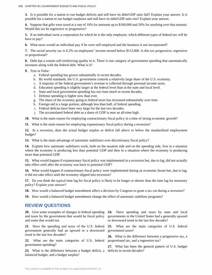
3. Is it possible for a nation to run budget deficits and still have its debt/GDP ratio fall? Explain your answer. Is itpossible for a nation to run budget surpluses and still have its debt/GDP ratio rise? Explain your answer.

4. Suppose that gifts were taxed at a rate of 10% for amounts up to $100,000 and 20% for anything over that amount.Would this tax be regressive or progressive?

5. If an individual owns a corporation for which he is the only employee, which different types of federal tax will hehave to pay?

6. What taxes would an individual pay if he were self-employed and the business is not incorporated?

7. The social security tax is 6.2% on employees’ income earned below $113,000. Is this tax progressive, regressiveor proportional?

8. Debt has a certain self-reinforcing quality to it. There is one category of government spending that automaticallyincreases along with the federal debt. What is it?

9. True or False:a. Federal spending has grown substantially in recent decades.b. By world standards, the U.S. government controls a relatively large share of the U.S. economy.c. A majority of the federal government’s revenue is collected through personal income taxes.d. Education spending is slightly larger at the federal level than at the state and local level.e. State and local government spending has not risen much in recent decades.f. Defense spending is higher now than ever.g. The share of the economy going to federal taxes has increased substantially over time.h. Foreign aid is a large portion, although less than half, of federal spending.i. Federal deficits have been very large for the last two decades.j. The accumulated federal debt as a share of GDP is near an all-time high.

10. What is the main reason for employing contractionary fiscal policy in a time of strong economic growth?

11. What is the main reason for employing expansionary fiscal policy during a recession?

12. In a recession, does the actual budget surplus or deficit fall above or below the standardized employmentbudget?

13. What is the main advantage of automatic stabilizers over discretionary fiscal policy?

14. Explain how automatic stabilizers work, both on the taxation side and on the spending side, first in a situationwhere the economy is producing less than potential GDP and then in a situation where the economy is producingmore than potential GDP.

15. What would happen if expansionary fiscal policy was implemented in a recession but, due to lag, did not actuallytake effect until after the economy was back to potential GDP?

16. What would happen if contractionary fiscal policy were implemented during an economic boom but, due to lag,it did not take effect until the economy slipped into recession?

17. Do you think the typical time lag for fiscal policy is likely to be longer or shorter than the time lag for monetarypolicy? Explain your answer?

18. How would a balanced budget amendment affect a decision by Congress to grant a tax cut during a recession?

19. How would a balanced budget amendment change the effect of automatic stabilizer programs?

REVIEW QUESTIONS20. Give some examples of changes in federal spendingand taxes by the government that would be fiscal policyand some that would not.

21. Have the spending and taxes of the U.S. federalgovernment generally had an upward or a downwardtrend in the last few decades?

22. What are the main categories of U.S. federalgovernment spending?

23. What is the difference between a budget deficit, abalanced budget, and a budget surplus?

24. Have spending and taxes by state and localgovernments in the United States had a generally upwardor downward trend in the last few decades?

25. What are the main categories of U.S. federalgovernment taxes?

26. What is the difference between a progressive tax, aproportional tax, and a regressive tax?

27. What has been the general pattern of U.S. budgetdeficits in recent decades?



28. What is the difference between a budget deficit andthe national debt?

29. What is the difference between expansionary fiscalpolicy and contractionary fiscal policy?

30. Under what general macroeconomic circumstancesmight a government use expansionary fiscal policy?When might it use contractionary fiscal policy?

31. What is the difference between discretionary fiscalpolicy and automatic stabilizers?

32. Why do automatic stabilizers function“automatically?”

33. What is the standardized employment budget?

34. What are some practical weaknesses of discretionaryfiscal policy?

35. What are some of the arguments for and againsta requirement that the federal government budget bebalanced every year?

CRITICAL THINKING QUESTIONS36. Why is government spending typically measured asa percentage of GDP rather than in nominal dollars?

37. Why are expenditures such as crime prevention andeducation typically done at the state and local level ratherthan at the federal level?

38. Why is spending by the U.S. government onscientific research at NASA fiscal policy while spendingby the University of Illinois is not fiscal policy? Why is acut in the payroll tax fiscal policy whereas a cut in a stateincome tax is not fiscal policy?

39. Excise taxes on tobacco and alcohol and state salestaxes are often criticized for being regressive. Althougheveryone pays the same rate regardless of income, whymight this be so?

40. What is the benefit of having state and local taxes onincome instead of collecting all such taxes at the federallevel?

41. In a booming economy, is the federal governmentmore likely to run surpluses or deficits? What are thevarious factors at play?

42. Economist Arthur Laffer famously pointed out that,in some cases, income tax revenue can actually go upwhen tax rates go down. Why might this be the case?

43. Is it possible for a nation to run budget deficits andstill have its debt/GDP ratio fall? Explain your answer. Is

it possible for a nation to run budget surpluses and stillhave its debt/GDP ratio rise? Explain your answer.

44. How will cuts in state budget spending affect federalexpansionary policy?

45. Is expansionary fiscal policy more attractive topoliticians who believe in larger government or topoliticians who believe in smaller government? Explainyour answer.

46. Is Medicaid (federal government aid to low-incomefamilies and individuals) an automatic stabilizer?

47. What is a potential problem with a temporary taxincrease designed to increase aggregate demand if peopleknow that it is temporary?

48. If the government gives a $300 tax cut to everyonein the country, explain the mechanism by which this willcause interest rates to rise.

49. Do you agree or disagree with this statement: “It isin the best interest of our economy for Congress and thePresident to run a balanced budget each year.” Explainyour answer.

50. During the Great Recession of 2008–2009, whatactions would have been required of Congress and thePresident had a balanced budget amendment to theConstitution been ratified? What impact would that havehad on the unemployment rate?

PROBLEMS51. A government starts off with a total debt of $3.5billion. In year one, the government runs a deficit of $400million. In year two, the government runs a deficit of $1billion. In year three, the government runs a surplus of$200 million. What is the total debt of the government atthe end of year three?

52. If a government runs a budget deficit of $10 billiondollars each year for ten years, then a surplus of $1 billionfor five years, and then a balanced budget for another tenyears, what is the government debt?

53. Specify whether expansionary or contractionaryfiscal policy would seem to be most appropriate in

response to each of the situations below and sketch adiagram using aggregate demand and aggregate supplycurves to illustrate your answer:

a. A recession.b. A stock market collapse that hurts consumer

and business confidence.c. Extremely rapid growth of exports.d. Rising inflation.e. A rise in the natural rate of unemployment.f. A rise in oil prices.


31 | The Impacts ofGovernment Borrowing

Figure 31.1 President Lyndon B. Johnson President Lyndon Johnson played a pivotal role in financing highereducation. (Credit: modification of image by LBJ Museum & Library)

Financing Higher EducationOn November 8, 1965, President Lyndon B. Johnson signed The Higher Education Act of 1965 into law.With a stroke of the pen, he implemented what we know as the financial aid, work study, and studentloan programs to help Americans pay for a college education. In his remarks, the President said:

Here the seeds were planted from which grew my firm conviction that for the individual,education is the path to achievement and fulfillment; for the Nation, it is a path to a societythat is not only free but civilized; and for the world, it is the path to peace—for it is educationthat places reason over force.

This Act, he said, "is responsible for funding higher education for millions of Americans. It is theembodiment of the United States’ investment in ‘human capital’." Since the Act was first signed into law,it has been renewed several times.

The purpose of The Higher Education Act of 1965 was to build the country’s human capital by creatingeducational opportunity for millions of Americans. The three criteria used to judge eligibility are income,full-time or part-time attendance, and the cost of the institution. According to the 2011–2012 NationalPostsecondary Student Aid Study (NPSAS:12), in the 2011–2012 school year, over 70% of all full-time college students received some form of federal financial aid; 47% received grants; and another55% received federal government student loans. The budget to support financial aid has increasednot only because of increased enrollment, but also because of increased tuition and fees for highereducation. These increases are currently being questioned. The President and Congress are chargedwith balancing fiscal responsibility and important government-financed expenditures like investing inhuman capital.

CHAPTER 31 | THE IMPACTS OF GOVERNMENT BORROWING 641

Introduction to the Impacts of Government BorrowingIn this chapter, you will learn about:

• How Government Borrowing Affects Investment and the Trade Balance

• Fiscal Policy, Investment, and Economic Growth

• How Government Borrowing Affects Private Saving

• Fiscal Policy and the Trade Balance

Governments have many competing demands for financial support. Any spending should be tempered by fiscalresponsibility and by looking carefully at the spending’s impact. When a government spends more than it collects in taxes,it runs a budget deficit. It then needs to borrow. When government borrowing becomes especially large and sustained, itcan substantially reduce the financial capital available to private sector firms, as well as lead to trade imbalances and evenfinancial crises.

The Government Budgets and Fiscal Policy chapter introduced the concepts of deficits and debt, as well as howa government could use fiscal policy to address recession or inflation. This chapter begins by building on the nationalsavings and investment identity, first introduced in The International Trade and Capital Flows chapter, to show howgovernment borrowing affects firms’ physical capital investment levels and trade balances. A prolonged period of budgetdeficits may lead to lower economic growth, in part because the funds borrowed by the government to fund its budgetdeficits are typically no longer available for private investment. Moreover, a sustained pattern of large budget deficits canlead to disruptive economic patterns of high inflation, substantial inflows of financial capital from abroad, plummetingexchange rates, and heavy strains on a country’s banking and financial system.

31.1 | How Government Borrowing Affects Investmentand the Trade BalanceBy the end of this section, you will be able to:

• Explain the national saving and investment identity in terms of demand and supply• Evaluate the role of budget surpluses and trade surpluses in national saving and investment identity

When governments are borrowers in financial markets, there are three possible sources for the funds from a macroeconomicpoint of view: (1) households might save more; (2) private firms might borrow less; and (3) the additional funds forgovernment borrowing might come from outside the country, from foreign financial investors. Let’s begin with a reviewof why one of these three options must occur, and then explore how interest rates and exchange rates adjust to theseconnections.

The National Saving and Investment IdentityThe national saving and investment identity, first introduced in The International Trade and Capital Flows chapter,provides a framework for showing the relationships between the sources of demand and supply in financial capital markets.The identity begins with a statement that must always hold true: the quantity of financial capital supplied in the market mustequal the quantity of financial capital demanded.

The U.S. economy has two main sources for financial capital: private savings from inside the U.S. economy and publicsavings.

Total savings = Private savings (S) + Public savings (T – G)

These include the inflow of foreign financial capital from abroad. The inflow of savings from abroad is, by definition, equalto the trade deficit, as explained in The International Trade and Capital Flows chapter. So this inflow of foreigninvestment capital can be written as imports (M) minus exports (X). There are also two main sources of demand for financialcapital: private sector investment (I) and government borrowing. Government borrowing in any given year is equal to thebudget deficit, and can be written as the difference between government spending (G) and net taxes (T). Let’s call thisequation 1.

Quantity supplied of finacial capi al = Quantity demanded of finacial capi alPrivate savings + Infl w of foreign savings = Private investment + Government budget defici

S + (M – X) = I + (G –T)

Governments often spend more than they receive in taxes and, therefore, public savings (T – G) is negative. This causes aneed to borrow money in the amount of (G – T) instead of adding to the nation’s savings. If this is the case, governments can

642 CHAPTER 31 | THE IMPACTS OF GOVERNMENT BORROWING


be viewed as demanders of financial capital instead of suppliers. So, in algebraic terms, the national savings and investmentidentity can be rewritten like this:

Private investment = Private savings + Public savings + Trade deficiI = S + (T – G) + (M – X)

Let’s call this equation 2. A change in any part of the national saving and investment identity must be accompanied byoffsetting changes in at least one other part of the equation because the equality of quantity supplied and quantity demandedis always assumed to hold. If the government budget deficit changes, then either private saving or investment or the tradebalance—or some combination of the three—must change as well. Figure 31.2 shows the possible effects.

Figure 31.2 Effects of Change in Budget Surplus or Deficit on Investment, Savings, and The Trade BalanceChart (a) shows the potential results when the budget deficit rises (or budget surplus falls). Chart (b) shows thepotential results when the budget deficit falls (or budget surplus rises).

What about Budget Surpluses and Trade Surpluses?The national saving and investment identity must always hold true because, by definition, the quantity supplied and quantitydemanded in the financial capital market must always be equal. However, the formula will look somewhat different if thegovernment budget is in deficit rather than surplus or if the balance of trade is in surplus rather than deficit. For example,in 1999 and 2000, the U.S. government had budget surpluses, although the economy was still experiencing trade deficits.When the government was running budget surpluses, it was acting as a saver rather than a borrower, and supplying ratherthan demanding financial capital. As a result, the national saving and investment identity during this time would be moreproperly written:

Quantity supplied of financial capi al = Quantity demanded of financial capi alPrivate savings + Trade deficit + G vernment surplus = Private investment

S + (M – X) + (T – G) = I

Let's call this equation 3. Notice that this expression is mathematically the same as equation 2 except the savings andinvestment sides of the identity have simply flipped sides.

During the 1960s, the U.S. government was often running a budget deficit, but the economy was typically running tradesurpluses. Since a trade surplus means that an economy is experiencing a net outflow of financial capital, the national savingand investment identity would be written:

Quantity supplied of financial capi al = Quantity demanded of financial capi alPrivate savings = Private investment + Outfl w of foreign savings + Government budget defici

S⏞

Private savings

= I + (X – M) + (G – T)

Instead of the balance of trade representing part of the supply of financial capital, which occurs with a trade deficit, a tradesurplus represents an outflow of financial capital leaving the domestic economy and being invested elsewhere in the world.

Quantity supplied of financial capi al = Quantity demanded of financial capi al demandPrivate savings = Private investment + Government budget deficit + rade surplus

S = I + (G – T) + (X – M)

The point to this parade of equations is that the national saving and investment identity is assumed to always hold. So whenyou write these relationships, it is important to engage your brain and think about what is on the supply side and what is onthe demand side of the financial capital market before you put pencil to paper.


As can be seen in Figure 31.3, the Office of Management and Budget shows that the United States has consistently runbudget deficits since 1977, with the exception of 1999 and 2000. What is alarming is the dramatic increase in budget deficitsthat has occurred since 2008, which in part reflects declining tax revenues and increased safety net expenditures due to theGreat Recession. (Recall that T is net taxes. When the government must transfer funds back to individuals for safety netexpenditures like Social Security and unemployment benefits, budget deficits rise.) These deficits have implications for thefuture health of the U.S. economy.

Figure 31.3 United States On-Budget, Surplus, and Deficit, 1977–2012 (in millions) The United States has runa budget deficit for over 30 years, with the exception of 1999 and 2000. Military expenditures, entitlement programs,and the decrease in tax revenue coupled with increased safety net support during the Great Recession are majorcontributors to the dramatic increases in the deficit after 2008. (Source: www.whitehouse.gov/omb)

A rising budget deficit may result in a fall in domestic investment, a rise in private savings, or a rise in the trade deficit. Thefollowing modules discuss each of these possible effects in more detail.

31.2 | Fiscal Policy, Investment, and Economic GrowthBy the end of this section, you will be able to:

• Explain crowding out and its effect on physical capital investment• Explain the relationship between budget deficits and interest rates• Identify why economic growth is tied to investments in physical capital, human capital, and technology

The underpinnings of economic growth are investments in physical capital, human capital, and technology, all set in aneconomic environment where firms and individuals can react to the incentives provided by well-functioning markets andflexible prices. Government borrowing can reduce the financial capital available for private firms to invest in physicalcapital. But government spending can also encourage certain elements of long-term growth, such as spending on roads orwater systems, on education, or on research and development that creates new technology.

Crowding Out Physical Capital InvestmentA larger budget deficit will increase demand for financial capital. If private saving and the trade balance remain the same,then less financial capital will be available for private investment in physical capital. When government borrowing soaksup available financial capital and leaves less for private investment in physical capital, the result is known as crowding out.

To understand the potential impact of crowding out, consider the situation of the U.S. economy before the exceptionalcircumstances of the recession that started in late 2007. In 2005, for example, the budget deficit was roughly 4% of GDP.Private investment by firms in the U.S. economy has hovered in the range of 14% to 18% of GDP in recent decades.However, in any given year, roughly half of U.S. investment in physical capital just replaces machinery and equipment thathas worn out or become technologically obsolete. Only about half represents an increase in the total quantity of physical



capital in the economy. So investment in new physical capital in any year is about 7% to 9% of GDP. In this situation, evenU.S. budget deficits in the range of 4% of GDP can potentially crowd out a substantial share of new investment spending.Conversely, a smaller budget deficit (or an increased budget surplus) increases the pool of financial capital available forprivate investment.

Visit this website (http://openstaxcollege.org/l/debtclock) to view the “U.S. Debt Clock.”

The patterns of U.S. budget deficits and private investment since 1980 are shown in Figure 31.4. If greater governmentdeficits lead to less private investment in physical capital, and reduced government deficits or budget surpluses lead to moreinvestment in physical capital, these two lines should move up and down at the same time. This pattern occurred in the late1990s and early 2000s. The U.S. federal budget went from a deficit of 2.2% of GDP in 1995 to a budget surplus of 2.4% ofGDP in 2000—a swing of 4.6% of GDP. From 1995 to 2000, private investment in physical capital rose from 15% to 18%of GDP—a rise of 3% of GDP. Then, when the U.S. government again started running budget deficits in the early 2000s,less financial capital became available for private investment, and the rate of private investment fell back to about 15% ofGDP by 2003.

Figure 31.4 U.S. Budget Deficits/Surpluses and Private Investment The connection between private savingsand flows of international capital plays a role in budget deficits and surpluses. Consequently, government borrowingand private investment sometimes rise and fall together. For example, the 1990s show a pattern in which reducedgovernment borrowing helped to reduce crowding out so that more funds were available for private investment.

This argument does not claim that a government's budget deficits will exactly shadow its national rate of private investment;after all, private saving and inflows of foreign financial investment must also be taken into account. In the mid-1980s,for example, government budget deficits increased substantially without a corresponding drop off in private investment.In 2009, nonresidential, private fixed investment dropped by $300 billion from its previous level of $2,432.6 billion in2008, primarily because, during a recession, firms lack both the funds and the incentive to invest. Investment growthbetween 2009 and 2013 averaged approximately 5.7% to $1,931 billion—below its 2008 levels, according to the Bureauof Economic Analysis. During that same period, interest rates dropped from 3.94% to less than a quarter percent as theFederal Reserve took dramatic action to prevent a depression by increasing the money supply through lowering short-terminterest rates. The "crowding out" of private investment due to government borrowing to finance expenditures appears tohave been suspended during the Great Recession. However, as the economy improves and interest rates rise, borrowing bythe government may potentially create pressure on interest rates.


http://openstaxcollege.org/l/debtclock

The Interest Rate ConnectionAssume that government borrowing of substantial amounts will have an effect on the quantity of private investment. Howwill this affect interest rates in financial markets? In Figure 31.5, the original equilibrium (E0) where the demand curve(D0) for financial capital intersects with the supply curve (S0) occurs at an interest rate of 5% and an equilibrium quantityequal to 20% of GDP. However, as the government budget deficit increases, the demand curve for financial capital shiftsfrom D0 to D1. The new equilibrium (E1) occurs at an interest rate of 6% and an equilibrium quantity of 21% of GDP.

Figure 31.5 Budget Deficits and Interest Rates In the financial market, an increase in government borrowing canshift the demand curve for financial capital to the right from D0 to D1. As the equilibrium interest rate shifts from E0 toE1, the interest rate rises from 5% to 6% in this example. The higher interest rate is one economic mechanism bywhich government borrowing can crowd out private investment.

A survey of economic studies on the connection between government borrowing and interest rates in the U.S. economysuggests that an increase of 1% in the budget deficit will lead to a rise in interest rates of between 0.5 and 1.0%, other factorsheld equal. In turn, a higher interest rate tends to discourage firms from making physical capital investments. One reasongovernment budget deficits crowd out private investment, therefore, is the increase in interest rates. There are, however,economic studies that show a limited connection between the two (at least in the United States), but as the budget deficitgrows, the dangers of rising interest rates become more real.

At this point, you may wonder about the Federal Reserve. After all, can the Federal Reserve not use expansionary monetarypolicy to reduce interest rates, or in this case, to prevent interest rates from rising? This useful question emphasizes theimportance of considering how fiscal and monetary policies work in relation to each other. Imagine a central bank faced witha government that is running large budget deficits, causing a rise in interest rates and crowding out private investment. If thebudget deficits are increasing aggregate demand when the economy is already producing near potential GDP, threatening aninflationary increase in price levels, the central bank may react with a contractionary monetary policy. In this situation, thehigher interest rates from the government borrowing would be made even higher by contractionary monetary policy, andthe government borrowing might crowd out a great deal of private investment.

On the other hand, if the budget deficits are increasing aggregate demand when the economy is producing substantially lessthan potential GDP, an inflationary increase in the price level is not much of a danger and the central bank might react withexpansionary monetary policy. In this situation, higher interest rates from government borrowing would be largely offset bylower interest rates from expansionary monetary policy, and there would be little crowding out of private investment.

However, even a central bank cannot erase the overall message of the national savings and investment identity. Ifgovernment borrowing rises, then private investment must fall, or private saving must rise, or the trade deficit must fall. Byreacting with contractionary or expansionary monetary policy, the central bank can only help to determine which of theseoutcomes is likely.

Public Investment in Physical CapitalGovernment can invest in physical capital directly: roads and bridges; water supply and sewers; seaports and airports;schools and hospitals; plants that generate electricity, like hydroelectric dams or windmills; telecommunications facilities;and weapons used by the military. In 2011, the U.S. federal government budget for Fiscal Year 2012 shows that the UnitedStates spent $59.9 billion on transportation, including highways, mass transit, and airports. Table 31.1 shows the totaloutlay for 2011 for major public physical capital investment by the federal government in the United States. Physical capitalrelated to the military or to residences where people live is omitted from this table, because the focus here is on publicinvestments that have a direct effect on raising output in the private sector.



Type of Public Physical Capital Federal Outlays 2011 ($ billions)

Transportation $59,920

Community and regional development $10,544

Natural resources and the environment $6,741

Education, training, employment, and social services $71

Other $8,427

Total $85,703

Table 31.1 Grants for Major Physical Capital Investment, 2011

Public physical capital investment of this sort can increase the output and productivity of the economy. An economy withreliable roads and electricity will be able to produce more. But it is hard to quantify how much government investment inphysical capital will benefit the economy, because government responds to political as well as economic incentives. Whena firm makes an investment in physical capital, it is subject to the discipline of the market: If it does not receive a positivereturn on investment, the firm may lose money or even go out of business.

In some cases, lawmakers make investments in physical capital as a way of spending money in the districts of keypoliticians. The result may be unnecessary roads or office buildings. Even if a project is useful and necessary, it mightbe done in a way that is excessively costly, because local contractors who make campaign contributions to politiciansappreciate the extra business. On the other hand, governments sometimes do not make the investments they should becausea decision to spend on infrastructure does not need to just make economic sense; it must be politically popular as well.Managing public investment so that it is done in a cost-effective way can be difficult.

If a government decides to finance an investment in public physical capital with higher taxes or lower government spendingin other areas, it need not worry that it is directly crowding out private investment. Indirectly however, higher householdtaxes could cut down on the level of private savings available and have a similar effect. If a government decides to financean investment in public physical capital by borrowing, it may end up increasing the quantity of public physical capital at thecost of crowding out investment in private physical capital, which is more beneficial to the economy would be dependenton the project being considered.

Public Investment in Human CapitalIn most countries, the government plays a large role in society's investment in human capital through the education system.A highly educated and skilled workforce contributes to a higher rate of economic growth. For the low-income nations ofthe world, additional investment in human capital seems likely to increase productivity and growth. For the United States,tough questions have been raised about how much increases in government spending on education will improve the actuallevel of education.

Among economists, discussions of education reform often begin with some uncomfortable facts. As shown in Figure 31.6,spending per student for kindergarten through grade 12 (K–12) increased substantially in real dollars through 2010. The U.S.Census Bureau reports that current spending per pupil for elementary and secondary education rose from $5,001 in 1998 to$10,615 in 2010. However, as measured by standardized tests like the SAT, the level of student academic achievement hasbarely budged in recent decades. Indeed, on international tests, U.S. students lag behind students from many other countries.(Of course, test scores are an imperfect measure of education for a variety of reasons. It would be difficult, however, toargue that there are not real problems in the U.S. education system and that the tests are just inaccurate.)


Figure 31.6 Total Spending for Elementary, Secondary, and Vocational Education (1998–2012) in the UnitedStates The graph shows that government spending on education was continually increasing up until 2006 where itleveled off until 2008 when it increased dramatically. Since 2010, spending has steadily decreased. (Source: Office ofManagement and Budget)

The fact that increased financial resources have not brought greater measurable gains in student performance has led someeducation experts to question whether the problems may be due to structure, not just to the resources spent.

Other government programs seek to increase human capital either before or after the K–12 education system. Programs forearly childhood education, like the federal Head Start program, are directed at families where the parents may have limitededucational and financial resources. Government also offers substantial support for universities and colleges. For example,in the United States about 60% of students take at least a few college or university classes beyond the high school level.In Germany and Japan, about half of all students take classes beyond the comparable high school level. In the countries ofLatin America, only about one student in four takes classes beyond the high school level, and in the nations of sub-SaharanAfrica, only about one student in 20.

Not all spending on educational human capital needs to happen through the government: many college students in theUnited States pay a substantial share of the cost of their education. If low-income countries of the world are going toexperience a widespread increase in their education levels for grade-school children, government spending seems likely toplay a substantial role. For the U.S. economy, and for other high-income countries, the primary focus at this time is moreon how to get a bigger return from existing spending on education and how to improve the performance of the average highschool graduate, rather than dramatic increases in education spending.

How Fiscal Policy Can Improve TechnologyResearch and development (R&D) efforts are the lifeblood of new technology. According to the National ScienceFoundation, federal outlays for research, development, and physical plant improvements to various governmental agencieshave remained at an average of 8.8% of GDP. About one-fifth of U.S. R&D spending goes to defense and space-orientedresearch. Although defense-oriented R&D spending may sometimes produce consumer-oriented spinoffs, R&D that isaimed at producing new weapons is less likely to benefit the civilian economy than direct civilian R&D spending.

Fiscal policy can encourage R&D using either direct spending or tax policy. Government could spend more on the R&D thatis carried out in government laboratories, as well as expanding federal R&D grants to universities and colleges, nonprofitorganizations, and the private sector. By 2010, the federal share of R&D outlays totaled $137.5 billion, or about 4% ofthe federal government’s overall budget, according to data from the National Science Foundation. Fiscal policy can alsosupport R&D through tax incentives, which allow firms to reduce their tax bill as they increase spending on research anddevelopment.

Summary of Fiscal Policy, Investment, and Economic GrowthInvestment in physical capital, human capital, and new technology is essential for long-term economic growth, assummarized in Table 31.2. In a market-oriented economy, private firms will undertake most of the investment in physicalcapital, and fiscal policy should seek to avoid a long series of outsized budget deficits that might crowd out such investment.The effects of many growth-oriented policies will be seen very gradually over time, as students are better educated, physicalcapital investments are made, and new technologies are invented and implemented.



Physical Capital HumanCapital New Technology

PrivateSector

New investment inproperty and equipment

On-the-jobtraining Research and development

PublicSector Public infrastructure

Publiceducation Jobtraining

Research and development encouraged throughprivate sector incentives and direct spending.

Table 31.2 Investment Role of Public and Private Sector in a Market Economy

31.3 | How Government Borrowing Affects Private SavingBy the end of this section, you will be able to:

• Apply Ricardian equivalence to evaluate how government borrowing affects private saving• Interpret a graphic representation of Ricardian equivalence

A change in government budgets may impact private saving. Imagine that people watch government budgets and adjust theirsavings accordingly. For example, whenever the government runs a budget deficit, people might reason: “Well, a higherbudget deficit means that I’m just going to owe more taxes in the future to pay off all that government borrowing, so I’llstart saving now.” If the government runs budget surpluses, people might reason: “With these budget surpluses (or lowerbudget deficits), interest rates are falling, so that saving is less attractive. Moreover, with a budget surplus the country willbe able to afford a tax cut sometime in the future. I won’t bother saving as much now.”

The theory that rational private households might shift their saving to offset government saving or borrowing is known asRicardian equivalence because the idea has intellectual roots in the writings of the early nineteenth-century economistDavid Ricardo (1772–1823). If Ricardian equivalence holds completely true, then in the national saving and investmentidentity, any change in budget deficits or budget surpluses would be completely offset by a corresponding change in privatesaving. As a result, changes in government borrowing would have no effect at all on either physical capital investment ortrade balances.

In practice, the private sector only sometimes and partially adjusts its savings behavior to offset government budget deficitsand surpluses. Figure 31.7 shows the patterns of U.S. government budget deficits and surpluses and the rate of privatesaving—which includes saving by both households and firms—since 1980. The connection between the two is not at allobvious. In the mid-1980s, for example, government budget deficits were quite large, but there is no corresponding surge ofprivate saving. However, when budget deficits turn to surpluses in the late 1990s, there is a simultaneous decline in privatesaving. When budget deficits get very large in 2008 and 2009, on the other hand, there is some sign of a rise in saving. Avariety of statistical studies based on the U.S. experience suggests that when government borrowing increases by $1, privatesaving rises by about 30 cents. A World Bank study done in the late 1990s, looking at government budgets and privatesaving behavior in countries around the world, found a similar result.

Figure 31.7 U.S. Budget Deficits and Private Savings The theory of Ricardian equivalence suggests that anyincrease in government borrowing will be offset by additional private saving, while any decrease in governmentborrowing will be offset by reduced private saving. Sometimes this theory holds true, and sometimes it does not holdtrue at all. (Source: Bureau of Economic Analysis and Federal Reserve Economic Data)


So private saving does increase to some extent when governments run large budget deficits, and private saving falls whengovernments reduce deficits or run large budget surpluses. However, the offsetting effects of private saving compared togovernment borrowing are much less than one-to-one. In addition, this effect can vary a great deal from country to country,from time to time, and over the short run and the long run.

If the funding for a larger budget deficit comes from international financial investors, then a budget deficit may beaccompanied by a trade deficit. In some countries, this pattern of a twin deficits has set the stage for international financialinvestors first to send their funds to a country and cause an appreciation of its exchange rate and then to pull their fundsout and cause a depreciation of the exchange rate and a financial crisis as well. It depends on whether funding comes frominternational financial investors.

31.4 | Fiscal Policy and the Trade BalanceBy the end of this section, you will be able to:

• Discuss twin deficits as they related to budget and trade deficit• Explain the relationship between budget deficits and exchange rates• Explain the relationship between budget deficits and inflation• Identify causes of recessions

Government budget balances can affect the trade balance. As The Keynesian Perspective chapter discusses, a netinflow of foreign financial investment always accompanies a trade deficit, while a net outflow of financial investmentalways accompanies a trade surplus. One way to understand the connection from budget deficits to trade deficits is that whengovernment creates a budget deficit with some combination of tax cuts or spending increases, it will increase aggregatedemand in the economy, and some of that increase in aggregate demand will result in a higher level of imports. A higherlevel of imports, with exports remaining fixed, will cause a larger trade deficit. That means foreigners’ holdings of dollarsincrease as Americans purchase more imported goods. Foreigners use those dollars to invest in the United States, whichleads to an inflow of foreign investment. One possible source of funding our budget deficit is foreigners buying Treasurysecurities that are sold by the U.S. government. So a budget deficit is often accompanied by a trade deficit.

Twin Deficits?In the mid-1980s, it was common to hear economists and even newspaper articles refer to the twin deficits, as the budgetdeficit and trade deficit both grew substantially. Figure 31.8 shows the pattern. The federal budget deficit went from 2.6%of GDP in 1981 to 5.1% of GDP in 1985—a drop of 2.5% of GDP. Over that time, the trade deficit moved from 0.5% in1981 to 2.9% in 1985—a drop of 2.4% of GDP. In the mid-1980s, the considerable increase in government borrowing wasmatched by an inflow of foreign investment capital, so the government budget deficit and the trade deficit moved together.

Figure 31.8 U.S. Budget Deficits and Trade Deficits In the 1980s, the budget deficit and the trade deficit declinedat the same time. However, since then, the deficits have stopped being twins. The trade deficit grew smaller in theearly 1990s as the budget deficit increased, and then the trade deficit grew larger in the late 1990s as the budgetdeficit turned into a surplus. In the first half of the 2000s, both budget and trade deficits increased. But in 2009, thetrade deficit declined as the budget deficit increased.

Of course, no one should expect the budget deficit and trade deficit to move in lockstep, because the other parts of thenational saving and investment identity—investment and private savings—will often change as well. In the late 1990s, forexample, the government budget balance turned from deficit to surplus, but the trade deficit remained large and growing.



During this time, the inflow of foreign financial investment was supporting a surge of physical capital investment by U.S.firms. In the first half of the 2000s, the budget and trade deficits again increased together, but in 2009, the budget deficitincreased while the trade deficit declined. The budget deficit and the trade deficits are related to each other, but they aremore like cousins than twins.

Budget Deficits and Exchange RatesExchange rates can also help to explain why budget deficits are linked to trade deficits. Figure 31.9 shows a situationusing the exchange rate for the U.S. dollar, measured in euros. At the original equilibrium (E0), where the demand for U.S.dollars (D0) intersects with the supply of U.S. dollars (S0) on the foreign exchange market, the exchange rate is 0.9 eurosper U.S. dollar and the equilibrium quantity traded in the market is $100 billion per day (which was roughly the quantityof dollar–euro trading in exchange rate markets in the mid-2000s). Then the U.S. budget deficit rises and foreign financialinvestment provides the source of funds for that budget deficit.

International financial investors, as a group, will demand more U.S. dollars on foreign exchange markets to purchase theU.S. government bonds, and they will supply fewer of the U.S. dollars that they already hold in these markets. Demandfor U.S. dollars on the foreign exchange market shifts from D0 to D1 and the supply of U.S. dollars falls from S0 to S1. Atthe new equilibrium (E1), the exchange rate has appreciated to 1.05 euros per dollar while, in this example, the quantity ofdollars traded remains the same.

Figure 31.9 Budget Deficits and Exchange Rates Imagine that the U.S. government increases its borrowing andthe funds come from European financial investors. To purchase U.S. government bonds, those European investorswill need to demand more U.S. dollars on foreign exchange markets, causing the demand for U.S. dollars to shift tothe right from D0 to D1. European financial investors as a group will also be less likely to supply U.S. dollars to theforeign exchange markets, causing the supply of U.S. dollars to shift from S0 to S1. The equilibrium exchange ratestrengthens from 0.9 euro/ dollar at E0 to 1.05 euros/dollar at E1.

A stronger exchange rate, of course, makes it more difficult for exporters to sell their goods abroad while making importscheaper, so a trade deficit (or a reduced trade surplus) results. Thus, a budget deficit can easily result in an inflow of foreignfinancial capital, a stronger exchange rate, and a trade deficit.

You can also imagine this appreciation of the exchange rate as being driven by interest rates. As explained earlier in BudgetDeficits and Interest Rates in Fiscal Policy, Investment, and Economic Growth, a budget deficit increasesdemand in markets for domestic financial capital, raising the domestic interest rate. A higher interest rate will attract aninflow of foreign financial capital, and appreciate the exchange rate in response to the increase in demand for U.S. dollars byforeign investors and a decrease in supply of U. S. dollars. Because of higher interest rates in the United States, Americansfind U.S. bonds more attractive than foreign bonds. When Americans are buying fewer foreign bonds, they are supplyingfewer U.S. dollars. The depreciation of the U.S. dollar leads to a larger trade deficit (or reduced surplus). The connectionsbetween inflows of foreign investment capital, interest rates, and exchange rates are all just different ways of drawing thesame economic connections: a larger budget deficit can result in a larger trade deficit, although the connection should notbe expected to be one-to-one.

From Budget Deficits to International Economic CrisisThe economic story of how an outflow of international financial capital can cause a deep recession is laid out, step-by-step,in the Exchange Rates and International Capital Flows chapter. When international financial investors decide towithdraw their funds from a country like Turkey, they increase the supply of the Turkish lira and reduce the demand for lira,depreciating the lira exchange rate. When firms and the government in a country like Turkey borrow money in internationalfinancial markets, they typically do so in stages. First, banks in Turkey borrow in a widely used currency like U.S. dollarsor euros, then convert those U.S. dollars to lira, and then lend the money to borrowers in Turkey. If the value of the lira


exchange rate depreciates, then Turkey’s banks will find it impossible to repay the international loans that are in U.S. dollarsor euros.

The combination of less foreign investment capital and banks that are bankrupt can sharply reduce aggregate demand, whichcauses a deep recession. Many countries around the world have experienced this kind of recession in recent years: alongwith Turkey in 2002, this general pattern was followed by Mexico in 1995, Thailand and countries across East Asia in1997–1998, Russia in 1998, and Argentina in 2002. In many of these countries, large government budget deficits played arole in setting the stage for the financial crisis. A moderate increase in a budget deficit that leads to a moderate increase ina trade deficit and a moderate appreciation of the exchange rate is not necessarily a cause for concern. But beyond somepoint that is hard to define in advance, a series of large budget deficits can become a cause for concern among internationalinvestors.

One reason for concern is that extremely large budget deficits mean that aggregate demand may shift so far to the right asto cause high inflation. The example of Turkey is a situation where very large budget deficits brought inflation rates wellinto double digits. In addition, very large budget deficits at some point begin to raise a fear that the borrowing will notbe repaid. In the last 175 years, the government of Turkey has been unable to pay its debts and defaulted on its loans sixtimes. Brazil’s government has been unable to pay its debts and defaulted on its loans seven times; Venezuela, nine times;and Argentina, five times. The risk of high inflation or a default on repaying international loans will worry internationalinvestors, since both factors imply that the rate of return on their investments in that country may end up lower thanexpected. If international investors start withdrawing the funds from a country rapidly, the scenario of less investment,a depreciated exchange rate, widespread bank failure, and deep recession can occur. The following Clear It Up featureexplains other impacts of large deficits.

What are the risks of chronic large deficits in the United States?If a government runs large budget deficits for a sustained period of time, what can go wrong? Accordingto a recent report by the Brookings Institution, a key risk of a large budget deficit is that government debtmay grow too high compared to the country’s GDP growth. As debt grows, the national savings rate willdecline, leaving less available in financial capital for private investment. The impact of chronically largebudget deficits is as follows:

• As the population ages, there will be an increasing demand for government services that may causehigher government deficits. Government borrowing and its interest payments will pull resourcesaway from domestic investment in human capital and physical capital that is essential to economicgrowth.

• Interest rates may start to rise so that the cost of financing government debt will rise as well,creating pressure on the government to reduce its budget deficits through spending cuts and taxincreases. These steps will be politically painful, and they will also have a contractionary effect onaggregate demand in the economy.

• Rising percentage of debt to GDP will create uncertainty in the financial and global marketsthat might cause a country to resort to inflationary tactics to reduce the real value of the debtoutstanding. This will decrease real wealth and damage confidence in the country’s ability tomanage its spending. After all, if the government has borrowed at a fixed interest rate of, say, 5%,and it lets inflation rise above that 5%, then it will effectively be able to repay its debt at a negativereal interest rate.

The conventional reasoning suggests that the relationship between sustained deficits that lead to highlevels of government debt and long-term growth is negative. How significant this relationship is, how bigan issue it is compared to other macroeconomic issues, and the direction of causality, is less clear.

What remains important to acknowledge is that the relationship between debt and growth is negativeand that for some countries, the relationship may be stronger than in others. It is also important toacknowledge the direction of causality: does high debt cause slow growth, slow growth cause high debt,or are both high debt and slow growth the result of third factors? In our analysis, we have argued simplythat high debt causes slow growth. There may be more to this debate than we have space to discusshere.



Using Fiscal Policy to Address Trade ImbalancesIf a nation is experiencing the inflow of foreign investment capital associated with a trade deficit because foreign investorsare making long-term direct investments in firms, there may be no substantial reason for concern. After all, many low-income nations around the world would welcome direct investment by multinational firms that ties them more closely intothe global networks of production and distribution of goods and services. In this case, the inflows of foreign investmentcapital and the trade deficit are attracted by the opportunities for a good rate of return on private sector investment in aneconomy.

However, governments should beware of a sustained pattern of high budget deficits and high trade deficits. The dangerarises in particular when the inflow of foreign investment capital is not funding long-term physical capital investment byfirms, but instead is short-term portfolio investment in government bonds. When inflows of foreign financial investmentreach high levels, foreign financial investors will be on the alert for any reason to fear that the country’s exchange rate maydecline or the government may be unable to repay what it has borrowed on time. Just as a few falling rocks can trigger anavalanche; a relatively small piece of bad news about an economy can trigger an enormous outflow of short-term financialcapital.

Reducing a nation’s budget deficit will not always be a successful method of reducing its trade deficit, because otherelements of the national saving and investment identity, like private saving or investment, may change instead. In thosecases when the budget deficit is the main cause of the trade deficit, governments should take steps to reduce their budgetdeficits, lest they make their economy vulnerable to a rapid outflow of international financial capital that could bring a deeprecession.

Financing Higher EducationOver the period between 1982 and 2012, the increases in the cost of a college education had faroutpaced that of the income of the typical American family. According to the research done by thePresident Obama’s staff, the cost of education at a four-year public college increased by 257%compared to an increase in family incomes of only 16% over the prior 30 years. The ongoing debateover a balanced budget and proposed cutbacks accentuated the need to increase investment inhuman capital to grow the economy versus deepening the already significant debt levels of the U.S.government. In the summer of 2013, President Obama presented a plan to make college moreaffordable that included increasing Pell Grant awards and the number of recipients, caps on interestrates for student loans, and providing education tax credits. In addition, the plan includes anaccountability method for institutions of higher education that focuses on completion rates and creates aCollege Scorecard. Whether or not all these initiatives come to fruition remains to be seen, but they areindicative of creative approaches that government can take to meet its obligation from both a public andfiscal policy perspective.


Head Start program

Ricardian equivalence

twin deficits

KEY TERMSa program for early childhood education directed at families with limited educational and financial

resources.

the theory that rational private households might shift their saving to offset government savingor borrowing

deficits that occur when a country is running both a trade and a budget deficit


31.1 How Government Borrowing Affects Investment and the Trade Balance

A change in any part of the national saving and investment identity suggests that if the government budgetdeficit changes, then either private savings, private investment in physical capital, or the trade balance—or somecombination of the three—must change as well.

31.2 Fiscal Policy, Investment, and Economic Growth

Economic growth comes from a combination of investment in physical capital, human capital, and technology.Government borrowing can crowd out private sector investment in physical capital, but fiscal policy can alsoincrease investment in publicly owned physical capital, human capital (education), and research and development.Possible methods for improving education and society’s investment in human capital include spending more moneyon teachers and other educational resources, and reorganizing the education system to provide greater incentivesfor success. Methods for increasing research and development spending to generate new technology include directgovernment spending on R&D and tax incentives for businesses to conduct additional R&D.

31.3 How Government Borrowing Affects Private Saving

The theory of Ricardian equivalence holds that changes in government borrowing or saving will be offset by changesin private saving. Thus, higher budget deficits will be offset by greater private saving, while larger budget surpluseswill be offset by greater private borrowing. If the theory holds true, then changes in government borrowing or savingwould have no effect on private investment in physical capital or on the trade balance. However, empirical evidencesuggests that the theory holds true only partially.

31.4 Fiscal Policy and the Trade Balance

The government need not balance its budget every year. However, a sustained pattern of large budget deficits overtime risks causing several negative macroeconomic outcomes: a shift to the right in aggregate demand that causes aninflationary increase in the price level; crowding out private investment in physical capital in a way that slows downeconomic growth; and creating a dependence on inflows of international portfolio investment which can sometimesturn into outflows of foreign financial investment that can be injurious to a macroeconomy.

SELF-CHECK QUESTIONS1. In a country, private savings equals 600, the government budget surplus equals 200, and the trade surplus equals100. What is the level of private investment in this economy?

2. Assume an economy has a budget surplus of 1,000, private savings of 4,000, and investment of 5,000.a. Write out a national saving and investment identity for this economy.b. What will be the balance of trade in this economy?c. If the budget surplus changes to a budget deficit of 1000, with private saving and investment unchanged,

what is the new balance of trade in this economy?

3. Why have many education experts recently placed an emphasis on altering the incentives faced by U.S. schoolsrather than on increasing their budgets? Without endorsing any of these proposals as especially good or bad, list someof the ways in which incentives for schools might be altered.

4. What are some steps the government can take to encourage research and development?

5. Imagine an economy in which Ricardian equivalence holds. This economy has a budget deficit of 50, a tradedeficit of 20, private savings of 130, and investment of 100. If the budget deficit rises to 70, how are the other termsin the national saving and investment identity affected?



6. In the late 1990s, the U.S. government moved from a budget deficit to a budget surplus and the trade deficit inthe U.S. economy grew substantially. Using the national saving and investment identity, what can you say about thedirection in which saving and/or investment must have changed in this economy?

REVIEW QUESTIONS7. Based on the national saving and investment identity,what are the three ways the macroeconomy might react togreater government budget deficits?

8. How would you expect larger budget deficits to affectprivate sector investment in physical capital? Why?

9. What are some of the ways fiscal policy mightencourage economic growth?

10. What are some fiscal policies for improving asociety’s human capital?

11. What are some fiscal policies for improving thetechnologies that the economy will have to draw upon inthe future?

12. Explain how cuts in funding for programs such asHead Start might affect the development of human capitalin the United States.

13. What is the theory of Ricardian equivalence?

14. What does the concept of rationality have to do withRicardian equivalence?

15. Under what conditions will a larger budget deficitcause a trade deficit?

CRITICAL THINKING QUESTIONS16. Assume there is no discretionary increase ingovernment spending. Explain how an improvingeconomy will affect the budget balance and, in turn,investment and the trade balance.

17. Explain how decreased domestic investments thatoccur due to a budget deficit will affect future economicgrowth.

18. The U.S. government has shut down a number oftimes in recent history. Explain how a governmentshutdown will affect the variables in the nationalinvestment and savings identity. Could the shutdownaffect the government budget deficit?

19. Explain why the government might prefer to provideincentives to private firms to do investment or researchand development, rather than simply doing the spendingitself?

20. Under what condition would crowding out notinhibit long-run economic growth? Under what conditionwould crowding out impede long-run economic growth?

21. What must take place for the government to rundeficits without any crowding out?

22. Explain whether or not you agree with the premiseof the Ricardian equivalence theory that rational peoplemight reason: “Well, a higher budget deficit (surplus)means that I’m just going to owe more (less) taxes in thefuture to pay off all that government borrowing, so I’llstart saving (spending) now.” Why or why not?

23. Explain how a shift from a government budgetdeficit to a budget surplus might affect the exchange rate.

24. Describe how a plan for reducing the governmentdeficit might affect a college student, a youngprofessional, and a middle-income family.

PROBLEMS25. During the most recent recession, some economistsargued that the change in the interest rates that comesabout due to deficit spending implied in the demand andsupply of financial capital graph would not occur. Asimple reason was that the government was stepping into invest when private firms were not. Using a graph,explain how the deficit demand is offset by the use bygovernment in investment.

26. Illustrate the concept of Ricardian equivalence usingthe demand and supply of financial capital graph.

27. Sketch a diagram of how a budget deficit causesa trade deficit. (Hint: Begin with what will happen tothe exchange rate when foreigners demand more U.S.government debt.)

28. Sketch a diagram of how sustained budget deficitscause low economic growth.

29. Assume that you are employed by the governmentof Tanzania in 1964, a new nation recently independentfrom Britain. The Tanzanian parliament has decided thatit will spend 10 million shillings on schools, roads, andhealthcare for the year. You estimate that the net taxes forthe year are eight million shillings. The difference willbe financed by selling 10-year government bonds at 12%interest per year. The interest on outstanding bonds mustbe added to government expenditure each year. Assumethat additional taxes are added to finance this increase ingovernment expenditure so the gap between governmentspending is always two million. If the school, road, andhealthcare budget are unchanged, compute the value ofthe accumulated debt in 10 years.


32 | Macroeconomic PolicyAround the World

Figure 32.1 Looking for Work Job fairs and job centers are often available to help match people to jobs. This fairtook place in the U.S. (Hawaii), a high-income country with policies to keep unemployment levels in check.Unemployment is an issue that has different causes in different countries, and is especially severe in the low- andmiddle-income economies around the world. (Credit: modification of work by Daniel Ramirez/Flickr CreativeCommons)

Youth Unemployment: Three CasesChad Harding, a young man from Cape Town, South Africa, completed school having done well on hisexams. He had high hopes for the future. Like many young South Africans, however, he had difficultyfinding a job. “I was just stuck at home waiting, waiting for something to come up,” he said in a BBCinterview in 2012. In South Africa 54.6% of young females and 47.2% of males are unemployed. In fact,the problem is not limited to South Africa. Seventy-three million of the world’s youth aged 15 to 24 arecurrently unemployed, according to the International Labour Organization.

According to the Wall Street Journal, in India, 60% of the labor force is self-employed, largely becauseof labor market regulation. A recent World Development Report by The World Bank says that India’sunemployed youth accounted for 9.9% of the youth work force in 2010. In Spain (a far richer country) inthe same year, the female/male youth unemployment rate was 39.8% and 43.2% respectively.

Youth unemployment is a significant issue in many parts of the world. However, despite the apparentsimilarities in rates between South Africa, Spain, and India, macroeconomic policy solutions to decreaseyouth unemployment in these three countries are different. This chapter will look at macroeconomicpolicies around the world, specifically those related to reducing unemployment, promoting economic

CHAPTER 32 | MACROECONOMIC POLICY AROUND THE WORLD 657

growth, and stable inflation and exchange rates. Then we will look again at the three cases of SouthAfrica, Spain, and India.

Introduction to Macroeconomic Policy around theWorldIn this chapter, you will learn about:

• The Diversity of Countries and Economies across the World

• Improving Countries’ Standards of Living

• Causes of Unemployment around the World

• Causes of Inflation in Various Countries and Regions

• Balance of Trade Concerns

There are extraordinary differences in the composition and performance of economies across the world. What explains thesedifferences? Are countries motivated by similar goals when it comes to macroeconomic policy? Can we apply the samemacroeconomic framework developed in this text to understand the performance of these countries? Let’s take each of thesequestions in turn.

Explaining differences: Recall from Unemployment that we explained the difference in composition and performanceof economies by appealing to an aggregate production function. We argued that the diversity of average incomes acrossthe world was explained by differences in productivity, which in turn were affected by inputs such as capital deepening,human capital, and “technology.” Every economy has its own distinctive economic characteristics, institutions, history, andpolitical realities, which imply that access to these “ingredients” will vary by country and so will economic performance.

For example, South Korea invested heavily in education and technology to increase agricultural productivity in the early1950s. Some of this investment came from its historical relationship with the United States. As a result of these and manyother institutions, its economy has managed to converge to the levels of income in leading economies like Japan and theUnited States.

Similar goals and frameworks: Many economies that have performed well in terms of per capita income have—for better orworse—been motivated by a similar goal: to maintain the quality of life of their citizens. Quality of life is a broad term, butas you can imagine it includes but is not limited to such things as low level of unemployment, price stability (low levels ofinflation), and the ability to trade. These seem to be universal macroeconomic goals as discussed in The MacroeconomicPerspective. No country would argue against them. To study macroeconomic policy around the world, we begin bycomparing standards of living. In keeping with these goals, we also look at indicators such as unemployment, inflation, andthe balance of trade policies across countries. Remember that every country has had a diverse set of experiences; thereforealthough our goals may be similar, each country may well require macroeconomic policies tailored to its circumstances.

For more reading on the topic of youth unemployment, visit this website (http://openstaxcollege.org/l/genjobless) to read “Generation Jobless” in the Economist.

658 CHAPTER 32 | MACROECONOMIC POLICY AROUND THE WORLD


http://openstaxcollege.org/l/genjobless

http://openstaxcollege.org/l/genjobless

32.1 | The Diversity of Countries and Economies acrossthe WorldBy the end of this section, you will be able to:

• Analyze GDP per capita as a measure of the diversity of international standards of living• Identify what classifies a country as low-income, middle-income, or high-income• Explain how standards of living are influenced by geography, demographics, industry structure, and economic

institutions

The national economies that make up the global economy are remarkably diverse. Let us use one key indicator of thestandard of living, GDP per capita, to quantify this diversity. You will quickly see that quantifying this diversity is fraughtwith challenges and limitations. As explained in The Macroeconomic Perspective, we must consider using purchasingpower parity or “international dollars” to convert average incomes into comparable units. Purchasing power parity, asformally defined in Exchange Rates and International Capital Flows, takes into account the fact that prices of thesame good are different across countries.

The Macroeconomic Perspective explained how to measure GDP, the challenges of using GDP to compare standardsof living, and the difficulty of confusing economic size with distribution. In China’s case, for example, China ranks as thethird largest global economy along with Japan and the United States. But, when we take its GDP of $4,522,140,211,438 anddivide it by its population of 1,350,695,000 people, then the per capita GDP is only $3,348, which is significantly lowerthan that of Japan, at $36,938, and that of the United States, at $43,063. Measurement issues aside, it’s worth repeating thatthe goal, then, is to not only increase GDP, but to strive toward increased GDP per capita to increase overall standards ofliving for individuals. As we have learned from Economic Growth, this can be achieved at the national level by designingpolicies that increase worker productivity, deepen capital, and advance technology.

GDP per capita also allows us to rank countries into high-, middle-, or low-income groups. Low-income countries are thosewith $1,025 per capita GDP per year; middle-income countries have a per capita GDP between $1,025 and $12,475; whilehigh-income countries have over $12,475 per year per capita income. As seen in Table 32.1 and Figure 32.2, high-incomecountries earn 68% of world income, but represent just 12% of the global population. Low-income countries earn 1% oftotal world income, but represent 18.5% of global population.

Ranking based on GDP/capita

GDP (inmillions)

% of GlobalGDP Population % of Global

Population

Low income ($1,025 or less) $501,001 0.7% 1,302,107,523 18.5%

Middle income ($1,025 -$12,475) $22,353,932 31.1% 4,897,806,355 69.5%

High income (more than$12,475) $49,112,539 68.3% 846,454,901 12.0%

World Total income $71,918,394 7,046,368,779

Table 32.1 World Income versus Global Population (Source:http://databank.worldbank.org/data/views/reports/tableview.aspx?isshared=true&ispopular=series&pid=20)


Figure 32.2 Percent of Global GDP and Percent of Population The pie charts show the GDP (from 2011) forcountries categorized into low, middle, or high income. Low-income are those earning less than $1,025 (less than 1%of global income). They represent 18.5% of the world population. Middle-income countries are those with per capitaincome of $1,025–$12,475 (31.1% of global income). They represent 69.5% of world population. High-incomecountries have 68.3% of global income and 12% of the world’s population. (Source: http://databank.worldbank.org/data/views/reports/tableview.aspx?isshared=true&ispopular=series&pid=20)

An overview of the regional averages of GDP per person for developing countries, measured in comparable internationaldollars as well as population in 2008 (Figure 32.3), shows that the differences across these regions are stark. As Table32.2 shows, nominal GDP per capita in 2012 for the 581.4 million people living in Latin America and the Caribbean regionwas $9,190, which far exceeds that of South Asia and sub-Saharan Africa. In turn, people in the high-income nations of theworld, such as those who live in the European Union nations or North America, have a per capita GDP three to four timesthat of the people of Latin America. To put things in perspective, North America and the European Union have slightlymore than 9% of the world’s population, but they produce and consume close to 70% of the world’s GDP.

Figure 32.3 GDP Per Capita in U.S. Dollars (2008) There is a clear imbalance in the GDP across the world. NorthAmerica, Australia, and Western Europe have the highest GDPs while large areas of the world have dramaticallylower GDPs. (Credit: modification of work by Bsrboy/Wikimedia Commons)



Population (in millions) GDP Per Capita

East Asia 1,992 $5,246

South Asia 1,649 $1,388

Sub-Saharan Africa 910 $1,415

Latin America 581 $9,190

Middle East and North Africa 340 $4,535

Europe and Central Asia 272 $6,847

Table 32.2 Regional Comparisons of Nominal GDP per Capita and Population in 2012 (Source:http://databank.worldbank.org/data/home.aspx)

Such comparisons between regions are admittedly rough. After all, per capita GDP cannot fully capture the quality oflife. Many other factors have a large impact on the standard of living, like health, education, human rights, crime andpersonal safety, and environmental quality. These measures also reveal very wide differences in the standard of livingacross the regions of the world. Much of this is correlated with per capita income, but there are exceptions. For example,life expectancy at birth in many low-income regions approximates those who are more affluent. The data also illustratethat nobody can claim to have perfect standards of living. For instance, despite very high income levels, there is stillundernourishment in Europe and North America.

Economists know that there are many factors that contribute to your standard of living. People in high-income countries may have very little time due to heavy workloads and may feel disconnected fromtheir community. Lower-income countries may be more community centered, but have little in the wayof material wealth. It is hard to measure these characteristics of standard of living. The Organizationfor Economic Co-Operation and Development has developed the “OECD Better Life Index.” Visit thiswebsite (http://openstaxcollege.org/l/standofliving) to see how countries measure up to your expectedstandard of living.

The differences in economic statistics and other measures of well-being, substantial though they are, do not fully capture thereasons for the enormous differences between countries. Aside from the neoclassical determinants of growth, four additionaldeterminants are significant in a wide range of statistical studies and are worth mentioning: geography, demography,industrial structure, and institutions.

Geographic and Demographic Differences

Countries have geographic differences: some have extensive coastlines, some are landlocked. Some have large rivers thathave been a path of commerce for centuries, or mountains that have been a barrier to trade. Some have deserts, somehave rain forests. These differences create different positive and negative opportunities for commerce, health, and theenvironment.

Countries also have considerable differences in the age distribution of the population. Many high-income nations areapproaching a situation by 2020 or so in which the elderly will form a much larger share of the population. Most low-incomecountries still have a higher proportion of youth and young adults, but by about 2050, the elderly populations in these low-income countries are expected to boom as well. These demographic changes will have considerable impact on the standardof living of the young and the old.

Differences in Industry Structure and Economic Institutions


http://openstaxcollege.org/l/standofliving

Countries have differences in industry structure. In the high-income economies of the world, only about 2% of GDP comesfrom agriculture; the average for the rest of the world is 12%. Countries have strong differences in degree of urbanization.

Countries also have strong differences in economic institutions: some nations have economies that are extremely market-oriented, while other nations have command economies. Some nations are open to international trade, while others usetariffs and import quotas to limit the impact of trade. Some nations are torn by long-standing armed conflicts; other nationsare largely at peace. There are differences in political, religious, and social institutions as well.

No nation intentionally aims for a low standard of living, high rates of unemployment and inflation, or an unsustainabletrade imbalance. However, nations will differ in their priorities and in the situations in which they find themselves, andso their policy choices can reasonably vary, too. The next modules will discuss how nations around the world, from highincome to low income, approach the four macroeconomic goals of economic growth, low unemployment, low inflation, anda sustainable balance of trade.

32.2 | Improving Countries’ Standards of LivingBy the end of this section, you will be able to:

• Analyze the growth policies of low-income countries seeking to improve standards of living• Analyze the growth policies of middle-income countries, particularly the East Asian Tigers with their focus on

technology and market-oriented incentives• Analyze the struggles facing economically-challenged countries wishing to enact growth policies• Evaluate the success of sending aid to low-income countries

Jobs are created in economies that grow. Where does economic growth come from? According to most economistswho believe in the growth consensus, economic growth (as discussed in Economic Growth) is built on a foundationof productivity improvements. In turn, productivity increases are the result of greater human and physical capital andtechnology, all interacting in a market-driven economy. In the pursuit of economic growth, however, some countries andregions start from different levels, as illustrated by the differences in per capita GDP presented earlier in Table 32.2.

Growth Policies for the High-Income CountriesFor the high-income countries, the challenge of economic growth is to push continually for a more educated workforce thatcan create, invest in, and apply new technologies. In effect, the goal of their growth-oriented public policy is to shift theiraggregate supply curves to the right (refer to The Aggregate Demand/Aggregate Supply Model). The main publicpolicies targeted at achieving this goal are fiscal policies focused on investment, including investment in human capital,in technology, and in physical plant and equipment. These countries also recognize that economic growth works best in astable and market-oriented economic climate. For this reason, they use monetary policy to keep inflation low and stable,and to minimize the risk of exchange rate fluctuations, while also encouraging domestic and international competition.

However, early in the second decade of the 2000s, many high-income countries found themselves more focused on theshort term than on the long term. The United States, Western Europe, and Japan all experienced a combination of financialcrisis and deep recession, and the after-effects of the recession—like high unemployment rates—seemed likely to lingerfor several years. Most of these governments took aggressive, and in some cases controversial, steps to jump-start theireconomies by running very large budget deficits as part of expansionary fiscal policy. These countries must adopt a coursethat combines lower government spending and higher taxes.

Similarly, many central banks ran highly expansionary monetary policies, with both near-zero interest rates andunconventional loans and investments. For example, in 2012, Shinzo Abe (see Figure 32.4), then newly-elected PrimeMinister of Japan, unveiled a plan to get his country out of its two-decade-long slump in economic growth. It included bothfiscal stimulus and an increase in the money supply. The plan was quite successful in the short run. However, accordingto the Economist, with public debt “expected to approach 240% of GDP,” printing money and public-works spending wereonly short-term solutions.



Figure 32.4 Japan’s Prime Minister, Shinzo Abe Japan’s Prime Minister used fiscal and monetary policies tostimulate his country’s economy, which has worked in only the short run. (Credit: modification of work by ChathamHouse/Flickr Creative Commons)

As other chapters discuss, macroeconomics needs to have both a short-run and a long-run focus. The challenge for manyof the developed countries in the next few years will be to exit from the short-term policies that were used to correct the2008–2009 recession. Since the return to growth has been sluggish, it has been politically challenging for these governmentsto refocus their efforts on new technology, education, and physical capital investment.

Growth Policies for the Middle-Income EconomiesThe world’s great economic success stories in the last few decades began in the 1970s with that group of nations sometimesknown as the East Asian Tigers: South Korea, Thailand, Malaysia, Indonesia, and Singapore. The list sometimes includesHong Kong and Taiwan, although these are often treated under international law as part of China, rather than as separatecountries. The economic growth of the Tigers has been phenomenal, typically averaging 5.5% real per capita growth forseveral decades. In the 1980s, other countries began to show signs of convergence. China began growing rapidly, often atannual rates of 8% to 10% per year. India began growing rapidly, first at rates of about 5% per year in the 1990s, but thenhigher still in the first decade of the 2000s.

The underlying causes of these rapid growth rates are known:

• China and the East Asian Tigers, in particular, have been among the highest savers in the world, often saving one-thirdor more of GDP as compared to the roughly one-fifth of GDP, which would be a more typical saving rate in LatinAmerica and Africa. These higher savings were harnessed for domestic investment to build physical capital.

• These countries had policies that supported heavy investments in human capital, first building up primary-leveleducation and then expanding secondary-level education. Many focused on encouraging math and science education,which is useful in engineering and business.

• Governments made a concerted effort to seek out applicable technology, by sending students and governmentcommissions abroad to look at the most efficient industrial operations elsewhere. They also created policies to supportinnovative companies that wished to build production facilities to take advantage of the abundant and inexpensivehuman capital.

• China and India in particular also allowed far greater freedom for market forces, both within their own domesticeconomies and also in encouraging their firms to participate in world markets.

This combination of technology, human capital, and physical capital, combined with the incentives of a market-orientedeconomic context, proved an extremely powerful stimulant to growth. Challenges faced by these middle-income countriesare a legacy of government economic controls that for political reasons can be dismantled only slowly over time. In many ofthem, the banking and financial sector is heavily regulated. Governments have also sometimes selected certain industries toreceive low-interest loans or government subsidies. These economies have found that an increased dose of market-orientedincentives for firms and workers has been a critical ingredient in the recipe for faster growth. To learn more about measuringeconomic growth, read the following Clear It Up feature.

What is the rule of 72?It is worth pausing a moment to marvel at the growth rates of the East Asian Tigers. If per capita GDPgrows at, say, 6% per year, then you can apply the formula for compound growth rates—that is (1 +0.06)30—meaning a nation’s level of per capita GDP will rise by a multiple of almost six over 30 years.Another strategy is to apply the rule of 72. The rule of 72 is an approximation to figure out doubling time.


The rule number, 72, is divided by the annual growth rate to obtain the approximate number of years itwill take for income to double. So if we have a 6% growth rate, it will take 72/6, or 12 years, for incomesto double. Using this rule here suggests that a Tiger that grows at 6% will double its GDP every 12 years.In contrast, a technological leader, chugging along with per capita growth rates of about 2% per year,would double its income in 36 years.

Growth Policies for Economically-Challenged CountriesMany economically-challenged or low-income countries are geographically located in Sub-Saharan Africa. Other pocketsof low income are found in the former Soviet Bloc, and in parts of Central America and the Caribbean.

There are macroeconomic policies and prescriptions that might alleviate the extreme poverty and low standard of living.However, many of these countries lack the economic and legal stability, along with market-oriented institutions, needed toprovide a fertile climate for domestic economic growth and to attract foreign investment. Thus, macroeconomic policies forlow income economies are vastly different from those of the high income economies. The World Bank has made it a priorityto combat poverty and raise overall income levels through 2030. One of the key obstacles to achieving this is the politicalinstability that seems to be a common feature of low-income countries.

Figure 32.5 shows the ten lowest income countries as ranked by The World Bank. These countries share some commontraits, the most significant of which is the recent failures of their governments to provide a legal framework for economicgrowth. Ethiopia and Eritrea recently ended a long-standing war in 2000. Civil and ethnic wars have plagued countries suchas Burundi and Liberia. Command economies, corruption, as well as political factionalism and infighting are commonlyadopted elements in these low-income countries. The Democratic Republic of the Congo (often referred to as “Congo”)is a resource-wealthy country that has not been able to increase its subsistence standard of living due to the politicalenvironment.

Figure 32.5 The Ten Lowest Income Countries Low-income countries, like those in this chart, share commonelements such as political factionalism, infighting, and corruption. (Source: http://databank.worldbank.org/data/views/reports/map.aspx#)

Low-income countries are at a disadvantage because any incomes received are spent immediately on necessities such asfood. People in these countries live on less than $1,035 per year, which is less than $100 per month. Lack of saving meansa lack of capital accumulation and a lack of loanable funds for investment in physical and human capital. Recent researchby two MIT economists, Abhijit Bannerjee and Esther Duflo, has confirmed that the households in these economies aretrapped in low incomes because they cannot muster enough investment to push themselves out of poverty.

For example, the average citizen of Burundi, the lowest-income country, subsists on $150 per year (adjusted to 2005dollars). According to data collected by the Central Intelligence Agency in its CIA Factbook, as of 2012, 90% of Burundi’spopulation is agrarian, with coffee and tea as the main income producing crop. Only one in two children attends schooland, as shown in Figure 32.6, many are not in schools comparable to what is found in developed countries. The CIAFactbook also estimates that 15% of Burundi’s population suffers from HIV/AIDS. Political instability has made it difficultfor Burundi to make significant headway toward growth, as verified by the electrification of only 2% of households and42% of its national income coming from foreign aid.



Figure 32.6 Lack of Funds for Investing in Human Capital In low-income countries, all income is often spent onnecessities for living and cannot be accumulated or invested in physical or human capital. The students in thisphotograph learn in an outside “classroom” void of not only technology, but even chairs and desks. (Credit: RafaelaPrintes/Flickr Creative Commons)

The World Factbook website (http://openstaxcollege.org/l/worldfactbook) is loaded with maps, flags, andother information about countries across the globe.

Other low-income countries share similar stories. These countries have found it difficult to generate investments forthemselves or to find foreign investors willing to put up the money for more than the basic needs. Foreign aid and externalinvestment comprise significant portions of the income in these economies, but are not sufficient to allow for the capitalaccumulation necessary to invest in physical and human capital. But is foreign aid always a contributor to economic growth?It can be a controversial issue, as the next Clear it Up feature points out.

Does foreign aid to low-income countries work?According to the Organization of Economic Cooperation and Development (OECD), about $134 billionper year in foreign aid flows from the high-income countries of the world to the low-income ones. Relativeto the size of their populations or economies, this is not a large amount for either donors or recipients.For low-income countries, aid averages about 1.3 percent of their GDP. But even this relatively smallamount has been highly controversial.

Supporters of additional foreign aid point to the extraordinary human suffering in the low-and middle-income countries of the world. They see opportunities all across Africa, Asia, and Latin America to setup health clinics and schools. They want to help with the task of building economic infrastructure: cleanwater, plumbing, electricity, and roads. Supporters of this aid include formal state-sponsored institutionslike the United Kingdom’s Department for International Development (DFID) or independent non-governmental organizations (NGOs) like CARE International that also receive donor government funds.


http://openstaxcollege.org/l/worldfactbook

For example, because of an outbreak of meningitis in Ethiopia in 2010, DFID channeled significant fundsto the Ethiopian Ministry of Health to train rural health care workers and also for vaccines. These monieshelped the Ministry offset shortfalls in their budget.

Opponents of increased aid do not quarrel with the goal of reducing human suffering, but they suggestthat foreign aid has often proved a poor tool for advancing that goal. For example, according to an articlein the Attaché Journal of International Affairs, the Canadian foreign aid organization (CIDA) provided$100 million to Tanzania to grow wheat. The project did produce wheat, but nomadic pastoralists andother villagers who had lived on the land were driven off 100,000 acres of land to make way for theproject. The damage in terms of human rights and lost livelihoods was significant. Villagers were beatenand killed because some refused to leave the land. At times, the unintended collateral damage fromforeign aid can be significant.

William Easterly, professor of economics at New York University and author of The White Man’s Burden,argues that aid is often given for political reasons and ends up doing more harm than good. If thegovernment of a country creates a reasonably stable and market-oriented macroeconomic climate, thenforeign investors will be likely to provide funds for many profitable activities. For example, according toThe New York Times, Facebook is partnering with multiple organizations in a project called Internet.orgto provide access in remote and low-income areas of the world, and Google began its own initiativecalled Project Loon. Facebook’s first forays into providing Internet access via mobile phones began instable, market-oriented countries like India, Brazil, Indonesia, Turkey, and the Philippines.

Policymakers are now wiser about the limitations of foreign aid than they were a few decades ago.In targeted and specific cases, especially if foreign aid is channeled to long-term investment projects,foreign aid can have a modest role to play in reducing the extreme levels of deprivation experienced byhundreds of millions of people around the world.

Watch this video (http://openstaxcollege.org/l/foodafrica) on the complexities of providing economic aidin Africa.

32.3 | Causes of Unemployment around the WorldBy the end of this section, you will be able to:

• Explain the nature and causes of unemployment• Analyze the natural rate of unemployment and the factors that affect it• Identify how undeveloped labor markets can result in the same hardships as unemployment

The causes of unemployment in high-income countries of the world can be categorized in two ways: either cyclicalunemployment caused by the economy being in a recession, or the natural rate of unemployment caused by factors in labormarkets, such as government regulations regarding hiring and starting businesses.

Unemployment from a RecessionFor unemployment caused by a recession, the Keynesian economic model points out that both monetary and fiscal policytools are available. The monetary policy prescription for dealing with recession is straightforward: run an expansionarymonetary policy to increase the quantity of money and loans, drive down interest rates, and increase aggregate demand. Ina recession, there is usually relatively little danger of inflation taking off, and so even a central bank, with fighting inflationas its top priority, can usually justify some reduction in interest rates.



http://openstaxcollege.org/l/foodafrica

With regard to fiscal policy, the automatic stabilizers discussed in Government Budgets and Fiscal Policy should beallowed to work, even if this means larger budget deficits in times of recession. There is less agreement over whether, inaddition to automatic stabilizers, governments in a recession should try to adopt discretionary fiscal policy of additional taxcuts or spending increases. In the case of the Great Recession, the case for this kind of extra-aggressive expansionary fiscalpolicy is stronger, but for a smaller recession, given the time lags of implementing fiscal policy, discretionary fiscal policyshould be used with caution.

However, the aftermath of the Recession emphasizes that expansionary fiscal and monetary policies do not turn off arecession like flipping a switch turns off a lamp. Even after a recession is officially over, and positive growth has returned,it can take some months—or even a couple of years—before private-sector firms believe the economic climate is healthyenough that they can expand their workforce.

The Natural Rate of UnemploymentUnemployment rates in the nations of Europe have typically been higher than in the United States. In 2006, before thestart of the Great Recession, the U.S. unemployment rate was 4.6%, compared with 9% in France, 10.4% in Germany, and7.1% in Sweden. The pattern of generally higher unemployment rates in Europe, which dates back to the 1970s, is typicallyattributed to the fact that European economies have a higher natural rate of unemployment because they have a greaternumber of rules and restrictions that discourage firms from hiring and unemployed workers from taking jobs.

Addressing the natural rate of unemployment is straightforward in theory but difficult in practice. Government can play auseful role in providing unemployment and welfare payments, passing rules about where and when businesses can operate,assuring that the workplace is safe, and so on. But these well-intentioned laws can, in some cases, become so intrusive thatbusinesses decide to place limits on their hiring.

For example, a law that imposes large costs on a business that tries to fire or lay off workers will mean that businessestry to avoid hiring in the first place, as is the case in France. According to Business Week, “France has 2.4 times as manycompanies with 49 employees as with 50 ... according to the French labor code, once a company has at least 50 employeesinside France, management must create three worker councils, introduce profit sharing, and submit restructuring plans tothe councils if the company decides to fire workers for economic reasons.” This labor law essentially limits employment (orraises the natural rate of unemployment).

Undeveloped Labor MarketsLow-income and middle-income countries face employment issues that go beyond unemployment as it is understood in thehigh-income economies. A substantial number of workers in these economies provide many of their own needs by farming,fishing, or hunting. They barter and trade with others and may take a succession of short-term or one-day jobs, sometimesbeing paid with food or shelter, sometimes with money. They are not “unemployed” in the sense that the term is used in theUnited States and Europe, but neither are they employed in a regular wage-paying job.

The starting point of economic activity, as discussed in Welcome to Economics!, is the division of labor, in whichworkers specialize in certain tasks and trade the fruits of their labor with others. Workers who are not connected to a labormarket are often unable to specialize very much. Because these workers are not “officially” employed, they are often noteligible for social benefits like unemployment insurance or old-age payments—if such payments are even available in theircountry. Helping these workers to become more connected to the labor market and the economy is an important policy goal.Indeed, recent research by development economists suggests that one of the key factors in raising people in low-incomecountries out of the worst kind of poverty is whether they can make a connection to a somewhat regular wage-paying job.

32.4 | Causes of Inflation in Various Countries andRegionsBy the end of this section, you will be able to:

• Identify the causes and effects of inflation in various economic markets• Explain the significance of a converging economy

Policymakers of the high-income economies appear to have learned some lessons about fighting inflation. First, whateverhappens with aggregate supply and aggregate demand in the short run, monetary policy can be used to prevent inflation frombecoming entrenched in the economy in the medium and long term. Second, there is no long-run gain to letting inflationbecome established. In fact, allowing inflation to become lasting and persistent poses undesirable risks and tradeoffs. Wheninflation is high, businesses and individuals need to spend time and effort worrying about protecting themselves againstinflation, rather than seeking out better ways to serve customers. In short, the high-income economies appear to have botha political consensus to hold inflation low and the economic tools to do so.

In a number of middle- and low-income economies around the world, inflation is far from a solved problem. In the early2000s, Turkey experienced inflation of more than 50% per year for several years. Belarus had inflation of about 100% per


year from 2000 to 2001. From 2008 to 2010, Venezuela and Myanmar had inflation rates of 20% to 30% per year. Indonesia,Iran, Nigeria, the Russian Federation, and Ukraine all had double-digit inflation for most of the years from 2000 to 2010.Zimbabwe had hyperinflation, with inflation rates that went from more than 100% per year in the mid-2000s to a rate ofseveral million percent in 2008.

In these countries, the problem of very high inflation generally arises from huge budget deficits, which are financed bythe government printing its domestic currency. This is a case of “too much money chasing too few goods.” In the case ofZimbabwe, the government covered its widening deficits by printing ever higher currency notes, including a $100 trillionbill. By late 2008, the money was nearly worthless, which led Zimbabwe to adopt the U.S. dollar, immediately halting theirhyperinflation. In some countries, the central bank makes loans to politically favored firms, essentially printing money todo so, and this too leads to higher inflation.

A number of countries have managed to sustain solid levels of economic growth for sustained periods of time with levels ofinflation that would sound high by recent U.S. standards, like 10% to 30% per year. In such economies, most contracts, wagelevels, and interest rates are indexed to inflation. Indexing wage contracts and interest rates means that they will increasewhen inflation increases to retain purchasing power. When wages do not rise as price levels rise, this leads to a decline inthe real wage rate and a decrease in the standard of living. Likewise, interest rates that are not indexed mean that the lendersof money will be paid back in devalued currency and will also lose purchasing power on monies that were lent. It is clearlypossible—and perhaps sometimes necessary—for a converging economy (the economy of a country that demonstrates theability to catch up to the technology leaders) to live with a degree of uncertainty over inflation that would be politicallyunacceptable in the high-income economies.

32.5 | Balance of Trade ConcernsBy the end of this section, you will be able to:

• Explain the meaning of trade balance and its implications for the foreign exchange market• Analyze concerns over international trade in goods and services and international flows of capital• Identify and evaluate market-oriented economic reforms

In the 1950s and 1960s, and even into the 1970s, openness to global flows of goods, services, and financial capital was oftenviewed in a negative light by low- and middle-income countries. These countries feared that foreign trade would mean botheconomic losses as their economy was “exploited” by high-income trading partners and a loss of domestic political controlto powerful business interests and multinational corporations.

These negative feelings about international trade have evolved. After all, the great economic success stories of recent yearslike Japan, the East Asian Tiger economies, China, and India, all took advantage of opportunities to sell in global markets.The economies of Europe thrive with high levels of trade. In the North American Free Trade Agreement (NAFTA), theUnited States, Canada, and Mexico pledged themselves to reduce trade barriers. Many countries have clearly learned thatreducing barriers to trade is at least potentially beneficial to the economy. Indeed, many smaller economies of the worldhave learned an even tougher lesson: if they do not participate actively in world trade, they are unlikely to join the successstories among the converging economies. There are no examples in world history of small economies that remained apartfrom the global economy but still attained a high standard of living.

Although almost every country now claims that its goal is to participate in global trade, the possible negative consequenceshave remained highly controversial. It is useful to divide up these possible negative consequences into issues involvingtrade of goods and services and issues involving flows of international capital. These issues are related, but not the same. Aneconomy may have a high level of trade in goods and services relative to GDP, but if exports and imports are balanced, thenet flow of foreign investment in and out of the economy will be zero. Conversely, an economy may have only a moderatelevel of trade relative to GDP, but find that it has a substantial current account trade imbalance. Thus, it is useful to considerthe concerns over international trade of goods and services and international flows of financial capital separately.

Concerns over International Trade in Goods and ServicesThere is a long list of worries about foreign trade in goods and services: fear of job loss, environmental dangers, unfairlabor practices, and many other concerns. These arguments are discussed at some length in The International Trade andCapital Flows.

Of all of the arguments for limitations on trade, perhaps the most controversial one among economists is the infant industryargument; that is, subsidizing or protecting new industries for a time until they become established. (Globalization andProtectionism explains this concept in more detail.) Such policies have been used with some success at certain points intime, but in the world as a whole, support for key industries is far more often directed at long-established industries withsubstantial political power that are suffering losses and laying off workers, rather than potentially vibrant new industries thathave yet to be established. If government is going to favor certain industries, it needs to do so in a way that is temporary andthat orients them toward a future of market competition, rather than a future of unending government subsidies and tradeprotection.



Concerns over International Flows of CapitalRecall from The Macroeconomic Perspective that a trade deficit exists when a nation’s imports exceed its exports.In order for a trade deficit to take place, foreign countries must provide loans or investments, which they are willing todo because they expect they will be repaid eventually (that the deficit will become a surplus). A trade surplus, you mayremember, exists when a nation’s exports exceed its imports. So, in order for a trade deficit to switch to a trade surplus,a nation’s exports must rise and its imports must fall. Sometimes this happens when the currency decreases in value. Forexample, if the U.S. had a trade deficit and the dollar depreciated, imports would become more expensive. This would, inturn, benefit the foreign countries who provided the loans or investments.

The expected pattern of trade imbalances in the world economy has been that high-income economies will run tradesurpluses, which means they will experience a net outflow of capital to foreign destinations or export more than they import,while low- and middle-income economies will run trade deficits, which means that they will experience a net inflow offoreign capital.

This pattern of international investing can benefit all sides. Investors in the high-income countries benefit because they canreceive high returns on their investments, and also because they can diversify their investments so that they are at less risk ofa downturn in their own domestic economy. The low-income economies that receive an inflow of capital presumably havepotential for rapid catch-up economic growth, and they can use the inflow of international financial capital to help spur theirphysical capital investment. In addition, inflows of financial capital often come with management abilities, technologicalexpertise, and training.

However, for the last couple of decades, this cheerful scenario has faced two “dark clouds.” The first cloud is the very largetrade or current account deficits in the U.S. economy. (See The International Trade and Capital Flows.) Instead ofoffering net financial investment abroad, the U.S. economy is soaking up savings from all over the world. These substantialU.S. trade deficits may not be sustainable according to Sebastian Edwards writing for the National Bureau of EconomicResearch. While trade deficits on their own are not bad, the question is whether they will be reduced gradually or hastily. Inthe gradual scenario, U.S. exports could grow more rapidly than imports over a period of years, aided by a depreciation ofthe U.S. dollar. An unintended consequence of the slow growth since the Great Recession has been a decline in the size ofthe U.S. current account deficit from 6% pre-recession to 3% most recently.

The other option is that the U.S. trade deficit could be reduced in a rush. Here is one scenario: if foreign investors becameless willing to hold U.S. dollar assets, the dollar exchange rate could weaken. As speculators see this process happening,they might rush to unload their dollar assets, which would drive the dollar down still further.

A lower U.S. dollar would stimulate aggregate demand by making exports cheaper and imports more expensive. It wouldmean higher prices for imported inputs throughout the economy, shifting the short-term aggregate supply curve to the left.The result could be a burst of inflation and, if the Federal Reserve were to run a tight monetary policy to reduce the inflation,it could also lead to recession. People sometimes talk as if the U.S. economy, with its great size, is invulnerable to this sortof pressure from international markets. While it is tough to rock, it is not impossible for the $14 trillion U.S. economy toface these international pressures.

The second “dark cloud” is how the smaller economies of the world should deal with the possibility of sudden inflowsand outflows of foreign financial capital. Perhaps the most vivid recent example of the potentially destructive forces ofinternational capital movements occurred in the economies of the East Asian Tigers in 1997–1998. Thanks to their excellentgrowth performance over the previous few decades, these economies had attracted considerable interest from foreigninvestors. In the mid-1990s, however, foreign investment into these countries surged even further. Much of this money wasfunneled through banks that borrowed in U.S. dollars and loaned in their national currencies. Bank lending surged at ratesof 20% per year or more. This inflow of foreign capital meant that investment in these economies exceeded the level ofdomestic savings, so that current account deficits in these countries jumped into the range of 5–10% of GDP.

The surge in bank lending meant that many banks in these East Asian countries did not do an especially good job ofscreening out safe and unsafe borrowers. Many of the loans—as high as 10% to 15% of all loans in some of thesecountries—started to turn bad. Fearing losses, foreign investors started pulling their money out. As the foreign money left,the exchange rates of these countries crashed, often falling by 50% or more in a few months. The banks were stuck with amismatch: even if the rest of their domestic loans were repaid, they could never pay back the U.S. dollars that they owed.The banking sector as a whole went bankrupt. The lack of credit and lending in the economy collapsed aggregate demand,bringing on a deep recession.

If the flow and ebb of international capital markets can flip even the economies of the East Asian Tigers, with their stellargrowth records, into a recession, then it is no wonder that other middle- and low-income countries around the world areconcerned. Moreover, similar episodes of an inflow and then an outflow of foreign financial capital have rocked a numberof economies around the world: for example, in the last few years, economies like Ireland, Iceland, and Greece have allexperienced severe shocks when foreign lenders decided to stop extending funds. Especially in Greece, this caused thegovernment to enact austerity measures which led to protests throughout the country (Figure 32.7).


Figure 32.7 Protests in Greece The economic conditions in Greece have deteriorated from the Great Recessionsuch that the government had to enact austerity measures, (strict rules) cutting wages and increasing taxes on itspopulation. Massive protests are but one byproduct. (Credit: modification of work by Apostolos/Flickr CreativeCommons)

Many nations are taking steps to reduce the risk that their economy will be injured if foreign financial capital takes flight,including having their central banks hold large reserves of foreign exchange and stepping up their regulation of domesticbanks to avoid a wave of imprudent lending. The most controversial steps in this area involve whether countries should tryto take steps to control or reduce the flows of foreign capital. If a country could discourage some of the inflow of speculativeshort-term capital, and instead only encourage investment capital that was committed for the medium term and the longterm, then it could be at least somewhat less susceptible to swings in the sentiments of global investors.

If economies participate in the global trade of goods and services, they will also need to participate in international flowsof financial payments and investments. These linkages can offer great benefits to an economy. However, any nation that isexperiencing a substantial and sustained pattern of trade deficits, along with the corresponding net inflow of internationalfinancial capital, has some reason for concern. During the Asian Financial Crisis in the late 1990s, countries that grewdramatically in the years leading up to the crisis as international capital flowed in, saw their economies collapse when thecapital very quickly flowed out.

Market-Oriented Economic ReformsThe standard of living has increased dramatically for billions of people around the world in the last half century. Suchincreases have occurred not only in the technological leaders like the United States, Canada, the nations of Europe, andJapan, but also in the East Asian Tigers and in many nations of Latin America and Eastern Europe. The challenge formost of these countries is to maintain these growth rates. The economically-challenged regions of the world have stagnatedand become stuck in poverty traps. These countries need to focus on the basics: health and education, or human capitaldevelopment. As Figure 32.8 illustrates, modern technology allows for the investment in education and human capitaldevelopment in ways that would have not been possible just a few short years ago.

Figure 32.8 Solar-powered Technology Modern technologies, such as solar-power and Wi-Fi, enable education tobe delivered to students even in remote parts of a country without electricity. These students in Ghana are sharing alaptop provided by a van with solar-power. (Credit: EIFL/Flickr Creative Commons)



Other than the issue of economic growth, the other three main goals of macroeconomic policy—that is, low unemployment,low inflation, and a sustainable balance of trade—all involve situations in which, for some reason, the economy failsto coordinate the forces of supply and demand. In the case of cyclical unemployment, for example, the intersection ofaggregate supply and aggregate demand occurs at a level of output below potential GDP. In the case of the natural rateof unemployment, government regulations create a situation where otherwise-willing employers become unwilling to hireotherwise-willing workers. Inflation is a situation in which aggregate demand outstrips aggregate supply, at least for a time,so that too much buying power is chasing too few goods. A trade imbalance is a situation where, because of a net inflow oroutflow of foreign capital, domestic savings are not aligned with domestic investment. Each of these situations can create arange of easier or harder policy choices.

Youth Unemployment: Three CasesSpain and South Africa had the same high youth unemployment in 2011, but the reasons for thisunemployment are different. Spain’s youth unemployment surged due to the Great Recession of2008–2009 and heavy indebtedness on the part of its citizens and its government. Spain’s currentaccount balance is negative, which means it is borrowing heavily. To cure cyclical unemployment duringa recession, the Keynesian model suggests increases in government spending—fiscal expansion ormonetary expansion. Neither option is open to Spain. It currently can borrow at only high interest rates,which will be a real problem in terms of debt service. In addition, the rest of the European Union (EU)has dragged its feet when it comes to debt forgiveness. Monetary expansion is not possible becauseSpain uses the euro and cannot devalue its currency unless it convinces all of the EU to do so. Sowhat can be done? The Economist, summarizing some of the ideas of economists and policymakers,suggests that Spain’s only realistic (although painful) option is to reduce government-mandated wages,which would allow it to reduce government spending. As a result, the government would be able to lowertax rates on the working population. With a lower wage or lower tax environment, firms will hire moreworkers. This will lower unemployment and stimulate the economy. Spain can also encourage greaterforeign investment and try to promote policies that encourage domestic savings.

South Africa has more of a natural rate of unemployment problem. It is an interesting case because itsyouth unemployment is mostly due to the fact that its young are not ready to work. This is commonlyreferred to as an employability problem. According to interviews of South African firms as reported inthe Economist, the young are academically smart but lack practical skills for the workplace. Despitea big push to increase investment in human capital, the results have not yet borne fruit. Recently thegovernment unveiled a plan to pay unemployed youth while they were “trained-up” or apprenticed inSouth African firms. The government has room to increase fiscal expenditure, encourage domesticsavings, and continue to fund investment in education, vocational training, and apprentice programs.South Africa can also improve the climate for foreign investment from technology leaders, which wouldencourage economic growth.

India has a smaller youth employment problem in terms of percentages. However, bear in mind thatsince this is a populous country, it turns out to be a significant problem in raw numbers. According toKaushik Basu, writing for the BBC, “there are 45 national laws governing the hiring and firing decisionsof firms and close to four times that amount at the state level”. These laws make it difficult for companiesto fire workers. To stay nimble and responsive to markets, Indian companies respond to these laws byhiring fewer workers. The Indian government can do much to solve this problem by adjusting its laborlaws. Essentially, the government has to remove itself from firms’ hiring and firing decisions, so thatgrowing Indian firms can freely employ more workers. Indian workers, like those in South Africa, donot have workforce skills. Again, the government can increase its spending on education, vocationaltraining, and workforce readiness programs.

Finally, India has a significant current account deficit. This deficit is mainly a result of short- and long-term capital flows. To solve this deficit, India has experimented by lifting the limitation on domestic saversfrom investing abroad. This is a step in the right direction that may dampen the growth in the currentaccount deficit. A final policy possibility is to improve domestic capital markets so many self-employedIndians can get access to capital to realize their business ideas. If more Indians can get access to capitalto start businesses, employment might increase.


converging economy

East Asian Tigers

growth consensus

high-income country

low-income country

middle-income country

KEY TERMSeconomy of a country that has demonstrated the ability to catch up to the technology leaders by

investing in both physical and human capital

the economies of Taiwan, Singapore, Hong Kong, and South Korea, which maintained high growthrates and rapid export-led industrialization between the early 1960s and 1990 allowing them to converge with thetechnological leaders in high-income countries

a series of studies that show, statistically, that 70% of the differences in income per person across theworld is explained by differences in physical capital (savings/investment)

nation with a per capita income of $12,475 or more; typically has high levels of human andphysical capital

a nation that has a per capita income of less than $1,025; a third of the world’s population

a nation with per capita income between $1,025 and $12, 475 and that has shown some ability,even if not always sustained, to catch up to the technology leaders in high-income countries


32.1 The Diversity of Countries and Economies across the World

Macroeconomic policy goals for most countries strive toward low levels of unemployment and inflation, as wellas stable trade balances. Countries are analyzed based on their GDP per person and ranked as low-, middle-, and high-income countries. Low-income are those earning less than $1,025 (less than 1%) of global income.They currently have 18.5% of the world population. Middle-income countries are those with per capital income of$1,025–$12,475 (31.1% of global income). They have 69.5% of world population. High-income countries are thosewith per capita income greater than $12,475 (68.3% of global income). They have 12% of the world’s population.Regional comparisons tend to be inaccurate because even countries within those regions tend to differ from eachother.

32.2 Improving Countries’ Standards of Living

The fundamentals of growth are the same in every country: improvements in human capital, physical capital, andtechnology interacting in a market-oriented economy. Countries that are high-income tend to focus on developingand using new technology. Countries that are middle-income focus on increasing human capital and becomingmore connected to technology and global markets. They have charted unconventional paths by relying more onstate-led support rather than relying solely on markets. Low-income, economically-challenged countries have manyhealth and human development needs, but they are also challenged by the lack of investment and foreign aid todevelop infrastructure like roads. There are some bright spots when it comes to financial development and mobilecommunications, which suggest that low-income countries can become technology leaders in their own right, but itis too early to claim victory. These countries must do more to connect to the rest of the global economy and find thetechnologies that work best for them.

32.3 Causes of Unemployment around the World

Cyclical unemployment can be addressed by expansionary fiscal and monetary policy. The natural rate ofunemployment can be harder to deal with, because it involves thinking carefully about the tradeoffs involved in lawsthat affect employment and hiring. Unemployment is understood differently in high-income countries compared tolow- and middle-income countries. People in these countries are not “unemployed” in the sense that term is used inthe United States and Europe, but neither are they employed in a regular wage-paying job. While some may haveregular wage-paying jobs, others are part of a barter economy.

32.4 Causes of Inflation in Various Countries and Regions

Most high-income economies have learned that their central banks can control inflation in the medium and the longterm. In addition, they have learned that inflation has no long-term benefits but potentially substantial long-term costsif it distracts businesses from focusing on real productivity gains. However, smaller economies around the world mayface more volatile inflation because their smaller economies can be unsettled by international movements of capitaland goods.



32.5 Balance of Trade Concerns

There are many legitimate concerns over possible negative consequences of free trade. Perhaps the single strongestresponse to these concerns is that there are good ways to address them without restricting trade and thus losing itsbenefits. There are two major issues involving trade imbalances. One is what will happen with the large U.S. tradedeficits, and whether they will come down gradually or with a rush. The other is whether smaller countries aroundthe world should take some steps to limit flows of international capital, in the hope that they will not be quite sosusceptible to economic whiplash from international financial capital flowing in and out of their economies.

SELF-CHECK QUESTIONS1. Using the data provided in Table 32.3, rank the seven regions of the world according to GDP and then accordingto GDP per capita.

Population (inmillions)

GDP PerCapita

GDP = Population × Per Capita GDP(in millions)

East Asia 1,992 $5,246 $10,450,032

South Asia 1,649 $1,388 $2,288,812

Sub-Saharan Africa 910 $1,415 $1,287,650

Latin America 581 $9,190 $5,339,390

Middle East and NorthAfrica 340 $4,535 $1,541,900

Europe and CentralAsia 272 $6,847 $1,862,384

Table 32.3 GDP and Population of Seven Regions of the World

2. What are the drawbacks to analyzing the global economy on a regional basis?

3. Create a table that identifies the macroeconomic policies for a high-income country, a middle-income country,and a low-income country.

4. Use the data in the text to contrast the policy prescriptions of the high-income, middle-income, and low-incomecountries.

5. What are the different policy tools for dealing with cyclical unemployment?

6. Explain how the natural rate of unemployment may be higher in low-income countries.

7. How does indexing wage contracts to inflation help workers?

8. Use the AD/AS model to show how increases in government spending can lead to more inflation.

9. Show, using the AD/AS model, how monetary policy can be used to decrease the price level.

10. What do international flows of capital have to do with trade imbalances?

11. Use the demand-and-supply of foreign currency graph to determine what would happen to a small, openeconomy that experienced capital outflows.

REVIEW QUESTIONS12. What is the primary way in which economistsmeasure standards of living?

13. What are some of the other ways of comparing thestandard of living in countries around the world?

14. What are the four other factors that determine theeconomic standard of living around the world?

15. What other factors, aside from labor productivity,capital investment, and technology, impact the economicgrowth of a country? How?

16. What strategies were employed by the East AsianTigers to stimulate economic growth?

17. What are the two types of unemployment problems?


18. In low-income countries, does it make sense to arguethat most of the people without long-term jobs areunemployed?

19. Is inflation likely to be a severe problem for at leastsome high-income economies in the near future?

20. Is inflation likely to be a problem for at least somelow- and middle-income economies in the near future?

21. What are the major issues with regard to tradeimbalances for the U.S. economy?

22. What are the major issues with regard to tradeimbalances for low- and middle-income countries?

CRITICAL THINKING QUESTIONS23. Demography can have important economic effects.The United States has an aging population. Explain oneeconomic benefit and one economic cost of an agingpopulation as well as of a population that is very young.

24. Explain why is it difficult to set aside funds forinvestment when you are in poverty.

25. Why do you think it is difficult for high-incomecountries to achieve high growth rates?

26. Is it possible to protect workers from being firedwithout distorting the labor market?

27. Explain what will happen in a nation that tries tosolve a structural unemployment problem using

expansionary monetary and fiscal policy. Draw one AD/AS diagram, based on the Keynesian model, for whatthe nation hopes will happen. Then draw a second AD/AS diagram, based on the neoclassical model, for what ismore likely to happen.

28. Why are inflationary dangers lower in the high-income economies than in low-income and middle-income economies?

29. Explain why converging economies may present astrong argument for limiting flows of capital but not forlimiting trade.

PROBLEMS30. Retrieve the following data from The World Bankdatabase (http://databank.worldbank.org/data/home.aspx) for India, Spain, and South Africa for themost recent year available:

• GDP in constant international dollars or PPP• Population• GDP per person in constant international dollars• Mortality rate, infant (per 1,000 live births)• Health expenditure per capita (current U.S. dollars)• Life expectancy at birth, total (years)

31. Prepare a chart that compares India, Spain, andSouth Africa based on the data you find. Describe the keydifferences between the countries. Rank these as high-, medium-, and low-income countries, explain what issurprising or expected about this data.

32. Use the Rule of 72 to estimate how long it willtake for India, Spain, and South Africa to double theirstandards of living.

33. Using the research skills you have acquired, retrievethe following data from The World Bank database(http://databank.worldbank.org/data/home.aspx) forIndia, Spain, and South Africa for 2008–2012, ifavailable:

• Telephone lines• Mobile cellular subscriptions• Secure Internet servers (per one million people)• Electricity production (kWh)

Prepare a chart that compares these three countries.Describe the key differences between the countries.

34. Retrieve the unemployment data from The WorldBank database (http://databank.worldbank.org/data/home.aspx) for India, Spain, and South Africa for2008–2012. Prepare a chart that compares India, Spain,and South Africa based on the data. Describe the keydifferences between the countries. Rank these countriesas high-, medium-, and low-income countries. Explainwhat is surprising or expected about this data. How werethese countries impacted by the Great Recession?

35. Retrieve inflation data from The World Bank database (http://databank.worldbank.org/data/home.aspx) forIndia, Spain, and South Africa for 2008–2012. Prepare achart that compares India, Spain, and South Africa basedon the data. Describe the key differences between thecountries. Rank these countries as high-, medium-, andlow-income. Explain what is surprising or expected aboutthe data.



33 | International Trade

Figure 33.1 Apple or Samsung iPhone? While the iPhone is readily recognized as an Apple product, 26% of thecomponent costs in it come from components made by rival phone-maker, Samsung. In international trade, there areoften “conflicts” like this as each country or company focuses on what it does best. (Credit: modification of work byYutaka Tsutano Creative Commons)

Just Whose iPhone Is It?The iPhone is a global product. Apple does not manufacture the iPhone components, nor does itassemble them. The assembly is done by Foxconn Corporation, a Taiwanese company, at its factory inSengzhen, China. But, Samsung, the electronics firm and competitor to Apple, actually supplies many ofthe parts that make up an iPhone—about 26%. That means, that Samsung is both the biggest supplierand biggest competitor for Apple. Why do these two firms work together to produce the iPhone? Tounderstand the economic logic behind international trade, you have to accept, as these firms do, thattrade is about mutually beneficial exchange. Samsung is one of the world’s largest electronics partssuppliers. Apple lets Samsung focus on making the best parts, which allows Apple to concentrate onits strength—designing elegant products that are easy to use. If each company (and by extension eachcountry) focuses on what it does best, there will be gains for all through trade.

Introduction to International TradeIn this chapter, you will learn about:

• Absolute and Comparative Advantage

• What Happens When a Country Has an Absolute Advantage in All Goods

• Intra-industry Trade between Similar Economies

• The Benefits of Reducing Barriers to International Trade

CHAPTER 33 | INTERNATIONAL TRADE 675

We live in a global marketplace. The food on your table might include fresh fruit from Chile, cheese from France, andbottled water from Scotland. Your wireless phone might have been made in Taiwan or Korea. The clothes you wear mightbe designed in Italy and manufactured in China. The toys you give to a child might have come from India. The car you drivemight come from Japan, Germany, or Korea. The gasoline in the tank might be refined from crude oil from Saudi Arabia,Mexico, or Nigeria. As a worker, if your job is involved with farming, machinery, airplanes, cars, scientific instruments, ormany other technology-related industries, the odds are good that a hearty proportion of the sales of your employer—andhence the money that pays your salary—comes from export sales. We are all linked by international trade, and the volumeof that trade has grown dramatically in the last few decades.

The first wave of globalization started in the nineteenth century and lasted up to the beginning of World War I. Over thattime, global exports as a share of global GDP rose from less than 1% of GDP in 1820 to 9% of GDP in 1913. As the NobelPrize-winning economist Paul Krugman of Princeton University wrote in 1995:

It is a late-twentieth-century conceit that we invented the global economy just yesterday. In fact,world markets achieved an impressive degree of integration during the second half of the nineteenthcentury. Indeed, if one wants a specific date for the beginning of a truly global economy, one mightwell choose 1869, the year in which both the Suez Canal and the Union Pacific railroad werecompleted. By the eve of the First World War steamships and railroads had created markets forstandardized commodities, like wheat and wool, that were fully global in their reach. Even the globalflow of information was better than modern observers, focused on electronic technology, tend torealize: the first submarine telegraph cable was laid under the Atlantic in 1858, and by 1900 all of theworld’s major economic regions could effectively communicate instantaneously.

This first wave of globalization crashed to a halt in the beginning of the twentieth century. World War I severed manyeconomic connections. During the Great Depression of the 1930s, many nations misguidedly tried to fix their owneconomies by reducing foreign trade with others. World War II further hindered international trade. Global flows of goodsand financial capital rebuilt themselves only slowly after World War II. It was not until the early 1980s that global economicforces again became as important, relative to the size of the world economy, as they were before World War I.

33.1 | Absolute and Comparative AdvantageBy the end of this section, you will be able to:

• Define absolute advantage, comparative advantage, and opportunity costs• Explain the gains of trade created when a country specializes

The American statesman Benjamin Franklin (1706–1790) once wrote: “No nation was ever ruined by trade.” Manyeconomists would express their attitudes toward international trade in an even more positive manner. The evidence thatinternational trade confers overall benefits on economies is pretty strong. Trade has accompanied economic growth in theUnited States and around the world. Many of the national economies that have shown the most rapid growth in the lastfew decades—for example, Japan, South Korea, China, and India—have done so by dramatically orienting their economiestoward international trade. There is no modern example of a country that has shut itself off from world trade and yetprospered. To understand the benefits of trade, or why we trade in the first place, we need to understand the concepts ofcomparative and absolute advantage.

In 1817, David Ricardo, a businessman, economist, and member of the British Parliament, wrote a treatise called On thePrinciples of Political Economy and Taxation. In this treatise, Ricardo argued that specialization and free trade benefit alltrading partners, even those that may be relatively inefficient. To see what he meant, we must be able to distinguish betweenabsolute and comparative advantage.

A country has an absolute advantage in producing a good over another country if it uses fewer resources to produce thatgood. Absolute advantage can be the result of a country’s natural endowment. For example, extracting oil in Saudi Arabiais pretty much just a matter of “drilling a hole.” Producing oil in other countries can require considerable exploration andcostly technologies for drilling and extraction—if indeed they have any oil at all. The United States has some of the richestfarmland in the world, making it easier to grow corn and wheat than in many other countries. Guatemala and Colombia haveclimates especially suited for growing coffee. Chile and Zambia have some of the world’s richest copper mines. As somehave argued, “geography is destiny.” Chile will provide copper and Guatemala will produce coffee, and they will trade.When each country has a product others need and it can be produced with fewer resources in one country over another,then it is easy to imagine all parties benefitting from trade. However, thinking about trade just in terms of geography andabsolute advantage is incomplete. Trade really occurs because of comparative advantage.

Recall from the chapter Choice in a World of Scarcity that a country has a comparative advantage when a good can beproduced at a lower cost in terms of other goods. The question each country or company should be asking when it tradesis this: “What do we give up to produce this good?” It should be no surprise that the concept of comparative advantage isbased on this idea of opportunity cost from Choice in a World of Scarcity. For example, if Zambia focuses its resourceson producing copper, its labor, land and financial resources cannot be used to produce other goods such as corn. As a result,Zambia gives up the opportunity to produce corn. How do we quantify the cost in terms of other goods? Simplify the

676 CHAPTER 33 | INTERNATIONAL TRADE


problem and assume that Zambia just needs labor to produce copper and corn. The companies that produce either copperor corn tell you that it takes 10 hours to mine a ton of copper and 20 hours to harvest a bushel of corn. This means theopportunity cost of producing a ton of copper is 2 bushels of corn. The next section develops absolute and comparativeadvantage in greater detail and relates them to trade.

Visit this website (http://openstaxcollege.org/l/WTO) for a list of articles and podcasts pertaining tointernational trade topics.

A Numerical Example of Absolute and Comparative AdvantageConsider a hypothetical world with two countries, Saudi Arabia and the United States, and two products, oil and corn.Further assume that consumers in both countries desire both these goods. These goods are homogeneous, meaning thatconsumers/producers cannot differentiate between corn or oil from either country. There is only one resource available inboth countries, labor hours. Saudi Arabia can produce oil with fewer resources, while the United States can produce cornwith fewer resources. Table 33.1 illustrates the advantages of the two countries, expressed in terms of how many hours ittakes to produce one unit of each good.

Country Oil (hours per barrel) Corn (hours per bushel)

Saudi Arabia 1 4

United States 2 1

Table 33.1 How Many Hours It Takes to Produce Oil and Corn

In Table 33.1, Saudi Arabia has an absolute advantage in the production of oil because it only takes an hour to produce abarrel of oil compared to two hours in the United States. The United States has an absolute advantage in the production ofcorn.

To simplify, let’s say that Saudi Arabia and the United States each have 100 worker hours (see Table 33.2). We illustratewhat each country is capable of producing on its own using a production possibility frontier (PPF) graph, shown in Figure33.2. Recall from Choice in a World of Scarcity that the production possibilities frontier shows the maximum amountthat each country can produce given its limited resources, in this case workers, and its level of technology.

Country Oil Production using 100 workerhours (barrels)

Corn Production using 100 workerhours (bushels)

SaudiArabia 100 or 25

UnitedStates 50 or 100

Table 33.2 Production Possibilities before Trade


http://openstaxcollege.org/l/WTO

Figure 33.2 Production Possibilities Frontiers (a) Saudi Arabia can produce 100 barrels of oil at maximum andzero corn (point A), or 25 bushels of corn and zero oil (point B). It can also produce other combinations of oil and cornif it wants to consume both goods, such as at point C. Here it chooses to produce/consume 60 barrels of oil, leaving40 work hours that can be allocated to producing 10 bushels of corn, using the data in Table 33.1. (b) If the UnitedStates produces only oil, it can produce, at maximum, 50 barrels and zero corn (point A'), or at the other extreme, itcan produce a maximum of 100 bushels of corn and no oil (point B'). Other combinations of both oil and corn arepossible, such as point C'. All points above the frontiers are impossible to produce given the current level ofresources and technology.

Arguably Saudi and U.S. consumers desire both oil and corn to live. Let’s say that before trade occurs, both countriesproduce and consume at point C or C'. Thus, before trade, the Saudi Arabian economy will devote 60 worker hours toproduce oil, as shown in Table 33.3. Given the information in Table 33.1, this choice implies that it produces/consumes60 barrels of oil. With the remaining 40 worker hours, since it needs four hours to produce a bushel of corn, it can produceonly 10 bushels. To be at point C', the U.S. economy devotes 40 worker hours to produce 20 barrels of oil and the remainingworker hours can be allocated to produce 60 bushels of corn.

Country Oil Production (barrels) Corn Production (bushels)

Saudi Arabia (C) 60 10

United States (C') 20 60

Total World Production 80 70

Table 33.3 Production before Trade

The slope of the production possibility frontier illustrates the opportunity cost of producing oil in terms of corn. Using allits resources, the United States can produce 50 barrels of oil or 100 bushels of corn. So the opportunity cost of one barrelof oil is two bushels of corn—or the slope is 1/2. Thus, in the U.S. production possibility frontier graph, every increase inoil production of one barrel implies a decrease of two bushels of corn. Saudi Arabia can produce 100 barrels of oil or 25bushels of corn. The opportunity cost of producing one barrel of oil is the loss of 1/4 of a bushel of corn that Saudi workerscould otherwise have produced. In terms of corn, notice that Saudi Arabia gives up the least to produce a barrel of oil. Thesecalculations are summarized in Table 33.4.

Country Opportunity cost of one unit — Oil (interms of corn)

Opportunity cost of one unit — Corn (interms of oil)

SaudiArabia ¼ 4

UnitedStates ½ 2

Table 33.4 Opportunity Cost and Comparative Advantage



Again recall that comparative advantage was defined as the opportunity cost of producing goods. Since Saudi Arabia givesup the least to produce a barrel of oil, ( 1

4 < 12 in Table 33.4) it has a comparative advantage in oil production. The United

States gives up the least to produce a bushel of corn, so it has a comparative advantage in corn production.

In this example, there is symmetry between absolute and comparative advantage. Saudi Arabia needs fewer worker hoursto produce oil (absolute advantage, see Table 33.1), and also gives up the least in terms of other goods to produce oil(comparative advantage, see Table 33.4). Such symmetry is not always the case, as we will show after we have discussedgains from trade fully. But first, read the following Clear It Up feature to make sure you understand why the PPF line in thegraphs is straight.

Can a production possibility frontier be straight?When you first met the production possibility frontier (PPF) in the chapter on Choice in a Worldof Scarcity it was drawn with an outward-bending shape. This shape illustrated that as inputs weretransferred from producing one good to another—like from education to health services—there wereincreasing opportunity costs. In the examples in this chapter, the PPFs are drawn as straight lines,which means that opportunity costs are constant. When a marginal unit of labor is transferred away fromgrowing corn and toward producing oil, the decline in the quantity of corn and the increase in the quantityof oil is always the same. In reality this is possible only if the contribution of additional workers to outputdid not change as the scale of production changed. The linear production possibilities frontier is a lessrealistic model, but a straight line simplifies calculations. It also illustrates economic themes like absoluteand comparative advantage just as clearly.

Gains from TradeConsider the trading positions of the United States and Saudi Arabia after they have specialized and traded. Before trade,Saudi Arabia produces/consumes 60 barrels of oil and 10 bushels of corn. The United States produces/consumes 20 barrelsof oil and 60 bushels of corn. Given their current production levels, if the United States can trade an amount of corn fewerthan 60 bushels and receives in exchange an amount of oil greater than 20 barrels, it will gain from trade. With trade,the United States can consume more of both goods than it did without specialization and trade. (Recall that the chapterWelcome to Economics! defined specialization as it applies to workers and firms. Specialization is also used to describethe occurrence when a country shifts resources to focus on producing a good that offers comparative advantage.) Similarly,if Saudi Arabia can trade an amount of oil less than 60 barrels and receive in exchange an amount of corn greater than 10bushels, it will have more of both goods than it did before specialization and trade. Table 33.5 illustrates the range of tradesthat would benefit both sides.

The U.S. Economy, after Specialization,Will Benefit If It:

The Saudi Arabian Economy, after Specialization,Will Benefit If It:

Exports no more than 60 bushels of corn Imports at least 10 bushels of corn

Imports at least 20 barrels of oil Exports less than 60 barrels of oil

Table 33.5 The Range of Trades That Benefit Both the United States and Saudi Arabia

The underlying reason why trade benefits both sides is rooted in the concept of opportunity cost, as the following Clear ItUp feature explains. If Saudi Arabia wishes to expand domestic production of corn in a world without international trade,then based on its opportunity costs it must give up four barrels of oil for every one additional bushel of corn. If Saudi Arabiacould find a way to give up less than four barrels of oil for an additional bushel of corn (or equivalently, to receive morethan one bushel of corn for four barrels of oil), it would be better off.


What are the opportunity costs and gains from trade?The range of trades that will benefit each country is based on the country’s opportunity cost of producingeach good. The United States can produce 100 bushels of corn or 50 barrels of oil. For the UnitedStates, the opportunity cost of producing one barrel of oil is two bushels of corn. If we divide the numbersabove by 50, we get the same ratio: one barrel of oil is equivalent to two bushels of corn, or (100/50 =2 and 50/50 = 1). In a trade with Saudi Arabia, if the United States is going to give up 100 bushels ofcorn in exports, it must import at least 50 barrels of oil to be just as well off. Clearly, to gain from trade itneeds to be able to gain more than a half barrel of oil for its bushel of corn—or why trade at all?

Recall that David Ricardo argued that if each country specializes in its comparative advantage, it will benefit from trade, andtotal global output will increase. How can we show gains from trade as a result of comparative advantage and specialization?Table 33.6 shows the output assuming that each country specializes in its comparative advantage and produces no othergood. This is 100% specialization. Specialization leads to an increase in total world production. (Compare the total worldproduction in Table 33.3 to that in Table 33.6.)

Country Quantity produced after 100%specialization — Oil (barrels)

Quantity produced after 100%specialization — Corn (bushels)

Saudi Arabia 100 0

United States 0 100

Total WorldProduction 100 100

Table 33.6 How Specialization Expands Output

What if we did not have complete specialization, as in Table 33.6? Would there still be gains from trade? Consider anotherexample, such as when the United States and Saudi Arabia start at C and C', respectively, as shown in Figure 33.2.Consider what occurs when trade is allowed and the United States exports 20 bushels of corn to Saudi Arabia in exchangefor 20 barrels of oil.



Figure 33.3 Production Possibilities Frontier in Saudi Arabia Gains from trade of oil can increase only byachieving less from trade of corn. The opposite is true as well: The more gains from trade of corn, the fewer gainsfrom trade of oil.

Starting at point C, reduce Saudi Oil production by 20 and exchange it for 20 units of corn to reach point D (see Figure33.3). Notice that even without 100% specialization, if the “trading price,” in this case 20 barrels of oil for 20 bushels ofcorn, is greater than the country’s opportunity cost, the Saudis will gain from trade. Indeed both countries consume more ofboth goods after specialized production and trade occurs.

Visit this website (http://openstaxcollege.org/l/tradevisuals) for trade-related data visualizations.

33.2 | What Happens When a Country Has an AbsoluteAdvantage in All GoodsBy the end of this section, you will be able to:

• Show the relationship between production costs and comparative advantage• Identify situations of mutually beneficial trade• Identify trade benefits by considering opportunity costs

What happens to the possibilities for trade if one country has an absolute advantage in everything? This is typical forhigh-income countries that often have well-educated workers, technologically advanced equipment, and the most up-to-date production processes. These high-income countries can produce all products with fewer resources than a low-incomecountry. If the high-income country is more productive across the board, will there still be gains from trade? But goodstudents of Ricardo understand that trade is about mutually beneficial exchange. Even when one country has an absolute


http://openstaxcollege.org/l/tradevisuals

advantage in all products, trade can still benefit both sides. This is because gains from trade come from specializing in one’scomparative advantage.

Production Possibilities and Comparative AdvantageConsider the example of trade between the United States and Mexico described in Table 33.7. In this example, it takesfour U.S. workers to produce 1,000 pairs of shoes, but it takes five Mexican workers to do so. It takes one U.S. workerto produce 1,000 refrigerators, but it takes four Mexican workers to do so. The United States has an absolute advantage inproductivity with regard to both shoes and refrigerators; that is, it takes fewer workers in the United States than in Mexicoto produce both a given number of shoes and a given number of refrigerators.

Country Number of Workers needed to produce1,000 units — Shoes

Number of Workers needed to produce1,000 units — Refrigerators

UnitedStates 4 workers 1 worker

Mexico 5 workers 4 workers

Table 33.7 Resources Needed to Produce Shoes and Refrigerators

Absolute advantage simply compares the productivity of a worker between countries. It answers the question, “How manyinputs do I need to produce shoes in Mexico?” Comparative advantage asks this same question slightly differently. Insteadof comparing how many workers it takes to produce a good, it asks, “How much am I giving up to produce this good inthis country?” Another way of looking at this is that comparative advantage identifies the good for which the producer’sabsolute advantage is relatively larger, or where the producer’s absolute productivity disadvantage is relatively smaller. TheUnited States can produce 1,000 shoes with four-fifths as many workers as Mexico (four versus five), but it can produce1,000 refrigerators with only one-quarter as many workers (one versus four). So, the comparative advantage of the UnitedStates, where its absolute productivity advantage is relatively greatest, lies with refrigerators, and Mexico’s comparativeadvantage, where its absolute productivity disadvantage is least, is in the production of shoes.

Mutually Beneficial Trade with Comparative AdvantageWhen nations increase production in their area of comparative advantage and trade with each other, both countries canbenefit. Again, the production possibility frontier is a useful tool to visualize this benefit.

Consider a situation where the United States and Mexico each have 40 workers. For example, as Table 33.8 shows, if theUnited States divides its labor so that 40 workers are making shoes, then, since it takes four workers in the United States tomake 1,000 shoes, a total of 10,000 shoes will be produced. (If four workers can make 1,000 shoes, then 40 workers willmake 10,000 shoes). If the 40 workers in the United States are making refrigerators, and each worker can produce 1,000refrigerators, then a total of 40,000 refrigerators will be produced.

Country Shoe Production — using 40workers

Refrigerator Production — using 40workers

UnitedStates 10,000 shoes or 40,000 refrigerators

Mexico 8,000 shoes or 10,000 refrigerators

Table 33.8 Production Possibilities before Trade with Complete Specialization

As always, the slope of the production possibility frontier for each country is the opportunity cost of one refrigerator interms of foregone shoe production–when labor is transferred from producing the latter to producing the former (see Figure33.4).



Figure 33.4 Production Possibility Frontiers (a) With 40 workers, the United States can produce either 10,000shoes and zero refrigerators or 40,000 refrigerators and zero shoes. (b) With 40 workers, Mexico can produce amaximum of 8,000 shoes and zero refrigerators, or 10,000 refrigerators and zero shoes. All other points on theproduction possibility line are possible combinations of the two goods that can be produced given current resources.Point A on both graphs is where the countries start producing and consuming before trade. Point B is where they endup after trade.

Let’s say that, in the situation before trade, each nation prefers to produce a combination of shoes and refrigerators that isshown at point A. Table 33.9 shows the output of each good for each country and the total output for the two countries.

Country Current Shoe Production Current Refrigerator Production

United States 5,000 20,000

Mexico 4,000 5,000

Total 9,000 25,000

Table 33.9 Total Production at Point A before Trade

Continuing with this scenario, each country transfers some amount of labor toward its area of comparative advantage. Forexample, the United States transfers six workers away from shoes and toward producing refrigerators. As a result, U.S.production of shoes decreases by 1,500 units (6/4 × 1,000), while its production of refrigerators increases by 6,000 (thatis, 6/1 × 1,000). Mexico also moves production toward its area of comparative advantage, transferring 10 workers awayfrom refrigerators and toward production of shoes. As a result, production of refrigerators in Mexico falls by 2,500 (10/4× 1,000), but production of shoes increases by 2,000 pairs (10/5 × 1,000). Notice that when both countries shift productiontoward each of their comparative advantages (what they are relatively better at), their combined production of both goodsrises, as shown in Table 33.10. The reduction of shoe production by 1,500 pairs in the United States is more than offset bythe gain of 2,000 pairs of shoes in Mexico, while the reduction of 2,500 refrigerators in Mexico is more than offset by theadditional 6,000 refrigerators produced in the United States.

Country Shoe Production Refrigerator Production

United States 3,500 26,000

Mexico 6,000 2,500

Total 9,500 28,500

Table 33.10 Shifting Production Toward Comparative Advantage Raises Total Output

This numerical example illustrates the remarkable insight of comparative advantage: even when one country has an absoluteadvantage in all goods and another country has an absolute disadvantage in all goods, both countries can still benefitfrom trade. Even though the United States has an absolute advantage in producing both refrigerators and shoes, it makes


economic sense for it to specialize in the good for which it has a comparative advantage. The United States will exportrefrigerators and in return import shoes.

How Opportunity Cost Sets the Boundaries of TradeThis example shows that both parties can benefit from specializing in their comparative advantages and trading. By usingthe opportunity costs in this example, it is possible to identify the range of possible trades that would benefit each country.

Mexico started out, before specialization and trade, producing 4,000 pairs of shoes and 5,000 refrigerators (see Figure 33.4and Table 33.9). Then, in the numerical example given, Mexico shifted production toward its comparative advantage andproduced 6,000 pairs of shoes but only 2,500 refrigerators. Thus, if Mexico can export no more than 2,000 pairs of shoes(giving up 2,000 pairs of shoes) in exchange for imports of at least 2,500 refrigerators (a gain of 2,500 refrigerators), it willbe able to consume more of both goods than before trade. Mexico will be unambiguously better off. Conversely, the UnitedStates started off, before specialization and trade, producing 5,000 pairs of shoes and 20,000 refrigerators. In the example,it then shifted production toward its comparative advantage, producing only 3,500 shoes but 26,000 refrigerators. If theUnited States can export no more than 6,000 refrigerators in exchange for imports of at least 1,500 pairs of shoes, it will beable to consume more of both goods and will be unambiguously better off.

The range of trades that can benefit both nations is shown in Table 33.11. For example, a trade where the U.S. exports4,000 refrigerators to Mexico in exchange for 1,800 pairs of shoes would benefit both sides, in the sense that both countrieswould be able to consume more of both goods than in a world without trade.

The U.S. economy, after specialization, willbenefit if it:

The Mexican economy, after specialization, willbenefit if it:

Exports fewer than 6,000 refrigerators Imports at least 2,500 refrigerators

Imports at least 1,500 pairs of shoes Exports no more than 2,000 pairs of shoes

Table 33.11 The Range of Trades That Benefit Both the United States and Mexico

Trade allows each country to take advantage of lower opportunity costs in the other country. If Mexico wants to producemore refrigerators without trade, it must face its domestic opportunity costs and reduce shoe production. If Mexico, instead,produces more shoes and then trades for refrigerators made in the United States, where the opportunity cost of producingrefrigerators is lower, Mexico can in effect take advantage of the lower opportunity cost of refrigerators in the United States.Conversely, when the United States specializes in its comparative advantage of refrigerator production and trades for shoesproduced in Mexico, international trade allows the United States to take advantage of the lower opportunity cost of shoeproduction in Mexico.

The theory of comparative advantage explains why countries trade: they have different comparative advantages. It showsthat the gains from international trade result from pursuing comparative advantage and producing at a lower opportunitycost. The following Work It Out feature shows how to calculate absolute and comparative advantage and the way to applythem to a country’s production.

Calculating Absolute and Comparative AdvantageIn Canada a worker can produce 20 barrels of oil or 40 tons of lumber. In Venezuela, a worker canproduce 60 barrels of oil or 30 tons of lumber.

Country Oil (barrels) Lumber (tons)

Canada 20 or 40

Venezuela 60 or 30

Table 33.12

a. Who has the absolute advantage in the production of oil or lumber? How can you tell?

b. Which country has a comparative advantage in the production of oil?



c. Which country has a comparative advantage in producing lumber?

d. In this example, is absolute advantage the same as comparative advantage, or not?

e. In what product should Canada specialize? In what product should Venezuela specialize?

Step 1. Make a table like Table 33.12.

Step 2. To calculate absolute advantage, look at the larger of the numbers for each product. One workerin Canada can produce more lumber (40 tons versus 30 tons), so Canada has the absolute advantagein lumber. One worker in Venezuela can produce 60 barrels of oil compared to a worker in Canada whocan produce only 20.

Step 3. To calculate comparative advantage, find the opportunity cost of producing one barrel of oil inboth countries. The country with the lowest opportunity cost has the comparative advantage. With thesame labor time, Canada can produce either 20 barrels of oil or 40 tons of lumber. So in effect, 20 barrelsof oil is equivalent to 40 tons of lumber: 20 oil = 40 lumber. Divide both sides of the equation by 20 tocalculate the opportunity cost of one barrel of oil in Canada. 20/20 oil = 40/20 lumber. 1 oil = 2 lumber. Toproduce one additional barrel of oil in Canada has an opportunity cost of 2 lumber. Calculate the sameway for Venezuela: 60 oil = 30 lumber. Divide both sides of the equation by 60. One oil in Venezuelahas an opportunity cost of 1/3 lumber. Because 1/3 lumber < 2 lumber, Venezuela has the comparativeadvantage in producing oil.

Step 4. Calculate the opportunity cost of one lumber by reversing the numbers, with lumber on the leftside of the equation. In Canada, 40 lumber is equivalent in labor time to 20 barrels of oil: 40 lumber = 20oil. Divide each side of the equation by 40. The opportunity cost of one lumber is 1/2 oil. In Venezuela,the equivalent labor time will produce 30 lumber or 60 oil: 30 lumber = 60 oil. Divide each side by 30. Onelumber has an opportunity cost of two oil. Canada has the lower opportunity cost in producing lumber.

Step 5. In this example, absolute advantage is the same as comparative advantage. Canada hasthe absolute and comparative advantage in lumber; Venezuela has the absolute and comparativeadvantage in oil.

Step 6. Canada should specialize in what it has a relative lower opportunity cost, which is lumber, andVenezuela should specialize in oil. Canada will be exporting lumber and importing oil, and Venezuelawill be exporting oil and importing lumber.

Comparative Advantage Goes CampingTo build an intuitive understanding of how comparative advantage can benefit all parties, set aside examples that involvenational economies for a moment and consider the situation of a group of friends who decide to go camping together. Thesix friends have a wide range of skills and experiences, but one person in particular, Jethro, has done lots of camping beforeand is also a great athlete. Jethro has an absolute advantage in all aspects of camping: he is faster at carrying a backpack,gathering firewood, paddling a canoe, setting up tents, making a meal, and washing up. So here is the question: BecauseJethro has an absolute productivity advantage in everything, should he do all the work?

Of course not! Even if Jethro is willing to work like a mule while everyone else sits around, he, like most mortals, only has24 hours in a day. If everyone sits around and waits for Jethro to do everything, not only will Jethro be an unhappy camper,but there will not be much output for his group of six friends to consume. The theory of comparative advantage suggeststhat everyone will benefit if they figure out their areas of comparative advantage—that is, the area of camping where theirproductivity disadvantage is least, compared to Jethro. For example, it may be that Jethro is 80% faster at building fires andcooking meals than anyone else, but only 20% faster at gathering firewood and 10% faster at setting up tents. In that case,Jethro should focus on building fires and making meals, and others should attend to the other tasks, each according to wheretheir productivity disadvantage is smallest. If the campers coordinate their efforts according to comparative advantage, theycan all gain.

33.3 | Intra-industry Trade between Similar EconomiesBy the end of this section, you will be able to:

• Identify at least two advantages of intra-industry trading• Explain the relationship between economies of scale and intra-industry trade

Absolute and comparative advantages explain a great deal about patterns of global trade. For example, they help to explainthe patterns noted at the start of this chapter, like why you may be eating fresh fruit from Chile or Mexico, or why lowerproductivity regions like Africa and Latin America are able to sell a substantial proportion of their exports to higher


productivity regions like the European Union and North America. Comparative advantage, however, at least at first glance,does not seem especially well-suited to explain other common patterns of international trade.

The Prevalence of Intra-industry Trade between Similar EconomiesThe theory of comparative advantage suggests that trade should happen between economies with large differences inopportunity costs of production. Roughly half of all world trade involves shipping goods between the fairly similar high-income economies of the United States, Canada, the European Union, Japan, Mexico, and China (see Table 33.13).

Country U.S. Exports Go to ... U.S. Imports Come from ...

European Union 17.0% 16.0%

Canada 19.0% 14.0%

Japan 5.0% 6.0%

Mexico 14.0% 12.0%

China 7.0% 18.0%

Table 33.13 Where U.S. Exports Go and U.S. Imports Originate (2013) (Source: http://www.census.gov/foreign-trade/statistics/highlights/toppartners.html)

Moreover, the theory of comparative advantage suggests that each economy should specialize to a degree in certainproducts, and then exchange those products. A high proportion of trade, however, is intra-industry trade—that is, trade ofgoods within the same industry from one country to another. For example, the United States produces and exports autos andimports autos. Table 33.14 shows some of the largest categories of U.S. exports and imports. In all of these categories, theUnited States is both a substantial exporter and a substantial importer of goods from the same industry. In 2012, accordingto the Bureau of Economic Analysis, the United States exported $146 billion worth of autos, and imported $298 billionworth of autos. About 60% of U.S. trade and 60% of European trade is intra-industry trade.

Some U.S. Exports Quantity of Exports ($ billions) Quantity of Imports ($ billions)

Autos $146 $298

Food and beverages $133 $110

Capital goods $527 $549

Consumer goods $182 $516

Passenger fares $39 $35

Other transportation $45 $55

Table 33.14 Some Intra-Industry U.S. Exports and Imports in 2012 (Source:http://bea.gov/newsreleases/international/trade/2013/pdf/trad1212.pdf)

Why do similar high-income economies engage in intra-industry trade? What can be the economic benefit of having workersof fairly similar skills making cars, computers, machinery and other products which are then shipped across the oceansto and from the United States, the European Union, and Japan? There are two reasons: (1) The division of labor leads tolearning, innovation, and unique skills; and (2) economies of scale.

Gains from Specialization and LearningConsider the category of machinery, where the U.S. economy has considerable intra-industry trade. Machinery comes inmany varieties, so the United States may be exporting machinery for manufacturing with wood, but importing machineryfor photographic processing. The underlying reason why a country like the United States, Japan, or Germany producesone kind of machinery rather than another is usually not related to U.S., German, or Japanese firms and workers havinggenerally higher or lower skills. It is just that, in working on very specific and particular products, firms in certain countriesdevelop unique and different skills.

Specialization in the world economy can be very finely split. In fact, recent years have seen a trend in international tradecalled splitting up the value chain. The value chain describes how a good is produced in stages. As indicated in thebeginning of the chapter, the production of the iPhone involves the design and engineering of the phone in the United



States, parts supplied from Korea, the assembly of the parts in China, and the advertising and marketing done in the UnitedStates. Thanks in large part to improvements in communication technology, sharing information, and transportation, it hasbecome easier to split up the value chain. Instead of production in a single large factory, all of these steps can be split upamong different firms operating in different places and even different countries. Because firms split up the value chain,international trade often does not involve whole finished products like automobiles or refrigerators being traded betweennations. Instead, it involves shipping more specialized goods like, say, automobile dashboards or the shelving that fits insiderefrigerators. Intra-industry trade between similar countries produces economic gains because it allows workers and firmsto learn and innovate on particular products—and often to focus on very particular parts of the value chain.

Visit this website (http://openstaxcollege.org/l/iphoneassembly) for some interesting information aboutthe assembly of the iPhone.

Economies of Scale, Competition, VarietyA second broad reason that intra-industry trade between similar nations produces economic gains involves economies ofscale. The concept of economies of scale, as introduced in Cost and Industry Structure, means that as the scale ofoutput goes up, average costs of production decline—at least up to a point. Figure 33.5 illustrates economies of scale fora plant producing toaster ovens. The horizontal axis of the figure shows the quantity of production by a certain firm or at acertain manufacturing plant. The vertical axis measures the average cost of production. Production plant S produces a smalllevel of output at 30 units and has an average cost of production of $30 per toaster oven. Plant M produces at a mediumlevel of output at 50 units, and has an average cost of production of $20 per toaster oven. Plant L produces 150 units ofoutput with an average cost of production of only $10 per toaster oven. Although plant V can produce 200 units of output,it still has the same unit cost as Plant L.

In this example, a small or medium plant, like S or M, will not be able to compete in the market with a large or a very largeplant like L or V, because the firm that operates L or V will be able to produce and sell their output at a lower price. Inthis example, economies of scale operate up to point L, but beyond point L to V, the additional scale of production does notcontinue to reduce average costs of production.

Figure 33.5 Economies of Scale Production Plant S, has an average cost of production of $30 per toaster oven.Production plant M has an average cost of production of $20 per toaster oven. Production plant L has an averagecost of production of only $10 per toaster oven. Production plant V would still have an average cost of production of$10 per toaster oven. Thus, production plant M can produce toaster ovens more cheaply than plant S because ofeconomies of scale, and plants L or V can produce more cheaply than S or M because of economies of scale.However, the economies of scale end at an output level of 150. Plant V, despite being larger, cannot produce morecheaply on average than plant L.


http://openstaxcollege.org/l/iphoneassembly

The concept of economies of scale becomes especially relevant to international trade when it enables one or two largeproducers to supply the entire country. For example, a single large automobile factory could probably supply all the carspurchased in a smaller economy like the United Kingdom or Belgium in a given year. However, if a country has only oneor two large factories producing cars, and no international trade, then consumers in that country would have relatively littlechoice between kinds of cars (other than the color of the paint and other nonessential options). Little or no competition willexist between different car manufacturers.

International trade provides a way to combine the lower average production costs that come from economies of scale andstill have competition and variety for consumers. Large automobile factories in different countries can make and sell theirproducts around the world. If the U.S. automobile market was made up of only General Motors, Ford, and Chrysler, thelevel of competition and consumer choice would be quite a lot lower than when U.S. carmakers must face competitionfrom Toyota, Honda, Suzuki, Fiat, Mitsubishi, Nissan, Volkswagen, Kia, Hyundai, BMW, Subaru, and others. Greatercompetition brings with it innovation and responsiveness to what consumers want. America’s car producers make far bettercars now than they did several decades ago, and much of the reason is competitive pressure, especially from East Asian andEuropean carmakers.

Dynamic Comparative AdvantageThe sources of gains from intra-industry trade between similar economies—namely, the learning that comes from a highdegree of specialization and splitting up the value chain and from economies of scale—do not contradict the earlier theoryof comparative advantage. Instead, they help to broaden the concept.

In intra-industry trade, the level of worker productivity is not determined by climate or geography. It is not even determinedby the general level of education or skill. Instead, the level of worker productivity is determined by how firms engage inspecific learning about specialized products, including taking advantage of economies of scale. In this vision, comparativeadvantage can be dynamic—that is, it can evolve and change over time as new skills are developed and as the value chainis split up in new ways. This line of thinking also suggests that countries are not destined to have the same comparativeadvantage forever, but must instead be flexible in response to ongoing changes in comparative advantage.

33.4 | The Benefits of Reducing Barriers to InternationalTradeBy the end of this section, you will be able to:

• Explain tarrifs as barriers to trade• Identify at least two benefits of reducing barriers to international trade

Tariffs are taxes that governments place on imported goods for a variety of reasons. Some of these reasons includeprotecting sensitive industries, for humanitarian reasons, and protecting against dumping. Traditionally, tariffs were usedsimply as a political tool to protect certain vested economic, social, and cultural interests. The World Trade Organization(WTO) is committed to lowering barriers to trade. The world’s nations meet through the WTO to negotiate how they canreduce barriers to trade, such as tariffs. WTO negotiations happen in “rounds,” where all countries negotiate one agreementto encourage trade, take a year or two off, and then start negotiating a new agreement. The current round of negotiations iscalled the Doha Round because it was officially launched in Doha, the capital city of Qatar, in November 2001. In 2009,economists from the World Bank summarized recent research and found that the Doha round of negotiations would increasethe size of the world economy by $160 billion to $385 billion per year, depending on the precise deal that ended up beingnegotiated.

In the context of a global economy that currently produces more than $30 trillion of goods and services each year, thisamount is not huge: it is an increase of 1% or less. But before dismissing the gains from trade too quickly, it is worthremembering two points.

• First, a gain of a few hundred billion dollars is enough money to deserve attention! Moreover, remember that thisincrease is not a one-time event; it would persist each year into the future.

• Second, the estimate of gains may be on the low side because some of the gains from trade are not measured especiallywell in economic statistics. For example, it is difficult to measure the potential advantages to consumers of havinga variety of products available and a greater degree of competition among producers. Perhaps the most importantunmeasured factor is that trade between countries, especially when firms are splitting up the value chain of production,often involves a transfer of knowledge that can involve skills in production, technology, management, finance, andlaw.

Low-income countries benefit more from trade than high-income countries do. In some ways, the giant U.S. economyhas less need for international trade, because it can already take advantage of internal trade within its economy. However,many smaller national economies around the world, in regions like Latin America, Africa, the Middle East, and Asia, havemuch more limited possibilities for trade inside their countries or their immediate regions. Without international trade,



they may have little ability to benefit from comparative advantage, slicing up the value chain, or economies of scale.Moreover, smaller economies often have fewer competitive firms making goods within their economy, and thus firms haveless pressure from other firms to provide the goods and prices that consumers want.

The economic gains from expanding international trade are measured in hundreds of billions of dollars, and the gains frominternational trade as a whole probably reach well into the trillions of dollars. The potential for gains from trade may beespecially high among the smaller and lower-income countries of the world.

Visit this website (http://openstaxcollege.org/l/tradebenefits) for a list of some benefits of trade.

From Interpersonal to International TradeMost people find it easy to believe that they, personally, would not be better off if they tried to grow and process all oftheir own food, to make all of their own clothes, to build their own cars and houses from scratch, and so on. Instead, we allbenefit from living in economies where people and firms can specialize and trade with each other.

The benefits of trade do not stop at national boundaries, either. Earlier we explained that the division of labor could increaseoutput for three reasons: (1) workers with different characteristics can specialize in the types of production where they havea comparative advantage; (2) firms and workers who specialize in a certain product become more productive with learningand practice; and (3) economies of scale. These three reasons apply from the individual and community level right up to theinternational level. If it makes sense to you that interpersonal, intercommunity, and interstate trade offer economic gains, itshould make sense that international trade offers gains, too.

International trade currently involves about $20 trillion worth of goods and services moving around the globe. Anyeconomic force of that size, even if it confers overall benefits, is certain to cause disruption and controversy. This chapterhas only made the case that trade brings economic benefits. Other chapters discuss, in detail, the public policy argumentsover whether to restrict international trade.

It’s Apple’s (Global) iPhoneApple Corporation uses a global platform to produce the iPhone. Now that you understand the conceptof comparative advantage, you can see why the engineering and design of the iPhone is done in theUnited States. The United States has built up a comparative advantage over the years in designingand marketing products, and sacrifices fewer resources to design high-tech devices relative to othercountries. China has a comparative advantage in assembling the phone due to its large skilled laborforce. Korea has a comparative advantage in producing components. Korea focuses its production byincreasing its scale, learning better ways to produce screens and computer chips, and uses innovationto lower average costs of production. Apple, in turn, benefits because it can purchase these qualityproducts at lower prices. Put the global assembly line together and you have the device with which weare all so familiar.


http://openstaxcollege.org/l/tradebenefits

absolute advantage

gain from trade

intra-industry trade

splitting up the value chain

tariffs

value chain

KEY TERMSwhen one country can use fewer resources to produce a good compared to another country; when a

country is more productive compared to another country

a country that can consume more than it can produce as a result of specialization and trade

international trade of goods within the same industry

many of the different stages of producing a good happen in different geographic locations

taxes that governments place on imported goods

how a good is produced in stages


33.1 Absolute and Comparative Advantage

A country has an absolute advantage in those products in which it has a productivity edge over other countries; ittakes fewer resources to produce a product. A country has a comparative advantage when a good can be produced ata lower cost in terms of other goods. Countries that specialize based on comparative advantage gain from trade.

33.2 What Happens When a Country Has an Absolute Advantage in All Goods

Even when a country has high levels of productivity in all goods, it can still benefit from trade. Gains from tradecome about as a result of comparative advantage. By specializing in a good that it gives up the least to produce, acountry can produce more and offer that additional output for sale. If other countries specialize in the area of theircomparative advantage as well and trade, the highly productive country is able to benefit from a lower opportunitycost of production in other countries.

33.3 Intra-industry Trade between Similar Economies

A large share of global trade happens between high-income economies that are quite similar in having well-educatedworkers and advanced technology. These countries practice intra-industry trade, in which they import and export thesame products at the same time, like cars, machinery, and computers. In the case of intra-industry trade betweeneconomies with similar income levels, the gains from trade come from specialized learning in very particular tasksand from economies of scale. Splitting up the value chain means that several stages of producing a good take place indifferent countries around the world.

33.4 The Benefits of Reducing Barriers to International Trade

Tariffs are placed on imported goods as a way of protecting sensitive industries, for humanitarian reasons, and forprotection against dumping. Traditionally, tariffs were used as a political tool to protect certain vested economic,social, and cultural interests. The WTO has been, and continues to be, a way for nations to meet and negotiate throughbarriers to trade. The gains of international trade are very large, especially for smaller countries, but are beneficial toall.

SELF-CHECK QUESTIONS1. True or False: The source of comparative advantage must be natural elements like climate and mineral deposits.Explain.

2. Brazil can produce 100 pounds of beef or 10 autos; in contrast the United States can produce 40 pounds ofbeef or 30 autos. Which country has the absolute advantage in beef? Which country has the absolute advantage inproducing autos? What is the opportunity cost of producing one pound of beef in Brazil? What is the opportunity costof producing one pound of beef in the United States?

3. In France it takes one worker to produce one sweater, and one worker to produce one bottle of wine. In Tunisiait takes two workers to produce one sweater, and three workers to produce one bottle of wine. Who has the absoluteadvantage in production of sweaters? Who has the absolute advantage in the production of wine? How can you tell?

4. In Germany it takes three workers to make one television and four workers to make one video camera. In Polandit takes six workers to make one television and 12 workers to make one video camera.



a. Who has the absolute advantage in the production of televisions? Who has the absolute advantage in theproduction of video cameras? How can you tell?

b. Calculate the opportunity cost of producing one additional television set in Germany and in Poland. (Yourcalculation may involve fractions, which is fine.) Which country has a comparative advantage in theproduction of televisions?

c. Calculate the opportunity cost of producing one video camera in Germany and in Poland. Which countryhas a comparative advantage in the production of video cameras?

d. In this example, is absolute advantage the same as comparative advantage, or not?e. In what product should Germany specialize? In what product should Poland specialize?

5. How can there be any economic gains for a country from both importing and exporting the same good, like cars?

6. Table 33.15 shows how the average costs of production for semiconductors (the “chips” in computer memories)change as the quantity of semiconductors built at that factory increases.

a. Based on these data, sketch a curve with quantity produced on the horizontal axis and average cost ofproduction on the vertical axis. How does the curve illustrate economies of scale?

b. If the equilibrium quantity of semiconductors demanded is 90,000, can this economy take full advantage ofeconomies of scale? What about if quantity demanded is 70,000 semiconductors? 50,000 semiconductors?30,000 semiconductors?

c. Explain how international trade could make it possible for even a small economy to take full advantage ofeconomies of scale, while also benefiting from competition and the variety offered by several producers.

Quantity of Semiconductors Average Total Cost

10,000 $8 each

20,000 $5 each

30,000 $3 each

40,000 $2 each

100,000 $2 each

Table 33.15

7. If the removal of trade barriers is so beneficial to international economic growth, why would a nation continue torestrict trade on some imported or exported products?

REVIEW QUESTIONS8. What is absolute advantage? What is comparativeadvantage?

9. Under what conditions does comparative advantagelead to gains from trade?

10. What factors does Paul Krugman identify thatsupported the expansion of international trade in the1800s?

11. Is it possible to have a comparative advantage inthe production of a good but not to have an absoluteadvantage? Explain.

12. How does comparative advantage lead to gains fromtrade?

13. What is intra-industry trade?

14. What are the two main sources of economic gainsfrom intra-industry trade?

15. What is splitting up the value chain?

16. Are the gains from international trade more likely tobe relatively more important to large or small countries?

CRITICAL THINKING QUESTIONS17. Are differences in geography behind the differencesin absolute advantages?

18. Why does the United States not have an absoluteadvantage in coffee?

19. Look at Exercise 33.2. Compute the opportunitycosts of producing sweaters and wine in both France

and Tunisia. Who has the lowest opportunity cost ofproducing sweaters and who has the lowest opportunitycost of producing wine? Explain what it means to have alower opportunity cost.

20. You just overheard your friend say the following:“Poor countries like Malawi have no absolute advantages.


They have poor soil, low investments in formal educationand hence low-skill workers, no capital, and no naturalresources to speak of. Because they have no advantage,they cannot benefit from trade.” How would yourespond?

21. Look at Table 33.9. Is there a range of trades forwhich there will be no gains?

22. You just got a job in Washington, D.C. You moveinto an apartment with some acquaintances. All yourroommates, however, are slackers and do not clean upafter themselves. You, on the other hand, can clean fasterthan each of them. You determine that you are 70% fasterat dishes and 10% faster with vacuuming. All of thesetasks have to be done daily. Which jobs should you assignto your roommates to get the most free time overall?Assume you have the same number of hours to devote tocleaning. Now, since you are faster, you seem to get done

quicker than your roommate. What sorts of problems maythis create? Can you imagine a trade-related analogy tothis problem?

23. Does intra-industry trade contradict the theory ofcomparative advantage?

24. Do consumers benefit from intra-industry trade?

25. Why might intra-industry trade seem surprisingfrom the point of view of comparative advantage?

26. In World Trade Organization meetings, what do youthink low-income countries lobby for?

27. Why might a low-income country put up barriers totrade, such as tariffs on imports?

28. Can a nation’s comparative advantage change overtime? What factors would make it change?

PROBLEMS29. France and Tunisia both have Mediterraneanclimates that are excellent for producing/harvesting greenbeans and tomatoes. In France it takes two hours foreach worker to harvest green beans and two hours toharvest a tomato. Tunisian workers need only one hourto harvest the tomatoes but four hours to harvest greenbeans. Assume there are only two workers, one in eachcountry, and each works 40 hours a week.

a. Draw a production possibilities frontier foreach country. Hint: Remember the productionpossibility frontier is the maximum that allworkers can produce at a unit of time which, inthis problem, is a week.

b. Identify which country has the absoluteadvantage in green beans and which countryhas the absolute advantage in tomatoes.

c. Identify which country has the comparativeadvantage.

d. How much would France have to give up interms of tomatoes to gain from trade? Howmuch would it have to give up in terms of greenbeans?

30. In Japan, one worker can make 5 tons of rubber or80 radios. In Malaysia, one worker can make 10 tons ofrubber or 40 radios.

a. Who has the absolute advantage in theproduction of rubber or radios? How can youtell?

b. Calculate the opportunity cost of producing 80additional radios in Japan and in Malaysia.(Your calculation may involve fractions, whichis fine.) Which country has a comparativeadvantage in the production of radios?

c. Calculate the opportunity cost of producing 10additional tons of rubber in Japan and inMalaysia. Which country has a comparativeadvantage in producing rubber?

d. In this example, does each country have anabsolute advantage and a comparativeadvantage in the same good?

e. In what product should Japan specialize? Inwhat product should Malaysia specialize?

31. Review the numbers for Canada and Venezuela fromTable 33.12 which describes how many barrels of oiland tons of lumber the workers can produce. Use thesenumbers to answer the rest of this question.

a. Draw a production possibilities frontier foreach country. Assume there are 100 workersin each country. Canadians and Venezuelansdesire both oil and lumber. Canadians want atleast 2,000 tons of lumber. Mark a point ontheir production possibilities where they canget at least 3,000 tons.

b. Assume that the Canadians specializecompletely because they figured out they havea comparative advantage in lumber. They arewilling to give up 1,000 tons of lumber. Howmuch oil should they ask for in return for thislumber to be as well off as they were withno trade? How much should they ask for ifthey want to gain from trading with Venezuela?Note: We can think of this “ask” as the relativeprice or trade price of lumber.

c. Is the Canadian “ask” you identified in (b) alsobeneficial for Venezuelans? Use the productionpossibilities frontier graph for Venezuela toshow that Venezuelans can gain from trade.

32. In Exercise 33.31, is there an “ask” whereVenezuelans may say “no thank you” to trading withCanada?

33. From earlier chapters you will recall thattechnological change shifts the average cost curves. Drawa graph showing how technological change couldinfluence intra-industry trade.



34. Consider two countries: South Korea and Taiwan.Taiwan can produce one million mobile phones per day atthe cost of $10 per phone and South Korea can produce50 million mobile phones at $5 per phone. Assume thesephones are the same type and quality and there is only oneprice. What is the minimum price at which both countrieswill engage in trade?

35. If trade increases world GDP by 1% per year, whatis the global impact of this increase over 10 years? Howdoes this increase compare to the annual GDP of a

country like Sri Lanka? Discuss. Hint: To answer thisquestion, here are steps you may want to consider. Go tothe World Development Indicators (online) published bythe World Bank. Find the current level of World GDP inconstant international dollars. Also, find the GDP of SriLanka in constant international dollars. Once you havethese two numbers, compute the amount the additionalincrease in global incomes due to trade and compare thatnumber to Sri Lanka’s GDP.


34 | Globalization andProtectionism

Figure 34.1 Flat Screen Competition The market for flat-panel displays in the United States is huge. Themanufacturers of flat screens in the United States must compete against manufacturers from around the world.(Credit: modification of work by “Jemimus”/Flickr Creative Commons)

What’s the Downside of Protection?Governments are motivated to limit and alter market outcomes for political or social ends. Whilegovernments can limit the rise in prices of some products, they cannot control how much people wantto buy or how much firms are willing to sell. The laws of demand and supply still hold. Trade policy isan example where regulations can redirect economic forces, but it cannot stop them from manifestingthemselves elsewhere.

Flat-panel displays, the displays for laptop computers, tablets, and flat screen televisions, are anexample of such an enduring principle. In the early 1990s, the vast majority of flat-panel displays usedin U.S.-manufactured laptops were imported, primarily from Japan. The small but politically powerfulU.S. flat-panel-display industry filed a dumping complaint with the Commerce Department. They arguedthat Japanese firms were selling displays at “less than fair value,” which made it difficult for U.S.firms to compete. This argument for trade protection is referred to as anti-dumping. Other argumentsfor protection in this complaint included national security. After a preliminary determination by theCommerce Department that the Japanese firms were dumping, the U.S. International Trade Commissionimposed a 63% dumping margin (or tax) on the import of flat-panel displays. Was this a successfulexercise of U.S. trade policy? See what you think after reading the chapter.

Introduction to Globalism and ProtectionismIn this chapter, you will learn about:

CHAPTER 34 | GLOBALIZATION AND PROTECTIONISM 695

• Protectionism: An Indirect Subsidy from Consumers to Producers

• International Trade and Its Effects on Jobs, Wages, and Working Conditions

• Arguments in Support of Restricting Imports

• How Trade Policy Is Enacted: Globally, Regionally, and Nationally

• The Tradeoffs of Trade Policy

The world has become more connected on multiple levels, especially economically. In 1970, imports and exports madeup 11% of U.S. GDP, while now they make up 32%. However, the United States, due to its size, is less internationallyconnected than most countries. For example, according to the World Bank, 97% of Botswana’s economic activity isconnected to trade. This chapter explores trade policy—the laws and strategies a country uses to regulate international trade.This topic is not without controversy.

As the world has become more globally connected, firms and workers in high-income countries like the United States,Japan, or the nations of the European Union, perceive a competitive threat from firms in medium-income countries likeMexico, China, or South Africa, that have lower costs of living and therefore pay lower wages. Firms and workers in low-income countries fear that they will suffer if they must compete against more productive workers and advanced technologyin high-income countries.

On a different tack, some environmentalists worry that multinational firms may evade environmental protection laws bymoving their production to countries with loose or nonexistent pollution standards, trading a clean environment for jobs.Some politicians worry that their country may become overly dependent on key imported products, like oil, which in a timeof war could threaten national security. All of these fears influence governments to reach the same basic policy conclusion:to protect national interests, whether businesses, jobs, or security, imports of foreign products should be restricted. Thischapter analyzes such arguments. First, however, it is essential to learn a few key concepts and understand how the demandand supply model applies to international trade.

34.1 | Protectionism: An Indirect Subsidy fromConsumers to ProducersBy the end of this section, you will be able to:

• Explain protectionism and its three main forms• Analyze protectionism through concepts of demand and supply, noting its effects on equilibrium• Calculate the effects of trade barriers

When a government legislates policies to reduce or block international trade it is engaging in protectionism. Protectionistpolicies often seek to shield domestic producers and domestic workers from foreign competition. Protectionism takes threemain forms: tariffs, import quotas, and nontariff barriers.

Recall from International Trade that tariffs are taxes imposed on imported goods and services. They make imports moreexpensive for consumers, discouraging imports. For example, in recent years large, flat-screen televisions imported fromChina have faced a 5% tariff rate.

Another way to control trade is through import quotas, which are numerical limitations on the quantity of products that canbe imported. For instance, during the early 1980s, the Reagan Administration imposed a quota on the import of Japaneseautomobiles. In the 1970s, many developed countries, including the United States, found themselves with declining textileindustries. Textile production does not require highly skilled workers, so producers were able to set up lower-cost factoriesin developing countries. In order to “manage” this loss of jobs and income, the developed countries established aninternational Multifiber Agreement that essentially divided up the market for textile exports between importers and theremaining domestic producers. The agreement, which ran from 1974 to 2004, specified the exact quota of textile importsthat each developed country would accept from each low-income country. A similar story exists for sugar imports into theUnited States, which are still governed by quotas.

Nontariff barriers are all the other ways that a nation can draw up rules, regulations, inspections, and paperwork to makeit more costly or difficult to import products. A rule requiring certain safety standards can limit imports just as effectively ashigh tariffs or low import quotas, for instance. There are also nontariff barriers in the form of “rules-of-origin” regulations-these rules describe the “Made in Country X” label as the one in which the last substantial change in the product took place.A manufacturer wishing to evade import restrictions may try to change the production process so that the last big change inthe product happens in his or her own country. For example, certain textiles are made in the United States, shipped to othercountries, combined with textiles made in those other countries to make apparel—and then re-exported back to the UnitedStates for a final assembly, to escape paying tariffs or to obtain a “Made in the USA” label.

Despite import quotas, tariffs, and nontariff barriers, the share of apparel sold in the United States that is imported rosefrom about half in 1999 to about three-quarters today. The U.S. Bureau of Labor Statistics (BLS), estimated the number ofU.S. jobs in textiles and apparel fell from about 542,000 in 2007 to 541,000 in 2012, an 8% decline. Even more U.S. textile

696 CHAPTER 34 | GLOBALIZATION AND PROTECTIONISM


industry jobs would have been lost without tariffs, however, domestic jobs that are saved by import quotas come at a cost.Because textile and apparel protectionism adds to the costs of imports, consumers end up paying billions of dollars morefor clothing each year.

When the United States eliminates trade barriers in one area, consumers spend the money they save on that productelsewhere in the economy—so there is no overall loss of jobs for the economy as a whole. Of course, workers in some ofthe poorest countries of the world who would otherwise have jobs producing textiles, would gain considerably if the UnitedStates reduced its barriers to trade in textiles. That said, there are good reasons to be wary about reducing barriers to trade.The 2012 and 2013 Bangladeshi fires in textile factories, which resulted in a horrific loss of life, present complications thatour simplified analysis in the chapter will not capture.

Realizing the compromises between nations that come about due to trade policy, many countries came together in 1947 toform the General Agreement on Tariffs and Trade (GATT). (We’ll cover the GATT in more detail later in the chapter.) Thisagreement has since been superseded by the World Trade Organization (WTO), whose membership includes about 150nations and most of the economies of the world. It is the primary international mechanism through which nations negotiatetheir trade rules—including rules about tariffs, quotas, and nontariff barriers. The next section examines the results of suchprotectionism and develops a simple model to show the impact of trade policy.

Demand and Supply Analysis of ProtectionismTo the non-economist, restricting imports may appear to be nothing more than taking sales from foreign producers andgiving them to domestic producers. Other factors are at work, however, because firms do not operate in a vacuum. Instead,firms sell their products either to consumers or to other firms (if they are business suppliers), who are also affected by thetrade barriers. A demand and supply analysis of protectionism shows that it is not just a matter of domestic gains and foreignlosses, but a policy that imposes substantial domestic costs as well.

Consider two countries, Brazil and the United States, who produce sugar. Each country has a domestic supply and demandfor sugar, as detailed in Table 34.1 and illustrated in Figure 34.2. In Brazil, without trade, the equilibrium price of sugaris 12 cents per pound and the equilibrium output is 30 tons. When there is no trade in the United States, the equilibriumprice of sugar is 24 cents per pound and the equilibrium quantity is 80 tons. These equilibrium points are labeled with thepoint E.

Figure 34.2 The Sugar Trade between Brazil and the United States Before trade, the equilibrium price of sugar inBrazil is 12 cents a pound and for 24 cents per pound in the United States. When trade is allowed, businesses willbuy cheap sugar in Brazil and sell it in the United States. This will result in higher prices in Brazil and lower prices inthe United States. Ignoring transaction costs, prices should converge to 16 cents per pound, with Brazil exporting 15tons of sugar and the United States importing 15 tons of sugar. If trade is only partly open between the countries, itwill lead to an outcome between the free-trade and no-trade possibilities.

Price Brazil: QuantitySupplied (tons)

Brazil: QuantityDemanded (tons)

U.S.: QuantitySupplied (tons)

U.S.: QuantityDemanded (tons)

8cents 20 35 60 100

Table 34.1 The Sugar Trade between Brazil and the United States


Price Brazil: QuantitySupplied (tons)

Brazil: QuantityDemanded (tons)

U.S.: QuantitySupplied (tons)

U.S.: QuantityDemanded (tons)

12cents 30 30 66 93

14cents 35 28 69 90

16cents 40 25 72 87

20cents 45 21 76 83

24cents 50 18 80 80

28cents 55 15 82 78

Table 34.1 The Sugar Trade between Brazil and the United States

If international trade between Brazil and the United States now becomes possible, profit-seeking firms will spot anopportunity: buy sugar cheaply in Brazil, and sell it at a higher price in the United States. As sugar is shipped from Brazilto the United States, the quantity of sugar produced in Brazil will be greater than Brazilian consumption (with the extraproduction being exported), and the amount produced in the United States will be less than the amount of U.S. consumption(with the extra consumption being imported). Exports to the United States will reduce the supply of sugar in Brazil, raisingits price. Imports into the United States will increase the supply of sugar, lowering its price. When the price of sugar is thesame in both countries, there is no incentive to trade further. As Figure 34.2 shows, the equilibrium with trade occurs at aprice of 16 cents per pound. At that price, the sugar farmers of Brazil supply a quantity of 40 tons, while the consumers ofBrazil buy only 25 tons.

The extra 15 tons of sugar production, shown by the horizontal gap between the demand curve and the supply curve inBrazil, is exported to the United States. In the United States, at a price of 16 cents, the farmers produce a quantity of72 tons and consumers demand a quantity of 87 tons. The excess demand of 15 tons by American consumers, shownby the horizontal gap between demand and domestic supply at the price of 16 cents, is supplied by imported sugar. Freetrade typically results in income distribution effects, but the key is to recognize the overall gains from trade, as shownin Figure 34.3. Building on the concepts outlined in Demand and Supply and Demand, Supply, and Efficiency(http://cnx.org/content/m48832/latest/) in terms of consumer and producer surplus, Figure 34.3 (a) shows thatproducers in Brazil gain by selling more sugar at a higher price, while Figure 34.3 (b) shows consumers in the UnitedStates benefit from the lower price and greater availability of sugar. Consumers in Brazil are worse off (compare their no-trade consumer surplus with the free-trade consumer surplus) and U.S. producers of sugar are worse off. There are gainsfrom trade—an increase in social surplus in each country. That is, both the United States and Brazil are better off than theywould be without trade. The following Clear It Up feature explains how trade policy can influence low-income countries.





Figure 34.3 Free Trade of Sugar Free trade results in gains from trade. Total surplus increases in both countries.However, there are clear income distribution effects.

Visit this website (http://openstaxcollege.org/l/sugartrade) to read more about the global sugar trade.

Why are there low-income countries?Why are the poor countries of the world poor? There are a number of reasons, but one of them willsurprise you: the trade policies of the high-income countries. Following is a stark review of socialpriorities which has been widely publicized by the international aid organization, Oxfam International.

High-income countries of the world—primarily the United States, Canada, countries of the EuropeanUnion, and Japan—subsidize their domestic farmers collectively by about $360 billion per year. Bycontrast, the total amount of foreign aid from these same high-income countries to the poor countries ofthe world is about $70 billion per year, or less than 20% of the farm subsidies. Why does this matter?

It matters because the support of farmers in high-income countries is devastating to the livelihoodsof farmers in low-income countries. Even when their climate and land are well-suited to products likecotton, rice, sugar, or milk, farmers in low-income countries find it difficult to compete. Farm subsidiesin the high-income countries cause farmers in those countries to increase the amount they produce.This increase in supply drives down world prices of farm products below the costs of production. AsMichael Gerson of the Washington Post describes it: “[T]he effects in the cotton-growing regions of West


http://openstaxcollege.org/l/sugartrade

Africa are dramatic . . . keep[ing] millions of Africans on the edge of malnutrition. In some of the poorestcountries on Earth, cotton farmers are some of the poorest people, earning about a dollar a day. . . .Who benefits from the current system of subsidies? About 20,000 American cotton producers, with anaverage annual income of more than $125,000.”

As if subsidies were not enough, often, the high-income countries block agricultural exports from low-income countries. In some cases, the situation gets even worse when the governments of high-incomecountries, having bought and paid for an excess supply of farm products, give away those products inpoor countries and drive local farmers out of business altogether.

For example, shipments of excess milk from the European Union to Jamaica have caused greathardship for Jamaican dairy farmers. Shipments of excess rice from the United States to Haiti drovethousands of low-income rice farmers in Haiti out of business. The opportunity costs of protectionism arenot paid just by domestic consumers, but also by foreign producers—and for many agricultural products,those foreign producers are the world’s poor.

Now, let’s look at what happens with protectionism. U.S. sugar farmers are likely to argue that, if only they could beprotected from sugar imported from Brazil, the United States would have higher domestic sugar production, more jobs inthe sugar industry, and American sugar farmers would receive a higher price. If the United States government sets a high-enough tariff on imported sugar, or sets an import quota at zero, the result will be that the quantity of sugar traded betweencountries could be reduced to zero, and the prices in each country will return to the levels before trade was allowed.

Blocking only some trade is also possible. Suppose that the United States passed a sugar import quota of seven tons. TheUnited States will import no more than seven tons of sugar, which means that Brazil can export no more than seven tons ofsugar to the United States. As a result, the price of sugar in the United States will be 20 cents, which is the price where thequantity demanded is seven tons greater than the domestic quantity supplied. Conversely, if Brazil can export only seventons of sugar, then the price of sugar in Brazil will be 14 cents per pound, which is the price where the domestic quantitysupplied in Brazil is seven tons greater than domestic demand.

In general, when a country sets a low or medium tariff or import quota, the equilibrium price and quantity will be somewherebetween no trade and completely free trade. The following Work It Out explores the impact of these trade barriers.

Effects of Trade BarriersLet’s look carefully at the effects of tariffs or quotas. If the U.S. government imposes a tariff or quotasufficient to eliminate trade with Brazil, two things occur: U.S. consumers pay a higher price andtherefore buy a smaller quantity of sugar. U.S. producers obtain a higher price so they sell a largerquantity of sugar. The effects of a tariff on producers and consumers in the United States can bemeasured using two concepts developed in Demand, Supply, and Efficiency (http://cnx.org/content/m48832/latest/) : consumer surplus and producer surplus.





Figure 34.4 U.S. Sugar Supply and Demand When there is free trade, the equilibrium is at point A.When there is no trade, the equilibrium is at point E.

Step 1. Look at Figure 34.4, which shows a hypothetical version of the demand and supply of sugar inthe United States.

Step 2. Note that the sugar market is in equilibrium at point A where Domestic Quantity Demanded (Qd)= Quantity Supplied (Domestic Qs + Imports from Brazil) at a price of PTrade when there is free trade.

Step 3. Note, also, that imports are equal to the distance between points C and A.

Step 4. Recall that consumer surplus is the value a consumer gets beyond what they paid for when theybuy a product. Graphically, it is the area under a demand curve but above the price. In this case, theconsumer surplus in the United States is the area of the triangle formed by the points PTrade, A, and B.

Step 5. Recall, also, that producer surplus is another name for profit—it is the income producers getabove the cost of production, which is shown by the supply curve here. In this case, the producer surpluswith trade is the area of the triangle formed by the points Ptrade, C, and D.

Step 6. Suppose that the barriers to trade are imposed, imports are excluded, and the price risesto PNoTrade. Look what happens to producer surplus and consumer surplus. At the higher price, thedomestic quantity supplied increases from Qs to Q at point E. Because producers are selling morequantity at a higher price, the producer surplus increases to the area of the triangle PNoTrade, E, and D.

Step 7. Compare the areas of the two triangles and you will see the increase in the producer surplus.

Step 8. Examine the consumer surplus. Consumers are now paying a higher price to get a lower quantity(Q instead of Qd). Their consumer surplus shrinks to the area of the triangle PNoTrade, E, and B.

Step 9. Determine the net effect. The producer surplus increases by the area Ptrade, C, E, PNoTrade.The loss of consumer surplus, however, is larger. It is the area Ptrade, A, E, PNoTrade. In other words,consumers lose more than producers gain as a result of the trade barriers and the United States has alower social surplus.

Who Benefits and Who Pays?Using the demand and supply model, consider the impact of protectionism on producers and consumers in each of the twocountries. For protected producers like U.S. sugar farmers, restricting imports is clearly positive. Without a need to faceimported products, these producers are able to sell more, at a higher price. For consumers in the country with the protectedgood, in this case U.S. sugar consumers, restricting imports is clearly negative. They end up buying a lower quantity of thegood and paying a higher price for what they do buy, compared to the equilibrium price and quantity without trade. Thefollowing Clear It Up feature considers why a country might outsource jobs even for a domestic product.


Why are Life Savers, an American product, not made in America?Life Savers, the hard candy with the hole in the middle, were invented in 1912 by Clarence Crane inCleveland, Ohio. Starting in the late 1960s and for 35 years afterward, 46 billion Life Savers a year,in 200 million rolls, were produced by a plant in Holland, Michigan. But in 2002, the Kraft Companyannounced that the Michigan plant would be closed and Life Saver production moved across the borderto Montreal, Canada.

One reason is that Canadian workers are paid slightly less, especially in healthcare and insurance coststhat are not linked to employment there. Another main reason is that the United States governmentkeeps the price of sugar high for the benefit of sugar farmers, with a combination of a government pricefloor program and strict quotas on imported sugar. According to the Coalition for Sugar Reform, from2009 to 2012, the price of refined sugar in the United States ranged from 64% to 92% higher than theworld price. Life Saver production uses over 100 tons of sugar each day, because the candies are 95%sugar.

A number of other candy companies have also reduced U.S. production and expanded foreignproduction. Indeed, from 1997 to 2011, some 127,000 jobs in the sugar-using industries, or more thanseven times the total employment in sugar production, were eliminated. While the candy industry isespecially affected by the cost of sugar, the costs are spread more broadly. U.S. consumers pay roughly$1 billion per year in higher food prices because of elevated sugar costs. Meanwhile, sugar producers inlow-income countries are driven out of business. Because of the sugar subsidies to domestic producersand the quotas on imports, they cannot sell their output profitably, or at all, in the United States market.

The fact that protectionism pushes up prices for consumers in the country enacting such protectionism is not alwaysacknowledged openly, but it is not disputed. After all, if protectionism did not benefit domestic producers, there wouldnot be much point in enacting such policies in the first place. Protectionism is simply a method of requiring consumers tosubsidize producers. The subsidy is indirect, since it is paid by consumers through higher prices, rather than a direct subsidypaid by the government with money collected from taxpayers. But protectionism works like a subsidy, nonetheless. TheAmerican satirist Ambrose Bierce defined “tariff” this way in his 1911 book, The Devil’s Dictionary: “Tariff, n. A scale oftaxes on imports, designed to protect the domestic producer against the greed of his consumer.”

The effect of protectionism on producers and consumers in the foreign country is complex. When an import quota is usedto impose partial protectionism, the sugar producers of Brazil receive a lower price for the sugar they sell in Brazil—buta higher price for the sugar they are allowed to export to the United States. Indeed, notice that some of the burdenof protectionism, paid by domestic consumers, ends up in the hands of foreign producers in this case. Brazilian sugarconsumers seem to benefit from U.S. protectionism, because it reduces the price of sugar that they pay. On the other hand,at least some of these Brazilian sugar consumers also work as sugar farmers, so their incomes and jobs are reduced byprotectionism. Moreover, if trade between the countries vanishes, Brazilian consumers would miss out on better prices forimported goods—which do not appear in our single-market example of sugar protectionism.

The effects of protectionism on foreign countries notwithstanding, protectionism requires domestic consumers of a product(consumers may include either households or other firms) to pay higher prices to benefit domestic producers of that product.In addition, when a country enacts protectionism, it loses the economic gains it would have been able to achieve through acombination of comparative advantage, specialized learning, and economies of scale, concepts discussed in InternationalTrade.

34.2 | International Trade and Its Effects on Jobs, Wages,and Working ConditionsBy the end of this section, you will be able to:

• Discuss how international trade influences the job market• Analyze the opportunity cost of protectionism• Explain how international trade impacts wages, labor standards, and working conditions

In theory at least, imports might injure workers in several different ways: fewer jobs, lower wages, or poor workingconditions. Let’s consider these in turn.



Fewer Jobs?In the early 1990s, the United States was negotiating the North American Free Trade Agreement (NAFTA) with Mexico,an agreement that reduced tariffs, import quotas, and nontariff barriers to trade between the United States, Mexico, andCanada. H. Ross Perot, a 1992 candidate for U.S. president, claimed, in prominent campaign arguments, that if the UnitedStates expanded trade with Mexico, there would be a “giant sucking sound” as U.S. employers relocated to Mexico to takeadvantage of lower wages. After all, average wages in Mexico were, at that time, about one-eighth of those in the UnitedStates. NAFTA passed Congress, President Bill Clinton signed it into law, and it took effect in 1995. For the next six years,the United States economy had some of the most rapid job growth and low unemployment in its history. Those who fearedthat open trade with Mexico would lead to a dramatic decrease in jobs were proven wrong.

This result was no surprise to economists. After all, the trend toward globalization has been going on for decades, not justsince NAFTA. If trade did reduce the number of available jobs, then the United States should have been seeing a steady lossof jobs for decades. While the United States economy does experience rises and falls in unemployment rates—according tothe Bureau of Labor Statistics, from spring 2008 to late 2009, the unemployment rate rose from 4.4% to 10%; it has sincefallen back to 7.5% in spring 2013—the number of jobs is not falling over extended periods of time. The number of U.S.jobs rose from 71 million in 1970 to 138 million in 2012.

Protectionism certainly saves jobs in the specific industry being protected but, for two reasons, it costs jobs in otherunprotected industries. First, if consumers are paying higher prices to the protected industry, they inevitably have lessmoney to spend on goods from other industries, and so jobs are lost in those other industries. Second, if the protectedproduct is sold to other firms, so that other firms must now pay a higher price for a key input, then those firms will lose salesto foreign producers who do not need to pay the higher price. Lost sales translate into lost jobs. The hidden opportunitycost of using protectionism to save jobs in one industry is jobs sacrificed in other industries. This is why the United StatesInternational Trade Commission, in its study of barriers to trade, predicts that reducing trade barriers would not lead to anoverall loss of jobs. Protectionism reshuffles jobs from industries without import protections to industries that are protectedfrom imports, but it does not create more jobs.

Moreover, the costs of saving jobs through protectionism can be very high. A number of different studies have attempted toestimate the cost to consumers in higher prices per job saved through protectionism. Table 34.2 shows a sample of results,compiled by economists at the Federal Reserve Bank of Dallas. Saving a job through protectionism typically costs muchmore than the actual worker’s salary. For example, a study published in 2002 compiled evidence that using protectionismto save an average job in the textile and apparel industry would cost $199,000 per job saved. In other words, those workerscould have been paid $100,000 per year to be unemployed and the cost would only be half of what it is to keep them workingin the textile and apparel industry. This result is not unique to textiles and apparel.

Industry Protected with Import Tariffs or Quotas Annual Cost per Job Saved

Sugar $826,000

Polyethylene resins $812,000

Dairy products $685,000

Frozen concentrated orange juice $635,000

Ball bearings $603,000

Machine tools $479,000

Women’s handbags $263,000

Glassware $247,000

Apparel and textiles $199,000

Rubber footwear $168,000

Women’s nonathletic footwear $139,000

Table 34.2 Cost to U.S. Consumers of Saving a Job through Protectionism (Source: Federal ReserveBank of Dallas)

Why does it cost so much to save jobs through protectionism? The basic reason is that not all of the extra money paidby consumers because of tariffs or quotas goes to save jobs. For example, if tariffs are imposed on steel imports so thatbuyers of steel pay a higher price, U.S. steel companies earn greater profits, buy more equipment, pay bigger bonuses tomanagers, give pay raises to existing employees—and also avoid firing some additional workers. Only part of the higher


price of protected steel goes toward saving jobs. Also, when an industry is protected, the economy as a whole loses thebenefits of playing to its comparative advantage—in other words, producing what it is best at. So, part of the higher pricethat consumers pay for protected goods is lost economic efficiency, which can be measured as another deadweight loss, likethat discussed in Labor and Financial Markets.

There’s a bumper sticker that speaks to the threat some U.S. workers feel from imported products: “Buy American—SaveU.S. Jobs.” If the car were being driven by an economist, the sticker might declare: “Block Imports—Save Jobs for SomeAmericans, Lose Jobs for Other Americans, and Also Pay High Prices.”

Trade and WagesEven if trade does not reduce the number of jobs, it could affect wages. Here, it is important to separate issues about theaverage level of wages from issues about whether the wages of certain workers may be helped or hurt by trade.

Because trade raises the amount that an economy can produce by letting firms and workers play to their comparativeadvantage, trade will also cause the average level of wages in an economy to rise. Workers who can produce more will bemore desirable to employers, which will shift the demand for their labor out to the right, and increase wages in the labormarket. By contrast, barriers to trade will reduce the average level of wages in an economy.

However, even if trade increases the overall wage level, it will still benefit some workers and hurt others. Workers inindustries that are confronted by competition from imported products may find that demand for their labor decreases andshifts back to the left, so that their wages decline with a rise in international trade. Conversely, workers in industries thatbenefit from selling in global markets may find that demand for their labor shifts out to the right, so that trade raises theirwages.

View this website (http://openstaxcollege.org/l/fairtradecoffee) to read an article on the issuessurrounding fair trade coffee.

One concern is that while globalization may be benefiting high-skilled, high-wage workers in the United States, itmay also impose costs on low-skilled, low-wage workers. After all, high-skilled U.S. workers presumably benefit fromincreased sales of sophisticated products like computers, machinery, and pharmaceuticals in which the United States hasa comparative advantage. Meanwhile, low-skilled U.S. workers must now compete against extremely low-wage workersworldwide for making simpler products like toys and clothing. As a result, the wages of low-skilled U.S. workers are likelyto fall. There are, however, a number of reasons to believe that while globalization has helped some U.S. industries and hurtothers, it has not focused its negative impact on the wages of low-skilled Americans. First, about half of U.S. trade is intra-industry trade,. That means the U.S. trades similar goods with other high-wage economies like Canada, Japan, Germany,and the United Kingdom. For instance, in 2012 the U.S. exported over 1 million cars, from all the major automakers, andalso imported several million cars from other countries.

Most U.S. workers in these industries have above-average skills and wages—and many of them do quite well in the world ofglobalization. Some evidence suggested that intra-industry trade between similar countries had a small impact on domesticworkers but later evidence indicates that it all depends on how flexible the labor market is. In other words, the key is howflexible workers are in finding jobs in different industries. Trade on low-wage workers depends a lot on the structure of labormarkets and indirect effects felt in other parts of the economy. For example, in the United States and the United Kingdom,because labor market frictions are low, the impact of trade on low income workers is small.

Second, many low-skilled U.S. workers hold service jobs that cannot be replaced by imports from low-wage countries. Forexample, lawn care services or moving and hauling services or hotel maids cannot be imported from countries long distancesaway like China or Bangladesh. Competition from imported products is not the primary determinant of their wages.

Finally, while the focus of the discussion here is on wages, it is worth pointing out that low-wage U.S. workers suffer dueto protectionism in all the industries—even those that they do not work in the U.S. For example, food and clothing are



http://openstaxcollege.org/l/fairtradecoffee

protected industries. These low-wage workers therefore pay higher prices for these basic necessities and as such their dollarstretches over fewer goods.

The benefits and costs of increased trade in terms of its effect on wages are not distributed evenly across the economy.However, the growth of international trade has helped to raise the productivity of U.S. workers as a whole—and thus helpedto raise the average level of wages.

Labor Standards and Working ConditionsWorkers in many low-income countries around the world labor under conditions that would be illegal for a worker in theUnited States. Workers in countries like China, Thailand, Brazil, South Africa, and Poland are often paid less than theUnited States minimum wage. For example, in the United States, the minimum wage is $7.25 per hour; a typical wage inmany low-income countries might be more like $7.25 per day, or often much less. Moreover, working conditions in low-income countries may be extremely unpleasant, or even unsafe. In the worst cases, production may involve the labor ofsmall children or even workers who are treated nearly like slaves. These concerns over standards of foreign labor do notaffect most of U.S. trade, which is intra-industry and carried out with other high-income countries that have labor standardssimilar to the United States, but it is, nonetheless, morally and economically important.

In thinking about labor standards in other countries, it is important to draw some distinctions between what is trulyunacceptable and what is painful to think about. Most people, economists included, have little difficulty with the idea thatproduction by six-year-olds confined in factories or by slave labor is morally unacceptable. They would support aggressiveefforts to eliminate such practices—including shutting out imported products made with such labor. Many cases, however,are less clear-cut. An opinion article in the New York Times several years ago described the case of Ahmed Zia, a 14-year-old boy from Pakistan. He earned $2 per day working in a carpet factory. He dropped out of school in second grade. Shouldthe United States and other countries refuse to purchase rugs made by Ahmed and his co-workers? If the carpet factorieswere to close, the likely alternative job for Ahmed is farm work, and as Ahmed says of his carpet-weaving job: “This makesmuch more money and is more comfortable.”

Other workers may have even less attractive alternative jobs, perhaps scavenging garbage or prostitution. The real problemfor Ahmed and many others in low-income countries is not that globalization has made their lives worse, but rather thatthey have so few good life alternatives. The United States went through similar situations during the nineteenth and earlytwentieth centuries.

In closing, there is some irony when the United States government or U.S. citizens take issue with labor standards in low-income countries, because the United States is not a world leader in government laws to protect employees. In WesternEuropean countries and Canada, all citizens are guaranteed some form of national healthcare by the government; the UnitedStates does not offer such a guarantee but has moved in the direction of universal health insurance coverage under therecent Affordable Care Act. Many European workers receive six weeks or more of paid vacation per year; in the UnitedStates, vacations are often one to three weeks per year. If European countries accused the United States of using unfairlabor standards to make U.S. products cheaply, and announced that they would shut out all U.S. imports until the UnitedStates adopted guaranteed national healthcare, added more national holidays, and doubled vacation time, Americans wouldbe outraged. Yet when U.S. protectionists start talking about restricting imports from poor countries because of low wagelevels and poor working conditions, they are making a very similar argument. This is not to say that labor conditions inlow-income countries are not an important issue. They are. However, linking labor conditions in low-income countries totrade deflects the emphasis from the real question to ask: “What are acceptable and enforceable minimum labor standardsand protections to have the world over?”

34.3 | Arguments in Support of Restricting ImportsBy the end of this section, you will be able to:

• Explain and analyze various arguments that are in support of restricting imports, including the infant industryargument, the anti-dumping argument, the environmental protection argument, the unsafe consumer productsargument, and the national interest argument

• Explain dumping and race to the bottom• Evaluate the significance of countries’ perceptions on the benefits of growing trade

As previously noted, protectionism requires domestic consumers of a product to pay higher prices to benefit domesticproducers of that product. Countries that institute protectionist policies lose the economic gains achieved through acombination of comparative advantage, specialized learning, and economies of scale. With these overall costs in mind, letus now consider, one by one, a number of arguments that support restricting imports.

The Infant Industry ArgumentImagine Bhutan wants to start its own computer industry, but it has no computer firms that can produce at a low enoughprice and high enough quality to compete in world markets. However, Bhutanese politicians, business leaders, and workers


hope that if the local industry had a chance to get established, before it needed to face international competition, then adomestic company or group of companies could develop the skills, management, technology, and economies of scale thatit needs to become a successful profit-earning domestic industry. Thus, the infant industry argument for protectionism isto block imports for a limited time, to give the infant industry time to mature, before it starts competing on equal terms inthe global economy. (Revisit Macroeconomic Policy Around the World for more information on the infant industryargument.)

The infant industry argument is theoretically possible, even sensible: give an industry a short-term indirect subsidy throughprotection, and then reap the long-term economic benefits of having a vibrant, healthy industry. Implementation, however,is tricky. In many countries, infant industries have gone from babyhood to senility and obsolescence without ever havingreached the profitable maturity stage. Meanwhile, the protectionism that was supposed to be short-term often took a verylong time to be repealed.

As one example, Brazil treated its computer industry as an infant industry from the late 1970s until about 1990. In anattempt to establish its computer industry in the global economy, Brazil largely barred imports of computer products forseveral decades. This policy guaranteed increased sales for Brazilian computers. However, by the mid-1980s, due to lackof international competition, Brazil had a backward and out-of-date industry, typically lagging behind world standardsfor price and performance by three to five years—a long time in this fast-moving industry. After more than a decade,during which Brazilian consumers and industries that would have benefited from up-to-date computers paid the costs andBrazil’s computer industry never competed effectively on world markets, Brazil phased out its infant industry policy for thecomputer industry.

Protectionism for infant industries always imposes costs on domestic users of the product, and typically has provided littlebenefit in the form of stronger, competitive industries. However, several countries in East Asia offer an exception. Japan,Korea, Thailand, and other countries in this region have sometimes provided a package of indirect and direct subsidiestargeted at certain industries, including protection from foreign competition and government loans at interest rates belowthe market equilibrium. In Japan and Korea, for example, subsidies helped get their domestic steel and auto industries upand running.

Why did the infant industry policy of protectionism and other subsidies work fairly well in East Asia? A study by the WorldBank in the early 1990s offered three guidelines to countries thinking about infant industry protection:

1. Do not hand out protectionism and other subsidies to all industries, but focus on a few industries where your countryhas a realistic chance to be a world-class producer.

2. Be very hesitant about using protectionism in areas like computers, where many other industries rely on having thebest products available, because it is not useful to help one industry by imposing high costs on many other industries.

3. Have clear guidelines for when the infant industry policy will end.

In Korea in the 1970s and 1980s, a common practice was to link protectionism and subsidies to export sales in globalmarkets. If export sales rose, then the infant industry had succeeded and the protectionism could be phased out. If exportsales did not rise, then the infant industry policy had failed and the protectionism could be phased out. Either way, theprotectionism would be temporary.

Following these rules is easier said than done. Politics often intrudes, both in choosing which industries will receive thebenefits of being treated as “infants” and when to phase out import restrictions and other subsidies. Also, if the governmentof a country wishes to impose costs on its citizens so that it can provide subsidies to a few key industries, it has many toolsfor doing so: direct government payments, loans, targeted tax reductions, government support of research and developmentof new technologies, and so on. In other words, protectionism is not the only or even the best way to support key industries.

Visit this website (http://openstaxcollege.org/l/integration) to view a presentation by Pankaj Ghemawatquestioning how integrated the world really is.



http://openstaxcollege.org/l/integration

The Anti-Dumping ArgumentDumping refers to selling goods below their cost of production. Anti-dumping laws block imports that are sold belowthe cost of production by imposing tariffs that increase the price of these imports to reflect their cost of production. Sincedumping is not allowed under the rules of the World Trade Organization (WTO), nations that believe they are on thereceiving end of dumped goods can file a complaint with the WTO. Anti-dumping complaints have risen in recent years,from about 100 cases per year in the late 1980s to about 200 new cases each year by the late 2000s. Note that dumping casesare countercyclical. During recessions, case filings increase. During economic booms, case filings go down. Individualcountries have also frequently started their own anti-dumping investigations. The U.S. government has dozens of anti-dumping orders in place from past investigations. In 2009, for example, some U.S. imports that were under anti-dumpingorders included pasta from Turkey, steel pipe fittings from Thailand, pressure-sensitive plastic tape from Italy, preservedmushrooms and lined paper products from India, and cut-to-length carbon steel and non-frozen apple juice concentrate fromChina.

Why Might Dumping Occur?

Why would foreign firms export a product at less than its cost of production—which presumably means taking a loss? Thisquestion has two possible answers, one innocent and one more sinister.

The innocent explanation is that market prices are set by demand and supply, not by the cost of production. Perhaps demandfor a product shifts back to the left or supply shifts out to the right, which drives the market price to low levels—even belowthe cost of production. When a local store has a going-out-of-business sale, for example, it may sell goods at below the costof production. If international companies find that there is excess supply of steel or computer chips or machine tools that isdriving the market price down below their cost of production—this may be the market in action.

The sinister explanation is that dumping is part of a long-term strategy. Foreign firms sell goods at prices below the cost ofproduction for a short period of time, and when they have driven out the domestic U.S. competition, they then raise prices.This scenario is sometimes called predatory pricing, which is discussed in the Monopoly chapter.

Should Anti-Dumping Cases Be Limited?

Anti-dumping cases pose two questions. How much sense do they make in economic theory? How much sense do theymake as practical policy?

In terms of economic theory, the case for anti-dumping laws is weak. In a market governed by demand and supply, thegovernment does not guarantee that firms will be able to make a profit. After all, low prices are difficult for producers, butbenefit consumers. Moreover, although there are plenty of cases in which foreign producers have driven out domestic firms,there are zero documented cases in which the foreign producers then jacked up prices. Instead, foreign producers typicallycontinue competing hard against each other and providing low prices to consumers. In short, it is difficult to find evidenceof predatory pricing by foreign firms exporting to the United States.

Even if one could make a case that the government should sometimes enact anti-dumping rules in the short term, and thenallow free trade to resume shortly thereafter, there is a growing concern that anti-dumping investigations often involvemore politics than careful analysis. The U.S. Commerce Department is charged with calculating the appropriate “cost ofproduction,” which can be as much an art as a science.

For example, if a company built a new factory two years ago, should part of the factory’s cost be counted in this year’s costof production? When a company is in a country where prices are controlled by the government, like China for example,how can one measure the true cost of production? When a domestic industry complains loudly enough, governmentregulators seem very likely to find that unfair dumping has occurred. Indeed, a common pattern has arisen where a domesticindustry files an anti-dumping complaint, the governments meet and negotiate a reduction in imports, and then the domesticproducers drop the anti-dumping suit. In such cases, anti-dumping cases often appear to be little more than a cover story forimposing tariffs or import quotas.

In the 1980s, almost all of the anti-dumping cases were initiated by the United States, Canada, the European Union,Australia, and New Zealand. By the 2000s, countries like Argentina, Brazil, South Korea, South Africa, Mexico, and Indiawere filing the majority of the anti-dumping cases before the WTO. As the number of anti-dumping cases has increased,and as countries such as the United States and the European Union feel targeted by the anti-dumping actions of others, theWTO may well propose some additional guidelines to limit the reach of anti-dumping laws.

The Environmental Protection ArgumentThe potential for global trade to affect the environment has become controversial. A president of the Sierra Club, anenvironmental lobbying organization, once wrote: “The consequences of globalization for the environment are not good.… Globalization, if we are lucky, will raise average incomes enough to pay for cleaning up some of the mess that we havemade. But before we get there, globalization could also destroy enough of the planet’s basic biological and physical systemsthat prospects for life itself will be radically compromised.”

If free trade meant the destruction of life itself, then even economists would convert to protectionism! Whileglobalization—and economic activity of all kinds—can pose environmental dangers, it seems quite possible that, with the


appropriate safeguards in place, the environmental impacts of trade can be minimized. In some cases, trade may even bringenvironmental benefits.

In general, high-income countries such as the United States, Canada, Japan, and the nations of the European Union haverelatively strict environmental standards. In contrast, middle- and low-income countries like Brazil, Nigeria, India, andChina have lower environmental standards. The general view of the governments of such countries is that environmentalprotection is a luxury: as soon as their people have enough to eat, decent healthcare, and longer life expectancies, then theywill spend more money on sewage treatment plants, scrubbers to reduce air pollution from factory smokestacks, nationalparks to protect wildlife, and so on.

This gap in environmental standards between high-income and low-income countries raises two worrisome possibilities in aworld of increasing global trade: the “race to the bottom” scenario and the question of how quickly environmental standardswill improve in low-income countries.

The Race to the Bottom Scenario

The race to the bottom scenario of global environmental degradation runs like this. Profit-seeking multinational companiesshift their production from countries with strong environmental standards to countries with weak standards, thus reducingtheir costs and increasing their profits. Faced with such behavior, countries reduce their environmental standards to attractmultinational firms, which, after all, provide jobs and economic clout. As a result, global production becomes concentratedin countries where it can pollute the most and environmental laws everywhere “race to the bottom.”

Although the race-to-the-bottom scenario sounds plausible, it does not appear to describe reality. In fact, the financialincentive for firms to shift production to poor countries to take advantage of their weaker environmental rules does not seemespecially powerful. When firms decide where to locate a new factory, they look at many different factors: the costs of laborand financial capital; whether the location is close to a reliable suppliers of the inputs that they need; whether the locationis close to customers; the quality of transportation, communications, and electrical power networks; the level of taxes; andthe competence and honesty of the local government. The cost of environmental regulations is a factor, too, but typicallyenvironmental costs are no more than 1 to 2% of the costs faced by a large industrial plant. The other factors that determinelocation are much more important to these companies than trying to skimp on environmental protection costs.

When an international company does choose to build a plant in a low-income country with lax environmental laws, ittypically builds a plant similar to those that it operates in high-income countries with stricter environmental standards. Partof the reason for this decision is that designing an industrial plant is a complex and costly task, and so if a plant works wellin a high-income country, companies prefer to use the same design everywhere. Also, companies realize that if they createan environmental disaster in a low-income country, it is likely to cost them a substantial amount of money in paying fordamages, lost trust, and reduced sales—by building up-to-date plants everywhere they minimize such risks. As a result ofthese factors, foreign-owned plants in low-income countries often have a better record of compliance with environmentallaws than do locally-owned plants.

Pressuring Low-Income Countries for Higher Environmental Standards

In some cases, the issue is not so much whether globalization will pressure low-income countries to reduce theirenvironmental standards, but instead whether the threat of blocking international trade can pressure these countries intoadopting stronger standards. For example, restrictions on ivory imports in high-income countries, along with strongergovernment efforts to catch elephant poachers, have been credited with helping to reduce the illegal poaching of elephantsin certain African countries.

However, it would be highly undemocratic for the well-fed citizens of high-income countries to attempt to dictate tothe ill-fed citizens of low-income countries what domestic policies and priorities they must adopt, or how they shouldbalance environmental goals against other priorities for their citizens. Furthermore, if high-income countries want strongerenvironmental standards in low-income countries, they have many options other than the threat of protectionism. Forexample, high-income countries could pay for anti-pollution equipment in low-income countries, or could help to pay fornational parks. High-income countries could help pay for and carry out the scientific and economic studies that wouldhelp environmentalists in low-income countries to make a more persuasive case for the economic benefits of protecting theenvironment.

After all, environmental protection is vital to two industries of key importance in many low-income countries—agricultureand tourism. Environmental advocates can set up standards for labeling products, like “this tuna caught in a net that keptdolphins safe” or “this product made only with wood not taken from rainforests,” so that consumer pressure can reinforceenvironmentalist values. These values are also reinforced by the United Nations, which sponsors treaties to address issuessuch as climate change and global warming, the preservation of biodiversity, the spread of deserts, and the environmentalhealth of the seabed. Countries that share a national border or are within a region often sign environmental agreements aboutair and water rights, too. The WTO is also becoming more aware of environmental issues and more careful about ensuringthat increases in trade do not inflict environmental damage.

Finally, it should be noted that these concerns about the race to the bottom or pressuring low-income countries for morestrict environmental standards do not apply very well to the roughly half of all U.S. trade that occurs with other high-income



countries. Indeed, many European countries have stricter environmental standards in certain industries than the UnitedStates.

The Unsafe Consumer Products ArgumentOne argument for shutting out certain imported products is that they are unsafe for consumers. Indeed, consumer rightsgroups have sometimes warned that the World Trade Organization would require nations to reduce their health and safetystandards for imported products. However, the WTO explains its current agreement on the subject in this way: “It allowscountries to set their own standards.” But it also says “regulations must be based on science. . . . And they should notarbitrarily or unjustifiably discriminate between countries where identical or similar conditions prevail.” Thus, for example,under WTO rules it is perfectly legitimate for the United States to pass laws requiring that all food products or cars sold inthe United States meet certain safety standards approved by the United States government, whether or not other countrieschoose to pass similar standards. However, such standards must have some scientific basis. It is improper to impose oneset of health and safety standards for domestically produced goods but a different set of standards for imports, or one set ofstandards for imports from Europe and a different set of standards for imports from Latin America.

In 2007, Mattel recalled nearly two million toys imported from China due to concerns about high levels of lead in thepaint, as well as some loose parts. It is unclear if other toys were subject to similar standards. More recently, in 2013,Japan blocked imports of U.S. wheat because of concerns that genetically modified (GMO) wheat might be included in theshipments. The science on the impact of GMOs on health is still developing.

The National Interest ArgumentSome argue that a nation should not depend too heavily on other countries for supplies of certain key products, such asoil, or for special materials or technologies that might have national security applications. On closer consideration, thisargument for protectionism proves rather weak.

As an example, in the United States, oil provides about 40% of all the energy and about 40% of the oil used in the UnitedStates economy is imported. Several times in the last few decades, when disruptions in the Middle East have shifted thesupply curve of oil back to the left and sharply raised the price, the effects have been felt across the United States economy.This is not, however, a very convincing argument for restricting imports of oil. If the United States needs to be protectedfrom a possible cutoff of foreign oil, then a more reasonable strategy would be to import 100% of the petroleum supplynow, and save U.S. domestic oil resources for when or if the foreign supply is cut off. It might also be useful to import extraoil and put it into a stockpile for use in an emergency, as the United States government did by starting a Strategic PetroleumReserve in 1977. Moreover, it may be necessary to discourage people from using oil, and to start a high-powered programto seek out alternatives to oil. A straightforward way to do this would be to raise taxes on oil. What’s more, it makes nosense to argue that because oil is highly important to the United States economy, then the United States should shut out oilimports and use up its domestic supplies of oil more quickly.

Whether or not to limit certain kinds of imports of key technologies or materials that might be important to national securityand weapons systems is a slightly different issue. If weapons’ builders are not confident that they can continue to obtain akey product in wartime, they might decide to avoid designing weapons that use this key product, or they can go ahead anddesign the weapons and stockpile enough of the key high-tech components or materials to last through an armed conflict.Indeed, there is a U.S. Defense National Stockpile Center that has built up reserves of many materials, from aluminumoxides, antimony, and bauxite to tungsten, vegetable tannin extracts, and zinc (although many of these stockpiles have beenreduced and sold in recent years). Think every country is pro-trade? How about the U.S.? The following Clear it Up mightsurprise you.

How does the United States really feel about expanding trade?How do people around the world feel about expanding trade between nations? In summer 2007, thePew Foundation surveyed 45,000 people in 47 countries. One of the questions asked about opinionson growing trade ties between countries. Table 34.3 shows the percentages who answered either “verygood” or “somewhat good” for some of countries surveyed.

For those who think of the United States as the world’s leading supporter of expanding trade, thesurvey results may be perplexing. When adding up the shares of those who say that growing trade tiesbetween countries is “very good” or “somewhat good,” Americans had the least favorable attitude towardincreasing globalization, while the Chinese and South Africans ranked highest. In fact, among the 47countries surveyed, the United States ranked by far the lowest on this measure, followed by Egypt, Italy,and Argentina.


Country Very Good Somewhat Good Total

China 38% 53% 91%

South Africa 42% 43% 87%

South Korea 24% 62% 86%

Germany 30% 55% 85%

Canada 29% 53% 82%

United Kingdom 28% 50% 78%

Mexico 22% 55% 77%

Brazil 13% 59% 72%

Japan 17% 55% 72%

United States 14% 45% 59%

Table 34.3 The Status of Growing Trade Ties between Countries (Source:http://www.pewglobal.org/files/pdf/258.pdf)

One final reason why economists often treat the national interest argument skeptically is that almost any product canbe touted by lobbyists and politicians as vital to national security. In 1954, the United States became worried that it wasimporting half of the wool required for military uniforms, so it declared wool and mohair to be “strategic materials” andbegan to give subsidies to wool and mohair farmers. Although wool was removed from the official list of “strategic”materials in 1960, the subsidies for mohair continued for almost 40 years until they were repealed in 1993, and then werereinstated in 2002. All too often, the national interest argument has become an excuse for handing out the indirect subsidyof protectionism to certain industries or companies. After all, decisions about what constitutes a key strategic material aremade by politicians, not nonpartisan analysts.

34.4 | How Trade Policy Is Enacted: Globally, Regionally,and NationallyBy the end of this section, you will be able to:

• Explain the origin and role of the World Trade Organization (WTO) and General Agreement on Tariffs and Trade(GATT)

• Discuss the significance and provide examples of regional trading agreements• Analyze trade policy at the national level• Evaluate long-term trends in barriers to trade

These public policy arguments about how nations should react to globalization and trade are fought out at several levels: atthe global level through the World Trade Organization and through regional trade agreements between pairs or groups ofcountries.

The World Trade OrganizationThe World Trade Organization (WTO) was officially born in 1995, but its history is much longer. In the years after theGreat Depression and World War II, there was a worldwide push to build institutions that would tie the nations of the worldtogether. The United Nations officially came into existence in 1945. The World Bank, which assists the poorest people inthe world, and the International Monetary Fund, which addresses issues raised by international financial transactions, wereboth created in 1946. The third planned organization was to be an International Trade Organization, which would manageinternational trade. The United Nations was unable to agree to this. Instead, the General Agreement on Tariffs and Trade(GATT), was established in 1947 to provide a forum in which nations could come together to negotiate reductions in tariffsand other barriers to trade. In 1995, the GATT was transformed into the WTO.

The GATT process was to negotiate an agreement to reduce barriers to trade, sign that agreement, pause for a while, and thenstart negotiating the next agreement. The rounds of talks in the GATT, and now the WTO, are shown in Table 34.4. Notice



that the early rounds of GATT talks took a relatively short time, included a small number of countries, and focused almostentirely on reducing tariffs. Since the 1970s, however, rounds of trade talks have taken years, included a large number ofcountries, and an ever-broadening range of issues.

YearPlace orName ofRound

Main SubjectsNumber ofCountriesInvolved

1947 Geneva Tariff reduction 23

1949 Annecy Tariff reduction 13

1951 Torquay Tariff reduction 38

1956 Geneva Tariff reduction 26

1960–61 Dillon round Tariff reduction 26

1964–67 Kennedyround Tariffs, anti-dumping measures 62

1973–79 Tokyo round Tariffs, nontariff barriers 102

1986–94 Uruguay round Tariffs, nontariff barriers, services, intellectual property,dispute settlement, textiles, agriculture, creation of WTO 123

2001– Doha round Agriculture, services, intellectual property, competition,investment, environment, dispute settlement 147

Table 34.4 The Negotiating Rounds of GATT and the World Trade Organization

The sluggish pace of GATT negotiations led to an old joke that GATT really stood for Gentleman’s Agreement to Talkand Talk. The slow pace of international trade talks, however, is understandable, even sensible. Having dozens of nationsagree to any treaty is a lengthy process. GATT often set up separate trading rules for certain industries, like agriculture,and separate trading rules for certain countries, like the low-income countries. There were rules, exceptions to rules,opportunities to opt out of rules, and precise wording to be fought over in every case. Like the GATT before it, the WTO isnot a world government, with power to impose its decisions on others. The total staff of the WTO in 2013 is 629 people andits annual budget (as of 2012) is $196 million, which makes it smaller in size than many large universities.

Regional Trading AgreementsThere are different types of economic integration across the globe, ranging from free trade agreements, in whichparticipants allow each other’s imports without tariffs or quotas, to common markets, in which participants have a commonexternal trade policy as well as free trade within the group, to full economic unions, in which, in addition to a commonmarket, monetary and fiscal policies are coordinated. Many nations belong both to the World Trade Organization and toregional trading agreements.

The best known of these regional trading agreements is the European Union. In the years after World War II, leaders ofseveral European nations reasoned that if they could tie their economies together more closely, they might be more likelyto avoid another devastating war. Their efforts began with a free trade association, evolved into a common market, and thentransformed into what is now a full economic union, known as the European Union. The EU, as it is often called, has anumber of goals. For example, in the early 2000s it introduced a common currency for Europe, the euro, and phased outmost of the former national forms of money like the German mark and the French franc, though a few have retained theirown currency. Another key element of the union is to eliminate barriers to the mobility of goods, labor, and capital acrossEurope.

For the United States, perhaps the best-known regional trading agreement is the North American Free Trade Agreement(NAFTA). The United States also participates in some less-prominent regional trading agreements, like the Caribbean BasinInitiative, which offers reduced tariffs for imports from these countries, and a free trade agreement with Israel.

The world has seen a flood of regional trading agreements in recent years. About 100 such agreements are now in place. Afew of the more prominent ones are listed in Table 34.5. Some are just agreements to continue talking; others set specificgoals for reducing tariffs, import quotas, and nontariff barriers. One economist described the current trade treaties as a“spaghetti bowl,” which is what a map with lines connecting all the countries with trade treaties looks like.


There is concern among economists who favor free trade that some of these regional agreements may promise free trade,but actually act as a way for the countries within the regional agreement to try to limit trade from anywhere else. In somecases, the regional trade agreements may even conflict with the broader agreements of the World Trade Organization.

TradeAgreements Participating Countries

Asia PacificEconomicCooperation(APEC)

Australia, Brunei, Canada, Chile, People’s Republic of China, Hong Kong, China,Indonesia, Japan, Republic of Korea, Malaysia, Mexico, New Zealand, Papua NewGuinea, Peru, Philippines, Russia, Singapore, Chinese Taipei, Thailand, United States,Vietnam

European Union(EU)

Austria, Belgium, Bulgaria, Cyprus, Czech Republic, Denmark, Estonia, Finland, France,Germany, Greece, Hungary, Ireland, Italy, Latvia, Lithuania, Luxembourg, Malta,Netherlands, Poland, Portugal, Romania, Slovakia, Slovenia, Spain, Sweden, UnitedKingdom

North AmericaFree TradeAgreement(NAFTA)

Canada, Mexico, United States

Latin AmericanIntegrationAssociation(LAIA)

Argentina, Bolivia, Brazil, Chile, Columbia, Ecuador, Mexico, Paraguay, Peru, Uruguay,Venezuela

Association ofSoutheast AsianNations(ASEAN)

Brunei, Cambodia, Indonesia, Laos, Malaysia, Myanmar, Philippines, Singapore, Thailand,Vietnam

SouthernAfricanDevelopmentCommunity(SADC)

Angola, Botswana, Congo, Lesotho, Malawi, Mauritius, Mozambique, Namibia, Seychelles,South Africa, Swaziland, Tanzania, Zambia, Zimbabwe

Table 34.5 Some Regional Trade Agreements

Trade Policy at the National LevelYet another dimension of trade policy, along with international and regional trade agreements, happens at the national level.The United States, for example, imposes import quotas on sugar, because of a fear that such imports would drive down theprice of sugar and thus injure domestic sugar producers. One of the jobs of the United States Department of Commerceis to determine if imports from other countries are being dumped. The United States International Trade Commission—agovernment agency—determines whether domestic industries have been substantially injured by the dumping, and if so, thepresident can impose tariffs that are intended to offset the unfairly low price.

In the arena of trade policy, the battle often seems to be between national laws that increase protectionism and internationalagreements that try to reduce protectionism, like the WTO. Why would a country pass laws or negotiate agreements to shutout certain foreign products, like sugar or textiles, while simultaneously negotiating to reduce trade barriers in general? Oneplausible answer is that international trade agreements offer a method for countries to restrain their own special interests. Amember of Congress can say to an industry lobbying for tariffs or quotas on imports: “Sure would like to help you, but thatpesky WTO agreement just won’t let me.”

If consumers are the biggest losers from trade, why do they not fight back? The quick answer isbecause it is easier to organize a small group of people around a narrow interest versus a largegroup that has diffuse interests. This is a question about trade policy theory. Visit this website(http://openstaxcollege.org/l/tradepolicy) and read the article by Jonathan Rauch.



http://openstaxcollege.org/l/tradepolicy

http://openstaxcollege.org/l/tradepolicy

Long-Term Trends in Barriers to TradeIn newspaper headlines, trade policy appears mostly as disputes and acrimony. Countries are almost constantly threateningto challenge the “unfair” trading practices of other nations. Cases are brought to the dispute settlement procedures of theWTO, the European Union, NAFTA, and other regional trading agreements. Politicians in national legislatures, goaded onby lobbyists, often threaten to pass bills that will “establish a fair playing field” or “prevent unfair trade”—although mostsuch bills seek to accomplish these high-sounding goals by placing more restrictions on trade. Protesters in the streets mayobject to specific trade rules or to the entire practice of international trade.

Through all the controversy, the general trend in the last 60 years is clearly toward lower barriers to trade. The averagelevel of tariffs on imported products charged by industrialized countries was 40% in 1946. By 1990, after decades of GATTnegotiations, it was down to less than 5%. Indeed, one of the reasons that GATT negotiations shifted from focusing on tariffreduction in the early rounds to a broader agenda was that tariffs had been reduced so dramatically there was not much moreto do in that area. U.S. tariffs have followed this general pattern: After rising sharply during the Great Depression, tariffsdropped off to less than 2% by the end of the century. Although measures of import quotas and nontariff barriers are lessexact than those for tariffs, they generally appear to be at lower levels, too.

Thus, the last half-century has seen both a dramatic reduction in government-created barriers to trade, such as tariffs, importquotas, and nontariff barriers, and also a number of technological developments that have made international trade easier,like advances in transportation, communication, and information management. The result has been the powerful surge ofinternational trade.

34.5 | The Tradeoffs of Trade PolicyBy the end of this section, you will be able to:

• Asses the complexity of international trade• Discuss why a market-oriented economy is so affected by international trade• Explain disruptive market change

Economists readily acknowledge that international trade is not all sunshine, roses, and happy endings. Over time, theaverage person gains from international trade, both as a worker who has greater productivity and higher wages becauseof the benefits of specialization and comparative advantage, and as a consumer who can benefit from shopping all overthe world for a greater variety of quality products at attractive prices. The “average person,” however, is hypothetical, notreal—representing a mix of those who have done very well, those who have done all right, and those who have done poorly.It is a legitimate concern of public policy to focus not just on the average or on the success stories, but also on those have notbeen so fortunate. Workers in other countries, the environment, and prospects for new industries and materials that mightbe of key importance to the national economy are also all legitimate issues.

The common belief among economists is that it is better to embrace the gains from trade, and then deal with the costs andtradeoffs with other policy tools, than it is to cut off trade to avoid the costs and tradeoffs.

To gain a better intuitive understanding for this argument, consider a hypothetical American company called Technotron.Technotron invents a new scientific technology that allows the firm to increase the output and quality of its goods with asmaller number of workers at a lower cost. As a result of this technology, other U.S. firms in this industry will lose moneyand will also have to lay off workers—and some of the competing firms will even go bankrupt. Should the United Statesgovernment protect the existing firms and their employees by making it illegal for Technotron to use its new technology?Most people who live in market-oriented economies would oppose trying to block better products that lower the cost ofservices. Certainly, there is a case for society providing temporary support and assistance for those who find themselveswithout work. Many would argue for government support of programs that encourage retraining and acquiring additionalskills. Government might also support research and development efforts, so that other firms may find ways of outdoingTechnotron. Blocking the new technology altogether, however, seems like a mistake. After all, few people would advocategiving up electricity because it caused so much disruption to the kerosene and candle business. Few would suggest holdingback on improvements in medical technology because they might cause companies selling leeches and snake oil to losemoney. In short, most people view disruptions due to technological change as a necessary cost that is worth bearing.


Now, imagine that Technotron’s new “technology” is as simple as this: the company imports what it sells from anothercountry. In other words, think of foreign trade as a type of innovative technology. The objective situation is now exactlythe same as before. Because of Technotron’s new technology—which in this case is importing goods from anothercounty—other firms in this industry will lose money and lay off workers. Just as it would have been inappropriate andultimately foolish to respond to the disruptions of new scientific technology by trying to shut it down, it would beinappropriate and ultimately foolish to respond to the disruptions of international trade by trying to restrict trade.

Some workers and firms will suffer because of international trade. In a living, breathing market-oriented economy, someworkers and firms will always be experiencing disruptions, for a wide variety of reasons. Corporate management can bebetter or worse. Workers for a certain firm can be more productive or less. Tough domestic competitors can create just asmuch disruption as tough foreign competitors. Sometimes a new product is a hit with consumers; sometimes it is a flop.Sometimes a company is blessed by a run of good luck or stricken with a run of bad luck. For some firms, internationaltrade will offer great opportunities for expanding productivity and jobs; for other firms, trade will impose stress and pain.The disruption caused by international trade is not fundamentally different from all the other disruptions caused by the otherworkings of a market economy.

In other words, the economic analysis of free trade does not rely on a belief that foreign trade is not disruptive ordoes not pose tradeoffs; indeed, the story of Technotron begins with a particular disruptive market change—a newtechnology—that causes real tradeoffs. In thinking about the disruptions of foreign trade, or any of the other possiblecosts and tradeoffs of foreign trade discussed in this chapter, the best public policy solutions typically do not involveprotectionism, but instead involve finding ways for public policy to address the particular issues, while still allowing thebenefits of international trade to occur.

What’s the Downside of Protection?The domestic flat-panel display industry employed many workers before the ITC imposed the dumpingmargin tax. Flat-panel displays make up a significant portion of the cost of producing laptopcomputers—as much as 50%. Therefore, the antidumping tax would substantially increase the cost, andthus the price, of U.S.-manufactured laptops. As a result of the ITC’s decision, Apple moved its domesticmanufacturing plant for Macintosh computers to Ireland (where it had an existing plant). Toshiba shutdown its U.S. manufacturing plant for laptops. And IBM cancelled plans to open a laptop manufacturingplant in North Carolina, instead deciding to expand production at its plant in Japan. In this case,rather than having the desired effect of protecting U.S. interests and giving domestic manufacturing anadvantage over items manufactured elsewhere, it had the unintended effect of driving the manufacturingcompletely out of the country. Many people lost their jobs and most flat-panel display production nowoccurs in countries other than the United States.



anti-dumping laws

common market

disruptive market change

dumping

economic union

free trade agreement

General Agreement on Tariffs and Trade (GATT)

import quotas

national interest argument

nontariff barriers

protectionism

race to the bottom

World Trade Organization (WTO)

KEY TERMSlaws that block imports sold below the cost of production and impose tariffs that would increase the

price of these imports to reflect their cost of production

economic agreement between countries to allow free trade in goods, services, labor, and financialcapital between members while having a common external trade policy

innovative new product or production technology which disrupts the status quo in a market,leading the innovators to earn more income and profits and the other firms to lose income and profits, unless they cancome up with their own innovations

selling internationally traded goods below their cost of production

economic agreement between countries to allow free trade between members, a common external tradepolicy, and coordinated monetary and fiscal policies

economic agreement between countries to allow free trade between members

forum in which nations could come together to negotiatereductions in tariffs and other barriers to trade; the precursor to the World Trade Organization

numerical limits on the quantity of products that can be imported

the argument that there are compelling national interests against depending on key importsfrom other nations

ways a nation can draw up rules, regulations, inspections, and paperwork to make it more costly ordifficult to import products

government policies to reduce or block imports

when production locates in countries with the lowest environmental (or other) standards, puttingpressure on all countries to reduce their environmental standards

organization that seeks to negotiate reductions in barriers to trade and to adjudicatecomplaints about violations of international trade policy; successor to the General Agreement on Tariffs and Trade(GATT)


34.1 Protectionism: An Indirect Subsidy from Consumers to Producers

There are three tools for restricting the flow of trade: tariffs, import quotas, and nontariff barriers. When a countryplaces limitations on imports from abroad, regardless of whether it uses tariffs, quotas, or nontariff barriers, it is saidto be practicing protectionism. Protectionism will raise the price of the protected good in the domestic market, whichcauses domestic consumers to pay more, but domestic producers to earn more.

34.2 International Trade and Its Effects on Jobs, Wages, and Working Conditions

As international trade increases, it contributes to a shift in jobs away from industries where that economy doesnot have a comparative advantage and toward industries where it does have a comparative advantage. The degreeto which trade affects labor markets has a lot to do with the structure of the labor market in that country and theadjustment process in other industries. Global trade should raise the average level of wages by increasing productivity.However, this increase in average wages may include both gains to workers in certain jobs and industries and lossesto others.

In thinking about labor practices in low-income countries, it is useful to draw a line between what is unpleasant tothink about and what is morally objectionable. For example, low wages and long working hours in poor countriesare unpleasant to think about, but for people in low-income parts of the world, it may well be the best option opento them. Practices like child labor and forced labor are morally objectionable and many countries refuse to importproducts made using these practices.


34.3 Arguments in Support of Restricting Imports

There are a number of arguments that support restricting imports. These arguments are based around industry andcompetition, environmental concerns, and issues of safety and security.

The infant industry argument for protectionism is that small domestic industries need to be temporarily nurtured andprotected from foreign competition for a time so that they can grow into strong competitors. In some cases, notablyin East Asia, this approach has worked. Often, however, the infant industries never grow up. On the other hand,arguments against dumping (which is setting prices below the cost of production to drive competitors out of themarket), often simply seem to be a convenient excuse for imposing protectionism.

Low-income countries typically have lower environmental standards than high-income countries because they aremore worried about immediate basics such as food, education, and healthcare. However, except for a small numberof extreme cases, shutting off trade seems unlikely to be an effective method of pursuing a cleaner environment.

Finally, there are arguments involving safety and security. Under the rules of the World Trade Organization, countriesare allowed to set whatever standards for product safety they wish, but the standards must be the same for domesticproducts as for imported products and there must be a scientific basis for the standard. The national interest argumentfor protectionism holds that it is unwise to import certain key products because if the nation becomes dependent onkey imported supplies, it could be vulnerable to a cutoff. However, it is often wiser to stockpile resources and to useforeign supplies when available, rather than preemptively restricting foreign supplies so as not to become dependenton them.

34.4 How Trade Policy Is Enacted: Globally, Regionally, and Nationally

Trade policy is determined at many different levels: administrative agencies within government, laws passed by thelegislature, regional negotiations between a small group of nations (sometimes just two), and global negotiationsthrough the World Trade Organization. During the second half of the twentieth century, trade barriers have, in general,declined quite substantially in the United States economy and in the global economy. One reason why countriessign international trade agreements to commit themselves to free trade is to give themselves protection against theirown special interests. When an industry lobbies for protection from foreign producers, politicians can point out that,because of the trade treaty, their hands are tied.

34.5 The Tradeoffs of Trade Policy

International trade certainly has income distribution effects. This is hardly surprising. All domestic or internationalcompetitive market forces are disruptive. They cause companies and industries to rise and fall. Government has a roleto play in cushioning workers against the disruptions of the market. However, just as it would be unwise in the longterm to clamp down on new technology and other causes of disruption in domestic markets, it would be unwise toclamp down on foreign trade. In both cases, the disruption brings with it economic benefits.

SELF-CHECK QUESTIONS1. Explain how a tariff reduction causes an increase in the equilibrium quantity of imports and a decrease in theequilibrium price. Hint: Consider the Work It Out "Effects of Trade Barriers."

2. Explain how a subsidy on agricultural goods like sugar adversely affects the income of foreign producers ofimported sugar.

3. Explain how trade barriers save jobs in protected industries, but only by costing jobs in other industries.

4. Explain how trade barriers raise wages in protected industries by reducing average wages economy-wide.

5. How does international trade affect working conditions of low-income countries?

6. Do the jobs for workers in low-income countries that involve making products for export to high-income countriestypically pay these workers more or less than their next-best alternative?

7. How do trade barriers affect the average income level in an economy?

8. How does the cost of “saving” jobs in protected industries compare to the workers’ wages and salaries?

9. Explain how predatory pricing could be a motivation for dumping.

10. Why do low-income countries like Brazil, Egypt, or Vietnam have lower environmental standards than high-income countries like the Germany, Japan, or the United States?

11. Explain the logic behind the “race to the bottom” argument and the likely reason it has not occurred.



12. What are the conditions under which a country may use the unsafe products argument to block imports?

13. Why is the national security argument not convincing?

14. Assume a perfectly competitive market and the exporting country is small. Using a demand and supply diagram,show the impact of increasing standards on a low-income exporter of toys. Show the impact of a tariff. Is the effecton the price of toys the same or different? Why is a standards policy preferred to tariffs?

15. What is the difference between a free trade association, a common market, and an economic union?

16. Why would countries promote protectionist laws, while also negotiate for freer trade internationally?

17. What might account for the dramatic increase in international trade over the past 50 years?

18. How does competition, whether domestic or foreign, harm businesses?

19. What are the gains from competition?

REVIEW QUESTIONS20. Who does protectionism protect? What does itprotect them from?

21. Name and define three policy tools for enactingprotectionism.

22. How does protectionism affect the price of theprotected good in the domestic market?

23. Does international trade, taken as a whole, increasethe total number of jobs, decrease the total number ofjobs, or leave the total number of jobs about the same?

24. Is international trade likely to have roughly the sameeffect on the number of jobs in each individual industry?

25. How is international trade, taken as a whole, likelyto affect the average level of wages?

26. Is international trade likely to have about the sameeffect on everyone’s wages?

27. What are main reasons for protecting “infantindustries”? Why is it difficult to stop protecting them?

28. What is dumping? Why does prohibiting it oftenwork better in theory than in practice?

29. What is the “race to the bottom” scenario?

30. Do the rules of international trade require that allnations impose the same consumer safety standards?

31. What is the national interest argument forprotectionism with regard to certain products?

32. Name several of the international treaties wherecountries negotiate with each other over trade policy.

33. What is the general trend of trade barriers overrecent decades: higher, lower, or about the same?

34. If opening up to free trade would benefit a nation,then why do nations not just eliminate their trade barriers,and not bother with international trade negotiations?

35. Who gains and who loses from trade?

36. Why is trade a good thing if some people lose?

37. What are some ways that governments can helppeople who lose from trade?

CRITICAL THINKING QUESTIONS38. Show graphically that for any tariff, there is anequivalent quota that would give the same result. Whatwould be the difference, then, between the two types oftrade barriers? Hint: It is not something you can see fromthe graph.

39. From the Work It Out "Effects of Trade Barriers,"you can see that a tariff raises the price of imports. Whatis interesting is that the price rises by less than the amountof the tariff. Who pays the rest of the tariff amount? Canyou show this graphically?

40. If trade barriers hurt the average worker in aneconomy (due to lower wages), why does governmentcreate trade barriers?

41. Why do you think labor standards and workingconditions are lower in the low-income countries of theworld than in countries like the United States?

42. How would direct subsidies to key industries bepreferable to tariffs or quotas?

43. How can governments identify good candidates forinfant industry protection? Can you suggest some keycharacteristics of good candidates? Why are industrieslike computers not good candidates for infant industryprotection?

44. Microeconomic theory argues that it economicallyrationale (and profitable) to sell additional output as longas the price covers the variable costs of production. Howis this relevant to the determination of whether dumpinghas occurred?

45. How do you think Americans would feel if othercountries began to urge the United States to increaseenvironmental standards?


46. Is it legitimate to impose higher safety standards onimported goods than exist in the foreign country wherethe goods were produced?

47. Why might the unsafe consumer products argumentbe a more effective strategy (from the perspective of theimporting country) than using tariffs or quotas to restrictimports?

48. Why might a tax on domestic consumption ofresources critical for national security be a more efficientapproach than barriers to imports?

49. Why do you think that the GATT rounds and, morerecently, WTO negotiations have become longer andmore difficult to resolve?

50. An economic union requires giving up somepolitical autonomy to succeed. What are some examplesof political power countries must give up to be membersof an economic union?

51. What are some examples of innovative products thathave disrupted their industries for the better?

52. In principle, the benefits of international trade to acountry exceed the costs, no matter whether the countryis importing or exporting. In practice, it is not alwayspossible to compensate the losers in a country, forexample, workers who lose their jobs due to foreign

imports. In your opinion, does that mean that trade shouldbe inhibited to prevent the losses?

53. Economists sometimes say that protectionism is the“second-best” choice for dealing with any particularproblem. What they mean is that there is often a policychoice that is more direct or effective for dealing with theproblem—a choice that would still allow the benefits oftrade to occur. Explain why protectionism is a “second-best” choice for:

a. helping workers as a groupb. helping industries stay strongc. protecting the environmentd. advancing national defense

54. Trade has income distribution effects. For example,suppose that because of a government-negotiatedreduction in trade barriers, trade between Germany andthe Czech Republic increases. Germany sells house paintto the Czech Republic. The Czech Republic sells alarmclocks to Germany. Would you expect this pattern oftrade to increase or decrease jobs and wages in the paintindustry in Germany? The alarm clock industry inGermany? The paint industry in Czech Republic? Thealarm clock industry in Czech Republic? What has tohappen for there to be no increase in total unemploymentin both countries?

PROBLEMS55. Assume two countries, Thailand (T) and Japan (J),have one good: cameras. The demand (d) and supply(s) for cameras in Thailand and Japan is described bythe following functions: QdT = 60 – P

QsT = –5 + 14P QdJ = 80 – P QsJ = –10 + 12P

P is the price measured in a common currency used inboth countries, such as the Thai Baht.

a. Compute the equilibrium price (P) andquantities (Q) in each country without trade.

b. Now assume that free trade occurs. The free-trade price goes to 56.36 Baht. Who exportsand imports cameras and in what quantities?

56. You have just been put in charge of trade policyfor Malawi. Coffee is a recent crop that is growing welland the Malawian export market is developing. As such,Malawi coffee is an infant industry. Malawi coffeeproducers come to you and ask for tariff protection fromcheap Tanzanian coffee. What sorts of policies will youenact? Explain.

57. The country of Pepperland exports steel to the Landof Submarines. Information for the quantity demanded(Qd) and quantity supplied (Qs) in each country, in aworld without trade, are given in Table 34.6 and Table34.7.

Price ($) Qd Qs

60 230 180

70 200 200

80 170 220

90 150 240

100 140 250

Table 34.6 Pepperland

Price ($) Qd Qs

60 430 310

70 420 330

80 410 360

90 400 400

100 390 440

Table 34.7 Land of Submarines

a. What would be the equilibrium price andquantity in each country in a world withouttrade? How can you tell?



b. What would be the equilibrium price andquantity in each country if trade is allowed tooccur? How can you tell?

c. Sketch two supply and demand diagrams, onefor each country, in the situation before trade.

d. On those diagrams, show the equilibrium priceand the levels of exports and imports in theworld after trade.

e. If the Land of Submarines imposes an anti-dumping import quota of 30, explain in generalterms whether it will benefit or injureconsumers and producers in each country.

f. Does your general answer change if the Land ofSubmarines imposes an import quota of 70?


Appendix A(This appendix should be consulted after first reading Welcome to Economics!) Economics is not math. There is noimportant concept in this course that cannot be explained without mathematics. That said, math is a tool that can be usedto illustrate economic concepts. Remember the saying a picture is worth a thousand words? Instead of a picture, think ofa graph. It is the same thing. Economists use models as the primary tool to derive insights about economic issues andproblems. Math is one way of working with (or manipulating) economic models.

There are other ways of representing models, such as text or narrative. But why would you use your fist to bang a nail, if youhad a hammer? Math has certain advantages over text. It disciplines your thinking by making you specify exactly what youmean. You can get away with fuzzy thinking in your head, but you cannot when you reduce a model to algebraic equations.At the same time, math also has disadvantages. Mathematical models are necessarily based on simplifying assumptions,so they are not likely to be perfectly realistic. Mathematical models also lack the nuances which can be found in narrativemodels. The point is that math is one tool, but it is not the only tool or even always the best tool economists can use. Sowhat math will you need for this book? The answer is: little more than high school algebra and graphs. You will need toknow:

• What a function is

• How to interpret the equation of a line (i.e., slope and intercept)

• How to manipulate a line (i.e., changing the slope or the intercept)

• How to compute and interpret a growth rate (i.e., percentage change)

• How to read and manipulate a graph

In this text, we will use the easiest math possible, and we will introduce it in this appendix. So if you find some math in thebook that you cannot follow, come back to this appendix to review. Like most things, math has diminishing returns. A littlemath ability goes a long way; the more advanced math you bring in, the less additional knowledge that will get you. Thatsaid, if you are going to major in economics, you should consider learning a little calculus. It will be worth your while interms of helping you learn advanced economics more quickly.

Algebraic ModelsOften economic models (or parts of models) are expressed in terms of mathematical functions. What is a function? Afunction describes a relationship. Sometimes the relationship is a definition. For example (using words), your professor isAdam Smith. This could be expressed as Professor = Adam Smith. Or Friends = Bob + Shawn + Margaret.

Often in economics, functions describe cause and effect. The variable on the left-hand side is what is being explained(“the effect”). On the right-hand side is what is doing the explaining (“the causes”). For example, suppose your GPA wasdetermined as follows:

GPA = 0.25 × combined_SAT + 0.25 × class_attendance + 0.50 × hours_spent_studying

This equation states that your GPA depends on three things: your combined SAT score, your class attendance, and thenumber of hours you spend studying. It also says that study time is twice as important (0.50) as either combined_SAT score(0.25) or class_attendance (0.25). If this relationship is true, how could you raise your GPA? By not skipping class andstudying more. Note that you cannot do anything about your SAT score, since if you are in college, you have (presumably)already taken the SATs.

Of course, economic models express relationships using economic variables, like Budget = money_spent_on_econ_books+ money_spent_on_music, assuming that the only things you buy are economics books and music.

Most of the relationships we use in this course are expressed as linear equations of the form:

y = b + mx

Expressing Equations Graphically

Graphs are useful for two purposes. The first is to express equations visually, and the second is to display statistics or data.This section will discuss expressing equations visually.

To a mathematician or an economist, a variable is the name given to a quantity that may assume a range of values. In theequation of a line presented above, x and y are the variables, with x on the horizontal axis and y on the vertical axis, andb and m representing factors that determine the shape of the line. To see how this equation works, consider a numericalexample:

APPENDIX A | THE USE OF MATHEMATICS IN PRINCIPLES OF ECONOMICS 721

y = 9 + 3x

In this equation for a specific line, the b term has been set equal to 9 and the m term has been set equal to 3. Table A1 showsthe values of x and y for this given equation. Figure A1 shows this equation, and these values, in a graph. To construct thetable, just plug in a series of different values for x, and then calculate what value of y results. In the figure, these points areplotted and a line is drawn through them.

x y

0 9

1 12

2 15

3 18

4 21

5 24

6 27

Table A1 Values for the Slope Intercept Equation

Figure A1 Slope and the Algebra of Straight Lines This line graph has x on the horizontal axis and y on thevertical axis. The y-intercept—that is, the point where the line intersects the y-axis—is 9. The slope of the line is3; that is, there is a rise of 3 on the vertical axis for every increase of 1 on the horizontal axis. The slope is thesame all along a straight line.

This example illustrates how the b and m terms in an equation for a straight line determine the shape of the line. The b termis called the y-intercept. The reason for this name is that, if x = 0, then the b term will reveal where the line intercepts, orcrosses, the y-axis. In this example, the line hits the vertical axis at 9. The m term in the equation for the line is the slope.Remember that slope is defined as rise over run; more specifically, the slope of a line from one point to another is the changein the vertical axis divided by the change in the horizontal axis. In this example, each time the x term increases by one (therun), the y term rises by three. Thus, the slope of this line is three. Specifying a y-intercept and a slope—that is, specifyingb and m in the equation for a line—will identify a specific line. Although it is rare for real-world data points to arrangethemselves as an exact straight line, it often turns out that a straight line can offer a reasonable approximation of actual data.

Interpreting the Slope

The concept of slope is very useful in economics, because it measures the relationship between two variables. A positiveslope means that two variables are positively related; that is, when x increases, so does y, or when x decreases, y decreasesalso. Graphically, a positive slope means that as a line on the line graph moves from left to right, the line rises. The length-weight relationship, shown in Figure A3 later in this Appendix, has a positive slope. We will learn in other chapters thatprice and quantity supplied have a positive relationship; that is, firms will supply more when the price is higher.

A negative slope means that two variables are negatively related; that is, when x increases, y decreases, or when x decreases,y increases. Graphically, a negative slope means that, as the line on the line graph moves from left to right, the line falls.

722 APPENDIX A | THE USE OF MATHEMATICS IN PRINCIPLES OF ECONOMICS


The altitude-air density relationship, shown in Figure A4 later in this appendix, has a negative slope. We will learn thatprice and quantity demanded have a negative relationship; that is, consumers will purchase less when the price is higher.

A slope of zero means that there is no relationship between x and y. Graphically, the line is flat; that is, zero rise over therun. Figure A5 of the unemployment rate, shown later in this appendix, illustrates a common pattern of many line graphs:some segments where the slope is positive, other segments where the slope is negative, and still other segments where theslope is close to zero.

The slope of a straight line between two points can be calculated in numerical terms. To calculate slope, begin bydesignating one point as the “starting point” and the other point as the “end point” and then calculating the rise over runbetween these two points. As an example, consider the slope of the air density graph between the points representing analtitude of 4,000 meters and an altitude of 6,000 meters:

Rise: Change in variable on vertical axis (end point minus original point)

= 0.100 – 0.307 = –0.207

Run: Change in variable on horizontal axis (end point minus original point)

= 6,000 – 4,000= 2,000

Thus, the slope of a straight line between these two points would be that from the altitude of 4,000 meters up to 6,000meters, the density of the air decreases by approximately 0.1 kilograms/cubic meter for each of the next 1,000 meters

Suppose the slope of a line were to increase. Graphically, that means it would get steeper. Suppose the slope of a line wereto decrease. Then it would get flatter. These conditions are true whether or not the slope was positive or negative to beginwith. A higher positive slope means a steeper upward tilt to the line, while a smaller positive slope means a flatter upwardtilt to the line. A negative slope that is larger in absolute value (that is, more negative) means a steeper downward tilt to theline. A slope of zero is a horizontal flat line. A vertical line has an infinite slope.

Suppose a line has a larger intercept. Graphically, that means it would shift out (or up) from the old origin, parallel to theold line. If a line has a smaller intercept, it would shift in (or down), parallel to the old line.

Solving Models with Algebra

Economists often use models to answer a specific question, like: What will the unemployment rate be if the economy growsat 3% per year? Answering specific questions requires solving the “system” of equations that represent the model.

Suppose the demand for personal pizzas is given by the following equation:

Qd = 16 – 2P

where Qd is the amount of personal pizzas consumers want to buy (i.e., quantity demanded), and P is the price of pizzas.Suppose the supply of personal pizzas is:

Qs = 2 + 5P

where Qs is the amount of pizza producers will supply (i.e., quantity supplied).

Finally, suppose that the personal pizza market operates where supply equals demand, or

Qd = Qs

We now have a system of three equations and three unknowns (Qd, Qs, and P), which we can solve with algebra:

Since Qd = Qs, we can set the demand and supply equation equal to each other:

Qd = Qs16 – 2P = 2 + 5P

Subtracting 2 from both sides and adding 2P to both sides yields:

16 – 2P – 2 = 2 + 5P – 214 – 2P = 5P

14 – 2P + 2P = 5P + 2P14 = 7P147 = 7P

72 = P

In other words, the price of each personal pizza will be $2. How much will consumers buy?

Taking the price of $2, and plugging it into the demand equation, we get:


Qd = 16 – 2P = 16 – 2(2) = 16 – 4 = 12

So if the price is $2 each, consumers will purchase 12. How much will producers supply? Taking the price of $2, andplugging it into the supply equation, we get:

Qs = 2 + 5P = 2 + 5(2) = 2 + 10 = 12

So if the price is $2 each, producers will supply 12 personal pizzas. This means we did our math correctly, since Qd = Qs.

Solving Models with Graphs

If algebra is not your forte, you can get the same answer by using graphs. Take the equations for Qd and Qs and graph themon the same set of axes as shown in Figure A2. Since P is on the vertical axis, it is easiest if you solve each equation forP. The demand curve is then P = 8 – 0.5Qs and the demand curve is P = –0.4 + 0.2Qd. Note that the vertical intercepts are8 and –0.4, and the slopes are –0.5 for demand and 0.2 for supply. If you draw the graphs carefully, you will see that wherethey cross (Qs = Qd), the price is $2 and the quantity is 12, just like the algebra predicted.

Figure A2 Supply and Demand Graph The equations for Qd and Qs are displayed graphically by the slopedlines.

We will use graphs more frequently in this book than algebra, but now you know the math behind the graphs.

Growth RatesGrowth rates are frequently encountered in real world economics. A growth rate is simply the percentage change in somequantity. It could be your income. It could be a business’s sales. It could be a nation’s GDP. The formula for computing agrowth rate is straightforward:

Percentage change = Change in quantityQuantity

Suppose your job pays $10 per hour. Your boss, however, is so impressed with your work that he gives you a $2 per hourraise. The percentage change (or growth rate) in your pay is $2/$10 = 0.20 or 20%.

To compute the growth rate for data over an extended period of time, for example, the average annual growth in GDP over adecade or more, the denominator is commonly defined a little differently. In the previous example, we defined the quantityas the initial quantity—or the quantity when we started. This is fine for a one-time calculation, but when we compute thegrowth over and over, it makes more sense to define the quantity as the average quantity over the period in question, whichis defined as the quantity halfway between the initial quantity and the next quantity. This is harder to explain in wordsthan to show with an example. Suppose a nation’s GDP was $1 trillion in 2005 and $1.03 trillion in 2006. The growth ratebetween 2005 and 2006 would be the change in GDP ($1.03 trillion – $1.00 trillion) divided by the average GDP between2005 and 2006 ($1.03 trillion + $1.00 trillion)/2. In other words:



= $1.03 trillion – $1.00 trillion($1.03 trillion + $1.00 trillion) / 2

= 0.031.015

= 0.0296 = 2.96% growth

Note that if we used the first method, the calculation would be ($1.03 trillion – $1.00 trillion) / $1.00 trillion = 3% growth,which is approximately the same as the second, more complicated method. If you need a rough approximation, use the firstmethod. If you need accuracy, use the second method.

A few things to remember: A positive growth rate means the quantity is growing. A smaller growth rate means the quantityis growing more slowly. A larger growth rate means the quantity is growing more quickly. A negative growth rate meansthe quantity is decreasing.

The same change over times yields a smaller growth rate. If you got a $2 raise each year, in the first year the growth ratewould be $2/$10 = 20%, as shown above. But in the second year, the growth rate would be $2/$12 = 0.167 or 16.7% growth.In the third year, the same $2 raise would correspond to a $2/$14 = 14.2%. The moral of the story is this: To keep the growthrate the same, the change must increase each period.

Displaying Data Graphically and Interpreting the GraphGraphs are also used to display data or evidence. Graphs are a method of presenting numerical patterns. They condensedetailed numerical information into a visual form in which relationships and numerical patterns can be seen more easily.For example, which countries have larger or smaller populations? A careful reader could examine a long list of numbersrepresenting the populations of many countries, but with over 200 nations in the world, searching through such a list wouldtake concentration and time. Putting these same numbers on a graph can quickly reveal population patterns. Economistsuse graphs both for a compact and readable presentation of groups of numbers and for building an intuitive grasp ofrelationships and connections.

Three types of graphs are used in this book: line graphs, pie graphs, and bar graphs. Each is discussed below. We alsoprovide warnings about how graphs can be manipulated to alter viewers’ perceptions of the relationships in the data.

Line Graphs

The graphs we have discussed so far are called line graphs, because they show a relationship between two variables: onemeasured on the horizontal axis and the other measured on the vertical axis.

Sometimes it is useful to show more than one set of data on the same axes. The data in Table A2 is displayed in Figure A3which shows the relationship between two variables: length and median weight for American baby boys and girls during thefirst three years of life. (The median means that half of all babies weigh more than this and half weigh less.) The line graphmeasures length in inches on the horizontal axis and weight in pounds on the vertical axis. For example, point A on thefigure shows that a boy who is 28 inches long will have a median weight of about 19 pounds. One line on the graph showsthe length-weight relationship for boys and the other line shows the relationship for girls. This kind of graph is widely usedby healthcare providers to check whether a child’s physical development is roughly on track.


Figure A3 The Length-Weight Relationship for American Boys and Girls The line graph shows therelationship between height and weight for boys and girls from birth to 3 years. Point A, for example, shows thata boy of 28 inches in height (measured on the horizontal axis) is typically 19 pounds in weight (measured onthe vertical axis). These data apply only to children in the first three years of life.

Boys from Birth to 36 Months Girls from Birth to 36 Months

Length (inches) Weight (pounds) Length (inches) Weight (pounds)

20.0 8.0 20.0 7.9

22.0 10.5 22.0 10.5

24.0 13.5 24.0 13.2

26.0 16.4 26.0 16.0

28.0 19.0 28.0 18.8

30.0 21.8 30.0 21.2

32.0 24.3 32.0 24.0

34.0 27.0 34.0 26.2

36.0 29.3 36.0 28.9

38.0 32.0 38.0 31.3

Table A2 Length to Weight Relationship for American Boys and Girls

Not all relationships in economics are linear. Sometimes they are curves. Figure A4 presents another example of a linegraph, representing the data from Table A3. In this case, the line graph shows how thin the air becomes when you climb amountain. The horizontal axis of the figure shows altitude, measured in meters above sea level. The vertical axis measuresthe density of the air at each altitude. Air density is measured by the weight of the air in a cubic meter of space (that is,a box measuring one meter in height, width, and depth). As the graph shows, air pressure is heaviest at ground level andbecomes lighter as you climb. Figure A4 shows that a cubic meter of air at an altitude of 500 meters weighs approximatelyone kilogram (about 2.2 pounds). However, as the altitude increases, air density decreases. A cubic meter of air at the top ofMount Everest, at about 8,828 meters, would weigh only 0.023 kilograms. The thin air at high altitudes explains why manymountain climbers need to use oxygen tanks as they reach the top of a mountain.



Figure A4 Altitude-Air Density Relationship This line graph shows the relationship between altitude,measured in meters above sea level, and air density, measured in kilograms of air per cubic meter. As altituderises, air density declines. The point at the top of Mount Everest has an altitude of approximately 8,828 metersabove sea level (the horizontal axis) and air density of 0.023 kilograms per cubic meter (the vertical axis).

Altitude (meters) Air Density (kg/cubic meters)

0 1.200

500 1.093

1,000 0.831

1,500 0.678

2,000 0.569

2,500 0.484

3,000 0.415

3,500 0.357

4,000 0.307

4,500 0.231

5,000 0.182

5,500 0.142

6,000 0.100

6,500 0.085

7,000 0.066

7,500 0.051

8,000 0.041

8,500 0.025

Table A3 Altitude to Air Density Relationship


Altitude (meters) Air Density (kg/cubic meters)

9,000 0.022

9,500 0.019

10,000 0.014

Table A3 Altitude to Air Density Relationship

The length-weight relationship and the altitude-air density relationships in these two figures represent averages. If you wereto collect actual data on air pressure at different altitudes, the same altitude in different geographic locations will haveslightly different air density, depending on factors like how far you are from the equator, local weather conditions, andthe humidity in the air. Similarly, in measuring the height and weight of children for the previous line graph, children ofa particular height would have a range of different weights, some above average and some below. In the real world, thissort of variation in data is common. The task of a researcher is to organize that data in a way that helps to understandtypical patterns. The study of statistics, especially when combined with computer statistics and spreadsheet programs, is agreat help in organizing this kind of data, plotting line graphs, and looking for typical underlying relationships. For mosteconomics and social science majors, a statistics course will be required at some point.

One common line graph is called a time series, in which the horizontal axis shows time and the vertical axis displays anothervariable. Thus, a time series graph shows how a variable changes over time. Figure A5 shows the unemployment rate inthe United States since 1975, where unemployment is defined as the percentage of adults who want jobs and are lookingfor a job, but cannot find one. The points for the unemployment rate in each year are plotted on the graph, and a line thenconnects the points, showing how the unemployment rate has moved up and down since 1975. The line graph makes iteasy to see, for example, that the highest unemployment rate during this time period was slightly less than 10% in the early1980s, while the unemployment rate declined from the early 1990s to the end of the 1990s, before rising and then fallingback in the early 2000s, and then rising sharply during the recession from 2008–2009.

Figure A5 U.S. Unemployment Rate, 1975–2012 This graph provides a quick visual summary ofunemployment data. With a graph like this, it is easy to spot the times of high unemployment and of lowunemployment.

Pie Graphs

A pie graph (sometimes called a pie chart) is used to show how an overall total is divided into parts. A circle represents agroup as a whole. The slices of this circular “pie” show the relative sizes of subgroups.

Figure A6 shows how the U.S. population was divided among children, working age adults, and the elderly in 1970, 2000,and what is projected for 2030. The information is first conveyed with numbers in Table A4, and then in three pie charts.The first column of Table A4 shows the total U.S. population for each of the three years. Columns 2–4 categorize the totalin terms of age groups—from birth to 18 years, from 19 to 64 years, and 65 years and above. In columns 2–4, the firstnumber shows the actual number of people in each age category, while the number in parentheses shows the percentage ofthe total population comprised by that age group.

Year Total Population 19 and Under 20–64 years Over 65

1970 205.0 million 77.2 (37.6%) 107.7 (52.5%) 20.1 (9.8%)

Table A4 U.S. Age Distribution, 1970, 2000, and 2030 (projected)



Year Total Population 19 and Under 20–64 years Over 65

2000 275.4 million 78.4 (28.5%) 162.2 (58.9%) 34.8 (12.6%)

2030 351.1 million 92.6 (26.4%) 188.2 (53.6%) 70.3 (20.0%)

Table A4 U.S. Age Distribution, 1970, 2000, and 2030 (projected)

Figure A6 Pie Graphs of the U.S. Age Distribution (numbers in millions) The three pie graphs illustratethe division of total population into three age groups for the three different years.

In a pie graph, each slice of the pie represents a share of the total, or a percentage. For example, 50% would be half of thepie and 20% would be one-fifth of the pie. The three pie graphs in Figure A6 show that the share of the U.S. population65 and over is growing. The pie graphs allow you to get a feel for the relative size of the different age groups from 1970to 2000 to 2030, without requiring you to slog through the specific numbers and percentages in the table. Some commonexamples of how pie graphs are used include dividing the population into groups by age, income level, ethnicity, religion,occupation; dividing different firms into categories by size, industry, number of employees; and dividing up governmentspending or taxes into its main categories.

Bar Graphs

A bar graph uses the height of different bars to compare quantities. Table A5 lists the 12 most populous countries in theworld. Figure A7 provides this same data in a bar graph. The height of the bars corresponds to the population of eachcountry. Although you may know that China and India are the most populous countries in the world, seeing how the barson the graph tower over the other countries helps illustrate the magnitude of the difference between the sizes of nationalpopulations.


Figure A7 Leading Countries of the World by Population, 2009 (in millions) The graph shows the 12countries of the world with the largest populations. The height of the bars in the bar graph shows the size of thepopulation for each country.

Country Population

China 1,306

India 1,080

United States 296

Indonesia 241

Brazil 186

Pakistan 162

Bangladesh 144

Russia 143

Nigeria 129

Japan 128

Mexico 106

Philippines 89

Table A5 Leading 12 Countries of the World by Population

Bar graphs can be subdivided in a way that reveals information similar to that we can get from pie charts. Figure A8 offersthree bar graphs based on the information from Figure A6 about the U.S. age distribution in 1970, 2000, and 2030. FigureA8 (a) shows three bars for each year, representing the total number of persons in each age bracket for each year. FigureA8 (b) shows just one bar for each year, but the different age groups are now shaded inside the bar. In Figure A8 (c),still based on the same data, the vertical axis measures percentages rather than the number of persons. In this case, all threebar graphs are the same height, representing 100% of the population, with each bar divided according to the percentage ofpopulation in each age group. It is sometimes easier for a reader to run his or her eyes across several bar graphs, comparingthe shaded areas, rather than trying to compare several pie graphs.



Figure A8 U.S. Population with Bar Graphs Population data can be represented in different ways. (a)Shows three bars for each year, representing the total number of persons in each age bracket for each year. (b)Shows just one bar for each year, but the different age groups are now shaded inside the bar. (c) Sets thevertical axis as a measure of percentages rather than the number of persons. All three bar graphs are the sameheight and each bar is divided according to the percentage of population in each age group.

Figure A7 and Figure A8 show how the bars can represent countries or years, and how the vertical axis can representa numerical or a percentage value. Bar graphs can also compare size, quantity, rates, distances, and other quantitativecategories.

Comparing Line Graphs with Pie Charts and Bar Graphs

Now that you are familiar with pie graphs, bar graphs, and line graphs, how do you know which graph to use for your data?Pie graphs are often better than line graphs at showing how an overall group is divided. However, if a pie graph has toomany slices, it can become difficult to interpret.

Bar graphs are especially useful when comparing quantities. For example, if you are studying the populations of differentcountries, as in Figure A7, bar graphs can show the relationships between the population sizes of multiple countries. Notonly can it show these relationships, but it can also show breakdowns of different groups within the population.

A line graph is often the most effective format for illustrating a relationship between two variables that are both changing.For example, time series graphs can show patterns as time changes, like the unemployment rate over time. Line graphsare widely used in economics to present continuous data about prices, wages, quantities bought and sold, the size of theeconomy.

How Graphs Can Be Misleading

Graphs not only reveal patterns; they can also alter how patterns are perceived. To see some of the ways this can be done,consider the line graphs of Figure A9, Figure A10, and Figure A11. These graphs all illustrate the unemploymentrate—but from different perspectives.


Figure A9



Figure A10


Figure A11 Presenting Unemployment Rates in Different Ways, All of Them Accurate Simply changingthe width and height of the area in which data is displayed can alter the perception of the data.

Suppose you wanted a graph which gives the impression that the rise in unemployment in 2009 was not all that large, orall that extraordinary by historical standards. You might choose to present your data as in Figure A9 (a). Figure A9 (a)includes much of the same data presented earlier in Figure A5, but stretches the horizontal axis out longer relative to thevertical axis. By spreading the graph wide and flat, the visual appearance is that the rise in unemployment is not so large,and is similar to some past rises in unemployment. Now imagine you wanted to emphasize how unemployment spikedsubstantially higher in 2009. In this case, using the same data, you can stretch the vertical axis out relative to the horizontalaxis, as in Figure A9 (b), which makes all rises and falls in unemployment appear larger.

A similar effect can be accomplished without changing the length of the axes, but by changing the scale on the vertical axis.In Figure A10 (c), the scale on the vertical axis runs from 0% to 30%, while in Figure A10 (d), the vertical axis runs from3% to 10%. Compared to Figure A5, where the vertical scale runs from 0% to 12%, Figure A10 (c) makes the fluctuationin unemployment look smaller, while Figure A10 (d) makes it look larger.

Another way to alter the perception of the graph is to reduce the amount of variation by changing the number of pointsplotted on the graph. Figure A10 (e) shows the unemployment rate according to five-year averages. By averaging out someof the year- to-year changes, the line appears smoother and with fewer highs and lows. In reality, the unemployment rateis reported monthly, and Figure A11 (f) shows the monthly figures since 1960, which fluctuate more than the five-yearaverage. Figure A11 (f) is also a vivid illustration of how graphs can compress lots of data. The graph includes monthlydata since 1960, which over almost 50 years, works out to nearly 600 data points. Reading that list of 600 data points innumerical form would be hypnotic. You can, however, get a good intuitive sense of these 600 data points very quickly fromthe graph.

A final trick in manipulating the perception of graphical information is that, by choosing the starting and ending pointscarefully, you can influence the perception of whether the variable is rising or falling. The original data show a generalpattern with unemployment low in the 1960s, but spiking up in the mid-1970s, early 1980s, early 1990s, early 2000s,and late 2000s. Figure A11 (g), however, shows a graph that goes back only to 1975, which gives an impression that



unemployment was more-or-less gradually falling over time until the 2009 recession pushed it back up to its “original”level—which is a plausible interpretation if one starts at the high point around 1975.

These kinds of tricks—or shall we just call them “presentation choices”— are not limited to line graphs. In a pie chart withmany small slices and one large slice, someone must decided what categories should be used to produce these slices in thefirst place, thus making some slices appear bigger than others. If you are making a bar graph, you can make the vertical axiseither taller or shorter, which will tend to make variations in the height of the bars appear more or less.

Being able to read graphs is an essential skill, both in economics and in life. A graph is just one perspective or point of view,shaped by choices such as those discussed in this section. Do not always believe the first quick impression from a graph.View with caution.

Key Concepts and SummaryMath is a tool for understanding economics and economic relationships can be expressed mathematically using algebra orgraphs. The algebraic equation for a line is y = b + mx, where x is the variable on the horizontal axis and y is the variableon the vertical axis, the b term is the y-intercept and the m term is the slope. The slope of a line is the same at any point onthe line and it indicates the relationship (positive, negative, or zero) between two economic variables.

Economic models can be solved algebraically or graphically. Graphs allow you to illustrate data visually. They can illustratepatterns, comparisons, trends, and apportionment by condensing the numerical data and providing an intuitive sense ofrelationships in the data. A line graph shows the relationship between two variables: one is shown on the horizontal axis andone on the vertical axis. A pie graph shows how something is allotted, such as a sum of money or a group of people. Thesize of each slice of the pie is drawn to represent the corresponding percentage of the whole. A bar graph uses the height ofbars to show a relationship, where each bar represents a certain entity, like a country or a group of people. The bars on a bargraph can also be divided into segments to show subgroups.

Any graph is a single visual perspective on a subject. The impression it leaves will be based on many choices, such as whatdata or time frame is included, how data or groups are divided up, the relative size of vertical and horizontal axes, whetherthe scale used on a vertical starts at zero. Thus, any graph should be regarded somewhat skeptically, remembering that theunderlying relationship can be open to different interpretations.

Review QuestionsExercise A1

Name three kinds of graphs and briefly state when is most appropriate to use each type of graph.

Exercise A2

What is slope on a line graph?

Exercise A3

What do the slices of a pie chart represent?

Exercise A4

Why is a bar chart the best way to illustrate comparisons?

Exercise A5

How does the appearance of positive slope differ from negative slope and from zero slope?


Appendix BEconomists use a vocabulary of maximizing utility to describe people’s preferences. In Consumer Choices, the level ofutility that a person receives is described in numerical terms. This appendix presents an alternative approach to describingpersonal preferences, called indifference curves, which avoids any need for using numbers to measure utility. By settingaside the assumption of putting a numerical valuation on utility—an assumption that many students and economists finduncomfortably unrealistic—the indifference curve framework helps to clarify the logic of the underlying model.

What Is an Indifference Curve?People cannot really put a numerical value on their level of satisfaction. However, they can, and do, identify what choiceswould give them more, or less, or the same amount of satisfaction. An indifference curve shows combinations of goods thatprovide an equal level of utility or satisfaction. For example, Figure B1 presents three indifference curves that representLilly’s preferences for the tradeoffs that she faces in her two main relaxation activities: eating doughnuts and readingpaperback books. Each indifference curve (Ul, Um, and Uh) represents one level of utility. First we will explore the meaningof one particular indifference curve and then we will look at the indifference curves as a group.

Figure B1 Lilly’s Indifference Curves Lilly would receive equal utility from all points on a given indifferencecurve. Any points on the highest indifference curve Uh, like F, provide greater utility than any points like A, B, C,and D on the middle indifference curve Um. Similarly, any points on the middle indifference curve Um providegreater utility than any points on the lowest indifference curve Ul.

The Shape of an Indifference Curve

The indifference curve Um has four points labeled on it: A, B, C, and D. Since an indifference curve represents a set ofchoices that have the same level of utility, Lilly must receive an equal amount of utility, judged according to her personalpreferences, from two books and 120 doughnuts (point A), from three books and 84 doughnuts (point B) from 11 books and40 doughnuts (point C) or from 12 books and 35 doughnuts (point D). She would also receive the same utility from any ofthe unlabeled intermediate points along this indifference curve.

Indifference curves have a roughly similar shape in two ways: 1) they slope down; 2) they are steeper on the left and flatteron the right. The downward slope of the indifference curve means that as less of the good on the vertical axis (doughnuts)is consumed, if Lilly’s utility is to remain the same, it will be necessary to have more consumption of the good on thevertical axis (in this case, books). For example, points A and B sit on the same indifference curve Um, which means thatthey provide Lilly with the same level of utility. Thus, the marginal utility that Lilly would gain from, say, increasing hernumber of books from two to three must be equal to the marginal utility that she would lose if her number of doughnuts

APPENDIX B | INDIFFERENCE CURVES 737

was cut from 120 to 84—so that her overall utility remains unchanged between points A and B. Indeed, the slope along anindifference curve is referred to as the marginal rate of substitution, which is the rate at which a person is willing to tradeone good for another so that utility will remain the same.

Indifference curves like Um are steeper on the left and flatter on the right. The reason behind this shape involves diminishingmarginal utility—the notion that as a person consumes more of a good, the marginal utility from each additional unitbecomes lower. Compare two different choices between points that all provide Lilly an equal amount of utility along theindifference curve Um: the choice between A and B, and between C and D. In both choices, Lilly consumes one more book,but between A and B her consumption of doughnuts falls by 36 (from 120 to 84) and between C and D it falls by only five(from 40 to 35). The reason for this difference is that points A and C are different starting points, and thus have differentimplications for marginal utility. At point A, Lilly has few books and many doughnuts. Thus, her marginal utility from anextra book will be relatively high while the marginal utility of additional doughnuts is relatively low—so on the margin,it will take a relatively large number of doughnuts to offset the utility from the marginal book. At point C, however, Lillyhas many books and few doughnuts. From this starting point, her marginal utility gained from extra books will be relativelylow, while the marginal utility lost from additional doughnuts would be relatively high—so on the margin, it will take arelatively smaller number of doughnuts to offset the change of one marginal book. In short, the slope of the indifferencecurve changes because the marginal rate of substitution—that is, the quantity of one good that would be traded for the othergood to keep utility constant—also changes, as a result of diminishing marginal utility of both goods.

The Field of Indifference Curves

Each indifference curve represents the choices that provide a single level of utility. Every level of utility will have its ownindifference curve. Thus, Lilly’s preferences will include an infinite number of indifference curves lying nestled together onthe diagram—even though only three of the indifference curves, representing three levels of utility, appear on Figure B1.In other words, an infinite number of indifference curves are not drawn on this diagram—but you should remember thatthey exist.

Higher indifference curves represent a greater level of utility than lower ones. In Figure B1, indifference curve Ul can bethought of as a “low” level of utility, while Um is a “medium” level of utility and Uh is a “high” level of utility. All of thechoices on indifference curve Uh are preferred to all of the choices on indifference curve Um, which in turn are preferred toall of the choices on Ul.

To understand why higher indifference curves are preferred to lower ones, compare point B on indifference curve Um topoint F on indifference curve Uh. Point F has greater consumption of both books (five to three) and doughnuts (100 to 84),so point F is clearly preferable to point B. Given the definition of an indifference curve—that all the points on the curvehave the same level of utility—if point F on indifference curve Uh is preferred to point B on indifference curve Um, thenit must be true that all points on indifference curve Uh have a higher level of utility than all points on Um. More generally,for any point on a lower indifference curve, like Ul, you can identify a point on a higher indifference curve like Um or Uhthat has a higher consumption of both goods. Since one point on the higher indifference curve is preferred to one point onthe lower curve, and since all the points on a given indifference curve have the same level of utility, it must be true that allpoints on higher indifference curves have greater utility than all points on lower indifference curves.

These arguments about the shapes of indifference curves and about higher or lower levels of utility do not require anynumerical estimates of utility, either by the individual or by anyone else. They are only based on the assumptions that whenpeople have less of one good they need more of another good to make up for it, if they are keeping the same level ofutility, and that as people have more of a good, the marginal utility they receive from additional units of that good willdiminish. Given these gentle assumptions, a field of indifference curves can be mapped out to describe the preferences ofany individual.

The Individuality of Indifference Curves

Each person determines their own preferences and utility. Thus, while indifference curves have the same generalshape—they slope down, and the slope is steeper on the left and flatter on the right—the specific shape of indifferencecurves can be different for every person. Figure B1, for example, applies only to Lilly’s preferences. Indifference curvesfor other people would probably travel through different points.

Utility-Maximizing with Indifference CurvesPeople seek the highest level of utility, which means that they wish to be on the highest possible indifference curve.However, people are limited by their budget constraints, which show what tradeoffs are actually possible.

Maximizing Utility at the Highest Indifference Curve

Return to the situation of Lilly’s choice between paperback books and doughnuts. Say that books cost $6, doughnuts are 50cents each, and that Lilly has $60 to spend. This information provides the basis for the budget line shown in Figure B2.Along with the budget line are shown the three indifference curves from Figure B1. What is Lilly’s utility-maximizingchoice? Several possibilities are identified in the diagram.

738 APPENDIX B | INDIFFERENCE CURVES


Figure B2 Indifference Curves and a Budget Constraint Lilly’s preferences are shown by the indifferencecurves. Lilly’s budget constraint, given the prices of books and doughnuts and her income, is shown by thestraight line. Lilly’s optimal choice will be point B, where the budget line is tangent to the indifference curve Um.Lilly would have more utility at a point like F on the higher indifference curve Uh, but the budget line does nottouch the higher indifference curve Uh at any point, so she cannot afford this choice. A choice like G isaffordable to Lilly, but it lies on indifference curve Ul and thus provides less utility than choice B, which is onindifference curve Um.

The choice of F with five books and 100 doughnuts is highly desirable, since it is on the highest indifference curve Uhof those shown in the diagram. However, it is not affordable given Lilly’s budget constraint. The choice of H with threebooks and 70 doughnuts on indifference curve Ul is a wasteful choice, since it is inside Lilly’s budget set, and as a utility-maximizer, Lilly will always prefer a choice on the budget constraint itself. Choices B and G are both on the opportunityset. However, choice G of six books and 48 doughnuts is on lower indifference curve Ul than choice B of three books and84 doughnuts, which is on the indifference curve Um. If Lilly were to start at choice G, and then thought about whether themarginal utility she was deriving from doughnuts and books, she would decide that some additional doughnuts and fewerbooks would make her happier—which would cause her to move toward her preferred choice B. Given the combination ofLilly’s personal preferences, as identified by her indifference curves, and Lilly’s opportunity set, which is determined byprices and income, B will be her utility-maximizing choice.

The highest achievable indifference curve touches the opportunity set at a single point of tangency. Since an infinite numberof indifference curves exist, even if only a few of them are drawn on any given diagram, there will always exist oneindifference curve that touches the budget line at a single point of tangency. All higher indifference curves, like Uh, willbe completely above the budget line and, although the choices on that indifference curve would provide higher utility, theyare not affordable given the budget set. All lower indifference curves, like Ul, will cross the budget line in two separateplaces. When one indifference curve crosses the budget line in two places, however, there will be another, higher, attainableindifference curve sitting above it that touches the budget line at only one point of tangency.

Changes in IncomeA rise in income causes the budget constraint to shift to the right. In graphical terms, the new budget constraint will nowbe tangent to a higher indifference curve, representing a higher level of utility. A reduction in income will cause the budgetconstraint to shift to the left, which will cause it to be tangent to a lower indifference curve, representing a reduced level ofutility. If income rises by, for example, 50%, exactly how much will a person alter consumption of books and doughnuts?Will consumption of both goods rise by 50%? Or will the quantity of one good rise substantially, while the quantity of theother good rises only a little, or even declines?

Since personal preferences and the shape of indifference curves are different for each individual, the response to changes inincome will be different, too. For example, consider the preferences of Manuel and Natasha in Figure B3 (a) and FigureB3 (b). They each start with an identical income of $40, which they spend on yogurts that cost $1 and rental moviesthat cost $4. Thus, they face identical budget constraints. However, based on Manuel’s preferences, as revealed by hisindifference curves, his utility-maximizing choice on the original budget set occurs where his opportunity set is tangent to


the highest possible indifference curve at W, with three movies and 28 yogurts, while Natasha’s utility-maximizing choiceon the original budget set at Y will be seven movies and 12 yogurts.

Figure B3 Manuel and Natasha’s Indifference Curves Manuel and Natasha originally face the same budgetconstraints; that is, same prices and same income. However, the indifference curves that illustrate theirpreferences are not the same. (a) Manuel’s original choice at W involves more yogurt and more movies, and hereacts to the higher income by mainly increasing consumption of movies at X. (b) Conversely, Natasha’soriginal choice (Y) involves relatively more movies, but she reacts to the higher income by choosing relativelymore yogurts. Even when budget constraints are the same, personal preferences lead to different originalchoices and to different reactions in response to a change in income.

Now, say that income rises to $60 for both Manuel and Natasha, so their budget constraints shift to the right. As shown inFigure B3 (a), Manuel’s new utility maximizing choice at X will be seven movies and 32 yogurts—that is, Manuel willchoose to spend most of the extra income on movies. Natasha’s new utility maximizing choice at Z will be eight moviesand 28 yogurts—that is, she will choose to spend most of the extra income on yogurt. In this way, the indifference curveapproach allows for a range of possible responses. However, if both goods are normal goods, then the typical responseto a higher level of income will be to purchase more of them—although exactly how much more is a matter of personalpreference. If one of the goods is an inferior good, the response to a higher level of income will be to purchase less of it.

Responses to Price Changes: Substitution and IncomeEffectsA higher price for a good will cause the budget constraint to shift to the left, so that it is tangent to a lower indifferencecurve representing a reduced level of utility. Conversely, a lower price for a good will cause the opportunity set to shift tothe right, so that it is tangent to a higher indifference curve representing an increased level of utility. Exactly how much achange in price will lead to the quantity demanded of each good will depend on personal preferences.

Anyone who faces a change in price will experience two interlinked motivations: a substitution effect and an income effect.The substitution effect is that when a good becomes more expensive, people seek out substitutes. If oranges become moreexpensive, fruit-lovers scale back on oranges and eat more apples, grapefruit, or raisins. Conversely, when a good becomescheaper, people substitute toward consuming more. If oranges get cheaper, people fire up their juicing machines and ease offon other fruits and foods. The income effect refers to how a change in the price of a good alters the effective buying powerof one’s income. If the price of a good that you have been buying falls, then in effect your buying power has risen—you areable to purchase more goods. Conversely, if the price of a good that you have been buying rises, then the buying power ofa given amount of income is diminished. (One common source of confusion is that the “income effect” does not refer to achange in actual income. Instead, it refers to the situation in which the price of a good changes, and thus the quantities ofgoods that can be purchased with a fixed amount of income change. It might be more accurate to call the “income effect” a“buying power effect,” but the “income effect” terminology has been used for decades, and it is not going to change duringthis economics course.) Whenever a price changes, consumers feel the pull of both substitution and income effects at thesame time.



Using indifference curves, you can illustrate the substitution and income effects on a graph. In Figure B4, Ogden faces achoice between two goods: haircuts or personal pizzas. Haircuts cost $20, personal pizzas cost $6, and he has $120 to spend.

Figure B4 Substitution and Income Effects The original choice is A, the point of tangency between theoriginal budget constraint and indifference curve. The new choice is B, the point of tangency between the newbudget constraint and the lower indifference curve. Point C is the tangency between the dashed line, where theslope shows the new higher price of haircuts, and the original indifference curve. The substitution effect is theshift from A to C, which means getting fewer haircuts and more pizza. The income effect is the shift from C toB; that is, the reduction in buying power that causes a shift from the higher indifference curve to the lowerindifference curve, with relative prices remaining unchanged. The income effect results in less consumed ofboth goods. Both substitution and income effects cause fewer haircuts to be consumed. For pizza, in this case,the substitution effect and income effect cancel out, leading to the same amount of pizza consumed.

The price of haircuts rises to $30. Ogden starts at choice A on the higher opportunity set and the higher indifference curve.After the price of pizza increases, he chooses B on the lower opportunity set and the lower indifference curve. Point Bwith two haircuts and 10 personal pizzas is immediately below point A with three haircuts and 10 personal pizzas, showingthat Ogden reacted to a higher price of haircuts by cutting back only on haircuts, while leaving his consumption of pizzaunchanged.

The dashed line in the diagram, and point C, are used to separate the substitution effect and the income effect. To understandtheir function, start by thinking about the substitution effect with this question: How would Ogden change his consumptionif the relative prices of the two goods changed, but this change in relative prices did not affect his utility? The slope ofthe budget constraint is determined by the relative price of the two goods; thus, the slope of the original budget line isdetermined by the original relative prices, while the slope of the new budget line is determined by the new relative prices.With this thought in mind, the dashed line is a graphical tool inserted in a specific way: It is inserted so that it is parallelwith the new budget constraint, so it reflects the new relative prices, but it is tangent to the original indifference curve, so itreflects the original level of utility or buying power.

Thus, the movement from the original choice (A) to point C is a substitution effect; it shows the choice that Ogden wouldmake if relative prices shifted (as shown by the different slope between the original budget set and the dashed line) butif buying power did not shift (as shown by being tangent to the original indifference curve). The substitution effect willencourage people to shift away from the good which has become relatively more expensive—in Ogden’s case, the haircutson the vertical axis—and toward the good which has become relatively less expensive—in this case, the pizza on the verticalaxis. The two arrows labeled with “s” for “substitution effect,” one on each axis, show the direction of this movement.

The income effect is the movement from point C to B, which shows how Ogden reacts to a reduction in his buying powerfrom the higher indifference curve to the lower indifference curve, but holding constant the relative prices (because thedashed line has the same slope as the new budget constraint). In this case, where the price of one good increases, buyingpower is reduced, so the income effect means that consumption of both goods should fall (if they are both normal goods,which it is reasonable to assume unless there is reason to believe otherwise). The two arrows labeled with “i” for “incomeeffect,” one on each axis, show the direction of this income effect movement.

Now, put the substitution and income effects together. When the price of pizza increased, Ogden consumed less of it, fortwo reasons shown in the exhibit: the substitution effect of the higher price led him to consume less and the income effectof the higher price also led him to consume less. However, when the price of pizza increased, Ogden consumed the samequantity of haircuts. The substitution effect of a higher price for pizza meant that haircuts became relatively less expensive(compared to pizza), and this factor, taken alone, would have encouraged Ogden to consume more haircuts. However,the income effect of a higher price for pizza meant that he wished to consume less of both goods, and this factor, taken


alone, would have encouraged Ogden to consume fewer haircuts. As shown in Figure B4, in this particular example thesubstitution effect and income effect on Ogden’s consumption of haircuts are offsetting—so he ends up consuming the samequantity of haircuts after the price increase for pizza as before.

The size of these income and substitution effects will differ from person to person, depending on individual preferences. Forexample, if Ogden’s substitution effect away from pizza and toward haircuts is especially strong, and outweighs the incomeeffect, then a higher price for pizza might lead to increased consumption of haircuts. This case would be drawn on the graphso that the point of tangency between the new budget constraint and the relevant indifference curve occurred below point Band to the right. Conversely, if the substitution effect away from pizza and toward haircuts is not as strong, and the incomeeffect on is relatively stronger, then Ogden will be more likely to react to the higher price of pizza by consuming less of bothgoods. In this case, his optimal choice after the price change will be above and to the left of choice B on the new budgetconstraint.

Although the substitution and income effects are often discussed as a sequence of events, it should be remembered that theyare twin components of a single cause—a change in price. Although you can analyze them separately, the two effects arealways proceeding hand in hand, happening at the same time.

Indifference Curves with Labor-Leisure and IntertemporalChoicesThe concept of an indifference curve applies to tradeoffs in any household choice, including the labor-leisure choice or theintertemporal choice between present and future consumption. In the labor-leisure choice, each indifference curve showsthe combinations of leisure and income that provide a certain level of utility. In an intertemporal choice, each indifferencecurve shows the combinations of present and future consumption that provide a certain level of utility. The general shapesof the indifference curves—downward sloping, steeper on the left and flatter on the right—also remain the same.

A Labor-Leisure Example

Petunia is working at a job that pays $12 per hour but she gets a raise to $20 per hour. After family responsibilities and sleep,she has 80 hours per week available for work or leisure. As shown in Figure B5, the highest level of utility for Petunia, onher original budget constraint, is at choice A, where it is tangent to the lower indifference curve (Ul). Point A has 30 hoursof leisure and thus 50 hours per week of work, with income of $600 per week (that is, 50 hours of work at $12 per hour).Petunia then gets a raise to $20 per hour, which shifts her budget constraint to the right. Her new utility-maximizing choiceoccurs where the new budget constraint is tangent to the higher indifference curve Uh. At B, Petunia has 40 hours of leisureper week and works 40 hours, with income of $800 per week (that is, 40 hours of work at $20 per hour).

Figure B5 Effects of a Change in Petunia’s Wage Petunia starts at choice A, the tangency between heroriginal budget constraint and the lower indifference curve Ul. The wage increase shifts her budget constraint tothe right, so that she can now choose B on indifference curve Uh. The substitution effect is the movement fromA to C. In this case, the substitution effect would lead Petunia to choose less leisure, which is relatively moreexpensive, and more income, which is relatively cheaper to earn. The income effect is the movement from C toB. The income effect in this example leads to greater consumption of both goods. Overall, in this example,income rises because of both substitution and income effects. However, leisure declines because of thesubstitution effect but increases because of the income effect—leading, in Petunia’s case, to an overallincrease in the quantity of leisure consumed.



Substitution and income effects provide a vocabulary for discussing how Petunia reacts to a higher hourly wage. The dashedline serves as the tool for separating the two effects on the graph.

The substitution effect tells how Petunia would have changed her hours of work if her wage had risen, so that income wasrelatively cheaper to earn and leisure was relatively more expensive, but if she had remained at the same level of utility. Theslope of the budget constraint in a labor-leisure diagram is determined by the wage rate. Thus, the dashed line is carefullyinserted with the slope of the new opportunity set, reflecting the labor-leisure tradeoff of the new wage rate, but tangent tothe original indifference curve, showing the same level of utility or “buying power.” The shift from original choice A topoint C, which is the point of tangency between the original indifference curve and the dashed line, shows that because ofthe higher wage, Petunia will want to consume less leisure and more income. The “s” arrows on the horizontal and verticalaxes of Figure B5 show the substitution effect on leisure and on income.

The income effect is that the higher wage, by shifting the labor-leisure budget constraint to the right, makes it possible forPetunia to reach a higher level of utility. The income effect is the movement from point C to point B; that is, it shows howPetunia’s behavior would change in response to a higher level of utility or “buying power,” with the wage rate remainingthe same (as shown by the dashed line being parallel to the new budget constraint). The income effect, encouraging Petuniato consume both more leisure and more income, is drawn with arrows on the horizontal and vertical axis of Figure B5.

Putting these effects together, Petunia responds to the higher wage by moving from choice A to choice B. This movementinvolves choosing more income, both because the substitution effect of higher wages has made income relatively cheaper oreasier to earn, and because the income effect of higher wages has made it possible to have more income and more leisure.Her movement from A to B also involves choosing more leisure because, according to Petunia’s preferences, the incomeeffect that encourages choosing more leisure is stronger than the substitution effect that encourages choosing less leisure.

Figure B5 represents only Petunia’s preferences. Other people might make other choices. For example, a person whosesubstitution and income effects on leisure exactly counterbalanced each other might react to a higher wage with a choicelike D, exactly above the original choice A, which means taking all of the benefit of the higher wages in the form of incomewhile working the same number of hours. Yet another person, whose substitution effect on leisure outweighed the incomeeffect, might react to a higher wage by making a choice like F, where the response to higher wages is to work more hoursand earn much more income. To represent these different preferences, you could easily draw the indifference curve Uh tobe tangent to the new budget constraint at D or F, rather than at B.

An Intertemporal Choice Example

Quentin has saved up $10,000. He is thinking about spending some or all of it on a vacation in the present, and then willsave the rest for another big vacation five years from now. Over those five years, he expects to earn a total 80% rate ofreturn. Figure B6 shows Quentin’s budget constraint and his indifference curves between present consumption and futureconsumption. The highest level of utility that Quentin can achieve at his original intertemporal budget constraint occurs atpoint A, where he is consuming $6,000, saving $4,000 for the future, and expecting with the accumulated interest to have$7,200 for future consumption (that is, $4,000 in current financial savings plus the 80% rate of return).

However, Quentin has just realized that his expected rate of return was unrealistically high. A more realistic expectationis that over five years he can earn a total return of 30%. In effect, his intertemporal budget constraint has pivoted to theleft, so that his original utility-maximizing choice is no longer available. Will Quentin react to the lower rate of return bysaving more, or less, or the same amount? Again, the language of substitution and income effects provides a framework forthinking about the motivations behind various choices. The dashed line, which is a graphical tool to separate the substitutionand income effect, is carefully inserted with the same slope as the new opportunity set, so that it reflects the changed rate ofreturn, but it is tangent to the original indifference curve, so that it shows no change in utility or “buying power.”

The substitution effect tells how Quentin would have altered his consumption because the lower rate of return makes futureconsumption relatively more expensive and present consumption relatively cheaper. The movement from the original choiceA to point C shows how Quentin substitutes toward more present consumption and less future consumption in response tothe lower interest rate, with no change in utility. The substitution arrows on the horizontal and vertical axes of Figure B6show the direction of the substitution effect motivation. The substitution effect suggests that, because of the lower interestrate, Quentin should consume more in the present and less in the future.

Quentin also has an income effect motivation. The lower rate of return shifts the budget constraint to the left, whichmeans that Quentin’s utility or “buying power” is reduced. The income effect (assuming normal goods) encourages less ofboth present and future consumption. The impact of the income effect on reducing present and future consumption in thisexample is shown with “i” arrows on the horizontal and vertical axis of Figure B6.


Figure B6 Indifference Curve and an Intertemporal Budget Constraint The original choice is A, at thetangency between the original budget constraint and the original indifference curve Uh. The dashed line isdrawn parallel to the new budget set, so that its slope reflects the lower rate of return, but is tangent to theoriginal indifference curve. The movement from A to C is the substitution effect: in this case, futureconsumption has become relatively more expensive, and present consumption has become relatively cheaper.The income effect is the shift from C to B; that is, the reduction in utility or “buying power” that causes a moveto a lower indifference curve Ul, but with the relative price the same. It means less present and less futureconsumption. In the move from A to B, the substitution effect on present consumption is greater than theincome effect, so the overall result is more present consumption. Notice that the lower indifference curve couldhave been drawn tangent to the lower budget constraint point D or point F, depending on personal preferences.

Taking both effects together, the substitution effect is encouraging Quentin toward more present and less futureconsumption, because present consumption is relatively cheaper, while the income effect is encouraging him to less presentand less future consumption, because the lower interest rate is pushing him to a lower level of utility. For Quentin’s personalpreferences, the substitution effect is stronger so that, overall, he reacts to the lower rate of return with more presentconsumption and less savings at choice B. However, other people might have different preferences. They might react to alower rate of return by choosing the same level of present consumption and savings at choice D, or by choosing less presentconsumption and more savings at a point like F. For these other sets of preferences, the income effect of a lower rate ofreturn on present consumption would be relatively stronger, while the substitution effect would be relatively weaker.

Sketching Substitution and Income EffectsIndifference curves provide an analytical tool for looking at all the choices that provide a single level of utility. Theyeliminate any need for placing numerical values on utility and help to illuminate the process of making utility-maximizingdecisions. They also provide the basis for a more detailed investigation of the complementary motivations that arise inresponse to a change in a price, wage or rate of return—namely, the substitution and income effects.

If you are finding it a little tricky to sketch diagrams that show substitution and income effects so that the points of tangencyall come out correctly, it may be useful to follow this procedure.

Step 1. Begin with a budget constraint showing the choice between two goods, which this example will call “candy” and“movies.” Choose a point A which will be the optimal choice, where the indifference curve will be tangent—but it is ofteneasier not to draw in the indifference curve just yet. See Figure B7.



Figure B7

Step 2. Now the price of movies changes: let’s say that it rises. That shifts the budget set inward. You know that the higherprice will push the decision-maker down to a lower level of utility, represented by a lower indifference curve. But at thisstage, draw only the new budget set. See Figure B8.

Figure B8

Step 3. The key tool in distinguishing between substitution and income effects is to insert a dashed line, parallel to thenew budget line. This line is a graphical tool that allows you to distinguish between the two changes: (1) the effecton consumption of the two goods of the shift in prices—with the level of utility remaining unchanged—which is thesubstitution effect; and (2) the effect on consumption of the two goods of shifting from one indifference curve to theother—with relative prices staying unchanged—which is the income effect. The dashed line is inserted in this step. Thetrick is to have the dashed line travel close to the original choice A, but not directly through point A. See Figure B9.


Figure B9

Step 4. Now, draw the original indifference curve, so that it is tangent to both point A on the original budget line and to apoint C on the dashed line. Many students find it easiest to first select the tangency point C where the original indifferencecurve touches the dashed line, and then to draw the original indifference curve through A and C. The substitution effect isillustrated by the movement along the original indifference curve as prices change but the level of utility holds constant,from A to C. As expected, the substitution effect leads to less consumed of the good that is relatively more expensive, asshown by the “s” (substitution) arrow on the vertical axis, and more consumed of the good that is relatively less expensive,as shown by the “s” arrow on the horizontal axis. See Figure B10.

Figure B10

Step 5. With the substitution effect in place, now choose utility-maximizing point B on the new opportunity set. When youchoose point B, think about whether you wish the substitution or the income effect to have a larger impact on the good (inthis case, candy) on the horizontal axis. If you choose point B to be directly in a vertical line with point A (as is illustratedhere), then the income effect will be exactly offsetting the substitution effect on the horizontal axis. If you insert point B sothat it lies a little to right of the original point A, then the substitution effect will exceed the income effect. If you insert pointB so that it lies a little to the left of point A, then the income effect will exceed the substitution effect. The income effectis the movement from C to B, showing how choices shifted as a result of the decline in buying power and the movementbetween two levels of utility, with relative prices remaining the same. With normal goods, the negative income effect meansless consumed of each good, as shown by the direction of the “i” (income effect) arrows on the vertical and horizontal axes.See Figure B11.



Figure B11

In sketching substitution and income effect diagrams, you may wish to practice some of the following variations: (1) Pricefalls instead of a rising; (2) The price change affects the good on either the vertical or the horizontal axis; (3) Sketch thesediagrams so that the substitution effect exceeds the income effect; the income effect exceeds the substitution effect; and thetwo effects are equal.

One final note: The helpful dashed line can be drawn tangent to the new indifference curve, and parallel to the originalbudget line, rather than tangent to the original indifference curve and parallel to the new budget line. Some students find thisapproach more intuitively clear. The answers you get about the direction and relative sizes of the substitution and incomeeffects, however, should be the same.

Key Concepts and SummaryAn indifference curve is drawn on a budget constraint diagram that shows the tradeoffs between two goods. All pointsalong a single indifference curve provide the same level of utility. Higher indifference curves represent higher levels ofutility. Indifference curves slope downward because, if utility is to remain the same at all points along the curve, a reductionin the quantity of the good on the vertical axis must be counterbalanced by an increase in the quantity of the good onthe horizontal axis (or vice versa). Indifference curves are steeper on the far left and flatter on the far right, because ofdiminishing marginal utility.

The utility-maximizing choice along a budget constraint will be the point of tangency where the budget constraint touchesan indifference curve at a single point. A change in the price of any good has two effects: a substitution effect and an incomeeffect. The substitution effect motivation encourages a utility-maximizer to buy less of what is relatively more expensiveand more of what is relatively cheaper. The income effect motivation encourages a utility-maximizer to buy more of bothgoods if utility rises or less of both goods if utility falls (if they are both normal goods).

In a labor-leisure choice, every wage change has a substitution and an income effect. The substitution effect of a wageincrease is to choose more income, since it is cheaper to earn, and less leisure, since its opportunity cost has increased. Theincome effect of a wage increase is to choose more of leisure and income, since they are both normal goods. The substitutionand income effects of a wage decrease would reverse these directions.

In an intertemporal consumption choice, every interest rate change has a substitution and an income effect. The substitutioneffect of an interest rate increase is to choose more future consumption, since it is now cheaper to earn future consumptionand less present consumption (more savings), since the opportunity cost of present consumption in terms of what is beinggiven up in the future has increased. The income effect of an interest rate increase is to choose more of both present andfuture consumption, since they are both normal goods. The substitution and income effects of an interest rate decrease wouldreverse these directions.

Review QuestionsExercise B1

What point is preferred along an indifference curve?


Exercise B2

Why do indifference curves slope down?

Exercise B3

Why are indifference curves steep on the left and flatter on the right?

Exercise B4

How many indifference curves does a person have?

Exercise B5

How can you tell which indifference curves represent higher or lower levels of utility?

Exercise B6

What is a substitution effect?

Exercise B7

What is an income effect?

Exercise B8

Does the “income effect” involve a change in income? Explain.

Exercise B9

Does a change in price have both an income effect and a substitution effect? Does a change in income have both an incomeeffect and a substitution effect?

Exercise B10

Would you expect, in some cases, to see only an income effect or only a substitution effect? Explain.

Exercise B11

Which is larger, the income effect or the substitution effect?



Appendix CAs explained in Financial Markets, the prices of stocks and bonds depend on future events. The price of a bond dependson the future payments that the bond is expected to make, including both payments of interest and the repayment of the facevalue of the bond. The price of a stock depends on the expected future profits earned by the firm. The concept of a presentdiscounted value (PDV), which is defined as the amount you should be willing to pay in the present for a stream of expectedfuture payments, can be used to calculate appropriate prices for stocks and bonds. To place a present discounted value on afuture payment, think about what amount of money you would need to have in the present to equal a certain amount in thefuture. This calculation will require an interest rate. For example, if the interest rate is 10%, then a payment of $110 a yearfrom now will have a present discounted value of $100—that is, you could take $100 in the present and have $110 in thefuture. We will first shows how to apply the idea of present discounted value to a stock and then we will show how to applyit to a bond.

Applying Present Discounted Value to a StockConsider the case of Babble, Inc., a company that offers speaking lessons. For the sake of simplicity, say that the founderof Babble is 63 years old and plans to retire in two years, at which point the company will be disbanded. The company isselling 200 shares of stock and profits are expected to be $15 million right away, in the present, $20 million one year fromnow, and $25 million two years from now. All profits will be paid out as dividends to shareholders as they occur. Given thisinformation, what will an investor pay for a share of stock in this company?

A financial investor, thinking about what future payments are worth in the present, will need to choose an interest rate. Thisinterest rate will reflect the rate of return on other available financial investment opportunities, which is the opportunity costof investing financial capital, and also a risk premium (that is, using a higher interest rate than the rates available elsewhereif this investment appears especially risky). In this example, say that the financial investor decides that appropriate interestrate to value these future payments is 15%.

Table C1 shows how to calculate the present discounted value of the future profits. For each time period, when a benefit isgoing to be received, apply the formula:

Present discounted value = Future value received years in the future(1 + Interest rate)numbers of years t

Payments from Firm Present Value

$15 million in present $15 million

$20 million in one year $20 million/(1 + 0.15)1 = $17.4 million

$25 million in two years $25 million/(1 + 0.15)2 = $18.9 million

Total $51.3 million

Table C1 Calculating Present Discounted Value of a Stock

Next, add up all the present values for the different time periods to get a final answer. The present value calculations askwhat the amount in the future is worth in the present, given the 15% interest rate. Notice that a different PDV calculationneeds to be done separately for amounts received at different times. Then, divide the PDV of total profits by the number ofshares, 200 in this case: 51.3 million/200 = 0.2565 million. The price per share should be about $256,500 per share.

Of course, in the real world expected profits are a best guess, not a hard piece of data. Deciding which interest rate to applyfor discounting to the present can be tricky. One needs to take into account both potential capital gains from the future saleof the stock and also dividends that might be paid. Differences of opinion on these issues are exactly why some financialinvestors want to buy a stock that other people want to sell: they are more optimistic about its future prospects. Conceptually,however, it all comes down to what you are willing to pay in the present for a stream of benefits to be received in the future.

Applying Present Discounted Value to a BondA similar calculation works in the case of bonds. Financial Markets explains that if the interest rate falls after a bond isissued, so that the investor has locked in a higher rate, then that bond will sell for more than its face value. Conversely, if

APPENDIX C | PRESENT DISCOUNTED VALUE 749

the interest rate rises after a bond is issued, then the investor is locked into a lower rate, and the bond will sell for less thanits face value. The present value calculation sharpens this intuition.

Think about a simple two-year bond. It was issued for $3,000 at an interest rate of 8%. Thus, after the first year, the bondpays interest of 240 (which is 3,000 × 8%). At the end of the second year, the bond pays $240 in interest, plus the $3,000 inprinciple. Calculate how much this bond is worth in the present if the discount rate is 8%. Then, recalculate if interest ratesrise and the applicable discount rate is 11%. To carry out these calculations, look at the stream of payments being receivedfrom the bond in the future and figure out what they are worth in present discounted value terms. The calculations applyingthe present value formula are shown in Table C2.

Stream of Payments(for the 8% interest

rate)

Present Value (forthe 8% interest

rate)

Stream of Payments(for the 11% interest

rate)

Present Value (forthe 11% interest

rate)

$240 payment after oneyear

$240/(1 + 0.08)1 =$222.20

$240 payment after oneyear

$240/(1 + 0.11)1 =$216.20

$3,240 payment aftersecond year

$3,240/(1 + 0.08)2 =$2,777.80

$3,240 payment aftersecond year

$3,240/(1 + 0.11)2 =$2,629.60

Total $3,000 Total $2,845.80

Table C2 Computing the Present Discounted Value of a Bond

The first calculation shows that the present value of a $3,000 bond, issued at 8%, is just $3,000. After all, that is how muchmoney the borrower is receiving. The calculation confirms that the present value is the same for the lender. The bond ismoving money around in time, from those willing to save in the present to those who want to borrow in the present, but thepresent value of what is received by the borrower is identical to the present value of what will be repaid to the lender.

The second calculation shows what happens if the interest rate rises from 8% to 11%. The actual dollar payments in thefirst column, as determined by the 8% interest rate, do not change. However, the present value of those payments, nowdiscounted at a higher interest rate, is lower. Even though the future dollar payments that the bond is receiving have notchanged, a person who tries to sell the bond will find that the investment’s value has fallen.

Again, real-world calculations are often more complex, in part because, not only the interest rate prevailing in the market,but also the riskiness of whether the borrower will repay the loan, will change. In any case, the price of a bond is always thepresent value of a stream of future expected payments.

Other ApplicationsPresent discounted value is a widely used analytical tool outside the world of finance. Every time a business thinks aboutmaking a physical capital investment, it must compare a set of present costs of making that investment to the presentdiscounted value of future benefits. When government thinks about a proposal to, for example, add safety features to ahighway, it must compare costs incurred in the present to benefits received in the future. Some academic disputes overenvironmental policies, like how much to reduce carbon dioxide emissions because of the risk that they will lead to awarming of global temperatures several decades in the future, turn on how one compares present costs of pollution controlwith long-run future benefits. Someone who wins the lottery and is scheduled to receive a string of payments over 30 yearsmight be interested in knowing what the present discounted value is of those payments. Whenever a string of costs andbenefits stretches from the present into different times in the future, present discounted value becomes an indispensable toolof analysis.

750 APPENDIX C | PRESENT DISCOUNTED VALUE


Appendix D(This appendix should be consulted after first reading The Aggregate Demand/Aggregate Supply Model and TheKeynesian Perspective.) The fundamental ideas of Keynesian economics were developed before the AD/AS model waspopularized. From the 1930s until the 1970s, Keynesian economics was usually explained with a different model, known asthe expenditure-output approach. This approach is strongly rooted in the fundamental assumptions of Keynesian economics:it focuses on the total amount of spending in the economy, with no explicit mention of aggregate supply or of the pricelevel (although as you will see, it is possible to draw some inferences about aggregate supply and price levels based on thediagram).

The Axes of the Expenditure-Output DiagramThe expenditure-output model, sometimes also called the Keynesian cross diagram, determines the equilibrium level of realGDP by the point where the total or aggregate expenditures in the economy are equal to the amount of output produced. Theaxes of the Keynesian cross diagram presented in Figure D1 show real GDP on the horizontal axis as a measure of outputand aggregate expenditures on the vertical axis as a measure of spending.

Figure D1 The Expenditure-Output Diagram The aggregate expenditure-output model shows aggregateexpenditures on the vertical axis and real GDP on the horizontal axis. A vertical line shows potential GDPwhere full employment occurs. The 45-degree line shows all points where aggregate expenditures and outputare equal. The aggregate expenditure schedule shows how total spending or aggregate expenditure increasesas output or real GDP rises. The intersection of the aggregate expenditure schedule and the 45-degree line willbe the equilibrium. Equilibrium occurs at E0, where aggregate expenditure AE0 is equal to the output level Y0.

Remember that GDP can be thought of in several equivalent ways: it measures both the value of spending on final goods andalso the value of the production of final goods. All sales of the final goods and services that make up GDP will eventuallyend up as income for workers, for managers, and for investors and owners of firms. The sum of all the income received forcontributing resources to GDP is called national income (Y). At some points in the discussion that follows, it will be usefulto refer to real GDP as “national income.” Both axes are measured in real (inflation-adjusted) terms.

The Potential GDP Line and the 45-degree Line

The Keynesian cross diagram contains two lines that serve as conceptual guideposts to orient the discussion. The first isa vertical line showing the level of potential GDP. Potential GDP means the same thing here that it means in the AD/ASdiagrams: it refers to the quantity of output that the economy can produce with full employment of its labor and physicalcapital.

The second conceptual line on the Keynesian cross diagram is the 45-degree line, which starts at the origin and reaches upand to the right. A line that stretches up at a 45-degree angle represents the set of points (1, 1), (2, 2), (3, 3) and so on, wherethe measurement on the vertical axis is equal to the measurement on the horizontal axis. In this diagram, the 45-degree lineshows the set of points where the level of aggregate expenditure in the economy, measured on the vertical axis, is equal tothe level of output or national income in the economy, measured by GDP on the horizontal axis.

APPENDIX D | THE EXPENDITURE-OUTPUT MODEL 751

When the macroeconomy is in equilibrium, it must be true that the aggregate expenditures in the economy are equal to thereal GDP—because by definition, GDP is the measure of what is spent on final sales of goods and services in the economy.Thus, the equilibrium calculated with a Keynesian cross diagram will always end up where aggregate expenditure andoutput are equal—which will only occur along the 45-degree line.

The Aggregate Expenditure Schedule

The final ingredient of the Keynesian cross or expenditure-output diagram is the aggregate expenditure schedule, whichwill show the total expenditures in the economy for each level of real GDP. The intersection of the aggregate expenditureline with the 45-degree line—at point E0 in Figure D1—will show the equilibrium for the economy, because it is thepoint where aggregate expenditure is equal to output or real GDP. After developing an understanding of what the aggregateexpenditures schedule means, we will return to this equilibrium and how to interpret it.

Building the Aggregate Expenditure ScheduleAggregate expenditure is the key to the expenditure-income model. The aggregate expenditure schedule shows, either in theform of a table or a graph, how aggregate expenditures in the economy rise as real GDP or national income rises. Thus, inthinking about the components of the aggregate expenditure line—consumption, investment, government spending, exportsand imports—the key question is how expenditures in each category will adjust as national income rises.

Consumption as a Function of National Income

How do consumption expenditures increase as national income rises? People can do two things with their income: consumeit or save it (for the moment, let’s ignore the need to pay taxes with some of it). Each person who receives an additionaldollar faces this choice. The marginal propensity to consume (MPC), is the share of the additional dollar of income a persondecides to devote to consumption expenditures. The marginal propensity to save (MPS) is the share of the additional dollara person decides to save. It must always hold true that:

MPC + MPS = 1

For example, if the marginal propensity to consume out of the marginal amount of income earned is 0.9, then the marginalpropensity to save is 0.1.

With this relationship in mind, consider the relationship among income, consumption, and savings shown in Figure D2.(Note that we use “Aggregate Expenditure” on the vertical axis in this and the following figures, because all consumptionexpenditures are parts of aggregate expenditures.)

An assumption commonly made in this model is that even if income were zero, people would have to consume something.In this example, consumption would be $600 even if income were zero. Then, the MPC is 0.8 and the MPS is 0.2. Thus,when income increases by $1,000, consumption rises by $800 and savings rises by $200. At an income of $4,000, totalconsumption will be the $600 that would be consumed even without any income, plus $4,000 multiplied by the marginalpropensity to consume of 0.8, or $ 3,200, for a total of $ 3,800. The total amount of consumption and saving must alwaysadd up to the total amount of income. (Exactly how a situation of zero income and negative savings would work in practiceis not important, because even low-income societies are not literally at zero income, so the point is hypothetical.) Thisrelationship between income and consumption, illustrated in Figure D2 and Table D1, is called the consumption function.

752 APPENDIX D | THE EXPENDITURE-OUTPUT MODEL


Figure D2 The Consumption Function In the expenditure-output model, how does consumption increasewith the level of national income? Output on the horizontal axis is conceptually the same as national income,since the value of all final output that is produced and sold must be income to someone, somewhere in theeconomy. At a national income level of zero, $600 is consumed. Then, each time income rises by $1,000,consumption rises by $800, because in this example, the marginal propensity to consume is 0.8.

The pattern of consumption shown in Table D1 is plotted in Figure D2. To calculate consumption, multiply the incomelevel by 0.8, for the marginal propensity to consume, and add $600, for the amount that would be consumed even if incomewas zero. Consumption plus savings must be equal to income.

Income Consumption Savings

$0 $600 –$600

$1,000 $1,400 –$400

$2,000 $2,200 –$200

$3,000 $3,000 $0

$4,000 $3,800 $200

$5,000 $4,600 $400

$6,000 $5,400 $600

$7,000 $6,200 $800

$8,000 $7,000 $1,000

$9,000 $7,800 $1,200

Table D1 The Consumption Function

However, a number of factors other than income can also cause the entire consumption function to shift. These factors weresummarized in the earlier discussion of consumption, and listed in Table D1. When the consumption function moves, itcan shift in two ways: either the entire consumption function can move up or down in a parallel manner, or the slope of theconsumption function can shift so that it becomes steeper or flatter. For example, if a tax cut leads consumers to spend more,but does not affect their marginal propensity to consume, it would cause an upward shift to a new consumption function thatis parallel to the original one. However, a change in household preferences for saving that reduced the marginal propensityto save would cause the slope of the consumption function to become steeper: that is, if the savings rate is lower, then everyincrease in income leads to a larger rise in consumption.

Investment as a Function of National Income

Investment decisions are forward-looking, based on expected rates of return. Precisely because investment decisions dependprimarily on perceptions about future economic conditions, they do not depend primarily on the level of GDP in the currentyear. Thus, on a Keynesian cross diagram, the investment function can be drawn as a horizontal line, at a fixed level ofexpenditure. Figure D3 shows an investment function where the level of investment is, for the sake of concreteness, set at


the specific level of 500. Just as a consumption function shows the relationship between consumption levels and real GDP(or national income), the investment function shows the relationship between investment levels and real GDP.

Figure D3 The Investment Function The investment function is drawn as a flat line because investment isbased on interest rates and expectations about the future, and so it does not change with the level of currentnational income. In this example, investment expenditures are at a level of 500. However, changes in factorslike technological opportunities, expectations about near-term economic growth, and interest rates would allcause the investment function to shift up or down.

The appearance of the investment function as a horizontal line does not mean that the level of investment never moves. Itmeans only that in the context of this two-dimensional diagram, the level of investment on the vertical aggregate expenditureaxis does not vary according to the current level of real GDP on the horizontal axis. However, all the other factors that varyinvestment—new technological opportunities, expectations about near-term economic growth, interest rates, the price ofkey inputs, and tax incentives for investment—can cause the horizontal investment function to shift up or down.

Government Spending and Taxes as a Function of National Income

In the Keynesian cross diagram, government spending appears as a horizontal line, as in Figure D4, where governmentspending is set at a level of 1,300. As in the case of investment spending, this horizontal line does not mean that governmentspending is unchanging. It means only that government spending changes when Congress decides on a change in the budget,rather than shifting in a predictable way with the current size of the real GDP shown on the horizontal axis.

Figure D4 The Government Spending Function The level of government spending is determined by politicalfactors, not by the level of real GDP in a given year. Thus, government spending is drawn as a horizontal line.In this example, government spending is at a level of 1,300. Congressional decisions to increase governmentspending will cause this horizontal line to shift up, while decisions to reduce spending would cause it to shiftdown.

The situation of taxes is different because taxes often rise or fall with the volume of economic activity. For example, incometaxes are based on the level of income earned and sales taxes are based on the amount of sales made, and both income andsales tend to be higher when the economy is growing and lower when the economy is in a recession. For the purposes ofconstructing the basic Keynesian cross diagram, it is helpful to view taxes as a proportionate share of GDP. In the United



States, for example, taking federal, state, and local taxes together, government typically collects about 30–35 % of incomeas taxes.

Table D2 revises the earlier table on the consumption function so that it takes taxes into account. The first columnshows national income. The second column calculates taxes, which in this example are set at a rate of 30%, or 0.3. Thethird column shows after-tax income; that is, total income minus taxes. The fourth column then calculates consumptionin the same manner as before: multiply after-tax income by 0.8, representing the marginal propensity to consume, andthen add $600, for the amount that would be consumed even if income was zero. When taxes are included, the marginalpropensity to consume is reduced by the amount of the tax rate, so each additional dollar of income results in a smallerincrease in consumption than before taxes. For this reason, the consumption function, with taxes included, is flatter than theconsumption function without taxes, as Figure D5 shows.

Figure D5 The Consumption Function Before and After Taxes The upper line repeats the consumptionfunction from Figure D2. The lower line shows the consumption function if taxes must first be paid on income,and then consumption is based on after-tax income.

Income Taxes After-Tax Income Consumption Savings

$0 $0 $0 $600 –$600

$1,000 $300 $700 $1,160 –$460

$2,000 $600 $1,400 $1,720 –$320

$3,000 $900 $2,100 $2,280 –$180

$4,000 $1,200 $2,800 $2,840 –$40

$5,000 $1,500 $3,500 $3,400 $100

$6,000 $1,800 $4,200 $3,960 $240

$7,000 $2,100 $4,900 $4,520 $380

$8,000 $2,400 $5,600 $5,080 $520

$9,000 $2,700 $6,300 $5,640 $660

Table D2 The Consumption Function Before and After Taxes

Exports and Imports as a Function of National Income

The export function, which shows how exports change with the level of a country’s own real GDP, is drawn as a horizontalline, as in the example in Figure D6 (a) where exports are drawn at a level of $840. Again, as in the case of investmentspending and government spending, drawing the export function as horizontal does not imply that exports never change.It just means that they do not change because of what is on the horizontal axis—that is, a country’s own level of domesticproduction—and instead are shaped by the level of aggregate demand in other countries. More demand for exports fromother countries would cause the export function to shift up; less demand for exports from other countries would cause it toshift down.


Figure D6 The Export and Import Functions (a) The export function is drawn as a horizontal line becauseexports are determined by the buying power of other countries and thus do not change with the size of thedomestic economy. In this example, exports are set at 840. However, exports can shift up or down, dependingon buying patterns in other countries. (b) The import function is drawn in negative territory becauseexpenditures on imported products are a subtraction from expenditures in the domestic economy. In thisexample, the marginal propensity to import is 0.1, so imports are calculated by multiplying the level of incomeby –0.1.

Imports are drawn in the Keynesian cross diagram as a downward-sloping line, with the downward slope determined bythe marginal propensity to import (MPI), out of national income. In Figure D6 (b), the marginal propensity to import is0.1. Thus, if real GDP is $5,000, imports are $500; if national income is $6,000, imports are $600, and so on. The importfunction is drawn as downward sloping and negative, because it represents a subtraction from the aggregate expenditures inthe domestic economy. A change in the marginal propensity to import, perhaps as a result of changes in preferences, wouldalter the slope of the import function.

Using an Algebraic Approach to the Expenditure-Output ModelIn the expenditure-output or Keynesian cross model, the equilibrium occurs where the aggregateexpenditure line (AE line) crosses the 45-degree line. Given algebraic equations for two lines, the pointwhere they cross can be readily calculated. Imagine an economy with the following characteristics.

Y = Real GDP or national income

T = Taxes = 0.3Y

C = Consumption = 140 + 0.9(Y – T)

I = Investment = 400

G = Government spending = 800

X = Exports = 600

M = Imports = 0.15Y

Step 1. Determine the aggregate expenditure function. In this case, it is:

AE = C + I + G + X – MAE = 140 + 0.9(Y – T) + 400 + 800 + 600 – 0.15Y

Step 2. The equation for the 45-degree line is the set of points where GDP or national income onthe horizontal axis is equal to aggregate expenditure on the vertical axis. Thus, the equation for the45-degree line is: AE = Y.

Step 3. The next step is to solve these two equations for Y (or AE, since they will be equal to each other).Substitute Y for AE:

Y = 140 + 0.9(Y – T) + 400 + 800 + 600 – 0.15Y



Step 4. Insert the term 0.3Y for the tax rate T. This produces an equation with only one variable, Y.

Step 5. Work through the algebra and solve for Y.

Y = 140 + 0.9(Y – 0.3Y) + 400 + 800 + 600 – 0.15YY = 140 + 0.9Y – 0.27Y + 1800 – 0.15YY = 1940 + 0.48Y

Y – 0.48Y = 19400.52Y = 19400.52Y0.52 = 1940

0.52Y = 3730

This algebraic framework is flexible and useful in predicting how economic events and policy actions willaffect real GDP.

Step 6. Say, for example, that because of changes in the relative prices of domestic and foreigngoods, the marginal propensity to import falls to 0.1. Calculate the equilibrium output when the marginalpropensity to import is changed to 0.1.

Y = 140 + 0.9(Y – 0.3Y) + 400 + 800 + 600 – 0.1YY = 1940 – 0.53Y

0.47Y = 1940Y = 4127

Step 7. Because of a surge of business confidence, investment rises to 500. Calculate the equilibriumoutput.

Y = 140 + 0.9(Y – 0.3Y) + 500 + 800 + 600 – 0.15Y Y = 2040 + 0.48Y

Y – 0.48Y = 20400.52Y = 2040

Y = 3923

For issues of policy, the key questions would be how to adjust government spending levels or taxrates so that the equilibrium level of output is the full employment level. In this case, let the economicparameters be:

Y = National income

T = Taxes = 0.3Y


I = Investment = 600

G = Government spending = 1,000

X = Exports = 600

Y = Imports = 0.1(Y – T)

Step 8. Calculate the equilibrium for this economy (remember Y + AE).

Y = 200 + 0.9(Y – 0.3Y) + 600 + 1000 + 600 – 0.1(Y – 0.3Y)Y – 0.63Y + 0.07Y = 2400

0.44Y = 2400Y = 5454

Step 9. Assume that the full employment level of output is 6,000. What level of government spendingwould be necessary to reach that level? To answer this question, plug in 6,000 as equal to Y, but leaveG as a variable, and solve for G. Thus:

6000 = 200 + 0.9(6000 – 0.3(6000)) + 600 + G + 600 – 0.1(6000 – 0.3(6000))

Step 10. Solve this problem arithmetically. The answer is: G = 1,240. In other words, increasinggovernment spending by 240, from its original level of 1,000, to 1,240, would raise output to the fullemployment level of GDP.


Indeed, the question of how much to increase government spending so that equilibrium output will risefrom 5,454 to 6,000 can be answered without working through the algebra, just by using the multiplierformula. The multiplier equation in this case is:

11 – 0.56 = 2.27

Thus, to raise output by 546 would require an increase in government spending of 546/2.27=240, whichis the same as the answer derived from the algebraic calculation.

This algebraic framework is highly flexible. For example, taxes can be treated as a total set by politicalconsiderations (like government spending) and not dependent on national income. Imports might bebased on before-tax income, not after-tax income. For certain purposes, it may be helpful to analyzethe economy without exports and imports. A more complicated approach could divide up consumption,investment, government, exports and imports into smaller categories, or to build in some variability in therates of taxes, savings, and imports. A wise economist will shape the model to fit the specific questionunder investigation.

Building the Combined Aggregate Expenditure Function

All the components of aggregate demand—consumption, investment, government spending, and the trade balance—arenow in place to build the Keynesian cross diagram. Figure D7 builds up an aggregate expenditure function, based on thenumerical illustrations of C, I, G, X, and M that have been used throughout this text. The first three columns in Table D3are lifted from the earlier Table D2, which showed how to bring taxes into the consumption function. The first column isreal GDP or national income, which is what appears on the horizontal axis of the income-expenditure diagram. The secondcolumn calculates after-tax income, based on the assumption, in this case, that 30% of real GDP is collected in taxes. Thethird column is based on an MPC of 0.8, so that as after-tax income rises by $700 from one row to the next, consumptionrises by $560 (700 × 0.8) from one row to the next. Investment, government spending, and exports do not change withthe level of current national income. In the previous discussion, investment was $500, government spending was $1,300,and exports were $840, for a total of $2,640. This total is shown in the fourth column. Imports are 0.1 of real GDP in thisexample, and the level of imports is calculated in the fifth column. The final column, aggregate expenditures, sums up C +I + G + X – M. This aggregate expenditure line is illustrated in Figure D7.

Figure D7 A Keynesian Cross Diagram Each combination of national income and aggregate expenditure(after-tax consumption, government spending, investment, exports, and imports) is graphed. The equilibriumoccurs where aggregate expenditure is equal to national income; this occurs where the aggregate expenditureschedule crosses the 45-degree line, at a real GDP of $6,000. Potential GDP in this example is $7,000, so theequilibrium is occurring at a level of output or real GDP below the potential GDP level.



NationalIncome

After-TaxIncome Consumption Government Spending +

Investment + Exports Imports AggregateExpenditure

$3,000 $2,100 $2,280 $2,640 $300 $4,620

$4,000 $2,800 $2,840 $2,640 $400 $5,080

$5,000 $3,500 $3,400 $2,640 $500 $5,540

$6,000 $4,200 $3,960 $2,640 $600 $6,000

$7,000 $4,900 $4,520 $2,640 $700 $6,460

$8,000 $5,600 $5,080 $2,640 $800 $6,920

$9,000 $6,300 $5,640 $2,640 $900 $7,380

Table D3 National Income-Aggregate Expenditure Equilibrium

The aggregate expenditure function is formed by stacking on top of each other the consumption function (after taxes), theinvestment function, the government spending function, the export function, and the import function. The point at which theaggregate expenditure function intersects the vertical axis will be determined by the levels of investment, government, andexport expenditures—which do not vary with national income. The upward slope of the aggregate expenditure function willbe determined by the marginal propensity to save, the tax rate, and the marginal propensity to import. A higher marginalpropensity to save, a higher tax rate, and a higher marginal propensity to import will all make the slope of the aggregateexpenditure function flatter—because out of any extra income, more is going to savings or taxes or imports and less tospending on domestic goods and services.

The equilibrium occurs where national income is equal to aggregate expenditure, which is shown on the graph as the pointwhere the aggregate expenditure schedule crosses the 45-degree line. In this example, the equilibrium occurs at 6,000. Thisequilibrium can also be read off the table under the figure; it is the level of national income where aggregate expenditure isequal to national income.

Equilibrium in the Keynesian Cross ModelWith the aggregate expenditure line in place, the next step is to relate it to the two other elements of the Keynesian crossdiagram. Thus, the first subsection interprets the intersection of the aggregate expenditure function and the 45-degree line,while the next subsection relates this point of intersection to the potential GDP line.

Where Equilibrium Occurs

The point where the aggregate expenditure line that is constructed from C + I + G + X – M crosses the 45-degree line willbe the equilibrium for the economy. It is the only point on the aggregate expenditure line where the total amount being spenton aggregate demand equals the total level of production. In Figure D7, this point of equilibrium (E0) happens at 6,000,which can also be read off Table D3.

The meaning of “equilibrium” remains the same; that is, equilibrium is a point of balance where no incentive exists to shiftaway from that outcome. To understand why the point of intersection between the aggregate expenditure function and the45-degree line is a macroeconomic equilibrium, consider what would happen if an economy found itself to the right ofthe equilibrium point E, say point H in Figure D8, where output is higher than the equilibrium. At point H, the level ofaggregate expenditure is below the 45-degree line, so that the level of aggregate expenditure in the economy is less than thelevel of output. As a result, at point H, output is piling up unsold—not a sustainable state of affairs.


Figure D8 Equilibrium in the Keynesian Cross Diagram If output was above the equilibrium level, at H,then the real output is greater than the aggregate expenditure in the economy. This pattern cannot hold,because it would mean that goods are produced but piling up unsold. If output was below the equilibrium levelat L, then aggregate expenditure would be greater than output. This pattern cannot hold either, because itwould mean that spending exceeds the number of goods being produced. Only point E can be at equilibrium,where output, or national income and aggregate expenditure, are equal. The equilibrium (E) must lie on the45-degree line, which is the set of points where national income and aggregate expenditure are equal.

Conversely, consider the situation where the level of output is at point L—where real output is lower than the equilibrium.In that case, the level of aggregate demand in the economy is above the 45-degree line, indicating that the level of aggregateexpenditure in the economy is greater than the level of output. When the level of aggregate demand has emptied the storeshelves, it cannot be sustained, either. Firms will respond by increasing their level of production. Thus, the equilibrium mustbe the point where the amount produced and the amount spent are in balance, at the intersection of the aggregate expenditurefunction and the 45-degree line.



Finding EquilibriumTable D4 gives some information on an economy. The Keynesian model assumes that there is somelevel of consumption even without income. That amount is $236 – $216 = $20. $20 will be consumedwhen national income equals zero. Assume that taxes are 0.2 of real GDP. Let the marginal propensityto save of after-tax income be 0.1. The level of investment is $70, the level of government spending is$80, and the level of exports is $50. Imports are 0.2 of after-tax income. Given these values, you needto complete Table D4 and then answer these questions:

• What is the consumption function?

• What is the equilibrium?

• Why is a national income of $300 not at equilibrium?

• How do expenditures and output compare at this point?

NationalIncome Taxes After-tax

income Consumption I + G+ X Imports Aggregate

Expenditures

$300 $236

$400

$500

$600

$700

Table D4

Step 1. Calculate the amount of taxes for each level of national income(reminder: GDP = nationalincome) for each level of national income using the following as an example:

National Income (Y) $300Taxes = 0.2 or 20% × 0.2Tax amount (T) $60

Step 2. Calculate after-tax income by subtracting the tax amount from national income for each level ofnational income using the following as an example:

National income minus taxes $300–$60

After-tax income $240

Step 3. Calculate consumption. The marginal propensity to save is given as 0.1. This means that themarginal propensity to consume is 0.9, since MPS + MPC = 1. Therefore, multiply 0.9 by the after-taxincome amount using the following as an example:

After-tax Income $240MPC × 0.9Consumption $216

Step 4. Consider why the table shows consumption of $236 in the first row. As mentioned earlier, theKeynesian model assumes that there is some level of consumption even without income. That amountis $236 – $216 = $20.

Step 5. There is now enough information to write the consumption function. The consumption function isfound by figuring out the level of consumption that will happen when income is zero. Remember that:

C = Consumption when national income is zero + MPC (after-tax income)

Let C represent the consumption function, Y represent national income, and T represent taxes.


C = $20 + 0.9(Y – T) = $20 + 0.9($300 – $60) = $236

Step 6. Use the consumption function to find consumption at each level of national income.

Step 7. Add investment (I), government spending (G), and exports (X). Remember that these do notchange as national income changes:

Step 8. Find imports, which are 0.2 of after-tax income at each level of national income. For example:

After-tax income $240Imports of 0.2 or 20% of Y – T × 0.2Imports $48

Step 9. Find aggregate expenditure by adding C + I + G + X – I for each level of national income. Yourcompleted table should look like Table D5.

NationalIncome

(Y)

Tax =0.2 ×Y (T)

After-taxincome (Y

– T)

ConsumptionC = $20 + 0.9(Y

– T)

I +G +X

MinusImports

(M)

AggregateExpenditures AE = C

+ I + G + X – M

$300 $60 $240 $236 $200 $48 $388

$400 $80 $320 $308 $200 $64 $444

$500 $100 $400 $380 $200 $80 $500

$600 $120 $480 $452 $200 $96 $556

$700 $140 $560 $524 $200 $112 $612

Table D5

Step 10. Answer the question: What is equilibrium? Equilibrium occurs where AE = Y. Table D5 showsthat equilibrium occurs where national income equals aggregate expenditure at $500.

Step 11. Find equilibrium mathematically, knowing that national income is equal to aggregateexpenditure.

Y = AE = C + I + G + X – M = $20 + 0.9(Y – T) + $70 + $80 + $50 – 0.2(Y – T) = $220 + 0.9(Y – T) – 0.2(Y – T)

Since T is 0.2 of national income, substitute T with 0.2 Y so that:

Y = $220 + 0.9(Y – 0.2Y) – 0.2(Y – 0.2Y) = $220 + 0.9Y – 0.18Y – 0.2Y + 0.04Y = $220 + 0.56Y

Solve for Y.

Y = $220 + 0.56YY – 0.56Y = $220

0.44Y = $2200.44Y0.44 = $220

0.44Y = $500

Step 12. Answer this question: Why is a national income of $300 not an equilibrium? At national incomeof $300, aggregate expenditures are $388.



Step 13. Answer this question: How do expenditures and output compare at this point? Aggregateexpenditures cannot exceed output (GDP) in the long run, since there would not be enough goods to bebought.

Recessionary and Inflationary Gaps

In the Keynesian cross diagram, if the aggregate expenditure line intersects the 45-degree line at the level of potential GDP,then the economy is in sound shape. There is no recession, and unemployment is low. But there is no guarantee that theequilibrium will occur at the potential GDP level of output. The equilibrium might be higher or lower.

For example, Figure D9 (a) illustrates a situation where the aggregate expenditure line intersects the 45-degree line atpoint E0, which is a real GDP of $6,000, and which is below the potential GDP of $7,000. In this situation, the level ofaggregate expenditure is too low for GDP to reach its full employment level, and unemployment will occur. The distancebetween an output level like E0 that is below potential GDP and the level of potential GDP is called a recessionary gap.Because the equilibrium level of real GDP is so low, firms will not wish to hire the full employment number of workers,and unemployment will be high.

Figure D9 Addressing Recessionary and Inflationary Gaps (a) If the equilibrium occurs at an output belowpotential GDP, then a recessionary gap exists. The policy solution to a recessionary gap is to shift theaggregate expenditure schedule up from AE0 to AE1, using policies like tax cuts or government spendingincreases. Then the new equilibrium E1 occurs at potential GDP. (b) If the equilibrium occurs at an outputabove potential GDP, then an inflationary gap exists. The policy solution to an inflationary gap is to shift theaggregate expenditure schedule down from AE0 to AE1, using policies like tax increases or spending cuts.Then, the new equilibrium E1 occurs at potential GDP.

What might cause a recessionary gap? Anything that shifts the aggregate expenditure line down is a potential cause ofrecession, including a decline in consumption, a rise in savings, a fall in investment, a drop in government spending or arise in taxes, or a fall in exports or a rise in imports. Moreover, an economy that is at equilibrium with a recessionary gapmay just stay there and suffer high unemployment for a long time; remember, the meaning of equilibrium is that there is noparticular adjustment of prices or quantities in the economy to chase the recession away.

The appropriate response to a recessionary gap is for the government to reduce taxes or increase spending so that theaggregate expenditure function shifts up from AE0 to AE1. When this shift occurs, the new equilibrium E1 now occurs atpotential GDP as shown in Figure D9 (a).

Conversely, Figure D9 (b) shows a situation where the aggregate expenditure schedule (AE0) intersects the 45-degreeline above potential GDP. The gap between the level of real GDP at the equilibrium E0 and potential GDP is called aninflationary gap. The inflationary gap also requires a bit of interpreting. After all, a naïve reading of the Keynesian crossdiagram might suggest that if the aggregate expenditure function is just pushed up high enough, real GDP can be as large asdesired—even doubling or tripling the potential GDP level of the economy. This implication is clearly wrong. An economyfaces some supply-side limits on how much it can produce at a given time with its existing quantities of workers, physicaland human capital, technology, and market institutions.

The inflationary gap should be interpreted, not as a literal prediction of how large real GDP will be, but as a statement ofhow much extra aggregate expenditure is in the economy beyond what is needed to reach potential GDP. An inflationary


gap suggests that because the economy cannot produce enough goods and services to absorb this level of aggregateexpenditures, the spending will instead cause an inflationary increase in the price level. In this way, even though changes inthe price level do not appear explicitly in the Keynesian cross equation, the notion of inflation is implicit in the concept ofthe inflationary gap.

The appropriate Keynesian response to an inflationary gap is shown in Figure D9 (b). The original intersection ofaggregate expenditure line AE0 and the 45-degree line occurs at $8,000, which is above the level of potential GDP at $7,000.If AE0 shifts down to AE1, so that the new equilibrium is at E1, then the economy will be at potential GDP without pressuresfor inflationary price increases. The government can achieve a downward shift in aggregate expenditure by increasing taxeson consumers or firms, or by reducing government expenditures.

The Multiplier EffectThe Keynesian policy prescription has one final twist. Assume that for a certain economy, the intersection of the aggregateexpenditure function and the 45-degree line is at a GDP of 700, while the level of potential GDP for this economy is $800.By how much does government spending need to be increased so that the economy reaches the full employment GDP? Theobvious answer might seem to be $800 – $700 = $100; so raise government spending by $100. But that answer is incorrect.A change of, for example, $100 in government expenditures will have an effect of more than $100 on the equilibrium levelof real GDP. The reason is that a change in aggregate expenditures circles through the economy: households buy fromfirms, firms pay workers and suppliers, workers and suppliers buy goods from other firms, those firms pay their workersand suppliers, and so on. In this way, the original change in aggregate expenditures is actually spent more than once. This iscalled the multiplier effect: An initial increase in spending, cycles repeatedly through the economy and has a larger impactthan the initial dollar amount spent.

How Does the Multiplier Work?

To understand how the multiplier effect works, return to the example in which the current equilibrium in the Keynesian crossdiagram is a real GDP of $700, or $100 short of the $800 needed to be at full employment, potential GDP. If the governmentspends $100 to close this gap, someone in the economy receives that spending and can treat it as income. Assume that thosewho receive this income pay 30% in taxes, save 10% of after-tax income, spend 10% of total income on imports, and thenspend the rest on domestically produced goods and services.

As shown in the calculations in Figure D10 and Table D6, out of the original $100 in government spending, $53 is left tospend on domestically produced goods and services. That $53 which was spent, becomes income to someone, somewherein the economy. Those who receive that income also pay 30% in taxes, save 10% of after-tax income, and spend 10% oftotal income on imports, as shown in Figure D10, so that an additional $28.09 (that is, 0.53 × $53) is spent in the thirdround. The people who receive that income then pay taxes, save, and buy imports, and the amount spent in the fourth roundis $14.89 (that is, 0.53 × $28.09).

Figure D10 The Multiplier Effect An original increase of government spending of $100 causes a rise inaggregate expenditure of $100. But that $100 is income to others in the economy, and after they save, paytaxes, and buy imports, they spend $53 of that $100 in a second round. In turn, that $53 is income to others.Thus, the original government spending of $100 is multiplied by these cycles of spending, but the impact ofeach successive cycle gets smaller and smaller. Given the numbers in this example, the original governmentspending increase of $100 raises aggregate expenditure by $213; therefore, the multiplier in this example is$213/$100 = 2.13.



Original increase in aggregate expenditure from government spending 100

Which is income to people throughout the economy: Pay 30% in taxes. Save 10% of after-tax income. Spend 10% of income on imports. Second-round increase of… 70 – 7 – 10 = 53

Which is $53 of income to people through the economy: Pay 30% in taxes. Save 10% ofafter-tax income. Spend 10% of income on imports. Third-round increase of…

37.1 – 3.71 – 5.3= 28.09

Which is $28.09 of income to people through the economy: Pay 30% in taxes. Save 10%of after-tax income. Spend 10% of income on imports. Fourth-round increase of…

19.663 –1.96633 – 2.809= 14.89

Table D6 Calculating the Multiplier Effect

Thus, over the first four rounds of aggregate expenditures, the impact of the original increase in government spendingof $100 creates a rise in aggregate expenditures of $100 + $53 + $28.09 + $14.89 = $195.98. Figure D10 shows thesetotal aggregate expenditures after these first four rounds, and then the figure shows the total aggregate expenditures after30 rounds. The additional boost to aggregate expenditures is shrinking in each round of consumption. After about 10rounds, the additional increments are very small indeed—nearly invisible to the naked eye. After 30 rounds, the additionalincrements in each round are so small that they have no practical consequence. After 30 rounds, the cumulative value of theinitial boost in aggregate expenditure is approximately $213. Thus, the government spending increase of $100 eventually,after many cycles, produced an increase of $213 in aggregate expenditure and real GDP. In this example, the multiplier is$213/$100 = 2.13.

Calculating the Multiplier

Fortunately for everyone who is not carrying around a computer with a spreadsheet program to project the impact of anoriginal increase in expenditures over 20, 50, or 100 rounds of spending, there is a formula for calculating the multiplier.

Spending Multiplier = 1/(1 – MPC * (1 – tax rate) + MPI)

The data from Figure D10 and Table D6 is:

• Marginal Propensity to Save (MPS) = 30%

• Tax rate = 10%

• Marginal Propensity to Import (MPI) = 10%

The MPC is equal to 1 – MPS, or 0.7. Therefore, the spending multiplier is:

Spending Multiplier = 11 – (0.7 – (0.10)(0.7) – 0.10)

= 10.47

= 2.13

A change in spending of $100 multiplied by the spending multiplier of 2.13 is equal to a change in GDP of $213. Notcoincidentally, this result is exactly what was calculated in Figure D10 after many rounds of expenditures cycling throughthe economy.

The size of the multiplier is determined by what proportion of the marginal dollar of income goes into taxes, saving, andimports. These three factors are known as “leakages,” because they determine how much demand “leaks out” in eachround of the multiplier effect. If the leakages are relatively small, then each successive round of the multiplier effect willhave larger amounts of demand, and the multiplier will be high. Conversely, if the leakages are relatively large, then anyinitial change in demand will diminish more quickly in the second, third, and later rounds, and the multiplier will be small.Changes in the size of the leakages—a change in the marginal propensity to save, the tax rate, or the marginal propensity toimport—will change the size of the multiplier.

Calculating Keynesian Policy Interventions

Returning to the original question: How much should government spending be increased to produce a total increase inreal GDP of $100? If the goal is to increase aggregate demand by $100, and the multiplier is 2.13, then the increase ingovernment spending to achieve that goal would be $100/2.13 = $47. Government spending of approximately $47, whencombined with a multiplier of 2.13 (which is, remember, based on the specific assumptions about tax, saving, and importrates), produces an overall increase in real GDP of $100, restoring the economy to potential GDP of $800, as Figure D11shows.


Figure D11 The Multiplier Effect in an Expenditure-Output Model The power of the multiplier effect is thatan increase in expenditure has a larger increase on the equilibrium output. The increase in expenditure is thevertical increase from AE0 to AE1. However, the increase in equilibrium output, shown on the horizontal axis, isclearly larger.

The multiplier effect is also visible on the Keynesian cross diagram. Figure D11 shows the example we have beendiscussing: a recessionary gap with an equilibrium of $700, potential GDP of $800, the slope of the aggregate expenditurefunction (AE0) determined by the assumptions that taxes are 30% of income, savings are 0.1 of after-tax income, andimports are 0.1 of before-tax income. At AE1, the aggregate expenditure function is moved up to reach potential GDP.

Now, compare the vertical shift upward in the aggregate expenditure function, which is $47, with the horizontal shiftoutward in real GDP, which is $100 (as these numbers were calculated earlier). The rise in real GDP is more than doublethe rise in the aggregate expenditure function. (Similarly, if you look back at Figure D9, you will see that the verticalmovements in the aggregate expenditure functions are smaller than the change in equilibrium output that is produced onthe horizontal axis. Again, this is the multiplier effect at work.) In this way, the power of the multiplier is apparent in theincome–expenditure graph, as well as in the arithmetic calculation.

The multiplier does not just affect government spending, but applies to any change in the economy. Say that businessconfidence declines and investment falls off, or that the economy of a leading trading partner slows down so that exportsales decline. These changes will reduce aggregate expenditures, and then will have an even larger effect on real GDPbecause of the multiplier effect. Read the following Clear It Up feature to learn how the multiplier effect can be applied toanalyze the economic impact of professional sports.

How can the multiplier be used to analyze the economic impactof professional sports?Attracting professional sports teams and building sports stadiums to create jobs and stimulate businessgrowth is an economic development strategy adopted by many communities throughout the UnitedStates. In his recent article, “Public Financing of Private Sports Stadiums,” James Joyner of Outsidethe Beltway looked at public financing for NFL teams. Joyner’s findings confirm the earlier work of JohnSiegfried of Vanderbilt University and Andrew Zimbalist of Smith College.

Siegfried and Zimbalist used the multiplier to analyze this issue. They considered the amount of taxespaid and dollars spent locally to see if there was a positive multiplier effect. Since most professionalathletes and owners of sports teams are rich enough to owe a lot of taxes, let’s say that 40% of anymarginal income they earn is paid in taxes. Because athletes are often high earners with short careers,let’s assume that they save one-third of their after-tax income.

However, many professional athletes do not live year-round in the city in which they play, so let’s saythat one-half of the money that they do spend is spent outside the local area. One can think of spendingoutside a local economy, in this example, as the equivalent of imported goods for the national economy.



Now, consider the impact of money spent at local entertainment venues other than professional sports.While the owners of these other businesses may be comfortably middle-income, few of them are in theeconomic stratosphere of professional athletes. Because their incomes are lower, so are their taxes; saythat they pay only 35% of their marginal income in taxes. They do not have the same ability, or need, tosave as much as professional athletes, so let’s assume their MPC is just 0.8. Finally, because more ofthem live locally, they will spend a higher proportion of their income on local goods—say, 65%.

If these general assumptions hold true, then money spent on professional sports will have less localeconomic impact than money spent on other forms of entertainment. For professional athletes, out of adollar earned, 40 cents goes to taxes, leaving 60 cents. Of that 60 cents, one-third is saved, leaving 40cents, and half is spent outside the area, leaving 20 cents. Only 20 cents of each dollar is cycled into thelocal economy in the first round. For locally-owned entertainment, out of a dollar earned, 35 cents goesto taxes, leaving 65 cents. Of the rest, 20% is saved, leaving 52 cents, and of that amount, 65% is spentin the local area, so that 33.8 cents of each dollar of income is recycled into the local economy.

Siegfried and Zimbalist make the plausible argument that, within their household budgets, people havea fixed amount to spend on entertainment. If this assumption holds true, then money spent attendingprofessional sports events is money that was not spent on other entertainment options in a givenmetropolitan area. Since the multiplier is lower for professional sports than for other local entertainmentoptions, the arrival of professional sports to a city would reallocate entertainment spending in a waythat causes the local economy to shrink, rather than to grow. Thus, their findings seem to confirmwhat Joyner reports and what newspapers across the country are reporting. A quick Internet searchfor “economic impact of sports” will yield numerous reports questioning this economic developmentstrategy.

Multiplier Tradeoffs: Stability versus the Power of Macroeconomic Policy

Is an economy healthier with a high multiplier or a low one? With a high multiplier, any change in aggregate demand willtend to be substantially magnified, and so the economy will be more unstable. With a low multiplier, by contrast, changesin aggregate demand will not be multiplied much, so the economy will tend to be more stable.

However, with a low multiplier, government policy changes in taxes or spending will tend to have less impact on theequilibrium level of real output. With a higher multiplier, government policies to raise or reduce aggregate expenditureswill have a larger effect. Thus, a low multiplier means a more stable economy, but also weaker government macroeconomicpolicy, while a high multiplier means a more volatile economy, but also an economy in which government macroeconomicpolicy is more powerful.

Key Concepts and SummaryThe expenditure-output model or Keynesian cross diagram shows how the level of aggregate expenditure (on the verticalaxis) varies with the level of economic output (shown on the horizontal axis). Since the value of all macroeconomic outputalso represents income to someone somewhere else in the economy, the horizontal axis can also be interpreted as nationalincome. The equilibrium in the diagram will occur where the aggregate expenditure line crosses the 45-degree line, whichrepresents the set of points where aggregate expenditure in the economy is equal to output (or national income). Equilibriumin a Keynesian cross diagram can happen at potential GDP, or below or above that level.

The consumption function shows the upward-sloping relationship between national income and consumption. The marginalpropensity to consume (MPC) is the amount consumed out of an additional dollar of income. A higher marginal propensityto consume means a steeper consumption function; a lower marginal propensity to consume means a flatter consumptionfunction. The marginal propensity to save (MPS) is the amount saved out of an additional dollar of income. It is necessarilytrue that MPC + MPS = 1. The investment function is drawn as a flat line, showing that investment in the current year doesnot change with regard to the current level of national income. However, the investment function will move up and downbased on the expected rate of return in the future. Government spending is drawn as a horizontal line in the Keynesian crossdiagram, because its level is determined by political considerations, not by the current level of income in the economy. Taxesin the basic Keynesian cross diagram are taken into account by adjusting the consumption function. The export function isdrawn as a horizontal line in the Keynesian cross diagram, because exports do not change as a result of changes in domesticincome, but they move as a result of changes in foreign income, as well as changes in exchange rates. The import function isdrawn as a downward-sloping line, because imports rise with national income, but imports are a subtraction from aggregatedemand. Thus, a higher level of imports means a lower level of expenditure on domestic goods.

In a Keynesian cross diagram, the equilibrium may be at a level below potential GDP, which is called a recessionary gap, orat a level above potential GDP, which is called an inflationary gap.


The multiplier effect describes how an initial change in aggregate demand generated several times as much as cumulativeGDP. The size of the spending multiplier is determined by three leakages: spending on savings, taxes, and imports. Theformula for the multiplier is:

Multiplier = 11 – (MPC × (1 – tax rate) + MPI)

An economy with a lower multiplier is more stable—it is less affected either by economic events or by government policythan an economy with a higher multiplier.

Self-Check QuestionsExercise D1

Sketch the aggregate expenditure-output diagram with the recessionary gap.

Solution

The following figure shows the aggregate expenditure-output diagram with the recessionary gap.

Figure D12

Exercise D2

Sketch the aggregate expenditure-output diagram with an inflationary gap.

Solution

The following figure shows the aggregate expenditure-output diagram with an inflationary gap.



Figure D13

Exercise D3

An economy has the following characteristics:

Y = National income

Taxes = T = 0.25Y


I = 300

G = 200

X = 500

M = 0.1(Y – T)

Find the equilibrium for this economy. If potential GDP is 3,500, then what change in government spending is needed toachieve this level? Do this problem two ways. First, plug 3,500 into the equations and solve for G. Second, calculate themultiplier and figure it out that way.

Solution

First, set up the calculation.

AE = 400 + 0.85(Y – T) + 300 + 200 + 500 – 0.1(Y – T)AE = Y

Then insert Y for AE and 0.25Y for T.

Y = 400 + 0.85(Y – 0.25Y) + 300 + 200 + 500 – 0.1(Y – 0.25Y)Y = 1400 + 0.6375Y – 0.075Y

0.4375Y = 1400Y = 3200

If full employment is 3,500, then one approach is to plug in 3,500 for Y throughout the equation, but to leave G as a separatevariable.

Y = 400 + 0.85(Y – 0.25Y) + 300 + G + 500 + 0.1(Y – 0.25Y)3500 = 400 + 0.85(3500 – 0.25(3500)) + 300 + G + 500 – 0.1(3500 – 0.25(3500))

G = 3500 – 400 – 2231.25 – 1300 – 500 + 262.5G = 331.25

A G value of 331.25 is an increase of 131.25 from its original level of 200.

Alternatively, the multiplier is that, out of every dollar spent, 0.25 goes to taxes, leaving 0.75, and out of after-tax income,0.15 goes to savings and 0.1 to imports. Because (0.75)(0.15) = 0.1125 and (0.75)(0.1) = 0.075, this means that out of everydollar spent: 1 –0.25 –0.1125 –0.075 = 0.5625.


Thus, using the formula, the multiplier is:

11 – 0.5625 = 2.2837

To increase equilibrium GDP by 300, it will take a boost of 300/2.2837, which again works out to 131.25.

Exercise D4

Table D7 represents the data behind a Keynesian cross diagram. Assume that the tax rate is 0.4 of national income; theMPC out of the after-tax income is 0.8; investment is $2,000; government spending is $1,000; exports are $2,000 andimports are 0.05 of after-tax income. What is the equilibrium level of output for this economy?

NationalIncome

After-taxIncome Consumption I + G +

XMinus

ImportsAggregate

Expenditures

$8,000 $4,340

$9,000

$10,000

$11,000

$12,000

$13,000

Table D7

Solution

The following table illustrates the completed table. The equilibrium is level is italicized.

NationalIncome

After-taxIncome Consumption I + G +

XMinus

ImportsAggregate

Expenditures

$8,000 $4,800 $4,340 $5,000 $240 $9,100

$9,000 $5,400 $4,820 $5,000 $270 $9,550

$10,000 $6,000 $5,300 $5,000 $300 $10,000

$11,000 $6,600 $5,780 $5,000 $330 $10,450

$12,000 $7,200 $6,260 $5,000 $360 $10,900

$13,000 $7,800 $46,740 $5,000 $4,390 $11,350

Table D8

The alternative way of determining equilibrium is to solve for Y, where Y = national income, using: Y = AE = C + I + G +X – M

Y = $500 + 0.8(Y – T) + $2,000 + $1,000 + $2,000 – 0.05(Y – T)

Solving for Y, we see that the equilibrium level of output is Y = $10,000.

Exercise D5

Explain how the multiplier works. Use an MPC of 80% in an example.

Solution

The multiplier refers to how many times a dollar will turnover in the economy. It is based on the Marginal Propensity toConsume (MPC) which tells how much of every dollar received will be spent. If the MPC is 80% then this means that outof every one dollar received by a consumer, $0.80 will be spent. This $0.80 is received by another person. In turn, 80%of the $0.80 received, or $0.64, will be spent, and so on. The impact of the multiplier is diluted when the effect of taxesand expenditure on imports is considered. To derive the multiplier, take the 1/1 – F; where F is equal to percent of savings,taxes, and expenditures on imports.



Review QuestionsExercise D6

What is on the axes of an expenditure-output diagram?

Exercise D7

What does the 45-degree line show?

Exercise D8

What determines the slope of a consumption function?

Exercise D9

What is the marginal propensity to consume, and how is it related to the marginal propensity to import?

Exercise D10

Why are the investment function, the government spending function, and the export function all drawn as flat lines?

Exercise D11

Why does the import function slope down? What is the marginal propensity to import?

Exercise D12

What are the components on which the aggregate expenditure function is based?

Exercise D13

Is the equilibrium in a Keynesian cross diagram usually expected to be at or near potential GDP?

Exercise D14

What is an inflationary gap? A recessionary gap?

Exercise D15

What is the multiplier effect?

Exercise D16

Why are savings, taxes, and imports referred to as “leakages” in calculating the multiplier effect?

Exercise D17

Will an economy with a high multiplier be more stable or less stable than an economy with a low multiplier in response tochanges in the economy or in government policy?

Exercise D18

How do economists use the multiplier?

Critical Thinking QuestionsExercise D19

What does it mean when the aggregate expenditure line crosses the 45-degree line? In other words, how would you explainthe intersection in words?

Exercise D20

Which model, the AD/AS or the AE model better explains the relationship between rising price levels and GDP? Why?

Exercise D21


What are some reasons that the economy might be in a recession, and what is the appropriate government action to alleviatethe recession?

Exercise D22

What should the government do to relieve inflationary pressures if the aggregate expenditure is greater than potential GDP?

Exercise D23

Two countries are in a recession. Country A has an MPC of 0.8 and Country B has an MPC of 0.6. In which country willgovernment spending have the greatest impact?

Exercise D24

Compare two policies: a tax cut on income or an increase in government spending on roads and bridges. What are both theshort-term and long-term impacts of such policies on the economy?

Exercise D25

What role does government play in stabilizing the economy and what are the tradeoffs that must be considered?

Exercise D26

If there is a recessionary gap of $100 billion, should the government increase spending by $100 billion to close the gap?Why? Why not?

Exercise D27

What other changes in the economy can be evaluated by using the multiplier?

ReferencesJoyner, James. Outside the Beltway. “Public Financing of Private Sports Stadiums.” Last modified May 23, 2012.http://www.outsidethebeltway.com/public-financing-of-private-sports-stadiums/.

Siegfried, John J., and Andrew Zimbalist. “The Economics of Sports Facilities and Their Communities.” Journal ofEconomic Perspectives. no. 3 (2000): 95-114. http://pubs.aeaweb.org/doi/pdfplus/10.1257/jep.14.3.95.



ANSWER KEYChapter 11. . Scarcity means human wants for goods and services exceed the available supply. Supply is limited because resources arelimited. Demand, however, is virtually unlimited. Whatever the supply, it seems human nature to want more.

2. . 100 people / 10 people per ham = a maximum of 10 hams per month if all residents produce ham. Since consumption is limitedby production, the maximum number of hams residents could consume per month is 10.

3. . She is very productive at her consulting job, but not very productive growing vegetables. Time spent consulting would producefar more income than it what she could save growing her vegetables using the same amount of time. So on purely economicgrounds, it makes more sense for her to maximize her income by applying her labor to what she does best (i.e. specialization oflabor).

4. . The engineer is better at computer science than at painting. Thus, his time is better spent working for pay at his job and payinga painter to paint his house. Of course, this assumes he does not paint his house for fun!

5. . There are many physical systems that would work, for example, the study of planets (micro) in the solar system (macro), orsolar systems (micro) in the galaxy (macro).

6. . Draw a box outside the original circular flow to represent the foreign country. Draw an arrow from the foreign country tofirms, to represents imports. Draw an arrow in the reverse direction representing payments for imports. Draw an arrow from firmsto the foreign country to represent exports. Draw an arrow in the reverse direction to represent payments for imports.

7. . There are many such problems. Consider the AIDS epidemic. Why are so few AIDS patients in Africa and Southeast Asiatreated with the same drugs that are effective in the United States and Europe? It is because neither those patients nor the countriesin which they live have the resources to purchase the same drugs.

8. . Public enterprise means the factors of production (resources and businesses) are owned and operated by the government.

9. . The United States is a large country economically speaking, so it has less need to trade internationally than the other countriesmentioned. (This is the same reason that France and Italy have lower ratios than Belgium or Sweden.) One additional reason is thateach of the other countries is a member of the European Union, where trade between members occurs without barriers to trade,like tariffs and quotas.

Chapter 21. . The opportunity cost of bus tickets is the number of burgers that must be given up to obtain one more bus ticket. Originally,when the price of bus tickets was 50 cents per trip, this opportunity cost was 0.50/2 = .25 burgers. The reason for this is that at theoriginal prices, one burger ($2) costs the same as four bus tickets ($0.50), so the opportunity cost of a burger is four bus tickets,and the opportunity cost of a bus ticket is .25 (the inverse of the opportunity cost of a burger). With the new, higher price of bustickets, the opportunity cost rises to $1/$2 or 0.50. You can see this graphically since the slope of the new budget constraint isflatter than the original one. If Alphonso spends all of his budget on burgers, the higher price of bus tickets has no impact so thehorizontal intercept of the budget constraint is the same. If he spends all of his budget on bus tickets, he can now afford only halfas many, so the vertical intercept is half as much. In short, the budget constraint rotates clockwise around the horizontal intercept,flattening as it goes and the opportunity cost of bus tickets increases.

2. . Because of the improvement in technology, the vertical intercept of the PPF would be at a higher level of healthcare. In otherwords, the PPF would rotate clockwise around the horizontal intercept. This would make the PPF steeper, corresponding to anincrease in the opportunity cost of education, since resources devoted to education would now mean forgoing a greater quantity ofhealthcare.

3. . No. Allocative efficiency requires productive efficiency, because it pertains to choices along the production possibilitiesfrontier.

4. . Both the budget constraint and the PPF show the constraint that each operates under. Both show a tradeoff between havingmore of one good but less of the other. Both show the opportunity cost graphically as the slope of the constraint (budget or PPF).


5. . When individuals compare cost per unit in the grocery store, or characteristics of one product versus another, they are behavingapproximately like the model describes.

6. . Since an op-ed makes a case for what should be, it is considered normative.

7. . Assuming that the study is not taking an explicit position about whether soft drink consumption is good or bad, but justreporting the science, it would be considered positive.

Chapter 31. . Since $1.60 per gallon is above the equilibrium price, the quantity demanded would be lower at 550 gallons and the quantitysupplied would be higher at 640 gallons. (These results are due to the laws of demand and supply, respectively.) The outcome oflower Qd and higher Qs would be a surplus in the gasoline market of 640 – 550 = 90 gallons.

2. . To make it easier to analyze complex problems. Ceteris paribus allows you to look at the effect of one factor at a time on whatit is you are trying to analyze. When you have analyzed all the factors individually, you add the results together to get the finalanswer.

3. .a. An improvement in technology that reduces the cost of production will cause an increase in supply. Alternatively, you can

think of this as a reduction in price necessary for firms to supply any quantity. Either way, this can be shown as a rightward(or downward) shift in the supply curve.

b. An improvement in product quality is treated as an increase in tastes or preferences, meaning consumers demand more paintat any price level, so demand increases or shifts to the right. If this seems counterintuitive, note that demand in the future forthe longer-lasting paint will fall, since consumers are essentially shifting demand from the future to the present.

c. An increase in need causes an increase in demand or a rightward shift in the demand curve.d. Factory damage means that firms are unable to supply as much in the present. Technically, this is an increase in the cost of

production. Either way you look at it, the supply curve shifts to the left.

4. .a. More fuel-efficient cars means there is less need for gasoline. This causes a leftward shift in the demand for gasoline and

thus oil. Since the demand curve is shifting down the supply curve, the equilibrium price and quantity both fall.b. Cold weather increases the need for heating oil. This causes a rightward shift in the demand for heating oil and thus oil. Since

the demand curve is shifting up the supply curve, the equilibrium price and quantity both rise.c. A discovery of new oil will make oil more abundant. This can be shown as a rightward shift in the supply curve, which will

cause a decrease in the equilibrium price along with an increase in the equilibrium quantity. (The supply curve shifts downthe demand curve so price and quantity follow the law of demand. If price goes down, then the quantity goes up.)

d. When an economy slows down, it produces less output and demands less input, including energy, which is used in theproduction of virtually everything. A decrease in demand for energy will be reflected as a decrease in the demand for oil, ora leftward shift in demand for oil. Since the demand curve is shifting down the supply curve, both the equilibrium price andquantity of oil will fall.

e. Disruption of oil pumping will reduce the supply of oil. This leftward shift in the supply curve will show a movement up thedemand curve, resulting in an increase in the equilibrium price of oil and a decrease in the equilibrium quantity.

f. Increased insulation will decrease the demand for heating. This leftward shift in the demand for oil causes a movement downthe supply curve, resulting in a decrease in the equilibrium price and quantity of oil.

g. Solar energy is a substitute for oil-based energy. So if solar energy becomes cheaper, the demand for oil will decrease asconsumers switch from oil to solar. The decrease in demand for oil will be shown as a leftward shift in the demand curve. Asthe demand curve shifts down the supply curve, both equilibrium price and quantity for oil will fall.

h. A new, popular kind of plastic will increase the demand for oil. The increase in demand will be shown as a rightward shift indemand, raising the equilibrium price and quantity of oil.

5. . Step 1. Draw the graph with the initial supply and demand curves. Label the initial equilibrium price and quantity. Step 2. Didthe economic event affect supply or demand? Jet fuel is a cost of producing air travel, so an increase in jet fuel price affects supply.Step 3. An increase in the price of jet fuel caused an increase in the cost of air travel. We show this as an upward or leftward shiftin supply. Step 4. A leftward shift in supply causes a movement up the demand curve, raising the equilibrium price of air traveland lowering the equilibrium quantity.

6. . Step 1. Draw the graph with the initial supply and demand curves. Label the initial equilibrium price and quantity. Step 2. Didthe economic event affect supply or demand? A tariff is treated like a cost of production, so this affects supply. Step 3. A tariffreduction is equivalent to a decrease in the cost of production, which we can show as a rightward (or downward) shift in supply.Step 4. A rightward shift in supply causes a movement down the demand curve, lowering the equilibrium price and raising theequilibrium quantity.

7. . A price ceiling (which is below the equilibrium price) will cause the quantity demanded to rise and the quantity supplied tofall. This is why a price ceiling creates a shortage.

8. . A price ceiling is just a legal restriction. Equilibrium is an economic condition. People may or may not obey the price ceiling,so the actual price may be at or above the price ceiling, but the price ceiling does not change the equilibrium price.



9. . A price ceiling is a legal maximum price, but a price floor is a legal minimum price and, consequently, it would leave roomfor the price to rise to its equilibrium level. In other words, a price floor below equilibrium will not be binding and will have noeffect.

10. . Assuming that people obey the price ceiling, the market price will be above equilibrium, which means that Qd will be lessthan Qs. Firms can only sell what is demanded, so the number of transactions will fall to Qd. This is easy to see graphically. Byanalogous reasoning, with a price floor the market price will be below the equilibrium price, so Qd will be greater than Qs. Sincethe limit on transactions here is demand, the number of transactions will fall to Qd. Note that because both price floors and priceceilings reduce the number of transactions, social surplus is less.

11. . Because the losses to consumers are greater than the benefits to producers, so the net effect is negative. Since the lostconsumer surplus is greater than the additional producer surplus, social surplus falls.

Chapter 41. . Changes in the wage rate (the price of labor) cause a movement along the demand curve. A change in anything else that affectsdemand for labor (e.g., changes in output, changes in the production process that use more or less labor, government regulation)causes a shift in the demand curve.

2. . Changes in the wage rate (the price of labor) cause a movement along the supply curve. A change in anything else that affectssupply of labor (e.g., changes in how desirable the job is perceived to be, government policy to promote training in the field) causesa shift in the supply curve.

3. . Since a living wage is a suggested minimum wage, it acts like a price floor (assuming, of course, that it is followed). If theliving wage is binding, it will cause an excess supply of labor at that wage rate.

4. . Changes in the interest rate (i.e., the price of financial capital) cause a movement along the demand curve. A change inanything else (non-price variable) that affects demand for financial capital (e.g., changes in confidence about the future, changesin needs for borrowing) would shift the demand curve.

5. . Changes in the interest rate (i.e., the price of financial capital) cause a movement along the supply curve. A change in anythingelse that affects the supply of financial capital (a non-price variable) such as income or future needs would shift the supply curve.

6. . If market interest rates stay in their normal range, an interest rate limit of 35% would not be binding. If the equilibrium interestrate rose above 35%, the interest rate would be capped at that rate, and the quantity of loans would be lower than the equilibriumquantity, causing a shortage of loans.

7. . b and c will lead to a fall in interest rates. At a lower demand, lenders will not be able to charge as much, and with moreavailable lenders, competition for borrowers will drive rates down.

8. . a and c will increase the quantity of loans. More people who want to borrow will result in more loans being given, as willmore people who want to lend.

9. . A price floor prevents a price from falling below a certain level, but has no effect on prices above that level. It will have itsbiggest effect in creating excess supply (as measured by the entire area inside the dotted lines on the graph, from D to S) if it issubstantially above the equilibrium price. This is illustrated in the following figure.

It will have a lesser effect if it is slightly above the equilibrium price. This is illustrated in the next figure.


It will have no effect if it is set either slightly or substantially below the equilibrium price, since an equilibrium price above a pricefloor will not be affected by that price floor. The following figure illustrates these situations.

10. . A price ceiling prevents a price from rising above a certain level, but has no effect on prices below that level. It will haveits biggest effect in creating excess demand if it is substantially below the equilibrium price. The following figure illustrates thesesituations.



When the price ceiling is set substantially or slightly above the equilibrium price, it will have no effect on creating excess demand.The following figure illustrates these situations.

11. . Neither. A shift in demand or supply means that at every price, either a greater or a lower quantity is demanded or supplied.A price floor does not shift a demand curve or a supply curve. However, if the price floor is set above the equilibrium, it willcause the quantity supplied on the supply curve to be greater than the quantity demanded on the demand curve, leading to excesssupply.

12. . Neither. A shift in demand or supply means that at every price, either a greater or a lower quantity is demanded or supplied.A price ceiling does not shift a demand curve or a supply curve. However, if the price ceiling is set below the equilibrium, it willcause the quantity demanded on the demand curve to be greater than the quantity supplied on the supply curve, leading to excessdemand.

Chapter 51. . From point B to point C, price rises from $70 to $80, and Qd decreases from 2,800 to 2,600. So:


% change in quantity = 2600 – 2800(2600 + 2800) ÷ 2× 100

= –2002700× 100

= –7.41% change in price = 80 – 70

(80 + 70) ÷ 2× 100

= 1075× 100

= 13.33Elasticity of Demand = –7.41%

13.33%= 0.56

The demand curve is inelastic in this area; that is, its elasticity value is less than one. Answer from Point D to point E:


= –2002300× 100

= –8.7% change in price = 100 – 90

(100 + 90) ÷ 2× 100

= 1095× 100


10.53%= 0.83

The demand curve is inelastic in this area; that is, its elasticity value is less than one. Answer from Point G to point H:


= –2001700× 100

= –11.76% change in price = 130 – 120

(130 + 120) ÷ 2× 100

= 1075× 100


13.33%= 0.88

The demand curve is still inelastic in this interval, but approaching unit elasticity.

2. . From point J to point K, price rises from $8 to $9, and quantity rises from 50 to 70. So:


= 2060× 100

= 33.33

% change in price = $9 – $8($9 + $8) ÷ 2× 100

= 18.5× 100

= 11.76Elasticity of Supply = 33.33%

11.76%= 2.83

The supply curve is elastic in this area; that is, its elasticity value is greater than one. From point L to point M, the price rises from$10 to $11, while the Qs rises from 80 to 88:




= 884× 100

= 9.52

%change in price = $11 – $10($11 + $10) ÷ 2× 100

= 110.5× 100

= 9.52Elasticity of Demand = 9.52%

9.52%= 1.0

The supply curve has unitary elasticity in this area. From point N to point P, the price rises from $12 to $13, and Qs rises from 95to 100:

% change in quantity = 100 – 95(100 + 95) ÷ 2×100

= 597.5×100

= 5.13

% change in price = $13 – $12($13 + $12) ÷ 2× 100

= 112.5× 100

= 8.0Elasticity of Supply = 5.13%

8.0% = 0.64

The supply curve is inelastic in this region of the supply curve.

3. . The demand curve with constant unitary elasticity is concave because at high prices, a one percent decrease in price resultsin more than a one percent increase in quantity. As we move down the demand curve, price drops and the one percent decrease inprice causes less than a one percent increase in quantity.

4. . The constant unitary elasticity is a straight line because the curve slopes upward and both price and quantity are increasingproportionally.

5. . Carmakers can pass this cost along to consumers if the demand for these cars is inelastic. If the demand for these cars is elastic,then the manufacturer must pay for the equipment.

6. . If the elasticity is 1.4 at current prices, you would advise the company to lower its price on the product, since a decrease inprice will be offset by the increase in the amount of the drug sold. If the elasticity were 0.6, then you would advise the company toincrease its price. Increases in price will offset the decrease in number of units sold, but increase your total revenue. If elasticity is1, the total revenue is already maximized, and you would advise that the company maintain its current price level.

7. . The percentage change in quantity supplied as a result of a given percentage change in the price of gasoline.

8. .

In this example, bread is an inferior good because its consumption falls as income rises.

9. . The formula for cross-price elasticity is % change in Qd for apples / % change in P of oranges. Multiplying both sides by% change in P of oranges yields: % change in Qd for apples = cross-price elasticity X% change in P of oranges = 0.4 × (–3%) =–1.2%, or a 1.2 % decrease in demand for apples.

Chapter 61. . The rows of the table in the problem do not represent the actual choices available on the budget set; that is, the combinationsof round trips and phone minutes that Jeremy can afford with his budget. One of the choices listed in the problem, the six round

Percentage change in quantity demanded = [(change in quantity)/(original quantity)] × 100= [22 – 30]/[(22 + 30)/2] × 100= –8/26 × 100= –30.77

Percentage change in income = [(change in income)/(original income)] × 100= [38,000 – 25,000]/[(38,000 + 25,000)/2] × 100= 13/31.5 × 100= 41.27


trips, is not even available on the budget set. If Jeremy has only $10 to spend and a round trip costs $2 and phone calls cost $0.05per minute, he could spend his entire budget on five round trips but no phone calls or 200 minutes of phone calls, but no roundtrips or any combination of the two in between. It is easy to see all of his budget options with a little algebra. The equation for abudget line is:

Budget = PRT× QRT + PPC × QPCwhere P and Q are price and quantity of round trips (RT) and phone calls (PC) (per minute). In Jeremy’s case the equation for thebudget line is:

$10 = $2 × QRT + $.05 × QPC

$10$.05 = $2QRT + $.05QPC

$.05200 = 40QRT + QPC

QPC = 200 - 40QRTIf we choose zero through five round trips (column 1), the table below shows how many phone minutes can be afforded with thebudget (column 3). The total utility figures are given in the table below.

Round Trips Total Utility for Trips Phone Minutes Total Utility for Minutes Total Utility

0 0 200 1100 1100

1 80 160 1040 1120

2 150 120 900 1050

3 210 80 680 890

4 260 40 380 640

5 300 0 0 300

Adding up total utility for round trips and phone minutes at different points on the budget line gives total utility at each point onthe budget line. The highest possible utility is at the combination of one trip and 160 minutes of phone time, with a total utility of1120.

2. . The first step is to use the total utility figures, shown in the table below, to calculate marginal utility, remembering thatmarginal utility is equal to the change in total utility divided by the change in trips or minutes.

RoundTrips

TotalUtility

Marginal Utility (pertrip)

PhoneMinutes

TotalUtility

Marginal Utility (perminute)

0 0 - 200 1100 -

1 80 80 160 1040 60/40 = 1.5

2 150 70 120 900 140/40 = 3.5

3 210 60 80 680 220/40 = 5.5

4 260 50 40 380 300/40 = 7.5

5 300 40 0 0 380/40 = 9.5

Note that we cannot directly compare marginal utilities, since the units are trips versus phone minutes. We need a commondenominator for comparison, which is price. Dividing MU by the price, yields columns 4 and 8 in the table below.

RoundTrips

TotalUtility

Marginal Utility(per trip)

MU/P

PhoneMinutes

TotalUtility

Marginal utility(per minute) MU/P

0 0 - - 200 1100 60/40 = 1.5 1.5/$0.05= 30



RoundTrips

TotalUtility

Marginal Utility(per trip)

MU/P

PhoneMinutes

TotalUtility

Marginal utility(per minute) MU/P

1 80 80 80/$2= 40 160 1040 140/40 = 3.5 3.5/$0.05

= 70

2 150 70 70/$2= 35 120 900 220/40 = 5.5 5.5/$0.05

= 110

3 210 60 60/$2= 30 80 680 300/40 =7.5 7.5/$0.05

= 150

4 260 50 50/$2= 25 40 380 380/40 = 9.5 9.5/$0.05

= 190

5 300 40 40/$2= 20 0 0 - -

Start at the bottom of the table where the combination of round trips and phone minutes is (5, 0). This starting point is arbitrary,but the numbers in this example work best starting from the bottom. Suppose we consider moving to the next point up. At (4, 40),the marginal utility per dollar spent on a round trip is 25. The marginal utility per dollar spent on phone minutes is 190. Since 25 <190, we are getting much more utility per dollar spent on phone minutes, so let’s choose more of those. At (3, 80), MU/PRT is 30< 150 (the MU/PM), but notice that the difference is narrowing. We keep trading round trips for phone minutes until we get to (1,160), which is the best we can do. The MU/P comparison is as close as it is going to get (40 vs. 70). Often in the real world, it isnot possible to get MU/P exactly equal for both products, so you get as close as you can.

3. . This is the opposite of the example explained in the text. A decrease in price has a substitution effect and an income effect.The substitution effect says that because the product is cheaper relative to other things the consumer purchases, he or she will tendto buy more of the product (and less of the other things). The income effect says that after the price decline, the consumer couldpurchase the same goods as before, and still have money left over to purchase more. For both reasons, a decrease in price causesan increase in quantity demanded.

4. . This is a negative income effect. Because your parents’ check failed to arrive, your monthly income is less than normal andyour budget constraint shifts in toward the origin. If you only buy normal goods, the decrease in your income means you will buyless of every product.

5. . This problem is straightforward if you remember leisure hours plus work hours are limited to 50 hours total. If you reverse theorder of the last three columns so that more leisure corresponds to less work and income, you can add up columns two and five tofind utility is maximized at 10 leisure hours and 40 work hours:

LeisureHours

Total Utility fromLeisure

WorkHours Income Total Utility from

IncomeTotal Utility from

Both

0 0 50 400 1,400 1,400

10 200 40 320 1,240 1,440

20 350 30 240 1,040 1,390

30 450 20 160 800 1,250

40 500 10 80 500 1,000

50 530 0 0 0 530

6. . Begin from the last table and compute marginal utility from leisure and work:

LeisureHours


MU fromLeisure


IncomeMU fromIncome

0 0 - 50 400 1,400 160

10 200 200 40 320 1,240 200


LeisureHours


MU fromLeisure


IncomeMU fromIncome

20 350 150 30 240 1,040 240

30 450 100 20 160 800 300

40 500 50 10 80 500 500

50 530 30 0 0 0 -

Suppose Sid starts with 50 hours of leisure and 0 hours of work. As Sid moves up the table, he trades 10 hours of leisure for 10hours of work at each step. At (40, 10), his MULeisure = 50, which is substantially less than his MUIncome of 500. This shortfallsignals Sid to keep trading leisure for work/income until at (10, 40) the marginal utility of both is equal at 200. This is the sign thathe should stop here, confirming the answer in question 1.

7. . An increase in expected income would cause an outward shift in the intertemporal budget constraint. This would likelyincrease both current consumption and saving, but the answer would depend on one’s time preference, that is, how much one iswilling to wait to forgo current consumption. Children are notoriously bad at this, which is to say they might simply consumemore, and not save any. Adults, because they think about the future, are generally better at time preference—that is, they are morewilling to wait to receive a reward.

8. . Lower interest rates would make lending cheaper and saving less rewarding. This would be reflected in a flatter intertemporalbudget line, a rotation around the amount of current income. This would likely cause a decrease in saving and an increase in currentconsumption, though the results for any individual would depend on time preference.

Chapter 71. . Accounting profit = total revenues minus explicit costs = $1,000,000 – ($600,000 + $150,000 + $200,000) = $50,000.

2. . Economic profit = accounting profit minus implicit cost = $50,000 – $30,000 = $20,000.

3. .

4. .a. Total revenues in this example will be a quantity of five units multiplied by the price of $25/unit, which equals $125. Total

costs when producing five units are $130. Thus, at this level of quantity and output the firm experiences losses (or negativeprofits) of $5.

b. If price is less than average cost, the firm is not making a profit. At an output of five units, the average cost is $26/unit. Thus,at a glance you can see the firm is making losses. At a second glance, you can see that it must be losing $1 for each unitproduced (that is, average cost of $26/unit minus the price of $25/unit). With five units produced, this observation impliestotal losses of $5.

c. When producing five units, marginal costs are $30/unit. Price is $25/unit. Thus, the marginal unit is not adding to profits, butis actually subtracting from profits, which suggests that the firm should reduce its quantity produced.

5. . The new table should look like this:

Quantity VariableCost

FixedCost

TotalCost

Average TotalCost


MarginalCost

0 0 $30 $30 - -

1 $10 $30 $40 $10.00 $40.00 $10

2 $25 $30 $55 $12.50 $27.50 $15

3 $45 $30 $75 $15.00 $25.00 $20

4 $70 $30 $100 $17.50 $25.00 $25

5 $100 $30 $130 $20.00 $26.00 $30

6 $135 $30 $165 $22.50 $27.50 $35







The firm should choose production technology 3 since it has the lowest total cost. This makes sense since, with cheaper machinehours, one would expect a shift in the direction of more machines and less labor.

6. .

The firm should choose production technology 2 since it has the lowest total cost. Because the cost of machines increased (relativeto the previous question), you would expect a shift toward less capital and more labor.

7. . This is the situation that existed in the United States in the 1970s. Since there is only demand enough for 2.5 firms to reachthe bottom of the average cost curve, you would expect one firm will not be around in the long run, and at least one firm will bestruggling.

Chapter 81. . No, you would not raise the price. Your product is exactly the same as the product of the many other firms in the market.If your price is greater than that of your competitors, then your customers would switch to them and stop buying from you. Youwould lose all your sales.

2. . Possibly. Independent truckers are by definition small and numerous. All that is required to get into the business is a truck (notan inexpensive asset, though) and a commercial driver’s license. To exit, one need only sell the truck. All trucks are essentially thesame, providing transportation from point A to point B. (We’re assuming we not talking about specialized trucks.) Independenttruckers must take the going rate for their service, so independent trucking does seem to have most of the characteristics of perfectcompetition.

3. . Holding total cost constant, profits at every output level would increase.

4. . When the market price increases, marginal revenue increases. The firm would then increase production up to the point wherethe new price equals marginal cost, at a quantity of 90.

5. . If marginal costs exceeds marginal revenue, then the firm will reduce its profits for every additional unit of output it produces.Profit would be greatest if it reduces output to where MR = MC.

6. . The firm will be willing to supply fewer units at every price level. In other words, the firm’s individual supply curve decreasesand shifts to the left.

7. . With a technological improvement that brings about a reduction in costs of production, an adjustment process will take placein the market. The technological improvement will result in an increase in supply curves, by individual firms and at the marketlevel. The existing firms will experience higher profits for a while, which will attract other firms into the market. This entry processwill stop whenever the market supply increases enough (both by existing and new firms) so profits are driven back to zero.

8. . When wages increase, costs of production increase. Some firms would now be making economic losses and would shut down.The supply curve then starts shifting to the left, pushing the market price up. This process ends when all firms remaining in themarket earn zero economic profits. The result is a contraction in the output produced in the market.

9. . Perfect competition is considered to be “perfect” because both allocative and productive efficiency are met at the same time ina long-run equilibrium. If a market structure results in long-run equilibrium that does not minimize average total costs and/or doesnot charge a price equal to marginal cost, then either allocative or productive (or both) efficiencies are not met, and therefore themarket cannot be labeled “perfect.”

10. . Think of the market price as representing the gain to society from a purchase, since it represents what someone is willing topay. Think of the marginal cost as representing the cost to society from making the last unit of a good. If P > MC, then the benefitsfrom producing more of a good exceed the costs, and society would gain from producing more of the good. If P < MC, then the






social costs of producing the marginal good exceed the social benefits, and society should produce less of the good. Only if P =MC, the rule applied by a profit-maximizing perfectly competitive firm, will society’s costs and benefits be in balance. This choicewill be the option that brings the greatest overall benefit to society.

Chapter 91. .

a. A patent is a government-enforced barrier to entry.b. This is not a barrier to entry.c. This is not a barrier to entry.d. This is a barrier to entry, but it is not government-enforced.e. This is a barrier to entry, but it is not directly government enforced.

2. .a. This is a government-enforced barrier to entry.b. This is an example of a government law, but perhaps it is not much of a barrier to entry if most people can pass the safety test

and get insurance.c. Trademarks are enforced by government, and therefore are a barrier to entry.d. This is probably not a barrier to entry, since there are a number of different ways of getting pure water.e. This is a barrier to entry, but it is not government-enforced.

3. . Because of economies of scale, each firm would produce at a higher average cost than before. (They would each have to buildtheir own power lines.) As a result, they would each have to raise prices to cover their higher costs. The policy would fail.

4. . Shorter patent protection would make innovation less lucrative, so the amount of research and development would likelydecline.

5. . If price falls below AVC, the firm will not be able to earn enough revenues even to cover its variable costs. In such a case, itwill suffer a smaller loss if it shuts down and produces no output. By contrast, if it stayed in operation and produced the level ofoutput where MR = MC, it would lose all of its fixed costs plus some variable costs. If it shuts down, it only loses its fixed costs.

6. . This scenario is called “perfect price discrimination.” The result would be that the monopolist would produce more output,the same amount in fact as would be produced by a perfectly competitive industry. However, there would be no consumer surplussince each buyer is paying exactly what they think the product is worth. Therefore, the monopolist would be earning the maximumpossible profits.

Chapter 101. . An increase in demand will manifest itself as a rightward shift in the demand curve, and a rightward shift in marginal revenue.The shift in marginal revenue will cause a movement up the marginal cost curve to the new intersection between MR and MC ata higher level of output. The new price can be read by drawing a line up from the new output level to the new demand curve, andthen over to the vertical axis. The new price should be higher. The increase in quantity will cause a movement along the averagecost curve to a possibly higher level of average cost. The price, though, will increase more, causing an increase in total profits.

2. . As long as the original firm is earning positive economic profits, other firms will respond in ways that take away the originalfirm’s profits. This will manifest itself as a decrease in demand for the original firm’s product, a decrease in the firm’s profit-maximizing price and a decrease in the firm’s profit-maximizing level of output, essentially unwinding the process described inthe answer to question 1. In the long-run equilibrium, all firms in monopolistically competitive markets will earn zero economicprofits.

3. .a. If the firms form a cartel, they will act like a monopoly, choosing the quantity of output where MR = MC. Drawing a line

from the monopoly quantity up to the demand curve shows the monopoly price. Assuming that fixed costs are zero, and withan understanding of cost and profit, we can infer that when the marginal cost curve is horizontal, average cost is the sameas marginal cost. Thus, the cartel will earn positive economic profits equal to the area of the rectangle, with a base equal tothe monopoly quantity and a height equal to the difference between price (on the demand above the monopoly quantity) andaverage cost, as shown in the following figure.



b. The firms will expand output and cut price as long as there are profits remaining. The long-run equilibrium will occur atthe point where average cost equals demand. As a result, the oligopoly will earn zero economic profits due to “cutthroatcompetition,” as shown in the next figure.

c. Pc > Pcc. Qc < Qcc. Profit for the cartel is positive and large. Profit for cutthroat competition is zero.

4. . Firm B reasons that if it cheats and Firm A does not notice, it will double its money. Since Firm A’s profits will declinesubstantially, however, it is likely that Firm A will notice and if so, Firm A will cheat also, with the result that Firm B will lose90% of what it gained by cheating. Firm A will reason that Firm B is unlikely to risk cheating. If neither firm cheats, Firm A earns$1000. If Firm A cheats, assuming Firm B does not cheat, A can boost its profits only a little, since Firm B is so small. If bothfirms cheat, then Firm A loses at least 50% of what it could have earned. The possibility of a small gain ($50) is probably notenough to induce Firm A to cheat, so in this case it is likely that both firms will collude.

Chapter 111. . Yes, it is true. The HHI example is easy enough: since the market shares of all firms are included in the HHI calculation,a merger between two of the firms will change the HHI. For the four-firm concentration ratio, it is quite possible that a mergerbetween, say, the fifth and sixth largest firms in the market could create a new firm that is then ranked in the top four in the market.In this case, a merger of two firms, neither in the top four, would still change the four-firm concentration ratio.

2. . No, it is not true. The HHI includes the market shares of all firms in its calculation, but the squaring of the market shares hasthe effect of making the impact of the largest firms relatively bigger than in the 4-firm or 8-firm ratio.

3. . The bus companies wanted the broader market definition (i.e., the second definition). If the narrow definition had been used,the combined bus companies would have had a near-monopoly on the market for intercity bus service. But they had only a sliverof the market for intercity transportation when everything else was included. The merger was allowed.

4. . The common expectation is that the definition of markets will become broader because of greater competition from farawayplaces. However, this broadening doesn’t necessarily mean that antitrust authorities can relax. There is also a fear that companieswith a local or national monopoly may use the new opportunities to extend their reach across national borders, and that it will bedifficult for national authorities to respond.

5. . Because outright collusion to raise profits is illegal and because existing regulations include gray areas which firms may beable to exploit.

6. . Yes, all curves have normal shapes.


7. . Yes it is a natural monopoly because average costs decline over the range that satisfies the market demand. For example, atthe point where the demand curve and the average cost curve meet, there are economies of scale.

8. . Improvements in technology that allowed phone calls to be made via microwave transmission, communications satellites, andother wireless technologies.

9. . More consumer choice. Cheaper phone calls, especially long distance. Better-quality phone service in many cases. Cheaper,faster, and better-quality data transmission. Spin-off technologies like free Internet-based calling and video calling.

10. . More choice can sometimes make for difficult decisions—not knowing if you got the best plan for your situation, forexample. Some phone service providers are less reliable than AT&T used to be.

Chapter 121. .

a. positive externalityb. negative externalityc. positive externalityd. negative externalitye. negative externality

2. .a. supply shifts leftb. supply shifts leftc. supply stays the samed. supply shifts left

3. .a. price will riseb. price will risec. price stays the samed. price will rise.

4. . The original equilibrium (before the external social cost of pollution is taken into account) is where the private supply curvecrosses the demand curve. This original equilibrium is at a price of $15 and a quantity of 440. After taking into account theadditional external cost of pollution, the production becomes more costly, and the supply curve shifts up. The new equilibrium willbe at a price of $30 and a quantity of 410.

5. . The first policy is command-and-control because it is a requirement that applies to all producers.

6. .a. market-basedb. command-and-controlc. command-and-controld. market-basede. market-based

7. . Even though state or local governments impose these taxes, a company has the flexibility to adopt technologies that will helpit avoid the tax.

8. . First, if each firm is required to reduce its garbage output by one-fourth, then Elm will reduce five tons at a cost of $5,500;Maple will reduce 10 tons at a cost of $13,500; Oak will reduce three tons at a cost of $22,500; and Cherry will reduce four tonsat a cost of $18,000. Total cost of this approach: $59,500. If the system of marketable permits is put in place, and those permits



shrink the weight of allowable garbage by one-quarter, then pollution must still be reduced by the same overall amount. However,now the reduction in pollution will take place where it is least expensive.

Reductions in Garbage Who does the reducing? At what cost?

First 5 tons Cherry $3,000

Second 5 tons Cherry $4,000

Third 5 tons Cherry $5,000

Fourth 5 tons Elm $5,500

Fifth and sixth 5 tons Elm and Cherry $6,000 each

Seventh 5 tons Maple $6,300

Eighth 5 tons Elm $6,500

Ninth and tenth 5 tons Elm and Cherry $7,000 each

Thus, the overall pattern of reductions here will be that Elm reduces garbage by 20 tons and has 15 tons of permits to sell. Maplereduces by five tons and needs to buy five tons of permits. Oak does not reduce garbage at all, and needs to buy 15 tons of permits.Cherry reduces garbage by 25 tons, which leaves it with five tons of permits to sell. The total cost of these reductions would be$56,300, a definite reduction in costs from the $59,500 cost of the command-and-control option.

9. .

10. .a. See the answers in the following table. The marginal cost is calculated as the change in total cost divided by the change in

quantity.

Total Cost (in thousands of dollars)[marginal cost]

Total Benefits (in thousands of dollars)[marginal benefit]

16 milliongallons Current situation Current situation

12 milliongallons 50 [50] 800 [800]

8 milliongallons 150 [100] 1,300 [500]

4 milliongallons 500 [350] 1,850 [350]

0 gallons 1,200 [700] 2,000 [150]

Incentives to GoBeyond

Flexibility about Where andHow Pollution Will Be

Reduced

Political ProcessCreates Loopholes and

Exceptions

PollutionCharges

If you keep reducing pollutionyou reduce your charge

Reducing pollution by any method isfine

If charge applies to all emissionsof pollution then no loopholes

MarketablePermits

If you reduce your pollution youcan sell your extra pollutionpermits

Reductions of pollution will happen atfirms where it is cheapest to do so, bythe least expensive methods

If all polluters are required tohave permits then there are noloopholes

PropertyRights

The party that has to pay for thepollution has incentive to do soin a cost effect way

Reducing pollution by any method isfine

If the property rights are clearlydefined, then it is not legallypossible to avoid cleanup


b. The “optimal” level of pollution is where the marginal benefits of reducing it are equal to the marginal cost. This is at fourmillion gallons.

c. Marginal analysis tells us if the marginal costs of cleanup are greater than the marginal benefit, society could use thoseresources more efficiently elsewhere in the economy.

11. .a. See the next table for the answers, which were calculated using the traditional calculation of marginal cost equal to change

in total cost divided by change in quantity.

Land Restored (in acres) Total Cost [marginal cost] Total Benefit [marginal benefit]

0 $0 $0

100 $20 [0.2] $140 [1.4]

200 $80 [0.6] $240 [1]

300 $160 [0.8] $320 [0.8]

400 $280 [1.2] $480 [0.6]

b. The optimal amount of restored land is 300 acres. Beyond this quantity the marginal costs are greater than the marginalbenefits.

12. .

Country B will reason this way: If A protects the environment, then we will have benefits of 6 if we act to protect the environment,but 8 if we do not, so we will not protect it. If A is not protecting the environment, we will have losses of 2 if we protect, but havezero if we do not protect, so again, we will not protect it. Country A will reason in a similar manner. The result is that both countrieschoose to not protect, even though they will achieve the largest social benefits—a combined benefit of 12 for the two countries—ifthey both choose to protect. Environmental treaties can be viewed as a way for countries to try to extricate themselves from thissituation.

13. .

a.b. Of the choices provided, P, R, and S demonstrate productive efficiency. These are the choices on the production possibility

frontier.

Country B

Protect Not Protect

Protect Both A and B have a cost of 10 and a benefit of16; each country has net = 6

A has a cost of 10 and a benefit of 8 (net = –2); Bhas a cost of 0 and a benefit of 8 ( net = 8)Country

A NotProtect

A has a cost of 0 and a benefit of 8 (net = 8); B hasa cost of 10 and a benefit of 8 (net = –2)

Both A and B have a zero cost and a zero benefit;each country has net = 0



c. Allocative efficiency is determined by the preferences—in this case by the preferences of society as expressed throughgovernment and other social institutions. Because you do not have information about these preferences, you really cannot saymuch about allocative efficiency.

d. In the choice between T and R, R should clearly be preferred, because it has both more corn and more trees. This answerillustrates why productive efficiency is beneficial. Compared with choices inside the PPF, it means more of one or bothgoods.

e. In the choice between T and S, it is not possible to say which choice is better. True, S is on the PPF and T is not—but thatonly addresses the issue of productive efficiency. If a society has a strong preference for economic output and places a lowervalue on trees, then allocative efficiency may lead to a choice of T over S. Of course, the reverse could also be true, leading toa choice of S. Without information on society’s preferences to judge allocative efficiency, this question cannot be answered.

f. Compared with command-and-control policies, market-oriented policies allow either more output with the sameenvironmental protection or more environmental protection with the same level of output—or more of both environmentalprotection and output. Thus, a choice like Q inside the PPF is more likely to represent a command-and-control policy demandthan a choice like S on the frontier of the PPF.

Chapter 131. . No. A market demand curve reflects only the private benefits of those who are consuming the product. Positive externalitiesare benefits that spill over to third parties, so they create social benefits, and are not captured by a market (or private benefit)demand curve.

2. . Clearly Samsung is benefiting from the investment, so the 20% increase in profits is a private benefit. If Samsung is unable tocapture all of the benefit, perhaps because other companies quickly copy and produce close substitutes, then Samsung’s investmentwill produce social benefits.

3. .a. $102 million.b. If the interest rate is 9%, the cost of financial capital, and the firm can capture the 5% return to society, the firm would invest

as if its effective rate of return is 4%, so it will invest $183 million.

4. . When the Junkbuyers Company purchases something for resale, presumably both the buyer and the seller benefit—otherwise,they would not need to make the transaction. However, the company also reduces the amount of garbage produced, which savesmoney for households and/or for the city that disposes of garbage. So the social benefits are larger than the private benefits.

5. . Government programs that either pay for neighborhood clean-up directly or that provide reduced tax payments for those whoclean up or fix up their own property could be enacted. It is also easy to imagine how a city might allow its businesses to form agroup that would pay for and manage neighborhood cleanup.

6. . Government programs that either pay for education directly or that provide loans or reduced tax payments for education couldcreate positive spillovers. A city might allow its businesses to form a group that would coordinate business efforts with schools andlocal colleges and universities—allowing students to obtain real-world experience in their chosen fields and providing businesseswith enthusiastic, trained workers.

7. .a. Once citizens are protected from crime, it is difficult to exclude someone from this protection, so it is nonexcludable.b. Some satellite radio services, such as SiriusXM, are sold by subscription fee, so it is excludable.c. Once a road is built it is difficult to exclude people, although toll roads can exclude non-payers.d. Primary education can be provided by private companies and so it is excludable.e. Companies sell cell phone service and exclude those who do not pay.

8. .a. Two people cannot enjoy the same slice of pizza at the same time, so private goods, such as a slice of pizza, are rivalrous.b. Two people cannot use one laptop at the same time, so they are rivalrous in consumption.c. Public radio can be heard by anyone with a radio, so many people can listen at the same time—the good is nonrivalrous.d. It is difficult for two people to simultaneously eat an ice cream cone, so it is rivalrous in consumption.

Chapter 141. .

a. Poverty falls, inequality rises.b. Poverty rises, inequality falls.

2. . Jonathon’s options for working and total income are shown in the following table. His labor-leisure diagram is shown in thefigure following the table.

Number of Work Hours Earnings from Work Government Benefits Total Income

1,500 $9,000 $1,000 $10,000



1,200 $7,200 $2,800 $10,000

900 $5,400 $4,600 $10,000

600 $3,600 $6,400 $10,000

300 $1,800 $8,200 $10,000

0 $0 $10,000 $10,000

3. . The following table shows a policy where only 30 cents in government support is pulled right back for every $1 of incomeearned. Jonathon’s labor-leisure diagram is shown in the figure following the table. “Opportunity set after program” extends from(0, $16,300) to (1,500, $10,000). “Opportunity set before program” slopes downward from (0, $9,000) to (1,500, $0).


1,500 $9,000 $7,300 $16,300

1,200 $7,200 $7,840 $15,040

900 $5,400 $8,380 $13,780

600 $3,600 $8,920 $12,520

300 $1,800 $9,460 $22,260

0 $0 $10,000 $10,000



4. . The earned income tax credit works like this: a poor family receives a tax break that increases according to how much theywork. Families that work more get more. In that sense it loosens the poverty trap by encouraging work. As families earn abovethe poverty level, the earned income tax credit is gradually reduced. For those near-poor families, the earned income tax credit isa partial disincentive to work.

5. . TANF attempts to loosen the poverty trap by providing incentives to work in other ways. Specifically, it requires that peoplework (or complete their education) as a condition of receiving TANF benefits, and it places a time limit on benefits.

6. . A useful first step is to rank the households by income, from lowest to highest. Then, since there are 10 households total, thebottom quintile will be the bottom two households, the second quintile will be the third and fourth households, and so on up to thetop quintile. The quintiles and percentage of total income for the data provided are shown in the following table. Comparing thisdistribution to the U.S. income distribution for 2005, the top quintile in the example has a smaller share of total income than in theU.S. distribution and the bottom quintile has a larger share. This pattern usually means that the income distribution in the exampleis more equal than the U.S. distribution.

Income Quintile % of Total Income

$10,000

$12,000Total first quintile income: $22,000 6.0%

$16,000

$18,000Total second quintile income: $34,000 9.2%

$24,000

$24,000Total third quintile income: $48,000 13.0%

$36,000

$50,000Total fourth quintile income: $86,000 23.2%

$80,000

$100,000Total top quintile income: $180,000 48.6%

$370,000 Total Income

7. . Just from glancing at the quintile information, it is fairly obvious that income inequality increased in the United Kingdomover this time: The top quintile is getting a lot more, and the lowest quintile is getting a bit less. Converting this information intoa Lorenz curve, however, is a little trickier, because the Lorenz curve graphs the cumulative distribution, not the amount receivedby individual quintiles. Thus, as explained in the text, you have to add up the individual quintile data to convert the data to thisform. The following table shows the actual calculations for the share of income in 1979 versus 1991. The figure following the tableshows the perfect equality line and the Lorenz curves for 1979 and 1991. As shown, the income distribution in 1979 was closerto the perfect equality line than the income distribution in 1991—that is, the United Kingdom income distribution became moreunequal over time.


Share of income received 1979 1991

Bottom 20% 7.0% 6.6%

Bottom 40% 18.5% 18.1%

Bottom 60% 35.5% 34.4%

Bottom 80% 60.3% 57.1%

All 100% 100.0% 100.0%

8. . In the market for low-wage labor, information technology shifts the demand for low-wage labor to the left. One reason is thattechnology can often substitute for low-wage labor in certain kinds of telephone or bookkeeping jobs. In addition, informationtechnology makes it easier for companies to manage connections with low-wage workers in other countries, thus reducing thedemand for low-wage workers in the United States. In the market for high-wage labor, information technology shifts the demandfor high-wage labor to the right. By using the new information and communications technologies, high-wage labor can becomemore productive and can oversee more tasks than before. The following figure illustrates these two labor markets. The combinationof lower wages for low-wage labor and higher wages for high-wage labor means greater inequality.

9. . In the market for low-wage labor, a skills program will shift supply to the left, which will tend to drive up wages for theremaining low-skill workers. In the market for high-wage labor, a skills program will shift supply to the right (because after thetraining program there are now more high-skilled workers at every wage), which will tend to drive down wages for high-skillworkers. The combination of these two programs will result in a lesser degree of inequality. The following figure illustrates thesetwo labor markets. In the market for high-wage labor, a skills program will shift supply to the right, which will tend to drive downwages for high-skill workers.



10. . A very strong push for economic equality might include extremely high taxes on high-wage earners to pay for extremelylarge government social payments for the poor. Such a policy could limit incentives for the high-wage workers, lock the poor intoa poverty trap, and thus reduce output. The PPF in this case will have the standard appearance: it will be downward sloping.

11. . For the second hypothesis, a well-funded social safety net might make people feel that even if their company goes bankruptor they need to change jobs or industries, they will have some degree of protection. As a result, people may be more willing toallow markets to work without interference, and not to lobby as hard for rules that would prevent layoffs, set price controls, orblock foreign trade. In this case, safety net programs that increase equality could also allow the market to work more freely in away that could increase output. In this case, at least some portion of the PPF between equality and economic output would slopeup.

12. . Pure redistribution is more likely to cause a sharp tradeoff between economic output and equality than policies aimed at theladder of opportunity. A production possibility frontier showing a strict tradeoff between economic output and equality will bedownward sloping. A PPF showing that it is possible to increase equality, at least to some extent, while either increasing output orat least not diminishing it would have a PPF that first rises, perhaps has a flat area, and then falls.

13. . Many view the redistribution of income to achieve greater equality as taking away from the rich to pay the poor, or as a “zerosum” game. By taking taxes from one group of people and redistributing them to another, the tax system is robbing some of theAmerican Dream.

Chapter 151. .

a. With no union, the equilibrium wage rate would be $18 per hour and there would be 8,000 bus drivers.b. If the union has enough negotiating power to raise the wage to $4 per hour higher than under the original equilibrium, the

new wage would be $22 per hour. At this wage, 4,000 workers would be demanded while 10,000 would be supplied, leadingto an excess supply of 6,000 workers.

2. . Unions have sometimes opposed new technology out of a fear of losing jobs, but in other cases unions have helped to facilitatethe introduction of new technology because unionized workers felt that the union was looking after their interests or that theirhigher skills meant that their jobs were essentially protected. And the new technologies meant increased productivity.

3. . In a few other countries (such as France and Spain), the percentage of workers belonging to a union is similar to that inthe United States. Union membership rates, however, are generally lower in the United States. When the share of workers whosewages are determined by union negotiations is considered, the United States ranks by far the lowest (because in countries likeFrance and Spain, union negotiations often determine pay even for nonunion employees).

4. . No. While some unions may cause firms to go bankrupt, other unions help firms to become more competitive. No overallpattern exists.

5. . From a social point of view, the benefits of unions and the costs seem to counterbalance. There is no evidence that in countrieswith a higher percentage of unionized workers, the economies grow more or less slowly.

6. .a. Firms have a profit incentive to sell to everyone, regardless of race, ethnicity, religion, or gender.b. A business that needs to hire workers to expand may also find that if it draws only from its accustomed pool of workers—say,

white men—it lacks the workers it needs to expand production. Such a business would have an incentive to hire more womenand minorities.

c. A discriminatory business that is underpaying its workers may find those workers leaving for jobs with another employerwho offers better pay. This market pressure could cause the discriminatory business to behave better.


7. . No. The earnings gap does not prove discrimination because it does not compare the wages of men and women in the samejob who have the same amounts of education, experience, and productivity.

8. . If a large share of immigrants have relatively low skills, then reducing the number of immigrants would shift the supply curveof low-skill labor back to the left, which would tend to raise the equilibrium wage for low-skill labor.

Chapter 161. .

a. Imperfect information is relatively low; after all, you can see the apples.b. Imperfect information is relatively low. The neighborhood restaurant probably has a certain local reputation.c. Imperfect information is relatively high. How can you tell whether the computer is really in good working order? Why are

they selling it?d. Imperfect information is relatively high. What do those flowers really look like?

2. . Asymmetric information often exists in the labor market because employers cannot observe many key employee attributesuntil after the person is hired. Employees, however, know whether they are energetic or detailed-oriented. Employers, therefore,often seek schools to pre-screen candidates. Employers may not even interview a candidate unless he has a degree and often adegree from a particular school. Employers may also view awards, a high grade point average, and other accolades as a signal ofhard work, perseverance, and ability. Finally, employers seek references for insights into key attributes such as energy level, workethic, and so on.

3. . It is almost impossible to distinguish whether a health outcome such as life expectancy was the result of personal preferencesthat might affect health and longevity, such as diet, exercise, certain risky behavior, and consumption of certain items like tobacco,or the result of expenditures on health care (for example, annual check-ups).

Chapter 171. .

a. The management of small companies might rather do an IPO right away, but until they get the company up and running, mostpeople would pay very much for the stock because of the risks involved.

b. A small company may be earning few or zero profits, and its owners want to reinvest their earnings in the future growth ofthe company. If this company issues bonds or borrows money, it is obligated to make interest payments, which can eat up thecompany’s cash. If the company issues stock, it is not obligated to make payments to anyone (although it may choose to paydividends).

c. Venture capitalists are private investors who can keep close tabs on the management and strategy of the company—andthus reduce the problems of imperfect information about whether the firm is being well run. Venture capitalists often own asubstantial portion of the firm and have much better information than a typical shareholder would.

2. . From a firm’s point of view, a bond is very similar to a bank loan. Both are ways of borrowing money. Both require payinginterest. The major difference is who must be persuaded to lend money: a bank loan requires persuading the bank, while issuingbonds requires persuading a number of separate bondholders. Since a bank often knows a great deal about a firm (especially if thefirm has its accounts with that bank), bank loans are more common where imperfect information would otherwise be a problem.

3. .a. Remember, equity is the market value of the house minus what is still owed to the bank. Thus: the value of the house is

$200,000, Fred owes $180,000 to the bank, and his equity is $20,000.b. The value of Freda’s house is $250,000. It does not matter what price she bought it for. She owes zero to the bank, so her

equity is the whole $250,000.c. The value of Frank’s house is $160,000. He owes $60,000 to the bank (the original $80,000 minus the $20,000 he has paid

off the loan). His equity is $100,000.

4. . Over a sustained period of time, stocks have an average return higher than bonds, and bonds have an average return higherthan a savings account. This is because in any given year the value of a savings account changes very little. In contrast, stock valuescan grow or decline by a very large amount (for example, the S&P 500 increased 26% in 2009 after declining 37% in 2008. Thevalue of a bond, which depends largely on interest rate fluctuations, varies far less than a stock, but more than a savings account.

5. . When people believe that a high-risk investment must have a low return, they are getting confused between what risk andreturn mean. Yes, a high-risk investment might have a low return, but it might also have a high return. Risk refers to the fact thata wide range of outcomes is possible. However, a high-risk investment must, on average, expect a relatively high return or else noone would be willing to take the risk. Thus, it is quite possible—even likely—for an investment to have high risk and high return.Indeed, the reason that an investment has a high expected return is that it also has a high risk.

6. . Principal + (principal × rate × time) $5,000 + ($5,000 × 0.06 × 3) = $5,900

7. . Principal + (principal × rate × time); Interest = Principal × rate × time; $500 = $10,000 × rate × 5 years; $500 = $50,000 ×rate; $500/$50,000 = rate; Rate = 1%

8. . Principal(1 + interest rate)time = $1,000(1+0.02)5 =$1,104.08



Chapter 181. . All other things being equal, voter turnout should increase as the cost of casting an informed vote decreases.

2. . The cost in time of voting, transportation costs to and from the polling place, and any additional time and effort spent becominginformed about the candidates.

3. . The costs of organization and the small benefit to the individual.

4. . Domestic cotton producers would lobby heavily to protect themselves from the competition, whereas the consumers have littleincentive to organize.

5. . True. This is exactly what occurs in a voting cycle. That is, the majority can prefer policy A to policy B, policy B to policy C,but also prefer policy C to policy A. Then, the majority will never reach a conclusive outcome.

6. . The problem is an example of a voting cycle. The group will vote for mountain biking over canoeing by 2–1. It will vote forcanoeing over the beach by 2–1. If mountain biking is preferred to canoeing and canoeing is preferred to the beach, it might seemthat it must be true that mountain biking is the favorite. But in a vote of the beach versus mountain biking, the beach wins by a 2–1vote. When a voting cycle occurs, choosing a single favorite that is always preferred by a majority becomes impossible.

7. . The four Coca-Cola candidates compete with each other for Coca-Cola voters, whereas everyone who prefers Pepsi had onlyone candidate to vote for. Thus the will of the majority is not satisfied.

Chapter 191. . GDP is C + I + G + (X – M). GDP = $2,000 billion + $50 billion + $1,000 billion + ($20 billion – $40 billion) = $3,030

2. .a. Hospital stays are part of GDP.b. Changes in life expectancy are not market transactions and not part of GDP.c. Child care that is paid for is part of GDP.d. If Grandma gets paid and reports this as income, it is part of GDP, otherwise not.e. A used car is not produced this year, so it is not part of GDP.f. A new car is part of GDP.g. Variety does not count in GDP, where the cheese could all be cheddar.h. The iron is not counted because it is an intermediate good.

3. . From 1980 to 1990, real GDP grew by (8,225.0 – 5,926.5) / (5,926.5) = 39%. Over the same period, prices increased by (72.7– 48.3) / (48.3/100) = 51%. So about 57% of the growth 51 / (51 + 39) was inflation, and the remainder: 39 / (51 + 39) = 43% wasgrowth in real GDP.

4. . Two other major recessions are visible in the figure as slight dips: those of 1973–1975, and 1981–1982. Two other recessionsappear in the figure as a flattening of the path of real GDP. These were in 1990–1991 and 2001.

5. . 11 recessions in approximately 70 years averages about one recession every six years.

6. . The table lists the “Months of Contraction” for each recession. Averaging these figures for the post-WWII recessions gives anaverage duration of 11 months, or slightly less than a year.

7. . The table lists the “Months of Expansion.” Averaging these figures for the post-WWII expansions gives an average expansionof 60.5 months, or more than five years.

8. . Yes. The answer to both questions depends on whether GDP is growing faster or slower than population. If population growsfaster than GDP, GDP increases, while GDP per capita decreases. If GDP falls, but population falls faster, then GDP decreases,while GDP per capita increases.

9. . Start with Central African Republic’s GDP measured in francs. Divide it by the exchange rate to convert to U.S. dollars,and then divide by population to obtain the per capita figure. That is, 1,107,689 million francs / 284.681 francs per dollar / 4.862million people = $800.28 GDP per capita.

10. .a. A dirtier environment would reduce the broad standard of living, but not be counted in GDP, so a rise in GDP would overstate

the standard of living.b. A lower crime rate would raise the broad standard of living, but not be counted directly in GDP, and so a rise in GDP would

understate the standard of living.c. A greater variety of goods would raise the broad standard of living, but not be counted directly in GDP, and so a rise in GDP

would understate the rise in the standard of living.d. A decline in infant mortality would raise the broad standard of living, but not be counted directly in GDP, and so a rise in

GDP would understate the rise in the standard of living.


Chapter 201. . The Industrial Revolution refers to the widespread use of power-driven machinery and the economic and social changesthat resulted in the first half of the 1800s. Ingenious machines—the steam engine, the power loom, and the steamlocomotive—performed tasks that would have taken vast numbers of workers to do. The Industrial Revolution began in GreatBritain, and soon spread to the United States, Germany, and other countries.

2. . Property rights are the rights of individuals and firms to own property and use it as they see fit. Contractual rights are basedon property rights and they allow individuals to enter into agreements with others regarding the use of their property providingrecourse through the legal system in the event of noncompliance. Economic growth occurs when the standard of living increasesin an economy, which occurs when output is increasing and incomes are rising. For this to happen, societies must create a legalenvironment that gives individuals the ability to use their property to their fullest and highest use, including the right to trade orsell that property. Without a legal system that enforces contracts, people would not be likely to enter into contracts for current orfuture services because of the risk of non-payment. This would make it difficult to transact business and would slow economicgrowth.

3. . Yes. Since productivity is output per unit of input, we can measure productivity using GDP (output) per worker (input).

4. . In 20 years the United States will have an income of 10,000 × (1 + 0.01)20 = $12,201.90, and South Korea will have an incomeof 10,000 × (1 + 0.04)20 = $21,911.23. South Korea has grown by a multiple of 2.1 and the United States by a multiple of 1.2.

5. . Capital deepening and technology are important. What seems to be more important is how they are combined.

6. . Government can contribute to economic growth by investing in human capital through the education system, building a strongphysical infrastructure for transportation and commerce, increasing investment by lowering capital gains taxes, creating specialeconomic zones that allow for reduced tariffs, and investing in research and development.

7. . Public education, low investment taxes, funding for infrastructure projects, special economic zones

8. . A good way to think about this is how a runner who has fallen behind in a race feels psychologically and physically as hecatches up. Playing catch-up can be more taxing than maintaining one’s position at the head of the pack.

9. .a. No. Capital deepening refers to an increase in the amount of capital per person in an economy. A decrease in investment by

firms will actually cause the opposite of capital deepening (since the population will grow over time).b. There is no direct connection between and increase in international trade and capital deepening. One could imagine particular

scenarios where trade could lead to capital deepening (for example, if international capital inflows which are the counterpartto increasing the trade deficit) lead to an increase in physical capital investment), but in general, no.

c. Yes. Capital deepening refers to an increase in either physical capital or human capital per person. Continuing education orany time of lifelong learning adds to human capital and thus creates capital deepening.

10. . The advantages of backwardness include faster growth rates because of the process of convergence, as well as the ability toadopt new technologies that were developed first in the “leader” countries. While being “backward” is not inherently a good thing,Gerschenkron stressed that there are certain advantages which aid countries trying to “catch up.”

11. . Capital deepening, by definition, should lead to diminished returns because you're investing more and more but using thesame methods of production, leading to the marginal productivity declining. This is shown on a production function as a movementalong the curve. Improvements in technology should not lead to diminished returns because you are finding new and more efficientways of using the same amount of capital. This can be illustrated as a shift upward of the production function curve.

12. . Productivity growth from new advances in technology will not slow because the new methods of production will be adoptedrelatively quickly and easily, at very low marginal cost. Also, countries that are seeing technology growth usually have a vast andpowerful set of institutions for training workers and building better machines, which allows the maximum amount of people tobenefit from the new technology. These factors have the added effect of making additional technological advances even easier forthese countries.

Chapter 211. . The population is divided into those “in the labor force” and those “not in the labor force.” Thus, the number of adults not inthe labor force is 237.8 – 153.9 = 83.9 million. Since the labor force is divided into employed persons and unemployed persons,the number of unemployed persons is 153.9 – 139.1 = 14.8 million. Thus, the adult population has the following proportions:

• 139.1/237.8 = 58.5% employed persons• 14.8/237.8 = 6.2% unemployed persons• 83.9/237.8 = 35.3% persons out of the labor force

2. . The unemployment rate is defined as the number of unemployed persons as a percentage of the labor force or 14.8/153.9 =9.6%. This is higher than the 2012 unemployment rate, computed earlier, of 8.1%.

3. . Over the long term, the U.S. unemployment rate has remained basically the same level.

4. .a. Nonwhites



b. The youngc. High school graduates

5. . Because of the influx of women into the labor market, the supply of labor shifts to the right. Since wages are sticky downward,the increased supply of labor causes an increase in people looking for jobs (Qs), but no change in the number of jobs available(Qe). As a result, unemployment increases by the amount of the increase in the labor supply. This can be seen in the followingfigure. Over time, as labor demand grows, the unemployment will decline and eventually wages will begin to increase again. Butthis increase in labor demand goes beyond the scope of this problem.

6. . The increase in labor supply was a social demographic trend—it was not caused by the economy falling into a recession.Therefore, the influx of women into the work force increased the natural rate of unemployment.

7. . New entrants to the labor force, whether from college or otherwise, are counted as frictionally unemployed until they find ajob.

Chapter 221. . To compute the amount spent on each fruit in each year, you multiply the quantity of each fruit by the price.

• 10 apples × 50 cents each = $5.00 spent on apples in 2001.• 12 bananas × 20 cents each = $2.40 spent on bananas in 2001.• 2 bunches of grapes at 65 cents each = $1.30 spent on grapes in 2001.• 1 pint of raspberries at $2 each = $2.00 spent on raspberries in 2001.

Adding up the amounts gives you the total cost of the fruit basket. The total cost of the fruit basket in 2001 was $5.00 + $2.40 +$1.30 + $2.00 = $10.70. The total costs for all the years are shown in the following table.

2001 2002 2003 2004

$10.70 $13.80 $15.35 $16.31

2. . If 2003 is the base year, then the index number has a value of 100 in 2003. To transform the cost of a fruit basket each year,we divide each year’s value by $15.35, the value of the base year, and then multiply the result by 100. The price index is shown inthe following table.

2001 2002 2003 2004

69.71 84.61 100.00 106.3

Note that the base year has a value of 100; years before the base year have values less than 100; and years after have values morethan 100.

3. . The inflation rate is calculated as the percentage change in the price index from year to year. For example, the inflation ratebetween 2001 and 2002 is (84.61 – 69.71) / 69.71 = 0.2137 = 21.37%. The inflation rates for all the years are shown in the last rowof the following table, which includes the two previous answers.


Items Qty (2001)Price

(2001)AmountSpent

(2002)Price

(2002)AmountSpent

(2003)Price

(2003)AmountSpent

(2004)Price

(2004)AmountSpent

Apples 10 $0.50 $5.00 $0.75 $7.50 $0.85 $8.50 $0.88 $8.80

Bananas 12 $0.20 $2.40 $0.25 $3.00 $0.25 $3.00 $0.29 $3.48

Grapes 2 $0.65 $1.30 $0.70 $1.40 $0.90 $1.80 $0.95 $1.90

Raspberries 1 $2.00 $2.00 $1.90 $1.90 $2.05 $2.05 $2.13 $2.13

Total $10.70 $13.80 $15.35 $16.31

Price Index 69.71 84.61 100.00 106.3

InflationRate 21.37% 18.19% 6.3%

4. . Begin by calculating the total cost of buying the basket in each time period, as shown in the following table.

Items Quantity (Time 1) Price (Time 1) Total Cost (Time 2) Price (Time 2) Total Cost

Gifts 12 $50 $600 $60 $720

Pizza 24 $15 $360 $16 $384

Blouses 6 $60 $360 $50 $300

Trips 2 $400 $800 $420 $840

Total Cost $2,120 $2,244

The rise in cost of living is calculated as the percentage increase: (2244 – 2120) / 2120 = 0.0585 = 5.85%.

5. . Since the CPI measures the prices of the goods and services purchased by the typical urban consumer, it measures the pricesof things that people buy with their paycheck. For that reason, the CPI would be the best price index to use for this purpose.

6. . The PPI is subject to those biases for essentially the same reasons as the CPI is. The GDP deflator picks up prices of what isactually purchased that year, so there are no biases. That is the advantage of using the GDP deflator over the CPI.

7. . The calculator requires you to input three numbers:• The first year, in this case the year of your birth• The amount of money you would want to translate in terms of its purchasing power• The last year—now or the most recent year the calculator will accept

My birth year is 1955. The amount is $1. The year 2012 is currently the latest year the calculator will accept. The simple purchasingpower calculator shows that $1 of purchases in 1955 would cost $8.57 in 2012. The website also explains how the true answer ismore complicated than that shown by the simple purchasing power calculator.

8. . The state government would benefit because it would repay the loan in less valuable dollars than it borrowed. Plus, taxrevenues for the state government would increase because of the inflation.

9. . Higher inflation reduces real interest rates on fixed rate mortgages. Because ARMs can be adjusted, higher inflation leads tohigher interest rates on ARMs.

10. . Because the mortgage has an adjustable rate, the rate should fall by 3%, the same as inflation, to keep the real interest ratethe same.

Chapter 231. . The stock and bond values will not show up in the current account. However, the dividends from the stocks and the interestfrom the bonds show up as an import to income in the current account.

2. . It becomes more negative as imports, which are a negative to the current account, are growing faster than exports, which area positive.

3. .



a. Money flows out of the Mexican economy.b. Money flows into the Mexican economy.c. Money flows out of the Mexican economy.

4. . GDP is a dollar value of all production of goods and services. Exports are produced domestically but shipped abroad. Thepercent ratio of exports to GDP gives us an idea of how important exports are to the national economy out of all goods and servicesproduced. For example, exports represent only 14% of U.S. GDP, but 50% of Germany’s GDP

5. . Divide $447 billion by $1,736 trillion.

6. . Divide –291 billion by $14.7 trillion.

7. . The trade balance is the difference between exports and imports. The current account balance includes this number (whetherit is a trade balance or a trade surplus), but also includes international flows of money from global investments.

8. .a. An export sale to Germany involves a financial flow from Germany to the U.S. economy.b. The issue here is not U.S. investments in Brazil, but the return paid on those investments, which involves a financial flow

from the Brazilian economy to the U.S. economy.c. Foreign aid from the United States to Egypt is a financial flow from the United States to Egypt.d. Importing oil from the Russian Federation means a flow of financial payments from the U.S. economy to the Russian

Federation.e. Japanese investors buying U.S. real estate is a financial flow from Japan to the U.S. economy.

9. . The top portion tracks the flow of exports and imports and the payments for those. The bottom portion is looking atinternational financial investments and the outflow and inflow of monies from those investments. These investments can includeinvestments in stocks and bonds or real estate abroad, as well as international borrowing and lending.

10. . If more monies are flowing out of the country (for example, to pay for imports) it will make the current account morenegative or less positive, and if more monies are flowing into the country, it will make the current account less negative or morepositive.

11. . Write out the national savings and investment identity for the situation of the economy implied by this question:Supply of capital = Demand for capital

S + (M – X) + (T – G) = I Savings + (trade deficit) (government budget surplus) = Investment

If domestic savings increases and nothing else changes, then the trade deficit will fall. In effect, the economy would be relyingmore on domestic capital and less on foreign capital. If the government starts borrowing instead of saving, then the trade deficitmust rise. In effect, the government is no longer providing savings and so, if nothing else is to change, more investment funds mustarrive from abroad. If the rate of domestic investment surges, then, ceteris paribus, the trade deficit must also rise, to provide theextra capital. The ceteris paribus—or “other things being equal”—assumption is important here. In all of these situations, there isno reason to expect in the real world that the original change will affect only, or primarily, the trade deficit. The identity only saysthat something will adjust—it does not specify what.

12. . The government is saving rather than borrowing. The supply of savings, whether private or public, is on the left side of theidentity.

13. . A trade deficit is determined by a country’s level of private and public savings and the amount of domestic investment.

14. . The trade deficit must increase. To put it another way, this increase in investment must be financed by an inflow of financialcapital from abroad.

15. . Incomes fall during a recession, and consumers buy fewer good, including imports.

16. . A booming economy will increase the demand for goods in general, so import sales will increase. If our trading partners’economies are doing well, they will buy more of our products and so U.S. exports will increase.

17. .a. Increased federal spending on Medicare may not increase productivity, so a budget deficit is not justified.b. Increased spending on education will increase productivity and foster greater economic growth, so a budget deficit is

justified.c. Increased spending on the space program may not increase productivity, so a budget deficit is not justified.d. Increased spending on airports and air traffic control will increase productivity and foster greater economic growth, so a

budget deficit is justified.

18. . Foreign investors worried about repayment so they began to pull money out of these countries. The money can be pulled outof stock and bond markets, real estate, and banks.

19. . A rapidly growing trade surplus could result from a number of factors, so you would not want to be too quick to assume aspecific cause. However, if the choice is between whether the economy is in recession or growing rapidly, the answer would haveto be recession. In a recession, demand for all goods, including imports, has declined; however, demand for exports from othercountries has not necessarily altered much, so the result is a larger trade surplus.

20. . Germany has a higher level of trade than the United States. The United States has a large domestic economy so it has a largevolume of internal trade.


21. .a. A large economy tends to have lower levels of international trade, because it can do more of its trade internally, but this has

little impact on its trade imbalance.b. An imbalance between domestic physical investment and domestic saving (including government and private saving) will

always lead to a trade imbalance, but has little to do with the level of trade.c. Many large trading partners nearby geographically increases the level of trade, but has little impact one way or the other on

a trade imbalance.d. The answer here is not obvious. An especially large budget deficit means a large demand for financial capital which,

according to the national saving and investment identity, makes it somewhat more likely that there will be a need for aninflow of foreign capital, which means a trade deficit.

e. A strong tradition of discouraging trade certainly reduces the level of trade. However, it does not necessarily say much aboutthe balance of trade, since this is determined by both imports and exports, and by national levels of physical investment andsavings.

Chapter 241. . In order to supply goods, suppliers must employ workers, whose incomes increase as a result of their labor. They use thisadditional income to demand goods of an equivalent value to those they supply.

2. . When consumers demand more goods than are available on the market, prices are driven higher and the additionalopportunities for profit induce more suppliers to enter the market, producing an equivalent amount to that which is demanded.

3. . Higher input prices make output less profitable, decreasing the desired supply. This is shown graphically as a leftward shift inthe AS curve.

4. . Equilibrium occurs at the level of GDP where AD = AS. Insufficient aggregate demand could explain why the equilibriumoccurs at a level of GDP less than potential. A decrease (or leftward shift) in aggregate supply could be another reason.

5. . Immigration reform as described should increase the labor supply, shifting SRAS to the right, leading to a higher equilibriumGDP and a lower price level.

6. . Given the assumptions made here, the cuts in R&D funding should reduce productivity growth. The model would show thisas a leftward shift in the SRAS curve, leading to a lower equilibrium GDP and a higher price level.

7. . An increase in the value of the stock market would make individuals feel wealthier and thus more confident about theireconomic situation. This would likely cause an increase in consumer confidence leading to an increase in consumer spending,shifting the AD curve to the right. The result would be an increase in the equilibrium level of GDP and an increase in the pricelevel.

8. . Since imports depend on GDP, if Mexico goes into recession, its GDP declines and so do its imports. This decline in ourexports can be shown as a leftward shift in AD, leading to a decrease in our GDP and price level.

9. . Tax cuts increase consumer and investment spending, depending on where the tax cuts are targeted. This would shift AD tothe right, so if the tax cuts occurred when the economy was in recession (and GDP was less than potential), the tax cuts wouldincrease GDP and “lead the economy out of recession.”

10. . A negative report on home prices would make consumers feel like the value of their homes, which for most Americans isa major portion of their wealth, has declined. A negative report on consumer confidence would make consumers feel pessimisticabout the future. Both of these would likely reduce consumer spending, shifting AD to the left, reducing GDP and the price level.A positive report on the home price index or consumer confidence would do the opposite.

11. . A smaller labor force would be reflected in a leftward shift in AS, leading to a lower equilibrium level of GDP and higherprice level.

12. . Higher EU growth would increase demand for U.S. exports, reducing our trade deficit. The increased demand for exportswould show up as a rightward shift in AD, causing GDP to rise (and the price level to rise as well). Higher GDP would requiremore jobs to fulfill, so U.S. employment would also rise.

13. . Expansionary monetary policy shifts AD to the right. A continuing expansionary policy would cause larger and larger shifts(given the parameters of this problem). The result would be an increase in GDP and employment (a decrease in unemployment)and higher prices until potential output was reached. After that point, the expansionary policy would simply cause inflation.

14. . Since the SRAS curve is vertical in the neoclassical zone, unless the economy is bordering the intermediate zone, a decreasein AS will cause a decrease in the price level, but no effect on real economic activity (for example, real GDP or employment).

15. . Because the SRAS curve is horizontal in the Keynesian zone, a decrease in AD should depress real economic activity buthave no effect on prices.

Chapter 251. .

a. An increase in home values will increase consumption spending (due to increased wealth). AD will shift to the right and maycause inflation if it goes beyond potential GDP.



b. Rapid growth by a major trading partner will increase demand for exports. AD will shift to the right and may cause inflationif it goes beyond potential GDP.

c. Increased profit opportunities will increase business investment. AD will shift to the right and may cause inflation if it goesbeyond potential GDP.

d. Higher interest rates reduce investment spending. AD will shift to the left and may cause recession if it falls below potentialGDP.

e. Demand for cheaper imports increases, reducing demand for domestic products. AD will shift to the left and may berecessionary.

2. .a. A tax increase on consumer income will cause consumption to fall, pushing the AD curve left, and is a possible solution to

inflation.b. A surge in military spending is an increase in government spending. This will cause the AD curve to shift to the right. If real

GDP is less than potential GDP, then this spending would pull the economy out of a recession. If real GDP is to the right ofpotential GDP, then the AD curve will shift farther to the right and military spending will be inflationary.

c. A tax cut focused on business investment will shift AD to the right. If the original macroeconomic equilibrium is belowpotential GDP, then this policy can help move an economy out of a recession.

d. Government spending on healthcare will cause the AD curve to shift to the right. If real GDP is less than potential GDP, thenthis spending would pull the economy out of a recession. If real GDP is to th right of potential GDP, then the AD curve willshift farther to the right and healthcare spending will be inflationary.

3. . An inflationary gap is the result of an increase in aggregate demand when the economy is at potential output. Since the AScurve is vertical at potential GDP, any increase in AD will lead to a higher price level (i.e. inflation) but no higher real GDP. Thisis easy to see if you draw AD1 to the right of AD0.

4. . A decrease in government spending will shift AD to the left.

5. . A decrease in energy prices, a positive supply shock, would cause the AS curve to shift out to the right, yielding more realGDP at a lower price level. This would shift the Phillips curve down toward the origin, meaning the economy would experiencelower unemployment and a lower rate of inflation.

6. . Keynesian economics does not require microeconomic price controls of any sort. It is true that many Keynesian economicprescriptions were for the government to influence the total amount of aggregate demand in the economy, often throughgovernment spending and tax cuts.

7. . The three problems center on government’s ability to estimate potential GDP, decide whether to influence aggregate demandthrough tax changes or changes in government spending, and the lag time that occurs as Congress and the President attempt to passlegislation.

Chapter 261. . No, this statement is false. It would be more accurate to say that rational expectations seek to predict the future as accuratelyas possible, using all of past experience as a guide. Adaptive expectations are largely backward looking; that is, they adapt asexperience accumulates, but without attempting to look forward.

2. . An unemployment rate of zero percent is presumably well below the rate that is consistent with potential GDP and with thenatural rate of unemployment. As a result, this policy would be attempting to push AD out to the right. In the short run, it ispossible to have unemployment slightly below the natural rate for a time, at a price of higher inflation, as shown by the movementfrom E0 to E1 along the short-run AS curve. However, over time the extremely low unemployment rates will tend to cause wagesto be bid up, and shift the short-run AS curve back to the left. The result would be a higher price level, but an economy still atpotential GDP and the natural rate of unemployment, as determined by the long-run AS curve. If the government continues thispolicy, it will continually be pushing the price level higher and higher, but it will not be able to achieve its goal of zero percentunemployment, because that goal is inconsistent with market forces.

3. . The statement is accurate. Rational expectations can be thought of as a version of neoclassical economics because it argues thatpotential GDP and the rate of unemployment are shaped by market forces as wages and prices adjust. However, it is an “extreme”version because it argues that this adjustment takes place very quickly. Other theories, like adaptive expectations, suggest thatadjustment to the neoclassical outcome takes a few years.

4. . The short-term Keynesian model is built on the importance of aggregate demand as a cause of business cycles and a degree ofwage and price rigidity, and thus does a sound job of explaining many recessions and why cyclical unemployment rises and falls.The neoclassical model emphasizes aggregate supply by focusing on the underlying determinants of output and employment inmarkets, and thus tends to put more emphasis on economic growth and how labor markets work.

Chapter 271. . As long as you remain within the walls of the casino, chips fit the definition of money; that is, they serve as a medium ofexchange, a unit of account, and a store of value. Chips do not work very well as money once you leave the casino, but many kinds


of money do not work well in other areas. For example, it is hard to spend money from Turkey or Brazil at your local supermarketor at the movie theater.

2. . Many physical items that a person buys at one time but may sell at another time can serve as an answer to this question.Examples include a house, land, art, rare coins or stamps, and so on.

3. . The currency and checks in M1 are easiest to spend. It is harder to spend M2 directly, although if there is an automatic tellermachine in the shopping mall, you can turn M2 from your savings account into an M1 of currency quite quickly. If your answeris about “credit cards,” then you are really talking about spending M1—although it is M1 from the account of the credit cardcompany, which you will repay later when you credit card bill comes due.

4. .a. Neither in M1 or M2b. That is part of M1, and because M2 includes M1 it is also part of M2c. Currency out in the public hands is part of M1 and M2d. Checking deposits are in M1 and M2e. Money market accounts are in M2

5. . A bank’s assets include cash held in their vaults, but assets also include monies that the bank holds at the Federal ReserveBank (called “reserves”), loans that are made to customers, and bonds.

6. .a. A borrower who has been late on a number of loan payments looks perhaps less likely to repay the loan, or to repay it on

time, and so you would want to pay less for that loan.b. If interest rates generally have risen, then this loan made at a time of relatively lower interest rates looks less attractive, and

you would pay less for it.c. If the borrower is a firm with a record of high profits, then it is likely to be able to repay the loan, and you would be willing

to pay more for the loan.d. If interest rates in the economy have fallen, then the loan is worth more.

Chapter 281. . Longer terms insulate the Board from political forces. Since the presidency can potentially change every four years, theFederal Reserve’s independence prevents drastic swings in monetary policy with every new administration and allows policydecisions to be made only on economic grounds.

2. . Banks make their money from issuing loans and charging interest. The more money that is stored in the bank’s vault, the lessis available for lending and the less money the bank stands to make.

3. . The fear and uncertainty created by the suggestion that a bank might fail can lead depositors to withdraw their money. If manydepositors do this at the same time, the bank may not be able to meet their demands and will, indeed, fail.

4. . The bank has to hold $1,000 in reserves, so when it buys the $500 in bonds, it will have to reduce its loans by $500 to makeup the difference. The money supply decreases by the same amount.

5. . An increase in reserve requirements would reduce the supply of money, since more money would be held in banks rather thancirculating in the economy.

6. . Contractionary policy reduces the amount of loanable funds in the economy. As with all goods, greater scarcity leads a greaterprice, so the interest rate, or the price of borrowing money, rises.

7. . An increase in the amount of available loanable funds means that there are more people who want to lend. They, therefore,bid the price of borrowing (the interest rate) down.

8. . In times of economic uncertainty, banks may worry that borrowers will lose the ability to repay their loans. They may alsofear that a panic is more likely and they will need the excess reserves to meet their obligations.

9. . If consumer optimism changes, spending can speed up or slow down. This could also happen in a case where consumers needto buy a large number of items quickly, such as in a situation of national emergency.

Chapter 291. .

a. The British use the pound sterling, while Germans use the euro, so a British exporter will receive euros from export sales,which will need to be exchanged for pounds. A stronger euro will mean more pounds per euro, so the exporter will be betteroff. In addition, the lower price for German imports will stimulate demand for British exports. For both these reasons, astronger euro benefits the British exporter.

b. The Dutch use euros while the Chileans use pesos, so the Dutch tourist needs to turn euros into Chilean pesos. An increase inthe euro means that the tourist will get more pesos per euro. As a consequence, the Dutch tourist will have a less expensivevacation than he planned, so the tourist will be better off.



c. The Greek use euros while the Canadians use dollars. An increase in the euro means it will buy more Canadian dollars. As aresult, the Greek bank will see a decrease in the cost of the Canadian bonds, so it may purchase more bonds. Either way, theGreek bank benefits.

d. Since both the French and Germans use the euro, an increase in the euro, in terms of other currencies, should have no impacton the French exporter.

2. . Expected depreciation in a currency will lead people to divest themselves of the currency. We should expect to see an increasein the supply of pounds and a decrease in demand for pounds. The result should be a decrease in the value of the pound vis à visthe dollar.

3. . Lower U.S. interest rates make U.S. assets less desirable compared to assets in the European Union. We should expect to seea decrease in demand for dollars and an increase in supply of dollars in foreign currency markets. As a result, we should expect tosee the dollar depreciate compared to the euro.

4. . A decrease in Argentine inflation relative to other countries should cause an increase in demand for pesos, a decrease in supplyof pesos, and an appreciation of the peso in foreign currency markets.

5. . The problem occurs when banks borrow foreign currency but lend in domestic currency. Since banks’ assets (loans they made)are in domestic currency, while their debts (money they borrowed) are in foreign currency, when the domestic currency declines,their debts grow larger. If the domestic currency falls substantially in value, as happened during the Asian financial crisis, then thebanking system could fail. This problem is unlikely to occur for U.S. banks because, even when they borrow from abroad, theytend to borrow dollars. Remember, there are trillions of dollars in circulation in the global economy. Since both assets and debts arein dollars, a change in the value of the dollar does not cause banking system failure the way it can when banks borrow in foreigncurrency.

6. . While capital flight is possible in either case, if a country borrows to invest in real capital it is more likely to be able togenerate the income to pay back its debts than a country that borrows to finance consumption. As a result, an investment-stimulatedeconomy is less likely to provoke capital flight and economic recession.

7. . A contractionary monetary policy, by driving up domestic interest rates, would cause the currency to appreciate. The highervalue of the currency in foreign exchange markets would reduce exports, since from the perspective of foreign buyers, they arenow more expensive. The higher value of the currency would similarly stimulate imports, since they would now be cheaper fromthe perspective of domestic buyers. Lower exports and higher imports cause net exports (EX – IM) to fall, which causes aggregatedemand to fall. The result would be a decrease in GDP working through the exchange rate mechanism reinforcing the effectcontractionary monetary policy has on domestic investment expenditure. However, cheaper imports would stimulate aggregatesupply, bringing GDP back to potential, though at a lower price level.

8. . For a currency to fall, a central bank need only supply more of its currency in foreign exchange markets. It can print asmuch domestic currency as it likes. For a currency to rise, a central bank needs to buy its currency in foreign exchange markets,paying with foreign currency. Since no central bank has an infinite amount of foreign currency reserves, it cannot buy its currencyindefinitely.

9. . Variations in exchange rates, because they change import and export prices, disturb international trade flows. When trade is alarge part of a nation’s economic activity, government will find it more advantageous to fix exchange rates to minimize disruptionsof trade flows.

Chapter 301. . The government borrows funds by selling Treasury bonds, notes, and bills.

2. . The funds can be used to pay down the national debt or else be refunded to the taxpayers.

3. . Yes, a nation can run budget deficits and see its debt/GDP ratio fall. In fact, this is not uncommon. If the deficit is small ina given year, than the addition to debt in the numerator of the debt/GDP ratio will be relatively small, while the growth in GDPis larger, and so the debt/GDP ratio declines. This was the experience of the U.S. economy for the period from the end of WorldWar II to about 1980. It is also theoretically possible, although not likely, for a nation to have a budget surplus and see its debt/GDP ratio rise. Imagine the case of a nation with a small surplus, but in a recession year when the economy shrinks. It is possiblethat the decline in the nation’s debt, in the numerator of the debt/GDP ratio, would be proportionally less than the fall in the sizeof GDP, so the debt/GDP ratio would rise.

4. . Progressive. People who give larger gifts subject to the higher tax rate would typically have larger incomes as well.

5. . Corporate income tax on his profits, individual income tax on his salary, and payroll tax taken out of the wages he payshimself.

6. . individual income taxes

7. . The tax is regressive because wealthy income earners are not taxed at all on income above $113,000. As a percent of totalincome, the social security tax hits lower income earners harder than wealthier individuals.

8. . As debt increases, interest payments also rise, so that the deficit grows even if we keep other government spending constant.

9. .a. As a share of GDP, this is false. In nominal dollars, it is true.


b. False.c. False.d. False. Education spending is much higher at the state level.e. False. As a share of GDP, it is up about 50.f. As a share of GDP, this is false, and in real dollars, it is also false.g. False.h. False; it’s about 1%.i. False. Although budget deficits were large in 2003 and 2004, and continued into the later 2000s, the federal government ran

budget surpluses from 1998–2001.j. False.

10. . To keep prices from rising too much or too rapidly.

11. . To increase employment.

12. . It falls below because less tax revenue than expected is collected.

13. . Automatic stabilizers take effect very quickly, whereas discretionary policy can take a long time to implement.

14. . In a recession, because of the decline in economic output, less income is earned, and so less in taxes is automaticallycollected. Many welfare and unemployment programs are designed so that those who fall into certain categories, like“unemployed” or “low income,” are eligible for benefits. During a recession, more people fall into these categories and becomeeligible for benefits automatically. The combination of reduced taxes and higher spending is just what is needed for an economy inrecession producing below potential GDP. With an economic boom, average income levels rise in the economy, so more in taxesis automatically collected. Fewer people meet the criteria for receiving government assistance to the unemployed or the needy, sogovernment spending on unemployment assistance and welfare falls automatically. This combination of higher taxes and lowerspending is just what is needed if an economy is producing above its potential GDP.

15. . Prices would be pushed up as a result of too much spending.

16. . Employment would suffer as a result of too little spending.

17. . Monetary policy probably has shorter time lags than fiscal policy. Imagine that the data becomes fairly clear that an economyis in or near a recession. Expansionary monetary policy can be carried out through open market operations, which can be donefairly quickly, since the Federal Reserve’s Open Market Committee meets six times a year. Also, monetary policy takes effectthrough interest rates, which can change fairly quickly. However, fiscal policy is carried out through acts of Congress that need tobe signed into law by the president. Negotiating such laws often takes months, and even after the laws are negotiated, it takes moremonths for spending programs or tax cuts to have an effect on the macroeconomy.

18. . The government would have to make up the revenue either by raising taxes in a different area or cutting spending.

19. . Programs where the amount of spending is not fixed, but rather determined by macroeconomic conditions, such as foodstamps, would lose a great deal of flexibility if spending increases had to be met by corresponding tax increases or spending cuts.

Chapter 311. . We use the national savings and investment identity to solve this question. In this case, the government has a budget surplus,so the government surplus appears as part of the supply of financial capital. Then:

Quantity supplied of financial capi al = Quantity demanded of financial capi alS + (T – G) = I + (X – M)

600 + 200 = I + 100I = 700

2. .a. Since the government has a budget surplus, the government budget term appears with the supply of capital. The following

shows the national savings and investment identity for this economy.Quantity supplied of financial capi al = Quantity demanded of financial capi al

S + (T – G) = I + (X – M)b. Plugging the given values into the identity shown in part (a), we find that (X – M) = 0.c. Since the government has a budget deficit, the government budget term appears with the demand for capital. You do not

know in advance whether the economy has a trade deficit or a trade surplus. But when you see that the quantity demandedof financial capital exceeds the quantity supplied, you know that there must be an additional quantity of financial capitalsupplied by foreign investors, which means a trade deficit of 2000. This example shows that in this case there is a higherbudget deficit, and a higher trade deficit.

Quantity supplied of financial capi al = Quantity demanded of financial capi alS + (M – X) = I + (G – T)4000 + 2000 = 5000 + 1000

3. . In the last few decades, spending per student has climbed substantially. However, test scores have fallen over this time. Thisexperience has led a number of experts to argue that the problem is not resources—or is not just resources by itself—but is also a



problem of how schools are organized and managed and what incentives they have for success. There are a number of proposalsto alter the incentives that schools face, but relatively little hard evidence on what proposals work well. Without trying to evaluatewhether these proposals are good or bad ideas, you can just list some of them: testing students regularly; rewarding teachers orschools that perform well on such tests; requiring additional teacher training; allowing students to choose between public schools;allowing teachers and parents to start new schools; giving student “vouchers” that they can use to pay tuition at either public orprivate schools.

4. . The government can direct government spending to R&D. It can also create tax incentives for business to invest in R&D.

5. . Ricardian equivalence means that private saving changes to offset exactly any changes in the government budget. So, if thedeficit increases by 20, private saving increases by 20 as well, and the trade deficit and the budget deficit will not change fromtheir original levels. The original national saving and investment identity is written below. Notice that if any change in the (G – T)term is offset by a change in the S term, then the other terms do not change. So if (G – T) rises by 20, then S must also increase by20.

Quantity supplied of financial capi al = Quantity demanded of financial capi alS + (M – X) = I + (G – T)

130 + 20 = 100 + 50

6. . In this case, the national saving and investment identity is written in this way:Quantity supplied of financial capi al = Quantity demanded of financial capi al

(T – G) + (M – X) + S = IThe increase in the government budget surplus and the increase in the trade deficit both increased the supply of financial capital.If investment in physical capital remained unchanged, then private savings must go down, and if savings remained unchanged,then investment must go up. In fact, both effects happened; that is, in the late 1990s, in the U.S. economy, savings declined andinvestment rose.

Chapter 321. . The answers are shown in the following two tables.

Region GDP (in millions)

East Asia $10,450,032

Latin America $5,339,390

South Asia $2,288,812

Europe and Central Asia $1,862,384

Middle East and North Africa $1,541,900

Sub-Saharan Africa $1,287,650

Region GDP Per Capita (in millions)

East Asia $5,246

Latin America $1,388

South Asia $1,415

Europe and Central Asia $9,190

Middle East and North Africa $4,535

Sub-Saharan Africa $6,847

East Asia appears to be the largest economy on GDP basis, but on a per capita basis it drops to third, after Europe and Central Asiaand Sub-Saharan Africa.

2. . A region can have some of high-income countries and some of the low-income countries. Aggregating per capita real GDPwill vary widely across countries within a region, so aggregating data for a region has little meaning. For example, if you wereto compare per capital real GDP for the United States, Canada, Haiti, and Honduras, it looks much different than if you looked


at the same data for North America as a whole. Thus, regional comparisons are broad-based and may not adequately capture anindividual country’s economic attributes.

3. . The following table provides a summary of possible answers.

High-IncomeCountries

Middle-IncomeCountries

Low-IncomeCountries

• Foster a more educated workforce• Create, invest in, and apply new

technologies• Adopt fiscal policies focused on

investment, including investment inhuman capital, in technology,and in physical plant and equipment

• Create stable and market-orientedeconomic climate

• Use monetary policy to keep inflationlow and stable

• Minimize the risk of exchange ratefluctuations, while also encouragingdomestic and international competition

• Invest in technology, humancapital, and physical capital

• Provide incentives of a market-oriented economic context

• Work to reduce governmenteconomic controls on marketactivities

• Deregulate the banking andfinancial sector

• Reduce protectionist policies

• Eradicate poverty and extremehunger

• Achieve universal primaryeducation

• Promote gender equality• Reduce child mortality rates• Improve maternal health• Combat HIV/AIDS, malaria,

and other diseases• Ensure environmental

sustainability• Develop global partnerships

for development

4. . Low-income countries must adopt government policies that are market-oriented and that educate the workforce andpopulation. After this is done, low-income countries should focus on eradicating other social ills that inhibit their growth. Theeconomically challenged are stuck in poverty traps. They need to focus more on health and education and create a stablemacroeconomic and political environment. This will attract foreign aid and foreign investment. Middle-income countries strivefor increases in physical capital and innovation, while higher-income countries must work to maintain their economies throughinnovation and technology.

5. . If there is a recession and unemployment increases, we can call on an expansionary fiscal policy (lower taxes or increasedgovernment spending) or an expansionary monetary policy (increase the money supply and lower interest rates). Both policiesstimulate output and decrease unemployment.

6. . Aside from a high natural rate of unemployment due to government regulations, subsistence households may be counted asnot working.

7. . Indexing wage contracts means wages rise when prices rise. This means what you can buy with your wages, your standard ofliving, remains the same. When wages are not indexed, or rise with inflation, your standard of living falls.

8. . An increase in government spending shifts the AD curve to the right, raising both income and price levels.

9. . A decrease in the money supply will shift the AD curve leftward and reduce income and price levels. Banks will have lessmoney to lend. Interest rates will increase, affecting consumption and investment, which are both key determinants of aggregatedemand.

10. . Given the high level of activity in international financial markets, it is typically believed that financial flows across bordersare the real reason for trade imbalances. For example, the United States had an enormous trade deficit in the late 1990s and early2000s because it was attracting vast inflows of foreign capital. Smaller countries that have attracted such inflows of internationalcapital worry that if the inflows suddenly turn to outflows, the resulting decline in their currency could collapse their bankingsystem and bring on a deep recession.

11. . The demand for the country’s currency would decrease, lowering the exchange rate.

Chapter 331. . False. Anything that leads to different levels of productivity between two economies can be a source of comparative advantage.For example, the education of workers, the knowledge base of engineers and scientists in a country, the part of a split-up valuechain where they have their specialized learning, economies of scale, and other factors can all determine comparative advantage.

2. . Brazil has the absolute advantage in producing beef and the United States has the absolute advantage in autos. The opportunitycost of producing one pound of beef is 1/10 of an auto; in the United States it is 3/4 of an auto.

3. . In answering questions like these, it is often helpful to begin by organizing the information in a table, such as in the followingtable. Notice that, in this case, the productivity of the countries is expressed in terms of how many workers it takes to produce aunit of a product.



Country One Sweater One Bottle of wine

France 1 worker 1 worker

Tunisia 2 workers 3 workers

In this example, France has an absolute advantage in the production of both sweaters and wine. You can tell because it takes Franceless labor to produce a unit of the good.

4. . (a) In Germany, it takes fewer workers to make either a television or a video camera. Germany has an absolute advantage inthe production of both goods.(b) Producing an additional television in Germany requires three workers. Shifting those three German workers will reduce videocamera production by 3/4 of a camera. Producing an additional television set in Poland requires six workers, and shifting thoseworkers from the other good reduces output of video cameras by 6/12 of a camera, or 1/2. Thus, the opportunity cost of producingtelevisions is lower in Poland, so Poland has the comparative advantage in the production of televisions. Note: Do not let thefractions like 3/4 of a camera or 1/2 of a video camera bother you. If either country was to expand television production by asignificant amount—that is, lots more than one unit—then we will be talking about whole cameras and not fractional ones. Youcan also spot this conclusion by noticing that Poland’s absolute disadvantage is relatively lower in televisions, because Polandneeds twice as many workers to produce a television but three times as many to produce a video camera, so the product with therelatively lower absolute disadvantage is Poland’s comparative advantage.(c) Producing a video camera in Germany requires four workers, and shifting those four workers away from television productionhas an opportunity cost of 4/3 television sets. Producing a video camera in Poland requires 12 workers, and shifting those 12workers away from television production has an opportunity cost of two television sets. Thus, the opportunity cost of producingvideo cameras is lower in Germany, and video cameras will be Germany’s comparative advantage.(d) In this example, absolute advantage differs from comparative advantage. Germany has the absolute advantage in the productionof both goods, but Poland has a comparative advantage in the production of televisions. (e) Germany should specialize, at leastto some extent, in the production of video cameras, export video cameras, and import televisions. Conversely, Poland shouldspecialize, at least to some extent, in the production of televisions, export televisions, and import video cameras.

5. . There are a number of possible advantages of intra-industry trade. Both nations can take advantage of extreme specializationand learning in certain kinds of cars with certain traits, like gas-efficient cars, luxury cars, sport-utility vehicles, higher- and lower-quality cars, and so on. Moreover, nations can take advantage of economies of scale, so that large companies will compete againsteach other across international borders, providing the benefits of competition and variety to customers. This same argument appliesto trade between U.S. states, where people often buy products made by people of other states, even though a similar product ismade within the boundaries of their own state. All states—and all countries—can benefit from this kind of competition and trade.

6. . (a) Start by plotting the points on a sketch diagram and then drawing a line through them. The following figure illustrates theaverage costs of production of semiconductors.

The curve illustrates economies of scale by showing that as the scale increases—that is, as production at this particular factory goesup—the average cost of production declines. The economies of scale exist up to an output of 40,000 semiconductors; at higheroutputs, the average cost of production does not seem to decline any further.(b) At any quantity demanded above 40,000, this economy can take full advantage of economies of scale; that is, it can produce atthe lowest cost per unit. Indeed, if the quantity demanded was quite high, like 500,000, then there could be a number of differentfactories all taking full advantage of economies of scale and competing with each other. If the quantity demanded falls below40,000, then the economy by itself, without foreign trade, cannot take full advantage of economies of scale.


(c) The simplest answer to this question is that the small country could have a large enough factory to take full advantage ofeconomies of scale, but then export most of the output. For semiconductors, countries like Taiwan and Korea have recently fitthis description. Moreover, this country could also import semiconductors from other countries which also have large factories,thus getting the benefits of competition and variety. A slightly more complex answer is that the country can get these benefits ofeconomies of scale without producing semiconductors, but simply by buying semiconductors made at low cost around the world.An economy, especially a smaller country, may well end up specializing and producing a few items on a large scale, but thentrading those items for other items produced on a large scale, and thus gaining the benefits of economies of scale by trade, as wellas by direct production.

7. . A nation might restrict trade on imported products to protect an industry that is important for national security. For example,nation X and nation Y may be geopolitical rivals, each with ambitions of increased political and economic strength. Even if nationY has comparative advantage in the production of missile defense systems, it is unlikely that nation Y would seek to export thosegoods to nation X. It is also the case that, for some nations, the production of a particular good is a key component of nationalidentity. In Japan, the production of rice is culturally very important. It may be difficult for Japan to import rice from a nation likeVietnam, even if Vietnam has a comparative advantage in rice production.

Chapter 341. . This is the opposite case of the Work It Out feature. A reduced tariff is like a decrease in the cost of production, which isshown by a downward (or rightward) shift in the supply curve.

2. . A subsidy is like a reduction in cost. This shifts the supply curve down (or to the right), driving the price of sugar down. If thesubsidy is large enough, the price of sugar can fall below the cost of production faced by foreign producers, which means they willlose money on any sugar they produce and sell.

3. . Trade barriers raise the price of goods in protected industries. If those products are inputs in other industries, it raises theirproduction costs and then prices, so sales fall in those other industries. Lower sales lead to lower employment. Additionally, if theprotected industries are consumer goods, their customers pay higher prices, which reduce demand for other consumer products andthus employment in those industries.

4. . Trade based on comparative advantage raises the average wage rate economy-wide, though it can reduce the incomes ofimport-substituting industries. By moving away from a country’s comparative advantage, trade barriers do the opposite: they giveworkers in protected industries an advantage, while reducing the average wage economy-wide.

5. . By raising incomes, trade tends to raise working conditions also, even though those conditions may not (yet) be equivalent tothose in high-income countries.

6. . They typically pay more than the next-best alternative. If a Nike firm did not pay workers at least as much as they would earn,for example, in a subsistence rural lifestyle, they many never come to work for Nike.

7. . Since trade barriers raise prices, real incomes fall. The average worker would also earn less.

8. . Workers working in other sectors and the protected sector see a decrease in their real wage.

9. . If imports can be sold at extremely low prices, domestic firms would have to match those prices to be competitive. Bydefinition, matching prices would imply selling under cost and, therefore, losing money. Firms cannot sustain losses forever. Whenthey leave the industry, importers can “take over,” raising prices to monopoly levels to cover their short-term losses and earn long-term profits.

10. . Because low-income countries need to provide necessities—food, clothing, and shelter—to their people. In other words, theyconsider environmental quality a luxury.

11. . Low-income countries can compete for jobs by reducing their environmental standards to attract business to their countries.This could lead to a competitive reduction in regulations, which would lead to greater environmental damage. While pollutionmanagement is a cost for businesses, it is tiny relative to other costs, like labor and adequate infrastructure. It is also costly forfirms to locate far away from their customers, which many low-income countries are.

12. . The decision should not be arbitrary or unnecessarily discriminatory. It should treat foreign companies the same way asdomestic companies. It should be based on science.

13. . Restricting imports today does not solve the problem. If anything, it makes it worse since it implies using up domesticsources of the products faster than if they are imported. Also, the national security argument can be used to support protection ofnearly any product, not just things critical to our national security.

14. . The effect of increasing standards may increase costs to the small exporting country. The supply curve of toys will shift tothe left. Exports will decrease and toy prices will rise. Tariffs also raise prices. So the effect on the price of toys is the same. Atariff is a “second best” policy and also affects other sectors. However, a common standard across countries is a “first best” policythat attacks the problem at its root.

15. . A free trade association offers free trade between its members, but each country can determine its own trade policy outsidethe association. A common market requires a common external trade policy in addition to free trade within the group. An economicunion is a common market with coordinated fiscal and monetary policy.



16. . International agreements can serve as a political counterweight to domestic special interests, thereby preventing strongerprotectionist measures.

17. . Reductions in tariffs, quotas, and other trade barriers, improved transportation, and communication media have made peoplemore aware of what is available in the rest of the world.

18. . Competition from firms with better or cheaper products can reduce a business’s profits, and may drive it out of business.Workers would similarly lose income or even their jobs.

19. . Consumers get better or less expensive products. Businesses with the better or cheaper products increase their profits.Employees of those businesses earn more income. On balance, the gains outweigh the losses to a nation.


REFERENCESWelcome to Economics!Williamson, Lisa. “US Labor Market in 2012.” Bureau of Labor Statistics. Accessed December 1, 2013. http://www.bls.gov/

opub/mlr/2013/03/art1full.pdf.

The Heritage Foundation. “2013 Index of Economic Freedom, Country Rankings.” http://www.heritage.org/index/ranking.

Garling, Caleb. “S.F. plane crash: Reporting, emotions on social media,” The San Francisco Chronicle. July 7, 2013.http://www.sfgate.com/news/article/S-F-plane-crash-Reporting-emotions-on-social-4651639.php.

Irvine, Jessica. “Social Networking Sites are Factories of Modern Ideas.” The Sydney Morning Herald. November 25,2011.http://www.smh.com.au/federal-politics/society-and-culture/social-networking-sites-are-factories-of-modern-ideas-20111124-1nwy3.html#ixzz2YZhPYeME.

Twitter. Twitter Statistics. Accessed July 5, 2013. http://www.statisticbrain.com/twitter-statistics/.

Choice in a World of ScarcityBureau of Labor Statistics. “Earnings and unemployment rates by educational attainment.” Accessed August 2013.

http://www.bls.gov/emp/ep_chart_001.htm

Robbins, Lionel. An Essay on the Nature and Significance of Economic Science. London: Macmillan. 1932.

United States Department of Transportation. “Total Passengers on U.S Airlines and Foreign Airlines U.S. Flights Increased 1.3%in 2012 from 2011.” Accessed October 2013. http://www.rita.dot.gov/bts/press_releases/bts016_13

Smith, Adam. “Of Restraints upon the Importation from Foreign Countries.” In The Wealth of Nations. London: Methuen & Co.,1904, first pub 1776), I.V. 2.9.

Smith, Adam. “Of the Propriety of Action.” In The Theory of Moral Sentiments. London: A. Millar, 1759, 1.

Demand and SupplyCostanza, Robert, and Lisa Wainger. “No Accounting For Nature: How Conventional Economics Distorts the Value of Things.”

The Washington Post. September 2, 1990.

Radford, R. A. “The Economic Organisation of a P.O.W. Camp.” Economica. no. 48 (1945): 189-201. http://www.jstor.org/stable/2550133.

Landsburg, Steven E. The Armchair Economist: Economics and Everyday Life. New York: The Free Press. 2012. specificallySection IV: How Markets Work.

Wessel, David. “Saudi Arabia Fears $40-a-Barrel Oil, Too.” The Wall Street Journal. May 27, 2004, p. 42. http://online.wsj.com/news/articles/SB108561000087822300.

Pew Research Center. “Pew Research: Center for the People & the Press.” http://www.people-press.org/.

Labor and Financial MarketsNational Center for Educational Statistics. “Digest of Education Statistics.” (2008 and 2010). Accessed December 11, 2013.

nces.ed.gov.

CreditCards.com. 2013. http://www.creditcards.com/credit-card-news/credit-card-industry-facts-personal-debt-statistics-1276.php.

ElasticityAbkowitz, A. “How Netflix got started: Netflix founder and CEO Reed Hastings tells Fortune how he got the idea for the DVD-

by-mail service that now has more than eight million customers.” CNN Money. Last Modified January 28, 2009.http://money.cnn.com/2009/01/27/news/newsmakers/hastings_netflix.fortune/.

Associated Press (a). ”Analyst: Coinstar gains from Netflix pricing moves.” Boston Globe Media Partners, LLC. Accessed June24, 2013. http://www.boston.com/business/articles/2011/10/12/analyst_coinstar_gains_from_netflix_pricing_moves/.

Associated Press (b). “Netflix loses 800,000 US subscribers in tough 3Q.” ABC Inc. Accessed June 24, 2013.http://abclocal.go.com/wpvi/story?section=news/business&id=8403368

Laporte, Nicole. “A tale of two Netflix.” Fast Company 177 (July 2013) 31-32. Accessed December 3 2013.http://www.fastcompany-digital.com/fastcompany/20130708?pg=33#pg33

Liedtke, Michael, The Associated Press. “Investors bash Netflix stock after slower growth forecast - fee hikes expected to taketoll on subscribers most likely to shun costly bundled Net, DVD service.” The Seattle Times. Accessed June 24, 2013 fromNewsBank on-line database (Access World News).


Savitz, Eric. “Netflix Warns DVD Subs Eroding; Q4 View Weak; Losses Ahead; Shrs Plunge.” Forbes.com, 2011. AccessedDecember 3, 2013. http://www.forbes.com/sites/ericsavitz/2011/10/24/netflix-q3-top-ests-but-shares-hit-by-weak-q4-outlook/.

Stone, Marcie. “Netflix responds to customers angry with price hike; Netflix stock falls 9%.” News & Politics Examiner, 2011.Clarity Digital Group. Accessed June 24, 2013. http://www.examiner.com/article/netflix-responds-to-customers-angry-with-price-hike-netflix-stock-falls-9.

Weinman, J. (2012). Die hard, hardly dying. Maclean's, 125(18), 44.

Yahoo Finance. Retrieved from http://finance.yahoo.com/q?s=NFLX

Consumer ChoicesBureau of Labor Statistics. “Consumer Expenditures in 2011.” Accessed December 5, 2013. http://www.bls.gov/cex/

csxann11.pdf.

Holden, Sarah, and Daniel Schrass. 2012. “The rose of IRAs in U.S Households’ Saving for Retirement, 2012.” ICI ResearchPerspective 18.8 (2012). http://www.ici.org/pdf/per18-08.pdf.

Kahneman, Daniel and Amos Tversky. “Prospect Theory: An Analysis of Decision under Risk.” Econometrica 47.2 (March1979) 263-291.

Thaler, Richard H. “Shifting Our Retirement Savings into Automatic.” The New York Times, April 6, 2013.http://www.nytimes.com/2013/04/07/business/an-automatic-solution-for-the-retirement-savings-problem.html?pagewanted=all.

UNESCO Institute for Statistics. “Statistics in Brief / Profiles” Accessed August 2013. http://stats.uis.unesco.org/unesco/TableViewer/document.aspx?ReportId=121 &IF_Language=en&BR_Country=5580.

Cost and Industry Structure2010 U.S. Census. www.census.gov.

Perfect CompetitionKnutson, J. “Wheat on the Defensive in the Northern Plains.” Agweek, Associated Press State Wire: North Dakota (ND). April

14, 2013.

MonopolyAboukhadijeh, Feross. “Chapter 20: Girding for War - The North and the South, 1861-1865.” StudyNotes, Inc. Accessed July 7,

2013. http://www.apstudynotes.org/us-history/outlines/chapter-20-girding-for-war-the-north-and-the-south-1861-1865/.

British Parliament. “(28 August 1833). Slavery Abolition Act 1833; Section LXIV.” Accessed July 2013. http://www.pdavis.nl/Legis_07.htm.

Dattel, E. (nd). "Cotton and the Civil War." Mississippi Historical Society. Accessed July 2013.http://mshistorynow.mdah.state.ms.us/articles/291/cotton-and-the-civil-war.

Massachusetts Historical Society. “The Coming of the American Revolution 1764-1776: The Boston Tea Party.” Retrieved fromhttp://www.masshist.org/revolution/teaparty.php.

Massachusetts Historical Society. “Whereas our Nation.” The Massachusetts Gazette, p. 2. Accessed July 2013http://www.masshist.org/revolution/image-viewer.php?old=1&item_id=457&img_step=1&nmask=1&mode=large.

Monopolistic Competition and OligopolyKantar Media. “Our Insights: Infographic—U.S. Advertising Year End Trends Report 2012.” Accessed October 17, 2013.

http://kantarmediana.com/insight-center/insight-briefs/infographic-us-advertising-year-end-trends-report-2012.

The United States Department of Justice. “Antitrust Division.” Accessed October 17, 2013. http://www.justice.gov/atr/.

Federal Trade Commission. “About the Federal Trade Commission.” Accessed October 17, 2013. http://www.ftc.gov/ftc/about.shtm.

Monopoly and Antitrust PolicyCatan, T., & Dezember, R. “Kinder-El Paso Merger to Face Antitrust Scrutiny,” Wall Street Journal. October 19, 2011.

Collins, A. “Tallgrass Energy to Acquire Kinder Morgan Assets for $1.8B.” The Middle Market, Accessed August2013http://www.themiddlemarket.com/news/tallgrass-energy-to-acquire-kinder-morgan-assets-for-1-point-8-billion-232862-1.html.

Conoco Phillips. “Why Natural Gas.” Accessed August 2013. http://www.powerincooperation.com/en/pages/useful.html?gclid=COXg7rH3hrgCFWlp7AodtkgA3g.

De la Merced, M. (2012, August 20). “Kinder Morgan to Sell Assets to Tallgrass for $1.8 Billion.” The New York Times. August20, 2012.



Kahn, C. “Kinder Morgan to Buy El Paso Corp. for $20.7B.” USA Today. October 17, 2011.

Kinder Morgan. (2013). “Investor Information.” Accessed August 2013. http://www.kindermorgan.com/investor/.

U.S. Energy Information Administration (a). “Natural Gas Consumption by End User.” Accessed May 31, 2013.http://www.eia.gov/dnav/ng/ng_cons_sum_dcu_nus_a.htm.

U.S. Energy Information Administration (b). “Natural Gas Prices.” Accessed June 28, 2013. http://www.eia.gov/dnav/ng/ng_pri_sum_dcu_nus_a.htm.

Environmental Protection and Negative ExternalitiesJohnson, Oscar William. “Back on Track: Earth Day Success Story; The Chattanooga Choo-Choo No Longer Spews Foul Air.”

Sports Illustrated. April 30, 1990. http://sportsillustrated.cnn.com/vault/article/magazine/MAG1136920/.

U.S. Energy Information Administration. “Total Energy: Monthly Energy Review.” U.S. Department of Energy. AccessedDecember 19, 2013. http://www.eia.gov/totalenergy/data/monthly/.

Environmental Protection Agency. “2006 Pay-As-You-Throw Programs.” Accessed December 20, 2013. http://www.epa.gov/epawaste/conserve/tools/payt/states/06comm.htm.

European Union. “Durban Conference Delivers Breakthrough for Climate.” Press release. December 11, 2012. AccessedDecember 19, 2013. http://europa.eu/rapid/press-release_MEMO-11-895_en.htm?locale=en.

Positive Externalities and Public GoodsArias, Omar and Walter W. McMahon. “Dynamic Rates of Return to Education in the U.S.” Economics of Education Review. 20,

2001. 121–138.

Hyclak, Thomas, Geraint Johnes, and Robert Thornton. Fundamentals of Labor Economics. Boston: Houghton Mifflin Company,2005.

McMahon, Walter. Education and Development: Measuring the Social Benefits. Oxford: Oxford University Press, 2000.

Psacharopoulos, George. “Returns to Investment in Education: A Global Update.” World Development 22, 1994. 1325–1343.

Salientes-Narisma, Corrie. “Samsung Shift to Innovative Devices Pay Off.” Inquirer Technology. Accessed May 15, 2013.http://technology.inquirer.net/23831/samsungs-shift-to-innovative-devices-pays-off.

United States Department of the Treasury. “Research and Experimentation Tax Credit.” Accessed November 2013.http://www.treasury.gov/press-center/news/Pages/investing-in-us-competitiveness.aspx.

The United States Patent and Trademark Office. “Patents.” Accessed November 2013. http://www.uspto.gov/patents/index.jsp.

United for Medical Research. “Profiles of Prosperity: How NIH-Supported Research Is Fueling Private Sector Growth andInnovation.” Introduction. Accessed January 2014. http://www.unitedformedicalresearch.com/wp-content/uploads/2013/07/UMR_ProsperityReport_071913a.pdf.

Cowen, Tyler. Average Is Over: Powering America Beyond the Age of the Great Stagnation. Dutton Adult, 2013.

Hardin, Garret. “The Tragedy of the Commons.” Science 162 (3859): 1243–48 (1968).

Poverty and Economic InequalityFederal Register: The Daily Journal of the United States Government. “State Median Income Estimates for a Four-Person

Household: Notice of the Federal Fiscal Year (FFY) 2013 State Median Income Estimates for Use Under the Low IncomeHome Energy Assistance Program (LIHEAP).” Last modified March 15, 2012. https://www.federalregister.gov/articles/2012/03/15/2012-6220/state-median-income-estimates-for-a-four-person-household-notice-of-the-federal-fiscal-year-ffy-2013#t-1.

Orshansky, Mollie. “Children of the Poor.” Social Security Bulletin. 26 no. 7 (1963): 3–13. http://www.ssa.gov/policy/docs/ssb/v26n7/v26n7p3.pdf.

The World Bank. “Data: Poverty Headcount Ratio at $1.25 a Day (PPP) (% of Population).” http://data.worldbank.org/indicator/SI.POV.DDAY.

U.S. Department of Commerce: United States Census Bureau. “American FactFinder.” http://factfinder2.census.gov/faces/nav/jsf/pages/index.xhtml.

U.S. Department of Commerce: United States Census Bureau. “Current Population Survey (CPS): CPS Table Creator.”http://www.census.gov/cps/data/cpstablecreator.html.

U.S. Department of Commerce: United States Census Bureau. “Income: Table F-6. Regions—Families (All Races) by Medianand Mean Income.” http://www.census.gov/hhes/www/income/data/historical/families/.

U.S. Department of Commerce: United States Census Bureau. “Poverty: Poverty Thresholds.” Last modified 2012.http://www.census.gov/hhes/www/poverty/data/threshld/.

Congressional Budget Office. “An Overview of the Supplemental Nutrition Assistance Program.” Last modified April 19, 2012.http://www.cbo.gov/publication/43175.


Falk, Gene. Congressional Research Service. “The Temporary Assistance for Needy Families (TANF) Block Grant: Responses toFrequently Asked Questions.” Last modified October 17, 2013. http://www.fas.org/sgp/crs/misc/RL32760.pdf.

Library of Congress. “Congressional Research Service.” http://www.loc.gov/crsinfo/about/.

Office of Management and Budget. “Fiscal Year 2013 Historical Tables: Budget of the U.S. Government.”http://www.whitehouse.gov/sites/default/files/omb/budget/fy2013/assets/hist.pdf.

Tax Policy Center: Urban Institute and Brookings Institution. “The Tax Policy Briefing Book: Taxation and the Family: What isthe Earned Income Tax Credit?” http://www.taxpolicycenter.org/briefing-book/key-elements/family/eitc.cfm.

Frank, Robert H., and Philip J. Cook. The Winner-Take-All Society. New York: Martin Kessler Books at The Free Press, 1995.

Institute of Education Sciences: National Center for Education Statistics. “Fast Facts: Degrees Conferred by Sex and Race.”http://nces.ed.gov/fastfacts/display.asp?id=72.

Nhan, Doris. “Census: More in U.S. Report Nontraditional Households.” National Journal. Last modified May 1, 2012.http://www.nationaljournal.com/thenextamerica/demographics/census-more-in-u-s-report-nontraditional-households-20120430.

U.S. Bureau of Labor Statistics: BLS Reports. “Report 1040: Women in the Labor Force: A Databook.” Last modified March 26,2013. http://www.bls.gov/cps/wlf-databook-2012.pdf.

U.S. Department of Commerce: United States Census Bureau. “Income: Table H-2. Share of Aggregate Income Received byEach Fifth and Top 5 Percent of Households.” http://www.census.gov/hhes/www/income/data/historical/household/.

Board of Governors of the Federal Reserve System. “Research Resources: Survey of Consumer Finances.” Last modifiedDecember 13, 2013. http://www.federalreserve.gov/econresdata/scf/scfindex.htm.

Congressional Budget Office. “The Distribution of Household Income and Federal Taxes, 2008 and 2009.” Last modified July10, 2012. http://www.cbo.gov/publication/43373.

Huang, Chye-Ching, and Nathaniel Frentz. “Myths and Realities About the Estate Tax.” Center on Budget and Policy Priorities.Last modified August 29, 2013. http://www.cbpp.org/files/estatetaxmyths.pdf.

Issues in Labor Markets: Unions, Discrimination, ImmigrationAFL-CIO. “Training and Apprenticeships.” http://www.aflcio.org/Learn-About-Unions/Training-and-Apprenticeships.

Central Intelligence Agency. “The World Factbook.” https://www.cia.gov/library/publications/the-world-factbook/.

Clark, John Bates. Essentials of Economic Theory: As Applied to Modern Problems of Industry and Public Policy. New York: A.M. Kelley, 1907, 501.

United Auto Workers (UAW). “About: Who We Are.” http://www.uaw.org/page/who-we-are.

United States Department of Labor: Bureau of Labor Statistics. “Economic News Release: Union Members Summary.” Lastmodified January 23, 2013. http://www.bls.gov/news.release/union2.nr0.htm.

United States Department of Labor: Bureau of Labor Statistics. “News Release: Job Openings and Labor Turnover—October2013.” Last modified December 10, 2013. http://www.bls.gov/news.release/pdf/jolts.pdf.

Anderson, Deborah J., Melissa Binder, and Kate Krause. “The Motherhood Wage Penalty Revisited: Experience, Heterogeneity,Work Effort, and Work-Schedule Flexibility.” Industrial and Labor Relations Review. no. 2 (2003): 273–294.http://www2.econ.iastate.edu/classes/econ321/orazem/anderson_motherhood-penalty.pdf.

Turner, Margery Austin, Rob Santos, Diane K. Levy, Doug Wissoker, Claudia Aranda, Rob Pitingolo, and The Urban Institute.“Housing Discrimination Against Racial and Ethnic Minorities 2012.” U.S. Department of Housing and Urban Development.Last modified June 2013. http://www.huduser.org/Publications/pdf/HUD-514_HDS2012.pdf.

Austin, Algernon. “The Unfinished March: An Overview.” Economic Policy Institute. Last modified June 18, 2013.http://www.epi.org/publication/unfinished-march-overview/.

Bertrand, Marianne, and Sendhil Mullainathan. “Are Emily and Greg More Employable Than Lakisha and Jamal? A FieldExperiment on Labor Market Discrimination.” American Economic Review. no. 4 (2004): 991-1013. https://www.aeaweb.org/articles.php?doi=10.1257/0002828042002561&fnd=s.

Blau, Francine D., and Laurence M. Kahn. “The Gender Pay Gap: Have Women Gone as Far as They Can?” Academy ofManagement Perspectives. no. 1 (2007): 7–23. 10.5465/AMP.2007.24286161.

Card, David, and Alan B. Kruger. “Trends in Relative Black–White Earnings Revisited (Working Paper #310).” PrincetonUniversity and the National Bureau of Economic Research. December 1992. http://www.stanford.edu/group/scspi/_media/pdf/Classic_Media/Card%20and%20Krueger_1993_Race%20and%20Ethnicity.pdf.

Donovan, Theresa. Jurist. “Federal Judge Rejects Class Status in Wal-Mart Discrimination Suit.” Last modified August 5, 2013.http://jurist.org/paperchase/2013/08/federal-judge-rejects-class-status-in-wal-mart-discrimination-suit.php.

Harris, Elizabeth A. “Labor Panel Finds Illegal Punishments at Walmart.” The New York Times, November 18, 2013.http://www.nytimes.com/2013/11/19/business/labor-panel-finds-illegal-punishments-at-walmart.html?_r=1&.



Kolesnikova, Natalia A., and Yang Liu. Federal Reserve Bank of St. Louis: The Regional Economist. “Gender Wage Gap MayBe Much Smaller Than Most Think.” Last modified October 2011.http://www.stlouisfed.org/publications/re/articles/?id=2160.

Podmolik, Mary Ellen. “HUD Finds Housing Discrimination ‘Hidden’ But Prevalent.” Chicago Tribune: Business, June 12,2013. http://articles.chicagotribune.com/2013-06-12/business/ct-biz-0612-housing-discrimination-20130612_1_renters-testers-chicago-area.

Spreen, Thomas Luke. United States Department of Labor: Bureau of Labor Statistics. “Recent College Graduates in the U.S.Labor Force: Data from the Current Population Survey.” Monthly Labor Review (February, 2013). http://www.bls.gov/opub/mlr/2013/02/art1full.pdf .

U.S. Bureau of Labor Statistics: BLS Reports. “Women in the Labor Force: A Databook (Report 1040).” Last modified February2013. http://www.bls.gov/cps/wlf-databook-2012.pdf.

U.S. Equal Employment Opportunity Commission, “Walmart to Pay More than $11.7 Million to Settle EEOC Sex DiscriminationSuit.” Last modified March 1, 2010. http://www.eeoc.gov/eeoc/newsroom/release/3-1-10.cfm.

United States Department of Labor: Bureau of Labor Statistics. “News Release: Usual Weekly Earnings of Wage and SalaryWorkers (Third Quarter 2013).” November 1, 2013. http://www.bls.gov/news.release/pdf/wkyeng.pdf.

Weinberger, Catherine J., and Lois Joy. “The Relative Earnings of Black College Graduates, 1980–2001.” In Race and EconomicOpportunity in the 21st Century, edited by Marlene Kim. New York: Routledge, 2007. http://www.econ.ucsb.edu/~weinberg/grads.pdf.

Clune, Michael S. “The Fiscal Impacts of Immigrants: A California Case Study.” In The Immigration Debate: Studies on theEconomic, Demographic, and Fiscal Effects of Immigration, edited by James P. Smith and Barry Edmonston. Washington,DC: National Academy Press, 1998, 120–182. http://www.nap.edu/openbook.php?record_id=5985&page=120.

Smith, James P. “Immigration Reform.” Rand Corporation: Rand Review. http://www.rand.org/pubs/periodicals/rand-review/issues/2012/fall/leadership/immigration-reform.html.

U.S. Department of Homeland Security: Office of Immigration Statistics. “2011 Yearbook of Immigration Statistics.” September2012. http://www.dhs.gov/sites/default/files/publications/immigration-statistics/yearbook/2011/ois_yb_2011.pdf.

Information, Risk, and InsuranceConsumer Reports. “Consumer Reports.org.” http://www.consumerreports.org/cro/index.htm.

Federal Trade Commission. “About the Federal Trade Commission.” Last modified October 17, 2013. http://www.ftc.gov/ftc/about.shtm.

Kahneman, Daniel, and Amos Tversky. “Prospect Theory: An Analysis of Decision under Risk.” Econometrica. 47, no. 2 (1979):263-291. http://www.princeton.edu/~kahneman/docs/Publications/prospect_theory.pdf.

Rasmussen Reports, LLC. “Rasmussen Reports.” http://www.rasmussenreports.com/.

Central Intelligence Agency. “The World Factbook.” https://www.cia.gov/library/publications/the-world-factbook/.

National Association of Insurance Commissioners. “National Association of Insurance Commissioners & The Center forInsurance Policy and Research.” http://www.naic.org/.

OECD. “The Organisation for Economic Co-operation and Development (OECD).” http://www.oecd.org/about/.

Thaler, Richard H., and Sendhil Mullainathan. “The Concise Encyclopedia of Economics: Behavioral Economics.” Library ofEconomics and Liberty. http://www.econlib.org/library/Enc/BehavioralEconomics.html.

The Henry J. Kaiser Family Foundation. “Health Reform: Summary of the Affordable care Act.” Last modified April 25, 2013.http://kff.org/health-reform/fact-sheet/summary-of-new-health-reform-law/.

Financial MarketsNational Venture Capital Association. “Recent Stats & Studies.” http://www.nvca.org/

index.php?option=com_content&view=article&id=344&Itemid=103Update.

Former, Jamie D. “Should Your Small Business Go Public? Consider the Benefits and Risks of Becoming a Publicly TradedCompany.” U.S. Small Business Administration: Community Blog (blog). Publication date March 23, 2010.http://www.sba.gov/community/blogs/community-blogs/business-law-advisor/should-your-small-business-go-public-consider-0.

Howley, Kathleen M. Bloomberg. “Home Value Highest Since ’07 as U.S. Houses Make Cash.” Last modified March 26, 2013.http://www.bloomberg.com/news/2013-03-26/home-value-highest-since-07-as-u-s-houses-make-cash-mortgages.html.

Rooney, Ben. “Trading Program Sparked May ‘Flash Crash’.” CNN Money. Last modified October 1, 2010.http://money.cnn.com/2010/10/01/markets/SEC_CFTC_flash_crash/index.htm.

Investment Company Institute. “2013 Investment Company Fact Book, Chapter 6: Characteristics of Mutual Fund Owners.”http://icifactbook.org/fb_ch6.html.


U.S. Department of Commerce: United States Census Bureau. “Income: Table H-13. Educational Attainment ofHouseholder—Households with Householder 25 Years Old and Over by Median and Mean Income.” http://www.census.gov/hhes/www/income/data/historical/household/.

Public EconomyOlson, Mancur. The Logic of Collective Action: Public Goods and the Theory of Groups, (Boston: Harvard University Press,

1965).

Downs, Anthony. An Economic Theory of Democracy. New York: Harper, 1957.

Skinner, B.F. Walden Two. Indianapolis: Hackett Publishing Company, Inc., 1948.

American Civil Liberties Union (ACLU). “Defending the Freedom to Vote.” https://www.aclu.org/defending-freedom-vote.

The New York Times. “The 2012 Money Race: Compare the Candidates.” http://elections.nytimes.com/2012/campaign-finance.

The Washington Post. “Exit Polls 2012: Where Americans Stood this Election.” Last modified November 7, 2012.http://www.washingtonpost.com/wp-srv/special/politics/2012-exit-polls/national-breakdown/.

Cornell University Law School: Legal Information Institute. “Citizens United v. Federal Election Committee (No. 08-205).” Lastmodified January 21, 2010. http://www.law.cornell.edu/supct/html/08-205.ZS.html.

U.S. Department of Commerce: United States Census Bureau. “Voting and Registration: Historical Time Series Tables; TableA-9: Reported Voting Rates in Presidential Election Years, by Selected Characteristics: November 1964 to 2012.”http://www.census.gov/hhes/www/socdemo/voting/publications/historical/index.html

Roper Center Public Opinion Archives. “A Brief History of Public Opinion on the Government’s Role in Providing Health Care.”Last modified September 23, 2013.

U.S. Department of Commerce: United States Census Bureau. “Voting and Registration: Historical Time Series Tables; TableA-10: Reported Registration Rates in Presidential Election Years, by Selected Characteristics: November 1968 to 2012.”http://www.census.gov/hhes/www/socdemo/voting/publications/historical/index.html

Nixon, Ron. “American Candy Makers. Pinched by Inflated Sugar Prices. Look Abroad.” The New York Times. Last modifiedOctober 30, 2013. http://www.nytimes.com/2013/10/31/us/american-candy-makers-pinched-by-inflated-sugar-prices-look-abroad.html?_r=0.

Hufbauer, Gary Clyde, and Sean Lowry. “U.S. Tire Tariffs: Saving Few Jobs at High Cost (Policy Brief 12-9).” Peterson Institutefor International Economics. Last modified April 2012.

The Macroeconomic PerspectiveU.S. Department of Commerce: Bureau of Economic Analysis. “National data: National Income and Product Accounts Tables.”

http://bea.gov/iTable/iTable.cfm?ReqID=9&step=1.

U.S. Department of Commerce: United States Census Bureau. “Census of Governments: 2012 Census of Governments.”http://www.census.gov/govs/cog2012/.

United States Department of Transportation. “About DOT.” Last modified March 2, 2012. http://www.dot.gov/about.

U.S. Department of Energy. “Energy.gov.” http://energy.gov/.

U.S. Department of Health & Human Services. “Agency for Healthcare Research and Quality.” http://www.ahrq.gov/.

United States Department of Agriculture. “USDA.” http://www.usda.gov/wps/portal/usda/usdahome.

Schneider, Friedrich. Department of Economics. “Size and Development of the Shadow Economy of 31 European and 5 otherOECD Countries from 2003 to 2013: A Further Decline.” Johannes Kepler University. Last modified April 5, 2013.http://www.econ.jku.at/members/Schneider/files/publications/2013/ShadEcEurope31_Jan2013.pdf.

The National Bureau of Economic Research. “Information on Recessions and Recoveries, the NBER Business Cycle DatingCommittee, and related topics.” http://www.nber.org/cycles/main.html.

Economic GrowthBolt, Jutta, and Jan Luiten van Zanden. “The Maddison Project: The First Update of the Maddison Project Re-Estimating Growth

Before 1820 (Maddison-Project Working Paper WP-4).” University of Groningen: Groningen Growth and DevelopmentCentre. Last modified January 2013. http://www.ggdc.net/maddison/publications/pdf/wp4.pdf.

Central Intelligence Agency. “The World Factbook: Country Comparison GDP (Purchasing Power Parity).” https://www.cia.gov/library/publications/the-world-factbook/rankorder/2001rank.html.

DeLong, Brad. “Lighting the Rocket of Growth and Lightening the Toil of Work: Another Outtake from My ‘Slouching TowardsUtopia’ MS....” This is Brad DeLong's Grasping Reality (blog). September 3, 2013. http://delong.typepad.com/sdj/2013/09/lighting-the-rocket-of-growth-and-lightening-the-toil-of-work-another-outtake-from-my-slouching-towards-utopia-ms.html.

Easterlin, Richard A. “The Worldwide Standard of Living since 1800.” The Journal of Economic Perspectives. no. 1 (2000):7–26. http://pubs.aeaweb.org/doi/pdfplus/10.1257/jep.14.1.7.



Maddison, Angus. Contours of the World Economy 1-2030 AD: Essays in Macro-Economic History. Oxford: Oxford UniversityPress, 2007.

British Library. “Treasures in Full: Magna Carta.” http://www.bl.uk/treasures/magnacarta/.

Rothbard, Murray N. Ludwig von Mises Institute. “Property Rights and the Theory of Contracts.” The Ethics of Liberty. Lastmodified June 22, 2007. http://mises.org/daily/2580.

Salois, Matthew J., J. Richard Tiffin, and Kelvin George Balcombe. IDEAS: Research Division of the Federal Reserve Bank ofSt. Louis. “Impact of Income on Calorie and Nutrient Intakes: A Cross-Country Analysis.” Presention at the annual meetingof the Agricultural and Applied Economics Association, Pittsburg, PA, July 24–26, 2011. http://ideas.repec.org/p/ags/aaea11/103647.html.

van Zanden, Jan Luiten. The Long Road to the Industrial Revolution: The European Economy in a Global Perspective,1000–1800 (Global Economic History Series). Boston: Brill, 2009.

The World Bank. “CPIA Property Rights and Rule-based Governance Rating (1=low to 6=high).” http://data.worldbank.org/indicator/IQ.CPA.PROP.XQ.

Rex A. Hudson, ed. Brazil: A Country Study. “Spectacular Growth, 1968–73.” Washington: GPO for the Library of Congress,1997. http://countrystudies.us/brazil/64.htm.

“Women and the World Economy: A Guide to Womenomics.” The Economist, April 12, 2006. http://www.economist.com/node/6802551.

Farole, Thomas, and Gokhan Akinci, eds. Special Economic Zones: Progress, Emerging Challenges, and Future Directions.Washington: The World Bank, 2011. http://publications.worldbank.org/index.php?main_page=product_info&products_id=24138.

Garcia, Abraham, and Pierre Mohnen. United Nations University, Maastricht Economic and Social Research and Training Centreon Innovation and Technology: UNU-MERIT. “Impact of Government Support on R&D and Innovation (Working PaperSeries #2010-034).” http://www.merit.unu.edu/publications/wppdf/2010/wp2010-034.pdf.

Heston, Alan, Robert Summers, and Bettina Aten. “Penn World Table Version 7.1.” Center for International Comparisons ofProduction, Income and Prices at the University of Pennsylvania. Last modified July 2012. https://pwt.sas.upenn.edu/php_site/pwt71/pwt71_form.php.

United States Department of Labor: Bureau of Labor Statistics. “Women at Work: A Visual Essay.” Monthly Labor Review,October 2003, 45–50. http://www.bls.gov/opub/mlr/2003/10/ressum3.pdf.

Central Intelligence Agency. “The World Factbook: Country Comparison: GDP–Real Growth Rate.” https://www.cia.gov/library/publications/the-world-factbook/rankorder/2003rank.html.

Sen, Amartya. “Hunger in the Contemporary World (Discussion Paper DEDPS/8).” The Suntory Centre: London School ofEconomics and Political Science. Last modified November 1997. http://sticerd.lse.ac.uk/dps/de/dedps8.pdf.

UnemploymentBureau of Labor Statistics. Labor Force Statistics from the Current Population Survey. August 14, 2013 http://data.bls.gov/

timeseries/LNS14000000.

Cappelli, P. (20 June 2012). “Why Good People Can’t Get Jobs: Chasing After the Purple Squirrel.”http://knowledge.wharton.upenn.edu/article.cfm?articleid=3027.

InflationSources for Table 22.1:

http://data.bls.gov/cgi-bin/surveymost?aphttp://www.bls.gov/ro3/apmw.htmhttp://www.forbes.com/sites/moneybuilder/2012/05/10/average-price-of-a-new-car/http://www.realtor.org/topics/existing-home-saleshttp://www.bls.gov/news.release/empsit.t24.htmhttp://business.time.com/2013/02/19/movie-ticket-prices-hit-all-time-high-in-2012-why-thats-probably-good-for-moviegoers/http://www.gpo.gov/fdsys/pkg/ERP-2013/pdf/ERP-2013-table31.pdf

US Inflation Calculator. "Historical Inflation Rates: 1914-2013." Accessed November, 2013.http://www.usinflationcalculator.com/inflation/historical-inflation-rates/.

Bernhard, Kent. “Pump Prices Jump Across U.S. after Katrina.” NBC News, September 1, 2005. http://www.nbcnews.com/id/9146363/ns/business-local_business/t/pump-prices-jump-across-us-after-katrina/#.U00kRfk7um4.

Wynne, Mark A. “Core Inflation, A Review of Some Conceptual Issues.” Federal Reserve Bank of St. Louis. p. 209. AccessedApril 14, 2014. http://research.stlouisfed.org/publications/review/08/05/part2/Wynne.pdf

Shiller, Robert. “Why Do People Dislike Inflation?” NBER Working Paper Series, National Bureau of Economic Research, p. 52.1996.


Wines, Michael. “How Bad is Inflation in Zimbabwe?” The New York Times, May 2, 2006. http://www.nytimes.com/2006/05/02/world/africa/02zimbabwe.html?pagewanted=all&_r=0.

Hanke, Steve H. “R.I.P. Zimbabwe Dollar.” CATO Institute. Accessed December 31, 2013. http://www.cato.org/zimbabwe.

The International Trade and Capital FlowsCentral Intelligence Agency. “The World Factbook.” Last modified October 31, 2013. https://www.cia.gov/library/publications/

the-world-factbook/geos/gm.html.

U.S. Department of Commerce. “Bureau of Economic Analysis.” Last modified December 1, 2013. http://www.bea.gov/.

U.S. Department of Commerce. “United States Census Bureau.” http://www.census.gov/.

Tabuchi, Hiroko. “Japan Reports a $78 Billion Trade Deficit for 2012.” The New York Times, January 23, 2013.http://www.nytimes.com/2013/01/24/business/global/japan-reports-a-78-billion-trade-deficit-for-2012.html?_r=0.

The Aggregate Demand/Aggregate Supply ModelKeynes, John Maynard. The General Theory of Employment, Interest and Money. London: Palgrave Macmillan, 1936.

U.S. Department of Commerce: United States Census Bureau. “New Residential Sales: Historical Data.” http://www.census.gov/construction/nrs/historical_data/.

Mercer. “Pay Increases for U.S. Employees Illustrate the “New Normal” by Staying the Course: Employers’ Focus Remains onTop Performer Pay and Employee Engagement.” Last modified July 16, 2013. http://www.mercer.com/press-releases/1539840.

The Conference Board, Inc. “Consumer Measures.” Last modified November 2013. http://www.conference-board.org/data/consumerdata.cfm.

Library of Economics and Liberty. “The Concise Encyclopedia of Economics: Jean-Baptiste Say.” http://www.econlib.org/library/Enc/bios/Say.html.

Library of Economics and Liberty. “The Concise Encyclopedia of Economics: John Maynard Keynes.” http://www.econlib.org/library/Enc/bios/Keynes.html.

The Keynesian PerspectiveMahapatra, Lisa. “US Exports To China Have Grown 294% Over The Past Decade.” International Business Times. Last modified

July 09, 2013. http://www.ibtimes.com/us-exports-china-have-grown-294-over-past-decade-1338693.

The Conference Board, Inc. “Global Economic Outlook 2014, November 2013.” http://www.conference-board.org/data/globaloutlook.cfm.

Thomas, G. Scott. “Recession claimed 170,000 small businesses in two years.” The Business Journals. Last modified July 24,2012. http://www.bizjournals.com/bizjournals/on-numbers/scott-thomas/2012/07/recession-claimed-170000-small.html.

United States Department of Labor: Bureau of Labor Statistics. “Top Picks.” http://data.bls.gov/cgi-bin/surveymost?bls.

Harford, Tim. “What Price Supply and Demand?” http://timharford.com/2014/01/what-price-supply-and-demand/?utm_source=dlvr.it&utm_medium=twitter.

National Employment Law Project. “Job Creation and Economic Recovery.” http://www.nelp.org/index.php/content/content_issues/category/job_creation_and_economic_recovery/.

Hoover, Kevin. “Phillips Curve.” The Concise Encyclopedia of Economics. http://www.econlib.org/library/Enc/PhillipsCurve.html.

U.S. Government Printing Office. “Economic Report of the President.” http://1.usa.gov/1c3psdL.

Blinder, Alan S., and Mark Zandi. “How the Great Recession Was Brought to an End.” Last modified July 27, 2010.http://www.princeton.edu/~blinder/End-of-Great-Recession.pdf.

The Neoclassical PerspectiveThe National Bureau of Economic Research. http://www.nber.org/.

U.S. Department of Commerce: United States Census Bureau. “The 2012 Statistical Abstract.” http://www.census.gov/compendia/statab/cats/education.html.

U.S. Department of the Treasury. “TARP Programs.” Last modified December 12, 2013. http://www.treasury.gov/initiatives/financial-stability/TARP-Programs/Pages/default.aspx.

United States Government. “Recovery.gov: Track the Money.” Last modified October 30, 2013. http://www.recovery.gov/Pages/default.aspx.

American Statistical Association. “ASA Headlines.” http://www.amstat.org/.



Haubrich, Joseph G., George Pennacchi, and Peter Ritchken. “Working Paper 11-07: Inflation Expectations, Real Rates, and RiskPremia: Evidence from Inflation Swaps.” Federal Reserve Bank of Cleveland. Last modified March 2011.http://www.clevelandfed.org/research/workpaper/2011/wp1107.pdf.

University of Michigan: Institute for Social Research. “Survey Research Center.” http://www.src.isr.umich.edu/.

Carvalho, Carlos, Stefano Eusepi, and Christian Grisse. “Policy Initiatives in the Global Recession: What Did ForecastersExpect?” Federal Reserve Bank of New York: Current Issues in Economics and Finance, 18, no. 2 (2012).http://www.newyorkfed.org/research/current_issues/ci18-2.pdf.

Money and BankingHogendorn, Jan and Marion Johnson. The Shell Money of the Slave Trade. Cambridge University Press, 2003. 6.

Federal Reserve Statistical Release. November 23, 2013. http://www.federalreserve.gov/RELEASES/h6/current/default.htm#t2tg1link.

Richard W. Fisher. “Ending 'Too Big to Fail': A Proposal for Reform Before It's Too Late (With Reference to Patrick Henry,Complexity and Reality) Remarks before the Committee for the Republic, Washington, D.C. Dallas Federal Reserve. January16, 2013.

“Commercial Banks in the U.S.” Federal Reserve Bank of St. Louis. Accessed November 2013. http://research.stlouisfed.org/fred2/series/USNUM.

Bitcoin. 2013. www.bitcoin.org.

National Public Radio. Lawmakers and Regulators Take Closer Look at Bitcoin. November 19, 2013.http://thedianerehmshow.org/shows/2013-11-19/lawmakers-and-regulators-take-closer-look-bitcoin.

Monetary Policy and Bank RegulationMatthews, Dylan. “Nine amazing facts about Janet Yellen, our next Fed chair.” Wonkblog. The Washington Post. Posted October

09, 2013. http://www.washingtonpost.com/blogs/wonkblog/wp/2013/10/09/nine-amazing-facts-about-janet-yellen-our-next-fed-chair/.

Appelbaum, Binyamin. “Divining the Regulatory Goals of Fed Rivals.” The New York Times. Posted August 14, 2013.http://www.nytimes.com/2013/08/14/business/economy/careers-of-2-fed-contenders-reveal-little-on-regulatory-approach.html?pagewanted=3.

U.S. Department of the Treasury. “Office of the Comptroller of the Currency.” Accessed November 2013. http://www.occ.gov/.

National Credit Union Administration. “About NCUA.” Accessed November 2013. http://www.ncua.gov/about/Pages/default.aspx.

Board of Governors of the Federal Reserve System. “Federal Open Market Committee.” Accessed September 3, 2013.http://www.federalreserve.gov/monetarypolicy/fomc.htm.

Board of Governors of the Federal Reserve System. “Reserve Requirements.” Accessed November 5, 2013.http://www.federalreserve.gov/monetarypolicy/reservereq.htm.

Tobin, James. “The Concise Encyclopedia of Economics: Monetary Policy.” Library of Economics and Liberty. AccessedNovember 2013. http://www.econlib.org/library/Enc/MonetaryPolicy.html.

Federal Reserve Bank of New York. “The Founding of the Fed.” Accessed November 2013. http://www.newyorkfed.org/aboutthefed/history_article.html.

Exchange Rates and International Capital FlowsFriedman, Milton. Capitalism and Freedom. Chicago: University of Chicago Press, 1962.

Government Budgets and Fiscal PolicyKramer, Mattea, et. al. A People's Guide to the Federal Budget. National Priorities Project. Northampton: Interlink Books, 2012.

Kurtzleben, Danielle. “10 States With The Largest Budget Shortfalls.” U.S. News & World Report. Januray 14, 2011.http://www.usnews.com/news/articles/2011/01/14/10-states-with-the-largest-budget-shortfalls.

Miller, Rich, and William Selway. “U.S. Cities and States Start Spending Again.” BloombergBusinessweek, January 10, 2013.http://www.businessweek.com/articles/2013-01-10/u-dot-s-dot-cities-and-states-start-spending-again.

Weisman, Jonathan. “After Year of Working Around Federal Cuts, Agencies Face Fewer Options.” The New York Times, October26, 2013. http://www.nytimes.com/2013/10/27/us/politics/after-year-of-working-around-federal-cuts-agencies-face-fewer-options.html?_r=0.

Chantrill, Christopher. USGovernmentSpending.com. “Government Spending Details: United States Federal State and LocalGovernment Spending, Fiscal Year 2013.” http://www.usgovernmentspending.com/year_spending_2013USbn_15bs2n_20.

Burman, Leonard E., and Joel Selmrod. Taxes in America: What Everyone Needs to Know. New York: Oxford University Press,2012.


Hall, Robert E., and Alvin Rabushka. The Flat Tax (Hoover Classics). Stanford: Hoover Institution Press, 2007.

Kliff, Sarah. “How Congress Paid for Obamacare (in Two Charts).” The Washington Post: WonkBlog (blog), August 30, 2012.http://www.washingtonpost.com/blogs/wonkblog/wp/2012/08/30/how-congress-paid-for-obamacare-in-two-charts/.

Matthews, Dylan. “America’s Taxes are the Most Progressive in the World. Its Government is Among the Least.” TheWashington Post: WonkBlog (blog). April 5, 2013. http://www.washingtonpost.com/blogs/wonkblog/wp/2013/04/05/americas-taxes-are-the-most-progressive-in-the-world-its-government-is-among-the-least/.

Eisner, Robert. The Great Deficit Scares: The Federal Budget, Trade, and Social Security. New York: Priority Press Publications,1997.

Weisman, Jonathan, and Ashley Parker. “Republicans Back Down, Ending Crisis Over Shutdown and Debt Limit.” The New YorkTimes, October 16, 2013. http://www.nytimes.com/2013/10/17/us/congress-budget-debate.html.

Wessel, David. Red Ink: Inside the High-Stakes Politics of Federal Budget. New York: Crown Publishing Group, 2013.

Alesina, Alberto, and Francesco Giavazzi. Fiscal Policy after the Financial Crisis (National Bureau of Economic ResearchConference Report). Chicago: University Of Chicago Press, 2013.

Martin, Fernando M. “Fiscal Policy in the Great Recession and Lessons from the Past.” Federal Reserve Bank of St. Louis:Economic Synopses. no. 1 (2012). http://research.stlouisfed.org/publications/es/12/ES_2012-01-06.pdf.

Bivens, Josh, Andrew Fieldhouse, and Heidi Shierholz. “From Free-fall to Stagnation: Five Years After the Start of the GreatRecession, Extraordinary Policy Measures Are Still Needed, But Are Not Forthcoming.” Economic Policy Institute. Lastmodified February 14, 2013. http://www.epi.org/publication/bp355-five-years-after-start-of-great-recession/.

Lucking, Brian, and Dan Wilson. Federal Reserve Bank of San Francisco, “FRBSF Economic Letter—U.S. Fiscal Policy:Headwind or Tailwind?” Last modified July 2, 2012. http://www.frbsf.org/economic-research/publications/economic-letter/2012/july/us-fiscal-policy/.

Greenstone, Michael, and Adam Looney. Brookings. “The Role of Fiscal Stimulus in the Ongoing Recovery.” Last modified July6, 2012. http://www.brookings.edu/blogs/jobs/posts/2012/07/06-jobs-greenstone-looney.

Leduc, Sylvain, and Daniel Wilson. Federal Reserve Bank of San Francisco: Working Paper Series. “Are State GovernmentsRoadblocks to Federal Stimulus? Evidence from Highway Grants in the 2009 Recovery Act. (Working Paper 2013-16).” Lastmodified July 2013. http://www.frbsf.org/economic-research/files/wp2013-16.pdf.

Lucking, Brian, and Daniel Wilson. “FRBSF Economic Letter-Fiscal Headwinds: Is the Other Shoe About to Drop?” FederalReserve Bank of San Francisco. Last modified June 3, 2013. http://www.frbsf.org/economic-research/publications/economic-letter/2013/june/fiscal-headwinds-federal-budget-policy/.

Recovery.gov. “Track the Money.” http://www.recovery.gov/Pages/default.aspx.

Bastagli, Francesca, David Coady, and Sanjeev Gupta. International Monetary Fund. “IMF Staff Discussion Note: IncomeInequality and Fiscal Policy.” Last modified June 28, 2012. http://www.imf.org/external/pubs/ft/sdn/2012/sdn1208.pdf.

The Impacts of Government BorrowingU.S. Department of Commerce: Bureau of Economic Analysis. “National Data: National Income and Product Accounts Tables.”

Accessed December 1, 2013. http://www.bea.gov/iTable/iTable.cfm?ReqID=9&step=1#reqid=9&step=3&isuri=1&910=X&911=0&903=146&904=2008&905=2013&906=A.

Board of Governors of the Federal Reserve System, “Selected Interest Rates (Daily) – H.15.” Accessed December 10, 2013.http://www.federalreserve.gov/releases/h15/data.htm.

The White House. “Fiscal Year 2013 Historical Tables: Budget of the U.S. Government.” Accessed December 12, 2013.http://www.whitehouse.gov/sites/default/files/omb/budget/fy2013/assets/hist.pdf.

The National Science Foundation. Accessed December 19, 2013. http://www.nsf.gov/.

The White House. “This is why it's time to make college more affordable.” Last modified August 20, 2013.http://www.whitehouse.gov/share/college-affordability.

Rubin, Robert E., Peter R. Orszag, and Allen Sinai. “Sustained Budget Deficits: Longer-Run U.S. Economic Performance and theRisk of Financial and Fiscal Disarray.” Last modified January 4, 2004. http://www.brookings.edu/~/media/research/files/papers/2004/1/05budgetdeficit%20orszag/20040105.pdf.

Macroeconomic Policy Around the WorldInternational Labour Organization. “Global Employment Trends for Youth 2013.” http://www.ilo.org/global/research/global-

reports/global-employment-trends/youth/2013/lang—en/index.htm.

International Monetary Fund. “World Economic and Financial Surveys: World Economic Outlook—Transitions and Tensions.”Last modified October 2013. http://www.imf.org/external/pubs/ft/weo/2013/02/pdf/text.pdf.

Nobelprize.org. “The Prize in Economics 1987 - Press Release.” Nobel Media AB 2013. Last modified October 21, 1987.http://www.nobelprize.org/nobel_prizes/economic-sciences/laureates/1987/press.html.



Redvers, Louise. BBC News Business. “Youth unemployment: The big question and South Africa.” Last modified October 31,2012. http://www.bbc.co.uk/news/business-20125053.

The World Bank. “The Complete World Development Report Online.” http://www.wdronline.worldbank.org/.

The World Bank. “World DataBank.” http://databank.worldbank.org/data/home.aspx.

Todaro, Michael P., and Stephen C Smith. Economic Development (11thEdition). Boston, MA: Addison-Wesley: Pearson, 2011,chap. 1–2.

“Shinzo Abe’s Government Looks Likely to Disappoint on Fiscal Consolidation.” The Economist, May 4, 2013.http://www.economist.com/news/finance-and-economics/21577080-shinzo-abes-government-looks-likely-disappoint-fiscal-consolidation-dont.

Banerjee, Abhijit V., and Esther Duflo. Poor Economics. “About the Book: Overview.” http://pooreconomics.com/about-book.

CARE International. “About Us.” Accessed January 14, 2014. http://www.care-international.org/about-us.aspx.

Central Intelligence Agency. “The World Factbook: Africa, Burundi.” Last modified November 12, 2013. https://www.cia.gov/library/publications/the-world-factbook/geos/by.html.

Central Intelligence Agency. “The World Factbook: Africa, Democratic Republic of the Congo.” Last modified November 12,2013. https://www.cia.gov/library/publications/the-world-factbook/geos/cg.html.

Easterly, William. The White Man’s Burden: Why the West’s Efforts to Aid the Rest Have Done So Much Ill and So Little Good.Penguin Group (USA), 2006.

Goel, Vindu. “Facebook Leads an Effort to Lower Barriers to Internet Access,” The New York Times. Last modified August 20,2013.

Google. “Project Loon.” http://www.google.com/loon/.

GOV.UK. “Department for International Development.” https://www.gov.uk/government/organisations/department-for-international-development.

The World Bank. “Millennium Development Goals.” http://www.worldbank.org/mdgs/.

Todaro, Michael P., and Stephen C Smith. Economic Development (11th Edition). Boston, MA: Addison-Wesley: Pearson, 2011,chap. 3.

Vercillo, Siera. “The Failures of Canadian Foreign Aid: Tied, Mismanaged and Uncoordinated.” The Attaché Journal ofInternational Affairs. (2010). http://sieravercillo.wordpress.com/2010/04/17/published-article-the-failures-of-canadian-foreign-aid-tied-mismanaged-and-uncoordinated/.

Viscusi, Gregory, and Mark Deen. “Why France Has So Many 49-Employee Companies.” Business Week. Last modified May 3,2012. http://www.businessweek.com/articles/2012-05-03/why-france-has-so-many-49-employee-companies.

Edwards, S. (n.d.). “America’s Unsustainable Current Account Deficit.” National Bureau of Economic Research Digest.http://www.nber.org/digest/mar06/w11541.html. http://www.ustr.gov/trade-agreements/free-trade-agreements/north-american-free-trade-agreement-nafta.

New Country Classifications | Data. (n.d.). Accessed January 14, 2014. http://data.worldbank.org/news/new-country-classifications.

Office of the United States Trade Representative: Executive Office of the President. “North American Free Trade Agreement(NAFTA).”

Why India’s Labour Laws are a Problem. (2006, May 18). BBC. May 18, 2006. http://news.bbc.co.uk/2/hi/south_asia/4984256.stm.

International TradeKrugman, Paul R. Pop Internationalism. The MIT Press, Cambridge. 1996.

Krugman, Paul R. “What Do Undergrads Need to Know about Trade?” American Economic Review 83, no. 2. 1993. 23-26.

Ricardo, David. On the Principles of Political Economy and Taxation. London: John Murray, 1817.

Ricardo, David. “On the Principles of Political Economy and Taxation.” Library of Economics and Liberty.http://www.econlib.org/library/Ricardo/ricP.html.

Bernstein, William J. A Splendid Exchange: How Trade Shaped the World. Atlantic Monthly Press. New York. 2008.

Vernengo, Matias. “What Do Undergraduates Really Need to Know About Trade and Finance?” in Political Economy andContemporary Capitalism: Radical Perspectives on Economic Theory and Policy, ed. Ron Baiman, Heather Boushey, andDawn Saunders. M. E. Sharpe Inc, 2000. Armonk. 177-183.

World Trade Organization. “The Doha Round.” Accessed October 2013. http://www.wto.org/english/tratop_e/dda_e/dda_e.htm.

The World Bank. “Data: World Development Indicators.” Accessed October 2013. http://data.worldbank.org/data-catalog/world-development-indicators.


Globalization and ProtectionismBureau of Labor Statistics. “Industries at a Glance.” Accessed December 31, 2013. http://www.bls.gov/iag/.

Oxfam International. Accessed January 6, 2014. http://www.oxfam.org/.

Bureau of Labor Statistics. “Data Retrieval: Employment, Hours, and Earnings (CES).” Last modified February 1, 2013.http://www.bls.gov/webapps/legacy/cesbtab1.htm.

Kristof, Nicholas. “Let Them Sweat.” The New York Times, June 25, 2002. http://www.nytimes.com/2002/06/25/opinion/let-them-sweat.html.

Kohut, Andrew, Richard Wike, and Juliana Horowitz. “The Pew Global Attitudes Project.” Pew Research Center. Last modifiedOctober 4, 2007. http://www.pewglobal.org/files/pdf/258.pdf.

United States Department of Commerce. “About the Department of Commerce.” Accessed January 6, 2014.http://www.commerce.gov/about-department-commerce.

United States International Trade Commission. “About the USITC.” Accessed January 6, 2014. http://www.usitc.gov/press_room/about_usitc.htm.

E. Helpman, and O. Itskhoki, “Labour Market Rigidities, Trade and Unemployment,” The Review of Economic Studies, 77. 3(2010): 1100-1137.

M.J. Melitz, and D. Trefler. “Gains from Trade when Firms Matter.” The Journal of Economic Perspectives, 26.2 (2012): 91-118.

Rauch, J. “Was Mancur Olson Wrong?” The American, February 15, 2013. http://www.american.com/archive/2013/february/was-mancur-olson-wrong.

Office of the United States Trade Representative. “U.S. Trade Representative Froman Announces FY 2014 WTO Tariff-RateQuota Allocations for Raw Cane Sugar, Refined and Specialty Sugar and Sugar-Containing Products.”Accessed January 6,2014. http://www.ustr.gov/about-us/press-office/press-releases/2013/september/WTO-trq-for-sugar.

The World Bank. “Merchandise trade (% of GDP).” Accessed January 4, 2014. http://data.worldbank.org/indicator/TG.VAL.TOTL.GD.ZS.



INDEXSymbols401(k), 139, 465

AA.W. Phillips, 527AARP, 369Abhijit Bannerjee, 664Abraham García, 418absolute advantage, 676, 690Accounting profit, 149accounting profit, 162, 213acquisition, 226, 238actual rate of return, 346, 360Adam Smith, 15, 39, 216, 497adaptive expectations, 541, 549additional external cost, 257additional external costs, 246adjustable-rate mortgage (ARM),468, 470Adverse selection, 334adverse selection, 338adverse selection of wage cutsargument, 439, 447Affirmative action, 317affirmative action, 321Affordable Care Act (ACA), 325,336, 369Age Discrimination inEmployment Act, 316aggregate demand, 496, 521,538, 541, 545, 582, 586, 605,626, 666, 758aggregate demand (AD), 381,513Aggregate demand (AD), 500aggregate demand (AD) curve,500, 513aggregate demand/aggregatesupply (AD/AS), 552aggregate demand/aggregatesupply model, 498, 513, 537aggregate expenditure function,759aggregate expenditure line, 758aggregate expenditure schedule,752aggregate expenditures, 758aggregate production function,409, 415, 422, 424aggregate supply, 496, 538, 626aggregate supply (AS), 381, 513Aggregate supply (AS), 498aggregate supply (AS) curve,498, 513aggregate supply curve, 545

Agriculture and Food ResearchInitiative (AFRI), 273Aid to Families with DependentChildren (AFDC), 288Alexander Gerschenkron, 420Alfred Marshall, 69Allocative efficiency, 37, 201allocative efficiency, 42, 183, 203,258American Federation of State,311American Recovery andReinvestment Act of 2009, 526Anthony Downs, 366Anti-dumping laws, 707anti-dumping laws, 715Antitrust Division of the JusticeDepartment, 216antitrust laws, 227, 238appreciating, 597, 613arbitrage, 604, 613Asian Financial Crisis, 670asset, 558, 565asset-liability time mismatch, 560assets, 573asset–liability time mismatch, 565asymmetric information, 326, 338automatic stabilizers, 629, 636,667average cost curve, 233average profit, 154, 162Average total cost, 152average total cost, 162Average variable cost, 152average variable cost, 162

Bbackward-bending supply curvefor labor, 134, 142balance of payments, 483balance of trade, 476, 489, 491,612balance sheet, 558, 565balanced budget, 618, 634, 636bank capital, 558, 565Bank capital, 573Bank regulation, 573bank run, 574, 589banking system, 556bankrupt, 606bar graph, 729Barriers to entry, 190barriers to entry, 203Barter, 552barter, 565base year, 455, 470basic quantity equation of money,585, 589

basket of goods and services,453, 470behavioral economics, 140, 142behavioral economists, 328biodiversity, 255, 257Bipartisan Campaign Reform Act(BCRA), 367bond, 343, 360bond yield, 348, 360bondholder, 344, 360bonds, 348, 468, 558, 576, 749budget constraint, 30, 42, 123,128, 138, 739budget constraint line, 123, 142,285budget deficit, 618, 636budget line, 738budget surplus, 618, 636bundling, 231, 238Bureau of Economic Analysis(BEA), 477Bureau of Labor Statistics, 398business confidence, 505business cycle, 394, 400

Ccapital deepening, 415, 424capital gain, 344, 360cartel, 216, 221Celler-Kefauver Act, 228central bank, 570, 582, 589, 604,609certificate of deposit (CD), 347,360certificates of deposit (CDs), 554ceteris paribus, 51, 61, 71, 80checking account, 347, 360circular flow diagram, 19, 25Civil Rights Act of 1964, 315Civil Rights Act of 1991, 316Clayton Antitrust Act, 228Clean Air Act, 248, 251, 252Clean Water Act, 248coins and currency in circulation,554, 565coinsurance, 333, 338collateral, 331, 338collective bargaining, 307, 321collusion, 216, 221command economy, 20, 25command-and-control regulation,248, 257commodity money, 553, 565Commodity-backed currencies,553commodity-backed currencies,565common market, 715common markets, 711

824 INDEX


common resources, 275comparative advantage, 16, 38,42, 482, 676, 704competition, 267competitive market, 316complements, 53, 71compound growth rate, 414, 424Compound interest, 357compound interest, 360concentration ratio, 228, 238Conference Board, 505constant cost industry, 182constant returns to scale, 158,162Constant unitary elasticity, 105constant unitary elasticity, 116consumer confidence, 505consumer equilibrium, 127, 142Consumer Price Index (CPI),456, 470consumer surplus, 67, 71, 700consumption, 122consumption budget constraint,36consumption choice budgetconstraint, 133consumption demand, 383consumption function, 752contractionary fiscal policy, 530,532, 626, 636contractionary monetary policy,578, 589, 609, 646contractual rights, 408, 424convergence, 419, 424converging economy, 668, 672coordination argument, 524, 532copayment, 333, 338copyright, 192, 203core competency, 16core inflation index, 459, 470corporate bond, 343, 360corporate governance, 345, 360corporate income tax, 622, 636corporation, 344, 360cosigner, 330, 338cost, 36cost of living, 456cost-of-living adjustments(COLAs), 468, 470cost-plus regulation, 235, 238countercyclical, 580, 589County and Municipal Employees(AFSCME), 311coupon rate, 348, 360credit card, 556, 565credit union, 557cross-price elasticity of demand,113, 116crowding out, 632, 636, 644CTC, 289

current account balance, 476,491cyclical unemployment, 437, 447,545Cyclical unemployment, 509

DDavid Ricardo, 676deadweight loss, 68, 71dealers, 597debit card, 347, 360, 555, 565decreasing cost industry, 183deductible, 338deductibles, 333deficit, 643deflation, 461, 470Deflation, 584demand, 46, 71, 268, 381, 497,594demand and supply diagram, 67demand and supply models, 90demand curve, 46, 51, 71, 103,104, 209, 212, 601, 646, 698demand curves, 231demand deposit, 565demand deposits, 554demand schedule, 46, 71Democracy, 371Deposit insurance, 332deposit insurance, 574, 589depository institution, 565depository institutions, 557depreciating, 597, 613depreciation, 387, 400depression, 394, 400, 433deregulation, 192, 203, 235differentiated product, 221differentiated products, 209, 214diminishing marginal returns, 151diminishing marginal utility, 123,142, 738direct investment, 610discount rate, 577, 589Discouraged workers, 430discouraged workers, 447discretionary fiscal policy, 629,636, 667Discrimination, 313discrimination, 321diseconomies of scale, 158, 162disposable income, 521, 532disruptive market change, 714,715diversification, 352, 360diversify, 560, 565dividend, 344, 360division of labor, 15, 25, 686Dodd-Frank Act, 237dollarize, 594, 613

double coincidence of wants,552, 565double counting, 386, 400Dow Jones, 586Dow Jones Index, 350dumping, 688, 715Dumping, 707duopoly, 217, 221durable good, 400durable goods, 385

Eearned income tax credit (EITC),289, 301East Asian Tigers, 663, 672economic efficiency, 40economic growth, 552Economic profit, 149economic profit, 162economic surplus, 68, 71economic union, 715economic unions, 711Economics, 14economics, 25economies of scale, 16, 25, 687Economies of scale, 156, 191ecotourism, 252effective income tax, 298, 301efficiency, 67Efficiency wage theory, 438efficiency wage theory, 447elastic demand, 100, 116elastic supply, 100, 116Elasticity, 100elasticity, 116elasticity of savings, 114, 116Employment Cost Index, 460,470entry, 181, 185Equal Employment OpportunityCommission (EEOC), 317Equal Pay Act of 1963, 316equilibrium, 50, 67, 71, 79, 213,327, 697, 759equilibrium exchange rate, 601equilibrium price, 50, 71, 328equilibrium quantity, 50, 63, 71equity, 352, 360estate and gift tax, 622, 636estate tax, 299, 301Esther Duflo, 664European Union, 711European Union (EU), 66excess demand, 50, 71excess reserves, 583, 589excess supply, 50, 71exchange rate, 395, 400, 594,651exchange rates, 587

INDEX 825

excise tax, 622, 636exclusive dealing, 231, 238exit, 181, 185expansionary fiscal policy, 530,532, 626, 636expansionary monetary policy,578, 589, 609, 646, 666expected inflation, 542, 549expected rate of return, 346, 360expenditure multiplier, 526, 532expenditure-output model, 751Explicit costs, 149explicit costs, 162export, 684Exports, 23exports, 25, 477, 500, 522, 605exports of goods and services asa percentage of GDP, 480, 491external costs, 246externality, 245, 257

Fface value, 348, 360factors of production, 55, 71Federal Deposit InsuranceCorporation (FDIC), 348, 574federal funds rate, 579, 589Federal Open Market Committee(FOMC), 575Federal Reserve, 570, 573, 586,646, 669Federal Reserve Bank, 554Federal Trade Commission, 216Federal Trade Commission(FTC), 330fee-for-service, 333, 338fiat money, 553, 565final good and service, 400final goods and services, 386financial capital, 85, 481, 484,491, 587, 642financial capital market, 330, 484financial capital markets, 326,631, 642Financial capital markets, 342financial intermediary, 346, 360,557, 565firm, 37, 57, 148, 162, 213, 219,266, 309, 343, 372firms, 208, 595Fiscal policy, 18fiscal policy, 25, 618, 667fixed cost, 162Fixed costs, 150floating exchange rate, 607, 613Foreign direct investment (FDI),595foreign direct investment (FDI),613

foreign exchange market, 594,602, 613foreign financial capital, 487foreign investment capital, 606fossil fuels, 255four-firm concentration ratio, 238Francine Blau, 313free rider, 274, 277free trade, 707free trade agreement, 715free trade agreements, 711frictional unemployment, 441,447full-employment GDP, 500, 513function, 721fungible, 140, 142

Ggain from trade, 679, 690game theory, 216, 221Gary Becker, 316GDP, 594, 604GDP deflator, 389, 460, 470GDP per capita, 396, 398, 400,415, 503, 659General Agreement on Tariffsand Trade (GATT), 710, 715George Psacharopoulos, 269globalization, 22, 25, 230, 297,676, 704good, 48goods and services market, 19,25Great Depression, 394, 497, 536,547, 676Great Recession, 290, 384, 394,462, 536, 667gross domestic product (GDP),23, 25, 256, 381, 400gross national product (GNP),387, 400growth consensus, 662, 672growth rate, 724

Hhard peg, 608, 613Head Start program, 648, 654Health Care for America Now(HCAN), 369health maintenance organization(HMO), 333, 338hedge, 596, 613Herfindahl-Hirschman Index(HHI), 229, 238hidden unemployment, 430high yield, 348high yield bonds, 360High-income countries, 699

high-income countries, 708high-income country, 672Human capital, 409human capital, 424, 537, 634,648, 663hyperinflation, 462, 470

Iimmigrants, 318imperfect information, 326, 338imperfectly competitive, 208, 221implementation lag, 632, 636implicit contract, 438, 447Implicit costs, 149implicit costs, 162import quotas, 696, 715Imports, 23imports, 25, 477, 500, 522, 684Income, 282, 298income, 301income effect, 129, 142, 740income elasticity of demand, 113income inequality, 301income payments, 477increasing cost industry, 183index fund, 352, 360index number, 455, 470indexed, 468, 470indifference curve, 737individual income tax, 621, 636Individual Retirement Accounts(IRAs), 139Industrial Revolution, 406, 424inelastic demand, 100, 116inelastic supply, 100, 116inequality, 282infant industry argument, 668,706inferior good, 53, 71, 113, 129Infinite elasticity, 104infinite elasticity, 116Inflation, 452inflation, 470, 496, 508, 530, 552,570, 667inflation rate, 581inflation targeting, 586, 589inflationary gap, 521, 532, 763infrastructure, 415, 424, 634initial public offering (IPO), 344,360innovation, 409, 424inputs, 55, 71insider-outsider model, 439, 447Insurance, 331insurance, 338intellectual property, 192, 203,277Intellectual property, 270interbank market, 597

826 INDEX


interest rate, 86, 94, 522, 749interest rates, 570, 579intermediate good, 400Intermediate goods, 386intermediate zone, 512, 513international capital flows, 610,613international externalities, 255,257international financial flows, 610International Price Index, 460,470international trade, 606, 688, 714International Trade Commission(ITC), 373intertemporal budget constraint,136, 137intertemporal choices, 41intertemporal decision making, 87intra-industry trade, 686, 690invention, 409, 424inventories, 385inventory, 400Investment demand, 383Investment expenditure, 383investment expenditure, 522investment function, 754investment income, 483invisible hand, 41, 42involuntary unemployment, 438

JJames Tobin, 610Jan Luiten van Zanden, 406Janet L. Yellen, 571Jean-Baptiste Say, 497Joan Robinson, 373John Maynard Keynes, 18, 497,540, 631junk bonds, 348, 360

Kkey input, 108Keynesian aggregate supplycurve, 579Keynesian cross diagram, 751Keynesian economic model, 666Keynesian economics, 536, 547Keynesian macroeconomicpolicy, 634Keynesian zone, 511, 513Keynes’ law, 497, 511, 513kinked demand curve, 219, 221

Llabor, 150

labor force participation rate, 431,447labor market, 19, 25, 80, 330,437labor markets, 292, 467Labor productivity, 409labor productivity, 424labor union, 307, 321labor-leisure budget constraint,132, 285labor-leisure diagram, 743Laurence Kahn, 313law of demand, 46, 71, 86law of diminishing marginal utility,33, 42law of diminishing returns, 36, 42,420law of supply, 48, 71legal monopoly, 190, 203legislative lag, 632, 636lender of last resort, 575, 589level of trade, 489leverage cycle, 587leviathan effect, 159liability, 558, 565line graphs, 725liquidity, 346, 360Liquidity, 554living wage, 83loan market, 558lobbyists, 368logrolling, 371, 375long run aggregate supply(LRAS) curve, 503, 513long-run average cost (LRAC)curve, 157, 162long-run equilibrium, 182, 185loose monetary policy, 578, 589Lorenz curve, 293, 301loss aversion, 140low-income countries, 437, 699,708low-income country, 672

MM1, 584M1 money supply, 554, 565M2, 585M2 money supply, 554, 565macro economy, 437macroeconomic externality, 526,532Macroeconomics, 17macroeconomics, 25marginal analysis, 33, 42marginal benefits, 253Marginal cost, 152marginal cost, 162, 173, 197, 234marginal cost curve, 253

marginal cost curves, 248Marginal profit, 199marginal profit, 203marginal propensity to consume(MPC), 752marginal propensity to import(MPI), 756marginal propensity to save(MPS), 752marginal rate of substitution, 738marginal revenue, 171, 185, 197marginal tax rates, 621, 636marginal utility, 123, 142, 737Marginal utility per dollar, 125marginal utility per dollar, 142market, 21, 25, 230, 334market economy, 21, 25, 37, 267,441, 466market failure, 247, 257market price, 209market share, 228, 238market structure, 168, 185marketable permit program, 250,257maturity date, 348, 360maximizing utility, 126median, 725median voter theory, 371, 375Medicaid, 284, 291, 301Medicare, 369medium of exchange, 552, 565menu costs, 524, 532merchandise trade balance, 476,491merged currency, 611, 613merger, 226, 238Michael S. Clune, 318Microeconomics, 17microeconomics, 25middle-income country, 672Midpoint Formula, 102Midpoint Method, 101, 103Milton Friedman, 544, 585, 608minimum resale pricemaintenance agreement, 231,238minimum wage, 83, 94, 438, 465,705model, 19, 25modern economic growth, 406,424Mollie Orshansky, 282Monetary policy, 18monetary policy, 25, 570, 575,609, 618money, 553, 565money market fund, 565money market funds, 554money multiplier, 587

INDEX 827

money multiplier formula, 562,565money-back guarantee, 329, 338monopolistic competition, 208,221monopoly, 190, 203, 232monopoly firm, 309Moody’s, 349Moral hazard, 333moral hazard, 338multiplier effect, 764municipal bond, 343municipal bonds, 360mutual funds, 352, 360

NNasdaq, 586National Academy of Engineers,273National Academy of Scientists,273National Association of InsuranceCommissioners, 335National Bureau of EconomicResearch, 395, 669National Credit UnionAdministration (NCUA), 573national debt, 623, 636National Education Association,311national income, 387, 400, 751National Institutes of Health, 273national interest argument, 710,715National Labor-ManagementRelations Act, 312national saving and investmentidentity, 484national savings and investmentidentity, 491National Venture CapitalAssociation, 343natural monopoly, 190, 203, 215,233natural rate of unemployment,441, 447, 509, 545near-poor, 288, 301negative externalities, 368negative externality, 245, 257negative slope, 722neoclassical determinants ofgrowth, 661neoclassical economists, 497,513neoclassical model, 585neoclassical perspective, 536,549neoclassical zone, 512, 513Net national product (NNP), 387

net national product (NNP), 400net worth, 558, 565, 573nominal GDP, 392, 585nominal interest rate, 464, 584nominal value, 388, 400nondurable good, 400nondurable goods, 385nonexcludable, 273, 277nonrivalrous, 273, 277Nontariff barriers, 696nontariff barriers, 715normal good, 53, 71normal goods, 113, 129normative statement, 42normative statements, 39North American Free TradeAgreement (NAFTA), 668, 703,711

Ooccupational license, 338Occupational licenses, 330oligopoly, 208, 221Oligopoly, 215open market operations, 575, 589opportunity cost, 31, 42, 428,610, 676, 684, 703opportunity set, 30, 42, 741Organization of PetroleumExporting Countries (OPEC), 218out of the labor force, 429, 447output, 217Oxfam International, 699

Ppartnership, 344, 360patent, 192, 203, 270Patient Protection and AffordableCare Act (PPACA), 325, 336payment system, 556, 565payroll tax, 621, 636peak, 394, 400Pension insurance, 332pensions, 465per capita GDP, 453, 488percentage change, 454perfect competition, 168, 185perfect elasticity, 104, 116perfect inelasticity, 105, 116perfectly competitive firm, 168,169, 182, 194perfectly elastic, 209Pew Research Center for Peopleand the Press, 61Phillips curve, 527, 532, 542physical capital, 150, 415, 424,644, 663Physical capital per person, 537

physical capital per person, 549pie chart, 728pie graph, 728Pierre Mohnen, 418pollution charge, 248, 257pork-barrel spending, 370, 375portfolio investment, 595, 610,613positive externalities, 267, 277positive externality, 245, 257positive slope, 722positive statement, 42positive statements, 39potential GDP, 499, 513, 520,530, 537, 579, 586, 751poverty, 282, 301poverty line, 282, 301poverty rate, 282, 301poverty trap, 285, 301predatory pricing, 193, 203, 232premium, 338premiums, 331present discounted value (PDV),749present value, 348, 361price, 32, 46, 51, 71, 219price cap regulation, 235, 238price ceiling, 64, 68, 71price control, 68, 71Price controls, 64price controls, 91, 370Price elasticity, 100price elasticity, 116price elasticity of demand, 100,116price elasticity of supply, 100, 116price floor, 64, 69, 71price level, 453price taker, 168, 185price takers, 208prisoner’s dilemma, 216, 221private benefits, 267, 277private company, 344, 361private enterprise, 21, 25, 162Private enterprise, 148private insurance, 332Private markets, 245private markets, 468private rates of return, 268, 277Producer Price Index (PPI), 459,470producer surplus, 68, 71, 700product differentiation, 209production, 148, 162production function, 409, 424production possibilities frontier(PPF), 34, 42production possibility frontier(PPF), 255, 677

828 INDEX


production technologies, 155,162Productive efficiency, 37, 183productive efficiency, 42, 213,258productivity, 682Productivity growth, 412productivity growth, 503profit, 169profit margin, 154profit-maximizing, 210profits, 217progressive tax, 621, 636progressive tax system, 298, 301property rights, 251, 257, 408proportional tax, 622, 636protectionism, 696, 700, 715Protectionism, 703public company, 345, 361public good, 273, 277Public policy, 298purchasing power parity, 659purchasing power parity (PPP),395, 604, 613

Qquality/new goods bias, 457, 470quantitative easing (QE), 582,589quantity demanded, 46, 71, 609Quantity demanded, 215quantity supplied, 48, 71, 609quintile, 301quintiles, 292quotas, 371

Rrace to the bottom, 708, 715rational expectations, 540, 549rational ignorance, 366, 375real GDP, 392, 476, 489, 520,532, 537, 583, 585, 752real interest rate, 464real value, 388, 400recession, 394, 400, 433, 497,507, 523, 583, 652, 666recessionary gap, 521, 532, 763recognition lag, 632, 636Redistribution, 298redistribution, 301redistributions, 464, 466regressive tax, 622, 636regulatory capture, 236, 238, 368relative wage coordinationargument, 439, 447reserve requirement, 577, 589reserves, 558, 565, 573, 577, 610restrictive practices, 231, 238

Retirement insurance, 332revenue, 149, 162, 623Ricardian equivalence, 649, 654Richard Easterlin, 408Risk, 346risk, 361risk group, 333, 338Robert Shiller, 464Robert Solow, 547rule of law, 408, 424

Ssafety net, 288, 301salary, 78Sarbanes-Oxley Act, 236savings account, 347, 361savings deposit, 566savings deposits, 554Say’s law, 497, 511, 513Scarcity, 14scarcity, 25, 40Sebastian Edwards, 669Securitization, 559service, 48, 400service contract, 329, 338Service Employees InternationalUnion, 311services, 385, 521shareholders, 344, 361shares, 344, 361Sherman Antitrust Act, 228shift in demand, 54, 72shift in supply, 55, 72short run aggregate supply(SRAS) curve, 503, 513short-run average cost (SRAC)curve, 162short-run average cost (SRAC)curves, 157shortage, 50, 72shortages, 466shutdown point, 185Simple interest, 356simple interest, 361slope, 35, 722smart card, 556, 566social benefits, 267, 277social costs, 245, 257social rate of return, 269, 277Social Security Indexing Act of1972, 468social surplus, 68, 72soft peg, 608, 613sole proprietorship, 344, 361special economic zone (SEZ),424special economic zones (SEZ),418Special interest groups, 368

special interest groups, 375Special Supplemental FoodProgram for Women, Infants andChildren (WIC), 291specialization, 16, 25, 679spillover, 257spillovers, 245splitting up the value chain, 686,690stagflation, 504, 513, 529Standard & Poor’s 500 index,350standard of deferred payment,553, 566standard of living, 398, 400standardized employmentbudget, 630, 636standards of living, 661sticky, 438sticky wages and prices, 523,532Stock, 344stock, 355, 361stocks, 749store of value, 552, 566straight-line demand curve, 103structural unemployment, 441,447structure, 400structures, 385subprime loans, 560subsidies, 699substitute, 53, 72substitution bias, 457, 470substitution effect, 129, 142, 740sunk costs, 34, 42, 153Supplemental NutritionAssistance Program (SNAP),290, 301supply, 48, 72, 497, 594supply curve, 48, 51, 72, 601,646, 698supply curves, 231supply schedule, 48, 72surplus, 50, 72, 477, 643surpluses, 466

TT-account, 558, 566Taft-Hartley Act, 310tariff, 368Tariffs, 688tariffs, 690, 696tax, 507tax incidence, 110, 116Technological change, 409technological change, 424technology, 267, 415, 424, 663

INDEX 829

Temporary Assistance for NeedyFamilies (TANF), 288The Land of Funny Money, 464theory, 19, 25thick market, 328thin market, 328tight monetary policy, 578, 589time deposit, 566time deposits, 554time series, 728Tobin taxes, 610, 613total cost, 162total costs, 150, 169Total revenue, 169total revenue, 197total surplus, 68, 72total utility, 123, 142trade balance, 384, 400trade deficit, 384, 400, 476, 669trade secrets, 192, 203trade surplus, 384, 400, 476, 669trademark, 192, 203tradeoffs, 40traditional economy, 20, 25Transaction costs, 556transaction costs, 566Treasury bills, 582Treasury bond, 343, 361Treasury bonds, 582trough, 394, 400twin deficits, 650, 654Tying sales, 231tying sales, 238Tyler Cowen, 276

UU.S. Census Bureau, 53U.S. Department of Commerce,477U.S. Department of the Treasury,343U.S. Patent and TrademarkOffice, 417underemployed, 430, 447underground economies, 22underground economy, 25unemployment, 496, 508, 530,552, 570, 666Unemployment insurance, 332unemployment rate, 429, 447,581unilateral transfers, 477, 491unit of account, 553, 566Unitary elasticities, 100unitary elasticity, 116United Mineworkers union, 310usury laws, 90, 94utility, 33, 42, 123, 737utility maximizing, 328

utility-maximizing, 366utility-maximizing choice, 128

Vvalue chain, 686, 690variable, 721variable cost, 162Variable costs, 150velocity, 584, 589Venture capital, 343venture capital, 361voting cycle, 372, 375

Wwage, 78wage elasticity of labor supply,113, 116Wages, 442wages, 453, 464Walter McMahon, 269warranty, 329, 338wealth, 298, 301Workman’s compensationinsurance, 332World Trade Organization (WTO),688, 697, 707, 710, 715

ZZero elasticity, 105zero inelasticity, 116

830 INDEX


Principles of Economics - SOL*R |

Documents

Transcript of Principles of Economics - SOL*R |