WORKING PAPERS SERIES

WP06-02

Price and Wealth Dynamics in a

Speculative Market with Generic

Procedurally Rational Traders

Mikhail Anufriev and Gulio Bottazzi

Price and Wealth Dynamics in a Speculative Market withGeneric Procedurally Rational Traders !

Mikhail Anufriev a,b,† Giulio Bottazzi b,‡

a CeNDEF, Department of Economics, University of Amsterdam,Roetersstraat 11, NL-1018 WB Amsterdam, Netherlands

b LEM, Sant’Anna School of Advanced Studies,Piazza Martiri della Liberta 33, 56127 Pisa, Italy

February 2006

Abstract

An agent-based model of a simple financial market with arbitrary number of tradershaving relatively general behavioral specifications is analyzed. In a pure exchange econ-omy with two assets, riskless and risky, trading takes place in discrete time under en-dogenous price formation setting. Traders’ demands for the risky asset are expressed asfractions of their individual wealths, so that the dynamical system in terms of wealth andreturn is obtained. Agents’ choices, i.e. investment fractions, are described by means ofthe generic smooth functions of an infinite information set. The choices can be consistentwith (but not limited to) the solutions of the expected utility maximization problems.

A complete characterization of equilibria is given. It is shown that irrespectively of thenumber of agents and of their behavior, all possible equilibria belong to a one-dimensional“Equilibrium Market Line”. This geometric tool helps to illustrate possibility of di!erentphenomena, like multiple equilibria, and also can be used for comparative static analysis.The stability conditions of equilibria are derived for general model specification and allowto discuss the relative performances of di!erent strategies and the selection principlegoverning market dynamics.

JEL codes: G12, D83.

Keywords: Asset Pricing Model, Procedural Rationality, Heterogeneous Agents, CRRAFramework, Equilibrium Market Line, Stability Analysis, Multiple Equilibria.

!We thank Pietro Dindo, Cars Hommes, Marco Lippi, Francesca Pancotto, Angelo Secchi and the partic-ipants of the seminars, conferences and workshops in Amsterdam, Bielefeld, Kiel, Pisa and Washington foruseful discussions and helpful comments on earlier versions of this paper. This work was supported by theComplexMarkets E.U. STREP project 516446 under FP6-2003-NEST-PATH-1.

†Tel.: +31-20-5254248; fax: +31-20-5254349; e-mail: m.anufriev@uva.nl.‡Tel.: +39-050-883365; fax: +39-050-883344; e-mail: bottazzi@sssup.it.

1

1 Introduction

This paper is devoted to the analytic investigation of an asset pricing model where an arbitrarynumber of heterogeneous generic traders participate in a speculative activity. We consider asimple, pure exchange economy where one asset is a riskless security, yielding a constant returnon investment, and another asset is a risky equity, paying a stochastic dividend. Trading takesplace in discrete time and in each trading period the relative price of the risky asset is fixedthrough a market clearing condition. Agents participation to the market is described in termsof their individual demand for the risky asset. We impose only one restriction on the way inwhich the individual demands of traders are formed. Namely, the amount of the risky securitydemanded by any trader is assumed to be proportional to his current wealth. Correspondinginvestment shares of the agents’ wealth are chosen at each period on the basis of the commonlyavailable information.

This behavioral assumption is consistent with a number of strategies based on optimization,and in particular on the maximization of expected utility function with constant relative riskaversion (CRRA). However, the framework is not limited to such rational behaviors. Worksof Herbert Simon (see e.g. Simon (1976)) emphasize that agents operating in the markets maynot be optimizers, but still avoid to behave in completely random or irrational manner. Thatis even if they are not “rational” in the sense as this word is widely used in economics, thetraders can follow some deliberately chosen or invented procedures. Such agents can be calledprocedurally rational to stress the di!erence with respect to the smaller class of substantivelyrational optimizers. We model procedural rationality by means of smooth investment functionswhich map the information set to the present investment share.

The presence of procedural rationality in the market naturally leads to the idea of hetero-geneity of agents. There are not doubts that even rational agents di!er in terms of preferencesand implied actions. In the last years, many contributions emphasize an importance of theheterogeneity in expectations for explanation of observed “anomalies” of financial markets(i.e. those facts that cannot be explained by classic financial models) like huge trading volumeor excess volatility, see e.g. Brock (1997). In this paper investment functions are agent-specificand, thus, describe the outcome of an idiosyncratic procedures which can be defined as thecollective description of the preferences, beliefs and implied actions.

Using assumption of CRRA-type of behavior but avoiding the precise specification of in-vestment functions we derive the dynamical system governing asset price and agents’ wealths.The natural rest points of this system turn out to correspond to the constant levels of pricereturn and relative wealths. We provide a complete characterization of such equilibria in termsof few parameters related with investment functions and derive their stability conditions. Wefind that, irrespectively of the number of agents operating in the market and of the shape ofinvestment functions, there exist a simple relation between equilibrium price return and in-vestment fractions. A simple function, the “Equilibrium Market Line”, previously introducedin Anufriev, Bottazzi, and Pancotto (2006), can be used to obtain a geometric characterizationof both the location of all possible equilibria and the conditions of their stability.

Our model can be confronted with the last contributions in the field of the HeterogeneousAgent Models (HAMs) extensively reviewed in Hommes (2006). First, the majority of HAMsare built assuming independence of the agents’ demands from their wealths. In terms ofexpected utility theory, it amounts to consider constant absolute risk averse (CARA) traders.CARA-type of behavior is assumed for the sake of simplicity, in order to decouple wealthevolution from the system and concentrate on the analysis of price dynamics. Our choice ofthe CRRA framework is motivated, instead, by the empirical and experimental evidence in

2

its favor (see the discussions in Levy, Levy, and Solomon (2000) and Campbell and Viceira(2002)) and also by a relative rarity of corresponding HAMs (exceptions are Chiarella andHe (2001), Chiarella, Dieci, and Gardini (2006), Anufriev, Bottazzi, and Pancotto (2006)).Second, since HAMs are concentrated on the heterogeneity in expectations, it is typical to workwith common demand functions (i.e. preferences, attitude towards risk, etc.). Furthermore,the expectations are modeled in the simplest possible way su"cient to reflect di!erent stylizedbehaviors, like “fundamental”, “trend chaser” or “contrarian” attitude. Keeping investmentfunctions generic, we intend to avoid unrealistic simplicity of the agents’ expectations andassumption of fixed preferences. Consequently, the role of such parameters as the length ofmemory or coe"cient of trend extrapolation can be analyzed without changing the model set-up. Third, HAMs usually deal either few types of investors (e.g. two types in DeLong, Shleifer,Summers, and Waldmann (1991) and Chiarella and He (2001), three in Day and Huang (1990)and up to four types in Brock and Hommes (1998)) or with the limiting properties of the marketwhen the number of types is large enough (Brock, Hommes, and Wagener, 2005) to apply somevariation of the Central Limit Theorem. Instead, our results are valid for any finite numberof investors.

At the same time, the current model can also be compared with so-called, evolutionaryfinance literature (see, e.g. Blume and Easley (1992), Sandroni (2000) and Hens and Schenk-Hoppe (2005)). These are analytic investigations of the market with many assets populatedby the agents of CRRA-type behavior. One important drawback of these contributions is theassumption of short life of the assets leading to the ignorance of the capital gain on the agents’wealths. Our work can be seen, thus, as an extension of the evolutionary finance analysis inthis direction, even if we consider simpler market setting with only one risky asset.

Finally, one can consider this model as an analytic counterpart of the numerous simulationsof the artificial financial markets with CRRA agents (see, e.g. Levy, Levy, and Solomon (1994),Levy, Levy, and Solomon (2000) and Zschischang and Lux (2001) and recent review in LeBaron(2006)). The need of such analytic investigation seems apparent because of the inherentdi"culty to interpret the results of simulations in a systematic way. Model with generic agents’behaviors is especially useful given the tendency to simulate markets with many di!erent typesof behavior.

There is one common question which unify all three streams of the literature mentionedabove. Is the Milton Friedman’s hypothesis about impossibility for the non-rational agentsto survive in the market valid? Our general results provide a simple and clear answer to thisquestion. Indeed, we show that the survivors in the market are determined not only by theirstrategies, but instead by the total behavioral ecology. Consequently, the Friedman’s hypoth-esis is not valid in our framework, even if it can hold for some particular cases. E.g. applyingour results to the set of expected utility maximizing behaviors one can re-obtain findings ofBlume and Easley (1992) that the survivor is rational agent but not any rational agent willsurvive.

The rest of the paper is organized as follows. In Section 2 we describe our economy,presenting assumptions and briefly discussing them. First, we explicitly write the traders’inter-temporal budget constraints. Second, we derive the resulting dynamics in terms ofreturns and wealth shares. Finally, we introduce agent specific investment functions. InSection 3 we start the equilibrium and stability analysis of the system from the simplestcase of a single agent in the market. The Equilibrium Market Line is derived, and its useis discussed. The stability conditions are obtained in general and, then, specified for someeconomically important special cases. Section 4 is devoted to the analysis of the general casewith arbitrarily large number of traders in the market. Our findings and implications are

3

summarized in Section 5.

2 Model Definition

Consider a simple pure exchange economy where trading activities take place in discrete time.The economy is composed by a riskless asset (bond) giving in each period a constant interestrate rf > 0 and a risky asset (equity) paying a random dividend Dt at the beginning of eachperiod t. The riskless asset is considered the numeraire of economy and its price is fixed to 1.The ex-dividend price Pt of the risky asset is determined at each period, on the basis of theaggregate demand, through market-clearing condition. The resulting intertemporal budgetconstraint is derived below and the main hypotheses, on the nature of the investment choicesand of the fundamental process, are discussed. These hypotheses will allow us to derive theexplicit dynamical system governing the evolution of the economy.

2.1 Intertemporal budget constraint

We consider general situation when the economy is populated by a fixed number N of traders1.Let Wt,n stand for the wealth of trader n at time t and let xt,n stand for the fraction of thiswealth invested into the risky asset. We consider the model without consumption where totalagent’s wealth has to be reinvested. Thus, after the trading session at time t, agent n possessesxt,n Wt,n/Pt shares of the risky asset and (1" xt,n) Wt,n shares of the riskless security. In thebeginning of time t + 1 the agent gets (in terms of the numeraire) random dividends Dt+1 pereach share of the risky asset and constant interest rate rf for all shares of the riskless asset.Therefore, at time t + 1 the wealth of agent n reads

Wt+1,n(Pt+1) = (1" xt,n) Wt,n (1 + rf ) +xt,n Wt,n

Pt(Pt+1 + Dt+1) . (2.1)

Through the capital gain, the new wealth depends on the price Pt+1 of the risky asset, whichis fixed so that aggregate demand equals aggregate supply. Assuming a constant supply ofrisky asset, whose quantity can then be normalized to 1, price Pt+1 is defined as the solutionof the equation

N!

n=1

xt+1,n Wt+1,n(Pt+1) = Pt+1 . (2.2)

Simultaneous solution of (2.1) and (2.2) provides new price Pt+1. Once the price is fixed, thenew portfolios and wealths are determined and economy is ready for the next round.

The dynamics defined by (2.1) and (2.2) describe an exogenously growing economy due tothe continuous injections of new riskless assets, whose price remains, under the assumptionof totally elastic supply, unchanged. It is convenient to remove this exogenous economicexpansion from the dynamics of the model. To this purpose we introduce rescaled variables

wt,n = Wt,n/(1 + rf )t , pt = Pt/(1 + rf )

t , et = Dt/(Pt!1 (1 + rf )) , (2.3)

1Using the terminology of the literature about heterogeneous agent modeling, we consider N types of agents(cf. Brock, Hommes, and Wagener (2005)). However, the relative wealth of all traders with the same investmentbehavior (type) is constant inside our framework. Furthermore, only the total wealth belonging to all tradersof the same type matters for the aggregate market dynamics. Consequently, we associate each type with a soletrader. In the terminology of the evolutionary finance literature we deal with N di!erent strategies (cf. Hensand Schenk-Hoppe (2005)).

4

denoted with lower case names. The last quantity, et, represents (to within the factor) thedividend yield. Rewriting (2.1) and (2.2) using new variables one obtains

"###$

###%

pt+1 =N!

n=1

xt+1,n wt+1,n

wt+1,n = wt,n + wt,n xt,n

&pt+1

pt" 1 + et+1

'#n $ {1, . . . , N} .

(2.4)

These equations represent an evolution of state variables wt,n and pt over time, provided thatstochastic process {et} is given and the set of investment shares {xt,n} is specified.

In this paper the agents’ investment shares are assumed to be independent of the contem-poraneous price and wealth, the assumption which will be formalized in Section 2.3. Undersuch assumption, the dynamics imply a simultaneous determination of the equilibrium pricept+1 and of the agents’ wealths wt+1,n, so that N + 1 equations in (2.4) define the state of thesystem at time t + 1 only implicitly. Indeed, the N variables wt+1,n, defined in the secondequation, appear on the right-hand side of the first, and, at the same time, the variable pt+1,defined in the first equation, appears in the right-hand side of the second. For analyticalpurposes, one has to derive the explicit equations that govern the system dynamics.

2.2 The dynamical system for wealth shares and price return

Let an be an agent specific variable, dependent or independent from time t. We denote with(a)

tthe wealth weighted average of this variable at time t on the population of agents, i.e.

(a)

t=

N!

n=1

an !t,n , where !t,n =wt,n

wtand wt =

N!

n=1

wt,n. (2.5)

The transformation of the implicit dynamics (2.4) into an explicit one is not, in general,possible also because the market price should remain positive over time. On the other hand,the agents are allowed to have negative wealth, which is interpreted as debt in that case.Therefore, !t,n are arbitrary numbers whose sum over all agents is equal to 1 for any period t.

The next result gives the condition for which the dynamical system implicitly defined in(2.4) can be made explicit without violating the requirement of positiveness of prices.

Proposition 2.1. Let us assume that initial price p0 is positive. From equations (2.4) it ispossible to derive a map RN % RN that describes the evolution of traders’ wealth wt,n withpositive prices pt $ R+ #t provided that

*(xt

)t"

(xt xt+1

)t

+ *(xt+1

)t" (1" et+1)

(xt xt+1

)t

+> 0 #t . (2.6)

If previous condition is met, the growth rate of (rescaled) price rt+1 = pt+1/pt " 1 reads

rt+1 =

(xt+1 " xt

)t+ et+1

(xt xt+1

)t(

xt (1" xt+1))

t

, (2.7)

the individual growth rates of (rescaled) wealth "t+1,n = wt+1,n/wt,n " 1 are given by

"t+1,n = xt,n

,rt+1 + et+1

-#n $ {1, . . . , N} , (2.8)

5

and the agents’ (rescaled) wealth shares !t,n evolve according to

!t+1,n = !t,n1 + (rt+1 + et+1) xt,n

1 + (rt+1 + et+1)(xt

)t

#n $ {1, . . . , N} . (2.9)

Proof. See appendix A.

The market evolution is explicitly described by the system of N + 1 equations in (2.7) and(2.8), or, equivalently, in (2.7) and (2.9). The dynamics of rescaled price pt can be derivedfrom (2.7) in a trivial way, but price will remain positive only if condition (2.6) is satisfied2.Finally, using (2.4), one can easily obtain the evolution of unscaled price Pt.

Expression (2.7) for the return determination stresses the role of the relative agents’ wealthsin our model. Agents who are more rich have a higher influence on the price determination.However, our model di!ers from other contributions with the same feature (Blume and Easley,1992; Hens and Schenk-Hoppe, 2005) in that the capital gain is included into the price returnso that the latter depends on the investment decisions from two consequent periods. Wealthdynamics (2.8) reveal that individual returns are proportional to the gross return (capital gainor loss plus the dividend yield), which is typical for the market with the CRRA agents. Finally,equation (2.9) describes the evolution of the relative wealth. One can interpret this relationas a replicator dynamics, initially used in mathematical biology and then in evolutionaryeconomics, since it shows that an market influence of any agent changes according to hisperformance relative to the average performance. Furthermore, one has to take the (rescaled)wealth return as a measure of performance.

Having obtained the explicit dynamics for the evolution of price and wealth one is interestedin the asymptotic behavior of the system. It turns out that the dynamics defined by (2.7) and(2.8) does not possess any interesting fixed point in terms of the levels of price and wealth.Indeed, if the price and the wealth were constant, one would have rt+1 = "t+1,n = 0 for all tand n. This implies that for all agents xt,n = 0 in those periods when a positive dividend ispaid, i.e. there is no demand for the risky asset (and (2.6) is violated). The reason is that therescaling of variables in (2.3) does not remove an expansion due to the wealth growth of theCRRA agents. The presence of this expansion suggests to look for possible asymptotic statesof steady growth. In order to guarantee that the dynamics given in Proposition 2.1 is definedin terms of the price return and wealth shares3 we make the following

Assumption 1. The dividend yields et are i.i.d. random variables obtained from a commondistribution with positive support.

This assumption implies that price and dividends grow at the same rate. Even if this prop-erty characterizes the fundamental price in an economy with geometrically growing dividend,Assumption 1 is restrictive in our framework. The price in our model is determined throughthe market clearing condition and is not necessary fixed on the fundamental level. On theother hand, the annual historical data for the Standard&Poor 500 index suggest that yieldcan be reasonably described as a bounded positive random variable whose behavior is roughlystationary. Moreover, Assumption 1 is also common to several works in literature (Chiarellaand He, 2001; Anufriev, Bottazzi, and Pancotto, 2006).

2In general, it may be quite di"cult to check the validity of this condition at each time step. However, ifagents are diversifying and do not go short, then inequality (2.6) is satisfied (Anufriev, Bottazzi, and Pancotto,2006).

3Recall that the dividend yield term, appearing in (2.7) and (2.9), contains asset price in the denominator.

6

2.3 Agents’ investment functions

In definition of the agents’ behavior we intend do not rely on any particular specification ofthe functional form for the demand. Instead, we define it as general as possible inside ourframework. One of the principle leading to our definition of the investment decisions is thatthese decisions, being idiosyncratic and endogenous, have to be independent of the contempo-raneous price and wealth levels. Moreover, since in this paper we are mainly concerned withthe e!ect of speculative behaviors on the market aggregate performance, we let aside thoseissues which may occur under asymmetric knowledge of the underlying fundamental process.Thus, we assume that the structure of the yield process defined in Assumption 1 is known toeverybody. Along the same line, we assume that all agents base their investment decisions attime t exclusively on the public and commonly available information set It!1 formed by pastrealized prices. This set can alternatively be defined through the past return realizations asIt!1 = {rt!1, rt!2, . . . } and we make the following

Assumption 2. For each agent n there exists a di!erentiable investment function fn whichmaps the present information set into his investment share:

xt,n = fn(It!1) . (2.10)

Function fn in the right-hand side of (2.10) gives a complete description of the investmentdecision of the n-th agent. The knowledge about the fundamental process is not explicitlyinserted in the information set but is embedded in the functional form of fn. Past realiza-tions of the fundamental process do not a!ect agents’ decisions, which, rather, tend to adaptto observed price fluctuations. One can refer to this investment behavior, common in theagent-based literature (e.g. Brock and Hommes (1998)), as “technical trading”, stressing thesimilarity with trading practices observed in real markets. At the same time, Assumption 2rules out other possible dependencies in the investment function fn, like an explicit relationof the present investment choice with past investment choices or with investment choices ofother traders. It is also clearly violated for those agents whose demand is independent of thewealth, like in case with CARA expected utility maximizers.

The investment choice described by (2.10) can be obtained as the result of two distinctsteps. In the first step agent n, using a set of estimators {gn,1, gn,2, . . . }, forms his expectationat time t about the behavior of future prices, #n,j = gn,j(It!1) where #.,j stands for somestatistics of the returns distribution at time t + 1, e.g. the average return, the variance or theprobability that a given return threshold be crossed. With these expectations, using a choicefunction hn possibly derived from some optimization procedure, he computes the fraction ofthe wealth invested in the risky asset xt+1,n = hn(#n,1, #n,2, . . . ). For such interpretations, theinvestment function fn from Assumption 2 would be a composition of estimators {gn,·} andchoice function hn. This intuitive and common in the economic literature interpretation is notrequired by our framework, even if it is perfectly compatible with (2.10). In our model agentsare not forced to use some specific predictors, rather they are allowed to map the past returnhistory into the future investment choice, using whatever smooth function they like. Usingthe terminology coined by Herbert Simon, the traders modeled here are procedurally rational.Investment functions describe the outcome of an idiosyncratic procedures which can be definedas the collective description of the preferences, beliefs and implied actions. As a consequence,many behavioral specifications both from the classical framework with rational optimizersand also from the agent-based models with boundedly rational agents can be represented bysuitable investment function. It opens a great space for applicability of our framework. Letus briefly outline two examples. (See Anufriev (2005) for a thorough discussion.)

7

Consider an agent who maximizes expected utility of his wealth and has power utilityU(W, $) = W 1!!/(1 " $), where $ > 0 is the relative risk aversion coe"cient. Solution ofthis problem has a desirable property that investment share x" is wealth independent. Thisproperty holds for any distribution of the next period return which agent is assumed to perceivenow. However, x" is unavailable in explicit form for continuous distributions. This technicalissue had two consequences for the agent-based modeling. On one hand, the majority ofelaborated analytic models were built in the CARA framework, which is less realistic thanthe CRRA one. On the other hand, the models with CRRA expected utility maximizers werebased on the computer simulations, i.e. they lacked rigorous treatment. Now notice that onecan define a certain class of investment functions, describing solutions of the expected utilitymaximization for di!erent $n and the agent’s perceptions of the return distribution. In otherwords, all such rational behaviors are covered by our framework. Furthermore, developedbelow geometric representation of equilibria allows to perform comparative static exerciseswithin this class even without explicit knowledge of the investment functions from it.

The second example is inspired by the first analytical attempt to investigate a model withheterogeneous agents in the CRRA framework. Chiarella and He (2001) consider the marketwhere all agents have mean-variance demand function, while their expectations about thefuture return and variance are heterogeneous. Apparently, our framework incorporates suchagents’ behaviors for any type of the expectation formation, not only for those considered inthe original paper.

Under Assumption 1, the dynamics in terms of price return, wealth shares and investmentshares are described by (2.7), (2.9) and (2.10). In order to analyse a finite-dimensional systemwe restrict each agent n to base his decision on the past Ln price returns. Without loss ofgenerality we can assume that the “memory span” is the same for all traders and denote it asL. For the following discussion L must be finite, but can be arbitrarily large.

3 Single Agent Case

We start with the analysis of the very special situation in which a single agent operates onthe market. The main reason to perform this analysis rests in its relevance for the multi-agentcase, as we will see in the next Section. In particular, some type of the generic equilibriumin the setting with N heterogeneous traders requires, as necessary condition for stability, thestability of a suitably defined single agent equilibrium. Another application of the single agentanalysis is to provide a succinct description of the aggregate properties of a system with manyrelatively homogeneous agents (Anufriev and Bottazzi, 2006).

This Section starts laying down the dynamics of the single agent economy as a multidi-mensional dynamical system of di!erence equations of the first order. All possible equilibriaof the system are identified and the associated characteristic polynomial, which can be usedto analyze their stability, derived.

3.1 Dynamical system

In the case of one single agent the dynamical system describing the market evolution can beconsiderably simplified since the explicit evolution of wealth shares in (2.8) is not needed. Asa consequence, the whole system can be described with only L + 1 variables representing oneinvestment choice and L pas returns. We denote the price return at time t" l as rt,l, so that

8

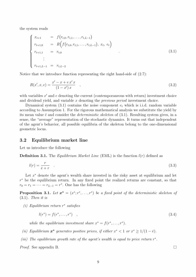
the system reads"########$

########%

xt+1 = f,rt,0, rt,1, . . . , rt,L!1

-

rt+1,0 = R*f,rt,0, rt,1, . . . , rt,L!1

-, xt, et

+

rt+1,1 = rt,0

...

rt+1,L!1 = rt,L!2

. (3.1)

Notice that we introduce function representing the right hand-side of (2.7):

R(x#, x, e) =x# " x + e x# x

(1" x#) x, (3.2)

with variables x# and e denoting the current (contemporaneous with return) investment choiceand dividend yield, and variable x denoting the previous period investment choice.

Dynamical system (3.1) contains the noise component et which is i.i.d. random variableaccording to Assumption 1. For the rigorous mathematical analysis we substitute the yield byits mean value e and consider the deterministic skeleton of (3.1). Resulting system gives, in asense, the “average” representation of the stochastic dynamics. It turns out that independentof the agent’s behavior, all possible equilibria of the skeleton belong to the one-dimensionalgeometric locus.

3.2 Equilibrium market line

Let us introduce the following

Definition 3.1. The Equilibrium Market Line (EML) is the function l(r) defined as

l(r) =r

e + r. (3.3)

Let x" denote the agent’s wealth share invested in the risky asset at equilibrium and letr" be the equilibrium return. In any fixed point the realized returns are constant, so thatr0 = r1 = · · · = rL!1 = r". One has the following

Proposition 3.1. Let x! = (x"; r", . . . , r") be a fixed point of the deterministic skeleton of(3.1). Then it is

(i) Equilibrium return r" satisfies

l(r") = f(r", . . . , r") , (3.4)

while the equilibrium investment share x" = f(r", . . . , r").

(ii) Equilibrium x! generates positive prices, if either x" < 1 or x" & 1/(1" e).

(iii) The equilibrium growth rate of the agent’s wealth is equal to price return r".

Proof. See appendix B.

9

Inv

estm

ent

Sh

are

Rescaled Price Return

Equilibrium Market Line

0

1

-1 -e- 0

S1

U1

S2

U2

E

I

II-e- 0

r*-e-0

r*

-1

-0.5

0

0.5

1

1.5

r0

r1

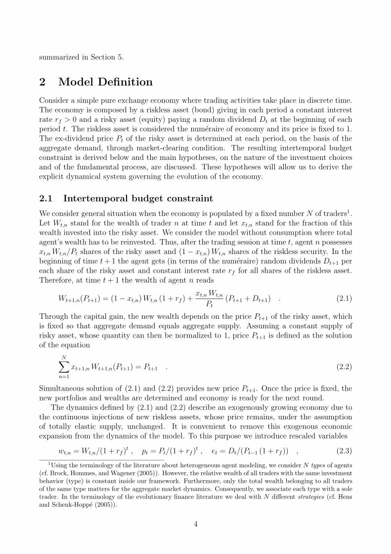
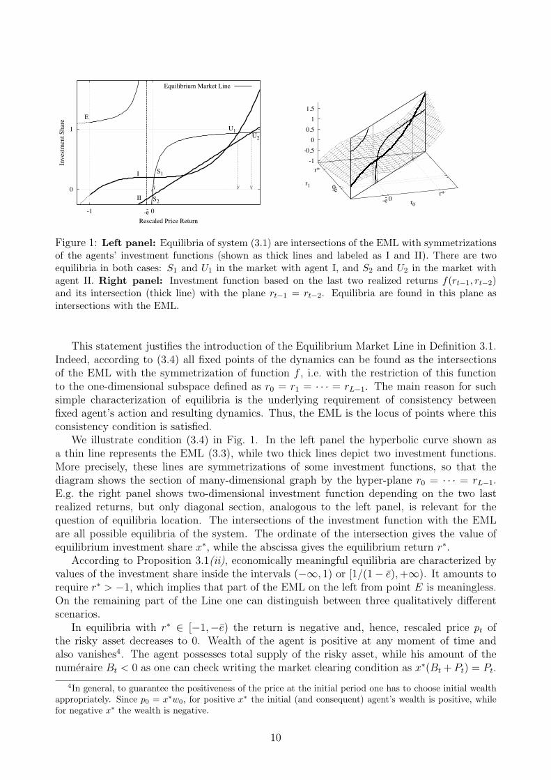
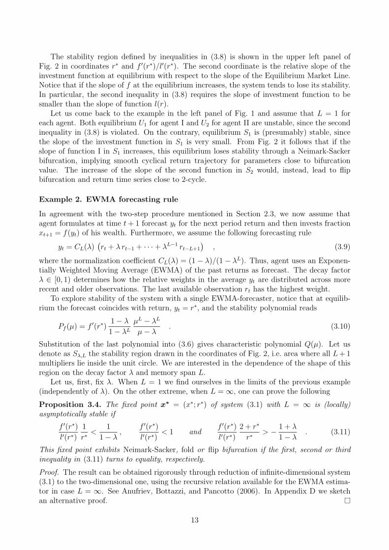
Figure 1: Left panel: Equilibria of system (3.1) are intersections of the EML with symmetrizationsof the agents’ investment functions (shown as thick lines and labeled as I and II). There are twoequilibria in both cases: S1 and U1 in the market with agent I, and S2 and U2 in the market withagent II. Right panel: Investment function based on the last two realized returns f(rt!1, rt!2)and its intersection (thick line) with the plane rt!1 = rt!2. Equilibria are found in this plane asintersections with the EML.

This statement justifies the introduction of the Equilibrium Market Line in Definition 3.1.Indeed, according to (3.4) all fixed points of the dynamics can be found as the intersectionsof the EML with the symmetrization of function f , i.e. with the restriction of this functionto the one-dimensional subspace defined as r0 = r1 = · · · = rL!1. The main reason for suchsimple characterization of equilibria is the underlying requirement of consistency betweenfixed agent’s action and resulting dynamics. Thus, the EML is the locus of points where thisconsistency condition is satisfied.

We illustrate condition (3.4) in Fig. 1. In the left panel the hyperbolic curve shown asa thin line represents the EML (3.3), while two thick lines depict two investment functions.More precisely, these lines are symmetrizations of some investment functions, so that thediagram shows the section of many-dimensional graph by the hyper-plane r0 = · · · = rL!1.E.g. the right panel shows two-dimensional investment function depending on the two lastrealized returns, but only diagonal section, analogous to the left panel, is relevant for thequestion of equilibria location. The intersections of the investment function with the EMLare all possible equilibria of the system. The ordinate of the intersection gives the value ofequilibrium investment share x", while the abscissa gives the equilibrium return r".

According to Proposition 3.1(ii), economically meaningful equilibria are characterized byvalues of the investment share inside the intervals ("', 1) or [1/(1" e), +'). It amounts torequire r" > "1, which implies that part of the EML on the left from point E is meaningless.On the remaining part of the Line one can distinguish between three qualitatively di!erentscenarios.

In equilibria with r" $ ["1,"e) the return is negative and, hence, rescaled price pt ofthe risky asset decreases to 0. Wealth of the agent is positive at any moment of time andalso vanishes4. The agent possesses total supply of the risky asset, while his amount of thenumeraire Bt < 0 as one can check writing the market clearing condition as x"(Bt + Pt) = Pt.

4In general, to guarantee the positiveness of the price at the initial period one has to choose initial wealthappropriately. Since p0 = x!w0, for positive x! the initial (and consequent) agent’s wealth is positive, whilefor negative x! the wealth is negative.

10

Thus, the agent has to borrow money in order to keep his relatively high demand for the riskyasset. Due to the decrease in the agent’s wealth, this demand is unsu"cient to provide high(even positive) return.

If r" $ ("e, 0) the capital gain on the risky asset is negative and price of the asset falls.However, the contribution from the dividend makes the gross return r" + e positive. Further-more, agent has to be in debt and have negative wealth in order to guarantee the positivenessof price. From Proposition 3.1(iii) it follows that his wealth increases to 0. The agent pos-sesses total supply of the risky asset and negative amount of the numeraire Bt. In this caseagent has to borrow money in order to keep positive demand of the asset. Ultimately, thedividend payment allows the agent’s wealth to increase. Equilibrium S2 for the agent II in theleft panel of Fig. 1 is of such kind.

Finally, if the rescaled return is positive, the price pt of the asset increases. Agent has apositive amount of the numeraire and his total wealth is positive and increases. Such situationwill be observed in equilibria S1, U1 and U2.

What can be said about the dynamics of price Pt in all these three scenarios? To answerthis question it is important to bear in mind the following relation between the scaled returnrt and return Rt in terms of unscaled price:

1 + Rt = (1 + rt) (1 + rf ) .

Thus, in the third scenario where the rescaled price increases, the unscaled price also increaseswith the higher rate. However, in the first and second scenarios where the rescaled price isfalling down, the price before scaling may increase for high enough risk-free interest rate.

To conclude our discussion about equilibrium properties notice that in all possible equilibriathere exists a non-zero equity premium, i.e. di!erence in the total return of the riskless andrisky asset. The equity premium is observed in the real markets (Mehra and Prescott, 1985).It can be explained within the classical paradigm as a monetary incentive existing in theequilibrium to encourage an optimizing risk-averse representative agent to hold a risky asset.In our framework an equity premium in equilibrium can be easily computed as

Pt+1 " Pt + Dt+1

Pt" rf =

e (1 + rf )

1" x".

In our framework the risk premium is endogenously generated due to the interplay of the totalwealth reinvesting and dynamics feedback of the return to the wealth level. Consequently,equity premium increases with the dividend yield, risk-free interest rate and agent’s investmentshare.

3.3 Stability of single-agent equilibria

As the next natural step we move to discuss the stability conditions of the equilibria. Thestability conditions are derived from the analysis of the roots of the characteristic polynomialassociated with the Jacobian of system (3.1) computed at equilibrium. The characteristicpolynomial does, in general, depend on the behavior of the individual investment function fin an infinitesimal neighborhood of the equilibrium x!. This dependence can be summarizedwith the help of the following

Definition 3.2. The stability polynomial P (µ) of the investment function f in x! is

Pf (µ) =%f

%r0µL!1 +

%f

%r1µL!2 + · · · + %f

%rL!2µ +

%f

%rL!1, (3.5)

11

where all the derivatives are computed in point (r", . . . , r").

Using the previous definition the equilibrium stability conditions can be formulated interms of the equilibrium return r", and of the slope of the EML in equilibrium

l#(r") =e

(e + r")2.

The following applies

Proposition 3.2. The fixed point x! = (x"; r", . . . , r") of system (3.1) is (locally) asymptoti-cally stable if all the roots of the polynomial

Q(µ) = µL+1 " Pf (µ)

r" l#(r")

*,1 + r"

-µ" 1

+, (3.6)

are inside the unit circle.The equilibrium x! is unstable if at least one of the roots of Q(µ) lies outside the unit

circle.

Proof. The condition above is a direct consequence of the characteristic polynomial of theJacobian matrix at equilibrium. See appendix C for derivation.

Once investment function f is known, polynomial Pf (µ) and, in turn, polynomial Q(µ) areexplicitly derived. The analysis of L+1 roots of Q(µ), which are usually called multipliers, canbe performed in order to reveal the role of the di!erent parameters in stabilization of a givenequilibrium. Such rigorous analysis is often unfeasible even for simple investment functions, soone should rely on the computational approach, mostly. For illustrative purposes we presentbelow three special cases, where analytical results are available to a certain extent. The readeris referred to Appendix D for justification of the results and further discussion.

Example 1. Agent with short memory, L = 1.

Consider an agent with single memory lag, i.e. with investment share depending only on thepast return, xt+1 = f(rt). This is satisfied, e.g. for any agent with naıve forecast of the nextperiod return. The stability polynomial is simple in this case, Pf = f #(r"), and multipliers areroots of the second-degree polynomial

Q(µ) = µ2 " f #(r")

l#(r") r"

*,1 + r"

-µ" 1

+. (3.7)

Using general results reproduced in Propositions D.1 and D.2, one gets

Proposition 3.3. The fixed point x! = (x"; r") of system (3.1) with L = 1 is (locally)asymptotically stable if

f #(r")

l#(r")

1

r"< 1 ,

f #(r")

l#(r")< 1 and

f #(r")

l#(r")

2 + r"

r"> "1 . (3.8)

Fixed point exhibits Neimark-Sacker, fold or flip bifurcation if the first, second or third in-equality in (3.8) turns to equality, respectively.

12

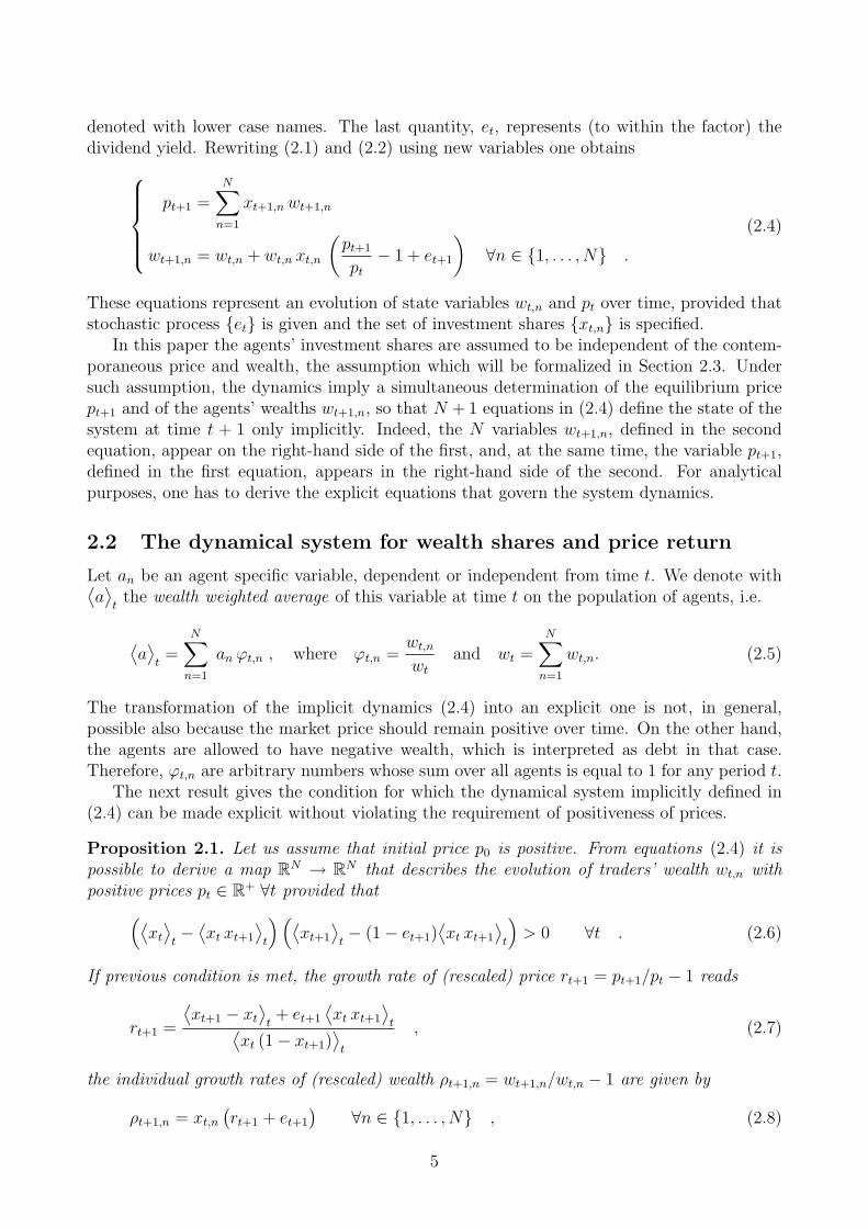
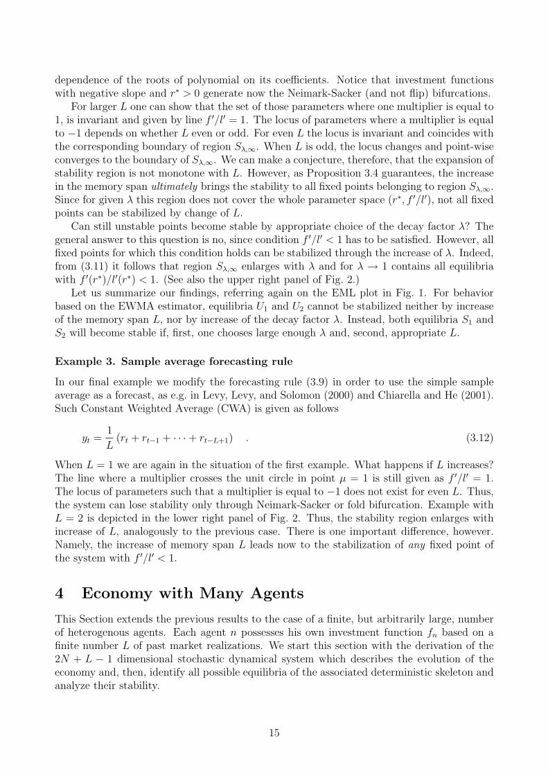
The stability region defined by inequalities in (3.8) is shown in the upper left panel ofFig. 2 in coordinates r" and f #(r")/l#(r"). The second coordinate is the relative slope of theinvestment function at equilibrium with respect to the slope of the Equilibrium Market Line.Notice that if the slope of f at the equilibrium increases, the system tends to lose its stability.In particular, the second inequality in (3.8) requires the slope of investment function to besmaller than the slope of function l(r).

Let us come back to the example in the left panel of Fig. 1 and assume that L = 1 foreach agent. Both equilibrium U1 for agent I and U2 for agent II are unstable, since the secondinequality in (3.8) is violated. On the contrary, equilibrium S1 is (presumably) stable, sincethe slope of the investment function in S1 is very small. From Fig. 2 it follows that if theslope of function I in S1 increases, this equilibrium loses stability through a Neimark-Sackerbifurcation, implying smooth cyclical return trajectory for parameters close to bifurcationvalue. The increase of the slope of the second function in S2 would, instead, lead to flipbifurcation and return time series close to 2-cycle.

Example 2. EWMA forecasting rule

In agreement with the two-step procedure mentioned in Section 2.3, we now assume thatagent formulates at time t + 1 forecast yt for the next period return and then invests fractionxt+1 = f(yt) of his wealth. Furthermore, we assume the following forecasting rule

yt = CL(&),rt + & rt!1 + · · · + &L!1 rt!L+1

-, (3.9)

where the normalization coe"cient CL(&) = (1" &)/(1" &L). Thus, agent uses an Exponen-tially Weighted Moving Average (EWMA) of the past returns as forecast. The decay factor& $ [0, 1) determines how the relative weights in the average yt are distributed across morerecent and older observations. The last available observation rt has the highest weight.

To explore stability of the system with a single EWMA-forecaster, notice that at equilib-rium the forecast coincides with return, yt = r", and the stability polynomial reads

Pf (µ) = f #(r")1" &

1" &L

µL " &L

µ" &. (3.10)

Substitution of the last polynomial into (3.6) gives characteristic polynomial Q(µ). Let usdenote as S",L the stability region drawn in the coordinates of Fig. 2, i.e. area where all L + 1multipliers lie inside the unit circle. We are interested in the dependence of the shape of thisregion on the decay factor & and memory span L.

Let us, first, fix &. When L = 1 we find ourselves in the limits of the previous example(independently of &). On the other extreme, when L = ', one can prove the following

Proposition 3.4. The fixed point x! = (x"; r") of system (3.1) with L = ' is (locally)asymptotically stable if

f #(r")

l#(r")

1

r"<

1

1" &,

f #(r")

l#(r")< 1 and

f #(r")

l#(r")

2 + r"

r"> " 1 + &

1" &. (3.11)

This fixed point exhibits Neimark-Sacker, fold or flip bifurcation if the first, second or thirdinequality in (3.11) turns to equality, respectively.

Proof. The result can be obtained rigorously through reduction of infinite-dimensional system(3.1) to the two-dimensional one, using the recursive relation available for the EWMA estima-tor in case L = '. See Anufriev, Bottazzi, and Pancotto (2006). In Appendix D we sketchan alternative proof.

13

Rel

ativ

e sl

op

e, f

’/l’

Neimark

-Sac

ker

fold

Neimark

-Sac

ker

flip

flip

0

1

-1 -e- 0 1

fold fold

Neimark-Sacker

Neimark-Sacker

flip

flip

0

1

-1 -e- 0 1

Rel

ativ

e sl

op

e, f

’/l’

Equilibrium Rescaled Price Return

0

1

-1 -e- 0 1

fold fold

N-S

, L=!

N-S

, L=!

N-S, L=2

N-S

, L=2

N-S

, L=2

flip

flip

Equilibrium Rescaled Price Return

0

1

-1 -e- 0 1

fold fold

N-S

, CW

A

N-S

, CW

A

N-S, CWA

N-S, CWA

N-S, EWM

A

N-S

, EW

MA

N-S, E

WM

A

flip, EW

MA

Figure 2: Stability regions and types of bifurcations for system (3.1) in special cases. Upper LeftPanel: Example 1, L = 1. Fixed point is stable if (r", f #/l#) belongs to the dark gray area. UpperRight Panel: Example 2, EWMA estimator for di!erent ! and L = '. For ! = 0 the stabilityregion is the same as in example 1, shown as the dark gray area. If ! = 0.2 it expands and becomesthe union of the dark and semi-dark gray areas. When ! = 0.6 the region expands further andcontains the light gray areas in addition. Lower Left Panel: Example 2, EWMA estimator with! = 0.6 for di!erent L. When L = 1 the stability region is the same as in example 1, shown asthe dark gray area. If L = 2 the region expands and contains the light gray areas in addition. Theboundaries for L = ' are shown as dotted lines. Lower Right Panel: Example 3, CWA estimatorfor di!erent L. When L = 1 the stability region is the same as in example 1, shown as the dark grayarea. For L = 2 the region expands and becomes the union of the dark and light gray areas. Thebifurcation loci for the EWMA case with L = 2 and ! = 0.6 are shown as dotted lines for comparison.

The regions S0,$, S0.2,$ and S0.6,$ defined by (3.11) for di!erent values of & are depictedon the upper right panel of Fig. 2.

For the intermediate case, when L > 1 but finite, analytic results are limited. In Ap-pendix D we derive the relations between parameters when one of the multipliers crosses theunit circle for the case L = 2. The corresponding curves are shown, when & = 0.6, in thelower left panel of Fig. 2. They are labeled as “N-S”, “flip” and “fold” depending on wherethis crossing happens exactly (e.g. ”N-S” curve corresponds to those points where two com-plex conjugated multipliers cross the circle). Since all equilibria generated by the horizontalinvestment functions are stable, the points on the horizontal axes should lie in the stabilityregion. The construction of this region can now be finalized using the argument of continuous

14

dependence of the roots of polynomial on its coe"cients. Notice that investment functionswith negative slope and r" > 0 generate now the Neimark-Sacker (and not flip) bifurcations.

For larger L one can show that the set of those parameters where one multiplier is equal to1, is invariant and given by line f #/l# = 1. The locus of parameters where a multiplier is equalto "1 depends on whether L even or odd. For even L the locus is invariant and coincides withthe corresponding boundary of region S",$. When L is odd, the locus changes and point-wiseconverges to the boundary of S",$. We can make a conjecture, therefore, that the expansion ofstability region is not monotone with L. However, as Proposition 3.4 guarantees, the increasein the memory span ultimately brings the stability to all fixed points belonging to region S",$.Since for given & this region does not cover the whole parameter space (r", f #/l#), not all fixedpoints can be stabilized by change of L.

Can still unstable points become stable by appropriate choice of the decay factor &? Thegeneral answer to this question is no, since condition f #/l# < 1 has to be satisfied. However, allfixed points for which this condition holds can be stabilized through the increase of &. Indeed,from (3.11) it follows that region S",$ enlarges with & and for & % 1 contains all equilibriawith f #(r")/l#(r") < 1. (See also the upper right panel of Fig. 2.)

Let us summarize our findings, referring again on the EML plot in Fig. 1. For behaviorbased on the EWMA estimator, equilibria U1 and U2 cannot be stabilized neither by increaseof the memory span L, nor by increase of the decay factor &. Instead, both equilibria S1 andS2 will become stable if, first, one chooses large enough & and, second, appropriate L.

Example 3. Sample average forecasting rule

In our final example we modify the forecasting rule (3.9) in order to use the simple sampleaverage as a forecast, as e.g. in Levy, Levy, and Solomon (2000) and Chiarella and He (2001).Such Constant Weighted Average (CWA) is given as follows

yt =1

L(rt + rt!1 + · · · + rt!L+1) . (3.12)

When L = 1 we are again in the situation of the first example. What happens if L increases?The line where a multiplier crosses the unit circle in point µ = 1 is still given as f #/l# = 1.The locus of parameters such that a multiplier is equal to "1 does not exist for even L. Thus,the system can lose stability only through Neimark-Sacker or fold bifurcation. Example withL = 2 is depicted in the lower right panel of Fig. 2. Thus, the stability region enlarges withincrease of L, analogously to the previous case. There is one important di!erence, however.Namely, the increase of memory span L leads now to the stabilization of any fixed point ofthe system with f #/l# < 1.

4 Economy with Many Agents

This Section extends the previous results to the case of a finite, but arbitrarily large, numberof heterogenous agents. Each agent n possesses his own investment function fn based on afinite number L of past market realizations. We start this section with the derivation of the2N + L " 1 dimensional stochastic dynamical system which describes the evolution of theeconomy and, then, identify all possible equilibria of the associated deterministic skeleton andanalyze their stability.

15

4.1 Dynamical system

The evolution of agents’ wealths is not any longer decoupled from the system and, conse-quently, all equations in (2.9) are relevant for the dynamics. The first-order dynamical systemwill be defined in terms of the following 2N + L" 1 independent variables

xt,n #n $ {1, . . . , N} ; !t,n #n $ {1, . . . , N " 1} ; rt,l #l $ {0, . . . , L" 1} , (4.1)

where rt,l denotes the price return at time t"l. Notice that only N"1 wealth shares are needed.Indeed, since wealth shares are summed up to 1 at any time step t, !t,N = 1 "

.N!1n=1 !t,n.

The dynamics of the system is provided by the following

Lemma 4.1. The 2N+L"1 dynamical system defined by (2.7) and (2.9) under Assumptions 1and 2 reads

X :

/

01xt+1,1 = f1

,rt,0, . . . , rt,L!1

-

......

...xt+1,N = fN

,rt,0, . . . , rt,L!1

-

W :

/

00000000000001

!t+1,1 = '1

*xt,1, . . . , xt,N ; !t,1, . . . , !t,N!1; et+1;

R,f1(rt,0, . . . , rt,L!1), . . . , fN(rt,0, . . . , rt,L!1);

xt,1, . . . , xt,1; !t,1, . . . , !t,N!1; et+1

-+

......

...

!t+1,N!1 = 't,N!1

*xt,1, . . . , xt,N ; !t,1, . . . , !t,N!1; et+1;

R,f1(rt,0, . . . , rt,L!1), . . . , fN(rt,0, . . . , rt,L!1);

xt,1, . . . , xt,N ; !t,1, . . . , !t,N!1; et+1

-+

(4.2)

R :

/

00000001

rt+1,0 = R*f1(rt,0, . . . , rt,L!1), . . . , fN(rt,0, . . . , rt,L!1);

xt,1, . . . , xt,N ; !t,1, . . . , !t,N!1; et+1

+

rt+1,1 = rt,0...

......

rt+1,L!1 = rt,L!2

,

where

R*y1, y2, . . . , yN ; x1, x2, . . . , xN ; !1,!2, . . . , !N!1; e

+=

=

.N!1n=1 !n

,yn (1 + e xn)" xn

-+

*1"

.N!1n=1 !n

+ ,yN (1 + e xN)" xN

-

.N!1n=1 !n xn (1" yn) + (1"

.N!1n=1 !n) xN (1" yN)

(4.3)

and

'n

,x1, x2, . . . , xN ; !1,!2, . . . , !N!1; e; R

-=

= !n1 + xn (R + e)

1 + (R + e)*.N!1

m=1 !m xm +,1"

.N!1m=1 !m

-xN

+ #n $ {1, . . . , N " 1} .(4.4)

16

Proof. We ordered the equations to obtain three separated blocks: X, W and R. In blockX there are N equations defining the investment choices of agents. Block W contains N " 1equations describing the evolution of the wealth shares. Finally, block R is composed byL equations which describe the evolution of the return. In the last block equations are inascending order with respect to the time lag.

The set X is immediately obtained from the definition of the investment functions. Thefirst equation of block R is (2.7) rewritten in terms of variables (4.1) using (4.3) and (2.5),while the remaining equations are just the result of a “lag” operation. Notice that (4.3) reducesto (3.2) in the case of a single agent. Finally, the evolution of wealth shares described in blockW is obtained from (2.9) once the notation introduced in (2.5) is explicitly expanded. Noticethat, due to the presence of function R in the last expression, all functions 'n depend on thesame set of variables as R.

The rest of this Section is devoted to the analysis of the deterministic skeleton of (4.2):we replace the yield realizations {et} by their mean value e and analyze the equilibria of theresulting deterministic system.

4.2 Determination of equilibria

The characterization of fixed points of system (4.2) is in many respects similar to the singleagent case discussed above. Let x! = (x"1, . . . , x

"N ; !"

1, . . . ,!"N!1; r

", . . . , r") denotes a fixedpoint where r" is the equilibrium return, and x"n and !"

n stay for the equilibrium value ofthe investment function and the equilibrium wealth share of agent n, respectively. Let usintroduce the following

Definition 4.1. Agent n is said to survive in x! if his equilibrium wealth share is di!erentfrom zero, !"

n (= 0. Agent n is said to dominate the economy if he is the only survivor,i.e. !"

n = 1.

One can recognize the parallel between our definition above and the frameworks in DeLong,Shleifer, Summers, and Waldmann (1991) and Blume and Easley (1992). We adopt here thedeterministic version of the concepts of survival and dominance used in that papers. Thefollowing statement characterizes all possible equilibria of system (4.2).

Proposition 4.1. Let x! be a fixed point of the deterministic skeleton of system (4.2). Thenequilibrium investment shares are defined according to

x"n = fn(r", . . . , r") #n $ {1, . . . , N} , (4.5)

and three mutually exclusive cases are possible:

(i) Single agent survival. In x! only one agent survives and, therefore, dominates theeconomy. Without loss of generality we can assume this agent to be agent 1 so that!"

1 = 1 and all other equilibrium wealth shares are equal to zero.

The equilibrium return r" is determined as the solution of

l(r") = f1(r", . . . , r") , (4.6)

and equal to the wealth growth rate of the survivor.

17

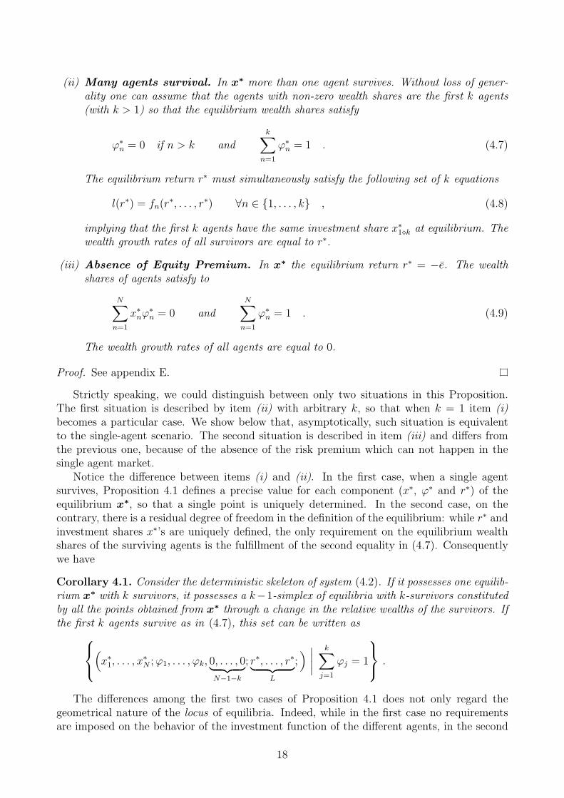
(ii) Many agents survival. In x! more than one agent survives. Without loss of gener-ality one can assume that the agents with non-zero wealth shares are the first k agents(with k > 1) so that the equilibrium wealth shares satisfy

!"n = 0 if n > k and

k!

n=1

!"n = 1 . (4.7)

The equilibrium return r" must simultaneously satisfy the following set of k equations

l(r") = fn(r", . . . , r") #n $ {1, . . . , k} , (4.8)

implying that the first k agents have the same investment share x"1%k at equilibrium. Thewealth growth rates of all survivors are equal to r".

(iii) Absence of Equity Premium. In x! the equilibrium return r" = "e. The wealthshares of agents satisfy to

N!

n=1

x"n!"n = 0 and

N!

n=1

!"n = 1 . (4.9)

The wealth growth rates of all agents are equal to 0.

Proof. See appendix E.

Strictly speaking, we could distinguish between only two situations in this Proposition.The first situation is described by item (ii) with arbitrary k, so that when k = 1 item (i)becomes a particular case. We show below that, asymptotically, such situation is equivalentto the single-agent scenario. The second situation is described in item (iii) and di!ers fromthe previous one, because of the absence of the risk premium which can not happen in thesingle agent market.

Notice the di!erence between items (i) and (ii). In the first case, when a single agentsurvives, Proposition 4.1 defines a precise value for each component (x", !" and r") of theequilibrium x!, so that a single point is uniquely determined. In the second case, on thecontrary, there is a residual degree of freedom in the definition of the equilibrium: while r" andinvestment shares x"’s are uniquely defined, the only requirement on the equilibrium wealthshares of the surviving agents is the fulfillment of the second equality in (4.7). Consequentlywe have

Corollary 4.1. Consider the deterministic skeleton of system (4.2). If it possesses one equilib-rium x! with k survivors, it possesses a k"1-simplex of equilibria with k-survivors constitutedby all the points obtained from x! through a change in the relative wealths of the survivors. Ifthe first k agents survive as in (4.7), this set can be written as

"$

%

*x"1, . . . , x

"N ; !1, . . . , !k, 0, . . . , 02 34 5

N!1!k

; r", . . . , r"2 34 5L

;+ 6666

k!

j=1

!j = 1

78

9 .

The di!erences among the first two cases of Proposition 4.1 does not only regard thegeometrical nature of the locus of equilibria. Indeed, while in the first case no requirementsare imposed on the behavior of the investment function of the di!erent agents, in the second

18

0

1

-e- 0

Inv

estm

ent

Sh

are

Rescaled Price Return

S1

U1

S2

U2

I II III

Equilibrium Market Line

0

1

-e- 0

Inv

estm

ent

Sh

are

Rescaled Price Return

S1

S2

S3

I

II

III

A1

A2

A3

Equilibrium Market Line

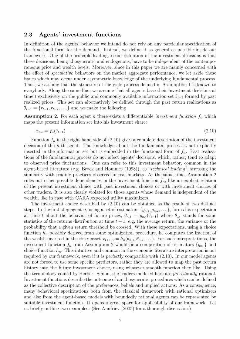
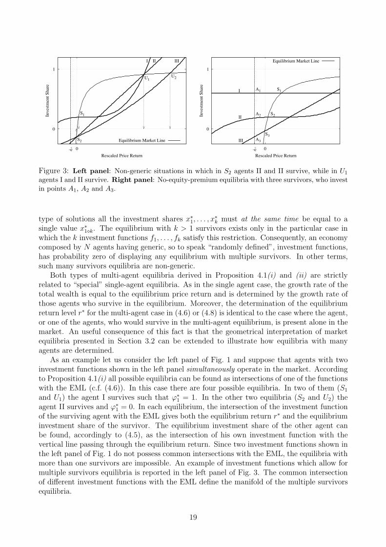
Figure 3: Left panel: Non-generic situations in which in S2 agents II and II survive, while in U1

agents I and II survive. Right panel: No-equity-premium equilibria with three survivors, who investin points A1, A2 and A3.

type of solutions all the investment shares x"1, . . . , x"k must at the same time be equal to a

single value x"1%k. The equilibrium with k > 1 survivors exists only in the particular case inwhich the k investment functions f1, . . . , fk satisfy this restriction. Consequently, an economycomposed by N agents having generic, so to speak “randomly defined”, investment functions,has probability zero of displaying any equilibrium with multiple survivors. In other terms,such many survivors equilibria are non-generic.

Both types of multi-agent equilibria derived in Proposition 4.1(i) and (ii) are strictlyrelated to “special” single-agent equilibria. As in the single agent case, the growth rate of thetotal wealth is equal to the equilibrium price return and is determined by the growth rate ofthose agents who survive in the equilibrium. Moreover, the determination of the equilibriumreturn level r" for the multi-agent case in (4.6) or (4.8) is identical to the case where the agent,or one of the agents, who would survive in the multi-agent equilibrium, is present alone in themarket. An useful consequence of this fact is that the geometrical interpretation of marketequilibria presented in Section 3.2 can be extended to illustrate how equilibria with manyagents are determined.

As an example let us consider the left panel of Fig. 1 and suppose that agents with twoinvestment functions shown in the left panel simultaneously operate in the market. Accordingto Proposition 4.1(i) all possible equilibria can be found as intersections of one of the functionswith the EML (c.f. (4.6)). In this case there are four possible equilibria. In two of them (S1

and U1) the agent I survives such that !"1 = 1. In the other two equilibria (S2 and U2) the

agent II survives and !"1 = 0. In each equilibrium, the intersection of the investment function

of the surviving agent with the EML gives both the equilibrium return r" and the equilibriuminvestment share of the survivor. The equilibrium investment share of the other agent canbe found, accordingly to (4.5), as the intersection of his own investment function with thevertical line passing through the equilibrium return. Since two investment functions shown inthe left panel of Fig. 1 do not possess common intersections with the EML, the equilibria withmore than one survivors are impossible. An example of investment functions which allow formultiple survivors equilibria is reported in the left panel of Fig. 3. The common intersectionof di!erent investment functions with the EML define the manifold of the multiple survivorsequilibria.

19

Let us now turn to the “no-equity-premium” equilibria identified in Proposition 4.1(iii).In these equilibria many agents survive, and their investment and wealth shares are balancedin such a way that the capital gain and the dividend yield o!set each other so that the risklessand the risky assets have the same expected return. As opposite to the situation described inProposition 4.1(ii), these are generic equilibria with many survivors. Furthermore, if N > 2then definition of any no-arbitrage equilibrium has additional degrees of freedom correspondingto a change in the relative wealths of the survivors. Namely, there exist the following N " 2-dimensional manifold of equilibria

"$

%

*x"1, . . . , x

"N ; !1, . . . , !N!1!k;"e, . . . ,"e2 34 5

L

+ 6666N!

j=1

!j = 1 ,N!

j=1

!jx"j = 0

78

9 .

Geometrically, the “no-equity-premium” equilibria can be represented by the vertical asymp-tote of the EML. Points A1, A2 and A3 in the right panel of Fig. 3 represents correspondinginvestment shares of the agents, while the wealth shares are defined from (4.9).

4.3 Stability of multi-agents equilibria

This Section presents the stability analysis of the equilibria defined in Proposition 4.1. Thethree Propositions below provide the stability region in the parameter space for the casesenumerated in Proposition 4.1, i.e. for generic case of a single survivor, for non-generic caseof many survivors and for generic case with many survivors and without the equity premium.The derivation of these Propositions requires quite cumbersome algebraic manipulations andwe refer the reader to Appendix F for the intermediate lemmas and final proofs.

For the generic case of a single survivor equilibrium we have the following

Proposition 4.2. Let x! be a fixed point of (4.2) associated with a single survivor equilibrium.Without loss of generality we can assume that the survivor is the first agent. Let Pf1(µ) denotethe (L " 1)-dimensional stability polynomial associated with the investment function of thesurvivor.

Equilibrium x! is (locally) asymptotically stable if the two following conditions are met:1) all the roots of polynomial

Q1(µ) = µL+1 " (1 + r") µ" 1

r" l#(r")Pf1(µ) , (4.10)

are inside the unit circle.2) the equilibrium investment shares of the non-surviving agents satisfy to

"2" r" < x"n,r" + e

-< r" , 1 < n ) N . (4.11)

The equilibrium x! is unstable if at least one of the roots of polynomial in (4.10) is outsidethe unit circle or if at least one of the inequalities in (4.11) holds with the opposite (strict)sign.

In particular, the system exhibits a fold bifurcation if one of the N"1 right-hand inequalitiesin (4.11) becomes an equality and a flip bifurcation if one of the N " 1 left-hand inequalitiesbecomes an equality.

20

Inv

estm

ent

Sh

are

Rescaled Price Return

Equilibrium Market Line

0

1

-1 -e- 0

S1

U1

S2

U2

E

I II

Inv

estm

ent

Sh

are

Rescaled Price Return

Equilibrium Market Line

0

-e- 0

SL

U

SH

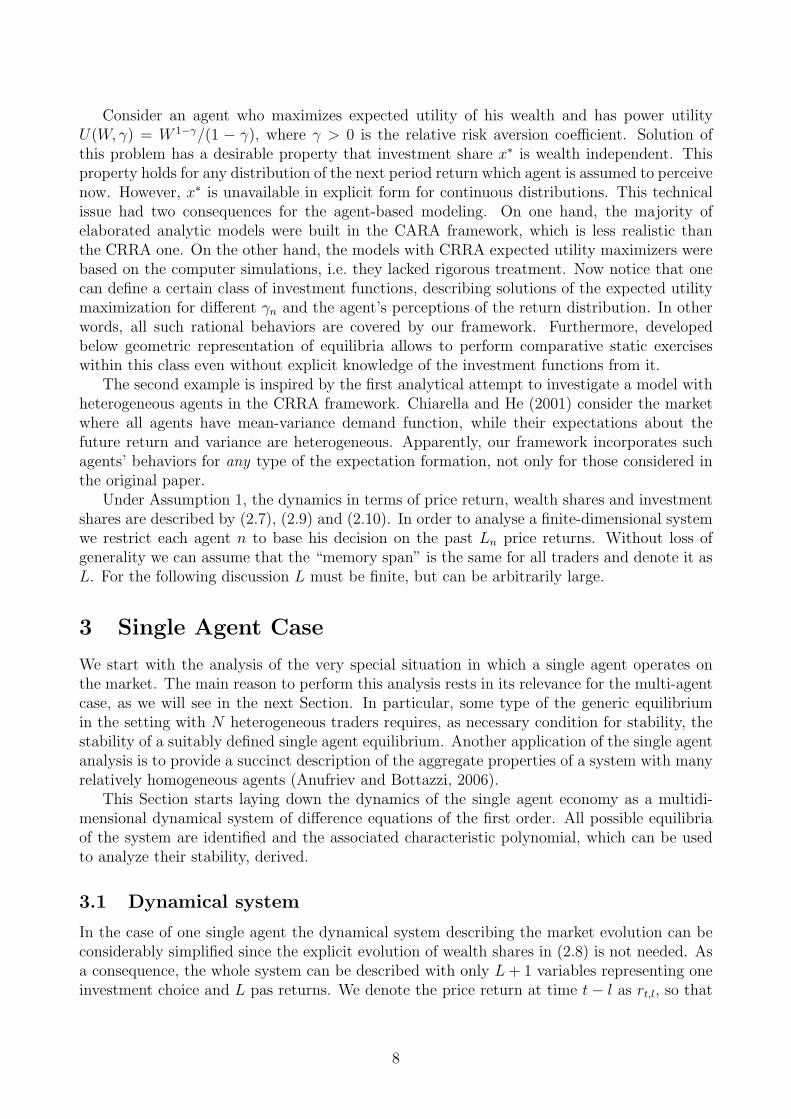
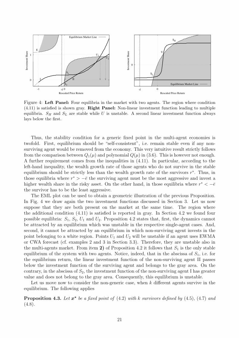
Figure 4: Left Panel: Four equilibria in the market with two agents. The region where condition(4.11) is satisfied is shown gray. Right Panel: Non-linear investment function leading to multipleequilibria. SH and SL are stable while U is unstable. A second linear investment function alwayslays below the first.

Thus, the stability condition for a generic fixed point in the multi-agent economies istwofold. First, equilibrium should be “self-consistent”, i.e. remain stable even if any non-surviving agent would be removed from the economy. This very intuitive result strictly followsfrom the comparison between Q1(µ) and polynomial Q(µ) in (3.6). This is however not enough.A further requirement comes from the inequalities in (4.11). In particular, according to theleft-hand inequality, the wealth growth rate of those agents who do not survive in the stableequilibrium should be strictly less than the wealth growth rate of the survivors r". Thus, inthose equilibria where r" > "e the surviving agent must be the most aggressive and invest ahigher wealth share in the risky asset. On the other hand, in those equilibria where r" < "ethe survivor has to be the least aggressive.

The EML plot can be used to obtain a geometric illustration of the previous Proposition.In Fig. 4 we draw again the two investment functions discussed in Section 3. Let us nowsuppose that they are both present on the market at the same time. The region wherethe additional condition (4.11) is satisfied is reported in gray. In Section 4.2 we found fourpossible equilibria: S1, S2, U1 and U2. Proposition 4.2 states that, first, the dynamics cannotbe attracted by an equilibrium which was unstable in the respective single-agent cases. And,second, it cannot be attracted by an equilibrium in which non-surviving agent invests in thepoint belonging to a white region. Points U1 and U2 will be unstable if an agent uses EWMAor CWA forecast (cf. examples 2 and 3 in Section 3.3). Therefore, they are unstable also inthe multi-agents market. From item 2) of Proposition 4.2 it follows that S1 is the only stableequilibrium of the system with two agents. Notice, indeed, that in the abscissa of S1, i.e. forthe equilibrium return, the linear investment function of the non-surviving agent II passesbelow the investment function of the surviving agent and belongs to the gray area. On thecontrary, in the abscissa of S2, the investment function of the non-surviving agent I has greatervalue and does not belong to the gray area. Consequently, this equilibrium is unstable.

Let us move now to consider the non-generic case, when k di!erent agents survive in theequilibrium. The following applies

Proposition 4.3. Let x! be a fixed point of (4.2) with k survivors defined by (4.5), (4.7) and(4.8).

21

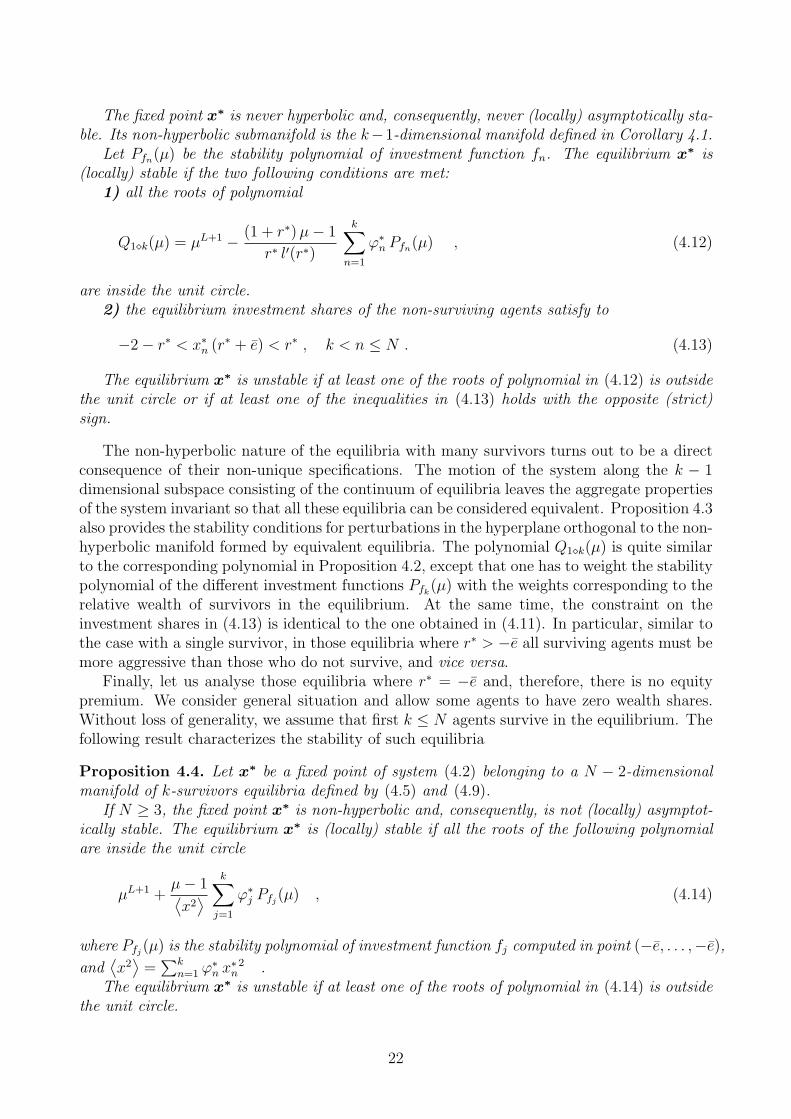
The fixed point x! is never hyperbolic and, consequently, never (locally) asymptotically sta-ble. Its non-hyperbolic submanifold is the k"1-dimensional manifold defined in Corollary 4.1.

Let Pfn(µ) be the stability polynomial of investment function fn. The equilibrium x! is(locally) stable if the two following conditions are met:

1) all the roots of polynomial

Q1%k(µ) = µL+1 " (1 + r") µ" 1

r" l#(r")

k!

n=1

!"n Pfn(µ) , (4.12)

are inside the unit circle.2) the equilibrium investment shares of the non-surviving agents satisfy to

"2" r" < x"n (r" + e) < r" , k < n ) N . (4.13)

The equilibrium x! is unstable if at least one of the roots of polynomial in (4.12) is outsidethe unit circle or if at least one of the inequalities in (4.13) holds with the opposite (strict)sign.

The non-hyperbolic nature of the equilibria with many survivors turns out to be a directconsequence of their non-unique specifications. The motion of the system along the k " 1dimensional subspace consisting of the continuum of equilibria leaves the aggregate propertiesof the system invariant so that all these equilibria can be considered equivalent. Proposition 4.3also provides the stability conditions for perturbations in the hyperplane orthogonal to the non-hyperbolic manifold formed by equivalent equilibria. The polynomial Q1%k(µ) is quite similarto the corresponding polynomial in Proposition 4.2, except that one has to weight the stabilitypolynomial of the di!erent investment functions Pfk

(µ) with the weights corresponding to therelative wealth of survivors in the equilibrium. At the same time, the constraint on theinvestment shares in (4.13) is identical to the one obtained in (4.11). In particular, similar tothe case with a single survivor, in those equilibria where r" > "e all surviving agents must bemore aggressive than those who do not survive, and vice versa.

Finally, let us analyse those equilibria where r" = "e and, therefore, there is no equitypremium. We consider general situation and allow some agents to have zero wealth shares.Without loss of generality, we assume that first k ) N agents survive in the equilibrium. Thefollowing result characterizes the stability of such equilibria

Proposition 4.4. Let x! be a fixed point of system (4.2) belonging to a N " 2-dimensionalmanifold of k-survivors equilibria defined by (4.5) and (4.9).

If N & 3, the fixed point x! is non-hyperbolic and, consequently, is not (locally) asymptot-ically stable. The equilibrium x! is (locally) stable if all the roots of the following polynomialare inside the unit circle

µL+1 +µ" 1(

x2)

k!

j=1

!"j Pfj(µ) , (4.14)

where Pfj(µ) is the stability polynomial of investment function fj computed in point ("e, . . . ,"e),

and(x2

)=

.kn=1 !"

n x"n2 .

The equilibrium x! is unstable if at least one of the roots of polynomial in (4.14) is outsidethe unit circle.

22

As in the case of Proposition 4.3, the “no-equity-premium” equilibria can be non-hyperbolic,due to possibility to change wealth between agents without changing the aggregate propertiesof the dynamics. For the complete stability analysis, the roots of polynomial (4.14) shouldbe analyzed for specific investment functions, analogously to our analysis in Section 3.3. Inparticular, when all investment functions are horizontal in point "e, the equilibrium (if itexists) is always stable.

4.4 Optimal selection and multiple equilibria

In this Section, using the geometric interpretation based on the EML we discuss some relevantimplications of Proposition 4.2 about the asymptotic behavior of the model and its globalproperties. We confine the discussion to the generic case of equilibria with a single survivor.

The first implication concerns the aggregate dynamics of the economy. Let us considera stable many-agent equilibrium x!. Let us suppose that r" is the equilibrium return in x!

and that the first agent survives. Then his wealth return is equal to r" and this is also theasymptotic growth rate of the total wealth. Then, we can interpret the second requirement ofProposition 4.2 as saying that, in the dynamic competition, those agent survives who allowsthe economy to have the highest possible rate of growth. Indeed, if any other agent n (= 1survived, the economy would have grown with rate x"n (r" + e), which is less than r" accordingto (4.11). This result can be called an optimal selection principle since it clearly states themarket endogenous selection toward the best aggregate outcome.

To be a bit more specific, notice that in equilibria with r" > "e the overall wealth of theeconomy grows (in particular for r" < 0 the negative wealth grows to 0), while in equilibriawith r" < "e the wealth of the economy falls. Thus, according to the optimal selectionprinciple the surviving agent must be the most aggressive in equilibria where the economygrows and must be the least aggressive investor in equilibria where the economy shrinks.

Notice, however, that this selection does not apply to the whole set of equilibria, but onlyto the subset formed by equilibria associated with stable fixed points in the single agent case(c.f. (4.12)). For instance, with the investment functions shown in the left panel of Fig. 4,the dynamics will never end up in U2, even if this is the equilibrium with the highest possiblereturn. Furthermore, the variety of possible investment functions implies that the optimalselection principle has a local character. Indeed, even if we exclude all unstable single-agentequilibria, the market will not choose the equilibrium with the highest growth rate. Sometimesit can be the case like in the left panel of Fig. 4. However, it is often not the case and asimple counter-example is provided by a single investment function possessing multiple stableequilibria as shown in the right panel of Fig. 4. For this investment function both SL andSH are stable equilibria. Now suppose that an agent possessing this function competes onthe market with other agents which are more risk averse than him and always invest smallershares of wealth in the risky asset. An example of more risk averse behavior is provided bythe linear investment function in the same plot. In this situation, these two equilibria of thenonlinear function remain stable and the riskier agent will ultimately dominate the market.The resulting market equilibrium will only depend on the initial conditions.

Possible presence of the equilibria without equity premium, identified for the multi-agentmarket in Proposition 4.1(iii), is another source of multiple equilibria. For example, in thesituation depicted in the right panel of Fig. 3 there is a stable equilibrium where agent I survivesalone (point S1) and many no-equity-premium stable equilibria where all three agents surviveand agent I possesses high enough wealth share !"

1 (cf. polynomial (4.14) in Proposition 4.4).

23

5 Conclusion

This paper introduces novel results concerning the characterization and stability of equilibriain speculative pure exchange economies with heterogeneous CRRA traders. The frameworkis relatively general in terms of agents’ behaviors and di!ers from most of the models withheterogeneous agents in two important respects.

First, we analyze the aggregate dynamics and asymptotic behavior of the market whenan arbitrary large number of traders participate to the trading activity. Second, we do notrestrict in any way the procedure used by agents in order to build their forecast about futureprices, nor the way in which agents can use this forecast to obtain their present asset demand.In our terms, agent with any smooth investment function mapping the information set to thepresent investment choice can present in the model.

Even if consideration of an arbitrary number of generic agents’ behaviors leads us tostudy dynamical systems of an arbitrarily large dimension, we are able to provide a completecharacterization of market equilibria and a description of their stability conditions in terms offew parameters characterizing the traders investment strategies. In particular, we find that,irrespectively of the number of agents operating in the market and of the structure of theirdemand functions, only three types of equilibria are possible:

• generic equilibria, associated with isolated fixed points, where a single agent asymptot-ically possesses the entire wealth of the economy,

• non-generic equilibria, associated with continuous manifolds of fixed points, where manyagents possess a finite shares of the total wealth,

• generic equilibria associated with many survivors, where the economy does not possessthe equity premium.

Furthermore, we show in total generality that a simple function, the “Equilibrium MarketLine”, can be used to obtain a geometric characterization of the location of all these types ofequilibria. Furthermore, some results about stability conditions can also be inferred from thesame EML.

Our general results provide, we believe, a simple and clear description of the principlesgoverning the asymptotic market dynamics resulting from the competition of di!erent trad-ing strategies. The optimizing agents may dominate non-optimizing agents but may also bedominated by them. In general, the ultimate result of competition between agents dependson the whole market ecology. The EML is a handy and useful tool for demonstration suchphenomena as absence of equilibrium, presence of multiple equilibria, and also for comparativestatics exercises. From this plot (and results of stability analysis of Section 4.3) the followingtwo “impossibility theorems” follow in an obvious way. First, there exist no “best” strategy,independently of what “best” means exactly, since any possible market equilibrium can bedestabilized by some investment function. Second, it is impossible to build a dominance orderrelation inside the space of trading strategies, since two strategies may generate multiple sta-ble equilibria with di!erent survivors in them, so that the outcome will depend on the initialconditions or noise.

The present analysis can be extended in many directions. First of all, one may raise thequestion of the robustness of the results with respect to Assumption 1 about constant dividendyield. Our preliminary results of the analytic investigation in this direction show that someresults (like presence of equity premium in equilibria and possibility to represent the equilibria

24

by the EML) are actually robust and do not depend on the exact dividend specification.Second, in the limits of our framework, one can wonder about other possible dynamics. Forinstance, we have shown that there is a theoretical possibility do not have any equilibrium atall. The dynamics in this case remain unknown. Also the dynamics after bifurcations, whichis the key question in many heterogeneous agent models, were not investigated. Probablynumerical methods can be e!ectively applied to study these questions and also clarify the roleof initial conditions and the determinants of the relative size of the basins of attraction formultiple equilibria scenarios. Third, our general CRRA-framework led us in Proposition 2.1 tothe system in terms of returns and wealth shares. There are numerous behavioral specificationswhich were not analyzed here and still consistent with such framework. These specificationsrange from the evaluation of the “fundamental” value of the asset, possibly obtained froma private source of information, to a strategic behavior that try to keep in consideration thereaction of other market participants to the revealed individual choices. Furthermore, one mayask what are the consequences of the optimal selection principle for a market in which the setof strategies is not “frozen”, but instead is evolving in time, plausibly following some adaptiveprocess. For instance, one can assume that agents imitate the behavior of other traders (seee.g. Kirman (1991)) or that they update strategies according to recent relative performances(see e.g. Brock and Hommes (1998)). The analysis of the consequences of the introduction ofsuch strategies on the optimal selection principle may, ultimately, refute the statement aboutthe impossibility of defining a dominance relation among strategies.

APPENDIX

A Proof of Proposition 2.1Plugging the expression for wt+1,n from the second equation in system (2.4) into the right-hand side of the firstequation of the same system, and assuming that pt > 0 and, consistently with (2.6), pt (=

.xt+1,n xt,n wt,n

one gets

pt+1 =

:1" 1

pt

N!

n=1

xt+1,n xt,n wt,n

;"1 :N!

n=1

xt+1,n wt,n +,et+1 " 1

- N!

n=1

xt+1,n wt,n xt,n

;=

= pt

.n xt+1,n wt,n + (et+1 " 1)

.n xt+1,n wt,n xt,n.

n xt,n wt,n ".

n xt+1,n xt,n wt,n=

= pt

(xt+1

)t"

(xt xt+1

)t+ et+1

(xt xt+1

)t(

xt

)t"

(xt xt+1

)t

,

where we used the first equation of (2.4) rewritten for time t to get the second equality. Condition (2.6) isobtained imposing pt+1 > 0, and the dynamics of price return in (2.7) are immediately derived. From thesecond equation of (2.4) it follows that

wt+1,n = wt,n

,1 + xt,n (rt+1 + et+1)

-#n $ {1, . . . , N} , (A.1)

25

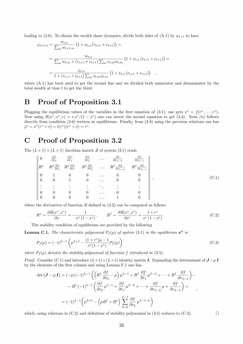
leading to (2.8). To obtain the wealth share dynamics, divide both sides of (A.1) by wt+1 to have

"t+1,n =wt,n.

m wt+1,m

,1 + xt,n (rt+1 + et+1)

-=

=wt,n.

m wt,m + (rt+1 + et+1).

m xt,mwt,m

,1 + xt,n (rt+1 + et+1)

-=

="t,n

1 + (rt+1 + et+1).

m xt,m"t,m

,1 + xt,n (rt+1 + et+1)

-,

where (A.1) has been used to get the second line and we divided both numerator and denominator by thetotal wealth at time t to get the third.

B Proof of Proposition 3.1Plugging the equilibrium values of the variables in the first equation of (3.1), one gets x! = f(r!, . . . , r!).Now using R(x!, x!, e) = e x!/(1 " x!) one can invert the second equation to get (3.4). Item (ii) followsdirectly from condition (2.6) written at equilibrium. Finally, from (2.8) using the previous relations one has#! = x!(r! + e) = l(r!)(r! + e) = r!.

C Proof of Proposition 3.2The (L + 1)* (L + 1) Jacobian matrix J of system (3.1) reads

<<<<<<<<<<<<<<<<<<

0 !f!r0

!f!r1

!f!r2

. . . !f!rL!2

!f!rL!1

Rx Rf !f!r0

Rf !f!r1

Rf !f!r2

. . . Rf !f!rL!2

Rf !f!rL!1

0 1 0 0 . . . 0 00 0 1 0 . . . 0 0...

......

.... . .

......

0 0 0 0 . . . 0 00 0 0 0 . . . 1 0

<<<<<<<<<<<<<<<<<<

, (C.1)

where the derivatives of function R defined in (3.2) can be computed as follows

Rx =$R(x!, x!)

$x= " 1

x! (1" x!), Rf =

$R(x!, x!)$x#

=1 + r!

x! (1" x!). (C.2)

The stability condition of equilibrium are provided by the following

Lemma C.1. The characteristic polynomial PJ(µ) of system (3.1) in the equilibrium x! is

PJ(µ) = ("1)L"1

&µL+1 " (1 + r!)µ" 1

x!(1" x!)Pf (µ)

'(C.3)

where Pf (µ) denotes the stability polynomial of function f introduced in (3.5).

Proof. Consider (C.1) and introduce (L+1)*(L+1) identity matrix I. Expanding the determinant of J"µ Iby the elements of the first column and using Lemma F.1 one has

det,J " µ I

-= ("µ) ("1)L"1

&*Rf $f

$r0" µ

+µL"1 + Rf $f

$r1µL"2 + · · · + Rf $f

$rL"1

'"

"Rx ("1)L"1

&$f

$r0µL"1 +

$f

$r1µL"2 + · · · + $f

$rL"2µ +

$f

$rL"1

'=

= ("1)L"1

&µL+1 "

*µRf + Rx

+ L"1!

k=0

$f

$rkµL"1"k

',

which, using relations in (C.2) and definition of stability polynomial in (3.5) reduces to (C.3).

26

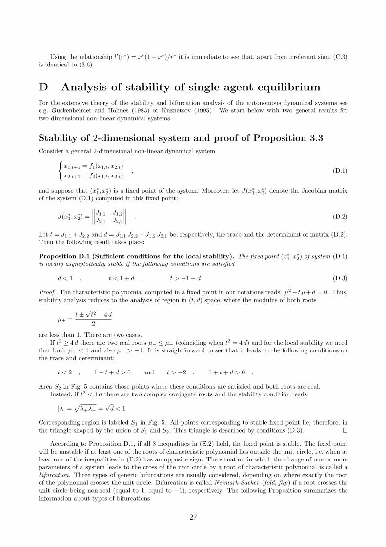
Using the relationship l#(r!) = x!(1" x!)/r! it is immediate to see that, apart from irrelevant sign, (C.3)is identical to (3.6).

D Analysis of stability of single agent equilibriumFor the extensive theory of the stability and bifurcation analysis of the autonomous dynamical systems seee.g. Guckenheimer and Holmes (1983) or Kuznetsov (1995). We start below with two general results fortwo-dimensional non-linear dynamical systems.

Stability of 2-dimensional system and proof of Proposition 3.3Consider a general 2-dimensional non-linear dynamical system

=x1,t+1 = f1(x1,t, x2,t)x2,t+1 = f2(x1,t, x2,t)

, (D.1)

and suppose that (x!1, x!2) is a fixed point of the system. Moreover, let J(x!1, x!2) denote the Jacobian matrixof the system (D.1) computed in this fixed point:

J(x!1, x!2) =

<<<<J1,1 J1,2

J2,1 J2,2

<<<< . (D.2)

Let t = J1,1 + J2,2 and d = J1,1 J2,2"J1,2 J2,1 be, respectively, the trace and the determinant of matrix (D.2).Then the following result takes place:

Proposition D.1 (Su!cient conditions for the local stability). The fixed point (x!1, x!2) of system (D.1)is locally asymptotically stable if the following conditions are satisfied

d < 1 , t < 1 + d , t > "1" d . (D.3)

Proof. The characteristic polynomial computed in a fixed point in our notations reads: µ2" t µ+d = 0. Thus,stability analysis reduces to the analysis of region in (t, d) space, where the modulus of both roots

µ± =t ±

+t2 " 4 d

2

are less than 1. There are two cases.If t2 & 4 d there are two real roots µ" ) µ+ (coinciding when t2 = 4 d) and for the local stability we need

that both µ+ < 1 and also µ" > "1. It is straightforward to see that it leads to the following conditions onthe trace and determinant:

t < 2 , 1" t + d > 0 and t > "2 , 1 + t + d > 0 .

Area S2 in Fig. 5 contains those points where these conditions are satisfied and both roots are real.Instead, if t2 < 4 d there are two complex conjugate roots and the stability condition reads

|!| =>

!+!" =+

d < 1

Corresponding region is labeled S1 in Fig. 5. All points corresponding to stable fixed point lie, therefore, inthe triangle shaped by the union of S1 and S2. This triangle is described by conditions (D.3).

According to Proposition D.1, if all 3 inequalities in (E.2) hold, the fixed point is stable. The fixed pointwill be unstable if at least one of the roots of characteristic polynomial lies outside the unit circle, i.e. when atleast one of the inequalities in (E.2) has an opposite sign. The situation in which the change of one or moreparameters of a system leads to the cross of the unit circle by a root of characteristic polynomial is called abifurcation. Three types of generic bifurcations are usually considered, depending on where exactly the rootof the polynomial crosses the unit circle. Bifurcation is called Neimark-Sacker (fold, flip) if a root crosses theunit circle being non-real (equal to 1, equal to "1), respectively. The following Proposition summarizes theinformation about types of bifurcations.

27

Determinant

Trace

-2

-1

0

1

2

-3 -2 -1 0 1 2 3

S2

S1

I1

I2

I3

I4

Figure 5: Stability region for a fixed point ofa two-dimensional dynamical system in the Trace-Determinant coordinates. The system is stable inthe triangle defined as union of the areas S1 and S2.

Rel

ativ

e sl

op

e, f

’/l’

Equilibrium Rescaled Price Return

fold fold

0

1

-1 -e- 0 1

L=1

L=3, EWMA

L=5, CW

A

Figure 6: Loci where flip bifurcations can occurin the system with EWMA forecast and ! = 0.6(thick lines) and with CWA forecast (thin lines).If L = 1 in both cases the loci define the stabilityregion shown as dark. For the EWMA behavior: theloci for odd L rotate clock-wise and approach thelocus corresponding to even L (thick dotted curve).For the CWA behavior: for even L loci do not exist,while for odd L they rotate faster w.r. to EWMAcase and approach the ordinate axes.

Proposition D.2. The fixed point of the system (D.1) looses its stability when one of the inequalities inconditions (D.3) is changing its sign. Moreover, the system exhibits

• Neimark-Sacker bifurcation, if d = 1,

• fold bifurcation, if t = 1 + d,

• flip bifurcation, if t = "1" d.

Proof. From the proof of the previous proposition it is clear that when the parameters cross the line separatingregion S1 from I1 at Fig. 5 (when d = 1), the modulus of the complex eigenvalues become larger than 1. Thusthe system exhibits a Neimark-Sacker bifurcation. When the line between S2 and I2 is crossed (and so t = 1+d)the largest real eigenvalue becomes greater than 1, so that a fold bifurcation is observed. Finally, if the linebetween S2 and I3 is crossed (i.e. t = "1" d) the smallest real eigenvalue becomes less than "1, and the flipbifurcation is observed.

Proposition 3.3 follows straight-forwardly from the last two Propositions applied to polynomial (3.7).

Stability for the system with EWMA forecastUsing stability polynomial (3.10), the characteristic polynomial for this case can be written as follows:

Q(µ) = µL"1

:µ2 " 1" !

1" !L

1" (!/µ)L

1" !/µ

Y

X

*(1 + X)µ" 1

+;, (D.4)

where variables X = r! and Y = l#(r!)/f #(r!) correspond to the abscissa and ordinate of the stability regiondiagrams in Fig. 2.

Bifurcations Loci

Unfortunately, for the polynomials of degree higher than 2, conditions on the roots analogous to (D.3) areunavailable. One can, however, characterize the loci of di!erent types of bifurcations, where by locus of, say,flip bifurcation we mean the set of those pairs (X,Y ) under which one of the roots of (D.4) is equal to "1.Notice that, in general, not any point on such locus corresponds to flip bifurcation, since bifurcation happensonly if all other roots are inside the unit circle. With this remark in mind, we formulate

28

Lemma D.1. Consider polynomial (D.4) for arbitrary ! and L. The locus of fold bifurcations is given byY = 1, while the locus of flip bifurcations is provided as follows:

1 + Y2 + X

X

1" !

1 + !

1 + !L

1" !L= 0 for L odd and 1 + Y

2 + X

X

1" !

1 + != 0 for L even .

Proof. The computations are pretty straight-forward: one has to let µ = 1 and µ = "1 in (D.4).

We illustrate the last result in Fig. 6, where we show the locus of fold bifurcations, and loci of flipbifurcations when ! = 0.6 for L = 1, 3, 5 and for even L (coinciding with the case L = '). Notice that thecentral interval in the locus of fold bifurcations does not correspond, in reality, to any bifurcation.

The last possible boundary of the stability region is a locus of Neimark-Sacker bifurcation. Pluggingµ = ei", where % is arbitrary angle and i is the imaginary unit, into equation Q(µ) = 0 one can derivecorresponding locus. For high L the corresponding curve may have high dimension, so we confine ourselves onthe example with L = 2.

Lemma D.2. Consider polynomial (D.4) for L = 2 and arbitrary !. The locus of Neimark-Sacker bifurcationsis given by the following curve of the second order

Y 2 !,X + 1 + !

-+ Y X (1 + !)

,1" !" !X

-"X2 (1 + !)2 = 0 , (D.5)

subject to constraint 4(1 + !2)X2 " (1 + ! + X)2Y 2 > 0.

Proof. One has to solve the following equation

(1 + !)Xe3i" " (1 + X)Y e2i" +,1" !(1 + X)

-Y ei" + !Y = 0 . (D.6)

Using the Euler formula and equalizing the real and imaginary parts of the left- and right-hand sides, one getsthe system of two equations. From the equation for the imaginary parts it follows that

sin %*(1 + !)X(3" 4 sin2 %)" 2(1 + X)Y cos % + Y " !(1 + X)Y

+= 0 .

Since, we are interested in the pure complex roots of the characteristic polynomial, let us assume that sin% (= 0.Thus, the expression in the big parenthesis is equal to 0. Then, we substitute the resulting expression for3" 4 sin2 % in the equation of the real parts of (D.6) and, using relation cos 3% = cos %(1" 4 sin2 %), obtain

cos % =Y (1 + X) + Y !

2 (1 + !)X.

Plugging this expression into both the equation for the real and for imaginary parts of (D.6), we get thefollowing system

(1 + ! + X) Y*" !(1 + !)Y 2 + (1 + !)(1 + ! + !Y )X2 " (1" !2 + !Y )XY

+= 0

>4(1 + !)2X2 " (1 + ! + X)2Y 2

*" !(1 + !)Y 2 + (1 + !)(1 + ! + !Y )X2 " (1" !2 + !Y )XY

+= 0 .

In any solution of this system, the common expression in the parenthesis must be equal to zero, which gives(D.5). Additional constraint guarantees that the squared root in the second equation is defined.

We depict curve (D.5) in the lower left panel of Fig. 2 and complete the construction of the stability regionsapplying the property of the continuity of the roots of polynomial on its coe"cients.

Limiting case, L %'Finally, we sketch here heuristic proof of Proposition 3.4, concerning the stability region of the system whenL % '. Consider the region outside of the unit circle of complex plane (including the circle itself) and fixµ = µ0. Since |µ0| & 1, the first term in (D.4) cannot be equal to zero. Therefore, in order µ0 would be a rootof the characteristic polynomial Q(µ), it should be the case that the expression in the parenthesis of (D.4)cancels out. But when L % ', since ! < 1, it is (!/µ0)L % 0. Therefore, the zeroes of the Q(µ) lie in theneighborhoods of solutions of the following quadratic equation

µ2 " (1" !)1

1" !/µ

Y

X

*(1 + X)µ" 1

+= 0 . (D.7)

29

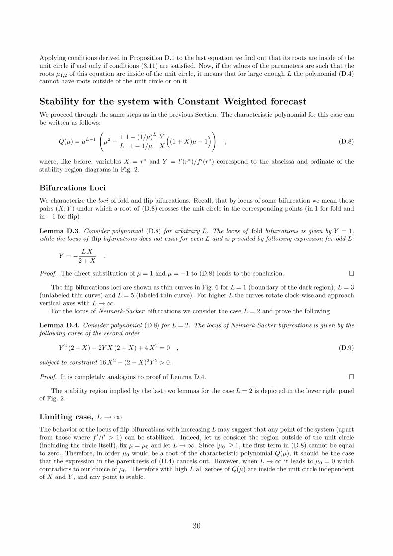
Applying conditions derived in Proposition D.1 to the last equation we find out that its roots are inside of theunit circle if and only if conditions (3.11) are satisfied. Now, if the values of the parameters are such that theroots µ1,2 of this equation are inside of the unit circle, it means that for large enough L the polynomial (D.4)cannot have roots outside of the unit circle or on it.

Stability for the system with Constant Weighted forecastWe proceed through the same steps as in the previous Section. The characteristic polynomial for this case canbe written as follows:

Q(µ) = µL"1

:µ2 " 1

L

1" (1/µ)L

1" 1/µ

Y

X

*(1 + X)µ" 1

+;, (D.8)

where, like before, variables X = r! and Y = l#(r!)/f #(r!) correspond to the abscissa and ordinate of thestability region diagrams in Fig. 2.

Bifurcations Loci

We characterize the loci of fold and flip bifurcations. Recall, that by locus of some bifurcation we mean thosepairs (X, Y ) under which a root of (D.8) crosses the unit circle in the corresponding points (in 1 for fold andin "1 for flip).

Lemma D.3. Consider polynomial (D.8) for arbitrary L. The locus of fold bifurcations is given by Y = 1,while the locus of flip bifurcations does not exist for even L and is provided by following expression for odd L:

Y = " LX

2 + X.

Proof. The direct substitution of µ = 1 and µ = "1 to (D.8) leads to the conclusion.

The flip bifurcations loci are shown as thin curves in Fig. 6 for L = 1 (boundary of the dark region), L = 3(unlabeled thin curve) and L = 5 (labeled thin curve). For higher L the curves rotate clock-wise and approachvertical axes with L %'.

For the locus of Neimark-Sacker bifurcations we consider the case L = 2 and prove the following

Lemma D.4. Consider polynomial (D.8) for L = 2. The locus of Neimark-Sacker bifurcations is given by thefollowing curve of the second order

Y 2 (2 + X)" 2Y X (2 + X) + 4 X2 = 0 , (D.9)

subject to constraint 16 X2 " (2 + X)2Y 2 > 0.

Proof. It is completely analogous to proof of Lemma D.4.

The stability region implied by the last two lemmas for the case L = 2 is depicted in the lower right panelof Fig. 2.

Limiting case, L %'The behavior of the locus of flip bifurcations with increasing L may suggest that any point of the system (apartfrom those where f #/l# > 1) can be stabilized. Indeed, let us consider the region outside of the unit circle(including the circle itself), fix µ = µ0 and let L %'. Since |µ0| & 1, the first term in (D.8) cannot be equalto zero. Therefore, in order µ0 would be a root of the characteristic polynomial Q(µ), it should be the casethat the expression in the parenthesis of (D.4) cancels out. However, when L % ' it leads to µ0 = 0 whichcontradicts to our choice of µ0. Therefore with high L all zeroes of Q(µ) are inside the unit circle independentof X and Y , and any point is stable.

30

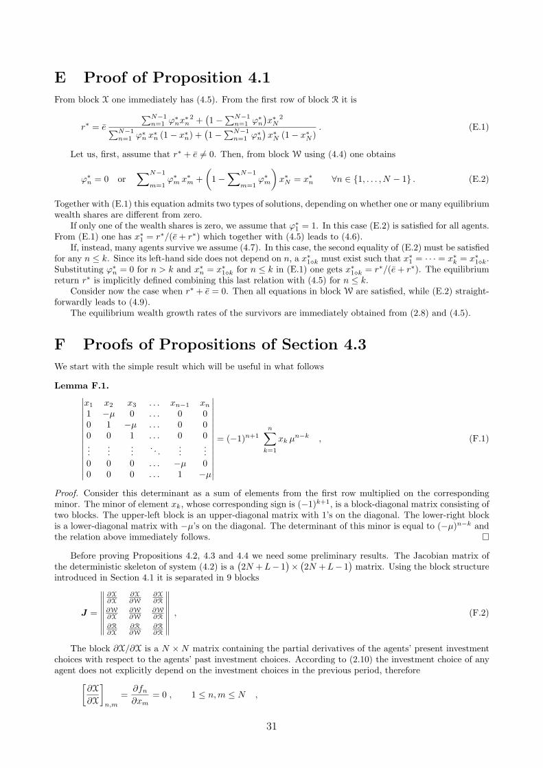
E Proof of Proposition 4.1From block X one immediately has (4.5). From the first row of block R it is

r! = e

.N"1n=1 "!

nx!n2 +

,1"

.N"1n=1 "!

n

-x!N

2

.N"1n=1 "!

n x!n (1" x!n) +,1"

.N"1n=1 "!

n

-x!N (1" x!N )

. (E.1)

Let us, first, assume that r! + e (= 0. Then, from block W using (4.4) one obtains

"!n = 0 or

!N"1

m=1"!

m x!m +&

1"!N"1

m=1"!

m

'x!N = x!n #n $ {1, . . . , N " 1} . (E.2)

Together with (E.1) this equation admits two types of solutions, depending on whether one or many equilibriumwealth shares are di!erent from zero.

If only one of the wealth shares is zero, we assume that "!1 = 1. In this case (E.2) is satisfied for all agents.

From (E.1) one has x!1 = r!/(e + r!) which together with (4.5) leads to (4.6).If, instead, many agents survive we assume (4.7). In this case, the second equality of (E.2) must be satisfied

for any n ) k. Since its left-hand side does not depend on n, a x!1$k must exist such that x!1 = · · · = x!k = x!1$k.Substituting "!

n = 0 for n > k and x!n = x!1$k for n ) k in (E.1) one gets x!1$k = r!/(e + r!). The equilibriumreturn r! is implicitly defined combining this last relation with (4.5) for n ) k.

Consider now the case when r! + e = 0. Then all equations in block W are satisfied, while (E.2) straight-forwardly leads to (4.9).

The equilibrium wealth growth rates of the survivors are immediately obtained from (2.8) and (4.5).

F Proofs of Propositions of Section 4.3We start with the simple result which will be useful in what follows

Lemma F.1.666666666666666

x1 x2 x3 . . . xn"1 xn

1 "µ 0 . . . 0 00 1 "µ . . . 0 00 0 1 . . . 0 0...

......

. . ....

...0 0 0 . . . "µ 00 0 0 . . . 1 "µ

666666666666666

= ("1)n+1n!

k=1

xk µn"k , (F.1)

Proof. Consider this determinant as a sum of elements from the first row multiplied on the correspondingminor. The minor of element xk, whose corresponding sign is ("1)k+1, is a block-diagonal matrix consisting oftwo blocks. The upper-left block is an upper-diagonal matrix with 1’s on the diagonal. The lower-right blockis a lower-diagonal matrix with "µ’s on the diagonal. The determinant of this minor is equal to ("µ)n"k andthe relation above immediately follows.

Before proving Propositions 4.2, 4.3 and 4.4 we need some preliminary results. The Jacobian matrix ofthe deterministic skeleton of system (4.2) is a

,2N + L" 1

-*

,2N + L" 1

-matrix. Using the block structure

introduced in Section 4.1 it is separated in 9 blocks

J =

<<<<<<<<

!X!X

!X!W

!X!R

!W!X

!W!W

!W!R

!R!X

!R!W

!R!R

<<<<<<<<, (F.2)

The block $X/$X is a N *N matrix containing the partial derivatives of the agents’ present investmentchoices with respect to the agents’ past investment choices. According to (2.10) the investment choice of anyagent does not explicitly depend on the investment choices in the previous period, therefore

?$X

$X

@

n,m

=$fn

$xm= 0 , 1 ) n,m ) N ,

31

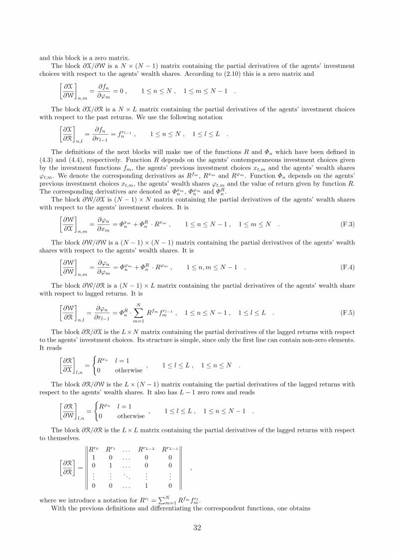
and this block is a zero matrix.The block $X/$W is a N * (N " 1) matrix containing the partial derivatives of the agents’ investment

choices with respect to the agents’ wealth shares. According to (2.10) this is a zero matrix and?

$X

$W

@

n,m

=$fn

$"m= 0 , 1 ) n ) N , 1 ) m ) N " 1 .

The block $X/$R is a N * L matrix containing the partial derivatives of the agents’ investment choiceswith respect to the past returns. We use the following notation

?$X

$R

@

n,l

=$fn

$rl"1= frl!1

n , 1 ) n ) N , 1 ) l ) L .

The definitions of the next blocks will make use of the functions R and &n which have been defined in(4.3) and (4.4), respectively. Function R depends on the agents’ contemporaneous investment choices givenby the investment functions fm, the agents’ previous investment choices xt,m and the agents’ wealth shares"t,m. We denote the corresponding derivatives as Rfm , Rxm and R#m . Function &n depends on the agents’previous investment choices xt,m, the agents’ wealth shares "t,m and the value of return given by function R.The corresponding derivatives are denoted as &xm

n , &#mn and &R

n .The block $W/$X is (N " 1) * N matrix containing the partial derivatives of the agents’ wealth shares

with respect to the agents’ investment choices. It is?$W

$X

@

n,m

=$"n

$xm= &xm

n + &Rn · Rxm , 1 ) n ) N " 1 , 1 ) m ) N . (F.3)

The block $W/$W is a (N " 1)* (N " 1) matrix containing the partial derivatives of the agents’ wealthshares with respect to the agents’ wealth shares. It is

?$W

$W

@

n,m

=$"n

$"m= &#m

n + &Rn · R#m , 1 ) n, m ) N " 1 . (F.4)

The block $W/$R is a (N " 1) * L matrix containing the partial derivatives of the agents’ wealth sharewith respect to lagged returns. It is

?$W

$R

@

n,l

=$"n

$rl"1= &R

n ·N!

m=1

Rfmfrl!1m , 1 ) n ) N " 1 , 1 ) l ) L . (F.5)

The block $R/$X is the L*N matrix containing the partial derivatives of the lagged returns with respectto the agents’ investment choices. Its structure is simple, since only the first line can contain non-zero elements.It reads

?$R

$X

@

l,n

=

=Rxn l = 10 otherwise

, 1 ) l ) L , 1 ) n ) N .

The block $R/$W is the L* (N " 1) matrix containing the partial derivatives of the lagged returns withrespect to the agents’ wealth shares. It also has L" 1 zero rows and reads

?$R

$W

@

l,n

=

=R#n l = 10 otherwise

, 1 ) l ) L , 1 ) n ) N " 1 .

The block $R/$R is the L*L matrix containing the partial derivatives of the lagged returns with respectto themselves.

?$R

$R

@=

<<<<<<<<<<<

Rr0 Rr1 . . . RrL!2 RrL!1

1 0 . . . 0 00 1 . . . 0 0...

.... . .

......

0 0 . . . 1 0

<<<<<<<<<<<

,

where we introduce a notation for Rrl =.N

m=1 Rfmfrlm .

With the previous definitions and di!erentiating the correspondent functions, one obtains

32

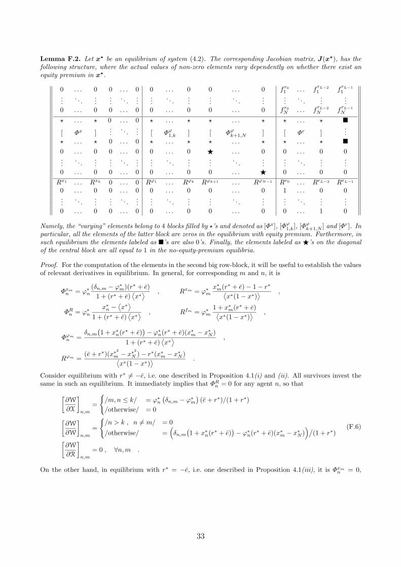
Lemma F.2. Let x! be an equilibrium of system (4.2). The corresponding Jacobian matrix, J(x!), has thefollowing structure, where the actual values of non-zero elements vary dependently on whether there exist anequity premium in x!.

<<<<<<<<<<<<<<<<<<<<<<<<<<<<<<<<

0 . . . 0 0 . . . 0 0 . . . 0 0 . . . 0 fr01 . . . frL!2

1 frL!11

.... . .

......

. . ....

.... . .

......

. . ....

.... . .

......

0 . . . 0 0 . . . 0 0 . . . 0 0 . . . 0 fr0N . . . frL!2

N frL!1N

' . . . ' 0 . . . 0 ' . . . ' ' . . . ' ' . . . ' ![ &x ]

.... . .

... [ &#1,k ] [ &#

k+1,N ] [ &r ]...

' . . . ' 0 . . . 0 ' . . . ' ' . . . ' ' . . . ' !0 . . . 0 0 . . . 0 0 . . . 0 " . . . 0 0 . . . 0 0...

. . ....

.... . .

......

. . ....

.... . .

......

. . ....

...0 . . . 0 0 . . . 0 0 . . . 0 0 . . . " 0 . . . 0 0

Rx1 . . . Rxk 0 . . . 0 R#1 . . . R#k R#k+1 . . . R#N!1 Rr0 . . . RrL!2 RrL!1

0 . . . 0 0 . . . 0 0 . . . 0 0 . . . 0 1 . . . 0 0...

. . ....

.... . .

......

. . ....

.... . .

......

. . ....

...0 . . . 0 0 . . . 0 0 . . . 0 0 . . . 0 0 . . . 1 0

<<<<<<<<<<<<<<<<<<<<<<<<<<<<<<<<

Namely, the “varying” elements belong to 4 blocks filled by '’s and denoted as [&x], [&#1,k], [&#

k+1,N ] and [&r]. Inparticular, all the elements of the latter block are zeros in the equilibrium with equity premium. Furthermore, insuch equilibrium the elements labeled as !’s are also 0’s. Finally, the elements labeled as "’s on the diagonalof the central block are all equal to 1 in the no-equity-premium equilibria.

Proof. For the computation of the elements in the second big row-block, it will be useful to establish the valuesof relevant derivatives in equilibrium. In general, for corresponding m and n, it is

&xmn = "!

n((n,m " "!

m)(r! + e)1 + (r! + e)

(x!

) , Rxm = "!m

x!m(r! + e)" 1" r!(x!(1" x!)

) ,

&Rn = "!

n

x!n "(x!

)

1 + (r! + e)(x!

) , Rfm = "!m

1 + x!m(r! + e)(x!(1" x!)

) ,

&#mn =

(n,m

,1 + x!n(r! + e)

-" "!

n(r! + e)(x!m " x!N )1 + (r! + e)

(x!

) ,

R#m =(e + r!)(x!

2

m " x!2

N )" r!(x!m " x!N )(x!(1" x!)

) .

Consider equilibrium with r! (= "e, i.e. one described in Proposition 4.1(i) and (ii). All survivors invest thesame in such an equilibrium. It immediately implies that &R

n = 0 for any agent n, so that

?$W

$X

@

n,m

=

=/m, n ) k/ = "!

n

,(n,m " "!

m

-(e + r!)/(1 + r!)

/otherwise/ = 0?$W

$W

@

n,m

=

=/n > k , n (= m/ = 0/otherwise/ =

*(n,m

,1 + x!n(r! + e)

-" "!

n(r! + e)(x!m " x!N )+A

(1 + r!)?$W

$R

@

n,m

= 0 , #n,m .

(F.6)

On the other hand, in equilibrium with r! = "e, i.e. one described in Proposition 4.1(iii), it is &xmn = 0,

33

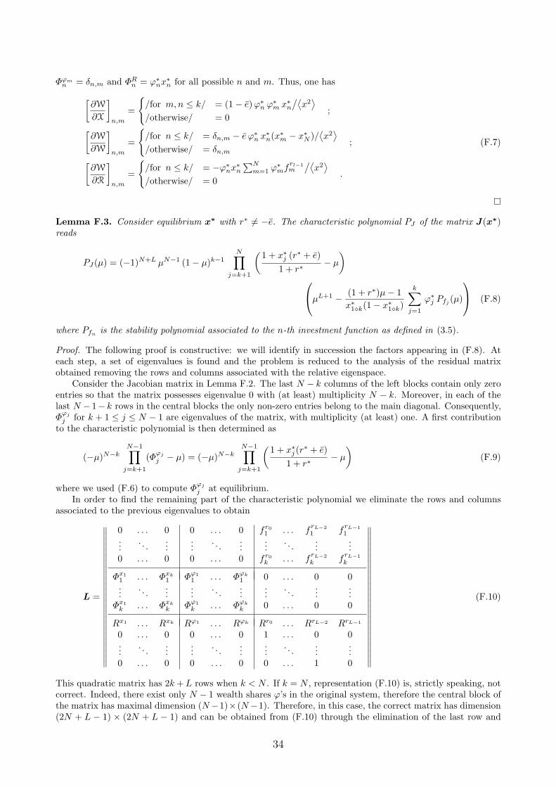
&#mn = (n,m and &R

n = "!nx!n for all possible n and m. Thus, one has

?$W

$X

@

n,m

=

=/for m,n ) k/ = (1" e)"!

n "!m x!n

A(x2

)

/otherwise/ = 0;

?$W

$W

@

n,m

=

=/for n ) k/ = (n,m " e"!

n x!n(x!m " x!N )/(x2

)

/otherwise/ = (n,m;

?$W

$R

@

n,m

=

=/for n ) k/ = ""!

nx!n.N

m=1 "!mf

rl!1m

A(x2

)

/otherwise/ = 0.

(F.7)

Lemma F.3. Consider equilibrium x! with r! (= "e. The characteristic polynomial PJ of the matrix J(x!)reads

PJ(µ) = ("1)N+L µN"1 (1" µ)k"1NB

j=k+1

&1 + x!j (r! + e)1 + r!

" µ

'

C

DµL+1 " (1 + r!)µ" 1x!1$k(1" x!1$k)

k!

j=1

"!j Pfj (µ)

E

F (F.8)

where Pfn is the stability polynomial associated to the n-th investment function as defined in (3.5).

Proof. The following proof is constructive: we will identify in succession the factors appearing in (F.8). Ateach step, a set of eigenvalues is found and the problem is reduced to the analysis of the residual matrixobtained removing the rows and columns associated with the relative eigenspace.

Consider the Jacobian matrix in Lemma F.2. The last N " k columns of the left blocks contain only zeroentries so that the matrix possesses eigenvalue 0 with (at least) multiplicity N " k. Moreover, in each of thelast N " 1" k rows in the central blocks the only non-zero entries belong to the main diagonal. Consequently,&

#j

j for k + 1 ) j ) N " 1 are eigenvalues of the matrix, with multiplicity (at least) one. A first contributionto the characteristic polynomial is then determined as

("µ)N"kN"1B

j=k+1

(&#j

j " µ) = ("µ)N"kN"1B

j=k+1

&1 + x!j (r! + e)1 + r!

" µ

'(F.9)

where we used (F.6) to compute &#j

j at equilibrium.In order to find the remaining part of the characteristic polynomial we eliminate the rows and columns

associated to the previous eigenvalues to obtain

L =

<<<<<<<<<<<<<<<<<<<<<<<<<

0 . . . 0 0 . . . 0 fr01 . . . frL!2

1 frL!11

.... . .

......

. . ....

.... . .

......

0 . . . 0 0 . . . 0 fr0k . . . frL!2

k frL!1k

&x11 . . . &xk

1 &#11 . . . &#k

1 0 . . . 0 0...

. . ....

.... . .

......

. . ....

...&x1

k . . . &xkk &#1

k . . . &#k

k 0 . . . 0 0

Rx1 . . . Rxk R#1 . . . R#k Rr0 . . . RrL!2 RrL!1

0 . . . 0 0 . . . 0 1 . . . 0 0...

. . ....

.... . .

......

. . ....

...0 . . . 0 0 . . . 0 0 . . . 1 0

<<<<<<<<<<<<<<<<<<<<<<<<<

(F.10)

This quadratic matrix has 2k + L rows when k < N . If k = N , representation (F.10) is, strictly speaking, notcorrect. Indeed, there exist only N " 1 wealth shares "’s in the original system, therefore the central block ofthe matrix has maximal dimension (N"1)*(N"1). Therefore, in this case, the correct matrix has dimension(2N + L " 1) * (2N + L " 1) and can be obtained from (F.10) through the elimination of the last row and

34

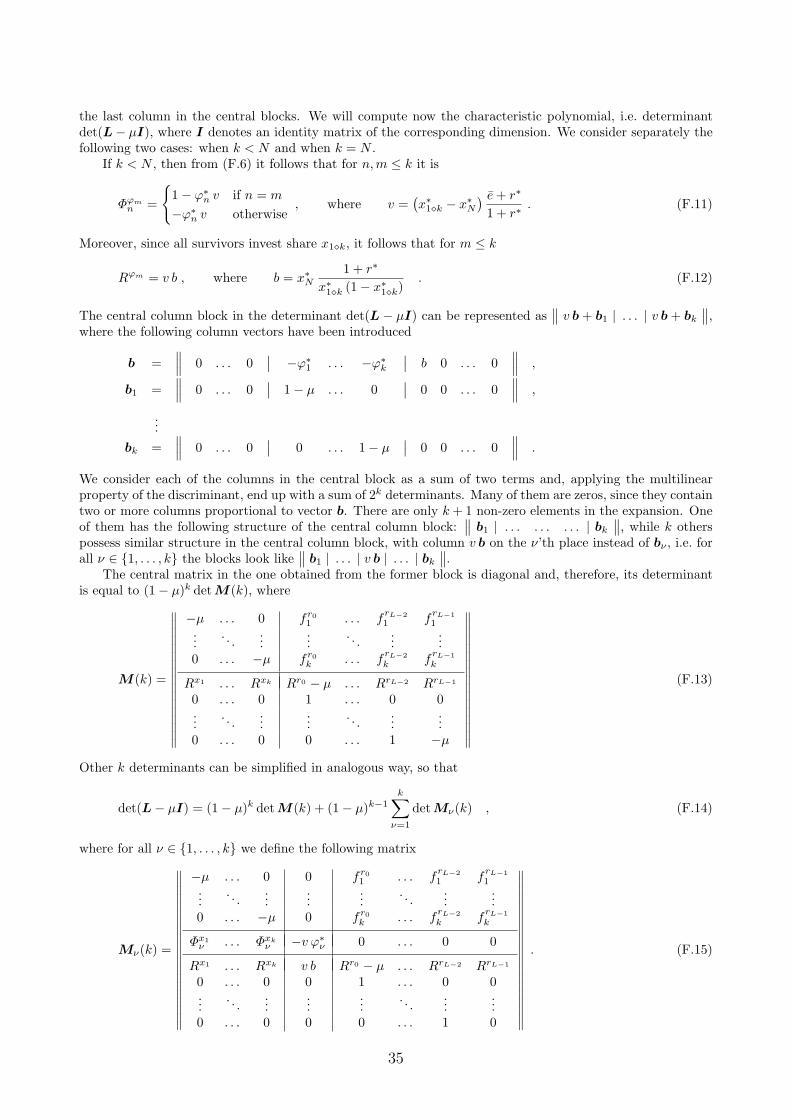
the last column in the central blocks. We will compute now the characteristic polynomial, i.e. determinantdet(L" µI), where I denotes an identity matrix of the corresponding dimension. We consider separately thefollowing two cases: when k < N and when k = N .

If k < N , then from (F.6) it follows that for n,m ) k it is

&#mn =

=1" "!

n v if n = m

""!n v otherwise

, where v =,x!1$k " x!N

- e + r!

1 + r!. (F.11)

Moreover, since all survivors invest share x1$k, it follows that for m ) k

R#m = v b , where b = x!N1 + r!

x!1$k (1" x!1$k). (F.12)

The central column block in the determinant det(L" µI) can be represented as<< v b + b1 | . . . | v b + bk

<<,where the following column vectors have been introduced

b =<<< 0 . . . 0

66 ""!1 . . . ""!

k

66 b 0 . . . 0<<< ,

b1 =<<< 0 . . . 0

66 1" µ . . . 066 0 0 . . . 0

<<< ,

...bk =

<<< 0 . . . 066 0 . . . 1" µ

66 0 0 . . . 0<<< .

We consider each of the columns in the central block as a sum of two terms and, applying the multilinearproperty of the discriminant, end up with a sum of 2k determinants. Many of them are zeros, since they containtwo or more columns proportional to vector b. There are only k + 1 non-zero elements in the expansion. Oneof them has the following structure of the central column block:

<< b1 | . . . . . . . . . | bk

<<, while k otherspossess similar structure in the central column block, with column v b on the )’th place instead of b$ , i.e. forall ) $ {1, . . . , k} the blocks look like

<< b1 | . . . | v b | . . . | bk

<<.The central matrix in the one obtained from the former block is diagonal and, therefore, its determinant

is equal to (1" µ)k det M(k), where

M(k) =

<<<<<<<<<<<<<<<<<

"µ . . . 0 fr01 . . . frL!2

1 frL!11

.... . .

......

. . ....

...0 . . . "µ fr0

k . . . frL!2k frL!1

k

Rx1 . . . Rxk Rr0 " µ . . . RrL!2 RrL!1

0 . . . 0 1 . . . 0 0...

. . ....

.... . .

......

0 . . . 0 0 . . . 1 "µ

<<<<<<<<<<<<<<<<<

(F.13)

Other k determinants can be simplified in analogous way, so that

det(L" µI) = (1" µ)k det M(k) + (1" µ)k"1k!

$=1

det M$(k) , (F.14)

where for all ) $ {1, . . . , k} we define the following matrix

M$(k) =

<<<<<<<<<<<<<<<<<<<<

"µ . . . 0 0 fr01 . . . frL!2

1 frL!11

.... . .

......

.... . .

......

0 . . . "µ 0 fr0k . . . frL!2

k frL!1k

&x1$ . . . &xk

$ "v "!$ 0 . . . 0 0

Rx1 . . . Rxk v b Rr0 " µ . . . RrL!2 RrL!1

0 . . . 0 0 1 . . . 0 0...

. . ....

......

. . ....

...0 . . . 0 0 0 . . . 1 0

<<<<<<<<<<<<<<<<<<<<

. (F.15)

35

We expand the last matrix on the minors of the elements of the central column. For this purpose we for each) $ {1, . . . , k} introduce yet another matrix

N$(k) =

<<<<<<<<<<<<<<<<<<<

"µ . . . 0 fr01 fr1

1 . . . frL!21 frL!1

1...

. . ....

......

. . ....

...0 . . . "µ fr0

k fr1k . . . frL!2

k frL!1k

&x1$ . . . &xk

$ 0 0 . . . 0 00 . . . 0 1 "µ . . . 0 00 . . . 0 0 1 . . . 0 0...

. . ....

......

. . ....

...0 . . . 0 0 0 . . . 1 "µ

<<<<<<<<<<<<<<<<<<<

.

Then it is:

detM$(k) = v," "!

$ detM(k)" b detN$(k)-

. (F.16)

Let us compute the determinant of matrix M(k) in a recursive way. Consider the expansion by the minorsof the elements from the first column. The minor of the first element "µ is a matrix with a structure similarto M(k), whose determinant we denote as M(k " 1). The minor associated with Rx1 has a left upper blockwith k " 1 entries equal to "µ below the main diagonal. This block generates a contribution µk"1 to thedeterminant and once its columns and rows are eliminated, one remains with a matrix of the type in (F.1).Applying Lemma F.1 one then has

detM(k) = ("µ) detM(k " 1) + ("1)kRx1µk"1 ("1)L"1 Pf1(µ) ,

where Pf1 is the stability polynomial associated with the first investment function. Applying recursively therelation above, the dimension of the determinant is progressively reduced. At the end the lower right block ofthe original matrix remains, which is again a matrix similar to (F.1). Applying once more Lemma F.1 one hasfor M(k) the following

detM(k) = ("1)L"1+k µk"1k!

j=1

Rxj Pfj (µ) + ("1)L"1+k µk

C

DL"1!

j=0

Rrj µL"1"j " µL

E

F . (F.17)

The determinant of matrix N$(k) can be computed using the similar strategy. The only di!erence is that inthe last recursive step one of the matrix has zero determinant. Therefore, we have:

detN$(k) = ("µ) detN$(k " 1) + ("1)k&x1$ µk"1 ("1)L"1 Pf1(µ) = ("1)L"1+k µk"1

k!

j=1

&xj$ Pfj (µ) ,

which, taking into account (F.16), implies

k!

$=1

detM$(k) = v

:"det M(k)" b

k!

$=1

det N$(k)

;=

= "v detM(k) + v b ("1)L+k µk"1k!

$=1

k!

j=1

&xj$ Pfj (µ) = "v detM(k) .

(The last equality above follows directly from expression for &xj$ .) Let us now substitute the last relation into

(F.14). Then using the expression for detM(k) from (F.17) where the corresponding values of the derivativesof function R are computed in accordance with results of Lemma F.2, the last contribution into characteristicpolynomial follows:

det(L" µI) = (1" µ)k"1 (1" µ" v) det M(k) =

= ("1)L"1+k µk"1 (1" µ)k"1

&1 + x!N (r! + e)

1 + r!" µ

' C

D (1 + r!)µ" 1x!1$k(1" x!1$k)

k!

j=1

"!j Pfj (µ)" µL+1

E

F .

36

If k = N , i.e. all agents survive, then all investment shares are the same. In this case, from (F.6), allelements in the central column block of matrix (F.10) are zeros apart from the 1’s on the diagonal in thecentral matrix. It contributes to the characteristic polynomial by the factor (1" µ)N"1. The remaining partis the determinant of matrix M in this case. This is consistent with the expression above.

The product of the det(L" µI) and (F.9) gives (F.8), what completes the proof.

Lemma F.4. Consider no-equity-premium equilibrium x! with r! = "e. The characteristic polynomial PJ ofthe matrix J(x!) reads

PJ(µ) = ("1)L+N (1" µ)N"2 µN"1,µ + e" 1

-C

DµL+1 +µ" 1(x2

)k!

j=1

"!j Pfj (µ)

E

F (F.18)

Proof. Since the proof is analogous to the proof of Lemma F.3. some details are omitted. In particular, weconfine analysis on the case k < N . From the Jacobian matrix in Lemma F.2 we can immediately identify thatin each of the N " 1 " k last rows belonging to the central row clock of the matrix the only non-zero entriesbelong to the main diagonal of [$W/$W] and equal to 1. In addition, the last N " k columns of the leftmostblocks contain only zero entries. Together, it gives the first entry in the characteristic polynomial:

("µ)N"k (1" µ)N"1"k , (F.19)

while the rows and columns associated to the previous eigenvalues can be eliminated. We obtain

L =

<<<<<<<<<<<<<<<<<<<<<<<<<

0 . . . 0 0 . . . 0 fr01 . . . frL!2

1 frL!11

.... . .

......

. . ....

.... . .

......

0 . . . 0 0 . . . 0 fr0N . . . frL!2

N frL!1N

&R1 Rx1 . . . &R

1 Rxk 1 + &R1 R#1 . . . &R

1 R#k &r01 . . . &rL!2

1 &rL!11

.... . .

......

. . ....

.... . .

......

&Rk Rx1 . . . &R

k Rxk &Rk R#1 . . . 1 + &R

k R#k &r0k . . . &rL!2

k &rL!1k

Rx1 . . . Rxk R#1 . . . R#k Rr0 . . . RrL!2 RrL!1

0 . . . 0 0 . . . 0 1 . . . 0 0...

. . ....

.... . .

......

. . ....

...0 . . . 0 0 . . . 0 0 . . . 1 0

<<<<<<<<<<<<<<<<<<<<<<<<<

(F.20)

To compute det(L"µI), where I is an identity matrix of the corresponding dimension, we apply the multilinearproperty of the determinant to the central block of columns in matrix L. In order to implement this idea, weintroduce the following column vectors of the length 2k + L:

d =<<< 0 . . . 0

66 &R1 . . . &R

k

66 1 0 . . . 0<<< ,

d1 =<<< 0 . . . 0

66 1" µ . . . 066 0 0 . . . 0

<<< ,

...dk =

<<< 0 . . . 066 0 . . . 1" µ

66 0 0 . . . 0<<< .

The central column block in the determinant det(L"µI) can be represented as<< R#1 d+d1 | . . . | R#k d+dk

<<.We consider each of the columns in the central block as a sum of two terms and end up with a sum of2k determinants. Notice, however, that many of them are zeros, since they contain two or more columnsproportional to vector d. There are only k + 1 non-zero elements in the expansion. The determinant of thematrix with the structure

<< d1 | . . . . . . . . . | dk

<< in the central part is equal to (1 " µ)k det N(k),where matrix N(k) is identical to the matrix M(k) defined in (F.13). (We use here another notation in orderto stress that the partial derivatives Rxj and Rfj used in these two matrices have di!erent values in di!erentequilibria.) Using (F.17) together with (F.7) it is immediate to see that

detN(k) = ("1)L+k µk"1

C

DµL+1 +µ + e" 1(

x2)

k!

j=1

"!j Pfj (µ)

E

F . (F.21)

37

Other non-zero elements possess similar structure in the central column block, with column R#! d on the)’th place instead of d$ for all ) $ {1, . . . , k}. Their determinants can be represented as (1"µ)k"1 det N$(k),where for all ) $ {1, . . . , k} we define matrix

N$(k) =

<<<<<<<<<<<<<<<<<<<<

"µ . . . 0 0 fr01 . . . frL!2

1 frL!11

.... . .

......

.... . .

......

0 . . . "µ 0 fr0k . . . frL!2

k frL!1k

&R$ Rx1 . . . &R

$ Rxk R#! &Rv &r0

$ . . . &rL!2$ &rL!1

$

Rx1 . . . Rxk R#! Rr0 " µ . . . RrL!2 RrL!1

0 . . . 0 0 1 . . . 0 0...

. . ....

......

. . ....

...0 . . . 0 0 0 . . . 1 "µ

<<<<<<<<<<<<<<<<<<<<

.

This matrix can be simplified, since its central row is (almost) proportional to the next row (the first row inthe bottom block). Applying multilinear property of the determinant, and computing the determinant of theresulting matrix we get

detN$(k) = ("µ)L+kR#! &Rv .

Using the corresponding expressions from Lemma F.2, one can check that.k

$=1 &R$ R#! = "e. Therefore,

det(L" µI) = (1" µ)k det N(k) + (1" µ)k"1k!

$=1

detN$(k) =

= (1" µ)k det N(k)" (1" µ)k"1("µ)L+ke =

= (1" µ)k"1("1)L+k µk"1

C

D(1" µ)µL+1 + (1" µ)µ + e" 1(

x2)

k!

j=1

"!j Pfj (µ)" µL+1e

E

F =

= (1" µ)k"1("1)L+k µk"1 (µ + e" 1)

C

DµL+1 +µ" 1(x2

)k!

j=1

"!j Pfj (µ)

E

F

Combining now the last expression with (F.19) we get polynomial (F.18).

Using the characteristic polynomial of the Jacobian matrix in the corresponding equilibrium, it is straight-forward to derive the equilibrium stability conditions of Section 4.3.

The case of one survivor: Proof of Proposition 4.2

If k = 1 the characteristic polynomial (F.8) reduces to

PJ(µ) = ("1)N+L µN"1NB

j=2

&1 + x!j (r! + e)1 + r!

" µ

' &µL+1 " (1 + r!)µ" 1

x!1(1" x!1)Pf1(µ)

'.

From the expression of the derivative of the EML at equilibrium l#(r!) one can see that last factor correspondsto the polynomial Q1 in (4.10). The conditions in (4.11) are derived from the requirement

66661 + x!j (r! + e)

1 + r!

6666 < 1 j & 2 ,

and the Proposition is proved.

38

The case of many survivors: Proof of Proposition 4.3

In the case of k > 1 survivors the characteristic polynomial in (F.8) possesses a unit root with multiplicityk " 1. Consequently, the fixed point is non-hyperbolic.

To find the eigenspace associated with the eigenvalue 1 we subtract from the initial Jacobian matrix (F.2)computed at equilibrium the identity matrix of the corresponding dimension and analyze the kernel of theresulting J " I matrix. This can be done through the analysis of the kernel of the matrix obtained by thesubstitution of the identity matrix from matrix L given in (F.10). Let us consider the k < N and the k = Ncases separately.

When k < N , as we showed in the proof of Lemma F.3, in the matrix obtained as a result of subtractionof an identity matrix from (F.10), the central k " 1 columns are identical, see (F.11) and (F.12). Therefore,the kernel of the matrix J " I can be generated by a basis containing the following k " 1 vectors

un =*

0, . . . , 02 34 5N

; 0, . . . , 02 34 5n"1

, 1, 0, . . . , 02 34 5k"n"1

,"1; 0, . . . , 02 34 5N"1"k

; 0, . . . , 02 34 5L

+, 1 ) n ) k " 1 . (F.22)

Notice that the direction of vector un corresponds to a change in the relative wealths of the n-th and k-thsurvivor.

If, instead, k = N , then the last k" 1 columns in the resulting (from (F.10)) matrix are zero vectors, andthen the kernel of the matrix J " I can be generated with the N " 1 vectors of the canonical basis

vn =*

0, . . . , 02 34 5N

; 0, . . . , 02 34 5n"1

, 1, 0, . . . , 02 34 5N"n"1

; 0, . . . , 02 34 5L

+, 1 ) n ) N " 1 . (F.23)

whose direction corresponds to a change in the relative wealths of the n-th and N -th survivors.If the system is perturbed away from equilibrium x! along the directions defined in (F.22) or (F.23), a

new fixed point is reached. Then, the system is stable, but not asymptotically stable, with respect to theseperturbations.

Moreover, since the eigenspaces identified above do not depend on the system parameters, it is immediateto realize that they do constitute not only the tangent spaces to the corresponding non-hyperbolic manifolds,but the manifolds themselves.

The polynomial (4.12) is the last factor in (F.8), while conditions (4.13) are obtained by imposing66661 + x!j (r! + e)

1 + r!

6666 < 1 j > k + 1 ,

which completes the proof.

The case of “no-equity-premium” equilibria. Proof of Proposition 4.4

Independently of the number of survivors, the characteristic polynomial in (F.18) possesses a unit root withmultiplicity N " 2. Consequently, the fixed point x! is never hyperbolic, when N & 3. It is easy to see thatin this case all equilibria belong to the manifold of dimension N " 2 and that this is exactly a non-hyperbolicmanifold of x!. For the stability of equilibrium x! with respect to the perturbations in the directions orthogonalto this manifold, it is su"cient to have all other eigenvalues inside the unit circle. If this condition is satisfied,then equilibrium x! of the system is stable, but not asymptotically stable. Since e > 0, this su"cient conditioncan be expressed through the roots of the last term in (F.18). This term is exactly polynomial (4.14).

References

Anufriev, M. (2005): “Wealth-Driven Competition in a Speculative Financial Market: Ex-amples with Maximizing Agents,” CeNDEF Working Paper 2005-17, University of Amster-dam.

Anufriev, M., and G. Bottazzi (2006): “Noisy Trading in the Large Market Limit,” inArtificial Economics: Agent-based Methods in Finances, Game Theory and their Applica-tions, ed. by P. Mathieu, B. Beaufils, and O. Brandouy. Springer-Verlag (Lecture Notes inEconomics and Mathematical Systems, vol.564), Berlin.

39

Anufriev, M., G. Bottazzi, and F. Pancotto (2006): “Equilibria, Stability and Asymp-totic Dominance in a Speculative Market with Heterogeneous Agents,” Journal of EconomicDynamics and Control, forthcoming.

Blume, L., and D. Easley (1992): “Evolution and Market Behavior,” The Journal ofEconomic Theory, 58, 9–40.

Brock, W. (1997): “Asset Price Behavior in Complex Environment,” in The Economy asan Evolving Complex System II, ed. by W. Arthur, S. Durlauf, and D. Lane, pp. 385–423.Addison-Wesley.

Brock, W., and C. Hommes (1998): “Heterogeneous Beliefs and Routes to Chaos in aSimple Asset Pricing Model,” Journal of Economic Dynamics and Control, 22, 1235–1274.

Brock, W., C. Hommes, and F. Wagener (2005): “Evolutionary Dynamics in Marketswith Many Trader Types,” Journal of Mathematical Economics, 41, 7–42.

Campbell, J., and L. Viceira (2002): Strategic Asset Allocation: Portfolio Choice forLong-Term Investors. Oxford University Press, Oxford.

Chiarella, C., R. Dieci, and L. Gardini (2006): “Asset Price and Wealth Dynamicsin a Financial Market with Heterogeneous Agents,” Journal of Economic Dynamics andControl, forthcoming.

Chiarella, C., and X. He (2001): “Asset Price and Wealth Dynamics under HeterogeneousExpectations,” Quantitative Finance, 1, 509–526.

Day, R., and W. Huang (1990): “Bulls, bears and market sheep,” Journal of EconomicBehaviour and Organization, 14, 299–329.

DeLong, J., A. Shleifer, L. Summers, and R. Waldmann (1991): “The survival ofnoise traders in financial markets,” Journal of Business, 64(1), 1–19.

Guckenheimer, J., and P. Holmes (1983): Nonlinear Oscillations, Dynamical Systems,and Bifurcations of Vector Fields. Springer, New York.

Hens, T., and K. Schenk-Hoppe (2005): “Evolutionary Stability of Portfolio Rules inIncomplete Markets,” Journal of Mathematical Economics, 41, 43–66.

Hommes, C. (2006): “Heterogeneous Agent Models in Economics and Finance,” in Hand-book of Computational Economics Vol. 2: Agent-Based Computational Economics, ed. byK. Judd, and L. Tesfatsion. North-Holland (Handbooks in Economics Series), Amsterdam,forthcoming.

Kirman, A. (1991): “Epidemics of opinion and speculative bubbles in financial markets,” inMoney and Financial Markets, ed. by M. Taylor, chap. 17, pp. 354–368. Blackwell, Cam-bridge.

Kuznetsov, Y. (1995): Elements of Applied Bifurcation Theory. Springer, New York.

LeBaron, B. (2006): “Agent-Based Computational Finance,” in Handbook of ComputationalEconomics Vol. 2: Agent-Based Computational Economics, ed. by K. Judd, and L. Tesfat-sion. North-Holland (Handbooks in Economics Series), forthcoming.

40

Levy, M., H. Levy, and S. Solomon (1994): “A Microscopic Model of the Stock Market:Cycles, Booms, and Crashes,” Economics Letters, 45, 103–111.

(2000): Microscopic Simulation of Financial Markets. Academic Press, London.

Mehra, R., and E. C. Prescott (1985): “The equity premium: A puzzle,” Journal ofMonetary Economics, 15, 145–161.

Sandroni, A. (2000): “Do Markets Favor Agents Able to Make Accurate Predictions,”Econometrica, 68(6), 1303–1341.

Simon, H. (1976): “From substantive to procedural rationality,” in Method and appraisal ineconomics, ed. by S. Latsis. Cambridge: Cambridge University Press.

Zschischang, E., and T. Lux (2001): “Some new results on the Levy, Levy and Solomonmicroscopic stock market model,” Physica A, 291, 563–573.

41

!!"#$%&'()*)+#,(,+#%+,(

(

List of other working papers:

2006

1. Roman Kozhan, Multiple Priors and No-Transaction Region, WP06-24 2. Martin Ellison, Lucio Sarno and Jouko Vilmunen, Caution and Activism? Monetary Policy

Strategies in an Open Economy, WP06-23 3. Matteo Marsili and Giacomo Raffaelli, Risk bubbles and market instability, WP06-22 4. Mark Salmon and Christoph Schleicher, Pricing Multivariate Currency Options with Copulas,

WP06-21 5. Thomas Lux and Taisei Kaizoji, Forecasting Volatility and Volume in the Tokyo Stock Market:

Long Memory, Fractality and Regime Switching, WP06-20 6. Thomas Lux, The Markov-Switching Multifractal Model of Asset Returns: GMM Estimation

and Linear Forecasting of Volatility, WP06-19 7. Peter Heemeijer, Cars Hommes, Joep Sonnemans and Jan Tuinstra, Price Stability and

Volatility in Markets with Positive and Negative Expectations Feedback: An Experimental Investigation, WP06-18

8. Giacomo Raffaelli and Matteo Marsili, Dynamic instability in a phenomenological model of correlated assets, WP06-17

9. Ginestra Bianconi and Matteo Marsili, Effects of degree correlations on the loop structure of scale free networks, WP06-16

10. Pietro Dindo and Jan Tuinstra, A Behavioral Model for Participation Games with Negative Feedback, WP06-15

11. Ceek Diks and Florian Wagener, A weak bifucation theory for discrete time stochastic dynamical systems, WP06-14

12. Markus Demary, Transaction Taxes, Traders’ Behavior and Exchange Rate Risks, WP06-13 13. Andrea De Martino and Matteo Marsili, Statistical mechanics of socio-economic systems with

heterogeneous agents, WP06-12 14. William Brock, Cars Hommes and Florian Wagener, More hedging instruments may

destabilize markets, WP06-11 15. Ginwestra Bianconi and Roberto Mulet, On the flexibility of complex systems, WP06-10 16. Ginwestra Bianconi and Matteo Marsili, Effect of degree correlations on the loop structure of

scale-free networks, WP06-09 17. Ginwestra Bianconi, Tobias Galla and Matteo Marsili, Effects of Tobin Taxes in Minority Game

Markets, WP06-08 18. Ginwestra Bianconi, Andrea De Martino, Felipe Ferreira and Matteo Marsili, Multi-asset

minority games, WP06-07 19. Ba Chu, John Knight and Stephen Satchell, Optimal Investment and Asymmetric Risk for a

Large Portfolio: A Large Deviations Approach, WP06-06 20. Ba Chu and Soosung Hwang, The Asymptotic Properties of AR(1) Process with the

Occasionally Changing AR Coefficient, WP06-05 21. Ba Chu and Soosung Hwang, An Asymptotics of Stationary and Nonstationary AR(1)

Processes with Multiple Structural Breaks in Mean, WP06-04 22. Ba Chu, Optimal Long Term Investment in a Jump Diffusion Setting: A Large Deviation

Approach, WP06-03 23. Mikhail Anufriev and Gulio Bottazzi, Price and Wealth Dynamics in a Speculative Market with

Generic Procedurally Rational Traders, WP06-02 24. Simonae Alfarano, Thomas Lux and Florian Wagner, Empirical Validation of Stochastic

Models of Interacting Agents: A “Maximally Skewed” Noise Trader Model?, WP06-01

2005

1. Shaun Bond and Soosung Hwang, Smoothing, Nonsynchronous Appraisal and Cross-Sectional Aggreagation in Real Estate Price Indices, WP05-17

2. Mark Salmon, Gordon Gemmill and Soosung Hwang, Performance Measurement with Loss Aversion, WP05-16

3. Philippe Curty and Matteo Marsili, Phase coexistence in a forecasting game, WP05-15 4. Matthew Hurd, Mark Salmon and Christoph Schleicher, Using Copulas to Construct Bivariate

Foreign Exchange Distributions with an Application to the Sterling Exchange Rate Index (Revised), WP05-14

5. Lucio Sarno, Daniel Thornton and Giorgio Valente, The Empirical Failure of the Expectations Hypothesis of the Term Structure of Bond Yields, WP05-13

6. Lucio Sarno, Ashoka Mody and Mark Taylor, A Cross-Country Financial Accelorator: Evidence from North America and Europe, WP05-12

7. Lucio Sarno, Towards a Solution to the Puzzles in Exchange Rate Economics: Where Do We Stand?, WP05-11

8. James Hodder and Jens Carsten Jackwerth, Incentive Contracts and Hedge Fund Management, WP05-10

9. James Hodder and Jens Carsten Jackwerth, Employee Stock Options: Much More Valuable Than You Thought, WP05-09

10. Gordon Gemmill, Soosung Hwang and Mark Salmon, Performance Measurement with Loss Aversion, WP05-08

11. George Constantinides, Jens Carsten Jackwerth and Stylianos Perrakis, Mispricing of S&P 500 Index Options, WP05-07

12. Elisa Luciano and Wim Schoutens, A Multivariate Jump-Driven Financial Asset Model, WP05-06

13. Cees Diks and Florian Wagener, Equivalence and bifurcations of finite order stochastic processes, WP05-05

14. Devraj Basu and Alexander Stremme, CAY Revisited: Can Optimal Scaling Resurrect the (C)CAPM?, WP05-04

15. Ginwestra Bianconi and Matteo Marsili, Emergence of large cliques in random scale-free networks, WP05-03

16. Simone Alfarano, Thomas Lux and Friedrich Wagner, Time-Variation of Higher Moments in a Financial Market with Heterogeneous Agents: An Analytical Approach, WP05-02

17. Abhay Abhayankar, Devraj Basu and Alexander Stremme, Portfolio Efficiency and Discount Factor Bounds with Conditioning Information: A Unified Approach, WP05-01

2004

1. Xiaohong Chen, Yanqin Fan and Andrew Patton, Simple Tests for Models of Dependence Between Multiple Financial Time Series, with Applications to U.S. Equity Returns and Exchange Rates, WP04-19

2. Valentina Corradi and Walter Distaso, Testing for One-Factor Models versus Stochastic Volatility Models, WP04-18

3. Valentina Corradi and Walter Distaso, Estimating and Testing Sochastic Volatility Models using Realized Measures, WP04-17

4. Valentina Corradi and Norman Swanson, Predictive Density Accuracy Tests, WP04-16 5. Roel Oomen, Properties of Bias Corrected Realized Variance Under Alternative Sampling

Schemes, WP04-15 6. Roel Oomen, Properties of Realized Variance for a Pure Jump Process: Calendar Time

Sampling versus Business Time Sampling, WP04-14 7. Richard Clarida, Lucio Sarno, Mark Taylor and Giorgio Valente, The Role of Asymmetries and

Regime Shifts in the Term Structure of Interest Rates, WP04-13 8. Lucio Sarno, Daniel Thornton and Giorgio Valente, Federal Funds Rate Prediction, WP04-12 9. Lucio Sarno and Giorgio Valente, Modeling and Forecasting Stock Returns: Exploiting the

Futures Market, Regime Shifts and International Spillovers, WP04-11 10. Lucio Sarno and Giorgio Valente, Empirical Exchange Rate Models and Currency Risk: Some

Evidence from Density Forecasts, WP04-10 11. Ilias Tsiakas, Periodic Stochastic Volatility and Fat Tails, WP04-09 12. Ilias Tsiakas, Is Seasonal Heteroscedasticity Real? An International Perspective, WP04-08 13. Damin Challet, Andrea De Martino, Matteo Marsili and Isaac Castillo, Minority games with

finite score memory, WP04-07 14. Basel Awartani, Valentina Corradi and Walter Distaso, Testing and Modelling Market

Microstructure Effects with an Application to the Dow Jones Industrial Average, WP04-06

15. Andrew Patton and Allan Timmermann, Properties of Optimal Forecasts under Asymmetric Loss and Nonlinearity, WP04-05

16. Andrew Patton, Modelling Asymmetric Exchange Rate Dependence, WP04-04 17. Alessio Sancetta, Decoupling and Convergence to Independence with Applications to

Functional Limit Theorems, WP04-03 18. Alessio Sancetta, Copula Based Monte Carlo Integration in Financial Problems, WP04-02 19. Abhay Abhayankar, Lucio Sarno and Giorgio Valente, Exchange Rates and Fundamentals:

Evidence on the Economic Value of Predictability, WP04-01

2002

1. Paolo Zaffaroni, Gaussian inference on Certain Long-Range Dependent Volatility Models, WP02-12

2. Paolo Zaffaroni, Aggregation and Memory of Models of Changing Volatility, WP02-11 3. Jerry Coakley, Ana-Maria Fuertes and Andrew Wood, Reinterpreting the Real Exchange Rate

- Yield Diffential Nexus, WP02-10 4. Gordon Gemmill and Dylan Thomas , Noise Training, Costly Arbitrage and Asset Prices:

evidence from closed-end funds, WP02-09 5. Gordon Gemmill, Testing Merton's Model for Credit Spreads on Zero-Coupon Bonds, WP02-

08 6. George Christodoulakis and Steve Satchell, On th Evolution of Global Style Factors in the

MSCI Universe of Assets, WP02-07 7. George Christodoulakis, Sharp Style Analysis in the MSCI Sector Portfolios: A Monte Caro

Integration Approach, WP02-06 8. George Christodoulakis, Generating Composite Volatility Forecasts with Random Factor

Betas, WP02-05 9. Claudia Riveiro and Nick Webber, Valuing Path Dependent Options in the Variance-Gamma

Model by Monte Carlo with a Gamma Bridge, WP02-04 10. Christian Pedersen and Soosung Hwang, On Empirical Risk Measurement with Asymmetric

Returns Data, WP02-03 11. Roy Batchelor and Ismail Orgakcioglu, Event-related GARCH: the impact of stock dividends

in Turkey, WP02-02 12. George Albanis and Roy Batchelor, Combining Heterogeneous Classifiers for Stock Selection,

WP02-01

2001

1. Soosung Hwang and Steve Satchell , GARCH Model with Cross-sectional Volatility; GARCHX Models, WP01-16

2. Soosung Hwang and Steve Satchell, Tracking Error: Ex-Ante versus Ex-Post Measures, WP01-15

3. Soosung Hwang and Steve Satchell, The Asset Allocation Decision in a Loss Aversion World, WP01-14

4. Soosung Hwang and Mark Salmon, An Analysis of Performance Measures Using Copulae, WP01-13

5. Soosung Hwang and Mark Salmon, A New Measure of Herding and Empirical Evidence, WP01-12

6. Richard Lewin and Steve Satchell, The Derivation of New Model of Equity Duration, WP01-11

7. Massimiliano Marcellino and Mark Salmon, Robust Decision Theory and the Lucas Critique, WP01-10

8. Jerry Coakley, Ana-Maria Fuertes and Maria-Teresa Perez, Numerical Issues in Threshold Autoregressive Modelling of Time Series, WP01-09

9. Jerry Coakley, Ana-Maria Fuertes and Ron Smith, Small Sample Properties of Panel Time-series Estimators with I(1) Errors, WP01-08

10. Jerry Coakley and Ana-Maria Fuertes, The Felsdtein-Horioka Puzzle is Not as Bad as You Think, WP01-07

11. Jerry Coakley and Ana-Maria Fuertes, Rethinking the Forward Premium Puzzle in a Non-linear Framework, WP01-06

12. George Christodoulakis, Co-Volatility and Correlation Clustering: A Multivariate Correlated ARCH Framework, WP01-05

13. Frank Critchley, Paul Marriott and Mark Salmon, On Preferred Point Geometry in Statistics, WP01-04

14. Eric Bouyé and Nicolas Gaussel and Mark Salmon, Investigating Dynamic Dependence Using Copulae, WP01-03

15. Eric Bouyé, Multivariate Extremes at Work for Portfolio Risk Measurement, WP01-02 16. Erick Bouyé, Vado Durrleman, Ashkan Nikeghbali, Gael Riboulet and Thierry Roncalli,

Copulas: an Open Field for Risk Management, WP01-01

2000

1. Soosung Hwang and Steve Satchell , Valuing Information Using Utility Functions, WP00-06 2. Soosung Hwang, Properties of Cross-sectional Volatility, WP00-05 3. Soosung Hwang and Steve Satchell, Calculating the Miss-specification in Beta from Using a

Proxy for the Market Portfolio, WP00-04 4. Laun Middleton and Stephen Satchell, Deriving the APT when the Number of Factors is

Unknown, WP00-03 5. George A. Christodoulakis and Steve Satchell, Evolving Systems of Financial Returns: Auto-

Regressive Conditional Beta, WP00-02 6. Christian S. Pedersen and Stephen Satchell, Evaluating the Performance of Nearest

Neighbour Algorithms when Forecasting US Industry Returns, WP00-01

1999

1. Yin-Wong Cheung, Menzie Chinn and Ian Marsh, How do UK-Based Foreign Exchange Dealers Think Their Market Operates?, WP99-21

2. Soosung Hwang, John Knight and Stephen Satchell, Forecasting Volatility using LINEX Loss Functions, WP99-20

3. Soosung Hwang and Steve Satchell, Improved Testing for the Efficiency of Asset Pricing Theories in Linear Factor Models, WP99-19

4. Soosung Hwang and Stephen Satchell, The Disappearance of Style in the US Equity Market, WP99-18

5. Soosung Hwang and Stephen Satchell, Modelling Emerging Market Risk Premia Using Higher Moments, WP99-17

6. Soosung Hwang and Stephen Satchell, Market Risk and the Concept of Fundamental Volatility: Measuring Volatility Across Asset and Derivative Markets and Testing for the Impact of Derivatives Markets on Financial Markets, WP99-16

7. Soosung Hwang, The Effects of Systematic Sampling and Temporal Aggregation on Discrete Time Long Memory Processes and their Finite Sample Properties, WP99-15

8. Ronald MacDonald and Ian Marsh, Currency Spillovers and Tri-Polarity: a Simultaneous Model of the US Dollar, German Mark and Japanese Yen, WP99-14

9. Robert Hillman, Forecasting Inflation with a Non-linear Output Gap Model, WP99-13 10. Robert Hillman and Mark Salmon , From Market Micro-structure to Macro Fundamentals: is

there Predictability in the Dollar-Deutsche Mark Exchange Rate?, WP99-12 11. Renzo Avesani, Giampiero Gallo and Mark Salmon, On the Evolution of Credibility and

Flexible Exchange Rate Target Zones, WP99-11 12. Paul Marriott and Mark Salmon, An Introduction to Differential Geometry in Econometrics,

WP99-10 13. Mark Dixon, Anthony Ledford and Paul Marriott, Finite Sample Inference for Extreme Value

Distributions, WP99-09 14. Ian Marsh and David Power, A Panel-Based Investigation into the Relationship Between

Stock Prices and Dividends, WP99-08 15. Ian Marsh, An Analysis of the Performance of European Foreign Exchange Forecasters,

WP99-07 16. Frank Critchley, Paul Marriott and Mark Salmon, An Elementary Account of Amari's Expected

Geometry, WP99-06 17. Demos Tambakis and Anne-Sophie Van Royen, Bootstrap Predictability of Daily Exchange

Rates in ARMA Models, WP99-05 18. Christopher Neely and Paul Weller, Technical Analysis and Central Bank Intervention, WP99-

04 19. Christopher Neely and Paul Weller, Predictability in International Asset Returns: A Re-

examination, WP99-03

20. Christopher Neely and Paul Weller, Intraday Technical Trading in the Foreign Exchange Market, WP99-02

21. Anthony Hall, Soosung Hwang and Stephen Satchell, Using Bayesian Variable Selection Methods to Choose Style Factors in Global Stock Return Models, WP99-01

1998

1. Soosung Hwang and Stephen Satchell, Implied Volatility Forecasting: A Compaison of Different Procedures Including Fractionally Integrated Models with Applications to UK Equity Options, WP98-05

2. Roy Batchelor and David Peel, Rationality Testing under Asymmetric Loss, WP98-04 3. Roy Batchelor, Forecasting T-Bill Yields: Accuracy versus Profitability, WP98-03 4. Adam Kurpiel and Thierry Roncalli , Option Hedging with Stochastic Volatility, WP98-02 5. Adam Kurpiel and Thierry Roncalli, Hopscotch Methods for Two State Financial Models,

WP98-01