Premarital Cohabitation and Marital Stabilityin West Germany*

Josef BrüderlUniversity of Mannheim

Faculty of the Social Sciences

Andreas DiekmannUniversity of Berne

Institute of Sociology

Henriette EngelhardtMax Planck Institute for

Human Development, Berlin

April 1999

* We received helpful suggestions from Walter Müller, Michael Wagner, several anonymous reviewers,the editor of the Journal of Marriage and the Family and participants at the following meetings: DGSsection “Family Sociology,” Munich, March 1996; ISA section “Rational Choice,” New York, August1996; ASA, Toronto, August 1997; ISA, Montreal, August 1998.

Premarital Cohabitation and Marital Stability in West Germany

Summary

This paper investigates whether premarital cohabitation affects the likelihood of divorce in a

subsequent marriage. The well-known “trial marriage“ hypothesis postulates that cohabitation

should decrease the divorce rate because high-risk partners will separate before marrying. We

use data from the West German Family Survey from 1988 to test this hypothesis. We find –

contrary to the trial marriage hypothesis – that cohabitation increases the risk of a subsequent

marriage ending in divorce. However, more sophisticated analyses indicate that this result is due

to self-selection: High-risk persons sort themselves into cohabitation. Using a bivariate probit

model, we can show that cohabitation – net of self-selection – actually decreases the risk of

divorce.

KEY WORDS: Cohabitation, Divorce, Self-Selection, Family Economics

1

A change in marriage behavior that parallels the rise in divorce rates has occurred in most

Western industrial nations. While it was still the exception at the beginning of the 1970s for

potential marriage partners to found a joint household before marriage, premarital cohabitation

has become the rule today in many countries (Blossfeld 1995: 20). In Germany, for instance, less

than 10 percent of couples lived together before marriage prior to 1970. In contrast, more than

one in two couples from the more recent marriage cohorts lived together before marrying (Kopp

1994: 64).

How does premarital cohabitation affect marital stability? The widely accepted thesis is that

cohabitation increases the stability of a subsequent marriage because it is an institution that

provides the opportunity of putting the maxim “Look before you leap!” into action. In this sense,

cohabitation is a trial marriage. Yet this trial marriage hypothesis regularly fails to find

confirmation in empirical studies. Various studies have shown that couples who cohabited before

marriage show a higher risk of divorce. This startling result has stimulated many studies.

Meanwhile, there seems to be consensus that self-selection produces this result: cohabiting

couples are distinct from non-cohabiting ones in many characteristics that influence marriage

stability. It is not the trial marriage that is responsible for the increased risk of divorce; these

couples would have a higher risk of divorce anyway. To identify the “true” impact of

cohabitation, one must control for self-selection by means of suitable statistical methods.

This study addresses this task using German data. We use the German Family Survey from 1988

to determine whether cohabitation, net of self-selection, actually increases or decreases the risk

of divorce. By using bivariate and multivariate event history methods, we investigate the effect

of cohabitation on the divorce rate. Next, we apply several indirect tests of the trial marriage and

self-selection arguments. Finally, we propose a simultaneous cohabitation-divorce model which

controls statistically for self-selection.

Cohabitation and the Risk of Divorce

Theory

The widely accepted trial marriage hypothesis maintains that premarital cohabitation reduces the

risk of divorce because the partners can test if they are compatible. This mechanism can be

described more precisely with the help of arguments from family economics (Becker et al. 1977;

2

Becker 1991). Reliable information on a partner can only be gained for manifest characteristics

such as education and appearance. These are called “search traits.” On the other hand,

information on experience traits such as psychological characteristics remains incomplete. The

lack of such information and the “mismatches” inherent from it are the primary cause for divorce,

according to family economics. An empirical confirmation for this is the observation that most

divorces occur in the first few years after marriage, when information on experience traits is

revealed (e.g., Fisher 1993). Given these arguments, better information on experience traits

should sharply reduce the risk of divorce.

Yet precisely this information is available through cohabitation. By actually living the match,

information on experience traits is revealed. For some matches this information will be negative,

that is, at least one partner dislikes some of the traits now known to him. Therefore, the

probability is high that “mismatches” can be detected and terminated before marriage (empirical

details of this “weeding out” process are provided by Vaskovics und Rupp 1995). The trial

marriage functions as a filter, so to speak, which separates “compatible” relationships from

“incompatible” ones. That this happens very often in practice is indicated by studies showing that

the separation rate of cohabiting partners is much higher than that of married partners (Teachman

et al. 1991; Hoem und Hoem 1992). Accordingly, one would expect premarital cohabitation to

reduce the risk of divorce in a subsequent marriage.

Empirical Studies

However, empirical studies provide an entirely different picture. The available studies

unanimously agree that marriages with a prior history of cohabitation show a higher risk of

divorce than those in which the partners did not live together before marriage (for the USA:

Bumpass und Sweet 1989; Teachman und Polonko 1990; for Canada: Balakrishnan et al. 1987;

Trussel und Rao 1989; Hall und Zhao 1995; for Australia: Bracher et al 1993; for Sweden:

Bennett et al. 1988; Trussel et al. 1992; for Germany: Hall 1997; Gostomski et al. 1998). Thus,

the trial marriage hypothesis would appear to be refuted.

Given these results, several arguments have been offered to explain why cohabitation increases

the divorce rate. Two main arguments can be found in the literature: (i) Marital partners who

have cohabited before marrying have learnt from this experience that there are alternatives to

3

marriage. This has the consequence that the minimum level of marital quality they are willing to

accept is higher. This increases the probability that a marriage will be terminated (e.g., Booth und

Johnson 1988). (ii) The experience of cohabitation makes people more unconventional and this

reduces the stability of a subsequent marriage (Bennett et al. 1988; Axinn and Thornton 1992).

Both of these arguments interpret the divorce rate increasing effect of cohabitation as a causal

effect: Cohabitation makes people more divorce prone.

Self-Selection

Yet does the evidence cited above really show that there is a causal cohabitation effect? This

cannot be concluded firmly because the problem of self-selection arises here, as with many other

comparisons based on non-experimental data. Cohabitors may differ already before starting a

cohabitation from those who pursue the traditional marriage pattern. They might show less

commitment towards partnerships (Bennett et al. 1988), they might have more „unconventional“

attitudes, and they might more often show a deviant lifestyle (Booth and Johnson 1988).

Empirical evidence that cohabiting partners are less marriage-oriented or have more

unconventional attitudes was found in cross-sectional studies (Thomson und Collela 1992;

DeMaris und MacDonald 1993) as well as in panel studies (Rindfuss und Van den Heuvel 1990;

Axinn und Thornton 1992; Cunningham und Antill 1994; Clarkberg et al. 1995). If these traits

increase the risk of divorce, the observed proneness to divorce displayed by cohabitors might be

spurious.

Therefore, in order to isolate the true causal effect of a cohabitation, it is necessary to control for

these traits. However, this analytical strategy is not viable for the most part because standard

surveys usually do not include appropriate measurements for these traits. This is the reason why

all the studies cited above find a higher risk of divorce for prior cohabitors, even after controlling

for standard socio-demographic variables. This is also true of our data, as we will demonstrate

below. Given the fact that we, like other authors, do not have data with appropriate

measurements of the traits by which cohabitors select themselves, the question arises, how would

it nevertheless be possible to identify the true causal effect of cohabitation. In the literature, two

strategies have been proposed:

1) Indirect Tests. With this strategy, the original trial marriage and self-selection hypothesis is

4

supplemented with additional assumptions. Implications are then derived which can be

empirically tested (good examples for this strategy can be found in Bennett et al. 1988). For

instance, a plausible assumption would be that those who experienced more than one

cohabitation before marriage, are an even more self-selected group. For this group, we would

therefore expect a very high divorce rate. This implication can be tested with our data. If we find

an empirical pattern as predicted, our confidence in the trial marriage and/or self-selection

hypotheses increases. We call this strategy “indirect” because we are not testing these hypotheses

directly; only the implications derived with the help of additional assumptions are being tested.

Below, we derive several of these indirect tests.

2) Simultaneous Models. A second strategy reformulates the self-selection problem as a

simultaneous equation model (Kahn und London 1991; Lillard et al. 1995). Figure 1 gives a

graphical representation of this argument. Some covariates (marriage cohort, etc.) influence the

probabilities of cohabitation and also divorce. The probability of divorce depends on additional

variables (e.g., marriage age, birth of a child) and – central to our argument – possibly on

cohabitation. The ( parameter informs us about the cohabitation effect. Further, both

probabilities are affected by several unobservables. Self-selection now has the consequence that

these unobservables are correlated (symbolized by D). For instance, we argue above that

unmeasured attitudes towards marriage might influence the probability of both cohabitation and

divorce. Therefore, the error terms of the two equations are correlated. If we estimate a single

divorce equation – the standard approach – this has the consequence that the estimate of ( is

biased because the cohabitation dummy is correlated with the error term. Only a simultaneous

equation model that allows for correlated error terms overcomes this bias. Such a statistical

model is therefore able to identify the unbiased effect of cohabitation on the probability of

divorce. Below we will describe and use such a model.

[Figure 1 here]

Both strategies use additional assumptions that cannot be tested. This is obvious for the indirect

tests. However, the simultaneous equation approach also relies on many assumptions concerning

the correct specification of the model. Therefore, both strategies would lead us to incorrect

conclusions if these assumptions are empirically invalid. For this reason, we will not rely on a

5

single test of this type in this paper. Instead, we will use several such tests. The general argument

will be that our confidence in the results will be high, if all these tests provide concordant

answers.

Data and Methods

This study is based on the West German Family Survey from 1988 which was administered by

the German Youth Institute (DJI). The DJI study is a random sample of the total West German

residential population between the ages of 18 and 55 living in private households. 10,043 people

participated in a personal interview in which detailed information on their partnership history was

collected. Although the response rate was relatively low (52%), comparisons of the distributions

of the socio-demographic variables with official statistics show that deviations are no greater

than in other national surveys. Women, married persons, and persons not in the labor force are

somewhat oversampled, while type of family and household type correspond well with official

statistics (Bender et al. 1996). The data are available under code ZA-Nr. 2245 from the

Zentralarchiv in Cologne. For the following analyses, we only consider first marriages for both

spouses. There are 6,716 first marriages in the data. Some of these had missing values on either

the dates of cohabitation, marriage or divorce. A total of 6,179 respondents provided all the

necessary timing information.

This data set is especially well suited to our research problem. The first advantage of the Family

Survey is that a relatively large number of interviews were completed. As mentioned previously,

cohabitation was the exception in older cohorts. Therefore, to obtain robust estimates of the

cohabitation effect for older cohorts, an adequate number of cases are necessary. This is also true

for the indirect tests, some of which rely on very small populations. Secondly, with the Family

Survey, very detailed partnership careers were collected. In particular, the exact timing of

premarital cohabitation is important for our research question. Most other German surveys do

not contain this information.

Finally, the Family Survey provides relatively detailed information on the characteristics of the

respondent’s spouse. In contrast to many other studies on divorce, we were therefore able to use

couple-specific variables (e.g., religious and ethnic identity, age and education of the partners at

start of the partnership) instead of only using variables for a single respondent alone. This is

6

desirable, because the basic unit of analysis in divorce studies is a marriage, not a person. In

addition, this feature of the survey allows us to exclude marriages where the respondent’s spouse

had previously been married. Including these marriages would bias the cohabitation effect

upwards, because previously married persons are more likely to enter into a premarital union and

also exhibit higher divorce rates (Teachman et al. 1991).

Variables

Marriage Duration. The dependent variable in our analyses is the duration of a marriage. It is

measured in years and computed from information on the timing of marriage, divorce, death of

a spouse, and interview. We know only the year and month of the marriage date and the

marriage day is therefore set to the 15th of the month. Dates on divorce and spouse’s death are

reported only to the year, so that the day and month are set as June 30. Since the exact date of

the interview is not included in the data set, we set this date to October 20, 1988 (the median of

field time). 12.4 percent of the marriages ended in divorce. 3.0 percent ended as a result of the

death of a spouse and 84.6 percent were still intact at the time of the interview. The latter two

events will be treated as censoring events.

Cohabitation. Our central independent variable is cohabitation. If a couple founded a joint

household before entering marriage, the dummy variable “premarital cohabitation” equals 1,

otherwise it is 0. 21.9 percent of our marriages showed a premarital cohabitation.

Control Variables. In the multivariate analyses, we use several control variables. Their expected

effects on the divorce rate are described in the literature (e.g., Becker et al. 1977; White 1990)

and we do not develop specific hypotheses for their effects in this paper. The means of these

controls are presented in Table 1.

Three dummy variables were formed for the 1961–70, 1971–80, and 1981–88 “marriage

cohorts.” The reference category is the 1949–60 marriage cohort.

Place of residence is coded with two dummies (at time of interview): “village” for respondents

who live in communities with less than 5,000 inhabitants, and “town” for those with

5,000–100,000 inhabitants. The reference category is cities with more than 100,000 inhabitants.

Religious faith of marriage partners is coded with three dummies: both spouses Catholic

(“catholic couple”), neither partner with religious affiliation (“without denomination”), couple

7

with mixed denominations (“mixed denomination”). The reference category embraces couples

where both partners have the same denomination (Protestant and other churches).

If the couple is of mixed nationality, a dummy variable (“partner is foreigner”) is coded 1,

otherwise it is 0.

“Age at start of partnership” is measured in years for both partners. We only include couples,

where both partners were 14 years of age or older at the start of the union.

“Education” of the respondents and their spouses is measured by the number of years that it

usually takes to obtain a qualification: still attending school: 8 years; dropped out of

primary/secondary school: 8 years; primary/secondary school: 9 years; middle school/ classical

secondary school completion: 10 years; trade school completion: 12 years; high school

completion (Abitur): 13 years. For the respondent, we know the highest qualification completed

at the time of interview; for the spouse, at the beginning of the partnership.

If the birth of the first child occurred before entering into marriage, the “child born before

marriage” variable is equal to 1, otherwise it is 0. Only children procreated with the first marriage

partner are taken into account.

“Birth of first child” is a time-varying variable that is 0 up to the time the first marital child is

born, and 1 afterwards.

If the respondent has “no siblings”, the variable takes the value 1, otherwise it is 0.

Education of the respondent’s father is measured by a dummy variable that gets a 1, if the “father

completed high school” (Abitur). A father with Abitur indicates a higher social origin.

The type of parental family is captured with three dummy variables: living, up to the age of 15,

mainly with “no parents,” with “one parent,” or with “divorced parents.” Reference category is

those who, aged 15, still lived with both parents.

“Church attendance” is coded 1 if a person attends church at least once a month, otherwise 0.

“Marital orientation” is measured by a simple additive index. The four underlying items are: “A

marriage means security,” “Only if the parents are married, do the children really have a home,”

“Marriage means readiness to assume responsibilities for each other,” and “If two people love

one another, they should also marry.” These items were selected from a longer list by using an

exploratory factor analysis. The index ranges from 0 to 12 (0 = marriage unimportant; 12 =

marriage very important).

Methodological Note. We do not use marriage age, as most other studies do, but age at start of

8

partnership. For cohabiting couples, this is the age when they started living together, for

non-cohabiting partners, it is the age at marriage. According to family economics, marriage age

is an indicator for the length of mate search. The longer you search for a mate, the better wil be

the match. Therefore, people who marry late should have a lower divorce rate. However, for

cohabiting couples, the search period ends when they start living together. For them, the

marriage age would be an inappropriate indicator because, by using marriage age, we associate

the effect of the years spent cohabitating with a longer search period, not with cohabitation.

When using marriage age, some of the divorce-lowering effect of a cohabitation is captured by

the typically negative effect of marriage age. Therefore, Cohen (1991) argued that the effect of

cohabitation on divorce will be biased severely upwards if marriage age is used instead of age at

start of partnership as a control. This is exactly what happens in practice. If we use marriage age

instead of age at start of partnership as a control in Model 1 below, the cohabitation effect

almost doubles. Therefore, future studies on cohabitation and divorce should follow Cohen’s

advice.

Methods

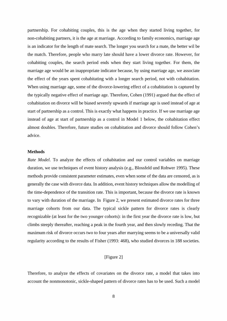
Rate Model. To analyze the effects of cohabitation and our control variables on marriage

duration, we use techniques of event history analysis (e.g., Blossfeld und Rohwer 1995). These

methods provide consistent parameter estimates, even when some of the data are censored, as is

generally the case with divorce data. In addition, event history techniques allow the modelling of

the time-dependence of the transition rate. This is important, because the divorce rate is known

to vary with duration of the marriage. In Figure 2, we present estimated divorce rates for three

marriage cohorts from our data. The typical sickle pattern for divorce rates is clearly

recognizable (at least for the two younger cohorts): in the first year the divorce rate is low, but

climbs steeply thereafter, reaching a peak in the fourth year, and then slowly receding. That the

maximum risk of divorce occurs two to four years after marrying seems to be a universally valid

regularity according to the results of Fisher (1993: 468), who studied divorces in 188 societies.

[Figure 2]

Therefore, to analyze the effects of covariates on the divorce rate, a model that takes into

account the nonmonotonic, sickle-shaped pattern of divorce rates has to be used. Such a model

9

r(t) ' ct e &t/8,

c ' "0"X1

1 "X2

2 ..."Xm

m .

is the sickle model. It assumes the following parametric function of the divorce rate r(t)

(Diekmann and Mitter 1984):

whereby

X1, ..., Xm denote covariates while "0, ..., "m are relative risk effects to be estimated empirically.

("k - 1) @ 100 can be interpreted as the percentage effect of the covariate k on the divorce rate.

If " > 1 (" < 1), there is a positive (negative) influence of a covariate on the risk of divorce. The

parameter 8 provides an estimate of the time at which a peak in the divorce rate occurs.

Moreover, the model allows for “immunity,” that is, for the fact that many marriages never end

in divorce. In comparison with other two-parameter models, the sickle model yields a very good

fit for divorce data (Diekmann and Mitter 1984).

X1 will be the cohabitation dummy. The trial marriage hypothesis predicts that "1 will be less

than one, that is, that cohabitation decreases the divorce rate (the cohabitation effect is negative).

Contrary to this, according to the self-selection hypothesis, the estimate of "1 might be greater

than one (positive cohabitation effect). This positive effect is spurious, however. The estimate

should decline if we control for traits by which cohabitors self-select. If our measures of these

traits are valid, the estimate of "1 should eventually become less than one.

In the presence of censored observations, the maximum likelihood method provides consistent

and asymptotically normally distributed estimates for the parameters. To estimate the effects of

covariates that vary with marriage duration, we use the technique of episode splitting. The

program Transition Data Analysis (TDA) written by Götz Rohwer is employed to obtain the ML

estimates (cf. Blossfeld and Rohwer 1995).

Bivariate Probit Model. Two strategies have been proposed to estimate the simultaneous

equation model depicted in Figure 1. Lillard proposes a simultaneous transition rate model

(Lillard 1993; Lillard et al. 1995). Holm-Larsen and Rohwer (1993) discuss a similar transition

10

c (

i ' $)

1 x1i % g1i ,

d (

i ' $)

2 x2i % (ci % g2i ,

ci ' 1, if c (

i > 0, ci ' 0, otherwise,

di ' 1, if d (

i > 0, di ' 0, otherwise.

∂∂

β φ βP c

Xx

jj

( )( )

== ′

1

rate model with correction for selectivity. However, these models have not yet been tested

sufficiently regarding robustness and convergence characteristics. Our own experience with such

models is that they do not converge, given reasonable convergence criteria. Therefore, we do not

use such models in this paper.

Kahn and London (1991) dealt with a similar self-selection problem: the effect of premarital

sexual activity on divorce. They proposed estimating the simultaneous equations on the

probabilities of premarital sex and divorce via a bivariate probit model. In this paper we will

follow their suggestion and use the bivariate probit model to estimate the parameters in Figure

1. The formulae for this model are:

ci* and di

* symbolize the latent variables “cohabitation tendency” and “divorce tendency”. ci and

di are the observable and dichotomous “cohabitation” and “divorce” indicators for a person i. x1

and x2 are vectors of covariates, $$1 and $$2 are vectors of coefficients, and g1, g2 are bivariate

normally distributed error terms with mean 0, variance 1, and correlation D. We are primarily

interested in the cohabitation effect (. This will be biased, however, if we assume D = 0 as in the

univariate model. This bias will be removed by allowing for D … 0. Thus, the bivariate probit

model provides a solution for the self-selection problem.

We obtain the ML-estimates for this model by using LIMDEP (Greene 1995). To make

interpretation easier, the probit parameter estimates were transformed to “marginal effects.” For

instance, the effect of Xj on the probability of cohabitation is computed by the following formula

(evaluated at the mean value of the covariate vector):

Marginal effects indicate approximately by how many percentage points the cohabitation

probability changes if the independent variable increases by a unit.

11

Note that, by using the bivariate probit model, we have departed from the event history

framework used above. There, we were using information on the exact timing of divorce; here,

a dichotomous divorce indicator. This indicator should not be derived from the answer to the

question “Was a divorce ever observed?” but from “Was a divorce observed after t years?” For

our analyses, we defined t as being equal to 7. That is, 1 means that a marriage was divorced

within its first 7 years, a 0, that it lasted at least 7 years. Consequently, we had to restrict our

sample to the marriage cohorts 1949–80. We also had to exclude widowed persons, whose

marriage did not last at least 7 years. This left us with 4,830 marriages of which 13.9 percent

cohabited and 5.7 percent ended in divorce after 7 years.

Empirical Results

Bivariate Analysis

Firstly, we will consider a simple bivariate comparison of survivor functions for marriages with

and without previous cohabitation. Figure 3 plots these survivor functions. To control for the

increasing incidence of cohabitation over time we only look at the 1971–1988 marriage cohorts

(otherwise the younger cohorts with higher divorce rate would be over-represented amongst

cohabitors). It is clear that the two types of marriages differ significantly: Marriages with

cohabitation prior to the wedding are less stable than those without previous trial marriages.

After 10 years, the proportions of those having divorced amount to 15 and 10 percent

respectively. This is also confirmed by an application of the parametric sickle model to our data

(Table 1, Model 0). Compared to marriages without cohabitation, the divorce rate of marriages

with premarital cohabitation is higher by a factor of 2.28. Thus, the bivariate analyses show the

astounding, yet well-known result that previously cohabiting partners have a higher risk of

divorce.

[Figure 3 here]

Controlling for Self-Selection

As argued with the self-selection hypothesis, the bivariate cohabitation effect is spurious.

Therefore, we add a set of standard control variables. Model 1 in Table 1 gives the results. The

correlation between cohabitation and risk of divorce declines in the multivariate analysis, but is

still positive. The divorce rate is 34 percent higher for marriages with cohabitation. Effects of

12

similar magnitude have been reported for other countries (e.g., Bennett et al. 1988; DeMaris und

Rao 1992; Trussel et al. 1992; Bracher et al. 1993). At first glance, these results clearly

contradict the trial marriage hypothesis. However, the drastic reduction in the size of the

cohabitation effect from Model 0 to Model 1 suggests that cohabiting couples are self-selected

towards characteristics associated with a higher divorce risk. We control for some of these

characteristics in Model 1, but there is much room for unobserved characteristics by which

cohabiting couples self-select, as shown by the pseudo R2 value of only 5.7 percent.

[Table 1 here]

We obtain a first hint of the existence of such unobserved factors through the second multivariate

model that includes two indicators of personal attitudes: an index of attitudes towards marriage

and an indicator of religiosity. The mean comparisons presented in Table 2 reveal lower degrees

of marital orientation and religiosity among cohabiting respondents on average. For marriages

not divorced at the time of the interview, these differences are highly significant (we do not

present tests for divorced marriages because the direction of causality might be reversed for

them). Now we incorporate these two indicators into Model 1. Model 2 in Table 1 gives the

results. Both indicators have strong, divorce-rate lowering effects. Consequently, the

cohabitation effect declines even further and becomes non-significant. The lower marriage

orientation and religiosity of cohabitors explain part of the cohabitation effect (see also Booth

and Johnson 1988). This is a first hint that the positive correlation between cohabitation and

divorce risk is due to the fact that cohabiting persons are a selected group. We say “hint,”

because the cohabitation effect is still not less than one. We would argue that this is due to our

two indicators not being perfect measures for the self-selected traits. In addition, they also have

the problem that they are measured at time of interview, not at time of the marriage, as would

have been preferable. Given the imperfect nature of these two indicators, they are not used

further in the following.

[Table 2 here]

Effects of Controls. Besides the cohabitation effect, the analysis presented in Table 1 (Model 1)

provides some interesting results not previously observed in German divorce studies (e.g.,

13

Diekmann und Klein 1991; Wagner 1993). Firstly, consider the couple-specific variables in the

second panel of Table 1. Our model reproduces the well-known fact that divorce rates increased

steadily after the Second World War, as can be seen by the monotonic increasing cohort effects.

Divorce rates in towns, and especially in villages, are much lower than in large cities. The village

effect of 0.54 means that the divorce rate is 46 percent lower in villages than in large cities.

Catholic couples have a lower divorce risk, couples without religious affiliation a higher one.

Heterogamous couples (regarding religion and nationality) have higher divorce rates. Age at the

start of the partnership has a strong effect: the older the partners are, the lower the divorce rate.

Education shows no effects. The same is true for premarital birth, but the birth of a child during

marriage lowers the divorce rate drastically (this effect might be overestimated due to

self-selection, cf. Lillard 1993). The respondent-specific origin variables in panel three of Table

1 all increase the divorce rate. Having no siblings and being of higher social origin increases

divorce risk. The same is true for respondents from incomplete families, especially for those,

whose parents were divorced by the time the respondent was aged 15 (more on this

“transmission effect” can be found in Diekmann und Engelhardt 1999).

Methodological Note. At this point, a methodological objection must be dealt with: Some

authors (e.g., Teachman und Polonko 1990) argue that cohabitation simply increases the divorce

rate because previously cohabiting marriage partners live together longer. This argument,

however, is incorrect because the cohabitation time is not included in the risk set (only

“successful” cohabitation is included in our sample). However, it could be argued that most

cohabiting couples start their marriage right in the “high risk” period, two or three years after the

start of their relationship. This is not taken into account by the standard approach, where time

starts at zero with the beginning of marriage for all observations. If we let time start at the

number of cohabitation years (conditional likelihood) and re-estimate Model 1, we actually then

see that the cohabitation effect is reduced substantially to 1.13 (t-value 1.20). This is even more

in accordance with our argument that the cohabitation effect should decline in a multivariate

model. Nevertheless, we prefer the standard modelling approach because it is easier to

understand.

Indirect Tests of the Self-Selection Hypothesis

In the following, we will derive two indirect tests that could possibly reinforce the self-selection

14

argument. Our first argument is based on the fact that the proportion of marriages with

premarital cohabitation has increased over time. In our data, this proportion has increased from

under 10 percent for the marriage cohorts before 1970 to more than 50 percent for the most

recent marriage cohorts. Obviously, strong no-cohabit norms existed in former times and those

who nonetheless cohabited were those with unconventional attitudes. In more recent cohorts,

these norms declined and the decision to cohabit was no longer an indicator of unconventionality.

Therefore, if the self-selection theory is correct, we would expect much stronger cohabitation

effects in older cohorts in Germany because cohabitors were much more unusual in those days

(this argument was put forward by Schoen 1992).

To investigate this argument empirically, we add interaction effects for cohabitation and marriage

cohort to Model 1. The results (Table 3, panel one) confirm this hypothesis. Cohabiting couples

from the 1970s and 1980s show lower effects than the cohorts from the 1950s and 1960s (the

difference is not significant, however). Their divorce rates become almost equal to those who did

not cohabit. (Note that, in Table 3, cohabiting couples from the 1950s and 1960s are the

reference group. Consequently, the effect for “no cohabitation” is lower than one.)

It is an interesting digression to look at a second implication of this argument. For societies

where premarital cohabitation became the norm, we would expect that non-cohabitors are the

special group. This seems to be the case for Sweden. As Hoem and Hoem (1992) demonstrate,

the divorce rate difference between cohabitors and non-cohabitors increased over cohorts.

A second indirect test of the self-selection argument follows from the additional argument that

those with more than one cohabitation should be an even more self-selected group (Bennett et al.

1988; Teachman and Polonko 1990). That is, these respondents already displayed in their

behavior that they are more separation prone. Therefore, we would expect that multiple

cohabitors show even higher divorce rates than single cohabitors. Panel two in Table 3 shows

that this group actually does have a higher divorce risk compared to those who cohabited only

with their first spouse. However, the effect is not significant.

[Table 3 here]

15

Indirect Tests of the Trial Marriage Hypothesis

Next, we will consider three indirect tests of the information argument from family economics.

Firstly, some respondents cohabited for some time before their first marriage, but not with their

spouse (N = 74). Those should be self-selected in a similar way compared to those respondents

who only cohabited with their spouse. However, this group clearly lacks the more reliable

information about the spouse which is obtained by living together before marriage. There simply

was no trial marriage. Thus, they should have a higher divorce risk. The difference could even be

interpreted as the „pure“ trial marriage effect (if both groups are really self-selected in a similar

way; an assumption that we cannot test). Panel two in Table 3 shows that the divorce rate of

those not having cohabited with their spouse is higher by a factor of 1.87. With some

reservation, we can conclude that a trial marriage with the spouse seems to provide information

that reduces the divorce rate (a counterargument could be that those cohabiting not with the

spouse have already experienced a separation, what might increase their divorce proneness).

According to the information argument, one would also expect that the longer the trial marriage

lasts, the lower the risk of divorce. The reason for this is that the longer cohabitation lasts, the

more reliable the information gained will be. To test this hypothesis, we add three dummies that

differentiate cohabitors by the length of their cohabitation to Model 1. Panel three in Table 3

gives the results. It can be seen clearly that those with longer cohabitation have lower divorce

rates. Those cohabiting for four years or more no longer differ from those with no cohabitation

(see also Bennett et al. 1988; Lillard et al. 1995). Although these effects are not significant, the

pattern at least supports the information argument.

A third test of the information argument departs from the observation that a child born in a

non-marital partnership increases the probability of marriage (Blossfeld 1995: 20). When a child

is on its way, some cohabitors might marry even though the information-gathering process is not

yet complete. Consequently, cohabitors with a premarital child should show higher divorce rates.

Panel four in Table 3 provides an empirical test of this hypothesis. It shows that there is a non-

significant difference in the expected direction.

Overall, the results of these five indirect tests are fully compatible with our argument: A trial

marriage provides information that lowers the divorce rate of a subsequent marriage.

16

Self-selection obscures this in the standard regression approach. The evidence, however, is only

indirect in that it relies on additional assumptions. Nevertheless, such a consistent picture as we

observe it in Table 3 strongly increases our confidence in the argumentation. The most direct

evidence is the result that cohabitation with the spouse decreases the divorce rate drastically

(compared to those cohabiting with another person). This demonstrates most directly the

informational value of a cohabitation.

A Simultaneous Model

The estimation results of the bivariate probit model appear in Table 4. The specification is similar

to Model 1 in Table 1, with the exception that “no siblings” and “child before marriage” were not

included due to their non-significant effects. In addition, we excluded “education” from the

divorce equation to make identification of the model easier. The first two columns are from the

single-equation probits, the last two are simultaneously estimated with a bivariate probit model.

[Table 4 here]

We include the single equation estimates as a comparison. The results for cohabitation are very

similar, but they differ for divorce. This demonstrates that single-equation models are potentially

misleading for these data. The cohabitation effect changes dramatically. The single equation

divorce probit shows a small positive cohabitation effect. This is not completely in line with the

result from the divorce rate model in Table 1, but it would still suggest that the trial marriage

hypothesis is wrong. However, if we allow for correlated error terms and estimate a bivariate

probit model the cohabitation effect becomes (non-significantly) negative (the same result was

obtained by Lillard et al. (1995) using a simultaneous transition rate model). As predicted by the

trial marriage hypothesis, cohabitation reduces the probability of divorce. The single equation

estimates are biased because they do not allow for correlated error terms that are due to self-

selection. This refined statistical model finally provides us with some direct evidence that the trial

marriage hypothesis is correct.

Before concluding, let us take a brief look at some further results of the bivariate probit in Table

4. The first thing to note is that most effects are in the same direction for cohabitation and

divorce. This supports the argument underlying our self-selection theory because it shows that

17

most factors that increase the probability of a divorce also increase the probability of

cohabitation. This is also valid for the unmeasured variables as suggested by the positive estimate

of D.

Finally, let us take a closer look at the cohabitation part of the bivariate probit. These results

inform us about the factors that determine the probability of a (premarital) cohabitation. We can

see that the probability of cohabitation is lower in rural areas and among Catholics. The opposite

is true for people with no denomination and for women with higher education. These results are

well in accordance with those obtained by other studies on those entering into cohabitation (e.g.,

Bumpass und Sweet 1989; Bumpass et al. 1991; Thornton 1991; Clarkberg et al. 1995).

Conclusion

Taken together, we think that these results show that the information argument put forward by

family economists is correct. Premarital cohabitation provides information which allows for a

more precise estimate of match quality with the prospective spouse. Therefore, marriages with

prior cohabitation will be more stable on average. Demonstrating this is not easy, however. A

simple comparison of couples who cohabited with those who did not shows that the former have

higher divorce rates. By using several indirect tests and a more direct bivariate probit model, we

demonstrated that this is due to self-selection. Cohabitors have characteristics that increase the

probability of divorce. This overcompensates the stabilizing effect of a trial marriage.

The secular increase in divorce rates in most industrialized countries, therefore, cannot be

explained by the growing prevalence of premarital cohabitation. On the contrary, according to

our results cohabitation is a counteracting factor. Divorce rates would be even higher if trial

marriages had not become a common demographic phenomenon.

We want to conclude by discussing three problems of our study. First, we argued that cohabitors

differ from non-cohabitors already before they start to cohabit. However, we cannot rule out the

possibility that they become different while cohabiting. The latter would mean that cohabitation

has two opposing causal effects: making people more divorce prone and providing them with

information on their potential mate. Though we think these arguments are not very plausible, a

stringent empirical test would be only possible by using panel data (cf. Axinn and Thornton

18

1992).

Second, our analysis also delivers a methodological message. Sociologists and demographers

using non-experimental survey data have to be much more aware of the possibility of self-

selection to avoid incorrect causal conclusions. For that purpose, indirect tests are necessary as

well as more refined statistical models that take self-selection into account, as we demonstrated

in this paper. However, an even more preferable way for tackling self-selection would be better

measurement. There would be no need for refined statistical models if one could measure those

characteristics on which respondents self-select. Thus, the problems we have in disentangling

self-selection from causal effects are an important argument for putting more effort into

collecting better data.

Third, we argued in another paper that standard divorce models as we use them in this paper are

misspecified (Brüderl et al. 1999). Two of these specification improvements we already

discussed in this paper: using age at start of partnership and the conditional likelihood approach.

A third improvement is the inclusion of two additional information indicators (how long the

mates knew each other before beginning the relationship, and how long they had a relationship

before starting to live together). All these improvements together have the consequence that the

cohabitation effect is already significantly negative in Model 1. This means that we do not need

the indirect tests and simultaneous models of this paper to show that cohabitation provides

information that increases the stability of a subsequent marriage.

19

References

Axinn, William G., and Arland Thornton, 1992: The Relationship Between Cohabitation and Divorce:Selectivity or Causal Influence? Demography 29: 357–374.

Balakrishnan, T. R., K. Vaninadha Rao, Evelyne Lapierre-Adamcyk and Karol J. Krotki, 1987: A HazardModel Analysis of the Covariates of Marriage Dissolution in Canada, Demography 24: 395–406.

Becker, Gary S., 1991: A Treatise on the Family. Cambridge: Harvard University Press.Becker, Gary S., Elisabeth M. Landes and Robert T. Michael, 1977: An Economic Analysis of Marital

Instability, Journal of Political Economy 85: 1141–1187.Bender, Donald, Walter Bien and Hiltrud Bayer, 1996: Wandel und Entwicklung familialer

Lebensformen: Datenstruktur der DJI-Familiensurvey. Munich: unpublished paper.Bennett, Neil G., A. K. Blanc and David E. Bloom, 1988: Commitment and the Modern Union: Assessing

the Link Between Premarital Cohabitation and Subsequent Marital Stability, AmericanSociological Review 53: 127–138.

Blossfeld, Hans-Peter, 1995: Changes in the Process of Family Formation and Women's GrowingEconomic Independence: A Comparison of Nine Countries. pp. 3–32 in: Hans-Peter Blossfeld(ed.): The New Role of Women: Family Formation in Modern Societies. Boulder: Westview.

Blossfeld, Hans-Peter, and Götz Rohwer, 1995: Techniques of Event History Modeling: New Approachesto Causal Analysis. Hillsdale, N.J.: Lawrence Erlbaum.

Booth, Alan, and David Johnson, 1988: Premarital Cohabitation and Marital Success, Journal of FamilyIssues 9: 255–272.

Bracher, Michael, Gigi Santow, S. Philip Morgan and James Trussell, 1993: Marriage Dissolution inAustralia: Models and Explanations, Population Studies 47: 403–425.

Brüderl, Josef, Andreas Diekmann and Henriette Engelhardt, 1999: Artefakte in derScheidungsursachenforschung? Eine Erwiderung auf einen Artikel von Yasemin Niephaus,Kölner Zeitschrift für Soziologie und Sozialpsychologie 51: 744-753.

Bumpass, Larry L., and James A. Sweet, 1989: National Estimates of Cohabitation, Demography 26:615–625.

Bumpass, Larry L., James A. Sweet and Andrew Cherlin, 1991: The Role of Cohabitation in DecliningRates of Marriage, Journal of Marriage and the Family 53: 913–927.

Clarkberg, Marin, Ross M. Stolzenberg and Linda J. Waite, 1995: Attitudes, Values, and Entrance intoCohabitational versus Marital Unions, Social Forces 74: 609–634.

Cohen, Blair A., 1991: Using Age at First Union to Explain the Relationship Between Cohabitation andDivorce. Population Studies Center, University of Michigan, Research Report No. 91–209.

Cunningham, John D., and John K. Antill, 1994: Cohabitation and Marriage: Retrospective and PredictiveComparisons, Journal of Social and Personal Relationships 11: 77–93.

DeMaris, Alfred, and K. Vaninadha Rao, 1992: Premarital Cohabitation and Subsequent Marital Stabilityin the United States: A Reassessment, Journal of Marriage and the Family 54: 178–190.

DeMaris, Alfred, and William MacDonald, 1993: Premarital Cohabitation and Marital Instability: A Testof the Unconventionality Hypothesis, Journal of Marriage and the Family 55: 399–407.

Diekmann, Andreas, and Henriette Engelhardt, 1999: The Social Inheritance of Divorce: Effects ofParent‘s Family Type in Postwar Germany, American Sociological Review 64: 783–793.

Diekmann, Andreas and Thomas Klein, 1991: Bestimmungsgründe des Ehescheidungsrisikos: Eineempirische Untersuchung mit den Daten des sozioökonomischen Panels, Kölner Zeitschrift fürSoziologie und Sozialpsychologie 43: 271–290.

Diekmann, Andreas and Peter Mitter, 1984: A Comparison of the „Sickle Function“ with AlternativeStochastic Models of Divorce Rates. pp. 123–153 in: Andreas Diekmann and Peter Mitter (eds.):Stochastic Modelling of Social Processes. Orlando: Academic Press.

Fisher, Helen, 1993: Anatomie der Liebe. München: Droemer Knaur.Gostomski, Christian Babka von, Josef Hartmann and Johannes Kopp (1998) Soziostrukturelle

Bestimmungsgründe der Ehescheidung, Zeitschrift für Sozialisationsforschung undErziehungssoziologie 18: 117–133.

20

Greene, William, 1995: LIMDEP, 7.0. User’s Manual. New York: Econometric Software.Hall, Anja, 1997: ‘Drum prüfe, wer sich ewig bindet’: Eine empirische Untersuchung zum Einfluß

vorehelichen Zusammenlebens auf das Scheidungsrisiko, Zeitschrift für Soziologie 26: 275–295.Hall, David R., and John Z. Zhao, 1995: Cohabitation and Divorce in Canada: Testing the Selectivity

Hypothesis, Journal of Marriage and the Family 57: 421–427.Hoem, Britta, and Jan M. Hoem, 1992: The Disruption of Marital and Non-Marital Unions in

Contemporary Sweden. pp. 61–93 in: James Trussell, R. Hankinson and J. Tilton (eds.):Demographic Applications of Event History Analysis. Oxford: Clarendon Press.

Holm Larsen, Anders, and Götz Rohwer, 1993: Self Selection in Transition Rate Models. Bremen: TDAWorking Paper 5–8.

Kahn, Joan R., and Kathryn A. London, 1991: Premarital Sex and the Risk of Divorce, Journal ofMarriage and the Family 53: 845–855.

Kopp, Johannes, 1994: Scheidung in der Bundesrepublik: Zur Erklärung des langfristigen Anstiegs derScheidungsraten. Wiesbaden: Deutscher Universitäts-Verlag.

Lillard, Lee A., 1993: Simultaneous Equations for Hazards: Marriage Duration and Fertility Timing,Journal of Econometrics 56: 198–217.

Lillard, Lee A., Michael J. Brien and Linda J. Waite, 1995: Premarital Cohabitation and SubsequentMarital Dissolution: A Matter of Self-Selection? Demography 32: 437–457.

Rindfuss, Ronald R. and Audrey VandenHeuvel, 1990: Cohabitation: A precursor to marriage or analternative to being single? Population and Development Review 16: 703–726.

Schoen, Robert, 1992: First Unions and the Stability of First Marriages, Journal of Marriage and theFamily 54: 281–284.

Teachman, Jay D., and Karen A. Polonko, 1990: Cohabitation and Marital Stability in the United States,Social Forces 69: 207–220.

Teachman, Jay D., Jeffrey Thomas and Kathleen Paasch, 1991: Legal Status and the Stability ofCoresidential Unions, Demography 28: 571–586.

Thomson, Elizabeth, and Ugo Colella, 1992: Cohabitation and Marital Stability: Quality or Commitment?Journal of Marriage and the Family 54: 259–267.

Thornton, Arland, 1991: Influences of the Marital History of Parents on the Marital and CohabitationalExperiences of Children, American Journal of Sociology 96: 868–894.

Trussell, James, and K. Vaninadha Rao, 1989: Premarital Cohabitation and Marital Stability: AReassessment of the Canadian Evidence, Journal of Marriage and the Family 51: 535–544.

Trussell, James, German Rodriguez and Barbara Vaughan, 1992: Union Dissolution in Sweden. pp.38–60 in: James Trussell, R. Hankinson and J. Tilton (eds.): Demographic Applications of EventHistory Analysis. Oxford: Clarendon Press.

Vaskovics, Laszlo A., and Marina Rupp, 1995: Partnerschaftskarrieren: Entwicklungspfadenichtehelicher Lebensgemeinschaften. Opladen: Westdeutscher Verlag.

Wagner, Michael, 1993: Soziale Bedingungen des Ehescheidungsrisikos aus der Perspektive desLebensverlaufs. pp. 372–393 in: Andreas Diekmann and Stefan Weick (eds.): Der Familienzyklusals sozialer Prozeß. Berlin: Duncker & Humblot.

White, Lynn, 1990: Determinants of Divorce: A Review of Research in the Eighties. Journal of Marriageand the Family 52: 904–912.

Table 1: Models for the Divorce Rate of German Marriages (Sickle Models,Relative Risks): German Family Survey, Marriage Cohorts 1949–1988

Mean Model 0 Model 1 Model 2

Premarital cohabitation(|t|-value)

21.9% 2.28***(9.56)

1.34**(3.02)

1.21(1.92)

Marriage cohorts 1961–70 32.2% 1.83*** 1.59***

Marriage cohorts 1971–80 31.7% 2.44*** 1.80***

Marriage cohorts 1981–88 21.3% 2.86*** 2.02***

Living in village (-5,000 inhabit.) 14.4% 0.54*** 0.71*

Living in town (5,000–100,000) 27.1% 0.75** 0.88

Catholic couple 32.8% 0.71*** 0.83

Couple without denomination 4.5% 2.10*** 1.60***

Couple with mixed denomination 26.2% 1.27** 1.24*

Partner is foreigner 3.1% 1.64** 1.74**

Age at start of partnership (man) 24.69 0.96*** 0.97*

Age at start of partnership (woman) 22.15 0.91*** 0.92***

Years of education (man) 9.92 0.94 0.92**

Years of education (woman) 9.69 1.00 0.94

Child born before marriage 6.2% 0.93 0.93

Birth of first child (time varying) 75.0% 0.42*** 0.44***

No siblings 10.8% 1.29* 1.33**

Father completed high-school 7.7% 1.53** 1.38*

No parents 3.1% 1.53* 1.55*

One parent 9.6% 1.27* 1.15

Divorced parents 2.4% 1.71** 1.55*

Church attendance 21.4% 0.64***

Index of marriage orientation 9.29 0.77***

Constant "0 0.00 0.11 1.37

Ponstant 8 7.84 10.28 11.25

Pseudo R2 0.9% 5.7% 9.4%

Number of marriages 6179 5846 5786

Number of splits 10183 10080

* statistically significant at the 5% level, ** 1%-level, *** 0.1% level (two-sided test). Pseudo R2 iscomputed as the relative likelihood improvement compared to the model without covariates.

Table 2: Means of Attitude Variables for Persons with and without Cohabitation:German Family Survey, Marriage Cohorts 1949–1988

Not divorced Divorced

Cohabitation Without With Without With

Church attendance 26.6%***

10.5% 10.1% 7.7%

Index of marriage orientation 9.79***

8.54 7.88 7.45

Number of marriages 4076 1173 577 182

*** statistically significant difference at the 0.1% level (two-sided test). Tests are onlyperformed for marriages not divorced.

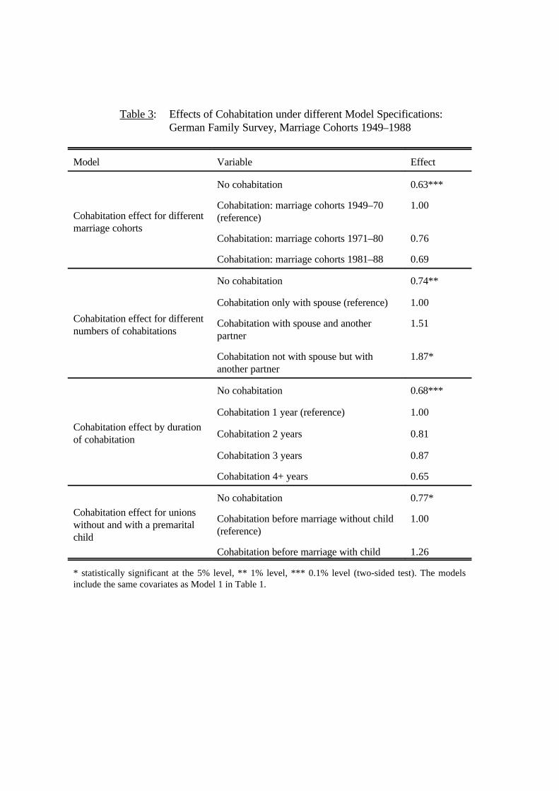
Table 3: Effects of Cohabitation under different Model Specifications:German Family Survey, Marriage Cohorts 1949–1988

Model Variable Effect

Cohabitation effect for differentmarriage cohorts

No cohabitation 0.63***

Cohabitation: marriage cohorts 1949–70(reference)

1.00

Cohabitation: marriage cohorts 1971–80 0.76

Cohabitation: marriage cohorts 1981–88 0.69

Cohabitation effect for differentnumbers of cohabitations

No cohabitation 0.74**

Cohabitation only with spouse (reference) 1.00

Cohabitation with spouse and anotherpartner

1.51

Cohabitation not with spouse but withanother partner

1.87*

Cohabitation effect by durationof cohabitation

No cohabitation 0.68***

Cohabitation 1 year (reference) 1.00

Cohabitation 2 years 0.81

Cohabitation 3 years 0.87

Cohabitation 4+ years 0.65

Cohabitation effect for unionswithout and with a premaritalchild

No cohabitation 0.77*

Cohabitation before marriage without child(reference)

1.00

Cohabitation before marriage with child 1.26

* statistically significant at the 5% level, ** 1% level, *** 0.1% level (two-sided test). The modelsinclude the same covariates as Model 1 in Table 1.

Table 4: A Simultaneous Model for the Probabilities of Cohabitation and Divorce (Marginal Effects):German Family Survey, Marriage Cohorts 1949–1980

Probit Cohabitation

Probit Divorce

Bivariate Probit Cohabitation Divorce

Cohabitation before marriage(|t|-value)

0.005(0.83)

-0.085(1.35)

Marriage cohorts 1961–70 0.024 0.024** 0.024 0.030**

Marriage cohorts 1971–80 0.162*** 0.040*** 0.162*** 0.071***

Living in village (-5,000 inhab.) -0.053*** -0.026** -0.054*** -0.038***

Living in town (5,000–100,000) -0.049** -0.009 -0.049*** -0.018*

Catholic couple -0.060*** -0.027*** -0.060*** -0.040***

Couple without denomination 0.058** 0.026** 0.058** 0.039***

Couple with mixed denomination -0.004 0.007 -0.004 0.008

Partner is foreigner 0.044 -0.001 0.042 0.009

Years of education/10 (man) -0.012 -0.003

Years of education/10 (woman) 0.115* 0.113*

Age at start of union/10 (man) -0.016 -0.017

Age at start of union/10 (woman) -0.053*** -0.059***

Child born during first 7 years -0.062*** -0.071***

Father completed high school 0.034* 0.007 0.033 0.015***

No parents 0.039 0.029** 0.039 0.039**

One parent 0.020 0.018* 0.022 0.023*

Divorced parents 0.047 0.012 0.046 0.021

Correlation coefficient 0.59

Pseudo R2 9.8% 17.5% 12.6%

-Log-likelihood 1641.5 828.0 2468.4

Number of marriages 4577 4577 4577

* statistically significant at the 5% level, ** 1% level, *** 0.1% level (two-sided test). Pseudo R2 is computed as therelative likelihood improvement compared to the model without covariates.

marriage cohortfamily of origin

regiondenomination

P(divorce)marriage age

P(cohabitation)

$1 (

$2 $2 child

unobservables

unobservables

D

Figure 1: A Model of the Relationship of Cohabitation and Divorce

Diese Datei enthält Daten fürfür PostScript-Drucker geeignet

Figure 2: Life-table Divorce Rates for three German Marriage Cohorts:German Family Survey, Marriage Cohorts 1949-1988

Diese Datei enthält Daten fürfür PostScript-Drucker geeignet

Figure 3: Proportion of Marriages not Divorced (Kaplan-Meier Estimates; 95% ConfidenceInterval Shaded): German Family Survey, Marriage Cohorts 1971–1988