Polynomial Datapath Synthesis and Optimization Based on Vanishing Polynomial over Z2

m and Algebraic Techniques

Samaneh Ghandali1, Bijan Alizadeh1, Zainalabedin Navabi1, Masahiro Fujita2

1School of Electrical and Computer Engineering, University of Tehran, Tehran, Iran 2VLSI Design and Education Center (VDEC), University of Tokyo, Tokyo, Japan

s.ghandali@ece.ut.ac.ir, b.alizadeh@ece.ut.ac.ir, navabi@cad.ece.ut.ac.ir, fujita@ee.t.u-tokyo.ac.jp

Abstract— The growing market for Digital Signal Processing (DSP), Computer graphics and embedded systems applications that can be modeled as polynomial computations in their datapath designs, requires improvements in high-level synthesis and optimization techniques for such systems. This paper concentrates on how to find common sub-expressions between s given polynomial functions over … in order to optimize the area and delay as much as possible. Our main contributions in this paper is proposing an optimization method based on adding/deleting vanishing polynomials over Z2

m, i.e., those polynomials that are equivalent to zero over Z2m,

to/from given polynomial functions in the hope of achieving further common sub-expressions. After applying our optimization techniques, experimental comparisons with the state-of-the-art techniques show an average improvement in the area by 36.80% with an average delay decrease of 2.41%. Regarding the comparison with our previous works, the area and delay are improved by 21.4% and 8.7% respectively.

Keywords-component; High-level synthesis, finite ring algebra, modular optimization, polynomial datapath

I. INTRODUCTION As the complexity and size of modern embedded

application is continuously increasing, designing hardware at higher levels of abstraction for faster design adjustments and higher simulation speed is necessary. Conventional high level synthesis techniques are not efficient to eliminate redundancy and common sub-expression for polynomial datapaths over

. Such polynomial functions have been optimized manually to achieve efficient register-transfer-level (RTL) implementation. This process can be time consuming and error prone. Hence, developing high level synthesis and optimization techniques to automate the design of custom polynomial datapaths from a behavioral description is desirable.

Such polynomial functions have been used in different areas such as encryption, error coding and management, security and etc. As it is noted in [8], Many subjects in combinatorial study such as homomorphisms between combinatorial objects, the (edge) colorings of labeled graphs, and the m-ary code words in coding theory, can be considered as functions from … to can be used to represent more subjects in combinatorial study. For example, a labeled digraph with n vertices can be represented by a

function from to ; a labeled graph with n vertices and m edges can be represented by a function from to ; a Latin square of order n can be represented by a function from to ; a simple uniform hypergraph of rank r with n vertices (refer to [9] for definition) can be represented by a function from to ; a code of length r over an n-element alphabet can also be represented by a function from to .

In addition to the above mentioned applications, polynomials are widely used in real embedded systems such as DSP, image processing, and automotive applications. For instance, multivariate Cosine Wavelet in graphic applications, digital image rejection unit and Savitzky-Golay filters in image processing applications. Quartic filters in DSP applications. Phase-Shift Keying in digital communication makes use of such polynomial arithmetic in their computations. By considering these important applications, introducing new algorithms for high level synthesis and optimization of polynomial datapaths is valuable and necessary.

This paper concentrates on more efficient ways to extract common sub-expressions between given polynomial functions from … to in order to save the area and delay as much as possible. Adding/deleting vanishing polynomials is a technique similar to logic optimization based on redundancy addition/removal which has been developed in logic synthesis area. In this paper for the first time, we are proposing a kind of polynomial optimization based on redundancy addition/removal on the fixed bit-width polynomial computation. One way to extract better common sub-expressions is to consider polynomials over finite ring. The basic idea is the fact that if we are to use the original polynomials along with different related vanishing polynomials, we may get more opportunities to extract better common sub-expressions. For example, let us consider P = 6x3+x2y+x2z-11x2+6x+yz over Z2

3. It can be factored out as P = (x2+z)×(x2+y) if P + Y4(x) is taken into account where Y4(x)=x×(x-1)×(x-2)×(x-3) is a vanishing polynomial over Z2

3, i.e., Y4(x) mod 23 = 0. In other words, we add or remove a large number of vanishing polynomials to or from each of the given polynomials without changing their values, and generating the large equivalent polynomials for each input polynomial. This means that instead of using the input

65978-1-4673-1313-1/12/$31.00 ©2012 IEEE

polynomials, we use a large equivalence class of polynomials for each input polynomial. The main question we would like to answer in this paper is how to determine such vanishing polynomials so that further saving in terms of area and delay can be achieved.

In summary, our main contributions in this paper are as follows:

• Proposing a vanish-based optimization technique to assess suitable vanishing polynomials which helps us to select more suitable common sub-expressions.

• Generating a large set of vanishing polynomials which do not change the value of the given polynomial expressions but aid in their factorization. In other words, to obtain more common sub-expressions and hence more optimization, we generate a large equivalence class of polynomials for each input polynomial by adding or deleting a large number of vanishing polynomials to or from them.

• Using a kernel-based common sub-expression extraction technique which helps us to extract suitable common sub-expressions.

• Evaluating the performance of the proposed optimization techniques and showing their effectiveness by comparing them with the state-of-the-art polynomial optimization methods in the literature.

In the rest of this section, some related works in this area are described briefly.

Although Horner form is a popular representation of polynomial functions, symbolic computer algebra based manipulation and factorization with Common Sub-expression Elimination (CSE) are much better techniques to optimize polynomial functions in terms of the area and delay [1, 2, 3]. The CSE technique in [1] is a straightforward way of optimizing polynomial datapath designs. However, it is not able to efficiently extract those common sub-expressions that are not explicitly exposed in the original polynomials.

Another algebraic technique is based on kernel and co-kernel computation [6]. In this technique, first of all, polynomials are transformed to two different forms; that is, canonization form, and square-free factorization form. Then one solution from three existing solutions, i.e., original form, canonization and square-free factored form, is taken into consideration as an optimal solution that has the lowest cost of implementation and the optimization algorithm proceeds to the next step. In the next step, the optimization algorithm tries to find more common sub-expressions in two phases: 1) factorizing integer coefficients of each polynomial by using greatest common divisor concept and 2) extracting kernel/co-kernels of each polynomial after coefficient factorization. Finally, by using algebraic division algorithm, common sub-expressions are determined. In this method in the most real cases, canonization solution is selected in which all polynomials are represented based on their reduced forms over Z2

m which cannot be reduced any more. In spite of this

advantage, this form causes less common sub-expression among polynomials can be found. Another disadvantage of this method is that, common sub-expressions are searched in the expressions which are resulted in each polynomial after applying common coefficient extraction phase and not in the whole polynomial. The main difference of our proposed method with the work of [6] is expanding the equivalence set in a practical way. We use a large equivalence classes of vanishing polynomials over Z2

m , which do not alter the value of the expressions but aid in their factorization. This way, we can find more suitable common sub-expressions. The results we obtained in comparison with those reported in [6] show noticeable improvement in the area and critical path delay, as reported in Section IV.

The algebraic technique in [4] makes use of finite ring algebra and a canonical polynomial representation called Modular Horner Expansion Diagram (M-HED) [5] to fulfill modular polynomial synthesis and optimization. This technique first reduces the original polynomials over Z2

m. Then common sub-expressions are extracted based on two heuristics: 1) partitioning heuristic to partition each polynomial poly into three sub-polynomials p1, p2 and p3 so that poly = p1×p2 + p3 and 2) compensation heuristic to assess the coefficients in such a way that p3 is minimized. The main disadvantage of this technique is that decompositions are started from reduced polynomials over Z2

m while if we were to use the original polynomials we would get more degree of freedom to extract common sub-expressions.

The remainder of this paper is organized as follows. Section II introduces some definitions which are used in the rest of the paper, and describes some preliminaries. Section III explains, in detail, our proposed polynomial optimization technique. Section IV evaluates the performance of our algorithms and presents experimental results that demonstrate their effectiveness. Finally, section V provides our conclusion.

II. DEFINITIONS AND PRELIMINARIES In this paper arithmetic data paths are modeled as

polynomial functions from … to [7]. In general, represents the ring of integers modulo 2n which is written as = {0, 1, …, 2n-1}, Z denotes the ring of integers. Let ,…, be s given polynomial function from … to as the specification of the design, where =< x1,x2,…,xd > is a vector of d input variables and n1, n2, …, nd denote the size of the corresponding variables, so and . m is the size of the output bit-vector f, so .

Definition 1: A function from … to is said to be a polynomial function (from … to ) if it is represented by a polynomial F ∈ Z2

m[x1,…, xd], i.e. f ( , … , ) ≡ F( , … , ) for all xi = 0,1, . . . , 2 - 1; i = 1, 2, . . . , d.

A number theory result: For any , ! divides the product of n consecutive numbers, i.e., n! divides ∏ which is referred to as ! | ∏ .

For example 6! divides 6×5×4×3×2×1 , also 6! divides 89×90×91×92×93×94.

66

Definition 2: the least such that n divides k!, is denoted as SF(n), where SF denotes Smarandache function. In the ring Z2

m, let SF (2m) =k! i.e. 2m|k! [10,11]. For example, let n be 8, then for all values of k ≥ 4, k! is divided by n, i.e., 8|4!, so SF(8=23)=4.

Lemma 1: if F(x) over Z2m for all x can be exposed as a

product of SF(2m) consecutive numbers, then F(x) vanishes over Z2

m.

If F(x) is equivalent to 0 in Z2m, then 2m|F(x). Let 23|F(x),

but based on the previous example, since 4= SF(23), 23|4! too. Hence, if F(x) over Z2

3 for all x can be exposed as a product of 4 consecutive numbers, then F(x) vanishes over Z2

3 (i.e. F(x) is equivalent to 0 in Z2

3). For example, F(x) = x×(x-1)×(x-2)×(x-3) vanishes in Z2

3, because it represents a product of 4 consecutive numbers on all x.

Definition 3: The following equations define falling factorials of degree .

Y0(x) =1 Y1(x) =x

Y2(x) =x×(x-1) …

Yk(x) =Yk-1(x)×(x-k+1)

Definition 4: For multivariate expression with d variables (x1,x2,…,xd) over Z2

m, falling factorials are defined as (1).

… (1)

Lemma 2: A multivariate polynomial with d variables (x1,x2,…,xd) over Z2

m[x1,…, xd] vanishes (i.e. it is equivalent to 0 in Z2

m) if it can be represented as a product of SF(2m) consecutive number in at least one of the variables xi.

The proof of lemma 1 and 2 can be found in [7].

A. Vanishing polynomial In Lemma 2, we assume that all input and output variables

are in Z2m. Now let us consider the multivariate polynomials

over … to . In order to see whether or not such a multivariate polynomial vanishes, μi is defined as follows:

min 2 , 2 ; 1,2, … , (2)

In two cases, a multivariate polynomial vanishes over … to (i.e. it is equivalent to 0) [7]. These two cases are described in lemma 3 and Lemma 4.

Lemma 3: Let K= (k1, k2,…, kd) be the maximum degree of d variables ( , … , in a given polynomial , … , . F ( , … , , … , . … equal to 0 over … to if and only if there at least exists i (1≤i≤d) such that ki ≥ μi.

Example 1: F(x,y,z)=x4yz-6x3yz+11x2yz-6xyz over is a vanishing polynomial. That is because SF(23)=4, μ1=min(2,4)=2, μ2=min(22,4)=4, μ3=min(22,4)=4, and k1=4, k2=1, k3=1, so due to the value of k1 which is greater than μ1, F(x,y,z)=x(x-1)(x-2)(x-3)yz is a vanishing polynomial in .

Lemma 4: , … , , … ,… vanishes over… if ,∏ ! | , where C is an arbitrary integer, and gcd(x,y) computes the greatest common divisor of x and y.

Example 2: F(x,y,z)=8x2y2z-8x2yz-8xy2z+8xyz over vanishes because here F(x,y,z)=8Y(2,2,1), k1=2, k2=2, k3=1, and gcd 2 , ∏ !4, therefore C=8 divides ,∏ ! 2.

The proof of these two lemmas can be found in [7].

B. Canonization algorithm Each polynomial can be represented in a canonical form by

eliminating vanishing parts from the polynomial. Lemam 3 and Lemam 4 described in the previous section, account for the vanishing parts of a given polynomial.

Theorem 1: Let f be a polynomial function from … to . Then f can be uniquely represented by a polynomial.

where 1≤ak < ,∏ ! .

Its proof is available in [7].

(3)

Where Qi is a polynomial, Ck is an integer, and ak is an integer such that 1≤ak < ,∏ ! . Equation (3) can be reduced to (4), because two first terms in (3) are vanishing polynomials over … and hence can be eliminated.

(4)

III. PROPOSED METHOD Our proposed polynomial optimization techniques are

based on algebraic manipulations and modulo optimization. For higher degree of optimization, we introduce some

67

techniques for transformation of the given system of polynomials, which offer more common sub-expressions. Our optimization methods reduce the complexity of polynomial datapaths in terms of the number of multipliers and adders over Z2

m.

In the proposed techniques, the mathematical concepts of finite-ring algebra and modulo optimization are used to transform polynomials over Z2

m. Fig.1 shows the pseudo code of the proposed method. In the first phase, kernels and co-kernels of the given system of polynomials are extracted (line 8 of Fig. 1), then in the next phase some vanishing polynomials over Z2

m are used to transform the given polynomials in order to extract more common sub-expressions (line 9). In the third phase, common divisors of transformed polynomials are determined (line 10). Finally, among various representations of the polynomials in terms of extracted common sub-expressions, the lowest cost implementation is obtained (lines 12-18).

Figure 1. Vanish-based method algorithm

Before explaining these phases in more details, In order to clarify our optimization technique step by step, let us consider a system of polynomials over Z2

3 shown in Fig. 2(a). Before applying our optimization technique, their hardware implementation consists of 29 additions and 133 multiplications. However, after applying our optimization technique, their hardware implementation consists of 9 additions and 29 multiplications. Now let us see how to obtain their optimizations forms based on the following steps:

I. Kernels and co-kernels of all polynomials are extracted by applying kernel/co-kernel algorithm, and stored in a set named kernel-set (Fig. 2(b)).

II. Vanishing polynomials over … to are automatically generated by using an algorithm that is introduced in IV-B. Then they are added to each input polynomial in the hope of obtaining more common sub-expressions. Some of these vanishing polynomials are shown in Fig. 2(c).

III. Then by using algebraic division, each polynomial obtained from the previous step is divided separately by each member of kernel-set.

IV. Finally, if the quotient of the division operation is divisible by other members of kernel-set, it will be consecutively divided by these members of kernel-set (Fig. 2(d)).

Please note that these steps are repeated for all members of kernel-set and for all polynomials generated in step II.

P1 = x5y3+x4y5+x4z2+x3y2+x3z4+x2z+xy4+xz3

P2 = x4yz2+x4y+x3y4+x3y3z2+6x3y2-6x3y-11x2y2 +12x2y+x2z2+6xy2-6xy+y3+y2z2

P3 = 3x3yz+2x2y2z3+6x2y2z+x2yz3-6x2yz-4xy2z +2xy2+4xyz+xy+2y2z2+yz2

(a)

kernels(P1) = (x2+x4y+x3y3+y2 ),

( x3z+x2z3+z2+x)

kernels(P2) = (x3yz2+x3y+x2y4+x2y3z2+6x2y2-11xy2+12xy+xz2+6y2-6y),

(x4z2+x4+x3y3+x3y2z2+6x3y-11x2y+12x2+6xy-6x+y2+yz2),

(x2+x4y+x3y3+y2)

kernels( P3) = (3x2z+2xyz3+6xyz+xz3-6xz-4yz+2y+4z+1),

(3x3+2x2yz2+6x2y+x2z2-6x2-4xy+4x+2yz+z)

(b)

VP1= Y4(x)×Y2(y)×Y0(z)

VP2= 24Y1(x)Y1(y)Y1(z)+8Y2(x)Y0(y)Y1(z)

VP3= Y2(x)×Y2(y)×Y2(z)+2Y2(x)Y2(y)Y3(z)

VP4= 2Y3(x)×Y2(y)×Y1(z)

......

(c)

P1 = (x2+x4y+x3y3+y2) × xy2 + (x3z+x2z3+z2+x) × xz

P2 = P2 + Y4(x)×Y2(y)×Y0(z)=

(x2+x4y+x3y3+y2) × (z2+y)

P3 = P3 + 2×Y3(x)×Y2(y)×Y1(z)=

(x3z+x2z3+z2+x ) × (2y2+y)

(d) Figure 2. An example, (a) input polynomials before optimization (29

additions, 133 multiplications), (b) kernel-set, (c) some generated vanishing polynomials, (d) polynomials after optimization (9 additions, 29

multiplications)

These phases are explained in more details in the following

subsections.

68

A. Kernel and co-kernel extraction In order to make this paper self contained, in this section

we briefly review kernel and co-kernel concepts. A cube like a monomial is a multiplication of different constants or variables with non-negative powers. A polynomial is said to be cube-free when it has at least two monomials and cannot be factored by a monomial. In other words, there is no common variable among all monomials of the polynomial [12, 13]. For Example f = ac + bc + d is a cube-free expression.

A kernel of a polynomial is a cub-free quotient of the polynomial divided by a cube which is called co-kernel. In effect, kernels are sum of monomials that form building blocks for constructing the common sub-expression. For example consider expression f = ace + bce + de + g. Dividing f by variable c, yields f quotient = ae + be, which is not cube-free. Dividing f by variable e, yields f quotient =ac + bc + d, which is cube-free. Hence ac + bc + d is one of the kernels of f, and e is the corresponding co-kernel.

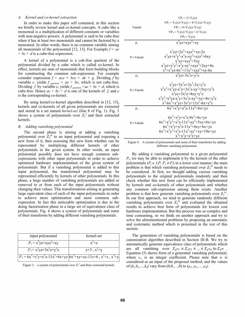
By using kernel/co-kernel algorithm described in [12, 13], kernels and co-kernels of all given polynomials are extracted and stored in a set named kernel-set (line 8 of Fig. 1). Fig. 3 shows a system of polynomials over Z2

2 and their extracted kernels.

B. Adding vanishing polynomial The second phase is aiming at adding a vanishing

polynomial over Z2m to an input polynomial and exposing a

new form of it, then assessing this new form whether can be represented by multiplying different kernels of other polynomials in the given system. In other words, an input polynomial possibly does not have enough common sub-expressions with other input polynomials in order to achieve optimized hardware implementation of the given system of polynomials. But if a vanishing polynomial is added to this input polynomial, the transformed polynomial may be represented efficiently by kernels of other polynomials. In this phase, a large number of vanishing polynomials are added or removed to or from each of the input polynomials without changing their values. This transformation aiming at generating large equivalent class of each of the input polynomials in order to achieve more optimization and more common sub-expression. In fact this noticeable optimization is due to the doing factorization phase in a large set of equivalence class of polynomials. Fig. 4 shows a system of polynomials and some of their transforms by adding different vanishing polynomials.

input polynomial kernel-set

P1 = x3yz+xyz2+xy x2+z

P2 = x2yz+3x2z+y2z y+3 , x2+y

P3 = 6x3+x2y+x2z-11x2+6x+yz 6x2+xy+xz-11x+6 , x2+z , x2+y

Figure 3. a system of polynomials over Z22 and their extracted kernels

Vanish

VP1 = 2×Y2(x) VP2 = Y2(x)×Y2(y) + 4×Y1(x)×Y1(y)

VP3 = 4×Y1(x)×Y1(y) VP4 = Y2(x)×Y2(y) + 4×Y1(x)

VP5 = Y4(x) P1

P1+Vanish

x3yz+xyz2+xy

x3yz+2x2+xyz2+xy-2x x3yz+x2y2-x2y-xy2+xyz2+6xy

x3yz+xyz2+5xy x3yz+x2y2-x2y-xy2+xyz2+2xy+4x x4+x3yz-6x3+11x2+xyz2+xy-6x

P2

P2+Vanish

x2yz+3x2z+y2z

x2yz+3x2z+2x2-2x+y2z x2y2+x2yz-x2y+3x2z-xy2+5xy+y2z

x2yz+3x2z+4xy+y2z x2y2+x2yz-x2y+3x2z-xy2+xy+4x+y2z

x4-6x3+x2yz+3x2z+11x2-6x+y2z P3

P3+Vanish

6x3+x2y+x2z-11x2+6x+yz

6x3+x2y+x2z-9x2+4x+yz 6x3+x2y2+x2z-11x2-xy2+5xy+6x+yz

6x3+x2y+x2z-11x2+4xy+6x+yz 6x3+x2y2+x2z-11x2-xy2+xy+10x+yz

x4+x2y+x2z+yz Figure 4. A system of polynomials and some of their transforms by adding

different vanishing polynomias

By adding a vanishing polynomial to a given polynomial Pi, we may be able to implement it by the kernels of the other polynomials (Pj ∈ LP, Pj ≠ Pi) in a lower cost manner; the main problem is that which vanishing polynomial over Z2

m needs to be considered. At first, we thought adding various vanishing polynomials to the original polynomials randomly and then check whether this new form can be efficiently implemented by kernels and co-kernels of other polynomials and whether any common sub-expression among them exists. Another problem is that how generate vanishing polynomials over Z2

m. In our first approach, we tried to generate randomly different vanishing polynomials over Z2

m and evaluated the obtained results to achieve best form of polynomials for lowest cost hardware implementation. But this process was so complex and time consuming, so we think on another approach and try to solve the aforementioned problems by proposing an automatic and systematic method which is presented in the rest of this section.

The generation of vanishing polynomials is based on the canonization algorithm described in Section III-B. We try to automatically generate equivalence class of polynomials which are all vanishing over … to . Equation (5) shows form of a generated vanishing polynomial, where cw is an integer coefficient. Please note that w is considered as an input of the proposed method, and the values of (k1,k2,…,kd) vary from (0,0,…,0) to (μ1, μ2,…, μd).

69

Vanish_Poly . … (5)

Fig. 5 illustrates the pseudo code of the vanishing polynomials generation. First, (μ1, μ2,…, μd) where d is number of variables, are initialized by using (2). Then based on Lemma 3 and Lemma 4 all possible vanishing polynomials over … to in which the degree of each variable xi varies from 0 to at most μi, are constructed. Please note that the number of all vanishing polynomials are very many, so in order to slightly decrease the memory usage and time complexity we have to discount those vanishing polynomials in which the degree of variables are more than (μ1, μ2,…, μd). Corresponding to Lemma 3, a multivariate polynomial is a vanishing polynomial if and only if at least one i exists such that ki ≥ μi (1≤i≤d). So every possible . … that satisfies this condition, will be added to the vanish-set (lines 2-3 of Fig. 5). Corresponding to Lemma 4, a multivariate polynomial is a vanishing polynomial if

,∏ ! | . So for every . … that doesn’t

satisfy the condition of Lemma 3 ,∏ !. … will be added to the vanish-set (lines 4-6). Finally for each w-combination of vanish-set, a vanishing polynomial is constructed based on (5) and added to Vanish_Poly set (lines 8-10). Note that a vanishing polynomial can be a zero polynomial as well.

It should be noted that we have automated the process of generating vanishing polynomials by using Singular, which is a computer algebra system for polynomial computations [14]. The complexity of this algorithm is 2 , where m is the size of the output bit-vector and d is number of input variables

Figure 5. Vanishing polynomials generation

C. Common sub-expression extraction Fig. 6 illustrates the pseudo code of the third phase of the

proposed method where common sub-expressions are extracted. All generated vanishing polynomials are separately added to each input polynomial Pi (1≤i≤s), and by performing algebraic division, each new form of Pi is divided separately by

the members of kernel-set (line 3 of Fig. 6). Equation (6) shows the overall form of this transformation and implementation of the transformed polynomial by multiplication of kernels of other polynomials in the given system.

1 , 1 _ , 1| _ | (6)

Where Pi is a given polynomial, Pvanish[j] is jth generated vanishing polynomial of Vanish_poly set. Moreover, and are quotient and remainder of the algebraic division Pi+Pvanish[j]/kernelh, respectively. kernelh is one of the members of kernel-set which is not a kernel of Pi , and i j is the new form of Pi+Pvanish[j] in terms of suitable kernels.

It should be noted that new polynomials resulting from algebraic division are used to determine if the resulting transformed polynomials are optimized for hardware implementation. For example, consider the polynomials in Fig. 4 again. Fig. 7 shows various forms of P3+vanish which are generated by using kernels of P1 and P2.

Figure 6. Common sub-expression extraction algorithm

P3+Vanish

(y) × (x2+z) + (6x3+x2z-9x2+4x)

(x2) × (y+3) + (6x3+x2z-12x2+4x+yz)

(xy+x) × (y+3) + (6x3+x2y2+x2z-11x2-2xy2+xy+3x+yz)

(x2+2x) × (y+3) + (6x3+x2z-14x2+2xy+yz)

(2x+z) × (x2+y) + (4x3+x2y-11x2+2xy+6x)

(x2+y) × (x2+z) + (0)

Figure 7. Various representation of P3

70

In the next step of this phase, is passed to the canonization algorithm as input, and assessed whether it is a vanishing polynomial. If is a vanishing polynomial, it is deleted from i j . Otherwise, if the cost of after applying canonization is less than the cost of , then is exposed by its canonical form which cannot be further reduced (lines 5-7 of Fig. 6). Note that cost_func determines the number of arithmetic operations such as additions and multiplications needed for hardware implementation of the given system of polynomials.

In the last step of this phase, all members of kernel-set can be subsequently used for applying algebraic division on in order to identify an efficient decomposition. Decomposition and factoring of continues via different kernels as far as possible (lines 8-11 of Fig. 6). The transformation of the given polynomial after the last step is shown in (7) (line 13 of Fig. 6). … 1 , 1 _ , 1 , | _ |, ,

(7)

Where is quotient of the last algebraic division which cannot be factored any further, is the reminder which was obtained from the previous step. kr … kz are some members of the kernel-set which should not be the kernels of Pi.

As discussed before (lines 12-17 of Fig. 1), every new generated form of Pi (1≤ i ≤ s) is used to evaluate related hardware implementation and therefore the best form of the given polynomials is chosen.

IV. EXPERIMENTAL RESULTS In order to show the effectiveness of our proposed

optimization technique, we have employed different polynomials extracted from real embedded systems such as DSP, image processing, automotive and communication applications. Various combinations of a multivariate Cosine Wavelet (MVCS) which is used in graphic applications [13], Savitzky-Golay (SG) filters that is used in image processing applications [15], Quartic filters (Quad) for DSP applications [16], Phase-Shift Keying (PSK) that is used in digital communication from [17], Mibench polynomial is used in automotive applications [18], and digital image rejection unit (DIRU) benchmarks which are used in image processing application, have been taken into account. We have implemented our algorithms in Singular as a computer algebra system for polynomial computations [14]. We have also synthesized the polynomials as combinational designs using commercial synthesis tools in 130 nm CMOS technology.

The complexity of our proposed method is 2 , where s is number of input polynomials, d is number of input variables and m is output bit-vector width, and SF is Smarandache function. Although the complexity of our method seems to be high, by considering the type of polynomials that used in our experiments, and considering the

obtained results, it is seemed that this added complexity is valuable in practice. Experimental results show that we have achieved more optimizations in the area and delay in comparisons with the state-of-the-art techniques.

In the first experiment, we have considered 4 configurations of the input polynomials and compare our results with those of technique in [6] as well as Horner form. Table I reports the results, where column M/V/D/n shows the number of monomials, the number of different variables, maximum degree, and bit-vector size of each variable in the given system of polynomials.

It is worth noting that in order to find more common sub-expressions we have generated 1810 vanishing polynomials while the input parameter w is set to 5. After taking into account the restriction of the degree mentioned in Section III-B, this number of vanishing polynomials can significantly be reduced. In our experiments, in order to reduce the time complexity, we use a simple heuristic to decrease the number of vanishing polynomials. In this heuristic we decline those vanishing polynomials which are not useful to create more common sub-expression among input polynomials. These useless vanishing polynomials do not have any monomials in common with polynomials of kernel-set, so they cannot create any new common sub-expressions among input polynomials and can be declined.

The results show that the proposed optimization approach can efficiently determine common sub-expressions to minimize the area as well as critical path delay. In comparison with the Horner form and the technique presented in [6], an average area improvement of 36.80% and delay decrease of 2.41% are obtained. As we mentioned before, the technique in [6] selects canonization form of input polynomials in the most real cases that may cause less common sub-expression among polynomials can be found. Regarding the critical path delay, since the number of common sub-expressions extracted by using vanishing polynomials is so higher than that of [6], and also since we consider these polynomials as combinational circuits as against the real circuits that are sequential circuits in which delay is calculated in another way, our reported delay in Table I, is slightly higher than that of [6].

In order to show our improvements in comparison with our previous work, in another experiment, we have compared our proposed optimization technique to the technique in [4]. Table II shows the results. As can be seen, the area and delay are improved by 21.4% and 8.7%, respectively. It is worth noting that in our previous method, decompositions are started from reduced polynomials over Z2

m instead of the original polynomials. That is why we cannot obtain more common sub-expressions in [4] compared to the proposed method in this paper.

V. CONCLUSIONS In this paper for the first time, we have proposed a kind of

polynomial optimization technique based on redundancy addition/removal on the fixed bit-width polynomial computation. we have proposed a high level optimization approach for arithmetic data paths implemented using a system of polynomials. Our method optimizes polynomials to reduce

71

the complexity of polynomial datapaths in terms of the number of multipliers and adders over Z2

m. In the proposed method, first kernels and co-kernels of all the given polynomials are extracted and then some vanishing polynomials over Z2

m are used to transform the given polynomials in order to extract more common sub-expressions. Experimental results show superiority of our approach in the area and delay savings in contrast with the other related works with an average improvement in the area by 36.80% with an average delay decrease of 2.41%. Regarding the comparison with our previous works, the area and delay are improved by 21.4% and 8.7%, respectively.

REFRENCES [1] O. Sarbishei, B. Alizadeh and M. Fujita, "Polynomial datapath

optimization using partitioning and compensation heuristics", Design Automation Conference (DAC), 2009, pp. 931-936.

[2] B. Alizadeh and M. Fujita, "Improved heuristics for finite word-length polynomial datapath optimization", IEEE/ACM International Conference on Computer-Aided Design - Digest of Technical Papers(ICCAD), 2009, pp. 739-744

[3] F. Haedicke, B. Alizadeh, G. Fey, M. Fujita, R. Drechsle, "Polynomial Datapath Optimization using Constraint Solving and Formal Modelling", IEEE/ACM International Conference Computer-Aided Design (ICCAD), 2010, pp. 756 - 761.

[4] B. Alizadeh and M. Fujita, "Modular Datapath Optimization and Verification Based on Modular-HED", IEEE Trans. on CAD of Integrated Circuits and Systems, vol. 29, No. 9, pp. 1422-1435, 2010.

[5] B. Alizadeh and M. Fujita, "Modular-HED: A Canonical Decision Diagram for Modular Equivalence Verification of Polynomial Functions", fifth Workshop on Constraints in Formal Verification (CFV), pp. 22-40, 2008.

[6] S. Gopalakrishnan and P. Kalla, "algebraic techniques to enhance common sub-expression elimination for polynomial system synthesis",

Design, Automation & Test in Europe (DATE) Conference, 2009, pp. 1452 - 1457.

[7] Z. CHEN, "On polynomial functions from Zn1×Zn2 ×· · · ×Znr to Zm", Discrete Math., Vol. 162, No. 1–3, pp. 67–76, 1996.

[8] Z. Chen, On polynomial functions from Zn to Zm Discrete Math. 137 (1995) 137-145.

[9] C. Berge, Graphes et Hypergraphes (Dunod, Paris, 1970). [10] E. Lucas, "Question nr. 288", Mathesis, vol. 3, pp. 232, 1883. [11] F. Smarandache, "A function in number theory", Analele Univ.

Timisoara, Fascicle 1, vol. XVII, pp. 79–88, 1980. [12] G. DEMICHELI,"Synthesis and Optimization of Digital Circuits",

McGraw-Hill, New York, 1994. [13] A. Hosangadi, F. Fallah and R. Kastner, "Optimizing polynomial

expressions by algebraic factorization and common subexpression elimination", IEEE Trans. on Computer-Aided Design of Integrated Circuits and Systems, vol. 25, pp. 2012–2022, 2006.

[14] “Singular”, Available at: http://www.singular.uni-kl.de [15] J. Krumm, “Savitzky-Golay Filters for 2D Images”, Available at:

http://homepages.inf.ed.ac.uk/rf/CVonline/LOCAL_COPIES/KRUMMI/SavGol.htm .

[16] V. J. Mathews and G. L. Sicuranza, Polynomial Signal processing, Wiley-Interscience, 2000.

[17] A. Peymandoust and G. DeMicheli, “Application of symbolic computer algebra in high-level data-flow synthesis,” IEEE TCAD, vol. 22, no. 9, pp. 1154–1165, Sep. 2003.

[18] M. R. Guthaus, J. S. Ringenberg, D. Ernst, T. M. Austin, T. Mudge, and R. B. Brown, “Mibench: A free, commercially representative embedded benchmark suite,” in Proc. IEEE 4th Annu. Workshop Workload Characterizat., 2001, pp. 3–14.

TABLE I. PROPOSED OPTIMIZATION ALGORITHM COMPARED TO OTHER RELATED TECHNIQUES

Functions M/V/D/n Horner Technique in [6] Our approach #Gates Delay #Gates Delay #Gates Delay

1- DIRU 2- PSK 3- Quad

22/2/4/16 85603 57.33 84909 37.16 45471 51.94

1- DIRU 2- PSK 3- SG2

26/2/4/16 90341 57.28 90539 41.06 54291 50.39

1- DIRU 2- Quad 3- SG2

22/2/4/16 63047 42.12 78213 33.03 50403 32.46

1- DIRU 2- MVCS

3- SG2 26/2/4/16 68485 42.31 72420 32.96 50040 32.68

Average saving compared to Horner (%) 0.0 0.0 -7.2 +26.8 +33.4 +16.8

72

TABLE II. PROPOSED OPTIMIZATION ALGORITHM COMPARED TO OUR PREVIOUS METHOD [4]

Functions M/V/D/n Technique in [4] Our approach #Gates Delay #Gates Delay

1- DIRU 2- PSK 3- SG2

26/2/4/16 68659 44.90 54291 50.39

1- DIRU 2- PSK

3- Mibench 26/3/4/16 65340 44.20 51040 31.08

Average saving compared to [4] (%) 0.0 0.0 +21.4 +8.7

73