First Interval Skin Conductance Responses: Conditioned or Orienting Responses
Upload
khangminh22Category
view
1download
0
ADVERTIMENT. Lʼaccés als continguts dʼaquesta tesi queda condicionat a lʼacceptació de les condicions dʼúsestablertes per la següent llicència Creative Commons: http://cat.creativecommons.org/?page_id=184
ADVERTENCIA. El acceso a los contenidos de esta tesis queda condicionado a la aceptación de las condiciones de usoestablecidas por la siguiente licencia Creative Commons: http://es.creativecommons.org/blog/licencias/
WARNING. The access to the contents of this doctoral thesis it is limited to the acceptance of the use conditions setby the following Creative Commons license: https://creativecommons.org/licenses/?lang=en
Study of vegetation dynamics from satellite: phenological responses to
climate change
Doctoral thesis
Kevin Bórnez Mejías
To apply for the degree of Doctor
Directors: Dr. Josep Peñuelas & Dr. Aleixandre Verger
PhD in Terrestrial Ecology
Centre for Ecological Research and Forestry Applications (CREAF)
Universitat de Autònoma de Barcelona
Bellaterra, July 2021


“However difficult life may seem, there is always something you can do and succeed at.”
Stephen Hawking

Todo comenzó allá por el año 2016. Por aquel entonces, me encontraba finalizando mi
segundo máster en Granada; cuando mi madre, ilusionada porque su hijo encontrara un
trabajo después de los estudios, me envió una captura de pantalla con una oferta laboral.
Se trataba de una oferta en la que un tal Dr. Aleixandre Verger buscaba candidatos para
optar a un contrato FPU durante 4 años en Barcelona. Tras una deliberación, decidí
realizar la solicitud para ser el candidato para optar a esa ayuda FPU y, por suerte fui
seleccionado.
Tras disfrutar mi último verano de estudiante, me fui con mis enseres personales a
Barcelona, concretamente a Cerdanyola del Vallès. La elección del lugar para buscar
piso, no fue nada fácil, pero teniendo en cuenta que me gustar tener todo a mano y poder
ir a los sitios caminando, la decisión estaba tomada. Tras unos días de toma de contacto
por la ciudad, llegó el tres de octubre, día en el que la vida que conocía daría un cambio
de 360º (nuevo trabajo, nuevos compañeros, hábitos, etc.). Y aquí estoy hoy, cinco años
después, finalizando esta etapa. El tiempo ha pasado tan rápido que apenas me he dado
cuenta. De no ser por el tamaño que ha alcanzado el potus del despacho, pensaría que
llevo aquí unos meses.
Durante esta etapa he tenido la suerte de encontrarme con personas fantásticas, a las que
querría agradecer que hayan estado junto a mí por unos motivos u otros. Quiero
agradecer en primer lugar a Aleixandre que me diera esta oportunidad, lo que me ha
permitido crecer como persona, aumentar conocimientos e introducirme en el mundo de
la ciencia, del que conocía poco. Desde que te fuiste de vuelta a Valencia no nos hemos
visto mucho, pero por unos métodos u otros siempre has estado ahí para guiarme y
ayudarme. Agradecerte también que, tras finalizar la ayuda predoctoral, no dudaras en
contratarme durante unos meses adicionales, que sirvieron para poder llevar a buen
puerto esta tesis. Josep, gracias por ayudarme en todo lo que he necesitado durante estos
años, y aunque también sé que siempre estás ocupado, nunca has dejado de atenderme,
aunque fuera fin de semana o festivo. También quiero agradecer al Ministerio de
Educación que haya financiado mi contrato durante el periodo predoctoral.
Nunca olvidaré el primer día que Aleixandre me enseñó aquel despacho (-148). Había
tal desorden que hasta él mismo se sorprendió. Era difícil ver a los compañeros con los
que trabajaría entre aquel montón de cajas y armarios repletos de material de campo,
cuyos delitos ya habían prescrito hacía décadas. Con el paso de los días, ese despacho
gris y marrón empezaba a tomar un color verde intenso gracias al gran potus, que se
extendía por los armarios dejando atrás todas aquellas cajas, convirtiéndose en la envidia
de todo aquel que osaba asomarse por la puerta.
Pero lo mejor de ese despacho no han sido las plantas, sino los grandes compañeros/as
y amigos que me han acompañado en esta andadura. Unos se fueron y otros seguirán,
pero sin lugar a dudas, he aprendido algo de cada uno de ellos. A pesar de que este
último año haya sido un poco diferente y no nos hayamos podido ver las caras, siempre
que veníais a hacer una visita, me alegráis el día. Marina, Helena, gracias por vuestras
mañanas de cháchara intentando arreglar el planeta y sacarnos unos eurillos extra, que
junto con los días de tertulias con Laura, Irene y Paolo hacían cada jornada un poco más
amena. También mencionar a una de las jóvenes promesas del despacho, Luca, que
tendrás que ser el encargado de cuidar las plantas, aunque he de decir que te dejaré una
nota con las instrucciones de riego. Me siento orgulloso de haber estado en el mejor
despacho del CREAF y con los mejores compañeros.
También querría agradecer al resto de personas con las que he tenido el placer de
cruzarme por estos pasillos, especialmente aquellos que apostaron por una navidad 2021
feliz con la celebración de la Kevineta, que, aunque sean de un despacho rival, me han
terminado cayendo bien. Manu (compañero de noches y festivos), Victor (no es persona
sin un café mañanero), Carlos, Javi, Aina, M.ª Ángeles, Judit, ha sido un placer
conoceros y espero que, aunque pasen los años, el día en que haya un reencuentro
parezca que no ha pasado el tiempo. También quisiera agradecer a otros compañeros/as
con los que he compartido experiencias y charlas, aunque sea por los pasillos del
CREAF, Albert, Luciana, Jordi, Susana, Adrià. Y en general, gracias a toda la familia
del CREAF, por la acogida, y por aquellas celebraciones pre-covid cada vez que había
un cumpleaños o una festividad, que terminaban convirtiéndose en una forma de
relacionarse, de conocerse, y que servían para apartar un momento los ojos de la pantalla
del ordenador y volver con las pilas recargadas.

No puedo olvidarme de que durante el segundo año de tesis tuve la oportunidad de
realizar una estancia de investigación en Estados Unidos, que se convirtió en una de las
mejores experiencias que he vivido. Thanks to Andrew Richardson and its research
group at Northern Arizona University for making me feel at home at all times; and for
the learning and experiences I had during those three months. Por otro lado, entre las
experiencias relativas al aprendizaje y formación como estudiante de doctorado, he
tenido la posibilidad de realizar un gran número de horas de docencia en distintos grados
universitarios de la UAB, y principalmente las he realizado con Miquel, al que quería
agradecer el tratamiento que ha tenido hacia mí y lo que he aprendido con él desde el
punto de vista docente.
Para ir finalizando con los agradecimientos, y aunque seguro que me he dejado a alguien
por el camino, quería agradecerte a ti, Marta, que me has apoyado en esta última etapa
de la tesis, tanto sentimental como logísticamente, haciendo que los agobios finales no
lo fueran tanto y, sobre todo, teniendo mucha paciencia conmigo.
Por último, agradecer a mi familia los esfuerzos que han realizado a lo largo de mi vida
para que finalmente haya podido realizar el doctorado. A mi madre, que seguro me ha
echado mucho de menos durante todos estos años lejos de casa; a mi hermana “reto”,
que, aunque es la peque de la familia, siempre ha estado ahí en los momentos buenos y
malos; y a mi padre, que allá donde estés siempre formarás parte de mí y me
acompañarás en el corazón. Seguro que los tres estaréis orgullosos de que aquel pequeño
travieso haya llegado a convertirse en la persona que es ahora y que esté escribiendo
estas palabras para finalizar su etapa predoctoral.
.
Cerdanyola de Vallès,
Julio 2021


v
Table of Contents
Acronyms ............................................................................................................................... xi
1 Introduction ...................................................................................................................... 17
1.1. Land surface phenology under climate change .................................................. 18
1.2. Vegetation phenology estimation ......................................................................... 20
1.3. Thesis objectives...................................................................................................... 26
2 Land surface phenology from VEGETATION and PROBA-V data. ................................... 29
Abstract ............................................................................................................................ 30
2.1. Introduction ............................................................................................................. 31
2.2. Materials and Methods........................................................................................... 33
2.3. Results....................................................................................................................... 38
2.4. Discussion and conclusions ................................................................................... 47
3 Evaluation of VEGETATION and PROBA-V phenology using PhenoCam and eddy
covariance data ........................................................................................................... 51
Abstract ............................................................................................................................ 52
3.1. Introduction ............................................................................................................. 53
3.2. Materials and Methods........................................................................................... 55
3.3. Results....................................................................................................................... 59
3.4. Discussion ................................................................................................................ 65
3.5. Conclusions .............................................................................................................. 67
4 Monitoring the responses of deciduous forest phenology to 2000-2018 climatic
anomalies in the Northern Hemisphere ..................................................................... 69
Abstract ............................................................................................................................ 70
4.1. Introduction ............................................................................................................. 71
4.2. Materials and Methods........................................................................................... 73
4.3. Results....................................................................................................................... 80
4.4. Discussion ................................................................................................................ 91
4.5. Conclusions .............................................................................................................. 93
5 General discussion and conclusions ................................................................................. 95
5.1. Discussion ................................................................................................................ 96
5.2. Conclusions ............................................................................................................ 101

vi
A Appendix Chapter 3 ............................................................................................. 106
B Appendix Chapter 4 ............................................................................................. 128
References ................................................................................................................ 134

vii
List of Tables
2.1 Algorithm principles of NDVI V2.1, and LAI, FAPAR, FCOVER V1 and V2. ............... 35
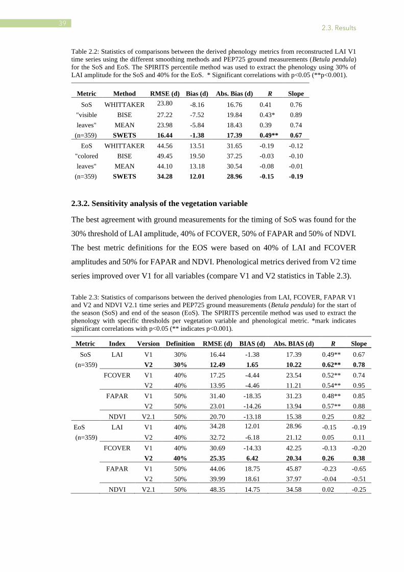
2.2 Statistics of comparisons between the derived phenology metrics from reconstructed LAI
V1 time series using the different smoothing methods and PEP725 ground measurements
........................................................................................................................................... 39
2.3 Statistics of comparisons between the derived phenologies from LAI, FCOVER, FAPAR
V1 and V2 and NDVI V2.1 time series and PEP725 ground measurements .................... 39
2.4 Statistics of comparisons between LAI V2 derived phenology and the ground measurements
for the various methods (percentiles, logistic function, derivative and moving average) . 42
3.1 Description of the evaluated methods for the extraction of phenology metrics. ................ 58
3.2 Statistics of the comparison between the SOS and EOS dates retrieved using the LAI, GCC,
and GPP estimates for the four methods: thresholds, logistic function, derivative and
moving average ................................................................................................................. 60
4.1 Classification of drought based on SPEI data. ................................................................... 76
4.2 Percentage of pixels with significant correlations (P<0.05) between the anomalies of
phenological events and climatic variables ....................................................................... 81
4.3 Classification of SPEI data for characterizing drought in the three case studies: Europe, North
America, and Balkans for 2003, 2012, and 2005, respectively ......................................... 88
A.1 Characteristics of PhenoCam and FLUXNET sites ........................................................ 110
B.1 Areas with significant trends (P≤0.05) in the time series (2000-2018) for the timing of SoS
and EoS. .......................................................................................................................... 132
B.2 Percentages of pixels with positive and negative correlations (P≤0.05) between phenology
and climatic variables ...................................................................................................... 132
B.3 Percentage of pixels with significant partial correlations between anomalies of phenology,
temperature, precipitation, and SPEI at different time lags ............................................. 132
viii
List of Figures
1.1 Diagram showing the data sources used for the phenological estimation ........................... 21
1.2 The spectral response patterns of vegetation, that remote sensors use to estimate vegetation
indices ................................................................................................................................ 24
1.3 An example of determining growing season of vegetation from seasonal patterns of the Leaf
Area Index (LAI) over deciduous forest ............................................................................ 25
2.1 Location of selected phenological ground observations at PEP725 sites and USA – NPN
sites .................................................................................................................................... 34
2.2 LAI (V1 and V2) and NDVI (V2.1) time series for the PEP725 site 5449 representative of
birch forest in Europe ......................................................................................................... 35
2.3 Schematic representation of SoS and EoS retrieved with the four methods for the PEP725
site 4959 for 2011 .............................................................................................................. 37
2.4 Boxplots of the bias errors for SoS and EoS estimated from the LAI, FCOVER, FAPAR V1
and V2 and NDVI V2.1 time series minus the PEP725 ground measurements ................. 40
2.5 Boxplots of the bias error for the SoS estimated from LAI V2 minus the ground
measurements at the USA-NPN and PEP725 sites ............................................................ 41
2.6 Scatterplots between the SoS predicted from LAI V2 by the percentile method, SPIRITS,
logistic function, derivative and moving average compared with the ground phenology
(USA-NPN “leaves”). ........................................................................................................ 43
2.7 Scatterplots between SoS predicted from LAI V2 by the percentile, SPIRITS, logistic
function, derivative and moving average methods and ground phenology (PEP725 “first
visible leaves”). .................................................................................................................. 43
2.8 Boxplots of the bias error for the EoS estimated from LAI V2 minus the ground
measurements at the USA-NPN and PEP725 sites ............................................................ 44
2.9 Scatterplots between the EoS predicted from LAI V2 by the percentile, SPIRITS, logistic
function, derivative and moving average methods and ground phenology (USA-NPN
“colored leaves”) ................................................................................................................ 45
2.10 Scatterplots between the EoS predicted from LAI V2 by the percentile, SPIRITS, logistic
function, derivative and moving average methods and ground phenology (PEP725 “colored
leaves”)............................................................................................................................... 45
2.11 Global Map of average SoS, EoS and LoS derived from the LAI V2 time series (1999-
2017) and the threshold-based method .............................................................................. 47

ix
3.1 Locations of the selected PhenoCam sites and FLUXNET towers over deciduous forests. 55
3.2 PhenoCam images captured in spring, summer, autumn and winter over the
NEON.D05.UNDE.DP1.00033 site ................................................................................... 57
3.3 Illustration of the threshold, logistic-function, derivative and moving-average phenological
extraction methods applied to PhenoCam GCC time series of Acadia site ......................... 59
3.4 Scatterplots for SoS and EoS estimated from CGLS LAI V2 and PhenoCam GCC time series
by the threshold (10th, 25th, 30th, 40th and 50th percentiles of LAI amplitude), logistic-
function, derivative and moving-average methods ............................................................ 62
3.5 Scatterplots for SoS and EoS estimated from CGLS LAI V2 and FLUXNET GPP time series
by the threshold (10th, 25th, 30th, 40th and 50th percentiles of LAI amplitude, logistic-
function, derivative and moving-average methods ............................................................ 63
3.6 Latitudinal gradients of average phenological metrics for the SoS, EoS and LoS extracted
from CGLS LAI V2 and PhenoCam GCC time series over the PhenoCam deciduous sites
........................................................................................................................................... 64
3.7 Interannual variation of the SoS and EoS estimated from the CGLS LAI V2, PhenoCam
GCC and FLUXNET GPP with the threshold method (percentile 30 for the timing of SoS,
and percentile 40 for the timing of EoS) over the Harvard Forest. .................................... 66
4.1 Map showing the study area with the distribution of the deciduous forests analyzed ........ 73
4.2 Distribution of trends for the SoS time series in the Northern Hemisphere between 2000 and
2018 (P<0.05). Distribution of sensitivity coefficients between SoS and mean preseason
temperature. Distribution of sensitivity coefficients between SoS and preseason
accumulated precipitation. ................................................................................................. 82
4.3 Frequencies of the correlations between phenology and the climatic variables. ................ 83
4.4 Boxplots of the sensitivities of the timings of SoS and EoS to temperature (ST), precipitation
(SP), and SPEI before SoS and EoS .................................................................................. 83
4.5 Distribution of trends for the EoS time series in the Northern Hemisphere between 2000 and
2018 (P<0.05). Distribution of sensitivity coefficients between EoS and mean
presenescence temperature. Distribution of sensitivity coefficients between EoS and
presenescence accumulated precipitation .......................................................................... 85
4.6 Spatial patterns of the partial correlations between SPEI and SoS and EoS for 2000–2018 in
the Northern Hemisphere ................................................................................................... 86
4.7 Distribution of the anomalies for the timing of EoS and SPEI before EoS in western Europe
for 2003 .............................................................................................................................. 87
4.8 Distribution of the anomalies for the timing of SoS and preseason mean temperature in
eastern USA for 2012 ........................................................................................................ 89

x
4.9 Distribution of the anomalies for the timing of SoS and preseason mean temperature in the
Balkans for 2005 ................................................................................................................ 90
A.1 Boxplots of the bias errors of satellite-based minus the near-surface estimates of SoS and
EoS over the 64 PhenoCam sites and the 16 FLUXNET towers ..................................... 107
A.2 Time series of CGLS LAI, PhenoCam GCC and FLUXNET GPP for the Harvard Forest
site over the 2008-2012 period. ........................................................................................ 108
A.3 Maps of average SoS, EoS and LoS derived from CGLS LAI V2 time series (1999-2017)
using the threshold method (30th percentile of annual LAI amplitude for SoS and 40th
percentile for EoS) ........................................................................................................... 109
B.1 Spatial patterns of partial correlation coefficients between pre-season temperature and SoS
and EoS for 2000-2018 in the Northern Hemisphere. ...................................................... 129
B.2 Spatial patterns of partial correlations between presenescence accumulated precipitation,
and SoS and EoS for 2000-2018 in the Northern Hemisphere ........................................ 130
B.3 Spatial distributions of the coefficients (color scale) for the sensitivity of SOS and EoS to
pre-season SPEI ............................................................................................................... 131

xi
Acronyms
AGF: Asymmetric Gaussian Function
AVHRR: Advanced Very High-Resolution Radiometer
BBCH: Biologische Bundesanstalt, Bundessortenamt and Chemical industry
CCI: Climate Change Initiative
CGLS: Copernicus Global Land Service
DN: Digital Numbers
DoY: Day of the Year
EoS: End of the Season
EVI: Enhanced Vegetation Index
FAO: Food and Agriculture Organization
FAPAR: Fraction of Absorbed Photosynthetically Active Radiation
FCOVER: Fraction of Vegetation Cover
FPU: Formación del Profesorado Universitario
GCC: Green Chromatic Coordinates
GCOS: Global Climate Observing System
GEE: Google Earth Engine
GMES: Global Monitoring of the Environment and Security
GPP: Gross Primary Production
IPCC: Intergovernmental Panel on Climate Change
LAI: Leaf Area Index
LC: land-cover
LFP: Low Pass Filtering
LoS: Length of the growing Season
LSP: Land Surface Phenology
MERIS: Medium Resolution Imaging Spectrometer
MODIS: Moderate Resolution Imaging Spectroradiometer
NDVI: Normalized Difference Vegetation Index
NIR: Red and Near Infrared
PEP: Pan European Phenology

xii
PET: Potential Evapotranspiration
RGB: Red-Green-Blue
RMA: Reduced Major Axis regression
RMSE: Root Mean Square Error
SGF: Adaptive Savitzky-Golay Filter
SoS: Start of the Season
SPEI: Standardized Precipitation-Evapotranspiration Index
SPI: Standardized Precipitation Index
SPIRITS: Software for the Processing and Interpretation of Remotely Sensed Image
Time Series
SPOT – VGT: VEGETATION on board the Satellite Pour l'Observation de la Terre
SWIR: Short-Wave Infrared
TOC: Top Of the Canopy
TS: Theil-Sen
US: The United States
USA-NPN: United States of America - National Phenology Network
VIIRS: Visible Infrared Imaging Radiometer Suite

xiii

xiv
Abstract
Phenology is key to control physicochemical and biological processes, especially
albedo, surface roughness, canopy conductance and fluxes of carbon, water and energy.
High-quality retrieval of land surface phenology (LSP) is thus increasingly important
for understanding the effects of climate change on ecosystem function and biosphere–
atmosphere interactions. Remote sensing is a useful tool for characterizing LSP although
no consensus exists on the optimal satellite dataset and the method to extract phenology
metrics.
I aimed to (i) improve the retrieval of Land Surface Phenology from satellite data, (ii)
validate LSP with ground observations and near surface remote sensing, and (iii)
understand the relationships between climate variables and phenology in a climate
change context, as well as to assess the responses of vegetation to extreme events. These
three main research objectives are explored in the three chapters of the thesis.
In chapter 2, I investigated the sensitivity of phenology to (I) the input vegetation
variable: normalized difference vegetation index (NDVI), leaf area index (LAI), fraction
of absorbed photosynthetically active radiation (FAPAR), and fraction of vegetation
cover (FCOVER); (II) the smoothing and gap filling method for deriving seasonal
trajectories; and (III) the phenological extraction method: threshold, logistic-function,
moving-average and first derivative based approaches. The threshold-based method
applied to the smoothed and gap-filled Copernicus Global Land LAI V2 time series
agreed the best with the ground phenology, with root mean square errors of ~10 d and
~25 d for the timing of the start of the season (SoS) and the end of the season (EoS),
respectively.
In the third chapter, I took advantage of PhenoCam and FLUXNET capability of
continuous monitoring of vegetation seasonal growth at very high temporal resolution
(every 30 minutes). This allows a more robust and accurate comparison with LSP
derived from satellite time series avoiding problems related to the differences in the
definition of phenology metrics. I validated LSP estimated from LAI time series with

xv
near-surface PhenoCam and eddy covariance FLUXNET data over 80 sites of deciduous
broadleaf forest. Results showed a strong correlation (R2 > 0.7) between the satellite
LSP and ground-based observations from both PhenoCam and FLUXNET for the timing
of the start (SoS) and R2 > 0.5 for the end of season (EoS). The threshold-based method
performed the best with a root mean square error of ~9 d with PhenoCam and ~7 d with
FLUXNET for the timing of SoS, and ~12 d and ~10 d, respectively, for the timing of
EoS.
In the fourth chapter, I investigated the spatio-temporal patterns of the response of
deciduous forests to climatic anomalies in the Northern Hemisphere using LSP derived
in Chapter 1 and validated in Chapter 1 and Chapter 2, and multi-source climatic data
sets for 2000–2018 at resolutions of 0.1°. I also assessed the impact of extreme
heatwaves and droughts on deciduous forest phenology. Analyses of partial correlations
of phenological metrics with the timing of the start of the season (SoS), end of the season
(EoS), and climatic variables indicated that changes in preseason temperature played a
stronger role than precipitation in the interannual variability of SoS anomalies: the
higher the temperature, the earlier the SoS in most deciduous forests in the Northern
Hemisphere (mean correlation coefficient of -0.31). Both temperature and precipitation
contributed to the advance and delay of EoS. A later EoS was significantly correlated
with a positive standardized precipitation-evapotranspiration index (SPEI) at the
regional scale (~30% of deciduous forests). The timings of EoS and SoS shifted by >20
d in response to heat waves throughout most of Europe in 2003 and in the United States
of America in 2012.

xvi

17
1
Introduction

1. Introduction
18
1.1. Land surface phenology under climate change
Phenology is defined as the study of the timing of recurrent biological events (such as
plant growing, migration and breeding of birds, or emergence of insects), as well as the
causes of their timing with regard to biotic and abiotic forces, and the relationship among
phases of the same or different species (Lieth, 1974). In this thesis I focus on the field
of vegetation phenology, which deals with the seasonal life-cycle phenophases of plants,
from the start of the greenness to senescence and their biotic or abiotic drivers (Saxena
and Rao, 2020). Fluctuations in vegetation phenology are related to factors such as
carbon, energy, and climate within terrestrial ecosystems (Estiarte and Peñuelas, 2015;
Garrity et al., 2011).
The scientific discipline of vegetation phenology has a long history. The first robust
studies date from the 1950s (Schnelle, 1955). However, vegetation phenology has
received increasing scientific attention in more recent times, by the early 1990s (Bajocco
et al., 2019; Donnelly and Yu, 2017; Saxena and Rao, 2020) due to the growing evidence
that the timing of growing stages is mostly dependent on environmental cues (Chuine
and Regniere, 2017), especially as phenological events are deeply sensitive to climate
variations (Menzel et al., 2006). Moreover, vegetation phenology has raised an
increasing interest as a key indicator of climate change (IPCC, 2007, 2013, 2014) due to
its important role as regulator of processes in terrestrial ecosystems, including carbon
and water cycle (Peñuelas et al., 2009; Richardson et al., 2013; Verger et al., 2016).
Unlike human and animals with the ability to quickly move from one region to another,
vegetation is fixed to a location, with slow and limited migrations, so it has to withstand
the climatic changes (Saxena and Rao, 2020). Vegetation phenology varies greatly
between species and geographic gradients (Peñuelas et al., 2009; Zhao et al., 2013), and
it is the outcome of the interaction of inherent attributes of each specie and their
sensitivity to external factors, such as radiation (photoperiod) (Borchert and Rivera,
2001), temperature (Wang et al., 2019), and precipitation (Chuine, 2010; Ibáñez et al.,
2010; Visser et al., 2010; Zhao et al., 2013). Assessing phenological transitions dates
has played an important role for understanding the climatic drivers of interannual
variability and for analyzing how vegetations respond to climate conditions
(Chmielewski and Rötzer, 2001; Cleland et al., 2007; Menzel et al., 2006; Schwartz et
al., 2006; Walther, 2010).

1.1. Land surface phenology under climate change
19
Climate change is recognized for being a direct consequence of greenhouse gas
emissions, and it is especially reflected in a significant and continuous increase in the
average temperature of the earth (IPCC, 2007, 2013). The Intergovernmental Panel on
Climate Change (IPCC) 4th Assessment Report on Impacts, Adaptation and
Vulnerability highlighted that the average global temperature has risen by 0.85 °C, over
the period 1880–2012 and projections indicate that it will continue to rise (IPCC, 2007,
2013). Most studies in the late 1990s and early twenty-first century highlighted that
elevated temperatures have contributed to the increase of vegetation greening through
the early leaf unfolding (Chmielewski and Rötzer; Menzel and Fabian, 1999; Zhang et
al., 2004) and later senescence (Delbart et al., 2008; Menzel and Fabian 1999; Menzel,
2006), which extends the length of the growing season in most areas of the Northern
Hemisphere (Saxena and Rao. 2020).
Global climate change and particularly extreme weather events such as floods, droughts
and heatwaves are reflected in vegetation phenology anomalies (IPCC, 2007, 2012;
Tang et al., 2017). Therefore, understanding the responses of vegetation phenology to
climate extremes is crucial and challenging, considering that climatic projections
indicate that future anomalies in the climate will become more intense and frequent than
those experienced in the past decades (IPCC, 2007, 2012; Jentsch et al., 2009; Reichstein
et al., 2013; Tang et al., 2017; Zheng et al., 2018; Zhao et al., 2018). Studies on
vegetation and climatic interactions have demonstrated that vegetation phenology
respond directly to climate, and phenological shifts in turn disturb climate through
feedback, affecting the CO2 uptake in function of the water availability in the soil,
regional characteristics, as well as the plant species and location (Atkinson et al., 2013;
Chen et al., 2018; Keenan et al., 2014; Peñuelas et al., 2001, 2009; Richardson et al.,
2013), which would alter the hydrological cycle through changes in the
evapotranspiration pattern (Berg et al., 2016; Bonan et al., 2008; Buermann et al., 2013,
2018; Peñuelas et al., 2009).

1. Introduction
20
1.2. Vegetation phenology estimation
Traditionally, phenological datasets were compiled from annual ground-based
observations of the timing of specific phenological events for particular plant species
based on periodic visual inspection by scientists or by volunteer observers (Morin et al.,
2009; Peñuelas et al., 2002; Richardson et al., 2006; Schwartz et al., 2002, 2013). Human
observations of plant phenology phases have been conducted for centuries (Templ et al.,
2018). The earliest known phenological data collection date from the ninth century in
Japan, where local citizens recorded the spring cherry blossoms and maple leaves for
the timing of autumn (Aono and Kazui, 2008; Aono and Tani, 2014). In the sixteenth
and seventeenth century records of phenology are also found in England, recording the
growth of more than 20 different species of plants, including records of tree-leaf out
from temperate forest (Sparks and Carey, 1995; Thompson and Clark, 2008). In France,
the scientists and farmers have also a long tradition observing the grapevine phenology
since the 1950s (García de Cortazar et al., 2017).
In the late twentieth and early twenty-first centuries, several international initiatives
including PEP725 (Pan European Phenology), PlantWatch program (Templ et al.,2018;
Vliet et al., 2003), and USA-NPN (National Phenology Network) (Mayer, 2010), aim to
manage and coordinate the databases of phenological records, establishing common
protocols and techniques to support and standardize phenological data collection across
large geographical areas in order to provide detailed plant phenology data at species-
scale or individual plant scale (Donnelly and Yu, 2017; Morin et al., 2009; Richardson
et al., 2006; Schwartz et al., 2012; Templ et al., 2018).
Most of the ground-based observations and phenological networks are usually carried
out by observing the vegetation and recording only a small choice of phenophases (e.g.
leaf unfolding, senescence), avoiding the possibility of analyzing the progression of the
seasonality (Templ et al., 2018). Moreover, the number of ground-based observations
are insufficiently distributed, mainly near to the cities, agricultural fields, or in low
altitude areas, and usually are restricted to a few species (Liang et al., 2011). To solve
these issues, the scientific community has begun to take advantage of (1) near-surface
observations (Hufkens et al., 2012; Richardson et al., 2009; Sonnentag et al., 2012;
Zhang et al., 2018) and (2) satellite remote sensing data (Bórnez et al., 2020a, 2020b;

1.2. Vegetation phenology estimation
21
Verger et al., 2016; Wu et al., 2014; Zhang et al., 2018), which allow more objective,
long-term and continuous phenological observations of different plant species over a
broad area (Morisette et al., 2009).
Near-surface observations usually includes imagery acquired from visible-wavelength
digital cameras, such as PhenoCam (Hufkens et al., 2012; Richardson et al., 2009;
Sonnentag et al., 2012) with RGB (Red, Green and Blue) bands (Wingate et al., 2015;
Vrieling et al., 2018), and continuous CO2 flux measurements based on eddy covariance
technique (e.g. FluxNet Network) (Gonsamo et al., 2013; Wu et al., 2013). Near-surface
observations (e.g. PhenoCam and FluxNet) provide higher temporal resolution and
greater spatial coverage than ground measurements, allowing to analyze site-level
phenological variation and mechanisms (Vrieling et al., 2018). Near-surface imagery
acquired by PhenoCam are based on optical principles similar to those used by sensors
onboard on satellites, bridging the scale between ground and satellite-based data (Figure
1.1) (Moura et al., 2017; Sonnentag et al., 2012).
Figure 1.1: Diagram showing the data sources used in the thesis for the phenological estimation, as well
as their properties regarding the temporal frequency and the spatial coverage and representability of the
measurements. Ground measurements have the lowest temporal resolution while near surface remote
sensing data and eddy covariance observations as well as satellite remote sensing provide more frequent
observations and higher spatial coverage

1. Introduction
22
1.2.1. Land surface phenology: the role and importance of remote sensing for
vegetation monitoring
Attention to changes in vegetation phenophases such as the start (SoS), end (EoS) or
length (LoS) of the growing season has increased over the last three decades (Donnelly
and Yu, 2017) with the use of remote sensing technology and climate models (Daham
et al., 2019; Shen et al., 2015; Wang et al., 2019), which allows to collect climatic and
phenological data over larger scales (Donnelly and Yu, 2017). Remote sensing imagery
has been improving the spatial resolutions ranging from centimeters to kilometers and
the temporal frequencies ranging from months or weeks to minutes (Xie et al., 2008).
Therefore, unlike in-situ observations, CO2 flux data or PhenoCam imagery, sensors
onboard satellites allow to measure phenological events over larger areas. The study of
the seasonal pattern of variation in vegetated land surfaces from remote sensing is
commonly known as Land Surface Phenology (LSP) (de Beurs and Henebry, 2005).
The first monitoring of LSP began with the Landsat I satellite in the early 1970s with
frequency temporal acquisition of images (16-day) at 30m of spatial resolution (Tucker,
1979). However, for monitoring vegetation, frequent observations are necessary (Miao
et al., 2013), so other satellites and sensors have been developed over the last few
decades for monitoring vegetation with higher temporal resolution, but with lower
spatial resolution (>250 m), such as the Advanced Very High-Resolution Radiometer
(AVHRR) sensor launched in the 1980‘s (Duchemt al. 1999; Heumann et al., 2007;
Lloyd, 1990; Reed et al., 1994), the Moderate resolution Imaging Spectroradiometer
(MODIS) (Tan et al., 2011; Zhang et al., 2003), Visible Infrared Imaging Radiometer
Suite (VIIRS) (Liu et al., 2017; Zhang et al., 2018), Système Pour L'Observation de la
Terre (SPOT)-VEGETATION (VGT) (Atzberger and Eilers, 2011; Verger et al., 2015;
Xie et al., 2008), Medium Resolution Imaging Spectrometer (MERIS) (Brown et al.,
2017), PROBA-V (Bórnez et al., 2020a, 2020b, Guzman et al., 2019; Verger et al.,
2017), and more recently, Sentinel-2A/B tandem satellites, which unlike the previous
ones, have been used for the estimation of LSP at greater spatial resolution ranging from
10 to 60 m and frequent revisit times <5 d (Addabbo et al., 2016; Descals et al., 2020).
LSP dynamics reflect the response of vegetation to seasonal and annual changes in the
climate and hydrologic cycle (de Beurs and Henebry, 2004, 2010). The application of

1.2. Vegetation phenology estimation
23 23
remote sensing imagery to study vegetation phenology and climate relationship found a
great catalyst with the development of vegetation indices, and its implementation in
Landsat and the AVHRR sensor in the late 1970s (Jones and Vaughan, 2010). From that
moment, a broad variety of vegetation products have been developed for the study of
LSP and climate at multiple scales (Henebry and de Beurs, 2013; Zeng et al., 2020). The
European Union has developed operational land monitoring services, known as
Copernicus Global Land Service (CGLS), as continuity of the Global Monitoring of the
Environment and Security (GMES) (Verger et al., 2014). CGLS provides a series of bio-
geophysical products and vegetation indices (VI), describing the status and dynamics of
vegetation at global scale from time series of remote sensing observations (Verger et al.,
2014).
VI and biophysical products use the land surface reflectance through the spectral
signatures of photosynthetically and non-photosynthetically of green healthy vegetation
(leaves) over the 0.4–2.6 µm wavelengths (Figure 1.2) to estimate the greenness
(Gonsamo et al., 2013). The vegetation signature shows low spectral reflectance in the
visible and middle-infrared wavelengths (high chlorophyll and water absorption) and
high reflectance in the near-infrared (NIR) wavelengths (Gates, 1970; Zheng et al.,
2020), which aids to monitor the seasonal cycle of vegetation. Time series of VIs and
biophysical variables are commonly used to identify seasonal transitions in vegetation,
especially for deciduous forests, since they have a clearly defined seasonal response (e.g.
Figure 1.3) compared to the small seasonal variations of evergreen vegetation. (Garrity
et al., 2011; Liu et al., 2016; Melaas et al., 2013).

1. Introduction
24 24
Figure 1.2: The spectral response patterns of vegetation, that remote sensors use to estimate vegetation
indices. It shows the area of absorption by chlorophyll pigment in the visible spectrum, the reflectance of
the leaves mainly in the near infrared, and the absorption of radiation by the water content in most of the
incoming radiation over the shortwave infrared region. Note that the figure shows the average spectral
signature of the vegetation, which varies slightly between different vegetation types and species. To
explore the spectral response characteristics of specific species, visit the ASTER Spectral Library
https://speclib.jpl.nasa.gov/library/ecoviewplot, California Institute of Technology, 2002.
Among the different vegetation products, most previous approaches for estimating LSP
have been based on the use of biophysical variables, including the Leaf Area Index (LAI)
(Bórnez et al., 2020b; Hanes and Schwartz, 2011; Kang et al., 2003; Verger et al., 2015;
Wang et al., 2017), Fraction of Absorbed Photosynthetic Active Radiation (FAPAR)
(Meroni et al., 2014; Verger 2016, 2017), the fraction of vegetation cover (FCover)
(Verger et al., 2016), as well as spectral vegetation indices such as the Normalized
Difference Vegetation Index (NDVI) (Fischer, 1994; Yu et al., 2003; Wu et al., 2014),
and Enhanced Vegetation Index (EVI) (Zhang et al., 2003; Wang et al., 2017). All of
them are associated with the biophysical and biochemical properties of vegetation
(Gonsamo et al., 2012), being recognized as essential climate variables by the Global
Climate Observing System (GCOS) (Verger et al., 2014).
NDVI has been the most widely used index to estimate vegetation phenology because
of its easy calculation and its broad acceptance into the scientific community (Jeong et
al., 2011; Myneni et al., 2002; Reed et al., 1994; White et al., 2014). However,
biophysical variables such the LAI are being increasingly studied to describe plant

1.2. Vegetation phenology estimation
25 25 25
canopy structure (Figure 1.3) because it represents direct biophysical measures of
vegetation, estimated by models, and it is more sensitive than NDVI or FPAR for larger
vegetation amounts (Myneni and Williams, 1994; Verger et al., 2013). It is based on leaf
development rather than on proxies provided by vegetation indices which avoid
distortions associated with the canopy structure and the biochemical composition of the
existing foliage (Richardson et al., 2009; Verger et al., 2014, 2016).
Figure 1.3: Example of determining growing season of vegetation from seasonal patterns of the Leaf Area
Index (LAI) over deciduous forest. Phenology can be extracted from the seasonal LAI curve (in green),
as defined in Bórnez et al., 2020b. Phenological date vary according to the method for phenological
estimation used. In this example (a) Start of season, (b) Greenup phase, (c) Maximum LAI, (d) Senescence
phase, (e) End of season, (f) Length of season, (g) Seasonal amplitude are shown.
Various methods have been developed to estimate phenological transitions from a time
series of VI and biophysical variables. The main metrics of interest in the studies of LSP
have been the start (SoS) (White et al., 2009; Liang et al., 2011) and the end of the
growing season (EoS) due to its importance within the context of climate change
(Garrity et al., 2011; Menzel, 2002). The methodologies on LSP estimation are mainly
based on a two-step approach (Verger et al., 2016; Zeng et al., 2020) including (1) curve-
fitting and (2) extraction of phenology metrics. Firstly, the original remote sensing
products typically have noisy and spurious points, so to perform the curve fitting
approach smoothing methods are typically applied to the time-series datasets to filter
and minimize residual noise and fill in the gaps, since noise and missing data in satellite
time series can introduce uncertainties in the phenological estimates. Several smoothing
techniques are available, including low pass filtering (LPF), Whittaker smoother,

1. Introduction
26
Adaptive Savitzky-Golay filter (SGF), and asymmetric Gaussian function (AGF)
(Verger et al., 2016).
Regarding the methods for phenological estimation from the reconstructed daily time
series, a broad variety of strategies has been designed. The most commonly used
strategies are based on thresholds (Myneni et al., 1997; White et al., 1997), moving
averages (Reed et al., 1994), first derivatives (Tateishi and Ebata, 2004; White et al.,
2009), and curvature of piecewise logistic functions (Zhang et al., 2003). De Beurs and
Henebry (2010) indicated that there is no better method to estimate phenology for all the
vegetation types and areas. White et al. (2009) and Atkinson et al. (2012) investigated
the effects of using different methodologies to derive LSP metrics, highlighting that also
phenological metrics estimation accuracy varies among the different methods and VI or
biophysical variables. Therefore, the method and variable selected for phenological
estimation can significantly influence the performance of the phenology extraction from
the smoothed time series (Kandasamy et al., 2013; Atkinson et al., 2012), and this is
especially important for analyzing the interrelationships between phenological estimates
and climate variables.
Understanding the relationship between the different elements of global climate change
and LSP is one of the most studied and challenged topics of the 21st century (Sykes,
2009). The 4th Assessment Report of the IPCC indicated that spring onset has been
advancing by about 2.3 and 5.2 days per decade since the 1970s to early twenty-first
century (Parmesan, 2007) and it concluded that phenology “is perhaps the simplest
process in which to track changes in the ecology of species in response to climate
change” (IPCC, 2007). In this sense, the LSP estimated in this thesis from remote
sensing data serves for detecting the response of vegetation to environmental changes at
multiple scales by analyzing the anomalies in time series.
1.3. Thesis objectives
The general objective of the thesis is to analyze the dynamics of vegetation phenology
in response to climatic change, through the use of satellite imagery from CGLS
vegetation products. Particularly, I aim to estimate Land Surface Phenology from
satellite data, validate it with ground observations and near surface remote sensing and

1.3 Thesis objectives
27
understand the relationships between climate variables and phenology in a climate
change context, as well as to assess the responses of vegetation to extreme events.
Meeting this goal is challenging due to the wide availability of vegetation variables and
phenological estimation methods from which phenology metrics can be obtained (de
Beurs and Hennery, 2010; Schwartz and Hanes, 2010; White et al., 2009), which
requires a series of previous steps, including the identification of the biophysical variable
or vegetation index that best assesses the vegetation phenology found in ground
observations (chapter 2). In order to evaluate the robustness of the phenological metrics
estimated from satellite, and compared with ground measurement, near surface remote
sensing and eddy covariance techniques were used by using continuous time series GCC
(from PhenoCam) and GPP (from FluxNet), which allowed me to validate the results
(chapter 3). Finally, I analyzed the response of phenology to the changes in climate
variables as a result of global climate change, focusing on anomalies and extreme
climatic events (chapter 4).
The thesis is thus structured in three research chapters:
Chapter 2. Phenological metrics estimation from remote sensing time series and
validation with ground measurements
The objectives of Chapter 2 are (1) to select the best biophysical variable or vegetation
index for estimating phenological metrics on a global scale within the portfolio of the
CGLS vegetation products (NDVI, LAI, FCOVER or FAPAR) from time series of the
sensors SPOT-VGT and PROBA-V, and (2) to define the method that best matched with
ground data (using PEP725 and NPN). I evaluated four methods for estimating
phenology: the threshold method based on percentiles, the derivative method, the
autoregressive moving-average method, and the logistic-function method.
Chapter 3. Validation of satellite phenological metrics by using near-surface
remote sensing and eddy covariance flux data
In the s third chapter, I completed the validation of LSP retrievals developed in Chapter
2 by taking advantage of continuous measurements of near surface remote sensing
(PhenoCam) and eddy covariance CO2 flux measurements (FluxNet) at very high
temporal resolution. The aim was to conduct a more robust and accurate comparison

28
with LSP derived from satellite time series avoiding problems related to the differences
in the definition of phenological metrics. In this chapter, I evaluated the same four
methods as in Chapter 2 for estimating phenology: the threshold method based on
percentiles, the derivative method, the autoregressive moving-average method, and the
logistic-function method. These methods were applied both to satellite CGLS LAI V2
time series and ground observations from PhenoCam GCC and eddy covariance flux
data.
Chapter 4. Assessment of phenological response to climate and extreme
events
In this chapter, I explored the relationship between the LSP estimated from LAI time
series and climate variables. Specifically, the objectives of this chapter were: (1) to
identify and quantify statistically the spatial pattern of correlation between the anomalies
of vegetation phenology and climate (temperature, precipitation and drought) to this way
identify the main cause of phenological change, (2) to quantify the sensitivity of
phenology to climate; and (3) to determine the consequences of extreme events on
phenology in the areas with the highest sensitivity to climate.

29
2
Land surface phenology
from VEGETATION and
PROBA-V data.
Assessment over
deciduous forests
Kevin Bórnez, Adrià Descals, Aleixandre Verger, Josep Peñuelas
Published in International Journal of Applied Earth Observation and Geoinformation
(2020), Vol.84: 101974. https://doi.org/10.1016/j.jag.2019.101974
Scan this code to download the published version

2. Land surface phenology from VEGETATION and PROBA-V data
30
Abstract
Land surface phenology has been widely retrieved although no consensus exists on the
optimal satellite dataset and the method to extract phenology metrics. This study is the
first comprehensive comparison of vegetation variables and methods to retrieve land
surface phenology for 1999-2017 time series of Copernicus Global Land products
derived from SPOT-VEGETATION and PROBA-V data. We investigated the
sensitivity of phenology to (I) the input vegetation variable: normalized difference
vegetation index (NDVI), leaf area index (LAI), fraction of absorbed photosynthetically
active radiation (FAPAR), and fraction of vegetation cover (FCOVER); (II) the
smoothing and gap filling method for deriving seasonal trajectories; and (III) the method
to extract phenological metrics: thresholds based on a percentile of the annual amplitude
of the vegetation variable, autoregressive moving averages, logistic function fitting, and
first derivative methods. We validated the derived satellite phenological metrics (start
of the season (SoS) and end of the season (EoS)) using available ground observations of
Betula pendula, B. alleghaniensis, Acer rubrum, Fagus grandifolia, and Quercus rubra
in Europe (Pan-European PEP725 network) and the USA (National Phenology Network,
USA-NPN). The threshold-based method applied to the smoothed and gap-filled LAI
V2 time series agreed best with the ground phenology, with root mean square errors of
~10 d and ~25 d for the timing of SoS and EoS respectively. This research is expected
to contribute for the operational retrieval of land surface phenology within the
Copernicus Global Land Service.
2.1. Introduction
31
2.1. Introduction
Phenology is the study of the timing of recurrent biological and seasonal events and their
biotic and abiotic factors (Beaumont et al., 2015). Studies of plant phenology focus on
how these events and factors are influenced by seasonal and interannual variations in
climate and how they modulate abundance and diversity (Beaumont et al., 2015).
Phenology is, moreover, key to control physicochemical and biological processes,
especially albedo, surface roughness, canopy conductance and fluxes of carbon, water
and energy (Peñuelas et al., 2009; Richardson et al., 2013). Phenological metrics are
thus relevant parameters for modeling land surface processes and the global carbon cycle
(Wu et al., 2014).
Phenological metrics are estimated based on ground observations and data derived from
satellites. Ground observations provide accurate timing of vegetation phenophases but
cannot cover continuously large-scale areas (Garrity et al., 2011; Yu et al., 2017).
Satellite sensors with moderate spatial resolutions, including AVHRR, MODIS,
MERIS, SPOT-VEGETATION and PROBA-V, provide long-term time series of daily
observations that allow improving the characterization of land surface phenology on a
global scale (Atkinson et al., 2012; Verger et al., 2016; Zhang et al., 2004). However,
the noise in the data and missing observations mainly due to cloud contamination may
induce significant uncertainties in the estimation of phenological metrics (Kandasamy
et al., 2013; Verger et al., 2013). The literature shows a broad variety of time-series
processing methods designed to reconstruct gap-filled vegetation seasonal trajectories
from noisy satellites signals. This includes the best index slope method (Viovy et al.,
1992), mean filters (Reed et al., 1994), moving-window filters (Sweets et al. 1999),
asymmetric Gaussian functions (Jönsson and Eklundh, 2002), Savitzky–Golay filters
(Chen et al., 2004) or the Whittaker smoother (Eilers, 2003). However, no single method
always performs better than others for smoothing vegetation time series (Cai et al., 2017)
and their performance vary spatially and temporally with land surface conditions and
cloud influence (Atkinson, et al. 2012; Kandasamy and Fernandes, 2015).
A broad variety of statistical methods have been designed to extract phenological
metrics from satellite time series. Metrics typically include the start of the season (SoS),
the end of the season (EoS), the timing of maximum growth and the length of the
2. Land surface phenology from VEGETATION and PROBA-V data
32
growing season (LoS) (Reed et al., 1994; Zhang et al., 2004). De Beurs and Henebry
(2010) provided a comprehensive review of the exiting phenology retrieval approaches
that can be classified in four main categories: thresholds and percentile based methods
(Atzberger and Eilers, 2011; Verger et al., 2016), moving averages (Reed et al., 1994),
first derivatives (White et al., 2009) and fitted models (de Beurs and Henebry, 2005).
White, et al. (2009) compared ten different phenology retrieval methods applied to
AVHRR NDVI in North America and found large discrepancies of up to two months in
the detection of the SoS.
In addition to the sensitivity to the smoothing and phenological extraction algorithm, the
derived phenological metrics are also dependent on the sensor, spatial and temporal
resolution, processing chain, and satellite data set. The satellite-derived spectral
vegetation indices (e.g. the Normalized Difference Vegetation Index (NDVI)) vary in
their strength of phenological prediction across sites and plant functional types (Wu et
al., 2014). Unlike previous studies based on vegetation indices, the present study aimed
to characterize the phenology not only with NDVI but also with biophysical variables:
the leaf area index (LAI), the fraction of absorbed photosynthetically active radiation
(FAPAR), the fraction of vegetation cover (FCOVER). We used NDVI version V2.1
(Toté et al., 2017), LAI, FAPAR and FCOVER V1 (Baret et al., 2013) and V2 (Verger
et al., 2014) time series derived within the Copernicus Global Land Service (CGLS)
from SPOT-VEGETATION and PROBA-V data. Verger et al. (2017) showed that the
phenology derived from the interannual climatology of LAI V1 improved other existing
products including MODIS-EVI when compared to ground observations for the average
date of the SoS and EoS. However, their study was limited to the baseline LAI
phenology as derived from a single extraction method. This paper is a continuation of
the previous paper by Verger et al. (2017) and we address now the interannual variation
of the yearly phenology, the impact of the input vegetation variable and the phenological
extraction method. Further, we incorporate LAI, FAPAR and FCOVER V2 that
improved continuity (no missing data in V2) and smoothness as compared to V1.
Our study had two main objectives: to select the best biophysical variable or vegetation
index for estimating phenological metrics on a global scale within the portfolio of the
CGLS vegetation products (NDVI, LAI, FCOVER or FAPAR) and to define the method
that best matched the ground data.

2.2. Materials and Methods
33
2.2. Materials and Methods
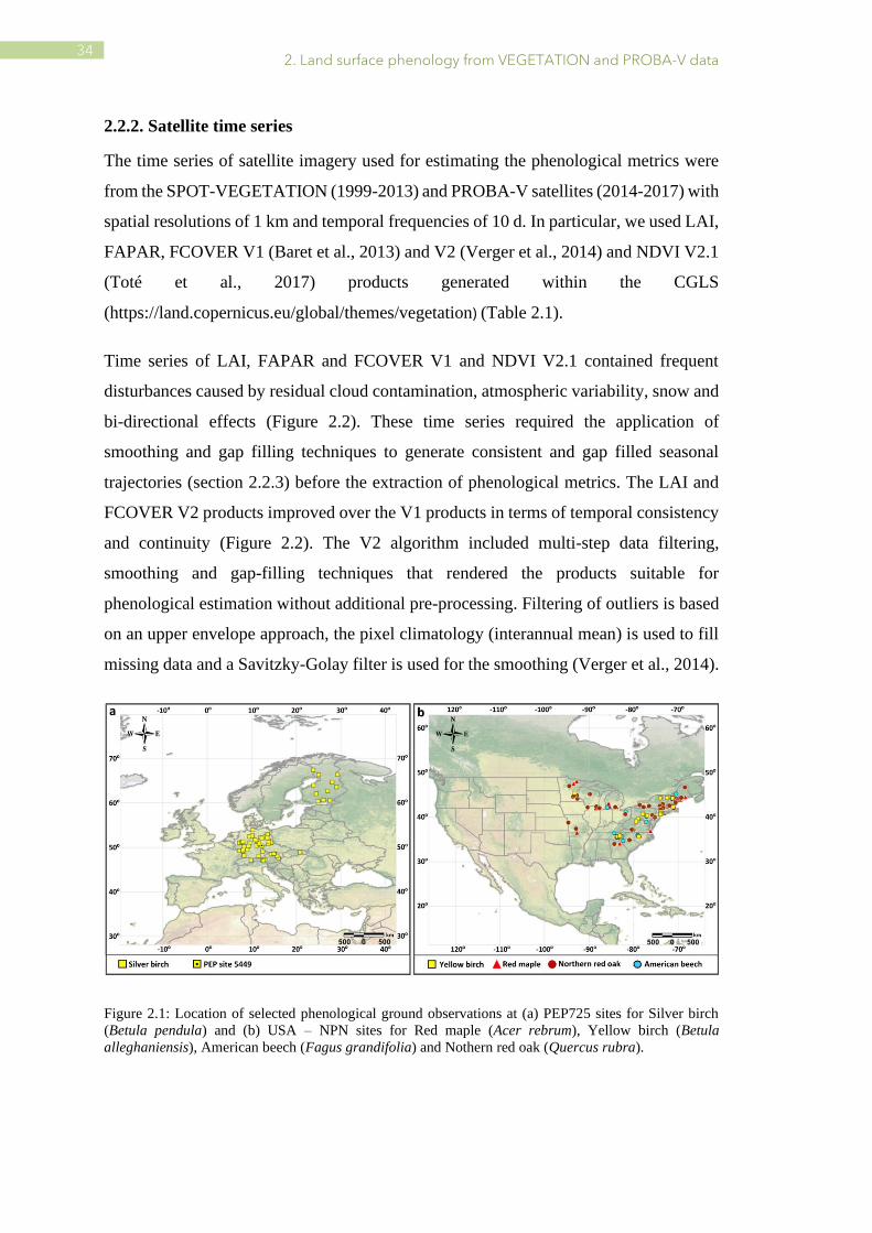
2.2.1. Phenological ground observations
Ground-based phenological data from PEP725 and USA-NPN were examined, focusing
on the dates of leaf out and leaf senescence for Betula (birch) in Europe (Figure 2.1a)
and the USA and for Quercus (oak), Fagus (beech) and Acer (maple) in the USA (Figure
2.1b). These genera were chosen because they are present in both Europe and the USA
and have large numbers of records in the combined data set.
The PEP725 Pan-European Phenology database (Templ et al., 2018) (www.pep725.eu)
has complete records from 1990 to the present. The phenophases defined in PEP725 are
based on BBCH (Biologische Bundesanstalt, Bundessortenamt and Chemical industry)
code (Meier et al., 2009). We used the phenophases corresponding to the first visible
leaves (BBCH 11) as the reference for the timing of SoS and the date corresponding to
50% of leaves with autumn coloration (BBCH 94) for the timing of EoS.
The USA National Phenology Network was established in 2007 to collect, store and
share historical and contemporary phenological data on a North American scale
(Schwartz et al., 2012). The data are freely available at https://www.usanpn.org/. This
network provides measurements of several phenophases. We used the phenophases
“leaves” which corresponds to first visible leaves and “increasing leaf size” for SoS and
“colored leaves” for EoS.
We discarded ground sites with less than four yearly measurements to obtain consistent
data records over the time series. We used ground-site located pixels. The spatial
heterogeneity hamper comparing ground-based phenology for individual plants with
satellite phenology at a resolution of 1 km. We filtered the ground sites located in
agricultural or urban areas using high-resolution images from Google Earth
(https://earth.google.com/) and the ESA Land Cover Map (CCI-LC)
(http://maps.elie.ucl.ac.be/CCI/viewer/index.php). In Europe, we used only the points
with forest coverages >5% using a tree cover map for European forests (Brus et al.,
2012).
2. Land surface phenology from VEGETATION and PROBA-V data
34
2.2.2. Satellite time series
The time series of satellite imagery used for estimating the phenological metrics were
from the SPOT-VEGETATION (1999-2013) and PROBA-V satellites (2014-2017) with
spatial resolutions of 1 km and temporal frequencies of 10 d. In particular, we used LAI,
FAPAR, FCOVER V1 (Baret et al., 2013) and V2 (Verger et al., 2014) and NDVI V2.1
(Toté et al., 2017) products generated within the CGLS
(https://land.copernicus.eu/global/themes/vegetation) (Table 2.1).
Time series of LAI, FAPAR and FCOVER V1 and NDVI V2.1 contained frequent
disturbances caused by residual cloud contamination, atmospheric variability, snow and
bi-directional effects (Figure 2.2). These time series required the application of
smoothing and gap filling techniques to generate consistent and gap filled seasonal
trajectories (section 2.2.3) before the extraction of phenological metrics. The LAI and
FCOVER V2 products improved over the V1 products in terms of temporal consistency
and continuity (Figure 2.2). The V2 algorithm included multi-step data filtering,
smoothing and gap-filling techniques that rendered the products suitable for
phenological estimation without additional pre-processing. Filtering of outliers is based
on an upper envelope approach, the pixel climatology (interannual mean) is used to fill
missing data and a Savitzky-Golay filter is used for the smoothing (Verger et al., 2014).
Figure 2.1: Location of selected phenological ground observations at (a) PEP725 sites for Silver birch
(Betula pendula) and (b) USA – NPN sites for Red maple (Acer rebrum), Yellow birch (Betula
alleghaniensis), American beech (Fagus grandifolia) and Nothern red oak (Quercus rubra).

2.2. Materials and Methods
35
Table 2.1: Algorithm principles of NDVI V2.1, and LAI, FAPAR, FCOVER V1 and V2.
Figure 2.2: LAI (V1 and V2) and NDVI (V2.1) time series for the PEP725 site 5449 (50º42'20.49"N,
13º46'59.55"E) representative of birch forest in Europe.
2.2.3. Smoothing methods
We tested several smoothing methods for reducing noise and reconstructing gap filled
seasonal trajectories from CGLS time series (Eerens and Haesen, 2015):
• WHITTAKER smoother (Atzberger and Eilers, 2011): It minimizes a cost
function describing the balance between fidelity (quadratic difference between
estimates and actual observations) and roughness (quadratic difference between
successive estimates).
NDVI
Version 2.1
LAI, FAPAR, FCOVER
Version 1
LAI, FAPAR, FCOVER
Version 2
Inputs Top of the canopy
(TOC) reflectances in
the red and near
infrared (NIR)
spectral bands
Nadir normalized TOC
reflectances in the red, NIR
and short-wave infrared
(SWIR) spectral bands, and
cosine of the sun zenith
angle at 10:00 local time
TOC reflectances in the red,
NIR and SWIR spectral
bands, and cosine of the 3
angles of sun and view
directions
Temporal
composition
10 d compositing
period. The maximum
NDVI value in the
composition window
is retained.
Starting date of
composition:1st, 11th
and 21th day of the
month
30 d compositing period
with Gaussian weighting
(minimum of two valid
observations)
Nominal dates: 3rd, 13th and
21-24th day of each month
Adaptive compositing within
15 and 60d semi-periods
defined by the availability of
6 valid observations at each
side of the date being
processed
Nominal dates: 10th, 20th
and last day of the month
Temporal
smoothing
and gap
filling
Not applied Not applied Multi-step filtering, temporal
smoothing and gap-filling

2. Land surface phenology from VEGETATION and PROBA-V data
36
• BISE (Best Index Slope Extraction) (Viovy et al., 1992): It retains the good
observations in a local window and replaces missing or eliminated suspect values
by linear interpolation.
• MEAN: A linear interpolation is first applied to fill missing data. A running mean
filter with a sliding window of 50 d length is then applied.
• SWETS method (Swets et al., 1999): A linear interpolation is first applied to fill
missing data. A weighted linear regression over a local window is then applied.
2.2.4. Methods for extracting phenological metrics
We tested four state of the art methods to extract phenological metrics from CGLS time
series (Figure 2.3):
• Thresholds based on a pixel percentile value: SoS is defined as the day of the
year (DoY) when a vegetation variable exceeds a particular threshold. EoS is
defined as the DoY when an index remains below a particular threshold. We
established dynamic thresholds per pixel based on a percentile of the annual
amplitude of the vegetation variable (Verger et al., 2016). The selected
percentiles were determined based on the comparison with available ground
measurements. We tested the 20th, 30th, 40th and 50th percentiles of the annual
amplitude for SoS, and the 30th, 40th, 50th and 60th percentiles for EoS. This
method is also the basis of SPIRITS phenological approach.
• Autoregressive moving average: A moving average is first computed at a
randomly chosen time lag (Ivits et al., 2009). We tested time lags from 50 to 150
d and selected a time lag of 100 d based on the comparison with ground
measurements. SoS and EoS are then defined as the DOY when the moving
average curves cross the original curve of the vegetation variable.
• First derivative: SoS is defined as the DoY of the maximum increase (maximum
first derivative) in the curve (Tateishi and Ebata, 2004). EoS is defined as the
DoY of the maximum decrease in the curve.
• Logistic function: SoS is defined as the DoY of the first local maximum rate of
change in the curvature of a logistic function fitted to the time series (Zhang et
al., 2003). EoS is defined as the DoY of the first local minimum rate of change
in the curvature.

2.2. Materials and Methods
37
Figure 2.3: Schematic representation of SoS (on the left of the peak) and EoS (on the right of the peak)
retrieved with the four methods for the PEP725 site 4959 (50º42'20.49"N, 13º46'59.55"E) for 2011. The
black circles correspond to the original LAI data at a 10-d frequency, and the green line corresponds to
the data interpolated at daily steps, which is used for phenological estimation.
2.2.5. Methodological approach
The several satellite-derived vegetation variables, smoothing methods and phenological
extraction approaches lead to a large number of combinations. We sequentially
investigated the impact of smoothing, variable and extraction method based on an initial
set of modalities. The initial modalities were defined a posteriori based on the analysis
of all the combinations:
1. Sensitivity analysis of the smoothing method: We used LAI V1 as input dataset
and the percentile phenology method.
2. Sensitivity analysis of the vegetation variable: We used the SWETS smoothing
method and the percentile phenology method.
3. Sensitivity analysis of the method to extract phenological metrics: We used the
LAI V2. Note that in this case the application of a smoothing method is not
required because LAI V2 is already smoothed and gap-filled.
The analysis 1 and 2 were carried out in Europe and for the validation we used ground
measurements of Betula Pendula, which showed a greater latitudinal distribution. The
analysis 3 was performed at the global scale. For the sensitivity analysis 1 and 2, we
used the Software for the Processing and Interpretation of Remotely Sensed Image Time

2. Land surface phenology from VEGETATION and PROBA-V data
38
Series (SPIRITS) (Eerens et al., 2014; Eerens and Haesen, 2015). For the sensitivity
analysis 3, we used Google Earth Engine (GEE) (https://earthengine.google.org) which
allowed implementing dedicated algorithms while only the threshold method is available
in SPIRITS. The input 10 d time series were linearly interpolated at daily steps before
phenological retrieval. For SPIRITS, the precision of phenological estimates is limited
by the frequency of the input time series (10 d in our case) (non interpolation). For pixels
with multiple growing seasons, we computed the phenological metrics for the growing
season having the highest LAI amplitude.
The agreement between metric estimates from satellite imagery and ground-based
measurements was quantified using the slope of the linear regression, the Pearson
correlation coefficient (R), bias, i.e. the average difference between the satellite-derived
phenology and the observed date (a positive bias indicated that SoS and EoS occurred
later than the observed leaf out and autumnal coloring, respectively), the absolute bias
and root mean square error (RMSE) calculated (e.g. for SoS) as:
𝑅𝑀𝑆𝐸𝑆𝑜𝑆 = √1
𝑛∑ (𝑆𝑜𝑆𝑔𝑟𝑜𝑢𝑛𝑑 − 𝑆𝑜𝑆𝑒𝑠𝑡.)
2𝑛
𝑗=1 (1)
where n is the number of samples
2.3. Results
2.3.1. Sensitivity analysis of the smoothing method
The SWETS method performed the best for the reconstruction of seasonal trajectories
and the estimation of phenological metrics:16 d in terms of RMSE and 1 d in terms of
bias for the timing of SoS, and 34 d (RMSE) and 12 d (bias) for the timing of EoS (Table
2.2).
2.3. Results
39
Table 2.2: Statistics of comparisons between the derived phenology metrics from reconstructed LAI V1
time series using the different smoothing methods and PEP725 ground measurements (Betula pendula)
for the SoS and EoS. The SPIRITS percentile method was used to extract the phenology using 30% of
LAI amplitude for the SoS and 40% for the EoS. * Significant correlations with p<0.05 (**p<0.001).
Metric Method RMSE (d) Bias (d) Abs. Bias (d) R Slope
SoS WHITTAKER 23.80 -8.16 16.76 0.41 0.76
"visible BISE 27.22 -7.52 19.84 0.43* 0.89
leaves" MEAN 23.98 -5.84 18.43 0.39 0.74
(n=359) SWETS 16.44 -1.38 17.39 0.49** 0.67
EoS WHITTAKER 44.56 13.51 31.65 -0.19 -0.12
"colored BISE 49.45 19.50 37.25 -0.03 -0.10
leaves" MEAN 44.10 13.18 30.54 -0.08 -0.01
(n=359) SWETS 34.28 12.01 28.96 -0.15 -0.19
2.3.2. Sensitivity analysis of the vegetation variable
The best agreement with ground measurements for the timing of SoS was found for the
30% threshold of LAI amplitude, 40% of FCOVER, 50% of FAPAR and 50% of NDVI.
The best metric definitions for the EOS were based on 40% of LAI and FCOVER
amplitudes and 50% for FAPAR and NDVI. Phenological metrics derived from V2 time
series improved over V1 for all variables (compare V1 and V2 statistics in Table 2.3).
Table 2.3: Statistics of comparisons between the derived phenologies from LAI, FCOVER, FAPAR V1
and V2 and NDVI V2.1 time series and PEP725 ground measurements (Betula pendula) for the start of
the season (SoS) and end of the season (EoS). The SPIRITS percentile method was used to extract the
phenology with specific thresholds per vegetation variable and phenological metric. *mark indicates
significant correlations with p<0.05 (** indicates p<0.001).
Metric Index Version Definition RMSE (d) BIAS (d) Abs. BIAS (d) R Slope
SoS LAI V1 30% 16.44 -1.38 17.39 0.49** 0.67
(n=359) V2 30% 12.49 1.65 10.22 0.62** 0.78
FCOVER V1 40% 17.25 -4.44 23.54 0.52** 0.74
V2 40% 13.95 -4.46 11.21 0.54** 0.95
FAPAR V1 50% 31.40 -18.35 31.23 0.48** 0.85
V2 50% 23.01 -14.26 13.94 0.57** 0.88
NDVI V2.1 50% 20.70 -13.18 15.38 0.25 0.82
EoS LAI V1 40% 34.28 12.01 28.96 -0.15 -0.19
(n=359) V2 40% 32.72 -6.18 21.12 0.05 0.11
FCOVER V1 40% 30.69 -14.33 42.25 -0.13 -0.20
V2 40% 25.35 6.42 20.34 0.26 0.38
FAPAR V1 50% 44.06 18.75 45.87 -0.23 -0.65
V2 50% 39.99 18.61 37.97 -0.04 -0.51
NDVI V2.1 50% 48.35 14.75 34.58 0.02 -0.25

2. Land surface phenology from VEGETATION and PROBA-V data
40
The best performances for SoS were obtained using the LAI and FCOVER V2 time
series (Figure 2.4a), with RMSEs of ~12 and 14 d, respectively (Table 2.3). In contrast,
RMSEs were ~21 and 23 d for NDVI V2.1 and FAPAR V2, respectively (Table 2.3),
and contained many outliers (Figure 2.4a). SoS was slightly underestimated for all cases,
except when using LAI (Figure 2.4a). EoS had a higher RMSE (25-48 d) and a lower R
(<0.3) (Table 2.3). The estimates of EoS from the LAI and FCOVER V2 time series also
agreed best with ground data although no significant correlations were found (Table 2.3,
Figure 2.4b).
Figure 2.4: Boxplots of the bias errors for (a) SoS and (b) EoS estimated from the LAI, FCOVER, FAPAR
V1 and V2 and NDVI V2.1 time series minus the PEP725 ground measurements. An elongated boxplot
indicates a greater dispersion of the average bias.

2.3. Results
41
2.3.3. Sensitivity analysis of the method to extract phenological metrics
The 30th percentile and SPIRITS applied to LAI V2 provided the best performances
among the different analyzed methods when compared both with USA-NPN and
Europe-PEP725 measurements of the SoS (Figure 2.5, Table 2.4). The results for the
30th percentile and SPIRITS were similar because both methods use the same definition
of SoS based on the 30% threshold of annual amplitude but the 30th percentile method
slightly improved SPIRITS in terms of precision (c.f. Figure 2.6a-6b, 2.7a-7b) and
accuracy (RMSE of 9 vs 14 d for USA-NPN “leaves”, 9 vs 10 d for USA-NPN
“increasing leaf size” and 11 vs 12 d for PEP725 “first visible leaves” (Table 2.4))
because of the daily interpolation applied to the input 10 d data. The logistic function
also performed well (RMSE from 13 to 18 d) but provided slightly advanced SoS as
compared to ground measurements (bias from -5 to -9 d). The derivative method
provided showed higher RMSE (up to 28 d) and positive bias (up to 19 d). The moving-
average method performance the worst (RMSE from 30 to 59 d) and systematically
advanced the timing of SoS as compared to ground measurements (bias from -24 to -
51d).
Figure 2.5: Boxplots of the bias error for the SoS estimated from LAI V2 minus the ground measurements
at the USA-NPN (a) and PEP725 (b) sites. An elongated boxplot indicates a greater dispersion of the
average bias in each method.

2. Land surface phenology from VEGETATION and PROBA-V data
42
Table 2.4: Statistics of comparisons between LAI V2 derived phenology for the start of the season (SoS)
and end of the season (EoS), and the ground measurements for the various methods (percentiles, logistic
function, derivative and moving average). *mark indicates significant correlations with p<0.05 (**
indicates p<0.001).
Validation source Metric Method RMSE (d) Bias (d) Abs. Bias (d) R Slope
USA-NPN SoS 30th percentile 9.19 1.59 6.77 0.81** 0.73
(n=462) "Leaves" SPIRITS 30% 13.75 0.58 7.05 0.60** 0.58
Logistic 14.14 -5.25 8.66 0.63** 0.60
Derivative 16.82 9.63 12.01 0.68** 0.82
Moving average 30.06 -24.33 23.95 0.59* 0.82
USA-NPN SoS 30th percentile 8.87 -2.20 6.11 0.83** 0.67
(n=158) "Increaising SPIRITS 30% 10.40 -3.46 6.18 0.78** 0.67
leaf size" Logistic 12.81 -7.24 6.86 0.74** 0.63
Derivative 10.04 4.22 7.73 0.83** 0.84
Moving average 34.49 -28.07 27.86 0.49* 0.70
PEP725 SoS 30th percentile 11.50 1.69 9.84 0.60** 0.90
(n=359) "visible SPIRITS 30% 12.49 1.65 10.22 0.62** 0.78
leaves" Logistic 17.96 -9.22 14.21 0.53* 0.71
Derivative 28.31 19.19 20.42 0.49* 0.88
Moving average 56.24 -51.35 54.27 0.50* 1.14
USA-NPN EoS 40th percentile 25.61 6.39 17.60 0.14 0.10
(n=241) "Colored SPIRITS 40% 30.79 -3.69 20.17 0.06 0.07
leaves" Logistic 30.70 21.80 23.66 0.10 0.15
Derivative 40.40 -10.11 26.70 0.02 0.01
Moving average 58.75 50.35 44.26 0.13 0.01
PEP725 EoS 40th percentile 27.69 -5.15 18.89 0.11 0.15
(n=359) "Colored SPIRITS 40% 32.72 -6.18 21.12 0.05 0.11
leaves" Logistic 30.15 11.91 24.29 0.03 0.28
Derivative 64.93 -43.96 48.49 0.00 -0.11
Moving average 54.95 37.81 52.55 0.01 0.21

2.3. Results
43
Figure 2.6: Scatterplots between the SoS predicted from LAI V2 by the percentile method (a), SPIRITS
(b), logistic function (c), derivative (d) and moving average (e) compared with the ground phenology
(USA-NPN “leaves”). Values are given in DoY. Statistics of the comparison are indicated in Table 2.4.
Figure 2.7: Scatterplots between SoS predicted from LAI V2 by the percentile (a), SPIRITS (b), logistic
function (c), derivative (d) and moving average (e) methods and ground phenology (PEP725 “first visible
leaves”). Values are given in DoY. Statistics of the comparison are indicated in Table 2.4.

2. Land surface phenology from VEGETATION and PROBA-V data
44
The different methods provided poorer performances for the EoS (Table 2.4, Figure 2.8).
The best agreement with ground measurements was found for the 40th percentile method
(RMSE of 25 d for USA-NPN and 28 d for PEP725 “colored leaves” measurements).
The logistic function provided similar performances in terms of RMSE but slightly
overestimated ground measurements (bias from 12 to 22 d). The derivative method
showed higher scattering (RMSE from 40 to 65 d) and lower correlation than other
methods (Table 2.4, Figure 2.9 and Figure 2.10). The moving average retrievals showed
a positive delay as compared to ground data (bias of 38 d for PEP725 and 50 d for USA-
NPN).
Figure 2.8: Boxplots of the bias error for the EoS estimated from LAI V2 minus the ground measurements
at the USA-NPN (a) and PEP725 (b) sites. An elongated boxplot indicates a greater dispersion of the
average bias in each method.

2.3. Results
45
Figure 2.9: Scatterplots between the EoS predicted from LAI V2 by the percentile (a), SPIRITS (b),
logistic function (c), derivative (d) and moving average (e) methods and ground phenology (USA-NPN
“colored leaves”) for Acer rubrum (green), Betula alleghaniensis (orange), Fagus grandifolia (blue) and
Quercus rubra (yellow). Values are given in DoY. Statistics of the comparison are indicated in Table 2.4.
Figure 2.10: Scatterplots between the EoS predicted from LAI V2 by the percentile (a), SPIRITS (b),
logistic function (c), derivative (d) and moving average (e) methods and ground phenology (PEP725
“colored leaves”). Brown for heterogeneous sites (forest cover <50%) and yellow for homogeneous sites
(forest cover >50%). Values are given in DoY. Statistics of the comparison are indicated in Table 2.4.

2. Land surface phenology from VEGETATION and PROBA-V data
46
2.3.4. Spatial patterns of land surface phenology
Figure 2.11 shows the average timing of SoS, EoS and LoS phenophases at the global
scale by using the percentile method (30th and 40th percentiles for SoS and EoS,
respectively) and time series of V2 LAI (1999-2017). The LoS is estimated as the length
of time between the SoS and the EoS. The derived maps show consistent spatial patterns
of the seasonality of vegetation at the global scale which is driven by the distribution of
latitudinal climatic patterns, type of vegetation and topographic elements, among other
factors (Verger et al., 2015; Zhang et al., 2004). The timing of SoS (Figure 2.11a) and
EoS (Figure 2.11b) reflected a broad variation in the range of values and their spatial
pattern at the middle and high latitudes of the Northern Hemisphere strongly depend on
the thermal and photoperiod latitudinal gradient (Verger et al., 2016).
The LoS (Figure 2.11c) in some ecoclimatic and biogeographic regions of transition
such as Sahel shows a broad range of variation from 10 to 200 d following the positive
north-south gradient of rainfall (Verger et al., 2016). On the contrary, in northern
latitudes >50º the LoS showed a limited range of variation from 10 to 60 d with shorter
days at higher latitudes following the latitudinal gradient of temperature and radiation
(Verger et al., 2016).

2.4. Discussion and conclusions
47
Figure 2.11: Global Map of average SoS (a), EoS (b) and LoS (c) derived from the LAI V2 time series
(1999-2017) and the threshold-based method. The continental areas in white are deserts and evergreen
forests with limited seasonality where phenology was not computed.
2.4. Discussion and conclusions
Land surface phenology (LSP) provides a synoptic view of vegetation dynamics and it
can substantially improve our macroecological knowledge and the representation of
phenology in earth-system models. Unlike previous studies limited to NDVI, we used
three additional biophysical variables: LAI, FAPAR and FCOVER generated within
CGLS from SPOT-VEGETATION (1999-2013) and PROBA-V (2014-2017) satellite
imagery. We found that the phenology derived from LAI (or FCOVER) was more
closely related to actual ground observation than the NDVI-derived phenology (Table

2. Land surface phenology from VEGETATION and PROBA-V data
48 48
2.3). LAI-phenology is based on leaf development rather than on proxies provided by
vegetation indices which are not driven solely by the amount of leaves but also by the
canopy structure and the leaf biochemical properties (Richardson et al., 2009). LAI is
more sensitive than vegetation indices such as NDVI to larger amounts of vegetation
(Myneni and Williams, 1994). In addition, NDVI V2.1 is affected by variations in solar
zenith and viewing angles and surface reflectance bidirectional effects (Tote et al.,
2017).
In addition to the vegetation variable, the derived phenology was found to be highly
sensitive to the retrieval algorithm and processing chain. We found that the retrieved
phenology performed the best using LAI V2 (Table 2.3) due to the improved continuity
(no missing data in V2) and smoothness as compared to V1. In V1 products and in NDVI
time-series, the noise primarily due to cloud contamination and atmospheric effects is
an important shortcoming in the study of land surface phenology. To overcome this
limitation, smoothing methods were applied in SPIRITS approach as a pre-processing
step to phenological retrieval. The choice of the smoothing method introduced
differences of up to 50% in the performance of the phenology derived from LAI V1
(Table 2.2). These conclusions agree with previous literature studies highlighting the
importance of the temporal reconstruction methods (Kandasamy et al., 2013; Verger et
al., 2013). However, the phenology derived from original LAI V2 (smoothing and gap
filling was already included in the retrieval algorithm) outperforms the phenology
derived from the seasonal trajectories derived after smoothing LAI V1 (Table 2.3).
We tested four state of the art methods to extract phenological metrics: thresholds,
logistic function, derivative and moving average. Each method has its own strengths and
limitations (de Beurs and Henebry, 2010). The threshold approach based on a percentage
of the annual amplitude is simple and robust but it is sensitive to the minimum and
maximum values that may be affected by noise in the signal. The logistic function
approach has been widely used (e.g. Zhang et al., 2003) but it is limited to the
performance of the model fitting (Beck et al., 2006) and it may fail when the curvature
function is too flat to determine the phenophases (de Beurs and Henebry, 2010). The
derivative approach based on the maximum increase and decrease of the vegetation
variable is very sensitive to the noise in the signal and the temporal smoothing and
composition approach and it cannot represent short growing seasons well, especially

2.4. Discussion and conclusions
49
when the increase and decrease in the annual time series occur rapidly and abruptly
(Beck et al., 2006). The moving average approach is based on the assumption that
vegetation growth follows a well-defined temporal profile and it may fail in cases of
disturbances and abrupt changes. Further, the selection of the time lag is arbitrary.
We found that the choice of the extraction method introduced differences >150% and >
85% in the performance of the SoS and EoS, respectively, derived from LAI V2 when
compared to ground observations (PEP725 and USA-NPN) (Table 2.4). The percentile
method agreed the best with ground measurements. The validation over ground
observations indicated that the 30% threshold of the LAI amplitude was optimal for
detecting SoS but that a 40% threshold was more suitable for detecting EoS in agreement
with Verger et al. (2016). The accuracy for SoS using ground observations produced
overall RMSEs of 9 and 11 d for the date of increasing leaf size and leaf unfolding,
respectively, for the forests in Europe and the USA. The biases were <2 d (~10 d of
standard deviation). We found poorer performances for EoS, than SoS, with higher
RMSE of 25 d (28 d) and a bias of 8 d (-6 d) in USA (Europe). The lower performances
for the EoS as compared to the SoS is associated to higher uncertainties of both satellite
(atmospheric effects, snow and poor illumination conditions) (Delbart et al., 2005) and
ground (the timing of leaf colouring is more subjective and difficult to identify than
spring phenophases like leaf unfolding) (Estrella and Menzel, 2006) phenology for
autumn. Richardson et al. (2009) also reported higher variabilities across the canopy of
the timing and rate of foliar development in autumn than spring.
The validation of land surface phenology with ground observations presented some
difficulties, such as the spatial distribution and the spatial representability of the data.
The ground measurements represent the phenology for a limited number of individual
plants that are not necessarily the most representative species of the 1-km satellite pixels.
Conversely, satellite phenology at 1-km resolution represented an integrated response
across landscapes with diverse species and phenological behaviors. The phenology of
each species and their characteristics (sizes, ages, homogeneity), though, influenced the
satellite signal, depending on its abundance within the pixel sampling area and on the
timing of their phenophases (Delbart et al., 2015). Statistics of the comparison between
LAI V2 derived EoS using the percentile method and ground measurements improved
significantly when the analysis is restricted to Acer rubrum in USA-NPN (RMSE of 10

2. Land surface phenology from VEGETATION and PROBA-V data
50 50
d, bias of -6 d and significant correlation (p<0.001) of 0.8 (c.f. Table 2.4)) and to
homogeneous sites (forest cover>50% based on GEE high resolution imagery) in
PEP725 (RMSE of 22 d, bias of 6 d and significant correlation (p<0.05) of 0.4 (c.f. Table
2.4)).
The differences in the definition of the ground phenophases and satellite metrics hamper
the comparison. The logistic function and, specially, the moving-average approaches
systematically advanced the SoS as compared to ground measurements since these
methods determine the SoS as the timing when the vegetation variable starts to increase
(Table 2.4). On the contrary, the derivative approach based on the most rapid increase
of the signal introduces positive delays in the SoS. The opposite trend is observed for
the EoS (Table 2.4): the logistic function and moving-average show a delay in the
detection of the EoS while the derivatives advances the timing of EoS. On the other
hand, ground measurements are subjective and some ambiguity exists in the definition
of phenophases. In this sense, we found positive bias of 2 d for the SoS retrieved with
the 30th percentile of LAI amplitude when comparing with USA-NPN “leaves”
phenophase but negative bias of -2 d when comparing to “increasing leaf size”. Further
studies will focus on the comparison of the retrieved land surface phenology with
continuous ground observations from PhenoCam (Zhang et al., 2018). This should
ultimately lead to propose a standardization in the definition of phenological metrics.
This research is expected to contribute for the development of a dedicated algorithm for
the operational retrieval of land surface phenology within CGLS. Validation using
ground observations was limited to deciduous broadleaf forests. Further studies should
extend the analysis to other vegetation types. The methods may need to be adapted to
handle multiple and irregularly occurring vegetation growing cycles. Finally, forecasting
approaches need to be developed for near-real time land surface phenology retrieval.

51
3
Evaluation of
VEGETATION and
PROBA-V phenology
using PhenoCam and
eddy covariance data
Kevin Bórnez, Andrew D. Richardson, Aleixandre Verger, Adrià Descals, Josep
Peñuelas
Published in Remote Sens (2020), Vol. 12 (18), 3077. https://doi.org/10.3390/rs12183077
Scan this code to download the published version

3. Evaluation of VEGETATION and PROBA – V phenology using PhenoCam and eddy covariance data
52 52
Abstract
High-quality retrieval of land surface phenology (LSP) is increasingly important for
understanding the effects of climate change on ecosystem function and biosphere–
atmosphere interactions. We analyzed four state-of-the-art phenology methods:
threshold, logistic-function, moving-average and first derivative based approaches, and
retrieved LSP in the North Hemisphere for the period 1999–2017 from Copernicus
Global Land Service (CGLS) SPOT-VEGETATION and PROBA-V leaf area index
(LAI) 1km V2.0 time series. We validated the LSP estimates with near-surface
PhenoCam and eddy covariance FLUXNET data over 80 sites of deciduous forests.
Results showed a strong correlation (R2 > 0.7) between the satellite LSP and ground-
based observations from both PhenoCam and FLUXNET for the timing of the start (SoS)
and R2 > 0.5 for the end of season (EoS). The threshold-based method performed the
best with a root mean square error of ~9 d with PhenoCam and ~7 d with FLUXNET for
the timing of SoS (30th percentile of the annual amplitude), and ~12 d and ~10 d,
respectively, for the timing of EoS (40th percentile).

3.1. Introduction
53
3.1. Introduction
The study of vegetation phenology and its patterns on a global scale have become more
important since the late twentieth century for analyzing the effects of climate change
(Chimielewski and Rotzae, 2001; Peñuelas and Filella, 2001). Remote sensing is a useful
tool for characterizing land surface phenology (LSP) (Baumann et al., 2017) and global
changes of vegetation (Wu and Chen, 2013; White et al., 2014; Zhang et al., 2018). De
Beurs and Henebry (2010) analyzed a broad range of statistical methods designed to
extract phenological metrics from satellite time series based on threshold percentiles
(Atzberger et al., 2013; Reed et al., 2003; Verger et al., 2016), moving averages (Reed
et al., 1994), first derivatives (Tateishi and Ebata, 2004; White et al., 2009), smoothing
functions (Piao et al., 2006) and fitted models (de Beurs and Henebry, 2005).
Most literature on LSP has focused on the use of time series of vegetation indices mainly
derived from MODIS data (Ganguly et al., 2010; Zhang et al., 2006; Zhang et al., 2018).
In previous studies, we showed the added value of using Copernicus Global Land
Service (CGLS) leaf area index (LAI) time series derived from VEGETATION and
PROBA-V data (Bórnez et al., 2020a; Verger et al., 2016). Bórnez et al. (2020a) found
that the phenological metrics extracted from the CGLS LAI Version 2 (V2) time series
agreed best with the available human-based ground observations of phenological
transition dates for deciduous broadleaf forest in Europe (PEP727) and United States of
America (USA-NPN) as compared to other biophysical variables and NDVI vegetation
index or previous version V1 of the CGLS products.
Validating LSP is challenging due, in part, to the differences in the definition of satellite
metrics and ground phenophases (Schwartz and Hanes, 2009; White et al., 2009).
Volunteer observers have traditionally collected data for the timing of specific
phenophases of individual plants Menzel (2002). Human observations of phenology,
however, are not uniform and may induce uncertainties, despite efforts to establish
protocols for monitoring phenophases (Denny et al., 2014; Templ et al., 2018; Tierney
et al., 2013).
Near-surface remote sensing using conventional red-green-blue (RGB) digital cameras
provides an alternative to human observations to monitor vegetation phenology
(Hufkens et al., 2018; Jacobs et al., 2009; Keenan et al., 2014; Richardson et al., 2007,

3. Evaluation of VEGETATION and PROBA – V phenology using PhenoCam and eddy covariance data
54 54
2009) because of their low cost, ease of set up and capacity to collect detailed spectral
information at high temporal frequencies (Hufkens et al., 2012) of individual plants,
species or canopies (Bater et al., 2011) across broad spatial scales (Brown et al., 2016;
Laskin and McDermid, 2016; Morisette et al., 2009). PhenoCam
(https://daac.ornl.gov/VEGETATION/guides/PhenoCam_V1.html) is a network of
digital cameras that currently includes >600 site-years of imagery, with high-quality and
high temporal resolution providing data of vegetation phenology. Deciduous
broadleaved forests (68 sites) are the dominant vegetation type within the PhenoCam
Network (Richardson et al., 2018), and the focus of this study. A growing number of
studies have compared transition dates derived from the PhenoCam time series of green
chromatic coordinates (GCC) with satellite phenological metrics derived mainly from
MODIS data (Hufkens et al., 2012; Klosterman et al., 2014; Melaas et al., 2016;
Richardson et al., 2018).
Continuous flux measurements from eddy covariance technique also started to be used
as a new perspective for estimating LSP at the landscape level (Ahrends et al., 2009;
Gonsamo et al., 2012, 2013; Noormets et al., 2009; Richardson et al., 2010; Wu and
Chen, 2013). The flux measurements sites are organized as a confederation of regional
networks around the world, called FLUXNET. Until the last updated of February 2020,
the most recent dataset produces was the FLUXNET2015 dataset
(https://fluxnet.org/data/fluxnet2015-dataset/) which includes data from 212 sites
(Joiner et al., 2018).
In this study, we build on our previous work (Bórnez et al., 2020a) and take advantage
now of PhenoCam and FLUXNET capability of continuous monitoring of vegetation
seasonal growth at very high temporal resolution, with data every 30 minutes (Hollinger
and Richardson, 2005, 2009; Xiao et al., 2005, 2009; Yan et al., 2019). This allows a
more robust and accurate comparison with LSP derived from satellite time series
avoiding problems related to the differences in the definition of phenology metrics. We
evaluated four methods for estimating phenology: the threshold method based on
percentiles (Verger et al., 2016), the derivative method (Tateishi and Ebata, 2004), the
autoregressive moving-average method (Reed et al., 1994) and the logistic-function
method (Zhang et al., 2003). These methods were applied both to satellite CGLS LAI

3.2. Materials and Methods
55
V2 time series and ground observations from PhenoCam GCC and eddy covariance flux
towers over deciduous forests to assess the accuracy of LSP retrievals.
3.2. Materials and Methods
3.2.1. Study area
The study was conducted over the North Hemisphere in pixels classified as deciduous
forests or mixed vegetation according to the annual C3S Global Land Cover for the year
2018 (http://maps.elie.ucl.ac.be/CCI/viewer/download.php). The validation was done
over PhenoCam sites distributed across North America and one in Europe, and
FLUXNET towers sites both in North America and Europe and one in Japan. We
selected only deciduous forests sites with at least 2 years of available observations. This
resulted in 64 sites from PhenoCam, and 16 towers of FLUXNET covering a broad range
of latitudes (30–60°N) and elevations (1-1870 m a.s.l.) (Figure 3.1 and Table A1).
Figure 3.1: Locations of the selected PhenoCam sites (red) and FLUXNET towers (black) over deciduous
forests.
3.2.2. Satellite Data: CGLS LAI
We used Copernicus land surface products (CGLS LAI V2) derived from SPOT-
VEGETATION (1999–2013) and PROBA-V (2014-2017) data. The spatial resolution
is 1 km and the temporal frequency is 10 d
(https://land.copernicus.eu/global/themes/vegetation).
The algorithm for LAI V2 product (Verger et al., 2014, 2019) capitalizes on the
development and validation of already existing products (CYCLOPES version 3.1 and
MODIS collection 5 products) and the use of neural networks (Verger et al., 2008). The

3. Evaluation of VEGETATION and PROBA – V phenology using PhenoCam and eddy covariance data
56 56
inputs of the neural networks are daily top of the canopy reflectances from
VEGETATION and PROBA-V in the red, near-infrared and shortwave infrared spectral
bands and the sun and view geometry. A multi-step procedure for filtering, temporal
smoothing, gap-filling and compositing is then applied to the daily estimates to generate
the final 10 d products (Verger et al., 2014).
3.2.3. PhenoCam Data
We used PhenoCam Dataset V1.0
(https://daac.ornl.gov/VEGETATION/guides/PhenoCam_V1.html; Richardson et al.,
2017). It provides digital images every 30 min. In each image, a “region of interest” was
defined manually based on the dominant vegetation type in the camera field of view
(Richardson et al., 2018) (Figure 3.2). The size of the ROI typically ranges from ~50 to
~500 m2 (Richardson et al., 2018). The green chromatic coordinate (GCC) index
(Richardson et al., 2018) was calculated from the red (R), green (G) and blue (B) digital
numbers (DN) as:
𝐺𝑐𝑐 =𝐺𝐷𝑁
𝑅𝐷𝑁+𝐺𝐷𝑁+𝐵𝐷𝑁 (1)
We used the 90th percentile GCC value and 1 d high quality composites to avoid noise
from variations in meteorological, atmospheric or illumination conditions (Sonnentag et
al., 2012). We manually filtered the poor-quality GCC observations and then gap-filled
the missing data with a locally weighted scatter-plot smoother (lowess)-based filter
(Richardson et al., 2018).

3.2. Materials and Methods
57
Figure 3.2: PhenoCam images captured in (a) spring, (b) summer, (c) autumn and (d) winter over the
NEON.D05.UNDE.DP1.00033 site (46.23°N, 89.54°W). The red rectangle indicates the borders of the
selected region of interest.
3.2.4. FLUXNET data
We used FLUXNET 2015 collection of gross primary production (GPP) flux data over
16 forest tower sites (Figure 3.1) for the period 2003–2014 (110 site-years)
(https://fluxnet.org/data/fluxnet2015-dataset/). We used the daily GPP (g C m-2 d-1)
derived from half-hourly eddy covariance flux measurements using the night time based
approach (Reichstein et al., 2005; Vuichard and Papale, 2015). We smoothed the series
of the daily GPP by using a Savitzky–Golay filter based on a second degree polynomial
and a 30-day smoothing window (Chen et al., 2004; Savitzky and Golay, 1964; Wu et
al., 2017).
3.2.5. Methods for Estimating Vegetation Phenology
We tested four methods for estimating phenology (Table 3.1 and Figure 3.3, (Bórnez et
al., 2020a) from satellite (CGLS LAI time series) and ground-based data (PhenoCam
GCC, FLUXNEX GPP) (e.g., Figure A2). The phenological metrics are the timing of
the start of the growing season (SoS), the end of the growing season (EoS) and the length

3. Evaluation of VEGETATION and PROBA – V phenology using PhenoCam and eddy covariance data
58 58
of the growing season (LoS). LoS was estimated as the length of time between the EoS
and the SoS. The CGLS LAI 10 d time series were linearly interpolated at daily steps
before phenological retrieval.
Table 3.1: Description of the evaluated methods for the extraction of phenology metrics.
Method. Reference Principles and parameters
Threshold based
on percentiles
Verger et al.,
2010
SoS is defined as the first day of the year (DoY) when the vegetation
variable exceeds a particular threshold. EoS is defined as the DoY when
an index descends below a threshold. We established dynamic
thresholds per pixel based on a percentile (10th, 25th, 30th, 40th and
50th) of the annual amplitude
Logistic function Zhang et al.,
2003
SoS is defined as the DoY with the first local maximum rate of change
in the curvature of a logistic function fitted to the time series. EoS is
defined as the DoY with the first local minimum rate of change in the
curvature
First derivative Tateishi and
Ebata, 2004
SoS is defined as the DoY of the maximum increase (maximum first
derivative) in the curve. EoS is defined as the DoY of the maximum
decrease in the curve
Autoregressive
moving average
Reed et al.,
1994
A moving average is first computed at a given time lag (we tested 10–
50 d and selected a 30 d time lag). SoS and EoS are then defined as the
DoY when the moving-average curves cross the original time series of
the vegetation index
3.2.6. Validation Approach
The LSP derived from VEGETATION and PROBA-V LAI V2 time series was
compared with the LSP estimates using ground data from PhenoCam and FLUXNET
when the same phenological extraction method was applied (Section 3.1). The statistical
metrics used for assessing the performance are the root mean square error (RMSE), the
mean error (bias); the coefficient of determination (R2), slope and intercept of the
Reduced Major Axis regression (RMA). Further the spatial patterns and latitudinal
gradients of LSP estimates were assessed in Section 3.2. We used RStudio for the
statistical analysis, Google Earth Engine (GEE, https://earthengine.google.org) for the
retrieval of LSP over the North Hemisphere, and ESRI ArcGIS 10.5 and gvSIG-desktop-
2.3.1 for the graphs and maps.

3.3. Results
59 59
Figure 3.3: Illustration of the threshold (a), logistic-function (b), derivative (c) and moving-average (d)
phenological extraction methods applied to PhenoCam GCC time series of Acadia site (44.37ºN, 68.26ºW)
for 2014. The green and red points correspond to SoS and EoS, respectively. The different points in panel
a correspond to the percentiles 10th, 25th, 30th, 40th and 50th. The purple line corresponds to the first
derivative in c, and to the moving average in d.
3.3. Results
3.3.1. Comparison of Satellite and Ground Phenologies
The coefficient of determination, R2, between the satellite- and ground-based estimates
from PhenoCam and FLUXNET phenology ranges from 0.01 to 0.81 (p < 0.001) (Table
3.2). The threshold-based method provided the best performances. The 30th percentile
of annual amplitude was the best threshold for the SoS (RMSE <9 d, bias <2 d and R2 =
0.74 with p < 0.001 for CGLS LAI V2 estimates compared to PhenoCam; and RMSE
<7 d, bias <4 d and R2 = 0.81 with p < 0.001 when compared to FLUXNET) and the
40th percentile for the EoS (RMSE = 12 d, bias <1 d and R2 = 0.51 with p < 0.001
compared to PhenoCam; RMSE < 10 d, bias < 5 d and R2 = 0.53 with p < 0.001 compared
to FLUXNET).

3. Evaluation of VEGETATION and PROBA – V phenology using PhenoCam and eddy covariance data
60 60
Table 3.2: Statistics of the comparison between the SOS and EOS dates retrieved using the LAI, GCC,
and GPP estimates for the four methods: thresholds, logistic function, derivative and moving average. *
indicates significant correlations at p < 0.05; **, significant correlations at p < 0.001. The bold type
highlights the best method. Evaluation over the 64 PhenoCam sites (356 samples (sites × years)) and 16
FLUXNET towers (110 samples (sites × years)) over deciduous forests in the North Hemisphere (Figure
3.1).
Metric Validation Method RMSE BIAS R2 Slope Intercept
SoS PhenoCam Threshold (10th percentile) 17.80 -0.53 0.29 1.07 -8.57
Threshold (25th percentile) 9.92 1.29 0.61** 1.02 -2.11
Threshold (30th percentile) 8.82 1.96 0.74** 1.01 0.7
Threshold (40th percentile) 9.05 2.61 0.67** 1.02 -0.39
Threshold (50th percentile) 9.45 3.74 0.65** 1.00 2.98
Logistic function 10.79 1.21 0.58** 0.99 1.18
Derivative 19.27 2.40 0.18 0.93 11.12
Moving average 15.49 0.48 0.42* 1.24 -30.9
SoS FLUXNET Threshold (10th percentile) 16.50 3.54 0.31 0.90 14.03
Threshold (25th percentile) 7.91 -2.08 0.7** 1.00 -2.91
Threshold (30th percentile) 6.77 -3.56 0.81** 1.03 -8.02
Threshold (40th percentile) 7.21 -3.91 0.80** 0.99 -3.24
Threshold (50th percentile) 8.42 -5.65 0.77** 1.04 -11.8
Logistic function 8.05 -0.42 0.69** 0.94 6.06
Derivative 23.63 -14.31 0.19 0.61 41.66
Moving average 16.09 1.99 0.37* 0.79 30.13
EoS PhenoCam Threshold (10th percentile) 15.33 5.59 0.33* 0.88 40.86
Threshold (25th percentile) 12.90 2.27 0.45* 0.91 28.12
Threshold (30th percentile) 13.49 1.36 0.39* 0.92 22.75
Threshold (40th percentile) 12.07 0.65 0.51** 0.95 13.51
Threshold (50th percentile) 29.31 7.23 0.09 0.49 142.16
Logistic function 17.64 -0.93 0.26 0.82 52.52
Derivative 50.74 -1.50 0.03 0.33 179.59
Moving average 27.40 2.15 0.01 1.46 -140.06
EoS FLUXNET Threshold (10th percentile) 10.84 6.25 0.5** 1.00 5.93
Threshold (25th percentile) 9.80 5.29 0.55** 1.04 -5.93
Threshold (30th percentile) 9.99 4.90 0.44* 1.06 -12.38
Threshold (40th percentile) 9.67 4.67 0.53** 1.18 -46.54
Threshold (50th percentile) 17.39 9.88 0.18 0.76 71.9
Logistic function 10.26 2.97 0.41* 1.10 -26.47
Derivative 48.06 32.40 0.01 -0.09 289.18
Moving average 31.50 -14.30 0.04 0.53 114.78

3.3. Results
61
Figures 4 and 5 show the scatter plots of the comparison of satellite and ground-based
SoS and EoS retrievals for the four methods. The points were very close to the 1:1 line
using the percentile and logistic-function methods while the derivative and moving-
average methods produced worse results with more widely dispersed points, especially
for the timing of EoS.
The satellite SoS (Figure 3.4, Figure 3.5 and Figure A1) retrieved with threshold and
logistic-function methods showed RMSE <11 d and bias <2 d compared to PhenoCam,
and RMSE <8 d and bias <4 d with FLUXNET (Table 3.2). Higher discrepancies for the
SoS were found with the derivative and moving-average methods: RMSE of 19 d and
15 d, and bias of 2 d and <1 d, respectively using PhenoCam estimates, and RMSE of
24 d and 16 d, and bias of –14 d and 2 d, respectively with FLUXNET estimates (Table
3.2).
The EoS can be also robustly estimated using remote sensing observations (Figure 3.4,
Figure 3.5 and Figure A1) although we observed a degradation of performances for all
the methods for the estimation of the EoS as compared to the SoS: higher dispersion of
points, higher RMSE and lower correlation for EoS (Table 3.2). The EoS estimates from
satellite time series of LAI agreed the best with GCC and GPP derived phenology
metrics using the threshold method followed by the logistic function: RMSE of 12 d and
18 d, respectively, and biases <1 d compared to PhenoCam, and RMSE of 10 d and bias
<5 d with FLUXNET (Table 3.2). The performance highly decreased for the derivative
and moving average methods with RMSE of 50 d and 27 d, respectively, compared to
PhenoCam, and RMSE of 48 d and 31 d with FLUXNET, and no significant correlation
(R2<0.2) (Table 3.2).

3. Evaluation of VEGETATION and PROBA – V phenology using PhenoCam and eddy covariance data
62 62
Figure 3.4: Scatterplots for SoS (in green) and EoS (in orange) estimated from CGLS LAI V2 and
PhenoCam GCC time series by the threshold (10th (a), 25th (b), 30th (c), 40th (d) and 50th (e) percentiles
of LAI amplitude), logistic-function (f), derivative (g) and moving-average (h) methods. Statistics of the
comparison are presented in Table 3.2.

3.3. Results
63
Figure 3.5: Scatterplots for SoS (in green) and EoS (in orange) estimated from CGLS LAI V2 and
FLUXNET GPP time series by the threshold (10th (a), 25th (b), 30th (c), 40th (d) and 50th (e) percentiles
of LAI amplitude, logistic-function (f), derivative (g) and moving-average (h) methods. Statistics of the
comparison are presented in Table 3.2.

3. Evaluation of VEGETATION and PROBA – V phenology using PhenoCam and eddy covariance data
64 64
3.3.2. Latitudinal Gradients of Satellite and Ground-Based Phenology
Figure A3 shows the spatial distribution of the GCLS LAI phenological estimates (SoS,
EoS, and LoS) from 2000 to 2017 over the North Hemisphere using the threshold
method. The length of the vegetation cycles regularly decreases from 220 days to 80
days when latitude increases from temperate to boreal regions. The SoS ranges widely
from late march in the south to approximately mid-July in the north. The SoS is slightly
earlier in central Europe than in North America for the same latitude. The EoS date
ranges from early August to December.
The latitudinal patterns of the timings of SoS and Eos derived from CGLS LAI V2
(Figure A3) and PhenoCam GCC over deciduous forests from 30ºN to 53ºN in North
America showed a very good agreement with a gradual decrease in the length of growing
season of approximately five days per degree of latitude which resulted from symmetric
variations of 2.5 days per degree of latitude in the start and end of season (Figure 3.6).
We found a correlation R2 of 0.92 for the timing of SoS and 0.88 for the EoS when
comparing the average satellite and PhenoCam phenology per latitude.
Figure 3.6: Latitudinal gradients of average phenological metrics for the start (SoS), end (EoS) and length
of season (LoS) extracted from CGLS LAI V2 and PhenoCam GCC time series over the PhenoCam
deciduous sites in North America (Figure 3.1). Data was aggregated in five groups of latitude, taking into
account the number of sites: 30–34ºN, 34–38ºN, 38–42ºN, 42–46ºN and 46–53°N.

3.4. Discussion
65
3.4. Discussion
We assessed the agreement of the phenological metrics derived from satellite LAI
(CGLS LAI V2 from VEGETATION and PROBA-V time series, 1999-2017) with those
derived from PhenoCam (GCC) and FLUXNET flux towers (GPP) across 80 sites of
deciduous forests mainly located in North America and Europe. The agreement between
satellite and ground-based estimates depends on the method used to extract the transition
dates. We compared four phenology methods: thresholds based on percentiles of the
annual amplitude (Verger et al., 2016), first derivatives (Tateishi and Ebata, 2004),
autoregressive moving average (Reed et al., 1994) and a logistic function fitting
approach (Zhang et al., 2003). Thresholds and logistic function resulted the most robust
methods and the phenological metrics extracted from CGLS LAI V2 time series were
strongly correlated with those derived from PhenoCam GCC and FLUXNET GPP. On
the contrary the derivative and moving average methods showed higher discrepancies
between satellite and ground estimates specifically for the timing of the EoS.
The threshold-based method performed the best in terms of accuracy of satellite
estimates for the timing of the SoS and EoS: RMSE ~ 9 d and bias < 2d for the SoS,
RMSE ~12 d and bias < 1d for the EoS, and correlation of R2~0.7 compared to
PhenoCam data; and RMSE <7d and bias < 4d for the SoS, RMSE <10 d and bias < 5d
for the EoS, and correlation R2~0.8 compared to FLUXNET data. In both PhenoCam
and FLUXNET comparison, the 30th percentile of the annual amplitude provided the
best performances for the timing of the SoS and the 40th percentile for the EoS,
confirming our previous findings (Bórnez et al., 2020a; Verger et al., 2016). These
thresholds slightly outperformed 10th, 25th and 50th percentiles of the amplitude as
proposed in PhenoCam Dataset V1.0 for the extraction of the phenological transition
dates (Richardson et al., 2018). For the sites with concomitant measurements from the 3
sources of data: satellite LAI, PhenoCam GCC and FLUXNET GPP, we observed that
the phenology derived from LAI V2 using percentiles 30 and 40 accurately reproduce
the interannual variation of the SoS and EoS and usually provides an intermediate
solution between PhenoCam and FLUXNET estimates with differences lower than 10
days (Figure 3.7). The latitudinal gradient in the northern hemisphere of the CGLS LAI
V2 phenophases highly agree with PhenoCam observations with an advance (delay) of
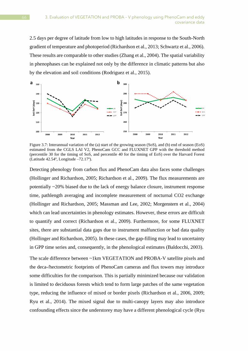
3. Evaluation of VEGETATION and PROBA – V phenology using PhenoCam and eddy covariance data
66 66
2.5 days per degree of latitude from low to high latitudes in response to the South-North
gradient of temperature and photoperiod (Richardson et al., 2013; Schwartz et al., 2006).
These results are comparable to other studies (Zhang et al., 2004). The spatial variability
in phenophases can be explained not only by the difference in climatic patterns but also
by the elevation and soil conditions (Rodriguez et al., 2015).
Figure 3.7: Interannual variation of the (a) start of the growing season (SoS), and (b) end of season (EoS)
estimated from the CGLS LAI V2, PhenoCam GCC and FLUXNET GPP with the threshold method
(percentile 30 for the timing of SoS, and percentile 40 for the timing of EoS) over the Harvard Forest
(Latitude 42.54º, Longitude –72.17º).
Detecting phenology from carbon flux and PhenoCam data also faces some challenges
(Hollinger and Richardson, 2005; Richardson et al., 2009). The flux measurements are
potentially ~20% biased due to the lack of energy balance closure, instrument response
time, pathlength averaging and incomplete measurement of nocturnal CO2 exchange
(Hollinger and Richardson, 2005; Massman and Lee, 2002; Morgenstern et al., 2004)
which can lead uncertainties in phenology estimates. However, these errors are difficult
to quantify and correct (Richardson et al., 2009). Furthermore, for some FLUXNET
sites, there are substantial data gaps due to instrument malfunction or bad data quality
(Hollinger and Richardson, 2005). In these cases, the gap-filling may lead to uncertainty
in GPP time series and, consequently, in the phenological estimates (Baldocchi, 2003).
The scale difference between ~1km VEGETATION and PROBA-V satellite pixels and
the deca-/hectometric footprints of PhenoCam cameras and flux towers may introduce
some difficulties for the comparison. This is partially minimized because our validation
is limited to deciduous forests which tend to form large patches of the same vegetation
type, reducing the influence of mixed or border pixels (Richardson et al., 2006, 2009;
Ryu et al., 2014). The mixed signal due to multi-canopy layers may also introduce
confounding effects since the understorey may have a different phenological cycle (Ryu

3.5. Conclusions
67
et al., 2014). The emergence of forest understorey is interpreted in both ground-based
and satellite observations as an increase in the greening signal.
The agreement between the PhenoCam, FLUXNET and remotely sensed phenological
metrics showed generally a higher accuracy for SoS than EoS, consistent with previous
studies (Bórnez et al., 2020a; Garrity et al., 2011; Hufkens et al., 2012; Liang et al.,
2011; Melaas et al., 2013; Nijland et al., 2016; Richardson et al., 2013). Differences in
the structure, ecophysiology and dynamics of the vegetation canopy at the start and end
of the growing season (Klosterman et al., 2014) may partially explain this. The
phenological dynamics for the timing of EoS tend to vary with species, age, dispersion
and homogeneity, and can also differ across the same species, with differences of up to
two weeks within the same ROI (Delbart et al., 2005; Richardson et al., 2006, 2009,
2010, 2019). Further studies will use high resolution satellite data from Sentinel-2 to
mitigate these issues and capture the spatial variability of EoS (Snyder et al., 2019).
Note, however, that monitoring EoS is affected by the intrinsic uncertainties of satellite
remote sensing at northern latitudes in autumn: atmospheric effects, snow and poor
illumination conditions (Luquez et al., 2007).
3.5. Conclusions
Phenological data from PhenoCam, FLUXNET and satellite remotely sensed data have
become a broad resource for analyzing the relationships between global change and
vegetation (Hufkens et al., 2012; Richardson et al., 2018). The network of PhenoCam
webcams and eddy covariance towers cover only small areas around the camera or flux
tower (Churkina et al., 2005; Gonsamo et al., 2012). Satellite imagery has the advantage
of providing continuous spatio-temporal coverage at the global scale. Near-surface
digital cameras and flux towers have nevertheless become a good tool for characterizing
local phenology and validate satellite estimates (Klosterman et al., 2014; Migliavacca et
al., 2011; Richardson et al., 2009; Sonnentag et al., 2012). The high temporal frequency
of PhenoCam and flux measurements provide continuous time series for applying the
same phenology extraction methods to ground and satellite time series. This way, we
avoid some of the issues identified in our previous research (Bórnez et al., 2020a) related
to the differences in the definition of satellite phenology metrics and ground
phenophases when PEP725 and USA-NPN data were used for the validation (e.g.; the

3. Evaluation of VEGETATION and PROBA – V phenology using PhenoCam and eddy covariance data
68 68
representativity and spatial distribution of the data as well as the gaps in the time series
of ground measurements).
Results validate the land surface phenology estimated from CGLS LAI V2 time series,
as well as the robustness of PhenoCam and FLUXNET data to analyze vegetation
phenology. This study has put bounds on the uncertainty in satellite-derived
phenological transitions, which should allow to analyze changes in the phenological
distribution pattern and serve as a starting point for other studies that characterize
anomalies and trends over vegetation phenology, as well as its possible relationship with
changes in the climate pattern as a result of climate change.

69 69
4
Monitoring the responses
of deciduous forest
phenology to 2000-2018
climatic anomalies in the
Northern Hemisphere
Kevin Bórnez, Aleixandre Verger, Adrià Descals, Josep Peñuelas
Article (in press) Remote Sens. 2021, 13,xxx

4. Monitoring the responses of deciduous forest phenology to climatic anomalies
70 70 70 70
Abstract
Monitoring the phenological responses of deciduous forests to climate is important due
to the increasing frequency and intensity of extreme climatic events associated with
climate change and global warming, which will in turn affect vegetation seasonality. We
investigated the spatiotemporal patterns of the response of deciduous forests to climatic
anomalies in the Northern Hemisphere using satellite-derived phenological metrics from
the Copernicus Global Land Service Leaf Area Index and multi-source climatic data sets
for 2000–2018 at resolutions of 0.1°. Thereafter, we assessed the impact of extreme
heatwaves and droughts on this deciduous forest phenology. We assumed that changes
in the deciduous forest phenology in the Northern Hemisphere for the period 2000-2018
were monotonic and temperature and precipitation were the main climatic drivers.
Analyses of partial correlations of phenological metrics with the timing of the start of
the season (SoS), end of the season (EoS), and climatic variables indicated that changes
in preseason temperature played a stronger role than precipitation in affecting the
interannual variability of SoS anomalies: the higher the temperature, the earlier the SoS
in most deciduous forests in the Northern Hemisphere (mean correlation coefficient of -
0.31). Correlations between SoS and temperature were significantly negative in 57% of
the forests and significantly positive in 15% of the forests (P<0.05). Both temperature
and precipitation contributed to the advance and delay of EoS. A later EoS was
significantly correlated with a positive standardized precipitation-evapotranspiration
index (SPEI) at the regional scale (~30% of deciduous forests). The timings of EoS and
SoS shifted by >20 d in response to heat waves throughout most of Europe in 2003 and
in the United States of America in 2012. This study contributes to improve our
understanding of the phenological responses of deciduous forests in the Northern
Hemisphere to climate change and climate extreme events.

4.1. Introduction
71 71
4.1. Introduction
Interest in understanding the interactions between phenology and climate has increased
in the last few decades (Ceccherini et al., 2014) because vegetation phenology plays an
important role in balancing biogeochemical cycles, such as the exchange of water,
energy, and carbon (He et al., 2018; Peñuelas et al., 2009; Richardson et al., 2013; White
et al., 2005). Changes in the timing of phenology provide the first signals of adjustments
in the responses of species to climatic anomalies (Walther et al., 2002).
Changes in the pattern of distribution of temperatures and precipitation as a consequence
of global climate change, and the interactions with other cues such as photoperiod, could
strongly alter vegetation phenology (Bradley et al., 2011; Cleland et al., 2017; IPCC,
2007, 2012, 2013). Investigating the interactive effects of temperature and precipitation
on phenology to understand and anticipate the effects of climate change on vegetation
is therefore crucial (Du et al., 2019). Many previous studies have investigated the
changes in vegetation phenology as a result of the climate change and the associated
global warming (de Beurs and Henebry, 2005; Jeong et al., 2011; Piao et al., 2007; Zhou
et al., 2001). In this sense, the analysis of the sensitivity of vegetation to hydroclimatic
anomalies is increasingly studied (Ceccherini et al., 2014; Shen et al., 2015), especially
the role of the temperature on phenology (Cong, et al., 2017; Forrest and Miller, 2010;
Forzieri et al., 2014; Thackeray et al., 2016; Wang et al., 2007). Previous studies have
demonstrated that temperature has been one of the most decisive factors affecting
phenology in the last four decades, with strong correlations between deciduous forest
phenology and temperature (R2>0.5) in central Europe, China (Estrella and Menzel,
2006; Lu et al., 2016), and the Mediterranean region, especially with temperatures in the
months prior to the phenophases (Peñuelas et al., 2002). Phenology is changing in
response to global warming, leading to an earlier SoS and a later EoS during the last few
decades in some areas of the Northern Hemisphere (Peñuelas and Filella, 2001; Piao et
al., 2019), such as North America (Richardson et al., 2013), China (Piao et al., 2006;
Kang et al., 2018), and Eurasia (Menzel, 2003; Piao et al., 2011). Droughts also play an
important role where humidity determines vegetation growth (Piao et al., 2015; Ramos
et al., 2015).
Global warming has increased the intensity, frequency, and spatial distribution of
extreme climatic events at global and regional scales (Chen and Sun, 2017; Held and

4. Monitoring the responses of deciduous forest phenology to climatic anomalies
72 72
Soden, 2006; Javed et al., 2021; Sheffield and Wood, 2008). Extreme climatic events
are often accompanied by anomalies of temperature and precipitation (He et al., 2018;
Ma et al., 2015). These events are characterized by being severe and unique compared
to average conditions over a particular time series (Butt et al., 2015; Menzel et al., 2011).
Understanding the responses of phenology to climatic extremes is therefore crucial and
challenging, because future climatic anomalies will become more intense and frequent
relative to those in past decades (IPCC, 2007 2013; Jentsch et al., 2009; Reichstein et
al., 2013; Tang et al., 2017; Zhao et al., 2018; Zheng et al., 2018). Climatic extremes
early in the 21st century have affected most regions of the Northern Hemisphere, such
as Europe (Ivits et al., 2014; Reichstein et al., 2007) and North America (Ponce-Campos
et al., 2013), where heat waves were more common than in previous decades (Fischer
and Schär, 2010; Trumbore et al., 2015). Some previous studies have also focused on
assessing the vegetation phenological responses to climate extreme events in Europe
(Ciais et al., 2005; Gobron et al., 2005; Lorenz et al., 2013) and North America
(Diffenbaugh, 2005; Ellwood et al., 2013; Karl et al., 2012).
Remotely sensed data have been widely used to analyze vegetation dynamics and
estimate phenological metrics at hemispherical and global scale (Bórnez et al., 2020a,
2020b; Richardson et al., 2009; Verger et al., 2014., 2019). Several phenological
metrics, including the start of the growing season (SoS) and the end of the season (EoS),
have been estimated from time series of vegetation indices derived from medium
resolution satellite instruments such as the Moderate Resolution Imaging
Spectroradiometer (MODIS), the Advanced Very High-Resolution Radiometer
(AVHRR), VEGETATION on board the Satellite Pour l'Observation de la Terre (SPOT-
VGT) and PROBA-V (Atkinson et al., 2012; Bórnez et al., 2020a; Delbart et al., 2005;
Verger et al., 2016; Zhang et al., 2004). Estimates of land-surface phenology (LSP) using
remotely sensed data play an important role in monitoring terrestrial responses to climate
change (White et al., 2005). Numerous LSP studies e.g. (Beaubien and Freeland, 2000;
Chmielewski and Rotzer, 2002; Menzel and Fabian, 1999; Schwartz et al., 2006) have
been focused on the northern hemisphere. These studies commonly use the NDVI for
detecting phenological trend and interannual variation (de Beurs and Henebry, 2005;
Julien and Sobrino, 2009; White et al., 2009), and mainly focus on determining trends
and investigating the advance for the timing of SoS during the last decades.

4.2. Materials and Methods
73 73
This is the first study analyzing the response of vegetation phenology to climate
anomalies by using phenological metrics derived from leaf area index (LAI) time series
from both SPOT-VGT and PROBA-V sensors that were demonstrated to outperform
NDVI time series for phenology detection (Bórnez et al., 2020a). Our study focusses on
understanding the changes and the sensitivity of deciduous forest phenology to the
anomalies of temperature, precipitation and drought for 2000–2018 in the Northern
Hemisphere. We assumed that changes in the deciduous forest phenology in the
Northern Hemisphere for the period 2000-2018 were monotonic and temperature and
precipitation were the main climatic drivers. Our specific objectives were to: (1) quantify
the spatial patterns of correlations of the anomalies of deciduous forest phenology with
precipitation and temperature, (2) identify the main causes of phenological change, (3)
determine the impact of drought on phenology, (4) quantify the sensitivity of phenology
to climate, and (5) assess the effects of some climate extreme events (e.g. heat wave) on
phenology. This study contributes to improve our understanding of the phenological
response to climate change and climate extreme events in the Northern Hemisphere.
4.2. Materials and Methods
4.2.1. Data sources and processing
4.2.1.1. Study area
Our study is focused on deciduous forests in the Northern Hemisphere (Figure 4.1)
where the used LSP retrievals were validated (Bradley et al., 2011; Cleland et al., 2017).
According to the Intergovernmental Panel on Climate Change (IPCC) predictions (de
Beurs and Henebry, 2005; Zhou et al., 2001), these northern regions are highly sensitive
to climate change.
Figure 4.1: Map showing the study area with the distribution of the deciduous forests analyzed (in green).
The red dashed lines show the regional areas assessed in section 3.2.

4. Monitoring the responses of deciduous forest phenology to climatic anomalies
74 74
4.2.1.2. Land – cover / vegetation map
Because we focused on deciduous forests, we used a land-cover (LC) map that identified
this type of vegetation: the Climate Change Initiative (CCI-LC) map series for 2015 at
a spatial resolution of 300 m, available from the European Space Agency (ESA)
(http://maps.elie.ucl.ac.be/CCI/viewer/download.php). CCI-LC discriminates 38
classes of land cover. We resampled the map to 0.1° and analyzed only pixels containing
deciduous forest.
4.2.1.3. Vegetation phenology from SPOT VEGETATION and Proba-V data
SoS and EoS during 2000–2018 were estimated using the time series of Copernicus
Global Land Service LAI 1km version 2 derived from SPOT VEGETATION (VGT)
and Prova-V data (Verger et al., 2014)
(https://land.copernicus.eu/global/themes/vegetation). These metrics were based on
previous protocols and research (Bórnez et al., 2020a; Bórnez et al., 2020b; Verger, et
al., 2016) that used dynamic thresholds. This method is based on the percentage of the
LAI amplitude in each pixel, in which SoS is defined as the day of the year (DoY) when
LAI exceeds the 30% threshold and EoS is defined as the DoY when LAI overpasses
the 40% threshold after the growing season.
4.2.1.4. Rainfall and temperature data sets
The data for temperature and precipitation were collected from the ERA5 hourly gridded
data sets from 2000 to 2018 with a spatial resolution of 0.25°
(https://cds.climate.copernicus.eu/). To achieve higher resolution, we interpolated all
climatological data from the spatial resolution of 0.25 to 0.1° using a cubic convolution
that calculated the value of each pixel by fitting a smooth curve based on the surrounding
16 pixels. Temperature was the air temperature at a height of 2 m, and precipitation was
the accumulated amount of liquid or frozen water that fell, calculated as the sum of large-
scale and convective precipitation in millimeters.
We used the mean temperature and accumulated precipitation for the preseason using
time lags of 1, 3, and 6 months prior to the timings of SoS and EoS.

4.2. Materials and Methods
75 75
4.2.1.5. SPEI
Drought indices have become useful tools for analyzing, assessing, and estimating the
dry and humid periods that may impact on phenology (Javed et al., 2021). Various
drought indices are available, such as the standardized precipitation index (SPI) or the
Palmer drought severity index (Palmer, 1965) (PDSI), and several recent studies have
analyzed drought conditions using the standardized precipitation-evapotranspiration
index (SPEI) (Chen et al., 2015; Wang et al., 2017). SPEI is based on precipitation and
potential evapotranspiration, which includes the role of temperature in drought severity
(Beguería et al., 2013; Vicente-Serrano et al., 2010., 2013). SPEI considers drought
timescales, which represent the cumulative water balance over the previous 1–48
months. It is based on the Standardized Precipitation Index (SPI) calculation method but
with improvements to include the potential evapotranspiration (PET). The SPEI uses the
weekly (or monthly) difference between precipitation and PET (based on Thornthwaite
method), and it is calculated as a standardized variable, which allows the comparison
with other SPEI values and climatic variables over time and space (Vicente-Serrano et
al., 2010). Unlike SPI, SPEI includes the effects of temperature variability on drought
estimation and therefore, it takes into account the effect of warming processes on
drought severity (Vicente-Serrano et al., 2010., 2013).
SPEI data set Version 2.6 was downloaded from the Global SPEI database
(https://spei.csic.es/database.html) at a spatial resolution of 0.5° and was resampled to
0.1° for the analysis. This data set is based on the United Nations Food and Agriculture
Organization (FAO)-56 Penman-Monteith estimation of potential evapotranspiration.
The complete procedure for calculating SPEI is provided by Vicente-Serrano et al.
(2010).
We determined drought severity for the timings of SoS and EoS using different SPEI
timescales (1, 3, 6, and 12 months), representing the cumulative water balance for the
timings of preseason and presenescence. Positive SPEI values indicate that humidity is
higher than the historical median, and negative values indicate a water deficit (Vicente-
Serrano et al., 2010., 2013). The SPEI data were classified into seven categories (Table
4.1) based on the World Atlas of Desertification (Cherlet et al., 2018) for analyzing
conditions of wetness or dryness.

4. Monitoring the responses of deciduous forest phenology to climatic anomalies
76 76 76 76
Table 4.1: Classification of drought based on SPEI data.
Range Condition
SPEI ≤ -2 Extremely dry
-2 < SPEI ≤ -1.5 Severely dry
-1.5 < SPEI ≤ -1 Moderately dry
-1 < SPEI ≤ 1 Near normal
1 < SPEI ≤ 1.5 Moderately wet
1.5 < SPEI ≤ 2 Severely wet
SPEI ≥ 2 Extremely wet
4.2.2. Methodology and statistical analysis
We first estimated the significant trends in the time series of the estimates (SoS and
EoS). Secondly, we explored the impacts of anomalies in hydroclimatic variables, such
as temperature, precipitation, and drought on deciduous phenology throughout the
Northern Hemisphere for 2000–2018. We applied spatiotemporal response analysis to
determine the relationships of phenology and climate variables. Moreover, we
investigated the spatial pattern of the sensitivity of phenology to climate and its
relationship with preseason and presenescence temperature, precipitation, and drought.
We thereafter focused on some of the extreme events, including high temperatures, low
temperatures and severe drought, that have occurred in the last two decades.
We used different software to calculate and evaluate the effects of climatic variables on
vegetation phenology. We first used Google Earth Engine (Gorelick et al., 2017) to
download and process the time series of the hydroclimatic variables and for estimating
land-surface phenological metrics in the Northern Hemisphere (Bórnez et al., 2020a;
2020b). We then used RStudio, XLSAT and Idrisi TerrSet for processing and
statistically analyzing all data. Finally, we used ESRI ArcGIS 10.5 for generating the
graphs and maps.
4.2.2.1. Trend analysis
We calculated the trends in the estimated time series of SoS and EoS before analyzing
the relationships between phenology and climate. Temporal trends in the data sets were
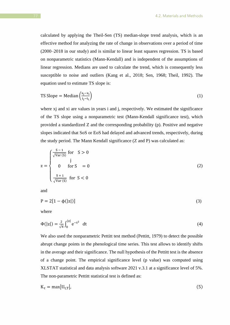
4.2. Materials and Methods
77 77
calculated by applying the Theil-Sen (TS) median-slope trend analysis, which is an
effective method for analyzing the rate of change in observations over a period of time
(2000–2018 in our study) and is similar to linear least squares regression. TS is based
on nonparametric statistics (Mann-Kendall) and is independent of the assumptions of
linear regression. Medians are used to calculate the trend, which is consequently less
susceptible to noise and outliers (Kang et al., 2018; Sen, 1968; Theil, 1992). The
equation used to estimate TS slope is:
TS Slope = Median (xj−xi
tj−ti) (1)
where xj and xi are values in years i and j, respectively. We estimated the significance
of the TS slope using a nonparametric test (Mann-Kendall significance test), which
provided a standardized Z and the corresponding probability (p). Positive and negative
slopes indicated that SoS or EoS had delayed and advanced trends, respectively, during
the study period. The Mann Kendall significance (Z and P) was calculated as:
z =
{
S − 1
√Var (S) for S > 0
j 0 for S = 0
S + 1
√Var (S) for S < 0
(2)
and
P = 2[1 − ϕ(|z|)] (3)
where
Φ(|z|) =2
√π∫ e−t
2 dt
|z|
0 (4)
We also used the nonparametric Pettitt test method (Pettitt, 1979) to detect the possible
abrupt change points in the phenological time series. This test allows to identify shifts
in the average and their significance. The null hypothesis of the Pettitt test is the absence
of a change point. The empirical significance level (p value) was computed using
XLSTAT statistical and data analysis software 2021 v.3.1 at a significance level of 5%.
The non-parametric Pettitt statistical test is defined as:
Kτ = max|Ut,T|, (5)

4. Monitoring the responses of deciduous forest phenology to climatic anomalies
78 78 78 78 78 78
𝑤here
Ut,T = ∑ ∑ sgnnj=i+1 (xj − xj)
ti=1 (6)
where t is the period length and n is the number of data in the statistical series. p-value
and an interval around the p-value was evaluated by using a Monte Carlo method.
4.2.2.2. Standardized anomalies
We calculated standardized anomalies in the interannual time series (2000–2018) of
phenology, temperature, and precipitation. Standardized anomalies were calculated by
dividing anomalies by the standard deviation. The equation is (Funk et al., 2019):
Z =X−μ
σ (7)
where Z is a standardized anomaly, X is the annual value, and µ and σ are the interannual
mean and standard deviation, respectively, for each variable analyzed (i.e. the timings
of SoS and EoS, the mean preseason or presenescence temperature, or the accumulated
preseason or presenescence precipitation).
Note that we estimated the anomalies in the time series of temperature and precipitation
using the mean temperature and the accumulated precipitation for different timescales
(1, 3, and 6 months) before estimating the timings of SoS and EoS (see section 2.1.3).
4.2.2.3. Correlations and partial correlation analyses
We calculated the coefficients for the correlations between the estimated time series of
phenology (SoS and EoS), temperature, precipitation, and SPEI for different preseason
lengths. We used two types of correlation analysis to quantify the response of vegetation
to climatic drivers. We first calculated the linear correlation (Pearson’s correlation)
between the interannual anomalies of phenology (y) and hydroclimatic variables (x) at
a significant level of 95%:
rxy =n Σxiyi−ΣxiΣyi
√n∑xi2 − (Σxi)
2 √n ∑yi2−(Σyi)
2 (8)
where rxy is the Pearson correlation coefficient between x and y, n is the number of
observations, xi is the value of x for observation i, and yi is the value of y for observation
i. A multivariate linear regression model was used for multivariate cases.

4.2. Materials and Methods
79 79
We correlated SoS and EoS anomalies with the climatic variables (temperature and
precipitation) for timescales of 1, 3, and 6 months prior to the dates of SoS and EoS and
summarized the climatic variables for the preseason periods in which the correlation was
highest. For SPEI, we used timescales from 1 to 12 months (Vicente-Serrano et al.,
2013).
We then applied a partial correlation analysis of SoS and EoS using the preseason and
presenescence climatic variables for the three-time lags (1, 3, and 6 months). The
precipitation data for the same timescale were used as a constant factor for calculating
the partial correlation between phenology and temperature. Similarly, the influence of
temperature was considered a constant for calculating the correlation with accumulated
precipitation. The partial correlation coefficient between vegetation and mean
temperature and its significance were tested as:
rvt.p =rvt− rvprtp
√(1−r vp2 )(1−r tp
2 )
(9)
where v is the vegetation phenology, t is temperature, p is precipitation, and rvt and rvp
are the simple correlation coefficients of the phenology (SoS or EoS) with the mean
preseason or presenescence temperature and accumulated precipitation, respectively.
Eq. (8) is also valid for calculating the partial correlation between phenology and
precipitation by changing the order in which the data are entered. The significance of
the partial correlation coefficients at the 95% level was evaluated using the Student’s t-
test.
The Pearson’s correlation and partial correlation analysis produced similar maps, so the
results obtained by partial correlation will be taken into account in subsequent sections
for analyzing the correlations between phenology, temperature, and precipitation.
4.2.2.4. Sensitivity analysis
We used multiple linear regression and sensitivity analysis to further investigate the
interactions of phenology with temperature, precipitation, and SPEI. The responses of
the sensitivity of vegetation phenology to the climatic variables corresponded to the
slopes of the linear regressions between the phenological metrics and the climatic
variables, representing the unit change in phenological date divided by the unit change
in temperature, precipitation, or SPEI.
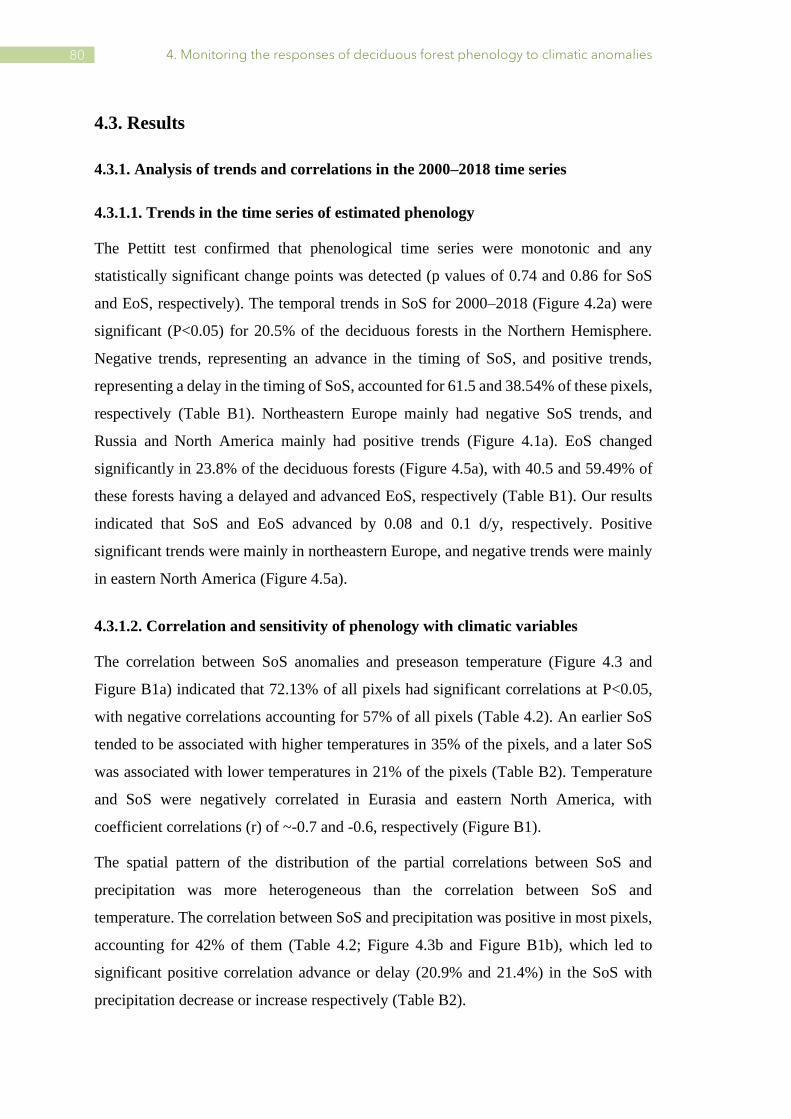
4. Monitoring the responses of deciduous forest phenology to climatic anomalies
80 80
4.3. Results
4.3.1. Analysis of trends and correlations in the 2000–2018 time series
4.3.1.1. Trends in the time series of estimated phenology
The Pettitt test confirmed that phenological time series were monotonic and any
statistically significant change points was detected (p values of 0.74 and 0.86 for SoS
and EoS, respectively). The temporal trends in SoS for 2000–2018 (Figure 4.2a) were
significant (P<0.05) for 20.5% of the deciduous forests in the Northern Hemisphere.
Negative trends, representing an advance in the timing of SoS, and positive trends,
representing a delay in the timing of SoS, accounted for 61.5 and 38.54% of these pixels,
respectively (Table B1). Northeastern Europe mainly had negative SoS trends, and
Russia and North America mainly had positive trends (Figure 4.1a). EoS changed
significantly in 23.8% of the deciduous forests (Figure 4.5a), with 40.5 and 59.49% of
these forests having a delayed and advanced EoS, respectively (Table B1). Our results
indicated that SoS and EoS advanced by 0.08 and 0.1 d/y, respectively. Positive
significant trends were mainly in northeastern Europe, and negative trends were mainly
in eastern North America (Figure 4.5a).
4.3.1.2. Correlation and sensitivity of phenology with climatic variables
The correlation between SoS anomalies and preseason temperature (Figure 4.3 and
Figure B1a) indicated that 72.13% of all pixels had significant correlations at P<0.05,
with negative correlations accounting for 57% of all pixels (Table 4.2). An earlier SoS
tended to be associated with higher temperatures in 35% of the pixels, and a later SoS
was associated with lower temperatures in 21% of the pixels (Table B2). Temperature
and SoS were negatively correlated in Eurasia and eastern North America, with
coefficient correlations (r) of ~-0.7 and -0.6, respectively (Figure B1).
The spatial pattern of the distribution of the partial correlations between SoS and
precipitation was more heterogeneous than the correlation between SoS and
temperature. The correlation between SoS and precipitation was positive in most pixels,
accounting for 42% of them (Table 4.2; Figure 4.3b and Figure B1b), which led to
significant positive correlation advance or delay (20.9% and 21.4%) in the SoS with
precipitation decrease or increase respectively (Table B2).

4.3. Results
81 81
Table 4.2: Percentage of pixels with significant correlations (P<0.05) between the anomalies of
phenological events (SoS and EoS) and climatic variables (temperature, precipitation, and SPEI) in the
Northern Hemisphere for 2000–2018.
Phenological event Climatic variable Positive (%) Negative (%)
SoS Temperature 14.94 57.19
Precipitation 42.30 20.07
SPEI 17.57 9.87
EoS Temperature 23.57 20.75
Precipitation 34.44 28.42
SPEI 28.78 9.04

4. Monitoring the responses of deciduous forest phenology to climatic anomalies
82 82
The mean sensitivities of SoS to temperature and precipitation were -2.45 d/°C and 0.8
d/10 mm, respectively (Figure 4.4). The sensitivity to temperature was highest (~-5
d/°C) in Eurasia and southeastern North America (Figure 4.2b), and the sensitivity to
precipitation was highest (3 d/10 mm) at latitudes >60°N (Figure 4.2c).
Figure 4.2: (a) Distribution of trends for the SoS time series in the Northern Hemisphere between 2000
and 2018 in pixels with significant correlations between phenology and climate (a positive trend indicates
a delayed SoS, and a negative trend indicates an advanced SoS). Regions with black dots indicate
significant trends (Mann-Kendall test, P<0.05). For visualization purposes, the size of black dots has been
increased. (b) Distribution of sensitivity coefficients between SoS and mean preseason temperature (d/°C).
(c) Distribution of sensitivity coefficients between SoS and preseason accumulated precipitation (d/10
mm). White indicates unvegetated areas and areas with no deciduous forests, and light gray (in b and c)
indicates vegetated areas with nonsignificant correlations (P>0.05).
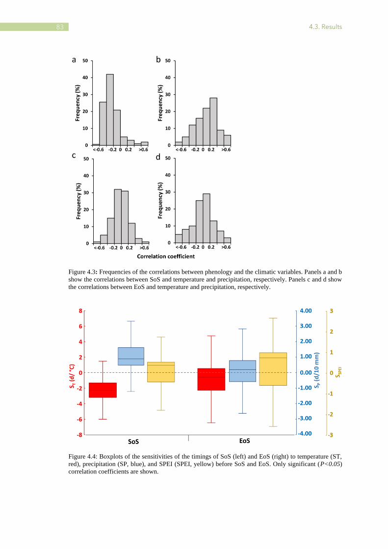
4.3. Results
83 83 83 83
Figure 4.3: Frequencies of the correlations between phenology and the climatic variables. Panels a and b
show the correlations between SoS and temperature and precipitation, respectively. Panels c and d show
the correlations between EoS and temperature and precipitation, respectively.
Figure 4.4: Boxplots of the sensitivities of the timings of SoS (left) and EoS (right) to temperature (ST,
red), precipitation (SP, blue), and SPEI (SPEI, yellow) before SoS and EoS. Only significant (P<0.05)
correlation coefficients are shown.

4. Monitoring the responses of deciduous forest phenology to climatic anomalies
84 84
The sensitivity analysis (Figure 4.4 and Figure 4.5) indicated that the response of
phenology to climatic anomalies was lower for the timing of EoS than the timing of SoS.
The pattern of temperature sensitivity was very heterogeneous, with symmetric
distributions of positive and negative correlations between temperature and EoS in 23.57
and 20.75% of the pixels, respectively (Table 4.2, Figure 4.3c). EoS advanced with
temperature by an average of ~0.5 d/°C (Figure 4.5b). The sensitivity of EoS to
precipitation had the opposite pattern: the timing of EoS was delayed by an average of
~0.5 d/10 mm. Correlations were significantly positive (i.e. a delay in the timing of EoS
with an increase in precipitation) in 34.44% of the study area (Figure B2), with
sensitivities highest in southern and southwestern Europe (~3 d/10 mm). In contrast,
28.42% of the pixels had negative correlations (i.e. an advance in the timing of EoS with
an increase in precipitation), mainly in northeastern Europe and areas of Russia (Figure
4.5c).

4.3. Results
85 85 85 85
Figure 4.5: (a) Distribution of trends for the EoS time series in the Northern Hemisphere between 2000
and 2018 in pixels with significant correlations between phenology and climate (a positive trend indicates
a delayed EoS, and a negative trend indicates an advanced EoS). Regions with black dots indicate
significant trends (Mann-Kendall test, P<0.05). For visualization purposes, the size of the black dots has
been increased. (b) Distribution of sensitivity coefficients between EoS and mean presenescence
temperature (d/°C). (c) Distribution of sensitivity coefficients between EoS and presenescence
accumulated precipitation (d/10 mm). White indicates unvegetated areas and areas with no deciduous
forests, and light gray (in b and c) indicates vegetated areas with nonsignificant correlations (P>0.05).
4.3.1.3. Response of vegetation phenology to drought using SPEI
When analyzing the influence of drought on vegetation, we found that SPEI calculated
using time lags between 1 and 3 months was correlated the best with the timings of SoS
and EoS in >50% of the pixels (Table B3).
The Spearman correlations between SoS and SPEI were positive in 52.3% of the
Northern Hemisphere and were significant (P<0.05) in 17.5% of the pixels (Table 4.2),

4. Monitoring the responses of deciduous forest phenology to climatic anomalies
86 86
mostly >60°N in northeastern Europe and North America (Figure 4.6a). The correlations
were negative (47.6% of the pixels, significant in 9.8%) in northeastern Europe (between
50° and 60°) in areas where the sensitivity of SoS to SPEI was highest (Figure B3a).
Correlations between the timings of EoS and SPEI were positive in 58.8% of the study
area (Table 4.2), with significant correlations for 28.8% of the pixels (P<0.05). The
correlations were particularly strong in southwestern Europe and northeastern North
America (Figure 4.6b) in areas where the sensitivity of EoS to SPEI was highest (Figure
B3b). Drought weakly affected phenology at high northern latitudes (>60°N), where
temperature (Figure 4.5b), not precipitation (Figure 4.5c), was the main variable limiting
phenology. The correlations between EoS and SPEI were thus weak.
Figure 4.6: Spatial patterns of the partial correlations between SPEI and (a) SoS and (b) EoS for 2000–
2018 in the Northern Hemisphere. The color scale represents the maximum correlation coefficient for
each pixel, independently of the SPEI timescale. White indicates unvegetated areas and areas with no
deciduous forests, and light gray indicates vegetated areas with nonsignificant correlations (P>0.05).
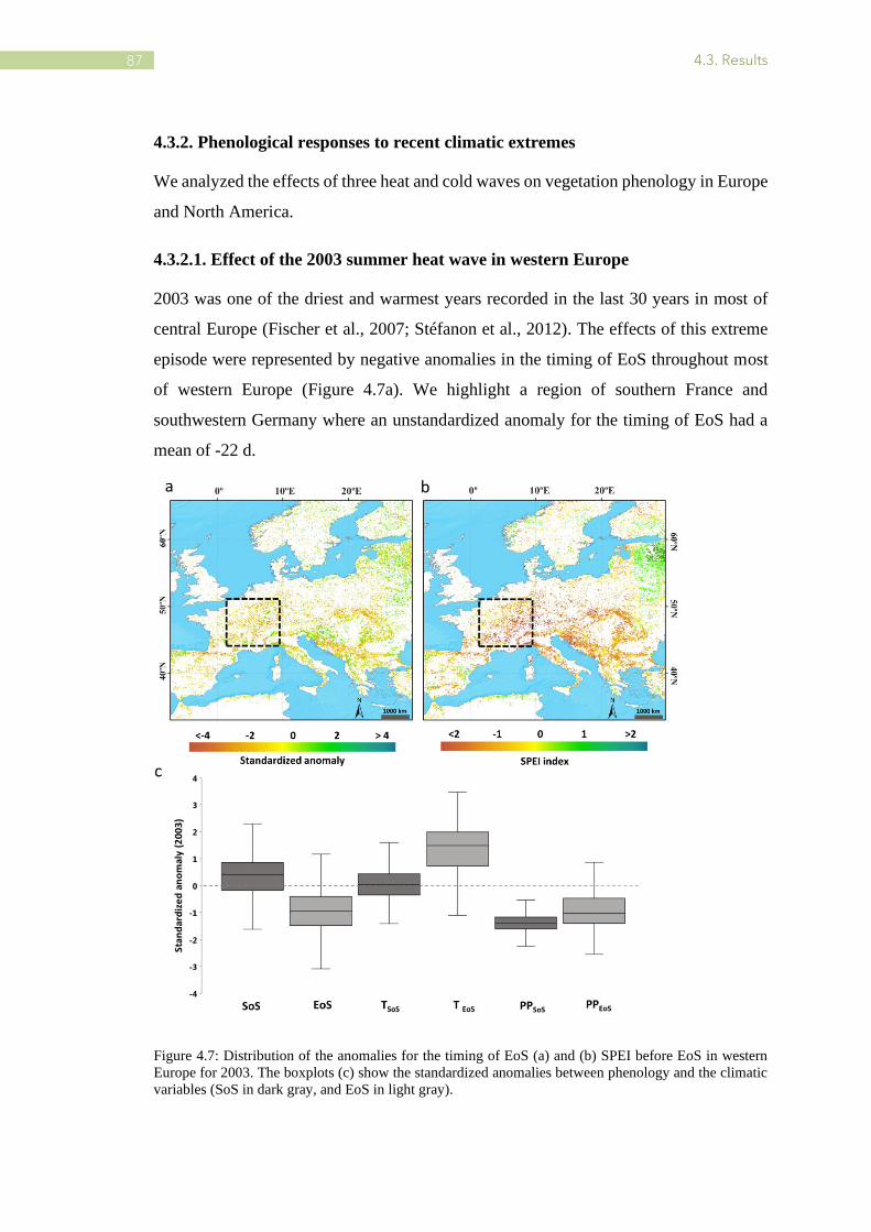
4.3. Results
87 87 87 87
4.3.2. Phenological responses to recent climatic extremes
We analyzed the effects of three heat and cold waves on vegetation phenology in Europe
and North America.
4.3.2.1. Effect of the 2003 summer heat wave in western Europe
2003 was one of the driest and warmest years recorded in the last 30 years in most of
central Europe (Fischer et al., 2007; Stéfanon et al., 2012). The effects of this extreme
episode were represented by negative anomalies in the timing of EoS throughout most
of western Europe (Figure 4.7a). We highlight a region of southern France and
southwestern Germany where an unstandardized anomaly for the timing of EoS had a
mean of -22 d.
Figure 4.7: Distribution of the anomalies for the timing of EoS (a) and (b) SPEI before EoS in western
Europe for 2003. The boxplots (c) show the standardized anomalies between phenology and the climatic
variables (SoS in dark gray, and EoS in light gray).

4. Monitoring the responses of deciduous forest phenology to climatic anomalies
88 88
An intense drought also occurred in 2003, which we identified using SPEI (Figure 4.7b,
Table 4.3). More than 80% of the pixels indicated an intense drought prior to the timing
of EoS. Fischer et al. (2007) observed that an early EoS and stress from the lack of soil
moisture contributed greatly to the suppression of evapotranspiration after the summer
and that this interaction may have amplified the temperature anomaly by locally
increasing the flux of sensible heat. Figure 4.7c shows the standardized anomalies
between phenology and the climatic variables, which allows the visualization of the
positive temperature anomaly for the timing of EoS and the precipitation deficit for the
timings of both SoS and EoS.
Table 4.3: Classification of SPEI data for characterizing drought in the three case studies: Europe, North
America, and Balkans for 2003, 2012, and 2005, respectively. Two analytical periods are used: preseason
(for the timing prior to SoS) and presenescence (for the timing prior to EoS). The SPEI timescale with the
highest correlation in each pixel was considered.
SoS (area, %) EoS (area, %)
Range Condition
Europe
2003
North
America 2012
Balkans
2005
Europe
2003
North
America 2012
Balkans
2005
SPEI ≤ -2 Extremely dry 0 0.77 0 26.30 3.96 0
-2 SPEI ≤ -1.5 Severely dry 2.88 9.60 0 29.75 5.56 0
-1.5 SPEI ≤ -1 Moderately dry 15.96 16.69 0 23.99 4.68 1.04
-1 < SPEI ≤ 1 Near normal 80.96 72.93 14.44 19.96 52.44 67.56
1 SPEI ≤ 1.5 Moderately wet 0 0 35.13 0 29.57 28.78
1.5 SPEI ≤ 2 Severely wet 0 0 35.08 0 3.81 2.40
SPEI ≥ 2 Extremely wet 0 0 15.35 0 0 0.23
4.3.2.2. Effect of the 2012 spring heat wave in eastern North America
We analyzed the early spring for 2012 in North America, focusing on southeastern of
The United States (US). We calculated the interannual anomalies for the phenological
metrics and climatic variables for each pixel to assess the spatial patterns of the
phenological responses to the climatic extreme. Previous studies (Ellwood et al., 2013;
Karl et al., 2012) considered the spring SoS anomaly in 2012 as the earliest spring
recorded since 1900 across North America (Figure 4.8a). Karl et al. (2012) reported that

4.3. Results
89 89 89 89
the anomaly was driven by a strong and stable high-pressure anticyclone that remained
over much of the northeast from late February to April, causing record high temperatures
(Figure 4.8b, c) and phenological advancement.
Spring in many central and eastern areas of North America began between -15 and -30
d (unstandardized anomalies) before mean SoS for the time series analyzed (2000–2018)
(Figure 4.8c). The anomalies for the timing of SoS were negative in most of the pixels
(96.2%) (Figure 4.8a). Figure 4.8c shows the dominant role of temperature in the
phenological advancement of SoS in 2012, with mean standardized anomalies >2 °C.
Precipitation was slightly negatively anomalous before the timing of SoS in 2012, but
with no water stress, and the majority of the pixels (73%) indicated a normal SPEI
between -1 and 1 (Table 4.3).
Figure 4.8: Distribution of the anomalies for the timing of SoS (a) and (b) preseason mean temperature in
eastern USA for 2012. The boxplots (c) show the standardized anomalies between phenology and the
climatic variables (SoS in dark gray, and EoS in light gray).

4. Monitoring the responses of deciduous forest phenology to climatic anomalies
90 90
4.3.2.3. Effect of the late 2005 cold wave in the Balkans
Unlike the two previous analyses, this third case refers to a delayed SoS due to a negative
temperature anomaly for the timing of the preseason. Figure 4.9a and b shows the SoS
anomaly and preseason mean temperature for 2005, respectively. The positive anomalies
of SoS affected much of central and eastern Europe, especially the northern Balkan
Peninsula and Carpathian Mountains, where positive anomalies were 10 d in most of the
pixels (80.3%) (Figure 4.9a, c). The average standardized temperature anomaly was ~-
1 °C (Figure 4.9b,c), which greatly delayed the timing of SoS (~10 d). This delay also
coincided with a positive SPEI. Eighty percent of the pixels represented moderate or
very high humidities prior to SoS (Table 4.3).
Figure 4.9: Distribution of the anomalies for the timing of SoS (a) and (b) preseason mean temperature in
the Balkans for 2005. The boxplots (c) show the standardized anomalies between phenology and the
climatic variables (SoS in dark gray, and EoS in light gray).

4.4. Discussion
91 91
4.4. Discussion
Climatic projections indicate a likely increase in temperatures in much of the world,
especially at the higher latitudes of the Northern Hemisphere (IPCC, 2007, 2012).
Recent studies (Du et al., 2019; Lin et al., 2017) have also found that extreme climatic
events have increased in frequency, intensity, and duration, consistent with IPCC
projections, which will affect many ecosystems, particularly vegetation. Climatic
variability adds uncertainty in analyzing and predicting the impacts of climate change
on vegetation phenology (Ma et al., 2015; Peñuelas et al., 2009; Siegmund et al., 2016).
Previous studies have attributed the recent shifts in phenology to climate change and the
effects of variations in temperature and precipitation (de Beurs and Henebry, 2005; Shen
et al., 2015; Vitasse et al., 2009; Zhou et al., 2001). Assessing the pattern of distribution,
the variability of phenology, and the correlations between phenology and climatic
variables is crucial for understanding the potential effects of future climate change (Miao
et al., 2017). Remotely sensed data have been widely used to assess trends in
phenological time series and their responses to climatic variability. Numerous studies
have reported that the phenological trends from 2000 to 2018 were lower than the rates
of change from 1980 to 1999 (Jeong et al., 2011; Wang et al., 2015; Zeng et al., 2011;
Zhao et al., 2015). De Beurs et al. (2005) and Piao et al. (2006) reported that SoS
advanced by 6.6 and 7.9 d/decade in North America and China, respectively, between
1982 and 1999. Jeong et al. (2011) and Zeng et al. (2011), however, found that
phenological trends declined significantly after 2000, with an advanced for the timing
of SoS of 0.1–0.2 d/decade, respectively, consistent with our results. Some studies have
even reported delays of 1 d/decade in the timing of SoS after 2000, specifically in
western North America (Wang et al., 2015; Zhao et al., 2015).
In our study we used land-surface phenological metrics at the continental scale derived
from LAI time series (2000–2018) of the SPOT-VGT and PROBA-V sensors (Bórnez
et al., 2020a, 2020b). Since the time series start in 2000, the detected trends are limited
to reduced areas. For this reason, we mainly target on analyzing the correlations between
phenology and climatic variables and analyzing the responses of phenological anomalies
to recent climatic events.
4. Monitoring the responses of deciduous forest phenology to climatic anomalies
92 92
Most previous studies have only emphasized the role of preseason temperature in
determining SoS, because an increase in the advance of SoS is a consequence of global
warming (Cleland et al., 2017; Kang et al., 2018; Monahan et al., 2016; Peng et al., 2017;
Piao et al., 2006; Zhang et al., 2007). Other studies focusing on EoS have recorded a
delay in senescence, which led to longer growing seasons in some areas of Eurasia and
North America (Jeong et al., 2011; Liu et al., 2016). We focused on analyzing the
responses of phenology to mean preseason and presenescence temperatures,
accumulated precipitation, and drought across the deciduous forests in the Northern
Hemisphere. Our results indicated that anomalies of temperature and precipitation
controlled the changes in phenological metrics in the deciduous forests, consistent with
previous studies (He et al., 2018; Zhou et al., 2016), particularly the anomalies of SoS
strongly associated with the changes in mean preseason temperature, so this climatic
variable may have been the main cause of the advance or delay in the start of the growing
season, affecting 72.1% of the study area (mean r of -0.31) (P<0.05). Correlations were
significantly negative in 57% of the pixels (P<0.05), i.e. an advance or delay in SoS due
to higher or lower temperatures, respectively.
The effects of the relationships between the climatic variables and vegetation on the
timing of EoS were more complex. The timing of the end of the growing season in
response to temperature was generally delayed in most pixels. Water stress associated
with droughts during summer, however, advanced EoS in some regions such as southern
Europe (Figure B2 and Figure 4.6) with negative anomalies longer than -20 d for the
timing of EoS throughout most of Europe (in 2003), consistent with other studies
(Angert et al., 2005; Hmimina et al., 2013; Li et al., 2019; Wang et al., 2011).
The influence of drought on the timing of EoS was lower in humid and cold regions
(such as those pixels located between 55 and 80°N) than drier regions, such as areas
with a Mediterranean climate (Figure. S3). The availability of water in Mediterranean
areas was the primary limiting resource for the timing of EoS, but temperature and other
variables such as photoperiod may have a larger role at higher latitudes.
The distribution of the regression coefficients between the anomalies in phenology and
the climatic variables were highly spatially heterogeneous, due to the spatial and
latitudinal heterogeneity in climate and to the biological characteristics of the species,

4.5. Conclusions
93 93
which could account for the variable responsiveness to climate (Hou et al., 2015;
Peñuelas et al., 2002). The responses of phenology to climate, especially to climatic
extremes, also vary with climatic gradients, type of event, and biome, and even among
individuals of the same species (Ma et al., 2015; Siegmund et al., 2016).
These phenological changes may affect climate change by the feedbacks between
vegetation and climate (Beer et al., 2010; Bonan et al., 2015; Ceccherini et al., 2014;
Lian et al., 2020; Peñuelas et al., 2009). For example, climatic anomalies or extremely
high temperatures (such as during heatwaves) alter vegetation growth due to both the
high temperatures and lower amounts of soil moisture (Ciais et al., 2005; Reichstein et
al., 2007; Seneviratne et al., 2006). Altered vegetation growth greatly affects the uptake
of CO2, depending on the availability of soil water, regional characteristics, and plant
species (Peñuelas et al., 2009). Deficits in soil moisture lead to lower water evaporation,
which lowers the release of latent heat from the land, prevents the development of
clouds, and may consequently intensify droughts because precipitation is reduced (Berg
et al., 2016; Buermann et al., 2013, 2018), which could also involve teleconnections
between areas (Lian et al., 2020).
4.5. Conclusions
This study comprehensively analyzed the response of vegetation to climatic anomalies
in the Northern Hemisphere and assessed the impact of extreme climatic events on
deciduous phenology. Our results suggest that deciduous phenology in the Northern
Hemisphere is very sensitive to shifts in temperature, especially for the timing of SoS,
but also indicate the importance of water availability to the timing of EoS as the increase
in drought stress contribute to its advance throughout some regions (e.g., southern
Europe). Results also revealed that climate extremes events exert severe impacts on
vegetation phenology both for the timing of SoS and EoS. These findings highlight the
need to develop strategies focused on mitigating future climate changes on vegetation
and their monitoring. The interactions of temperature, precipitation, drought, and
phenology with other variables such as solar radiation, soil type, soil moisture, and the
coupling between variables and feedbacks between vegetation and climate warrant
future research.

94

95
5
General discussion and
conclusions

5. General discussion and conclusions
96
5.1. Discussion
My doctoral thesis is framed within the increasing interest in the retrieval of Land
Surface Phenology (LSP) from remote sensing and in the study of their changes and
interactions with climate change (Ceccherini et al., 2014; Peñuelas et al., 2009;
Richardson et al., 2013). I aimed to (i) improve estimation of Land surface Phenology
(LSP) from satellite time series, (ii) evaluate the uncertainty associated to its estimation,
and (iii) assess phenology-climate relationships in a climate change context.
5.1.1. Ground based phenological estimation techniques and challenges of LSP
validation
Validating LSP is challenging due, in part, to the differences in the definition of satellite
metrics and ground phenophases (White et al., 2009, Schwartz and Hanes, 2009). The
timing of vegetation seasonality has traditionally been recorded by researchers and
volunteers from in situ measurements by observing the leaf growth from bud to fall.
These observations have proven to be useful to validate the satellite estimates. However,
human-based ground observations of phenological transition dates are not uniform and
depend on the criterion used for visual inspection which may induce uncertainties,
despite efforts to establish protocols for monitoring phenophases (Denny et al. 2014,
Tierney et al. 2013). Some studies have reported differences of ~7 days among different
observers for the same place and species (Klosterman et al., 2014).
In recent years near-surface remote sensing techniques have emerged, providing an
alternative to human observations to monitor vegetation phenology (Hufkens et al.,
2012; Richardson et al., 2009; Sonnentag et al., 2012), including digital cameras and
continuous flux measurements from eddy covariance towers. Near-surface remote
sensing provides a new perspective for estimating phenology at the landscape level,
becoming an advanced technique to validate remote sensing estimates by using
consistent and continuously measurements at high temporal frequencies (e.g. PhenoCam
imagery) across broad spatial scales. In particular, in this work I used PhenoCam
Network and the existing eddy covariance flux data from FLUXNET, and the results

5.1. Discussion
97
were significantly more robust compared to those observed with PEP725 or USA-NPN,
especially for the timing of EoS, with a RMSE of 10 d and 12 d (FLUXNET and
PhenoCam) compared with 25 d and 27d (USA-NPN and PEP725) when the threshold
method was used.
The validation of land surface phenology with ground observations presented also some
difficulties associated to the spatial distribution and the spatial representability of the
data. The ground measurements represent the phenology for a limited number of
individual plants that are not necessarily the most representative species of the 1-km
satellite pixels. Conversely, satellite phenology at 1-km resolution represented an
integrated response across landscapes with diverse species and phenological behaviors.
The phenology of each species and their characteristics (sizes, ages, homogeneity),
though, influenced the satellite signal, depending on its abundance within the pixel
sampling area and on the timing of their phenophases (Delbart et al., 2015). Chapter 2
showed that statistics of the comparison between LAI V2 derived EoS using the
percentile method and ground measurements improved significantly when the analysis
was restricted to homogeneous forest sites. The scale difference between ~1km
VEGETATION and PROBA-V satellite pixels and the deca-/hectometric footprints of
PhenoCam cameras and flux towers may also introduce some difficulties for the
comparison in Chapter 3. This is partially minimized because our validation is limited
to deciduous forests which tend to form large patches of the same vegetation type,
reducing the influence of mixed or border pixels (Richardson et al., 2006, 2009; Ryu et
al., 2014).
5.1.2. Sensitivity of LSP to the satellite time series
Unlike ground observations and near-surface measurements, which only cover a small
area for a reduced number of trees, the development of satellite remote sensing has
allowed phenological dates to be estimated from local to global scale at different
temporal periods, using time series of vegetation indices and biophysical variables (e.g.
Verger et al., 2016; Zhang et al., 2006). Traditionally, the most used index for estimate
phenology from satellite has been the Normalized Difference Vegetation Index (NDVI)
(Rouse et al., 1974). However, NDVI is sensor dependent and saturates for high amounts

5. General discussion and conclusions
98
of vegetation. In Chapter 2 I derived land surface phenology from Copernicus Global
Land time series not only from NDVI time series but also using three biophysical
variables: LAI, FAPAR and FCOVER (version I and version II products) to determine
the variable that best allows to estimate LSP. Comparison with ground data showed that
phenological metrics extracted from the CGLS LAI Version 2 (V2) time series
performed the best as compared to other biophysical variables and NDVI vegetation
index or previous version V1 of the CGLS products. For this reason, I used LSP derived
from LAI V2 CGLS in Chapter 2 and Chapter 3.
The estimation of LSP from VI or biophysical variables presents several challenges.
Firstly, the presence of clouds has been a major difficulty for acquiring high temporal
resolution image time series of vegetation over the same location. Therefore, data
smoothing approaches are employed as a necessary procedure in image preprocessing
(Reed et al., 1994; Bradley et al., 2007), and the method selected for this purpose can
influence the performance of the phenology extraction from the reconstructed time series
(Atkinson et al., 2012; Kandasamy et al., 2013; Verger et al., 2016). Several studies
have used existing software tools to analyze and reconstruct time series data (Heumann
et al., 2007; Jia et al., 2014; Rodrigues et al., 2013) that include TIMESAT (Jönsson and
Eklundh, 2004), SPIRITS (Bórnez et al., 2020; Rembold et al., 2015), Phenosat
(Rodrigues et al., 2012), Hants (Zhou et al., 2015), Crop Phenology (Araya et al., 2018)
and QPhenoMetrics (Duarte et al., 2018). In chapter 2, I used SPIRITS software proving
the functionalities for the reconstruction of time series data and extraction of phenology
for V1 time series (e.g. SoS, EoS) by using the threshold method. However, it is still
limited for applying other methods. I found the choice of the smoothing method
(Whittaker, BISE or Swets) in SPIRITS software introduced differences of up to 50%
in the performance of the phenology metrics.
5.1.3. Sensitivity of LSP to the phenological extraction method
The second challenge for satellite estimates relates to the variety of methods available
to derive LSP estimates, which can lead to very different results (de Beurs and Henebry,
2010; Zeng et al., 2020). This includes thresholds (Myneni et al., 1997; White et al.,
1997), moving averages (Reed et al., 1994), first derivatives (Tateishi and Ebata, 2004;

5.1. Discussion
99 99
White et al., 2009], and curvature of piecewise logistic functions (Zhang et al., 2003).
The choice of the most appropriate approach is important to establish a robust,
quantitative method that best estimates the phenology, especially when the goal is the
comparison with climate variables (de Beurs and Henebry, 2010). However, it is difficult
to determine the best method for all datasets, vegetation types or spatial scales as each
method has its own strengths and limitations (Atkinson et al., 2012; de Beurs and
Henebry, 2010).
White et al. (2009) analyzed different methods to derive LSP from satellite time series
across North America using 8 km 15-day composite AVHRR NDVI data for 1982–2006,
and found that the differences between the methods were up to ±60 days and none of the
methods performed uniformly well across the different regions and species. In this sense,
by focusing on deciduous forest in the Northern Hemisphere, I tested four state of the
art methods to extract phenological metrics: thresholds, logistic function, derivative and
moving average, and found (1) that threshold method bears a closer resemblance to
ground observations than the other methods, and (2) that the differences between
methods were up to ±40 days when comparing with ground observation and near-surface
estimates over deciduous broadleaf forests in the Northern Hemisphere for the period
1999-2017 (Bórnez et al., 2020a, 2020b).
5.1.4. Monitoring the responses of vegetation phenology to climate change
The phenology estimated from LAI time series offered an approach to connect
vegetation growth to its climate drivers, providing a quantitative description of
vegetation variation as a consequence of climate change. Global change has significantly
affected vegetation and it is reflected as anomalies in the phenological and climatic time
series (Ceccherini et al., 2014; Keenan et al., 2014; Mu et al., 2011). Therefore, the study
of LSP and the analysis of changes in the climatic variability is serving the scientific
community to analyze vegetation and climate from local to global scale (White et al.,
2009).
Remote sensing plays an important and increasing role in the assessment of LSP,
especially important because the changes in phenology can also be used as a sensitive
indicator of climatic changes (Chmura et al., 2019; Inouye, 2008; Moore et al., 2015).

5. General discussion and conclusions
100
Numerous studies have reported shifts in vegetation phenology as a response to climate
anomalies, especially related to changes in temperature in various areas of the Northern
Hemisphere (e.g. Cleland et al., 2007; Fitchett et al., 2015, Piao et al., 2019; Shen et al.,
2014). Thompson and Clark (2008) reported phenological advances of 3–8 days per 1ºC
increase in temperature analyzing data for the period 1772–2006 in England. In Europe,
Menzel et al. (2006) reported an advancement of ~2.5 days for the timing of SoS, and a
delay of ~1 day for the timing of EoS associated with 1ºC increase in temperature.
Significant phenological changes have also been found in areas of the USA advanced
~8 days in the period 1885–2002 (Primack et al., 2004).
Assessing the pattern of distribution, the variability of phenology, and the correlations
between phenology and climatic variables is crucial for understanding the potential
effects of future climate change. In this sense, the results (Chapter 4) showed that the
climatic drivers play a strong role on regulating vegetation phenology. Temperature
anomalies had the greatest impact on the SoS. This finding agrees with other studies
which indicate that the SoS was mainly driven by temperature (Miao et al., 2017; Ramos
et al., 2015; Wang et al., 2015).
Chapter 4 also focused on understanding the responses of vegetation ecosystem to
climate extreme events. A better understanding of the sensitivity of vegetation to climate
change and to the extreme climate events, as well as its feedback at different spatial
scales is one of the major research challenges over the next few years (Peñuelas et al.,
2009; Richardson et al., 2013). This sensitivity is particularly relevant because the
frequency and intensity of climate extreme events have increased across a wide range of
spatial scales in recent decades (Trumbore et al., 2015). Among these extreme events,
droughts and heat waves stand out for their adverse effects on vegetation over large areas
of the Northern Hemisphere, and the IPCC reports indicate that future extreme events
(Brown et al., 2008; Meroni et al., 2013) will become more intense than those
experienced in the past century (IPCC, 2007, 2012, 2014). In chapter 4, I report that
these extreme climate events, especially heat waves, cause abrupt changes in vegetation
phenology (e.g. advanced of ~20 days for the timing of SoS (2012) over large areas of
North America).
5.2. Conclusions
101 101
5.1.5. Future research directions
The results of my PhD thesis show a consistent correspondence between the phenology
estimated from SPOT-VGT and PROBA-V LAI and the continuous monitoring from
near-surface observations, despite the mismatch between the camera/tower field of view
and the satellite pixels. However, satellite LSP still has limitations regarding the accurate
monitoring of phenology shifts, at least in terms of specific plant species, and it is even
more challenging in heterogeneous forests. To analyze small areas or regions, an
alternative approach to bridging in situ phenology with LSP could be attempted using
Landsat TM/TME data at high spatial resolution (30 m), and a repeat coverage of 16
days (Fisher et al. 2006; Fisher and Mustard 2007). Recent studies (Descals et al., 2020;
Lange et al., 2017; Jonsson et al., 2018; Vrieling et al., 2018) have also demonstrated
the potential of Sentinel-2 for vegetation phenology due to the improvement in spatial
(10-60 m) and temporal resolution (<5d). In addition, the use of new sensors onboard
unmanned aerial vehicles (UAVs) to monitor LSP is continually increasing. The use of
these remote sensing tools for vegetation monitoring, in combination with other sensors
with greater spatial and temporal coverage, would bring new opportunities to assess
satellite LSP at local scale (Berra et al., 2021; D’Odorico et al., 2020), leading to greater
utility of phenological estimates.
Long term data records from the combination of Landsat and Sentinel-2 high spatial
resolution data are expected to contribute to a better understanding of phenology-climate
relationship at local and regional scales. A better interpretation of shifts in the sensitivity
of vegetation to climate change will result from the improvements in Earth observation
data and land surface models, as well as the analysis of the interactions of temperature,
precipitation, drought, solar radiation, and phenology with other variables such as soil
type or soil moisture, and the coupling between variables and feedbacks.
5.2. Conclusions
Chapter 2
• The phenology derived from Copernicus Global Land Service (CGLS) products
derived from 1km VEGETATION and PROBA-V data improved other existing

5. General discussion and conclusions
102
• products including MODIS-EVI (MCD12Q2) when compared with available
ground observations from PEP725 and USA National Phenology Network
(NPN). The phenology derived from the Leaf Area Index (LAI) or the Fraction
of Vegetation Cover (FCOVER) was more closely related to actual ground
observation than the Fraction of Absorbed Photosynthetically Active Radiation
(FAPAR) or the Normalized Difference Vegetation Index (NDVI) derived
phenology.
• Noise and missing data in satellite time series can introduce significant
uncertainties in the estimation of phenological metrics. The choice of the method
for data filtering, smoothing and gap filling can have a large impact on the
accuracy of the phenology extracted from the reconstructed time series.
• The LSP was found to be highly sensitive to the retrieval algorithm and
processing chain. The retrieved phenology performed the best using LAI Version
2 (V2) due to the improved continuity (no missing data in V2) and smoothness
as compared to Version 1 products.
• The threshold method agreed the best with ground measurements. The validation
over ground observations indicated that the 30% threshold of the LAI amplitude
was optimal for detecting Start of Season (SoS) but that a 40% threshold was
more suitable for detecting End of Season (EoS). The logistic function and,
specially, the moving-average approaches showed lower accuracy and higher
bias: systematic advance in the timing of the SoS as compared to ground
measurements of leaf out.
• The lower performances for the EoS as compared to the SoS is associated to
higher uncertainties of both satellite (atmospheric effects, snow and poor
illumination conditions) and ground (the timing of leaf colouring is more
subjective and difficult to identify than spring phenophases like leaf unfolding)
phenology for autumn.
• Ground observations of vegetation phenology provide a large volume of data
across diverse ecosystems. However, there still exists an enormous challenge in
5.2. Conclusions
103 103
• quantifying its uncertainties relating the definition of the phenophases and the
spatial distribution.
Chapter 3
• Near-surface digital cameras (PhenoCam) and flux measurements (FluxNet)
have been shown to be valuable tools to interpret, evaluate and validate the
phenology results derived from time series of LAI, as a support of traditional
ground observations.
• PhenoCam and FluxNet provide continuous time series and agree with the
estimated LSP when the same method is used to extract the phenology metrics
both to ground and satellite time series. This avoids some of the issues identified
in Chapter 2 related to the differences in the definition of satellite phenology
metrics and ground phenophases. It allows a more straightforward comparison
with satellite derived phenology.
• Thresholds and logistic function resulted the most robust methods and the
phenological metrics extracted from CGLS LAI V2 time series were strongly
correlated with those derived from PhenoCam and FLUXNET, showing
generally a higher accuracy for SoS than EoS.
• LAI V2 using percentiles 30 and 40 accurately reproduced the interannual
variation of the SoS and EoS, and usually provided an intermediate solution
between PhenoCam and FLUXNET estimates with differences lower than 10
days.
• Results validate the land surface phenology estimated from CGLS LAI V2 time
series, as well as the robustness of PhenoCam and FLUXNET data to analyze
vegetation phenology.
Chapter 4
• Phenological estimates from the LAI time series have considerable potential for
characterizing and analyzing the response of vegetation to climate variables at
large scale.
5. General discussion and conclusions
104
• Deciduous forest phenology in the Northern Hemisphere is very sensitive to
shifts in temperature and precipitation. Especially important is the role of pre-
season temperature for the timing of SoS. Temperature anomalies are the main
cause of the observed anomalies in the start of the growing season, affecting
more than 70% of the study area.
• The response of vegetation to temperature for the timing of EoS were complex,
and it was generally delayed in most pixels. However, water stress associated
with droughts during summer could advance the EoS in some regions such as
Southern Europe.
• The influence of drought on the timing of EoS was lower in humid and cold
regions than drier regions, such as areas with a Mediterranean climate. The
availability of water in Mediterranean areas was the primary limiting resource
for the timing of EoS, where vegetation responds to drought at short time-scales.
• Results also revealed that climate extremes events exert severe impacts on
vegetation phenology both for the timing of SoS and EoS, and these findings
highlight the need for developing strategies focused on mitigating future climate
changes on vegetation and its monitoring

105

106
A
Appendix Chapter 3

A. Appendix Chapter 3
107
Figure A.1: Boxplots of the bias errors of satellite-based minus the near-surface estimates of SoS (a) and
EoS (b) over the 64 PhenoCam sites (a,b) and the 16 FLUXNET towers (c,d) for the four extraction
methods: threshold method (the 30th percentile of annual amplitude for the SoS (a, c) and the 40th
percentile for the EoS (b, d)), the logistic-function, first derivatives and moving-average. An elongated
boxplot indicates a larger dispersion of the average bias.

A. Appendix Chapter 3
108
Figure A.2: Time series of CGLS LAI, PhenoCam GCC and FLUXNET GPP for the Harvard Forest site
(42.5378N, -72.1715O) over the 2008-2012 period.

A. Appendix Chapter 3
109
Figure A.3: Maps of average SoS (a), EoS (b) and LoS (c) derived from CGLS LAI V2 time series (1999-
2017) using the threshold method (30th percentile of annual LAI amplitude for SoS and 40th percentile for
EoS). The maps show the estimated phenology in deciduous or mixed forest based on the annual C3S
Global Land Cover for the year 2018 (http://maps.elie.ucl.ac.be/CCI/viewer/download.php). The
continental areas in white are lakes, deserts, agricultural areas and evergreen forests. The phenology was
not computed for pixels with very limited seasonality: when the annual amplitude ((max (LAI) – min
(LAI)) was lower than the 30% of the median value in the time series (0.3 * LAI50th). For pixels with
multiple growing seasons, we computed the phenological metrics for the growing season having the
highest LAI amplitude.
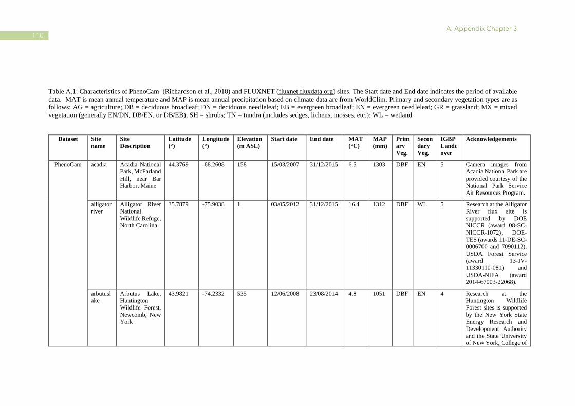
A. Appendix Chapter 3
110
Table A.1: Characteristics of PhenoCam (Richardson et al., 2018) and FLUXNET (fluxnet.fluxdata.org) sites. The Start date and End date indicates the period of available
data. MAT is mean annual temperature and MAP is mean annual precipitation based on climate data are from WorldClim. Primary and secondary vegetation types are as
follows: AG = agriculture; DB = deciduous broadleaf; DN = deciduous needleleaf; EB = evergreen broadleaf; EN = evergreen needleleaf; GR = grassland; MX = mixed
vegetation (generally EN/DN, DB/EN, or DB/EB); SH = shrubs; TN = tundra (includes sedges, lichens, mosses, etc.); WL = wetland.
Dataset Site
name
Site
Description
Latitude
(°)
Longitude
(°)
Elevation
(m ASL)
Start date End date MAT
(°C)
MAP
(mm)
Prim
ary
Veg.
Secon
dary
Veg.
IGBP
Landc
over
Acknowledgements
PhenoCam acadia Acadia National
Park, McFarland
Hill, near Bar
Harbor, Maine
44.3769 -68.2608 158 15/03/2007 31/12/2015 6.5 1303 DBF EN 5 Camera images from
Acadia National Park are
provided courtesy of the
National Park Service
Air Resources Program.
alligator
river
Alligator River
National
Wildlife Refuge,
North Carolina
35.7879 -75.9038 1 03/05/2012 31/12/2015 16.4 1312 DBF WL 5 Research at the Alligator
River flux site is
supported by DOE
NICCR (award 08-SC-
NICCR-1072), DOE-
TES (awards 11-DE-SC-
0006700 and 7090112),
USDA Forest Service
(award 13-JV-
11330110-081) and
USDA-NIFA (award
2014-67003-22068).
arbutusl
ake
Arbutus Lake,
Huntington
Wildlife Forest,
Newcomb, New
York
43.9821 -74.2332 535 12/06/2008 23/08/2014 4.8 1051 DBF EN 4 Research at the
Huntington Wildlife
Forest sites is supported
by the New York State
Energy Research and
Development Authority
and the State University
of New York, College of

A. Appendix Chapter 3
111
Environmental Science
and Forestry.
asa Asa, Sweden 57.1645 14.7825 180 28/10/2010 31/12/2015 6.3 639 DBF GR 5 Research at the SITES
Asa Research Station,
Sweden, is jointly
supported by the
Swedish University of
Agricultural Science and
the Swedish Research
Council
(Vetenskapsradet).
ashburn
ham
Ashburnham
State Forest /
Overlook
Middle School,
Ashburnham,
Massachusetts
42.6029 -71.926 292 13/09/2011 31/12/2015 7.1 1147 DBF EN 5
bartlett Bartlett
Experimental
Forest, Bartlett,
New Hampshire
44.0646 -71.2881 268 04/10/2005 31/12/2015 5.5 1224 DBF EN 5 Research at the Bartlett
Experimental Forest
tower is supported by the
National Science
Foundation (grant DEB-
1114804) and the USDA
Forest Service's
Northern Research
Station.
bartlettir Bartlett
Experimental
Forest, Bartlett,
New Hampshire
44.0646 -71.2881 268 18/04/2008 31/12/2015 5.5 1224 DBF EN 5 Research at the Bartlett
Experimental Forest
tower is supported by the
National Science
Foundation (grant DEB-
1114804) and the USDA
Forest Service's
Northern Research
Station.
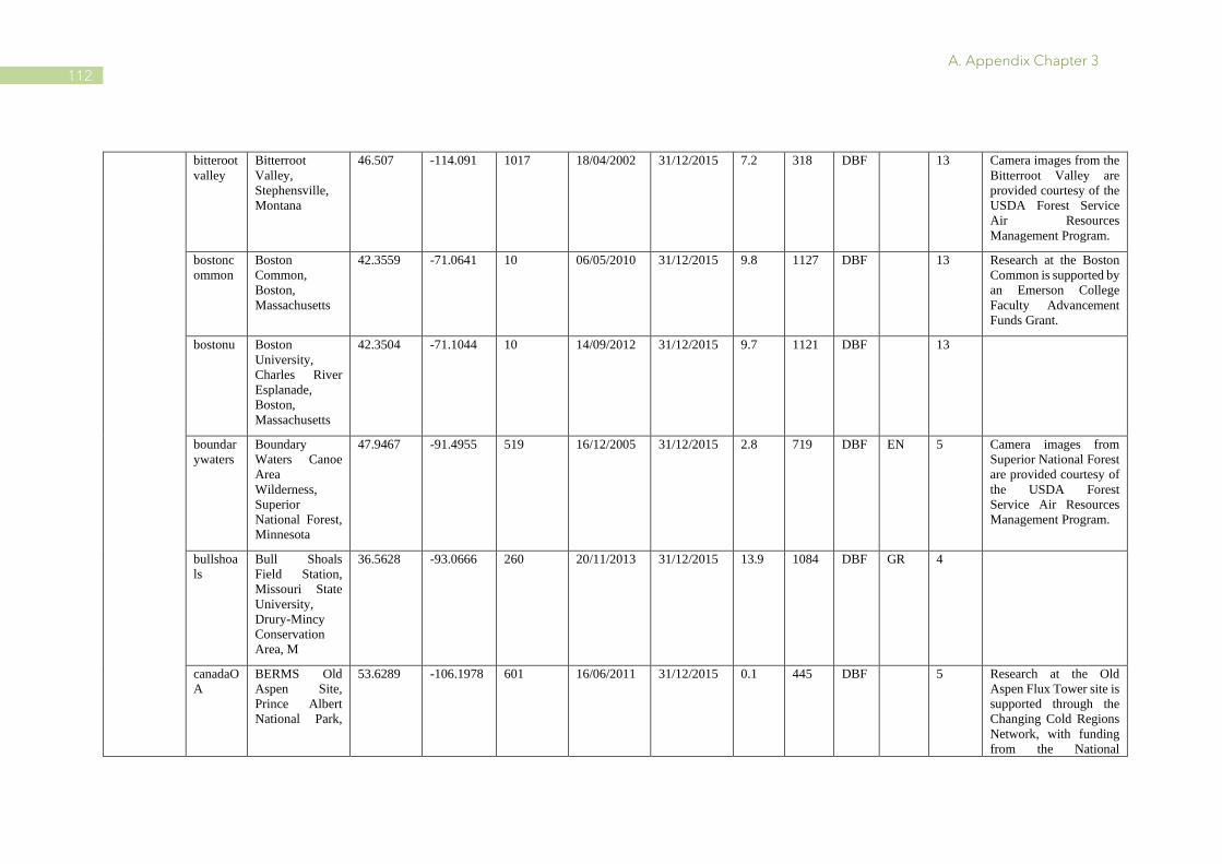
A. Appendix Chapter 3
112
bitteroot
valley
Bitterroot
Valley,
Stephensville,
Montana
46.507 -114.091 1017 18/04/2002 31/12/2015 7.2 318 DBF 13 Camera images from the
Bitterroot Valley are
provided courtesy of the
USDA Forest Service
Air Resources
Management Program.
bostonc
ommon
Boston
Common,
Boston,
Massachusetts
42.3559 -71.0641 10 06/05/2010 31/12/2015 9.8 1127 DBF 13 Research at the Boston
Common is supported by
an Emerson College
Faculty Advancement
Funds Grant.
bostonu Boston
University,
Charles River
Esplanade,
Boston,
Massachusetts
42.3504 -71.1044 10 14/09/2012 31/12/2015 9.7 1121 DBF 13
boundar
ywaters
Boundary
Waters Canoe
Area
Wilderness,
Superior
National Forest,
Minnesota
47.9467 -91.4955 519 16/12/2005 31/12/2015 2.8 719 DBF EN 5 Camera images from
Superior National Forest
are provided courtesy of
the USDA Forest
Service Air Resources
Management Program.
bullshoa
ls
Bull Shoals
Field Station,
Missouri State
University,
Drury-Mincy
Conservation
Area, M
36.5628 -93.0666 260 20/11/2013 31/12/2015 13.9 1084 DBF GR 4
canadaO
A
BERMS Old
Aspen Site,
Prince Albert
National Park,
53.6289 -106.1978 601 16/06/2011 31/12/2015 0.1 445 DBF 5 Research at the Old
Aspen Flux Tower site is
supported through the
Changing Cold Regions
Network, with funding
from the National

A. Appendix Chapter 3
113
Saskatchewan,
Canada
Science and Engineering
Research Council of
Canada (NSERC), Greg
Neufeld/Eagle Bay
Resort
caryinsti
tute
Cary Institute of
Ecosystem
Studies,
Millbrook, NY
41.7839 -73.7341 127 08/01/2001 31/12/2015 8.9 1084 DBF 4
cedarcre
ek
Cedar Creek
Ecosystem
Science Reserve
(LTER), East
Bethel,
Minnesota
45.4019 -93.2042 276 01/12/2009 10/08/2010 6.3 750 DBF 14 Research at Cedar Creek
Ecosystem Science
Reserve is supported by
the National Science
Foundation LTER
program and the
Minnesota Agriculture
Experiment Station.
columbi
amissou
ri
University of
Missouri,
Ashland
Wildlife
Research Area,
Missouri
38.7441 -92.1997 232 23/01/2009 12/01/1900 12.4 974 DBF EN 4
coweeta Coweeta
Hydrologic
Laboratory,
USDA Forest
Service,
Southern
Research
Station, Otto, N
35.0596 -83.428 680 08/04/2011 31/12/2015 12.5 1722 DBF 5 Research at the Coweeta
flux tower is funded
through the USDA
Forest Service, Southern
Research Station; USDA
Agriculture and Food
Research Initiative
Foundational Program,
award number 2012-
67019-19484; EPA
agreement number 13-
IA-11330140-044; and
the National Science
Foundation, Long-Term

A. Appendix Chapter 3
114
Ecological Research
(LTER) program, award
#DEB-0823293.
dollysod
s
Canaan Valley /
Dolly Sods
Wilderness,
Monongahala
National Forest,
West Virginia
39.0995 -79.427 1133 21/11/2003 31/12/2015 7.6 1328 DBF 4 Camera images from the
Dolly Sods Wilderness,
Mononghahela National
Forest are provided
courtesy of the USDA
Forest Service Air
Resources Management
Program.
downer
woods
UW-Milwaukee
Field Station,
Downer Woods
Natural Area,
Milwaukee,
Wisconsin
43.0794 -87.8808 213 25/03/2013 31/12/2015 8.2 812 DBF 13
dripping
springs
Cleveland
National Forest,
California
33.3 -116.8 400 06/04/2001 26/05/2009 13.2 599 DBF SH 8 Camera images from
Cleveland National
Forest are provided
courtesy of the USDA
Forest Service Air
Resources Management
Program.
dukehw Hardwood
Stand, Duke
Forest, North
Carolina
35.9736 -79.1004 400 31/05/2013 31/12/2015 14.6 1166 DBF 5
freeman
wood
Woodland Site,
Texas State
University,
Freeman Ranch,
29.94 -97.99 254 27/06/2012 21/03/2014 19.6 862 DBF EN 8
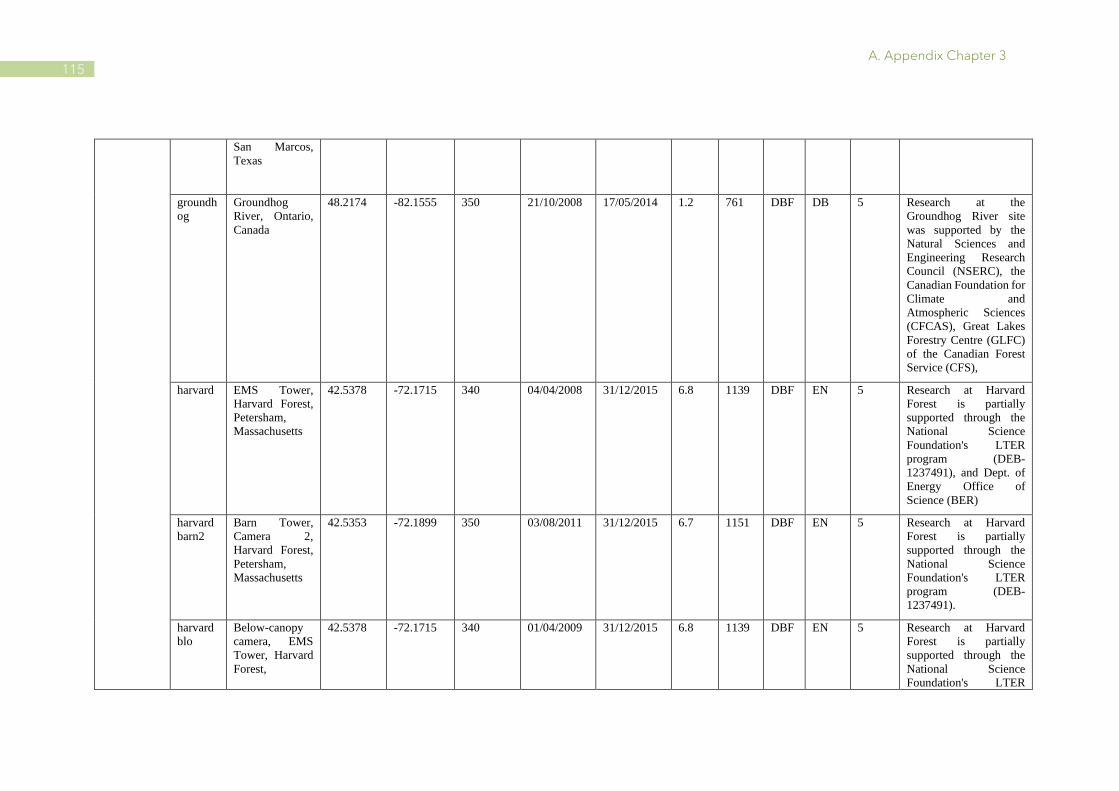
A. Appendix Chapter 3
115
San Marcos,
Texas
groundh
og
Groundhog
River, Ontario,
Canada
48.2174 -82.1555 350 21/10/2008 17/05/2014 1.2 761 DBF DB 5 Research at the
Groundhog River site
was supported by the
Natural Sciences and
Engineering Research
Council (NSERC), the
Canadian Foundation for
Climate and
Atmospheric Sciences
(CFCAS), Great Lakes
Forestry Centre (GLFC)
of the Canadian Forest
Service (CFS),
harvard EMS Tower,
Harvard Forest,
Petersham,
Massachusetts
42.5378 -72.1715 340 04/04/2008 31/12/2015 6.8 1139 DBF EN 5 Research at Harvard
Forest is partially
supported through the
National Science
Foundation's LTER
program (DEB-
1237491), and Dept. of
Energy Office of
Science (BER)
harvard
barn2
Barn Tower,
Camera 2,
Harvard Forest,
Petersham,
Massachusetts
42.5353 -72.1899 350 03/08/2011 31/12/2015 6.7 1151 DBF EN 5 Research at Harvard
Forest is partially
supported through the
National Science
Foundation's LTER
program (DEB-
1237491).
harvard
blo
Below-canopy
camera, EMS
Tower, Harvard
Forest,
42.5378 -72.1715 340 01/04/2009 31/12/2015 6.8 1139 DBF EN 5 Research at Harvard
Forest is partially
supported through the
National Science
Foundation's LTER

A. Appendix Chapter 3
116
Petersham,
Massachusetts
program (DEB-
1237491).
harvardl
ph
LPH Tower,
Harvard Forest,
Petersham,
Massachusetts
42.542 -72.185 380 15/06/2010 31/12/2015 6.8 1139 DBF EN 5 Research at Harvard
Forest is partially
supported through the
National Science
Foundation's LTER
program (DEB-
1237491).
howland
2
North Tower
(Regrowing
clearcut, ca.
1990), Howland
Forest,
Howland, Maine
45.2128 -68.7418 79 30/03/2008 31/12/2015 5.3 1058 DBF EN 5 Research at Howland
Forest is supported by
the Office of Science
(BER), US Department
of Energy, and the
USDA Forest Service's
Northern Research
Station.
hubbard
brook
Hubbard Brook
Experimental
Forest, USDA
Forest Service
Headquarters,
North
Woodstock,
43.9438 -71.701 253 16/04/2008 31/12/2015 5.6 1060 DBF 4 Research at the Hubbard
Brook Experimental
Forest is
partially supported by
the National Science
Foundation's LTER
program (grant DEB-
1114804) and the USDA
Forest Service's
Northern Research
Station
hubbard
brooknf
ws
North Facing
Watersheds,
Hubbard Brook
Experimental
Forest,
Thornton, New
Hampshire
42.958 -71.7762 930 24/09/2012 31/12/2015 7.4 1111 DBF 5 The Hubbard Brook
Ecosystem Study is a
collaborative effort at
the Hubbard Brook
Experimental Forest,
which is operated and
maintained by the
USDA Forest Service,

A. Appendix Chapter 3
117
Northern Research
Station, Newtown
Square, PA.
joycekil
mer
Joyce Kilmer
Slickrock
Wilderness,
North Carolina
35.257 -83.795 1373 06/06/2006 31/12/2015 9.2 1905 DBF 4 Camera images from the
Joyce Kilmer Slickrock
Wilderness are provided
courtesy of the USDA
Forest Service Air
Resources Management
Program.
laurenti
des
Station de
biologie des
Laurentides,
University of
Montreal, St-
Hippolyte, Queb
ec
45.9881 -74.0055 350 16/09/2011 31/12/2015 3.7 1066 DBF 5
mammo
thcave
Environmental
Learning
Center,
Mammoth Cave
National Park,
Kentucky
37.1858 -86.1019 226 01/01/2002 31/12/2015 13.5 1312 DBF 4 Camera images from
Mammoth Cave
National Park are
provided courtesy of the
National Park Service
Air Resources Program.
missouri
ozarks
University of
Missouri,
Ashland
Wildlife
Research Area,
Missouri
38.7441 -92.2 219 05/03/2012 31/12/2015 12.4 974 DBF 4 Research at the
MOFLUX site is
supported by the U.S.
Department of Energy,
Office of Science, Office
of Biological and
Environmental Research
Program, Climate and
Environmental Sciences
Division. ORNL is
managed by UT-
Battelle, LLC, for the
U.S. Department of

A. Appendix Chapter 3
118
Energy under contract
DE-AC05-00OR22725.
U.S. Department of
Energy support for the
University of Missouri
(Grant DE-FG02-
03ER63683) is
gratefully
acknowledged.
monture Lolo National
Forest, Ovando,
Montana
47.0202 -113.1283 1255 08/06/2001 31/12/2015 5 407 DBF DB 12 Camera images from
Lolo National Forest are
provided courtesy of the
USDA Forest Service
Air Resources
Management Program.
morgan
monroe
Morgan Monroe
State Forest,
Indiana
39.3231 -86.4131 275 27/08/2008 31/12/2015 11.2 1087 DBF 4 Research at the Morgan-
Monroe Ameriflux site
is supported by the US
Departement of Energy,
Office of Science, Office
of Biological and
Environmental Research
throuth the Ameriflux
Management Project
administered by
Lawrence Berkeley
National Lab
national
capital
Park Police
Headquarters,
National Capital
Parks,
Washington DC
38.8882 -77.0695 28 25/07/2003 31/12/2015 13.1 1020 DBF 13 Camera images from the
National Capital are
provided courtesy of the
National Park Service
Air Resources Program.
northattl
eboroma
North Attleboro
High School,
North Attleboro,
Massachusetts
41.9837 -71.3106 60 21/02/2012 31/12/2015 9.4 1202 DBF 14

A. Appendix Chapter 3
119
oakridge
1
Chestnut Ridge,
Oak Ridge,
Tennessee
35.9311 -84.3323 371 12/10/2006 31/12/2015 13.8 1365 DBF 4 Research at Chestnut
Ridge is funded by US
Dept of Commerce,
National Oceanic and
Atmospheric
Administration, Office
of Atmospheric
Research, Air Resources
Lab, Atmospheric
Turbulence and
Diffusion Division as
part of the Surface
Energy Budget Network
(SEBN)
oakridge
2
Chestnut Ridge,
Oak Ridge,
Tennessee
35.9311 -84.3323 371 12/10/2006 31/12/2015 13.8 1365 DBF 4 Research at Chestnut
Ridge is funded by US
Dept of Commerce,
National Oceanic and
Atmospheric
Administration, Office
of Atmospheric
Research, Air Resources
Lab, Atmospheric
Turbulence and
Diffusion Division as
part of the Surface
Energy Budget Network
(SEBN)
proctor University of
Vermont,
Proctor Maple
Research
Center,
Underhill,
Vermont
44.525 -72.866 403 11/09/2008 31/12/2015 5 1081 DBF 4 Supported by the
Agricultural Experiment
Station of the University
of Vermont
queens Queen's
University
Biological
44.565 -76.324 126 26/05/2008 31/12/2015 6.4 887 DBF 5

A. Appendix Chapter 3
120
Station, Lake
Opinicon,
Ontario, Canada
reading
ma
Austin Prep
School,
Reading,
Massachusetts
42.5304 -71.1272 100 06/03/2012 31/12/2015 9.3 1107 DBF 13
russellsa
ge
Russell Sage
State Wildlife
Management
Area, near
Monroe,
Louisiana
32.457 -91.9743 20 20/11/2013 31/12/2015 18.1 1341 DBF 5
sanford Sanford Natural
Area, Michigan
State University,
East Lansing,
Michigan
42.7268 -84.4645 268 20/12/2013 31/12/2015 8.1 781 DBF 13
shalehill
sczo
Susquehanna
Shale Hills
Critical Zone
Observatory
(CZO),
Pennsylvania
40.65 -77.9 310 18/04/2012 31/12/2015 9.8 980 DBF 4 Research at the Penn
State Sone Valley Forest
is supported by the
National Science
Foundation EAR 07-
25019 (C. Duffy), and
EAR 12-39285, EAR
13-31726 (S. Brantley)
for the Susquehanna
Shale Hills Critical Zone
Observatory and the
College of Agricultural
Sciences, Department of
Ecosystem Science and
Management.
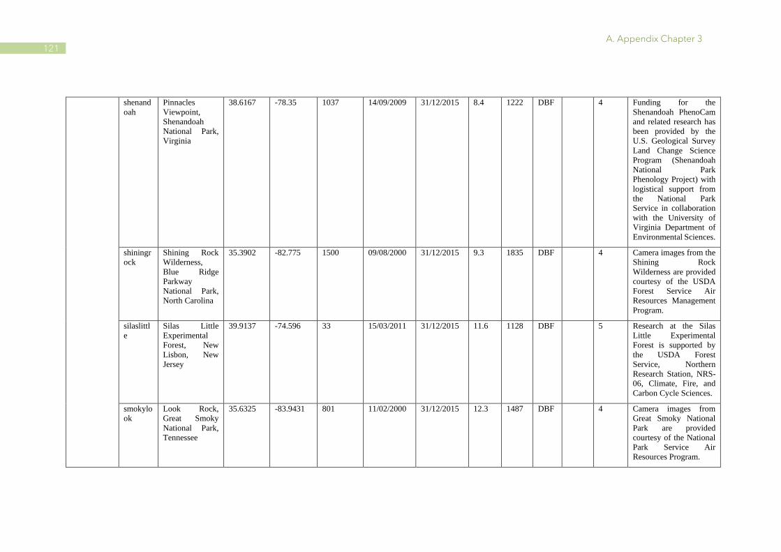
A. Appendix Chapter 3
121
shenand
oah
Pinnacles
Viewpoint,
Shenandoah
National Park,
Virginia
38.6167 -78.35 1037 14/09/2009 31/12/2015 8.4 1222 DBF 4 Funding for the
Shenandoah PhenoCam
and related research has
been provided by the
U.S. Geological Survey
Land Change Science
Program (Shenandoah
National Park
Phenology Project) with
logistical support from
the National Park
Service in collaboration
with the University of
Virginia Department of
Environmental Sciences.
shiningr
ock
Shining Rock
Wilderness,
Blue Ridge
Parkway
National Park,
North Carolina
35.3902 -82.775 1500 09/08/2000 31/12/2015 9.3 1835 DBF 4 Camera images from the
Shining Rock
Wilderness are provided
courtesy of the USDA
Forest Service Air
Resources Management
Program.
silaslittl
e
Silas Little
Experimental
Forest, New
Lisbon, New
Jersey
39.9137 -74.596 33 15/03/2011 31/12/2015 11.6 1128 DBF 5 Research at the Silas
Little Experimental
Forest is supported by
the USDA Forest
Service, Northern
Research Station, NRS-
06, Climate, Fire, and
Carbon Cycle Sciences.
smokylo
ok
Look Rock,
Great Smoky
National Park,
Tennessee
35.6325 -83.9431 801 11/02/2000 31/12/2015 12.3 1487 DBF 4 Camera images from
Great Smoky National
Park are provided
courtesy of the National
Park Service Air
Resources Program.

A. Appendix Chapter 3
122
smokyp
urchase
Purchase Knob,
Great Smoky
National Park,
Tennessee
35.59 -83.0775 1550 19/08/2003 31/12/2015 8.7 1786 DBF GR 4 Camera images from
Great Smoky National
Park are provided
courtesy of the National
Park Service Air
Resources Program.
snakeriv
ermn
Hay-Snake State
Wildlife
Management
Area, near
Woodland,
Minnesota
46.1206 -93.2447 1181 18/11/2009 31/12/2015 4.4 742 DBF 5
springfi
eldma
Academy Hill
School,
Springfield,
Massachusetts
42.1352 -72.586 56 21/02/2012 31/12/2015 9.3 1115 DBF 13
thompso
nfarm2
N
University of
New
Hampshire,
Thompson Farm
Observatory,
Durham, New
Hampshire
43.1086 -70.9505 23 11/01/2009 31/12/2015 8.1 1108 DBF EN 5 Research at the
Thompson Farm
Observatory is
supported by NH
EPSCoR with support
from the National
Science Foundation's
Research Infrastructure
Improvement Award
(#EPS 1101245) and by
the NH Agricultural
Experiment
Station/USDA NIFA
(Hatch project
#1006997).
tonzi Tonzi Ranch,
Amador County,
California
38.4309 -120.9659 177 26/10/2011 31/12/2015 15.9 603 DBF GR 9 Funding for AmeriFlux
core site data was
provided by the U.S.
Department of Energy's
Office of Science.
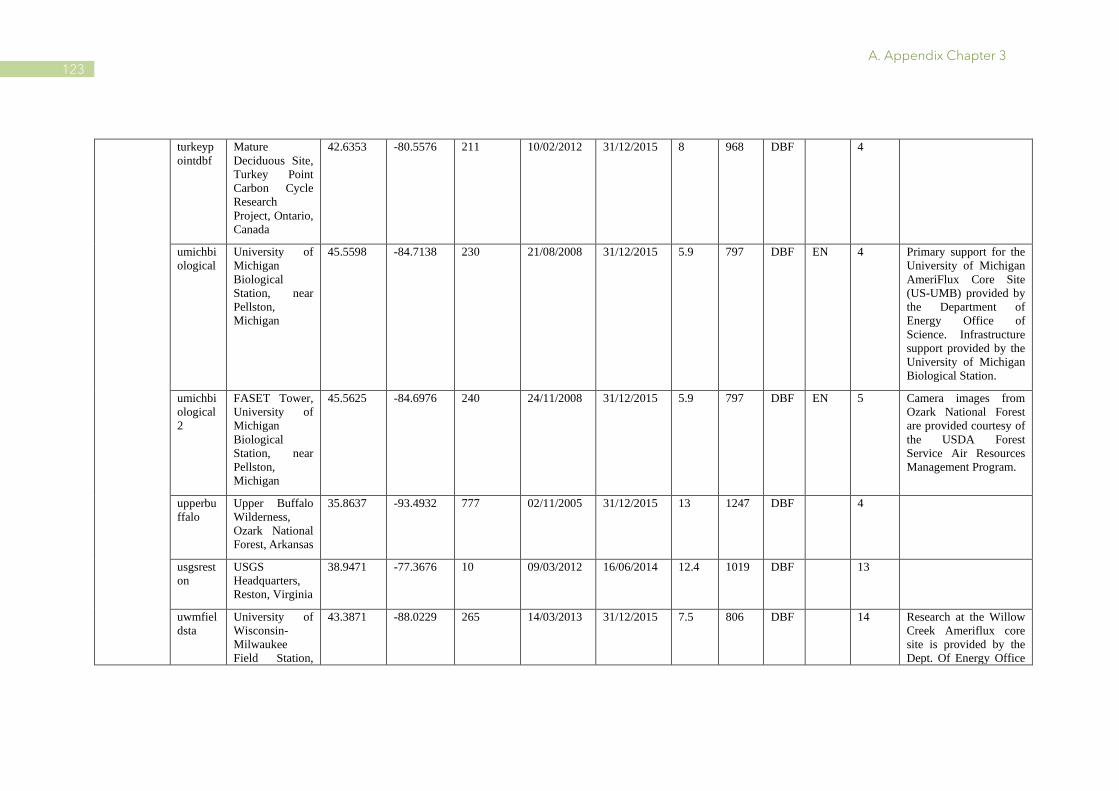
A. Appendix Chapter 3
123
turkeyp
ointdbf
Mature
Deciduous Site,
Turkey Point
Carbon Cycle
Research
Project, Ontario,
Canada
42.6353 -80.5576 211 10/02/2012 31/12/2015 8 968 DBF 4
umichbi
ological
University of
Michigan
Biological
Station, near
Pellston,
Michigan
45.5598 -84.7138 230 21/08/2008 31/12/2015 5.9 797 DBF EN 4 Primary support for the
University of Michigan
AmeriFlux Core Site
(US-UMB) provided by
the Department of
Energy Office of
Science. Infrastructure
support provided by the
University of Michigan
Biological Station.
umichbi
ological
2
FASET Tower,
University of
Michigan
Biological
Station, near
Pellston,
Michigan
45.5625 -84.6976 240 24/11/2008 31/12/2015 5.9 797 DBF EN 5 Camera images from
Ozark National Forest
are provided courtesy of
the USDA Forest
Service Air Resources
Management Program.
upperbu
ffalo
Upper Buffalo
Wilderness,
Ozark National
Forest, Arkansas
35.8637 -93.4932 777 02/11/2005 31/12/2015 13 1247 DBF 4
usgsrest
on
USGS
Headquarters,
Reston, Virginia
38.9471 -77.3676 10 09/03/2012 16/06/2014 12.4 1019 DBF 13
uwmfiel
dsta
University of
Wisconsin-
Milwaukee
Field Station,
43.3871 -88.0229 265 14/03/2013 31/12/2015 7.5 806 DBF 14 Research at the Willow
Creek Ameriflux core
site is provided by the
Dept. Of Energy Office

A. Appendix Chapter 3
124
Saukville,
Wisconsin
of Science to the ChEAS
Cluster
willowc
reek
Willow Creek,
Chequamegon-
Nicolet National
Forest,
Wisconsin
45.806 -90.0791 521 25/10/2011 31/12/2015 3.9 820 DBF 4 Logistical support is
provided by the Woods
Hole Research Center.
woodsh
ole
Woods Hole
Research
Center,
Falmouth,
Massachusetts
41.5495 -70.6432 10 14/04/2011 31/12/2015 10 1178 DBF 5
worcest
er
Worcester State
University,
Worcester,
Massachusetts
42.2697 -71.8428 185 13/05/2013 31/12/2015 8.3 1174 DBF NV 13
FLUXNET CA-Oas Broadleaf tree
communities
with an annual
cycle of leaf-on
and leaf-off
periods
53.6289 -106.1978 600 1996 2010 0.34 428 DBF 5
CA-
TPD
The forest is
approximately
90 years old.
Naturally
regenerated on
sandy terrain
and abandoned
agricultural land
42.6353 -80.5577 260 2012 2017 8 1036 DBF

A. Appendix Chapter 3
125
DE-Hai Deciduous
Broadleaf
Forests
51.0792 10.453 430 2000 2012 8.3 720 DBF
DE-Lnf Leinefelde,
deciduous
Broadleaf
Forests
51.3282 10.3678 451 2002 2012 6.9 895 DBF
Dk-Sor Soroe 55.4858 11.6446 40 1996 2014 8.2 660 DBF
IT-CA3 Castel d'Asso3 42.38 12.0222 197 2011 2014 14 766 DBF
IT-Col Collelongo,
deciduous
forests
41.8494 13.5881 1560 1996 2014 6.3 1180 DBF
IT-Isp Ispra ABC-IS,
deciduoust
forest
45.8126 8.6336 210 2013 2014 12.2 1300 DBF
IT-PT1 Parco Ticino
forest
45.2009 9.061 60 2002 2004 12.7 984 DBF
JP-MBF Moshiri Birch
Forest Site
44.3869 142.3186 2003 2005 DBF
US-Ha1 The Harvard
Forest tower is
on land owned
by Harvard
University.
42.5378 -72.1715 240 1991 2012 6.62 1071 DBF Operation of the US-Ha1
site is supported by the
AmeriFlux Management
Project with funding by
the U.S
US-
MMS
Owned by the
Indiana
Department of
Natural
Resources
(IDNR), the
39.3232 -86.4131 275 1999 2014 10.85 1032 DBF AmeriFlux Management
Project
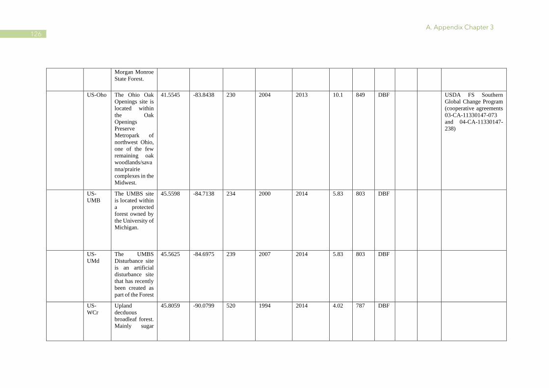
A. Appendix Chapter 3
126
Morgan Monroe
State Forest.
US-Oho The Ohio Oak
Openings site is
located within
the Oak
Openings
Preserve
Metropark of
northwest Ohio,
one of the few
remaining oak
woodlands/sava
nna/prairie
complexes in the
Midwest.
41.5545 -83.8438 230 2004 2013 10.1 849 DBF USDA FS Southern
Global Change Program
(cooperative agreements
03-CA-11330147-073
and 04-CA-11330147-
238)
US-
UMB
The UMBS site
is located within
a protected
forest owned by
the University of
Michigan.
45.5598 -84.7138 234 2000 2014 5.83 803 DBF
US-
UMd
The UMBS
Disturbance site
is an artificial
disturbance site
that has recently
been created as
part of the Forest
45.5625 -84.6975 239 2007 2014 5.83 803 DBF
US-
WCr
Upland
decduous
broadleaf forest.
Mainly sugar
45.8059 -90.0799 520 1994 2014 4.02 787 DBF

A. Appendix Chapter 3
127
maple, also
basswood.

128
B
Appendix Chapter 4

B. Appendix Chapter 4
129
Figure B.1: Spatial patterns of partial correlation coefficients between pre-season temperature and (a) SoS
and (b) EoS for 2000-2018 in the Northern Hemisphere. The color scale represents the maximum
correlation coefficients recorded for each pixel, independently of the SPEI timescale. White indicates
unvegetated areas and areas with no deciduous forests, and light gray indicates vegetated areas with
nonsignificant correlations (P>0.05).
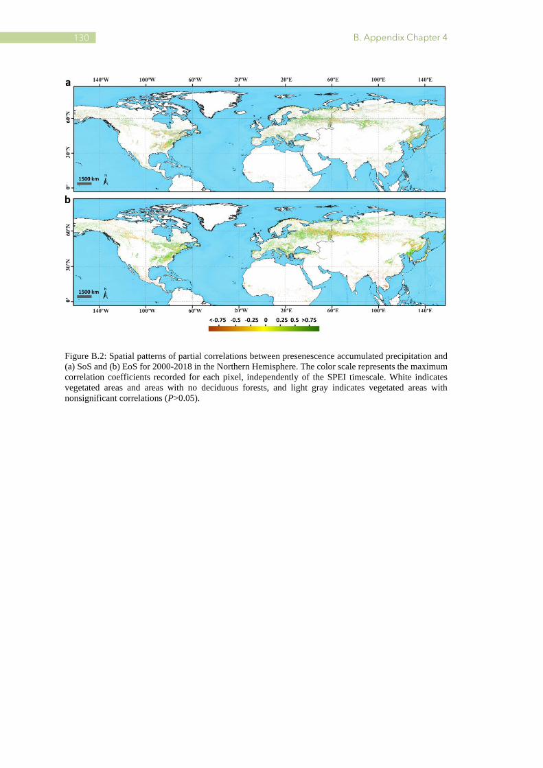
B. Appendix Chapter 4
130
Figure B.2: Spatial patterns of partial correlations between presenescence accumulated precipitation and
(a) SoS and (b) EoS for 2000-2018 in the Northern Hemisphere. The color scale represents the maximum
correlation coefficients recorded for each pixel, independently of the SPEI timescale. White indicates
vegetated areas and areas with no deciduous forests, and light gray indicates vegetated areas with
nonsignificant correlations (P>0.05).

B. Appendix Chapter 4
131
Figure B.3: Spatial distributions of the coefficients (color scale) for the sensitivity of (a) SOS and (b) EoS
to pre-season SPEI. White indicates unvegetated areas and areas with no deciduous forests, and light gray
indicates vegetated areas with nonsignificant correlations (P>0.05).
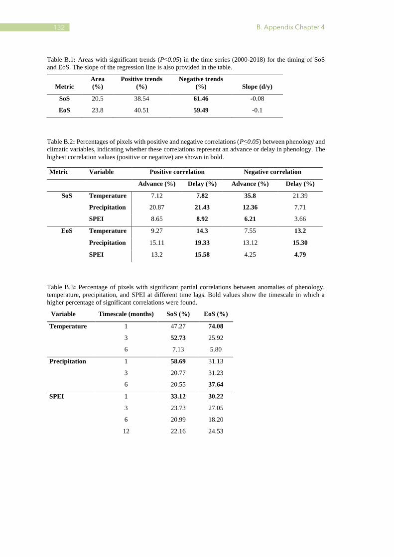
B. Appendix Chapter 4
132
Table B.1: Areas with significant trends (P≤0.05) in the time series (2000-2018) for the timing of SoS
and EoS. The slope of the regression line is also provided in the table.
Metric
Area
(%)
Positive trends
(%)
Negative trends
(%) Slope (d/y)
SoS 20.5 38.54 61.46 -0.08
EoS 23.8 40.51 59.49 -0.1
Table B.2: Percentages of pixels with positive and negative correlations (P≤0.05) between phenology and
climatic variables, indicating whether these correlations represent an advance or delay in phenology. The
highest correlation values (positive or negative) are shown in bold.
Metric Variable Positive correlation Negative correlation
Advance (%) Delay (%) Advance (%) Delay (%)
SoS Temperature 7.12 7.82 35.8 21.39
Precipitation 20.87 21.43 12.36 7.71
SPEI 8.65 8.92 6.21 3.66
EoS Temperature 9.27 14.3 7.55 13.2
Precipitation 15.11 19.33 13.12 15.30
SPEI 13.2 15.58 4.25 4.79
Table B.3: Percentage of pixels with significant partial correlations between anomalies of phenology,
temperature, precipitation, and SPEI at different time lags. Bold values show the timescale in which a
higher percentage of significant correlations were found.
Variable Timescale (months) SoS (%) EoS (%)
Temperature 1 47.27 74.08
3 52.73 25.92
6 7.13 5.80
Precipitation 1 58.69 31.13
3 20.77 31.23
6 20.55 37.64
SPEI 1 33.12 30.22
3 23.73 27.05
6 20.99 18.20
12 22.16 24.53

133

134
References
Addabbo, P., Focareta, M., Marcuccio, S., Votto, C., and Ullo, S. (2016). Contribution
of Sentinel-2 data for applications in vegetation monitoring. Acta Imeko, 5 (2), 44
Ahrends, H., Etzold, S., Kutsch, W., Stoeckli, R., Bruegger, R., Jeanneret, F., Wanner,
H., Buchmann, N., and Eugster, W. (2009). Tree phenology and carbon dioxide
fluxes: use of digital photography for process-based interpretation at the ecosystem
scale. Clim. Res., 39, 261–274
Angert, A., Biraud, S., Bonfils, C., Henning, C.C., Buermann, W., Pinzon, J., Tucker
CJ., and Fung, I. (2005). Drier summers cancel out the CO2 uptake enhancement
induced by warmer springs. Proc Natl Acad Sci USA, 102 (31), 10823–10827
Aono Y., and Kazui K. (2008). Phenological data series of cherry tree flowering in
Kyoto, Japan, and its application to reconstruction of springtime temperatures since
the 9th century. Int J Climatol., 28, 905–914
Aono Y., and Tani A. (2014). Autumn temperature deduced from historical records of
autumn tints phenology of maple tree in Kyoto, Japan. Climate in Biosphere., 14, 18–
28
Araya, S., Ostendorf, B., Lyle, G., and Lewis, M. (2018). CropPhenology: an R package
for extracting crop phenology from time series remotely sensed vegetation index
imagery. Ecol. Inf., 46, 45–56
Atkinson, C., Brennan, R.M., and Jones, H.G. (2013). Declining chilling and its impact
on temperate perennial crops. Environmental and Experimental Botany, 91,48–62
Atkinson, P.M., Jeganathan, C., Dash, J., and Atzberger, C. (2012). Inter-comparison of
four models for smoothing satellite sensor time-series data to estimate vegetation
phenology. Remote Sens. Environ., 123, 400–417

References
135
Atzberger, C., and Eilers, P.H. (2011). Evaluating the effectiveness of smoothing
algorithms in the absence of ground reference measurements. Int. J. Remote Sens.,
32, 3689–3709
Atzberger, C., and Eilers, P.H.C. (2011a). A time series for monitoring vegetation
activity and phenology at 10-daily time steps covering large parts of South America.
International Journal of Digital Earth, 4(5), 365–386
Atzberger, C., Klisch, A., Mattiuzzi, M., and Vuolo, F. (2013). Phenological metrics
derived over the European continent from NDVI3g data and MODIS time series.
Remote. Sens., 6, 257–284
Bajocco, S., Ferrara, C., Alivernini, A., Bascietto, M., and Ricotta, C. (2019). Remotely-
sensed phenology of Italian forests: going beyond the species. Int. J. Appl. Earth Obs.
Geoinf., 74, 314–321
Baldocchi, D. (2003). Assessing the eddy covariance technique for evaluating carbon
dioxide exchange rates of ecosystems: Past, present and future. Glob. Change Biol.,
9, 479–492
Baret, F., Weiss, M., Lacaze, R., Camacho, F., Makhmara, H., Pacholcyzk, P., and
Smets, B. (2013). GEOV1: LAI, FAPAR essential climate variables and FCOVER
global time series capitalizing over existing products. Part 1: Principles of
development and production. Remote Sens. Environ., 137, 299–309
Bater, C.W., Coops, N.C., Wulder, M.A., Nielsen, S.E., McDermid, G.J., and Stenhouse,
G. (2011). Design and installation of a camera network across an elevation gradient
for habitat assessment. Instrum. Sci. Technol., 39, 231–247
Baumann, M., Özdoğan, M., Richardson, A.D., and Radeloff, V.C. (2017). Phenology
from Landsat when data is scarce: Using MODIS and Dynamic Time-Warping to
combine multi-year Landsat imagery to derive annual phenology curves. Int. J. Appl.
Earth Obs. Geoinformation, 54, 72–83
Beaubien, E.G., and Freeland, H.J. (2000). Spring phenology trends in Alberta, Canada:
links to ocean temperature. Int J of Biom., 44, 53–59

References
136
Beaumont, L., Hartenthaler, T., Keatley, M., and Chambers, L. (2015). Shifting time:
recent changes to the phenology of Australian species. Clim. Res., 63, 203–214
Beck, P.S.A., Atzberger, C., Hogda, K.A., Johansen, B., and Skidmore, A.K. (2006).
Improved monitoring of vegetation dynamics at very high latitudes: A new method
using MODIS NDVI. Remote Sensing of Environment, 100, 321–334
Beer, C., Reichstein, M., Tomelleri, E., Ciais, P., Jung, M., Carvalhais, N., Rödenbeck,
C., Arain, M., Baldocchi, D., and Bonan, G. (2010). Terrestrial gross carbon dioxide
uptake: Global distribution and covariation with climate. Sci., 329, 834–838
Beguería, S., Vicente-Serrano, S.M., Reig, F., and Latorre, B. (2013). Standardized
precipitation evapotranspiration index (SPEI) revisited: parameter fitting,
evapotranspiration models, tools, datasets and drought monitoring. Int. J. Climatol.,
34, 3001–3023
Berg, A., Findell, K., Lintner, B. (2016). Land–atmosphere feedbacks amplify aridity
increase over land under global warming. Nature Clim Change., 6, 869–874
Berra, E., and Gaulton, R. (2021). Remote sensing of temperate and boreal forest
phenology: A review of progress, challenges and opportunities in the intercomparison
of in-situ and satellite phenological metrics. Forest Ecology and Management, 480,
118663
Bonan, G. B. (2008). Ecological Climatology: Concepts and Applications (Cambridge
Univ. Press, Cambridge, 2nd ed.)
Borchert, R., and Rivera, G. (2001). Photoperiodic control of seasonal development and
dormancy in tropical stem–succulent trees. Tree Physiol, 21, 213–221
Bórnez, K., Descals, A., Verger, A., and Peñuelas, J. (2020a). Land surface phenology
from VEGETATION and PROBA-V data. Assessment over deciduous forests. Int. J.
Appl. Earth Obs. Geoinf., 84, 101974
Bórnez, K., Richardson, A.D., Verger, A., Descals, A., and Peñuelas, J. (2020b).
Evaluation of VEGETATION and PROBA-V Phenology Using PhenoCam and Eddy
Covariance Data. Remote Sens., 12, 3077

References
137
Bradley, A.V., Gerard, F.F., Barbier, N., Weedon, G.P., Anderson, L.O., Huntingford,
C., Aragao, L.E., Zelazowski, P., and Arai, E. (2011). Relationships between
phenology, radiation and precipitation in the Amazon region. Global Change Biol.,
17, 2245–2260
Bradley, B.A., Jacob, R.W., Hermance, J.F., and Mustard, J.F. (2007). A curve fitting
procedure to derive inter-annual phenologies from time series of noisy satellite NDVI
data. Remote Sens Environ., 106, 137–145
Brown, J., Wardlow, B., Tadesse, T., Hayes, M., and Reed, B. (2008). The vegetation
drought response index (VegDRI): a new integrated approach for monitoring drought
stress in vegetation. GIScience Remote Sens., 45, 16–46
Brown, T., Hultine, K.R., Steltzer, H., Denny, E., Denslow, M., Granados, J.,
Henderson, S., Moore, D.J.P., Nagai, S., and San Clements, M. (2016). Using
phenocams to monitor our changing Earth: Toward a global phenocam network.
Front. Ecol. Environ., 14, 84–93
Brus, D., Hengeveld, G., Walvoort, D., Goedhart, P., Heidema, A., Nabuurs, G., and
Gunia, K. (2012). Statistical mapping of tree species over Europe. Eur. J. Forest Res.,
131, 145–157
Buermann, W., Forkel, M., O'Sullivan, M., Sitch, S., Friedlingstein, P., Haverd, V., Jain,
AK., Kato, E., Kautz, M., Lienert, S., Lombardozzi, D., Nabel, JEMS., Tian, H.,
Wiltshire, AJ., Zhu, D., Smith, WK., and Richardson, AD. (2018). Widespread
seasonal compensation effects of spring warming on northern plant productivity.
Nature, 562(7725), 110-114
Buermann, W., Parida, B., Jung, M., Burn, D., and Reichstein, M. (2013). Earlier springs
decrease peak summer productivity in North American boreal forests. Environmental
Research Letters, 8, 024027
Butt, N., Seabrook, L., Maron, M., Law, B.S., Dawson, T.P., Syktus, J., and McAlpine,
C.A. (2015). Cascading effects of climate extremes on vertebrate fauna through
changes to low‐latitude tree flowering and fruiting phenology. Global Change Biol.,
21(9), 3267–3277

References
138
C3S Global Land Cover Map. Available online:
http://maps.elie.ucl.ac.be/CCI/viewer/download.php (accessed on 18 July 2021)
Cai, Z., Jönsson, P., Jin, H., and Eklundh, L. (2017). Performance of Smoothing
Methods for Reconstructing NDVI Time-Series and Estimating Vegetation
Phenology from MODIS Data. Remote Sensing, 9, 1271
Ceccherini, G., Gobron, N., and Migliavacca, M. (2014). On the Response of European
Vegetation Phenology to Hydroclimatic Anomalies. Remote Sens., 6, 3143–3169
CGLS LAI V2 Data. Available online:
https://land.copernicus.eu/global/themes/vegetation (accessed on 8 July 2021)
Chen, H., and Sun, J. (2015). Changes in drought characteristics over China using the
standardized precipitation evapotranspiration index. J Clim., 28, 5430–5447
Chen, J., Jönsson, P., Tamura, M., Gu, Z., Matsushita, B., and Eklundh, L. (2004). A
simple method for reconstructing a high-quality NDVI time-series data set based on
the Savitzky–Golay filter. Remote Sens. Environ., 91, 332–344
Chen, S., Zhang, L.G., Tang, R., Yang, K., and Huang, Y. (2017). Analysis on temporal
and spatial variation of drought in Henan Province based on SPEI and TVDI. Trans
Chin Soc Agric Eng., 33, 126–132
Chen, Z., Tang, X., Gu, Q., Wang, T., Wei, J., Song, L., and Ma, M. (2018). Climatic
anomaly and its impact on vegetation phenology, carbon sequestration and water-use
efficiency at a humid temperate forest. Journal of Hydrology., 565, 150-159
Cherlet, M., Hutchinson, C., Reynolds, J., Hill, J., Sommer, S., and von Maltitz, G.
(Eds.). (2018). World Atlas of Desertification, Publication Office of the European
Union, Luxembourg
Chmielewski, F.M., and Rötzer, T. (2001). Response of tree phenology to climate
change across Europe. Agric. For. Meteorol., 108, 101–112

References
139
Chmielewski, F.M., and Rotzer, T. (2002). Annual and spatial variability of the
beginning of growing season in Europe in relation to air temperature changes.
Climate Research, 19, 257–264
Chmura, H.E. (2019). The mechanisms of phenology: the patterns and processes of
phenological shifts. Ecol. Monogr., 89, e01337
Chuine, I. (2010). Why does phenology drive species distribution? Philos Trans R Soc
B., 365, 3149–3160
Chuine, I., and Régnière, J. (2017). Process-based models of phenology for plants and
animals. Annual Review of Ecology, Evolution, and Systematics, 48, 159–182
Churkina, G., Schimel, D., Braswell, B., and Xiao, X. (2005). Spatial analysis of
growing season length control over net ecosystem exchange. Glob. Change Biol., 11,
1777–1787
Ciais, P., Reichstein, M., Viovy, N., Granier, A., Ogée, J., Allard, V., Aubinet, M.,
Buchmann, N., Bernhofer, C., and Carrara, A. (2005). Europe-wide reduction in
primary productivity caused by the heat and drought in 2003. Nature, 437, 529–533
Cleland, E.E., Chuine, I., Menzel, A., Mooney, H.A., and Schwartz, M.D. (2017).
Shifting plant phenology in response to global change. Trends Ecol. Evol., 22, 357–
365
Cong, N., Shen, M.G., and Piao, S.L. (2017). Spatial variations in responses of
vegetation autumn phenology to climate change on the Tibetan Plateau. J. Plant
Ecol., 10, 744–752
D’Odorico, P., Besik, A., Wong, C.Y.S., Isabel, N., and Ensminger, I. (2020). High-
throughput drone-based remote sensing reliably tracks phenology in thousands of
conifer seedlings. New Phytol., 226, 1667–1681
Daham, A., Han, D., Jolly, WM., Rico-Ramirez, M., and Marsh, A. (2019). Predicting
vegetation phenology in response to climate change using bioclimatic indices in Iraq.
J Water Clim Change, 10 (4): 835–851

References
140
de Beurs, K., and Henebry, G. (2005). Land surface phenology and temperature
variation in the International Geosphere–Biosphere Program high-latitude transects.
Global Change Biol., 11, 779–790
de Beurs, K., and Henebry, G. (2010). Spatio-temporal statistical methods for modelling
land surface phenology. In Hudson, & Keatley (Eds.), Phenological research:
Methods for environmental and climate change analysis. Springer, Dordrecht
de Beurs, K.M., and Henebry, G.M. (2004). Land surface phenology, climatic variation,
and institutional change: analyzing agricultural land cover change in Kazakhstan.
Remote Sens Environ., 89, 497–509
de Moura, Y.M., Galvao, L.S, Hilker, T., Wu, J., Saleska, S., do Amaral, C.H., Nelson,
B.W., Lopes, A.P., Wiedeman, K.K., Prohaska, N., de Oliveira, R.C., Machado, C.B.,
and Aragao, L.E.O.C. (2017). Spectral analysis of amazon canopy phenology during
the dry season using a tower hyperspectral camera and modis observations. ISPRS J.
Photogramm. Remote Sens., 131, 52–64
Delbart, N., Beaubien, E., Kergoat, L., and Le Toan, T. (2015). Comparing land surface
phenology with leafing and flowering observations from the PlantWatch citizen
network. Remote Sens. Environ., 160, 273–280
Delbart, N., Kergoat, L., Le Toan, T., Lhermitte, J., and Picard, G. (2005). Determination
of phe- nological dates in boreal regions using normalized difference water index.
Remote Sens. Environ., 97, 26–38
Delbart, N., Picard, G., Le Toans, T., Kergoat, L., Quegan, S., Woodward, I., Dye, D.,
and Fedotova, V. (2008). Spring phenology in boreal Eurasia over a nearly century
time scale, Global Change Biol., 14(3), 603–614
Denny, E., Gerst, K.L., Miller-Rushing, A.J., Tierney, G.L., Crimmins, T.M., Enquist,
C.A.F., Guertin, P., Rosemartin, A.H., Schwartz, M.D., and Thomas, K.A., (2014).
Standardized phenology monitoring methods to track plant and animal activity for
science and resource management applications. Int. J. Biometeorol., 58, 591–601

References
141
Descals, A., Wich, S., Wich., Meijaard, E., Gaveau, D., Peedell, S., and Szantoi Z.
(2020). High-resolution global map of small holder and industrial closed-canopy oil
palm plantations. Earth Syst. Sci. Data, 13, 1211–1231
Diffenbaugh, N. (2005). Sensitivity of extreme climate events to CO2 induced
biophysical atmosphere-vegetation feedbacks in the western United States. Geophys.
Res. Lett., 32, 1–4
Donnelly. A., and Yu, R. (2017). The rise of phenology with climate change: an
evaluation IJB publications. Int J Biometerol, 61, 29–50
Du, J., He, Z., Piatek, K., Chen, L.F., Lin, P., and Zhu, Xi. (2019). Interacting effects of
temperature and precipitation on climatic sensitivity of spring vegetation green-up in
arid mountains of China. Agric. For. Meteorol., 269, 71–77
Duarte, L., Teodoro, A.C., Monteiro, A.T., Cunha, M., and Gonçalves, H. (2018).
QPhenoMetrics: an open-source software application to assess vegetation phenology
metrics. Comput. Electron. Agric., 148, 82–94
Duchemin, B., Goubier, J., and Courrier, G. (1999). Monitoring phenological key stages
and cycle duration of temperate deciduous forest ecosystems with NOAA/AVHRR
data. Remote Sens. Environ., 67, 68–82
Eerens, H., and Haesen, D. (2015). User’s manual of Software for the Processing and
Interpretation of Remotely Sensed Image Time Series. Version 1.4.0. Available at
http://spirits.jrc.ec.europa.eu/files/SpiritsManual_140.pdf
Eerens, H., Haesen, D., Rembold, F., Urbano, F., Tote, C., and Bydekerke, L. (2014).
Image time series processing for agriculture monitoring. Environ. Model. Soft., 53,
154–162
Eilers, P. H. C. (2003). A perfect smoother. Analytical Chemistry., 75(14), 3631–3636
Ellwood, E., Temple, S., Primack, R., Bradley, N., and Davis, C. (2013). Record-
Breaking Early Flowering in the Eastern United States. PLoS ONE., 8(1), e53788

References
142
ERA5 Climate Dataset. Available online: https://cds.climate.copernicus.eu/ (accessed
on 2 May 2021)
ESA. Land Cover CCI Product C3S. Available online:
http://maps.elie.ucl.ac.be/CCI/viewer/download.php (accessed on 2 May 2021)
Estiarte, M., and Peñuelas, J. (2015). Alteration of the phenology of leaf senescence and
fall in winter deciduous species by climate change: effects on nutrient proficiency.
Glob Chang Biol., 21(3), 1005–1017
Estrella, N., and Menzel, A. (2006). Responses of leaf colouring in four deciduous tree
species to climate and weather in Germany. Climate Research., 32, 253–267
Fischer, A. (1994). A model for the seasonal variations of vegetation indices in coarse
resolution data and its inversion to extract crop parameters. Remote Sens. Environ.,
48, 220–230
Fischer, E.M., and Schär, C. (2010). Consistent geographical patterns of changes in
high-impact European heatwaves. Nat. Geosci., 3(6), 398–403
Fischer, E.M., Seneviratne, S.I., Vidale, P., Lüthi, D., and Schär, C. (2007). Soil
moisture–atmosphere interactions during the 2003 European summer heat wave. J.
Clim., 20, 5081–5099
Fisher, J.I., and Mustard, J.F. (2007). Cross-scalar satellite phenology from ground,
Landsat, and MODIS data. Remote Sens. Environ., 109, 261–273
Fisher, J.I., Mustard, J.F., and Vadeboncoeur, M.A. (2006). Green leaf phenology at
Landsat resolution: Scaling from the field to the satellite. Remote Sens. Environ., 100,
265–279
Fitchett, J.M., Grab, S.W., and Thompson, D.I. (2015). Plant phenology and climate
change: Progress in methodological approaches and application. Progress in Physical
Geography, 39, 460–482
Forrest, J., and Miller-Rushing, A.J. (2010). Toward a synthetic understanding of the
role of phenology in ecology and evolution. Philos. Trans. R. Soc., 365, 3101–3112

References
143
Forzieri, G., Feyen, L., Cescatti, A., and Vivoni, E.R. (2014). Spatial and temporal
variations in ecosystem response to monsoon precipitation variability in southwestern
North America. J. Geophys. Res., 119, 1999–2017
Funk, C., Pedreros, D., Nicholson, S., Hoell, A., Korecha, D., Galu, G., Artan, G.,
Segele, Z., Tadege, A., Atheru, Z., Teshome, F., Hailermariam, K., Harrison, L., and
Pomposi, C. (2019). Examining the potential contributions of extreme “Western V”
sea surface temperatures to the 2017 March–June East African Drought. Bull Am
Meteorol Soc., 100, 55–60
Ganguly, S., Friedl, M.A., Tan, B., Zhang, X., and Verma, M. (2010). Land surface
phenology from MODIS: Characterization of the Collection 5 global land cover
dynamics product. Remote. Sens. Environ., 114, 1805–1816
García de Cortázar, I., Duchêne, E., Destrac‐Irvine, A., Barbeau, G., de Rességuier, L.,
Lacombe, T., Parker, A.K., Saurin, N., and Van Leeuwen, C. (2017). Grapevine
phenology in France: From past observations to future evolutions in the context of
climate change. OENO One., 51, 115–126
Garrity, S., Bohrer, G., Maurer, K., Mueller, K., Vogel, C., and Curtis, P. (2011). A
comparison of multiple phenology data sources for estimating seasonal transitions in
deciduous forest carbon exchange. Agric. Forest Meteorol., 151, 1741–1752
Gobron, N., Pinty, B., Mélin, F., Taberner, M., Verstraete, M., Belward, A., Lavergne,
T., and Widlowski, J.L. (2005). The state of vegetation in Europe following the 2003
drought. Int. J. Remote Sens., 26, 2013–2020
Gonsamo, A., Chen, J., and D'Odorico, P. (2013). Deriving land surface phenology
indicators from CO2 eddy covariance measurements. Ecological Indicators, 29, 203–
207
Gonsamo, A., Chen, J.M., Price, D.T., Kurz, W.A., and Wu, C. (2012). Land surface
phenology from optical satellite measurement and CO2 eddy covariance technique.
J. Geophys. Res.-Biogeosci., 117, (G3):1-18

References
144
Gorelick, N., Matt, H., Mike, S., David, T., and Rebecca, M. (2017). Google Earth
Engine: Planetary-Scale Geospatial Analysis for Everyone. Remote Sens Environ.,
202, 18–27
Guzmán., J.A., Sanchez-Azofeifa, G.A.; and Espírito-Santo, M.M. (2019). MODIS and
PROBA-V NDVI Products Differ when Compared with Observations from
Phenological Towers at Four Tropical Dry Forests in the Americas. Remote Sens.,
11, 2316
Hanes, J.M., and Schwartz, M.D. (2011). Modeling land surface phenology in a mixed
temperate forest using MODIS measurements of leaf area index and land surface
temperature. Theor. Appl. Climatol., 105, 37–50
He, Z., Du, J., Chen, L., Zhu, X., Lin, P., Zhao, M., and Fang, S. (2018). Impacts of
recent climate extremes on spring phenology in arid-mountain ecosystems in China.
Agric. For. Meteorol., 260, 31–40
Held, I.M., and Soden, B. (2006). Robust responses of the hydrological cycle to global
warming, J. Clim., 19(21), 5686–5699
Henebry, G.M., and de Beurs, K.M. (2013). Remote sensing of land surface phenology:
a prospectus. In: Schwartz, M.D. (Ed.), Phenology: An Integrative Environmental
Science. Springer, pp. 385–411
Heumann, B.W., Seaquist, J.W., Eklundh, L., and Jönsson, P. (2007). AVHRR derived
phenological change in the Sahel and Soudan, Africa, 1982–2005. Remote Sens.
Environ., 108, 385–392
Hmimina, G., Dufrêne, E., Pontailler, J., Delpierre, N., Aubinet, M., Caquet, B., De
Grandcourt, A., Burban, B., Flechard, C., Granier, A., Gross, P., Heinesch, B.,
Bernard, L., Moureaux, C., Ourcival, J.M., Rambal, S., and Soudani, K. (2013).
Evaluation of the potential of MODIS satellite data to predict vegetation phenology
in different biomes: An investigation using ground-based NDVI measurements.
Remote Sens Environ., 132, 145–158

References
145
Hollinger, D.Y., and Richardson, A.D. (2005). Uncertainty in eddy covariance
measurements and its application to physiological models. Tree Physiol., 25, 873–
885
Hou, W., Gao, J., Wu, S., and Dai, E. (2015). Interannual Variations in Growing-Season
NDVI and Its Correlation with Climate Variables in the Southwestern Karst Region
of China. Remote Sens., 7(9), 11105–11124
Hufkens, K., Basler, D., Milliman, T., Melaas, E.K., and Richardson, A.D. (2018). An
integrated phenology modelling framework in r. Methods Ecol. Evol., 9, 1276–1285
Hufkens, K., Friedl, M., Sonnentag, O., Braswell, B.H., Milliman, T., and Richardson,
A.D. (2012). Linking near-surface and satellite remote sensing measurements of
deciduous broadleaf leaf forest phenology. Remote Sens. Environ., 117, 307–321
Hufkens, K., Friedl, M.A., Keenan, T.F., Sonnentag, O., Bailey, A., O’Keefe, J., and
Richardson, A.D. (2012). Ecological impacts of a widespread frost event following
early spring leaf-out. Glob. Chang. Boil., 18, 2365–2377
Ibáñez, I., Primack, R.B., Miller-Rushing, A.J., Ellwood, E., Higuchi, H., Lee, S.D.,
Kobori, H., and Silander, J.A. (2010). Forecasting phenology under global warming.
Philos Trans R Soc., 365, 3247–3260
Inouye, D.W. (2008). Effects of climate change on phenology, frost damage, and floral
abundance of montane wildflowers. Ecology, 89, 353–362
IPCC. Climate Change 2007. Contribution of Working Group 1 to the fourth assessment
report of the Intergovernmental Panel on Climate Change; Solomon, S., Qin, M.,
Manning, Z., Chen, M., Marquis, K.B., Averyt, M., and Miller, H., Eds.; Cambridge
University Press: Cambridge, United Kingdom and New York, NY, USA, 2007; p
976
IPCC. Climate Change 2013: The Physical Science Basis. Contribution of Working
Group I to the Fifth Assessment Report of the Intergovernmental Panel on Climate
Change; Stocker, T.F., Qin, D., Plattner, G.-K., Tignor, M., Allen, S.K., Boschung,

References
146
J., Nauels, A., Xia, Y., Bex, V., and Midgley, P.M., Eds.; Cambridge University
Press: Cambridge, UK, 2013; p. 1535
IPCC. Climate Change, 2014. Impacts, Adaptation, and Vulnerability. Part a: Global
and Sectoral Aspects. Contribution of Working Group II to the Fifth Assessment
Report of the Intergovernmental Panel on Climate Change. Cambridge University
Press, Cambridge, United Kingdom and New York,NY, USA, 2014; p.1132
IPCC. Climate Change 2012. Managing the Risks of Extreme Events and Disasters to
Advance Climate Change Adaptation. A Special Report of Working Groups I and II
of the Intergovernmental Panel on Climate Change. Field, C.B., Barros, V., Stocker,
T.F., Qin, D., Dokken, D.J., Ebi, K.L., Mastrandrea, M.D., Mach, K.J., Plattner, G.,
Allen, S.K., Tignor, M., and Midgley, P., Eds.; Cambridge University Press,
Cambridge, UK, and New York, NY, USA, 2012; p. 582
Ivits, E., Cherlet, M., Mehl, W., and Sommer, S. (2009). Estimating the ecological status
and change of riparian zones in Andalusia assessed by multi-temporal AVHHR
datasets. Ecol. Indic., 9, 422–431
Ivits, E., Horion, S., Fensholt, R., and Cherlet, M. (2014). Drought footprint on European
ecosystems between 1999 and 2010 assessed by remotely sensed vegetation
phenology and productivity, Global Change Biol., 20(2), 581–593
Jacobs, N., Burgin, W., Fridrich, N., Abrams, A., Miskell, K., Braswell, B., Richardson,
A.D., and Pless, R. (2009). The global network of outdoor webcams: Properties and
applications In Proceedings of the 17th ACM International Conference on Advances
in Geographic Information Systems, Seattle, WA, USA, 3–6 November; pp. 111–120
Javed, T., Li, Y., Feng, K. (2021). Monitoring responses of vegetation phenology and
productivity to extreme climatic conditions using remote sensing across different sub-
regions of China. Environ Sci Pollut Res., 28, 3644–3659
Jentsch, A., Kreyling, J., Boettcher, J., and Beierkuhnlein, C. (2009). Beyond gradual
warming: Extreme weather events alter flower phenology of European grassland and
heath species, Global Change Biol., 15(4), 837–849
References
147
Jeong, S. J., Ho, C.H., Gim, H. J., and Brown, M. E. (2011). Phenology shifts at start vs.
end of growing season in temperate vegetation over the Northern Hemisphere for the
period 1982–2008. Global Change Biology, 17, 2385–2399
Jia, K., Liang, S., Wei, X., Yao, Y., Su, Y., Jiang, B., and Wang, X. (2014). Land cover
classification of Landsat data with phenological features extracted from time series
MODIS NDVI data. Remote Sens., 6, 11518–11532
Joiner, J., Yoshida, Y., Zhang, Y., Duveiller, G., Jung, M., Lyapustin, A., Wang, Y., and
Tucker, C.J. (2018). Estimation of terrestrial global gross primary production (GPP)
with satellite data-driven models and eddy covariance flux data. Remote. Sens., 10,
1346
Jones, H. G., and Vaughan, R. A. (2010). Remote sensing of vegetation: Principles,
techniques, and applications. Oxford: Oxford University Press.
Jönsson, P., and Eklundh, L. (2002). Seasonality extraction by function fitting to time-
series of satellite sensor data. IEEE Transactions on Geoscience and Remote
Sensing., 40, 1824–1832
Jonsson, P., and Eklundh, L. (2004). TIMESAT—a program for analyzing time-series
of satellite sensor data. Comput. Geosci., 30, 833–845
Jonsson, P., Cai, Z.Z., Melaas, E., Friedl, M.A., and Eklundh, L. (2018). A Method for
Robust Estimation of Vegetation Seasonality from Landsat and Sentinel-2 Time
Series Data. Remote Sens, 10(4), 635
Julien, Y., and Sobrino, J. (2009). Global land surface phenology trends from GIMMS
database. Int J Remote Sens., 30, 13, 3495–3513
Kandasamy, S., and Fernandes, R. (2015). An approach for evaluating the impact of
gaps and measurement errors on satellite land surface phenology algorithms:
Application to 20year NOAA AVHRR data over Canada. Remote Sensing of
Environment., 164, 114–129

References
148
Kandasamy, S., Baret, F., Verger, A., Neveux, P., and Weiss, M. (2013). A comparison
of methods for smoothing and gap filling time series of remote sensing observations-
Application to MODIS LAI products. Biogeosciences., 10, 4055–4071
Kang, S., Running, S.W., Lim, J.H., Zhao, M., Park, C.R., and Loehman, R. (2003). A
regional phenology model for detecting onset of greenness in temperate mixed
forests, Korea: an application of MODIS leaf area index. Remote Sens. Environ., 86,
232–242
Kang, W., Wang, T., and Liu, S. (2018). The Response of Vegetation Phenology and
Productivity to Drought in Semi-Arid Regions of Northern China. Remote Sens., 10,
727
Karl, T.R., Gleason, B., Menne, M., Mcmahon, J., Heim, J., Brewer, M., Kunkel, K.,
Arndt, D., Privette, J., Bates, J., and Groisman, P. (2012). Easterling, D. U.S.
temperature and drought: Recent anomalies and trends. EoS Transactions., 93, 473–
474
Keenan, T.F., Darby, B., Felts, E., Sonnentag, O., Friedl, M.A., Hufkens, K., O'Keef, J.,
Klosterman, S., Munger, J.W., Toome, M., and Richardson, A.D. (2014). Tracking
forest phenology and seasonal physiology using digital repeat photography: a critical
assessment. Ecol Appl., 24(6), 1478-1489
Keenan, T.F.; Gray, J., Friedl, M.A., Toomey, M., Bohrer, G., Hollinger, D.Y., Munger,
J.W., O’Keefe, J, Schmid, H.P., Wing,I.S., Yang, B., and Richardson, A.D. (2014).
Net carbon uptake has increased through warming-induced changes in temperate
forest phenology. Nature Climate Change., 4(7), 598-604
Klosterman, S.T., Hufkens, K., Gray, J.M., Melaas, E., Sonnentag, O., LaVine, I.,
Mitchell, L., Norman, R., Friedl, M.A., and Richardson, A.D. (2014). Evaluating
remote sensing of deciduous forest phenology at multiple spatial scales using
PhenoCam imagery. Biogeosciences, 11, 4305–4320
Laskin, D.N., and McDermid, G.J. (2016). Evaluating the level of agreement between
human and time-lapse camera observations of understory plant phenology at multiple
scales. Ecol. Informatics, 33, 1–9
References
149
Li, Y., Zhang, Y., Gu, F., and Liu, S. (2019). Discrepancies in vegetation phenology
trends and shift patterns in different climatic zones in middle and eastern Eurasia
between 1982 and 2015. Ecol Evol., 9, 8664–8675
Lian, X., Piao, S., Li, L., Li, Y., Huntingford, C., Ciais, P., Cescatti, A., Janssens, I.A.,
Penuelas, J., Buermann, W., Chen, A., Li, X., Myneni, R., Wang, X., Wang, Y., Yang,
Y., Zeng, Z., Zhang, Y., and Mcvicar, T.R. (2020). Summer soil drying exacerbated
by earlier spring greening of northern vegetation. Sci. Adv., 6(1), eaax0255
Liang, E.Y., Liu, B., Zhu, L.P., and Yin, Z.Y. (2011). A short note on linkage of climatic
records between a river valley and the upper timberline in the Sygera Mountains,
southeastern Tibetan Plateau. Global Planet Change., 77, 97–102
Liang, L., Schwartz, M.D., and Fei, S. (2011). Validating satellite phenology through
intensive ground observation and landscape scaling in a mixed seasonal forest.
Remote. Sens. Environ., 115, 143–157
Lieth, H., (edit.). (1974). Phenology and Seasonality Modeling, Springer Verlag, New
York, 444pp
Lin, P., He, Z., Du, J., Chen, L., Zhu, X., and Li, J. (2017). Recent changes in daily
climate extremes in an arid mountain region, a case study in northwestern China’s
Qilian Mountains. Sci. Rep., 7, 2245
Liu, L., Zhang, X., Yu, Y., and Guo, W. (2017). Real-time and short-term predictions of
spring phenology in North America from VIIRS data. Remote Sens. Environ., 194,
89–99
Liu, Q., Fu, Y.S.H., Zhu, Z.C., Liu, Y.W., Liu, Z., Huang, M.T., Janssens, I.A., and Piao,
S.L. (2016). Delayed autumn phenology in the Northern Hemisphere is related to
change in both climate and spring phenology. Global Change Biol., 22, 3702–3711
Lloyd, D. (1990). A phenological classification of terrestrial vegetation cover using
shortwave vegetation index imagery. Remote Sens., 11, 2269–2279

References
150
Lorenz, R., Davin, E., Lawrence, D., Stöckli, R., and Seneviratne, S. (2013). How
important is vegetation phenology for European climate and heatwaves?. J. Clim., 26,
10077–10100
Lu, P.L., Yu, Q., Liu, J.D., and He, Q.T. (2016). Effects of changes in spring temperature
on flowering dates of woody plants across China. Botanical Studies., 47, 153–161
Luquez, V.M., Hall, D., Albrectsen, B.R., Karlsson, J., Ingvarsson, P., and Jansson, S.
(2007). Natural phenological variation in aspen (Populus tremula): The SwAsp
collection. Tree Genet. Genomes, 4, 279–292
Meroni, M., Marinho, E., Sghaier, N., Verstrate, M., and Leo, O. (2013). Remote sensing
based yield estimation in a stochastic framework — case study of durum wheat in
Tunisia. Remote Sens., 5, 539–557
Miao, L., Müller, D., Cui, X., and Ma, M. (2017). Changes in vegetation phenology on
the Mongolian Plateau and their climatic determinants. Plos One., 12, e0190313
Miao, R., N. Lu, L. Yao, Y. Zhu, J. Wang, and J. Sun. (2013). Multi-year comparison of
carbon dioxide from satellite data with ground-based FTS measurements (2003–
2011), Remote Sens., 5(7), 3431–3456
Migliavacca, M., Galvagno, M., Cremonese, E., Rossini, M., Meroni, M., Sonnentag,
O., Cogliati, S., Manca, G., Diotri, F., and Busetto, L. (2011). Using digital repeat
photography and eddy covariance data to model grassland phenology and
photosynthetic CO2 uptake. Agric. For. Meteorol., 151, 1325–1337Monahan, W.B.,
Rosemartin, A., Gerst, K.L., Fisichelli, N.A., Ault, T., Schwartz, M.D., Gross, J.E.,
and Weltzin, J.F. (2013). Climate change is advancing spring onset across the US
national park system. Ecosphere, 7, e01465
Moore, L.M., Lauenroth, WK., Bell, DM., and Schlaepfer, DR. (2015). Soil water and
temperature explain canopy phenology and onset of spring in a semiarid steppe. Great
Plains Research., 25, 121–138Morgenstern, K., Black, T.A., Humphreys, E., Griffis,
T.J., Drewitt, G.B., Cai, T., Nesic, Z., Spittlehouse, D.L., and Livingston, N.J. (2004).
Sensitivity and uncertainty of the carbon balance of a Pacific Northwest Douglas-fir
forest during an El Niño/La Niña cycle. Agric. For. Meteorol., 123, 201–219

References
151
Morin, X., Lechowicz, M.J., Augspurger, C., O’Keefe, J., Viner, D., and Chuine, I.
(2009). Leaf phenology in 22 North American tree species during the 21st century.
Glob. Change Biol., 15, 961–975
Morisette, J.T., Richardson, A.D., Knapp, A.K., Fisher, J.I., Graham, E.A., Abatzoglou,
J., Wilson, B.E., Breshears, D.D., Henebry, G.M., and Hanes, J.M. (2009). Tracking
the rhythm of the seasons in the face of global change: Phenological research in the
21st century. Front. Ecol. Environ., 7, 253–260
Mu, Q., Xiao, J., John, R., and Chen, J. (2011). Upscaling key ecosystem functions
across the conterminous United States by a water-centric ecosystem model. J
Geophys Res Biogeosci, 116, G00J05
Myneni, R. B., and Williams, D. L. (1994). On the relationship between FAPAR and
NDVI. Remote Sens. Environ., 49(3), 200–211
Myneni, R. B., Hoffman, S., Knyazikhin, Y., Privette, J. L., Glassy, J., Tian, Y., Wang,
Y., Song, X., Zhang, Y., Smith, G. R., Lotsch, A., Friedl, M., Morisette, J. T., Votava,
P., Nemani, R. R., and Running, S. W. (2002). Global products of vegetation leaf area
and absorbed PAR from year one of MODIS data. Remote Sens. Environ., 83, 214–
231
Myneni, R.B., Keeling, C.D., Tucker, C.J., Asrar, G., and Nemani, R.R. (1997).
Increased plant growth in the northern high latitudes from 1981–1991. Nature, 386,
698–702
Nijland, W., Bolton, D., Coops, N., and Stenhouse, G. (2016). Imaging phenology;
scaling from camera plots to landscapes. Remote Sens. Environ., 177, 13–20
Noormets, A., Chen, J., Gu, L., and Desai, A.R. (2009). The phenology of gross
ecosystem productivity and ecosystem respiration in temperate hard-wood and
conifer chronosequences. In Phenology of Ecosystem Processes: Applications in
Global Change Research; Noormets A. (eds) Phenology of Ecosystem Processes.
Springer, New York, NY. pp. 58–85

References
152
Palmer, W.C. (1965). Meteorological drought. U.S. Research Paper No. 45. US Weather
Bureau, Washington, DC, p. 58
Parmesan, C. (2007). Influences of species, latitudes and methodologies on estimates of
phenological response to global warming. Global Change Biology, 13, 1860–1872
Peng, D., Wu, C., Li, C., Zhang, X., Liu, Z, Ye, H., Luo, S., Liu, X., Hu, Y., and Fang,
B. (2017). Spring green-up phenology products derived from MODIS NDVI and
EVI: Intercomparison, interpretation and validation using National Phenology
Network and AmeriFlux observations. Ecol. Indic., 77,. 323–336
Peñuelas J., and Filella I. (2001). Phenology: Responses to a warming world. Sci., 294,
793–795
Peñuelas J., Filella I., and Comas P. (2002). Changed plant and animal life cycles from
1952-2000 in the Mediterranean region. Global Change Biology, 8, 531–544
Peñuelas, J., Rutishauser, T., and Filella, I. (2009). Phenology feedbacks on climate
change. Science., 324 (5929), 887-888
Pettitt, A.N. (1979). A non-parametric approach to the change-point problem. Appl.
Stat., 351, 126–135
PhenoCam Dataset v1.0 used in this study is publicly available through the ORNL
DAAC (https://daac.ornl.gov/VEGETATION/guides/PhenoCam_V1.html)
(accessed on 12 July 2021)
Piao S.L., Friedlingstein, P., Ciais, P., Viovy, N., and Demarty, J. (2007). Growing
season extension and its effects on terrestrial carbon flux over the last two decades.
Global Biogeochemical Cycles., 21, GB3018Piao, S., Fang, J., Zhou, L.M., Ciais, P.,
and Zhu, B. (2006). Variations in satellite-derived phenology in China’s temperate
vegetation. Global Change Biol., 12, 672–685
Piao, S., Friedlingstein, P., Ciais, P., Zhou, L., and Chen, A. (2006). Effect of climate
and CO2 changes on the greening of the Northern Hemisphere over the past two
decades. Geophys. Res. Lett., 33, 23402

References
153
Piao, S., Liu, Q., Chen, A., Janssens, I.A., Fu, Y., and Dai, J. (2019). Plant phenology
and global climate change: current progresses and challenges. Glob. Change Biol.,
25, 1922–1940
Piao, S., Tan, J., Chen, A., Fu, Y.H., Ciais, P., and Liu, Q. (2015). Leaf onset in the
northern hemisphere triggered by daytime temperature. Nat. Commun., 6, 6911
Piao, S., Wang, X., Ciais, P., Zhu, B.,Wang, T., and Liu, J. (2011). Changes in satellite-
derived vegetation growth trend in temperate and Boreal Eurasia from 1982 to 2006.
Glob. Chang. Biol., 17, 3228–3239
Ponce-Campos, G., Moran, M., Huete, A., Zhang, Y., Bresloff, C., Huxman, T., and
Starks, P. (2013). Ecosystem resilience despite large-scale altered hydroclimatic
conditions, Nature., 494 (7437), 349–52
Primack, D., Imbres, C., Primack, R.B., Miller-Rushing, A.J., and Del Tredici, P. (2004).
Herbarium specimens demonstrate earlier flowering times in response to warming in
Boston. Am. J. Bot., 91, 1260–1264
Ramos, A., Pereira, M.J., Soares, A., Rosário, L.D., Matos, P., and Nunes, A. (2015).
Seasonal patterns of Mediterranean evergreen woodlands (Montado) are explained
by long term precipitation. Agric. For. Meteorol., 202, 44–50
Reed, B.C., Brown, J.F., VanderZee, D., Loveland, T.R., Merchant, J.W., and Ohlen, D.
O. (1994). Measuring phenological variability from satellite imagery. Journal of
Vegetation Science, 5, 703–714
Reed, B.C., White, M., and Brown, J.F. (2003). Remote sensing phenology. In
Phenology: An integrative Environmental Science; Tasks for Vegetation Science, vol
39. Springer, Dordrecht
Reichstein, M. (2013). Climate extremes and the carbon cycle, Nature, 500(7462), 287–
295
Reichstein, M., Ciais, P., Papale., D. (2007). Reduction of ecosystem productivity and
respiration during the European summer 2003 climate anomaly: A joint flux tower,
remote sensing and modelling analysis, Global Change Biol., 13(3), 634–651

References
154
Reichstein, M., Falge, E., Baldocchi, D., Papale, D., Aubinet, M., Berbigier, P.,
Bernhofer, C., Buchmann, N., Gilmanov, T., and Granier, A. (2005). On the
separation of net ecosystem exchange into assimilation and ecosystem respiration:
Review and improved algorithm. Glob. Chang. Biol., 11, 1424–1439
Rembold F., Meroni M., Urbano F., Royer A., Atzberger C., Lemoine G., Eerens H.,
Haesen D., Aidco D.G., and Klisch A. (2015). Remote sensing time series analysis
for crop monitoring with the SPIRITS software: new functionalities and use
examples. Front. Environ. Sci., 3, 129–134
Richardson, A.D., Black, T.A., Ciais, P., Delbart, N., Friedl, M.A., Gobron, N.,
Hollinger, D.Y., Kutsch, W.L., Longdoz, B., and Luyssaert, S. (2010). Influence of
spring and autumn phenological transitions on forest ecosystem productivity. Philos.
Trans. R. Soc. B: Boil. Sci., 365, 3227–3246
Richardson, A.D., Braswell, B., Hollinger, D.Y., Jenkins, J.P., and Ollinger, S.V.
(2009). Near-surface remote sensing of spatial and temporal variation in canopy
phenology. Ecol. Appl., 19, 1417–1428
Richardson, A.D., Hufkens, K., Li, X., and Ault, T.R. (2019). Testing Hopkins’
Bioclimatic Law with PhenoCam data. Appl. Plant Sci., 7, e01228
Richardson, A.D., Hufkens, K., Milliman, T., and Frolking, S. (2018). Intercomparison
of phenological transition dates derived from the PhenoCam Dataset V1.0 and
MODIS satellite remote sensing. Sci. Rep., 8, 5679
Richardson, A.D., Hufkens, K., Milliman, T., Aubrecht, D.M., Chen, M., Gray, J.M.,
Johnston, M.R., Keenan, T.F., Klosterman, S.T., and Kosmala, M. (2018). Tracking
vegetation phenology across diverse North American biomes using PhenoCam
imagery. Sci. Data, 5, 180028
Richardson, A.D., Jenkins, J.P., Braswell, B., Hollinger, D.Y., Ollinger, S.V., and Smith,
M.L. (2007). Use of digital webcam images to track spring green-up in a deciduous
broadleaf forest. Oecologia, 152, 323–334

References
155
Richardson, A.D., Keenan, T.F., Migliavacca, M., Ryu, Y., Sonnentag, O., and Toomey,
M. (2013). Climate change, phenology, and phenological control of vegetation
feedbacks to the climate system. Agricultural and Forest Meteorology, 169, 156–173
Richardson, A.D., Milliman, T., Hufkens, K., Aubrecht, D.M.L., Chen, M., Gray, J.M.,
Johnston, M.R., Keenan, T., Klosterman, S.T., and Kosmala, M. (2017). PhenoCam
Dataset v1.0: Vegetation Phenology from Digital Camera Imagery, 2000–2015;
ORNL Distributed Active Archive Center: Washington, DC, USA
Richardson, AD., Bailey, AS., Denney, EG., Martin, CW., Keenan, T.F., and O’Keefe,
J. (2006). Phenology of a northern hardwood forest canopy. Glob Chang Biol., 12(7),
1174–1188
Rodrigues, A., Marcal, A.R.S., and Cunha, M. (2013). Monitoring vegetation dynamics
inferred by satellite data using the PhenoSat tool. IEEE Trans. Geosci. Remote Sens.,
51, 2096–2104
Rodriguez-Galiano, V.F., Dash, J., and Atkinson, P.M. (2015). Characterising the land
surface phenology of Europe using decadal MERIS data. Remote. Sens., 7, 9390–
9409
Rouse, J.W., R.H. Haas, J.A. Schell, and D.W. Deering. (1974). Monitoring vegetation
systems in the Great Plains with ERTS, In: S.C. Freden, E.P. Mercanti, and M. Becker
(eds) Third Earth Resources Technology Satellite–1 Syposium. Volume I: Technical
Presentations., NASA SP-351, NASA, Washington, D.C., pp. 309-317
Ryu, Y., Lee, G., Jeon, S., Song, Y., and Kimm, H. (2014). Monitoring multi-layer
canopy spring phenology of temperate deciduous and evergreen forests using low-
cost spectral sensors. Remote Sens. Environ., 149, 227–238
Savitzky, A., and Golay, M.J.E. (1964). Smoothing and differentiation of data by
simplified least squares procedures. Anal. Chem., 36, 1627–1639
Saxena, K.G., and Rao, K.S. (2020). Climate Change and Vegetation Phenology. In:
Tandon R., Shivanna K., Koul M. (eds) Reproductive Ecology of Flowering Plants:
Patterns and Processes. Springer, Singapore, pp. 25–39

References
156
Schnelle, F. (1955). Pflanzen-Phänologie. Akademische VerlagsgeselIschaft, Leipzig.
Schwartz, M. D., and Hanes, J. M. (2010). Continental-scale phenology: warming and
chill. Int. J. Climatol., 30, 1595–1598
Schwartz, M., Betancourt, J., and Weltzin, J. (2012). From Caprio’s lilacs to the USA
National Phenology Network Front. Ecol. Environ., 10, 324-327
Schwartz, M.D., Ahas, R., and Aasa, A. (2006). Onset of spring starting earlier across
the Northern Hemisphere. Global Change Biol., 12, 343–351
Schwartz, M.D., and Hanes, J.M. (2009). Intercomparing multiple measures of the onset
of spring in eastern North America. Int. J. Clim., 30, 1614–1626
Schwartz, M.D., Ault, T.R., and Betancourt, J.L. (2013). Spring onset variations and
trends in the continental United States: past and regional assessment using
temperature-based indices. Int. J. Climatol., 33, 2917–2922
Schwartz, M.D., Reed, B.C., and White, M.A. (2002). Assessing satellite-derived start-
of-season measures in the conterminous USA. Int. J. Climatol., 22, 1793–1805
Sen, P.K. (1968). Estimates of the regression coefficient based on kendall’s tau. J. Am.
Stat. Assoc., 63, 1379–1389
Seneviratne, S. I., Luthi, D., Litschi, M., and Schar, C. (2006). Land atmosphere
coupling and climate change in Europe, Nature., 443, 205–209
Sheffield, J., and Wood, E. (2008). Projected changes in drought occurrence under future
global warming from multi-model, multi-scenario, IPCC AR4 simulations, Clim.
Dyn., 31(1), 79–105
Shen, M., Piao, S., Dorji, T., Liu, Q., Cong, N., Chen, X., An, S., Wang, S., Wang, T.,
and Zhang, G. (2015). Plant phenological responses to climate change on the Tibetan
plateau: research status and challenges. Natl Sci Rev., 2, 454–467
Shen, M., Tang, Y., Chen, J., Yang, X., Wang, C., Cui, X., Yang, Y., Han, K., Li, L.,
Du, J., Zhang, G., and Cong, N.(2014). Earlier-Season Vegetation Has Greater

References
157
Temperature Sensitivity of Spring Phenology in Northern Hemisphere. PLoS ONE,
9(2), e88178
Shen, M.G., Piao, S.L., Cong, N., Zhang, G.X., and Jassens, I.A. (2015). Precipitation
impacts on vegetation spring phenology on the Tibetan Plateau. Glob. Change Biol.
Bioenergy., 21, 3647–3656
Siegmund, J.F., Wiedermann, M., Donges, J.F., and Donner, R.V. (2016). Impact of
temperature and precipitation extremes on the flowering dates of four German
wildlife shrub species. Biogeosciences., 13(19), 5541
Snyder, K.A., Huntington, J.L., Wehan, B.L., Morton, C.G., and Stringham, T. (2019).
Comparison of Landsat and Land-based phenology camera Normalized Difference
Vegetation Index (NDVI) for dominant plant communities in the Great Basin.
Sensors, 19, 1139
Sonnentag, O., Hufkens, K., Teshera-Sterne, C., Young, A.M., Friedl, M., Braswell,
B.H., Milliman, T., O’Keefe, J., and Richardson, AD. (2012). Digital repeat
photography for phenological research in forest ecosystems. Agric. For. Meteorol.,
152, 159–177
Sparks, TH., and Carey, PD. (1995). The response of species to climate over two
centuries: an analysis of the Marsham phenological record, 1736–1947. Journal of
Ecology, 83, 321–329
SPEI database. Available online: https://spei.csic.es/database.html (accessed on 2 May
2021)
Stéfanon, M., Drobinski, P., NOBLET, N., and D'Andrea, F. (2012). Effects of
interactive vegetation phenology on the 2003 summer heat waves. Journal of
Geophysical Res., 117, D24103
Swets, D. L., Reed, B. C., Rowland, J. R., and Marko, S. E. (1999). A weighted least-
squares approach to temporal smoothing of NDVI. In Proceedings of the ASPRS
Annual Conference, Portland, OR, USA, 17-21 May 1999; pp. 526–536

References
158
Sykes, M.T. (2009). Climate Change Impacts: Vegetation. In: Encyclopedia of Life
Sciences (ELS). John Wiley & Sons, Ltd: Chichester
Tan, B., Morisette, J.T., Wolfe, R.E., Gao, F., Ederer, G.A., Nightingale, J., and Pedelty,
J.A. (2011). An enhanced TIMESAT algorithm for estimating vegetation phenology
metrics from MODIS data. IEEE J. Sel. Top. Appl. Earth Observ. Remote Sens., 4,
361–371
Tang, X.G., Li, H.P., Ma, M.G., Yao, L., Peichl, M., Arain, A., Xu, X.B., and Goulden,
M. (2017). How do disturbances and climate effects on carbon and water fluxes differ
between multi-aged and even-aged coniferous forests? Sci. Total Environ., 599,
1583–1597
Tateishi, R., and Ebata, M. (2004). Analysis of phenological change patterns using
1982–2000 Advanced Very High-Resolution Radiometer (AVHRR) data.
International Journal of Remote Sensing, 25, 2287–2300
Templ, B., Koch, E., Bolmgren, K., Ungersböck, M., Paul, A., and Scheifinger, H.
(2018). Pan European Phenological database (PEP725): a single point of access for
European data. Int. J. Biometeoroly, 62, 1109–1113
Thackeray, S., Henrys, P. and Hemming, D. (2016). Phenological sensitivity to climate
across taxa and trophic levels. Nature., 535, 241–245
Theil, H. (1992). A rank-invariant method of linear and polynomial regression analysis.
In Henri Theil’s Contributions to Economics and Econometrics; Springer: Berlin,
Germany; pp. 345–381
Thompson, R., and Clark, R. M. (2008). Is spring starting earlier? The Holocene, 18(1),
95–104
Tierney, G., Mitchell, B., Miller-Rushing, A., Katz, J., Denny, E., Brauer, C., Donovan,
T., Richardson, A., Toomey, M., Kozlowski, A. (2013). Phenology Monitoring
Protocol: Northeast Temperate Network; Technical Report No. NPS/NETN//NRR-
2013/681; National Park Service: Fort Collins, CO, USA; pp. 254.

References
159
Toté, C., Swinnen, E., Sterckx, S., Clarijs, D., Quang, C., and Maes, R. (2017).
Evaluation of the SPOT/VEGETATION collection 3 reprocessed dataset: surface
reflectances and NDVI. Remote Sens. Environ., 201, 219–233
Trumbore, S., Brando, P., and Hartmann, H. (2015). Forest health and global change.
Sci., 349, 814–818
Tucker, C. J. (1979). Red and photographic infrared linear combination for monitoring
vegetation. Remote Sensing of Environment, 8(2), 127-150
Verger, A., Baret , F., and Weiss, M. (2014). Near real time vegetation monitoring at
global scale. IEEE Journal of Selected Topics in Applied Earth Observations and
Remote Sensing, 7, 3473–3481
Verger, A., Baret, F., and Weiss, M. (2008). Performances of neural networks for
deriving LAI estimates from existing CYCLOPES and MODIS products. Remote.
Sens. Environ., 112, 2789–2803
Verger, A., Baret, F., and Weiss, M. (2017). Algorithm Theoretical Basis Document:
LAI, FAPAR, FCOVER Collection 1km, Version 2, Issue I1.40. Available at:
https://land.copernicus.eu/global/sites/cgls.vito.be/files/products/GIOGL1_ATBD_
FAPAR1kmV2_I1.40.pdf.
Verger, A., Baret, F., and Weiss, M. (2019). Algorithm Theoretical Basis Document:
LAI, FAPAR, FCOVER Collection 1km, Version 2, Issue I1.41.. Available online:
https://land.copernicus.eu/global/sites/cgls.vito.be/files/products/CGLOPS1_ATBD
_LAI1km-V2_I1.41.pdf (accessed on 10 July 2021)
Verger, A., Baret, F., Weiss, M., Kandasamy, S., and Vermote, E. (2013). The CACAO
method for smoothing, gap filling and characterizing seasonal anomalies in satellite
time series. IEEE transactions on Geoscience and Remote Sensing., 51, 1963–1972
Verger, A., Bater, M., Weiss, M., Filella, and Peñuelas, J. (2015). GEOCLIM A global
climatology of LAI, FAPAR, and FCOVER from VEGETATION observations for
1999-2010. Remote Sens. Environ., 166, 126–137

References
160
Verger, A., Filella, I., Baret, F., and Penuelas, J. (2016). Vegetation baseline phenology
from kilometric global LAI satellite products. Remote Sens. Environ., 178, 1–14
Vicente-Serrano, S. M., Beguería, S., and López-Moreno, J. (2010). A multiscalar
drought index sensitive to global warming: The Standardized Precipitation
Evapotranspiration Index, J. Clim., 23(7), 1696–1718
Vicente-Serrano, S. M., Gouveia, C., Camarero, J., Beguería, S., Trigo, R., López-
Moreno, J., Azorín-Molina, C., Pasho, E., Lorenzo-Lacruz, J., Revuelto, J., Morán-
Tejeda, E., and Sánchez-Lorenzo, A. (2013). Response of vegetation to drought time-
scales across global land biomes, Proc. Natl. Acad. Sci., 110(1), 52–57
Viovy, N., Arino, O., and Belward, A. S. (1992). The best index slope extraction (BISE):
A method for reducing noise in NDVI time-series. Int J of Remote Sens., 13, 1585–
1590
Visser, ME., Caro. SP., Van Oers, K., Schaper, SV., and Helm, B. (2010). Phenology,
seasonal timing and circannual rhythms: towards a unified framework. Philos Trans
R Soc B., 365, 3113–3127
Vitasse, Y., Delzon, S., Dufrêne, E., Pontailler, J.Y., Louvet, J.M., Kremer, A., and
Michalet, R. (2009). Leaf phenology sensitivity to temperature in European trees: do
within-species populations exhibit similar responses? Agric. For. Meteorol., 149,
735–744
Vliet, A.J.H.V., de Groot, R.S., Bellens, Y., Braun, P., Bruegger, R., Bruns, E., Clevers,
J., Estreguil, C., Flechsig, M., and Jeanneret, F.O. (2003). The European Phenology
Network
Vrieling, A., Meroni, M., Darvishzadeh, R., Skidmore, A., Wang, T., Zurita-Milla, R.,
Oosterbeek, K., O'Connor, B., and Paganini, M. (2018). Vegetation phenology from
Sentinel-2 and field cameras for a Dutch barrier island. Remote Sensing of
Environment,, 215, 517–529

References
161
Vuichard, N., and Papale, D. (2015). Filling the gaps in meteorological continuous data
measured at FLUXNET sites with ERA-Interim reanalysis. Earth Syst. Sci. Data, 7,
157–171
Walther, G.R. (2010). Community and ecosystem responses to recent climate change.
Philos. Trans. R. Soc. Lond. Ser. B., 365, 2019–2024
Walther, G.R., Post, E., Convey, P., Menzel, A., Parmesan, C., Beebee, T.J., Fromentin,
J.M., Hoegh-Guldberg, O., and Bairlein, F. (2002). Ecological responses to recent
climate change. Nature, 416(6879), 389–395
Wang, C., Li, J., Liu, Q., Zhong, B., Wu, S., and Xia, C. (2017). Analysis of differences
in phenology extracted from the enhanced vegetation index and the leaf area index.
Sensors, 17, 1982
Wang, H., Dai, J., and Ge, Q. (2014). Comparison of Satellite and Ground-Based
Phenology in China’s Temperate Monsoon Area. Advances in Meteorology 2014
Wang, H., Tetzlaff, D., Buttle, J., Carey, SK., Laudon, H., McNamara, JP., Spence, C.,
and Soulsby, C. (2019). Climate-phenology-hydrology interactions in northern high
latitudes: assessing the value of remote sensing data in catchment ecohydrological
studies. Sci Total Environ., 656, 19–28
Wang, W., Anderson, B., Entekhabi, D., Huang, D., Su, Y., Kaufmann, R., and Myneni,
R. (2007). Intraseasonal interactions between temperature and vegetation over the
boreal forests. Earth Interact., 11, 1–30
Wang, X., Piao, S., Ciais, P., Li, J., Friedlingstein, P., Koven, C., and Chen, A. (2011).
Spring temperature change and its implication in the change of vegetation growth in
North America from 1982 to 2006. Proceedings of the National Academy of Sciences,
108, 1240–1245
Wang, X., Piao, S., Xu, X., Ciais, P., MacBean, N., Myneni, R.B., and Li, L. (2015).
Has the advancing onset of spring vegetation green-up slowed down or changed
abruptly over the last three decades? Global Ecol. Biogeogr., 24, 621–631

References
162
Wang, Z., Li, J., Lai, C., Huang, Z., Zhong, R., Zeng, Z., and Chen, X. (2017). Increasing
drought has been observed by SPEI_pm in Southwest China during 1962–2012.
Theor Appl Climatol., 133, 23-28
White, K., Pontius, J., and Schaberg, P. (2014). Remote sensing of spring phenology in
northeastern forests: A comparison of methods, field metrics and sources of
uncertainty. Remote Sensing of Environment, 148, 97–107
White, M. A., de Beurs, K. M., Didan, K., Inouye, D. W., Richardson, A. D., Jensen, O.
P., and Lauenroth, W. K. (2009). Intercomparison, interpretation, and assessment of
spring phenology in North America estimated from remote sensing for 1982–2006.
Global Change Biology, 15, 2335–2359
White, M. A., Thornton, P. E., and Running, S.W. (1997). A continental phenology
model for monitoring vegetation responses to interannual climatic variability. Global
Biogeochemical Cycles, 11, 217–234
White, M.A., Hoffman, F., and Hargrove, W.W. (2005). A global framework for
monitoring phenological responses to climate change. Geophys. Res. Lett., 32,
L04705
Wingate, L., Ogée, J., Cremonese, E., Filippa, G., Mizunuma, T., Migliavacca, M.,
Moisy, C., Wilkinson, M., Moureaux, C., and Wohlfahrt, G. (2015). Interpreting
canopy development and physiology using a European phenology camera network at
flux sites. Biogeosciences, 12(20), 7979–8034
Wu, C., and Chen, J.M. (2013). Deriving a new phenological indicator of interannual
net carbon exchange in contrasting boreal deciduous and evergreen forests. Ecol.
Indic., 24, 113–119
Wu, C., Gonsamo, A., Gough, C. M., Chen, J. M., and Xu, S. (2014). Modeling growing
season phenology in North American forests using seasonal mean vegetation indices
from MODIS. Remote Sensing of Environment, 147, 79–88
Wu, C., Peng, D., Soudani, K., Siebicke, L., Gough, C.M., Arain, M.A., Bohrer, G.,
LaFleur, P.M., Peichl, M., Gonsamo, A., Xu, S., Fang, B., and Ge, Q. (2017). Land

References
163
surface phenology derived from normalized difference vegetation index (NDVI) at
global FLUXNET sites. Agric. For. Meteorol., 233, 171–182
Xiao, X., Zhang, J., Yan, H., Wu, W., and Biradar, C. (2009). Land surface phenology.
Convergence of satellite and Co2 eddy flux observations in Phenology of Ecosystem
Processes: Applications in Global Change Research edited by Noormets, A, pp. 247–
270, Springer, New York
Xiao, X., Zhang, Q., Hollinger, D., Aber, J., and Moore, B. (2005). Modeling gross
primary production of an evergreen needleleaf forest using MODIS and climate data.
Ecol. Appl., 15, 954–969
Xie, Y., Sha, Z., and Yu, M. (2008). Remote sensing imagery in vegetation mapping: a
review, Journal of Plant Ecology, 1, 9–23
Yan, D., Scott, R., Moore, D., Biederman, J., and Smith, W. (2019). Understanding the
relationship between vegetation greenness and productivity across dryland
ecosystems through the integration of PhenoCam, satellite, and eddy covariance data.
Remote Sens. Environ., 223, 50–62
Yu, F., Price, K.P., Ellis, J., and Shi, P. (2003). Response of seasonal vegetation
development to climatic variations in eastern central Asia. Remote Sens. Environ.,
87, 42–54
Yu, L., Liu, T., Bu, K., Yan, F., Yang, J., Chang, L., and Zhang, S. (2017). Monitoring
the long-term vegetation phenology change in northeast China from 1982 to 2015.
Scientific Report., 7, 14770
Zeng, H., Jia, G., and Epstein, H. (2011). Recent changes in phenology over the northern
high latitudes detected from multi-satellite data. Environ. Res. Lett., 6, 045508
Zeng, L., Wardlow, B., Xiang, D., Hu, S., and Li, D. (2020). A review of vegetation
phenological metrics extraction using time-series, multispectral satellite data. Remote
Sensing of Environment, 237, 111511

References
164
Zhang, X., Friedl, M. A., Schaaf, C. B., Strahler, A. H., Hodges, J. C. F., Gao, F., and
Huete, A. (2003). Monitoring vegetation phenology using MODIS. Remote Sens.
Environ., 84, 471-475
Zhang, X., Friedl, M.A., and Schaaf, C. (2006). Global vegetation phenology from
Moderate Resolution Imaging Spectroradiometer (MODIS): Evaluation of global
patterns and comparison with in situ measurements. J. Geophys. Res. Space Phys.,
111, G04017
Zhang, X., Friedl. M,, Schaaf. CB., and Strahler, AH. (2004). Climate controls on
vegetation phenological patterns in northern mid-and high latitudes inferred from
MODIS data. Glob Chang Biol., 10, 1133–1145
Zhang, X., Jayavelu, S., Liu, L., Friedl, M.A., Henebry, G.M., Liu, Y., Schaaf, C.B.,
Richardson, A.D., and Gray, J. (2018). Evaluation of land surface phenology from
VIIRS data using time series of PhenoCam imagery. Agr. Forest Meteorol., 256, 137-
149
Zhang, X., Tarpley, D., and Sullivan, J. (2007). Diverse responses of vegetation
phenology to a warming climate, Geophys. Res. Lett., 34, L19405
Zhao, A., Zhang, A., Cao, S., Liu, X.F., Liu, J.H., and Cheng, D. (2018). Responses of
vegetation productivity to multi-scale drought in Loess Plateau, China. Catena., 163,
165–171
Zhao, J., Zhang, H., Zhang, Z., Guo, X., Li, X., and Chen, C. (2015). Spatial and
Temporal Changes in Vegetation Phenology at Middle and High Latitudes of the
Northern Hemisphere over the Past Three Decades. Remote Sens., 7, 10973–10995
Zhao, M., Peng, C., Xiang, W., Deng, X., Tian, D., Zhou, X., Yu, G., He, H., and Zhao,
Z. (2013). Plant phenological modeling and its application in global climate change
research: overview and future challenges. Environ Rev., 21, 1–14
Zheng, C., Tang, X, Gu, Q., Wang, T., Wei, J., Song, L., and Ma, M. (2018). Climatic
anomaly and its impact on vegetation phenology, carbon sequestration and water-use
efficiency at a humid temperate forest. J. Hydrol., 565, 150–159
References
165
Zheng, Z., Zhu, W., and Zhang, Y. (2020). Seasonally and spatially varied controls of
climatic factors on net primary productivity in alpine grasslands on the Tibetan
Plateau. Glob. Ecol. Conserv., 21, e00814
Zhou, J., Jia, L., and Menenti, M. (2015). Reconstruction of global MODIS NDVI time
series: performance of harmonic ANalysis of time series (HANTS). Remote Sens.
Environ., 163, 217–228
Zhou, J.H., Cai, W.T., Qin, Y., Lai, L.M., Guan, T.Y., Zhang, X.L., Jiang, L.H., Du, H.,
Yang, D.W., Cong, Z.T., and Zheng, Y.R. (2016). Alpine vegetation phenology
dynamic over 16 years and its covariation with climate in a semi-arid region of China.
Sci. Total Environ., 572, 119–128
Zhou, L., Tucker, C.J., Kaufmann, R.K., Slayback, D., Shabanov, N.V., and Myneni,
R.B. (2001). Variations in northern vegetation activity inferred from satellite data of
vegetation index during 1981–1999. J of Geophy Research., 106, 20069–20083

166
Copyright © 2022 FDOKUMEN