PGDCA-107 - Data Structure - UPRTOU
320
Postgraduate Diploma in Computer Application Block-1 Introduction of Data Structures, Basics of Algorithms and Array 3 UNIT-1 Introduction to Data Structure 7 UNIT-2 Basics of Algorithm 17 UNIT-3 Array 31 Block-2 Stack, Queue and Recursion 49 UNIT-4 Stack 53 UNIT-5 Recursion 71 UNIT-6 Queue 81 Block-3 Linked List, Tree and Graph 95 UNIT-7 Linked List 99 UNIT-8 Tree 133 UNIT-9 Graph 181 Block-4 Searching and Sorting, Hashing and File Organization 227 UNIT-10 Searching and Sorting 231 UNIT-11 Hashing 289 UNIT-12 File Organization 305 Uttar Pradesh Rajarshi Tandon Open University PGDCA-107 Data Structure PGDCA-107/1 RIL-102
-
Upload
khangminh22 -
Category
Documents
-
view
0 -
download
0
Transcript of PGDCA-107 - Data Structure - UPRTOU
Postgraduate Diploma in Computer Application
Block-1 Introduction of Data Structures, Basics of Algorithms and Array 3
UNIT-1 Introduction to Data Structure 7
UNIT-2 Basics of Algorithm 17
UNIT-3 Array 31
Block-2 Stack, Queue and Recursion 49 UNIT-4 Stack 53
UNIT-5 Recursion 71
UNIT-6 Queue 81
Block-3 Linked List, Tree and Graph 95 UNIT-7 Linked List 99
UNIT-8 Tree 133
UNIT-9 Graph 181
Block-4 Searching and Sorting, Hashing and File Organization 227
UNIT-10 Searching and Sorting 231
UNIT-11 Hashing 289
UNIT-12 File Organization 305
Uttar Pradesh Rajarshi Tandon Open University
PGDCA-107 Data Structure
PGDCA-107/1
RIL
-102

PGDCA-107/2
RIL
-102

BLOCK
1 Introduction of Data Structures, Basics of Algorithms and ArrayUNIT-1
Introduction to Data Structure
UNIT-2
Basics of Algorithm
UNIT-3
Array
Uttar Pradesh Rajarshi Tandon Open University
Postgraduate Diploma in
Computer Application
PGDCA-107
Data Structure
07-16
31-48
17-30
PGDCA-107/3
RIL
-102
Curriculum Design Committee Dr.P.P.Dubey Coordinator Director, School of Agri. Sciences, UPRTOU, Prayagraj Prof. U. N. Tiwari Member Dept. of Computer Science and Engg., Indian Inst. Of Information Science and Tech., Prayagraj Prof. R.S. Yadav, Member Dept. of Computer Science and Engg., MNNIT, Allahabad, Prayagraj Prof. P. K. Mishra Member Dept. of Computer Science, Baranas Hindu University, Varanasi Mr. Prateek Kesrwani Member Secretary Academic Consultant-Computer Science School of Science, UPRTOU, Prayagraj
Course Design Committee Member
Member
Member
Prof. U. N. Tiwari Dept. of Computer Science and Engg., Indian Inst. Of Information Science and Tech., Prayagraj Prof. R.S. Yadav, Dept. of Computer Science and Engg., MNNIT, Allahabad, Prayagraj Prof. P. K. Mishra Dept. of Computer Science, Baranas Hindu University, Varanasi Faculty Members, School of Sciences Dr. Ashutosh Gupta, Director, School of Science, UPRTOU, Prayagraj Dr. Shruti, Asst. Prof., (Statistics), School of Science, UPRTOU, Prayagraj Ms. Marisha Asst. Prof., ( Computer Science), School of Science, UPRTOU, Prayagraj Mr. Manoj K Balwant Asst. Prof., (Computer Science), School of Science, UPRTOU, Prayagraj Dr. Dinesh K Gupta Academic Consultant (Chemistry), School of Science, UPRTOU, Prayagraj
PGDCA-107/4
RIL
-102
Dr. Academic Consultant ( Maths), School of Science, UPRTOU, Prayagraj Dr. Dharamveer Singh, Academic Consultant (Bio-Chemistry), School of Science, UPRTOU, Prayagraj Dr. R . P . S ingh, A cademic C onsultant ( Bio-Chemistry), School of Science, UPRTOU, Prayagraj Dr. S usma C huhan, A cademic C onsultant ( Botany), School of S cience, UPRTOU, Prayagraj Dr. Deepa pathak, Academic Consultant (Chemistry), School of Science, UPRTOU, Prayagraj Dr. A. K. Singh, A cademic C onsultant ( Physics), School of S cience, UPRTOU, Prayagraj Dr. S . S . T ripathi, A cademic C onsultant ( Maths), School of S cience, UPRTOU, Prayagraj
Course Preparation Committee Prof. Manu Pratap Singh, Author Dept. of Computer Science Dr. B. R. Ambedkar University, Agra-282002 Dr. Ashutosh Gupta Editor Director, School of Sciences, UPRTOU, Prayagraj Prof. U. N. Tiwari Member Dept. of Computer Science and Engg., Indian Inst. Of Information Science and Tech., Prayagraj Prof. R.S. Yadav Member Dept. of Computer Science and Engg., MNNIT, Allahabad, Prayagraj Prof. P. K. Mishra Member Dept. of Computer Science Baranas Hindu University, Varanasi Dr. Dinesh K Gupta, SLM Coordinator Academic Consultant- Chemistry School of Science, UPRTOU, Prayagraj
© UPRTOU, Prayagraj. 2020 ISBN : 978-93-83328-15-4 All Rights are reserved. No part of this work may be reproduced in any form, by mimeograph or any other means, without permission in writing from the Uttar Pradesh Rajarshi Tandon Open University, Prayagraj. Printed and Published by Dr. Arun Kumar Gupta Registrar, Uttar Pradesh Rajarshi Tandon Open University, 2020. Printed By: Chandrakala Universal Pvt. Ltd. 42/7 Jawahar Lal Neharu Road, Prayagraj. 211002 PGDCA-107/5
RIL
-102

COURSE INTRODUCTION The obj ective of this c ourse i s t o i ntroduce t he ba sic c oncepts of da ta structures. The implementation details of various types of data s tructures and t heir a pplications f or t he c omputations a nd in c omputer s cience f or solving t he r eal w orld problems. V arious t ypes of da ta s tructures l ike linear a nd non -linear are d iscussed i n d etail. A fter r eading t his co urse material you are able to understand the meaning of data structure and also learn about their implementation. You will also able to see how the data structures useful for the computation. The aim is to provide an extensive variety of topics on t his subject with appropriate examples. The course is organized into following blocks:
Block-1 Introduction of data structures, basics of algorithms and Array
Block-2 Data structures like Stack & Queue and recursion.
Block-3 Linked list, Tree and Graph.
Block-4 Searching & Sorting, Hashing and File organization
PGDCA-107/6
RIL
-102
UNIT-1 INTRODUCTION TO DATA STRUCTURE
Structure
1.0 Introduction
1.1 Objective
1.2 Algorithm Definition
1.3 Basic criteria of Algorithm
1.4 Data structure Definition
1.5 Data types
1.6 Types of data Structures
1.7 Representation of Data structure
1.8 Data Structure operations
1.9 Summary
1.0 INTRODUCTION
This unit is an introductory unit and gives you an understanding of data structure, A lgorithm, D ata r epresentation, various D ata t ypes and a general overview about linear and non-linear data structures. It is a bout structuring and or ganizing da ta a s a fundamental a spect of developing a computer application.
1.1 OBJECTIVES
After the end of this unit, you should be able to: 1. Understand about algorithm.2. Understand of the data organization and representation3. Define the term data structure4. Understand about various data types5. Know the classification of data structure i.e. linear and non-linear6. Introduce with data structure representation and operation on data
structures
1.2 ALGORITHM DEFINITION An algorithm is a set of instructions to be done sequentially. Any
work to be done can be thought as series of steps. For example, to perform an experiment, one must do some sequential tasks like: PGDCA-107/7
RIL
-102

1. Set up the required apparatus
2. Do the process required
3. Note any observations
4. Summarize the results
These tasks accomplish an experiment. Let us see where such sequential steps are employed.
A computer or other electronic device which accomplishes a logical task is not a ctually lo gical b ut is s imply f ollowing a s eries o f p rogrammed, sequential instructions. A computer algorithm consists of a series of well-defined s teps given t o t he c omputer t o f ollow. W e can al so d efine t he algorithm as:
1. “An algorithm is a well define procedure that takes some value asinput a nd pr oduces s ome va lue a s t he out put i n f inite num ber ofsteps.”
2. “An a lgorithm i s t hus a s equence of computational s teps t hattransform t he i nput i nto t he out put t hat m ust h alt af ter a f inalnumber of steps or time”
3. “An algorithm is a procedure for processing that i s formulated soprecisely t hat i t m ay be performed b y a m echanical o r el ectronicdevices m ust b e f ormulated s o ex actly t hat t he s equence o f t heprocessing st eps i s completely clear an d i t h as t o t erminate i ndefinite time.”
The t ypical examples for a lgorithms a re computer p rograms written in a formal programming language.
Example: Write an algorithm to exchange the value of two variables.
Algorithm: 1. Consider the two variables a, b with some values.
2. Consider a third variable t.
3. Do the following steps
(a) Assign the value of a to t
(b) Assign the value of b to a
(c) Assign the value of t to b
4. Print the exchange value of a and b
1.3 BASIC CRITERIA FOR ALGORITHMS:
There are following basic criteria for an algorithm: PGDCA-107/8
RIL
-102

1. The a lgorithm m ust be expressed i n a f ashion t hat i s c ompletelyfree of ambiguity.
2. The a lgorithm m ust be efficient. It s hould not unne cessarily us ememory l ocations nor s hould i t r equire a n e xcessive num ber oflogical operations.
3. The a lgorithm s hould be c oncise a nd compact t o f acilitateverification of their correctness.
4. The a lgorithm m ust b e i ndependent f rom a ny pr ogramminglanguage mostly its written in pseudo code, so it can convert to anyprogramming la nguage w ith the pr oper us e of pr ogramminglanguage syntax.
1.4 DATA STRUCTURE DEFINITION
First we define the meaning of simple data. Data are simply values or set of values. A data item is either the value of a variable or a constant. For example, the value of a v ariable x is 5 which is described by the data type integer, a data item is a row in a database table, which is described by a data type. A data item that does not have subordinate data items is called an elementary ite m. A d ata ite m th at i s c omposed of one o r m ore subordinate data i tems is cal led a group i tem. A record can be ei ther an elementary item or a group item. For example, an employee’s name may be divided into three sub i tems – first name, middle name and last name but t he social_security_number would nor mally be t reated a s a s ingle item. Data may be organized in many different ways:
• The logical or mathematical model of a particular organization ofdata is called a data structure.
• A data structure is an arrangement of data in a computer’s memoryor even disk storage.
• Data structure is the method to store and organize data to facilitateaccess and modifications
• A data structure, sometimes called data type, can be thought of as acategory o f data. Like, Integer i s a d ata category which can onl ycontain i ntegers. S tring is da ta c ategory hol ding onl y s trings. Adata structure not only defines what elements it may contain, it alsosupports a set of operations on these elements, such as addition ormultiplication.
• Data s tructures a re ways t o or ganize da ta ( information) f orexample:
o Simple variables are consider as the Primitive types
o Array, the collection of data items of the same type, stored inmemory at contiguously
PGDCA-107/9
RIL
-102
o Linked list, the sequence of data items, each one points to thenext one, stored in memory at non-contiguously.
• Data s tructures a re bui lding bl ocks o f a pr ogram. If pr ogram i sbuilt us ing i mproper da ta s tructures, t hen t he pr ogram m ay notwork as expected always.
• The p ossible w ays i n w hich t he d ata i tems ar e logically r elateddefine different data structures.
• A d ata s tructure is a c ollection o f d ifferent d ata ite ms th at a restored together in a clearly defined way.
The ex amples o f s everal co mmon d ata s tructures ar e string, arrays, Stacks, Queues, Linked list, Binary Trees, Graph and Hash Tables.
In combination with Algorithm we may define the data structures as:
• Algorithms go with the data s tructures to manipulate the data i. e.Algorithms are used to manipulate the data contained in these datastructures as in the form of sorting and searching.
• More generally w e can s ay: Algorithms + Data Structures =Programs.
1.5 DATA TYPE
A data t ype is a cl assification o f data, which can s tore a s pecific type of i nformation. Data t ypes ar e p rimarily u sed i n computer programming, in which variables are created to store data. Each variable is assigned a d ata t ype t hat d etermines w hat t ype o f d ata t he v ariable m ay contain. Thus a d ata t ype i s a m ethod o f i nterpreting a p attern of bi ts. There a re num erous di fferent da ta t ypes. T hey a re us ed t o m ake t he storage and processing of data easier and more efficient.
A data type is a t erm which refers to the kinds of data that variables may hold. W ith e very p rogramming la nguage th ere is a s et of bui lt-in d ata types. This means that the language allows variables to name data of that type and pr ovides a s et of ope rations w hich m eaningfully m anipulates these v ariables. Some d ata t ypes are eas y to p rovide b ecause t hey are built-in i nto the c omputer’s m achine l anguage instruction s et, s uch as integer, character etc. Other data types require considerably more efficient ways to implement. In some languages, these are features which allow one to c onstruct combinations of t he bui lt-in t ypes (like structures i n ‘C ’). However, i t i s ne cessary to ha ve s uch m echanism t o c reate t he ne w complex data types which are not provided by the programming language. The ne w t ype a lso must be m eaningful f or m anipulations. S uch meaningful data types are referred as abstract data type.
Different programming languages have their own set of basic data types.
PGDCA-107/10
RIL
-102
Basic data types or primitive data types The most common basic or intrinsic data types or primitive data types are as follows:
• Integer : It is a positive or negative number that does not containany fractional part.
• Real : A number that contains the decimal part
• Boolean : It i s a da ta t ype that can s tore one of only two values,usually these values are TRUE or FALSE
• Character : It i s any l etter, num ber, p unctuation m ark or s pace,which takes up a single unit of storage, usually a byte
• String : It is s ometimes ju st r eferred to as ‘ text’. A ny t ype o falphabetic or numeric data can be stored as a s tring: “Delhi City”,“30/05/2013” a nd “ 459.78” a re all e xamples of t he s trings. E achcharacter within a string will be stored in one byte using its ASCIIcode. T he ma ximum le ngth o f a s tring is limi ted o nly b y th eavailable memory.
Structure data types or Non Primitive data types There is another class of data types which is considered as structure data types or non primitive data types. These data types are user defined data types. Structured da ta types hol d a c ollection of da ta va lues. T his collection will generally consist of the primitive data types. Examples of this w ould i nclude ar rays, r ecords, lis t, tree and f iles. T hese d ata t ypes, which ar e c reated b y p rogrammers, ar e ex tremely i mportant an d ar e t he building block of data structures. These are more complex data structures. They stress on f ormation of sets of homogeneous and heterogeneous data elements.
Abstract data types or Non-primitive data types It i s another form o f t he non-primitive data t ypes. An abstract d ata t ype can be assumed as a mathematical model with a collection of operations defined on that model i.e. an Abstract data type (ADT) is a new data type derived or c reated f rom ba sic or bui lt i n d ata t ype b ased o n a p articular logical or mathematical model. For example Set of integers consisting of different numbers may be an ADT. A set i s a combination of more than one i nteger, but t he o perations on s et i s a generalized op eration o f different integers such as union, intersection, product, and difference.
Note: If the data contains a single value this can be organized using primitive data type. If the data contains set of values they can be represented using non-primitive data types.
Now on the basis of above mentioned data types the data structure can be defined as:
PGDCA-107/11
RIL
-102
“An implementation of abstract data type is data structure i.e. a mathematical or logical model of a particular organization of data is called data structure.”
1.6 TYPE OF DATA STRUCTURES
A data structure is the portion of memory allotted for a model, in which the required data can be arranged in a proper fashion. Normally The data s tructures a re of t wo t ypes or i t c an be broadly cl assified i nto two types of data structures:
(i) Primitive data structure
(ii) Non-primitive data structure
1. Primitive d ata s tructure : The d ata s tructures t hat t ypically aredirectly op erated upon b y m achine l evel i nstruction. E xamples:Integers, R eal num bers, C haracters a nd poi nters, a nd t heircorresponding s torage r epresentation. P rogrammers c an us e t hesedata types when creating variables in their programs. For example,a programmer may create a variable say “z” and define it as a realdata type. The variable will then store data as a real number.
2. Non primitive data s tructure : Non – primitive data s tructures arenot defined by the programming language, but are instead createdby the programmer. They are also called as the reference variables,since t hey reference a memory l ocation, w hich s tores t he d ata.These d ata s tructures ar e d erived f rom t he p rimitive d atastructures. Examples: A rray, S tack, Q ueues, Linked l ist, T ree,Graphs and hash table.
There are two type of-primitive data structures.
a) Linear Data Structures:-
In l inear data s tructure t he elements are s tored i n sequentialorder. Hence they are in the form of a list, which shows therelationship of adjacency between elements and is said to belinear data structure. The most, simplest linear data structureis a 1-D array, but because of its deficiency, list is frequentlyused for different kinds of data. The linear data structures are:
(i) Array : The Array is a collection of data of same datatype s tored i n c onsecutive m emory l ocation a nd i s referred by common name.
(ii) Stack : A stack is a L ast-In-First-Out or First-In-Last-Out linear data structure in which insertion and deletion takes pl ace at onl y f rom one end called t he t op of t he stack.
PGDCA-107/12
RIL
-102

(iii) Queue : A Q ueue i s a F irst-In-First-Out or Last-In-Last-Out da ta s tructure in w hich i nsertion t akes pl ace from o ne en d called t he r ear an d t he d eletions t akes place at one end called the Front.
(iv) Linked List : Linked list is a collection of data of same type but t he d ata i tems ne ed not be s tored i n consecutive m emory l ocations. It i s l inear but non -contiguous t ype d ata s tructure. A l inked l ist m ay be a single list or double list.
• Single Linked list: - A s ingle lis t is u sed t otraverse among the nodes in one direction.
• Double linked list: - A double linked list is usedto traverse among the nodes in both the directions.
b) Non-linear data structure:-
In non l inear data structure the elements are stored based onthe h ierarchical r elationship am ong t he d ata. A lis t, w hichdoesn’t show the relationship of adjacency between elements,is s aid t o be non -linear d ata s tructure. The non -linear d atastructures are:
(i) Tree: This data structure is used to represent data that has s ome h ierarchical relationship am ong t he data elements. Thus, it ma intains h ierarchical relationship between various elements.
(ii) Graph: This d ata s tructure i s u sed t o r epresent data that ha s r elationship be tween pa ir o f e lements not necessarily hierarchical in nature. It maintains random relationship or poi nt-to-point r elationship be tween various el ements. For example el ectrical an d communication ne tworks, a irline r outes, f low c hart and graphs for planning projects.
1.7 REPRESENATION OF DATA STRUCTURES There are generally t wo co mmon m ethods f or t he d ata s tructure
representation. These methods can be specified as: (i) Sequential representation (ii) Linked representation
(i) Sequential representation A s equential r epresentation m aintains t he da ta i n c ontinuous memory lo cations w hich ta kes le ss time to r etrieve th e d ata b ut leads to more time during insertion and deletion operations due to its sequential nature. PGDCA-107/13
RIL
-102
(ii) Linked Representation Linked r epresentation maintains th e lis t b y me ans o f a lin k between t he ad jacent elements w hich n eed not b e s tored i n continuous m emory l ocations. D uring i nsertion a nd de letion operations, links will be created or removed between which it takes less t ime w hen c ompared t o t he corresponding op erations of sequential r epresentation. G enerally, l inked r epresentation i s preferred for any data structure.
1.8 DATA STRUCTURE OPERATIONS
The data elements appearing in the data s tructure i s processed by means o f certain operations. In fact the particular data s tructure that one chooses for a given situation depends largely on the frequency with which specific ope rations a re pe rformed. T he f ollowing m ajor ope rations performed on data structures are:
Insertion It provides the means for adding new details or new node into the
existing data structure.
Deletion It provides the means for removing a node from the data structure.
Traversing It provides the means for accessing each node exactly once so that
the nodes of a data structure can be processed. It is also called the visiting to data structure.
Searching It provides the means for finding the location of node for a given
key value or finding the locations of all records, which satisfy one or more conditions.
Sorting It provides the means for arranging the data in a particular order in
given data structure.
Merging It provides the means for joining the two data structures.
Note : Sometimes two or more data structure of operations may be used in a g iven s ituations; e. g. w e m ay want t o d elete the r ecords with a given key, w hich m ay m eans w e f irst ne ed t o s earch f or t he l ocation of t he record.
PGDCA-107/14
RIL
-102
1.9 SUMMARY • Data s tructure is th e p articular o rganization o f data e ither in a
logical or mathematical manner
• Data type is a concept that defines internal representation of data.
• Data s tructures a re bui lding bl ocks o f a pr ogram. If pr ogram i sbuilt us ing i mproper da ta s tructures, t hen t he pr ogram m ay notwork as expected always
• An algorithm is a s et of instructions to be done sequentially. Anywork to be done can be thought as series of steps.
• An ab stract d ata t ype i s t he s pecification o f l ogical an dmathematical p roperties o f d ata t ypes o r s tructure. It act s as aguideline to implement a data structure.
• A data structure is the portion of memory allotted for a model, inwhich the required data can be arranged in a proper fashion
• Primitive a nd non -primitive ar e t he t wo b asic d ata t ypes o f d atastructure.
• The r elationship b etween ab stract d ata t ype an d d ata s tructure i swell d efined. A n ab stract d ata t ype i s t he s pecification o f a d atatype whereas data type is the implementation of abstract data typeand d ata s tructure co mprises co mputer v ariable o f s ame o rdifferent data types.
• There ar e g enerally two common m ethods f or t he da ta s tructurerepresentation i.e. Sequential and linked representation.
Bibliography Horowitz, E ., S. Sahni: “ Fundamental of computer Algorithms”, Computer Science Press, 1978
J. P. Tremblay, P . G. Sorenson “An Introduction to Data Structures with Applications”, Tata McGraw-Hill, 1984
M. A llen W eiss: “ Data s tructures a nd P roblem s olving us ing C ++”, Pearson Addison Wesley, 2003
Ulrich Klehmet: “Introduction to Data Structures and Algorithms”, URL: http://www7 . Informatik.uni-erlangen.de/~klehmet/teaching/SoSem/dsa
Markus Blaner: “ Introduction t o A lgorithms a nd D ata S tructures”, Saarland University, 2011
R. B. Patel “Fundamental of Data Structures in C”, PHI Publication
V. Abo. Hopcropft, Ullaman, “data Structure and Algorithms”, I.P.E.
Seymour Lipschutz, “Data Structure”, Schaum’s outline Series. PGDCA-107/15
RIL
-102
SELF EVALUATION1. Define the data structure and Algorithm.
2. What are different data types? Give the example of each data type.
3. Specify the types of data structure with the example of each type.
4. What are the various operations on data structures?
5. While C onsidering th e data s tructure imp lementations, th e f actorunder consideration is/are:
a. Time
b. Space and Time
c. Time, Space and Processor
d. None of the above
6. A data type is the collection of values and the set of operations onvalues (True/False)
7. ………………..refers t o t he collection of computer va riables t hatare connected in some specific manner.
8. One o f t he example o f a s tructured data t ype canbe…………………..
9. Explain abstract data type with an example.
10. What is a d ata structure and what are the difference between datatypes, abstract data type and data structure?
11. An -------------data t ype is a keyword of a programming languagethat specifies the amount of memory needed to s tore data and thekind of data that will be stored in that memory location.
a. Abstract b. int
c. vector d. None of these
12. Graphs are classified into …………….. category of data structure.
13. What do you mean by LIFO and FIFO?
PGDCA-107/16
RIL
-102
UNIT-2 BASICS OF ALGORITHM
Structure
2.0 Introduction
2.1 Objectives
2.2 Algorithm
2.3 Format Convention of algorithm
2.4 Complexity of Algorithm
2.5 Time Complexity
2.6 Common Computing Times of Algorithm
2.7 Example and analysis
2.8 Summary
2.0 INTRODUCTION
This uni t i s a n i ntroductory uni t about t he a lgorithm ba sics a nd complexity of t he a lgorithm. I t gives you an unde rstanding a bout Algorithm structure, the format for writing the algorithm and the time of execution a nd s pace i n memory dur ing t he c ourse of e xecution f or t he algorithm w hich c onsiders a s t he t ime and s pace c omplexity of t he algorithm.
2.1 OBJECTIVES
Algorithm de signing i s a n i mportant pr ocess of s olving t he problem. T he de signing of a n a lgorithm c onsiders va rious a spects l ike space and time requirement for the execution of algorithm. At the end of this unit, you will be able to:
1. Understand about basic of algorithm.
2. Understand of Computation time for execution of algorithm
3. Understand about r equirement of t he s pace dur ing t he c ourse o fexecution for algorithm.
4. Notation f or d etermining th e time c omplexity of th e a lgorithm(Asymptotic notations)
5. Understand the analysis of algorithm with asymptotic notations
PGDCA-107/17
RIL
-102
2.2 ALGORITHM
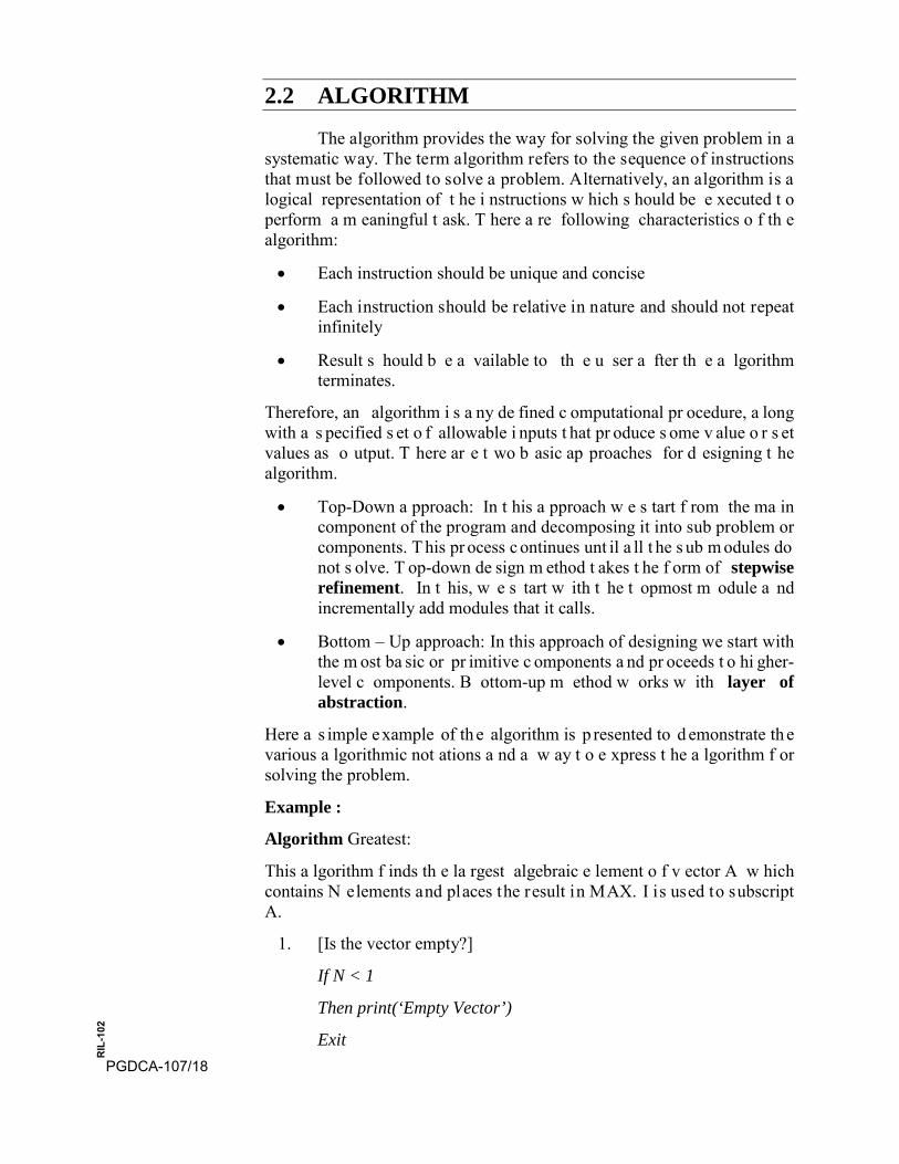
The algorithm provides the way for solving the given problem in a systematic way. The term algorithm refers to the sequence of instructions that must be followed to solve a problem. Alternatively, an algorithm is a logical representation of t he i nstructions w hich s hould be e xecuted t o perform a m eaningful t ask. T here a re following characteristics o f th e algorithm:
• Each instruction should be unique and concise
• Each instruction should be relative in nature and should not repeatinfinitely
• Result s hould b e a vailable to th e u ser a fter th e a lgorithmterminates.
Therefore, an algorithm i s a ny de fined c omputational pr ocedure, a long with a s pecified s et o f allowable i nputs t hat pr oduce s ome v alue o r s et values as o utput. T here ar e t wo b asic ap proaches for d esigning t he algorithm.
• Top-Down a pproach: In t his a pproach w e s tart f rom the ma incomponent of the program and decomposing it into sub problem orcomponents. T his pr ocess c ontinues unt il a ll t he s ub m odules donot s olve. T op-down de sign m ethod t akes t he f orm of stepwiserefinement. In t his, w e s tart w ith t he t opmost m odule a ndincrementally add modules that it calls.
• Bottom – Up approach: In this approach of designing we start withthe m ost ba sic or pr imitive c omponents a nd pr oceeds t o hi gher-level c omponents. B ottom-up m ethod w orks w ith layer ofabstraction.
Here a s imple example of th e algorithm is p resented to d emonstrate th e various a lgorithmic not ations a nd a w ay t o e xpress t he a lgorithm f or solving the problem.
Example :
Algorithm Greatest:
This a lgorithm f inds th e la rgest algebraic e lement o f v ector A w hich contains N elements and places the result in MAX. I is used to subscript A.
1. [Is the vector empty?]
If N < 1
Then print(‘Empty Vector’)
ExitPGDCA-107/18
RIL
-102
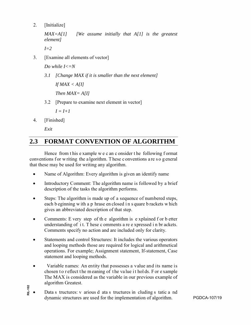
2. [Initialize]
MAX=A[1] [We assume initially that A[1] is the greatestelement]
I=2
3. [Examine all elements of vector]
Do while I<=N
3.1 [Change MAX if it is smaller than the next element]
If MAX < A[I]
Then MAX= A[I]
3.2 [Prepare to examine next element in vector]
I = I+1
4. [Finished]
Exit
2.3 FORMAT CONVENTION OF ALGORITHM
Hence from t his e xample w e c an c onsider t he following f ormat conventions f or w riting the a lgorithm. T hese c onventions a re s o g eneral that these may be used for writing any algorithm.
• Name of Algorithm: Every algorithm is given an identify name
• Introductory Comment: The algorithm name is followed by a briefdescription of the tasks the algorithm performs.
• Steps: The algorithm is made up of a sequence of numbered steps,each b eginning w ith a p hrase en closed i n s quare b rackets w hichgives an abbreviated description of that step.
• Comments: E very step of th e algorithm is e xplained f or b etterunderstanding of i t. T hese c omments a re e xpressed i n br ackets.Comments specify no action and are included only for clarity.
• Statements and control Structures: It includes the various operatorsand looping methods those are required for logical and arithmeticaloperations. For example; Assignment statement, If-statement, Casestatement and looping methods.
• Variable names: An entity that possesses a value and its name ischosen t o r eflect t he m eaning of t he va lue i t hol ds. F or e xample The MAX is considered as the variable in our previous example of algorithm Greatest.
• Data s tructures: v arious d ata s tructures in cluding s tatic a nddynamic structures are used for the implementation of algorithm. PGDCA-107/19
RIL
-102
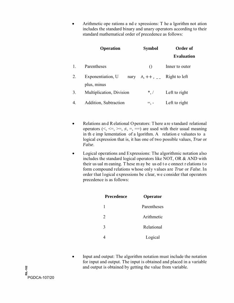
• Arithmetic ope rations a nd e xpressions: T he a lgorithm not ationincludes the standard binary and unary operators according to theirstandard mathematical order of precedence as follows:
Operation Symbol Order of
Evaluation
1. Parentheses () Inner to outer
2. Exponentiation, U nary
plus, minus
∧, ++ , _ _ Right to left
3. Multiplication, Division *, / Left to right
4. Addition, Subtraction =, - Left to right
• Relations an d R elational O perators: T here a re s tandard relationaloperators (<, <=, >=, ≠, =, ==) are used with their usual meaningin th e imp lementation of a lgorithm. A relation e valuates to alogical expression that is, it has one of two possible values, True orFalse.
• Logical operations and Expressions: The algorithmic notation alsoincludes the standard logical operators like NOT, OR & AND withtheir us ual m eaning. T hese m ay be us ed t o c onnect r elations t oform compound relations whose only values are True or False. Inorder that logical expressions be clear, we consider that operatorsprecedence is as follows:
Precedence Operator
1 Parentheses
2 Arithmetic
3 Relational
4 Logical
• Input and output: The algorithm notation must include the notationfor input and output. The input is obtained and placed in a variableand output is obtained by getting the value from variable.
PGDCA-107/20
RIL
-102
• Functions: A f unction is us ed w hen w e w ant a s ingle va luereturned to the calling routine. Transfer of control and returning ofthe value are accomplished by ‘Return (value)’.
• Procedures: A p rocedure i s s imilar t o a f unction but t here i s novalue returned explicitly. A procedure is also invoked differently,where there are parameters, a procedure returns its results throughthe parameters.
All algorithms must satisfy the following criteria.
1. Input
2. Output
3. Definiteness
4. Finiteness
5. Effectiveness
The criteria 1 & 2 r equire that an algorithm produces one or moreoutputs & have zero or more input. According to criteria 3, each operation must be definite such that it must be perfectly clear what should be done. According t o t he 4 th criteria a lgorithm s hould te rminate a fter a f inite number of operations. According to 5th criteria, every instruction must be very basic so t hat i t can be carried out b y a pe rson us ing onl y pencil & paper.
After an al gorithm h as b een d esigned i ts ef ficiency m ust b e analysed. This involves determining whether the algorithm is economical in t he us e of c omputer r esources, i .e. CPU time and memory requirement. The t erm u sed t o r efer t o t he memory r equired b y an algorithm is memory space and t he t erm us ed t o r efer t o t he computational time is the execution time. The importance of efficiency of an algorithm is the correctness. Thus, it always produces the correct result and algorithm complexity which c onsiders bot h the d ifficulty o f implementing an algorithm along with its efficiency.
Therefore the requirement for implementation of an algorithm with correctness co nsiders m any as pects. T he f undamental q uestion ar ises i s that “H ow can w e j udge h ow u seful a certain co mbination of da ta structures and a lgorithm i s?” O f c ourse t he answer of t his qu estion depends that how can we evaluate the effort that arises from performing a computation us ing t he c ertain c ombination of da ta s tructures a nd algorithms. There may be many algorithms devised for an application and we must analyse and validate the algorithms to judge the suitable one.
Hence th is e ffort is me asured n ormally with f ollowing tw o imp ortant factors t hose ha ve t he di rect r elationship w ith t he pe rformance of t he algorithm:
• Memory space used i.e. Space complexity. The space complexityof an algorithm is the amount of memory it needs to run. PGDCA-107/21
RIL
-102
• CPU t ime i nvolves r untime or e xecution t ime f or t he pr ogrambased on t he a lgorithm i .e. Time Complexity. The timecomplexity of an algorithm is given by the number of steps takenby the algorithm to compute the function it was written for.
2.4 COMPLEXITY OF ALGORITHM
The Complexity of algorithm is considered actually as in the form of c omputational c omplexity. C omputational c omplexity is a characterization of the t ime or space requirements for solving a p roblem by a particular algorithm. These requirements are expressed in terms of a single parameter that represents the size of the problem. For example we consider a problem of size n. Let the time required of a specific algorithm for solving this problem is expressed by a function:
f: R⟼R
Such t hat f(n)is th e la rgest a mount o f time n eeded b y th e a lgorithm to solve t he pr oblem of s ize n. T he f unction ‘f’ is u sually called th e time complexity function. Thus, we can say that the analysis of the algorithm requires two main considerations:
• Time Complexity
• Space Complexity
The time complexity of an algorithm is the amount of computer time that it needs to run to completion. The space of an algorithm is the amount of memory that it needs to run to completion.
2.5 TIME COMPLEXITY
In o rder to compute th e time c omplexity o f a n a lgorithm w e consider onl y t he f requency count of t he important s teps or i nstructions. Since these data structures are so widespread, it is important to implement them e fficiently. T his e fficiency is me asured u sing th e f ollowing tw o methods:
• Asymptotic Analysis
• Big-O analysis
It is v ery general th at t he a ctual time ( wall-clock time ) o f a p rogram i s affected by:
• Size of the input
• Programming language
• Programming tricks
• CompilerPGDCA-107/22
RIL
-102
• CPU Speed
• Multiprogramming level
Hence i nstead o f w all clock t ime f or t he p rogram i f w e co nsider t he pattern of the program’s behaviour as the program size increases. This is called the Asymptotic Analysis.
Big- O Analysis If f(n) represent the computing time of some algorithm and g(n) represents a known s tandard function l ike n, n2, n log n etc then to write: f(n) is O g(n) means that f(n) of n is equal to biggest order of function g(n). This implies only when:
f(n)≤Clog (n) for all sufficiently large integers n, where C is the constant. Thus from the above statements we can say that the computing time of an algorithm is O(g(n)), we mean that its execution time is no more than a constant time g(n), n is the parameter which characterizes the input and / or outputs. From the practical point of view, we get the Big-O notation for a function by:
1. Ignoring multiplicative constants (these are due to pesky differencein compiler, CPU, etc.)
2. Discarding the lower order terms (as n gets larger, the largest termhas the biggest impact). Like;
• 8410 = O(1)
• 100n3+nlogn+67n7+4n = O(n7)
The Bi g-O n otation h elps to d etermine th e t ime a s w ell as s pace complexity of t he a lgorithms. T he B og-O n otation h as b een ex tremely useful to classify algorithms by their performances. Now we consider the three simple algorithms with different number of sequences or steps:
Algorithm 1:
a=a+1
Algorithm 2:
For i= 1 to n do:
a=a+1
end loop
Algorithm 3:
For i=1 to n do
For j= 1to n do
a=a+1 PGDCA-107/23
RIL
-102
end loop
end loop
Now w e d o t he an alysis o f t hese t hree al gorithms an d can s ee t heir performance with Big – O notation. In the algorithm 1 w e may f ind that the execution statement a=a+1 is the independent and is not constrained within a ny l oop. T herefore, t he num ber o f t imes th is w ill e xecute is 1 . Thus, t he f requency c ount of t his a lgorithm i s 1. H ence i ts Time Complexity is O(1).
In the second algorithm, the execution statement a=a+1 is inside the loop. The number of times it is executed is n as the loop runs for n times. The frequency c ount for t his a lgorithm i s n. Hence i ts Time Complexity is O(n).
In t he t hird a lgorithm, t he f requency c ount f or the e xecution s tatement a=a+1 is n2 as the inner loop runs n times, each time the outer loop runs, the outer loop also runs for n times. Hence its Time Complexity is O(n2).
Therefore dur ing t he a nalysis of a lgorithm w e ha ve t he c oncern t o determine the order of magnitude of an algorithm. Thus, we consider only those statements which may have the greatest frequency count.
2.6 COMMON COMPUTING TIMES OF ALGORITHM
The common computing t imes of a lgorithms in the order of their performance are as follows:
• O(1): It means that the computing time of the algorithm is constant
• O(log n): It m eans th at th e c omputing time o f th e a lgorithm i slogarithmic
• O(n): It means that the computing time of the algorithm is directlyproportional to n. It is known as the linear time.
• O(n log n): It means that the computing time o f the a lgorithm islogarithmic
• O(n2): It is known as the quadratic time
• O(n3): It is known as the cubic time
• O(2n): It is known as the exponential time. Generally the algorithmwith exponential time has no practical use.
There ar e d ifferent t ypes o f t ime complexities w hich c an analyse f or a n algorithm: • Best c ase time complexity: T he b est c ase complexity o f an
algorithm is a measure of the minimum time that the algorithm will require f or a n i nput of s ize ‘n’. T he r unning t ime of m any PGDCA-107/24
RIL
-102
algorithm varies not only for the input of different size but for the different inputs of the same size.
• Average c ase time c omplexity: T he time th at a n a lgorithm w illrequire to execute input data of size ‘n’ is known as average case time c omplexity. W e can s ay th at th e v alue th at is o btained b y averaging the running t ime of an algorithm for all possible inputs of size ‘n’ can determine average-case time complexity.
• Worst c ase time c omplexity: T he w orst time complexity o f analgorithm is a me asure of th e ma ximum time that th e a lgorithm will require for an input of size ‘n’. The worst case complexity is useful for a number of reasons. After knowing the worst case time complexity, w e c an guarantee t hat t he al gorithm w ill n ever t ake more than this time.
Hence th e c omputation o f e xact time taken b y th e a lgorithm f or its execution i s ve ry di fficult. T hus, t he w ork done b y a n a lgorithm f or t he execution of the input of size ‘n’ defines the time analysis as function f(n) of the input data items.
2.7 EXAMPLE AND ANALYSIS
Example: This ex ample ex hibits t he an alysis o f l inear s earch al gorithm complexity.
Consider the algorithm to search vector (array) V of size N for the location containing value X.
Algorithm SEARCH [Given a v ector V co ntaining N el ements, t his algorithm s earches V for t he va lue of a given X. F OUND i s a Boolean variable. I and LOCATION are integer variables.]
1. [Search for the location of value X in vector V]
FOUND = false
I=1
Do while ((I<=N) && (FOUND ==false))
If V[I] ==X
Then FOUND==true
LOCATION = I
EXIT
Else I = I + 1
Print(“Value of”, X,”NOT FOUND”)
2. [Finished]
Exit PGDCA-107/25
RIL
-102
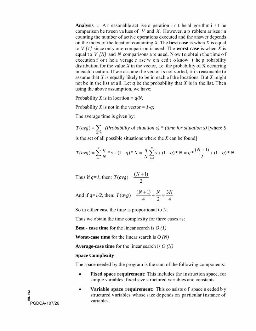
Analysis : A r easonable act ive o peration i n t he al gorithm i s t he comparison be tween va lues of V and X. However, a p roblem ar ises i n counting the number of active operations executed and the answer depends on the index of the location containing X. The best case is when X is equal to V [1] since only one comparison is used. The worst case is when X is equal t o V [N] and N comparisons a re us ed. N ow t o obt ain t he t ime o f execution f or t he a verage c ase w e n eed t o know t he p robability distribution for the value X in the vector, i.e. the probability of X occurring in each location. If we assume the vector is not sorted, it is reasonable to assume that X is equally likely to be in each of the locations. But X might not be in the list at all. Let q be the probability that X is in the list. Then using the above assumption, we have;
Probability X is in location = q/N;
Probability X is not in the vector = 1-q;
The average time is given by:
∑=S
avgTsin
)( (Probability of situation s) * (time for situation s) [where S
is the set of all possible situations where the X can be found]
∑ ∑= =
−++
=−+=−+=N
s
N
sNqNqNqs
NqNqs
NqavgT
1 1*)1(
2)1(**)1(*)1(*)(
Thus if q=1, then: 2
)1()( +=
NavgT
And if q=1/2, then: 4
324
)1()( NNNavgT ≈++
=
So in either case the time is proportional to N.
Thus we obtain the time complexity for three cases as:
Best - case time for the linear search is O (1)
Worst-case time for the linear search is O (N)
Average-case time for the linear search is O (N)
Space Complexity
The space needed by the program is the sum of the following components:
• Fixed space requirement: This includes the instruction space, forsimple variables, fixed size structured variables and constants.
• Variable space requirement: This co nsists o f space n eeded b ystructured v ariables whose s ize de pends on pa rticular i nstance ofvariables.PGDCA-107/26
RIL
-102
2.8 SUMMARY
This uni t described the algorithm and i ts analysis in very concise manner. The algorithm provides the way for solving the given problem in a systematic way. The following points are described in this unit:
• The term algorithm refers to the sequence of instructions that mustbe followed to solve a problem.
• An algorithm is a logical representation of the instructions whichshould be executed to perform a meaningful task.
• Analysis of t he algorithm i s done a fter de termining t he r unningtime of a n a lgorithm ba sed on t he num ber of b asic ope rations i tperforms.
• There are t wo b asic ap proaches f or d esigning t he al gorithm i .e.Top-down approach and Bottom –Up approach.
• The running t ime varies depending upon t he order in which inputdata is supplied to it.
• Analysis of an algorithm is done on the following basis:
∗ Best case time complexity
∗ Worst case time complexity
∗ Average case time complexity
• Comparison of algorithm is done on the basis of the programmingefforts f or a pr ogram a nd on t he ba sis of t ime a nd s pacerequirements for the program.
• Big ‘O’ notation is extremely useful for classifying algorithms bytheir performances.
• Examples a nd a nalysis f or c omputing t he t ime c omplexity of t healgorithm is explained.
Bibliography Horowitz, E ., S . S ahni: “ Fundamental of computer A lgorithms”, Computer Science Press, 1978
J. P. Tremblay, P . G. Sorenson “An Introduction to Data Structures with Applications”, Tata McGraw-Hill, 1984
M. A llen W eiss: “ Data s tructures a nd P roblem s olving us ing C ++”, Pearson Addison Wesley, 2003
Ulrich Klehmet: “Introduction to Data Structures and Algorithms”, URL: http://www7 . Informatik.uni-erlangen.de/~klehmet/teaching/SoSem/dsa
PGDCA-107/27
RIL
-102
Markus Blaner: “ Introduction t o A lgorithms a nd D ata S tructures”, Saarland University, 2011
V. Abo. Hopcropft, Ullaman, “data Structure and Algorithms”, I.P.E.
Seymour Lipschutz, “Data Structure”, Schaum’s outline Series.
PGDCA-107/28
RIL
-102
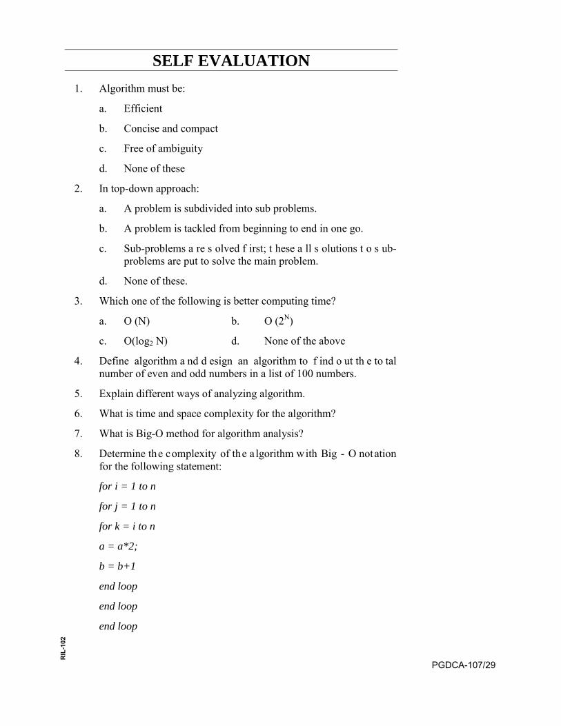
SELF EVALUATION 1. Algorithm must be:
a. Efficient
b. Concise and compact
c. Free of ambiguity
d. None of these
2. In top-down approach:
a. A problem is subdivided into sub problems.
b. A problem is tackled from beginning to end in one go.
c. Sub-problems a re s olved f irst; t hese a ll s olutions t o s ub-problems are put to solve the main problem.
d. None of these.
3. Which one of the following is better computing time?
a. O (N) b. O (2N)
c. O(log2 N) d. None of the above
4. Define algorithm a nd d esign an algorithm to f ind o ut th e to talnumber of even and odd numbers in a list of 100 numbers.
5. Explain different ways of analyzing algorithm.
6. What is time and space complexity for the algorithm?
7. What is Big-O method for algorithm analysis?
8. Determine the complexity of the a lgorithm with Big - O notationfor the following statement:
for i = 1 to n
for j = 1 to n
for k = i to n
a = a*2;
b = b+1
end loop
end loop
end loop
PGDCA-107/29
RIL
-102
PGDCA-107/30
RIL
-102
UNIT-3 ARRAY
Structure
3.0 Introduction
3.1 Objective
3.2 Definition of Array
3.3 Declaration and initialization of array
3.4 One dimensional array and its memory representation
3.5 Operation on Linear Array
3.6 Two-Dimensional Array
3.7 2-D array representation
3.8 Multi-Dimensional Arrays
3.9 Sparse Matrices
3.10 Summary
3.0 INTRODUCTION
This uni t discusses about one of the l inear t ype data s tructure i .e. Array. It also presents about the various operations that can be performed on A rrays. T his uni t a lso pr esents th e tw o-dimensional a nd multidimensional a rrays a nd t heir r epresentations i n r ow-major an d column-major or der. It also c onsiders about t he f ormulation of address calculation f or s ingle, t wo a nd mu lti d imensional a rrays. In th e la st i t introduces the concept of sparse matrices.
3.1 OBJECTIVE
Array is a l inear data s tructure with contiguous memory location. The ar ray d ata s tructure i s u sed t o s tore t he s ame t ype o f d ata t ype i n sequential manner. At the end of this unit, you will be able to;
1. Understand t he d efinition a nd r epresentation of one di mensionalarray.
2. Know a bout t he r epresentation of t wo d imensional a ndmultidimensional arrays in row-major and column-major way.
3. Calculation of address for one, two and multidimensional arrays.
4. Understanding and representation of the sparse matrices.
PGDCA-107/31
RIL
-102

3.2 DEFINITION OF ARRAY
The simplest type of linear data structure is an array. The array is preferred for the situation which requires similar type of data items to be stored t ogether as i n c ontiguous m emory lo cation in s tatic me mory allocation manner. Thus, an array is a finite collection of similar elements stored in adjacent memory locations, for example an array may contain all integers or all characters. Therefore an array is a collection of variables of the same type that are referred by a common name. Alternatively we can also say that an array is a list of a finite number n of similar data elements referenced respectively by a set of n consecutive numbers, usually 1, 2, 3, …n.
An a rray wi th n number of e lements i s r eferenced us ing a n i ndex t hat ranges fro m 0 to n-1. T he l owest i ndex of a n a rray i s c alled i ts lower bound and hi ghest i ndex i s c alled t he upper bound. T he num ber o f elements in an array is called its range or length or size of the array. For example the element of an array A[n] containing n elements are referenced as A[0], A[1], A[2],......A[n-1] here the 0 (zero) is the lowest bound and n-1 is t he uppe r bound o f t he a rray. T he array defined i n t his f orm i s considered as the linear array or the one-dimensional array. The linear or one-dimensional array may also be defined as:
A linear array is a lis t o f a f inite n umber n of i nhomogeneous da ta elements (i.e., data elements of the same type) such that:
a) The elements of the array are referenced respectively by an indexset consisting of n consecutive numbers.
b) The el ements o f t he ar ray a re s tored r espectively i n s uccessivememory locations.
As an example if we choose the name A for the array, then the elements of A are denoted by subscript notation: a1, a2, a3 , ……., an
Or, by the parenthesis notation: A (1), A (2), A (3) ,……., A(N)
Or, by the bracket notation: A [1], A [2], A [3] ,…….., A[N]
Regardless of the notation, the number K in A [K] is called a subscript and A [K] is cal led a subscripted variable. The g eneral e quation t o f ind t he length or the number of data elements of the array can define as:
Length = UB – LB + 1
Here, UB is the upper bound or largest index of the array and LB is the lower bound o r the smallest index of the array. This is quite obvious that if: LB = 1 then Length = UB.
PGDCA-107/32
RIL
-102

3.3 DECLARATION & INITIALIZATION OF ARRAY
Here we consider the declaration of array and its initialization. As per the majority of people are aware from the C language so we choose the syntax o f C l anguage for t he d eclaration o f array as w ell as f or i ts initialization. T herefore an ar ray can b e d eclared j ust l ike an y o ther variable i n C i .e. da ta t ype f ollowed b y a rray na me w ith s ubscription in bracket w hich i ndicates t he num ber of e lements i t w ill hol d. T hus b y declaring an array, the specified number of memory locations i.e. the size of array are allocated in the memory. The declaration of array is specified with given example as:
int A[10]; // This is an integer t ype ar ray w here each el ement h olds an integer value and in total 10 integers can hold.
float b_charge [20]; // This is a float type array where each element holds a float value and in total 20 values can hold.
char name [50]; // This is a character type array where each element holds a character value and in total 50 characters can hold.
The el ements o f an ar ray can b e e asily p rocessed as t hey a re s tored i n contiguous m emory l ocations a nd i t c an be s een f rom t he f ollowing example:
int a [5]
This is stored as:
100 102 104 106 108 a[0] a[1] a[2] a[3] a[4]
Initialization of Array Any array can be in itialized a t the time of its declaration as specified in following example:
int A[5] = [67, 102, 6, 8, 90];
float B[3] = [20.67, 100.78, 1000];
This array declaration and its initialization can be represented as:
[0] [1] [2] [3] [4] 67 102 6 8 90
Address⟼ 100 102 104 106 108
In this array representation the address is mentioning the memory location i.e. the array A is of type integer and every integer occupies 2 bytes in the memory. S o if th e f irst e lement o f a rray s tores a t me mory lo cation 1 00 PGDCA-107/33
RIL
-102
then the next element of array will store on location 102 and so on. Thus, it is showing the contiguous memory location for the array.
Now w e co nsider t he ex ample o f an a rray o f ch aracter an d i ts representation in the form of contiguous memory location.
Char name [4] = “Ram”
The values assigned in the name array as follows:
[0] [1] [2] [3] R a m ‘\0’
Address⟼ 100 101 102 103
An ar ray o f ch aracters i s cal led a string and it is te rminated b y a n ull character (‘\0’).
3.4 ONE D IMENSIONAL ARRAY AND ITS MEMORY REPRESENTATION
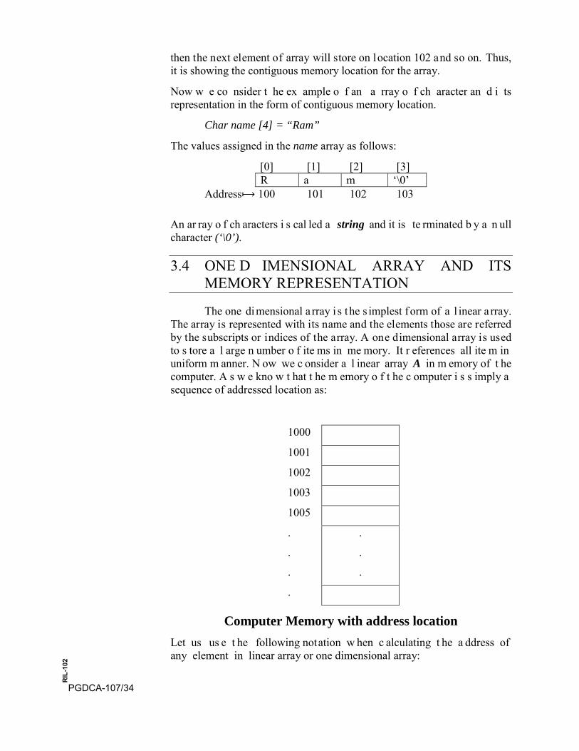
The one dimensional a rray i s t he s implest form of a l inear a rray. The array is represented with its name and the elements those are referred by the subscripts or indices of the array. A one dimensional array is used to s tore a l arge n umber o f ite ms in me mory. It r eferences all ite m in uniform m anner. N ow we c onsider a l inear array A in m emory of t he computer. A s w e kno w t hat t he m emory o f t he c omputer i s s imply a sequence of addressed location as:
1000
1001
1002
1003
1005
.
.
.
.
.
.
.
Computer Memory with address location Let us us e t he following notation w hen c alculating t he a ddress of any element in linear array or one dimensional array:
PGDCA-107/34
RIL
-102
LOC (A [k]) = address of the element A [K] of the array A. As we have di scussed pr eviously that the e lements o f any linear a rray s tores in contiguous or successive memory locations. Therefore the computer does not ne ed t o ke ep t rack of t he address of every memory element of t he array but i t needs to keep t rack of the address of the f irst element of the array. T his ad dress o f the l ocation o f f irst el ement o f t he a rray we represent it by base address of the array as: Base (A). The address of any element of the array can be calculated by using this base address of the array as:
Loc (A [k]) = Base (A) + w (k- lower bound); here w is the number of words per memory cell for the array A.
Note: The t ime t o calculate Loc (A [k]) is es sentially t he s ame f or an y value of k. We can l ocate an d ac cess t he content o f A [K] without scanning any other element of A.
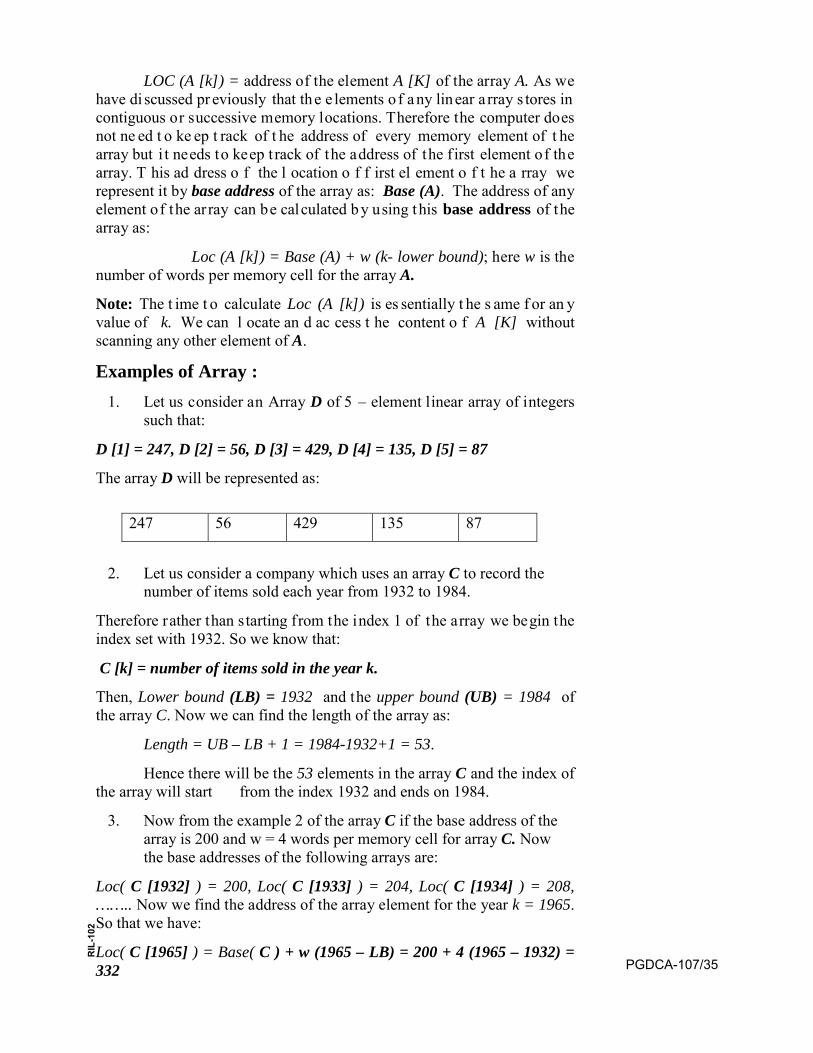
Examples of Array : 1. Let us consider an Array D of 5 – element linear array of integers
such that:
D [1] = 247, D [2] = 56, D [3] = 429, D [4] = 135, D [5] = 87
The array D will be represented as:
247 56 429 135 87
2. Let us consider a company which uses an array C to record thenumber of items sold each year from 1932 to 1984.
Therefore rather than starting from the index 1 of the array we begin the index set with 1932. So we know that:
C [k] = number of items sold in the year k.
Then, Lower bound (LB) = 1932 and the upper bound (UB) = 1984 of the array C. Now we can find the length of the array as:
Length = UB – LB + 1 = 1984-1932+1 = 53.
Hence there will be the 53 elements in the array C and the index of the array will start from the index 1932 and ends on 1984.
3. Now from the example 2 of the array C if the base address of thearray is 200 and w = 4 words per memory cell for array C. Nowthe base addresses of the following arrays are:
Loc( C [1932] ) = 200, Loc( C [1933] ) = 204, Loc( C [1934] ) = 208, …….. Now we find the address of the array element for the year k = 1965. So that we have:
Loc( C [1965] ) = Base( C ) + w (1965 – LB) = 200 + 4 (1965 – 1932) = 332 PGDCA-107/35
RIL
-102
3.5 OPERATION ON LINEAR ARRAY
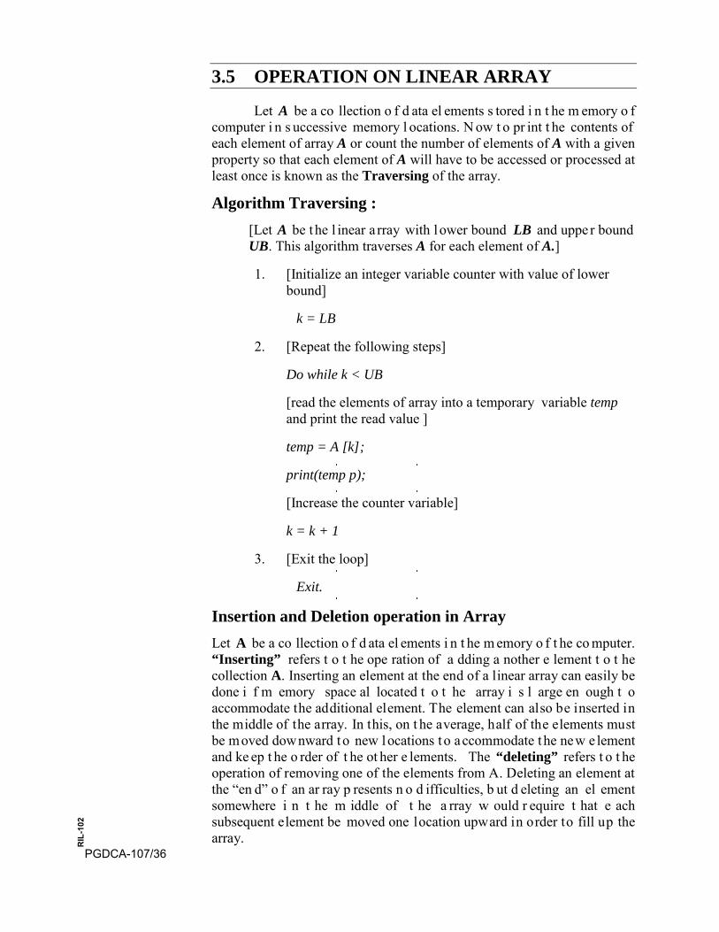
Let A be a co llection o f d ata el ements s tored i n t he m emory o f computer i n s uccessive memory l ocations. N ow t o pr int t he contents of each element of array A or count the number of elements of A with a given property so that each element of A will have to be accessed or processed at least once is known as the Traversing of the array.
Algorithm Traversing : [Let A be t he l inear a rray with l ower bound LB and uppe r bound UB. This algorithm traverses A for each element of A.]
1. [Initialize an integer variable counter with value of lowerbound]
k = LB
2. [Repeat the following steps]
Do while k < UB
[read the elements of array into a temporary variable tempand print the read value ]
temp = A [k];
print(temp p);
[Increase the counter variable]
k = k + 1
3. [Exit the loop]
Exit.
Insertion and Deletion operation in Array Let A be a co llection o f d ata el ements i n t he m emory o f t he co mputer. “Inserting” refers t o t he ope ration of a dding a nother e lement t o t he collection A. Inserting an element at the end of a linear array can easily be done i f m emory space al located t o t he array i s l arge en ough t o accommodate the additional element. The element can also be inserted in the middle of the array. In this, on t he average, half of the elements must be moved downward to new locations t o accommodate t he new e lement and ke ep t he o rder of t he ot her e lements. The “deleting” refers t o t he operation of removing one of the elements from A. Deleting an element at the “en d” o f an ar ray p resents n o d ifficulties, b ut d eleting an el ement somewhere i n t he m iddle of t he a rray w ould r equire t hat e ach subsequent element be moved one location upward in order to fill up the array.
PGDCA-107/36
RIL
-102
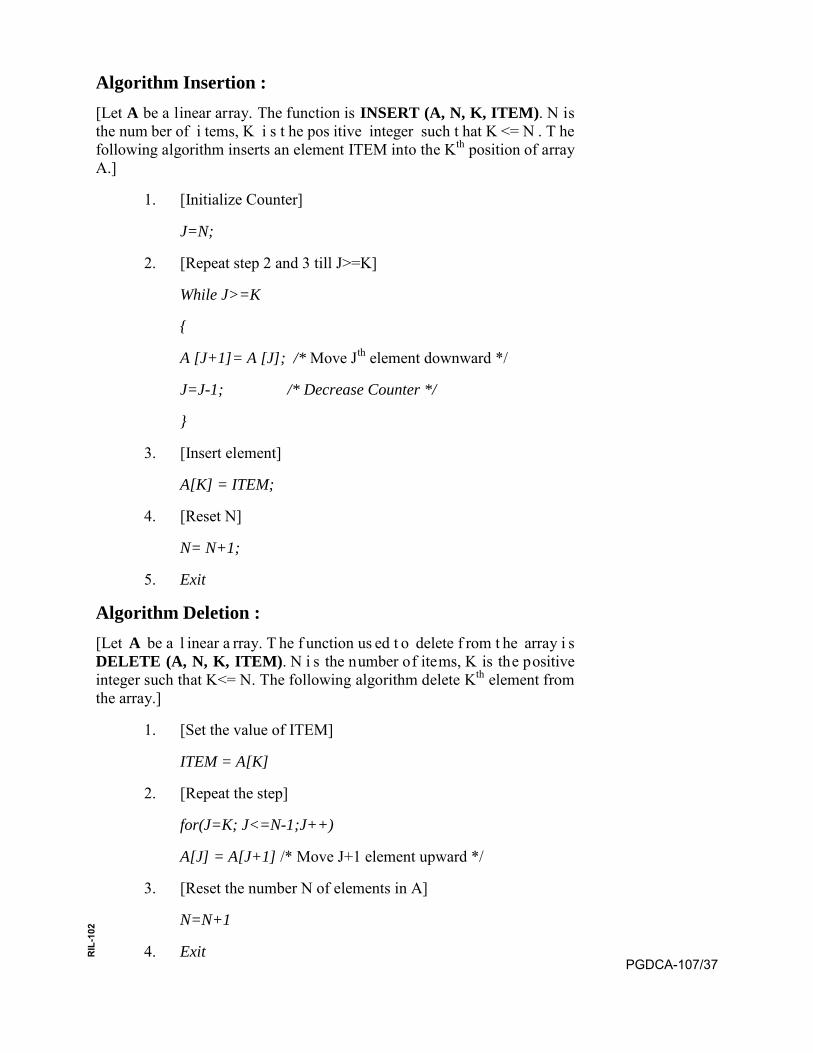
Algorithm Insertion : [Let A be a linear array. The function is INSERT (A, N, K, ITEM). N is the num ber of i tems, K i s t he pos itive integer such t hat K <= N . T he following algorithm inserts an element ITEM into the Kth position of array A.]
1. [Initialize Counter]
J=N;
2. [Repeat step 2 and 3 till J>=K]
While J>=K
{
A [J+1]= A [J]; /* Move Jth element downward */
J=J-1; /* Decrease Counter */
}
3. [Insert element]
A[K] = ITEM;
4. [Reset N]
N= N+1;
5. Exit
Algorithm Deletion : [Let A be a l inear a rray. T he f unction us ed t o delete f rom t he array i s DELETE (A, N, K, ITEM). N i s the number of items, K is the positive integer such that K<= N. The following algorithm delete Kth element from the array.]
1. [Set the value of ITEM]
ITEM = A[K]
2. [Repeat the step]
for(J=K; J<=N-1;J++)
A[J] = A[J+1] /* Move J+1 element upward */
3. [Reset the number N of elements in A]
N=N+1
4. ExitPGDCA-107/37
RIL
-102
Example : Consider T has b een d eclared as a 5 -element ar ray b ut d ata h ave b een recorded only fo r T [1], T [2], and T [3]. If X i s t he va lue t o t he next element, th en w e ma y s imply assign, T [4] = X t o a dd X t o t he Linear Array. Similarly, if Y is the value of the subsequent element, then we may assign, T [5] = Y to add Y to the Linear Array. Thus, we cannot add any new element to this Linear Array for T [6] because it exceeds the limit of this array upper bound.
3.6 TWO-DIMENSIONAL ARRAY
A two-dimensional array of size m x n is a collection of elements placed in m rows and n columns. Each element in array is specified by a pair of i ntegers ( such t hat j , k) kno ws a s subscripts, with th e f ollowing property:
0 <=j<=m and 0<=k<=n
Thus, t here a re t wo s ubscripts i n t he s yntax of 2 -D a rray i n w hich one specifies the number of rows and the other the number of columns. In a 2-D array each element is itself an array. Let A be a 2-D array. The element of A with first subscripts j and second subscript k is represented as:
kjA , Or ],[ kjA
Any 2 -D ar ray i s al so cal led as t he matrix in m athematics an d Table in business application. Thus, a 2-D array is also called the matrix arrays.
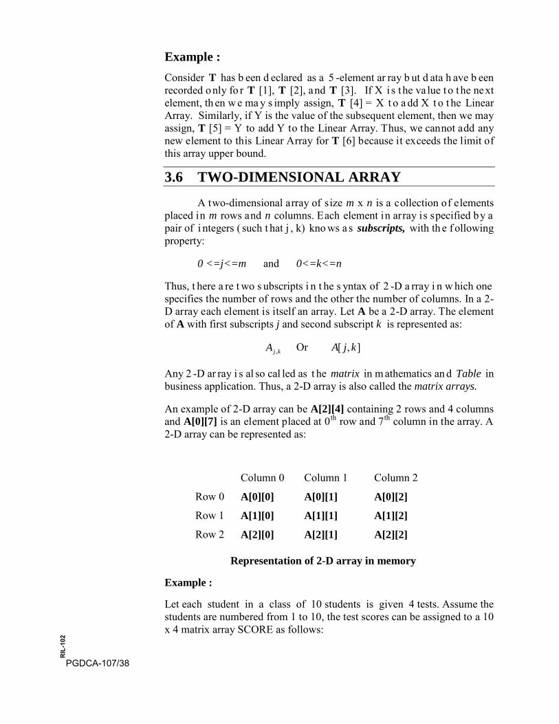
An example of 2-D array can be A[2][4] containing 2 rows and 4 columns and A[0][7] is an element placed at 0th row and 7th column in the array. A 2-D array can be represented as:
Column 0 Column 1 Column 2
Row 0 A[0][0] A[0][1] A[0][2]
Row 1 A[1][0] A[1][1] A[1][2]
Row 2 A[2][0] A[2][1] A[2][2]
Representation of 2-D array in memory
Example :
Let each student in a class of 10 students is given 4 tests. Assume the students are numbered from 1 to 10, the test scores can be assigned to a 10 x 4 matrix array SCORE as follows:
PGDCA-107/38
RIL
-102
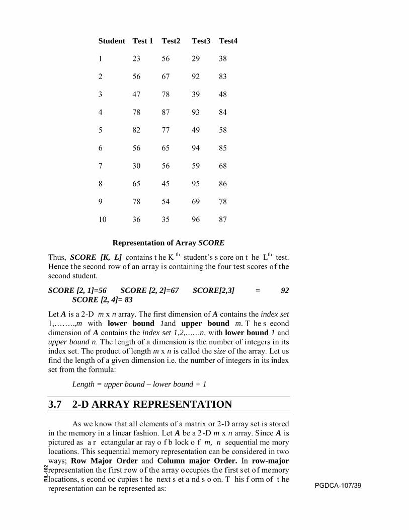
Student Test 1 Test2 Test3 Test4
1 23 56 29 38
2 56 67 92 83
3 47 78 39 48
4 78 87 93 84
5 82 77 49 58
6 56 65 94 85
7 30 56 59 68
8 65 45 95 86
9 78 54 69 78
10 36 35 96 87
Representation of Array SCORE
Thus, SCORE [K, L] contains t he K th student’s s core on t he Lth test. Hence the second row of an array is containing the four test scores of the second student.
SCORE [2, 1]=56 SCORE [2, 2]=67 SCORE[2,3] = 92SCORE [2, 4]= 83
Let A is a 2-D m x n array. The first dimension of A contains the index set 1,……..,m with lower bound 1and upper bound m. T he s econd dimension of A contains the index set 1,2,……n, with lower bound 1 and upper bound n. The length of a dimension is the number of integers in its index set. The product of length m x n is called the size of the array. Let us find the length of a given dimension i.e. the number of integers in its index set from the formula:
Length = upper bound – lower bound + 1
3.7 2-D ARRAY REPRESENTATION
As we know that all elements of a matrix or 2-D array set is stored in the memory in a linear fashion. Let A be a 2 -D m x n array. Since A is pictured as a r ectangular ar ray o f b lock o f m, n sequential me mory locations. This sequential memory representation can be considered in two ways; Row Major Order and Column major Order. In row-major representation the f irst row of the array occupies the f irst set of memory locations, s econd oc cupies t he next s et a nd s o on. T his f orm of t he representation can be represented as: PGDCA-107/39
RIL
-102
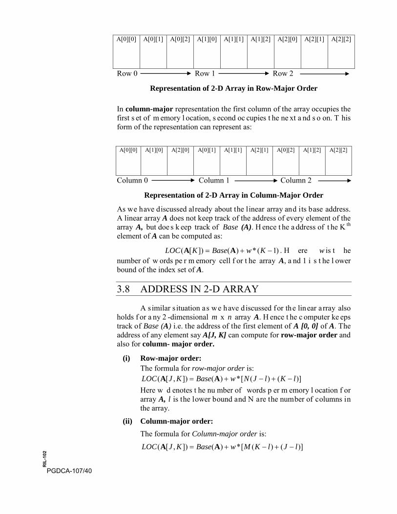
A[0][0] A[0][1] A[0][2] A[1][0] A[1][1] A[1][2] A[2][0] A[2][1] A[2][2]
Row 0 Row 1 Row 2
Representation of 2-D Array in Row-Major Order
In column-major representation the first column of the array occupies the first s et of m emory l ocation, s econd oc cupies t he ne xt a nd s o on. T his form of the representation can represent as:
A[0][0] A[1][0] A[2][0] A[0][1] A[1][1] A[2][1] A[0][2] A[1][2] A[2][2]
Column 0 Column 1 Column 2
Representation of 2-D Array in Column-Major Order
As we have discussed already about the linear array and its base address. A linear array A does not keep track of the address of every element of the array A, but doe s k eep track of Base (A). H ence t he a ddress of t he K th element of A can be computed as:
)1(*)(])[( −+= KwBaseKLOC AA . H ere w is t he number of w ords pe r m emory cell f or t he array A, a nd 1 i s t he l ower bound of the index set of A.
3.8 ADDRESS IN 2-D ARRAY
A s imilar s ituation as we have d iscussed for the linear array also holds f or a ny 2 -dimensional m x n array A. H ence t he c omputer ke eps track of Base (A) i.e. the address of the first element of A [0, 0] of A. The address of any element say A[J, K] can compute for row-major order and also for column- major order.
(i) Row-major order: The formula for row-major order is:
)]()([*)(]),[( lKlJNwBaseKJLOC −+−+= AA Here w d enotes t he nu mber of words p er m emory l ocation f or array A, l is the lower bound and N are the number of columns in the array.
(ii) Column-major order: The formula for Column-major order is:
)]()([*)(]),[( lJlKMwBaseKJLOC −+−+= AA
PGDCA-107/40
RIL
-102

Here w d enotes t he nu mber of words p er memory lo cation f or array A, l is the lower bound and M are the number of Rows in the array.
Example : Calculate the address of an element in the following 2-D array:
int M [3][4] = { {1, 2, 3, 4}, {5, 6, 7, 8},{9, 10, 11, 12}}; The ba se a ddress of t he a rray M is 100. S ince w = 2 (The ar ray i s o f integer type and integer occupies 2 byte in memory), according to the row-major formula the address of (2, 3)th element in the array M is:
LOC (2, 3) = 100 + 2[4*(2-1) + (3-1)] = 100 + (4+2)*2 = 112 [lower bound of the array is assumed to be 1] Now a ccording t o t he column-major f ormula the a ddress of (2, 3) th element in the array M is:
LOC (2, 3) = 100 + 2[3*(3-1) + (2-1)] = 100 + (6+1)*2=114
3.9 MULTI-DIMENSIONAL ARRAYS
The arrays can also have more than two dimensions. For example, a three – dimensional (3-D) array may be declared as:
int A[2][3][4];
The number of elements in any array is the product of the ranges of all its dimensions. Therefore the array A contains 2*3*4 = 24 e lements of type integers. An element of this array is referenced with three subscripts. The first s pecifies th e p lane o r rack number, t he s econd s pecifies t he r ow number and the third specifies the column number. It is just like the library of books. The book is available in a particular column of the selected row in the specific rack. This array can be represented in memory as:
A[0][0][0] A[0][0][1] A[0][0][2] A[0][0][3]
A[0][1][0] A[0][1][1] A[0][1][2] A[0][1][3]
A[0][2][0] A[0][2][1] A[0][2][2] A[0][2][3]
A[1][0][0] A[1][0][1] A[1][0][2] A[1][0][3]
A[1][1][0] A[1][1][1] A[1][1][2] A[1][1][3]
A[1][2][0] A[1][2][1] A[1][2][2] A[1][2][3]
3-Dimensional Memory Representation if array in row major order
Similarly t he c olumn major or der can b e c onsidered. T he general multidimensional arrays are defined analogously. More specifically, an n-dimensional m1 x m2 x…………x mn, a rray A is a c ollection o f m1, m2, …………, mn, data elements in which each element is specified by a list of
PGDCA-107/41
RIL
-102

n integers such as K1, K2, …………Kn called subscripts, with the property that:
0 <= K1 <= m1, 0 <= K2 <= m2, ……….. 0 <= Kn <= mn,
The element of B with subscripts K1, K2,…. Kn will be denoted by:
B[K1, K2,…. Kn ]
The a rray will be s tored in memory in a sequence of memory locations. Specifically, th e p rogramming la nguage will s tore th e a rray B either i n row-major order or column-major order.
3.10 SPARSE MATRICES
Any matrices with relatively high proportion of zero or null entries are c alled s parse m atrices. T hus, a s parse m atrix can b e d efined as a matrix with maximum number of zero entries. In the sparse matrix space and c omputing t ime c ould be s aved i f t he non -zero en tries were s tored explicitly i .e. ignoring the zero entries the processing time and space can be minimized in sparse matrices. A sparse matrix can be divided into two categories:
• N2 Sparse matrix: N2 sparse matrix is a matrix with zero entriesthat form a square or a bar.
• Triangular sparse matrix: In this sparse matrix the zero entriesare in its diagonal, either in the upper or lower side.
Now we consider the following sparse matrix:
00800000018000000900000000000050000000024000
In t his s parse m atrix w e ha ve t he 6 r ows a nd 7 c olumns. T here a re 5 nonzero entries out of 42 entries. Therefore it requires an alternate form to represent the matrix without considering the null entries. Now we consider a data structure triplet to represent a s parse matrix. The triplet is a two dimensional a rray h aving t +1 r ows a nd 3 c olumns. H ere t i s the t otal number of nonzero entries.
In t his r epresentation of triplet the f irst r ow c ontains num ber of r ows, columns and nonzero entries available in the matrix in its 1st, 2nd and 3rd column r espectively. S econd r ow onw ards i t c ontains t he r ow s ubscript, column subscript and the value of the nonzero entry in its 1st, 2nd and 3rd
PGDCA-107/42
RIL
-102
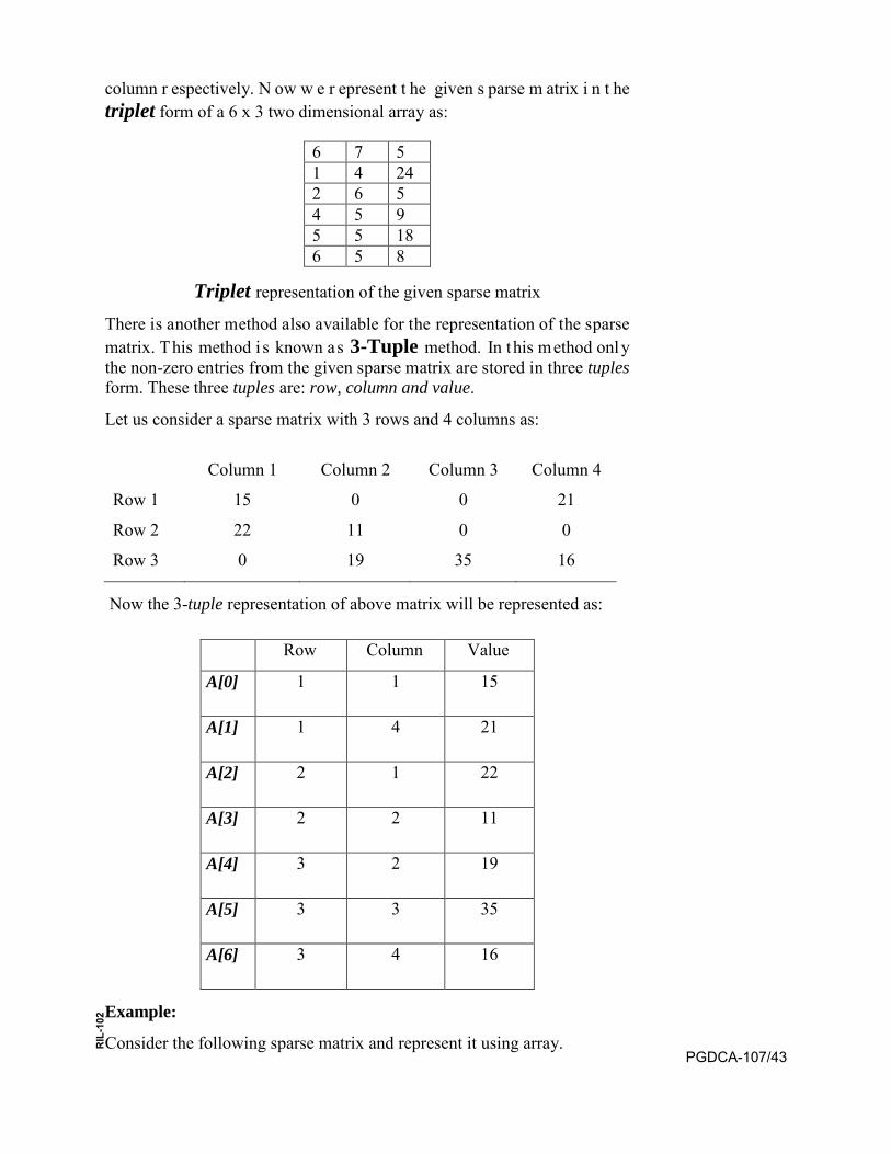
column r espectively. N ow w e r epresent t he given s parse m atrix i n t he triplet form of a 6 x 3 two dimensional array as:
6 7 5 1 4 24 2 6 5 4 5 9 5 5 18 6 5 8
Triplet representation of the given sparse matrix
There is another method also available for the representation of the sparse matrix. This method i s known as 3-Tuple method. In this method only the non-zero entries from the given sparse matrix are stored in three tuples form. These three tuples are: row, column and value.
Let us consider a sparse matrix with 3 rows and 4 columns as:
Column 1 Column 2 Column 3 Column 4
Row 1
Row 2
Row 3
15
22
0
0
11
19
0
0
35
21
0
16
Now the 3-tuple representation of above matrix will be represented as:
Row Column Value
A[0] 1 1 15
A[1] 1 4 21
A[2] 2 1 22
A[3] 2 2 11
A[4] 3 2 19
A[5] 3 3 35
A[6] 3 4 16
Example:
Consider the following sparse matrix and represent it using array. PGDCA-107/43
RIL
-102

=1635190001122210015
A
As we k now that as parse matrix i s o ne w here m ost o f i ts el ements ar e zero. The idea i s t o s tore i nformation of non-zero el ements. Information about non-zero elements has three parts:
• An integer representing its row.
• An integer representing its column.
• The data associated with its elements.
The el ements o f t he ab ove s parse m atrix can b e r epresented as f ollows using array:
0, 0, 15 0, 3, 21 1, 0, 22 1, 1, 11 2, 1, 19 2, 2, 35 2, 3, 16
3.11 SUMMARY An array is a simplest t ype o f l inear d ata s tructure. T he ar ray i s
preferred for the situation which requires similar type of data items to be stored t ogether as i n c ontiguous m emory l ocation i n s tatic m emory allocation manner. An array is a finite collection of similar elements stored in a djacent me mory lo cations. T his u nit h as d escribed th e lin ear d ata structure array. The contents of this unit can be summarized as:
• An array is a finite collection of similar elements stored in adjacentmemory locations.
• There a re m any ope rations w hich c ould be pe rformed on a rrayslike insertion, deletion, searching, sorting and traversing.
• Arrays can b e s ingle-dimensional, t wo-dimensional o r mu lti-dimensional.
• There are t wo w ays of r epresenting t wo-dimensional a rrays i nmemory i.e. Row-major and column-major order.
• Multidimensional arrays have more than two dimensions.
• Any matrices with relatively high proportion of zero or null entriesare called sparse matrices.
• In t he sparse m atrix space and computing t ime could be s aved i fthe non-zero en tries w ere s tored ex plicitly i .e. i gnoring t he z eroentries the processing t ime and space can be minimized in sparsematrices.
PGDCA-107/44
RIL
-102

Bibliography Horowitz, E ., S . S ahni: “ Fundamental of computer A lgorithms”, Computer Science Press, 1978
J. P. Tremblay, P . G. Sorenson “An Introduction to Data Structures with Applications”, Tata McGraw-Hill, 1984
M. A llen W eiss: “ Data s tructures a nd P roblem s olving us ing C ++”, Pearson Addison Wesley, 2003
Ulrich Klehmet: “Introduction to Data Structures and Algorithms”, URL: http://www7 . Informatik.uni-erlangen.de/~klehmet/teaching/SoSem/dsa
Markus Blaner: “ Introduction t o A lgorithms a nd D ata S tructures”, Saarland University, 2011
T. H . C ormen, C . E . Leiserson and R . L. R ivest, “ i ntroduction to Algorithms”, MIT Press, Combridge, 1990
R. Sedgewick, “Algorithm in C++”, Addison-Wesley, 1992
R. B. Patel “Fundamental of Data Structures in C”, PHI Publication
V. Abo. Hopcropft, Ullaman, “data Structure and Algorithms”, I.P.E.
Seymour Lipschutz, “Data Structure”, Schaum’s outline Series.
PGDCA-107/45
RIL
-102
SELF EVALUATION
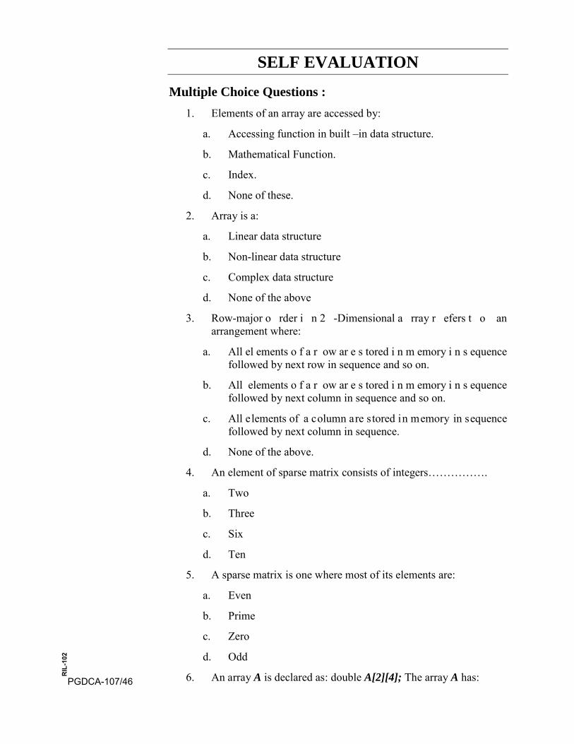
Multiple Choice Questions : 1. Elements of an array are accessed by:
a. Accessing function in built –in data structure.
b. Mathematical Function.
c. Index.
d. None of these.
2. Array is a:
a. Linear data structure
b. Non-linear data structure
c. Complex data structure
d. None of the above
3. Row-major o rder i n 2 -Dimensional a rray r efers t o anarrangement where:
a. All el ements o f a r ow ar e s tored i n m emory i n s equencefollowed by next row in sequence and so on.
b. All elements o f a r ow ar e s tored i n m emory i n s equencefollowed by next column in sequence and so on.
c. All elements of a column are stored in memory in sequencefollowed by next column in sequence.
d. None of the above.
4. An element of sparse matrix consists of integers…………….
a. Two
b. Three
c. Six
d. Ten
5. A sparse matrix is one where most of its elements are:
a. Even
b. Prime
c. Zero
d. Odd
6. An array A is declared as: double A[2][4]; The array A has:PGDCA-107/46
RIL
-102

a. 2 elements
b. 4elements
c. 8 elements
d. None of these.
Answer the following Questions: 1. Write a ‘C ’ function t o find out t he m aximum a nd s econd
maximum number from an array of integers.
2. Write a ‘ C’ f unction t o c ompute t he pr oduct of t wo s parsematrices, represented with two-dimensional arrays.
3. Calculate the address of an element M [2][3] and M [3][1] in thefollowing 2-D array:
int M [4][4] = { {10, 12, 23, 14}, {15, 16, 17, 18},{19, 1, 2, 3}, {5, 6, 9, 4}};
The base address of the array M is 200.
4. The num ber K in A[K] is cal led a… …… and A[K] is cal leda………….
5. In linear array, the “downward” refers to………
6. At Maximum, an array can be a Three dimensional Array (True /False)
7. In……………………, t he e lements o f a rray are s tored columnwise.
8. Write a n a lgorithm t o a dd t he t wo one di mensional a rrays a ndstored the sum in third array.
9. Write a n a lgorithm to r ead th e a rray in reverse o rder i .e. fromupper bound to lower bound.
10. Calculate the address of an element A[4] and A[2] in the followingone dimensional array
int A[6] = {3, 6, 8, 1, 90, 62}; The base address of the array is 100.
PGDCA-107/47
RIL
-102

PGDCA-107/48
RIL
-102
BLOCK
2 Stack, Queue and Recursion UNIT-4
Stack
UNIT-5
Recursion
UNIT-6
Queue
Uttar Pradesh Rajarshi Tandon Open University
Postgraduate Diploma in
Computer Application
PGDCA-107
Data Structure
53-70
71-80
81-94
PGDCA-107/49
RIL
-102
Curriculum Design Committee Coordinator
Member
Member
Member
Member Secretary
Dr.P.P.Dubey Director, School of Agri. Sciences, UPRTOU, Prayagraj Prof. U. N. Tiwari Dept. of Computer Science and Engg., Indian Inst. Of Information Science and Tech., Prayagraj Prof. R.S. Yadav, Dept. of Computer Science and Engg., MNNIT, Allahabad, Prayagraj Prof. P. K. Mishra Dept. of Computer Science, Baranas Hindu University, Varanasi Mr. Prateek Kesrwani Academic Consultant-Computer Science School of Science, UPRTOU, Prayagraj
Course Design Committee Member
Member
Member
Prof. U. N. Tiwari Dept. of Computer Science and Engg., Indian Inst. Of Information Science and Tech., Prayagraj Prof. R.S. Yadav, Dept. of Computer Science and Engg., MNNIT, Allahabad, Prayagraj Prof. P. K. Mishra Dept. of Computer Science, Baranas Hindu University, Varanasi Faculty Members, School of Sciences Dr. Ashutosh Gupta, Director, School of Science, UPRTOU, Prayagraj Dr. Shruti, A sst. P rof., ( Statistics), School of S cience, UPRTOU, Prayagraj Ms. M arisha Asst. P rof., ( Computer S cience), School of S cience, UPRTOU, Prayagraj Mr. Manoj K Balwant Asst. Prof., (Computer Science), School of Science, UPRTOU, Prayagraj Dr. Dinesh K Gupta Academic Consultant (Chemistry), Scool of Science, UPRTOU, Prayagraj
PGDCA-107/50
RIL
-102

Dr. A cademic C onsultant ( Maths), School of S cience, UPRTOU, Prayagraj Dr. Dharamveer Singh, Academic Consultant (Bio-Chemistry), School of Science, UPRTOU, Prayagraj Dr. R . P . S ingh, A cademic C onsultant ( Bio-Chemistry), School of Science, UPRTOU, Prayagraj Dr. S usma C huhan, A cademic C onsultant ( Botany), School of S cience, UPRTOU, Prayagraj Dr. Deepa pathak, Academic Consultant (Chemistry), School of Science, UPRTOU, Prayagraj Dr. A. K. Singh, A cademic C onsultant ( Physics), School of S cience, UPRTOU, Prayagraj Dr. S . S . T ripathi, A cademic C onsultant ( Maths), School of S cience, UPRTOU, Prayagraj
Course Preparation Committee Prof. Manu Pratap Singh, Author Dept. of Computer Science Dr. B. R. Ambedkar University, Agra-282002 Dr. Ashutosh Gupta Editor Director, School of Sciences, UPRTOU, Prayagraj Prof. U. N. Tiwari Member Dept. of Computer Science and Engg., Indian Inst. Of Information Science and Tech., Prayagraj Prof. R.S. Yadav Member Dept. of Computer Science and Engg., MNNIT, Allahabad, Prayagraj Prof. P. K. Mishra Member Dept. of Computer Science Baranas Hindu University, Varanasi Dr. Dinesh K Gupta, SLM Coordinator Academic Consultant- Chemistry School of Science, UPRTOU, Prayagraj
© UPRTOU, Prayagraj. 2020 ISBN : 978-93-83328-15-4 All Rights are reserved. No part of this work may be reproduced in any form, by mimeograph or any other means, without permission in writing from the Uttar Pradesh Rajarshi Tondon Open University, Prayagraj.
PGDCA-107/51
RIL
-102
BLOCK INTRODUCTION
This block will cover the two important types of linear data structures i.e.
stack and queue with an important problem solving technique i.e.
Recursion. This block includes the formal definition of these data
structures and the method of their implementations. The array is used for
the representation of these linear data structures. Therefore these data
structures are implemented in sequential and static manner. There are
various ope rations like insertion and delete are discussed for these two
data s tructures. The applications in the computer and for computation of
these d ata s tructures are d iscussed. E nough number o f ex amples i s
discussed to show the operations of stack and queue.
Recursion i s a n i mportant c oncept i n c omputer s cience s pecially f or
solving the many problems of recursive nature. Any problem is considered
as recursive nature if the certain step of the problem or the entire problem
is repeating with different parameters each time of repetition. Thus, many
algorithms c an be b est de scribed i n t erms of r ecursion. R ecursion i s a n
important f acility in m any programming la nguages. T here are ma ny
problems w hose a lgorithmic de scription i s be st described i n a r ecursive
manner. T he r ecursive i mplementation of va rious pr oblems i s di scussed
with examples.
PGDCA-107/52
RIL
-102
UNIT-4 STACK
Structure 4.0 Introduction
4.1 Objectives
4.2 Stack
4.3 Array Representation of Stack
4.4 Operations on stack
4.5 Evaluation of Arithmetic expression (infix, postfix and prefix
notions) using stack
4.6 Applications of Stack
4.7 Summary
4.0 INTRODUCTION
This unit is introducing the concept of another linear data structure i.e. Stack. It provides the definition of stack, its representation in memory, implementation procedure and different common and important operations those c an pe rform on t he e lements of s tack. T his uni t a lso i ncludes t he method for evaluation of arithmetic expressions using stack. In the end it highlights about the multiple s tack concept and the different applications of the stack.
4.1 OBJECTIVES
After going through this unit, you should be able to:
• Understand for the concept of stack
• Implementation of the stack using array.
• Implementation for the various operations on stack (Push, Pop).
• Understanding f or t he m ethod of e valuation of a rithmeticexpressions using stack (infix, prefix and postfix representation).
• Understanding the concept of multiple stacks and its application.
4.2 STACK A stack is a linear data structure where all the elements in the stack
can insert and delete from one side only rather than at the middle or from both the side. Thus, from the stack the elements may be added or removed only from one s ide. T he f ollowing f igure s hows t he t hree e veryday
PGDCA-107/53
RIL
-102

PGDCA-107/54
RIL
-102
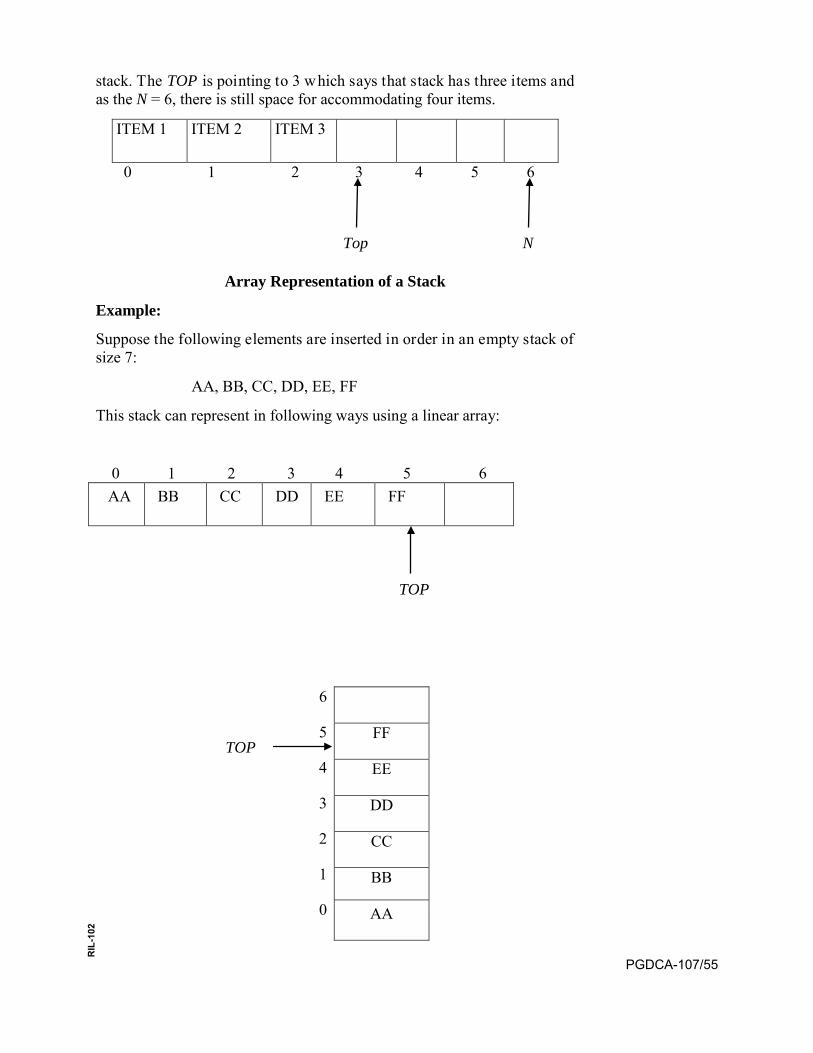
stack. The TOP is pointing to 3 which says that stack has three items and as the N = 6, there is still space for accommodating four items.
ITEM 1 ITEM 2 ITEM 3
0 1 2 3 4 5 6
Top N
Array Representation of a Stack
Example:
Suppose the following elements are inserted in order in an empty stack of size 7:
AA, BB, CC, DD, EE, FF
This stack can represent in following ways using a linear array:
0 1 2 3 4 5 6 AA BB CC DD EE FF
TOP
6
5
4
3
2
1
0
FF
EE
DD
CC
BB
AA
TOP
PGDCA-107/55
RIL
-102
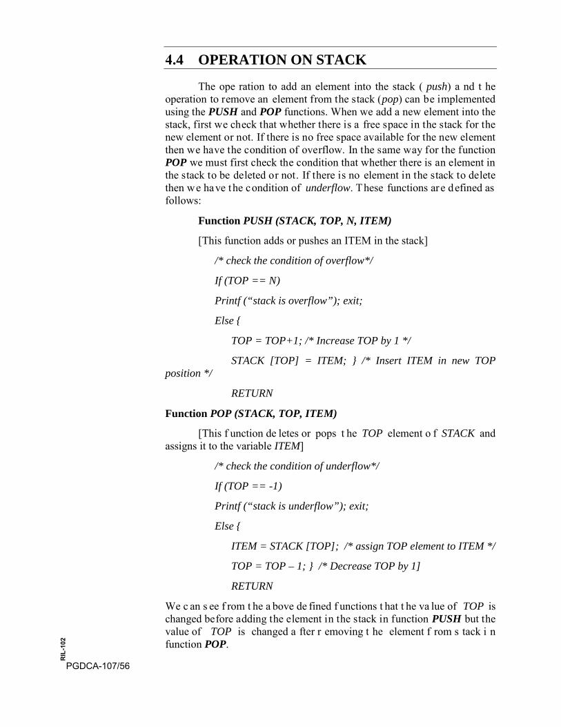
4.4 OPERATION ON STACK
The ope ration to add an element into the stack ( push) a nd t he operation to remove an element from the stack (pop) can be implemented using the PUSH and POP functions. When we add a new element into the stack, first we check that whether there is a free space in the stack for the new element or not. If there is no free space available for the new element then we have the condition of overflow. In the same way for the function POP we must first check the condition that whether there is an element in the stack to be deleted or not. If there is no element in the stack to delete then we have the condition of underflow. These functions are defined as follows:
Function PUSH (STACK, TOP, N, ITEM)
[This function adds or pushes an ITEM in the stack]
/* check the condition of overflow*/
If (TOP == N)
Printf (“stack is overflow”); exit;
Else {
TOP = TOP+1; /* Increase TOP by 1 */
STACK [TOP] = ITEM; } /* Insert ITEM in new TOP position */
RETURN
Function POP (STACK, TOP, ITEM)
[This f unction de letes or pops t he TOP element o f STACK and assigns it to the variable ITEM]
/* check the condition of underflow*/
If (TOP == -1)
Printf (“stack is underflow”); exit;
Else {
ITEM = STACK [TOP]; /* assign TOP element to ITEM */
TOP = TOP – 1; } /* Decrease TOP by 1]
RETURN
We c an s ee f rom t he a bove de fined f unctions t hat t he va lue of TOP is changed before adding the element in the stack in function PUSH but the value of TOP is changed a fter r emoving t he element f rom s tack i n function POP.
PGDCA-107/56
RIL
-102

Example:
Consider the following stack with size of 9.
XX YY ZZ
0 1 2 3 4 5 6 7 8
TOP N
If we perform the operation PUSH (STACK, WW); then the status of the stack can determine as:
Since TOP = 2, so TOP = 2 + 1 = 3.
And STACK [ TOP ] = STACK [3] = WW.
Therefore the i tem WW is now top element of the stack. This can represent as:
XX YY ZZ WW
0 1 2 3 4 5 6 7 8
TOP N
Now, on the same stack we perform the operations POP (STACK, ITEM); POP (STACK, ITEM); then the status of the stack can determine as:
Right now the TOP = 3 and the operation POP is performed two times. So, after the execution of first POP operation:
ITEM = WW and TOP = 3-1 = 2
Now after the execution of second POP operation:
ITEM = ZZ and TOP = 2-1 = 1
Therefore STACK [TOP] = STACK [1] = YY is now t he t op element in the stack.
XX YY
0 1 2 3 4 5 6 7 8
TOP N PGDCA-107/57
RIL
-102
4.5 EVALUATION OF ARITHMETIC EXPRESSION (INFIX, POSTFIX AND PREFIX NOTIONS) USING STACK This i s well known that the computer s ystem can understand and
work only on bi nary paradigm. In which an arithmetic operation can take place between two operands only l ike A + B, C * D, D / A. generally an arithmetic e xpression m ay consist of m ore t han one operator a nd t wo operands, for example (A + B) * (D / (J + D)). Such form of the arithmetic expression i s c ommonly known a s t he infix expression. N ormally t he evaluation of the any arithmetic expression does not take place in its infix form. H ere w e ar e i ntroducing t he m ethod f or e valuating t he infix expression form computation point of view. The stack is found to be more efficient to evaluate an infix arithmetical expression by first converting to a prefix or postfix expression a nd t hen e valuating t hese converted expressions. This approach will eliminate the repeated scanning of an infix expression i n or der t o obtain i ts va lue. Therefore t here are t hree b asic notations ar e r eferred f or t he r epresentation o f an y co mplex ar ithmetic expression. These forms are as follows:
• If t he ope rator s ymbols a re pl aced before i ts o perands, t hen t heexpression is in prefix form.
• If t he ope rator s ymbols a re pl aced after i ts op erands, t hen t heexpression is in postfix form.
• If the operator symbols are placed between the operands then theexpression is in infix form.
Hence, a normal a rithmetic e xpression is n ormally c alled a s in fix expression i.e. A+B. A Polish mathematician found a way to represent the same ex pression cal led polish notation or pr efix e xpression b y ke eping operators as p refix i .e. +AB. We u se t he r everse w ay o f t he ab ove expression for our evaluation. The representation is called Reverse Polish Notation (RPN) or postfix expression i.e. AB+.
Let Q be an i nfix a rithmetic e xpression i nvolving c onstants a nd operations. T his e xpression w ill be e valuated with t he c ommon r ule of arithmetic evaluation with the following level of operator precedence:
Highest: Exponentiation ( ↑ )
Next highest: Multiplication (*) and division (/)
Lowest: Addition (+) and Subtraction (-)
Now let we evaluate the following parenthesis free arithmetic expression:
6/1222*532 −↑+↑
First we evaluate the exponentiations to obtain:
PGDCA-107/58
RIL
-102

8 + 5 * 4 – 12 / 6
Then w e ev aluate th e m ultiplication a nd d ivision to o btain 8 + 20 – 2. Last, we evaluate the addition and subtraction to obtain the final result i.e. 26. We c an obs erve t hat i n t his e valuation t he w hole e xpression i straversed three times, each time corresponding to a level of precedence of the operations.
Second important i ssue about t he infix notation is t hat t hese ex pressions use parentheses for clarity and to make the evaluation convenient like (A + (B – C)) * D) / E. On the ot her ha nd t he pol ish not ation expression i .e. prefix and reverse polish notation expression i.e. postfix do not include any parentheses for clarity.
Now w e c onsider for example t he s tep b y s tep t ranslation of f ollowing infix e xpression i nto p olish not ation us ing s quare br ackets i .e. [ ] t o indicate a partial translation:
CDABCDABDCBABCABCACBA
ABCCABCBA
−+=−+=−++=+=++=+=+
/]/[][)/()(*][*)*(
**][*)(
The fundamental property of Polish notation is that the order in which the operations are to be performed is completely determined by the positions of t he ope rators a nd ope rands in t he e xpression. T here i s no ne ed of parentheses when w riting e xpressions i n P olish notation. T he computer usually ev aluates an ar ithmetic ex pression w ritten i n i nfix notation i n following two steps.
Coverts the expression in Reverse Polish notation form (postfix notation).
Evaluate the post fix expression using stack.
Algorithm for transforming Infix Expression into Postfix Expression
Let Q be an arithmetic expression written in infix notation. The following algorithm tr ansforms th e g iven in fix e xpression Q into its e quivalent postfix e xpression P. T his a lgorithm us es a s tack t o t emporarily hol d operators and l eft pa rentheses. T he pos tfix e xpression P will b e constructed from left to right using the operands from Q and the operators which are removed from STACK. We begin by pushing a left parenthesis onto STACK and adding a right parenthesis at the end of Q. The algorithm is completed when STACK is empty:
Algorithm: Conv_POLISH (Q, P) [Suppose Q is a n arithmetic e xpression w ritten in infix notation. T he algorithm finds the equivalent postfix expression P]
1. Push “(“onto STACK, and add “)” to the end of Q.
2. Scan Q from left to right and repeat step3 to 6 for each element ofQ until the STACK is empty. PGDCA-107/59
RIL
-102
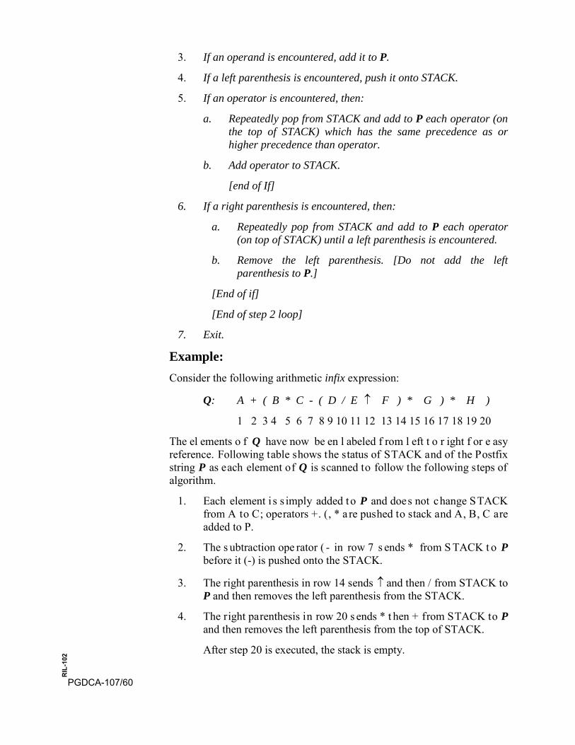
3. If an operand is encountered, add it to P.
4. If a left parenthesis is encountered, push it onto STACK.
5. If an operator is encountered, then:
a. Repeatedly pop from STACK and add to P each operator (onthe top of STACK) which has the same precedence as orhigher precedence than operator.
b. Add operator to STACK.
[end of If]
6. If a right parenthesis is encountered, then:
a. Repeatedly pop from STACK and add to P each operator(on top of STACK) until a left parenthesis is encountered.
b. Remove the left parenthesis. [Do not add the leftparenthesis to P.]
[End of if]
[End of step 2 loop]
7. Exit.
Example: Consider the following arithmetic infix expression:
Q: A + ( B * C - ( D / E ↑ F ) * G ) * H )
1 2 3 4 5 6 7 8 9 10 11 12 13 14 15 16 17 18 19 20
The el ements o f Q have now be en l abeled f rom l eft t o r ight f or e asy reference. Following table shows the status of STACK and of the Postfix string P as each element of Q is scanned to follow the following steps of algorithm.
1. Each element i s s imply added to P and does not change STACKfrom A to C; operators +. (, * a re pushed to stack and A, B, C areadded to P.
2. The s ubtraction ope rator ( - in row 7 s ends * from S TACK t o Pbefore it (-) is pushed onto the STACK.
3. The right parenthesis in row 14 sends ↑ and then / from STACK toP and then removes the left parenthesis from the STACK.
4. The right parenthesis in row 20 s ends * t hen + from STACK to Pand then removes the left parenthesis from the top of STACK.
After step 20 is executed, the stack is empty.
PGDCA-107/60
RIL
-102

Symbol Scanned STACK Expression P
(1) A ( A
(2) + (+ A
(3) ( (+( A
(4) B (+( AB
(5) * (+(* AB
(6) C (+(* ABC
(7) - (+(- ABC*
(8) ( (+(-( ABC*
(9) D (+(-( ABC*D
(10) / (+(-(/ ABC*D
(11) E (+(-(/ ABC*DE
(12) ↑ (+(-(/↑ ABC*DE
(13) F (+(-(/↑ ABC*DEF
(14) ) (+(- ABC*DEF↑ /
(15) * (+(-* ABC*DEF↑ /
(16) G (+(-* ABC*DEF↑ /G
(17) ) (+ ABC*DEF↑ /G*-
(18) * (+* ABC*DEF↑G*-
(19) H (+* ABC*DEF↑G*-H
(20) ) ABC*DEF↑G*-H*+
PGDCA-107/61
RIL
-102

Evaluation of Post Fix Expression As we know that in the infix expression it is difficult for the computer to keep t rack of p recedence of op erators. O n t he ot her h and, a postfix expression i tself d etermines t he p recedence of o perators d ue t o t he placement of the operator. Hence it is easier for the computer to perform the evaluation of a postfix expression. The evaluation rule for the postfix expression is stated as:
1. Read the expression from left to right.
2. If it is an operand then push the element into the stack.
3. If the element is an operator except NOT operator, pop the twooperands from the stack and evaluate them with the read operatorand push back the result of the evaluation into the stack.
4. If it is the NOT operator then pop one operand from the stack andthen evaluate it and push back the result of the evaluation into thestack.
5. Repeat it till the end of stack.
Now w e de fine t he a lgorithm f or e valuation of postfix e xpression us ing STACK. Let P be a arithmetic expression written in postfix notation. The following algorithm us es t he S TACK t o hol d t he ope rands and evaluate expression P.
[This a lgorithm f inds V ALUE o f a n arithmetic expression P written in postfix notation.]
1. Add a right parenthesis “)” at the end of P.
2. Scan P from left to right and repeat step 3 and 4 for each elementuntil “)” is not encountered.
3. If an operand is encountered , put it on STACK
4. If an operator is encountered then:
a. Remove the two top elements of STACK, where A is the topelement and B is the next –to-top element.
b. Evaluate B and A for the encountered operator.
c. Place the result of evaluation on step b back on STACK
[End of if]
[End of step 2 loop].
5. Set VALUE equal to the top element on STACK.
6. Exit.PGDCA-107/62
RIL
-102
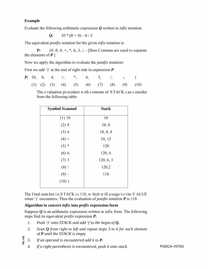
Example
Evaluate the following arithmetic expression Q written in infix notation:
Q: 10 * (8 + 4) – 6 / 3
The equivalent postfix notation for the given infix notation is:
P: 10, 8, 4, +, *, 6, 3, /, - [Here Commas are used to separate the elements of P ]
Now we apply the algorithm to evaluate the postfix notation:
First we add ‘)’ at the end of right side in expression P.
P: 10, 8, 4, +, *, 6, 3, /, -, )
(1) (2) (3) (4) (5) (6) (7) (8) (9) (10)
The e valuation pr ocedure w ith c ontents of S TACK c an c onsider from the following table:
Symbol Scanned Stack
(1) 10
(2) 8
(3) 4
(4) +
(5) *
(6) 6
(7) 3
(8) /
(9) –
(10) )
10
10, 8
10, 8, 4
10, 12
120
120, 6
120, 6, 3
120,2
118
The f inal num ber i n S TACK i s 118, w hich w ill a ssign t o t he V ALUE when ‘)’ encounters. Thus the evaluation of postfix notation P is 118. Algorithm to convert infix into prefix expression form Suppose Q is an arithmetic expression written in infix form. The following steps find its equivalent prefix expression P.
1. Push ‘)’ onto STACK and add ‘(‘to the begin of Q.2. Scan Q from right to left and repeat steps 3 to 6 for each element
of P until the STACK is empty.3. If an operand is encountered add it to P.4. If a right parenthesis is encountered, push it onto stack. PGDCA-107/63
RIL
-102
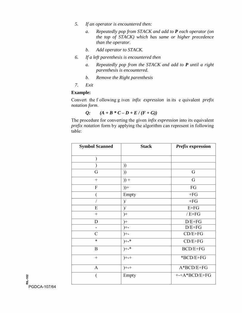
5. If an operator is encountered then:a. Repeatedly pop from STACK and add to P each operator (on
the top of STACK) which has same or higher precedencethan the operator.
b. Add operator to STACK.6. If a left parenthesis is encountered then
a. Repeatedly pop from the STACK and add to P until a rightparenthesis is encountered.
b. Remove the Right parenthesis7. Exit
Example: Convert the f ollowing g iven infix expression in its e quivalent prefix notation form.
Q: (A + B * C – D + E / (F + G)) The procedure for converting the given infix expression into its equivalent prefix notation form by applying the algorithm can represent in following table:
Symbol Scanned Stack Prefix expression
) ) )) G )) G
+ )) + G F ))+ FG ( Empty +FG / )/ +FG E )/ E+FG + )+ / E+FG D )+ D/E+FG - )+- D/E+FG C )+- CD/E+FG * )+-* CD/E+FG B )+-* BCD/E+FG
+ )+-+ *BCD/E+FG
A )+-+ A*BCD/E+FG ( Empty +-+A*BCD/E+FG
PGDCA-107/64
RIL
-102

Hence the resultant equivalent prefix notation for the given infix notation is:
P: +, -, *, +, A, B, C, D, / E + F G
Algorithm for evaluation of Prefix Expression
[This algorithm performs the evaluation for the infix notation expression. Here the expression will read from right to left]
1. Read the next element.
2. If element is operand then
a. Push the element in the stack
3. If element is operator then
a. Pop two operands from the stack
b. Evaluate the expression formed by two operands andthe operator
c. Push the results of the expression in the stack
4. If no more elements then
a. Pop the result
Else
Go to step 1.
Example:
Evaluate the following prefix notation expression.
P: + 2 * 3 + 4 5
Now we start to read it from right to left: +2 * 3 + 45+
Symbol Scanned Stack
5
4
+
3
*
2
+
5 (push)
4, 5 (push)
9 (pop, push)
3, 9 (push)
27 (pop, push)
2, 27 (push)
29 (pop, push)
PGDCA-107/65
RIL
-102

The final number in STACK is 29. Thus the evaluation of prefix notation P is 29.
4.6 APPLICATION OF STACKS
The stack has various applications in computer science. It includes the a pplication of t he l evel of c omputer or ganization a nd pr ogramming level. Generally being a linear data structure the following applications of stacks are highlighted:
• The s tack i s used for reversal o f a given l ist. We can accomplishthis task by pushing each element onto the stack as it is read. Whenthe line is finished, elements are then popped off the stack, so theycome off in reverse order.
• The important application of the stack in computer organization isfor t he e valuation o f a rithmetic e xpressions. I t a ccomplishes b yconverting first the given expression in reverse polish notation andthen evaluates the expression.
• It is a lso u sed for th e z ero address in struction imp lementation incomputer organization.
• Stacks ar e u sed f or t he a ddress hol ding i n f unction c allingprocedure of programming.
• The stacks are used to implement recursive procedures. Recursionis useful in developing algorithm for specific problems. Suppose afunction contains either a call statement to itself or a call statementto a second function that may eventually result in a call statementback t o t he or iginal f unction. T hen s uch a function i s c alledrecursive f unction. T he s tacks ar e u sed generally f or t heimplementation of such type of recursive functions.
4.7 SUMMARY
In this unit we presented another important linear data structure i.e. Stack. A stack is a linear data structure where all the elements in the stack can insert and delete from one side only rather than at the middle or from both th e s ide. W e h ave e xplored th e imp lementation o f s tack in s tatic manner us ing array. T he t wo ba sic ope rations of P USH a nd P OP a re discussed with example for the stack. The contents can be summarized as follows:
• A s tack is a lin ear s tructure imp lemented in LIFO ( Last In F irstOut) manner where insertions and deletions take place at the sameend.
• An insertion is a stack is called pushing and deletion from a stackis called popping.
PGDCA-107/66
RIL
-102
• When a stack implemented as an array, is full and no new elementcan be accommodated, it is called OVERFLOW.
• When a stack is empty and an attempt is made to delete an elementfrom the stack, it is called UNDERFLOW.
• The m ain application of s tack can b e i mplementation of P olishnotation w hich r efers t o a not ation i n w hich op erator s ymbol i splaced either b efore i ts ope rands ( prefix not ation) or a fter i tsoperands (postfix not ation). The usual form, i n which operator i splaced in between the operands, is called infix notation.
• The other application of stack can be reversing a list and providingrecursion in various programs.
• It i s a lso us ed f or t he z ero a ddress i nstruction imp lementation incomputer organization.
• Stacks a re us ed f or t he a ddress hol ding i n f unction c allingprocedure of programming.
Bibliography • Horowitz, E ., S. S ahni: “Fundamental of c omputer A lgorithms”,
Computer Science Press, 1978
• J. P. Tremblay, P. G. Sorenson “An Introduction to Data Structureswith Applications”, Tata McGraw-Hill, 1984
• M. Allen Weiss: “Data structures and Problem solving using C++”,Pearson Addison Wesley, 2003
• Ulrich Klehmet: “Introduction to Data Structures and Algorithms”,URL: http://www7 . I nformatik.uni-erlangen.de/~klehmet/teaching/SoSem/dsa
• Markus Blaner: “Introduction to Algorithms and Data Structures”,Saarland University, 2011
• M. E . D ’imperio, “ Data s tructures and t heir representation i nstorage”, Annual Review in Automatic programming, Vol. 5 pp. 1-75, Pergammon Press, Oxford, 1969.
• B. Flaming, “Practical Data Strcture in C++”, Jhon Wiley & Sons,New York, 1983
• D. E . K nuth, “ The a rt of C omputer pr ogramming”, V ol. 2:Seminumerical Algorithms, 3rd edition, Addison-Wesley, 1997.
PGDCA-107/67
RIL
-102
SELF EVALUATION
Multiple Choice Questions: 1. ........................ f orm of a ccess i s us ed t o a dd a nd r emove node s
from a stack
(a) LIFO (b) FIFO
(c) Both (a) and (b) (d) None of these
2. A data structure in which elements are added and removed only atone end is know as:
(a) Queue (b) Stack
(c) Array (d) None of these
3. Underflow is a condition where you:
(a) Insert a new node when there is no free space for it
(b) Delete a non-existent node in the list
(c) Delete a node from the empty list
(d) None of the above
4. Stack is:
(a) Static data structure
(b) Dynamic data structure
(c) A built in data structure
(d) None of these
5. Which ope ration i n the s tack i s us ed f or g etting va lue of m ostrecent node and delete the node:
(a) PUSH
(b) POP
(c) Empty
(d) None of these
6. If A, B, C are inserted into a stack in the lexicographic order, theorder of removal will be:
(a) A, B, C
(b) C, B, A
(c) B, C, A
(d) None of these.PGDCA-107/68
RIL
-102
Fill in the blank: 1. A stack may be represented by a …………… l inked list. (linear /
non-linear)
2. Push ope ration i n s tack m ay r esult i n……………… ( overflow /underflow)
3. If T OP poi nts t o t he t op of s tack, t hen T OP i s……. ( increased /decreased)
State whether True or False 1. Push operation in stack is performed at the rear end.
2. PUSH operation in stack may result in underflow
3. For a s tack imp lemented w ith lin ear a rray arbitrary a mount o fmemory can be allocated.
Descriptive Questions 1. Consider t he f ollowing stack, w here STACK is al located N = 6
memory cells.
STACK: AA, DD, EE, FF, GG…………………..
Describe the stack as the following operations take place and alsoconsider the overflow condition.
a. PUSH (STACK, KK)
b. POP (STACK, ITEM)
c. PUSH (STACK, LL)
d. PUSH (STACK, SS)
e. POP (STACK, ITEM)
f. PUSH (STACK, TT)
2. Write a n a lgorithm w hich upon us er’s c hoice, e ither pus hes orPops an el ement f rom the s tack i mplemented as an a rray (theelement should not shifted after the push or pop).
3. Write a p rogram to c onvert a n in fix a rithmetic expression in to aprefix a rithmetic e xpression. T he a lgorithm f or your pr ogramshould use the following expression:
Q: (A – B) * (C / D) + E
Show in tabular form the changing status of stack.
4. Convert the expression (A + B) / (C – D) into pos tfix expressionand then evaluate it for A = 10, B = 20, C = 15, D = 5. Display thestack status after each operation.
PGDCA-107/69
RIL
-102
5. Write a program to read a string (one line of characters) and pushany vowels in the string to a stack. Then pop your stack repeatedlyand count the number of vowels in the string.
PGDCA-107/70
RIL
-102
UNIT-5 RECURSION
Structure
5.0 Introduction
5.1 Objectives
5.2 Definition of Recursion
5.3 Process of Recursion
5.4 Designing of Recursive algorithm
5.5 Examples of Recursive Algorithms
5.6 Summary
5.0 INTRODUCTION
This uni t introduces the c oncept of Recursion. It h ighlights th e basic concepts of recursion, its definition with the method for its working. The solutions of some problems are performed with the recursive method. The unit also considers the recursive algorithm for solving the problems. It also e xplores t he us e o f s tack f or r ecursive algorithms or f inding t he solution with recursive method.
5.1 OBJECTIVES
At the end of this unit, you may be able to:
• Understand the concept of Recursion and recursive method.
• Understand the principle of recursion and use of stack for theimplementation of recursive methods.
• Understand the working of recursive procedures andimplementation it for the solution of problems.
• Designing of Recursive algorithm for the solution of some popularproblems.
5.2 DEFINITION OF RECURSION
Recursion i s an i mportant co ncept i n co mputer science s pecially for s olving t he m any problems of r ecursive nature. A ny p roblem i s considered as r ecursive nature i f t he c ertain s tep of t he pr oblem or t he entire p roblem is r epeating w ith d ifferent parameters each t ime o f repetition. T hus, m any algorithms c an be be st de scribed i n t erms of recursion. Suppose P is any function containing either a Call statement to itself or a call statement to a second function that may eventually result in a call statement back to the original function P. The P is called a recursive PGDCA-107/71
RIL
-102
function. T hus, a recursive function is a f unction th at e ither d irectly o r indirectly makes a call to itself. The important aspect is that the function P calls itself on a different, generally simpler instance, for example files on a computer ar e generally stored i n d irectories. U sers m ay create subdirectories that store more files and directories. Suppose that we want to ex amine ev ery file i n a d irectory D, in cluding all f iles in all subdirectories a nd s ubdirectories, and s o on. W e do s o b y r ecursively examining every file in each subdirectory and then examining all files in the d irectory D. H ence t his lo gic s eem to b e circular lo gic b ut w ith th e method to come out from this infinite circular loop.
Therefore, a r ecursion is a n imp ortant f acility in ma ny p rogramming languages. There are many problems whose algorithmic description is best described i n a r ecursive manner. Hence, a function i s cal led r ecursive if the f unction de finition r efers t o i tself or do es r efer t o another f unction which in turn refers back to the same function but this procedure should not i nclude i nfinite l oop or e ndless pr ocess. Hence i n or der f or t he definition does not contain any endless ci rcular process, t m ust have t he following properties:
(i) There must be certain arguments called base values, for which the function does not refer to itself. Alternatively there must be certain criteria, cal led base criteria, for which the function does not cal l itself.
(ii) Each t ime t he f unction does r efer t o i tself, t he argument of t he function must be closer to the base value.
Any recursive function with these two properties is said to be well defined recursive function. Similarly, a function is said to be recursively defined if the function definition refers to itself.
5.3 PROCESS OF RECURSION
Recursion i s a pow erful pr oblem-solving t ool. M any a lgorithms are m ost easily ex pressed i n a recursive formulation. F urthermore, t he most e fficient s olution for m any problems i s based on t his recursive formulation but t his f ormulation doe s not c ontain a ny infinite l oop a nd process. Generally the idea of Recursion is closely related to the principle of mathematical induction which pr ovides t he following i ssues for t he recursion procedure:
• Solve the problem for small problem instances.
• Assume a solution for smaller problem instance.
• Figure out how to do a little more work which in combination withsolutions to smaller instances, solves the larger problem instance.
PGDCA-107/72
RIL
-102
It can see that sometimes mathematical functions are defined recursively. Let us consider the example of sum S (N) for the first N integers. The base condition is defined as S (1) = 1, and the recursive function can define as:
NNSNS +−= )1()(
Here w e h ave d efined t he f unction S in t erms of a s maller in stance o f itself. The s traight forward recursive evaluation of the sum of the f irst N integers ba sed on t he r ecursive function a s given a bove with i ts ba se condition can define as:
[Recursive function to compute sum of first n integers.]
Function sum (int n)
{
If (n == 1) /* base condition */
Return 1;
Else
Return (s (n – 1) + n);
}
We can realize from the above algorithm that i f N=1, we have the basis, for which we know that S (1) = 1 and the recursive step is with the return statement as S (N) = S (N-1) + N. Now from the algorithm we can get an idea for the working process of the recursive method and as well as for the recursive function. W e c an c onsider i n t he a bove a lgorithm t hat a ba se case is an instance that we can solve without recursion. Any recursive call must progress towards the case in order to terminate eventually. Thus we have the two fundamental rules of recursion:
1. Base case : Always h ave at l east o ne c ase t hat can b e s olvedwithout using recursion.
2. Make Progress : Any recursive call must progress t oward a basecase.
This i s qui te obvi ous t hat i f t he ba se c ondition i s not a vailable f or t he recursive function then the function will stuck in infinite recursive call and never terminates.
5.4 DESIGNING FOR RECURSIVE ALGORITHM
We h ave d iscussed ab out t he r ecursive function a nd r ecursive process. The important point which we have analyzed is that any recursive function s hould ha ve a based criteria or base condition or termination condition otherwise the recursive procedure becomes unsolvable. Thus in order to design any recursive process in terms of the algorithm, the base PGDCA-107/73
RIL
-102
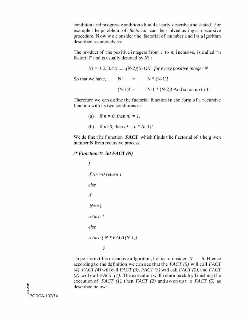
condition a nd pr ogress c ondition s hould c learly describe a nd s tated. F or example t he pr oblem of factorial can be s olved us ing a r ecursive procedure. N ow w e c onsider t he factorial of nu mber a nd i ts a lgorithm described recursively as:
The pr oduct of t he pos itive i ntegers f rom 1 to n, i nclusive, i s c alled “ n factorial” and is usually denoted by N! :
N! = 1.2. 3.4.5.......(N-2)(N-1)N for every positive integer N
So that we have, N! = N * (N-1)!
(N-1)! = N-1 * (N-2)! And so on up to 1.
Therefore we can define the factorial function in the form of a recursive function with its two conditions as:
(a) If n = 0, then n! = 1.
(b) If n>0, then n! = n * (n-1)!
We de fine t he f unction FACT which f inds t he f actorial of t he g iven number N from recursive process:
/* Function:*/ int FACT (N)
{
if N==0 return 1
else
if
N==1
return 1
else
return ( N * FACT(N-1))
}
To pe rform t his r ecursive a lgorithm, l et us c onsider N = 5. H ence according to the definition we can see that the FACT (5) will call FACT (4), FACT (4) will call FACT (3), FACT (3) will call FACT (2), and FACT (2) will c all FACT (1). The ex ecution w ill r eturn ba ck b y f inishing t he execution of FACT (1), t hen FACT (2) and s o on up t o FACT (5) as described below:
PGDCA-107/74
RIL
-102
1) 5! = 5 * 4!
2) 4! = 4 * 3!
3) 3! = 3 * 2!
4) 2! = 2 * 1!
5) 1! = 1
6) 2! = 2 * 1 = 2
7) 3! = 3 * 2 = 6
8) 4! = 4 * 6 = 24
9) 5! = 5 * 24 = 120
From above it is clear that every sub function contain parameters and local variables. T he p arameters ar e t he a rguments w hich r eceive v alues f rom objects i n t he c alling pr ogram a nd w hich t ransmit va lues ba ck t o the calling pr ogram. T he s ub-function m ust a lso keep t rack of t he r eturn address i n t he calling program. T his r eturn a ddress i s e ssential s ince control must be transferred back to its proper place in the calling program. After completion of the sub-function when the control is transferred back to its calling program, the local values and returning address is no l onger needed. Suppose our sub-program is a r ecursive one, when i t cal ls itself, then current values must be saved, since they will be used again when the program i s reactivated. T hus, i n r ecursive pr ocess a da ta s tructure i s required t o handle t he d ata of on going c alled function a nd t he f unction which i s cal led at la st mu st b e p rocessed f irst i.e. the d ata accessed l ast must be processed fist i .e. Last in first out pr inciple. So, a stack may b e suitable d ata s tructure t hat f ollows LIFO to im plement r ecursion. Thus when a recursive method is executed, each invocation of the method gets a separate s tack f rame. H ence each i nvocation h as a s eparate co py o f t he following:
• Formal parameters
• Local variables
• Return value
Therefore t he recursion i s us eful i n de veloping a lgorithms f or s pecific problems a nd t he Stack may us e t o i mplement r ecursive f unctions or processes. Now we discuss the method for translating a recursive method into a non-recursive method using stack.
5.5 EXAMPLES OF RECURSIVE ALGORITHMS
Here w e are p resenting s ome ex amples o f v ery common an d important recursive algorithms:
PGDCA-107/75
RIL
-102
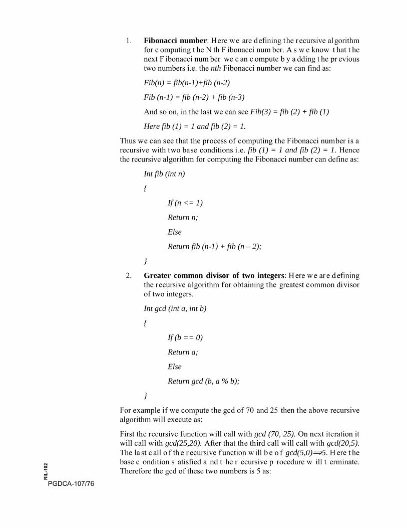
1. Fibonacci number: Here we are defining the recursive algorithmfor c omputing t he N th F ibonacci num ber. A s w e know t hat t henext F ibonacci num ber we c an c ompute b y a dding t he pr evioustwo numbers i.e. the nth Fibonacci number we can find as:
Fib(n) = fib(n-1)+fib (n-2)
Fib (n-1) = fib (n-2) + fib (n-3)
And so on, in the last we can see Fib(3) = fib (2) + fib (1)
Here fib (1) = 1 and fib (2) = 1.
Thus we can see that the process of computing the Fibonacci number is a recursive with two base conditions i.e. fib (1) = 1 and fib (2) = 1. Hence the recursive algorithm for computing the Fibonacci number can define as:
Int fib (int n)
{
If (n <= 1)
Return n;
Else
Return fib (n-1) + fib (n – 2);
}
2. Greater common divisor of two integers: Here we are definingthe recursive algorithm for obtaining the greatest common divisorof two integers.
Int gcd (int a, int b)
{
If (b == 0)
Return a;
Else
Return gcd (b, a % b);
}
For example if we compute the gcd of 70 and 25 then the above recursive algorithm will execute as:
First the recursive function will call with gcd (70, 25). On next iteration it will call with gcd(25,20). After that the third call will call with gcd(20,5). The la st c all o f th e r ecursive f unction w ill b e o f gcd(5,0)⟹5. H ere t he base c ondition s atisfied a nd t he r ecursive p rocedure w ill t erminate. Therefore the gcd of these two numbers is 5 as:
PGDCA-107/76
RIL
-102
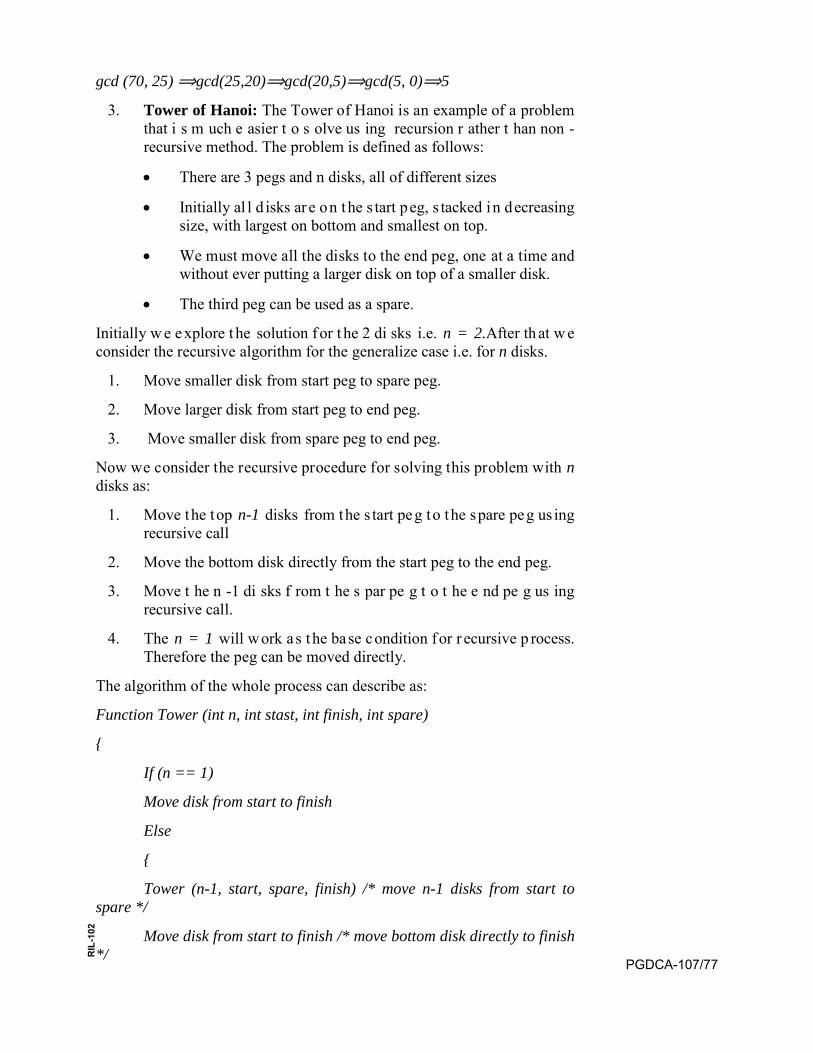
gcd (70, 25) ⟹gcd(25,20)⟹gcd(20,5)⟹gcd(5, 0)⟹5
3. Tower of Hanoi: The Tower of Hanoi is an example of a problemthat i s m uch e asier t o s olve us ing recursion r ather t han non -recursive method. The problem is defined as follows:
• There are 3 pegs and n disks, all of different sizes
• Initially al l d isks ar e on the s tart peg, s tacked in decreasingsize, with largest on bottom and smallest on top.
• We must move all the disks to the end peg, one at a time andwithout ever putting a larger disk on top of a smaller disk.
• The third peg can be used as a spare.
Initially w e e xplore t he solution f or t he 2 di sks i.e. n = 2.After th at w e consider the recursive algorithm for the generalize case i.e. for n disks.
1. Move smaller disk from start peg to spare peg.
2. Move larger disk from start peg to end peg.
3. Move smaller disk from spare peg to end peg.
Now we consider the recursive procedure for solving this problem with n disks as:
1. Move the top n-1 disks from the s tart peg to the spare peg us ingrecursive call
2. Move the bottom disk directly from the start peg to the end peg.
3. Move t he n -1 di sks f rom t he s par pe g t o t he e nd pe g us ingrecursive call.
4. The n = 1 will work as t he base condition for r ecursive p rocess.Therefore the peg can be moved directly.
The algorithm of the whole process can describe as:
Function Tower (int n, int stast, int finish, int spare)
{
If (n == 1)
Move disk from start to finish
Else
{
Tower (n-1, start, spare, finish) /* move n-1 disks from start to spare */
Move disk from start to finish /* move bottom disk directly to finish */
PGDCA-107/77
RIL
-102

Tower (n-1, spare, finish, start) /* move n-1 disks from spare to finish */
}
}
5.6 SUMMARY
Recursion is useful in developing algorithm for specific problems. Suppose a f unction c ontains e ither a call s tatement to its elf o r a c all statement to a s econd f unction th at ma y eventually result in a c all statement ba ck t o t he o riginal function. T hen s uch a function i s c alled recursive function. The stacks a re used generally for t he implementation of s uch t ype of r ecursive f unctions. A ny p roblem i s co nsidered as recursive nature if the certain step of the problem or the entire problem is repeating w ith d ifferent parameters e ach time o f r epetition. T hus, ma ny algorithms c an be be st described i n t erms of recursion. T he contents of this unit can be summarized as follows:
• Recursion i s t he na me given t o t he phe nomenon of de fining afunction in terms of itself.
• There m ust be ba se c ondition i n t he r ecursive definition of a nyprocess which indicates its initial condition.
• Each t ime t he f unction does r efer to its elf, th e argument o f th efunction must be closer to the base value.
• Recursion i s c losely related t o t he pr inciple of mathematicalinduction.
• A stack may b e s uitable d ata s tructure th at f ollows LIFO toimplement recursion.
• Important e xamples l ike f actorial, G CD and t ower of H anoi a reexplained and implemented with the help of recursive process.
Bibliography • Horowitz, E ., S. S ahni: “Fundamental of c omputer A lgorithms”,
Computer Science Press, 1978
• J. P. Tremblay, P. G. Sorenson “An Introduction to Data Structureswith Applications”, Tata McGraw-Hill, 1984
• M. Allen Weiss: “Data structures and Problem solving using C++”,Pearson Addison Wesley, 2003
• Ulrich Klehmet: “Introduction to Data Structures and Algorithms”,URL: http://www7 . I nformatik.uni-erlangen.de/~klehmet/teaching/SoSem/dsa
PGDCA-107/78
RIL
-102

• Markus Blaner: “Introduction to Algorithms and Data Structures”,Saarland University, 2011
• T. H. Cormen, C. E. Leiserson and R. L. Rivest, “ Introduction toAlgorithms”, MIT Press, cambridge, Mass., 1990
• B. Flaming, “Practical Data Strcture in C++”, Jhon Wiley & Sons,New York, 1983
• R. Sedgewick, “Algorithms in C++”, Addison-Wesley, 1992.
PGDCA-107/79
RIL
-102
SELF EVALUATION 1. State whether it is TRUE or FALSE: “ Recursion is generally more
efficient than iteration”
2. What are the two fundamental rules of recursion?
3. Stack is used whenever ……………….. function is called(Recursive / Non- recursive)
4. Write a p rogram for evaluatingn
rc for t he g iven v alue of n and r
using recursive procedure.
5. Formulate the recursive function for evaluating the least commonmultiplier (LCM).
PGDCA-107/80
RIL
-102
UNIT-6 QUEUE
Structure
6.0 Introduction
6.1 Objectives
6.2 Definition of Queue
6.3 Representation of Queue
6.4 Insertion and deletion in Linear Queue
6.5 Example
6.6 Circular Queue
6.7 Insertion and Deletion in the circular Queue
6.8 Example
6.9 Types of Queue
6.10 Summary
6.0 INTRODUCTION
This uni t introduces the c oncept of another imp ortant lin ear d ata structure us ed t o r epresent a l inear l ist i .e. Q ueue. T his uni t s tarts b y giving a n i ntroduction t o t he ba sic c oncept of q ueue. It a lso de fines t he operation of i nsertion and de letion f rom t he Q ueue. T he qu eue allows insertion of an element to be made at one end and deletion of an element to be performed at the other end. This unit further introduces various type of queues like circular queue, de-queue and priority queue. It also provides the operation of insertion and deletion in these types of queues. In the last it highlights the application of queue.
6.1 OBJECTIVES
After working through this unit, you should be able to:
• Understand the concept of queue and its working with itsdefinition.
• Implementation of queue using Array and perform the operation ofinsertion and deletion in it with the condition of overflow andunderflow of the queue.
• Understand the concept of circular queue and its implementationwith array.
PGDCA-107/81
RIL
-102
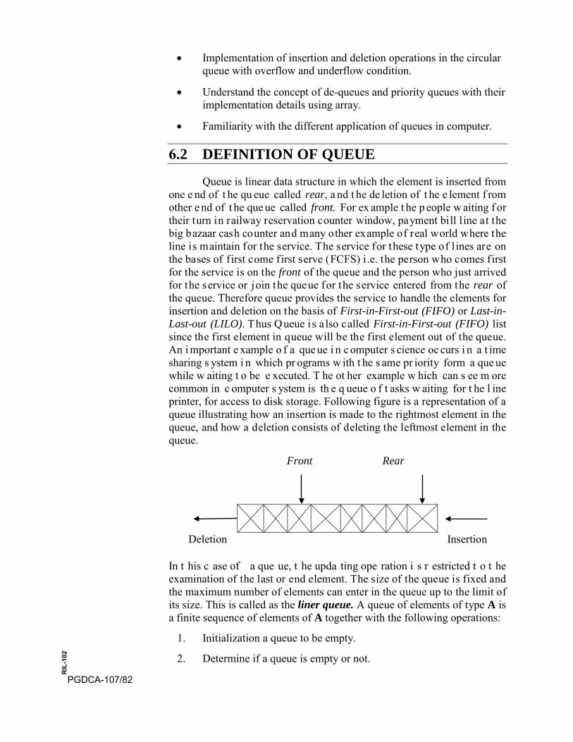
• Implementation of insertion and deletion operations in the circularqueue with overflow and underflow condition.
• Understand the concept of de-queues and priority queues with theirimplementation details using array.
• Familiarity with the different application of queues in computer.
6.2 DEFINITION OF QUEUE
Queue is linear data structure in which the element is inserted from one e nd of t he qu eue called rear, a nd t he de letion of t he e lement f rom other e nd of t he que ue called front. For ex ample t he p eople w aiting f or their turn in railway reservation counter window, payment bill line at the big bazaar cash counter and many other example of real world where the line is maintain for the service. The service for these type of lines are on the bases of first come first serve (FCFS) i.e. the person who comes first for the service is on the front of the queue and the person who just arrived for the service or join the queue for the service entered from the rear of the queue. Therefore queue provides the service to handle the elements for insertion and deletion on the basis of First-in-First-out (FIFO) or Last-in-Last-out (LILO). Thus Queue i s a lso called First-in-First-out (FIFO) list since the first element in queue will be the first element out of the queue. An i mportant e xample o f a que ue i n c omputer s cience oc curs i n a t ime sharing s ystem i n which pr ograms w ith t he s ame pr iority form a que ue while w aiting t o be e xecuted. T he ot her example w hich can s ee m ore common in c omputer s ystem is th e q ueue o f t asks w aiting for t he l ine printer, for access to disk storage. Following figure is a representation of a queue illustrating how an insertion is made to the rightmost element in the queue, and how a deletion consists of deleting the leftmost element in the queue.
Front Rear
Deletion Insertion
In t his c ase of a que ue, t he upda ting ope ration i s r estricted t o t he examination of the last or end element. The size of the queue is fixed and the maximum number of elements can enter in the queue up to the limit of its size. This is called as the liner queue. A queue of elements of type A is a finite sequence of elements of A together with the following operations:
1. Initialization a queue to be empty.
2. Determine if a queue is empty or not.
PGDCA-107/82
RIL
-102

3. Determine if a queue is full or not.
4. Insert a new element after the last element in a queue, if it is notfull.
5. Retrieve the first element of a queue, if it is empty.
6. Delete the first element in a queue, if it is not empty.
6.3 REPRESENTATION OF QUEUE
Queues m ay be r epresented i n t he c omputer i n va rious w ays, generally b y means of one -way l ists or l inear a rrays. Queues are maintained by a linear array say QUEUE and two pointer type variables: FRONT, containing t he l ocation of t he f ront element of t he que ue ( the oldest element in the queue or the element which will be first delete); and REAR, c ontaining t he l ocation of t he r ear e lement of t he qu eue ( the newest element in the queue or the recently inserted element in the queue). The condition FRONT = REAR = NULL will indicate that the queue is empty a nd FRONT = 1, REAR = FRONT = MAX_SIZE indicates th at the queue is full. These conditions are valid only for the linear queue. The following figure represents the implementation of queue as an array which is declared to its maximum size as per the requirement of the problem or the number of elements those has to be entered in the queue. The size of the Queue keeps on changing as the elements are either removed from the front e nd or a dded a t t he r ear end but t he s ize of t he a rray w ill r emain fixed.
X[0] X[1] X[2] X[3] X[4] X[5] X[6] X[7]
A B C D E F G H
Front Rear
6.4 INSERTION AND DELETION IN THE LINEAR QUEUE
Now we formulate algorithms for the insertion of an element of an element t o an d t he d eletion o f an el ement from a q ueue. W e co nsider a linear ar ray o f arbitrary size. This ar ray i s as sumed t o consist o f a l arge number of elements, enough to be sufficient to handle the elements of the linear que ue. T his a rray representation of a que ue c onsists w ith t wo pointer type variables Rear (R) and Front (F). The algorithms of insertion and deletion from the linear queue which is implemented with linear array (Q) can describe as:
PGDCA-107/83
RIL
-102
Function QINSERT (Q, F, R, Y): [Given F and R, pointers to the front and rear elements of a queue, a queue Q consisting of N elements, and an element Y, this function inserts Y at the rear of the queue.]
If( R>=N) /* check for the overflow condition */
Printf (“Overflow”); return;
Else
{
R = R + 1; /*Increment rear pointer */
Q[R] = Y; /* insert element */
If (F == 0) /* set the front pointer */
F = 1;
Return;
}
Function QDELETE (Q, F, R): [Given F and R, pointers to the front and rear el ements o f a q ueue r espectively and t he queue Q to w hich t hey correspond, this function deletes and returns the last element of the queue. Y is a temporary variable.]
If (F==0) /* check for the underflow condition */
Printf (“underflow”); return 0; /* 0 denotes the empty queue */
Else
{
Y = Q [F]; /* delete element */
If (F == R)
F = R = 0;
Else
F = F + 1; /* increment front pointer */
Return Y;
}
6.5 EXAMPLE
Consider an example where the size of the queue is four elements. Initially, the queue is empty. It is required to insert symbols ‘A’, ‘B’ and ‘C’, delete ‘A’ and ‘B’, and insert ‘D’ and ‘E’. The trace for the insertion and deletion algorithms can represent as follows for the given Queue:
PGDCA-107/84
RIL
-102
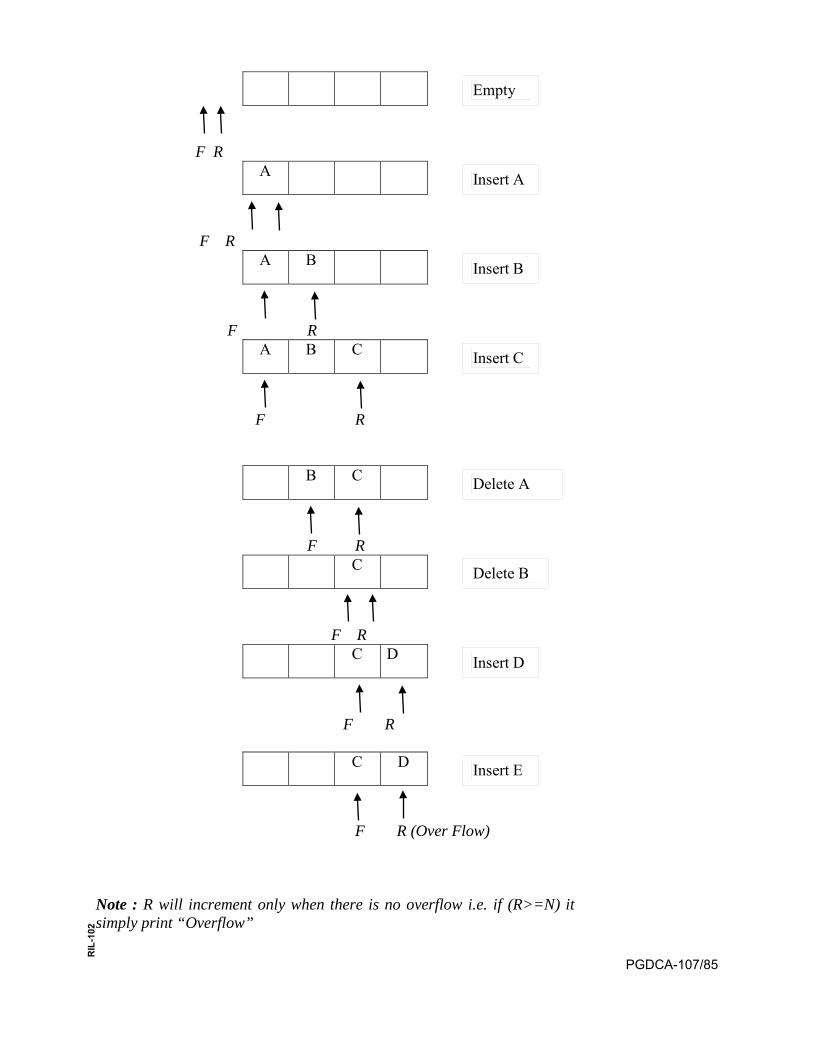
F R A
F R A B
F R A B C
F R
B C
F R C
F R C D
F R
C D
F R (Over Flow)
Note : R will increment only when there is no overflow i.e. if (R>=N) it simply print “Overflow”
Empty
Insert A
Insert B
Insert C
Delete A
Delete B
Insert D
Insert E
PGDCA-107/85
RIL
-102
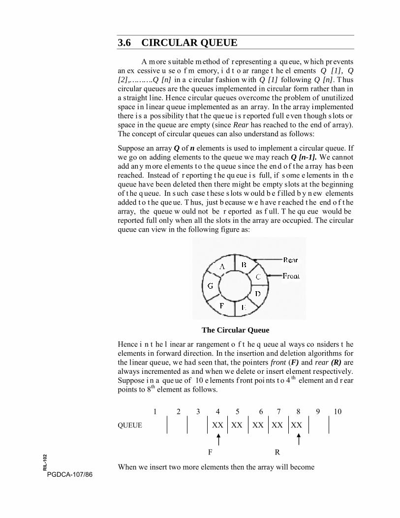
3.6 CIRCULAR QUEUE
A m ore s uitable m ethod of r epresenting a qu eue, w hich pr events an ex cessive u se o f m emory, i d t o ar range t he el ements Q [1], Q [2],……….Q [n] in a c ircular f ashion with Q [1] following Q [n]. Thus circular queues are the queues implemented in circular form rather than in a straight line. Hence circular queues overcome the problem of unutilized space in l inear queue implemented as an array. In the array implemented there i s a pos sibility t hat t he que ue i s r eported f ull e ven t hough s lots or space in the queue are empty (since Rear has reached to the end of array). The concept of circular queues can also understand as follows:
Suppose an array Q of n elements is used to implement a circular queue. If we go on adding elements to the queue we may reach Q [n-1]. We cannot add an y more elements to the queue s ince the end of the a rray has been reached. Instead of r eporting t he qu eue i s full, if s ome e lements in th e queue have been deleted then there might be empty slots at the beginning of t he q ueue. In s uch case t hese s lots w ould b e f illed b y n ew elements added t o t he que ue. T hus, just b ecause w e h ave r eached t he end o f t he array, the queue w ould not be r eported as f ull. T he qu eue would be reported full only when all the slots in the array are occupied. The circular queue can view in the following figure as:
The Circular Queue
Hence i n t he l inear ar rangement o f t he q ueue al ways co nsiders t he elements in forward direction. In the insertion and deletion algorithms for the linear queue, we had seen that, the pointers front (F) and rear (R) are always incremented as and when we delete or insert element respectively. Suppose i n a que ue of 10 e lements f ront poi nts t o 4 th element an d r ear points to 8th element as follows.
1 2 3 4 5 6 7 8 9 10
QUEUE XX XX XX XX XX
F R
When we insert two more elements then the array will become
Front
Rear
G
F E
D
CBA
PGDCA-107/86
RIL
-102
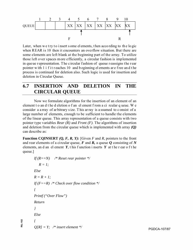
1 2 3 4 5 6 7 8 9 10
QUEUE XX XX XX XX XX XX XX
F R
Later, when w e t ry t o i nsert s ome el ements, t hen acco rding to th e lo gic when REAR is 10 then i t encounters an overflow situation. But there are some elements are left blank at the beginning part of the array. To utilize those left over spaces more efficiently, a circular fashion is implemented in queue representation. The c ircular f ashion of queue r eassigns t he r ear pointer w ith 1 i f i t r eaches 10 and b eginning el ements ar e f ree an d t he process is continued for deletion also. Such logic is used for insertion and deletion in Circular Queue.
6.7 INSERTION AND DELETION IN THE CIRCULAR QUEUE
Now we formulate algorithms for the insertion of an element of an element t o an d t he d eletion o f an el ement f rom a ci rcular q ueue. W e consider a a rray of ar bitrary s ize. T his ar ray is a ssumed to c onsist of a large number of elements, enough to be sufficient to handle the elements of the linear queue. This array representation of a queue consists with two pointer type variables Rear (R) and Front (F). The algorithms of insertion and deletion from the circular queue which is implemented with array (Q) can describe as:
Function CQINSERT (Q, F, R, Y): [Given F and R, pointers to the front and rear elements of a circular queue, F and R, a queue Q consisting of N elements, an d an el ement Y, t his f unction i nserts Y at t he r ear o f t he queue.]
If (R==N) /* Reset rear pointer */ R = 1; Else R = R + 1; If (F==R) /* Check over flow condition */ { Printf (“Over Flow”) Return } Else { Q[R] = Y; /* insert element */ PGDCA-107/87
RIL
-102
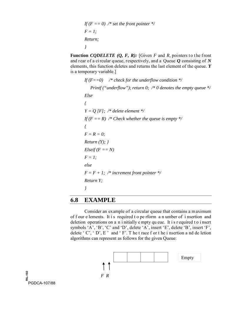
If (F == 0) /* set the front pointer */ F = 1; Return; }
Function CQDELETE (Q, F, R): [Given F and R, pointers t o t he f ront and rear of a ci rcular queue, respectively, and a Queue Q consisting of N elements, this function deletes and returns the last element of the queue. Y is a temporary variable.]
If (F==0) /* check for the underflow condition */ Printf (“underflow”); return 0; /* 0 denotes the empty queue */ Else { Y = Q [F]; /* delete element */ If (F == R) /* Check whether the queue is empty */ { F = R = 0; Return (Y); } Elseif (F == N) F = 1; else F = F + 1; /* increment front pointer */ Return Y; }
6.8 EXAMPLE
Consider an example of a circular queue that contains a maximum of f our e lements. It i s required t o pe rform a n umber of i nsertion and deletion operations on a n i nitially e mpty qu eue. It i s r equired t o i nsert symbols ‘A’, ‘B’, ‘C’ and ‘D’, delete ‘A’, insert ‘E’, delete ‘B’, insert ‘F’, delete ‘ C’, ‘ D’, E ’ and ‘ F’. T he t race f or t he i nsertion a nd de letion algorithms can represent as follows for the given Queue:
F R
Empty
PGDCA-107/88
RIL
-102
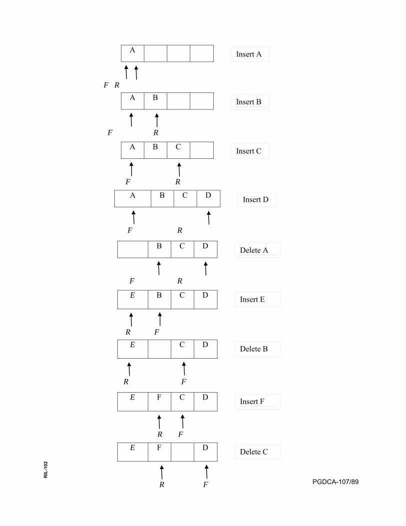
A
F R A B
F R
A B C
F R
A B C D
F R
B C D
F R
E B C D
R F E C D
R F
E F C D
R F
E F D
R F
Insert A
Insert B
Insert C
Insert D
Delete A
Insert E
Delete B
Insert F
Delete C
PGDCA-107/89
RIL
-102
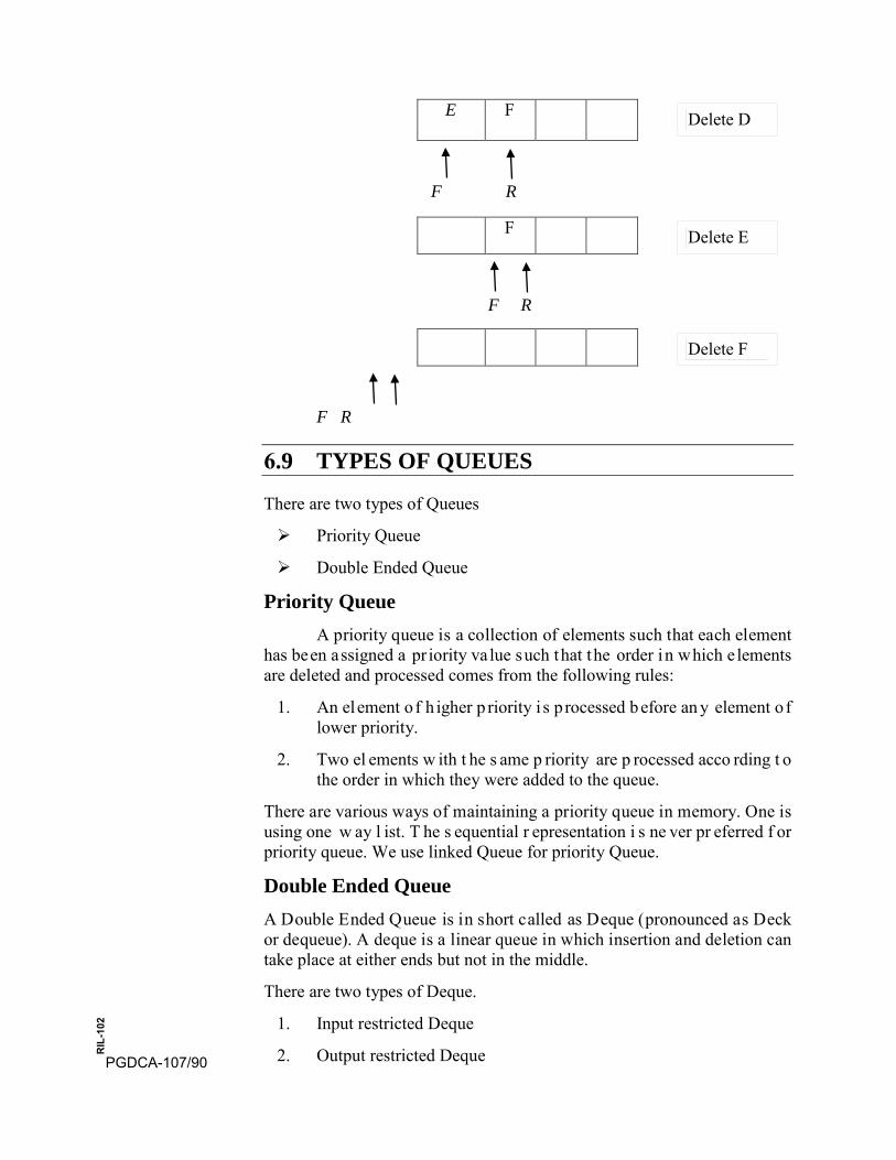
E F
F R
F
F R
F R
6.9 TYPES OF QUEUES
There are two types of Queues
Priority Queue
Double Ended Queue
Priority Queue A priority queue is a collection of elements such that each element
has been assigned a pr iority va lue such that the order in which e lements are deleted and processed comes from the following rules:
1. An element o f h igher p riority i s p rocessed before an y element o flower priority.
2. Two el ements w ith t he s ame p riority are p rocessed acco rding t othe order in which they were added to the queue.
There are various ways of maintaining a priority queue in memory. One is using one w ay l ist. T he s equential r epresentation i s ne ver pr eferred f or priority queue. We use linked Queue for priority Queue.
Double Ended Queue A Double Ended Queue is in short called as Deque (pronounced as Deck or dequeue). A deque is a linear queue in which insertion and deletion can take place at either ends but not in the middle.
There are two types of Deque.
1. Input restricted Deque
2. Output restricted Deque
Delete D
Delete E
Delete F
PGDCA-107/90
RIL
-102

• A Deque which allows insertion at only at one end of the listbut allows deletion at both the ends of the list is called Inputrestricted Deque.
• A Deque which allows deletion at only at one end of the listbut a llows i nsertion a t both t he e nds of t he l ist i s c alledOutput restricted Deque.
The tw o p ossibilities th at mu st b e c onsidered w hile in serting o r deleting elements into the queue are:
• When an a ttempt is made to insert an el ement i nto a d equewhich is already full, an over flow occurs.
• When an attempt is made to delete an element from a d equewhich is empty, underflow occurs.
The Deque can represent as follows:
A B C D E
F R
6.10 SUMMARY Queue is linear data structure in which the element is inserted from
one e nd of t he que ue. Queue i s a lso c alled First-in-First-out ( FIFO) list since the first element in queue will be the first element out of the queue. In this unit we have described the insertion and deletion of an element in the linear queue with the condition of Overflow and underflow. The same operations a re pe rformed f or c ircular qu eue and a gain t he c onditions of overflow a nd unde rflow a re e xplicitly de fined. T he c ontents of t his uni t can be summarized as:
• Queue is a lin ear d ata s tructure th at p ermits in sertion o f n ewelement at o ne end an d d eletion o f an el ement at t he other e nd.Queue is also referred to as first-in-first-out (FIFO) list.
• Two pointers are used in the queue i .e. r ear and f ront. From rearthe e lements a re inserted and f rom front the e lements are deletedbut one at a time.
• Circular queues are the queues implemented in circle rather than astraight line.
• Conditions of ove rflow a nd und erflow are di fferent f or l inearqueue and circular queue.
• Deques are the queues in which elements can be added or removedat either end but not in the middle.
Deletion Insertion
InsertionDeletion
PGDCA-107/91
RIL
-102

• An input-restricted deque is a deque which allows insertion at onlyone end but does not allow deletions at both the ends of the list.
• An out put-restricted d eque i s a d eque which allows d eletions atonly one end of the list but allows insertions at both the ends of thelist.
• A queue in which it is possible to insert an element or remove anelement a t a ny pos ition de pending on s ome priority i s c alledpriority queue.
• Queue i s a d ata s tructure u sed i n m any applications l ike ev entsimulation, job scheduling, etc.
Bibliography • Horowitz, E ., S. S ahni: “Fundamental of c omputer A lgorithms”,
Computer Science Press, 1978
• J. P. Tremblay, P. G. Sorenson “An Introduction to Data Structureswith Applications”, Tata McGraw-Hill, 1984
• M. Allen Weiss: “Data structures and Problem solving using C++”,Pearson Addison Wesley, 2003
• M. C . H arrison, “ Data S tructures a nd P rogramming”, S cott,Foresman and Company, Glenview, III, 1973
• Markus Blaner: “Introduction to Algorithms and Data Structures”,Saarland University, 2011
• A. I. F orsythe, T . A . K eenan, E . I. O rganick a nd W . S tenberg,“Computer Science: A First Course”, John Wiley & sons, Inc. NewYork, 1969.
• Seymour Lipschutz, “Data Structure”, Schaum’s outline Series.
PGDCA-107/92
RIL
-102
SELF EVALUATION
Multiple Choice Questions : 1. “FRONT = REAR” pointer refer to empty:
a. Stack
b. Queue
c. Array
d. None of the above
2. A data structure in which insertion and deletion can take place atboth ends is called:
a. Deque b. Stack
c. Circular Queue d. None of these
3. Using arrays, most efficient implementation of queue is on:
a. Linear queue b. Priority queue
c. Circular queue d. None of the above
4. …………… form of access is used to add and remove nodes froma queue
a. LIFO, Last In First Out.
b. FIFO, First In First Out
c. LILO, Last in Last Out
d. Both b and c.
5. New nodes are added to the ……………. of the queue.
a. Front
b. Back
c. Middle
d. Both a and b.
Fill in the Blanks
1. A queue can be defined as a ……………. (data type / datastructure)
2. The term head of the queue is same as the term…………. (front /rear)
3. FRONT = REAR pointer refers to……………. Queue. (empty /full)
PGDCA-107/93
RIL
-102
4. A / An……………… is a queue in which insertion of an elementtakes place at both the ends but deletion occurs at one end only.(input-restricted / output restricted)
5. A --------------------is a data structure that organizes data similar toa line in the super market, where the first one in the line is the firstone out (Linear queue / Circular queue)
State whether True or False 1. A queue can be implemented using a circular array with front and
rear indices and one position left vacant.
2. Queue is a useful data structure for any simulation application.
3. A priority queue is implemented using an array of stacks.
4. Queues ar e o ften r eferred t o as L ast i n F irst o ut ( LIFO) d atastructure.
5. A deque is a generalization of both a stack and a queue.
Descriptive Questions:
1. Show how a s equence of i nsertion a nd r emovals f rom a que uerepresented by a linear array can cause overflow to occur upon anattempt to insert an element into an empty queue.
2. How would you implement a queue of stacks? A stack of queues?A que ue of qu eues? W rite r outines to imp lement th e a ppropriateoperations of each of these data structures.
3. What is a ci rcular queue? Write a C program to insert an elementin t he c ircular qu eue. Write a nother C function f or p rintingelements of the queue in reverse order.
4. Given the circular queue of with F = 6 and R = 2, give the valuesof R and F after each operation i n t he s equence: i nsert, d elete,delete, insert and delete.
PGDCA-107/94
RIL
-102
BLOCK
3 Linked List, Tree and Graph UNIT-7
Linked List
UNIT-8
Tree
UNIT-9
Graph
Uttar Pradesh Rajarshi Tandon Open University
Postgraduate Diploma in
Computer Application
PGDCA-107
Data Structure
99-132
133-180
181-226
PGDCA-107/95
RIL
-102

Curriculum Design Committee Dr.P.P.Dubey Coordinator Director, School of Agri. Sciences, UPRTOU, Prayagraj Prof. U. N. Tiwari Member Dept. of Computer Science and Engg., Indian Inst. Of Information Science and Tech., Prayagraj Prof. R.S. Yadav, Member Dept. of Computer Science and Engg., MNNIT, Allahabad, Prayagraj Prof. P. K. Mishra Member Dept. of Computer Science, Baranas Hindu University, Varanasi Mr. Prateek Kesrwani Member Secretary Academic Consultant-Computer Science School of Science, UPRTOU, Prayagraj
Course Design Committee Prof. U. N. Tiwari Member Dept. of Computer Science and Engg., Indian Inst. Of Information Science and Tech., Prayagraj Prof. R.S. Yadav, Member Dept. of Computer Science and Engg., MNNIT, Prayagraj Prof. P. K. Mishra Member Dept. of Computer Science, Baranas Hindu University, Varanasi Faculty Members, School of Sciences Dr. Ashutosh Gupta, Director, School of Science, UPRTOU, Prayagraj Dr. Shruti, A sst. P rof., ( Statistics), School of S cience, UPRTOU, Prayagraj Ms. M arisha Asst. P rof., ( Computer S cience), School of S cience, UPRTOU, Prayagraj Mr. Manoj K Balwant Asst. Prof., (Computer Science), School of Science, UPRTOU, Prayagraj Dr. Dinesh K Gupta Academic Consultant (Chemistry), Scool of Science, UPRTOU, Prayagraj
PGDCA-107/96
RIL
-102

Dr. A cademic C onsultant ( Maths), School of S cience, UPRTOU, Prayagraj Dr. Dharamveer Singh, Academic Consultant (Bio-Chemistry), School of Science, UPRTOU, Prayagraj Dr. R . P . S ingh, A cademic C onsultant ( Bio-Chemistry), School of Science, UPRTOU, Prayagraj Dr. S usma C huhan, A cademic C onsultant ( Botany), School of S cience, UPRTOU, Prayagraj Dr. Deepa pathak, Academic Consultant (Chemistry), School of Science, UPRTOU, Prayagraj Dr. A. K. Singh, A cademic C onsultant ( Physics), School of S cience, UPRTOU, Prayagraj Dr. S . S . T ripathi, A cademic C onsultant ( Maths), School of S cience, UPRTOU, Prayagraj
Course Preparation Committee Prof. Manu Pratap Singh, Author Dept. of Computer Science Dr. B. R. Ambedkar University, Agra-282002 Dr. Ashutosh Gupta Editor Director, School of Sciences, UPRTOU, Prayagraj Prof. U. N. Tiwari Member Dept. of Computer Science and Engg., Indian Inst. Of Information Science and Tech., Prayagraj Prof. R.S. Yadav Member Dept. of Computer Science and Engg., MNNIT, Allahabad, Prayagraj Prof. P. K. Mishra Member Dept. of Computer Science Baranas Hindu University, Varanasi Dr. Dinesh K Gupta, SLM Coordinator Academic Consultant- Chemistry School of Science, UPRTOU, Prayagraj
© UPRTOU, Prayagraj. 2020 ISBN : 978-93-83328-15-4 All Rights are reserved. No part of this work may be reproduced in any form, by mimeograph or any other means, without permission in writing from the Uttar Pradesh Rajarshi Tondon Open University, Prayagraj.
PGDCA-107/97
RIL
-102
BLOCK INTRODUCTION
This block will cover the one linear but non-contiguous data structure i.e. linked l ist a nd t wo non -linear & non -contiguous da ta s tructure i .e. T ree and G raph. A ll of t hese t hree d ata s tructures s upport d ynamic m emory allocation. The operations of insertion and deletion are explained with the help of e xamples f or s ingle l inked l ist, c ircular l inked l ist a nd doubl y linked l ist. T he a pplications of l inked l ist da ta s tructure a re di scussed specifically f or r epresentation of pol ynomial. E nough num ber of examples is discussed to show the operations in linked list.
Tree data structure is also discussed in full detail. The basic terminology of t ree an d i ts r epresentation i s ex plained w ith suitable ex amples. T he concepts o f b inary t ree, co mplete b inary t ree, binary s earch t ree, AVL tree, B -tree a re illu strated with suitable examples. The traversing for the tree is explained w ith in -order, p re-order a nd post-order m anner. T he iterative and recursive al gorithms for these t raversing are al so described. The insertion and deletion of an element from the binary tree and binary search t ree i s al so explained w ith s uitable examples. T hreaded t ree i s explained a nd i ts r epresentation i s c onsidered w ith e xample. T he operations of insertion and deletion are de fined for B-tree and AVL-tree also.
Graph is explained with its used terminology. Various methods for graph representation ar e co vered l ike m atrix r epresentation an d l inked l ist representation. T he ad jacency m atrix, p ath m atrix an d r each m atrix ar e explained w ith s uitable examples. T he ac yclic graph an d d irected graph are a lso c overed i n t his bl ock. T he t wo b asic s earch t echniques of searching i .e. B readth first s earch and d epth f irst s earch for t he graph i s also discussed and explained with examples. The concept of spanning tree and m inimum s panking t ree i s s tated with t he K ruskal’s a nd pr im’s algorithm f or min imum s panning tr ee construction f orm th e given weighted di graph. T he S hortest pa th a lgorithms l ike be llman F ord, Dijkstra’s a nd F loyd-Warshall ar e ex plained w ith ex amples. T he topological sort for the graph is also covered with example.
This bl ock w ill he lp you t o r ealize t he c oncept of non -primitive d ata structures and illustrate you about the application of these important data structure i n t he c omputer or ganization a nd f or pr ocessing o f va rious common operations of system software.
PGDCA-107/98
RIL
-102
UNIT-7 LINKED LIST
Structure
7.0 Introduction
7.1 Objectives
7.2 Definition of linked list
7.3 Dynamic memory Allocation for Linked list
7.4 Creation of Linked list in ‘C’
7.5 Operation on Linked List
7.6 Insertion into a Linked List
7.7 Deletion form the Linked List
7.8 Copy of the Linked List
7.9 Circular Linked List
7.10 Doubly Linked Lists
7.11 Insertion in doubly linked list
7.12 Deletion in doubly linked list
7.13 Doubly linked list as Queue
7.14 Circularly doubly linked list
7.15 Application of linked list: Polynomial representation
7.16 Stack implementation with Linked list
7.17 Garbage Collation
7.18 Summary
7.0 INTRODUCTION
A l ist can b e d efined a s a co llection o f el ements. W e can ad d, search, or delete elements in a list. The list in maintained either with array or linked list. This unit introduces the concept of another important linear but non -contiguous da ta s tructure i .e. lin ked lis t w hich is a l inear collection of data elements called nodes, which pointing to the next node by me ans o f p ointers. T his u nit s tarts w ith th e r epresentation a nd implementation o f th e s ingle lik ed lis t w ith o peration o f in sertion a nd deletion of the element in the liked list on various locations i.e. at first, last and a t m iddle. I t gives t he i mplementation of s tack a nd que ue w ith t he help of single liked list. The concept and implementation of circular liked list & d oubly lik ed lis t is p resented with t he op eration of i nsertion a nd deletion of an element on different locations. The application of linked list PGDCA-107/99
RIL
-102
is presented for representation of a polynomial and shows the operation of addition in between two polynomials b y using l inked l ist. In the last the concept o f garbage collection i s i ntroduced. Linked l ists ove rcome t he drawbacks of arrays. In a l inked l ist the number of elements need not be predetermined; m ore m emory can b e al located an d r eleased d uring processing. It s upports t he d ynamic m emory allocation me chanism to make insertion and deletion easier.
7.1 OBJECTIVES
After going through this unit, you should be able to:
• Understand the concept of linked list and its representation.
• Implementation of s ingle l inked l ist a nd pe rforming f or t heoperation of i nsertion and de letion for an element i n t he existinglinked list on various locations.
• Implementation of stack and queue with single linked list.
• Understand t he concept of c ircular l inked l ist a nd i tsrepresentation.
• Implementation of circular l inked l ist a nd pe rforming f or t heoperation of i nsertion and de letion for an element i n t he existingcircular linked list on various locations.
• Implementation of doubl y l inked l ist a nd pe rforming f or t heoperation of i nsertion and de letion for an element in the existingdoubly linked list on various locations.
• Understand the application of l inked l ist for the representation ofpolynomial a nd pe rforming t he ope ration of addition f or t wopolynomials using linked list.
• Understand the concept of garbage collection.
7.2 DEFINITION OF LINKED LIST
A s tructure in volved in ma ny d ata p rocessing a ctivities is th e ordered lis t o f d ata ite ms, lik e a lphabetical lis ts of n ames. T his t ype o f data processing is conveniently performed with Array. In Array there is a linear relationship; between the data elements those are stored in memory at contiguous location with static memory requirement. The address of any element in the array can be easily computed but it is very difficult to insert and delete an y element i n an ar ray. Usually, a l arge block of memory i s occupied by an array which may not be in use and it is difficult to increase the size of an array, if required. There is another way also for storing the ordered list is to have each element in a list contain a field called a link or pointer, which contains the address of the next element in the list. Thus it provides t he non c ontiguous memory a llocation but i n l iner r elationship. PGDCA-107/100
RIL
-102
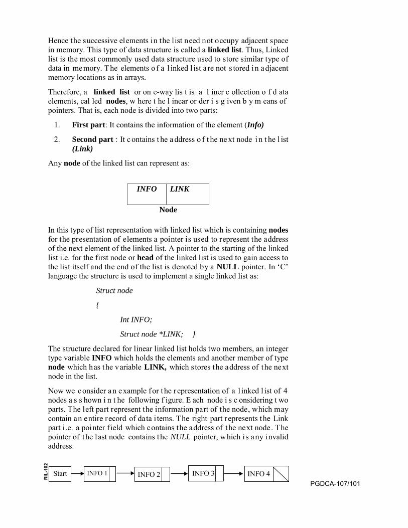
Hence the successive elements in the list need not occupy adjacent space in memory. This type of data structure is called a linked list. Thus, Linked list is the most commonly used data structure used to store similar type of data in memory. The elements o f a l inked l ist a re not s tored in adjacent memory locations as in arrays.
Therefore, a linked list or on e-way lis t is a l iner c ollection o f d ata elements, cal led nodes, w here t he l inear or der i s g iven b y m eans of pointers. That is, each node is divided into two parts:
1. First part: It contains the information of the element (Info)
2. Second part : It c ontains t he a ddress o f t he ne xt node i n t he l ist(Link)
Any node of the linked list can represent as:
INFO LINK
Node
In this type of list representation with linked list which is containing nodes for the presentation of elements a pointer is used to represent the address of the next element of the linked list. A pointer to the starting of the linked list i.e. for the first node or head of the linked list is used to gain access to the list itself and the end of the list is denoted by a NULL pointer. In ‘C’ language the structure is used to implement a single linked list as:
Struct node
{
Int INFO;
Struct node *LINK; }
The structure declared for linear linked list holds two members, an integer type variable INFO which holds the elements and another member of type node which has the variable LINK, which s tores the address of the next node in the list.
Now we consider an example for t he r epresentation of a l inked l ist of 4 nodes a s s hown i n t he following f igure. E ach node i s c onsidering t wo parts. The left part represent the information part of the node, which may contain an entire record of data i tems. The right part represents the Link part i .e. a pointer f ield which contains the address of the next node. The pointer of the last node contains the NULL pointer, which i s any invalid address.
Start INFO 1 INFO 2 INFO 3 INFO 4 PGDCA-107/101
RIL
-102
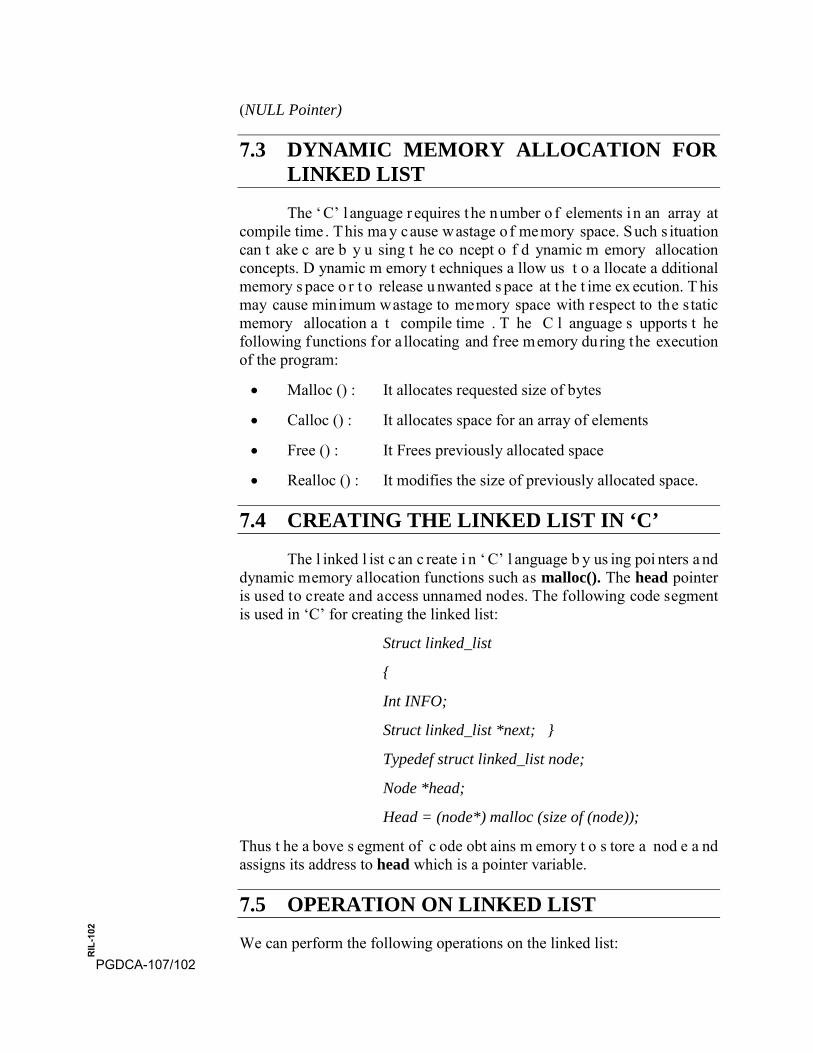
(NULL Pointer)
7.3 DYNAMIC MEMORY ALLOCATION FOR LINKED LIST
The ‘C’ l anguage r equires t he number o f elements i n an array at compile time . This ma y cause wastage o f memory space. Such s ituation can t ake c are b y u sing t he co ncept o f d ynamic m emory allocation concepts. D ynamic m emory t echniques a llow us t o a llocate a dditional memory s pace o r t o release u nwanted s pace at t he t ime ex ecution. T his may cause minimum wastage to memory space with respect to the s tatic memory allocation a t compile time . T he C l anguage s upports t he following functions for a llocating and f ree memory du ring the execution of the program:
• Malloc () : It allocates requested size of bytes
• Calloc () : It allocates space for an array of elements
• Free () : It Frees previously allocated space
• Realloc () : It modifies the size of previously allocated space.
7.4 CREATING THE LINKED LIST IN ‘C’
The l inked l ist c an c reate i n ‘ C’ l anguage b y us ing poi nters a nd dynamic memory allocation functions such as malloc(). The head pointer is used to create and access unnamed nodes. The following code segment is used in ‘C’ for creating the linked list:
Struct linked_list
{
Int INFO;
Struct linked_list *next; }
Typedef struct linked_list node;
Node *head;
Head = (node*) malloc (size of (node));
Thus t he a bove s egment of c ode obt ains m emory t o s tore a nod e a nd assigns its address to head which is a pointer variable.
7.5 OPERATION ON LINKED LIST
We can perform the following operations on the linked list: PGDCA-107/102
RIL
-102

1. Traversing a Linked ListLet w e h ave th e lin ked list LIST in me mory w ith its tw o f ieldsINFO and LINK with START pointing to the f irst element andNULL indicating the end of LIST. Suppose we want to traverseLIST and print the element of the list in order to process each nodeexactly on ce. O ur t raversing a lgorithm us es a poi nter va rivablePTR which points t o t he node that i s currently being p rocessed.Accordingly, LINK[PTR] points to the next node to be processed.The assignment PTR = LINK[PTR] moves the pointer to the nextnode in the list. The algorithmic steps for the traversing process areas follows:
Algorithm (Traversing a Linked List) :[Initialize PTR and then process INFO [PTR], the information atthe first node. Update PTR by the assignment PTR = LINK[PTR],and then process INFO[PTR], the information at the second nodeand so on until PTR = NULL, which signals the end of the list.]
1. PTR = START [Initialize pointer PTR]
2. Repeat steps 3 and 4 while PTR ≠NULL
3. Print (INFO [PTR])
4. PTR = LINK [PTR] [Update pointer]
[End of step 2 loop]
5. Return
2. Count the nodes in a Linked ListLet w e h ave th e lin ked list LIST in me mory w ith its tw o f ieldsINFO and LINK with START pointing to the f irst element andNULL indicating the end of LIST. Suppose we want to count thenumber of nodes in the linked list by traversing the LIST in orderto process each node exactly once. Our counting algorithm uses apointer varivable PTR which points to the node that i s currentlybeing processed. Accordingly, LINK[PTR] points to the next nodeto be pr ocessed. T he a ssignment PTR = LINK[PTR] moves t hepointer t o t he n ext node in t he l ist. The algorithmic s teps for t hetraversing process are as follows:
Algorithm COUNT (INFO, LINK, START, NUM)[Initialize PTR and NUM and t hen pr ocess INFO [PTR], theinformation at the first node. Update PTR by the assignment PTR= LINK[PTR], and t hen pr ocess INFO[PTR], a nd i ncrement t heNUM by one each t ime of t his pr ocessing unt il PTR = NULL,which signals the end of the list.]
PGDCA-107/103
RIL
-102
1. PTR = START and NUM = 0; [Initialize pointer PTR andNUM]
2. Repeat steps 3 and 4 while PTR ≠NULL
3. NUM = NUM + 1; [Increase NUM by 1]
4. PTR = LINK [PTR] [Update pointer]
5. Print (“The number of nodes in the linked list are = “,NUM)
[End of step 2 loop]
6. Return
3. Searching a Linked List
Let w e h ave th e lin ked list LIST in me mory w ith its tw o f ieldsINFO and LINK with START pointing to the f irst element andNULL indicating the end of LIST. We have given an ITEM ofinformation. The process here is for finding the location LOC forthe node where ITEM first appears in LIST.
Algorithm (Searching a Linked List):
[Initialize PTR and then process INFO [PTR], the information atthe first node. Update PTR by the assignment PTR = LINK[PTR],and t hen p rocess INFO[PTR]. N ow co mpare t he co ntentINFO[PTR] of each node with LOC, one by one by updating thepointer PTR by PTR = LINK[PTR] until PTR = NULL, whichsignals t he e nd of t he list. H ere w e ha ve t he t wo t erminatingcondition i.e. the end of the linked list or the item LOC is found i.e.INFO[PTR]=ITEM.
Search(INFO, LINK, START, ITEM, LOC)
1. PTR = START [Initialize pointer PTR]
2. Repeat steps 3 while PTR ≠NULL
3. If (ITEM == INFO[PTR]) {
LOC = PTR; Return (PTR); }
Else
PTR = LINK [PTR] [PTR now points to the next node]
[End of Step 2 loop]
4. LOC = NULL [Search is unsuccessful.]
5. Exit.
PGDCA-107/104
RIL
-102
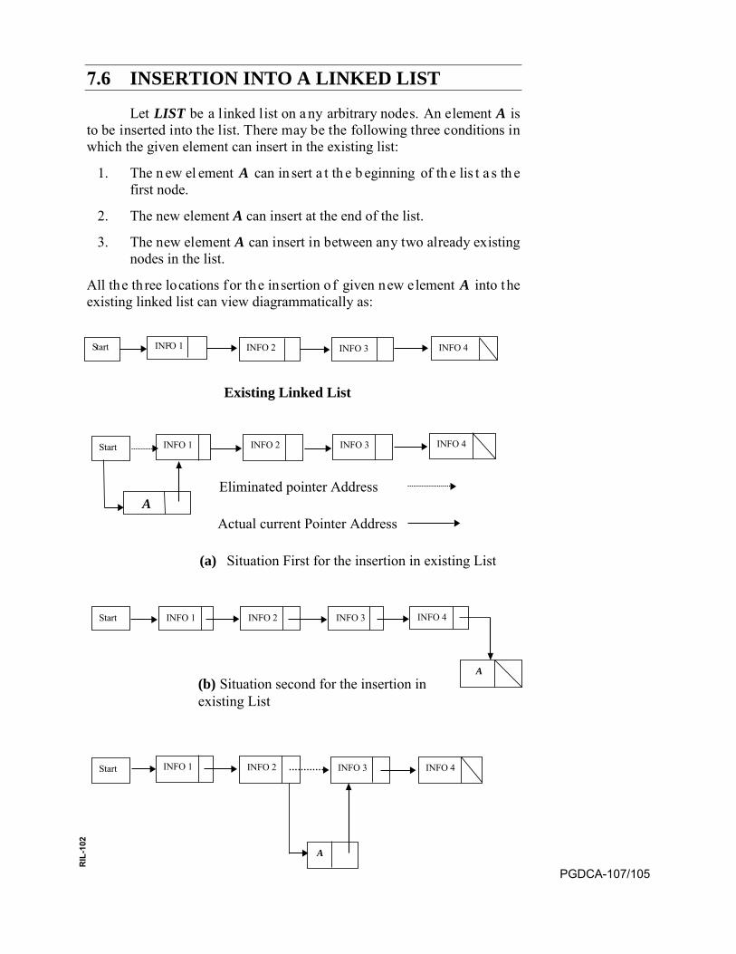
7.6 INSERTION INTO A LINKED LIST
Let LIST be a linked list on a ny arbitrary nodes. An element A is to be inserted into the list. There may be the following three conditions in which the given element can insert in the existing list:
1. The n ew el ement A can in sert a t th e b eginning of th e lis t a s th efirst node.
2. The new element A can insert at the end of the list.
3. The new element A can insert in between any two already existingnodes in the list.
All the three locations for the insertion of given new element A into the existing linked list can view diagrammatically as:
Existing Linked List
Eliminated pointer Address
Actual current Pointer Address
(a) Situation First for the insertion in existing List
(b) Situation second for the insertion in existing List
Start INFO 1 INFO 2 INFO 3 INFO 4
A
Start INFO 1 INFO 2 INFO 3 INFO 4
A
S tart INF O 1 INFO 2 INFO 3 INFO 4
Start INFO 1 INFO 2 INFO 3 INFO 4
A
PGDCA-107/105
RIL
-102
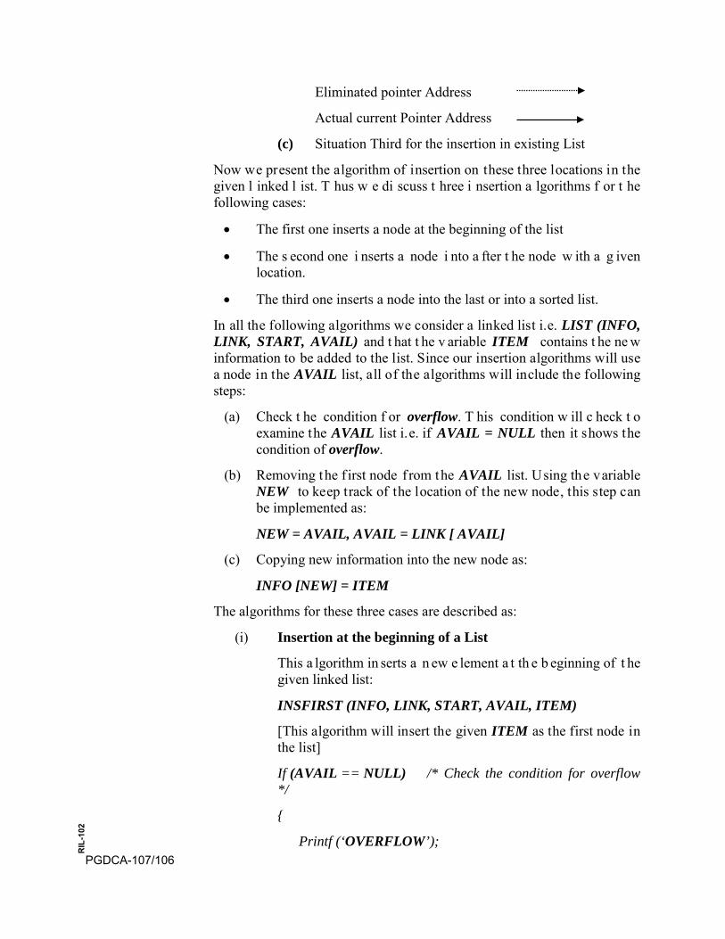
Eliminated pointer Address
Actual current Pointer Address
(c) Situation Third for the insertion in existing List
Now we present the algorithm of insertion on these three locations in the given l inked l ist. T hus w e di scuss t hree i nsertion a lgorithms f or t he following cases:
• The first one inserts a node at the beginning of the list
• The s econd one i nserts a node i nto a fter t he node w ith a g ivenlocation.
• The third one inserts a node into the last or into a sorted list.
In all the following algorithms we consider a linked list i.e. LIST (INFO, LINK, START, AVAIL) and t hat t he v ariable ITEM contains t he ne w information to be added to the list. Since our insertion algorithms will use a node in the AVAIL list, all of the algorithms will include the following steps:
(a) Check t he condition f or overflow. T his condition w ill c heck t o examine the AVAIL list i.e. if AVAIL = NULL then it shows the condition of overflow.
(b) Removing the f irst node f rom the AVAIL list. Using the variable NEW to keep track of the location of the new node, this step can be implemented as:
NEW = AVAIL, AVAIL = LINK [ AVAIL]
(c) Copying new information into the new node as:
INFO [NEW] = ITEM
The algorithms for these three cases are described as:
(i) Insertion at the beginning of a List
This a lgorithm in serts a n ew e lement a t th e b eginning of t he given linked list:
INSFIRST (INFO, LINK, START, AVAIL, ITEM)
[This algorithm will insert the given ITEM as the first node in the list]
If (AVAIL == NULL) /* Check the condition for overflow */
{
Printf (‘OVERFLOW’); PGDCA-107/106
RIL
-102
Return;
}
Else {
NEW = AVAIL;
AVAIL = LINK [AVAIL]; /* remove first node from AVAIL list */
INFO[NEW] = ITEM; /* Copy new data into new node */
LINK [NEW] = START; /* new node to point the original first node */
START = NEW; /* Change START so it points to the new node */
}
Return (NEW);
(ii) Insertion at end of a List
This algorithm inserts a new element at the end or at the last of the given linked list:
INSFIRST (INFO, LINK, START, AVAIL, ITEM)
[This algorithm will insert the given ITEM as the last node in the list]
If (AVAIL == NULL) /* Check the condition for overflow */
{
Printf (‘OVERFLOW’);
Return;
}
Else {
NEW = AVAIL; /* obtain address of next free node */
AVAIL = LINK [AVAIL]; /* re remove first node from AVAIL list */
INFO [NEW] = ITEM; /* Copy new data into new node */
LINK [NEW] = NULL /* new node to point the last node of the list */ PGDCA-107/107
RIL
-102
If (START == NULL) /* check for the list that is list empty? */
Return (NEW);
TEMP = START /* Initiate search for the last node */
while (LINK [TEMP] != NULL)
{
TEMP = LINK [TEMP]
}
LINK [TEMP] = NEW /* Set LINK field of last node to NEW */
Return (START)
}
(i) Insertion after a given Node of a List
This a lgorithm in serts a n ew e lement after t he given nod e of t he given linked list:
INSORDER (INFO, LINK, START, AVAIL, ITEM)
[This a lgorithm i nserts t he g iven nod e ITEM into LIST on t he given l ocation i .e. LOC is t he l ocation of a n ode s ay A. T hus ITEM follows node A. Let N denote the new node (whose location is NEW). If LOC=NULL, then N is inserted as the first node in LIST. Let the node N point t o node B (which or iginally followed no de A) by th e s tatement, LINK [NEW] = LINK [LOC] and we let node A point to the new node N by the statement, LINK [LOC] = NEW;
If (AVAIL == NULL) /* Check the condition for overflow */
{
Printf (‘OVERFLOW’);
Return;
}
Else {
NEW = AVAIL; /* obtain address of next free node */
AVAIL = LINK [AVAIL]; /* re remove first node from AVAIL list */
PGDCA-107/108
RIL
-102
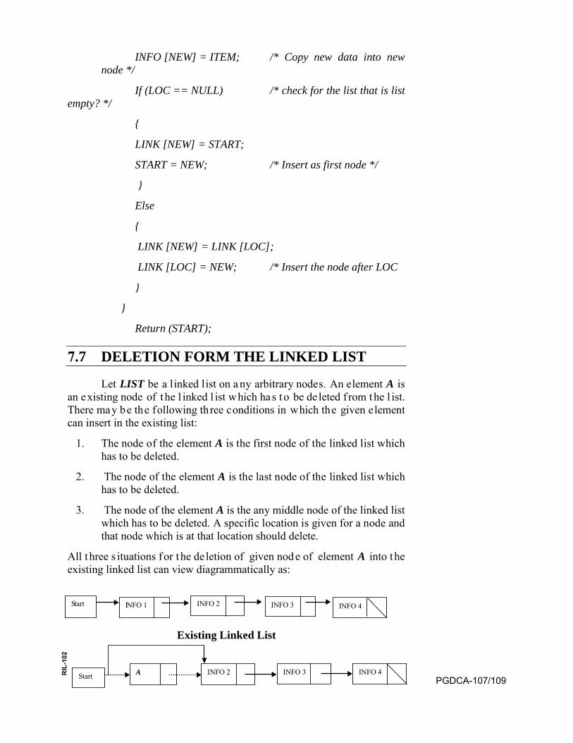
INFO [NEW] = ITEM; /* Copy new data into new node */
If (LOC == NULL) /* check for the list that is list empty? */
{
LINK [NEW] = START;
START = NEW; /* Insert as first node */
}
Else
{
LINK [NEW] = LINK [LOC];
LINK [LOC] = NEW; /* Insert the node after LOC
}
}
Return (START);
7.7 DELETION FORM THE LINKED LIST
Let LIST be a linked list on a ny arbitrary nodes. An element A is an existing node of t he l inked l ist which has t o be de leted f rom the l ist. There may be the following three conditions in which the given element can insert in the existing list:
1. The node of the element A is the first node of the linked list whichhas to be deleted.
2. The node of the element A is the last node of the linked list whichhas to be deleted.
3. The node of the element A is the any middle node of the linked listwhich has to be deleted. A specific location is given for a node andthat node which is at that location should delete.
All t hree s ituations for t he de letion of given nod e of element A into t he existing linked list can view diagrammatically as:
Existing Linked List
Start A INFO 2 INFO 3 INFO 4
S tart I NFO 1 INFO 2 INFO 3 INFO 4
PGDCA-107/109
RIL
-102

Eliminated pointer Address
Actual current Pointer Address
(a) Situation First for the deletion from the existing List
(b) Situation second for the deletion from the existing List
Eliminated pointer Address
Actual current Pointer Address
Eliminated pointer Address
Actual current Pointer Address
(c) Situation Third for the deletion from the existing list
Now w e p resent a general al gorithm f or d eleting an el ement f rom t he given lin ked lis t. T his a lgorithm e ncompasses all th e th ree s ituations a s described in above mentioned figures for deletion.
Algorithm DELTE (X, FIRST): [Given X and FIRST pointer v ariables whose values denote the address of a node in a linked list and the address of the first node in the linked list, respectively, this procedure deletes the node whose address is given by X. TEMP is used to find the desired node, and PRED keeps t rack of t he p redecessor o f TEMP. FIRST is changed only when X is the first element of the list.]
If (FIRST == NULL) /* Check the condition for empty list */
{
Printf (‘UNDER FLOW’);
Start INFO 1 INFO 2 INFO 3 INFO 4
A
Start INFO 1 INFO 2 A INFO 4
PGDCA-107/110
RIL
-102
Return;
}
Else { /* Initialize search for X */
TEMP = FIRST;
While ((TEMP != X) && (LINK (TEMP) != NULL)) /* find X */
{
PRED = TEMP /* Update predecessor marker */
TEMP = LINK (TEMP) /* Move to next node */
}
If ( TEMP != X) /* end of the list */
{
Printf (“Node not found”);
Return;
}
If (X == FIRST) /* X is the first node i.e. the deletion of the first node */
FIRST = LINK (FIRST);
Else
LINK (PRED) = LINK (X);
LINK (X) = AVAIL; /* Return node to available area */
AVAIL = X;
Return;
}
7.8 COPY OF THE LINKED LIST
Let LIST be a l inked l ist on a ny arbitrary nodes. We formulate a algorithm which copies a linked list into the another linked list. A general algorithm to copy a linked list is as follows:
Algorithm COPY (FIRST): [Given FIRST, a pointer to the first node in a linked list, this algorithm makes a copy of this list. A typical node in the given lis t consists o f INFO and LINK fields. T he n ew lis t is to contain nodes w hose i nformation a nd poi nter f ields are denoted b y FIELD and PGDCA-107/111
RIL
-102
PTR, respectively. The address of the first node in the newly created list is to be placed in BEGIN. NEW, SAVE and PRED are pointer variables. ]
If (FIRST == NULL) /* Check the condition for empty list */
{
Printf (‘EMPTY LIST’);
Return; }
Else
{
If (AVAIL == NULL)
{
Printf (“Availability stack underflow”);
Return (0); }
Else {
NEW = AVAIL; /* copy the first node */
AVAIL = LINK (AVAIL);
FIELD (NEW) = INFO (FIRST);
BEGIN = NEW; }
SAVE = FIRST; /* Initialize traversal */
While (LINK (SAVE) != NULL) /* Move to next node if not at end of list */
{
PRED = NEW;
SAVE = LINK (SAVE); /* update predecessor and save pointer */
NEW = AVAIL;
AVAIL = LINK (AVAIL);
FIELD (NEW) = INFO (SAVE); /* copy node */
PTR (PRED) = NEW;
}
PTR (NEW) = NULL; PGDCA-107/112
RIL
-102
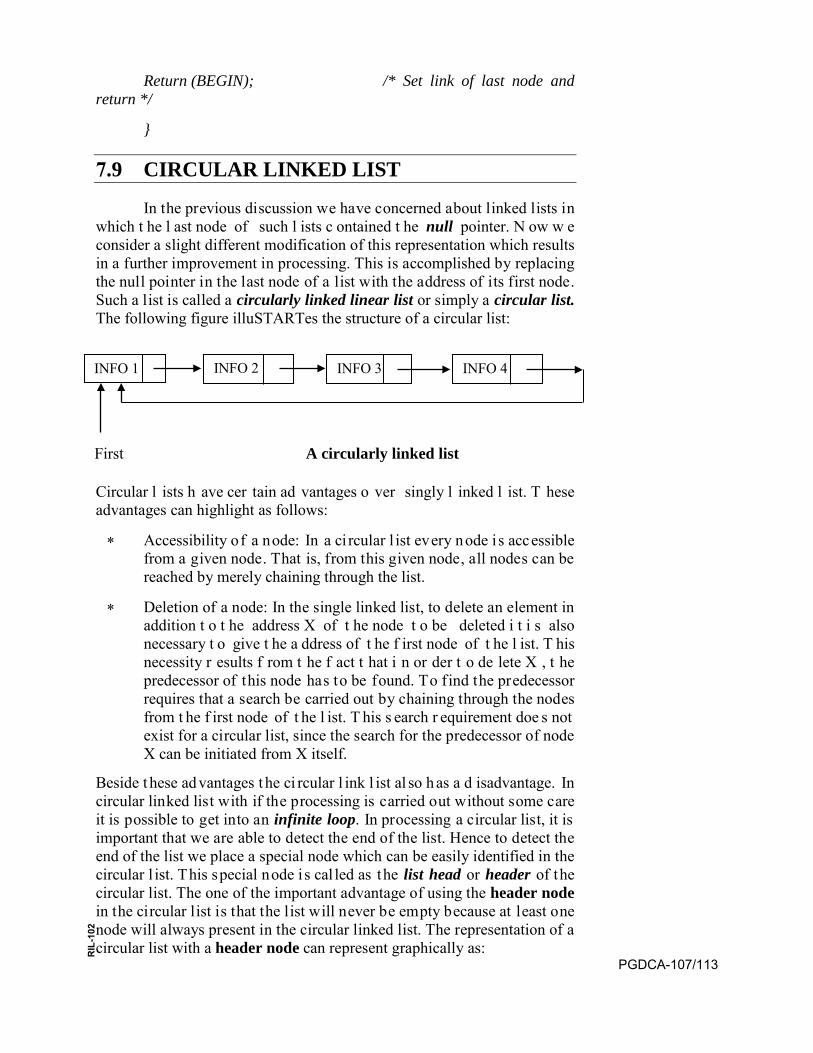
Return (BEGIN); /* Set link of last node and return */
}
7.9 CIRCULAR LINKED LIST
In the previous discussion we have concerned about linked lists in which t he l ast node of such l ists c ontained t he null pointer. N ow w e consider a slight different modification of this representation which results in a further improvement in processing. This is accomplished by replacing the null pointer in the last node of a list with the address of its first node. Such a list is called a circularly linked linear list or simply a circular list. The following figure illuSTARTes the structure of a circular list:
First A circularly linked list
Circular l ists h ave cer tain ad vantages o ver singly l inked l ist. T hese advantages can highlight as follows:
∗ Accessibility of a node: In a ci rcular l ist every node i s accessible from a given node. That is, from this given node, all nodes can be reached by merely chaining through the list.
∗ Deletion of a node: In the single linked list, to delete an element in addition t o t he address X of t he node t o be deleted i t i s also necessary t o give t he a ddress of t he f irst node of t he l ist. T his necessity r esults f rom t he f act t hat i n or der t o de lete X , t he predecessor of this node has to be found. To find the predecessor requires that a search be carried out by chaining through the nodes from t he f irst node of t he l ist. T his s earch r equirement doe s not exist for a circular list, since the search for the predecessor of node X can be initiated from X itself.
Beside t hese advantages t he ci rcular l ink l ist al so has a d isadvantage. In circular linked list with if the processing is carried out without some care it is possible to get into an infinite loop. In processing a circular list, it is important that we are able to detect the end of the list. Hence to detect the end of the list we place a special node which can be easily identified in the circular l ist. This special node i s cal led as the list head or header of the circular list. The one of the important advantage of using the header node in the circular list is that the list will never be empty because at least one node will always present in the circular linked list. The representation of a circular list with a header node can represent graphically as:
INFO 1 INFO 2 INFO 3 INFO 4
PGDCA-107/113
RIL
-102

HEAD
A circularly linked list with a head node
Here the variable HEAD denotes the address of the l ist head. The INFO filed in the l ist head node is not used, which is i lluSTARTed by shading the field. An empty list is represented by having:
LINK (HEAD) = HEAD. The f ollowing a re t he va rious ope rations performed on a circular header list:
• Traversing a circular header list
• Searching in a circular header list
• Deleting from a circular header list
Now we consider the algorithms for these three operations.
Algorithm (Traversing a circular header Linked List)
[Initialize PTR and then process INFO [PTR], the information at the first node. U pdate PTR by the a ssignment PTR = LINK [PTR], and t hen process INFO [PTR], the information at the second node and so on unt il PTR ≠ START.]
1. PTR = LINK [START] [Initialize pointer PTR]
2. Repeat steps 3 and 4 while PTR ≠START
3. Print (INFO [PTR])
4. PTR = LINK [PTR] [Update pointer]
[End of step 2 loop]
5. Return
Algorithm (Searching the circular header Linked List)
[This a lgorithm f inds th e lo cation LOC of t he node w here ITEM first appears in LIST or sets LOC = NULL.]
1. PTR = LINK [START]; [Initialize pointer PTR]
2. Repeat while INFO [PTR] ≠ ITEM and PTR ≠START
PTR = LINK [PTR]; [PTR now points to the next node]
[End of loop]
INFO 1 INF O 2 INFO 3 INFO 4
PGDCA-107/114
RIL
-102
3. If (INFO [PTR] == ITEM) then
LOC = PTR;
Else
LOC = NULL;
[End of if structure]
4. Exit
Algorithm CRDELTE (X, FIRST): [Given X and FIRST pointer variables whose values denote the address of a node in a linked list and the address of t he f irst node i n t he l inked l ist, r espectively, t his pr ocedure deletes the node whose address is given by X. TEMP is used to find the desired node, and PRED keeps track of the predecessor of TEMP. FIRST is changed only when X is the first element of the list.]
If (FIRST == NULL) /* Check the condition for empty list */
{
Printf (‘UNDER FLOW’);
Return;
}
Else { /* Initialize search for X */
TEMP = FIRST;
While ((TEMP != X) && (LINK (TEMP) != FIRST))/* find X */
{
PRED = TEMP /* Updatepredecessor marker */
TEMP = LINK (TEMP) /* Move to next node */
}
If ( TEMP != X) /* end of the list */
{
Printf (“Node not found”);
Return;
}
PGDCA-107/115
RIL
-102
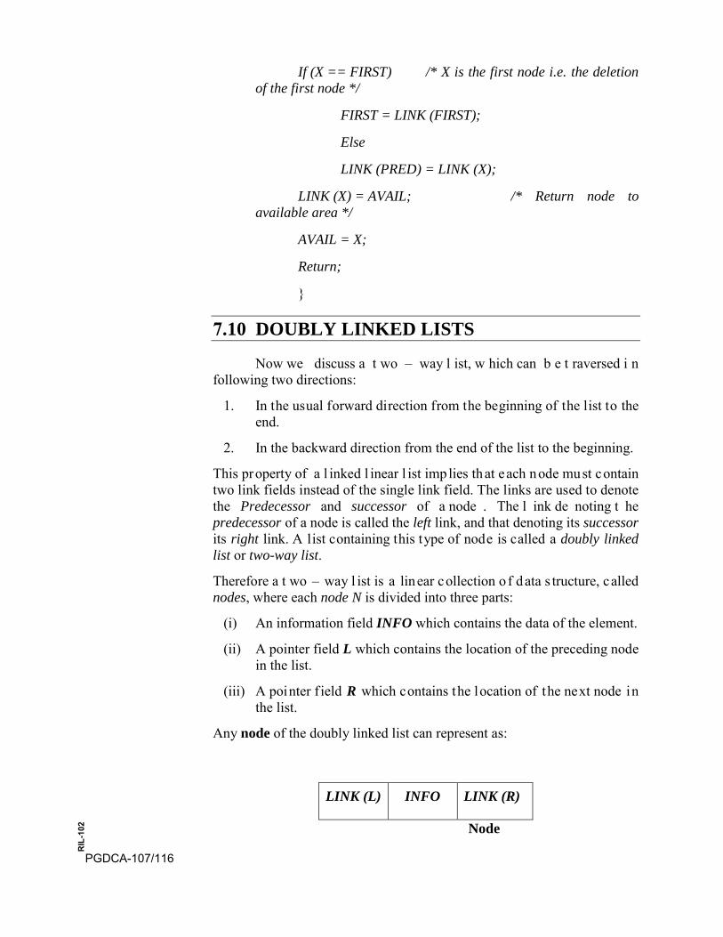
If (X == FIRST) /* X is the first node i.e. the deletion of the first node */
FIRST = LINK (FIRST);
Else
LINK (PRED) = LINK (X);
LINK (X) = AVAIL; /* Return node to available area */
AVAIL = X;
Return;
}
7.10 DOUBLY LINKED LISTS
Now we discuss a t wo – way l ist, w hich can b e t raversed i n following two directions:
1. In the usual forward direction from the beginning of the list to theend.
2. In the backward direction from the end of the list to the beginning.
This property of a l inked l inear l ist implies that each node must contain two link fields instead of the single link field. The links are used to denote the Predecessor and successor of a node . The l ink de noting t he predecessor of a node is called the left link, and that denoting its successor its right link. A list containing this type of node is called a doubly linked list or two-way list.
Therefore a t wo – way l ist is a linear collection o f data s tructure, called nodes, where each node N is divided into three parts:
(i) An information field INFO which contains the data of the element.
(ii) A pointer field L which contains the location of the preceding node in the list.
(iii) A pointer f ield R which contains the location of the next node in the list.
Any node of the doubly linked list can represent as:
LINK (L) INFO LINK (R)
Node
PGDCA-107/116
RIL
-102
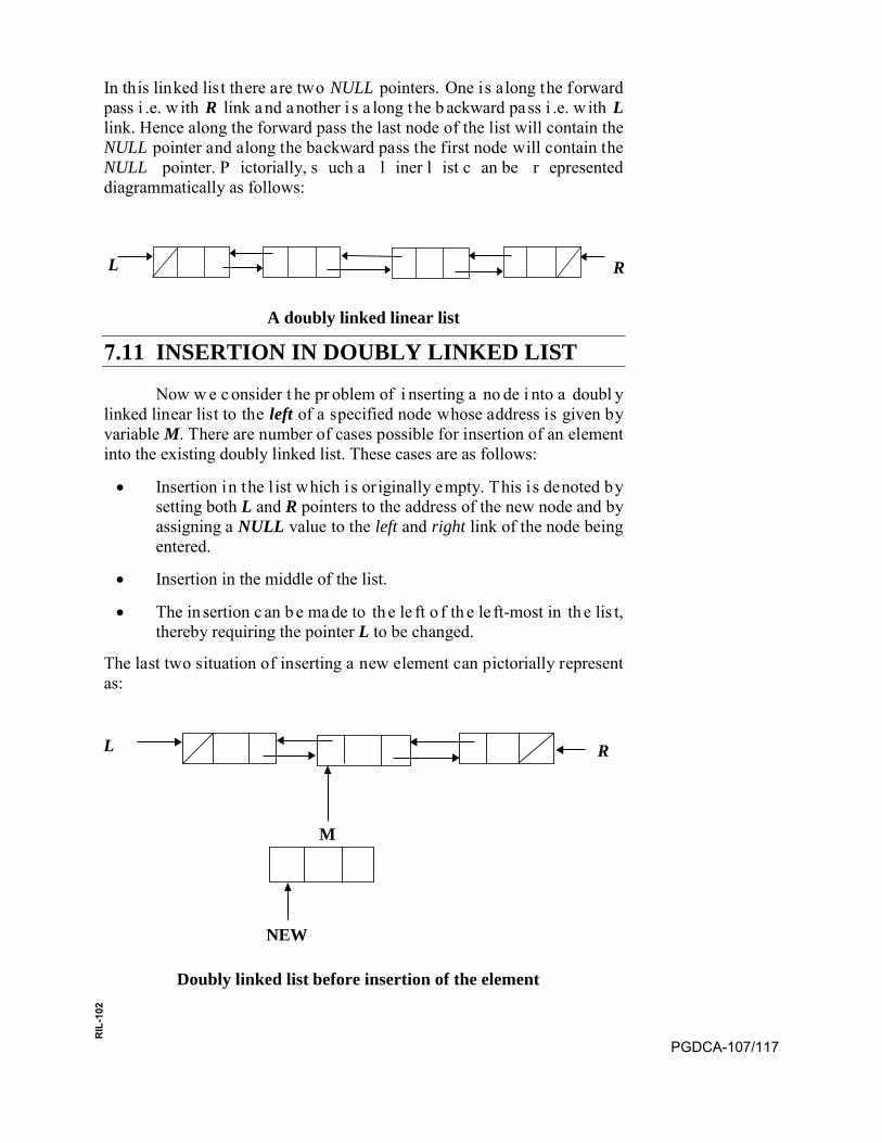
In this linked list there are two NULL pointers. One is along the forward pass i .e. w ith R link a nd a nother i s a long t he b ackward pa ss i .e. w ith L link. Hence along the forward pass the last node of the list will contain the NULL pointer and along the backward pass the first node will contain the NULL pointer. P ictorially, s uch a l iner l ist c an be r epresented diagrammatically as follows:
A doubly linked linear list
7.11 INSERTION IN DOUBLY LINKED LIST
Now w e c onsider t he pr oblem of i nserting a no de i nto a doubl y linked linear list to the left of a specified node whose address is given by variable M. There are number of cases possible for insertion of an element into the existing doubly linked list. These cases are as follows:
• Insertion in the l ist which is or iginally empty. This is denoted bysetting both L and R pointers to the address of the new node and byassigning a NULL value to the left and right link of the node beingentered.
• Insertion in the middle of the list.
• The in sertion c an b e ma de to th e le ft o f th e le ft-most in th e lis t,thereby requiring the pointer L to be changed.
The last two situation of inserting a new element can pictorially represent as:
M
NEW
Doubly linked list before insertion of the element
L R
L R
PGDCA-107/117
RIL
-102
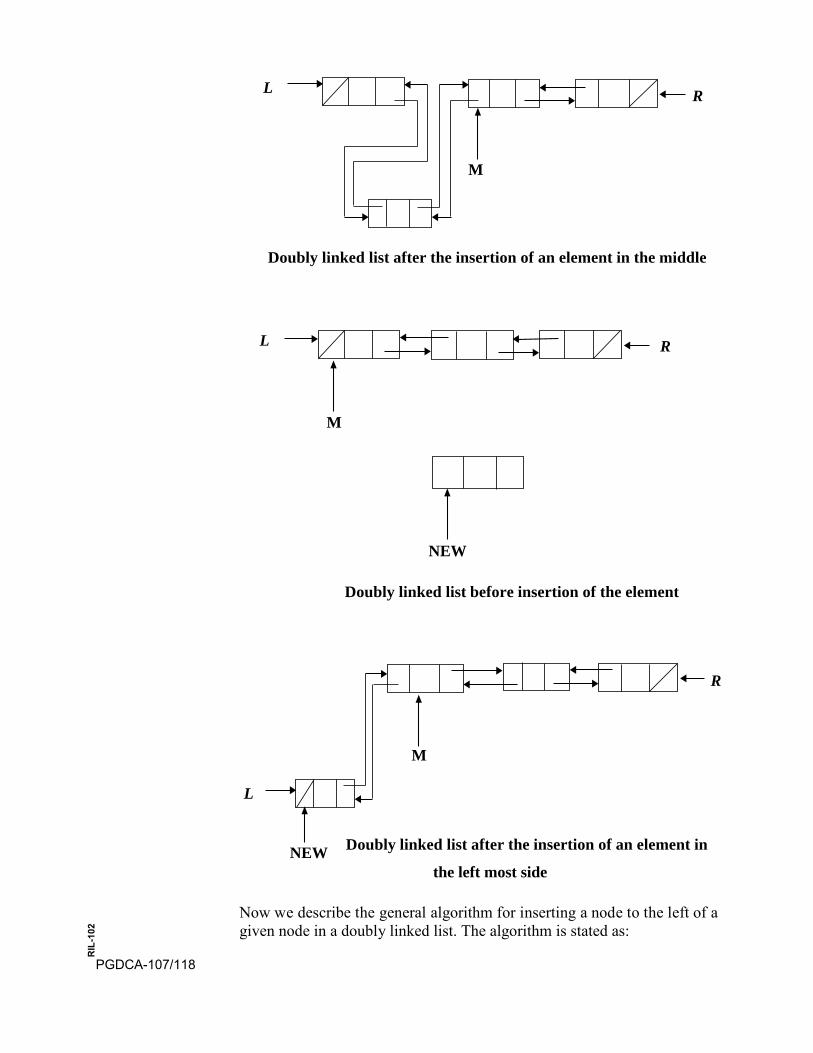
M
Doubly linked list after the insertion of an element in the middle
M
NEW
Doubly linked list before insertion of the element
M
Doubly linked list after the insertion of an element in
the left most side
Now we describe the general algorithm for inserting a node to the left of a given node in a doubly linked list. The algorithm is stated as:
L R
L R
L
R
NEW
PGDCA-107/118
RIL
-102
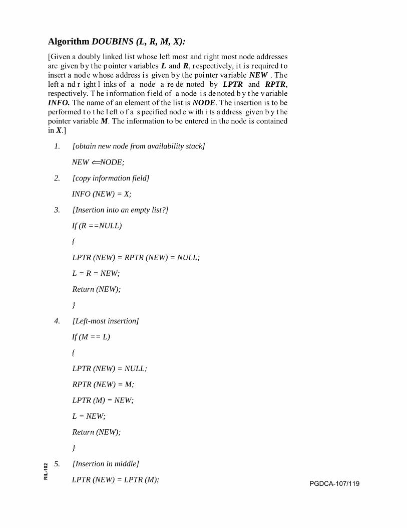
Algorithm DOUBINS (L, R, M, X): [Given a doubly linked list whose left most and right most node addresses are given by the pointer variables L and R, respectively, i t i s required to insert a node whose address is given by the pointer variable NEW . The left a nd r ight l inks of a node a re de noted by LPTR and RPTR, respectively. T he i nformation f ield of a node i s de noted b y t he v ariable INFO. The name of an element of the list is NODE. The insertion is to be performed t o t he l eft o f a s pecified nod e w ith i ts a ddress given b y t he pointer variable M. The information to be entered in the node is contained in X.]
1. [obtain new node from availability stack]
NEW ⟸NODE;
2. [copy information field]
INFO (NEW) = X;
3. [Insertion into an empty list?]
If (R ==NULL)
{
LPTR (NEW) = RPTR (NEW) = NULL;
L = R = NEW;
Return (NEW);
}
4. [Left-most insertion]
If (M == L)
{
LPTR (NEW) = NULL;
RPTR (NEW) = M;
LPTR (M) = NEW;
L = NEW;
Return (NEW);
}
5. [Insertion in middle]
LPTR (NEW) = LPTR (M); PGDCA-107/119
RIL
-102
RPTR (NEW) = M;
LPTR (M) = NEW;
RPTR (LPTR (NEW))= NEW;
Return (NEW);
7.12 DELETION IN DOUBLY LINKED LIST
Now w e c onsider t he pr oblem of d eleting a nod e f rom a doubl y linked l inear l ist. In t his pr ocess t here i s no need of a ny s earch f or determining the predecessor node of the node to be deleted. In the doubly linked l ist on g iving t he a ddress of t he nod e w hich i s t o be de leted, t he predecessor a nd s uccessor node s a re i mmediately know n. T herefore doubly linked lists are much more efficient with respect to deletions than singly linked lists.
There a re n umber o f p ossibilities a rises f or th e d eletion o peration in doubly linked list. These possibilities are as follows:
• If the list contains a single node, then a deletion results in an emptylist with the left – most and right-most pointers being set to NULL.
• The node being deleted could be the left-most node of the l ist. Inthis case the pointer variable L must be changed.
• The node being deleted could be the Right-most node of the list. Inthis case the pointer variable R must be changed.
• The deletion can occur from the middle of the list.
A general algorithm for deleting a node f rom the doubly l inked l ist i s as follows:
Algorithm DOUBDEL (L, R, OLD):
[Given a doubl y l inked list w ith the addresses o f t he l eft most and r ight most node s given b y t he poi nter v ariables L and R, r espectively, it is required to delete the node whose address is given by the pointer variable OLD. The left and right links of a node are denoted by LPTR and RPTR, respectively.]
1. [check the condition for underflow]
If (R == NULL)
{
Printf (”Underflow”);
Return
}PGDCA-107/120
RIL
-102
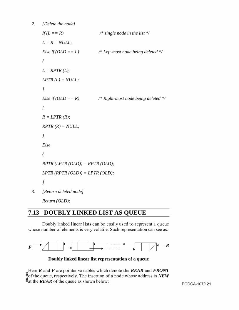
2. [Delete the node]
If (L == R) /* single node in the list */
L = R = NULL;
Else if (OLD == L) /* Left-most node being deleted */
{
L = RPTR (L);
LPTR (L) = NULL;
}
Else if (OLD == R) /* Right-most node being deleted */
{
R = LPTR (R);
RPTR (R) = NULL;
}
Else
{
RPTR (LPTR (OLD)) = RPTR (OLD);
LPTR (RPTR (OLD)) = LPTR (OLD);
}
3. [Return deleted node]
Return (OLD);
7.13 DOUBLY LINKED LIST AS QUEUE
Doubly l inked l inear l ists can be easily used to represent a queue whose number of elements is very volatile. Such representation can see as:
Doubly linked linear list representation of a queue
Here R and F are pointer variables which denote the REAR and FRONT of the queue, respectively. The insertion of a node whose address is NEW at the REAR of the queue as shown below:
F R ..............
PGDCA-107/121
RIL
-102
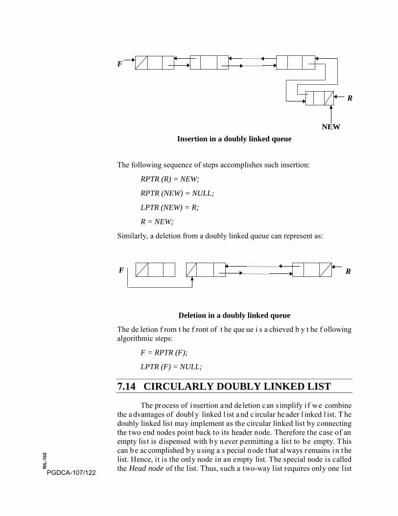
NEW Insertion in a doubly linked queue
The following sequence of steps accomplishes such insertion:
RPTR (R) = NEW;
RPTR (NEW) = NULL;
LPTR (NEW) = R;
R = NEW;
Similarly, a deletion from a doubly linked queue can represent as:
Deletion in a doubly linked queue
The de letion f rom t he f ront of t he que ue i s a chieved b y t he f ollowing algorithmic steps:
F = RPTR (F);
LPTR (F) = NULL;
7.14 CIRCULARLY DOUBLY LINKED LIST
The process of insertion and deletion can s implify i f we combine the a dvantages of doubl y linked l ist a nd c ircular he ader l inked l ist. T he doubly linked list may implement as the circular linked list by connecting the two end nodes point back to its header node. Therefore the case of an empty lis t is dispensed with by never permitting a lis t to be empty. This can be ac complished b y u sing a s pecial node t hat al ways r emains i n t he list. Hence, it is the only node in an empty list. The special node is called the Head node of the list. Thus, such a two-way list requires only one list
F
R
F R
PGDCA-107/122
RIL
-102
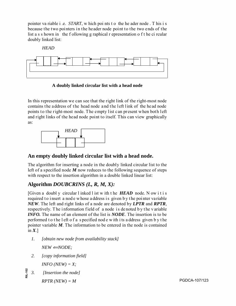
pointer va riable i .e. START, w hich poi nts t o the he ader node . T his i s because the two pointers in the header node point to the two ends of the list a s s hown in the f ollowing g raphical r epresentation o f t he ci rcular doubly linked list:
HEAD
A doubly linked circular list with a head node
In this representation we can see that the right link of the right-most node contains t he address of t he head node and the l eft l ink of the head node points to the r ight-most node. The empty l ist can present when both left and right links of the head node point to itself. This can view graphically as:
HEAD
An empty doubly linked circular list with a head node. The algorithm for inserting a node in the doubly linked circular list to the left of a specified node M now reduces to the following sequence of steps with respect to the insertion algorithm in a double linked linear list:
Algorithm DOUBCRINS (L, R, M, X): [Given a doubl y circular l inked l ist w ith t he HEAD node. N ow i t i s required t o i nsert a nod e w hose a ddress i s given b y t he poi nter va riable NEW. The left and right links of a node are denoted by LPTR and RPTR, respectively. T he i nformation f ield of a node i s de noted b y t he v ariable INFO. The name of an element of the list is NODE. The insertion is to be performed t o t he l eft o f a s pecified nod e w ith i ts a ddress given b y t he pointer variable M. The information to be entered in the node is contained in X.]
1. [obtain new node from availability stack]
NEW ⟸NODE;
2. [copy information field]
INFO (NEW) = X;
3. [Insertion the node]
RPTR (NEW) = M PGDCA-107/123
RIL
-102
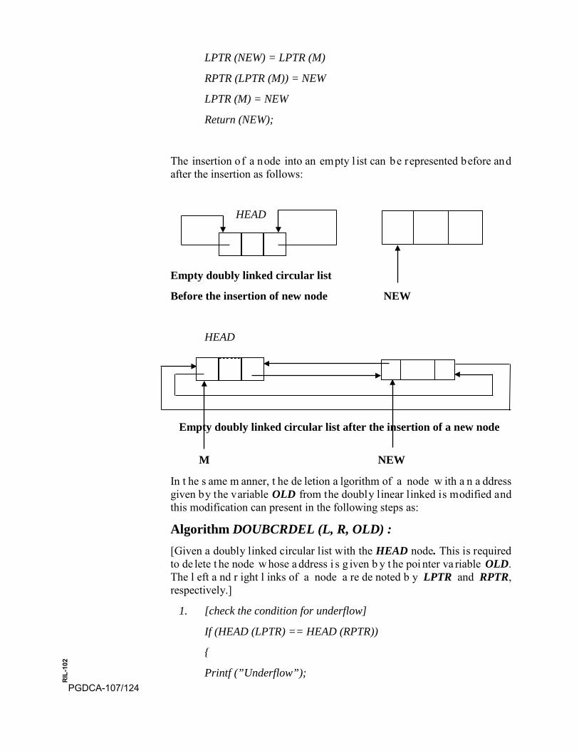
LPTR (NEW) = LPTR (M)
RPTR (LPTR (M)) = NEW
LPTR (M) = NEW
Return (NEW);
The insertion of a node into an empty l ist can be represented before and after the insertion as follows:
HEAD
Empty doubly linked circular list
Before the insertion of new node NEW
HEAD
Empty doubly linked circular list after the insertion of a new node
M NEW
In t he s ame m anner, t he de letion a lgorithm of a node w ith a n a ddress given by the variable OLD from the doubly linear linked is modified and this modification can present in the following steps as:
Algorithm DOUBCRDEL (L, R, OLD) : [Given a doubly linked circular list with the HEAD node. This is required to de lete t he node w hose a ddress i s g iven b y t he poi nter va riable OLD. The l eft a nd r ight l inks of a node a re de noted b y LPTR and RPTR, respectively.]
1. [check the condition for underflow]
If (HEAD (LPTR) == HEAD (RPTR))
{
Printf (”Underflow”);PGDCA-107/124
RIL
-102
Return
}
2. [Delete the node]
{
RPTR (LPTR (OLD)) = RPTR (OLD);
LPTR (RPTR (OLD)) = LPTR (OLD);
}
3. [Return deleted node]
Return (OLD);
7.15 APPLICATION OF LINKED LIST: POLYNOMIAL REPRESENTATION
Here we consider the applications of linked list. A very common and important a pplication of lin ked lis t is f or t he r epresentation o f a polynomial. A polynomial, p (x), is an expression in variable x of the form ( kjxbxax nn ++++ − .....1 ) where a, b, c, …k are real numbers and n is a non-negative integer. The number n is called the degree of the polynomial. An imp ortant c haracteristic o f a p olynomial is th at e ach te rm in th e polynomial expression consists of following two parts:
• Coefficient
• Exponent
Consider the following polynomial:
dxcxbxax −−+ 235
Here, (a, b, -c, -d) are coefficients and (5, 3, 2, 1) are exponents.
Exponents a re t he pl aceholders f or a ny value t hat r emains c onstant for each t erm i n a s ingle e xpression. In da ta s tructure, a pol ynomial c an be represented as a list of nodes where each node consists of coefficient and an exponent.
Points to be considered when working with polynomials are:
• Sign of each c oefficient a nd e xponent i s s tored w ithin t hecoefficient and exponent itself.
• Only addition of term with equal exponent is possible.
• Storage of each term in the polynomial must be done in ascending /descending order of their exponent.
Consider t he e xample of r epresenting a t erm of a pol ynomial i n t he variables x, y, z. A typical node of the linked list can represent as: PGDCA-107/125
RIL
-102

POWER_X POWER_Y POWER_Z COEFF LINK
A typical node of the linked list for the representation of a polynomial of three variables This t ypical node c onsists of f ive s equentially allocated f ields t hat w e collectively refer to as TERM. The first three fields represent the power of the variables x, y, z, respectively. The fourth and fifth fields represent the coefficient of the term in the polynomial and the address of the next term in t he pol ynomial, r espectively. For example, the t erm 3xy would be represented as:
1 1 0 3
We c onsider t he poi nter a ddress P to r eference t he node f or our algorithmic n otation. COEFF (P) denotes t he c oefficient f ield of a nod e pointed t o b y P. Similarly, t he e xponents of x , y a nd z a re given b y POWER_X (P), POWER_Y (P), and POWER_Z (P), respectively, and the pointer to the next node is given by LINK (P).
Consider as an example t he r epresentation of t he pol ynomial: yzyxyx +++ 22 52 as a linked list. Assume that the nodes in the list are
to be s tored s uch t hat a t erm poi nted t o b y P precedes an other t erm indicated by Q if POWER_X (P) is greater than POWER_X (Q); or, if the power of x is equal, then POWER_Y (P) must be greater than POWER_Z (Q). For our example, the list is represented as:
We can formulate an algorithm which inserts a term of a polynomial into a linked list.
Algorithm POLYFRONT (NX, NY, NZ, NCOEFF, POLY):
[Given the definition of the node structure TERM and an availability area from which we can obtain such nodes, it is required to insert a node in the linked l ist s o t hat i t i mmediately pr ecedes t he node w hose a ddress i s designated by the pointer POLY. The f ields of the new term are denoted by NX, NY, NZ, and NCOEFF, which correspond to the exponents for x,
2 0 0 2 1 1 0 5 0 2 0 1
0 1 1 1
PGDCA-107/126
RIL
-102
y, a nd z , a nd t he c oefficient v alue o f t he t erm, r espectively. NEW is a pointer variable which contains the address of the new node.]
1. [Obtain a node from available storage]
NEW ⟸ TERM
2. [Initialize numeric fields]
POWER_X (NEW) = NX;
POWER_Y (NEW) = NY;
POWER_Z (NEW) = NZ;
COEFF (NEW) = NCOEFF
3. [Set link to the list]
LINK (NEW) = POLY;
4. [Return first node pointer]
Return (NEW)
This f unction pe rforms all i ts i nsertions a t one end of t he l inked l ist. In general, it is also possible to perform insertions at the other end or in the middle o f th e lis t. T he zero p olynomial ( polynomial w ith n o te rms) is represented b y t he NULL pointer. B efore a ny t erm of a pol ynomial h as been added to a list, its first node pointer, which we call POLY, has a value of NULL. W hen f unction POLYFRONT is invoked, t he address of t he created node is returned, and it is this value that replaces the function call i.e. POLY = POLYFRONT (NX, NY, NZ, NCOEFF, POLY. T he construction of a linked list for a polynomial is achieved by having a zero polynomial in itially and b y r epeatedly i nvoking f unction POLYFRONT until all terms of the polynomial are processed.
7.16 STACK IMPLEMENTATION WITH LINKED LIST
The pr oblem w ith a rray-based s tacks i s t hat t he s ize m ust b e determined at compile time. Thus the size of the stack is fixed. The stack implementation with array reflects the static memory allocation. Hence to implement the stack with dynamic memory allocation we use a linked list, with the stack pointer pointing to the TOP element, let FRESH be the new node. To push a new element on the stack, we must do:
FRESH->NEXT= TOP;
TOP = FRESH;
To pop an item from a linked stack, we just have to reverse the operation.
ITEM = TOP;
TOP = TOP->NEXT; PGDCA-107/127
RIL
-102
7.17 GARBAGE COLLECTION
Garbage c ollection i s t he pr ocess of c ollecting all unus ed node s and returning them to available space. Therefore the garbage collection is about f reeing d ynamically allocated m emory when n ot i n u se. This process is carried out in two phases:
• First phase, known as marking phase. It involves marking of allnodes that are accessible from the external pointer.
• Second phase, known as collection phase. It involves proceedingsequentially through memory and freeing all nodes that have notbeen marked.
In t he i mplementation f or l inked l ist w hen w e de lete a node from t he linked list and return it to the memory back i.e. free (node) then the space allocated t o t he de leted node a nd i ts poi nter address r eturn ba ck t o t he memory. This process is considered as the garbage collection.
7.18 SUMMARY
Linked list is a linear dynamic data structure which allows storing the e lements i n non -contiguous me mory lo cations. It is n ot restricted a s the array. It provides the way of dynamic memory allocation. The contents of this unit can be summarized as:
• Linked l ist i s t he m ost c ommonly us ed da ta s tructure t o s toresimilar type of data in memory.
• It i s l inear t ype da ta s tructure but a llocate t he m emory i n noncontiguous manner.
• It is a d ata s tructure w hich a llocates th e d ynamic me moryallocation aspect.
• Self referential s tructure and pointer data types may represent thesingly connected linked lists.
• To make the traversal operation easy, doubly connected linked listsare u sed, i n w hich e very node c ontains l inks t o i ts l eft a nd r ightneighbours.
• The NULL value in the end of a single linked list denotes the endof t he l ist. T he NULL link w hen s et t o t he be ginning of t he l ist,results in the list called circular linked list.
• The i dea o f d ynamic me mory allocation is to b e a ble to a llocateand de -allocate m emory at r untime i n r esponse t o pr ogramrequirement and thus manage that space efficiently.
• Stack and queue can implement with the linked linear lists.PGDCA-107/128
RIL
-102
• The polynomial can represent and implement with linked list.
Bibliography Horowitz, E ., S . S ahni: “ Fundamental of computer A lgorithms”, Computer Science Press, 1978
J. P. Tremblay, P . G. Sorenson “An Introduction to Data Structures with Applications”, Tata McGraw-Hill, 1984
M. A llen W eiss: “ Data s tructures a nd P roblem s olving us ing C ++”, Pearson Addison Wesley, 2003
Ulrich Klehmet: “Introduction to Data Structures and Algorithms”, URL: http://www7 . Informatik.uni-erlangen.de/~klehmet/teaching/SoSem/dsa
Markus Blaner: “ Introduction t o A lgorithms a nd D ata S tructures”, Saarland University, 2011
T. H . C ormen, C . E . Leiserson and R . L. R ivest, “ i ntroduction t o Algorithms”, MIT Press, Combridge, 1990
Yedidyah Langsam, Moshe J . Augentein, and Aaron M Tenenbau, “Data structure using C and C++”, Second edition, PHI Publication.
R. B. Patel “Fundamental of Data Structures in C”, PHI Publication
Niklaus W irth, “ Algorithm + Data S tructures = P rograms”, P HI publications .
Seymour Lipschutz, “Data Structure”, Schaum’s outline Series.
PGDCA-107/129
RIL
-102
SELF EVALUATION Multiple Choice Questions:
1. In linked list, a node contains:
a. Node, address field and data field.
b. Node number, data field
c. Next address field, information field.
d. None of these
2. In linked list, the logical order of elements
a. Is same as their physical arrangement
b. Is not necessarily equivalent to their physical arrangement
c. Is determined by their physical arrangement.
d. None of the above
3. NULL pointer is used to tell
a. End of linked list.
b. Empty pointer field of a structure
c. The linked list is empty
d. All of the above
4. List pointer variable in linked list contains address of the:
a. Following node in the list
b. Current node in the list
c. First node in the list
d. None of the above
5. Due t o t he l inear s tructure of l inked l ist ha ving l inear or dering,there is similarity between linked list and array in:
a. Insertion of a node
b. Deletion of a node
c. Traversal of element of list
d. None of the above
6. Searching of linked list requires linked list to be created:
a. In stored order only.
b. In any orderPGDCA-107/130
RIL
-102
c. Without underflow condition
d. None of the above
Fill in the blanks 1. The next address field is known as............ (pointer / address)
2. Linked list provides ...... memory allocation (static / dynamic)
3. In lin ked lis t, th e id entity o f n ext e lement i s...........defined.(explicitly / implicitly)
4. Beside data f ield, each node of l inked l ist contains a t l east...........more fields. (one / two)
5. End of t he l inked l ist is m arked b y put ting.......... i n t he ne xtaddress field in the last node. (next / NULL pointer)
6. Attempting t o d elete a new node i n ............ l inked l ist r esults i nunderflow. (Empty / non-empty).
7. Polynomials in memory can be represented by ....... lists. (Linear /Circular).
8. For representing polynomial in memory using linked list each nodemust have ............... fields (three / two)
9. A polynomial is made of different terms each of which consists ofa .............. and .....................
State whether True or False 1. Doubly linked list is the two way linked lists.
2. List – null can be used to initialize list as empty list.
3. In linked list, successive elements need not occupy adjacent spacein memory.
4. Circular linked list can be used without header node efficiently.
5. Linear queue cannot implement with doubly linked list.
Answer the following questions 1. Write a program in “C” which reads the name, age and salary of 10
persons and maintains them in linked list sorted by name.
2. There are two linked lists A and B containing the following data:
A : 2, 5, 9, 14, 15, 7, 20, 17, 30
B : 14, 2, 9, 13, 37, 8, 7, 28
Write programs to create :
(i) A l inked l ist C t hat c ontains onl y t hose e lements t hose a recommon in linked list A and B. PGDCA-107/131
RIL
-102
(ii) A linked list D which contains all elements of A as well as B ensuring that there is no repetition of elements.
3. Define polynomial as an abstract data type. Write a “C ” functionsto add the two polynomials and return the sum.
4. What do you mean by linked list? What are the elements availablein t he l ist? S pecify t he advantages o f doubl y l inked l ist ove r t hesingly linked list. What is garbage collection?
5. Write a function in “C’ that constructs a doubly l inked list with alist head from a singly linked list that is accessed through a pointerFIRST. The original singly linked list need not be destroyed.
6. Write a program in “C” to insert and delete the element from thecircular doubly linked list.
PGDCA-107/132
RIL
-102
UNIT-8 TREE
Structure
8.0 Introduction
8.1 Objectives
8.2 Tree and its basic terminology
8.3 Binary Tree
8.4 Binary Tree representation
8.5 Linked storage Representation for binary trees
8.6 Traversing Binary Tree
8.7 Operation on the binary Tree
8.8 Reconstruction of Binary Tree
8.9 Threaded Binary Tree
8.10 Binary Search Tree
8.11 Operation on BST
8.12 AVL Tree
8.13 Operation in AVL Tree
8.14 B- Tree
8.15 Insertion in a B-Tree
8.16 Deletion in B- tree
8.17 Summary
8.0 INTRODUCTION
This uni t i ntroduces on e of t he m ost i mportant da ta s tructures which is of type nonl inear and noncontiguous. The t ree is a fundamental structure in computer science. Almost all operating systems store files in tree o r t ree l ike s tructures. T rees a re also u sed in co mplier d esign, t ext processing a nd s earching algorithms. In t his u nit th e c oncept o f tr ee is introduced with va rious kinds of t rees and the o perations on t hese t rees. This uni t s tarts w ith t he i ntroduction of ba sic t erminology us ed f or t he tree. It i ntroduces t he c oncept of bi nary t ree, complete bi nary t ree a nd extended bi nary t ree a nd t heir representation w ith a rray and l inked l ist. This uni t g ives a d etailed a ccount of t he va rious ope rations t hat c an be performed on t he bi nary t ree l ike t raversing a nd s earching i n t he bi nary tree. T he concept of t hreaded bi nary t ree is in troduced w ith its implementation. This unit covers the discussion about BST, AVL tree and PGDCA-107/133
RIL
-102
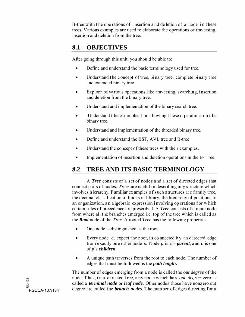
B-tree w ith t he ope rations of i nsertion a nd de letion of a node i n t hese trees. Various examples are used to elaborate the operations of traversing, insertion and deletion from the tree.
8.1 OBJECTIVES
After going through this unit, you should be able to:
• Define and understand the basic terminology used for tree.
• Understand t he c oncept of t ree, bi nary tree, complete bi nary t reeand extended binary tree.
• Explore of va rious operations l ike t raversing, s earching, i nsertionand deletion from the binary tree.
• Understand and implementation of the binary search tree.
• Understand t he e xamples f or s howing t hese o perations i n t hebinary tree.
• Understand and implementation of the threaded binary tree.
• Define and understand the BST, AVL tree and B-tree
• Understand the concept of these trees with their examples.
• Implementation of insertion and deletion operations in the B- Tree.
8.2 TREE AND ITS BASIC TERMINOLOGY
A Tree consists of a set of nodes and a set of directed edges that connect pairs of nodes. Trees are useful in describing any structure which involves h ierarchy. F amiliar ex amples o f such s tructures ar e f amily t ree, the decimal classification of books in library, the hierarchy of positions in an or ganization, a n a lgebraic expression i nvolving op erations f or w hich certain rules of precedence are prescribed. A Tree consists of a main node from where all the branches emerged i.e. top of the tree which is called as the Root node of the Tree. A rooted Tree has the following properties:
• One node is distinguished as the root.
• Every node c, expect t he r oot, i s co nnected b y an d irected edgefrom exactly one other node p. Node p is c’s parent, and c is oneof p’s children.
• A unique path traverses from the root to each node. The number ofedges that must be followed is the path length.
The number of edges emerging from a node is called the out degree of the node. T hus, i n a di rected t ree, a ny nod e w hich ha s out degree zero i s called a terminal node or leaf node. Other nodes those have nonzero out degree are called the branch nodes. The number of edges directing for a PGDCA-107/134
RIL
-102

node is called the in degree of the node. Thus, in a directed tree, any node which has in degree zero is called a root node. It is important to note that every t ree m ust ha ve a t l east one node . A s ingle i solated node i s a lso called as the directed tree.
The level of any node is the length of its path from the root. The level of the root of a directed tree is zero, while the level of any node is equal to its distance from the root.
The Tree with the information of height and depth
In t his given t ree t he r oot node i s A: A’s children ar e B, C, D and E. Because A is the root, i t has no pa rent. All other nodes have parents l ike B’s parent is A. The leaves in this tree are C, F, G, H, I and K. The length of the path from A to K is 3 (edges). The length of the path from A to A is 0 (edges). A tree with N nodes must have N-1 edges because every node except the parent has an incoming edge. The depth of a node is a t ree is the length of the path from the node to the deepest leaf. Thus the height of E is 2. The height of any node is 1 m ore than the height of its maximum height child. Thus, the height of a tree is the height of the root.
Nodes with the same parent a re called siblings. Thus B, C, D and E are siblings. If there is a path from any node u to node v, then u is an ancestor of v and v is a descendant of u. If u ≠ v, then u is a proper ancestor of v and v is a proper descendant of u. The size of a node is t he number of descendants the node has (including the node itself). Thus the size of B is 3, and the size of C is 1. The size of a tree is the size of the root. Thus the size of the given tree is the size of its root A, or 11.
If in a directed tree the out degree of every node is less than or equal to m, then t he t ree i s cal led an m-ary tree. If t he out degree of e very nod e i s
PGDCA-107/135
RIL
-102
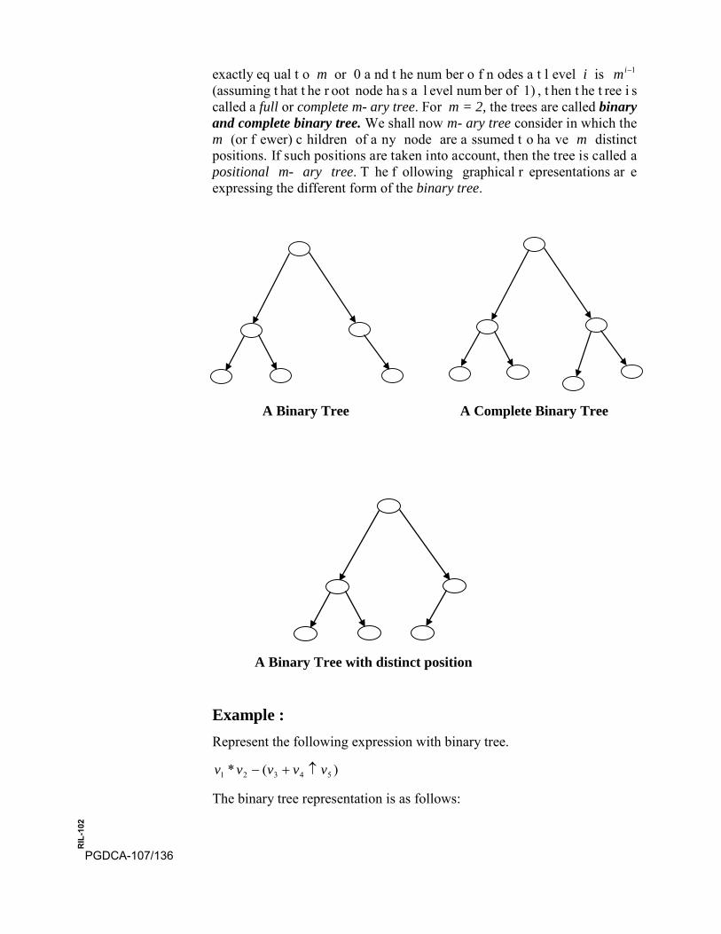
exactly eq ual t o m or 0 a nd t he num ber o f n odes a t l evel i is 1−im (assuming t hat t he r oot node ha s a l evel num ber of 1) , t hen t he t ree i s called a full or complete m- ary tree. For m = 2, the trees are called binary and complete binary tree. We shall now m- ary tree consider in which the m (or f ewer) c hildren of a ny node are a ssumed t o ha ve m distinct positions. If such positions are taken into account, then the tree is called a positional m- ary tree. T he f ollowing graphical r epresentations ar e expressing the different form of the binary tree.
A Binary Tree A Complete Binary Tree
A Binary Tree with distinct position
Example : Represent the following expression with binary tree.
)(* 54321 vvvvv ↑+−
The binary tree representation is as follows:
PGDCA-107/136
RIL
-102
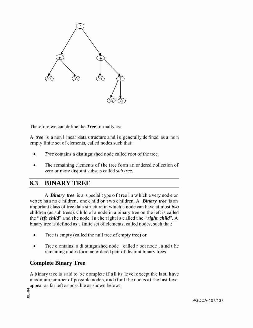
-
* +
v1 v2 v3 ↑
v4 v5
Therefore we can define the Tree formally as:
A tree is a non l inear data s tructure a nd i s generally de fined as a no n empty finite set of elements, called nodes such that:
• Tree contains a distinguished node called root of the tree.
• The remaining e lements of the t ree form an ordered collection ofzero or more disjoint subsets called sub tree.
8.3 BINARY TREE
A Binary tree is a s pecial t ype o f t ree i n w hich e very nod e or vertex ha s no c hildren, one c hild or t wo c hildren. A Binary tree is an important class of tree data structure in which a node can have at most two children (as sub trees). Child of a node in a binary tree on the left is called the “ left child” a nd t he node i n t he r ight i s c alled t he “ right child”. A binary tree is defined as a finite set of elements, called nodes, such that:
• Tree is empty (called the null tree of empty tree) or
• Tree c ontains a di stinguished node called r oot node , a nd t heremaining nodes form an ordered pair of disjoint binary trees.
Complete Binary Tree
A b inary tr ee is s aid to b e complete if a ll its le vel except th e la st, h ave maximum number of possible nodes, and if all the nodes at the last level appear as far left as possible as shown below:
PGDCA-107/137
RIL
-102
PGDCA-107/138
RIL
-102
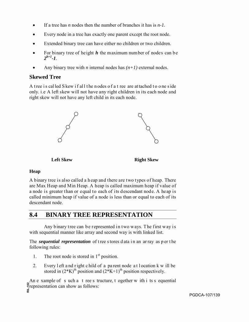
• If a tree has n nodes then the number of branches it has is n-1.
• Every node in a tree has exactly one parent except the root node.
• Extended binary tree can have either no children or two children.
• For binary t ree of height h the maximum number of nodes can be2h+1-1.
• Any binary tree with n internal nodes has (n+1) external nodes.
Skewed Tree A t ree i s cal led S kew i f al l t he n odes o f a t ree are at tached t o o ne s ide only. i.e A left skew will not have any right children in its each node and right skew will not have any left child in its each node.
Left Skew Right Skew
Heap
A binary tree is also called a h eap and there are two types of heap. There are Max Heap and Min Heap. A heap is called maximum heap if value of a node is greater than or equal to each of i ts descendant node. A heap is called minimum heap if value of a node is less than or equal to each of its descendant node.
8.4 BINARY TREE REPRESENTATION
Any binary t ree can be represented in two ways. The f irst way is with sequential manner like array and second way is with linked list.
The sequential representation of t ree s tores d ata i n an ar ray as p er t he following rules:
1. The root node is stored in 1st position.
2. Every l eft a nd r ight c hild of a pa rent node a t l ocation k w ill bestored in (2*K)th position and (2*K+1)th position respectively.
An e xample of s uch a t ree s tructure, t ogether w ith i ts s equential representation can show as follows:
PGDCA-107/139
RIL
-102
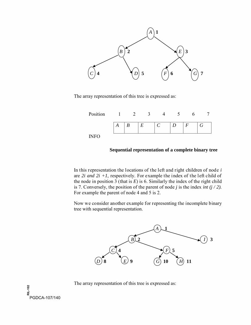
A 1
B 2 E 3
C 4 D 5 F 6 G 7
The array representation of this tree is expressed as:
Position 1 2 3 4 5 6 7
A B E C D F G
INFO
Sequential representation of a complete binary tree
In this representation the locations of the left and right children of node i are 2i and 2i +1, respectively. For example the index of the left child of the node in position 3 (that is E) is 6. Similarly the index of the right child is 7. Conversely, the position of the parent of node j is the index int (j / 2). For example the parent of node 4 and 5 is 2.
Now we consider another example for representing the incomplete binary tree with sequential representation.
A 1
B 2 I 3
C 4 F 5
D 8 E 9 G 10 H 11
The array representation of this tree is expressed as:
PGDCA-107/140
RIL
-102
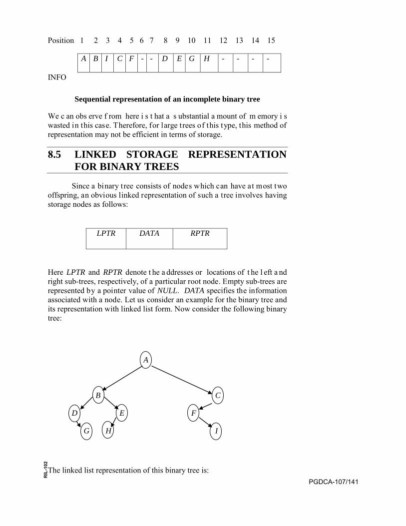
Position 1 2 3 4 5 6 7 8 9 10 11 12 13 14 15
A B I C F - - D E G H - - - -
INFO
Sequential representation of an incomplete binary tree
We c an obs erve f rom here i s t hat a s ubstantial a mount of m emory i s wasted in this case. Therefore, for large trees of this type, this method of representation may not be efficient in terms of storage.
8.5 LINKED STORAGE REPRESENTATION FOR BINARY TREES
Since a binary tree consists of nodes which can have at most two offspring, an obvious linked representation of such a tree involves having storage nodes as follows:
LPTR DATA RPTR
Here LPTR and RPTR denote t he a ddresses or locations of t he l eft a nd right sub-trees, respectively, of a particular root node. Empty sub-trees are represented by a pointer value of NULL. DATA specifies the information associated with a node. Let us consider an example for the binary tree and its representation with linked list form. Now consider the following binary tree:
A
B C
D E F
G H I
The linked list representation of this binary tree is: PGDCA-107/141
RIL
-102
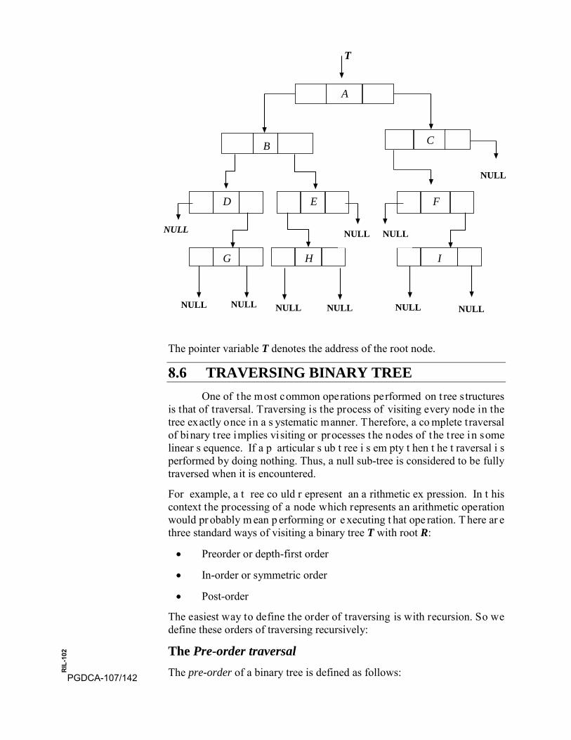
T
The pointer variable T denotes the address of the root node.
8.6 TRAVERSING BINARY TREE One of the most common operations performed on t ree s tructures
is that of traversal. Traversing is the process of visiting every node in the tree exactly once in a s ystematic manner. Therefore, a co mplete traversal of binary t ree implies visiting or processes the nodes of the t ree in some linear s equence. If a p articular s ub t ree i s em pty t hen t he t raversal i s performed by doing nothing. Thus, a null sub-tree is considered to be fully traversed when it is encountered.
For example, a t ree co uld r epresent an a rithmetic ex pression. In t his context the processing of a node which represents an arithmetic operation would pr obably m ean p erforming or e xecuting t hat ope ration. T here ar e three standard ways of visiting a binary tree T with root R:
• Preorder or depth-first order
• In-order or symmetric order
• Post-order
The easiest way to define the order of traversing is with recursion. So we define these orders of traversing recursively:
The Pre-order traversal The pre-order of a binary tree is defined as follows:
A
C B
D E F
G H I
NULL NULL NULL
NULL NULL NULL NULL NULL NULL
NULL
PGDCA-107/142
RIL
-102
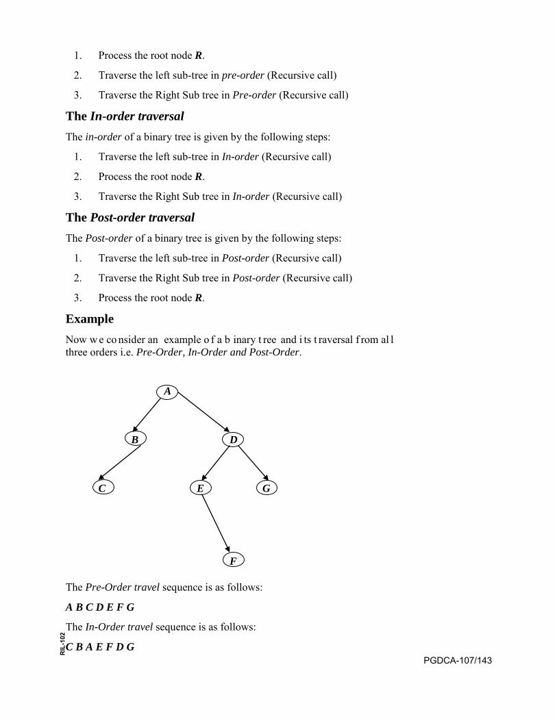
1. Process the root node R.
2. Traverse the left sub-tree in pre-order (Recursive call)
3. Traverse the Right Sub tree in Pre-order (Recursive call)
The In-order traversal The in-order of a binary tree is given by the following steps:
1. Traverse the left sub-tree in In-order (Recursive call)
2. Process the root node R.
3. Traverse the Right Sub tree in In-order (Recursive call)
The Post-order traversal The Post-order of a binary tree is given by the following steps:
1. Traverse the left sub-tree in Post-order (Recursive call)
2. Traverse the Right Sub tree in Post-order (Recursive call)
3. Process the root node R.
Example Now w e co nsider an example o f a b inary t ree and i ts t raversal f rom al l three orders i.e. Pre-Order, In-Order and Post-Order.
A
B D
C E G
F
The Pre-Order travel sequence is as follows:
A B C D E F G
The In-Order travel sequence is as follows:
C B A E F D G PGDCA-107/143
RIL
-102

The Post-Order travel sequence is as follows:
C B F E G D A
Now we can formulate the algorithms for the t raversal. These algorithms can formulate in recursive as well as in iterative manner.
Let us c onsider t he t raversal of bi nary t rees by iterations. S ince i n traversing a tree it is required to descend and subsequently ascend parts of the tree, pointer information which will permit movement up the tree must be temporarily s tored. Because movement up t he t ree must be made in a reverse manner from that taken in descending a tree, a stack is required to save pointer variables as t he t ree i s t raversed. A general al gorithm for a Pre-order traversal of a binary tree using iteration is given as:
Algorithm PREORDER (T): [Given a bi nary tree w hose r oot nod e address is given by a pointer variable T. This method traverses the tree in Pre-Order in i terative manner. S and TOP denote an auxiliary s tack and its associated top index, respectively. The pointer variable P denotes the current node in the tree.]
/* Initialize the pointers */
If (T == NULL)
{
Printf (“Empty tree”)
Return
}
Else {
TOP = 0;
PUSH (S, TOP, T) /* the PUSH is the function call which is already defined in stack previous unit */
}
While (TOP > 0)
{
P = POP (S, TOP) /* get stored address and branch left. The PUSH is the function call which is already defined in stack previous unit */
While (P != NULL)
Printf (DATA (P));
If (RPTR (P) != NULL)
PGDCA-107/144
RIL
-102
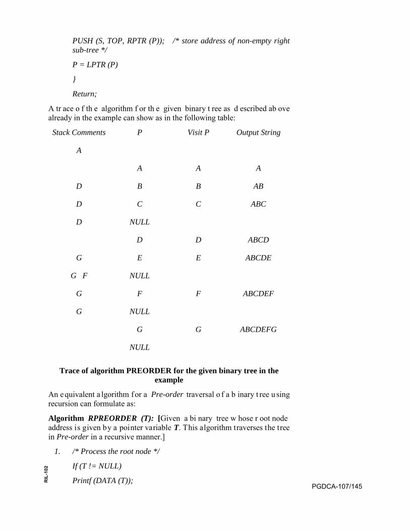
PUSH (S, TOP, RPTR (P)); /* store address of non-empty right sub-tree */
P = LPTR (P)
}
Return;
A tr ace o f th e algorithm f or th e given binary t ree as d escribed ab ove already in the example can show as in the following table:
Stack Comments P Visit P Output String
A
A A A
D B B AB
D C C ABC
D NULL
D D ABCD
G E E ABCDE
G F NULL
G F F ABCDEF
G NULL
G G ABCDEFG
NULL
Trace of algorithm PREORDER for the given binary tree in the example
An e quivalent a lgorithm f or a Pre-order traversal o f a b inary t ree u sing recursion can formulate as:
Algorithm RPREORDER (T): [Given a bi nary tree w hose r oot node address is given by a pointer variable T. This algorithm traverses the tree in Pre-order in a recursive manner.]
1. /* Process the root node */
If (T != NULL)
Printf (DATA (T));PGDCA-107/145
RIL
-102
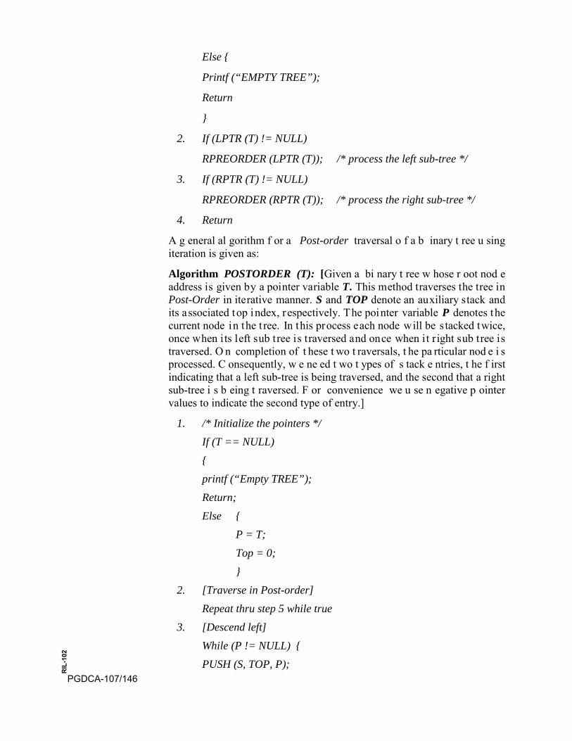
Else {
Printf (“EMPTY TREE”);
Return
}
2. If (LPTR (T) != NULL)
RPREORDER (LPTR (T)); /* process the left sub-tree */
3. If (RPTR (T) != NULL)
RPREORDER (RPTR (T)); /* process the right sub-tree */
4. Return
A g eneral al gorithm f or a Post-order traversal o f a b inary t ree u sing iteration is given as:
Algorithm POSTORDER (T): [Given a bi nary t ree w hose r oot nod e address is given by a pointer variable T. This method traverses the tree in Post-Order in iterative manner. S and TOP denote an auxiliary stack and its associated top index, respectively. The pointer variable P denotes the current node in the t ree. In this process each node will be s tacked twice, once when its left sub tree is traversed and once when it right sub tree is traversed. O n completion of t hese t wo t raversals, t he pa rticular nod e i s processed. C onsequently, w e ne ed t wo t ypes of s tack e ntries, t he f irst indicating that a left sub-tree is being traversed, and the second that a right sub-tree i s b eing t raversed. F or convenience we u se n egative p ointer values to indicate the second type of entry.]
1. /* Initialize the pointers */If (T == NULL){printf (“Empty TREE”);Return;Else {
P = T; Top = 0; }
2. [Traverse in Post-order]Repeat thru step 5 while true
3. [Descend left]While (P != NULL) {PUSH (S, TOP, P);
PGDCA-107/146
RIL
-102
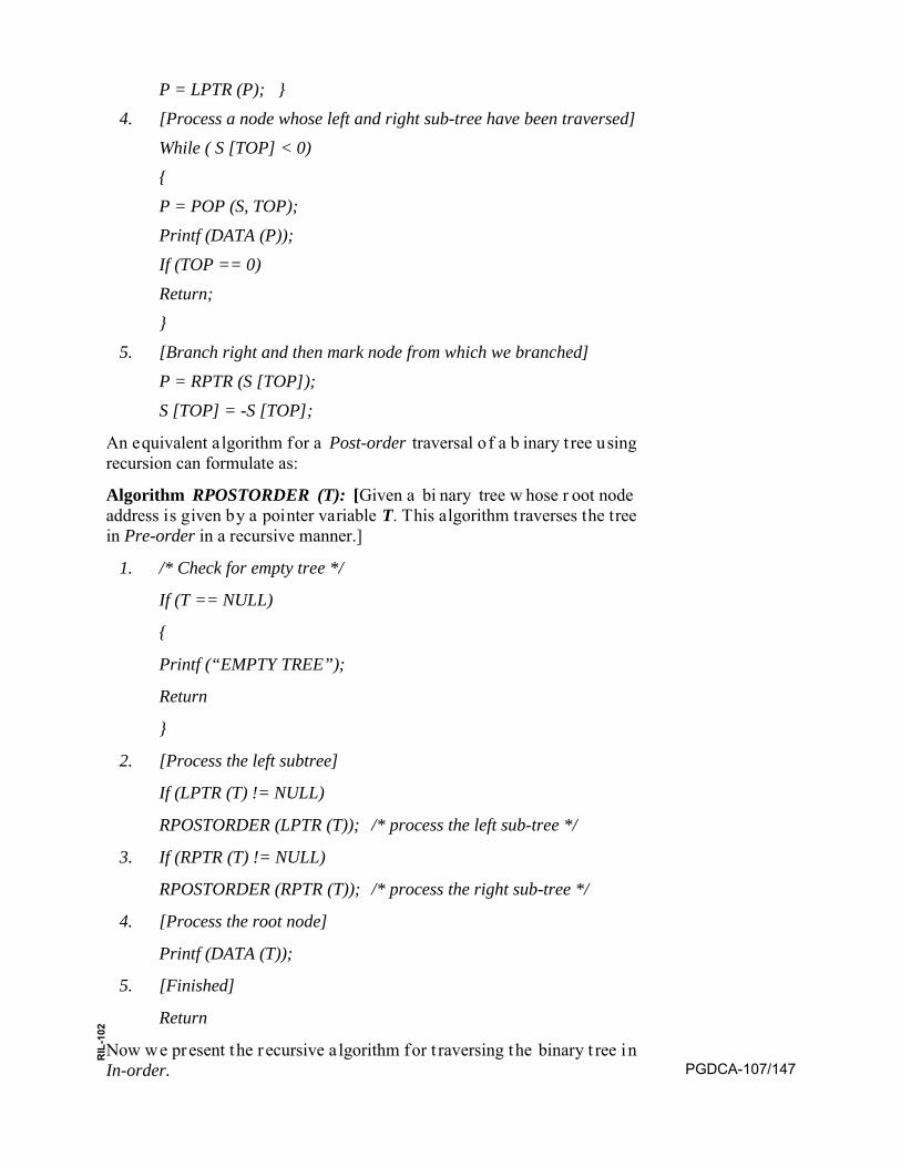
P = LPTR (P); } 4. [Process a node whose left and right sub-tree have been traversed]
While ( S [TOP] < 0){P = POP (S, TOP);Printf (DATA (P));If (TOP == 0)Return;}
5. [Branch right and then mark node from which we branched]P = RPTR (S [TOP]);S [TOP] = -S [TOP];
An equivalent algorithm for a Post-order traversal of a b inary t ree using recursion can formulate as:
Algorithm RPOSTORDER (T): [Given a bi nary tree w hose r oot node address is given by a pointer variable T. This algorithm traverses the tree in Pre-order in a recursive manner.]
1. /* Check for empty tree */
If (T == NULL)
{
Printf (“EMPTY TREE”);
Return
}
2. [Process the left subtree]
If (LPTR (T) != NULL)
RPOSTORDER (LPTR (T)); /* process the left sub-tree */
3. If (RPTR (T) != NULL)
RPOSTORDER (RPTR (T)); /* process the right sub-tree */
4. [Process the root node]
Printf (DATA (T));
5. [Finished]
Return
Now we present the r ecursive a lgorithm for t raversing the binary t ree in In-order. PGDCA-107/147
RIL
-102
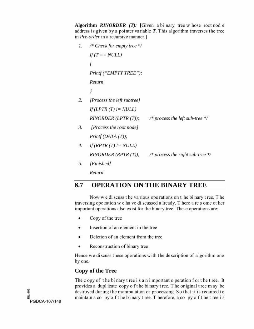
Algorithm RINORDER (T): [Given a bi nary tree w hose root nod e address is given by a pointer variable T. This algorithm traverses the tree in Pre-order in a recursive manner.]
1. /* Check for empty tree */
If (T == NULL)
{
Printf (“EMPTY TREE”);
Return
}
2. [Process the left subtree]
If (LPTR (T) != NULL)
RINORDER (LPTR (T)); /* process the left sub-tree */
3. [Process the root node]
Printf (DATA (T));
4. If (RPTR (T) != NULL)
RINORDER (RPTR (T)); /* process the right sub-tree */
5. [Finished]
Return
8.7 OPERATION ON THE BINARY TREE
Now w e di scuss t he va rious ope rations on t he bi nary t ree. T he traversing ope ration w e ha ve di scussed a lready. T here a re s ome ot her important operations also exist for the binary tree. These operations are:
• Copy of the tree
• Insertion of an element in the tree
• Deletion of an element from the tree
• Reconstruction of binary tree
Hence we di scuss these operations with the description of a lgorithm one by one.
Copy of the Tree The c opy of t he bi nary t ree i s a n i mportant o peration f or t he t ree. It provides a dupl icate copy o f t he bi nary t ree. T he or iginal t ree m ay be destroyed during the manipulation or processing. So that i t is required to maintain a co py o f t he b inary t ree. T herefore, a co py o f t he t ree i s
PGDCA-107/148
RIL
-102
produces be fore s uch pr ocessing be gins. T he f ollowing algorithm generates a copy of a tree.
Algorithm Copy (T) [Given a bi nary t ree w hose r oot node a ddress i d given b y t he poi nter T. T his a lgorithm ge nerates a co py o f t he t ree an d returns the address of its root node. New is a temporary pointer variable.]
1. [Check for the NULL pointer ]
If (T ==NULL)
Return (NULL);
2. [Create a new node]
NEW ⟸NODE;
3. [Copy of the information field]
DATA (NEW) = DATA (T);
4. [Set the structural links]
LPTR (NEW) = COPY (LPTR (T));
RPTR (NEW) = COPY (RPTR (T));
5. [Return address of new node]
Return (NEW);
Insertion in the tree A tree can be created through the repeated use o f an insertion operation. Now we assume that a binary t ree exists. Such a t ree, however, must be constructed. T his construction can b e r ealized b y the r epeated u se o f an insertion operation that adds a new node into an existing tree. For example the in sertion o f a n ode in to a le xically o rdered tr ee mu st ma intain th at ordering. Such an insertion i s pe rformed a t t he l eaf l evel. There a re two cases arise:
1. As a s pecial c ase, a n insertion in to a n e mpty tree r esults inappending the new node as the root of the tree.
2. The m ore general c ase i nvolves i nserting a n ew node i nto anonempty tree. The new node i.e. in lexically ordered tree the newname is first compared with the name of the root node. If the newname l exically precedes t he r oot node , t hen the ne w node i sappended to the tree as a left leaf to the existing tree if the left subtree i s e mpty, ot herwise t he c omparison pr ocess i s r epeated w iththe r oot node of t he l eft s ub t ree. If on t he ot her ha nd, t he ne wname lexically follows the root node name, then the new node i sappended as a r ight leaf to the present t ree i f the r ight sub-tree i sempty, otherwise the comparison process is repeated with the rootnode of the right sub-tree.
PGDCA-107/149
RIL
-102
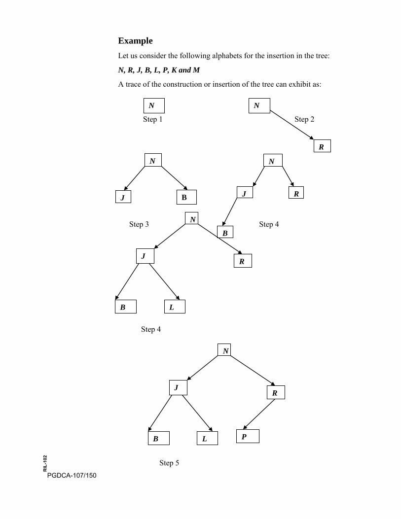
Example Let us consider the following alphabets for the insertion in the tree:
N, R, J, B, L, P, K and M
A trace of the construction or insertion of the tree can exhibit as:
Step 1 Step 2
Step 3 Step 4
Step 4
Step 5
N N
R
N
J B
N
J R
B
N
J
B
R
L
N
J R
B L P
PGDCA-107/150
RIL
-102
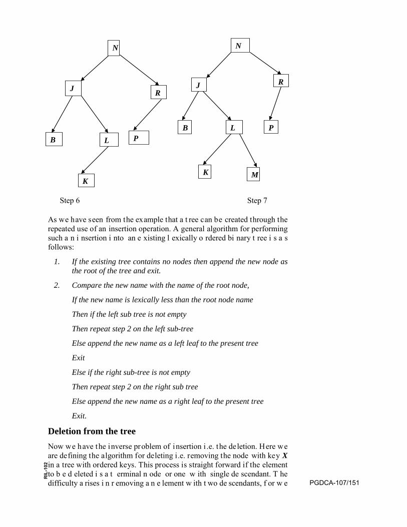
Step 6 Step 7
As we have seen from the example that a t ree can be created through the repeated use of an insertion operation. A general algorithm for performing such a n i nsertion i nto an e xisting l exically o rdered bi nary t ree i s a s follows:
1. If the existing tree contains no nodes then append the new node asthe root of the tree and exit.
2. Compare the new name with the name of the root node,
If the new name is lexically less than the root node name
Then if the left sub tree is not empty
Then repeat step 2 on the left sub-tree
Else append the new name as a left leaf to the present tree
Exit
Else if the right sub-tree is not empty
Then repeat step 2 on the right sub tree
Else append the new name as a right leaf to the present tree
Exit.
Deletion from the tree Now we have the inverse problem of insertion i .e. the deletion. Here we are defining the algorithm for deleting i.e. removing the node with key X in a tree with ordered keys. This process is straight forward if the element to b e d eleted i s a t erminal n ode or one w ith single de scendant. T he difficulty a rises i n r emoving a n e lement w ith t wo de scendants, f or w e
N
J R
B L P
K
N
J R
B L P
K M
PGDCA-107/151
RIL
-102
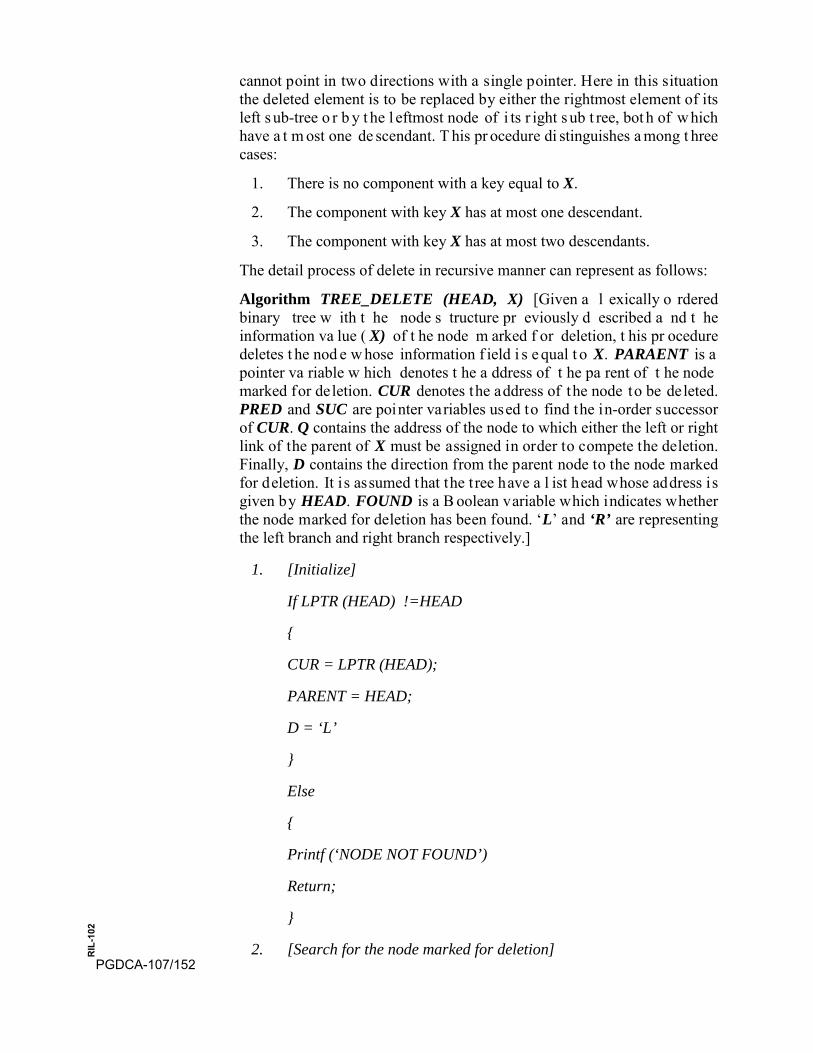
cannot point in two directions with a single pointer. Here in this situation the deleted element is to be replaced by either the rightmost element of its left s ub-tree o r b y t he l eftmost node of i ts r ight s ub t ree, bot h of w hich have a t m ost one de scendant. T his pr ocedure di stinguishes a mong t hree cases:
1. There is no component with a key equal to X.
2. The component with key X has at most one descendant.
3. The component with key X has at most two descendants.
The detail process of delete in recursive manner can represent as follows:
Algorithm TREE_DELETE (HEAD, X) [Given a l exically o rdered binary tree w ith t he node s tructure pr eviously d escribed a nd t he information va lue ( X) of t he node m arked f or deletion, t his pr ocedure deletes t he nod e w hose information f ield i s e qual t o X. PARAENT is a pointer va riable w hich denotes t he a ddress of t he pa rent of t he node marked for deletion. CUR denotes the address of the node to be deleted. PRED and SUC are pointer variables used to find the in-order successor of CUR. Q contains the address of the node to which either the left or right link of the parent of X must be assigned in order to compete the deletion. Finally, D contains the direction from the parent node to the node marked for deletion. It is assumed that the t ree have a l ist head whose address is given by HEAD. FOUND is a B oolean variable which indicates whether the node marked for deletion has been found. ‘L’ and ‘R’ are representing the left branch and right branch respectively.]
1. [Initialize]
If LPTR (HEAD) !=HEAD
{
CUR = LPTR (HEAD);
PARENT = HEAD;
D = ‘L’
}
Else
{
Printf (‘NODE NOT FOUND’)
Return;
}
2. [Search for the node marked for deletion]PGDCA-107/152
RIL
-102
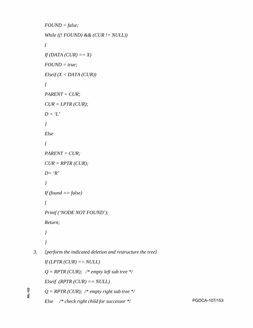
FOUND = false;
While ((! FOUND) && (CUR != NULL))
{
If (DATA (CUR) == X)
FOUND = true;
Elseif (X < DATA (CUR))
{
PARENT = CUR;
CUR = LPTR (CUR);
D = ‘L’
}
Else
{
PARENT = CUR;
CUR = RPTR (CUR);
D= ‘R’
}
If (found == false)
{
Printf (‘NODE NOT FOUND’);
Return;
}
}
3. [perform the indicated deletion and restructure the tree]
If (LPTR (CUR) == NULL)
Q = RPTR (CUR); /* empty left sub tree */
Elseif (RPTR (CUR) == NULL)
Q = RPTR (CUR); /* empty right sub tree */
Else /* check right child for successor */ PGDCA-107/153
RIL
-102
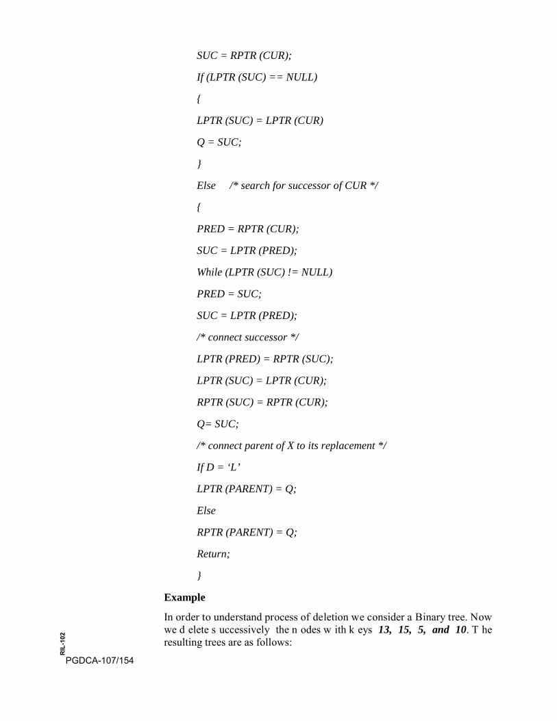
SUC = RPTR (CUR);
If (LPTR (SUC) == NULL)
{
LPTR (SUC) = LPTR (CUR)
Q = SUC;
}
Else /* search for successor of CUR */
{
PRED = RPTR (CUR);
SUC = LPTR (PRED);
While (LPTR (SUC) != NULL)
PRED = SUC;
SUC = LPTR (PRED);
/* connect successor */
LPTR (PRED) = RPTR (SUC);
LPTR (SUC) = LPTR (CUR);
RPTR (SUC) = RPTR (CUR);
Q= SUC;
/* connect parent of X to its replacement */
If D = ‘L’
LPTR (PARENT) = Q;
Else
RPTR (PARENT) = Q;
Return;
}
Example
In order to understand process of deletion we consider a Binary tree. Now we d elete s uccessively the n odes w ith k eys 13, 15, 5, and 10. T he resulting trees are as follows:
PGDCA-107/154
RIL
-102
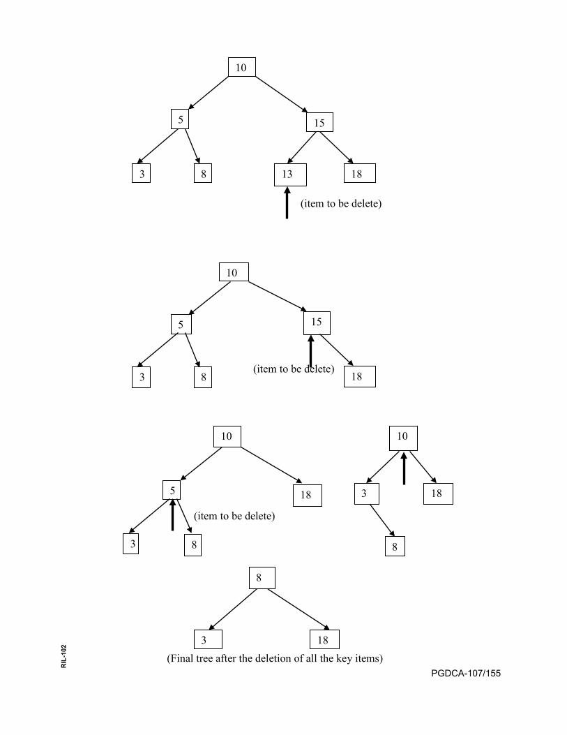
(item to be delete)
(item to be delete)
(item to be delete)
(Final tree after the deletion of all the key items)
10
5 15
3 8 13 18
10
5 15
3 8 18
10
5
3 8
18
10
3 18
8
8
3 18
PGDCA-107/155
RIL
-102
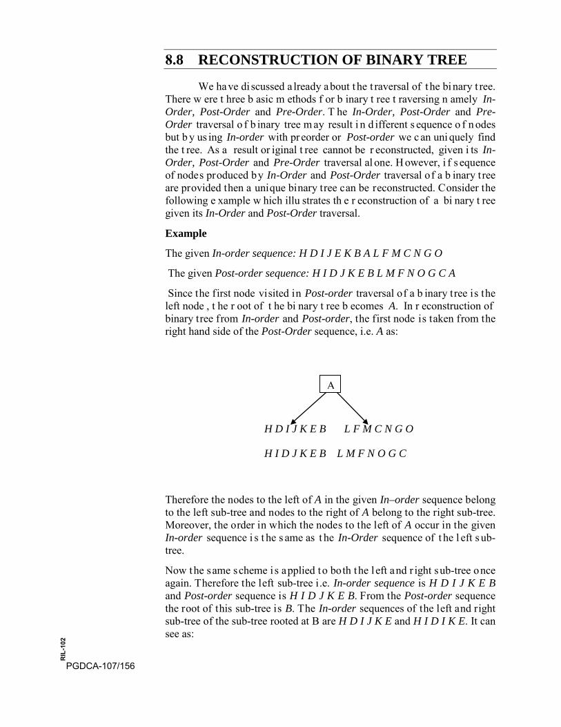
8.8 RECONSTRUCTION OF BINARY TREE
We have di scussed a lready about t he t raversal of t he binary t ree. There w ere t hree b asic m ethods f or b inary t ree t raversing n amely In-Order, Post-Order and Pre-Order. T he In-Order, Post-Order and Pre-Order traversal o f b inary tree m ay result i n d ifferent s equence o f n odes but b y us ing In-order with pr eorder or Post-order we c an uni quely find the t ree. As a result or iginal t ree cannot be r econstructed, given i ts In-Order, Post-Order and Pre-Order traversal al one. H owever, i f s equence of nodes produced by In-Order and Post-Order traversal of a b inary tree are provided then a unique binary tree can be reconstructed. Consider the following e xample w hich illu strates th e r econstruction of a bi nary t ree given its In-Order and Post-Order traversal.
Example
The given In-order sequence: H D I J E K B A L F M C N G O
The given Post-order sequence: H I D J K E B L M F N O G C A
Since the first node visited in Post-order traversal of a b inary tree is the left node , t he r oot of t he bi nary t ree b ecomes A. In r econstruction of binary tree from In-order and Post-order, the first node is taken from the right hand side of the Post-Order sequence, i.e. A as:
H D I J K E B L F M C N G O
H I D J K E B L M F N O G C
Therefore the nodes to the left of A in the given In–order sequence belong to the left sub-tree and nodes to the right of A belong to the right sub-tree. Moreover, the order in which the nodes to the left of A occur in the given In-order sequence i s t he s ame as t he In-Order sequence of t he l eft s ub-tree.
Now the same scheme i s applied to both the left and r ight sub-tree once again. Therefore the left sub-tree i.e. In-order sequence is H D I J K E B and Post-order sequence is H I D J K E B. From the Post-order sequence the root of this sub-tree is B. The In-order sequences of the left and right sub-tree of the sub-tree rooted at B are H D I J K E and H I D I K E. It can see as:
A
PGDCA-107/156
RIL
-102
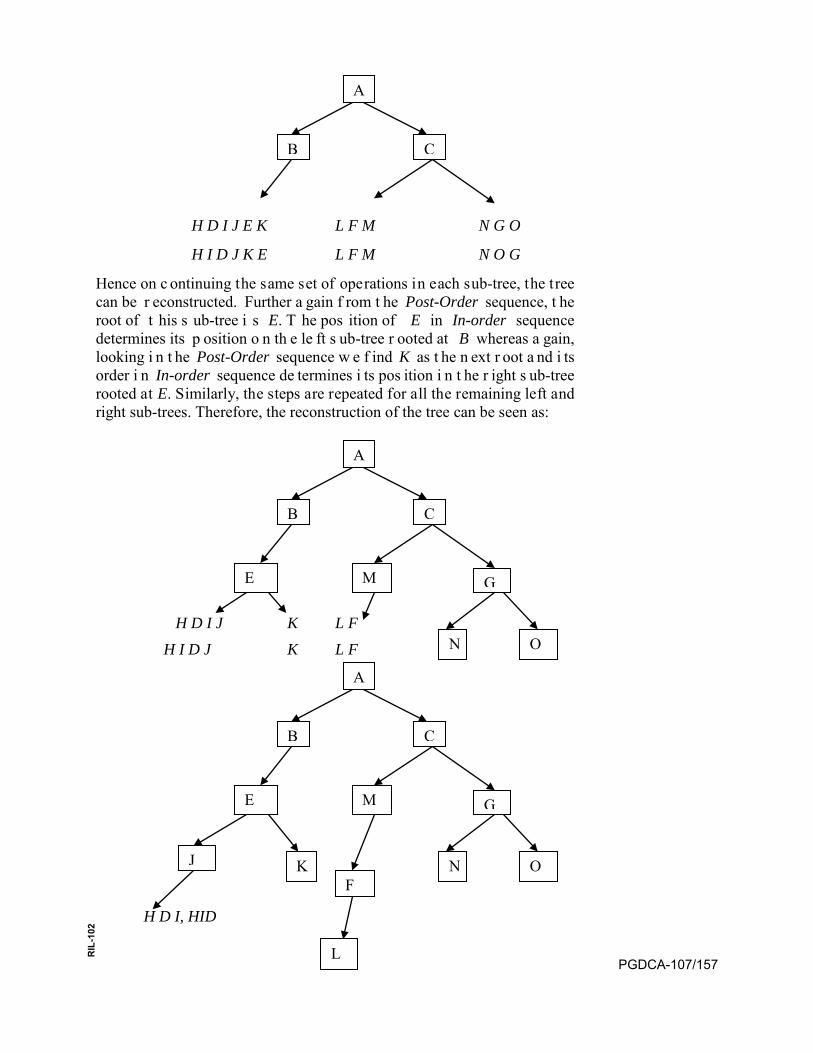
H D I J E K L F M N G O
H I D J K E L F M N O G
Hence on c ontinuing the same set of operations in each sub-tree, the tree can be r econstructed. Further a gain f rom t he Post-Order sequence, t he root of t his s ub-tree i s E. T he pos ition of E in In-order sequence determines its p osition o n th e le ft s ub-tree r ooted at B whereas a gain, looking i n t he Post-Order sequence w e f ind K as t he n ext r oot a nd i ts order i n In-order sequence de termines i ts pos ition i n t he r ight s ub-tree rooted at E. Similarly, the steps are repeated for all the remaining left and right sub-trees. Therefore, the reconstruction of the tree can be seen as:
H D I J K L F H I D J K L F
H D I, HID
A
B C
A
B C
E M G
N O
A
B C
E M G
N O J K F
L PGDCA-107/157
RIL
-102
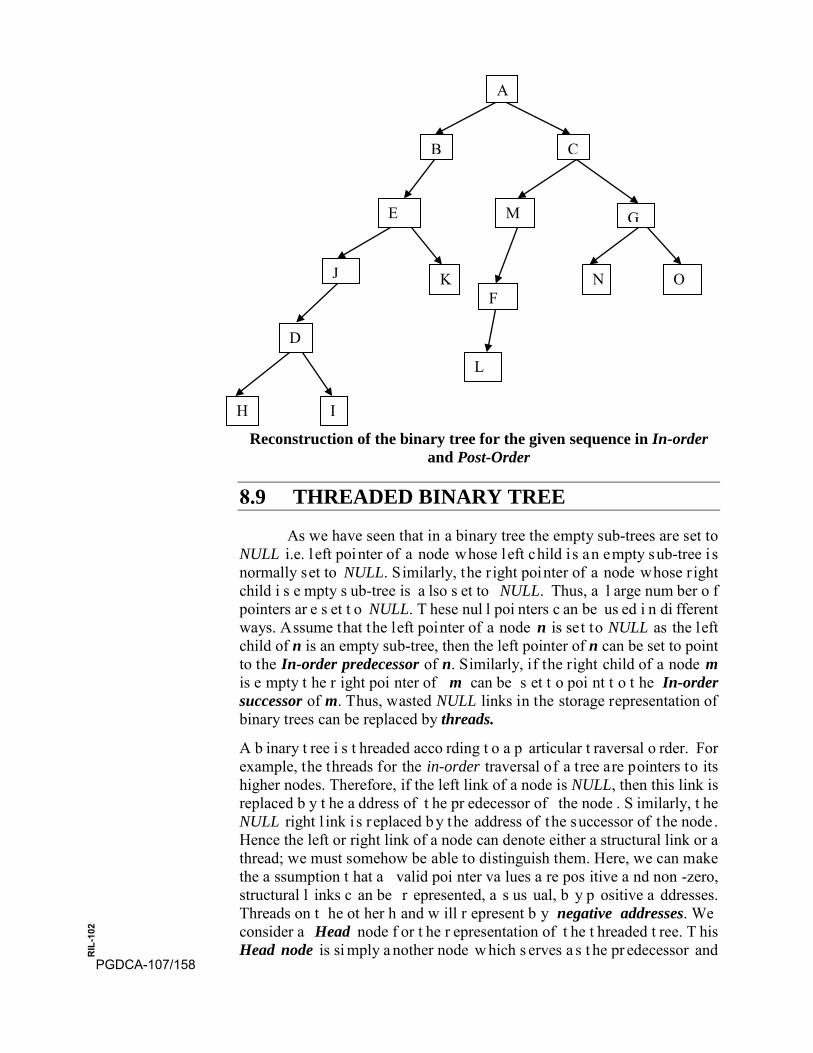
Reconstruction of the binary tree for the given sequence in In-order and Post-Order
8.9 THREADED BINARY TREE
As we have seen that in a binary tree the empty sub-trees are set to NULL i.e. l eft pointer of a node whose left child i s an empty sub-tree i s normally set to NULL. Similarly, the r ight pointer of a node whose r ight child i s e mpty s ub-tree is a lso s et to NULL. Thus, a l arge num ber o f pointers ar e s et t o NULL. T hese nul l poi nters c an be us ed i n di fferent ways. Assume that the left pointer of a node n is set to NULL as the left child of n is an empty sub-tree, then the left pointer of n can be set to point to the In-order predecessor of n. Similarly, if the right child of a node m is e mpty t he r ight poi nter of m can be s et t o poi nt t o t he In-order successor of m. Thus, wasted NULL links in the storage representation of binary trees can be replaced by threads.
A b inary t ree i s t hreaded acco rding t o a p articular t raversal o rder. For example, the threads for the in-order traversal of a tree are pointers to its higher nodes. Therefore, if the left link of a node is NULL, then this link is replaced b y t he a ddress of t he pr edecessor of the node . S imilarly, t he NULL right l ink i s replaced b y the address of the successor of the node. Hence the left or right link of a node can denote either a structural link or a thread; we must somehow be able to distinguish them. Here, we can make the a ssumption t hat a valid poi nter va lues a re pos itive a nd non -zero, structural l inks c an be r epresented, a s us ual, b y p ositive a ddresses. Threads on t he ot her h and w ill r epresent b y negative addresses. We consider a Head node f or t he r epresentation of t he t hreaded t ree. T his Head node is si mply a nother node w hich s erves a s t he pr edecessor and
A
B C
E M G
N O J K F
L
D
I H
PGDCA-107/158
RIL
-102

successor of the first and last tree nodes with respect to in-order traversal. The empty threaded binary tree can represent as:
HEAD
Here the dashed ar row denotes a thread link. The t ree i s at tached to the left branch of the Head node making the pointer to the root node o f the tree i .e. LPTR (HEAD). T he t hreading of t he binary tree f or in-order traversal is given as:
HEAD
8.10 BINARY SEARCH TREE
When we place constraints on how data elements can be stored in the tree, the items must be stored in such a way that the key values in the left sub-tree of the root are less than the key value of the root, and the key
A
B
C
D
E G
F
PGDCA-107/159
RIL
-102
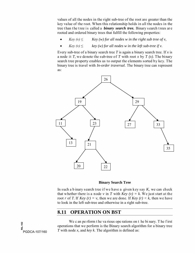
values of all the nodes in the right sub-tree of the root are greater than the key value of the root. When this relationship holds in all the nodes in the tree t han t he t ree i s called a binary search tree. Binary s earch t rees ar e rooted and ordered binary trees that fulfill the following properties:
• Key (v) ≤ Key (w) for all nodes w in the right sub tree of v,
• Key (v) ≤ key (w) for all nodes w in the left sub-tree if v. Every sub-tree of a binary search tree T is again a binary search tree. If x is a node i t T, we denote the sub-tree of T with root x by T (x). The binary search tree property enables us to output the elements sorted by key. The binary tree is travel with In-order traversal. The binary tree can represent as:
Binary Search Tree
In such a b inary search t ree i f we have a given key say K, we can check that whether there is a node v in T with Key (v) = k. We just start at the root r of T. If Key (r) = v, then we are done. If Key (r) < k, then we have to look in the left sub-tree and otherwise in a right sub-tree.
8.11 OPERATION ON BST
We c an pe rform t he va rious ope rations on t he bi nary. T he f irst operations that we perform is the Binary search algorithm for a binary tree T with node x, and key k. The algorithm is defined as:
26
19
11 23
13
29
27 33
35 21
20 22
PGDCA-107/160
RIL
-102
Algorithm BST-Search [This algorithm considers the two inputs. The first input is the node x and the second input is the value of the key say k. This algorithm returns a node y if Key (y) = k if such a y exists, otherwise it returns NULL.]
if ((x == NULL) ||( k = key [x]))
return (x);
if (k < Key (y))
return (BST-search (LPTR (x), k));
else
return (BST-search (RPTR (x), k));
The second operation that we perform is to find the minimum in a binary search tree. This operation is performed by always going to the left child until we reach a node that has no left child. Now we present the algorithm to determine the minimum in a binary search tree
Algorithm BST-minimum [This algorithm returns a node that has the minimum key. Here we consider the input a node x in a binary tree T. The output of the algorithm is a node in T (x) with minimum key.]
If (LPTR (x) != NULL)
Return (BST-minimum (LPTR (x));
Return (x);
The ot her ope ration t hat w e pe rform on t he BST i s t o de termine t he successor of the given node x. This means that we are looking for the node with smallest key that is greater than K (x). This successor is completely determined by the position in the tree, so we can find it without comparing any elements. If a n ode x has a right child, that is RPTR (v) ≠NULL, then the successor simply is the node in T (RPTR (x)) with minimum key. If x does not have a right child, then the successor of x is the lowest ancestor of x that h as a l eft ch ild t hat i s al so an an cestor o f x. BS T-successor computes the successor of a node x. The second part deals with the case that x has no r ight child. We go up t he paths from x to the root and y is always the parent of x. We stop when either y = NULL or x = LPTR (y). Now w e pr esent t he a lgorithm f or d etermining t he s uccessor of a given node from the binary search tree.
Algorithm BST-successor [This algorithm returns the successor of a given node x in a binary search tree T. The input to this algorithm is the node x for the given binary search tree. The output of this algorithm is the successor of node x, if x has it, otherwise it returns the value NULL.]
If (RPTR (x) != NULL) Return (BST-minimum (RPTR (x)); y= parent (x); PGDCA-107/161
RIL
-102
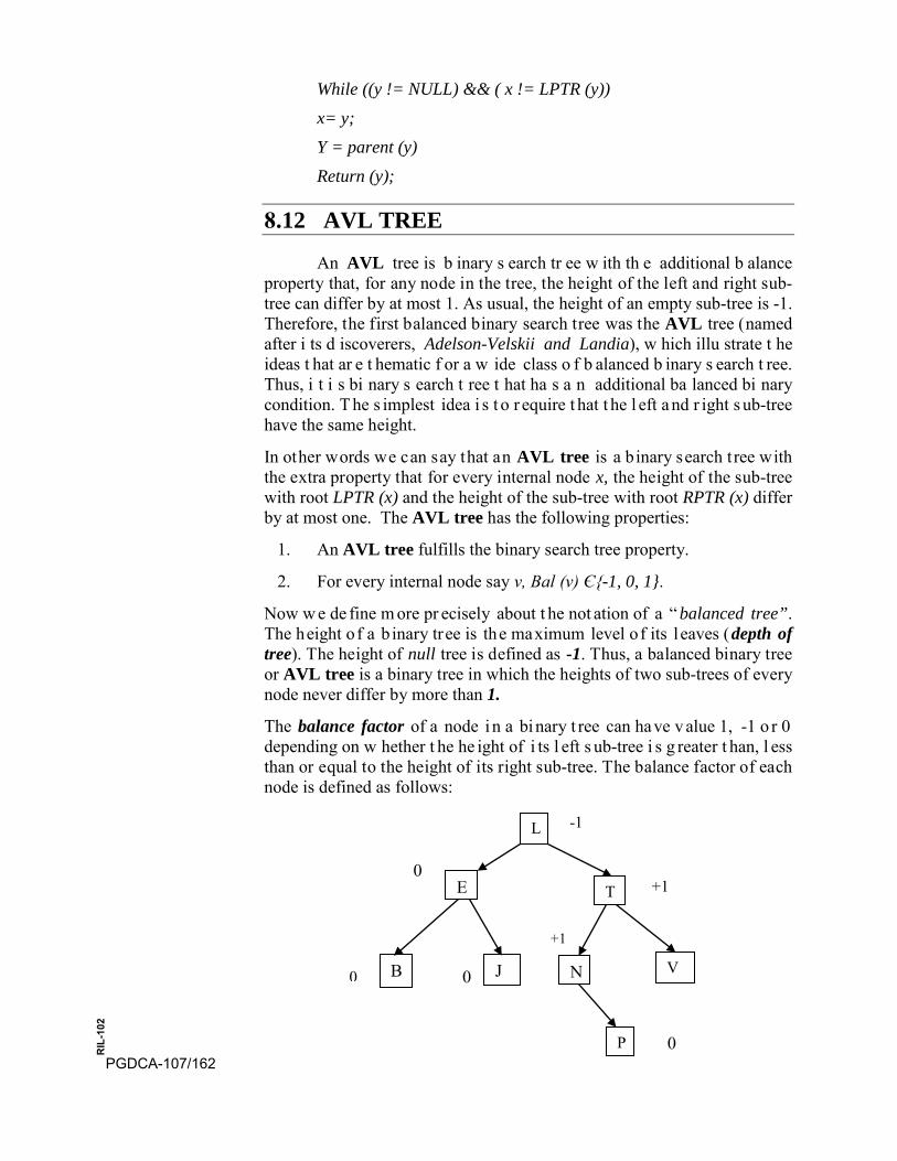
While ((y != NULL) && ( x != LPTR (y)) x= y; Y = parent (y) Return (y);
8.12 AVL TREE
An AVL tree is b inary s earch tr ee w ith th e additional b alance property that, for any node in the tree, the height of the left and right sub-tree can differ by at most 1. As usual, the height of an empty sub-tree is -1. Therefore, the first balanced binary search tree was the AVL tree (named after i ts d iscoverers, Adelson-Velskii and Landia), w hich illu strate t he ideas t hat ar e t hematic f or a w ide class o f b alanced b inary s earch t ree. Thus, i t i s bi nary s earch t ree t hat ha s a n additional ba lanced bi nary condition. T he s implest idea i s t o r equire t hat t he l eft a nd r ight s ub-tree have the same height.
In other words we can say that an AVL tree is a binary search tree with the extra property that for every internal node x, the height of the sub-tree with root LPTR (x) and the height of the sub-tree with root RPTR (x) differ by at most one. The AVL tree has the following properties:
1. An AVL tree fulfills the binary search tree property.
2. For every internal node say v, Bal (v) Є{-1, 0, 1}.
Now w e de fine m ore pr ecisely about t he not ation of a “ balanced tree”. The height of a b inary tree is the maximum level of its l eaves (depth of tree). The height of null tree is defined as -1. Thus, a balanced binary tree or AVL tree is a binary tree in which the heights of two sub-trees of every node never differ by more than 1.
The balance factor of a node in a binary t ree can have v alue 1, -1 o r 0 depending on w hether t he he ight of i ts l eft s ub-tree i s g reater t han, l ess than or equal to the height of its right sub-tree. The balance factor of each node is defined as follows:
L
E T
B NJ V
P
-1
0
0 0
+1
+1
0PGDCA-107/162
RIL
-102
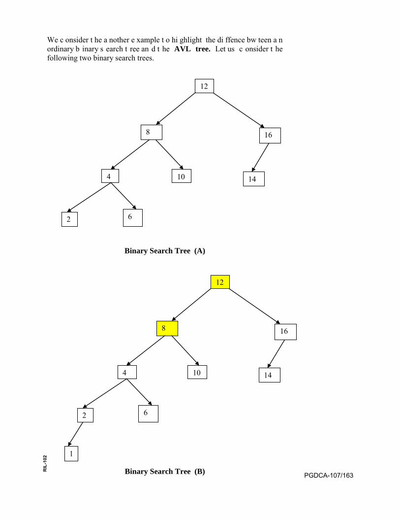
We c onsider t he a nother e xample t o hi ghlight the di ffence bw teen a n ordinary b inary s earch t ree an d t he AVL tree. Let us c onsider t he following two binary search trees.
Binary Search Tree (A)
Binary Search Tree (B)
12
8
4 10
6
16
14
2
12
8
4 10
6
16
14
2
1
PGDCA-107/163
RIL
-102
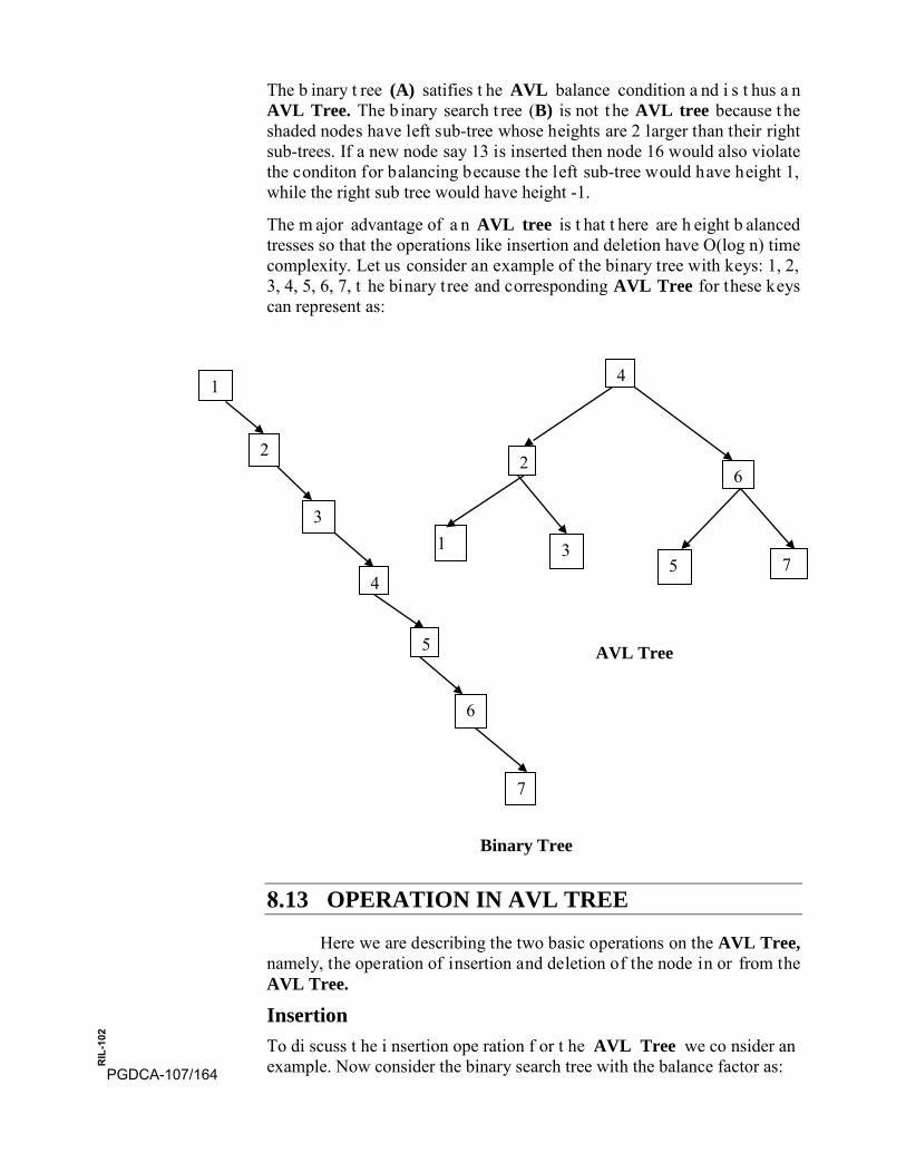
The b inary t ree (A) satifies t he AVL balance condition a nd i s t hus a n AVL Tree. The b inary search t ree (B) is not t he AVL tree because t he shaded nodes have left sub-tree whose heights are 2 larger than their right sub-trees. If a new node say 13 is inserted then node 16 would also violate the conditon for balancing because the left sub-tree would have height 1, while the right sub tree would have height -1.
The m ajor advantage of a n AVL tree is t hat t here are h eight b alanced tresses so that the operations like insertion and deletion have O(log n) time complexity. Let us consider an example of the binary tree with keys: 1, 2, 3, 4, 5, 6, 7, t he binary tree and corresponding AVL Tree for these keys can represent as:
AVL Tree
Binary Tree
8.13 OPERATION IN AVL TREE
Here we are describing the two basic operations on the AVL Tree, namely, the operation of insertion and deletion of the node in or from the AVL Tree.
Insertion To di scuss t he i nsertion ope ration f or t he AVL Tree we co nsider an example. Now consider the binary search tree with the balance factor as:
1
2
3
4
5
6
7
4
26
1 3 5 7
PGDCA-107/164
RIL
-102
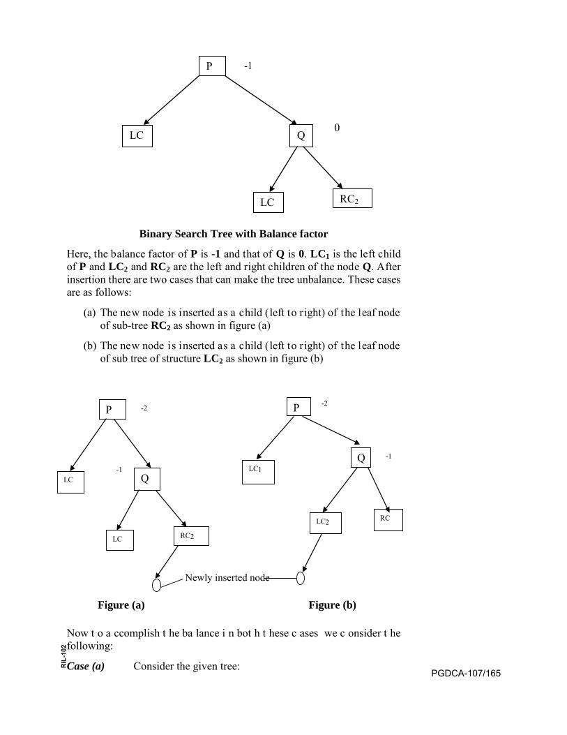
Binary Search Tree with Balance factor
Here, the balance factor of P is -1 and that of Q is 0. LC1 is the left child of P and LC2 and RC2 are the left and right children of the node Q. After insertion there are two cases that can make the tree unbalance. These cases are as follows:
(a) The new node is inserted as a child (left to right) of the leaf node of sub-tree RC2 as shown in figure (a)
(b) The new node is inserted as a child (left to right) of the leaf node of sub tree of structure LC2 as shown in figure (b)
Figure (a) Figure (b)
Now t o a ccomplish t he ba lance i n bot h t hese c ases we c onsider t he following:
Case (a) Consider the given tree:
P
LC
RC2
Q
LC
-1
0
P
LC
RC2
Q
LC
-2
-1
Newly i nserted node
P
LC1 Q
LC2 RC
-2
-1
PGDCA-107/165
RIL
-102
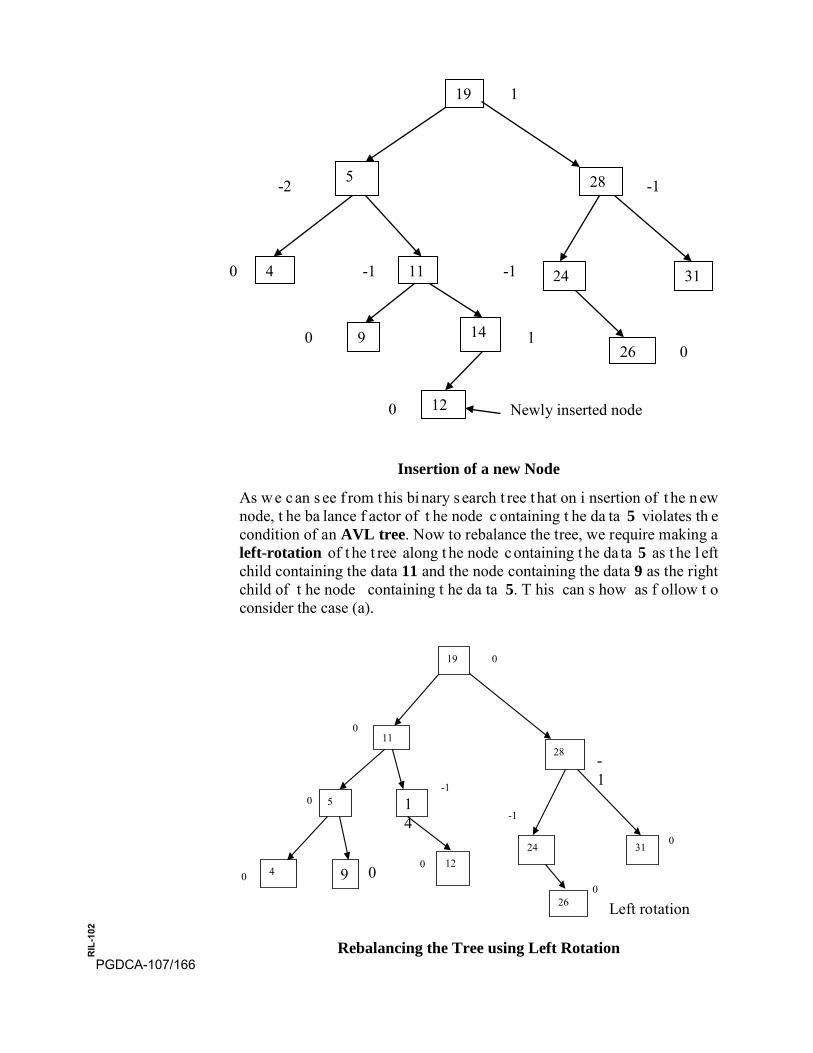
Insertion of a new Node
As w e c an s ee f rom t his bi nary s earch t ree t hat on i nsertion of t he n ew node, t he ba lance f actor of t he node c ontaining t he da ta 5 violates th e condition of an AVL tree. Now to rebalance the tree, we require making a left-rotation of t he t ree along t he node c ontaining t he da ta 5 as t he l eft child containing the data 11 and the node containing the data 9 as the right child of t he node containing t he da ta 5. T his can s how as f ollow t o consider the case (a).
Rebalancing the Tree using Left Rotation
19
5
4 11
14
28
24
9
31
26
12 Newly inserted node 0
0 1 0
-1 -10
-2 -1
1
19
11
5 14
12
28
24
9
31
26
4
Left rotation
0 0 0
0
0
-1
-1 0
0
-1
0
PGDCA-107/166
RIL
-102
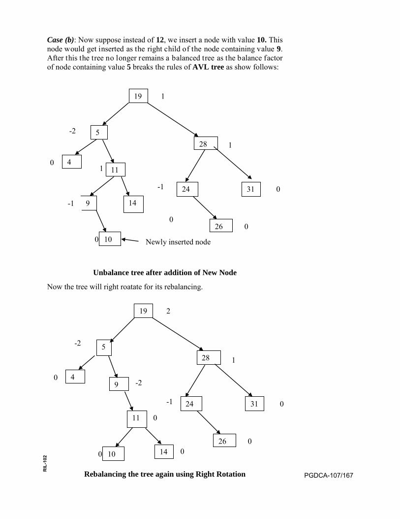
Case (b): Now suppose instead of 12, we insert a node with value 10. This node would get inserted as the right child of the node containing value 9. After this the tree no longer remains a balanced tree as the balance factor of node containing value 5 breaks the rules of AVL tree as show follows:
Unbalance tree after addition of New Node
Now the tree will right roatate for its rebalancing.
Rebalancing the tree again using Right Rotation
19
5
411
14
28
24
9
31
2610 Newly inserted node 0
-1
0 0
0 -1
10
-2
1
1
19
5
49
11
28
24
14
31
2610 0 0
0
0
0 -1
-20
-2
1
2
PGDCA-107/167
RIL
-102
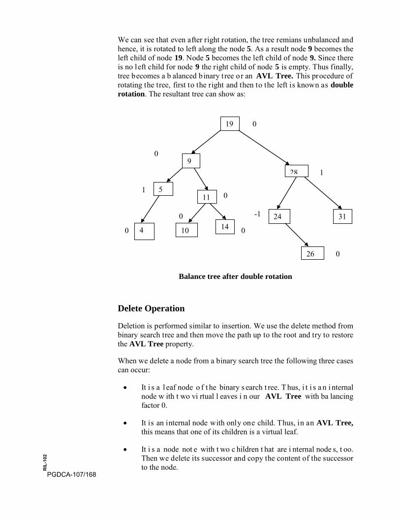
We can see that even after right rotation, the tree remians unbalanced and hence, it is rotated to left along the node 5. As a result node 9 becomes the left child of node 19. Node 5 becomes the left child of node 9. Since there is no left child for node 9 the right child of node 5 is empty. Thus finally, tree becomes a b alanced binary t ree or an AVL Tree. This procedure of rotating the tree, first to the right and then to the left is known as double rotation. The resultant tree can show as:
Balance tree after double rotation
Delete Operation
Deletion is performed similar to insertion. We use the delete method from binary search tree and then move the path up to the root and try to restore the AVL Tree property.
When we delete a node from a binary search tree the following three cases can occur:
• It i s a l eaf node o f t he binary s earch t ree. T hus, i t i s a n i nternalnode w ith t wo vi rtual l eaves i n our AVL Tree with ba lancingfactor 0.
• It is an internal node with only one child. Thus, in an AVL Tree,this means that one of its children is a virtual leaf.
• It i s a node not e with t wo c hildren t hat are i nternal node s, t oo.Then we delete its successor and copy the content of the successorto the node.
19
9
511
4
28
24 14
31
26
10
0
0 0
0
-1
01
0
1
0
PGDCA-107/168
RIL
-102
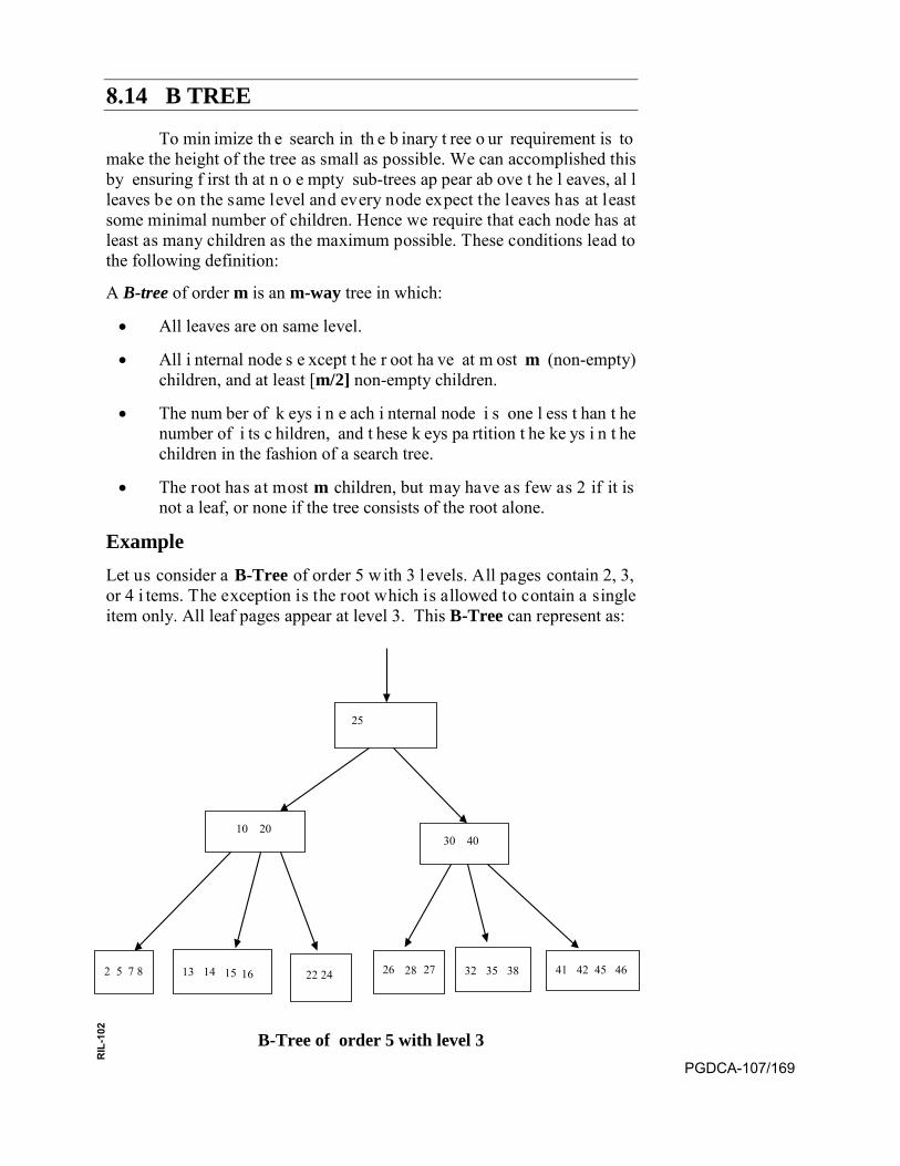
8.14 B TREE
To min imize th e search in th e b inary t ree o ur requirement is to make the height of the tree as small as possible. We can accomplished this by ensuring f irst th at n o e mpty sub-trees ap pear ab ove t he l eaves, al l leaves be on the same level and every node expect the leaves has at least some minimal number of children. Hence we require that each node has at least as many children as the maximum possible. These conditions lead to the following definition:
A B-tree of order m is an m-way tree in which:
• All leaves are on same level.
• All i nternal node s e xcept t he r oot ha ve at m ost m (non-empty)children, and at least [m/2] non-empty children.
• The num ber of k eys i n e ach i nternal node i s one l ess t han t henumber of i ts c hildren, and t hese k eys pa rtition t he ke ys i n t hechildren in the fashion of a search tree.
• The root has at most m children, but may have as few as 2 if it isnot a leaf, or none if the tree consists of the root alone.
Example Let us consider a B-Tree of order 5 with 3 l evels. All pages contain 2, 3, or 4 i tems. The exception is the root which is allowed to contain a single item only. All leaf pages appear at level 3. This B-Tree can represent as:
B-Tree of order 5 with level 3
25
10 20 30 40
2 5 7 8 13 14 15 16 22 24 26 27 28 32 35 38 41 42 45 46
PGDCA-107/169
RIL
-102

8.15 INSERTION IN A B-TREE The B-Tree are not allowed to grow at their l eaves instead they
are forced t o grow at t he r oot. T he general m ethod of i nsertion i s a s follows: • First a search is made to see if the new key is the tree. This search
will terminate in failure at a leaf. • The new key is added to the leaf node. If the node was not
previously full, then insertion is finished. • When a key is added to a full node, then the nodes split into two
nodes on the same level except that the median key is not put into either of the new nodes but instead sent up the tree to be inserted into the parent node.
• When a search is later made through a t ree, a comparison with themedian key will serve to direct the search into proper sub-tree.
• When a key is added to full root, then the root splits into two andthe median key sent upward becomes a new root.
Example Now we consider an example to understand the process of insertion in the B-Tree. The following keys are inserted into the B-Tree of order 5. a g f b k d m j e s i r x c l n t u p The first four keys will insert into one node, as follows:
1. a g f b:a
a g
a f g
a b f g
The keys are stored into proper order as they inserted.
2. k :
f
a b k g PGDCA-107/170
RIL
-102

Now t he i nsertion of k ey k causes t he node t o s plit i nto t wo a nd t he median key f moves up to enter a new node.
3. d, h, m:
f
Since t he s plit node s a re now onl y ha lf full, t he ne xt t hree ke ys can b e inserted w ithout di fficulty. However, t hese s imple i nsertions c an r equire rearrangement of keys within a node.
4. j:
f j
The next insertion j again splits a node and this time it is j itself that is the median key and therefore moves up to join f in the root.
5. e s i r :
f j
6. x :
f j
r
b d h g a k m
b d h g a k m
d e h g b k m a i r s
k m g h i s x a b c d.PGDCA-107/171
RIL
-102
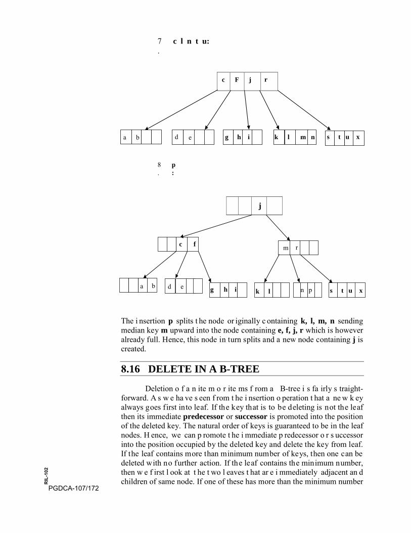
7.
c l n t u:
c F j r
8.
p:
j
The i nsertion p splits t he node or iginally c ontaining k, l, m, n sending median key m upward into the node containing e, f, j, r which is however already full. Hence, this node in turn splits and a new node containing j is created.
8.16 DELETE IN A B-TREE
Deletion o f a n ite m o r ite ms f rom a B-tree i s fa irly s traight-forward. A s w e ha ve s een f rom t he i nsertion o peration t hat a ne w k ey always goes first into leaf. If the key that is to be deleting is not the leaf then its immediate predecessor or successor is promoted into the position of the deleted key. The natural order of keys is guaranteed to be in the leaf nodes. H ence, we can p romote t he i mmediate p redecessor o r s uccessor into the position occupied by the deleted key and delete the key from leaf. If the leaf contains more than minimum number of keys, then one can be deleted with no further action. If the leaf contains the minimum number, then w e f irst l ook at t he t wo l eaves t hat ar e i mmediately adjacent an d children of same node. If one of these has more than the minimum number
g h i k l m n
c f
g h i k l
s t u x a b d e
m r
a b d e n p s t u x
PGDCA-107/172
RIL
-102

of keys, then one of them can be moved into the parent node and the key from the parent is moved into the leaf where the deletion is occurring. If finally the adjacent leaf has only the minimum number of keys, then the two leaves and the median key from the parent can all be combined as one new leaf which will contain no m ore than the maximum number of keys allowed. If this step leaves parent node with too few keys, then the process propagates upwards. In this case, the last key is removed from the root and then t he he ight of t he t ree de creases. T hus w e m ay di stinguish t wo different circumstances in the deletion process:
1. The i tem to be deleted i s on a leaf page. In this case the removalalgorithm is plain and simple
2. The item is not on a leaf page so it must be replaced by one of thetwo l exicographically adjacent i tems w hich h appen t o b e o n l eafpages and can easily be deleted.
Example Here we consider an example for demonstrating the deletion the items or keys f rom the g iven B-Tree. Here w e have the following ke ys for t hem the sequential deletion will occur.
Keys: 25 45 24; 38 32; 8 27 46 13 42; 5 22 18 26; 7 35 15;
The s equential de letion of t hese ke y f rom t he e xisting B-Tree can represent as:
Given exisitng B-Tree
Solution Steps : (1) Check the key from leaf, if the key that is to be deleting is not the
leaf then its immediate predecessor or successor is promoted into the position of the deleted key.
25
10 20
2 5 7 8 13 14 15 18 22 24 26 27 28 32 35 38 41 42 45 46
30 40
PGDCA-107/173
RIL
-102
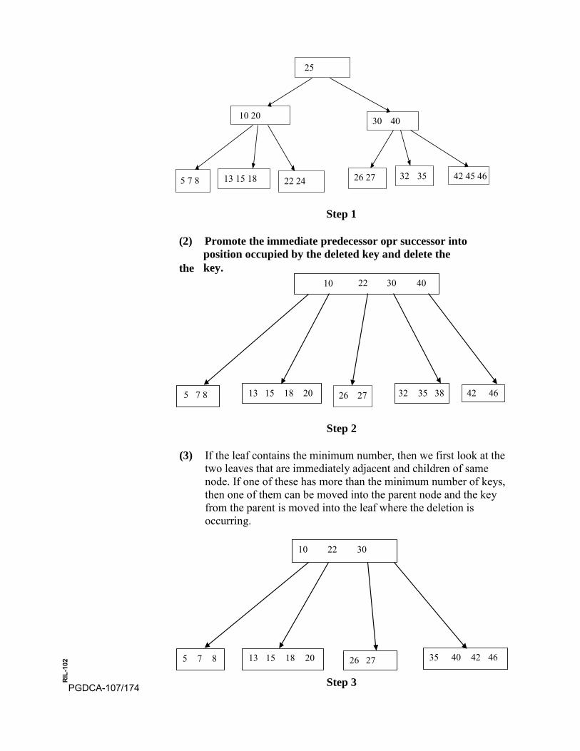
Step 1
(2) Promote the immediate predecessor opr successor into
the position occupied by the deleted key and delete the key.
Step 2
(3) If the leaf contains the minimum number, then we first look at the two leaves that are immediately adjacent and children of same node. If one of these has more than the minimum number of keys, then one of them can be moved into the parent node and the key from the parent is moved into the leaf where the deletion is occurring.
Step 3
25
10 22 30 40
5 7 8 13 15 18 20 26 27 32 35 38 42 46
10 22 30
5 7 8 13 15 18 20 26 27 35 40 42 46
10 20
5 7 8 13 15 18 22 24 26 27 32 35 42 45 46
30 40
PGDCA-107/174
RIL
-102
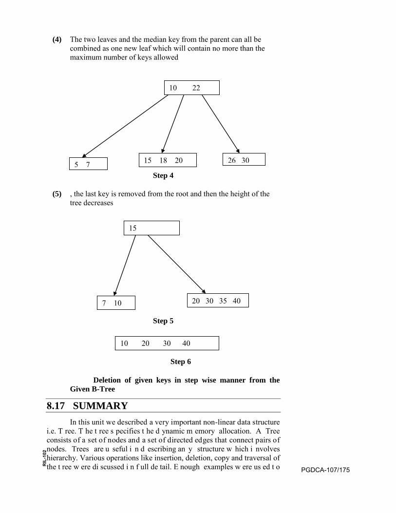
(4) The two leaves and the median key from the parent can all be combined as one new leaf which will contain no more than the maximum number of keys allowed
Step 4
(5) , the last key is removed from the root and then the height of the tree decreases
Step 5
Step 6
Deletion of given keys in step wise manner from the Given B-Tree
8.17 SUMMARY In this unit we described a very important non-linear data structure
i.e. T ree. T he t ree s pecifies t he d ynamic m emory allocation. A Tree consists of a set of nodes and a set of directed edges that connect pairs of nodes. Trees are u seful i n d escribing an y structure w hich i nvolves hierarchy. Various operations like insertion, deletion, copy and traversal of the t ree w ere di scussed i n f ull de tail. E nough examples w ere us ed t o
10 22
5 7 15 18 20 26 30
15
7 10 20 30 35 40
10 20 30 40
PGDCA-107/175
RIL
-102

describe the tree and i ts various operations. The contents of this unit can be summarized as:
• Tree is the nonlinear data structure.
• A tree consists of a root node and a number of sub-trees.
• There are d ifferent t ypes o f t rees s howing d ifferent t ypes o fproperties.
• There are m any t erms a ssociated w ith a b inary tree l ike i ts r ightand left c hild, s ub-tree, i n-degree, out -degree, s uccessor,predecessor and leaf nodes.
• The b inary t ree c an r epresent w ith s equential d ata s tructure l ikearray and with non-contiguous data structure like linked list.
• There are various operations can performs on the Binary tree likeinsertion, deletion, searching and traversing.
• A f undamental a nd i mportant ope ration on t he tree i s t raversal.Traversal of a b inary tree implies v isiting every node of that treeexactly once in some specified sequence. There are three standardtraversal techniques for binary tree. These techniques are: In-order,Post-Order and Pre-Order.
• The bi nary t ree c an c onstruct f rom t he g iven s equence oftraversing in the form of In-Order and Post-Order.
• The r ecursive an d i terative m ethods can u se f or t he t raversing i nany specified order.
• In a bi nary t ree, m any n odes ha ve one c hild or no c hildren. T hepointers for the empty children for these nodes are set to NULL. Amore effective utilization of these pointers is possible if NULL leftpointers a re s et t o point t o t he In-Order predecessor of t hat nodeand NULL right pointers are set to point to the In-Order successorof t hat node . T hese poi nters, s o i ntroduced a re c alled threads.Threads he lp i n writing non -recursive ve rsion o f In-Order, P ost-order and Pre-Order traversal.
• When we place constraints on how data elements can be stored inthe tree, the items must be stored in such a way that the key valuesin th e le ft s ub-tree o f t he r oot ar e l ess t han t he key v alue o f t heroot, and the key values of all the nodes in the right sub-tree of theroot a re greater t han t he ke y value of t he root. W hen t hisrelationship holds in all the nodes in the tree than the tree is calleda binary search tree.
• Operation of i nsertion a nd de letion c an de scribe f or the b inarysearch tree.
PGDCA-107/176
RIL
-102

• AVL Trees are height balanced trees where the difference betweenheights of l eft a nd r ight s ub-trees r ooted a t a ny node c annot belarger than one.
• The f undamental ope rations, na mely s earching, i nsertion a nddeletion can be performed more efficiently on AVL Trees.
• In an AVL Trees the only case that causes difficulty when the newnode is added to sub-tree of the root that is strictly taller than othersub-tree then the height is increased. This would cause one sub treeto ha ve h eight 2 more t han ot her; whereas t he AVL Treescondition is that the height difference is never more than1.
• When an AVL Trees is right high the action needed in this case iscalled left rotation. On the other hand when the tree is left high, theright r otation is performed. In s ome c ases, t he t ree i s ne eded t orotate twice, and then the condition is called double rotation.
• A B-Tree of o rder m is an m-way search t ree where ea ch n odeexcept the root must have m / 2 children at most “m” children. Theroot node is allowed to have two children at the minimum.
• The s earching i nsertion a nd de letion ope ration on a B-Tree aresame as that of 2-3 trees.
• It is in teresting to n ote th at B-Tree grows o r s hrinks upw ardsduring insertion and deletion of key values.
Bibliography Horowitz, E ., S . S ahni: “ Fundamental of computer A lgorithms”, Computer Science Press, 1978
J. P. Tremblay, P . G. Sorenson “An Introduction to Data Structures with Applications”, Tata McGraw-Hill, 1984
M. A llen W eiss: “ Data s tructures a nd P roblem s olving us ing C ++”, Pearson Addison Wesley, 2003
Markus Blaner: “ Introduction t o A lgorithms a nd D ata S tructures”, Saarland University, 2011
Niklaus W irth, “ Algorithm + Data S tructures = P rograms”, PHI Publications
Seymour Lipschutz, “Data Structure”, Schaum’s outline Series
B. Flaming, “Practical Data Structures in C++”, John Wiley & Sons, New York, 1994
R. Sedgewick, “Algorithms in C++, Addision-Wesley, 1992.
PGDCA-107/177
RIL
-102
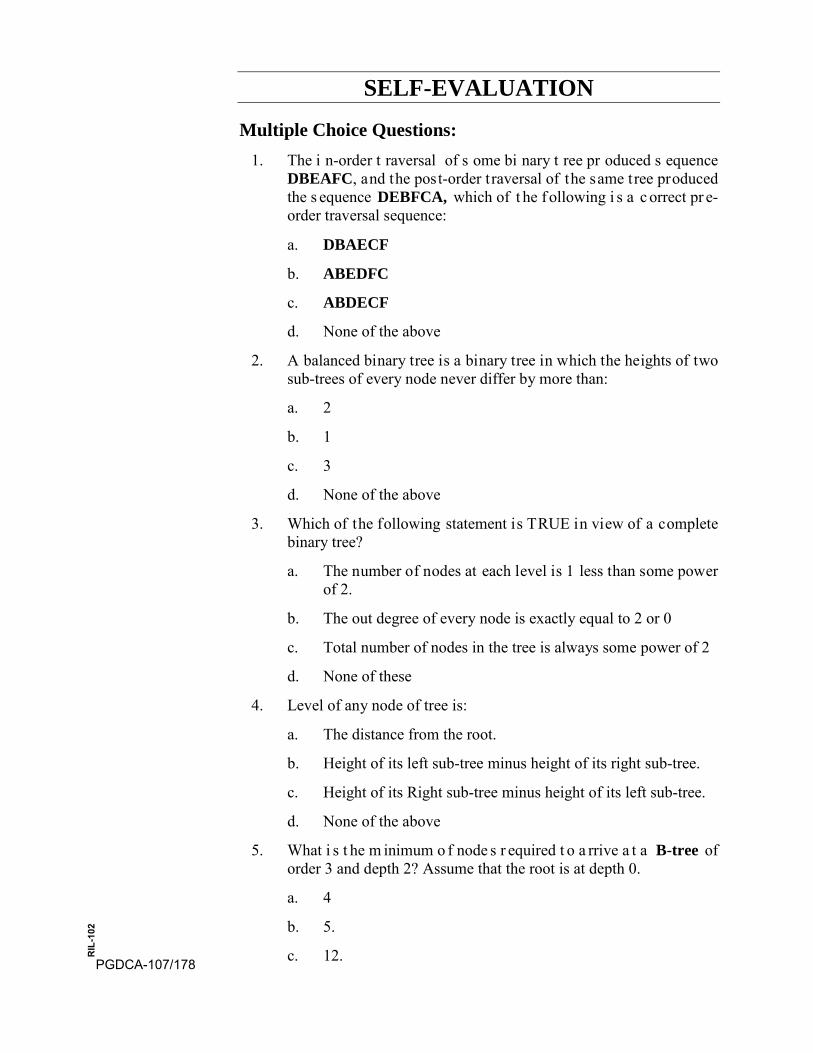
SELF-EVALUATION
Multiple Choice Questions: 1. The i n-order t raversal of s ome bi nary t ree pr oduced s equence
DBEAFC, and the post-order traversal of the same tree producedthe s equence DEBFCA, which of t he f ollowing i s a c orrect pr e-order traversal sequence:
a. DBAECF
b. ABEDFC
c. ABDECF
d. None of the above
2. A balanced binary tree is a binary tree in which the heights of twosub-trees of every node never differ by more than:
a. 2
b. 1
c. 3
d. None of the above
3. Which of the following statement is TRUE in view of a completebinary tree?
a. The number of nodes at each level is 1 less than some powerof 2.
b. The out degree of every node is exactly equal to 2 or 0
c. Total number of nodes in the tree is always some power of 2
d. None of these
4. Level of any node of tree is:
a. The distance from the root.
b. Height of its left sub-tree minus height of its right sub-tree.
c. Height of its Right sub-tree minus height of its left sub-tree.
d. None of the above
5. What i s t he m inimum o f node s r equired t o a rrive a t a B-tree oforder 3 and depth 2? Assume that the root is at depth 0.
a. 4
b. 5.
c. 12. PGDCA-107/178
RIL
-102
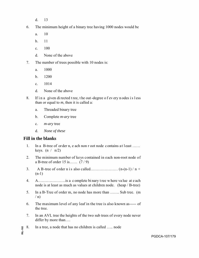
d. 13
6. The minimum height of a binary tree having 1000 nodes would be
a. 10
b. 11
c. 100
d. None of the above
7. The number of trees possible with 10 nodes is:
a. 1000
b. 1200
c. 1014
d. None of the above
8. If i n a given di rected t ree, t he out -degree o f ev ery n odes i s l essthan or equal to m, then it is called a:
a. Threaded binary tree
b. Complete m-ary tree
c. m-ary tree
d. None of these
Fill in the blanks 1. In a B-tree of order n, e ach non r oot node contains a t l east ……
keys. (n / n/2)
2. The minimum number of keys contained in each non-root node ofa B-tree of order 15 is…… (7 / 9)
3. A B-tree of order n i s also called………………… (n-(n-1) / n +(n-1)
4. A…………………is a c omplete bi nary t ree w here va lue at e achnode is at least as much as values at children node. (heap / B-tree)
5. In a B-Tree of order m, no node has more than ……. Sub tree. (m/ n)
6. The maximum level of any leaf in the tree is also known as----- ofthe tree.
7. In an AVL tree the heights of the two sub trees of every node neverdiffer by more than….
8. In a tree, a node that has no children is called ….. node
PGDCA-107/179
RIL
-102
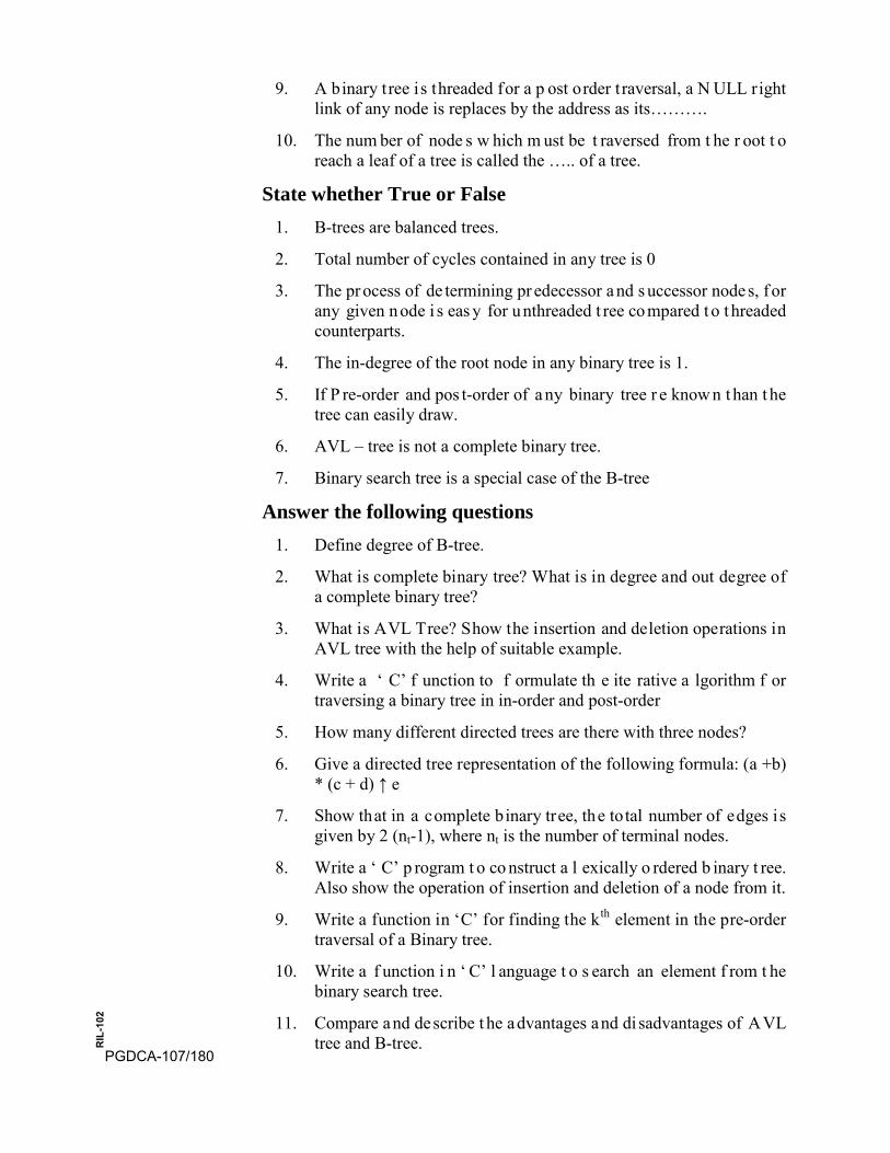
9. A binary tree is threaded for a p ost order t raversal, a N ULL rightlink of any node is replaces by the address as its……….
10. The num ber of node s w hich m ust be t raversed from t he r oot t oreach a leaf of a tree is called the ….. of a tree.
State whether True or False 1. B-trees are balanced trees.
2. Total number of cycles contained in any tree is 0
3. The pr ocess of de termining pr edecessor a nd s uccessor node s, f orany given node i s eas y for unthreaded t ree compared t o t hreadedcounterparts.
4. The in-degree of the root node in any binary tree is 1.
5. If P re-order and pos t-order of a ny binary tree r e know n t han t hetree can easily draw.
6. AVL – tree is not a complete binary tree.
7. Binary search tree is a special case of the B-tree
Answer the following questions 1. Define degree of B-tree.
2. What is complete binary tree? What is in degree and out degree ofa complete binary tree?
3. What is AVL Tree? Show the insertion and deletion operations inAVL tree with the help of suitable example.
4. Write a ‘ C’ f unction to f ormulate th e ite rative a lgorithm f ortraversing a binary tree in in-order and post-order
5. How many different directed trees are there with three nodes?
6. Give a directed tree representation of the following formula: (a +b)* (c + d) ↑ e
7. Show that in a complete binary tree, the total number of edges isgiven by 2 (nt-1), where nt is the number of terminal nodes.
8. Write a ‘ C’ p rogram t o co nstruct a l exically o rdered b inary t ree.Also show the operation of insertion and deletion of a node from it.
9. Write a function in ‘C’ for finding the kth element in the pre-ordertraversal of a Binary tree.
10. Write a f unction i n ‘ C’ l anguage t o s earch an element f rom t hebinary search tree.
11. Compare and describe t he advantages and di sadvantages of AVLtree and B-tree.
PGDCA-107/180
RIL
-102

UNIT-9 GRAPH
Structure
9.0 Introduction
9.1 Objective
9.2 Mathematical Definition of the graph and its basic terminology
9.3 Graph Representation
9.4 Path Matrix or Reach-ability Matrix
9.5 Linked Representation of the graph
9.6 Graph Traversal
9.7 Spanning Tree
9.8 Algorithm for computing Minimal Spanning Tree
9.9 Shortest Path Algorithms
9.10 Bellman-Ford Algorithm
9.11 Topological Sort
9.12 Summary
9.0 INTRODUCTION
This unit consists with the concept of graphs in general as well as in mathematical form and its basic terminology. It includes the method for the g raph representation l ike m atrix r epresentation o r ad jacency m atrix form w ith l inked l ist. It c overs t he va rious a lgorithms f or s earching t he graph l ike br eadth f irst s earch a nd d epth f irst s earch. T he c oncept of spanning t ree f or obt aining t he opt imal pa th from t he g raph i s a lso introduced and implemented with Kruskal’s and pr ism’s a lgorithms. The technique f or obt aining the s hortest pa th f rom t he gr aph i s i mplemented with B ellman f ord algorithm, D ijkstr’s a lgorithm a nd F loyd-Warshall algorithm. A Graph is a nonlinear data structure that is used to represent a relational d ata e. g. a s et o f t erminals i n a n etwork o r a r oad m ap o f all cities i n a country. S uch t ype o f c omplex r elationship c an onl y b e represented using a graphs data structure. Thus, a graph is such type of a non linear data structure which is having point to point relationship among the nodes. A tree can view as a restricted graph. Each node of the graph is called as a vertex and l ink or l ine drawn between them is called edge. A general graph can view with the following diagram which consists with 6 (six) nodes or vertices and eight (08) links or edges.
PGDCA-107/181
RIL
-102

9.1 OBJECTIVES
After reading this unit the learner is able to do the following task.
• Interpret the graph mathematically.
• Represent the graph as adjacency matrix and path matrix
• Perform the search in the graph either in breadth first or depth firstsearch manner
• Able to construct spanning tree from the given graph usingKruskal’s and Prim’s algorithms
• Able to explore the shortest path from the given graph
9.2 MATHEMATICAL DEFINITION OF THE GRAPH AND ITS BASIC TERMINOLOGY
Mathematically, A graph ‘G’ consists of two sets V and ‘E’ such that G={V, E},Where V is finite nonempty set of vertices or nodes, V(G) represents s et o f vertices, E is a s et o f edges an d E(G) represents s et o f Edges. Therefore we can say that a graph G consists of a non empty set V called the set of nodes (points, vertices) of the graph, a set E which is the set of edges of the graph, and a mapping from the set of edges E to a set of pairs of elements of V.
Example
Let us consider the graph as follows:
A
B
D
C
E
PGDCA-107/182
RIL
-102
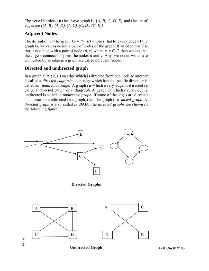
The s et o f v ertices i n t he ab ove graph i s {A, B, C, D, E} and t he s et of edges are {(A, B), (A, D), (A, C), (C, D), (C, E)}
Adjacent Nodes The definition of the graph G = (V, E) implies that to every edge of the graph G, we can associate a pair of nodes of the graph. If an edge Ex∈ is thus associated with a pair of node (u, v) where u, v Є V, then we say that the edge x connects or joins the nodes u and v. Any two nodes which are connected by an edge in a graph are called adjacent Nodes.
Directed and undirected graph In a graph G = (V, E) an edge which is directed from one node to another is called a directed edge, while an edge which has no specific direction is called an undirected edge. A g raph i n w hich e very edge i s d irected i s called a directed graph or a diagraph. A g raph i n w hich e very e dge i s undirected is called an undirected graph. If some of the edges are directed and some ar e undirected i n a g raph, t hen the graph i s a mixed graph. A directed graph is also called as DAG. The directed graphs are shown in the following figure:
Directed Graphs
Undirected Graph
A
B
D
C
E
A B
C D
A C
D B
PGDCA-107/183
RIL
-102

PGDCA-107/184
RIL
-102
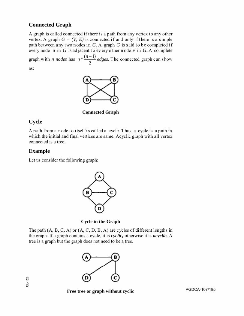
Connected Graph A graph is called connected if there is a path from any vertex to any other vertex. A graph G = (V, E) is connected i f and only i f there i s a s imple path between any two nodes in G. A graph G is said to be completed i f every node u in G is ad jacent t o ev ery o ther n ode v in G. A co mplete
graph with n nodes has 2
)1(* −nn edges. The connected graph can show
as:
Connected Graph
Cycle A path f rom a node to i tself i s cal led a cycle. Thus, a cycle is a path in which the initial and final vertices are same. Acyclic graph with all vertex connected is a tree.
Example Let us consider the following graph:
Cycle in the Graph
The path (A, B, C, A) or (A, C, D, B, A) are cycles of different lengths in the graph. If a graph contains a cycle, it is cyclic, otherwise it is acyclic. A tree is a graph but the graph does not need to be a tree.
Free tree or graph without cyclic PGDCA-107/185
RIL
-102

Loop If an edge i s having identical end points, t hen the edge i s c alled a l oop. Thus, an edge e is called a loop if it has identical end points, i.e. e = (u, u).
Degree, incidence, adjacency
A vertex v is incident to an edge e if V is one of the two vertices in the ordered pair of vertices that constitute e.
The degree of a vertex is the number of edges incident to it. The in-degree of a vertex V is the number of edges that have V as the head and the out-degree of a vertex V is the number of edges that have V as the tail.
Example
Let us consider the following graph
In t his graph vertex V has in-degree 1, out-degree 2 and degree 3. A V vertex i s ad jacent t o v ertex U if t here i s an ed ge f rom U to V. If V is adjacent to U, V is called a successor of U and U a predecessor of V.
Isolated node If degree of a node is zero i.e. if the node is not having any edges, then the node is called isolated node.
Complete Graph A g raph i s cal led complete i f al l t he n odes o f t he g raph a re ad jacent t o each other. A complete graph with n nodes will have n*(n-1)/2 edges.
Weighted Graph A graph is said to be weighted if each edge in the graph is assigned a non-negative numerical value called the weight or cost of the edge. If an edge does not have any weight then the weight is considered as 1.
PGDCA-107/186
RIL
-102
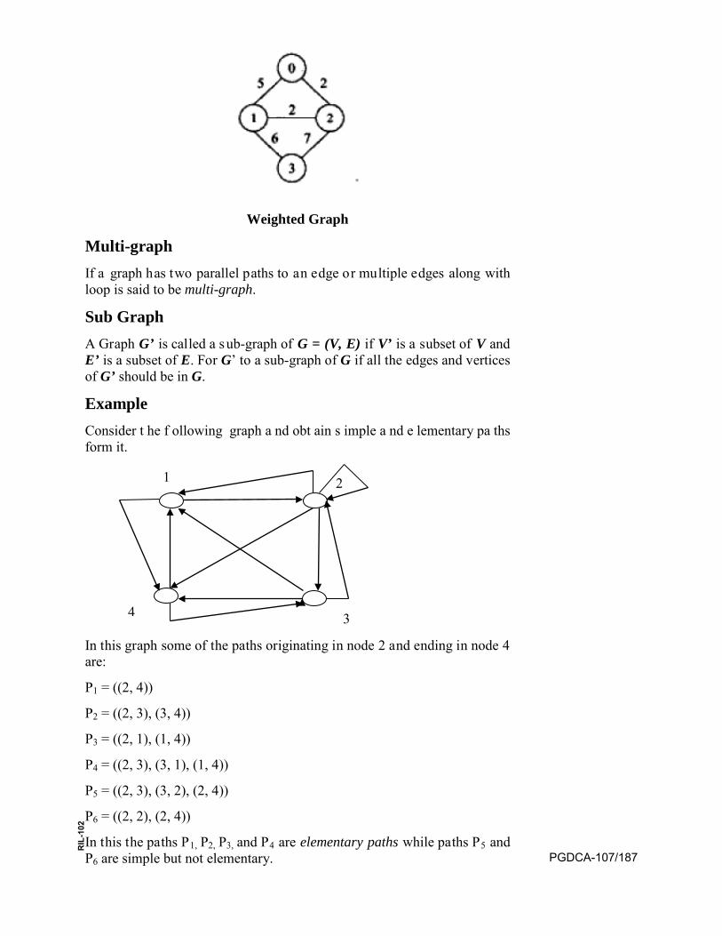
Weighted Graph
Multi-graph If a graph has two parallel paths to an edge or multiple edges along with loop is said to be multi-graph.
Sub Graph A Graph G’ is called a sub-graph of G = (V, E) if V’ is a subset of V and E’ is a subset of E. For G’ to a sub-graph of G if all the edges and vertices of G’ should be in G.
Example Consider t he f ollowing graph a nd obt ain s imple a nd e lementary pa ths form it.
In this graph some of the paths originating in node 2 and ending in node 4 are:
P1 = ((2, 4))
P2 = ((2, 3), (3, 4))
P3 = ((2, 1), (1, 4))
P4 = ((2, 3), (3, 1), (1, 4))
P5 = ((2, 3), (3, 2), (2, 4))
P6 = ((2, 2), (2, 4))
In this the paths P1, P2, P3, and P4 are elementary paths while paths P5 and P6 are simple but not elementary.
1 2
3 4
PGDCA-107/187
RIL
-102
The following are some of the cycles in this graph:
C1 = ((2, 2))
C2 = ((1, 2), (2, 1))
C3 = ((2, 3), (3, 1), (1, 2))
C4 = ((2, 1), (1, 4), (4, 3), (3, 2))
9.3 GRAPH REPRESENTATION
A d iagrammatic r epresentation o f a g raph ma y h ave a limite d usefulness. H owever, s uch a r epresentation i s not f easible w hen t he number of nodes and edges in a graph is large. There are different methods for the alternative representation of graph. The basic three methods for the methods for the graph representation are as follows:
• Representation of the graph by using matrices.
• Representation of a graph by a list structure.
• Representation of a graph by a Adjacency lists and edge lists.
Matrix Representation of Graphs Given a s imple diagraph G = (V, E), it is necessary to assume some kind or ordering of the nodes of a graph in the sense that a particular node is called a first node , a nother s econd nod e, and s o on. A m atrix representation of G depends upon the ordering of the nodes. Therefore, in the g iven di agraph G we h ave V = {v1, v2,……vn } and the node s a re assumed to be ordered from v1 to vn. An n X n matrix A whose elements aij are given by:
∈
=otherwise
Eif vva jiij 0
),(1
This is called the adjacency matrix of the graph G.
Any element of the adjacency matrix is either 0 or 1. Any matrix whose elements are 0 or 1 is called a bit matrix or a Boolean matrix. Hence the ith row in the adjacency matrix is determined by the edges which originate in the node vi. T he num ber of elements i n t he ith row w hose va lue i s 1 is equal to the out-degree of the node vi. Similarly, the number of elements whose value is 1 in a column, say the jth column, is equal to the in-degree of t he node vj. A n adjacency matrix completely d efines a s imple diagraph. If two diagraphs are such that the adjacency matrix of one can be obtained from the adjacency matrix of the other by interchanging some of t he r ows a nd t he c orresponding c olumns, then t he di agraphs a re equivalent. PGDCA-107/188
RIL
-102

Example
Obtain the adjacency matrix for the following diagraph.
Diagraph
The corresponding adjacency matrix for this diagraph is as follows:
4321 vvvv
4
3
2
1
vvvv
0010101100011010
Adjacency Matrix
Now we consider the powers of an adjacency matrix. Naturally, an entry of 1 in the ith row and jth column of A shows the existence of an edge (vi, vj), that is, a path of length 1 from vi to vj. Let us denote the elements of A2 by aij
(2). Then:
∑=
=n
kkjikij aaa
1
)2(
So that for any fixed k, 1=aa kjikif and only if both aik and akj
equal 1;
i.e. ),( ki vv and ),( jk vv are edges of the graph. For each such k we get a contribution of 1 in the sum. Now ),( ki vv and ),( jk vv imply that there is a
path f rom vi to vj of l ength 2. T herefore, 2ija is e qual t o t he num ber of
different p aths o f ex actly l ength 2 from vi to vj. Similarly, th e d iagonal element 2
ija shows the number of cycles of length 2 at the node for vi for i=1, 2,….,,n. By a similar argument, one can show that the element in the ith row and jth column of 3A gives the number of paths of exactly length 3 from vi to vj. In general, the following statement can be shown:
Let A be the adjacency matrix of the digraph G. The element in the ith row and jth column of nA (n>1) is e qual t o t he num ber of pa ths of l ength n from the ith node and jth node.
V V
VV
PGDCA-107/189
RIL
-102
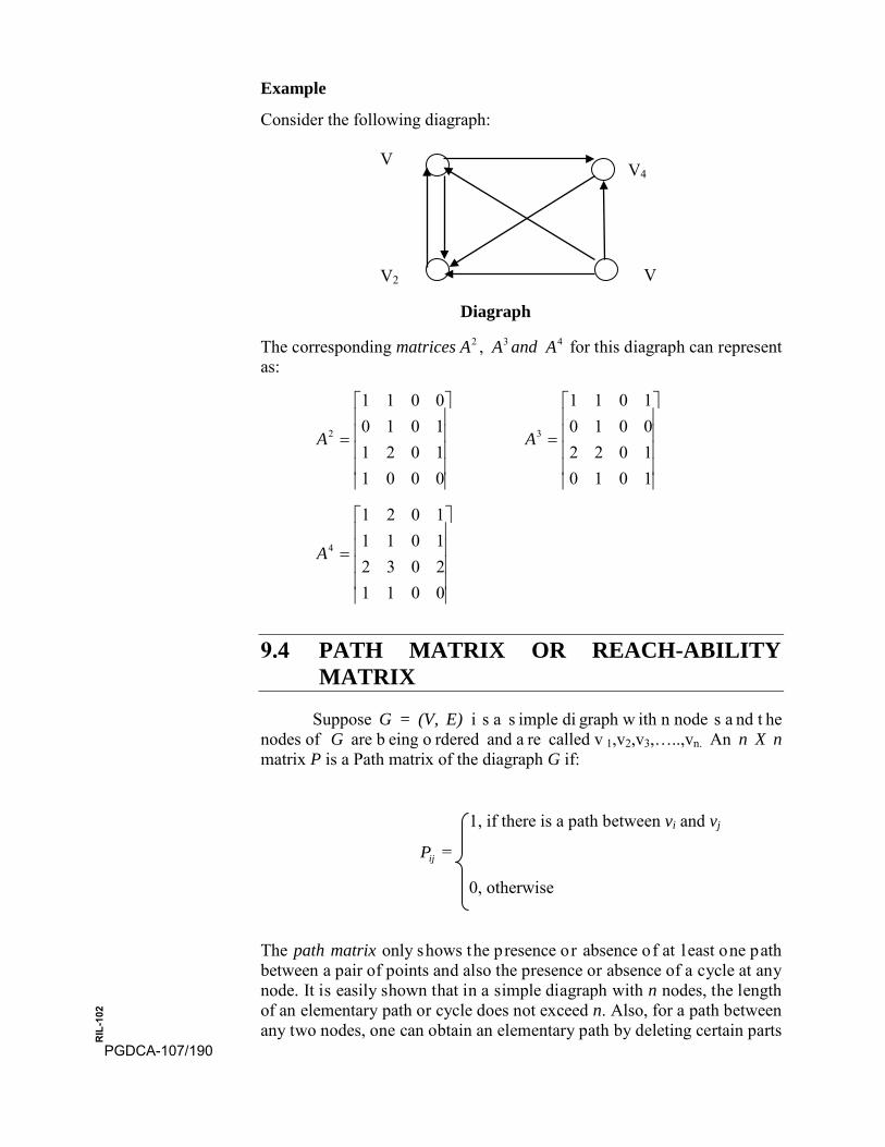
Example
Consider the following diagraph:
Diagraph
The corresponding matrices 2A , 3A and 4A for this diagraph can represent as:
=
0001102110100011
2A
=
1010102200101011
3A
=
0011203210111021
4A
9.4 PATH MATRIX OR REACH-ABILITY MATRIX
Suppose G = (V, E) i s a s imple di graph w ith n node s a nd t he nodes of G are b eing o rdered and a re called v 1,v2,v3,…..,vn. An n X n matrix P is a Path matrix of the diagraph G if:
1, if there is a path between vi and vj
ijP =
0, otherwise
The path matrix only shows the presence or absence of at least one path between a pair of points and also the presence or absence of a cycle at any node. It is easily shown that in a simple diagraph with n nodes, the length of an elementary path or cycle does not exceed n. Also, for a path between any two nodes, one can obtain an elementary path by deleting certain parts
V2
V V4
V
PGDCA-107/190
RIL
-102
of the path that are cycles. Similarly (for cycles), we can always obtain an elementary c ycle f rom a given c ycle. If we a re i nterested in determining whether there exists a path from vi to vj, , all we need to examine are the elementary paths of length less than or equal to n-1. In the case where vi = vj and t he p ath i s a c ycle, w e n eed t o ex amine al l p ossible el ementary cycles o f le ngth le ss th an or e qual t o n. S uch cycles o r p aths ar e e asily determined from the matrix nB where;
nn AAAAB ++++= .........32
The element in the ith row and jth column of Bn shows the number of paths of l ength n or less which exist f rom vi to vj. I f th is e lement is non-zero, then it is we need to know the existence of a path, and not the number of paths b etween any t wo nodes. In an y case, t hen m atrix Bn furnishes t he required i nformation a bout r each-ability of a ny node of t he g raph f rom any other node.
Therefore, t he p ath m atrix can b e cal culated f rom t he m atrix Bn by choosing pij = 1 if the element in the ith row and the jth column of Bn is non-zero, and pij = 0 otherwise.
Example
Now w e a pply t his m ethod of c alculating t he p ath m atrix t o t he g iven diagraph in the above mentioned examples. The adjacency matrix A and the pow ers 2A , 3A and 4A have al ready b een cal culated i n t he p revious example. We thus have B4 and the path matrix P given by:
=
1032508620333053
4B and
=
0011101110111011
P
The method of obtaining the path matrix of a simple diagraph can easily be computed by using the following WARSHALL algorithm
Algorithm WARSHALL [Given th e a djacency matrix A , th is algorithm produces the path matrix P.]
1. [Initialize]P = A
2. [perform a Pass]Repeat through step 4 for k = 1, 2,…..,n
3. [Process rows]Repeat step 4 for I = 1, 2,……,n
4. [Process columns]Repeat for j = 1, 2,….,nPij = Pij ⋁ (Pik ∧ Pkj)
5. [Finished]Exit PGDCA-107/191
RIL
-102
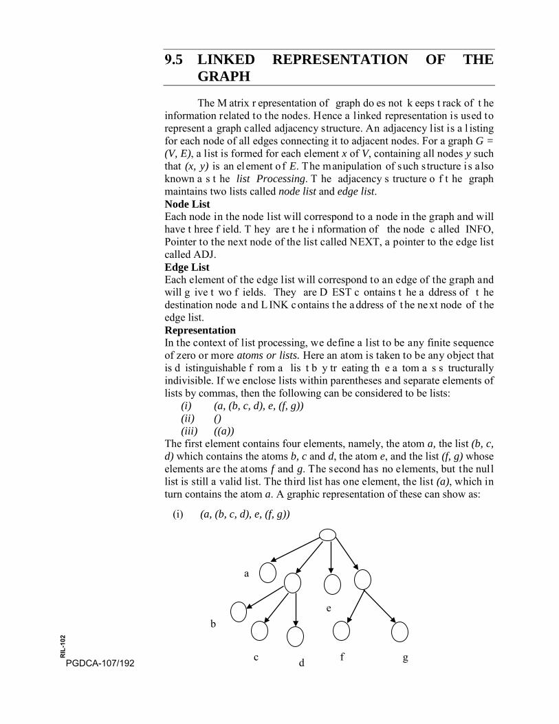
9.5 LINKED REPRESENTATION OF THE GRAPH
The M atrix r epresentation of graph do es not k eeps t rack of t he information related to the nodes. Hence a linked representation is used to represent a graph called adjacency structure. An adjacency list is a l isting for each node of all edges connecting it to adjacent nodes. For a graph G = (V, E), a list is formed for each element x of V, containing all nodes y such that (x, y) is an element o f E. The manipulation of such s tructure is also known a s t he list Processing. T he adjacency s tructure o f t he graph maintains two lists called node list and edge list. Node List Each node in the node list will correspond to a node in the graph and will have t hree f ield. T hey are t he i nformation of the node c alled INFO, Pointer to the next node of the list called NEXT, a pointer to the edge list called ADJ. Edge List Each element of the edge list will correspond to an edge of the graph and will g ive t wo f ields. They are D EST c ontains t he a ddress of t he destination node a nd L INK c ontains t he a ddress of t he ne xt node of t he edge list. Representation In the context of list processing, we define a list to be any finite sequence of zero or more atoms or lists. Here an atom is taken to be any object that is d istinguishable f rom a lis t b y tr eating th e a tom a s s tructurally indivisible. If we enclose lists within parentheses and separate elements of lists by commas, then the following can be considered to be lists:
(i) (a, (b, c, d), e, (f, g)) (ii) () (iii) ((a))
The first element contains four elements, namely, the atom a, the list (b, c, d) which contains the atoms b, c and d, the atom e, and the list (f, g) whoseelements are the atoms f and g. The second has no elements, but the null list is still a valid list. The third list has one element, the list (a), which in turn contains the atom a. A graphic representation of these can show as:
(i) (a, (b, c, d), e, (f, g))
a
b
c d
e
f g PGDCA-107/192
RIL
-102
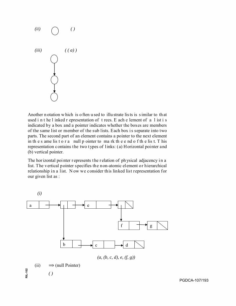
(ii) ( )
(iii) ( ( a) )
Another n otation w hich is o ften u sed to illu strate lis ts is s imilar to th at used i n t he l inked r epresentation of t rees. E ach e lement of a l ist i s indicated by a box and a pointer indicates whether the boxes are members of the same list or member of the sub lists. Each box i s separate into two parts. The second part of an element contains a pointer to the next element in th e s ame lis t o r a null p ointer to ma rk th e e nd o f th e lis t. T his representation contains the two types of l inks: (a) Horizontal pointer and (b) vertical pointer.
The hor izontal poi nter r epresents t he r elation of ph ysical adjacency i n a list. The vertical pointer specifies the non-atomic element or h ierarchical relationship in a l ist. N ow we consider this linked list representation for our given list as :
(i)
(a, (b, c, d), e, (f, g))
(ii) ⟹ (null Pointer)
( )
a e
f g
b c d
PGDCA-107/193
RIL
-102

(iii)
((a))
Example
Consider the following graph and represent it with adjacency list edge list representation.
The Adjacency list representation of this graph is as:
a b c d
b a c e
c d f
d e f
e F
f
The edge list of this graph is as follows:
a
B
A C
E
D F
61 1
2
3
6 1
1
2
2
2
PGDCA-107/194
RIL
-102
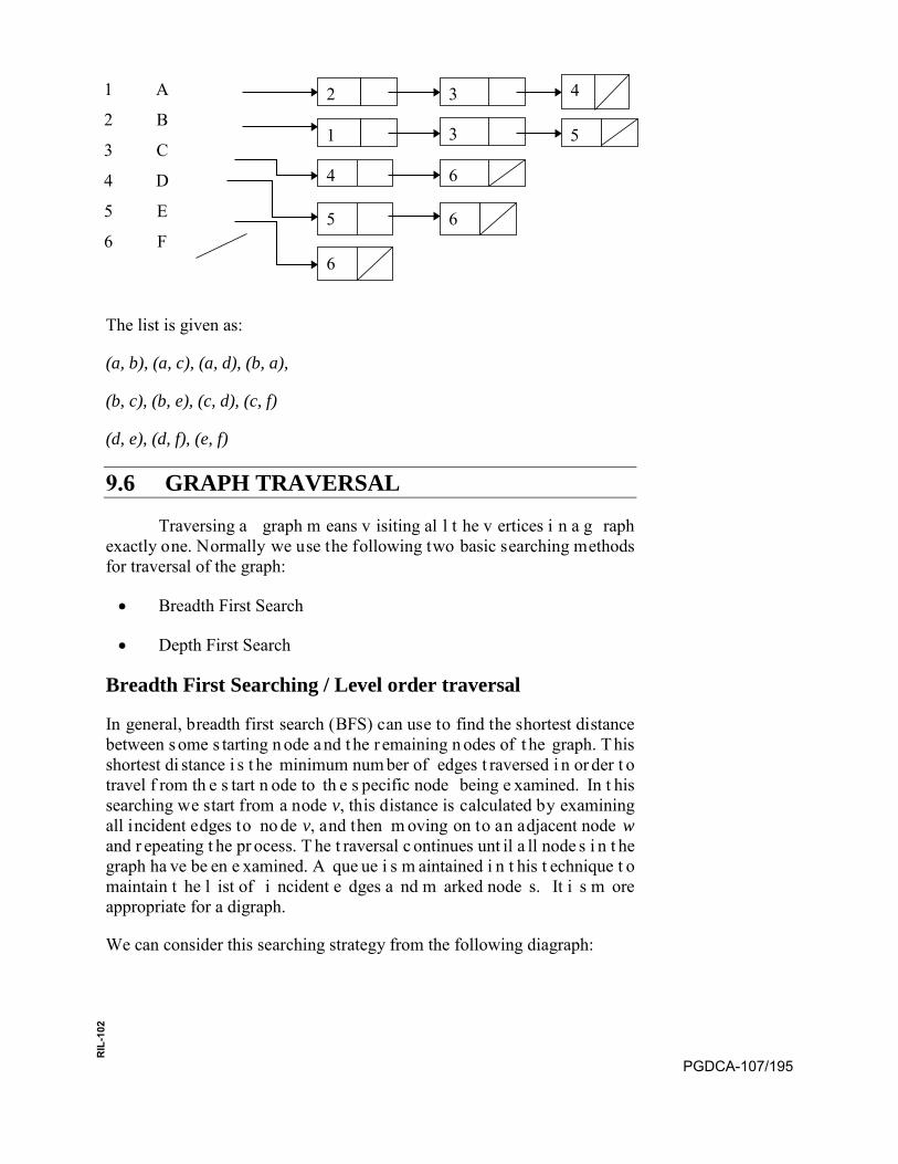
1 A
2 B
3 C
4 D
5 E
6 F
The list is given as:
(a, b), (a, c), (a, d), (b, a),
(b, c), (b, e), (c, d), (c, f)
(d, e), (d, f), (e, f)
9.6 GRAPH TRAVERSAL
Traversing a graph m eans v isiting al l t he v ertices i n a g raph exactly one. Normally we use the following two basic searching methods for traversal of the graph:
• Breadth First Search
• Depth First Search
Breadth First Searching / Level order traversal
In general, breadth first search (BFS) can use to find the shortest distance between s ome s tarting n ode a nd t he r emaining n odes of t he graph. T his shortest di stance i s t he minimum num ber of edges t raversed i n or der t o travel f rom th e s tart n ode to th e s pecific node being e xamined. In t his searching we start from a node v, this distance is calculated by examining all incident edges to no de v, and then m oving on to an adjacent node w and r epeating t he pr ocess. T he t raversal c ontinues unt il a ll node s i n t he graph ha ve be en e xamined. A que ue i s m aintained i n t his t echnique t o maintain t he l ist of i ncident e dges a nd m arked node s. It i s m ore appropriate for a digraph.
We can consider this searching strategy from the following diagraph:
2 3 4
1 3 5
4
5
6
6
6
PGDCA-107/195
RIL
-102
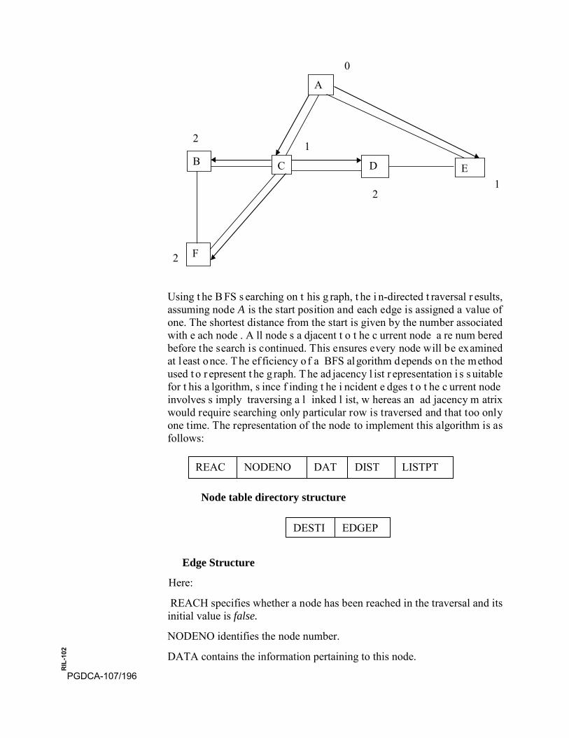
Using t he B FS s earching on t his g raph, t he i n-directed t raversal r esults, assuming node A is the start position and each edge is assigned a value of one. The shortest distance from the start is given by the number associated with e ach node . A ll node s a djacent t o t he c urrent node a re num bered before the search is continued. This ensures every node will be examined at l east once. The ef ficiency of a BFS algorithm depends on the method used t o r epresent t he g raph. T he ad jacency l ist r epresentation i s s uitable for t his a lgorithm, s ince f inding t he i ncident e dges t o t he c urrent node involves s imply traversing a l inked l ist, w hereas an ad jacency m atrix would require searching only particular row is traversed and that too only one time. The representation of the node to implement this algorithm is as follows:
Node table directory structure
Edge Structure
Here:
REACH specifies whether a node has been reached in the traversal and its initial value is false.
NODENO identifies the node number.
DATA contains the information pertaining to this node.
A
C B D E
F
0
1 2
2 1
2
REAC NODENO DAT DIST LISTPT
DESTI EDGEP
PGDCA-107/196
RIL
-102
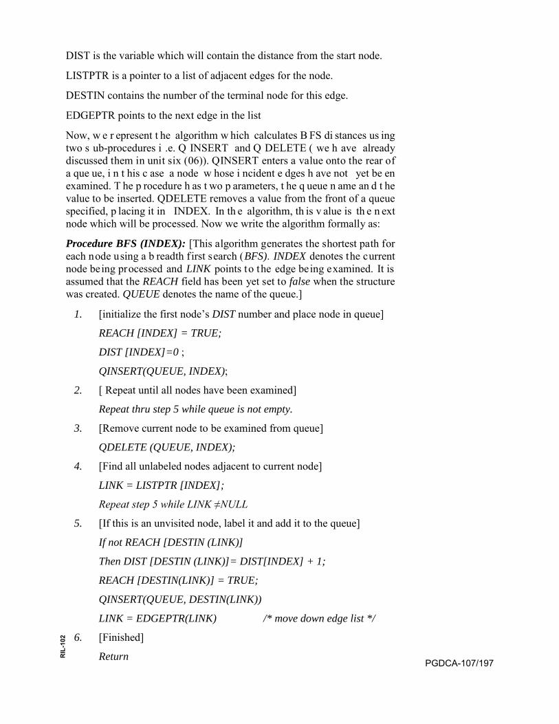
DIST is the variable which will contain the distance from the start node.
LISTPTR is a pointer to a list of adjacent edges for the node.
DESTIN contains the number of the terminal node for this edge.
EDGEPTR points to the next edge in the list
Now, w e r epresent t he algorithm w hich calculates B FS di stances us ing two s ub-procedures i .e. Q INSERT and Q DELETE ( we h ave already discussed them in unit six (06)). QINSERT enters a value onto the rear of a que ue, i n t his c ase a node w hose i ncident e dges h ave not yet be en examined. T he p rocedure h as t wo p arameters, t he q ueue n ame an d t he value to be inserted. QDELETE removes a value from the front of a queue specified, p lacing it in INDEX. In th e algorithm, th is v alue is th e n ext node which will be processed. Now we write the algorithm formally as:
Procedure BFS (INDEX): [This algorithm generates the shortest path for each node using a b readth first search (BFS). INDEX denotes the current node being processed and LINK points to the edge being examined. It is assumed that the REACH field has been yet set to false when the structure was created. QUEUE denotes the name of the queue.]
1. [initialize the first node’s DIST number and place node in queue]
REACH [INDEX] = TRUE;
DIST [INDEX]=0 ;
QINSERT(QUEUE, INDEX);
2. [ Repeat until all nodes have been examined]
Repeat thru step 5 while queue is not empty.
3. [Remove current node to be examined from queue]
QDELETE (QUEUE, INDEX);
4. [Find all unlabeled nodes adjacent to current node]
LINK = LISTPTR [INDEX];
Repeat step 5 while LINK ≠NULL
5. [If this is an unvisited node, label it and add it to the queue]
If not REACH [DESTIN (LINK)]
Then DIST [DESTIN (LINK)]= DIST[INDEX] + 1;
REACH [DESTIN(LINK)] = TRUE;
QINSERT(QUEUE, DESTIN(LINK))
LINK = EDGEPTR(LINK) /* move down edge list */
6. [Finished]
ReturnPGDCA-107/197
RIL
-102
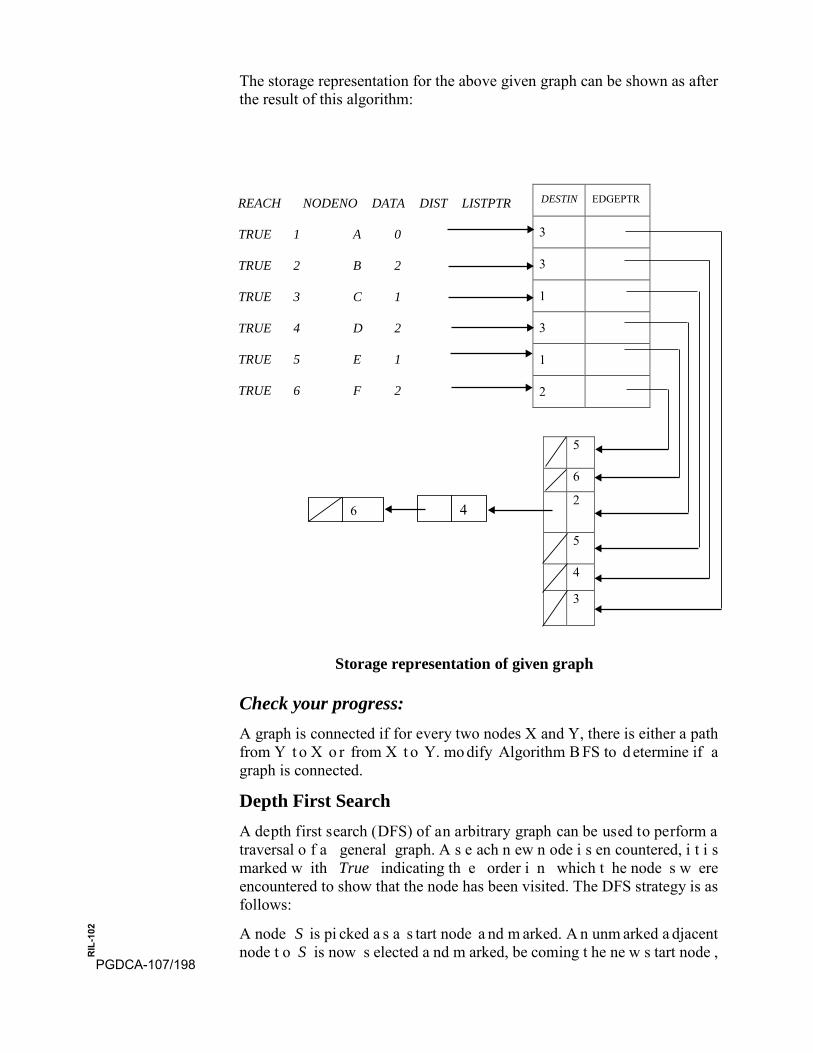
The storage representation for the above given graph can be shown as after the result of this algorithm:
REACH NODENO DATA DIST LISTPTR
TRUE 1 A 0
2 B 2
3 C 1
4 D 2
5 E 1
TRUE
TRUE
TRUE
TRUE
TRUE 6 F 2
Storage representation of given graph
Check your progress: A graph is connected if for every two nodes X and Y, there is either a path from Y t o X o r from X t o Y. mo dify Algorithm B FS to d etermine if a graph is connected.
Depth First Search A depth first search (DFS) of an arbitrary graph can be used to perform a traversal o f a general graph. A s e ach n ew n ode i s en countered, i t i s marked w ith True indicating th e order i n which t he node s w ere encountered to show that the node has been visited. The DFS strategy is as follows:
A node S is pi cked a s a s tart node a nd m arked. A n unm arked a djacent node t o S is now s elected a nd m arked, be coming t he ne w s tart node ,
DESTIN EDGEPTR
3
3
1
3
1
2
5
6
2
5
4
3
46
PGDCA-107/198
RIL
-102
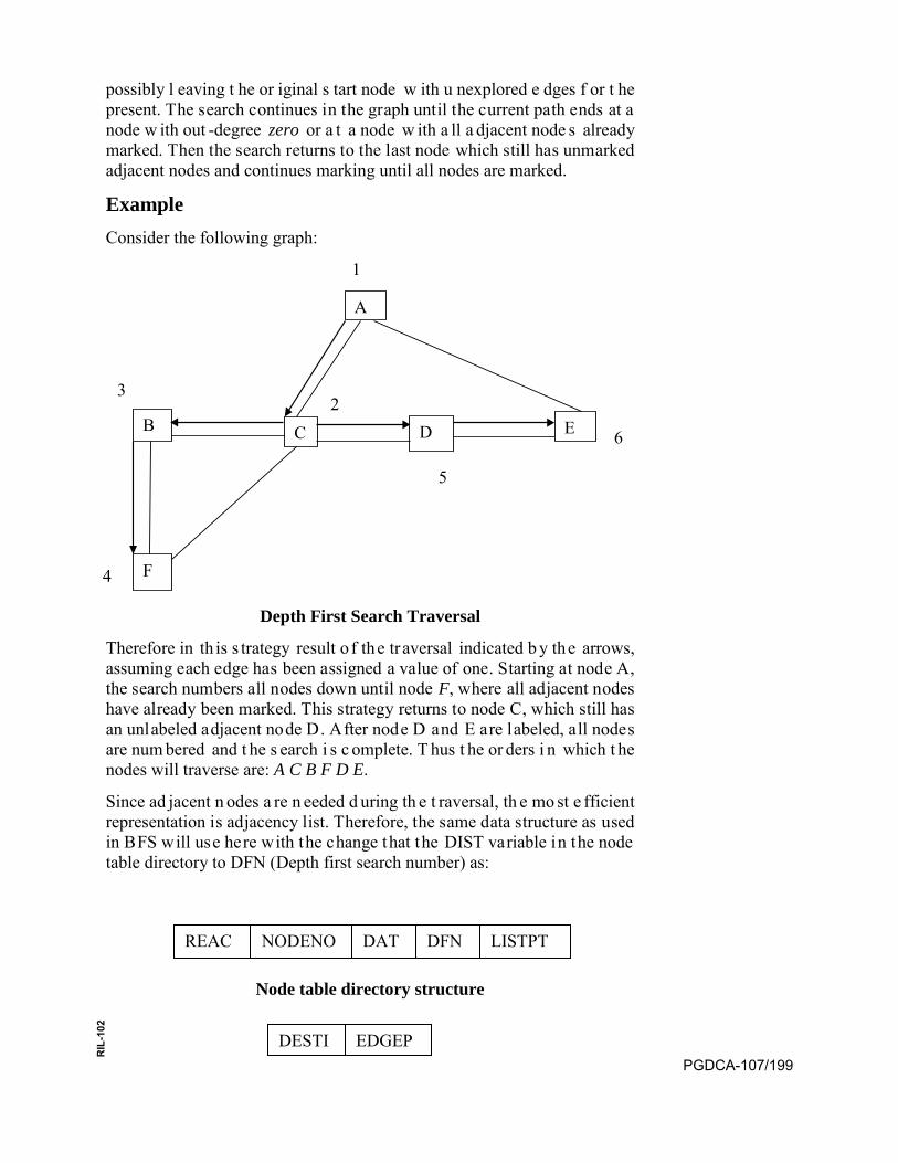
possibly l eaving t he or iginal s tart node w ith u nexplored e dges f or t he present. The search continues in the graph until the current path ends at a node w ith out -degree zero or a t a node w ith a ll a djacent node s already marked. Then the search returns to the last node which still has unmarked adjacent nodes and continues marking until all nodes are marked.
Example Consider the following graph:
Depth First Search Traversal
Therefore in th is s trategy result o f the tr aversal indicated b y the arrows, assuming each edge has been assigned a value of one. Starting at node A, the search numbers all nodes down until node F, where all adjacent nodes have already been marked. This strategy returns to node C, which still has an unlabeled adjacent node D. After node D and E are labeled, all nodes are num bered and t he s earch i s c omplete. T hus t he or ders i n which t he nodes will traverse are: A C B F D E.
Since ad jacent n odes a re n eeded d uring th e t raversal, th e mo st e fficient representation is adjacency list. Therefore, the same data structure as used in BFS will use here with the change that the DIST variable in the node table directory to DFN (Depth first search number) as:
Node table directory structure
A
C B D E
F
2
5
6
4
3
REAC NODENO DAT DFN LISTPT
DESTI EDGEP
1
PGDCA-107/199
RIL
-102
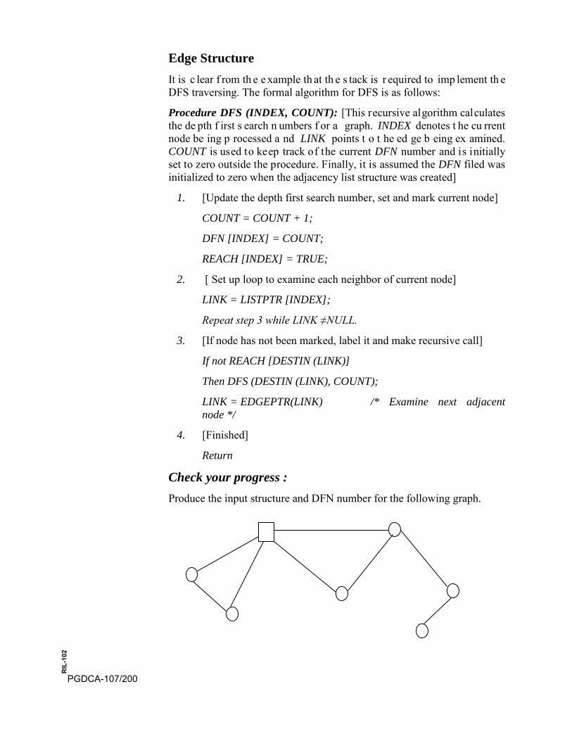
Edge Structure It is c lear f rom th e e xample th at th e s tack is r equired to imp lement th e DFS traversing. The formal algorithm for DFS is as follows:
Procedure DFS (INDEX, COUNT): [This recursive algorithm calculates the de pth f irst s earch n umbers f or a graph. INDEX denotes t he cu rrent node be ing p rocessed a nd LINK points t o t he ed ge b eing ex amined. COUNT is used to keep track of the current DFN number and is initially set to zero outside the procedure. Finally, it is assumed the DFN filed was initialized to zero when the adjacency list structure was created]
1. [Update the depth first search number, set and mark current node]
COUNT = COUNT + 1;
DFN [INDEX] = COUNT;
REACH [INDEX] = TRUE;
2. [ Set up loop to examine each neighbor of current node]
LINK = LISTPTR [INDEX];
Repeat step 3 while LINK ≠NULL.
3. [If node has not been marked, label it and make recursive call]
If not REACH [DESTIN (LINK)]
Then DFS (DESTIN (LINK), COUNT);
LINK = EDGEPTR(LINK) /* Examine next adjacent node */
4. [Finished]
Return
Check your progress : Produce the input structure and DFN number for the following graph.
1
PGDCA-107/200
RIL
-102

9.7 SPANNING TREE
A spanning tree of a graph is an undirected tree consisting of only those e dges ne cessary t o c onnect a ll t he nod es in t he or iginal graph. A spanning tree has the properties that for any pair of nodes there exists only one path between them, and the insertion of any edge to a spanning t ree forms a u nique c ycle. Those e dges l eft out of t he s panning t ree w ere present i n t he or iginal graph c onnect p aths t ogether i n t he t ree. W hen determine t he c ost of a s panning t ree of a w eighted graph, t he c ost i s simply t he s um of t he w eights of t he t ree’s edges. A m inimal c ost spanning tree is formed when the edges are picked to minimize the total cost.
We may define the spanning tree alternatively as follows also:
“If G is a w eighted graph and T1, T2 are two spanning trees of G than the sum o f w eights o f all e dges in T1 may be di fferent f rom t hat of T2. A spanning t ree T of G where t he s um of w eights of a ll e dges i n T is minimum is called the minimal cost spanning tree or minimal spanning tree of G.
Mathematical i nterpretation of t he s panning t ree c an unde rstand a s follows:
A sub-graph of a Graph G = (V, E) which is tree containing all vertices of V is called a s panning t ree o f G. If G is not c onnected t hen t here i s no spanning tree of G.
Example
Now consider the graph G given as follows:
0
3
1
4 5
6
2
PGDCA-107/201
RIL
-102
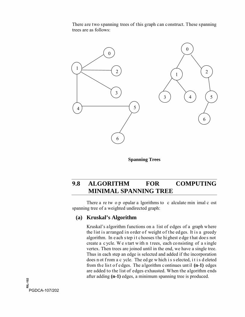
There are two spanning trees of this graph can construct. These spanning trees are as follows:
Spanning Trees
9.8 ALGORITHM FOR COMPUTING MINIMAL SPANNING TREE
There a re tw o p opular a lgorithms to c alculate min imal c ost spanning tree of a weighted undirected graph:
(a) Kruskal’s Algorithm Kruskal’s algorithm functions on a l ist of edges of a graph where the l ist i s arranged in order of weight of the edges. It i s a greedy algorithm. In e ach s tep i t c hooses t he hi ghest e dge t hat doe s not create a c ycle. W e s tart w ith n t rees, each co nsisting of a s ingle vertex. Then trees are joined until in the end, we have a single tree. Thus in each step an edge is selected and added if the incorporation does n ot f rom a c ycle. The ed ge w hich i s s elected, i t i s d eleted from th e lis t o f edges. The a lgorithm continues unt il (n-1) edges are added to the list of edges exhausted. When the algorithm ends after adding (n-1) edges, a minimum spanning tree is produced.
1
0
2
3
4 5
6
0
2 1
3 4 5
6
PGDCA-107/202
RIL
-102

Example
Consider t he f ollowing graph. T here a re e leven e dges. A n e dge connecting the vertices ‘i’ and ‘j’ may be represented by a tuple (i, j)
The l ist of edges of t he gr aph s orted i n non -descending or der m ay b e given by:
{(0,2), (1, 2), (0, 1), (1, 3), (2, 3), (2, 5), (4, 6), (4, 5), (3, 6), (5, 6), (1, 4)}
The initial tree we can show as:
The first edge (0,2) from the list of edges is taken into account. Since the addition of this edge does not form a cycle. It can be added to change the partial minimum spanning tree as show below:
0
1 2
3
5
6
5
2
6 7 25
11 15
10
14
12
1 2
3
4 5
6
PGDCA-107/203
RIL
-102
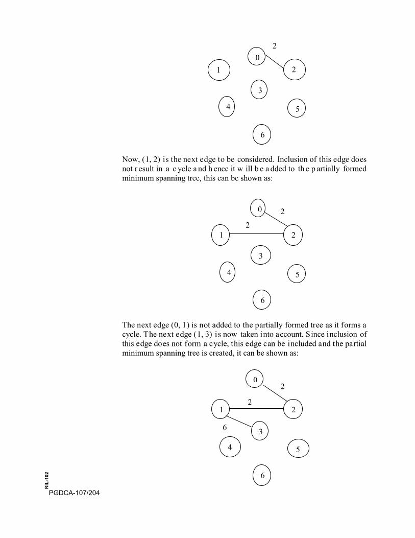
Now, (1, 2) is the next edge to be considered. Inclusion of this edge does not r esult in a c ycle a nd h ence it w ill b e a dded to th e p artially formed minimum spanning tree, this can be shown as:
The next edge (0, 1) is not added to the partially formed tree as it forms a cycle. The next edge (1, 3) is now taken into account. Since inclusion of this edge does not form a cycle, this edge can be included and the partial minimum spanning tree is created, it can be shown as:
01 2
3
4 5
6
2
0
1 2
3
4 5
6
2
2
0
1 2
3
4 5
6
2
2
6
PGDCA-107/204
RIL
-102
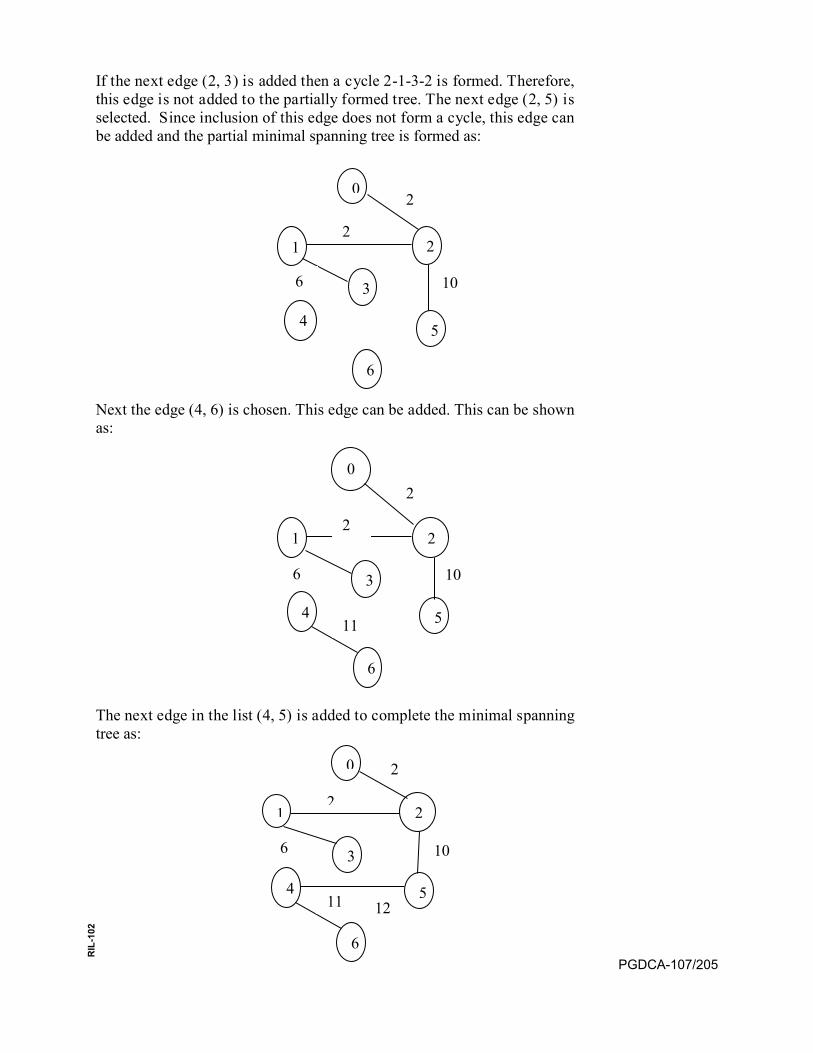
If the next edge (2, 3) is added then a cycle 2-1-3-2 is formed. Therefore, this edge is not added to the partially formed tree. The next edge (2, 5) is selected. Since inclusion of this edge does not form a cycle, this edge can be added and the partial minimal spanning tree is formed as:
Next the edge (4, 6) is chosen. This edge can be added. This can be shown as:
The next edge in the list (4, 5) is added to complete the minimal spanning tree as:
0
1 2
3
4 5
6
2
2
6 10
0
1 2
3
4 5
6
2
2
6 10
11
0
1 2
3
4 5
6
2
2
6 10
11 12
PGDCA-107/205
RIL
-102
Now we formally define the kruskal’s Minimum spanning tree algorithm as:
Function Kruskal [This al gorithm accep ts a co nnected w eighted undirected g raph G = (V, E, w) as t he i nput a nd pr oduces a m inimum spanning tree T of G as output]
1. Sort the edges by increasing weight
2. For each vertex v Є V do
3. Make-set (v)
4. ET = Ф
5. For each edge e = {u, v} Є E, in order by increasing weight do
6. If Find (u) ≠Find (v) then
7. ET = ET {e}
8. Union (u, v)
9. Return (V, ET)
(b) Prim’s Algorithm
Prim’s a lgorithm a lso w orks i n a gr eedy m anner but i t doe s not grow s everal c omponents. It j ust e xtends on e c omponent b y successively a dding ne w node s. In t his a lgorithm w e s tore a ll vertices in a priority queue. As long as a vertex y is not adjacent to a vertex of the spanning tree selected so far, its key is set to ∞. If it becomes ad jacent to some vertex say x, then i ts key becomes the weight of w({x, y}). If it becomes a adjacent to a new vertex, then we only set the key to the new weight if this will decrease the key. Thus, Key [x] is the cost of adding x to the tree grown so far.
Therefore w e c an s ay t hat th e P rim’s a lgorithm s tarts w ith a ny arbitrary v ertex a s th e p artial min imal s panning tree ‘T’. I n ea ch iteration of the algorithm one edge say (u, v) is added to the partial tree ‘T’ so that exactly one end of this edge belongs to the set of vertices in ‘T’. Hence, of all such possible edges, the edge having the l east cost i s s elected. T he algorithm co ntinues t o ad d (n-1) edges.
Example
Consider the following graph:
PGDCA-107/206
RIL
-102

Now we s tart with the vertex 0 and construct the min imal spanning tree from prim’s algorithm as:
Now we formally define the Prim’s Minimum spanning tree algorithm as:
Function Prim’s [This algorithm accepts a connected weighted undirected graph G = (V, E, w) as the input and produces a minimum spanning tree T of G as output]
1. Choose an arbitrary root r Є V.
2. Key [ r] = 0; key [v] = ∞ for all v Є V expect r.
3. Let Q be a min-priority queue filled with the vertices in V.
4. P [r] = NULL
5. While Q is not empty do
6. X = Extract-min (Q)
7. If p [x] ≠ NULL then
12
1 2
3
4 5
6
5
2
6 7 25
11 15
10
14
02
1 2
3
4 5
6
2
6
11
10
14
02
PGDCA-107/207
RIL
-102
8. Et = ET {p[x], x}
9. For each vertex y adjacent to x do
10. If y Є Q and w({x, y}) < Key [y] then
11. P[y] = z;
12. Key [y] = w({x, y})
13. Return (V, ET)
9.9 SHORTEST PATH ALGORITHMS
Suppose we are given a d irected graph G in which every edge has a w eight attached a nd o ur pr oblem i s t o obt ain the pa th w hich ha s t he shortest l ength be tween s ource a nd d estination node s or t he l ength of shortest path between the nodes. Thus we can say that let G = (V, E, w) be an edge-weighted directed graph and let s, t Є V. Let P = (v0,…….,vl) be the path from s to t, that is v0= s, vl=t. The issue is here to compute the shortest pa th f rom s to t. The f irst point which we have to investigate i s that is that whether the shortest walk from s to t is always a path. This is certainly the case if all weights are non-negative. Consider a walk from s to t that is not a path. Then this walk contains a cycle C. If the weight of C is non-negative, then we can remove this cycle and get a new walk whose weight is equal to w(C) = 0 or shorter than i f w(C)>0 the weight of the original walk. If the weight of C is negative, then the walk gets shorter if we go through C once more. In this case, there is no shortest walk from s to t. Thus, if on every walk from s to t there is no negative cycle, then the weight of shortest walk from s to t is well – defined and is always attained by a p ath. If there is a w alk with a n egative cycle from s to t, then we set weight to -∞.
Now w e explore th e general a lgorithm o f d etermining th e s hortest p ath from t he given weighted di agraph. T his a lgorithm i s know n a s WARSHALL algorithm. This algorithm is used to obtain a matrix which gives t he l engths of s hortest pa ths be tween t he node s. T he a lgorithm is defined as follows:
Algorithm MINIMAL [Given the adjacency matrix, B, in which the zero elements are replaced by infinity or some very large number, the matrix C produced by this algorithm shows the minimum lengths of paths between the nodes.]
1. [Initialize]
C = B;
2. [Perform a pass]
Repeat thru step 4 for k = 1, 2,,….,n
3. [process row]PGDCA-107/208
RIL
-102
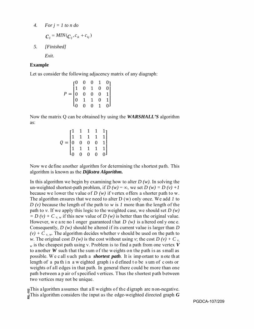
4. For j = 1 to n do
),( kjikijij ccMIN cc +=
5. [Finished]
Exit.
Example
Let us consider the following adjacency matrix of any diagraph:
𝑃 =
⎣⎢⎢⎢⎡0 0 0 1 01 0 1 0 00 0 0 0 10 1 1 0 10 0 0 1 0⎦
⎥⎥⎥⎤
Now the matrix Q can be obtained by using the WARSHALL’S algorithm as:
𝑄 =
⎣⎢⎢⎢⎡1 1 1 1 11 1 1 1 10 0 0 0 11 1 1 1 10 0 0 0 0⎦
⎥⎥⎥⎤
Now we define another algorithm for determining the shortest path. This algorithm is known as the Dijkstra Algorithm.
In this algorithm we begin by examining how to alter D (w). In solving the un-weighted shortest-path problem, if D (w) = ∞, we set D (w) = D (v) +1 because we lower the value of D (w) if vertex offers a shorter path to w. The algorithm ensures that we need to alter D (w) only once. We add 1 to D (v) because the length of the path to w is 1 more than the length of the path to v. If we apply this logic to the weighted case, we should set D (w) = D (v) + C v, w if this new value of D (w) is better than the original value. However, w e a re no l onger guaranteed t hat D (w) is a ltered onl y onc e. Consequently, D (w) should be altered if its current value is larger than D (v) + C v, w. The algorithm decides whether v should be used on the path to w. The original cost D (w) is the cost without using v; the cost D (v) + C v,
w is the cheapest path using v. Problem is to find a path from one vertex V to another W such that the sum of the weights on the path is as small as possible. W e c all s uch path a shortest path. It is imp ortant to n ote th at length of a pa th i n a w eighted graph i s d efined t o be s um of c osts or weights of all edges in that path. In general there could be more than one path between a p air of specified vertices. Thus the shortest path between two vertices may not be unique.
This a lgorithm assumes that a ll weights of the d igraph are non-negative. This algorithm considers the input as the edge-weighted directed graph G
PGDCA-107/209
RIL
-102
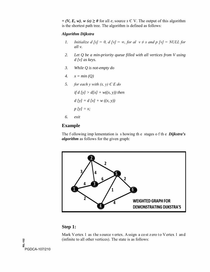
= (V, E, w), w (e) ≥ 0 for all e, source s Є V. The output of this algorithm is the shortest path tree. The algorithm is defined as follows:
Algorithm Dijkstra
1. Initialize d [s] = 0, d [v] = ∞, for al v ≠ s and p [v] = NULL forall v.
2. Let Q be a min-priority queue filled with all vertices from V usingd [v] as keys.
3. While Q is not-empty do
4. x = min (Q)
5. for each y with (x, y) Є E do
if d [y] > d[x] + w((x, y)) then
d [y] = d [x] + w ((x, y))
p [y] = x;
6. exit
Example
The f ollowing imp lementation is s howing th e stages o f th e Dijkstra’s algorithm as follows for the given graph:
Step 1: Mark Vertex 1 as t he source v ertex. Assign a co st z ero t o Vertex 1 and (infinite to all other vertices). The state is as follows:
PGDCA-107/210
RIL
-102
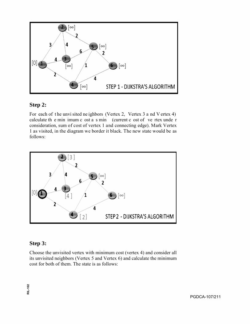
Step 2: For each of t he unvi sited ne ighbors (Vertex 2, Vertex 3 a nd V ertex 4) calculate th e min imum c ost a s min (current c ost of ve rtex unde r consideration, sum of cost of vertex 1 and connecting edge). Mark Vertex 1 as visited, in the diagram we border it black. The new state would be as follows:
Step 3: Choose the unvisited vertex with minimum cost (vertex 4) and consider all its unvisited neighbors (Vertex 5 and Vertex 6) and calculate the minimum cost for both of them. The state is as follows:
PGDCA-107/211
RIL
-102
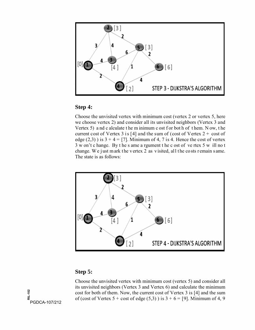
Step 4: Choose the unvisited vertex with minimum cost (vertex 2 or vertex 5, here we choose vertex 2) and consider all its unvisited neighbors (Vertex 3 and Vertex 5) a nd c alculate t he m inimum c ost f or bot h of t hem. N ow, t he current cost of Vertex 3 i s [4] and the sum of (cost of Vertex 2 + cost of edge (2,3) ) is 3 + 4 = [7]. Minimum of 4, 7 is 4. Hence the cost of vertex 3 w on’t c hange. By t he s ame a rgument t he c ost of ve rtex 5 w ill no t change. W e j ust m ark t he vertex 2 as v isited, al l t he costs r emain s ame. The state is as follows:
Step 5: Choose the unvisited vertex with minimum cost (vertex 5) and consider all its unvisited neighbors (Vertex 3 and Vertex 6) and calculate the minimum cost for both of them. Now, the current cost of Vertex 3 is [4] and the sum of (cost of Vertex 5 + cost of edge (5,3) ) is 3 + 6 = [9]. Minimum of 4, 9
PGDCA-107/212
RIL
-102
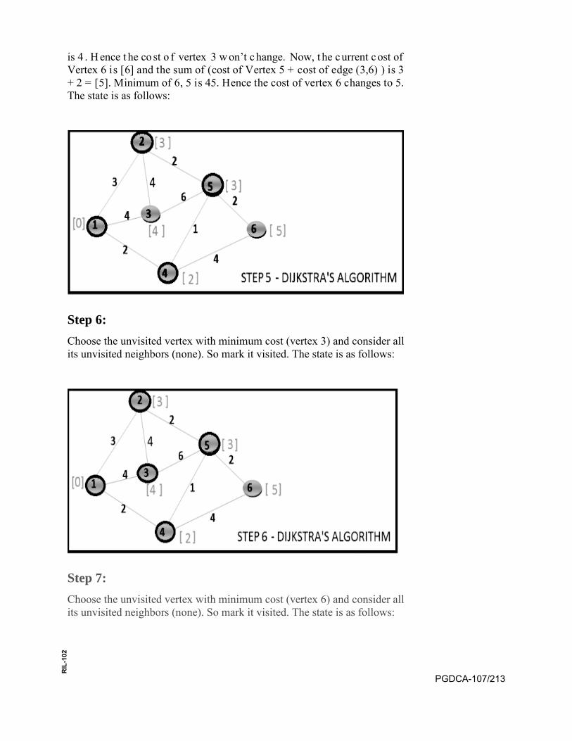
is 4 . H ence t he co st o f vertex 3 w on’t c hange. Now, t he c urrent c ost of Vertex 6 is [6] and the sum of (cost of Vertex 5 + cost of edge (3,6) ) is 3 + 2 = [5]. Minimum of 6, 5 is 45. Hence the cost of vertex 6 changes to 5. The state is as follows:
Step 6: Choose the unvisited vertex with minimum cost (vertex 3) and consider all its unvisited neighbors (none). So mark it visited. The state is as follows:
Step 7: Choose the unvisited vertex with minimum cost (vertex 6) and consider all its unvisited neighbors (none). So mark it visited. The state is as follows:
PGDCA-107/213
RIL
-102
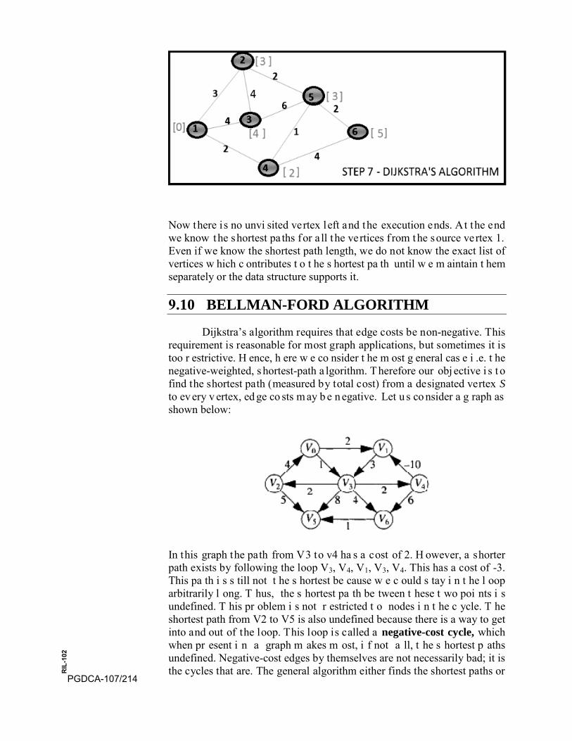
Now there is no unvi sited vertex left and the execution ends. At the end we know the shortest pa ths for a ll the vertices f rom the source vertex 1. Even if we know the shortest path length, we do not know the exact list of vertices w hich c ontributes t o t he s hortest pa th until w e m aintain t hem separately or the data structure supports it.
9.10 BELLMAN-FORD ALGORITHM
Dijkstra’s algorithm requires that edge costs be non-negative. This requirement is reasonable for most graph applications, but sometimes it is too r estrictive. H ence, h ere w e co nsider t he m ost g eneral cas e i .e. t he negative-weighted, s hortest-path a lgorithm. T herefore our obj ective i s t o find the shortest path (measured by total cost) from a designated vertex S to ev ery v ertex, ed ge co sts m ay b e n egative. Let u s co nsider a g raph as shown below:
In this graph the path from V3 to v4 ha s a cost of 2. H owever, a shorter path exists by following the loop V3, V4, V1, V3, V4. This has a cost of -3. This pa th i s s till not t he s hortest be cause w e c ould s tay i n t he l oop arbitrarily l ong. T hus, the s hortest pa th be tween t hese t wo poi nts i s undefined. T his pr oblem i s not r estricted t o nodes i n t he c ycle. T he shortest path from V2 to V5 is also undefined because there is a way to get into and out of the loop. This loop is called a negative-cost cycle, which when pr esent i n a graph m akes m ost, i f not a ll, t he s hortest p aths undefined. Negative-cost edges by themselves are not necessarily bad; it is the cycles that are. The general algorithm either finds the shortest paths or
PGDCA-107/214
RIL
-102

reports the existence of a negative-cost cycle is known as the Bellman – Ford algorithm.
Now w e f ormally define t he Bellman-Ford algorithm, th is a lgorithm accept the edge-weighted directed graph G = (V, E, w) and source s Є V as the input and return a shortest path tree.
Algorithm Bellman-Ford algorithm
1. Initialize d and p.
2. For I = 1,….., |V|-1 do
3. For each e = (u, v) Є E do
if d [v] > d[u] + w((u, v)) then
d [v] = d [u] + w ((u, v))
p [v] = u;
4. For each (u, v) Є E do
5. If d [v] > d [u] + w ((u, v)) then
6. Error “negative cycle”
7. Exit.
Example The following implementation is showing the stages of the Bellman-Ford algorithm as follows for the given graph:
Step 1 :
Considering A as the source, assign i t the cost zero. Add all the vertices (A, B, C, D, E, F, G, H) to a l ist. For all vertices except A assign a cost infinity. Also, it is advisable to maintain a list of edges handy. Here is the graph to start with:
PGDCA-107/215
RIL
-102
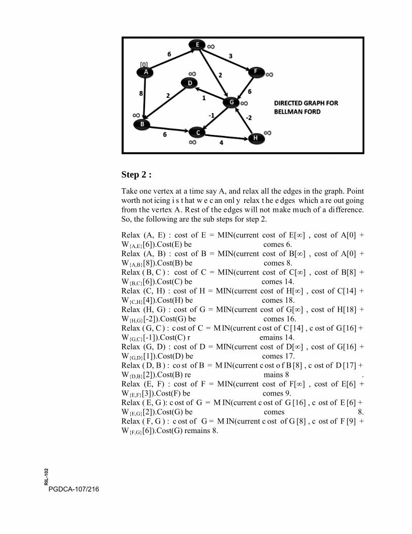
Step 2 :
Take one vertex at a time say A, and relax all the edges in the graph. Point worth not icing i s t hat w e c an onl y relax t he e dges which a re out going from the vertex A. Rest of the edges will not make much of a difference. So, the following are the sub steps for step 2.
Relax (A, E) : cost of E = MIN(current cost of E[∞] , cost of A[0] + W{A,E}[6]).Cost(E) be comes 6. Relax (A, B) : cost of B = MIN(current cost of B[∞] , cost of A[0] + W{A,B}[8]).Cost(B) be comes 8. Relax ( B, C ) : cost of C = MIN(current cost of C[∞] , cost of B[8] + W{B,C}[6]).Cost(C) be comes 14. Relax (C, H) : cost of H = MIN(current cost of H[∞] , cost of C[14] + W{C,H}[4]).Cost(H) be comes 18. Relax (H, G) : cost of G = MIN(current cost of G[∞] , cost of H[18] + W{H,G}[-2]).Cost(G) be comes 16. Relax (G, C) : cost of C = M IN(current cost of C[14] , c ost of G[16] + W{G,C}[-1]).Cost(C) r emains 14. Relax (G, D) : cost of D = MIN(current cost of D[∞] , cost of G[16] + W{G,D}[1]).Cost(D) be comes 17. Relax ( D, B ) : co st of B = M IN(current c ost o f B [8] , c ost of D [17] + W{D,B}[2]).Cost(B) re mains 8 . Relax (E, F) : cost of F = MIN(current cost of F[∞] , cost of E[6] + W{E,F}[3]).Cost(F) be comes 9. Relax ( E, G ): c ost of G = M IN(current c ost of G [16] , c ost of E [6] + W{E,G}[2]).Cost(G) be comes 8. Relax ( F, G ) : c ost of G = M IN(current c ost of G [8] , c ost of F [9] + W{F,G}[6]).Cost(G) remains 8.
PGDCA-107/216
RIL
-102
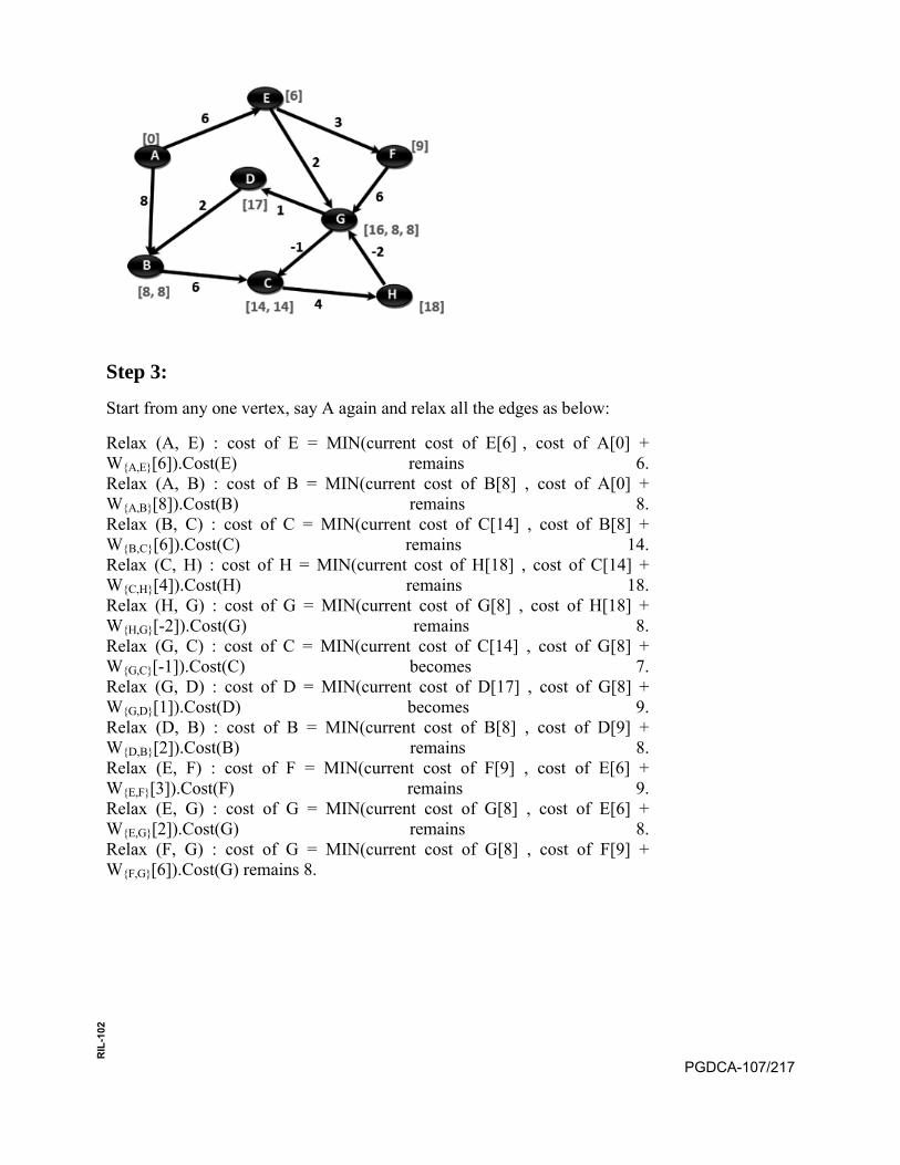
Step 3:
Start from any one vertex, say A again and relax all the edges as below:
Relax (A, E) : cost of E = MIN(current cost of E[6] , cost of A[0] + W{A,E}[6]).Cost(E) remains 6.Relax (A, B) : cost of B = MIN(current cost of B[8] , cost of A[0] + W{A,B}[8]).Cost(B) remains 8.Relax (B, C) : cost of C = MIN(current cost of C[14] , cost of B[8] + W{B,C}[6]).Cost(C) remains 14.Relax (C, H) : cost of H = MIN(current cost of H[18] , cost of C[14] + W{C,H}[4]).Cost(H) remains 18.Relax (H, G) : cost of G = MIN(current cost of G[8] , cost of H[18] + W{H,G}[-2]).Cost(G) remains 8.Relax (G, C) : cost of C = MIN(current cost of C[14] , cost of G[8] + W{G,C}[-1]).Cost(C) becomes 7.Relax (G, D) : cost of D = MIN(current cost of D[17] , cost of G[8] + W{G,D}[1]).Cost(D) becomes 9.Relax (D, B) : cost of B = MIN(current cost of B[8] , cost of D[9] + W{D,B}[2]).Cost(B) remains 8.Relax (E, F) : cost of F = MIN(current cost of F[9] , cost of E[6] + W{E,F}[3]).Cost(F) remains 9.Relax (E, G) : cost of G = MIN(current cost of G[8] , cost of E[6] + W{E,G}[2]).Cost(G) remains 8.Relax (F, G) : cost of G = MIN(current cost of G[8] , cost of F[9] + W{F,G}[6]).Cost(G) remains 8.
PGDCA-107/217
RIL
-102

Step 4:
Start from any one vertex, say A again and relax all the edges as below:
Relax (A, E) : cost of E = MIN(current cost of E[6] , cost of A[0] + W{A,E}[6]).Cost(E) remains 6.Relax (A, B) : cost of B = MIN(current cost of B[8] , cost of A[0] + W{A,B}[8]).Cost(B) remains 8.Relax (B, C) : cost of C = MIN(current cost of C[7] , cost of B[8] + W{B,C}[6]).Cost(C) becomes 7.Relax (C, H) : cost of H = MIN(current cost of H[18] , cost of C[7] + W{C,H}[4]).Cost(H) becomes 11.Relax (H, G) : cost of G = MIN(current cost of G[8] , cost of H[11] + W{H,G}[-2]).Cost(G) remains 8.Relax (G, C) : cost of C = MIN(current cost of C[7] , cost of G[8] + W{G,C}[-1]).Cost(C) remains 7.Relax (G, D) : cost of D = MIN(current cost of D[9] , cost of G[8] + W{G,D}[1]).Cost(D) remains 9.Relax (D, B) : cost of B = MIN(current cost of B[8] , cost of D[9] + W{D,B}[2]).Cost(B) remains 8.Relax (E, F) : cost of F = MIN(current cost of F[9] , cost of E[6] + W{E,F}[3]).Cost(F) remains 9.Relax (E, G) : cost of G = MIN(current cost of G[8] , cost of E[6] + W{E,G}[2]).Cost(G) remains 8.Relax (F, G) : cost of G = MIN(current cost of G[8] , cost of F[9] + W{F,G}[6]).Cost(G) remains 8.
PGDCA-107/218
RIL
-102
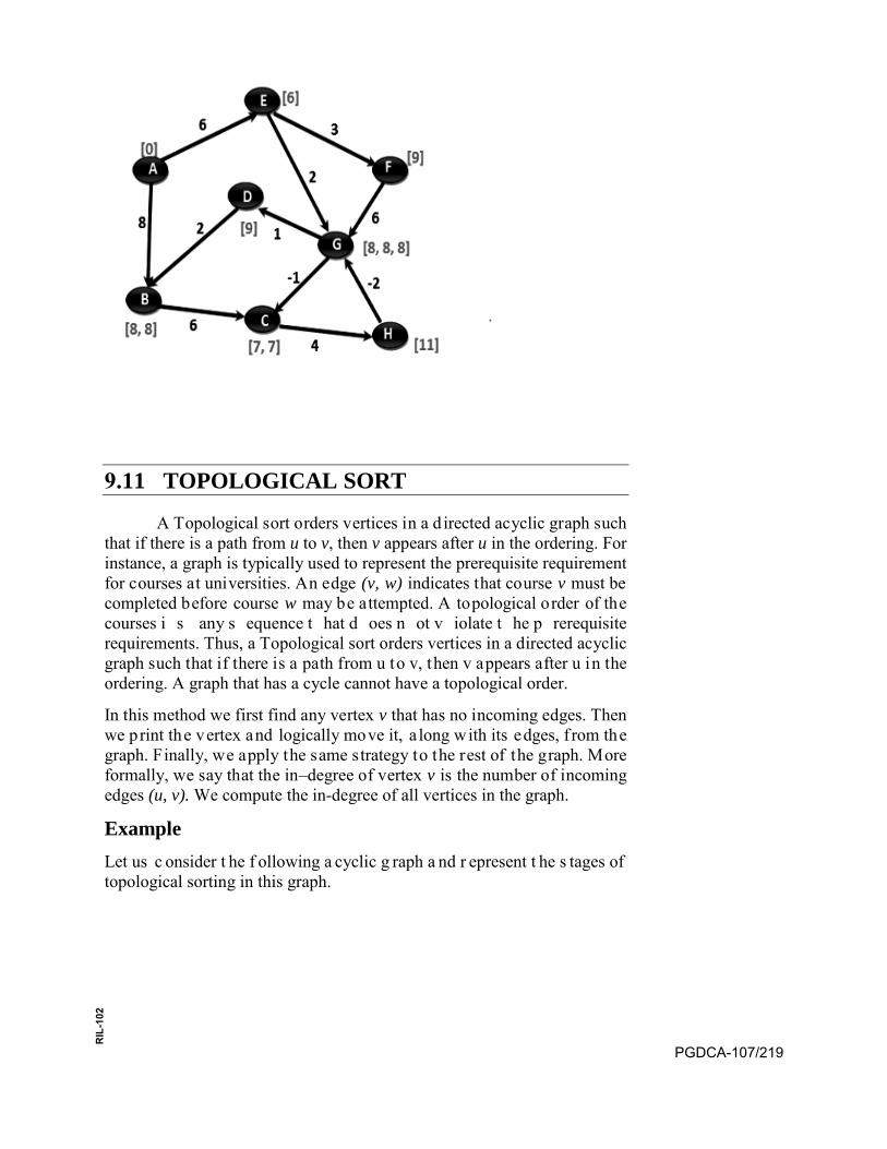
9.11 TOPOLOGICAL SORT
A Topological sort orders vertices in a d irected acyclic graph such that if there is a path from u to v, then v appears after u in the ordering. For instance, a graph is typically used to represent the prerequisite requirement for courses at universities. An edge (v, w) indicates that course v must be completed before course w may be attempted. A topological order of the courses i s any s equence t hat d oes n ot v iolate t he p rerequisite requirements. Thus, a Topological sort orders vertices in a directed acyclic graph such that if there is a path from u to v, then v appears after u in the ordering. A graph that has a cycle cannot have a topological order.
In this method we first find any vertex v that has no incoming edges. Then we print the vertex and logically move it, a long with its edges, f rom the graph. Finally, we apply the same strategy to the rest of the graph. More formally, we say that the in–degree of vertex v is the number of incoming edges (u, v). We compute the in-degree of all vertices in the graph.
Example Let us c onsider t he f ollowing a cyclic g raph a nd r epresent t he s tages of topological sorting in this graph.
PGDCA-107/219
RIL
-102
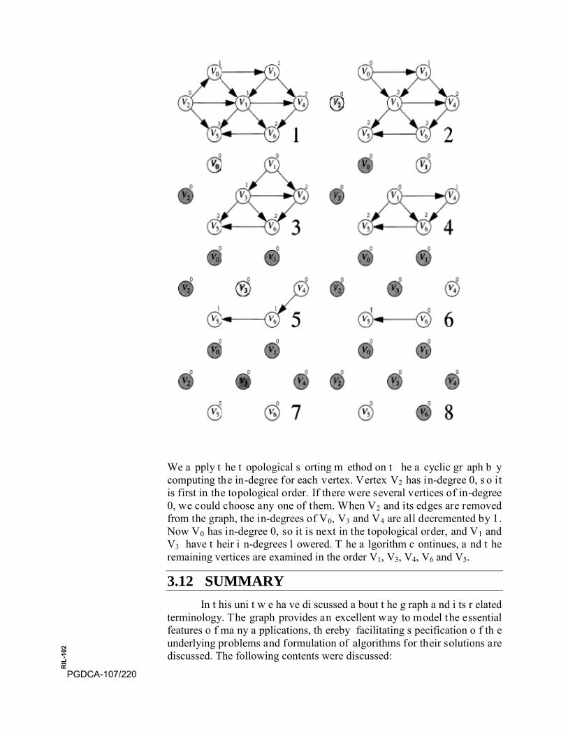
We a pply t he t opological s orting m ethod on t he a cyclic gr aph b y computing the in-degree for each vertex. Vertex V2 has in-degree 0, s o it is first in the topological order. If there were several vertices of in-degree 0, we could choose any one of them. When V2 and its edges are removed from the graph, the in-degrees of V0, V3 and V4 are all decremented by 1. Now V0 has in-degree 0, so it is next in the topological order, and V1 and V3 have t heir i n-degrees l owered. T he a lgorithm c ontinues, a nd t he remaining vertices are examined in the order V1, V3, V4, V6 and V5.
3.12 SUMMARY In t his uni t w e ha ve di scussed a bout t he g raph a nd i ts r elated
terminology. The graph provides an excellent way to model the essential features o f ma ny a pplications, th ereby facilitating s pecification o f th e underlying problems and formulation of algorithms for their solutions are discussed. The following contents were discussed:
PGDCA-107/220
RIL
-102
• A G raph i s a nonl inear data s tructure that i s us ed t o r epresent arelational data
• Each node of the graph is called as a vertex and link or line drawnbetween them is called and edge
• The i mplementation of graph a nd i ts r epresentations w ay w erediscussed. It has been seen that the graph is implemented in manyways by the use of different kinds of data structures.
• In m any a pplications, e dges are t o be a ssigned costs or w eights.Such graphs are known as weighted graphs.
• The directed graph and acyclic graphs were also described.
• There are various ways of representing a graph.
• Adjacency matrix of a graph is a matrix representation.
• Adjacency list of a graph is a linked list representation.
• The reach matrix and path matrix can also be constructed from theadjacency matrix representation of the graph.
• The method of obtaining the path matrix of a simple diagraph caneasily be computed by using the WARSHALL algorithm
• There ar e two popul ar t echniques f or graph t raversal i .e. br eadthfirst search and Depth first search.
• A spanning tree of a graph is an undirected tree consisting of onlythose edges necessary to connect all the nodes in the original graph
• The two famous algorithms to complete a minimal spanning tree ofa weighted graph are Kruskal’s and prim’s algorithm.
• The shortest pa th determination i s important for any di rected andweighted graph.
• For positive – weighted graphs the Dijkstr’a algorithm is used butfor t he ne gative w eighted g raphs t he pr oblem be comes m oredifficult.
• The general algorithm either finds the shortest paths or reports theexistence of a negative-cost cycle is known as the Bellman – Fordalgorithm.
• Finally, for acyclic graphs, the running time reverts to linear timethe aid of topological sort.
PGDCA-107/221
RIL
-102
Bibliography
Horowitz, E ., S . S ahni: “ Fundamental of computer A lgorithms”, Computer Science Press, 1978
J. P. Tremblay, P . G. Sorenson “An Introduction to Data Structures with Applications”, Tata McGraw-Hill, 1984
M. A llen W eiss: “ Data s tructures a nd P roblem s olving us ing C ++”, Pearson Addison Wesley, 2003
Markus Blaner: “ Introduction t o A lgorithms a nd D ata S tructures”, Saarland University, 2011
Niklaus W irth, “ Algorithm + Data Structures = P rograms”, PHI Publications
Seymour Lipschutz, “Data Structure”, Schaum’s outline Series
B. Flaming, “Practical Data Structures in C++”, John Wiley & Sons, New York, 1994
R. Sedgewick, “Algorithms in C++, Addision-Wesley, 1992.
R. E . B ellman, “On a r outing P roblem”, Q uarterly o f A pplied Mathematics, 16 (1958) 87-90
D. E . K nuth, “ The S tanford G raphBase”, A ddison-Wesley, R eading, Mass. 1993.
R. E . T arjan, “ Data S tructures a nd ne twork Algorithms”, S ociety f or Industrial and Applied Mathematics, Philadelphia, 1985.
PGDCA-107/222
RIL
-102
SELF EVALUATION 1. A vertex with degree one is a graph is called
a. A leaf
b. Pendant Vertex
c. Adjacency list
d. None of the above
2. In an adjacency matrix parallel edges are given by:
a. Similar Columns
b. Similar rows
c. Not represent-able
d. None of the above
3. Which of the following representation of graph is more adequate?
a. Stack representation of graphs.
b. Adjacency matrix representation of graphs
c. Linked representation of graphs.
d. None of the above.
4. Prim’s a lgorithm is a me thod a vailable f or f inding o ut theminimum cost of a spanning tree.
a. O(n*n)
b. O(n log n)
c. O (n)
d. O (1)
5. What is a Path matrix?
6. Kruskal’s a lgorithm f or bui lding m inimal c ost spanning t ree of agraph c onsiders e dges f or i nclusion i n t he t ree i n t he……………… order of the cost.
7. Write P rim’s a lgorithm for f inding m inimal s panning t ree of anygraph.
8. By considering the complete graph with n v ertices, show that thenumber of spanning trees is at least 12 1 −−n
9. Find t he s hortest un -weighted p ath f rom V 3 to all o thers in th egraph show in figure (A) below.
PGDCA-107/223
RIL
-102
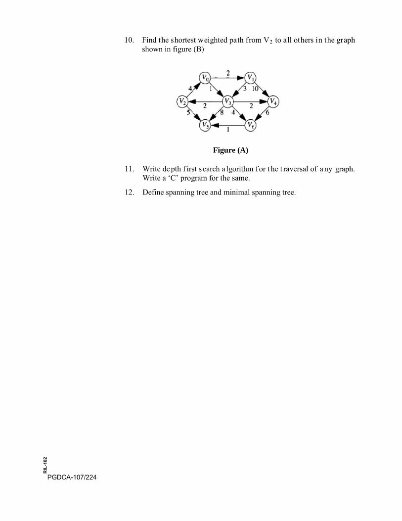
10. Find the shortest weighted path from V2 to all others in the graphshown in figure (B)
Figure (A)
11. Write de pth f irst s earch a lgorithm f or t he t raversal of a ny graph.Write a ‘C’ program for the same.
12. Define spanning tree and minimal spanning tree.
PGDCA-107/224
RIL
-102

PGDCA-107/225
RIL
-102

PGDCA-107/226
RIL
-102
BLOCK
4 Searching and Sorting, Hashing and File Organization UNIT-10
Searching and Sorting
UNIT-11
Hashing
UNIT-12
File Organization
Postgraduate Diploma in Computer Application
Uttar Pradesh Rajarshi Tandon Open University
PGDCA-107 Data Structure
231-288
289-304
305-320
PGDCA-107/227
RIL
-102
Curriculum Design Committee Dr.P.P.Dubey Coordinator Director, School of Agri. Sciences, UPRTOU, Prayagraj Prof. U. N. Tiwari Member Dept. of Computer Science and Engg., Indian Inst. Of Information Science and Tech., Prayagraj Prof. R.S. Yadav, Member Dept. of Computer Science and Engg., MNNIT, Allahabad, Prayagraj Prof. P. K. Mishra Member Dept. of Computer Science, Baranas Hindu University, Varanasi Mr. Prateek Kesrwani Member Secretary Academic Consultant-Computer Science School of Science, UPRTOU, Prayagraj
Course Design Committee Prof. U. N. Tiwari Member Dept. of Computer Science and Engg., Indian Inst. Of Information Science and Tech., Prayagraj Prof. R.S. Yadav, Member Dept. of Computer Science and Engg., MNNIT, Prayagraj Prof. P. K. Mishra Member Dept. of Computer Science, Baranas Hindu University, Varanasi Faculty Members, School of Sciences Dr. Ashutosh Gupta, Director, School of Science, UPRTOU, Prayagraj Dr. Shruti, A sst. P rof., ( Statistics), School of S cience, UPRTOU, Prayagraj Ms. M arisha Asst. P rof., ( Computer S cience), School of S cience, UPRTOU, Prayagraj Mr. Manoj K Balwant Asst. Prof., (Computer Science), School of Science, UPRTOU, Prayagraj Dr. Dinesh K Gupta Academic Consultant (Chemistry), Scool of Science, UPRTOU, Prayagraj
PGDCA-107/228
RIL
-102
Dr. A cademic C onsultant ( Maths), School of S cience, UPRTOU, Prayagraj Dr. Dharamveer Singh, Academic Consultant (Bio-Chemistry), School of Science, UPRTOU, Prayagraj Dr. R . P . S ingh, A cademic C onsultant ( Bio-Chemistry), School of Science, UPRTOU, Prayagraj Dr. S usma C huhan, A cademic C onsultant ( Botany), School of S cience, UPRTOU, Prayagraj Dr. Deepa pathak, Academic Consultant (Chemistry), School of Science, UPRTOU, Prayagraj Dr. A. K. Singh, A cademic C onsultant ( Physics), School of S cience, UPRTOU, Prayagraj Dr. S . S . T ripathi, A cademic C onsultant ( Maths), School of S cience, UPRTOU, Prayagraj
Course Preparation Committee Prof. Manu Pratap Singh, Author Dept. of Computer Science Dr. B. R. Ambedkar University, Agra-282002 Dr. Ashutosh Gupta Editor Director, School of Sciences, UPRTOU, Prayagraj Prof. U. N. Tiwari Member Dept. of Computer Science and Engg., Indian Inst. Of Information Science and Tech., Prayagraj Prof. R.S. Yadav Member Dept. of Computer Science and Engg., MNNIT, Allahabad, Prayagraj Prof. P. K. Mishra Member Dept. of Computer Science Baranas Hindu University, Varanasi Dr. Dinesh K Gupta, SLM Coordinator Academic Consultant- Chemistry School of Science, UPRTOU, Prayagraj
© UPRTOU, Prayagraj. 2020 ISBN : 978-93-83328-15-4 All Rights are reserved. No part of this work may be reproduced in any form, by mimeograph or any other means, without permission in writing from the Uttar Pradesh Rajarshi Tondon Open University, Prayagraj.
PGDCA-107/229
RIL
-102
BLOCK INTRODUCTION
This block will cover the various searching & sorting techniques, hashing techniques a nd f ile or ganization i n t he s ystem. We w ill co ncentrate o n some techniques to search a particular data or piece of information from a large amount of data in Unit 10. There are basically two types of searching techniques, l inear o r s equential search a nd binary search. W e w ill al so discuss va rious s orting a lgorithms l ike S election s ort, B ubble s ort, Insertion s ort, H eap s ort, Q uick S ort, M erge s ort, S hell s ort a nd R adix sort. E nough number of examples is discussed to show the operations in searching & sorting.
Hashing technique is also discussed in Unit 11. Hashing is the process of mapping la rge a mount of d ata ite m to s maller ta ble w ith th e h elp o f hashing f unction. Hashing i s a lso know n a s H ashing A lgorithm. It i s a technique to convert a range of key values into a range of indexes of an array. It is u sed to facilitate th e n ext le vel searching me thod w hen compared with the linear or binary
In c ommon t erminology, a f ile i s a bl ock of i mportant da ta which i s available t o a ny c omputer s oftware a nd i s us ually s tored on a ny s torage device. Storing a file on any storage medium like pen drive, hard disk or floppy disk ensures the availability of the file in future. Now days all file are stored in computers to reduce paper work and easy availability in any office, ba nk o r l ibrary. The f ile o rganization i s also c overed i n Unit 12 with examples.
This bl ock w ill he lp you t o r ealize t he c oncept of s earching, s orting, hashing and file organization in detail with suitable examples and with the help of codes.
PGDCA-107/230
RIL
-102
UNIT-10 SEARCHING AND SORTING Structure
10.0 Introduction
10.1 Objectives
10.2 Sequential Search
10.3 Binary Search
10.4 Sorting
10.5 Selection Sort
10.6 Bubble Sort
10.7 Insertion Sort
10.8 Heap Sort
10.9 Quick Sort
10.10 Merge Sort
10.11 Shell Sort
10.12 Radix Sort
10.13 Summary
10.0 INTRODUCTION
Searching i s t he pr ocess of l ooking f or s omething: F inding one piece of data that has been stored within a whole group of data. However, if the value is not present in the array, the searching process displays an appropriate message and in this case searching is said to be unsuccessful. It is o ften th e mo st time -consuming pa rt of m any c omputer pr ograms. There are a va riety of methods, or a lgorithms, us ed t o s earch f or a da ta item, depending on how much data there is to look through, what kind of data it is, what type of structure the data is stored in, and even where the data is stored - inside computer memory or on some external medium.
Sorting me ans a rranging th e elements o f a n a rray in s mallest to la rgest (ascending) or largest to smallest (descending) order. A sorting algorithm is defined as an algorithm that puts the elements of a list in a certain order. Sorting algorithms are widely used to optimize the use of other algorithms like s earch an d m erge al gorithms w hich r equire s orted l ists t o w ork correctly. There are two types of sorting:
• Internal s orting which deals w ith s orting th e d ata s tored in th ecomputer’s main memory (RAM)
PGDCA-107/231
RIL
-102
• External s orting w hich deals w ith s orting th e d ata s tored in f iles(Secondary Storage)
In this unit, we will concentrate on some techniques to search a particular data or pi ece of i nformation f rom a l arge a mount of da ta. There a re basically t wo t ypes o f s earching t echniques, Linear o r Sequential Search and B inary S earch. W e will al so d iscuss v arious s orting algorithms lik e Selection s ort, Bubble s ort, Insertion s ort, H eap s ort, Q uick S ort, M erge sort, Shell sort and Radix sort.
10.1 OBJECTIVES
After going through this unit, you should be able to:
• Understand the concept of searching and its types.
• Implementation of sequential and binary with example.
• Understand the concept of sorting and its types.
• Understand the concept of Selection sort with example.
• Understand the concept of Bubble sort with example.
• Understand the concept of Insertion sort with example.
• Understand the concept of Heap sort with example.
• Understand the concept of Quick sort with example.
• Understand the concept of Merge sort with example.
• Understand the concept of Shell sort with example.
• Understand the concept of Radix sort with example.
10.2 SEQUENTIAL SEARCH
Sequential s earch i s v ery simple t o i mplement for s earching an item in a collection. It is also known as Linear search. It is not the most efficient way to search for an item in a collection. It works by comparing the value to be searched with every element of the array one by one in a sequential manner until an item is found. Moreover, if the array elements are a rranged in random order, i t i s the only reasonable way to search an item. Thus, for many situations, Sequential search is a valid approach.
For example, if an array A [ ] is initialized as under,
int A[ ] = {25, 18, 22, 67, 33, 54, 69, 10, 87,78};
and the value to be searched is 67. So we have to search whether the value VAL=67 is present in the array or not. If yes, then it returns the position of its occurrence. Here, POS = 3 (index starting from 0).
PGDCA-107/232
RIL
-102
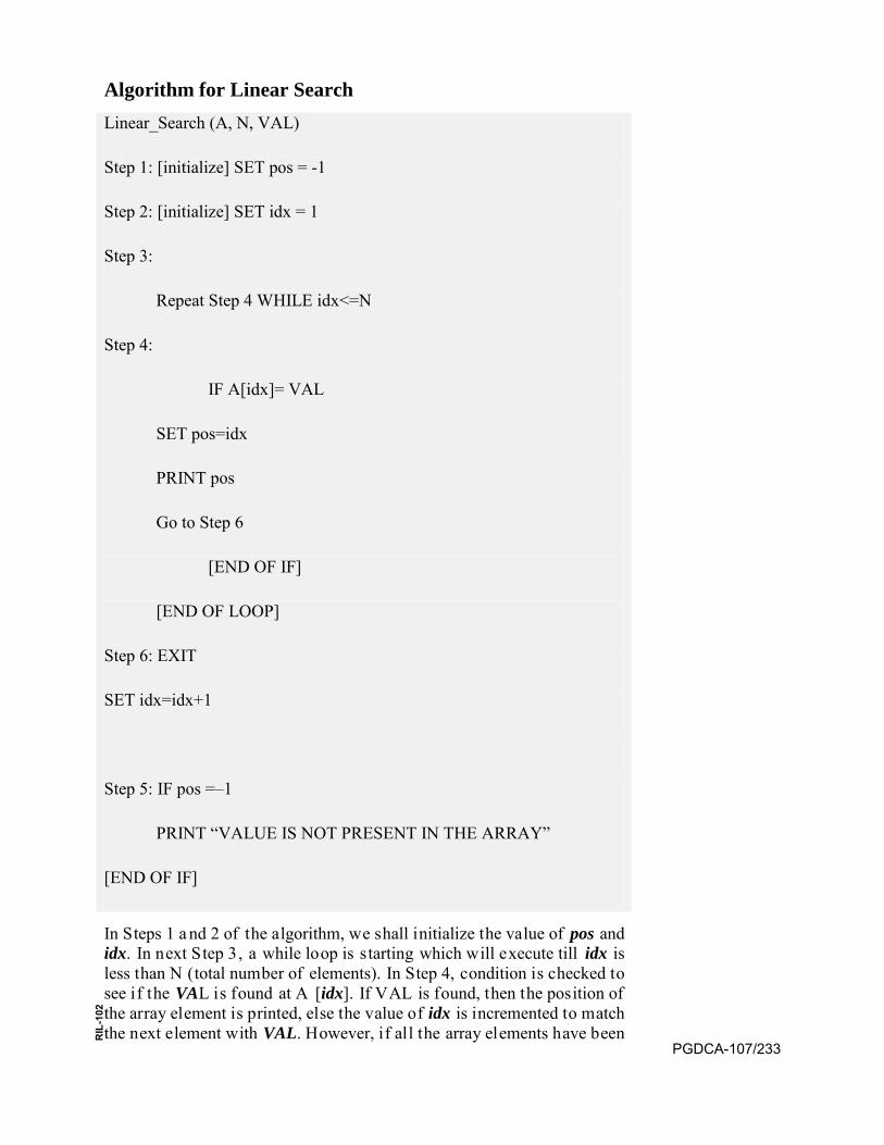
Algorithm for Linear Search Linear_Search (A, N, VAL)
Step 1: [initialize] SET pos = -1
Step 2: [initialize] SET idx = 1
Step 3:
Repeat Step 4 WHILE idx<=N
Step 4:
IF A[idx]= VAL
SET pos=idx
PRINT pos
Go to Step 6
[END OF IF]
[END OF LOOP]
Step 6: EXIT
SET idx=idx+1
Step 5: IF pos =–1
PRINT “VALUE IS NOT PRESENT IN THE ARRAY”
[END OF IF]
In Steps 1 a nd 2 of the algorithm, we shall initialize the value of pos and idx. In next Step 3, a while loop is starting which will execute till idx is less than N (total number of elements). In Step 4, condition is checked to see if the VAL is found at A [idx]. If VAL is found, then the position of the array element is printed, else the value of idx is incremented to match the next element with VAL. However, if all the array elements have been
PGDCA-107/233
RIL
-102
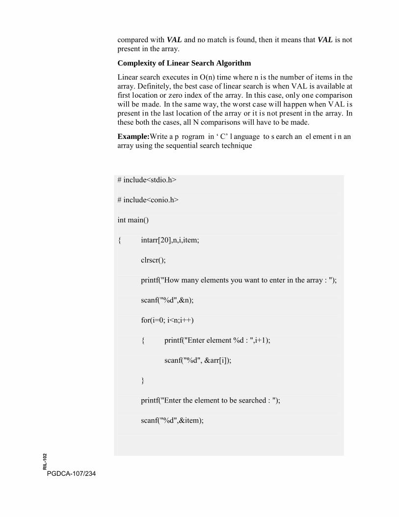
compared with VAL and no match is found, then it means that VAL is not present in the array.
Complexity of Linear Search Algorithm
Linear search executes in O(n) time where n is the number of items in the array. Definitely, the best case of linear search is when VAL is available at first location or zero index of the array. In this case, only one comparison will be made. In the same way, the worst case will happen when VAL is present in the last location of the array or it is not present in the array. In these both the cases, all N comparisons will have to be made.
Example:Write a p rogram in ‘ C’ l anguage to s earch an el ement i n an array using the sequential search technique
# include<stdio.h>
# include<conio.h>
int main()
{ intarr[20],n,i,item;
clrscr();
printf("How many elements you want to enter in the array : ");
scanf("%d",&n);
for(i=0; i<n;i++)
{ printf("Enter element %d : ",i+1);
scanf("%d", &arr[i]);
}
printf("Enter the element to be searched : ");
scanf("%d",&item);
PGDCA-107/234
RIL
-102
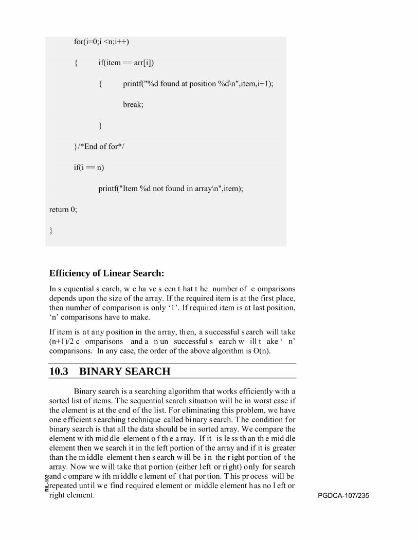
for(i=0;i <n;i++)
{ if(item == arr[i])
{ printf("%d found at position %d\n",item,i+1);
break;
}
}/*End of for*/
if(i == n)
printf("Item %d not found in array\n",item);
return 0;
}
Efficiency of Linear Search: In s equential s earch, w e ha ve s een t hat t he number of c omparisons depends upon the size of the array. If the required item is at the first place, then number of comparison is only ‘1’. If required item is at last position, ‘n’ comparisons have to make.
If item is at any position in the array, then, a successful search will take (n+1)/2 c omparisons and a n un successful s earch w ill t ake ‘ n’ comparisons. In any case, the order of the above algorithm is O(n).
10.3 BINARY SEARCH
Binary search is a searching algorithm that works efficiently with a sorted list of items. The sequential search situation will be in worst case if the element is at the end of the list. For eliminating this problem, we have one efficient searching t echnique called binary search. The condition for binary search is that all the data should be in sorted array. We compare the element w ith mid dle element o f th e a rray. If it is le ss th an th e mid dle element then we search it in the left portion of the array and if it is greater than t he m iddle element t hen s earch w ill be i n the r ight por tion of t he array. Now we will take that portion (either left or right) only for search and c ompare w ith m iddle e lement of t hat por tion. T his pr ocess will be repeated unt il we find required element or middle element has no l eft or right element. PGDCA-107/235
RIL
-102

For understanding this searching method, let us take 3 variables Beg, End and Mid. The Beg variable will indicate to first item’s index of array (zero index of array), End variable will indicate to the last index of array. Mid will take care of average of both Beg and End as under:
Mid = (Beg + End) / 2
To unde rstand t he concept of bi nary s earch, l et us t ake a n a rray o f 10 elements which is as under in ascending order.
Now we are searching the item 85 in the above array.
Step 1: Beg = 0 End = 9 Mid = (Beg + End) / 2 = 4
Now at index 4, middle item is 67 which is smaller than required item 85. So we will search in right side from middle point. Now, Beg = Mid + 1 = 5, and End will be the same.
Step 2: Beg = 5 End = 9 Mid = (Beg + End) / 2 = 7
Array [10] 0 1 2 3 4 5 6 7 8 9
Values 12 34 39 45 67 73 85 93 102 110
12 34 39 45 67 73 85 93 102 110
0 1 2 3 4 5 6 7 8 9
12 34 39 45 67 73 85 93 102 110
0 1 2 3 4 5 6 7 8 9
12 34 39 45 67 73 85 93 102 110
PGDCA-107/236
RIL
-102

Now at index 7, middle item is 93 which is greater than required item 85. So we will search in left side from middle point. Now, End = Mid - 1 = 6, and Beg will be the same.
Step 3: Beg = 5 End = 6 Mid = (Beg + End) / 2 = 5
Now at index 5, middle item is 73 which is less than required item 85. So we will search in right side from middle point. Now, Beg = Mid+ 1 = 6, and End will be the same.
Step 4: Beg = 6 End = 6 Mid = (Beg + End) / 2 = 6
Now at index 6, middle item is 85 which is equal to required item 85.
Let see the algorithm of binary search.
BINARY_SEARCH(A, LB, UB, VAL)
Step 1: [INITIALIZE]
SET BEG= LB
END= UB,
POS= -1
Step 2: Repeat Step 3 and 4 while BEG <= END
Step 3: SET MID= (BEG+ END)/2
Step 4: IF A[MID]= VAL
0 1 2 3 4 5 6 7 8 9
12 34 39 45 67 73 85 93 102 110
0 1 2 3 4 5 6 7 8 9
12 34 39 45 67 73 85 93 102 110
PGDCA-107/237
RIL
-102
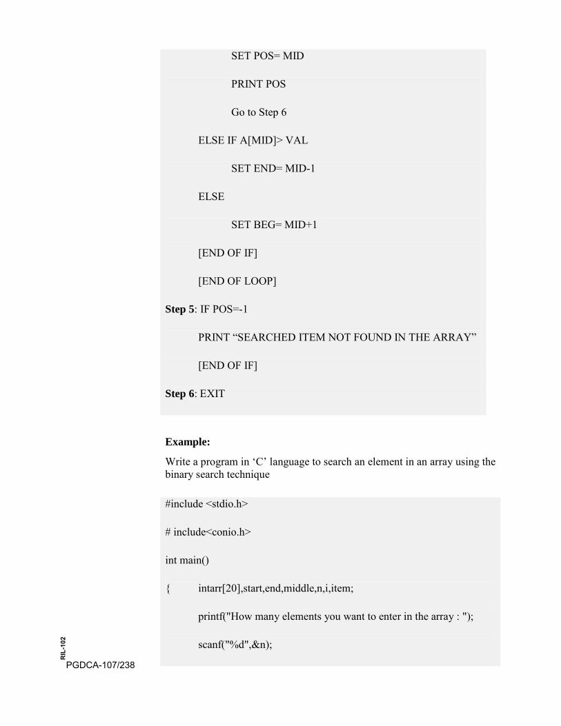
SET POS= MID
PRINT POS
Go to Step 6
ELSE IF A[MID]> VAL
SET END= MID-1
ELSE
SET BEG= MID+1
[END OF IF]
[END OF LOOP]
Step 5: IF POS=-1
PRINT “SEARCHED ITEM NOT FOUND IN THE ARRAY”
[END OF IF]
Step 6: EXIT
Example:
Write a program in ‘C’ language to search an element in an array using the binary search technique
#include <stdio.h>
# include<conio.h>
int main()
{ intarr[20],start,end,middle,n,i,item;
printf("How many elements you want to enter in the array : ");
scanf("%d",&n);
PGDCA-107/238
RIL
-102

for(i=0; i< n; i++)
{ printf("Enter element %d : ",i+1);
scanf("%d",&arr[i]);
}
printf("Enter the element to be searched : ");
scanf("%d",&item);
start=0;
end=n-1;
middle=(start+end)/2;
while(item != arr[middle] && start <= end)
{ if(item >arr[middle])
start=middle+1;
else
end=middle-1;
middle=(start+end)/2;
}
if(item==arr[middle])
printf("%d found at position %d\n",item,middle+1);
if(start>end)
printf("%d not found in array\n",item);
return 0;
} PGDCA-107/239
RIL
-102
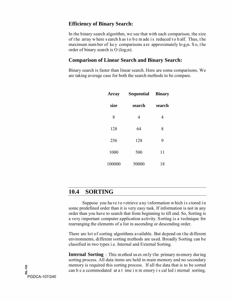
Efficiency of Binary Search:
In the binary search algorithm, we see that with each comparison, the size of t he array w here s earch h as t o b e m ade i s reduced t o h alf. Thus, t he maximum num ber of ke y comparisons a re approximately lo g2n. S o, t he order of binary search is O (log2n).
Comparison of Linear Search and Binary Search:
Binary search is faster than linear search. Here are some comparisons. We are taking average case for both the search methods to be compare.
Array
size
Sequential
search
Binary
search
8 4 4
128 64 8
256 128 9
1000 500 11
100000 50000 18
10.4 SORTING
Suppose you ha ve t o r etrieve a ny i nformation w hich i s s tored i n some predefined order than it is very easy task. If information is not in any order than you have to search that from beginning to till end. So, Sorting is a very important computer application activity. Sorting is a technique for rearranging the elements of a list in ascending or descending order.
There are lot of sorting algorithms available. But depend on t he different environments, different sorting methods are used. Broadly Sorting can be classified in two types i.e. Internal and External Sorting.
Internal Sorting : This m ethod us es on ly t he primary m emory dur ing sorting process. All data items are held in main memory and no secondary memory is required this sorting process. If all the data that is to be sorted can b e a ccommodated at a t ime i n m emory i s cal led i nternal sorting.
PGDCA-107/240
RIL
-102
There is a limita tion f or in ternal s orts; th ey can o nly p rocess r elatively small lists due to memory constraints. There are 3 types of internal sorts.
1. EXCHANGE SORT :- Ex:- Bubble Sort Algorithm, Quick sortalgorithm
2. INSERTION SORT :- Ex:- Insertion sort algorithm, Shell Sortalgorithm
3. SELECTION S ORT : - Ex:- Selection sort a lgorithm, Heap Sort algorithm
External Sorting : S orting l arge a mount of d ata r equires e xternal or secondary memory. This process uses ex ternal memory such as HDD, to store the data which is not fit into the main memory. So, primary memory holds the currently being sorted data only. All external sorts are based on process of merging. Different parts of data are sorted separately and then merged together. Ex: Merge Sort
10.5 SELECTION SORT
Selection sort is the process to select the smallest element from the array and put i t at f irst place (zero i ndex) i n t he a rray. Suppose A i s an array of size n stored in memory. The selection sort algorithm first selects the smallest element in the array A and place it in array at index 0; then it selects th e n ext s mallest e lement in th e a rray A a nd p lace it in a rray at index 1 a nd s o on. It s imply c ontinues t his p rocedure unt il i t pl aces t he biggest element in the last position of the array.
The array is passed through (n-1) times and the smallest element is placed in its respective position in the array as detailed below:
Pass 1: Find the location j o f the smallest e lement in the a rray x [0], A [1],....A [n-1], and then interchange x[j] with A [0]. Then A [0] is sorted.
Pass 2: Leave th e f irst element a nd f ind th e lo cation j o f th e s mallest element in the sub-array A [1], A [2],....A[n-1], and then interchange A[1] with A[j]. Then A[0], A[1] are sorted.
Pass 3: Leave the first two elements and find the location j of the smallest element in the sub-array A [2], A [3],....A[n-1], and then interchange A [2] with A [j]. Then A [0], A [1], A[2] are sorted.
Pass (n-1): Find the location j o f the smaller of the elements A[n-2] and A[n-1], and then interchange A[j] and A[n-2]. Then A[0], A[1], . . . . A [n-2] are s orted. O f c ourse, dur ing t his pa ss A [n-1] w ill b e th e b iggestelement and so the entire array is sorted.
PGDCA-107/241
RIL
-102

0 1 2 3 4 5 6 7 8 Remarks
65 70 75 80 50 60 55 85 45 find the smallest element
i j swap a[i] & a[j]
45 70 75 80 50 60 55 85 65 find the second smallest
i j swap a[i] & a[j]
45 50 75 80 70 60 55 85 65 Find the third smallest
i j swap a[i] & a[j]
45 50 55 80 70 60 75 85 65 Find the fourth smallest
i j swap a[i] & a[j]
45 50 55 60 70 80 75 85 65 Find the fifth smallest
i j swap a[i] & a[j]
45 50 55 60 65 80 75 85 70 Find the sixth smallest
i j swap a[i] & a[j]
45 50 55 60 65 70 75 85 80 Find the seventh smallest
i j swap a[i] & a[j]
45 50 55 60 65 70 75 85 80 Find the eighth smallest
i j swap a[i] & a[j]
45 50 55 60 65 70 75 80 85 The outer loop ends.
Complexity of Selection Sort In general we prefer selection sort in case where the insertion sort or the bubble s ort r equires e xclusive s wapping. In s pite of s uperiority o f t he selection sort over bubbl e sort and the i nsertion sort ( there i s s ignificant decrease in run time), its efficiency is also O(n2) for n data items.
PGDCA-107/242
RIL
-102
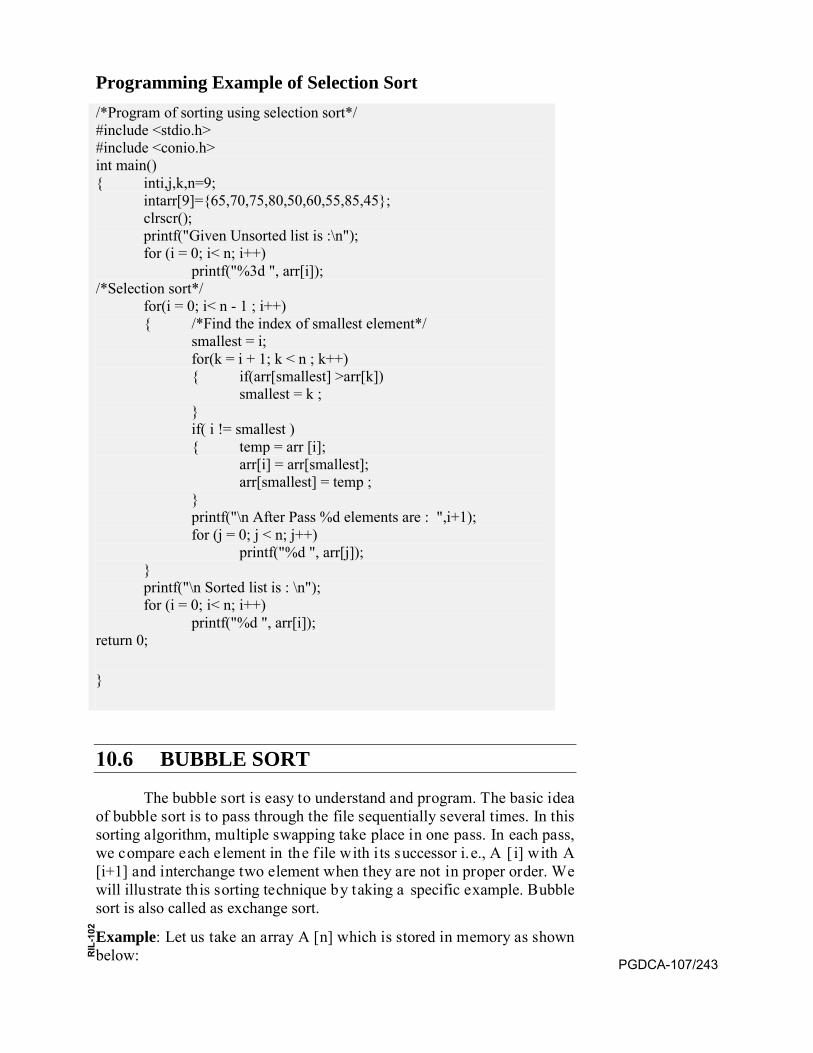
Programming Example of Selection Sort /*Program of sorting using selection sort*/ #include <stdio.h> #include <conio.h> int main() { inti,j,k,n=9;
intarr[9]={65,70,75,80,50,60,55,85,45}; clrscr(); printf("Given Unsorted list is :\n"); for (i = 0; i< n; i++)
printf("%3d ", arr[i]); /*Selection sort*/
for(i = 0; i< n - 1 ; i++) { /*Find the index of smallest element*/
smallest = i; for(k = i + 1; k < n ; k++) { if(arr[smallest] >arr[k])
smallest = k ; } if( i != smallest ) { temp = arr [i];
arr[i] = arr[smallest]; arr[smallest] = temp ;
} printf("\n After Pass %d elements are : ",i+1); for (j = 0; j < n; j++)
printf("%d ", arr[j]); } printf("\n Sorted list is : \n"); for (i = 0; i< n; i++)
printf("%d ", arr[i]); return 0;
}
10.6 BUBBLE SORT
The bubble sort is easy to understand and program. The basic idea of bubble sort is to pass through the file sequentially several times. In this sorting algorithm, multiple swapping take place in one pass. In each pass, we compare each element in the f ile with i ts successor i.e., A [ i] with A [i+1] and interchange two element when they are not in proper order. We will illustrate this sorting technique by taking a specific example. Bubble sort is also called as exchange sort.
Example: Let us take an array A [n] which is stored in memory as shown below: PGDCA-107/243
RIL
-102
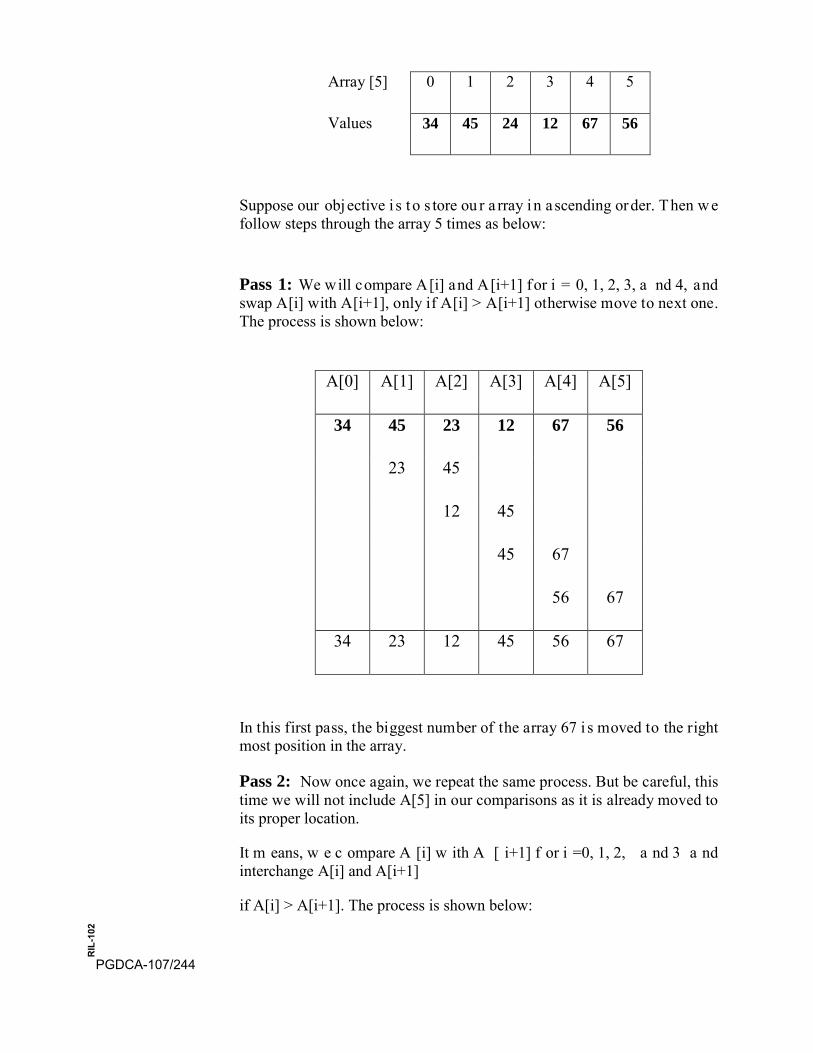
Array [5] 0 1 2 3 4 5
Values 34 45 24 12 67 56
Suppose our obj ective i s t o s tore ou r a rray in ascending order. Then w e follow steps through the array 5 times as below:
Pass 1: We will compare A[i] and A[i+1] for i = 0, 1, 2, 3, a nd 4, and swap A[i] with A[i+1], only if A[i] > A[i+1] otherwise move to next one. The process is shown below:
A[0] A[1] A[2] A[3] A[4] A[5]
34 45 23 12 67 56
23 45
12 45
45 67
56 67
34 23 12 45 56 67
In this first pass, the biggest number of the array 67 i s moved to the right most position in the array.
Pass 2: Now once again, we repeat the same process. But be careful, this time we will not include A[5] in our comparisons as it is already moved to its proper location.
It m eans, w e c ompare A [i] w ith A [ i+1] f or i =0, 1, 2, a nd 3 a nd interchange A[i] and A[i+1]
if A[i] > A[i+1]. The process is shown below:
PGDCA-107/244
RIL
-102

A[0] A[1] A[2] A[3] A[4] A[5]
34 23 12 45 56 67
23 34
12 34
34 45
45 56
23 12 34 45 56 67
Pass 3: We repeat the same process, but this time we leave both A[4] and A [ 5] a s t hese both are on correct pos ition. By doing this, w e move the third biggest number 45 to A [3].
A[0] A[1] A[2] A[3] A[4] A[5]
23 12 34 45 56 67
12 23
23 34
34 45
12 23 34 45 56 67
Pass 4: We r epeat t he p rocess b y l eaving el ements at A [3], A [4] a nd A[5]. By doing this, we move the fourth biggest number 34 to A[2].
PGDCA-107/245
RIL
-102

A[0] A[1] A[2] A[3] A[4] A[5]
12 23 34 45 56 67
12 23
23 33
12 23 34 45 56 67
Pass 5: We repeat the process by leaving elements at A [2], A [3], A[4] and A[5]. By doing this, we move the fifth biggest number 23 to A[1]. At this time, we will have the smallest number 12 in A[0]. Thus, we see that we can sort the array of size 6 in 5 passes.
A[0] A[1] A[2] A[3] A[4] A[5]
12 23 34 45 56 67
12 23
12 23 34 45 56 67
For an array of size n, we required (n-1) passes using bubble sort.
Algorithm for bubble sort:
BUBBLE_SORT(A, N)
Step 1: Repeat Step2 For I=0 to N-1
Step 2: Repeat For J= 0 to N-I
Step 3: IF A[J]> A[J+1]
SWAP A[J] and A[J+1]
[END OF INNER LOOP]
[END OF OUTER LOOP]
Step 4: EXIT PGDCA-107/246
RIL
-102
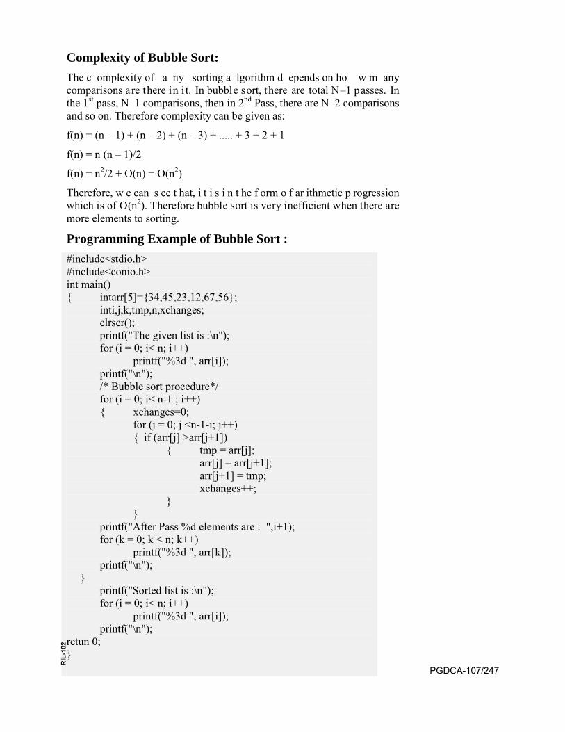
Complexity of Bubble Sort: The c omplexity of a ny sorting a lgorithm d epends on ho w m any comparisons are there in i t. In bubble sort, there are total N–1 passes. In the 1st pass, N–1 comparisons, then in 2nd Pass, there are N–2 comparisons and so on. Therefore complexity can be given as:
f(n) = (n – 1) + (n – 2) + (n – 3) + ..... + 3 + 2 + 1
f(n) = n (n – 1)/2
f(n) = n2/2 + O(n) = O(n2)
Therefore, w e can s ee t hat, i t i s i n t he f orm o f ar ithmetic p rogression which is of O(n2). Therefore bubble sort is very inefficient when there are more elements to sorting.
Programming Example of Bubble Sort : #include<stdio.h> #include<conio.h> int main() { intarr[5]={34,45,23,12,67,56};
inti,j,k,tmp,n,xchanges; clrscr(); printf("The given list is :\n"); for (i = 0; i< n; i++)
printf("%3d ", arr[i]); printf("\n"); /* Bubble sort procedure*/ for (i = 0; i< n-1 ; i++) { xchanges=0;
for (j = 0; j <n-1-i; j++) { if (arr[j] >arr[j+1])
{ tmp = arr[j]; arr[j] = arr[j+1]; arr[j+1] = tmp; xchanges++;
} }
printf("After Pass %d elements are : ",i+1); for (k = 0; k < n; k++)
printf("%3d ", arr[k]); printf("\n");
} printf("Sorted list is :\n"); for (i = 0; i< n; i++)
printf("%3d ", arr[i]); printf("\n");
retun 0; }
PGDCA-107/247
RIL
-102
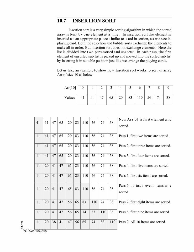
10.7 INSERTION SORT
Insertion sort is a very simple sorting algorithm in which the sorted array is b uilt b y o ne e lement a t a time . In in sertion s ort th e element is inserted a t an a ppropriate p lace s imilar to c ard in sertion, a s w e s ee in playing card. Both the selection and bubble sorts exchange the elements to make all in order. But insertion sort does not exchange elements. Here the list is d ivided i nto t wo parts s orted a nd uns orted. In each p ass, t he first element of unsorted sub list is picked up and moved into the sorted sub list by inserting it in suitable position just like we arrange the playing cards.
Let us take an example to show how Insertion sort works to sort an array Arr of size 10 as below:
41 11 47 65 20 83 110 56 74 38 Now Ar r[0] is f irst e lement a nd
sorted.
11 41 47 65 20 83 110 56 74 38 Pass 1, first two items are sorted.
11 41 47 65 20 83 110 56 74 38 Pass 2, first three items are sorted.
11 41 47 65 20 83 110 56 74 38 Pass 3, first four items are sorted.
11 20 41 47 65 83 110 56 74 38 Pass 4, first five items are sorted.
11 20 41 47 65 83 110 56 74 38 Pass 5, first six items are sorted.
11 20 41 47 65 83 110 56 74 38 Pass 6 , f irst s even i tems ar e
sorted.
11 20 41 47 56 65 83 110 74 38 Pass 7, first eight items are sorted.
11 20 41 47 56 65 74 83 110 38 Pass 8, first nine items are sorted.
11 20 38 41 47 56 65 74 83 110 Pass 9, All 10 items are sorted.
Arr[10] 0 1 2 3 4 5 6 7 8 9
Values 41 11 47 65 20 83 110 56 74 38
PGDCA-107/248
RIL
-102
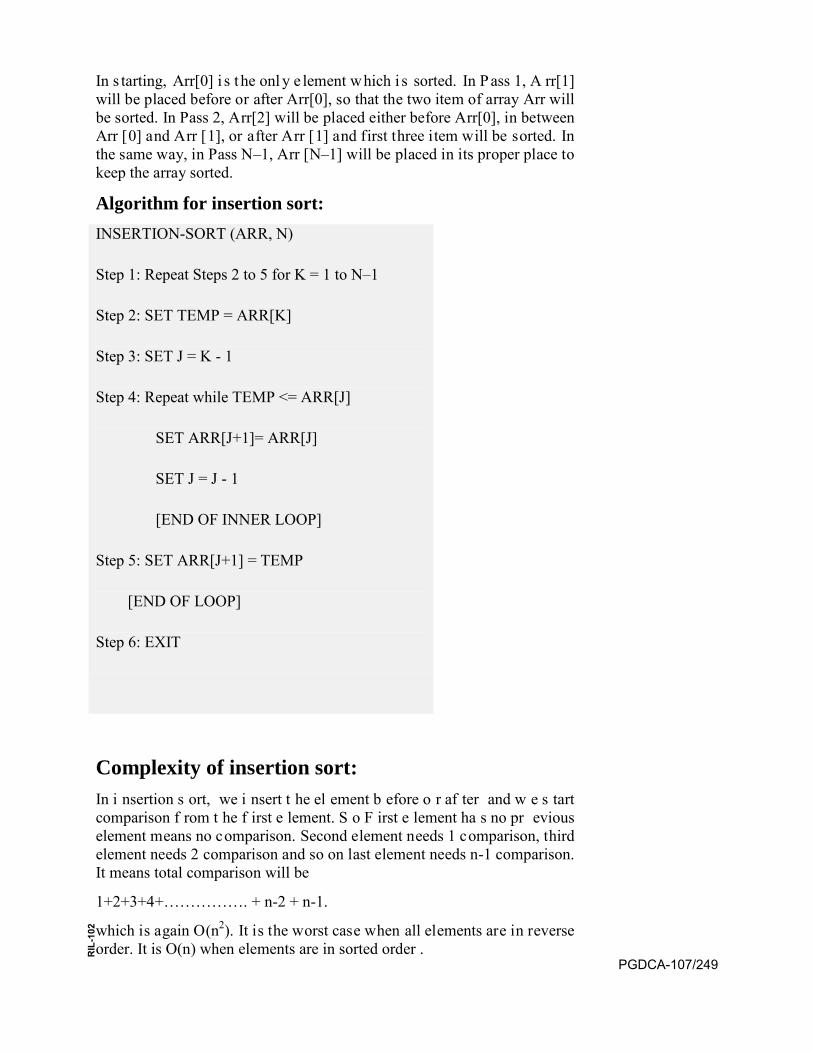
In s tarting, Arr[0] i s t he onl y e lement which i s sorted. In Pass 1, A rr[1] will be placed before or after Arr[0], so that the two item of array Arr will be sorted. In Pass 2, Arr[2] will be placed either before Arr[0], in between Arr [0] and Arr [1], or after Arr [1] and first three item will be sorted. In the same way, in Pass N–1, Arr [N–1] will be placed in its proper place to keep the array sorted.
Algorithm for insertion sort: INSERTION-SORT (ARR, N)
Step 1: Repeat Steps 2 to 5 for K = 1 to N–1
Step 2: SET TEMP = ARR[K]
Step 3: SET J = K - 1
Step 4: Repeat while TEMP <= ARR[J]
SET ARR[J+1]= ARR[J]
SET J = J - 1
[END OF INNER LOOP]
Step 5: SET ARR[J+1] = TEMP
[END OF LOOP]
Step 6: EXIT
Complexity of insertion sort: In i nsertion s ort, we i nsert t he el ement b efore o r af ter and w e s tart comparison f rom t he f irst e lement. S o F irst e lement ha s no pr evious element means no comparison. Second element needs 1 comparison, third element needs 2 comparison and so on last element needs n-1 comparison. It means total comparison will be
1+2+3+4+……………. + n-2 + n-1.
which is again O(n2). It is the worst case when all elements are in reverse order. It is O(n) when elements are in sorted order .
PGDCA-107/249
RIL
-102
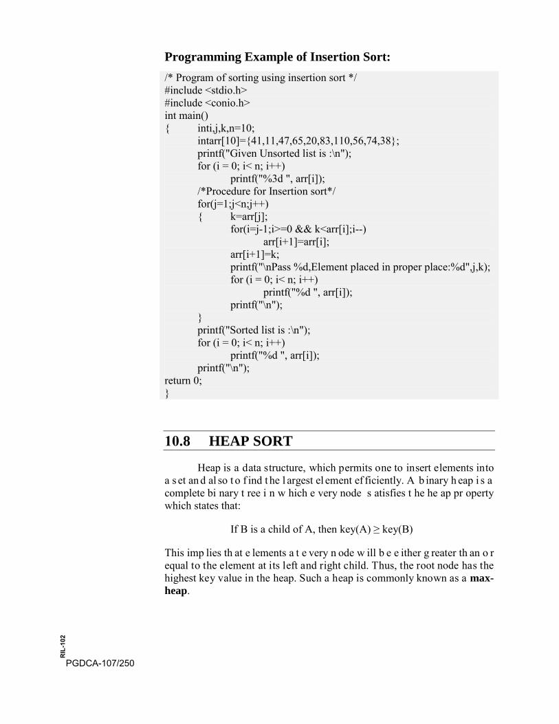
Programming Example of Insertion Sort: /* Program of sorting using insertion sort */ #include <stdio.h> #include <conio.h> int main() { inti,j,k,n=10;
intarr[10]={41,11,47,65,20,83,110,56,74,38}; printf("Given Unsorted list is :\n"); for (i = 0; i< n; i++)
printf("%3d ", arr[i]); /*Procedure for Insertion sort*/ for(j=1;j<n;j++) { k=arr[j];
for(i=j-1;i>=0 && k<arr[i];i--) arr[i+1]=arr[i];
arr[i+1]=k; printf("\nPass %d,Element placed in proper place:%d",j,k); for (i = 0; i< n; i++)
printf("%d ", arr[i]); printf("\n");
} printf("Sorted list is :\n"); for (i = 0; i< n; i++)
printf("%d ", arr[i]); printf("\n");
return 0; }
10.8 HEAP SORT
Heap is a data structure, which permits one to insert elements into a s et an d al so t o f ind t he l argest el ement ef ficiently. A b inary h eap i s a complete bi nary t ree i n w hich e very node s atisfies t he he ap pr operty which states that:
If B is a child of A, then key(A) ≥ key(B)
This imp lies th at e lements a t e very n ode w ill b e e ither g reater th an o r equal to the element at its left and right child. Thus, the root node has the highest key value in the heap. Such a heap is commonly known as a max-heap.
PGDCA-107/250
RIL
-102
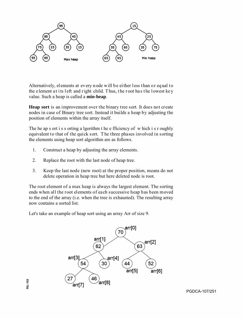
Alternatively, el ements at every node will be ei ther l ess than or equal to the e lement a t i ts l eft and r ight child. T hus, t he r oot ha s t he l owest ke y value. Such a heap is called a min-heap.
Heap sort is an improvement over the binary tree sort. It does not create nodes in case of Binary tree sort. Instead it builds a heap by adjusting the position of elements within the array itself.
The he ap s ort i s s orting a lgorithm t he e fficiency of w hich i s r oughly equivalent to that of the quick sort. T he three phases involved in sorting the elements using heap sort algorithm are as follows.
1. Construct a heap by adjusting the array elements.
2. Replace the root with the last node of heap tree.
3. Keep the last node (new root) at the proper position, means do notdelete operation in heap tree but here deleted node is root.
The root element of a max heap is always the largest element. The sorting ends when all the root elements of each successive heap has been moved to the end of the array (i.e. when the tree is exhausted). The resulting array now contains a sorted list.
Let's take an example of heap sort using an array Arr of size 9.
PGDCA-107/251
RIL
-102
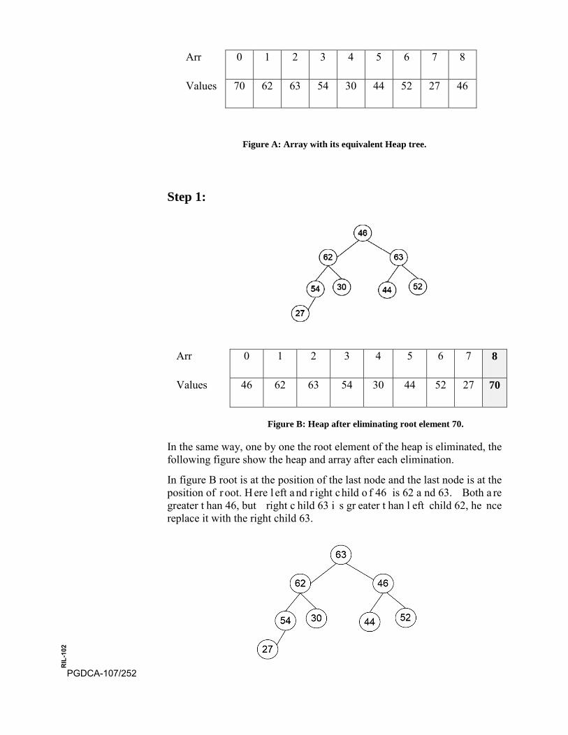
Arr 0 1 2 3 4 5 6 7 8
Values 70 62 63 54 30 44 52 27 46
Figure A: Array with its equivalent Heap tree.
Step 1:
Figure B: Heap after eliminating root element 70.
In the same way, one by one the root element of the heap is eliminated, the following figure show the heap and array after each elimination.
In figure B root is at the position of the last node and the last node is at the position of r oot. H ere l eft a nd r ight c hild o f 46 is 62 a nd 63. Both a re greater t han 46, but right c hild 63 i s gr eater t han l eft child 62, he nce replace it with the right child 63.
Arr 0 1 2 3 4 5 6 7 8
Values 46 62 63 54 30 44 52 27 70
PGDCA-107/252
RIL
-102
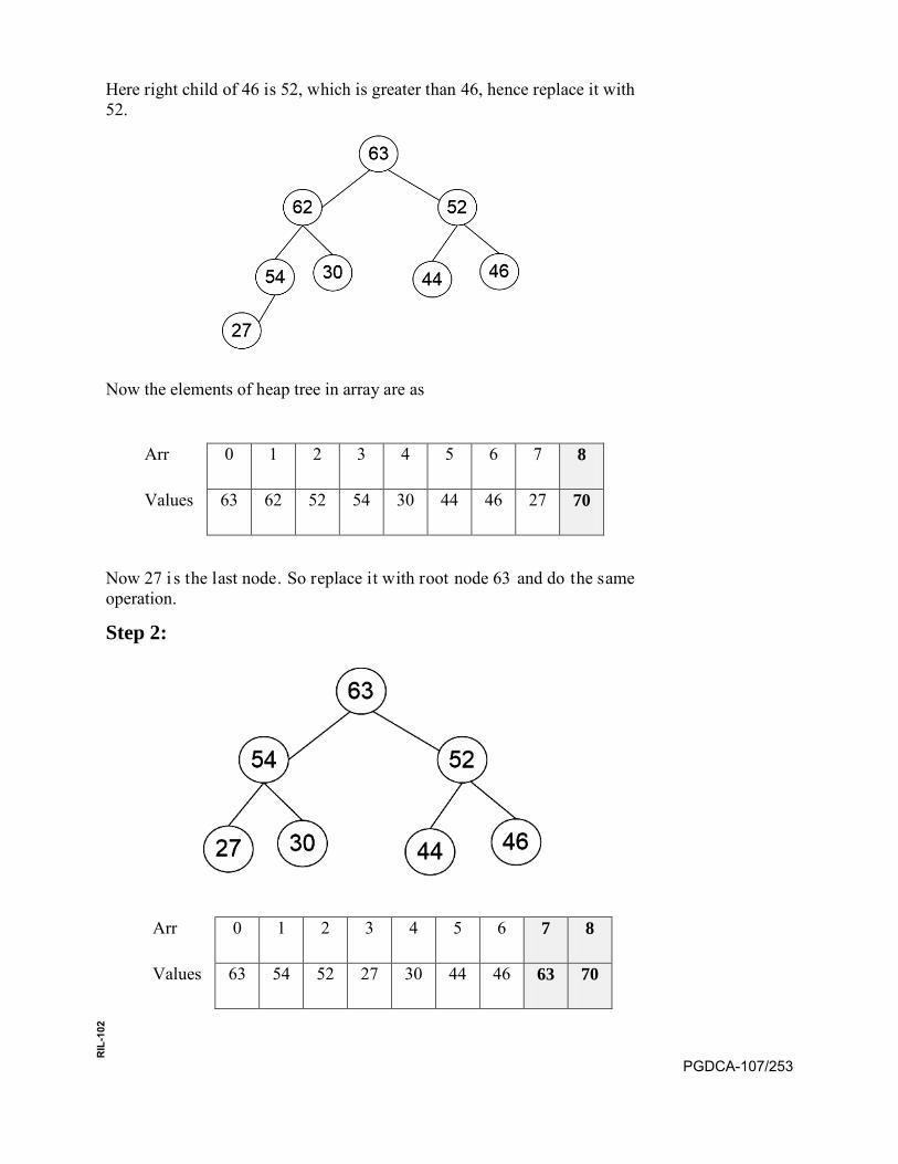
Here right child of 46 is 52, which is greater than 46, hence replace it with 52.
Now the elements of heap tree in array are as
Arr 0 1 2 3 4 5 6 7 8
Values 63 62 52 54 30 44 46 27 70
Now 27 i s the last node. So replace it with root node 63 and do the same operation.
Step 2:
Arr 0 1 2 3 4 5 6 7 8
Values 63 54 52 27 30 44 46 63 70
PGDCA-107/253
RIL
-102
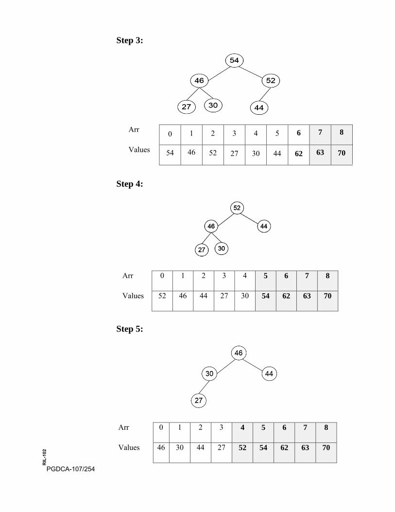
Step 3:
Step 4:
Step 5:
Arr 0 1 2 3 4 5 6 7 8
Values 54 46 52 27 30 44 62 63 70
Arr 0 1 2 3 4 5 6 7 8
Values 52 46 44 27 30 54 62 63 70
Arr 0 1 2 3 4 5 6 7 8
Values 46 30 44 27 52 54 62 63 70
PGDCA-107/254
RIL
-102
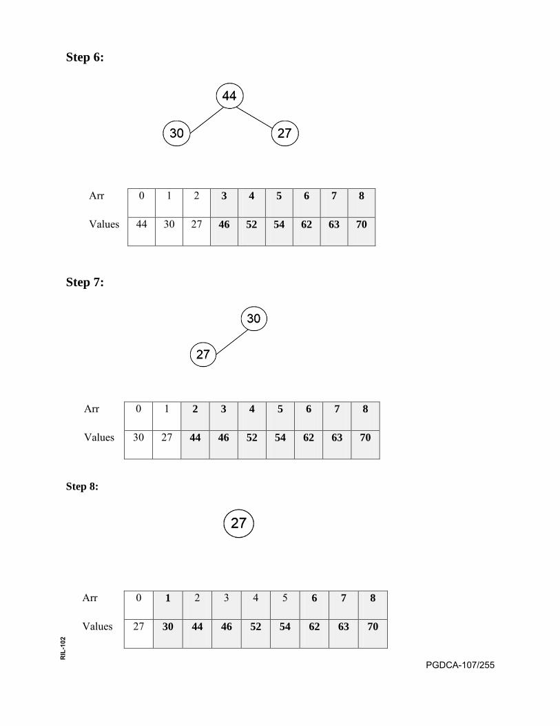
Step 6:
Arr 0 1 2 3 4 5 6 7 8
Values 44 30 27 46 52 54 62 63 70
Step 7:
Step 8:
Arr 0 1 2 3 4 5 6 7 8
Values 30 27 44 46 52 54 62 63 70
Arr 0 1 2 3 4 5 6 7 8
Values 27 30 44 46 52 54 62 63 70
PGDCA-107/255
RIL
-102
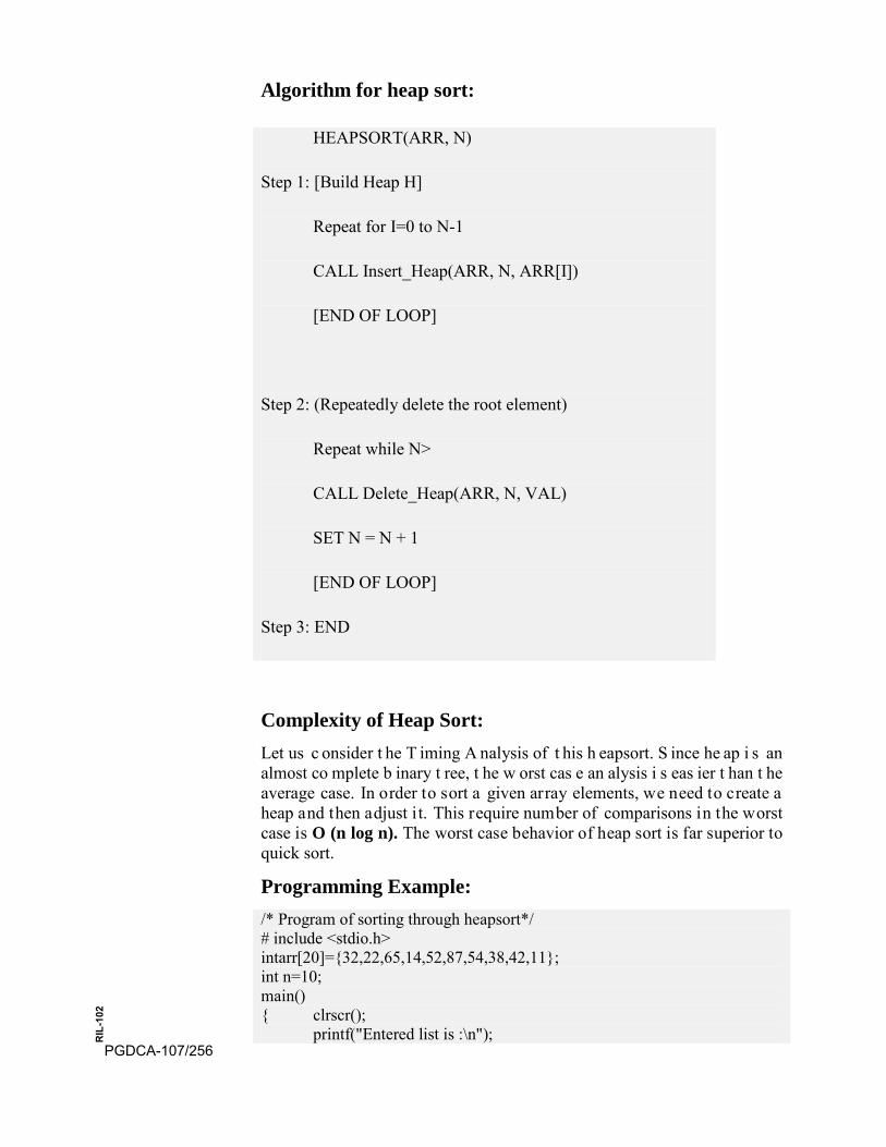
Algorithm for heap sort:
HEAPSORT(ARR, N)
Step 1: [Build Heap H]
Repeat for I=0 to N-1
CALL Insert_Heap(ARR, N, ARR[I])
[END OF LOOP]
Step 2: (Repeatedly delete the root element)
Repeat while N>
CALL Delete_Heap(ARR, N, VAL)
SET N = N + 1
[END OF LOOP]
Step 3: END
Complexity of Heap Sort: Let us c onsider t he T iming A nalysis of t his h eapsort. S ince he ap i s an almost co mplete b inary t ree, t he w orst cas e an alysis i s eas ier t han t he average case. In order to sort a given array elements, we need to create a heap and then adjust it. This require number of comparisons in the worst case is O (n log n). The worst case behavior of heap sort is far superior to quick sort.
Programming Example: /* Program of sorting through heapsort*/ # include <stdio.h> intarr[20]={32,22,65,14,52,87,54,38,42,11}; int n=10; main() { clrscr();
printf("Entered list is :\n"); PGDCA-107/256
RIL
-102
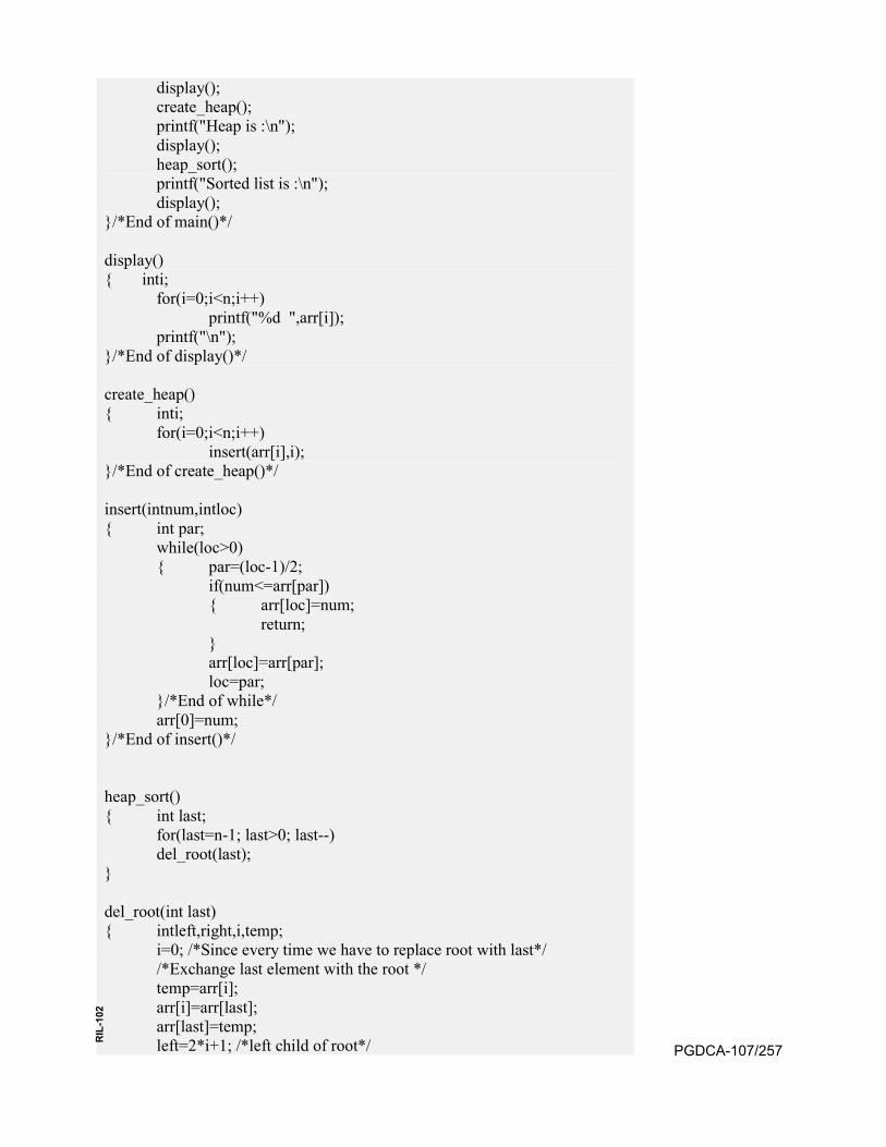
display(); create_heap(); printf("Heap is :\n"); display(); heap_sort(); printf("Sorted list is :\n"); display();
}/*End of main()*/
display() { inti;
for(i=0;i<n;i++) printf("%d ",arr[i]);
printf("\n"); }/*End of display()*/
create_heap() { inti;
for(i=0;i<n;i++) insert(arr[i],i);
}/*End of create_heap()*/
insert(intnum,intloc) { int par;
while(loc>0) { par=(loc-1)/2;
if(num<=arr[par]) { arr[loc]=num;
return; } arr[loc]=arr[par]; loc=par;
}/*End of while*/ arr[0]=num;
}/*End of insert()*/
heap_sort() { int last;
for(last=n-1; last>0; last--) del_root(last);
}
del_root(int last) { intleft,right,i,temp;
i=0; /*Since every time we have to replace root with last*/ /*Exchange last element with the root */ temp=arr[i]; arr[i]=arr[last]; arr[last]=temp; left=2*i+1; /*left child of root*/ PGDCA-107/257
RIL
-102
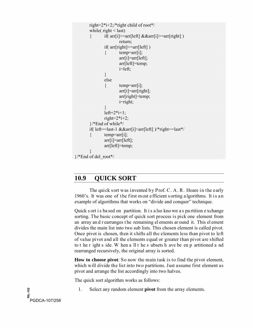
right=2*i+2;/*right child of root*/ while( right < last) { if( arr[i]>=arr[left] &&arr[i]>=arr[right] )
return; if( arr[right]<=arr[left] ) { temp=arr[i];
arr[i]=arr[left]; arr[left]=temp; i=left;
} else { temp=arr[i];
arr[i]=arr[right]; arr[right]=temp; i=right;
} left=2*i+1; right=2*i+2;
}/*End of while*/ if( left==last-1 &&arr[i]<arr[left] )/*right==last*/ { temp=arr[i];
arr[i]=arr[left]; arr[left]=temp;
} }/*End of del_root*/
10.9 QUICK SORT
The quick sort was invented by Prof. C. A. R. Hoare in the early 1960’s. It was one of t he f irst m ost e fficient s orting a lgorithms. It i s a n example of algorithms that works on “divide and conquer” technique.
Quick s ort i s ba sed on partition. It i s a lso kno wn a s pa rtition e xchange sorting. The basic concept of quick sort process is pick one element from an array an d r earranges t he remaining el ements ar ound it. This el ement divides the main list into two sub lists. This chosen element is called pivot. Once pivot is chosen, then it s hifts all the elements less than pivot to left of value pivot and all the elements equal or greater than pivot are shifted to t he r ight s ide. W hen a ll t he s ubsets h ave be en p artitioned a nd rearranged recursively, the original array is sorted.
How to choose pivot: So now the main task is to find the pivot element, which will divide the list into two partitions. Just assume first element as pivot and arrange the list accordingly into two halves.
The quick sort algorithm works as follows:
1. Select any random element pivot from the array elements.
PGDCA-107/258
RIL
-102
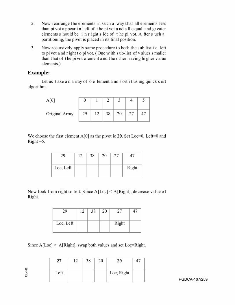
2. Now r earrange t he el ements i n s uch a way t hat all el ements l essthan pi vot a ppear i n l eft of t he pi vot a nd a ll e qual a nd gr eaterelements s hould be i n r ight s ide of t he pi vot. A fter s uch apartitioning, the pivot is placed in its final position.
3. Now recursively apply same procedure to both the sub list i.e. leftto pi vot a nd r ight t o pi vot. ( One w ith s ub-list of v alues s mallerthan t hat of t he pi vot e lement a nd t he ot her h aving hi gher v alueelements.)
Example: Let us t ake a n a rray of 6 e lement a nd s ort i t us ing qui ck s ort
algorithm.
A[6] 0 1 2 3 4 5
Original Array 29 12 38 20 27 47
We choose the first element A[0] as the pivot ie 29. Set Loc=0, Left=0 and Right =5.
29 12 38 20 27 47
Loc, Left Right
Now look from right to left. Since A[Loc] < A[Right], decrease value of Right.
29 12 38 20 27 47
Loc, Left Right
Since A[Loc] > A[Right], swap both values and set Loc=Right.
27 12 38 20 29 47
Left Loc, Right PGDCA-107/259
RIL
-102
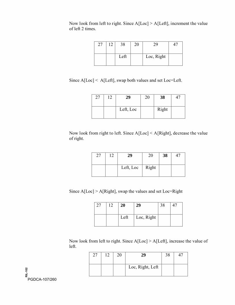
Now look from left to right. Since A[Loc] > A[Left], increment the value of left 2 times.
27 12 38 20 29 47
Left Loc, Right
Since A[Loc] < A[Left], swap both values and set Loc=Left.
27 12 29 20 38 47
Left, Loc Right
Now look from right to left. Since A[Loc] < A[Right], decrease the value of right.
27 12 29 20 38 47
Left, Loc Right
Since A[Loc] > A[Right], swap the values and set Loc=Right
27 12 20 29 38 47
Left Loc, Right
Now look from left to right. Since A[Loc] > A[Left], increase the value of left.
27 12 20 29 38 47
Loc, Right, Left
PGDCA-107/260
RIL
-102

Now s ee t he ab ove l ast s tep i n w hich Left = Loc. S o t erminates t his process here. Now you can see that the pivot element 29 i s at right place. All th e s maller ite ms a re in le ft s ide a nd b ig it ems a re in r ight s ide o f pivot. Now same procedure will applied to both left and right list of pivot.
Algorithm of Quick sort : The quick sort algorithm makes use of a function Quick to divide the array into two sub-arrays and fix the pivot at its suitable location.
PARTITION (ARR, BEG, END, LOC)
Step 1: [Initialize] Set Left= BEG, Right= END, LOC= BEG, Flag =0
Step 2: Repeat Step 3 To 6 While Flag =0
Step 3: Repeat While ARR[LOC] <= ARR[Right] And LOC != Right
Set Right= Right-1
[End Loop]
Step 4: If LOC= Right
Set Flag=1
Else If ARR[LOC]> ARR[Right]
Swap ARR[LOC] With ARR[Right]
Set LOC= Right
[End If]
Step 5: If Flag =0
Repeat While ARR[LOC] >= ARR[Left] And LOC != Left
Set Left= Left+1
[End Loop]
Step 6: If LOC= Left
Set Flag=1 PGDCA-107/261
RIL
-102
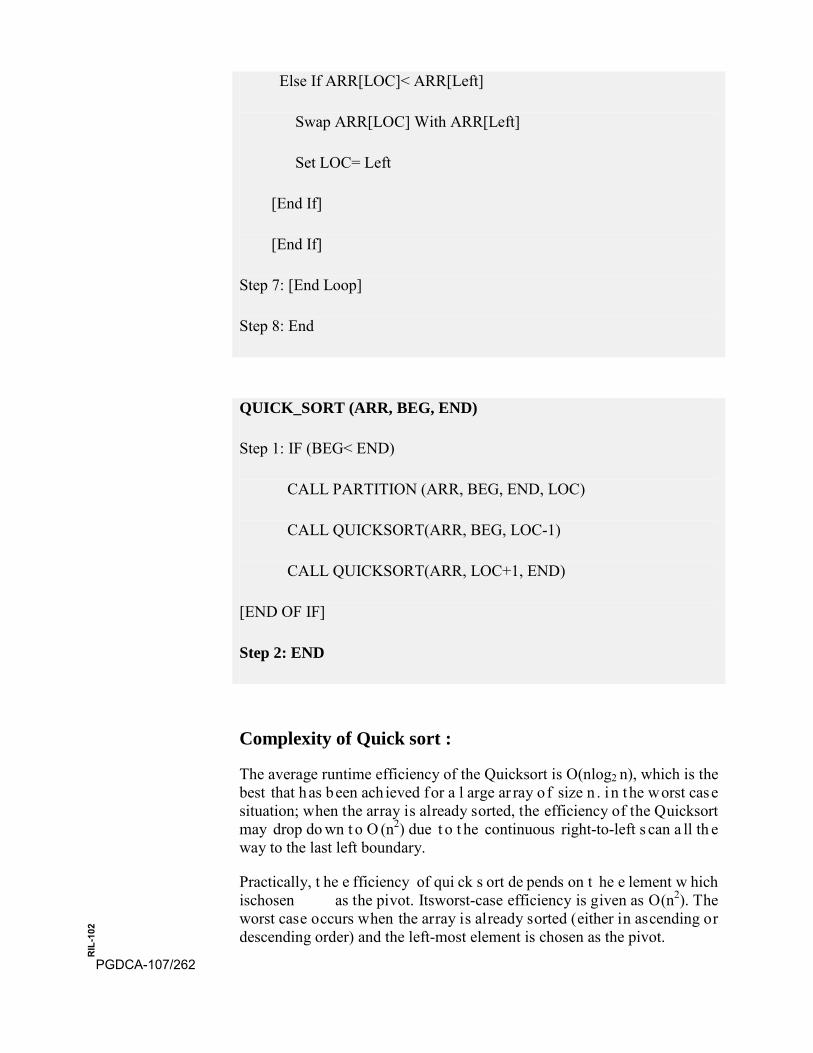
Else If ARR[LOC]< ARR[Left]
Swap ARR[LOC] With ARR[Left]
Set LOC= Left
[End If]
[End If]
Step 7: [End Loop]
Step 8: End
QUICK_SORT (ARR, BEG, END)
Step 1: IF (BEG< END)
CALL PARTITION (ARR, BEG, END, LOC)
CALL QUICKSORT(ARR, BEG, LOC-1)
CALL QUICKSORT(ARR, LOC+1, END)
[END OF IF]
Step 2: END
Complexity of Quick sort :
The average runtime efficiency of the Quicksort is O(nlog2 n), which is the best that has been ach ieved for a l arge ar ray o f size n . in the worst case situation; when the array is already sorted, the efficiency of the Quicksort may drop do wn t o O (n2) due t o t he continuous right-to-left s can a ll th e way to the last left boundary.
Practically, t he e fficiency of qui ck s ort de pends on t he e lement w hich ischosen as the pivot. Itsworst-case efficiency is given as O(n2). The worst case occurs when the array is already sorted (either in ascending or descending order) and the left-most element is chosen as the pivot.
PGDCA-107/262
RIL
-102
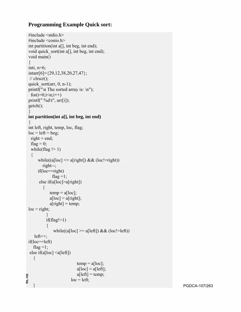
Programming Example Quick sort:
#include <stdio.h> #include <conio.h> int partition(int a[], int beg, int end); void quick_sort(int a[], int beg, int end); void main() { inti, n=6; intarr[6]={29,12,38,20,27,47}; // clrscr(); quick_sort(arr, 0, n-1); printf("\n The sorted array is: \n"); for(i=0;i<n;i++) printf(" %d\t", arr[i]); getch(); } int partition(int a[], int beg, int end) { int left, right, temp, loc, flag; loc = left = beg; right = end; flag = 0; while(flag != 1) { while((a[loc] <= a[right]) && (loc!=right)) right--; if(loc==right)
flag =1; else if(a[loc]>a[right]) {
temp = a[loc]; a[loc] = a[right]; a[right] = temp;
loc = right; }
if(flag!=1) { while((a[loc] >= a[left]) && (loc!=left))
left++; if(loc==left) flag =1; else if(a[loc] <a[left]) {
temp = a[loc]; a[loc] = a[left]; a[left] = temp; loc = left;
} PGDCA-107/263
RIL
-102
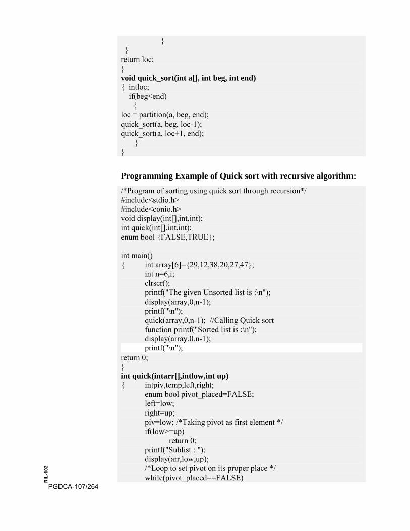
} } return loc; } void quick_sort(int a[], int beg, int end) { intloc; if(beg<end) { loc = partition(a, beg, end); quick_sort(a, beg, loc-1); quick_sort(a, loc+1, end); } }
Programming Example of Quick sort with recursive algorithm:
/*Program of sorting using quick sort through recursion*/ #include<stdio.h> #include<conio.h> void display(int[],int,int); int quick(int[],int,int); enum bool {FALSE,TRUE};
int main() { int array[6]={29,12,38,20,27,47};
int n=6,i; clrscr(); printf("The given Unsorted list is :\n"); display(array,0,n-1); printf("\n"); quick(array,0,n-1); //Calling Quick sort function printf("Sorted list is :\n"); display(array,0,n-1); printf("\n");
return 0; } int quick(intarr[],intlow,int up) { intpiv,temp,left,right;
enum bool pivot_placed=FALSE; left=low; right=up; piv=low; /*Taking pivot as first element */ if(low>=up)
return 0; printf("Sublist : "); display(arr,low,up); /*Loop to set pivot on its proper place */ while(pivot_placed==FALSE)
PGDCA-107/264
RIL
-102

{ /*Compare from Right to Left */
while( arr[piv]<=arr[right] &&piv!=right ) right=right-1;
if( piv==right ) pivot_placed=TRUE; if( arr[piv] >arr[right] ) {
temp=arr[piv]; arr[piv]=arr[right]; arr[right]=temp; piv=right;
} /*Compare from Left to Right */
while( arr[piv]>=arr[left] && left!=piv ) left=left+1;
if(piv==left) pivot_placed=TRUE;
if( arr[piv] <arr[left] ) { temp=arr[piv];
arr[piv]=arr[left]; arr[left]=temp; piv=left;
} } printf("-> Pivot Placed is %d -> ",arr[piv]); display(arr,low,up); printf("\n"); quick(arr,low,piv-1); quick(arr,piv+1,up);
return 0; } void display(intarr[],intlow,int up) { inti;
for(i=low;i<=up;i++) printf("%d ",arr[i]);
}
10.10 MERGE SORT
The basic concept of merge sort is divides the list into two smaller sub-lists of approximately equal size. Recursively repeat this procedure till only one element is left in the sub-list. After this, various sorted sub-lists are merged to form sorted parent list. This process goes on recursively till the original sorted list arrived.
Merge s ort a lgorithm f ocuses on t wo m ain c oncepts t o i mprove i ts performance (running time): PGDCA-107/265
RIL
-102
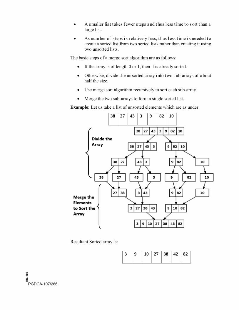
• A s maller lis t t akes f ewer s teps a nd t hus l ess t ime t o s ort t han alarge list.
• As num ber of s teps i s r elatively l ess, t hus l ess t ime i s ne eded t ocreate a sorted list from two sorted lists rather than creating it usingtwo unsorted lists.
The basic steps of a merge sort algorithm are as follows:
• If the array is of length 0 or 1, then it is already sorted.
• Otherwise, divide the unsorted array into two sub-arrays of abouthalf the size.
• Use merge sort algorithm recursively to sort each sub-array.
• Merge the two sub-arrays to form a single sorted list.
Example: Let us take a list of unsorted elements which are as under
38 27 43 3 9 82 10
Resultant Sorted array is:
3 9 10 27 38 42 82
PGDCA-107/266
RIL
-102
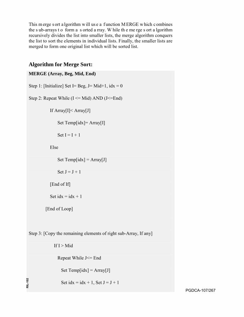
This m erge s ort a lgorithm w ill us e a f unction M ERGE w hich c ombines the s ub-arrays t o form a s orted a rray. W hile th e me rge s ort a lgorithm recursively divides the list into smaller lists, the merge algorithm conquers the list to sort the elements in individual lists. Finally, the smaller lists are merged to form one original list which will be sorted list.
Algorithm for Merge Sort: MERGE (Array, Beg, Mid, End)
Step 1: [Initialize] Set I= Beg, J= Mid+1, idx = 0
Step 2: Repeat While (I <= Mid) AND (J<=End)
If Array[I]< Array[J]
Set Temp[idx]= Array[I]
Set I = I + 1
Else
Set Temp[idx] = Array[J]
Set J = J + 1
[End of If]
Set idx = idx + 1
[End of Loop]
Step 3: [Copy the remaining elements of right sub-Array, If any]
If I > Mid
Repeat While J<= End
Set Temp[idx] = Array[J]
Set idx = idx + 1, Set J = J + 1 PGDCA-107/267
RIL
-102
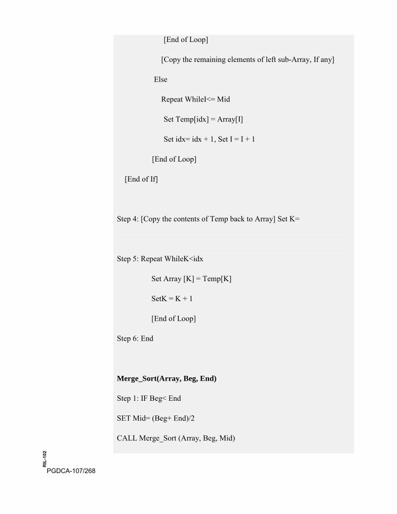
[End of Loop]
[Copy the remaining elements of left sub-Array, If any]
Else
Repeat WhileI<= Mid
Set Temp[idx] = Array[I]
Set idx= idx + 1, Set I = I + 1
[End of Loop]
[End of If]
Step 4: [Copy the contents of Temp back to Array] Set K=
Step 5: Repeat WhileK<idx
Set Array [K] = Temp[K]
SetK = K + 1
[End of Loop]
Step 6: End
Merge_Sort(Array, Beg, End)
Step 1: IF Beg< End
SET Mid= (Beg+ End)/2
CALL Merge_Sort (Array, Beg, Mid)
PGDCA-107/268
RIL
-102

CALL Merge_Sort (Array, Mid+1, End)
Merge (Array, Beg, Mid, End)
[End of If]
Step 2: End
The running time of merge sort in the average case and the worst case can be g iven a s O (n l og n). A lthough m erge s ort ha s a n opt imal t ime complexity, i t needs an additional space o f O(n) for the t emporary array TEMP.
Programming Example:
/* Program of sorting using merge sort */ #include<stdio.h> #include<conio.h> void mergesort(int a[],inti,int j); void merge(int a[],int i1,int j1,int i2,int j2); int main() { int a[10]={38, 27, 43, 3, 9, 82, 10, 28, 89,74};
inti,n=10; clrscr(); printf("The given unsorted list is as under:\n"); for(i=0;i<n;i++)
printf("%d ",a[i]); mergesort(a,0,n-1); printf("\nSorted array is :"); for(i=0;i<n;i++)
printf("%d ",a[i]); return 0;
} void mergesort(int a[],inti,int j) { int mid;
if(i<j) { mid=(i+j)/2;
mergesort(a,i,mid); //left recursion mergesort(a,mid+1,j); //right recursion merge(a,i,mid,mid+1,j); //merging o f tw o s orted s ub-
arrays }
} void merge(int a[],int i1,int j1,int i2,int j2) { int temp[50]; //array used for merging PGDCA-107/269
RIL
-102
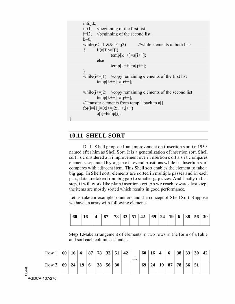
inti,j,k; i=i1; //beginning of the first list j=i2; //beginning of the second list k=0; while(i<=j1 && j<=j2) //while elements in both lists { if(a[i]<a[j])
temp[k++]=a[i++]; else
temp[k++]=a[j++]; } while(i<=j1) //copy remaining elements of the first list
temp[k++]=a[i++];
while(j<=j2) //copy remaining elements of the second list temp[k++]=a[j++];
//Transfer elements from temp[] back to a[] for(i=i1,j=0;i<=j2;i++,j++)
a[i]=temp[j]; }
10.11 SHELL SORT
D. L. S hell pr oposed an i mprovement on i nsertion s ort i n 1959 named after him as Shell Sort. It is a generalization of insertion sort. Shell sort i s c onsidered a n i mprovement ove r i nsertion s ort a s i t c ompares elements s eparated b y a g ap o f s everal p ositions w hile i n Insertion s ort compares with adjacent item. This Shell sort enables the element to take a big gap. In Shell sort, elements are sorted in multiple passes and in each pass, data are taken from big gap to smaller gap sizes. And finally in last step, i t will work l ike plain insertion sort. As we reach towards last step, the items are mostly sorted which results in good performance.
Let us take an example to understand the concept of Shell Sort. Suppose we have an array with following elements.
Step 1.Make arrangement of elements in two rows in the form of a t able and sort each columns as under.
60 16 4 87 78 33 51 42 69 24 19 6 38 56 30
Row 1 60 16 4 87 78 33 51 42 →
60 16 4 6 38 33 30 42
Row 2 69 24 19 6 38 56 30 69 24 19 87 78 56 51
PGDCA-107/270
RIL
-102

Now the elements of the array will be as under after merging both sorted rows.
Step 2. Now repeat s tep 1 a gain with small column gap s ize as under in three rows.
Now t he e lements of t he a rray w ill be a s unde r a fter m erging s orted column
19 16 4 6 24 33 30 42 56 38 60 87 78 69 51
Step 3. Now r epeat pr evious s tep a gain w ith s mall c olumn gap s ize as under in five rows.
Row 1 19 16 4 6 16 4
Row 2 6 24 33 →
19 24 33
Row 3 30 42 56 30 42 51
Row 4 38 60 87 38 60 56
Row 5 78 69 51 78 69 87
Now t he e lements of t he a rray w ill be a s unde r a fter m erging s orted column.
60 16 4 6 38 33 30 42 69 24 19 87 78 56 51
Row 1 60 16 4 6 38 19 16 4 6 24
Row 2 33 30 42 69 24 → 33 30 42 56 38
Row 3 19 87 78 56 51 60 87 78 69 51
PGDCA-107/271
RIL
-102
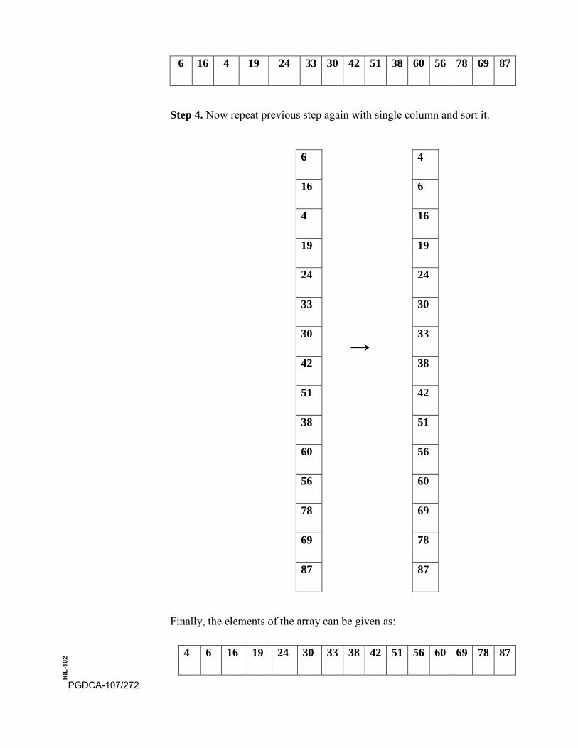
Step 4. Now repeat previous step again with single column and sort it.
6 4
16 6
4 16
19 19
24 24
33 30
30 →
33
42 38
51 42
38 51
60 56
56 60
78 69
69 78
87 87
Finally, the elements of the array can be given as:
6 16 4 19 24 33 30 42 51 38 60 56 78 69 87
4 6 16 19 24 30 33 38 42 51 56 60 69 78 87
PGDCA-107/272
RIL
-102
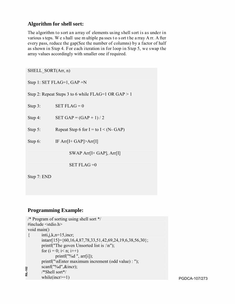
Algorithm for shell sort: The algorithm to sort an array of elements using shell sort is as under in various s teps. W e s hall use m ultiple pa sses t o s ort t he a rray A rr. A fter every pass, reduce the gap(See the number of columns) by a factor of half as shown in Step 4. For each iteration in for loop in Step 5, we swap the array values accordingly with smaller one if required.
SHELL_SORT(Arr, n)
Step 1: SET FLAG=1, GAP =N
Step 2: Repeat Steps 3 to 6 while FLAG=1 OR GAP > 1
Step 3: SET FLAG = 0
Step 4: SET GAP = (GAP + 1) / 2
Step 5: Repeat Step 6 for I = to I < (N- GAP)
Step 6: IF Arr[I+ GAP]>Arr[I]
SWAP Arr[I+ GAP], Arr[I]
SET FLAG =0
Step 7: END
Programming Example: /* Program of sorting using shell sort */ #include <stdio.h> void main() { inti,j,k,n=15,incr;
intarr[15]={60,16,4,87,78,33,51,42,69,24,19,6,38,56,30}; printf("The goven Unsorted list is :\n"); for (i = 0; i< n; i++)
printf("%d ", arr[i]); printf("\nEnter maximum increment (odd value) : "); scanf("%d",&incr); /*Shell sort*/ while(incr>=1) PGDCA-107/273
RIL
-102
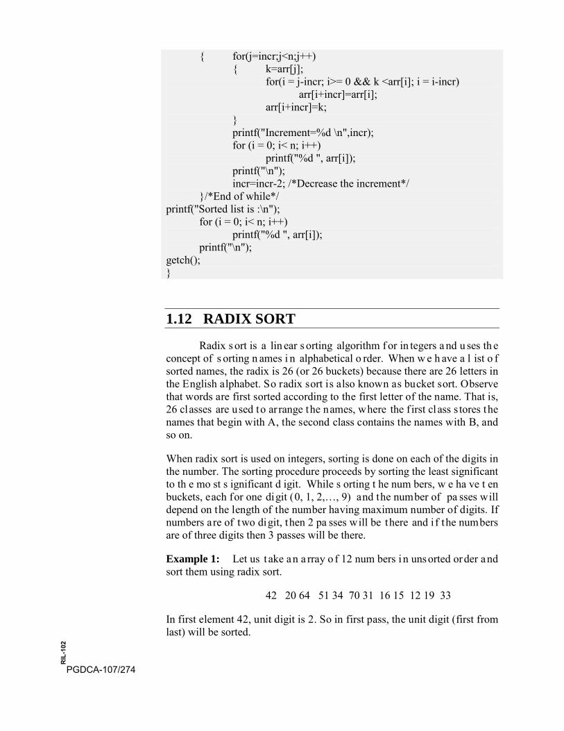
{ for(j=incr;j<n;j++) { k=arr[j];
for(i = j-incr; i>= 0 && k <arr[i]; i = i-incr) arr[i+incr]=arr[i];
arr[i+incr]=k; } printf("Increment=%d \n",incr); for (i = 0; i< n; i++)
printf("%d ", arr[i]); printf("\n"); incr=incr-2; /*Decrease the increment*/
}/*End of while*/ printf("Sorted list is :\n");
for (i = 0; i< n; i++) printf("%d ", arr[i]);
printf("\n"); getch(); }
1.12 RADIX SORT
Radix s ort is a lin ear s orting algorithm f or in tegers a nd u ses th e concept of s orting n ames i n alphabetical o rder. When w e h ave a l ist o f sorted names, the radix is 26 (or 26 buckets) because there are 26 letters in the English alphabet. So radix sort is also known as bucket sort. Observe that words are first sorted according to the first letter of the name. That is, 26 classes are used to ar range the names, where the f irst cl ass s tores the names that begin with A, the second class contains the names with B, and so on.
When radix sort is used on integers, sorting is done on each of the digits in the number. The sorting procedure proceeds by sorting the least significant to th e mo st s ignificant d igit. While s orting t he num bers, w e ha ve t en buckets, each for one digit (0, 1, 2,…, 9) and the number of pa sses will depend on the length of the number having maximum number of digits. If numbers are of two digit, then 2 pa sses will be there and i f the numbers are of three digits then 3 passes will be there.
Example 1: Let us t ake an a rray o f 12 num bers i n unsorted order and sort them using radix sort.
42 20 64 51 34 70 31 16 15 12 19 33
In first element 42, unit digit is 2. So in first pass, the unit digit (first from last) will be sorted.
PGDCA-107/274
RIL
-102
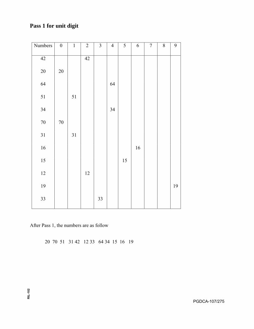
Pass 1 for unit digit
Numbers 0 1 2 3 4 5 6 7 8 9
42 42
20 20
64 64
51 51
34 34
70 70
31 31
16 16
15 15
12 12
19 19
33 33
After Pass 1, the numbers are as follow
20 70 51 31 42 12 33 64 34 15 16 19
PGDCA-107/275
RIL
-102
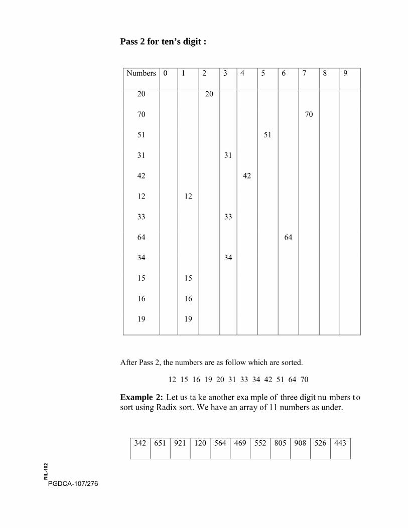
Pass 2 for ten’s digit :
Numbers 0 1 2 3 4 5 6 7 8 9
20 20
70 70
51 51
31 31
42 42
12 12
33 33
64 64
34 34
15 15
16 16
19 19
After Pass 2, the numbers are as follow which are sorted.
12 15 16 19 20 31 33 34 42 51 64 70
Example 2: Let us ta ke another exa mple of three digit nu mbers to sort using Radix sort. We have an array of 11 numbers as under.
342 651 921 120 564 469 552 805 908 526 443
PGDCA-107/276
RIL
-102
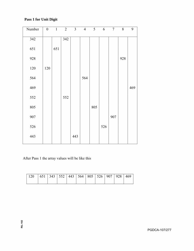
Pass 1 for Unit Digit
Number 0 1 2 3 4 5 6 7 8 9
342 342
651 651
928 928
120 120
564 564
469 469
552 552
805 805
907 907
526 526
443 443
After Pass 1 the array values will be like this
120 651 343 552 443 564 805 526 907 928 469
PGDCA-107/277
RIL
-102
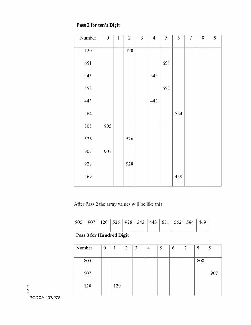
Pass 2 for ten's Digit
Number 0 1 2 3 4 5 6 7 8 9
120 120
651 651
343 343
552 552
443 443
564 564
805 805
526 526
907 907
928 928
469 469
After Pass 2 the array values will be like this
805 907 120 526 928 343 443 651 552 564 469
Pass 3 for Hundred Digit
Number 0 1 2 3 4 5 6 7 8 9
805 808
907 907
120 120
PGDCA-107/278
RIL
-102
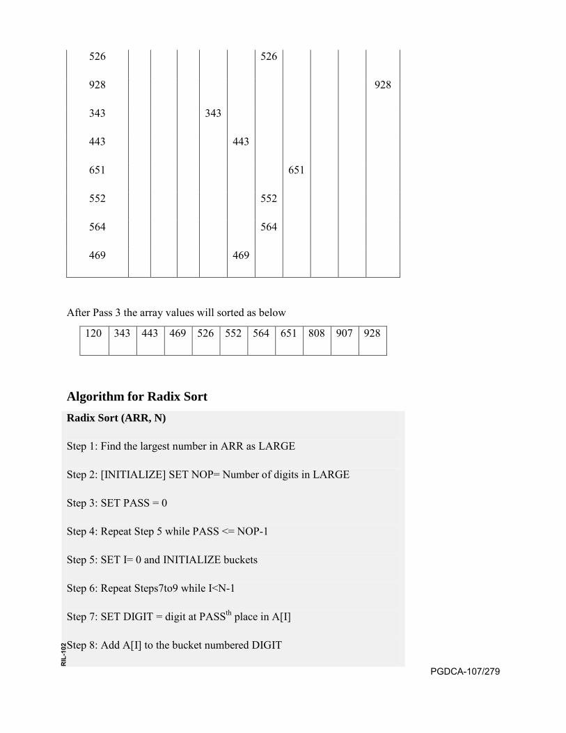
526 526
928
928
343 343
443 443
651
651
552 552
564
564
469 469
After Pass 3 the array values will sorted as below
120 343 443 469 526 552 564 651 808 907 928
Algorithm for Radix Sort Radix Sort (ARR, N)
Step 1: Find the largest number in ARR as LARGE
Step 2: [INITIALIZE] SET NOP= Number of digits in LARGE
Step 3: SET PASS = 0
Step 4: Repeat Step 5 while PASS <= NOP-1
Step 5: SET I= 0 and INITIALIZE buckets
Step 6: Repeat Steps7to9 while I<N-1
Step 7: SET DIGIT = digit at PASSth place in A[I]
Step 8: Add A[I] to the bucket numbered DIGIT
PGDCA-107/279
RIL
-102
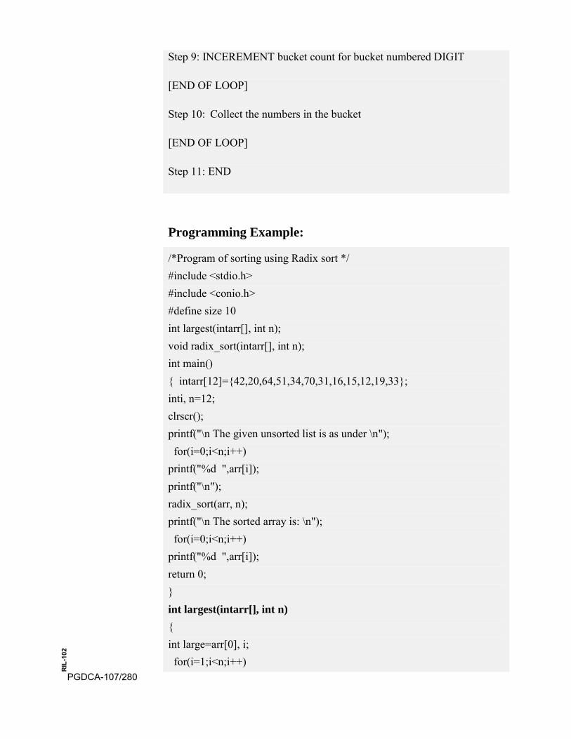
Step 9: INCEREMENT bucket count for bucket numbered DIGIT
[END OF LOOP]
Step 10: Collect the numbers in the bucket
[END OF LOOP]
Step 11: END
Programming Example:
/*Program of sorting using Radix sort */ #include <stdio.h> #include <conio.h> #define size 10 int largest(intarr[], int n); void radix_sort(intarr[], int n); int main() { intarr[12]={42,20,64,51,34,70,31,16,15,12,19,33}; inti, n=12; clrscr(); printf("\n The given unsorted list is as under \n"); for(i=0;i<n;i++) printf("%d ",arr[i]); printf("\n"); radix_sort(arr, n); printf("\n The sorted array is: \n"); for(i=0;i<n;i++) printf("%d ",arr[i]); return 0; } int largest(intarr[], int n) { int large=arr[0], i; for(i=1;i<n;i++)
PGDCA-107/280
RIL
-102

{ if(arr[i]>large) large = arr[i]; } return large; } void radix_sort(intarr[], int n) { int bucket[size][size], bucket_count[size]; inti, j, k, remainder, NOP=0, divisor=1, large, pass; large = largest(arr, n); while(large>0) { NOP++; large/=size; } for(pass=0;pass<NOP;pass++) // Initialize the buckets { for(i=0;i<size;i++) bucket_count[i]=0; for(i=0;i<n;i++) { // sort the numbers according to the digit at passth place
remainder = (arr[i]/divisor)%size; bucket[remainder][bucket_count[remainder]] = arr[i];
bucket_count[remainder] += 1; } // collect the numbers after PASS pass i=0; for(k=0;k<size;k++) { for(j=0;j<bucket_count[k];j++) { arr[i] = bucket[k][j]; i++; } } divisor *= size; } PGDCA-107/281
RIL
-102

}
1.13 SUMMARY
Now w e ha ve unde rstand all th e s orting a lgorithms w ith th eir worst, average and best cases. But one thing should be very clear that, no sorting t echnique i s be st. It s hould de pend on t he s ituation of t he da ta. Choice of algorithm should depends on t he order of the data and storage location of it. Now let us summarize all the sorting algorithms with respect to their best, average and best case behavior in term of O notation.
Sorting
Technique
Best Case Average case Worst case
Selection Sort O(n2) O(n2) O(n2)
Bubble Sort O(n) O(n2) O(n2)
Insertion Sort O(n) O(n2) O(n2)
Heap Sort O(n log n) O(n log n) O(n log n)
Quick Sort O(n2) O(n log n) O(n log n)
Merge Sort O(n log n) O(n log n) O(n log n)
Shell Sort - - -
Radix Sort O(n2) O(n log n) O(n log n)
Bibliography • J. P . T remblay, P . G . S orenson “ An Introduction t o D ata
Structures with Applications”, Tata McGraw-Hill, 1984
• Markus Blaner: “Introduction to Algorithms and Data Structures”,Saarland University, 2011
• Seymour Lipschutz, “Data Structure”, Schaum ‟s outline Series
• ReemaThareja, “Data Structure using C” Oxford University Press,Jai Singh Road, New Delhi, 2011
PGDCA-107/282
RIL
-102
• S. K . Shrivastav, D eepaliShrivastav, “ Data S tructure us ing C i nDepth” BPB Publication, New Delhi, 2008
• G. S. Baluja, “Data Structure through C” (A Practical Approach),Dhanpat Rai & Co. (Pvt) Ltd. NaiSarak, Delhi, 2007
• Dr. M adhulika J ain, S atish J ain, S hashi S ingh, “ Data S tructurethough C Language” BPB Publication, New Delhi, 2008
PGDCA-107/283
RIL
-102
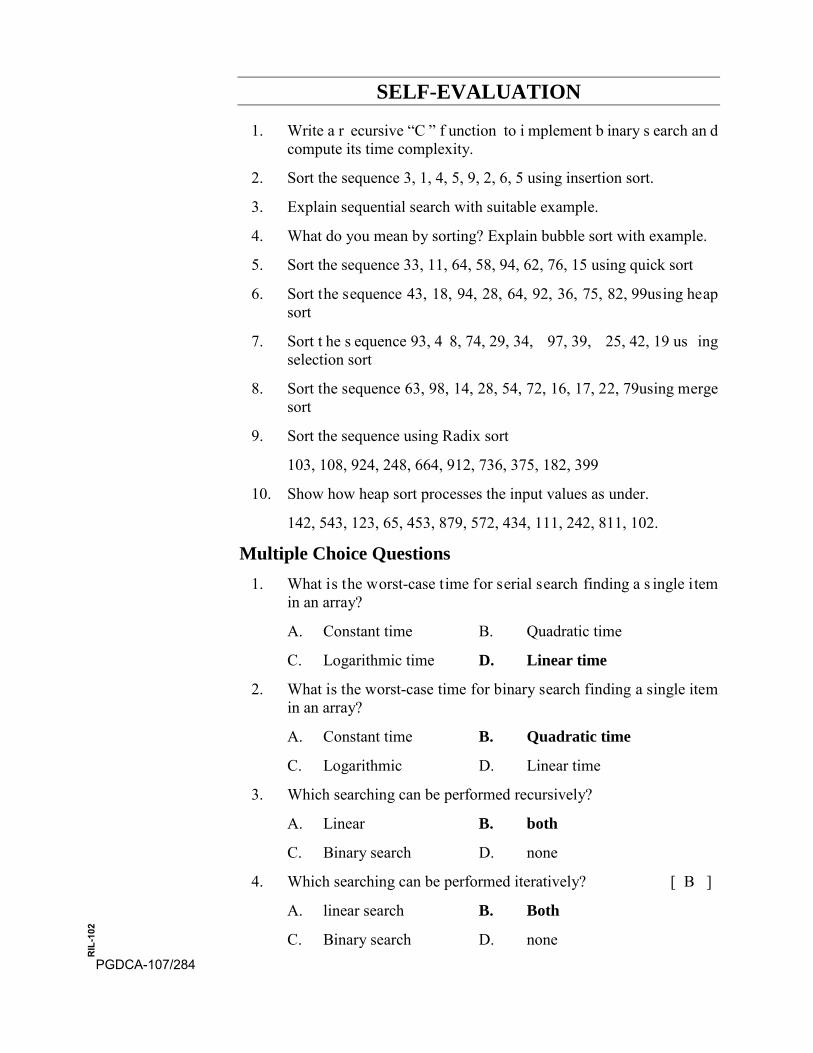
SELF-EVALUATION
1. Write a r ecursive “C ” f unction to i mplement b inary s earch an dcompute its time complexity.
2. Sort the sequence 3, 1, 4, 5, 9, 2, 6, 5 using insertion sort.
3. Explain sequential search with suitable example.
4. What do you mean by sorting? Explain bubble sort with example.
5. Sort the sequence 33, 11, 64, 58, 94, 62, 76, 15 using quick sort
6. Sort the sequence 43, 18, 94, 28, 64, 92, 36, 75, 82, 99using heapsort
7. Sort t he s equence 93, 4 8, 74, 29, 34, 97, 39, 25, 42, 19 us ingselection sort
8. Sort the sequence 63, 98, 14, 28, 54, 72, 16, 17, 22, 79using mergesort
9. Sort the sequence using Radix sort
103, 108, 924, 248, 664, 912, 736, 375, 182, 399
10. Show how heap sort processes the input values as under.
142, 543, 123, 65, 453, 879, 572, 434, 111, 242, 811, 102.
Multiple Choice Questions 1. What is the worst-case time for serial search finding a s ingle item
in an array?
A. Constant time B. Quadratic time
C. Logarithmic time D. Linear time
2. What is the worst-case time for binary search finding a single itemin an array?
A. Constant time B. Quadratic time
C. Logarithmic D. Linear time
3. Which searching can be performed recursively?
A. Linear B. both
C. Binary search D. none
4. Which searching can be performed iteratively? [ B ]
A. linear search B. Both
C. Binary search D. none PGDCA-107/284
RIL
-102
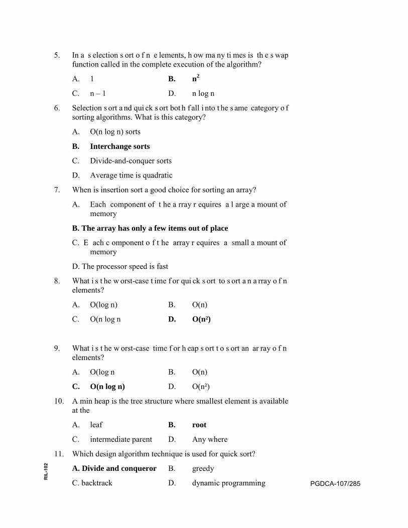
5. In a s election s ort o f n e lements, h ow ma ny ti mes is th e s wapfunction called in the complete execution of the algorithm?
A. 1 B. n2
C. n – 1 D. n log n
6. Selection s ort a nd qui ck s ort bot h f all i nto t he s ame category o fsorting algorithms. What is this category?
A. O(n log n) sorts
B. Interchange sorts
C. Divide-and-conquer sorts
D. Average time is quadratic
7. When is insertion sort a good choice for sorting an array?
A. Each component of t he a rray r equires a l arge a mount ofmemory
B. The array has only a few items out of place
C. E ach c omponent o f t he array r equires a small a mount of memory
D. The processor speed is fast
8. What i s t he w orst-case t ime f or qui ck s ort to s ort a n a rray o f nelements?
A. O(log n) B. O(n)
C. O(n log n D. O(n²)
9. What i s t he w orst-case time f or h eap s ort t o s ort an ar ray o f nelements?
A. O(log n B. O(n)
C. O(n log n) D. O(n²)
10. A min heap is the tree structure where smallest element is availableat the
A. leaf B. root
C. intermediate parent D. Any where
11. Which design algorithm technique is used for quick sort?
A. Divide and conqueror B. greedy
C. backtrack D. dynamic programming PGDCA-107/285
RIL
-102
12. Which a mong t he f ollowing i s f astest s orting t echnique ( forunordered data)
A. Heap sort B. Selection Sort
C. Quick Sort D. Bubble sort
13. In w hich s earching t echnique el ements ar e eliminated b y h alf i neach pass.
A. Linear search B. Binary search
C. Both D. none
14. Binary search algorithm performs efficiently on a
A. linked list B. both
C. Array D. None
14. Heap is a good data structure to implementA. priority Queue B. Deque C. linear queue D. None
True or False
1. Binary search is also called sequential search.
2. Linear search is performed on a sorted array.
3. For i nsertion s ort, t he b est cas e o ccurs w hen t he ar ray i s al readysorted.
4. Selection sort has a linear running time complexity.
5. The running time of merge sort in the average case and the worstcase is O(n log n).
6. The worst case running time complexity of qui ck sort i s O(n logn).
7. Heap sort is an efficient and a stable sorting algorithm.
8. External s orting de als w ith s orting t he da ta s tored i n t hecomputer’s memory.
9. Insertion sort is less efficient than quick sort, heap sort, and mergesort.
10. The average case of insertion sort has a quadratic running time.
11. The partitioning of the array in quick sort is done in O(n) time.
12. In i nternal s orting m ethods, i t i s ne cessary for a ll da ta s houldreside in main memory.
PGDCA-107/286
RIL
-102
Answer 1. False 2. False 3. False 4. False 5. True 6. False
7.True 8. False 9. True 10. True 11. True 12. True
PGDCA-107/287
RIL
-102
PGDCA-107/288
RIL
-102
UNIT-11 HASHING
Structure:
11.0 Introduction:
11.1 Objective:
11.2 Hashing:
11.3 Hash Table:
11.4 Hash Function
11.5 Resolving Collision:
11.6 Some Applications of Hash Tables:
11.7 Summary
11.0 INTRODUCTION
The s earching t echniques t hat w e ha ve di scussed i n t he pr evious unit 10 a re based on c omparison of values with each other. In sequential search, we have to search from the beginning and move up to last element, so all items are compared with the searched items depend on its location in the a rray. In bi nary s earch, l ess c omparison a re t here with r espect t o sequential search as on e ach step list is divided in two halves. So there is less c omparison. S o t here i s a n eed w here w e ha ve t o do m inimum comparisons so that complexity could be reduced. So now our need is to search the element i n constant t imes and l ess ke y comparison should be involved. Finally, the main objective is that, how to reduce the number of comparisons in order to find the appropriate record within minimum time and minimum comparison.
11.1 OBJECTIVE
After reading this unit the learner is able to do the following task.
• Understand the concept of hashing and its need.
• Understand hash function and its methods
• Understand Collision and its resolution strategies
• Understand hash table and its implementation
11.2 Hashing
Hashing is a technique that is used to uniquely identify a specific object from a group of similar objects. Some examples of how hashing is used in our lives include: PGDCA-107/289
RIL
-102
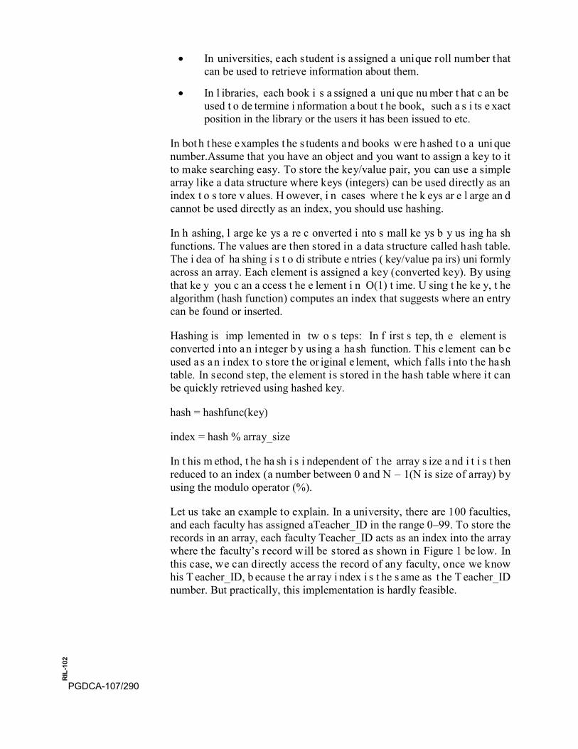
• In universities, each student is assigned a unique roll number thatcan be used to retrieve information about them.
• In l ibraries, each book i s a ssigned a uni que nu mber t hat c an beused t o de termine i nformation a bout t he book, such a s i ts e xactposition in the library or the users it has been issued to etc.
In bot h t hese e xamples t he s tudents a nd books w ere h ashed t o a uni que number.Assume that you have an object and you want to assign a key to it to make searching easy. To store the key/value pair, you can use a simple array like a data structure where keys (integers) can be used directly as an index t o s tore v alues. H owever, i n cases where t he k eys ar e l arge an d cannot be used directly as an index, you should use hashing.
In h ashing, l arge ke ys a re c onverted i nto s mall ke ys b y us ing ha sh functions. The values are then stored in a data structure called hash table. The i dea of ha shing i s t o di stribute e ntries ( key/value pa irs) uni formly across an array. Each element is assigned a key (converted key). By using that ke y you c an a ccess t he e lement i n O(1) t ime. U sing t he ke y, t he algorithm (hash function) computes an index that suggests where an entry can be found or inserted.
Hashing is imp lemented in tw o s teps: In f irst s tep, th e element is converted i nto an i nteger b y us ing a hash function. This e lement can b e used a s a n i ndex t o s tore t he or iginal e lement, which f alls i nto t he ha sh table. In second step, the element is stored in the hash table where it can be quickly retrieved using hashed key.
hash = hashfunc(key)
index = hash % array_size
In t his m ethod, t he ha sh i s i ndependent of t he array s ize a nd i t i s t hen reduced to an index (a number between 0 and N – 1(N is size of array) by using the modulo operator (%).
Let us take an example to explain. In a university, there are 100 faculties, and each faculty has assigned aTeacher_ID in the range 0–99. To store the records in an array, each faculty Teacher_ID acts as an index into the array where the faculty’s record will be stored as shown in Figure 1 be low. In this case, we can directly access the record of any faculty, once we know his T eacher_ID, b ecause t he ar ray i ndex i s t he s ame as t he T eacher_ID number. But practically, this implementation is hardly feasible.
PGDCA-107/290
RIL
-102
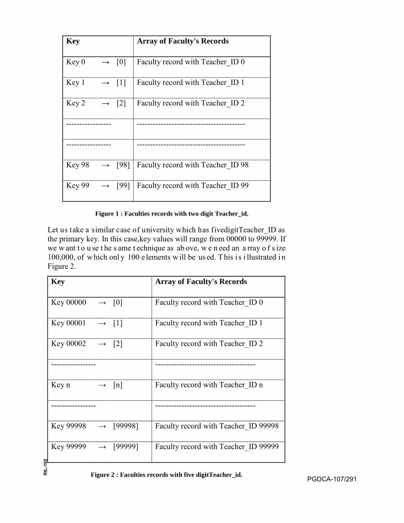
Key Array of Faculty's Records
Key 0 → [0] Faculty record with Teacher_ID 0
Key 1 → [1] Faculty record with Teacher_ID 1
Key 2 → [2] Faculty record with Teacher_ID 2
----------------- -----------------------------------------
----------------- -----------------------------------------
Key 98 → [98] Faculty record with Teacher_ID 98
Key 99 → [99] Faculty record with Teacher_ID 99
Figure 1 : Faculties records with two digit Teacher_id.
Let us take a similar case of university which has fivedigitTeacher_ID as the primary key. In this case,key values will range from 00000 to 99999. If we w ant t o u se t he s ame t echnique as ab ove, w e n eed an a rray o f s ize 100,000, of w hich onl y 100 e lements w ill be us ed. T his i s i llustrated i n Figure 2.
Key Array of Faculty's Records
Key 00000 → [0] Faculty record with Teacher_ID 0
Key 00001 → [1] Faculty record with Teacher_ID 1
Key 00002 → [2] Faculty record with Teacher_ID 2
----------------- --------------------------------------
Key n → [n] Faculty record with Teacher_ID n
----------------- --------------------------------------
Key 99998 → [99998] Faculty record with Teacher_ID 99998
Key 99999 → [99999] Faculty record with Teacher_ID 99999
Figure 2 : Faculties records with five digitTeacher_id. PGDCA-107/291
RIL
-102

It is o bvious to w aste a lo t o f me mory storage space j ust t o en sure t hat each employee’s record is unique and it is on predictable location.
So if we use a two-digit primary key (Teacher_ID) or a five-digit key, we have onl y 100 f aculties in t he university. For t his we will be us ing onl y 100 locations in the array. Therefore, in order to keep the array size down to t he s ize t hat w e w ill a ctually be us ing ( 100 e lements), a nother good option is to u se ju st t he la st tw o d igits o f th e k ey to id entify e ach employee. For example, the faculty with Teacher_ID79439 will be stored in t he e lement of t he a rray w ith i ndex 39. S imilarly, t he f aculty w ith Teacher_ID12345 w ill ha ve hi s r ecord s tored in t he a rray a t t he 45t h location.
11.3 HASH TABLE
Hash t able i s a d ata s tructure i n which k eys a re mapped t o ar ray positions by a hash function which is arranged in the form of an array that is addressed via a hash function. The hash table is divided into a number of buc kets a nd each bu cket i s i n t urn c apable of s toring a num ber o f records. Thus we can say that a bucket has number of slots and each slot is capable of holding one record.
The time r equired to lo cate a ny element in th e hash ta ble is 0 ( 1). It is constant and it is not depend on the number of data elements stored in the table. N ow que stion i s how w e m ap t he num ber of ke ys t o a p articular location in the hash table i.e., h (k). It is computed using the hash function.
11.4 HASH FUNCTION
Hash f unction is ju st a mathematical calculation to calculate t he key used as an index. The basic idea in hashing is the transformation of a key i nto t he c orresponding l ocation i n t he h ash table. T his i s done b y a hash f unction. T o a chieve a good ha shing m echanism, i t i s i mportant t o have a good hash function with the following basic requirements: PGDCA-107/292
RIL
-102

• Easy to compute: It s hould be e asy t o c ompute a nd m ust notbecome an algorithm in itself.
• Uniform distribution: I t s hould pr ovide a uni form di stributionacross the hash table and should not result in clustering.
• Less collision: C ollisions oc cur w hen pa irs of e lements a remapped to the same hash value. These should be avoided.
Sometimes, this hash function may not yield distinct values; it is possible that two different keys K1 and K2 will yield the same hash address. This situation is called Hash collision.
Note: Irrespective of how good a hash function is, collisions are bound to occur. T herefore, t o m aintain t he pe rformance of a ha sh t able, i t i s important t o m anage collisions t hrough va rious c ollision r esolution techniques.
There are three different types of Hash functions. There are two points to be in mind while choosing a function H : K → M . The first one is that, it should be easy and fast to calculate. Another one is that, it should always give d ifferent location (un occupied) locations in the hash table to avoid collisions.
These hash functions are as under:
(i) Truncate Method
(ii) Division reminder method
(iii) Mid square method –
(iv) Folding method.
(v) For Floating point number
(vi) For Strings
11.4.1 Truncate Method
This is one of the easiest method for calculating the key value for hash function. In this method, we take only a part of the key as address. It could be from leftmost digits or rightmost digits.
EXAMPLE 1. C alculate t he ha sh va lues or k eys of following 8 di git numbers for hash table of size 100.
76895534 78933524 93592415 18935445
SOLUTION.
Now as the table size is 100, so take 2 rightmost digit for getting the hash table address as under.
34 24 15 45 PGDCA-107/293
RIL
-102
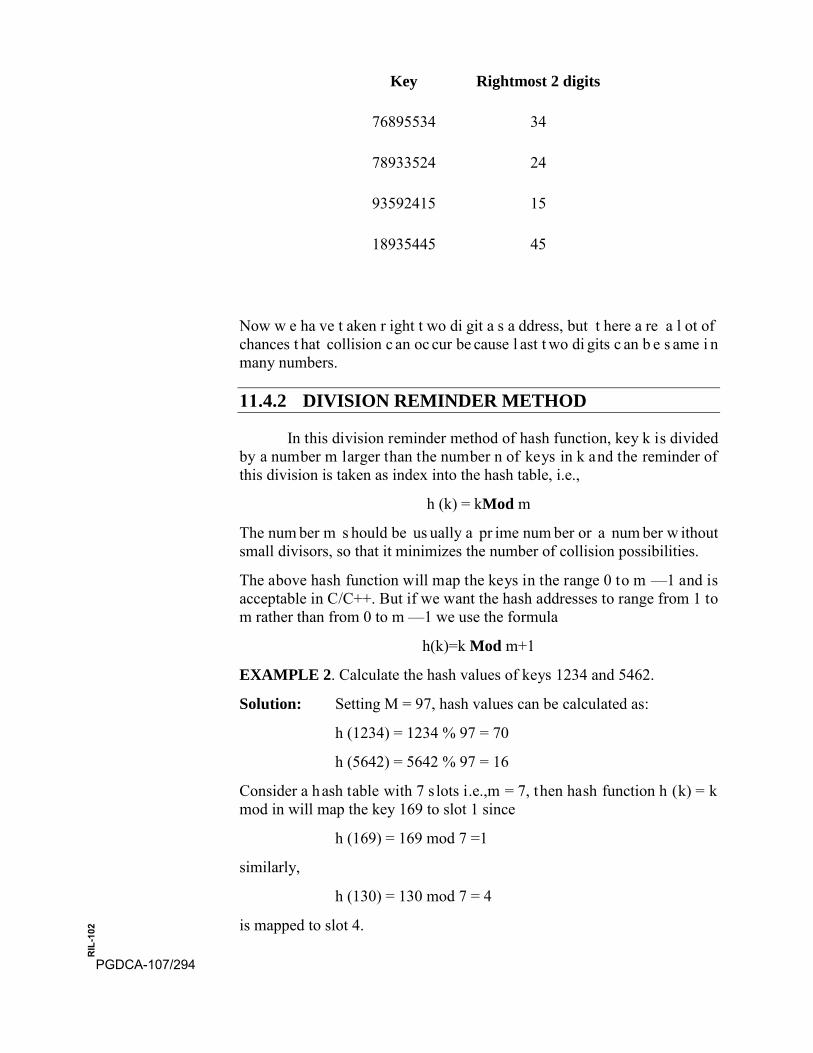
Key Rightmost 2 digits
76895534 34
78933524 24
93592415 15
18935445 45
Now w e ha ve t aken r ight t wo di git a s a ddress, but t here a re a l ot of chances t hat collision c an oc cur be cause l ast t wo di gits c an b e s ame i n many numbers.
11.4.2 DIVISION REMINDER METHOD
In this division reminder method of hash function, key k is divided by a number m larger than the number n of keys in k and the reminder of this division is taken as index into the hash table, i.e.,
h (k) = kMod m
The num ber m s hould be us ually a pr ime num ber or a num ber w ithout small divisors, so that it minimizes the number of collision possibilities.
The above hash function will map the keys in the range 0 to m —1 and is acceptable in C/C++. But if we want the hash addresses to range from 1 to m rather than from 0 to m —1 we use the formula
h(k)=k Mod m+1
EXAMPLE 2. Calculate the hash values of keys 1234 and 5462.
Solution: Setting M = 97, hash values can be calculated as:
h (1234) = 1234 % 97 = 70
h (5642) = 5642 % 97 = 16
Consider a hash table with 7 s lots i.e.,m = 7, then hash function h (k) = k mod in will map the key 169 to slot 1 since
h (169) = 169 mod 7 =1
similarly,
h (130) = 130 mod 7 = 4
is mapped to slot 4.
PGDCA-107/294
RIL
-102

11.4.3 MID SQUARE METHOD
In t he m id s quare m ethod t he ke y i s f irst s quared. T herefore t he hash function is defined by
h(k)=p where p i s obtained by deleting digits from both sides of k2. To properly implement this the same position of k2 must be used for all the keys. EXAMPLE 3. Consider a ha sh t able w ith 50 s lots i .e., m = 50 and ke y values k= 1632, 1739,3123.
SOLUTION.
k 1632 1739 3123
k2 2663424 3024121 9753129
h(k) 34 41 31
The hash values are obtained by taking the fourth and fifth digits counting from right.
11.4.4 FOLDING METHOD
In folding method the key, k i s partitioned into a number of parts k1, k2….kr where each part, except possibly the last, has the same number of di gits a s t he r equired a ddress: T hen t he pa rts a re a dded t ogether, ignoring the last carry i.e.,
H(k)=k1+k2+……….. +kr
wherethe leading-digits carries, if any are ignored.
EXAMPLE 4. Consider a hash table with 100 slots i.e., m = 100 and key values k = 7325, 76321, 1623, 7613.
SOLUTION.
k Parts Sum of parts h (k)
7325 73, 25 98 98
76321 76, 32, 1 109 09
1623 16, 23 39 39
7613 76, 13 89 89 PGDCA-107/295
RIL
-102

11.4.5 FOR FLOATING POINT NUMBER
The a pproach f or ha sh a ddress f or f loating p oint num bers i s something different but also needs modulus operation within the range of hash t able. T here a re f ollowing s teps for calculating t he h ash v alues f or such floating point numbers.
1. Take fractional part of the key.
2. Multiply this part with size of hash table array.
3. Now take integer part from it as the result of hash address of thatkey.
Example 5 : Calculate t he ha sh va lues of k eys 123.6721, 970.663, 123.0558 and 679.99156 with table size 99.
Solution :
Let us take the fractional part of the keys and multiply with table size 99.
0.6721 × 99 = 66.5379
0.663 × 99 = 65.637
0.0558 × 99 = 5.5242
0.99156 × 99 = 98.16444
Now the hash address will be integer part of these numbers.
H (66.5379) = 66
H (65.637) = 65
H (5.5242) = 5
H (98.16444) = 98
11.4.6 FOR STRINGS
In m any c ases s trings a re us ed a s t he ke y w hich c ould be alphabetic o r alphanumeric. W e can see it in E nglish d ictionary v ery frequently. We can take ASCII value of each character and sum all values then take modulus by the table size to calculate the key for hash table.
Let us take an example.
Suppose we have a hash table of size 99 and the key is “Manisha”. Now we have to calculate the hash value for it.
First sum up all the ASCII values respected to each character in the key as under
PGDCA-107/296
RIL
-102
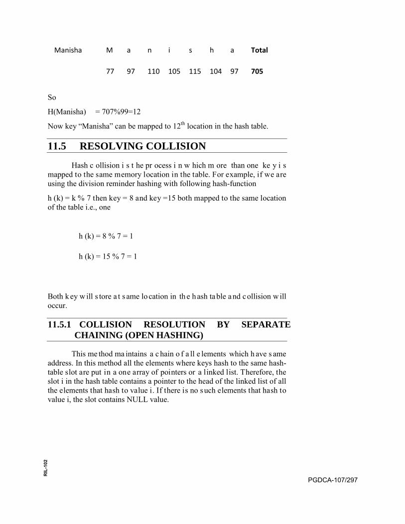
So
H(Manisha) = 707%99=12
Now key “Manisha” can be mapped to 12th location in the hash table.
11.5 RESOLVING COLLISION
Hash c ollision i s t he pr ocess i n w hich m ore than one ke y i s mapped to the same memory location in the table. For example, if we are using the division reminder hashing with following hash-function
h (k) = k % 7 then key = 8 and key =15 both mapped to the same location of the table i.e., one
h (k) = 8 % 7 = 1
h (k) = 15 % 7 = 1
Both k ey w ill s tore a t s ame lo cation in th e h ash table and collision w ill occur.
11.5.1 COLLISION RESOLUTION BY SEPARATE CHAINING (OPEN HASHING)
This me thod ma intains a c hain o f a ll e lements which h ave s ame address. In this method all the elements where keys hash to the same hash-table slot are put in a one array of pointers or a linked list. Therefore, the slot i in the hash table contains a pointer to the head of the linked list of all the elements that hash to value i. If there is no such elements that hash to value i, the slot contains NULL value.
Manisha M a n i s h a Total
77 97 110 105 115 104 97 705
PGDCA-107/297
RIL
-102
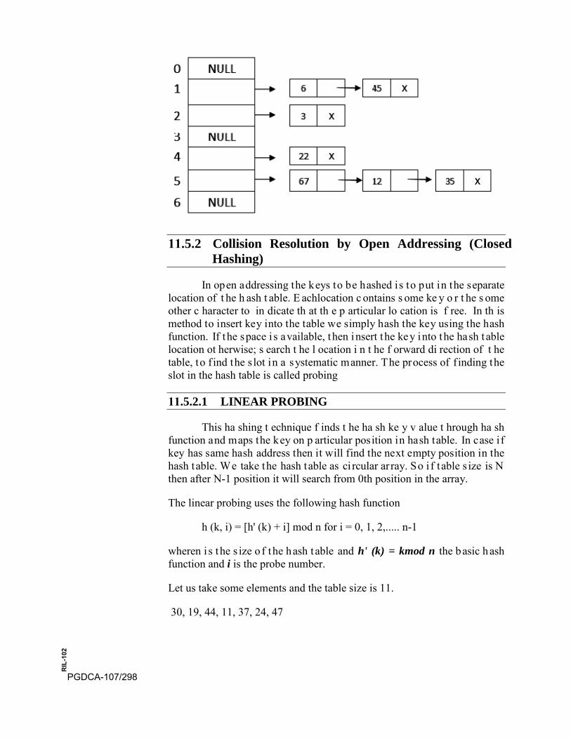
11.5.2 Collision Resolution by Open Addressing (Closed Hashing)
In open addressing the keys to be hashed is to put in the separate location of t he h ash t able. E achlocation c ontains s ome ke y o r t he s ome other c haracter to in dicate th at th e p articular lo cation is f ree. In th is method to insert key into the table we simply hash the key using the hash function. If the space i s available, then insert the key into the hash table location ot herwise; s earch t he l ocation i n t he f orward di rection of t he table, to f ind the s lot in a systematic manner. The process of f inding the slot in the hash table is called probing
11.5.2.1 LINEAR PROBING
This ha shing t echnique f inds t he ha sh ke y v alue t hrough ha sh function and maps the key on p articular position in hash table. In case if key has same hash address then it will find the next empty position in the hash table. We take the hash table as ci rcular array. So i f table s ize is N then after N-1 position it will search from 0th position in the array.
The linear probing uses the following hash function
h (k, i) = [h' (k) + i] mod n for i = 0, 1, 2,..... n-1
wheren i s the s ize o f the hash t able and h' (k) = kmod n the basic hash function and i is the probe number.
Let us take some elements and the table size is 11.
30, 19, 44, 11, 37, 24, 47
PGDCA-107/298
RIL
-102
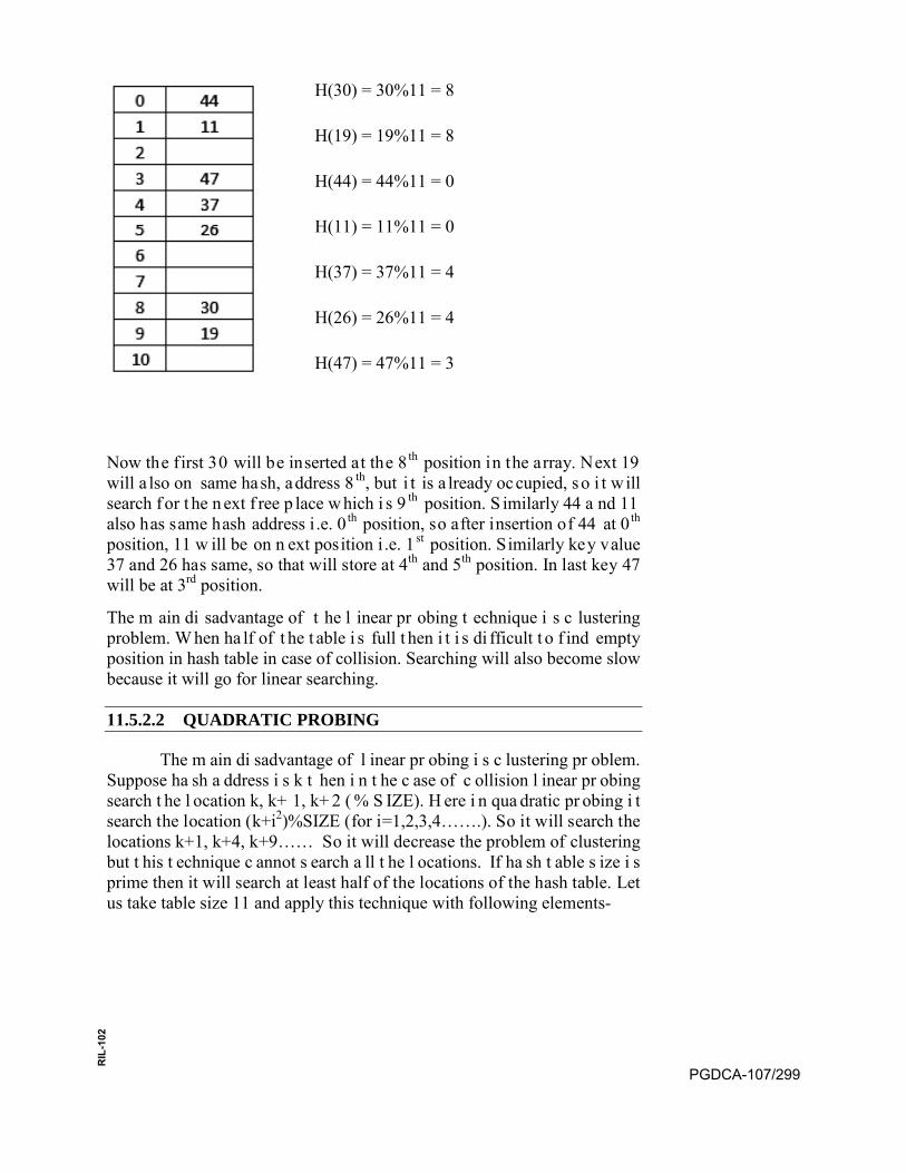
H(30) = 30%11 = 8
H(19) = 19%11 = 8
H(44) = 44%11 = 0
H(11) = 11%11 = 0
H(37) = 37%11 = 4
H(26) = 26%11 = 4
H(47) = 47%11 = 3
Now the first 30 will be inserted at the 8th position in the array. Next 19 will a lso on same hash, address 8 th, but i t is a lready oc cupied, so i t w ill search f or t he n ext f ree p lace w hich i s 9 th position. S imilarly 44 a nd 11 also has same hash address i .e. 0th position, so after insertion of 44 at 0th position, 11 w ill be on n ext position i .e. 1st position. Similarly key value 37 and 26 has same, so that will store at 4th and 5th position. In last key 47 will be at 3rd position.
The m ain di sadvantage of t he l inear pr obing t echnique i s c lustering problem. W hen ha lf of t he t able i s full t hen i t i s di fficult t o f ind empty position in hash table in case of collision. Searching will also become slow because it will go for linear searching.
11.5.2.2 QUADRATIC PROBING
The m ain di sadvantage of l inear pr obing i s c lustering pr oblem. Suppose ha sh a ddress i s k t hen i n t he c ase of c ollision l inear pr obing search t he l ocation k, k+ 1, k+ 2 ( % S IZE). H ere i n qua dratic pr obing i t search the location (k+i2)%SIZE (for i=1,2,3,4…….). So it will search the locations k+1, k+4, k+9…… So it will decrease the problem of clustering but t his t echnique c annot s earch a ll t he l ocations. If ha sh t able s ize i s prime then it will search at least half of the locations of the hash table. Let us take table size 11 and apply this technique with following elements-
PGDCA-107/299
RIL
-102
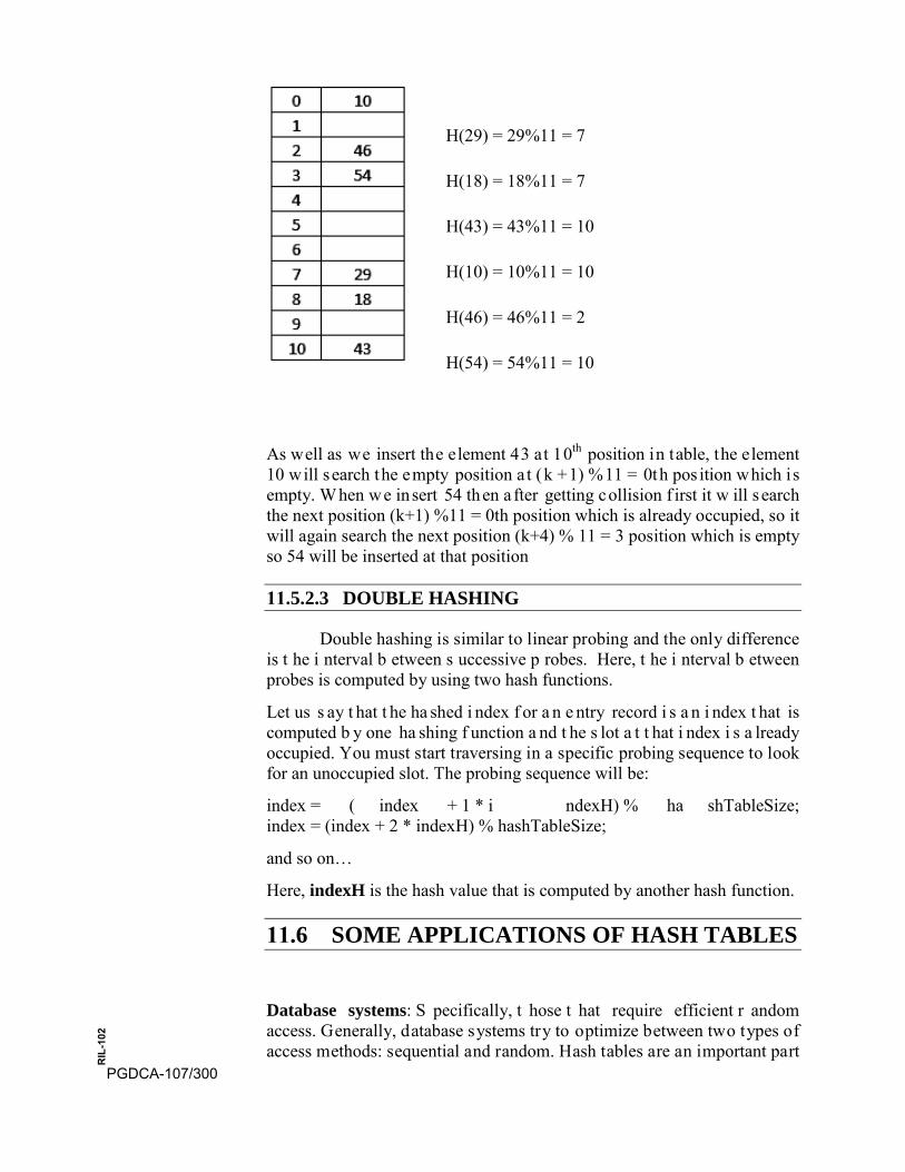
H(29) = 29%11 = 7
H(18) = 18%11 = 7
H(43) = 43%11 = 10
H(10) = 10%11 = 10
H(46) = 46%11 = 2
H(54) = 54%11 = 10
As well as we insert the element 43 at 10th position in table, the element 10 will search the empty position a t (k +1) %11 = 0th pos ition which is empty. When we insert 54 then a fter getting collision f irst it w ill s earch the next position (k+1) %11 = 0th position which is already occupied, so it will again search the next position (k+4) % 11 = 3 position which is empty so 54 will be inserted at that position
11.5.2.3 DOUBLE HASHING
Double hashing is similar to linear probing and the only difference is t he i nterval b etween s uccessive p robes. Here, t he i nterval b etween probes is computed by using two hash functions.
Let us s ay t hat t he ha shed i ndex f or a n e ntry record i s a n i ndex t hat is computed b y one ha shing f unction a nd t he s lot a t t hat i ndex i s a lready occupied. You must start traversing in a specific probing sequence to look for an unoccupied slot. The probing sequence will be:
index = ( index + 1 * i ndexH) % ha shTableSize; index = (index + 2 * indexH) % hashTableSize;
and so on…
Here, indexH is the hash value that is computed by another hash function.
11.6 SOME APPLICATIONS OF HASH TABLES
Database systems: S pecifically, t hose t hat require efficient r andom access. Generally, database systems try to optimize between two types of access methods: sequential and random. Hash tables are an important part
PGDCA-107/300
RIL
-102
of efficient random access because they provide a way to locate data in a constant amount of time.
Symbol tables: T he t ables u sed b y c ompilers to ma intain in formation about s ymbols f rom a pr ogram. C ompilers a ccess i nformation a bout symbols f requently. T herefore, it is imp ortant th at s ymbol ta bles b e implemented very efficiently.
Data dictionaries: D ata s tructures t hat s upport a dding, de leting, a nd searching for d ata. A lthough t he ope rations of a ha sh t able a nd a d ata dictionary are similar, other data structures may be used to implement data dictionaries. Using a hash table is particularly efficient.
Network processing algorithms: H ash tables ar e f undamental components of s everal network pr ocessing algorithms a nd a pplications, including route lookup, packet classification, and network monitoring.
Associative arrays: Hash tables are commonly used to implement many types of in-memory tables. They are used to implement associative arrays (arrays whose indices are arbitrary strings or other complicated objects).
Caches: Hash tables can be used to implement caches i .e. auxiliary data tables t hat a re u sed t o speed u p t he a ccess t o data, w hich i s p rimarily stored in slower media.
Object representation: Several dynamic languages, such as Perl, Python, JavaScript, and Ruby use hash tables to implement objects.
Browser Cashes: Hash tables are used to implement browser cashes.
11.7 SUMMARY
Hashing i s t he pr ocess of m apping l arge a mount of da ta i tem t o smaller table with the help of hashing function. Hashing is also known as Hashing Algorithm.It is a technique to convert a range of key values into a r ange o f i ndexes o f an ar ray. It is u sed to facilitate t he n ext l evel searching method when compared with the linear or binary search.
Hash table or hash map is a data structure used to store key-value pairs.It is a collection of items stored to make it e asy to find them later.It uses a hash function to compute an index into an array of buckets or slots from which the desired value can be found.It contains value based on the key.
Hash Function is a f ixed process which converts a key to a hash key to store in array.This function takes a key and maps it to a value of a cer tain length which i s cal led a Hash value o r Hash using va rious methods l ike Truncate, D ivision R eminder, M id S quare M ethod a nd F olding M ethod etc. Using these functions we calculate a Hash value which represents the original value, but it is normally smaller than the original.
In s ome cases, t here a re ch ances o f s ame h ash v alues i s cal culated for same memory location. It means collisions occur when the hash function maps t wo di fferent k eys t o t he s ame l ocation. O bviously, t wo r ecords PGDCA-107/301
RIL
-102
cannot be stored in the same location. Therefore, a method used to solve the pr oblem of c ollision, a lso c alled c ollision r esolution t echnique, i s applied. T he t wo m ost popul ar m ethods of r esolving c ollisions a re Collision Resolution by Separate Chaining (Open Hashing) and Collision Resolution by Open Addressing (Closed Hashing)
Bibliography : • J. P . T remblay, P . G . S orenson “ An Introduction t o D ata
Structures with Applications”, Tata McGraw-Hill, 1984
• Markus Blaner: “Introduction to Algorithms and Data Structures”,Saarland University, 2011
• Seymour Lipschutz, “Data Structure”, Schaum ‟s outline Series
• ReemaThareja, “Data Structure using C” Oxford University Press,Jai Singh Road, New Delhi, 2011
• S. K. Shrivastav, D eepaliShrivastav, “ Data S tructure us ing C i nDepth” BPB Publication, New Delhi, 2008
• G. S. Baluja, “Data Structure through C” (A Practical Approach),DhanpatRai& Co. (Pvt) Ltd. NaiSarak, Delhi, 2007
• Dr. M adhulika J ain, S atish J ain, S hashi S ingh, “ Data S tructurethough C Language” BPB Publication, New Delhi, 2008
Self - Evaluation 1. What do you mean by hash table?
2. What i s ha sh f unction? W hat a re t he qua lities of a g ood ha shfunction?
3. Write a s hort not e on t he di fferent h ash f unctions. G ive s uitableexamples to justify your answers.
4. Calculate hash va lues o f ke ys: 8922, 9241, 3807 , 5643 a nd 4522using different methods of hashing.
5. What is collision? How to resolve a collision. Which technique doyou think is better and why?
6. Consider a hash table with size = 10. U sing l inear probing, insertthe keys 72, 27, 33, 54, 26, 68, 59,and 101 into the table.
7. What is hashing? Give its applications. Also, discuss the pros andcons of hashing.
8. Explain chaining with examples.
9. Write short notes on:
• Mid square MethodPGDCA-107/302
RIL
-102
• Folding Method
• Modular Method
• Linear probing
• Quadratic probing
• Double hashing
10. What are applications of hashing?
MCQ : 1. What is a hash table?
a) A structure that maps values to keys
b) A structure that maps keys to values
c) A structure used for storage
d) A structure used to implement stack and queue
2. If several elements are competing for the same memory location inthe hash table, what is it called?
a) Diffusion
b) Replication
c) Collision
d) None of the mentioned
3. What is direct addressing?
a) Distinct array position for every possible key
b) Fewer array positions than keys
c) Fewer keys than array positions
d) None of the mentioned
4. What can be the techniques to avoid collision?
a) Make the hash function appear random
b) Use the chaining method
c) Use uniform hashing
d) All of the mentioned
5. What is a hash function?
a) A function has allocated memory to keys
b) A function that computes the location of the key in thearray PGDCA-107/303
RIL
-102
c) A function that creates an array
d) None of the mentioned
PGDCA-107/304
RIL
-102
UNIT-12 FILE STRUCTURE
Structure
12.0 Introduction
12.1 Objectives
12.2 File Terminology
12.3 File Organization
12.4 Basic File Operations
12.5 Sequential Files
12.6 Direct File
12.7 Indexed Sequential Files
12.8 Summary
12.0 INTRODUCTION
File o rganization r efers to th e w ay d ata is s tored in a f ile. F ile organization i s ve ry i mportant be cause i t de termines t he m ethods of access, efficiency, flexibility and storage devices to use in efficient way.
Nowadays, almost all organizations use data collection software to collect large amounts o f d ata. For example, w hen w e approach an y college f or admission, our a ll da ta l ike name, address, phon e number, t he r equested course, aggregate of m arks obt ained i n t he l ast e xamination et c. i s collected.
A university mi ght like to s tore data related to a ll s tudents—the courses they sign up for etc., all this implies the following:
• Data will be stored on external storage devices like magnetic tapes,disk, floppy etc.
• Data will be accessed by many people and software programs
• Users of the data will expect that
o It is always reliably available for processing
o It is secure
o It is stored in a manner flexible enough to allow the users toadd new data as per changing needs
In c ommon t erminology, a f ile i s a bl ock of i mportant da ta which i s available t o a ny c omputer s oftware a nd i s us ually s tored on a ny s torage device. Storing a file on any storage medium like pen drive, hard disk or floppy disk ensures the availability of the file in future.Now a days all file PGDCA-107/305
RIL
-102
are stored in computers to reduce paper work and easy availability in any office, bank or library.
12.1 OBJECTIVES
After reading this unit the learner is able to do the following task.
• Understand the concept of File and its terminology.
• File Organization and its uses
• Operations that could be performed of file
• Sequential File organization and its features
• Direct File organization and its features
• Index Sequential File organization and its features
12.2 FILE TERMINOLOGY
Every file c ontains r ecords w hich could be o f a c ustomer ( in Business), s tudents ( in uni versity or c ollege), pa tient ( in hos pital), passenger (in t rain/flight r eservation) w hich can be or ganized i n a hierarchy to present a systematic way so that it could be utilized in future as requested.
Now we will define the terms of the hierarchical s tructure of data which we are storing in computer in the form of file.
Field : It i s an el ementary d ata i tem t hat s tores a s ingle f act an d characterized by its length and types.
For example :
Name : Size= 25 Type= Character
Age : Size=2 Type= Integer/Numeric
Address: Size=100 Type=Character
Record : It i s a collection o f related f ields that can be t reated as a unit from an applications point of view.
For example : The s tudent’s record may contain data f ields such as name, address, phone number, roll number, marks obtained, and so on.
File : Data is o rganized f or s torage in f iles. A f ile is a c ollection o f similar, related records. It has an identifying name.
For example : There are 100 students in a class, then there are 100 records, one for each student. All these related records are stored in a file with the respective class name.
PGDCA-107/306
RIL
-102
Directory : A directory stores information of files belongs to one group or related in any manner. A directory is used to store files so that users can access all files easily.
For example :
Teachers : This directory will stores all files of teachers.
BSc_Part1 : This directory will stores all first year students.
Courses : T his d irectory w ill stores a ll in formation o f available courses.
12.3 FILE ORGANIZATION
File organization tell that what is the way to store data and how to retrieve t hat d ata. Basically F ile O rganization is a w ay o f a rranging th e records in a file when the file is stored on the disk. The factors involved in selecting a particular file organization for uses are:
• Easily storing and retrieval of information
• Easily modify or updates
• Less storage space
• Reliability of data for future
• Security
• Integrity
Different f ile o rganizations assures t he a bove f actors w ith di fferent weightages. The choice of particular file organization depends on the type of application and need of the user.
Now we will discuss some of the file organization in brief.
Sequential Files : Data r ecords are s tored i n some s pecific s equence e.g., order o f arrival, va lue of ke y field etc. Records of a s equential filecannot b e ac cessed at r andom i .e., t o acces s t he n th r ecord, on e m ust traverse the preceding (n - 1) records. Sequential files will be dealt with at length in the next section.
Relative Files : Each data record has a fixed place in a relative file. Each record m ust ha ve associated w ith i t a n i nteger key value th at w ill h elp identify t his s lot. T his key, t herefore, w ill be used f or i nsertion a nd retrieval of the records. Random as well as sequential access i s possible. Relative files can exist only on random access devices like disks.
Direct Files : These are similar to relative files, except that the key value need not be an integer. The user can specify keys which make sense to his application.
PGDCA-107/307
RIL
-102

Indexed Sequential Files : An i ndex i s a dded t o t he s equence f ile t o provide random access. An overflow area needs to be maintained to permit insertion in sequence.
12.4 BASIC FILE OPERATIONS
Before moving to a p articular organization, let usunderstand basic file operations that can be performed on any kind of file.
A. Creation of file
B. Updation of file
I. Insert a new record
II. Modify an existing record
III. Delete a particular record
C. Retrieval of Information
I. Inquiry of record
II. Generate a report
D. Maintenance
I. Restructuring the file records
II. Reorganizing the records
A. Creation of File:
Before creating a file we have to collect the data, validate the data and pr ocess t he d ata t o g ive i t a r ecord l ike s tructure. T hen w e choose the name for the file and open the file on secondary storage device and store the collected data on it.
B. Updating File:
It means to change/delete/modify the contents of the file. A file can be updated in the following ways:
• Inserting a new record: F or e xample, i f a ne w s tudentcomes later and joins the course, we have to add his record inthe STUDENT file.
• Modifyingan existing record: For example, if the name of astudent w as s pelt in correctly, th en c orrecting th e n ame w illbe a modification of the existing record.
• Deletingan existing record. For example, if a student switchor quits a particular course in the initial/middle of the session,his/her record has to be deleted from the STUDENT file.
PGDCA-107/308
RIL
-102

C. Retrieving from a File :
It means, we are accessing only the useful data from a given file as per the requirement. Information can be retrieved for an inquiry or for report generation. For any inquiry less data is retrieved while to generate a report needs large amount of data from the file.
D. Maintenance of File:
It i nvolves r estructuring or r e-organizing th e file to imp rove th e performance of the programs that access this f ile. Restructuring a file k eeps t he file or ganization unc hanged a nd c hanges onl y t he structural aspects of the file (for example, changing the field width or a dding/deleting f ields). O n t he ot her ha nd, f ile r eorganization may involve changing the entire organization of the f ile. We will discuss file organization in detail in the next section.
12.5 SEQUENTIAL FILE Sequential f iles h ave d ata
records s tored in a s pecific sequence. A s equential or ganized f ile m ay b e stored o n ei ther a s erial access o r a direct access storage medium.
A sequentially or ganized f ile stores t he r ecords i n t he or der i n which they were entered. That is, the first record that was entered is written as th e f irst r ecord in the f ile, th e second record entered is written as the second r ecord i n t he f ile, a nd s o on . As a r esult, n ew r ecords ar e added only at the end of the file. Sequential files can b e r ead o nly s equentially, starting w ith th e v ery first r ecord in the f ile to the last r ecord o f the f ile. It is the m ost basic and s imple f ile organization to organize a large collection of records in a file.
Once we store the records in a file, we cannot modify the records means deletion or Updation in sequential file is not allowed. You have to create a n ew file with existing file to do any such operation like delete or modify.
All r ecords h ave t he s ame s ize an d t he s ame f ield f ormat. T he records are sorted based on the value of one field or a combination of two or m ore fields. R ecords can be s orted i n either ascending or d escending order.
These files are used to generate reports or to perform sequential reading of large a mount of da ta w hich s ome pr ograms ne ed t o do s uch a s pa yroll
PGDCA-107/309
RIL
-102
processing, or billing of all customers. Sequential files can be easily stored on both disks and tapes.
The features, advantages, and disadvantages of sequential file organization are as under.
Features • Records are written in the order in which they are entered
• Records are read and written sequentially
• Deletion or Updation of one or more records calls for replacing theoriginal file with a new file that contains the desired changes
• Records have the same size and the same field format
• Records are sorted on a key value
• Generally used for report generation or sequential reading
Advantages :
• Simple and easy to handle
• No extra overheads involved
• Sequential f iles can be stored on magnetic disks as well asmagnetic tapes
• Well suited for batch oriented applications
Disadvantages : • All records must be structurally identical. If a new field has to be
added, then every record must be rewritten to provide space for thenew field.
• Records can be read only sequentially. If ith record has to be read,then all the i–1 records must be read
• Updates a re not e asily accommodated. D oes n ot s upport upda teoperation? A new file has to be created and the original file has tobe replaced with the new file that contains the desired changes
• By definition, random access is not possible
• Continuous a reas may n ot be pos sible be cause both t he pr imarydata file and the transaction file must be looked during merging.
Areas of Use : Sequential f iles ar e m ost f requently u sed i n co mmercial b atch o riented data processing where there is the concept of a master file to which details are added periodically. For example, Payroll applications.
PGDCA-107/310
RIL
-102

Example: Write a program to implement sequential file operation (Write, Read) using C.
#include <stdio.h> #include <conio.h>
typedefstruct { intusn; char name[25]; int m1,m2,m3;
}Student; Student s; void display(FILE *); int search(FILE *,int); void main() { inti,n,usn_key,opn;
FILE *fp; printf(" How many Records ? "); scanf("%d",&n); fp=fopen("stud.dat","w"); for (i=0;i<n;i++) {
printf("Read the Info for Student: %d (usn,name,m1,m2,m3) \n",i+1);
scanf("%d%s%d%d%d",&s.usn,s.name,&s.m1,&s.m2,&s.m3); fwrite(&s,sizeof(s),1,fp);
} fclose(fp); fp=fopen("stud.dat","r");
do { printf("Press 1- Display\t 2- Search\t 3- Exit\t Your Option?"); scanf("%d",&opn); switch(opn) { case 1: printf("\n Student Records in the File \n");
display(fp); break;
case 2: printf(" Read the USN of the student to be searched ?"); scanf("%d",&usn_key); if(search(fp,usn_key)) {printf("Success ! Record found in the file\n");
printf("%d\t%s\t%d\t%d\t%d\n",s.usn,s.name,s.m1,s.m2,s.m3); }
else printf(" Failure!! Record with USN %d not
found\n",usn_key); break;
case 3: printf(" Exit!! Press a key . . ."); PGDCA-107/311
RIL
-102
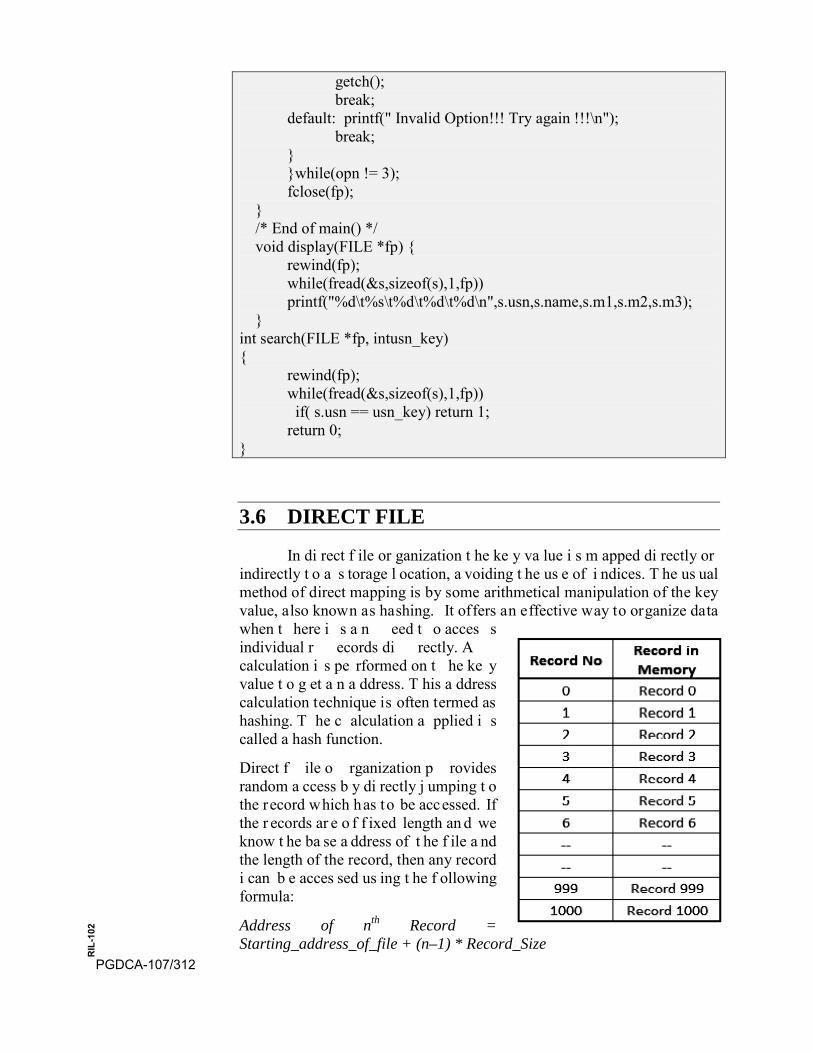
getch(); break;
default: printf(" Invalid Option!!! Try again !!!\n"); break;
} }while(opn != 3); fclose(fp);
} /* End of main() */ void display(FILE *fp) {
rewind(fp); while(fread(&s,sizeof(s),1,fp)) printf("%d\t%s\t%d\t%d\t%d\n",s.usn,s.name,s.m1,s.m2,s.m3);
} int search(FILE *fp, intusn_key) {
rewind(fp); while(fread(&s,sizeof(s),1,fp)) if( s.usn == usn_key) return 1; return 0;
}
3.6 DIRECT FILE
In di rect f ile or ganization t he ke y va lue i s m apped di rectly or indirectly t o a s torage l ocation, a voiding t he us e of i ndices. T he us ual method of direct mapping is by some arithmetical manipulation of the key value, also known as hashing. It offers an effective way to organize data when t here i s a n eed t o acces s individual r ecords di rectly. A calculation i s pe rformed on t he ke y value t o g et a n a ddress. T his a ddress calculation technique is often termed as hashing. T he c alculation a pplied i s called a hash function.
Direct f ile o rganization p rovides random a ccess b y di rectly j umping t o the record which has to be accessed. If the r ecords ar e o f f ixed length an d we know t he ba se a ddress of t he f ile a nd the length of the record, then any record i can b e acces sed us ing t he f ollowing formula:
Address of nth Record = Starting_address_of_file + (n–1) * Record_Size
PGDCA-107/312
RIL
-102
Therefore, i n d irect f iles, r ecords are o rganized i n as cending r elative record number. A direct file can be thought of as a single dimension table stored on a disk, in which the relative record number is the index into the table. D irect f iles c an be u sed f or b oth r andom as w ell as s equential access. For sequential access, records are simply read one after another.
Features
• Provides an effective way to access individual records
• The record number represents the location of the record relative tothe beginning of the file
• Records in a relative file are of fixed length
• Relative f iles can b e u sed f or b oth random as well as s equentialaccess
• Every l ocation i n t he t able ei ther s tores a r ecord o r i s m arked asFREE
Advantages of Direct File Organization 1. Records can be immediately accessed for Updation.
2. Several f iles c an be s imultaneously upd ated d uring t ransactionprocessing.
3. Transaction need not be sorted.
4. Existing records can be amended or modified.
5. Most suitable for interactive online applications.
6. Very easy to handle random enquiries.
Disadvantages of Direct File Organization 1. Data m ay be accidentally e rased o r o ver w ritten u nless s pecial
precautions are taken.
2. Risk of loss of accuracy and breach of Security.
3. Special backup and reconstruction procedures must be established.
4. Expensive hardware and Software are required.
5. High complexity in programming.
6. Use of relative files is restricted to disk devices
7. Records can be of fixed length only
8. For random access of records, the relative record number must beknown in advance
PGDCA-107/313
RIL
-102
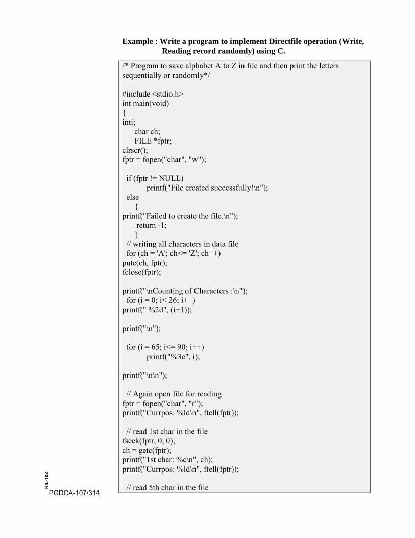
Example : Write a program to implement Directfile operation (Write, Reading record randomly) using C.
/* Program to save alphabet A to Z in file and then print the letters sequentially or randomly*/
#include <stdio.h> int main(void) { inti; char ch; FILE *fptr; clrscr(); fptr = fopen("char", "w");
if (fptr != NULL) printf("File created successfully!\n");
else { printf("Failed to create the file.\n"); return -1; } // writing all characters in data file for (ch = 'A'; ch<= 'Z'; ch++) putc(ch, fptr); fclose(fptr);
printf("\nCounting of Characters :\n"); for (i = 0; i< 26; i++) printf(" %2d", (i+1));
printf("\n");
for (i = 65; i<= 90; i++) printf("%3c", i);
printf("\n\n");
// Again open file for reading fptr = fopen("char", "r"); printf("Currpos: %ld\n", ftell(fptr));
// read 1st char in the file fseek(fptr, 0, 0); ch = getc(fptr); printf("1st char: %c\n", ch); printf("Currpos: %ld\n", ftell(fptr));
// read 5th char in the file PGDCA-107/314
RIL
-102

fseek(fptr, 4, 0); ch = getc(fptr); printf("5th char: %c\n", ch); printf("Currpos: %ld\n", ftell(fptr));
fseek(fptr, 25, 0); // read 26th char in the file ch = getc(fptr); printf("26th char: %c\n", ch); printf("Currpos: %ld\n", ftell(fptr)); printf("Rewind : Moving to first location in the file\n"); rewind(fptr); printf("Currpos: %ld\n", ftell(fptr)); fseek(fptr, 9, 0); // read 10th char in the file ch = getc(fptr); printf("10th char: %c\n", ch); printf("Currpos: %ld\n", ftell(fptr));
// read 15th char in the file fseek(fptr, 4, 1); // move 4 bytes forward from current position ch = getc(fptr); printf("15th char: %c\n", ch); printf("Currpos: %ld\n", ftell(fptr));
// read 20th char in the file fseek(fptr, 4, 1); // move 4 bytes forward from current position ch = getc(fptr); printf("20th char: %c\n", ch);
printf("Currpos: %ld\n", ftell(fptr));
fclose(fptr); return 0; }
3.7 Indexed Sequential Files
On an av erage, t he r etrieval o f a record f rom a s equential f ile, requires a ccess t o ha lf t he r ecords i n t he f ile. It m akes i t not onl y inefficient b ut v ery tim e c onsuming p rocess for th e la rge file. S o to improve the query response time from a sequential file, a type of indexing technique can be added.When there is need to access records sequentially by s ome k ey v alue an d also t o acces s r ecords d irectly b y t he s ame k ey value, t he collection of records m ay be o rganizedin a n e ffective m anner called Indexes Sequential Organization.
PGDCA-107/315
RIL
-102
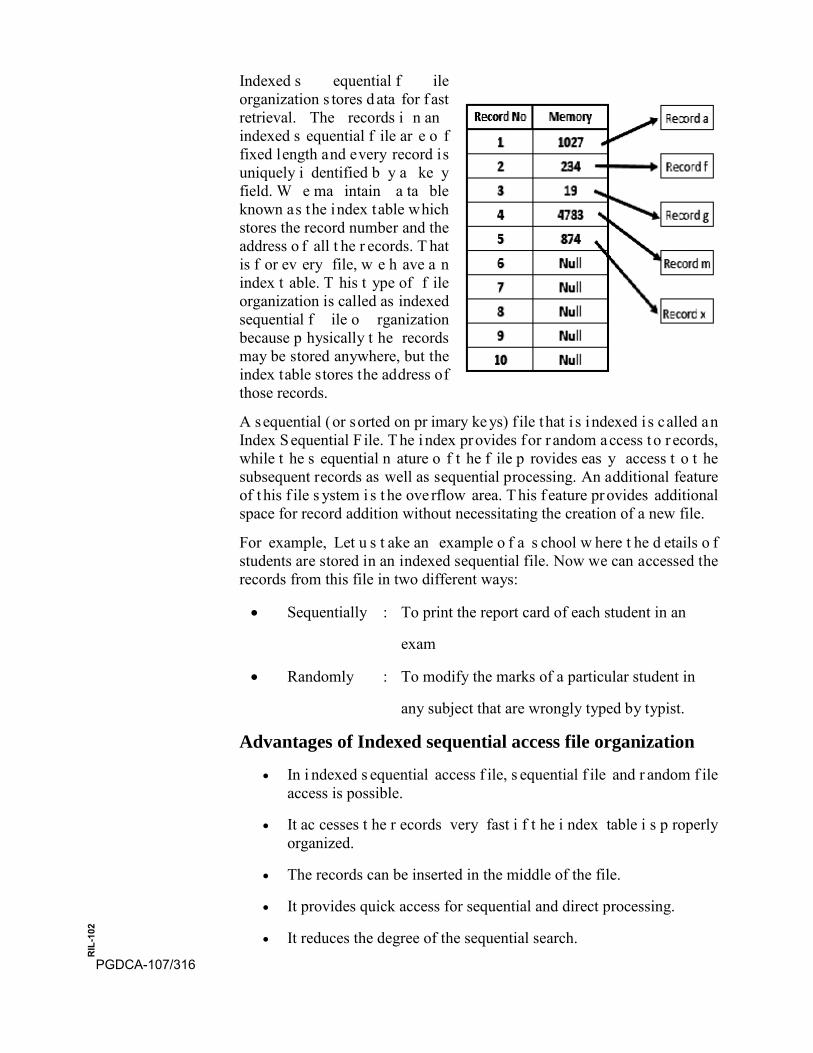
Indexed s equential f ile organization s tores d ata for f ast retrieval. The records i n an indexed s equential f ile ar e o f fixed length and every record is uniquely i dentified b y a ke y field. W e ma intain a ta ble known as the index table which stores the record number and the address o f all t he r ecords. T hat is f or ev ery file, w e h ave a n index t able. T his t ype of f ile organization is called as indexed sequential f ile o rganization because p hysically t he records may be stored anywhere, but the index table stores the address of those records.
A sequential (or sorted on pr imary ke ys) f ile that i s indexed i s called an Index Sequential F ile. T he index provides for r andom access t o r ecords, while t he s equential n ature o f t he f ile p rovides eas y access t o t he subsequent records as well as sequential processing. An additional feature of t his f ile s ystem i s t he ove rflow area. T his f eature pr ovides additional space for record addition without necessitating the creation of a new file.
For example, Let u s t ake an example o f a s chool w here t he d etails o f students are stored in an indexed sequential file. Now we can accessed the records from this file in two different ways:
• Sequentially : To print the report card of each student in an
exam
• Randomly : To modify the marks of a particular student in
any subject that are wrongly typed by typist.
Advantages of Indexed sequential access file organization
• In i ndexed s equential access f ile, s equential f ile and r andom f ileaccess is possible.
• It ac cesses t he r ecords very fast i f t he i ndex table i s p roperlyorganized.
• The records can be inserted in the middle of the file.
• It provides quick access for sequential and direct processing.
• It reduces the degree of the sequential search.PGDCA-107/316
RIL
-102
Disadvantages of Indexed sequential access file organization • Indexed s equential access f ile r equires uni que k eys a nd pe riodic
reorganization.
• Indexed sequential access file takes longer time to search the indexfor the data access or retrieval.
• It requires more storage space.
• It is expensive because it requires special software.
• It is less efficient in the use of storage space as compared to otherfile organizations.
3.8 SUMMARY
A file is a collection or bag of records. Having stored the records in a f ile, i t i s n ecessary to ac cess t hese records u sing either a p rimary o r secondary key. The type and frequency of access required determines the type o f f ile or ganization t o be us ed f or a given s et of r ecords. In t his chapter we looked at some common file organizations: Sequential, Index sequential, direct etc.
In a sequential file, records are maintained in the logical sequence of their primary ke y value. The s earch f or a given r ecord r equires, on average, access t o ha lf t he r ecords i n t he f ile. U pdate o perations, i ncluding t he appending of a new record, require creation of a new file. Updates could be batched and a t ransaction f ile o f updates used to create a new m aster file f rom th e existing o ne. T his s cheme a utomatically c reates a b ackup copy of the file.
Access to a sequential file can be enhance by creating an index. The index provides r andom a ccess t o r ecords and t he s equential n ature o f t he f ile provides easy access to the next record. To avoid frequent reorganization, an index sequential file uses overflow areas. This scheme provides space for the addition of records without the need for the creation of a new file. In index sequential organization, it is the usual practice to have a hierarchy of i ndexes w ith t he l owest l evel i ndex poi nting to t he r ecords w hile t he higher level ones point to the index below them.
In direct file organization the key value is mapped directly or indirectly to a storage location, avoiding the use of indices. The usual method of direct mapping is b y some arithmetical ma nipulation o f th e k ey v alue, th e process is called hashing.
Bibliography : • ReemaThareja, “Data Structure using C” Oxford University Press,
New Delhi, 2011
• S. K . Shrivastav, D eepaliShrivastav, “ Data S tructure us ing C i nDepth” BPB Publication, New Delhi, 2008 PGDCA-107/317
RIL
-102
• G. S. Baluja, “Data Structure through C” (A Practical Approach),Dhanpat Rai & Co. (Pvt) Ltd. NaiSarak, Delhi, 2007
• Dr. M adhulika J ain, S atish J ain, S hashi S ingh, “ Data S tructurethough C Language” BPB Publication, New Delhi, 2008
• Markus Blaner: “Introduction to Algorithms and Data Structures”,Saarland University, 2011
• Niklaus W irth, “A lgorithm +D ata S tructures = P rograms”, P HIPublications
• Seymour Lipschutz, “Data Structure”, Schaum ‟ s outline Series
• B. F laming, “Practical Data S tructures i n C ++”, J ohn W iley &Sons, New York, 1994
• R. E . B ellman, “ On a routing P roblem”, Q uarterly of A ppliedMathematics, 16 (1958) 87-90
• D. E . K nuth, “ The Stanford G raphBase”, Addison-Wesley,Reading, Mass. 1993.
• R. E . T arjan, “ Data S tructures a nd ne twork A lgorithms”, S ocietyfor Industrial and Applied
Mathematics, Philadelphia, 1985.
PGDCA-107/318
RIL
-102
SELF EVALUATION
Short Answer Questions
1. Why do you mean by file concept?
2. What is the need of file in computer system?
3. Explain the terms field, record, directory and index.
4. What are various operations that you can perform on file?
5. What do you understand by the File organization? Discuss in briefwith suitable example.
6. What is Sequential file organization and its advantage?
7. Differentiate b etween S equential f ile o rganization a nd D irect f ileorganization.
8. What is Index Sequential file organization and its advantages?
Multiple Choice Questions 1. A ……………….. i s t he ba sic e lement of da ta w here i ndividual
field contains a s ingle value, such as an employee’s l ast name orDOB or Mob No.
A) Field B) record
C) file D) database
2. A ………is collection of related fields that can be treated as aunit by some application program.
A) Field B) record
C) file D) database
3. In ………………f ile or ganization, a f ixed f ormat i s us ed forrecords where all records are of the same length, consisting of thesame number of fixed length fields in a particular order.
A) Flat File B) sequential
C) indexed sequential D) indexed
4. The ……………………… m aintains the key characteristic of thesequential file: Records are organized in sequence based on a keyfield.
A) Flat File B) sequential file
C) indexed sequential file D) indexed file
5. The …………………. greatly reduced the time required to accessa single record, without sacrificing the sequential nature of the file. PGDCA-107/319
RIL
-102

A) Flat File B) sequential file
C) indexed sequential file D) indexed file
6. An a lternative is to o rganize th e s equential f ile p hysically is a……………..
A) List B) Linked List
C) Queue D) Stack
7. …………… a re t ypically us ed i n ba tch a pplications a nd a regenerally opt imum f or s uch a pplications i f t hey i nvolve t heprocessing of all the records.
A) Indexed files B) Direct files
C) Sequential files D) Indexed Sequential files
8. Which is the simplest file structure.
A) Indexed files B) Direct files
C) Sequential files D) Flat File
PGDCA-107/320
RIL
-102