Manuscript 2007-4-17

Perspectives on Team Dynamics: Meta Learning and

Systems Intelligence

Jukka Luoma, Raimo P. Hämäläinen and Esa Saarinen

jukka.luoma@hut.fi, raimo@hut.fi, esa@hut.fi

Systems Analysis Laboratory

Helsinki University of Technology

Corresponding author:

Jukka Luoma

Helsinki University of Technology,

Systems Analysis Laboratory, P.O. Box 1100,

02150 HUT, Finland

Email: jukka.luoma@tkk.fi

Tel.: +358 9 451 3053

Fax: +358 9 451 3096

Manuscript 2007-4-17

Abstract

Losada (1999) observed management teams develop their annual strategic plans in a lab

designed for studying team behavior. Based on these findings he developed a dynamical

model of team interaction and introduced the concept of Meta Learning (ML) which

represents the ability of a team to avoid undesirable attractors. This paper analyzes the

dynamic model in more detail and discusses the relationship between meta learning and

the new concept of Systems Intelligence (SI) introduced by Saarinen and Hämäläinen

(2004). In our view, the meta learning ability of a team clearly represents a systems

intelligent competence. Losada’s mathematical model predicts interesting dynamic

phenomena in team interaction. However, our analysis shows how the model also

produces strange and previously unreported behavior under certain conditions. Thus, the

predictive validity of the model also becomes problematic. It remains unclear whether the

model behavior can be said to be in satisfactory accordance with the observations of team

interaction.

Key words: team interaction, meta learning, systems intelligence, chaotic dynamics,

Lorenz attractor

1

Introduction

The perspective taken in Systems Intelligence1 (SI) (Saarinen and Hämäläinen, 2004; Hämäläinen

and Saarinen, 2006, 2007) is the acknowledgement that we are always embedded in and a part of

systems involving interaction and feedback, which we cannot escape but in which we can take

intelligent actions. The study of systems intelligence is concerned with the behavioral intelligence

of human agents in systemic environments. Systems intelligence looks for efficient ways for an

individual to change her own behavior in order to influence the behavior of a system in different

environments.

We see the concept of a system as a useful one in understanding human action in dynamic settings.

Today, many organizational studies describe organizational phenomena by drawing analogies to

concepts which originate in the field of mathematical modeling of dynamical systems. The use of

systems studies ranges from quantitative to qualitative modeling; from numerical modeling (e.g.

Sterman, 2000, 2002) to making simulation experiments which are considered analogous to

organizational phenomena (e.g. Morel and Ramanujam, 1999; Stacey, 1995, 2001, 2003) and

identifying organizations as systems (e.g. Senge, 1990; Senge et al., 1994). Complexity studies

have also been suggested as tools to make sense of organizational phenomena (see e.g. Andersson,

1999). Yet opinions about the real usefulness of complex systems studies in organizational life vary

(see e.g. Stacey et al., 2000). We believe that mathematical modeling of human systems does,

indeed, provide a convenient way of analyzing the systems’ behavior and testing the possible

1 http://www.systemsintelligence.hut.fi [accessed 2007-04-17]

2

consequences of different interventions. Models of social interaction allow us to analyze how

micro-level phenomena can influence macro-level outcomes.

The literature on the modeling of social interaction is extensive. It dates back to the early work of

Herbert A. Simon (1952) who illustrated how mathematical modeling could be used in “clarifying

of concepts” of a theory, and in “derivation of new propositions”. Here, we only list some recent

studies, which in our view have connections to the topic of this paper. Robert Axelrod (1984) used

game theoretical experiments to show that under suitable conditions cooperation can emerge

without a central authority. Young (2001) built a dynamical model of conformity based on Blume’s

(1993) work on strategic interaction. Gintis et al. (2005) used game theoretical models and

experimental game theory to study decision making in social interaction and the evolution of

cooperation. Collins and Hanneman (1998) suggested a common framework for modeling the

theory of interaction rituals (Collins, 1981, 2004). Gottman et al. (2002a, 2002b) developed

nonlinear difference equations to model marital interaction as well as to design of counseling

interventions for unhappy couples. Losada (1999; Losada and Heaphy, 2004) and his associates

used nonlinear differential equations to describe team behavior. They paid particular attention to the

potentially chaotic behavior of the model, and to the interpretation of that behavior. They discussed

the model behavior in connection with the concept of meta learning which, as introduced by Losada

(1990), refers to conversational, or micro-behavioral competence of teams. What is common to all

of these studies is that they all use modeling as a tool to understand phenomena related to the

dynamics of human interaction. This paper focuses on Losada’s research on team interaction and in

particular, on the characteristics of the dynamical model proposed by him.

3

Meta Learning and Systems Intelligence

Losada (1999, p. 190) defines Meta Learning (ML) “as the ability of a team to dissolve attractors

that close possibilities and evolve attractors that open possibilities for effective action”. Attractors

of the first type are something that “trap individuals and organizations into rigid patterns of thinking

that inevitably lead to limiting behavior”. The ‘attractor’ that Losada refers to as closing

possibilities is used as a metaphor for behavioral patterns that ‘teams get stuck’ with.

The concept of meta learning is presented in connection with a dynamical model of team

interaction. The development of the model is said to reflect observations of team interaction and

team performance, Losada (1999) made. Losada collected the data by observing sixty strategic

business unit management teams of a large information processing corporation in sessions where

they were developing their annual strategic plans. These sessions were held in a lab designed for

team research. The measurements were coded using bipolar scales which were positivity-negativity,

inquiry-advocacy and other-self. The coding was based on the observed verbal communication of

the teams. The interaction patterns and, in particular, the interrelatedness of participants’ behaviors

were studied by analyzing the time series of the observations.

4

The team interaction model (Losada, 1999) is used to analyze the dynamics of the three team

interaction variables, Losada recorded. It predicts what types of dynamics are possible. These can

be of three types: “point attractor, limit cycle, and complexor” dynamics (Losada and Heaphy,

2004) The authors argue that point attractor dynamics correspond to low performance, limit cycle

dynamics to medium performance, and complexor (chaotic) dynamics to high performance of

teams, respectively. In terms of the meta learning ability, the model presents one way of describing

some behavioral patterns a team might get stuck with.

Losada (1999) also reports that his research has had practical implications for his personal

consulting work. His strategy for organizational interventions is based on identifying which

attractors trap teams into “low performance patterns” and designing interventions that dissolve these

attractors and allow them to evolve new ones that open possibilities. The approach is similar to

Gottman’s et al. (2002a, 2002b) way of designing and implementing martial counseling

interventions. Systems intelligence shares a similar motivation for the modeling of social

interaction. If there is a valid model of team interaction, it could serve as a valuable tool for

simulating and analyzing the efficiency of organizational interventions. A systems intelligence

research question would be: How can an individual influence the meta learning ability of a team,

i.e. how does a team learn to meta learn?

Systems intelligence research is interested in the type of micro-behavior in team interaction that

Losada observed. The behavior of the model that is reported in the original papers seems to reflect

the observations. In this sense, the model configuration for different teams can be said to reflect

teams’ micro-behavioral competence that Losada referred to as the meta learning ability. This paper

attempts to contribute to the deeper understanding of the model behavior and its accordance with

Losada’s observations.

5

Background of the Model

The verbal communication of the teams was coded using the three bipolar scales, positivity-

negativity, inquiry-advocacy and other-self as follows.

A speech act was coded as inquiry if it involved a question aimed at exploring and examining

a position and as advocacy if it involved arguing in favor of the speaker’s viewpoint. A

speech act was coded as self if it referred to the person speaking or to the group present at

the lab or to the company the person speaking belonged, and it was coded as other if the

reference was to a person or group outside the lab and not part of the company to which the

person speaking belonged. A speech act was coded as positive if the person speaking showed

support, encouragement, or appreciation, and it was coded as negative if the person speaking

showed disapproval, sarcasm, or cynicism. (Losada 1999)

The coded speech acts “were aggregated in one-minute intervals” to generate the time series of

observations. The teams’ time series were analyzed and, for each team, a parameter called the

degree of connectivity was estimated by counting “the number of cross-correlations [between the

participants’ time series] significant at the .001 level or better” (Losada, 1999). It is said that this

measure is indicative of “a process of mutual influence” (Losada, 1999; Losada and Heaphy, 2004).

Dutton and Heaphy (2003) interpret the degree of connectivity as a “measure of a relationship’s

generativity and openness to new ideas and influences, and its ability to deflect behaviors that will

shut down generative processes”. Losada (1999) links the connectivity parameter with the concept

of connectivity of the elements in a boolean network (see e.g. Kauffman, 1993). In general, the

cross-correlation function is indicative of interrelatedness of time series and of the lags related to

this interrelatedness. Thus, there is not yet a clear interpretation of the degree of connectivity,

although it is used in the model of team interaction.

6

The observed teams were classified according to three performance measures as high, medium and

low performance teams. The performance level was indicated by profitability, customer satisfaction,

and assessment of the team by superiors, peers and subordinates.

Losada found that the average ratios of the three bipolar scales and the estimated connectivity

parameter correlated with the performance level of a team. On the average, high performing teams

had high positivity/negativity ratios, and inquiry/advocacy and other/self ratios near one. Low

performing teams had low positivity/negativity ratios, and low inquiry/advocacy and other/self

ratios, i.e. there is more advocacy than inquiry and more self-orientation than other-orientation.

High performance teams had a high level of connectivity whereas low performance teams had a

much lower level of connectivity. Medium performance teams were found to be somewhere in the

middle. For details, see Table 1.

Table 1. Average positivity/negativity, inquiry/advocacy and other/self ratios, and rounded

averages of the connectivity parameter. (Losada and Heaphy, 2004, p. 747)

Positivity/Negativity Inquiry/Advocacy Other/Self Connectivity

High performance teams 5.614 1.143 0.935 32

Medium performance teams 1.855 0.667 0.633 22

Low performance teams 0.363 0.052 0.034 18

The amplitudes of the time series of the observations were high and nondecreasing for the high

performance teams, whereas the low performance teams’ time series “showed a dramatic decrease

in amplitude…about the first fourth of the meeting and stayed locked…” (Losada, 1999). Again

medium performance teams were found to be somewhere in the middle. (Losada 1999; Losada and

Heaphy, 2004)

7

The modeling process is described as a search for a set of nonlinear differential equations that

would produce time series that would match the general characteristics of the time series of

observations. Below is a related quote from Losada (1999, p. 182)

Thinking about the model that would generate time series that would match the general

characteristics of the actual time series … it was clear that it had to include nonlinear terms

… One such interaction is that between inquiry-advocacy and other-self … represented by

the product XY. I also knew from my observations at the lab, that this interaction should be a

factor in the rate of change driving emotional space. …

… I also knew that connectivity … should interact with X and the product of this interaction

should be a part of the rate of change of Y, according to the time series observed.

The equations which Losada suggests to describe the dynamics of the three variables are identical to

those that Lorenz (1963) presented in his seminal paper entitled Deterministic Nonperiodic Flow.

Lorenz used these equations to describe the dynamics of heat convection in a fluid. This is also

mentioned in (Losada, 1999) and (Losada and Heaphy, 2004), but it is not further discussed why the

authors ended up with the same equations.

Only very limited explanations are given about the modeling process and the meaning and

interpretation of its parameters. Thus, the reasoning behind the model equations remains unclear for

the reader. Although research related to chaos theory in general (for an introduction see e.g.

Alligood, 1996), and the Lorenz equations in particular (for an introduction, see e.g. Sparrow 1983),

can be used to understand the mathematical behavior of the model, the assumptions and

interpretations, when used for the modeling of team interaction, should be better understood.

8

The Model

Losada’s model of team interaction has three variables, inquiry-advocacy (denoted by X ), other-

self (denoted by Y ) and emotional space (denoted by Z ). Our interpretation of the variables, which

is based on Losada’s speech act coding method (Losada, 1999, p. 181; Losada and Heaphy, 2004, p.

745), is as follows.

The model variables X and Y refer to the difference between the number of inquiry and advocacy

speech acts and the number of other-referring and self-referring speech acts, respectively. At time

t , X and Y are thought to represent the subtraction of the amount of advocacy speech acts from

the amount of inquiry speech acts and the amount of other-referring speech acts from the amount of

self-referring speech acts, respectively. Thus, a positive )(tX means that there is more advocacy

than inquiry at time t , whereas a negative )(tX means that there is more inquiry. Similarly, a

positive )(tY means that there are more self-referring than other-referring speech acts at time t ,

whereas a negative )(tY means that there are more other-referring speech acts. The model does not

include a variable which would indicate the difference of the number of positive and negative

speech acts. Instead, it is considered that the emotional space variable indicates the ratio of positive

and negative speech acts (Losada and Heaphy, 2004, p. 757). The ratio is computed using the

equation

b

ZtZNP

)0()(/

−

= (1)

where )(tZ is the level of emotional space at time t , )0(Z is the level emotional space at time

0=t and b is a dissipation coefficient of the emotional space variable, see equation (2) below

(Losada and Heaphy, 2004, p. 757). Thus, high values of emotional space correspond to high

9

positivity/negativity ratios, whereas low values of emotional space correspond to low

positivity/negativity ratios. (Losada, 1999)

The rate of change of emotional space is assumed to depend on the interaction between inquiry-

advocacy and other-self and on the level of emotional space itself, so that:

bZXYdt

dZ−= , (2)

where b is the proportionality coefficient determining the dissipation rate of emotional space. In

the model2 b is fixed to 8/3. The growth rate is determined by the product of inquiry-advocacy and

other-self variables. The dissipation term, bZ− , is directly proportional to the level of emotional

space itself.

Emotional space increases when inquiry-advocacy and other-self are both either negative or positive

and the product of these variables is greater than the absolute value of the dissipation term. Thus,

whether emotional space either decreases or increases, depends on the quadrant, on the ( X ,Y )

plane, in which the team operates (see Figure 1). The justification of this assumption is, however,

unclear. There can be problematic situations, for example, when speech acts refer to a person or a

group in the lab or within the company. The model predicts that in this case emotional space, and

2 One should note that there is a typographical error in Losada (1999): parameters b in equation (2) and a in

equation (4) have been interchanged in the paper. In both papers that present the model equations, Losada

(1999) and Fredrickson and Losada (2005), a = 10 and b = 8/3, but in Losada (1999), a is in equation (2) and

b in equation (4). The equations are correct in Fredrickson and Losada (2005).

10

thus positivity, increases only if speech acts involve arguing in favor of the speaker’s viewpoint

rather than exploring and examining another team member’s position.

advocacy > inquiryadvocacy < inquiry

self

> o

ther

self

< o

ther

Y

X

XY>0

XY>0 XY<0

XY<0

advocacy > inquiryadvocacy < inquiry

self

> o

ther

self

< o

ther

Y

X

XY>0

XY>0 XY<0

XY<0

Figure 1. The sign of the term XY on the ( X ,Y ) plane.

The rate of change of other-self is assumed to depend on all the three variables and, in addition, on

the connectivity of the team, so that:

YXZcXdt

dY−−= , (3)

where c is the connectivity parameter. The rate of change of Y increases with the level of X , the

inquiry-advocacy variable, with the connectivity parameter as a multiplier. The second term XZ−

represents interaction between the inquiry-advocacy and emotional space variables. The impact of

the can be positive or negative. The sign of the term the term depends solely on the sign of X

provided that Z is nonnegative. It is assumed that other-self dissipates at a rate proportional to the

level of other-self itself which is represented by the Y−

11

YZcXdt

dY−−= )( . (4)

Note that the term )( ZcX − acts as a positive feedback mechanism, i.e. it increases the rate of

change of Y , the other-self variable, as long as )( Zc − remains positive. As Z exceeds the level

of connectivity ( cZ > ), the term becomes negative and starts restraining the rate of change.

Finally, the rate of change of inquiry-advocacy is assumed to be proportional to the difference

between the other-self variable and the inquiry-advocacy variable, so that:

)( XYadt

dX−= , (5)

The related assumption made here, is that the level of inquiry-advocacy is connected to the level of

the other-self variable. If other-self is smaller or greater than inquiry-advocacy, inquiry-advocacy

decreases or increases, respectively. Similarly, in Losada’s (1999) time series of observations, self

orientation typically preceded advocacy and other orientation preceded inquiry. Parameter a is a

proportionality coefficient determining the rate at which inquiry-advocacy follows other-self. In the

model a is fixed to 10.

By looking at the set of equations, one is able see the impact of the parameter c in the system. In

equation (4) one sees how c , through the )( Zc − term, introduces a negative and a positive

boundary for Y , the other-self variable. The rate of change of other-self, dt

dY, becomes zero when

Z approaches c . Consequently, it introduces a negative and a positive boundary for X , the

inquiry-advocacy variable, see equation (5). Furthermore it sets an upper limit to Z , the emotional

space variable, see equation (2). Thus, it determines how much positivity (see equation (1)) the

12

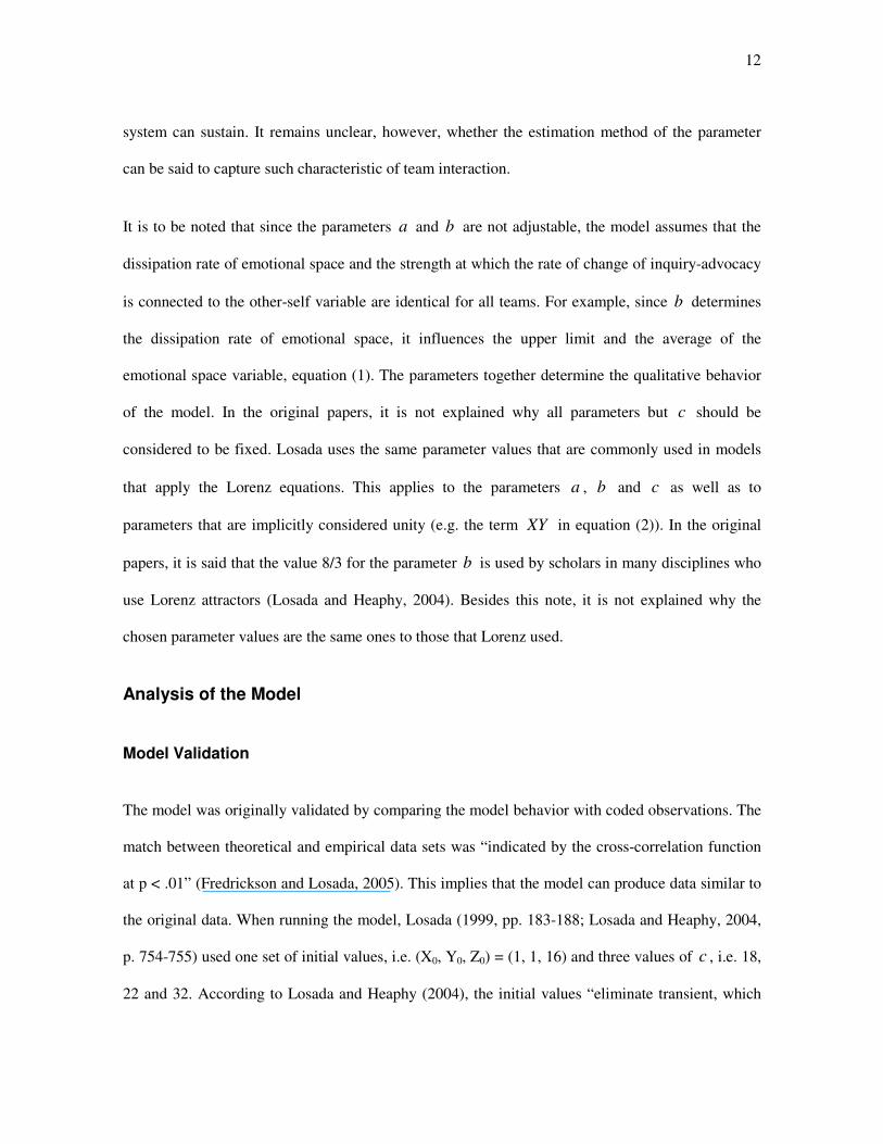
system can sustain. It remains unclear, however, whether the estimation method of the parameter

can be said to capture such characteristic of team interaction.

It is to be noted that since the parameters a and b are not adjustable, the model assumes that the

dissipation rate of emotional space and the strength at which the rate of change of inquiry-advocacy

is connected to the other-self variable are identical for all teams. For example, since b determines

the dissipation rate of emotional space, it influences the upper limit and the average of the

emotional space variable, equation (1). The parameters together determine the qualitative behavior

of the model. In the original papers, it is not explained why all parameters but c should be

considered to be fixed. Losada uses the same parameter values that are commonly used in models

that apply the Lorenz equations. This applies to the parameters a , b and c as well as to

parameters that are implicitly considered unity (e.g. the term XY in equation (2)). In the original

papers, it is said that the value 8/3 for the parameter b is used by scholars in many disciplines who

use Lorenz attractors (Losada and Heaphy, 2004). Besides this note, it is not explained why the

chosen parameter values are the same ones to those that Lorenz used.

Analysis of the Model

Model Validation

The model was originally validated by comparing the model behavior with coded observations. The

match between theoretical and empirical data sets was “indicated by the cross-correlation function

at p < .01” (Fredrickson and Losada, 2005). This implies that the model can produce data similar to

the original data. When running the model, Losada (1999, pp. 183-188; Losada and Heaphy, 2004,

p. 754-755) used one set of initial values, i.e. (X0, Y0, Z0) = (1, 1, 16) and three values of c , i.e. 18,

22 and 32. According to Losada and Heaphy (2004), the initial values “eliminate transient, which

13

represents features of the model that are neither essential nor lasting”. It is, however, not explained

why all teams should start with more advocacy than inquiry and more self-orientation than other-

orientation. The validation by simulation that is presented in the original papers does not, in general,

guarantee that the model could be used to predict behavior in different environmental conditions.

The simulations presented here were run with MATLAB3 and, following Losada, a fourth-order

Runge-Kutta algorithm with a time step of 0.02 was used for the numerical integration.

Qualitative Behavior of the Model

In the model, Losada considers parameters a and b to be constant and the connectivity parameter,

c , to be an adjustable one. The lowest value Losada used for the adjustable parameter, c , was 18

and the highest value was 32 (Losada, 1999). The model displays limit cycle dynamics for some

large values of c and chaotic dynamics for others, see e.g. Fredrickson and Losada (2005) and

Sparrow (1983) for details. Here, parameter values are allowed to range from 0 to 35, as this range

sufficiently covers the range of parameter estimates Losada obtained (see Figure 4).

Since the model equations are identical to the ones in Lorenz’s model of fluid convection, related

research (see e.g. Yorke and Yorke, 1979; Sparrow 1983; Lorenz, 1963, 1993; Csernák and Stépán,

2000) can be referred to in studying the model behavior. The Lorenz system is also dealt with in

books on dynamical systems (see e.g. Seydel, 1988; Hilborn, 1994; Alligood et al., 1996; Verhulst,

1996). These studies are of interest here, they show how the behavior of the model changes as the

model parameter c is varied.

3 http://www.mathworks.com [accessed 2007-04-17]

14

The Lorenz system – characterized by equations (2), (4) and (5) – has one to three steady states

which are obtained when the time derivatives are set to zero. This gives the following three steady

state solutions.

0=== ZYX , (6)

−=

−==

1

)1(

cZ

cbYX, (7)

−=

−−==

1

)1(

cZ

cbYX (8)

of which the latter two steady states only exist when c > 1.

With the chosen range of parameter values, the system exhibits three types of dynamics:

convergence towards a stable steady state, metastable chaotic behavior and chaotic behavior. In

general, deterministic chaos refers to dynamic behavior that is bounded, nonperiodic and sensitively

dependent on initial conditions. (see e.g. Alligood et al., 1996). Nonperiodicity refers to behavior

that is not asymptotically periodic. Sensitivity in initial conditions means that an arbitrarily small

change in the initial conditions may lead to significantly different future behavior. Metastable chaos

refers to dynamic behavior that is similar to chaotic behavior, with the exception that the chaotic

behavior is transient, i.e. after some time the system no longer behaves chaotically and thereafter

evolves towards an attractor. Accordingly, this initial phase of chaotic behavior is referred to as a

chaotic transient.

For the system when 10 << c , only the origin (0, 0, 0) is stable. This means that it converges to

the origin from all initial states. 1=c is a bifurcation point which means that when c passes this

15

value, the qualitative behavior of the model suddenly changes. As a result of this bifurcation, the

origin becomes unstable and two stable steady states – (7) and (8) – emerge. When 01 cc << , the

system converges to one of the steady states. Both of these steady states have a basin of attraction

from which the system converges towards the steady state. A basin of attraction refers to a set of

initial states in the phase space from which the system evolves to a particular attractor. Another

bifurcation point is at 0cc = . Now, there is a region of metastable chaos. Depending on the initial

state the system either converges to one of the steady states, or exhibits a chaotic transient before

eventually ending up in one of the steady states. Yet a new basin of attraction emerges at another

bifurcation point, 1cc = . The two steady states are still stable, but a chaotic attractor now emerges.

Depending on the initial state, the system will converge to one of the two stable steady states or it

will behave chaotically indefinitely. When c passes crc , which is here the last relevant bifurcation

point, the two steady states lose their stability and the basin of attraction for the chaotic attractor is

the entire ( X ,Y , Z ) space. (Dykstra et al., 1997)

For parameter values 10=a and 3/8=b the critical values for the parameter c are 93.130 ≈c ,

06.241 ≈c and 74.24≈crc (Sparrow, 1983). With randomly chosen initial values, the average

duration of the chaotic transient depends upon the initial values and on the difference between 1c

and the chosen value of the adjustable parameter. When the adjustable parameter, c , is close to 1c ,

the average duration of the chaotic transient is long, and when the adjustable parameter is close to

0c , the average duration tends to zero. (Dykstra et al., 1997)

16

Model Dynamics for the Three Team Performance Categories

The behavior of the model of team interaction is determined solely by the initial values and the

value of the parameter c , which is in this case interpreted as the connectivity of a team. The model

predicts metastable chaos for low ( 18=c ) and medium ( 22=c ) performance teams and chaotic

dynamics for high performance teams ( 32=c ). Low and medium performance teams end up in

either steady state whereas high performance teams end up in neither. The interpretation of the

steady state solution (7) is that there is more advocacy than inquiry and more self-referring speech

acts than other-referring speech acts, whereas in (8) there is more inquiry and other-referring speech

acts. Chaotic solutions do not end up in either steady state, but oscillate around both, thus predicting

roughly equal amount of inquiry and advocacy, and other- and self-referring speech acts.

The time series of observations of the low performance teams “showed a dramatic decrease in

amplitude for all three dimensions about the first fourth of the meeting and stayed locked […] for

the rest of the meeting“ (Losada, 1999, p. 182). When connectivity is set to 18, the system

converges to either of the steady states, typically displaying a chaotic transient of short or zero

length. This type of behavior of the model is in agreement with what was reported of the time series

of observations of low performance teams. Losada and Heaphy (2004, p. 752) refer to this type of

dynamics as the “point attractor dynamics”. However, as shown in Figure 2, the system may exhibit

a chaotic transient before being attracted to either of the steady states.

17

-15 -10 -5 0 5 10 150

5

10

15

20

25

30

X

Z

Figure 2. The development of inquiry-advocacy, X, and emotional space, Z, as a projection of the

trajectory on the (X, Z) plane when c = 18 and (X0,Y0,Z0) = (1, 0, 16).

The time series of observations of the medium performance teams in all three dimensions “tended

to have patterns of decreasing amplitude.” (Losada, 1999, p. 182) When connectivity is set to 22

and initial conditions are chosen randomly, typically a chaotic transient is seen. After the chaotic

transient, the system converges to either of the steady states. This is in relatively good qualitative

agreement with the reported characteristics of time series of observations. Losada and Heaphy

(2004, p. 752) refer to the dynamics of medium performance teams as “limit cycle dynamics”.

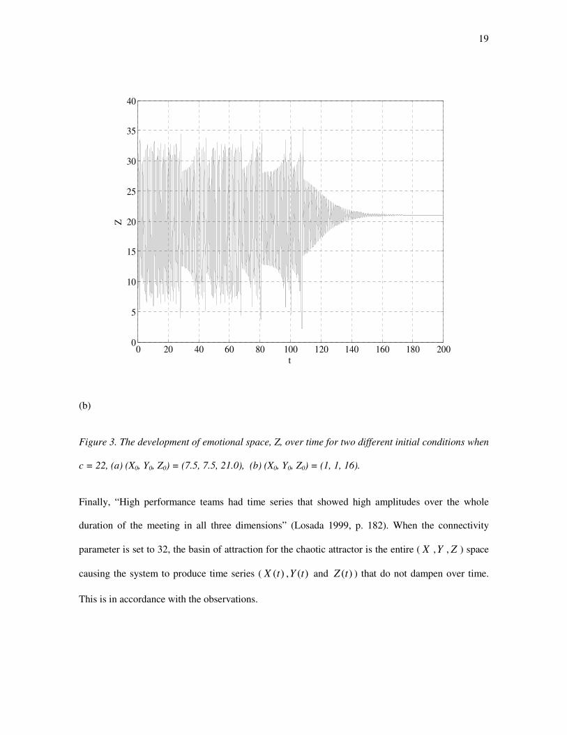
However, as shown in Figure 3 below, the system is not drawn towards a periodic orbit but

converges towards either of the steady states, potentially exhibiting a chaotic transient before that.

18

0 20 40 60 80 100 120 140 160 180 20020.97

20.98

20.99

21

21.01

21.02

21.03

t

Z

(a)

19

0 20 40 60 80 100 120 140 160 180 2000

5

10

15

20

25

30

35

40

t

Z

(b)

Figure 3. The development of emotional space, Z, over time for two different initial conditions when

c = 22, (a) (X0, Y0, Z0) = (7.5, 7.5, 21.0), (b) (X0, Y0, Z0) = (1, 1, 16).

Finally, “High performance teams had time series that showed high amplitudes over the whole

duration of the meeting in all three dimensions” (Losada 1999, p. 182). When the connectivity

parameter is set to 32, the basin of attraction for the chaotic attractor is the entire ( X ,Y , Z ) space

causing the system to produce time series ( )(tX , )(tY and )(tZ ) that do not dampen over time.

This is in accordance with the observations.

20

In terms of amplitudes, the model behavior is in accordance with what was observed of the time

series of observations. However, neither these amplitudes nor the chaotic behavior of the model

implies that the real world system of team interaction has the potential to produce chaotic behavior.

As is the case with studies of dynamical systems in general, the chaos should be detected from the

time series of observations (Kodba et al., 2005).

Model Predictions

The average positivity/negativity ratio is obtained from equation (1), by substituting the mean of the

emotional space time series generated by the model into )(tZ , and letting 16)0( =Z and 3/8=b .

Actually, Losada and Heaphy (2004) computed the positivity/negativity ratio from equation (1) by

letting 1)( −= ctZ . However, to compare the model behavior and observations, the mean value of

the emotional space variable should be used. This will cause a small deviation from the

positivity/negativity ratio computed the way Losada and Heaphy suggest.

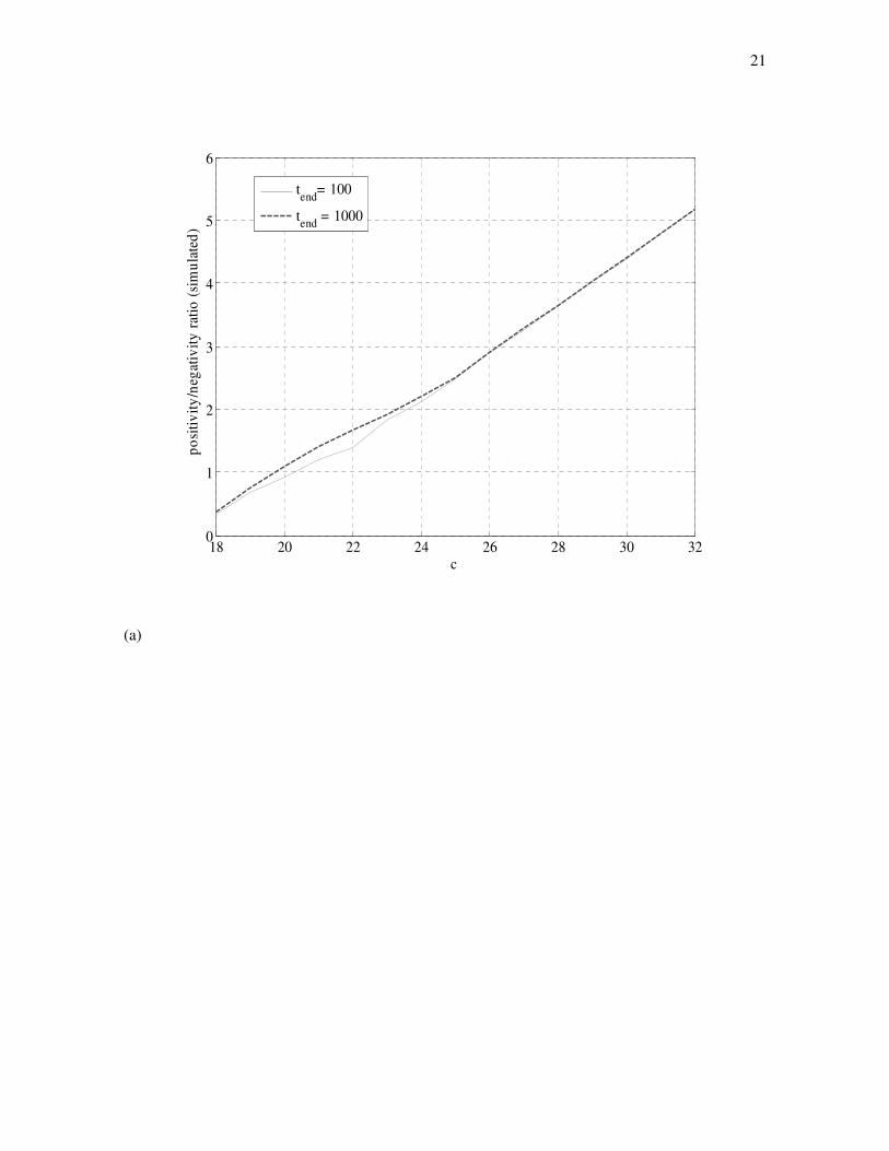
When the model is run with different values of the connectivity parameter, a linear dependence

between connectivity and the positivity/negativity ratio is seen (Figure 3a). This is in good

agreement with Losada’s observations (Figure 3b). However, because of the few data points that are

presented in the original papers (low, medium and high performance teams), the question of linear

dependence is left open. It is to be noted that, if equation (1) is used to compute the

positivity/negativity ratio when the model is run with a different )0(Z , the model predicts a

positivity/negativity ratio which is substantially different from the observed ratios. If )0(Z in

equation (1) is set to 16, no matter what the initial values are, the positivity/negativity ratios

predicted by the model are close to the observed ratios.

21

18 20 22 24 26 28 30 320

1

2

3

4

5

6

c

po

siti

vit

y/n

egat

ivit

y r

atio

(si

mu

late

d)

tend

= 100

tend

= 1000

(a)

22

16 18 20 22 24 26 28 30 32 34 360

1

2

3

4

5

6

c

po

siti

vit

y/n

eg

ati

vit

y r

ati

o (

ob

serv

ed

)

Observations

Least squares regression line

(b)

Figure 4. Positivity/negativity ratios for different values of the connectivity parameter. The model

predicts a linear dependence between the connectivity parameter of the model and the

positivity/negativity ratio (a). Simulation length is denoted with tend. In figure (b) averages of the

observed positivity/negativity ratios are plotted against estimated values of the connectivity

parameter (Losada, 1999). The error bars represent standard deviations.

The initial values of the inquiry-advocacy and other-self variables affect the behavior of the model.

Since for sufficiently small c , the two steady states outside the origin are stable the teams with

relatively low connectivity can end up in either of these two steady states.

23

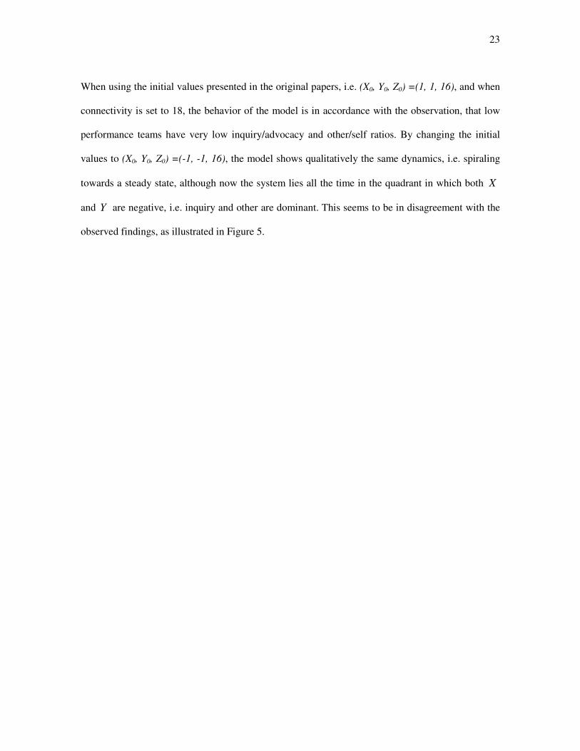
When using the initial values presented in the original papers, i.e. (X0, Y0, Z0) =(1, 1, 16), and when

connectivity is set to 18, the behavior of the model is in accordance with the observation, that low

performance teams have very low inquiry/advocacy and other/self ratios. By changing the initial

values to (X0, Y0, Z0) =(-1, -1, 16), the model shows qualitatively the same dynamics, i.e. spiraling

towards a steady state, although now the system lies all the time in the quadrant in which both X

and Y are negative, i.e. inquiry and other are dominant. This seems to be in disagreement with the

observed findings, as illustrated in Figure 5.

24

-15 -10 -5 0 5 10 15

10

15

20

25

30

X

Z

(X0, Y

0, Z

0) = (1, 1, 16)

(X0, Y

0, Z

0) = (-1, -1, 16)

(a)

25

-15 -10 -5 0 5 10 15

10

15

20

25

30

Y

Z

(X0, Y

0, Z

0) = (1, 1, 16)

(X0, Y

0, Z

0) = (-1, -1, 16)

(b)

Figure 5. The development of inquiry-advocacy, X, other-self, Y, and emotional space, Z, in the (a)

(X,Z) and (b) in the (Y,Z) planes when c = 18. The projected trajectories refer to two different

initial states.

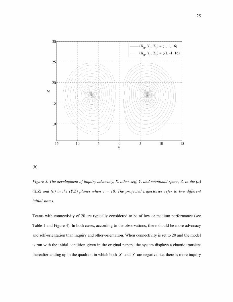
Teams with connectivity of 20 are typically considered to be of low or medium performance (see

Table 1 and Figure 4). In both cases, according to the observations, there should be more advocacy

and self-orientation than inquiry and other-orientation. When connectivity is set to 20 and the model

is run with the initial condition given in the original papers, the system displays a chaotic transient

thereafter ending up in the quadrant in which both X and Y are negative, i.e. there is more inquiry

26

than advocacy and more other-orientation than self-orientation. This behavior seems to be in

disagreement with the reported observations (see Figure 6).

0 10 20 30 40 50 60-15

-10

-5

0

5

10

15

t

X

(a)

27

0 10 20 30 40 50 60-15

-10

-5

0

5

10

15

20

t

Y

(b)

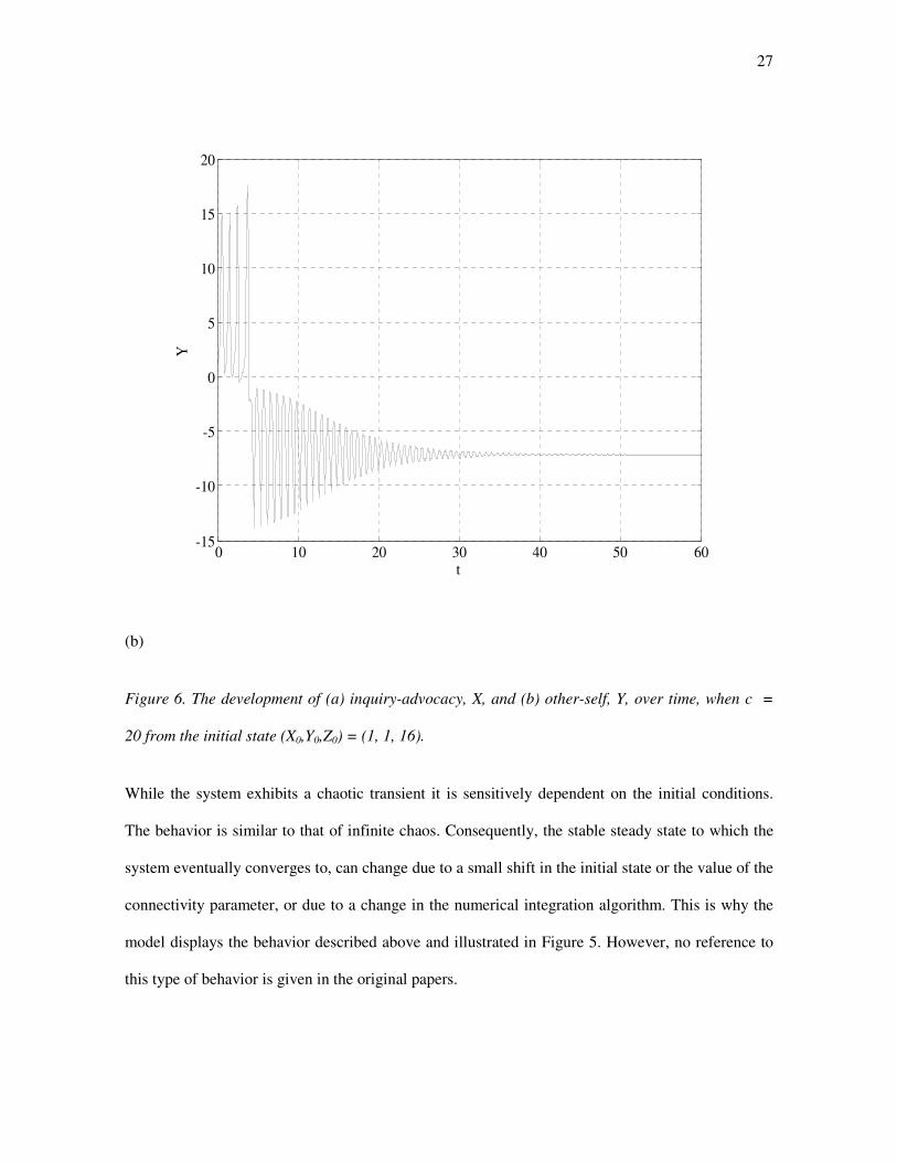
Figure 6. The development of (a) inquiry-advocacy, X, and (b) other-self, Y, over time, when c =

20 from the initial state (X0,Y0,Z0) = (1, 1, 16).

While the system exhibits a chaotic transient it is sensitively dependent on the initial conditions.

The behavior is similar to that of infinite chaos. Consequently, the stable steady state to which the

system eventually converges to, can change due to a small shift in the initial state or the value of the

connectivity parameter, or due to a change in the numerical integration algorithm. This is why the

model displays the behavior described above and illustrated in Figure 5. However, no reference to

this type of behavior is given in the original papers.

28

Discussion

Losada’s observations imply that the rigidity of behavioral patterns correlates with excess

negativity, advocacy and self-orientation. High performance teams are high in inquiry but also high

in advocacy. The same applies to other variables used to describe teams, i.e. positivity and

negativity, as well as other and self. Based on this, it would appear that negativity, advocacy and

self all have a role in a team, or at least, they are something inherently present in human interaction.

Advocacy is most often seen as a negative characteristic but it has, indeed, been recognized by

others too to have a role in team work as an element of dialogue (Senge et al., 1994).

What seems to be differentiating high performance teams from low performance teams is that high

performance teams do not get ‘locked’ with negativity, advocacy or self modes, They are able to

dissolve these ‘attractors’, i.e. they are able to meta learn. This also implies that the average

positivity/negativity, inquiry/advocacy and other/self ratios do not tell the whole story of team

interaction and its relation to team performance. The systems intelligence approach is interested in

developing such capabilities of human agents where one avoids myopic behavioral schemas which

might result in undesired lock-ins, for example, by finding ways to avoid getting locked into

temporary negativity or advocacy.

Saarinen and Hämäläinen (2004, see also (Hämäläinen and Saarinen, 2006)) describe another

behavioral pattern resulting in a lock-in. The mechanism is called the system of “holding back in

return” which refers to myopic reactive behavior commonly observed in everyday life. Human

agents reacting to their social environment by reciprocally ‘holding back’ co-produce a lock-in

system. This can create a perception that the lock-in cannot be dissolved. Furthermore, this sustains

the behavioral pattern which is beneficial to no one. We see that this behavioral pattern is similar to

29

the undesired lock-ins in the Losada setting. Thus, the meta learning ability refers to such micro-

behavioral competence of teams that is a part of a human competence we call systems intelligence.

Systems intelligence research strives to search and develop models of social interaction which help

reveal the hidden potential that is inherent in most human systems. What kind of modeling tools for

systems intelligence are most appropriate, for example, in the analysis of the ‘attractors’ that Losada

observed, remains an open question for future research.

30

References

Alligood KT, Sauer TD, Yorke JA. 1996. Chaos – An Introduction to Dynamical Systems. Springer,

New York.

Andersson. P. 1999. Complexity Theory and Organization Science, Organization Science 10: 216-

232.

Axelrod R. 1984. The Evolution of Cooperation. Basic Books, New York.

Blume L. 1993. The Statistical Mechanisms of Strategic Interaction. Games and Economic

Behavior 4: 387-424.

Collins R. 1981. On the Microfoundations of Macrosociology. The American Journal of Sociology

86: 984-1014.

Collins R. 2004. Interaction Ritual Chains. Princeton University Press, Princeton.

Collins R, Hanneman R. 1998, Modelling the Interaction Ritual Theory of Solidarity In The

Problem of Solidarity: Theories and Models, Doreian P. and Fararo T. (Eds.). Gordon Breach:

Amsterdam; 213-237.

Dutton J, Heaphy E. 2003. The Power of High Quality Connections. In Positive Organizational

Scholarship: Foundations of a New Discipline, Cameron Kim, Dutton Jane, and Quinn Robert

(Eds.). Berrett-Koehler Publishers, San Francisco; 263-278

Csernák G and Stépán G. 2000. Life Expectancy Calculations of Transient Chaotic Behavior in the

Lorenz Model. Periodica Polytechnica - Mechanical Engineering 44: 9-22.

31

Dykstra R, Malos JT., Heckenberg NR. 1997. Metastable Chaos in the Ammonia Ring Laser.

Physical Review A 56: 3180-3186.

Fredrickson B, Losada M. 2005. Positive Affect and the Complex Dynamics of Human Flourishing.

American Psychologist 60: 678-686.

Gintis H, Bowles S, Boyd RT, Fehr E. 2005. Moral Sentiments and Material Interests: The

Foundations of Cooperation and Economic Life. The MIT Press, Cambridge.

Gottman J, Murray J, Swanson C, Tyson R, Swanson K. 2002a. The Mathematics of Marriage –

Dynamic Nonlinear Models. The MIT Press, Cambridge.

Gottman J, Swanson C, Swanson K. 2002b. A General Systems Theory of Marriage: Nonlinear

Difference Equation Modeling of Marital Interaction. Personality and Social Psychology Review 6:

326-340.

Hilborn R. 1994. Chaos and Nonlinear Dynamics: An Introduction to Scientists and Engineers,

Oxford University Press, New York.

Hämäläinen RP, Saarinen E. 2006. Systems Intelligence: A Key Competence in Organizational

Life. Reflections – The SoL Journal on Knowledge, Learning and Change 4: 17-28.

Hämäläinen RP, Saarinen E. 2007. Systems Intelligent Leadership. Manuscript 2007-04-13,

available online at http://www.systemsintelligence.tkk.fi/SI2007.html.

Kauffman SA. 1993. The Origins of Order: Self-organization and Selection in Evolution, Oxford

University Press.

32

Kobda S, Perc M, Marhl M. 2005. Detecting Chaos From a Time Series. European Journal of

Physics 26: 205-215.

Lorenz EN. 1963. Deterministic Nonperiodic Flow. Journal of the Athmospheric Sciences 20: 130-

141.

Lorenz EN. 1993. The Essence of Chaos. University of Washington Press, Seattle.

Losada M. 1999. The Complex Dynamics of High Performance Teams. Mathematical and

Computer Modeling 30: 179-192.

Losada M, Heaphy E. 2004. The Role of Positivity and Negativity in the Performance of Business

Teams. The American Behavioral Scientist 47: 740-765.

Morel B, Ramanujam R. 1999. Through Looking Glass of Complexity: The Dynamics of

Organizations as Adaptive and Evolving Systems. Organization Science 10: 278-293.

Saarinen E, Hämäläinen RP. 2004. Systems Intelligence: Connceting Engineering Thinking with

Human Sensitivity. In Systems Intelligence – Discovering a Hidden Competence in Human Action

and Organizational Life, Hämäläinen R. P. and Saarinen E. (Eds.). Helsinki University of

Technology, Systems Analysis Laboratory Research Reports, A88, October 2004; 9-37.

Senge P. 1990. The Fifth Discipline: The Art and Practice of Learning Organizations, Doubleday

Currency, New York.

Senge P, Ross R, Smith B, Roberts C, Kleiner A. The Fifth Discipline Fieldbook: Strategies and

Tools for Building a Learning Organization. Doubleday Currency, New York.

33

Seydel R. 1988. From Equilibrium to Chaos: Practical Bifurcation and Stability Analysis. Elsevier,

New York.

Simon HA. 1952. A Formal Theory of Interaction in Social Groups. American Sociological Review

17: 202-211.

Sparrow C. 1983. An Introduction to the Lorenz Equations. IEEE Transactions on Circuits and

Systems. 30: 533-543.

Stacey R. 1995. The Science of Complexity: An Alternative Perspective for Strategic Change

Management. Strategic Management Journal. 16: 477-495.

Stacey R. 2001. Complex Responsive Processes in Organizations: Learning and Knowledge

Creation. Routledge, London.

Stacey R. 2003. Learning as an Activity of Interdependent People. Learning Organization 10: 325-

331.

Stacey R, Griffin D, Shaw P. 2000. Complexity and Management: Fad or a Radical Challenge to

Systems Thinking? Routledge, London.

Verhulst F. 1996. Nonlinear Differential Equations and Dynamical Systems, Second Edition.

Springer, Berlin.

Yorke JA, Yorke ED. 1979. Metastable Chaos: The Transition to Sustained Chaotic Behavior in

The Lorenz Model. Journal of Statistical Physics 21: 263-277.

Young PH. 2001. The Dynamics of Conformity. In Social Dynamics, Durlauf S. and Peyton P. H.

(Eds.). The MIT Press, Cambridge; 133-153.