
Perception of Objective Parameter Variations in Virtual ...
284
Perception of Objective Parameter Variations in Virtual Acoustic Spaces Aglaia Foteinou Doctor of Philosophy University of York Department of Electronics October 2013
-
Upload
khangminh22 -
Category
Documents
-
view
4 -
download
0
Transcript of Perception of Objective Parameter Variations in Virtual ...

Perception of Objective Parameter
Variations in Virtual Acoustic Spaces
Aglaia Foteinou
Doctor of Philosophy
University of York
Department of Electronics
October 2013

Perception of Objective Parameter Variations in Virtual Acoustic Spaces ii

Abstract
Perception of Objective Parameter Variations in Virtual Acoustic Spaces iii
Abstract
This thesis investigates if reliability in objective acoustic metrics obtained for an
auralized space implies accuracy and reliability in terms of the subjective listening
experience. Auralizations can be created based either on impulse response
measurements of an existing space, or simulations using computer-based acoustic
models. Validations of these methods usually focus on the observation of standard
objective acoustic measures and how these vary under certain conditions. However,
for accurate and believable auralization, the subjective quality of the resulting
virtual auditory environment should be considered as being at least as important,
if not more so.
This study is focused in the most part on St. Margaret’s Church, York, UK.
Impulse responses have been acquired in the actual space and virtual acoustic
models created using CATT-Acoustic and ODEON-Auditorium auralization
software, both based on geometric acoustic algorithms. Variations in objective
acoustic parameters are examined by changing the physical characteristics of the
space, the receiver position and the sound source orientation. It is hypothesised
that the perceptual accuracy of the auralizations depends on optimising the model
to minimise observed changes in objective acoustic parameters. This objective
evaluation is used to ascertain the behaviour of certain standard acoustic
parameters. From these results, impulse responses with suitable acoustic values
are selected for subjective evaluation via listening tests.
These acoustic parameters, in combination with the physical factors that influence
them, are examined, and the importance of variation in these values in relation to
our perception of the result is investigated. Conclusions are drawn for both
measurement and modelling approaches, demonstrating that model optimisation
based on key acoustic parameters is not sufficient to guarantee perceptual accuracy
as perceptual differences are still evident when only a simple acoustic parameter
demonstrates a difference of greater than 1 JND. It is also essential to add that the
overall perception of the changes in the acoustic parameters is independent of the
auralization technique used. These results aim to give some confidence to acoustic
designers working in architectural and archeoacoustic design in terms of how their
models might be best created for optimal perceptual presentation.

Perception of Objective Parameter Variations in Virtual Acoustic Spaces iv

Contents
Perception of Objective Parameter Variations in Virtual Acoustic Spaces v
Contents
Abstract ........................................................................................................................... iii
Contents ........................................................................................................................... v
List of Tables ................................................................................................................... xi
List of Figures ................................................................................................................ xv
Acknowledgements ..................................................................................................... xxvi
Declaration ................................................................................................................. xxvii
Thesis Introduction .................................................................................... 1 Chapter 1.
Interest ................................................................................................................ 1 1.1
Acoustic Revival of Heritage Sites ..................................................................... 2 1.2
Primary Aims and Thesis Hypothesis ............................................................... 3 1.3
Structure of Thesis .............................................................................................. 4 1.4
Contributions to the Field .................................................................................. 5 1.5
Room Acoustics ........................................................................................... 6 Chapter 2.
Introduction ......................................................................................................... 6 2.1
Sound in a Free Field ......................................................................................... 6 2.2
Sound in an Enclosed Space ............................................................................... 8 2.3
Growth and Decay of Sound in a Room ...................................................... 8 2.3.1
Sound Reflection ........................................................................................ 12 2.3.2
Sound Diffusion/Scattering ....................................................................... 12 2.3.3
Sound Absorption ....................................................................................... 13 2.3.4
Sound Diffraction ....................................................................................... 14 2.3.5
Standing Waves ......................................................................................... 15 2.3.6

Contents
Perception of Objective Parameter Variations in Virtual Acoustic Spaces vi
Schroeder Frequency ................................................................................. 15 2.3.7
Room Impulse Response ................................................................................... 16 2.4
Acoustic Parameters ......................................................................................... 18 2.5
Reverberation Time ................................................................................... 19 2.5.1
Early Decay Time (EDT) ........................................................................... 21 2.5.2
Initial Time Delay Gap (ITDG) ................................................................. 22 2.5.3
Centre Time (Ts) ........................................................................................ 22 2.5.4
Clarity C50/C80 ............................................................................................ 23 2.5.5
Definition (D50) ........................................................................................... 24 2.5.6
Sound Strength (G) .................................................................................... 24 2.5.7
Early Lateral Energy Fraction (LF) ......................................................... 25 2.5.8
Inter-Aural Cross-Correlation (IACC) ...................................................... 25 2.5.9
Just Noticeable Difference (JND) .................................................................... 26 2.6
Summary ........................................................................................................... 28 2.7
Auralization .............................................................................................. 29 Chapter 3.
Introduction ...................................................................................................... 29 3.1
Measurements of Impulse Responses .............................................................. 31 3.2
Excitation signal ........................................................................................ 31 3.2.1
Sound Source Directivity ........................................................................... 36 3.2.2
Microphones ............................................................................................... 38 3.2.3
Measured Uncertainties ............................................................................ 39 3.2.4
Computer Modelling - Introduction ................................................................. 41 3.3
Wave Models .............................................................................................. 42 3.3.1

Contents
Perception of Objective Parameter Variations in Virtual Acoustic Spaces vii
Acoustic Radiance Transfer/Radiosity Method ........................................ 43 3.3.2
Geometrical Acoustic Models .................................................................... 43 3.3.3
Round Robin for Acoustic Computer Simulations .................................... 55 3.3.4
Summary ........................................................................................................... 58 3.4
The Perception of Changes in Objective Acoustic Parameters – A Pilot Chapter 4.
Study .................................................................................................................. 59
Introduction ....................................................................................................... 59 4.1
Methodology ...................................................................................................... 60 4.2
Case Study A .............................................................................................. 61 4.2.1
Case Study B .............................................................................................. 68 4.2.2
Case Study C .............................................................................................. 71 4.2.3
Summary ........................................................................................................... 72 4.3
Capturing the Acoustic Impulse Responses in St. Margaret’s Church . 74 Chapter 5.
Introduction ....................................................................................................... 74 5.1
History of St. Margaret’s Church ..................................................................... 75 5.2
Renovation of St. Margaret’s Church .............................................................. 76 5.3
Impulse Response Measurements .................................................................... 83 5.4
Computer Modelling ......................................................................................... 90 5.5
Designing the model .................................................................................. 92 5.5.1
Calibrating the Model ................................................................................ 97 5.5.2
Virtual sound source and receivers ......................................................... 105 5.5.3
General Settings in Geometric Software ................................................ 107 5.5.4
Summary ......................................................................................................... 108 5.6

Contents
Perception of Objective Parameter Variations in Virtual Acoustic Spaces viii
Analysis of Objective Acoustic Parameters of St. Margaret’s Church 110 Chapter 6.
Introduction .................................................................................................... 110 6.1
Acoustic Parameters as Design Variables ..................................................... 110 6.2
Calculation Process ......................................................................................... 115 6.3
“Acoustic Floor Maps” ..................................................................................... 120 6.4
Acoustic Impulse Response Measurements .................................................. 123 6.5
Results obtained from changes in acoustic configuration ..................... 123 6.5.1
Results obtained from changes in source orientations .......................... 133 6.5.2
CATT-Acoustic IRs ......................................................................................... 138 6.6
ODEON IRs ..................................................................................................... 144 6.7
Summary ......................................................................................................... 150 6.8
Subjective evaluations of Auralized St. Margaret’s Church ................ 151 Chapter 7.
Introduction .................................................................................................... 151 7.1
Pilot Experiment from Auralized St. Margaret’s Church ............................ 152 7.2
Selection of the Impulse Responses for Auralization ................................... 153 7.3
Impulse responses from measurements ................................................. 155 7.3.1
Impulse responses from the CATT-Acoustic model ............................... 159 7.3.2
Impulse responses from the ODEON model ........................................... 162 7.3.3
Convolution with Anechoic Stimuli ............................................................... 165 7.4
Sound Reproduction ........................................................................................ 166 7.5
Listening Tests Procedure .............................................................................. 168 7.6
The Subjects .................................................................................................... 173 7.7
Listening Test Subjects’ Response ................................................................. 176 7.8

Contents
Perception of Objective Parameter Variations in Virtual Acoustic Spaces ix
Analysis based on JND values ................................................................ 179 7.8.1
Analysis based on auralization method .................................................. 187 7.8.2
Analysis based on the stimuli ................................................................. 190 7.8.3
Summary ......................................................................................................... 193 7.9
Conclusions ............................................................................................. 194 Chapter 8.
Summary ......................................................................................................... 195 8.1
Contributions .................................................................................................. 199 8.2
Further Work .................................................................................................. 200 8.3
Appendix A ................................................................................................................... 202
Architectural Plans for the refurbishment of St. Margaret’s Church (1999) ............. 202
Appendix B ................................................................................................................... 206
Appendix C ................................................................................................................... 208
Appendix D ................................................................................................................... 226
Measurements .............................................................................................................. 226
Objective results for Configurations A, B and C, sorted in increase order ................ 226
Objective results for Configurations A, B and C, sorted based on the JND values in
increase order ............................................................................................................... 228
Objective results for Source Orientations 0°, 40°and 70° sorted in increase order .... 231
Objective results for Source Orientations 0°, 40° and 70° sorted based on the JND
values in increase order ............................................................................................... 233
CATT-Acoustic ............................................................................................................. 235
Objective results for Configurations A, B and C, sorted in increase order ................ 235
Objective results for Configurations A, B and C, sorted based on the JND values in
increase order ............................................................................................................... 237

Contents
Perception of Objective Parameter Variations in Virtual Acoustic Spaces x
ODEON ........................................................................................................................ 239
Objective results for Configurations A, B and C, sorted in increase order ................ 239
Objective results for Configurations A, B and C, sorted based on the JND values in
increase order ............................................................................................................... 241
Appendix E ................................................................................................................... 243
Supporting materials on DVD ..................................................................................... 243
References .................................................................................................................... 244

List of Tables
Perception of Objective Parameter Variations in Virtual Acoustic Spaces xi
List of Tables
Table 2.1 Just noticeable differences for the acoustic parameters, according to
ISO3382. ...................................................................................................................... 27
Table 5.1 Guidance notes for the various acoustic qualities, provided by Arup
Acoustics [185] ............................................................................................................. 83
Table 5.2 Settings for the generation of the logarithmic sine sweep in Aurora plug-
in. ................................................................................................................................. 84
Table 5.3 Distance between sound source and each of the 26 receiver positions. Left
(L) is defined as the left side of the sound source. ..................................................... 89
Table 5.4 Absorption coefficients of the materials used for modelling St. Margaret's
church in CATT-Acoustic, values presented in %. .................................................. 102
Table 5.5 Absorption coefficients of the materials used for modelling St. Margaret's
church in ODEON on a scale from 0 to 1. ................................................................ 102
Table 5.6 Scattering coefficients of the materials used in the ODEON model, on a
scale from 0 to 1. ....................................................................................................... 104
Table 5.7 Scattering coefficients of the materials used with the CATT-Acoustic
model, values presented in %. .................................................................................. 105
Table 7.1 Calculating the JNDs obtained from the single number averaged across
500Hz and 1000Hz octave bands, for each parameter based on the minimum
observed values (Appendix D, Measurements, Configurations A, B and C) from the
measured impulse responses of the three acoustic configurations ........................ 155
Table 7.2 Calculating the JNDs obtained from the single number averaged across
500Hz and 1000Hz octave bands, for each parameter based on the minimum
observed values (Appendix D, Measurements, Source Orientations 0°, 40°, 70°)
from the measured impulse responses of the three source orientations. ............... 156
Table 7.3 The groups of pairs from the in-situ measured impulse responses. 20
pairs of A/B impulse responses were selected based on the calculated acoustic
parameter values. The colours indicate the acoustic configurations for each impulse

List of Tables
Perception of Objective Parameter Variations in Virtual Acoustic Spaces xii
response (Blue for Configuration A, Red for configuration B and Green for
configuration C). The pairs defined with (*) are impulse responses from the source
orientation configurations (Blue for the 0° orientation of the source, Red for the 40°
and Green for the 70°). .............................................................................................. 157
Table 7.4 The groups of pairs from the in-situ measured impulse responses. 20
pairs of A/B impulse responses were selected based on their difference in absolute
JND values (approximated at the second decimal) obtained from the single number
averaged across 500Hz and 1000Hz octave bands. The colours indicate the acoustic
configurations for each impulse response (Blue for Configuration A, Red for
configuration B and Green for configuration C), while the differences with more
than 1 JND value are highlighted in grey. The pairs defined with (*) are impulse
responses from the source orientation configurations (Blue for the 0° orientation of
the source, Red for the 40° and Green for the 70°). .................................................. 158
Table 7.5 Calculating the JNDs obtained from the single number averaged across
500Hz and 1000Hz octave bands, for each parameter based on the minimum
observed values (Appendix D, CATT-Acoustic, Configurations A, B and C) from the
measured impulse responses of the three acoustic configurations in CATT-Acoustic.
.................................................................................................................................... 159
Table 7.6 The groups of pairs from the impulse responses of the CATT-Acoustic
model. 18 pairs of A/B impulse responses were selected based on the calculated
acoustic parameter values. The colours indicate the acoustic configurations for each
impulse response (Blue for Configuration A, Red for configuration B and Green for
configuration C). ........................................................................................................ 160
Table 7.7 The groups of the pairs from the impulse responses of the CATT-Acoustic
model. 18 pairs of A/B impulse responses were selected based on their difference in
absolute JND values (approximated at the second decimal) obtained from the
single number averaged over 500Hz and 1000Hz octave bands. The colours indicate
the acoustic configurations for each impulse response (Blue for Configuration A,
Red for configuration B and Green for configuration C), while the differences with
more than 1 JND value are highlighted in grey. ..................................................... 161
Table 7.8 Calculating the JNDs obtained from the single number averaged across
500Hz and 1000Hz octave bands, for each parameter based on the minimum
List of Tables
Perception of Objective Parameter Variations in Virtual Acoustic Spaces xiii
observed values (Appendix D, ODEON, Configurations A, B and C) from the
impulse responses of the three acoustic configurations in ODEON. ...................... 162
Table 7.9 The groups of pairs from the impulse responses of the ODEON model. 18
pairs of A/B impulse responses were selected based on the calculated acoustic
parameter values. The colours indicate the acoustic configurations for each impulse
response (Blue for Configuration A, Red for configuration B and Green for
configuration C). ........................................................................................................ 163
Table 7.10 The groups of the pairs from the impulse responses of the ODEON
model. 18 pairs of A/B impulse responses were selected based on their difference in
absolute JND values (approximated at the second decimal) obtained from the
single number averaged over 500Hz and 1000Hz octave bands. The colours indicate
the acoustic configurations for each impulse response (Blue for Configuration A,
Red for configuration B and Green for configuration C), while the differences with
more than 1 JND value are highlighted in grey. ..................................................... 164
Table 7.11 The groups of pairs used for the training session from the in-situ
measured impulse responses. 18 pairs of A/B impulse responses were selected
based on their difference in absolute JND values. The colours indicate the acoustic
configurations for each impulse response (Blue for Configuration A, Red for
configuration B and Green for configuration C). ..................................................... 170
Table 7.12 The groups of pairs used for the training session from the CATT-
Acoustic model impulse responses. 18 pairs of A/B impulse responses were selected
based on their difference in absolute JND values. The colours indicate the acoustic
configurations for each impulse response (Blue for Configuration A, Red for
configuration B and Green for configuration C). ..................................................... 170
Table 7.13 The groups of pairs used for the training session from the ODEON
model impulse responses. 18 pairs of A/B impulse responses were selected based on
their difference in absolute JND variations. The colours indicate the acoustic
configurations for each impulse response (Blue for Configuration A, Red for
configuration B and Green for configuration C). ..................................................... 170
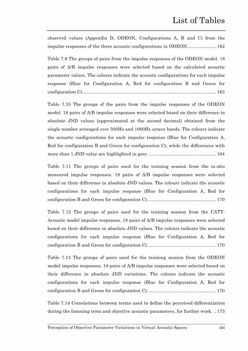
Table 7.14 Correlations between terms used to define the perceived differentiation
during the listening tests and objective acoustic parameters, for further work. .. 173

List of Tables
Perception of Objective Parameter Variations in Virtual Acoustic Spaces xiv
Table 7.15 The answers reported by the thirteen subjects for the in-situ
measurement listening test, for each of the two stimuli. ........................................ 176
Table 7.16 The answers reported by the thirteen subjects for the CATT-Acoustic
listening test, for each of the two stimuli. ................................................................ 177
Table 7.17 The answers reported by the thirteen subjects for the ODEON listening
test, for each of the two stimuli. ................................................................................ 178
Table 7.18 The JND values at 500Hz and 1000Hz for the in-situ measurements
compared with the JND values observed from the average of these two octave
bands (Table 7.4). The values with less than 1 JND from the average of the two
bands are highlighted in green, while their corresponding values in the single
octave bands with more than 1 JND observed are in black font. Note that for clarity
of presentation, the values from Table 7.4 have been reduced to three decimal
places. ......................................................................................................................... 182
Table 7.19 The JND values at 500Hz and 1000Hz for the CATT-Acoustic results,
compared with the JND values observed from the average of these two octave
bands (Table 7.7). The values with less than 1 JND from the average of the two
bands are highlighted in green, while their corresponding values of the single
octave bands with more than 1 JND observed are in black font. Note that for clarity
of presentation, the values from Table 7.7 have been reduced to three decimal
places. ......................................................................................................................... 184
Table 7.20 The JND values at 500Hz and 1000Hz for the ODEON results,
compared with the JND values observed from the average of these two octave
bands (Table 7.10). The values with less than 1 JND from the average of the two
bands are highlighted in green, while their corresponding values of the single
octave bands with more than 1 JND observed are in black font. Note that for clarity
of presentation, the values from Table 7.10 have been reduced to three decimal
places. ......................................................................................................................... 186
Table 7.21 The questions from the same group of acoustic characteristics for the
three auralization techniques. .................................................................................. 188

List of Figures
Perception of Objective Parameter Variations in Virtual Acoustic Spaces xv
List of Figures
Figure 2.1 The measured sound intensity is inversely proportional to the square of
the distance r from the source S (describing the phenomenon by 2D waves), after
[36]. ................................................................................................................................ 7
Figure 2.2 The growth of a sound at receiver R for a continuous sound source S
based on the build-up of impulse arrivals. The direct sound D arrives at the
receiver at time t1 after a continuous sound source starts at time t0 (left). The sound
energy at the receiver point builds up from the added sound energy of the
reflections refl1, refl2, refl3 arrive at the receiver at times t2, t3, t4 (right) (describing
the phenomenon by 2D particles). ................................................................................ 9
Figure 2.3 The sound energy related to the growth and the decay of sound for a
continuous source S that is turned off at time t = tx. ................................................ 10
Figure 2.4 Sound Reflection, demonstrating specular reflection when the angle of
incidence θi is equal to the angle of reflection θr according to Law of Reflection -
(describing the phenomenon by 2D particles). .......................................................... 12
Figure 2.5 Sound Scattering according to Lambert’s cosine law, demonstrating
scattered reflection in angle θo when θi is the angle of incidence (describing the
phenomenon by 2D particles) ..................................................................................... 13
Figure 2.6 Sound Absorption, demonstrating the energy absorbed by the surface
while the remaining energy is reflected according to the Law of Reflection
(describing the phenomenon by 2D particles). .......................................................... 14
Figure 2.7 Nodes (N) and Anti-nodes (A) of three standing waves occurring between
two fixed reflective barriers ........................................................................................ 15
Figure 2.8 The input signal as the Dirac Delta Function interacts with the acoustic
characteristics of a linear time invariant (LTI) system to give the output signal, the
room impulse response (RIR) as a function of time. .................................................. 17
Figure 2.9 Input and Output Signal of a Linear Time Invariant (LTI) system with
added noise at the output. .......................................................................................... 18

List of Figures
Perception of Objective Parameter Variations in Virtual Acoustic Spaces xvi
Figure 2.10 The backwards integrated decay curve obtained from the squared
impulse response presented in Figure 2.8, as a function of time. ............................. 19
Figure 2.11 Reverberation Time, RT60, measured by the time difference t2 – t1, from
the initial slope of the obtained energy decay curve, determined when the sound
energy level has decreased by 30dB. .......................................................................... 20
Figure 2.12 T30, measured using the time difference t3 – t2, from the slope of the
obtained energy decay curve determining when the sound level has decreased by
30dB. ............................................................................................................................. 21
Figure 2.13 Early Decay Time, EDT, measured using the time differences t2 – t1,
from the slope of the obtained energy decay curve determining when the sound
level has decreased by 10dB. ....................................................................................... 22
Figure 2.14 Clarity (C50/C80) defined as the early-to-late sound index, with the early
sound threshold defined at t2=50 ms or 80 ms according to application. ................. 24
Figure 3.1 Visual demonstration of the auralization concept, where a listener is
“placed” in a virtual acoustic realisation of St. Patrick’s Church, Patrington, UK
[21, 22]. ......................................................................................................................... 29
Figure 3.2 Time Domain representation of an input logarithmic sine sweep, from
22Hz to 22kHz and lasting 0.5s. ................................................................................. 35
Figure 3.3 The resulting output signal after deconvolution with the inverse filter.
The harmonic distortions are easily observed before the required system impulse
response. ....................................................................................................................... 36
Figure 3.4 Differentiations observed at low frequencies for the calculation of RT
from 37 different participants, from [98]. ................................................................... 40
Figure 3.5 Ray tracing emitted from sound a source S in a 2D environment and the
representation of the impulse responses from each of the example rays as
registered at receiver R ............................................................................................... 44
Figure 3.6 Demonstrating the Mirror Image-Source method. Reflections are
calculated by building up the paths from the sources to the receiver point. An
image source S1 is created on the opposite side of the boundary, after the first-

List of Figures
Perception of Objective Parameter Variations in Virtual Acoustic Spaces xvii
order reflection at point A. After the second-order reflection at points B and C, a
second image source S2 is created on the opposite side of the second boundary. ... 45
Figure 3.7 Demonstrating a likely case in the Mirror Image-Source method, where
the created image source S1, while detected by R1, is not visible via reflections by
R2. ................................................................................................................................ 46
Figure 3.8 Ray Tracing method, where the source S emits sound rays in different
directions and is detected by the receiver position R, defined as an area. .............. 48
Figure 3.9 Cone and Pyramidal tracing as emitted from a spherical source, from
[124]. ............................................................................................................................ 48
Figure 3.10 Representation of the beam tree. The beam is emitted from the source
S to the surface area A where the beam is flipped to the surface areas B, E and F,
after [126]. ................................................................................................................... 49
Figure 3.11 Comparing early reflection for the first 0.025s of a ray-based impulse
response (top) and a real impulse response (bottom). The lack of diffuse sound is
clear for the first case due to the limitation of geometric acoustic algorithms to
describe accurately diffusion effects. .......................................................................... 51
Figure 4.1 Demonstrating the virtual shoebox model, where the grid of 12 receiver
points is represented in blue and the variation in source position (A-E) are
represented in red. ...................................................................................................... 62
Figure 4.2 3D Directivity plots of the virtual source in ODEON: the left plot
demonstrates an omnidirectional source and the right plot a semidirectional source
(both in elevation view). Both sources have the same directivity characteristics
across all octave bands. ............................................................................................... 63
Figure 4.3 Mean values of C50 observed across the 12 receiver points by varying the
source positions and directivity. The colours indicate the same source position
(from position A to E respectively), while solid lines represent an omnidirectional
source and dashed lines a semidirectional source. .................................................... 64
Figure 4.4 Mean values of T30 observed across the 12 receiver points by varying the
absorption coefficient values at the boundaries (0.4, 0.45, 0.49, 0.5). ...................... 65

List of Figures
Perception of Objective Parameter Variations in Virtual Acoustic Spaces xviii
Figure 4.5 Mean values of T30 observed across the 12 receiver points by varying
scattering coefficient values (0.05, 0.1, 0.6, 0.9). ....................................................... 66
Figure 4.6 Mean values of C50 observed across the 12 receiver points by varying
scattering coefficient values (0.05, 0.1, 0.6, 0.9). ....................................................... 66
Figure 4.7 Mean values of T30 observed across the 12 receiver points by varying
Transition Order (T.O.) (0, 1, 5). ................................................................................. 67
Figure 4.8 Mean values of C50 observed across the 12 receiver points by varying
Transition Order (T.O.) (0, 1, 5). ................................................................................. 67
Figure 4.9 Mean values of EDT observed across the 12 receiver points by varying
Transition Order (T.O.) (0, 1, 5). ................................................................................. 68
Figure 4.10 The virtual shoebox model used in Case Study B, where a grid of 80
receiver points is represented in blue and the source position is represented in red,
at the centre of the space. ............................................................................................ 68
Figure 4.11 Colour-map showing EDT (s) at 1000Hz across the grid of 80 receiver
points based on an omnidirectional source, placed at the centre of the space. ........ 69
Figure 4.12 Colour-map showing EDT (s) at 1000Hz across the grid of 80 receiver
points with a semidirectional source, placed at the centre of the space (left), and
with the semidirectional source oriented 60° (anti-clockwise rotation) (right). ....... 70
Figure 4.13 Colour-map showing EDT (s) at 1000Hz across the grid of 80 receiver
points with an omnidirectional source, placed 2m away from the upper boundary.
...................................................................................................................................... 70
Figure 4.14 Comparing T30 values observed from a single receiver point (R8 as
shown in Figure 4.1) from the ODEON shoebox model by varying the orientation of
the virtual Genelec S30D sound source (0°, 10°, 40°, 70°). .......................................... 71
Figure 4.15 Comparing C80 values observed from a single receiver point (R8 as
shown in Figure 4.1) from the ODEON shoebox model by varying the orientation of
the virtual Genelec S30D sound source ( 0°, 10°, 40°, 70°). ......................................... 72
Figure 5.1 The outside view of St. Margaret's Church, in York, UK, looking at the
west side of the church and its tower. ........................................................................ 75

List of Figures
Perception of Objective Parameter Variations in Virtual Acoustic Spaces xix
Figure 5.2 St. Margaret's Church before the refurbishment, towards the east-south
(left) and the east (right) side of the church [184, 185]. ............................................ 76
Figure 5.3 St. Margaret's Church after the refurbishment, towards the east-south
(left) and the west-north (right) side of the church. .................................................. 77
Figure 5.4 Ground Floor Plan of St. Margaret’s Church as proposed [187]. ........... 78
Figure 5.5 Long Section North of St. Margaret’s Church as proposed [187]. .......... 78
Figure 5.6 Long Section South of St. Margaret’s Church as proposed [187]. .......... 79
Figure 5.7 West and East Cross Sections of St. Margaret’s Church as proposed
[187] ............................................................................................................................. 79
Figure 5.8 Acoustic panels set at the south wall. The 4 square absorbing panels (on
the left) are folded in half, replaced by 2 reflecting panels (on the right). ............... 81
Figure 5.9 Acoustic panels set at the south-east walls. The 26 square absorbing
panels (on the left) are folded in half, replaced by 13 reflecting panels (on the
right). ........................................................................................................................... 81
Figure 5.10 Acoustic drapes set on the ceiling; drapes out (on the left) and drapes
back (on the right) ....................................................................................................... 82
Figure 5.11 Genelec S30D (left) and its horizontal polar plots with 0° facing up for
the octave bands of 250Hz, 1kHz, 2kHz, 4kHz, 8kHz and 16kHz, from [189] (right).
...................................................................................................................................... 85
Figure 5.12 Frequency response of Genelec S30D cited in [27] ................................ 86
Figure 5.13 Floor plan of the church. The position of the sound source (S) and the
26 measurement positions are represented. .............................................................. 87
Figure 5.14 Marked Grid on the floor for the positions. ........................................... 88
Figure 5.15 Floor plan of the church. Distances between the measurement
positions and the boundary surfaces. ......................................................................... 88
Figure 5.16 Acoustic panels set at the north wall. The 28 square absorbing panels
(on the left) are folded in half, replaced by 14 reflecting panels (on the left). ......... 90

List of Figures
Perception of Objective Parameter Variations in Virtual Acoustic Spaces xx
Figure 5.17 Modelling walls using subdivision of surfaces in CATT-Acoustic. This
represents an example of the north wall. In the top image, the wall subdivisions
can be observed, while in the bottom image, the wall is represented as a single
surface using the 3D viewer tool. The stone memorials were also included as
subdivisions in the wall surfaces. ............................................................................... 94
Figure 5.18 Modelling walls as a single surface in ODEON. This represents an
example of the north wall. In the top image, the wall has been modelled as a single
surface, while in the bottom image, the wall is represented using the 3D OpenGL
tool. ............................................................................................................................... 94
Figure 5.19 Modelling arches between the columns and at the top of the windows
using subdivision of surfaces. On the top left, the CATT-Acoustic model is
represented, on the top right, the ODEON model, and at the bottom, the actual
space is pictured. ......................................................................................................... 95
Figure 5.20 Modelling interior objects; a piano and a wooden cupboard, in CATT-
Acoustic (top left) and in ODEON (top right) based on their dimensions and
locations in the actual space (picture at the bottom). ................................................ 96
Figure 5.21 Modelling groups of acoustic panels, as demonstrated with ODEON.
The red arrows are pointing at the opened panels, the green arrows at those closed.
The left model is based on configuration A and the right model on configuration B.
...................................................................................................................................... 97
Figure 5.22 Comparing T30 values observed from R17 in CATT-Acoustic models and
impulse response measurements for the three configurations. ................................ 99
Figure 5.23 Comparing T30 values observed from R17 in ODEON models and
impulse response measurements for the three configurations. .............................. 100
Figure 5.24 Evidence for the gunshot method used by Arup Acoustics for the
acoustic measurements carried out in St. Margaret’s Church during the
development of the space in 1998 [185]. ................................................................... 101
Figure 5.25 Frequency dependent scattering coefficients for materials with
different surface roughness as used in ODEON [204]. ............................................ 103

List of Figures
Perception of Objective Parameter Variations in Virtual Acoustic Spaces xxi
Figure 5.26 Editor tools for creating source directivity patterns in CATT-Acoustic
(left) and ODEON (right). ......................................................................................... 106
Figure 5.27 3D Directivity plots of the virtual Genelec S30D as used in the
simulation source (azimuth top, and elevation bottom), across the octave bands
125Hz, 250Hz, 500Hz, 1000Hz, 2000Hz, 4000Hz and 8000Hz. ............................. 106
Figure 5.28 Demonstration of the virtual non-active sources at the south wall,
represented with a cross symbol. The active source is indicated as P1 at the middle
of the length of the south wall. In this example, the R15 is pointing towards the
non-active P7 source, while the sound is produced by the virtual Genelec source.107
Figure 6.1 Mean values and standard deviation of T30 observed across the 26
receiver points for configurations A, B and C. ......................................................... 114
Figure 6.2 Mean values and standard deviation of EDT observed across the 26
receiver points for configurations A, B and C. ......................................................... 114
Figure 6.3 Mean values and standard deviation of C80 observed across the 26
receiver points for configurations A, B and C. ......................................................... 115
Figure 6.4 A closer observation of R2, configuration A, 0° sound source orientation
at the beginning of the measured impulse response, where ripples can be observed
just before the direct sound (as the arrow shows). .................................................. 117
Figure 6.5 A closer observation of R9, configuration A, 70° source orientation. In
this example the early reflections are stronger than the direct sound. The defined
threshold from where the acoustic parameter calculation starts, is after the grey
area where the signal amplitude is less than 5% of full scale level. ...................... 118
Figure 6.6 Visualisation of Clarity (C80) and Spatial Impression parameters across
different measurement positions in a space. The differences of early-to-late energy
(left) and left-to-right energy (right) for the corresponding parameters are
presented with further details, from [212]. ............................................................. 121
Figure 6.7 Acoustic floor map with radar charts centred at each receiver position
across the grid, representing values across the six octave bands. ......................... 122
Figure 6.8 Acoustic floor map of T30 values obtained from the measurements
varying with configurations A, B and C across the grid of 26 receiver positions. . 123

List of Figures
Perception of Objective Parameter Variations in Virtual Acoustic Spaces xxii
Figure 6.9 Degree of variation in average values of T30 based on ISO3382 JND,
observed for each acoustic configuration, A, B and C. ............................................. 124
Figure 6.10 Acoustic floor map of EDT values obtained from the measurements
varying with configurations A, B and C across the grid of 26 receiver positions. . 126
Figure 6.11 Acoustic floor map of C50 values obtained from the measurements
varying with configuration A, B and C across the grid of 26 receiver positions. ... 128
Figure 6.12 Acoustic floor map of C80 values obtained from the measurements
varying with configuration A, B and C across the grid of 26 receiver positions. ... 129
Figure 6.13 Observing C80 values across measurement positions in divided into
three regions, (a), (b) and (c). .................................................................................... 131
Figure 6.14 Frequency domain analysis of R10 (red line), R16 (blue line) and R18
(green line) for configuration A (using Hamming window and with FFT size at
4096). .......................................................................................................................... 132
Figure 6.15 Acoustic floor map of T30 values obtained from the measurements
varying with source orientation 0°, 40° and 70°, across the grid of 26 receiver
positions. .................................................................................................................... 133
Figure 6.16 Acoustic floor map of EDT values obtained from the measurements
varying with source orientation 0°, 40° and 70°, across the grid of 26 receiver
positions. .................................................................................................................... 134
Figure 6.17 Acoustic floor map of C50 values obtained from the measurements
varying with source orientation, 0°, 40° and 70°, across the grid of 26 receiver
positions. .................................................................................................................... 135
Figure 6.18 Acoustic floor map of C80 values obtained from the measurements
varying with source orientation, 0°, 40° and 70°, across the grid of 26 receiver
positions. .................................................................................................................... 136
Figure 6.19 Acoustic floor map of T30 values obtained from the CATT-Acoustic
model varying with configuration A, B and C across the grid of 26 receiver
positions. .................................................................................................................... 138

List of Figures
Perception of Objective Parameter Variations in Virtual Acoustic Spaces xxiii
Figure 6.20 Acoustic floor map of EDT values obtained from the CATT-Acoustic
model varying with configuration A, B and C across the grid of 26 receiver
positions. .................................................................................................................... 139
Figure 6.21 Acoustic floor map of C50 values obtained from the CATT-Acoustic
model varying with configurations A, B and C across the grid of 26 receiver
positions. .................................................................................................................... 141
Figure 6.22 Acoustic floor map of C80 values obtained from CATT-Acoustic model
varying with configurations A, B and C across the grid of 26 receiver positions. . 142
Figure 6.23 Acoustic floor map of T30 values obtained from the ODEON model
varying with configurations A, B and C across the grid of 26 receiver positions. . 144
Figure 6.24 Acoustic floor map of EDT values obtained from the ODEON model
varying with configurations A, B and C across the grid of 26 receiver positions. . 145
Figure 6.25 Acoustic floor map of C50 values obtained from the ODEON model
varying with configurations A, B and C across the grid of 26 receiver positions. . 147
Figure 6.26 Acoustic floor map of C80 values obtained from the ODEON model
varying with configurations A, B and C across the grid of 26 receiver positions. . 148
Figure 7.1 For auralization, impulse responses are convolved with anechoic stimuli
and the output is reproduced in laboratories applying multi-channel reproduction,
under the control of the researchers. ....................................................................... 152
Figure 7.2 The impulse responses required for the first step of the auralization
procedure are selected from the impulse responses obtained from the acoustic
measurements in-situ, and from the impulse responses generated by both acoustic
models, in CATT-Acoustic and ODEON software. .................................................. 155
Figure 7.3 Frequency domain analysis (using Hamming window and with FFT size
at 4096) of the two anechoic examples selected for the listening tests. The excerpt
of male speech is represented in blue and the excerpt of cello in red. ................... 166
Figure 7.4 For the auralization procedure the impulse responses are convolved
with anechoic stimuli (a) an excerpt of solo cello by Weber and (b) an excerpt of
male speech. .............................................................................................................. 166

List of Figures
Perception of Objective Parameter Variations in Virtual Acoustic Spaces xxiv
Figure 7.5 For the listening tests a mono-channel system replayed over headphones
was used for sound reproduction. The auralization examples were based on the W-
channel of the B-format files from both in-situ measurements and acoustic models.
.................................................................................................................................... 167
Figure 7.6 The graphical user interface (GUI) in Matlab for the listening test
comparing the pairs obtained from the in-situ measurements. .............................. 169
Figure 7.7 The optional graphical user interface (GUI) for the listening test
comparing the pairs obtained from in-situ measurements. .................................... 172
Figure 7.8 Waveforms of the impulse responses for the Pair 3 used for the
measurement listening tests are represented, where the samples were assumed to
be “identical”. On the left the impulse response of the R8, from configuration C is
represented and on the right the impulse response of the R18, from the
configuration C is represented. ................................................................................. 180
Figure 7.9 The bars represent the average number of subjects who perceived a
difference across all three auralization methods, for each group of questions based
on the corresponding acoustic characteristics. The first bar is the average of all the
listening tests. The standard deviations show the variation in the number of
subjects who perceived the difference for each group. ............................................. 189
Figure 7.10 Bars showing the effectiveness of each stimulus for each question of
the in-situ measurement listening tests. The number of subjects who perceived
differences with the cello stimulus are presented in green, while in yellow the
corresponding answers for the voice stimulus are presented. The black axis across
the x-axis defines the point where the effect of the two stimuli should be balanced.
.................................................................................................................................... 191
Figure 7.11 Bars showing the effectiveness of each stimulus for each question of
the CATT-Acoustic listening tests. In green the number of subjects who perceived
differences with the cello stimulus is presented, while in yellow the corresponding
answers for the voice stimulus is presented. The black axis across the x-axis
defines the point where the effect of the two stimuli should be balanced. ............. 192
Figure 7.12 The bars show the effectiveness of each stimulus for each question of
the ODEON listening tests. In green the number of subjects who perceived

List of Figures
Perception of Objective Parameter Variations in Virtual Acoustic Spaces xxv
differences with the cello stimulus is presented, while in yellow the corresponding
answers for the voice stimulus is presented. The black axis across the x-axis
defines the point where the effect of the two stimuli should be balanced. ............ 192

Acknowledgements
Perception of Objective Parameter Variations in Virtual Acoustic Spaces xxvi
Acknowledgements
It has been a great privilege to have Dr Damian Murphy as my supervisor for this
journey, to whom I would like to express my gratitude for his support, constant
guidance and major inspiration during my studies.
I would like to thank all my colleagues and friends, past and present, of the Audio
Lab, one by one and all of them, particularly Andrew, Simon, Matt, Anocha and
Christine, for their assistance, support, and encouragement. I would also like to
thank Angelo Farina of the University of Parma; Jens Holger Rindel from ODEON;
and Bengt-Inge Dalenbäck from CATT-Acoustic for their advices and guidance
regarding their software which have been extensively used throughout this work. A
huge thanks to those friends, students and staff from Electronics, Music and
Theatre, Film and Television Departments who volunteered to participate in
several “difficult” listening tests; their contribution to my research is sincerely
appreciated. I would like also to thank Chris Mellor of the Maths Skills Centre of
the University of York, for his help about statistics.
I am grateful to my great friends who despite the geographic distances, have
always been very supportive and encouraged me throughout my experience as PhD
student; especially Marina, Niki and Sarah, who agreed to performed in “cold”
anechoic chambers or being covered in dust to measure the dimensions of acoustic
panels. My gratitude goes also to Daniel for helping me with the final editing of
this thesis and to my piano pupils who, maybe being unaware, had made me smile,
feel confident and positive.
I would like to say a huge thanks to Pier Paolo, for the love and support he has
given me throughout this work. Finally, I would like to thank my parents who have
always been there for me. Their contribution to this work is greater than words can
possibly express.
The opportunity to study this PhD course has been awarded by the Empirikion
Foundation, Athens, Greece, in 2009, committing financial support for the full
course, which is still expected.

Declaration
Perception of Objective Parameter Variations in Virtual Acoustic Spaces xxvii
Declaration
I declare that the contents of this thesis are entirely my own work and that all
contributions from external sources, such as publications, websites or personal
contact, have been explicitly stated and referenced appropriately.
In addition, I declare that some parts of this research has been previously presented
at conferences. These publications are listed below:
• Foteinou, A., and Murphy, D.T., "The Control of Early Decay Time on
Auralization Results based on Geometric Acoustic Modelling", Proc. of BNAM
2012, Odense, Denmark, June 2012
• Foteinou, A., and Murphy, D.T., "Perceptual validation in the acoustic
modelling and auralization of heritage sites: The Acoustics Measurement and
Modelling of St. Margaret's Church, York, UK", Proc. of Conference of Ancient
Theatres, Greece, September 2011
• Foteinou, A., and Murphy, D.T., "Evaluation of the Psychoacoustic Perception
of Geometric Acoustic Modelling Based Auralization", Proc. of the 130th AES
Convention, London, UK, May, 2011
• Shelley, S., Foteinou, A., and Murphy, D.T., "OpenAir: An Online
Auralization Web Resource with Applications for Game Audio Development",
Proc. of the 41st International Conference of AES, Audio for Games, London,
UK, February, 2011
• Foteinou, A., Murphy, D.T., and Masinton, A., "Investigation of Factors
Influencing Acoustic Characteristics in Geometric Acoustics Based
Auralization", Proc. of 13th International Conference on Digital Audio Effects
(DAFx-10), p.171-181, Graz, Austria, September , 2010
• Foteinou, A., Murphy, D.T., and Masinton, A., "Verification of Geometric
Acoustics-Based Auralization Using Room Acoustics Measurement
Techniques", Proc. of the 128th AES Convention, London, UK, May 22-25,
2010, Convention paper 7968


Chapter 1. Thesis Introduction
Perception of Objective Parameter Variations in Virtual Acoustic Spaces 1
Chapter 1.
Thesis Introduction
Interest 1.1
Over the last few decades, the creation of virtual acoustic spaces has aroused
considerable interest and had an impact on several areas of modern life. The
introduction of such spaces gives users the opportunity to listen to sounds placed
within a virtual environment as if they, the listeners, were also present. This
process is known as “Auralization” and there are several ways to create an
auralized space. However, not all of these methods are reliable or convincing
enough to create the impression amongst listeners of being present in a “real”
space. Auralization methods can be categorised into: those which attempt to
“capture” the acoustics of existing spaces and reproduce them in any auditory
reproduction system; and those involving mathematical and computer models in
place of an existing space, in a similar way to how architects use such models to
create the visual representation of a space. An additional method combines
elements of both these approaches through the use of a physical scale architectural
model of the space to be auralized. This approach is not commonly used any more
since the introduction of computer models, and so will not be considered further as
part of this thesis.
To create an accurate auralized space, it is essential to have in-depth knowledge of
the science of room acoustics and the principles of sound propagation. The sound
energy in an enclosed space depends on the shape and volume of the space, the
acoustic characteristics of the surfaces and the location of both sound source and
sound receiver. In addition, it is important to take into consideration the field of
psychoacoustics when seeking to understand and evaluate the perceived results
and correlate them with the acoustic characteristics of the space.
Chapter 1. Thesis Introduction
Perception of Objective Parameter Variations in Virtual Acoustic Spaces 2
This listening experience can be used in architectural and acoustic design, where
the results of an acoustic treatment can be presented to the client before final
decisions and construction have been finished [1-6]. In the music production
industry, sound engineers or composers aim to create the impression that the
recordings were made in an acoustic space different to the one that was actually
used. In the entertainment industry, virtual spaces have become significant as part
of film production and digital cinema, and especially the game audio industry
where 3D is now considered essential. An application of such a virtual acoustic
experience was demonstrated by the author in [7]. A walkthrough animation has
been created based on a virtual acoustic model of St. Margaret’s Church, York,
where the viewer-listener moves through the virtual space, listening to the sound
produced from a musical source placed within it.
Acoustic Revival of Heritage Sites 1.2
There is an abiding interest in the acoustic properties of archaeological or heritage
sites and researchers have sought to revive and reproduce the sound of these places
in order to better understand how they sounded in the past and to clarify their
acoustic evolution over time.
Pre-historic sites such as Stonehenge in England, or Maes Howe in Orkney have
often, until more recently, been overlooked by archaeological and archaeoacoustic
studies [8, 9]. The acoustics of Greek and Roman Theatres has been the focus of
research in several projects, with the aim to understand their cultural impact for
historical, educational and even entertainment purposes [10-12]. The ERATO
Project (identification Evaluation and Revival of the Acoustical heritage of ancient
Theatres and Odea) [13-17] and the ATLAS project (Ancient Theatres Lighting and
Acoustics Support) [18] attempted the virtual restitution of their past use based on
historical descriptions of the theatres’ history, clothing, hairstyles as well as
acoustics, audience behaviour, sound and early music. As part of these projects,
virtual acoustic spaces, as well as musical instruments, were constructed as
reported in the primary literary sources. Additionally, the CAHRISMA project
(Conservation of the Acoustical Heritage by the Revival and Identification of the
Sinan's Mosques Acoustics) [19] considered acoustics as well as visual features for
conservation and restoration projects.

Chapter 1. Thesis Introduction
Perception of Objective Parameter Variations in Virtual Acoustic Spaces 3
As part of the CAMERA project (Centre for Acoustic and Musical Experiments in
Renaissance Architecture), the acoustics of churches were studied in order to
investigate what the audience’s acoustic perception of such spaces would have been
during the Renaissance period [20]. Several other projects which considered
reviving the acoustics of potential historical spaces have been carried out, such as
St. Patrick’s Church near Hull (by the author [21, 22] and others [23]) the virtual
reconstruction of the cathedrals of the region of Andalusia [24] and the
reconstruction of the acoustics of the Temple of Decision (by the author), as part of
the Re-sounding Falkland project [25].
Additionally, there is great interest in capturing the sound of existing spaces
considered as being acoustically important, for posterity as in [9, 26, 27] and
impulse responses libraries have been created recently for these purposes such as
the Open AIR Library [28].
Primary Aims and Thesis Hypothesis 1.3
It is essential to create objectively accurate and perceptually believable
auralizations for any space, in order to give the listener an experience that be
considered authentic and as ‘correct’ as the designer is able to achieve. In recent
works [29-34], the evaluation of an auralization is based on the observation of
objective metrics, often comparing the results from a virtual space with those
observed in an actual space. However, when reconstructing the sound of heritage
sites that no longer exist or are partly ruined, where acoustic information about the
real space is not available, these evaluation of the virtual acoustic environments
becomes more problematic.
Hence, the subjective evaluation of an auralized space, together with the study of
more readily available and standardised objective acoustic characteristics, is an
essential step in its overall design. The primary aims of this thesis are to:
• address how changes made to the acoustic characteristics of a simulated
space might affect the acoustic perceptions of a listener and,
• if so, what the physical factors are which influence these perceptual results.
It is hoped that the conclusions of this study will help acousticians working in
architectural and archaeoacoustic design, in terms of how their auralizations might
be best created for optimal perceptual presentation.

Chapter 1. Thesis Introduction
Perception of Objective Parameter Variations in Virtual Acoustic Spaces 4
The main hypothesis of this research is as follows:
In virtual acoustic reconstructions, perceptual accuracy is dependent on
minimising the changes in objective acoustic metrics through
optimisation of physical parameters in the auralized space.
Structure of Thesis 1.4
The chapters that follow describe the process of the research as well as the results
obtained, in order to support and assess the validity of the hypothesis of this thesis.
To begin with, in Chapter 2 there is an explanation of sound propagation as a
physical phenomenon and the key properties of room acoustics are also considered.
The main objective acoustic metrics are defined according to existing international
standards and the theory about measuring their related subjective effects based on
previous work is presented here as well.
In Chapter 3 the concept of auralization is considered along with the well-known
auralization techniques that have been developed over the years. Auralization
results can be produced from real measurements or synthesised impulse responses.
The advantages and limitations of each of these methods, with respect to the
excitation signal used as well as the sound source and microphone properties, are
considered and the chapter concludes with an evaluation of which techniques are
most suitable for the purposes of this study.
Chapter 4 describes the pilot experiments that were carried out in order to explore
how, by controlling the physical factors and acoustic properties of an acoustic
model, the user can influence the objective and subjective results obtained from the
space. Important information has been extracted from these experiments and used
for the investigation of the case study that focuses the main part of this thesis.
Chapter 5 presents the space chosen as the case study, used to test the studied
hypothesis. The process followed for capturing and producing the impulse
responses with three different auralization techniques is described in detail. The
in-situ impulse response measurements and the modelling technique followed for
the acoustic models based on two commercial geometric acoustic software
packages, CATT-Acoustic and ODEON, are also detailed here.

Chapter 1. Thesis Introduction
Perception of Objective Parameter Variations in Virtual Acoustic Spaces 5
Chapter 6 reviews the objective results observed from the impulse responses
generated by these three auralization techniques. The chapter begins by explaining
the reasons for focusing only on specific acoustic parameters in the current work
and continues with a description of the calculation process for the acoustic
parameters. The results are analysed and discussed based on the changes in the
acoustic parameters obtained due to variations in the acoustic characteristics of the
auralized spaces.
Chapter 7 outlines the strategy followed for the subjective evaluation of the results
and the procedure of the listening tests is also described in detail. The results are
analysed based on the changes obtained in the acoustic parameters compared with
the perceptual results of the listening tests and conclusions are drawn relevant to
the stated hypothesis.
A summary of the results and the main conclusions that can be drawn from the
research are presented in Chapter 8. The novel contributions of the study are
identified and in the final sections of the thesis, suggestions are made regarding
future research in the area.
Contributions to the Field 1.5
The following contributions to the field are presented throughout the course of this
work:
• An acoustic study of a space based on a wide data set obtained from varying
the acoustic characteristics of the space, receiver position and sound source
orientation.
• An investigation of the objective acoustic metrics observed from three
different auralization techniques applied to a single space.
• The introduction of a novel way to represent data for multiple positions in
the same space and with respect to their acoustic behaviour across
frequency bands, by using the “acoustic floor maps”.
• An investigation based on both objective and subjective terms for the
evaluation of the auralization results.

Chapter 2. Room Acoustics
Perception of Objective Parameter Variations in Virtual Acoustic Spaces 6
Chapter 2.
Room Acoustics
Introduction 2.1
Room acoustics is the study of how sound propagates within an enclosed space and
how it is then perceived by a listener. The evaluation of the space can therefore be
determined using both objective and subjective measures.
In order to understand the resulting sound and its propagation, it is necessary to
approach it as a physical phenomenon while at the same time it has to be
examined in terms of psychoacoustic perception. For this reason, in this chapter
the following are discussed:
1) The characteristics of sound in a free field;
2) How sound behaves in an enclosed space;
3) How to measure the acoustic characteristics of a space;
4) How to measure their impact on the human perception of sound.
Sound in a Free Field 2.2
In a free field it is assumed that sound propagates freely from, ideally, a point
source in all directions with no return and with no influence due to interactions
from surrounding objects. The intensity of the sound therefore follows the inverse
square law according to which the intensity of the sound is inversely proportional
to the square of the distance from the source, as described by,
24 r
PIπ
= ( 2.1 )
Chapter 2. Room Acoustics
Perception of Objective Parameter Variations in Virtual Acoustic Spaces 7
where I is the intensity of the sound at any point (in watts/square metres), P is the
power of the source (in watts) and r is the distance from the source to the receiver’s
point (in metres).
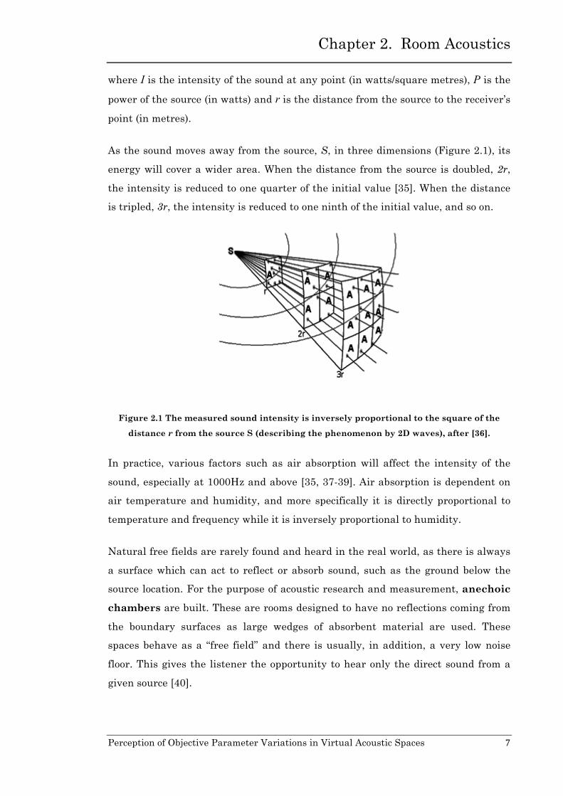
As the sound moves away from the source, S, in three dimensions (Figure 2.1), its
energy will cover a wider area. When the distance from the source is doubled, 2r,
the intensity is reduced to one quarter of the initial value [35]. When the distance
is tripled, 3r, the intensity is reduced to one ninth of the initial value, and so on.
Figure 2.1 The measured sound intensity is inversely proportional to the square of the
distance r from the source S (describing the phenomenon by 2D waves), after [36].
In practice, various factors such as air absorption will affect the intensity of the
sound, especially at 1000Hz and above [35, 37-39]. Air absorption is dependent on
air temperature and humidity, and more specifically it is directly proportional to
temperature and frequency while it is inversely proportional to humidity.
Natural free fields are rarely found and heard in the real world, as there is always
a surface which can act to reflect or absorb sound, such as the ground below the
source location. For the purpose of acoustic research and measurement, anechoic
chambers are built. These are rooms designed to have no reflections coming from
the boundary surfaces as large wedges of absorbent material are used. These
spaces behave as a “free field” and there is usually, in addition, a very low noise
floor. This gives the listener the opportunity to hear only the direct sound from a
given source [40].

Chapter 2. Room Acoustics
Perception of Objective Parameter Variations in Virtual Acoustic Spaces 8
Sound in an Enclosed Space 2.3
In an enclosed space, sound waves interact with the surrounding boundaries, as
well as the air filling the space and any physical objects placed within these
boundaries, influencing propagation through the space and contributing to the
final audible result. The contributions of such acoustic interactions are described in
the following section.
Growth and Decay of Sound in a Room 2.3.1
Consider a closed space, as shown in Figure 2.2, where a point-like sound source, S,
emits a continuous sound in all directions, starting at time t0. At the receiver
position, R, the sound arrives through an infinite number of paths. The first sound
is perceived by the receiver at t1, such that t1>t0, which is defined as the time
needed for the sound to travel the shortest path from the source to the receiver.
This is called the direct sound and behaves similarly to a sound source
propagating in free space. The direct sound arrives at the receiver point with less
sound energy than that emitted from the source, according to the inverse square
law and due to air absorption losses. The level of the direct sound affects the
perception of any sound heard within a given space, influencing the overall clarity
and in particular the intelligibility of speech [41].
After a short time, t2, the reflection refl1 arrives at the receiver and adds its sound
power to that of the direct sound, resulting in the energy D + refl1. Thereafter, at t3,
the reflection refl2 arrives and the sound energy at the receiver’s position is
increased to D + refl1 + refl2.

Chapter 2. Room Acoustics
Perception of Objective Parameter Variations in Virtual Acoustic Spaces 9
Figure 2.2 The growth of a sound at receiver R for a continuous sound source S based on
the build-up of impulse arrivals. The direct sound D arrives at the receiver at time t1 after
a continuous sound source starts at time t0 (left). The sound energy at the receiver point
builds up from the added sound energy of the reflections refl1, refl2, refl3 arrive at the
receiver at times t2, t3, t4 (right) (describing the phenomenon by 2D particles).
These sounds, produced by one or more reflections from surfaces in the space, are
called early reflections and arrive at the receiver position at different times and
from different directions. The energy of early reflections is reduced due to the
distance travelled, air absorption, and also the absorption effect of the surface from
which they are reflected. As with the direct sound, early reflections also contribute
to the overall clarity of sound together with the perceived intelligibility of speech.
Additionally, early reflections are responsible for the phenomenon of echo. This
happens when a reflection arrives at the receiver position with a sufficient delay
(typically greater than 50ms to 80ms [35]) after the previous sound such that the
ear perceives it as a separate sound event.
After these early reflections, many more reflections arrive at the listener from all
directions and as a result the sound loses its sense of perceived direction. This part
of the sound is called the reverberant sound.
The above process continues until the source, S, stops producing sound. At this
point the sound energy starts to decay as the energy in the space is absorbed by the
surfaces, illustrated in Figure 2.3. At tx, the sound source has stopped and the

Chapter 2. Room Acoustics
Perception of Objective Parameter Variations in Virtual Acoustic Spaces 10
direct sound produced as a consequence of this terminating sound event arrives at
the receiver position at ta, such that ta>tx. At tb, the first reflection refl1 arrives at
the receiver position and so on.
Figure 2.3 The sound energy related to the growth and the decay of sound for a continuous
source S that is turned off at time t = tx.
It takes some time for the sound to die away after the sound source is stopped. In
Figure 2.3, the decay is a straight line, which is the ideal case, although, in reality,
the energy of sequential reflections does not necessarily decay in such a linear
manner.
By measuring this reverberant sound, important information can be obtained
about how the sound is perceived in the space. This decay is dependent on the
absorptive capacity of the surfaces in the space, the shape, the volume of the room
and also the air conditions, such as humidity and temperature.
In an enclosed space, there are three distinct regions where sound can be
characterised differently. These are 1) the near field, 2) the far field and 3) the
reverberant field. The region which is very close to the sound source is known as
the near field. In this area, the receiver perceives only the direct sound from the
sound source and as a result, any acoustic measurements in this area cannot
acquire the acoustic behaviour of the space.

Chapter 2. Room Acoustics
Perception of Objective Parameter Variations in Virtual Acoustic Spaces 11
Beyond the near field, in the far field the sound energy can be related to the
inverse square law and the receiver perceives the direct sound as well as any early
reflections that are strong enough to give information about the acoustic
characteristics of the space.
An important term that needs to be defined at this point is the critical distance.
In theory, this is the distance at which the sound energy of the direct and the
reflected sound (or reverberation) are equal [35, 42]. In practice, it is determined by
the room constant and the directivity of the sound source using the following
equation [41]:
QR.r room1410= ( 2.2 )
where r is the distance (in metres) and Q defines the source directivity and is equal
to 1 for an omnidirectional source and equal to 2 for a semi-directional one. Rroom is
the room constant (in square metres), defined by the following equation:
)1( αα−
=SRroom ( 2.3 )
where S is the total surface area (in square metres) and α is the average absorption
coefficient associated with this total surface area, as will be explained in section
2.3.4.
Alternatively, if this information is not available, Sabine’s approximation as a
function of volume and reverberation time can be used:
60
057.0RTVr = ( 2.4 )
where r is the distance (in metres), V is the volume (in cubic metres) and RT60 is the
reverberation time (in seconds). Reverberation time will be discussed in more detail
in section 2.5.1.
It is clear that the critical distance is dependent on the complexity, the size, the
absorptive materials of the space and the source directivity. For example, in large
and complicated rooms, and where the sound source and receiver point are not

Chapter 2. Room Acoustics
Perception of Objective Parameter Variations in Virtual Acoustic Spaces 12
affected by surrounding objects, the critical distance is longer than in the case of a
smaller room where the reflections from the boundaries arrive at the receiver point
earlier. Following the same logic, the critical distance is shorter when an obstacle
with a reflective surface is very close to the receiver point.
In the reverberant field, the perceived sound is a combination of direct sound
from the source and reflected sound from the boundaries and any surrounding
objects. These reflections arrive from all directions, thus due to their diffuse nature
the sound energy remains approximately constant in this region.
Sound Reflection 2.3.2
When a sound meets a planar boundary, a specular reflection is the result, based
on the Law of Reflection, where the angle of incidence θi is equal to the angle of
reflection θr. It is assumed that the dimensions of the obstacle are sufficiently large
in comparison to the wavelength of the incident sound.
Figure 2.4 Sound Reflection, demonstrating specular reflection when the angle of
incidence θi is equal to the angle of reflection θr according to Law of Reflection -
(describing the phenomenon by 2D particles).
Sound Diffusion/Scattering 2.3.3
The Law of Reflection does not apply if the boundary under consideration is not flat
and smooth. If the dimensions of the surface are smaller than the half the
wavelength λ of the incident sound wave, it can be assumed smooth at low
frequencies [43]. At high frequencies, however, the sound is reflected in different
directions and the phenomenon is called diffusion or scattering. The ideal case of

Chapter 2. Room Acoustics
Perception of Objective Parameter Variations in Virtual Acoustic Spaces 13
calculating the direction of this reflected sound is based on Lambert’s cosine law
[44]. This law says that the intensity of the diffused sound is proportional to the
cosine of the angle θi between the observer's line of sight and the projection of the
surface (Figure 2.5), defined by the following equation:
2
00
coscos
rdSII i
π
ϑϑ= ( 2.5 )
where I is the intensity of the sound (in watts/square metres) which is scattered in
a direction characterised by an angle θ0, I0 is the intensity of the incident sound (in
watts/square metres) which hits an area element dS under an angle θi, measured
at distance r from dS and r is the distance from the source to the measured point
(in metres).
Figure 2.5 Sound Scattering according to Lambert’s cosine law, demonstrating scattered
reflection in angle θo when θi is the angle of incidence (describing the phenomenon by 2D
particles)
Sound Absorption 2.3.4
In reality, the energy which is transmitted from the sound source and incident to a
boundary is not equal to the energy of the reflected wave. This is because when the
sound interacts with a surface it causes vibrations in the surface and energy is
transferred. The amount of absorbed energy is dependent on the material that
makes up the surface and this is defined by the absorption coefficient, α , of the
material. This coefficient, according to Sabine, expresses the ratio between the

Chapter 2. Room Acoustics
Perception of Objective Parameter Variations in Virtual Acoustic Spaces 14
absorbed and the incident energy of the sound at the surface. It is defined with
values from 0, for zero absorption, to 1 being a completely absorbing surface. In
practice the values of 0 and 1 only occur in theoretically ideal conditions.
Figure 2.6 Sound Absorption, demonstrating the energy absorbed by the surface while the
remaining energy is reflected according to the Law of Reflection (describing the
phenomenon by 2D particles).
Sound is not only absorbed by the surfaces in the room but also from the air
through which it travels. In the case of small rooms, the boundaries are sufficiently
close to each other such that the sound spends a relatively small amount of time in
the air between reflections. Thus, air absorption is not a major factor in the
resulting sound at the receiver. However, in large rooms (greater than about
500m3) [45] such as concert halls or churches, air absorption has a much more
noticeable effect. In particular, reverberation sound falls off at higher frequencies
(above 1000Hz) [46].
Sound Diffraction 2.3.5
Diffraction is the acoustic phenomenon where the propagated sound changes its
direction due to obstructions in the space and as a result it apparently bends,
spreads out and travels around such objects. The degree of diffraction depends on
the wavelength of the sound. Thus, the effect is greater at low frequencies than
high frequencies where the obstacle is large enough to become a reflecting surface.
This also happens when sound passes through an opening in a surface, such as a

Chapter 2. Room Acoustics
Perception of Objective Parameter Variations in Virtual Acoustic Spaces 15
doorway. If the wavelength is large relative to the width of the opening, the sound
is diffracted strongly.
Standing Waves 2.3.6
If a sound source is positioned between two reflective parallel surfaces, standing
waves occur. Reflected sound interferes with the incident sound, which will have
the same amplitude, speed and frequency, but be moving in the opposite direction.
The effect of this interaction is a number of nodes and anti-nodes, as shown in
Figure 2.7.
Figure 2.7 Nodes (N) and Anti-nodes (A) of three standing waves occurring between two fixed reflective barriers
At the nodes and at the boundary edges, the amplitude of the oscillation of the
wave is zero, while the opposite phenomenon occurs at the antinodes, where the
amplitude of the wave is at its maximum. The sound energy peaks in
correspondence of the antinodes [41, 47-49].
Schroeder Frequency 2.3.7
The phenomenon of standing waves in an enclosed space has a significant impact
on its acoustic characteristics, especially at low frequencies. In this region, the
individual standing waves are sparsely distributed and highly position dependent,
and the distribution of nodes and anti-nodes can, in some cases, be audible. In the
high frequency region, standing waves are much more densely distributed and it is
not possible to perceive specific resonant frequencies. The critical frequency, also

Chapter 2. Room Acoustics
Perception of Objective Parameter Variations in Virtual Acoustic Spaces 16
known as the Schroeder frequency [50, 51], between these two frequency regions
is given by:
VRTfs602000= ( 2.6 )
where RT60 is the reverberation time in seconds (defined in section 2.5.1) and V is
the volume of the space in cubic metres.
Room Impulse Response 2.4
The perception of the acoustic characteristics of a room depends first of all on both
the source and listener’s position. These physical positions have an impact on the
resulting effect of the direct sound and reflections from other surfaces within the
room. Considering the room as a system into which a very brief sound is introduced
as the input signal, the output signal is then determined by the interaction of the
input signal with the room over time.
The room impulse response (RIR) is a time domain function that represents the
response of the room measured at the receiver position to an ideal impulse-like
sound at the source location. This ideal input signal includes all audible
frequencies, has a flat frequency response, and is mathematically represented by
the Dirac Delta function, which for a signal applied at t=t1 is defined as
00
,0,
)(≠
=
⎩⎨⎧ ∞+
=tt
tδ ( 2.7 )
with the condition
δ (t)−∞
∞
∫ dt =1 (2.8 ).
Because of (2.8), this input is often referred to as unit impulse function. In this
context, the value t=0 is chosen to be the time at which the excitation signal is
applied to the system. The acoustic response of the system is therefore given by any
output detected after the application of the initial impulse, as shown in Figure 2.8.
The common assumption is that the system is linear time invariant (LTI). This
means that:

Chapter 2. Room Acoustics
Perception of Objective Parameter Variations in Virtual Acoustic Spaces 17
• as a linear system, the relationship between the input and the output of
the system is a linear map
• and as a time-invariant system, the output does not depend on when the
input is applied to the system.
Figure 2.8 The input signal as the Dirac Delta Function interacts with the acoustic
characteristics of a linear time invariant (LTI) system to give the output signal, the room
impulse response (RIR) as a function of time.
The output signal y(t) in term of the input x(t) can be formally written as:
)]([)( txFty = , ( 2.9 )
where the function F, for an LTI system, assumes the form of the convolution
between the input signal x(t) and the system impulse response h(t) [52]:
)()()( thtxty ⊗= ( 2.10 )
Convolution is the mathematical operation for determining the output signal of a
LTI system resulting from the interaction of the input signal with the impulse
response of the system [53]. In simple words, convolution can be considered as a
form of superposition between the two signals [54].
In reality, LTI systems only exist in ideal circumstances. For example, non-linear
distortions can occur due to the loudspeaker used to apply the input signal.
Another case is non-time-invariance, where the impulse response changes in time
perhaps due to air movement or an increase in air temperature. As long as this

Chapter 2. Room Acoustics
Perception of Objective Parameter Variations in Virtual Acoustic Spaces 18
variation is slow enough as is usually the case, there are no significant differences
in the results obtained [52].
In order to appropriately describe the impulse response of a real space, it is
necessary to take into consideration the noise, generated inside the system, which
is the “added” to the ideal output signal, as shown in Figure 2.9.
Figure 2.9 Input and Output Signal of a Linear Time Invariant (LTI) system with added
noise at the output.
Acoustic Parameters 2.5
In order to measure the impact of acoustic space on the human perception of sound,
subjective terms such as “reverberant”, “dry” or “clear” in isolation cannot give
reliable and useful information for further analysis. Therefore, some of the most
important objective parameters commonly used for acoustic analysis are defined
below, according to ISO3382 [55]. For the calculation of these parameters the room
impulse response (RIR) of a space, for a given source and receiver position, plays a
central role.
For this purpose, a graphical representation of the decay of the acoustic energy of
the impulse response as a function of time is used, based on the Schroeder Decay
method, or Energy Decay Curve (EDC), as introduced in [56]. This makes use of
the backwards integrated squared impulse response for each frequency band, using
the following equation, according to [55]:
E (t ) = p2 (τ )dτt
∞
∫ ( 2.11 )
where E(t) is the energy of the decay curve (in decibels) as a function of time, p is
the sound pressure of the impulse response (in Pascal) as a function of time and t is
time (in seconds).

Chapter 2. Room Acoustics
Perception of Objective Parameter Variations in Virtual Acoustic Spaces 19
Thus, the EDC is the total amount of energy remaining in the RIR at time t. It
gives a much smoother decay than the RIR itself and is much more suitable for
acoustic calculations. Figure 2.10 shows such an EDC as obtained using this
process, for the room impulse response shown in Figure 2.8.
Figure 2.10 The backwards integrated decay curve obtained from the squared impulse
response presented in Figure 2.8, as a function of time.
Reverberation Time 2.5.1
In theory, reverberation refers to the time that it takes for sound to die away in a
room after the source has stopped. This is dependent on the time required for the
sound to reach the receiver point after interacting with the surfaces within the
space.
There are many ways to calculate this time value. The most commonly used
definition is the well-known Reverberation Time RT60 [41]. This is the time
expressed in seconds that a sound takes to decrease by 60dB from its original
sound pressure level at the receiver. In order to measure this reverberation time,
the energy decay curve (EDC) as defined in section 2.5, is used, an example of
which is shown in Figure 2.11.

Chapter 2. Room Acoustics
Perception of Objective Parameter Variations in Virtual Acoustic Spaces 20
Figure 2.11 Reverberation Time, RT60, measured by the time difference t2 – t1, from the
initial slope of the obtained energy decay curve, determined when the sound energy level
has decreased by 30dB.
At t1 the sound source is switched off and the level L1 from the source starts to
decrease until the time t2 when it can no longer be distinguished from the level of
ambient noise. The reverberation time is the time equal to t2 – t1 when the
difference between the L1 and L2 is 60dB. In reality, this time is not so simple to be
measured because a) any noise floor in the system or room, being constant (not
sufficiently low), may prevent an acoustic measure of decay from being taken and
b). the decay is not linear (the relationship between the sound energy level and
time is not linear).For example, double-slope decay occurs when the sound
absorption is not evenly distributed across the surface materials of the space, there
is poor diffusion of the sound or the space includes coupled volumes [57]. Thus,
according to ISO3382 [55] the reverberation time is measured as the rate of decay
given by linear least squares regression of the measured decay curve from a level
5dB below the initial level to 35dB below. When the decay rate used is measured
between these levels, RT60 is referred to as T30, as shown in Figure 2.12. When the
decay rate used is measured from 5dB below the initial level to 25dB below, RT60 is
referred as T20.

Chapter 2. Room Acoustics
Perception of Objective Parameter Variations in Virtual Acoustic Spaces 21
Figure 2.12 T30, measured using the time difference t3 – t2, from the slope of the obtained
energy decay curve determining when the sound level has decreased by 30dB.
Early Decay Time (EDT) 2.5.2
Early Decay Time (EDT) is the time, in seconds, needed for the reverberant sound
to decay 10dB. This means that in comparison with RT60, T30 or even T20, EDT
gives a more detailed indication of the behaviour of early reflections in the impulse
response from the initial 10dB of the decay, and is considered to give a more
detailed indication of the perception of the reverberation in a space [55]. The slope
of the decay curve is determined from the slope of the best linear regression line. In
the following diagram, EDT is the time between t2 and t1, in which the level has
reduced L1 – L2 = 10dB.

Chapter 2. Room Acoustics
Perception of Objective Parameter Variations in Virtual Acoustic Spaces 22
Figure 2.13 Early Decay Time, EDT, measured using the time differences t2 – t1, from the
slope of the obtained energy decay curve determining when the sound level has decreased
by 10dB.
Initial Time Delay Gap (ITDG) 2.5.3
Initial Time Delay Gap (ITDG) is defined as the time delay, in seconds, from the
direct sound to the first reflection. In the case of small spaces or short distances
between the sound source and the receiver points, the ITDG is shorter than when
the sound source is far away. Thus, this parameter is normally used in order to
determine the size of a space or the distance between the sound source and the
receiver point. It corresponds with the subjective impression of "intimacy" [58, 59].
Centre Time (Ts) 2.5.4
The Centre Time (Ts) corresponds to the centre of the gravity of the squared
impulse response [60] and determines the time (in seconds) where the energy of the
early part is equal to the energy of the later part of the impulse response [61]. It is
defined by:

Chapter 2. Room Acoustics
Perception of Objective Parameter Variations in Virtual Acoustic Spaces 23
∫
∫∞
∞
=
02
02
)(
)(
dttp
dttptTs ( 2.12 )
A small value of Ts in comparison with the overall length of the impulse response
means that the energy is concentrated in the early part.
Clarity C50/C80 2.5.5
Clarity is the early-to-late arriving sound energy ratio, expressed in decibels. More
specifically, it describes the importance of the direct sound and early reflections (in
the far field) in comparison with the late reflections that cause reverberation, as
shown in Figure 2.14. With C50, clarity is determined according to the first 50ms,
which is more associated with the study of the perception of speech. C80 is clarity
determined according to the first 80ms of the impulse response and is used in
studies relating to the perception of music. Clarity is especially important for the
study of speech, because it helps to describe the perceived intelligibility of words
and is formally defined according to [60] by:
⎟⎟⎟
⎠
⎞
⎜⎜⎜
⎝
⎛
=
∫
∫∞
e
e
e
t
t
tdttp
dttpC
)(
)(log10
2
0
2
( 2.13 )
where Cte is termed the early-to-late sound index, te is the early time limit of either
50ms or 80ms and p(t) is the pressure of the measured impulse response (in
Pascal).

Chapter 2. Room Acoustics
Perception of Objective Parameter Variations in Virtual Acoustic Spaces 24
Figure 2.14 Clarity (C50/C80) defined as the early-to-late sound index, with the early sound
threshold defined at t2=50 ms or 80 ms according to application.
Definition (D50) 2.5.6
Definition (D50) is related to C50/C80 as it is the ratio of the early to total sound
energy. This parameter is also often used in cases of speech intelligibility and is
defined according to [60] by:
∫
∫∞
=
0
2
050.0
0
2
50)(
)(
dttp
dttpD ( 2.14 )
in which p(t) is the pressure of the measured impulse response (in Pascal). This
parameter is directly related to C50 as follows:
⎟⎟⎠
⎞⎜⎜⎝
⎛
−=
50
5050 1
log10DD
C ( 2.15 ).
Sound Strength (G) 2.5.7
Sound Strength (G) is the difference, expressed in decibels, between the pressure
level of the measured sound and that produced by the same omnidirectional source
in a free field, at 10m distance from its centre. It is defined as follows [60]:

Chapter 2. Room Acoustics
Perception of Objective Parameter Variations in Virtual Acoustic Spaces 25
∫
∫∞
∞
=
0
210
0
2
10)(
)(log10
dttp
dttpG
( 2.16 )
in which p(t) is the pressure of measured impulse response (in Pascal) and p10 (t)
is that measured at a distance of 10m from the source in a free field.
Early Lateral Energy Fraction (LF) 2.5.8
Early Lateral Energy Fraction (LF) is the fraction of energy arriving within the
first 80ms from lateral directions and can be measured from impulse responses
obtained from an omnidirectional and a figure-of-eight pattern microphone. It is
defined by the following equation [60]:
∫
∫= 080.0
0
2
080.0
005.0
2
)(
)(
dttp
dttpLF
L ( 2.17 )
where pL2(t) is measured with a figure-of-eight pattern microphone and p
2(t) is the
response from the omnidirectional microphone (in Pascal).
Inter-Aural Cross-Correlation (IACC) 2.5.9
Inter-Aural Cross-Correlation (IACC) is a parameter associated with binaural
measures and is obtained via a dummy head or with small microphones at the
entrance of the ear canals of a real head. It measures the correlation of the
pressure impulse responses received at the two ears in the first 50ms. The inter-
aural cross-correlation coefficient, IACC, is given by [60]:
( )τ
2121max tttt IACFIACC = , for -1ms < � < +1ms ( 2.18 ).
The normalised inter-aural cross correlation function, IACF is defined as:

Chapter 2. Room Acoustics
Perception of Objective Parameter Variations in Virtual Acoustic Spaces 26
⎟⎠⎞⎜
⎝⎛
⎟⎠⎞⎜
⎝⎛ +
=
∫∫
∫2
1
2
1
2
1
21
)()(
)()(
22 t
t r
t
t L
t
t rL
tt
dttpdttp
dttppIACF
ττ ( 2.19 )
where pL (t) is the impulse response at the entrance to the left ear canal, and pr (t)
is that for the right ear canal.
Just Noticeable Difference (JND) 2.6
The measurable acoustic parameters described above do not provide, enough
information about the subjective perception of these objective measures, as the
human ear is always the final receiver of these sound events.
Just noticeable difference is defined as the smallest perceived/detectable difference
between changes of the values in a given objective measured parameter.
As in any other area of psychoacoustics, the just noticeable difference (JND) or just
audible difference, as described by Kuttruff [44], has aroused interest in several
previous works in which the JND of various parameters have been determined
through laboratory listening tests. An earlier approach to study the sensitivity of
listeners to changes was made by Reichardt et al. [62]. In that study, the limens for
the delay and the level of individual lateral and ceiling reflections in an impulse
response were investigated. However, the samples were not based on properly
simulated concert hall conditions and the results are not considered reliable. In
Cremer et al.’s work [63], the JND for reverberation values is reported to be about
4% for RT60 value greater than 0.6s, while an absolute subjective limen equal to
0.024s is noticed for RT60 < 0.06s. Following study by Niaounakis et al. [64] has
been shown that RT60 values below 0.6s, the same difference limen of RT60 is 0.042
± 0.015s, based on realistic binaural reproduction of sound fields.
Cox et al. [65] used artificial simulated impulse responses, more similar to those
typically observed in concert-halls, for reverberation time of 2.1s. Their study was
focused on changes in the early sound field and measured the difference limens for
early lateral energy fraction (LF), centre time (Ts), clarity (C80) and initial time
delay gap (ITDG). They found that the JND for centre time (Ts) was 8.6 ± 1.6ms for
a reference value of 80ms and the JND values for clarity (C80) to be 0.67 ± 0.13dB.
These values, however, were the average values observed by investigating the
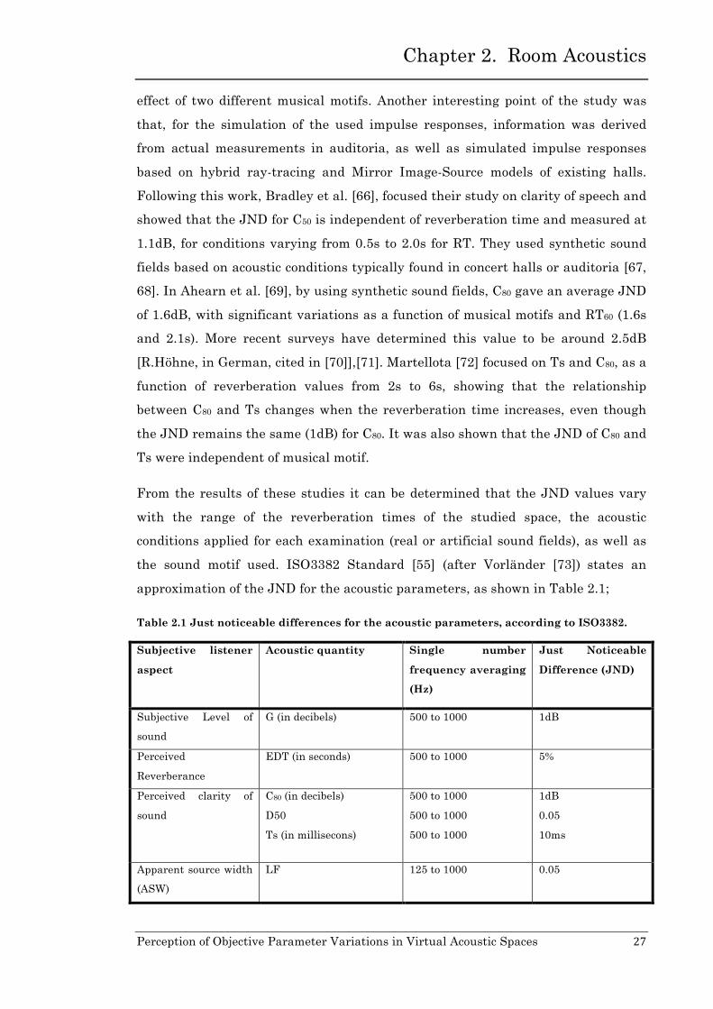
Chapter 2. Room Acoustics
Perception of Objective Parameter Variations in Virtual Acoustic Spaces 27
effect of two different musical motifs. Another interesting point of the study was
that, for the simulation of the used impulse responses, information was derived
from actual measurements in auditoria, as well as simulated impulse responses
based on hybrid ray-tracing and Mirror Image-Source models of existing halls.
Following this work, Bradley et al. [66], focused their study on clarity of speech and
showed that the JND for C50 is independent of reverberation time and measured at
1.1dB, for conditions varying from 0.5s to 2.0s for RT. They used synthetic sound
fields based on acoustic conditions typically found in concert halls or auditoria [67,
68]. In Ahearn et al. [69], by using synthetic sound fields, C80 gave an average JND
of 1.6dB, with significant variations as a function of musical motifs and RT60 (1.6s
and 2.1s). More recent surveys have determined this value to be around 2.5dB
[R.Höhne, in German, cited in [70]],[71]. Martellota [72] focused on Ts and C80, as a
function of reverberation values from 2s to 6s, showing that the relationship
between C80 and Ts changes when the reverberation time increases, even though
the JND remains the same (1dB) for C80. It was also shown that the JND of C80 and
Ts were independent of musical motif.
From the results of these studies it can be determined that the JND values vary
with the range of the reverberation times of the studied space, the acoustic
conditions applied for each examination (real or artificial sound fields), as well as
the sound motif used. ISO3382 Standard [55] (after Vorländer [73]) states an
approximation of the JND for the acoustic parameters, as shown in Table 2.1;
Table 2.1 Just noticeable differences for the acoustic parameters, according to ISO3382.
Subjective listener
aspect
Acoustic quantity Single number
frequency averaging
(Hz)
Just Noticeable
Difference (JND)
Subjective Level of
sound
G (in decibels) 500 to 1000 1dB
Perceived
Reverberance
EDT (in seconds) 500 to 1000 5%
Perceived clarity of
sound
C80 (in decibels)
D50
Ts (in millisecons)
500 to 1000
500 to 1000
500 to 1000
1dB
0.05
10ms
Apparent source width
(ASW)
LF 125 to 1000 0.05

Chapter 2. Room Acoustics
Perception of Objective Parameter Variations in Virtual Acoustic Spaces 28
Although doubts about the “accuracy” of the JND have been expressed [29, 74],
these values are commonly used as a guideline to evaluate the accuracy of
measured acoustic parameters, the accuracy of computer models to predict acoustic
parameters, as well as by acousticians for designing acoustic spaces based on
listener’s perception [29, 30, 33, 73].
Summary 2.7
In this chapter, sound is approached as a physical phenomenon and its behaviour
is studied in a free field and in an enclosed space. The propagation of sound is
explained along with the key properties of this phenomenon. The room impulse
response is introduced as an output of a system excited by an input signal and
ideally the room impulse response contains all the acoustic characteristics of the
system. The main objective acoustic parameters used for measuring the impact of
sound on human perception have also been define based on the ISO3382 standard
[55].
The just noticeable difference (JND) is defined as the smallest perceived difference
between changes in the acoustic parameters and is introduced as a guideline to
evaluate the variations of the acoustic parameters values. The uncertainties of the
recommended values by ISO3382 standard are also expressed, as the JND values
vary with
• the range of the reverberation time
• different types of impulse responses (mesured or synthetic) and
• the sound motif used (different musical motifs, speech, noise).
The above points are carefully considered throughout this thesis.

Chapter 3. Auralization
Perception of Objective Parameter Variations in Virtual Acoustic Spaces 29
Chapter 3.
Auralization
Introduction 3.1
“Auralization is the technique for creating audible sound files from numerical
(simulated, measured, synthesized) data” [43].
Auralization can be considered as the audio equivalent to visualization and
through its application we are able to synthesize the acoustics of either a complete
virtual environment or a particular building, and listen to sounds placed within
this virtual space as if we, the listener, were also present.
Figure 3.1 Visual demonstration of the auralization concept, where a listener is “placed” in
a virtual acoustic realisation of St. Patrick’s Church, Patrington, UK [21, 22].
Auralization techniques are commonly applied nowadays for presentation of
building design proposals, for the revival of the acoustics of heritage sites, in the
sound recording and music production industry, and for 3D acoustic reconstruction
in the fields of animation, computer games and digital cinema.

Chapter 3. Auralization
Perception of Objective Parameter Variations in Virtual Acoustic Spaces 30
Although the term auralization was introduced by Kleiner et al. [75] in 1993, the
concept and methodology actually date back further to 1962, with the paper titled
“Digital computers in room acoustics” by Schroeder et al. at the ICA in Copenhagen
(cited in [76]). This was when the main steps necessary to be able to listen to a
computerised simulation of the acoustics of a space were first defined:
• Convolution of impulse response with anechoic music,
• Cross-talk cancellation technique for reproduction of binaural signal over
two sound sources (loudspeakers) in an anechoic room, and
• “the development of a natural sounding reverberation unit without needing
to carry out a convolution with a huge number of discrete reflections” [76].
The technique of convolving the response of an artificial reverberator with a
stimulus for the impression of a simulated space as carried out by a digital
computer was already in use in 1970, by Allen and Berkley [42]. Nowadays, due to
the development of computing power and recording techniques, auralization results
can be produced from both real measurements, or synthesised, artificial impulse
responses.
Due to the complexity of the nature of sound propagation within an enclosed space,
the study of room acoustics is considered difficult. Accurate and practical
measurement techniques were the goal of scientists from the beginning of the 20th
century. Measurements of impulse responses have been used more recently,
starting with very simple techniques (based on gunshots and balloons as the sound
source) [77, 78] and developing into the very high quality, accurate and repeatable
measurements used today. This data can also be used for auralization, where the
impulse responses obtained are applied to anechoic recordings. The result being
that these recordings are heard as if they had been produced within the space
being studied.
Additionally, acoustic simulation software has improved in terms of the quality of
the artificial impulse responses produced and the methods used to produce them.
They are now commonly used for acoustic research and architectural acoustic
design [77], as well as for auralization and perceptual studies.

Chapter 3. Auralization
Perception of Objective Parameter Variations in Virtual Acoustic Spaces 31
In this chapter, the most well-known auralization techniques will be described
together with their advantages and disadvantages, in order to establish the most
suitable techniques for this research.
Measurements of Impulse Responses 3.2
Several techniques are documented for how impulse response measurements can
be obtained, often based on the ISO3382 standard [55]. More recent approaches
tend to differ from this recommended method however, as more accurate and
reliable results can be obtained with alternative techniques based on parallel
improvements in both computing power and recording methods during the last
decades. Acoustic measurements have often been used in order to collect more
information about the acoustic characteristics of the measured space but more and
more, these impulse responses are used also for auralization purposes and related
perceptual studies.
Excitation signal 3.2.1
The excitation signal used in the measurement process must have sufficient energy
across the whole audible spectrum to decay properly without being covered by
background noise from either the space itself or the equipment used in the
measured position [35, 79]. Based on ISO standards [55], the pressure level of the
impulse source should be sufficient to ensure a decay curve starting at least 35dB
above the background noise and at least 45dB above if the quantity T30 is to be
considered. As a measure to compare the level of the desired signal with the
background noise, the signal-to-noise ratio is used, defined as the ratio of the
peak value of the excitation signal to the background noise observed at the end of
the signal.
Based on the definition of the room impulse response given, it is deduced that the
excitation signal should include all audible frequencies, from 20Hz to 20,000Hz and
the spectrum should be flat across this range of frequencies.
The duration of the excitation signal needs to be sufficient to let the sound field
achieve a steady state before any decay. The minimum duration should be half of
the estimated reverberation time and at least a few seconds for large volumes [55].

Chapter 3. Auralization
Perception of Objective Parameter Variations in Virtual Acoustic Spaces 32
Below, different types of measurements with respect to the excitation signal are
presented and grouped in two methods: a) interrupted noise method and b)
integrated impulse response method, based on the ISO3382 standard [55].
Interrupted Noise Method
With this method, the excitation signal is a random or pseudo-random broadband
noise, played from a loudspeaker. The advantage of this method is that the
required instrumentation is simple. The decay curve is then obtained by measuring
directly the decay of the excitation signal at the receiver point once the source has
been turned off (as used for example for acoustic measurements at St. Paul’s
Cathedral, London, in 1951 (cited in [80]). However, the big disadvantage is that
only reverberation time parameters can be calculated as other acoustic parameters
are based on the obtained impulse response [60], which is not measured directly
using this approach.
Integrated Impulse Response Method
Direct Method - Measurements using Impulsive Source
In this type of measurement developed by Schroeder [56], an impulse-like source
such as a cannon, pistol, or powerful electrical spark discharge is used as the
excitation signal [81, 82]. The measured response is then squared and integrated,
such that greater accuracy for measuring reverberation time is obtained when
compared with the Interrupted Noise Method, and early decay time is able to be
measured as well [80].
This method does not need any post-processing for the recordings obtained, which
is one of the reasons why it is still being used for acoustic measurements. Its main
disadvantage, however, is that the excitation signal does not have a perfectly flat
frequency response [77, 83, 84].
Additionally, it cannot always be guaranteed that the energy of the signal will be
sufficient to ensure that the decay curve starts at least 45dB above the noise floor
(as required by ISO3382 [55]). Another problem with this method is that the signal
and any signal distortion cannot be separated from the impulse response as they
occur simultaneously [26].

Chapter 3. Auralization
Perception of Objective Parameter Variations in Virtual Acoustic Spaces 33
Indirect Method – Electro-acoustic Impulse Responses
Due to the developments of electro-acoustic techniques, the background noise of the
space can be overcome and high signal-to-noise ratios achieved by determining the
characteristics of a test signal reproduced via loudspeaker(s). The most commonly
used signals are; a) MLS and b) sine sweep signals.
Maximum Length Sequence Signal Analysis (MLSSA) measurement
method
MLS measurements use a binary sequence of pulses switched between two values
(1 and 0) in a pseudo-random manner. For N defined as the group of the binary
elements, the number of the possible values for a binary number with N digits is
2N. Thus, the maximum length L of an MLS signal must be L = 2N-1, from which
the set of all zeros has been excluded as that only leads to another zero state, and
this equation also defines the periodicity of the signal. The signal is reproduced by
a loudspeaker and the subjective perception of the result is a system excited by
noise. The cross-correlation of such a signal resembles the Dirac Delta function,
with a flat spectrum as all frequency components have the same amplitude [26].
This method has been widely used for acoustic measurements [29, 43, 77], although
there are several problems which need to be taken into account [27]. Firstly, the
risk of this method is the time aliasing error which could happen if the MLS signal
length is no longer or at least the same length as the impulse response of the
system (its reverberation time). As a result, parts of the end of the impulse
response overlap the beginning part. To avoid this aliasing problem the excitation
signal used should be longer (higher order N) than the reverberation time of the
system. One of the main problems is the requirement for an LTI system [52, 77],
otherwise underestimations of calculated acoustic parameters can be caused by
signal distortion which might affect the measurements. Another undesired
property of the MLS method is the flat spectrum of the source signal [26]. Low
frequencies do not have sufficient time to disperse especially for large spaces and
high frequencies can be affected by ambient noise.
Chapter 3. Auralization
Perception of Objective Parameter Variations in Virtual Acoustic Spaces 34
Sine Sweep Measurements Method
Time-Delay Spectrometry (TDS) Method
For this method, suggested by Heyser, the excitation signal for TDS is a linear sine
sweep wave which means that the frequencies across the whole range of excitation
increase equally per time unit. With this signal, it has been possible to avoid
problems of time-variant systems [27]. However, due to the linearity of the signal,
its spectrum is flat, as was the case with MLS method.
Both MLS and TDS are commonly used in measurement studies, as they generally
provide better results in terms of the signal-to-noise ratio obtained, and the
frequency response is wider and flatter than with previous methods based on an
impulsive source. However, as has been mentioned, they are based on perfect
linearity and time-invariance (LTI) of the system during the measurement process.
Another important disadvantage of these methods is that, in order to improve the
signal-to-noise ratio, multiple repetitions of the input signal are required for post
measurement averaging. Thus, these methods are considered time consuming and
with the added risk of time-variant aspects of the system being introduced by using
this technique [26].
Exponential-Swept Sine (ESS) Method
This method can be used with non-linear systems, as suggested by Farina [52].
Historically, this method is based on one of the oldest methods, where a
logarithmic sweep was generated by an analogue generator and the resulting
voltage was drawn by a writing pen on a sheet of paper [79]. The excitation signal
used for this new method is a logarithmic sweep. A logarithmic sine sweep means
that the frequency increases constantly per time unit. The sequence of low
frequencies sweeps slowly and continues more quickly over an increasing
bandwidth [52, 79, 85]. As the signal amplitude is constant (as shown in Figure
3.2), this results in a pink spectrum attenuated by 3dB/octave, with each octave
having the same energy. This decay of the magnitude corresponds roughly to the
magnitude spectra of the background of a typical measured room, which shows the
need of more energy for low frequencies [86].

Chapter 3. Auralization
Perception of Objective Parameter Variations in Virtual Acoustic Spaces 35
Figure 3.2 Time Domain representation of an input logarithmic sine sweep, from 22Hz to
22kHz and lasting 0.5s.
The linear impulse response of the system is deconvolved from the recorded output
sine signal. This is done by convolving the output signal with an inverse filter of
the input sine sweep. This results in the linear response of the system appearing as
an almost perfect impulse response, with a delay equal to the length of the input
signal [27].
The generation of the inverse filter is the reverse of the input signal along the time
axis. Additionally, an amplitude modulation is necessary, in order to get a flat
spectrum by applying to it an amplitude envelope to generate the different energy
from low to high frequencies [87]. This is done by reducing the level by 3dB/octave
[83], starting from 0dB and ending at -6log2(ω2/ω1), in which ω1 is the start
frequency and ω2 is the end frequency of the sine sweep [52].
Additionally, the harmonic distortion of the output signal produced by the
loudspeaker can be observed now in the time domain, as a sequence of impulse
responses clearly separate and before the impulse response of the system, as shown
in Figure 3.3. For this example, the length of the input sine sweep for this example
was 15s. The impulse response of the system can be observed exactly after that
length of the input signal, while the harmonic distortions are now clearly
noticeable before the impulse response.

Chapter 3. Auralization
Perception of Objective Parameter Variations in Virtual Acoustic Spaces 36
Figure 3.3 The resulting output signal after deconvolution with the inverse filter. The
harmonic distortions are easily observed before the required system impulse response.
In addition, it is possible to use a suitable frequency range of the input signal based
on each transducer requirements, avoiding speaker damage in out-of-range
frequencies [77, 78].
This method has been commonly accepted during the last decade for in-situ
acoustic measurements of buildings such as churches [20], auditoriums, concert
halls [86, 88] or opera houses [77, 78, 89].
Despite the advantages of the ESS method there are still some problems. The
deconvolved impulse response is not a perfect Dirac delta function, which the MLS
method can provide, as some oscillations before and after the main pulse can be
observed [83]. Proposed solutions using different filters have been suggested,
although no one result has as yet been proposed as an optimal solution.
Sound Source Directivity 3.2.2
According to ISO3382 [55], the sound source and the microphone should be as close
to omnidirectional as possible, even if in reality the source (such as human voice,
musical instruments or loudspeakers) and the receivers (such as human ears) could

Chapter 3. Auralization
Perception of Objective Parameter Variations in Virtual Acoustic Spaces 37
never be perfectly omnidirectional. This helps to avoid the potential for the source
focusing unevenly on specific points of the tested space.
An omnidirectional source is usually based on using an electroacoustic system, as
omnidirectivity is not always achievable with mechanical/physical sources such as
balloons or pistols. A common method for this purpose is to use a dodecahedron
speaker, with 12 full-range drivers [18, 20, 52].
However, these types of loudspeakers, designed typically for noise-based acoustic
measurements, have three main problems [27, 85, 90]:
• non-flat frequency response across the frequency range,
• cannot radiate efficiently below 100Hz and above 5kHz,
• the homogeneity of the spherical directivity at higher frequencies cannot be
guaranteed.
This means that there is a systematic error introduced into the measured
parameters for specific frequencies [26, 91]. As a solution for the first problem,
previous studies suggested equalisation to create a flat frequency response [26, 85,
88, 89]. However, the overall power of the loudspeaker is sacrificed as a result [27,
86]. In order to obtain a flat frequency response in the lowest frequency bands, a
subwoofer is used, with a typical upper limit of 120Hz [5, 8, 20, 26, 86, 88, 89, 92].
However, due to its complexity, this could cause further difficulties at the
measurement stage such as further equalisation between the two sound sources
being required or spatial distribution of the two sources.
The non-uniform directivity of a dodecahedral loudspeaker at high frequencies is
dependent on the size of the loudspeaker driver. A smaller driver could be used
where the cut-off point of the response is at a higher frequency [27, 89, 90, 93].
An interesting experiment in [83] measures the polar patterns of three different
dodecahedron systems and shows significant differences at medium and high
frequencies, such that omnidirectional characteristics can no longer be assumed.
Differences have been shown in similar studies at low frequencies as well [86, 90].

Chapter 3. Auralization
Perception of Objective Parameter Variations in Virtual Acoustic Spaces 38
Microphones 3.2.3
The ISO3382 standard [55] for the purpose of calculating the acoustic parameters
also requires an omnidirectional microphone to be used for obtaining monaural
impulse responses. Additionally, ISO3382 requires binaural impulse responses for
IACC calculation, as well as a figure-of-eight microphone for the calculation of
lateral-energy parameters such as LE or LF [85].
Furthermore, recent studies focus on the performance of 3D auralization and
relevant 3D acoustic parameters. By using omnidirectional equipment (either
sound source or microphones) as recommended in ISO3382, any spatial information
relating to the directivity of the source and the spatial perception of the receiver is
lost. Depending on the measurement method, and more specifically on the
microphones being used for each case, multichannel impulse responses and spatial
information should be captured when possible [8, 84, 90, 94].
The collection of 3D impulse responses was first proposed by Gerzon [94]. Due to
the improved performance of personal computers and the availability of
sophisticated digital signal processing (DSP) techniques, that were not available at
the time of this original proposal, this has only more recently started to become
common practice [9, 21, 22, 26, 27, 85, 86, 88, 90, 92, 95-97]. Generalizing, for these
studies, a binaural dummy head, a pair of cardioids in ORTF configuration, and a
4-channel Soundfield microphone are combined with a rotating turntable such that
they are able to capture 8 impulse responses at 36 positions, measured every 10°
around a circle, centred exactly to the axis of the turntable. With this set up, it is
possible to reproduce stereo and ITU 5.1 surround-sound based on either the ORTF
configuration of the cardioid pair, or from the appropriate azimuth at positions of
the Soundfield microphone.
It is important to note that the polar patterns of existing microphones do not match
the theoretical required ones. Measurements of the polar patterns of four
Soundfield microphones are presented in [83] showing significant differences at
medium and high frequencies, for both figure-of-eight and omnidirectional
patterns. It is also observed that the gain of these patterns is not always properly
matched across the frequency range.
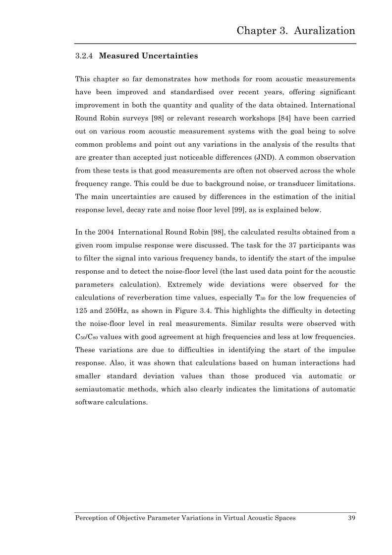
Chapter 3. Auralization
Perception of Objective Parameter Variations in Virtual Acoustic Spaces 39
Measured Uncertainties 3.2.4
This chapter so far demonstrates how methods for room acoustic measurements
have been improved and standardised over recent years, offering significant
improvement in both the quantity and quality of the data obtained. International
Round Robin surveys [98] or relevant research workshops [84] have been carried
out on various room acoustic measurement systems with the goal being to solve
common problems and point out any variations in the analysis of the results that
are greater than accepted just noticeable differences (JND). A common observation
from these tests is that good measurements are often not observed across the whole
frequency range. This could be due to background noise, or transducer limitations.
The main uncertainties are caused by differences in the estimation of the initial
response level, decay rate and noise floor level [99], as is explained below.
In the 2004 International Round Robin [98], the calculated results obtained from a
given room impulse response were discussed. The task for the 37 participants was
to filter the signal into various frequency bands, to identify the start of the impulse
response and to detect the noise-floor level (the last used data point for the acoustic
parameters calculation). Extremely wide deviations were observed for the
calculations of reverberation time values, especially T30 for the low frequencies of
125 and 250Hz, as shown in Figure 3.4. This highlights the difficulty in detecting
the noise-floor level in real measurements. Similar results were observed with
C50/C80 values with good agreement at high frequencies and less at low frequencies.
These variations are due to difficulties in identifying the start of the impulse
response. Also, it was shown that calculations based on human interactions had
smaller standard deviation values than those produced via automatic or
semiautomatic methods, which also clearly indicates the limitations of automatic
software calculations.

Chapter 3. Auralization
Perception of Objective Parameter Variations in Virtual Acoustic Spaces 40
Figure 3.4 Differentiations observed at low frequencies for the calculation of RT from 37 different participants, from [98].
For a round robin comparison of room acoustics measurement methods based on
artificial impulse responses [100], approximately one-third of the participants
diverged significantly from the average calculated values for each of ISO parameter
considered. The remaining measurements agreed very closely. Any deviations
observed between these best-case results were caused for two reasons: 1)
uncertainties in the determination of the best fit regression line to the decay curve
for the calculation of EDT values [101], as defined in ISO3382 [55] and 2) small
differences in the starting point of the impulse response giving variations in C50/C80
values due to strong reflections close to the time boundary of 50/80ms.
For determining the reverberation time, the backwards integrated squared impulse
response is calculated based on Schroeder’s method. In reality though, a recorded
impulse response could contain background noise and a systematic error could be
introduced to the calculation methods of the acoustic parameters as a result. Thus,
different noise-removal algorithms have been introduced in order to minimise such
errors [27, 61, 93, 102, 103]. This adds additional uncertainties to the results
obtained, depending on what algorithm has been applied.
Additionally, it has been mentioned in a few previous studies [21, 30, 70, 84, 104],
that slight changes (of the order of 15cm) in the position of the source and receivers
can cause significant differences in the measured results - with respect to the just
noticeable difference (JND). These changes, as will explained in detail in Chapter
6, are specifically observed in parameters that are position dependent, such as EDT

Chapter 3. Auralization
Perception of Objective Parameter Variations in Virtual Acoustic Spaces 41
and C50/C80. Finally, as already discussed in sections 3.2.2 and 3.2.3, the
measurement equipment itself can cause inaccuracies in the measured impulse
responses obtained.
Computer Modelling - Introduction 3.3
An alternative to the direct acoustic measurement of a given space is to use an
appropriate computer modelling method to synthesise the impulse response for a
given set of initial conditions and obtain the acoustic parameters indirectly. For the
production of a synthesized room impulse response, the general requirements for
accurate and convincing auralization results are available information about the
architectural characteristics of the studied space, information about the nature and
the characteristics of the source and receiver and the calculation algorithm used for
sound propagation.
In recent decades, there has been huge progress in auralization and the prediction
of room acoustics using computer modelling software, a development that has been
made possible because of the improvements in the capability of personal
computers. Following initial scale modelling experiments, where optical rays were
used to measure the mean free path for the prediction of reverberation time,
computers offered a solution to collect this data more quickly and with greater
accuracy [76]. The first reference to the use of a ray-tracing computation system
was made by Allred and Newhouse [105] in 1958, who used the system for
prediction purposes and more specifically for determining the mean free path. That
study was followed by Krokstad et al., in 1968 [106], who developed the first ray-
tracing based room acoustic software for actually simulating of the impulse
response in a 3D model.
More recent developments give the capability to calculate the acoustics of a space
with more complex algorithms, based on fewer assumptions and incorporating
more accurate modelling of sound propagation behaviour.
The basic question for computer modelling of room acoustics is whether the
phenomenon of sound will be described by particles or by waves [107]. This section
introduces commonly used modelling techniques and considers their accuracy in
Chapter 3. Auralization
Perception of Objective Parameter Variations in Virtual Acoustic Spaces 42
simulating the behaviour of sound propagation in a given space together with the
resulting acoustic parameters.
Wave Models 3.3.1
Algorithms representing sound as a wave are based on the wave equation; hence,
wave phenomena such as interference and diffraction are included.
Element Methods, such as the Finite Element Method (FEM) and Boundary
Element Method (BEM) approximate the computation of a complicated system by
discretising the acoustic space in small, finite volumes whose boundary are defined
by a mesh of nodes. The relevant physical parameters and equations are then
defined for each nodes so that the total system will be represented by a system of
equations (one for each node).
Finite Difference Time Domain (FDTD) schemes produce impulse responses by
calculating the 2D or 3D equation for the wave propagation in time domain. The
volume of geometric space is represented by a 2D or 3D grid of points or nodes,
while the time is discretised as t0, t1, t2, ..., tn with t0 and tn initial and final time of
the simulation. At each time tm (t0<tm<tn) the value of the quantity under study at
each node is defined in terms of the values of this quantity at its neighbouring
nodes (including the node itself) at the time tm-1 [108-111].
Digital waveguide mesh (DWM), as a variant of FDTD method, is based on the
d’Alembert solution of the 1D wave equation which is the given by the sum of two
waves propagating in opposite direction [53, 111]. This method is used for the
simulation of wave propagation in strings and tubes with 1D meshes and is
extended to membranes and plates simulations with 2D meshes and rooms and
musical instruments simulations with 3D meshes [112, 113].
Although these models are very accurate for single frequencies, especially low
frequencies and small rooms or two dimensional representation of rooms [107], the
level of computation and their computation times are very high due to the large
number of calculations. For example, FDTD method requires a large number of
nodes in order to reliably approximate a real space. Due to these aforementioned
limitations and the fact that this research focuses on large real-world spaces, the
geometrical acoustic algorithms will be used instead of the wave-based methods.
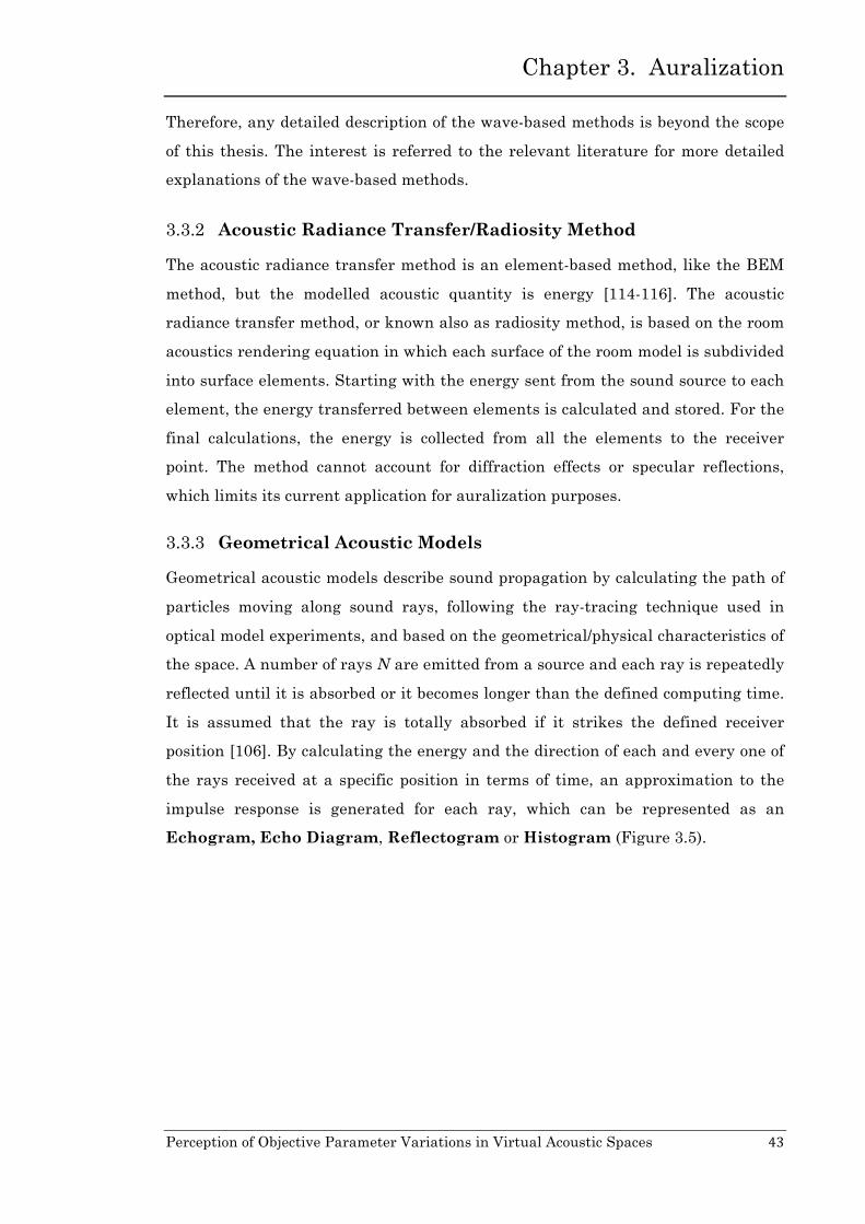
Chapter 3. Auralization
Perception of Objective Parameter Variations in Virtual Acoustic Spaces 43
Therefore, any detailed description of the wave-based methods is beyond the scope
of this thesis. The interest is referred to the relevant literature for more detailed
explanations of the wave-based methods.
Acoustic Radiance Transfer/Radiosity Method 3.3.2
The acoustic radiance transfer method is an element-based method, like the BEM
method, but the modelled acoustic quantity is energy [114-116]. The acoustic
radiance transfer method, or known also as radiosity method, is based on the room
acoustics rendering equation in which each surface of the room model is subdivided
into surface elements. Starting with the energy sent from the sound source to each
element, the energy transferred between elements is calculated and stored. For the
final calculations, the energy is collected from all the elements to the receiver
point. The method cannot account for diffraction effects or specular reflections,
which limits its current application for auralization purposes.
Geometrical Acoustic Models 3.3.3
Geometrical acoustic models describe sound propagation by calculating the path of
particles moving along sound rays, following the ray-tracing technique used in
optical model experiments, and based on the geometrical/physical characteristics of
the space. A number of rays N are emitted from a source and each ray is repeatedly
reflected until it is absorbed or it becomes longer than the defined computing time.
It is assumed that the ray is totally absorbed if it strikes the defined receiver
position [106]. By calculating the energy and the direction of each and every one of
the rays received at a specific position in terms of time, an approximation to the
impulse response is generated for each ray, which can be represented as an
Echogram, Echo Diagram, Reflectogram or Histogram (Figure 3.5).

Chapter 3. Auralization
Perception of Objective Parameter Variations in Virtual Acoustic Spaces 44
Figure 3.5 Ray tracing emitted from sound a source S in a 2D environment and the
representation of the impulse responses from each of the example rays as registered at
receiver R.
The energy of each ray is dependent on the atmospheric conditions defined in the
computer model for air absorption (temperature and humidity) and the absorption
coefficients which characterise the properties of the reflective boundaries.
There are two methods to calculate and simulate the propagation paths of the
particles: 1) the Mirror Image-Source Method (MISM) and 2) the ray tracing
Method.
Mirror Image-Source Method (MISM)
Image methods were commonly used in very early analyses of the acoustic
properties of a space [106, 117, 118], the principle being that a mirror image of the
original sound source is created in the plane represented by the reflecting surface.
The distance between this image source and the receiver is equal to the reflection
path from the original source to the receiver. The method was first used to predict
the acoustic properties of small rectangular rooms using a digital computer [42]. In
a rectangular box-shaped room, all image sources are easily constructed up to a
certain order of reflection and the number of the image sources, N, can be
calculated according to:

Chapter 3. Auralization
Perception of Objective Parameter Variations in Virtual Acoustic Spaces 45
33
34 tVcN π
= ( 3.1 )
where V is the volume of the space, c is the speed of sound in the air and t is the
time of the emission of the sound from the source to the receiver point, and
statistically this can be applied to any geometry [119].
All image sources are visible from the receiver and the calculation of the arrival
time of each one is efficient as it is determined only by the distance between these
images and the receiver.
Figure 3.6 represents an example of the image source method in the simplest case
of a two dimensional rectangular space. The source S emits rays which are
reflected by a surface before they arrive to the receiver R. A first-order reflection
i.e. meaning that the ray has been reflected only once before R at the point A,
creates an image source S1 on the opposite side of that boundary. The path length
that the ray has to travel from S to R, through this first-order reflection is
equivalent to the distance between S1 and R. A second-order reflection, where the
ray has been reflected twice before it arrives at the receiver, requires a new image
source, added after the reflection at point C, on the opposite side of this second
boundary. Here, the same effect happens: the path length of the ray travelling from
S to R via C is equal to the distance between R and S2.
Figure 3.6 Demonstrating the Mirror Image-Source method. Reflections are calculated by
building up the paths from the sources to the receiver point. An image source S1 is created
on the opposite side of the boundary, after the first-order reflection at point A. After the
second-order reflection at points B and C, a second image source S2 is created on the
opposite side of the second boundary.

Chapter 3. Auralization
Perception of Objective Parameter Variations in Virtual Acoustic Spaces 46
Computer modelling software based on this theory creates a mirror image source,
every time a ray is reflected from a surface. If it is characterised as visible, then the
corresponding reflection from it is added to the echogram. Every reflection is
counted only once, even if it has been detected several times by different rays [120].
This algorithm is considered the fastest and simplest way for the prediction of
simple rectangular acoustic models, however, calculations with this method become
more complicated in the case of irregular spaces where image sources are not
always visible from the receiver. Figure 3.7 shows an example of such an irregular
room, with a source S and two receiver points, R1 and R2. The first-order reflection
from the source S to the receiver R1 is calculated as the distance between the valid
image source S1 and R1. The receiver R2 is not visible from the source S1, as the
reflection path between S1 and R2 is intercepted by the boundary surfaces D, E
and F. Thus, further reflection orders are needed for this source to be considered
visible via reflections by this receiver point.
Figure 3.7 Demonstrating a likely case in the Mirror Image-Source method, where the
created image source S1, while detected by R1, is not visible via reflections by R2.
Borish [117] extended the Mirror Image-Source method to include non-rectangular
spaces by introducing three criteria in order to assure that the created image
source is valid for the calculations of the reflection paths between source and
receiver points. The first criterion is called “validity” and checks that the image
sources are created by reflecting across the non-reflective side of the boundary, as
the invalid S2 image source in Figure 3.7 created by the non-reflective side of the
boundary surface J. The second criterion is “proximity” and discards image sources

Chapter 3. Auralization
Perception of Objective Parameter Variations in Virtual Acoustic Spaces 47
which are further from the listener than a distance defined by the user. The third
is “visibility” and tests if an extended line between the image source and the
listener lies inside the boundary of the reflecting side. If all of these criteria are
satisfied the examined image source contributes to the sound received by the
listener. However, there are still limitations on the application of this method. As
the order of the reflections increases, the number of the image sources increases
exponentially and influences the initial calculation time.
Ray-Tracing Method
In ray-tracing, the sound source emits a large number of sound rays in all
directions. Sound particles are traced along these rays and they are reflected from
surfaces in the space according to the geometrical law of reflection and depending
also on the geometrical data of the room. The results are plotted using an echogram
or histogram based on the energy and arrival time of each ray/particle at a receiver
position.
Detection of the receiver position
Due to the fact that a point-like receiver would require an infinite number of rays
to be detected accurately, two calculation methods are used in order to detect the
reflections passing by a specific receiver position.
The first is to define the receiver position not as a point, but as a region around the
receiver, centred on its geometrical location [121]. When a ray arrives in this
region, it is considered as having been detected and contributes to the output.
Figure 3.8 represents such an example of ray-tracing. A point source S propagates
rays across different directions. The rays are reflected from boundary surfaces with
some reflections passing across the defined receiver area around the receiver R.

Chapter 3. Auralization
Perception of Objective Parameter Variations in Virtual Acoustic Spaces 48
Figure 3.8 Ray Tracing method, where the source S emits sound rays in different
directions and is detected by the receiver position R, defined as an area.
The second method, known generally as Beam Tracing, replaces rays with “thick”
rays, or volumetric beams, in order to detect the receiver position with more
accuracy and greater computational efficiency. The beam of rays is uniformly
propagated from the centre of the defined spherical source, and the rays propagate
with the same angle between them [106].
In cone-tracing, circular cones are propagated from the source. As a
spherical/omnidirectional source is required, due to the shape of the cones, there
are overlapping areas between the adjacent cones, as shown in Figure 3.9 (left
image) which cause multiple detections of the same paths [122, 123].
In triangular/pyramidal tracing, a pyramidal beam is used to represent a group of
rays, and is emitted from the source avoiding the overlapping areas possible in
cone-tracing leading to the same path being detected more than once [107, 124,
125]. The pyramids perfectly cover the surface of the spherical source and there is
no overlap as shown in Figure 3.9 (right image).
Figure 3.9 Cone and Pyramidal tracing as emitted from a spherical source, from [124].

Chapter 3. Auralization
Perception of Objective Parameter Variations in Virtual Acoustic Spaces 49
When the beams hit a wall, new beams are reflected based on a newly created
image source S, as shown in the Figure 3.10. These sequences of beam structures
are called a beam tree, with the sound source to be the root of the tree and the
first level beams to be the branches. The next level of beams is reflected from the
boundary surface A, then from the boundary surface B and C, and so on [126].
Figure 3.10 Representation of the beam tree. The beam is emitted from the source S to the
surface area A where the beam is flipped to the surface areas B, E and F, after [126].
When a cone or beam passes by the receiver position, an individual hitting ray,
from the central path (the axis of each beam) between source and receiver, is
determined and calculated [125]. This fact introduces a risk, however, that a
number of image sources will not be detected, or false impressions are created in
the case where the beam does not pass exactly through the receiver position.
Beam tracing methods, as an improvement of the basic ray-tracing method, have
provided a noticeable reduction in computation time compared with normal ray-
tracing methods [125, 127]. However, corrections are required for the
underestimated reverberation tail, due to the increase of the base of the beam that
becomes larger than the room [128, 129]. A typical way to deal with this problem is
to add a statistically generated reverberant tail at the late part of the impulse
response resulting in a “hybrid” model [130]. Various studies are working to correct
these problems and different implementations have been used in the field going
back to the Godot system, in 1982 [131], till more recent software such as Ramsete
[124, 128] and EVERTims based on [132].

Chapter 3. Auralization
Perception of Objective Parameter Variations in Virtual Acoustic Spaces 50
Avoiding false reflections in the Ray-Tracing method
Another problem with ray-tracing methods is the generation of false reflections or
the non-calculation of true reflections. Based on the probability that a ray is
incident upon a surface, the minimum number of used rays N can be calculated
from the following equation,
228 t
AcN π
≥ ( 3.2 )
where A is the area of the surface, c is the speed of sound in air and t is the
travelling time needed from the source to the receiver area [107]. Although a
smaller number of rays can underestimate acoustic behaviour within the space, no
major changes have been observed by increasing the number of rays above the
recommended number [16, 133].
Ray-Tracing is applicable to more irregularly shaped rooms, in contrast with the
Mirror Image-Source method. However, the Mirror Image-Source method is
considered more accurate as it is unlikely to miss important early reflections.
The limitations of geometric algorithms
Geometric acoustic algorithms generally assume that boundary surfaces are flat
and reflect specularly, and so diffusion effects cannot be described. Recently
solutions have been introduced [29, 119] by suggesting the use of
diffusion/scattering for each surface, which has improved reliability of the results.
Thus, in addition to air absorption and the absorption characteristics of the
surfaces, scattering has an important impact in the calculation of the reflection
energy. Depending on the defined scattering coefficient for each surface, the
reflections can be modified to have perfectly specular direction, based on the Law of
Reflection, or scattered more or less at random [107] with directions determined
according to Lambert’s Law [134]. However, after this treatment, the differences
between a real impulse response and a ray-based one are still obvious in the time
domain, as shown in Figure 3.11. In the simulated response (Figure 3.11, top),
there is still no comparable diffuse sound energy between the early reflections as
evidenced in the real response (Figure 3.11, bottom) [135].

Chapter 3. Auralization
Perception of Objective Parameter Variations in Virtual Acoustic Spaces 51
Figure 3.11 Comparing early reflection for the first 0.025s of a ray-based impulse response
(top) and a real impulse response (bottom). The lack of diffuse sound is clear for the first
case due to the limitation of geometric acoustic algorithms to describe accurately
diffusion effects.

Chapter 3. Auralization
Perception of Objective Parameter Variations in Virtual Acoustic Spaces 52
Additionally due to the consideration of sound as particles, and not as waves, wave
based phenomena are disregarded by these algorithms. For example, the
phenomenon of interference cannot be taken into account with the calculations, as
these algorithms do not consider and calculate the phase components of a “ray” and
their changes after a reflection occurs [136]. According to [137] this is a problem
especially for absorptive surfaces, where the phase change effect is more critical.
Harder and more reflective surfaces will provide more accurate results in these
cases. Additionally lack of phase information means that the effects of standing
waves cannot be simulated.
Diffraction effects cannot be described by considering the straight line propagation
of sound rays. Thus, the method tends to create high-order reflections which do not
occur in the real world. This leads to poor accuracy, especially for low frequencies
where diffraction can have a significant effect.
Additionally, assuming that the full audio spectrum ranges from 22Hz to 22kHz,
geometric acoustic methods are only really valid for spaces and surfaces with
dimensions in the range of 15.5m to 1.55cm. If the dimensions of an object are
smaller than this range, the rays instead of propagating through and around it are
assumed to be reflected by the object. Thus, as a modelling technique it is
recommended to avoid surfaces that are very small and to simplify the
architectural representation of the room in order to obtain a reasonable degree of
precision, compatible with this modelling technique [106].
Hybrid Method
Similar to the example of a “hybrid” algorithm discussed above adding statistically
generated reverberant tail at beam tracing method in order to improve the method
(p.49), several acoustic simulation methods have used hybrid approaches by
combining the best features of individual modelling types. Vorländer in [138]
introduced a hybrid method where Mirror Image-Source and ray-tracing methods
are combined for improved accuracy of the early reflection paths of an impulse
response. An algorithm introduced by Lewers combines beam tracing and radiance
transfer method, which replaces surfaces with nodes and south paths with lines, in
order to correct the diffuse reverberant tail of an impulse response [125]. Since
then, several other approaches have been introduced based on different hybrid

Chapter 3. Auralization
Perception of Objective Parameter Variations in Virtual Acoustic Spaces 53
algorithms, combining geometric models with wave based algorithms, acoustic
radiance transfer methods, or even scale model measurements such as in the DIVA
software [135], HAM [139], Epidaure software [140], RAIOS software [141, 142],
EASE-AURA [5] and other research focused algorithms [110, 143-147].
In summary, algorithms based on geometric acoustic methods are considered
accurate at high frequencies, within certain limitations (as they neglect wave
effects), and can deal very well with large and complicated spaces [107] in a time
efficient manner. Hence, these methods have been identified as suitable for use in
this study. Two leading commercial acoustic simulation software packages, both
based on hybrid calculation methods, have been used and their main properties are
described below.
CATT Acoustic
CATT Acoustic is a hybrid simulation software, combining Mirror Image-Source,
ray-tracing and cone-tracing methods [148-150]. The software provides three
independent prediction methods options to the user. The “Early part detailed
Mirror Image-Source Model (ISM)” calculates all the image sources on the
boundary surfaces, up to a requested maximum order of reflection or defined length
of time. From each detected image source, rays are reflected in both specular and
diffuse ways, avoiding an exponential growth of the reflected sound. To calculate
the diffuse reflection, each diffusing surface is subdivided into square patches
which act as secondary sources, radiating according to Lambert’s Law (see section
2.3.3) in a frequency dependent manner [148].
The “Audience area mapping” is based on the classical method of ray-tracing with a
receiver point defined as a spherical region. The rays, after hitting a boundary
surface, are reflected based on Lambert’s Law, in a frequency-dependent manner.
Due to the nature of this method, the echograms of the ray-tracing method are
basically used for predictions and mapping of energy parameters (such as Clarity
C80) in a regular grid across the audience area. Hence, this method is not suitable
for auralization purposes.
The “Full detailed calculation” is based on a randomised tail-corrected cone-tracing
(RTC) algorithm which combines features of specular cone-tracing, classic ray-
tracing and image-source algorithms. The first- and second-order specular
Chapter 3. Auralization
Perception of Objective Parameter Variations in Virtual Acoustic Spaces 54
reflections are calculated based on the Mirror Image-Source method. The first-
order diffuse reflection is calculated based on the secondary patch sources, as
described above in the ISM method [150]. For higher-order reflections, randomised
cone-tracing method, or “approximate” cone-tracing, as was first introduced by
Dalenbäck [148], is used, where the calculated ray directions are randomised,
unlike with the specular cone-tracing method where only the centre ray is traced.
CATT-Acoustic has been used for research purposes, in objective and subjective
studies of room acoustics, as well as by acoustic consultants for providing
predictions during the acoustic design process, some of which are reported in the
following [5, 24, 73, 126, 143, 151-157].
ODEON
The ODEON room acoustic software is a hybrid model that contains elements of
both the Mirror Image-Source and ray-tracing methods [158, 159]. As the early
part of the reflections in an impulse response requires accuracy for efficient results,
for this part of the echogram, a combination method between ray-tracing and
Mirror Image-Source methods is used in order to calculate the early reflections.
Rays are emitted to all directions from the source, creating image sources behind
the surfaces from which they have been reflected. The data relating to the
reflection paths is stored and these image sources are evaluated for their
contribution at the receiver point, with visibility checks [134, 160]. It is also
checked that each reflection is not duplicated. Once the reflection paths have been
stored, the same ones can be used for any different receiver points. The transition
from early-to-late reflections is abrupt, defined by the “Transition Order” (T.O.), a
term introduced by ODEON. This defines the reflection order of the early
reflections below when the hybrid method of combining ray-tracing and Mirror
Image-Source methods, as described above is used.
For the later part of the reflections, the “secondary source” method is used. Above
the reflection order defined by the Transition Order, secondary sources are created
on the reflecting surfaces and emit rays into a hemisphere, carrying energy
following Lambert’s Law. With this method for the late reflection, a sufficient
mixing of the specular and diffused reflections is obtained [107, 119, 160].
The two calculation methods for early and late reflection parts are overlapped for a
time interval. A transition order of 0 means that the calculation method is based

Chapter 3. Auralization
Perception of Objective Parameter Variations in Virtual Acoustic Spaces 55
only on the “secondary source” method, which does not guarantee, however, that all
early reflections will be captured. It is recommended by the developers of ODEON
that the Transition Order be estimated according to the complexity and the shape
of the room [16, 158].
ODEON has been used in studies for research purposes, in the objective and
subjective study of room acoustics as a reference tool for new experimental
approaches in room acoustic modelling, and as a tool for acoustic consultants
providing predictions during the acoustic design process, some of which are
reported in the following [6, 10, 12, 13, 16-18, 20, 39, 73, 161-176].
Round Robin for Acoustic Computer Simulations 3.3.4
Just as Round Robin surveys have been carried out in order to identify variations
in the various acoustic impulse response measurement systems, International
Round Robin surveys have been carried out on room acoustic computer simulation
systems, mainly based on Mirror Image-Source, ray-tracing or hybrid geometric
algorithms. The goal of these surveys is to perform validity checks on their
algorithms, with respect to the JND of the acoustic parameters.
Individual participants using different simulation software have been given the
task of comparing their results for a specific space, based on the calculation of
acoustic parameters according to ISO3382. The followed process for these surveys
comprises two phases. Firstly, the room geometry and material data are provided
with basic architectural plans, photos or drawings and material descriptions in
words. Additionally, the location of the sources and the receivers is given and in
some cases the climatic conditions are also described [29]. Thus, the results are
based on the “guesses” and experience of each participant. In the second phase,
common absorption coefficients (and diffusion data wherever is applicable) for the
materials are given to the participants, thus the examination is focused on the
algorithms rather than the users’ estimations. The results are compared with the
results observed from impulse response measurements performed in the actual
space.
In 1994, the 1st International Round Robin was organised by Physikalisch –
Technische Bundesanstalt, in German, for a speech auditorium, the PTB
Audirorium [73]. Fourteen software packages were compared based on the
simulations by sixteen participants, most of them developers of the software. The

Chapter 3. Auralization
Perception of Objective Parameter Variations in Virtual Acoustic Spaces 56
results were observed for eight acoustic parameters (T, EDT, D, C, Ts, G, LF and
LFC) as an average of the measured positions (two source and five receiver
positions) for the 1kHz octave band. Significant differences were reported between
the results of the simulations and those observed from the measurements, with
respect to the JND values, even for the second phase (by applying general
absorption data).
In 1997-8, for the 2nd International Round Robin, the ELMIA concert hall in
Sweden was selected as the test space and it was modelled by sixteen participants
(the developers themselves and also software users)[29]. The results for nine
acoustic parameters (T30, EDT, D50, C80, G, Ts, LF, LFC and IACC) within six
octave bands (from 125Hz to 4kHz) were observed as well an average of the
measured positions (two source and six receiver positions).
For the 3rd International Round Robin in 2002, the music recording studio of the
Physikalisch-Technische Bundesanstalt Braunschweig was the test space [31-34].
It was modelled by twenty-one participants using nine software packages and the
results were observed in six octave bands for the same nine acoustic parameters as
in the 2nd Round Robin. In order to minimise any bias due to users’ experience and
guesses, this Round Robin was performed in three phases, providing more
information to the users each time. For the first phase, a simple model was
employed, giving the dimensions of the space and applying the same frequency-
independent absorption and scattering coefficients. For the second phase, a more
detailed model was used, with frequency-dependent coefficients applied to the
diffusing walls. For the third phase, geometrical details were given for the diffusing
elements of these walls. In addition, variations of the room acoustic properties were
examined by varying the use of the curtains which covered the two boundary walls.
Important deviations in the results were observed in terms of JND values, that
also showed the importance of applying frequency-dependent absorption and
scattering coefficients, as well that using very detailed geometrical models does not
necessarily guarantee accuracy at the results stage.
In 2008, the Danish Acoustical Society [30], organised a Round Robin where all
eight participants used them the same software, ODEON. Significant differences
were observed even in this case, proving that the skills and the experience of the
users are very important factors for the accuracy of the results.
Chapter 3. Auralization
Perception of Objective Parameter Variations in Virtual Acoustic Spaces 57
The conclusions of the Round Robin tests provide a “rough” overview of the
accuracy of different algorithms and highlight the important issues that need to be
resolved or clarified for accurate predictions and auralization results [177-180].
The main issues are:
• the required level of detail in a geometrical models and their geometrical
accuracy,
• the uncertainties of the impulse response measurement techniques, as
already discussed in 3.2.4, which do not provide reliable results for using
them as reference for the evaluation of the modelled results,
• the accuracy of the absorption and scattering coefficients, estimated by the
users, as in-situ measurement techniques for these data are still not readily
available,
• the neglect of wave-phenomena in ray-based techniques, pointing out once
more the importance of including diffuse reflections in the algorithms,
• the vast number of settings and parameters available to the users for each
software,
• the fact that the results are mainly observed by averaging the results of
various measured positions and frequency bands, rather than studying the
acoustic behaviour of the simulations for individual positions within the
space.
The most interesting observation though from the results of the Round Robins is
that a single mean value across all the measured positions does not provide
sufficient information about the acoustic behaviour of the space and further more
about the accuracy of the different algorithms, as a lot of individual information is
lost. Additionally, after the 2nd and 3rd Round Robin conclusions the need for
listening tests of the analysis of the auralization results has been even more
emphasised [29, 34, 178], as optimisation of the results based on the just noticeable
difference (JND) between the variations of the results for each calculated acoustic
parameter does not necessarily guarantee optimisation at their auralization
results.

Chapter 3. Auralization
Perception of Objective Parameter Variations in Virtual Acoustic Spaces 58
Summary 3.4
In this chapter, the concept of Auralization, and the most well-known auralization
techniques have been described based on real and synthesised impulse responses.
For the capture of the impulse responses in an actual space, a number of different
techniques have been applied. Their advantages and their limitations have been
explained, dependent on the excitation signal used, the sound source and
microphone properties, as well as the calculation process used for the analysis of
the impulse responses.
Synthesised impulse responses are generated through computer-based models,
where different algorithms simulate the physical and acoustic characteristics of the
studied space. The main different between these algorithms is the consideration of
the phenomenon of sound as particles or as waves. Geometric acoustic algorithms
were examined in detail and the state-of-the-art described, in order to identify the
most suitable technique for the purposes of this study. It is also clarified that, even
if geometric acoustic algorithms are considered accurate at high frequencies, they
have a limitation to low frequencies calculation. This is because these methods
neglect wave effects, such as diffraction effects. Thus, the methods tend to create
high-order reflections, leading to poor accuracy for low frequencies, where
diffraction can occur.

Chapter 4. The Perception of Changes in Objective Acoustic
Parameters – A Pilot Study
Perception of Objective Parameter Variations in Virtual Acoustic Spaces 59
Chapter 4.
The Perception of Changes in
Objective Acoustic Parameters –
A Pilot Study
Introduction 4.1
It is common in acoustic design to use 3D computer models and simulation
methods to investigate how changes in the physical characteristics of the space
relate to changes in the resulting acoustic experience [77]. However, the exact
relationship between design parameters, objective acoustic metrics and the
perception of the sound heard within the designed space are not well understood.
Several studies have aimed to explain these correlations in more detail, often based
on simulations in which the acoustic properties of the space could be easily
controlled and changed by the researcher [42].
Tsingos et al. [181] motivated by the experimental use of the "Cornell Box", a
simply constructed real-world space for the simulation of light in computer
graphics, built their own simple test space for investigating sound propagation
algorithms. Due to the simplicity of this space, the researchers were able to
carefully control a variety of geometric configurations and check how accurately
these phenomena can be acoustically simulated, based on the beam tracing method
(as explained in section 3.3.3).
Klosak et al. [170] examined the influence of room shape and room volume using a
virtual rectangular “shoebox” type concert hall using ODEON. In 24 models with a
variety of room dimensions and three different room volumes, results were

Chapter 4. The Perception of Changes in Objective Acoustic
Parameters – A Pilot Study
Perception of Objective Parameter Variations in Virtual Acoustic Spaces 60
averaged over 300-850 receiver points, spread over the audience area based on a
1x1 metre grid. It was concluded that there was a linear relationship between
variations in Clarity (C80) and Strength (G) and the changes in the geometric
characteristics of the models. Changes in the values of these two parameters
became wider as the volume and the dimensions of the models were increased.
However, conclusions could not be drawn with confidence about the effect of the
variations of room dimensions on Early Lateral Energy Fraction (LF80) values.
Similarly, in Berardi’s work [157], 25 box-shaped church models were used to study
the influence of geometrical dimensions, volume and source position on acoustic
parameters, derived from simulations based on CATT-Acoustic. As with the work
conducted by Klosak et al. [170], it was shown that C80 and Ts values increase in
direct proportion to an increase in the length-to-width ratios of the space.
Motivated by these previous works, a preliminary study was carried out for this
thesis using a 3D shoebox-shaped room in ODEON, which allows the user to
control a range of physical acoustic properties relating to the simulation. The aim
was to better understand how physical factors relate to variations in derived
acoustic parameters that might influence the perception of resulting auralizations.
This chapter describes the pilot study and presents the results, which will be then
used to influence the direction of the main modelling and measurement work that
follows (Chapter 5).
Methodology 4.2
For this pilot study, the dimensions of the modelled room were 10m x 8m x 5m,
based approximately on the dimensions of existing large reverberation chambers.
The reason for this was to have the opportunity to investigate different
source/receiver positions in a large space and observe the results in both objective
and subjective terms. As a geometric based algorithm is used for this model and
standing waves cannot generally be taken into account using this method, it was
therefore not necessary to select room dimensions without common factors, to avoid
this sound effect.
For each case study, different versions of the model were created wherein different
variables such as variations in source directivity, source orientation, absorption

Chapter 4. The Perception of Changes in Objective Acoustic
Parameters – A Pilot Study
Perception of Objective Parameter Variations in Virtual Acoustic Spaces 61
and scattering coefficients, calculation settings, and source/receiver positions were
examined in turn. The results of these variations were verified through objective
comparisons of the most relevant acoustic parameters and a series of listening
tests, considering the critical distance for each case and the JND values for each
acoustic parameter (results which have partly been published in [74, 182]).
For the listening tests, six experienced subjects (all of whom musicians,
acousticians or musicologists) listened to pairs of samples, each of them based on
different versions of the model, and were asked to express the degree of similarity
between the paired sounds by choosing a number on a scale of values from 1, very
similar to 10, very different.
Case Study A 4.2.1
The aim of this case study [74] was to investigate the influence of source
directivity, source position, absorption and scattering coefficients, as well as the
ODEON specific parameter, Transition Order (T.O.), on the three main acoustic
parameters, T30, EDT and C50. The perceptual effects of these changes observed in
these acoustic parameters were then investigated through a series of listening
tests. For an appropriate coverage of the space, a grid of 12 equidistant receiver
points (as shown in blue and identified with the numbers 1-12 in Figure 4.1) and
five different positions of a single sound source (as shown in red and identified with
the letters A-E in Figure 4.1) were used. The distance of the source and receiver
positions was no closer than 1m away from the boundaries, as recommended in
ISO3382-2 [183] in order to avoid strong reflections in the results.

Chapter 4. The Perception of Changes in Objective Acoustic
Parameters – A Pilot Study
Perception of Objective Parameter Variations in Virtual Acoustic Spaces 62
Figure 4.1 Demonstrating the virtual shoebox model, where the grid of 12 receiver points
is represented in blue and the variation in source position (A-E) are represented in red.
Different versions of the model were studied, in which a different factor was
changed and examined by observing T30, EDT and C50 averaged across all receiver
positions. For the subjective evaluations, the impulse response for the middle
receiver point (R8) of the grid was used and convolved with an anechoic male
speech.
The versions of the model used for this experiment were based on changes in the
following factors:
Source Directivity and Position
The influence of the source directivity was examined by changing the directivity
from an omnidirectional to a semidirectional source, as shown in Figure 4.2.

Chapter 4. The Perception of Changes in Objective Acoustic
Parameters – A Pilot Study
Perception of Objective Parameter Variations in Virtual Acoustic Spaces 63
Figure 4.2 3D Directivity plots of the virtual source in ODEON: the left plot demonstrates
an omnidirectional source and the right plot a semidirectional source (both in elevation
view). Both sources have the same directivity characteristics across all octave bands.
In addition, the source position was moved across the equidistantly spaced
positions A to E as shown in Figure 4.1. From the objective results, it was observed
that the effect of source directivity was correlated to the distance between source
and receiver positions. For instance, as shown in Figure 4.3, C50 increases as the
source is moved progressively closer to the grid of receivers. However, this was not
confirmed, in the subjective tests, where subjects could only detect minimal
changes.

Chapter 4. The Perception of Changes in Objective Acoustic
Parameters – A Pilot Study
Perception of Objective Parameter Variations in Virtual Acoustic Spaces 64
Figure 4.3 Mean values of C50 observed across the 12 receiver points by varying the source
positions and directivity. The colours indicate the same source position (from position A to
E respectively), while solid lines represent an omnidirectional source and dashed lines a
semidirectional source.
Absorption Coefficients
To study the effect of varying absorption coefficients, the same value was applied to
all boundaries in the shoebox model. These values were chosen to be 0.4, 0.45, 0.49
to 0.5. Using the model with absorption coefficient of 0.5 as a reference, it is noted
that T30 changed noticeably, with even the smallest changes in absorption
coefficient (compare the cases with absorption coefficient values of 0.49 and 0.5), as
shown in Figure 4.4. In the listening tests the subjects clearly perceived absorption
coefficient differences between values of 0.5 and 0.4, scoring the perceived
difference at points 6 and 7 of the scale being used. For absorption coefficient
values of 0.45 and 0.49 with 0.5 as the reference model, the subjects marked the
perceived difference at points 1 and 2 on the scale.

Chapter 4. The Perception of Changes in Objective Acoustic
Parameters – A Pilot Study
Perception of Objective Parameter Variations in Virtual Acoustic Spaces 65
Figure 4.4 Mean values of T30 observed across the 12 receiver points by varying the
absorption coefficient values at the boundaries (0.4, 0.45, 0.49, 0.5).
Scattering Coefficients
Significant differences in the objective results are observed when the scattering
coefficient at the boundaries was varied between the values of 0.05, 0.1, 0.6 and 0.9
used. The absorption coefficient was set at 0.5 in all surfaces. Note here that the
acoustic parameters responded differently across octave bands, as shown in Figure
4.5 and Figure 4.6 for T30 and C50 respectively. However, from the subjective
evaluations it was observed that the listeners were not able to discern these
changes.
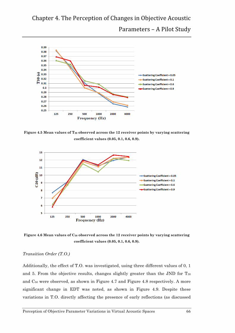
Chapter 4. The Perception of Changes in Objective Acoustic
Parameters – A Pilot Study
Perception of Objective Parameter Variations in Virtual Acoustic Spaces 66
Figure 4.5 Mean values of T30 observed across the 12 receiver points by varying scattering
coefficient values (0.05, 0.1, 0.6, 0.9).
Figure 4.6 Mean values of C50 observed across the 12 receiver points by varying scattering
coefficient values (0.05, 0.1, 0.6, 0.9).
Transition Order (T.O.)
Additionally, the effect of T.O. was investigated, using three different values of 0, 1
and 5. From the objective results, changes slightly greater than the JND for T30
and C50 were observed, as shown in Figure 4.7 and Figure 4.8 respectively. A more
significant change in EDT was noted, as shown in Figure 4.9. Despite these
variations in T.O. directly affecting the presence of early reflections (as discussed

Chapter 4. The Perception of Changes in Objective Acoustic
Parameters – A Pilot Study
Perception of Objective Parameter Variations in Virtual Acoustic Spaces 67
in section 3.3.3), leading to them being absent with a T.O. = 0, there was no
consensus between the listeners about this obvious change at the early reflections.
Figure 4.7 Mean values of T30 observed across the 12 receiver points by varying Transition
Order (T.O.) (0, 1, 5).
Figure 4.8 Mean values of C50 observed across the 12 receiver points by varying Transition
Order (T.O.) (0, 1, 5).

Chapter 4. The Perception of Changes in Objective Acoustic
Parameters – A Pilot Study
Perception of Objective Parameter Variations in Virtual Acoustic Spaces 68
Figure 4.9 Mean values of EDT observed across the 12 receiver points by varying
Transition Order (T.O.) (0, 1, 5).
Case Study B 4.2.2
EDT is considered an important acoustic parameter for evaluation of auralization,
as it is related to the perception of reverberance, as referred to in ISO3382. Hence,
the interest for Case Study B [182] focused on investigating how physical changes
in source-boundary and source-receiver distances, together with source directivity,
influence EDT. The results were based on the mean values observed from a grid of
80 equally spaced receiver points (shown in Figure 4.10).
Figure 4.10 The virtual shoebox model used in Case Study B, where a grid of 80 receiver
points is represented in blue and the source position is represented in red, at the centre of
the space.

Chapter 4. The Perception of Changes in Objective Acoustic
Parameters – A Pilot Study
Perception of Objective Parameter Variations in Virtual Acoustic Spaces 69
In order to control the energy of the early reflections, only specular reflections were
used for the calculations, as scattering coefficient value greater than 0 results in
random changes to the energy of early reflection. Variations in EDT values for an
omnidirectional source, placed at the centre of the space, were obtained directly
from ODEON and examined using colour-mapping across the grid of receiver
positions. This is shown in Figure 4.11 below.
Figure 4.11 Colour-map showing EDT (s) at 1000Hz across the grid of 80 receiver points
based on an omnidirectional source, placed at the centre of the space.
The scale on the right side of the colour-map shows the range of the EDT values in
seconds for 1000Hz. Results were also obtained with the same methodology for a
semidirectional source placed at the centre and oriented to 30°, 60° and 90° (Figure
4.12) and an omnidirectional source, placed 2m away from the upper boundary,
shown in Figure 4.13.

Chapter 4. The Perception of Changes in Objective Acoustic
Parameters – A Pilot Study
Perception of Objective Parameter Variations in Virtual Acoustic Spaces 70
Figure 4.12 Colour-map showing EDT (s) at 1000Hz across the grid of 80 receiver points
with a semidirectional source, placed at the centre of the space (left), and with the
semidirectional source oriented 60° (anti-clockwise rotation) (right).
Figure 4.13 Colour-map showing EDT (s) at 1000Hz across the grid of 80 receiver points
with an omnidirectional source, placed 2m away from the upper boundary.
Non-symmetric behaviour of EDT values were observed across the space, especially
at low and middle frequencies, which means we cannot be confident about the
conclusions reached regarding the behaviour of EDT for these physical variations
in the space. Nevertheless, although this experiment did not offer additional

Chapter 4. The Perception of Changes in Objective Acoustic
Parameters – A Pilot Study
Perception of Objective Parameter Variations in Virtual Acoustic Spaces 71
information about the behaviour of EDT values, it did show from this non-
symmetric behaviour of EDT that specular reflections are not sufficient for an
accurate simulation of the acoustic characteristics of a space, even with a very
simplified model like this. The experiment thus confirmed the importance of using
appropriate scattering coefficient value in geometrical acoustic algorithms.
Case Study C 4.2.3
A directional sound source, a Genelec S30D, was used for the investigation that
forms the main part of this thesis (Chapter 5). In order to consider the influence of
speaker directionality, a 3D version of this source was created (the modelling
technique of which will be explained further in section 5.5.3) and tested in the
shoebox shaped acoustic model. The source was rotated anti-clockwise from 0° to
10°, 40° and 70°, and changes in T30 and C80 were measured and noted, as shown in
Figure 4.14 and Figure 4.15. A more detailed inspection reveals that T30 values
have changed slightly across the octave bands, but more significant changes were
observed in C80 parameters in the middle and high octave bands (above 500Hz).
Figure 4.14 Comparing T30 values observed from a single receiver point (R8 as shown in
Figure 4.1) from the ODEON shoebox model by varying the orientation of the virtual
Genelec S30D sound source (0°, 10°, 40°, 70°).

Chapter 4. The Perception of Changes in Objective Acoustic
Parameters – A Pilot Study
Perception of Objective Parameter Variations in Virtual Acoustic Spaces 72
Figure 4.15 Comparing C80 values observed from a single receiver point (R8 as shown in
Figure 4.1) from the ODEON shoebox model by varying the orientation of the virtual
Genelec S30D sound source ( 0°, 10°, 40°, 70°).
Summary 4.3
An experimental shoebox shaped acoustic model was created using ODEON in
order to study and control different physical factors and acoustic properties, and to
investigate their influence on both objective and subjective results. Source
directivity, source orientation, absorption and scattering coefficients, together with
Transition Order (T.O.) calculation settings and source/receiver positions, were
examined, based on T30, EDT and C50/C80 objective metrics. For the subjective
evaluations, listening tests were carried out for the first two case studies.
From Case Study A, it was observed that C50 values are directly affected by source
directivity and thus this relationship was also influenced by source-receiver
distance. It was further observed that variations in absorption coefficient values
resulted in similar variations in the objective results, as expected. The acoustic
parameters studied did not respond evenly across octave bands when the
application of variations in the scattering coefficients and Transition Order values.
In most cases, subjects were not able to confirm these objective changes in a series
of listening tests.
From Case Study B, conclusions could not be drawn with confidence about the
influence of source/receiver positions and source orientation and directivity. The
main reason being that the results of such acoustic simulations are realistic only

Chapter 4. The Perception of Changes in Objective Acoustic
Parameters – A Pilot Study
Perception of Objective Parameter Variations in Virtual Acoustic Spaces 73
when they reflect the geometry, absorption, diffusion and so forth of real spaces.
Thus, setting scattering coefficient to zero, an unnatural acoustic space was
created, as the non-symmetric behaviour of EDT evidenced.
From Case Study C, useful information were extracted about the influence of the
Genelec S30D sound source in the acoustic parameters studied, which will be used
in the main part of this thesis, detailed in the following chapter.

Chapter 5. Capturing the Acoustic Impulse Responses in St.
Margaret’s Church
Perception of Objective Parameter Variations in Virtual Acoustic Spaces 74
Chapter 5.
Capturing the Acoustic Impulse
Responses in St. Margaret’s
Church
Introduction 5.1
In order to validate and generalise how changes in objective acoustic metrics,
caused by variations of the physical parameters of an auralization space, influence
the resulting subjective experience, a huge number of spaces would need to be
tested. However, this would be impractical, very time consuming and beyond the
scope of this research. This study therefore focuses mainly on the results of one
specific space, in which measurements of impulse responses in-situ can be applied
and used for auralization purposes. The main requirement, being that the physical
acoustic characteristics of the space could be easily changed in order to achieve
variations in the values of the derived acoustic parameters, controlled as much
possible by the researcher. Additionally, the space should have a sufficiently long
reverberation time and relatively simple architectural characteristics.
The chosen space, St. Margaret’s Church located in York, UK, was considered
suitable as it has been redeveloped and acoustically treated in 1998 for concerts
and conference use. The church’s physical acoustic characteristics can be easily
changed through variable reversible wall acoustic panels with a reflective and an
absorptive side, and drapes arranged throughout the space, depending on the
acoustic requirements of the activity within the venue [184].

Chapter 5. Capturing the Acoustic Impulse Responses in St.
Margaret’s Church
Perception of Objective Parameter Variations in Virtual Acoustic Spaces 75
History of St. Margaret’s Church 5.2
St. Margaret’s Church was founded in the 12th century and rebuilt a number of
times before falling into disuse in 1974. The building was held in trust by the York
Civic Trust until 1997, when the York Early Music Foundation secured a grant
from the Arts Council Lottery Fund, in order to create the National Centre for
Early Music, as it is currently known.
Only one feature remains from the original 12th century building, the section
between the west wall and the first pillar of the arcade, which formed the north-
west corner of the original rectangular church (the shape and size of the current
nave). When the church was first built, the sanctuary was on the eastern side and
the congregation sat on in the western side. In 1308, the church was rebuilt and
enlarged by adding a tower to the north-west side. The English Reformation in the
16th century also affected the internal structure of the church, removing the altar
and the sanctuary screen. In the 19th century more changes were made, with
features such as pews, a new pulpit, choir stalls and an organ installed. The church
continued to be used until 1974, when it was declared pleonastic and therefore
became a store for the Theatre Royal of York [185].
Figure 5.1 The outside view of St. Margaret's Church, in York, UK, looking at the west side
of the church and its tower.
The main feature of this work, of considerable architectural significance, is an
ornate Romanesque doorway from the 12th century, with carvings of mythological

Chapter 5. Capturing the Acoustic Impulse Responses in St.
Margaret’s Church
Perception of Objective Parameter Variations in Virtual Acoustic Spaces 76
beasts, such as signs of the Zodiac and the Labours of the Month or illustrations
from bestiaries and Aesop’s Fables on the outer side. Another notable characteristic
of the architecture is the unusual brick bell tower, which was rebuilt in the 17th
century after the steeple collapsed on the nave.
The east and west windows are lancet type, while the windows on the north and
south walls are rectangular, most of them decorated with stained glass. There are
still several memorial tablets “which witness the gentle way of life at the beginning
of 18th century” [186].
Renovation of St. Margaret’s Church 5.3
As part of the York Civic Trust’s plans to redevelop abandoned churches into places
for activities and public events, St. Margaret’s Church, which is located on
Walmgate, was handed over to the York Early Music Foundation Trustees, thereby
creating the National Centre for Early Music. The refurbishment included spaces
for offices, rehearsals, recordings and conferences and the work involved
professionals in architecture, interior design and acoustics.
Figure 5.2 St. Margaret's Church before the refurbishment, towards the east-south (left) and the east (right) side of the church [184, 185].

Chapter 5. Capturing the Acoustic Impulse Responses in St.
Margaret’s Church
Perception of Objective Parameter Variations in Virtual Acoustic Spaces 77
Figure 5.3 St. Margaret's Church after the refurbishment, towards the east-south (left) and the west-north (right) side of the church.
The maximum dimensions of the space are approximately 24.3m in width, 12.5m in
length and 11.2m in height and the volume is approximately calculated to be
2,700m3.
The floor has been reconstructed with huge, smooth flagstone plates. Due to many
decades of rain entry, a further coat of lime-wash to the stonework had to be added
and it was also necessary to install underfloor heating. Most of the stonework of
the walls has been repaired and covered with lime and paint, except for the
memorial tables which have remained untouched. The five columns and their
arches that divide the north aisle from the main nave have kept their original
stonework and no changes have been made to the wooden beam ceiling. A wooden
frame, 0.955m high, was repaired and extended across the length of the bottom of
the walls, while some storage cupboards, 2.00m in height, covered half of the west
side wall. Extra doors have been built for the needs of the current use of the space
and the windows have been covered internally with double glazing, keeping the
view of the old stained glass. The ground floor of the tower has been opened and is
now directly connected with the nave, being used mainly for storage.
The architectural plans for the refurbishment (1999) were received for this
research from the archive of the National Centre for Early Music, and are
presented in the following figures.

Chapter 5. Capturing the Acoustic Impulse Responses in St.
Margaret’s Church
Perception of Objective Parameter Variations in Virtual Acoustic Spaces 78
Figure 5.4 Ground Floor Plan of St. Margaret’s Church as proposed [187].
Figure 5.5 Long Section North of St. Margaret’s Church as proposed [187].

Chapter 5. Capturing the Acoustic Impulse Responses in St.
Margaret’s Church
Perception of Objective Parameter Variations in Virtual Acoustic Spaces 79
Figure 5.6 Long Section South of St. Margaret’s Church as proposed [187].
Figure 5.7 West and East Cross Sections of St. Margaret’s Church as proposed [187].

Chapter 5. Capturing the Acoustic Impulse Responses in St.
Margaret’s Church
Perception of Objective Parameter Variations in Virtual Acoustic Spaces 80
Arup Acoustics were consulted during the acoustic design of St. Margaret’s Church.
The aim was to create a space acoustically suitable for the variety of events that
were planned to be held in the venue, from conferences (implying a short
reverberation time) to classical and early music recitals (requiring longer
reverberation time). Absorbing acoustic panels and drapes were also considered in
the architectural redevelopment, as the quote below illustrates;
“Variable Acoustic Absorption. In ceiling – Acoustic drapes on Unistrut,
stored bunched up at end archbrace truss positions, total surface area
of fabric = 100sqm (comprising 4 no. drapes of 15sqm in nave and 4 no.
drapes of 10sqm in north aisle). On walls – Acoustic banners, stored
rolled up at internal eaves level, total surface area of fabric = 270sqm
(the individual dimensions vary to suit internal elevations, each wall
banner comprises double thickness of fabric, a constant gap between the
two layers is maintained by aluminium framing, banner is handle
operated” [187].
It is worth noting that just as the quote above indicates, the dimensions and the
exact position of the acoustic panels as well as the dimensions of the space were
approximated to the states specified in the architectural plans. The original plans
recommended: “All dimensions to be checked on site” (see Appendix A for the
original architectural plans [187]).
The total number of acoustic panels is 58, spread in groups of two to ten across the
north and south walls as well as the ground floor tower area and corners of the
space. Each group of panels can be folded in half, so that the absorbing front faces
are covered, revealing only a hard reflecting rear panel, as shown in Figure 5.8 and
Figure 5.9.

Chapter 5. Capturing the Acoustic Impulse Responses in St.
Margaret’s Church
Perception of Objective Parameter Variations in Virtual Acoustic Spaces 81
Figure 5.8 Acoustic panels set at the south wall. The 4 square absorbing panels (on the left)
are folded in half, replaced by 2 reflecting panels (on the right).
Figure 5.9 Acoustic panels set at the south-east walls. The 26 square absorbing panels (on
the left) are folded in half, replaced by 13 reflecting panels (on the right).
Acoustic drapes were also mounted on two rails in the nave and north aisle
ceilings, thus enabling them to be opened or closed as needed, as shown in Figure
5.10.

Chapter 5. Capturing the Acoustic Impulse Responses in St.
Margaret’s Church
Perception of Objective Parameter Variations in Virtual Acoustic Spaces 82
Figure 5.10 Acoustic drapes set on the ceiling; drapes out (on the left) and drapes back (on
the right).
By changing the configurations of panels and drapes arranged throughout the
space, it is possible to vary the acoustic qualities to cater for a range of different
activities. The acoustic characteristics of the space for each recommended
configuration are given in Table 5.1. Note that the panels are referred as ‘boxes’.

Chapter 5. Capturing the Acoustic Impulse Responses in St.
Margaret’s Church
Perception of Objective Parameter Variations in Virtual Acoustic Spaces 83
Table 5.1 Guidance notes for the various acoustic qualities, provided by Arup Acoustics [185].
Activity
Acoustic
boxes:
absorption
exposure
Drapes:
absorption
exposure
Acoustic qualities of
space
RT (s) (Based
on Arup
measurements)
Large choral All boxes closed All drawn
back
Highest reverberation,
warmth, spaciousness 2-2.6
Music
recitals All boxes closed
All drawn
out
Even balance between clarity
and reverberation; discrete
sounds stand apart clearly,
but ample reverberation
1.5–1.8
Small
ensembles
25% of boxes
open
All drawn
out
Balance towards clarity
(assume 100+ padded seats) 1.4
Opera/
musicals
75% of boxes
open
All drawn
out
High degree of clarity,
modest reverberation 1.2
Lectures/
speech All fully open
All drawn
out
Sound absorbent space,
giving maximum clarity for
speech
1.0
Impulse Response Measurements 5.4
To fully exploit the opportunity to acoustically survey and measure impulse
responses in St. Margaret’s Church, different physical factors were changed and
their acoustic effects recorded for further study. First, changes in the acoustic
characteristics of the space were applied by considering the configurations of
panels and drapes. Additionally, changes in the orientation of the sound source
were applied to test for the effects of source directionality.
Measurement technique and Excitation Signal
The Exponential-Swept Sine (ESS) Method was used as it is considered the best
solution for auralization purposes [79], as explained in section 3.2.1. It gives a flat
frequency response and a strong input signal compared with the ambient noise
(high signal-to-noise ratio) but, more importantly, separates the nonlinear
harmonic distortion of the speaker from the linear response. The logarithmic sine-
sweep excitation signal was generated using the Aurora Plug-in [188]. The frequency
range of the sweep is from 22Hz to 22kHz, approximately the audible range of

Chapter 5. Capturing the Acoustic Impulse Responses in St.
Margaret’s Church
Perception of Objective Parameter Variations in Virtual Acoustic Spaces 84
frequencies, and it lasts 15 seconds. In ISO3382 [55] it is strongly recommended to
use sweeps with a length of two to four times the longest reverberation time, in
order to increase the total radiated energy and reduce the influence of external
noise. The length of the silence after the sweep depends on the reverberation of the
room where the sine sweep is recorded. In order to minimise onset/offset effects, a
fade-in and fade-out has been applied at the beginning and end of the test signal
[61].
Table 5.2 Settings for the generation of the logarithmic sine sweep in Aurora plug-in.
Log Sweep
Start Frequency (Hz) 22
End Frequency (Hz) 22000
Duration (s) 15
Fade-in and Fade-out duration
Fade-in (s) 0.1
Fade-out (s) 0.1
Silence
Duration (s) 10
Sound Source
For this study, a Genelec S30D was used as the source transducer. This is a
directional three-way active tri-amplified system with 96kHz/24-bit AES/EBU
digital input. Its directivity tends to be omnidirectional at low frequencies, while at
mid-range and high frequencies it tends to a more consistent cardioid
characteristic, as shown in Figure 5.11.

Chapter 5. Capturing the Acoustic Impulse Responses in St.
Margaret’s Church
Perception of Objective Parameter Variations in Virtual Acoustic Spaces 85
Figure 5.11 Genelec S30D (left) and its horizontal polar plots with 0° facing up for the
octave bands of 250Hz, 1kHz, 2kHz, 4kHz, 8kHz and 16kHz, from [189] (right).
The main reason for using this directional source, instead of the omnidirectional
source recommended in ISO3382 [55], is that the acoustic measurements for this
study have been performed for auralization purposes, rather than for directly
analysing the acoustic characteristics of the space. The measured impulse
responses will be convolved with directional anechoic sources, such as voice or
music [176, 190, 191]. Thus, any bias from effects caused by omnidirectional
excitation should be avoided.
Secondly, the frequency response of the speaker, rated from 36Hz to 48kHz, has
small variations in SPL (dB) values, as shown in Figure 5.12, and it is considered
almost flat for the audible spectrum and so does not require any additional
equalization [27] for the purposes of this study.

Chapter 5. Capturing the Acoustic Impulse Responses in St.
Margaret’s Church
Perception of Objective Parameter Variations in Virtual Acoustic Spaces 86
Figure 5.12 Frequency response of Genelec S30D cited in [27].
In addition, this loudspeaker is very convenient for in-situ measurements as it is
both active, and can supplied with a digital input.
Microphone
For this study, a Soundfield SPS422B was used as the main receiver microphone.
The Soundfield microphone captures B-format signals and consists of 4 channels: W,
the omnidirectional component, and three figure-of-eight signals on the Cartesian
axes, X for the horizontal axis, with position orientation pointing towards the front, Y
for the horizontal axis pointing to the left, and Z for the vertical axis. The quoted
frequency range of the Soundfield SPS422B is from 20Hz to 20kHz [192].
Playback system, hardware and software
For playback and recording, Steinberg Nuendo 2 was used. The chosen soundcard for
this project was the RME Fireface 800, providing balanced mic/line inputs to record
the microphone signals and a digital output to feed the Genelec. The signals were
stored directly on the laptop during the recording process as 32 bit floating point
files at 96kHz. This same equipment and measuring technique has been used for
measurements in previous studies [9, 26].
Measurement Conditions
The atmospheric conditions are relatively stable in the studied space, as the leaded
windows are internally supported with double glazing and the temperature and
humidity are permanently controlled by the underfloor heating system. Thus,

Chapter 5. Capturing the Acoustic Impulse Responses in St.
Margaret’s Church
Perception of Objective Parameter Variations in Virtual Acoustic Spaces 87
during the measurement process the temperature was measured at a constant
21.5°C and the relative humidity at 44.5-45%, even though the measurements were
taken over two complete days. The space was empty when the measurements were
performed, without any audience or seating. A piano and harpsichord were the only
additional features in the main space, with any other smaller items stored in the
ground floor tower space.
Measured Positions of Sound Source and Microphone
The sound source was placed at a position within the space typical in terms of
performer location, approximately at the middle of the length of the south wall and
1.66m distant from it, facing towards the north wall. Its height was set at 1.5 m.
The SPL level during the measurements was calibrated at 94-95dBA at 1m
distance from the source in order for the signal-to-noise ratio to be sufficient to
limit background noise and avoid too much distortion at the speaker due to peak
levels. For the microphone measurement positions, 26 receiver positions were used,
for an appropriate acoustic coverage of the space, as shown in the following floor
plan (Figure 5.13).
Figure 5.13 Floor plan of the church. The position of the sound source (S) and the 26
measurement positions are represented.
The receivers were placed in a marked grid (shown in Figure 5.14) consisting of
three rows across the length; a first row of 9 receivers at the middle of the north

Chapter 5. Capturing the Acoustic Impulse Responses in St.
Margaret’s Church
Perception of Objective Parameter Variations in Virtual Acoustic Spaces 88
aisle, a second row of 9 receivers in the nave, symmetrical with the first one and a
third row of 8 receivers between the columns.
Figure 5.14 Marked Grid on the floor for the positions.
According to the recommendations in ISO3382-2 [183] the distance of the source
and receivers from the walls should be at least ¼ of a wavelength, which is
approximately 1m for 125Hz. The distances between each measurement position
and from the walls and columns are represented in Figure 5.15. The microphone
was set at a height of 1.5m, in order to be at the same height as the source.
Figure 5.15 Floor plan of the church. Distances between the measurement positions and
the boundary surfaces.
Each receiver was orientated towards the south wall of the church. As was
explained in section 2.3.1, the critical distance is defined, based on Sabine’s

Chapter 5. Capturing the Acoustic Impulse Responses in St.
Margaret’s Church
Perception of Objective Parameter Variations in Virtual Acoustic Spaces 89
approximation (equation 2.4), as a function of volume and reverberation time.
Thus, as for these measurements the same positions were required for each of the
acoustic configurations studied, the distances of each measurement position from
the sound source were based on the maximum critical distance calculated from the
three studied configurations of the panels and drapes, depending on the acoustic
characteristics of the space. The longest critical distance calculated was 2.88m
(observed from the less reverberant configuration, being Congifuration B), while
the closest receiver, (R14), was placed at a distance of 3.6m from the sound source.
The final distance between sound source and each receiver position is listed in
Table 5.3. It is worth mentioning, however, that receivers R2 and R5 have no direct
line-of sight with the source.
Table 5.3 Distance between sound source and each of the 26 receiver positions. Left (L) is
defined as the left side of the sound source.
Row 1 Row 2 Row 3
Receiver
Position
Distance from
the source (m)
Receiver
Position
Distance from
the source (m)
Receiver
Position
Distance from
the source (m)
R1 11L R10 7.8L R19 8.6L
R2 9.9L R11 6.1L R20 7.7L
R3 9L R12 4.6L R21 6L
R4 8.5L R13 3.6L R22 5.7L
R5 8.5R R14 3.5R R23 6R
R6 9R R15 4.5R R24 6.6R
R7 9.8R R16 6R R25 8.8R
R8 11R R17 7.7R R26 9.8R
R9 12.3R R18 9.6R
Acoustic Characteristics and Configurations
Three configurations of panels and drapes were used during the impulse response
measurements of this study based on the recommendations in Table 5.1:
• Configuration A, for “Opera/Musical” events, with RT values of 1.2s,
• Configuration B, for “Lectures/speech” events, with RT values of 1s, and

Chapter 5. Capturing the Acoustic Impulse Responses in St.
Margaret’s Church
Perception of Objective Parameter Variations in Virtual Acoustic Spaces 90
• Configuration C, for “Music recitals” events, with RT values of 1.5-1.8s.
For the measurements in configuration A, the acoustic panels of the north wall
were folded in half as shown in Figure 5.16.
Figure 5.16 Acoustic panels set at the north wall. The 28 square absorbing panels (on the
left) are folded in half, replaced by 14 reflecting panels (on the left).
During the measurements, the loudspeaker remained in the same position while
the acoustic panels and drapes were set respectively for configurations A, B and C.
The Soundfield microphone then captured the usual responses for each
configuration, for each receiver position and source orientation.
Sound Directivity
The influence of the directionality of the source was also examined in this study
and hence, during the acoustic measurement, impulse responses were captured
with the Genelec rotated on its axis for the same receiver positions for
configuration A. As shown in section 4.2.3, through the shoebox experimental
model, the effects of Genelec orientation was studied by observing the variations in
T30 and C80 values. Based on these results, the loudspeaker was rotated 40° and
70° right respective to its original orientation.
Computer Modelling 5.5
The acoustic model of St. Margaret’s Church was designed by using two
commercial software packages, CATT-Acoustic v8.0j and ODEON 10.1 Auditorium,

Chapter 5. Capturing the Acoustic Impulse Responses in St.
Margaret’s Church
Perception of Objective Parameter Variations in Virtual Acoustic Spaces 91
both based on hybrid geometrical algorithms, as described in detail in section 3.3.3.
The acoustic modelling of a space depends on many factors and not all of which can
be controlled by the user. However, depending on the software, some of these
parameters can be manipulated by a user with the necessary skills and experience.
In the Round Robin tests [29, 73] of room acoustic computer modelling, variations
in modelling methods were observed regarding:
• the level of geometric details (number of surfaces),
• the number of rays used for the calculations,
• reflection order,
• inclusion of diffuse reflections and edge diffraction,
• length of impulse response.
For the modelling process in this current study, for both of the simulation software
packages used, previous acoustic modelling projects as well as personal
communications between the author and the software developers have been used
as guidelines. The aim was to examine the perceptual effect of variations in
obtained acoustic parameters, and different versions of the space were designed
based on the actual acoustic configurations used during the acoustic measurements
process. The models were created in such a way that existing acoustic panels and
drapes will be easily altered by any other user from opened to closed. The
modelling procedure followed with both software packages was the same;
1) import the geometrical data of the space (after considering which surfaces
and how detailed a model was necessary),
2) determine the absorption and scattering coefficients for the materials
included,
3) define the source and receiver positions,
4) choose appropriate settings for the calculation process,
the steps of which are explained in more detail below.

Chapter 5. Capturing the Acoustic Impulse Responses in St.
Margaret’s Church
Perception of Objective Parameter Variations in Virtual Acoustic Spaces 92
Designing the model 5.5.1
Architectural characteristics
The first draft of the model was developed based on the architectural plans created
during the refurbishment of the space [187]. However, as the space was not
symmetric and the outer walls were not exactly parallel to each other in the
supplied plans, it was considered best to have an accurate model in terms of the
main dimensions. Hence, these dimensions were later altered based on physical
measurements of St. Margaret’s Church in its current state. This also incorporated
the physical measurements of additional objects and furniture which had not been
included in the original architectural plans.
Modelling process
It is possible to convert the geometry data for the space from other CAD-platforms
in both CATT-Acoustic and ODEON. However, for the current study the geometries
were imported manually for each included surface based on a coordinate system.
This method was a much more time consuming process, but the user has total
control of surface corner locations and their identifications. The data for surfaces
and corners is listed and numbered based on the modelling order, which has the
advantage of making changes very easy if necessary for future studies.
There are no standards providing recommendations about the level of the
geometric details which should be modelled - this depends mainly on the skills and
the experience of the user. Previous studies have shown that the final results can
be modified either by the user, or depend on the algorithm that has been used [73].
In the 2nd Round Robin [29], the number of surfaces in the participating models
varied from 94 to 3530 surfaces. There were also participants that had used the
same .DXF files as the basis for their models, although significant differences were
observed between results. However, there is an important rule that should be
followed for acoustic modelling. Apart from being impossible to simulate every
detailed object and structure within a space, an extremely detailed model would
cause an increase in the number of the reflection order, leading to a loss of
accuracy in the results, especially for low frequencies (as discussed in section

Chapter 5. Capturing the Acoustic Impulse Responses in St.
Margaret’s Church
Perception of Objective Parameter Variations in Virtual Acoustic Spaces 93
3.3.3). Some exceptions have been reported, such as in open air ancient theatres,
where due to the lack of strong reflections for the ceiling, geometrically detailed
surfaces are necessary for the accurate prediction of early reflections [16].
Following recommendations in previous works about the steps to be taken in the
modelling procedure [16], the construction of the model geometry started with the
basic boundary elements of the space.
The floor and the ceiling were modelled as flat large planes. As the vaults in the
ceiling (shown in Figure 5.10) were not modelled in detail, the sloping flat surfaces
of the ceiling were defined with higher values of scattering, as will be explained
below.
For modelling the boundary walls, in order to include the surfaces of the windows
and doors, a different process was followed due to differences in the modelling
requirements of CATT-Acoustic and ODEON [193, 194]. In CATT-Acoustic, the
walls were subdivided in smaller surfaces, as shown in the example in Figure 5.17,
modelling the north wall. In ODEON, the walls are modelled as single surfaces
around the window areas, as shown in Figure 5.18.

Chapter 5. Capturing the Acoustic Impulse Responses in St.
Margaret’s Church
Perception of Objective Parameter Variations in Virtual Acoustic Spaces 94
Figure 5.17 Modelling walls using subdivision of surfaces in CATT-Acoustic. This
represents an example of the north wall. In the top image, the wall subdivisions can be
observed, while in the bottom image, the wall is represented as a single surface using the
3D viewer tool. The stone memorials were also included as subdivisions in the wall
surfaces.
Figure 5.18 Modelling walls as a single surface in ODEON. This represents an example of
the north wall. In the top image, the wall has been modelled as a single surface, while in
the bottom image, the wall is represented using the 3D OpenGL tool.

Chapter 5. Capturing the Acoustic Impulse Responses in St.
Margaret’s Church
Perception of Objective Parameter Variations in Virtual Acoustic Spaces 95
The door and window surfaces were then mounted on the appropriately defined
areas of the walls, and thus, overlapping surfaces were avoided for these main
parts of the structure.
The simulation of curved surfaces is a general problem in such acoustic models, as
only straight lines can be defined. As a result, curved surfaces can only be designed
as a summary of subdivided plane surfaces. This does mean that scattering and
absorption effects can be calculated differently than what might occur in reality.
This was a problem for the current model, when it came to defining the arches on
the top of the columns and some of the windows. These surfaces had to be modelled
in a more detailed fashion, including small subdivision of surfaces, as shown in
Figure 5.19.
Figure 5.19 Modelling arches between the columns and at the top of the windows using
subdivision of surfaces. On the top left, the CATT-Acoustic model is represented, on the
top right, the ODEON model, and at the bottom, the actual space is pictured.
In previous work [30], tables were modelled either as 2D plates, 3D planes or
boxes. In this model, large interior objects such as tables, pianos, cupboards or the
wooden frame across the length of the bottom of the walls were simulated as simple

Chapter 5. Capturing the Acoustic Impulse Responses in St.
Margaret’s Church
Perception of Objective Parameter Variations in Virtual Acoustic Spaces 96
boxes, excluding those surfaces of these objects which were abutting on other main
structure surfaces.
Figure 5.20 Modelling interior objects; a piano and a wooden cupboard, in CATT-Acoustic
(top left) and in ODEON (top right) based on their dimensions and locations in the actual
space (picture at the bottom).
The stone memorials on the walls were simulated as 2D plates. In CATT-Acoustic,
they were included as subdivided surfaces in the main wall surfaces, as shown in
Figure 5.17. In ODEON, the stone memorials were modelled at a distance of 5mm
from the walls, in order to avoid overlapping surfaces. This was because in some
cases of overlapping surfaces, it might not be clear which absorption characteristics
should be used by ODEON between two overlapping surfaces with different
absorption [30].
Both sides of the reversible absorbing panels were simulated, giving the user the
ability to exert a great deal of control over which ones should be activated; the
opened or closed one, depending on the requirements of the configuration in each
case. An example of these settings is presented in Appendix B, for both CATT-

Chapter 5. Capturing the Acoustic Impulse Responses in St.
Margaret’s Church
Perception of Objective Parameter Variations in Virtual Acoustic Spaces 97
Acoustic and ODEON. However, the groups of two to ten panels were modelled as
single surfaces, as shown in Figure 5.21, demonstrating the north wall (as pictured
in Figure 5.16).
Figure 5.21 Modelling groups of acoustic panels, as demonstrated with ODEON. The red
arrows are pointing at the opened panels, the green arrows at those closed. The left model
is based on configuration A and the right model on configuration B.
As it was considered better to model the drapes on the ceiling as single 2D plates, it
was necessary in CATT-Acoustic, to duplicate and flip one of them, as the software
takes into account the acoustic properties of a surface from only one side.
Finally, the models were checked for overlapping or wrapped surfaces, which can
lead to incorrect calculation of the related absorption characteristics. The 3D tools
(such as the 3D viewer, 3D OpenGL, and 3D Investigate rays) provided in both
software were used to detect these kind of error during the modelling process. In
addition, the models were checked for loss of rays.
Calibrating the Model 5.5.2
The defined acoustic characteristics of the surfaces in the model plays a crucial role
in the accuracy of the acoustic results of the simulated space. Defining these
characteristics is quite a challenge for acousticians [6, 30, 173] and users of such
computer modelling software, and depends on their skills and experience [29, 34].
The main limitation is that the user has to rely on the materials provided in the
existing libraries for absorption and scattering coefficients. It is not likely that an
exact material will be found for the specific materials of a given project and it must

Chapter 5. Capturing the Acoustic Impulse Responses in St.
Margaret’s Church
Perception of Objective Parameter Variations in Virtual Acoustic Spaces 98
also be remembered that these characteristics will be both frequency and angle
dependent, and the current state-of-the-art does not provide acousticians with
sufficient data for these requirements. Round Robin tests (as discussed in section
3.3.4) have shown that such data is of the underestimated when based on the users’
judgement [29, 30, 73].
The scarce availability of absorption coefficient data in the literature can be
circumvented by taking in-situ absorption coefficient measurements of the
boundaries. A considerable number of relevant previous studies have been
performed to describe absorption coefficient measurements for surfaces used in
computer modelling [5, 33, 34, 195]. There are also interesting measurements of
absorption coefficients performed in-situ, mainly based on the method proposed by
Garai [196]. However, the methods are still at a preliminary stage and cannot be
used for reliability acoustic modelling purposes with the required accuracy. The
main problem that still needs solving is how to factor into the geometric algorithms
the angle dependent absorption coefficients, as previous experiments have shown
that the values can vary significantly depending on the incident angle of the
reflection [197].
For the acoustic characterisation of the surfaces included in the St. Margaret’s
Church model, existing libraries have been searched, as well as absorption and
scattering coefficient data used in previous work, modelling similar spaces [16, 20,
24, 29, 30, 155, 157, 168, 170, 198]. This also includes ODEON software default
models based on the ERATO projects, for the Hagia Irene church and Jerash
theatre.
As well as gathering information about absorption coefficients from the literature,
it is commonplace to use acoustic measurements of the actual space, when these
are available, as a reference for the model calibration [16, 153, 155].
For the current study, it was considered that optimisation based on matching the
average values of reverberation parameters, as often applied in prior work, does
not guarantee the accuracy of the results, as explained in the following chapter.
Thus, the absorption coefficients of the walls were adjusted after a more detailed
examination of early reflection energy observed in W-channel B-format waveforms
obtained from modelled and measured impulse responses for each measurement

Chapter 5. Capturing the Acoustic Impulse Responses in St.
Margaret’s Church
Perception of Objective Parameter Variations in Virtual Acoustic Spaces 99
position. It was observed that by varying the wall absorption coefficients provided
by CATT-Acoustic and ODEON material libraries between several “wall materials”
with plaster or without, painted or not, significant changes in the results were
obtained. This optimisation was based on the measured impulse responses for
configuration A, with the assumption that these measurement results are
sufficiently accurate. Thus, the model calibration was based on the results of
configuration A, with the same coefficients then copied for configurations B and C.
As an example, Figure 5.22 and Figure 5.23 present the values of T30 obtained for
R17, for configurations A, B, C for both models and measurements.
Figure 5.22 Comparing T30 values observed from R17 in CATT-Acoustic models and
impulse response measurements for the three configurations.

Chapter 5. Capturing the Acoustic Impulse Responses in St.
Margaret’s Church
Perception of Objective Parameter Variations in Virtual Acoustic Spaces 100
Figure 5.23 Comparing T30 values observed from R17 in ODEON models and impulse
response measurements for the three configurations.
It can be observed from these results that even if the values of the T30 parameter
for configuration A are in agreement, clear differences can be observed for the same
values across configurations and modelling software.
Additional experimentation could be undertaken at this stage to optimise the
results further. However, the aim of this study is not to create accurate acoustic
models and compare the results, in either objective or subjective terms, with those
obtained from the acoustic measurements. Rather the aim is to investigate the
perception of variations in objective acoustic parameters via auralization; hence the
conditions studied are based on the experience of the author and the acoustic
information available about the surface materials used. Thus, further optimisation
of the models against the measurement data is not desirable for this work.
Note also, that the results do not agree with the acoustic characteristics provided
by the designers in Table 5.1. This could be due to differences in the measurement
methods used as the approach taken here has been developed after the original
design and construction work took place, as evidenced in Figure 5.24.

Chapter 5. Capturing the Acoustic Impulse Responses in St.
Margaret’s Church
Perception of Objective Parameter Variations in Virtual Acoustic Spaces 101
Figure 5.24 Evidence for the gunshot method used by Arup Acoustics for the acoustic
measurements carried out in St. Margaret’s Church during the development of the space
in 1998 [185].
Summarising, for the calibration of the model the following steps were followed:
• gathering information about absorption coefficients from the existing
libraries and literature of previous modelling work,
• using the W-channel B-format waveforms of the measured impulse
responses of the actual space as a reference for the model calibration, and
comparing their early reflection energy with those observed from the
corresponding modelled positions, the absorption coefficients of the walls
were re-adjusted,
• this detailed examination was carried out for each measurement position
from configuration A, instead of optimising the average values of
reverberation parameters, as often applied in previous work,
• scattering coefficients were based on user’s estimation of the roughness and
dimensions of the surfaces, compared and confirmed for their validity with
previous modelling works, and finally,
• the same absorption and scattering coefficients were then copied for
configurations B and C.
Hence, the final absorption coefficients used to define the acoustic properties of the
surfaces in CATT-Acoustic and ODEON are listed in able 5.4 and Table 5.5,
respectively [199].

Chapter 5. Capturing the Acoustic Impulse Responses in St.
Margaret’s Church
Perception of Objective Parameter Variations in Virtual Acoustic Spaces 102
Table 5.4 Absorption coefficients of the materials used for modelling St. Margaret's church
in CATT-Acoustic, values presented in %.
Materials 125Hz 250Hz 500Hz 1000Hz 2000Hz 4000Hz Main Floor 1 2 3 7 9 10 Main Wall 11 8 7 6 5 5 Windows 1 7 5 3 2 2 Wood 10 7 5 4 4 10 Stone 8 06 6 4.5 4.5 6.5 Ceiling 10 15 13 7 10 8 Black Hole (open gate for the tower) * 80 80 80 80 80 80 Plastic 10 25 45 58 65 70 Fabric 3 4 11 17 24 35 Marble 1 1 1 1 2 2 Dark Wood 10 7 5 4 4 10 Reflector 15 3 3 4 5 14 Absorption 90 92 100 98 83 6 Drapes 14 35 55 72 7 65
*The surfaces marked in grey were less important as they cover small areas.
Table 5.5 Absorption coefficients of the materials used for modelling St. Margaret's church
in ODEON on a scale from 0 to 1.
Materials 63Hz 125Hz 250Hz 500Hz 1000Hz 2000Hz 4000Hz 8000Hz Main Floor 0.01 0.01 0.02 0.03 0.07 0.09 0.1 0.1 Main 0.11 0.11 0.08 0.07 0.06 0.05 0.05 0.05 Windows 0.1 0.1 0.07 0.05 0.03 0.02 0.02 0.02 Wood 0.1 0.1 0.07 0.05 0.04 0.04 0.1 0.1 Stone 0.1 0.08 0.06 0.06 0.045 0.045 0.065 0.055 Ceiling 0.3 0.1 0.15 0.13 0.07 0.1 0.08 0.08 Black Hole (open gate for the tower) *
0.8 0.8 0.8 0.8 0.8 0.8 0.8 0.8
Plastic 0.1 0.1 0.25 0.45 0.58 0.65 0.7 0.7 Fabric 0.03 0.03 0.04 0.11 0.17 0.24 0.35 0.35 Marble 0.01 0.01 0.01 0.01 0.01 0.02 0.02 0.02 Dark Wood 0.1 0.1 0.07 0.05 0.04 0.04 0.1 0.1 Reflector 0.03 0.15 0.03 0.03 0.04 0.05 0.14 0.14 Absorption 0.66 0.9 0.92 1.00 0.98 0.83 0.6 0.69 Drapes 0.14 0.14 0.35 0.55 0.72 0.7 0.65 0.65 *The surfaces marked in grey were less important as they cover small areas.
In reality, scattering effects depend on the wavelength of the sound (as a wave)
being compared with the dimensions of the reflecting surfaces. In practice, this
means that the scattering coefficients increase at high frequencies, as explained in
the previous chapter (section 3.3.2). Geometric acoustic software designers have
found different ways to include this wave-based effect in ray-tracing calculations,
but require that the users define the scattering coefficients of the surfaces
modelled. The available data, relating to the scattering characteristics of materials
is, however, very limited and at a relatively early stage of research [195, 200-203].

Chapter 5. Capturing the Acoustic Impulse Responses in St.
Margaret’s Church
Perception of Objective Parameter Variations in Virtual Acoustic Spaces 103
Empirical information is provided for only a limited number of octave bands, even
though the importance of frequency dependence in relation to scattering has been
repeatedly discussed in the literature [20-22, 74, 127, 147, 182]. Hence, an accepted
solution for this problem is to estimate the coefficients, mainly by the size of the
geometrical irregularities [153]. The guidelines provided by the acoustic
simulation software developers suggest using high scattering coefficients for large
surfaces that have not been modelled with significant detail [34, 193, 194]. This is
a way to simplify complicated geometries and to achieve sufficiently accurate
results, a method that has been used in the current study for modelling the ceiling
as flat single surfaces and to define high scattering coefficients for the materials, in
order to take into account the non-modelled vaults of the ceiling. Additionally, it is
suggested not to use the extreme values of 0 and 1, while it is recommended for
highly irregular surfaces to use a maximum value of 0.7, and for smooth, large
surfaces, values between 0.05-0.1 [107, 166].
The scattering coefficients for the St. Margaret’s model are defined and
implemented differently for CATT-Acoustic and ODEON simulation software. With
ODEON, the user specifies the scattering coefficient for the middle frequency of
707Hz, and then ODEON expands these coefficients into values for each octave
band based on the curves provided in Figure 5.25 [166, 194, 204].
Figure 5.25 Frequency dependent scattering coefficients for materials with different
surface roughness as used in ODEON [204].
The scattering coefficients used for the ODEON model were defined separately for
each surface, based on their irregularities. This means that different surfaces with

Chapter 5. Capturing the Acoustic Impulse Responses in St.
Margaret’s Church
Perception of Objective Parameter Variations in Virtual Acoustic Spaces 104
the same material do not necessarily have the same scattering coefficients.
Generally, scattering coefficients values were defined as 0.1 for large planar
surfaces, wooden doors, smooth wooden furniture, absorbing panels; 0.05 for
smaller wall surfaces (such as walls around windows) as well as glazed window
surfaces; 0.15 for wooden carved surfaces (such as cupboards and frames across the
walls); 0.2 for stone surfaces; 0.5 for the wooden beamed ceiling which was
modelled without considering the details of the structure. The stone memorial
scattering coefficients varied between 0.1 and 0.2 depending on the amount of
carving they featured. There are all listed in Table 5.6.
Table 5.6 Scattering coefficients of the materials used in the ODEON model, on a scale
from 0 to 1.
Materials 707Hz (default value) Main Floor 0.1 Main Wall 0.1 Windows 0.05 Wood 0.1 – 0.15 Stone 0.2 Ceiling 0.5 Black Hole (open gate for the tower) 0.05 Plastic 0.1 Fabric 0.1 Marble 0.1 – 0.2 Dark Wood 0.1 Reflector 0.1 Absorption 0.1 Drapes 0.1
In CATT-Acoustic, scattering coefficients are defined for each of the materials used
(not for individual surfaces, as occurs with ODEON) and the user is required to
specify the scattering coefficients for each of the octave bands. To simplify the
estimation, the function “estimate (x.xx m)” was used for some of the materials.
With this function, the scattering coefficients across the octave bands are estimated
based on the roughness of the surfaces, calculated in metres. For instance, if the
vaults of a corrugated ceiling are 0.4m in depth, the user should use the function as
follows: “estimate (0.40 m)” [193]. Thus, for the current study the roughness of the
wooden surfaces, the vaults of the ceiling and the featured marbles of the stone
memorials were estimated by the author for this model. For the rest of the
materials, as the definition of scattering coefficients in a frequency dependent
manner is a challenge, it was considered better to estimate these values based on

Chapter 5. Capturing the Acoustic Impulse Responses in St.
Margaret’s Church
Perception of Objective Parameter Variations in Virtual Acoustic Spaces 105
the curves provided by ODEON (Figure 5.25). Additionally, the values were
compared and confirmed for their validity with previous modelling works in CATT-
Acoustic, where scattering coefficients were reported [24, 157]. The final scattering
coefficients used for CATT-Acoustic model are listed in Table 5.7.
Table 5.7 Scattering coefficients of the materials used with the CATT-Acoustic model,
values presented in %.
Materials 125Hz 250Hz 500Hz 1000Hz 2000Hz 4000Hz Main Floor 12 14 14 15 16 17 Main Wall 12 14 14 15 16 17 Windows 12 14 14 15 16 17 Wood (estimate (0.02) Stone 12 14 14 15 16 17 Ceiling (estimate (0.4) Black Hole (open gate for the tower) 12 14 14 15 16 17 Plastic 12 14 14 15 16 17 Fabric 12 14 14 15 16 17 Marble (estimate (0.05) Dark Wood 12 14 14 15 16 17 Reflector 12 14 14 15 16 17 Absorption 12 14 14 15 16 17 Drapes 12 14 14 15 16 17
However, it is very important to note that there is a strong inter-dependent
relationship between the defined absorption and scattering coefficients. It has been
reported in several works that by changing one of these parameters, a re-
adjustment of the other will be necessary for matching real world sound
propagation behaviour [16, 22, 34].
Virtual sound source and receivers 5.5.3
The source and receiver points in the acoustic models were located at exactly the
same positions as they were for the measurement process (section 1.1). The data
was imported with the use of the model coordinate system. Both CATT-Acoustic
and ODEON software consider receivers and sound sources as points with no
physical size. However, the directivity of the source is taken into account and the
user can select the appropriate one from the libraries provided in both packages, or
create a directivity pattern in plot editors in a frequency dependent manner, as
shown in Figure 5.26.

Chapter 5. Capturing the Acoustic Impulse Responses in St.
Margaret’s Church
Perception of Objective Parameter Variations in Virtual Acoustic Spaces 106
Figure 5.26 Editor tools for creating source directivity patterns in CATT-Acoustic (left)
and ODEON (right).
For the current study, the user designed the characteristics of the sound source,
based on the 2D source directivity data for the Genelec S30D, available from [189]
and shown in Figure 5.11. Thus, an approximate 3D plot for the virtual source in
the simulated model was created, as shown in Figure 5.27.
Figure 5.27 3D Directivity plots of the virtual Genelec S30D as used in the simulation
source (azimuth top, and elevation bottom), across the octave bands 125Hz, 250Hz, 500Hz,
1000Hz, 2000Hz, 4000Hz and 8000Hz.
In addition, the receiver’s head direction was defined, as the microphone was
aligned towards the south wall for each location during the acoustic measurements
in the actual space.
With CATT-Acoustic, the head direction of each receiver is defined by adding
optional coordinates to the receiver data, such as;
r_id r_x , r_y , r_z h_x , h_y , h_z
Receiver ID
Receiver location coordinates
Optional individual head direction

Chapter 5. Capturing the Acoustic Impulse Responses in St.
Margaret’s Church
Perception of Objective Parameter Variations in Virtual Acoustic Spaces 107
With ODEON, the option for the receiver’s head direction is limited to the option of
pointing the receiver towards a source. For this reason, as the Genelec location was
not ideal for this scenario, additional virtual non-active sources were created as
mirror “receiver” points toward the south wall. Hence, each receiver position was
matched with the corresponding mirror source, while the sound was produced only
from the main Genelec location, as shown in Figure 5.28.
Figure 5.28 Demonstration of the virtual non-active sources at the south wall, represented
with a cross symbol. The active source is indicated as P1 at the middle of the length of the
south wall. In this example, the R15 is pointing towards the non-active P7 source, while
the sound is produced by the virtual Genelec source.
General Settings in Geometric Software 5.5.4
The total number of surfaces used for the St. Margaret’s model, as well as the total
surface area calculated varied, depending on the software and the different
versions of the model, according to the acoustic configurations A, B and C. The
average number of surfaces across all three configurations in both simulation
software CATT-Acoustic and ODEON was 980, while the approximate average
surface area was estimated to be 1900 m2.
The number of rays used for the calculations was defined at 50,000 and this was
considered sufficient for all the model versions, as results did not show significant
changes in the calculated acoustic parameters as this number was increased [133,

Chapter 5. Capturing the Acoustic Impulse Responses in St.
Margaret’s Church
Perception of Objective Parameter Variations in Virtual Acoustic Spaces 108
159]. The impulse response length was defined at 2000ms and atmospheric
conditions were set to those noted during the actual measurement process i.e. 45%
humidity and 21.5 °C.
Additional settings in CATT–Acoustic fixed the ray truncation time at 2500ms.
This is the time needed for rays to be traced and it is recommended that it is set to
be greater than the estimation of the reverberation time [193].
For ODEON, the settings included a Transition Order (T.O.) of 2, as the “safe”
recommendation by the developers [194]. As explained in p.54, the developers of
ODEON originally recommended the adjustment of T.O. values according to the
complexity and shape of the space [30, 198]. However, from version ODEON 8
onwards, results are no longer significantly affected by the value of T.O..
As has been mentioned already, good results can be obtained regardless of how
detailed the model is providing the appropriate settings in the software are
applied, based on the skills and experience of the user [12, 16, 34, 155, 168]. Hence,
the settings for the software reported in this section are considered appropriate for
the current models but re-adjustments will be necessary when other parameters in
the models change. For example, if the number of surfaces changes the number of
rays used will also need to change.
Summary 5.6
In this chapter, St. Margaret’s church has been introduced and its architectural
and physical characteristics have been described. With respect to the hypothesis of
this thesis, the space was chosen to apply the three different auralization
techniques being considered. The advantage of this specific space, St. Margaret’s
Church, in York, is that after the renovation and the acoustic treatment, its
physical acoustic characteristics can be easily changed through sets of acoustic
panels and drapes. Hence, variations in the obtained acoustic parameters can be
easily changed and controlled by the researcher. For the purpose, of this study,
three configurations of panels and drapes have been used.
The basis of these three auralization techniques have been described in detail.
First, impulse response measurements were carried out in the actual space, by
using the currently most reliable measurement technique, which is based on the

Chapter 5. Capturing the Acoustic Impulse Responses in St.
Margaret’s Church
Perception of Objective Parameter Variations in Virtual Acoustic Spaces 109
exponential sine sweep signal. The equipment, the sound source and the
microphone used for the measurements have been introduced. The space was
tested in different acoustic conditions, across a grid of 26 receiver points covering
the audience area and with variations in the orientation of the loudspeaker.
Additionally, two commercial acoustic simulation software packages, CATT-
Acoustic and ODEON, were used for modelling the same space based on geometric
algorithms. The modelling technique has been described in detail, with respect to
the requirements of each package. The models were firstly developed based on the
architectural plans and physical measurements of St. Margaret’s Church in its
state. The level of geometric details was discussed based on recommendations in
previous works. The models have been calibrated by using suitable absorption and
scattering. Different versions of the model have been used in order to simulate the
different acoustic configurations, while a virtual grid of 26 receiver points was used
for generating impulse responses, corresponding to those captured during the in-
situ impulse response measurements.
The next chapter will consider the objective data derived from the obtained impulse
responses, by observing the relevant acoustic parameters for each of the three
auralization methods, for each configuration and source/receiver combination.

Chapter 6. Analysis of Objective Acoustic Parameters
Perception of Objective Parameter Variations in Virtual Acoustic Spaces 110
Chapter 6.
Analysis of Objective Acoustic
Parameters of St. Margaret’s
Church
Introduction 6.1
So far, the methodology that was followed in order to capture/produce the impulse
responses required for the auralizations proposed in this study, have been
explained. The three auralization techniques have been introduced in detail and
the studied space, wherein these techniques were applied, described based on the
space’s physical acoustic characteristics and their exploitation for the investigation
of the hypothesis of this thesis.
It was considered necessary to determine a common method for the calculation of
the objective acoustic parameters derived from these impulse responses. These
have been obtained from both acoustic measurements and acoustic simulation
models, using CATT-Acoustic and ODEON. The calculation method is described in
detail in the current chapter, followed by the analysis of the results obtained from
the acoustic parameters. For the representation of this data, “acoustic floor maps”
are introduced, combining position and frequency dependent characteristics.
Acoustic Parameters as Design Variables 6.2
Room acoustic parameters are the traditional way to represent and understand the
acoustic characteristics of a space in objective terms. However, the observed
parameters are often not strongly related to the perception of the acoustics of a
given space [205]. The goal of this study is to establish an interpretation of the
observed objective results in relation to the perceptual results also obtained. The

Chapter 6. Analysis of Objective Acoustic Parameters
Perception of Objective Parameter Variations in Virtual Acoustic Spaces 111
key parameters are clearly listed in ISO3382 [55], and most commonly presented
and interpreted in related literature.
The acoustic parameters can be categorised into time relative parameters (RT60,
T30, T20, EDT) and energetic parameters (C50/C80, Ts, D50, LF, IACC). Another
important categorisation of these parameters is based on the spatial information
that they might provide. Thus, RT60, T30, T20, EDT, Clarity, Ts, D50 are defined as
monoaural ISO parameters, while LF and IACC are 3D spatial parameters.
With respect to the most important subjective aspects of the acoustic perception of
a space, Jordan [206] suggested a group of parameters where each of them express
a) the reverberance of the space, b) location variations or c) the sense of
involvement, considering the influence of the frequency dependence of the
parameters as well.
Reverberance impression
Of the time relative parameters, reverberation time (RT60) is the oldest and most
commonly used parameter for the description of room acoustics. It describes the
time it takes for a sound to decay 60dB in the space after the source has been
turned off. However, as stated in recent approaches [16, 18], optimisation of
reverberation time in an acoustic simulation model does not imply optimisation of
the remaining parameters. This is because the reverberation time is a global
parameter for the space and it is not expected to change significantly with spatial
variation.
A more detailed view of the first 10dB of decay of sound is provided by the early
decay time (EDT). However, in practice reverberation time (RT60) and EDT differ
as the latter depends more on the energy of early reflections and hence on the
geometry of the space and the source/receiver positions within it [34]. Based on
Jordan [206], EDT is assigned “the role of leading criterion” and as referred into
ISO3382 [55] is strongly related with perceived reverberance.
Sense of source directivity
In addition to EDT, acoustic position dependent variation and the sense of source
directivity can be very well expressed with the Clarity (C80/C50) parameter. As
defined, C80/C50 expresses the ratio of early-to-late energy and is dependent on the

Chapter 6. Analysis of Objective Acoustic Parameters
Perception of Objective Parameter Variations in Virtual Acoustic Spaces 112
geometry of the space [170] and the distance from the source. C80/C50 is inversely
correlated with the reverberation parameters, and directly with sound pressure
level (SPL) [30, 206]. However, positions with the same observed reverberation
time could have significant differentiation in EDT and Clarity values as an effect of
the changes in early reflections.
Sense of spatial impression
Spatial impression is correlated with a sense of involvement, of being “immersed”
in the sound [206], and depends on the ratio of lateral and total energy arriving at
the receiver. Hence, it is also related to LF which is also dependent on these
quantities [55].
For this study, as measured high definition impulse responses from the actual
space using the Soundfield microphone, spatial parameters can also be studied
based on the W and Y channels, and as used in [26, 85, 88]. However, factors that
cannot be completely controlled should be taken into account when considering 3D
parameters. As the aim of this thesis is to investigate the influence of the
variations of acoustic parameters on our perception, we were trying to avoid any
bias irrelevant to the hypothesis factor, caused for example from the reproduction
system used, or the physical aspects of the listening room. Thus, it was decided
that the current study be limited to monoaural parameters only.
It is reasonable to consider that the same principles that determine the use of the
objective parameters presented above for the acoustic perception of the space,
should be considered similarly for auralization. Previous studies have been based
on the study of T30, EDT, Clarity (C50/C80), and in some cases Centre Time and
Definition [5, 18, 73, 81, 89]. It is worth mentioning in Round Robins surveys,
computer simulation programs had shown a relatively higher error, in respect to
the JND values, for the calculations of T30 and EDT [34] and EDT and Clarity
(C50/C80) [73], while parameters such as Ts, G, LF and LFC can be calculated more
easily with values close or below the JND values.
Therefore, for the investigation of how variations of the acoustic characteristics of a
simulated space might affect the perceptual results, the current work will focus on
those parameters which are commonly used in room acoustics and auralization
studies, namely T30, EDT, C80 and C50. In addition, as described above, the values of
these acoustic parameters have shown higher level of variations, in respect to the

Chapter 6. Analysis of Objective Acoustic Parameters
Perception of Objective Parameter Variations in Virtual Acoustic Spaces 113
JND values, than Ts, G, LF and LFC. Once these first parameters be studied,
further work of this research could focus on to the less common parameters, as well
as to the study of the spatial parameters.
A common approach for studying the acoustics of spaces, such as concert halls and
churches, based on either actual impulse response measurements or simulated
ones, is to measure across different positions and use average values of the acoustic
parameters obtained in order to describe the acoustics of the space [5, 18, 20, 33,
73, 86, 89, 168, 170, 207-209]. For example, in the Round Robin surveys,
conclusions were mainly drawn based on the average values observed across a few
measurement positions. However, some results were reported by comparing the
results of individual combinations of source and receiver positions, which showed a
significant difference between the computer-based impulse responses and the
measured impulse responses in the actual space across measured positions [73], or
across octave bands [29]. This observation highlights the importance of studying
the acoustic behaviour of the simulations for individual positions, rather than
using spatial averaging.
For the current study, the average measures of T30, EDT and C80 across the 26
measured positions (as discussed in Chapter 5) are presented in order to study the
overall acoustic behaviour of the space, as shown in Figure 6.1, Figure 6.2 and
Figure 6.3 for acoustic configurations A, B and C. Across these configurations, the
acoustic treatment of the space can be easily noticed. The values of T30 from
configuration C, in which the acoustic panels are all closed and only the drapes are
out (in use), establish that this configuration is the one with the least acoustic
modifications. Generally, in large halls and churches, there is a drop in the
reverberation time values at high frequencies due to the effect of air absorption, as
described in 2.3.4. Acoustic designers aim to create a smooth reduction in the
reverberation curve as frequency increases and at the same time to increase clarity
(C50/C80), as these two parameters are inversely related. Acoustic changes due to
the ‘designed in’ acoustic treatment can be observed in the results of configurations
A and B, in which 75% of the panels are open or all the panels are open,
respectively.

Chapter 6. Analysis of Objective Acoustic Parameters
Perception of Objective Parameter Variations in Virtual Acoustic Spaces 114
Figure 6.1 Mean values and standard deviation of T30 observed across the 26 receiver points for configurations A, B and C.
Figure 6.2 Mean values and standard deviation of EDT observed across the 26 receiver points for configurations A, B and C.

Chapter 6. Analysis of Objective Acoustic Parameters
Perception of Objective Parameter Variations in Virtual Acoustic Spaces 115
Figure 6.3 Mean values and standard deviation of C80 observed across the 26 receiver points for configurations A, B and C.
However, the results obtained from averaging the values of the acoustic
parameters are not very useful in terms of determining the quantity of the
resulting subjective experience, an issue which several other studies have also
raised [70, 82, 91, 170, 205, 210]. The values averaged across different
measurement positions cannot represent the acoustic characteristics at a given
point and consequently the acoustic result perceived by a listener at this specific
position. In addition, the acoustic parameters can vary significantly from one
position to another across the same space, as described in section 3.2.4, especially
for position dependent parameters such as EDT, Strength (G) and Clarity (C80/C50),
as observed from the wide standard deviation values across octave bands in Figure
6.2 and Figure 6.3.
Thus, the analysis of this study will based on position dependent results, instead of
the mean values for each parameter, in order to investigate which changes in
acoustic parameters, significant or not, could change the perceptual accuracy of
these auralizations for a specific point within the space.
Calculation Process 6.3
For the study of the main monoaural acoustic parameters, the results are based on
impulse responses captured from the W (omnidirectional pressure) channel of the
Soundfield microphone as used in the actual measurements, and the corresponding

Chapter 6. Analysis of Objective Acoustic Parameters
Perception of Objective Parameter Variations in Virtual Acoustic Spaces 116
W-channel of the B-format impulse responses generated from the acoustic
simulation software.
As discussed previously (section 3.2.4), the acoustic parameter derivations can
differ significantly, especially at low frequencies, depending on the analysis and
calculation algorithms applied to the impulse responses. This was confirmed by
using the same impulse response for acoustic parameter calculations in Aurora,
CATT-Acoustic and ODEON, where important variations were observed. In order
to avoid any bias caused by this fact, only Aurora will be used for all calculations.
Thus, the W-channel of the B-format impulse responses from both computer
simulations were imported into Adobe Audition, and the same acoustic parameter
calculation method, as used for the measured impulse responses, was followed1.
Deconvolution for the recorded sine sweeps
The logarithmic sine sweep, recorded in the actual space, had to be deconvolved
with the inverse sine sweep of the system in order to obtain the impulse response.
Before this step, however, the recorded files were edited in order to remove the
silence at the end of each measurement. The duration of the silent part was
estimated to be at least as long as the reverberation time, based on the values
provided by Arup measurements.
Deconvolution was performed in Matlab, where normalization was applied for each
set of measurements with respect to the level of the individual position, so that the
difference between levels across measurement positions can be maintained.
Editing the impulse response
The first 15s were removed from each impulse response in order to remove the
harmonic distortion that appears in the first 15s (as described in section 3.2.1).
A common problem which can cause variations in obtained acoustic parameters ,is
the definition of the beginning and end points of the impulse response file,
especially for Clarity (C80/C50) and Ts. Ripples observed due to onset effects from
1 It should be mentioned here that the necessity of using of the same calculation method
has been already recognized by ODEON, where in the latest update, measured impulse
responses can be imported and calculated by the software itself.

Chapter 6. Analysis of Objective Acoustic Parameters
Perception of Objective Parameter Variations in Virtual Acoustic Spaces 117
the speaker before the direct sound arrives should not be included in the
calculations as part of the impulse response data. By setting a threshold in Aurora,
the acoustic parameter calculation only starts at a point in time where the signal
amplitude is greater than 5% of full scale. For these results, the threshold point
was not defined higher, as it is sometimes applied, as it was observed in few
measurements that the early reflections were stronger than the direct sound, due
to the nature of the source directivity, as shown in Figure 6.4 and Figure 6.5.
Figure 6.4 A closer observation of R2, configuration A, 0° sound source orientation at the beginning of the measured impulse response, where ripples can be observed just before
the direct sound (as the arrow shows).

Chapter 6. Analysis of Objective Acoustic Parameters
Perception of Objective Parameter Variations in Virtual Acoustic Spaces 118
Figure 6.5 A closer observation of R9, configuration A, 70° source orientation. In this example the early reflections are stronger than the direct sound. The defined threshold from where the acoustic parameter calculation starts, is after the grey area where the
signal amplitude is less than 5% of full scale level.
It is important to mention that the two receiver positions (R2 and R5) are not
visible from the source, which implies that there was no direct sound reaching
these positions.
In addition, a section had to be removed from the beginning of each impulse
response, due to the recording system latency calculated approximately at 200ms.
This correction was not essential for the calculations of the acoustic parameters, as
the threshold for the starting point of the calculations had been already defined.
However, this helps to ensure the correct time of the direct sound for each receiver
position.
Also, the determination of the end of the room impulse response is significant for
the calculations of energy parameters [211]. According to ISO3382 [55], Ts, Clarity
(C80/C50), Definition and Strength parameters are calculated based on equations
(2.7), (2.8), (2.9), (2.11), where the end of room impulse response is defined with
infinite measurement times, which obviously is not realistic. Furthermore,
additional “silence” after the end of the impulse response could include background
noise in the calculations and give error values. Thus, the files were trimmed to 3
seconds in total, as after detailed examination, it was observed that the

Chapter 6. Analysis of Objective Acoustic Parameters
Perception of Objective Parameter Variations in Virtual Acoustic Spaces 119
reverberation tail of all the measured impulse responses was never greater than
2.5 seconds.
Acoustic parameter calculation
Aurora makes its calculations according to the ISO3382 standard; first the impulse
response is octave-band filtered by means of IIR IEC-compliant filters. The impulse
response is then squared in order to obtain the energy for the estimation of the
energy parameters. The squared impulse response is then backwards-integrated to
obtain the Schroeder delay curve and a noise-removal algorithm is also applied. A
linear regression is performed over the required dB range, for the reverberation
parameters and EDT.
It should also be noted that, before the calculation process, the impulse responses
were all normalised for the purposes of the listening tests, which will be explained
in Chapter 7. It was checked that the acoustic information was not affected by this
modification, as no changes at the values of the acoustic parameters were observed
by comparing the results before and after the normalisation.
Moreover, it is important to note here how EDT is calculated in Aurora. Based on
ISO3382 [55], EDT is estimated from the best-fit regression line of the first 10dB.
It was observed, however, that Aurora calculates EDT for a different portion of the
decay curve, starting at 0.1dB and dropping down to the first 10.1dB. The reason
for this is to avoid the ripples caused by the onset effects of the speaker when
recording in-situ impulse responses2. As this phenomenon does not occur with the
computer based impulse responses for this modelled data, the T-user parameter
value was used for calculating EDT between the values of 0dB-10dB.
The frequency range of interest is limited to 125Hz to 4000Hz in one-octave bands,
as the absorption and scattering coefficient values based on existing libraries, used
for the calibration of the simulated models, are available for these octave bands.
Additionally, these octave bands are considered sufficient for the frequency range
of the stimuli used for auralization examples, for the purposes of this current
study, as will be described in section 7.4. It should be mentioned here that the
Schroeder frequency for this space varies, based on the equation (2.6)
2 After personal communication with the developer of Aurora, Prof. Angelo Farina.

Chapter 6. Analysis of Objective Acoustic Parameters
Perception of Objective Parameter Variations in Virtual Acoustic Spaces 120
(explained in section 2.3.7), from 39Hz to 44Hz, depending on the chosen
configuration of the acoustic panels. Thus, the acoustic parameters at the
examined frequencies can be assumed to give accurate results, based on the
assumption of a diffuse field.
For handling the huge amount of data and avoiding typing errors, all the data
calculated by Aurora was copied with the “copy to clipboard” feature to Excel files,
where they were categorised according to the auralization method, acoustic
configurations, and receiver positions.
“Acoustic Floor Maps” 6.4
In the analysis that follows, the results from the three auralization techniques
studied (acoustic measurements, acoustic simulations in CATT-Acoustic and
ODEON software), which were collected at exactly the same positions and using
the same process to calculate the acoustic parameters described above, are
considered in more detail.
As discussed above, it was considered necessary to observe the overall acoustic
behaviour for each individual measurement position and variations according to
configuration A, B, C, and source orientation. One method of presenting data
across spatially distant measurement positions is the use of colour-maps, as used
in section 4.2.2. This function is a feature of both CATT-Acoustic and ODEON.
Stenner [212] had introduced a different way to represent multivariate data across
many measured positions in a space, as shown at Figure 6.6. By using 3D images
with shape and colour variations dependent on the measured values, Stenner
achieved a visualisation of the acoustic parameter information for individual
measured positions in the simulations.

Chapter 6. Analysis of Objective Acoustic Parameters
Perception of Objective Parameter Variations in Virtual Acoustic Spaces 121
Figure 6.6 Visualisation of Clarity (C80) and Spatial Impression parameters across different measurement positions in a space. The differences of early-to-late energy (left)
and left-to-right energy (right) for the corresponding parameters are presented with further details, from [212].
For the current study, “acoustic floor maps” have been used, combining the position
dependent characteristics of the space and frequency dependence of each acoustic
parameter. Thus, the grid of measurement positions has been replaced with a grid
of radar charts, as shown in Figure 6.7. These radar charts are centred at the
numbered measurement positions, across the three rows of receiver positions and
the values of the acoustic parameters studied are presented clockwise across the
six octave bands, 125Hz, 250Hz, 500Hz, 1000Hz, 2000Hz and 4000Hz. Position of
the source S is represented at the corresponding position and an arrow points out
the orientation of the source. The bottom right floor plan within the main figure is
a guide of the source/receiver positions being used.
It is important also to mention that the axes for each radar chart are set depending
on the overall maximum and minimum values for each parameter. In this way, the
differences of the values between positions are much easier to observe, although
careful attention is necessary to avoid underestimating JND values.

Chapter 6. Analysis of Objective Acoustic Parameters
Perception of Objective Parameter Variations in Virtual Acoustic Spaces 122
Figure 6.7 Acoustic floor map with radar charts centred at each receiver position across the grid, representing values across the six octave bands.
1"2"
3"4"
5"6"
7"8"
9"
10"
11"
12"
13"
14"
15"
16"
17"
18"
19"
20"
21"
22"
23"
24"
25"
26"

Chapter 6. Analysis of Objective Acoustic Parameters
Perception of Objective Parameter Variations in Virtual Acoustic Spaces 123
Acoustic Impulse Response Measurements 6.5
Results obtained from changes in acoustic configuration 6.5.1
Figure 6.8 Acoustic floor map of T30 values obtained from the measurements varying with configurations A, B and C across the grid of 26 receiver positions.
T30$
Confi
gura)o
n*A*
Confi
gura)o
n*B*
Confi
gura)o
n*C*
1*2*
3*4*
5*6*
7*8*
9*
10*
11*
12*
13*
14*
15*
16*
17*
18*
19*
20*
21*
22*
23*
24*
25*
26*
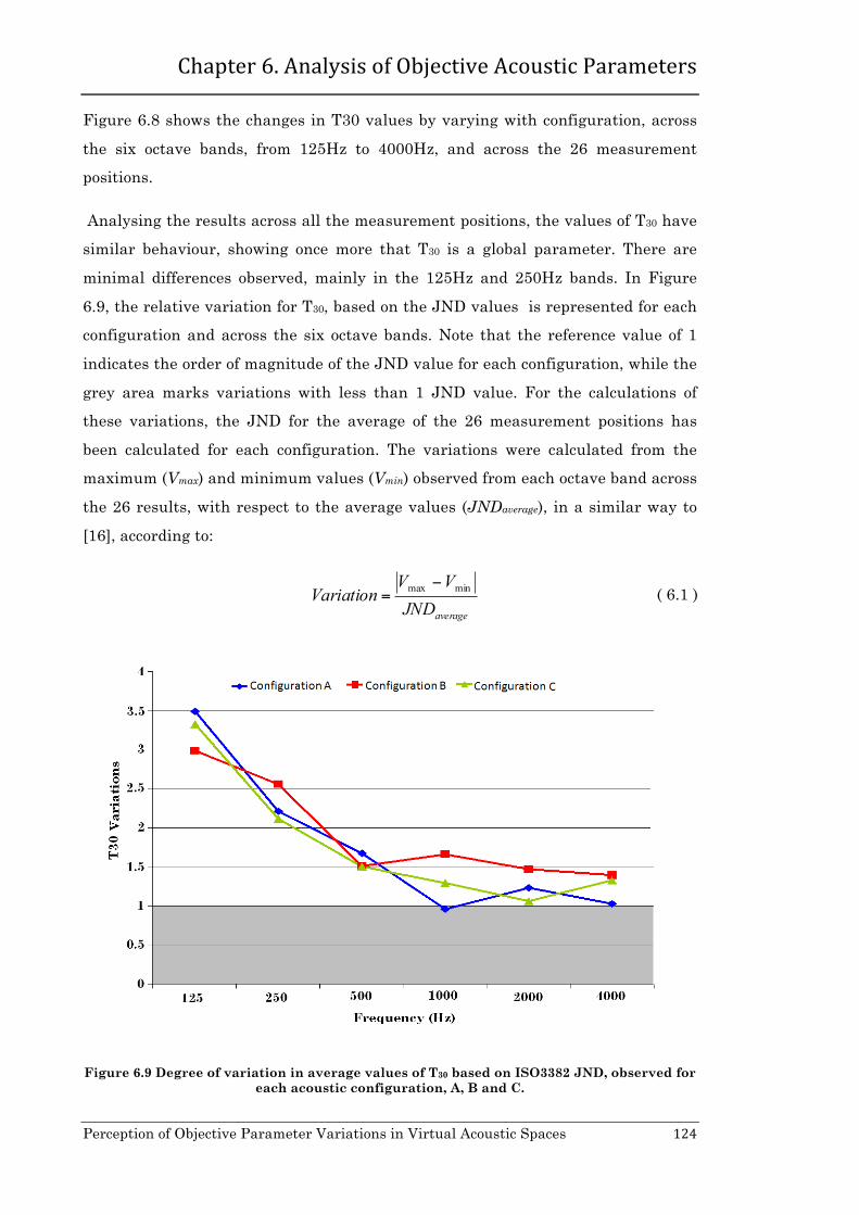
Chapter 6. Analysis of Objective Acoustic Parameters
Perception of Objective Parameter Variations in Virtual Acoustic Spaces 124
Figure 6.8 shows the changes in T30 values by varying with configuration, across
the six octave bands, from 125Hz to 4000Hz, and across the 26 measurement
positions.
Analysing the results across all the measurement positions, the values of T30 have
similar behaviour, showing once more that T30 is a global parameter. There are
minimal differences observed, mainly in the 125Hz and 250Hz bands. In Figure
6.9, the relative variation for T30, based on the JND values is represented for each
configuration and across the six octave bands. Note that the reference value of 1
indicates the order of magnitude of the JND value for each configuration, while the
grey area marks variations with less than 1 JND value. For the calculations of
these variations, the JND for the average of the 26 measurement positions has
been calculated for each configuration. The variations were calculated from the
maximum (Vmax) and minimum values (Vmin) observed from each octave band across
the 26 results, with respect to the average values (JNDaverage), in a similar way to
[16], according to:
averageJNDVV
Variation minmax −= ( 6.1 )
Figure 6.9 Degree of variation in average values of T30 based on ISO3382 JND, observed for each acoustic configuration, A, B and C.

Chapter 6. Analysis of Objective Acoustic Parameters
Perception of Objective Parameter Variations in Virtual Acoustic Spaces 125
Analysing each individual position, there is an obvious difference in the T30 values
for configuration C (all the acoustic panels closed), compared to those observed
with configurations A and B. However, the differences between configuration A
(75% of the acoustic panels open) and configuration B (all the acoustic panels open)
are minimal, with the maximum value of 2.38 JND (as will be explained further in
7.2 and represented in Appendix D).

Chapter 6. Analysis of Objective Acoustic Parameters
Perception of Objective Parameter Variations in Virtual Acoustic Spaces 126
Figure 6.10 Acoustic floor map of EDT values obtained from the measurements varying with configurations A, B and C across the grid of 26 receiver positions.
EDT$
Confi
gura)o
n*A*
Confi
gura)o
n*B*
Confi
gura)o
n*C*
1*2*
3*4*
5*6*
7*8*
9*
10*
11*
12*
13*
14*
15*
16*
17*
18*
19*
20*
21*
22*
23*
24*
25*
26*

Chapter 6. Analysis of Objective Acoustic Parameters
Perception of Objective Parameter Variations in Virtual Acoustic Spaces 127
Figure 6.10 shows the changes in EDT values across all measurement positions, for
configurations A, B and C. It is observed that firstly, the behaviour of EDT follows
that observed for T30 values (Figure 6.8), although differences in the results across
positions are more noticeable. As Behler [91] notes, EDT seems to be more
sensitive to position than T30, as it considers the effect of early reflections.
However, from these results the effects of walls, corners, or columns on EDT values
are not obvious at adjacent measurement positions. It is interesting to note that,
for the north wall, changes had been made by closing and opening panels according
to configurations A and B. However this change does not have significant effects on
the observed EDT values.
The differences across the positions are calculated to be more than the quoted JND
for this parameter, according to ISO3382 [55]. At shorter distances between source
and receiver positions, where the direct sound level is higher, lower EDT values are
expected to be observed, as explained in [34]. However, this phenomenon is only
more obvious for the low frequencies of 125Hz and 250Hz, as due to air absorption
(as described in section 2.3.4) the phenomenon is masked for the high frequencies,
especially above 1000Hz. For example in the results observed at R4, R22 and R13
where values increase with an increase in distance for 125Hz an 250 Hz, while
values are approximately the same for higher frequencies. The acoustic floor maps
for each configuration are presented in Appendix C, Measurements, for a more
detailed observation.

Chapter 6. Analysis of Objective Acoustic Parameters
Perception of Objective Parameter Variations in Virtual Acoustic Spaces 128
Figure 6.11 Acoustic floor map of C50 values obtained from the measurements varying with configuration A, B and C across the grid of 26 receiver positions.
C50$
Confi
gura)o
n*A*
Confi
gura)o
n*B*
Confi
gura)o
n*C*
1*2*
3*4*
5*6*
7*8*
9*
10*
11*
12*
13*
14*
15*
16*
17*
18*
19*
20*
21*
22*
23*
24*
25*
26*

Chapter 6. Analysis of Objective Acoustic Parameters
Perception of Objective Parameter Variations in Virtual Acoustic Spaces 129
Figure 6.12 Acoustic floor map of C80 values obtained from the measurements varying with configuration A, B and C across the grid of 26 receiver positions.
C80$
Confi
gura)o
n*A*
Confi
gura)o
n*B*
Confi
gura)o
n*C*
1*2*
3*4*
5*6*
7*8*
9*
10*
11*
12*
13*
14*
15*
16*
17*
18*
19*
20*
21*
22*
23*
24*
25*
26*

Chapter 6. Analysis of Objective Acoustic Parameters
Perception of Objective Parameter Variations in Virtual Acoustic Spaces 130
It has been discussed in previous works [70, 74, 182], how C80 and C50 change over
a space, depending on the shape of the room and the distance from the source. The
results presented in Figure 6.11 and Figure 6.12 confirm that both parameters, C50
and C80 are position dependent parameters.
It is also observed that for each individual measurement position, C50/C80 values
are very similar for each of the configurations, A, B and C. This does not
necessarily mean, however, that the same early and late energy is arriving at the
receiver positions for all acoustic configurations, as clarity (C50/C80), from
definition, describes the ratio of energy. This implies that if a physical change in
the space influences both early and late reflections in the same way, the values of
Clarity (C50/C80) and LF will remain similar but the audible results and
reverberation times (T30 and EDT) will significantly change. This could also explain
the “unexpected” results of Clarity and LF when seats have been present in a
concert hall project [88], where the resulting longer reverberation and increased
values for strength (G) did not influence the energetic parameters.
Comparing the results of the measurement positions row by row, one would expect
that positions closer to the source to have better (higher) values for C50/C80. Going
further away from the source, one would expect to observe more energy in the later
part of the impulse response, due to the greater diffusion of sound, and as a result
of that, lower values for C50/C80, as shown in [104]. However, in this study case,
these expected results are not observed across all the measured positions in a
similar way. Dividing the space into region (a), region (b), and region (c), as shown
in Figure 6.13, it is noticeable that the expected results can be observed in region
(a) and to an even greater extent in region (b). In particular, the receivers R13,
R14, R15, which are closest to the source, have higher values for C50/C80. However,
in region (c), C50/C80 has smaller values for all 3 rows. This could be the result of
later reflections coming from the floor tower section, at the south west side of the
church.

Chapter 6. Analysis of Objective Acoustic Parameters
Perception of Objective Parameter Variations in Virtual Acoustic Spaces 131
Figure 6.13 Observing C80 values across measurement positions in divided into three regions, (a), (b) and (c).
For 125Hz and 250Hz especially, at a few measurement positions there is a steep
incline in C50/C80 values compared with the rest of the charts. For example, at R18
there is a sharp increase of C50/C80 values at 250Hz, while at R16, the opposite
behaviour is observed for 125Hz and 250Hz. A further investigation was carried
out for these measured positions by comparing the frequency domain analysis
obtained from these two impulse responses, at positions R18 and R16 and
comparing them with R10, which has more regular curve at these frequencies
(Figure 6.14). The observed differences at the frequency range between 150Hz and
400Hz could be explained due to nodes/anti-nodes of standing waves, which as
discussed in section 2.3.6 influence the sound energy.
C80$
Confi
gura)o
n*A*
Confi
gura)o
n*B*
Confi
gura)o
n*C*
1*2*
3*4*
5*6*
7*8*
9*
10*
11*
12*
13*
14*
15*
16*
17*
18*
19*
20*
21*
22*
23*
24*
25*
26*
a"
c"
b"

Chapter 6. Analysis of Objective Acoustic Parameters
Perception of Objective Parameter Variations in Virtual Acoustic Spaces 132
Figure 6.14 Frequency domain analysis of R10 (red line), R16 (blue line) and R18 (green line) for configuration A (using Hamming window and with FFT size at 4096).
As with the EDT values, the effects of specific walls, corners, or columns on
adjacent measurement positions cannot be observed with C50/C80 parameters.
Even though the critical distance had been considered for the measurement
positions, from the results observed in Figure 6.11 and Figure 6.12, much higher
C50/C80 values R13 and R14 have been noted compared with the rest. Hence, it is
assumed that their distance is not sufficiently far away from the source and these
measurement positions should not be used for the purposes of the current study.

Chapter 6. Analysis of Objective Acoustic Parameters
Perception of Objective Parameter Variations in Virtual Acoustic Spaces 133
Results obtained from changes in source orientations 6.5.2
Figure 6.15 Acoustic floor map of T30 values obtained from the measurements varying with source orientation 0°, 40° and 70°, across the grid of 26 receiver positions.
T30$
0°#Orie
nta+
on#
40#°#Orie
nta+
on#
70#°#Orie
nta+
on#
1#2#
3#4#
5#6#
7#8#
9#
10#
11#
12#
13#
14#
15#
16#
17#
18#
19#
20#
21#
22#
23#
24#
25#
26#
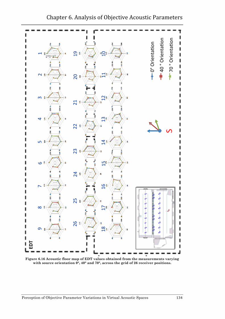
Chapter 6. Analysis of Objective Acoustic Parameters
Perception of Objective Parameter Variations in Virtual Acoustic Spaces 134
Figure 6.16 Acoustic floor map of EDT values obtained from the measurements varying with source orientation 0°, 40° and 70°, across the grid of 26 receiver positions.
EDT$
0°#Orie
nta+
on#
40#°#Orie
nta+
on#
70#°#Orie
nta+
on#
1#2#
3#4#
5#6#
7#8#
9#
10#
11#
12#
13#
14#
15#
16#
17#
18#
19#
20#
21#
22#
23#
24#
25#
26#

Chapter 6. Analysis of Objective Acoustic Parameters
Perception of Objective Parameter Variations in Virtual Acoustic Spaces 135
Figure 6.17 Acoustic floor map of C50 values obtained from the measurements varying with source orientation, 0°, 40° and 70°, across the grid of 26 receiver positions.
C50$
0°#Orie
nta+
on#
40#°#Orie
nta+
on#
70#°#Orie
nta+
on#
1#2#
3#4#
5#6#
7#8#
9#
10#
11#
12#
13#
14#
15#
16#
17#
18#
19#
20#
21#
22#
23#
24#
25#
26#

Chapter 6. Analysis of Objective Acoustic Parameters
Perception of Objective Parameter Variations in Virtual Acoustic Spaces 136
C80$
0°#Orie
nta+
on#
40#°#Orie
nta+
on#
70#°#Orie
nta+
on#
1#2#
3#4#
5#6#
7#8#
9#
10#
11#
12#
13#
14#
15#
16#
17#
18#
19#
20#
21#
22#
23#
24#
25#
26#
Figure 6.18 Acoustic floor map of C80 values obtained from the measurements varying with source orientation, 0°, 40° and 70°, across the grid of 26 receiver positions.

Chapter 6. Analysis of Objective Acoustic Parameters
Perception of Objective Parameter Variations in Virtual Acoustic Spaces 137
As described in section 5.4, the orientation of the Genelec loudspeaker used for the
impulse response measurements was changed from 0°, facing the “audience”, to 40°
and 70° respectively on its axis. The set up of the acoustic panels was the same as
that of configuration A. From Figure 6.15 and Figure 6.16, it can be observed that
the effects on the reverberation parameters range from no change (in T30 values) to
minimal changes only (in EDT values), if the changes in each measurement
position are considered individually. It is interesting to note that most of the
changes in EDT values are obtained at positions where the physical characteristics
of the space (such as nearly walls or columns), combined with the effects of source
directivity influence the energy of the early reflections. This is because by rotating
the on axis position of the loudspeaker, stronger reflections arrive at the
measurement positions, after their interaction with the boundaries of the space.
In the waveforms of the impulse responses, as discussed at Figure 6.5 above, the
first reflections appear much stronger than the direct sound, as a result of the non-
omnidirectivity of the sound source. These strong early reflections influence the
related EDT values (even if the changes are minimal) and even more obviously the
C50/C80 parameters.
By comparing the behaviour of C50 and C80 across measurement positions and
source orientation, there was a greater variation in C80 across individual positions
than for corresponding C50 results, as shown in Figure 6.17and Figure 6.18. The
acoustic floor maps for each configuration are presented in Appendix C,
Measurements, for a more detailed observation.

Chapter 6. Analysis of Objective Acoustic Parameters
Perception of Objective Parameter Variations in Virtual Acoustic Spaces 138
CATT-Acoustic IRs 6.6
Figure 6.19 Acoustic floor map of T30 values obtained from the CATT-Acoustic model varying with configuration A, B and C across the grid of 26 receiver positions.
T30$
Confi
gura)o
n*A*
Confi
gura)o
n*B*
Confi
gura)o
n*C*
1*2*
3*4*
5*6*
7*8*
9*
10*
11*
12*
13*
14*
15*
16*
17*
18*
19*
20*
21*
22*
23*
24*
25*
26*

Chapter 6. Analysis of Objective Acoustic Parameters
Perception of Objective Parameter Variations in Virtual Acoustic Spaces 139
Figure 6.20 Acoustic floor map of EDT values obtained from the CATT-Acoustic model varying with configuration A, B and C across the grid of 26 receiver positions.
EDT$
Confi
gura)o
n*A*
Confi
gura)o
n*B*
Confi
gura)o
n*C*
1*2*
3*4*
5*6*
7*8*
9*
10*
11*
12*
13*
14*
15*
16*
17*
18*
19*
20*
21*
22*
23*
24*
25*
26*
Chapter 6. Analysis of Objective Acoustic Parameters
Perception of Objective Parameter Variations in Virtual Acoustic Spaces 140
In Figure 6.19, T30 values are represented across the 26 measurement positions for
configurations A, B and C across the six octave bands studied, from 125Hz to
4000Hz. It is important to note that the values of T30 vary with acoustic
configuration, as the curves of the three configurations change respectively from
the less (configuration B) to the most reverberant (configuration C). T30 values have
small variations across all receiver positions. The largest differences were observed
mainly at 125Hz and 250Hz for configuration A. By observing individual positions
and the T30 values, between the configuration A and configuration B there are only
minimal differences, while T30 values for configuration C have increased up to 0.5s
more than those observed for the other two configurations across all the octave
bands.
Figure 6.20 shows the changes in EDT values across all measurement positions, for
each of the three configurations. It can be observed that EDT has similar behaviour
with T30 values, across the three configurations studied, as the curves change
respectively from the less to the most reverberant. However, the curves have some
steep changes across octave bands, which are not comparable with the
corresponding T30 values. This could indicate the direct influence of specific
surfaces, such as walls or columns, on early reflections. It is difficult to draw more
definite conclusions as these effects do not seem to demonstrate any repeated
and/or symmetric behaviour across the measurement positions.
Appendix C, CATT-Acoustic, contain corresponding figures, showing in more detail
the behaviour of EDT across the space for each configuration.
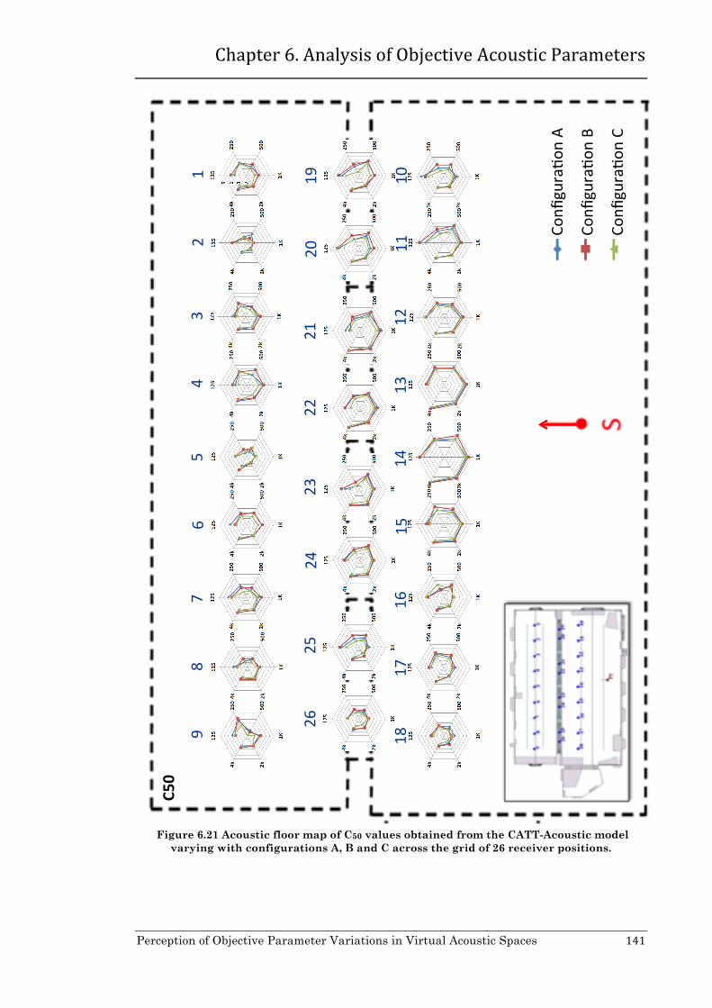
Chapter 6. Analysis of Objective Acoustic Parameters
Perception of Objective Parameter Variations in Virtual Acoustic Spaces 141
Figure 6.21 Acoustic floor map of C50 values obtained from the CATT-Acoustic model varying with configurations A, B and C across the grid of 26 receiver positions.
C50$
Confi
gura)o
n*A*
Confi
gura)o
n*B*
Confi
gura)o
n*C*
1*2*
3*4*
5*6*
7*8*
9*
10*
11*
12*
13*
14*
15*
16*
17*
18*
19*
20*
21*
22*
23*
24*
25*
26*

Chapter 6. Analysis of Objective Acoustic Parameters
Perception of Objective Parameter Variations in Virtual Acoustic Spaces 142
Figure 6.22 Acoustic floor map of C80 values obtained from CATT-Acoustic model varying with configurations A, B and C across the grid of 26 receiver positions.
C80$
Confi
gura)o
n*A*
Confi
gura)o
n*B*
Confi
gura)o
n*C*
1*2*
3*4*
5*6*
7*8*
9*
10*
11*
12*
13*
14*
15*
16*
17*
18*
19*
20*
21*
22*
23*
24*
25*
26*

Chapter 6. Analysis of Objective Acoustic Parameters
Perception of Objective Parameter Variations in Virtual Acoustic Spaces 143
C50 (Figure 6.21) and C80 (Figure 6.22) change over the space, confirming that both
parameters are position dependent, as C50 and C80 vary across the receiver
positions. It is also observed that for each individual measurement position, C50/C80
curves have quite similar behaviour across the three configurations.
Dividing the space into three regions as before, shown in Figure 6.13, it is
noticeable that in the regions (a) and (b) (with the exception of R10) the further
away from the source the receiver positions are, the lower the values for C50/C80,
while C50/C80 increases for positions closer to the source. This cannot be noticed
however, in region (c), where low values for C50/C80 are observed for all 3 rows.
Finally, as was the case with the measurement results, higher values of C50/C80 are
observed for R13 and R14 here as well, which confirms that these impulse
responses are unsuitable for the purposes of this study.
Appendix C, CATT-Acoustic contains corresponding figures, showing in more
detail the behaviour of C80 across the space, separately for each configuration.

Chapter 6. Analysis of Objective Acoustic Parameters
Perception of Objective Parameter Variations in Virtual Acoustic Spaces 144
ODEON IRs 6.7
Figure 6.23 Acoustic floor map of T30 values obtained from the ODEON model varying with configurations A, B and C across the grid of 26 receiver positions.
T30$
Confi
gura)o
n*A*
Confi
gura)o
n*B*
Confi
gura)o
n*C*
1*2*
3*4*
5*6*
7*8*
9*
10*
11*
12*
13*
14*
15*
16*
17*
18*
19*
20*
21*
22*
23*
24*
25*
26*

Chapter 6. Analysis of Objective Acoustic Parameters
Perception of Objective Parameter Variations in Virtual Acoustic Spaces 145
Figure 6.24 Acoustic floor map of EDT values obtained from the ODEON model varying with configurations A, B and C across the grid of 26 receiver positions.
EDT$
Confi
gura)o
n*A*
Confi
gura)o
n*B*
Confi
gura)o
n*C*
1*2*
3*4*
5*6*
7*8*
9*
10*
11*
12*
13*
14*
15*
16*
17*
18*
19*
20*
21*
22*
23*
24*
25*
26*

Chapter 6. Analysis of Objective Acoustic Parameters
Perception of Objective Parameter Variations in Virtual Acoustic Spaces 146
The T30 values are increased respectively across the three configurations, from the
less (configuration B) to the most reverberant configuration (configuration C), as
shown in Figure 6.23.
Across all receiver positions, there are minimal variations in T30. For the individual
positions, small differences are noted, especially between configurations A and B,
with configuration A slightly more reverberant, as would be expected. T30 values
for configuration C have increased up to 0.5s more than those observed for the
other two configurations across all the octave bands.
Figure 6.24 shows that changes in EDT across all measured positions are minimal
for the three configurations. It is also observed that EDT has behaviour
corresponding to that of T30, across each of the three configurations studied.
Additionally, it can be noticed once more that higher values of C50/C80 are observed
for R13 and R14, as observed in measurements and CATT-Acoustic results as well.
Appendix C, ODEON, contains corresponging figures, showing in more detail the
behaviour of EDT across the space, separately for each configuration.

Chapter 6. Analysis of Objective Acoustic Parameters
Perception of Objective Parameter Variations in Virtual Acoustic Spaces 147
Figure 6.25 Acoustic floor map of C50 values obtained from the ODEON model varying with configurations A, B and C across the grid of 26 receiver positions.
C50$
Confi
gura)o
n*A*
Confi
gura)o
n*B*
Confi
gura)o
n*C*
1*2*
3*4*
5*6*
7*8*
9*
10*
11*
12*
13*
14*
15*
16*
17*
18*
19*
20*
21*
22*
23*
24*
25*
26*

Chapter 6. Analysis of Objective Acoustic Parameters
Perception of Objective Parameter Variations in Virtual Acoustic Spaces 148
Figure 6.26 Acoustic floor map of C80 values obtained from the ODEON model varying with configurations A, B and C across the grid of 26 receiver positions.
C80$
Confi
gura)o
n*A*
Confi
gura)o
n*B*
Confi
gura)o
n*C*
1*2*
3*4*
5*6*
7*8*
9*
10*
11*
12*
13*
14*
15*
16*
17*
18*
19*
20*
21*
22*
23*
24*
25*
26*

Chapter 6. Analysis of Objective Acoustic Parameters
Perception of Objective Parameter Variations in Virtual Acoustic Spaces 149
As expected C50, (Figure 6.25) and C80 (Figure 6.26) vary across the space, as these
are highly position dependent parameters. It is also observed that for each
individual measurement position, C50/C80 values are similar for each of the three
configurations. It is important to note here once more though that this does not
necessarily mean the same early and late energy is arriving at the receiver
positions for all acoustic configurations, as C50/C80, from definition, describes the
ratio of early to late energy.
Dividing the space into three regions, as previously shown in Figure 6.13, it is
noticeable that in the regions (a) and (b), the receiver positions further away from
the source have lower C50/C80 values, while C50/C80 increases for positions closer to
the source. This cannot be noticed however, in region (c), where low values for
C50/C80 are observed for all 3 rows, and as explained before this could be the
influence of the late reflections arriving from the ground tower area, in region (c) of
the space. Higher values of C50/C80 for R13 and R14 are observed as well. Appendix
C, ODEON, contains corresponding figures, showing in more detail the behaviour
of C80 across the space, separately for each configuration.

Chapter 6. Analysis of Objective Acoustic Parameters
Perception of Objective Parameter Variations in Virtual Acoustic Spaces 150
Summary 6.8
In this chapter, the process used to calculate the acoustic parameters is explained
in more detail, followed by a description of the methodology, which involved
deconvolution of the recorded sine sweeps obtained from the actual space, as well
as a discussion of the reasons for choosing the parameters considered for this
current study. A novel to analyse and represent the data collected - “acoustic floor
maps” – is also described, along with the data for the multiple positions studied,
based on their behaviour across octave bands.
The analysis includes data obtained from the measured impulse responses, and the
impulses responses produced by CATT-Acoustic and ODEON models. The results
of these three different auralization techniques were presented separately, as there
was not any intention in this study to make comparisons between them. The
simulated models, as described in the previous chapter, were created quite
independently from the measurement results, as the optimisation of the models
was not necessary for the purposes of this study.
The next step, explained in the following chapter, is to select the appropriate
impulse responses from this wide data set, based on observed acoustic parameters
values for the purposed listening tests leading to confirmation of the hypothesis
under investigation.

Chapter 7.Subjective evaluations of Auralized St. Margaret’s
Church
Perception of Objective Parameter Variations in Virtual Acoustic Spaces 151
Chapter 7.
Subjective evaluations of
Auralized St. Margaret’s Church
Introduction 7.1
A considerable amount of literature exists regarding various procedures for
evaluating the acoustic quality of spaces, both real and virtual. Over the years
researchers have sought to build a framework capable of explaining the subjective
sense of these acoustic effects and to correlate them with the objective parameters
values [43, 80, 82, 101, 163, 207, 213-219].
The common approach to studying the psychoacoustic impression of a space is to
analyse the perceptual results obtained from asking listeners who have visited the
space, either in the audience or as music performers. Surveys of such cases are
based on questionnaires administered to the listeners during or after their
presence in the space [82, 219, 220].
Auralization applications have introduced an additional approach for the study of
these psychoacoustic effects. Anechoic recording samples are convolved with
impulse responses, either obtained from measurements in-situ or from computer
models. Convolution can be applied in real-time in laboratories, in conditions where
researchers can control the reproduction and rendering process [26, 42, 65, 72, 161,
221], as shown in Figure 7.1.

Chapter 7.Subjective evaluations of Auralized St. Margaret’s
Church
Perception of Objective Parameter Variations in Virtual Acoustic Spaces 152
Figure 7.1 For auralization, impulse responses are convolved with anechoic stimuli and the output is reproduced in laboratories applying multi-channel reproduction, under the
control of the researchers.
However, acoustic perception has a variety of aspects and is influenced by factors
such as the loudness of the sound, its intelligibility, the reverberation and the
spatial information [209, 222]. Hence, even “after a hundred years of reverberation
time” [205], we still cannot describe with accuracy what we listen to nor the
correlation of subjective and objective measures.
As stated in this thesis, the subjective quality of the auralization results of a
virtual acoustic environment is at least as important as the objective evaluation of
the relevant acoustic parameters. In order to investigate the sensitivity of listeners
to auralization changes occurring in a particular space, changes have been made to
the physical acoustic characteristics of St. Margaret’s Church. In the previous
chapters, the methodology followed for the purpose of this work was described in
detail. It has been explained how the required impulse responses of real spaces
were measured in situ or produced by acoustic simulation, using CATT-Acoustic
and ODEON software (Chapter 5). The four main objective measures of these
impulse responses were then analysed and presented in Chapter 6.
For the subjective evaluation of these changes, listening tests were performed for
each of the three different auralization techniques. In this chapter, the procedure
followed for the selection of the auralization examples as well as the procedure for
carrying out the listening tests conducted, are described in detail and the results
are analysed in-depth.
Pilot Experiment from Auralized St. Margaret’s 7.2
Church
Before introducing the listening tests conducted for the purposes of this research,
the results of a preliminary listening test are worth mentioning [133]. The
experiment was also based on impulse responses obtained from in-situ

Chapter 7.Subjective evaluations of Auralized St. Margaret’s
Church
Perception of Objective Parameter Variations in Virtual Acoustic Spaces 153
measurements of St. Margaret’s Church and the two simulation models in CATT-
Acoustic and ODEON. These tests were based on preliminary versions of the
models, with less appropriately defined material for the walls. The results
ultimately showed longer reverberation time for the models than those observed
with the final versions, were used in the main test (Figure 5.22 and Figure 5.23).
The goal of the initial listening tests was to validate the objective results observed
using the three different auralization techniques in each of the three acoustic
configurations. Six subjects were asked to listen to 16 pairs of samples, which were
created by convolving impulse responses of the three acoustic configurations and
the three auralization techniques with female singing and male speech. The
subjects’ first task was to identify the most reverberant sound of each pair and
then to express the degree of similarity in terms of the perceived reverberation by
marking a point on a scale with values from 1 (very similar) to 10 (very different).
The results shown a clear perceptual difference between the real and virtual cases.
However, a very interesting point was that all participants indicated that the
measurement results were more reverberant than either the ODEON or CATT
models when comparison between them was taking place, even though both models
had significantly longer reverberation times than the actual measurements. This
confirmed the importance of looking at parameters other than reverberation time
when optimising such models even if the study is focused on the perception of
reverberance.
Selection of the Impulse Responses for Auralization 7.3
Three different auralization methods are examined for the current hypothesis;
based on impulse responses: 1) measured in the actual space and generated in
virtual acoustic models by using 2) CATT-Acoustic and 3) ODEON software. Thus,
for the evaluation of the results, it was necessary to conduct listening tests
separately for each case, but following exactly the same procedure.
It was crucial to find a suitable method to compare the values of the parameters
studied across configurations A, B and C, and over the different receiver positions.
Following the precedent set by previous studies [29], the corresponding JND values
for each parameter, averaged over 500Hz and 1000Hz octave bands were used as a

Chapter 7.Subjective evaluations of Auralized St. Margaret’s
Church
Perception of Objective Parameter Variations in Virtual Acoustic Spaces 154
reference value for these comparisons. According to ISO3382 [55] (section 2.6), the
JND for parameters such as T30 and EDT, are defined to be within 5% of the
measured values, assuming a typical range of 1.0s to 3.0s. For clarity (C50/C80) JND
is defined to be 1dB, for a typical range of values from -5dB to +5dB.
Thus, in order to include all the results obtained from the study, from all the 26
receiver positions for each of the three acoustic configurations, A, B, and C, the
values of the four acoustic parameters were sorted in increasing order. The JND of
the minimum observed value was calculated and used as a reference value for the
comparison of the changes for each of the parameters. For the calculation of the
JND, the average values of T30, EDT, C50 and C80 over 500 and 1000Hz octave
bands were used, based on the recommendations of ISO3382 [55]. The lists are
represented in Appendix D.
From these lists, the R13 and R14 positions were excluded as their distance from
the source was not considered large enough for reliable results, even if they were
placed further away from the corresponding critical distance in each measurement
configuration (theoretically calculated). The direct sound was too strong and there
was not as good a balance between early and late reflections.
Note that the goal of this study is not to compare the different auralization
methods. As explained previously in the thesis, such a comparison is not accurate
and will not give scientific results about the perceptual differences that occur due
to observed changes in the related acoustic parameters. Their comparison is used
in other work as a guide for acoustic designers and developers of acoustic
simulation software, as discussed in previous chapters. In this study, it is
necessary to focus on the results of each auralization method individually in order
to examine the perceptual differences of different acoustic metrics and parameters.
The method for the evaluation of these changes was to ask the subjects if they
could perceive differences by comparing pairs using the A/B comparison method as
in [72, 190, 213, 222]. The pairs were categorised in different groups according to
the parameter(s) studied. For each pair in the group, the samples differed from
each other in terms of the JND variations, which were increased for each pair,
while keeping the rest of the acoustic parameters studied within 1 JND variation.

Chapter 7.Subjective evaluations of Auralized St. Margaret’s
Church
Perception of Objective Parameter Variations in Virtual Acoustic Spaces 155
Due to this methodology, the selected samples differed in terms of physical acoustic
changes as well. Hence, pairs would compare samples from different acoustic
configurations, different orientation of the source (for the samples obtained from
the actual measurements), or from different measurement positions within the
space. As mentioned earlier (in section 6.3), the impulse responses were all
normalised so that the level of the direct sound was equal in each of them, as in
[190].
The same methodology was followed for all the impulse responses observed from
each of the three different auralization techniques, the characteristics of which are
presented in detail in the following section. Hence, the first step of the auralization
procedure was completed with the selection of suitable impulse responses from all
three auralization techniques, as represented in Figure 7.2.
Figure 7.2 The impulse responses required for the first step of the auralization procedure are selected from the impulse responses obtained from the acoustic measurements in-situ, and from the impulse responses generated by both acoustic models, in CATT-Acoustic and
ODEON software.
Impulse responses from measurements 7.3.1
For the perceptual evaluation of the variations of the four acoustic parameters
observed from the acoustic measurements in-situ, data from all three acoustic
configurations and from the three source orientation configurations were included.
The selected examples were based on different groups based on the values of the
acoustic parameters and the relative JND values, as shown in Table 7.1 and Table
7.2 based on the measurements of the three acoustic configurations and the three
source orientations respectively.

Chapter 7.Subjective evaluations of Auralized St. Margaret’s
Church
Perception of Objective Parameter Variations in Virtual Acoustic Spaces 156
Table 7.1 Calculating the JNDs obtained from the single number averaged across 500Hz and 1000Hz octave bands, for each parameter based on the minimum observed values (Appendix D, Measurements, Configurations A, B and C) from the measured impulse
responses of the three acoustic configurations.
T30 EDT C50 C80 Minimum Values R24 1.358 R22 1.2535 R18 -‐4.6015 R8 -‐1.787 JND 0.0679 0.062675 1 1
Table 7.2 Calculating the JNDs obtained from the single number averaged across 500Hz and 1000Hz octave bands, for each parameter based on the minimum observed values
(Appendix D, Measurements, Source Orientations 0°, 40°, 70°) from the measured impulse responses of the three source orientations.
T30 EDT C50 C80 Minimum Values R18 1.4305 R10 1.2115 R18 -‐7.0295 R18 -‐3.547 JND 0.071525 0.060575 1 1
As shown in Table 7.3 and Table 7.4, the pairs of examples for the A/B comparison
differed in each group, based on a defined characteristic. The colours indicate the
acoustic configuration from which each impulse response was captured, while the
examples defined with (*) include the impulse responses captured from the
different source orientation configurations. Out of the 130 possible total recordings
from the actual space, 33 were used for the listening tests and 20 pairs of impulse
responses were selected as appropriate for the purpose of this study.

Chapter 7.Subjective evaluations of Auralized St. Margaret’s
Church
Perception of Objective Parameter Variations in Virtual Acoustic Spaces 157
Table 7.3 The groups of pairs from the in-situ measured impulse responses. 20 pairs of A/B
impulse responses were selected based on the calculated acoustic parameter values. The
colours indicate the acoustic configurations for each impulse response (Blue for
Configuration A, Red for configuration B and Green for configuration C). The pairs
defined with (*) are impulse responses from the source orientation configurations (Blue
for the 0° orientation of the source, Red for the 40° and Green for the 70°).
Selected Pairs for Measurements Pair A B T30 EDT C50 C80 1 R26 R5 1.378 1.3825 1.4425 1.4395 -‐2.357 -‐2.1815 0.472 0.7875 2* R1 R15 1.475 1.4625 1.5505 1.546 -‐1.471 -‐1.1735 0.6465 0.601 3 R8 R18 1.795 1.7755 1.8045 1.7555 -‐4.195 -‐4.6015 -‐1.787 -‐1.5025 4 R23 R12 1.8165 1.81653 1.767 1.761 0.3285 1.175 2.785 3.1355 5 R6 R6 1.454 1.373 1.5875 1.468 -‐1.3155 -‐0.3575 1.788 2.4065 6 R6 R6 1.454 1.78 1.5875 1.7865 -‐1.3155 -‐2.437 1.788 0.4985 7 R6 R6 1.373 1.78 1.468 1.7865 -‐0.3575 -‐2.437 2.4065 0.4985 8 R23 R24 1.4385 1.358 1.3145 1.5555 1.36 0.133 4.3455 1.8025 9 R17 R17 1.4495 1.794 1.5065 1.9075 -‐2.1595 -‐3.0455 0.085 -‐0.3015 10 R9 R8 1.3855 1.4905 1.5325 1.533 -‐1.078 -‐2.6455 0.9905 0.5185 11 R22 R21 1.476 1.41 1.2535 1.275 1.292 2.2455 5.101 4.5365 12 R24 R11 1.358 1.366 1.5555 1.416 0.133 0.09 1.8025 2.8795
13 R3 R20 1.8495 1.7935 1.705 1.9165 -‐1.7435 -‐1.564 0.886 0.84 14 R5 R2 1.3825 1.3785 1.4395 1.314 -‐2.1815 -‐1.555 0.7875 0.7575 15 R20 R21 1.387 1.41 1.2775 1.275 -‐0.426 2.2455 2.7935 4.5365 16* R20 R20 1.468 1.476 1.394 1.3995 -‐1.01 0.7755 2.01 3.444 17 R11 R17 1.4465 1.4495 1.5105 1.5065 2.235 -‐2.1595 4.1775 0.085 18 R18 R15 1.7755 1.7765 1.7555 1.873 -‐4.6015 -‐0.2605 -‐1.5025 1.1455 19 R3 R1 1.514 1.4935 1.4555 1.517 -‐0.4155 -‐2.796 1.963 -‐0.38 20* R18 R18 1.4505 1.4305 1.4275 1.5695 -‐4.2625 -‐7.0295 -‐0.745 -‐3.547
3 These two positions had exactly the same calculated T30 values, as an average of 500Hz
and 1000Hz octave bands.

Chapter 7.Subjective evaluations of Auralized St. Margaret’s
Church
Perception of Objective Parameter Variations in Virtual Acoustic Spaces 158
Table 7.4 The groups of pairs from the in-situ measured impulse responses. 20 pairs of A/B
impulse responses were selected based on their difference in absolute JND values
(approximated at the second decimal) obtained from the single number averaged across
500Hz and 1000Hz octave bands. The colours indicate the acoustic configurations for each
impulse response (Blue for Configuration A, Red for configuration B and Green for
configuration C), while the differences with more than 1 JND value are highlighted in
grey. The pairs defined with (*) are impulse responses from the source orientation
configurations (Blue for the 0° orientation of the source, Red for the 40° and Green for the
70°).
Differences in JND values Pair A B T30 EDT C50 C80 1 R26 R5 0.0662739 0.047866 0.1755 0.3155 T30/EDT/C50/C80 < JND 2* R1 R15 0.1747641 0.0742881 0.2975 0.0455 T30/EDT/C50/C80 < JND 3 R8 R18 0.287187 0.7818109 0.4065 0.2845 T30/EDT/C50/C80 < JND 4 R23 R12 0 0.095732 0.8465 0.3505 T30/EDT/C50/C80 < JND 5 R6 R6 1.1929308 1.9066613 0.958 0.6185 C50/C80 < JND, T30/EDT ≥ JND 6 R6 R6 4.8011782 3.1751097 1.1215 1.2895 T30/EDT/C50/C80 ≥ JND 7 R6 R6 5.994109 5.081771 2.0795 1.908 T30/EDT/C50/C80 ≥ JND 8 R23 R24 1.185567 3.8452333 1.227 2.543 T30/EDT/C50/C80 ≥ JND 9 R17 R17 5.0736377 6.3980854 0.886 0.3865 C50/C80 < JND, T30/EDT ≥ JND 10 R9 R8 1.5463918 0.0079777 1.5675 0.472 EDT/C80 < JND, T30/C50 ≥ JND 11 R22 R21 0.9720177 0.3430395 0.9535 0.5645 EDT/C80 < JND, T30/C50 ≥ JND 12 R24 R11 0.1178203 2.2257679 0.043 1.077 T30/C50 < JND, EDT/C80 ≥JND 13 R3 R20 0.8247423 3.3745513 0.1795 0.046 T30/C50/C80 < JND, EDT >JND 14 R5 R2 0.0589102 2.0023933 0.6265 0.03 T30/C50/C80 < JND, EDT >JND 15 R20 R21 0.3387334 0.0398883 2.6715 1.743 T30/EDT < JND, C50/C80 > JND 16* R20 R20 0.111849 0.0907965 1.7855 1.434 T30/EDT < JND, C50/C80 > JND 17* R11 R17 0.0419434 0.0660338 4.3945 4.0925 T30/EDT < JND, C50/C80 > JND 18 R18 R15 0.0147275 1.8747507 4.341 2.648 T30 < JND, C50/C80/EDT ≥ JND 19 R3 R1 0.3019146 0.9812525 2.3805 2.343 T30 < JND, C50/C80/EDT ≥ JND 20* R18 R18 0.2796225 2.3442014 2.767 2.802 T30 < JND, C50/C80/EDT ≥ JND Note from Table 7.3 that R17 (blue) (as A in the 9th pair and as B at the 17th pair)
is the same measured impulse response. However, for the comparison of the pairs,
variations between acoustic configurations and variations in source orientations,
different JND values were used in each case as reference, which resulted in
different JND values in Table 7.4.

Chapter 7.Subjective evaluations of Auralized St. Margaret’s
Church
Perception of Objective Parameter Variations in Virtual Acoustic Spaces 159
Impulse responses from the CATT-Acoustic model 7.3.2
For the perceptual evaluation of the variations in the four acoustic parameters
observed from the CATT-Acoustic model, data from all three acoustic
configurations (but not the source orientation) were included. The selected
examples were based on the same groups as those presented for the in-situ
measurement impulse responses (Table 7.3 and Table 7.4) according to the values
of the acoustic parameters and the relative JND values, as shown in Table 7.5.
Table 7.5 Calculating the JNDs obtained from the single number averaged across 500Hz and 1000Hz octave bands, for each parameter based on the minimum observed values (Appendix D, CATT-Acoustic, Configurations A, B and C) from the measured impulse
responses of the three acoustic configurations in CATT-Acoustic.
T30 EDT C50 C80 Minimum Values R26 1.4685 R21 1.08 R2 -‐3.882 R18 -‐1.428 JND 0.073425 0.054 1 1
As shown in Table 7.6 and Table 7.7, the pairs of examples for the A/B comparison
differed in each group based on a defined characteristic. The colours indicate the
acoustic configuration from which each impulse response was captured. Out of the
78 possible total recordings from the actual space, 29 of them were used for the
listening tests and 18 pairs of impulse responses were selected as appropriate for
the purpose of this study.

Chapter 7.Subjective evaluations of Auralized St. Margaret’s
Church
Perception of Objective Parameter Variations in Virtual Acoustic Spaces 160
Table 7.6 The groups of pairs from the impulse responses of the CATT-Acoustic model. 18
pairs of A/B impulse responses were selected based on the calculated acoustic parameter
values. The colours indicate the acoustic configurations for each impulse response (Blue
for Configuration A, Red for configuration B and Green for configuration C).
Selected Pairs for CATT-‐Acoustic Pair A B T30 EDT C50 C80 1 R26 R9 1.4685 1.4985 1.579 1.599 -‐2.343 -‐1.432 0.6285 1.5685 2 R1 R10 1.5515 1.577 1.8635 1.845 -‐0.1635 -‐0.219 1.3875 1.761 3 R19 R24 1.9235 1.9475 2.174 2.1375 -‐0.8005 -‐0.6235 0.828 1.195 4 R7 R20 1.947 1.9605 2.3165 2.334 -‐0.8165 -‐0.9315 1.083 1.3335 5 R6 R6 1.4845 1.599 1.545 1.64 0.791 0.6185 2.341 2.844 6 R6 R6 1.4845 1.9375 1.545 2.1005 0.791 -‐0.776 2.341 0.606 7 R6 R6 1.599 1.9375 1.64 2.1005 0.6185 -‐0.776 2.844 0.606
8 R12 R12 1.6405 1.5035 1.6745 1.7115 1.548 2.3345 4.1215 4.6885 9 R9 R25 1.4985 1.59 1.599 1.628 -‐1.432 -‐1.2105 1.5685 1.2595 10 R22 R21 1.5225 1.5385 1.1455 1.08 2.0935 2.6825 4.9475 4.81 11 R8 R1 1.8845 1.918 2.403 2.252 -‐3.209 -‐2.7805 -‐0.923 0.2705 12 R22 R11 1.6285 1.633 1.476 1.212 1.9635 1.968 4.042 4.6395 13 R25 R6 1.59 1.599 1.628 1.64 -‐1.2105 0.6185 1.2595 2.844 14 R8 R4 1.5845 1.6235 1.6635 1.6435 -‐2.3475 1.165 0.768 2.751 15 R21 R17 1.9205 1.975 1.9515 2.0025 2.1135 -‐3.0545 3.2915 -‐1.103 16 R20 R26 1.565 1.566 1.3175 1.7655 0.3715 -‐2.74 3.5865 0.8205 17 R2 R17 1.5195 1.5135 1.6195 1.4685 -‐2.734 -‐0.965 0.137 1.799 18 R21 R10 1.9205 1.9075 1.9515 2.1365 2.1135 -‐1.3665 3.2915 1.0025

Chapter 7.Subjective evaluations of Auralized St. Margaret’s
Church
Perception of Objective Parameter Variations in Virtual Acoustic Spaces 161
Table 7.7 The groups of the pairs from the impulse responses of the CATT-Acoustic model.
18 pairs of A/B impulse responses were selected based on their difference in absolute JND
values (approximated at the second decimal) obtained from the single number averaged
over 500Hz and 1000Hz octave bands. The colours indicate the acoustic configurations for
each impulse response (Blue for Configuration A, Red for configuration B and Green for
configuration C), while the differences with more than 1 JND value are highlighted in
grey.
Differences in JND values Pair A B T30 EDT C50 C80 1 R26 R9 0.41 0.37 0.91 0.94 T30/EDT/C50/C80 <JND 2 R1 R10 0.35 0.34 0.06 0.37 T30/EDT/C50/C80 <JND 3 R19 R24 0.33 0.68 0.18 0.37 T30/EDT/C50/C80 <JND 4 R7 R20 0.18 0.32 0.12 0.25 T30/EDT/C50/C80 <JND
5 R6 R6 1.56 1.76 0.17 0.50 C50/C80 < JND, T30/EDT
> JND 6 R6 R6 6.17 10.29 1.57 1.74 T30/EDT/C50/C80 ≥ JND 7 R6 R6 4.61 8.53 1.39 2.24 T30/EDT/C50/C80 ≥ JND
8 R12 R12 1.87 0.69 0.79 0.57 EDT/C50/C80 < JND, T30
> JND
9 R9 R25 1.25 0.54 0.22 0.31 EDT/C50/C80 < JND, T30
> JND
10 R22 R21 0.22 1.21 0.59 0.14 T30/C50/C80 < JND, EDT
>JND
11 R8 R1 0.46 2.80 0.43 1.19 T30/C50/C80 < JND, EDT
>JND
12 R22 R11 0.06 4.89 0.00 0.60 T30/C50/C80 < JND, EDT
>JND
13 R25 R6 0.12 0.22 1.83 1.58 T30/EDT < JND, C50/C80
> JND
14 R8 R4 0.53 0.37 3.51 1.98 T30/EDT < JND, C50/C80
> JND
15 R21 R17 0.74 0.94 5.17 4.39 T30/EDT < JND, C50/C80
> JND
16 R20 R26 0.014 8.30 3.11 2.77 T30 < JND, C50/C80/EDT
> JND
17 R2 R17 0.082 2.80 1.77 1.66 T30 < JND, C50/C80/EDT
> JND
18 R21 R10 0.18 3.43 3.48 2.29 T30 < JND, C50/C80/EDT
> JND

Chapter 7.Subjective evaluations of Auralized St. Margaret’s
Church
Perception of Objective Parameter Variations in Virtual Acoustic Spaces 162
Impulse responses from the ODEON model 7.3.3
For the perceptual evaluation of the variations in the four acoustic parameters
observed from the ODEON model, data from all three acoustic configurations were
included (but not the source orientation). The selected examples were based on the
same groups, as those presented for the in-situ measurement impulse responses
(Table 7.3 and Table 7.4) according to the values of the acoustic parameters and
the relative JND values, as shown in Table 7.8.
Table 7.8 Calculating the JNDs obtained from the single number averaged across 500Hz and 1000Hz octave bands, for each parameter based on the minimum observed values
(Appendix D, ODEON, Configurations A, B and C) from the impulse responses of the three acoustic configurations in ODEON.
T30 EDT C50 C80 Minimum Values R2 1.307 R17 1.147 R5 -‐4.8025 R5 -‐1.237 JND 0.06535 0.05735 1 1
As shown in Table 7.9 and Table 7.10, the pairs of examples for the A/B comparison
differed in each group based on a defined characteristic. The colours indicate the
acoustic configuration from which each impulse response was captured. Out of the
78 possible total recordings in the actual space, 29 of them were used for the
listening tests and 18 pairs of impulse responses were selected as appropriate for
the purpose of this study.

Chapter 7.Subjective evaluations of Auralized St. Margaret’s
Church
Perception of Objective Parameter Variations in Virtual Acoustic Spaces 163
Table 7.9 The groups of pairs from the impulse responses of the ODEON model. 18 pairs of
A/B impulse responses were selected based on the calculated acoustic parameter values.
The colours indicate the acoustic configurations for each impulse response (Blue for
Configuration A, Red for configuration B and Green for configuration C).
Selected Pairs for ODEON Pair A B T30 EDT C50 C80 1 R19 R25 1.3305 1.3645 1.3325 1.29 -‐0.173 -‐0.0465 2.5975 2.998 2 R19 R25 1.4635 1.473 1.4205 1.386 -‐0.6435 -‐0.4635 2.168 2.5515 3 R20 R9 1.792 1.7935 1.8155 1.779 -‐0.746 -‐0.6865 1.379 1.1065 4 R24 R23 1.352 1.3525 1.4 1.377 1.4695 1.49 3.527 3.69 5 R6 R6 1.3435 1.4725 1.3955 1.3805 0.5625 -‐0.1775 3.255 2.729 6 R6 R6 1.3435 1.7795 1.3955 1.75 0.5625 -‐1.1095 3.255 1.4455 7 R6 R6 1.4725 1.7795 1.3805 1.75 -‐0.1775 -‐1.1095 2.729 1.4455 8 R7 R23 1.335 1.475 1.4185 1.3975 0.812 1.3165 3.057 3.4385 9 R16 R8 1.341 1.431 1.4135 1.3935 -‐1.1985 -‐1.017 1.4925 2.0515 10 R1 R20 1.3265 1.318 1.425 1.29 0.375 0.59 2.2795 3.2375 11 R10 R25 1.4575 1.473 1.4755 1.386 -‐1.255 -‐0.4635 1.65 2.5515 12 R24 R11 1.789 1.805 1.8005 1.6035 0.02 0.0405 2.103 2.498 13 R19 R26 1.4635 1.47 1.4205 1.4475 -‐0.6435 -‐2.978 2.168 0.6435 14 R2 R3 1.307 1.335 1.415 1.4275 -‐3.29 0.3035 0.184 3.0655 15 R26 R24 1.8235 1.789 1.7965 1.8005 -‐4.112 0.02 -‐0.461 2.103 16 R25 R26 1.3645 1.361 1.29 1.3695 -‐0.0465 -‐2.511 2.998 1.35 17 R16 R17 1.7785 1.7615 1.8635 1.6675 -‐2.406 -‐1.0455 -‐0.016 1.7405 18 R10 R21 1.3315 1.351 1.313 1.176 -‐1.0195 4.4765 2.1015 6.397
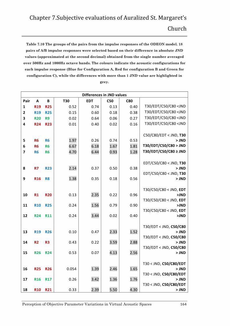
Chapter 7.Subjective evaluations of Auralized St. Margaret’s
Church
Perception of Objective Parameter Variations in Virtual Acoustic Spaces 164
Table 7.10 The groups of the pairs from the impulse responses of the ODEON model. 18
pairs of A/B impulse responses were selected based on their difference in absolute JND
values (approximated at the second decimal) obtained from the single number averaged
over 500Hz and 1000Hz octave bands. The colours indicate the acoustic configurations for
each impulse response (Blue for Configuration A, Red for configuration B and Green for
configuration C), while the differences with more than 1 JND value are highlighted in
grey.
Differences in JND values Pair A B T30 EDT C50 C80 1 R19 R25 0.52 0.74 0.13 0.40 T30/EDT/C50/C80 <JND 2 R19 R25 0.15 0.60 0.18 0.38 T30/EDT/C50/C80 <JND 3 R20 R9 0.02 0.64 0.06 0.27 T30/EDT/C50/C80 <JND 4 R24 R23 0.01 0.40 0.02 0.16 T30/EDT/C50/C80 <JND
5 R6 R6 1.97 0.26 0.74 0.53 C50/C80/EDT < JND, T30
> JND 6 R6 R6 6.67 6.18 1.67 1.81 T30/EDT/C50/C80 > JND 7 R6 R6 4.70 6.44 0.93 1.28 T30/EDT/C50/C80 ≥ JND
8 R7 R23 2.14 0.37 0.50 0.38 EDT/C50/C80 < JND, T30
> JND
9 R16 R8 1.38 0.35 0.18 0.56 EDT/C50/C80 < JND, T30
> JND
10 R1 R20 0.13 2.35 0.22 0.96 T30/C50/C80 < JND, EDT
>JND
11 R10 R25 0.24 1.56 0.79 0.90 T30/C50/C80 < JND, EDT
>JND
12 R24 R11 0.24 3.44 0.02 0.40 T30/C50/C80 < JND, EDT
>JND
13 R19 R26 0.10 0.47 2.33 1.52 T30/EDT < JND, C50/C80
> JND
14 R2 R3 0.43 0.22 3.59 2.88 T30/EDT < JND, C50/C80
> JND
15 R26 R24 0.53 0.07 4.13 2.56 T30/EDT < JND, C50/C80
> JND
16 R25 R26 0.054 1.39 2.46 1.65 T30 < JND, C50/C80/EDT
> JND
17 R16 R17 0.26 3.42 1.36 1.76 T30 < JND, C50/C80/EDT
> JND
18 R10 R21 0.33 2.39 5.50 4.30 T30 < JND, C50/C80/EDT
> JND

Chapter 7.Subjective evaluations of Auralized St. Margaret’s
Church
Perception of Objective Parameter Variations in Virtual Acoustic Spaces 165
Convolution with Anechoic Stimuli 7.4
For auralization it is necessary to convolve a dry signal (anechoic recording) with
the selected impulse responses (measured or artificial ones). In previous studies
such as [65, 66, 72, 190, 206, 222, 223], it has been shown that perceived
differences in the acoustic parameters, and more specifically the JND values,
depend on the characteristics of the motif being tested.
There are three main types of signal that can be used for auralization proposes,
after Bech et al.[224];
• Music (anechoic recordings),
• Speech (anechoic recordings),
• Noise (artificial signals by random noise generators).
Variations between these types of signal can significantly affect the perceived
result. For instance, Cox et al. in [65] show that a slow excerpt from Mendelssohn’s
Symphony No. 3 in A minor and a fast moving piece from Handel’s Water Music
Suite have a significant effect on the JND values for Centre Time (Ts) and C80, but
not for Early Lateral Energy Fraction (LF).
Listening tests are assumed more robust when different types of stimuli are able to
be tested for the same hypothesis, with respect to the main aims of the test. For the
current study due to the large number of tested pairs and the time consuming
process of the listening tests involved, two different source signals have been used,
one for each anechoic recording type described above. Hence, an excerpt of speech
and instrumental music were used, considering the recommended activities within
the space by Arup (Table 5.1) for the corresponding configurations of this study. In
addition, this choice of samples was suitable for studying in detail the changes in
both at C50 and C80 values, as according to ISO 3382, C50 is more associated with
the study of the perception of speech and C80 for music.
The first was an excerpt of the initial 9s of an anechoic recording from a theme for
solo cello by Weber, and the second was a 7s excerpt of male speech (between 30s
and 37s from the original recording), both from the “Archimedes” project [225]. The
passages of the cello are shorter than the human voice [72] and were considered a

Chapter 7.Subjective evaluations of Auralized St. Margaret’s
Church
Perception of Objective Parameter Variations in Virtual Acoustic Spaces 166
suitable example for listening to the attacks and the effect of early reflections.
Additionally, these stimuli were characterised by different spectra, as observed in
Figure 7.3. The spectrum of the male speech can be characterised as flatter than
the spectrum of the cello which demonstrates a wider variation across the
frequency range.
Figure 7.3 Frequency domain analysis (using Hamming window and with FFT size at 4096) of the two anechoic examples selected for the listening tests. The excerpt of male speech is
represented in blue and the excerpt of cello in red.
Once the anechoic stimuli had been chosen they were convolved with the selected
impulse responses (as described in the previous section) using Aurora [226].
Figure 7.4 For the auralization procedure the impulse responses are convolved with anechoic stimuli (a) an excerpt of solo cello by Weber and (b) an excerpt of male speech.
Sound Reproduction 7.5
The development of both auralization and sound reproduction techniques in recent
years means that it is now possible to reproduce 3D spatial audio environments
with a high degree of accuracy and realism [26, 72, 94, 136, 161, 190, 209, 213, 219,
227, 228]. However, each of these techniques has its own limitations and

Chapter 7.Subjective evaluations of Auralized St. Margaret’s
Church
Perception of Objective Parameter Variations in Virtual Acoustic Spaces 167
uncertainties, and there is still room for argument and further improvement
regarding the perceived accuracy of the auralized spaces that resulted [27, 85, 190,
218].
It is essential to choose the appropriate sound reproduction system based on a
consideration of the overall aim of the subjective evaluations. As the current study
focuses only on the perception of the influence of variations in monoaural acoustic
parameters, as discussed in 6.2, a mono-channel system was used for the
reproduction of the auralization results. The anechoic material was convolved with
the W-channel of the B-format files obtained from both in-situ measurements and
acoustic models.
Figure 7.5 For the listening tests a mono-channel system replayed over headphones was used for sound reproduction. The auralization examples were based on the W-channel of
the B-format files from both in-situ measurements and acoustic models.
In order to avoid the effect of additional reflections from the architectural
characteristics of the listening room on the test samples, it was considered best to
use closed-type headphones for the purposes of this study, (SRH440 Professional
studio headphones). As two PCs were used simultaneously for the listening tests, it
was important to use two identical headphones, calibrated approximately at the
same level between 64 and 65 dB (A weighted). Note that the mono-channel
auralizations are presented for headphone reproduction by replaying this single-
channel convolution over both left and right headphone channels.
Due to the use of headphone reproduction for the listening tests, the influence of
the acoustic characteristics of the listening room are actually insignificant [224].
The shape of the room was rectangular, one of the boundaries was an acoustically
absorbing curtain and there was carpet on the floor, with an average T30 less than
0.4s. The noise level in the room was calculated between 40 and 43 dB (A

Chapter 7.Subjective evaluations of Auralized St. Margaret’s
Church
Perception of Objective Parameter Variations in Virtual Acoustic Spaces 168
weighted). Although the above details should not affect the sound produced
through closed-type headphones, it was considered better to “introduce” the
participants to a quiet and dry enough room, before the actual listening test.
The comfort of the subjects was considered an important factor that might
influence their answers and as a result the reliability of the listening tests [224].
Hence, it was ensured that the heating and the ventilation of the room were
confortable. In addition, the window curtains were opened and any irrelevant
equipment and furnishings were hidden with curtains, in order to avoid any
external distraction.
As the subjects were using a computer interface during the tests, blind listening
tests as suggested in [136, 228, 229] were not possible, although a black
background desktop monitor screen was set to avoid further possible distractions.
Listening Tests Procedure 7.6
The question defined as central to these listening tests pertains to the overall focus
of this thesis: “Can we perceive an acoustic difference when minimal
changes have been observed in objective acoustic parameters?”. As
described previously, the subjects were asked to compare the selected pairs of
samples using the A/B comparison method.
For the investigation of each auralization technique, the selected impulse
responses were convolved with the relevant anechoic stimuli (cello, male speech).
Hence, for the listening tests for the in-situ measured impulse responses, 40 (20
(pairs) x 2 (stimuli)) question were used in total, and for the listening tests based
on the impulse responses from CATT-Acoustic and ODEON models, 36 (18 (pairs) x
2 (stimuli)) questions were used.
In order to ensure the listening tests proceeded smoothly, a graphical user
interface (GUI) in Matlab was used4 (Figure 7.6) in a similar way for all three
listening tests. The convolving pairs were loaded and performed in random order
4 The graphical user interface (GUI) in Matlab was developed by Andrew Chadwick, PhD
Candidate in Audio Lab, Department of Electronics, University of York.

Chapter 7.Subjective evaluations of Auralized St. Margaret’s
Church
Perception of Objective Parameter Variations in Virtual Acoustic Spaces 169
for every subject to reduce errors in the responses due to habituation and
expectation by playing the samples in a specific order. The interface gave the
option to the user to switch in real-time between samples A and B, or to stop each
sample and replay it as many times as necessary, as in previous work [136].
Figure 7.6 The graphical user interface (GUI) in Matlab for the listening test comparing the pairs obtained from the in-situ measurements.
It was considered important to train the subjects before taking the main listening
test. This method is commonly used in listening tests, such as in [72, 163, 182, 224]
to ensure the subjects are familiar with the interface used. The process of the
listening test was explained to the subjects during the training session, where they
were given the same tasks but for a reduced number of pairs. For the current tests,
however, there was a second purpose for these training sessions for the
investigator. The four pairs used were carefully chosen in order to also check the
reliability of the participants and their ability to perceive variations using only one
of the two chosen stimuli. One of the pairs had exactly the same sample for A and
B, and the rest were exposed to evenly increased differentiation across all
parameters, within the values used in the main test, compared with the first
“reference” sample, as shown in Table 7.11, Table 7.12 and Table 7.13. Similar
techniques have been used for investigating the subjects’ reliability in previous
studies by the current author [133], as well as in [72].

Chapter 7.Subjective evaluations of Auralized St. Margaret’s
Church
Perception of Objective Parameter Variations in Virtual Acoustic Spaces 170
Table 7.11 The groups of pairs used for the training session from the in-situ measured
impulse responses. 18 pairs of A/B impulse responses were selected based on their
difference in absolute JND values. The colours indicate the acoustic configurations for
each impulse response (Blue for Configuration A, Red for configuration B and Green for
configuration C).
JND values for Training Session Pair A B T30 EDT C50 C80 1 R19 R19 0 0 0 0 2 R19 R15 1.539028 0.4706821 1.257 0.1075 3 R19 R18 1.0751105 2.0263263 3.469 2.544 4 R19 R18 4.4035346 5.0578381 4.2115 4.189
Table 7.12 The groups of pairs used for the training session from the CATT-Acoustic model
impulse responses. 18 pairs of A/B impulse responses were selected based on their
difference in absolute JND values. The colours indicate the acoustic configurations for
each impulse response (Blue for Configuration A, Red for configuration B and Green for
configuration C).
JND values for Training Session Pair A B T30 EDT C50 C80 1 R18 R18 0 0 0 0 2 R18 R26 0.490296 0.675926 1.215 0.738 3 R18 R10 0.776302 3.287037 1.4275 2.2345 4 R18 R21 1.069118 2.62963 3.9915 2.753
Table 7.13 The groups of pairs used for the training session from the ODEON model
impulse responses. 18 pairs of A/B impulse responses were selected based on their
difference in absolute JND variations. The colours indicate the acoustic configurations for
each impulse response (Blue for Configuration A, Red for configuration B and Green for
configuration C).
JND values for Training Session Pair A B T30 EDT C50 C80 1 R24 R24 0 0 0 0 2 R24 R9 0.084162 0.104621 0.424 0.382 3 R8 R24 1.208875 0.113339 2.4865 1.4755 4 R24 R16 1.973986 1.14211 3.1715 2.315

Chapter 7.Subjective evaluations of Auralized St. Margaret’s
Church
Perception of Objective Parameter Variations in Virtual Acoustic Spaces 171
Due to the complexity of planning and conducting such rigorous listening tests, the
main part of the tests was considered a good opportunity to gather some additional
information from the subjects, not directly relevant to the main listening test
hypothesis for the current research but certainly a further step towards future
work based on this study. Hence, the subjects were asked the “if the sounds are the
same” question to define the perceived differentiation in terms of the following:
• Loudness
• Reverberance (Duration)
• Diffusion
• Pitch / Frequency Response
• Clarity
• Attack.
The graphical user interface (GUI) with the additional questions is shown in
Figure 7.7. It is well-known [59] that usually these terms are correlated to each
other. For instance, in reality clarity is directly related with reverberation time,
and frequency response (pitch) is correlated with the reverberance of the space. For
this reason, the participants were able to choose more than one of the above terms.
However this answer was optional, especially for those cases where the perceived
difference could not be explicitly identified.

Chapter 7.Subjective evaluations of Auralized St. Margaret’s
Church
Perception of Objective Parameter Variations in Virtual Acoustic Spaces 172
Figure 7.7 The optional graphical user interface (GUI) for the listening test comparing the pairs obtained from in-situ measurements.
These terms could be correlated in future with variations in specific acoustic
parameters, as several works have been focused on these subjective terms [43, 59,
80, 82, 101, 163, 207, 215, 217, 230], as shown in . It is interesting to mention,
however, the observation, as noted in [82], that there was a different
understanding of some of these terms between musicians, acousticians and sound
engineers/designers, and further explanation of the use of the terms was necessary
in many cases during the training session.

Chapter 7.Subjective evaluations of Auralized St. Margaret’s
Church
Perception of Objective Parameter Variations in Virtual Acoustic Spaces 173
Table 7.14 Correlations between terms used to define the perceived differentiation during
the listening tests and objective acoustic parameters, for further work.
Terms Correlations with
Objective Parameters
Loudness Strength (G), ITDG
Reverberance (Duration) T30, EDT, C50, C80
Diffusion C50, C80
Pitch/Frequency Response T30, EDT,
frequency dependence across
the octave bands
Clarity EDT, C50, C80
Attack EDT, C50, C80, ITDG
The Subjects 7.7
The test subjects were musically experienced listeners (either musicians, concert
goers or those with audio engineering experience) based on the assumption that if
“trained ears” could not perceive any difference between the samples of each pair,
naive listeners would require larger differentiations in order to perceive the
difference, as has been mentioned in [72]. The subjects were all experienced
listeners - either they were musicians, or had many years of musical training, or
they were working in audio engineering/acoustics/sound design. Although their
hearing was not tested with an audiometric test, 8% of the subjects declared slight
hearing problems (such as slightly tinnitus problem in one ear) although the rest
declared normal auditory capacity. As explained in the previous section, the
reliability of the subjects and their hearing ability were additionally checked
through their responses during the training session of the listening tests.

Chapter 7.Subjective evaluations of Auralized St. Margaret’s
Church
Perception of Objective Parameter Variations in Virtual Acoustic Spaces 174
The category of “experienced” listeners has a significant impact on the number of
subjects required for listening tests and according to Bech [224] a listening test
which requires experienced subjects should involve twenty participants, as was the
case in some previous studies [163, 209, 213, 219, 228]. However, in several studies
this number was difficult to obtain and the number of subjects varied between 4
and 17 [136, 209, 215, 222, 230]. For the current study, thirteen subjects
participated in each test, based on the in-situ measurements, CATT-Acoustic and
ODEON impulse responses. Their age varied from 21 to 48 years old. For the in-
situ measurements listening test, ten of the subjects were male and three female.
For the CATT-Acoustic listening tests, eight of the subjects were male and five
female. For the ODEON listening tests, nine of the subjects were male and four of
them female.
Before the analysis of the listening tests results, the answers of the subjects were
checked for their reliability (post-selection process of the subjects) by comparing
with their answers at the training session. It was considered sufficient to exclude
those subjects who could not indicate the difference for at least two of the three
different pairs from the training session examples. There were no subjects with
more than one answer wrong. For the in-situ measurements, three of the thirteen
subjects could not hear the difference in one of the pairs, while in the CATT-
Acoustic tests, three subjects could not and in for ODEON, two. Note that for each
test, the thirteen subjects were not the same participants. However, this was only
an indication of their reliability as the procedure could not confirm the reliability of
their answers during the main test. Biases such as tiredness, loss of concentration
or an unexpected noise event from the outer environment or from the equipment
could have affected the perception of the subjects during the listening test.
It was very interesting to observe that one to three subjects in each test indicated
as different the pair with exactly the same sample for A and B. This could be
explained as a psychological effect due to the wording of the task and their
desires/expectations to hear differences that were not there, as explained in [229].
These participants, however, where not excluded from the final analysed results as
this attribute at the training session does not necessarily mean they were
answering in a similar way during the main test. Their answers were taken into

Chapter 7.Subjective evaluations of Auralized St. Margaret’s
Church
Perception of Objective Parameter Variations in Virtual Acoustic Spaces 175
consideration and it was observed that, overall, their answers in the main test did
not deviate from the average answers of the rest of the participants.
Most of the participants characterised the tests as “difficult”, meaning that in most
cases they could hear a difference between the samples but could not discriminate
exactly what the difference they were hearing was. The duration of each test was
surprisingly varied, from less than 10 minutes to more than one hour (for three
cases). For those cases where the participants needed more time, a short break was
usually taken in the middle of the test. A significant difference in the answers of
those who had completed the test more quickly than the others and vice versa, was
not observed.

Chapter 7.Subjective evaluations of Auralized St. Margaret’s
Church
Perception of Objective Parameter Variations in Virtual Acoustic Spaces 176
Listening Test Subjects’ Response 7.8
Table 7.15 The answers reported by the thirteen subjects for the in-situ measurement
listening test, for each of the two stimuli.
Questions for
measurements
Cello (Participants out of 13 who
perceived a difference)
Voice (Participants out of 13 who
perceived a difference)
Pair 1 10 10
Pair 2 10 13
Pair 3 12 12
Pair 4 12 9
Pair 5 8 9
Pair 6 9 8
Pair 7 7 11
Pair 8 11 11
Pair 9 3 8
Pair 10 12 3
Pair 11 3 6
Pair 12 10 7
Pair 13 12 7
Pair 14 9 8
Pair 15 9 11
Pair 16 12 6
Pair 17 13 12
Pair 18 12 13
Pair 19 10 9
Pair 20 11 9

Chapter 7.Subjective evaluations of Auralized St. Margaret’s
Church
Perception of Objective Parameter Variations in Virtual Acoustic Spaces 177
Table 7.16 The answers reported by the thirteen subjects for the CATT-Acoustic listening
test, for each of the two stimuli.
Questions for
CATT-‐Acoustic
Cello (Participants out of 13 who
perceived a difference)
Voice (Participants out of 13 who
perceived a difference)
Pair 1 9 9
Pair 2 11 13
Pair 3 6 11
Pair 4 13 13
Pair 5 4 5
Pair 6 11 10
Pair 7 4 11
Pair 8 12 6
Pair 9 7 9
Pair 10 10 6
Pair 11 12 13
Pair 12 12 12
Pair 13 11 10
Pair 14 9 13
Pair 15 13 13
Pair 16 13 11
Pair 17 11 11
Pair 18 12 13

Chapter 7.Subjective evaluations of Auralized St. Margaret’s
Church
Perception of Objective Parameter Variations in Virtual Acoustic Spaces 178
Table 7.17 The answers reported by the thirteen subjects for the ODEON listening test, for
each of the two stimuli.
Questions for
ODEON
Cello (Participants out of 13 who
perceived a difference)
Voice (Participants out of 13 who
perceived a difference)
Pair 1 11 10
Pair 2 11 9
Pair 3 6 11
Pair 4 10 12
Pair 5 8 7
Pair 6 6 9
Pair 7 5 9
Pair 8 11 12
Pair 9 10 12
Pair 10 7 11
Pair 11 7 11
Pair 12 13 10
Pair 13 9 13
Pair 14 10 12
Pair 15 12 13
Pair 16 5 8
Pair 17 7 12
Pair 18 13 13

Chapter 7.Subjective evaluations of Auralized St. Margaret’s
Church
Perception of Objective Parameter Variations in Virtual Acoustic Spaces 179
Analysis based on JND values 7.8.1
As discussed above, based on ISO3382, it was expected that the pairs of samples
with less than 1 JND value would be perceived as the same and it was
hypothesised that by increasing these JND values, the number of subjects who
would perceive the difference would increase as well. Observing the results from all
three listening tests (Table 7.15, Table 7.16 and Table 7.17), it is clear this
hypothesis was not confirmed as the subjects could indicate a difference between
the samples of each pair in most cases even if the objective values claimed the
opposite. It is worth mentioning the received responses for the first four pairs, from
all three listening tests. These pairs had been chosen as examples in which the
differences between all the studied acoustic parameters were observed with less
than 1 JND value. However, it is very interesting to observe that the majority of
the responses had indicated a perceived difference between these pairs under
examination, for all three listening tests.
Statistical analysis could not be applied to these listening tests because the
expected result was known a priori. In fact, the test hypothesis was that all
thirteen experienced subjects must not perceive the difference between the samples
with less than 1 JND value according to ISO3382, therefore giving zero for the
expected error of these tests. Additionally, there was not any correlation between
the pairs of each group and the number of positive answers due to the non-
parametric values of the “Yes” and “No” answer type.
Hence, in order to investigate further the possible reasons for the perceptual
difference, an observation of the waveforms was undertaken and the differences
between the waveforms of the samples of the hypothesised “identical” pairs
analysed. As the impulse responses were all normalised, this fact was not related
to the distance of the receivers from the source. However, in all the cases, a
difference in the overall energy of the impulse responses was very clear. An
example of such pairs is demonstrated in Figure 7.9. This was confirmed with a
numerical calculation of the overall energy of the squared impulse responses. It is
very important here to note that the clarity parameters (C50/C80) cannot give
information about the total amount for energy of an impulse response, as by
definition this shows just the ratio of early-to-late energy. This observation raised
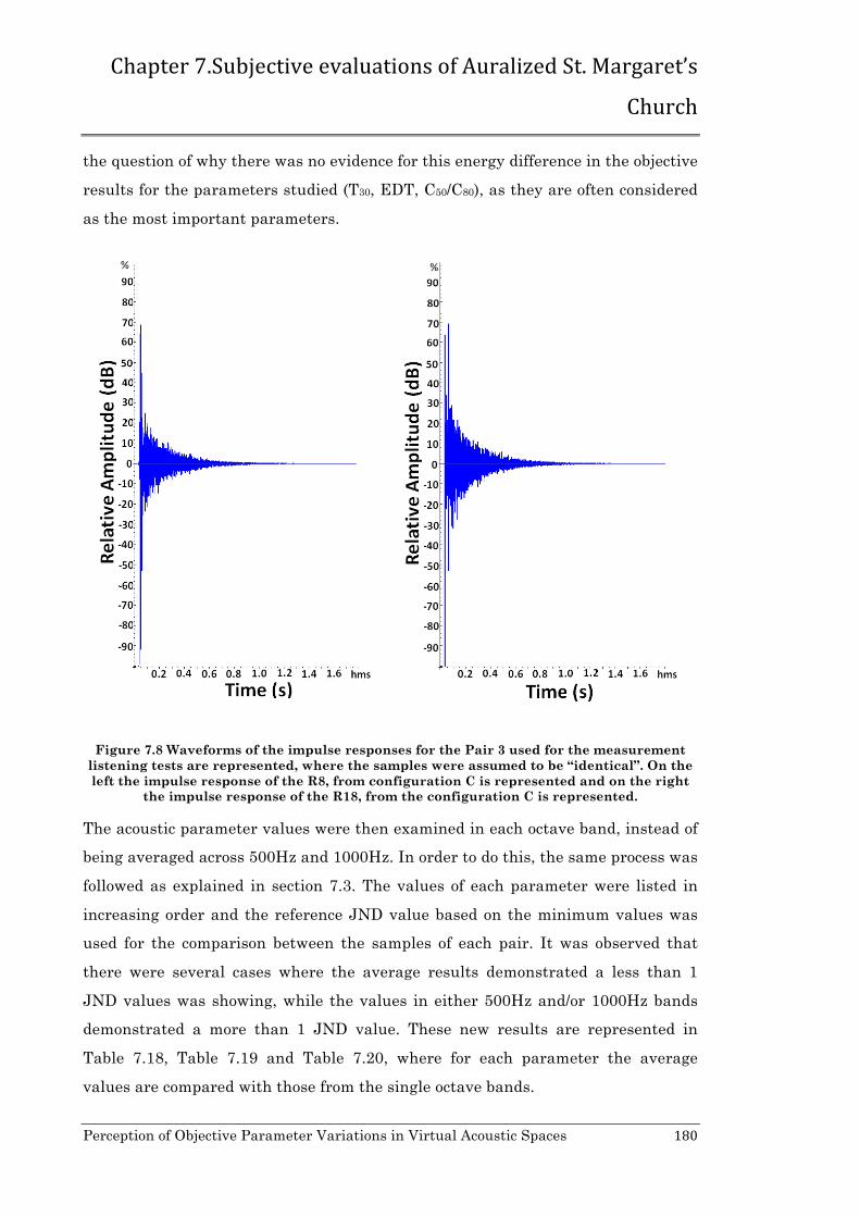
Chapter 7.Subjective evaluations of Auralized St. Margaret’s
Church
Perception of Objective Parameter Variations in Virtual Acoustic Spaces 180
the question of why there was no evidence for this energy difference in the objective
results for the parameters studied (T30, EDT, C50/C80), as they are often considered
as the most important parameters.
Figure 7.8 Waveforms of the impulse responses for the Pair 3 used for the measurement listening tests are represented, where the samples were assumed to be “identical”. On the left the impulse response of the R8, from configuration C is represented and on the right
the impulse response of the R18, from the configuration C is represented.
The acoustic parameter values were then examined in each octave band, instead of
being averaged across 500Hz and 1000Hz. In order to do this, the same process was
followed as explained in section 7.3. The values of each parameter were listed in
increasing order and the reference JND value based on the minimum values was
used for the comparison between the samples of each pair. It was observed that
there were several cases where the average results demonstrated a less than 1
JND values was showing, while the values in either 500Hz and/or 1000Hz bands
demonstrated a more than 1 JND value. These new results are represented in
Table 7.18, Table 7.19 and Table 7.20, where for each parameter the average
values are compared with those from the single octave bands.

Chapter 7.Subjective evaluations of Auralized St. Margaret’s
Church
Perception of Objective Parameter Variations in Virtual Acoustic Spaces 181
Hence, it can be concluded that the JND based on the average of the values in
500Hz and 1000Hz octave bands, as recommended in ISO3382, is not sufficient to
show with accuracy the reliability of perceived auralization results. A more
detailed analysis is essential in order to observe perceived differences across all the
octave bands, and not necessarily only at 500Hz and 1000Hz.

Chapter 7.Subjective evaluations of Auralized St. Margaret’s
Church
Perception of Objective Parameter Variations in Virtual Acoustic Spaces 182
Table 7.18 The JND values at 500Hz and 1000Hz for the in-situ measurements compared
with the JND values observed from the average of these two octave bands (Table 7.4). The
values with less than 1 JND from the average of the two bands are highlighted in green,
while their corresponding values in the single octave bands with more than 1 JND
observed are in black font. Note that for clarity of presentation, the values from Table 7.4
have been reduced to three decimal places.
Selected Pairs for in-‐situ measurements T30 EDT C50 C80
Average of
500Hz,1000Hz Average of
500Hz,1000Hz Average of
500Hz,1000Hz Average of
500Hz,1000Hz A B 500Hz 1000Hz 500Hz 1000Hz 500Hz 1000Hz 500Hz 1000Hz
1 R26 R5 0.066 0.048 0.176 0.316 0.071 0.063 1.349 1.633 1.794 1.443 1.143 0.512
2 R1 R15 0.175 0.074 0.298 0.046 0.346 0.739 1.180 1.112 2.706 2.111 1.501 1.592
3 R8 R18 0.287 0.782 0.407 0.285 0.395 0.172 1.783 3.793 0.261 1.074 1.624 1.055
4 R23 R12 0.000 0.096 0.847 0.351 0.423 0.469 2.635 3.194 0.491 1.202 1.051 1.752
5 R6 R6 1.193 1.907 0.958 0.619 0.805 1.643 1.317 2.849 1.503 0.413 0.336 0.901
6 R6 R6 4.801 3.175 1.122 1.290 3.783 6.009 4.498 2.142 0.683 1.560 1.027 1.552
7 R6 R6 5.994 5.082 2.080 1.908 4.587 7.653 5.815 4.991 2.186 1.973 1.363 2.453
8 R23 R24 1.186 3.845 1.227 2.543
1.355 1.017 4.996 3.103 1.197 1.257 3.153 1.933
9 R17 R17 5.074 6.398 0.886 0.387 3.571 6.823 8.546 4.900 0.839 0.933 0.511 0.262
10 R9 R8 1.546 0.008 1.568 0.472 1.962 1.111 3.213 3.648 0.819 2.316 0.244 0.700
11 R22 R21 0.972 0.343 0.954 0.565 0.353 1.674 0.434 1.270 0.499 2.406 0.606 0.523
12 R24 R11 0.118 2.226 0.043 1.077 0.085 0.156 0.032 5.027 0.741 0.655 0.346 1.808
13 R3 R20 0.825 3.375 0.180 0.046 1.171 0.454 2.056 5.354 0.302 0.057 0.181 0.273
14 R5 R2 0.059 2.002 0.627 0.030 0.183 0.329 2.008 2.287 0.104 1.357 1.014 0.954
15 R20 R21 0.339 0.040 2.672 1.743 1.214 0.626 2.602 2.849 1.972 3.371 1.887 1.599
16 R20 R20 0.112 0.091 1.786 1.434

Chapter 7.Subjective evaluations of Auralized St. Margaret’s
Church
Perception of Objective Parameter Variations in Virtual Acoustic Spaces 183
0.526 0.325 0.670 0.907 1.833 1.738 1.853 1.015
17 R11 R17 0.042 0.066 4.395 4.093 0.235 0.163 2.265 2.293 3.517 5.272 4.365 3.820
18 R18 R15 0.015 1.875 4.341 2.648 0.847 0.970 1.687 2.359 4.258 4.424 2.052 3.244
19 R3 R1 0.302 0.981 2.381 2.343 0.409 0.188 0.386 2.668 4.183 0.578 4.448 0.238
20 R18 R18 0.280 2.344 2.767 2.802 0.498 0.059 4.386 0.154 2.219 3.315 3.797 1.807

Chapter 7.Subjective evaluations of Auralized St. Margaret’s
Church
Perception of Objective Parameter Variations in Virtual Acoustic Spaces 184
Table 7.19 The JND values at 500Hz and 1000Hz for the CATT-Acoustic results, compared
with the JND values observed from the average of these two octave bands (Table 7.7). The
values with less than 1 JND from the average of the two bands are highlighted in green,
while their corresponding values of the single octave bands with more than 1 JND
observed are in black font. Note that for clarity of presentation, the values from Table 7.7
have been reduced to three decimal places.
Selected Pairs for CATT
Average of
500Hz,1000Hz Average of
500Hz,1000Hz Average of
500Hz,1000Hz Average of
500Hz,1000Hz 500Hz 1000Hz 500Hz 1000Hz 500Hz 1000Hz 500Hz 1000Hz
A B T30 EDT C50 C80 1 R26 R9 0.409 0.370 0.911 0.940 0.858 0.042 0.855 0.111 1.256 3.078 0.473 2.353
2 R1 R10 0.347 0.343 0.056 0.374 1.389 0.709 2.974 2.269 0.468 0.579 0.587 0.160
3 R19 R24 0.327 0.676 0.177 0.367 0.831 0.181 0.446 1.790 0.516 0.162 0.147 0.881
4 R7 R20 0.184 0.324 0.115 0.251 0.722 0.362 0.911 1.550 0.273 0.503 0.771 0.270
5 R6 R6 1.559 1.759 0.173 0.503 1.920 1.224 1.599 1.919 0.972 1.317 1.813 0.807
6 R6 R6 6.170 10.287 1.567 1.735 6.195 6.273 15.483 5.129 0.535 2.599 0.895 2.575
7 R6 R6 4.610 8.528 1.395 2.238 4.275 5.049 13.885 3.210 1.507 1.282 2.708 1.768
8 R12 R12 1.866 0.685 0.787 0.567 1.770 2.003 2.621 3.967 1.235 0.338 0.649 0.485
9 R9 R25 1.246 0.537 0.222 0.309 1.661 0.848 1.022 0.055 3.177 2.734 1.622 2.240
10 R22 R21 0.218 1.213 0.589 0.138 0.477 0.042 0.836 1.587 1.149 0.029 0.578 0.303
11 R8 R1 0.456 2.796 0.429 1.194 1.675 0.779 7.807 2.177 1.305 0.448 2.705 0.318
12 R22 R11 0.061 4.889 0.005 0.598 0.300 0.431 7.974 1.827 0.248 0.257 1.222 0.027
13 R25 R6 0.123 0.222 1.829 1.585 0.000 0.250 0.985 1.421 1.652 2.006 1.830 1.339
14 R8 R4 0.531 0.370 3.513 1.983 1.157 0.097 4.591 3.819 3.239 3.786 2.242 1.724
15 R21 R17 0.742 0.944 5.168 4.395 0.899 0.598 2.844 4.705 3.765 6.571 3.066 5.723
16 R20 R26 0.014 8.296 3.112 2.766

Chapter 7.Subjective evaluations of Auralized St. Margaret’s
Church
Perception of Objective Parameter Variations in Virtual Acoustic Spaces 185
0.340 0.376 6.710 9.871 4.621 1.602 2.323 3.209
17 R2 R17 0.082 2.796 1.769 1.662 1.076 0.932 6.710 1.089 2.540 0.998 3.734 0.410
18 R21 R10 0.177 3.426 3.480 2.289 0.436 0.083 3.104 3.745 2.869 4.091 1.903 2.675

Chapter 7.Subjective evaluations of Auralized St. Margaret’s
Church
Perception of Objective Parameter Variations in Virtual Acoustic Spaces 186
Table 7.20 The JND values at 500Hz and 1000Hz for the ODEON results, compared with the
JND values observed from the average of these two octave bands (Table 7.10). The values
with less than 1 JND from the average of the two bands are highlighted in green, while
their corresponding values of the single octave bands with more than 1 JND observed are
in black font. Note that for clarity of presentation, the values from Table 7.10 have been
reduced to three decimal places.
Selected Pairs for ODEON
Average of
500Hz,1000Hz Average of
500Hz,1000Hz Average of
500Hz,1000Hz Average of
500Hz,1000Hz 500Hz 1000Hz 500Hz 1000Hz 500Hz 1000Hz 500Hz 1000Hz
A B T30 EDT C50 C80 1 R19 R25 0.520 0.741 0.127 0.401 0.742 0.292 0.994 2.546 0.036 0.217 0.095 0.896
2 R19 R25 0.145 0.602 0.180 0.384 0.252 0.032 0.110 1.374 0.401 0.761 0.629 1.396
3 R20 R9 0.023 0.636 0.060 0.273 0.015 0.065 2.116 0.769 0.664 0.783 1.265 0.720
4 R24 R23 0.008 0.401 0.021 0.163 0.045 0.032 1.049 0.201 0.677 0.718 0.446 0.772
5 R6 R6 1.974 0.262 0.740 0.526 1.780 2.240 1.049 0.495 1.169 0.311 0.789 0.263
6 R6 R6 6.672 6.181 1.672 1.810 6.647 6.883 6.587 6.429 1.827 1.517 1.926 1.693
7 R6 R6 4.698 6.443 0.932 1.284 4.866 4.643 7.636 5.934 0.658 1.206 1.137 1.430
8 R7 R23 2.142 0.366 0.505 0.382 2.433 1.883 0.846 0.073 0.622 0.387 0.001 0.764
9 R16 R8 1.377 0.349 0.182 0.559 1.172 1.640 0.368 0.366 1.262 0.899 0.923 0.195
10 R1 R20 0.130 2.354 0.215 0.958 0.163 0.097 5.354 0.385 0.216 0.646 1.089 0.827
11 R10 R25 0.237 1.561 0.792 0.902 0.312 2.841 1.546 4.029 0.624 4.649 0.104 4.025
12 R24 R11 0.245 3.435 0.021 0.395 0.252 7.166 3.073 4.158 0.016 0.057 0.090 0.700
13 R19 R26 0.099 0.471 2.335 1.525 0.312 2.808 1.270 5.403 3.542 3.888 2.430 2.629
14 R2 R3 0.428 0.218 3.594 2.882 0.445 0.422 1.141 1.593 2.014 5.173 2.777 2.986
15 R26 R24 0.528 0.070 4.132 2.564 0.564 0.503 1.141 0.989 4.952 3.312 2.882 2.246
16 R25 R26 0.054 1.386 2.465 1.648
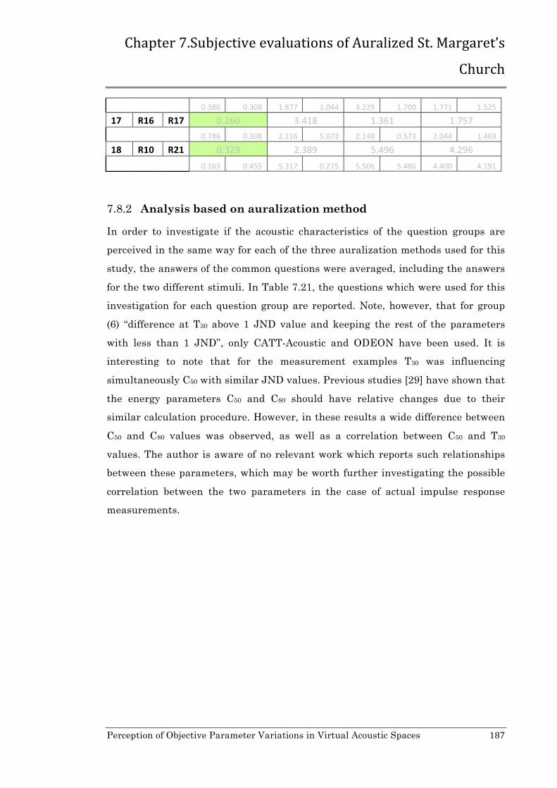
Chapter 7.Subjective evaluations of Auralized St. Margaret’s
Church
Perception of Objective Parameter Variations in Virtual Acoustic Spaces 187
0.386 0.308 1.877 1.044 3.229 1.700 1.771 1.525
17 R16 R17 0.260 3.418 1.361 1.757 0.786 0.308 2.116 5.073 2.148 0.573 2.044 1.469
18 R10 R21 0.329 2.389 5.496 4.296 0.163 0.455 5.317 0.275 5.506 5.486 4.400 4.191
Analysis based on auralization method 7.8.2
In order to investigate if the acoustic characteristics of the question groups are
perceived in the same way for each of the three auralization methods used for this
study, the answers of the common questions were averaged, including the answers
for the two different stimuli. In Table 7.21, the questions which were used for this
investigation for each question group are reported. Note, however, that for group
(6) “difference at T30 above 1 JND value and keeping the rest of the parameters
with less than 1 JND”, only CATT-Acoustic and ODEON have been used. It is
interesting to note that for the measurement examples T30 was influencing
simultaneously C50 with similar JND values. Previous studies [29] have shown that
the energy parameters C50 and C80 should have relative changes due to their
similar calculation procedure. However, in these results a wide difference between
C50 and C80 values was observed, as well as a correlation between C50 and T30
values. The author is aware of no relevant work which reports such relationships
between these parameters, which may be worth further investigating the possible
correlation between the two parameters in the case of actual impulse response
measurements.

Chapter 7.Subjective evaluations of Auralized St. Margaret’s
Church
Perception of Objective Parameter Variations in Virtual Acoustic Spaces 188
Table 7.21 The questions from the same group of acoustic characteristics for the three
auralization techniques.
(1) T30/EDT/C50/C80 <JND
(2) T30/EDT/C50/C80 ≥ JND
(3) T30/C50/C80
< JND, EDT >JND
(4) T30/EDT < JND, C50/C80 > JND
(5) T30 < JND,
C50/C80/EDT > JND
(6) EDT/C50/C80 < JND,
T30>JND
Measurements Q1, Q2,
Q3, Q4
Q6, Q7,
Q8
Q13, Q14 Q15, Q16,
Q17
Q18, Q19,
Q20
-‐
CATT-‐Acoustic Q1, Q2,
Q3, Q4
Q6, Q7 Q10, Q11,
Q12
Q13, Q14,
Q15
Q16, Q17,
Q18
Q8, Q9
ODEON Q1, Q2,
Q3, Q4
Q6, Q7 Q10, Q11,
Q12
Q13,
Q14,. Q15
Q16, Q17,
Q18
Q8, Q9
By presenting the average of the responses as well as their standard deviations in
Figure 7.9, it is easier to draw conclusions for each auralization technique.
For the measurements, when only EDT values were changed above 1 JND values
(question group (3)), this had less influence on the subjects’ perception than when
C50 and C80 values or C50/C80 and EDT at the same time were changed above 1 JND
values (question groups (4) and (5) respectively).
For CATT-Acoustic, very interestingly, an increased degree of perceptual difference
has been observed from changes in T30 (question group (6)), EDT (question group
(3)), C50/C80 (question group (4)) and EDT/C50/C80 (question group (5)).
For ODEON, changes in T30 (question group (6)) and EDT (question group (3)), as
well as when changes above 1 JND values have been observed in all three
EDT/C50/C80 (question group (5)), were perceived with the same degree of difference
from the subjects. On the other hand, changes in C50/C80 (question group (4)) are
more audible than the other parameters.
Conclusions from the overall average of the three auralization techniques can be
drawn as well. Here there is an increased degree of perceptual difference from
changes in T30 (question group (6)), EDT (question group (3)), C50/C80 (question

Chapter 7.Subjective evaluations of Auralized St. Margaret’s
Church
Perception of Objective Parameter Variations in Virtual Acoustic Spaces 189
group (4)). However, the perceived difference in EDT/C50/C80 (question group (5)) is
less than the latter case of C50/C80 (question group (4)).
From all these cases, an overall conclusion is the fact that changes in the energy
parameters C50/C80 are more audible than changes observed in EDT. Changes in T30
were found to have even less influence on the subjects’ perception than the other
three parameters.
An additional comment on the results shown in Figure 7.9 is that the subjects were
more confident about the perceived difference when all the acoustic parameters
were hypothesised to be with less than 1 JND value (question group (1)) than those
with more than 1 JND value observed across all the studied parameters (question
group (2)). One obvious reason for this fact is the variations of the values across the
octave bands, as discussed in section 7.8.1.
Figure 7.9 The bars represent the average number of subjects who perceived a difference
across all three auralization methods, for each group of questions based on the
corresponding acoustic characteristics. The first bar is the average of all the listening
tests. The standard deviations show the variation in the number of subjects who perceived
the difference for each group.
Chapter 7.Subjective evaluations of Auralized St. Margaret’s
Church
Perception of Objective Parameter Variations in Virtual Acoustic Spaces 190
Analysis based on the stimuli 7.8.3
As discussed in section 7.4, it has been shown in previous studies that different
results can lead to different conclusions in perceptual studies, depending on the
original stimulus used for convolution. The current knowledge that we have about
the influence of the stimuli on our perception is still limited. For the listening tests
in this study, two different stimuli were convolved with the selected impulse
responses, and it will be interesting to investigate their effect on results. Hence, in
Figure 7.10, Figure 7.11 and Figure 7.12 the percentage of the number of subjects
who perceived a difference for each question/pair was calculated for both cases
stimuli and the relationship between them compared in each bar.
In the ideal case, where the stimuli do not affect the perception of the acoustic
characteristics being tested, the number of subjects for the two stimuli for each
question should be equal. This would be represented by the colours for each bar
(green for cello and yellow for voice) both reaching the middle of the y-axis.
As observed, however, this was not the case with any of the three auralization
techniques. For the in-situ measurements (Figure 7.10), in about 45% of the
answers it was observed that the two stimuli had the same effect on the subjects’
perception. An interesting point regarding these results was the responses for each
stimulus for Q10, where T30 and C50 parameters differed with more than 1 JND
values. The subjects indicated the difference more clearly with the cello as the
stimulus rather than with the voice. This was not expected, as from the definition;
C50 is more relative to speech than music.
For the CATT-Acoustic results (Figure 7.11), for about 50% of the answers the
stimuli had the same effect on the responses for each question, while for the rest of
the answers - with a few exceptions - pairs with voice as the stimulus were more
easily perceived as different.
For the ODEON results (Figure 7.12), for about 30% of the answers the stimuli
affected the responses for each question in the same way, while for the rest of the
answers voice seemed to have more effect on the perception of the difference
between the samples.
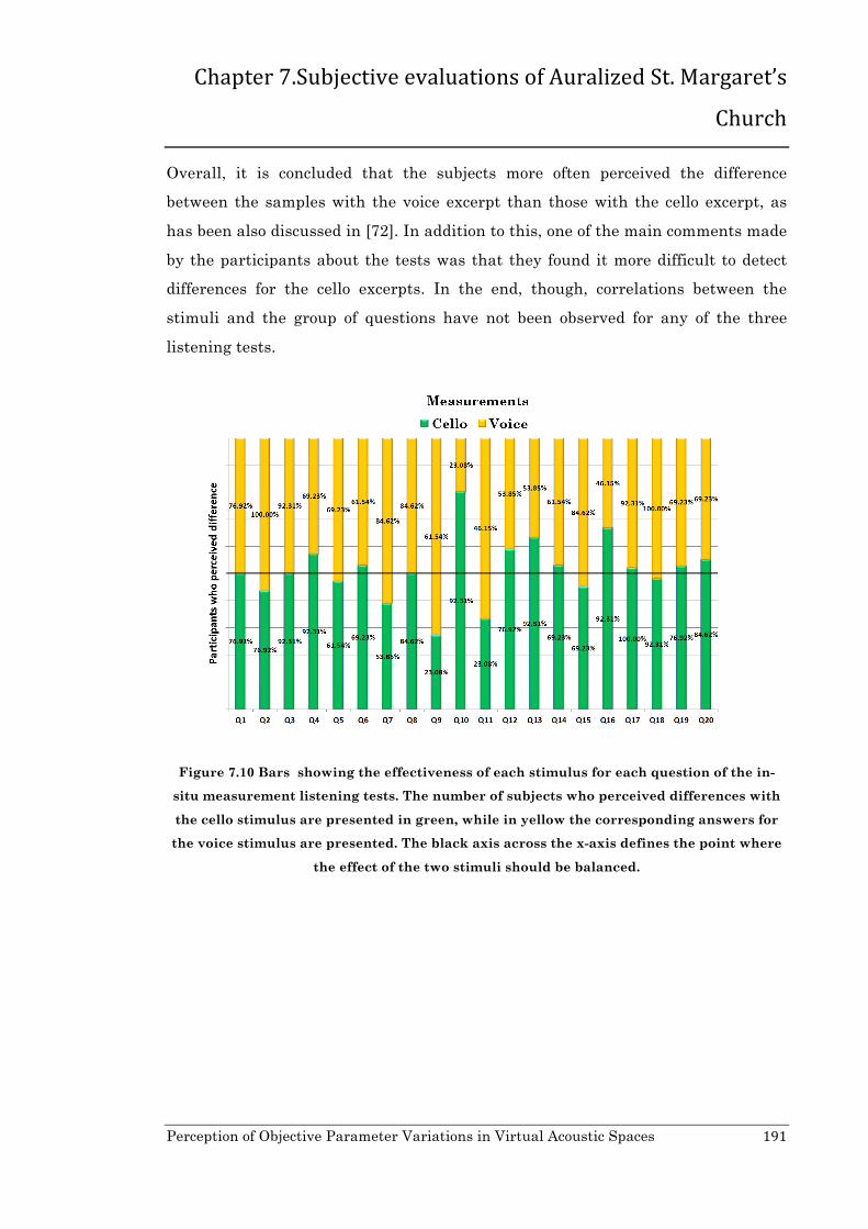
Chapter 7.Subjective evaluations of Auralized St. Margaret’s
Church
Perception of Objective Parameter Variations in Virtual Acoustic Spaces 191
Overall, it is concluded that the subjects more often perceived the difference
between the samples with the voice excerpt than those with the cello excerpt, as
has been also discussed in [72]. In addition to this, one of the main comments made
by the participants about the tests was that they found it more difficult to detect
differences for the cello excerpts. In the end, though, correlations between the
stimuli and the group of questions have not been observed for any of the three
listening tests.
Figure 7.10 Bars showing the effectiveness of each stimulus for each question of the in-
situ measurement listening tests. The number of subjects who perceived differences with
the cello stimulus are presented in green, while in yellow the corresponding answers for
the voice stimulus are presented. The black axis across the x-axis defines the point where
the effect of the two stimuli should be balanced.

Chapter 7.Subjective evaluations of Auralized St. Margaret’s
Church
Perception of Objective Parameter Variations in Virtual Acoustic Spaces 192
Figure 7.11 Bars showing the effectiveness of each stimulus for each question of the CATT-
Acoustic listening tests. In green the number of subjects who perceived differences with
the cello stimulus is presented, while in yellow the corresponding answers for the voice
stimulus is presented. The black axis across the x-axis defines the point where the effect of
the two stimuli should be balanced.
Figure 7.12 The bars show the effectiveness of each stimulus for each question of the
ODEON listening tests. In green the number of subjects who perceived differences with
the cello stimulus is presented, while in yellow the corresponding answers for the voice
stimulus is presented. The black axis across the x-axis defines the point where the effect of
the two stimuli should be balanced.

Chapter 7.Subjective evaluations of Auralized St. Margaret’s
Church
Perception of Objective Parameter Variations in Virtual Acoustic Spaces 193
Summary 7.9
To evaluate the reliability of auralizations based on the perception of changes in
acoustic characteristics, listening tests were conducted and the results have been
analysed in this chapter. Each auralization method was investigated
independently, hence, three similar listening tests were conducted.
Focusing the investigation on the subjective sensitivity of the listeners to
variations in T30, EDT, and C50/C80, the impulse responses had to be carefully
selected based on the requirements of the study with respect to JND values. The
same process was followed for all three auralization techniques, such that the final
test examples were based only on JND values across combination of parameters.
The steps followed were to use appropriate anechoic stimuli and convolve them
with the selected impulse responses. The selection of the stimuli was based on the
findings of previous studies and the purposes of the current study. Additionally,
the sound reproduction system used as well as test planning, the administration
and the reporting of the results of the listening tests have been described in detail.
The analysis of the results was based on groups of questions which represented
different acoustic conditions, while all different aspects of this study were taken
into consideration. It was found that averaging JND values for acoustic parameters
across 500Hz and 1000Hz octave bands, as recommended in ISO3382, masks the
fact that differences can still be perceived. These differences are revealed by
considering non-averaged JND values individually for each octave band.
The results have also been analysed based on the auralization method used, in
order to draw conclusions about the effect of each technique on the subjective
results. The influence of the two different stimuli was also investigated, showing
once more that they can have an effect on the perceptual result observed.

Chapter 8. Conclusions
Perception of Objective Parameter Variations in Virtual Acoustic Spaces 194
Chapter 8.
Conclusions
Auralization has become a highly useful tool for the acoustic design of spaces, as
well as for the acoustic revival of heritage sites. Several auralization techniques
have been developed, either based on in-situ acoustic measurements where
possible, or on synthesised acoustic virtual environments. Evaluation of the quality
of auralization techniques is typically achieved numerically by observing objective
acoustic parameters and comparing them with those obtained from in-situ
measurements. However, the lack of certainty regarding the accuracy of the
perceptual results of these techniques has not been investigated in significant
depth. This thesis has been motivated by the need to achieve accurate results in
auralization, in term of objective and subjective measures.
The hypothesis on which this research has been based is as follows:
In virtual acoustic reconstructions, perceptual accuracy is dependent on
minimising the changes in objective acoustic metrics through
optimisation of physical parameters in the auralized space.
In order to support this research hypothesis, the steps below have been followed:
• Theoretical explanations of commonly adopted auralization techniques used
have been given, with a presentation of the advantages and limitations of
each of these methods.
• A virtual acoustic space has been created by using three of the most
common auralization techniques. Impulse responses were captured and
produced using each method, by varying the receiver positions, the acoustic
configurations of the space and in one of the techniques, the orientation of
the sound source.

Chapter 8. Conclusions
Perception of Objective Parameter Variations in Virtual Acoustic Spaces 195
• Objective studies were carried out in order to observe and analyse the
changes in obtained acoustic parameters.
• Finally, the perceptual results of these changes were evaluated through
listening tests.
Summary 8.1
A theoretical examination of the principles of acoustics has been presented,
explaining in detail the characteristic properties of sound propagation in an
enclosed space (Chapter 2). The contributions of the acoustic interactions such as
sound reflection, sound diffusion, sound absorption or standing waves, have been
described. The room impulse response has been introduced as an output of a
system, excited by a given input signal, and ideally encapsulating all the acoustic
characteristics of the system. The main acoustic parameters, used to objectively
represent and evaluate the properties of an impulse response, as recommended in
ISO3382, have been defined and discussed. However, these acoustic parameters do
not provide sufficient information about the subjective perception of these objective
measures. Thus, the relevant just noticeable difference (JND) values had been
determined from previous work and used for the subjective evaluations of this
thesis.
The concept of auralization and the most well-known auralization techniques have
been described (Chapter 3). A considerable amount of theoretical work has resulted
in the introduction of a number of different auralization techniques, which can be
categorised according to the nature of the impulse responses used, the main
difference being those which use impulse responses from an actual space and those
relying on synthesised impulse responses from computer-based models. For in-situ
measurements, the nature of the excitation signal used, the sound source and
microphone properties, as well as the calculation process used for the analysis of
the impulse responses affect the accuracy and the reliability of the method.
For computer-based impulse responses, the main difference between existing
algorithms is the consideration of the phenomenon of sound as particles or as
waves. Geometric acoustic algorithms were examined in detail and their
advantages and limitations were presented, in order to identify the most suitable
technique for the purposes of this study. The auralization techniques used for this
study are based on: 1) in-situ impulse response measurements using the

Chapter 8. Conclusions
Perception of Objective Parameter Variations in Virtual Acoustic Spaces 196
Exponential-Swept Sine (ESS) Method and 2) two computer simulations using
commercial software, CATT-Acoustic and ODEON, both based on geometric
acoustic algorithms.
Some pilot studies have been carried out before the main work presented in this
thesis (Chapter 4). An experimental shoebox shaped acoustic model was created in
ODEON and used in order to study the impact of physical factors and acoustic
properties on both objective and subjective results. Physical parameters such as
source directivity, source orientation, absorption and scattering coefficients,
calculation settings and source/receiver positions are easy to control in such a
virtual space. Their impact on T30, EDT and C80/C80 was examined and validated in
subjective terms through listening tests. The information collected from these pilot
studies was then carried over into the main investigation, which was about the
influence of the sound source orientation and modelling techniques on the objective
values of the space. It was noted that the results of such acoustic simulation
models are realistic only when they reflect the geometry, absorption, diffusion and
so forth of real spaces.
Thus, for the purpose of this thesis an existing heritage space was used to study
the influence of variations in obtained acoustic parameters and their relationship
to what a listener perceives. St. Margaret’s church was chosen for this study due to
the potential to change its physical acoustic characteristics through sets of acoustic
panels and drapes (Chapter 5). Hence, variations in the obtained acoustic
parameters can be easily controlled by the researcher, for both in-situ
measurements, as well as for the computer modelling techniques used. The space
was tested in different acoustic configurations, for both measurements and
computer models, across a grid of 26 receiver points covering the audience area.
Additionally, variations in the orientation of the sound source were applied for the
in-situ measurements.
The acoustic characteristics of the captured/synthesised impulse responses were
analysed by calculating the acoustic parameters for each auralization technique,
acoustic configuration and receiver/source positions (Chapter 6). This research has
concentrated on what are assumed to be the most important acoustic parameters.
It was considered best to exclude from the study those parameters assumed to be
directly affected by the sound source, microphone properties and reproduction

Chapter 8. Conclusions
Perception of Objective Parameter Variations in Virtual Acoustic Spaces 197
systems. Hence, the investigation was focused on the monoaural parameters T30,
EDT and C50/C80.
The importance of studying these objective results in terms of their spatial
variation across receiver positions, varying also with frequency has been
emphasised in this thesis. For this purpose, a novel way of analysing and
representation the data collected - “acoustic floor maps” – has been also introduced.
The analysis has included data obtained from the measured impulse responses, as
well as the impulses responses produced by CATT-Acoustic and ODEON models.
As a comparison between their different auralization techniques was not a goal of
this study.
To perceptually evaluate the changes in acoustic characteristics applied to the test
space, listening tests were conducted and each auralization technique was studied
independently (Chapter 7). For each listening test, impulse responses were selected
from the wide data set for each cases based on the observed acoustic parameter
values and their changes, due to the measured position and/or the acoustic
configuration used. The selection process of the appropriate impulse responses has
been explained with respect to the JND value observed for each acoustic
parameter, as an average between 500Hz and 1000Hz as recommended in
ISO3382.
The selected impulse responses were convolved with two anechoic stimuli, a solo
cello and male speech. Pairs of samples with differences in specific acoustic
parameter values, with respect to recommended JND, have been examined by
using the A/B comparison method. The 39 subjects in total (13 for each listening
test/auralization technique) were asked to identify if they could perceive differences
between the comparison pairs.
For the analysis of the results of the listening tests, the following aspects were
taken into consideration:
• The influence of changes observed amongst specific acoustic parameters,
grouped according to JND criteria and varying with both receiver position
and acoustic configuration, representing the different acoustic conditions of
the measurements and computer auralization results.

Chapter 8. Conclusions
Perception of Objective Parameter Variations in Virtual Acoustic Spaces 198
• The influence of the auralization method used for each perceptual
evaluation (in-situ measurement, CATT-Acoustic, ODEON).
• The effect of the different stimuli used.
A number of conclusions were reached as follows:
• From the listening tests, it is clear that subjects were able to perceive a
difference between samples with acoustic parameter values of less than 1
JND value, when averaged across the 500Hz and 1000Hz octave bands.
However, further investigation revealed that values above 1 JND were
observed in either the 500Hz and 1000Hz octave band, a feature which is
then hidden by taking the average measure. A more detailed analysis across
octave bands is thus essential for the subjective evaluation of these
perceived differences; similarly observations have been made in this thesis
regarding the objective representation of the results, via the suggested
“acoustic floor maps”. Therefore, it is concluded that in order to
achieve accurate results in auralization, optimisation across the
octave bands with respect to the JND values is essential, arguing
with the ISO3382 recommendations for averaging across 500Ha and
1000Hz.
• By studying the perceptual results across the three auralization techniques
used, it was observed that the subjects had generally given similar
responses to the corresponding group of questions for all three listening
tests. This reveals that the defined hypothesis for this thesis is not directly
affected by the auralization technique used for this study. Summarising
these conlcusions:
o Different auralization techniques did not result different level of the
perceived auralization variations,
o C50/C80 changes are more audible than changes observed in EDT.
o Changes in T30 were found to have even less influence on the
subjects’ perception than the other three parameters.
• It was also confirmed in this study, in line with several previous works, that
different perceptual responses can be given to auralizations based on
different stimuli. From the results of all three listening tests, changes in the
acoustic parameters using the cello excerpt were less audible to the subjects
than those obtained by using the voice excerpt. However, no correlation

Chapter 8. Conclusions
Perception of Objective Parameter Variations in Virtual Acoustic Spaces 199
between stimuli and perceived changes based on specific acoustic parameter
groups have been observed.
Therefore, the hypothesis defined for this thesis has been confirmed and it is
concluded that: for the perceptual accuracy of virtual acoustic reconstructions it is
indeed necessary to minimise changes in the obtained acoustic parameters as
perceptual differences are still evident when only a simple acoustic parameter
demonstrates a difference of greater than 1 JND in a single frequency band.
However, it is essential to add that:
• the perceived differences were not observed to the same degree across all
four studied acoustic parameters,
• optimisation of the acoustic parameter values across all the frequency bands
is important,
• the overall perception of the changes in the acoustic parameters is
independent of the auralization technique used, however, it should be also
considered the possibility of non-linear distortions of the resulted
auralization results, based on the computer based algorithms.
Contributions 8.2
The novel contributions of this thesis are as follow:
• An acoustic study of an existing, unique heritage site and performance
venue based on a wide data set obtained from varying the acoustic
characteristics of the space, receiver position and sound source orientation,
with results obtained from in-situ measurements and two different acoustic
modelling techniques.
• The introduction of “acoustic floor maps” as a novel way for representing
data for multiple positions in the same space and with respect to their
acoustic behaviour across octave bands.
• An investigation of the objective acoustic results observed from three
different auralization techniques applied to a single space, all of which were
controlled by and dependent on the skills and experience of only one
researcher/user.

Chapter 8. Conclusions
Perception of Objective Parameter Variations in Virtual Acoustic Spaces 200
• An investigation based on both objective and subjective terms for the
evaluation of the resulting auralizations.
Further Work 8.3
The work presented in this thesis, reporting the results of several research studies,
has answered some questions but at the same time has raised some others. The
ways in which this research could be developed further are summarised below.
Extension to spatial acoustic parameters
The current study was based only on monoaural acoustic parameters (T30, EDT, C50
and C80) and mono sound reproduction of the auralization results. Further work
would apply the study of spatial parameters (such as LF and IACC) , following the
same approach. It would be very interesting to study how changes in these
parameters affect the perception of resulting auralizations, as sound reproduction
is now mainly based on multichannel formats. As has been described in Chapter 5,
the impulse responses captured in-situ or produced from the acoustic models were
B-format files, which are sufficient and high quality data for such an investigation.
Additionally, this would require the objective results obtained from these spatial
parameters to be studied, as well as a new approach for reproducing the resulting
auralizations. Such a study would contribute to the perceptual accuracy of multi-
dimensional acoustic representation of a virtual space.
Frequency dependent analysis of JND values
It was observed in this study that the recommended values of JND given by
ISO3382 are ultimately not sufficient to describe or minimise differences perceived
by a listener. These values are based on an average taken across the two middle
octave bands, 500Hz and 1000Hz. It has been proved that variations in a single
octave band could determine if a listener can perceive a difference in the resulting
auralization. It would be particularly interesting to investigate how changes in the
acoustic parameters are perceived across different octave bands. This would
require very rigorous listening tests using a broader range of stimuli, in order to
study these effects further.

Chapter 8. Conclusions
Perception of Objective Parameter Variations in Virtual Acoustic Spaces 201
Correlation between C50 and T30 values
In the case of actual impulse response measurements, carrying out for this
research, it was observed that T30 and C50 values were affected with similar JND
values by acoustic variations applied in the space, while the rest of the acoustic
parameters were keeping values with less than 1 JND. This is a very interesting
observation, as this correlation has not been reported in relevant work, and further
more it shows a distinctive differentiation between C50 and C80 values. It would be
worth further investigating the possible correlation between the two parameters,
based on real impulse responses, and if so, how this correlation could be described
by computer based impulse responses.
Correlation between subjective senses and changes in specific acoustic
parameter values
It has been recognised that there is still limited knowledge about the correlation
between acoustic factors and their resulting perceptual effect. During the listening
tests carried out for this current study, an additional task was given to the
subjects, asking them to identify how they had perceived differences between the
examined pairs using musical/subjective terms. A further investigation based on
these results could show how changes in specific acoustic parameters can be
correlated with particular subjective senses.

Appendix A
Perception of Objective Parameter Variations in Virtual Acoustic Spaces 202
Appendix A
Architectural Plans for the refurbishment of St. Margaret’s
Church (1999)
Ground Floor Plan of St. Margaret’s Church

Appendix A
Perception of Objective Parameter Variations in Virtual Acoustic Spaces 203
Long Section North of St. Margaret’s Church

Appendix A
Perception of Objective Parameter Variations in Virtual Acoustic Spaces 204
Long Section South of St. Margaret’s Church

Appendix A
Perception of Objective Parameter Variations in Virtual Acoustic Spaces 205
West and East Cross Sections of St. Margaret’s Church

Appendix B
Perception of Objective Parameter Variations in Virtual Acoustic Spaces 206
Appendix B
Both sides of the reversible absorbing panels were simulated, giving the user the
ability to use them either as opened or closed, depending on the requirements of
the configuration in each case. Here an example of the model data in both
simulation software is presented, were panel “14)” is used as “opened”, by
commenting the lines for the “closed” panel.
CATT-Acoustic Model Data for the acoustic panel “14)”

Appendix B
Perception of Objective Parameter Variations in Virtual Acoustic Spaces 207
ODEON Model Data for the acoustic panel “14)”

Appendix C
Perception of Objective Parameter Variations in Virtual Acoustic Spaces 208
Appendix C
Measurements
Acoustic floor map of EDT values obtained from configuration A across
the grid of 26 receiver positions. Note that EDT values for 125Hz and
250Hz increase with an increase in distance.
EDT$
Confi
gura)o
n*A*
1*2*
3*4*
5*6*
7*8*
9*
10*
11*
12*
13*
14*
15*
16*
17*
18*
19*
20*
21*
22*
23*
24*
25*
26*

Appendix C
Perception of Objective Parameter Variations in Virtual Acoustic Spaces 209
Measurements
Acoustic floor map of EDT values obtained from configuration B across
the grid of 26 receiver positions. Note that EDT values for 125Hz and
250Hz increase with an increase in distance. ED
T$
Confi
gura)o
n*B*
1*2*
3*4*
5*6*
7*8*
9*
10*
11*
12*
13*
14*
15*
16*
17*
18*
19*
20*
21*
22*
23*
24*
25*
26*

Appendix C
Perception of Objective Parameter Variations in Virtual Acoustic Spaces 210
Measurements
Acoustic floor map of EDT values obtained from configuration C across
the grid of 26 receiver positions. Note that EDT values for 125Hz and
250Hz increase with an increase in distance.
EDT$
Confi
gura)o
n*C*
1*2*
3*4*
5*6*
7*8*
9*
10*
11*
12*
13*
14*
15*
16*
17*
18*
19*
20*
21*
22*
23*
24*
25*
26*

Appendix C
Perception of Objective Parameter Variations in Virtual Acoustic Spaces 211
Measurements
Acoustic floor map of C80 values obtained from source orientation at 0°
across the grid of 26 receiver positions. C8
0$
0°#Orie
nta+
on#
1#2#
3#4#
5#6#
7#8#
9#
10#
11#
12#
13#
14#
15#
16#
17#
18#
19#
20#
21#
22#
23#
24#
25#
26#

Appendix C
Perception of Objective Parameter Variations in Virtual Acoustic Spaces 212
Measurements
Acoustic floor map of C80 values obtained from source orientation at 40°
across the grid of 26 receiver positions
C80$
40°$O
rienta,
on$
1$2$
3$4$
5$6$
7$8$
9$
10$
11$
12$
13$
14$
15$
16$
17$
18$
19$
20$
21$
22$
23$
24$
25$
26$

Appendix C
Perception of Objective Parameter Variations in Virtual Acoustic Spaces 213
Measurements
Acoustic floor map of C80 values obtained from source orientation at 70°
across the grid of 26 receiver positions. C8
0$
70°$O
rienta,
on$
1$2$
3$4$
5$6$
7$8$
9$
10$
11$
12$
13$
14$
15$
16$
17$
18$
19$
20$
21$
22$
23$
24$
25$
26$

Appendix C
Perception of Objective Parameter Variations in Virtual Acoustic Spaces 214
CATT-Acoustic
Acoustic floor map of EDT values obtained from configuration A across
the grid of 26 receiver positions.
EDT$
Confi
gura)o
n*A*
1*2*
3*4*
5*6*
7*8*
9*
10*
11*
12*
13*
14*
15*
16*
17*
18*
19*
20*
21*
22*
23*
24*
25*
26*

Appendix C
Perception of Objective Parameter Variations in Virtual Acoustic Spaces 215
CATT-Acoustic
Acoustic floor map of EDT values observed obtained from configuration B
across the grid of 26 receiver positions. ED
T$
Confi
gura)o
n*B*
1*2*
3*4*
5*6*
7*8*
9*
10*
11*
12*
13*
14*
15*
16*
17*
18*
19*
20*
21*
22*
23*
24*
25*
26*

Appendix C
Perception of Objective Parameter Variations in Virtual Acoustic Spaces 216
CATT-Acoustic
Acoustic floor map of EDT values obtained from configuration C across
the grid of 26 receiver positions .
EDT$
Confi
gura)o
n*C*
1*2*
3*4*
5*6*
7*8*
9*
10*
11*
12*
13*
14*
15*
16*
17*
18*
19*
20*
21*
22*
23*
24*
25*
26*

Appendix C
Perception of Objective Parameter Variations in Virtual Acoustic Spaces 217
CATT-Acoustic
Acoustic floor map of C80 values obtained from configuration A across the
grid of 26 receiver positions. C8
0$
Confi
gura)o
n*A*
1*2*
3*4*
5*6*
7*8*
9*
10*
11*
12*
13*
14*
15*
16*
17*
18*
19*
20*
21*
22*
23*
24*
25*
26*

Appendix C
Perception of Objective Parameter Variations in Virtual Acoustic Spaces 218
CATT-Acoustic
Acoustic floor map of C80 values obtained from configuration B across the
grid of 26 receiver positions.
C80$
Confi
gura)o
n*B*
1*2*
3*4*
5*6*
7*8*
9*
10*
11*
12*
13*
14*
15*
16*
17*
18*
19*
20*
21*
22*
23*
24*
25*
26*

Appendix C
Perception of Objective Parameter Variations in Virtual Acoustic Spaces 219
CATT-Acoustic
Acoustic floor map of C80 values obtained from configuration C across the
grid of 26 receiver positions C8
0$
Confi
gura)o
n*C*
1*2*
3*4*
5*6*
7*8*
9*
10*
11*
12*
13*
14*
15*
16*
17*
18*
19*
20*
21*
22*
23*
24*
25*
26*

Appendix C
Perception of Objective Parameter Variations in Virtual Acoustic Spaces 220
ODEON
Acoustic floor map of EDT values obtained from configuration A across
the grid of 26 receiver positions.
EDT$
Confi
gura)o
n*A*
1*2*
3*4*
5*6*
7*8*
9*
10*
11*
12*
13*
14*
15*
16*
17*
18*
19*
20*
21*
22*
23*
24*
25*
26*

Appendix C
Perception of Objective Parameter Variations in Virtual Acoustic Spaces 221
ODEON
Acoustic floor map of EDT values obtained from configuration B across
the grid of 26 receiver positions ED
T$
Confi
gura)o
n*B*
1*2*
3*4*
5*6*
7*8*
9*
10*
11*
12*
13*
14*
15*
16*
17*
18*
19*
20*
21*
22*
23*
24*
25*
26*

Appendix C
Perception of Objective Parameter Variations in Virtual Acoustic Spaces 222
ODEON
Acoustic floor map of EDT values obtained from configuration C across
the grid of 26 receiver positions .
EDT$
Confi
gura)o
n*C*
1*2*
3*4*
5*6*
7*8*
9*
10*
11*
12*
13*
14*
15*
16*
17*
18*
19*
20*
21*
22*
23*
24*
25*
26*

Appendix C
Perception of Objective Parameter Variations in Virtual Acoustic Spaces 223
ODEON
Acoustic floor map of C80 values obtained from configuration A across the
grid of 26 receiver positions C8
0$
Confi
gura)o
n*A*
1*2*
3*4*
5*6*
7*8*
9*
10*
11*
12*
13*
14*
15*
16*
17*
18*
19*
20*
21*
22*
23*
24*
25*
26*

Appendix C
Perception of Objective Parameter Variations in Virtual Acoustic Spaces 224
ODEON
Acoustic floor map of C80 values obtained from configuration B across the
grid of 26 receiver positions.
C80$
Confi
gura)o
n*B*
1*2*
3*4*
5*6*
7*8*
9*
10*
11*
12*
13*
14*
15*
16*
17*
18*
19*
20*
21*
22*
23*
24*
25*
26*

Appendix C
Perception of Objective Parameter Variations in Virtual Acoustic Spaces 225
ODEON
Acoustic floor map of C80 values obtained from configuration C across the
grid of 26 receiver positions. C8
0$
Confi
gura)o
n*B*
1*2*
3*4*
5*6*
7*8*
9*
10*
11*
12*
13*
14*
15*
16*
17*
18*
19*
20*
21*
22*
23*
24*
25*
26*

Appendix D
Perception of Objective Parameter Variations in Virtual Acoustic Spaces 226
Appendix D
This Appendix contains results observed from the 24 receiver positions for each of
the three acoustic configurations and the three sound source orientations, observed
from the in-situ measurements, in CATT-Acoustic and ODEON. These results have
been used for the subjective evaluations of the resulting auralizations.
For the calculations, the average values of T30, EDT, C50 and C80 over 500Hz and
1000Hz octave bands were used, based on the recommendations of ISO3382. The
colours indicate the acoustic configurations for each impulse response (Blue for
Configuration A, Red for configuration B and Green for configuration C). Note that
two of the positions, R13, and R14, have been excluded from these results for the
reasons that have been explained in Chapter 6.
Measurements
Objective results for Configurations A, B and C, sorted in
increase order
T30 EDT C50 C80 R24 1.358 R22 1.2535 R18 -‐4.6015 R8 -‐1.787 R11 1.366 R21 1.275 R18 -‐4.2625 R18 -‐1.5025 R15 1.372 R20 1.2775 R8 -‐4.195 R1 -‐1.346 R6 1.373 R22 1.2875 R18 -‐3.859 R25 -‐0.7815 R8 1.377 R7 1.3075 R1 -‐3.5455 R18 -‐0.745 R26 1.378 R12 1.3095 R5 -‐3.3185 R26 -‐0.6085 R2 1.3785 R18 1.3115 R26 -‐3.262 R2 -‐0.579 R5 1.3825 R2 1.314 R25 -‐3.1525 R5 -‐0.4895 R9 1.3855 R23 1.3145 R17 -‐3.0455 R4 -‐0.395 R20 1.387 R3 1.3635 R1 -‐2.796 R1 -‐0.38 R22 1.387 R19 1.367 R2 -‐2.6835 R17 -‐0.3015 R12 1.3915 R12 1.3765 R8 -‐2.6455 R9 -‐0.068 R4 1.393 R7 1.391 R6 -‐2.437 R10 -‐0.002 R18 1.4035 R20 1.394 R26 -‐2.3915 R17 0.085 R17 1.4065 R25 1.4035 R26 -‐2.357 R26 0.127 R21 1.41 R1 1.404 R25 -‐2.321 R18 0.1425 R7 1.417 R16 1.4105 R5 -‐2.306 R2 0.1575 R19 1.4185 R8 1.412 R4 -‐2.3015 R24 0.228 R10 1.4195 R10 1.415 R5 -‐2.1815 R17 0.3205 R25 1.4195 R11 1.416 R17 -‐2.1595 R1 0.3455 R3 1.425 R18 1.4275 R2 -‐2.077 R26 0.472
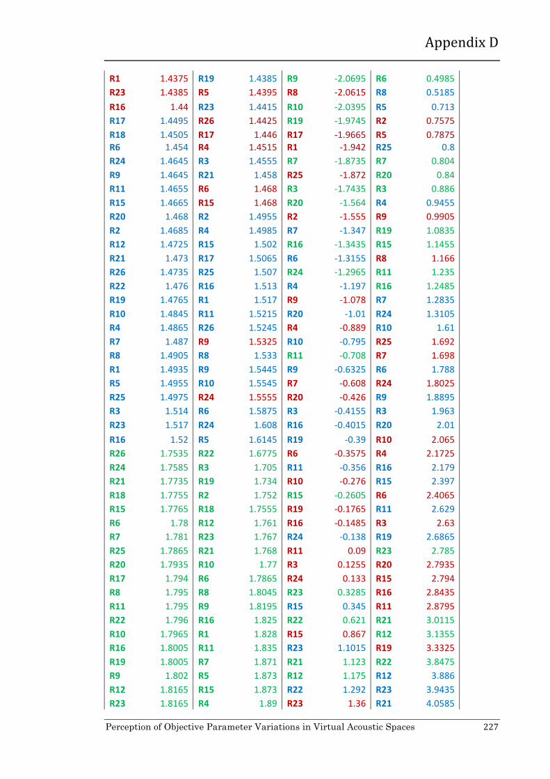
Appendix D
Perception of Objective Parameter Variations in Virtual Acoustic Spaces 227
R1 1.4375 R19 1.4385 R9 -‐2.0695 R6 0.4985 R23 1.4385 R5 1.4395 R8 -‐2.0615 R8 0.5185 R16 1.44 R23 1.4415 R10 -‐2.0395 R5 0.713 R17 1.4495 R26 1.4425 R19 -‐1.9745 R2 0.7575 R18 1.4505 R17 1.446 R17 -‐1.9665 R5 0.7875 R6 1.454 R4 1.4515 R1 -‐1.942 R25 0.8 R24 1.4645 R3 1.4555 R7 -‐1.8735 R7 0.804 R9 1.4645 R21 1.458 R25 -‐1.872 R20 0.84 R11 1.4655 R6 1.468 R3 -‐1.7435 R3 0.886 R15 1.4665 R15 1.468 R20 -‐1.564 R4 0.9455 R20 1.468 R2 1.4955 R2 -‐1.555 R9 0.9905 R2 1.4685 R4 1.4985 R7 -‐1.347 R19 1.0835 R12 1.4725 R15 1.502 R16 -‐1.3435 R15 1.1455 R21 1.473 R17 1.5065 R6 -‐1.3155 R8 1.166 R26 1.4735 R25 1.507 R24 -‐1.2965 R11 1.235 R22 1.476 R16 1.513 R4 -‐1.197 R16 1.2485 R19 1.4765 R1 1.517 R9 -‐1.078 R7 1.2835 R10 1.4845 R11 1.5215 R20 -‐1.01 R24 1.3105 R4 1.4865 R26 1.5245 R4 -‐0.889 R10 1.61 R7 1.487 R9 1.5325 R10 -‐0.795 R25 1.692 R8 1.4905 R8 1.533 R11 -‐0.708 R7 1.698 R1 1.4935 R9 1.5445 R9 -‐0.6325 R6 1.788 R5 1.4955 R10 1.5545 R7 -‐0.608 R24 1.8025 R25 1.4975 R24 1.5555 R20 -‐0.426 R9 1.8895 R3 1.514 R6 1.5875 R3 -‐0.4155 R3 1.963 R23 1.517 R24 1.608 R16 -‐0.4015 R20 2.01 R16 1.52 R5 1.6145 R19 -‐0.39 R10 2.065 R26 1.7535 R22 1.6775 R6 -‐0.3575 R4 2.1725 R24 1.7585 R3 1.705 R11 -‐0.356 R16 2.179 R21 1.7735 R19 1.734 R10 -‐0.276 R15 2.397 R18 1.7755 R2 1.752 R15 -‐0.2605 R6 2.4065 R15 1.7765 R18 1.7555 R19 -‐0.1765 R11 2.629 R6 1.78 R12 1.761 R16 -‐0.1485 R3 2.63 R7 1.781 R23 1.767 R24 -‐0.138 R19 2.6865 R25 1.7865 R21 1.768 R11 0.09 R23 2.785 R20 1.7935 R10 1.77 R3 0.1255 R20 2.7935 R17 1.794 R6 1.7865 R24 0.133 R15 2.794 R8 1.795 R8 1.8045 R23 0.3285 R16 2.8435 R11 1.795 R9 1.8195 R15 0.345 R11 2.8795 R22 1.796 R16 1.825 R22 0.621 R21 3.0115 R10 1.7965 R1 1.828 R15 0.867 R12 3.1355 R16 1.8005 R11 1.835 R23 1.1015 R19 3.3325 R19 1.8005 R7 1.871 R21 1.123 R22 3.8475 R9 1.802 R5 1.873 R12 1.175 R12 3.886 R12 1.8165 R15 1.873 R22 1.292 R23 3.9435 R23 1.8165 R4 1.89 R23 1.36 R21 4.0585

Appendix D
Perception of Objective Parameter Variations in Virtual Acoustic Spaces 228
R2 1.8265 R17 1.9075 R22 1.9005 R12 4.2015 R4 1.8295 R20 1.9165 R12 2.009 R23 4.3455 R5 1.8305 R24 1.939 R21 2.035 R21 4.5365 R1 1.837 R25 1.959 R21 2.2455 R22 5.101 R3 1.8495 R26 1.9935 R12 2.272 R22 5.3155
The relevant JNDs have been calculated based on the following minimum observed
values.
T30 EDT C50 C80 Minimum Values R24 1.358 R22 1.2535 R18 -‐4.6015 R8 -‐1.787 JND 0.0679 0.062675 1 1
Objective results for Configurations A, B and C, sorted
based on the JND values in increase order
JND values T30 EDT C50 C80
R24 0 R22 0 R18 0 R8 0 R11 0.11782 R21 0.343039 R18 0.339 R18 0.2845 R15 0.206186 R20 0.382928 R8 0.4065 R1 0.441 R6 0.220913 R22 0.542481 R18 0.7425 R25 1.0055 R8 0.279823 R7 0.861588 R1 1.056 R18 1.042 R26 0.294551 R12 0.893498 R5 1.283 R26 1.1785 R2 0.301915 R18 0.925409 R26 1.3395 R2 1.208 R5 0.360825 R2 0.965297 R25 1.449 R5 1.2975 R9 0.405007 R23 0.973275 R17 1.556 R4 1.392 R20 0.427099 R3 1.755086 R1 1.8055 R1 1.407 R22 0.427099 R19 1.810929 R2 1.918 R17 1.4855 R12 0.493373 R12 1.962505 R8 1.956 R9 1.719 R4 0.515464 R7 2.193857 R6 2.1645 R10 1.785 R18 0.670103 R20 2.241723 R26 2.21 R17 1.872 R17 0.714286 R25 2.393299 R26 2.2445 R26 1.914 R21 0.765832 R1 2.401276 R25 2.2805 R18 1.9295 R7 0.868925 R16 2.504986 R5 2.2955 R2 1.9445 R19 0.891016 R8 2.528919 R4 2.3 R24 2.015 R10 0.905744 R10 2.576785 R5 2.42 R17 2.1075 R25 0.905744 R11 2.59274 R17 2.442 R1 2.1325 R3 0.986745 R18 2.776227 R2 2.5245 R26 2.259 R1 1.170839 R19 2.951735 R9 2.532 R6 2.2855 R23 1.185567 R5 2.96769 R8 2.54 R8 2.3055 R16 1.207658 R23 2.999601 R10 2.562 R5 2.5

Appendix D
Perception of Objective Parameter Variations in Virtual Acoustic Spaces 229
R17 1.34757 R26 3.015556 R19 2.627 R2 2.5445 R18 1.362297 R17 3.0714 R17 2.635 R5 2.5745 R6 1.413844 R4 3.159154 R1 2.6595 R25 2.587 R24 1.568483 R3 3.222976 R7 2.728 R7 2.591 R9 1.568483 R21 3.262864 R25 2.7295 R20 2.627 R11 1.583211 R6 3.422417 R3 2.858 R3 2.673 R15 1.597938 R15 3.422417 R20 3.0375 R4 2.7325 R20 1.620029 R2 3.861189 R2 3.0465 R9 2.7775 R2 1.627393 R4 3.909055 R7 3.2545 R19 2.8705 R12 1.686303 R15 3.964898 R16 3.258 R15 2.9325 R21 1.693667 R17 4.036697 R6 3.286 R8 2.953 R26 1.701031 R25 4.044675 R24 3.305 R11 3.022 R22 1.73785 R16 4.140407 R4 3.4045 R16 3.0355 R19 1.745214 R1 4.204228 R9 3.5235 R7 3.0705 R10 1.863034 R11 4.276027 R20 3.5915 R24 3.0975 R4 1.892489 R26 4.323893 R4 3.7125 R10 3.397 R7 1.899853 R9 4.451536 R10 3.8065 R25 3.479 R8 1.951399 R8 4.459513 R11 3.8935 R7 3.485 R1 1.995582 R9 4.643 R9 3.969 R6 3.575 R5 2.025037 R10 4.802553 R7 3.9935 R24 3.5895 R25 2.054492 R24 4.818508 R20 4.1755 R9 3.6765 R3 2.297496 R6 5.329079 R3 4.186 R3 3.75 R23 2.341679 R24 5.656163 R16 4.2 R20 3.797 R16 2.385862 R5 5.759872 R19 4.2115 R10 3.852 R26 5.824742 R22 6.765058 R6 4.244 R4 3.9595 R24 5.89838 R3 7.203829 R11 4.2455 R16 3.966 R21 6.119293 R19 7.666534 R10 4.3255 R15 4.184 R18 6.148748 R2 7.95373 R15 4.341 R6 4.1935 R15 6.163476 R18 8.009573 R19 4.425 R11 4.416 R6 6.215022 R12 8.097327 R16 4.453 R3 4.417 R7 6.22975 R23 8.193059 R24 4.4635 R19 4.4735 R25 6.310751 R21 8.209015 R11 4.6915 R23 4.572 R20 6.413844 R10 8.240925 R3 4.727 R20 4.5805 R17 6.421208 R6 8.504188 R24 4.7345 R15 4.581 R8 6.435935 R8 8.791384 R23 4.93 R16 4.6305 R11 6.435935 R9 9.030714 R15 4.9465 R11 4.6665 R22 6.450663 R16 9.118468 R22 5.2225 R21 4.7985 R10 6.458027 R1 9.166334 R15 5.4685 R12 4.9225 R16 6.516937 R11 9.278022 R23 5.703 R19 5.1195 R19 6.516937 R7 9.852413 R21 5.7245 R22 5.6345 R9 6.539028 R5 9.884324 R12 5.7765 R12 5.673 R12 6.752577 R15 9.884324 R22 5.8935 R23 5.7305 R23 6.752577 R4 10.15556 R23 5.9615 R21 5.8455 R2 6.899853 R17 10.43478 R22 6.502 R12 5.9885 R4 6.944035 R20 10.57838 R12 6.6105 R23 6.1325 R5 6.958763 R24 10.93738 R21 6.6365 R21 6.3235

Appendix D
Perception of Objective Parameter Variations in Virtual Acoustic Spaces 230
R1 7.054492 R25 11.25648 R21 6.847 R22 6.888 R3 7.238586 R26 11.80694 R12 6.8735 R22 7.1025

Appendix D
Perception of Objective Parameter Variations in Virtual Acoustic Spaces 231
Objective results for Source Orientations 0°, 40°and 70°
sorted in increase order
The colours here indicate the source orientation configurations for each impulse
response (Blue for the 0° orientation of the source, Red for the 40° and Green for
the 70°).
T30 EDT C50 C80 R18 1.4305 R10 1.2115 R18 -‐7.0295 R18 -‐3.547 R22 1.4315 R22 1.2535 R18 -‐6.4505 R18 -‐2.974 R6 1.438 R20 1.324 R26 -‐5.653 R6 -‐1.982 R19 1.442 R10 1.3355 R8 -‐5.3785 R16 -‐1.943 R22 1.446 R12 1.353 R26 -‐5.375 R8 -‐1.8775 R11 1.4465 R12 1.3765 R25 -‐5.3395 R26 -‐1.5955 R6 1.4485 R21 1.3805 R8 -‐5.191 R17 -‐1.5685 R17 1.4495 R7 1.391 R17 -‐5.0915 R24 -‐1.426 R4 1.4495 R20 1.394 R9 -‐4.922 R5 -‐1.3935 R18 1.4505 R20 1.3995 R7 -‐4.8345 R25 -‐1.3585 R23 1.4505 R22 1.401 R16 -‐4.6505 R26 -‐1.34 R11 1.451 R21 1.414 R25 -‐4.643 R17 -‐1.331 R17 1.452 R22 1.4185 R6 -‐4.376 R8 -‐1.1575 R18 1.4535 R18 1.4275 R5 -‐4.3195 R9 -‐1.1405 R6 1.454 R19 1.4385 R18 -‐4.2625 R7 -‐0.9965 R23 1.4555 R23 1.4415 R24 -‐4.1295 R25 -‐0.9675 R26 1.459 R19 1.4525 R17 -‐4.1145 R5 -‐0.798 R24 1.4595 R3 1.4555 R9 -‐3.794 R6 -‐0.7805 R5 1.461 R21 1.458 R5 -‐3.4285 R18 -‐0.745 R19 1.462 R12 1.4615 R16 -‐3.2685 R9 -‐0.5865 R15 1.4625 R11 1.469 R6 -‐3.011 R16 -‐0.549 R26 1.4635 R4 1.4715 R15 -‐2.868 R1 -‐0.38 R12 1.4635 R3 1.472 R1 -‐2.796 R15 -‐0.289 R24 1.464 R19 1.475 R8 -‐2.6455 R17 0.085 R24 1.4645 R16 1.4775 R7 -‐2.6385 R7 0.0935 R9 1.4645 R16 1.491 R4 -‐2.4705 R4 0.097 R11 1.4655 R24 1.492 R26 -‐2.3915 R24 0.1195 R15 1.4665 R1 1.493 R25 -‐2.321 R26 0.127 R20 1.468 R2 1.4955 R24 -‐2.308 R2 0.1575 R2 1.4685 R4 1.4985 R5 -‐2.306 R23 0.389 R17 1.4685 R15 1.502 R17 -‐2.1595 R1 0.509 R21 1.469 R17 1.5065 R23 -‐2.0945 R8 0.5185 R8 1.4705 R25 1.507 R2 -‐2.077 R15 0.601 R10 1.4705 R11 1.5105 R3 -‐1.918 R1 0.6465 R12 1.4725 R16 1.513 R1 -‐1.7505 R2 0.6675 R21 1.473 R1 1.517 R2 -‐1.5845 R5 0.713

Appendix D
Perception of Objective Parameter Variations in Virtual Acoustic Spaces 232
R26 1.4735 R11 1.5215 R4 -‐1.563 R25 0.8 R1 1.475 R26 1.5245 R1 -‐1.471 R4 0.9455 R10 1.4755 R18 1.527 R7 -‐1.347 R3 0.985 R12 1.4755 R2 1.53 R6 -‐1.3155 R4 1.0305 R22 1.476 R8 1.533 R2 -‐1.239 R2 1.176 R20 1.476 R3 1.5395 R4 -‐1.197 R7 1.2835 R25 1.4765 R8 1.541 R15 -‐1.1735 R24 1.3105 R19 1.4765 R9 1.5445 R20 -‐1.01 R3 1.386 R2 1.478 R15 1.546 R10 -‐0.795 R10 1.61 R16 1.478 R1 1.5505 R3 -‐0.786 R6 1.788 R9 1.479 R7 1.5535 R23 -‐0.7115 R23 1.836 R2 1.48 R10 1.5545 R9 -‐0.6325 R9 1.8895 R15 1.4815 R26 1.5545 R22 -‐0.4495 R3 1.963 R16 1.4835 R15 1.5575 R3 -‐0.4155 R20 2.01 R10 1.4845 R25 1.5615 R16 -‐0.4015 R22 2.1095 R4 1.4865 R18 1.5695 R19 -‐0.39 R16 2.179 R21 1.4865 R23 1.5735 R11 -‐0.356 R15 2.397 R7 1.487 R24 1.5825 R24 -‐0.138 R11 2.629 R25 1.4895 R25 1.5865 R22 0.043 R19 2.6865 R5 1.49 R6 1.5875 R20 0.3065 R19 2.9365 R8 1.4905 R7 1.606 R15 0.345 R22 3.1225 R3 1.4915 R2 1.607 R19 0.7555 R20 3.388 R20 1.492 R24 1.608 R20 0.7755 R10 3.434 R1 1.4935 R9 1.61 R21 0.8195 R20 3.444 R9 1.494 R8 1.613 R19 0.9735 R21 3.6135 R8 1.494 R5 1.6145 R23 1.1015 R19 3.744 R7 1.4945 R23 1.6165 R22 1.292 R12 3.886 R5 1.4955 R4 1.6385 R21 1.593 R23 3.9435 R7 1.4955 R17 1.6455 R10 1.666 R21 4.0325 R25 1.4975 R26 1.688 R12 2.009 R21 4.0585 R3 1.4975 R9 1.6965 R21 2.035 R10 4.166 R4 1.5 R6 1.7025 R11 2.235 R11 4.1775 R3 1.514 R17 1.7205 R12 2.2705 R11 4.372 R23 1.517 R5 1.7235 R10 2.4855 R12 4.4875 R16 1.52 R5 1.752 R11 2.642 R22 5.101 R1 1.523 R6 1.788 R12 3.163 R12 5.1545
The relevant JNDs have been calculated based on the following minimum observed
values.
T30 EDT C50 C80 Minimum Values R18 1.4305 R10 1.2115 R18 -‐7.0295 R18 -‐3.547 JND 0.071525 0.060575 1 1

Appendix D
Perception of Objective Parameter Variations in Virtual Acoustic Spaces 233
Objective results for Source Orientations 0°, 40° and 70°
sorted based on the JND values in increase order
JND values T30 EDT C50 C80 R18 0 R10 0 R18 0 R18 0 R22 0.013981 R22 0.693355 R18 0.579 R18 0.573 R6 0.104858 R20 1.857202 R26 1.3765 R6 1.565 R19 0.160783 R10 2.047049 R8 1.651 R16 1.604 R22 0.216707 R12 2.335947 R26 1.6545 R8 1.6695 R11 0.223698 R12 2.723896 R25 1.69 R26 1.9515 R6 0.25166 R21 2.78993 R8 1.8385 R17 1.9785 R17 0.265641 R7 2.963269 R17 1.938 R24 2.121 R4 0.265641 R20 3.012794 R9 2.1075 R5 2.1535 R18 0.279623 R20 3.103591 R7 2.195 R25 2.1885 R23 0.279623 R22 3.128353 R16 2.379 R26 2.207 R11 0.286613 R21 3.342963 R25 2.3865 R17 2.216 R17 0.300594 R22 3.417251 R6 2.6535 R8 2.3895 R18 0.321566 R18 3.565827 R5 2.71 R9 2.4065 R6 0.328556 R19 3.747421 R18 2.767 R7 2.5505 R23 0.349528 R23 3.796946 R24 2.9 R25 2.5795 R26 0.398462 R19 3.978539 R17 2.915 R5 2.749 R24 0.405453 R3 4.028064 R9 3.2355 R6 2.7665 R5 0.426424 R21 4.069336 R5 3.601 R18 2.802 R19 0.440405 R12 4.127115 R16 3.761 R9 2.9605 R15 0.447396 R11 4.250929 R6 4.0185 R16 2.998 R26 0.461377 R4 4.2922 R15 4.1615 R1 3.167 R12 0.461377 R3 4.300454 R1 4.2335 R15 3.258 R24 0.468368 R19 4.349979 R8 4.384 R17 3.632 R24 0.475358 R16 4.391251 R7 4.391 R7 3.6405 R9 0.475358 R16 4.614115 R4 4.559 R4 3.644 R11 0.489339 R24 4.630623 R26 4.638 R24 3.6665 R15 0.503321 R1 4.647132 R25 4.7085 R26 3.674 R20 0.524292 R2 4.688403 R24 4.7215 R2 3.7045 R2 0.531283 R4 4.737928 R5 4.7235 R23 3.936 R17 0.531283 R15 4.795708 R17 4.87 R1 4.056 R21 0.538273 R17 4.869996 R23 4.935 R8 4.0655 R8 0.559245 R25 4.87825 R2 4.9525 R15 4.148 R10 0.559245 R11 4.93603 R3 5.1115 R1 4.1935 R12 0.587207 R16 4.977301 R1 5.279 R2 4.2145 R21 0.594198 R1 5.043335 R2 5.445 R5 4.26 R26 0.601188 R11 5.117623 R4 5.4665 R25 4.347 R1 0.62216 R26 5.167148 R1 5.5585 R4 4.4925 R10 0.629151 R18 5.208419 R7 5.6825 R3 4.532 R12 0.629151 R2 5.257945 R6 5.714 R4 4.5775

Appendix D
Perception of Objective Parameter Variations in Virtual Acoustic Spaces 234
R22 0.636141 R8 5.30747 R2 5.7905 R2 4.723 R20 0.636141 R3 5.414775 R4 5.8325 R7 4.8305 R25 0.643132 R8 5.439538 R15 5.856 R24 4.8575 R19 0.643132 R9 5.497317 R20 6.0195 R3 4.933 R2 0.664103 R15 5.52208 R10 6.2345 R10 5.157 R16 0.664103 R1 5.596368 R3 6.2435 R6 5.335 R9 0.678085 R7 5.645894 R23 6.318 R23 5.383 R2 0.692066 R10 5.662402 R9 6.397 R9 5.4365 R15 0.713037 R26 5.662402 R22 6.58 R3 5.51 R16 0.741 R15 5.711927 R3 6.614 R20 5.557 R10 0.754981 R25 5.777961 R16 6.628 R22 5.6565 R4 0.782943 R18 5.910029 R19 6.6395 R16 5.726 R21 0.782943 R23 5.976063 R11 6.6735 R15 5.944 R7 0.789934 R24 6.124639 R24 6.8915 R11 6.176 R25 0.824886 R25 6.190673 R22 7.0725 R19 6.2335 R5 0.831877 R6 6.207181 R20 7.336 R19 6.4835 R8 0.838868 R7 6.512588 R15 7.3745 R22 6.6695 R3 0.852849 R2 6.529096 R19 7.785 R20 6.935 R20 0.859839 R24 6.545605 R20 7.805 R10 6.981 R1 0.880811 R9 6.578622 R21 7.849 R20 6.991 R9 0.887801 R8 6.628147 R19 8.003 R21 7.1605 R8 0.887801 R5 6.65291 R23 8.131 R19 7.291 R7 0.894792 R23 6.685927 R22 8.3215 R12 7.433 R5 0.908773 R4 7.049113 R21 8.6225 R23 7.4905 R7 0.908773 R17 7.164672 R10 8.6955 R21 7.5795 R25 0.936735 R26 7.866281 R12 9.0385 R21 7.6055 R3 0.936735 R9 8.006603 R21 9.0645 R10 7.713 R4 0.971688 R6 8.105654 R11 9.2645 R11 7.7245 R3 1.167424 R17 8.402806 R12 9.3 R11 7.919 R23 1.209367 R5 8.452332 R10 9.515 R12 8.0345 R16 1.251311 R5 8.922823 R11 9.6715 R22 8.648 R1 1.293254 R6 9.517128 R12 10.1925 R12 8.7015

Appendix D
Perception of Objective Parameter Variations in Virtual Acoustic Spaces 235
CATT-Acoustic
Objective results for Configurations A, B and C, sorted in
increase order
T30 EDT C50 C80 R26 1.4685 R21 1.08 R2 -‐3.882 R18 -‐1.428 R7 1.48 R22 1.1455 R2 -‐3.844 R9 -‐1.3695 R6 1.4845 R11 1.212 R5 -‐3.618 R2 -‐1.313 R9 1.4985 R11 1.291 R9 -‐3.418 R17 -‐1.103 R12 1.5035 R20 1.3175 R8 -‐3.209 R8 -‐0.923 R18 1.5045 R10 1.365 R25 -‐3.126 R25 -‐0.819 R8 1.5055 R4 1.368 R5 -‐3.0905 R26 -‐0.7025 R5 1.5115 R24 1.3805 R26 -‐3.079 R5 -‐0.678 R17 1.5135 R15 1.3895 R5 -‐3.0615 R2 -‐0.2415 R11 1.516 R21 1.4005 R17 -‐3.0545 R5 -‐0.2405 R2 1.5195 R3 1.403 R18 -‐2.9045 R9 0.0465 R4 1.5215 R19 1.408 R1 -‐2.7805 R2 0.137 R25 1.522 R20 1.435 R26 -‐2.74 R5 0.2245 R22 1.5225 R3 1.4455 R2 -‐2.734 R1 0.2705 R15 1.5235 R16 1.453 R9 -‐2.408 R3 0.4325 R3 1.5275 R17 1.4685 R8 -‐2.3475 R7 0.4495 R19 1.537 R22 1.476 R26 -‐2.343 R18 0.46 R21 1.5385 R8 1.5065 R18 -‐2.055 R6 0.606 R7 1.5465 R18 1.5425 R16 -‐2.032 R26 0.6285 R9 1.549 R6 1.545 R8 -‐1.613 R8 0.768 R1 1.5515 R5 1.5695 R9 -‐1.432 R26 0.8205 R24 1.5515 R1 1.5725 R3 -‐1.3795 R19 0.828 R23 1.552 R23 1.575 R10 -‐1.3665 R16 0.8835 R16 1.5585 R26 1.579 R25 -‐1.2105 R17 0.9805 R1 1.5585 R9 1.599 R16 -‐1.1535 R23 0.983 R10 1.5615 R25 1.6155 R7 -‐1.14 R10 1.0025 R16 1.565 R19 1.6165 R18 -‐1.128 R7 1.083 R20 1.565 R2 1.6195 R17 -‐0.965 R24 1.195 R26 1.566 R25 1.628 R16 -‐0.94 R4 1.2065 R10 1.577 R6 1.64 R20 -‐0.9315 R25 1.2595 R21 1.583 R18 1.6405 R17 -‐0.905 R20 1.3335 R8 1.5845 R4 1.6435 R25 -‐0.8935 R18 1.3665 R19 1.586 R8 1.6635 R7 -‐0.8165 R1 1.3875 R25 1.59 R12 1.6745 R19 -‐0.8005 R25 1.39 R2 1.5915 R17 1.6875 R6 -‐0.776 R7 1.42 R6 1.599 R2 1.701 R23 -‐0.703 R9 1.5685 R15 1.6015 R16 1.704 R24 -‐0.6235 R10 1.761 R3 1.6035 R12 1.7115 R3 -‐0.5805 R17 1.799 R24 1.6055 R5 1.7335 R4 -‐0.5375 R16 1.8135

Appendix D
Perception of Objective Parameter Variations in Virtual Acoustic Spaces 236
R18 1.607 R7 1.738 R7 -‐0.2645 R8 1.8885 R17 1.6155 R26 1.7655 R10 -‐0.219 R16 2.1005 R20 1.617 R24 1.7985 R1 -‐0.1635 R12 2.311 R23 1.6215 R9 1.809 R3 -‐0.1595 R6 2.341 R4 1.6235 R23 1.8345 R10 0.2995 R19 2.427 R22 1.6285 R15 1.8415 R20 0.3715 R1 2.431 R11 1.633 R10 1.845 R12 0.492 R22 2.508 R5 1.6395 R7 1.8535 R11 0.5965 R20 2.6935 R12 1.6405 R1 1.8635 R6 0.6185 R11 2.7085 R25 1.8745 R21 1.9515 R1 0.7405 R4 2.751 R8 1.8845 R17 2.0025 R22 0.774 R15 2.7785 R10 1.9075 R22 2.061 R6 0.791 R3 2.8315 R26 1.916 R15 2.0735 R24 0.9105 R6 2.844 R1 1.918 R6 2.1005 R20 0.9265 R3 3.0185 R23 1.9185 R11 2.128 R19 0.936 R4 3.0915 R18 1.92 R10 2.1365 R15 1.031 R24 3.092 R21 1.9205 R24 2.1375 R4 1.165 R21 3.2915 R19 1.9235 R2 2.138 R19 1.19 R24 3.294 R9 1.9265 R23 2.1395 R4 1.2135 R19 3.3105 R16 1.934 R4 2.153 R23 1.504 R23 3.4475 R4 1.935 R25 2.163 R23 1.544 R15 3.5325 R6 1.9375 R19 2.174 R12 1.548 R20 3.5865 R12 1.9405 R5 2.193 R24 1.587 R10 3.601 R3 1.9415 R18 2.2095 R22 1.9635 R23 3.6445 R7 1.947 R16 2.219 R11 1.968 R22 4.042 R22 1.9475 R12 2.234 R15 2.057 R21 4.1195 R24 1.9475 R26 2.24 R22 2.0935 R12 4.1215 R5 1.9525 R3 2.2425 R21 2.1135 R11 4.5565 R2 1.956 R1 2.252 R12 2.3345 R11 4.6395 R11 1.9585 R9 2.279 R11 2.4775 R15 4.67 R20 1.9605 R7 2.3165 R15 2.633 R12 4.6885 R17 1.975 R20 2.334 R21 2.6825 R21 4.81 R15 2.002 R8 2.403 R21 2.8635 R22 4.9475
The relevant JNDs have been calculated based on the following minimum observed
values.
T30 EDT C50 C80 Minimum Values R26 1.4685 R21 1.08 R2 -‐3.882 R18 -‐1.428 JND 0.073425 0.054 1 1

Appendix D
Perception of Objective Parameter Variations in Virtual Acoustic Spaces 237
Objective results for Configurations A, B and C, sorted
based on the JND values in increase order
JND values T30 EDT C50 C80 R26 0 R21 0 R2 0 R18 0 R7 0.156622 R22 1.212963 R2 0.038 R9 0.0585 R6 0.217909 R11 2.444444 R5 0.264 R2 0.115 R9 0.40858 R11 3.907407 R9 0.464 R17 0.325 R12 0.476677 R20 4.398148 R8 0.673 R8 0.505 R18 0.490296 R10 5.277778 R25 0.756 R25 0.609 R8 0.503916 R4 5.333333 R5 0.7915 R26 0.7255 R5 0.585632 R24 5.564815 R26 0.803 R5 0.75 R17 0.61287 R15 5.731481 R5 0.8205 R2 1.1865 R11 0.646919 R21 5.935185 R17 0.8275 R5 1.1875 R2 0.694586 R3 5.981481 R18 0.9775 R9 1.4745 R4 0.721825 R19 6.074074 R1 1.1015 R2 1.565 R25 0.728635 R20 6.574074 R26 1.142 R5 1.6525 R22 0.735444 R3 6.768519 R2 1.148 R1 1.6985 R15 0.749064 R16 6.907407 R9 1.474 R3 1.8605 R3 0.803541 R17 7.194444 R8 1.5345 R7 1.8775 R19 0.932925 R22 7.333333 R26 1.539 R18 1.888 R21 0.953354 R8 7.898148 R18 1.827 R6 2.034 R7 1.062308 R18 8.564815 R16 1.85 R26 2.0565 R9 1.096357 R6 8.611111 R8 2.269 R8 2.196 R1 1.130405 R5 9.064815 R9 2.45 R26 2.2485 R24 1.130405 R1 9.12037 R3 2.5025 R19 2.256 R23 1.137215 R23 9.166667 R10 2.5155 R16 2.3115 R16 1.225741 R26 9.240741 R25 2.6715 R17 2.4085 R1 1.225741 R9 9.611111 R16 2.7285 R23 2.411 R10 1.266599 R25 9.916667 R7 2.742 R10 2.4305 R16 1.314266 R19 9.935185 R18 2.754 R7 2.511 R20 1.314266 R2 9.990741 R17 2.917 R24 2.623 R26 1.327886 R25 10.14815 R16 2.942 R4 2.6345 R10 1.477698 R6 10.37037 R20 2.9505 R25 2.6875 R21 1.559414 R18 10.37963 R17 2.977 R20 2.7615 R8 1.579843 R4 10.43519 R25 2.9885 R18 2.7945 R19 1.600272 R8 10.80556 R7 3.0655 R1 2.8155 R25 1.65475 R12 11.00926 R19 3.0815 R25 2.818 R2 1.675179 R17 11.25 R6 3.106 R7 2.848 R6 1.777324 R2 11.5 R23 3.179 R9 2.9965 R15 1.811372 R16 11.55556 R24 3.2585 R10 3.189 R3 1.838611 R12 11.69444 R3 3.3015 R17 3.227 R24 1.86585 R5 12.10185 R4 3.3445 R16 3.2415 R18 1.886279 R7 12.18519 R7 3.6175 R8 3.3165

Appendix D
Perception of Objective Parameter Variations in Virtual Acoustic Spaces 238
R17 2.002043 R26 12.69444 R10 3.663 R16 3.5285 R20 2.022472 R24 13.30556 R1 3.7185 R12 3.739 R23 2.083759 R9 13.5 R3 3.7225 R6 3.769 R4 2.110998 R23 13.97222 R10 4.1815 R19 3.855 R22 2.179094 R15 14.10185 R20 4.2535 R1 3.859 R11 2.240381 R10 14.16667 R12 4.374 R22 3.936 R5 2.328907 R7 14.32407 R11 4.4785 R20 4.1215 R12 2.342526 R1 14.50926 R6 4.5005 R11 4.1365 R25 5.529452 R21 16.13889 R1 4.6225 R4 4.179 R8 5.665645 R17 17.08333 R22 4.656 R15 4.2065 R10 5.97889 R22 18.16667 R6 4.673 R3 4.2595 R26 6.094654 R15 18.39815 R24 4.7925 R6 4.272 R1 6.121893 R6 18.89815 R20 4.8085 R3 4.4465 R23 6.128703 R11 19.40741 R19 4.818 R4 4.5195 R18 6.149132 R10 19.56481 R15 4.913 R24 4.52 R21 6.155941 R24 19.58333 R4 5.047 R21 4.7195 R19 6.196799 R2 19.59259 R19 5.072 R24 4.722 R9 6.237657 R23 19.62037 R4 5.0955 R19 4.7385 R16 6.339803 R4 19.87037 R23 5.386 R23 4.8755 R4 6.353422 R25 20.05556 R23 5.426 R15 4.9605 R6 6.38747 R19 20.25926 R12 5.43 R20 5.0145 R12 6.428328 R5 20.61111 R24 5.469 R10 5.029 R3 6.441948 R18 20.91667 R22 5.8455 R23 5.0725 R7 6.516854 R16 21.09259 R11 5.85 R22 5.47 R22 6.523664 R12 21.37037 R15 5.939 R21 5.5475 R24 6.523664 R26 21.48148 R22 5.9755 R12 5.5495 R5 6.59176 R3 21.52778 R21 5.9955 R11 5.9845 R2 6.639428 R1 21.7037 R12 6.2165 R11 6.0675 R11 6.673476 R9 22.2037 R11 6.3595 R15 6.098 R20 6.700715 R7 22.89815 R15 6.515 R12 6.1165 R17 6.898195 R20 23.22222 R21 6.5645 R21 6.238 R15 7.265918 R8 24.5 R21 6.7455 R22 6.3755

Appendix D
Perception of Objective Parameter Variations in Virtual Acoustic Spaces 239
ODEON
Objective results for Configurations A, B and C, sorted in
increase order
T30 EDT C50 C80 R2 1.307 R17 1.147 R5 -‐4.8025 R5 -‐1.237 R20 1.318 R21 1.176 R2 -‐4.5655 R2 -‐1.0275 R1 1.3265 R12 1.1775 R26 -‐4.112 R26 -‐0.461 R18 1.3295 R21 1.191 R5 -‐4.055 R18 -‐0.212 R19 1.3305 R11 1.2315 R2 -‐3.71 R16 -‐0.016 R10 1.3315 R22 1.254 R2 -‐3.29 R2 -‐0.016 R3 1.335 R20 1.29 R5 -‐3.2145 R5 0.0255 R7 1.335 R25 1.29 R18 -‐3.1055 R2 0.184 R11 1.335 R4 1.2985 R26 -‐2.978 R5 0.432 R15 1.3355 R17 1.305 R26 -‐2.511 R10 0.532 R16 1.341 R18 1.312 R16 -‐2.406 R1 0.547 R6 1.3435 R10 1.313 R18 -‐2.3365 R26 0.6435 R12 1.344 R12 1.318 R10 -‐1.9715 R8 0.9785 R9 1.3465 R19 1.3325 R8 -‐1.8705 R18 1.022 R4 1.351 R8 1.3475 R25 -‐1.789 R9 1.1065 R21 1.351 R11 1.3545 R16 -‐1.702 R25 1.108 R22 1.3515 R26 1.3695 R18 -‐1.648 R19 1.1105 R24 1.352 R4 1.375 R19 -‐1.5975 R16 1.212 R23 1.3525 R23 1.377 R10 -‐1.255 R26 1.35 R5 1.3585 R22 1.3795 R1 -‐1.213 R20 1.379 R26 1.361 R6 1.3805 R16 -‐1.1985 R3 1.3805 R8 1.363 R25 1.386 R3 -‐1.134 R6 1.4455 R25 1.3645 R8 1.3935 R6 -‐1.1095 R7 1.4455 R17 1.3725 R5 1.394 R17 -‐1.0455 R16 1.4925 R8 1.431 R9 1.394 R10 -‐1.0195 R18 1.528 R1 1.432 R15 1.3945 R8 -‐1.017 R10 1.65 R17 1.432 R6 1.3955 R7 -‐0.966 R17 1.7405 R15 1.438 R23 1.3975 R20 -‐0.746 R1 1.8335 R7 1.4445 R24 1.4 R9 -‐0.6865 R8 2.0515 R11 1.446 R18 1.409 R19 -‐0.6435 R10 2.1015 R12 1.448 R20 1.412 R25 -‐0.4635 R24 2.103 R5 1.449 R16 1.4135 R1 -‐0.3345 R19 2.168 R2 1.4535 R2 1.415 R17 -‐0.286 R1 2.2795 R4 1.454 R7 1.4185 R8 -‐0.2105 R23 2.2985 R18 1.456 R19 1.4205 R6 -‐0.1775 R7 2.469 R10 1.4575 R1 1.425 R19 -‐0.173 R11 2.498 R22 1.459 R3 1.4275 R25 -‐0.0465 R25 2.5515 R19 1.4635 R1 1.431 R24 0.02 R19 2.5975 R21 1.4655 R26 1.4475 R3 0.0345 R3 2.6855

Appendix D
Perception of Objective Parameter Variations in Virtual Acoustic Spaces 240
R3 1.468 R2 1.465 R11 0.0405 R6 2.729 R26 1.47 R9 1.465 R17 0.092 R15 2.817 R6 1.4725 R16 1.4655 R7 0.117 R17 2.836 R9 1.473 R10 1.4755 R3 0.3035 R4 2.9435 R25 1.473 R5 1.4765 R20 0.338 R20 2.9485 R24 1.4735 R15 1.4775 R1 0.375 R9 2.958 R23 1.475 R7 1.5225 R23 0.418 R8 2.9975 R16 1.481 R3 1.525 R6 0.5625 R25 2.998 R20 1.489 R24 1.5515 R20 0.59 R7 3.057 R22 1.75 R21 1.5525 R9 0.593 R3 3.0655 R17 1.7615 R11 1.6035 R7 0.812 R24 3.1415 R12 1.7655 R12 1.626 R11 0.895 R9 3.145 R21 1.773 R22 1.6625 R4 0.9365 R12 3.1775 R16 1.7785 R17 1.6675 R24 0.983 R20 3.2375 R6 1.7795 R25 1.6685 R11 1.0055 R6 3.255 R15 1.7815 R23 1.7435 R15 1.0065 R17 3.313 R4 1.782 R6 1.75 R9 1.0455 R23 3.4385 R10 1.7835 R4 1.755 R12 1.056 R22 3.5085 R3 1.7865 R19 1.7565 R23 1.3165 R24 3.527 R2 1.787 R15 1.7725 R24 1.4695 R11 3.619 R24 1.789 R9 1.779 R23 1.49 R23 3.69 R18 1.79 R8 1.7935 R15 1.77 R11 3.8015 R7 1.792 R26 1.7965 R12 1.844 R15 3.803 R20 1.792 R24 1.8005 R4 1.9125 R15 4.0745 R9 1.7935 R3 1.809 R22 1.939 R4 4.299 R23 1.7965 R10 1.813 R15 1.96 R12 4.301 R5 1.7975 R20 1.8155 R12 2.0445 R22 4.435 R11 1.805 R7 1.833 R4 2.4705 R12 4.672 R19 1.8105 R1 1.837 R22 2.6655 R4 4.723 R25 1.815 R18 1.8385 R22 3.201 R21 4.7615 R1 1.819 R5 1.8425 R21 3.2525 R22 4.884 R26 1.8235 R16 1.8635 R21 4.02 R21 5.9505 R8 1.826 R2 1.906 R21 4.4765 R21 6.397
The relevant JNDs have been calculated based on the following minimum observed
values.
T30 EDT C50 C80 Minimum Values R2 1.307 R17 1.147 R5 -‐4.8025 R5 -‐1.237 JND 0.06535 0.05735 1 1

Appendix D
Perception of Objective Parameter Variations in Virtual Acoustic Spaces 241
Objective results for Configurations A, B and C, sorted
based on the JND values in increase order
JND values T30 EDT C50 C80 R2 0 R17 0 R5 0 R5 0 R20 0.168324 R21 0.505667 R2 0.237 R2 0.2095 R1 0.298393 R12 0.531822 R26 0.6905 R26 0.776 R18 0.3443 R21 0.767219 R5 0.7475 R18 1.025 R19 0.359602 R11 1.473409 R2 1.0925 R16 1.221 R10 0.374904 R22 1.865737 R2 1.5125 R2 1.221 R3 0.428462 R20 2.493461 R5 1.588 R5 1.2625 R7 0.428462 R25 2.493461 R18 1.697 R2 1.421 R11 0.428462 R4 2.641674 R26 1.8245 R5 1.669 R15 0.436113 R17 2.755013 R26 2.2915 R10 1.769 R16 0.520275 R18 2.877071 R16 2.3965 R1 1.784 R6 0.558531 R10 2.894507 R18 2.466 R26 1.8805 R12 0.566182 R12 2.981691 R10 2.831 R8 2.2155 R9 0.604438 R19 3.234525 R8 2.932 R18 2.259 R4 0.673298 R8 3.496077 R25 3.0135 R9 2.3435 R21 0.673298 R11 3.618134 R16 3.1005 R25 2.345 R22 0.680949 R26 3.879686 R18 3.1545 R19 2.3475 R24 0.6886 R4 3.975588 R19 3.205 R16 2.449 R23 0.696251 R23 4.010462 R10 3.5475 R26 2.587 R5 0.788064 R22 4.054054 R1 3.5895 R20 2.616 R26 0.82632 R6 4.071491 R16 3.604 R3 2.6175 R8 0.856924 R25 4.167393 R3 3.6685 R6 2.6825 R25 0.879878 R8 4.298169 R6 3.693 R7 2.6825 R17 1.002295 R5 4.306888 R17 3.757 R16 2.7295 R8 1.897475 R9 4.306888 R10 3.783 R18 2.765 R1 1.912777 R15 4.315606 R8 3.7855 R10 2.887 R17 1.912777 R6 4.333043 R7 3.8365 R17 2.9775 R15 2.004591 R23 4.367916 R20 4.0565 R1 3.0705 R7 2.104055 R24 4.411508 R9 4.116 R8 3.2885 R11 2.127008 R18 4.568439 R19 4.159 R10 3.3385 R12 2.157613 R20 4.62075 R25 4.339 R24 3.34 R5 2.172915 R16 4.646905 R1 4.468 R19 3.405 R2 2.241775 R2 4.67306 R17 4.5165 R1 3.5165 R4 2.249426 R7 4.734089 R8 4.592 R23 3.5355 R18 2.280031 R19 4.768963 R6 4.625 R7 3.706 R10 2.302984 R1 4.847428 R19 4.6295 R11 3.735 R22 2.325937 R3 4.89102 R25 4.756 R25 3.7885 R19 2.394797 R1 4.952049 R24 4.8225 R19 3.8345 R21 2.425402 R26 5.239756 R3 4.837 R3 3.9225 R3 2.463657 R2 5.5449 R11 4.843 R6 3.966

Appendix D
Perception of Objective Parameter Variations in Virtual Acoustic Spaces 242
R26 2.494262 R9 5.5449 R17 4.8945 R15 4.054 R6 2.532517 R16 5.553618 R7 4.9195 R17 4.073 R9 2.540168 R10 5.727986 R3 5.106 R4 4.1805 R25 2.540168 R5 5.745423 R20 5.1405 R20 4.1855 R24 2.547819 R15 5.76286 R1 5.1775 R9 4.195 R23 2.570773 R7 6.547515 R23 5.2205 R8 4.2345 R16 2.662586 R3 6.591107 R6 5.365 R25 4.235 R20 2.785004 R24 7.053182 R20 5.3925 R7 4.294 R22 6.778883 R21 7.070619 R9 5.3955 R3 4.3025 R17 6.954858 R11 7.959895 R7 5.6145 R24 4.3785 R12 7.016067 R12 8.352223 R11 5.6975 R9 4.382 R21 7.130834 R22 8.988666 R4 5.739 R12 4.4145 R16 7.214996 R17 9.07585 R24 5.7855 R20 4.4745 R6 7.230298 R25 9.093287 R11 5.808 R6 4.492 R15 7.260903 R23 10.40105 R15 5.809 R17 4.55 R4 7.268554 R6 10.51439 R9 5.848 R23 4.6755 R10 7.291507 R4 10.60157 R12 5.8585 R22 4.7455 R3 7.337414 R19 10.62772 R23 6.119 R24 4.764 R2 7.345065 R15 10.90671 R24 6.272 R11 4.856 R24 7.375669 R9 11.02005 R23 6.2925 R23 4.927 R18 7.390972 R8 11.27289 R15 6.5725 R11 5.0385 R7 7.421576 R26 11.3252 R12 6.6465 R15 5.04 R20 7.421576 R24 11.39494 R4 6.715 R15 5.3115 R9 7.444529 R3 11.54316 R22 6.7415 R4 5.536 R23 7.490436 R10 11.6129 R15 6.7625 R12 5.538 R5 7.505738 R20 11.6565 R12 6.847 R22 5.672 R11 7.620505 R7 11.96164 R4 7.273 R12 5.909 R19 7.704667 R1 12.03139 R22 7.468 R4 5.96 R25 7.773527 R18 12.05754 R22 8.0035 R21 5.9985 R1 7.834736 R5 12.12729 R21 8.055 R22 6.121 R26 7.903596 R16 12.49346 R21 8.8225 R21 7.1875 R8 7.941852 R2 13.23452 R21 9.279 R21 7.634

Appendix E
Perception of Objective Parameter Variations in Virtual Acoustic Spaces 243
Appendix E
Supporting materials on DVD
Supporting material of this research can be found on the accompanying DVD,
providing results, audio examples and digital copies of the thesis and the author’s
publications. The DVD is designed to be used as a website, thus the index.html file
should be used for the navigation to the contents. The contents of the DVD are:
A. Impulse Responses from:
a. acoustic measurements in St. Margaret’s Church
b. CATT-Acoustic model of St. Margaret’s Church
c. ODEON model of St. Margaret’s Church
B. CAD model
a. in CATT-Acoustic
b. in ODEON
C. Listening tests data:
a. Documentation
b. Anechoic Stimuli
c. Sound Examples
d. Subjective Responses
D. Publications:
a. PhD Thesis (pdf file)
b. Conference Papers

References
Perception of Objective Parameter Variations in Virtual Acoustic Spaces 244
References
1. Commins, D., Pompoli, R., Farina, A., Fausti, P., Prodi, N., Acoustics of Teatro Degli Archimboli in Milano Design, Computer and Scale Models, Details, Results. Proceedings of the Institute of Acoustics, 2002. 24(Pt 4).
2. Farina, A., Cocchi, A., Garai, M., Semprini, G. Old Churches as Concert Halls: a Non-Sabinian Approach to Optimum Design of Acoustic Correction. in Proc. of 14th I.C.A. . 1992. Beijing, China.
3. Exton, P., Marshall, H. The Room Acoustic design of the Guangzhou Opera House. Proceedings of the Institute of Acoustics. in Proc. of the Institute of Acoustics. 2011. Dublin, Ireland.
4. Dilworth, C., Smyth, S. The Acoustic Requirements of the Irish Chamber Orchestra. in Proc. of the Institute of Acoustics. 2011. Dublin, Ireland.
5. Facondini, M., Ponteggia, D. Acoustics of the Restored Petruzzelli Theater. in Proc. of the 128th AES Convention 2010. London, UK.
6. Buen, A., Strand, L., Room Acoustics in the Scene II in the New Oslo Opera and the Ridehuset - Two Variable Acoustics Coupled Space Venues. Proc. of the Institute of Acoustics, 2008. 30(2): p. 240-260.
7. A virtual acoustic walkthrough animation in St. Margaret's Church, York. the Open AIR Library [cited 2011]; Available from: http://www.openairlib.net/auralizationdb/content/st-margarets-church-national-centre-early-music.
8. Fazenda, B., Drumm, I. Recreating the Sound of Stonehenge. in The Acoustics of Ancient Theatres Conference. 2011. Patras.
9. Murphy, D., Archaeological Acoustic Space Measurement for Convolution Reverberation and Auralization Applications. Proc. Of the 9th Int.Conference on Digital Effects (DAFx-06), 2006: p. 221-226.
10. Niaounakis, T.I. The Acoustics of Ancient Theatre of Hephastia - Limnos Island, Greece. in The Acoustics of Ancient Theatres Conference. 2011. Patras.
11. Vassilantonopoulos, S.L., Hatziantoniou, P., Tatlas, N-A., Zakynthizons, T., Mourjopoulos, J.N. . Measurements and Analysis of the Acoustics of the Ancient Theatre of Epidaurus. in The Acoustics of Ancient Theatres Conference. 2011. Patras.
12. Iannace, G., Maffei, L., Trematerra, P. The Acoustic Evolution of the Large Theatre of Pompeii. in The Acoustics of Ancient Theatres. 2011. Patras.
13. Rindel, J.H., Lisa, M. The ERATO project and its contribution to our understanding of the acoustics of ancient Greek and Roman theatres. in ERATO Project Symposium. 2006. Istanbul, Turkey.
14. Rindel, J.H. The Erato Project and its Contribution to our Understanding of the Acoustics of Ancient Theatres. in The Acoustics od Ancient Theatres. 2011. Patras.
15. Prodi, N., Farnetani, A., Pompoli, R., Fausti, P. Acoustics and Architecture in Ancient Open Air Theatres. in The acoustics of Ancient Theatres Conference. 2011. Patras.
16. Lisa, M., Rindel, J.H. and Christensen, C.L. Predicting the Acoustics of Ancient Open-Air Theaters: The importance of Calculation Methods and Geometrical Details. in Joint Baltic-Nordic Acoustics Meeting. 2004.
17. Rindel, J.H., Gade, A.C., Lisa, M., The Virtual Reconstruction of the Ancient Roman Concept Hall in Aphrodisias, Turkey. Proc. of the Institute of Acoustics, 2006. 28(2): p. 316-323.

References
Perception of Objective Parameter Variations in Virtual Acoustic Spaces 245
18. Dragonetti, R., Ianniello, C., Mercoglaino, F., Romano, R. The Acoustics of two Ancient Roman Theatres in Pompeii. in 9th International Congress on Acoustics. 2007. Madrid.
19. Fausti, P., Pompoli, R., Prodi, N. Comparing the Acoustics of Mosques and Byzantine Churches. in 19th International Symposium CIPA. 2003. Antalya, Turkey.
20. Boren, B., Longair, M. A Method for Acoustic Modelling of Past Soundscapes. in The acoustics of Ancient Theatres Conference. 2011. Patras.
21. Foteinou, A., Murphy, D., Masinton, A. Verification of Geometric Acoustics Based Auralization. in Proc. of the128th AES Convention. 2010. London.
22. Foteinou, A., Murphy D. and Masinton, A. Investigation of Factors Influencing Acoustic Characteristics in Geometric Acoustics Based Auralization. in Proc. of the 13th Int. Conference on Digital Audio Effects (DAFx-10). 2010. Graz, Austria.
23. Masinton, A., A Sacred Space: priorities, perception and the presence of God in late medieval Yorkshire parish churches, in Medieval Studies. 2006, University of York: York.
24. Álvarez, L., Alonso, A., Zamarreño, T., Girón, S., Galindo, M. . Virtual Acoustics of the Cathedral of Malaga (Spain). in Proc. of Forum Acusticum 2011. 2011. Aalborg, Denmark.
25. Temple of Decision (video installation). Re-sounding Falkland [cited 2010]; Available from: http://resoundingfalkland.com/video.html.
26. Farina, A., Ayalon, R. Recording Concert Hall Acoustics for Posterity. in AES 24th International Conference on Multichannel Audio. 2003. Banff, Canada.
27. Farina, A., Armelloni, E., Martignon, P. An experimental comparative study of 20 Italian opera houses: measurement techniques. in 147th Meeting of the Acoustical Society of America. 2004. New York (USA).
28. The Open AIR Library. [cited 2010]; Available from: http://www.openairlib.net/.
29. Bork, I., A comparison of Room Simulation Software - The 2nd Round Robin on Room Acoustical Computer Simulation. Acta Acustica, 2000. 86: p. 943-956.
30. Christensen, C.L., Nielsen, G., Rindel, J.H., Danish Acoustical Society Round Robin on Room Acoustic Computer Modeling. 2008, Odeon A/S: Lyngby, Denmark.
31. Bork, I., Simulation and Measurement of Auditorium Acoustics – The Round Robins on Room Acoustical Simulation. Proceedings of the Institute of Acoustics, 2002. 24(Pt. 4).
32. Bork, I. Evaluation of Room Acoustical Simulation Software. in CFA/DAGA’04. 2004. Strasbourg.
33. Bork, I., Report on the 3rd Round Robin on Room Acoustical Computer Simulation – Part I: Measurements. Acta Acustica United with Acustica, 2005. 91: p. 740-752.
34. Bork, I., Report on the 3rd Round Robin on Room Acoustical Computer Simulation - Part II: Calculations. Acta Acustica United with Acustica, 2005. 91: p. 753-763.
35. Everest, F.A., Master Handbook of Acoustics. 4th ed. 2001, USA: McGraw-Hill.
36. Inverse-square law. Wikipedia: The Free Encyclopedia [cited 15 August 2009]; Available from: http://en.wikipedia.org/wiki/File:Inverse_square_law.svg].

References
Perception of Objective Parameter Variations in Virtual Acoustic Spaces 246
37. Evans, L.B., Bass, H.E., Sutherland, L.C., Atmospheric Absorption of Sound: Theoretical Predictions. Journal of Acoustical Society of America, 1972. 51(5 (Part 2)): p. 1565-1575.
38. Bass, H.E., Bauer, H.-J., Evans, L.B., Atmospheric Absorption of Sound: Analytical Expressions. Journal of Acoustical Society of America, 1972. 52(3 (Part2)): p. 821-825.
39. Lisa, M., Rindel, J.H., Gade, A.C. and Christensen, C.L. , Acoustical Computer Simulations of the Ancient Roman Theatres. ERATO Project Symposium, 2006: p. 20-26.
40. Howard, D., Murphy, D., Voice Science Acoustics and Recording. 2008: Plural Publishing.
41. Howard, D., Angus, J., Acoustics and Psychoacoustics. 2nd ed. 2001, UK: Focal Press.
42. Allen, J.B., Berkley, D.A., Image Method for Efficiently Simulating Small-room Acoustics. Journal of Acoustical Society of America, 1979. 65(4): p. 943-950.
43. Vorländer, M., Auralization. 1st ed, ed. Springer. 2008, Berlin. 44. Kuttruff, H., Room Acoustics. 5th ed. Elsevier Applied Science. 2009,
Netherlands. 45. ISO354, Acoustics - Measurement of sound absorption in a reverberation
room. ISO. 1985. 46. Beranek, L.L., Acoustics. 1952, New York: McGraw-Hill. 47. Bolt, R., H., Note on Normal Frequency Statistics for Rectangular Rooms.
Acoustical Society of America, 1946. 18(1). 48. Gilford, C.L.S., The acoustic design of talk studios and listening rooms.
Journal of Audio Engineering Society, 1979. 27: p. 17-31. 49. Louden, M.M., Dimension ratios of rectangular rooms with good distribution
of eigentones. Acustica, 1971. 24: p. 101-104. 50. Skålevik, M. Schroeder Frequency Revisited. in Forum Acusticum. 2011.
Aalborg, Denmark. 51. Schroeder, M., R., The "Schroeder frequency" revisited. Acoustical Society of
America, 1996. 99((5)). 52. Farina, A. Simultaneous Measurement of Impulse Response and Distortion
with a Swept-Sine technique. in 108th AES Convention. 2000 53. Murphy, D., Digital waveguide mesh topologies in room acoustics modelling,
in Electronics D.Phil. thesis. 2000, University of York: York. 54. Lynn, P.A., Digital Signals, Processors and Noise. First ed. 1992, London:
Macmillan New Electronics Series. 55. ISO3382, I.S.-. Acoustics - Measurement of room acoustic parameters, Part 1:
Performance spaces, ed. B. Standards. 2009. 56. Schroeder, M., R., New Method of Measuring Reverberation Time. Journal of
Acoustical Society of America, 1965. 37: p. 409-412. 57. Barron, M., Non-linear Decays in Simple Spaces and their Possible
Exploitation. Proceedings of the Institute of Acoustics, 2011. 34(2). 58. Beranek, L., Subjective Rank-Orderings and Acoustical Measurements for
Fifty-Eight Concert Halls. Acta Acustica United with Acustica, 2003. 89: p. 494-508.
59. Beranek, L., Acoustics and Musical Qualities. Journal of Acoustical Society of America, 1996. 99(5): p. 2647-2652.
60. ISO3382, I.S.-. Acoustics – Measurement of reverberation time of rooms with reference to other acoustical parameters. 2nd ed. ISO. 1997

References
Perception of Objective Parameter Variations in Virtual Acoustic Spaces 247
61. Popa, V., Culda, T., Negrescu, C. Software Library for Managing a Complete Audio Chain Intended for Determining Acoustic Room Parameters and Spatial Impression. in SISOM 2012 and Session of the Commission of Acoustics. 2012. Bucharest.
62. Reichardt, W., Schmidt, W., The detectability of changes in sound field parameters for music. Acustica, 1967. 18: p. 275-282.
63. Cremer, L., Muller, H.A., Principles and Applications of Room Acoustics. Applied Science. Vol. 1. 1982, London.
64. Niaounakis, T.I., Davies, W.J., Perception of reverberation time in small listening rooms. Journal of Audio Engineering Society, 2002. 50: p. 343-350.
65. Cox, T.J., Davies, W.J., Lam, Y.W., The Sensitivity of Listeners to Early Sound Field Changes in Auditoria. Acustica, 1993. 79: p. 27-41.
66. Bradley, J.S., Reich, R., Norcross, S.G., A just noticeable difference in C50 for speech. Applied Acoustics, 1999. 58: p. 99-108.
67. Bradley, J.S., Halliwell, R.E., Making Auditorium Acoustics More Quantitative. Journal of Sound and Vibration, 1989. 23: p. 16-23.
68. Bradley, J.S. Hall average characteristics of 10 halls. in Proc. 13th International Congress on Acoustics (ICA). 1989. Belgrade.
69. Ahearn, M.J., Schaeffler, M.J., Celmer, R.D., Vigeant, M.C., The just noticeable difference of the clarity index of music, C80. Journal of Acoustical Society of America, 2009. 126(2288).
70. Witew, I., Dietrich, P., de Vries, D.,Vorländer, M. Uncertainty of room acoustic measurements – How many measurement positions are necessary to describe the conditions in auditoria? in Proceedings of the International Symposium on Room Acoustics, ISRA 2010. Melbourne, Australia.
71. Witew, I. Is the perception of listener envelopment in concert halls affected by clarity? in Proc. DAGA. 2006. Munich.
72. Martellotta, F., The Just Noticeable Difference of Center Time and Clarity Index in Large Reverberant Spaces. Acoustical Society of America, 2010. 128(2): p. 654-663.
73. Vorländer, M. International Round Robin on Room Acoustical Computer Simulations. in 15th International Congress on Acoustics. 1995. Trondheim, Norway.
74. Foteinou, A., Murphy, D.T. Evaluation of the psychoacoustic perception of geometric acoustic modeling based auralization. in Proc. of the130th AES Convention. 2011. London.
75. Kleiner, M., Dalenbäck, B.-I., Svensson, P., Auralization - An Overview. Journal of Acoustical Society of America, 1993. 41(11): p. 861-875.
76. Svensson, P., The Early History of Ray Tracing in Room Acoustics, in Reflections on Sound. In honour of Professor Emeritus Asbjørn Krokstad, . 2008: Trondheim.
77. Cocchi, A., Tronchin, L., Farina, A., Cesare, M., A Comparison Between Some Measurement Techniques in the Foligno Auditorium. Proceedings of the Institute of Acoustics, 2002. 24(2002).
78. Fausti, P., Farina, A., Acoustic Measurements in Opera Houses: Comparison Between Different Techniques and Equipment. Journal of Sound and Vibration, 2000. 232(1): p. 213-229.
79. Müller, S., Massarani, P., Transfer-Function Measurement with Sweeps. Journal of Autio Engineering Society, 2001. 49(6): p. 443-471.
80. Lewers, T.H., Anderson, J.S., Some Acoustical Properties of St Paul's Cathedral, London. Journal of Sound and Vibration, 1984. 92(2): p. 285-297.

References
Perception of Objective Parameter Variations in Virtual Acoustic Spaces 248
81. Tronchin, L., Farina, A., Acoustics of the Former Teatro "La Fenice" in Venice. Journal of Audio Engineering Society, 1997. 45(12): p. 1051-1062.
82. Farina, A., Acoustic Quality of Theatres: Correlations between Experimental Measures and Subjective Evaluations. Applied Acoustics, 2001. 62: p. 889-916.
83. Farina, A. Impulse Response Measurements. in 23rd Norbic Sound Symposium. 2007.
84. James, A., Results of the NPL Study into Comparative Room Acoustic Measurement Techniques Part 1, Reverberation Time in Large Rooms. Proceedings of the Institute of Acoustics, 2003. 25(4).
85. Farina, A., Tronchin, L. New Measurement Technique for 3D Sound Characterization in Theatres. in The Acoustics of Ancient Theatres Conference. 2011. Patras.
86. Merimaa, J., Peltonen, T., Lokki, T., Concert Hall Impulse Responses - Pori, Finland: Reference, in a free documented room response database available at http://www.acoustics.hut.fi/projects/poririrs/. 2005.
87. Meng, Q., Sen, D., Wang, S., Hayes, L. Impulse response measurement with sine sweeps and amplitude modulation schemes. in 2nd International Conference on Signal Processing and Communication Systems. 2008. Gold Coast
88. Farina, A., Commins, D. E., Prodi, N. Experimental Analysis of the acoustical behaviour of Musikverein in Concert and Ballet Configurations. in Acoustics'08. 2008. Paris.
89. Farina, A., Tronchin, L., Tarabusi, V. Comparison between Opera houses: Italian and Japanese cases. in Awaji Yumebutai International Conference Center. 2004. Hyogo, Japan.
90. Witew, I.B., Behler, G.K. Uncertainties in measurement of single number parameters in room acoustics. in Forum Acusticum. 2005. Budapest.
91. Behler, G. Uncertainties of measured parameters in room acoustics caused by the directivity of source and/or receiver. in 3rd European Congress on Acoustics. 2002. Sevilla Forum Acusticum
92. Bassuet, A.A.A. Acoustics of a Selection of Famous 18th Century Opera Houses: Versailles, Markgräfliches, Drottningholm, Schweitzingen. in Proc. of Acoustics '08. 2008. Paris.
93. Lundeby, A., Vigran, T.E., Bietz, H., Vorländer, M., Uncertainties of Measurements in Room Acoustics. Acustica, 1995. 81: p. 344-355.
94. Gerzon, M., Recording concert hall acoustics for posterity. JAES, 1975. 23(Number 7): p. 569.
95. Ueda, L.K., Figueiredo, F.L., Iazzetta, F., Kon, F. A User-Friendly Graphical System for Room Acoustics Measurement and Analysis. In Anais do 10.o Simpósio Brasileiro de Computação Musical. . Belo Horizonte: Sociedade Brasileira de Computação.
96. Peltonen, T., Lokki, T., Gouatarbès, B., Merimaa, J., Karjalainen, M. A System for Multi-Channel and Binaural Room Response Measurements. in Proc. of 110th AES Convention. 2001. Amsterdam, The Netherlands.
97. Queiroz, M., Iazzetta, F., Kon, F., Gomes, M. H. A., Fiqueiredo, F. L., Masiero, B., Ueda, L. K., Dias, L., Torres, M. H. C., Thomaz, L. F., AcMus: an Open, Integrated Platform for Room Acoustics Research. Journal of the Brazilian Computer Society, 2008. 14 (3): p. 87-103.
98. Katz, B.F.G., International Round Robin on Room Acoustical Impulse Response Analysis Software 2004. Acoustics Research Letters Online, 2004. 5: p. 158-164.

References
Perception of Objective Parameter Variations in Virtual Acoustic Spaces 249
99. Karjalainen, M., Antsalo, P., Mäkivirta, A., Peltonen, T., Välimäki, V., Estimation of Modal Decay Parameters from Noisy Response Measurements. Journal of Audio Engineering Society, 2002. 50(11): p. 867-878.
100. Bradley, J.S., An International Comparison of Room Acoustics Measurement Systems, in IRC Internal Report. 1996.
101. Bradley, J.S. Review of Objective Room Acoustics Measures and Future Needs. in Proceedings of the International Symposium on Room Acoustics, ISRA. 2010. Melbourne, Australia.
102. Chu, W.T., Comparison of Reverberation Measurements Using Schroeder's Impulse Method and Decay-curve Averaging Method. Journal of Acoustical Society of America, 1978. 63(5): p. 1444-1450.
103. Hirata, Y., A method of eliminating noise in power responses (Letter to the editor). Journal of Sound and Vibration, 1982. 82(4): p. 593-595.
104. Witew, I., Vorländer, M. Uncertainties of room acoustical measurements - influence of the exact source and receiver positions. in Proceedings of the Institute of Acoustics (IoA). 2011.
105. Allred, J.C., Newhouse, A., Applications of the Monte Carlo Method to Architectural Acoustics. Journal of Acoustical Society of America, 1958. 30(1): p. 1-3.
106. Krokstad, A., Strøm, S., Sørsdal, S., Calculating the Acoustical Room Response by the Use of a Ray Tracing Technique. Journal of Sound and Vibration, 1968. 8(1): p. 118-125.
107. Rindel, J.H., The Use of Computer Modeling in Room Acoustics. Journal of Vibroengineering, 2000. Vol.3(5): p. 219-224.
108. Southern, A., Murphy, D., Campos, G., Dias, P. Finite Difference Room Acoustic Modelling on a General Purpose Graphics Processing Unit. in Proc. of the 128th AES Convention. 2010. London, UK.
109. Webb, C.J., Bilbao, S. Virtual Room Acoustics : A Comparison of Techniques for computing 3D-FDTD schemes using CUDA. in Proc. of the 130th AES Convention. 2011. London, UK.
110. Southern, A., Siltanen, S., Savioja, L. Spatial Room Impulse Responses with a Hybrid Modelling Method. in Proc. of the 130th AES Convention. 2011. London, UK.
111. Southern, A., The Synthesis and Auralization of Physically Modelled Soundfields, in Department of Electronics. 2010, University of York.
112. Murphy, D.T., Kelloniemi, A., Mullen, J., Shelley, S., Acoustic Modelling using the Digital Waveguide Mesh. IEEE Signal Processing Magazine, 2007. 24(2): p. 55-66.
113. Kelloniemi, A., Huang, P., Välimäki, V., Savioja, L. Hyper-dimensional Digital Waveguide Mesh for Reverberation Modeling. in Proc. of the 10th Int. Conference on Digiral Audio Effects (DAFx-07). 2007. Bordeaux, France.
114. Siltanen, S., Lokki, T., Kiminki, S., Savioja, L., The Room Acoustic Rendering Equation. Journal of Acoustical Society of America, 2007. 122(3): p. 1624-1635.
115. Siltanen, S., Lokki, T., Savioja, L. Room Acoustics Modeling with Acoustic Radiance Transfer. in Proc. of the ISRA. 2010. Melbourne, Australia.
116. Kang, J. Application of Radiosity Method in Acoustic Simulation. in 18th International Conference on Acoustics (ICA). 2004. Kyoto, Japan.
117. Borish, J., Extension of the image model to arbitrary polyhedra. Journal of Acoustical Society of America, 1984. 75(6): p. 1827-1836.
118. Stephenson, U., Comparison of the Mirror Image Source Method and the Sound Particle Simulation Method. Applied Acoustics, 1990. 29: p. 35-72.

References
Perception of Objective Parameter Variations in Virtual Acoustic Spaces 250
119. Rindel, J.H. Computer Simulation Techniques for Acoustical Design of Rooms - How to Treat Reflections in Sound Field Simulation. in Proc. of ASVA 97. 1997. Tokyo.
120. Christensen, C.L., ODEON Room Acoustics Program Version 7.0 Industrial, Auditorium and Combined Editions. 2003.
121. Alpkocak, A., Sis, M.K., Computing Impulse Response of Room Acoustics Using the Ray-Tracing Method in Time Domain. Archives of Acoustics, 2010. 35(4): p. 505-519.
122. van Maercke, D., Simulation of Sound Fields in Time and Frequency Domain using a Geometrical Model. Acta Acustica United with Acustica, 1996. 82(3): p. 517-525.
123. Vian, J.P., van Maercke, D. Calculation of the Room Impulse Response using a Ray-tracing Method. in Proc. of 12th ICA Symposium. 1986. Vancouver.
124. Farina, A. RAMSETE - A New Pyramid Tracer for Medium and Large Scale Acoustic Problems. in Proc. of EURO-NOISE 95 Conference. 1995. Lyon.
125. Lewers, T., A Combined Beam Tracing and Radiant Exchange Computer Model of Room Acoustics. Applied Acoustics, 1993. 38: p. 161-178.
126. Noisternig, M., Katz, B.F.G., Siltanen, S., Savioka, L., Framework for Real-time Auralization in Architectural Acoustics. Acta Acustica United with Acustica, 2008. 94: p. 1000-1015.
127. Arnošt, V. Discrete Simulation of Sound Wave Propagation. in Proceedings of 34th Spring International Conference on Modelling and Simulation of Systems (MOSIS 2000). 2000. Rožnov pod Radhošt�m, CZ.
128. Farina, A., Pyramid Tracing vs. Ray Tracing for the simulation of sound propagation in large rooms, in Computational Acoustics and its Environmental Applications, C.A. Brebbia, Editor. 1995: Southampton (GB) p. 109-116.
129. Funkhouser, T., Tsingos, N., Carlbom, I., Elko, G., Sondi, M., West, J.E., Pingali, G., Min, P., Ngan, A., A beam tracing method for interactive architectural acoustics. Journal of Acoustical Society of America, 2004. 115(2): p. 739-756.
130. Farina, A. Verification of the accuracy of the Pyramid Tracing algorithm by comparison with experimental measurements by objective parameters. in ICA95 (International Conference on Acoustics). 1995. Trondheim (Norway).
131. Walsh, J.P., Rivard, M.T. Signal Processing Aspects of Godot: A System for Computer-aided Room Acoustics Modeling and Simulation. in Proc. of th 72nd AES Convention. 1982. Anaheim, California.
132. Laine, S., Siltanen, S., Lokki, Savioja, L., Accelerated Beam Tracing Algorithm. Applied Acoustics, 2008. 70(1): p. 172-181.
133. Foteinou, A., Murphy, D.T. Perceptual validation in the acoustic modelling and auralization of heritage sites: The Acoustics Measurement and Modelling of St Margaret's Church, York, UK. in Proc. of Conference of Ancient Theatres. 2012. Patras, Greece.
134. Christensen, C.L. Modelling Large sound sources in a room acoustical calculation program. in Joint Meeting of the Acoustical Society of America and the European Acoustics Association. 1999. Berlin.
135. Savioja, L., Huopaniemi, J., Lokki, T., Väänänen, R., Creating Interactive Virtual Acoustic Environments. Journal of Audio Engineering Society, 1999. 47(9).
136. Farina, A., Fontana, S., Campanini, S. New Method for Auralizing the Results of Room Acoustics Simulations. in 19th International Congress on Acoustics Simulations (ICA). 2007. Madrid.

References
Perception of Objective Parameter Variations in Virtual Acoustic Spaces 251
137. Cox, T.J., D'Antonio, P. Room Optimizer: A Computer Program to Optimize the Placement of Listener, Loudspeakers, Acoustical Surface Treatment and Room Dimensions in Critical Listening Rooms. in 103rd Convention of the Audio Engineering Society. 1997. New York.
138. Vorländer, M., Simulation of the Transient and Steady-State Sound Propagation in Rooms using a New Combined Ray-Tracing/Image-Source Algorithm. Journal of Acoustical Society of America, 1989. 86(1): p. 172-178.
139. Southern, A., Siltanen, S., Murphy, D.T., Savioja, L. , Room Impulse Response Synthesis and Validation Using a Hybrid Acoustic Model. IEEE Transactions on Audio, Speech, and Language Processing, 2013. 21(9).
140. van Maercke, D., Jacques, M., The Prediction of Echograms and Impulse Responses within the Epidaure Software. Applied Acoustics, 1993. 38.
141. Tenenbaum, R.A., Camilo, T.S., Torres, J.C.B., Gerges, S.N.Y., Hybrid Method for Numerical Simulation of Room Acoustics: Part 1 - Theoretical and Numerical Aspects. J. of Braz. Soc. of Mech Sci. & Eng., 2007. 29(2): p. 222-231.
142. Tenenbaum, R.A., Camilo, T.S., Torres, J.C.B., Stutz, L.T., Hybrid Method for Numerical Simulation of Room Acoustics: Part 2 - Validation of the Computational Code RAIOS 3. J. of Braz. Soc. of Mech Sci. & Eng., 2007. 29(2): p. 222-231.
143. Otani, M., Iwaya, Y., Saito, F., Suzuki, Y., Yamada, Y., Hidaka, T. Hybrid Auralization of Concert-hall Acoustics based on Scale Model Measurement and Geometric Acoustics Simulation. in Proc. of the EAA Symposium on Auralization. 2009. Espoo, Finland.
144. Wang, H., Huang, K., Simulation of Room Impulse Response by using Hybrid Method of Wave and Geometric Acoustics. J. Temporal Des. Arch. Environ., 2009. 9(1): p. 9-13.
145. Aretz, M., Nöthen, R., Vorländer, M., Schröder, D. Combined Broadband Impulse Responses using FEM and Hybrid Ray-based Methods. in Proc. of the EAA Symposium on Auralization. 2009. Espoo, Finland.
146. Lokki, T., Southern, A., Siltanen, S., Savioja, L. Studies of Epidaurus with a Hybrid Room Acoustics Modelling Method. in The Acoustics of Ancient Theatres Conference. 2011. Patras.
147. Gomes, M.H.A. Implementation and Comparison of Room Acoustical Simulation Methods and an Auralisation Tool. in 19th International Congress on Acoustics. 2007. Madrid.
148. Dalenbäck, B.-I., Room Acoustic Prediction based on a Unified Treatment of Diffuse and Specular Reflection. Journal of Acoustical Society of America, 1996. 100(2): p. 899-909.
149. CATT-Acoustic v8.0g, User's Manual. 2002. 150. James, A., Dalenbäck, B.-I., Naqvi, A., Computer Modelling with CATT-
Acoustic - Theory and Practice of Diffuse Reflection and Array Modelling, in Technical Paper by Adrian James Acoustics: UK.
151. Laird, I., Murphy, D., Chapman, P, Jouan, S. Development of a Virtual Performance Studio with Application of Virtual Acoustic Recording Methods. in Proc. of the 130th Convention. 2011. London, UK.
152. Vallejo-Ortega, G., Sánchez-Rivera, J.I., de la Iglesia, M.Á. Acoustic Study of a Roman Theatre in Hispania: Colonia Clunia Sulpicia. in The Acoustics of Ancient Theatres Conference. 2011. Patras.
153. Galindo, M., Zamarreño, T., Girón, S., Acoustic Simulations of Mudejar-Gothic Churches. Journal of Acoustical Society of America, 2009. 126(3): p. 1207-1218.

References
Perception of Objective Parameter Variations in Virtual Acoustic Spaces 252
154. Vassilantonopoulos, S.L., Mourjopoulos, J.N., Hatziantoniou, P., Zarouhas, T. The Acoustics of Roman Odeion of Patras. in Acoustics 2006 (In Greek). 2006. Herakleion, Creta.
155. Vassilantonopoulos, S.L., Mourjopoulos, J.N., The Acoustics of Roofed Ancient Odeia: The Case of Herodes Atticus Odeion. Acta Acustica United with Acustica, 2009. 95: p. 291-299.
156. Segura, J., Giménez, A., Romero, J., Cerdá, S., A Comparison of Different Techniques for Simulating and Measuring Acoustic Parameters in a Place of Worship: Sant Jaume Basílica in Valencia, Spain. Acta Acustica United with Acustica, 2011. 97: p. 155-170.
157. Berardi, U., Simulation of acoustical parameters in rectangular churches. Journal of Building Performance Simulation, 2013. 6(7).
158. Naylor, G.M., ODEON - Another Hybrid Room Acoustical Model. Applied Acoustics, 1993. 38: p. 131-143.
159. Naylor, G.M., Rindel, J.H. Predicting Room Acoustical Behaviour with the ODEON Computer Model. in 124th ASA Meeting. 1992. New Orleans.
160. Naylor, G. Treatment of Early and Late Reflections in a Hybrid Computer Model for Room Acoustics. in 124th ASA meeting. 1992. New Orleans.
161. Bradley, J.S., Sato, H., Picard, M., On the Importance of Early Reflections for Speech in Rooms. Journal of Acoustical Society of America, 2003. 113(6): p. 3233-3243.
162. Vigeant, M.C., Wang, L.M., Rindel, J.H., Objective and Subjective evaluations of the multi-channel auralization technique as applied to solo instruments. Applied Acoustics, 2011. 72: p. 311-323.
163. Vigeant, M.C., Celmer, R.D., Dick, D.A. Investigation of the Correlation between Late Lateral Sound Level and Total Acoustic Absorption, and an Overview of a Related SUbjective Study. in Proc. of the International Symposium on Room Acoustics, ISRA 2010. 2010. Melbourne, Australia.
164. Rathsam, J., Wang, L.M., Rindel, J.H., Christensen, C.L. Reflector Responses: A Comparison between ODEON's Modified Ray Tracing Algorithm and a Filtered Boundary Element Method Model. in DAGA. 2007. Stuttgart, Germany.
165. Reich, R., Bradley, J., Optimizing Classroom Acoustics using Computer Model Studies. Canadian Acoustics, 1998. 26(4): p. 15-21.
166. Rindel, J.H. Room Acoustic Prediction Modelling. in 23rd Encontro da Sociedade Brasileira de Acústica. 2010. Salvador - BA.
167. Rindel, J.H. Echo Problems in Ancient Theatres and a Comment to the 'Sound Vessels' Described by Vitruvius. in The Acoustics of Ancient Theatres Conference. 2011. Patras.
168. Iannace, G., Maffei, L., Aletta, F. Computer Simulation of the Effect of the Audience on the Acoustics of the Roman Theatre of Beneventum (Italy). in The Acoustics of Ancient Theatres. 2011. Patras.
169. Skålevik, M., Room Acoustic Parameters and their Distribution over Concert Hall Seats. www.akutek.info, 2008. 30 (2).
170. Klosak, A.K., Gade, A.C. Relationship between Room Shape and Acoustics of Rectangular Concert Halls. in Acoustic' 08. 2008. Paris.
171. Shiokawa, H., Rindel, J.H., Comparisons between Computer Simulations of Room Acoustical Parameters and Those Measured in Concert Halls, in Report of the Research Institute of Industrial Technology. 2007, Nibon University.
References
Perception of Objective Parameter Variations in Virtual Acoustic Spaces 253
172. Støfringsdal, B., Integrated Room Acoustic and Electro-acoustic Design -The Concept Venue at Rockheim, Norway. Proc. of the Institute of Acoustics, 2011. 33(2): p. 273-277.
173. Vigeant, M.C., Wang, L.M., Rindel, J.H., Effects of Changing the Amount of Absorption in a Computer Model of Queen's Hall, Copenhagen, Denmark. Proc. of the Institute of Acoustics, 2006. 28(2): p. 247-254.
174. Wang, L.M., Rathsam, J., Ryherd, S. Interactions of Model Detail Level and Scattering Coefficients in Room Acoustic Computer Simulation. in International Symposium on Room Acoustics: Design and Science. 2004. Kyoto, Japan.
175. Weitze, C.A., Rindel, J.H., Christensen, C.L., Gade, A.C. The Acoustical History of Hagia Sophia revived through Computer Simulation. in Forum Acusticum. 2002. Sevilla.
176. Bradley, D. The Effect of Source Directivity and Side-Wall Scattering on Binaural Hearing Objective Measures. in Forum Acusticum. 2011. Aalborg.
177. Vorländer, M. Prediction tools in acoustics - Can we trust the PC? in BNAM. 2010. Bergen, Norway.
178. Vorländer, M. Performance of Computer simulations for Architectural Acoustics. in Proc. of 20th International Congress on Acoustics, ICA. 2010. Sydney, Australia.
179. Vorländer, M., Computer Simulations in Room Acoustics: Concepts and Uncertainties. Journal of Acoustical Society of America, 2013. 133(3): p. 1203-1213.
180. Lokki, T., Savioja, L. State-of-the-art in Auralization of Concert Hall Models - What is still missing? in Joint Baltic-Norbic Acoustics Meeting. 2008. Reykjavik, Iceland.
181. Tsingos, N., Carlbom, I., Elko, G., Funkhouser, T., Kubli, B., Validation of Acoustical Simulations in the “Bell Labs Box. IEEE CG&A, 2002(Special Issue on Virtual World, Real Sound).
182. Foteinou, A., Murphy, D.T. The Control of Early Decay Time on Auralization Results based on Geometric Acoustic Modelling. in Joint Baltic-Nordic Acoustics Meeting (BNAM). 2012. Odense, Denmark.
183. ISO3382-2, I.S.-. Acoustics - Measurement of room acoustic parameters, Part 2: Reverberation time in ordinary rooms. ISO. 2008.
184. The Church of St Margaret. The National Centre for Early Music [cited 12 December 2010]; Available from: http://www.ncem.co.uk/?idno=245.
185. NCEM Site Development History. The National Centre for Early Music [cited 12 December 2010]; Available from: http://www.ncem.co.uk/code/download.aspx?name=NCEM%20Site%20Development%20History&file=/uploads/ncem/mainsite/downloads/website_content/attachments/NCEM%20Site%20Development%20History.pdf.
186. NCEM History. The National Centre for Early Music [cited 12 December 2010]; Available from: http://www.ncem.co.uk/?idno=175.
187. Architectural Plans as proposed for York Early Music Foundation - National Centre for Early Music. 1998, Van Heyningen and Haward Architects.
188. Farina, A. AURORA Plug-ins, . [cited 7th August 2009]; Available from: http://www.aurora-plugins.com/.
189. Farina, A. Presentation at 24th AES International Conference (slide 16). 2003 [cited 7th August 2009]; Available from: http://pcfarina.eng.unipr.it/Public/Presentations/AES24-Presentation_files/frame.htm.

References
Perception of Objective Parameter Variations in Virtual Acoustic Spaces 254
190. Lokki, T., Subjective comparison of four concert halls based on binaural impulse responses. Acoust. Sci. & Tech. , 2005. 26(2).
191. Ma�ecki, P., Wiciak, J. Acoustic Parameters of Chosen Orthodox Churches Overview and Preliminary Psychoacoustic Tests Using Choral Music. in 130th AES Convention. 2011. London, UK.
192. the SoundField SPS422B studio microphone system [cited 15 April 2013]; Available from: http://www.soundfield.com/downloads/sps422b.pdf.
193. CATT-Acoustic, User's Manual v8g. 2007, Gothenburg, Sweden: CATT 194. ODEON, User Manual, version 10.0. 2009, Lyngby, Denmark: ODEON A/S. 195. Farina, A. Measurement of Surface Scattering Coefficient: Comparison of the
Mommertz/Vorlander approach with the new Wave Field Synthesis method. in International SYmposium on Surface Diffusion in Room Acoustics. 2000. Liverpool, (GB.
196. Garai, Measurement of sound-absorption coefficient in-situ: The reflection method using periodic pseudo-random sequences of maximum length. Applied Acoustics, 1993. 39: p. 119-139.
197. Mommertz, E., Angle-dependent in-situ measurements of reflection coefficients using a subtraction technique. Applied Acoustics, 1995. 46(3): p. 251-263.
198. Gade, A., Lynge, C., Lisa, M., Rindel, J. Matching simulations with measured acoustic data from Roman Theatres using the ODEON programme. in Forum Acusticum. 2005. Budapest.
199. Kamisi�ski, T., Rubacha, J., Pilch, A., The Study of Sound Scattering Structures for the Purposes of Room Acoustic Enhancement. Acta Physica Polonica A, 2010. 118(1): p. 83-86.
200. Pulkki, V., Lokki, T., Visualization of Edge Diffraction. Acoustics Research Letters Online (ARLO), 2003. 4(4): p. 118-123.
201. Cox, T.J., Dalenback, B.-I. L., D'Antonio, P., Embrechts, J. J., Jeon, J. Y., Mommertz, E., Vorländer, M., A Tutorial on Scattering and Diffusion Coefficients for Room Acoustic Surfaces. Acta Acustica United with Acustica, 2006. 92: p. 1-15.
202. Cox, T.J., D'Antonio, P. Surface characterization for room acoustic modelling and design. in International Symposium on Room Acoustics: Design and Science 2004. Kyoto, Japan.
203. Gomes, M.H.A., Vorländer, M., Gerges, S.N.Y. Measurement and use of scattering coefficients in room acoustic computer simulations. in Acústica. 2004. Guimarães - Portugal.
204. Christensen, C.L., Rindel, J.H. A new scattering method that combines roughness and diffraction effects. in Forum Acusticum. 2005. Budapest.
205. Skålevik, M. On the Struggle to Find a Set of Room Acoustical Parameters that explains and Predicts Subjective Ranking of Concert Halls. in Auditorium Acoustics, IOA. 2011. Dublin.
206. Jordan, V., L., A Group of Objective Acoustical Criteria For Concert Halls. Applied Acoustics, 1981. 14: p. 253-266.
207. Merimaa, J., Peltonen, T., Lokki, T., Concert Hall Impulse Responses - Pori, Finland: Analysis results, in a free documented room response database available at http://www.acoustics.hut.fi/projects/poririrs/. 2005.
208. Angelakis, K., Rindel, J.H., Gade, A.C. Theatre of the Sanctuary of Asklepios at Epidaurus and the Theatre of Ancient Epidaurus: Objective measurements and computer simulations. in Proc. of The Acoustics of Ancient Theatres Conference. 2011. Patras, Greece.

References
Perception of Objective Parameter Variations in Virtual Acoustic Spaces 255
209. Lokki, T., Pätynen, J., Kuusinen, A., Tervo, S., Disentangling preference ratings of concert hall acousics using subjective sensory profiles. Journal of Acoustical Society of America, 2012. 132(5): p. 3148-3161.
210. �opa, M.D., Toma, N., Kirei, B. S., S�r�cu�, I., Farina, A., Experimental Acoustic Evaluation of an Auditorium. Advances in Acoustics and Vibration, 2012. Volume 2012.
211. Hak, C., Vertegaal, H. What Exactly is Time Infinity for Acoustical Parameters. in The Sixteen International Congress on Sound and Vibration (ICSV16). 2009. Kraków, Poland.
212. Stettner, A., Greenberg, D. P. Computer Graphics Visualization For Acoustic Simulation. in Computer Graphics. 1989. New York: Proc. Siggraph 89.
213. Farina, A., Martignon, P., Azzali, A., Capra, A. Listening Tests Performed Inside a Virtual Room Acoustic Simulator. in I seminario Música Ciênca e Tecnologia "Acústica Musical". 2004. São Paolo do Brasil.
214. Merimaa, J., Pulkki, V. , Spatial Impulse Response Rendering I: Analysis and Synthesis. Journal of Audio Engineering Society, 2005. 53(12): p. 1115-1127.
215. Okano, T., Beranek, L.L., Hidaka, T., Relations among interaural cross-correlation coefficient (IACCE), lateral fraction (LFE), and apparent source width (ASW) in concert halls. Journal of Acoustical Society of America, 1998. 104(1): p. 255-265.
216. Barron, M., Lee, L-J., Energy relations in concert auditoriums. I. Journal of Acoustical Society of America, 1988. 84(2): p. 618.
217. Beranek, L., The sound strength parameter G and its importance in evaluating and planning the acoustics of halls for music. Journal of Acoustical Society of America, 2011. 129(5): p. 3020-3026.
218. Kessler, R. An Optimized Method for Capturing Multidimensional "Acoustic Fingerprints". in 118th AES Convention. 2005. Barcelona, Spain.
219. Capra, A., Binelli, M., Marmiroli, D., Martignon, P., Farina, A. Correlation Between Subjective Descriptors and Objective Parameters of Theatres and Auditoria Acoustics Simulated with Binaural Sound Systems. in 13th International Congress on Sound and Vibration (ICSV13). 2006. Vienna, Austria.
220. Barron, M., Sybjective Study of British Symphony Concert Halls. Acta Acustica - Acustica, 1988. 66(1): p. 1-14.
221. Farina, A., Farina, A. Realtime Auralization Employing a Not-linear, Not-time-invariant Convolver. in 123rd AES Convention. 2007. New York, USA.
222. Ando, Y., Gottlob, D., Effects of Early multiple reflections on subjective preference judgments of music sound fields. Journal of Acoustical Society of America, 1979. 65(2)(0001-4966/79-020524-04$00.80): p. 524-529.
223. Merimaa, J., Pulkki, V. Spatial Impulse Response Rendering. in Proc. of the 7th Int. Conference on Digital Audio Effects (DAFx'04). 2004. Naples, Italy.
224. Bech, S., Zacharov, N., Perceptual Audio Evaluation - Theory, Method and Application, ed. Wiley. 2006, Chichester, England.
225. Bang&Olufsen, Music for Archimedes Project, CD reproduced for CATT-Acoustic auralization. 1992.
226. Farina, A. Auralization Software for the Evaluation of a Pyramid Tracing Code: Results of Subjective Listening Tests. in ICA95 (International Conference on Acoustics). 1995. Trondheim (Norway).

References
Perception of Objective Parameter Variations in Virtual Acoustic Spaces 256
227. Kearney, G., Auditory Scene Synthesis using Virtual Acoustic Recording and Reproduction, in Department of Electronic and Electrical Engineering. 2009, Trinity College: Dublin.
228. Lokki, T., Vertanen, H., Kuusinen, A., Pätynen, J., Tervo, S. Auditorium Acoustics Assessment with Sensory Evaluation Methods. in Proceedings of the International Symposium on Room Acoustics, ISRA. 2010. Melbourne, Australia.
229. Zielinski, S. On some biases encountered in modern listening tests. in Spatial Audio & Sensory Evaluation Techniques. 2006. Guildford, UK.
230. Bradley, J.S., Soulobre, G.A., The Influence of Late Arriving Energy on Spatial Impression. Journal of Acoustical Society of America, 1995. 97(4): p. 2263-2271.