Parallel Lives: Birth, Childhood and Adolescent Influences on Career Paths

Parallel Lives: Birth, Childhood and Adolescent Influences on Career Paths1

January 2003

Michael Anyadike-Danes and Duncan McVicar

Northern Ireland Economic Research Centre 22-24 Mount Charles, Belfast BT7 1NZ

Tel: +44 (0) 28 9026 1800 Fax: +44 (0) 28 9033 0054

E-mail: [email protected] E-mail: [email protected]

1 This paper is part of the NIERC Research Programme on Human Resources and Economic Development for which we gratefully acknowledge the support of the Northern Ireland Departments of Enterprise, Trade and Investment and of Finance and Personnel. Thanks also to the ESRC UK Data Archive for access to the data, and Gareth Wright and Garry Dane for excellent research assistance. All views are those of the authors.

mailto:[email protected]

mailto:[email protected]

Abstract

This paper uses sequence methods and cluster analysis to create a typology of career paths for a cohort of British 29 year olds born in 1970. There are clear career ‘types’ identified by these techniques, including several paths dominated by various forms of non-employment. These types are strongly correlated with individual characteristics and parental background factors observed at birth, age ten and age sixteen. By estimating a multinomial logit model of career types we show how policy makers might identify early on those young people likely to experience long-term non-employment as adults, enabling better targeted preventative policy intervention.

1. Introduction

The starting point for this paper is the view that, in terms of tackling long-term non-

employment, ‘prevention’ might sometimes be better than ‘cure’. A key step in turning such

a belief into effectively targeted social and labour market policy is the early identification of

those individuals most at risk. It is this early identification of at-risk individuals that we are

concerned with here.

We identify a typology of career paths through from age 16 years to age 29. Career paths

characterised by long-term non-employment include permanent unemployment from age 16

to age 29 for males, permanent non-employment on sickness and disability grounds for both

genders and long-term withdrawal from the labour market to the home for females. Other

‘types’ of potential concern to policy makers display significant amounts of non-employment

interspersed with employment or education.

We show to what extent young peoples’ observable personal and background characteristics,

observed at birth, age 10 and age 16, influence their chances of experiencing particular types

of career paths. In particular, we identify factors that influence the probability of following

career paths into long-term non-employment. Qualifications and school disciplinary history

measures, observed at age 16, are strong predictors. There are other key factors, however,

many of which can be observed at age 10 or even at birth, e.g. parental education, family

socio-economic indicators and health.

We also have a technical motivation for this paper. Our data consist of 10,000 career paths

taken from the latest sweep of the 1970 British Cohort Study (BCS). We use optimal

matching (OM) and cluster analyses to group these career paths – essentially sequences of

activities – into distinct types. These techniques are shown to be ideal for reducing the

dimensionality of our data whilst maintaining a considerable degree of their richness.

Further, by estimating a regression model for career path type, we show sequence methods to

be conducive to explanatory as well as descriptive analysis.

OM methods first appeared in the 1970s in studies of protein and DNA sequences (see

Sankoff and Kruskal, 1983). Abbott and Forest (1986) were the first to apply OM methods in

1

a social science context. A number of studies have followed, with analyses of career paths

being among the most common (e.g. Abbott and Hrychak, 1990; Halpin and Chan, 1998;

Scherer, 1999; Schoon et al., 2001; McVicar and Anyadike-Danes, 2002). Abbott and Tsay

(2000) provide a comprehensive review of these applications up to 1999.

Abbott and Tsay (2000) believe OM studies of career paths to be promising, but are

concerned that there are still no successful applications of OM outputs as dependent variables

in further explanatory analysis.2 This paper answers their concern, adding to earlier

regression applications of OM results, notably Scherer (1999) and McVicar and Anyadike-

Danes (2002).

The application of OM techniques to career paths has also been criticised for more

fundamental reasons. Levine (2000) and Wu (2000) both argue that, since careers grow step

by step through time, they are not like DNA, and are therefore better analysed with standard

event history techniques. In particular, Wu is uncomfortable about future events having the

same analytical weight as past ones. Abbott (2001) and others (e.g. Schoon et al, 2001) see

this – that OM considers sequences as a whole with no assumption of step by step causality –

as a strength of OM, at least in terms of the empirical identification of career path types. Our

belief is that the appropriate method depends on the question – we return to this in Section 3.

There are other criticisms of OM, some of which are also touched upon in Section 3 of this

paper. In short, it is still seen as a controversial technique in the context of career paths.

Abbott and Tsay (2000) admit that until there is a decisive social science application – one

that solves a major unanswered empirical question or that overthrows a standard

interpretation – OM will continue to receive less than universal support from social scientists.

We argue in the conclusion to this paper that, although we are still short of such a decisive

application, our analysis does make a significant contribution to the growing set of successful

OM applications in the study of career paths. OM’s route to acceptance may be incremental,

and here we hope to have added a small, but important step.

McVicar and Anyadike-Danes (2002) suggested OM might be a useful tool in creating a

typology of career paths from age 16 until age 22, and subsequently fed this typology into a

2 Wu (2000) also notes this lack of explanatory application of OM techniques.

2

regression model of career path type. Also, Schoon et al (2001) have applied OM to a

subsample of the BCS data covering activities between age 16 and age 21, but do not

progress to explanatory analysis. This paper builds significantly on both previous studies.

First, whereas these earlier papers track small samples (712 and 1548) from age 16 until age

21/22, this paper tracks a large sample (10214) from age 16 until age 29. This allows more

detailed analysis of non-standard career paths because of the increased sample size, plus more

detailed analysis of patterns that develop beyond the first few years, e.g. having children or

career paths after university. Second, given the wealth of information on qualifications,

individual and family characteristics in the BCS, measured at different points in time, we are

able to specify an explanatory model of career path type with considerably more detail than

McVicar and Anyadike-Danes (2002). Also, by showing how information (easily) observed

at different ages can predict subsequent career paths, this paper is closer than existing studies

to the needs of policy makers interested in targeting early interventions for those at risk of

non-employment.

The remainder of this paper is set out as follows. Section 2 introduces the data for our

application. Section 3 sets out the OM analysis. Section 4 sets out the cluster analysis and

presents the resulting typology of career path types. Section 5 uses this typology to estimate

a multinomial logit model of career paths. Section 6 presents sensitivity analyses and Section

7 concludes.

3

2. The Data

Our data are taken from the BCS, which longitudinally tracks all those born in Britain in the

week of 5-11th April 1970. There have been several sweeps of the cohort and our career

information is based on current and retrospective activity data from the most recent sweep in

1999/2000, or at age 29/30 years. Personal and background information observable up to age

16 is taken from this latest sweep and earlier sweeps at birth, age 10 and age 16. The

information was collected largely by face-to-face interviews with the cohort member, their

parents and in some cases their teachers. 64.5% of the original birth cohort were respondents

in the latest sweep, giving a sample size of 11,261. For this paper, we omit sample members

for whom retrospective or current activity information is not (fully) available giving us a

sample of 10,214.3

For our cohort, school is compulsory until the summer of 1986 (age 16 years). Our first

monthly activity variable is for October 1986 – the autumn following the end of compulsory

education.4 By this time, many young people are back in full-time education, generally either

for one year (retakes or short vocational courses) or two years (academic courses leading to

university or longer vocational courses). Vocational education tends to lead directly to

employment. Academic two-year education tends to lead to employment directly or via

university (there may also be a ‘gap-year’ in between). A further 10% are in government

supported training schemes, generally for one or two years, which tend to lead to

employment. Around 30% have entered employment directly by October 1986 and the rest

(less than 10%) are either unemployed or non-employed due to sickness, disability, looking

after children or ‘other’.

Figures 1 and 2 show cohort proportions in the various activities by gender. A higher

proportion of females than males begins in some form of education and a lower proportion

begins in training or directly in employment. More pronounced gender differences emerge as

the cohort gets older. By age 29, around 90% of males are full-time employed or self-

3 It is well known that non-respondents to such surveys are unlikely to be randomly distributed across the sample. In this case non-response is skewed slightly towards the more disadvantaged end of the original birth cohort. We adopt a simple weighting scheme for respondents, based on father’s social class and mother’s age at birth, to account for this bias in non-response. Nathan (1999) argues that sample attrition does not lead to significant bias in the BCS. 4 We omit the summer months of 1986 due to the high level of activity ‘churning’ and holidays over the period – by October things have begun to settle down.

4

employed. For females this figure is closer to 60%, with around 15% part-time employed

and a further 15% looking after the home. At age 29, less than 10% for both genders are

unemployed or non-employed for other reasons (e.g. sickness or disability).

Although monthly activities are recorded in one of 12 categories, we simplify by aggregating

male (female) activities into six (seven) groups. Males are defined as either in education,

training, employment (full and part-time), self-employment (full and part-time),

unemployment or other. Females are defined as either in education, training, full-time

employment or self-employment, part-time employment or self-employment, unemployment,

looking after the home, or other.

Our typology of career paths will be based on the above gender-specific activity categories.

To create such a typology, we need a method of comparing the similarities between the

thousands of activity sequences that lie behind Figures 1 and 2. The following section shows

OM to be an ideal method for this purpose.

5

3. Optimal Matching

Consider the following two sequences of activities, or career paths (we have simplified our

156 monthly activity variables into 13 annual modes).5

(a) Educ, Educ, Emp, Educ, Educ, Educ, Educ, Emp, Emp, Emp, Emp, Emp, Emp;

(b) Emp, Emp, Emp, Emp, Emp, Emp, Emp, Emp, Home, Home, Home, Home, Home.

To classify sequences into groups that are in some sense similar, we need a measure of the

difference or distance between them. OM measures such distances by asking the question

‘how could we turn one sequence into the other with the least possible cost?’ This cost is a

measure of the minimum combination or replacements (substitutions), insertions and

deletions (indels) of activities required for such a transformation.

The first step in the application of OM techniques is to specify a cost matrix for these

operations. This tends to be somewhat ad hoc in the literature, although often guided by

simple rules or some model in the background, and is one of the foremost criticisms of OM

(e.g. Wu, 2000).

Here we suggest substitution costs based on the degree of attachment to the labour market of

the different activities (see Tables 1 and 2 – we call these the ‘standard’ cost matrices). We

assume that employment and self-employment, for example, are more ‘similar’ than

employment and other. Although to us such a specification seems intuitive, we are conscious

of the potential fragility of OM results to this cost specification stage. One might imagine,

for example, that if we costed switches between employment and unemployment or other too

cheaply, we would be less likely to distinguish between ‘successful’ career paths and

‘unsuccessful’ ones. Interestingly, this turns out to be emphatically not the case. Any

reasonable set of costs will successfully distinguish distinct career types, quite simply

because these distinctions are there in the data. We return to this point in Section 6.

5 Schoon et al (2001) take the activity in April of each year and assume this is the activity for the whole year. We believe the annual mode loses less of the richness of the data (and might be less senstivie to recall error), but also estimate based on April activities to test the robustness of our results (see Section 6).

6

For females, the activity categories are slightly different – no self-employment and additional

part-time employment and home categories. We adopt the same intuition, however, giving

substitution costs as given in Table 2.

Returning to the example sequences above, and interpreting ‘Emp’ as full-time employment

(i.e. the sequences describe two females), we can calculate the cheapest way of turning

sequence (a) into sequence (b). Substituting education for full-time employment has a cost of

2, and is repeated six times. There are a further five necessary substitutions (employment to

home) each costing 3.6 This gives a total cost of 27. Costs are then normalised, so that

identical sequences are assigned a distance of 0 and maximally different sequences a distance

of 1. In this case, one sequence of all education and one of all ‘other’ would be farthest apart,

with a transformation cost of 13*3=39 (either substitutions or indels). The normalised

distance between sequences (a) and (b) above is therefore 27/39=0.69.

The sequences along with the cost matrices are input into the OPTIMIZE program which then

runs the OM algorithm (see http://www.svc.uchicago.edu/users/Abbott/optfdoc.htm). The

output is a ½*10214*10213 matrix of minimised and normalised distances between each

sequence pair. Scherer (1999) specifies distances relative to a base sequence (continuous

full-time employment) and goes on to estimate a simple regression model with the OM

distances from full-time employment as the dependent variable. In our case we are uncertain

how to interpret such a regression, since a sequence of education would be treated as equal to

a sequence of unemployment, say, despite one being likely to be favoured by policy makers

over the other. Given this difficulty in interpretation we do not use the OM distances directly

for explanatory analysis. Rather our distance matrix forms the input to a cluster analysis as

discussed in the following section, and this typology then becomes the dependent variable in

a logit regression of career path type, discussed in Section 5.

OM is not the only way of deriving ‘distances’ between sequences. McVicar and Anyadike-

Danes (2002) discuss alternatives – including clustering directly on the data using

correlations of binary monthly activity indicators and multiple correspondence analysis – but

argue that none of these methods deal with temporal misalignment as well as OM. In our

case here it is equally true that the particular order of events in a sequence can be important

6 Equally, we could delete employment and insert home five times.

7

http://www.svc.uchicago.edu/users/Abbott/optfdoc.htm)

(in terms of targeting early interventions on those most at risk of drifting into long-term non-

employment, for example).

Before moving on, let us consider further the rationale for using sequence analysis in general,

and optimal matching in particular. Our approach has been motivated in a quite

straightforward way: “we have data which are likely to shed light on important matters of

relevance to the design of public policy, how might these data be analysed most effectively?”

In other words, the choice of method has (implicitly) been treated as a matter of technique,

fairly narrowly conceived. Even so, where the data take the form of a categorical

classification of individuals observed at evenly spaced intervals of time over a long period,

there are alternatives. Our approach works with the relationship between the sequences, and

so treats the sequences themselves as the units of observation (e.g. optimal matching). A

more conventional alternative might treat the dated observations of the sequence as a series of

transition matrices (e.g. stationary/non-stationary markov chains of some order, see Wu

(2000)).

One simple way of intuiting the deeper implications of the distinction in the present context is

by considering the question: “how many careers are there?”. A markov-type answer, using

(roughly) the dimensions of our dataset for males (6 categories and 13 annual observations)

implies that there could be as many as 13×109 (≈ 613). The answer from our dataset is

≈13×102 (we are here talking about the number of unique sequences actually observed),

which is smaller by a factor of ten million. The contention is that this stark contrast may tell

us something about the ways ‘social context’ shapes lives.7 Moreover, the presumption

underpinning optimal matching is that ‘contextual’ factors influence career paths in such a

way that some of the ‘distinct’ sequences might not, in fact, be as distinct from others after

all. So it might be better to treat two sequences that differ only by a few steps as very close

‘relatives’ rather than treating them as forever divided after that initial ‘fork’ in the path.

7 Abbott addressed this same point in the autobiographical introduction to a recent collection of his essays and, in doing so, offered a rather striking analogy involving the detection of regularities in the movement of fish in a lake: if fish swim freely markov methods may well be appropriate; if however the fishes’ movement is constrained by weeds, then sequence methods are likely to have a better chance of uncovering the underlying patterns. (see Abbott (2001, p16)). For a contrary view see Wu (2000).

8

4. Cluster Analysis and a Typology of Career Paths

Cluster analysis is used to create homogenous groups of cases from large samples, according

to some distance measure between them. McVicar and Anyadike-Danes (2002) discuss how

such analysis can be used to create a simple typology of career paths in the transition from

school to work, without imposing any ex ante stochastic restrictions, and without necessarily

discarding any of the information contained within the data.

Cluster analysis has well-known weaknesses, however, as discussed by Morgan and Roy

(1995). These include sensitivity of results to different variants of cluster analysis, and ex

ante and ex post uncertainty as to the appropriate number of clusters. The best available

practical defence against these weaknesses is to subject the results to a battery of sensitivity

analyses, some of which we describe in Section 6.8 A further criticism of cluster analysis is

that it has tended not to lead into explanatory analysis. There are exceptions, however,

(McVicar and Anyadike-Danes (2002) is one) and we build significantly on this earlier

contribution here, as set out in Section 5.

Before going on to develop the classification and ‘explanation’ of the sequences of activities,

it is worth, just briefly, looking at the frequency distribution of the sequences.

Our male cohort has 4994 cases and these are distributed across 1367 unique sequences. The

frequency distribution is highly skewed with the 1394 cases (28% of the total) of the

commonest sequence and, at the other end of the scale 1077 sequences each recorded for just

a single case. Only 14 sequences with frequencies greater than 25 are observed but these 14

account for 2847 cases, or almost 60% of the total.

The most frequent sequence is 13 years as an employee and the second most frequent is two

years of education followed by 11 years as an employee. In fact the 14 in the list fall into

five distinct groups, three of which involve just single activities for all 13 years: employee

(1394); self-employed (45); inactivity (25). The other two involve mixtures of (secondary

and tertiary) education and vocational training with employment. There are nine sequences

8 In the context of the resulting multinomial logit model, an additional defense against this criticism is provided by the Cramer-Ridder test of aggregating categories of the dependent variable (see Section 5), which arguably therefore does determine the appropriate number of clusters ex post.

9

where a period (ranging from one to nine years) of education is followed by employment, and

together these account for more than 1100 cases. But of course they represent rather different

‘careers’. For British 16 year olds, two further years are usually required to complete their

secondary education9, and this probably influences the frequency of the commonest of these

sequences. Typically undergraduate university degrees in Britain require three or four years

and we see that the frequencies of the corresponding sequences (five and six years in

education) are rather larger than those either side of them.

There are 5237 females in the cohort, that is about 5% more females than males but there are

very many more distinct female sequences, 1989 in all10. Again the overall frequency

distribution is highly skewed, with 12% of the cases in the most common sequence and over

1600 sequences with just a single case. There are 22 female sequences with a frequency

greater than 25 and these account for just over 40% of the total.

There are some obvious similarities between the most common male and female sequences.

At the top of the female list is continuous employment with 636 cases. There is also, as for

males, a large set of education plus employment sequences recording comparable-sized

frequencies11. Whilst there is just one other ‘pure’ activity sequence: ‘looking after the

home’ (37 cases); it has a large number of quite common close relatives, where looking after

the home is preceded by varying years of full time employment. All together this group

(including the ‘pure’ sequence) account for 270 cases (about 5% of the total).

Returning to our typology, initially we set the number of clusters for each gender to be ten.

By allowing this many clusters we hope to identify distinct types of career paths, particularly

in terms of distinguishing different types of non-employment paths. The OM distances for

the whole sample by gender, based on the standard cost matrix, are then clustered by

hierarchical (between-groups linkage) cluster analysis.

9It is likely that the 284 with only one post-16 year of education followed by employment did not complete upper secondary. 10 It should not be entirely surprising that there are more, since there are seven activity categories for females and only six for males. 11 Perhaps unsurprisingly the two female vocational training sequences are much smaller than the male - the frequency is less than half.

10

4.1. Males

Around three-quarters of males fall into a single large Cluster 1 dominated by full-time

employment. Many display employment throughout the entire 1986-1999 period, as

discussed above. Others have a few years of training or education initially followed by

consistent employment. There are also spells out of employment dispersed throughout the

sample period, generally in unemployment, education or training, but these tend to be

relatively short and end in a return to employment. Table 3 gives mean and standard

deviation number of months of each activity in each cluster.

Cluster 2 is relatively small and best described as ‘employment into other non-employment’.

Employment tends to occur at the beginning of the period, and ‘other’ at the end of the

period. This clearly is picking up a transition from school, through work, into non-

employment. It is questionable whether standard agencies or policies would identify this

group as at risk given the apparently successful transition into work shown in the teens.

Interestingly, in many cases, there is a short-medium spell in unemployment before the move

into other non-employment. There are certain incentives built in to the GB welfare system

that might explain such a move from unemployment to other non-employment, e.g. the

relative generosity of sickness and disability benefits or pressure to job search in return for

unemployment benefits.

Cluster 3 groups together 40 sequences starting with employment and moving into long-term

unemployment. Again, despite initially successful transitions from school into work, these

men could potentially benefit from being identified early on as being at risk of long-term

non-employment. Cluster 4 is another group dominated by employment and long-term

unemployment, but the sequence of events differs from Cluster 3. These young men

generally start off their transitions from school in employment, education or training and then

move into long spells of unemployment, often throughout their early-mid twenties. By their

late twenties, however, most have returned to full-time employment. Because they re-enter

employment by age 29, they might be considered as broadly successful career paths. The

mean of unemployment is very high, however, so this group is certainly deserving of

intervention if policy makers are to successfully reduce long-term non-employment.

Cluster 5 is essentially a permanent other cluster. A large component of this group is likely

to be men with more serious health problems or disabilities or other substantial barriers to

11

employment. Since many have never worked, moving from school directly into non-

employment, it is likely that many in this group will be easily identifiable as at risk by policy

makers relatively early on. This is unlikely to be the case for all in the group, however, with

some starting out in education, training or employment briefly before moving into other.

Similarly, Cluster 6 is essentially a permanent unemployment cluster. Few have anything but

short spells of any other activity, and most enter unemployment directly from compulsory

education. Again, we imagine these men face considerable barriers to employment, but

should have been easily identifiable as at risk, at least shortly following the end of

compulsory education.

Cluster 7 is a large cluster that captures those young men with long further/higher education

spells followed by employment. An interesting sub-group here are those young men that

choose to take a ‘gap-year’, usually in employment, between further and higher education.

There is very little unemployment or other displayed by this group – what little there is

mostly falls as short spells of unemployment on completing further/higher education before

entering stable employment.

Clusters 8-10 are small clusters that are best described as short-medium other into

employment, long education into other, and long other into employment, respectively. A

graphical representation of these clusters can be found on http://www.qub.ac.uk/nierc/.

Interestingly, many of the moves into unemployment or other shown in these clusters

coincide with the deep UK recession of the early 1990s. There is no such clear ‘bouncing

back’, however, as the economic recovery gathered pace in subsequent years.

Given that we have identified a number of distinct career path types, our next question is

what are the characteristics of the young men in the different clusters? We concentrate on

information about our cohort members at three stages – at birth, at age 10 years, and at age 16

years.12 Table 4 gives sample means and standard deviations for our characteristics, family

background and qualifications measures, by cluster, for the ten-cluster solution described

above.

12 Given different sample sizes in the various sweeps of the survey used, and given a scattering of missing values for certain characetristics variables, sample means and standard deviations for these variables may be measured over slightly different samples in some cases.

12

Of the main clusters, Clusters 2 and 5 are essentially transitions into other, Clusters 3 and 6

are transitions into unemployment, Cluster 4 is a transition into employment via a lengthy

unemployment spell, and Cluster 7 is a transition into employment via long education. We

compare characteristics of cluster members in these groups to those of the base case – Cluster

1.

For many measures, differences between members of Cluster 2 and Cluster 1 are not

particularly large, although consistent in the picture they suggest of Cluster 2 being less

advantaged socially. Some notable differences do stand out, e.g. in the higher proportion of

Cluster 2 recording difficulties with maths at age 10, in rented accommodation at age 10,

excluded/suspended from school by age 16 and with no qualifications by age 16.

Males in Cluster 5 – the permanent other non-employment cluster – are a much more distinct

group from those in Cluster 1, with clear contrasts by most measures. Again these measures

are consistent in direction in terms of social advantage/disadvantage. For example, those in

Cluster 5 are twice as likely to have an unemployed father at birth, four times as likely to

record a disability at age 10, twice as likely to record difficulty with reading at age 10, and

twice as likely to attain no qualifications by age 16.

Cluster 3 can be thought of as falling between Clusters 1 and 6 in terms of its members.

Cluster 6 has twice as many members from ethnic minorities as Cluster 3, which in turn has

twice as many as Cluster 1, for example. Cluster 6 has around half the proportion of

members with fathers in social classes I/II than Cluster 1, with Cluster 3 having around two-

thirds the Cluster 1 figure. Both Clusters 3 and 6 display more than twice the level of

suspension/exclusion from school than for Cluster 1. Cluster 4 – the long spell of

unemployment within a transition from school to employment – is also in many ways similar

to Cluster 3 in terms of the characteristics of its members. It too can be thought of as falling

between Cluster 1 and Cluster 6 in this respect.

Cluster 7 – the long education into employment cluster – is markedly distinct from Cluster 1

in the opposite direction – that of increasing social advantage. Parents of members of Cluster

7 are more likely to be in social class I/II, leave education later, and are more qualified than

those in Cluster 1. Those in Cluster 7 are considerably less likely to have difficulty with

maths or reading at age 10, to receive free school meals, to have been suspended/excluded

13

from school and generally have far higher qualifications by age 16 than those in Cluster 1.

Ethnic minority males form a greater proportion of Cluster 7 than Cluster 1.

Finally, despite their small size, Clusters 8-10 display some interesting patterns. Cluster 9

(long education into other non-employment), for example, though small, appears to pick up a

distinct group of socially advantaged, highly educated males that apparently face

considerable barriers to employment, perhaps physical or behavioural problems. Clusters 8

and 10 display very high proportions of ethnic minority members.

4.2. Females

Table 5 presents cluster details for the female ten-cluster solution. It is immediately

noticeable that the females are more spread out amongst the ten clusters relative to the males

– there are fewer in the large full-time employment cluster (Cluster 1) and more in the other

clusters. In fact, just over half the females fall into the full-time employment cluster. The

next largest category is education, and all other activities are uncommon in this cluster.

Cluster 2 corresponds to the male Cluster 7 – long education into full-time employment –

although accounts for a slightly larger proportion of the females relative to the males.

Clusters 3-5 are variations on a theme – non-employment due to looking after the home – and

together account for around a fifth of the female cohort. The difference between the groups

is the starting point for the home state: those in Cluster 3 ‘begin’ looking after the home in

their teens, those in Cluster 4 in their early twenties (preceded largely by employment) and

those in Cluster 5 in their mid-late twenties (again preceded largely by employment).

Cluster 6 – permanent other non-employed – corresponds to Cluster 5 for the males, and is of

similar size.

Cluster 7 is dominated by employment, both full and part time, but includes a spell of looking

after the home usually in the early-mid twenties. A standard pattern here is one of full-time

employment followed by looking after the home followed by a return to the labour market on

a part-time basis.

Cluster 8 is the female long-term unemployed cluster. Full-time employment, part-time

employment and other make up the remaining months of the sample period. This cluster is

14

perhaps closest to the male Cluster 4 – long-term unemployment in early-mid twenties – and

although a small number remain unemployed at age 29 years, there is no real equivalent to

the male permanent unemployment cluster for the females.

Cluster 9 is a reverse sequence of Cluster 4 for the females – looking after the home into part-

time or full-time employment, with the transition generally made in the early-mid twenties.

Finally, Cluster 10 is a small other into employment cluster, broadly corresponding to the

male Clusters 8 and 10. As for males, a graphical representation of these clusters can be

found on http://www.qub.ac.uk/nierc/.

As we did for males, so we can examine personal and family characteristics measured at

birth, age 10 years and age 16 years by cluster. Sample means and standard deviations for

our characteristics measures are presented in Table 6.

First consider a comparison of Cluster 1 (full-time employment) with Cluster 2 (long

education into full-time employment). The pattern is very similar as for the comparison of

the corresponding male clusters, e.g. higher levels of parental education, a greater proportion

of ethnic minorities, and higher social class. Noticeably, the average number of high-grade

qualifications for this group is lower among the females than among the males – the group

that stay on in longer in post-compulsory education is broader for females than for males.

Now consider Clusters 3-5. We might imagine that these looking after the home clusters can

be placed on a scale in terms of characteristics of their members because of the differential

timing in the transition into the home state. This in fact turns out to be the case for almost all

of the measures presented in Table 6. For example, Cluster 3 has a higher proportion of

ethnic minority members than Cluster 4, which has a higher proportion than Cluster 5.

Conversely, Cluster 5 has a higher proportion of middle class members that Cluster 4 and

Cluster 3 respectively. By most measures, the members of these clusters are generally less

advantaged than the members of Cluster 1, with Cluster 3 members being the least

advantaged of the set.

Cluster 6 is very similar to the male Cluster 5 (permanent other) in terms of the

characteristics of its members, so we do not repeat that discussion here. Similarly the female

15

Clusters 8 (long-term unemployment) and 10 (other non-employment into employment)

broadly correspond to the male Clusters 4 and 10.

Cluster 7 is an interesting group – young women that display a similar activity pattern to

those of Cluster 1 but have a home break (most probably when they have young children).

Generally, members of this cluster appear less advantaged than members of Cluster 1, e.g.

their parents have less education and they are more likely to receive free school meals. In

many respects they are similar to members of Cluster 4, but not all. Interestingly, there is a

significantly lower proportion of ethnic minority women in Cluster 7 compared to Cluster 4.

We might interpret this as suggesting that less women from ethnic minorities return to work

while their children are young.

Finally, compared to Cluster 1, members of female Cluster 9 (home into employment) are

noticeably less advantaged in most respects. Those women that are in the home at these very

early ages tend to have been born to younger mothers themselves. This group also has the

largest proportion receiving free school meals, have the lowest proportion of fathers in

regular employment and live in the most crowded accommodation at age 10 years.

These patterns are generally not unexpected. Many previous studies have found similar

correlations between individual physical, educational and family socio-economic factors and

success in the labour market, using different parts of the BCS (e.g. Bynner, 1998; Schoon et

al., 2001; Bynner et al., 2002). Bynner et al. (2002), for example, study the influence of

these factors on the chances of being employed at a particular point of time when aged 26

years. In Tables 4 and 6, we have broadly followed their approach (and that of Schoon et al.,

2001) of measuring characteristics at different ages, and being based on overlapping data, our

study also shares some similar variables with these predecessors. Schoon et al. (2001)

conclude that division according to social class, gender and educational attainment are crucial

for understanding the transition from school to work, a conclusion entirely consistent with

our findings here. In a variety of respects, however, our study of labour market outcomes is

more detailed and considerably broader in scope than these earlier studies. The crucial

difference from Bynner et al. (2002) is that we look at career paths, through transition from

school and well beyond, distinguishing many different labour market states, compared to a

simple binary employed/not employed distinction at a particular point in time. By doing so

we believe we pick up on certain relationships not commonly identified in the literature, e.g.

16

the contrast between those male cohort members still in unemployment at age 29 and those

that have entered or re-entered employment in their late twenties. Schoon et al. (2001),

although they do identify a number of career paths, only do so up to age 21, with a small

sample, and carry out no further explanatory analysis using their typology.

17

5. Multinomial Logit Model: Predicting the Career Path

To the best of our knowledge, McVicar and Anyadike-Danes (2002) is the only existing

study to successfully use output from OM-based cluster analysis as the dependent variable in

further explanatory analysis – a multinomial logit model of transition type for a sample of

young people in Northern Ireland. Here we build on that earlier work with considerably more

detailed data, using the clusters identified in the previous section and the individual and

family characteristics introduced there. Our aim is to see to what extent these characteristics

can be used to predict career path. We estimate the model first including only those factors

observable at birth, then including those factors observable at age 10 years, and finally adding

factors observable at age 16. No information observed (e.g. of activities) beyond compulsory

education is used in the prediction.

For both genders, the dependent variables for the logits are defined as follows: Yi=0 if the

young person is in Cluster 1, Yi=1 if the young person is in Cluster 2, Yi=2 if the young

person is in Cluster 3, and so on.

5.1. Males

Our starting point is the ten-cluster solution identified in the previous section. Our first

question, however, is whether the logit model successfully distinguishes between all ten

clusters or whether some can be aggregated. Cramer and Ridder (1991) set out a test

procedure to establish whether the set of coefficients for different values of the dependent

variable can be treated as equal, essentially by comparing the log-likelihoods of the

disaggregated and aggregated models. Using the dendogram for the evolution of the ten-

cluster solution set out in Figure 3, we first test aggregation of Clusters 4 and 8, then Clusters

4, 8 and 6, and so on. The results suggest that for the purposes of the logit model, Clusters

3,4, 6 and 8 can be aggregated into a single cluster (Cluster X), which is essentially a super-

unemployment cluster.13 The next step of aggregation ‘up’ the dendogram is to group

Clusters 2 and 9 from the ten-cluster solution, but this is rejected at 95%.14 This leaves us

with the seven-cluster solution shown in Figure 3. Because of the small size of Clusters 9

13 The test statistic is –5.17 and the 95% critical chi-squared value is 11.59 (with 21 degrees of freedom representing the number of parameter restrictions being imposed). 14 The test statistic is 7.49 with critical value 2.17.

18

and 10, we also group these together for the purposes of the logit model into an aggregate

‘other’ cluster (Cluster Z).15

We are left with six clusters in the logit model, Cluster X, Cluster Z, and Clusters 1, 2, 5 and

7 from the ten-cluster solution. Tables 7a-7c present the results of the logit model for this

cluster solution. Cluster 1 (full-time employment) is the base case.16

First consider family background factors observed at birth. There is a clear pattern of

significant relationships between parental characteristics and the career paths of the birth

cohort. Having a father from outside the managerial and professional classes, having an

unemployed father at birth, and being resident in the north all increase the likelihood of

various transitions into non-employment relative to the standard transition into employment.

Conversely, having parents that left education later, having a father from the managerial or

professional classes, and being born later in the mother’s life all increase the chances of the

long education into employment transition. These patterns are consistent with existing

findings that suggest the social class you are born into is a strong predictor of your eventual

success in the labour market (e.g. Bynner et al., 2002), but arguably provide a more

comprehensive picture of this eventual labour market success than commonly presented.

Pseudo R2 – a measure of the explanatory power of the regression – is a creditable 0.1, but

there is clearly room for the inclusion of more and stronger predictors.

Including variables observed at age 10 years in the regression improves the fit considerably.

Some of the factors observed at birth now become insignificant – their explanatory power is

absorbed by the factors observed later. Most, however, stay significant (and signed) as

before. Having difficulty with maths or reading, having a father with no qualifications or not

in regular employment (at age 10), or having received a free school meal in the last twelve

months all increase the chances of non-employment career paths. Having a disability that

interferes with ordinary life at age ten also, unsurprisingly, strongly increases the chances of

being in the permanent other (mostly sickness and disability) cluster and the grouped long-

education into other and other into employment clusters. The chances of being in these

15 This is not supported by the Cramer-Ridder test at 5%, but is supported at 20%. 16 Because of insufficient variation within the smaller clusters, the ethnic variable is dropped from the regression. We also drop the variable for resident in the north at age 10 because of the number of missing observations.

19

clusters are also boosted relative to the full-time employment cluster, interestingly, by your

father having a degree. In fact this variable always moves us away from the full-time

employment cluster, but not significantly so in the case of some of the other clusters. The

factors that increase the chances of a transition into non-employment relative to full-time

employment also generally decrease the chances of a transition into employment via long-

term education, along with rented accommodation and father having no qualifications.

Finally we include three variables observed at age 16.17 There is a further reduction in the

significance of family factors observed at birth, although they still provide significant

predictors of the long education cluster and resident in the north at birth is still significant

more generally. There is also a slight reduction in the significance of some of the variables

observed at age 10, although these generally hold up well. Of the new variables, having been

suspended or excluded from school at some stage is a very strong predictor of all clusters –

positive for all non-employment clusters and negative for the long education into

employment cluster. Having high-grade qualifications at age 16 is strongly linked with the

long education cluster. Having no qualifications at age 16 increases the chances of

transitions into non-employment. Interestingly, other things being equal, having no

qualifications is also positively linked with the long education into employment cluster (there

may be a bimodal distribution here). Remember we do not distinguish between different

kinds of post-compulsory education – the long education route could be retakes and

vocational further education as well as academic further and higher education. The

explanatory power of the regression is again increased.

What do these measures of fit really mean in terms of early identification of those at risk of

non-employment career paths? Using the maximum of the predicted probabilities for the six

clusters, at all stages the model predicts a majority of transitions correctly. Most males,

however, are in the full-time employment group. Because of the small size of the other

clusters, they are rarely predicted, with the exception of the long education into employment

cluster. A more informative approach is to look at the set of predicted probabilities

themselves for a number of specific cases. This is shown in Table 8.

17 We do not include any variables observed beyond age 16, as Bynner et al. (2002) do, because our aim is to predict career paths from age 16-30 only with information (realistically) available beforehand.

20

The mean predicted probabilities are close to the actual proportion of the cohort in each

cluster. Middle class achievers are likely to be in the long education into employment group,

whereas working class achievers are likely to be in the full-time employment group. Chances

of transitions into non-employment are always higher for working class than for middle class

cohort members. Working class underachievers have a high probability of falling into the

long-term unemployment or permanent other non-employment groups. Finally, disabilities

increase the chances of transitions into non-employment, particularly the permanent other

group for disabled underachievers. Again, this pattern is stronger for those from the working

class.

If government agencies calculated such predicted probabilities from these easily available

data and intervened subject to some trigger point (e.g. 0.1 for Cluster X), would this improve

the targeting of preventative measures? We believe that it might, although there remains a lot

of variation not captured by the model. Clearly further exploration of this as a policy tool is

warranted, however.

5.2. Females

As for males, we start with the ten-cluster solution and see whether any clusters can be

aggregated according to the Cramer-Ridder test. We reject the aggregation of Clusters 5 and

7 so are unable to ‘move up’ the dendogram from the ten cluster solution (see Figure 4).18

We also test whether we can aggregate Clusters 9 and 10 and Clusters 6 and 10 due to their

small sizes, but both moves are rejected.19 The logit is therefore estimated for the full ten-

cluster solution. Tables 9a-9c present the results from the regression.

Despite a low pseudo R2 the covariates measured at birth display a number of significant

relationships with cluster membership.20 As for the males, social advantage, e.g. father in the

managerial or professional classes and parents leaving education later, increases the

likelihood of being in the long education cluster (Cluster 2) relative to Cluster 1. Social

disadvantage increases the likelihood of an early transition into home duties (Clusters 3 & 4).

18 The test statistic is 68.9, with 95% critical value 2.17. 19 Test statistics of 16.12 and 16.04 respectively. 20 The ethnic minority and father unemployed indicators are dropped because of insufficient variation in the smaller clusters.

21

Including covariates measured at age 10 years increases the overall explanatory power of the

regression but slightly reduces the number of significant relationships with variables

measured at birth and cluster membership. As for males, there is a strong link between the

disability indicator at age 10 and membership of the permanent other non-employment cluster

(Cluster 6). Paternal qualifications are linked with membership of the long-education cluster

and, with opposite signs, with membership of the early transition into the home cluster

(Cluster 3). Those with fathers not in regular employment and living in crowded and rented

accommodation are more likely to move into looking after the home early. Difficulty with

maths or reading variously act as predictors of membership of the non-employment clusters

and reduce the likelihood of membership of the long education cluster.

Finally, including covariates measured at age 16 years increases the overall explanatory

power of the regression further while reducing the significance of the factors measured at

birth as predictors. These factors, together with those measured at age 10, remain significant

in many cases, however. Of the new covariates, high grade qualifications increase chances of

the long education cluster and decrease chances of most transitions into non-employment,

having no qualifications generally has the opposite effect, and having been suspended or

excluded from school increases chances of the transitions into non-employment that entail the

least employment. The exception to this, as for the males, is the positive link between having

no qualifications and membership of Cluster 2 relative to Cluster 1 – suggestive of a possible

bimodal distribution, in terms of qualifications, for those staying on longer in post-

compulsory education. Our findings are consistent with those of Elliot et al. (2001), who find

qualifications to be strongly associated with the timing of motherhood in the UK.

Because of the greater spread of cohort members across the clusters for the females (i.e. there

are other ‘big’ clusters in addition to Cluster 1), the model predicts more transitions outside

of Cluster 1 correctly than for the males. As for the males, however, we find a more useful

exercise is to present the predicted probabilities for each cluster for a number of example

individuals, as shown in Table 10.

22

Once again, the mean predicted probabilities are close to the actual proportions of the cohort

in each cluster. As for males, middle class achievers are likely to be in the long education

into employment group, but in contrast, working class female achievers are likely to be split

evenly between the education and full-time employment groups. Working class

underachievers are most likely to fall into the early home cluster, whereas middle class

underachievers are most likely to fall into the full-time employment cluster. Having a

disability at age 10 years appears to have less effect on predicted probabilities for females

than for males, with the exception of the high probability of membership of Cluster 6 for

working class under-achievers.

23

6. Sensitivity Analysis

As discussed in Section 3 one criticism of OM methods has been the assignation of

substitution costs necessary to derive distance measures between sequences. We assume

costs that we believe sensible and consistent with the notion of ‘distance from the labour

market’. It is important to examine how sensitive our results are to these assumptions,

however. Here we repeat the exercise of Sections 3 and 4 using a substitution cost matrix

where all substitutions cost the same – the unit cost matrix. This has been used in previous

studies where there is no clear reason to assign different costs to different substitutions. As

before we examine the ten cluster solution.21

For males, once again we find a large cluster, with about three-quarters of the sample,

dominated by full-time employment. There is also a large education into employment

cluster, very similar to that described in Section 4. There are permanent unemployment and

permanent other non-employment clusters as before, although slightly larger in size and

slightly broader in scope. Similarly, one cluster now encompasses both Clusters 8 and 10

from Section 4 – other non-employment into employment. Generally, our clusters therefore

appear very robust to (major) changes in the substitution costs assumed. In many ways this is

no surprise, since there are distinct ‘types’ of career path in the data, e.g. those always

employed and those usually non-employed. These differences will be picked up using any

sensible assumptions on substitution costs.

What the unit cost matrix gives us that we didn’t pick up originally are three clusters

identifying the self-employed. Again, this is expected since self-employment is now no less

different from employment than unemployment, for example. One cluster (n=179) is a

permanent self-employment cluster, with mean (standard deviation) of 128.7 (22.9) months in

self-employment. One is an employment into self-employment cluster (n=115), and the other

is an education into self-employment cluster (n=72). In both these clusters the transition to

self-employment takes place around the early twenties.

For the females, again we find a similar large full-time employment cluster accounting for

around half the sample, and again we see a large long education into employment cluster.

21 We do not report results in full here to save space. These results are available on request from the authors, however.

24

The three previous home clusters have amalgamated into a larger home cluster with varying

entrance ages, alongside two smaller clusters identifying late movers to home and those with

long education spells initially. There is a larger, but otherwise similar ‘employment with

home break’ cluster. The unemployment and other non-employment clusters from Section 4

are here merged into a single cluster. Again, the cluster picture looks robust to changes in the

assumed substitution costs. What is new for females here, reflecting the self-employment

clusters for males, are two part-time employment clusters – one permanent part-time

employment cluster and one education into part-time employment cluster.

An examination of the characteristics of the members of the ‘new’ clusters gives a very

similar picture to those shown in Tables 4 and 6. Given this, our interest is in what

characterises the self-employed and the part-time employed compared to the full-time

employed. There is a consistent pattern here – the self-employed are more likely to be from

the north, to have received free school meals, to have lived in rented accommodation, to have

fewer qualifications at age 16 and to have been suspended or excluded from school. In the

terms of Table 8, these are more likely to look like working class under-achievers than high

fliers at age 16. The picture for female part-time employees compared to full-time employees

is not so clear, but nonetheless interesting. There is a similar pattern of the more

disadvantaged and less qualified being more likely to be employed part-time, but those that

have a mixture of full-time and part-time employment during their careers are the least

advantaged of these. The permanently part-time employed are more advantaged than this

group, though still less advantaged that the permanently full-time employed.

So far our analysis has been based on annual mode activities. In their analysis, Schoon et al.

(2001) use the activity measured in April of each year as their measure of that year’s labour

market status. We also examine the robustness of our results to adopting this alternative

measure of annual activity.

For males the ten cluster solution using April activities is very similar to that using annual

models. All the clusters discussed in Section 4 have corresponding clusters here, and

generally they are of similar size. The main difference is that the employment into

unemployment cluster here is somewhat broader and less distinct than the annual mode case.

For females, the picture is also very similar to that presented in Section 4. There are two

‘new’ clusters, however. One is a large employment into part-time employment cluster, often

25

with short spells of home duties included. The other is a small home into part-time

employment cluster. As we might expect, the characteristics of cluster members, whether

based on April activities or annual modes, are very similar. Overall, we find no reason ex

post to favour either the annual mode or April activity measure – both lead to very similar

solutions.

26

7. Concluding Remarks

This paper makes a key contribution to the social science literature applying OM techniques

in a number of ways. Perhaps most importantly, we show that the output from OM-based

cluster analysis can lead straightforwardly to successful further explanatory analysis. This

further analysis is not a token regression added on merely to make this point, but a detailed

model of career paths with considerable potential policy implications. We show how our

regression model can feed back into the cluster analysis helping to determine the appropriate

number of clusters ex post. Although we leave a detailed presentation of the arguments for

OM versus more standard statistical techniques to a later paper, we attempt throughout this

paper to show how, at least in the context of career paths, many of the assumptions behind

OM techniques may not be quite as unreasonable as some critics believe. Abbott believes we

are still waiting for a decisive social science application of OM and that until such an

application exists, OM techniques will not break into the mainstream. An alternative view is

that the acceptance of OM techniques may be more incremental, as a growing number of

successful and potentially useful applications find their way into the literature. This paper is

intended as a small, but significant, step in that direction.

In terms of predicting success in the adult labour market, what does this paper add to the

literature? We believe its key contribution to be the comprehensiveness of scope made

possible by the richness of the data and by non-standard methods for distinguishing

alternative routes through (or outside) the adult labour market. Studies focussing on labour

market status at a particular point in time are unlikely to tell us as much about the differential

timing of motherhood, for example, or differences in the persistence of alternative forms of

non-employment across characteristics. We are certainly unaware of any existing study, at

least of such rich data, that combines both longitudinal mapping and a predictive model of

career paths in any similar way.

Finally, we believe the model presented here to have potential uses for policy makers

interested in early intervention to reduce future long-term non-employment. Using

information at birth, age 10 and age 16, easily observable by policy makers, the model

calculates individual-level predicted probabilities for alternative types of career path. It gives

policy makers the potential to improve the targeting of particular types of intervention at

27

those young people with a high risk of experiencing a particular type of non-employment

career path.

28

References Abbott, A (2001), Time Matters On Theory and Method (Chicago, U.P.) Abbott, A. and Forrest, J. (1986). ‘Optimal matching methods for historical data.’ Journal of Interdisciplinary History, 16, pp 473-96. Abbott, A. and Hrycak, A. (1990). ‘Measuring resemblance in social sequences.’ American Journal of Sociology, 96, pp 144-85. Abbott, A. and Tsay, A. (2000). ‘Sequence analysis and optimal matching methods in sociology.’ Sociological Methods and Research, 29, 1, 3-33. Bynner, J. (1998). ‘Education and family components of identity in the transition from school to work.’ International Journal of Behavioural Development, 22, 1, 29-53. Bynner, J., Elias, P., McKnight, A., Pan, H. and Pierre, G. (2002). Young People’s Changing Routes to Independence. Joseph Rowntree Foundation, York, UK. Cramer, J. S. and Ridder, G. (1991). ‘Pooling states in the multinomial logit model,’ Journal of Econometrics, 47, pp 267-72. Elliot, J., Dale, A. and Egerton, M. (2001). ‘The influence of qualifications on women’s work histories, employment status and earnings at age 33.’ European Sociological Review, 17, 2, 145-168. Halpin, B. and Chan, T-W. (1998). Class careers as sequences. European Sociological Review, 14, 2, pp 111-30. Levine, J. H. (2000). ‘But what have you done for us lately?’ Sociological Methods and Research, 29, 1, 34-40. McVicar, D. and Anyadike-Danes, M. (2002). ‘Predicting successful and unsuccessful transitions from school to work by using sequence methods.’ Journal of the Royal Statistical Society Series A, 165, 2, 317-334. Morgan, B. J. T. and Ray, A. P. G. (1995). ‘Non-uniqueness and inversions in cluster analysis.’ Applied Statistics, 44, pp 117-34. Nathan, G. (1999). A Review of Sample Attrition and Representativeness in Three Longitudinal Surveys. Government Statistical Service Methodology Series No. 13. Sankoff, D. and Kruskal, J.B. eds (1983). Time warps, string edits and macromolecules. Reading MA: Addison Wesley.

Scherer, S. (1999). ‘Early career patterns: A comparison of Great Britain and Germany.’ European Sociological Review, 17, 2, 119-144.

29

Schoon, I., McCullough, A., Joshi, H., Wiggins, R. and Bynner, J. (2001). ‘Transitions from school to work in a changing social context.’ Young, 9, 4-22. Wu, Lawrence L. (2000). ‘Some comments on “sequence analysis and optimal matching methods in sociology: review and prospect.’ Sociological Methods and Research, 29, 1, 41-64.

30

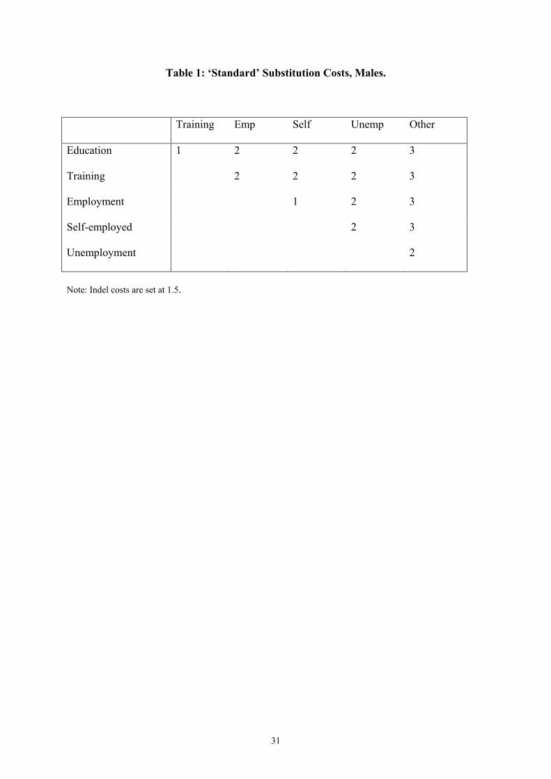
Table 1: ‘Standard’ Substitution Costs, Males.

Training Emp Self Unemp Other

Education 1 2 2 2 3

Training 2 2 2 3

Employment 1 2 3

Self-employed 2 3

Unemployment 2

Note: Indel costs are set at 1.5.

31

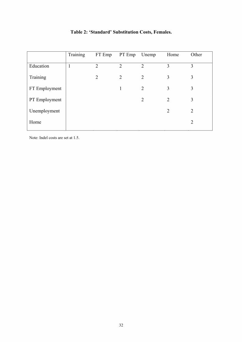
Table 2: ‘Standard’ Substitution Costs, Females.

Training FT Emp PT Emp Unemp Home Other

Education 1 2 2 2 3 3

Training 2 2 2 3 3

FT Employment 1 2 3 3

PT Employment 2 2 3

Unemployment 2 2

Home 2

Note: Indel costs are set at 1.5.

32

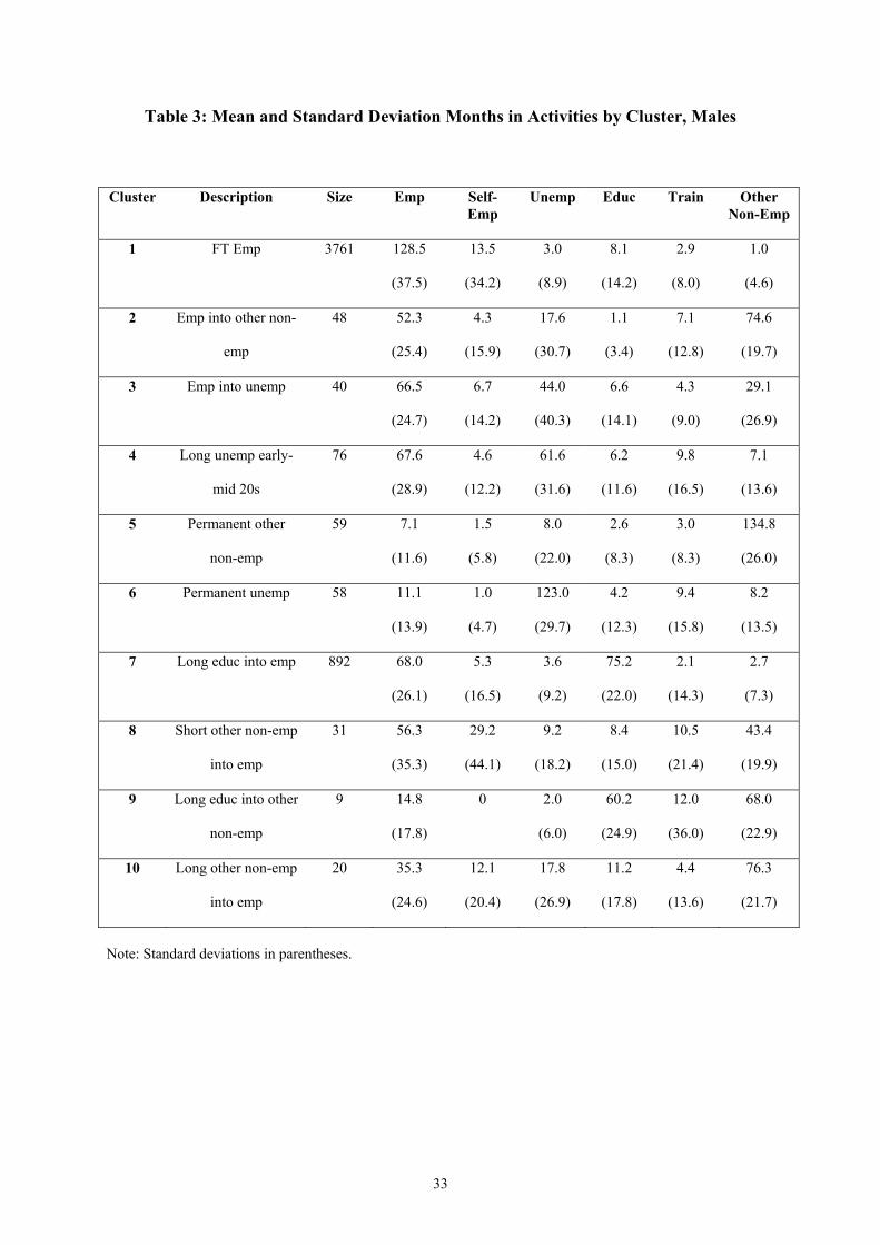
Table 3: Mean and Standard Deviation Months in Activities by Cluster, Males

Cluster Description Size Emp Self-Emp

Unemp Educ Train Other Non-Emp

1 FT Emp

3761 128.5

(37.5)

13.5

(34.2)

3.0

(8.9)

8.1

(14.2)

2.9

(8.0)

1.0

(4.6)

2 Emp into other non-

emp

48 52.3

(25.4)

4.3

(15.9)

17.6

(30.7)

1.1

(3.4)

7.1

(12.8)

74.6

(19.7)

3 Emp into unemp

40 66.5

(24.7)

6.7

(14.2)

44.0

(40.3)

6.6

(14.1)

4.3

(9.0)

29.1

(26.9)

4 Long unemp early-

mid 20s

76 67.6

(28.9)

4.6

(12.2)

61.6

(31.6)

6.2

(11.6)

9.8

(16.5)

7.1

(13.6)

5 Permanent other

non-emp

59 7.1

(11.6)

1.5

(5.8)

8.0

(22.0)

2.6

(8.3)

3.0

(8.3)

134.8

(26.0)

6 Permanent unemp

58 11.1

(13.9)

1.0

(4.7)

123.0

(29.7)

4.2

(12.3)

9.4

(15.8)

8.2

(13.5)

7 Long educ into emp

892 68.0

(26.1)

5.3

(16.5)

3.6

(9.2)

75.2

(22.0)

2.1

(14.3)

2.7

(7.3)

8 Short other non-emp

into emp

31 56.3

(35.3)

29.2

(44.1)

9.2

(18.2)

8.4

(15.0)

10.5

(21.4)

43.4

(19.9)

9 Long educ into other

non-emp

9 14.8

(17.8)

0 2.0

(6.0)

60.2

(24.9)

12.0

(36.0)

68.0

(22.9)

10 Long other non-emp

into emp

20 35.3

(24.6)

12.1

(20.4)

17.8

(26.9)

11.2

(17.8)

4.4

(13.6)

76.3

(21.7)

Note: Standard deviations in parentheses.

33

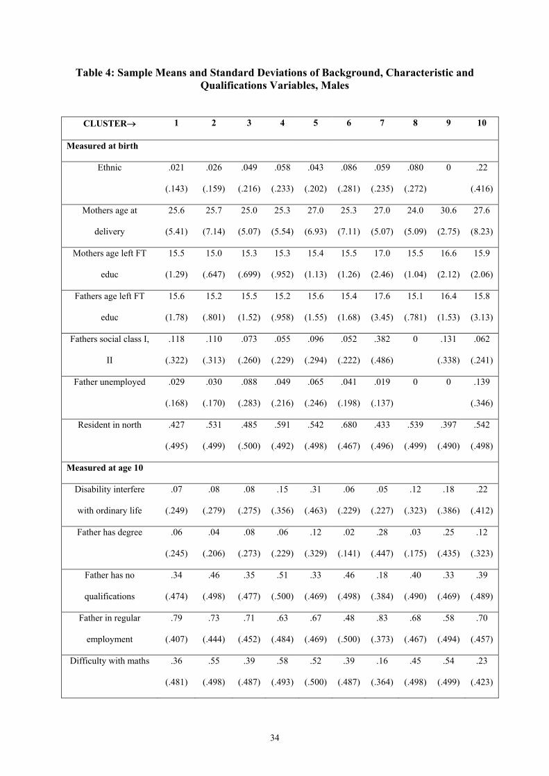
Table 4: Sample Means and Standard Deviations of Background, Characteristic and Qualifications Variables, Males

CLUSTER→ 1 2 3 4 5 6 7 8 9 10

Measured at birth

Ethnic .021

(.143)

.026

(.159)

.049

(.216)

.058

(.233)

.043

(.202)

.086

(.281)

.059

(.235)

.080

(.272)

0 .22

(.416)

Mothers age at

delivery

25.6

(5.41)

25.7

(7.14)

25.0

(5.07)

25.3

(5.54)

27.0

(6.93)

25.3

(7.11)

27.0

(5.07)

24.0

(5.09)

30.6

(2.75)

27.6

(8.23)

Mothers age left FT

educ

15.5

(1.29)

15.0

(.647)

15.3

(.699)

15.3

(.952)

15.4

(1.13)

15.5

(1.26)

17.0

(2.46)

15.5

(1.04)

16.6

(2.12)

15.9

(2.06)

Fathers age left FT

educ

15.6

(1.78)

15.2

(.801)

15.5

(1.52)

15.2

(.958)

15.6

(1.55)

15.4

(1.68)

17.6

(3.45)

15.1

(.781)

16.4

(1.53)

15.8

(3.13)

Fathers social class I,

II

.118

(.322)

.110

(.313)

.073

(.260)

.055

(.229)

.096

(.294)

.052

(.222)

.382

(.486)

0 .131

(.338)

.062

(.241)

Father unemployed .029

(.168)

.030

(.170)

.088

(.283)

.049

(.216)

.065

(.246)

.041

(.198)

.019

(.137)

0 0 .139

(.346)

Resident in north .427

(.495)

.531

(.499)

.485

(.500)

.591

(.492)

.542

(.498)

.680

(.467)

.433

(.496)

.539

(.499)

.397

(.490)

.542

(.498)

Measured at age 10

Disability interfere

with ordinary life

.07

(.249)

.08

(.279)

.08

(.275)

.15

(.356)

.31

(.463)

.06

(.229)

.05

(.227)

.12

(.323)

.18

(.386)

.22

(.412)

Father has degree .06

(.245)

.04

(.206)

.08

(.273)

.06

(.229)

.12

(.329)

.02

(.141)

.28

(.447)

.03

(.175)

.25

(.435)

.12

(.323)

Father has no

qualifications

.34

(.474)

.46

(.498)

.35

(.477)

.51

(.500)

.33

(.469)

.46

(.498)

.18

(.384)

.40

(.490)

.33

(.469)

.39

(.489)

Father in regular

employment

.79

(.407)

.73

(.444)

.71

(.452)

.63

(.484)

.67

(.469)

.48

(.500)

.83

(.373)

.68

(.467)

.58

(.494)

.70

(.457)

Difficulty with maths .36

(.481)

.55

(.498)

.39

(.487)

.58

(.493)

.52

(.500)

.39

(.487)

.16

(.364)

.45

(.498)

.54

(.499)

.23

(.423)

34

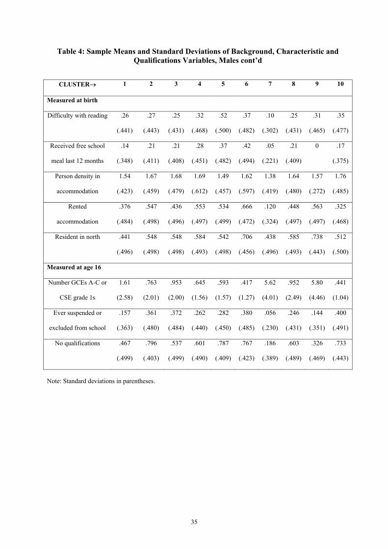
Table 4: Sample Means and Standard Deviations of Background, Characteristic and Qualifications Variables, Males cont’d

CLUSTER→ 1 2 3 4 5 6 7 8 9 10

Measured at birth

Difficulty with reading .26

(.441)

.27

(.443)

.25

(.431)

.32

(.468)

.52

(.500)

.37

(.482)

.10

(.302)

.25

(.431)

.31

(.465)

.35

(.477)

Received free school

meal last 12 months

.14

(.348)

.21

(.411)

.21

(.408)

.28

(.451)

.37

(.482)

.42

(.494)

.05

(.221)

.21

(.409)

0 .17

(.375)

Person density in

accommodation

1.54

(.423)

1.67

(.459)

1.68

(.479)

1.69

(.612)

1.49

(.457)

1.62

(.597)

1.38

(.419)

1.64

(.480)

1.57

(.272)

1.76

(.485)

Rented

accommodation

.376

(.484)

.547

(.498)

.436

(.496)

.553

(.497)

.534

(.499)

.666

(.472)

.120

(.324)

.448

(.497)

.563

(.497)

.325

(.468)


(.496)

.548

(.498)

.548

(.498)

.584

(.493)

.542

(.498)

.706

(.456)

.438

(.496)

.585

(.493)

.738

(.443)

.512

(.500)

Measured at age 16

Number GCEs A-C or

CSE grade 1s

1.61

(2.58)

.763

(2.01)

.953

(2.00)

.645

(1.56)

.593

(1.57)

.417

(1.27)

5.62

(4.01)

.952

(2.49)

5.80

(4.46)

.441

(1.04)

Ever suspended or

excluded from school

.157

(.363)

.361

(.480)

.372

(.484)

.262

(.440)

.282

(.450)

.380

(.485)

.056

(.230)

.246

(.431)

.144

(.351)

.400

(.491)

No qualifications .467

(.499)

.796

(.403)

.537

(.499)

.601

(.490)

.787

(.409)

.767

(.423)

.186

(.389)

.603

(.489)

.326

(.469)

.733

(.443)


35

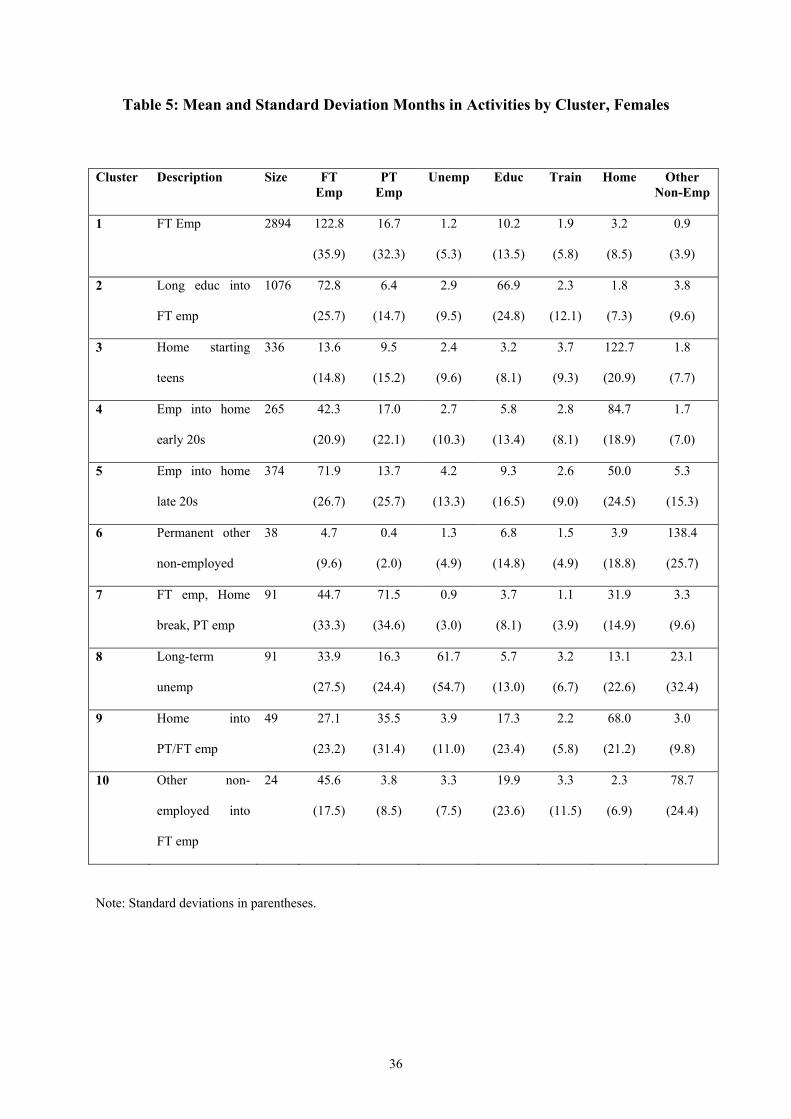
Table 5: Mean and Standard Deviation Months in Activities by Cluster, Females

Cluster Description Size FT Emp

PT Emp

Unemp Educ Train Home Other Non-Emp

1 FT Emp 2894 122.8

(35.9)

16.7

(32.3)

1.2

(5.3)

10.2

(13.5)

1.9

(5.8)

3.2

(8.5)

0.9

(3.9)

2 Long educ into

FT emp

1076 72.8

(25.7)

6.4

(14.7)

2.9

(9.5)

66.9

(24.8)

2.3

(12.1)

1.8

(7.3)

3.8

(9.6)

3 Home starting

teens

336 13.6

(14.8)

9.5

(15.2)

2.4

(9.6)

3.2

(8.1)

3.7

(9.3)

122.7

(20.9)

1.8

(7.7)

4 Emp into home

early 20s

265 42.3

(20.9)

17.0

(22.1)

2.7

(10.3)

5.8

(13.4)

2.8

(8.1)

84.7

(18.9)

1.7

(7.0)

5 Emp into home

late 20s

374 71.9

(26.7)

13.7

(25.7)

4.2

(13.3)

9.3

(16.5)

2.6

(9.0)

50.0

(24.5)

5.3

(15.3)

6 Permanent other

non-employed

38 4.7

(9.6)

0.4

(2.0)

1.3

(4.9)

6.8

(14.8)

1.5

(4.9)

3.9

(18.8)

138.4

(25.7)

7 FT emp, Home

break, PT emp

91 44.7

(33.3)

71.5

(34.6)

0.9

(3.0)

3.7

(8.1)

1.1

(3.9)

31.9

(14.9)

3.3

(9.6)

8 Long-term

unemp

91 33.9

(27.5)

16.3

(24.4)

61.7

(54.7)

5.7

(13.0)

3.2

(6.7)

13.1

(22.6)

23.1

(32.4)

9 Home into

PT/FT emp

49 27.1

(23.2)

35.5

(31.4)

3.9

(11.0)

17.3

(23.4)

2.2

(5.8)

68.0

(21.2)

3.0

(9.8)

10 Other non-

employed into

FT emp

24 45.6

(17.5)

3.8

(8.5)

3.3

(7.5)

19.9

(23.6)

3.3

(11.5)

2.3

(6.9)

78.7

(24.4)


36

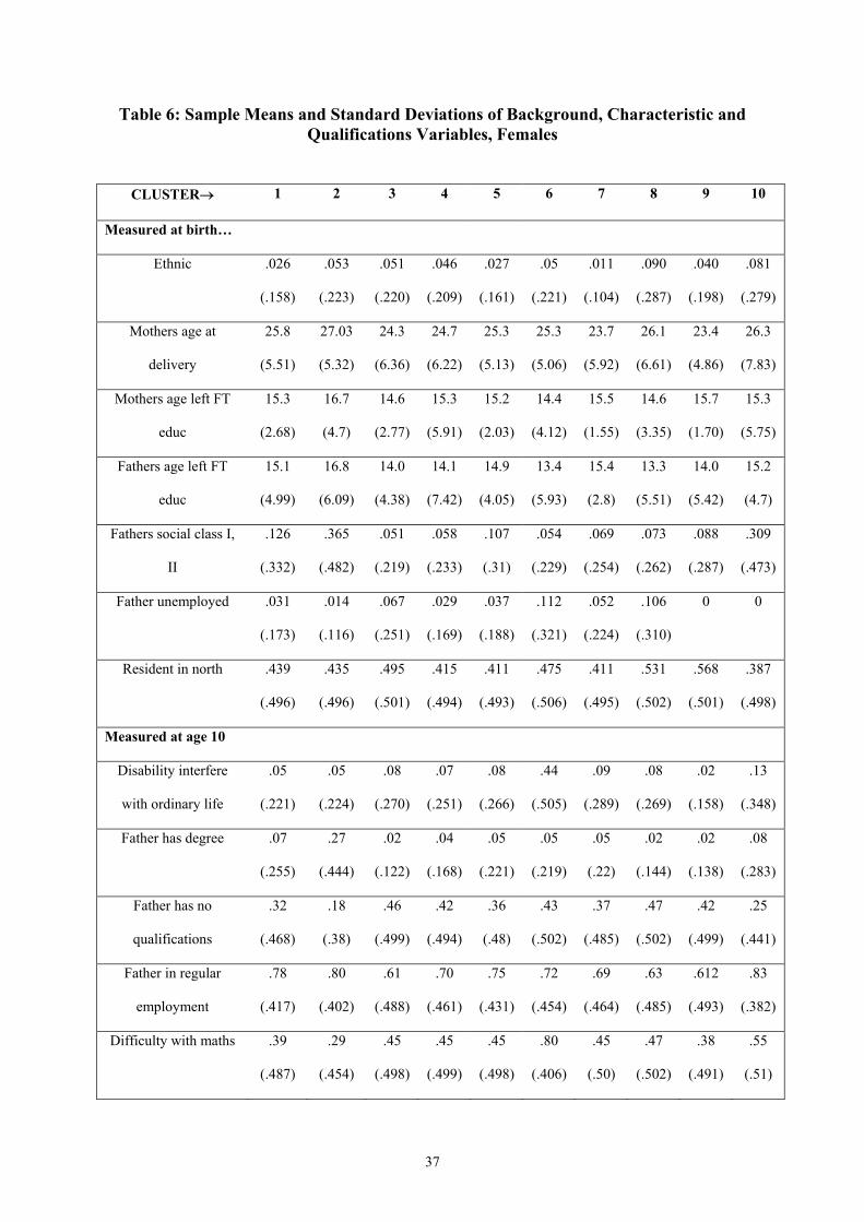
Table 6: Sample Means and Standard Deviations of Background, Characteristic and Qualifications Variables, Females

CLUSTER→ 1 2 3 4 5 6 7 8 9 10

Measured at birth…

Ethnic .026

(.158)

.053

(.223)

.051

(.220)

.046

(.209)

.027

(.161)

.05

(.221)

.011

(.104)

.090

(.287)

.040

(.198)

.081

(.279)

Mothers age at

delivery

25.8

(5.51)

27.03

(5.32)

24.3

(6.36)

24.7

(6.22)

25.3

(5.13)

25.3

(5.06)

23.7

(5.92)

26.1

(6.61)

23.4

(4.86)

26.3

(7.83)

Mothers age left FT

educ

15.3

(2.68)

16.7

(4.7)

14.6

(2.77)

15.3

(5.91)

15.2

(2.03)

14.4

(4.12)

15.5

(1.55)

14.6

(3.35)

15.7

(1.70)

15.3

(5.75)

Fathers age left FT

educ

15.1

(4.99)

16.8

(6.09)

14.0

(4.38)

14.1

(7.42)

14.9

(4.05)

13.4

(5.93)

15.4

(2.8)

13.3

(5.51)

14.0

(5.42)

15.2

(4.7)


II

.126

(.332)

.365

(.482)

.051

(.219)

.058

(.233)

.107

(.31)

.054

(.229)

.069

(.254)

.073

(.262)

.088

(.287)

.309

(.473)


(.173)

.014

(.116)

.067

(.251)

.029

(.169)

.037

(.188)

.112

(.321)

.052

(.224)

.106

(.310)

0 0


(.496)

.435

(.496)

.495

(.501)

.415

(.494)

.411

(.493)

.475

(.506)

.411

(.495)

.531

(.502)

.568

(.501)

.387

(.498)

Measured at age 10


with ordinary life

.05

(.221)

.05

(.224)

.08

(.270)

.07

(.251)

.08

(.266)

.44

(.505)

.09

(.289)

.08

(.269)

.02

(.158)

.13

(.348)


(.255)

.27

(.444)

.02

(.122)

.04

(.168)

.05

(.221)

.05

(.219)

.05

(.22)

.02

(.144)

.02

(.138)

.08

(.283)

Father has no

qualifications

.32

(.468)

.18

(.38)

.46

(.499)

.42

(.494)

.36

(.48)

.43

(.502)

.37

(.485)

.47

(.502)

.42

(.499)

.25

(.441)

Father in regular

employment

.78

(.417)

.80

(.402)

.61

(.488)

.70

(.461)

.75

(.431)

.72

(.454)

.69

(.464)

.63

(.485)

.612

(.493)

.83

(.382)

Difficulty with maths .39

(.487)

.29

(.454)

.45

(.498)

.45

(.499)

.45

(.498)

.80

(.406)

.45

(.50)

.47

(.502)

.38

(.491)

.55

(.51)

37

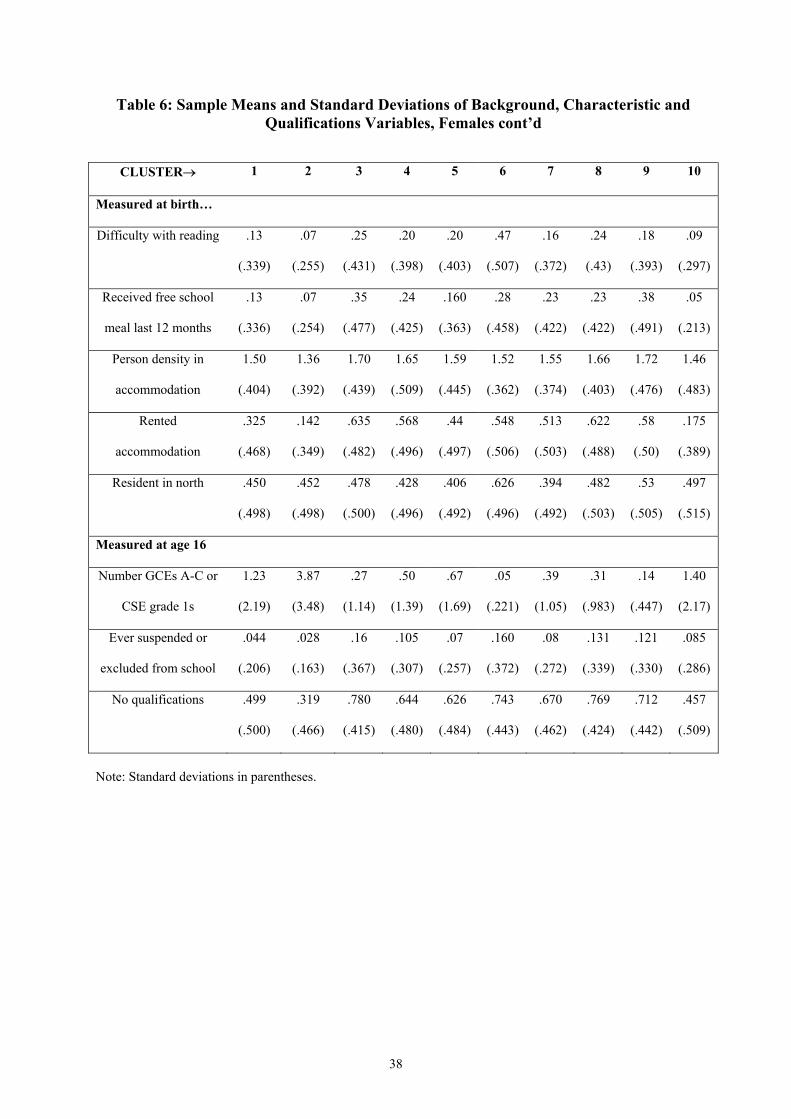
Table 6: Sample Means and Standard Deviations of Background, Characteristic and Qualifications Variables, Females cont’d

CLUSTER→ 1 2 3 4 5 6 7 8 9 10


Difficulty with reading .13

(.339)

.07

(.255)

.25

(.431)

.20

(.398)

.20

(.403)

.47

(.507)

.16

(.372)

.24

(.43)

.18

(.393)

.09

(.297)


meal last 12 months

.13

(.336)

.07

(.254)

.35

(.477)

.24

(.425)

.160

(.363)

.28

(.458)

.23

(.422)

.23

(.422)

.38

(.491)

.05

(.213)

Person density in

accommodation

1.50

(.404)

1.36

(.392)

1.70

(.439)

1.65

(.509)

1.59

(.445)

1.52

(.362)

1.55

(.374)

1.66

(.403)

1.72

(.476)

1.46

(.483)

Rented

accommodation

.325

(.468)

.142

(.349)

.635

(.482)

.568

(.496)

.44

(.497)

.548

(.506)

.513

(.503)

.622

(.488)

.58

(.50)

.175

(.389)


(.498)

.452

(.498)

.478

(.500)

.428

(.496)

.406

(.492)

.626

(.496)

.394

(.492)

.482

(.503)

.53

(.505)

.497

(.515)

Measured at age 16

Number GCEs A-C or

CSE grade 1s

1.23

(2.19)

3.87

(3.48)

.27

(1.14)

.50

(1.39)

.67

(1.69)

.05

(.221)

.39

(1.05)

.31

(.983)

.14

(.447)

1.40

(2.17)

Ever suspended or


.044

(.206)

.028

(.163)

.16

(.367)

.105

(.307)

.07

(.257)

.160

(.372)

.08

(.272)

.131

(.339)

.121

(.330)

.085

(.286)

No qualifications .499

(.500)

.319

(.466)

.780

(.415)

.644

(.480)

.626

(.484)

.743

(.443)

.670

(.462)

.769

(.424)

.712

(.442)

.457

(.509)


38

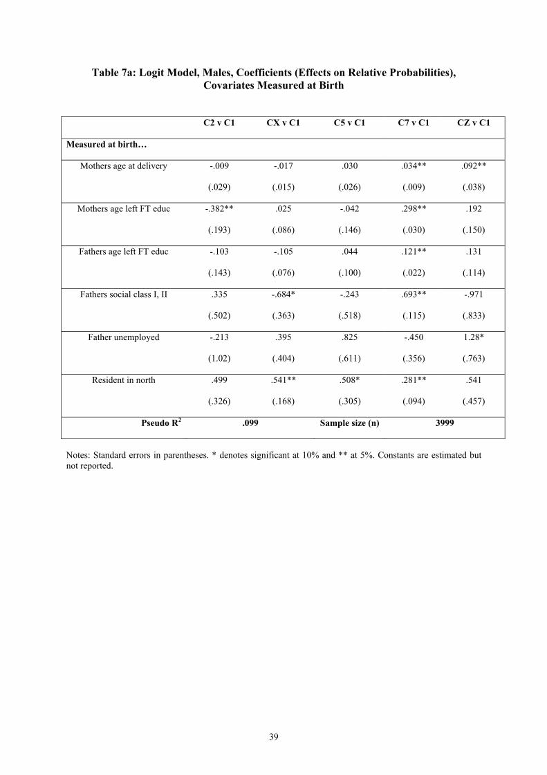
Table 7a: Logit Model, Males, Coefficients (Effects on Relative Probabilities), Covariates Measured at Birth

C2 v C1 CX v C1 C5 v C1 C7 v C1 CZ v C1


Mothers age at delivery -.009

(.029)

-.017

(.015)

.030

(.026)

.034**

(.009)

.092**

(.038)

Mothers age left FT educ -.382**

(.193)

.025

(.086)

-.042

(.146)

.298**

(.030)

.192

(.150)

Fathers age left FT educ -.103

(.143)

-.105

(.076)

.044

(.100)

.121**

(.022)

.131

(.114)

Fathers social class I, II .335

(.502)

-.684*

(.363)

-.243

(.518)

.693**

(.115)

-.971

(.833)

Father unemployed -.213

(1.02)

.395

(.404)

.825

(.611)

-.450

(.356)

1.28*

(.763)


(.326)

.541**

(.168)

.508*

(.305)

.281**

(.094)

.541

(.457)

Pseudo R2 .099 Sample size (n) 3999

Notes: Standard errors in parentheses. * denotes significant at 10% and ** at 5%. Constants are estimated but not reported.

39

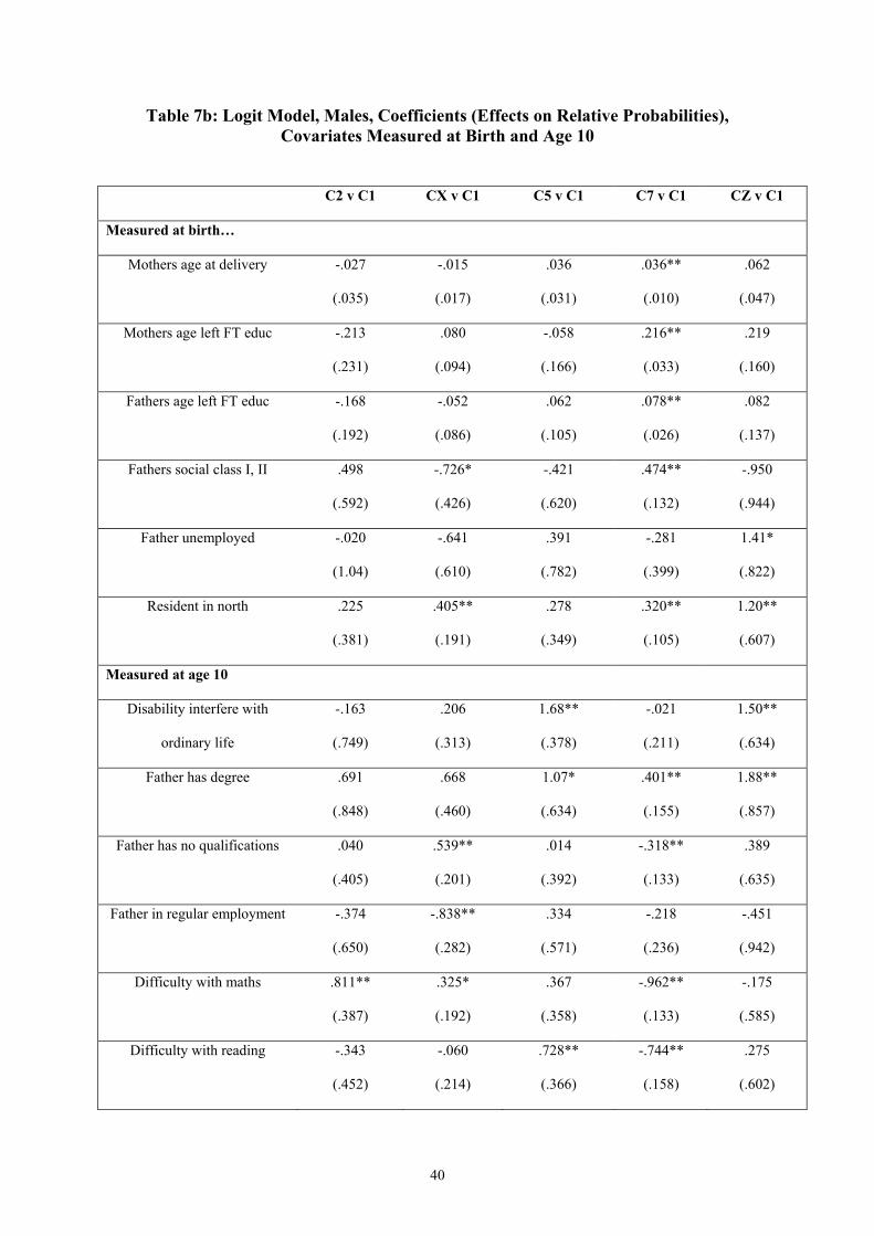
Table 7b: Logit Model, Males, Coefficients (Effects on Relative Probabilities), Covariates Measured at Birth and Age 10




(.035)

-.015

(.017)

.036

(.031)

.036**

(.010)

.062

(.047)

Mothers age left FT educ -.213

(.231)

.080

(.094)

-.058

(.166)

.216**

(.033)

.219

(.160)


(.192)

-.052

(.086)

.062

(.105)

.078**

(.026)

.082

(.137)


(.592)

-.726*

(.426)

-.421

(.620)

.474**

(.132)

-.950

(.944)

Father unemployed -.020

(1.04)

-.641

(.610)

.391

(.782)

-.281

(.399)

1.41*

(.822)


(.381)

.405**

(.191)

.278

(.349)

.320**

(.105)

1.20**

(.607)

Measured at age 10

Disability interfere with

ordinary life

-.163

(.749)

.206

(.313)

1.68**

(.378)

-.021

(.211)

1.50**

(.634)


(.848)

.668

(.460)

1.07*

(.634)

.401**

(.155)

1.88**

(.857)

Father has no qualifications .040

(.405)

.539**

(.201)

.014

(.392)

-.318**

(.133)

.389

(.635)

Father in regular employment -.374

(.650)

-.838**

(.282)

.334

(.571)

-.218

(.236)

-.451

(.942)

Difficulty with maths .811**

(.387)

.325*

(.192)

.367

(.358)

-.962**

(.133)

-.175

(.585)

Difficulty with reading -.343

(.452)

-.060

(.214)

.728**

(.366)

-.744**

(.158)

.275

(.602)

40

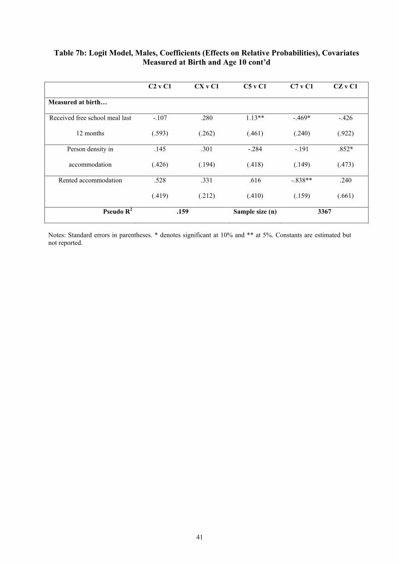
Table 7b: Logit Model, Males, Coefficients (Effects on Relative Probabilities), Covariates Measured at Birth and Age 10 cont’d



Received free school meal last

12 months

-.107

(.593)

.280

(.262)

1.13**

(.461)

-.469*

(.240)

-.426

(.922)

Person density in

accommodation

.145

(.426)

.301

(.194)

-.284

(.418)

-.191

(.149)

.852*

(.473)

Rented accommodation .528

(.419)

.331

(.212)

.616

(.410)

-.838**

(.159)

.240

(.661)



41

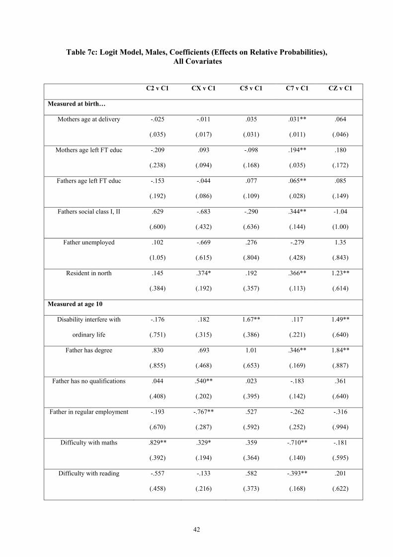
Table 7c: Logit Model, Males, Coefficients (Effects on Relative Probabilities), All Covariates




(.035)

-.011

(.017)

.035

(.031)

.031**

(.011)

.064

(.046)

Mothers age left FT educ -.209

(.238)

.093

(.094)

-.098

(.168)

.194**

(.035)

.180

(.172)


(.192)

-.044

(.086)

.077

(.109)

.065**

(.028)

.085

(.149)


(.600)

-.683

(.432)

-.290

(.636)

.344**

(.144)

-1.04

(1.00)


(1.05)

-.669

(.615)

.276

(.804)

-.279

(.428)

1.35

(.843)


(.384)

.374*

(.192)

.192

(.357)

.366**

(.113)

1.23**

(.614)

Measured at age 10

Disability interfere with

ordinary life

-.176

(.751)

.182

(.315)

1.67**

(.386)

.117

(.221)

1.49**

(.640)


(.855)

.693

(.468)

1.01

(.653)

.346**

(.169)

1.84**

(.887)

Father has no qualifications .044

(.408)

.540**

(.202)

.023

(.395)

-.183

(.142)

.361

(.640)

Father in regular employment -.193

(.670)

-.767**

(.287)

.527

(.592)

-.262

(.252)

-.316

(.994)

Difficulty with maths .829**

(.392)

.329*

(.194)

.359

(.364)

-.710**

(.140)

-.181

(.595)

Difficulty with reading -.557

(.458)

-.133

(.216)

.582

(.373)

-.393**

(.168)

.201

(.622)

42

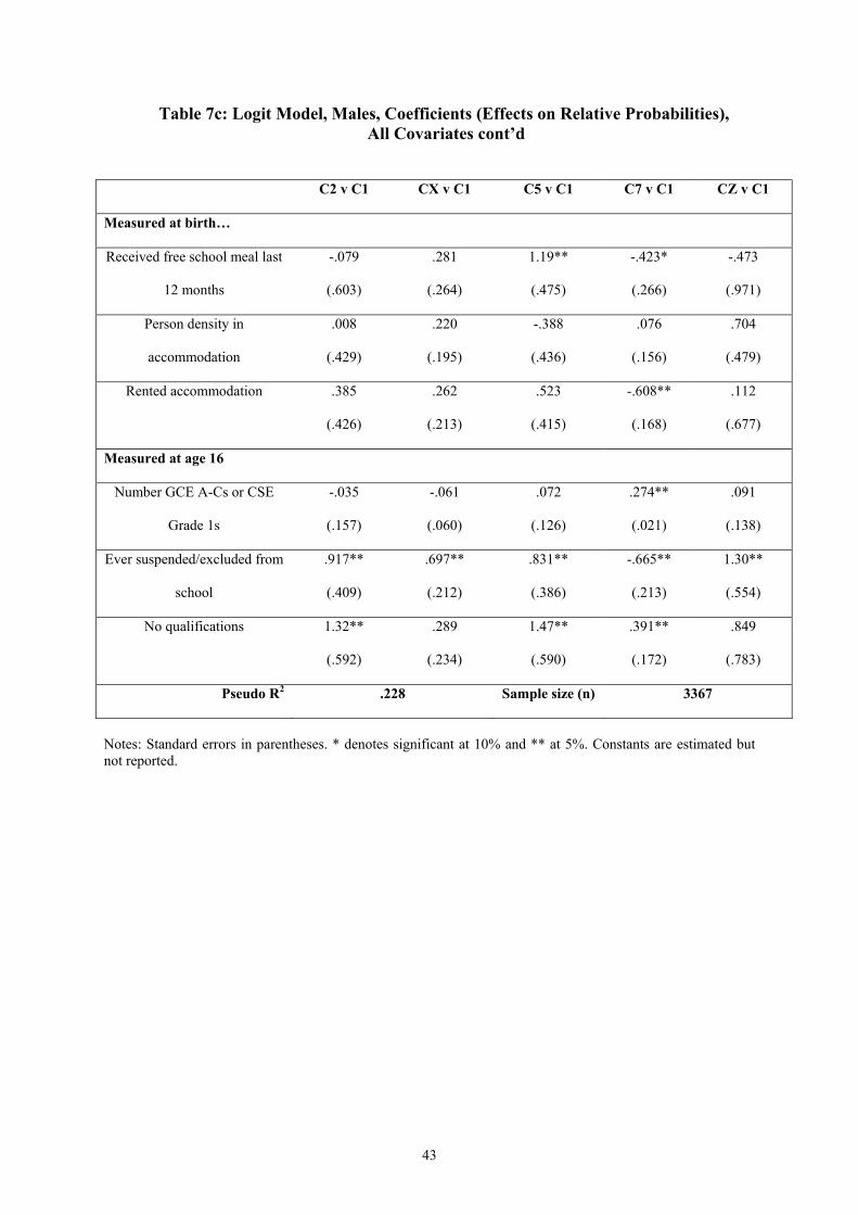
Table 7c: Logit Model, Males, Coefficients (Effects on Relative Probabilities), All Covariates cont’d



Received free school meal last

12 months

-.079

(.603)

.281

(.264)

1.19**

(.475)

-.423*

(.266)

-.473

(.971)

Person density in

accommodation

.008

(.429)

.220

(.195)

-.388

(.436)

.076

(.156)

.704

(.479)

Rented accommodation .385

(.426)

.262

(.213)

.523

(.415)

-.608**

(.168)

.112

(.677)

Measured at age 16

Number GCE A-Cs or CSE

Grade 1s

-.035

(.157)

-.061

(.060)

.072

(.126)

.274**

(.021)

.091

(.138)

Ever suspended/excluded from

school

.917**

(.409)

.697**

(.212)

.831**

(.386)

-.665**

(.213)

1.30**

(.554)

No qualifications 1.32**

(.592)

.289

(.234)

1.47**

(.590)

.391**

(.172)

.849

(.783)



43

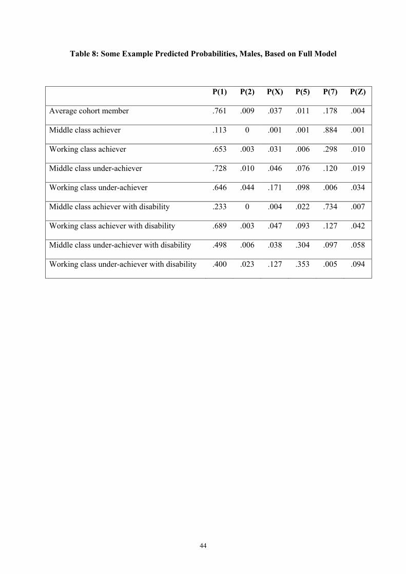
Table 8: Some Example Predicted Probabilities, Males, Based on Full Model

P(1) P(2) P(X) P(5) P(7) P(Z)

Average cohort member .761 .009 .037 .011 .178 .004

Middle class achiever .113 0 .001 .001 .884 .001

Working class achiever .653 .003 .031 .006 .298 .010

Middle class under-achiever .728 .010 .046 .076 .120 .019

Working class under-achiever .646 .044 .171 .098 .006 .034

Middle class achiever with disability .233 0 .004 .022 .734 .007

Working class achiever with disability .689 .003 .047 .093 .127 .042

Middle class under-achiever with disability .498 .006 .038 .304 .097 .058

Working class under-achiever with disability .400 .023 .127 .353 .005 .094

44

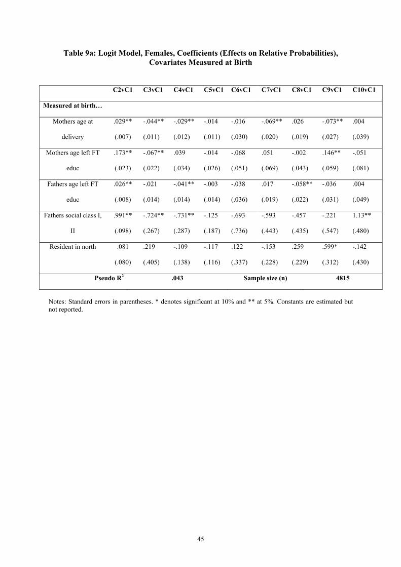
Table 9a: Logit Model, Females, Coefficients (Effects on Relative Probabilities), Covariates Measured at Birth

C2vC1 C3vC1 C4vC1 C5vC1 C6vC1 C7vC1 C8vC1 C9vC1 C10vC1


Mothers age at

delivery

.029**

(.007)

-.044**

(.011)

-.029**

(.012)

-.014

(.011)

-.016

(.030)

-.069**

(.020)

.026

(.019)

-.073**

(.027)

.004

(.039)

Mothers age left FT

educ

.173**

(.023)

-.067**

(.022)

.039

(.034)

-.014

(.026)

-.068

(.051)

.051

(.069)

-.002

(.043)

.146**

(.059)

-.051

(.081)

Fathers age left FT

educ

.026**

(.008)

-.021

(.014)

-.041**

(.014)

-.003

(.014)

-.038

(.036)

.017

(.019)

-.058**

(.022)

-.036

(.031)

.004

(.049)


II

.991**

(.098)

-.724**

(.267)

-.731**

(.287)

-.125

(.187)

-.693

(.736)

-.593

(.443)

-.457

(.435)

-.221

(.547)

1.13**

(.480)


(.080)

.219

(.405)

-.109

(.138)

-.117

(.116)

.122

(.337)

-.153

(.228)

.259

(.229)

.599*

(.312)

-.142

(.430)



45

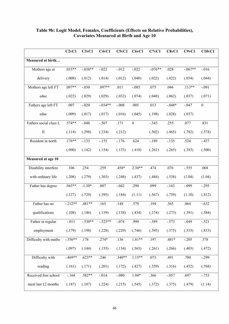
Table 9b: Logit Model, Females, Coefficients (Effects on Relative Probabilities), Covariates Measured at Birth and Age 10



Mothers age at

delivery

.033**

(.008)

-.038**

(.012)

-.022

(.014)

-.012

(.012)

-.022

(.040)

-.076**

(.022)

.028

(.022)

-.067**

(.034)

-.016

(.044)

Mothers age left FT

educ

.097**

(.022)

-.030

(.029)

.097**

(.029)

.011

(.032)

-.085

(.074)

.075

(.048)

.046

(.062)

.113**

(.037)

-.091

(.071)

Fathers age left FT

educ

.007

(.009)

-.020

(.017)

-.034**

(.017)

-.008

(.016)

.005

(.045)

.013

(.198)

-.048*

(.028)

-.047

(.037)

0


II

.574**

(.114)

-.048

(.298)

-.507

(.334)

.171

(.212)

0 -.343

(.502)

.255

(.465)

.077

(.782)

.831

(.574)

Resident in north .176**

(.090)

-.133

(.142)

-.155

(.154)

-.176

(.133)

.624

(.418)

-.189

(.261)

-.135

(.265)

.524

(.393)

-.437

(.500)

Measured at age 10


with ordinary life

.106

(.208)

.254

(.279)

.259

(.303)

.458*

(.248)

2.30**

(.437)

.474

(.484)

.076

(.538)

-.555

(1.04)

.068

(1.04)

Father has degree .943**

(.127)

-1.30*

(.729)

.007

(.395)

-.042

(.184)

.290

(1.11)

.099

(.567)

-.163

(.759)

-.099

(1.10)

-.293

(.812)

Father has no

qualifications

-.212**

(.108)

.481**

(.146)

.165

(.159)

.148

(.138)

.579

(.434)

.194

(.274)

.365

(.273)

.064

(.391)

-.632

(.584)

Father in regular

employment

-.011

(.179)

-.530**

(.198)

-.525**

(.228)

-.074

(.229)

.990

(.746)

-.389

(.395)

-.573

(.375)

-.049

(.535)

-.521

(.833)

Difficulty with maths -.356**

(.097)

.178

(.144)

.274*

(.155)

.136

(.134)

1.81**

(.563)

.197

(.261)

.481*

(.266)

-.205

(.403)

.378

(.472)

Difficulty with

reading

-.469**

(.161)

.623**

(.171)

.246

(.201)

.340**

(.172)

1.15**

(.427)

.073

(.359)

.491

(.316)

.700

(.452)

-.299

(.768)


meal last 12 months

-.164

(.187)

.582**

(.187)

-.014

(.224)

-.080

(.215)

1.04*

(.545)

.366

(.372)

-.057

(.375)

.697

(.479)

-.753

(1.14)

46

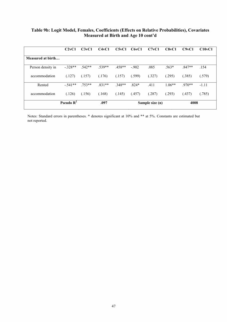
Table 9b: Logit Model, Females, Coefficients (Effects on Relative Probabilities), Covariates Measured at Birth and Age 10 cont’d



Person density in

accommodation

-.328**

(.127)

.542**

(.157)

.539**

(.176)

.458**

(.157)

-.902

(.599)

.085

(.327)

.563*

(.295)

.847**

(.385)

.154

(.579)

Rented

accommodation

-.541**

(.126)

.753**

(.156)

.831**

(.168)

.348**

(.145)

.824*

(.457)

.411

(.287)

1.06**

(.293)

.970**

(.437)

-1.11

(.785)



47

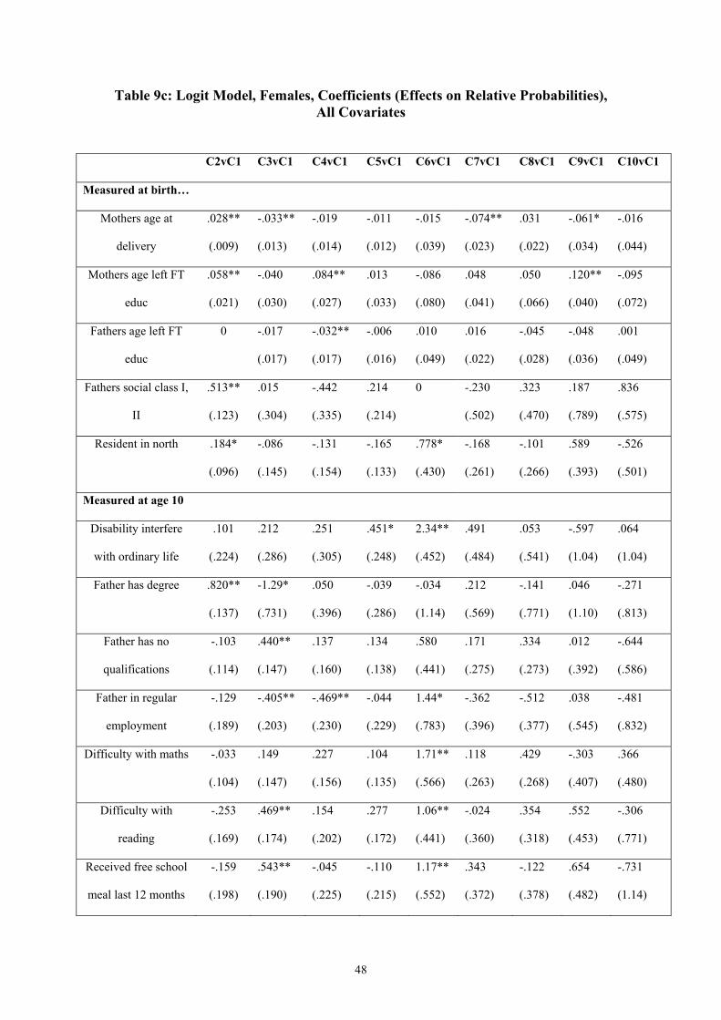
Table 9c: Logit Model, Females, Coefficients (Effects on Relative Probabilities), All Covariates



Mothers age at

delivery

.028**

(.009)

-.033**

(.013)

-.019

(.014)

-.011

(.012)

-.015

(.039)

-.074**

(.023)

.031

(.022)

-.061*

(.034)

-.016

(.044)

Mothers age left FT

educ

.058**

(.021)

-.040

(.030)

.084**

(.027)

.013

(.033)

-.086

(.080)

.048

(.041)

.050

(.066)

.120**

(.040)

-.095

(.072)

Fathers age left FT

educ

0 -.017

(.017)

-.032**

(.017)

-.006

(.016)

.010

(.049)

.016

(.022)

-.045

(.028)

-.048

(.036)

.001

(.049)


II

.513**

(.123)

.015

(.304)

-.442

(.335)

.214

(.214)

0 -.230

(.502)

.323

(.470)

.187

(.789)

.836

(.575)

Resident in north .184*

(.096)

-.086

(.145)

-.131

(.154)

-.165

(.133)

.778*

(.430)

-.168

(.261)

-.101

(.266)

.589

(.393)

-.526

(.501)

Measured at age 10


with ordinary life

.101

(.224)

.212

(.286)

.251

(.305)

.451*

(.248)

2.34**

(.452)

.491

(.484)

.053

(.541)

-.597

(1.04)

.064

(1.04)

Father has degree .820**

(.137)

-1.29*

(.731)

.050

(.396)

-.039

(.286)

-.034

(1.14)

.212

(.569)

-.141

(.771)

.046

(1.10)

-.271

(.813)

Father has no

qualifications

-.103

(.114)

.440**

(.147)

.137

(.160)

.134

(.138)

.580

(.441)

.171

(.275)

.334

(.273)

.012

(.392)

-.644

(.586)

Father in regular

employment

-.129

(.189)

-.405**

(.203)

-.469**

(.230)

-.044

(.229)

1.44*

(.783)

-.362

(.396)

-.512

(.377)

.038

(.545)

-.481

(.832)

Difficulty with maths -.033

(.104)

.149

(.147)

.227

(.156)

.104

(.135)

1.71**

(.566)

.118

(.263)

.429

(.268)

-.303

(.407)

.366

(.480)

Difficulty with

reading

-.253

(.169)

.469**

(.174)

.154

(.202)

.277

(.172)

1.06**

(.441)

-.024

(.360)

.354

(.318)

.552

(.453)

-.306

(.771)


meal last 12 months

-.159

(.198)

.543**

(.190)

-.045

(.225)

-.110

(.215)

1.17**

(.552)

.343

(.372)

-.122

(.378)

.654

(.482)

-.731

(1.14)

48

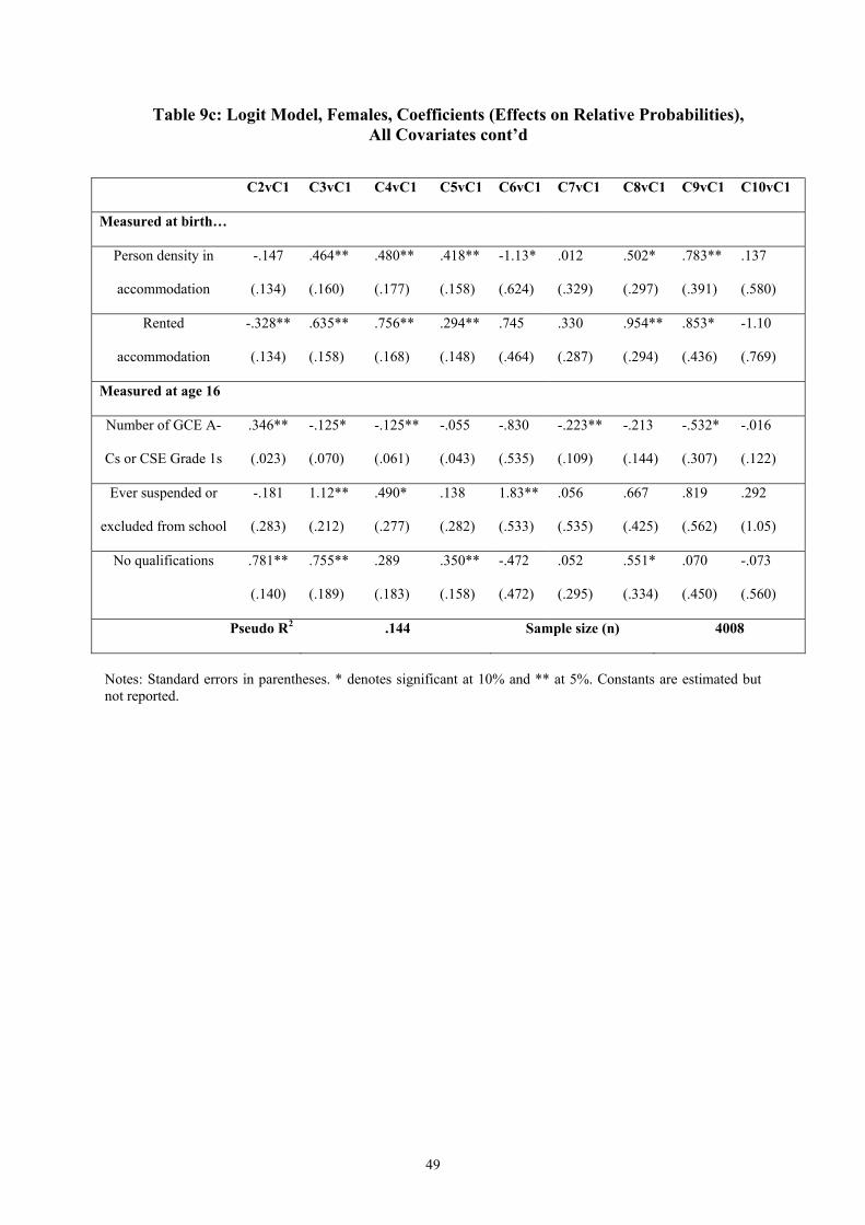
Table 9c: Logit Model, Females, Coefficients (Effects on Relative Probabilities), All Covariates cont’d



Person density in

accommodation

-.147

(.134)

.464**

(.160)

.480**

(.177)

.418**

(.158)

-1.13*

(.624)

.012

(.329)

.502*

(.297)

.783**

(.391)

.137

(.580)

Rented

accommodation

-.328**

(.134)

.635**

(.158)

.756**

(.168)

.294**

(.148)

.745

(.464)

.330

(.287)

.954**

(.294)

.853*

(.436)

-1.10

(.769)

Measured at age 16

Number of GCE A-

Cs or CSE Grade 1s

.346**

(.023)

-.125*

(.070)

-.125**

(.061)

-.055

(.043)

-.830

(.535)

-.223**

(.109)

-.213

(.144)

-.532*

(.307)

-.016

(.122)

Ever suspended or


-.181

(.283)

1.12**

(.212)

.490*

(.277)

.138

(.282)

1.83**

(.533)

.056

(.535)

.667

(.425)

.819

(.562)

.292

(1.05)

No qualifications .781**

(.140)

.755**

(.189)

.289

(.183)

.350**

(.158)

-.472

(.472)

.052

(.295)

.551*

(.334)

.070

(.450)

-.073

(.560)



49

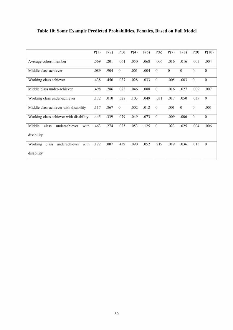
Table 10: Some Example Predicted Probabilities, Females, Based on Full Model

P(1) P(2) P(3) P(4) P(5) P(6) P(7) P(8) P(9) P(10)

Average cohort member .569 .201 .061 .050 .068 .006 .016 .016 .007 .004

Middle class achiever .089 .904 0 .001 .004 0 0 0 0 0

Working class achiever .438 .456 .037 .028 .033 0 .005 .003 0 0

Middle class under-achiever .498 .286 .023 .046 .088 0 .016 .027 .009 .007

Working class under-achiever .172 .010 .528 .103 .049 .031 .017 .050 .039 0

Middle class achiever with disability .117 .867 0 .002 .012 0 .001 0 0 .001

Working class achiever with disability .445 .339 .079 .049 .073 0 .009 .006 0 0

Middle class underachiever with

disability

.463 .274 .025 .053 .125 0 .023 .025 .004 .006

Working class underachiever with

disability

.122 .007 .439 .090 .052 .219 .019 .036 .015 0

50

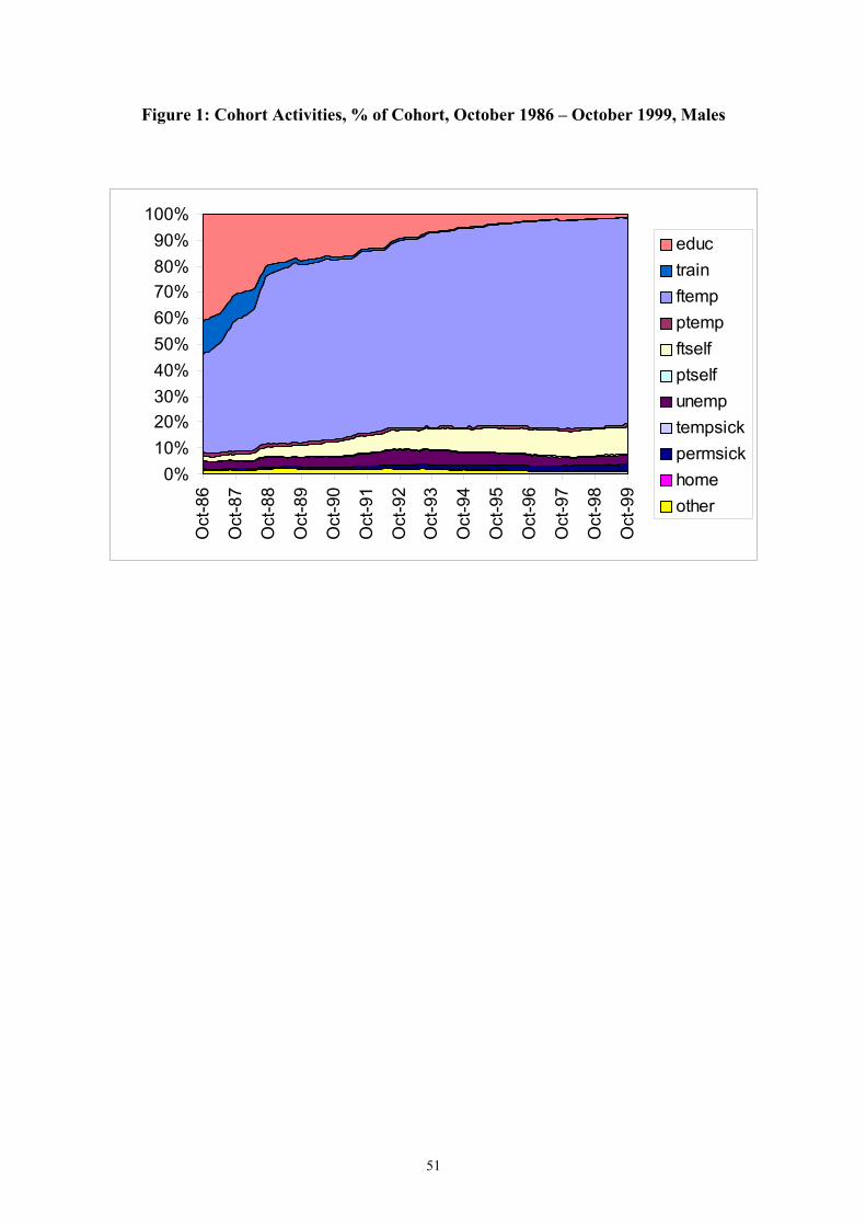
Figure 1: Cohort Activities, % of Cohort, October 1986 – October 1999, Males

0%10%20%30%40%50%60%70%80%90%

100%O

ct-8

6

Oct

-87

Oct

-88

Oct

-89

Oct

-90

Oct

-91

Oct

-92

Oct

-93

Oct

-94

Oct

-95

Oct

-96

Oct

-97

Oct

-98

Oct

-99

eductrainftempptempftselfptselfunemptempsickpermsickhomeother

51

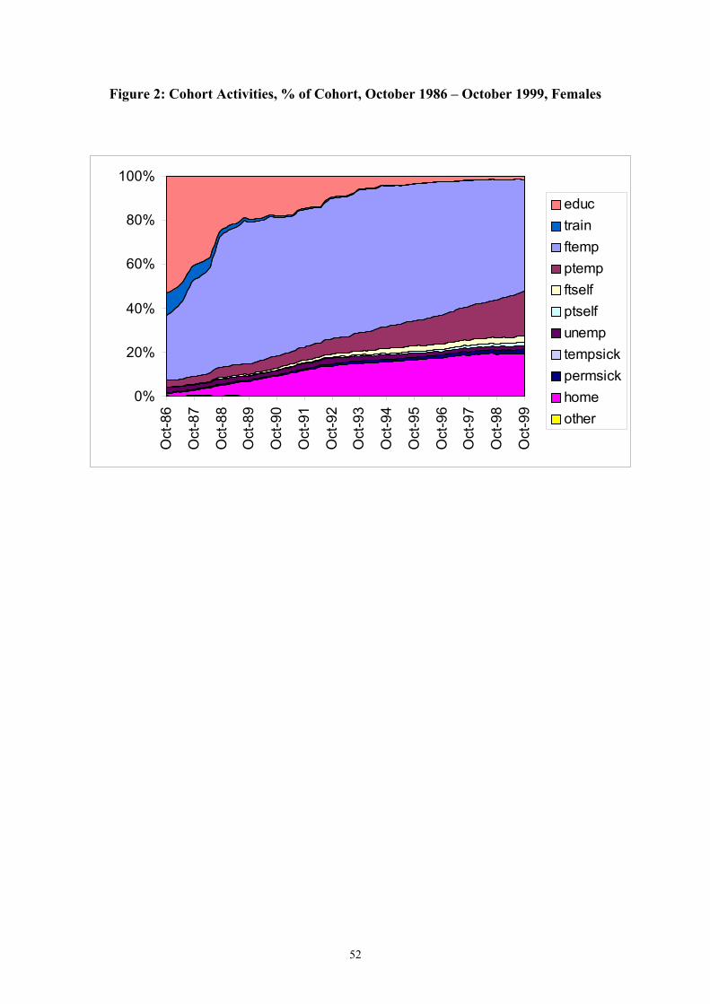
Figure 2: Cohort Activities, % of Cohort, October 1986 – October 1999, Females

0%

20%

40%

60%

80%

100%O

ct-8

6

Oct

-87

Oct

-88

Oct

-89

Oct

-90

Oct

-91

Oct

-92

Oct

-93

Oct

-94

Oct

-95

Oct

-96

Oct

-97

Oct

-98

Oct

-99

eductrainftempptempftselfptselfunemptempsickpermsickhomeother

52

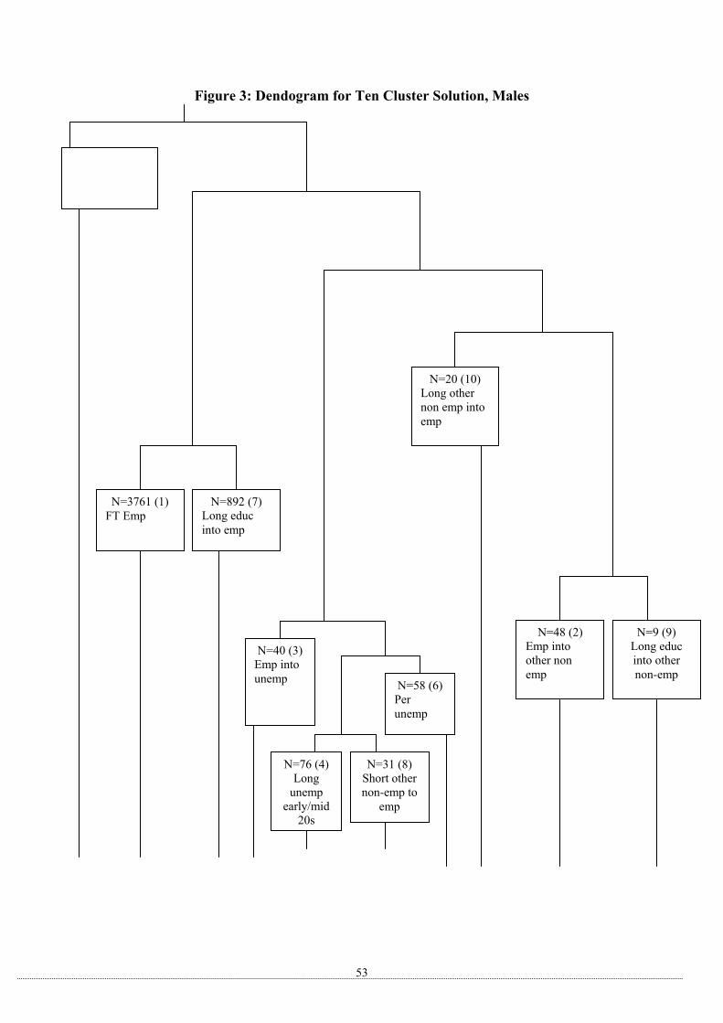
Figure 3: Dendogram for Ten Cluster Solution, Males

N=59 (5) Permanent other non emp

N=3761 (1) FT Emp

N=892 (7) Long educ into emp

N=40 (3) Emp into unemp

N=31 (8) Short other non-emp to

emp

N=9 (9) Long educ into other non-emp

N=58 (6) Per unemp

N=76 (4) Long

unemp early/mid

20s

N=48 (2) Emp into other non emp

N=20 (10) Long other non emp into emp

53

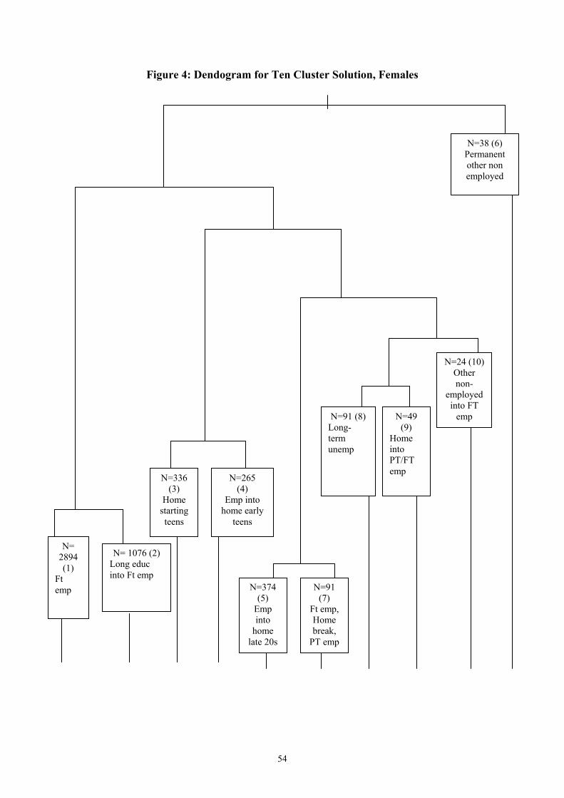
Figure 4: Dendogram for Ten Cluster Solution, Females

N= 2894 (1)

Ft emp

N=24 (10) Other non-

employed into FT

emp

N=38 (6) Permanent other non employed

N=336 (3)

Home starting teens

N=91 (8) Long-term unemp

N= 1076 (2) Long educ into Ft emp

N=265 (4)

Emp into home early

teens

N=91 (7)

Ft emp, Home break,

PT emp

N=374 (5)

Emp into

home late 20s

N=49 (9)

Home into PT/FT emp

54

Parallel Lives: Birth, Childhood and Adolescent Influences on Career Paths

Documents

Transcript of Parallel Lives: Birth, Childhood and Adolescent Influences on Career Paths