1196TneNsPoRTATroN RnsnencH RucoRD

P øa ement Ea øluøtion øndRehøbilitøtion

Tn^q.NsPoRTATIoN RnsnencH BoenpNerroNer RnsnencH CouNcrrWASHINGTON, D.C. 1988

Transportation Research Record l196Price: $41.50

modeI highway transportation

subject areas24 pavement design and performance40 maintenance

Transportation Research Board publications are available byordering directly from TRB. They may also be obtained on aregular basis through organizational or individual affiliation withTRB; affiliates or library subscribers are eligible for substantialdiscounts. For further information, write to the TransportationResearch Board, National Research Council, 2101 ConstitutionAvenue, N.W., Washington, D.C. 20418.

Printed in the United States of America

Library of Congress Cataloging-in-Publication DataNational Research Council. Transportation Research Board.

Pavement evaluation and rehabilitation.p. cm.-(Transportation research record, ISSN 3061-1981;

1196)Papers from the 67th annual meeting of the Transportation

Research Board held in Washington, D.C., 1988.

ISBN 0-309-04771-4l. Pavements-Maintenance and repair. L National

Research Council (U.S.). Transportation ResearchBoard. II. National Research Council (U.S.). TransportationResearch Board. Meeting (67th: 1988: Washington,D.C.) II. Series.TE7.H5 no. 1196

lrE2s0l388 s-dc20[625.81

Sponsorship of Transportation Research Record ll96

GROUP 2_DESIGN AND CONSTRUCTION OFTRANSPORTATION FACILITIESChairman: David S. Getlney, Harlantl Bartholomew & Associates

Pavement Management SectionChairman: R. G. Hicks, Oregon Slate Univenity

Committee on Pavement RehabilitationChairman: James F. Shook, ARE Inc.Secretary: RichardW. May, Asphalt InstitutePaul Autret, Michael C. Belangie, James L. Brown, Martin L'Cawley, John A. D'Angeto, WTrren G. Davison, Paul J. Diethelm'

Denis'8. Donnelly, Wade L. Gramling, Jerry J- Haiek, John P'

Hallin, Joseph B. Hannon, James W. Hill, Walter P. Kilareski, Joe

P. Mahoney, William G. Miley, David E. Newcomb,-Louis G'O'Brien, únn C. Pouer, R. N. Stubstad, Shiraz D. Tayabii, Robert

L. White, Loren M. Womack

Committee on Strength and Deformation Characteristics ofPavement Sections

Chairman: J. Brent Rauhut, Brent Rauhut Engineering Inc.

Ioseph H. Amend III, Gilbert Y. Baladi, Richard D. Barksdale'

Stephen F. Brown, Atbert J. Bush III, George,R. Cochtan, Billt G'

Connor, Amir N. Hanna, R. G. Hicks, Ignat V. Kalcheff, Willia¡n

J. Kenis, Thomas W. Kennedy, Erland Lukanen, Robert L. Lyttorr'Michaet S. Mamlouk, Edwin C. Novak, Jr., Lutfi Raatl, Byron E'Ruth, Gary Wayne Sharpe, James F' Shook, Roger.E. Smith, R' N'Srubstad, Marshall R. fhompson, IJlian L Tufektchiev, Thomøs D'White

Conrmittee on Pavement Monitoring, Evaluation and Data Storage

Chai¡'man: Witliam A. Phang, Ontario Mittistt'y of Transportationand Communicalions

Secretary: Don H. Kobi, Paris, Otttario, Canada

A. T. Bergan, FrankV. Botelho, Billy G. Connor, Brian E' Cox,

Michael I: Darter, Karl H. Dunn, Wouter Gultlen, William H'Highter, James W. Hilt, Andris A. lumikis, Scott A. Kutz, Kenneth

J.Law, W. N. Lofroos, K. H. McGhee, Edwin C' Novak, Jr.,Freddy L. Roberti, Ivan F. Scazziga, S. C. Shah,.Roger E. Smith'

Herbert F. Southgate, Elson B. Spangler, Richard L' Stewart,

Loren M. Womack, John P. Zaniewski

Committee on Surface Properties-Vehicle InteractionChairman: A. Scott Parrish, Maryland Department of

TransportatiottLouis Ë. Barora, Robert R. Blackburn, James L. Burchett, GaylotdCurnberledge, Thomas D. Gillespie, Wouter Gulden Lawrence E'Hart, Carløn M. Hayden, Rudolph R. Hegmon, John Jewett

Heniy, Walter B. Horne, Don L. Ivey, Michael S. Janoff, Kenneth

,1. Law, Jean Lucas, David C' Mahone, William G. Miley' Robert

L. Novak, Bobby G. Page, Richard N. Pierce, John J. Quinn, Jean

Reichert, Elson B. Spangler, William H' Temple, James C.

Wambold

George W. Ring III, Transportation Research Board staff

Sponsorship is indicated by a footnote at the end of each- paper'

The organiäational units, officers, and members are as ofDecember 31,1987.

NOTICE: The Transportation Research Board does not endorse

proclucts or manufacturers. Trade and manufacturers' names

äppear in this Record because they are considered essential to itsobject.

89-130s7CIP

Transportation Research Record !196

Contents

Asphalt Pavement Evaluation Using Fuzzy SetsD. J. Elton and C. H, Juang

Measuring Pavement Deflections Near a Super-Heavy OverloadW. A. Nokes

S_ome Approaches in Treating Automatically Collected Data on RuttingC. A. Lenngren

20

Field Survey Equipment and Data Analysis for Highway RehabilitationPlanningH. Taura, W. P. Kilareski, and M. Ohama

27

Comparison of Methods and Equipment To Conduct Pavement DistressSurveysK. R. Benson, G. E. Elkins, W. Uddin, andW. R. Hudson

40

Effect of Reflected Waves in SASW Testing of PavementsI. C. Sheu, K. H. Stokoe Il, and l. M. Roesset

51

Pavement Condition Diagnosis Based on Multisensor DataK. Maser, B. Brademeyer, and R. Littlfield

62

Three-Dimensional Analysis of Slab on Stress-Dependent FoundationA. M. loannides and I. P. Donnelly

72

Verification of Backcalculation of Pavement ModuliS. W. Lee, I. P. Mahoney, and N. C, lackson

85

Dynaflect Evaluation of Layer Moduli in Florida's Flexible Pavement 96

SystemsI(wasi Badu-Tweneboah, Byron E. Ruth, and William G' Miley

compaction specification for the control of Pavement subgrade 108

RuttingHani ,{, Lotfi, Charles W. Schwartz, and Matthqp W' Witczak

Resilient Modulus and AASHTO Pavement DesignRobert P. Elliott and Sam l. Thornton

Direct Calculation of Maximum Curvature and Strain in Asphalt 125

Concrete Layers of Pavements from Load Deflection BasinMeasurementsFriedrichW.lung

Determination of Pavement Layer Thicknesses and Moduli by SASW 133

MethodSoheíl Nazarian, Kenneth H, Stokoe ll, Robert C' Briggs, and Richard Rogers

Load-Associated Crack Movement Mechanisms in RoadsF. C, Rust and V. P. Seroas

Analyzing the Interactions Between Dynamic Vehicle Loads and 161

Highway PavementsMlchaet i. Markow,l, Karl Hedrick, Brian D' Brademeyer, and Edward Abbo

LEF Estimation from Canroad Pavement Load-Deflection DataL. R. Rilett and B. G. Hutchinson

151

770

Field Evaluation of Bonded Concrete OverlaysShiraz D. Tayabji and Claire G. Ball

779

Application of Deflection Testing to Overlay Design: A Case Study 193Cheryl Allen Richter and Lynne H. Irwin

Evaluation of the Performance of Bonded Conctete Overlay onInterstate Highway 610 North, Houston, TexasKoestomo Koesno and F. Frank McCullough

Flexible Pavement Rehabilitation Using Asphalt-RubberCombinations: Progress ReportRobert N. Doty

212

NetworkLevelOptimization/PrioritizationofPavementRehabilitation 224AIi Khatamí and K, P. George

Cold, In-Place Recycling on Indiana State Road 38Rebecca S. McDaniel

Data Acquisition for Mechanistic-Empirical Overlay Design Equations 243for Reflection Cracking in Flexible OverlaysP. W,layawickrøma, R. E. Smith, R. L. Lytton, and M. R. Tirado

Serviceability Index Base for Acceptance of Jointed ConcretePavementsWilliant H. Temple and Steaen L. Cumbaa

Profilograph Correlation Study with Present Serviceability Index 257Roger S. Walker and Hong-Tsung Lin

Establishing Relationships Between Pavement Roughness andPerceptions of AcceptabilityArun Garg, AIan Horowitz, and Fred RossDISCUSSION, Michnel S. Janot'f,283AUTHORS'CLOSURE, 285

251

Use of the Inertial Profilometer To Calibrate Kentucky Department ofHighways Mays Ride Meter SystemsElnn B. Spangier, Rolnnds L. Rizenbergs, James L. Burchett, and Donald C.Robinson

286

Road Characteristics and Skid Testinglames C. Wambold

294

Obtaining Skid Number at Any Speed from Test at Single Speed

James C. Wambold300

Concrete Pavement Rehabilitation for the Texas State Department ofHighways and Public Transportationlames L. Brown

306

Relative Influence of Accelerometer and Displacement TransducerSignals in Road Roughness MeasurementsBohdan T. Kulakowski, lohn l. Henry, and lames C. Wambold

313

TRANSPORTATION RESEARCH RECO RD I 196

Asphalt Pavement Evaluation UsingFuzzy Sets

D. J. Errox eun C. H. JueNc

A new method of asphalt pavement evaluation using fuzzy setsis proposed. The purpose is to provide a simple, cotrsistent,cost-effective procedure for pavement evaluation. Consistentpâvement evaluation is ¡reeded for adequate pavement main-tenance. The large turnover pending in the pavement engi-neering field over the next fïve years will leave many pavementagencies without adequate experlise to evaluate their pavementsystems. A computer prograrn, Fuzzy Evaluatio¡r of AsphaltPavement Systems (FEAPS), is presented to facilitate the method.The program uses the fuzzy weighted average operation tocombine distress ratings for five different types of pavementdistress (roughness, alligator cracks, transverse cracks, lon-gitudinal cracks, rutting). A, fuzzy set representing the pave-ment condition is produced. This final fuzzy set can be trans-lated to a natural language descriptor. A nerv function forcornparing the final fuzzy sets is described, allowing rankingof the pavements. rtrith FBAPS, the user can change the pave-ment rveights reflecting the local expert opinions to allorv fordifferences of interpretation of local pavement distress types.

Asphalt pavement maintenance is a very important issue fac-ing the state and local highway engineer today (1, 2). Properrnaintenance requires proper pavement evaluation. Unfor-tunately, the wicle variety of pavement types, loading con-ditions, and soil types rnakes pavement evaluation a complextask. Current effective pavement evaluation methods lequirethe services of a highly trained and experienced expelt, whichentails significant costs in time and money. The methods pro-posed by Shahin and Kohn (3) and the U.S. Department ofTransportation (4) are examples which, while effective, arealso time-consuming, expensive, and often unsuitable for manyagencies responsible for pavement maintenance and repair.This paper proposes a new evaluation procedure that reducesthe need for an expert to pelform the pavement evaluation.The procedure uses the experience of past experts and f.uzzy

arithmetic. Fuzzy sets, introduced by Zadeh (5), fuzzy arith-metic, and luzzy logic have been applied to many areas ofengineering problems where the inputs are vague or ill-defined(6-9). A recent National Science Foundation workshop atPurdue University examined areas in civil engineering wherefuzzy sets could be applied and included pavement evaluationas one of those areas (ó).

Many large highway structul'es in the U.S. are reaching theend of their design lives and thus are requiring ¡nore main-tenance. The problem is exacerbated by the anticipated retire-¡nent in the near future of large numbers of experienced pave-ment engineers and experts (10- l2). Many of these engineers

D. J. Elton, Civil Engineering Department Auburn University,Ala. 36849. C. H. Juang, Civil Engineering Departrnent, ClemsonUniversity, Clemson, S.C.

were hired by highway departments at the start of the NationalSystem of Interstate and Defense Highways, which was cre-ated by the Federal-Aid Highway Act of 1956. Because theinterstate system has grown slowly, hiring and turnover rateshave been low. Consequently, few new pavement engineershave been available to become expert at pavelnent evaluation.The low turnover in these positions has led to low job demand,and many universities have removed pavement engineeringfi'om their curricula. Finally, the dropping enrollments in civilengineering curricula at universities have reduced the supplyof potential pavement engineers (13). These factors accen-tuate the need for a consistent and simple pavement evalu-ation procedure that reduces the need for an expert. Theprocedure proposed here does not lequire an expert.

Pavement evaluation schemes are very local in characterand can vary even from county to county. Only local knowl-edge of the relative irnportance of such factors as soil type,weather, asphalt types, significance of distress types, and sea-sonal variations and magnitudes of pavement loadings is use-ful at a given location. Therefore, pavement evaluation pro-cedures must be tailored to every locale.

The combination of these factors has created an impendingcrisis in pavement engineering. In order to avert the crisis, a

method of preserving the knowledge of pavement evaluationexperts must be found and implemented.

A procedure employing luzzy logic can be a great aid insolving this problem. The procedure presented herein cancapture local knowledge about the importance of various formsof pavement distress in the fonn of weights for distress types.This knowledge is stored in a computer program and can berecalled. Each type of pavement distress is rated for severity,which is represented as a fuzzy set and then combined withthe severity of other distress types, using fuzzy arithmetic toproduce the pavernent rating. The procedure for capturingknowledge and manipulating it is explained below.

METHODOLOGY

Use of Fuzzy Sets

Fuzzy set theory can account for the uncel'tainty associatedwith the evaluation of engineering parameters. There is con-siderable uncertainty in pavement evaluation, as is evidencedby the unclear terms used to describe pavement condition.For exarnple, such general terms as "real bad," "poor," "good,"and "excellent" are often used, and a range of pavementconditions is associated with each descriptor. Fuzzy sets describethat range well.

')

In conventional mathematics, a single numerical rating rnightbe assigned to each descriptive term. This number might rep-resent the mean value, for example, when in reality somerange of values might all be classified with that same number.Fuzzy sets can be used to describe this uncertainty. Ratherthan assigning a single number to represent the pavernentrating, afuzzy set is used. This is a set of numbers that describethe "degree of belonging" or "support" QQ to each level ofrating to which the particular pavement belongs. In this study,a computer program performs fuzzy operations on the lin-guistic assessments of the pavement condition to produce thepavement rating.

Pavement Evaluation

Five forms of visual distress of asphalt pavements were selectedfor this study: rutting, longitudinal cracks, transverse cracks,alligator cracks, and roughness. All are indicators of structuraldistress. Although safety conditions are also important in eval-uating pavements and could be included in the procedureproposed herein, they were not included, for the sake ofbrevity and clarity. A more complete list of pavement distressis given by the Asphalt Institute (15) and Turner et al. (16).

The various forms of distress were weighted to reflect theirrelative importance, and the weights were determined throughthe collection of expert knowledge. Several experienced expertsin asphalt pavement analysis were interviewed for this study,in order to ascertain the importance of particular distresstypes. The experts used natural language terrns, such as "notimportant" or "very important," which reflected the fuzzinessassociated with pavernent evaluation. Each distress type wasgiven a weight, shown in table 1, that reflects the experienceof the local experts and was incorporated in the Fuzzy Eval-uation of Asphalt Pavement Systems (FEAPS) progra¡n.However, the user can easily change the weights to accorn-modate his or her own experience. The weights reflect thediffering importance of the same distress in different locales.For example, where the soils are very susceptible to pumping,small cracks in the pavement assume more significance. Sim-ilarly, where the soils are very susceptible to the formationof ice lenses, cracks allowing infiltration might have moresignificance than in soils where ice lenses do not form. Thisfeature of the procedure allows for important local variationsin soil types, weather, asphalt types, significance of distresstypes, and seasonal variations and magnitudes of pavementloadings to be incorporated in the methodology. Such flexi-bility makes FEAPS very versatile.

It is important to note that the results obtained are a direct

TABLE 1 WEIGHT SCALE FOR PAVEMENTDISTRESS

0i stress

Ruttl ng

Longitudinal cracks

Transverse cnacks

A1 l lgator cracks

Roughness

l'le i ght

important

moderately important

not important

extremely impontant

very important

TRANSPORTATION RESEARCH RECORD I 196

function of the experts chosen to assign weights. While agree-ment in the selection of experts is not likely to be unanimous,some measure of expertise can be applied to aid in the selec-tion of experts. Unfortunately, the profession still awaits a

perfect rnethod to select and evaluate experts.The pavement rating is assigned based on visual criteria

established by the agency conducting the survey. A trainedindividual is required to identify the kind and degree of dis-tress. The training for this task can be done in a short periodof time, whereas the training to understand the significanceof distress may take years and is expert knowledge. The com-puter program described herein provides the pavement eval-uation, a much more difficult task than distress evaluation.

Once the linguistic ratings are obtained, they are enteredinto the computer program. The ratings are represented inter-nally by fuzzy sets. The overall rating of the pavement is

determined from the fuzzy weighted average described belowand defined in equation 1 by Schmucker (17) as

)R, * lV,R= >w,

where

(1)

R : the f.uzzy set that represents the overall rating of thepavement,

R¿ : the f.uzzy set that represents the linguistic rating of aparticular distress l, and

W¡ = the ltzzy set that represents the weight (or relativeimportance) of a particular distress l, as compared toother distress.

The five major distress types have varying importance. Theweight of each type is shown in table '1.'|he f.uzzy sets rep-resenting each weight are given in table 2. Note that the weightindicates the relative importance of one distress type com-pared to the others. The weight is not an absolute scale. Thus,the table does not, for example, imply that transverse cracksare absolutely "not important."

The shape of the membership functions shown in figure I(as indicated by the fuzzy set) has been shown to have littleeffect on the finzy weighted average operation used in thisstudy (18). Figure 1 shows that the relative importance ofeach distress ranges from 1. to 9, with 9 representing the domainelement of greatest importance. "Support" values, whichexpress membership, range from 0.0 to 1.0. Thus, for exam-ple, in table 2 the weight "not important" is fully supported(1.0) at domain element 1 and also partially supported (0.5)at domain element 2. No support (0.0) is indicated at domainelements 3 and above, indicating that there is no high levelimportance associated with the rating "not important."

TABLE 2 WEIGHTS USED TO EVALUATE PAVEMENTDISTRESS

t{eight Symbol Fuzzy Set Representation

not important A {1.0/1, 0.5/2, 0/3}

moderately important B t0/1, 0.5/2, 1.0/3,0.5/4,0/51

important C {0/3, 0.5/4, I.0/5,0.5/6,0/7}

very important D l0/5, 0.5/6, 1.0/7 , 0.5/8, 0/9]

extremely important E l0/7,0.5/8, 1.0/9)

Elton and Juang

t.o

o.5

o

C¡.,.Ê,an

o,AÉoE

-AL / \ 'AR

3

ratings have been obtained, equation L can be used to cal-culate the final fuzzy set which represents the overall pave-ment rating.

Several pavements can be rated with this method, and theirfinal results compared, resulting in a ranking of pavementsfor use in maintenance strategies. This cornparison is a rationalway to establish the repair priority of each pavement, basedon structural evaluation of the pavement. The comparison isfacilitated by the establishment of a distress index, explainedbelow.

DISTRESS INDEX FOR COMPARISON OFPAVEMENTS

Pavements can be compared using a ranking index based onthe fuzzy sets representing the pavement condition. This indexis a quantitative measure of pavement distress. The rankingindex, here called the distress index (DI), can also be usedas an al¡solute measure of the pavement condition, based onlocal criteria.

The proposed distress index is based on a model proposedby Juang and Kalidindi (19). Referring to Figure la, the dis-tress index is

DI= Ar--AR+C

where

D1 = distress index,An = alrea to the right of the membership function which

characterized the final fuzzy set,A,- = area to the left of the membership function which

characterized the final fuzzy set, andC = a constant, equal to the area enclosed by the

universe.

The distress index value ranges from 0.0 to 1.0. A low indexindicates better pavement condition, while a high index indi-cates worse condition. For example, pavements with overallratings represented by luzzy sets E and ,I, given in figure 1b,are readily compared as follows:

¿ = {013,0.5/4, 1.015,0.516,017lr

For E,

?-2raDr=:-6--2=0.50

J = {0/5, 1.0t6,0.5t7,0t81

For,I,

DI=4'5 =r?+8 =0.662(8)

Thus, the pavement represented by fuzzy set ,I is in worsecondition than the pavement represented by fuzzy set E.

The distress index can be translated back into the naturallanguage rating, if desired, by assigning natural languagedescriptions to "standard" fuzzy sets representing differentpavement conditions. The DI for each of these fuzzy sets iscalculated, and the D/ of the pavement under considerationis cornpared to the DI of the standard. Table 4 gives standardfuzzy sets that rnight be assigned the natural language descrip-tions shown there.

34 5 6 7Idomoin elemenl

(o)

t.o

o.5

ot2345678

domoin elemenl

$)FIGURE I (a) Model of the distress index. (b)Comparison of fuzzy sets for the distress indexcalculation.

As mentioned above, the rating of the evaluated pavementwas expressed in linguistic terms. Because rating of the pave-ment by individuals is very subjective, use of linguistic termsappears to be more natural and appropriate than use of singlenumeric values. Consequently, fuzzy set representations ofthese linguistic ratings have been used in the proposed eval-uation procedure. Table 3 gives the f.uzzy sets correspondingto the linguistic rating grades usecl in this study. The domainele¡nents for these rating grades range frorn I to 9, with 9rcpresenting the domain element of greatest severity. As before,"support" values, which express rnembership, range frorn 0.Cto 1.0. Thus, for example, in table 3, the rating "slight', isunsupported (0.0) at domain element 1, partially supported(0.5) at domain element 2, fully supported (1.0) at domainelement 3, partially supported (0.5) at domain elernent 4, andunsupported (0.0) at domain element 5. No support (0.0) isindicated at domain elements 5 and above, indicating thatthere is no high level severity associated with the rating "slight."

Tables 1.,2, and 3 represent the opinion of the experts usedin this study. Other fuzzy sets could be used in the computerprogram to describe the pavement rating and weights, asdesired. Once these opinions are in place, and the pavements

TABLE 3 RATINC SCALE: QUALITATIVE RATING OFTHE DISTRESS

Ratinq Grade Symbol Fuzzy Set Representation

none A {1.0/1, 0.5/2,0/3}

slight

si gni fi cant

8 {o/1, 0.5/2, r.0/3,0.5/4,0/5}

c {0/3, 0.5/4, L.0/5, 0.5/6,0/7j

0.5/8, 0/9isevere D {O/5, 0.5/6, I.0/7,

extremely severe E f0/7,0.5/8, 1.0/9)

9

.9Êat

o.ôEoÊ

(2)2C

TRA NS PO R'I'A'N O N II, ES EA RC I1 R ECO R D I I 96

TABLE 4 NATURAL LANCUAGETRANSLATION OFTHEDISTRESS INDEX (D1)

Final Evaluation

Descri ptor

no distress

moderate dlstress

di stress

severe distress

total distness

l<i,j<n\Lastly, fuzzy division is defined as

XtY = {min [¡(,), y(j)] I (itj) ;1. = i, j = n]

Fuzzy set DI

{1.0/1, 0.5/2,0/31

Ío/r, 0.5/2, t.o/3, 0.5/4,

{0/3, 0.5/4 , r.o/5, 0.5/6,

l0/5, 0.5/6, r.0/7, 0.5/8,

l0/7 , 0.5/8, L.0/91

(4)

(s)

0.06

o/51 0.25

o/7\ o.50

0/ei 0.7s

0.94

FUZZY WEIGHTED AVERAGE

"fhe fuzzy weighted average (FWA) operation is defined inequation 1. The summation, multiplication, and division inequation I are fuzzy arithmetic operations and are definedby Schmucker (17) as follows:

First, let

X={x(i) I ¡;t-i-n\Y:{v(j) I j;t'j'n\where i, j and ,? are integers, and x(l) and y(i) are rnembershipfunctions that characterize luzzy sets X and Y respectively.Then, fuzzy addition is defined as

x + Y = {min ['(¡), y0)] I (¡ + i) ;

t=i,j=n\ (3)

Thefuzzy summation is simply fuzzy addition repeated. Fuzzymultiplication is defined as

X * Y : {min [¡(,), y(r)] I (¡ . r) ;

where

z(i): *1¡¡¡^ax[.r(i), l< i<n) (7)

Fuzzy normalization was used in this study.

COMPUTER PROGRAM

Created to perform the pavernent evaluation, the FEAPSprogram was written in FORTRAN 77 and, using theWATFORTT compiler (21), runs on IBM PC and IBM-com-patible microcomputers.

The simplified flowchart for the program is shown in fig-ure 2. The first part of the program accepts information fromthe user. The program then allows the user to tailor the eval-uation by assigning linguistic weights to the five different dis-tress types, based on his or her experience. The user can also

The implementation of fuzzy addition and multiplication is

straightforward;fuzzy division, however, is less so. For manyapplications, the Clements algorithm may be sufficient to solvethis problem. Mullarkey and Fenves (20) consider this algo-rithm to be the best f.or fuzzy division.

The Clements algorithm involves two assumptions: (1) anydivision (i/i) not resulting in an integer is deleted, and (2)any division resulting in a quotient greater than ¿ is discarded.

Another concern in the implementation of equation 1 iswhether the fuzzy "nor¡nalization" should be conducted aftereach f.uzzy operation (addition, multiplication, or division).Earlier studies (17, 20) have indicated that more reasonableresults can be obtained with normalization than without nor-malization. Fuzzy normalization is defined by Schmucker (17)as follows. Let

z = NoR [x]then

Z={z(i)li;L<i<nl

lnlormollon Acqulslllon

Throuqh User lnlerloce

lnlcrnol Fuzzy Scl Rcprcscnlollon

of Collccled lnformolion

Compulollon ol Dlslress lndex

(6) FIGURE 2 General florvchart for FDAPS.

Elton and Juang

TABLE 5 CASE STUDY 1: FOUR PAVEMENT RATINGS

0i stress

Rutti ng

Longitudinal cracks

Transverse cracks

Alligator cracks

Roughness

Distress Index

Pavement

2341

B

c

D

B

B

ccDBCCEBCCEEBCD

0.32 0.43 0.60 0.74

a NoTE: pavement ratings made according to the folìowing scale -A - noneB - slightC - significantD - severeE - extremely severe

select default weights embodied in the program, which areexpressed in linguistic terms (or phrases) for ease of use.Similarly, the rating of any pavement evaluated according toeach of the distress criteria is expressed in linguistic terms.

The second part of the program translates the input lin-guistic expressions into fuzzy sets. Once the required data areinput and translated into fuzzy sets, the FWA operation isperformed. The result is a final fuzzy set that represents thepavement rating.

Finally, the distress index ofthe finalfuzzy set is calculated,and this process is repeated for each pavement evaluated. Thepavement with the lowest D1 is in the best condition.

CASE STUDIBS

The procedure explained above was evaluated by selectingand rating four pavements. The default weights shown in table1 and the rating scale shown in table 3 were used.

Case I

Four pavements are shown in table 5: each exhibited a dif-ferent combination of distress. Pavements with different degreesof distress were chosen to show how the proposed procedurecould be used to differentiate among them. Pavement 1 ratingsintuitively indicate good condition. In particular, the smallamount of alligator cracks indicates good condition. Visualinspection of the ratings for pavements 2, 3, and 4 indicatesthat the condition of these pavements decreases with increas-ing pavement number.

Evaluation using FEAPS was performed. The D1 for eachis shown in table 5. As expected, pavement I is in the bestcondition (lowest D1), while pavement 4 is in the worst con-dition (highest D/). Pavements 2 and 3 are arranged in orderof decreasing condition.

Case 2

Four more pavements are shown in table 6, each again exhib-iting a different combination of distress. Intuitively, pavement

8 is in better condition than pavement 5, the only differencebetween the two being the lower rating given for alligatorcracks for pavement 5. Pavement 6 is in worse condition thanpavement 5, since all the ratings for pavement 6 are less thanor equal to the rating for pavement 5, except for the alligatorcracks. Although pavement 6 has a better rating for alligatorcracks than pavement 5, the overall rating is less, because ofthe lower ratings for several other distresses (particularlyroughness, which is heavily weighted). The FEAPS evaluationranks the pavements 8,7, 5, and 6 from best to worst, as

indicated by their respective distress indices.Pavements 2 and 7 had very similar distress indices. How-

ever, they had different amounts of distress. Although pave-ment 2 had a much better rating for longitudinal cracks (whichwere weighted as "moderately important"), it had a slightlylower rating for alligator cl'acks (which were weighted as "veryimportant"). This heavy weight resulted in the lower overallrating. The similarity in D/ with pavement 7 indicates thatFEAPS was able to weight longitudinal and alligator cracksproperly. Pavements 1 and 8 have different amounts of trans-verse cracks and roughness distress, but similar distress indices.This indicates that FEAPS was able to weight these types ofdistress properly.

CONCLUSION

A computer program for the structural evaluation of asphaltpavements has been presented that captures the knowledgeof experts and puts it in a htzzy framework. The pavementratings, also represented by fvzy sets, are used as programinput. The knowledge and the ratings are combined using thefuzzy weighted averaging technique in the computer programFEAPS to produce a fuzzy set that represents ttre þàïemèntcondition. The program provides a consistent, reliable, andfacile method of evaluating pavements. As such, it providesa tool that many pavement agencies-especially those withlimited resources-can use to reduce the impact of the lossof expertise during the next few years.

TRANSPORTATION RESEARCÍI RECORD I ]96

TABLE 6 CASE STUDY 2: FOUR PAVEMENTRATINGS

Di stress

Rutti ng

Longitudinaì cracks

Transverse cracks

Al l igator cracks

Roughness

Distress Index

5

B

c

A

E

c

ACKNOWLEDGMENTS

The authors are indebted to the asphalt pavement expertswho shared their knowledge with us: E. R. Brown, R. Griffin,F. Parker, and F. Roberts.

REFERENCES

1. A. F. DiMillio. Highway Infrastructure: Opportunities forInnovation. ASCE, New York, 1986.

2. K. A. Godfrey. Truck Weight Enforcement on a WIM. Civ¡IEngineering, Vol. 56, No. ll, 1986, pp. 60-63.

3. M. Y. Shahin and S. D. Kohn. Pavement Maintenance Man-agement for Roads and Parking Lots. U.S. Army EngineerConstruction Engineering Research Laboratory TechnicalReport M-294, 1981.

4. Pavement Maintenance Management for Roads and ParkingLo¡s. FHIVA, U.S. Department of Transportation, 1979.

5. L. A. Zadeh, Fuzzy Sets. Information and Control, Vol. 8,1965, pp. 338-353.

6. C. B. Brown, J. L. Chameau, R. N. Palmer, and J. T. P.Yao, eds. Proc., NSFWorkshop on Civil Engineering Appli'cations of Fuzzy,Sels, Purdue University, W. Lafayette, Ind.,1985.

7. A. C. Boissonnade, W. Dong, N. C. Shah, and F. S. Wong.Identification of Fuzzy Systems in Civil Engineering. Proc.,Internalional Symposium on Fuzzy Mathematics in Earth-quake Engineeralg, China, 1985.

8. C. B. Brown and J. T. P. Yao. Fuzzy Sets and StructuralEngineering. Journal of Strucnral Engineering, Vol. 109,

No. 5, 1983, pp. I2Ll-1255.9. M. Gunaratne, J. L, Chameau, and A. G. Altschaeffl. Fttzzy

Multiattributes Decision Making in Pavement Managernent.Journal of Civil Engineering Systems, Yol. 2, Sept. 1985,pp.166-170.

70. Special Report 207: Transportaliott Professionals. Future Needsand Opportunitier. TRB, National Research Council, Wash-ington, D.C., 1985.

Pavement

678DCBDECAEAOBBD8C

0.55 0.70 0.41 0.35

a NOTE: pavement ratings made acconding to the followìng scaìeA - noneB - slightC - sìgnificantD - severeE - extreme'ly severe

11. R. S. Page. Transportation Education-Meeting the Chal-lenge. lR News, No. 116, 1985, pp. 11-16.

12. Survey of Transit Agencies for the Transportation Profes-sional Needs Study. American Public Transit Association.Sp ecial Rep ort 207 : Transportation Professionals. Future N eeds

and Opportunr'ties. TRB, National Research Council, Wash-ington, D.C., 1985.

13. Scientific Manpower Commission. Supply and Demand forScientisls and Engineers. Washington, D.C., 1982.

14. L. A. Zadeh. The Concept of a Linguistic Variable and itsApplication to Approximate Reasoning. Inþrmation Sci-ences, vol.8, 1975, pp. 199-249.

15. A Pavement Rating System for Low-Volume Roads. AsphaltInstitute, College Park, Md., 1977.

16. D. S. Turner, J. V. Walters, T. C. Glover, and R. R. Mans-field. .4 Pavement Rating Procedare. Report No. 112-85.Transportation Management Systems Association, Univer-sity, Ala., 1985.

17. K. J. Schmucker. Fuzzy Sets, Natural Language Compul6-tions, and Risk Analysis. Computer Science Press, Rockville,Md., 1984.

18. C. H. Juang and D. J. Elton. Sorne Fuzzy Logics for Esti-mation of Earthquake Intensity Based on Building DamageRecords. Journal of Civil Engineering Systems, Vol. 3, Dec.1986, pp. 187-191.

19. C. H. Juang and S. N. Kalidindi. Development and Imple-mentation of a Fuzzy System for Bid Tender Evaluation onMiuocomputers. In Proc. (J. L. Chameau and J. T. P. Yao,eds.), NAFIPS, May 1987, pp. 353-373.

20. P. W. Mullarkey and S. J. Fenves. Fuzzy Logic in a Geo-technical Knowledge-based System: CONE. Proc., NSFWorkshop on Civil Engineering Applications of Fuzzy Sets,Purdue University, W. Lafayette, Ind., 1985.

21. G. Goschi and B. Schueler.WATFORTT User Guide.WAT-COM Publications, Ltd., Waterloo, Ontario, Canada, 1986.

Publication of this paper sponsored by Committee on PavementMonitoring, Evaluatiott, and Data Storage.

TRANSPORTATION RESEARCFI RECORD 1 196

Measuring Pavement Deflections Near aSuper-Heavy Overload

W. A. Noxns

Effects on in-service pavements from super-heavy overloadsweighing over 21000,000 pounds are investigated. A field studywas performed in which a crack survey was conducted, pave-ment deflections were measured using a Dynaflect before andafter overload transport, and several insfruments were deployedto measure surface deflection when the overload traversed thepavement. The field study also characterized materials, deter-mined dimensions of structural layers, and measured wheelloads applied to the pavement. Measured deflections are com-pared to predictions that are based on models used for flexiblepavement design. Results of crack surveys show no change inthe visible condition of the pavement after transporting theoverloads. Dynaflect measurements after transport wereapproximately equal to pavement deflections measured beforehauling the overloads. In-transit deflection measurements showthat a r'big basin" results from widely distributed trailer axle/tire loads. Deflections from tractor tires were not substantiallydifferent from those caused by trailer tires. Measured in-transitdeflections agree reasonably well with maximum displacementpredicted using elastic layer models.

Historical data from California's Department of Transpor-tation (CALTRANS), which is responsible for evaluating per-mit and variance requests, indicate that variances are beingrequested for heavier loads each year. Since 1982, permitsand variances for overweight loads jumped 57o/o, ftom ap-proximately thirty-seven thousand to sixty-one thousand. Aconspicuous increase is the number of permits approved forsuper-heavy overloads, which typically exceed 300,000 poundsgross vehicle weight (GVW). Only one permit was approvedin 1983; nearly twenty were granted in 1987.

California's continuing industrial and population growthpromises an increasing number of heavier loads. One reasonfor this trend is a lower cost associated with foreign manu-facture of large components, such as chemical reactor vessels,power genelators and electrical transformers. However, whenlarge components are not fabricated on site, costs and logisticsof transporting these parts become very important. Whenpublic roads are used, a crucial constraint in transporting theseloads is the physical limitation of highway structures, such as

inadequate bridge strength (/).Effects of super-heavy overloads on pavement deserve

investigation. In California, as in other states, typical over-loads are limited to no more than structural load limits estab-lished for bridges and overcrossings on a route. These limits,which generally use GVW, number of axles, and axle spacingas criteria, are based on structural analysis and load equiva-

State of California Department of Transportation, Division ofConstruction, Office of Transportation Laboratory, 5900 FolsomBoulevard, Sacrarnento, Calif. 95819.

lencies. When loads slightly exceed the criteria, engineeringjudgment is generally invoked to set a safe load limit. How-ever, when no structures are traversed and GVW greatlyexceeds previously permitted loads, an accurate procedurefor routine evaluation is not available, and engineering expe-rience is limited.

A field study and computer modeling analysis were con-ducted to investigate effects of super-heavy overloads onpavements. The goals of the investigation were to determineif any observable damage was caused by overloads; to checkfor invisible pavement damage; to measure pavement deflec-tions near the loads in transit; and to compare in-transitdeflections to predictions from mechanistic models.

BACKGROUND

In the spring of 1987, variances were requested to haul thetwo heaviest loads ever moved on a California state highway.Transporting these overloads on a state highway provided an

opportunity to study in-place pavement response and short-term damage. They were to be transported on State Route213, from the Port of Los Angeles to a refinery in Torrance,California (see figure 1). Route 213 is a four-lane, urban,principal arterial with peak hour traffic volume from 1,150 to1.,850 vehicles, and an annual average daily traffic (ADT)ranging from 19,400 to 31,000 vehicles (2).

The GVW of each load was estimated at 2,100,000 pounds,composed of 1,600,000 pounds from a chemical reactor vessel

and approximately 500,000 pounds trailer tare. The reactorscould not be transported by rail because they exceeded weightand width limits. Figure 2 shows dimensions and typical con-figuration ofeach reactor, trailers, and tractors. Table L showstrailer and tractor tire specifications. A total of 384 tires sup-ported each reactor, using 24 axle lines and 16 tires per axleline. Each trailer shown in figure 2 was composed of fourGerman-made Goldhofer trailers interconnected. These trail-ers have steerable axles and hydraulic suspensions that canbe adjusted to maintain a balanced load during transport.Tractor GVIV was approximately 110,000 pounds, composedof 62,000 pounds unladen weight and approximately 49,000pounds from added counterweights.

Before granting variances, a reliable procedure was soughtto predict pavement damage from these overloads. A liter-ature search revealed that a Highway Research Board taskforce developed guidelines and recommended evaluation pro-cedures in the early 1970s (3). It was recognized at that tirnethat methods were not available for engineers to predict accu-rately the destructive effects of overloads on pavement. Con-

TRANSPORT'ATION RESEARCH RECORD I 196

FIGURE I Location map for transporl of overloads.

'12 AXLES x 16 l2 AXLES x 16 WHEELS

FIGURE 2 Overload confìguration and dimensions.

cerns about the accuracy of predictive techniques remain tothe present day.

The task force recommended a mechanistic procedure thatwas used subsequently in several studies @-6). The mecha-nistic approach uses computer models and elastic layer theoryto predict the allowable number of 18 kip equivalent axle load(EAL) applications on a structural section. The task forcepresented stress/strain limits to estimate the number of EALsthat would cause failure by cracking and rutting. However,the task force warned that "it is . . . difficult to specify allow-able values for stress or strain since these data are not as yet

2 AXLESx 4 WHÊELS

24.s',

2 AXLESx 4 WHEELS

readily avallable from experience" (3). The task force's uncer-tainty remains justified because stress/strain response and fail-ure of pavements under super-heavy overloads are still notknown completely.

FIELD STUDY

Methodology

Concern about the uncertainties of the mechanistic approachled to a field study in which pavement response was investi-

l*-J

Nokes

lABLE I TRAILER AND TRACTOR TIRE SPECIFICATIONS

Average Loadl Ti re Contact2

Per Tire, lbs. Size Area. sq.in.

Contact Ti re

Pnessure. osi Pnessure- osi

Trai I er

Tractor

5,500

I 5 ,000

8.25 x 15

18.00 x 25 70

92

49

60

306

I Avenage trailer tine loads from second reactor were approximatel.y 12% higher.

2 Area shown has tread area of 15% (assuned) aìready deducted. Total area is

estimated using fieìd measunements of static contact perimeter.

gated. Observable damage was recorded by conducting a vis-ual crack survey before and after passage of the reactors onRoute 213. Comparing crack records would show visible dis-tress caused by each reactor. Invisible damage was investi-gated by measuring pavement deflections using a Dynaflectbefore and after each reactol'was transported along the route.Reduced structural strength of the highway would be inferredif Dynaflect deflections increased significantly after trans-porting the reactors.

To define existing structural sections along the route, dis-trict staff extracted cores a few days before the reactors weremoved. Cores and a visual survey of the route we|e used toselect roadway sections for before-ancl-after evaluation ofpavernent condition, as well to choose level test sites for in-transit measurements.

The most innovative aspect of the field study was rnea-surement of pavement deflection near the outer trailer tiresas each reactor passed sensors located on the surface. Toneasure i¡r-transit deflections, a seismometel', accelel'ometel',and displacernent tracker were deployed at test sites on Route213. Deflections from trailers and tractors were also measuredat the Port of Los Angeles. A seis¡nometer was used in allfield tests. The accelerorneter and optron recorded deflectionsfrom reactor 2 only. No routine, mobile, and nondestructiveprocedures are available for measuring pavement displace-ment under these circumstances. Instrumenting a pavementsection with linear variable differential transducers was con-sidered, but time and funding constraints precluded their use.In fact, deflection was chosen as the measure of pavetnentresponse because instrumenting pavement sections with straingauges was not feasible. Pavement deflections from an over-load were measured by Mahoney (5) using Benkelman beamsin a tandem configuratiou. The outside beam measureddeflections at the fulcrum of the inside bearn, which nteasureddeflections near the trailer tires. This was done to compensatefor the extraordinarily large deflection basin expected underall the closely spaced, heavily loaded trailer tires. Altemativemethods were sought that could detect the trailer's "big basin"and that would provide a permanent record of deflections as

the pavement was loaded and unloaded.Only one instrument was used successfully when the first

reactor was moved. A seismometer, that is, a velocity trans-ducer, was evaluated at Translab, and it showed that it couldsense pavement displacernerìt at freque¡ìcies expected frorn

each trailer axle. A seismometer offered the distinct advan-tage of using the center of the earth as a reference pointinstead of measuring differential displacement from some fixedpoint nearby. Considering all constraints, it was the only readilyavailable instrument to measure deflections from the firstreactor. Several other methods were suggested, such as dis-placement transducers, optical precision levels, and lasertransits, but none satisfied all constraints.

The seismometer used in the field study is a Kinemetricsmodel SS-1. Its practical minimum frequency response is 0.25Hz. Its resonant frequency is 0.5 Hz, overshoot ratio is 0.05,and the damping factor is 0.70. Its use requires calibrationfactors that were determined at Transl-ab. Correction factorsfor near-resonant vibrations were provided by the manufac-turer. The seis¡no¡neter was linked to a Kinemetrics SC-lsignal conditioner, then to a Clevite brush 16-2300-00 oscil-lograph. Damping calibrations were performed prior to fieldmeasurements and seismorneter calibration factors were ver-ified at Translab after the first reactor was moved. This sys-tem has a long history of stability and sensitivity in vibrationstudies conducted previously by CALTRANS personnel.

Figure 3 shows a plan view of the seismometer, event marker,and tire, as well as other instruments that were used whenthe second reactor was transported. A tire-triggered eventmarker was placed next to the seismometer to correlate load-ing with displacement and to check speed (i.e., frequency) ofload.

The seismometer's trace of velocity with respect to timeprovides a record of zero-to-peak vertical particle velocity as

the surface of the pavement near the tires is displaced. Dis-placement and velocity are related as shorvn below based onsinusoidal loading:

vD=- (1)Iry

where

¿ = peak-to-peak particle displacement,V : zero-to-peak particle velocity, and

"f : the frequency of sensor excitation.

Sorne limitations are inherent in this approach. Axles mayexcite the seismometer below threshold so that the sensordoes not detect some displacement. This appeared to be pos-

10

SEISMOMETER

TARGET

FIGURE 3 Plan schematic of instrumentation used i¡¡ fïeld studies.

TRANSPORTATION RESEARCH RECO RD I 19ó

OPTBONOPTICAL

HEAD

were not detected by the seismometer. This concern was rein-forced by the substantially higher model predictions (describedbelow). These factors made it important to find instrumentsthat were more sensitive or that could measure deflectionsdirectly.

When the second reactor was moved, two more instrumentwere used: a piezoelectric accelerometer and an electro-opti-cal displacement tracker. Figure 3 shows how these instru-ments were deployed at the test site.

The accelerometer is a model 8318 piezoelectric sensormanufactured by Brüel and Kjaer (B&K) Instruments, Inc.Frequency response for the accelerometer is 0.1 FIz to 1 kHz.Deflections from the accelerometer were recorded on a B&K7005 tape recorder. Frequency response on the tape recorderis 0 to 12.5 kHz. Recorded data were subsequently evaluatedon a B&K dual channel signal analyzer,type2034. Frequencyrange of the analyzer is 0 to 25.6 kHz.

A trace of pavement surface acceleration with respect totime provides a record of zero-to-peak vertical particle accel-eration as the surface is displaced. Displacement and accel-

sible but could not be determined without knowing the fre-quency of loading and the extent of deflections near the trailertires. For example, the idealized pavement response shownin figure 4 compares one long duration, low frequency load/unload cycle under an overload to typically higher frequencyaxle loads from a legal-sized truck (5). A deflection trace foran overload is composed of repetitious displacements, whichare caused by individual axle loads. These displacements aresuperimposed on a lower frequency cycle, which induces largerdeflections than those from individual axles. These largerdeflections form a "big basin" under the trailer. A seismom-eter was expected to detect deflections from individual axles;however, its ability to measure a "big basin" was uncertain.Another limitation is that deflections determined from theseismometer are relative displacements that are not neces-sarily additive. In addition, only one sensor detected data inthe deflection basin. More seismometers would have beendeployed had they been available.

After the first reactor was moved, there was considerableconcern that substantial deflections due to the "big basin"

zIF()ul)TLLrjot-zul

ul

o_

TIME

FIGURE 4 ldealized pavement response for super-heavy trailer and a typicaltruck.

\\\I

I

\\I

IIlrtlllilttU

I

v

STEEBINGAXLE

V DRIVE TRAILERAXLEAXLE

OVERLOADTRAILER \malUn¡XUES''BG BASIN''

Nokes

eration are related as shown below basedloading:

n- A" - 2r2f2

on sinusoidal

where

¿ : peak-to-peak particle displacement,A = zero-to-peak particle acceleration, and

,f: the frequency of sensor excitation.

The electro-optical displacement tracker, or optron, con-sists of a model 805M optical head and model 501 controlunit, manufactured by Optron Corporation, Woodbridge,Connnecticut. The optron is used for production and testingby companies such as IBM, Xerox, Ford, and General Motors.It has been used for.research at the National Aeronautic andSpace Administration, Rutgers University, the University ofSoutheln California, and by the U.S. armed forces.

Frequency response of the optron is from DC to 25 kHz.Changeable lenses allow measuring displacements with theoptical head as close as 2.6 inches or as remote as 704 feetfrom the target. Resolution of displacement is 0.0008 inch(0.8 mils) at 11 feet, which was the distance used during thisfield study. The optron was linked, via other instrumentsshown in figure 3, to a Kinemetrics SC-1 signal conditioner,then to a Clevite brush 16-2300-00 oscillograph.

Optron displacement trackers follow the motion of a dís-continuity in the irnage of a rnoving object, which in this studywas a black-over-white rectangular target attached to the seis-mometer. The irnage of the target is focused on the photo-cathode of an image dissector tube in the optical head (see

figure 5). Electrons are emitted from each point of the pho-tocathode in proportion to the image's light intensity. Theresultir.rg electron image is refocused on a plate with a srnallaperture. Electrons traversing the aperture form a signal cur'-rent propoÌtional to the intensity at the corresponding pointof the target. The signal is amplified and is used by a patentedservo loop to keep the electron image of the target centeredon the dissector aperture. As the optical target image moves,the servo control changes the current in deflecting coils so

that the electron image returns to its initial position. Thedeflection current required to recenter the electron imagecorresponds to displacement of the target.

The optron offers several advantages, including directmeasure¡nent of displacement and capability of measuring

MOTIONOF

IMAGE

OPTICAL IMAGEON PHOTOCATHODE

FIGURE 5 Components of optron optical head.

ll

DC, eliminating concerns about frequency response. It there-fore has the best chance of recording displacements due to a"big basin." The optron can document pavement responseduring loading and unloading, providing evidence of plasticdeformation if it did not rebound to its preloaded level. Thetarget, which is expendable, can be placed closer to a tirethan an expensive accelerometer or seismometer. Using theoptron does have disadvantages: it is sensitive to light inten-sity, and the displacement record ceases if the light beam fromthe target is broken. Calibration of the sensitive optron canbe difficult and should be performed at the test site.

In addition to measuring deflections on the highway as thereactors passed, pavement deflections were measured usingthe seismometer at the Port of Los Angeles before the secondreactor was moved. Measurements were recorded near thetrailer as it was hauled past the seismometer. Later, the trailerwas detached and only the tractor passed close to theseismometer.

The purpose of measurements at the port was to comparedeflections near the trailer with those near the tractor. Terreland Mahoney (4) used mechanistic procedures to concludethat high tractor tire loads could be more damaging than tireloads from a trailer. It was hoped that measurements at theport would provide a rough comparison of pavement deflec-tions under tl'actor and trailer tires.

Data Analysis

For reactor 1, a site to measure pavement response duringthe move was chosen at post mile (PM) 2.28. The structuralsection at this site is 0.4 foot asphalt concrete (AC) pavement,1.3 feet untreated aggregate base, over damp silty clay. Peakhour traffic volume is 1,150 and annual ADT is 19,400 vehicles(2). California's Pavement Management System (PMS) con-tains condition survey clata that were collected in 1985 alongthis section of Route 21,3.The PMS indicates that a maximumof.75o/o of one wheel path and 8Vo of both wheel paths exhib-ited alligator cracks. The 1985 survey also showed minorbleeding and no ruts greater than % inch.

The condition survey showed no discernible difference inthe pavement surface after the first reactor passecl. The surveywas done the afternoon before and the morning after thereactor was moved. Dynaflect measurements show substan-tially the sarne deflections before and after the reactor was

APERTURE

OUTPUT CURRENTTO SIGNAL PREAMP

(2)

MULTIPLIER

o''3å03EHo"'l ,l5r,'""-;*":N'"ï"o

!llsffittl--

t2

moved. Figure 6 shows sensor 1 deflections measured at PM2.23-2.53. Before moving the reactor, deflections were mea-sured when air temperature was 65oF and pavement temper-ature was estimated at 65'F under clear skies. These condi-tions are typical at the site during the spring (7). Deflectionswere later measured when air temperature was 70oF and pave-ment temperature was estimated at 90"F under sunny skies.Deflections were con'ected for differences in temperature usingthe American Association of State Highway and Transpor-tation Officials design guide for 1986 (8). Mean daily tem-peratures for the preceding five days were obtained from theLong Beach airport.

Deflections were measured at PM 2.23-2.53,2.80-3.10,and 5.88-6.18 in the early morning before the reactor was

transported. Deflections were measured again at the same

sites in the late morning after the reactor was moved. Dyna-flect measurements were recorded by a driver as another tech-nician walked alongside to paint spots on the pavernent wheresensor 1 deflection was measured, After the reactor was moved,the walking technician spotted the Dynaflect to assure sensor1 measurements were recorded on the same spots.

Results of the condition survey and Dynaflect measure-ments indicate that either no short-term damage occurred orelse damage was not detectable using these methods. In addi-tion, pavement response during loading is unknown. The thirdcomponent of the field study, measuring in-transit deflections,provides this useful information.

The seismometer successfully measured deflections as thefirst reactor passed the test site. Table 2 summarizes pertinentdata from in-transit measurements. The first trailer passed ata constant distance from the seismometer. The second trailerveered substantially more than the first, which seemed unfor-tunate initially. However, deflections closer to the tires were

TRANSPOII,TATION RESEARCII RECORD t t9(¡

measured as a result. The frequency at which the individualtrailer axles/tires passed was well above the minimum detect-able by the seismometer. Air temperature was approxirnately65'F and pavement temperature was estimated to be 75'F.The event was recorded on videotape for later verification ofdistances and speeds during the trailer's pa.ssage.

Pavement deflection data were studied to examine howdisplacement varied with dista¡rce and to estimate displace-ment under the outer trailer tires. Deflection data and a least-squares regression line are shown in figule 7. Pave¡nentdeflection under the outer trailer wheel is estimated to be 29mils, although adjustrnents of the regression line within theconfidence limits would alter this value. Figure 7 shows 95o/o

confidence limits as dotted lines above arrd below the regres-sion line. The correlation coefficient is significant at a 99o/o

confidence interval using a two-tail test (9).The seismometer velocity trace is depicted in figure 8. The

abscissa shows the number of seconds since the recorder wasturned on. Figure 8 shows a scale for peak vertical velocityalso. Axle 9 on the second trailer caused a deflection that wasunreadable. Axle 11 grazed the seismometer, which is whythe trace jumped off scale. A subsequent check of the seis-mo¡neter's calibration indicated no significant change.

The seisrnometer trace generally agrees with the pattern ofdeflections expected from individual axles shown for an over-load trailer in figure 4. The repetitious velocity shifts in fig-ure 8 correspond to deflections induced by individual axles.The seismometer data do not indicate additional deflectionexpected from a "big basin," however. Assuming that sucha basin did in fact exist, the rate of pavement displace-ment probably occurred below the detection level of theseismometer.

For reactor 2, a site was chosen at PM 5.90 to measure

âo.c

î80o3za'r-60t)u,)TLL!o¿o

.2302

POST MILE

FIGURE 6 Sensor I Dynaflect deflections before and after movingreactor l.

Nokes t3

TABLE 2 SUMMARY OF IN.TRANSIT SEISMOMETER MEASUREMENTS

Di stance,

feet

Deflection, Average

miìs Vehi cì e

Frequency of

Loading, Hz

Ranqe Mean Ranqe Mean Soeed. moh Ranqe Mean

REACTOR #1

(Pt4 2.28)

lst Trailer

2nd Trailen

REACTOR #2

(PM s.e0)

lst Trai I er

2nd Trai ì er'

REACTOR #2

(Port)

Run I -

lst Tnaiìer

2nd Trai ler

Run2-

lst Trailer

2nd Trai ler

Tractor **

Front Axle

Rear Axle

2.0

1.00.2

2.0

0.6

1.6 - 2.3 1.9

6.5 - 24.5 12.7

3.8

3.8

0.98 - 1.12 1.06

0.82 - 1.19 1.07

0.80 - 0.90 0.84

0.90 - 1.00 0.96

0.50 0.50

0.50 0.50

2.50 2.50

1.14 - 1.39 1.28

0.89 - 2.50 1.50

0.72 - t.39 0.99

3.0 2.8

3.2 2.8

?.0 1 .3

2,0 1.0

* 2.0

2.0

3.9 3.5

3.0 1.3

2.5 -

2.3 -

0.5 -

0.4 -

1.1 0.6 3.0

1.3 0.6 3.4

0 .8 4.4

6.4 4.6

3.7

3.7

1,2

1.8

3.2 -

0.8 -

0.5 -

1.4 -

- 2.3

- 3.7

1.3

9.3

1.9

2.7

1.8

2.r

2.7 - 5.2

2.7 - 5.2

3.6

3.6

0.20 - 2.0

0.3 - 3.8

* Average wheel ìoad on trailer was approximateìy 6,200 lbs/tire.** Average wheel load on axle I was approximately 12,800 lbs/tire. For axìe 2, avenage load was

16,000 I bs/ti re.

pavement response during passage of the reactor. The struc-tural section at this site is 0.2 feet AC, 0.65 feet portlandcement concrete pavement (PCCP), over fine, brown siltysand. Traffic at the site is typical for this route, peak hourtraffic volume is apptoximately 1,200, and annual ADT isestimated at20,400 vehicles (2). The PMS contains conditionsurvey data that were collected in 1985 along this section ofRoute 213 and indicates that 1,6Vo of one wheel path and 60/o

ofboth wheel paths showed alligator cracks. The 1985 surveyalso showed localized bleeding and no ruts greater than 3/q

inch.As before, the pavement condition survey showed no dis-

cernible difference in the pavement surface from transportingthe second reactor. The survey was done the morning beforeand the morning after reactor 2 was moved. Dynaflect mea-

surements again show similar deflections before and afterreactor 2 passed. Figure 9 shows sensor 1 deflections measuredat PM 5.92- 6.22. DynafTect defl ections measured before haulingthe reactor were recorded when the air temperature was 80oFand pavement temperature was 85oF under clear skies. Deflec-tions measured after the reactor passed were taken when theair temperature was 65oF and pavernent temperature was 69oF

under hazy skies. Again, these are typical spring conditionsat the site (7). Deflections again were adjusted for differencesin temperature (8). A wider difference between before andafter deflections is partially attributable to a more complexresponse of overlaid PCCP to temperature changes. In addi-tion, joints and cracks that were not visible in the underlyingPCCP may have affected deflections.

Deflections were measured midday before reactor 2 was

l4

FIGURE 8 Seismometer yelocity trâce.

moved and the morning after. Detlections were measured at

PM 5.40-5.70, 5.92-6.22, and 7.00-7.30. Unlike the firststudy, Dynaflect measurements were taken by only one tech-nician. He judged from the driver's seat how close sensor 1

was to its previous locations. This probably caused some ofthe difference between before-and-after measurements men-

tioned above.

TRANSPORTATION RESEARCH RECORD I j,96

45 50 55 60 65

TIME, seconds

As was the case with the condition survey and Dynaflectresults for the first reactor, either no short-term damageoccurred or damage was not detectable by these means.

All instruments successfully measured deflections from thesecond reactor, Table 2 shows pertinent in-transit data forreactor 2. Frequency of tire load application varied from 0.80to 0.90 Hz, which is above the minimum frequency detectable

-co.soo

20;ot-()IJJl!tljo

9,,Hq>ö

ÉËsE()99vlll

sto-

0612182430DISTANCE, (inch)

FIGURE 7 Pavement surface deflections near outer trailer tires forreactor 1.

=l Ël ãr

_a/q ,:

[ = 29.þ7 e-r.37xr 2 = 0.985n =22

Nokes

by the seismometer and accelerometer. Air temperature wasapproximately 65'F and pavement temperature was measuredat 70'F when the reactor passed.

The optron deflection trace shown in figure 10 providesevidence of a "big basin." Displacernents inferred from seis-mometer velocities are depicted superimposed on the optrontrace, assuming that it represents mean deflection. Optrondcllections were typically three to four times the displacementdetected by the seismometer. The ratio of optron/seismom-eter measurements is important to discussions presented laterin this paper. The optron trace clearly shows a slow displace-ment occurring during three to four seconds as the first traileraxle approached the target; no deflection is evident based onthe seismometer trace during this time. After the last axlepassed, the seismometer almost immediately returned to zero,although the optron shows that rebounding continued for nearlyeight seconds. The optron trace shows that the target returnedto its initial position.

Preliminary analysis of accelerometer data showed generalagreement with the optron in detecting the "big basin." Thesedata are being studied further. The accelerometer data alsoshow some higher frequency vibrations. It was concluded thatthe accelerometer bounced slightly on the pavement as the

3L0

l5

î70(,).E

ç

?uozI5soTJJJtrt¡Jo40

6.02

POST.MILE

FIGURE 9 Sensor I Dynaflect deflection before and after movingreactor 2.

6.12

tractor and trailers passed, probably because ofits light weight(470 grams). Displacements due to these vibrations were fil-tered in computing deflections.

Pavement deflections again were studied as a function ofdistance from tires. Least-squares regression did not show thegood correlation that was seen for the first reactor. Poorcorrelation is likely caused by the consistent remoteness ofthe trailer wheels from the sensors and by dissimilar responseof the AC overlay and PCCP layers. Unobserved joints andcracks probably also contributed to this response. Peak deflec-tion was not estimated for this test site.

To compare effects from tractor tires to those from trailertires, deflections were recorded near berth 131 at the Port ofLos Angeles. The structural section where deflections weremeasured is 9 inches AC over 8 inches untreated aggregatebase on compacted silty sandy clay (10). No surface crackingor rutting was evident in the test area. Air temperature duringthe test was approxirnately 75oF, and pavement temperaturewas estimated to be 100oF.

The seismometer successfully measured deflections fromtrailer and tractors at the port. Deflection data from the trail-ers and tractors are shown in table 2. Deflections and distanceswere well-distributed during run 2 and are the basis of the

eo.gob19zat-SzJrl.l¡lo

.'BIG BASIN''TRAILER AXLE

10 20 30 40TIME (seconds)

FIGURE l0 Optron displacement showing superimposed deflections from seismometer trace.

t6

regression line shown.in figure 11 . For run 1 , consistent deflec-tion levels resulted from the minor change in distance fromthe tires to the sensor. In addition, frequency of axle loadingswas near the seismometer's resonant frequency. Therefore,these data were not included in the least-squares regressionanalysis and are not shown in figure 11. The tractor madeseveral passes at roughly equal speeds. Figure 11 shows deflec-tions and distances from the tractor tires. Unfortunately, trac-tor tires came no closer than 2.7 feet to the sensor because

of concerns about hitting the seismometer.Figure 11 provides a rough comparison of deflections that

resulted from trailer and tractor tires. It also shows a regres-sion line and95Vo confidence limits for deflections from trailertires. Most of the tractor-induced deflections fall close to theregression line for displacements from the trailers. A least-squares regression line is not shown for the tractor data because

of the few number of deflections measured at a limited rangeof distances.

The trend in deflection shown in figure 11 is similar to thatin figure 7. Deflections are close to those from reactor 1.

Pavement deflection under the outer trailer wheel is estimatedto be 18 mils. Oncê again, adjustments of the regression linewithin the confidence limits would alter this value substan-tially. The correlation coefficient is significant at a99o/o con-fidence interval using a two-tail test (9).

Deflections from tractor tires are not substantially higherthan displacements from trailer tires at the distances mea-sured. Figure 11 shows that deflections from the tractor's rearaxle were higher than for the front. The rear axle was about

TRANS PO RTATI O N R ES EARC H Ia ECO R D I lg(t

25o/o heavier because the counterweight was carried towardthe back of the tractor. Figure 11 also shows that most of thedeflections from the tractor's rear axle are significantly higherthan displacements from trailer wheels. Based on seismom-eter data, deflections close to the tractor tires could be inferredto be several times higher than those measured close to trailerwheels. However, it is believed that deflections from tractorwheels were not significantly higher. In fact, peak deflectionsmay be very close, if seismometer deflections from the trailerare increased by a factor of three to four. This increase is

based on the ratio of optron/seismometer measurements dis-

cussecl previously and assumes that seismometer measure-ments of tractor-induced deflections do not need adjustment.Similar deflections for tractors and trailers are likely due tothe fact that, even though tractor wheel loads were two tothree times as heavy as trailer tires, lower contact pressures(from larger contact area-see table 1) occur under the tt'ac-tor tires. Levels of stress, strain, and shear induced by trailerand tractor tires remain unknown but should be investigated.

MECHANISTIC MODELING

Model predictions that were used initially to evaluate thevariance request were subsequently compared to measureddeflections. In this way, measurements served as a verificationdatabase. Field verification of model predictions could even-tually yield a sufficiently accurate mechanistically-based pro-cedure for routine evaluation of variance requests.

X .TRACTOR. FRONT AXLE6 -rn¡croR- REARAxLE

a-lz.dee0.e1'

DISTANCE, (feet)

FIGURE ll Pavement surface deflections near outer tires of trailerand tractor.

Nokes

TABLE 3 INPUTS USED FOR COMPUTER MODELS

Layer Thickness

l-AcP 5u

2-8ase 5u

3-8ase 5u

4-Base 5u

5-Subgrade ø

Measurements recorded when the first reactor was movedwere compared to predictions from elastic layer computermodels. Computer modeling was not done for the secondreactor, because a computer model for rigid pavement wasnot available. Deflections measured at the Port of Los Ange-les were not modeled due to substantial uncertainty aboutmaterial properties used in the test area (10). Model predic-

Resilient Modulus, ksi

Best Case Worst Case

I,000

35

30

tions were used to set seismometer signal attenuation priorto the field study and are presented here for a comparison tosubsequent seismometer and optron measurements.

Predictions were obtained using ELSYMS and BISAR com-puter models, which rely on elastic layer theory and simpli-fying assumptions to calculate primary response (11, 12).

Structural section geometry was characterized using data from

t7

Poi ssons

Ratio

0.40

0.3s

0.35

0.35

0.35

Wheel Load

500

25

20

15

4

25

10

Load: 5,500 lbs/tire

Contact Area: 55 inZ

Contact Pressure: 100 psi

06121824DISTANCE , (inch)

FIGURE 12 Predicted, measured, and adjusted pavement surfacedeflections near outer traller tires for reactor 1.

18

cores. Load inputs were based on information from the trans-porter. Best- and worst-case scenarios were developed usingestimated materials properties (6, I3). Table 3 shows in-puts used for model predictions. Figure 12 shows measureddata and predicted deflections under best- and worst-casescenarios.

Generally poor correlation in magnitude of predicted-to-measured deflections is shown in figure 12, although the gra-dient of deflections is similar for measurements and predic-tions. A likely reason for systematic overprediction is incor-rect characterization of materials propegies and conditions(such as resilient modulus, moisture content, and density,among others).

Another reason for poor correlation is that the seismometerdetected only localized deflections caused by each passing axleand missed the "big basin" deflection. For example, whenthe second reactor was moved, the optron recorded deflec-tions that typically were three to four times higher than thosedetected by the seismo¡neter. The optron's sensitivity to directdisplacement allowed it to record slow loading and rebound-ing that the seismometer could not detect. The "adjusted"deflection line shown in figure 12 results if a factor of threeis multiplied times the seismometer regression line. This"adjusted" line represents an estimate of deflections that theoptron likely would have measured. It nearly intersects thebest case line at the ordinate axis, where the maximum deflec-tion occurs.

A more accurate determination of the ratio of optron dis-placement to seismometer deflection is not possible with thesedata, but three appears to be a reasonable minimum. Detec-tion of displacement by the seismometer should have beenvery similar for both reactors since load frequency for bothreactors was approxirnately 1 Hz, which is well above theminimum frequency detectable by the seismometer. In addi-tion, air and pavement surface temperatures were nearly iden-tical when each reactor passed by. It is unclear, however, howthe PCCP at the second site influences this ratio.

CONCLUSIONS

1.. Results from the condition surveys do not show anydiscernible short-term damage to the pavement after the reac-tors were moved. Damage may have occurred that is simplynot detectable by these means.

2. Measurements from the Dynaflect reveal that pavementdeflections are not perceptibly different from those recordedbefore the reactors traversed Route 213.

3. Deflections measured near the tires must be evaluatedin light of the instruments used to detect them. Seismometerdeflections provide a good estimate of localized deflectionsdue to individual axles. Howevèr, optron-data show a "bigbasin" under the trailers that the seisrnometer did not detect.The accelerometer appears to have detected this basin also.Optron deflections were a minimum of three times the dis-placements detected by the seismometer.

4. Deflections from the tractor tires were not substan-tially different from those caused by trailer tires. However,the optron was not available to verify or augment thesemeasurements.

5. Mechanistic models yielded conservative estilnates ofseismometer deflections. Predicted maximum deflection is close

TRA NS PO RTATIO N R ES EARC LI R ECO R D I I 96

to measured deflection when seismometer data ale adjustedby a factor of three, which is the ratio of optron/seismometermeasurements.

RECOMMENDATIONS

1. Condition surveys should beeffects from overloads but should

used to evaluate visiblenot be the sole basis of

investigating damage.2. A Dynaflect or other nondestructive instrument should

be used to detect invisible damage. Backcalculation of layermoduli should be further studied for evaluating changes inmaterial conditions after passage of super-heavy overloads.Laboratory and field analyses (such as resilient modulus,moisture content, and density, a¡nong others) should be a

part of future investigations.3. Further research will be conducted to compare instru-

ments used for in-transit measurements. A seismometer shouldnot be used for loads that move as slowly as those describedherein. Use of an accelerometer and optron should be furtherinvestigated for measuring deflections induced by slow mov-ing loads. The optron will be correlated to seismometer responseand used for further pavernent research.

4. Accelerated pavement failure due to.excessive stressesand strains from super-heavy overloads should be investi-gated. Better understanding of failure mechanisms from suchoverloads ultimately will improve the accuracy of mechanistic-based predictions,

ACKNOWLEDGMENTS

This study was conducted in cooperation with the FHWA.The author wishes to express special appreciation to RudyHendriks for assistance and guidance in this project and toDick Wood, Eugene Lombardi, and other CALTRANS stafffor their help conducting field studies. Additional apprecia-tion is extended to Carl Monismith for lending his expertiseand to Jorge Sousa for encouraging preparation of this paper.Special thanks go to Marti Garcia-Corralejo for typing andediting.

REFERENCES

1. D. O. Wells. Super Heavy Transportation. C&H Transpor-tation Co., 1984.

2. 1986 Traffic Volumes on the California State Highway System,California Dept. of Transportation, 1986.

3. Highway Research Circular Number 156: TransportingAbnormally Heavy Loads on Pavements. HRB, NationalResearch Council, Washington, D.C.,May 1974.

4. R. L. Terrel and J. P. Mahoney. Pavement Analysis forHeavy Hauls in Washington Stale. Transporîation ResearchRecord 949,'lRB, National Research Council, Washington,D.C.,1983, pp.20-31.

5. J. P. Mahoney. A Study of Heavy-Haul Trailer Effects on aPavement Structure. Department of Civil Engineering, Uni-versity of Washington, 1986.

6. C. L. Monismith. Analysís of Proposed Overload Haul onCaliþrnia State Highway. Department of Civil Engineering,University of California, 1984.

Nokes

7 . Climatological Data, Caliþrnia (1984-86). National Oceanicand Atmospheric Administration, National Weather Service,Vols. 88-90.

8. AASHTO Guide for Design of Pavement Structures, 1986.American Association of State Highway and TransportationOfficials, 1986.

9. J. B. Kennedy and A. M. Neville. Basic Statistical Methodsfor Engineers and Scientists. Harper & Row, 1976.

10. Richard Davidson. Personal communication with author.Mechanical Section, Port of Los Angeles, 17 July 1987.

11. ELSYM5 Code and Documentation, University of Califor-nia, Berkeley.

12. D. J. DeJong, M. G. F. Peutz, and A. R. Kornswagen,Computer Program BISAR, Layered Systems Under Normaland Tangential Surface Loads. Report AMSR 0006.73. Kon-inklijke/Shell Laboratorium, Amsterdam, The Netherlands,t973.

l9

R. D. Barksdale and R. G. Hicks. Special Report 140: Mate-rial Characterization and Layered Theory for Use in FatigueAnalyses. HRB, National Research Council, Washington,D.C.,1973.

The Støte of Caliþrnia does not endorse producß or manulacturersdiscussed in this paper, Trade or manufacturers' names appearherein only because those identificalions are considered esiàntiatto this paper.

Publication of this paper sponsored by Committee on Pavemen!Monitoring, Evaluation, and Data Storage.

20 TRANSPORTATION RESEARCH RECORD I I9()

Some Approaches in Treatitg AutomaticallyCollected Data on RuttingC. A. LnmhTcnnN

New methods of collecting data on pavement rutting have ena-bled a more extensive use of this distress for pavement main'tenance. However, rut depth is merely an indicator of roadrideability and does not itself provide enough information onthe cause of pavement rutting. A statistical analysis of longi'tudinal variation of rut depth may indicate whether a certainlayer is deformed, conrpacted or abraded. Traffic and envi-ronmental data seem to be needed for feasible analyses. Meas'urements repeated three times a year or more will certainlyindicate if rutting can be attributed to studded tire wear, andone may also infer from these measurements when deformationduring hot days occurs. Deeplying deformations may be relatedto wet seasons or freeze-tharv cycles. Finally, by comparingcertain properties of transversal profiles, such as how wideand how far apart the wheel tracks are, one tnay have a goodbasis for taking the right maintenance actions as the distressitself reflects the cause of it. In order to do so, it is imperativethat the resolution be adequate both transversally and longi'tudinally. If this is tlte case, the profile evaluation methodseems to be most appropriate when climate, subgrader pave'ment and traflic data are scarce.

An appropriately designed, constructed, and maintained roadwill eventually wear down due to climate and traffic. Thisageing can be recognized in flexible roads as fatigue crackingand pavement rutting. In a very generic way, one may con-sider the former distress typical for asphalt concretes withhard binders and, consequently, one associates rutting withsoft binders.

Pavement rutting usually refers either to deformation orcompaction by heavy wheel loads in one or more layers. Abra-sion by studded tires is often included in this definition, largelybecause the adverse effect on traffic seems similar, that is,

one may quantify the maximum rut depth as a term in theserviceability index (PSI), In this context, rutting will referto the phenomenon of longitudinal depression of the roadsurface, whatever its cause.

However, the cause of rutting is not unimportant. Differentcauses will most certainly engender different maintenanceactions. Furthermore, assuming that the tnaximum depths are

the same, ruts caused by compaction of a deep-lying layerare not as severe for traffic as are deformation ruts near thesurface. Ruts from studded tire wear may be very difficult tomaster, because they are often narrow and have steep edges.

The extra wear and tear on pavements and tires inherent in

Royal Institute of Technology, Department of Highway Engi-neering, 5-100 44 Stockhohn, Srveden.

such ruts make repair actions feasible when they are shallowerthan the other causes of rutting.

Over the years, rut depth has been considered in assessing

the quality of road sections and whether to take maintenanceactions. îypically, a rut Yz inch deep would yield routinemaintenance, and a rut 3/q To I inch deep would rencler an

overlay. Some confusion prevails regarding the definition ofthe depth. In the AASHO road test, for instance, a rathershort (4 foot) straightedge was used. By increasing the base

(length of the straightedge), up to 30o/o greater depths maybe recorded (/). The accuracy and frequency of measurernentsmay also affect the result. It is evident, however, that manualmeasurements are extremely tedious and that rut depth is oflittle significance in the PSI formula as long as it is fairlymoderate. Therefore, a visual estimate is often consideredsufficient for rating purposes, especially where relatively hardbinders are used and rutting is of little or no significance.

In regions where softer binders are used, typically wheregreat temperature differences occur, rutting may be the dom-inating distless, as well as a good indicator of the state of theroad, In sections with much studded tire tiaffic, ruts developwhich are directly related to the number of passing studdedtires. Low-volume roads with thin asphalt-bound layers arealso susceptible to rutting. Carefully estimating the extent,severity, and type ofrutting for these road categories is essen-

tial to sound pavement management.In the wake of tedious manual measurements, various types

of equipment have been developed, many of which are elec-tromechanical. Ultrasonics, interferometers, and lasers haverecently been used either to obtain a reliable profile (standingstill) or to acquire data at high speeds on entire roadnets.Much of the data can be stored and treated in ways that makeit possible to judge road distress more delicately than as amere value of maximum depth within a profile.

It is important to deterrnine the initial cause of a lut. Insome cases, this may be sirnple, especially if construction,maintenance, climate, and traffic data are known. However,in most cases, different factors combine to cause ruts, makinga mathematical model desirable that contains all possiblecombinations.

This modeling provides several options that use the param-eter depth. Depth, as such, is often considered the thirddimension, with length and width the first and second dimen-sions. Time is generally denoted as the fourth dimension.Relating these dimensions to depth may indicate the type ofdistress. Using all four dimensions might provide feasibleguidelines for further maintenance strategies.

Lenngren 2t

VARIATION OF MAXIMUM RUT DEPTHALONG A SECTION

The variation of rut depth along the road (i.e., along the thirdand first dimensions) can be utilized in an analysis becausestudded tire wear is lengthwise more uniform thän are defor-mations, at least when no excessive traction, side, or brakingforces are applied. Pavement deformation is a much moretemperature-dependant variable, and therefore variation islikely to occur due to shadows and different materials in theroad structure.

Because materials also vary lengthwise, a good record isrequired of what is in the road. If rutting results from defor-mations lying deep in the structure, a thin asphalt pavementmight sustain a certain degree of deformation and then crack,giving way to even more deformation. A frequency graph ofrut depths may show two rnaxima, one for the uncrackedportion and one for the parts with thoroughly propagatedcracks. If the process is allowed to continue, the asphalt layerwill crack in all directions, a typical fatigue crack pattern willoccur, and the bound layer will no longer be able to provideload distribution support to the underlying layers. In suchcases, a third group of ruts may be agglomerated around astill deeper value, which is illustrated in figure 1. In this par-ticular case, maximum depths were measured every meterover a 100 m section of road with no apparent variation ofsubgrade and pavement properties. A millimeter precision ofclasses and a moving average of three measurements is pre-

sented in the figure. Thus, the influence of macrostructure issuppressed.

A different example from a high-volume road is shown infigure 2. In this case the bound layers were roughly a foot(300 mm) thick together, and no cracking was evident. Con-sequently, the rut depth does not vary greatly, even thoughthe average is as high as an inch (25 mm).

The differences in thickness in the examples above may bedetected statistically by calculating the second, third and fourthmoments of distribution. A low-volume road having a thinpavement yields high variance and skewness values but a lowkurtosis. A high-volume road having a more symmetrical dis-tribution is less skewed. It is understood that these quantitiesmay also be useful in determining a criterion for overlay androutine maintenance, especially for thin pavements.

In the above examples, measurements were carried outmanually along every meter of the sections. With automati-cally collected data, the sampling rate could be more frequent.It is not known if a higher sampling rate would improve thestatistical data or if a lower resolution could be permittedwithout deteriorating it. An appropriate rate can be deter-mined by autocorrelating various sample rates.

TIME.RELATED RELATIONSHIPS

A growth history can be obtained by relating rut depth totime. Classically, a new road will be aftercompacted by traffic,

20 30 40 50 60 70 8u

depth [nm]

FIGURE I Frequency diagram of rut depth: low volume road.

depth [nm]

FIGURE 2 Frequency diagram of rut depth: studded tire wear.

60504020

22

FIGURE 3 Classical rut growth.

that is, both granular and bound layers will be densified.Therefore, depths of Va to Va inch develop relatively quickly,then the process slows. As ageing occurs, the asphalt layerbecomes more brittle and susceptible to cracking. The crackedasphalt-bound layer cannot provide an adequte load distrib-ution on the granular courses, and growth accelerates (see

figure 3). Ruts caused by studded tire wear, however, aredirectly related to the number of studded tires passing thesection, as illustrated in figure 4. This type of wear is evenmore apparent if measurements are made at least twice a year,before and after each stud season, which is the concept illus-trated in figure 5. Figure 6, on the other hand, illustratesdeformation caused by heavy loads and high temperatures.In a similar way, compaction and/or deformation of deeper-

lying layers may be detected if rutting is recorded before and

after a wet season. Figures 3 through 6 illustrate well-knownconcepts in rut growth. In reality, however, a combination ofcauses often makes it difficult to appraise the growth satis-factorily. Therefore, determining the causes by evaluating rutgrowth will require repeated measurements and a good back-log of previously-known relationships.

TRANSPORTATION RESEARCH RECORD 1 196

MEASURING THE RUTS TRANSVERSALLY

The profile transversal to the direction of travel represents

the second and third dimensions. It contains information onthe width of the ruts and on how far separated they are'Deformation is usually caused by heavy loads in vehicles whose

tire configuration differs from passenger cars with studs. Bycarefully evaluating the profile, one may draw conclusions

from this fact and act accordingly. This is probably the best

way to trace the cause of ruts when earlier information on

the state of the road is poor and when the pavement and

underground materials are scarcely known.Commercial vehicles are wider than passenger cars, there'

fore the outer distance from tire wall to tire wall is much

greater. However, as implied by load, most trucks have dualtires on each side. The inner distance from tire to tire is

therefore about the same as for passenger cars. To determinewhich vehicle category caused the ruts, the mean distance

between tires can be measured. It can be assumed that a rutwill be deepest in the center if it was due to the same typeof vehicle. The vehicles passing the section' however, are

0

ge¿¡r5

FIGURE 4 Studded tire rvear growth.

Lenngren

fTmn-

randomly distributed transversally over the lane. Thus, pro-vided the section is passed by the same type of vehicle, onemay determine the gauge by measuring the distance betweenthe bottom points of the ruts. However, if the section is traf-ficked by various types of vehicles (as it is in most cases),using this distance would not suffice. For example, the wear-ing course may be deformed primarily by heavy traffic. Inthose ruts, studded tires wear down a few millimeters of thesurface. Then, by taking the maximum-to-maximum depth

rffiår

23

l5

10

J FMRM J J RSOND J FMFM J J RSONI)llmths

FIGURE 5 Studded tire wear growth: monthly measurements.

distance between the ruts, studded tire wear will be indicated,albeit the deformation dominates.

A measurement based on worn or depressed areas mayprovide a better indication of the cause. This is done by deter-mining the distance transversal to the direction oftravel betweenthe points where each rut profile area is divided in two equalhalves. Thus, the distance between ruts can be determinedbased on the deformed or worn profile area of each rut, as

shown in figure 7.

15

l0

J FMÊMJ J ÊSONDJ FMRMJ J FSOND

Ì'bnths

FIGURE 6 Deformation growth: monthly measurements.

Êl=Ê2,R3=Ê4

FIGURE 7 Deänition of rut gauge.

t\24

Another indicator of vehicle category is the width of theruts. Naturally, ruts from heavy vehicles are wider becauseof their wheel configuration. Examples are shown in figure8, which is taken from a lane dominated by passenger cars,and figure 9, which is a profile from a lane with slow andheavy traffic. The difference between these extremes is obvious.For most cases, however, it may be more difficult to discernthe dominating cause. Often the road is repaired with mate-rials whose properties differ from the original materials, often

1.0 2.odist*re [m]

FIGURE I Profile of studded tire wear.

1.0dist*re [m]

FIGURE 9 Profile of deformation.

TRANSPORTATION RESEARCH RECORD I /96

three lanes are made into four, and so forth. In such cases,the width of the ruts may complement the gauge mark deter-minations. The rut width can be determined as the gaugedistance. A certain portion of the rutted (abraded) area aroundthe middle of the rut can be considered (see figure 10). Astudded tire rut is much narrower than a deformation rut ofthe same profile area; deep-lying deformations are even wider.

Widespread use of super single tires also affects these mea-surements. The ruts resulting from this category of vehicles

trml

10

-30

-40

3.0

3.02.O

Êl=82=Ê3=F4

FIGURE 10 Delinition of rut width.

Lenngren

are probably narrower than the standal'd dual-wheel load con-figuration and even wider than those from studded passengercars. The distance between ruts, however, is greater than forany other vehicle category.

Quantifying these measures presents a method of deter-mining ¡'ut cause without necessarily having data on traffic,road, and climate. Width and gauge can easily be determinedby measuring systems currently in use, since the algorithmsare very simple. However, readings must be taken sufficientlyclose transversally in order to obtain a profile detailed enoughto trace the nal'row studded tire rut. Examples of measure-ments are shown in tables 1 and 2. The first example is asection from a fast, leftmost lane dominated by passengercars. The second is from a section where traffic often is con-gested, and thus the influence from heavy vehicles is larger.(Corresponding graphs are shown in figures 8 and 9, respec-tively.) The examples are excerpted from an unpublished studyon wheel track rutting on valious pavement types in the cityof Stockholm. Roughly one hundred profiles were analyzed

25

in the study, most of them from high volume roads. In orderto validate these concepts, further research is needed undercontrolled conditions, employing a wide range of traffic com-positions, as well as construction types and climate conditions.

CONCLUSION

New methods of collecting data on pavement rutting haveenabled a more extensive use of this important distress cat-egory in pavement management. Rutting, as such, may becaused by several factors and combinations thereof. A simplemaximum value of a transverse profile, known as rut depth,is merely an indicator of road rideability and will not provideinformation on the cause of rutting.

Rutting data must be treated statistically to see if the var-iation of depths follows a known rule for a certain reason.The reasons, as well as traffic data, must be known, or it willbe difficult to differentiate studded tire wear from shallow

TABLE 1 CHARACTERISTICS OF A PROFILE FROM A SECTION WITHMUCH STUDDED TIRE WEAR

Iaeasured profile at BlN, Left Lare at ÛIrfl<sdal Febuaryz 1984

Distarpe,lrm]: LOO 2@ 3O0 4OO 50O 600 7æ 80O 90O1O0O

Depttr,lrm]: 0 O O 2 3 6 10 L2 L7 30

Dj-starre, [¡nn]: l"L0o 1200 1300 L4OO 1500 L6OO L700 l-80O L90O 2000

Depth, [¡¡m]: 39 26 L5 L0 6 3 O O O 0

Distarpe,[rm]: 2L0O 22C0 23Co 24æ 25æ

Depth, [nm]: 3 10 1.6 29 35

Distance, [rm]: 31@ 3200 3300 3400 35OO

Depth,[rm]: 6 3 O O 0

I€ft Rut: LZg a#

Rfght Rr¡t: L77 crr?

l{orn/Depressed Area, Ilotal: 356 crìrF

zffi 27æ 2800 2900 3000

28r.8L487

ülorn/DePressed Area,

l{orn/Depressed Area,

Widttr of lêft Rut:

Ulldth of Rlght Rr.rt:

Dlstance beü.reen ruts:

29 o¡rt

31 crn

146 c¡n

26 TRANS PORTATION RESEARCH RECO RD I 196

TABLE 2 CHARACTERISTICS OF A PROFILE FROM A SECTION WITHSLOW TRAFFIC

tiþasr¡red ¡roftLe at 275't1, Rlght larn at BrqmEplan, July 1984

Dtstarpe, [rm]:

ln¡rth, [rm]:

100 2æ 300 400 500 600 7æ 800

2479L2L41619900 1000

20 2L

Distarpe,l¡rm]: 1100 1200 1300 1400 1500 1600 1700 18OO 1900 2000

oe¡Ètr,[rm]: 18 16 12 9 4 3 1 0 4 9

Distance,[rm]: 2100 22æ 2ffi 2M 2W 26æ 27æ 2800 2900 3000

Peptt¡, [¡rm]: L4 18 2L 22 2L 18 L2 8 2 0

lbrn/Depæssed Àrea,

l,trorn/De¡ressed Anea,

lþrn/Dep¡essed À¡¡ea,

$Ildth of lêft Rt¡t:

t{ldth of Rtght Rut:

Dtsbarpe bet¡¡eer¡ n¡ts:

Iêft Rut: L87 crrtz

Rtght Rt¡t: L49 crct2

Tìotal: 336 c¡n2

5O crr

36 c¡tt

149 c¡tt

asphalt layer deformation, since both causes have small lon-gitudinal variations.

Measurements repeated preferably three times a year ormore will indicate with certainty if the rutting can be attrib-uted to studded tire wear. If pavement temperatures are known,one may also conclude when deformation in hot wedther occurs

and thus obtain criteria for restraining loads for certain pave-

ment temperatures. Deep-lying deformations may be relatedto wet seasons or freeze-thaw cycles.

Finally, comparing certain properties of transversal pro-files, such as how wide and how far apart wheel tracks are,one may have a firm basis for taking the right actions as thedistress iiself reflects the cause of it. In order to do so, i:othtransversal and longitudinal resolution must be adequate. Pro-

vided that these criteria are fulfilled, this evaluation methodseems to be most appropriate when climate, subgrade, pave-

ment, and traffic data are scarce.

REFERNNCE

l. G. Kunz. Spurrinnen- und Befahrbarkeitsmessungen auf derN1 und der N6 im Kanton Bern. Srrass¿ und Verkehr,No. 8,1975.

Publícation of thís paper sponsored by Commiuee on Pavement

Monitoring, Evaluation, and Data Storage.

TRANSPOR'TA'NON RESEARCTI RECORD I 19(¡ 27

Field Survey Equipment and Data Analysisfor Highway Rehabilitation PlannirgH. Teune, W. P. Krrennsxr, AND M. OHervre

Highway systems are deteriorating at a rapid rate due toincreased traflic loads and severe climatic conditions. In orderto keep these highways in good condition, maintenance andrepair strategies mr¡st be based on the precise understandingof pavement conditions. Visual observations of pavement dis-tress by trainecl engineers is the most cornmon practice formonitoring and evaluating pavement surface conditions. Sincepavement management needs are great, alternative methodsof data collection and evaluation arc needed to manage thedata rapidly and accurately. In response to this need, the Jap-anese were among the first to develop high-speed photographicmethods that succcssfirlly measure cracking and rutting. TheJapanese were also successful in the development of field equip-¡nent for longitudinal profile surveys made rvith a three-lasersensor system. In a parallel effort, the development ofan over-all Road Sr¡rface (Pavement) Condition Evaluation Systern forJapan rvas begun in 1975. The application system rvas com-bined rvith the field hardware to form an integrated system ofpavement performance modeling. In this paper, a typical appli-cation of the road surface condition survey and data reductionin Japan is discr¡ssed. An exarnple of actual use of the high-speed photographic rccorders for sr¡rface distress antl the lon-gitudinal profile rneasuring device rvith threc laser se¡rsors isprcsented.

Many pavement systems are deteriorating at a rapid rate dueto increased traffic loacls and severe climatic conditions. High-way agencies are now facing reduced budgets and a shortageof experienced engineering staff. The combination of thesetrends can create difficult operating requirements for the high-way agency. Within the past few years, many of these agencieshave begun to irnplernent pavement rnanagement sys-tems (PMS) to help orgarize and manage their highwayinfrastructure.

Most PMS require that a centralized database be estab-lished as a repository for all information pertaining to thehighway systern. This database is then used to provide infor'-mation which is used to improve manageme¡ìt of the highwaynetwork. Data such as geometric design inforrnation, accidentstatistics, construction costs, and maintenance records can l¡efound in the database. All of this information is important tothe agency; however, some specialized data are more specificfor PMS, including pavement condition surveys, rut depthmeasurernents, longitudinal roughness, skid measurements,deflections, and drainage.

H. Taura, Department of Engineering, Tokai University, Kan-agawa Pref., Japan. W. P. Kilareski, The Pennsylvania Trans-portation Institute, The Pennsylvania State University, Univer-sity Park, Pa. M. Ohama, PASCO USA Inc., l-J Frasetto Way,Lincoln Park, N.J. 07035.

Considering the size and geographic distribution of highwaynetworks, it can be seen that data collection and managementcan become an enormous task for a typical highway agency.This paper discusses equipment which is available to collectPMS data at normal highway speeds. The paper also discussesa decision-analysis process which can be used to assess net-work- and project-level PMS needs. At this time, only rutting,longitudinal roughness, and surface conditions lend them-selves to high-speed data collection techniques. Skid resisrance, drainage, and other paralneters such as deflections donot lend themselves to continuous data collection methods.Consequently, they will not be addressed in this paper.

The equipment and data analysis techniques that aledescribed in this paper were developed in Japan. Feasibilitystudies and the design of the equipment began in the early1970s. The system description in this paper is a summary ofthe state of the art of the Japanese pavement managementsystem. Concepts, equipment, and algorithms are applicable,however, to any PMS.

PAVEMENT SURFACE CONDITION SURVBYEQUIPMENT AND DATA REDUCTION

Field Survey Equiprnent

The field survey equipment is mounted on a single-surveyvehicle chassis. A major component of the data collectionsystem is an automatic, photographic recording system whichis used for surface distress measurernents. Distress types suchas cracking, patching, joint deterioration, and potholes canbe measured with continuous photo equipment. Other photoinstrurnentation (pulse) is used to measure rut depths. Non-contact sensors are used to measul'e longitudinal roughness.The complete field survey systent is shown, in schematic form,in figure 1. Since all of the measurement equiprnent is mountedon a single vehicle chassis, the data collection can be done atnormal highway speeds. This is an advantage since the datacollection does not interfere with traffic flow. The data col-lection is also much safer than manual data collection, whichoften requires that a rater walk along the pavement or driveat slow speecls.

Surface Distress rvith Photographic Recorder

The surface distress of the pavement is measured with a high-speed photographic system. The recording system utilizes a

35-mm slit camera that continuously photographs the pave-

l¡rngl lutllnal Proll le

lleasuring Devlcelllgh Speed PhotoSrâphlc Recordor

PâDeÌ Strlp and/or Cassette illNegatlve Fl lr

^uto¡âtlc Fl l¡ Processor

Developed Nesatlve Fl lo

Prcparâtlon of Posi tlve

Flln' Paper Prlnt

Fl lEr/Data Ânalyzer

Quântlflcatlon / lnterpretatlon / Co¡rpl latlon

load Surlace

Cond I t lon

Dâtâ Fl le

28

FIGURE I Outline of field survey and data reductionprocedure.

TRANSPORT-ATION RESEARCH RECORD I 196

ment surface. Pavement widths of up to 16 feet can be pho-tographed in a single pass. This enables a travel lane and a

shoulder to be filmed at the same time. A single roll of filmcan capture approximately 37 miles of pavement for analysis.

The operating principle and configuration of the system are

shown in figures 2 and 3.

As can be seen in figure 2, an image, which is the size ofthe slit, is formed on the film as the object is projected onthe film by the lens. The film speed is synchronized with thevehicle speed so that a continuous photograph can be recorded.The photo becomes an actual record of the condition of thepavement surface. This type of record is very useful to thehighway engineer and administrator, because it can be used

to create digital information pertaining to the distress. Thephoto also becomes a historical recol'd of the pavement con-dition. Pavement deterioration over time can be seen with a

series of plots.The surface distress measurements are made at night, because

the pavement surface must be illuminated to maintain a highdegree of photographic detail. Because the lighting is constant(no shadows, for example), the various distress types can be

easily detçrmined from the photos. A typical photograph ofa highway section is shown in figure 4.

Surface Distress Data Processing

The exposed film is processed by an automatic film processor

which develops, fixes, washes, and dries the film in one unit.

Itiln lcüllrg speql

Vobxfvlt-

-

l)liquatlon (l)

lkrving spcsl of objecl

l)lstânco helve(nr lens and object

ll)cal lcilgth

FIGURE 2 Operating principle of photographic recorder for surface distress.

Vob :

D:[:

35nfl sl lt câncrâ

llovlng objecLlve

35ßlll sl i L cânerâ

Dlstrll[tor

Tracklng vheel

FIGURE 3 Configuration of high-speed photographic recorder for surface distress.

'l'aLtra e! nl

.1" ;

"t. Ì.-':d',: i, ;

FIGURB 4 Part of continuous photo taken byhigh-speed photographic rccorder for surfacedistress.

29

The 35-mm filrn is then in negative form, but it can be easilydeveloped on positive paper if needed. After the film is innegative form, pavement cracking can be digitized.

Quantification of the cracking is performed by a grid-cellmethod based on the images of ten magnification. The gridscan be imposed on the negative film as shown in figure 5.

Digitized data can then be used to develop a cracking ratio.The cracking ratio (percent) and cracking index (in2) arequantified by the following formulas:

Asphalt Pavement

Cracking Ratio : Crack Ratio (percent)

+ Patching Ratio (percent)

Crack Ratio (percent) =

Patching Ratio (percent)

Crack Area (yd2)

Observed Area (yd'?)

Area of Patching (yd'?): Observed Arca (yd1

Centent Concrete Pavemenl

Cracking Indcx (in./ycl'z) = ('lotal l-cngth of Linear Crack

+ Arca of Patching x 100/1.0 ft)

+ Obscrvcd ALca (ydr)

Rut Depth rvith Photographic Record

Rut depth surveys can also be carried out at normal highwayspeeds with photoglaphic techniques. The system is designedto identify photographically the sectional plofile of the pave-ment with a 35-mm pulse carnera. The pulse camera is mountedon the front of the vehicle and operates as shown in figule 6.

The carnera photographs hailline optical bars which are pro-jected onto the pavement sulface. The camera shuttel' andhairline projector are synchronized according to the distancecovered by the vehicle.

In this projection transformation method, a straight darkline is projected at an angle of26"33'. Since the pulse camerais mounted vertically, the distortions of the photograph lineare the rutting in the pavement. The opelating principle ofthe rut depth measurernents is presented in figure 7.

Rut Depth Data Processing

The film taken with the pulse camera is developed by an

automatic film processor. A typical rut depth photo is shownin figure 8. The rutting can have several definitions, dependingon the agency preference, as shown in figure 9. The rut depthphotos are enlargecl to ten times the negative size and thendigitized. The cornplete sequence for the digitizing of the rutdepth information is presented in figure 10.

Longitudinal Roughness Using Laser Sensors

Pavement longitudinal loughness is measured with three non-contact laser sensors. This enables a continuous record of the

"; i:r-:i, r

.'fi!.r

.is.:;

l,ane narlr

@ ,llllgâtor cracklng area

?reshesr0.25¡-1.?5(D Llnear cracklng area

7neshesx0.l5¡-1.05

@ Patchlng area

4neshesx0.25n-1.00 nt

ïlng vidth

(3.5n)

l,ane

Cracklng area (nl) - @ * (D * @

F-lllninum lnterpretatloil lenglh (Sm)-ì

30 T'RANSPORT'ATION RESEARCIi RECORD 1 196

---'-. Iìquatlon(2)coL 0

FIGURE 5 Measurement of cracking area by mesh method.

llal rl I ne

projector

@lracklng vheel

longitudinal profile. The roughness measurement is also madeat normal highway speeds.

The operating principle of the roughness measuring systemis shown in figure 11. The three laser sensors are installed onthe vehicle 4.9 feet apart in the longitudinal direction. Theoperation configuration is presented in figure 12. As can be

seen, the encoder detects the distance traveled and conveysa signal to the input/output (I/O) controller to generate basicsignals for equal interval data acquisition. Each time a certaininterval is covered, the I/O controller ahd the system con-troller are activated to permit differential measurement fromthe noncontact laser sensor'. The differential measurementsare then processed. An example of the roughness data is

FIGURE ó Operating principle of high-speed photographic recorder for rutting.

llairllne

Projcctor

FTGURE ? Configuration of high-speed photographic recorder for rutting.

Dr' (D2')ll dl ((12)

f- t00 . dt (t2)

c<>t0 - 2 (P- 2ô' 33')

dl(d2) : lleasute¡ent on photo

f : Focal length - lSnn

ll : Photocraphins helcht

shown in figure 13. Longitudinal data are recorded on mag-

netic tape, which is then edited. The longitudinal roughness

is represented by the standard deviations for the unit pavementsections.

Application System for Pavement Surface ConditionData

The application system is designed to provide necessary infor-mation for the effective implementation of pavement main-tenance and rehabilitation programs. The analysis system effi-ciently and effectively applies the road surface condition datato the schedule of lepair and rehabilitation treattnents. It

pulse cârera

Cancra

control ler

Pover trânslorner

,\C200V -> I)C24V

Pover source

(lllgh vol tâge)Distrlbuter

Taura et al.

consists of the three parts which are explained further in thefollowing sections in terms of concept, methodology, andpresent status of application.

Pavement Condition Evaluation System

In the past, many evaluation formulas were often based onregression analysis. AASHO road test design equations andthe Japanese construction ministry evaluation formula are allbased upon field experiments and statistical analysis. Theregression type of analysis requires a large number of samplehighway sections that are selected and evaluated for pavementconditions. Ultimately, the engineer expects to use the eval-

3l

a

.ht-r-. ..rt

IIII

iuT^f

FIGURE I Example of photo taken by high-speed photographic recorder for rutting.

uation formulas to predict performance of the pavement sys-tem. Consequently, a relationship must be established to relatethe subjective rater evaluations to the mechanical measure-ments of rutting, cracking, and roughness.

A long-term study was conducted in Japan to determinethe relationship between the rater and the data collected withthe equipment described above. Pavement evaluations werevisually made to rate overall pavement conditions in five cat-egories (4, B, C, D, and E) with five numerical values (5,4,3,2, and 1). In general, these methods attempt to establishrelationships between the evaluation values and the dataobtained with the survey vehicle.

The first question concerning the relationship was whetherhuman judgment is discriminative enough to distinguish among

32

FIGURE 9 Definition of rutting volume (rut depth).

FIGURE f0 Film and data analYzer.

TRANSPORT'ATION RESEARCH RECO RD I 196

as rnany as five levels of condition. The study involved theone-pair comparison method, the Hayashi method, and themultidiscriminant analysis. It was concluded that the multi-discriminant analysis approach was the most rational method.It was determined that it is beyond human capability to dis-criminate rationally among five categories. Therefore, it wasdecided to use three levels for condition surveys.

This final selection of three levels was based upon a Jap-anese study involving fifty asphaltic, concrete pavement sec-tions, which was used to form the basis for the developmentof evaluation formulas and predictive models in Japan. Apanel of twenty-one expert highway engineers visually ratedthe pavements and ranked them into five categories. The samepavements were then evaluated with the equipment for rut-tirrg, cracking, and roughness. The data were studied with themultidiscriminant method. As is shown in figure 14, groupsC, D, and E overlapped and were indistinguishable from eachother. Therefore, in this study, it appeared more reasonableto combine C, D, and E into one group, F. This resulted inthe formation of the three groups: A, B, and F.

Development of Perlbrmance Precliction EvaluationFor¡nula

In the development of accurate, overall evaluation formulas,the reliability of visual observation by pavement ratios is a

Ploppy dlsk

(3-l /2 I nches)

Prl nLer

Ploppy dlsk

(81 nches)

Câssette

¡âSnetlc tape

Xln + X3nxn .

-

- I2n -,-.,..-. lìquarion(8)I

Xln : f)lstance â1, lst Sensor

Xzn : Distance at 2nd Sonsor

X3n : Dlstâilce at 3rd Sensor

n - Sarpllng No.

(n'l'2'3'4,...)t,

t -f

II

l, :fivâluation Unit l,ength

flr-__l

Elo ol

ß type

[ìl ln projector

FIGURE ll Operating principle of measurement.

!o

o

o(J

o

o

o

ooË

u)

Taura el al.

critical factor. Consequently, there was a need to examinetne reliability of individual evaluation data. Individual visualevaluation ratings were compared in terrns of correlation ratios.The ratings of inspectors with an exceptionally small ratiowere deleted since they were considered unreliable.

In the next step, these visual ratings were related to thesurvey data on cracking, rutting, and longitudinal roughnessby discriminant analysis (as discussed earlier). The relation-ship was then expressed as a polynomial. The formula, thusdeveloped by discriminant analysis, was then compared withthe one based on regression analysis. It was found that themultidiscriminant method performed better in matching visualratings with manual data.

Example of Overall Evaluation Formula Development

Thirty-nine asphalt conc¡'ete pavement sections were studiedin Switzerland during an investigation of the Japanese system.Eleven raters visually surveyed the pavement for overall con-dition rating. Subsequently, the pavernent was surveyed withthe equipment for cracking, rutting, and longituclinal lough-ness. The following formulas were developed from the dis-criminant analysis:

Asphalt Concrete Pavement

EVA : 5 - 0.0489X1 - 0.0279X2

- 0.1257X3 - 0.0532X4

PCC Concrete Pavement

EVA : 5 - 0.1306X1, - 0.0378X2

- 0.29t5X3 - 0.2229X4

where

EVA = General evaluation rating,Xi = Cracking (percent),X2 = Rufting (mm),X3 = Longitudinal roughness (mm), andX4 = Pothole (percent).

Visual ratings by individual inspectors were compared bycorrelation ratios, as shown in table l. It can be seen that

CRT Displây

lìloppy Disketl

Prlnter

Câssetle ilagnellc

Tape $l

Câssette Nâgnetlc

lape $2

inspectors 5 and t had exceptiorrally low ratio values. Theseratings were determined to be biased and were, therefore,deleted.

In the next step, the data from the remaining eight inspec-

tors were used for a discrirninant analysis. A discriminativedistribution of the data is seen in figure 15. The data werefound to be distributed distinctly among A, B, and C.

The rates of matching (rates of samples whose categori-zation of visual evaluation ratings matches those of the eval-uation formula) were sought and compared with the rates ofmatching obtained from the same data using an evaluationformula based on regression analysis. The results show thatthe rates of matching are higher for the evaluation formulabased on discriminant analysis (66.7Vo) than for the formulabased on regression analysis (60.2Vo).

Road Surface Condition Forecast System Model

To develop a forecast formula, road surface condition datavalues as they relate to the factors that are accountable tothem were theoretically classified. The relationships, how-ever, are actually extremely complex and almost impossibleto explain (as discussed above). Therefore, an attempt was

made to approximate a relationship by building a mathemat-ical model that was simple but accurate enough to be appli-cable in a practical manner.

The model was constructed in the following manner.Assuming an arbitrarily chosen road section, l, with a poten-tial for deterioration, D,, and that the load it receives for thefirst year, cr, results in cracking, Ç,, their relationships are

expressed as

C,, : u¡D¡

and similarly,

C, = urorD, for the second Year

C,¡ = a¡. . c2c,D, for the i year

and further,

C,i*, = 0¡+r0¡. . . 0'2arD,

therefore,

C,j*t = u¡*rCi¡

33

l{heel lporrcr Cen,[;¡ |

lnrrrou, ,0,', I !'" .

I e.ol(v^ |

FIGURE 12 Confîguration of longitrrdinal profile measuring device.

Distance ( m )

Ø(r,o.ct'|aotr

F{(6ç

.Floa¿)-ÅtttCo

Þ1

( mm )

FIGIJRE 13 longitudinal profile surveyed by three laser sensors.

(r)20r Prer¡uency

Frequency

l5

l0

5

l5

t0

5

G)20r

28

24

20

l6

l2

8

4

0

6.88 (average)

Calegory Â

Category ß

Category C

20

l5

l0

5

20

l5

t0

5

20

t5

l0

5

FIGURE f4 Frequency distribution of engineering judgment.

28

24

20

l6

T2

I4

0

Frequency

l2

8

4

0

I I .65 (avcræe\

I 2 3 { 5 I ? 8 9t0ill2t3l4t5t8t7t8l920

FIGURE 15 Frequencydistril¡ution.

t23456789t011

I23456789t0ilt213t4

TABLE 1 VISUAL EVALUATION DATA CORRELATION RATIO MATRIX

NO I 2 3 4 6 7 B 10

l- 1.000 O.BBO 0.779 0.863 0.5 9 O.B9B 0.908 0.797 0.5 3 0.690

2 0.870 l. 000 0.7 43 0.891 0.6 I 0.817 0.870 0.847 0.5 3 0.833

3 0.7 49 0.733 1.000 0.767 0.4 5 0.569 0. 834 0.852 0.5 7 0 .646

4 0.872 0 .920 0.842 1.000 0.5 5 0.870 0.910 0 .847 0.4 5 0.720

-â----qrl-1- o:{+1- -0:-4 50- ^J-ac_ -1î'O H.6.8 0-Å44- -0ï586 1

6 O. BB9 O.BlB 0.683 0.871 0.4 4 t.000 0.857 0.705 0.4 0 0.714

7 0.908 O.BBO 0.855 0. 917 0.5 9 0 .829 1.000 O. BB7 0.4 1 0.690

B 0.790 0.857 O. B5B 0.882 0.5 9 0,712 O.BB4 1.000 0.5 I 0.638

0--55'6 0-.€ 0z-44Í"- -0-7+5'7* 1:-0 0-

10 0 ,694 0.870 0. 659 0.703 0.4 2 0. 807 0.694 0. 634 0.4 4 1.000

36

Coefficient d represents such factors as pavement structure,

traffic volume, years in service, and surface deterioration. Ofthese factors, it can be assumed that traffic volume is' ingeneral terms, proportional to the number of years the road

has been in service and the detelioration as represented by

cracking.The coefficient û was expressed by a two-dimensional matrix

of pavement structure, years in service' and cracking rate'

Foiecast values obtained from this table were examined, and

results showed that forecast values projected three years into

the future were good enough for practical application. Sim-

ilarly, forecast forrnulas were developed for rutting and lon-

gitudinal roughness.ln 1977, 423 pavement sections were surveyed in Japan'

and a matrix was developed for coefficient a with respect to

I'RANSPORTATION RESEARCH RDCORD I I 96

cracking (tables 2 and 3). The values illustrated in tables 2

and 3 were used to forecast cracking rates for 1979' ln 1979,

the same road sections were surveyed, and the survey results

were compared with the forecast values, as shown in table 4.

The results show a close relationship, which is acceptable forpractical application. The accuracy of the forecast formulawas tested several more times with similar results.

Application of Forecast Formula

When the field survey of road surface conditions involves

extensive lengths of pavements, in many cases, the entireroadway cannot be analyzed at one time due to budgetaryconstraints. In such cases, the entire road length can be equally

TABLE 2 COEFFICIEN'I o: ASPHALT PAVEMENT

\crack\ ttl

Year\ 0.0-0.9 r.. 0-9. 9 1.0.0-19.9 20 .0-29 .9 30. 0-

1

2

3

A

5

6

7

B

9

10

1t

I2

13

L4

15

16

).7

1B

19

20

4 .37

4.t2

4.06

4.01

3.9s

3.89

3.84

3.78

3.72

3 .67

3.61

3. 55

3.49

3.44

3.38

3 .32

3.26

3.20

3. 1s

3. 09

t.94

I .92

1.89

1. 86

1.84

1. 81

r..78

J..76

1.73

1.70

I .67

1.65

r..63

1..60

1.58

1.5s

t.52

1..49

1..47

t .44

1.38

r..36

1.3s

1.33

1.31

t.29

1.27

1.25

1, .23

t.2rr..20

1.18

l..L6

r..14

I.t21.10

r..07

1.05

1.04

1".03

1.31

I .29

1, .28

1.26

J..24

I .22

I .2).

1.19

1.t7

1.15

1.r.3

1. L2

1-.L0

1.08

1.06

1.05

1.03

1, .02

7 .27

L.2s

t.23

I .21

1.20

l..L8

1.16

L. r.4

1.13

1. L1

1. 09

1.08

1. 06

1.04

1.02

1.01

TABLE 3 COEFFICIENTo: CEMENT PAVEMENT

\crack\rtYear\ 0.0-0.9 1. 0-9. 9 10.0-19.9 20 . o-29 .9 30.0-

I2

3

4

5

6

7

I9

t0

11

t2

t3

14

15

16

7't

18

19

20

3. ?0

3. 68

3.67

3. 66

3. 6s

3. 63

3.62

3. 69

3. s9

3. s7

3.56

3.54

3.53

3.51

3.50

3.48

3.47

3.45

3.44

3.42

1.63

1.63

7.62

7.62

1. 61

1.60

1.60

1.59

1.58

1" 57

1.5?

1.56

1.56

1..55

1.55

1.54

1.53

I.52

L.52

1.51

1.25

I .24

1.23

7 .23

1 .23

I .22

L.22

1.21

I .21,

1.20

t .20

1. L9

1.19

1.16

1.18

1.17

1.17

1.16

1.16

1.1s

1.18

1.18

1.17

r..17

1.16

1.t6

1.16

1.15

1.15

1.14

1.14

1.13

1.13

1.12

1.12

1 .11

1 .11

1.10

1.10

1.09

1.14

1.14

1.13

1.13

L. t2

1. 12

1.11

1.11

1.11.

1.1.0

1. 10

1. 09

1.09

1. 08

1. 08

i.. 07

1.. 07

1. 06

1.06

1. 06

TABLE 4 ACCURACY ANALYSIS OF CRACKING FORECAST

(Àsphalt Pavement)

Crackingrtem rateeverage (Ï)

Standard devi-ation of error (d)

6lxSampling size

5.0-14. 9 25.0-34.9 3s.0-

8. 0s

2.84

0.35

L79

Ls.0-24.9

18.64

2.87

0.15

30

29.15 40. 39

4.87 3.45

0.I7 0.09

L2 L4

(Concrete Pavement)

RuttingItemAverage (x)

Standard devi-ation of error (¡l)

6t¡Sanpling síze

5.0-r.4.9 25.0-34.9 35. 0

30. 65 38. 83

1. 32 3. 68

0. 04 0. 09

24 18

8. 5s

2.59

0. 30

66

7s.0-24.9

17.04

1.. 84

0. 11

36

TABLE 5 LIST OF SECTIONS TO BE REPAIRED

SRsoRDPHCR[.

NO1

NO

ROUTE NA¡48ROUTE 16

CP NÀI,TE DIS. KP

(GUIDE LINE )=1 L=300m/500m)

DEF EVA

1010IL

677

13I771t-

KPl51KP151KPl46KPL46KPL49KP149KPl49KP152kP14 6KPl4 9KP149KP146KPl46

r.0 0600

02000

500110 01600

200500600100

15001000

500s94500502583500s08500500500s00500500

7 .2 0.021.6 0.000.5 0.000.6 0.100.1 0.000.1 0.080.8 0.141.1 0.020. 4 0.030.2 0.000.s 0.020.0 0.000.1 0.02

16 3.7L 0.3923 2.8s 0.6?24 3.35 0.291.6 3.L4 0.3216 L,20 0.6s22 3.02 0.4819 3. 38 0. 082L 2.29 0. B1L7 2.83 0.3118 2.69 0. 8219 2.38 0.2413 L.64 0.509 2.34 0.87

1.54 3.750.82 3.860.73 3. 680.77 4.771.61 4.38L.19 4.001. 41 4 .000. 46 4.080.31 4.L42.05 4.L40. 60 4.L40. s0 4.430. 87 4.45

100 6100 6100 6100 6100 6L00 5100 5100 5100 5100 5100 5100 560 3

NO. 1 ROUTE NAME: D ROUTE 16zof-ÞÈ¡

l¿

l¡¡A

?

á

1

â4

0

ã

âà7

*1KP

sP l{9 152 153

ll8 118 l5r ÊP

2ot<

ãzooÍ¡¡c)

ItdÞØ

êoÉ

^¡*øxlo-rA

605040z8r.0

AEúE

50AO

2810

rtt\ L _J-\

OEØE

8: I4.02.O

dØ

8: I0.40.60.8 Il&l¡¡ô

250200150100

50 ßJ\/A\f-*-- .4

REMARKS

BB B

oÉÞ

zEO,tn v'<n 6lqo

-tot0tF. ¡-V l¡¡E& Ø(.)ut z<Þ-¡

(^zzû

(,Z l¡¡ÞØN.ËÞol¡¡ú (¡¡vÞzz

FIGURE 16 Pavement performance chart. DÂT0 ( CR-83. 0{, RÞ83. 05.SÞ83. 03.SR-o, DDn-o )

Taura et al.

D ROUTE 16 ( AS )

5.0 4.1 4.4 4.1 3.8 3.5 3.2 2.5 2.6 2.8

EVA

FIGURE f7 Cumulative frequency diagram.

divided into three parts, so that surveying can be conductedon one part while forecasting is done on the remaining two-thirds. Thus, the entire length of the road is constantly andconveniently monitored in one way or another.

In order for the highway agency to make the best use ofthe limited funds available each year for pavement mainte-nance and repairing, it is important for it to determine effi-ciently and effectively the locations of highway sections whichrequire maintenance. The methodology used to identify such

39

locations consists of (1) identifying from the pavement surfacecondition data those sections of the road that require main-tenance and repair; (2) establishing priority for each of theroad sections on the basis of overall evaluation data; and(3) combining both of these techniques, which results in theselection of the road sections for which maintenance and repairwill be conducted.

In order to facilitate this procedure, pavement performancecharts (figure 16) can be developed. Cumulative frequencydiagrams from overall evaluation data (figure 17), a list ofsections to be repaired, and a tabulation of overall evaluationdata (table 5) can also be developed.

CONCLUSION

Based upon this study, the following conclusions can be made:

1. It is possible to photograph a continuous section of pave-ment using a 35-mm slit camera. The photographs can bedigitized and a surface condition survey can be obtained fromthe photos.

2. A pulse camera can be used to measule rut depths in apavement. The data can be digitized from the photos.

3. The surface condition slit camera and the pulse cameracan be mounted on a single vehicle with laser sensors so thatrutting, surface condition, and roughness can be measured athighway speeds with one vehicle.

4. Visual conditions survey data can be related to fieldmeasurements with a multidiscriminant analysis method. Thedata can then be used to develop prediction formulas f<rrpavement rehabilitation and repair scheduling.

Publication of this paper sponsored by Committee on PavementMonitoring, Evaluation, and Data Storage .

()z.¡¡ 80Þ@h.¡d509.

ßc

:40f-

,r 30Þ

Þ(J20

40 TRANSPOR'I'ATION Iì,ESEARCI.I RECORD I 196

Comparison of Methods and Equipment ToConduct Pavement Distress Surveys

K. R. Brxsor.r, G. E. Etruus, W. UpprN, AND W. R. HupsoN

Selected distress survey methods and equipment, representinga range in automation, rvere tested and evaluate¡|. The follow-ing methods and devices were included in the testing: manualmapping; detailed visual surveys using manual recording andautomatic data logging; and the PASCO ROADRECON' GroupeExamen Routier Photographic (GERPHO), Automatic RoadAnalyzer (ARAN), and Laser Road Surface Tester (RST) high-speed survey vehicles. Field tests were conducted on flexible'rigid, and composite pavements exhibiting a range of pavementdistresses. The distress survey nethods and equipment tvereevaluated based on their performance and capabilities in thefïeld. The study concludes that, at present, the GERPHO andPASCO ROADRECON can be used for both netrvork leveland project level distress surveys altd are well suited for pave-ment research studies. The ARAN and Laser RST are rec-ommended for consideration in network-level surveys. It is alsorecommended that automatic data loggers be used when man-ual distress surveys are conducted.

The Strategic Highway Research Progratn (SHRP) will plo-duce results in the areas of pavement design, construction,and rehabilitation. One phase of this program is entitled "Long-Term Pavement Performance" (LTPP) and will involve thecollection of uniform evaluation and performance data on

numerous pavement sections throughout the United States.

The Federal Highway Administration initiatecl the studyPavement Condition Monitoring Methods and Equipment toassist in this effort by providing a better understanding of theprocedures and devices tltat are used to evaluate pavements.

Although the study was initiated to aid in the SHIìP-LTPPprogram, the results that were produced are of great value tostate highway agencies and other agencies in their project-and network-level pavement managelnent. This paperdocuments inforrnation pertaining to the study in which selec-

ted distress survey methods and devices were tested and

evaluated (1).

INTRODUCTION

Pavement distress surveys, or condition surveys, are an irnpor-tant part of any pavement performance study or management

systern. They are used to quantify the condition of a pavementby classifying the amount and exte¡rt of distress present at a

K. R. Benson and G. E. Elkins, ARE Inc. Engineering Con-sultants,2600 Dellana Lane, Austin, Tex.78746. W. Uddin, Cen-ter for Transportation Research, The University of Texas at Aus-tin, 3208 Red River Street, Suite 200, Austin, Tex. 78705. W.R. Hudson, Department of Civil Engineeling, The University ofTexas at Austin, ECJ 6-100, Austin, Tex.,78712.

given time. The information collected from distress surveys

can be used to document the performance of a pavement and

can help determine appropriate rehabilitation alternatives.Distress surveys have been traditionally performed by raters

who walk or drive along the road and classify the distlesses

based on their visual observations, The distresses are recordedon data forms and the inforrnation is later reduced in theoffice. This type of manual procedule is slow, labor-intensive,and subject to transcription errors. Consistency between clas-

sification and quantification of the distresses can also be a

problem.Methods have been clevised by various agencies to stand-

ardize distress classifications and to speed up the process byautomating the recording, reduction, processing. and storage

of the data. Condition survey manuals which define distress

classifications using pictures and detailed descriptions have

been developed to minimize interpretation differences amongraters. So¡ne procedures employ detailed measuretnents ofthe distress to minimize quantification errors. Small, hand-held computers and data loggets have been used to improveefficiency in recording and transferring the data from field tooffice. Vehicles which take photographs or other visual images

of the pavement to be later interpreted in the office weredeveloped to speed the field data collection time and providea permanent visual record of the actual pavement condition.Other survey vehicles carry on-board microcompute¡'s formanual entry, recording, and storage of the data directly inthe field. In addition, a new class ofcondition survey vehicles

is emerging which uses objective measut'es of the pavementsurface to classify and quantify different types of distress.

The type and extent of condition survey performecl dependupon its intended use. Condition surveys for network-levelscreening of sections may need only a windshield survey ofthe pavement in whiclt only a few distresses are rated. At theother end of the spectrum are the detailed condition surveysneeded for research studies such as SFIRP-LTPP. This typeof survey attempts to classify and quantify precisely all dis-

tresses and other features of a pavement which may influenceits perforrnance. The required level of effort and cost to con-

duct these different types of condition surveys varies with theintensity of the data collection effort.

EQUIPMENT SELECTED FOR FIELD TESTING

To study improved metlìods of conducting distress surveys, avariety of distress survey procedures employing different lev-els of ar.¡tomation were selected for field testing. The base

level of distress survey metltods was manual mapping of the

Benson et ul.

distress on the pavement section. The next level was using adetailed visual survey in which the distresses were recordedon data sheets. A detailed visual survey was also conductedusing an automated data logger. The next level of automationwas using photographic survey vehicles in which the film was

interpreted in the office. Two other survey vehicles, whichcombined the use of on-board computers to record data andobjective measures to detect and quantify certain types ofdistresses, were also investigated in this study. The distresssurvey methods and devices selected for the field testing wereas follows:

o Manual mappingo Detailed visual survey, manual recordingo Detailed visual survey, automated data loggingo PASCO ROADRECON survey vehicle, featuring pho-

tographic equipment and laser height sensorso GERPHO survey vehicle, featuring photographic

equipment. Automatic Road Analyzer (ARAN) survey vehicle, fea-

turing video equipment, ultrasonic height sensors, and on-board cornputer

. Laser Road Surface Tester (RST) survey vehicle, fea-turing laser height sensors and on-board computer

4l

DESCRIPTION OF SELECTED METHODS ANDEQUIPMENT

A description of each of the distress survey procedures anddevices selected for field testing is presented below.

Manual Mapping

The manual mapping method used for field testing consistedof a rater walking the pavernent section and manually drawinga map showing the type and exact location of all distressespresent on the section. This procedure is similar to the oneused at the AASHO road test (2). The severity level of eachdistress was identified and lecorded on the map. The mappingform shown in figure 1 was used to record the distresses. Alldistresses were identified and measured according to thestandards found in the Highway Pavement Distress ldentifi-cation Manual (3).

Detailed Visual Survey

The PAVER and Concrete Pavement Evaluation System(COPES) methods of conducting condition surveys were

Dde

ïlnoTtrþ

Arrlvql-

DISTRESS MAPFHn

^ Prolocl: Pa,ernool Conün l¡lon¡rhg il€ffi ¡Ú Eq+msr

ARE Prclodllo. FH67

¿tAßüSúrtlo.úd$åeecth¡

Af Trnporan ro-tlreats: Dry / lryel

Cls/Clqdv

t.trttlûr-

Ii : i i li ii :i : i i: li :! iili::i llii:;, rii i iii:l! i l.;..¡ i i' ; i....i.....1....'' : : : : :...i.....i."..;...iI i i : i : ; i : i : i , i ; i' : 'i i i iI ! i . r.....1... : : ; r r ; : I .; i i i ! I : -!l;¡ ¡i :i l; i i i : :i i: ii i ¡l; î i i i i i"i"r i i i i i i l : i"i i

t. trSevcltyU -ModunSovqllyH - llgh Sovely

FIGURE I Manual mapping form used in the field.

42

selected as representative detailed visual distress survey meth-ods. PAVER is a pavement evaluation system developed bythe U.S. Army Construction Engineering Research Labora-tory (4). The detailed condition survey procedure employedby the PAVER system was used for the flexible, composite,and jointed reinforced concrete pavement sections in the fieldstudy. The COPES distress survey method was used to ratethe continuously reinforced concrete pavement (CRCP) sec-

tions, since PAVER was not developed for CRCP. COPESwas developed in an NCHRP study (5) for evaluation of plainjointed, jointed reinforced, and continuously reinforced con-crete pavement.

Automated Data Logger

The detailed distress survey using a field data logger wasperformed using a battery-operated Epson HX-20 portablecomputer programmed by ARE Inc. to record distress andsection information. The interactive program prompts the raterfor input of the severity and extent of each previously defineddistress category. The information is stored on a computer-encoded microcassette. This allows the information to bedownloaded in the office, using hardwired connections betweencomputers and a communications program. Paper tapes that

TRANSPORTATION RESEARCH RECORD I 196

are produced in the field as the information is recorded serveas a backup. The automatic data logging keyboard is shownin figure 2.

Flexible pavement sections were rated using a proceduredeveloped for the Rhode Island Department of Transporta-tion by ARE Inc. (ó), since the Epson was already pro-grammed for this procedure. The distress categories weresimilar to those used in the PAVER system. The distresscategories from the COPES method were used for the rigidpavement sections.

PASCO ROADRECON Systems

PASCO Corporation of Japan developed the continuouspavement surface photographing device (ROADRECON-70)in the late 1960s (/). The first operational survey vehicle wasproduced in i970. Cracking, patching, and other distressesare recorded using the ROADRECON-70. The vehicle trav-els at speeds between 3 and 53 mph (5 and 85 kmph). Acontinuous photographic record of the pavement surface ismade using a 35-mm slit camera. The system synchronizesfilm feed speed and camera aperture with the speed of thevehicle in order to equalize image density and photographicreduction. Road width of up to 16 feet (5 m) can be filmed.

EPSON HX-eo

ooa.Ja...Ja¿.¿aJ-.¿.aaaaa.{¿s .. waaaaaaa, ,w,OOOOttOOtOOe, aaaaaaaaaaa

PСIENúf OarIPAPÉNf€€oI

lvllCRO CASS€f I€ ORVC

O ntc

III PfI PÍ2 Pf3 PÍ4 Pf5IIIIImI- xuM tif '.þ* ;il

IIsEEE¡¡¡¡g¡TI¡r^s gHElEilnËilEl EilElgn I 1C'RL El H ËI Eil EI @ EI B ËI E @I RETURÌi

SHFT TIEIIE EBE|EIEIB ¡XFÏ OI'H

FIGURE 2 Epson HX-20 keyboard used for automatic distress data logging.

Benson et al.

Photographing is performed at night using on-boarcl lights.The lights are set at an angle to the road surface so thatshadows are produced at cracks and other defects in thesurface, making interpretation easier. Interpretations of thedistresses are made by a technician viewing the developed 35-mm film enlarged ten times on the ROADRECON film dig-itizer. A grid pattern is overlaid on the film to aid in quan-tification of the distress for input into a computer database.The ROADRECON-70 survey vehicle and other systems usedfor the field testing are illustrated in figure 3.

Rut depth surveys can be carried out at speeds up to 50mph (80 kmph) using the ROADRECON-7S system (/). Apulse camera mounted on the vehicle photographs hairlineoptical bars projected onto the road. The camera shutter andhairline projector are synchronized according to the distancecovered by the projection vehicle, so the system is able tocreate a photographic record of rutting at variable distanceintervals. The film is projected onto a digitizing table andtraced with a computer "mouse," enabling the wave patternsto be processed into a transverse profile of the pavementsurface.

Longitudinal roughness can be measured with the ROAD-RECON-77 by means of a tracking wheel, differential trans-former, and an accelerometer. Longitudinal profile measure-ments can be made with this device at speeds up to 38 mph(60 kmph) (7). The data are stored on magnetic cassette tapesand plotted on a strip chart. Roughness is expressed as thestandard deviation of the pavement profile measurements.

Ha¡r Lin€ Proioclol

lllum¡nat¡on3

43

A high-speed automatic longitudinal profile and rutting sur-vey device (ROADRECON-85B) was developed to measurelongitudinal profile and estimate rutting at speeds up to 50mph (80 kmph) (7). Three laser sensors, mounted on the rearbumper, are used to measure the longitudinal profile in thecenter of the vehicle and in both wheel paths. The data arerecorded on magnetic tape and/or a paper chart.

GERPHO System

The Groupe Exarnen Routier Photographic (GERPHO) sys-tem, developed in France by the Ministere des Transports,employs a survey vehicle to take continuous 35-mm photo-graphs of the pavement surface (8). The GERPHO has beenused extensively in France since 1972. It has also been usedto a limited extent in several other countries, including Spain,Portugal, and Tunisia (9). This system is similar to the PASCOROADRECON-70.

The GERPHO system consists of a 35-mm continuouslyrunning (strip film) camera, mounted on a van, with a lightsource that illuminates the pavement, as illustrated in fig-ure 4. The pavement surveys are conducted at night to allowfor uniform lighting conditions. The camera is fitted with a

14.5-mm lens with an aperture of F-3.5. The picture coversa width of pavement of 15 feet (a.6 m). The film and lightsource are controlled as a function of vehicle speed. The

Safely llluminalbî

FIGURE 3 Schematic illustrating components of PASCO ROADRECON systerns (Z).

Fuel Tank Fo¡ Generalor

44 TRANSPORTA'TrcN RESEARCII IIECOI?D I 196

:x'vv200

FILM RUNNING

FIGURE 4 Schematic illustrating principles of GERPHO's automated photographic systenr (8).

GERPHO systern takes a continuous image of the pavementsurface at speeds up to 40 mph (60 kmph).

The interpretation of distresses from the negative films is

done using a viewing table and data storage operating station.The distress data is directly entered into a microcomputer,using a keyboard equipped with a special template of distresscodes. The microcomputer, special keyboard, CRT, and printerform the operating station.

Automatic Road Analyzer

The Automatic Road Analyzer (ARAN) vehicle is producedby Highway Products International, Inc. of Paris, Ontario,Canada. An ARAN Model III unit was used in the fieldtesting (figure 5). The ARAN measures rut depth and trans-verse profile with ultrasonic sensors and ride/roughness qual-ity with an accelerometer on the rear axle. The ARAN alsotakes a video picture of the road right-of-way through thewindshield and the pavement surface with a shutteled videocamera (in which the shutter takes thirty stills per second)behind the vehicle, and uses an on-board microprocessor torecord distress data (/0). Seven ultrasonic sensors on 12-inch(305-mm) centers, mounted in a front bumper rut bar, arereported by the manufacturer to measul'e the distance to thepavement surface with one millimeter precision at operatingspeeds up to 55 mph (90 kmph). Additional sensors and barextensions can be used to extend the rut bar to a width of 10,

L'1., or L2 feet (3.1, 3.4, or 3.7 m). A calibration sensor is used

to compensate for changes in air density due to temperature

(o.o I t') x (o 90')RECIANGUTAN

orAPltnAM

variation. Microprocessor-controlled, plug-in keyboards, withbuilt-in liquid crystal displays, automate the collection andrecording process. Dual keyboards have the capacity to han-dle up to twenty distresses with three severity categories.

Laser Road Surface Tester

The Laser Road Surface Tester (RST) was developed by theSwedish road and traffic research institute and has been used

in Sweden for about three years (1/). The Laser RST can

reportedly measure clack depths and widths, rut depths, lon-gitudinal profile from which roughness is cornputed, macro-texture, cross profile, and distance. A "windshield" conditionsurvey can also be performed by one of the operators toidentify types of cracking and other distresses. The device

used in the field tests has eleven bumper-mounted laser rangefinders and an accelerometer to measure the transverse roadprofile and detect cracks while traveling at speeds of 18 to 55

mph (30 to 80 krnph) (personal communication, \V. Uddin,Sept. 1986). A pulse tLansducer, mounted on the wheel hub,measures the distance traveled by the unit. Seven of the laserspulse at 16kHz and are used for the lut depth measurements.

Four of the lasers pulse at 32kHz and are usecl for measure-

ment of rut depth and cracking. Two of these lasers are used

for macrotexture and longitudinal profile measurements. These

lasers have a reported accuracy of 0.01 inches (0.26 mm). Anon-board microcomputer integrates the sensor signals withthe accelerometer and distance transducer, averages the datainto rnanageable sections, and provides the processed data in

CAMENA

Benson e! al.

VDCO TOGGTIO C^I¡ERA(rcÆsutrAc€) -

EilGIIERI'G W( sÏAITH

RfEâCCE]ENCIEÂ

FIGURE 5 Sche¡natic illustrating components of the ARAN (I0).

real time. Eight three-position toggle switches are used to ratetypes of cracking and otlìer distresses. An illustration of theLaser RST is provided in figure 6.

DESCRIPTTON OF FIELD TEST SECTIONS

Test sections were selected to represent rigid, flexible, andcomposite (flexible overlay on a portland cement concretepavement) types of pavernent structure exhibiting good, mod-erate, and poor levels of distress. Potential locations weresurveyed by members of the study staff and classified, basedon subjective opinion, into the three distress-level categories.Twenty-five pavement sections, located in the central Texasarea to minirnize travel time, were selected.

Each test section was 1,000 feet (305 m) long. The sectionswere divided and marked at 100-foot (30.5-m) intervals. Allof the sections were located on in-sewice trafficked roads.Two of the sections were located on the inside lane; the restof the test sections on multilane highways were located in theoutside lane.

In order to obtain meaningful results from the surveys,experienced raters and trained equipment operators were used

for each procedure. The manual mapping, detailed conditionsurveys (PAVER and COPES), and detailed condition sur-veys using the data loggel were performed by ARE Inc. per-sonnel who had expelience in performing the type of surveyconducted. The surveys performed with the instrumented sur-

gffâcEotgtË8{¡R rìolqbdr

loÊùd2

ßrrEo flsl

vey vehicles used the operating configuration, standard testprocedure, and equipment operators which the manufactureror technical representative considered to be most appropriate.

"Repeat" and "replicate" measurements were performedon a subset of the test sections. Repeat measurements weretaken immediately after the initial survey was completed.Replicate measurements were taken three to four days afterthe initial survey, and the section ¡tumbers were changed inan effort to reduce bias from the previous measurements made

on the sections.It was initially planned to conduct side-by-side tests of all

the devices. Due to scheduling difficulties and time con-straints, the field surveys were instead performed at differenttimes over a three-month period. The test sections were mon-itored on a regular basis by the study staff to detect any

significant changes in the distresses present on the sections orany maintenance to the section which would change its char-acteristics. No significant changes were observed during thetesting period.

EVALUATION OF THE SELECTED DEVICES

Comparative evaluation of the manual methods and theinstrumented survey vehicles was made from several per-spectives: (1) availability of a permanent record of the pave-

ment surface, (2) evaluation and comparison based on theanalysis of the surface distress and rutting data collected dur-

45

E vlEoLo¡,rfimvtEotroffiEar-l-EËEr-ll--_l'=J

&-qYNOPÆI(^E

ø

8Y3rEr9rcufm

oofln l€v804fi)

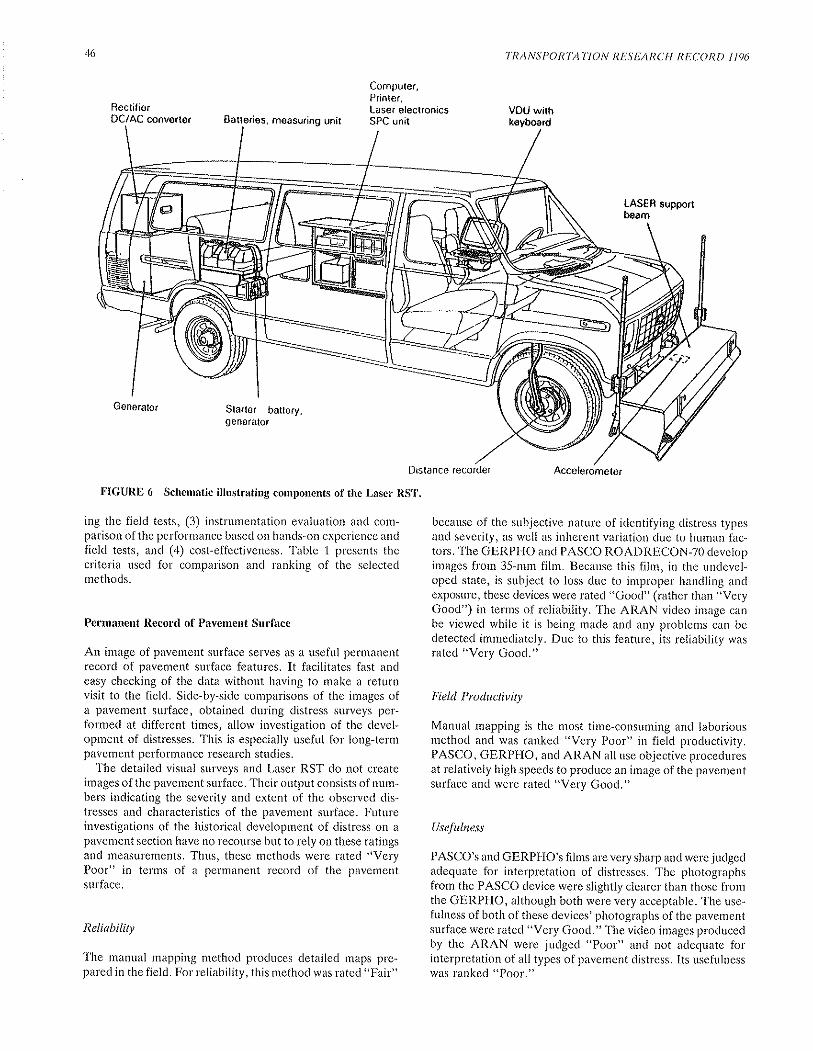
RectilierDC/AC converter Batteries, measuring unil

Compuler.Printer,Laser olectronicsSPC unit

TRANSPORTATION RESEARCH RECORD 1 196

VOU withkcybosrd

Generator slarter battery,9eneralor

FIGURE ó Schematic illustrating components of the Laser RST.

ing the field tests, (3) instrumentation evaluation and com-parison of the performance based on hands-on experience andfield tests, and (4) cost-effectiveness. Table 1 presents thecriteria used for comparison and ranking of the selectedmethods.

Permanent Record of Pavement Surface

An image of pavement surface serves as a useful permanentrecord of pavement surface features. It facilitates fast andeasy checking of the data without having to make a returnvisit to the field. Side-by-side comparisons of the images ofa pavement surface, obtained during distress surveys per-formed at different times, allow investigation of the devel-opment of distresses. This is especially useful for long-termpavement performance research studies.

The detailed visual surveys and Laser RST do not createimages of the pavement surface, Their output consists of num-bers indicating the severity and extent of the observed dis-tresses and characteristics of the pavement surface. Futureinvestigations of the historical development of distress on apavement section have no recourse but to rely on these ratingsand measurements. Thus, these methods were rated "VeryPoor" in terms of a permanent record of the pavementsurface.

Reliability

The manual mapping method produces detailed maps pre-pared in the field. For reliability, this method was rated "Fair"

LASER supporrbeam

otslance recorder Accelerometer

because of the subjective nature of identifying distress typesand severity, as well as inherent variation due to human fac-tors. The GERPHO and PASCO ROADRECON-7O developimages from 35-mm film. Because this film, in the undevel-oped state, is subject to loss due to improper handling andexposure, these devices were rated "Good" (rather than "VeryGood") in terms of reliability. The ARAN video image canbe viewed while it is being made and any problems can bedetected immediately. Due to this feature, its reliability wasrated "Very Good."

Field Productivity

Manual mapping is the most time-consuming and laboriousmethod and was ranked "Very Poor" in field productivity.PASCO, GERPHO, and ARAN all use objective proceduresat relatively high speeds to produce an image of the pavementsurface and were rated "Very Good."

Usefulness

PASCO's and GERPHO's films are very sharp and were judgedadequate for interpretation of distresses. The photographsfrom the PASCO device were slightly clearer than those fromthe GERPHO, although both were very acceptable. The use-fulness of both of these devices' photographs of the pavernentsurface were rated "Very Good." The video images producedby the ARAN were judged "Poor" and not adequate forinterpretation of all types of pavement distress. Its usefulnesswas ranked "Poor."

Benson et al.

The usefulness of the manually prepared maps was judged"Fair," because of the subjective nature of the distress inter-pretations and the possibility that pavement features are notrecorded which appear insignificant, but which may becomeimportant at a later date.

Field Data Collection, Processing, Interpretation,and Summary

Criteria in this category include level of automation, accuracyof surface distress data, quality of rut depth data, repeata-bility, ease of processing, and ease of interpretation ofoutputs.

Level of Automation

Autornation is a primary consideration for cost-effective dis-tress survey procedures. Mapping is not an automated methodand was rated "Very Poor." In detailed manual visual surveymethods, field data collection, processing, and interpretationare done manually, although the data can be input into thecomputer and used to generate reports. Therefore, they wereranked "Poor." The automated data logger was given a "Fair"

47

TABLE 1 A SUMMARY OF COMPARISON AND RANKING OF THE SELEC'TEDMETHODS

rating, due to the reduction in time and cost to transfer thefield data to an office computer for processing. The GER-PHO, PASCO, and ARAN instrumented vehicles were rated"Good" because data collection is automated, but furtherprocessing of the field data is required in the office. Theautomation of the Laser RSTwas rated "Very Good" becauseall of the information collected with this device is processedin the field with the on-board computer.

Accuracy of Surface Distress Data

Accuracy of the distress survey data was defined as how closethe reported distress data corresponded to the distresses actuallyon the test sections. The "truth" was taken as the ratings fromthe three manual methods when they were âll in agreement.Where conflicts in the data from the manual methods existed,return trips to those sites were made by the members of thestudy team to resolve the conflicts.

No single method was found to be totally correct for allsections. The manual mapping method yielded results thatapproximated what the truth was judged to be and was givena "Good" rating. The information from the GERPHO wasalso in close agreement with the observed distresses and givena "Good" rating. The fornr of distresses reported from the

CRITERIAManual

Mapping

PASCO.ROAD

RECONARAN

LaserRST

DEÍAILED VISUALSURVÊY

Manualìecordinc

AUtAmartsoDâta Logqot

1. Permanent Record ofPavement Surface

ReliabilityField ProduaivityUsefulness

2. Field Data Collec,tion,Processinq. lnteroretalion,and Summarv

Level ol AutomationAccuracyQuality of Rut DepthDataRep€atabilityEase of processingEase of intorpretationol outpuls

3. Operating RestriclionsEnvkonmental EffoctsTraffic lntederenceOperating Speed

4. Eouioment Durabilitv andRobustness

5. Cost Eflectiveness

353

52

1

22

1

255

1

5

21

I

22

51

3

'|

21

1

I

1

21

I

22

1

1

4

2

21

1

2

1

I4

24

232

3

31

1

2

2

555

'|

4

232

3

2'|

1

2

1

555

43

332

1

255

4

555

33

333

1

254

3

Rankings: 1=VeryGood 2-Ciood 3-Fair 4=Poor 5=VeryPoor

48

PASCO ROADRECON-7O were somewhat difficult to directlycompare, but was judged to be of "'Good" accuracy. Theaccuracy of the detailed visual surveys was judged "Fair,"even though the surveys were used, in part, to hélp definethe actual conditions. As might be expected, the accuracy ofthe surface distress information collected through the wind-shield of the ARAN and Laser RST were not as accurate as

the other methods and was judged "Poor."

Qualiry of Rut Depth Data

Quality of the rut depth measurements was based on theaccuracy of the measurement and the amount of detail pro-vided for the transvelse profile. Accuracy of the rut depthmeasurements was determined by comparison against trans-verse rut profiles manually measured with a 1O-foot (3-m)straightedge. The amount of detail was judged "Good" if botha transverse profile and maximum rut depth were produced.

Since the GERPHO does not measure rut depth, it was

rated "Very Poor" in this category. The manual rnappingmethod was rated "Very Good" because the l0-foot (3-m)straightedge was considered as a part of this technique.

Since the PASCO ROADRECON-7S rut depth measure-ments corresponded very well with the straightedge meas-urements, and detailed transverse profiles were produced, itwas rated "Very Good."

The maximum rut depth measurements made with the ARANand Laser RST were less than those measured with thestraightedge. However, due to differences in measurementintervals, the accuracy of these rut depths could not be directlyevaluated against the straightedge ¡neasurernents. Althoughthe ARAN measured a transverse profile using sensors spacedat l-foot (0.3-m) intervals, only the maximum rut depth was

reported. The Laser RST gave the average and stanclarddeviation of the depth measurements made with each laser,which gives some information on the transverse profile shape,but did not give profiles for each measurelnent made. Sincethe Laser RST made approximately 3,000 measurements oneach section, if transverse profiles were produced the arnountof information would lre overwhelming. Based on these con-

siderations, the ARAN and Laser RST quality of rut depthmeasurements were rated "Good."

The accuracy and detail provided with the detailed visualsurveys were rated "Fair." Some discrepancies were found inboth the extent and severity of rutting reported by these meth-ods. These survey techniques are not designed to produceinformation on the transverse profile of the pavement.

Repeatability

This criterion is related to the differences between the reporteddistresses from initial surveys and from surveys performedimmediately follorving or several days later. The PASCOmeasurements showed excellent agreement betrveen initialand repeat measurements and was therefore ranked "VeryGood." The distresses from the GERPHO photographs werenot interpreted for the repeat measurements. Since the repeatphotographs of the test sections made with the GERPHOwere judged by the study staff to be equal in quality to the

initial photographs, the repeatability of this device was also

TRANSPORTATION RESEARCH RECORD I 196

rated "Vely Good." The rut depth rneasulements made withthe ARAN and Laser RST had "Good" repeatability. How-ever, significant differences were found in the ratings of theothersurface distresses. Since rut depth is only one distress

category, these two devices were rated "Fair" in overallrepeatability.

Detailed survey methods showed discrepancies betweenraters, but repeat measurements with the same rating teamyielded "Fair" repeatability. The repeatability of the manualmapping technique was rated "Goocl."

Ease of Processing

The ease of processing the raw data is rated based on therequired background and training for the technician(s) and

the complexity involved in the processing, The lower therequirements for operator training and the less cornplex theprocess, the higher the rating. These ratings are relative toeach other and shor¡ld not be considered as an absolute meas-

ure, that is, a method rated as "Poor" was judged to requiremore operator training and be more complex than one witha "Fair" rating. Mapping was rated "Good" even though itis laborious and time-consuming. It is a straightforward proc-ess requiring technicians to summalize, from the preparedmaps, the distresses which have been intelpreted in the field.The ease of processing the GERPHO photographs was rated"Fair" because a technician trained to interpret the photo-graphs with keyboard skills is lequired.

The PASCO techniques were rated "PooL" overall in the

ease of processing because of the complexity of the procedures

and the following requirements for technicians: that they operate

a digitizing computer for rut depth measurements, that theybe trained for interpretation of the distlesses frorn the pho-tographs, and that they have keyboard skills for entry of theinterpreted data into a computer. Because the technicians whoprocess the raw data from the ARAN and Laser RST are notrequiled to interpret the distresses, the ease of processing was

rated "Good." The ease of processing the data from the detailedcondition survey was also rated "Good." Although keyboardentry skills are required to enter the data into the co¡nputer,the technicians processing the data are not required to inter-pret distresses. The automated data logger was rated as "Fair"because it was slightly more cornplex due to the need to have

the technician transfer the field data to the office computerplior to final processing.

Ease of Interpretation of Outputs

The case of interpreting the repofts or final output from each

method was rated according to how easy it was to understandthe outputs. All of the manual methods and GERPHO wereranked "Very Good" because the reports were given in termsof severity and extent of distresses in clearly distinguishablecategories. The reports from the PASCO ROADRECONdevice were only rated as "Good," prirnarily because theywere produced on an output fortnat printed in Japanese and

because cracking, patching, and potholes were grouped intoone category. It should be noted that a user agency shouldbe able to reformat reports into its desired format, using the

ROADRECON equipment. The ARAN and Laser RST

Benson et al.

devices were ranked "Fair" because interpretation of theiroutput was complex and not straightforward. The manualsand written procedures which accompanied their reports werealso found to be complex and required more effort to under-stand than the other methods.

Operating Restrictions

The three criteria in this category are summarized in table 1

and discussed below.

Environmental Effects

No method can be used during all weather co¡ìditions, or atall times of the day and night. All methods are rated "Good"except ARAN, which was rated "Fair" due to the problemscaused by the rain with the ultrasonic sensors during fieldtests.

Traffic Interference

Traffic interference during distress surveys affects the qualityand quantity of distress data. None of the foul instrurnentedsurvey vehicles interrupts traffic, poses hazards, or requireslane closure or other t¡'affic controls for routine use. Thesewere ranked "Very Good." All manual methods are subjectto potential conflicts with traffic becat¡se of the presence ofthe rating team taking measurements on the side of the roador in the traffic lane. Therefore, the manual mapping andvisual condition survey methods were ranked "Very Poor."

Operating Speed

The operating speed is related to productivity and cost-effec-tiveness of the complete system. Labor-intensive methods(mapping and manually-recorded detail survey) were ranked"Very Poor'," followed by the automated data loggers, whichwas somewhat faster but rated "Poor" in comparison to theinstrumented survey vehicles. The instrumented survey vehi-cles were all rated "Very Good."

Equipment Durability and Robustness

Equipment durability and robustness are important consid-erations for the long-terrn performance of a device. The man-ual mapping and detailed visual distress survey methods useequipment that is not subject to breakdow¡rs ol'that requireslittle maintenance and were, therefore, rated as having "VeryGood" equipment durability and robustness. The GERPHOand PASCO ROADRECON devices, which also rated "VeryGood," have a long history of use in their respective countriesand performed without problems during the field tests. TheARAN device tested in this study had two malfunctions duringthe testing period that were corrected without great delay.Although it was a new machine which had not had all of the"bugs" worked out, it was assigned a "Good" reliability ratingin comparison to the other methods. The Laser RST was also

49

given a "Good" rating is equipment reliability and robustness,because the instrumentation involved with the use of lasersand interfaces with the on-board computers could be subjectto more potential problems than the equipment rated as "VeryGood."

Cost-Effectiveness

Cost-effectiveness involves costs associated with severalparameters: field productivity, operating crew size, office dataplocessing time, manpower requirements, and usefulness ofdata. Cost analyses based on these criteria (1) resulted in theGERPHO and Laser RST ranked "Very Good," followed bythe other two instrumented survey vehicles. The automateddata logger was rated "Fair." The manual recording of visualsurvey method and rnanual mapping were ranked "Poor" and"Very Poor," respectively.

CONCLUSIONS

Distress surveys for pavement management purposes are con-ducted at two levels, network- and project-level evaluations.Network-level evaluations are conducted over a road or high-way network to determine its condition and establish prioritiesfor improvements to the sections competing for limited fund-ing. Project-level evaluations are conducted to provide infor-mation with which to design specific improvements or "4R"measures (resurfacing, rehabilitation, restoration, and recon-struction). There is a wide variation in the type and appli-cation of distress surveys for network- and project-level eval-uations. A great deal depends on the magnitude of the network,the type of pavement structures, the type of agency, and theavailable funding.

The PASCO and GERPHO photographic survey vehiclescan be used for both network-level and project-level distresssurveys. The GERPHO and PASCO devices are also wellsuited as high-speed distress survey devices for research stud-ies. They are capable of covering extensive networks in a

relatively short time. Either sum¡nary or detailed distressinformation can be interpreted from the photographs as desired.Photographs taken over time can yield useful information onthe development of distress to update distress prediction models.The additional rut depth and roughness measurement equip-ment contained on the PASCO vehicle gives it additionalutility for both network- and projectJevel surveys. While thesevehicles provide the basis for good quality distress informa-tion, the costs associated with film development, office inter-pretation, and film storage may offset their advantages forsome agencies. Although a permanent visual record of a pave-ment surface has many advantages, these lecords may not benecessary for a network-level pavement management system.

The other two distress survey vehicles investigated in thisstudy, the ARAN and Laser RST, lend themselves to net-work-level distress surveys. They both supplement wind-shield-type distress ratings with rneasurements of rutting androughness. They are capable of covering networks in a rela-tively short time. Since the distress information and pavementsurface measurements are recorded on on-board microcom-puters, the turnaround time on completion and assembly ofthe processed information is relatively short.

50

The video cameras on the ARAN provide additional infor-mation that may be useful to an agency. The through-the-windshield view of the road environment provides informa-tion useful for inventory purposes. Although the image of thepavement surface from the shuttered video camera was notadequate for interpretation of all distresses, it does providea record of major distresses, such as potholes, that can beuseful to the engineer in the office as a check on questionableratings, or to investigate a section of road that is of interest,prior to making a field trip.

Manual surveys are the traditional approach to distress sur-veys. Automated data loggers are more cost-effective thanmanual recording, and thus it is recommended that an agencyperforming manual surveys use an automated data logger torecord the distress survey information in the field and fortransfer to an office computer. Because manual mapping islaborious and time-consuming in the field, as well as duringoffice data reduction, it is not recommended for network- orproject-level distress surveys for pavement managementpurposes.

ACKNOWLEDGMENT

The work reported in this paper was sponsored by the U.S.Department of Transportation, Federal Highway Adminis-tration. The authors would like to acknowledge the supportof Douglas Brown of the Federal Highway Administration,the cooperation of the Texas State Department of Highwaysand Public Transportation, and the participation of the var-ious distress survey equipment representatives.

REFERENCES

l. W. R. Hudson, G. E. Elkins, W. Uddrn, and K. T. Reilley.Improved Methods ond Equipment to Concluct Pavement Dis-tress Surveys. Report FHWA-TS-87-213. FHWA, U.S.Department of Transportation, 1987.

TRA NS PO RTAT'I O N R ES EA RC I1 R ECO II D 1 I 9()

2. Special Report 6lE: The AASHO Road Test Report 5 Pave-men! Research. HSB, National Research Council, Washing-ton, D.C., 1962.

3. R. E. Smith, M. I. Darter, and S. M. Herrin. Highway Pave-ment Distress ldentification Manual. FHWA Contract DOT-FH-11-9175 and NCHRP Project 1-19. University of Illinoisat Urbana-Champaign, March 1979.

4. APWA PAVER Implementation Manual (Draft). AmericanPublic Works Association Research Foundation, April 1983.

5. M. I. Darter, J. M. Becker, M. B. Snyder', and R. E. Smith.NCHRP Report 277: Portland Cement Concrete PavementEvaluation System, COPES. TRB, National Research Coun-cil, Washington, D.C., Sept. 1985.

ó. R. F. Carmichael, III, D. S. Halbach, and L. O. Moser.Pavement Condition Survey Manual for Rhode Island Pave-ment Evaluation and Management System. Final Report No.RI-2/2. ARE Inc., Jan. 1985.

7. Report on Pavement Condition Monitoring Methods andEquipment. PASCO USA Inc., Lincoln Park, N.J., Sept.1985.

8. MAP Inc., Washington, D.C. Pavement Condition Monitor-ing Methods and Equipment. Final Report on GERPHO Sur-vey for ARE Inc. Austin, Federal Highway AdrninistrationStrategic Highway Research Program, August 1986.

9. M. DeWilder. GERPHO and the APL. Proc., RoadwayEvaluation Equipment Workshop. Report FHWA-TS-85-210.FHWA, U.S. Department of Transportation, May 1985.

10. Automatic Road Analyzer Mobile Data Acquisition Vehicle.Product Bulletin. Highway Products International, Inc., 1985.

11. R. L. Novak. Swedish Laser Road Surface Tester. Proc.,Roadway Evaluation Equipment Workshop. Report FHWA-TS-85-210. FHWA, U.S. Department of Transportation, May1985.

The contents of this paper reflect the views of the authors, who areresponsible for the facts and the accuracy of the data presenteclherein. The contents do not necessarily reflect the official views orpolicies of the Federal Highway Administration, U.S. DepailmentofTransportation. The papet'does not conslilute a standard, s\ec'ification, or regulation.

Publication of this paper sponsorecl by the Committee on PavementMonitoring, Evaluation, and Data Storage.

TRANSPORTATION RESEARCH RECORD 1 196-51

Effect of Reflected Waves in SASWTesting of Pavements

J. C. Sunu, K. H. Sroron II, eNo J. M. Ronssnr

The Spectral.Analysis-of-Surface-Waves (SASW) method is arapidly developing in situ seismic method for nondestructivelydetermining Youngts modulus profiles of pavement sites. Themethod is based on the generation and measurement of surfacewaves (Rayleigh waves). Due to the complex theoretical solu-tion of surface wave propagation in pavements, a multilayeredhalf space with infinite lateral extent has been assumed in theanalytical solutions of SASW testing. In addition, only planesurface waves were considered. The existence of direci andreflected body waves and any reflected surface waves, althoughknown to occur in pavements, was neglected in the analyticãlsolutions. To understand the impact ofreflected surface rvavesand direct and reflected body rvaves in SAS\{ testing, a sim-plified analytical model was developed. Reflecting boirndariessuch as edges orjoints ofa pavement system or the horizontalinterfaces between pavement layers were considered. To exam-ine the validity of the model, field tests on a jointed concretepavement were performed. The results show that reflectedsurface waves cause fluctuations to occur in the field data(dispersion curves) which rvould otherwise be a smooth func-tion ifonly direct surface rvaves tvere present. Direct and reflectedbody waves also create a similar result but to a much lesserextent. Reflected SV-waves (shear waves rvith vertical particlemotion) exhibit the most influence of all direct and rãflectedbody rvaves, rvith the effect more important at wavelengthslonger than the pavement surface layer. The adverse effecl ofreflections can be minimized by properly orienting the testarray (line passing between the source and receivers) in thefield with respect tojoints, edges, and cracks in the pavement.For instance, when a vertical rellecting boundary such as ajoint is oriented perpendicularly to the SASW array, the adverseeffect of reflections can be ntinimize¡l and nearly eliminatedby placing the source between the reflecting boundary and thereceivers. When a vertical reflecting boundary such as thepavement edge is near the zone of testing, the effect of reflec-tions can be greatly minimized by orienting the array parallelto and near (about 0.1 fimes the receiver spacing) the edge.

Nearly all nondestructive testing of pavements involves stresswave propagation. Due to the complex nature of stress wavepropagation in pavements, most analytical moclels are basedon the assumption that the seismic waves propagate in a lay-ered half space with no additional boundaries or interfaces.As a result, reflected surface and body waves created byboundaries in the real finite system are not inclucled in thesesolutions. In fact, whenever a pavement system is tested usinga stress wave propagation method, such as the Spectral-Anal-ysis-of-Surface-Waves (SASW) method, reflected waves from

J. C. Sheu, Dames & Moore, 221 Main Street, San Francisco,Calif. 94105. K. H. Stokoe II and J. M. Roesset, GeotechnicalEngineering, The University of Texas at Austin, Austin, Tex.78712.

discontinuities such as edges, joints, or cracks are inevitablygenerated. The key reflecting boundaries are nearly alwaysthose in the top layer, such as the concrete layer in a rigidpavement.

The existence of reflected surface waves is not consideredin the analytical model used to analyze (invert) SASW dis-persion curves (/-3). Therefore, it is important to investigatehow and to what extent reflected waves influence field results(dispersion culves) so that possible errors created by neglect-ing their existence al'e not accidentally overlooked. It maythen be possible either to avoid or reduce the influence ofreflected waves by adjusting the field test proceclure and/orin-house data reduction process.

In addition, only plane surface waves are assumed to existin the inversion process used in the SASW method (1-3).However, when the test is carried out in the field, surfacewaves are generated by applying a point load (impact) on thesurface. As a result, body waves (compression and shear) aregenerated simultaneously with the surface waves. These bodywaves may propagate directly from the source to the receivers(direct body waves), or they may be reflected, just like surfacewaves, by discontinuities in the system and then reach thereceivers (reflected body waves). The effect of direct andreflected body waves on the dispersion curve is not knownand needs to be studied. Sanchez-Salinero et al. (4) initiateda formulation which incorporates all waves in the system.However, more work is necessary before this formulation canbe easily used and parametric studies can be performed.

A mathematical model which is capable of simulating theeffect of direct and reflected body waves and reflected surfacewaves on dispersion curves in presented herein. Use of thismodel is first explained with a simple example involving sur-face waves reflected from the edge of a concrete pavement.To evaluate further the validity of this approach, modeleddispersion curves are compared to actual dispersion curvesmeasured in the field for various locations of pavement jointsand edges relative to the general location and orientation ofthe source and receivers used in SASW testing. Confidencein this model is established with these comparisons, and themodel is further used to predict the behavior of dispersioncurves for other conditions of interest, such as for the influ-ence of direct and reflected body waves and for multiplereflections of body and surface waves.

BACKGROUND OF SASW METHOD

The SASW method is an in situ seismic method which is usedfor near-surface profiling of pavement sites. The general

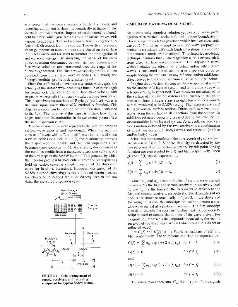
52

arrangement of the source, receivers (vertical sensors), and

recording equipment is shown schematically in figure 1. Thesource is a transient vertical impact, often delivered by a hand-

held hammer, which generates a group of surface waves withvarious frequencies. The surface waves travel along the sur-face in all directions from the source. Two vertical receivers,

either geophones or accelerometers, are placed on the surfacein a linear array and are used to monitor the propagation ofsurface wave energy, By analyzing the phase of the crosspower spectrum determined between the two Leceivers, sur-

face wave velocities are determined over the range of fre-quencies genelated. The shear wave velocity profile is thenobtained from the surface wave velocities, and finally theYoung's modulus profile is determined (1-4).

Since the stiffness of a pavement site varies with depth, thevelocity of the surface wave becomes a function of wavelength(or frequency). The variation of surface wave velocity withrespect to wavelength (frequency) is called a dispersion curve.This dispersive characteristic of Rayleigh (surface) waves isthe basis upon which the SASW method is founded. Thisdispersion curve can be considered the "raw data" collectedin the field. The purpose of this paper is to show how joints,edges, and other discontinuities in the pavement systern affectthe field dispersion curve.

The dispersion curve only represents the relation betweensurface wave velocity and wavelength. When the mediumconsists of layers with different stiffnesses (in terms of shearwave velocities or elastic moduli), the relationship betweenthe elastic modulus profile and the field dispersion curvebecomes quite complex (4, 5). As a result, development ofthe modulus profile from a measured dispersion curve is one

of the key steps in the SASW method. This process, by whichthe modulus profile is back-calculated from the correspondingfield dispersion curve, is called inversion of the dispersiortcurve (or in short, inversion). However, this aspect of theSASW method (inverting) is not addressed herein because

the effects of reflections are more directly seen in the rawdata, the measured dispersion curve.

Mass Storage(O¡sk Or¡vsr)

FIGURE I Field arrangement ofsource, receivers, and recordingequipment for typical SASIV testing.

TRANSPORTAT'ION RESEAII,CII RECORD I 196

SIMPLIFIED MATHEMATICAL MODEL

No theoretically complete solution yet exists for wave prop-

agation with vertical, horizontal, and oblique boundaries in

a layered system such as a pavement which involves all seismic

waves (ó, 7). In an attempt to simulate wave propagationproblems associated with such kinds of systems, a sirnplifiedmathematical model was developed. This simplified modeling

technique assumes that a true dispersion curve derived solelyfrom direct surface waves is known. The dispersion curvewhich includes the effects of reflected and/or other directwaves is calculated based on the true dispersion curve by

simply adding the influence of any reflected and/or additionaldirect waves to the true dispersion curve as outlined below.

Imagine that a vertical forcing function is applied at a pointon the surface of a layered system, and a pure sine wave witha frequency, /6, is generated. Two receivers are attached tothe surface of the layered system and aligned with the pointsource to form a linear array (straight line connects source

and all receivers) as in SASW testing. The receivers are used

to track vertical surface motion. Direct surface waves prop-agate along the surface in all dilections from the source. Inaddition, reflected waves are created due to the existence ofdiscontinuities in the layered system. As a result, surface (ver-

tical) motion detected by the two receivers is a combinationof direct (surface and/or body) waves and reflected (surface

and/or body) waves.Schematic representations of the time records of each receiver

are shown in figure 2, Suppose time signals detected by the

two receivers after the surface is excited by this point-forcingfunction are represerìted by g(r) and /r(t), respectively. Theng(t) and h(t) can be expressed by

8(Ð = ì a,,,sin2rfn(t - t,,,) (1)

hØ:4arosin2rfo(t - tr,,) (2)

in which ar,, and az.r ate amplitudes of various wave arrivals

measured by the first and second Leceivets, respectively, and

tro and t2,t are the times of the various wave arrivals at the

first and second receivers, respectively. The definitions of a's

and f's are shown schematically in figure 3. In the above and

following equations, the subscripts are used to denote a spe-

cific wave arrival at a particular receiver. The first subscriptis used to demote the receiver nutnber, and the second sub-

script is used to denote the number of the wave arrival. Forexample, a23 represents the amplitude recorded by the second

receiver of the third wave arrival (which could be a direct orreflected wave).

Let G(/) and H(/) be the Fourier transforms of g(l) and

å(t), respectively. The transforms can then be expressed as

G(î) = \or,,"*p(-i2r f¡trr) forf : ¡n (3a)

c(f) :0and

rorf*fu (3b)

H(f) : )arnexp(-i2rfotr,,) for/=6 (4a)

H(f) = 0 rorf * fn (4b)

The cross power spectrum, Gr*, for this pair of time signals

Sheu et al

is defined as

G.= G* x H (5)

in which G* denotes the cornplex conjugate of G. The phaseof the cross power spectrum at flequency,fo, ö(,fo), is

l> > a.,roro sin 2 n fn(tro - tro)1ô(,r.)=r^"-'lffil rol))

This phase is the key varial¡le used to calculate wavevelocity.

In a real SASW test, a wide range of frequencies is gen-erated simultaneously by applying a vertical impact on thesurface of the system. As a result, each arrival is no longer a

single-frequency arrival but contains a certain range of fre-quencies. Since equations 1 through 6 were derived with theconsideration of only a single frequency, the following mod-ifications are made so that they can be applied to the multiple-frequency condition. Assume while /¡ varies over a range offrequencies generated by the vertical impact, values of c,r,ezq, trp, 12q vaty accordingly. Let Ar, Aro, Tro, and Ir., bethe amplitude and time functions of frequency at receivers 1

FIGURE 3 Representation of amplitudes (¿'s)and arrival times (l's) for two single-wave arrivalsat each receiver.

53

Ampl¡tudeRecsiver

(s(t))

þ-irïjj --rl-------r Rerrected waves

FIGURE 2 Representation of time domain records received by eachreceiver in SASW testing illustrating combined direct and reflected(packets of e'ergy) waves.

atI

and 2, respectively.AS

A',(f) = atp(f) +

Arr(f) = aro(f') +

arr(fr) + a,r(fr) +

aro(fr) + arn(fr) +

Therefore, the functions can be written

(7)

(8)

(e)

(10)

0(/):

..""-,r

t

Troff) : tr,(fr) + t,r(f) + \r(fr) +

Trn(f) = tro(f) + hn(fr) + trn(fr) +

in which the notations for each subscript of Îs and A's, as

well as ,'s and a's, are the same as previously defined andfrequencies fr, fr, fr, and so forth are the desired modelingfrequencies. Hence, equation 6 can be rewritten as

22 r,r(Ð,qr,,(f) sin2¡ flT,r(f) - Tr,,(f))

22 A,,,(f) Ar,,(f) cos2¡ fÍT,r(f) - Tr"(Ðl

Each A, with two subscripts, is a series of amplitudes whichare a function of frequency and correspond to the particulararrival denoted by the subscripts. The absolute value of Aactually represents the amplitude of the linear spectrum forthis particular arrival. Each T, with two subscripts, is a seriesof travel times which are a function of frequency and corre-spond to the particular arrival denoted by the subscripts. Itis necessary to note that the connotation of "arrival" used inequation 6 is somewhat different than that used in equation11. In equation 6, each "arrival" has energy at only one fre-quency. On the other hand, in equation 11, each "arrival"represents a packet of energy containing a range of frequen-cies. Since equation 6 is a special case ofequation 11 and thelatter was used for all studies, the second connotation of"arrival," namely a packet of energy over a range of fre-quencies, is used herein.

It is important to notice that both 7-s and A's are functionsof frequency, and each arrival has its own T and A. Since Tis directly related to the arrival times of different frequenciesforming the arrival of a particular packet of energy, dispersivecharacteristics (that is, waves corresponding to different fre-quencies traveling at different velocities) of this particular

Ì( 11)

Tatt

Arrival 2

JArrivat ¡

Iî412

54

arrival can be accurately modeled by using the proper traveltime in "T" for each frequency. In addition, since the arrivalof each packet of energy has its own ?, waves with differentdispersive characteristics can be analyzed together; that is tosay, each arrival could have its own dispersion curve. A typicalneed of modeling waves with more than one type of dispersivecharacteristic is in the case when combined surface wave and

body wave effects are considered. Examples of this type ofmodeling are illustrated in the following sections.

The amplitude of the linear spectrum, A, for the arrival ofeach impulse (packet of energy) is sirnply a measure of theamplitudes of the different frequencies transmitted by thispacket ofenergy. Therefore, the value ofá is directly relatedto the damping characteristics and reflection coefficients ofthe system being tested. Due to the fact that the arrival ofeach impulse has its own .4, amplitudes of different frequen-cies which attenuate at different rates can be modeled by usingdifferent ratios of amplitudes between different arrivals of theimpulse at different frequencies.

In the present inversion process in SASW testing, it is assumed

that only plane surface waves exist (a-ó). As a lesult, it is

implicitly assumed that only one surface wave arrival is detectedby the receivers. Let ?rt and 12' be the arrival times of this

TRANSPORTA'ilON RESEARCH RECORD I 196

direct surface wave at each receiver. The corresponding phase

of the cross power spectrum, 0(f), can be expressed as

0(/):2nf[T',(f) - r,'ff)l (r2)

Equation 12 is just a special case of equation 11 with p and

q both equal to 1. Also notice that in equation 11, it is notnecessary to have Trr, Trr,.A,r, and A, associated with thearrival of the direct surface wave. In fact, arrivals in equation11 can be considered in any random order. However, to avoidany possible confusion, Trr, Trr,^A,,, and A^ are used torepresent only direct surface wave arrivals for all discussions

presented hereafter.The problem faced in typical SASW testing in terms of

reflections is now clear. In the field, measured phases of cross

power spectra are in the fashion of equation 11, but duringthe in-house inversion stage, the phases of cross power spectra

are assumed to be in the fashion of equation 12. The differencebetween these two equations is the errot introduced by waves

other than the direct surface wave. As such, it is possible tostudy the influence of reflected and direct waves on fielddispersion curves by using equations 11 and 12, as shown inthe following sections.

a. Plan View

b. Cross Section A-A

Note: Not to Scale

FIGURE 4 Plan and cross-sectional views of BRC pavement facility.

F¡xed Concrete Slab 12.5 lt Access

i fr Compacted Soil

Nalural Ground

Sheu et al.

FIGURE 5 Material profile at DRC pavement facility.

FIELD TESTING

To investigate the validity of the simplified mathematical model,field tests were perforrned. All field data referred to in thiswork are from tests perfonned on the jointed concrete pave-ment at the research facility at Balcones Research Center(BRC), The University of Texas at Austin. This researchfacility was designed fol the study of nondestructive pavementevaluation devices such as the SASW, Dynaflect, and fallingweight deflectometer clevices (8). A schematic of the BRCfacility is shown in figure 4, and the material profile at thefacility is presented in figure 5.

A Hewlett Packard model 35624 dynamic signal analyzerwas used in the field for data collection, mainly phases of thecross power spectrum and coherence functions (3, 9, l0).Different types of accelerometers and geophones were usedto monitor motions on the pavement surface. Most field data,however, were collected using PCB model 308802 accelero¡n-eters as motio¡r rnonitoring devices. Field data (phases of crosspower spectra) were transferred to a MASSCOMP modelMC5500 minicomputer through a general-purpose interfacebus for further processing. With the MASSCOMP computer,the user is able to filter out low quality and questionable phaseinformation acquired in the field, calculate the dispersion curvesfrorn the filtered phase information, average the dispersioncurves from different receiver spacings to find the final (aver-aged) dispersion curves, and perform other miscellaneousplotting and numerical manipulations.

SIMPLE EXAMPLE

A simple exarnple is given here to illustrate the use of theequations ancl procedures outlined above. This exarnple modelsa field test performed at the BRC facility on January 3, 1986.The test was performed on the north end of the fixed concreteslab. A detailed layout of this test is shown in figure 6. Threenearby reflecting boundaries are denoted as A, B, and C, as

shown in figure 6. Receivers were placed with a 40-foot (122crn) spacing between them, and each one was 4 feet (I22 cm)away from the nearest reflecting boundary. The source wasplaced at the edge of reflecting boundary A. The existenceof reflecting boundary C was neglected in this example.

FIGURE 6 Detailed layout of SASWtesting used in modeling examPle.

As soon as a pulse is generated with the source, this pulsestalts to travel from the source to receiver 1 and then receiver2 and finally reaches reflecting boundary B. Before this pulsereaches reflecting boundary B, it is considered as a directsurface wave. After the pulse reaches reflecting boundary B,it will reflect back and ne considered a t'eflected surface wavefrom now on. The reflected pulse will travel past receiver 2and then receiver 1 and finally reach reflectil.rg boundary A.It will then be reflected by boundary A and head towardsreflecting boundary B. The pulse will eventually be bouncedback and forth by reflecting boundaries A and B until allenergy is dissipated. Typical field time records for this siteare shown in figure 1. ^lhe reflected surface waves detectedby each receiver can easily be identified and are indicated by

@ nettectø wave cr€ated by Boundary A

@ Rettect"o wavo creatod by Eoundary B

Timo, Ssc

FIGURD 7 Typical time record illustrating theinfluence of reflected surface waves for testarrangement shown in figure 6.

1O '-"

-3iñ:6 in.T2ltt

î5ft

_1-

Rsf lectingBoundary

/c

1Source

5lrRoce¡vgr Rscoiver

12

;.........4 ft--N<-4 ft--ÐF.-4 fr

Rellecting-''Boundary

B

Concrete Slab

RoflectingBoundary

A

=o

o'oJ

=õ.E

=o

o'of,

=oE

@

I

Arrows Po¡nt to Rellected Wavos

56

Wavelenglh. tl

FIGURE 8 Comparison of field (measured)dispersion curve rvith the dispersion curve('(true") for no reflections for the testarrangement in figure 6.

the arrows shown in the figure . (Of course, there are morereflections than those indicated, but those indicated are thekey reflections.)

To simplify this example, the effect of reflecting boundaryC is neglected, and only the first reflected surface wave fromboundary B is considered. THe measured (field) dispersioncurve is shown by the solid line in figure 8. The "true" dis-persion curve for this case should look like the smooth, dashed

line drawn through the dispersion curve in figule 8. (The

"true" dispersion curve is the dispersion curve for only directsurface waves in a layeled systetn with infinite horizontalextent.) From figure 6, the distances that a direct pulse travelsfrom the source to receivers I and2 are 4 and 8 feet (122 and

244 cm), respectively. Since the "true" dispersion curve isknown (figure 8), ?,,(.f), Tr,(/) and "true" phase correspond-ing to each frequency can be calculated. The "true" phase

derived from this "true" dispersion curve is shown in figure9a, and the corresponding "true" dispersion curve (which has

been shown in figure 8) is shown in figure 9b.Notice that although there is a significant wave velocity

change in the dispersion curve shown in figure 9b at a wave-

length of about 1.5 feet (46 cm), the change is barely observ-

able in the phase of the cross power spectrurn (correspondingto figure 9a when the frequency is smaller than about 4000

Hz).From figure 6, the first reflected pulse detected by receiver

1 is the one which travels from the source to reflecting bound-ary B and then back to receiver 1. The distance oftravel forthis pulse is 20 feet (6.1 m). By the same token, the firstreflected pulse detected by receiver 2 is the one which travelsfrom the source to reflecting boundary B and then back toreceiver 2. The distance of travel for this pulse is 16 feet(4.9 rn). Based on this information and by assuming thatreflected surface waves have the same dispersive character-istics (same dispersion curve shown in figure 9b) as directsurface waves, it is possible to calculate Ttr(f) and Trr(f) atall frequencies for both reflected waves.

Reflecting boundary B represents a free boundary at theedge of the concrete pavement. Therefore, reflected waves

should have displacements in phase with direct waves. (AllA's should have the same sign.) The amplitudes for each pulse

detected by receiver L, Art(f) and Arr(f), are assumed to be

T'RANSPORT'A7'ION RESEARCI.I IIECORD I 196

Frequency,Hz

Phase of Cross Power Spectrum for 4-fl Receiver Spacinging

40001,,"' , ' ' ' ',',,0.5 r ---1--t* roWavelength, tt

b. Dispersion Curve Associated wilh Phase Shown Above

FIGURE 9 (a) "True" phase of the cross powerspectrum and (b) corresponding "truc" dispersion curvefor test arrangerrrent shown in figure 6 (only directsurface wave).

1.0 and 0.36, respectively. The amplitudes detected by receiver

2, Arr(f) and Ar'(f), are assumed to be 0.9 and 0.4, respec-

tively. The relative magnitudes of the amplitudes used for the

direct and reflected surface waves are more or less in the same

order as shown in figure 7. However, it is not correct to use

the exact amplitudes measured from the tirne records shown

in figure 7, because reflected waves tend to overlap with the

direct waves and with other reflected waves. As a result, theirreal arnplitudes are distorted. All needed information is com-plete at this point, and the modeled dispersion can be cal-

culated by using equation 11.

Comparison of the modeled and measured phases of the

cross power spectrum is shown in figure 10. Colnparison ofthe modeled and field dispersion curves in shown in fig-ure 11. These two cornparisons indicated that equation l1 is

quite capable of modeling the fluctuations (ripples) that appear

in the field data. The amplitudes and locations of the modeledripples are so¡newhat different, but are close to the field data.

The similarity of modeled and field data give strong supportto the modeling process discussed earlier. It also seems thateven though the lack of knowledge about amplitudes of allarrivals led to crude estimates of .21's ill equatiort 1 1 , the modelstill generated a dispersion curve which is similar to the fielddata.

It is also interesting to note that all ripples in the modeledphase (figure 10) have very similar amplitudes, but the arnpli-

(¡,

Eot(Dodah(úE0-

aàIo

ooI

'**[*rf80001-

::tIu*of

tto.

i.soo(ú

3

Slteu et al.

_ Fietd

Model (Basod on On€ SurlaceWav€ Rellection)

o 2ooo ooo8,.o::;:r, rlooo

loooo l2ooo

FIGURE f0 Comparison of field and modeledphases of cross power spectra for test arrangementin figure 6.

tudes of the ripples in the dispersion curve (figure 11) havean increasing trend as wavelength increases. This same phe-nomenon is found in the field data. In fact, experience indi-cates that this phenomenon commonly exists in most fielddata. This is due to the fact that when the phase of the crosspower spectruln is translated to the dispersion curve, anydisturbance in the high frequency range, which correspondsto the short wavelength range, is deamplified. Any disturb-ance in the low frequency range, on the other hand, corre-sponds to the long wavelength range and is amplified, As aresult, disturbances in the low frequency range cause moreproblems than disturbances in the high frequency range. Interms of sampling depth, short wavelengths sample shallowdepths. Therefore, material properties sampled at shallow

wavetength, ft

FIGURE f l Comparison of field and modeled dispersioncurves for test arrangement in ligure 6.

57

depths are less sensitive to disturbances caused by reflectedsurface or body waves. This material sarnpling character¡sticof the SASW method results in the method being very accu-rate for measurement of near-surface material properties, suchas in the pavement surface layer (/1).

REFLECTED SURFACE WAVES

The study of reflected surface waves was divided into threernajor subjects: (1) the effect of reflected surface waves froma vertical reflecting boundary oriented perpendicularly to thesource/receiver array, (2) the effect of reflected surface wavefrom a vertical reflecting boundary oriented parallel to thesource/receiver array, and (3) the effect of the distance betweena vertical reflecting boundary and the source/receiver array.Model and experimental studies were performed on all sub-jects, with the exception that a model study was not performedon the effect of distance between the source/receiver arrayand a vertical reflecting boundary oriented perpendicularlyto this array. This latter problem is directly related to damping(not geometry) in the system and is outside the scope of thesimplified mathematical model.

Typical results for the effects of cases 1, and2 cited aboveare shown in figures 12 and 1,3. First, consider the field dis-persion curves shown in figures 12 and 73. These curves con-sist of a basic smooth curve upon which ripples ol'fluctuationsare imposed. In the range of wavelengths shorter than about0.5 foot (15 cm), this basic curve can be approximated by ahorizontal line with an average wave velocity of about 7800fps (2377 m/s). This average surface wave velocity correctlyrepresents the stiffness of the concrete layer (modulus equalto 5.4 x 106 psi) and shows that the field data shouldbe "smoothed" to eliminate the effect of surface wavereflections.

Plan View olField Arrangement:

Wavelength, ft

FIGURE 12 Comparison of tield and modeleddispersion curves for surface rvaves reflected from avertical boundary; receivers placed between source andreflecting boundary.

ooo,ox,ot(ÍfL

o;'õIoooì

8000

7000

F¡etd

Mod€l (Based on onesurface wave relleclion)

58

Plan View ofField Arrangement:

i.0 ít 1.0 ftl+_+l<-rl

9000

8000

7000

6000

5000

4000

3000

2gggl , " " '0.1 0.2 ¡t__-i__å--s 10

Wavelenglh, tt

FIGURE f3 Comparison of lield and modeled dispersioncurves for surface waves reflected from a verticalboundary; test array oriented parallel to rellectingboundary.

Modeled dispersion curves, shown ln figures 1,2 and L3,closely describe the main ripples (fluctuations) present in thefield data. It is clear that reflections impose ripples or fluc-tuations onto the dispelsion curves. Although not all peaksand tl'oughs overlap for l¡oth curves, the modeled dispersioncurve shows the significant characteristics of the fluctuations.Since only one kind of reflected wave with only one reflectionis considered in this model, minor discrepancies between themocleled and field data are possibly due to other reflectedwaves which are not considered in this first approximationmodel. In addition, uncertainties in estimating amplitudes andtimes (á's and T's) also introduce some elrors into the mod-eled dispersion curves. However, it is clear that the model is

reproducing the general trend a¡rd major fluctuations in thefield curve. More importantly, the model shows that fluctua-tions in the field data should be smoothed to represent thetheoretical assumption of a multilayerecl half space with infi-nite lateral extent.

The model shows that the effects of reflected surface wavesfrom a reflection boundary oriented perpendicularly to thesource/receiver array are minimized by placing the sourcebetween the boundary and the receivers. When this config-uration is used, reflected surface waves travel in the samedirection as the direct surface waves, and both the direct andreflected waves can be combined and treated as one directwave of longer duration. This combination is not possiblewhen the direct and reflected surface waves travel in oppositedirections, as occurred in the testing illustrated in figure 12.

Field verification of the beneficial effect of orienting the

testing array so that reflected and direct surface waves prop-agate in the same direction is shown in figure 14. Upon com-parison of the field dispersion curves shown in figures 12 and

TRANS PORTATION RESEARCH RECORD 1 196

Plan View ofFiold Arrangement:

t

Øo.

*=E(D

o(ú

3

ø 7000êÉ'8 1000

õ9 ¡000õI

k>3.0of

k<0.2

(13)

(14)

L.=.*o-=f"K--ã+--ä.-Ðl

0.1 ft 0.9frt 1ft

Wavelengh, ft

FIGURE 14 Field dispersion curve for surfacewave reflected from a vertical boundary; sourceplaced between receivers and reflecting boundary.

14, especially in the range of wavelengths from about 0'35 to

0.75 foot (It to 23 cm), one can see that the amplitudes ofthe ripples in figure 14 are much smaller than in the case

illustrated in figure 12. This result occurs because, for the

case shown in figure 12, the reflected surface waves are prop-

agating in the opposite direction to the direct surface waves.

Hence, there is an adverse effect on the dispelsion curve in

figure 1.2. In the case shown in figure 14, the reflected surface

waves are propagating in the same direction as the directsurface waves, and essentially no interfelence occurs.

The model and experimental studies involving the effect ofreflected surface waves from vertical boundaries oriented par-

allel to the test array also showed that the adverse impact ofreflected waves could be minimized by proper placement ofthe array. As the center line of the SASW array is moved

away from the pavement edge, reflected surface waves are

increasingly out of phase with respect to direct waves and,

hence, have a more adverse effect on the dispersion curves.

However, at the same time, the amplitudes of reflected waves

decrease with increasing distance from the boundary whichreduces the adverse effect on the dispersion curves. The com-bination of these two effects makes the choice of the best

center line location of the array relative to the pavement edge

not completely straightforward. Suppose that the source/

receiver spacing is defined as D, as shown in figure 15, and

the distance between the array and the parallel bounclary is

k x D. The field and modeled data lead to the conclusionthat there are two possible ranges for /c which result in min-

imizing the effect of reflected surface waves. These ranges fork can be expressed as

Sheu et al. 59

D------ft+- D----+tReceiver2 Reco¡ver1 sô

VorticaRollectingBoundary

FIGURE 15 Normalized scale illustrating array/boundary configuration for the test arrayoriented parallel to the reftecting boundary.

Either of these criteria will result in making the influenceof reflected surface waves relatively small and can be used asa guide for locating the test array.

DIRECT AND REFLECTED BODY 1VAVES

Surface impacts, generally from hammers or drop weights,are used to generate surface waves in SASW testing. In addi-tion to generating surface waves, surface impacts also gen-erate unwanted body waves. These body waves reach thereceivers either directly or through reflections. problems arisefrom the fact that body waves propagate with different veloc-ities and have different dispersive characteristics than surfacewaves. As a result, body waves can alter the measured dis-persion curve adversely,

The adverse impact of body waves on the dispersion curveis expected to be less than the effect of reflected surface wavesjust shown. This expectation is based on the fact that theenergy generated by a vertically oscillating source on the sur-face of a homogeneous half space is distributed as follows(12): 670/o in Rayleigh (surface) waves, 260/o in shear waves(S-waves), and 7o/o in compression waves (p-waves). It isclear, therefore, that body waves carry only a small portionof the total energy generated by a surface irnpact. Further-more, geo¡netrical damping for body waves in much higherthan for surface waves, which means that the negative impactfrom body waves is further diminished.

There are instances when the boundary which reflects bodywaves (such as the bottom of the pavement surface layer) ismuch closer to the test array than the boundary which reflectssurface waves, Under these conditions, reflected body wavesmay become important, and their influence on dispersion curvesneeds investigation. The effects of body waves on dispersion

FIGURE f 6 Generation of reflected body waves frombottom of concrete slab.

curves have not been evaluated in the past. Therefore, studieswere conducted with the simplified mathematical model in anatternpt to identify their influence, to evaluate the severity oftheir influence, and to provide guidelines for r.educing tireiradverse effects on dispersion curves.

The generation of reflected body waves from the bottomof the pavement surface layer is shown schematically in figure16. Three kinds of body waves commonly exist in a pavementsystem: P-waves, SH-waves, and SV-waves. Since both thedirection of the impacts and the direction of the receivers areoriented vertically in SASW testing, particle motions in thevertical direction are usually dominant and are best measured.As a result, the influences of direct SV-waves, reflected SV-waves, and reflected P-waves are of the greatest concern.However, in this study, reflected SV-waves were found to bethe most important, so only these results are presented herein.

Ray paths of shear waves used in the model simulation areshown in figure 17. Only one reflecting boundary is consideredin this study, which is the bottom of the top concrete pavementlayer. Because this interface represents a location bf signifi-cant stiffness change, a fair amount of energy will be reflectedby-this interface. (An interface with a large stiffness changereflects more energy than an interface with a small stiffneischange.) In addition, this interface usually is much closer tothe source and receivers than other reflecting boundaries.Therefore, this reflecting boundary was selected for study.

LocetionsSource

1-0 0.0 1.0 2.0 3.0 4.0 5.0

Distance lrom Rece¡vsr l, ft

FIGURE f7 Ray paths assumed for body waves reflected from l¡ottomof concrete pavement.

60

SPacing, d1

_ 0.e5 fr

-.- 0.50 fr1.00 ft1.50 rt2.00 tt3.00 fr4.00 ft5.00 ft

I r r I lf rl5 10

Wavelenglh, tt

FIGURE l8 Modeled dispersion curves for shear wavesreflected from bottom of concrete pavement; fixed receiversspacing of I foot and various source-to-receiver distances.

The modeled dispersion curves are shown in figure 18. Theamplitudes, ..4, used for direct surface waves at receivers 1

and 2 are 1.0 and 0.9, respectively, and for reflected shearwaves are 0.15 and 0.12, respectively. These amplitudes areused without any change for all cases, so that the effect ofsource/receiver distance can be more easily identified. Sinceshear (body) waves attenuate at a much faster rate than sur-face waves, their effect on the dispersion curves will decreaseas the source/receiver distance increases. Therefore, the effectof reflected waves is somewhat overestimated for larger source/receiver spacings in the model.

The modeled dispersion curves shown in figure 18 dem-onstrate that, as the source/receiver spacing increases, fluc-tuations in the dispersion curve decrease. In addition, theshear wave has more influence in the long wavelength range(greater than about 0.7 foot, or 21 cm) than in the shortwavelength range. For wavelengths of less than about 0.5 foot(15 cm), the effect is negligible. Since surface waves withwavelengths less than 0.5 foot (15 cm) sample basically thetop concrete layer, reflected shear waves barely affect themeasurement of material stiffness in the concrete layer', an

important observation.The effects of the direct compression and shear waves, as

well as reflected compression waves, were much less than thatshown in figure 18, and, therefore, are not shown here. Arelative comparison of the effect on dispersion curves ofreflected body waves versus reflected surface waves is illus-trated in figure 19. The effect ofbody waves reflections, shownin figure t9a, is not nearly as important as the effect of a

single surface wave reflection (for the case of a reflected sur-face wave propagating in the opposite direction to the directsurface wave) which is imposed on the body wave reflectionsin figure 19b. As such, one can see that reflected surface wavescan cause the bulk of the fluctuations in the measured dis-

TIIANSPORTAT'ION RESEARCI] R ECO RD 1 196

persion curves in these tests. Body waves only contribute moreat wavelengths greater than the concrete slab thickness.

SUMMARY AND CONCLUSIONS

Seismic wave propagation methods, such as the SASW method,have proven through the years to be powerful methods forassessing moduli profiles. The nondestructive and easy-to-

apply nature of the SASW method has made this techniqueattractive to engineers. Significant theoretical and practicaladvances in the SASW method have occurred in the past fewyears, and this method is rapidly becoming an important method

for nondestructive testing of pavement systems.An investigation of the adverse effects of reflected surface

waves and direct and reflected body waves on field dispersioncurves, the "raw data" of the SASW method, is presented.

A simplified mathematical model to account for these effectsis given. Field measurements were performed at the rigidpavement facility at Balcones Research Center to comparewith the model. The usefulness of the model is confirmed by

the good agreement between modeled and field dispersioncurves. In the past, it was a puzzle to determine if the fluc-tuations in dispersion curves were really caused by fluctua-tions in the material properties or whether there were some

other explanations. In this study, it is found that the reflectedwaves can impose ripples (fluctuations) onto the "true" dis-persion curves. If the effect of reflected waves on the dis-persion curves is removed, the dispersion curve is basically a

smooth curve. At most pavement sites, the dispersion curvecorresponding to short wavelengths (about equal to the thick-ness of the top layer and less) is very flat and close to a straightline, which indicates that the material property in the toppavement layer is usually very uniform.

Based on both model and field studies, it is concluded thatthe adverse effects from reflected surface waves upon dis-persion curves can be reduced by proper arrangement of the

source and receiver relative to the boundary. In the case when

the vertical reflecting boundary is oriented perpendicularly tothe test array, the adverse effect of reflected waves can be

reduced to a minimum by placing the source between thereflecting boundary and the receivers. In the case when thereflecting boundaly is oriented parallel to the test array, it is

better to have the test array located either very close to thereflecting boundary, so that reflected surface waves are velymuch in phase with the direct surface waves, or as far as

possible from the reflecting boundary, so that the amplitudesor reflected surface waves are relatively low compared to thedirect surface waves.

Direct and reflected body waves were also studied with theanalytical model. Reflected body waves are more importantthan direct body waves in the top pavement layer and resultfrom reflections at the interfaces at the top and bottom ofthis layer. As shown in this study, body waves also cause

fluctuations in the field dispersion curve, but to a much lesserextent than reflected surface waves.

ACKNOWLEDGMENTS

The project was sponsored by the Texas State Departmentof Highways and Public Transportation, whose support is

Field Arrângement:

t.1 rttri5,

'{"Vgà 6000'õooI sooo

õì

Sheu et al 6l

Dsp€rsþn Curves:

----- -True"

CoÍtinod Rollecled S'

ard P'Wavos

gratefully acknowledged. The encouragement and helpfulsuggestions of R. Briggs and R. Rogers of that departmentand the constructive discussions and guidance ofS. Nazarian,I. Sanchez-Salinero and G. Rix of The University of Texasare sincerely appreciated.

REFERENCES

1. S. Nazarian and K. H. Stokoe, II. In Situ Determination ofElastic Moduli of Pavement Systems by Spectral-Analysis-of-Surface-Waves Method (Practical Aspects). Research Report368-l F. Center for Transportation Research, The Universityof Texas at Austin, May 1986, 187 pp.

2. S. Nazarian and K. H. Stokoe, IL In Situ Determination ofElastic Moduli of Pavements Systems by Spectral-Analysis-of-Surface-Waves Method (Theoretical Aspects). ResearchReport 437-2. Center for Transportation Research, The Uni-versity of Texas at Austin, Aug. 1986, 78 pp.

3. S. Nazarian and K. H. Stokoe, II. Use of Surface Waves inPavement Evaluation. In Transportation Research Record 1070,TRB, National Research Council. Washington, D.C., 1986,39 pp.

4. I. Sanchez-Salinero, E. W. Chang, J. M. Roesset, and K. H.Stokoe, II. Complete Analytical Solution for Wave Propa-gation in a Layered System, Research Report 1123-1. Centerfor Transportation Resealch, The University of Texas at Aus-tin (in press).

5. S. Nazarian. In Situ Determination of Elastic Moduli of Soildeposits and Pavement Systems by Spectral-Analysis-of-Sur-face-Waves Method. Ph.D. dissertation. The University ofTexas at Austin, Dec. 1984.

Plan View ofField Arrangemenl:

| ^------------- ¡---__¡>

___|>

l<-rt-*f*tn-tin-ì

6. I. Sanchez-Salinero. Analyticøl Investigation of Seismic Meth-ods Used for Engineering Applications. Ph.D. dissertation.The University of Texas at Austin, Dec. 1986.

7. J. C. Sheu, K. H. Stokoe, II, J. M. Roesset, and W. B.Hudson. Applications and Limitations of the Spectral-Anal-ysis-of-Surface-Waves Method. Research Report 437-3F.Center for Transportation Research, The University of Texasat Austin, 206 pp.

8. R. White, W. R. Hudson, A. H. Meyer, and K. H. Stokoe,II. Design and Construction of a Rigid Pavement ResearchFacility. Research Report 355-1. Center for TransportationResearch, The University of Texas at Austin, 121, pp.

9. S. Nazarian, K. H. Stokoe, II and R, C. Briggs. Nondes-tructively Delineating Changes in Modulus Profiles of Sec-ondary Roads. ln Transportation Research Record 1136,TR8,National Research Council, Washington, D.C., 1987.

10. S. Nazarian, K. H. Stokoe, II, R. C. Briggs, and R. Rogers.Determination of Pavement Layer Thicknesses and Moduliby SASW Method. ln Transportation Research Record 1196,TRB, 1988.

ll. J. C. Sheu, G. J. Rix and K. H. Stokoe, II. Rapid Deter-mination of Modulus and Thickness of Pavement SurfaceLayer. Presented at the Transportation Research Board AnnualMeeting, 1988.

12. F. E. Richart, Jr., J. R. Hall, Jr., and R. D. Woods. lzibra-tions of Soils and Foundations. Prentice-Hall, Inc., Engle-wood Cliffs, N.J., 1970.

\\

Ò-

i 6000oIoI soooß3

4000

.r 0.2 0.5 1 2 5

Wavelength, fl

a.) Modeled Dispersion Curve with CombinedReflected S-Waves and Reflected P-Waves.

b.) Modcled Dispcnion Cuwc wirh Combined Effect fromBody Wavc Refloctions and Reflected Su¡face Wave.

FIGURE 19 Comparison of the relative effect of reflected body wavcs versus reflected surface rvaves on dispersioncurves.

ø*cL

à eoooö(t)

g 5000aú

34000

Publication of thß paper sponsored by the Committee on PavementMonitoring, Evaluation, and Data Storage.

62 I'RA NS PO RTATI O N R ES EA RCH R ECO R D ] 1 96

Pavement Condition Diagnosis Based onMultisensor Data

K. Masnn, B. BneoEMEyER, eNo R. Lrrrr,nrrnrp

High-speed sensors have developed rapidly in recent years,and numerous such sensors can be operated frorn highwayspeed vehicles. This sensing technology can now provide pave-ment condition and performance information far beyond rvhatis currently exploited in pavement management. Data fromthese sensors, coupled with established knowledge of pavementbehavior, can be used to infer causes of pavement conditionsand to predict performance. Knowledge of cause can also beused to select appropriate maintenance strategies. This paperdemonstrates how the mechanisms of flexible pavernent dete-rioration can be inferred from the data obtained from a "suite"ofpavement sensors. Included are data on subsurface moduli,asphalt thickness, and subgrade moisture, none of which arecurrently measured with high-speed sensors. The paper goes

on to show how the subsurface moduli can be computed fromcontinuous data describing rut depth and fatigue cracks, bothof which are measurable with current technology. Finally, thecomputation of asphalt thickness and subgrade moisture con-tent from continuous radar profiles is described. Thus, a com-plete data set for explaining pavement condition and predictingfuture perfornance can nory be provided by high-speed sen-sors. What remains is to integrate these sensor data into cur-rent pavement management systems.

During the past fifteen to twenty years, sevel'al pavementmanagernent systems have been developed and implernentedin the United States, Canada, Euro¡re, and Austlalia. Thesesyste¡ns are quite diverse in the concepts and analytic approacheswhich they use to address equally diverse sets of pavementmanagement decisions. In all of these systerns, however,maintenance and lehabilitation management decisions are basedon measures of the condition and pelforrnance of thepavement.

Pave¡nent conditions are routinely surveyed for four distinctaspects: surface distress, longitudinal profile, structuralresponse, and skid resistance. A variety of instrurnents isutilized to obtain measures of these four featules, and thereadings from these instruments are converted into variousperformance indices. These aggregate indices, such as thepaverne¡rt condition index (PCI) are then used as a basis formaintenance rnanagement decisions. These condition andperformance indices, although simple and widely used, aggre-gate away much of the inforrnation available from conditionsensors and, more irnportantly, fail to explain the basic behav-ior of the pavement.

K. Maser', INFRASENSE, Inc., 19-R Blookline Street, Carn-bridge, Mass. 02139. B. Braderneyel and R. Littlefield, Massa-chusetts Institute of Technology, TT Massachusetts Avenue, Cam-bridge, Mass. 02139.

Concurrent with the emergence of pavement ¡nanagementsystems has been an explosion in technologies of high-speedsensing. While these technologies have originated in areassuch as geophysics, remote sensing, nondestructive testing,and factory automation, they are now expanding into thedornains of civil engineering. Many such technologies havebeen and are being developed for high-speed surveying ofpavement condition. Examples of such developments areacoustic, laser, and optical strobe techniques for continuousmeasurement of transverse pLofile (1); automated detectionand quantification of cracking and surface clistress using opti-cal techniques and image processing (2); and sensing of pave-ment layer thickness, subsulface moisture, and voids usingground penetrating radar (3). All of these technologies canbe implernented from highway speed vehicles, thus pelrnittingfrequent and comprehensive surveys of pavement condition.

With this rapid development of high-speed sensors, it is

now clear that the current generation of pavement tnanage-ment systems is based on outdated measurelnent technology.Thus, these systems are incapable of fully utilizing the infor-mation that is available from these new and emelging sensorsystems. Now that the full potential of these sensors is begin-ning to emerge, it is tirne to reconsider their impact on pave-ment marìagement. The cunent reliance on indices noted aboveis an example of a practice which lirnits the full potential ofthe managernent systern. Since these indices (for exarnple,PSI and PCI) do not explain patterns ancl causes, they cannotserve to project future performance, nor can they suggest theappropriate maintenance.

The approach developed in this paper is to pursue a mol'ediagnostic description of the pavement, which goes beyondthe simple index. As discussed in the next section, such a

description is now possible with the great deal of infor'¡nationprovided by high-speed sensors.

BACKGROUND

The pavernent conditions measured by sensors are all rnani-festatio¡rs of some behavior of the pavement. For exarnple,rutting comes fro¡n accu¡nulated plastic deforrnation; rough-ness from spatial variations in rutting, frost heaves, and sur-face distress; cracking from accu¡nulated strain producingfatigue; and so on. Pavement behavior has been studied formany years, and many of these cause-effect relationships arewell established. Therefore, if enough manifestations can bepicked up by sensors, it should be possible to infer the basicmechanisms which are consistent with the ¡nanifestations thatare sensed.

Maser et al.

Knowledge of pavement behavior is extensive. For exam-ple, it is known that excessive deformation of the pavementsurface is a common manifestation of distress in flexible (asphalt)pavement systems. Permanent deformation, in the form ofwheel path ruts, results either from shear failure, usually inthe asphalt layer, or from consolidation in one or more of theglanular pavement layers. The presence of water in either thegranular layers or the subgrade acts to l'educe internal frictionand, hence, to lower resistance to consolidation, particularlyduring periods of spring thaw. Cracking is another majormanifestation of distress in flexible pavements. Extensivecracking contributes to loss of subgrade suppol't and swellingby permitting moisture to directly infiltrate the pavementstl'ucture. Fatigue cracking involves fracture of the asphaltmaterial under repetitive loads at stress levels considerablybelow the ultimate tensile strength of the mix. Asphalt mod-ulus is strongly temperature-dependent, leading to a materialwhich exhibits high levels of strain and plastic behavior in thesummer, and which behaves in a more elastic and brittle man-ner in the winter. As such, susceptibility to fatigue crackingis greatest during the spring and fall, when the material is lessbrittle but the strains are considerably greater than in thewinter months.

Much of the qualitative knowledge described above hasbeen formalized in a quantitative manner. For example,empirical models have been developed to predict the per-formance of pavement over time based on certain pavementparameters (4). More complex rnodels have been developedto represent the changes in pavement structural propeÌties byseason or as a function of pavement age or condition. Thesemodels can include the preventive and restorative impacts ofa hierarchy of potential maintenance and rehabilitation activ-ities (5). Mechanistic models employing either continuum¡nechanics or finite element methods have been developed toincorporate elaborate materials/traffic/environment interac-tions on the stresses, strains, and deforrnations within thepavement structure. These are utilized in conjunction withempirical relations to predict the damage manifestationsresulting from these stress/strain/deformation histories (ó).

Most of the knowledge desclibed above has been appliedto new design rather than to conclition assessment, diagnosis,and maintenance management. The aim of this paper is toshow how it can be employed to interpret the data fro¡n sen-sors, and thus to serve as a basis for pavement management.The following section describes how the data from a suite ofsensors can be used to infer pavement properties and causesof observed conditions.

DIAGNOSIS FROM SENSORS

Figure 1 shows data obtained from a suite of sensors on a

hypothetical stretch of flexil¡le pavement. In this data set, thedefinitions and sources of data are as follows:

SZ represents slope valiance and is obtained from a slidingwindow of profile data (200 feet long, for example), using acornmercially available pavement profilorneter (1).

RD represents rut depth and is derived from transverseprofile as obtained by one of the devices mentioned earlier.

CR is density of fatigue (alligator) cracking and is derivedfrom crack sensing devices rnentioned earlier as a runningaverage of the percentage of length cracked.

63

E is asphalt modulus, which currently cannot be contin-uously measured from a high-speed sensing device. Spatialvariations in E" can be inferred from RD and CR, as describedlater in this paper.

E" is the combined base and suþgrade modulus, which alsocannot be continuously measured, but whose spatial varia-tions can also be inferred from S/ and CR.

å" is asphalt thickness, which can be continuously rneasuredusing ground penetrating radar. h" is an irnportant variablein explaining RD and CR, and in predicting ð..

MC is moisfure content in the subgrade, whose variationscan be continuously monitored using ground penetrating radar.MC is useful in explaining variations in 8".

Figure 1 thus represents a suite of direct and indirect sensordata which can be used to explain flexible pavement condi-tions. For example, locations where SV correlates with rapidfluctuations in rRD suggest that the rnechanisms causing rut-ting are dominating the pavement profile (and perforrnance).Where high values of SIz do not col'relate with fluctuationsin RD, the profile is dominated by other mechanisms, suchas differential settlement and frost heaves. This latter con-clusion can be reinforced by correlating fluctuations in E" andMC. Where high RD is correlated with low hn, one can inferthat the rutting is due to deformation in the asphalt. Wherethis correlation does not exist, the source of rutting is in thedeformation of the base and subgrade. This latter conclusioncan be reinforced by correlating leductions in 8,. Where highCR is correlated with low E" and high E , one can infer thatthe cracking of the asphalt is due to excessive asphalt strainsdue to a weak base and subgrade. Where high CR is correlatedwith high 8,, one ca¡r infer that the cracking in the asphalt isdue to its brittleness, related to inadequacy of the mix.

RD

CRK

E a

E

Lll

MC

DISTANCE ALONG PAVEI"IENT

FIGURE I Pavement sensor data.

SV

64

The inferences discussed above provide valuable informa-tion for maintenance management. The understanding of themechanisms producing the observed behavior can lead to thechoice of the appropriate model for predicting performance.The explanation of cause can lead to the proper selection ofmaintenance techniques. For example, if the source of fatiguecracking is known to be weakness in the subgrade, then itwould make no sense simply to resurface the road, since thenew surface will soon crack as well.

The simultaneous use of multiple sensor data, as discussedabove, can be implemented for pavement management in theforeseeable future. Before this can happen, however, certaintasks, like those described below, must be completed.

Completion of the Sensor Picture

Some of the data in figure 1 are not currently available. Basedon their current research and development status, automatedcrack sensing devices should be available within the next twoyears. Existing radar equipment now exists for continuousmonitoring of asphalt thickness, and finalizing this capabilityfor routine field application remains to be accomplished.Monitoring of changes in subsurface moisture content is aninherent radar capability which has already been demon-strated for asphalt-overlaid bridge decks (21, 22). Some fur-ther demonstration of this capability will be required for asphaltpavements, as discussed later in this paper. Finally, a capa-bility for continuous monitoring of asphalt and subgrade rnod-ulus has been explored, but this capability does not appearrealizable in the foreseeable future. As noted earlier, theseproperties can be inferred from rut depth and cracking.

Incorporation of Sensor Information into PavementManagement

Once the sensor picture of figure 1 is complete and available,mechanisms for utilizing the information must be incorpo-rated into pavement management systems. These mechanismswill include adaptation of performance predictions to knowl-edge of current conditions and their causes, as well as spec-ifying maintenance appropriate to the existing and projectedconditions.

The work described in the remainder of this paper focuseson the completion of the sensor picture for flexible pavements.The computation of E. and E" from rut depth and crackingwill first be discussed, and an algorithm along with numericalresults will be presented. This will be followed by a discussionof ground penetrating radar, including its capability for sensing

asphalt thickness and base and subgrade moisture content.

MODULI DETERMINATION FROM RUTTING ANDCRACKING DATA

It was assumed in this study that sensor data would be avail-able describing rut depth and fatigue cracking of asphalt pave-ments. Rut depth (inches or mm) is reported at regular dis-

I'RANSPORTATION RESEARCH RECORD I 196

tance intervals (e.g., every foot or 10 feet). Fatigue cracking,which assumes a characteristic alligator pattern in its advancedstages, is (assumed to be) reported as "Yes" or "No" valuesat similar distance intervals. No measure of the severity ofthe cracking is being considered at this time. The crackingsensor reports the percentage of cracked area over a pavementlength of interest.

The method for rnoduli determination utilizing these twosensor inputs can be summarized as follows: (a) formulatequantitative relationships which can predict rutting and crack-ing based on design, loading, and environmental parameters;and (b) using the measured rutting and cracking values, invertthe quantitative relationships formulated above to determinethe underlying pavement moduli.

The quantitative relationships for predicting rutting andcracking are described below.

Rutting

Rutting of asphalt pavements can be attributed plimarily toplastic deformation, if the rutting occt¡rs in the shear/consol-idation mode (7). In this formulation, the cumulative per-manent deformation A of a material specimen subjected to aseries of N repeated, identical load pulses is logarithmicallyproportional to the peak elastic deformation ô produced byany given load pulse, which is assumed to remain constant.

6 : põN" (1)

where

A = the permanent deformation of the rnaterial after Nload cycles,

ô = the peak elastic deformation of the material in a

load cycle, assumed independent of N,N = the number of applied load cycles, and

þ, a = materials properties related to compactibility.

The rnaterials parameters p and c are known to depend onthe stress state, load duration, temperature, and moisturecontent (8-10). Subsequent research (11, 12) indicates thatthe permanent deformation properties of asphalt concrete areprimarily a function of modulus; those of granular layers aredependent on stress state, while those of subgrade soils dependon moisture content.

The permanent deformation parameters for the pavementstructure as a whole have been determined in previous researchby regression analysis of the permanent deformations as a

function of the number of loads applied to the pavementstructure. Analyses of numerous sections from the AASHTOroad test results have shown that system p values range between0.25 and 0.50 for a spectrum of seasonal conditions and axleloads, while system c values are typically between 0.25 and0.30 (13, 14).

The peak elastic deformation of the pavement structure canbe computed mechanistically from the load footprint param-eters, layer thicknesses, and layer moduli and Poisson's ratiosusing elastic layer theory. A simplified relation (15) is

3pa'ô--

2KE(a2 + Z2)tt2(2)

Maser et al.

where

ô : the peak elastic deformation of the pavement surface,p : the average footprint contact pressure,a : the radius of the footprint (assumed circular),K : the fraction of total elastic deformation contributed

by the subgrade (typically 0.7 to 0.8 in the AASHTOsections analyzed in the research cited above),

ð : the subgrade modulus of elasticity, andZ : "equivalent" subgrade depth based on Odemark's

method (15) for equivalencing the deflection of a mul-tilayer elastic half space to that of a homogeneous halfspace, and is a function of all the layer thicknessesand moduli.

Si¡lce the amount of rutting occurring in a given season willdepend on the amount of consolidation present at the startof the season, the seasonal traffic, and the seasonal pavementproperties, an iterated prediction methodology can be appliedto account for the discontinuities across seasonal boundaries.This methodology results in the end-of-season rutting for eachseason, and, hence, provides the total rutting at any giventime by combining the contributions of all previous seaso¡ts.

Fatigue Cracking

Fatigue cracking is phenomenologically understood throughthe empirical validation of Miner's hypothesis. This relationis represented as (1ó)

VoC = 2lLosD (D > 1) (3)

where o/oC is the percentage of wheelpath area cracked andD is Miner's fatigue index.

By Miner's criterion, the fatigue index is defined as

65

where

e = the maximum tensile strain,p = the average footprint contact pressure,a = the radius of the footprint (assumed circular),E : the subgrade modulus of elasticity, andH : an "equivalent" depth based on equivalencing the

maximum tensile strain in a multilayer, elastic halfspace to the strain in a homogenous half space, andis a function of all the layer thicknesses and moduli.

The prediction of fatigue cracking also incorporates theseasonal variation in pavement properties. These are partic-ularly significant, since asphalt modulus can increase by anorder of magnitude from summer to winter, while subgradeproperties are also changing.

From a measurement perspective, observation of fatiguecracking is related to the fact that the pavement at that loca-tion has exceeded its fatigue life. The cracking model reportedherein computes peak seasonal strain at the bottom of theasphalt layer for each sampled point in the surveyed section.Average seasonal asphalt ¡noduli are determined from anempirical modulus-temperature relation. Local values ofsubgrade modulus are determined from the average modulusand the statistics of the rutting sensor. The local values of thegranular layer moduli (base and subbase) are determined froman empirical relation between granular modulus, and granularthickness and subgrade modulus.

A seasonal value of the "brittleness" coefficient K, can bedetermined as a function of asphalt modulus. The relationshipused in this work was regressed from laboratory test data, as

shown in figure 2. The coefficient K, was found to be relatedto K, as follows:

Kz : 1.859 - 0.241LogK, (7)

where K, and Ç are as given in equation 5.The probability of cracking at any location is determined

from the following bounded approximation to equation 3,valid for all D > 0:

Prob (crack) : r'"(i #) (8)

where

D = Miner's damage index (see equation 4),a = 0.217, andb = 0.266.

Finally, the estimated percent of cracked pavement area is

determined by summing the probability of cracking over alllocations, and dividing by the total number of sampled points.

Inversion Algorithm

The relationships presented above can be used to predictpavement rutting and cracking, given pavement materialproperties and loading and environmental parameters. Sincethe objective here is to predict pavement moduli from meas-urements of rutting and cracking, an iterative algorithm hasbeen developed to invert these relationships. The function ofthis algorithm is to compute local average values (at reference

o,:2r1,where

(4)

D¡ = the fatigue index at the end of season j,n¡ = the number of load applications in season I, andN, = the number of loads to failure in season i.

The number of loads to failure at a given strain level andenvironment is empirically known from laboratory tests (7)to be

l! - 6,.-r: (5)

where

N : the number of loads to failure in the laboratory,e : the applied tensile strain, and

Kr, Kz : brittleness materials properties.

The maximum tensile strain in the pavement structure isassumed to occur at the bottom of the asphalt layer. Thisstrain can be mechanistically computed from the load foot-print parameters, layer thicknesses, and layer moduli, usingelastic layer theory. A simplified relation, based on the workof Odernark (15), is

3pa2Ht-

4E(a2 + ÍP)ttz(6)

66

1. ôOc-o6

I . ô0r-07

1. OOe-08

1. O0c-09

1. O0e-10

1 .00e-11

1. 00e-12

1.00e-13

1.00t-14

Arphelt Hodulu¡

FIGURE 2 Fatigue coeff¡c¡ent K¡ as a function of asphalt modulus.

TRANSPORTATION RESEARCH RECORD I 1 96

thesis. Figure 5 shows a typical result ofsuch an analysis. Theentries in the body of the figure are the subgrade modulus(the upper value in each cell) and asphalt modulus (the lowervalue) computed by the inversion of the algorithm. Thesecomputations were made for various combinations of initialsubgrade and asphalt moduli, and cumulative traffic loads(M). The values used in the synthesis were 5,000 psi, 500,000psi, and 1,000,000 axle loads, respectively. The results showconvergence to within +20o/o of. the col'rect moduli values fora fairly wide spread of input assumptions.

As can be see¡r in the figure, the results are considerablyirnproved if the traffic estimate is correct (N = 1 million).However, even in such cases, both moduli tend to be slightlyunderestimated. This is partly due to the fact that the varianceof the observed rutting is not being used in the calculation ofthe subgrade modulus, which results in an underesti¡nate ofthe mean modulus in order to account for modulus variation.Inclusion of this effect (a slight modification of equation 1)would raise the computed moduli values.

The moduli also tend to be underestimated because allvariation in the rutting observations is assurned to be repre-sented by local variation in the subgrade modulus. Thus, anyvariation in asphalt modulus or thickness or base thicknesswill be reflected in a reduced estimation of the subgrade mod-ulus. However, given the current quantitative understandingof pavement damage, information from additional sensors isrequired in order to resolve the causes of variation in theobserved distress patterns.

Discussion of Results

The above results show that local average values of E" and

Q can be computed from measured rut depth and cracking.This is exactly the information identified in figure 1. It is clearthat the accuracy of this prediction is sensitive to a numberof assumptions, such as the nurnber of axle loads, climaticchanges, and various numerical constants and parameters.Most of these assumed values (e.9., traffic) are constant overa given stretch of pavement. Since our objective is to correlatespatial changes in E" and 4 with such changes in other sensor

KL

environmental conditions) of the asphalt and subgrade rnoduliwhich reproduce the observed behavior.

A flow chart of the inversion algorithm is shown in Fig-ure 3. The iterative process is initiated by having the userassume values for the reference subgrade tnodulus, 8", andthe reference asphalt modulus, E . The rut depths and percentcracking are then computed and compared with the sensordata. The reference moduli values are then adjusted to forcethe computed and measured rutting and cracking into greatercoincidence. This process continues until the computed andmeasured values are within some small tolerance (2o/o, forexample), at which point the algorithm is assumed to haveconverged. The following section describes nurnerical exper-iments carried out using this algorithm.

Computational Experiments

The algorithrnic approach described above was tested on syn-thesized pavement data. The algorithm, when applied to syn-thetic data, should yield the properties which were assumedin the synthesis. If it does not, then there is a problem withthe algorithm.

The synthesis generates random values of asphalt thicknessand modulus, base course thickness, and subgrade modulus,at l.-foot intervals. The values are determined from a second-order, autoregressive process, which requires a mean value,standard deviation or, and two correlation coefficients pr, p2

for each parameter. Figure 4 shows typical results from thissynthesis, together with the sensitivity of these results to changesin standard deviation and correlation coefficients. The syn-thesized pavement data were then utilized to generate ruttingand cracking "measurements" using the quantitative modelsdescribed earlier. The synthesized rutting and cracking valueswere used as simulated sensor data, to serve as input to theinversion algorithm.

The testing of the inversion algorithm on these data beganby using pavement properties known to be incorrect (i.e.,different from those used in the synthesis), computing pave-ment properties using the algorithm, and comparing theresultant properties with those assumed in the pavement syn-

Rrrd U¡or-lnpul mrrrrirl¡

cnv lronm rn t rl p ¡rtm r I c r !

R¡¡d Srnsor O.tr Fllcst

ComÞulc Avortgr!

C¡ll Rut Oroth t Crrcktng

Estlmrtlon 9ubroullnct

I t I Rctutnrd Ac,r"t-"-tr,,,t*t

Ratlo¡

0.99< rutting retio <1.O2_

IShil¡ Approprirt

Moclulur Ertlmrt¡

t

t OUTPUT F¡nal Moáutus

Ell¡rn¡tr¡

FIGURE 3 Inversion algorithm.

Distance (e,9., feet)

O*=0,01

{,=0.05

F1=0,6

P2=0.3

Py=0,7

Þ2=o '5

P1=o , 9

P2=0,7

trts3€a

Loc

rtoo

.€o

óooo

llo0

tooo

atoo

aaoc

aaoo

tltoo

toco

.w¡¡OOC

Distance (e.9., feet)FIGURE 4 Synthesized pavcment data.

Maser el al.

EXAMPI,F, DATA

h" =6" h¿*,=20"

E" =500 ksi 4 =5 ksi

N = l0ó RD",r. = 0.55 "

RTìSULTS

Eo cracking = 22o/o

69

NPUT250 500 1000

4.79 \48 '\ 48f

4.?9 \-\ 487

4.79 \.\

'. 48f

4.78 \49(

4.76\ \

- ... 481

4.80 \

4.80 \48;

4.77 \48t 487

5.61 \

FIGURE 5 Results of moduli prediction using ¡nvers¡onalgorithm.

data, absolute accuracy is not important. An incorrectassumption will displace the entire curve of figure 1 up ordown, but it will not affect the variations.

GROUND-PENETRATING RADAR FORDETERMINATION OF ASPHALT THICKNESSAND SUBGRADE MOISTURE

Ground-penetrating radar is the electromagnetic analog toultrasound. In radar, short pulses of electromagnetic energyare emitted from an antenna. These pulses penetrate materialswhich act as dielectrics (e.g., rock, soil, concrete, and asphalt).Dielectric discontinuities in these materials, such as materialinterfaces and metal inclusions, produce echoes which arereceived at the antenna. The pattern of echoes, referred toas the waveform, is produced by successive arrivals of echoes

from different interfaces. Thus, the waveform contains infor-mation regarding the location of interfaces, the nature of thematerial contrast at the interface, and the properties of thematerial layers. Radar has been applied to the determinationof thicknesses and subsurface properties in concrete pave-ments (3) and bridge decks (17, 18). The basic principle under-lying its application to asphalt pavements is illustrated in fig-ure 6. Here it is seen that the principal components of thewaveform are the reflection from the top of the asphalt, thereflection from the asphalt/base boundary, and the reflectionfrom the base/subgrade boundary. The intensity of thesereflections will be proportional to the strength of the contrastin dielectric properties between layers.

Asphalt Thickness

Asphalt thickness can be computed from the time differencebetrveen points á and C(tn) shown in Figure 6, and fromthe velocity of the electromagnetic wave in asphalt, 7". The

ïinìe(ns. )

fladarþvefo_Ij¡

PaYe¡ìentCroIs SðcEon

FIGURE 6 Radar model for Pavement.

velocity, Vo, can be cornputed as

V. = 1..81 t/ e,,(inches/nanosecond)

where en is the dielectric permittivity of asphalt. The dielectricpermittivity can be estimated using the flat plate reflectiontest (/9) on the asphalt of interest. Measurements by one ofthe authors yield values of e" ranging from 5.0 to 6.0, witltassociate I/" ranging from 4.8 to 5.3 in./ns. Since fr. is theround-trip travel time of the pulse in the asphalt layer, thethickness can be computed as

h. : Votnrl2

Figure 7 shows typical field data collected on a newly con-structed 9-inch thick asphalt pavement. In the data set illus-trated, fifty waveforrns were generated for each second ofvehicle travel, which, at 30 mph, yields approximately one

waveform per foot of pavernent. The waveforms shown infigure 7 represent a subsample of these data at 5-foot intervals'Note the sensitivity of t^c to gradual changes in å. at thissampling scale.

Subgrade Moisture

The response of radar to a layered mediu¡n can be predictedanalytically if one knows the thickness, dielectric pennittivity(e) and conductivity (o) of each layer. Such a model has been

developed for bridge decks (18) and applied to pavements(20).Litilefield has computed the dielectric properties of thesubgrade e, and o" as a function of moisture content, and has

studied the radar response versus subgrade moisture content.Figure 8 shows a typical result of this work. The amplitudeof the reflection from the top of the subgracle is plotted versus

moisture content of the subgrade. Note that the relationshipis strong, suggesting that this poltion of the radar waveformcan be used to infer spatial variations in moisture content.

The relationship described above has been successfully used

to detect moisture under the asphalt overlay of reinforced-concrete bridge decks (2/). Its adaptation to asphalt pave-

ments is straightforward, but will requile consideration of thenor¡nal variation in subgrade material properties.

Vo I tage

70

0.1f

o.1l

Ir Q.t;z

0.10

0.0€

o.o6

. o.o{3

0.0¿

0.0ô

¡ r.'t¡r*lan rå3rrdrFIGURE 8 Subgrade return (a3) versus saturation of subgrade (base course 25ølo).

CONCLUSIONS

This paper has described the level of information that state-of-the-art sensors can provide to pavement management. Thislevel of information is far greater than that being consideredby the current generation of pavement management systems.In addition, the nature of the sensor data is different fromthat which is currently utilized by pavement management sys-tems. A suite of high-speed sensor data representing slopevariance, rut depth, cracking, asphalt and subgrade moduli,

TRANSPORTATION RESEARCIl RECORD I 196

r.r¡Lcr I 20 nnlpárurt.r e 1OO F*ìcy'ru¡Lrn Q õOO rrrfæ/¡orlc¡..r1¡Lrd

asphalt thickness, and subgrade moisture content has beendescribed as a basis for explaining the condition and predictingthe performance ofasphalt pavement. It has been shown thatthe two moduli, while not continuously measurable directly,can be inferred from rut depth, cracking, and asphalt thick-ness. Also, it has been shown that spatial variations in asphaltthickness and subgrade moisture content can be determinedusing ground-penetrating radar. Thus, the sensor suite describedabove can be completed using highway speed survey vehicles.What remains now is to complete the development of the

Øc(l)EF-

PcËo)(oô-

go

3

üâ

PIttudt

i

I

I

Maser et al.

cracking and moisture sensors and to develop means for incor-porating all these data into the pavement managernentprocess.

ACKNOWLEDGMENT

The authors would like to acknowledge the National ScienceFoundation for its support, and Peter Kopac of the FederalHighway Administration's Turner-Fairbanks Research Cen-ter for making a radar van available for this work.

REFERENCES

1. J. A, Epps and C. L. Monismith. NCäRP Synthesis 126:Equipment for Obtaining Pavement Condition and TrafficLoading Dala. TRB, National Research Council, Washing-ton, D.C,, Sept. 1986.

2. D. H. Mendelsohn. Autotnated Pavement Crack Detection:An Assessment of Leading Technologies. Proc., Second NorthAmerican Conference on the Management of Pavements,Toronto, Ontario, Canada, 1987.

3. W, J. Steinway, J. D. Echard, and C. M. Luke. NCI/RPReport 237: Locating Voids Beneath Pavement Using PulsedElectromagnetic Waves. TRB, National Research Council,Washington, D.C., Nov. 1981.

4. P. Ullditz and B. K. Larsen. Mathematical Modeling forPredicting Pavement Performance. ln Transportation ResearchRecord 949,TRB, National Research Council, Washington,D.C., 1984, pp. 45-55.

5. M. Shahin and S. Kohn. Pavement Maintenance Managementfor Roads and Parking Lofs. Technical Report, M-294. U.S.Army Corps of Engineers Construction Engineering ResearchLaboratory, Oct, 1981.

6. J. Sharma, L. L. Smith, and B. E. Ruth. Implementationand Verification of Flexible Pavement Design Methodology.Proc., Fourth International Conference Structural Design ofAsphalt Pavement, Ann Arbor, Mich.,1977, pp. 175-187.

7. W. M. Kenis. Predictive Design Procedure-A Design Methodfor Flexible Pavements Using the VESYS Structural Subsys-tem, Proc., Fourth International Conference on the StructuralDesign of Asphalt Pavements, 1977,

8. D. R. Mclean and C. L, Monismith. Estimation of Per-manent Defor¡nation in Asphalt Concrete Layers Due toRepeated Traffic Loading. ln Transpotkttion Research Record510, TRB, National Research Council, Washington, D.C.,1974, pp. 14-30.

9. R. D. Barksdale. Laboratory Evaluation of Rutting in Base

7l

Course Materials. Proc., Third International Conference onthe Structural Design of Asphalt Pavements,1972.

10. C. L. Monismith, N. Ogawa, and C. R. Freeme. PermanentDeformation Characterization of Subgrade Soils Due toRepeated Loading. ln Transportation Research Record 537,TRB, National Research Council, Washington, D.C., 1975,pp. 1-17.

11. J. B. Rauhut and P. R. Jordahl. Effects of Flexible Highwaysof Increased Legal Vehicle Weighs Using VESYS-IIM. Report77-11.6. FHWA, U.S. Department of Transportation, Wash-ington, D.C., 1977.

12. W. J. Kenis and J. A. Sherwood. Sulphex Pavemenî Per-formance Evaluations from Laboratory lesls. TRB, NationalResearch Council, Washington, D.C., 1982.

13. B, D, Brademeyer, N. J. Delatte, and M, J. Markow. Anal-ysis of Moving Dynamic Loads on Highway Pavements-Part II: Pavement Response. Presented at the InternationalSymposium on Heavy Vehicle Weights and Dimensions,Kelowna, British Colu¡nbia, Canada, June 1986.

14. W. J. Kenis, J. A. Sherwood, and T. F. McMahon. Verifi-cation and Application of the VESYS Structural Subsystem.Proc., Fifth International Conference on the Structural Designof Asphalt Pavements, 1982.

15. N. Odemark. Design of Pavements According to the Theoryof Elasticity. Stockholm, Sweden, 1949.

16. M. J. Markow and B. D. Brademeyer. EAROMAR Version2, Final Technical Report. Report 82-086. FHWA, U.S.Department of Transportation, Washington, D.C., 1982.

17. C. R. Carter, T. Chung, F. B. Holt, and D. G. Manning.An Automated Signal Processing System for the SignatureAnalysis of Radar Waveforms from Bridge Decks. CanadianElectrical Engineering Journal, Vol. 11, No. 3, 1986.

18. K. R. Maser. Detection of Progressive Deterioration in BridgeDecks Using Ground Penetrating Radar. Proc., ExperimentalAssessment of the Perþrmance of Bridges. EM Division, ASCEconvention, Oct. 1986

19. R. P. Joyce. Rapid Non-Destructive Delamination Derccüon.Final report. Contract DTFH-81-C-00072. FHWA, U.S.Department of Transportation, April 1985.

20. R. G. Littlefield. Use and Interpretation of High Speed Sen-sors in the Diagnosis of Flexible Pavement Conditions. MS.Thesis. Massachusetts Institute of Technology, Jan. 1987.

21. K. R. Maser. New Technology for Bridge Deck Assessment.Final Report. New England Transportation Consortium,Center for Transportation Studies, Massachusetts Instituteof Technology, Cambridge, Oct. 1989.

22. K. R. Maser. From Guesswork to Guarantee. Civil Engïneering Magazine, Vol. 59, No. 9, Sept. 1989, pp. 78-79.

Publication of this paper sponsored by the Comtnittee on PavementMonitoring, Evaluation, and Data Storage.

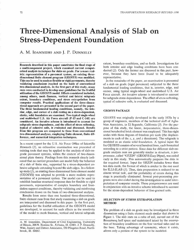
TRANSPOR'ÎATION RESEARCH RECORD I 196

Three-Dimensional Analysis of Slab onStress-Dependent Foundation

A. M. IoeNNrnns AND J. P. DoNNELLY

Research described in this paper constitutes the final stage ofa multicomponent project, which examined current comput-erized analysis techniques for slabs on grade. For a more real-istic representation of a pavement system, an existing three-dimensional finite element program (GEOSYS) was modified.This can be used to analyze flexible or rigid pavements, therebyvalidating conclusions reached on the basis of conventionaltwo-dimensional analysis. In the first part of this study, manyruns were conducted to develop user guidelines for the fruitfulutilization of the GEOSYS model. Effects considered included,among others, mesh fineness, vertical and lateral subgradeextent, boundary conditions, and stress extrapolation fromcomputer results. Practical applications of the three-dimen-sional approach are presented in the second part of the paper.The three fundamental loading conditions, namely, the inte'rior, edge, and corner ofa slab resting on a stress-dependent,elastic, solid foundation are examined. Two typical single-wheeland multiwheel U.S. Air Force aircraft (F-15 and C-l4l) areconsidered. An iterative scheme is introduced to account forsubgrade stress dependence, and the effect ofstress softening,typical of cohesive soils, is evaluated and discussed. Resultsfrom this program are compared to those from conventionaltwo-dimensional analyses, employing finite element, finite dif-ference, and numerical integration techniques.

In a recent report for the U.S, Air Force Office of ScientificResearch (/), an exhaustive examination was presented ofexisting tools that may be applied to the analysis of slab-on-grade pavement systems, within the context of two-dimen-sional plate theory. Findings from this research clearly indi-cated that no current procedure can model fully the behaviorof a slab of finite size, supported by a stress-dependent co-hesive subgrade extending beyond the slab edges. In a follow-up study (2), an existing three-dimensional finite element model(GEOSYS) was adapted to provide a more realistic repre-sentation of a pavement system. The model can be used toestablish baseline structural response data for flexible or rigidpavements, representative of complex boundary and foun-dation support conditions, thereby validating and reinforcingconclusions drawn on the basis of two-dimensional analysis.

Results from more than one hundred three-dimensional,finite element runs from that study examining a slab on gradeare interpreted and discussed in this paper. In the first part,guidelines for the fruitful utilization of the GEOSYS modelare developed, to account for such effects as the sensitivityof the model to mesh fineness, vertical and lateral subgrade

A. M. Ioannides, Department of Civil Engineering, Universityof Illinois, 208 N. Romine St., Urbana, Ill. 61801. J. P. Donnelly,rüiss, Janney and Elstner Associates, 330 Pfingsten Road, North-brook, Ill. 60062.

extent, boundary conditions, and so forth. Investigations forboth interior and edge loading conditions have been con-ducted (2). Only the former are discussed in this part, how-ever, because they have been found to be adequatelyrepresentative.

In the remainder of the paper, an examination is presentedof a slab on grade (rigid pavement) subjected to the threefundamental loading conditions, that is, interior, edge, andcorner, using typical single-wheel and multiwheel U.S. AirForce aircraft. An iterative scheme is introduced to accountfor subgrade stress dependence. The effect of stress softening,typical of cohesive soils, is evaluated and discussed.

GEOSYS PACKAGE

GEOSYS was originally developed in the early 1970s by a

group of engineers, members of the technical staff of Agba-bian Associates, in El Segundo, California (3). For the pur-pose of this study, the linear, isoparametric, three-dimen-sional hexahedral brick element was employed. This has eightnodes with three degrees of freedom per node (the displace-ments in each of the x,y, and z directions). The subgrade ismodeled as an elastic solid foundation. A typical input filefor GEOSYS consists of several hundred lines, each formattedaccording to a strict pattern. Since data for different slab-on-grade analysis runs are generally similar in structure, a pre-processor, called "GEZIN" (GEOSYS Easy lNput), was codedearly in this study. This automatically prepares the data inthe required format. Input for GEZIN includes fewer thanten data cards, the format of which is similar to the one usedfor ILLI-SLAB (1). Thus, data preparation is reduced to analmost trivial task, and the probability of errors during thisstage is practically eliminated. Several post-processing pro-grams were also coded during this investigation to assist inter-pretation of computer results. These postprocessors are usedin conjunction with an iterative scheme introduced to accountfor the stress-dependent behavior of fine-grained soils.

SELECTION OF STRESS EXTRAPOLATIONMETHOD

The problem of a slab on grade may be investigated in threedimensions using a finite element mesh similar that shown inFigure 1. The slab rests on a cube of soil, carved out of theBoussinesq half space and maintained intact by the assump-tion of boundary conditions on the four vertical sides and onthe base. Taking advantage of symmetry, where it exists,allows only a portion of the system to be modeled.

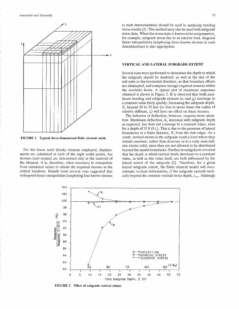
Ioannides und Donnelly

FIGURE I Typical threc-dimensional finite element mesh.

For the linear solid (brick) element employed, displace-ments are calculated at each of the eight nodal points, butstresses (and strains) are determined only at the centroid ofthe element. It is, therefore, often necessary to extrapolatefrom calculated values to obtain the required stresses at thecritical locations. Results frorn several runs suggested thatorthogonal linear extrapolation (employing four known stresses

73

in each determination) should be used in analyzing bendingstress results (2). This method may also be used with subgradestress data. IVhen the stress state is known to be axisymmetric,for example, subgrade stress due to an interior load, diagonallinear extrapolation (employing three known stresses in eachdetermination) is also appropriate.

VERTICAL AND LATERAL SUBGRADE EXTENT

Several runs were performed to determine the depth to whichthe subgrade should be modeled, as well as the size of thesoil cube in the horizontal direction, so that boundary effectsare eliminated, and computer storage required remains withinthe available limits. A typical plot of maximum responsesobtained is shown in Figure 2. It is observed that both max-imum bending and subgrade stresses (o, and q,) converge toa constant value fairly quickly. Increasing the subgrade depth,Z, beyond 20 to 25 feet (or five to seven times the radius ofrelative stiffness, /,) will have no effect on these stresses.

The behavior of deflection, however, requires more atten-tion. Maximum deflection, ô,, increases with subgrade depthas expected, but does not converge to a constant value, evenfor a depth of35 ft (9 /"). This is due to the presence oflateralboundaries at a finite distance, X, from the slab edges. As a

result, vertical strains in the subgrade reach a level where theyremain constant, rather than decrease as in a truly semi-infi-nite elastic solid, since they are not allowed to be distributedbeyond the model boundaries. Further investigations revealedthat the depth at which vertical strain decreases to a constantvalue, as well as this value itself, are both influenced by thelateral extent of the subgrade (2). Therefore, for a givenlateral subgrade extent, the finite element model will over-estimate vertical deformation, if the subgrade extends verti-cally beyond the constant vertical strain depth, 2",". Although

I

30I

35

z (fr)

I

40

È{

104

r02

100

96

9{

92

90

88

õnN0)qcIo

(ts

oqgoCIØoÉ.

86

84

82

80I

0

I

5

I

10

I

l5I

55I

50I

45I

25I

20

Totol Subgrode Deplh,

FIGURE 2 Effect ofsubgrade vertical extent.

À\ rQi_.{_\À_____

'\-toi ------ø-""-ø"-

ø"

O.-.OOEFLECTIONtr-.-gEENOING STRESSE-{ SUEGRRI]E STRESS

t..o ps(Z/tel

74

this is influenced by the lateral extent of the subgrade, a

subgrade depth of about 40 ft (10 /") may be used as a typicalvalue. A lateral extent between 25 and 35 ft (or 7-9 I") is

recommended.

BOUNDARY CONDITIONS

In order to examine the behavior of the two main types oflateral boundaries (i.e., free or on rollers), deflection basinsfrom four runs are compared in Figure 3. These confirm thatthe system response is more sensitive to the boundary con-ditions used when the lateral boundaries are closer to theload. Furthermore, maximum cleflection, ô,, was once againaffected much more significantly than the other two maximumresponses, o¡and q, (2). Based on these results, neither bound-ary condition appears to have an advantage over the other.Consideration of radial strains in the surface subgrade layer,however, led to the adoption ofroller-type lateral boundaries.The bottom boundary is also assumed to be on rollers, so thatelements can move laterally and distribute their load bydeforming.

VERTICAL DIVISION OF SLAB AND SUBGRADE

Results indicated that although there is a slight improvementin accuracy as the number of layers used in modeling thepavement slab increases, adequately reliable maximumresponses can be determined even using only two slab layers(2).

Additional analyses lecl to the following conclusions withrespect to the subgrade. The soil cube may be divided intothree portions in the vertical direction. The upper portionshould extend from 0 to 4 feet (0 to 1 /") and should co¡rsistof layers not more than 1 to 2 feet thick (0.25 to 0.5 /.). The

0.5

0

-0. 5

-t

-1. 5

-2

-2. S

-3

TRANSPORTATION RESEARCH RECORD I 196

middle portion should extend from 4 to 15 feet (1 to 4 /") orhalf the constant vertical strain depth, 2""", if known, andshould be divided into at least two layers. Finally, the lowerportion should cover the remainder of the soil cube and maybe divided into one or more layers.

HORIZONTAL SLAB AND SUBGRADE MESHFINENESS AND ELEMENT ASPECT RATIO

Three series of GEOSYS runs were conducted to examinethe influence of horizontal slab mesh fineness on the responseof the three-dimensional slab on grade. The trends observedin Figure 4 are similar to those noted in earlier two-dimen-sional finite element studies (1, 4), inasmuch as all three max-imum responses converge from below. Deflection and subgradestress appear to be less sensitive to horizontal mesh fineness,and adequate accuracy may be expected as the mesh finenessratio (2alh) of the (short) side length of the finite element(plan view) to the slab thickness approaches the value of 0.8.This is similar to the value determined from the two-dimen-sional studies. Bending stress appears to be more sensitiveto this effect, requiring values of (2alh) less than 0.8 forconvergence.

It was also found that the solution generally deterioratesas the maximum slab element aspect ratio, cn,"", increases.This is defined as the ratio of the element's long side, 2å, toits short side,2a (in plan view). The impact of this factor is

limited if cr.n* is kept below 4.The overriding importance of mesh fineness was first iden-

tified and quantified in previous University of Illinois studies,using two-dimensional models (I , 4).A major conclusionreached was that a more stringent mesh fineness criterion is

required under the loaded area than elsewhere in the finiteelement mesh (5). This counterbalances the approximationinvolved in discretizing applied distributed loads. A corollary

3E

c.oogq)o

rR-_l---------+

'þ". "'2t 'i i .''./ /'

¡''r'.kt,''í'i'nif È''

.i' ,rr'/ ,i tnz-srob Edoe

./,'f dt.',/,,/ú Type ond Distonce of Boundories From Lood

O...OROLLER EOUNOßßIES RT 15 FT.

.d' i::ãütJß0Hä3fl3ÄF?'!"T"5.'¡ o'.O--.'FREE BOUNOßR¡ES RT 3?.5 FT.

I

0

I

5

I

t0I

t5I

25I

30I

35I

20

oistonce From Lood (ft)

FIGURE 3 Effect of boundary conditions on subgrade surface deflection profile.

I

40

=ø-êc 5000t¡l

ø! noooî,o=* 3000cÊû& 2000

I 000

0 I 2 3 4 5 6 ? I I t0 u t2Deviotor Slress, øp (psi)

FIGURE 4 Effect of horizontal slab mesh fineness (interior loading).

TABLE 1 INVESTIGATION OF INTERIOR LOADING: F-ls swl-

SOLUTION61 qi ot

miLstpsitpsl

GEOSYS-3D (Cycle 1)

ILLI - SI^A,B- 2D

CLOSED-FORì,I

32.L5

37 .26

35.92

104

100

s.031 L04 609.55 96

s.099 106 697.L8 110

4.832 L00 636 .63 1-00

Notes:

E - 4x106 psi p-0.L5 h-BÍn.Es - 7682 psi ('SOFT') ps - 0.45 te - 33.10 in.

Slabr L5 ft x l-5 f.t (L/le - 5.44)Load: 30 kips @ 355 psÍ, converted co 4 work equivalent loads

(c - 9.193 tn.)

-GEOSYS Mesh (Double symmetry - slab exËends becween underlinedcoordinates) :

x-coordinates: 0; 30; 35; 36.5; 38;39;40;4L 4L75;42.5 f.cy-coordinates: 42.5; 12.5; 7.5; 6; 4.5; 3.5; 2.5; 1.5; 0.75; 0 ftz-coordlnates:0.6;0.3;0; -0.5; -1.0; -2.5; -6.5; -17.5; -40 fr

In slab: (2alh)r1r,-1 .L25; y-2.0; ar"*:2.0; (c/2a)-0.5LL.

-411 responses are at interÍor of sl_ab, under load:61 : at top of sLab;ql : at surface of subgrade, by dÍagonal excrapolation;ol i at boctorn of slab, by orthogonaL extrapolacion of ox

values.

-ILLI-SIAB-2D: (2a/h) - 0.75; square elements.CLOSED-FORM: Equations by Losberg (l-3), for infinire slab.

2 l3l4l 5l617l8

76

of this, which has seriòus implications with respect to recentefforts to model non-uniform pressure distributions (6, 7),may be stated as follows: in view of the conversion of externaldistributed loads into nodal components (which inevitablyleads to at least some approximation, especially in the case

of partially loaded elements), refinement of the applied pres-

sure distribution, for the purpose of simulating observed

deviations from simplistic uniformity, without due consider-ation and reciprocal improvement of mesh fineness, willbe self-defeating, leading only to an illusion of improvedaccuracy.

Based on additional results obtained (2), it is recommendedthat the lateral extent of the subgrade beyond the slab edges,

X, be divided into two elements, one 4 feet in size near theslab (1 /.) and another 26 feet for the remainder (7 /").

PRACTICAL APPLICATIONS

In the analyses presented in the remainder of this paper, thefollowing two fundamental questions are addressed:

1.. How do three-dimensional analysis results compare withthose from two-dimensional programs, such as ILLI-SLAB(1, 4), FIDIES (8), H51ES (9, /), CFES (5), and others? Acorollary to this is whether three-dimensional finite elementanalysis is necessary, and what the implications of its results

are on the routine application of two-dimensional models.

2. How important is the effect of introducing stress-dependent resilient subgrade behavior? This effect was foundearlier to depend on the placement and severity of the appliedloads, using the two-dimensional resilient subgrade inrLLr-sLAB (10).

Simplified versions of the curves of subgrade resilient mod-ulus, E^, versus repeated deviator stress, o¿r, developed by

I

0

I

100

TRANSPORTATION RESEAIICI I RECO RD I 196

Thompson and Robnett (11), are incorporated into the three-dirnensional GEOSYS analysis to account for subgrade stress

dependence. This is achieved through an iterative procedureimplemented by a postprocessor, a program that receives as

input results from GEOSYS. This iterative procedure is sim-ilar to that used for two-dimensional ILLI-SLAB analysis (12,

10). The modified Eo versus op relation for the "soft" subgrade

as employed in this study is shown in Figure 5. The deviatorstress was defined in this case as the maximum differencebetween the three principal stresses determined by GEOSYS.Based on the o¿ level, the subgrade elements are classified

into seven groups, and an average Eo is assigned to each.

FINITE ELEMENT MODEL FOR SINGLE.WHEELINTERIOR LOADING

In a previous study, it was shown that subgrade stress depend-ence is not important when slab-on-grade pavetnents are loaded

by a single tire print at the interior (/0). To magnify any

subgrade stress dependence effects, this study considered a

relatively high load on a thin slab (8 inches thick), resting onthe "soft" subgrade. The load applied at the interiol is an F-

1.5 single-wheel load (SWL) of 30 kips at 355 psi. Other per-tinent information for this case is given in Table 1. This tablealso presents the maximum responses from GEOSYS, ILLI-SLAB, and the closed-form solutions (13). In view of sym-

metry, only one-quartel of the system needs to be modeled.

Effect of Subgrade Stress Dependence

A good indicator of the effect of subgrade stress dependence

is the number of elements exceeding the 2 psi limit in or,below which constant modulus behavior is assumed. For thisGEOSYS run, only 5 out of 54 subgrade elements (or 9 per-

I

200I

250I

300

110

II ,rì

l¡9l,tctl -o lcot¡l l<(.DlJ

lutI'li

80

60d

O...O OEFLECT I ONg-.€BENOING STRESSÀ-{ SUEGRROE STREsS

r.9 t.t Og (20lh)I

50

I

150

Number of Elements in One Full-Slob Loyer (NUMEL)

FIGURE 5 Simplified E vs. o¿ retation for "soft" subgrade as used in GEOSYS.

Ioannides and Donnelly

cent) had a oD above 2 psi. The range of oD values in theseelements was 2.059 to2,270 psi, with an average of 2.135 psi.The five overstressed elements (which in a subsequent iter-ation would change subgrade group) were located in the upper2.5 f.eet of the subgrade, underneath the applied load. Theupdated Eo value for these would be 7,533 psi, a decrease ofless than 2 percent from the initial7,682 psi assurned for theconstant, low-stress foundation modulus. It is evident thatadditional runs would not be very useful, since such a smallchange cannot be expected to affect the system significantly.

Comparison with Two-Dimensional Results

In Table 1., maximum interior deflection, subgrade and bend-ing stress (ô¡, Q,, o,) from the three-dimensional GEOSYS runare compared to those from a similar two-dimensional ILLI-SLAB run. Values predicted by the closed-form solutions (/3)are also tabulated. The ILLI-SLAB run employed a ratherfine mesh. One-quarter of the slab was divided into225 squareelements, compared to only 49 elements used in the GEOSYSmodel. According to the results of extensive investigationsusing ILLI-SLAB (1, 4), such a fine mesh is necessary forresults of adequate accuracy. The coarseness of the GEOSYSmesh is considered to be the prime source of the discrepancybetween the finite element results and the closed-form solu-tions. The investigations conducted in the first part of thisstudy indicate that only about 5 percent of this discrepancymay be attributed to an overall mesh fineness effect. Theremainder is probably due to the fact that the mesh near theload needs to be even finer than elsewhere. In the mesh used,the load only partially covered the central element; this leaclsto some loss of accuracy when the applied load is convertedto four work equivalent nodal loads.

The necessity for a¡t even finer mesh under the load thanelsewhere was confirmed in a previous study (5). This addi-tional ¡nesh fineness requirement over the area of appliedload can also explain the high ILLI-SLAB results. All threeresponses may be expected to converge from above as thetire-print is subdivided into more elements. This assertion isreinforced by preliminary results obtained using the CRAYX-MP|Z supercomputer (14). Both GEOSYS and ILLI-SLABresults are also affected by the finite size of the slab in theseanalyses (compared to the infinite slab assumed in the closed-form solutions). This factor may partially explain why ILLI-SLAB ôi and qi are higher than the corresponding closed-formsolutions, since these responses converge from above as slabsize increases (4, 5, B). Bending stress, howevel', convergesfrom below, so the relatively high o, obtained by ILLI-SLABcannot be attributed to the slab size factor. The primary sourceof this discrepancy, therefore, is the mesh fineness effect relatedto the size of the loaded area.

EDGE LOAD CASE

In this investigation, an F-15 SWL is applied to a relativelythin slab on a weak subgrade. The same slab-and-subgradesystem used for interior loading is retained here for co¡npar-ison. The pertinent characteristics of this system have beenpresented in Table 1. The finite element mesh was modifiedappropriately, accorcling to the recommendations formulated

77

in the first part of this investigation. Bending stresses devel-oping in such a slab would be excessive in practice and areonly considered here so that the effect of subgrade stressdependence is magnified.

Convergence Criteria

The iterative scheme introduced above may be used to accountfor the stress-dependent behavior of the subgrade. Figure 6shows maximum responses for each of five cycles performedfor the single-wheel edge loading case, normalized with respectto the corresponding average values from the second and thirditerations. A uniform E, of 7,682 psi is assumed in the firstiteration, and its results correspond to those from a conven-tional linear elastic analysis. It is observed that the maximumresponses oscillate about a value to which, presumably, theywould eventually converge, if enough cycles were conducted.The amplitude of oscillation becomes progressively smalleras more cycles are perforrned.

The oscillation between maximum responses from the fourthand fifth iterations is only of the order -r2 percent. Thisindicates that for most practical purposes, five cycles are morethan adequate to achieve convergence. Furthermore, theaverage of the values of maximum responses obtained fromthe second and third iterations consistently give an estimatewithin -+2 percent of the projected converged values. It is,therefore, recommended that three iterations be performedand that the average of the responses from the second andthircl cycles be adopted.

Effect of Subgrade Stress Depenelence

A direct way to evaluate the effect of subgrade stress depend-ence for the F-i5 SWL at the slab edge is to compare themaximum responses from the first iteration (which correspondto those from a conventional linear elastic analysis using auniform, low o, soil modulus) to the average of those from

FIGURE 6 Maxinum responses normalized w¡th respect toaverage of second and third iterations.

Ifo

INat,c.9oq)

=ot,

(l)ancoCI¡1,(,É,io=

Q)anÉocto(l,É.i0=

\'\

V

78

the second and third iterations. Such a comparison shows inthis case that maximum deflection and bending stress increase

by 10 percent and 8 percent, respectively. This change is

comparable to that observed with the two-dimensional Komodel in ILLI-SLAB (10, 12). On the other hand, maximumsubgrade stress appears to be much more sensitive to stress

dependence, decreasing by about 23 percent. It will be shownbelow that this is largely due to the development of highsubgrade stress concentrations near the loaded edge. Subse-quent iterations redistribute these stresses, thereby modelinglocal yielding, which would occur in a real soil subjected tothese high stresses.

Results from this study indicate that the overall behaviorof the slab is quite similar for the constant modulus ancl the

stress-dependent subgrades. Furthermore, the differences inbehavior that do exist, occur in and around the location ofthe subgrade elements with decreased resilient moduli. Onlyabout 8 percent of all the subgrade elements experience a

decrease in Eo. These elements are located in the upper 6.5

feet of the subgrade. Additional bending stress and deflectionaccumulate in elements in and under the slab as more itera-tions are performed, due to the decrease in subgrade support.The surface deflection basin observed after five iterationsis, therefore, deeper than the one obtained after the firstiteration.

A different phenomenon is observed beyond the slab, inthe subgrade adjacent to the loaded edge. There, the cycle 5profile is generally shallower than the cycle 1 profile. In addi-tion, deflection of the stress-dependent subgrade (cycle 5) isreduced to 50 percent of the maximt¡m value within only 6inches from the loaded slab edge. The structural contributionof the subgrade beyond the slab is less significant for the stress-

dependent model than for the constant modulus subgrade.Therefore, it can be seen that stress dependence tends to move

the elastic solid model toward the direction of the dense liquididealization, in which the contribution of the subgrade adja-cent to the slab edges is altogether neglected.

Comparison with Two-Dimensional Results

Results obtained using GEOSYS may be compared to those

from a number of two-dimensional models available, in orderto establish the relative adequacy of the two approaches. Inthis section, results from programs FIDIES (8), H51ES (1,

9), and ILLI-SLAB ({ will be considered. FIDIES is a two-dimensional finite difference solution, employing square ele-

ments throughout the slab. The external loads are convertedto point loads, applied at the center of each element. Responses

are calculated at these points alone. Thus, an extrapolation,similar to that used with GEOSYS results, is necessary toobtain the edge responses. H5lES may only be used to cal-

culate maximum bending stress at the edge, but its results are

akin to a closed-form solution. Thus, they are not a functionof user-specified parameters, such as mesh fineness, a¡rd ele-

ment aspect ratio. These considerations can be crucial in thecase of programs such as FIDIES and ILL,I-SLAB. On the

other hand, the latter two programs can account for the finitesize of the slab and can determine the sparial distribution ofall three responses, rather than just the maximum value ofone of them.

Table 2 presents results obtained using these prograrns. The

TRANSPORTATION RESEARCH RECORD ] 196

grid employed in the FIDIES run consisted of 441 squareelements (no symmetry capability exists in FIDIES at thistime). Previous studies (1, 8, 15) suggest that this grid may

be slightly coarse, but it is dictated by computer memorylimitations. In any case, the approximation involved in rep-resenting the applied load as a point load, located a few inchesfrom the edge, is the overriding consideration here. Unfor-tunately, this approximation cannot be avoided. The ILLI-SLAB run was conducted using a mesh found to produceresults of adequate accuracy (15). The other results are nor-malized in Table 2 with respect to the ILLI-SLAB responses.

The value of o" from ILLI-SLAB is about 11 percent higherthan the closed-form solution from H51ES. This discrepancy

cannot be explained by reference either to an inadequate mesh

fineness or to the small slab size, since increasing these param-eters would tend to increase the ILLI-SLAB value of o". Asimilar discrepancy was observed with the dense liquid foun-dation as well, and was related to the size of the loaded area'For the (c//") value of 0.28 used, the discrepancy was 10 per-cent (1), which is close to that observed here. Prelirninaryresults using the CRAY X-MP|24 (/4) indicate that this dis-

crepancy disappears when the mesh under the loaded area is

refined further.On the other hand, FIDIES values of õ" and o, are higher

than the corresponding ILLI-SLAB ones, while q" is lower.Again, overall gt'id fineness and slab size considerations can-

not explain the discrepancy observed. It is considered thatthe rnajor sources of this are the conversion of the externalload to a point load acting at the center of an edge eletnent,and the extrapolation involved in obtaining the values in Table2 from the FIDIES output.

In Table 2, GEOSYS results from the first cycle are alsopresented. Comparison with those from ILLI-SLAB suggests

that three-dimensional analysis gives q" and o" values that are

lower than those from ILLI-SLAB by about 60 percent and

30 percent, respectively. Maximum edge deflections are inrelatively better agreement, the ILLI-SLAB value being only9 percent higher than the corresponding one from GEOSYS'Part ofthese discrepancies (5 to 10 percent) may be attributedto the coarse mesh used with GEOSYS. The rernainder ofthe discrepancy is probably due to the fact that both GEOSYSou and q" are extrapolated from calculated values at the cen-

troid of each brick element. This is particularly important inthe case of subgrade stresses. The contour plot of subgradestresses in Figure 7 indicates that high subgrade stl'esses occurin a narrow zone along the loaded edge. Such a drastic increase

in subgrade stress right at the edge of the slab has also been

observed under interior loading (5), and is similar in natureto the infinite reactions predicted by Boussinesq's theory at

the edge of a rigid punch. The linear extrapolation used todetermine q" from GEOSYS results is unable to reproducethe high stress gradients in this area.

In the narrow region immediately adjacent to the loadecledge, local yielding of the soil will occur. Thus, the theoreticalvalue of the subgrade stress at the physical edge of the slabmay not be of practical significance. A more meaningful valuemay be the subgrade stress developed a few inches inside fromthe edge, for example, at a distance of.0.21". A previous studyshowed that this value is relatively insensitive to mesh fineness(5). Additional iterations have the effect of redistributing thestress away from highly stressed elements. Thus, introducingsubgrade stress dependence enables the user to model local

TABLE 2 COMPARISON OF TWO- AND THREE-DIMENSIONAL SOLUTIONS: F-15EDGE SWL

SOLUTION

mils psi

oe9e6e

Psf

GEosYs-3D (cycle 1)

FIDIES-2D (Linear extrap. )

FIDIES-2D (Quadr. extrap. )

H51ES

ILLI -sl"A,B-2D (23xi.3 Mesh)

60.32 91

73.2L il.1

73.6L L11

66.09 100

24.63 42

30.93 s3

3s.36 60

58.84 1"00

826.0 70

1 s18. L L29

L60s. I 136

1055.9 89

1180.8 100

Notes:

-For slab and subgrade charaeteristlcs, see Table 1,

-GEOSYS Mesh (Syrnnetry about x-axls employed - slab extendsbetv¡een underllned coordínates) :

x-coordinates: 0; 18.5; 37; 4L; 45; 47; 48; 49; 49.5; 50; 50.9375;51.875; 53.750; 55.625; 57.5; 6O; 62.5; 65; 95 tt

y-coordlnates: 42.5; L2.5; 7.5; 5.625; 3.75; 1.875; 0 frz-coordinates: Lá; 0.3; 0; -0.5; -L.0; -2.5; -6.7; -L9.27; -40 ft.In slab: (2aþ)¡¡yn-2.8L; y-2.0; amax-2.0; (c/2a)-0.20.

FIDIES mesh: (Â/h) - 1.07; 2].x2]- square elements;ILLI-SLAB nesh (symmetry abour x-axls ernployed):

(23x13) : (2alh)r1rr-0.575; X-3.0; cr"*-2.18;H51ES: 50 points used co deflne ourline of applied load.

-A1L responses at intersectlon of loaded edge and centerline of load:6" : at top of slab;gs : at surface of subgrade, by orthogonal extrapolation;oe i at botcom of slab, by orthogonal extrapolation

of o.,, values.FIDIES resülts extrapolated uslng 2 (llnear) or 3 (qüadratic)eLemencs along the slab centerline;No extrapolatlon fs lnvolved in ILLI-SI,AB and H51ES resuLrs.

Conlour lntorvol: lps¡

,,\.1. ',ltii..

FIGURE 7 Surface subgrâde stress contours from GEOSYS under slab: constant modulus subgrade (cycle l).

80

yielding that would occur in a real subgrade. Notwithstandingthe differences in their maximum responses, ILLI-SLAB andGEOSYS produce similar response distributions outside thecritical edge region. The plots in Figure 8 reinforce the validityof the comments made above.

Similar conclusions were also reached from an investigationof multiwheel edge loading (MWL), using one landing gear

from a C-1.41 aircraft. The effect of accounting for subgradestress dependence is quite significant in this case. Maximumdeflection increases by about 30 percent, and maximum bend-ing stress by more than 20 percent. On the other hand, max-imum subgrade stress decreases by more than 30 percent.Furthermore, the extent of the region of reduced resilientmoduli obtained with the C-141 load is much larger comparedto the F-15 case. The subgrade stress distributions in Figure9 indicate that comparing only the maximum q" values fromthe two- and three-dimensional models may be misleading.The overall system responses are much closer to each other

TRANSPORTATION RESEARCH RECORD 1 196

maximum values would suggest. This isfine meshes are used.

than the individualespecially true when

CORNER LOAD CASE

To complete the series of three-dimensional investigationsusing GEOSYS, the corner loading condition is examined inthis section, with an F-15 single-wheel load. Unfortunately,the lack of symmetry along either of the two major coordinateaxes of the slab dictates the use of a full mesh in the finiteelement idealization. This results in prolonged execution times(in excess of 12 CPU hours on the HARRIS 800-2 virtualmemory computer), even using a rather coarse mesh, whichgives rise to less accurate results. General trends, however,may still be observed and these can be useful despite anylimitations in the accuracy of individual response values.

tvr>A

a----

I rao ¡n. I

FIGURE 8 Comparison of GEOSYS and ILLI-SLAB surface subgrade stress distributiorrs

for F-15 edge SWL' under slab.

,õCI

(tatoq)

t(noÌtoolr

..cl:ta

=ano.cr

anat,oØt¡,Í,c,

olll¡ãa

y ( in.)

(23x 13 Mesh, ol x = O in.)

Section A-A

x ( in.)

.ILLI-SLAB(23x l5 Mesh, ot y : g ¡n.¡

+ GEOSYS(Cycle l, ot Y : ¡ ¡.25 'n.t

Ioannides and Donnelly

Effect of Subgrade Stress Dependence

Table 3 presents a summary of maximum responses obtainedform three iterations perforrned for this case. Maximumdeflection, ô", and subgrade stress, qc, occur at the corner ofthe slab. On the other hand, maximum (tensile) bending stress,oc, occurs at the top of the slab, some distance from thecorner. Preliminary results using ILLI-SLAB (15) suggest thata slab resting on an elastic solid also develops a high tensilebending stress at the bottorn fiber under the load. This cannotbe confirmed at this time using GEOSYS, however, since amuch finer mesh would be required.

Subsequent iterations in Table 3lead to a maximum deflec-tion that is almost 20 percent higher than the value obtainedfrom cycle 1. Similarly, an increase of more than i0 percentis observed in the maximum bending stress developing in theslab. On the other hand, a dramatic decrease in the value ofthe maximum subgrade stress predicted by the first iterationis obtained as subgrade stress dependence is considered. This

rll

lYrÞA

Ø

Ø

I rao in. I

FIGURE 9 Comparison of GBOSYS and ILLI-SLAB surface subgrade stress distributionsfor C-l4l edge MWL, under slab.

'õêcral,.1,r¡t

anoÌ,oct-ô=Ø

reflects the redistribution of high subgrade stresses concen-trated at the slab edges, observed earlier. Local yielding ofsoil in the corner region prevents these high stresses fromdeveloping, and this is accounted for by the iterative proce-dure used with GEOSYS. The maximum subgrade stressoccurring at the slab corner itself, therefore, may not be ameaningful response. The subgrade stress developing underthe center of the load, q"*, for example, may be a morerealistic indication of subgrade response. This will be sub-stantially lower than the value at the corner and, therefore,less sensitive to stress dependence. The oscillation of q.x inTable 3 is of smaller amplitude than that of q. itself.

It is interesting to observe that about 20 percent of thesubgrade elements are affected by stress dependence, com-pared to only 8 percent for the F-15 edge load. Subgradestress dependence is predictably a more serious considerationunder corner than under edge loacling. The high values of oDare limited to the upper 5.5 feet of the subgrade, below whicho, is less than 2 psi.

y ( in.)

2oCI

(t6a^

,(l,

Øl¡,Ì,ctorrt¡ã(n

ILLI-SLAB(22 x l2 Mesh, ot x:8 in.)

,¿.t'

--J"É+a_?'_t

Loeosvs --(Ref ¡ned Mesh, ot x = 3 ¡n.)

ILLI-SLAB(22xl2Mesh,olx=0in.)

x ( in.)

. ILLI-SLAB(22x12 Mesh, ol Y=9 st6 y= I ¡n.)

+ GEOSYS(Ref ined Mesh, ot y: I in.)

82 TRANSPORTATION RESEARCH RECORD I ]96

TABLE 3 EFFECT OF SUBGRADE STRESS DEPENDENCE: F-15 CORNER SwL

ITERATIONpsl ps1

oc9c9c6c

mils psi

1

2

3

Avg. 2-3

72.42 100

87.67 L2L

82.99 lls

85.33 1l_B

42.93 L00

28.L6 66

22.16 52

25.2L

3r.27 100 3L2.L 100

19.95 64 358. s LLs

L9.86 64 343. I lLo

19.81 64 3s0.8 LLz

Notes:

¡ = 4x106 psi pEs : 7682 psi ('SOFT') ps

Slab: 15 fc x L5 ft (L/0e) - 3.63Load: 30 kips @ 355 psi, converted

Comparison with Two-Dimensional Results

In view of the relatively coarse mesh employed in the GEO-SYS runs, considerable discrepancies exist between three- andtwo-dimensional responses. GEOSYS gives a õ" which is about10 percent lower than the one predicted by ILLI-SLAB usinga fine mesh, Differences in o" and qc are even higher (+10percent and -70 percent, respectively). According to thecriteria developed above, GEOSYS results may be expectedto be too low by less than 5 percent. Possible causes of theremainder of the gap between the two- and three-dimensionalresults were identified above as the coarseness of the GEO-SYS mesh in the area of the load and the extrapolation involvedin obtaining maximum stress values from the GEOSYS out-put. The latter is more important in the case of subgradestress, in view of the high stress gradients existing near loadedslab edges and corners.

Figure 10 shows the distribution of subgrade stresses pre-dicted by ILLI-SLAB and GEOSYS. These confirm that the

: 0.1-5 h - L2 in.: 0.45 Le - 49.64 in.

to four work equivalent loads

two models are in good agreement, except in a region about8 inches wide (or 0.2 l") along the slab edges. Pronouncedsubgrade stress gradients develop very close to the edges ofthe slab under all three fundamental loading conditions.

DISCUSSION AND CONCLUSIONS

Three-dimensional finite element analysis is shown in thispaper to be a feasible and viable tool in pavemerìt studies.Although this sophisticated numerical technique is unlikelyto become a routine procedure in the near future, resultspresented herein indicate that it is possible to use a three-dimensional model to account for subgrade stress depend-ence, soil yielding, among other factors, as well as to accom-modate rnultiwheel gears situated anywhere on the pavementsurface. The GEOSYS model described is currently the onlyprogram that can be employed for analyzing both rigid andflexible pavements. Thus, it will be indispensable in future

(c : 9.193 in.)

-Mesh (Slab extends betrveen underlÍned coordinates):x-coordinates : 0; 27.5; 29.167; 30; 30.833; 32.5; 35; 40; 45;

60 fty-coordinares : 60; 45; 40; 35; 32.5; 30.833; 30; 29.L67; 27.5;

0frz-coordinaces:1; 0.5; 0; -0.5; -1; -2.5; -6.5; -L7.5;40 ft

In slab: (2alh)*1r.,-0.833; þ1 .0; c*"*-6 .O; (c/2a)-O .92.

-LocaËion and method of excrapolatlon of responses:6" : ac slab corner, ât top of the slab;o. : tension at tsop of slab, at some distance frorn corner:

oc: oL, from values of oy, oyt rayt excrapolated co the cop'uslng linear orthogonal extrapblatibn;

qc : compresslve, at surface of subgrade under corner of slab:extrapolated up to surface of subgrade from values under

. corner reglon of slab, uslng linear orthogonal extrapolation.q.* : cornpressive, at surface of subgrade, aË x-5 in', y-5 in. from

corner, under slab, extrapolated llke q".

Ioannides and Donnelly83

Horizonlol Dislonce, x (in.)

80 90

ILLI-SLAB(l2xlzl r y=9.2in.GEOSYSY:5in'

r30 r40

ILLI-SLAB(l2x12), y: Oin.

=ttÕ.

(t

atatt(¡)L

C,(l,:ctooll-o:tU)

---Y = 9.2 in.

-;-y=5.Oirì. +xLY=0in.

F'IGURB l0 Comparison of GDOSYS and ILLI-SLAB surface subgrade stress disrnourions torF-15 corner SWL, under slab.

efforts to establish the elusive "unified" approach and to developa generalized mechanistic design procedure.

A most significant conclusion reached, however, is that thethree-dimensional investigations reinforce the validity anddesirability of conventional two-dimensional analysis. In viewof the relatively limited amount of three-dimensional resultsgenerated during this investigation, the accuracy ofthese r.esultswas often assessed by reference to the corresponding two-dimensional values. Where these disagreed, probable causeswere considered and were usually found to be due to thecoarse three-dimensional mesh used in these analyses.

This is not to deny the desirability of three-dimensionalanalysis as a means of checking and validating two-dimen-sional results. It does suggest, however, that for a meaningfulutilization of the much more complex and demanding three-dimensional approach, adequate computer resources must beavailable. The rapid advances of computer technology in gen-eral, and the introduction of supercomputers in particular,provide reasons for optimism in this respect. Results fromthis study will be invaluable when considering the implemen-tation of such a model on the mammoth machines anticipatedin the near future.

From a more practical viewpoint, this study has shown thatsubgrade stress dependence may sometimes be important,primarily when considering heavy edge and corner loads.Subgrade stress dependence affects the maximum subgradestl'ess to a much greater extent than the maximum deflection

or bending stress. When the load becomes more severe, forexample, when it is placed near a corner rather than near anedge, the difference between the first and last iterations becomesmuch greater. These conclusions are similar to those reachedusing the two-dimensional Ko model (10, 12).

ACKNOWLEDGMENTS

The investigations for this paper were supported by a grantfrom the U.S. Air Force Office of Scientific Research, AirForce Systems Command, Bolling Air Force Base, Washing-ton, D.C. The project manager was Lt. Col. L. D. Hokanson.M. R. Thompson and E. J. Barenberg were the project super-visors. Their advice and comments on the manuscript aregreatly appreciated. The authors also acknowledge the coop-eration of M. W. Salmon, formerly a graduate research assist-ant at the University of Illinois.

REFERENCES

1. A. M. Ioannides. Analysis of Slabs-On-Grade for a Varietyof Loading and Support Conditions. Report TR-85-00S3. U.S.Air Force Office of Scientific Research, Air Force SystemsCommand, USAF, Bolling AFB, Washington, D.C.; Sept.1984.

2. A. M. Ioannides, J. P. Donnelly, M. R. Thompson, ancl E.

84

J. Barenberg. Three-Dimensional Finite Element Analysis ofa Slab on Stress Dependent Elaslic Solid Foundatlon. ReportTR-86-0143. U.S. Air Force Office of Scientific Research,Air Force Systems Command, USAF, Bolling AFB, Wash-ington, D.C., Oct. 1986.

3. Analytic Modeling of Rock-Stucture Interaction, Volumes l-3. Reports AD-761-648,649,650, Advanced Research Proj-ects Agency of U.S. Department of Defense and U.S. Bureauof Mines, April 1973.

4. A. M. Ioannides, M. R. Thompson, and E. J. Barenberg.Finite Element Analysis of Slabs-on-Grade Using a Varietyof Support Models. Proc., 3rd International Conference onConcrete Pavement Design and Rehabilitation, Purdue Uni-versity, West Lafayette, Ind., April, 1985, pp.309-324.

5. A. M. Ioannides. Axisymmetric Slabs of Finite Extent onElastic Solid. Journal of Transportation Engineering, ASCE,Vol. 113, No. 3, May 1987, pp. n7-290.

6. K. M. Marshek, H. H. Chen, R. B. Connell, and C. L. Saraf.The Effect of Truck Tire Inflation Pressure and Axle Loadon Flexible and Rigid Pavement Performance. ln Transpor'tation Research Record 1070,TRB, National Resealch Coun-cil, Washington, D.C., 1986,pp. 14-21.

7. H. H. Chen, K. M. Marshek, and C. L. Saraf. The Effectsof Truck Tire Contact Pressure Distribution on the Desiglìof Flexible Pavements-A 3D Finite Element Approach.Presented at the 65th Annual Meeting of the TransportationResearch Board, Washington, D.C., Jan. 1986.

8. A. M. Ioannides, Finite Difference Solution for Plate onElastic Solid, Journal of Transporîation Engineering, ASCE,Vol. 114, No. I, Jan. 1988, pp. 57-75.

9. W. C. Kreger. Computerized Aircraft Ground FlotationAnalysis-Edge Loaded Rigid Pavement. Reseat'ch ReportERR-FW-572. General Dynamics Corp., Fort Worth, Tex.,Jan. 7967.

TRANSPORTATION RESEARCTI RECORD 1 196

10. A. M. Ioannides, E. J. Barenberg, and M. R. Thompson.Finite Eleme¡rt Model with Stress Dependent Support, InTransportation Research Record 954, ^lRB, National Research

Council, Washington, D.C., 1984, pp. 10-16'11. M. R. Thompson and Q. L. Robnett. Resilient Properties of

Subgrade Soils. Transpo rtation Engineering Journal, ASCE'Vol. 105, No. TEl, Jan.1979, pp. 71-89.

12. M. R. Thompson, A. M. Ioannides, E. J. Barenberg, and

J. A. Fischei. Development of a Stress Dependent FiniteElement Slab Model. Report No. TR-83-1061. U.S. Air Force

Office of Scientific Reseãrch, Air Force Systems Command'USAF, Bolling AFB, Washington, D.C., May 1983.

13. A. Losberg. Structurally Reinforced Concrete Pavemenls.

Doktorsavñandlingar Vid Chalmers Tekniska Högskola'Göteborg, Sweden, 1960.

14. A. M. Ioannides. Insights from the Use of Supercomputersin Analyzing Rigid andFlexible Pavements. Presented at 66thAnnuai Mõeting of the Transportation Research Board,Washington, D.C., Jan. 1987'

15. A. M. Ióannides. Recent Findings Using Advanced AnalysisMethods for Slabs-On-Grade. Presented at 65th AnnualMeeting of the Transportation Research Board, Washington,D.C., Jan. 1986.

The contents of this paper reflect the views of the authors, who are

responsible for the facts and lhe accuracy of the data presented

herein. Stalements made do not necessarily reflect the official views

or policies of the IJ.S. Air Force. This paper does not constilutea standard, specification, or regulation.

Publication of this paper sponsoretl by the Committee on Strength

and Deþrmation Characterislics of Pavement Seclions.

TRANSPORTATION RESEARCI{ RECORD 1 196 85

Verification of Backcalculation ofPavement ModuliS. W. Lnn, J. P. ManoNEy, AND N. C. JacxsoN

This paper introduces a backcalculation computer programwhich can be used to estimate the elastic modulus for eachpavement layer. This microcomputer program, EVERCALC,is based on the Chevron N-layer elastic analysis computer pro-gram anel was developed primarily for flexible pavement anal-ysis and falling rveight deflectometer (FIVD) data. The pro-gram is capable of estimating the elastic modulus for each layerof a pavement structure (up to a maximum of three layers)directly from surface deflection measurements. Further, thestress sensitivity coefficients for r¡nstabilized layers (both baseand subgrade) are estimated, as well as a "standard,t asphaltconcrete modulus analogous to a laboratory condition. Resultsfrom EVERCALC were verified in two ways. The first approachwas to compare theoretical and backcalculated moduli for arange of three layer pavements. These comparisons shorvedmodest differences âmong the moduli (about 87o for asphaltconcrete, 6lo lor base course, and less thanL%o for the subgradesoils). The second verification approach was to cornpare back-calculated and laboratory moduli based on FWD tests and fieldmaterial sampling, along with appropriate laboratory testing.In general, the differences in moduli are significantly less thanthe "natural" variation of these materials within a relativelyshort pavement segmenl. (Pavement segrnents rvere originallyselected for their apparent uniformity.)

The need to evaluate in situ pavement properties, such aslayer moduli, is readily apparent to pavement engineers. Theevolution of pavement structural characterization by use ofboth mechanistic analysis and nondestructive testing equip-ment, such as the falling weight deflectometer (FWD), hasresulted in new pavement analysis tools.

This paper introduces a backcalculation computer programwhich can be used to estimate the elastic modulus for eachpavement layer. This microcomputer program, EVERCALC,is based on the Chevron N-layer elastic analysis computerprogram. EVERCALC was developed primarily for flexiblepavement analysis and the FWD. The program is capable ofestimating the elastic rnodulus for each layer of a pavementstructure (up to a maximum of three layers) directly fromsurface deflection measurements. Further, the stress sensitiv-ity coefficients for unstabilized layers (both base and subgrade)are estimated, as well as a "standard" asphalt concrete mod-ulus analogous to a laboratory condition. Comparisons ofEVERCALC solutions to both theoretical and laboratoryconditions are shown in an attempt to verify the backcalcu-lation process. It is important to note that the backcalculation

S. W. Lee and J. P. Mahoney, University of Washington, l2lMore Hall, FX-10, Seattle, Wash. 98195. N. C. Jackson, Wash-ington State Department of Transportation, TransportationBuilding, Olympia, Wash. 98504.

results presented in this paper were obtained in a ,,produc-

tion" mode, i.e., the program was limited to a maximum ofthree iterations or alJVo cumulative error. (This will be morefully explained later.)

NONDESTRUCTIVE TESTING

Of the various nondestructive testing (NDT) devices avail-able, the FWD was chosen as the primary focus of the reportedwork. There are a nu¡nber of reasons for this. First, the FWDis the primary deflection measuring instrument used by theWashington State Department of Trarrsporration (WSDOT).Second, it can provide variable and large impulse loadings tothe pavement surface which to some degree simulate actualtruck traffic.

\Vith the FÏVD (Dynatest model 8000), a transient impulseload is applied through a set of rubber cushions, which resultsin a load pulse of 25 to 30 milliseconds. The pavement deflec-tions are measured at up to seven locations with velocitytransducers (1 ,2). As with any NDT device, the FWD has afew (but generally minor) drawbacks. For example, the depthto a "rigid layer" in a pavement rnay affect the deflectionbasin and, hence, the backcalculation analysis (3). Further,the accelerations of the FWD load and moving wheel loadsare different. (The FWD is higher.) Thus, the inertia of thepavement mass may play an important role for the FWD,while it is negligible for the moving wheel (4, 5).

Overall, the FWD has been shown to be a powerful, if notthe best, NDT device currently available (6, 7).

CHARACTERISTICS OF PAVEMENT MATERIALS

General

A "typical" flexible pavement system consists of layers ofboth bituminous bound (asphalt concrete) and unbound (baseand subgrade) materials. The treatments performed on thesematerials in the backcalculation process will be described inthis section.

Asphalt Concrete

The stiffness of asphalt concrete is a function of numerousparameters, two of the most important being temperature andload duration (8). Based rnostly on laboratory resilient modulidata for WSDOT class B asphalt concrete rnixtures (tradi-

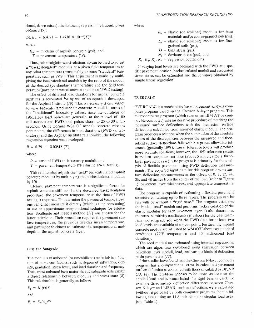
86

tional, dense mixes), the following regression relationship was

obtained (9):

log E". = 6.4721 - 1.4736 x 10-4(T)'?

where

Eu" = modulus of asphalt concrete (psi), and

f = pavement temperature ("F).

Thus, this straightforward relationship can be used to adjusta "backcalculated" modulus at a given field tempelature toany other temperature (presumably to some "standard" tem-perature, such as 77"F). This adjustment is made by multi-plying the backcalculated modulus by the ratio of the moduliat the desired (or standard) temperature and the field tem-perature (pavement temperature at the time of F WD testing).

The effect of different load durations for asphalt concretemixtures is accounted for by use of an equation developedfor the Asphalt Institute (10). This is necessary if one wishes

to view backcalculated asphalt concrete moduli in terms ofthe "traditional" laboratory values, since the durations oflaboratory load pulses are generally at the 4 level of 100

milliseconds and FWD load pulses closer to 25 to 30 milli-seconds. Using normal WSDOT asphalt concrete mixtureparameters, the differences in load durations (FWD vs' lab-oratory) and the Asphalt Institute relationship, the followingregression equation was developed:

R = 0.791 + 0.00813 (r)where

R = ratio of FWD to laboratory moduli, and

f = pavernent temperature ('F) duling FWD testing.

This relationship adjusts the "field" backcalculated asphalt

concl'ete modulus by rnultiplying the backcalculated ¡nodulusby 1/R.

Clearly, pavement temperature is a significant factor forasphalt concrete stiffness. In the described backcalculationprocedure, the pavement temperature at the titne of FWDtesting is required. To determine the pavelnent temperature,one can either measure it directly (which is time consurning)

or use an approximate computational technique for estima-

tion. Southgate and Deen's method (11) was chosen for thelatter technique. Their procedure requires the pavement sur-

face ternperatule, the previous five-day mean temperature,and pavement thickness to estimate the temperature at mid-depth in the asphalt concrete layer.

Base and Subgrade

The rnodulus of unbound (or unstabilized) rnaterials is a func-

tion of numerous factors, such as degree of saturatiotr, den-

sity, gradation, stress level, and load dulation and frequency.Thus, most unbound base materials and subgrade soils exhibita direct relationship between modulus and stress state (8).

This relationship is generally as follows:

Ea = KIO)K'

and

E, : Kr(oo)Ko

where

TRANSPORTATION RDSEARCH RECORD I 196

Er, : elastic (or resilient) modulus for base

materials and/or coarse-grained soils (psi),

4 : elastic (or resilient) modulus for fine-grained soils (psi),

O : bulk stress (psi),o¿ = deviator stress (psi), and

Kr, Kr, Kt, Ko = regression coefficients.

If varying load levels are obtained with the FWD at a spe-

cific pavement location, backcalculated moduli and associated

stress states can be estimated and the K values obtained by

sirnple linear regression.

EVERCALC

EVERCALC is a mechanistic-based pavement analysis corn-puter program based on the Chevron N-layer program. Thismicrocomputer program (which runs on an IBM AT or com-patible computer) uses an iterative procedure of matching the

measured surface deflections with the theoretical surface

deflections calculated from assumed elastic moduli. The pro-gram produces a solution when the summation of the absolute

values of the discrepancies between the measured and theo-

retical surface deflections falls within a preset allowable tol-erance (generally l0o/o). Lower tolerance levels will produce

more accurate solutions; however, the l0o/o tolerance results

in modest computer run time (about 5 tninutes for a three-

layer pavement case). The program is primarily for the anal-

ysis of flexible pavement using FWD deflection tneasure-

ments. The acquired input data for this program are six sur-

face deflection measurements at the offsets of 0, 8, 12, 24,

36, and 48 inches from the center of the load (refer to Figure

1), pavement layer thicknesses, and appropriate telnperature

data.The prograrn is capable of evaluating a flexible pavement

structure containing up to three layers' Tlte program can be

run with or without a "rigid base." The program estimates

the initial "seed" rnoduli and perforrns backcalculation of the

elastic modulus for each pavement layer. It also determines

the stress sensitivity coefficients (K values) for the base mate-

rials and subgrade soil when the FWD data for at least two

loacl levels are available at a given point. Further, the asphaltconcrete moduli are adjusted to WSDOT laboratory standard

conditions (77"F temperature and 100-millisecond load

duration).The seed moduli are estimated using internal regressions,

which are algorithms developed using regression betweenpavernent layer moduli, load, and various kinds of deflectionbasin parameters (12).

Priol'studies have found that the Chevron N-layer cotnputerprogram has a colnputational et'ror in calculated pavement

surface deflection as comparecl with those calculated by BISAR(13, l4). The problem appears to be tnore severe near the

applied load and is exacerbatecl if a Ligid base is used' Toexamine these surface deflection diffel'ences between Chev-

ron N-layel and BISAR, surface deflections were calculated(without rigid base) by both cornputer programs for the fol-lowing cases using an 11.8-inch diameter circular load area.

(see Table 1).

Lee et al. 87

FIGURE I Present configuration of I{SDOT FWD.

TABLE 1 COMPARISON OF CHEVRON N-LAYER AND BISARCALCULATIONS OF SURFACE DEFLECTION DIFFERENCES

Asph¡lt Cotrcrctc

Base

Subgrade

Lo¡d lcvels (lb)

Stiffaess (ksi):Thickncss (in):Poisson's ¡atio:

Stiffncss (ksi):Thickncss (in):Poisson's rst¡o:

Stiffness (ksi):Thickness (in):Poi¡son's ratio:

9,000 ¡nd 15,000

5 t5semi-infinite0.45

5060.35

¡0120.40

500 t,000l2

20 4021

The average surface deflection and associated standarddeviation differences for 216 cases are shown in Table 2.

Further, the maximum deflection difference wasï.2Vo directlyunder the load (8"" = 1,000 ksi, åu" = L}in., Eu = 40 ksi,hv: 24 in., Quue = 5 ksi), with only L2of the2l.6 cases overSVo. Generally, the largest differences (2.0Vo or more) werefor the thick, higher stiffness surfaces on lower stiffnesssubgrades.

The basic conclusion drawn from the above information isthat the Chevron N-layer program is adequate for backcal-culation of typical moduli for flexible pavements (given nor-mally used convergence errors). However, backcalculationprograms based on the Chevron N-layer should not be usedon rigid pavements at this time.

ACCURACY OF BACKCALCULATIONSOLUTIONS

A number of concerns about backcalculation of elastic modulican be raised. These can include (1) nonunique solutions, (2)requirement for equivalent moduli for a limited number oflayers (three or four), (3) differences between backcalculatedand laboratory obtained elastic moduli, and (4) selection ofthe optimum number and location of surface deflectionmeasurements,

Nonunique solutions simply mean that if different initialseed moduli are used, then different backcalculated moduliresult in a final solution. The equivalent moduli problem arisesfrom the fact that a limited number of pavement layers can

TABLE 2 AVERAGE SURFACE DEFLECTION AND ASSOCIATEDSTANDARD DEVIATION DIFFERENCES FOR 216 CASES

Statistics

Mc¡a (9ó)

Std. Dev. (9ô)

Rad¡al Offscr (¡n.)ott221t648r.r 0.4 0.2 0.0 o.t 0.r1.1 0.6 0.3 0.r 0.t o.t

88

be used in the backcafculation process (in part limited by the

number of measured surface deflections, computer run time,and theory associated with modeling complex materials). Thus,one must obtain (for example) a single modulus value for the

asphalt concrete materials even though such a layer may be

composed of different asphalt concrete mixtures, lifts, and

hence moduli. Finally, backcalculated and laboratoly modulimust show at least modest agreement in order for pavement

engineers to become more confident in backcalculationprocedures.

When the seed moduli are accurately estimated, the back-calculation process will produce solutions with less error in

fewer iterations, thus minimizing the nonuniqueness problem.

The seed moduli may be estimated by engineering judgment,

temperature-stiffness relationships, and surface deflections,among others. EVERCALC contains internal regression

equations (12), which are used to estimate the seed moduli(for up to three layers) from deflection basin parameters. Thisis done in an attempt to minimize nonuniqueness.

To address at least partially the nonuniqueness question

for backcalculated solutions, EVERCALC backcalculatedsolutions were cornpared with theoretical elastic layer solu-tions. This was accomplished by calculating "theoretical" sur-

face deflections for preselected layer ¡noduli and thicknesses(for three layer pavements). These calculations were per-

formed with the Chevron N-layer computer program for thefollowing cases, shown in Table 3.

Surface deflections were calculated at six offsets of 0, 8,

12,24,36, and 48 inches from the load. The load was assumed

to be 9,000 pounds, placed on a circular load plate 11.8 inches

in diameter. The cases were excluded in which the asphalt

concrete layer was of greater thickness than the base; thus,

384 cases were used. The surface deflections so calculatedwere then used as inputs into EVERCALC, and moduli foreach of the three layers backcalculated. This enabled a

straightforward comparison of the known moduli used orig-inally to calculate the surface deflections (via Chevron N-layerprogram) to the backcalculated moduli obtained from those

same surface deflection (via the EVERCALC program).A maximum of five surface deflections can be used for

direct backcalculation with EVERCALC; thus, two separate

runs were made for surface deflections at 0, 8, 12, 24, and 36

inches (case A) and those at 0,12,24,36, and 48 inches (case

B). These two deflection sensor configuratiolrs have been

commonly used by the WSDOT and appear to define the

deflection basin reasonably. A maximum allowable toleranceof lïVo was used for "matching" the deflection basins. The

I\Vo tolerance is an absolute value (i.e., the sum of the abso-

Asphalt Coocrcte

B¡se

Subgradc

TRANSPORT'ATION RESEARCH RECORD I 196

lute differences in surface deflections at all five locations).

This tolerance level resulted in three backcalculation itera-

tions or less to procure an "in tolerance" solution for the

cases studied. Thus, the backcalculation results reportedthroughout this paper were obtained in a "production" mode

representative of expected, everyday usage of EVERCALC.The percent differences between the backcalculated and

theoretical moduli were determined. The backcalculationsperformed for surface deflection measurements conformingto case A were slightly better than those for case B (i.e.,better agreement between backcalculated and theoretical

moduli). This is most likely due to the second surface deflec-

tion measurement being only 8 inches from the center of the

load plate for case A, as opposed to 12 inches for case B,thus better defining a critical portion of the deflection basin.

A summary of the absolute percent differences (or errors)

for the backcalculated and theoretical moduli is shown inTable 4 for case A surface deflection locations (i'e., sign

conventions were ignored which result in higher average errors).

Overall, the subgrade tnoduli have the closest agreement (about

1..5o/o). The base materials have an average difference of about

6.50/o and the pavement surfacing (asphalt concrete) about

8.2Vo. Figure 2 is used to show the cumulative frequency

distribution of the errors. Overall, most of the calculated

errors were less than I07o for the subgrade moduli. For asphalt

concrete and base layers, S2o/o of the comparisons had less

than a L\Vo error;90Vo had less than 20o/o errot; and 957o

had less than3\Vo error. Further, the errors tended to increase

for thin, low stiffness (i00,000 psi) asphalt concrete layers'

COMPARISON OF BACKCALCULATED ANDLABORATORY MODULI

Comparisons between backcalculated (or in situ) and labo-

ratory moduli are difficult because of variability of the mate-

rials, sampling, and testittg. The results pl'esented in this sec-

tion will show the results of such an attempt.Sixteen pavement test sites (Table 5) were used to co¡npare

the backcalculated and laboratory moduli. These test sites are

typical of flexible pavement sections on the state-maintainedroute system in Washington. In part, however, they were

selected for their apparent uniformity (for example, in con-

struction, distress, and subgrade soils). Surface distress at

these sites was observed to be mostly fatigue (alligator) crack-

ing or its usual precutsor, longitudinal cracking. Only five ofthe sixteen test sites were evaluated (for backcalculation pur-

5r020semi-infinite0.45

TABLE 3 COMPARISON OF EVERCALC BACKCALCULATEDSOLUTIONS WITH THEORETICAL ELASTIC LAYER SOLUTIONSPERFORMED WITH CHEVRON N-LAYER PROGRAM

Stiffness (ksi):Thicknes (in):Poissoa'! rat¡o:

Stiffncs¡ (ksi):Thickncss (in):Poisson's r¡tio:

Stiffness (ksi):Thickness (in):PoissoD's rrtior

r00 300 500 t0035t

0.35

l0 20 ¡10

6t2240.40

30

9gf?.. Enor(Vo\Thick. _ ..,,, rnggrgliçqlnaiticMo¿ffi(in.) Layer 100.000 300.000 50ci.000_ 800.000

Mean Std Mean Std Mean Std Mean Std Mean Srd

3.0 ACp 18.5 31.8 6.8 t2.2 5.0 9.s s.8 9.8 9.7 13.4

Base 3.9 6.0 3.7 4.4 4.0 4.8 4.8 6.4 4.6 4.7Subgrade O.7 0.5 0.9 0.9 1.4 t.7 t.4 Z.t 1.3 t.z

5.0 ACp 13.5 24.8 6.2 9.4 4.7 7.4 5.5 6.9 7 .7 lO.4Base 6.0 9.6 5.1 ó. I 5.1 4.6 6.5 4.8 5.S 5.9Subgrade 1.0 0.9 l.l 1.0 1.6 1.5 1.3 t.l l.Z t.2

8.0 ACP 9.8 24.3 6.2 9.2 3.6 5.2 5.5Base 8.6 10.7 8.0 I L3 8.0 7.8 I l.0Subgrade 2.2 1.7 2.3 1.8 2.4 1.8 2.1

.0 7.2 9.9

.7 9.s 9.4

.6 2.0 2.0

Lee et al 89

TABLE 4 CALCULATED ERRORS FROM COMPARISON OFBACKCALCULATED AND THEORETICAL LAYER MODULI

Nore I : Error (zo) = I (ffi t r*l¡

poses) as three-layer pavements. The remainder were eval-uated as two-layer systems ("full-depth" cases).

The field material sampling required for laboratory testingincluded obtaining asphalt concrete cores at three locations(stations 0 + 50, 5 + 50, and 9 + 50) wirhin the 1,000-foor-long test sites. This was done to estimate better the asphaltconcrete modulus and thickness changes within each test site.Disturbed base course and subgrade soil samples were obtainedat the pavement shoulder at approximately the middle of eachtest site (station 5 + 50). During this sampling in situ, mois-ture contents were made in the base and subgrade materials.

The laboratory testing of the asphalt concrete cores wasconducted in accordance with ASTM D4123 at three tem-perature levels (41o, 77o, and 104"F) and a loading durationof 100 milliseconds. The base and subgrade materials wererecompacted in the laboratory and tested in accordance withAASHTO T274. The remolding moisture content was keptas close as possible to those measured in the field at the timeof sampling. The triaxial testing was performed on each sam-ple with confining stresses of. 1,2,4, and 6 psi and deviatorstresses of. L,2, 4, 6,8,10, and 12 psi. All laboratory testingwas conducted by the WSDOT at its materials laboratory inOlympia, Washington.

Asphalt Concrete Comparisons

The comparisons of backcalculated (EVERCALC) and lab-oratory asphalt concrete moduli are shown in Table 6 for allsixteen test sites. All moduli values have been rounded off tothe nearest 1,000 psi; however, the percent differences werecalculated on the non-rounded values. Further, all backcal-culated moduli values were adjusted to a ',standard" loadingduration (100 milliseconds) and temperature (77"F) to providebetter comparisons with the laboratory moduli (for which alarge amount of published modulus data is available).

Differences in the backcalculated and laboratory modulirange from being essentially identical to over 400o/o. Overall,differences of 20o/o to 50Vo were common. The largest dif-ferences were observed for test site 8, which had extensive,severe fatigue cracking observed at the pavement surface.Thus, the low backcalculated values (40,000 to 100,000 psi)should be expected. Naturally, when this test site was cored,only those cores were obtained which had no cracks. There-fore, the large differences between backcalculation and lab-oratory moduli are understandable. This same discussion appliesto test site 10, since this site has extensive longitudinal crack-ing. If one views the moduli differences for the remaining test

CUþl.SOLUTION

(r)

t00

90

8t¡

70

60

50

10

3{t

20

e0 25

ERFOR (r)

€- A.C

+(- B,S

--l- s.G

FIGURE 2 Accuracy of backcalculation.

TABLE 5 TEST SITE DESCRIPTIONS

Test Site YearNo. Route No. Milepost Original ACP

Constuction ThickBaseThick.

ObservedSurfaceDistress

l,ong. cracking

l,ong. cracking

Futigu" "roafing

long. cracking

Long. & Trans. crack.

'lrans. cracking

I sR 11 20.85

2 SR 20 s3.50

3 SR 20 77.50

4 SR 20 108.20

5 SR 20 140.80

6 SR 167 17.80

7 SR 202 30.t2

I SR 410 9.60

9 SR 5 3s.80

l0 sR 14 18.15

I I sR 4l I 18.05

t2 SR s00 3.20

13 SR 90 208.65

14 sR 90 208.85

15 SR 195 7.24

16 SR

72

73

68 (8s)

78

72

68 (80)

78

68

73

73

79

79

73

73

70 (85)

76

5.2 28.8

4.9 4.8

10.9 6.6

3.s 9.0

3.4 6,6

tt.213.0

7.3 3.6

16.4

9.0 3.6

6.8 21.0

6.3 8.4

9.6 8.4

9.6 8.4

6.2 r 1.4

8.5 12

90

sites (excluding test sites 8 and 10), then the differences arenot alarming.

To put the asphalt concrete moduli differences into greaterperspective, the backcalculated moduli for test sites I and 3

("higher" and "lower" moduli test sites) were plotted and

shown in Figure 3. The backcalculated moduli were deter-mined from the FWD deflection basins taken every 50 feetwithin the 1,000-foot test sites. A quick inspection of Figurc3 shows that substantial variations in asphalt concrete modulican be expected, which suggests the power that NDT pave-

ment evaluation can provide.

Base Course Comparisons

The comparisons of backcalculated and laboratory base course

moduli for five of the sixteen test sites are showtì in Table 7.

These five test sites were judged to have base course thick-nesses which would provide for "reasonable" base modulidetermination. In general, use of the EVERCALC program

TRANSPORTATION RESEARCH IIECORD I 196

has led the authors to conclude (at this time) that the base

course thickness should be about 1.5 times thicker (or more)than the surfacing layer in order to attempt a three-layerbackcalculation.

The backcalculated and laboratory base course moduli werecompared at similar stress states (i.e., the in situ stresses

estimated during FWD testing and the laboratory triaxialstl'esses were similar). Overall, good agree¡nent was foundfor four of the five test sites. The unusually high laboratorymodulus for test site 5 (60,000 psi versus 38,000 psi for back-

calculation) may be attributecl largely to how the base course

material was sampled.Table 8 is provided to show compat'isons between the stress

sensitivity coefficients (Kr, Kr) for the backcalculated and

laboratory moduli. These coefficients are automatically com-puted by the EVERCALC program if two or more FWD loadlevels are used at a test point. Overall, the agreement is mod-est at best; however, the poorest comparison is again for test

site 5. Due to the small number of data points for deterrniningthese coefficients from FWD data and backcalculation, one

1000

800

nlPH!}" -'100

200

STATION

FIGURE 3 Variation of asphalt concrete modulus.

500200

-€- TS 1 -¡- ÏS 3

0600 700 800

Lee et al.9t

TABLE 6 COMPARISON OF BACKCALCULATED ANDLABORATORY ASPHALT CONCRETE MODULI

TestSiteNo.

SolutionMeùod 0+50 5+50 9+.50

l NDT/FWD 868,000 668,000 604,000 713,000tåb 426,0æ 469,000 387,000 421,OOO

Diffcrence(Zo) ¡fl -30 _36 -40

2 NDT/FIVD 725,000 498,000 487,000 570,000Iib 633,000 355,000 234,000 407,000Differcnce(7o) -13 -29 -SZ _29

3 NDT/FWD 246,000 373,000 568,000 39s,oootåb 333,000 s57,000 334,000 408,000Difference (7o) +36 +50 _41 3

4 NDT/F\VD 684,000 472,000 194,000 450,000ráb 346,000 2tS,000 Z44,O0O 268,000Difference (7o) -49 -54 +26 -40

5 NDT/FWD 531,000 494,000 74o,OOO 588,000Iåb 3s7,000 147,000 354,000 286,000Difference (7o) -33 -70 -SZ -51

6 NDT/FVD 722,000 741,000 5lo,00o 658,000táb 171,000 489,000 464,000 355,000Differcnce (7o) -76 -34 -Zt -46

7 NDT/FWD 460,000 577,000 75?,OOO s98,OO0

tåb 431,000 596,000 743,000 s90,000Differcnce (Vo) -6 +3 -Z - I

8 NDT/FWD 102,300 42,000 94,000 7g,4ooIrb 200,000 227,000 215,000 2l4,0OO

Dffercnce (7o) +96 +438 + 130 + l7O

9 NDT/FWD 455,000 657,000 s78,000 563,000t¿b 135,000 I 17,000 181,000 !44,000Differcnce(7¿) -70 -92 -69 -74

l0 NDT/FWD 131,000 289,000 340,000 2s3,o0orrb 779,0@ 687,000 s27,000 664,000Difference (7o) +495 +137 +55 t 162

r l NDT/FWD 215,000 243,000 358,000 272,0t0L.ab 3,14,000 352,000 219,000 305,000Differynce (9o) +60 +45 -39 +t2

t2 NDT/FWD 311,000 242,000 270,000 274,000

t¿b 343,000 414,000 380,000 379,000

Differemce(%o) +10 +71 +41 +38

13 NDT/FWD 264,000 232,0@ 344,000 280,000

Låb 198,000 343,000 3¡8,000 286,000

Difference(%o) -25 +47 -8 +2

t4 NDT/F$/D 260,000 218,000 256,000 24s,000

Låb 289,000 240,000 188,000 239,000

Dúferc¡ce(lo\ +l I +10 -27 -2

15 NDT/F-WD 404,000 262,000 49s,000 387,000

Lab 375,000 605,000 419,000 46ó,000

Differcnce(Vo\ -7 +l3l -15 +2O

16 NDT/FI!/D 307,000 214,000 321,000 281,000

Lrb 202,000 166,000 164,000 177,000

Difference(%o) -34 -22 -49 -37

should expect a wider range of coefficient values (as opposedto laboratory results).

To view these cornparisons against the expected field basecourse moduli, backcalculated moduli for test site I werecomputed every 50 feet and plotted in Figure 4. Thus, withinonly 1,000 feet of a pavement structul.e, these moduli caneasily vary by a factor of about 2.

Subgrade Soil Comparisons

The comparisons of backcalculated and laboratory subgradesoil moduli for all sixteen test sites are shown in Table 9. Aswas done for the base course comparisons, the moduli com-parisons shown in Table 9 were made at similar stress states.The observed differences for these subgrade soils are the least

92 TRANSPORTATION RESEARCH RECO RD I 196

TABLE 7 COMPARISON OF BACKCALCULATED ANDLABORATORY BASE COURSE MODULI

I 23,000 23,000 0 3.7 4.7 + 1.0

4 45,000 53,000 l8 4.4 4.5 +0.1

5 38,000 60,000 60 5.0 4.3 -0.7

l l 2r,000 2s,000 22 4.2 3.9 -0.3

31.000 36 4.4 4.

Ave¡age 30,000 38,000 28 4.3 4.5 +0.2

Std.Dev. 10.000 15,000 0.4 0.4

TABLE 8 BASE COURSE STRESS SENSITIVITY COEFFICIENTS

TestSite Solution

Method K

il

NDT/FWD

Låb

NDT/FWD

låb

NDT/FWD

l¡bNDT/FWD

låbNDT/FWD

4,680 0.68

7,350 0.49

1,149 l.16

ú,529 0.48

280 t.44

t4,270 0.42

l,590 l. l09,010 0.44

r 1,700 0.32

98

9l92

9l96

89

96

90a

92

l513.000 0.41

of the three pavement materials being compared. Overall, thepercent differences range from alow of ZVo to a high of. 84o/o,

with the average being 10o/o.Theaverage backcalculated modulifor all sites is 29,000 psi, compared with an average laboratorymodulus of 26,000 psi. (Recail that the laboratory moduli werefor disturbed, or recompacted, samples.) These differences,again, should be viewed against the kind of variation one

might expect in a relatively uniform, short length of pavement.Figure 5 shows the backcalculated subgrade soil moduli forFWD tests performed every 50 feet for two 1,000-foot longtest sites (test sites 1 and 3). The illustrated subgrade can

easily vary by a factor of 2.Table 10 is provided to illustrate comparisons of the stress

sensitivity coefficients (&, K.) for the backcalculated and

laboratory moduli. Overall, the agreement is somewhat better

than that observed for the base course comparisons.

SUMMARY AND CONCLUSIONS

A backcalculation program (EVERCALC), which is used todetermine pavernent-layer elastic moduli, has been examinedin two fundamental ways in an attempt to verify the results.

The first verification approach was to compare theoretical and

backcalculated moduli for a range of three-layer pavementsystems. This was accomplished by using the Chevron N-layer

nlP!!y"

10

3!t

3{r

å

t5

t0

5

0

TSl

500¿00300r00

STATI(]N

FIGURE 4 Variation of base modulus.

700 800 900

Lee et al. 93

TABLE 9 COMPARISON OF BACKCALCULATED ANDLABORATORY SUBGRADE SOIL MODULI

TestSiteNo.

Modulus lpsil Moisture Content (%)NDT/FWD l-ab Dtff . Øo\ Field Låb Diff.

I 26,000 20,000 -21 5.6 7 .3 +t.72 21,000 16,000 -23 2.4 ó.0 +3.6

3 15,000 20,000 +32 3.7 6.4 +2.7

4 27,000 49,000 +84 3.8 4.7 +0.9

5 36,000 32,000 -l I 3.5 4.8 +1.3

6 29,000 15,000 -47 9.6 6.0 -3.6

7 39,000 33,000 -14 5.6 s.s -0.1

8 9,000 5,000 -36 2r.5 15.7 -5.8

9 37,000 32,000 - 14 t2.2 12.6 +0.4

l0 39,000 26,000 -32 7.8 9.2 +1.4

I I 26,000 28,000 +8 6.9 I l.l +4.2

rz 36,000 35,000 -2 8.2 9.0 +0.8

t3 36,000 42,000 +t7 10.4 8.2 -2.2

t4 40,000 42,000 +4 10.4 8.2 -2.2

ls 20,000 12,000 -42 13.6 l5.l +l.s16 20.000 8.000 -59 I 1.8 l2.l +0.3

Avcrdge 29,000 26,000 -10 8.4 8.9 +0.5

Std. Dev. 10.000 13.000 5.0 3.6

M0DULUS 20

IKS IJ

30

25

t5

t0

5

0

SÏATION

FIGURE 5 Variation of subgrade modulus.

900 r000

differences between backcalculated and laboratory moduli donot offer a true verification, since laboratory test proceduresof disturbed (recompacted) samples do not necessarily pro-vide reference (or true) moduli. Further, these observed dif-ferences are generally much less than the variation of moduliexpected within relatively uniform, short lengths of pavement(in this case, 1,000 feet).The following conclusions are offered:

1. The backcalculation of layer moduli from measuredpavement deflection basins appears to provide reasonableestimates of in situ pavement moduli. Further, moduli can beestimated for cracked asphalt concrete conditions.

2. The EVERCALC program is a backcalculation proce-dure which should be of value to the pavement research com-munity and help meet the needs of road-owning agencies.

800700200r00

elastic analysis program to generate deflection basins for spec-ified layer moduli and thickness conditions. These compari-sons showed modest differences (about 8o/o for asphalt con-crete,6Vo for base course, and less than2o/o for the subgrade).The largest differences for asphalt concrete were observedfor thin surfaces with low stiffness. As the asphalt concretelayer thickness increases, both the base and subgrade modulidifferences increased.

The second verification approach was to compare back-calculated and laboratory moduli based on FWD tests andfield material sampling along with appropriate laboratory test-ing. The results show the greatest range of differences for theasphalt concrete layers followed by the base and subgradematerials; however, large diffelences between backcalculatedand laboratory asphalt concrete moduli should be expectedfor those test sites with extensive cracking. The observed

-€- ïS { -+- TS 3

'|.^ÞI T 1O STJBGRADE SOIL STRESS SENSITIVITY COEFFICIENTS

TestSiteNo.

I

SolutionMethod

Stress SensitivityCoefficients

K R2 (Eo)

ll

NDT/FWD

I¿b

NDT/FWD

l¿bNDT/FWD

tåbNDT/FWD

IåbNDT/FIü/D

t¿b

NDT/FWD

IåbNDT/FWD

I¡bNDT/FrI¡/D

t¿b

NDT/FWD

IåbNDT/FWD

Iåb

NDT/FWD

IåbNDT/FWD

IlbNDT/FWD

låbNDT/FWD

Lab

NDT/FWD

Låb

NDT/FWD

Iåb

34,160

16,850

7,600

3,140

20,6r0

16,360

59,0s0

32,680

48,7r0

20,4t048,670

I r,750

49,r76

27,360

l1,910

7,290

47,750

24,370

37,270

l I,670

44,730

23,750

21,030

4,640

65,390

26,480

39,260

26,480

28,760

t7,460

34,840

-0.24

0. r7

0.3 r

0.50

-0. l90. l3

-0.32

0. l6-0.t2

0.r6-0.38

0.20

-0. l90. r6-0.t2

-0. r0-0.2r

-0.21

0.02

o.l7-0.44

0. 15

0. l50.56

-0. l90.r8

-0.03

0. r8-o.29

-0.32

-0.30

-0.01

89

2t72

6

72

t7

87

54

99

l658

t4

58

42

79

7

59

68

20

50

97

34

76

53

94

2l29

2t

98

2l96

2t

t2

l5

50

94

3. The results of backcalculation analyses based on elasticsolutions appear to be influenced by at least the following:

(a) The backcalculation elror is higher for asphalt con-crete moduli with relatively thin, low stiffnesssurfaces.

(b) The base course thickness should be about 1.5 times(or more) greater than the asphalt concrete surfacecourse in order to achieve reasonable estimates ofbase moduli.

(c) The two sensor configurations on the WSDOT FWDdid not significantly alter the backcalculated moduli.(One of the two, however, did appear to have slightlysmaller errors.)

ACKNOWLEDGMENTS

The study described in this paper was conducted on a HighwayPlanning and Research study with the lVashington StateDepartment of Transportation, The cooperation of WSDOT,the Federal Highway Administration, and the WashingtonState Transportation Center is deeply appreciated.

TRANSPORTATION RESEARCH RECORD I 196

REFERENCES

1. R. E. Smith and R. L. Lytton. Synthesis of Study of Non-destructive Testing Devices for Use in Overlay Thickness Designof Flexible Pavements. Report FHWA-RD-83-/097, FHWA,Washington, D.C., April 1984.

2. A. J. Bush and D, R. Alexander. Pavement Evaluation UsinþDeflection Basin Measurements and Layered Theory. InTransportation Research Record I 022,TRB, National ResearchCouncil, Washington, D.C., 1985, pp. 16-29.

3. W. Udin, A. H. Meyer, and W. R, Hudson. Rigid BottomConsiderations for Nondestructive Evaluation of Pavements.ln Transportation Research Record 1070, TRB, NationalResearch Council, Washington, D.C., 1986, pp.2l-29.

4. M, S. Hoffman. Loading Mode Effects on Pavement Deflec-tions. Journal of Transportotion Engineering, Yol. 109,No. 5, Sept. 1983, pp. 651-668.

5. B. E. Sebaaly and M. S. Momlouk, Dynamic Analysis ofFalling Weight Deflectometer Data. Paper presented at theAnnual Transportation Research Board Meeting, Jan. 1986.

6. O. Tholen, J. Sharma, and R. L. Terrel. Comparison ofFalling Weight Deflectometer with Other Deflection TestingDevices. ln Transportation Research Record 1007, TRB,National Research Council, Washington, D.C., 1985,pp.20-26.

7.

Lee et al,

M. S. Hoffman and M, R. Thompson. Backcalculating Non-linear Resilient Moduli from Deflection Data. ln Transpor-tation Research Record 852, TRB, National Research Coun-cil, Washington, D.C., 1982, pp. 42-5L.Y. T. Chou. Engineering Behavior of Pavement Materials:State of Art. Report FAA-RD-77-37, U.S. Army EngineerWaterway Experiment Station, Vicksburg, Miss,, Feb. 1977.A. A. Bu-Bushait. Development of Flexible Pavement FatigueModel for Washington Stal¿. Ph.D. dissertation, Departmentof Civil Engineering, University of Washington, Seattle, Wash.,1986.J. F. Shook, F. N. Finn, M. W. tüitczak, and C. L. Mon-ismith. Thickness Design of Asphalt Pavement, The AsphaltInstitute Method. ln Proc., Sth International Conference onthe Structural Design of Asphalt Pavements. Delft Universityof Technology, The Netherlands, Vol. 1, Aug. 1982,pp. L7-44.H. F. Southgate and R. C. Dean. Temperature Distributionsin Asphalt Concrete Pavements. ln Transportation Research

95

Record 549,'lR.B, National Research Council, Washington,D.C., L975, pp.39-46.

12. E. E. Newcomb. Development and Evaluation of RegressionMethod to Interpret Dynamic Pavement Deflections. Ph.Ddissertation. Department of Civil Engineering, University ofWashington, Seattle, Wash., 1986.

13. F. Parker, W. R. Barker, R. C. Gunkel, and E. C. Odem.Development of a Structural Design Procedure for Rigid Air-port Pavements. Report FAA-RD-77-81. U.S. Army Water-ways Experiment Station, Vicksburg, Miss., 1979.

14. H. J. Southgate, R. C. Deen, D. H. Cain, and J. G. Mayes.Modifications to CHEVRON N-Layer Computer Program.Report UKTRP-87-XX. University of Kentucky, Lexington,Ky.,1987.

Publication of this paper sponsored by Committee on Strength andDeþrmalion Characteríslícs of Pavement Sections.

8.

10.

11.

96 TRANSPOIì,7'A'|'ION RESEARCH RECORD I l9()

Dynaflect Evaluation of Layer Moduli inFlorida's Flexible Pavement Systems

Kwesr Beou-TwENEBoAH, BvnoN E. RurH, eup Wrr,LrAM G. Mnny

Research conducted to investigate the nondestructive testing(NDT) characterization of in-place pavement materials hasresulted in the development of a modified sensor spacing forthe Dynaflect. The modified testing configuration provides thecapability to separate the deflection response contributed bythe subgrade, the stabilized subgrade, and the combination ofbase and asphalt concrete for typical Florida flexible pavementsystems. Analysis of Dynaflect data for in-service pavementsusing an elastic layer computer program resulted in the devel-opment of simple power law regression equations to predictlayer moduli from modified sensor deflections. This paper pre-sents the development of the simplified layer moduli predictionequations, and the recommended testing and analytical pro-cedures for pavement evaluation investigations. The use of thissimplifïed approach allow a large number of test locations tobe analyzed by eliminating the use of computer.iterative pro-grams which are usually time consuming, expensive, and oftensubject to substantial errors.

Nondestructive testing (NDT) and deflection measurementsare now universally recognized methods for the structuralevaluation of road and airfield pavements. NDT of pavementshas evolved from the very basic Benkelman Beam to the morerefined equipment such as Dynaflect, Road Rater, and FallingWeight Deflectometer. The Dynaflect is presently the mostcommonly used NDT device in the United States for evalu-ation and design of pavement. Like the Benkelman Beam, alarge number of data has been accumulated with the use ofthis device.

The Dynaflect is a steady-state vibratory device that isinstrumented to measure peak-to-peak dynamic deflection onthe pavement surface. It applies a load of 1000 lbs., at afrequency of 8 cycles per second, through two steel wheelsthat are 20 in. apart center to center. The resulting deflectionbasin is measured by five geophones spaced 12 in. apart, withthe first geophone located midway between the loading wheels.These deflection measurements represent the stiffness of theentire pavement section.

Although some significant accomplishments have been madein separating the effects of major parts of the pavement struc-ture, the separation of the effects of all of the various com-ponents of the structure with deflection basin measurementshas not yet been accomplished. Thus, with the possible excep-tion of the subgrade modulus, the moduli of the other layersare estimated using linear-elastic computer-iterative pro-

K. Badu-Tweneboah and B. E. Ruth, Department of Civil Engi-neering, University of Florida, Gainesville, Fla. 32611. W. G.Miley, Bureau of Materials and Research, Florida Departmentof Transportation, Gainesville, Fla. 32611.

grams, graphical solutions, or nomographs. The major prob-lems associated with the above solution techniques are thatunique solutions cannot be guaranteed, solutions can be timeconsuming, and the expertise required for interpretation maynot be available. The purpose of this paper is to present a

simplified approach that would allow a layer-by-layer analysisof the Dynaflect deflection basin. Such a simplified approachwould allow a large number of test points to be analyzed andconsequently enhance our ability to carry out mechanisticpavement evaluation on a routine basis.

BACKGROUND

The Florida Department of Transportation (FDOT) has formany years been interested in the use of NDT methods forpavement evaluation to typify pavement response and to pro-vide information for structural characterization. The Ben-kelman Beam was used extensively into the 1970s for researchprojects and for "troubleshooting" distressed pavernent sec-tions. The first Dynaflect unit was purchased by the FDOTin 1966. Initially, it was used as a research tool in combinationwith Benkelman Beam and plate bearing tests on pavementlayers. The Dynaflect evolved as a reliable device for assess-

ment of structural response uniformity for Florida's highwaypavement network.

In 1981, the FDOT's Bureau of Materials and Researchpavement section under the direction of tW. G. Miley devel-oped and adopted a method of predicting the structural subgradesupport value from Dynaflect sensor response. This was basedon correlations between plate bearing moduli and the mea-sured deflection at the fourth sensor (1). Subsequent use ofthe Dynaflect for pavement evaluation and to determine reha-bilitation design thickness requirements has proven valuableto the FDOT. However, determination of layer moduli usingelastic multilayered computer programs was time consumingand often yielded moduli that were outside the realm of pos-sibility. Consequently, a research project was initiated in 1984

for the purpose of developing simplified methods for thedetermination of layer moduli using the Dynaflect.

This investigation involved computer simulation of Dyna-flect response using ten different sensor positions (figure 1)for a parametric study of different layer thicknesses and mod-uli encompassing the range of values encountered in Florida.The results of the study indicated that modified sensor posi-tions provided a unique capability for separation of the deflec-tion response characteristics of asphalt concrete and limerockbase from the underlying materials. Also, power law rela-tionships for the fifth sensor was found to be reliable in assess-

Badu-T¡veneboah et al 97

@ 4 ln Spac¡ng

'12 ln

GEOPHONE NO.

Convent¡onal Modilled

@-xo\QJ

6II't0

FIGURD I Dynaflect modified geophone positions.

ing the subgrade modulus. A series of precliction equationswere developed from the computer-generated information forthe estimation of the moduli in four layer pavement systems(2, 3). Although the prediction accuracy appeared to be good,the complexity of the equations and the dependency uponreasonable estimates of E, or E, to solve for E, or E, , respec-tively, indicated that further research to simplify and improvethe accuracy of layer moduli predictions would be desirable.

Field tests were conducted on asphalt concrete pavementsusing the Dynaflect, Falling Weight Deflectometer (FWD),cone penetration test (CPT), Marchetti Dilatometer test(DMT), and plate loading test (PLT). The CPT and DMTdata were collected to evaluate the stlatigraphy of the sub-surface thatis valuable in tuning moduli for elastic layel anal-yses based on measured deflection basins (4). A thin layer ofextrernely low or high modulus subglade soil close to thepavement structure can prevent the matching of mea-sured NDT deflections when using the composite subgrademodulus (ão).

The field test data provided Dynaflect deflection values forstandard and modified sensor configurations. Regressionanalysis of the data, using moduli values that gave analysisprogram BISAR predicted deflections closely matching themeasured deflections, resulted !n simplified power law equa-tions for prediction of layer moduli (Err, Er, and Eo). Thecomposite modulus, Er.r, of. asphalt concrete and base coursemociuli can provide a direct means for evaluation of the ade-quacy of the upper pavernent layers and separation from theinfluence of the underlying support layers (E, and Eo). Theestimation of the asphalt concrete modulus (Ë,) from corre-lations between the constant power viscosity for recoveredasphalts and the resilient modulus (8,) of the mix (5) allowedfor direct computation of the base course moduli (Er).

Pavement evaluation is simplified using the Dynaflect andthese analysis procedures. This simplified approach enhancesour ability to directly determine the adequacy of a pavementstructure and to identify structural deficiencies. Also elasticlayer analysis can be performed to assess wheel-loading con-ditions at critical temperatures (ó) to aid in determining reha-bilitation design requirements.

The ensuing discussion presents the results of Dynaflecttests on various pavements, the development of the simplifiedlayer moduli relationships, and the recommended testing and

analytical procedures for pavement evaluation investigations.Finally, an application example is provided.

TEST PAVEMENT SECTIONS

Most of the pavement sections used in the study had beenscheduled for evaluation by the FDOT. These sections, as

listed in table 1, are representative of pavement deflectionresponse, type of construction, and soil moisture conditions.The thickness of the asphalt concrete layer ranges from 1.5

in. to 8.5 in., while the base course thicknesses vary from 6.0in. to 24.0 in. The subbase thicknesses were generally foundto be 12.0 in., except for the SR 24 and SR 80 test sites inwhich construction drawings indicated thicknesses of 17.0 in.and 36.0 in., respectively.

The base course material consisted of limerock except forSR 12 which was constructed with a sand-clay mixture. Inmost cases the subbase material was stabilized either mechan-ically or chemically with lime or cement. This layer is con-ventionally called stabilized subgrade by the FDOT. Theunderlying subgrade soils were generally sands with clay-siltlayers often encountered at depth, as indicated from the pen-etration tests (4). In certain locations (SR 715 and SR 80),clay and organic soil deposits were the primary subgrade layer.Water table locations inferred from the CPT holes are alsolisted in Table 1.

Most of the pavement sections were uncracked or had lim-ited (hairline) longituclinal and/or transverse cracking. How-ever, US 441 test section did exhibit block cracking eventhough the pavement structure was very stiff. Some segmentsof SR 80, a recently constructed highway, were highly dis-tressed due to construction problems that had resulted inpotholes, ponding of water, and cracks in the asphalt concretesurface. Therefore, two segments of this roadway were includedin this study: section 1, in which there was no visible surfacedistress, and section 2, in which cracks and potholes werepresent.

DESCRIPTION OF TESTING PROCEDURES

Testing with the Dynaflect was accomplished using the stan-dard sensor spacing to identify segments of pavement with

98 T'RANSPORTATION RESEARCLI RECORD 1 I 96

TABLE 1 CHARACTERISTICS OF TEST PAVEMENTS

TestRoad

County Mile PostNumber

Pavement Thlckness(in.)

AC Sase

llaterTabl e(in.)

SR 264 GilchristSR 268 GiìchristSR ?6C Gi lchristSR ?4 Alachua

US 301 Alachua

US 441 Columbia

I-l0A I'ladison

I-l0B Madison

I-toc t,|adison

SR l5A I'lartinSR 158 Mðrtin

SR 715 Palm Beôch

SR 12 Gadsden

SR 80 Paìm Beach

I I.8- I2.01¡.I-tt.310. t-I0.2ll,l-11.22t.5-21.81.2- 1.4

14.0-14. I2.7- 2.8

32.0-32. I6.5- 6.64.8- 5.0

4.7- 4.8

1.4- 1.6

Sec.l&2

1930( r982) 8.01930( 1982) 8,01930( ls82) 6.5

t976 2.51966 4.5

1960 3.0

t973( 1980) 8.0

1973( 1980) 7.0

r973( r9B0) 5.5

1973 8.51973 7.0

1969 4.51979 1,5

1986 1. s

9.0

7.5

8.5

I1.08.5

9.010.4

10.2

10.2

tz.512.0

24.0

6.0

10.5

62

44

33

NE**

45

NE

NE

NE

NE

65

65

NE

NE

NE

Year represerìts the approximate date the noôd was bulìt. oates inparentheses are th€ latest year of reconstruction--overlay, surfacetreðtment, etc.

Hater table not encountered åt depth up to 18 ft. Measurements were madeusing a moisture meter inserted in the holes produced from cone penetra-tion test (CPT).

TABLE 2 TYPICAL DYNAFLECT DEFLECTION DATA FROMTEST SECTIONS

Test Hi ìe PostRoôd llumber

Deflections (mils)

D.DD^D, D, D"D, o,o

sR 26A t1.912

sR 268 I t.205

sR 26C 10.168

sR 26C 10.166

sR 24 lr.102us 301 21.580

us 301 21.585

us 301 21.593

us 441 1.236

us 441 1,241

I-l0A 14.062

I-108 2,703r-loc 32.071

sR 158 4.811

sR t5A 6.549

sR 715 4.722

sR 715 4.720

sR 12 1.485

SR 80 Sec ISR 80 Sec 2

0.87 0.81

r.28 l. t80.89 0.77

0.90 0.77

0.50 0.5r0.56 0.50

0.62 0.47

0.39 0.43

0.65 0.68

0.73 0.63

0.30 0.29

0.44 0.46

0,70 0.46

l.l0 I.031.50 L461.37 r,29

1.45 1.38

0.86 0.68

z,tL ?,02

2.41 2.15

0.77 0.68

r.23 t,tz0.77 0,6?

0.i8 0.68

0.50 0. 33

0.49 0.37

0.46 0.35

0.42 0.330.64 0.52

0.57 0.4s

0,28 0. l80.40 0.29

0.43 0.30

1.04 0.91

1.48 1.40

t.23 1.08

1.36 1, 15

0.65 0.44

1.89 t.6t2.05 I .61

0,61 0.53

0.99 0.90

0.53 0.37

0.54 0.44

0.28 0.22

0.34 0,27

0.30 0.25

0.?7 0.23

0.45 0.34

0.40 0.32

0. 16 0. r0

0.25 0.17

0.29 0.22

0,92 0.82

1.36 t,27

I.02 0.96

l. 19 1.07

0,42 0.36

1, 48 1. 37

1.48 t,22

0.45 0.39

0.77 0.68

0.24 0. 16

0.27 0.17

0. 18 0. 15

0.20 0. ls0,18 0, 14

0. l7 0. l40.26 0.22

0,25 0.20

0.07 0.05

0. l2 0.09

0. 18 0. ts

0.75 0.66

l. t4 1.04

0.89 0.8r1.00 0.91

0.27 0.21

1.07 0.85

0.96 0.74

* Dêflections are for both modified and standard geophone positions.

fairly uniform deflection response. Each segment was testedat25 f1.. spacings until three or more locations provided essen-tially identical deflection basins. The modified Dynaflect sen-sor array was then used to obtain deflection measurements.These sensors were positioned by hand at.locations designatedas 1,4,7, and 10 (see figure 1). These positions were derivedfrom the analytical studies (2, 3) that provided the best responsefor layer separation. The initial part ofthe field testing involvedplacing the extra sensor at position 9 in the modified system

(standard position 4). This procedure was later changed toplacing one sensor near each Dynaflect loading wheel and theremaining sensors at modified positions 4,7, and 10. In thelatter case, an average value of D, was used in the analysis.Table 2 presents typical Dynaflect deflection data for thedifferent test sections.

Temperature measurements were obtained for the ambientair, the surface of pavement, and in the middle of the asphaltconcrete pavement layer using a temperature probe. The mean

Badu-Twenebocth et al.99

TABLE 3 TEMPERATURE MEASUREMENTS OF TESTPAVEMENT SECTIONS

TestRoad

Mi ìe PostNumber

TestDôte

lemperature ("F)

Air Surface

SR 26A

SR 268

5R 26C

sR 24

u5 301

us 441

t-l0A

I-t08

l-l0c

SR I5A

sR t58

sR 715

sR 12

sR 80

I I .912

I I .205

10.168

I l. 102

?1.580

l .236

14.062

2.703

32.07 |

6.549

4,81 1

4,72?

1.485

Secl&2

l0- 3 t-85

I t -05-85

i I -05-85

l2-03-85

2- l8-86

2-26-86

3- r8-86

3-25-86

3-26-86

4-28-86

4-28-86

4-29-86

8- ì 2-86

8-19-86

8l

59

o¿

57

69

79

t04

88

106

120

t27

lu102

94

79 82

45 48

60 60

57 55

63 65

5t 56

84 106

80 tol

82 99

B8 lto

93 lll80 BB

Bl 9l

B4 96

asphalt pavement temperatures, listed in table 3, were takenusing the probe to measure the temperature of motor oil thathad been poured into a drilled hole in the pavement. Themean pavement temperature measurements were necessaryfor correction of prediction of asphalt concrete moduli fromlow ternperature viscosity data of the asphalts l.ecovered frompavement cores (5).

TUNING OF LAYER MODULI

Moduli for four layer pavement systems were used as inputinJo an elastic layer analysis program (BISAR) for predictionof the Dynaflect deflection basin. Constant powei viscosity(n ) versus temperature relationships were d'eveloped usingrecovered asphalts tested by the Scheweyer Constant StressRheometer. The recovered asphalt viscosity corresponding tothe average asphalt concrete pavement temperature durìngD_ynaflect testing was used in previously estabiished equation;(5) to predict the modulus of the asphãlt concrere layèr (8,).Values for Er, Er, and Eo were estimated using equationsdeveloped from the analytical studies and reported úy Ruthand Badu-Tweneboah (2) and Ruth et al. (3). These modulusvalues (8,, Er, Er, and Eo) plus layer thicknesses and poisson'sratios served as the input data for BISAR. The interfaceconditions between layers were represented as perfectly rough(complete bonding). The BISARlpredicted Dynaflect deflei_tions were then compared to the measured values to deter_mine if any adjustment of the input moduli was necessary toachieve a suitable match of the measured deflection basin.This process of juggling E values is referred to, in this dis_cussion, as tuning.

Figure 2 illustrates measured and predicted deflection basinsfor US 441, SR 80, and SR 24 test sites. Most of the test sitesgave results similar to that of US 441 and SR g0, although

some adjustment in one or more of the layer modulus valueswas required. However, efforts to achieve a better fit betweenmeasured and predicted deflections on SR 24 proved to befruitless. Evaluation of the stratigraphy using the cone pen-etration test (cone tip resistance and friction ratio) indicatedthat either variable foundation soils or nonvisible cracks hadinfluenced the deflection response of the pavement. Tables 4and 5 give the tuned layer moduli and BISAR predicteddeflections, respectively, for each of the test sites.

Regression analyses were performed to evaluate the reli-ability of the BISAR predicted Dynaflect deflections, Figures3,4,5, and 6 present the results of the regression analysesfor deflections at modified sensor locations 1.,4,7, and 10,respectively. In all cases, the high R2 value (R, > 0.96) indi-cated an exceptionally good correlation between predictedand measured deflections. The regression equations for Doand D7 (figures 4 and 5) provided an almost perfect corre-lation, with the intercept and slope being within 0.015 milsof zero and 0.018 mils of unity, respectively.

The D, values (figure 3) tended to yield a slightly higherirltercept (0.065) and slope (1.107) which results in the þre-dicted deflections being slightly greater tha¡r those measured.There were four test sites where predicted D, values wereabout 0.2 to 0.3 mils greater than the measured D, values.This difference may be due to sensor placement variation, theuse of single D, measurement in the earlier tests, variationin measured D, response according to wheel positioning, orwhere complete tuning was not achieved (e.g., SR 24).

Except at one site, the D,o values provided an excellent,highly reliable relationship (figure 6). However, the slope of0.95 suggests that predicted deflections are about 5 percentless than measured D,o values. The discrepancy occurs becausethe straight line log-log relationship for predicting Eo fromD,o (standard Dr) tends to be a curvilinear (hyperbolic) rela-tionship for Eo values which fall belorv 1,000 psi or above200,000 psi (2).

aD

Eo.=o(Ju¡l¡- -tu l.cr

DISTANCE FROM CENTER OF LOADED AREA (in)

01020304050

DISTANCE FROM CENTER OF LOADED AREA (in)

010203040s0

DISTANCE FROM CENTER 0F LOADED AREA (in)

01020304050

0

oEo.=oLt)t¡¡Jfrt.f¡

1.

at

E r.

=o()¡¡¡ll- attl 1.Êr

3.

us 441 - M.P.

-@

-a- ¿-MeasuredPredicledE1=290000ps|E2 = 85000 pslE3 =

60000 PslEa = 27500 psi

v1 = 0.35V2 :0.35v3 ! 0.35Va = 0.40

-O-ù-&&

MeasuredPredictedE1= 338ilfXl pslE2 = 105000 pslE3 = 60000 pslEa = 38600 psl

V1=0.35v2 = 0.35v3 = 0.35V4 = 0.35

sR 24 - M.P. 11.102

SR 80 - Sec. I

ileasuredPred¡ctedE1 = 100000 psiE2 = 45000 pslE3 = 18000 PsiE¿ = 5750 psi

v1=0.35v2=0.35V3=0.40v4 = 0.45

FIGURE 2 Comparison of measured and predicted deflection basins.

TABLE 4 TUNED LAYER MODULI FOR TEST SECTIONS

Mlìe PostNumber

Layer Hoduìi (psl)TestRoad

E, E, EE,

SR 264

SR 268

sR 26C

sR 24

us 301

us 301

us 301

us 441

us 441

I.IOA

I -IOB

r-l0c

SR 158

SR I5A

sR 715

sR 715

sR 12

sR 80

sR 80

ll.9l2

I 1.20s

10.168

11.102

21,580

21.585

21. 593

t,236

t.241

14.062

2.703

32.07t

4.811

6.549

4.722

4.720

1.485

Sec I

Sec 2

171500 105000

360000 90000

171500 55000

338260 105000

250000 120000

250000 120000

250000 130000

290000 85000

290000 120000

65000 95000

113000 80000

67000 105000

150000 t20000

150000 120000

92600 75000

92600 65000

400000 120000

100000 45000

100000 26500

70000 14600

60000 7900

35000 28500

75000 38600

60000 38600

75000 42000

80000 44000

60000 27500

75000 28500

89400 105000

65000 60000

85000 40000

75000 8100

40000 4800

50000 6000

45000 5500

75000 26500

18000 5750

18000 5750

TABLE 5 PREDICTED DEFLECTIONS FROM TUNED LAYERMODULI

llile Postl{unber

Defìections (rnlìs)TestRoad DDDq56 t0

sR 264 11.912

sR 268 11.205

sR 26C 10.168

sR 24 11.102

us 30¡ 21.580

us 30r 21.58s

us 301 21.593

us 441 1,236

us 441 1.241

I-l0A 14.062

t-108 2.703

I-r0c 32,07t

sR 158 4.811

sR t5A 6.549

sR 7t5 4.722

sR 715 4.720

sR 12 r.485

SR 80 Sec I

SR 80 Sec 2

0.95 0.82

1.25 l. 19

0.93 0.79

0.62 0.50

0.65 0.54

0.59 0.49

0.56 0.46

0.85 0.71

0.73 0.62

0.70 0.35

0.66 0.45

0.83 0.50

1.25 l. l0

1.71 1.56

1.57 1.31

1.71 1.45

0.87 0.73

2.49 2.09

2,92 2,30

0.80 0.78

1.18 r.16

0.76 0.73

0.47 0.45

0.52 0.50

0.46 0.44

0,44 0,42

0.68 0.64

0.59 0.57

0.30 0.27

0.42 0.39

0.46 0.44

1.07 1.05

1.54 1.52

t,27 r.23

1.40 1.37

0.70 0.67

2.01 1.94

2.16 2,07

0.74 0.69

l. 12 1.06

0.65 0.56

0.40 0.35

0.45 0.39

0.40 0.35

0.38 0.33

0.58 0.5r

0.52 0.46

0.22 0.18

0.34 0.28

0.398 0.35

r.00 0.96

1.47 1.42

l. l7 1. l0

1.29 r,22

0.61 0.54

1.80 r.63

1.87 t.67

0.64 0.56

1.01 0.90

0.49 0.37

0.31 0.25

0.34 0.27

0.31 0.24

0.29 0,23

0.45 0.36

0.42 0.34

0.15 0.lt0.24 0. l8

0.31 0.25

0.91 0.83

0.36 0.26

1.05 0.96

1. l5 1.05

0.48 0.38

1.49 1.25

1.50 1.25

0.46 0.38

0.77 0.66

0.26 0.?0

0.19 0.15

0.19 0. t5

0.18 0.14

0. 17 0. 13

0.27 0.21

0.26 0.20

0.07 0.05

0.13 0.10

0. 19 0. l5

0.72 0.63

0. 13 1.00

0.86 0.76

0.94 0.83

0.29 0.22

1.01 0.85

1.01 0.86

r02

(N ! 2¡, R2= 0.9611

01p:0.0ô46 r 1.10ô5 D¡¡¡

o

o

2o

o

0 0.5 1,0 r.5 2.0 2.5 3.0

MEASURED q (mns)

FIGURE 3 Relationship between pred¡cted ândmeâsured sensor I deflections.

DEVELOPMENT OF SIMPLIFIED LAYERMODULI EQUATIONS

Since the tuned layer moduli provided predicted Dynaflectdeflections that correlated exceedingly well with the measureddeflections, regression analyses were performed to assess therelationship between

o Composite modulus of asphalt concrete and base courselayers (E,r) and D, -Do.

o Subbase or stabilized subgrade modulus (E¡) and Do- Dr,and

o Subgrade modulus (Eo) and D,o.

As mentioned previously, these sensor deflections wereselected from the analytical studies (2, 3) because they wererelated to the moduli of specific layers. It was necessary tocombine the asphalt concrete and base course moduli becausethe analyses had indicated that no sensor location or com-bination of sensor deflections was suitable for separation ofE, and Er. The series of equations (2, 3) developed for pre-diction of either E, or 8, from D,-Do, with a reasonable

MEASURED D4 (mits)

FIGURE 4 Relationship between predicted andmeasured sensor 4 deflections.

TRANSPORTATION RESEARCH RECO R D I 196

(N = 23, B2 = 0.997)

D7p :0.0152 + 0.9903 D7¡

MEASURED D7 (m¡ls)

FIGURE 5 Relationship between predicted andmeasured sensor 7 deflections.

estimate of Eror 8,, respectively, albeit their high degree ofprediction accuracy, were considered to be too complex forroutine evaluation of pavements. Therefore two equationswere employed to combine E, and Erto a composite 8,, value.The first formula is essentially a weighted average formula,and is of the form

2.O

ø

E ''uôE t.oFIoH o.uo.

0õ

I'Ë 2.o

ôc!l¡.t 1,5Foõl¡Jc 1.0o.

0.5

EJ, + E.t.D - ---:-:----------" tt+t2where

8,, : composite asphaltmodulus,

Er = modulus of the asphalt concrete layer,Ez : modulus of the base course layer,fr : the thickness of the asphalt concrete layer, andtz : the thickness of the base course layer.

Equation 1, which is a commonly used weighting formula,has been previously utilized by Vaswani (Z) to combine pave-ment layers over the subgrade. The second method used tocombine ã, and E, follows the approximation suggested by

N :23, R 2:0.989

DÍop= 0.0107 r 0.9671 D ioil(N

= 22, R2c 0.998)

Dlgp= 0.0121 r 0.9478 Dlg¡¡

o .2 .4 .ô .8 1.0

MEASURED Dt o (mils)

FIGURE ó Relationship between predicted andmeasured sensor 10 deflections.

(1)

concrete and base course

1.0

I'E 1.5

oÊ t.ot-9oH o.so.

.4

PE

ooÊl¡Jl-Iou,tÉÀ

(N = 23, R2:0.998)

Dap = 0.0138 r 1.018 D4¡¡

Badu-Tweneboah et al.

1 000

103

o

Er.2 = 34.072 (or. q to 83r i

(82=0.924, n=23) o\:,

Wpte: \_ Ettt+ E2 E, o

"' 11+ 12o

E3 = 8,754 (04 . Dr)'f oefe

(R2=0.924,n=22)

'tL0.0r

1000

râ¡nxoul

UiÐJÞ 1oooo=t¡¡oEofD

AroôLr¡!Jõt-ø

âaJN-

IJJ

Uô3JÐo loo(J

=¡JJ

tsØoo-

=oo

101-0.0r

FIGURE 7 Relationship between B¡,, (calculated usingweighted average formula) and Dt - D4.

Thenn de Barros (8). The equation is of the form

0.01 0,1 1.0 10

Do - D, (mlts)

FIGURE 9 Relationship betrveen E, and Do - D1,

The relationship between E3 and Do- D., is illustrated infigure 9. The results of the regression analysis is fairly goodexcept the range in E, values is narrow and limited to onlytwo values below 20 ksi (SR 80). Additional test data in thelower range would be helpful in either verifying the validityof the E3 prediction equation or modifying the regressionequatio¡r.

Subgrade modulus prediction equations and the modifiedDynaflect sensor 10 deflection values are shown in figure 10.The simplified equation was originally developed using datacollected in Quebec, Canada, and Florida (2). The resultsfrom this earlier study are not included in figure 10. From apractical standpoint, there is very little difference betweenthe E4 prediction equations. This difference is not significantenough to warrant the use of one equation in preference tothe other, except when D,n is less than 0.06 mil or muchgreater than 1.0 mil. Prior analyses (2, 3) using the simplified

0.1 1.0

Dt - D4 (mils)

D_Ll2 - (2)

where the variables are as previously defined.Figures 7 and 8 present the relationships between 8,, and

Dr- Do for each of the weighting methods. There is very littledifference between modulus deflection relationship for thestandard weighting merhod (Eqn. 1) and the Thenn de Barrosformula (Eqn. 2), as shown in figure 7 and figure 8, respec-tively. It would appear that either method would be suitablefor defining ,E,, although the difference between methods isgreatest with low 8,, values and high Dr-Do values (e.g.,En < 34.0 ksi, and Dr-Do > 1.0 mil). As will be shownlater, E, can be computed directly using ,Er2 and either lab-oratory-measured E, values or E, values predicted from con-stant power viscosity (n ).

o

Q¡=33.869(D1.DaJo8os- \o(R2:0.9'll,n=25) o \o

o

e,,, = ¡-dl:-dE,-f

D1 - Da (mils)

FIGURE 8 Relationship betrveen E¡,2 (determined usingThenn de Barros'equations) and D, - D¿.

1 000

rãoJ

ü rooU'ÞJÞêo=IJJôÉ(,oÞ(t,

âøll

N-

t¡J

aíÞJf

t loo

=¡¡ttsCI,oo.

=o(t

E¡ = 4.8471 (0¡¡ fr'0E81

(R2:0.998,n:2s)

0.1toL

0.0r 0.01 0,1 f .0

DYNAFLECT MODIFIED SENSORDEFLECTTON, D 1o (mits)

FIGURE f0 Relationship between Eo and D,o.

104

Eo prediction equation had indicated overprediction of weaksubgrades (E < tO ksi) and underprediction of high or stiffsubgrades (Eo > i00 ksi).

The findings from this investigation indicated that separa-

tion of loaded areas produces "double bending" which allowsfor the optimization of sensors to separate layer response.

Double bending occurs when two loads are spaced a sufficientdistance apart to produce two interacting deflection basins.

Proper selection of load and sensor spacing provides deflec-tion measurements that are directly related to the stiffness(modulus) of each pavement layer. Therefore, the uniqueload-sensor configuration obtained in this study made it pos-

sible to develop simplified (power law) equations for predic-tion of layer moduli. If desired, the predicted layer modulican be used as "seed moduli" in iterative elastic multilayercomputer programs. The results of another investigation dem-onstrated that predicted E, and ðo values are reliable and

seldom require much adjustment or tuning to match the mea-

sured deflection basin (9). It appears that the most desirableapproach in computer simulation is to use Er and Eo as fixedvalues with predicted E, and E, values as "seed moduli" foriterative or judgment modified analysis.

RECOMMENDED TESTING AND ANALYSISPROCEDURES

General testing requirements and procedures for analysis ofDynaflect data for pavement evaluation studies follow:

L. Pavement and air temperature data: Air and pavementsurface temperatures can be obtained at suitable intervalsduring Dynaflect testing using handheld or pocket probe,thermister, thermocouple, or other temperature measuringdevices. The mean pavement temperature can be determinedby recording the temperature of oil potrred into a 3/s' or V2-

inch-diameter hole drilled with a masonry bit into the pave-

ment within about a half-inch of the total thickness of the

asphalt concrete. One location for a segrnent of roadway may

be sufficient provided that solar radiation and wind effects

are fairly uniform and do not vary enough to alter the average

temperature more than -+ 2oF.

It is recommended that conventional pavement response

measurements (e.9., Dynaflect) be obtained when pavementtemperatures are between 30'F and 85'F. High pavement tem-

TRANSPORTATION RESEARCH RECORD I 196

peratures may affect the deflection measurements and make

it difficult to achieve reliable results. This is particularly truewhere binder viscosity and E, are very low, resulting in exces-

sive volume changes near the loaded area and erroneousdeflection measurements.

2. Conduct Dynaflect tests at the desired interval (longi-tudinal distance) with the sensors at locations conforrning tothose shown in figure 11. Due to the potential for eccentricloading and variations in pavement response for sensors 1 and

2, it is required that the average value be used in the analysis.3. Check whether measured deflections are within these

limits:

0.56 < D, or D, < 2.92 mil

0.n < D. < 2.07 mil

0.15 < D. < 1.50 mil

0.05 < D' < 1.00 mil

and also that the following criteria are met:

0.09 < Dt + D2 - ZDt < 0.85 mil

0.12 < D, - Do < 0.57 mil

These criteria conform approximately to the following range

of layer moduli and thicknesses:

65.0 < E, < 400 ksi 1.5 < tr < 8.5 in.

26.0 < Ez < 130 ksi 6.0 < t, < 24.0 in.

18.0 < E3 < 90.0 ksi 12.0 < /3 < 36.0 in.

5.0 < E'o < 105 ksi f¿ : semi'infinite

Note that for the prediction equations, E, is in ksi, f, in in.,and D, in mils. Also extremely high or low Dr values, outside

the stipulated range, may be used for estimates of Eo from1.0 to 200 ksi.

4. If the above conditions are satisfied proceed to step 5.

If not, check deflection measurements and then go to step 3'

If the checked deflections do not meet conditions in step 3,

proceed to step 5 considering that the predictions may be

approximate or significantly in error.5. Obtain pavement layer thicknesses from construction

drawings or by coring.

r'{<-rz" -+1.-32"-{o-3

O ceophono1;5 Number

FIGURE f l Schematic of Dynaflect loading and sensor positionsin the modified system.

IJad u-Twe na l¡ou h er 01.

6. Calculate colnposite modulus, 8,, rrsing Equations 3and 4.

105

9. lf. Et is known, calculate E, using ^E,, from Equation 4and the explicit form of Equation 2 as follows:

En = 60.611,(Dt + Dz - 2Dr)-o.ttt

En:59.174(Dt + D2 - 2Dr)-o.aos

(3)

(4)

Er=l (t, + tr)(Err)tt3 - t,.(8,)"'(2a)

7. Estimate E, from recovered asphalt viscosity-tempera-ture-modulus relationships or from dynamic indirect tensiletests on pavement cores (5, 9). In Florida, å, can be estimatedusing the relationships illustrated in figure 12.'fhe relation-ship for pavements with no visible cracks can be used todetermine E, for the average pavement temperature duringDynaflect testing. Ifthe pavement exhibits extensive cracking(e.g., alligator cracking), E, will be reduced considerably,even approaching the rnodulus (Er) of the granular base course.It may be impossible to estimate a realistic E, value that wouldsimulate the rneasured deflection basin using elastic layercomputer programs.

The relationship for considerable cracking in figure 12 cantre used when pavement cracks are spaced sufficiently to elim-inate their influence on the Dynaflect deflections. This wouldapply to pavement sections that have uncracked segmentswithin cracked segrnents. In this situation higher deflectionsand lower subgrade or stabilized subgrade moduli may causethe overstressing of these cracked segments. Analysis of thecracked pavements using the ð,,,,"* relation from uncrackedsegments could be performed using the ð, and E valuespredicted for clacked segments to verify high stress levels andthe cause of cracking.

8. If Er is known, calculate E, using 8,, fr.om Equation 3and the explicit form of Equation 1 as follows:

Ez:Err(tr+t?,)-Ell

t2(1a)

MEAN PAVEMENT TEMPERATURE, T ('F)

FIGURE f2 Relationship between asphalt concretemodulus D, and mean pâvement tenrperâture.

10. Compare E, from steps 8 and 9; use an average ifpossible.

11 . If ¿'r is unknown, use an average value of .E,, calculatedfrom Equations 3 and 4, if possible, and l, + f, as cornpositelayer thickness.

12. Calculate E, using Equation 5:

Es : 8.7541 (D, - Do¡'r.o'tro

13. Calculate Eo from Equation 6:

Ec : 5.40 (D'¡'' n (6)

Note that in Equations I through 6 rnodulus E, is in ksi,deflection D, is in mils, and thickness, t, in in.

14. Use Er, Er, or Err; Er; and ã. in an elastic layer com-puter pl'ogram to calculate Dynaflect deflections, D, throughD, with coordinates corresponding to that of figure 11. Rea-sonable values of Poisson's ratio can be assumed without mucherror on the predicted deflections.

15. Compare measured with predicted deflections; adjustlayer moduli to match measured deflections, as required.

The above steps or algorithms have been incorporated intothe BISAR elastic layer computer program to perform theiteration after the initial computation of the ,,seed moduli."The iteration process is interactive and user-specified withrespect to the modulus value to be adjusted to achieve thedesired tuning.

The FDOT currently has three Dynaflect units, one of whichhas been modified to rneet the systern described in this paper.Current plans are to use the standard and modified systemsside by side in their research and routine pavement evaluationstudies. The Department has also installed microcomputersin the Dynaflect vehicles to allow for on-site assessment ofmeasured data and analysis. With the accumulation of a suf-ficient data base, it is hoped that the modified system willeliminate the many hassles associated with the interpretationof Dynaflect deflection basins.

APPLICATION EXAMPLE

The following example is provided to illustrate the use of thepavement layer moduli prediction procedures. Dynaflect testswere conducted on SR 24 in Alachua County on January 30,1987. The air, surface, and mean pavement temperatures dur-ing testing were 65", 62o , and 60oF, respectively. Sensor deflec-tions in the modified system (figure 11) for Milepost 11.122were 0.83, 0.63, 0.56, 0.32, and 0.16 mils. Pavement layerthicknesses for the asphalt concrete, limerock base, and thestabilized subgrade was determined to be 2.5, L|.0, and 17.0inches, respectively.

The composite modulus 8,, was found from Equations 1

and 2 to be 148.6 and 141.0 ksi, respectively, resulting in anaverage value of 144.8 ksi. The stabilized subgrade and subgrademoduli were computed to be 41.6 ksi and33.75 ksi, respec-tively. From figure 12, using a temperature of 60"F, E, was

(s)

Er@= 1.453 x i06pst¡.Ox rdo na¡

oNNo Vlslblê Cracks

05

togq:6.4147.0.01487

(R2=0.967,n=l¡)

106

TABLE 6 LAYER MODULI AND PREDICTIONS INEXAMPLE PROBLEM

a ) Layer Modu I i

Modul us (psi )Layer

3-Layer* 4-Layer

.TRANSPOR'I'AT-ION RESEARCH RECORD I 196

maintained constant, and the iteration process was seeded

with the calculated modulus values from the prediction equa-

tions for the other layers. The third case is similar to case 2

except that both E, and Eo were kept fixed. It is interestingto note that in all cases, BISDEF predicted higher E, than82. CPT logs on this site did not indicate any possible weak-

ness of the base course laYer.

CONCLUSIONS

A nondestructive testing procedure using a modified Dyna-

flect sensor configuration has been developed and recom-mended for flexible pavement evaluation studies in Florida.This technique provides the capability of separating thedeflection response of each layer in a four-layer asphalt con-

crete pavement system. Analyses of Dynaflect data from test

pavements with a wide variety of subgrade soils (muck torock) resulted in the development of simple power law regres-

sion equations. The layer modulus prediction equations pre-

sented in this paper are applicable to the following range ofparameters:

65.0 < E, < 400 ksi 1.5 < ,r < 8.5 in.

26.0 < E, < 130 ksi

18.0 < E3 < 90.0 ksi

5.0 < E" < 105 ksi

6.0 < t, < 24.0 in.

12.0 < t, < 36.0 in.

/¿ : semi-infinite

TABLE 7 BISDEF SOLUTION FOR EXAMPLEPROBLEM

a) Layer nodul i

Hoduì us (psi )Lôyer

case l(a) case z(b) case 3(c)

Asphaìt Concrete

Li¡nerock Bðse

Stôbl I ized Subgrade

Subgråde

144 790

41587

33750

336000

10854i

41587

33750

336000

95000

55000

34000

b) Sensor 0efìections

Predicted Deflections (miìs)senson HeasuredNumber Deflections 4-Layer Tuned

l**

2**

3

4

5

0.73

0.73

0.56

0.32

0. 16

0. 755

0.755

0.555

0.399

0.171

0. i50

0. 750

0.569

0.394

0. li0

0. /33

0.733

0.534

0.365

0.167

Composite modulus, E,,the 3-layer case.

An avenage vaìue of 0,

estimated to be 336.0 ksi. The value of E, was then calculatedfrom Equatio¡rs 1a and 2a to be 105.9 ancl 111.1 ksi, respec-

tively, with an avel'age of 108.5 ksi being used in the analysis.

Table 6 sumrnarizes the layer ¡noduli and BISAR deflectionpredictions for the calculated or "seed" moduli and the "final"moduli after tuning.

The BISDEF computer plogra¡n (/0) was used to computethe moduli of the pavement for comparison purposes. It was

not feasible to model the modified sensor configuration (fig-ure 11) in BISDEF, so the corresponding standard arraydeflections were used. The use of the iterative program requiredthat a rigid layer (E = 1,000,000 psi) be placed at some user-

specified depth below the subgrade. The reason for using a

finite subgrade thickness, and hence a five-layer system, is tolimit the lateral extent of the calculated deflection basins, and

presumably it approximates the response of a more realisticsubgrade with a modulus of elasticity that increases with depth.

Although BISDEF (10) recommends a subgrade thickness of240 in., a value of 999 in. was used in the analysis. It was

necessary to simulate the BISAR four-layer solution pre-

sented in table 6 as much as possible, and sensitivity analysis(9) had shown that there was negligible difference in deflec-tions if a subgrade thickness of 30 ft. or more is used. Also,cone penetration tests (4) conducted on that section of high-way to a depth of.22 ft. did not indicate the presence ofbedrock or a hard layer.

Table 7 lists BISDEF solution using the. standard Dynaflectdeflections for three input conditions. Case 1, in which BIS-DEF used its default moduli to determine the four modulusvalues, predicted unreasonably high Et and E values. In case

2, the E, value from figure 12 was input into BISDEF and

(a) Using BIS0EF's default Íþduli

(b) E, value fixed and caìcuìated

(Table 6) used as seed moduìi.

(c) E, and Eu fixed, calcuìated E2

seed noduli in BISoEF.

is calculated for

and D2 is used in

Er and E2 in

the anðlysis.

Asphalt Concrete

Limerock Base

Stabi I ized Subgrade

Subgrade

1000000

59711

t50000

2B998

336000 336000

62330 67761

80000 80000

35604 34000

b) Sensor Defìections

Senson I'leasuredNumber 0efìections

Predicted Defìections (miìs)

Case l(a) case 2(b) Case 3(c)

I

2

3

4

5

0.55

0.35

0.23

0.19

0. t6

0.5

0.4

0.3

0,2

0.?

0,5

0.4

0.2

0.2

0.1

0.5

0.4

0,3

0.2

0.2

in the iteration process.

82, E3 ônd En values

and E3 vaìues used ðs

Badu-Tweneboah et al.

The advantages of the technique are:

1. An on-board computer (PC) can compute predictedmoduli for a four-layer pavement system and print out deflec-tion response and layer moduli profiles superimposed in graphicformat for visual interpretation of lineal segments of highwaypavement.

2. The deflection response of sensors 1,2, and 3 (see fig-ure 11) separates the stiffnesses of the asphalt concrete andbase course from the underlying support layers. Changes ordifferences in the average D, and D, values can be assessed

to determine if E, or Eo has produced the change, or if 8,,indicates stronger or weaker pave¡nent structure.

3. Predicted Er, 8r,E,, and Eo values appear to be morereliable than a four-layer iterative approach.

4. Improved results from iterative procedures seem feasibleusing predicted layer rnoduli as "seed moduli" or E, and Eo

being fixed with predicted E, and E, values as the "seedmoduli" in the computer iteration process.

REFERENCES

1. H. F. Godwin, and W. G. Miley. Pavement Deflection toEstimate Soil Support Value for Overlay Design. Proc. FirstInternational Symposium on Bearing Capacity and Aifields,Trondheim, Norway, 1982, pp. 684-691.

2. B. E. Ruth, and K. Badu-Tweneboah. Non-Destructive Test-ing for the Structural Characterization of In-Place PavementMaterials. Final Report: Project245-D29, Department of CivilEngineering, University of Florida, 1986.

3. B. E. Ruth, E. Puyana, and K. Badu-Tweneboah. PavementLayer Moduli Evaluation Using Dynaflect. Proc., Second

107

International Conference on the Bearing Capacity of Roadsand Airfields, Plymouth, England, 1986, pp. 299-308.

4. K. Badu-Tweneboah, J. L. Davidson, B. E. Ruth, and W.G. Miley. Evaluation of Flexible Pavement Substructure.Proc., VIII Pan-American Conference on Soil Mechanics andFoundation Engineering, Cartegena, Columbia, 1987, Vol. 3,pp.27-38.

5. K, Badu-Tweneboah, M. Tia, and B. E. Ruth. Proceduresfor Estimation of Asphalt Concrete Pavement Moduli at InSitu Temperatures. Presented at 66th Annual Meeting of theTransportation Research Board, Washington, D.C., 1987.

6. B. E. Ruth, M. Tia, and K. Badu-Tweneboah. FactorsAffecting the Cracking of Asphalt Concrete Pavernents. Proc.,Canadian Technical Asphalt Association, 1986, Vol. XXXI,pp.96-109.

7. N. K. Vaswani. Method for Separately Evaluating StructuralPerformance of Subgrades and Overlying Flexible Pave-merrts. I¡r Highway Research Recorcl 362, HRB, Washington,D.C.,1971, pp. 48-62.

8. S. Thenn de Barros. Deflection Factor Charts for Two- andThree-Layer Elastic Systems. ln Highway Research Record145, HRB, National Research Council, Washington, D.C.,1966, pp. 83-108.

9. B. E. Ruth, M. Tia, and K. Badu-Tweneboah. StructuralCharacterization of In-Place Materials by Falling WeightDeflectometer. Final Report Project 245-D51. Department ofCivil Engineering, University of Florida, 1986.

10. A. J. Bush III, and D. R. Alexander. Pavement EvaluationUsing Deflection Basin Measurements and Layered Theory.ln Transportation Research Record 1022,'fRB, NationalResearch Council, Washington, D.C., 1985, pp. 16-28.

Publication of this pøper sponsored by Commitrce on Strength andDeþrmation Characteristics of Pavement Sections.

t0{l 'l' RA NS PO Ill'A'n O N R ES LA RC I I R EOO R I) I I 9(¡

Compaction Specification for the Control ofPavement Subgrade RuttingHaNr A. Lorrr, Cnenrns W. ScnwARTZ, aNo MarrHEw W. Wrrczex

Soil compaction is a primary measure for controlling perma.nent deformations of pavement subgrade materials. Majorparameters in any compaction specification include the com-paction moisture content, compacted density, and depth ofcompaction. An analytical procedure for predicting subgraderut depth (permanent deformation) based on the resilient andpermanent deformation characteristics ofthe subgrade is pre.sented. Rut depths associate¡l with a range of values for themajor compaction parameters are evaluated for highrvay pave-ments using this nerv procedure. The analytical results suggesta nerv criterion for compaction moisture content that minimizessubgrade rutfing. Contour plots illustrating the trade.offs amongcompaction level, compaction depth, and natural subgradeconditions are also presented

Accurate assessment of pavement perforrnance throughoutits service life is an essential component of pavernent design.One of the key factors governing the performance of flexiblepavements is the perrnanent deformation or rutting of thepavement layer materials.

The subgrade is often responsible for much of the perrna-nent defor¡nation in flexible pavements. In many cases wherethe in situ soil can withstand a specific vehicle-pavement-traffic combination without failure or excessive deformation,it can be used directly as the subgrade material. If, on theother hand, the in situ soil is not suitable or is below therequired elevation, imported subglade materials may berequired to support the pavement structure. The compactionprocess used in placing this imported subgrade soil then becomesan important step in the design process.

A primary objective of compaction for highway and airfieldpavements is minimization of the deformations of the subgradesoil, especially those caused by the initial load repetitions.Current subgrade compaction specifications from differenthighway agencies are summarized in table 1. These specifi-cations are largely empirical, relying heavily upon previousengineering experience. The data in table 1 indicate somedisagreernent between use of the AASHTO T-180 (modifiedProctor compaction energy) and the AASHTO T-99 (stan-dard Proctor compaction energy) test specifications.

One quantitative criterion for comparing existing empiricalcompaction specifications or for developing new specificationsis the rut depth at the top of the subgrade layer. Rut depthmagnitude can be evaluated either by structural analysis ofthe layered pavement system or by statistical analysis of pastperformance data. The present study is an example of thefirst approach.

H. A. Lotfi, Cairo University, Giza, Egypt. C. W. Schwartz andM. Witczak, University of Maryland, College Park, Md. 20742.

In this study, a nonlinear analytical methodology for cal-culating subgrade rut depth is presented and used in a seriesof analytical studies to evaluate the influence of various com-paction parameters on subgrade rutting. Four specific com-paction parameters are explicitly considered: (a) compactionmoisture content; (b) compacted density (defined here as thepercent compaction relative to the modified Proctor maxi-rnum density); (c) compaction depth; and (d) narural subgradecondition. A widely used empirical compaction specificationfor highways is evaluated using this methodology. Finally,some guidelines for more rational compaction specificationfor cohesive subgrade soils a¡'e drawn from the analysis results.

SUBGRADE RUTTING MODEL

In pavement structures subjected to cyclic loading, the cumu-lative perrnanent vertical strain after N cycles of loading, rr,.(Ð,can be calculated as the sumrnation of the incremental per-manent strains developed in each cycle:

N

srfM) = ) r,,(/)l=l

in which eo(/) is the inclemental permanent strain for.the 1thloading cycle. F.quation I is represented graphically in fig-ure 1 , where linear behavior is assumed. Because of the plasticnature of pavement and subgrade materials, the loading mod-ulus, [,o, is iu general not equal to the unloading resilientmodulus, M,.

A relationship between E,oand M,(10) can be developedbased on the following the typical relationship between er,"(N)and N suggested by Monismith (8) and Barksdale (3):

e,,"(N) : aNb (2)

in which a and b are empirical material constants determinedfrom a plot of log eo.(N) vs. log N. The incremental per-manent strain caused by the Mh load lepetition is obtainedby differentiating Eq. 2:

deo,(N)_^/À,\_^r-r-iN : s'(N) = abNt''t (3)

The resilient vertical strain due to unloading during the Nthcycle, e,(N), is commonly assumed to be independent of thenumber of cycles (10), i.e.:

e,(N) = e,

Dividing Eq. 3 by e,:

u,(N) = Q ¡¡0.,

et E'r

(1)

(4)

(s)

Lotfi et al. 109

TABLE 1 EXAMPLES OF COMPACTION LEVELS SPECIFIED BYVARIOUS HIGHWAY AGENCIES

Federaì Highway Adninistration (4)

AASHTo (1)

Asphalt Institute (2)

90% AASHTo T-99

95% AASHTo T-99

957. AASHT0 T-180 (top 12 in.)

90% AASHT0 T-180 (below)

95% AASHT0 T-180 (top 12 in.)

92% AASHTO T-180 (below)

For convenience, Eq. 5 can be simplified by defining two newmaterial parameters:

abp-': (6)e,

c=l-b (7)

Eq. (5) then becomes:

eo(N) = o,þN-" (8)

On the other hand, as shown in figure 1:

er(N) = e,(N) - e, (9)

in which e,(N) is the total loading vertical strain developedduring the Nth load cycle. By assuming linear stress-strainbehavior during loading and unloading with different moduli

FIGURE I Strains developedduring cyclic loading.

aau,ccFø

l4aryìand State Highway Administration (7)

Indiana State Highway Administration (5) 95% AASHTO T-99

Colorado State Highways (9)

Note: AASHTO T-99 = standard Proctor test

AASHT0 T-180 - modified Proctor test

95% AASHT0 T-99 or

90% AASHTo T-180

E,"and M,,the total and resilienr strains in the vertical or z-direction can be represented respectively as

1olt,, = ffi[o. - u(o, + oy)] = Eñ (10)

and

1oI".: M,[o, - v(o, + or)) = ;, (11)

in which d" = o, - u(o, * or) and v is assumed the samefor both loading and unloading. Combining Eqs. 8, 9, 10, and11:

ol ol o1e,(N) = Eñ- *,: ñ,*N-" (12)

Rearranging Eq. 12:

M-E,(N) (13)

Based on Eqs. 1 and 13, the following procedures can be usedto calculate rut depth:

(1) Determine the stress-dependent unloading (resilient)modulus, M,;

(2) Use M, in a multilayer elastic solution to calculate thepavement recovery deformation during unloading, ô,,,¡o (con-stant for all N);

(3) For a specific load cycle N, determine E"(N) using Eq.13;

110

(4) Use 8,"(N) in a multilayer elastic solution to calculatethe pavement deformation during loading at cycle N, ô¡"(N);

(5) Determine the incrernental permanent deformation atload cycle N, ôe(N) = ô"(N) - ô,,roi

(6) Repeat steps 3 to 5 for various N values;(7) Determine the total accumulated rut depth at load cycle

N by numerical integration of the values obtained in step 5.

COMPUTER SOLUTION ALGORITHM

The computer program ERHAP (Evaluation of Rutting forHighway and Airfield Pavements) follows the proceduredescribed in the preceding section to calculate the rut depthat the top of the subgrade layer for flexible pavement systems.The unloading deformation is computed from the cyclic stresses

and the resilient modulus using the following equations torepresent the stress dependency of the pavement layers:

For cohesive soils:

M, = kt o¿'k'

For cohesionless soils;

(14)

M, : kr 0k' (15)

in which k, and k, are material coefficients, o., is the cyclicdeviator stress, and 0 is the bulk stress.

Stress states cannot be computed without specification ofthe moduli for the various soil layers in the pavement, andthe moduli cannot be determined without knowledge of theexisting stress states. Consequently, the solution must beobtained through an iterative procedure. Starting with an ini-tial assumed value of modulus for each stress dependent layer,stress states due to a specific load configuration are evaluatedusing multilayer linear elastic theory. Updated moduli valuesare obtained from these computed stresses using Eqs. 14 and15. The process is repeated until the differences between thecalculated stresses at successive iteratio¡r cycles are within aspecified tolerance level.

The computer program BISAR (11), developed by the ShellOil Company, is incorporated in ERHAP as a subprogramfor calculating the stresses at the mid-depth of each layer.The BISAR program is based on multilayer linear elastictheory and is capable of analyzing stresses, strains, and defor-mations for multiple load conditions.

For rut depth calculation, ERHAP again employs the BISARprogram as a subprogram to compute the vertical deformationat the top of the subgrade soil. The nonlinear lesilient moduli,calculated iteratively as described above, are used as unload-ing moduli for the calculation of the unloading recoverabledeformation, ô,,,,,,. The value of the loading modulus is deter-mined at each load cycle for each subgrade layer using Eq.1.3, and the incremental loading deformation ô¡"(À/) is calcu-lated by BISAR. Note that the stress dependence of the load-ing modulus is incorporated through the M, material param-eter in Eq. 13. The incremental permanent deforrnation ôr(N)is then:

ôr(N)=ô,o(N)-ô,,,,,o (16)

Values of ôo(N) are calculated at various values of N = N¡and the cumulative permanent deformation or rut depth, RD,

TRA NS PO RTATIO N Il ES EA RC H RECO R D I I 9()

.20246810WATER CONTENT BEYOND OPTIMUM

FIGURE 2 Values of p at differentdry density-compaction moisturecombinations (soaked condition).

is evaluated at the final load cycle by numerical integration:

100

z9esõ(L

oo>s0uJocctu(L

RD=i=1.2.3 ¿

(t7)

INFLUENCE OF COMPACTION PARAMETERSON SUBGRADE RUTTING

The permanent deforrnation at the top of the subgrade is usedin this study as the principal criterion for evaluating compac-tion specifications for subgrade soils. The soil pararneters ¡r,,c, and CBR for a typical cohesive soil at different compactionconditions are shown in figures 2 through 4 (ó). Other soilproperties are summarized in table 2.The p" and o parameterswill in general l¡e functions of soil type, moisture content,and compacted density. The influence of stress level on theseparameters for this soil is negligible (ó). The p and c coef-ficients are used as input to ERHAP to calculate rut depthsfor different compaction conditions. The CBR values are used

26 28 30 32 34 36

coMPACT|ON MOTSTUBE CONTENT (%)

FIGURE 3 Values of c at different drydensity-compaction moisture combinations(soaked condition).

c88sÈU)

ãBooEo

75

\Qry.aø

\ \6-

\ \-(¿ \\ \\ã-

\ \.,.1.0

2.0

Lotfi et al

-20246810WATER CONTENT BEYOND OPTIMUM

FIGURE 4 Values of CBR at differentdry density-compaction moisturecombinatíons (soaked condition).

to predict the nonlinear resilient modulus using the empiricalrelation (ó):

log M,: 1.0016 + 0.0430(cBR) (18)

- t'sssl (#) - o'17o5 rogo.,

in which M, is in ksi, ôo is in psi, and CBR is in percent.As the soaked CBR condition is the critical case for eval-

uating subgrade strength in highway pavement design, valuesof p and a at the soaked condition were accordingly used inall analyses reported here. Note that even if a flexible pave-ment section is located in a dry environment, the permanentdeformation that occurs during a short wet season is substan-tial and will often control the design.

As noted earlier, there is wide variation among the com-paction specifications of different highway agencies. TheAsphalt Institute compaction specification (2) was chosen forinvestigation in this study because it is the most comprehen-sive, i.e., all four major compaction parameters are consid-ered: compacted density, compaction moisture content, depthof compaction, and natural subgrade co¡rdition. The AsphaltInstitute compaction criteria for cohesive soils require a den-sity not less than 95 percent of the AASHTO T-180 (modified

TABLE 2 PROPERTIES OF COHESIVE SOIL USED INsruDY (ó)

W

USCS Class:

Plastic Limit:

Liquid Linit:

Clay content:

(available fron The Feldspar Corp.'

Spruce Pine, N.C.)

l.tL

4t.9%

48.27

34% (particìes smaìler than 0.002 nn.)

lll

Proctor) density for the top twelve inches of subgrade and 90

percent for below. The compaction moisture content must be

within one to two percentage points below the modified Proc-

tor optimum water content.Typical highway loads are represented in the analyses by a

standard 18-kip single axle load (i8 KSAL) with one millionrepetitions. This loading condition was used in conjunctionwith the AASHTO flexible pavement design procedures inall cases analyzed. A schematic pavement section is shown infigure 5. This pavement section, together with the standardhighway loading, was used to investigate the influence of thevarious compaction parameters.

Compaction \{ater Content

As shown in figure 3, each compaction level has an associatedcompaction water content at which p is minimized. Concep-tually, this should also represent the optimum condition forminimizing subgrade rutting. The relationship between com-paction level and water content for minimizing p can be rep-resented by the regression equation:

w":32.t-0.332(PC) (R2 = 0.97) (1e)

in which wo is the percentage point difference between thecompaction moisture content and the modified Proctor opti-mum moisture content and PC is the relative compaction inpercent based on the modified Proctor maximum dry density.

From figure 4, a different PC vs. wo relationship is foundto maximize CBR. This relationship can be represented bythe regression equation:

w"=39.6-0.392(PC) (R' = 0.99) (20)

Both CBR and p affect rutting magnitude. To investigatethe relative importance of these two parameters, rut depthwas calculated at different values of wo for two pavementsections, one resting on a uniform subgrade with PC = 95percent and the other on a subgrade with PC = 90 percent.One million 18-KSAL load repetitions were assumed in each

case. As is clearly shown in figure 6, the compaction moisturecontent corresponding to the minimum p-value produces less

rutting than does the compaction moisture content corre-sponding to the maximum CBR. Consequently, the relation-

18 KSAL

ASPHALT CONCRETE

GHANULAR BASE

GRANULAR SUBBASE

z9ssõfL

oOF90zUJoÉt¡JÈ

ñ.''vt\tsa.

\'\

85

UPPER COMPACTEDSUBGRADE

(w, Pc,THICKNESS

LOWER COMPACTEDSUBGRADE

(w, Pc,THICKNESS)

NATURAL SUBGRADE (PC)

FIGURE 5 Pavement section schematicfor rut depth analyses.

-z: 0.4IF.o-I.IJÔ 0.3FlE

0.6

0.5

o.2

0.1H Pc=goo/o

H PC=95%

TRANSPORTATION RESEARCII RECORD I l9()

The relation between RF and wo is shown in figure 7. TheRF values are always greater than one, implying that thelowest rut depth is obtained by varying wo with pC as pro-posed in Eq. 19. Compacting wet of optimum as specified byEq. 19 reduces the rut depth by 35 percent from that obtainedusing the Asphalt Institute specification of 1.5 percentagepoints dry of optimum (i.e., wo = - 1.5).

Compaction Level

Rut depths corresponding to five different compaction levelsand three different thicknesses for the top subgrade layer werecalculated. The five compaction combinations considered wereas follows:

1. As specified by the Asphalt Institute (95 percent com-paction for the top layer and 90 percent below)

2. Three percentage points dry of specifications (92 percentcompaction for the top layer and 87 percent below)

3. Five percentage points dry of specifications (90 percentcompaction for the top layer and 85 percent below)

4. Two percentage points wet of specifications (97 percentcompaction for the top layer and 92 percent below)

5. Five percentage points wet of specifications (100 percentcompaction for the top layer and 95 percent below)

The three different thickness values (d,) considered for thetop subgrade were 6, 72, and24 inches; recall that the AsphaltInstitute specifies 12 inches. The AASHTO design procedurewas used to determine the required thicknesses for the pave-ment layers. In this procedure, the total pavement thicknessis dependent on the compaction level of the top subgradelayer. The p, c, and CBR values for each subgrade layer weretaken from figures 2,3, and 4 while M,was calculated fromEq. 18.

Subgrade rut depth was calculated at one million 18-KSALload repetitions for each of the 15 combinations of compaction

-1

WATER CONTENT BEYOND OPTIMUM

FIGURE 6 Influence of compaction moisturecontent on rut depth at different compactionlevels.

ship between compaction moisture content and percent com-paction given in Eq. 19 is the more suitable criterion forcompaction moisture control.

The reduction in rutting resulting from this proposed com-paction moisture criterion can be illustrated by calculating therut depth at the top of a subgrade compacted to the AsphaltInstitute's minimum compaction level requirements (95 per-cent for the top twelve inches and 90 percent below), Forcompaction moisture contents based on Eq. 19 (*" : 0.6percentage points for PC = 95 percent and 2.3 points forPC = 90 percent; see Eq. 19), the calculated rut depth is0,382 inches. For comparison, rut depths were calculated atthe same compaction levels but at a variety of uniform mois-ture contents. A normalized rut depth factor RF is definedas

¡p = (Computed Rut Depth) I 0.382 in. (2t)

Éo r'{FoIr 1.3F.ÀIIJo5 1.2cc

cc 2.oot--oIL:Et--.ft 1.soF.lÉ.

'I .1

1.0

0.5-l

WATER CONTENT BEYOND OPTIMUM

FIGURE 7 Influence of compactionmoisture content on rut depth factor forAsphalt Institute compaction specification.

PERCENT COMPACTION BEYOND SPECIFICATION

FIGURE 8 Influence of compacted density oftop compacted subgrade layer on rut depthfactor.

lr3Lorfi et al.

level and compaction depth (5 values of PC and 3 values ofd,). The normalized rut depth factors determined using Eq.

20 are summarized in figure 8 for d, = 12 inches. The rutdepth factor increases significantly for negative PC" values

(PC" is defined as the percentage point difference between

the actual percent compaction and that specified by the Asphalt

Institute). An increase in compaction level by 5 percentage

points reduces RF from 1.0 to 0.7 while a decrease in com-

paction level by the same amount increases RF to 2.3.

The results to this point are all based on traffic levels ofone million repetitions of the standard 18-KSAL vehicle. The

influence of the number of load repetitions on the RF-PC"

relationship was investigated by analyzing repetition levels of50 thousand and 20 million. The variation in normalized RDwith PC" for different numbers of repetitions is shown infigure 9; the normalization factor used in the denominator ofEq. 21 in these cases is the rut depth computed for the spec-

ified traffic conditions and based ttpon a pavement design and

compaction conditions as specified by AASHTO and the

Asphalt Institute. The normalization process largely compen-

sates for the effect of load repetitions. Therefore, the analysis

of a single repetition level may be sufficient for investigating

the influence of the compaction parameters on the rut depth

factor.

Depth of Compaction

The thickness of the upper compacted subgrade layer (dt)

specified by the Asphalt Institute is 12 inches' Contours ofvarious PC,-d, combinations producing the same subgrade

rut depth are illustrated in figure 10. For example, a point on

the RF : 1 contour represents a PCo-d, combination that isequivalent to the Asphalt Institute specifications, at least in

terms of subgrade rutting. The contours graphically illustrate

-4-2024PERCENT COMPACTION BEYOND SPECIFICATION

FIGURE 9 Variation of rut depth factorwith compactcd density for all repetitionlevels.

zIt---

()traóUJù(t)o2zoturDOzot-o<-t(L

oot"-z-4tIJoccI.IJ(!

cÉ 1.8

Fot!IFÀB r.¿t-lff

.404812THICKNESS OF TOP SUBGRADE LAYEB

BEYOND SPECIFICATION (lN')

FIGURE l0 Combined influence of rt¡ andPC, on rut dePth factor.

the relative gains and losses in rut depth that result from any

PC;dl combination.

Natural Subgrade Condition

The Asphalt Institute compaction specification implicitlyassumes an infinite thickness for the lower compacted subgrade

layer. In effect, the Asphalt Institute specifications require

that the natural subgrade have an in situ density corresponding

to a cornpaction level of 90 percent. Clearly, tltis is not always

the case. The influence of the natural subgrade condition on

rut deptlt is illustrated through analyses of a pavement section

composed of three subgrade layers' The top two layers are

compacted layers and the bottom layer represents the natural

subgrade. Three natural subgrade conditions were investi-

gated: well compacted, defined as PC : 90 percent; mod-

erately compacted, defined as PC = 87 percent; and poorlycompacted, defined as PC : 85 percent.

It is clear that if the thickness of the middle subgrade layer

is increased to the limit where the induced stresses at the

bottom layer approach zero, then the natural subgrade con-

dition will have no effect on rut depth. Alternatively, when

the natural subgrade is well compacted (PC = 90 percent),

the middle compacted subgrade layer is equivalent to the

natural subgrade and only the top compacted subgrade layer

influences rut depth. Figure i1 shows the trade-offs for the

intermediate conditions where the natural subgrade is mod-

erately to poorly compacted for different thicknesses of a

middle subgrade layer (dt) compacted to the specified 90 per-

cent level. For example, a poorly compacted natural subgrade

requires a S0-inch middle subgrade layer to achieve a RF of1.0, while a moderately compacted natural subgrade requires

only 36 inches for the middle subglade layer.Because of the relatively large layer thicknesses needed to

overcome the influence of inferior natural subgrades, it is

worthwhile investigating the compaction levels for the upper

two subgrade layers required to achieve a rut depth factor of1.0 at smaller d, values. Figure 12 illustrates computed rut

-

NATURAL SUBGRADE PC=85%

-- _- NATURAL SUBGRADE PC=87%

_-_ NATURAL SUBGRADE PC=90%

subgrade cond¡t¡ons.

10 20 gO 40 50THICKNESS OF MIDDLE SUBGRADE LAYER (IN.)

FIGURE ll Inftuence of depth of middle compactedsubgrade layer on rut depth factor for various ñatural

TRA NS PO RT'ATI O N RES EA RC I] R ECO II, D I 1 96

the nonlinear moduli. A computer pl.ogram based on theBISAR multilayer elastic analysis algorithms has been devel-oped for performing these calculations.

. A series of analytical studies was performed using the rut-ting model to provide guidance for more rational compactionspecifications. Four major compaction parameters were con_sidered in these studies: compaction moisture content; com_paction level (percent compaction); depth of subgrade com_paction; and the natural subgrade condition. Soifpropertieswere based upon a single but typical cohesive soil typè. Thesoaked condition was assumed in all analyses as it representsthe critical case for rutting. Conclusions regarding túe influ_ence of each of the four compaction variables are as follows:

1,. Compaction Moisture Content. For a given compactionlevel, there exists a specific compaction moisture content thatminimizes subgrade rutting. The relationship between com-paction level and moisture content for minimum rutting isgiven by Eq. 19 for the cohesive subgrade soil considered inthis study.

2. Compaction Level. Results from this study confirm thereasonableness of the co¡npaction levels reco¡nmended by TheAsphalt Institute for highway loads. It was found that a decreasein compaction level from the specified values caused a sig-nificant increase in subgrade rutting while increases in com-paction level beyond the reco¡nmended values produced neg-ligible improvements. For example, calculated rut depthincreased by 130 percent when the compaction level wasdecreased by 5 percentage points from the Asphalt Institute'srecommendations; however, rut depth decreased by the com_paratively smaller value of 30 percent when the compactionlevel was increased by 5 percentage points over the recom-¡nended values.

3. Depth of Subgrade Compaction. The thickness of theup-per compacted subgrade layer was found to significantlyinfluence rut depth. For example, increasing the thickness ofthe top subgrade layer from 6 to 24 inches reduced the com-puted rut depth by approximately 30 percent. Contours show-ing the variation of rut depth for different cornpaction leveland-compaction depth combinations are provided for highwayIoads.

4. Natural Subgrade Condition. The Asphalt Institute com-paction specifications implicitly assume that the natural subgradeis compacted to 90 percent of the AASHTO T-1g0 maximum.In reality, this condition often does not occur. Contour lineshave been developed to illustrate the combinations of com-paction level and thickness for the middle subgrade layer thatcan be used to overcome the influence of moderately or poor.lycompacted natural subgrades.

The number of load repetitions was found to have a neg_ligible influence on all of the general conclusions summarizedabove.

Although the results from these analyses have producedmany interesting and useful observations regarding subgradecompaction criteria, it must be kept in mind that the anãlysesar_e all based upon properties for a single cohesive soil type.rtrhile it is expected that other cohesive subgrade soils willexhibit similar qualitative behavior, generãlly applicablequantitative conclusions will require additional studies thatconsider a range of cohesive soil properties.

3.0

cc9 2.6oñ 2.2:cl--l! <oLUo5 i.4E

.t.0

depth factors at different combinations of. drand subgradecompaction levels for a moderately compacted natural subgiade.For example, any point on the R.F = 1 line in figu-re 12represents a PCo-drcombination that can be used with a mod_erately compacted natural subgrade as a substitute for thenatural subgrade conditions implicitly assumed in the AsphaltInstitute specifications.

SUMMARY AND CONCLUSIONS

A methodology for calculating the rut depth at any pointthroughout a pavement subgrade has been presented. Thisapproach considers the stress dependency of the resilient mod_

{y as well as the plastic behavior (as rnanifested by thedifference between loading and unloading moduli) of cohesivesoils, The approach can treat any loading configuration (singleor multiple loads) and the effect of overburden stresses on

65F

IL!õ*tljo_U)o^Z.toLrJct)

Zoo-F_oÈ

oof-z3occuJII

10 15 20 25 30 35THICKNESS OF MIDDLE SUBGFADE LAYER (IN.)

FIGURE f 2 Combined influence of d, andPCo on rut depth factor for moderatelycompacted natural subgrade.

Lotfi et al.

ACKNOWLEDGMENT

The computations in this study were performed using resourcesprovided by the Computer Science Center at the Universityof Maryland. This support is gratefully acknowledged.

REFERENCES.

1.. American Association of State Highway and TransportationOfficials. AASHTO MaterÍal 3pecifícations,'M57_64,AASHTO, Washington, D.C., 197-8.

2. Asphalt Institute. Asphalt paving Manual,Series No. g. Col_lege Park, Md., 1978.

3. R. D. Barksdale. Laboratory Evaluation of Rutting in BaseCoarse Materials, Proc., Third International Confírence onStructural Desígn of Asphalt pavement Ann Arbbr, Mich.,1972.

4. Federal Highway Administration. Standard Specifications forConstruction 9[!.9gds yQ nridges on Federit Híghway pioj-ects. Section 203.L9. Washington, D.C., 1975.

il5

5, Indiana State Highway Administration. State Highway Stan-dard Specificafibrs, Secrion 203.23. 1978.

6. H. 4, t 9tfi.^Development of a Rational Compaction Specificatio-nfor Cohesive So¿ts. Ph.D. dissertation. Universiìy ofMaryland, College Park, 1984.

7. Specíficatons for Materials, Highways, Bridees, and Inciden-tal Structures. Maryland StateRoad Comm'íssion, 196g.

8. C. L. Monismith, K. Inkabi, C. R. Feem, and D. É. Mclean.A Sub-system to Predict Rutting in Asphalt Concrete pave-ment Structures. Proc., Fourth International Conference onthe_Structural Design of Asphalt pavement, Ann Arbor, Mich.,L977.

9. State of Colorado. Snndard Specification for Road and Bridge_ Constructìon, Section 203.11,, Denver, Co,1976.

10. J. Uzan. Permanent leformgtion in pavement Design andEvaluation. Technion-Israel Institute of Technology,igg2.

Plqlicatiolt of lis paper sponsored by Commiuee on Strength andDeþrmation Characterislics of Pavement.

ltó .TRANSPOR'TATION RESEARCI'I RT'CORD I 196

Resilient Modulus and AASHTOPavement Design

Ronrnr P. Er,lrorr AND Sau I. TsonuroN

In the 1986 AA SHTO Guíde for the Design of Pavement Struc-/øres, subgrades and granular base layers are evaluated by theresilient modulus test. Inclusion of the resilient modulus testrvas prompted by the need for a rational evaluation method.Resilient modulus is a measure of a material's deflection behav-ior. Since pavement life and surface deflection are stronglyrelated, resilient modulus is a fundamental and rational mate-rial property that needs to be included in pavement design.The effects of variations in subgrade resilient modulus on var-ious design parameters and on the AASHTO design thicknessare examined. The seasonal variations of subgrade resilientmodulus with moisture fluctuation and freezing and tharvingare discussed; and methods for selecting a single design resilientmodulus are examined. However, resilient modulus does notmeasure all of the material properties fhat can influence pave-ment behavior. Consequently, resilient modulus should not bethe only property used in selecting a pavement material or i¡rjudging the material's structural contribution to the pavement.

The 1986 AASHTO Guide for the Desigrr of Pavement Struc-tures (l) requires the use of the subgrade tesilient modulusto design a flexible pavement. Resilient modulus is also includedas the test for establishing the structural layer coefficient forbase and subbase rnaterials.

What is resilient modulus? How does resilient modulus relateto the "real world" structural capacity and performance offlexible pavements? How is a lesilient modulus value selected

for design? How is resilient moclulus used in design? Theseare questions being asked by many experienced highwaydesigners and materials engineers. The questions are partic-ularly bothersome because the standard resilient modulus test(AASHTO T-274) is quite time consuming.

Before trying to understand the resilient modulus, the needto replace the soil support scale that was used in the previousAASHTO Interim Guide for Design of Pavement Slructures(2) should be recognized. The fundamental basis for bothguides is the AASHO Road Test that was conducted in 1958-1960. Although the Road Test is the most comprehensivepavement research project ever undertaken, it did not (andcould not) include all variables that can affect the performanceof a pavement. One major factor not examined was subgrade

soil strength. Only one type of soil was used in the Road Test.Following the Road Test, pavement design procedures were

developed from the research findings. The design proceduresrequired some method for considering different subgrade soiltypes. Fol rigid pavements, a rational method for including

Department of Civil Engineering, University of Arkansas, Fay-etteville, Ark.72701.

subgrade soil was available that involved incorporatingWestergaard's modulus of subgrade reaction (k-value) and

Spangler's theoretical formula for corner stresses (3). How-ever, no similar approach was available for flexible pave-

ments.For flexible pavements, a "soil support" scale was estab-

lished using engineering judgment supplemented with limiteddata from Road Test sections having the greatest thickness

of crushed stone base. This scale was not based on any par-ticular method of test. Each highway agency was left to adopta test method and establish or select a relationship betweenthat test and the "soil support" scale. Without an analyticalbasis and a unified method of test, there was little possibilityof improving the soil support scale.

WHAT IS RESILIENT MODULUS?

Resilient modulus is a fundame¡ltal material property that issimilar in concept to the modulus of elasticity. That is, resilientmodulus is a stress-strain relationship. However, it differsfrom the modulus of elasticity in that it is determined froma repeated-load, triaxial-compression test ("unconfinedcompression" is used by sorne investigators) and is based ononly the resilient (or recoverable) portion of the strain. Resil-ient modulus is defined as:

stress amplitudeKeslllent modulus

strain amplitude

where

stress amplitude = load/area of the specimenstrain amplitude : recoverable deformation/original height

The general stress-strain behavior of a soil or granular mate-rial is illustrated in Figure 1. As the load is applied, the stressincreases as does the strain. When the stress is reduced, thestrain also reduces but all of the strain is not recovered afterthe stress is removed. The total strain, therefore, is composedof both a permanent (or plastic) component and a recoverable(or resilient) component. The plastic strain is not included inthe resilient modulus.

The resilient modulus test is designed to simulate the behav-ior of soils and granular materials when subjected to trafficloading within a pavement system. Consequently, the sarnplepreparation, conditioning, and testing are conducted so as tosimulate field conditions. The standard method of test is pre-scribed by AASHTO T-274.

Elliott and Thontton

FIGURE I Typical load response in the resilientmodulus test.

BASIS FOR RESILIENT MODULUS TESTING

The AASHO Road Test demonstrated that pavement surfacedeflection under load is a strong indicator of how well a pave-ment will perform (4): "The performance of the flexible pave-ments was predicted with essentially the same precision fromload-deflection data as from load-design information."

Other studies (5-9) found similar relationships betweenpavement deflection and performance (Figure 2).

Surface deflection results from the accumulation of load-induced strain within the pavement and subgrade with thesubgrade being the major contributor. At the AASHO RoadTest (4), 60 to 80 percent of the deflection measured at thesurface was found to develop within the subgrade. Conse-quently, the stress-strain relationship for the subgrade (resil-ient modulus) is a major factor contributing to surface deflec-

Il7

tion. It follows that subgrade resilient modulus is also a majorfactor in flexible pavement performance.

SIGNIFICANCE OF SUBGRADE RESILIENT MODULUS

Surface deflection is not itself detrimental to the pavement.However, deflection is an indicator of the factors that aredetrimental. There are two major types of load-induced flex-ible pavement failure-fatigue cracking and rutting. Fig-ure 3 illustrates the two prime structural parameters contrib-uting to failure: the tensile strain that develops in the bottomof the asphalt (AC) layer and the stress or strain applied tothe top of the subgrade.

Figures 4 and 5 illustrate the effect of subgrade resilientmodulus on the AC tensile strain and the subgrade stress.These plots were developed using the ILLI-PAVE designalgorithms developed by Thompson and Elliott (1/). Theyrepresent the structural response of a conventional flexiblepavement having a 3-inch AC surface and a 12-inch aggregatebase when subjected to a 9,000-pound wheel load. The effectswould be similar for other designs and other loads.

In Figure 4, the AC strain decreases as the resilient modulusof the subgrade increases. A strain decrease increases thefatigue life (load applications before cracking) for the ACsurfacing.

Figure 5 shows the change in subgrade stress ratio withresilient modulus. The stress ratio is the load-induced deviatorstress on the subgrade divided by the unconfined compressivestrength of the soil. In analyzing the performance of theAASHO Road Test pavements, Elliott and Thornpson (12)found a strong relationship between subgrade stress and loadapplications prior to cracking. As a result, the stress ratio wasselected as the design parameter to guard against overstressingthe subgrade. In Figure 5, the stress ratio decreases as theresilient modulus increases indicating an increasing pavementlife.

U'at,t¡læ,t-(¡,ccoFsl¡Jo

\ôb

co.-Ø8.ÞE.EoàEo2.oËL

3Ë=ä-õo!<vC¿

.300

.200

.loo

.o70

.050

.030

.o20

.oto

Equivolent 18 Kip Axle Loods Per

FIGURE 2 Reported deflection-life relationships (I0).

2005020

. I RESILIENT i

PLAsflC r---ê*=

AASHORood Tesl

Alconbury HitlRood Tesl

Þooo8P"l

sô.s7ot Q'o

--\ l-I

Lower limit Ie¡ g¡¡1¡s¡

-Jexperience

Doy, One Lone

500

118

Subgrade

FIGURE 3 Primarystructural responses thatcontrol pavementperformance.

Subgrode Resilient Modulus, KSI

FIGURE 4 Effect of subgrade resilient modutus onasphalt radial strain.

FIGURE 5 Effect of subgrade resilient modulus onsubgrade stress ratio.

TRANSPORTATION RESEARCH RECORD I 196

Subgrode Resilient Modulus, KSI

FIGURE 6 Effect of subgrade resilient modulus onrelative traffic life.

EFFECT ON DESIGN BY;ASHTO

Figures 6,7, and 8 illustrate the effect of subgrade resilientmodulus based on the 1986 AASHTO Guide.

Figure 6 is the relationship between resilient modulus anddesign traffic life. Relative traffic life is expressed as the total18-kip equivalent single axle loads (ESALs) for any givenresilient modulus divided by a base value. For this figure, thebase value is the ESAL's for a resilient modulus of 5 ksi. Forexample, a pavement constructed on a subgrade having aresilient modulus of 10 ksi will carry nearly 5 times the trafficthat the same pavement could carry if the resilient moduluswere 5 ksi. Similarly, the 5-ksi soil would permit the pavementto carry approximately 8 times as much traffic as it could ifbuilt on a soil having a resilient modulus of 2 ksi.

Figure 7 shows the relationship between resilient modulusand the design structural number. For Figure 7, a structural

Subgrode Resilient Modulus, KSI

FIGURE 7 Effect of subgrade resilient modulus ondesign structural number.

LOAD

$/:\

{@}\Vt4#

c)

:oEol-t-

C)

.5c'õt-

P(noL-

.9

-9!o

E.

L0)

_oEfzõ¡-f

PC)f!-

,Pu')

Subgrode Resilient Modulus, KSI

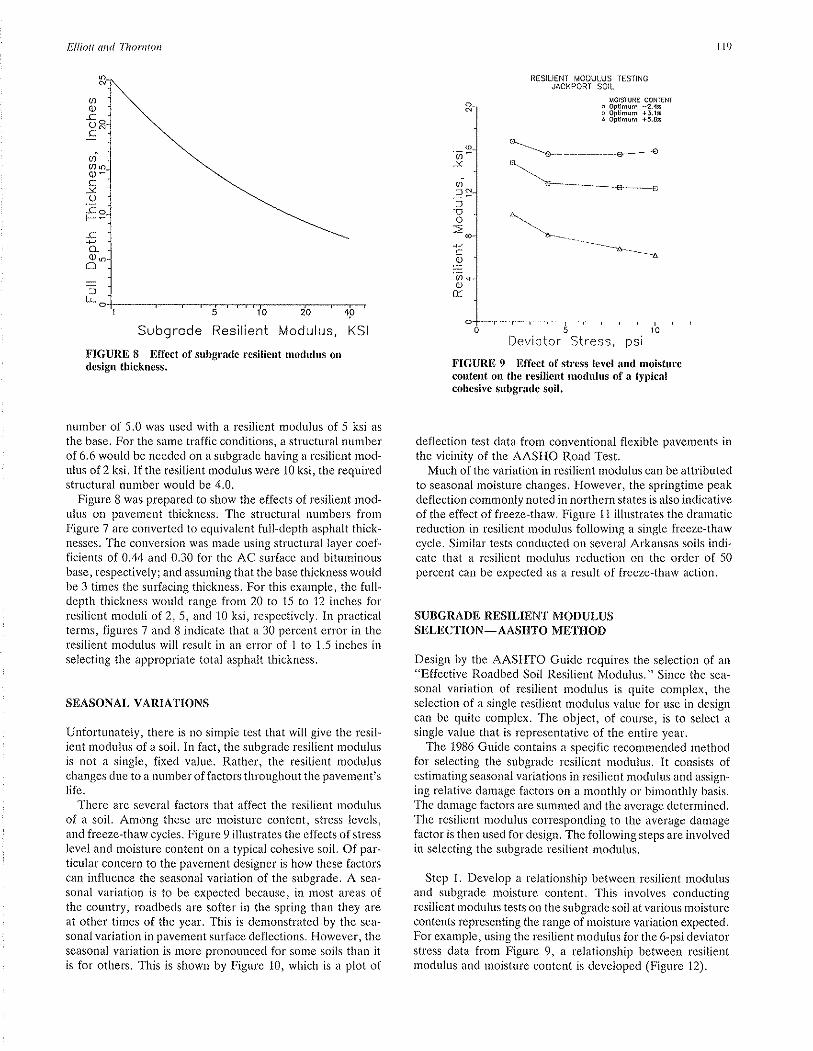
Elliott and Thomton

Subgrode Resilient Modulus, KSI

FIGURE 8 Effect of subgrade resilient modulus ondesign thickness.

number of 5.0 was used with a resilient modulus of 5 ksi as

the base. For the same traffic conditions, a structural numberof 6.6 would be needed on a subgrade having a resilient mod-ulus of 2 ksi. If the resilient modulus were 10 ksi, the requiredstructural number would be 4.0.

Figure 8 was prepared to show the effects of resilient mod-ulus on pavement thickness. The structural nurnbers fromFigure 7 are converted to equivalent full-depth asphalt thick-nesses. The conversion was made using structural layer coef-ficients of 0.44 ancl 0.30 for the AC surface and bituminousbase, respectively; and assuming that the base thickness wouldbe 3 times the surfacing thickness. For this example, the full-depth thickness would range from 20 to 15 to 12 inches forresilient moduli of 2,5, and 10 ksi, respectively. In practicalterms, figures 7 and 8 indicate that a 30 percent error in theresilient modulus will result in an error of 1 to 1.5 inches inselecting the appropriate total asphalt thickness.

SEASONAL VARIATIONS

Unfortunately, there is no simple test that will give the resil-ient modulus of a soil. In fact, the subgrade resilient modulusis not a single, fixed value. Rather, the resilient moduluschanges due to a number offactors throughout the pavement'slife.

There are several factors that affect the resilient modulusof a soil. Among these are moisture content, stress levels,and freeze-thaw cycles. Figure 9 illustrates the effects ofstresslevel and moisture content on a typical cohesive soil, Of par-ticular concern to the pavement designer is how these factorscan influence the seasonal variation of the subgrade. A sea-sonal variation is to be expected because, in most areas ofthe country, roadbeds are softer in the spring than they areat other times of the year. This is demonstrated by the sea-sonal variation in pavement surface deflections. However, theseasonal variation is more pronounced for some soils than itis for others. This is shown by Figure 10, which is a plot of

RESILIENT MODULUS TESTINGJACKPORT SOIL

MOISIURE CONTENTo oÞtimum -2.4¡o ootimum +5.1¡Â Oþtiñum +5.6¡

_T-a--]---_-l_--T--5 r0

Deviotor Stress, psi

FIGURD 9 Effect of stress level and moisturecontent on the resilient modulus of a typicalcohesive subgrade soil.

deflection test data from conventional flexible pavements inthe vicinity of the AASHO Road Test.

Much of the variation in resilient modulus can be attributedto seasonal moisture changes. However, the springtime peakdeflection commonly noted in northern states is also indicativeof the effect of freeze-thaw. Figure 11 illustrates the dramaticreduction in resilient modulus following a single freeze-thawcycle. Similar tests conducted on several Arkansas soils indi-cate that a resilient modulus reduction on the order of 50percent can be expected as a result of freeze-thaw action.

SUBGRADE RESILIENT MODULUSSELECTION_AASHTO METHOD

Design by the AASHTO Guide requires the selection of an"Effective Roadbed Soil Resilient Modulus." Since the sea-sonal variation of resilient modulus is quite complex, theselection of a single resilient modulus value for use in designcan be quite complex. The object, of course, is to select a

single value that is representative of the entire year.The 1986 Guide contains a specific recommended method

for selecting the subgrade resilient modulus. It consists ofestimating seasonal variations in resilient modulus and assign-ing relative damage factors on a monthly or bimonthly basis.The damage factors are summed and the average determined.The resilient modulus corresponding to the average damagefactor is then used for design. The following steps are involvedin selecting the subgrade resilient modulus.

Step 1. Develop a relationship between resilient rnodulusand subgrade moisture content. This involves conductingresilient modulus tests on the subgrade soil at various moisturecontents representing the range of moisture variation expected.For example, using the resilient modulus for the 6-psi deviatorstress data from Figure 9, a relationship between resilientmodulus and moisture content is developed (Figure 12).

ll9

@g)

o;:JN:l

!o

@

ce'õo(¡)

E.

120

Step 2. Estimate the seasonal variation in moisture content.Although there is no standard approach for making this esti-mate, a practical approach might be to sample a similarsubgrade. For this example it is assumed that moisture con-tents were determined four times during the year on a similarsubgrade soil from a nearby pavement. From these a seasonalvariation has been estimated as shown in Figure 13.

Step 3. Determine the monthly (or bimonthly) resilientmodulus. Figures 12 and 13 are used to estimate the resilientmodulus for each month of the year. The monthly values areentered on the AASHTO form (Figure 14). For example, themoisture content in March is about 25 percent. From Fig-

RESILIENT MODULUS TESTINGJACKPORT SOIL

ô No Facct!-fhow. Altø Frcczc-lhow

l _'-r'.T-ffi-=-f---5 10

Deviotor Stress, psi

FIGURE f f Effect of freeze-thaw on theresilient modulus of a typical cohesive subgradesoil.

TRANSPORTATION RESEARCH RECORD I 196

ure 12, the resilient modulus for 25 percent moisture contentis 9,500 psi. Except for January and February, the resilientmoduli for other months are found in a similar fashion. ForJanuary, it is assumed that the subgrade will be frozen result-ing in a very high resilient modulus. February is assumed tobe a period of thawing. To account for the freeze-thaw effect(Figure 11), the resilient modulus is determined in the normalfashion and reduced by 50 percent.

Step 4. Select a relative damage factor for each resilientmodulus. Relative damage factors corresponding to the monthlyresilient modulus values are selected using the scale on theright side of Figure 14. For the frozen subgrade (January),the resilient modulus would be high resulting in a low relative

Moisture Content, g

FIGURE 12 Moisture content-resilient modulusrelationship for soil used in example.

.10

¿c€ .06oo¡Ëoo .04

-o2

MAR. JUNE SEPT. DEC.

Time of Year

FIGURE 10 Seasonal variations in pavement deflections on various soils (datafrom lllinois Department of Transportation).

(nl¿

g;trfroo

Elliott and Thornton

JAN APR JUL OCT

FIGURE 13 Seasonal mo¡sture var¡at¡on used inexample.

t2l

damage factor. For practical purposes, a damage value of 0.0is assigned.

Step 5. Use the average monthly relative damage fâctor toselect the Effective Roadbed Soil Resilient Modulus. Theaverage damage value (.063) is used with the scale on theright side of Figure 14 to select the Effective Roadbed SoilResilient Modulus (9,900 psi) to be used in design.

ALTERNATIVE SELECTION APPROACH

The above method requires testing each soil at several dif-ferent moisture contents. An alternative approach would beto test each soil at a single representative "time-of-year" mois-ture content. Elliott and Thompson (/2) conducted an analysisto find the appropriate "time-of-year" condition that wouldbe representative of the entire year for the AASHO RoadTest pavements. The study included (a) an investigation ofthe seasonal variation of resilient modulus at the AASHORoad Test, and (b) a determination of the seasonal load dam-

R

Ëzl¡Jl-zoC)

tdÉ.lt-Øo

Month

RoadbedSoil

Modulus,M* losil

Relat¡veDamage,

ut

Jon.30,000 .005

Feb.5. s00 .25

Ma¡.9,500 .070

Apr.8,900 .081

May8. 600 .088

June r r .000 .050

July12,700 .038

Aug. I 3 .000 .034

Sept. l3 , 100 .033

Oct.12,800 .035

Nov.12,700 .036

Dec.12.300 .038

Summation: Eu, = 758

= .063

Eftcctiv€RoodbcdSoil Rosili€ntModulus,M.lpsil - 9,9U0 (correspondstoi¡r,

FIGURE 14 Example determination of design resilient modulus by the AASHTOmethod.

=oo

d

!;3fÞoE5c3õoæ

oU'ooooooG

lruoi d,31C

À>-Q'X.ào!9Ë;

:x

lc9ofoU

Average: i, = Eu,

122

age effects for pavements with various thicknesses of asphalt.Their study was based on asphalt fatigue damage effects andincluded consideration of seasonal variation in the AC stiff-ness modulus as well as the subgrade resilient modulus.

The seasonal subgrade resilient modulus variation (basedon analysis of deflection measurements taken during theAASHO Road Test) is shown on Figure 15. Figure 16 is theseasonal load damage effects expressed as a \Veighting Factor.Elliott and Thompson concluded that no single resilient mod-ulus could truly represent all pavement thicknesses. However,since all curves intersected in a fairly tight pattern in late

TRANSPORTATION RESEARCH RECORD I 196

April and mid-October, they stated that conditions duringeither of those periods should be acceptable for designpurposes.

The disadvantage of using this alternative selection approachis the need to identify the representative "time-of-year" con-ditions. Limited analyses suggest that late spring conditionsshould be reasonable for most areas of the United States andprobably no worse an approximation than the seasonal mois-ture variation estimate required by the AASHTO method.The advantage of this approach would be a significant reduc-tion in the amount of testing needed for an individual soil

6¡to:'t!o.Ba,

åoÊ.,EC'

oât(t,

T¡me ol Yeor

FIGURE 15 Seasonal subgrade resilient modulus variation at the AASHORoad Test (I2).

o(,C'l!ctt ,t-E.9o3

Jon Moy Sept

Time of Yeor

FIGURE 16 Seasonal weighting factors for various thicknesses ofasphaltsurfacing (12).

Elliott and Thornton

toooo

'High DensilyAASHTO T-I8O

lntermediote DørsityAASHTO T-99

lo 20 30 40 60 80 tooe" 0j+2Q,psi

FIGURE f7 Effect of density on resilient modulusof a granular base material (.13).

sample. This would permit testing more soils for the sametesting effort.

RESILIENT MODULUS IN PERSPECTIVE

Resilient modulus is a significant and rational material prop-erty that needs to be included in the pavement design process.However, the resilient modulus does not represent all prop-erties of a subgrade or granular layer that can affect the per-formance of a pavement.

The most direct evidence that other properties are alsosignificant comes from the AASHO Road Test (4). Two gran-ular materials were used-crushed stone and gravel. Of these,the gravel base sections deflected less. Inch for inch, the gravelwas more effective in reducing the deflections. This suggeststhat the gravel possessed the higher resilient modulus. Never-theless, the crushed stone sections had the superior perfor-mance. As stated in the Road Test report: "Perhaps the gravel

t23

possessed less internal stability than the stone; yet it may havebeen somewhat less resilient (i.e., higher resilient modulus)."

Similarly, Figure 17 indicates that density has only a limitedeffect on resilient modulus of a granular material. This couldlead one to conclude that density is not significant. However,Figure 18 shows that density is quite significant relative topermanent deformation (strain).

Resilient modulus reflects only the rebound or resilientdeformation behavior of the material. In so far as this relatesto the load-induced stresses, strains, and deflections, resilientmodulus is irnportant and significant. However, the resilientmodulus is not a good indicator of rutting potential. For manymaterials, the permanent deformation (rutting) behavior maywell be the factor controlling pavement life. Therefore, resil-ient modulus must not be the only property considered indesigning and selecting materials for a flexible pavement;layer coefficients based solely on resilient modulus can bemisleading.

CONCLUSIONS

1. Resilient modulus is a fundamental material property.It relates to pavement design and performance for the samereason that surface deflection relates. It provides a measureof the load-induced stress-strain behavior of the soil and gran-ular base layers which in turn governs the load response ofthe pavement system.

2. Resilient modulus should not be the only property con-sidered in judging the acceptability of a soil or granular mate-rial. Because resilient modulus provides no measure of thepermanent deformation (rutting) behavior, the selection of agranular material and assignment of layer coefficients basedsolely on resilient modulus can be misleading.

3. Many factors affect the resilient modulus causing it tovary seasonally throughout the life of the pavement. Conse-

aï 4oooo¡58 soooo

=

E 2ooooqa,q

É.t¡J

{CLt)

c'õ

Ø

gebEbfL

2,6

2,O

1.5

LO

o.5

ol lo loo tooÖ to,ooo

Numbsr of Lood Appllcotlons.N

FIGURE l8 Effect of density on permanent deformation behavior of a granular basematerial (13).

All Somples ore Su$ecled touDeviotor Slross of 45 psi

ond o Confining Prossure of lSpsi

g5%'AASHTO T-99

t00% AASHT0 T-99

124

quently, the selection of a single soil resilient modulus for usein design can be complicated.

4. While on paper the AASHTO Guide selection proce-dure is rational and straightforward, the estimation of sea-sonal moisture variation can be quite nebulous and the amountof testing required very time consuming. Consequently, amore practical approach is to test under a single, represen-tative time-of-year condition. Late spring is a reasonable firstapproximation of the appropriate time of year for most of theUnited States.

ACKNOWLEDGMENTS

This paper is in part based on Project TRC-94, "ResilientProperties of Arkansas Soils," which is being conducted bythe Arkansas Highway and Transportation Research Center.TRC-94 is sponsored by the Arkansas State Highway andTransportation Department and the U.S. Department ofTransportation (Federal Highway Administration).

REFERENCES

l. AASHTO Guide for Design of Pavement Structures. Amer-ican Association of State Highway and Transportation Offi-cials, Washington, D.C., 1986.

2. AASHO Interim Guide for Design of Pavement Structures.American Association of State Highway Officials, Washing-ton,D,C,,7972.

3. G. Langsner, T. S. Huff, and W. J. Liddle. Use of RoadTest Findings by AASHO Design Committee.lnspecial Report73: The AASHO Road Tesr, HRB, National Research Coun-cil, Washington, D.C., 1962, pp.399-438.

4. Special Report6I E-The AASHO Road Test, Report 5 : Pave-ment Research. HRB, National Research Council, Washing-ton, D.C., 1962.

5. M. E. Bvrt. Progress in Pavement Desþn. TRRL Report LR

TRANSPORTATION RES EARCH RECORD I 196

508. Transport and Road Research Laboratory, Departmentof the Environment, England, 1972.

6. Canadian Good Roads Association. Field Performance Stud-ies of Flexible Pavements in Canada. Proc., 2nd InternationalConference on the Structural Design of Asphalt Pavements,Ann Arbor, Mich., 1967.

7. F. N. Hveem. Pavement Deflections and Fatigue Failures.Bulletin //4, HRB, National Research Council, Washington,D.C., 1955.

8. F. P. Nichols. Deflections as an Indicator of Flexible Pave-ment Performance. In Highway Research Record 13, HRB,National Research Council, Washington, D.C., L963.

9. Special Report 22: The WASHO Road Test, Part 2, Test Data,Analysis, Findings. HRB, National Research Council, Wash-ington, D.C., 1955.

i0. R. I. Kingham. Development of the Asphalt Institute's Deflec-tion Method for Designing Asphalt Concrete Overlays forAsphalt Paveme¿ts. Research Report 69-3, The Asphalt Insti-tute, 1969.

11. M. R. Thompson and R. P. Elliott. ILLI-PAVE-BasedResponse Algorithms for Design of Conventional FlexiblePavements. ln Transportation Research Record 1043, TRB,National Research Council, Washington, D.C., 1985.

12. R. P. Elliott and M. R. Thompson. ILLI-PAVE MechanisticAnalysis of AASHO Road Test Flexible Pavements. InTransportation Research Record 1043,TRB,National ResearchCouncil, Washington, D.C,, 1985.

13. Techniques for Pavement Rehabilitation. National HighwayInstitute, FHWA, 1984.

The conîents of this paper reflect the views of the authors, who areresponsible for the facß and accuracy of the data presented herein.The contents do not necessarily reflect the official views or policiesof the Arkansas State Highway and Transportation Department orthe Federal Highway Administration. This paper does not constïtute a standard, specification, or regulation,

Publication of this paper is sponsored by the Commitlee on Strengthand Deþrmation Characteristics of Pavement.

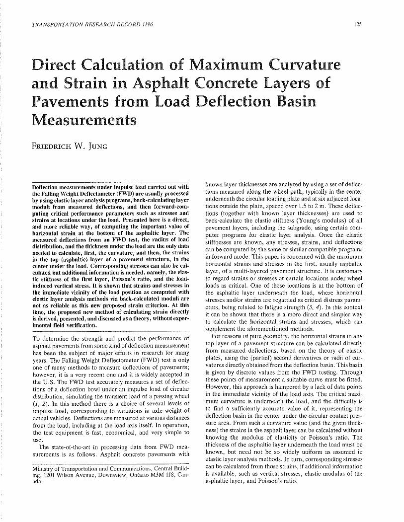
TRANSPORTATION RESEARCH RECORD 1 196 t25

Direct Calculation of Maximum Curvatureand Strain in Asphalt Concete Layers ofPavements from Load Deflection BasinMeasurements

Fnrnpnrcs W. JuNc

Deflection measurements under impulse load carried out withthe Falling Weight Deflectometer (FWD) are usually processed

by using elastic layer analysis programs, back-calculating layermoduli from measured deflections, and then forward.com.puting critical performance parameters such as stresses andstrains at locations under the load. Presented here is a direct,and more reliable way, of computing the important value ofhorizontal strain at the bottom of the asphaltic layer. Themeasured deflections from an FWD test, the radius of loaddistribution, and the thickness under the load are the only dataneeded to calculate, first, the curvature, and then, the strainsin the top (asphaltic) layer ot'a pavement structure, in thecenter under the load. Corresponding stresses can also be cal.culated but additional information is needed, namely, the elas.tic stiffness of the first layer, Poisson's ratio, and the load-induced vertical stress. It is shown that strains and stresses inthe immediate vicinity of the load position as computed withelastic layer analysis methods via back-calculated moduli arenot as reliable as this new proposed strain criterion. At thistime, the proposed new method of calculating strain directlyis derived, presented, and discussed as a theory, without exper-imental field verification.

To determine the strength and predict the performance ofasphalt pavements from some kind of deflection measurementhas been the subject of major efforts in research for manyyears. The Falling Weight Deflectometer (FWD) test is onlyone of many methods to measure deflections of pavements;

however, it is a very recent one and it is widely accepted inthe U.S. The FWD test accurately measures a set of deflec-tions of a deflection bowl under an impulse load of circulardistribution, simulating the transient load of a passing wheel(1,2). In this method there is a choice of several levels ofimpulse load, corresponding to variations in axle weight ofactual vehicles. Deflections are measured at various distancesfrom the load, including at the load axis itself. In operation,the test equipment is fast, economical, and very simple touse.

The state-of-the-art in processing data from FWD mea-surements is as follows. Asphalt concrete pavements with

Ministry of Transportation and Communications, Central Build-ing, 1201 Wilson Avenue, Downsview, Ontario M3M 1J8, Can-ada.

known layer thicknesses are analyzed by using a set ofdeflec-tions measured along the wheel path, typically in the centerunderneath the circular loading plate and at six adjacent loca-tions outside the plate, spaced over 1..5 to2m. These deflec-tions (together with known layer thicknesses) are used toback-calculate the elastic stiffness (Young's modulus) of allpavement layers, including the subgrade, using certain com-puter programs for elastic layer analysis, Once the elasticstiffnesses are known, any stresses, strains, and deflectionscan be computed by the same or similar compatible programsin forward mode. This paper is concerned with the maximumhorizontal strains and stresses in the first, usually asphalticlayer, of a multi-layered pavement structure. It is customaryto regard strains or stresses at certain locations under wheelloads as critical. One of these locations is at the bottom ofthe asphaltic layer underneath the load, where horizontalstresses and/or strains are regarded as critical distress param-eters, being related to fatigue strength (3, 4). ln this contextit can be shown that there is a more direct and simpler wayto calculate the horizontal strains and stresses, which cansupplement the aforementioned methods.

For reasons ofpure geometry, the horizontal strains in anytop layer of a pavement structure can be calculated directlyfrom measured deflections, based on the theory of elasticplates, using the (partial) second derivatives or radii of cur-vatures directly obtained from the deflection basin. This basinis given by discrete values from the FWD testing. Throughthese points of measurement a suitable curve must be fitted.However, this approach is hampered by a lack of data pointsin the immediate vicinity of the load axis. The critical maxi-mum curvature is underneath the load, and the difficulty is

to find a sufficiently accurate value of it, representing thedeflection basin in the center under the circular co¡ltact pres-sure area. From such a curvature value (and the given thick-ness) the strains in the asphalt layer can be calculated withoutknowing the modulus of elasticity or Poisson's ratio. Thethickness of the asphaltic layer underneath the load must beknown, but need not be so widely uniform as assumed inelastic layer analysis methods. In turn, corresponding stressescan be calculated from those strains, if additional informationis available, such as vertical stresses, elastic modulus of theasphaltic layer, and Poisson's ratio.

126

STRESSES AND STRAINS FOR CIRCULARLYDISTRIBUTED LOADS

For such a single load, well inside a (non-cracked) pavernent,the second derivative or curvature of the deflection basinunder the load axis can be assumed to be a maximum, andequal in all directions because of the circular contact pressurearea. The following equations apply:

Plate stiffness

-- ETFK:-12(t - ¡Ê)

Bending moment

M=-KW"(l +rr)Horizontal stress

S = 6MlH

Horizontal strain

e: S(1 - p)tE

where

K = bending stiffness of plate,E = elastic stiffness of asphaltic layer(s),¡1 : (total) thickness of asphaltic layer(s),F = Poisson's ratio,W : deflection as a function of distance,

Il/" : second derivative of deflection at zeÍo distance,M = bending moment under the load at zero distance,S = maximurn stress at bottom of asphaltic layer, and¿ = maximurn strain at bottom of asphaltic layer.

Note: The second derivative is negative. Bending moments,stresses and strains are equal in all directions.

Without a knowledge of the material properties of the firstlayer (the modulus, E, and Poisson's ratio), the strain, e, canstill be calculated from pure geometrical conditio¡rs:

either

e = W"H/2

or

e = Ht(zR)

The stress is then

S:eûl[(l-p.Xl +s,/s)]where

R : radius of curvature in mm, andS, : vertical stress in MPa.

At this stage, in order to calculate corresponding stressesfrom strains, additional information is required, namely theelastic stiffness (E) of the first asphaltic or concrete layer,the Poisson's ratio of this layer, and the vertical stress (S") atthe particular point. This vertical component of stress rnustbe obtained by an elastic layer analysis program; however, asimple version based on equivalent layer thickness would besufficient for an estimate of such stress.

The equations quoted above are based on the concept ofregarding the asphaltic layer as an elastic plate. This plate,

TRANSPORTATION RESEARCH RECORD 1 196

as a free body, deforms or deflects under two forces, theapplied wheel load or falling weight impulse load acting moreor less concentrated from above, and the corresponding reac-tions of soil pressure from the layers underneath, acting ontothe plate from below in a more distributed fashion (Figure1a). For a given load, the deflection bowl, its depth and large-ness, depends on the stiffness of the plate and the relativestiffness or strength of the base or soil layers underneath.

Equations 5, 6, and 7 constitute a direct calculation of hor-izontal strain and stress in the A.C. layer. However-andthis is the difficult part-it is now necessary to find an expres-sion for the curvature or second derivative from an accuratedeflection function.

CURVATURE CALCULATION INSIDE THECONTACT PRESSURE AREA

The maximum value of the second derivative (W") or cur-vature (1/,1?) of the asphaltic layer, for a circular, uniformlydistributed load þ), is located in the center of this circularcontact pressure area. The value, W", can be derived inaccordance with elastic plate theory. For the derivation, thefollowing general assumptions should be noted:

1. Single tire loads and impulse loads from the FWD testare uniformly distributed over a circular area.

2. The resultant load per unit area on the circular part ofthe asphaltic layer "plate" has a paraboloidal distribution, forthe following reason. Within the loaded area, frorn -a to+d, the tire or plate contact pressure ¡nust be combined withthe soil pressure acting from below, resulting in a reduceddiagram of parabolically distributed load as shown in Figure2. The resultant area load (i.e., load per unit area) on theasphaltic layer plate in this region is actually assumed to bedistributed in the form of a square paraboloid. (The derivationof the exact solution for this case from the differential equa-tion of circular plates is not presented here.) The result formaximum curvature is:

w,(o) = -2(Yt: Y.)

- a2(9Pn-!P)

(s)

where

W'(0) = second derivative in the center, in 1/mm;Yr = maximum deflection in the center, in mm;Y" = deflection at the edge of the loaded area, in mm;a = radius of the loaded area, in mm;p = circular contact pressure from load, in MPa;

po = resultant pressure in the center, in MPa;po : resultant pressure at the edge, at a, in MPa;K = plate stiffness (Equation 1); andr = distance from the cerìter, in mm.

A better understanding of the curvature function or secondderivative, W", within the circular contact pressul'e area canbe achieved by studying W" as a function of distance, ¡:

w(0)= -z(Y'\-Y') -*u

(1)

(2)

(3)

(4)

(s)

(6)

(7)

x (a, - 6Ò - P-:--!e (aa - 15f) (9)

t27

a/ pavom€nt load and delormalion

b/ measured delloclion, yr to yn (not )6 )

FIGURE I Deflection basin geometry.

x2

n = Oo* {Png¡$

FIGURE 2 Load distribution between -aand ta.

Equation 9 is plotted for a typical example as illustrated inFigure 3. Note, the maximum curvature is at r = 0, namely5.422*10-6(llmm). The first term of Equation 8, by itself,would lead to a value of. 4.764*L0-6 (l/mm), which can beinterpreted as an average within a distance, r, of about 100mm. This slightly lower value of average curvature agrees

fairly well with values obtained from manual curvature cal-culations using simulated Chevron deflection output, as shownbelow. Thus, the first term of Equation 8 or 9 constitutes anapproximate calculation of curvature compatible \ryith elasticlayer analysis programs, â smaller value than the actual max-imum. This first term would be an exact solution for a hypo-

¡+ xoryIII

I

Y¡

\Ye

_l \'-

Y2

Á

lYt Yn

"--rIy=,

second term = f(r,a,p,K)

first term =

S0 i00 a= 150 mm

FIGURE 3 Radial curvature in the asphattic layer.

TRANSPORTATION RESEARCH RECORD I 196

thetical case in which the soil pressure, q, and the contactpressure, p, were removed, and the plate were loaded via acircular ring of radius, a.

Unfortunately the deflection, Yo, cannot be measured, butmust be calculated by interpolation using the other measureddeflections. The ensuing error is positive, i.e., in the directionof higher values, being closer to the theoretical maximum(tables 1 and 2). Further, the deflection basin consists of twodifferent parts, i.e., oftwo curves not continuous in all deriv-atives, The inner part (-a to +ø) has been accurately derived,resulting in Equation 9. The outer part only is empiricallygiven by the measurements of outside sensors.

The curve-fitting function chosen is a reciprocal polynomial(Z) (Figure 1). It is used only to calculate the very influentialand important value of the deflection, Yo, at the edge of theloaded area (i.e., at x : a) by interpolation.

The curve-fitting and interpolation procedure to computean approximate substitute for the theoretical value of Y"becomes more reliable, thus leading to less erratic results,when the first outside sensor (Yr) is as close to the circulardisk as possible and when the center point deflection is includedas part of the curve (as illustrated in Figure lb and 1c), in

2(y I ya)

a2

TABLE 1 COMPARISON OF STRAIN R IVITH CHEVRON/ELSYMs

DESCRIPTIONCURVATURES* L0-6

1/run

STR.E IN

'r L0-6

DIRECT ELSYMs/ DIRECT

CHEVRON

ELSYM5/CHEVRON

bottom average

Typical 3-Iayer casea = l-50 mm, H = 100 mm

Typical 4-layer casea = 150 rün, H = 100 mm

Overload case, 2.5xa = 150 mm, H = l-00 mm

Deep strength 140 mmon weak soil

Reduced area a = L02 mmhigh pressure 400 psi

Wider area, a=203 mrn

normal pressure

Typical 3-1ayer caseaverage deflection

Very soft layer in-serted under asphalt

-5.160

-5 .426

-t4.46

-4.334

-26.97

-8 .753

-5.066

-8.438

-4.80

-5.28

-13.8

-4 .53

-26,75

-8. 66

-5.18

-8.74

258 .0

2'tt.3

642 .6

302.'7

r.198 . 9

389.0

253.3

42r .9

r.70.4 193

185.7 255

423.0 520

2'18.2 218

'786.4 860

243 ,2 341

208.2 204

383.8 38s

Note:In t.he Last column, "average" means the average of the absoLu¿e valueof the top and bottom stlains of the first layer from the outputlisting of CHEVRON or ELSYMS. These vaLues in the last colunn ought tobe close tö or equaJ. to H/2 times the curvature vaLues in the secondcolumn. This identity check wouLd estabLish consistency within theCHEVRON or ELSYMs programs themselves, not invoLving the STRAINR model-.Note that the check fails except in the case of a very soft insertedlayer in the Last line.

Jung t29

TABLE 2 CURVATURE BY SECOND DIFFERENCES VERSUS EQUATION 8

CASE

(see also Table 1)

SECOND DIFFERENCES EQUATION B

[1/mm¡ *19-e [1,/mm¡ *16-e

L/ Typical 3-1ayer case

2/ A-Layer case, example

3,/ Overl-oad case, 2,5 x

4/ Deep strength, weak soil5,/ Reduced area, high pr.6/ vfide area, normal pr.7,/ 3-layer case, av. def 1.

8/ Soft 2nd layer inserted

-4. B0

-5.28-13.78-4.53

-26.'75-8.66-5.182-8 .'7 44

-5.475-6.018

-15.535-4 . 603

-28 .93r-9.'722-5.562-B.875

^ (Y, - Y")2 + a2

z(Yt - Y")

where

spite of the fact that it belongs to the inner part which is

rnathematically different. Nevertheless, a useful solution has

been established which has been verified as follows:The first term ofboth Equations 8 and 9, using the accurate

value of Y", leads to practically the same curvatures as obtaitredby using the method of second differences, for the same datafrom Chevron or ELSYMS simulation examples.

Comparative computations show that the exact calculationof curvature by Equation 8 results in larger values (up to 15

percent) than the second differences from Chevron or ELSYMS.These results from second differences compare much betterwith the first term of Equations 8 or 9, omitting the secondterm. Thus there is a valid argument to dispense with thisterm which requires additional information about the asphal-tic layer. Thus, the following Equation 10 can be used tocalculate the minimum radius of curvature, R:

culations (based on Equation 11) with those from a corre-sponding case calculated by the Chevron program. For run-ning the small program of the proposed method, calculatedChevron deflections were selected as input, simulating fea-sibly-spaced FWD measurements, in the center and at fourother points outside the circular load area. In addition to thesemeasurements, the following data are needed to run the newprogram:

Radius of load areai a = 150 mm; layer thickness: H : 100

mm

The deflections chosen from the Chevron example output,used as simulated input into the new program, are as follows:

at 0.0 m 0.4903 mm

at 0.2 m 0.3951 mm

at 0.3 m 0.3394 mm

at 0.4 m 0.2949 mm

at 0.5 m 0.2585 mm

The following values were calculated by the proposed method:

Deflection at the edge of the loaded arcal. Y = 0.4293 mm(the actual Chevron value is 0.4305, an inevitable error incurve-fitting and interpolation)Radius of curvature at the center: R : - 184.3 mSecond derivative at center: W" = -5.43 * 10-ó (limm)Strain at bottom of asphaltic layer: e : +271 * 10-6

More information was needed to run the Chevron program,namely:

Load: 40.01 kN, tire pressure: 566.00 kPa, load radius: 150

mmLayer values:

(1) Modulus: 3000 MPa,100 mm

(2) Modulus: 500 MPa,

Poisson's ratio: 0.35, Thickness:

Poisson's ratio: 0.35, Thickness:200 mm

(3) Modulus: 80 MPa, Poisson's ratio: 0.35, Thickness:infinite

(10)

: maximum deflection in the center, in mm;: deflection at the edge of the load disk, in mm;: radius of the circular loading area, in mm; and: radius of curvature, in mm.

Note that the first term in the numerator is very small andcan be set to zero; then 1/R l¡ecomes exactly the first term ofthe second derivative, W", in Equations 8 and 9.

A small computer program can be written to calculate cur-vatures and strains of the asphaltic layer, based on Equation10, using a substitute value of Y. found by interpolation ofthe deflection basin function shown in Figure 1, which is curve-

fitted from relevant FWD measurements.Alternatively, one can take into account the second term

of Equation 9. This solution could ultimately be useful inconjunction with a simplified elastic layer analysis programbased on Odemark, using the concept of equivalent layerthickness.

EXAMPLE

The following example illustrates one of the verification tests

of the proposed method, comparing the new proposed cal-

YlYn

a

R

130

direct melhod ând manual

Note: (1) = surface course, (2) = base course, (3) =subgrade.

Using these input values for the Chevron program, thedeflections were calculated every 50 mm. Then the finite dif-ference method was used to manually compute the secondderivatives between X : 0 and 150 mm.

The results fluctuate somewhat inconsistently, and the aver-age was found to be -5.37, with a slightly smaller value atX : 0 of -5.28. This compares fairly well with the computedvalue of - 5.43 of the output listed above, being slightly largerand therefore closer to the theoretical maximum.

Figure 4 shows a comparison of the corresponding straincalculations. The strain diagram from the direct Chevronprintout is slightly curved at the topt it also exhibits a smallnet compressive strain. The strains of the direct output ( + 185.7* 10-ó and -246.0 * 10-o) are smaller, especially at thebottom ( + ), and the steeper slope of this strain diagram seemsto be inconsistent with the second derivative, manually com-puted from the same output (-5.37). At least the slope ofthe printed-out strain diagram of Chevron should concur withthe manually calculated curvature from the same printout(calculated by second differences).

With the strain calculated in the printout above, the stressat the bottom of the asphalt layer can be computed by meansof Equation 7. Setting S : 0, the result would be:

S = 0.000271 * 3000/0.65 = 1.25 MPa (tensile stress)

The vertical stress, S, under the load is not zero but ratheris negative, a fraction of the vertical contact pressure. Let usestimate the ratio of Sv/S to be -0.5; the value of the lastterm in the bracket of Equation 7 is then reduced to 0.5 *

0.35 = 0.175, and the factor e * E must be divided by 0.825instead of 0.65. The result is:

S = 0.000271 * 3000/0,825 = 0.99 MPa

TRANSPORTATION RESEARCH IIECO IID I 196

The corresponding value printed out from Chevron is onlyS = 0.6975 MPa

The example illustrates that curvatures or seconcl deriva-tives (1/R or W") can be calculated with great confidence andsufficient accuracy. The strain cornputed either as e : W" *Hl2, or as e = Hl2R is certainly more reliable than the incon-sistent output of the Chevron program. The stress, on theother hand, is dependent not only on layer material constants(ð and p), but also on the vertical stress component, whichcan be significant in the vicinity of the applied load.

Note: In the last column of Table 1, "average" means theaverage of the absolute value of the top and bottom strainsof the first layer from the output listing of Chevron or ELSYMS.These values in the last column ought to be close to or equalto Hl2 times the curvature values in the second I .rlumn. Thisidentity check would establish consistency within the Chevronor ELSYMS programs themselves, not involving the new directmethod. Note that the check fails except in the case of a verysoft inserted layer (Table 1).

TESTING OF THE PROPOSED NEW METHOD

Many different cases have been calculated by the Chevron orthe ELSYMS program to verify the new proposed method.The results are listed in Tables 1 and 2. In both tables cur-vatures were first calculated manually from densely spaceddeflection printouts from selected cases computed by elasticlayer analysis (Chevron or ELSYMS). The second differencesof the deflections were divided by the square of the selectedspace increments (50 or 25 mm). These manually calculatedcurvature values are listed under "Chevron/ELSYM5" in Ta-ble 1, and under "second differences" in Table 2.Then, anotherset of deflection printouts was selected in order to simulateFWD measurements, namely the deflection in the center and

91oo

ga?(o t.-NN

i B 6 . 1 o -6-

|¡å3"";t3;äï;l

80.5. 1o -6

Chevron prinlout

FIGURE 4 Comparison of strain calculation (Chevron example).

1Too

(oF.,j ¡riF-@N

Jung

some deflections outside the circular disk. These were usedto calculate curvatures in accordance with Equation 10 forTable 1., and Equation 8 for Table 2. The second term ofEquation 8 required the use of further printout values ofvertical pressures.

With regard to Table 1., it should be noted that there is afair agreement between rnanually calculated curvatures andthose calculated by the proposed direct method, listed under"direct". However, the horizontal strains at the bottom ofthe asphaltic layer do not agree (Table i, second and thirdcolumn from the right). Naturally, agreement cannot beexpected because the elastic layer analysis programs assumefull friction between the asphaltic and granular base layer,whereas the proposed direct method assumes zero friction.However, the slopes of the deflection diagrams ought to agree,concordant with the agreement in curvature.

In order to test this, the last column of Table 1 containsthe average of the absolute values of strains from top andbottom, printed out by Chevron or ELSYM5. It showsimprovement, but most of these average strains from printoutsare still too low. It seems that the elastic layer analysis pro-grams suffer from the phenomenon of quasi-singularity, whichresults in underestimating the maximum horizontal strain inthe first top layer. The assumption of full friction aggravatesthe situation. The assumption of zero friction in the proposeddirect method may not be quite correct either, however, itmay still be closer to reality to overestimate the tensile strainin this way because it may counteract neglecting the secondterm in Equation 8. Ivith regard to Table 2, for the regionunder the distributed load, from - a to + a, the curvature orsecond derivative has been independently derived by solvingthe differential equation of elastic circular plates, resulting inEquations 8 and 9. Using Equation 8, we can calculate max-imum curyatures and compare them with corresponding resultsfrom using the second differences of the deflections printedout by Chevron or ELSYM5. Eight cases, the same as inTable L, have been calculated and compared in this way, andare listed in Table 2. The comparison shows that the manualcalculations of curvature from printouts fall short of the the-oretical maxima. This proves the advantage of assuming zerofriction in the proposed direct method.

The curvatures calculated by Equation 9 are higher, andthe corresponding strains are again higher than the ones printedout by Chevron or ELSYM5.

These verification tests reveal that loads on pavements,distributed over a relatively small circular area, constitute apoint of quasi-singularity of the asphaltic "plate." This is themain reason why elastic layer analysis programs cannot catchthe true maxima of strain and curvature and why they computehorizontal strains and stresses under the load axis (close tothe load) too low.

Better results might be expected by finite element tech-niques with densely spaced grids around the contact pressurearea.

CONCLUSIONS AND RECOMMENDATIONS

For single loads on asphalt pavements, which can be assumedto be distributed over a circular area, the curvature of theasphaltic layer and the horizontal strain at the bottom of thislayer can be calculated directly from some measured values

131

of the deflection basin near the center. Other values neededare the radius of the contact pressure area, and the thicknessof the asphaltic layer at the load position. Because no otherinformation is needed (about layer materials and thicknessesof lower base layers), the horizontal strain calculated in thisparticular way is a very potent parameter for pavement design.

The bottom strain in the asphalt layer so calculated is largerthan the strain from elastic layer analysis, where full frictionbetween asphaltic and granular layers is assumed, which causestensile stresses at the top of the granular base..

Contrary to the proposed calculation of strain (based onpure geometry), the corresponding horizontal stresses areaffected by the usual uncertainties of determining materialparameters such as elastic stiffness, and Poisson's ratio.

The direct calculation of curvature and strain by this newapproach has been verified against more detailed computa-tions and output from Chevron or ELSYMS programs. Thesecond derivatives of the deflections in the center, the max-imum curvatures, were found to agree fairly well, but thecorresponding printed-out strains were found to be incon-sistent with Chevron's or ELSYMS's own deflections and cur-vatures. The slopes of printed-out strain diagrams from Chev-ron and ELSYMS did not concur (as they should have) withthe manually computed curvatures from the same runs of theprograms; thus, the maximum horizontal strains were muchtoo low. The new method has also been verified through anindependently derived formula, based on a solution of thedifferential equation of elastic plates for the region under thecircular load. The variability or function of curvature withinthe loaded area has been studied and discussed: Chevron andELSYMS deflection print-outs, via second differences, seem

to closely approximate an average cul'vature between the max-imum value at the load axis and the much lower value at a

distance from the axis about equal to the layer thickness. Thisaverage curvature is somewhat smaller than the maximumcurvature in the center, but sufficiently close to it (Figure 3).

Since the strain parameter is generally conceived to be cor-related to the fatigue strength of asphaltic pavement layers,routinely processing data from Falling Weight Deflectometertests by this new strain criterion is recommended, in additionto other current FWD processing methods.

There is as yet no immediate verification by field experi-ments of the new method proposed here. Theoretical deri-vation within an accepted theory of structural analysis andcomparison with elastic layer analysis methods can only go so

far. Thus carrying out experiments with various sizes of FWDdisks and various types and sizes of tires which may not haveexactly circular contact pressure areas is suggested. Can weuse an equivalent radius for noncircular pressure areas, andwhat would that radius be? Can we use a similar approachfor dual tires? If field experiments should prove too "rough"with respect to quality control, this might be an area forlaboratory tests.

REFERENCES

1. O. Tholen. Falling Weight Deflectometer-A Device forBearing Capacity Measurement: Properties and Performance.Department of Highway Engineering Bulletin, Vol. 1, 1980,The Royal Institute of Technology, Stockholm.

2. B. E. Sebaaly, et al. Dynarnic Analysis of Falling Weight

t32

Deflectometer Data. In Transportat¡on Reseerch Record 1070,TRB, National Research Council, lVashington D.C., 1986.

3. J. B. Rauhut, et al, Pavement Darnage Functìons for CostAllocatìon. Report F1VHA/RD-84/019. FI{\ryA, U.S. Depart-ment of Transportation, 1984 Vol. 2, Chapter 3.

4. R. B. Kulkarni, et â1. Use of Falling rrlVeighr DeflecrometerData in Predicting Fatigue Cncking. ln Trmsportøtìon Rqearch

TRANSPORTATION RESEARCH RECORD 1 196

Record 1070, TRB, National Research C.ouncil, Washington,D.C.,1986.

Publication of this paper sponsored by Comrníttee on Strength andD eformatìon CharaaerístÍcs of Pavemcnt,

TRANSPORTATION RESEARCH RECORD 1 196

Determination of Pavement LayerThicknesses and Moduli by SASW MethodSonnn Nazenreiv, KnNNnrn H. Sroxor II, Ronnnr C. BnIccs, ANDRrcHenp Rocnns

r33

Nondestructive tests are being used more than ever in evalu-ating the integrity of existing pavement systems. The nondes-tructive tests can be divided into two main categories:(l) deflection-based methods, in which devices such as theFalling \{eight Deflectometer (FWD) and dynaflect are used,and (2) wave propagation methods such as the Spectral-Anal-ysis-of-Surface-\{aves (SASW) method. The SASW methodhas several significant advantages over deflection-based meth-ods. One advantage is that moduli of thin pavement layers inthe upper portion of the pavement system can be easily andaccurately measured. A second advantage is that variations inmoduli within different layers, especially in the lower portionsof the base and in the subgrade, can be evaluated. This featureis particularly beneficial when bedrock is close to surface. Athird advantage is that layering in the pavement system doesnot have to be known. In fact, the thickness of the layers canbe determined as illustrated in the modulus profiles presentedin the paper. A series of tests was performed at nine flexiblepavement sections with significantly different profiles to eval-uate the accuracy oflayer thickness determination by the SASWmethod. The thicknesses ofthe asphaltic-concrete surface layervaried between I and 5 inches. The base and subbase materialsconsisted of substantially different materials. No informationregarding the types or thicknesses of the layers was providedduring data collection or reduction. Only after the results werereported to the Texas State Highway Department were thepavement profiles known. It was found that the SASW methodpredicted the thicknesses of the layers quite closely. In addi-tion, moduli determined by the SASW method were comparedwith moduli back-calculated from FWD tests performed at thesame sites. The variation in moduli of similar materials usedat different sections exhibit somewhat less scatler when obtainedfrom SAS\{ tests. However similar trends were found withboth methods.

The Spectral-Analysis-of-Surface-'Waves (SASW) method isa field seismic method for determining moduli and thicknessesof pavement systems. As with any in situ method, limitationsin terms of accuracy in the final modulus profiles should be

understood. The sources of these limitations can be varied.For instance, limitations can result from--

o The degree of sensitivity of the parameter being mea-sured to the moduli,

S. Nazarian, Department of Civil Engineering, The Universityof Texas, El Paso, Tex. K. H. Stokoe, II, Geotechnical Engi-neering, The University of Texas, Austin, Tex. R. C. Briggs andR. Rogers, Pavement Mânagement Section, Texas Departmentof Highways and Public Transportation.

o The amount of simplification introduced in the theoret-ical model used for data reduction,

o The degree to which the field data collection deviatesfrom the assumptions made in developing the theoretical model,

o Inevitable scatter in the data collected in the field, ando Any dependency of the method on personnel skills in

data collection and/or reduction.

To better understand the limitations of the SASW method,a series of theoretical, parametric, and sensitivity studies, as

well as extensive field investigations, have been conducted atThe University of Texas during the last several years. Thispaper presents the results of one of the field studies.

The SASW method was used at nine sites at the PavementTest Facility of Texas A&M University in Bryan, Texas, inMarch 1986. The primary objective of the tests was to evaluatethe effectiveness of the SASW method in determining thethicknesses of various layers of different materials comprisingthe pavement systems. A secondary objective was to studymoduli variations in similar materials at carefully controlledpavement sites. The results are reported herein, along withbrief background information on the SASW method and an

explanation of the procedures and data analyses. In addition,moduli obtained from FWD tests performed on the samesections are included for comparison purposes.

It should be noted that no information pertaining to thetypes of materials or thicknesses of the layers was providedat the time of testing or data reduction (except for Site 7).The material profiles reported herein were provided afterYoung's modulus profiles of the different sites were reportedto the Texas State Department of Highways and PublicTransportation.

SPECTRAL.ANALYSß.OF"SURFACE-lVAVESTESTING

General Background

The Spectral-Analysis-of-Surface-Waves (SASV/) method is

a method of seismic testing developed for determining small-strain Young's modulus profiles at pavement sites and small-strain shear modulus profiles at soil sites (1, 2). The SASWmethod is a nondestructive method in which both the sourceand receivers are located on the pavement surface. The sourceis simply a transient vertical impact that generates surfacewaves of various frequencies, which the medium transmits.Two vertical receivers, located on the surface, monitor the

134

propagation of surface wave energy past them. By analysis ofthe phase information of the cross power spectrum for eachfrequency determined between the two receivers, phase veloc-ity, shear wave velocity, and elastic moduli are determined.

The terms elastic or small-strain are generally used to describemoduli evaluated by SASW testing. These terms are used (ortheir use is implied) because stress waves generated in thistype of seismic testing create strains in the medium that areless than 0.001 percent. Moduli measured at these strain levelsare essentially constant and, hence, independent of strainamplitude (3, 4). Therefore, the medium being tested behaveslike an elastic material. This low stress level also allows fortruly nondestructive testing.

Two key points in SASW testing are the generation ofprimarily first-mode surface wave energy and the measure-ment of surface waves (Rayleigh waves) at significant dis-tances from the source. Rayleigh wave velocity, Vo, is con-stant in a homogeneous half-space and independent of thefrequency. Each frequency, /, has a corresponding wave-length, Lo, according to:

Vn=fL* (1)

Rayleigh wave and shear wave velocities are related byPoisson's ratio. In an isotropic elastic half-space, the ratio ofRayleigh-wave-to-shear-wave velocity increases as poisson,s

ratio increases. This ratio varies from 0.90 to 0.96 for valuesof Poisson's ratio ranging from 0.15 (concrete) to 0.5 (satu-rated subgrade).

If the stiffness of a site varies with depth, then the velocityof the Rayleigh wave (R-wave) will vary with frequency. Thevariation of R-wave velocity with frequency (wavelength) iscalled dispersion, The dispersive characteristic of surface wavesis the key to the SASW method. A plot of surface wavevelocity versus wavelength is called a dispersion cr¡rve. Thedispersion curve is developed from phase information ofthe cross power spectru¡n. This information provides the rel-ative phase between two signals (two-channel recorder) ateach frequency in the range of frequencies excited in theSAS\ry test. For a travel tirne equal to one period of the wave,the phase difference is 360 degrees. Thus, for each frequencythe travel time between receivers can be calculated by

t(f): ö(f)/(360f) (2)

where:

/ = frequency,t("f) = travel time for a given frequency, and$ff) = phase difference in degrees for a given frequency

The distance between the receivers, D, is a known param-eter. Therefore, R-wave velocity at a given frequency, Vo(/),is simply calculated by

v^(f) = Dtt(f) (3)

and the corresponding wavelength of the R-wave is equal to

L^(f) = v*(f))tî (4)

By repeating the procedure outlined by equations 2 through4 for every frequency, the R-wave velocity corresponding toeach wavelength is evaluated, and the dispersion curve isdetermined. Several studies have been performed recently toevaluate the optimum source/receiver array. The general array

.I'IIANSPORTATION RESEARCH RECORD I 196

PorlablsMicro-Computer

SpectralAnalyzer

VorticalReceiver

2lmpulsiveSource

\

VerticalRecsiver

1

\

þorzIts- d1_1._ D(variabte) _-rl

l¡-d2---=+lFIGURE I General configuration of SASW testing.

configuration is shown in figure 1. The distances are expressedas follows: source to near receiver = d,, source to far re-ceiver = dr, and receiver to receiver : D. Analytical studiesby Sanchez-Salinero (5) show that a desirable array config-uration can be expressed as:

d2ld, : 2 (5)

Sheu et al. (ó) combined experirnental studies on pavementswith the analytical work of Sanchez-Salinero (5) to determinethe range of wavelengths that can be accurately obtained witha fixed source/receiver spacing. They found that for an arraywith dtld, = 2 the distance between receivers can be relatedto useable wavelengths as

LR < 3D (6)

As the velocities of different layers are unknown beforetesting, it is difficult to know if the limit expressed in equation6 is satisfied. Practically speaking, it is more appropriate totest with various distances between the receivers in the fieldand then evaluate the range of wavelengths over which reli-able measurements were made. The procedure is to select aspacing between receivers, perform the test, and reduce thedata to determine the wavelengths and associated velocities.The ¡rext step is to eliminate the points that do not satisfyequation 6.

Rayleigh wave velocities determined by this method are notactual velocities of the layer, but apparent R-wave velocities(known as phase velocities). Existence of a layer with highor low velocity at the surface of the medium affects mea-surement of the velocities of the underlying layers. Therefore,a method for distinguishing shear-wave velocities from phasevelocities is necessary in SASW testing.

Inversion of the dispersion curve, or (in short) inversion,is the procedure of determining the shear-wave velocity pro-file from the dispersion curve. Inversion consists of deter-mination ofthe depth ofeach layer and the actual shear-wavevelocity of each layer from the apparent R-wave velocity ver-sus wavelength information.

The inversion process used herein is based on a modifiedversion of Thomson's (7) and Haskell's (8) matrix solutionfor elastic surface waves in a layered solid media. To simplifythe process of inversion, some assumptions were made. Theseassumptions include-

o The layers are horizontal,

Nazarian et al.

o The velocity of each layer is constant, ando The layers are homogeneous and linearly elastic.

The inversion process is an iterative process in which a

shear-wave velocity profile is assumed and a theoretical dis-persion curve is constructed. The experimental and theoret-ical dispersion curves are compared and necessary changesare made in the assumed shear-wave velocity profile until thetwo curves (experimental and theoretical dispersion curves)match within a reasonable tolerance.

Once the shear-wave velocities are determined, the follow-ing formulae are used to calculate shear and Young's moduli:

G=pV?

and

E:2G(1,+v)where

G = shear modulusE = Young's modulusp = mass density andv = Poisson's ratio

As mentioned earlier, moduli obtained in this manner arethe elastic, or small-strain, moduli. A methodology to accountfor non-linear behavior of moduli obtained for different layersutilizing the SASW method is suggested by Nazarian et al.(9). This methodology is the same as that employed in geo-technical earthquake engineering where small-strain modulievaluated by in situ seismic tests are adjusted to values appro-priate for large-strain earthquake excitation by combining(linear) field and (nonlinear) laboratory moduli.

Field Procedure

The general configuration ofthe source, receivers, and recordingequipment is shown in figure 1. Accelerometers were used as

receivers for close receiver spacings (<4 feet), and geophoneswith a natural frequency of 4.5 Hz were used as receivers forgreater spacings. This was done to optimize recording of thewave passage; that is, accelerometers produce more output

135

at closer receiver spacings where high frequencies are present,while geophones produce more output at larger receiver spac-ings where low-frequency R-waves are excited.

The common receivers midpoint (CRMP) geometry (10)was used for testing. With this geometry the two receiverswere each moved an equal distance away from an imaginarycenter line between the receivers, and the source was movedso that the distance between the source and near receiver wasequal to or greater than the distance between the two receiv-ers. In addition, the location of the source was reversed foreach receiver spacing so that forward and reverse profiles wererun. This testing sequence is illustrated in figure 2. Distancesbetween receivers of 0.5, 1, 2,4, and 8 feet were used at eachsite.

Different sources were used. For close receiver spacings, a

4-oz hammer was used. For greater distances, 2.5- and 5-lbsledge hammers were employed, with the largest hammergenerally used at the 8-ft spacing.

The recording device was a Hewlett-Packard 35624 Fourierspectral analyzer. This analyzer is a digital oscilloscope com-bined with a micro-processor that can perform directly ineither the time or the frequency domain.

It is worthwhile noting here that the field procedure out-lined above results in the performance of essèntially two tests,one for the forward profile and one for the reverse profile.The results (in terms of dispersion curves) are typically veryclose, so that an average dispersion curve is calculated fromthe forward and reverse tests. One can think of this type oftesting as a L-test run at each site for the SASW method.However, the SASrff method is very repeatable at the samesite, with typically less than a five percent scatter among threeor more tests (ó, 11). Therefore, duplicate SASW tests werenot performed in this study.

PRESENTATION OF RESULTS

Description of Sites

The general layout of the pavement test facility constructedat Texas A&M University in the mid-1960s is shown in fig-ure 3. This facility, which is 460-ft long and 50-ft wide, consists

(7)

(8)

-12 -8 -4 q_ 4 I 't2

,%i,t!

t!zt'it 0.5

V Geophone

0 Source

)¿t-s

%tg

1

t¿t----r¿-

wl_l¿ 2

g_t----iz-

vlf'

4

E-L=-v--

vlv I

FIGURE 2 Schematic of experimental arrangement for SAS\{ tests.

f1,lffi| l-,T-l1,il-l -n].l ,5 I

ll,r.1 6 frijl

r*l| 14 ll 15lfi3 I

I 1r-l frr I h. rt

FIffi.lWMN

ffi

l3ó

SASII Tests were Perfonned at the Nine Highlighted Sections (Nos. 2,4,7,9,10, 11, 16, 17 and lB).

TRANSPORTATION RESEARCH RECORD I 196

LS: Crushed Limestone43 Cement GR: Sandy Graveì23 Lime SC: Sandy Clay

PC: Plastic Clay

Nine randomly selected sections were tested in March 1986.The nine sections are marked in figure 3. Material profiles ofall sections, as reported by Scrivner and Michalak (12), areincluded in table 1. The top layer is always asphaltic-concretepavement. Base and subbase materials are either crushedlimestone or a mixture of crushed limestone with lime or

SHOULDER LINE

LTMESTONE H.M.A.C.LIMESTONE

LIMEST0NE+LIME

LIMESTONE

FIGURE 3 General layout of pavement test facility at Texas Transportation Institute.

AC: Hot llix Asphaltic ConcreteLS+C: Crushed Limestone mixed withLS+L: Crushed Limestone mixed with

of 27 different pavement sections. Each section is approxi-mately 40-ft long and 12-ft wide. Some of the sections in thefacility do not represent typical pavenient sections encoun-tered on roads, since the main function of the facility was todetermine the limitations and versatility of nondestructivetesting methods.

TABLE 1 MATERIAL PROFILES OF TTI PAVEMENT TEST FACILITY Q2)

;ecti onThickness (in.) llateriaI Type

Su rface Base Su bbase Embank. Su r face Base Subbase Embank.

2

4

7

9

l0

tì16

l7

l8

I

5

I

5

I

I

5

3

'|

12

12

4

4

12

4

t2

8

B

4

1?

1?

4

4

12

12

II

36

24

36

40

36

36

24

34

36

AC

AC

'AC

AC

AC

AC

AC

AC

AC

LS+C

LS+C

LS

LS

LS

LS

LS+C

LS+L

LS+L

LS

LS

LS+C

LS

LS

LS

LS+C

LS+L

LS+L

PC

PC

PC

GR

GR

GR

GR

sc

sc

Nazarian et al.

cement. Subgrade materials consist of three different sands

or clays. Engineering properties of each material determinedby laboratory tests are given in table 2.

Dispersion Curves

Typical dispersion curves from SASW testing at two of theni¡re sites (Sites 4 and 11) are shown in figures 4 and 5. (These

curues represent the average values for the forward and reverse

2000 4000

Phase Velocily, fps

FIGURE 4 Dispersion curve fromSASW tests at section 4.

r37

TABLE 2 ENGINEERING,PROPERTIES OF MATERIALS USED IN CONSTRUCTIONÔF TTI PAVEMENT FACILITY (12)

*By Texas trlaxial procedure at a lateral pressure of 5 psi

Note: The natura'l m¡terial below the erùankrents was plastlc c'lrysimiìar to that desc:^ibed above, changing to a denser clay ata depth of about 90 inches belovr the surface of the pavercnt.The dense clay ls abbreviated DC; its properties were notdetermined in the laboratory.

€4ocIo6

=6

€4¿o-9o

=6

profiles at each site.) Spectral analysis functions measured at

these sites are not presented for the sake of brevity. Typicalfunctions can be found in Nazarian and Stokoe (2). However,the quality of the data collected in the field was very good.

Shear-Wave Velocities

Typical shear-wave velocity profiles after inversion of the dis-

persion curves are given in tables 3 and 4 for sites 4 and 11,

r 000

Phase Velocity, þs

FIGURE 5 Dispersion curve fromSASW tests at section ll.

Descri pti on

AbbrevlôtlonUsed In

Table IAASHO

0l ass

Unl fledSoilCl ass

lexasTrl¡xial

Cl ass

Corçre ss i veStrength

(psi )'

Plastlc Clay

Sandy Cìay

Sandy Gravel

Crushed Limstone

Crushed Limstone+ 2f" L1îe

Crushed Lirestone+ 4ií Cement

Hot Mi x Aspha'ltConc rete

PC

sc

GR

LS

LS+L

LS+C

AC

A-7-6(20)

A-2-6(l )

A-l -6

A-l -a

A-l -a

A-l -a

CH

sc

sr,l

GS.GM

G}¡.GH

GTI.GH

5.0

4.0

3.6

1.7

1.0

1.0

22

40

43

t65

430

2270

TABLE 3 VARIATION OF SHEAR-WAVE VELOCITY AND YOUNG'SMODULUS ïYITH DEPTH AT SECTION 4

¡ Depth to the nldheight of the layer2 oenotes Half-Space

TABLE 4 VARIATION OF SHEAR.WAVE VELOCITY AND YOUNG'SMODULUS WITH DEPTH AT SECTION 11

r Depth to the midheight of the ìayer2 Denotes Hal f-Space

Layer

Number

Layer

Th I ckness

Layer

Depth¡

Shear lrlave

Ve l oci tyYoung I s

Modul us

Assumed

Poi sson's

Rati o

Assumed

Total Unit}'le i ght

ln. in. fps ksi pcf

I2

3

4

5

6

7

I9

10

l1L2

13

14

15

16

l718

19

t.201.20

1.20

1. 20

t.201.20

2.40

2.40

2.40

2.40

2.40

2,40

4.80

4.80

4.80

4 .80

4.80

4.80

H-S

0.60

1 .80

3. 00

4.20

5.40

6.60

8.40

10.80

13. 20

15. 60

18.00

20 .40

24.00

28.80

33 .60

38.40

43. 20

48.00

H-S2

2239

2239

2239

2508

626t

7115

7115

71 15

7115

7043

3005

275'l

2157

2757

1366

1335

1333

977

718

337 .9

337 .9

337 .9

421.2

2625.0

3390.0

3390.0

3390. 0

3390.0

3322.0

604.7

509. 1

509. 1

509.1

125.8

120. I119.8

60.4

32.6

0. 25

0.25

0.25

0.15

0. 15

0.15

0.15

0. t50.15

0.15

0. 15

0.15

0.15

0.15

0.25

0.25

0.25

0. 33

0. 33

r25

125

125

135

135

135

135

135

135

135

135

135

135

135

125

125

125

110

110

Layer

Number

Layer

Th i ckness

Layer

Depth tShear llave

Vel oci tyYoung's

Modul us

Assumed

Poi sson's

Rati o

Assumed

Total Unitt{ei ght

tn. tn. fps ksi pcf

I?

3

4

5

6

7

I9

10

11

L2

l3l415

t6L7

l819

L.20

r.201.20

I .20

1 .20

1. 20

2.40

2.40

2.40

2.40

2.40

2.40

4.80

4.80

4.80

4.80

4.80

4.80

H-S

0.60

1 .80

3.00

4.20

5.40

6. 60

8.40

10.80

13 .20

15.60

18.00

20 .40

24 .00

28.80

33 .60

38.40

43.20

48.00

H-S2

3005

1589

732

7t5

688

677

713

708

708

714

733

6t26t26t2660

582

582

660

687

604 .7

t70.2

33 .9

32 .3

29.9

29.0

32.2

31.7

31 .7

32.3

34.0

23.7

23.1

23.7

27 .6

21.4

21.4

27,6

29.9

0.25

0.25

0.33

0.33

0. 33

0. 33

0. 33

0. 33

0. 33

0. 33

0. 33

0. 33

0. 33

0. 33

0.33

0.33

0.33

0. 33

0. 33

125

125

110

110

110

110

110

110

110

110

110

110

110

110

110

110

110

110

110

Nazarian et al.

respectively. Nineteen layers were used in the inversion proc-ess for each site. The thicknesses of the layers ranged fromabout 1 inch (near the surface) to about 5 inches for subgradematerial. To simplify data reduction, the same profiles ofthicknesses were used at all sites as follows: six 0.1-ft-thicklayers, underlain by six layers each 0.2-ft thick, underlain bysix 0.4-ft-thick layers, and a final layer that was assumed toextend to infinity. The more refined the layering selected ininversion, the better determined are the thicknesses of dif-ferent layers. Also, if only a few layers are assumed (say 3or 4), it may be impossible to match the theoretical and exper-imental dispersion curves.

For each site the inversion process consisted of the followingsteps:

1. The experimental dispersion curve based on the fielddata was obtained.

2. This experimental dispersion curve was compared withthe ones from the previous sites and

139

¡ If a similar dispersion curve could be found, the shear-wave velocity profile from that site was used as the startingpoint to invert the shear-wave velocity profile of the presentsite;

o Otherwise, a rough inversion using a five-layer systemwas first performed after which that profile was again invertedusing the refined l9-layer system described above.

In the rough inversion process, values of Poisson's ratioand total unit weight of 0.33 and 110 pcf were assumed forall layers. Mis-estimations of Poisson's ratio and total unitweight have minimal effects on the shear-wave velocitiesobtained by the inversion process (11). However, for the finalinversion, the values of Poisson's ratio and total unit weightwere modified, based on the shear-wave velocity as shown

below (except for the asphaltic-concrete top layer where Pois-

son's ratio and total unit weights of.0.25 and 125 pcf wereused, respectively):

10.0

30.0

104

a) Material Prolile lromConstruclion Drawings

FIGURE 6 Composite profile ol section 2.

(1.2 in.)

I

II

I

_JJ111ill -J(19.2 in.)

JI

I

I

I

II

I I ogend

f AC: Hot Mix Asphalt

I concr€teI LS+C: Crushed L¡mestone

| + 4%Cement

I LS: Crushed Lim€stone

I eC: Plast¡c Clay

I --- Assumedlayerboundary basedon modulus prolile

0.0

20.0

.g-io-oo

40.0

50.0

t05 106

Young's Modulus, psi

b) Young's Modulus Prolile

d

140

Shear Wave Velocityffps)<1000>1000 and <2500>2500 (except for

Ac)

Poisson's Ratio Total Unit Weight(pcf)

The reason for categorizing total unit weight and poisson'sratio was that no insight into the nature of the materials ateach site was given to the first two authors at the time of datareduction. Based on previous experience with pavementmaterials, these values of Poisson's ratio and total unit weightseem most reasonably associated with the different materialsdivided upon the basis of material stiffness (wave velocity).

The material profile of Site 7 was known during data reduc-tion because of initiation of a cooperative project on thatsection between the time data were collected and the modulusprofile was reported.

r 0.0

20.0

40.0

1d

a) Matorial ProÌo fromConstruclion Drawings

TRANSPORTATION RESEARCH RECORD I196

Young's Modulus

Based on the shear-wave velocity profiles, Young's moduli atdifferent depths were calculated utilizing equations 7 and 8.The resulting Young's modulus profiles are presented in fig-ures 6 through 14. The total unit weights used in determiningYoung's moduli are reported in the above table.

DISCUSSION OF RESULTS

SASIV Tests

Although the primary intent of this study is to evaluate thesensitivity of the SAStff merhod in determining layer thick-nesses, it is interesting and informative to begin by lookingat the range in values of moduli determined for similar mate-

0.330.250. 15

110725135

0.0

c',8Et-oo

30.0

l06t05

Young's Modulus, psi

b) Young's Modulus Profile

AC

LS+C

LS

PC

(4.8 in.)

(16.8 in.)

(31.2 in.)

AC:

LS+C:

Legend

Hol Mix AsphaltConcreteCrushed Limestone+ 4olo CemenlCrushed LimestonePlaslic ClayAssumed layerboundary based onmodulus profile

LS:

:ti-

FIGURE 7 Composite profile of section e.

107

l4lNazarian el ø1,

rials at the nine sites. To simplify this comparison, only aver-age values of moduli near the center of each layer are used'

These average modulus values are summarized in table 5.

The modulus of the AC layer ranges from 338 to 1,392 ksiwhich seems to be a rather large range. However, if Site 9 is

deleted from this comparison, the modulus ranges from 338

to 605 ksi, a very reasonable range. The value of the moclulus

of the AC layer at Site 9 seems unusually high, but additionaltesting reconfirmed this value. The reason or reasons for thishigh value are unknown. The results do point out, however,the range in modulus, which can occur even under the iare-fully controlled conditions at this test facility.

Ranges in moduli for the base, subbase, and subgrade mate-rials are as follows:

Crushed Limestone: 32-509 ksiCrushed Limestone * 4Vo Cement: 2500-3390 ksiCrushed Limestone * 2Vo Lime: 1200-1340 ksi

0.0

r 0.0

20,o

40.0

104

a) Material Prolile fromConslruclion Drawings

FIGURE I Composite profile of section 7 (material profile was known before

inversion).

c,

ã-oô30.0

d1081os

I

I

I

I

1

I

i

Young's Modulus, psi

b) Young's Modulus Prolile

Sandy Gravel: 25-33 ksiSandy Clay 50-51 ksiPlastic Clay: 17-34 ksi

Except for the plain crushed limestone base and the sandy

clay subgrade, these materials all exhibit reasonable values

and ranges in values, with ranges in moduli on the order oftwo or less. The sandy clay exhibits rather high moduli which

are still possible based on the authors' experience. On the

other hand, the range in modulus for the limestone base seems

too large. The LS base exhibits a very low modulus at Site 9,

as if the base did not exist. On the other hand, the limestonebase exhibits very high modulus values at Sites 4 and 7. Thereason(s) for these low and high modulus values of the LS

base is unknown. It is hoped that some of the sites can be

cored to determine the precise materials and profiles in thenear future,

Prediction of layer thicknesses from the modulus profiles

------(1.2in.)

-(1.-8i!.1

-(1q-8iu

Legend

AC: Hot Mlx Asphalt ConcreteLS+C: Crushed Limestone

+ 4ol" CementLS: Crushed LimsstonoPC: Plastic Clay

--- Assum€d layer boundarybased on modulus Profile

AC

LS

LS

GR

10.0

20.0

50.0

104

a) Malerial Profile fromConstruclion Drawings

FIGURE 9 Composite profile of section 9.

is quite good at these sites, as summarized in table 6. Depthswhere the boundaries of different layers were selected aremarked on the corresponding Young's ¡nodulus profiles pre-sented in figures 6 through 14.

At six sections (Sections 9, 10, 1.1, 16,77 and i8) the baselayers are subdivided into two sublayers of similar materialssimply because of the experimental design procedure ernployedto determine material types and thicknesses of different layersat each section [see Scrivner and Michalak (12)]. These sixsections represent nothing but two-layer pavement systems.

It can be seen in figures 6 through 14 that when the baseand/or subbase materials are lime or cement stabilized, deter-mination of thicknesses is quite straightforward because ofabrupt changes in the modulus profiles as shown at Sites 4,16 and 17. However, for other types of base and subbasematerials, a transition zone occurs in the modulus profile atlayer boundaries which complicates definition of the layerboundaries (such as Site 2 at 79.2-in and Site 9 at 14.4-in).Intuitively, occurrence of this transition zone is logical because

TRANSPORTATION RESEARCH RECORD I 196

105 106

Young's Modulus, psi

b) Young's Modulus Prolile

107

of possible mixing or intrusion of materials on different sidesof the boundaries.

One important point when estirnating layer thicknesses frommodulus profiles is that when the stiffness of two adjacentlayers is quite sirnilar, it is not possible to distinguish betweenthese two layers. A good example of this result is the profileof Site 7 where the stiffness of the AC and LS layers is verysimilar down to a depth of about 5 inches. It is not possibleto identify the thickness of the AC layer at this site. From apavement design standpoint, however, the AC and LS layerswill act as one 5-in thick layer with a modulus of about 360ksi.

The following specific comments can be made about thevarious profiles:

o At Sites 2, 4, 9, 16 and 17 , the thicknesses of the layersestimated from the SASW modulus profiles agree closely withthe thicknesses described in the construction drawings. TheAC layer thickness is within 0.2 inch, and the base layer

0.0

tr

o_oô30.0

40.0

[a.8- i.n l

-(11._aj! )

Leoend

AC: Hot Mix Asphalt ConcreteLS: Crushed LimestoneGR: Sandy Gravel

- - - Assumsd layer boundarybased on modulus profile

Nazarian et al, t43

10.0

20.o

40.0

104

a) Mateñal Prolile fromConstruction Drawings

FIGURE l0 Composite profile of section 10.

thickness is generally within about one inch. There is, how-ever, a gradual transition area in the subbase and subgrade

layers. These can be due to a gradual change in the propertyof the subgrade-subbase interface.

o The layer thicknesses at Site 7 were known in advance.

However, a transition zone between'the subbase and subgrade

is detected in the SASW tests, which was unknown but seems

possible.o At Site 9, the modulus of the base layer (LS) is less than

similar materials at Sites 4 and 7 and is more similar to thebase layer at Sites 2 and 10.

o It seems that the crushed limestone used as a base has a

low modulus at Site 10. Once again, a transition zone betweenthe AC and base layers is evident at Site 10. This transitionzone seems quite reasonable and thus (probably) represents

the actual profile.o Site 11 has been reported to have an identical profile to

Site 10. The SASW profile shows that the layering is quiteclose for the two sites, but the crushed limestone base at Site

iii¡-¡ñj

Assumed layer boundarybased on modulus profilo

Young's Modulus, psi

b) Young's Modulus Profile

0.0

c

tl-oo

30.0

50.0107106105

I

¡

I

{

Ì

I

III

I

i

11 is much less stiff than at Site 10. (This matter is also reflectedin FWD deflections from the two sites (see table 7). As a

result, the depth of the bottom of the base at Site 11 is less

well defined than at Site 10. Those sites show that it becomes

difficult to select boundaries whenever stiffness contrastsbetween layers is less than about a factor of 2.

o At Site 18 the boundary of base and subgrade is predictedquite well. However, the boundary bettryeen the asphalt and

the base layer indicates a gradual change in stiffness, whichmay or may not exist in the actual profile.

Falling Weight Deflectometer Tesfs

On the same day that the SASW tests were carried out, deflec-tion data were collected using the FWD device. At each sec-

tion, one FWD test was performed at a nominal load of 9kips. (Other nominal loads were also applied but were notconsidered in this study.)

144 TRANSPORTATION RESEARCH IIECORD I 196

20.0

40.0

50.0

104

a) MaterialProlile lrcmConstruclion Drawings

FIGURE f l Composite profile of section ll.

Legend

0.0

10.0

c

o-(¡)ô

30.0

The actual deflection basins measured in the field are pre-sented in table 7. Preliminary modulus profiles back-calcu-lated by personnel of the Texas Transportation Institute usingProgram CHEVDEF (13) (see acknowledgements) are reportedin table 8. Also included in table 8 is the absolute sum ofdifferences between the measured and calculated deflections.Bush (/3) recornmends that the absolute sum of the differ-ences should be less than 10 percent for an acceptable fit. Itcan be seen that in all cases except one (Site 4) the absolutesum of differences is greater than this recommended value.Program BISDEF was also used for back-calculation of mod-uli. Overall, the absolute sum of the differences between themeasured deflection and with BISDEFcalculated were similarto those reported for CHEVDEF.

The main reason for the lack of ability in obtaining a bettermatch between the field and theoretical deflection basins canbe due to several factors, such as variations in moduli withindifferent layers cannot be considered. A good example is the

1d 1oo 107

Young's Modulus, psi

b) Young's Modulus Profile

subgrade, which consists of two distinct sublayers of fill mate-rial and a natural soil layer.

Comparison of Moduli from SASrff and FrflD Tests

In the last section it was mentioned that back-calculated mod-uli obtained from FWD devices are preliminary because ofsomewhat large variation between the measured and calcu-lated deflection basins. Therefore, the discussion presentedherein is very general in nature.

Moduli of the asphaltic concrete layers obtained by prelim-inary work on basin-fitting of the FWD data exhibit, in gen-eral, greater variation than those of the SASW tests. This isexpected because of the lack of sensitivity of the FWD methodto the stiffness of the top thin layer, while the SASV/ methodis quite sensitive in this region. It is, however, interesting to

Nazarian et al

AC

LS+C

LS+C

GR

0.0

cco.oo

20.0

30.0

10.0

40.0

50.0

a) Malerial Prolile fromConstruction Drawings

FIGURE 12 Cornposite profile of section 16.

note that in the FWO results the AC layer at Site 9 exhibitsthe highest value of modulus, as do the SASIV results.

Moduli of the crushed limestone used as the base and/orsubbase vary greatly from one section to another as obtainedby both methods. At Sites 7 and 10, the moduli are withinabout 20 percent tly both methods. However, for the othersites, modulus values from the two testing methods vary bya factor ranging from 2 to about 20, a poor comparison whichis under further study.

Moduli of the cement-stabilized crushed limestone are rel-atively constant as determined by the SASW tests, with amaximum variation of about 20 percent from the average. Amuch larger variation in modulus values exists in the FWDresults. However, at Sites 2, 4, and 16, the average moduliof this material are within about 15 percent of each other, agood comparison.

Only two sites were tested which have bases of lime-sta-bilized crushed limestone. The modulus values of this material

104 105 106 107

Young's Modulus, psi

b) Young's Modulus Profile

do not vary much, as shown in table 5. However, moduliobtained by the SASW method average about 75 percenthigher than those obtained by the FWD method.

The three fill materials (sandy gravel, sandy clay, and plasticclay) exhibit the same trends from the two testing methods.The moduli of the plastic clay and sandy gravel are generallywithin about 25 percent. However, the modulus values of thesandy clay fill from the SASW tests are about twice as largeas those obtained by the FWD tests.

Another way of comparing moduli from the two methodsconsists of inputting the SASW modulus profiles in a layered-theory algorithm (such as BISAR) and deterrnining theoret-ical deflection bowls. The theoretical deflection bowls canthen be compared with the field deflection bowls obtainedfrom the FWD tests. This approach is not very feasible in thisstudy, however, because the SASW modulus profiles are quiteshallow. Since the main goal of this project was to obtain thethicknesses of different layers in the upper portion of the

145

- t 1.-8i!.)

(31.2 in.)

Legend

AC: Hot Mix Asphalt ConcreteLS+C: Crushed Limestone

+ 4% LimeGR: Sandy Gravel

Assumed layer boundarybasod on modulus prolile

146 TRANSPORTATION RESEARCTI RECO RD I 196

107

0.0AC

LS+L

LS+L

SC

.sEô-oo

10.0

20.0

40.0

50.0

30.0

104 ios 106

Young's Modulus, psi

a) Malerial Profile fromConstruction Drawings

FICURE 13 Composite profile of section 17.

pavement systems, many layers were placed near the surface,and the moduli were determined accurately to a depth of onlyabout 50 inches.

CONCLUSIONS

Overall, moduli and thicknesses determined by the SASWtests seem very reasonable. The accuracy of the layer.bound-aries determined frorn the SASÌW profiles can be furtherimproved by assuming more layers. However, the value ofmore detailed profiles than presented herein is questionablein the design process. On the other hand, more detailed layerboundaries could be important for construction control, andthis result is quite feasible but requires more data-reductiontime, which constitutes no problem, and this occurrence should

b) Young's Modulus Prolile

be studied more rigorously. Most importantly, however, thestrength of the SASW method in terms of determining com-plex stiffness profiles with numerous layers is clearly dem-onstrated by these tests.

Comparison of modulus values from the SASW and FWDtests at the same sites show several genelal points. First, mod-uli of the top pavement layer exhibit less scatter in SASWtests than in FWD tests because of the higher sensitivity ofthe SASW method to properties in this region of the pave-ment. Second, moduli of other pavement layers, especiallythick, stiff layers such as at Site 16, are generally within about30 percent by the two types of tests. Third, moduli of thesubgrades at six of the nine sites are also within about 30percent.

Moduli from SASW tests are low-strain moduli. On theother hand, moduli back-calculated from FWD deflection basinsmay contain manifestations of nonlinear behavior induced by

(3.0 in.)

(19.2 in.)

Leoend

AC: Hol Mix Asphalt ConcreteLS+L: Crushed Limestone

+ 2loLimøSC: Sandy Ctay

- - - Assumed layer boundarybased on modulus profile

Nazarian el al.

10.0

20.0

40.0

50.0104

a) MatedalProlile lromConstruction Drawings

FIGURE 14 Composite profile of section 18.

the heavy loads imparted to the pavement surface. In theory,both tests should yield the same moduli if the boundary con-ditions for both methods are similar and satisfied properly inthe back-calculating procedures. Moduli obtained by the twomethods compare well when the predominant pavement lay-ers are thick and stiff. It seems that in these cases both testsare performed in the linear range and the pavement structureis relatively simple.

Young's Modulus, psi

b) Young's Modulus Profile

ACKNOWLEDGMENTS

This work was supported by the Texas State Department ofHighways and Public Transportation under Contract NumberIAC(86-87)0936. The preliminary modulus values obtainedfrom the FWD device were provided by Tom Scullion ofthe Texas Transportation Institute, whose cooperation is

appreciated.

147

ccCLoo

30.0

1071d

tl.ã i,t.l

-(19.-8irl - -

ï_-L

Legend

AC: Hot Mix Asphall ConcretoLS+L: Crushed Limestone

+'2IoLimeSC: Sandy Clay

- - - Assumed layer boundarybased on modulus profile

Secti onAverage Modulus of Each ltlateriaì, ksi

AC* LS LS+C LS+L GR sc PC

2

4

7

9

10

11

16

L7

18

409

338

338

1392+

500

605

371

395

395

85

509

362

99

60

32

2500

3390

2727

2700

1340

1200

29

25

25

33

51

50

34

33

L7

TABLE 5 SUMMARY OF AVERAGE MODULUS VALUES OF MATERIALSDETERMINED FROM SASW TESTS

*AC: Hot Mix Asphaìt ConcreteLS: Crushed LinestoneLS+C: Crushed Limestone + 4% CementLS+L: Crushed Limestone + 2% LimeGR: Sandy GravelSC: Sandy ClayPC: Plastic Clay

+ Unusually high value has been confirmed by additional tests

TABLE 6 COMPARISON OF THICKNESSES ESTIMATED FROM SASW TESTSAND CONSTRUCTION DRAWTNGS

* Subbase and Ease were constructed from the same nateri.a'ls.+ AC Layer and Base have about the same modulus and would be interpreted

as one layer with a thickness of 4.8 ln. if the material profile wasnever known.

!ecti on

Thlckness fro¡n Con-structlon Drawlngs, in.

Thlckness from SASI{Proflle, in.

Olffercnce ln LayerThlcknesses, in.

AC Ease Subbase AC Base Subbase AC Ease Subbase

2

4

7

9

l0

11

16

l7

l8

I5

1

5

1

I5

3

1

t2

L2

4

It16*

l6*

24*

16*

16*

4

L2

t2

t.2

4.8

1.2+

4.8

1.8

1.8

4.8

3

1.2

t3.2

12.0

3.6+

g. 6*

¡5*

17 .4*

26,4t

16. 2*

15.6*

5.0

14.4

12 .0

0.2

0.2

0.2

0.2

0.8

0.8

0.2

0

0.2

1.0

0

0.5

1.6

I

1.4

2.4

0.2

-0.4

1.0

2.4

0

TABLE 7 DEFLECTION BASINS MEASURED AT TTI PAVEMENT TESTFACILITIES

* Sensor Number I was located directìy under the load and the other6 sensors were placed one foot apart.

TABLE 8 SUMMARY OF MODULUS VALUES BACK-CALCULATEDFROM FWD TESTS

a ASO denotes Absolute Sum of Percent 0ifference between the measuredand backcalculated deflection basins,

*AC: Hot Mix Asphalt ConcreteLS: Crushed LimestoneLS+C¡ Crushed Limestone + 4% CementLS+L: Crushed Limestone + 2% LimeGR: Sandy GravelSC: Sandy ClayPC: Pl ast'i c Cl ay

bl,lodrlrc values for Site 9 backcaìculated by personnel at The Universityof Texas at Austin

Secti on Load,ìbs

Defìection, mils

Sensor Number*

I 2 3 4 5 6 7

2

4

7

9

10

1l

16

L7

18

9480

9392

9376

9368

9432

9U6

9288

9384

9392

6.8

3.2

11. 5

9.3

t6.2

L9.7

2.L

6.3

5.0

5.7

2.3

6.2

5.9

7.6

7.6

L.4

5.2

4.2

4.i

2.3

5.5

3.6

4.1

3.6

1.4

4.3

3.1

3.9

2.0

4.6

2.4

2.9

2.5

1.3

3.5

3.I

3.0

L.7

3.8

1.7

2.2

1.9

1.1

?.8

2.6

2.4

1.5

3.0

1.3

1.8

1.6

1.0

2.2

2.2

1.8

1.3

2.5

r.2

1.4

1.2

0.9

1.8

t.7

iecti onAverage f¡lodulus of Each Material, ksi

AC* LS LS+C LS+L GR SC PC Asoa'

2

4

7

9b

10

lll6

T7

18

947

609

864

1000

885

475

302

570

320

23

87

293

100

69

65

3119

4491

797

2125

851

631

23

27

32

46

22

2t

24

32

19

18. 7

4.1

19.6

61 .8

24.8

25.4

12.6

35 .0

24.6

150

REFERENCES

l, S. Nazarian and K. H. Stokoe, ll. In Situ Determination ofElastic Moduli of Pavement Systems by Spectal-Analysis-of-Surface-Waves M ethod ( Practical Aspecls,l. Research Report368-IF. Center for Transportation Research, The Universityof Texas at Austin, 1985.

2. S. Nazarian and K. H. Stokoe, ll. In Situ Determination ofElastic Moduli of Pavements Systems by Spectal-Analysis-of-Surface -W aves M ethod (Theoretical Aspects). Research Report437-2. Center for Transportation Research, The Universityof Texas at Austin, 1986,

3. B. O. Hardin and V. P. Drnevich. Shear Modulus and Damp-ing in Soils: Measurement and Parameter Effects. Journal ofthe Soil Mechanics and Foundations Division, ASCE, Vol.95, No. SM6, 1972, pp. 602-624.

4. R. D. Barksdale and R. G. Hicks. Material Characterizationand Layered Theory for Use in Fatigue Analysis. ln SpecialReport 140: Structural Design of Asphalt Concrete PavementsTo Prevent Fatigue Crøcking, HRB, National ResearchCouncil, Washington, D.C., 1973, pp.20-49.

5. I. Sanchez-Salinero. Analytical Investigation of Seismic Meth-ods Used for Engineering Applications. Ph.D. dissertation.The University of Texas at Austin, 1987.

6. J. C. Sheu, I. Sanchez-Salinero, J. M. Roesset, and W. R.Hudson. Investigation of Variables Affecting In Situ Deter-mination of Elastic Moduli of Pavement Systems by SurfaceWave Method. Research Report 437-3F. Center for Trans-portation Research, The University of Texas at Austin,November 1986.

7. W. T. Thomson. Transmission of Elastic Waves through aStratified Solid Medium. Journal of Applied Påysics, Vol.2t,19s0, pp. 89-93.

TRANSPORTATION RESEARCH RECORD I I 96

8. N. A. Haskell. The Dispersion of Surface Waves on Multi-layered Media. Bulletin of the Seismological Society of Amer-ica, Yol.43, No. 1., 1953, pp. l7-34.

9. S. Nazarian, K. H. Stokoe, II, and R. C. Briggs. Noncles-tructively Delineating Changes in Modulus Profiles of Sec-ondary Roads. ln Transportation Research Record lI36,TRB,National Research Council, Washington, D.C., 1987, pp. 96-108.

10. S. Nazarian, K. H. Stokoe II, and W. R. Hudson. Use ofSpectral-Analysis-of-Surface-Waves Method for Determi-nation of Moduli and Thicknesses of Pavement Systems. InTransportation Research Record 930, TRB, National ResearchCouncil, Washington, D,C., 1983, pp. 38-45.

11. S. Nazarian. In Situ Determination of Elastic Moduli of SoilDeposits and Pavement Systems by Spectal-Analysis-of-Sru-face-Waves Method. Ph.D. dissertation. The University ofTexas at Austin, 1984.

12. F. Scrivner and C. H. Michalak. Linear Elastic Layered The-ory as a Model of Dßplacemenîs Measured within and beneathFlexible Pavement Stuctures Loaded by the Dynaflect.Research Report 123-25. Texas Transportation Institute, TexasA&M University, College Station, Tex.,1974.

13. J. A. Bush. Nond¿stuctive Testing for Light Aircraft Pave-ments, Phase II, Development of Nondestructive EvaluationMethodology. Report No. FAA-RD-80-9-II. U.S. Army Corpsof Engineers, Vicksburg, Miss., 1980.

Publication of this paper sponsored by Committee on Strength andDeformation Characteristics of Pavement.

TIIANSPORTATION RESEARCH RECORD 1 196

Load-Associated Crack MovementMechanisms in Roads

F. C. Rusr eup V. P. Srnves

The increasing use of modified binders to inhibit reflectioncracking, and the fact that these materials are sometimesunsuccessful, highlights the need to investigate the mechanismsof load-associated crack movement and crack reflection. TheCrack-activity Meter (CAM), developed to measure load-asso-ciated crack movement, is discussed in this paper. Heavy Vehi-cle Simulator (HVS) tests, incorporating crack-movementmeasurements are discussed, as well as various types of crack-movement behavior. Four typical mechanisms of crack andjoint movement are identified and discussed. This work hasled to an improved understanding of the mechanisms of crackmovement and crack reflection and to a procedure, based onthe measurement of crack movement, that can be used to aidrehabilitation design.

The reflection of prirnary cracks through ovellays and sealson roads is recognized as a serious problem. The ingress ofrainwater through such surface cracks can cause pumping,leading to forms of distress such as pot-holing and/or defor-mation. This can, in turn, lead to the premature failure of anotherwise sound pavement.

Asphaltic overlays are often used to rehabilitate both flex-ible and rigid pavements. However, such efforts can be inval-idated by the reflection of cracks through overlays and seals,

Special or innovative materials such as bitu¡nen-¡'ubber, geo-fabrics and low-viscosity asphalt have been used in attemptsto solve this problem with varying degrees of success (/). Thisemphasizes the fact that the mechanis¡ns of crack movementand crack leflection are not yet fully understood.

Cracks in a pavement can reflect due to ther¡nal effects, as

well as wheel load effects. Extensive investigation has beendone regarding crack reflection due to thermal effects onconcrete pave¡nents. In South Afi'ica there are relatively fewconcrete pavements, and the thermal changes are not as severeas in some countries. Furthermore, many pavements containcemented bases where thermal rnovements are relatively lowand, therefore, wheel load-associated crack reflection is ofmore importance.

In order to investigate ancl measure load-associated crackmovement in the field a new instrument, the Crack-activityMeter (CAM), was developed (2). The CAM has been usedextensively with the Heavy Vehicle Simulator (HVS) duringthe accelerated testing of various types of pavements. Themeasurement of crack movement and changes in crack move-ment with pavement deterioration has led to the identificationof four typical mechanisms of clack and joint rnovement.

Division for Roads and Transport Technology, P.O. Box 395,Pretoria, 0001, South Africa.

Crack-movement measuremelìts and the analysis of crack-movement mechanisms has led to better understanding of howand why cracks move under heavy wheel loads. This improvedunderstanding has laid the foundation for more rneaningfulresearch into the problems of and possible solutions to crackreflection.

THE CRACK.ACTIVITY METER (CAM)

The Crack-activity Meter (CAM) can measure both relativevertical and horizontal crack movement simultaneously. Fig-ure L shows a schernatic diagram of the CAM. Data are recordedcontinuously as a wheel approaches the point of measurementand passes over it. A plot of crack movernent versus thedistance of the wheel from the measuring point is, therefore,the influence line of crack ¡novement.

The CAM was specifically designed to measure the relativecrack movements directly and with reasonable accuracy. TheCAM has the following features:

¡ Its reference point is as close as possible to the pointof measurement. This rninimizes the risk of errors resultingfrom calculating crack movernent fro¡n two deflectionmeasurements (,1).

o It is small enough to fit between the dual wheels of theI{VS o¡'a truck. Measurements can therefore be taken betweenthe tires of a dual wheel where the maximum crack movementand surface deflection occur.

o The contact area between the CAM and the roacl surfaceis as small as possible; this minimizes en'ors caused by thepossible tilting of its frame.

o The effect of the curvature of the road surface on theaccuracy of measurements is minirnal. The ratio between thedistance above the road surface where crack movement is

measured (10 mm) and the radius of cul'vature (say 100 m)is so small that its influence can be ignored.

o The data are recorded on a microco¡nputer, thus simpli-fying data validation and processing, and allowing the record-ing of total influence lines of data rather than only peakvalues.

The CAM can be used to measure crack movements on a

pavement at different stages during its structural life. Typicalinfluence lines of crack movernent recorded on a cementedbase pavement are shown in figure 2; the structure of thispavement is shown in figure 3, These influence lines showthat, on this pavernent, a crack goes through an opening-closing-opening cycle for one pass of a wheel. It is interesting

t52

CYANOACRALATEGLUE

FIGURE I The crack-activity meter (CAM).

to note that, on this pavement, the horizontal load-associatedcrack movement was much larger than the vertical crackmovement. This contradicts previous assumptions that hori-zontal crack movement is mainly due to thermal effects andthat wheel loads cause only vertical movement.

Naturally, the crack movements can change if the factorsinfluencing them change. Changes in crack movement arebrought about artificially during HVS testing when acceler-ated trafficking causes changes in parameters such as the shapeof the deflection basin or the size of the blocks defined bythe cracks. The peak crack movements recorded at variousstages of an HVS test can be plotted against trafficking toproduce a crack movement behavior curve (see figure 4). TheCAM can thus be used in conjunction with the HVS to deter-mine how the crack movement will change as a pavetnentdeteriorates.

CRACK MOVEMENT BEHAVIOR

The CAM has been used extensively to measure crack move-ments on various types of pavements as part of HVS testprograms to investigate typical mechanisms of crack move-ment and the crack movement behavior of various types of

2LONGITUOINAL

TRANSPORTATION RESEARCH RECORD I 196

FRAME

VERTICAL LVDT

RASS PIPE

SET SCREW

HORIZONTAL

STOPPER

LVDT

ROAO SURFACE

pavements. These included a flexible pavement, a crackedJointed Concrete Pavement (JCP) and rigid pavements(uncracked JCPs and Continuously Reinforced Concretepavements). On the uncracked JCPs the movement of thejoints was monitored to establish their mechanisms of failure.The crack movement behavior and their controlling mecha-nisms on these pavements are discussed below.

Crack Movement Behavior on a Flexible Pavement

The MR27 is a cemented base pavement near Cape Town;the structure of this pavernent is shown in figure 3. At certainlocations the pavement displayed severe signs of distress; thistook the form of cracking (block sizes two to three meters),rutting and pumping from the cemented base.

In order to aid the rehabilitation clesign for this pavernentan HVS test was conducted on a section in the fast lane ofthe pavement where the pavement structure was still in a

reasonable state. Crack movements were measured at twopoints on the test section. Figure 4 shows the crack movementbehavior recorded during the HVS test. The crack rnovementreached a maximum of 200 prn and then decreased again.Figure 5 shows the recorded surface deflections. The crack

4MOVEMENT ( m)

Er,l-zU-Uo=Y(JÈ()

3WHEEL

FIGURE 2 Typical infìuence lines of crack movement obtained on theMRN,

POSITION OF CRACK

-

HORIZONTAL MOVEMENT

-- VERTICAL MOVEMENT

....... TOTAL MOVEI,IENT

Rust and Servas

35 mm SURFACING

23O mm CTB( CRACKEO I

2OO mm LATERITE

IN SITU SANO

MR 27 -FLEXIBLEPAVEMENT

l4O mm ,JCP OVERLAY

3Omm FLEXIBLEASPHALT

2O0 mm PCC(CRACKED )

IOO mm C3

75 mm G6

SANO

N2/I WITH JCPOVERLAY

movement as well as the surface deflection increased initiallydue to the ingress of rainwater. After the pavement dried thesurface deflection decreased, as did the crack movement. Atest pit opened on completion of the HVS test revealed thatthe blocks had not broken down further under HVS traffic.The crack movement behavior on this pavement section wastherefore influenced by and correlated reasonably well withsurface deflection.

Crack Movement Behavior on a Semi-RigidPavement

The N2 between Cape Town and Somerset lVest is a jointedconcrete pavement (JCP); it shows unusual distress in the

20O mm PCC(CRACXEO JCP)

l0O mm C3

75 mm G6

CAPE FLATS SANO

N2/I - SEMI- RIGIDPAVEMENT

90 mm CRCP

30 mm FLEXIBLEASPHALT

2OO mm PCC( CRACKED }

IOO mm C3

75 mm 06

SAND

N2/I WITH CRCPOVERLAY

vicinity of the joints. Alkali-aggregate reaction in this pave-ment initiated cracking which, under the action of traffic load-ing, cyclic temperature, and moisture changes, led to struc-tural distress such as progressive spalling. The size of theblocks defined by the cracks ranged from 350 mm to 450 mmin the vicinity of the joints. The frequency of the crackingwas such that, for the purpose of analyzing crack movements,the pavement could no longer be regarded as a rigid pavementbut rather as a semi-rigid pavement. The HVS was used totest several experimental overlays placed on this pavement.These included the use of bitumen-rubber modified asphalts,geofabric interlayers, a bitumen-rubber interlayer with a gap-graded asphalt overlay, granular layers, and concrete over-lays. Viljoen et al. (3) discussed the behavior of a number ofthese overlays under HVS traffic.

153

FIGURE 3 Structures of pavements on which crack movement behavior was determined.

E

_{ 2ool-zl¡J

=l¡J9 roo

Yo(lo

o too 200 300 400 500 600REPETITIONS ( X IO3)

FIGURE 4 Crack movement behavior on the MR27 at measuringpoint 6.

z'/7',27 'z.tr',./ ,'./ ' /./ .t / ''

ii'/.'//i7r:r.;:o:,.,¿i;?i,3

t54

As part of the above work, crack movements were mea-sured in order to investigate the ability of the bitumen-rubbermodified asphalt overlay to retard reflection cracking on crackswith a known activity. These measurements were taken oncracks in the vicinity of two joints in rhe pavemenr (joint 131and joint 132). Joint condition ratings determined before the

TRANSPORTATION RES EARCH RECORD I T96

pavement was overlaid (4) indicated that joint 131 was in amore deteriorated state than joint 132. Figure 6 shows thecrack movement behavior. At joint I32 the crack movementincreased markedly to a maximum of approximately 600 pmas the test progressed and the blocks between the cracks brokedown to a critical block size. Further block breakdown led to

lrO

Or8

EE

f o,eoFo5opl!l¡.1o

MEASURING POINT.640kN 60

RAIN 72rmttü

SURFACE

zooooo 400000 600000 800000 tooooooLOAD REPETITIONS

FIGURE 5 Average surface deflection on the MR27 at measuring point 6 under a 40-kN wheelload.

REPETTTTONS (x lO 3)

FIGURE 6 Crack movement behavior of cracks in the vicinity of two jointsin the cracked JCP-Section l.

q2

Êi.l--zl¡J

=$ eooo=Y(tÉ,rJJÉot-

-

JOTNT t32

--r-- JOINT l3lWHEEL LOAD.4OKN

ü

Rust and Servas

a decrease in crack movement. In the case of joint 131 thecrack movement decreased from the beginning of the test.

The difference in crack movement behavior between tlle twojoints confirms their different states before commencetnentof the test.

A test pit opened at joint 132 after cornpletion of the test

showed signs of granulation of the top part of the concretelayer confirming that block breakdown had indeed taken place.

Cracks that developed in the concrete after deterioration ofthe blocks did not reflect through the rubberized overlay, thus

confirming that the crack movement had decreased after theblocks deteriorated.

Crack movement can be caused by the tilting ol rocking ofthe blocks under a wheel load. High-crack tnovements weretherefore still present in the case of this relatively stiff pave-

ment with low deflections. The crack movement increasedwith block breakdown until the critical block size was reached.

Further block breakdown led to a decrease in crack movementas the blocks became too small to tilt under the wheel. Forthis pavement, therefore, there was a clear corrclation between

block size and crack movement. Block size can therefore be

very important if tilting is the major mechanism of crackmovement.

Crack Movement Behavior on Rigid Pavements

The CAM was also used to measure the joint movement ofrigid pavements to investigate their mechanisms of failure.This was especially successful on experimental JCP and con-tinuously reinforced concrete pavement (CRCP) overlays placed

on the cracked JCP discussed above. The crack movementbehavior of these two pavement types, monitored during HVStesting, is discussed below.

A thin and a thick unbonded JCP overlay (115 mm and 145

mm respectively) were placed on the cracked JCP with an

asphaltic bond-bleaking layer separating them. Figure 3 shows

the pavement structure after the placing of the new JCP. Thethin JCP carried approxirnately 12 million equivalent axleloads (E80s) in the dry state before cracking. In the case of

r55

E$l-ztiJ

=l,¡Jo=YoÈo

LONGITUDINAL WHEEL MOVEMENT(MI

FIGURE 7 Typical i¡¡fluence lines of joint movement recorded on thethin JCP overlay-N2/1.

the thick JCP the pavement lasted approximately 30 millionE80s before it startecl cracking. Crescent-shaped crackingappeared at distances of 600 mm to 700 mm away from thejoint in the new JCP. Secondary cracking developed withfurther trafficking of the pavement. In the wet state the thinJCP (115 mm) started cracking after only 3 million E80s, andthe thick JCP (145 rnm) after only 7 million E80s. It is evidentthat the ingress of water into the pavement considerably short-ened its life.

CAM measurements were taken on the joints of the newJCP during testing of the thin as well as the thick overlay.Figure 7 shows typical influence lines of joint movement. Thehigh vertical movement (greater than the horizontal ¡nove-ment) is typical of an uncracked JCP-the slabs between thejoints are too large to rock under the wheel load.

Figure 8 shows the joint movement behavior recorded dur-ing HVS testing of the thin JCP in the dry state. The verticaljoint movement was, at first, relatively low but increasedquickly to a level of approximately 200 pm after approxi-mately 80,000 repetitions of a 100-kN dual wheel load. Thecrack movement remained constant at 200 pm up to approx-imately 320,000 repetitions. At this stage the JCP developedD-cracking about 600 mm away from the joint. Shortly aftercommencement of the test, a small void developed directlyunderneath the JCP in the vicinity of the joint; this explainsthe initial increase in joint movement. The high vertical move-ment caused tensile strains to develop at the surface of theslab. The joint move¡nent then remained constant for a num-ber of repetitions, while the slab was bending in a cantilevermotion because of the loss of support. The concrete eventuallyfatigued and D-cracking developed at the position where themaximum bending moment (and tensile strain) occurred inthe slab. After cracking, the joint movement increased mark-edly as the blocks between the cracks tilted or rocked underthe wheel.

ln the case of the wet test, the high vertical movement andthe presence of water created an aggressive purnping action,which caused erosion of the asphaltic bond-breaking layer,leading to a larger void and a correspondingly higher verticalmovement. The concrete was therefore subjected to much

156

higher levels of strain and lasted fewer repetitions. The thickerJCP (145 mm) lasted longer because of its greater strengthwhen subjected to bending or cantilever action.

The CRCP experimental overlays on the cracked JCP con-sisted of 90 mm and 125 mm continuously reinforced concretewith 0.67 percent longitudinal reinforcement and a flexibleasphalt levelling layer. The thin CRCP was tested both in theslow lane and on the shoulder. In the wheel path, the CRCPwas well supported by the levelling layer and the cracked JCP.On the shoulder, the support consisted of a thin asphalt sur-facing on top of a granular layer and Cape Flats sand. DuringHVS testing of both sections undel dry as well as wet con-ditions the structure performed extremely well. In the wheelpath, approximately 40 rnillion equivalent standard axles (880s)were applied with no apparent distress becoming visible. Fig-ure 9 shows the crack movement behavior during HVS testing.The mechanism of crack movement on a CRCP is mainly thatof a hinging action of the blocks (defined by the shrinkagecracks) on the reinforcement steel. This results in very lowvertical and horizontal crack movements (generally below 30pm). The aggressive pumping action, found under the JCPoverlays, did not therefore develop in this case. The result isthat the thin CRCP lasted much longer than even the thickJCP. Figure 10 shows a summary of the crack movementbehavior curves obtained during HVS testing.

.TRA N S PO RTATIO N R ES EA RCÍI R ECO II D I 1 96

The load-associated joint movements on JCPs are also influ-enced by thermal change. Under a 40-kN wheel load thevertical joint movement of a JCP has decreased by 30 percentand increased by 47 percent during a 24-hr cycle of HVStesting.

CRACK MOVEMENT MECHANISMS

The crack movernent measurements in conjunction with I-IVStesting indicate that cracks or joints on a pavement will ¡novedue to various mechanisrns. Furthermore, there are variousreasons for changes in crack movement. In particular, thefollowing were noted:

¡ The cracks on a flexible pavement can move due to theirposition in the deflection basin.

o Crack nrovement on a flexible pavement can change dueto a change in eithel the shape of the deflection basin or theblock size.

o The clacks in a semi-rigid pavement can move due to thetilting of the blocks under a wheel load; this crack rnovementcan change with the size of the blocks.

o On a rigid pavement (such as a JCP) the joints may move

?.+t--zl¡J

=l¡Jo=IoÉ,()

VERTICAL MOVEMENT

HORIZONTAL MOVEMENT

40 KN WHEEL LOAD ,//

/

REPETITIONS ( x lo3l

FIGURD 8 Joint movemcnt behavior recorded durilrg HVS testirtg ofthe thin JCP overlay in the dry state-N2/I.

r00ÉEl-ît 80

=t¡l

3GoYo

540J()É20É.l¡J

--/-/.-- suPPoRT

-/./././

'/- YulÈo*tro

too 200 300 400 500 600 700 800 900 roooo too 200 300 400 500 600 700 800 900

REPETITIoNS (x lo3)

FIGURE 9 Crack movenrent behavior recorded on the thin CRCPoverlay on the N2/1.

Rust and Servas

vertically due to a ca¡ìtilever action of the slabs if a void ispresent under the slab.

. On a CRCP the cracks can move due to the hinging ofthe blocks on the reinforcernent steel.

Four mechanisms of crack movement and changes in crack

movement will be discussed below. The understanding of these

lnechanisms has been instrumental in the explanation of crack

movement behavior on flexible pavements, as well as in the

explanation of the mechanisms of failure on rigid pavements.

Crack Movement Resulting from the Shape of the

Deflection Basin

The deflection basin of a flexible pavement under a heavy

wheel load will normally be as shown in figure 11. The middleportion of the deflection basin will be concave and toward

157

the end of the basin its shape at the surface will tend to be

convex. A typical deflection basin on a flexible pavernent willtherefore have one concave portion and two convex portions.The magnitude of the peak deflection is indicative of the

support conditions of the pavement, and the degree of cur-vature in the deflection basin is indicative of the state of thelayers closer to the surface. Horak (5) has indicated that anal-ysis of the deflection basin can l¡e used to assess the state ofthe structural layers in a pavement. The above indicates thatthe shape of the deflection basin can change with the supportconditions or with the state of the stt'uctural layers.

Figure 11 also shows that cracks on the sul'face of a pave-

¡nent will be open or closed, depending on their position inthe deflection basin. A particular crack will go through a cycle

of opening-closing-opening for every wheel that passes overit. The magnitude of the peak crack movement will dependon the degree of curvature of the deflection basin as well as

on the size of the blocks defined by the cracks. Figure 12

CONVEX

E3t-zl¡J

=ul

o=t-vo?!¿()

É.(J

Jt-of-

400 500REPETITIONS (x lO 3 )

FIGURE 10 Crack moventent behavior curves obtained during HVS testing.

WHEELLOAO

coNvEx CONCAVE

CURVAT U R E CURVATURE

¡rxþls,HäII

/ loo kN DUAL wHEEL LoAD

IIIt_

t ' - - '- 90 mm CRCP MEDIUM SUPPORT-I'//./ x"'* " _.. t

I '- \'oo.ii.iEJ'Xi"

// \;***/

----Y 90 mm cRcP

lrtã ' -'

-'-\ ' --{_::'-i"":tll.':::.:'.,,..^.. *ELL suPPoF

FIGURE ll Typical deflection basin of a flexible pavement.

CURVATURE

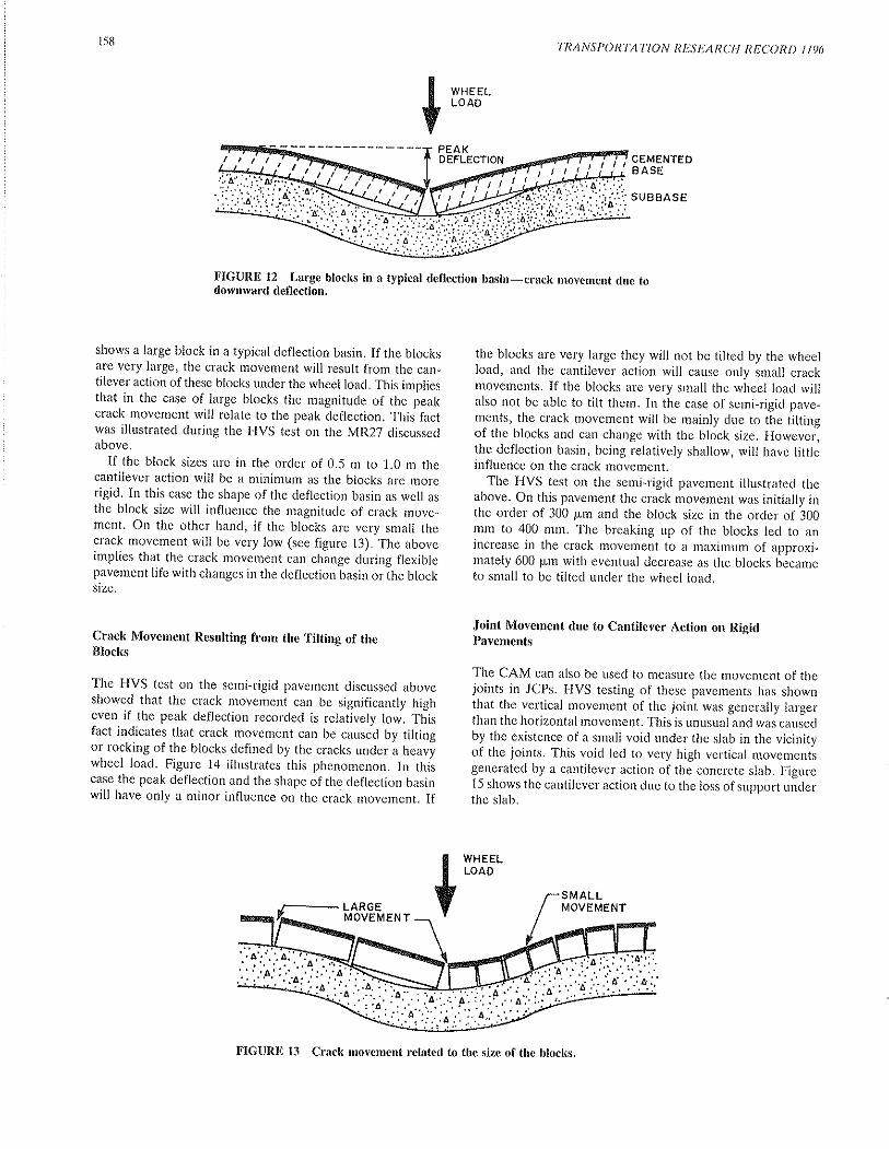
158

I rus'

FIGURE 12 Large blocks in a typical deflection basin-crack movement due todownward deflection.

shows a large block in a typical deflection basin. If the blocksare very large, the crack movement will result from the can_tilever action of these blocks under the wheel load. This impliesthat.in the case of large blocks the magnitude of the peakcrack movement will relate to the peak deflection. This factwas illustrated during the HVS test on the MR27 discussedabove.

If the block sizes are in the order of 0.5 m to 1.0 m thecantilever action will be a minimum as the blocks ate morerigid. In this case the shape of the deflection basin as well asthe block size will influence the magnitude of crack move-ment. On the other hand, if the blocks are very small thecrack movement will be very low (see figure 13). The aboveimplies that the crack movement can change during flexiblepavement life with changes in the deflection basin or the blocksize.

Crack Movement Resulting from the Tilting of theBlocks

The HVS test on the semi-rigid pavement discussed aboveshowed that the crack movement can be significantly higheven if the peak deflection recorded is relatively low. Thisfact indicates that crack movement can be caused by tiltingor rocking of the blocks defined by the cracks under a heavywheel load. Figure 14 illustrates this phenomenon. In thiscase the peak deflection and the shape of the deflection basinwill have only a minor influence on the crack movement. If

the blocks are very large they will not be tilted by rhe wheelload, and the cantilever action will cause only small crackmovements. If the blocks are very small the wheel load willalso not be able to tilt them. In the case of semi-rigid pave-ments, the crack movement will be mainly due to the tiltingof the blocks and can change with the block size. I{owever,the deflection basin, being relatively shallow, will have littleinfluence on the crack movement.

The HVS test on the semi-rigid pavement illustrated theabove. On this pavement the crack movement was initially inthe order of 300 pm and the block size in the order of 300mm to 400 mm, The breaking up of the blocks led to anincrease in the crack movement to a maximum of approxi-mately 600 prn with eventual decrease as the blocks becameto small to be tilted under the wheel load.

Joint Movement due to Cantilever Action on RigidPavements

The CAM can also be used to measure the movement of thejoints in JCPs. HVS testing of these pavements has shownthat the vertical movement of the joint was generally largerthan the horizontal movement. This is unusual and was causedby the existence of a small void under the slab in the vicinityof the joints. This void led to very high vertical movementsgenerated by a cantilever action of the concrete slab. Figure15 shows the cantilever action due to the loss of support underthe slab.

LARGEMOVEMENT

SMALLMOVEMENT+rtrf'

TRANSPORTATION RESEARCTI RECORD 1 ] 9ó

CEMENTED8 ASE

SUBEASE

FIGURE 13 Crack movement related to the size of the blocks.

Rust and Servas 159

FIGURE 14 Crack movement due to the tilting of the blocks.

I uxs'

Crack Movement due to Hinging Action

On CRCPs the crack movement mechanism is mainly one ofhinging of the blocks on the reinforcement. The reinforcementsteel in the concrete prevents excessive vertical crack move-ment. The crack movements are therefore very low and theaggressive pumping action is absent. This mechanism is shownin figure 16.

CONCLUSIONS

The phenomenon of the reflection of primary cracks throughoverlays and seals is partly due to repetitive thermal and/orload-associated crack movement. The development of theCrack-activity Meter (CAM) provides a means of measuringload-associated crack movements accurately and effectively.The CAM has been used extensively in conjunction with HeavyVehicle Simulator (HVS) testing.

PCC

CEMENTEOSUBBASE

The measuring and analysis of crack movements has led toa better understanding of the mechanisms of crack reflection.Four typical mechanisms ofcrack movement have been defined:

o Crack movement caused by the shape of the deflectionbasin,

o Crack movement caused by the tilting of blocks under a

heavy wheel load,o Joint movement on uncracked JCPs caused by the can-

tilever action of the slabs, ando Crack movement on CRCPs caused by the hinging of the

blocks on the reinforcement steel.

In the case of the deflection basin mechanism the crackmovement during pavement life can change should the shape

of the deflection basin or the block size change. In the case

of the block-tilting mechanism the deflection basin has a minorinfluence on the magnitude of the crack movement. Thismechanism is, however, influenced by a change in the block

REINFORCINGSTEEL

i;,;,iFIGURE 15 Movement of a joint in a JCP due to a void under the slalr-cantileveraction.

WHEELLOAD

VERY SMALLCRACK MOVEMENT

Itllltlttlllllr;trrttl

FIGURE 16 Crack movement on a CRCP-hinging of blocks onreinforcement steel.

I

160

size. On JCPs it was found that the vertical movement ofjoints can be very high due to cantilever action if a void ispresent directly under the slab. In the presence of water, thiscantilever action can lead to a very aggressive pumping action,which aggravates the joint movement and leads to very rapidfailure. On CRCPs the crack movements are generally lowand therefore no pumping takes place.

The analysis of the mechanisms of crack movement has alsoled to an improved understanding of how and why cracks onpavements move. This work has not only led to an improvedunderstanding of the mechanisms of load-associated crack andjoint movement but has also laid the foundation for résearchwhich has led to a procedure, based on the measurement ofcrack movement, that can be used to aid the rehabilitationdesign of cracked pavements.

ACKNOWLEDGMENT

The work described in this paper was done at the NationalInstitute forTransport and Road Research, CSIR, in pretoria,South Africa, and is published with the permission of theChief Director of the NITRR.

TRANSPORTATION RESEARCH RECORD I 196

REFERENCES

1. F. C. Rust. Sra¡¿ of the Art of Rehabilitating Reflection Crack-iyg_iy Cgmented Pavements. NITRR Technical Report RP/29.CSIR, Pretoria, South Africa, 1986.

2. F. C. Rust. á D eniled Descríp tìon of the Working of the Crack-activity Meter (CAM). NITRRTechnical Report RP/36. CSIR,Pretoria, South Africa, 1986.

3. A. \ry. Viljoen, C. R. Freeme, V. P Servas and F. C. Rust.Heavy Vehicle Simulator Aided Evaluation of Overlays onPavements with Active Cracks. Presented at the Sixth inter-national Conference on Asphalt Pavements, Ann Arbor,Michigan, 1987.

4. P. S. Strauss, O. Schnitter and C. P. Du Toit. NationalRoute 2, Section I near Somersel West: Experimental SectionsCgrystuclion Report. Directorate Land Transport referenceN16/4/6-02-010-06. South Africa, November 1983.

5. E. Horak. The Use of Surface Deflection Basin Measurementsin the Mechanistic Analysis of Flexible Pavements. proceed-ings of the Sixth International Conference on Asphalt pave-ments, Ann Arbor, Michigan, 1987.

P_ullícaion of thìs paper sponsored by Commiuee on Strength andDeþrmatíon Characteristics of Pavement.

TRANSPORTATION RESEARCH RECO RD I T96 l6l

Analyzing the Interactions BetweenDynamic Vehicle Loads and HighwayPavements

Mrcllanr J. Menxow,exn Eoweno Anno

J. Kanr HnonIcx, Bnrex D. BnaonMEYER/

Mechanistic models to predict structural performance anddeterioration have been developed for both flexible and rigidpavements. However, many of these models retain a simplifiedãnd idealized depiction of tire loads, and none really incor'porates a true representation ofa moving, dynamic force alongthe pavement surface. Thus, attempts to model the impacts topavements of new types of heavy vehicles have at best been

approximate and have often had to be supplemented by empir-ical data. In this paper we develop analytic models to studythe interactions between moving, dynamic loads and highwaypavements. One set of models simulates the dynamic behaviorof heavy vehicles, including their body configuration and mass

distribution, axle spacing and configuration, nonlinear sus-pension characteristics, and nonlinear tire behavior. The sec'

ond set of models simulates the primary responses (stressest

strains, etc.) of pavements to vehicle forces, and translatesprimary responses into pavement damage. Existing mecha'ñistic models are modified specificalty to treat moving, dynamicloads for both flexible and rigid pavements. This paper pre'sents examptes of results (in terms of both dynamic forces andpavement damage) for rigid pavements, although the conceptsapply as well to flexible surfaces. A parametric study is sum'marized, considering variations in both vehicle and pavement

characteristics. Those characteristics most important to dynarnicloading include vehicle suspension type and characteristics,speed, height of pavernent faults, and joint spacing. Otherfactors (such as tire pressure) contribute smaller effects (although

lire pressures are more important on flexible pavements). Results

indicate that under certain conditions, dynamic loads are 40

percent higher than static loads and affect the mid-region ofPCC slabs most significantly.

performance (3). Current models cannot account for this effect.

The prediction of pavement deterioration and serviceability

under dynamic vehicle loading becomes particularly impor-tant when pavement design and analysis methods must be

extended to encompass changing vehicle and pavement tech-

nology responding to new road design, construction, and reg-

ulatory practices. The purpose of this paper is to describe and

illustrate a general methodology to analyze pavement responses

to moving, dynamic vehicle loads, which may be used to pre-

dict pavement performance.

DYNAMIC VEHICLE-PAVEMENTINTERACTIONS

The interaction between vehicle loads and pavement responses

is frequently characterized as a one-way interaction, wherein

the vehicle loads influence pavement responses bt¡t not vice

versa. In reality, a mutually sustaining process occuls' The

roughness of the pavement surface excites dynamic forces

within the vehicle. These dynamic tire forces induce primary

responses (stresses, strains, deflections) within the pavernent,

which affect the amount of distress produced by the vehicle,

which in turn affects the dynamic tire forces experienced by

subsequent vehicles, and so on in a two-way interaction between

vehicles and pavements.

Analysis by Simulation Models

The study of this two'directional interaction between vehicles

and pavements is a fundamental tenet of the research project

described in this paper. The objective of this study is to assess

the impacts of moving, dynamic vehicle loads on both flexible

and rigid surfaces. Furthermore, an underlying prernise is togeneralize the problem description and analytic procedures

so that, for example, new axle configurations, new tire designs,

variations in tire pressures, as well as changes in pavement

design and construction may be analyzed simultaneously. To

do this, the study employs two sets of simulation models.

One set of models simulates the behavior of several com-

mercial vehicles, including their configuration and mass dis-

tribution, axle spacing and configuration, suspension char-

acteristics, and tire behavior. Each of these models simulates

the movement of a given vehicle along a pavement profile;

Current models of vehicle-pavement interaction employ sim-plified models of vehicle loading, such as static or pseudo-

moving loads. However, instantaneous dynamic vehicle loads

may be considerably higher than static loads (1 ,2); thus'

dynamic loading can have a considerable impact on pavement

M. J. Markow, Center for Construction Research and Education,Department of Civil Engineering, Massachusetts Institute ofTeéhnology, Cambridge, Mass. J. K. Hedrick, Vehicle DynarnicsLaboratoiy, Departmènt of Mechanical Engineering, Massachu-setts lnstiiute oi Technology, Cambridge, Mass. B. D' Brade-meyer, Center for Construction Research and Education, Depart-ment of Civil Engineering, Massachusetts Institute of Technology'Cambridge, Mass. E. Abbo, Vehicle Dynamics Laboratory'Departmènt of Mechanical Engineering, Massachusetts Instituteof Technology, Cambridge, Mass.

t62

any roughness inherent in the profile excites the dynamicelements of the simulated vehicle, as a function of the ampli-tude and frequency of the surface irregularities, the vehiclecharacteristics descril¡ed above, and vehicle speed. The resultof this simulation is a vehicle force profile containing digitizedvalues of tire forces over distance (or time), representing thecombined effects of all dynamic motions simulated. (Vehiclemotions are simulated in a vertical plane through the vehicle'slongitudinal axis (a "bicycle model"). The models thereforesimulate bounce and pitch of the vehicle body, suspension,and tires, but not roll from side to side.)

The second set of models simulates the response of a pave-ment to the dynamic force profile of a moving vehicle devel-oped above. The models used have been selected from theavailable ¡nechanistic models for flexible and rigid pavementsand adapted specifically to handle moving, dynamic loads.The objective was not to improve the modeling of pavementresponses per se, but rather to build in the coupling with thevehicle force profile and to modify the response calculationsto account for axle groupings (tandems, tridems, etc.). Arequirement placed on the models selected was that they pre-dict both primary responses (stresses, strains, and deflec-tions), as well as ultimate responses: both distress (cracking,rutting, spalling, faulting, etc.) and serviceability. Since dis-tress accumulates with the number of load repetitions and isalso influenced by the magnitude, duration, and configurationof loading, as well as environmental and time-dependent con-ditions, the behavioral response predicted by these modelsshould also be time- and temperature-dependent.

Separate analyses have been conducted for flexible anclrigid pavements to account for inherent differences inmechanistic behavior, boundary conditions, ancl design char-acteristics. For flexible pavements, a modified version of Fed-eral Highway Administration (FHWA) VESYS systern hasbeen used to represent pavement responses to moving, dynamicvehicle loads; for rigid pavements, a modified version ofPMARP (also developed for FHWA) has been used. Forpurposes of illustration, this paper examines a case study ofrigid pavements; the rnodifications to the PMARP pavementmodel are described in a subsequent section.

General Analytic Approach

Although separate models are used to simulate flexible andrigid pavements, the general approach is the same in eachcase. The force profile generated by the vehicle models sim-ulates a rnoving, dynamic load along the pavement. At oneor more points of measurement in the pavement, these dynamicforces are translated into primary responses and the maximumresponse computed. Where axle groups are encountered,appropriate superposition of responses is performed, and themaximum total response is identified. The maximum responseis then translated into the appropriate components of pave-ment distress. Increments of distress are accumulated throughrepeated vehicle passes and the results compiled. Thus, theresult of this simulation is a progression of damage in thepavement as a function of the pavement surface roughness(which i¡lcreases over time as a function of the thickness andmaterials properties of the pavement layers, subgrade strength,environmental factors, etc.), vehicle characteristics (as rep-resented by the dynamic tire force profile), and vehicle speed.

TRANSPORTATION RESEARCH RDCORD I ],96

In theory, the two analytic steps above should be performedin an iterative process in which vehicle forces are generatecland applied to a pavement, the increment in pavement dam-age (specifically, roughness) due to this force profile com-puted, that new force profile applied to the pavement, thenew increment in loughness computed, and so forth. Sincethis procedure would be extremely expensive in computertime, a close approximation is employed: vehicle force profilesare computed in the vehicle simulation for several discretelevels of pavement roughness. These results are interpolatedfor any other levels of roughness encountered in the subse-quent simulations of pavement deterioration.

Dynamic Vehicle Behavior

Models to simulate the behavior of moving vehicles have beendeveloped for several commercial trucks and buses and aredescribed by O'Connell, Abbo, a¡rd Hedrick (4); Hedrick,Cho, Gibson, et al. (5); Hedrick, Markow, Braderneyer etal. (ó); and Abbo (7). These models represent analyticallythe dynarnic behavior of the component rigid bodies, axlesuspensions, and tires as the vehicle moves along a pavementof specified roughness at a specified speecl. The result is aforce vs. ti¡ne or force vs. distance profile, again as a functionof (assumed constant) speed and pavement roughness. Sep-arate force profiles are produced for each axle of the vehicle,for each speed and roughness. These force profiles are usedas inputs to the models of pavement response.

Influence Functions to Reflect Moving Loads

For vehicle speeds of interest, the dynamic effect on pavementmass or inertia is negligible, as shown by Delatte (8). There-

xl xoDISTANCE, x

b. PROoUCES AN EFFECT AT xo EOUTVALENT TOA SMALLER LOAD AT x¡:

XO

DISTANCE, x

c. INFLUENCE FUNCTION AT xo FOR A NORMALTZE0(P=l)LOAD AT x:

DISTANCE, X

FIGURE I Load influence.

t-

ôoJ

Lof¡JJF

)6=<-oo,UJ

?tÊ.

ut(J2l,¡Jf,J

þo

A LOAD AT x¡,

Markow et al.

xoDISTANCE, x

b. HIGH -FREOUENCY LIMIT

D rsr;i c E, x

FIGURE 2 Variation of load influence rvithdynamic loads.

fore, one may represent the pavement response to a movingvehicle load as a quasi-static phenomenon, as shown in fig-ure L (where pavement response refers to stress, strain, ordeflection at a point in the pavement structure). Given thispremise, the pavement response to a load P at a distance x- xo x, is assumed to be equivalent to the response to a

lesser load (P' < P) placed directly above the point of interest(xo). This effect can be captured by influence functions relat-ing tlre effect at.r0 of a load P at xr. For a unit load (P = 1),the primary response at xo due to the load P at x' is charac-terized by the instantaneous static (or elastic) response 1(.rn

- x,), where the function l(xo - xr) is the influence function.As an arbitrary load traverses the pavement, the response at.16, R(.ro), due to the force F(x) imposed by this load at an

arbitrary location x is given by the response function:

R(xo) : I(xo - x) F(x)

The influence function in figure 1 is appropriate for a loadof constant (unit) magnitude traversing the pavement. In thegeneral case, however, the load will fluctuate, reflecting thedynamic vehicle forces discussed above. Thus, a dynamicallyvarying component will be superimposed on the influencefunction in figure 1.. The result of this superposition is illus-trated in figure 2 (at the low-frequency and high-frequencylimits). Therefore, the maximum influence a moving load canexert in the vertical plane at xo is a function of both the shapeof the basic influence function in figure 1 and the dynamiceffects superimposed on the basic function, as shown in fig-ure 2. It is this maximum influence (or, if appropriate, themean and variance of the maximum influence) that is used as

the basis of pavement damage prediction.Observe that the maximum influence a moving, dynamic

load may have on xo does not necessarily occur when the loadis directly above xo. First, because of viscoelastic behavior,pavement responses may exhibit a delay in relation to themoving load. Second, the dynamic effects illustrated in fig-ure 2 may shift the peak influence some distance from xn. Themagnitude of this distance depends on the frequency of thedynamic load variation.

163

Pavement Damage

Different response functions (equation 1) may be defined forstress, strain, strain-energy, or deflection and are obtainedfrom the particular mechanistic model used in the analysis.

For purposes of illustration, rigid pavements have been selected

as examples in this paper. Solutions yielding the primaryresponses in portland cement concrete pavements that havejoints or cracks have been developed over the past ten years.

These solutions rely on finite element methods to treat the

rigid behavior of the slab and the discontinuities (joints) between

slabs. Several candidate models were available for consider-ation for this project, as reviewed by Abbo (Z). The one

selected for this project was the PMARP program (9).In its original form, the PMARP program computes stresses

and strains due to a static point load at a critical slab location.Miner's hypothesis is used to determine fatigue cracking at

the individual nodes of the slab. Although the Miner's Lawcalculation is retained in the version used in this research,

several changes were made to PMARP to improve its simu-lation of a moving, dynamic load. First, influence functionswere introduced to model the travel of the load along theslab, Second, new equations were included (and some cor-rections made to existing equations in the model) to improveits predictions of pavement damage. A summary of the majoradditions is given below.

Joint Faulting Model

The joint faulting model used is the one adapted frorn PCAresearch for use in the EAROMAR-2 program developed forFederal Highway Administration (10). This model considersjointing as a function of traffic, pavement age, joint spacing,subgrade drainage, and type ofsubbase. For undoweled pave-

ments the equation for jointing is as follows:

JF : o.o4o3 . Wso.or (J _ 13.s)¿, (2)

where

7¡ = joint fault magnitude (in.),DTN = daily traffic number, or the number of vehicle passes

per day,A = age of pavement (yrs),I/ = slab thickness (in.),S = subgrade type (good = 1, poor = 2),¡ = joint spacing (ft.), andå : factor depending upon subbase characteristics,

equaling 0.241 for granular subbases and 0.037 forstabilized subbases.

The faulting model for doweled pavements is

1

JF"ro= ,+A'JF (3)

Thermal Gradient in the Slab

A difference in temperature between the top and bottom ofthe slab introduces thermal stresses that are superimposed on

o. LOW-FREOUENCY LIMIT

l¡J(Jlz.UJf,Jll

=ooJO

t¡Jo,2tt¡J

=JzooJO

(1)

164

(either constructively or in opposition to) the stresses causedby traffic loads. The thermal gradient in the slab rnay berepresented in the finite element model as an equivalent momentappliecl along the edge of the slab. The resulting stress maybe represented as follows:

*. : " ,+r"

where

TRANSPORTATION RESEARCH RECORD I 19()

tics. To do so we have used a base case cornprising a jointed,undoweled pavement having a slab length of 30 feet. Undow-eled pavements have been simulated because they exhibitgreater faulting and permit a fuller study of the effects offaults on vehicle dynamics. For the base case, a uniform faultheight of 0.5 inch has been assumed. (Doweled pavementjoints generally maintain faulting within 0.2 inch over thepavement service life, according to the faulting model usedin equation 3. At these relatively small fault heights, less than0.25 inch, there is no significant variation in vehicle dynamicswith respect to the parameters tested. This will be illustratedin the results below.) The vehicle used in testing the sensitivityto pavement parameters is a 2S1 combination with single-leafspring suspensions, travelling at 35 mph.

Loading and Responses Due to Multiple Axles

Although the outputs of the vehicle and pavement modelspermit detailed analyses by axle, more aggregate and concisemeasures of results make it easier to display the sensitivity ofdynamic loading to pavement and vehicle parameters. Thesemeasures embody the effects of the vehicle overall, ratherthan of any given axle combination. One such measure per-tains to the force imposed by the vehicle, the second to thepavement response, To compute these measures, the pave-ment slab is divided into equal-size sections sufficiently smallto enable resolution of the peak forces up to the highestfrequencies of interest. The aggregate force at a particularpoint K is defined by:

F* = 2 P¡o fork :'1,2,3,...,N,

where

N. = number of vehicle axles j,P,r : force imposed by axle j at slab location k, andN, = total number of stations k along the slab length.

The mean aggregate load is determined by averaging theaggregate load in equation 5 over several slabs (typically 20)to suppress any transient dynamic effects. The mean aggregateload is then normalized by the vehicle static load, and it isthis value that is displayed in the results below. It is importantto bear in mind that the aggregate force at a point dependson the cumulative effect of all vehicle axles that pass over it.Therefore, the maximum aggregate force will not necessarilyoccut at the same location as the maximum force generatedby any individual axle. Analogously, the aggregate responseof the pavement Rr(.r) at some point x is the sum of theresponses due to the individual vehicle axles:

Na

Rl¡) : ) R('lj=t

where R (.r) is the response function at x due to axle 7 (ascomputed in equation l). In applying equations 5 and 6, accountis taken of the proper spacing of the axles on a vehicle.

Effect of Slab Length

Four slab lengths, ranging from 10 feet to 45 feet, were inves-tigated. The vehicle behavior due to these varying intervals

(4)

M* = equivalent moment induced by thermal stresses (psi),a. = coefficient of thermal expansion (in./in./deg-F),I : thermal gradient (deg-F/in.),E = Young's Modulus of Elasticity of concrete (psi), andI : rhickness of rhe slab (in.).

Additional Assump tions

In applying the modified PMARP model ro the analysis ofdynamic loads, the following assumptions were made to sim-plify the computations and reduce computer time:

o The elastic modulus of concrete ancl the modulus of rup-ture were assumed to remain constant over the life of thepavement and were taken as average values.

o Subgrade weakening due to pumping was neglected.o The major contribution to roughness was taken to be the

faults at joints, rather than surface roughness in the interiorof the pavement slab.

RESULTS

Parametric Studies

These procedures \ryel'e applied in a set of parametric studies,in which the following parameters were varied:

1. Suspension Type:¡ Single-Leafo Four-LeafTandemo Walking-Beam Tandem

2. Suspension Stiffness, k3. B-parameter for Leaf-Springs4. Vehicle Speed5. Tire Pressure6. Axle Load Sharing Coefficient7. Tandem Axle Spacing8. Pavement Roughness (i.e., Fault Height)9. Joint Spacing

10. Slab Warping11. Slab Interior Roughness

The results of these studies are summarized below, with a

more complete presentation by Abbo (7).

Effects of Pave¡nent Characteristics on DynamicLoads

First it is useful to understand the pattern of dynamic loadingand how that pattern is influenced by pavernent characteris-

(s)

(6)

165Markow et al.

between faults was investigated (for example, by changes inthe power spectral density functions of the vehicles, as doc-umented in (7)), as well as the effects on dynamic loads. Asummary of these results follows.

The vehicle simulated in these examples has a steer-to-drivewheelbase of about 11.5 feet and a drive-to-rear wheelbase

of 19.5 feet. Therefore, the 10-ft joint spacing results in almostsimultaneous excitation of each of the three axles, stimulatingprimarily the vehicle bounce mode. For a joint spacing of 20

feet, there is a small time delay between inputs to the driveand rear axles, which excites the trailer bounce and tractorpitch modes, resulting in the largest pavement loads observed

in this study. The 30-ft and 45-ft joint spacings do not excitethe out-of-phase tractor-trailer pitch motions as much.

The effects of this behavior on aggregate vehicle load alongthe length of the slab can be seen in figure 3 for three of thejoint spacings (20,30, and 45 feet). A joint spacing of20 feetproduces a 12 percent increase in aggregate loading, with thepeak load occurring roughly 10 feet after the faulted joint.Note, however, that the load imposed on the subsequent slabjust after the joint is 20 percent lower for the 20-ft slab lengththan it is for the other slab lengths.

Effect of Height of loint Fault

For the base case used (30-ft joint spacing, 35-mph vehiclespeed) the height ofjoint faults did not affect the location ofpeak loads but did affect their magnitude. For example, con-sidering just the drive axle of the vehicle, the normalizeddynamic load (dynamic force divided by static force) meas-

ured at the peak load location 10 feet past the slab jointincreased from about 1.05 for a 0.1-in fault to over 1.25 fora 0.75-in fault.

On an aggregate vehicle basis the impacts of joint faultscan be seen in figure 4. There is a very small (about 3 percent)difference in the pattern and magnitude of loads for jointfaults less than 0.25 inch. However, there is up to a 20 percentincrease for a change in fault height from 0.25 inch to 0.75

inch. This illustrates the point mentioned above: relatively

o5lo15?o25303540DISTANCE FROM SLAB JOINT (FT)

FIGURE 3 Effect of slab length on aggregateload.

o ? 4 6 I rO 12 14 16 ß ?O??24 26?A30DISTANCE FROM SLAB JOINT (FT)

FIGURE 4 Effect of fault height on aggregateload.

small fault heights (as might be expected on new pavements

or those with good load transfer devices) result in insignificantchanges in dynamic loadings. The increase in dynamic force

that does take place when faulting becomes substantial sup-

ports the earlier contention that the two-way interactionbetween vehicles and pavements does indeed result in an

accelerating, progressive cycle of vehicle load and pavement

damage.

Effect of Slab Warping

For a vehicle speed of 35 mph and a slab length of 30 feet,the warping of the slab corresponds to an input to the vehicle

of.7.7 Hz. This frequency coincides with the natural frequencyof the tractor bounce and pitch modes, which influences the

changes in dynamic loading observed in figure 5. Specifically'the peak load regions of all the axles shift further away fromthe slab joint as the slab warping increases. The heaviest

t¡JoÉ.

et¡JF(9ul(tso(9ol¡JNJ

=É.oz

t.4

t.3

/,"'

"Jil\l 'l\¡.1 i !'-z

\/V

-

(o) no worping

---- ( b) m¡d-slob defl€cl¡on I inctr

--- (c ) mkt-slob def lecl¡on I ¡nch

l¡Jo t.2(tsot

r.rl¡Jt-ó

'.ol¡J

Ë'Ê.eN

1,Éo.6z

.5

.4 o2468lO12 14 16 182022?4262830DISTANCE FROM SLAB JOINT (FT)

FIGURE 5 Effect of slab warping on aggregateload.

---- (o) O.75inch foull

-

(b) 0.5 ¡nch foult

--- (c ) O.25 inch foult

-- (d) O. I inch foult

t66

loading is sustained in the middle third of the slab, due to theexcitation of the lower frequency body modes. This increasein aggregate loading is up to 25 percent for a slab radius ofcurvature of 1350 feet (equivalent to a f-in deflection at thecenter of a 30-ft slab).

Effect of Slab Roughness

The interior roughness of the slab was varied by adjusting theassumed slope variance between 1.7 x 10-6 and22 x 10-6in.2. Changes in the magnitudes of the resulting peak forceswere no more than 4 percent and were judged to be insig-nificant over the range of roughnesses typically associatedwith rigid pavements. The primary excitation of vehicledynamics was, therefore, taken to be the faults at rigid pave-ment joints.

Effects of Vehicle Parameters on Pavement Damage

The effects of vehicle parameters were also investigated.Although the results could again be expressed in terms ofaggregate load, we now take them one step further to use themodified PMARP model (including equations 2 through 4)to consider the impacts on pavement damage. In these runs,damage has been limited to fatigue cracking, which is pre-sented in two ways: (1) as a probability of occurrence overtime, taken as a weighted average of the Miner's Law cal-culations for all nodes in the slab, and (2) as the amount ofdamage (in square inches) occurring by region of the slab.(Five regions have been defined, where the load traverses theslab from region I to region 5.)

Static Versus Dynamic Moving Load

Damage due to dynamic loading was compared to the sim-ulated case of a moving constant load for the reference vehicle(a 2S1 tractor-semi-trailer) and the base case pavement con-ditions (30-ft slab length, 0.5-in fault height, 35-mph vehiclespeed). The results are illustrated in figures 6 and 7.

The moving dynamic load produces approximately 38 per-cent greater fatigue cracking damage than the static movingcase after 15 years of pavement service, as shown in figure 6.

This indicates the importance of considering vehicle dynamicloading when assessing pavement performance. A somewhatunexpected result is that the rate of additional damage accu-mulation is linear, rather than accelerating as had beenhypothesized. This result may be due to some of the simpli-fying assumptions made earlier, in particular the constantvalues of the concrete elastic modulus. (Note that these resultsdiffer from those discussed for faults earlier.)

Figure 7 illustrates the distribution of cracking along theslab length for the constant and dynamic moving load cases.

For constant (or moving static) loads we obtain a syrnrnetricaldistribution of cracking over the slab, with the rnost severecracking occurring in the regions close to the joints. Com-paring this to the dynamically moving load, we note thatthere is a 15 percent decrease in the cracking that occurs inthe regions close to the joints. Furtherrnore, there is a largeincrease in the cracking in the mid-slab regions, which is

TRANSPORTATION RESEARCH RECORD I 196

OYNAM IC

/¿

,/..\,t -srATlc

o 2 o T,"r lrroåo.,

tz t4 16

FIGURE 6 Growth in the probability of fatiguedamage: moving dynamic load vs. movingconstant load.

attributable directly to the body rnode contribution to the tireforce. The importance of the body mode contribution to totaldynamic loading on rigid pavements has already been alludedto in the discussion of the role of pavement faults and jointspacing in exciting this mode; this finding will be reinforcedin the analysis of vehicle characteristics below.

Single Leaf-Spring Suspension (2SI )

Effect of Leaf-Spring Stiffness The effect of increasing theleaf-spring stiffness is to reduce the wheel mode and increasethe body mode contribution to the tire force on the pavement.(Wheel-mode forces are of higher frequency, about 10-15Hz; body-mode forces are of lower frequency, about 2-3 Hz.)The resulting effect on pavement cracking over a 15-yr sim-ulated period is a 10 percent reduction in the cracking damagewhen the leaf-spring stiffness is halved. Furthermore, mid-slab cracking is lowered by a reduction in the leaf-spring stiff-

t2345REGION OF SLAB

(OIRECTION OF TRAFFIC +)FIGURE 7 Cracking damage (in.2) along slablength: moving dynamic load vs. nroving constantload.

(,zYoÉ.()lLo

F)(D

c0o(rfL

.8

.2

-t

.6

.5

.4

.3

N.g

t¡J(9

ô(,z;o(ro

Markow et al.

ness. However, these savings al'e somewhat offset by theincrease in cracking in the region close to the joint, due toan increase in the wheel mode contribution to the tire forcewith the softer suspension.

Effect of p-Parameter B is a friction parameter that describesthe hysteretic nature of the leaf-spring. The nominal (base-case) value of B is 4 x 10-3 feet. The effect of decreasingthe leaf-spring damping (increasing B) is to increase the wheelmode contribution and reduce the body mode contribution.The reduction in the cracking occurs in the mid-slab region,similar to the case described above for snspension stiffness.The results show that a larger value of B, or reduction in leaf-spring damping, produces a reduction in cracking (approxi-mately 12 percent) over the entire slab, due to the reductionin the body mode contribution.

Effect of Speed Vehicle loading was sirnulated at three dif-ferent speeds: 35, 55, and 70 mph. For the particular vehicleancl pavement characteristics used, 55 rnph was determinedto be the speed at which tire forces are maximum (in otherwords, the speed at which vehicle dynamics are reinforced bythe pavement characteristics). At speeds other than this crit-ical value the excitation of dynamic forces is reduced. Forvehicle speeds of about 35 mph the effect of dynamics becomeless important, and the damage distribution resembles that ofa static moving load. When speed is increased from 55 to 70

mph, pavement damage is reduced over most of the slab, butis increased in the latter part of the slab (where the vehicleleaves the slab).

Due to the coincidence of (1) the dimensions of the vehiclewheelbases, and (2) the slab length simulatecl, the vehicleexperiences simultaneous inputs to the steer ancl rear axles.On an actual pavement, the frequency at which the vehicleexperiences these inputs should be adjusted so it is not inthe range of the body mode frequency. The adjustment canbe made either by regulating vehicle speed or by changingthe slab length.

Walking- Beam Tandem Suspension (352)

Analyses of the walking-beam suspension were conducted ina way similar to that described for the single leaf-spring sus-pension described above. Of the three speeds tested (35, 55,and 70 mph), 55 mph was the most critical (as it was for singleaxles) because of the excitation of the lightly damped out-of-phase axle pitch mode (approximately 10 Hz). Damage at 55

rnph can be mitigated by reducing the tandem axle spacingfrom the standard of 52 inches simulated in these runs. How-ever, the walking-beam suspension performs better than thesingle-axle suspension at low speeds, since it has the abilityto filter out the faults in the pavement. This filtering occurswithout excessively exciting the axle pitching mode at lowspeeds.

Four-Leaf Tandem Suspension (352)

In comparison to other axle groups, the four-leaf tandem does

damage equivalent to the walking-beam (and rnore than the

t67

single-axle) at the slab joints, but it does no tnore damagethan the single-axle suspension (and much less than the walk-ing-beam) in the mid-slab regions. The reason that the four-leaf suspension does less damage than the walking-beam over-all is that the out-of-phase pitching mode of the suspensionis more restricted by the inherent coulomb friction in the leafsprings.

Effect of þ-Parameter

The amount of cracking simulated is relatively sensitive to the

B parameter. There is an optimal value of leaf-spring dampingaround I : 4 x 10-3 ft. (Recall that for single-axle suspen-sions, however, higher values of B were preferable.) The dif-ference in response to P between these two axle groups is due

to the coupling of the tandem axles (through the short-rocker).A lower value of p in the single-axle suspension translates toa larger contribution of the body mode, resulting in greatercracking damage (refer to the discussion of the single leaf-spring axle). In the tandem-axle case a very low value of B(high coulomb friction) results in increasing the contributionof the body mode to the tire force, thereby increasing thedamage. On the other hand, too high a value of p excites theaxle out-of-phase pitching mode, also increasing damage.Therefore, there exists an optimum value of B for the four-leaf tandem, lying between these extremes.

Effect of Tire Pressure

The effects of tire pressures were investigated for all the sus-

pension types; the results for the four-leaf tandem will illus-trate the trends observed. Tire pressure has some effect onvehicle dynamics, since lower pressures filter the input to theleaf-spring suspension, thereby attenuating the wheel modecontribution to the tire force. Also, lowering the tire pressul'eleads to a larger surface contact area, reducing the primaryresponse (for example, stress) of the pavement. This wouldreduce the rate of crack initiation and propagation throughthe slab.

68lO12l¿DISTANCE FROM SLAE JOINT (FT}

FIGURE I Effect of tire pressure, fourleaftandem axle.

5t.2

t.2UoÉorUJF(,uÉ.(,oôUNJ

Èo2

t. t5

t.to

t.

.95

---- (o) 75ps¡

- (b) lOOPsi

--- (c) l25psi

1ó8

The analysis of tire pressure effects are shown in figure g,where the aggregate dynamic force is shown for tire pressuresof 75, 100, and 125 psi. These plots show that the greatesteffect of tire pressure occurs at the second peak load, wherea 5.5 percent increase in load magnitude is attained by raisingthe tire pressure from 75 to 125 psi. Tire pressure thus appearsto have a small effect on vehicle dynarnics and, therefore, asmall effect on rigid pavement damage for the conditionstested in this study. This result differs from that observed forflexible pavements, where the influence functions tend to benarrower or tighter (the rigidness of the pCC slab renders itless sensitive to greater stress that may result from higher tirepressures).

Other Impacts

Other impacts are summarized below, with additional detailsin Reference 7:

o Increasing the leaf-spring stiffness by 50 percent producesa 6 percent reduction in the overall damage producecl. Thistrend is the opposite of that for the single-axle leaf-spring,where softer suspensions are more favorable.

o Reducing the axle spacing from 52 to 40 inches increasesthe pavement damage by 9 percent. This is opposite to theeffect produced in the walking-beam suspension, where thehigher stress produced by bringing the axles together is farout-weighed by the reduced dynamics.

¡ Changing the load sharing coefficient (LSC) from perfectload sharing (LSC : 1.0) to LSC = 0.9 does nor result in asignificant change in damage overall but does redistributedamage somewhat, increasing the amount of cracking nearthe approach joint.

CONCLUSION

New analytic procedures have been cleveloped to study in avery general way the interaction between vehicle dynamicloads and pavement damage. Detailed sirnulation programsof heavy truck dynamics have been created, and an existingrigid pavement program (PMARP) has been modified toaccount for dynamic tire loads on PCC slabs. To date, singleand tandem axles have been investigated, with the followingresults:

o The static load case indicates that the mid-slab r.egion haslower fatigue damage than the transverse joint regions. Forthe dynamic loading case, however, the mid-slab and trans-verse joint regions have similar fatigue damage values. Fur-thermore, fatigue damage due to dynamic rnoving loads inparticular slab locations is up to 40 percent greater than thatdue to static loads.

o The mid-slab regions are more sensitive to dynamics thanare the transverse joint regions. This results from the find-ing that the body mode contribution to the tire mode ismore detrimental to cracking damage than the wheel modecontribution.

. For the particular combination of factors that was tested,the walking-beam suspension produces the most damage athighway speeds, followed by the four-leaf tandem and the

TRANSPORTAT'ION RESEARCI,I RECORD I 19(,

single-axle suspension as the least damaging. These resultsmay vary for other combinations of pavement and vehiclecharacteristics.

The factors that have been shown to be most critical inaffecting dynamic loads on rigid pavements are

o Vehicle and axle configuration, and vehicle load,o Suspension characteristics (stiffness, hysteresis),o Vehicle speed, ando Pavement roughness, faults, joint spacing, and slab

warping.

Other factors are also important, although they were notspecifically tested in the parametric study (for example, pave-ment design and environmental conditions, which affect therate of pavement faulting and deterioration). Weakening ofthe pavement subgrade due to pavement pumping was notincluded in this set of analyses, and its inclusion might alterthe conclusions obtained above. Tire pressure was investi-gated but not found significant in affecting dynamic loads;this conclusion is different from that obtained in earlier sim-ulation of flexible pavements.

An important implication of these findings is the impor-tance of the vehicle itself in influencing dynamic loads, imply-ing that future policies governing the maintenance and reha-bilitation of highway infrastructure may need to look at thevehicle as well as the pavement (and bridges). Furthermore,regulating heavy vehicles simply by gross weight and axle loadmay not be sufficient; the clynamic loads actually irnposed bydifferent axle configurations, suspensions, and tires may needto be accounted for, Finally, pavement ma¡ìage¡nent shouldbe coordinated with the evolution in vehicle technology, sincedynamic loads arise through the interaction of factors such asslab length, vehicle wheelbase, fault height, suspension damp-ing, and axle spacing.

ACKNOWLEDGMENTS

This work has been supported by the U.S. Department ofTransportation, Office of University Research. Technicalsupervision has been performed by the Federal HighwayAdministration. The authors wish to thank particularly Wil-liam J. Kenis, Jr., who has served as Technical Monitor forthis research and has provided very helpful suggestions andguidance.

REFERENCES

1. P. F. Sweatman. A Study of Dynamic Wheel Forces in AxleGroup Suspensions of Heavy Vehicles. Special Report 27.Australian Road Research Boarcl, June 1983.

2. A. P. Whittemore, J. R. Wiley, p. C. Schultz, ancl D. E.Pollock. Dynamic Pavement Loads of Heavy Highway Vehi-9þ. ry_tigna-lcgoperative Highway Research program Report105. HRB, National Research Council, Washington, D.C.,1970.

3. P. Ullidtz and B. K. Larsen. Mathematical Moclel for pre-dicting Pavement Performance. ln Transportation ResearchRecord 949,TRB, National Research Council, Washington,D.C., 1984, pp. 45-55.

Markow et al.

4. S. P. O'Connell, E. Abbo, and J. K. Hedrick. Analyses ofMoving Dynamic Loads on Highway Pavements: Part 1:

Vehicle Response, Proceedings, International Symposiym 97tHeavy Vehlcle Weights and Dimensio,ns, Kelowna, BritishColumbia, June 1986.

5. K. Hedrick, D. Cho, A. Gibson, J. Isaacson, and S. O'Con-nell, Determination of Road Slress Factors for Buses.InterimReport. U.S. DOT, FebruarY 1985.

6. J. i<. Hedrick, M. Markow, B. Brademeyer, S. O'Connell,N. Delatte, and A. Gibson . Predicting Models for EvaluatingLoad Impact Factors of Heavy Trucks on Current Pavement

Conditions.Interim Report. U.S. DOT, December 1985.

7. E. Abbo, The Influence of Heavy Vehicle Dynamics on RigidPavements. Master's thesis. Massachusetts Institute of Tech-nology, January 1987.

8. N. J. Delatte. Characlerization of Dynamic Vehicle- Pavement

9.

10.

t69

Interaction. Master's thesis. Massachusetts Institute of Tech-nology, June 1986.J. Larralde, W. F. Chen, C. W. Lovell, and C. D. Sutton,Purdue Method for Analysís of Rigid Pavemenß: Users' Guide.Purdue University; Federal Highway Administration, U.S.DOT, December 1984.M. J. Markow and B. D. Brademeyer. EAROMAR Ver-sion 2: Final Technical Report. FHWA/RD-82/086. FederalHighway Adminisration, U.S. DOT, April 1984.

Publication of this paper sponsored by the Committee on Strenglhand Deþrmation Characteristics of Pavement.

t70 TRANSPORTATION RESEARCII RECORD 1 196

LEF Estimation from canroad PavementLoad-Deflection Data

L. R. Rrrnrr aNp B. G. HurcsrNsoN

Load equivalency factors (LEFs) versus axle.load regressionequations are reported for single-, tandeln-, and tridem-axlegroups. These functions have been developed from truck load-ing test data collected at nine sites across Canada in 1985 bythe Canroad Transportation Research Corporation. tilhile theload on the axle groups dominated the regression equations,pavement temperature, axle spacing, and vehicle velocity werefound to be statistically significant for the tandem-axle groupsat a number of the sites. Regression analysis of the pooledtandem data showed that load and axle spacing were signifï-cant. Analysis of the pooled tridem.axle group data showedthat load, axle spacing, structural number, and vehicle speedwere significant. The load equivalency functions are comparedwith the AASHTO functions and the differences highlighted.

A comprehensive set of field measurements of pavement sur-face deflections and surface course interfacial strains wereobtained at fourteen test sites across Canada in 1985. Thesemeasurements have been reported by Christison (1) and werepart of a major study of vehicle weights and dimensions con-ducted by the Canroad Transportation Research Cor.poration.Christison (2) analyzed these data and developed a set ofresponse-type load equivalency factors (LEFs) for single-,tandem-, and tridem-axle groups, and these LEFs form thel¡asis of a set of draft regulatory principles for interprovincialtrucking in Canada (3).

Hutchinson et al. (4) have reanalyzed the pavement deflec-tion data collected in this study using the ASTM StandardPractice for Counting Darnage Cycles (5), instead of the methodused by Christison (2), to extract the pavement damage cycles.This alternative method of analysis produced LEFs that were,on the average, 8 percent higher than those calculated byChristison (2) for the tandem-axle groups and 16 percent higherfor the tridem-axle groups.

Neither of the analyses cited above conducted an exhaustivestatistical analysis of this very rich data base. Variations inLEFs with vehicle speed, intra-axle spacing, pavement tem-perature, and pavement structural characteristics were notcomprehensively analyzed. This paper describes the resultsof a comprehensive regression analysis of the influence ofthese factors on the LEFs, using the surface deflection data.The surface course-base course interfacial strain data havenot been analyzed because they are not readily available tooutside users at this time.

DATA BASE

Surface deflections and interfacial (surface-base) strains wereobserved at fourteen test sites for a variety of test conditions.The Canroad Transportation Research Corporation devel-oped a test vehicle that allowed a variety of tandem- andtridem-axle configurations to be developed and tested undera range of axle-group loads. Tests were also conducted atspeeds of 6, 13, and 50 km/h. Each test run consisted of pairsof pavement response measurements under. a stanclard Ben-kleman Beam truck with an 8,160 kg single-axle load on dualtires and under the candidate axle group. Three test runs wereconducted at each velocity, and the published deflection dataconsist of the average, minimum, and maximurn deflectionsunder each axle of an axle group as well as the inter-axleresidual deflections for multiple-axle groups. Christison (1)provides a detailed description of the data base in terms ofthe test program and pavement properties.

Figure 1(a) shows a typical deflection profile under thepassage of a tridem-axle group. The load on the axle groupwas 26,036 kg, the axle spacing 3.7 rn, the truck speed 12.9km/h, and the pavement temperature 23.6.Ç. The diagramshows that the measured surface deflection increased from0.442 mm through 0.498 mm to 0.503 mm under the passageof this tridem. The inter-axle residual deflection increasedfrom 0.119 mm to 0.130 mm between the second and thirdaxles. The deflection under the Benkleman beam truck was0.422 lr:,m. The maximum deflection tencled to occur underthe last axle of both the tandem and tridem groups at mosttest sites.

ESTABLISHING LOAD EQUIVALENCY TACTORFUNCTIONS

The LEF for a particular load on a candidate axle group isusually defined as the ratio of the number of passes of astandard axle load to the nurnber of passes of a candidateaxle load to create the same amount of pavement damage.There are three broad approaches to establishing the LEFfunctions for different axle groups, and these are frequentlyreferred to as the empirical approach, the theoretical approach,and the mechanistic approach.

EMPIRICAL APPROACH

The principal source of information for. empirically deter-mined LEF functions is the AASHO Road Test, where theUniversity of Waterloo, Waterloo, Ontario N2L 3G1, Canada.

Rilett and Llutchinson t7l

EzaF()ulJuuJôU()ÍÉ.

a

0.

f.51-0

TIME (s€cs)

(a) SURFACE DEFLECTION PROFILE UNDER 26 036 KG TRIDEM

(b) LOAD - DEFLECTION HISTORY UNDER TRIDEM PASS

oIoooo15oJ

ulJx

DEFLECTION (mm)

LEF = (3f3å)" * (o'4lH2t 30

)' + e4#le)"

(c) LEF cALCUIATION FoB TRIDEM PASS

FIGURE 1 Calculation of LEF for tridem axle pass.

dete¡ioration of pavement sections of various thicknesses underhomogeneous truck loads on single axles and on tandem axles

were measured. It is well known that LEFs calculated fordifferent loads on single- and tandem-axle groups vary withthe PSI chosen to define failure and with the structural char-acteristics of a pavement. The AASHO Road Test analyses

suggested that the LEF of a candidate axle group could be

approximated by the fourth power of the ratio of a candidateaxle load to the standard axle load. The results obtained fromthe AASHO Road Test are difficult to apply directly to cur-rent legal axle group loads and to axle groups other thansingles and tandems, since this involves extrapolation of theresults outside the range for which they were developed. Forinstance, the AASHTO LEF functions for tridems assumes

that a tridem-axle group pass is equivalent to a single plus a

tandem pass (ó). This assumption is not supported by theo-retical considerations or field observations.

THEORETICAL APPROACH

The theoretical approach to LEF function estimation pro-

ceeds by calculating the deforrnations or stresses in a pave-

ment structure in combination with a fatigue damage law to

establish the relative damage created by different axle groups

and configurations.Deacon (7) used maximum principal tensile strain as the

fatigue damage parameter and compared his theoretical LEFmagnitudes with those established at the AASHO Road Test.The recommended AASHO tandem equivalences were 80

percent of the theoretical values for pavements with structuralnumbers greater than 3, while the equivalences for single axles

were approximately equal. Deacon suggested that for pave-

ments with structural numbers of less than 3 the primaryfailure mechanism was not fatigue, and his approach mightnot be appropriate.

Ramsamooj et al. (8) used theoretical fracture mechanics

to derive load equivalency factors from longitudinal stress

intensity factors. They defined the LEF for single axles as the

ratio of the maximum rise in the influence line for the stress

intensity factor K for the candidate axle load to the maximumrise in K for the standard load, raised to the fourth power.

For tandem axles the ratio of the peak-to-trough value of thestress intensity factor to that of the standard axle raised to

the fourth power was also calculated. The accumulation ofthe damage cycles caused by each axle in the tandem was

accomplished by adding these two calculations. This rnethodof damage accumulation is adopted in this paper.

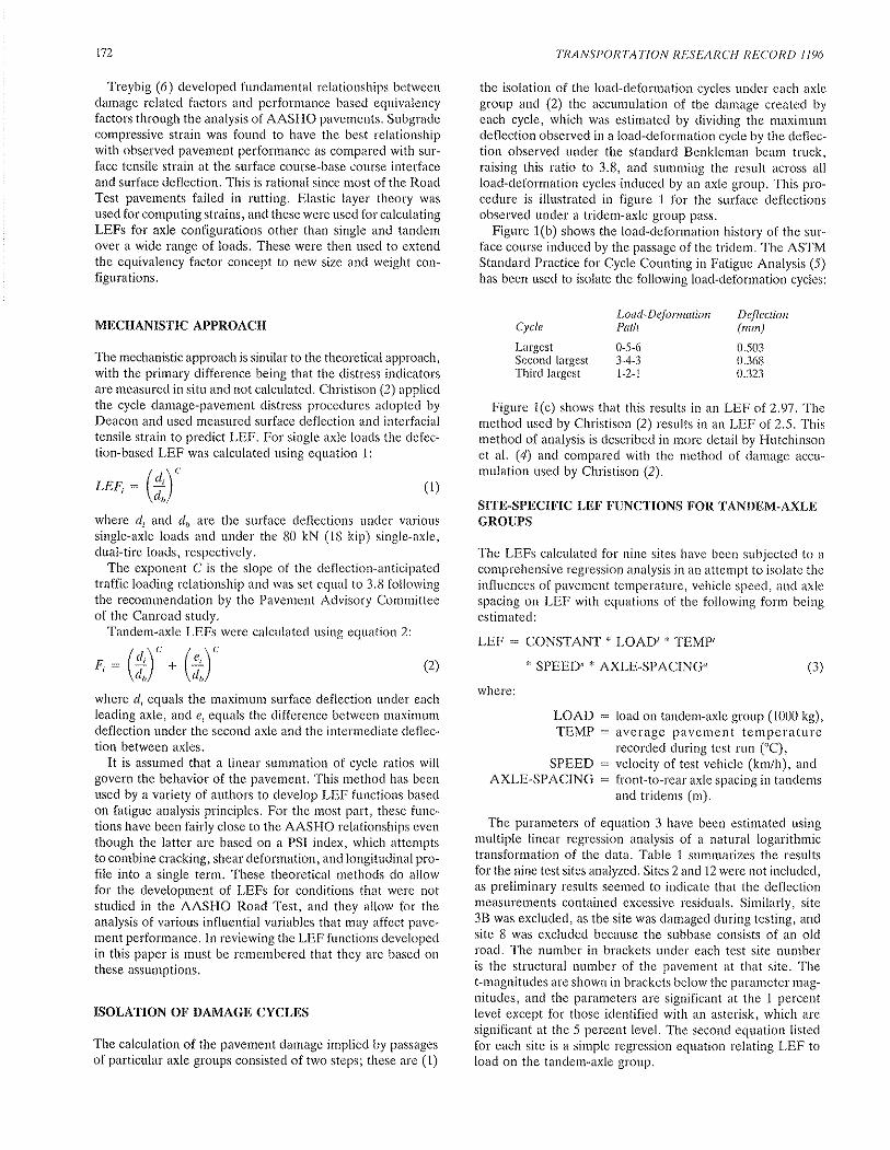
,uo = (2

172

Treybig (ó) developed fundamental relationships betweendamage related factors and performance based equivalencyfactors through the analysis of AASFIO pavements. Subgradecompressive strain was found to have the best relationshipwith observed pavement performance as compared with sur-face tensile strain at the surface course-base course interfaceand surface deflection. This is rational since most of the RoadTest pavements failed in rutting. Elastic layer theory wasused for computing strains, and these were used for calculatingLEFs for axle configurations other than single and tandemover a wide range of loads. These were then used to extendthe equivalency factor concept to new size and weight con-figurations.

MECHANISTIC APPROACH

The mechanistic approach is similar to the theoretical approach,with the primary difference being that the distress indicatorsare measured in situ and not calculated. Christison (2) appliedthe cycle damage-pavement distress procedures adopted byDeacon and used measured surface deflection and interfacialtensile strain to predict LEF. For single axle loads the defec-tion-based LEF was calculated using equation 1:

where d, and do are the surface deflections under varioussingle-axle loads and under the 80 kN (18 kip) single-axle,dual-tire loads, respectively.

The exponent C is the slope of the deflection-anticipatedtraffic loading relationship and was set equal to 3.8 followingthe recomrnendation by the Pavernent Advisory Colnnritteeof the Canroad study.

Tandem-axle LEFs were calculated using equation 2:

where d, equals the maximum surface deflection under eachleading axle, and e, equals the difference between maximumdeflection under the second axle and the intermediate deflec-tion between axles.

It is assumed that a linear summation of cycle ratios willgovern the behavior of the pavement. This rnethod has beenused by a variety of authors to develop LEF functions basedon fatigue analysis principles. For the most part, these func-tions have been fairly close to the AASHO relationships eventhough the latter are based on a PSI index, which attemptsto combine cracking, shear deformation, and longitudinal pro-file into a single term. These theoretical methods do allowfor the development of LEFs for conditions that were notstudied in the AASHO Road Test, and they allow for theanalysis of various influential variables that may affect pave-ment performance. In reviewing the LEF functions developedin this paper is must be remembered that they are based onthese assumptions.

ISOLATION OF DAMAGE CYCLES

The calculation of the pavement darnage implied by passagesof particular axle groups consisted of two steps; these are (1)

TRANSPORTATION RESEARCH RECORD 1 196

the isolation of the load-deformation cycles under each axlegroup and (2) the accu¡nulation of the damage created byeach cycle, which was estimated by dividing the maximurndeflection observed in a load-deformation cycle by the deflec-tion observed under the standard Benkleman beam truck,raising this ratio to 3.8, and summing the result across allload-deformation cycles induced by an axle group. This pro-cedure is illustrated in figure 1 for the surface deflectionsobserved under a tridem-axle group pass.

Figure 1(b) shows the load-deformation history of the sur-face course induced by the passage of the tridem. The ASTMStandard Practice for Cycle Counting in Fatigue Analysis (5)has been used to isolate the following load-deformation cycles:

Load-Defornrution DeflectionCycle Path (mm)

Largest 0-5-6 0.503Second largest 3-4-3 0.368Third largest l-2-l 0.323

Figure 1(c) shows that this results in an LEF of 2.97. Themethod used by Christison (2) results in an LEF of 2.5. Thismethod of analysis is described in more detail by Hutchinsonet al. (4) and compared with the method of damage accu-¡nulation used by Christison (2).

SITE.SPECIFIC LEF FUNCTIONS FOR TANDEM-AXLEGROUPS

The LEFs calculated for nine sites have been subjected to a

comprehensive regression analysis in an attempt to isolate theinfluences of pavement temperature, vehicle speed, and axlespacing on LEF with equations of the following form beingestimated:

LEF = CONSTANT * LOAD/ * TEMP'

* SPEED'x AXLE-SPACING" (3)

where:

LOAD = load on tandem-axle group (1000 kg),TEMP = average pavement temperature

recorded during test run ('C),SPEED = velocity of test vehicle (krn/h), and

AXLE-SPACING = front-to-rear axle spacing in tandemsand tridems (m).

The parameters of equation 3 have been estimated usingmultiple linear regression aualysis of a natural logarithmictransformation of the data. Table L su¡nmarizes the resultsfor the nine test sites analyzed. Sites 2 and 12 were not included,as preliminary results seemed to indicate that the deflectionmeasurem€nts contained excessive residuals. Similarly, site38 was excluded, as the site was damaged during testing, andsite 8 was excluded because the subbase consists of an oldroad. The number in brackets under each test site numberis the structural number of the pavement at that site. Thet-magnitudes are shown in brackets below the parameter mag-nitudes, and the parameters are significant at the 1 percentlevel except for those identified with an astel'isk, which aresignificant at the 5 percent level. The second equation listedfor each site is a sirnple regression equation relating LEF toload on the tandem-axle group.

(1)

(2),,: (t)' . (i)'

TABLE 1 REGRESSION EQUATIONS FOR TANDEM.AXLE GROUPS

strE coNsrANT I ¡ t a ¡l n

r .01174885 2,88 0.250 4.574' .9't 8o

(6.3) (æ.8) (83) (2.6)

.00367574 2.300 .47(21.0)

3 .002528gí' 2.380 0.o72r 'g2 oo

(6.1) (28.1) 12'21

.00308872 2.380 .s2

l27.Sl

4 .00048663 3,127(3.6) (28.3)

.000349$ 3.158127'21

a4,7A2 .æ ex)

(-2.4)

5 .00039922 2.876 {.ælt o.4g7' {.958 .96 d)(4.2) (30.2) l-7.n 12.21 F3.41

.ooo6d!49 2,Ú2 '88(æ.0)

6 .00012768 2.774 -0.136 0'676 '97 €o

(4.3) (43.61 G5.4) (s.4

.oooB27SO 2.W .94(32.8)

7 .000(Xn84 2,974(5.1) (28.e)

.00043420 2,Sn(25.5)

o,70712.41

.stt 42

.0.1

9 .00116971 2.74 0'æ7(3.6) (32.4) (6.1)

.00f15345 2,755124.21

-'t.34 .94 71

(4.8)

fo .00034395 2.869(3.4) 142.n

.00095672 2,8n(41.3)

to.3oo -0.4æ .97 71

e.n G2.1)

r 1 .00066150 2.U4(6.6) (34.8)

.97 44

13 .00257733 23U(6.s1 (æ.6)

n = numb€r of observations

.gt 42

fl SINGLES

+ TANDEMS

x TRTDEMS

REGRESSION EOUATION FOR TANOEMS

frollt-

B'1ooltBJ

f7lo6UJ

o594

u ]O aO

LOAD (1000 kg)

FIGURE 2 LEF vs. load on axle group for site l.

TRANSPORTATION RESEARCH RECORD I 196

result in a higher LEF. The second term could lower or raisethe LEF when comparing LEFs across speeds, but since thisvalue is usually less than unity, and it is raised to the 3.8thpower, its effect is minimal. For those sites that exhibitedpositive coefficients for the speed variable, the ratios of max-imum deflection over the Benkleman beam deflection increasedwith speed, while the opposite was true for those with negativecoefficients.

Temperature was found to be significant at five sites andthe exponents of temperature varied from 0.300 to 0.707 andwere all positive, except for site 1. The range of avel.agepavement temperatures at which the rnajority of tests wereconducted at the sites that did not experience a significanttemperature effect was about 10'C. The only exception to thiswas site 9, where the range was approximately 16"C to 30.C.The other sites experienced pavement temperature ranges ofabout 15oC, except for site L, where the rnajority of the tem-peratures were between 18"C and 28oC. The testing processwas not designed to isolate the effects of temperature; and,therefore, at those sites where pavement temperature wasrelatively constant, it would be expected that temperaturewould not have a significant influence.

Deflection tends to increase with increasing pavement tem-perature. A positive coefficient for a single-axle load wouldindicate that this increase in deflection is not the same per.cen-tage for all loads. More specifically, as temperature increasesthe deflections caused by larger loads increase faster thanthose for smaller loads. For tandem axles it may be hypoth-esized that the maximum deflection will increase with increas-ing pavement temperatures at a greater rate than for the lowerload of the Benkleman beam truck. This would explain thepositive signs of the pavement temperature variable.

It should also be noted that when the temperature effectwas not significant (sites 3a and 9), the speed coefficient waspositive. When the exponent of temperature was significantthe exponent of speed had the opposite sign. Sites 5 and 6have negative temperature exponents, while site t has a pos-itive temperature exponent.

Figure 2 shows the relationship between calculated LEFand load on axle group for site 1 for the three axle groups.The regression equation estimated for the tandems is alsoplotted on the diagram. Insufficient data are available to allowmeaningful regression equations to be estimated for the sin-gle- and tridem-axle groups.

In interpreting these regression equations it should beremembered that the LEFs have been calculated from theratios of deflections observed under the test vehicle to thoseobservations under the Benkleman beam vehicle, That is,speeds, temperature, and structural number are effectivelyconstant for each pair of test runs.

Inspection of the exponent of the load term shows that itvaries only marginally between the two equations for eachsite and that there are some differences in the magnitudes ofthe exponent between sites. For example, site t has an expo-nent of 2.266, while site 4 has a magnitude of 3.127. A com-parison of the coefficients of determination of the two modelsdeveloped for each site show that the load term dominatesthe explanation of the variation in LEF. .

Further inspection ofthe entries in table 1 shows that speedhas a significant effect at five of the sites but that the sign ofspeed is not consistent. Flexible pavement deflection decreasesas vehicle speed increases, and the results from the AASHORoad Test indicate that the percentage reduction in deflectionis less for heavier vehicles than for lighter ones. Given thatthe LEF calculation is based on a ratio, one rnight hypothesizethat increasing vehicle speed would result in an increase ofthe LEF, all things being equal. This would result in a positivecoefficient for single-axle calculations.

This question is a little more complex for the tandem axlesas there are two elements to the LEF calculation. The dorn-inant factor is the maximum deflection term, and this is alwayslower for the higher speeds. However, given that the loadingsequence is faster at higher speeds, the pavement does nothave as much time to recover before the second axle loadingoccurs. It could be argued that this increase in the maximumdeflection relative to the Benkleman beam deflection would

Rileu and Ílutchinson

This change in the sign of the speed variables might indicatea temperature x speed interaction in terms of load equiva-lency factors. For relatively constant temperatures the loadequivalency factor increases with increasing speed. However,when temperature is not constant there seems to be a decreasein LEF with increasing speed. This interaction is accountedfor implicitly in the multiplicative forms of the model used inthis analysis and would account for the differences found.

Perhaps more interesting are the results from the axle spac-ing variable. The coefficients were found to be significant onlyat four sites (4, 5,9, and 10) and they ranged from -0.46 to-1.34. This means that as axle spacing increases the calcu-lated load equivalency factor decreases. It should be notedthat the sites that had the lowest calculated structural numberwere the ones where axle spacing was significant. This makessense in that for the larger spacings, the pavement would havetime to recover from the deformation caused by the first wheelload before the arrival of the second. Due to the nature ofthe load equivalency factor calculations the maximum deflec-tion used would not be as high for the larger axle spacings.Conversely, the intermediate deflection used would be higherfor the larger axle spacings. However, the maximum deflec-tion term dominates, and this difference tends to yield lowerLEF factors and hence the negative exponent of axle spacing.

POOLED LEF FUNCTIONS FOR TANDEMS

The data for the tandems were pooled for all of the test sites,the structural number was added as the fifth independentvariable in equation 3, and the following equation resulted:

LEF = 0.0013563 . LOAD2.óe8(73)

x (AXLE SPACING)-oroe( - 3.4)

R2 = 0.90No. observations : 597

LEF : 0.0011,420' LOAD2704(72)

R = 0.90

Figure 3 shows the LEF versus load on axle group for the1.5-m tandems, while figure 4 shows the results for 1.2-m and1.8-m tandems. In addition, the regression lines for each axlespacing are also shown. Equation 4 indicates that axle spacingis the only significant independent variable in addition to loadon the tandem-axle group. The exponent of axle spacing meansthat the LEF decreases with increasing axle spacing. It shouldbe recalled that the maximum deflection normally occurs underthe second axle and that this maximum decreases with increas-ing axle spacing, since the pavement has more time to recoverfrom the deflection induced by the lead axle. For a 16,000-kg tandem-axle load, equation [4] implies that the LEF woulddecrease from2.2 at an axle spacing of 1.2 meters to 1.9 ata spacing of 1.8 meters, a reduction of about 14 percent.Sufficient data existed for the tests involving tandems with1.5-m axle spacing to explore further the impacts of each ofthe variables and the following equation was estimated:

LEF : 0.0008665 . LOAD2.6e2 . SNo.ter

(s3) (3,2) (6)R2 : 0.87No. observations : 433

Equation 6 indicates that LEF increases with increasingstructural number. From the previous discussion it might beexpected that as pavement strength increased, there wouldbe a relative decrease in maximum deflection resulting in a

lower LEF. Inspection of equation 6 shows that the exponentof structural number is positive, although the magnitude issmall and has little absolute impact on the LEF.

175

(s)

(4)

l5

14

r3

12

811oLblol'! o

2Bu.tJ

56otuô

94

LOAD (1000 kg)

FIGURE 3 LEF vs. load on axle group for 1.5-m tandem.

DATA POINTS FOR 1.5 m ONLY

<- 1.2 mt- 1.5 m{- l.gm

4+

t76

POOLED LEF FUNCTIONS FOR SINGLE AXLES

Data were pooled for the single axles, as there were insuffi-cient data to establish site-specific LEF functions. The fol-lowing regression equation was estimated:

LEF = 0.0153598 . LOAD2''5e (7)

R'? : 0.43 (75)No. observations : 75

TRANSPORTATION RESEARCH RECORD I 196

Equation 7 shows that only load is significant for singleaxles. Figure 5 shows the LEFs plotted against load on thesingle axle, along with equation 7. The coefficient of deter-mination of the model is rather low, and this reflects thenarrow load range for the single axles, which were only testedat three loads, all of which were very close to the standardaxle load. This tends to reduce the influence of the loadingvariable and helps to explain why the load coefficient valueis not closer to the theoretical value of 3.8.

511t-()10

ieC)z8l¡JJ

ã6Ltto594

LOAD (1000 kg)

FIGURE 4 LEF vs. load on axle group for 1.2-m and 1.8-m tandems.

LOAD (1000 kg)

FIGURE 5 LEf vs. load for single axles.

6rll-oloIL

()fr8J

ã6lrJO5

94

D r.2m

X r.8m

{- 1.2mts1.5m.F1.8m

0

Rilett und tlutchinson

LOAD (1000 kg)

FIGURE 6 LEF vs. load on axle group for tridems.

t77

an SN of 5. The tridem function is for a spacing of 3.7 meters,an SN of 5, and a velocity of 50 km/h. Inspection of the single-axle LEF function shows that it diverges significantly fromthe AASHTO function either side of an axle load of 10,000kg. This divergence reflects the lowel exponent of load shownin equation 7. It must be rernembered that the range of single-axle loads tested was quite narrow. A comparison of the LEFfunctions for tandem axles shows that the LEFs calculated inthis paper are significantly higher than the AASHTO func-tions for the range of axle groups between 10,000 and 20,000kg. The relative positions of the two tandem LEF functionswill change with changing assumptions about axle spacing andstructural nunrber. The LEF functions for the tridems havesimilar slopes, but the LEF function leported in this paperproduces significantly higher LEFs than the AASHTO func-tion. At a 25,000 kg axle group load the AASHTO LEF is

about 1.6 compared with about 3.

CONCLUDING REMARKS

The LEF functions described in this paper are based on thethe very strong assumption that load-associated pavementdamage is governed by the load-deformation cycles observedunder different axle groups. Load-deformation cycles have

been extracted using ASTM standard practice. The LEF func-tions described in this paper may be described as response

type functions in contrast to those that might be developedfrom field trials. The site-specific LEF functions for tandem-axle groups are dominated by the load term, but speed, tem-perature, and axle spacing also had significant impacts at Inanyof the sites. Inconsistencies in the signs of the exponents forspeed and temperature between sites suggest that a speed xtemperature interaction effect exists. It is difficult to isolatethis effect because the test pavement temperatures were not

tE 11oL

b10

ie2Bt¡J

i756aLrJ

ô5o4J

POOLBD LEF FUNCTIONS FOR TRIDEMS

The data available for the tridems were pooled, and the fol-lowing regression equations were estirnated:

LEF = 0.0008276 ' LOAD26(e ' AXLE-SPACING-o '68(2.e)

(8)x sN-0.25r . SPEED.074(22) (2.e)(-2.e)

R2 = 0.74No. observations = 190

LEF = .0006205' LOAD2.63e(2r)

Il2 = 0.71

The LEFs are plotted against the load on the axle groupfor triderns in figure 6, along with equation 8 for axle spacingsof 2.4,3,7 , and 4.9 meters. Equation 8 shows that axle spac-

ing, structural number, and vehicle speed are significant. Theexponent of axle spacing is negative, indicating that as axlespacing increases the calculated LEF decreases. This is thesame trend found for the tandem axles. The structural numberexponent is also negative, which is opposite to the sign foundfor the tandem analysis. The LEFs reported for singles andtandems in the AASHTO interim guide show that they changein different ways with load, structural number, and terminalPSI. The vehicle speed coefficient is positive, but it is of sucha low value that its impact on LEF is minimal.

COMPARISON WITH AASHTO LEF FUNCTIONS

Figure 7 compares some of the LEF fu¡lctions reported in thispaper with the AASHTO load equivalency functions. Thetandem-axle function is for an axle spacing of 1.5 meters and

(e)

o

t78 TRA NS PO RTATI O N R ES EARCII R ECO R D I I 96

É,ol-ofozUJJ

5oU

ôoJ

AXLE cROUp LoAD (tOO& k9)

FIGURE 7 Comparison of LEF functions w¡in AASHTO functions.

consistent between sites. Increasing axle spacing on the tan-dems produced statistically significant reductions in the LEFsat four sites, and these sites had the smallest structural num-bers. A regression analysis of the pooled data for all tandemsresulted in significant exponents for load and axle spacing butwith load dominating the regression equation. Analysis of thepooled data for the 1.5-m tandems resulted in significant expo-nents for load and structural number, although the exponentof the structural number is s¡nall. The LEF function for thesingle axles had a rather low explanatory power, but thisreflects the narrow range of loads tested.

Analyses of the pooled data for the tridems resulted instatistically significant exponents for load, axle spacing, struc-tural number, and speed. The signs of axle spacing and struc-tural number are negative while that of speed is positive,although small. Comparisons of the LEF functions developedin this paper with those of AASHTO showed some importantdifferences. The tandem LEF function produces significantlyhigher LEF magnitudes than AASHTO and the single andtridem LEF functions had smaller slopes but produced similarmagnitudes around LEFs of two.

REFERENCES

l. J. T. Christison. Pavements Response to Heavy Vehicle TesrProgram: Part L Canroad Transportation Research Corpo-ration, 1986.

2. J. "f . Christison. Pavements Response to Heavy Vehicle TestProgram: Part 2. Canroad Transportation Research Corpo-ration, 1986.

3. Recommended Regulatory Princi¡tles for Interprovincial HeavyVehicle Weighrc and Dimensions. Joint RTAC/CCMTA Com-mittee on Heavy Vehicle Weights and Dimensions, June, 1987.

4. B. G. Hutchinson, R. C. G. Haas, P. Meyer, K. Hadipour,and T. Papagiannakis. Equivalencies of Different Axle LoadGroups. Proceedings, 2nd North American Conference onManaging Pavements, Toronto, 1987, pp. 3.191-3.202.

5. ASTM Standard E 1049-85: Standard Practices for CycleCounting in Fatigue Analysis. Annual Book of ASTM Stand-ards,Yol.03.01, American Society for Testing and Materials,1986.

6. H. J. Treybig. Equivalency Factor Development for MultipleAxle Configurations. In Transporntion Research Record 949,TRB, National Research Council, 1983, pp. 32-44.

7. J. A. Deacon. Load Equivalency in Flexible Pavements. prc-ceedings, AAPT, 38, 1969, pp. 4OS-+l+.

8. D. V. Ramsamooj, K. Majidzadeh, and E. M. Kauffinann.The Analysis and Design of the Flexibility of Pavement. pro-ceedlngs, International Conference on the Structural Design ofAsphalt Pavements, 1972, pp. 692-704.

Publication of this paper sponsored by Commiuee on Strength andDeformation Characteristics of Pavement Sections.

AAsHro sl¡vo¿e ----.J

/+AASHT7 IRtDEM

TRANSPORTATION RESEARCH RECORD 1 196 179

Field Evaluation of Bonded ConcreteOverlays

Surnaz D. Teve¡Jr AND Crernn G. Ben

A field program of strain and deflection measur€ments wasconducted by the Construction Technology Laboratories (CTL)for the lowa Department of Transportation. The objective ofthe field measurement program was to obtain information onbonded concrete resurfaced pavements that can be used as adata base for verifying bonded resurfacing thickness designprocedures. Data gathered during the investigation includeda visual condition survey, engineering properties ofthe originaland resurfacing concrete, load related strain and deflectionmeasurements, and temperature-related curl (deflection)measurements. Field load testing was conducted by CTL atfive sites in Iowa during April 1986. This report presents theresults of field testing, analysis of results, and recommenda-tions to incorporate study results in lowa design proceduresfor bonded concrete overlays. Resulfs of the investigation indi-cate that the four overlaid pavement sections evaluated as partof the reported study are performing as monolithic pavemenfswith high interface shear strength at the interface. The strengthof the existing pavement at all of the four overlaid test sectionswas high. In addition, cores obtained from sections 4 and 5did not indicate D.cracking related damage in the overlay con-crete. Comparison ofthe condition surveys for Section I (non-overlaid JRCP) and Section 2 (overlaid JRCP) indicate thatall cracking in the existing pavement is not reflected throughthe overlay and that the cracks that did reflect through haveremained tightly closed. Similarly, the condition survey of sec-tions 4 and 5 indicate that cracks reflected through the overlaycontinue to remain tightly closed even after almost seven yearsof service. The field investigation conducted by CTL verifiesthat for properly constructed bonded overlays, pavementstrengthening is achieved and that the overlaid pavement behavesmonolithically as a full-depth concrete pavement.

A field testing program to measure strains and deflectionswas conducted by the Construction Technology Laboratories(CTL) for the Iowa Department of Transportation. Theobjective of the field measurement program was to obtaininformation on bonded concrete resurfaced pavements thatcould be used as a data base for verifying bonded resurfacingthickness design procedures. Data gathered during the inves-tigation included a visual condition survey, engineering prop-erties of the original and the overlay concrete, load relatedstrain and deflection measurements, and temperature-relatedcurl (deflection) measurements.

Resurfacing is basically the addition of a surface layer toextend the life of an existing pavement. Portland cement con-crete has been used to resurface existing pavements sinceabout 1913.

For many years concrete overlays were designed based onexperience or engineering judgment. Use was also made ofthe Corps of Engineers procedure for design, which requiresa coefficient that rates the condition of the existing pavement.However, since the rating for this procedure is based on theamount of surface cracking, it is subjective. In the last fewyears, several more rational procedures have been developedfor concrete overlays. These procedures incorporate an eval-uation of the existing pavement by nondestructive load testingand/or use the finite element methods of analysis to establishoverlay thickness requirements. A recent design procedurefor bonded overlays developed by the Portland Cement Asso-ciation (PCA) is based on the finite element method of anal-ysis (1). This procedure incorporates the strength character-istics of the existing and overlay pavement to compute overlaythickness. The procedure currently used by the Iowa DOT toestablish bonded overlay thickness requires use of the RoadRater equipment to evaluate the existing pavement.

Field load testing was conducted by CTL at five sites inIowa during April i986. This paper presents the results offield testing, analysis of results, and recommendations toincorporate study results in lowa's design procedure for bondedconcrete overlays.

RESEARCH OBJECTIVES

Objectives of the study were as follows:

1. Perform condition survey and load testing of the overlaidpavement sections.

2. Analyze field data.3. Prepare a report containing a discussion of use of the

field data to verify design procedures for bonded concreteoverlays.

PAVEMENT TEST SECTIONS

Field measurements were obtained at five pavement sectionslocated in the State of lowa. A brief description of each pave-ment section follows:

Section I

This test section, located along the westbound lanes near milepost 190 on I-80, is a 24-ft wide roadway. The original pave-ment, constructed in 1964,is jointed reinforced concrete with

Transportation Systems Section, Construction Technology Lab-oratories, lnc., Skokie, Ill.

180

joints spaced at76 f.eet 6 inches. This pavement is nominally10-in thick and has not been overlaid. The outside shoulderconsists of a granular base and asphalt concrete wearingsurface.

Section 2

This test section is located adjacent to (just west of) section1 and is also a 24-ft wide roadway. The pavement is jointedreinforced concrete with joints spaced at 76 feet 6 inches. Thepavement section had been overlaid with portland cementconcrete. The original pavement, constructed in 1964, is nom-inally 10-in thick. The overlay was constructed in 1984 and isnominally 4-in thick. The outside shoulder consists of a gran-ular base and asphalt concrete wearing surface.

Section 3

This test section is located along the northbou¡rd lane nearstation 435 +20 on County Road T-61, just south of Eddyvillealong the Monroe and Wapello County Line. The originalpavement, constructed in 7972, is reinforced concrete withjoints spaced at 40-ft intervals. The pavement section has beenoverlaid with portland cement concrete. The overlay, con-structed in 1985, is plain concrete. In the overlay, transversejoints were provided to match the joints in the existing pave-ment at 40-ft intervals and intermediate joints were providedat 20-ft intervals. The original pavement is norninally 6-inthick and overlay is about 4-in thick. The shoulder consistsof a granular base.

Section 4

This test section is located along the eastbound lanes of I-80¡rear mile post 39, just west of the Avoca intelchange. Thepavement is continuously reinforced co¡ìcrete (CRC) and isoverlaid. The existing pavement is nominally 8-in thick andoverlay is nominally 3-in thick. The outside shot¡lder consistsof a granular base and asphalt concrete wearing surface.

The original pavement was constructed in 1966 and exhib-ited D-cracking deterioration at time of overlay in 1979.

Section 5

This test section is located adjacent to (just east of) section4. The original pavement is jointed reinforced concrete withjoints spaced at 76 feet 6 inches. The pavement is overlaid

TRANSPORTATION RESEARCLI RECO R D I I 9ó

with portland cement concrete. Thickness of the original pave-ment is nominally 1.0 inches, and the overlay is nominally3-in thick.

The original pavement was constructed in 1965 and exhib-ited D-cracking deterioration at time of overlay in 1979.

BONDED OVERLAY CONSTRUCTION

When a bonded concrete overlay is used, steps are taken toensure complete bond with the existing pavernent so that theoverlay becomes an integral part of the base slab. A schematicof a bonded overlay is shown in figure 1.

This section summarizes Iowa construction procedures forbonded overlays. The procedures described were used for theoverlay construction at sections 4 and 5 along the eastboundlanes of I-80 in Pottawattawie County just west of Avoca.

A Yz-mi section of I-80 was rest¡rfaced in 1979 with nom-inally 3-in thick bonded plain concrete. The resurfaced pave-ment was an 8-in thick CRC except for about 2,100 feet of10-in thick jointed reinforced concrete near the east end ofthe project. The resurfaced pavement exhibited considerableD-cracking along joints and cracks.

The existing surface, milled to a depth of about % inch,was cleaned by sandblasting and air-blasting. A cement groutwas sprayed onto the cleaned surface just ahead of the overlayplacement. Work also included installing edge drains andpressure reliefjoints in the existing pavement and the overlay.Transverse joints were provided in the bonded overlay tomatch joints in the existing pavement along the jointed por-tion of the project.

CONDITION SURVEY OF TEST SECTIONS

A visual condition survey was conducted at each test section.For sections 7,2, and 5, the length sulveyed was al¡out 300

to 350 feet. For sections 3 and 4, the length surveyed was

about 100 feet. Extent and severity of visible cracking was

noted. For jointed pavements, severity of faulting was alsonotecl. It should be noted that sections 1,,2, 4, and 5 carryheavy truck traffic. The average daily traffic (ADT) in each

direction exceeds 6,000 vehicles and inclucles about 35 percenttrucks. Results of the condition survey are presented in thefollowing paragraphs.

Test Section I

The conditio¡l survey for section I is given in figure 2. Asseen in figure 2, the¡'e is a large amount of transverse cracking

FIGURE I Bonded concretc overlay.

Tayabji and Ball

within the test section area. Cracking was generally of low-to-medium severity. A few cracks did exhibit high severity.Transverse joints were faulted about 7¿ to 7e inches.

Two slab panels, denoted Slab A and Slab B, selected forinstrumentation are also indicated in figure 2.

Test Section 2

The condition survey for section 2 is given in figure 3. Crack-ing in section 2 is not as extensive as for section 1. Crackingwas generally of low-to-medium severity. Faulting was notevident at the transverse joints within and near the test

section.Two slab panels, denoted Slab A and Slab B, selected for

instrumentation are also indicated in figure 3.

l8l

ÕN

FTO

OIJTSIDELANE*

0.- -INSIDELANE+

SLAB B SLAB A

Crad(Sevotity: VH=VeryHigh H=High M.Mediumffihoul Nolal¡on = Low

S. Slrain Gago Locatlon

O . Dolleclomolor Localion

TJ - Trensvorso Joint

FIGURE 2 Condition survey for section 1.

OUTSIDELANE".'

0.- -INSIDELANE+

SLAB B StAB A

onekSovotfly: M-Mod¡umWlhot¡l Notâtlon . L0ï

6.8lraln Oago Looellon

0 .: Dollostomotor tooetlon

TJ - lråncvorôo Jolnt

FIGURE 3 Condition survey for section 2.

ôN

Test Section 3

No cracking or damage was visually evident at section 3. Jointspacing at this location is 20 feet for the overlay and 40 feet

for the existing pavement. There was no mid-slab cracking

for faulting at joints.

Test Section 4

Section 4 is a continuously reinforced concrete pavement. Thecondition survey for section 4 is given in figure 4. Crack spac-

ing within the length of pavement surveyed ranged from 1

foot to about 12 feet, with most cracks spaced 5 feet or more.All cracks were tight.

Locations of instruments (strain gages and deflectometers)are also identified in figure 4.

t82 TRANSPORTATION RESEARCH RECORD I 196

ÕN

FTO

Cract Severity: All cracks low severity - t¡ght cracts(crack mapping accuralo lor outside lan€)

S - Strain Gage Location

D. Dellectomoler Location

FIGURE 4 Condition survey for section 4.

SLAB A SLAB B

XJ TJ

INSIDELANE*a.---OUTSIDELANE *

50 roo rso 200 250 300 FT

Crack Sovority: All cracks low soverity - lighl cracts

S. Slraln Gago Localion

D - Dollectomoter Location

XJ - Transvorso Expans¡on Joint

TJ . Transverse Con|racllon Jo¡nt

FIGURE 5 Condition survey for section 5.

TABLE T RESULTS OF CORE TESTS

Test section2?â

õN

TJTJ

3500

Cryressive Strength of 0riginal Concrete, psiSplit Tensile Strength of Original Concrete, psiSplit Ìensile Strength of overlay Concrete, psiInterfåce Shear Strength, psi0verlay Thickness, in.Original Pav€oent lhickness

8,590 I,160630 ß0

660

490

4.3t0.5 t0.0

6,860 6,920 6,770680 600 6606t0 730 780

5s0 3r0 5004.5 4,3 4.06.0 8.0 t0.0

Test Section 5

The condition survey for section 5 is given in figure 5. Crack-ing was generally of low severity. Faulting was not evident attransverse joints within the length of pavement surveyed.

Two slab panels, denoted as Slab A and Slab B, selectedfor instrumentation are also indicated in figure 5.

CORE TESTING

The installation of deflectometerS used to measure slab deflec-tions required coring 4%-in diameter holes along the pave-ment edge. The 4-in diameter cores recovered were used forcompressive, split-tensile, and shear strength testing. Test resultsare summarized in table 1.

Tayabji and Ball

Results of core tests indicate that strengtlt of the originalpavement concrete at all test sections was very high. For theoriginal pavement core coltcrete compressive strength ranged

flom 6,770 to 8,590 psi and split-tensile strength ranged from600 to 730 psi. For the overlay concrete, split-tensile strengthranged from 660 to 780 psi. The interface shear strength forthe four sections with the bonded overlay ranged from 370 to550 psi.

Assuming that the 28-day concrete compressive strength ofconcrete (at time of construction) was about 5,000 psi, test

results indicate a compressive strength gain of about 35 to 72

percent in a period of about 20 years for the original concrete.

INSTRUMENTATION

All pavernent test sections were instrumented to measurc load-induced strains and deflections at the pavement surface. Inaddition, pavement temperature and slab curl were monitored

r83

with respect to time. Curl is the change in the vertical profileof the slab resulting fro¡n a change in the slab temperature.

For test sections with jointed pavement two adjacent slabpanels were instrumented. Each slab panel was instrumentedto obtain strains and deflections at rnid-slab edge and deflec-tion at a joint corner. For section 4, witlt the continuouslyreinforced concrete pavement, several cracked segments ofthe pavement were instrumented to obtain four replicate read-ings of edge longitudinal and interior transverse strains andedge deflection.

Typical strain gage and deflectometer locations for the jointedpavements of sections 1,2,3, and 5 are shown in figure 6.

Exact locations of the gages and deflectometers for sectionsl, 2, and 5 are shown in figures 2, 3, and 5, respectively.Instrumentation for section 4 is shown in figure 7. The instru-mentation plan was established to provide maximum valuesof strains and deflection due to edge loading.

A brief description of instrumentation procedures used atthe test sections follows.

LoneEdge

¡ Tronsverse Jolni

Stroin goge - Sl olong edgeS2 18 ín. inslde lrom edge

a0 Deflectomeler locollon

FIGURE 6 Typical instrunrentation for sections l, 2, 3, and 5.

- Stroln goge - S I olong edge ( longltudinol)S2 6 in. from edge (tronsverse)53 l8in. lrom edge (lronsverse)54 26|n. from edge (tronsverse)

oD Dollectom€ler locotlon

FIGURE 7 Instrumentation for section 4.

LoneEdge

ls4ls3ls2Do- Sl

184

Load Strains

Load strains \ryere measured with 4-in long electrical-resistantstrain gages bonded to the.pavement surface. All gages wereplaced in recessed grooves to protect them from direct appli-cation of wheel loads. The procedure for applying gage was:

o Grind a recess sufficient to remove the texture groovesin the pavement surface.

o Heat the concrete surface, when necessary,. Clean the recess with acetone.o Apply a thin coat of adhesive.o Place the gage in the adhesive and remove all air bubbles.o Connect lead wires to the gage.o Run lead wires in recessed grooves to the pavement edge.. \ryaterproof the gage.o Fill gage and lead wire recesses with silicon rubber.

Load Deflections

Load deflections were measured with resistance-bridgedeflectometers mounted in core holes located near the pave-

ment edge. Readings were referenced to encased rods drivenin the subgrade to a depth of 6 feet. The installation procedure

TRANSPORTATION RESEARCH RECORD I 196

used for the deflectometers allowed passage of the trucksdirectly over the deflectometer locations.

Curl Measurements

Pavement curl was measured with 0.001-in indicators placedat the same locations as the deflectometers. Curl readingswere referenced to the encased rods placed in the subgrade.Curl reailings were taken approximately once an hour.

Temperature Measurements

Changes in pavement temperature were measured with cop-per-constantan thermocouples placed at the surface of theconcrete pavement and at the bottom of the pavement in thecore holes used for placing deflectometers. Air temperaturewas monitored with a thermocouple shaded from direct sun.

Monitoring Equipment

Data were monitored and recorded with equipment carriedin Construction Technology Laboratories' field instrumen-

2gm

o

Tíme Air Temp, oF

8:lOom 72lO:25 om 7812¡50 pm 86

c

t()

s o.ol

c-9tt.9

t o.oz

o.o2

o.o4

0.06 !-8om il

Tlme

o.038om il

llmc

t2ro

20-klp SAL olong cdge

\;;

FIGURE I Variation of curl and deflection w¡th time at section l.

2pm

Tuyabji and Ball

tation van. Strain and deflection data were recorded with ahigh-speed computer-based data acquisition system. Up totwenty channels of instrumentation were monitored andrecorded simultaneously for each vehicle loading. Computerprograms were written to monitor, record, and tabulate allfield data. All analog clata from strain gages and deflectom-eters were digitized and stored on computer floppy ctisks.Readings from each item of instrumentation were digitizedsimultaneously at the rate of approxirnately 200 points persecond. Detailed loading curves for each strain gage anddeflectometer were stored on computer floppy disks for futureexamination.

All monitoring and recording instruments were calibratedprior to testing.

LOAD TESTING

Loading was applied using two trucks supplied by Iowa DOT.One truck was loaded to provide a 20-kip nominal single-axleload (SAL). The second truck was loaded to provided a 34-kip nominal tandem-axle load (TAL).

It had been planned to use Iowa DOT Model 400 RoadRater equipment in conjunction with CTL load testing. Thiswas planned to establish a correlation between Road Raterdeflections and measured responses under the 20-kip SALand 34-kip TAL. The Road Rater unit is an electronicallycontrolled, hydraulically powered unit mounted in the rear

TABLE 2 MEASURED RESPONSES AT SECTION 1

I85

of.a van. A dynamic load is applied at a fixed frequency. Theactual dynamic load applied is a function of displacement ofthe mass used to impart the loading. For rigid pavement, IowaDOT uses peak-to-peak dynamic load of about 2,000 lb at afrequency of 30 cycles per second. The Road Rater has beenused by Iowa DOT to determine AASHTO structural num-bers for flexible pavements, to determine subgrade supportvalues for rigid pavements, and to determine overlay require-ments for both rigid and flexible pavements (2, 3).

The Road Rater unit was available only for testing at sec-tions 1, 2, and 3 at the end of the CTL field testing program.

Strains and deflections were recorded for the 20-kip singleaxle and 34-kip tandem-axle loadings with the trucks movingat creep speed. Two wheel paths were used. For one wheelpath, tire placement was 2 inches from the pavement edge.For the second wheel path, tire placement was 18 inches fromthe pavement edge. The tire placement distance is the distancefrom the pavement edge to the outside edge of the outsidetire sidewall. Care was taken to ensure that wheel paths ofthe trucks coincided with the desired paths painted on thepavement.

Sections 1, and2 were tested on April 25,1986, section 3was tested on April 26,1986, and sections 4 and 5 were testedon April 23, 1,986. Each day, testing was generally startedbetween 8:00 and 9:00 am, and testing was repeated severaltimes until about 2:00 pm. Specific testing times were gov-erned by traffic control requirements and preparation timesrequired at each test section.

AxleResDonse TvDe Load

Test Tim8:3O a.m. 9:30 a.m. 10:30 a.m. ll:30 a.m. l:0O D.m.

t*{FFl PAIHI 2 in- frm pdop

Edç Strain SAL

TAL

tong. Stråin SAI

0 18 in. TÀL

Edge SAL

fÞflection, in. TAL

corner SAL

fÞflection, in, IAL

2620

æt8

26t9

æt5

27

r9

30t5

21

t9

32

t5

30t6

29t4

0.0 t20.020

0.0290.033

0.0130.0t8

0.0290.028

0.0 t20.0t7

0. 0260.026

0.0 t20.0 t5

0.0240.024

0.0 t20.0 t5

0.0t80.022

ltlEEL PATH: 18 in. fron edoe

Edge Strain

Long. StràinI l8 in.

Edge

tÞflection, in.

CornerDeflection, in.

sAtÌAL

t6II

t6t0

0.0080.0t4

5AtIAL

SAL

TAL

SAL

IAL0,0090.0 t2

0.0190.02 I

l49

t39

0.0090.0 t2

0.0190.020

0.0080.0t I

0.0 r?

0.019

0.0080.0t I

0.0 t30.0t 7

t6t0

¡6I

t3l0

t3I

t3t0

l6t0

0.02 ¡0.023

}'¡OTES: l. SAL = 20-kip single-axle loadfAt = 34-kip tandem¿xìe lo¿d

2. For TAL, strain values listed are the larger of the tro peak values under the tro axìes3. Strain readings are in milìionths.

I86

DATA ANALYSIS

This section presents a summary of the field data and co¡n-parison of field data with results of theoretical analysis ofbonded overlay sections. As stated previously, curl was mea-sured at each deflectometer location generally between 8:00am and 2:00 pm. Because of variations in slab curl with changesin temperature, measured deflections clue to load along a slabedge or corner are affected by the time of testing. In addition,measured slab strains may also be affected by time of testingbut at a lower level. Therefore, care has to be exercised ininterpreting deflection and strain rneasurements if these mea-surements are made at different times of a day or on differentdays.

Curling and Warping Effects

Soon after concrete is placed, drying shrinkage of the concretebegins. Drying shrinkage in a slab-on-grade occurs at a fasterrate at the slab surface than at the slab bottom. In addition,because the subgrade and subbase may remain wet, the slabbottom remains relatively moist. Thus, total shrinkage at thebottom is less than at the top. This differential in shrinkageresults in a lifting of the slab from the subbase at edges andcorner. Movements of this type resulting from moisture dif-ferentials are referred to as warping. Over a period of time,

TABLE 3 MEASURED RF,SPONSES AT SECTION 2

7'IIA N S PO RTAT' I O N II ES EA RC fI Iì, ECO II D I 1 96

the warping behavior is modified by creep effects. However,warping is almost never recoverable.

In addition to warping, a slab-on-grade is also subjected tocurling. Curling is the change in the slab profile due to tem-perature differential between slab top and bottom. Curling is

a daily phenomenon. Slabs are curled upward from their warpedshape during the night when ternperatul'es are low and curleddownward from their warped shape during the midday periodwhen temperatures are higher.

Typical variations with time of pavement curl and deflec-tions under load at slab edge and corner are shown in figure8 for section 1. As shown in figure 8, corner curl was highestfor jointed pavement sections 1,,2 and 5 with joint spacing of76 f.eet 6 inches. Edge curl at all sections was low ancl thushad almost no effect on deflections due to truck loading overa period of time.

Summary of Measured Strains and Deflections

Pavement responses (strains and deflections) measured at sec-tions 1 through 5 are listed in tables 2 through 6, respectively.Responses listed are generally an average of two readings(from Slab A and Slab B) for sections 1,2, 3, and 5. Forsection 4, responses listed are generally an average of fourreadings.

The strains reported in the tables are those measured at

AxleRp(mncê lvDe lmd 9:0O à-m. 9:50

Test Iima.m. lì:00 a.m. ll:50 a.m. l:20 o.m.

t¡{FFl PAIH: 2 in. fr^an edoe

Edge strain

Long. Strain€ l8 in.

Edge SAL

Deflection, in. IAL

Corn€r SAtfÞflection, in. TAL

l3t5

t2t5

sAtTAT

SAL

ïAt-

¡0il

12

9

l4¡4

ltt0

t4t3

iln

t3t3

l3t2

0.0t00.0 t5

0.0140.0t8

0.0090.014

0.0 t30.016

0,0090,0 t3

0.0ì20.0 r5

0.0090.0 t3

0.0120.0 r4

0.0080.0t2

0.01I0.014

l.t{FFl PATH: l8 in. frrrn prloe

Edge strain

Long, Strain6 18 in.

Edge

fÞflection, in.

CornerfÞflection, in.

7

5

91

SAL

¡AL

SAL

TAI

SAL

ÌAL

5

5

t0I

5

6

9

9

6

6

9

9

5

6

ì0I

sAtTAL

0.0070.01 1

0.0t00.0 t4

0.0070.0t0

0.0090.0t2

0.00,0.0 t0

0.0090.01I

0.00t0.0ì0

0.0080.0r I

0. 006

0.009

0.0080.0t0

IOTES: l. SAL = 20-kip singìe-axle ìoadTAI- = 34-kip tanden¡¿xle loadFor TAL, strain values listed are the larger of the trto peak values under the tlo axles.strain reàdings are in millionths

2.3.

TABLE 4 MEASURED RESPONSES AT SECTION 3

AxleResDonse lyDe toad

lesü Ii¡p8:00 a.m. 8:50 a.m- 9:55 a-m. lo:î5 ¡ m- ll:2ô ¡ m

ttlEEt PATH: 2 in. frm edqe

Edge Strain sALIAL

[ong. Strain SAI

€ l8 in. TAL

Edge SAIDeflection, in. TAL

Corner SAL

lÞflect,ion, in. T^L

4233

3426

0.0t60.020

0.0180.024

3832

3328

0.0t50.022

0.0t to.o24

3729

3l25

0.0t40,o22

0.01,0.024

35

2t

3026

0.0 t40.02t

0.0t I0.024

3428

æ26

0.0 t40.02t

0.0t I0.023

ltlEEt PAIH: 18 in, frc¡n edse

Edge Strain

Long. Strain€ l8 in.

Edge

Deflect,ion, in.

CornêrlÞflect,ion, in.

sAtIAI

sAtIAL

sÂ[TAT

sAttAt

2322

2222

0.0t00.0t7

0.0t20.0¡8

232l

2420

0.0t I0.0t6

0.0r20.0t8

0.0t00.0 t6

0.0120.0t 7

?020

22m

0.0t00.0t6

0.0r20.01?

2020

2220

0.0100.0 t6

0.0t20.0t?

202l

2420

SAL = 20-kip single-axle loadIAt = 34-kip tandec¡¿xle loadFor TAL, strain values listed are the larger of ùhe t¡ro peak values under the trrþ ¿x¡es.Strain readings are in millionths

TABLE 5 MEASURED RESPONSES AT SECTION 4

t.

2.3.

AxleResDoni€ TlDe load

Iest Tim9:45 a.m. I l: 15 a.m. l: 15 o.m- 2: 16 o m

t*lEEL ?4M: ? in. frm edqe

Edge Stràin SAITAI.

lràns. Strain SAL

(at 18 in.) IAI

frans. Strain SAL(at 26 in.) TAL

Edge SAttÞflection, in. IAL

302t

-9-12

-t3_t3

0.0130.016

-*

-t8

0.0120.0t6

2623

_t5

-23

25

-22

0.0t I0.0t5

2720

-t6-22

-24-23

0.0¡ I0.0t5

2920

ltlEEt PAIH: 18 in. frm edqe

Edge Strain

Trans. Strain(at 18 in.)

lrans. Strain(at 26 in.)

Edge

tÞflection, in.

sA[TAt

t6t4

-2-5

-t-9

0.0080.013

4-t0

-9_t2

0.0080.0t2

t6t5

-6-9

-9-t5

0.0080.0¡2

-l-8

-1_n

0.0080.0t I

t5t5

t4t4

s^tTAL

sAt

TAL

sAtTAt

NoIES: l. SAt = 20-kip single-axle loaoTAL = 34-kip tandem-axle loadFor lAL, strain values listed are the ìarger of the ùHo peak values under the t$o axles.Negðtive value of strain indicates tensile strain at slab surface,Strain readings are in millionths

2.3.4.

188 TRANSPORTA'ilON Iì.ESEARCH I?,ECORD I 19(¡

TABLE 6 MEASURED RESPONSES AT SECTION 5

Arle Iest TiÍppêcmnqo Ìw lmd l0: 15 a.m. ìì:40 a.m. l:35 o,m. 2:40 p.m.

l¡{FFl PAft{: 2 in. fron edoe

Edge strain

Long. Strain SAL

I ì8 in. rAL

Edge SAtfÞflection, in. TAL

Corner SAtlÞflection, in. lAt

sAtIAL

22t9

l2l0

222t

2320

l012

2l20

l0t0

l'l9

0.0120.0r,

0.0230.o24

0.01I0.0ì6

0.0180.0 t9

0.0t I0.0 r5

0.0 r60.0t,

0.0t00.015

0.0 t40.0t I

LilFFl PATH: 18 in. fron edoe

Edge strain

Long, Strain€ ì8 in.

Edge

Oefìection, in.

CornerfÞflection, in.

SAL

TAL

SAL

TAL

sAtïAt

S'\L

IAL

t6t4

t5t2

t2t4

t3il

t5n

0.0090. 012

0.0 t50.019

0.0080.0 r2

0.0t I0.0ì4

0.00t0.0 t2

0.0100.0 t2

t6t4

0.0070.0 r2

0.0 t00.0 ¡2

t6l2

t4t4

NOTES: l. SAt = 20-kip single-axle loadTAt = 34-kip tandem-axìe load

2. For TAL, strain values listed are the larger of the tHo peak values under the tHo axles,3. Strain readings are in millionths

the slab surface. It is assumed that strains at the slab bottomare equal in magnitude but opposite in sign. Thus, a reportedvalue of 20 millionths compressive strain at the slab surfacewould imply a 20 millionths tensile strain at the slab bottom.Typical graphical recordings of edge strain at section 2 are

shown in figure 9 for 20-kip single-axle and 34-kip ta¡rdem-axle loadings.

FIGURE 9 Typical recordings foredge strain.

A summary of the measured responses is presented for all

test sections in table 7 for the 20-kip SAL and 34-kip TALalong the lane edge.

It is seen from table 7 that tneasured responses were much

lower at section 2 with a total no¡ninal slab thickness of 14

inches compared to responses at section 1 with a total nominalslab thickness of 10 inches. Measured strain values at section

2 were less than half of those at section l. Measured deflectionvalues at section 2 were also much lower, indicating the ben-

eficial effects of the 4-in thick (nominal) overlay at section 2.

Measured responses at section 4 (overlaid CRCP) were a

little larger than at section 5 (overlaid JRCP). This differenceis accounted for by the larger thickness of the existing pave-

ment at section 5. Section 3 had generally the highest mea-

sured resporlses with strains under a 20-kip SAL ranging from34 to 42 millionths. Edge deflection, under the 20-kip SALat section 3 ranged from 0.014 to 0.016 inches.

Corner deflections at the sections with jointed pavementgenerally were about 30 to 60 percent greater than edge

deflections.For section 4 (overlaid CRCP), the magnitudes of tensile

transverse strains measured at the slab surface at26-in inwardfrom the edge were almost equal to edge longitudinal strains.

It should be noted that the Road Rater unit was used at

sections 1,2, and 3. At section 2, the Road Rater was used

at mid-slab, and at 2-in and 18-in intervals in from the edge.

At section 3, the Road Rater was used at mid-slab, at 7 inches

from the edge, and at a joint location at 9 inches inside frornthe edge. Because the Road Rater was not placed directly

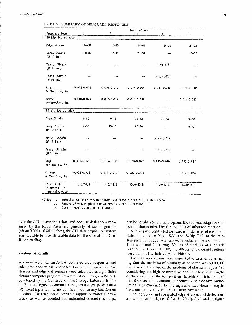
Ta¡,abji and Ball

TABLE 7 SUMMARY OF MEASURED RESPONSES

I tì9

Test Section

20-kip SAL at edse

Edge Strain

Long. Strain(€ 18 in.)

Trans. strain(€ 18 in.)

frans. Stràin(€ 26 in.)

Edge

Defìection, in.

CornertÞflection, in.

26-30

æ-32

0.012-0.0t3

0.0 t8-0.029

l0-r3

t2-t4

0.06-0.0t0

0.0ì2-0.015

3442

æ-34

0.0r4-o.016

0.0 tr-o.018

36-æ 2t-23

t0_t2

(-e) -( t6)

(- r3) - (-2s)

0.0r l-0.0t3 0.0t0-0.012

0.0 t4-0.023

34-kip IAL at edqe

Edge Strain

Long, Strain(@ l8 in.)

Trans, Strain(€ 18 in.)

frans. Strain(€ 26 in.)

Edge

Oeflection, ln.

ørnerDefloctlon, ln.

t6-20

t4- t8

0.0 I 5-0.020

0. 022-0.033

9-r2

t3-t5

0.0 l2-0.0 15

0,014-0,0t8

æ-33

25-28

0.020-0.022

0. 023-0. 024

20-23 t9-20

9-12

(-r2) -(-23)

(- r3) - (-23)

0.015-0.016 0.015-0.0tt

0, 0 t 7-0.024

Iotôl Slôb 10.5/10,5Ihlckness, ln.(notl n¡ l l¡ct!¡ l )

t4,0/ l4,s t0, 0/ t 0.5 n.0/12.3 t3.0/ t4.0

il01ÊSt l, llogatlve v¡luo of ctraln lndlc¿tes a2, ndneo3 of valuer glven for dlfforr,nt3, Straln roadlngr dro ln ml I I lonth¡,

over the CTL instrumentation, and because deflections mea-sured by the Road Rater are generally of low magnitude(about 0.001 to 0.002 inches), the CTL data acquisition sysremwas not able to provide usable data for the case of the RoadRater loadings.

Analysis of Results

A comparison was rnade between nreasured lesponses andcalculated theoretical responses. Pavement responses (edgestresses and edge deflections) were calculated using a fi¡riteelement computer program, Program JSLAB. Program JSLAB,developed by the Construction Technology Laboratories forthe Federal Highway Administration, can analyze jointed slabs(4). Load input is in terms of wheel loads at any location onthe slabs. Loss of support, variable support or material prop-erties, as well as bonded and unbonded concrete overlays,

can be considered. In the program, the subbase/subgrade sup-port is characterized by the modulus of subgrade reaction.

Analysis was conducted for various thicknesses of pavementslabs subjected to 20-kip SAL and 34-kip TAL at rhe mid-slab pavement edge. Analysis was conducted for a single slab12-ft wide and 20-ft long. Values of modulus of subgradereaction used were 100, 300, and 500 pci. The overlaid sectionswere assumed to behave monolithically.

The measured strains were converted to stresses by assum-ing that the modulus of elasticity of concrete was 5,000,000psi. Use of this value of the modulus of elasticity is justifiedconsidering the high compressive and split-tensile strengthsof the concrete at the test sections. In addition, it is assumedthat the overlaid pavements at sections 2 to 5 behave mono-lithically as evidenced by the high interface shear strengthsbetween the overlay and the existing pavement.

The measured and computed edge stresses and deflectionsare compared in figure 10 for the 20-kip SAL and in figure

tonslle str¡ln at sl¿b surfaco,t lms of tost lng,

190

11 for the 34-kip TAL. It is seen that the measured stresses

as well as deflections are a function of the total pavementthickness. Measured deflections are lower for larger totalpavement thickness.

The modulus of subgrade reaction, k, values at the five test

sections were reported to be about 200 pci. It is seen that the

measured edge deflections correspond well with computededge deflections at a k-value of about 200 pci for both the

SAL and the TAL. Measured edge stresses also correspondwell with computed edge stress except fol' sections L and 2.

Measured edge stresses at sections I and 2 are much lowerthan would have been anticipated, especially considering rea-

sonably good agreement between measured and computededge deflections at these sections. One reason for lower mea-

sured edge stl'esses could be that the effective panel length(distance between transvelse cracks) in the existing pavementis much shorter than the 20 feet assumed in the theoreticalanalysis. The condition survey for section l, shown in figure2, indicates an effective panel length of about 15 feet in thepanels containing the instrumentation. The condition survey

for section 2, shown in figure 3, indicates an effective panel

length of about 20 feet in the overlay in the panels containingthe instrumentation. However, the effective panel length inthe existing pavernent at section 2 may be less than 20 feet.

.TRANSPOR'TA7'ION Iì,ESEARCI'I Iì,ECO RI) I 196

Based on the comparisons shown in figures 10 and 11, it isseen that the overlaid pavements are behaving monolithicallyand that the overlaid pavements are responding as full-depthpavement.

Effect of Wheel Path

The field investigation was planned to also provide infor-mation on the effect of wheel path. As discussed previouslywheel paths used for both the SAL and the TAL were 2-inand 18-in inside from the edge. The 2-in wheel path simulatedthe edge loading condition. The effect of having a wheel pathjust 18 inches away from the edge is shown in figure 12. Thereis a significant reduction in measured edge stresses and edge

deflections at all five sections for the wheel path at 18 inches

compared to the wheel path at 2 inches. Similar reductionswere also measured for joint deflections.

Thus, lane widening at time of overlay, if practical, and

lane widening at time of new construction if a tied-concreteshoulder is not used, should be given serious consideration.Keeping truck traffic away from the free lane edge can sig-

nificantly improve pavement performance by reducing criticalstresses and deflections.

'ã. zoo6q,

tno€. tool¡J

c'-. o.o2EoEugoo!r O.Ol@!,l¡J

300

oL6 ro t2

Slob Thlckness, in.

oo3

ong edge

k, Pci

roo

Computed slress deflectionx Meosured stress deflectionSl Ssction

20-kip SAL olong

s3x

Slob Thlchness, in.

FIGURB l0 Com¡rarison of ¡neasured and calculated responses forthe 20-kþ single-axle loading.

t6t4t2to

20-klp SAL olong edge

k, pci

roo300500

- Compuled slressx Meosured slross S2(lSl Sectlon I

300

34-kip TAL olong edge

too

300soo

- Computed stress ÐSZr Meosured slress

Sl Sect ion I

'[ zooøoothoa tool¡J

o 68tOt214t6Slob Thlckness, ln.

34-k¡p TAL olong edge

- Computed Dollsctlon¡ Meosured DelleclionSl Sectlon I

s4(r *[î

68lOt2t4t6Slob Thlchness, in.

FIGURE f l Comparison of measured and calculated responses forthe 34-k¡p tandem.axle loading.

t2345Secllon

6 6 Ao

Ao

ô

O SALA TAL

t2345Section

FIGURE 12 Comparison of responses for wheel paths of 18-in. and 2-in.inside from the edge.

.g- o.o2c

.9(,c,;oôti ool!l¡J

.Ël.delo¡@þ o.sclcÞlÞ.,l.r,

LO

cl¿olo¡

õle.1" O.5.91.9oloorl 0¡

EIE

o

r.o

II tili

- SAL¡r TAL

r92

SUMMARY

Results of the investigation indicate that the four overlaidpavement sections evaluated as part of the reported study areperforming as monolithic pavements with high interface shear

strength at the interface. The strength of the existing pave-

ment at all of the four overlaid test sections was high. Inaddition, cores obtained from sections 4 and 5 did not indicateD-cracking related damage in the overlay concrete.

Comparison of the condition surveys for section 1 (non-overlaid JRCP) and section 2 (overlaid JRCP) indicate.thatall cracking in the existing pavement is not reflected throughthe overlay and that the cracks that did reflect through have

remained tightly closed. Similarly, the condition survey ofsections 4 and 5 indicate that cracks reflected through theoverlay continue to remain tightly closed even after almostseven years of service.

The field investigation conducted by CTL verifies that forproperly constructed bonded overlays, pavement strength-ening is achieved and that the overlaid pavement behaves

monolithically as a full-depth concrete pavement.

ACKNOWLEDGMENTS

Work was conducted by the Construction Technology Lab-oratories under the direction of W. G. Corley, Vice-President,Engineering Development Division. Vernon J. Marks of the

TRANSPORTATION RESEARCH RECO RD I I9(,

Iowa Department of Transportation provided technical coor-dination. The cooperation by the.many personnel of the IowaDepartment of Transportation is gratefully acknowledged.

The opinions and findings expressed or implied in the paperare those of the authors. They are not necessarily those ofthe Iowa Department of Transportation.

REFERENCES

1. S. D. Tayabji and P. A. Okamoto. Thickness Design ofConcrete Resurfacing. Proceedings of the Third InternationalConference on Concrete Pavement Design and Rehabilitation,Purdue University, April 1985.

2. D. Heins. Dynamìc Deflections for Determining StucturalRating of Flexible Pavements. Project HR-178 Report, IowaHighway Research Board, Iowa Department of Transporta-tion, Ames, Iowa, February 1979.

3. V. J. Marks. Improving Subgrade Support Values with Lon-gitudinal Drains. Project MLR-84-3 Interim Report. IowaDepartment of Transportation, Ames, Iowa, January 1984.

4. S. D. Tayabji and B. E. Colley. Improved Rigid Pavement,Ioints. Report FHWA-RD-86-040, Federal Highway Admin-istration, U.S. DOT, February 1984.

Publication of this paper sponsored by Committee on Pavement

Rehabilitation.

TRA NS PO R'TATI O N RES EA RC I'I II ECO R D 1 I 96 193

Application of Deflection Testing to OverlayDesign: A Case StudyCn¡nyr AnrN Rrcnrnn eun LyNNn H. InwrN

In the fall of 1985, the Engineering Research and DevelopmentBureau (ERDB) of the New York Statc Department of Trans.portatiou (NYSDOT) and the Cornell University Local RoadsProgram r¡ndertook a case study involving the application ofthe falling rveight deflectometer (FWD) to pavement evaluationand overlay design. The site for the case study rvas a l-misection of state highway in the Finger Lakes Region of CentralNew York State, which had already been scheduletl to receivean overlay during the 1986 construction season. Nondestruc-tive pavement testing rvas condr¡cted in December 1985 andMay 1986. Pavement laycr moduli were back-calculated fromthe FWD data using the computer program MODCOMP 2.As a part of the study, a mechanistically based cornpuúer pro-gram, called PAVMAN, was developed to calculate remainingpavement life and required overlay thickness. The pavementlayer moduli determined using MODCOMP 2 rvere used withthe PAVMAN progran¡ to estimate the remaining life of theexisting pavement and determine the required overlay thick-ness. The results obtained with PAVMAN compared well rvithdesign overlay thicknesses determined using more traditional¡nethods ofoverlay design (such as engineeringjudgement andthe Asphalt Institute's deflection based method).

In the fall of 1985, the Engineering Research and Develop-ment Bureau (ERDB) of the New York State Department ofTransportation (NYSDOT) and the Cornell Local Roads Pro-gram (CLRP) undertook a joint project co¡rcerned with theapplication of the falling weight deflectometer (FWD) topavement evaluation and overlay design. The project tookthe form of a case study involving a l-mi section of statehighway in the Finger Lakes Region of central New YorkState. The decision to place an overlay at the project siteduring the 1986 construction season had been rnade prior toits selection as the site for the case study. The thickness ofthat overlay had also been decided prior to the selection ofthe project site.

The case stucly was the initial phase of a project undertakenby ERDB for the purpose of assessing the capabilities andapplications of the falling weight deflectometer and the datait genel'ates. Goals of the case study included:

o To give ERDB personnel an opportunity to becomeacquainted with the falling weight deflectorneter and its use.

o To investigate potential applications of the FWD and thedata it generates.

o To investigate the use of rnechanistically-based analysisprocedures with nondestructive test data.

o To assess the relative merits of clifferent testing approaches(in terms of number and spacing of test points) for routinepavement evaluation.

PROJECT SITE

The site for the case study was a l-mi section of State Route96 in Seneca County, New York. Route 96 is a two-lane, ruralhighway, running basically north-south, with no access con-trol. Traffic data for the project al'ea are given in tables 1 and2. Because the terrain in the area is very flat and the soils arefairly shallow, clrainage in the project area is generally poor.

The pavement in the project area at the tirne of the testingfor the case study consisted of several surface tl'eatntents inter-layered with two asphalt concrete overlays (nominal com-bined thickness, three inches) over a biturninous macadampavement (3-in tar-bound crushed limestone top over a 7-inlayer of crushed stone) placed in 1914. The rnost recent over-lay was a l-in almor coat placed in 1965.

At the time of the deflection testing, the condition of thepavement variecl greatly. Some portions of the pavement wereintact and exhibited little or no distress. Other portions, par-ticularly sections of the northbound outer wheel path, werebadly rutted (rut depths of up to 3% inches) ancl/or exhibitedsevere alligator cracking. Recent pavement condition ratingsfor the project site are summarized in table 3. The surfaceand base ratings are orì a ten-point scale, where a score of 9or 10 indicates that the pavement is in excellent condition,while a score less than 6 indicates poor condition, and a scoreof 1 indicates the worst condition (1).

TESTING PROGRAM

Nondestructive Testing

Nondestructive pave¡nent testing for the case study was con-ducted in December 1985 and May 1986. The testing inDecember 1985 consisted of FWD and Benkelman beam testsin the inner and outer wheel paths of both lanes. These par-

TABLE I TRAFFIC VOLUMESYear 1960 1970 1973 1976 1977 1980 1986

AADT 1585. t723 1800 1850 2000 1800 3190

C. A Richter', Strategic Highrvay Research Progranr (SHRp),818 Connecticut Ave., N.W., Washington, D.C. 20006. L. H.Irwin, Cornell University Local Roads Progranr, Riley Robb Hall,Ithaca, N.Y. 14853.

TABLE 2 VEHICLE CLASSIFICATION DATA (MARCH 1986)

Vehicle Class Percentaqe of AAD I'Passenger Cars and Pickup 'Ilucks

2-Axle, &Tire Single Unit Trucks

Single Unit Trucks Having 3 or More Axles

3-Axle Tbactor/Tlailer Combinations

4-Âxle tactor/Tìailer Combinations

Tractor/tailer Combinations With 5 or More Axles

88

6

I

0

1

4

t94

allel tests were conducted at 50-ft intervals on two 500-ft

sections, one at each end of the project site.In addition, FWD tests were conducted at intervals of 250

feet over the full 1-mi section in the two outer wheel paths

and in the middle of the northbound lane, so that comparisonsof the two test strategies (testing at shot't intervals over sub-

sectlons of the pavement in question and testing at uniformintervals over the full length of the pavement section) couldbe made. Each of the test strategies resulted in about 22 tests

per mile along each line of test points. In May 1986, only thetwo 500-ft sections were tested, again with both devices, at

50-ft intervals in the inner and outer wheel paths of both lanes.

In all, FWD tests were conducted at 136 points in Decelnber1985 and at 88 points in May 1986.

Three or fou¡'FWD drops from one height were conductedat each test point. After discarding data indicative of sensor

overflow or other anomalies, the data for each test point were

averaged (on a sensor by sensor basis), so that the effects ofrandom error in deflection measurement woulcl be minimized.

Supplementary Testittg

In addition to the nondestructive deflection testing, a limitedamount of pavement coring, soil boring, and seismographic

testing was conducted. The pavernent coring and soil boringwere done to verify pavement layer thicknesses and to provide

samples for laboratory testing. The laboratory tests (includingsieve analyses, Proctor densities, sand equivalent tests, and

Atterberg limits for the unbound materials and resilient mod-ulus tests, asphalt extractions, and penetration tests for the

asphalt concrete) were conducted to characterize the pave-

TABLE 3

PAVEMENTCONDITIONRATINGS

,III,ANSPO RT-A'I'I ON R ES EARCH R DCO R D 1 I 9()

ment materials for research purposes and would not be neededfor routine pavement evaluation. Seismographic testing was

conducted to determine the depth to bedrock in the projectarea, so that the subgrade could be more accurately modeledin subsequent analyses. Seisrnographic testing would generallynot be required unless the depth to bedrock is relatively shal-low (less than 30 feet, or so).

ANALYTICAL METHODS

Back-Calculation of Pavement Layer Moduli

Pavement layer moduli were back-calculated using the com-puter program MODCOMP 2 (). ^fhe assurnptions on whichMODCOMP 2 is based include the following:

o Pavement layers ale homogeneous and isotropic, andextend infinitely in the horizontal plane.

o The deepest pavement layer is semi-infinite.o The load on the pavement is uniforrnly distributed over

a circular area, and the direction of the force is perpendicularto the pavement surface.

o Full friction exists at the pavement layer interfaces (inother words, there is no lateral slippage of the pavement layersrelative to each other).

Using MODCOMP 2, it was possible to obtain reasonablesets of layer moduli for 128 (94 percent) of the December1985 test points, and 82 (93 percent) of the May 198ó testpoints. The failure to obtain reasonable solutions for theremaining test points was most likely due to inaccuracies inthe pavement model (for exarnple, incorrectly defining thedepth to a bedrock layer, the use of a linear model for stless-dependent materials, inaccurate layer thicknesses, bouldersat shallow depths in the subgrade, etc.).

Remaining Life and Required Overlay ThicknessCalculations

A computer pl'ogram, called PAVMAN (for PAVementMANagement), was developed to facilitate mechanistically-based analyses of remaining pavement life and required over-lay thickness (3). PAVMAN was written in the FORTRANprogramming language to run on IBM-PC microcomputers.

Year Surface Base

l98t

r982

1983

1984

1986

8

7

I

7

6

8

7

I

7

6

Richter and Irwin

LayerModulus

É'max

tr- mrn+ 0.6Á

195

i year >l

FIGURIÐ I Freeze-thaw seasonal var¡ation model.

Selected characteristics of PAVMAN are as t'ollows:

. The pavement is modeled as a layered elastic system,using the same assumptions articulated above for MOD-COMP 2.

o Pavement materials may be modeled as being either lin-ear or stress-dependent in their response to load.

o Traffic is considered in terms of an eighteen-kip equiv-alent single axle load.

o The computer program NELAPAV (4) is used as a sub-routine to calculate the critical strains induced in the pavementsystem by a 9-kip dual wheel load.

o Subgrade rutting and surface fatigue are considered as

potential failure modes. The fatigue was summed for both theoverlay material and the existing surface.

o The revised Shell subgrade strain criteria (5) are used toestimate the allowable number of strain repetitions for thesubgrade.

¡ The Shell asphalt concrete fatigue criteria (ó, 7) are usedto estimate the allowable number of strain repetitions for an

asphalt concrete surface or overlay.o The user may select one of three seasonal variation models

for each of the pavement layers; a temperature-based modelfor asphalt concrete, a freeze-thaw seasonal model, or a wet-dry seasonal model. Schematic diagrams of the freeze-thawmodel and the wet-dry model are given in figures I and 2.Ramps in the layer moduli are modeled as a series of steps(dashed lines in the figures), with each step corresponding toa different season. Since the user defines the magnitude ofthe seasonal variation as well as the duration of each season,it is thought that these models are sufficiently versatile tomodel the present state of knowledge of seasonal variationfor most circumstances.

¡ Miner's hypothesis of cumulative fatigue damage (8) is

applied to sum the damage over the different seasons, andover the life of the pavement.

APPROACHES TO DATA EVALUATION

Having deflection data for roughly one hundred test pointsin a mile of pavement presents the engineer with an interestingproblem-how the data can be used to derive a design overlaythickness (or thicknesses, if it is deerned appropriate to sub-divide the section) or an overall remaining life estimate forthe section. Traditional deflectirn based overlay design meth-ods have used a single representative deflection measurement(e.g. mean Benkelman beam deflection plus two standard

LayerModulus

ç-mtn

r v""r IFIGURE 2 Wet-dry seasonal variation model.

196

deviations, 85th percentile deflection, etc.). At the otherextreme, one could determine the required overlay thicknessfol each individual test point and then decide how to translatethe individual overlay thicknesses into a design value.

In deciding between these two approaches to data evalu-ation, there are some definite tradeoffs. On the one hand,using a representative deflection basin is relatively simple andfast. However, it is not clear that the resulting design overlaythickness will be representative of what the pavement reallyneeds. On the other hand, analyzing the data for each testpoint individually has the potential to provide much moreinformation about the pavement, but is considerably moretime consuming.

Both approaches to the data analysis were used in this casestudy so that the merits of each could be evaluated morethoroughly. The representative deflection basins used weredetermined by estimating the 85th percentile deflection (inother words, the deflection that was greater than or equal to85 percent of the observed deflections) for each sensor in thedata set. Separate 85th percentile deflection basins were derivedfor the test points at 50-ft intervals ancl those at 250-ft inter-vals, in the northbound outer wheel path. For both analysisapproaches, the remaining life and overlay design analyseswere based primarily on the December 1985 deflection databecause it was the more extensive data set. Layer moduliderived from the May 1986 deflection data were used to definethe magnitude of seasonal variation for the seasonal variationmodel.

RESULTS

General

Mechanistic Overlay Design

Moduli for the four unknown upper layers (surface, base,subbase, and subgrade) were derived from the deflection basindata using the MODCOMP 2 computer program. The resultswere evaluated and spurious data were rejected. (It some-times happens rhar while MODCOMP 2 will give a good fitof the deflection data, within the specified tolerance, the results

7'Iì,ANSPOR'TATION RESEARCH RECORD I 196

TABLE4'TYPICAL' BACK.CALCULATED LAYERMODULI

l,ayerDepth Modulus

(Inches) (ksi)

LayerDepth Modulus

llnchesì fksiì

LayerDepth Modulus

llnchesl lksi)0-9 380

$36 63&66 30

6&33ô 25033&oo 1,250

G9 2t89-24 6

24-72 14

72-300 25030Goo 1.250

G9 6689-36 28

3&66 7

6&336 2sO

33G oo 1,250

G9 1009-24 lO

24-72 7

72-291 250291-oo 1,250

G99-24

24-4848-36036G'æ

0-9 2709-24 l9

24-72 13

72-204 250204-ø 1,250

588

94

t)

2501,250

are unreasonable and, therefore, must be regardecl as spu-rious.) After the screening process, a set of layer tnoduli wereselected for each test point for use in the overlay calculations.The results were highly variable. A complete summat'y of theback-calculated rnoduli is given elsewhere (3). Some typicalresults are given in table 4.

Required overlay thickness analyses were conducted for a

15-yr design life using the PAVMAN computer prograrn. Theresults of the analyses for the indiviclual test points we re highlyvariable, ranging fro¡n zero (no overlay needed) to seve¡linches.

It is believed that this valiability is plimarily due to vari-ations in the moisture content of the upper subgrade soil. Ahistogram of the required overlay thickness results is given infigure 3. The test points requiring the greater overlay thick-nesses wele predorninantly in the outer wheel path of thenorthbound lane but were scattered over the full length ofthe test section. Many of the larger overlay thicknesses occurredfor test points between the two 500-ft sections that were testedat 50-ft intervals (in other words, at points that would nothave been tested if only the two 500-ft subsections of thepavement had been tested).

In order to determine the overlay thickness required for a

given design life (in this case, fifteen years), PAVMAN cal-culates (and reports) the rernaining life of the pavement forfive different trial overlay thicknesses, ranging from zero to

gB0c'õ 70o_

Euot-bs0-E ootr=30z

Overlay Thickness (inches)

FIGURB 3 Required overlay thickness frrquency.

0. .1-1.0 1.1-2.0 2.1-3.0 3.1-4.0 4.1-5.0 5.1-6.0 6.1-7.0

640)

o.Ea/)^6.50)c-c.9.ct--

(d

=0)

o1

Richter arul lrwin

Life (Years)

FIGURE 4 Pavement life versus overlây thickness.

a user specified maximum. A typical plot of overlay thickness

versus pavement life is given in figure 4. The degree to whichsuch plots are linear in semi-log space appeal's to depend, tosome extent, on the layel that controls the design and whetherthe controlling layer is the same for all overlay thicknesses.

Eighty-fifth percentile overlay thicknesses were estimatedfrom the individual overlay thickness results for the test pointsat 50-ft and 250-ft intervals in the northbound outer wheelpath, as well as for all of tlìe test points, with results of 2.6,5.9, ancl 1.1 inches, r'espectively. The disparity between the

results for the different sets of test points indicates that thenurnber and location of test points selected may significantlyaffect the results. This indication is further supported by thevariability in the individual overlay thickness results.

The required overlay thickness results for the 85th percen-

tile deflection basins, 1.8 inches for the test points at 50-ftintervals, and 6.1 inches fol those at 250-ft intervals, cornparefavorably with the 85th percentile overlay thicknesses derivedfrom the individual test point results for this particular pave-

ment. However, it should not be assumed that this would be

true for all pavements. Furthermore, while the degree of vari-ability in the pavement is clearly evident from the individualtest point results, it is not at all evident when the represent-ative deflection basin approach is used.

Overlay Design Using the Asphalt Institute Method

The required overlay thickness for the ploject site was also

deter¡nined using the Asphalt Institute's deflection based

overlay design procedure for comparison (9). For these com-parisons, the overlay thickness requirement was first deter-mined using the FWD data, so that the comparison would be

between different analysis methods based on the same device.

Since the Asphalt Institute procedure was developed for use

with the Benkelman beam, the Benkelman beam data were

used in a subsequent analysis to check the results.The Asphalt Institute recommends that pavement testing

for overlay design be conducted in the outer wheel paths.

197

Therefore, only the data frorn the outer wheel paths wereused in the overlay designs. It was assumed that the deflec-tions measurecl in the spring of the year were 20 percent lowerthan the maximum spring values. This assumption was con-sistent with an assumption made in defining the seasonal var-iation in layer moduli for the mechanistic analysis. Both the

FWD data and the Benkelman beam data were normalizedto the 18-kip axle load prescribed in the Asphalt Instituteoverlay design method.

Although both FWD and Benkelman beam data were avail-able for the project site, it was assumed that the maximumFWD deflection was equal to 50 percent of the Benkelmanbeam deflection under a similar load. This assumption was

somewhat arbitlary, but is in reasonable agreement with thetest results for the pavement in question. The assumed cor-relation was used instead of an exact correlation, so a typicalassumption that might be made when only FWD data was

available might be tested. Accordingly, the FWD deflectionswere doubled to approximate Benkelman beam deflections.The traffic volumes and design life used in the Asphalt Insti-tute method were the same as those used for the mechanis-tically based analysis.

The overlay thicknesses derived from the doubled FWDdeflections and the Benkelman beam deflections, for a 15-yrdesign life, were both approximately 3.8 inches. Thus, for thegiven pavernent and assumptions, it does not matter whichdevice is used, as long as the Benkelman beam deflectionsare twice the FWD deflections. This will not always be the

case.

Interpretation and Application

If it is accepted that it is better to analyze the deflection data

on a point by point basis, the question that arises is how doesone apply the individual overlay thicknesses once they have

been calculated? The strict 85th percentile overlay thicknessapprcach used in the preceding conrparisons is one approach,but it has several flaws. First, it does not really make use ofthe information on the variability in the pavement, and sec-

ond, a design ovellay thickness so derived can be undulyinfluenced by a few excessively weak test points. To makefull use of the information available, the engineer must deter-mine what the required overlay thickness results tell aboutthe pavement.

One interpretation is that individual required overlay thick-nesses that are substantially higher than some norm (the mean,median, eighty-fifth percentile value, an arbitrarily selectedvalue, etc.) are indicative of areas that neecl spot improve-ments over and above the overlay to be place on the entirepavement. For the purposes of this case study, the followingprocedure for deriving a design overlay thickness was pro-posed and used:

1. Calculate the required overlay thickness for each testpoint.

2. Determine what proportion of the test results yield a

negligible requirecl overlay thickness.3. If the proportion of test points requiring negligible over-

lay thicknesses is large, consider spot improvements (such as

drainage improvements, cut-out and replacement of small sec-

tions of pavement, patching, etc.) for the locations that need

198

work, and use lemaining life analyses to determine when thepavement needs to be considered for an overlay. Alterna-tively, one could determine the overlay thickness required insome given future year.

4. If the number of test points requiring negligible overlaythickness is small, proceed as follows:

(a) Consider the spacing and magnitude of the non-zel'orequired overlay thickness results to determine whichpoints should be considered for spot improvementsin addition to the overlay placed on the entire pave-ment. Spot improvements might include additionaloverlay thickness, drainage improvements, cut-outand replacement of small sections of pavement, etc..

(b) Since the overlay is being designed to improve thoseareas that need an overlay, as opposed to those thatdo not, neglect all zero required overlay thicknessesin subsequent determinations.

(c) Determine the 85th (or other design level) pelcentileoverlay thickness from the set of non-zero overlaythicknesses for test points which have not beenselected for spot improvements. This becomes thedesign overlay thickness. The presumption here isthat spot improvements will reduce the requiredoverlay thickness at the spot improvement locationsto the level required by the remainder of the pave-ment.

Table 5 summarizes design overlay thicknesses derived fromthe data for the inner and outer wheel paths of both lanes,using the procedure outlined above, for the followingimprovernent options:

. No spot improvements are to be made.o Spot improvements will be made at locations requiring

overlay thicknesses of 6 inches or more.o Spot improvements will be made at locations requiring

overlay thicknesses of 5 inches or more.o Spot improvements will be made at locations requiring

overlay thicknesses of 4 inches or mol'e.o Spot improvements will be made a locations requiring

overlay thicknesses of 3 inches or more.

TABLE 5 DESIGN OVERLAYTHICKNESSES FOR VARIOUSIMPROVEMENT OPTIONS

TRA N S PO RTAT'IO N RES EA RCI-I R ECO R D I I 9()

For comparison, the 85th percentile value determined usingall of the test points in the wheel paths (including those requir-ing no overlay) is 1.6 inches.

The data from the testing in the middle of the northboundlane were not included in the determination of the designoverlay thickness for two reasons. First, unless some of thedata for the northbound lane were omitted, the overlay designwould be based more heavily on the northbound lane thanthe southbound lane because more testing was done in thenorthbound lane. With the mid-lane data omitted, the twolanes are equally represented in the data set. Second, therelevant portion of the pavement for overlay design purposes(in terms of structural requirements) is the portion of thepavement subjected to significant traffic. Since the portion ofthe pavement between the wheel paths is not subjected tosignificant traffic, it should not control or significantly affectthe thickness of the overlay required for structural purposesand, therefore, should not be considered in the analysis ofrequired overlay thickness.

In the discussions that follow, it is assumed that spotimprovements will be made in the vicinity of all test pointshaving required overlay thicknesses in excess of three inches(Improvement Option 5).

If it is assumed that the necessary spot improvements canbe made by placing greater thicknesses of asphalt concrete orby installing underdrains, and that the incremental cost of al-in thickness ofasphalt concrete is $4.25 per linear foot (basedon a pavement width of 20 feet, as per pavement records, anasphalt concrete cost (in place) of $35 per ton, and an asphaltconcrete density (in place) of 145 pounds per cubic foot),while underdrains cost $8.00 per linear foot (based on anaverage trench depth of two feet, a trench width of 18 inches,6-in perforated steel pipe at $4.65 per linear foot, excavationat $12.00 per cubic yard, filter material (average total depth,16 inches) at $25 per cubic yard, and backfill (8-in deep, onaverage) at $4.02 per cubic yard), the installation of under-drains is more economical than placing the required extrathickness of asphalt concrete whenever the underdrains replacemore than 1.9 inches ofasphalt concrete (whenever the requiredoverlay thickness exceeds the design overlay thickness by morethan 1.9 inches).

Under the assumption that spot improvements will be madeat all locations requiring overlay thicknesses in excess of threeinches, the design (85th percentile) overlay thickness is 2.1inches. Therefore, the installation of underdrains is the moreeconomical method of making the required spot improve-ments whenever the required overlay thickness is four inchesor more (2.1 + 1.9), and the placement of a thicker overlayis more economical where the required overlay thickness isless than four inches. For the purpose of these comparisons,it assumed that the additional overlay thickness would beplaced across the full width of the pavement. Under certaincircumstances, it might be possible to taper the overlay sothat only the portion of the pavement that needed the addi-tional thickness got the full thickness.

Of the locations that need spot irnprovements, only onearea has a required overlay thickness less than four inches.Therefore, under the given assumptions, with a design overlaythickness of 2.1 inches, the most economical method of reha-bilitating the pavement is to place a total overlay thicknessof 3.6 inches in that one area and to install underdrains at theother locations needing spot improvements.

lmprovement

Optionso

l,reslgn

Overlay

Thickness

Percentage of

Pavement Requiring

Spot Improvements

I

2

3

4

5

5.9

5.4

3.8

2.5

2.1

0.0

4.7

r3.3

15.8

16.3

ôNumbem refer to ühc lis¿ in the tex¿.

Richter and Iruin

Comparison With Other Methods

The thickness of the overlay placed at the project site in thesummer of 1986 was cletermined by NYSDOT engineers usingjudgment and experience, without the benefit of the nonde'structive testing or the subsequent analyses. That overlay con-sisted of up to 3/z inches of binder material placed to fill inpavement ruts, followed by a1.Vz-in binder course and a l-intop course. Thus, the pavement was overlaid with a ¡ninimumof 2Vzinches of asphalt concrete in areas with minimal ruttingand a maximum of 6 inches in severely rutted areas' Spotdrainage improvements were made only at the extreme north-ern end of the project site. Referring to table 5, the 2t/z-inminimum overlay thickness is comparable to the design over-lay thickness determined for the instance where all pointsneeding an overlay 4 or more inches in thickness were subjectto spot improvements. If it is assumed that the test points forwhich high required overlay thicknesses were calculated werein the more severely rutted sections of the pavement' thereis reasonable agreement between the required overlay thick-nesses calculated for a 15-yr design life and the overlay actuallyplaced.

The 3.8-inch design overlay thickness determined using theAsphalt Institute method is comparable to the design overlaythickness detelmined by using the PAVMAN program and

assuming that spot improvements would be made at pointsrequiring overlays in excess of 5 or 6 inches (see table 5).Thus, if the 3.8-in overlay were placed with no spot improve-ments, we would expect a higher premature failure rate thanif the spot improvements were made, as is assumed in the

mechanistically based design.

IMPLICATIONS AND UNANSWERED

QUESTTONS

Why Bother?

The reader may well be wondering if mechanistically based

pavement analysis and overlay design rnethods are really worth

all the trouble. In the authors'opinion, the answer is abso-

lutely yes, if they are usecl to their fullest potential. If thedecision to place an overlay has already been made, and the

year in which it is going to be placed has already been deter-mined, so that the only reason for using the analysis procedure

is to decide how thick the overlay should be, then a mecha-

nistically based analysis procedure may not be worth the trou-ble. However, if the procedure is instead used to determinethe optimal timing for a pavement rehabilitation project, and/or the most economical Ineans of rehabilitating a pavement,preferably within the framework of a network-level pavement

management system, then lnechanistically basecl pavement

analysis techniques have great potential.With rnechanistically based pavement analysis techniques,

one can examine the consequences of putting off an overlayfor a few more years or moclel the effects of base stabilization,surface recycling, or improved drainage. One can look at the

tradeoffs involved in rehal¡ilitating section A this year instead

of section B, or in constructing a new pavement in stages,

instead of placing the entire structure needed for the design

life at once. In short, mechanistically based pavement analysis

199

and design methods have the potential to be a tremendoustool for optimizing the use of funds in the highway industry.

What's Missing?

While mechanistically based pavement design atrd analysis

methods have tremendous potential, there are several areas

in which further research is needed to perfect the method-ology. The following sections discuss some of these areas.

Testing Program

The optimal number and spacing of NDT test points for use

with mechanistically based pavement evaluation and design

methods has not been determined. This case study attemptedto address the issue to a limited extent. From the work thatwas done, it appears that both closely spaced test points overshort subsections of the pavement in question and uniformlyspaced test points ovel'the full length of the pavement have

some advantages and disadvantages. Until further studies can

be done to develop reliable criteria, a reasonable cornpt'omise

would be to test the full length of the pavement in both theinner and outer wheel paths at 250-ft inte¡vals, with the test

points in the inner wheel path offset by 125 leet from those

in the outer wheel path (in other words, if the first test pointin the outer wheel path is at station 0+00, then the first test

point in the inner wheel path should be at station l+25)'

Failure Criteria

It is generally held that the critical strains in a pavementstructure are the ¡naximum horizontal tensile strain in the

surface material and the vertical compressive strain at the topof the subglade. The criteria used to determine the allowablenumber of strain repetitions at each of these locations are, as

a matter of necessity, empirically derived and, therefore, maynot be entirely applicable to materials and circumstances thatdiffer from those for which and under which they were devel-oped. For example, The Shell revised subgrade strain criteriaused in the PAVMAN program, as well as many other subgrade

strain criteria, were derived from the AASHO Road Testdata. Since the AASHO Road Test involved only one subgrade

soil and one climate, the use of those criteria for pavements

in other areas is an extrapolation that Inay or may not be

valid, Further research is needed to develop more universallyapplicable strain criteria, for both subgrade and surface mate-rials, and to establish limitatiorts for those that currently exist'

The l9-kip Equivalent Axle Load Question

Frequently, pavement design is based on the 18-kip equivalentsingle-axle load (ESAL). That is, all vehicle loads are trans-lated to an equivalent number of 18-kip single-axle loads. Likethe subgrade strain criteria, most commonly used sets of 18-

kip equivalency factors were derived fi'om the AASHO RoadTest data (separate factors exist for flexible and rigid pave-

ments). The problem with this is that the number of loads ofany given magnitude that is equivalent to an 18-kip ESAL is

200

different for every pavement, so that every time the AASHOequivalency factors are used, an error of unknown magnitudeis made. In a mechanistically based analysis, this weaknesscould be eliminated by treating each vehicle category sepa-rately and summing the damage due to each. The cost ofdoing this would be an increase in computation time. Whetherthe accuracy gained would be worth the added cost is some-thing that needs to be examined. Alternatively, as microcom-puter technology improves, the added cost ofconsidering thedamage due to individual vehicle classes may become negli-gible and thus negate the advantage of using the 18-kip ESAL.

Staged Construction, Alternative Materials, andRehabilitation Methods, and Network LevelPavement Management

While mechanistically based pavement analyses have thepotential to consider staged construction, alternative pave-ment materials, and alternative rehabilitation methods (sta-bilized, recycled, or otherwise modified materials, improveddrainage, etc.), such analysis alternatives have not necessarilybeen fully implemented at the project level, let alone at thenetwork level.

The PAVMAN program developed for this case study is astarting point. However, more advanced computel. programswith the capability to model staged const¡.uction, pavementnetworks instead of single projects, and rehabilitation meth-ods other than simple overlays, are needed before mecha-nistically based pavernent analysis methods can be used totheir fullest potential.

SUMMARY

A case study, in which nondestructive test technology andmechanistically based analysis techniques were applied to theevaluation of lequired overlay thickness for an existing pave-ment has been described. A computer program, PAVMAN,developed to facilitate the mechanistic analysis of the pave-ment, is also described. The design overlay thickness deter-mined using PAVMAN is in reasonable agreement with thosederived for the same pavement using the Asphalt Institute'sdeflection-based overlay design procedure. Actual construc-tion, based on design by experience, also closely matched theresults from the mechanistic analysis. Recommendationsregarding testing programs for similar activities are made, and

7'Iì,A N S PO III'ATION RDS EA RC I I R ECO R D I ] 96

areas in which the technology needs further development arediscussed.

ACKNOWLEDGMENTS

The work discussed herein was supported by the New yorkState Department of Transportation and the Cornell LocalRoads Prograrn.

The views and opinions expressed herein are those of theauthors, and do not represent official views or policies of theNew York State Department of Transportation or CornellUniversity.

REFERENCES

l. P. T. Hartgen. Status of Highway Condition Scoring in NewYork State. ln 'lransportation Research Record gg1, TRB,National Resealch Council, Washington, D.C., 1984, pp.g5-90.

2. L. H. Irwin, User's Gukle to MODCOM? 2. Cornell LocalRoads Program Report No. 83-8, Cornell University, Ithaca,N.Y., November 1983.

3. C. A. Richter and L. H. Irwin. Application of Nondestructive\esting to Pavement Evaluation and Overlay Design. CornellLocal Rolds Prograrn Report No. 87-3, Cornell University,Ithaca, N.Y., June 1987.

4. L. H. Irwin and D. P. T. Speck. NEL,4 PAV Ilser's Guide.Cornell Local Roads Program Report No. 86-1, Cornell Uni-versity, Ithaca, N.Y., January, 1986.

5. A. I. M. Claessen, J. M. Edwards, p. Sommer, and p. Uge.Asphalt Pavement Design-The Shell Method. proceedings,Fourth International Conference on the Structural Desigtr-ofAsphalt Pavements, Vol. l, 1977, pp. 39-74.

6. M. W. Witczak and K. R. Bell. Rèmaining Life Analysis ofFlexible Pavements. Proceedings, Associatiott of Asphait pav-ing Technologrsls, Vol. 47, 1978, pp.229-269.

7. W. Heukelon. Observaûons on the Rheology and Fracture oflltumens and Asphalt Mixes. Shell Bitumen Report No. 19,Shell Laboratorium-Koniklijke, 1966.

8. M. A. Miner. Cumulative Damage in Fatigue. In Journal ofApplied Mechanics, American Society of Mechanical Engi-neers, Vol. 12, No. 3, Seprember 1945, pp. A-159-A-164.-

9. The Asphalt Institute. Asphalt Overlays ancl pavement Reha-bilitation. Manual Series No. l7 (MS-17), College park, Mary-land, November 1977.

Publication of this paper sponsored by Committee on pavementRehal¡ilitation.

Evaluation of the Performance of BondedConcrete Overluy on Interstate Highway6L0 North, Houston, Texas

Konsrovro KossNo aNo F. FneNx McCunoucH

The objective of the study was to evaluate the performance ofthe bonded concrete overlay project on,IH 610 North i¡l Hous'ton and implement the fintlings in other studies on bondedconcrete overlay. The performance of the bonded concreteoverlay was monitored on ten experimental sections selected

from the 3-%-mi project and ranging from 400 to 600 feet long.Periodic field measurements were conducted, and an assess'

ment of overlay pavement life was made. The resulting con'clusions and recolnmendations were to be used by the TexasState Department of Highways and Public 'fralrsportation todcsign overlays for rehabilitation prograrns on continuous rein-forced concrete pavement (CRCP).

Since 1956 the United States has been involved in the largest

public works project ever undertaken, the 42,500-mi system

of intetstate highways. Unfortunately, these highways have

begun to weal out. Not only are we reaching the end of thedesign life of many sections of highways, btrt the amount oftraffic is far exceeding the design estimates (,1). In recent

years, the general interest of the highway adrninistration has

shifted from construction to maintenance, rehabilitation, and

resurfacing.Portland cement concrete (PCC) overlays have l¡een used

to resurface pavements for more than 60 years. However,experience in the use of bonded concrete overlays is mostlywith airport runways and bridge decks, although there are

instances in which bonded concrete overlay has been used forimproving skid resistance on highways (2,3).

The U,S. Air Force has more than 20 years of experiencewith thin bonded conct'ete overlay (4). Overlays ranging frorr2- to 4-in thick have been constructed on runways subject tolight as well as heavy traffic and used by small as well as large

aircraft. The condition of the overlays over a period of 17

years has ranged from good to very good, but there have been

a number of cases whele protrlems were encountered. Folexarnple, severe reflection clacking and rapid deteriorationfollowing loss of interface bond was experienced in a taxiwayat the Tulsa Airport.

During the past two to three years, several research studies

were undertaken at the Center for Transportation Research

to address questions concerrting the use of thin bonded con-

crete overlays for highway pavenìent rehabilitation. Tests were

made on laboratory specimens and cores froln constructed

Center for Transportation Research, The University of Texas at

Austin, Austin, Tex. 78705.

7'II.AN S PO R'I'ATION RES EA RC I-I R ECO I? D I I 96 201

slabs in the field in which a bonding agent was used. A majorfinding of this research (5) was that the interface betweenexisting slab and overlay develops a shear strength three tofour times the theoretically predicted shear stress due to wheel

loads of the expected traffic. Also, a condition survey of the

overlay section soon after overlaying ancl again in six monthsdid not show any significant distress. This experience encour-

age the SDHPT to use a 4-in bonded concrete overlay on a

length of about 3-% mi to improve the pavement conditionof Loop 610 North in Houston. It was suggested that several

sections of this pavement be identified and monitored to fatherperformance information periodically. It was planned that the

analysis carried out using the lesulting data would help answer

questions about the relative merits of different types of over-

lay materials.The overlay project is located on IH 610 North in Houston

between East T.C. Jester Blvd. and IH 45 (see figure l). Atthis location, the loadway is an eight-lane divided highwaywith four through lanes in each clilection a¡rd a concrete median

barrier. The main lanes are 12 leet wide and shottlclers are

10 feet wide.The 4-in bonded concrete overlay was placed on the existing

8-in continuous reinforced concl'ete pavement (CRCP). The

existing concrete pavement rests on 6-in thick stabilized sub-

base. The typical cross section of the project is presentecl in

figure 2.

OBJECTIVE OF THE STUDY

The primary objective of the study was to evaluate the per-formance of the bonded concrete overlay on IH 610 North inHouston and irnplement the findings of other studies on bonded

concrete overlays.The sub-objectives were-

1. To identify several sections to represent the va¡'iation inthe original pavement condition and the material used for theoverlay,

2. To observe and record the materials actually used forthe ovellay,

3. To make observations of the behavior parameters beforeand after-overlay, and

4. To perforrn statistical analyses to evaluate the field data.

202

FIGURE I Location of the overlay project.

DESCRIPTION OF THE STUDY

The following variables wel.e considered in the study:

1. Overlay reinforcement: CRCP and fiber reinforced con-crete pavement,

2. Overlay aggregate: siliceous river gravel and limestone,and

E Compacted Embankm€nt

E 4'Bonded Concreto Overlay

E 4'Asphalt Concrolo Overlayg Existing 8" Concrot€ pavomonl

E Exist¡ng 6" Stabilizod Base

E Existing t" Asphalt Concrete pavomont

FIGURE 2 A typical cross section of the bonded concreteoverlay pavement on IH 610 North, Houston.

TRANSPORTATION RESEARCI.I RECORD I 1 9ó

HOUSTON

3. Old pavement condition: no distress, moderate distress,and severe distress,

The use ofthe variables in 1 and 3 above is self-explanatory.The variables in 2 were used for two reasons: (1) the oldpavement was constructed using siliceous river gravel, and(2) research done at the Center for Transportation Researchat The University of Texas at Austin (10) showed that lime-stone is a better coarse aggregate than siliceous river gravelfrom a long-term performance standpoint. Therefore, sili-ceous river gravel was used in some sectio¡ts and limestonewas used in others.

From the 3-Vz-mi overlay project on eastbound IH 6i0 Northten test sections ranging from 400 to 600 feet long were iden-tified, to maintain homogeneity within a section (similar over-lay reinforcement, overlay aggregate, and distress) and alsoto have a length adequate for the desired observations. Theten sections were divided into two fiber-reinforced concleteoverlay sections, two reinforced concrete overlays sectionsusing limestone aggregate, and six reinforced concrete overlaysections using siliceous gravel aggregate. The reinforced con-crete overlays were reinforced with a grade 70 wire fabricmesh with spacing and size of 6 x 12 - D16 x D10 through-out the sections. Across transverse construction joints, barsof the same grade and size as the mesh were used at 12-inintervals, in addition to the mesh. For the fiber reinforcedconcrete overlays, 85 pounds of fibers per cubic yard wereused. The method of construction inclucled the following steps:

1. Scarifying the old pavement to a %-in depth,2. Placing reinforcing steel,3. Grouting over reinforcing, using l l gallons of water per

sack of cement grout, and4. Placing the concrete by slip forming.

G¡l¡n¡

60.0'(Usuall

Koesno antl McCullough 203

TABLE 1 CONCRETE MIX DESIGNS

Material

Mix Using

Silicious R¡ver Gravel Limestone SRG with F¡bers

Cemenl (lb)

Coarso Aggregate (lb)

Fine Aggregate (lb)

Retarder (POZZ.300R)

Air Entrainer (AE-10)

Waler (lb)

(oz.)

(oz.)

658

1950

1055

30

7

233

658

177 0

't 235

30

7

233

752

1 218

17 15

38

5

250

Note: All weighls are based on material in the SSD condition.

A summary of the concrete mix design data is shown in table1. Summaries of tensile and flexural strengths are shown intables 2 and 3, respectively. The average tensile strengths offiber reinforced sections, welded wire fabric with limestonesections, and welded wire fabric with siliceous river gravelsection are 698, 642, and 615 psi, respectively.

It was suggested that the ten experimental sections selectedbe monitored for at least three years so that it would bepossible to identify any correlation between materials andperformance based on the different environmental conditions.

Based on the results of the first condition survey, the dis-tress indexes of each experimental section were determinedusing the following formula (ó):

Z" = 1.0 - 0.065 i6'F - 0.015 MS - 0.009SS

TABLE2 SUMMARY OFAVERAGETENSTLE STRENGTH (PSr) (OVERLAYPORTTON), rH 610 NORTH, HOUSTON

Dates Core TakenTesl Seclion

Number February 1986 January 1987

where

Z" : distress index,FF : number of failures per mile (sum of punchouts and

patches),MS = percent minor spalling, and$g = percent severe spalling.

The distress values are subtracted from 1 and the value obtainedin a maximum value. As the distress index decreases, thequality of the road deteriorates, with zelo being the valuewhere major rehabilitation is necessary.

Three levels of distress were used in this study:

o No significant distress, with distress index ranges from 0to 1,

o Moderate distress, with distress index ranges from -2 to0, and

. Severe distress, with distress index less than -2.

The factorial design of the study is shown in figure 3. It isimportant to note that the factorial experiment design does

TABLE3 SUMMARYOFFLEXURAL STRENGTHVALUES OF CONCRETESAMPLES FROM TESTSECTIONS

Test Section Flexural Slrength

1

2

3

4

5

6

7

B

9

676

582

422

67 I

650

615

544

575

625

950

718

638

652

868

I234567I9

10

870

835885800880760775

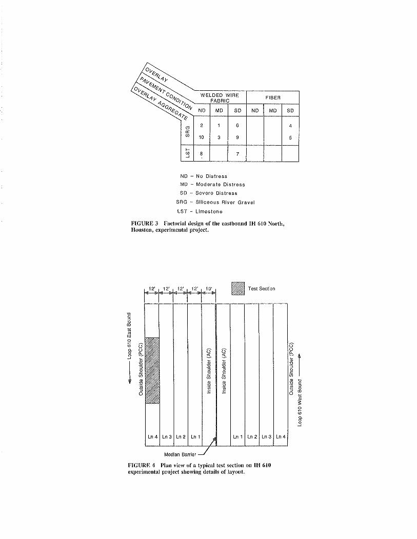
Ou

Ntrìløcrì

WELDEDFABRIAñò) ÍIRE FIBER

\"à3 ND MD SD ND MD SD

c(teU)

2

10

I

3

o

9

4

5

t-U'J I 7

ND - No DlstressMD - Moderate Dlslross

SD - Sevoro Dlstross

SRG - Slllceous Rlver Gravel

LST - Llmestone

FIGURE 3 Factorial design ofthe eastbound IH 610 North,Houston, experimcntal project.

FIGURE 4 Plan view of a typical test section on IH 610experimental project showing details of layout.

Þc5oco

o3<)@CLôoJ

Koesno and McCullough 20.5

Ella BlvdEast Bound----.......-----

264+23 I 286

I

276+00

not include fiber reinforced concrete with limestone aggregateand is, therefore, a partial factorial.

DBSCRIPTION OF TEST SECTION

The ten test sections are located on eastbound IH 610 Northbetween Ella Boulevard and about 700 feet beyond Yale Bou-levald. At this location, the roadway is a four-lane highwayin each direction. All the test sectiorìs are in the outside lane(the lane fulthest from the median barrier). A plan view ofa typical test section is shown on figure 4. Figure 5 shows thelocations and dirnensions of each test section.

RBSULTS

Various measurernents were taken in order to gather data touse to evaluate the parameter behavior before and after over-lay construction. The various data obtained pertain to deflec-tion, conditioll survey, and roughness. In acldition, data wet'e

gathered on a number of cores that were sect¡red from varioustest sections.

Deflection Measuremenfs

The Dynaflect was used to measure the pavement deflectionsbefore and after overlay. The deflection readings were takenat 50-ft intervals, approximately on the center line of theoutside lane ofeach experimental section. In order to evaluatethe performance of the pavement before and after overlay,measurements were taken at approximately the same test points

before and after overlay construction. During the period ofthe study, Center for Transpol'tation Research personnel tookcleflection measurements five different times.

Figures 6 and 7 show before and after overlay deflectionsof sensor 1 a¡rd sensor 5, respectively. As can be seen, theaverage deflection after overlay construction was significantlyless for all test sections. The l¡efore-overlay data show thatthe deflections increased in the second set of readings. 'I'he

F¡ber RsinforcedConcrsle Overlay

I

298+74.11

increase may have been caused by a combination of factors.Weather conditions and pavement temperature may haveinfluenced the pavement performance.

CRC sections, fiber reinforced concrete sections, ancl sec-

tions with limestone performed differently in deflection. CRCsections showed a better performance that the other sectionsdid, with a 37.1 percent clecrease in the average deflection ofsensor l. Lirnestone and fiber sections had 30.5 percent and26.8 percent decreases in the average deflection of sensor 1.

Condition Survey

Condition surveys were conducted to monitor the develop-ment of distress and distress types found in the pavementbefore and after overlay construction. The method used inthis study is called the Small Section Method. It is a detailedprocedure and is couducted by a team of two people. Theteam walks along a lane; one person walks with a rollingrneter, and the other maps all visible clistress with referenceto a highway milepost. The distress types that are mappedare tl'ansverse and longitudinal cracks, spallings, punchouts,and patches. This detailed procedure is appropriate for road-way that is experimental in nature (ó).

The transverse cracking was presented as average crackspacing, which was obtained by dividing the total length ofthe test section by the number of transverse cracks on thesection. The longitudinal cracking was measured in units oflinear feet per 100-ft section,

Before overlay placements, the average crack spacings werefairly uniform for all test sections (figure 8). After overlay,the average clack spacings varied. Overlay materials can affectthe crack spacing of the pavement. Section 8 (CRCP withlimestone aggregate) had the greatest transverse crack spac-ing, with section l0 (CRCP with siliceous river gravel) andsection 4 (Fiber reinforced concrete overlay), second ancl third,respectively. Overlay materials may not be the only cause ofthe large variations in after-overlay crack spacings. Concretetemperature during overlay placement, which is not consid-ered in this study, may be another cause of variation.

The longitudinal cracks before the overlay was placed var-

É+l' Limostons316r00 Aggfegato 326r00

FIGURE 5 Plan view showing locations of the ten test sections, eastbound lH 610 North,Houston.

206

Test Section Number

Nolo: B/O - Before OverlayÂ,/O - After Overaly

FIGURE 6 Comparison of before and after-overlay averagedeflection of sensor I, IH 610 North, Houston.

TRANSPORTATION RESEARCH RECOIID t t9()

May,1e8s (B/O)Dsc.,1985 (B/O)

Feb.,1eB6 (A/O)

Jan.,1987 (A/O)Mar.,1987 (A/O)

May,19B5 (B/O)

Dec.,1985 (B/O)Feb.,1eB6 (A/O)

Jan.,1987 (A/O)

Mar.,1987 (A/O)

TøEØtr2 0'B

E

5 0'6

i€ 0.4c)oo 0.2

IøEØng 0'4

E

g o.g

ioE 0.2o(l)c) o.l

Test Section Number

FIGURE 7 Comparison of before and after-overlay averagedeflection of sensor 5, IH 610 North, Houston.

ied for the ten test sections (figure 9). After overlay, the onlylongitudinal cracks were in section 4 (fiber reinforced) andsection 10 (CRCP).

It is important to note that until the last condition surveywas conducted, spalling and puchout did not exist in any ofthe test sections.

Roughness Data

The profilometer was used to evaluate the riding quality andchanges in profile of the pavement. The profilometer readingswere conducted before and after overlay. The after-overlayreadings give an indication of improvement in the riding qual-ity. It can be seen in figure 10 that, after overlay construction,

a general increase in present serviceability index (PSI) occurredon all test sections except section 10.

ANALYSIS OF DATA

The existing pavement materials were characterized by usingdeflection measurements. The moduli of elasticity of the con-crete layer (8,), subbase (E ), and subgrade (E ) were deter-mined by back-calculating from deflection data within eachtest section before and after overlay. The back-calculatingwas accomplished by using program RPEDD1 (8), which isavailable in the Center for Transportation Research.

Note that some test sections are on the embankment andsome are on the flat area (natural grade). The moduli versus

May, 1985(B/O)Jan.,1987(A/O)

TTIø

20

cñÉ()(I'o

U>

ü10clC)Q)CDclo

Koesno and McCullough

1 2 g 4 5 6 7 I I 10

Test Section Number

FIGURE 8 Comparison of before and after-overlaytrânsverse crack spacing of the ten testsections, IH 610 North, Houston.

the locations of test sections and various seasons are plottedon figures 11 through 13. Also note that the moduli vary withtest section location and the environmental conditions whendeflection readings are conducted.

CAUSES OF VARIATION IN LAYER STIFFNESS

CRC Layer

As can be seen in figure 11. , modulus values of the CRC layer,8,, for the first five sections were higher in May 1985 thanthose in December 1985, and the modulus values for sections6 through 10 were higher in May 1985 than those in January1987. This trend could be caused by the higher temperaturesin May 1985. A high temperature condition results in a decreasein pavement deflection due to pavement expansion and nar-rowing of transverse cracks in CRC pavement. As the cracks

1 2 3 4 5 6 7 I I 10

Test Section Number

FIGURE 9 Comparison of before and after-overlayaverage longitudinal cracks per 100-ft section of the tensections, IH 610 North, Houston.

207

May,l985 (B/O)

Feb.,1986(Â/0)May,l986(A/0)March,1987(Á/0)

1 2 3 4 5 6 7 I I 10

Test Section Number

FIGURE l0 Comparison of before and after-overlay presentserviceability indices of the ten test sections, IH 610 NorthtHouston.

narrow, the load transfer increases, which results in a stiffercRc.

Subbase Layer

Construction control may limit the variation in layer thicknessand modulus. Some variation in subbase modulus, as shownin figure 12, may be caused by use of material from differentsources in different areas of the project or use of differentquantities of stabilizing agent. It also may be caused by dif-ferent drainage conditions in different sections of the project.Sections \ryith better drainage will have stiffer subbase layers.The subbase layer, which consists of sand and shell materialsstabilized with cement, will be stiff with small amounts ofmoisture.

Subgrade Layer

Pavement in cut and fill areas may have different subgrademoduli of elasticity. In figure 13, most of the sections on theembankment have higher moduli. This may be the result ofgood drainage on the embankment sections; with good drain-age, less water will remain in the subgrade layer. In contrast,low (flat) areas with higher water tables and poorer drainagewill have a softer subgrade.

It also can be seen in figure 13 that the subgrade modulivary with seasons. Periods of higher rainfall result in highermoisture content in the subgrade and a corresponding lowersubgrade modulus.

COMPARISON OF PREDICTED ANDMEASURED AFTER.OVERLAY DEFLECTION

Measured and predicted after-overlay deflections were com-pared for a partial verification of the design procedure; ifthese are similar then the life predictions are more reliable.

'6oõ4psã(ú(l).9¿¿o)oC1olooo-

0

raË80o

Èð60E()(tt

€40.Eo,coJzo(l,ct)Eo

'3;'fc

. $ot'5 o.

$o2.

$o

$o

1.

4(oox^ \''õo.Ê^uJl

Qo4:g

lo10. $o lo go

go l. s. 4'

0EqJR

Date: May 1985

Air Temp: gooF

CumulativePrecip, in.: 1'40

$o $o.1

Q,C5.

- EMGR

Date: May 198s

Air Temp: 9o9F

Cumulatlve

EM - EmbankmentGR - Grade

EM GR EM GR EM GR EM GRv

- -Dec 1985 Fob 1986 Jan 1987 Mar 1987

49oF 68oF 53oF 78oF

3.38 1.36 NA0.0

Note: Cumulallvo prodpltatlon ls total (cumulative) inches of ralnfrom l0days before deflecllon roadlngs wero taken.

NA = Data Not Avallable

FIGURE lf Moduli of elasticity of concrete layer, E¡, versus test sectionlocations and environmental conditions.

EM - EmbankmenlGR - Grade

roo4F

x'63o.

ñt¡J

$o Q,o.1 2.

Q,t3.

toQo

3o

2.

6.lols s:z

lo3.

EM

Mar f987

TgoF

5.

EM GR

Dec 1985

490F

EM GR

Feb 1986

680F

EM GR

Jan 1987

530F

Precip, ln.: 1.40 3.so 1.36 0.0 NA

FIGURE 12 Modulus of elast¡city of subbase layer, 82, versus test section

locations and environmental conditions.

Koesno attd McCullouglr

l!ï ..e' ?rt

$9 2.0

5'õ {Ão-

CôUJ

6¡?' 10.g. go giz

QC

$oQo

lo1.

go 2o

3ool

EM GR EM GR

EM - EmbankmentGR - Grade

EM GR EM GR EM GR* *Date: May tses Dec 19Bs Feb 1986

Air Temp: gooF

CumulativePrecip, ln.: 1.40

Layer characterization should be established before the pre-dicted aftcr-ovcrlay deflection catr be calculated. Calculatingthe after-ovellay deflection involves the following steps:

1 . Calculate the mean, Ï, and standard deviation of before-overlay deflection for each experimental section.

2. Deter¡nine the moduli of the concrete layer (CRCP),subbase, and subgrade by back-calculating three deflectionvalues(x,x + s,x - s).

3. Assurne the moclulus value for the concrete overlay layer.Note that Eo = 5,000,000 psi was used fol the after-overlaydeflection calculation in this study.

4. Measure the overlay thickness of the cores secured fromthe test sections. Use the average thickness for deflectioncalculation.

5. With the ¡rew four-layer system, the after-overlay deflec-tions were calculated using program RPEDDl.

The accuracy of this method is reflected in the results pre-sented in figure 14 (deflections of sensor 1) and figure 15

(deflections of sensor 5). In these figures, calculated deflec-tions are a little above the equality line, which reflects con-servatism in the predicted measurements.

There are a number of factors that may result in inaccurateprediction of after-overlay deflections:

o Seasonal effects,. Concrete temperature effects, ando Assumptions macle for overlay layer Inodulus of

elasticity.

490F 680F

Jan 1987 Mar 1987

530F 780F

3.38 1.36 0.0 N A

As mentioned before, the first two factors lead to significantchanges in the deflection nreasurements and, consequently,to the moduli predicted from these deflections.

ESTIMATION OF PAVBMBNT FATIGUB LIFBAFTER OVERLAY PLACEMENT

Bonded concrete overlay is used not only to improve theriding quality and to correct grade problems but to add fatiguelife to an existing pavement by utilizing the existing structul'alcapacity. A pavement experiencing distress on the basis ofcondition surveys can be enhanced and its rernaining life canbe increased by using a bonded concrete overlay. Estimatingthe pavement fatigue life and pavement life in years after-overlay placement includes the following steps (9):

1. Calculate the mean after-overlay deflection, i, of eachexperimental section.

2. Determine the moduli of pavement layers and predictthe fatigue life of the pavernent in l8-kip ESAL after theoverlay was placed. Note that 12.5-in monolithic pavementwas used in the calculation, which was performed by back-calculating the deflection obtained from step 1 using programRPEDDl.

3. Calculate the total l8-kip ESAL per lane for overlaidpavement for the first year opened to traffic.

4. Predict the pavement life after overlay using the follow-ing formula.

À, f(t + s)" - tl/v¡s=r?¡sL g l

FIGURE 13 Modulus of elasticity of subgrade layer, 8., versus tcst scctionlocations and environmental conditions.

I'E 0.4

co

Ë 0'3

ooE o.z(Itf-9

I 0.1

u,

E

.6 o.o

o-9oo 0.3!,(¡,

-g

Ë 0.2

cto

2t0

Measured Deflectlon, mlla

FIGURE 14 Comparison of calculated and measured after-overlay deflections of sensor l.

where:

N,, = predicted fatigue life in 18-kip ESAL, as calculatedby RPEDDI,

n,r = total 18-kip ESAL for the first year,¿ = predicted pavement life in years, andg = growth rate/100.

The predicted fatigue life of each of the ten test sectionsand the corresponding predicted pavement life are presentedin table 4.

CONCLUSIONS

The conclusions from the field and laboratory measurementsand the theoretical analysis are summarized as follows:

Deflections

1. A bonded concrete overlay reduces the pavement deflec-tions by increasing the stiffness of pavement structure,

2. Siliceous river gravel sections show the greatest reduc-tion in deflection.

3. High temperature conditions result in a decrease in pave-ment deflection, due to pavement expansion and reductionof transverse crack widths.

Material Properties

1. The limestone sections have the least number of trans-verse cracks.

,I'II,A NS PO R'I'A'I'I O N R ES EA RCH R ECO R D I I 96

0.0 0.1 0.2 0.3 0.4 0.5

Measured Deflection, mlls

FIGURB 15 Comparison of calculated and measured after-overlay dellections of sensor 5.

2. The fiber and limestone sections showed a good bondstrength at the layer interface.

Environmental Effects

1. The subbase layer is stiffer in sections with better sulfacedrainage conditions.

2. The roadbed modulus varies with the season. Periods ofhigher rainfall result in higher roadbed moisture contents anda corresponding lower modulus.

Pavement Conditions

1. Bonded concrete overlay increases the load transfer across

the CRCP cracks.

TARI.F,4 PREDICTED FATIGUE LIFE

TeslSection Predicted Faligue L¡fe Predicted Pavement LifeNumber (18-k¡p ESAL) (Years)

0.50.40.30.2

1

2

3

4

5

6

7

I9

10

24.7

24.6

22.5

21 .1

22.6't 8.9

1 8.6

19.4

19 .4

19 .2

1 09,389,698

1 08,527,896

9 4 ,76 6,53 3

87,176,902

95,764,724

73 ,9 6 3,02 8

7 2,67 3,27 9

76,668,727

7 6,668,7 27

74,778,9't7

Koesno and McCullough

2. Bonded concrete overlay improves the riding quality.3. Existing pavement conditions do not affect the overlay

pavement performance as long as most of the existing distressis repaired before overlay placement.

4. Deflection measurements indicate that a bonded con-crete overlay adds fatigue life to an existing rigid pavement.

RECOMMENDATIONS

The recommendations are presented in two parts: field imple-mentation and future studies.

Field Implementation

i. A condition survey should be conducted shortly after a

light rain, when the cracks on CRCP are most visible.2. New cores should be taken close to the points where the

old cores were secured, to monitor the progress of bondstrength.

3. Steel rod sounding should be included in monitoringactivities so that the progress of delamination can be moni-tored periodically.

Future Studies

i. The long term monitoring program should be continuedin order to evaluate the long-term bonded concrete overlayperformance.

2. Gathering of information on past and future traffic load-ing should continue. This information is very important forpredicting the life of the overlay pavement.

3. The mode of failure of bonded concrete overlay pave-ment needs to be documented for future modeling.

4. The nature of interface bond failure should be modeledso that the delaminated sections may be formulated in termsof the distress producing mechanisms,

5. The effect of the temperature differential between thesubstrata and the overlay should be modeled.

2ll

REFERENCES

1. D. K. Ray. Repairing Concrete Pavements. Concrete Inler-national, June 1987, Vol. 9, No. 6.

2. M. M. Davis and J. A. Epps. Engineering Economy andEnergy Considerations Skid Resistant Surfaces. Texas Trans-portation Institute, Texas A&M University, College Station,Texas, December 1975.

3. R. R. Forrestal. Application and Field Evaluation of VeryThin Skid Resistant Pavement Surfaces. Purdue University,Indiana State Highway Commission, August 1978.

4. R. E. Boyer. Perþrmance of Thin Bonded Portland CementConcrete Overlays on Military Airfields. Purdue University,West Lafayette, Indiana, April 1981.

5. K. Kailasanathan, B. F. McCullough, and D. W. Fowler. áStudy of the Effects of Interface Condition on Thin BondedPCC Overlays. Research Report 357-1, Center for Trans-portation Research, The University of Texas at Austin,December 1984.

6. M. Gutierrez de Velasco and B. F. McCullough. Rigid Pave-ment Rehabilitation Scheduling Using Distress Quantities.Research Report 249-5, Center for Transportation Research,The University of Texas at Austin, August 1983.

7. J. N. Anagnos and T. W. Kennedy. Practical Method ofConducting the Indirect Tensile Test. Research Report 98-10,Center for Highway Research, The University of Texas atAustin, August 1972.

8. W. Uddin, A. H. Meyer, and W. R. Hudson. A User's Guidefor Pavement Evaluøtion Programs RPEDDI and FPEDDl.Research Report 387-2, Center for Transportation Research,The University of Texas at Austin, July 1985.

9. A. Taute, B. F. McCullough, and W. R. Hudson. Improve-ments to the Materials Characlerization and Fatigue Life Pre-diction Methods of the Texas Rigid Pavement Overlay DesignProcedure. Research Report 249-1, Center for Transporta-tion Research, The University of Texas at Austin, November1981.

10. V. Torres-Verdin, B. F. McCullough, and G. B. Peck. TheEffect of Coarse-Aggregate Type on CRCP Thickness. ResearchReport 249-7, Center for Transportation Research, The Uni-versity of Texas at Austin, November 1983.

Publication of this paper sponsored by Committee on PavementRehabilitation.

.I RA N S P O RTA'I'I O N R ES EA II,C LI II, EC O I? D I I 9ó

Flexible Pavement Rehabilitation usingAsphalt-Rubber Combinations:Progress ReportRonnnr N. Dorv

Several-flexible pavement rehabilitation strategies incorporat-ing asphalt-rubber were used experimentally õn a proþct innortheastern California in the fall of 1983. Included weie rub-berized dense-graded asphalt concrete (AC) overlays contain-ing a binder then being marketed by the Arizonâ RefiningCompany, PlusRide dense-graded AC overlays, and four thicklnesses of conventional dense-graded AC overlay for compar.ative evaluations. Some of the rubberized denie-graded ACoverlays were placed on a stress-absorbing membiane inter-layer_. In addition, two sections of double stress absorbingmembrane (SAM) and one section of conventional (single) SAMwere placed. Distress began to develop in the conventionaldense-graded AC within one year in ihe form of raveling,rutting, and cracking. This distress has become more extensiveand more severe during subsequent years. Distress has alsodeveloped in the other overlays and surface treatments. Todate,. however, all the asphalt-rubber combinations are per-forming equal to or better than equivalent or greater thick-nesses of conventional dense-graded asphalt conirete.

The California Department of Transportation (Caltrans) hasbeen using a deflection-based flexible pavement rehabilitationdesign procedure for more than 30 years. This procedureis used to obtain 10 or more years of additional service lifeduring which little or no pavement maintenance will be required.The rehabilitation strategy most frequently used is to overlaythe existing asphalt concrete (AC) pavement with one or morelayers of new AC. In May 1982 this procedure was used todevelop an overlay design for a portion of Route 395 in north-eastern California. To obtain the desired lO-yr service life, a0.7O-ft thick overlay of conventional Caltrans dense-gradedAC (DGAC) would have been required. The cost of thisoverlay would have been significantly more than the fundingavailable for the project. The results of limited Caltrans researchand research by others had indicated that asphalt-rubber com-binations might provide the desired service life at a lessercost, due to the possibility of being able to use substantiallythinner overlays or even surface treatments. Thus, it was clecidedto try several of these products in the fall of 1983 in lieu ofthe thick overlay required in the Caltrans standard procedure.

PROJECT FEATURES

The section of Route 395 involved was originally constructedin three segments. The first of these was built in 1948. This

was followed by additional contracts in 1952 and 1954 thatresulted in completion of the original pavement. Subse-quently, at least two thin overlays had been placed.

The two-lane pavement is located in a somewhat remoteportion of northeastern California about 100 miles north ofReno, Nevada. The highway at this location traverses a rockyvalley between two mountain masses. The elevation of thehighway is about 4,400 feet at the south end of the projectand approximately 5,400 feet at the north end of the project.Most of the southernmost2Vz rniles is on a low fill, whereasthe remainder is on solid or nearly solid basalt. The averageannual precipitation varies fiom 8 inches at the south encl, to12 inches in the middle, and 10 inches at the north end. Thisprecipitation falls throughout the year. In adclition, frost occursthroughout the year, with some snowfall during the periodfrom November to March. During the surnmer, the ambienttemperatures often exceed 90.F while winter temperaturesoccasionally drop to below zerooF. From May to November,the diurnal temperature range averages nearly 40"F. Duringthe remainder of the year, it is generally about 20.F.

The traffic using the roadway varies frorn al¡out 1,400 vehi-cles per day (VPD) in the summer to approxirnately 550 VpDin mid winter. The average annual daily traffic (AADT) is1,100. This includes about 100 five-axle trucks per day.

The roadway structural section as of mid 1983 consisted ofAC having an average thickness of 0.38 foot, suppor.tecl byan aggregate base (AB) of 0.42-ft average thickness. Under-lying the AB was aggregate subbase (ASB) that was 0.97-ftthick (average). There was some variation in these layer thick-nesses, as shown on table 1,

In situ pavement deflections were measured using theDynaflect (see figure 1). The lneasured values were convertedto equivalent Deflectometer values per standard Caltrans pro-cedures. The 80th percentile equivalent values ranged from0.023 inch to 0.063 inch. The average value was 0.043 inch.The tolerable deflection for the existing pavement was 0.017inch. The effects of this excessive deflection were obvious inthat the pavement throughout the project was cracked exten-sively. The percent of pavement cracked, as determined usingoverhead photos of representative portions of each pavementsegment, varied from 8 to 100 as indicated in table 1. For tenof the thirteen segments, the percent of pavement crackedwas in excess of 50. The cracking included both wicle trans-verse cracks of the type often associated with cold tempera-tures and extensive alligator cracking of the type associatedwith traffic loads. There was also substantial rutting noted

Califor_nia Department of Transportation, Office of Transpor-tation Laboratory, 5900 Folsom Boulevard, Sacr.amento, ialif.95819.

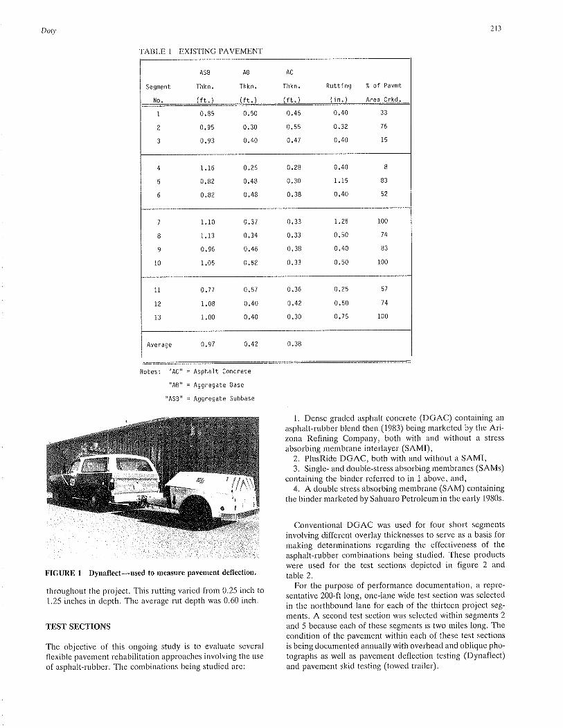
DotS, 2t3

TABLE 1 EXISTING PAVEMENT

ASB AB AC

Segment Thkn. Thkn. Thkn. Rutting Í of Pavmt

Nô- lft-) lft--) lft.) (in.) Area Crkd.

I 0.85 0.50 0.45 0.40 33

2 0.95 0.30 0.55 0.32 76

3 0.93 0.40 0,47 0.40 15

4 r. 16 0.26 0.28 0.40 I5 0.82 0.48 0.30 1. 15 83

6 0.82 0.48 0.38 0.40 52

7 1.10 0.37 0.33 1.25 100

8 l.l3 0.34 0.33 0.50 74

9 0.96 0.46 0.38 0.40 83

10 1.05 0,52 0.33 0.50 100

11 0.77 0.57 0.36 0.25 57

t2 1.08 0.40 0.42 0.50 74

13 1.00 0.40 0.30 0.75 100

Average 0,97 0.42 0.38

Notes: "AC" - Asphalt Concrete

"AB" = Aggregôte Base

UASBU - Aggregate Subbase

FIGURE I Dynallect-used to measure pavement deflection.

throughout the project. This rutting varied from 0.25 inch to1.25 inches in depth. The average rut depth was 0.60 inch.

TEST SECTIONS

The objective of this ongoing study is to evaluate several

flexible pavement rehabilitation approaches involving the use

of asphalt-rubber. The combinations being studied are:

1. Dense graded asphalt concrete (DGAC) containing an

asphalt-rubber blend then (1983) being marketed by the Ari-zona Refining Company, both with and without a stress

absorbing membrane interlayer (SAMI),2. PlusRide DGAC, both with and without a SAMI,3. Single- and double-stress absorbing membranes (SAMs)

containing the binder referred to in 1 above, and,4. A double stress absorbing membrane (SAM) containing

the binder marketed by Sahuaro Petroleum in the early 1980s.

Conventional DGAC was used for four short segmentsinvolving different overlay thicknesses to serve as a basis formaking determinations regarding the effectiveness of theasphalt-rubber combinations being studied. These productswere used for the test sections depicted in figure 2 and

table 2.For the purpose of performance documentation, a repre-

sentative 200-ft long, one-lane wide test section was selectedin the northbound lane for each of the thirteen project seg-

ments. A second test section was selected within segments 2

and 5 because each of these segments is two miles long. Thecondition of the pavement within each of these test sections

is being documented annually with overhead and oblique pho'tographs as well as pavement deflection testing (Dynaflect)and pavement skid testing (towed trailer).

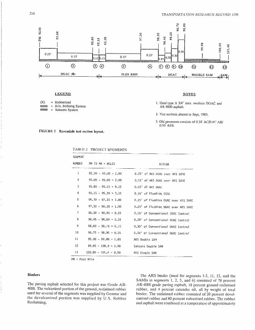
214

@

DGAC (R)

LEGNND

(R) = Rubberized@t = Ariz. Refining SystemSEE&I = Sahuaro System

FIGURE 2 Ravendale test section layout.

TABLE2 PROJECTSEGMENTS

TRANSPORTATION RESEARCH RECORD I 196

@ ooo@ @

DGAC DOUBLE SAM

NOTES

l. Used type A 3/4" max. medium DGAC andAR 4000 asphalt.

2. Test sections placed in Sept, 1983.

3. Old pavement consists of 0.38' AC/0.41' AB/0.96'ASB.

lt¡nbo\

I

êI(?¡o\

I

êcN6

A

I

eêF. O\€6âOl

o900o\

I

cqao\

I

€aè

I

è.'l

oê

@

SEGI.IENT

NUI'l8tR Pl'l T0 Pl4 = l,llLES DES IGN

I 92.00 - 93.00 = 1.00

2 93.00 - 95.00 = 2.00

3 95.00 - 95.15 = 0.15

4 95.15 - 95.30 = 0.15

5 95.30 - 97.30 = 2.00

6 97.30 - 98.30 = 1.00

7 98.30 - 98.4s = 0.15

8 98.45 - 98.60 = 0.15

9 98.60 - 98.75 = 0.15

l0 98.75 - 98.90 = 0.15

ll 98.90 - 99.90 = 1.00

12 99.90 - 100.9 = 1.00

13 100.90 - 101.4 = 0.s0

0.25' of ARS DGAC over ARS SAHI

0.15r of ARS DGAC over ARS SAt4l

0.15' oÏ ARS OGAC

0.15' of PlusRide DGAC

0.15r of PlusRide DGAC over ARS SAHI

0.25' of PIusRfde OGAC over ARS SAfil

0.15' of Conventlonal oGAC Control

0.20r of Conventional DGAC Control

0.30r of Conventional DGAC Control

0.50' of Conventional DGAC Controì

ARS Double SAH

Sahuano Double SAH

ARS Sinqle SAH

PM = Post ltllle

Binders

The paving asphalt selected for this project was Grade AR-4000. The vulcanized portion ofthe ground, reclaimed rubberused for several of the segments was supplied by Genstar andthe devulcanized portion was supplied by U.S. RubberReclaiming.

The ARS binder (used for segments 'L-3, I1,13, and theSAMIs in segments L,2, 5, and 6) consisted of 78 percentAR-4000 grade paving asphalt, L8 percent ground reclaimedrubber, and 4 percent extender oil, all by weight of totalbinder. The reclaimed rubber consisted of 20 percent devul-canized rubber and 80 percent vulcanized rubber. The rubberand asphalt were combined at a temperature of approximately

Doty

350"F using a special mixing/blending unit. The blencl to be

used for the DGAC in segments L to 3 was then recirculatedwithin a holding tank for approximately 45 minutes after which

it was pumped into the contractor's asphalt storage tanks at

the plant. This 45-min holding tirne requirement resulted ina discontinuous supply of binder to the plant that caused

occasional interruptions in plant production of the DGAC forsegments 1 to 3.

The asphalt-rubber binder used for segment 12 conformedto the specifications promulgated by the Sahuaro PetroleumCompany. The primary differences between the ARS binderand the Sahuaro binder were that more reclaimed rubber was

used (23 percent instead of 18 percent) and a diluent was used

instead of an extender oil. The blending times and telnper-atures also differed somewhat.

The binder for the PlusRide segments (a to 6) consisted ofAR-4000 grade paving asphalt. This asphalt was also used forthe conventional DGAC comprising segments 7 to 10.

Aggregate

AC aggregate confonning to the Caltlans' specifications for%-in maximum medium Type A DGAC was used for theconventional DGAC (see table 3). Aggregate conforming toCaltrans' specifications for Vz-in maximum medium Type ADGAC was specified for the ARS mixes (segments I to 3).The gap grading shown in table 3 was specified for the PlusRide.This gap in the aggregate grading was required to accom-modate the coarser portion of the reclaimed rubber that was

included in the PlusRide mix. The need to provide this gap

2t5

can and did result in the accumulation of some waste aggre-gate. The requirement of 8 to 12 pelcent passing the No. 200also created a problem in that this resulted in the need toimport and add 4.7 percent pozzolan to the mix.

The aggregate used for the SAMIs (segments I,2,5, and6) and for the single SAM (segment No. 13) conformed toCaltrans' specifications for 3/a x No. 6 ¡nedium screenings(see table 3). The specifications for the screenings used in thedouble SAMs (segments 11 and 12) are also shown ontable 3.

Construction

The project was constructed in August and September of1983. A Standard 10,000-lb capacity batch plant was used tomix the DGAC in 8,000-lb batches. The design asphalt con-tent (Hveem) for the conventional DGAC was 4.6 percentby dry weight of aggregate. The design binder content (asphalt-rubber blend) for the ARS DGAC, as provided by ArizonaRefining Company personnel, was 8.0 percent by dry weightof aggregate. The design asphalt content for the PlusRideprovided by All-Seasons personnel was initially 9.65 percentby dry weight of aggregate. In addition, 3.0 percent rubberby total weight of mix was added to PlusRide aggregate andpre-mixed for 20 seconds before the AR-4000 asphalt was

added.The mixes were transported to the street using bottom dumps

and placed using a Ko-Cal pickup machine and a Blaw KnoxPF-180 paver. A 20-ft ski was used for grade control.

No pre-leveling or milling was done to eliminate the pre-

TABLE 3 AGGREGATE GRADING SPECIFICATIONS (PERCENTPASSING)

Si eve

Si ze

ARS

DGAC

Pl usRide

DGAC

Conv.

DGAC

Double SAl4

rst Lirt |

,.0 t,r,

SAI,l

and

SAIII

1"

3/4

5t8

v2

3/B

r/4

#4

#8

#10

#16

#30

#200

100

95- I 00

80-85

55-6 5

38-48

t8-28

3-B

t00

60-80

30-50

t9-32

t3-25

8- 12

t00

95- 100

65-80

46-56

33-43

t4-24

3-B

100

90- 100

50-80

0- l5

0-5

0-2

100

60-85

0-25

0-5

0-3

0-2

100

90-100

5-30

0- r0

0-5

0-2

216

construction rutting prior to constructing the overlays. A lev-eling course was placed prior to placing the SAMs, however.The segments with design thicknesses of 0.15-foot and 0.20-foot were placed in one lift. Segments 1 and 7 (design thick-ness of 0.25 foot) were placed in lifts of 0.13-ft, then 0.12-ft.The 0.30-ft thick segment (No. 9) was placed in two lifts of0.15-ft each. Segment 10 (0.50-ft total design thickness) wasplaced in lifts of 0.20-ft, then 0.15-ft, and 0.15-ft.

A Dynapac CC50A vibratory steel-wheel roller was usedfor breakdown compaction. This roller was operated at highamplitude and 2,400 VPM in accordance with prior Caltransqualification testing of this roller for conventional DGACpaving. A Hyster C350 steel-wheel roller was used for finishrolling. No pneumatic rolling was required.

No problems were encountered when placing the ARSDGAC or the conventional DGAC. The PlusRide mix, how-ever, had a consistency resembling bubble gum when placedand was noticeably springy even after compaction. Thisappeared to contribute to the initial difficulties in obtainingat least the specified 96 percent (minimum) of theoreticalmaximum density. A reduction in the design binder content(from 9.65 percent to 9.41 percent) and an adjustment in theamount of supplemental fines (pozzolan) being added to themix resulted in compliance with the density specification butno change in the stickiness or resilience of the mix was noted.The tendency to stick to the rollers was subsequently alle-viated somewhat when the breakdown compaction was delayeduntil the mix temperature had dropped to 285'F or less in lieuof the originally specified 300'F minimum.

The construction of the SAMIs (segments l, 2, 5, and 6)and the SAMs (segments 11 to 13) involved placement of theARS and Sahuaro binders using a distributor truck followedby application of the pre-heated pre-coated (0.33 percentasphalt) screenings. These surfaces were then rolled with a

minimum of three coverages using pneumatic rollers. For seg-ments 11 and 12, the design binder application rate was 0.50

TABLE 4 ESTIMATED COST OF EACH STRATECY

SEGMENI

NUHBER

7'II,A NS PO R'TAT I O N R TiS EA RC ÍI R ECO R D I I 96

gal/sy. Fol the SAMIs and segrnent 13, the design applicationrate was 0.60 gallsy. The design application rates fol thescreenings were 34 lbs/sy for the first lift of segrnents ll and12,26 lbslsy for the second lift of segments 11 and 12, and35 lbs/sy for the SAMIs and segment 13. Prior to the place-me¡rt of the SAMs, a levelling course of minimal thicknesswas placed consisting of '/z-in maximum conventional DGAC.This was needed to adjust the cross slope of the pavementand to eliminate the rutting at these locations. The only prob-lem that occurred during the placement of the SAMs andSAMIs was caused by smoke generated by the distributortruck operation. This obsculed the spray bar, which resultedin a somewhat streaked appearance, due to undetected inter-mittent partial or complete plugging of some of the spray-barnozzles.

Cost Estimate

An estimate of the in-place cost of each of the segments isshown in table 4. This provides an indication of the extent towhich the val'ious asphalt-rubber proclucts must out-performthe conventional DGAC to be cost effective.

As-built Properties

The data in Table 5 indicate that conforrnance to the aggregategradation specifications was obtained. Table 6 contains dataindicating that the as-built thickness of the various segmentsdiffered from the design thicknesses to sorne extent. Thepermeability data indicates that the PlusRide DGAC was vir-tually impermeable, whereas the perrneability of the ARSDGAC was very low, ancl the permeability of the co¡rventionalDGAC was somewhat greater than the 150 ml/min consideredtypical of Caltrans ¡nixes. This suggests the need for a SAMI

COST

(Square Yard)

I 0.25 '

2 0.15'

3 0.15'

4 0.15,

5 0.15'

6 0.25'

7 0.15'

B 0.20 '

9 0.30'

l0 0.50'

of ARS DGAC over ARS-SAMI

of ARS DGAC over ARS-SA|II

of ARS DGAC

of PlusRide DGAC

of PlusRide DGAC over ARS-SAMI

of PlusRide DGAC over ARS-SAMI

of Conventional DGAC Controì

of Conventional DGAC Control

of Conventional DGAC Control

of Conventionaì DGAC Control

$ 10.41

6.88

5. 37

6.32

7 .83

12.00

3.04

4 .03

6.02

9.99

2.60

2.62

I .56

1t

t2

l3

Double SAM, ARS Binder

Double SAl4, Sahuaro Binder

Single SAH, ARS Binder

TABLE 5 AGGREGATE GRADATION SPECIFICATION COMPLIANCE

PERECENT PASSING

SI EVE

SI ZE

ARS

(Segment No. l)

PLUSR I DT

(segment No.5)

CONVENTIONAL DGAC

SEGMENT NUMBER

SPEC.EXTRACÏTD SPEC . IXTRACTED SPEC. 7 I 9 l0

1"

3/4

5/8

rl2

3/8

L/4

#4

#B

#10

#30

# 100

#200

100

97

80

57

44

25

l0

7

100

95 - 100

B0-85

55-65

38-48

l8-28

3-8

100

89

63

47

36

tq

23

l7

l1

9

100

60-80

30- 50

19-32

l3-25

8-12

100

100 100 98 100

79 86 82 84

70 72 69 75

48 5t 46 53

35 38 3s 40

21 23 21 23

r0119117868

100

95- 100

65-80

46- 56

33-43

t4-24

3-8

Doty

of some sort to provide a more impernreable pavement andthereby protect the underlying pavement from surface water(rainfall) intrusion.

Caltrans experience has revealed that surface abrasion losses

greater than 35 grams (per Calif. Test 360, Method B) gen-

erally are associated with DGAC exhibiting marginal or unsat-isfactory resistance to moisture. The surface abrasion testresults in table 6 indicate that the ARS DGAC (with an aver-age value of 17 g) and the PlusRide (average value of 13 g)

are substantially more resistant to surface abrasion than is theconventional DGAC used on this job (average loss of 41 g).

The results of the towed-trailer skid testing indicated tnatthe PlusRide pavement is adequate and the other surfaces(ARS DGAC, conventional DGAC, and the SAMs) are verygood.

In situ pavernent deflection measurements were made inMay of 1984. Comparison of these values with those measurein May of i983 provides an indication of the structural sectionstiffening provided by the various strategies. These valuesillustrate that substantial reductions in deflection were achievedin most cases. These values are discussed in more detail inthe next section of this paper.

LONG.TERM PERFORMANCE

Four rnonths after constluction, the first report of pavementdistress was received. A field condition survey revealed that

a considerable loss of surface fines had occurred, especially

in the wheel tracks in the two thinner segments of conven-

tional DGAC (segments 7 and 8-see figure 3). In addition,transverse cracks about 2 feet apart had developed over a

distance of approximately 400 feet and longitudinal crackinghad developed in the southbound lane outer wheel track, bothin segment 8. The other segments containing conventionalDGAC (9 and 10) had experienced the loss of a minor amountof surface fines but no cracking.

FIGURE 3 Loss of fines in wheel tracks, 0.15 ft DGAC-segrnerrt 7 (age 4 months).

]'ABLE 6 AS-BUILT PROPERTIES

Hateri al

Overl ay Thknl

(fr )

Conp.

Pernea-2

bjlity(ml /mi n )

Su rface3

Abrasi on

(gms ì oss )

skid4

No.

( sNqo )

Defl ecti on5

( 0.001')

Number {s-Bui l t Des i gn 5/83 5/84

ARS

DGAC

I2

J

0.27

0. l7

0.t2

0.28

0. lB

0. l5

93 .3

9t.7

92.8

36.3

22.3

17.1

r7.6

18. i

55

57

54

54

43

25

26

25

l6

Pì usRide

DGAC

4

5

6

0.19

0.2t

0 .28

0. l5

0.lB

0.28

97 .I98.4

96. I

1l .0

6.8

9.7

14.8

lr.4

39

39

44

55

30

27

27

26

l6

Conv.

DGAC

7

0

9

10

0. 20

0. 18

0.32

0. 52

0. l5

0.20

0 .30

0.50

91.7

91.2

91.4

92.t

177 0 47 .8

48.2

32.5

35. I

66

68

65

67

23

60

63

q6

t8

44

28

13

Doubl e

SAM

ll12

0. l0

0.13

0.04

0.04

62

59

44

5l

42

35

sAl't t3 0.14 0 .03 57 54 52

218

Includes SAMI, segments 1,2,5,Per Calif. Test 341

Per Caìif. Test 360, Method B

Per ASTM t274; tleas 10/B3

80th percentile deflections per

7' RA N S P O R'I'ATI O N II, ES EA II,C LI R ECO II, D I 1 96

and 6

Calif. Test 356 (Dynafìect Method)

results of these tests are summarized in table 7. Examinationof this data reveals some anomalies for which no explanationis apparent. For example, the reason for the significant reduc-tion in deflection between June of 1986 and May of 1987 forsegments 1 to 4 is unknown. The remainder of the deflectiondata is plausible in most cases, in that it indicates that ameasurable initial stiffening of the structural sections wasachieved via placement of each of the asphalt-rubber andconventional overlays. The percent reduction in deflectionwas directly related to the thickness of the overlay placed inmost cases. The surprisingly large percentage decreases indeflection as a result of the thinnest PlusRide overlay (seg-ment 4) and the Sahuaro double SAM (segment 12) are dif-ficult to explain. Based on inspection of the data, the May1984 deflection reported for segrnent 12 may be erroneous.The subsequent deflections indicate that most or all this stiff-ening effect has dissipated with the exception of segments 1,6, 9, and 10. These segments comprise the thickest of therubber-modified DGAC (segments I and 6, each of whichwere 0.25-ft+ thick) and the conventional DGAC (segments9 and 10, with nominal ovellay thicknesses of 0.30 and 0.50

Notes: 1.

2.

3.

4.

5.

The following June (nine months after construction), it wasnoted that a glaze observed on the PlusRide surface imme-diately after construction was no longer evident. In addition,the crack pattern in the underlying old AC pavernent wasbeginning to become visible in segmenr 11 (double SAM usingARS binder). Also, some hairline cracking was observed inthe SAM (segment 13). No other additional distress wasobserved at the time of the June 1984 review.

Because of some warm weather in July of 1984 (11 dayswith maximum temperatures of 90'F or more), the projectwas reviewed again on July 26,1984. So¡ne additional distresshad become evident. There was some localized bleeding atsome of the transverse construction joints in segment 4 (PlusRide) and some flushing beginning to develop in the doubleSAMs (segments 11 and 12). In addition, rutting 0.25-in deepwas noted in the thickest ofthe control sections (segment 10).No other significant rutting was noted.

Subsequent to the July 1984 survey, additional field con-dition surveys have been cornpleted in the late spring or earlysummer of 1985, 1986, and 1987. In addition, pavement skidnumbers and deflections have been measured each year. The

TABLE 7 PAVEMENT STIFFNESS AND SURFACE TEXTURE

Hateri al Segnent

Defl ect i ons

(80th percentile, 0.001" )

Skid No.

( sNqo )Date Tested

5183* 5/84** UrtU 6/86 5t87 10/83 5/87

ARS

DGAC

I

2

3

54 26(521 3s

43 25(42) 37

25 16(36) 28

43

44

37

2B

36

29

55 64

57 64

54 62

Pl us

Ri de

DGAC

4

5

6

55 27(51) 42 56 4s

30 26( 13 ) 34 41 4l

?7 16(41) 2t 2? 2t

39 60

39 62

44 59

Conv.

DGAC

7

8

9

10

23 t8(221 ?2 22 ?6

60 44(27) 52 51 59

63 28(56) 42 36 32

46 r3(72',1 ?1 20 19

66

68

65

67

64

56

65

62

Doubl e

SAM

1l

t2

44 42(5) 52 52 59

51 35(31 ) 53 54 5l

62

59

34

26

sA!,r 13 54 s2(4) 55 56 66 57 63

Doty

*Prior to construction of the segments

**Percent reductlon in deflection shown

foot, respectively). These also were the overlays that providedsome of the largest initial stiffening as indicated by percentreduction in deflection.

As expected, the deflections measured for the SAMs sug-gest that the stiffening effect of these surface treatments wasminimal. The significance of the pavement deflections, asrelated to the asphalt-rubber products, is one of the experi-mental features of this study.

All of the segments are now exhibiting some distress in theform ofcracking (longitudinal, transverse, block, and/or alli-gator-see figures 4 to 13). There is a small amount of ruttingpresent (conventional DGAC - segment 10) and some potholes (in the PlusRide). The amount of cracking, however,is probably the best indication of the remaining service lifefor each of the segments. Table 8 contains an estimate of theamount of cracking that has developed. Because of the flush-ing and bleeding that has developed in segments l'J. and 12,much of the cracking therein is sealed, due to the kneadingaction of traffic during warm weather. The deflections meas-ured in the badly cracked segment 7 and, in some cases,segment 8 (both conventional DGAC) have been comparableto or less than those measured for segments 1 to 6; yet theamount of cracking in segments 1 to 6 is relatively insignifi-cant. This suggests that the tolerable deflection for these asphalt-

in 9/83

in parenthesis

rubber dense graded AC pavements may be considerablygreater than that for comparable thicknesses of conventionalDGAC. It should be remembered that the conventional DGACoverlays were substantially under-designed in that 0.70-ft wasthe design thickness determined for this roadway using theconventional Caltrans design procedure.

FIGURE 4 Typical Cracking-longitudinal, test segment 2,0.15 ft ARS DGAC on SAMI (age 48 monrhs).

2t9

FIGURE 5 Typical cracking-alligator' test segment 3, 0.15 ftARS DGAC (age 48 months).

FIGURE 6 Typical cracking-alligâtor, test segment 3, 0.15ft ARS DGAC (age 48 months).

FIGURE 7 Typical cracking, test segments 7 and 8, 0.15 and

0.20 ft conventional DGAC (age 48 months).

FIGURE I Typical raveling' test segments 7 and 8, 0.15 and0.20 ft conventional DGAC (age 48 months).

FIGURE 9 Typical crackitrg-transverse' test segments 9

and 10, 0.30 and 0.50 ft conventional DGAC (age 48 months).

FIGURE l0 Typical wheel track bleeding, test segments ll ând12, double SAM (age 48 months).

Doty

.-. 9- ''.!....¡.'¡:

FIGURE U Typical wheel track bleeding, test segments 1land 12, double SAM (age 48 months).

FIGURE 12 Typical cracking-transverse, test segments 1land 12, double SAM (age 48 months).

FIGURE 13 Typical cracking, test segment no. 13' SAM (age

48 months).

221

The results of the skid testing (table 7) coincide with theloss of the glaze on the surface of the PlusRide after approx-imately 6 months of service. Thus, this glaze may have beenthe reason for the substantially lower skid numbers measuredinitially for the PlusRide as compared to the other segments.As of May 1987, the PlusRide values were comparable withall the other values measured except those for the DoubleSAMs. These substantially lower values indicate a marginalpavement and are no doubt associated with the flushing andbleeding that has been observed in segments l.l. and 12 sincethe 1985 survey.

CONCLUSIONS

The findings and observations to date indicate that for theconditions present at the test site location, the initial stiffeningeffect of the asphalt-rubber overlays studied is equal to orgreater than that of equivalent thicknesses of conventionalDGAC and that the tolerable deflection of these asphalt-rubber overlays is greater than that of equivalent thicknessesof DGAC. This would suggest that the service life of theasphalt-rubber DAGC overlays under study may be consid-erably greater than those of equivalent thicknesses of con-ventional DGAC, at least with some combinations of trafficand climate. In addition, both of the thin conventional DGACoverlays have failed (figures 7 and 8) whereas the asphalt-rubber overlays of comparable thickness (segments 2 to 5-figures 14to17) have not yet failed. However, the cost-effec-tiveness of these more expensive overlays cannot yet be deter-mined, as most of the segments being studied have not yetfailed. In addition, although a substantial amount of crackingis visible in the SAM segments (11 to 13), these pavementshave not yet required the amount ofmaintenance effort requiredin segments 7 and 8. This suggests that even the SAMs maybe superior to conventional overlays 0.20-ft thick. Based ona comparison of the single SAM versus double SAMs, thereis no apparent advantage provided by the double SAM.

Final conclusions for the conditions present at the test sitelocation will be contingent on the performance of the varioussegments during the next few years. In addition, some addi-tional similar experiments at locations having both similar anddifferent traffic and/or climatic conditions are needed beforeoverall conclusions regarding these asphalt-rubber combina-tions can be determined.

ACKNOWLEDGMENTS

The research described herein has been supported by theFederal Highway Administration. The contents of this paper,however, do not necessarily reflect the official views or pol-icies of either the Federal Highway Administration or theState of California. They reflect the views of the author, whois responsible for the facts and accuracy of the data presentedherein. Also, neither the State of California nor the UnitedStates Government endorse products or manufacturers. Tradeand manufacturers' names are presented herein because theyare considered essential to the objective of this document.

The Principal Investigators for the research project are BobbyG. Page of the Caltrans Office of Transportation Laboratory

{.

TABLE 8 ESTIMATE OF PAVEMENT CRACKING

Estimated

Percent Cracked

(May 1987)

Segment

Number

<51

<5Í

5- l0c

I

2

3

<5r

5-10%

5-10%

4

5

6

70-75L*

75-801*

10- l5T

<5Í

7

I9

10

*Fai I ed

FIGURE l4 Typical "oYerall" view, ARS DGAC (age 48

months).FIGURE 15 Typicat texture' ARS DGAC (age 48 months)'

Doty

FIGURE 16 Typical "overall" view, PlusRide DGAC (age 48months).

and Larry delaubenfels of Caltrans District 2. The previousPrincipal Investigator was Roger D. Smith, a former mem-ber of the Transportation Laboratory staff. Jack Van Kirkand other members of the Transportation Laboratory staffand Caltrans District 2 staff have also been involvedq/ith the study. In addition, the typing of this text by Lydia

223

FIGURE 17 Typical texture, PlusRide DGAC (age 48months).

Burgin of the Transportation Laboratory staff is gratefullyacknowledged.

Publication of this paper sponsored by Committee on PavementRehabilitation.

224 TRANSPORTATION RESEARCH RECORD I 196

tion rating (PCR), includes two component elements: roadroughness (RR), measured in terms of present serviceabilityrating (PSR) on a zero to five scale, and the distress datadetermined by a subjective field survey but reduced to distressrating (DR) employing deduct values and weighting factors.A complete description of the data reduction and subsequentPCR calculation plocedure by combining RR and DR can be

seen elsewhere (1). The condition data is collected by RDM-5000 equipment supplied by Dynatest. The rnajor componentsof RDM include HP-85 microcomputer, RDM-5000 electronicprocessor, ultra precision accelerometer, digital distanceencoder, and an eight-push-button control box. The rough-ness measurement by RDM is fully automatic, whereas dis-tress survey is subjective. A description of the equipment as

well as the data collection procedure is given in the manu-facturer's literature (2).

Not only the present condition of the network, but also thefuture condition of each pavement section is lequired forforecasting future needs. Site-specific prediction models arebeing investigated, and the details of these investigations can

be found elsewhere (3). For the purpose of this paper, thedeterioration of a road su¡'face may be described by two basicrelationsl one equation that describes the evolution of roadroughness and a second that describes the surface distress.Both equations are assumed to be linear, with a scale fromzero to 100. A prediction model, designated as the perfor-mance curve, is depicted in figure 1. As the curve indicates,during the early life of the pavernent, the roughness rating isgenerally lower than the distress rating, in which case theroughness rating governs the performance curve,

The fourth component of a PMS involves some form ofranking methodology or an optimization and/or prioritizationsystem. The ranking methodology generally encornpasses a

ranking of the pavement sections for scheduling the annualrehabilitation program. Programming at the network level fora predetermined period in the future, designated as the anal-ysis/programming period, would require cornplex optimiza-tion methodology that has the adclitional capability for shiftingprojects back and forth to result in maximum benefit to publicroad users. This paper presents the developrnent of an optim-ization/prioritization model followed by an example problemthat illustrates the salient features and typical results of themodel.

OPTIMIZATION AND PRIORITIZATION

A comprehensive process of priority programming shouldenable one to answer the following three questions:

Network Level Optim ization/Pri ofitizationof Pavement RehabilitationAu KserAMI AND K. P. Gnoncn

A procedure has been developed to optimize pavement reha-bilitation strategies for the highway network in Mississippi.The methodology is developed in two stages: project level andnetwork level. First, at the project level, a set of feasible dou-ble-action strategies and the corresponding times of imple'mentation ofeach alternative ofevery strategy are determine¡l.The optimum rehabilitative strategies are selected by maxi-mizing pavement performance for a l2-yr analysis period. Aunivariant search technique is employed to solve for the non.linear optimization problem. The second part of the analysisdeals with network level optimization. Selection of the set ofprojects is done by maximizing pavements performance rveightedwith respect to traffic. The projects for rehabilitation for thenext 12 years are selected using a 0-l integer linear program'which, for computational convenience, is transformed into a

dynamic program. The final results of the two-stage analysisare the selection and timing of mqior rehabilitative activities.An example problem involving 39 sections (250 two-lane miles)of Interstate highways in north Mississippi is solved, and salientresults are presented in the report.

A major objective of a pavement management system (PMS)is to assist highway engineers in making consistent and cost-

effective decisions related to the maintenance and lehabili-tation of pavements. Realizing the irnportance of PMS, the

Mississippi State Highway Department (MSHD) initiated a

research project to develop a pavement managernent infor-mation system (PMIS) in April 1986. An integral part of a

PMIS is a decision model that can be used to determine the

optimum type and timing of preservation actions for differentpavement segments. An optirnization model, with provisionto prioritize rehabilitation actions for maximum benefit, isdescribed in this paper.

The PMIS, as envisioned, comprises four distinct but inter-related components: data base, pavement rating system, pre-diction model, and ranking method for the selection of annualmaintenance and rehabilitation (M and R) program. A briefdescription of these items is included in the following sections.

The pavernent data compiled for the PMIS include bothhistorical data (geometlic information, original constructiondata, overlay information, junction details, ancl traffic data)and inventory or condition data (road t'oughness ancl distressinformation). The dBase III Plus in conjunction with a secondpackage, Symphony, compose the data base.

The inventory data, collected annually for the time being,need standardization, for which a rating scale, zero to 100, is

adopted. The pavement rating, designated.pavement condi-

Department of Civil Engineering, Carrier Hall, University of Mis-sissippi, University, Miss. 38677.

Khatsmi and George 225

100

BO

60 RoughnessRating

TIME ( YEARS )

FIGURE I Performance trend lines.

o What projects (or sections) should be built? (selection ofprojects)

r How should they be built? (selection of alternative strat-egies within projects)

o When should they be built? (selection of project timings)

Models, however, that simultaneously deal with these threequestions are complex. Consequently, most of the modelsused by highway agencies deal only with the first or first twoquestions. If the available funds are to be optirnized, however,all three questions need to be considered; the present studyaddresses all three questions.

Because of their interdependence the three questions can-not be answered independently; the two main programs devel-oped in this paper, however, address them collectively. Eachprogram covers the two phases of an optimization method-ology; project level and network level. The project-leveloptimization, employing the perforrnance equations in con-junction with cost-benefit ratio and maximizing user benefit,solves for project timings and economically feasible strategiesfor each project. For a given set of annual budgets, the net-work-level analysis produces an optimum (again, maximizinguser benefit) priority program of pavement improvements fora programming period of up to 12 years at the network level.

Project Level Optimization

The subsystem theoretically allows the engineer to analyze asmany different types of alternatives as he desires for eachroad section analyzed. It is not unusual, however, for theengineer to select subjectively a few (three to five) alternativesfrom the list of all possible alternatives (see table 1). Theselection of alternatives for a network depends prirnarily onthe severity and extent of distresses on the road surface.

The selection of a single alternative or a combination ofalternatives, hereafter referred to as a strategy, depends on

40

20

t()3(,zHE{4&zoHFrHozoU

HzÊltfd

dO¡

Distress Rating After Rehabilitation

Roughness Rating After RehabiLitation

-Distress

Rating

ThreshoLd Rat,ing (assumed)

the minimum life constraint. In other words, performanceequations must be defined for each alternative in order toestablish the most cost-effective rehabilitation strategy foreach project. Analytical or empirical methods have beenemployed in the past for predicting pavement condition as afunction of age and traffic (4). Judging from the previousstudies, several years'inventory data would be required toderive reliable performance relationships. The lack of ade-quate data has mandated that linear performance models,based primarily on projected life of rehabilitation, be adoptedin this study. That is, the course of deterioration is dictatedby the expected life ofeach alternative, as listed in table 1.

The distress rating increase to 100 after a rehabilitationtreatment; whereas the roughness rating, clictated by the treat-ment and also by the condition rating before the treatment,increases to a value not more than 84. A roughness rating of84 corresponds to a PSR value of 4.2, the maximum attainablein a new or overlaid pavement (5). Following rehabilitationtreatment, the condition rating continues to decrease linearlywith time.

A word of caution concerning the linearity assumed in theabove two models is appropriate. It is generally believed thatthe performance curves show an increasing rate of deterio-ration with time (5). Some recent studies (ó), however, showthe relationship to be neither linear nor exponential as gen-erally assumed, it assumes a sigmoidal shape. For lack of abetter relationship, and because the (prediction) modeldescription is not crucial for purposes of this study, theresearchers decided to employ linear relationships as shownin figure 1. Note that the linearity assumption does not alterthe basic problem; its use, however, may affect t, and tr-times at which the first and second rehabilitation actions areto be undertaken.

Using the performance prediction models described in fig-ure 1, one must define a threshold region within which arehabilitation alternative should be considered. As a pave-ment ages, its condition gradually deteriorates to a point where

226 TRANSPORTATION RESEARCH RECORD 1 196

TABLE I FIVE REHABILITATION ALTERNATIVES SELECTED FOR INTERSTATEHICHWAYS

NO Descriptlon of

Reha bi I i tati on

Expected

Life, years

Cost of

Rehabil I tati on,

$/sq. yd.

1. I

2. I

3. 3

{. 1

1/2 Lnch Hl,tAC overlay

1 /2 lnch HMAC overlay

wilh stress relleving

lnch Hl"lAC overlay

1/2 lnch Mllltng and

3 inch Hl,lAC overlay

1/2 lnch Hl'fAC with

slress relieving layer

3.75

\.25

layer

6. 00

7.50

10.00

tt.65

5. ¡t5

'1.20

9. 00

11 .00

5.

G1t\

Uppera 191n

TIME (YEARS)

FIGURE 2 Performance trend when rehabilitated. Moment of the shaded area (bounded 'oy linesegments ABCDEFGHD about the zero PCR level provides benefit.

some type of rehabilitation should be applied. At this state the upper and lower margins (figure 2), define a probable

of deteriorationdistressisshowingbutmightnotyetbesevere rehabilitation period. This concept is slightly different fromenough to call for immediate remedial action. Unfortunately , a single trigger rating, as shown in figure 1'

this point is all too often passed and the pavement continues 'When rehabilitation treatment is eventually applied, the

to deteriorate until something must be done to rehabilitate pavement rating increases abruptly, marking the beginning ofit. These two points on the performance curve, aptly named a new cycle (see figure 2). Throughout the life of a pavement,

Àl80

60

40

úU3(,zHFr

d,

zoHÍrHozo(J

Hzt:tf¡¡

4À

Khutami and George

many restorative actions occur, demonstrating a new per-formance cycle each time rehabilitation is applied. Obviously,many different remedies are possible, and each one generatesits own performance curve following applicatio¡r. Not onlyare many remedies possible, but a large number of differentcombinations are possible when the timing, sequence, or typeof action are changed over an extended period. In this report,a rehabilitation strategy is defined as a combination of reha-bilitation alternatives designated by type, sequence, andapplication time. Figure 2 illustrates pavement condition var-iation when two rehabilitation actions are applied at times /r

and lr, respectively.

Economic and Benefit Analysis

Each rehabilitation stl'ategy that rneets the minimum life con-straints is subject to an economic analysis, which involvescalculation of the capital cost of all the strategies for a 12-yrperiod from the start of the priority programming period. Thepresent worth of the total costs is calculated (accounting forinterest rate and inflation) in determining the cosheffective-ness of the strategy.

The benefit or effectiveness as used in this study is non-monetary and is a measure of the reliability with which a

pavement segment will serve its expected life. The area underthe performance curve (ABCDEFGHI in figure 2), weightedwith respect to user comfort, is judged to be an adequatemeasure to quantify the benefit accrued to the road user.Because a road section of higher condition level provides an

improved ride and enhances user comfort, area elements closerto the perforrnance curve (or farther away from the zero PCRlevel, figure 2) should be given a higher weighting factor thanarea elements closer to the zero PCR level. The weightingfactor in benefit calculation is included by taking the firstmoment of the area about the zero PCR level (ol time axis).The total benefit of each pavement section may be computedas the product of the above quantity with its length and witltsome function of the total traffic that it serves (AADT).

Project Level O¡ttintizalion Program (PLOP)

Figure 3 is a flowchart demonstrating the operations and workflow in the opti¡nizing program. The project level optimizationis a systematic procedure to select all the optimal double-action strategies and the corresponding tirnes of implemen-tation for each project. (A double-action strategy comprises

two alternatives.) Not I but 25 optimal double-action strat-egies are possible for each section. Five alternatives rnay resultin more than 25 strategies (several hundreds) depending on

the implementation tirnes (t' and tt) selected from 0- to 12-

yr analysis period. Out of all possible strategies, the search

technique selects 25 optirnal double-action strategies. Theselection procedure is based on maxi¡nizing the user benefit.First, the time of implementing all strategies is detertnined,followed by a benefit-cost analysis eliminating any unfeasiblestrategies for each project. The resulting ten to fifteen double-action strategies subsequently are subjected to incrementalbenefit-cost ratio (IBCR) analysis, as described later.

The decision variables of the first stage optimization includet, and tr, the times of implementation of the double-action

227

strategy, respectively. The objective function was to maximizethe total benefit of each sectiott, including the salvage value,for the analysis period of 12years. Besides being lengthy, the

objective function turned out to be nonlinear in f, and /2, thusadding to the complexity of the solution procedure. Because

conventional solution procedures (for example, Lagrangianmultipliers, constraint variation, and penalty function, etc.)are time consuming for large problems such as that encoun-

tered in a PMS, a direct-search method (univariant search

technique) is employed in this study. The univariant search

is one-dimensional, with only one variable altered over itsrange at one time. Other details of the search technique and

the software developed for this purpose can be seen elsewhere

Ø,

Selecting Feasible Strategies

The ten to fifteen double-action (optimal) strategies selected

for each section are theoretically feasible for implementationbecause they satisfy the constraints of the Network Optimi-zation/Prioritization System (NOPS).

The NOPS subsystem forms the priority or financial-plan-ning analysis part of the PMS. Priority planning leads to a

deeision regarding which combination (based on highest ben-

efit to the user), out of all the feasible combinations availablein the PLOP program, will be used, The nonlinear optimi-zation alluded to above results in five to eight alternativesthat are technically and economically feasible. Which solutionis selected depends on the condition of the rest of the networkand the budget available. In order to select one alternativeper section, one uses 0-l integer programming to optirnizethe benefits accrued to the network system. The optimizationprovides the best solution that can be accommodated withinbudget limitations (figure 4).

The problem is formulated as follows:

lùtMaximize))x,,R,,

¡=t j=l

subject to:

(1)

2 2 x,, c,¡ 3 B*,,

2 2 x,, C,¡,3 B,

(2)

forf :1,...,12:' (3)

2 X,,-- 1 for i: L,2,...,l;r-land

X, = 0or7 fori : L,2,..,l,

j=1,2,. ,tn

where:

X = ithdouble-actioncombinationof thelthploject(thedecision variables),

= 1 if selected or 0 if not selected,R,i = benefit of ith project if the ith double-action com-

bination is implemented,

(4)

(s)

POSSIBLE STRATEGTES(25 coMBrNArrONs)

UNIVARIÀNTSEÀRCHTECHNIQUE

OPTIMAL STRATEGIES ALONG WTTHIMPLEMENTATION TIMES OF EACHALTERNATIVE (10-15 COMBINATIONS)

ÏNCREMENTALBENEFIl-COSTRATIO ( TBCR)

ECONOMICALLYFEASI BLE

STRATEGIES(5-B CoMBrNArroNs)

228

C,, = cost of the jth double-action combination of ithproject,

C,r7 : cost of implementation of first or second action ofthe double-action combination i on lth project inyear t,

Bxtt : overall analysis period budget, andB, = agency budget in year t.

A detailed description of integer optimization formulation isgiven in references (7) and (B). The integer programmingmodel is found to be appropriate for probiems with compar-atively few variables. With an increase in the number of var-iables the computation time becomes prohibitively excessive,and the probability of convergence to an optimum solution is

TRANSPOIITATION IIESEARCI.I RECORD I 196

questionable. Taking advantage of the sequential structure ofthe integer programrning model transforms the problem intoa dynamic programming model.

The sequential structure of the integer programming model,from the first road section to the last one in the network,constitutes an N-decision problem, where N represents thenumber of road sections in the network. Using the dynamicprogramming model transforms the N-decision problem intoN one-decision problems. For example, if the decision processincluded three feasible strategies (ascertained from PLOP)and 10 sections the number of possible combinations of deci-sions would be 3'0. Figure 5a depicts the complexity of thedecision tree over just three decision levels.

When properly applied, dynamic programming reduces the

BENEFÏT-COSTRATTO ANALYSIS

I

---l

FIGURE 3 Various steps in the Project Level Optimization Program (PLOP).(Broken lines indicate optional operations.)

SELECTFEW

STRATEGIES( 3 coMBrNATroNs )

NETWORKLEVEL

PTTMI ZATI

Khatami and George

*.þroblem size ancl still gualantees an optimal or best solutionwithin the bounds of the model used. In the cited example,the 3r0 possible combinations or decisions reduce to 3 x 3 x9 clecisions for the sarne period.

The decision process of pavement rehabilitation at the proj-ect level is modeled as a series of staged decisions. At each

decision levei or stage, all the feasible strategies (only threein this study, signified by the three branches a, b, and c ofthe decision tree) are appliecl to each section. Only the strat-egy that gives each of the entering sections its maximum ben-

efit or performance is retained and passed on to the nextstage. The property of the dynamic programming algorithmpermits reduction of the decision tree to a feasible size forcomputer solution. This is illustrated in figure 5b.

The overall budget for the 12-yr analysis period is satisfiedin the dynamic problem algorithm, but the yearly (annual)budget may or may not have been satisfied. Should the fundsrequired in any of the 12 years exceed the annual budget forthe corresponding year, a benefit-cost ratio analysis is per-formed on all the rehabilitation strategies included in theoptimum solutions, and the strategy with the lowest benefit-cost ratio is eliminated from the set of economically feasible(three in this study) strategies. The dynamic programmingprocedure is repeated with the revised set (one less than inthe previous set) of feasible combinations to arrive at a pos-

sibly different optimum combination. This procedure is repeated

until all the yearly budgets are satisfied.Alternatively, a nearly optimum solution may be obtained

by judiciously revising the yearly budgets, as dictated by thenetwork condition. In the event that the road network is inuniform condition, the annual rehabilitation costs may fluc-tuate significantly from year to year. An indication of theyearly budget requirements is initially compiled from the firstrun of the dynamic optimization problem, this time employinga uniformly increasing yearly budget or any other appropilatecombination. Based on the first stage, or exploratory, solu-tion, the engineer may want to revise the yeally budgets

reflecting the trend of the exploratory solution and simulta-neously satisfying the financial constraints of the department.

Revised ,.IBC Line------>z.z

./

,'l 3HHfqÊlzÊ¡c0

rl4Þzzé

ANNUÀL COST¿ $ PER SQ. YD.

FIGURE 4 Incremental benefit-cost approach for selecting feasible strategies.

A second or third application of the dynamic program withthose revised budgets would guarantee a nearly optimum solu-tion for most problems.

In the unlikely event that the yearly budgets remain uni-form, and when the trial procedure is repeated to the extentthat only one feasible combination remains for every roadsection, there is no optimum solution for the problem subjectto the proposed budget level and the specified upper andlower margins. One or more of these para¡neters must be

altered toward a constraint relaxation condition. The dynamicoptimization problem should then be repeated followingchangesin the parameter(s).

Example Network Analysis

To illustrate the use ofthe programs developed, the research-ers analyzed the interstate system (250 miles of two-lane high-way) of District No. 2 of the Mississippi Highway Department.The system includes thirty-nine sections with both flexible andrigid pavements. The input included the features of the sec-

tions, the distress ratings and roughness ratings, and corre-sponding performance prediction models. The five pavemelttrehabilitation alternatives listed in table 1 were also input intothe program. The output from the dynamic programming modelis a listing of selected project plans giving the maxirnum objec-tive function within the network funding limit.

The nonlinear optimization programming algorithm uses 20

processing seconds to solve for the feasible combinations fora network with 39 projects on an AMDHAL 470-V8 computer(for 39 projects, 5 alternatives or 25 double-action strategiesfor each project for a 12-yr analysis period). One run of thedynamic programming algorithm consumes 6 minutes to solvefor the optimal double action combination for each projectsatisfying the overall 12-yr budget.

A partial output of the feasible alternatives for five typicalsections is included in table 2. The rehabilitation strategyselected (along with the two actions) by employing the dynamicprogramming algorithm again for the five typical sections, can

230 TRANSPORTAT-ION RESEARCH RECORD I l9()

l-<=l -'

-€l .*FIGURE 5 (a) Decision tree for network level decision process.(b) Dynamic programming equivalent of decision tree in (a).

be seen in the table. Note that for section 5, despite thatalternative 3 (3-in. HMAS overlay) would have lasted for sixyears, the dynamic programming solution stipulated thatalternative 5 be implemented at the end of five years. Simplystated, it is beneficial to place alternative 5 ( Vz-in. HMACwith stress relieving layer) over alternative 3 (3-in. HMAS)sooner than six years-the expected life of the latter. Thefirst stage analysis (dynamic program) started with a uniformannual budget of $4.5 x 106; subsequently it was revised,however, as listed in column 2 of table 3. The funds that maybe spent according to the optimization model are listed incolumn 3 of the table. Undertaking a plan of rehabilitation,as shown in column 4 of the table, would maintain the weightedaverage (weighted with respect to lengrh) PCR of the 250-miinterstate system at approximately 72. Figure 6 depicts the

general condition level of the system graphically during the12-yr analysis period. The top graph (figure 6a) signifies howthe average PCR of the system evolves with time. The writersare encouraged that the rehabilitation plan in accordance withthe optimization program maintains the average PCR atapproximately 72. The estimated percentage of projects withPCR less than 50 is represented by the graph labeled (b) infigure 6. The fact that the optimum plan costing $45.3 x 106dollars cannot preserve the entire system at the minimum levelof PCR = 50 suggests that the rehabilitation budget shouldbe increased in the future.

For comparison purposes, rehabilitation alternatives for thesame 39-section network are selected on the worst-first strat-egy in conjunction with benefit-cost ratio analysis. The net-work condition signified by the average PCR, in accordance

TABLE2 SUMMARY OFSAMPLE OUTPUT

Sectlon Three

No. Feasfble Strategle.3 at Network

Selecbed at Level

I S (1,1)a; S(1,2); S (1, 1)

s (2,2)

2 S(3,5),S(4,5) S(3,5)

s (5,5)

3 S(3,5),S(4,5) S(3,5)

s (5,5)

¡t s (t,3), s (3,2) s (1,3)

g (rr,2)

5 S(3,5),S(4,5) S(3,5)

St,râtegy Chosen Imple¡nentailon Time

First Secor¡d

ProJect Level ______åL!9fB!.!lg___{lLgltg!.ivg

7.\ 1r .1

0.7 5.7

0.2 5.2

q.6 8.3

2.2 7.2

___e_(¿Ð____

aS(1,1): Strategy with atternaLive 1 (implemented aL 7.4 year-s) foltowed by

bhe same alternative (implemented ab 1l.l years)

TABLE 3 ANNUAL REHABILITATION PROGRAM FOR |2.YEAR ANALYSIS PERIOD

Year Yearly Funds for opt.lmal Projects

Budget, Rehabi I itâtiorì Selecbed

$ x lO3 plan, g x 103 for Rehabilltatlon

I 988 2600 2590 2,3,21 ,27 ,28

1989 5300 527\ 7,8,16,17,18,22,2\,25,26,3ó,38

1990 31oo 3l1o 5,6,9,10,33,3?,39

1991 qooo 3857 13,15,29,3\,35

1992 l85o 1838 ll ,11,lll

1993 6650 6797 19,23,2,3,9,18,21,27,28,39

l99q 6650 66qq 7 ,8,16,22,2U,25,26,36,38

1995 ?q00 7587 1,12,20,30,31,32,5,6,11,1{,

29,3u

1 996 21 00 2125 rl ,35

1997 2o0o 2020 13,15,17

1998 650 652 10,23,3'l

l9gg 3000 2870 1,12,19,20,30,31 ,32,33

232 .TR,ANSPOR'TA'I'ION RESEAII.CI-I RDCOIìD I 196

0198 7

Year

FIGURE 6 Optimization prioritization results. (a) Weighted averagc PCR (end of year) during the analysisperiod (b) percentâge of projects with PCR less than 50.

Bo2HH

úzoH

60 1ozooHzf¡¡

40ËdO¡

ûl(,ú

209

Êl()

HzÊt(JúioO¡

ouì

z

H

<ntt)ûl!¡

ú()À

with the ranking/benefit-cost ratio, is graphed in figure 7a.The effectiveness of optimal solution is substantial indeed,because with the same overall expencliture for a 12-yr period,the network remains at a higher average PCR level (:72) as

opposed to a widely fluctuating PCR level, notably a PCR ofbelow 72. The percentage of projects with PCR less than 50,employing ranking/benefit-cost ratio, is graphed in figure 7band compared to figure 6b. The fact that fewer sections infigure 6b have their ratings fall below 50 attests to the premisethat the optimization-prioritization procedure indeed strivesto provicle maximum benefit (effectiveness) at a specific fund-ing level.

Although not discussed in this paper, if one employs thealgorithms, it is a simple matter to justify for adjustments toannual budgets in order to maintain the system at a highercondition level. By repeating the calculation, one can arriveat an approximate optimum level of network funding for theanalysis period. In summary, the plan represents the bestgroup of long-range rehabilitation plans at selected yearlybudget levels, and also strives to serve the user and pavementstructure in the best way possible.

SUMMARY AND CONCLUSIONS

The programs and procedures developed in this study focuson the long-range planning of only rnajor rehabilitative mea-sures of a highway network. The approach provides pavementengineers with a tool with which to consider many different

alternative plans and rationally select the series of major reha-bilitations that maximize the user benefit. The benefit is mea-sured in terms of the first moment of the area under theperformance curve, Employing the optimization methodol-ogy, one can comprehensively consider the available optionsand can identify the unique plan that is best for each pavenrentproject at a specific funding level. Reports generated by thisprocedure describe work to be done and when to schedule itfor all the projects in the network. The report listings sum-marize the results of the long-range plan with respect to totalnetwork composite parameters of condition, cost, and per-formance. Furthermore, if desired, all this information is gen-erated at each of the funding levels considered.

The practical utility of the optimization methodology isillustrated by devising a l2-yr rehabilitation strategy for theInterstate system of the second district of the Mississippi High-way Department. A comparison of the optimal selection pro-cedure with the conventional ranking/benefit-cost ratioapproach reveals that the optimal approach strives to providemaximum benefit (effectiveness) at a specific funding level.

ACKNOWLEDGMENT

This report is a part of the study titled "Pavement Manage-ment Information System" conducted by the Department ofCivil Engineering of The University of Mississippi, in coop-eration with the Mississippi State Highway Department andthe U.S. Department of Transportation, Federal Highway

À.verage plu

-a--L\_a _ _lr

__

s One Standard Devia

a-.t/,"

-.a/ .A././- (a) ^ d

tic¡nII

- a-u----o.-

- a- -''- \ ^ /l- /'o--{

Averêge Minus One Standard Diviation

Khatumi u,td George

Administration. The authors wish to acknowledge the excel-lent cooperation and assistance received from the Departmentpersonnel.

The opinions, findings and conclusions expressed in thisreport are those of the authors and not necessarily those ofthe Mississippi State Highway Department or the FederalHighway administration. This report does not constitute a

standard, specification, or regulation.

REFERENCES

l. Pavement D¡s¡r¿ss Manual-l'avemenl Mdnagemetu Informo-tion System. Report No. I, Department of Civil Engineering,The University of Mississippi, University, Miss., 1986.

Dynatest 5000 PDM Test System, Owner's Manual. DynatestConsulting, Inc., Ojai, Calif., 1986.Pavement Management Inþnnation System. Interim Report,

233

Department of Civil Engineering, The University of Missis-sippi, University, Miss., 1987.W. D. Cook, and R. Deighton. Program Analysis of Reha-bilitation Stategies-PARS. Report No. 9, Ministry of Trans-portation and Communications, Toronto, Ontario, 1983.The AASHO Road Test-Special Report ó18, HRB, NationalResearch Council, Washington, D.C., 1961.R. L. Lytton, F. L. Roberts, andZ. Hazeer. The Developmentof New Load Equivalency Factots for Flexible Pavement Designin Texas. Research Report 476-1, Texas Transportation Insti-tute, Texas A&M University, College Station, Tex., 1986.A. Khatami. Network Level Optimizationl Prioritization Meth-odology for Pavement Rehabilitation. Ph.D. Dissertation, TheUniversity of Mississippi, University, Miss., 1987.N. V. Ahmed. A Code for 0-l Integer Linear ProgrammingProblems with Multiple Choice Consttalnls. Ph.D. Disserta-tion, Texas A&M University, College Station, Tex., 1978.

Publication of this paper sponsored by Committee on Pavemenl

Rehabilitation.

90(,zH

ã80úzoã70Hooo60Hzf¡lt9soO¡

t¡¡

H40úfrl

4

30

20

IO

ûl()4Hzf¡¡OúÉlÀ

otr)

zdEFU'(nÊ1!¡

ú(_)

À

30

0

I987 93

YEAR

FIGURE ? Ranking/benefit-cost method (a) rveighted âveragc PCR (end of year) duringthe analysis period (b) Percentage of projects with PCR less than 50.

4.

5.

6.

7.

8.

2.

-t.

Average PIus one Standard Deviatiqn

verage Minus oneStandard Deviation

234 .TRANSPOR'I'AI-ION RESE,ARCI'I IIECO II.D I 196

Cold, In-Place Recycling on IndianaState Road 38

Rn¡ncce S. McDaNrn

A narrow, trvo-lane road in Indiana was widened in 1986 bycold recycling the existing bituminous pavement in place. Bitu-minous binder and surface rvere placed over this base. A five-year research project was planned to compare the cost, strengthand performance of the pavement with recycled base to a con-trol section rvith conventional widening and resurfacing. Thecontinuing evaluation of this recycled pavement includes mea-suring roughness and deflections annually. Visual inspectionsmonitor development of cracking and other distress. Cores areanalyzed for density, voids, asphalt content, and Hveem sta-bility. After one year in service, the recycled pavement is per-forming better than the conventional pavement. Transversereflection and longitudinal widening cracks are beginning todevelop on the resurfaced section. No cracks have appearedin the recycled section. There is no significant difference betweendeflections on the two types of pavement. The recycled sectioncost nearly twice as much as the couventional pavement, butinitial costs are expected to drop somervhat as the techniquebecomes more common. Maintenance costs rvill likely be loleron the recycled pavement and may result in lower life-cyclecosts. This technique rvill likely be uscd again in Indiana forroads with low to moderate traflic volumes (under 2,500 direc-tional ADT). Evaluation will continue to assess the perfor-mance, service life, and life-cycle costs for this method. Cold,in-place recycling seems to be a viable rvay to rehabilitate oldpavements and seems especially well suited to widening pave-ments on fairly low-volume roads.

A substantial portion of the Indiana state highway networkstill has inadequate lane widths, by present standards. Duringrehabilitation, these roads are frequently widened. The stan-dard technique used in Indiana is to cut a trench along theedge of the pavement. Typically 6 to 10 inches of bituminousbase are placed and compacted in the trench. The entire pave-ment is then resurfaced with 3 to 6 inches of bituminoussurface or binder and surface.

This widening technique has been used for yeals with fairlygood results. Problems often develop, however, that shortenthe life of the pavement. The major problem is the devel-opment of a so-called widening crack running the length ofthe pavement where the new material separates slightly fromthe original pavement. The potential for this cracking can belessened by cleaning and tacking the edge of the originalpavement. All too often, however, the crack develops withintwo to three years of widening. Reflection cracking throughthe overlay is another common problem.

Last year a cold, in-place recycling process was used forthe first time in Indiana. The technique had been used pre-

viously in Pennsylvania and a few other states. It allows wid-ening the pavement without cleating an interface between theold and new sections where cracks can occur. Recycling oblit-erates other longitudinal and transverse cracks, so reflectioncracking does not occur. After one yeaf in service, the recy-cled pavement is performing well. Indications are that thetechnique will completely obviate the widening crack andreflection cracks as well.

The pavement recycled here was built up of several layersof hot mix with both asphalt cements and emulsions.

RESEARCH OBJBCTIVES

A five-year research project was planned by the IndianaDepaltment of Highways to study the cold, in-place recyclingtechnique used on this project. Specifically, the research wasdesigned to evaluate the efficiency of the recycling and thestructural strength of the resulting pavernent.

TECHNICAL APPROACH

This research compares the composite pavement with recycledbase, binder and surface to the composite pavement withconventional widening and resurfacing. It was necessary tocompare the composite pavements because different typesand amounts of bituminous binder and surface were placedover the bases. The comparison focuses on cost and structuralstrength. Other factors are evaluated to ensure the quality ofconstruction and to supplement the stlength data. The tasksinvolved are as follows:

A. Before Construction1. Initial Dynaflect readings were recorded.2. The general condition of the existing pavement was

documented.B. During Construction

1. In-place density was measured by nuclear gaúge. Atest strip was rolled to establish the target density,according to Indiana Standard Specifications.

2. Random samples of the recycled material were takento assess the particle size, asphalt content, and mois-ture content.

3. Observations were made of the recycling process toassist in evaluating the efficiency of the operation.

C. After Construction1. Dynaflect testing was conducted shortly after con-

struction and will continue periodically for five years.Indiana Department of Highways, Division of Research, P.OBox2279, West Lafayette, Ind. 47906

McDaniel

2. Roughness is evaluated annually in conjunction withthe state roughness inventory.

3. Visual inspections are conducted at least annually,and focus on rutting, cracking, and other distresses.

4. Cores of the recycled pavement are taken and ana-lyzed for density, voids, asphalt content, and Hveemstabilities.

SITE OF TESTING

State Road 38 is a rulal, two-lane highway in west centralIndiana. The site is shown in figure 1. This area of Indiana,like most of the state, is subject to wet, freezing conditionsin the winter, with lows around - 10'F. Several cycles offreezing and thawing occur during a typical Indiana winter.Hot, humid conditions prevail in the summer, with highs inthe upper'90s. The roadway has already weathered one mildwinter and one ve¡'y hot summer.

The original roadway was composed of 7 inches of bitu-minous hot mix over a gravel base. The road had receivedsurface seals, crack seals and patching, leading to some con-cern that the material could be quite variable. The existingpavement had an asphalt content of about 5.6 percent. Otherasphalt and mix properties are shown in table l.

o rt^\

Begin Projecl

235

The twoJane pavement was 20-ft wide. The earthen shotrl-

ders were, and still are, very narrow. The total project lengthwas 9.76 miles. Of this length, the western half (4.88 miles)received the standard widening treatment. The eastern halfwas cold recycled in-place. The cross sections of the resurfacedand recycled pavements are sltown in figure 2.

Traffic volumes varied slightly over the length of the con-tract. The western end, which was resurfaced, had a direc-tional average daily traffic (ADT) count of 1,150 vehicles perday (vpd) over most of its length, when last counted in 1981.

In the small town of Mulberry, the traffic volume increasedto about 1,600 vehicles per day. The eastern, or recycled,portion had an ADT of 1,430 vpd. The traffic on the entireroad is expected to increase significantly in the next few years

due to construction of a large automobile manufacturing plantnear Lafayette, 4 miles west of the project.

RECYCLING PROCDSS

The eastern half of the project was cold recycled in-place, by

a company from Philadelphia, Pennsylvania. This companyhas used cold, in-place recycling on about 4 million squareyards of pavement in Pennsylvania, New York, and West

Vilginia. A Lafayette-based asphalt paving contractor was the

Tolol Projecl Length 9.76 Miles

RESURFACE Western /..88 Miles

RECYCLE Eoslern 4.88 Miles

Aroo Enlorged ï*

6

.t-tO.5i\ott -\-r-Y)P \t!tc

-Þwest Poinl

Zù ToYlor

5

Clorks

FIGURE I Location of test site.

236 7' Iì A N S P O Il7'A 7' I O N R E S EA IIC I1 R tt C' O R D I t 96

TABLE 1 PROPERTIES OF RECOVERED ASPHALT

Àsphalt content

Àbsolute Viscosity, L4oo, 3oomm Hg

Àsphalt Penetration, '77o, 5 sec.

s.64

lLt670 poise

36

RECOVERED

Sieve Size

1r

3/ 4"

L/2"

3/ 8"

No. 4

No. 8

No. L6

No.30

No.50

No. L00

No.200

ÀGGREGÀTE GRÀDÀTION

Percent Passing

l_00. 0

94.2

85.4

7L.7

39.1

24.9

L8. L

L2.5

7.8

5.6

4.3

prime contractor. The two companies worked togethef on therecycling, with the Pennsylvania company running the recy-cling machine and the Indiana contractor operating the grader,paver, rollers, and supply trucks.

The technique used required a minimurn of equipment andmaterial handling. The recycling train included the recyclingmachine, a water supply truck, an asphalt truck, and a con-ventional asphalt paver. Two rollers, one rul¡ber tired andone vibratory, were used. A motor grader cut the wideningtrench ahead of the recycling and closed the shoulders afterrecycling. Two water trucks and two asphalt trucks were usedto supply the recycling machine.

The primary piece of equipment was a downcutting recy-cling machine. This type of machine allowed the size of themilled material to be controlled by the forward speed. Themilled material was mixed with water and asphalt emulsionat the cutter head. The water is used to facilitate coating. Italso helped to control dust and to cool the cutter head.

A conveyor belt, attached to the recycling machine, dis-charged the recycled material into the hopper of a conven-tional paver. No windrowing was necessary. The paver was

connected to the milling machine by a stiff leg to keep thetwo machines moving together.

The original 10-ft wide lanes were milled to a depth of 6inches. A l-in "cushion" was left to avoid milling into thesubbase and to allow for some variation in the depth of mate-rial. The recycled material was relaid at Íi depth of about 5

inches to allow a finished lane width of 12 feet.The rubber tired roller achieved most of the cornpaction.

The vibratory roller followed to iron out the surface.

CONSTRUCTION OBSERVATIONS

This construction technique was totally new to the local pavingcrew, but they were able to adjust to it quickly. By the secondday of recycling, they had learned to work with the recyclingmachine and the material it produced. The processed materialwas very sticky and hard to work by hand. There were noproblems with rolling the recycled rnix.

Recycling progressed at about 17 or 18 feet per minute afterthe start-up problems were solved. This is equivalent 1o plac-ing about 375 to 400 tons per hour. Most downtime experi-enced during recycling was due to paver malfunctio¡rs. Effi-ciency varied from 68 to 93 percent.

The technique proved to be simple añd efficient. The fewproblems experienced during this fi$t attempt could be easilycorrected. Better planning and more local experience shouldresult in higher efficiency and production.

The recycled pavement was left exposed for seven weeksafter recycling was completed, due to a series of delays. It isgenerally recomrnended to let this cold-recycled nraterial curefor about two weeks before surfacing. A few soft spots showedup on this project before the binder was placed. The weakareas were believed to be caused by traffic action over local-ized areas of poor subgrade. All the soft spots were in theouter wheelpath near the shoulder, in the widened portion.This area had never been under traffic, and the trench hadnot been rolled when it was cut. The subgrade material, then,had never received much compaction. Traffic action plus heavyrains had brought the poor subgrade conclitions to light.

The soft areas were cut out and patched with hot mix.

McDanial

Bit. Mixture for "0" Compacteddenins (600#/SYD)

Exi s ti nq175#/SYD No. 9 Bit.

RESURFACTD PAVEMENT

RTCYCLED PAVEMINT

FIGURB 2 Typical cross sections.

Altogether, less than 1 ton of patching material was used.The patching evidently served its purpose; no further prob-lems have developed to date.

RESULTS OF MATERIALS AND PERFORMANCETESTING

Routine Construction Tests

Samples of the recycled material were taken randomly duringconstruction and analyzed for asphalt content, moisture con-tent, and aggregate gradation. Results of these tests are sum-marized in table 2. The gradation of the recycled ¡naterialwas finer than Indiana's dense-graded No. 5D Base. Speci-fication limits for No. 5D Base are shown in table 2 for com-parison. The recycled material was less variable than expected.

Approximately 2.5 percent asphalt emulsion was addedduring recycling. The emulsion used was AE-150, a medium-setting emulsion with about 69 percent residual asphalt and4 to 4.5 percent kerosene. The specifications used in Indianafor AE-150 are listed in table 3. The amount of emulsionadded was essentially determined and adjusted based on field

experience. Very limited laboratory work was done lreforeconstruction. The final asphalt content averaged 7.4 percent.

Density was monitored during construction with a nucleargauge. A control strip was run at the beginning of recyclingto establish a tal'get clensity. Indiana's test strip method involvesmonitoring the increase in density with successive passes ofa standard roller train until the density peaks. The targetdensity is then set at the rnean density of the test strip. Thedensity of the recycled material had not peaked after 24 passes

during the test strip rolling. Tiny cracks began to develop,which indicated the material was being over-compacted so

rolling was terminated. The ambient temperature increasedby 20" during the test strip rolling, which may help explainwhy the density did not peak.

The densities achieved during construction averaged 124.4pounds per cubic foot (s = 3.71,). A total of 220 tests weretaken on the recycled material. No rutting or other distress,with the exception of those areas with a soft subgrade, occurredbefore the binder was placed, indicating the compaction wasadequate.

After one year in service the recycled base is performingwell. The results of various evaluations are as follows.

110#/SYD HAE No. 11220#/SYD ll9 or

Bi t. Surface#9 Bit. ßinderRecycled Material

Existinq

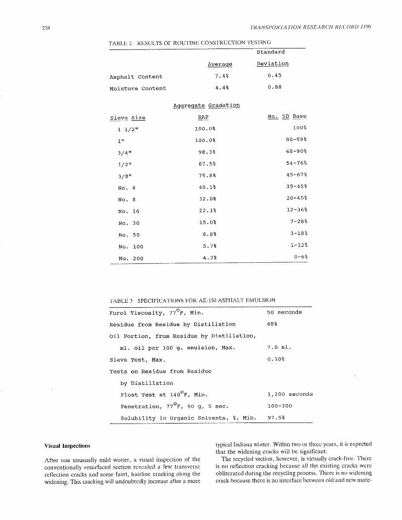
238 TRANSPORTATION RESEARCH RECORD 1 196

TABLE 2 RESULTS OF ROUTINE CONSTRUCTION TESTING

-

Standard

Deviation

o. 45

o.88

Asphalt Content

Moisture content

sieve Size

L t/z't

1x

3/ 4"

L/2"

3/au

No. 4

No. 8

No. L6

No. 30

No. 50

No.100

No. 200

Àverage

7.4*

4.42

Àgqreqate Gradation

RÀP

r.00.0t

100.08

98.38

87.52

75.88

48. lt

32.O*

22.34

15.0*

8.88

5.72

4.2*

No. 5D Base

L008

80-998

68-908

54-762

45-6?z

3 s-4 58

20-452

L2-362

7-282

3-188

L-t2z

0-6*

TABLE 3 SPECIFICATTONS FOR AE-150 ASPHALT EMULSION

Furol Viscosity, 77oF, !,tin.

Residue fron Residue by Distillationoil Portion, fron Residue by Distillation,

nI . oil per 10o g. enrulsion, l,{ax.

Sieve Test, Max.

Tests on Residue fron Residue

by DistillationFloat Test at L4ooF, Min.

Penetration, '77oF, 50 g, 5 sec.

sotubility in organic Solvents, 8, Min.

50 seconds

688

7.0 nl .

0. L08

L,200 seconds

L00-3 00

97.54

Visual Inspections

After one unusually mild winter, a visual inspection of the

conventionally resurfaced section revealed a few transverse

reflection cracks and some faint, hairline cracking along thewidening. This cracking will undoubtedly increase after a more

typical Indiana winter. Within two or three years, it is expected

that the widening cracks will be significant.The recycled section, however, is virtually crack-free. There

is no reflection cracking because all the existing cracks wereobliterated during the recycling process. There is no wideningcrack because there is no interface between old and new mate-

McDaniel

TABLE4 ROUGHNESSSUMMARY

1986 L987

Conventional Pave¡nent

Eastbound

Westbound

Àverage

Recycled Pavement

Eastbound

Westbound

Àverage

940

846

893

77?

652

7L4

836

869

852

75L

688

720

rial. An extremely hot summerapparent in the recycled section.lems to date.

has passed and no rutting is

In short, there are no prob-

Roughness Data

The initial roughness was evaluated with the Cox Roadmeterin December 1986. Roughness measurements were performedagain in July 1987. These results are summarized in table 4.

Roughness measurements are included in this study mainlyto monitor deterioration of the two pavements over time. Thesmoothness cannot be directly compared because the pave-

ments include different surface materials and numbers ofcourses.

The readings indicate that the pavement with recycled base

was initially smoother than the resurfaced pavement. Onelayer of hot asphaltic mixture was placed over the resurfacedpavement and two were placed over the recycled pavement,which helped level out the recycled section.

The follow-up testing in 1987 again showed the recycledpavement to be somewhat smoother than the resurfaced pave-

ment. Neither pavement showed an increase in roughness.

The roughness numbers measured in 1987 are not significantlydifferent from those measured in 1986.

Dynaflect Deflections

Results of Dynaflect testing are shown in figures 3 and 4 andare summarized in table 5. Deflections measured before con-

struction were essentially the same on the two portions of theproject. The amount of variation in deflections, as indicatedby the standard deviations and coefficients of variation, is also

essentially the same.After construction, the deflections were reduced by approx-

imately half. The deflections measured on the recycled pave-

ment were slightly lower than on the conventional resurface.The coefficients of variation show that the amount of varia-bility is roughly the same as before construction.

Dynaflect measurements were made again in June of 1987.

These results are not directly comparable to the previous tests

because of the seasonal variation in deflection measurements

on bituminous pavements. Nevertheless, the readings indicate

that, even in the heat of summer, the pavement is now stronger

than before construction. Again, there is no significant dif-

ference between the two pavement types.

Analysis of Cores

Cores of the recycled pavement were taken in July 1987 after

the pavement had been in place for about one year. These

cores were analyzed for density, voids, and Hveeln R and S

values. Cores will be taken annually to evaluate any furtherdensification under traffic. The results of the 1987 analysis ofcores are shown in table 6.

Intact cores of the recycled material were very difficult to

take. The cores obtained were fragmented, An unsuccessful

attempt was made to core without water to allow determi-nation of the in situ moisture content of the recycled base.

PROJECT COSTS

Past experience has shown that a new technique or materialis usually more expensive the first few times it is used thanwhen it is more widely used. This is due, in part, to contractorsbecoming accustomed to the process and the problems theymay encounter, Also, competition increases as more con-tractors obtain the necessary equipment and develop theexpertise.

In the case of this new recycling technique, the cost for therecycled pavement was almost double the cost of the con-ventional pavement. The cost breakdown was as shown intable 7. If this recycling method is used more often in Indiana,the costs are expected to drop somewhat.

Since indications are that the recycled pavement will have

significantly less cracking than the conventional pavement' atleast initially, the maintenance costs will be reduced. Life-cycle costs for the recycled pavement may then be lower thanfor the conventional pavement, depending on the relativeservice lives of the two pavements. The continued evaluationof this project should help estimate the service lives of thepavements.

239

!

oco+usoô

#Loocon

2.2

2

1.8

1.6

1.4

1.2

1

0.8

0.6

0.4

0.2

o

B Before 4/21186

FIGURE 3 Dynafloct deflectlons, recycled s€ction.

:v,co+ugoo

*LoncoØ

2.2

2

1.8

1.6

1.4

1.2

1

0.8

0.6

0.4

o.2

o

0islonceAfler 11/24/86

tr Before 4,/21 /86FIGURE 4 Dynaflect deflectlons, resurfaced sectlon.

DislonceAfler 11/24/86

McDaniel

TABLE 5 DYNAFLECT DEFLECTIONS SUMMARY

Before ÀfterConstruction Construction

4-86 L1-86 6-87

Resurfaced Eastbound

Àverage sensor No. L (nils)

Standard Deviation (nils)

Coefficient of Variation (8)

Resurfaced lvestbound

Average sensor No. 1 (nils)

standard Deviation (nils)

CoefficÍent of Variation (8)

Recycled Eastbound

Àverage Sensor No. l. (nifs)

Standard Deviation (¡nils)

Coefficient of Variation (8)

Recycled Westbound

Àverage sênsor No. 1 (nils)

Standard Deviation (nils)

Coefficient of Variation (8)

L.44

o,37

25.7

L.52

o.42

27.6

r..50

0. 38

25.3

L.46

0.40

27.4

o.79 L.10

0. 18 0.25

22.8 22.7

0.84 L.24

o.20 0.34

23.8 27.4

o.73 L.24

0.L8 0.36

24.6 29.O

o.7L L.20

0. L6 0.30

22.5 25.O

TABLE 6 RESULTS OF ANALYSIS OF CORES

standard

.Avera<¡e Deviation

Density, pcf

Air Voids, IHveem Stabilities

s-value (1400)

R-value (7oo)

14L.s pcf

5.08

25

gL2

3. l_

2.L

1

L

lBased on smaLl sanple size due to difficulties in getting

sampJ.es of sufficient thickness for Hvee¡n testing.2uncorrected for height of specinen.

CONCLUSIONS

After one year in service, the pavement with recycled baseseems to be perfonning at least as well as the conventionalpavement.

o The pavement with recycled base has less cracking thanthe conventional pavement. The deflections are essentiallythe same for the two types of pavements.

o Steps can be taken to improve the performance of therecycled pavement. When a widening trench is cut, as in thisapplication, the trench should be rolled as specified for otherwidening. The length of time the recycled base is left withouta surface should be limited to two weeks. This allows timefor the base to cure, but limits the length of time the pavementis left open to traffic and weather.

o The efficiency of the recycling could be increased. Thecapacity of the water trucks should be similar to avoid delays.

241

242 ,TRANSPORTATION RESEARCH RECORD I I9()

TABLE 7 PROJEC"T COSTS

Ouantitv Unit Pricê Total Cost

Resurfaced Section

I{idening(and Trenching) 3663

HAE No. 9 Surface 6118

Tons

Tons

Tons

Tons

Cost per Lane Mile

L Tons

57,300 SYD

5L,533 LFT

460 Tons

7r560 Tons

3,780 Tons

Cost per Lane Mile

9z¡. oo S84,249.00

iz3,z5 çL42,243.5o

97O. O0 $3, 640. 00

$23. 00 $18, 308.00

$248,440.50

ç25,454 .97

$70. 0o 970. 00

ç2.20 $t 26, 060. 00

s0. 20 $L0, 306. 60

$L50. oo 969, ooo. oo

$21-. oo gLsg, z6o. oo

$24.00 s9o,72o.oo

$454,916.60

$46,6r.0.3r.

Pat,ching

Vledqe and Level

Total

Recycled Section

Patching

Mitl ing

Trenching

AE-L50

Bit. Binder

HAE #LL Surface

Total

52

796

Obviously, keeping the paver and other equipment in goodrepair would reduce down time.

¡ Further evaluation is necessary to determine the long-term performance and to estimate the service life of the recy-cled base, but at this point the recycled material is performingwell.

o The recycled pavement cost nearly twice as much as theconventional pavement, but costs would likely drop if theprocess were used more. In this case, one more course ofbituminous mix was placed over the recycled base, signifi-cantly increasing the cost over that of the resurfaced section.Life cycle costs for the recycled pavement may be lower thanfor the conventional pavement if the service life is compa-rable, due to reduced maintenance costs.

RECOMMENDATIONS

The experience with this recycling technique in Indiana hasbeen very favorable so far. There is great interest in usingthe technique on more projects. Future uses may include thefollowing:

o The use of more exotic binders, such as foamed asphalt,rejuvenators, polymer modifiers, etc.

o Improving granular bases or gravel roads; this may beespecially attractive for county highway departments.

o Adding virgin aggregate, if needed, by spreading it onthe roadway ahead of the recycling machine.

o Surfacing the recycled base with a double chip seal insteadof a hot mix surface; again this may be especially useful onlow-volume roads, such as county roads.

Further evaluation may show that this type of base can beused on roadways with higher traffic volumes. The increasein traffic volume due to the auto plant will be monitored onState Road 38. Until further evaluation shows that this typeof base can withstand higher traffic volumes, it will only beused in low or moderate traffic volurne situations in Indiana(under 2,500 directional ADT).

This cold, in-place recycling technique appears to be a via-ble way to rehabilitate old bituminous pavements and to pre-vent reflective cracking. Its use for widening bituminous pave-ments, as in this case, seems especially appropriate.

Publication of this paper sponsored by Committee on PavementRehabilitation.

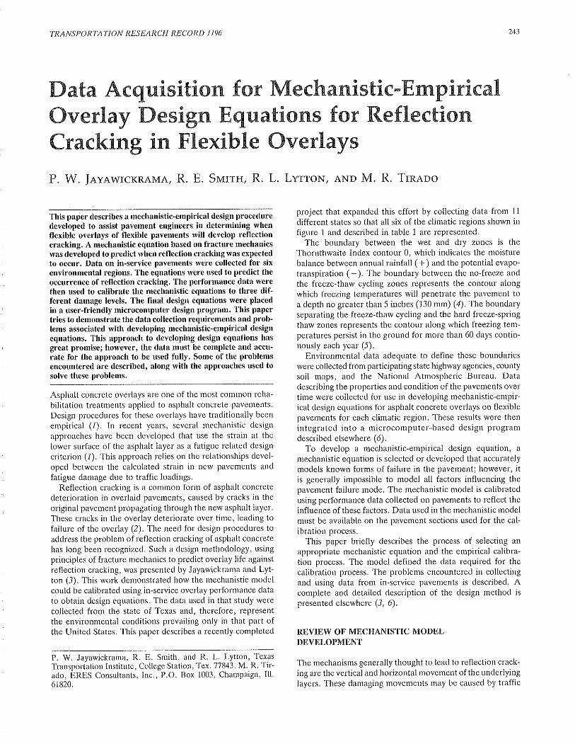
TRANSPORTATION RESEARCH RECORD I 196 243

Data Acquisition for Mechanistic-EmpiricalOverluy Design Equations for ReflectionCrackirg in Flexible Overlays

P. W. JavawrcxRAMA, R. E. SvtlrH, R. L. LvttoN, eNp M. R. Tlneoo

This paper describes a mechanistic-empirical design proceduredeveloped to assist pavement engineers in determining whenflexible overlays of ftexible pavements will develop reflectioncracking. A mechanistic equation based on fracture mechanicswas developed to predict when reflection cracking was expectedto occur. Data on in-service pavements rvere collected for sixenvironmental regions. The equations were used to predict theoccurrence of reflection cracking. The performance data werethen used to calibrate the mechanistic equations to three dif-ferent damage levels. The linal design equations were placedin a user-friendly microcomputer design program. This papertries to demonstrate the data collection requiremenfs and prob-lems associated with developing mechanistic-empirical designequations. This approach to developing design equations hasgreat promise; however, the data must be complete and accu'rate for the approach to be used fully. Some of the problemsencountered are described, along with the approaches used tosolve these problems.

Asphalt concrete overlays are one of the most common reha-bilitation treatments applied to asphalt concrete pavements.

Design procedures for these overlays have traditionally been

empirical (1). In recent years, several mechanistic design

approaches have been developed that use the strain at thelower surface of the asphalt layer as a fatigue related design

criterion (1). This approach relies on the relationships devel-oped between the calculated strain in new pavements and

fatigue damage due to traffic loadings.Reflection cracking is a common form of asphalt concrete

deterioration in overlaid pavements, caused by cracks in theoriginal pavement propagating through the new asphalt layer.These cracks in the overlay deteriorate over time, leading tofailure of the overlay (2). The need for design procedures toaddress the problem of reflection cracking of asphalt concretehas long been recognized. Such a design methodology, usingprinciples of fracture mechanics to predict overlay life against

reflection cracking, was presented by Jayawickrama and Lyt-ton (3). This work demonstrated how the mechanistic modelcould be calibrated using in-service overlay performance datato obtain design equations. The data used in that study werecollected from the state of Texas and, therefore, representthe environmental conditions prevailing only in that part ofthe United States. This paper describes a recently completed

project that expanded this effort by collecting data from 11

different states so that all six of the climatic regions shown infigure 1 and described in table 1 are represented.

The boundary between the wet and dry zones is theThornthwaite Index contour 0, which indicates the moisturebalance between annual rainfall (+) and the potential evapo-

transpiration (-). The boundary between the no-freeze and

the freeze-thaw cycling zones represents the contour alongwhich freezing temperatures will penetrate the pavement toa depth no greater than 5 inches (130 mm) (a). The boundaryseparating the freeze-thaw cycling and the hard freeze-springthaw zones represents the contour along which freezing tem-peratures persist in the ground for more than 60 days contin-uously each year (5).

Environmental data adequate to define these boundarieswere collected from participating state highway agencies, countysoil maps, and the National Atmospheric Bureau. Datadescribing the properties and condition of the pavements overtime were collected for use in developing mechanistic-empir-ical design equations for asphalt concrete overlays on flexiblepavements for each climatic region. These results were thenintegrated into a microcomputer-based design programdescribed elsewhere (ó).

To develop a mechanistic-empirical design equation, a

mechanistic equation is selected or developed that accuratelymodels known forms of failure in the pavement; however, itis generally impossible to model all factors influencing thepavement failure mode. The mechanistic model is calibratedusing performance data collected on pavements to reflect theinfluence of these factors. Data used in the mechanistic modelmust be available on the pavement sections used for the cal-ibration process.

This paper briefly describes the process of selecting an

appropriate rnechanistic equation and the empirical calibra-tion process. The model defined the data required for thecalibration process. The problems encountered in collectingand using data from in-service pavements is described. Acomplete and detailed description of the design method is

presented elsewhere (3, ó).

REVIEW OF MECHANISTIC MODELDEVELOPMENT

The mechanisms generally thought to lead to reflection crack-ing are the vertical and horizontal movement of the underlyinglayers. These damaging movements may be caused by traffic

244 TRANSPORTA'NON RESEARCLI RECO RD I I9ó

FIGURE I The six climatic rcgions in the United States (l).

loading, thermally induced contractions and expansions, or acombination of these mechanisms.

Figure 2 illustrates the changes in bending and shear stressesthat occur within an overlay as a wheel load passes over acrack in the original pavement. These stress conditions causethe crack to propagate into the overlay, due to shearing move-ment in one direction followed by a bending ¡novement anclagain by shearing movement in the opposite direction. Inaddition to the influence of the traffic loads, contraction andexpansion of the pavement and the underlying layers withchanges in temperature also contributes toward the growthof reflection cracks. In these three mechanisms of crack growth,the stresses generated cause a crack to form in the overlayand grow with repeated application. The principles offracturemechanics are used to determine the rate of crack growth dueto these mechanisms. In this process each crack growth mech-anism is treated independently, and their influence is com-bined in a final design equation.

The recent developments in linear elastic and viscoelasticfracture mechanics concepts have enabled a rational designapproach to the problem of reflection cracking of overlays.Experimental investigations carried out at Ohio State Uni-

TABLE 1 DESCRIPTION OF CLIMATICREGIONS

Region Character of the Region

versity (7-9) and Texas A&M University (10-]2) have ver-ified the applicability of fracture mechanics principles in pre-dicting fatigue life of asphalt conclete mixes. The results indicatethat the rate of crack propagation in asphalt concrete can bepredicted by using the ernpirical power law relation developedby Paris (13).

dc

ñ = A(^K)"

where

AK : stress intensity factor amplitude,A,n = f.racture parameters of the material,

c = crack length, andN = number of load applications.

Integrating Equation L we obtain,

¡v. = [" dc

' Jo A(AK),,

where

N¡ = numbel' of load applications to failurel¿ = thickness of the overlay

The use of Paris' crack growth law to deterrnine the overlaylife requires a knowledge of the stress intensity factor, K, andthe material constants, A and n, within the in-service overlay.The stress intensity factor, K, in the overlay due to each ofthe crack growth mechanisms was determined by using a for-mulation that combines beam-on-elastic founclation theoryand the finite element method. In the beam-on-elastic foun-dation analysis the original surface layer and the overlay aremodeled as a bea¡n. The base course and the subgrade are

(l)

(2)

I)J45

6

Wet, No-Freezerilet, Freeze-Thaw CyclingWet, Hard Freeze,'spring ThawDry, No-FreezcDry, Frceze-Tharv CyclingDry, Hard Freeze, Spring Thaw

Iayawickrama et al.

9,=ut(EuJ<cUJFTU)U'

POSITION OF WHEEL LOAD

FIGURE 2 Strcsses induced at a cracked sectiondue to a moving wheel load.

represented as a homogenous elastic meclium supporting thebeam. In order to calculate the stress intensity factors accu-rately and deter¡nine their variation with the crack length, afinite element method was used (ó).

The use of the mechanistic model for the analysis of crackpropagation through an overlay requires a knowledge of over-lay stiffness as well as fracture pararneters, A and n. The mixstiffness is cletermined using the nomograph procedure out-lined by Van der Poel (14) and Mcleod (/5). In this study,computerized versions of the nomographs were used. In addi-tion, the cornputer programs profile the slope, m, of the logof the mix stiffness versus log of the loading time curve whichis used to cletermine the exponent, n, in Paris'equation as

shown below:

n:2/m (3)

Theoretical justification for equation 3 can be found else-

where (1ó). This relationship has been verified for asphaltconcrete mixes by Gennann and Lytton (10) and Molenaar(17).

The following empilical relationships, developed based onthe crack growth tests of asphalt concrete mixes, were used

to determine the parameter, A:

For traffic associated cracking:

n -* -2.2 - 0.5 log ,4 (4)

For thermal cracking:

n = -0.92 - 0.42logA (5)

The propagation of reflection cracks is the result of allthree failure rnechanisms (bending, shearing, and thermal)acting sirnultaneously. However, in the integration of theParis' equation the three failure mechanisms are treatedindependently.

It is recognized that this idealized model may not provideaccurate estimates of the stress intensity factors induced by

245

the different loading mechanisms in the various mixes. How-ever, the model can be used to establish the forrn of theequation that reflects the correct influence trends of the var-iables. The form of the regression model in the empiricalcalibration was selected to incorporate the influence of thecombined action of the three mechanisms into the final designequation. The in-service performance data is then used in theregression analysis, which compares the mechanistically cal-culated time-to-crack formation with recorded crack devel-opment to develop equations that reflect the expected per-formance in each of the six climatic regions.

DATA NEEDS

The data required by the mechanistic equation to calculatethe time until the pavement develops a reflective crack mustbe available for the in-service pavement sections used in thisprocess. This same data will be required for use in the designprogram. The following information is required for calculatingthe overlay life using the mechanistic equations in this project:

. Laboratory data on the bitumen and the mix-to char-acterize the asphalt material used in the overlay,

o Deflection test data-to characterize the existing pave-ment structure,

o Environmental data pertaining to the location, ando Traffic data.

In order to combine the influence of the three differentmechanisms, the mechanistically computed overlay responsesare regressed against crack development rates in the overlays.Therefore it is also necessary to collect data on ovellayperformance,

DATA ACQUISITION

Previous studies indicated that sufficient data were not avail-able to develop one overlay design equation for the wholeUnited States, prirnarily because of the excessive amount ofdata required to account for climatic and regional differences.However, they did indicate that sufficient data were availableto develop regional equations (18). Considerable effort is

required to collect data adequate for use in calibratingmechanistic empirical design equations, Many state highwayagencies have some of the data needed to develop mecha-nistic-empirical equations; however, very few have all of thedata needed.

DATA SOURCE LOCATION

The information on available data (i,8,i,9), along with othersources, were used to begin the search for in-service data.Many of the agencies stated that they did not have all suchdata for their pavements. Others were reluctant to participatein the project because the data lequired were not readilyavailable or retrievable. Those agencies that did have theneeded data generally did not have all required data in onefile set.

(Ðøzu)EHH;

cl-u¡X

ÊÉl-c)

UØÍLu ¡-ot

frä(rFo

OVERLAY

246

In many instances during the data collection effort, it wasfound that the required data on a desiral¡le in-service pave-ment section was missing from the files. So an agency wouldoften start with 30 to 40 candidate in-service pavement sec-tions on which the researchers expected to collect data onlyto end with 5 to 15 sections with adequate data for use in theproject. As a result, the researchers nevet'knew the numberof sections on which daÊa could be collected until they wereon site at the agency. In some instances, it was not possibleto be sure that the data were usable until after the data wascollected and reduced into common-analysis units. When thedata were normally stored in several different files, each filewould often have a different referencing or cataloguing scheme,making it difficult to cross reference the data elements. Soeven when data could be found, it was not always possible toidentify corresponding data sets, such as which asphalt prop-erties corresponded to a given section of pavement.

DATA REDUCTION

Raw data were collected fro¡n several different agencies, asshown in table 2. In many instances the data gathered by theresearch team were not measured or collected in the sameform by the various highway agencies from which it was gath-ered. When data in different forms are used, they must bereduced to similar forms of material and response character-istics before they can be used in developing the desiredmechanistic-empirical design equations.

Asphalt Material Characterization for the Overlay

The stiffness of the asphalt-concrete overlay must be knownin order to determine the fracture properties and was calcu-lated using the Van der Poel or Mcleod method (14, 15). Touse the Van der Poel method, the following properties of thebitumen and the mix must be known:

o Penetration at77oF,o Ring and ball softening point,o Asphalt percentage in the mix or volume concentration

of aggregate,o Time of loading, ando Age of mix or time in service.

Many of the pavement sections did not have ring and ballsoftening point data. In those cases, the Mcleod procedurewas used which requires the following data.

o Penetration at77"F,o Viscosity at275'F or viscosity at 140oF,¡ Service Temperature,o Time of Loading,o Asphalt percentage in the mix or volume concentration

of aggregate, ando Percent of air voids.

Any set of data that could be used in either of these twoprocedures was accepted. These data were generally deter-mined from laboratory test results found in construction rec-ords. In some cases they were the result of many specific tests

TRANSPORTATION RESEARCII RECORD I 196

made for the project, which was the original intent; however,in other cases, asphalt properties were from asphalt sourcestested over the period of time during which the project wasconstructed.

Mix design properties were taken from quality control rec-ords in the construction records in most cases. When thesewere not available, the mix design parameters were takenfrom standard mix design requirements in effect at the timeof the overlay construction; however, this may add error tothe results. Time of loading was selected to represent a movingwheel load of a truck; service temperature was selected basedon environmental information for the areas; and age of rnixwas based on construction date. Availability, or locating, theasphalt cement and mix design properties for the overlay weremajor problems of this data collection effort.

Characterization of the Existing Pavement Structr¡re

The mechanistic model represents the existing pavement priorto the overlay as a beam on elastic foundation. The stiffnesscharacterizing the surface and foundation support can bedetermined from deflection testing data on the existing pave-ment prior to the time of the overlay, in conjunction withlayer thickness. A record ofconstruction history was obtainedfor each section used in this analysis to determine the thick-ness of each layer and its date of construction; in some cases

this was supplemented with coring reports. It would have beenbeneficial to have had deflection data across a series of cracksin the pavement prior to the overlay to determine the loadtransfer level; however, those data were not available. Manyprojects with otherwise usable data were discarded from thisproject when deflection data could not be located for them.

Climatic Data

The temperature and rnoisture information defining the cli-matic zone in which the pavement section is located weredescribed earlier. The 24-hour temperatul'e drop and averagemonthly temperature were the other two climatic data ele-ments required. They were found in the same sources.

Traffic

Traffic data regarding the average number of 18,000-lb equiv-alent single-axle loads (ESALs) per day over the life of theoverlay were collected from the highway agencies. Where theyhad some other measure of traffic such as average daily traffic(ADT), their conversion system of converting ADT to ESALwas used. It was then converted to average ESAL per day.Several of the agencies expressed reluctance at providing trafficdata because they were not sure of its accuracy.

Performance (Distress)

The mechanistically computed development of cracking iscompared to the observed crack development in the regres-sion process. To determine the amount of reflection crackingthat developed over time, distress data regarding reflection

TABLE 2 DISTRIBUTION OF PAVEMENT SECTIONS ON WHTCH DATA WERE COLLECTEDAND USED

cLr¡{AΡC zollt

SlATE trl2l3llAcPcclAcPccl âcPccl

5lrc Pcc l

4tac rcc I

6 I lot¡lrc Pcc I Àc Pcc

137t--149

03 134 I

l-- |06 143 I

I

I¡

I

I

I

III

Arizon¡

I l-- 03Arh¡n¡¡¡ ¡ l-- -l I

I lo3 o3l ¡

ll0t--l14

I

I

I

102t-lo¿

I

I

¡

03

103 03

120t--127

C¡liforni¡

tlorid¿

l06l--l0z 107 I

-¡l-tl0e 031 I

l',_

I

I

I 09 03

l-- 03

lor 03

I

II

I

II

03 I

01 03 I

I

Il

Gcorgir

ld¿ho¡

I

I

I

I

I

I

I

I

I

I

I

lrrt--lt4

lrtl--ll4

34

39

I

I

I

I 14 I

l--l¡ 15 I

¡ 20 I

t-lI 24 I

llliooi¡

t3 06

1,3 09

lo¡t-103 0l

Illiaac¡oc¡ I

I

lr0 061t--lIto 08l

36

36

I

I

l

24

24

03

03

l08t-108

lorlcr¿r I --101

l13t--l14

103 lr0r--t--103 lrr

I

II

I

1

I

I

I

I

I

I

I

0c¡h

05

05

42

43

I

I

I

I

I

I

I

I

I

07 t35 051l---l

07 l3ó 051lluhingtoa

I LtZ 5l

-t--0¡ ¡ 209 62

z4

28

20116 163

-¡--l-23123 174

lrorúÁL I --I19 03

493r¡r0-1--55 35¡r0

##

--#t|No. Pavement Sections Used¡¡o. Pavèment SectÍons Collected

llocr

248

cracking after the application of the overlay is required. Sincethe performance used in the mechanistic approach considereddamage that varied from zero to one, the distress data hadto be transformed into equivalent levels of damage (/8). Evenhad this not been required, the data would still have had tobe transformed into a common set. Each agency collects dis-tress data in its own form, and virtually no two agencies usedthe same distress identification system. The distress identifi-cation system from each agency was used to develop aconversion similar to that used in the initial program (3).The transformations used to convert the distress from eachdata set into a common damage function are presented else-where (ó).

DEVELOPMENT OF PERFORMANCE CURVE

The observed damage levels over time and traffic were usedto develop a mathematical equation to describe the growthof damage, or overlay reflection cracking, with increasing timeand increasing number of load passes for each pavement sec-tion included in the project. By comparing the mechanisticcrack development time with observed time to reach variouslevels of damage, design equations could be developed fordifferent amounts of allowable reflection cracking.

Two forms of reflection cracking were considered: trans-verse and longitudinal. It was hoped to use both distress areaand severity; however, only distress area was available formany of the in-service pavements. As a result, only area wasused for the final equations.

Different forms of equation have been used to fit the observedpavement distress data over increasing time or axle load appli-cations. The following equation was selected for use in thepresent analysis since it is in accordance with the physicalboundary conditions (18):

I - e-bt¡'04

where

I = the damage rating of the pavementN = the number of load applications in 18-kip ESALs

p,9 = characteristic parameters

An equation that relates the damage level of the distressedpavement to the number of load applications is commonly

TRANS PORTATION RESEARCH RECORD I I 96

retþrred to as a structural perfolmance curve, The damagerating of the pavement is a variable that ranges between 0,representing a smooth riding or undistressed surface, to l,representing a severely darnaged pavement structure. There-fore, the performance curve of a pavement will be boundedby 0 and 1. Pavement distress observations show that theperformance curue starts out holizontally, bounded fiom belowby a rating of 0. As the number of load applications increases,the curve will asymptotically reach the damage rating of LThese boundary conditions imply that the functional perfor-mance curve should be sigmoidal, or S-shaped.

Nonlinear regression analysis techniques were used to developthe performance cures to define a relationship between dam-age and the number of load applications, N,r. This allows thenumber of applications to be determined at any desired levelof damage. Several problems were encountered in using theseprogl'ams. The nonlinear regression procedures are not alwaysstraightforward, especially if the data are not well definedthrough the entire area defining all parameters in a curve.Thus, there is not always one unique curve that will fit thedata points and meet the convergence criteria, Since many ofthe data sets contained data with damage levels only to levelsof 0.1 or less, several sets of regression parameters could befit through those points and still meet the convergence criteria.Luckily, the major differences in predicted values are abovedamage levels of 0.5 and have little impact on the results usedin this project.

Because some of the distress identification procedures reportdistress in condition categories, for example, 5 to 15 percentequals distress rating of 2, some of the distress data had pla-teaus, as illustrated in figure 3. When regression was con-ducted, parameters could be calculated to define the curveshown as A in figure 4, or another set could be calculated todefine the curve shown as B in figure 4. The performancecurves for this type of data were forced to follow the shapeidentified as Curve B in figure 4 because it was believed thatthe observed data was in the earliest stages of distress devel-opment. Allowed to develop further, it is expected that theywould develop the S-shape defined by Curve B in figure 4.

In some of the in-service pavement sections, no distress haddeveloped at the time of data collection resulting in all zerodamage levels. These sections could be ignored; however,ignoring pavements that were performing well would bias thedata. To use these data, average p and B values for the non-

(6)

l¡Jo

ô

O REPORTED DAMAGE

ooo

NreFIGURE 3 Distress data rvith plateaus.

Jayawickrama et al 249

tu(,

o

zero data sets within each climatic/pavement type group weredetermined. Those values were used to define the curve throughthe all zero data points, as illustrated in figure 5. If the all-zero points extended to the right of the curve from the average

values, the p values were increased until the curve extendedthrough all of the reported zero points as shown in figure 5.

This allowed the influence of the all-zero points to be includedin the analysis.

RESULTS

A final set of design equations to acldress reflection crackingwere developed that allow the designel to select a damagelevel of 0.33 for a moderate amount of reflection cracking,0.50 for a high amount, and 0.44 for an intermediate amount.They have been placed in a user-friendly microcornputer pro-gram that can be used by highway engineers to determinewhen reflection cracking is expected to develop in an overlayof desired thickness for different asphalt cement and mixproperties. This research has extended the work that began

in NCHRP Project ZO-1 , Task 17, Phase II, and includesdesign equations for six climatic regions for asphalt overlays.

This is a major step forward in developing design equationsthat address the performance problems of asphalt concreteoverlays. The best available data was used to calibrate the

Nra

FIGURE 4 Curves fitting data with plateaus.

Nre

FIGURE 5 Using all zero data points.

mechanistic equations; however, they would be more reliableif the data used to calibrate the mechanistic equations weremore complete and comprehensive. They can be improvedby using more accurate in-service data when it becomes

available.The data used to calibrate the mechanistic equations were

collected from agencies with data on pavements of the typeneeded in the desired climatic zones. The data did not come

from a designed experiment, and all the problems inherentin using this type of data are incorporated into these design

equations. One of the biggest problems with this type of datais that unknown biases exist, making it impossible to deter-mine the true reliability of the resulting data. In addition, thevariability and reliability of the data collected were generallyunknown. This does not mean that the equations are unre-liable, but it does mean that the reliability of the design equa'tions developed using this type of data cannot be accuratelydefined.

The mechanistic empirical approach to overlay design has

been shown to be feasible and practical. It has also shown

the need for collecting accurate data with variability and reli-ability information included for use in developing mechan-

istic-empirical equations. The mechanistic empirical approachprovides an excellent means to develop design equations thatare soundly based on mechanistically correct concepts with a

limited number of parameters. However, they will only be as

uJo

ô

O REPORTED DAMAGE

CURVE A

O REPORTED OAMAGE

CURVE FROM

AVERAGE BETA

CURVE WITHAVERAGE BETA

AND INCRËASE RHO

250

good as the data used'to calibrate them. Until accuracy ofavailable data is known, accuracy of the resulting design equa-tions will be unknown.

RECOMMENDATIONS

The data collection problems in this and other projects dem-onstrate the need for a comprehensive centralized data col-lection effort if mechanistic-empirical procedures are to beused in the pavement engineering field. The data required tocalibrate these and other mechanistic empirical design equa-tions should be collected in the Strategic Highway ResearchProgram (SHRP). These data should be collected in a mannerto avoid the problems of possible bias and uncertainties thatoccur in using available data to calibrate mechanistic equa-tions. These data can then be used to update this first set ofdesign equations.

ACKNOWLEDGMENTS

This paper is based on work completed by ERES Consultants,Inc., and the Texas Transportation Institute. The work wassponsored by the Office of Research and Development, Fed-eral Highway Administration. The contracting officer's tech-nical representative was Peter Kopac. The assistance of theseveral state highway department personnel is gratefullyacknowledged.

REFERENCES

l. R. E. Smith, R. P. Palmieri, M. I. Darter, and R. L. Lytton.Pavement Overlay Design Procedures and Assumptions, Vol-ume I, Analysis of Existing Procedures. FHWA/RD 85/006,FHWA, Mclean, Va., 198ó.

2. R. E. Smith, M. I. Darter, and S. M. Herrin. Highway Dis-tress ldentification Manual. FHWA-RD-79-66, FHWA,Washington, D.C., 1979.

3. P. W. Jayawickrama and R. L. Lytton. Methodology forPredicting Asphalt Concrete Overlay Life Against ReflectionCracking. Proceedings, Vol 1, Sixth International Conferenceon Structural Design of Asphalt Pavemenls, Ann Arbor, Mich.,July 1987, pp.912-924.

4. Frost Action in Roads and Airfields. Special Report No. l,HRB, National Research Council, Washington, D.C., 1951,p.123.

5. Report on Frost: Investigation, 194H5. New England Divi-sion, U.S. Army Corps of Engineers, U.S. War Department,Boston, Mass., April 1947.

?'RANS PORTATION RESEARCH RECORD I 19ó

6. P. W. Jayawickrama, R. E. Smith, R. L. Lytton, and M. R.Tirado. Development of Asphalt Concreîe Overlay DesignEquations, Vol. 1, Development of Design Procedures. FHWA,Washington, D.C., 1987.

7. K. Majidzadeh, C. Buranarom, and M. Karakouzian. Appli-cation of Fracture Mechanics for Improved Design of Bitu-minous Concrete. Report No. FHWA-RD-76-91, Vol. l, June1976.

8. K. Majidzadeh, D. V. Ramsamooj, and T. A. Fletcher. Analysis of Fatigue of Sand Asphalt Mixtures. Proceedíngs, Asso-ciation of Asphalt Paving Technologists, Vol. 30, 1969.

9. K. Majidzadeh and D. V. Ramsamooj. Development of Test-ing Procedures and a Method to Predict Fatigue Failures ofAsphalt Concrete Pavement Systems. The Ohio State Uni-versity Research Foundation, Project RF 2873, March 1971.

10. F. P. Germann and R. L. Lytton. Methodology for PredictingReflection Cracking Life of Asphalt Concrete Overlays. ReportNo. FHWA/TX 791091207 -5, March 1979.

11. R. L. Lytton and U. Shanmugham. Fabric Reinforced Over-lays to Retard Reflection Cracking. Reporr RF-3424-5, TexasA&M Research Foundation, February 1983.

12. R. L. Lytton and K. H. Tseng. Laboratory Evaluation ofOverlays Reinþrced with Fabrics. Texas Transportation Insti-tute, Texas A&M University, College Station, Tex., May1983.

13. P. C. Paris and F. Erdogan. A Critical Analysis of CrackPropagation Laws. Transactions of the ASME, Journal ofBasic Engineerurg, Series D, 55, No. 3,1963.

14. C. Van der Poel. A General System of Describing the Vis-coelastic Properties of Bitumens and Its Relation to RoutineTest Data. Journal of Applied Chemistt'y, Vol. 4, May, 1954.

15. N. W. Mcleod. Asphalt Cements:aPen-Vis Number and ItsApplication to Moduli Stiffness. Journal of Testing ancl Eval-uation,YoL4, No. 4, 1976.

1ó. R. A. Schapery. A Theory of Crack Growth in ViscoelasticMedia. Report MM-2764-73-1, Mechanics and MaterialsCenter, Texas A&M University, College Station, Tex.,1973.

17. A. A. A. Molenaar. Structural Petformance ancl Design ofFlexible Load Constructions and Asphalt Concrete Overlays.Ph.D. thesis, Delft University of Technology, The Nether-lands, May 1983.

18. R. L. Lytton and A. Garcia-Diaz. Evaluation of AASIIORoad Test Satellite and Environmental Str.rdies. NCHRP Ploj-ect20-7, Task 17, Texas Transportation Institute, Texas A&MÇniversity, College Station, Tex., 1983.

19. R. L. Lytton, and G. L. Kohutek. Evaluation of AASHOLoad Test Satellite and Environmental Studies, Phase II FinalReport, NCHRP Project 20-7, Task 17, TexasTlansportarionInstitute, Texas A&M University, College Station, Tex., 1983.

Publication of this paper sponsored by Committee on PavementRehabilitation.

Serviceability Index Base for Acceptance offointed Concrete Pavements

Wrnren¿ H. Tnn¡prn AND SrnvnN L. Cuu¡e¿

This paper describes the techniques and relationships devel-oped to design a Serviceability Index (Sl)-based measurementsystem for acceptance ofjointed concrete pavement construc-tion in Louisiana. Pavement roughness statistics obtained fromMays Ride Meter equipment, a Surface Dynamics Profil-onreter, and a Chloe Profilometer tvere regressed to establishan AASHO Road Test-based SI measurement system for con-ccte pavernents with 2O-foot joint spacings (SI JCP 20). A1986 panel rating of 25 concrete pavements confirmed thevalidity of the model. Field testing of 50 newly constructedconcrete pavement test sections provided a relationship betweenthe SI JCP 20 model and profile statistics frorn rolling profi-lograph equipment and a l0-fl rolling straightedge. The researchresulted in the development of a rational lnethod of providingspecification limits for profilograph equi¡lrnent that relate topâvernent rideability. Specification limits in terms of profilestatistics are provided to indicate the quality of paving nec-essary to construct a jointcd concrete pavetnent with a Ser-viccability Index of 4.5.

The constructed ride quality of jointed concrete pavemerìtshas been the subject of considerable research in Louisiana,generally resulting in the conclusion that roughness that isbuilt into new pavernents has increased as transvelse jointspacings were recluced. In an attempt to revelse this trencl,efforts have been made to establish a level of rideability thatis consideled acceptable and that is also reasonably con-structable. A specification index that can be related to ridequality has been incorporated into a system for determiningcontractol compliance to the specification limits.

The research contained herein describes techniques andlelationships used to accomplish:

o The selection of a specific level of AASHO Road Testbased Serviceability Index (SI), which was set as a bench markfor ride acceptability on new jointed concrete pavements and

o The development of mathematical relationships to imple-ment a specification procedure that is manageable under fieldconditions and utilizes relatively inexpensive but repeatabletest equipment. Conversion relationships arnong a variety ofroughness measuling devices were developed to facilitate fielddetermination of the selected SI level for jointed concretepavements with 20-ft transverse joint spacing. The devicesinclude two different types of rolling profilograph, a Chloeprofilometer, a Surface Dynamics Profilometer (GeneralMotors), a Mays Ricle Meter trailer system, and a 10-ft rollingstraightedge.

.I'RANSPORTAT'ION RESEARCH RECORD 1 196 251

Louisiana Transportation Research Center, 4101 Gourrier- Ave-nr¡e, Baton Rouge, La. 70808.

SERVICEABILITY INDEX REQUIREMENTS

Paving specifications for jointed concrete in Louisiana havetraditionally been expressed in terms of the percent of projectlength that exceeds a 7s-in deviation in 10 feet as measuredwith a rolling straightedge. Surface tolerance specificationswhich have allowed up to 6 percent of the length of a projectto be out of tolerance have typically resulted in "as con-structed" Serviceability Index (SI) levels of between 3.0 and4.0 for jointed concrete pavements. In an effort to increasethe as-constructed SI level the surface tolerance specificationswere amended and reduced from 6 percent to 0 percent, asmeasured with the rolling straightedge. At the same tirne, a

decision was made to set a minimum acceptable SI level andto conduct research necessary to provide a limiting specifi-cation index that would produce this target SI.

At the request of the Federal Flighway Administration,Louisiana DOTD adopted a target SI of 4.5 for constructionof jointed concrete pavements. The basis for selecting thisparticular serviceability level was that it is an integral part ofthc assumptions in the current AASHTO clesign for rigidpavements. Jointed concrete pavements at the AASHO RoadTest were constructed to a mean SI of 4.5, which, using equa-tion 1, translates tc a slope variance (SV) of approxirnately2.2 (r).

SI : 5.41 - 1.80log (1 + SV)

Flexible (non-jointed) pavement sections frorn the Roacl Teslwere constructed to a mean SI of 4.2, which, by equation 2,translates into an SV of approximately 1.7.

SI = 5.03 - 1,.91los (1 + SV)

A comparison of jointed concrete and flexible pavelnentsmoothness using slope variance measurements indicates thatthe non-jointed sections at the Road Test contained less built-in roughness, since lower values of slope variance indicate asmoother pavement. A comparison by SI, however, seems tocontradict the slope variance trend, since the jointed pave-nlent was rated higher on a scale of 0 to 5, with 5 beingperfectly smooth. This apparent contradiction is attr.ibutableto the panel service ratings (PSR) from which equations Iand 2 were derived. The panel ratings confirm that at equallevels of serviceability rating, jointed-concl.ete pavements typ-ically contain a greater measure of roughness. A dual methodof relating roughness measurements obtained from jointecland non-jointed pavements is, therefore, indicated. This factis graphically illustrated in figure 1,

Recognition of these trends is necessary for a contractingagency to correctly use AASHO-based SI to establish con-

(1)

(2)

252

\

tr,.tr. 7 'tcr

\,/\ \<'----\-

\\---

HMAC

TRANSPORTATION RESEARCH RECO RD 1 196

struction limits for both jointed and non-jointed pavements

to control ride quality.

SERVICEABILITY INDEX FROM FIELDMEASUREMENTS

Research studies since the early 1970s in Louisiana have

involved a variety of rolling devices, each designed to providean index of pavement roughness. The flow chart shown infigure 2 contains an overview of the procedures followed and

the relationships between test equipment that lead to an

AASHO-based SI measurement system for control of jointed-concrete paving.

A Mays Ride Meter (MRM) trailer system (with a suspen-

sion system modified according to Georgia DOT specifica-tions to increase repeatability) provides a convenient means

of estimating the SI of a pavement. Since 1975 MRM responsemeasurements have been closely correlated to data from a

Surface Dynamics Profilometer (SDP) at the Texas SDHPTusing a procedure that relates SI to the inches-per-mile response

measurement of the MRM (2). The SI equation indicated infigure 2 is a function of the vehicle ride characteristics of an

individual vehicle (expressed as a and å) in conjunction withthe MRM response index, inches-per-mile.

o_ZJtrÉ.

Jl¡Jz<,

0 10 20 30 40 50 60 70 80 90 lod

MEN SLOPE VARIAI.ICE

FIGURE I Panel rating versus slope variance for rigidand flexible pavements-AASHO Road Test.

/*or, ilETEN

\ $nftrtel

/

R1

T

/ SURFACE \I DYNAIT rcs

\

Yo'l!?fy

' -,lnMra\

Sl = 5e'T'

^otìtï,ut'*\--s?. Non Joìnted ^/ I

\ Pavement / I

/ CHLOE \/pRo

F IL0M ET ER', (sr)\ Joi nted /\ a^ó.rôla f

,/røo\PAN EL RAT IN G

(sl)Joi nted

\onc..terl

- JCPnted ',7R3

Jo'TEN FOOT

RO LL¡N6TRAIGHTEDGst

I'layron

Rq,

R5

^c\FILOGTyoe A

' SPLU IFILA I IUN

LMNS FOR

ACCEPTANCT OF

d*or'rou^. Type I\ (intmile)

(in/miìe

APH.(zo-Foot Joint l.. Spacing) /

FIGURE 2 Regression relationsnips (Rl-R7) for Sl'based acceptânceprocedure using profilograph equipment.

Temple and Cumbaa

The test sections used in the MRM-SDP correlation pro-cedure have primarily been flexible, non-jointed pavements.

The resulting relationships between the SI and inches-per-

mile produced reasonable results when applied to flexiblepavements in Louisiana; however, when applied to jointedconcrete pavements, the SI predictions seem low. A reviewof pertinent literature confirmed the need for a dual ratingsystem as previously indicated (1).

The Chloe Profilometer provided a mechanism for estab-

lishing a relationship between MRM-SDP SI for non-jointedpavements and a MRM-SI for concrete pavements with a 20-

ft joint spacing, hereafter referred to as "SI JCP 20." In 1975,

a field study of jointed-pavement roughness was initiated todevelop the correlation. The results of the testing are pre-sented in equation 3 and in figure 3.

IMRM, sDP(sI)l = t_t).Sn e, SI JCP 20) (3)

The regression analysis was perfolmed in terms of SI valuesinstead of using slope variance (SV) since the SVs of the twopavement types are not equal at a given SI level. Using thisrelationship, Louisiana DOT was able to implement a dual-rating system with correctly based SI relationships for fieldtesting with MRM equipment, as depicted in figure 4.

PANEL RATING VERIFICATION

I¡r 1986, as a result of the Louisiana Transportation ResearchCenter's (LTRC) participation in NCHRP 1'-23(2), a panel

rating of 25 jointed-concrete pavements was conducted using36 raters. MRM tests were also conducted on the rating sec-

tions to provide LTRC with an opportunity to verify theirSDP-Chloe based SI relationship.

\

\i\1 -.'- JCe

\- ___

HMAC

0 50 r00 150 200 250 300 350 400 450 500

MRM

rN / MrLr

FIGURE 4 Mays ride meter (in/mile) versus SI forrigid and llexible pavements-Louisiana.

The results of the comparison, equation 4, provided a nearly1:1. relationship between the 1986 panel rating and the "SIJCP 20" measurement as depicted in figure 5.

SI JCP 20 = O.94(Ratins) + 0.19 (4)

The SDP-SI (non-jointed) when applied to jointed pave-ment does not correspond to the 1986 panel rating data with-out the benefit of a correctly based panel relationship (Chloe)for jointed pavement as expressed in equation 3. This againillustrates the fact that panel raters respond differently tojointed-concrete and non-jointed pavements.

01234PAliTL RATING

FIGURE 5 SI JCP 20 versus panel rating.

253

J.5

J.06> 2.5É.

2.0

't.5

1.0

5.0

4.5

4.0

q

0

5.0

4.5

4,0

3.5

J.0

2.5

2.0

t,5

t.0

_oLDN

ÈL>oa

3rttx>qt'>c

Yo

CHLOT SI

(JcP-20)

FIGURtr 3 Mays ride meter/surface dynamicsprofilometer SI versus Chloe profilometer SI.

^-= sDP Sl

(Non-Joínted)

254

SPECIFICATION COMPLIANCE

Hand-operated rolling equipment can be used to provide con-struction personnel with verification of specification compli-ance in a timely manner. Vehicle response type measurementsystems cannot be used as effectively to control a paving oper-ation on a day-to-day basis, due to the physical limitations ofheavy equipment being placed on concrete pavements thatare gaining strength. The hand-operated devices must alsoprovide reproducible results to instill in the users the level ofconfidence necessary for a successful testing program. Loui-siana DOT has traditionally used only the 10-ft rolling straight-edge for acceptance testing; however, because of calibrationand reproducibility problems, the agency is now phasing in a

rolling profilograph for concrete pavement acceptance.

IO-FOOT ROLLING STRAIGHTEDGE

The rolling straightedge is a relatively inexpensive test device

that can be used to control roughness during the paving pro-cess. Research testing with a carefully calibrated straightedgehas resulted in a general correlation between "SI JCP 20"and the percentage of a test section that exceeds a 7e-in devia-tion in 10 feet, expressed as equation 5 and depicted in fig-ure 6.

SI JCp 20 = 2.0 + 2.5 eeo.rcsott (5)

Results of the testing indicate that in general a paving levelof SI JCP 20 equivalent to 4.5 is possible only where therearezeÍo deviations beyond 7s-in in 10 feet. Surface tolerancespecifications were amended in 1986 to require a "zero pet-cent" specification in an attempt to implement this level ofpaving quality. Under the new specification, the consequenceof non-compliance is surface grinding instead of a provisionfor contract payment reduction. The success of this approach

¡-tt¡\¡t\.T T

I \¡.' \.

¡

ara

051015202530J54045STRAIGHTEDCE

(PERCTNT BEYoNo 1/B')

FIGURE ó SI JCP 20 versus l0.foot rollingstraightedge (percent out of tolerance).

TRANSPORTATION RESEARCH RECO RD I 196

in achieving the desired level of serviceability is currentlybeing evaluated. In addition to calibration difficulties, it was

observed that two rolling straightedge devices that were pulledtogether in the same wheelpath occasionally did not identifythe same locations as needing grinding. Observations such as

these quickly undermine confidence in a specification system

that, at times, results in substantial quantities of ride correc-tion on the part of the contractor.

ROLLING PROFILOGRAPH

Research underway using a 25-ft rolling profilograph (Amesmodel, designated Type A in figule 2) is producing improve-ments in terms of measurement repeatability and in the inter-pretation of exactly where ride correction is necessary. Theprofilograph is styled after the California profilograph in thatthe axes of the reference platform wheels are not uniformlyspaced along the length ofthe device. Support is instead pro-vided on each end by a group of wheels. Internal equipmentcalibration prior to testing is apparently not necessary formeasurement reproducibility for this device. The pavementprofile, which is graphically recorded, can be referenced todetermine exactly where grinding is needed. Follow-up testingafter grinding can be used to determine the need for additionalreduction in the inches-per-mile statistic required for speci-fication compliance.

Profile statistics (inches/mile) were calculated from the pro-file graphs on 50 test sections (0.2 miles in length) using botha 0.l-in and a 0.2-in blanking band for compat'ison. The pro-filograph roughness statistic accounts for only the rnagnitudeof each bump or dip, whereas the rolling straightedge statisticaccounts for the length of each deviation beyond a selectedtolerance. For this reason profilograph testing on projects thatcontain many deviations of a srnall magnitude (such as 0.05in) will result in a significantly lower summary statistic whenusing the 0.2-in band. Smoothness specification limits must,therefore, reflect the size of blanking band used to surnmarizethe profile data,

A correlation between profilograph statistics and the SI JCP20 reference data is depicted in figures 7 and 8 for the 0.I-inand 0.2-in bands, respectively. The equations for the tworelationships are expressed as equations 6 and 7.

0.1-in band:

in/mile = 124.5 - 26.4 (6)

0.2-in band:

in/mile = -1.9 + g9g1 .4 e(-¡.7ó(sr)) (7)

The results indicate that to achieve an SI of 4.5, approxi-mate specification limits should be 6 in/mi using a 0.1-in bandand I in/rni using a 0.2-in band. The 12-inlmi specificationlimit currently used by several contracting agencies is likelyto produce a SI level less than 4.0 using the 0.2-in blankingband relationship.

Another style of profilograph (Rainhart, designated TypeB in figure 2) was used to test 18 sections. The device contains12 reference platform wheels with axes evenly spaced alongits length. The two different types of profilograph consistentlyagreed on the location of bumps and dips, altlìough not tothe same magnitude of surface deviation, as indicated by therelationship in equation 8 and figure 9. Specification limits

^aôJN

ñ'0-(.)

32

Temple and Cumbaa

a

t¡t

I r ! \- 'I t\:I

rl\.

3.0 J.2 J.4 J.6 3.8 4.0 4.2 4.4 4.6 4.8 5.0

MAYS RIDI METIR SI

(JcP-20)

FIGURD 7 Ames Profilograph (i¡r/milc) with 0.l.inchblanking band versus SI JCP 20.

expressed in inches-per-mile must recognize the proper SIequivalency associated with a particular style of profilographused to conduct field tests.

in/mi, Type, - (in/mile' TyPllA) - 4'18

SIGNIFICANCE OF REGRESSION EQUATIONS

Statistical tables indicate that the six regression relationshipsdeveloped in the study each contain correlation coefficientsthat are significant at all levels. Variance in test data is expressedas R2 (coefficient of determination) and s2 (residual meansquare) in table 1.

ADDITIONAL RESEARCH

LTRC is using the rolling profilograph to evaluate roughnessin newly constructed jointed concrete pavements to determineamong other things:

o The magnitude and frequency of surface deviations typ-ically occurring in paving projects,

o The location of surface deviations with respect to trans-verse joints created by sawing or by using inserts, and

o The success of grinding as a ride correction technique.

Early indications are that using the l0-ft rolling straightedgeas an identifier for grinding does not result in significantimprovements in SI measured after ride correction. Addi-tionally, it appears that profilograph and rolling straightedge

255

a¡

I

¡I(I

I

¡¡

I

I¡I

IIII

¡t

trl

I

3.0 3.2 3.4 J.6 J.8 4.0 4.2 4.4 4.6 4.8 5.0

MAYS RIDE METER SI

(JcP-20)

FIGURE I Ames Profilograph (in/mile) with 0.2-inchblanking band versus SI JCP 20.

equipment often do not identify the same locations as needingride correction.

CONCLUSIONS

1. Rating panels react differently to jointed concrete and

non-jointed flexible pavements at equivalent levels of mea-

sured roughness; therefore, models used to predict the pave-

35

30

25

60

50

LJJiro1¡\uJ_>z

î't9

rr¡ 40J

=1¡\9z ¡o

îo"zo

t0

r0

UJtr<

]rz

55.0

49.4

4J.8

JB.1

32.5

26.9

21.3

r5.6

r0.0

ll

¡

a

t

510152025J0354045RÄINIIART

rN / M|LE

FIGURD 9 Rainhart Profilograph (in/mile) versusAmes Profilograph (in/mile).

256

TABLE 1 REGRESSION RELATIONSHIPS

TRANSPORTATION RESEARCH RECORD I 196

REGRTSS IONHODELS VARIABLES STAT I STI CS

Referenced inFigune 2 DE PE NDINT I NDTPENDENT R2 g2

RI

Surface Dynamìcs

SI Profilometer (Non Jointed)Mays Meter

In/Mile (Non Jointed) 0. 99 0,32

R2

I'lays Meter

SI (Non Jointed)Chloe Profilometer

sl (JCP 20*) 0. 96 0. 04

R3

Mays Meter

SI (JCP 20)

Panel Rating

SI IJCP 20) 0. 73 0.10

R4

Profilograph - Type A

In/Nile 0.1" blankino band

Hays Meter

sr (JcP 20) 0.79 7.95

R5

Profilograph - Type A

ln/Mile 0.2" blankins band

Mays Meter

SI (JCP 20) 0.7 5 3. 03

R6

Profilograph - Type B

In/Mile 0.l" blankino

Profiìograph - Type A

InlMiìe 0. l" blankinq b(ìnd 0.9r 9. 43

R7

Mays Meter

sr (JcP 20)

Percent l0-Foot Roì 1 ì ng

out Straioht tdoe 0. 89 0. 05

ment Serviceability Index using the output from response typeroughness devices and profilographs need to reflect this fact.

2. Profile statistics from hand-operated profilograph equip-ment can be related to a selected level of SI for developmentof specification limits. A contracting agency can use thisapproach to develop a rational method of specifying a levelof ride quality measured with profilograph equipment.

3. Roadway profile measurements obtained from two dif-ferent styles of profilograph indicate that the devices agreeon the location of surface deviations but do not agree on themagnitude of the deviations. The 10-ft rolling straightedgeoften did not agree with the two profilographs on either thelocation or the magnitude of surface deviations.

4. A Serviceability Index measurement procedure forjointed-concrete pavements developed from field tests usingthe Mays Ride Meter, the Surface Dynamics Profilometer,

Profi ì ographType A - California Style (Ames)Type B - Multi-l,lheeì/Multi-Axle (Rainhart)

*Jointed Concrete with 20-foot Spacing

and the Chloe Profilo¡neter was verified in 1986 by a 36-member panel rating.

REFERENCES

l. The AASHO Road Test-Report 5 Pavement Research, Spe-cial Report 6lE, HRB, National Research Council, Washing-ton, D.C.,1962.

2. R. S. Walker and W. R. Hudson. Correlation Study of the MaysRoad Meter with the Surface Dynamics Profilometer. Center forHighway Research, University of Texas at Austin, February1973.

Publication of this paper sponsored by Committee on SurfaceP rop e rties-V e hicle I nte ract io n.

Profilograph Correlation Study withPresent Serviceabitity Index

Rocnn S. W¡,rxrR AND HoNc-TsuNc LrN

Several slates are beginning to use roughness measurementsfrom the Rainhart and California profilographs for construc-tion control of rigid pavements. Texas is also considering usingthe profilograph for such purposes. However, the relationshipbetrveen the roughness measurements providcd by these devicesand Present Serviceability Index (PSI), as obtained from theSurface Dynamics Profilometer (SDP), is unknorvn. Since theinitial PSI of pavements is currently used in estirnating the lifeof a pavement, the relatiortship between roughness measure-ments from the profilograph and PSI is needed. The other trvoroughness measuring devices used by the state, the WalkerSelf-Calibrating Roughness Device (WRD) and the Mays RideMeter (MRM), have been correlated to PSl. A commolr mea-sure of roughness, the PSI, is needed for all roughness mea.suring units to maintain consistent measurements. The paperprovides correlations betrveen Present Serviceability Index (PSD'as obtained frorn the Surface Dynamics ProfÏlometer (SDP)'and Profile Index (PI) from the California and Rainhart Pro-filographs. In addition to the correlations with PSI, correla-tions are also provided between cach profilograph rvith oneanother and l¡etween roughness data from the WRD. A math-ematical model of the two profilographs is provided' and therncasuring capabilities of the trvo profilographs to various roadprofile frequencies or wavelength componelrts is illustrated.

Several states al'e using roughness measurements from theRainhart and California profilographs for construction controlof ligid pavements. However, the relationship between theroughness measurements provided by these devices and Pres-

ent Serviceability Index (PSI), computed fro¡n profile dataobtained with the Surface Dynamics Profilometer (SDP), is

unknown. Since the initial PSI of pavements is currently used

in estimating the life of a pavement, the relationship betweenroughness measurements from the profilograph and PSI is

needed.Texas is considering the use of the profilograph fol new

construction specifications. The SDP has been used by theTexas State Department of Highways and Public Transpor-tation (TSDHPT) for a number of years for obtaining roadprofile measurements. These measurements are then used forobtaining PSI. The PSI obtained has been found to provideconsistent, objective, and reliable results and is currently used

in the state as the standard for roughness measurements.Because of the high use and maintenance costs of the SDP,the less expensive Mays Ride Meter (MRM) and, more recently,the Walker Self Calibrating Roughness Measuring Device(WRD) are currently used in the state for large scale rough-ness measurements. These two devices are correlated to PSI

Department of Computer Science and Engineering, The Uni-versity of Texas at Arlington, Arlington, Tex. 76019.

I'RANSPORTAT'ION RESEARCII RECOIì,D I 196

from the SDP to provide a standard roughness measurementstatistic. Since the profilographs may become the standardroughness measuring device for accepting or rejecting new orrehabilitated pavements, a study of its measuring capabilitywas needed.

STUDY PLAN

The initial study plan of the project was to select 20 to 25

rigid pavement sections 0.2 mi long and to measure thesedevices with the California and Rainhart Profilographs, theSDP, and the WRD. The profile index of the two deviceswould then be computed using both a 0.1- and 0.2-in blankingband. The PSI of the sections would also be computed forboth the SDP and WRD.

Details on the measuring equipment used and the datasections selected are presented. The equipment used is ownedby the State Department of Highways and Public Transpor-tation. Forty-one rigid sections were obtained as opposed tothe originally planned 20 to 25. These sections were selectedfrom newly constructed and older rigid pavements in theBeaumont, Angleton, and Dallas areas.

Mathematical models of the two profilographs are devel-oped, and the accuracy of the model is determined by com-paring the actual profilograph output and the output pre-dicted. The models could be used to investigate the effects ofdifferent roughness wavelengths and amplitudes. Also includedare the power spectral estimates of the road profile data ofthese sections, grouped according to PSI.

The Data Analysis section discusses the correlations per-formed. These correlations include correlations between thetwo profilographs for the two blanking bands, correlationsbetween the profilographs and PSI, correlations between theprofilographs and the WRD, and correlations between theSDP and the WRD.

MEASUREMENT EQUIPMENT AND DATACOLLECTION

Four different roughness measuring devices were used in thisresearch study: the Surface Dynamics Profilometer, the Cal-ifornia and Rainhart Profilographs, and the Walker Self-Cal-ibrating Roughness Device (also known as the Slometer).Forty-one rigid pavement sections, each 0.2 mi long, wereselected in three different areas of the state. Each device was

used on each section to get roughness measurements.A brief description of the roughness measuring devices is

provided in the next four sectio¡rs. The pavement sections,

258

data collection procedures used, and corresponding roughnessmeasurements are given in the last section.

Surface Dynamics Profi lometer

The Surface Dynamics Profilometer was originally designedby General Motors and built by K. J. Law Engineers in 1967.The device has, as primary sensors, two accelerometers andtwo linear potentiometers. The potentiometers are connectedto road-following wheels. The accelerometers determine theamount and direction of vertical accelelation undergone bythe vehicle while the potentiometers and wheels measure thedistance from the vehicle body to the road surface. A profilemeasurement is calculated by summing the double integral ofthe accelerometer signal and the displacement signal from thepotentiometer (3). Recently, two non-contact, or Selcom laser,probes were installed on the SDP, replacing the potentiom-eter/road-following wheel combination (7).

California Profilograph

The California style profilograph used is a 32-Yz-foot-longmechanical pavement roughness measuring device with 12

wheels, purchased from McCracken Co. The profilograph canbe quickly assembled or diassembled so that it can be easilytransported from location to location. When used to collectroughness information, it is pushed by an operator at walkingspeeds. It records roughness traces through a recording wheelat the center of the device. As the profilograph travels, a

tracing pe¡r connected to the recording wheel picks up theupward and downward rnotions of the wheel. The recordedtrace (profilogram) usually has a l-inch : 25-foot ratio inthe horizontal direction and actual variation in the verticaldirection.

Rainhart Profilograph

The Rainhart Profilograph operates on a similar principle as

the California Profilograph. The major difference betweenthese two devices is in the reference plane on which the

recording device is supported. The Rainhart Profilograph also

has 12 wheels; however, each wheel travels on a differentprofile path, whereas the California profilograph travels onlyon three profile paths (the left right wheels on one path, theright four wheels on another, and the third under the record-ing wheel). The Rainhart Profilograph, with a length of 26

feet 10 inches, is composed of a major body frame and fourrigid tripods, each being a rigid frame and wheels at each

apex. These four tripods are then connected to the majorbody of the profilograph through a ball joint support located

on the geometric center of the tripods. The recording wheel

travels on the center path of the profilograph and records thevertical movement of the recording wheels relative to the bodyframe.

The profilogram recorded by Rainhart profilograph is pro-cessed in the same manner as the California profilogram inorder to obtain the Profile Index (1). However, a blankingband of 0.1 inch is typically used for Rainhart profilogram in

TRANSPORTATION RESEARCH RECORD I 196

calculation of PI. A similar ruler with a 0.1-in blanking banclcan be used to count the scallops and to compute the index.

Although a 0.1-in blanking band is typically used whencomparing with the California profilograph, for the researcheffort both a 0.1- and 0.2-in blanking band were used andcompared.

lflalker Roughness Device

Even though the profilometer produces accurate measure-ments, it is rather expensive to obtain and operate. Becauseof this the Mays Ride Meter and, more recently, the WRDare currently being used in Texas for roughness measure-ments. The WRD provides an estimate of the road profile.From these measurements various statistics can then beobtained. The WRD currently uses slope variance of the pre-dicted profile, which has been correlated to PSI, to determinethe serviceability index (SI) ofthe road. Considelation is alsobeing given to providing other statistics such as RMSVA orthe International Roughness Index Statistic.

The'WRD consists of three components: a sensor unit, maincontrol module and, optionally, a computer for storing theresults. The device uses an accelerometer as its primary sen-sor. Before using the device for measurements it is drivenover a short road section, which is used by the WRD toperform a statistical model of the vehicle's response. Themodel parameters determined in this dynamic calibration pro-cedure are later used during the measuring process foL remov-ing the vehicle's charactelistics. Iclentifying and rnodeling thecurrent or dynamic vehicle characteristics are referred to as

the self-calibrating process.The WRD, in general, is a compact device that ca¡r be

installed and operated in virtually any vehicle. It is sirnple touse and can be operated by one person. It is inexpensivecompared to the SDP and is not lnuch moLe than the cost ofthe MRM with trailer.

Data Collection Procedures

Forty-one rigid pavements sections 0.2 mile long were selectedfor the research. These sections were selected from roads inthe Angleton, Beaumont, and Dallas areas of Texas. Eachsection was run by all four roughness measuring devices. Thegeneral geographical section location and name given to eachsection can be found in Walker and Lin (7).

The time and effort required to assemble and dismantleeach profilograph, as well as to operate them (such as trafficcontrol, etc.), played a major role in selecting the sections.Additionally, attempts were made to select sections that hadvarious levels of roughness, although more sections wereselected for the newer and smoother sections. The larger num-ber of smoother sections were selected, as one of the majorinterests in the study was to determine the relationship betweenPSI and profile index for control of newly constructed pave-ments. Some older and rougher sections were selected, how-ever, so that a broader comparison could be made in corre-lating the devices with one another and to provide boundarypoints for the models.

Table I provides a matrix of the processed measurementvalues. The table provides the profile index of each profilo-

Walker antl Lin 259

TABLE 1 VALUES OFPROCESSED MEASUREMENTS

SECTION SDPNAME PSI

2. rL1.84 60.75 47 .25' 2.5

1.752.753.252.7 53.5

5. 564 .25

73.756.253.25

45 .2553.2550. 5

5632. 534.527.5

60. 25L7.75

t727

77.'.t526.25

2215. 7513.2513.69.75

10 .2510.59.758.753.25

1.51

6

A1BA2AA2BA2CA2DAzEA3AA3BA3CA3DA3EA4AA4BB1B2AB29B2CB3AB3BB3CB4B5B6AB6BB7AB7BB7CB8AB8BB8CD1ADlBD1CDlDD1ED2AD2BD2CD2DD2E

70.7575

10. 510.754.',l5

10.25t2.25

13L4.7511.515.5

I1.2551. 578. 5

7378

38. 544.2539. 75

90. s34. 531.5

42 .2542.7546. 75

302826

19.522 .5

18.7521

18.7510.759.256.2518. 5

17 .25

4.444.224 .21.4.284 .324.173. 994.1

4.224. 163. 88

42. 682.773.112.632.9

2.872.732.163.493.6

3. 843.013.033. 163 .273. 143.223.793.7

3. 853.9

4.024.514.584 .544.163. 97

32.254.253. ?5

22.25

74.59.5

2.75b

5 .2542 .2561.555. 5

63.7526.2529.7526.5

72.2523.5

2L .2524

24.528.25

30. 519.517.5

r8 .'7 511.5

12.25t216

9.755

3. 751.759. 75

9

26. 5176 4. 33

0.75 232 4.17o.25 249 4.05

245 4.060.5 205 4.270.5 205 4.27r.4 81 3.890. s 192 4.261. 5 148 4.46

0.25 169 4.360.5 254 4.04

o.25 227 4.1227 .75 811 3. 11

37. I 1601 2.5734.8

40 2433 2.2412.5 934 39.?5 764 3.16

t3.25 6L2 3.3439. 5

I 555 3.417 .76 539 3.448. 25 554 3.427.5 1006 2.94

13.75 757 3.177.5 724 3.29. 5 688 3.24

10. 5 453 3. 585. 5 631 3. 31

2.75 524 3. 682.25 1521 3.6

3. 5 1120 3. 851.25 651 3.92

2 302 4.O22.5 295 4.37

r.25 204 4. 5o.25 180 4.33.25 377 3. 93t .75 3. 64

graph for the 0.1- and 0.2-in blanking bands' The profilo-graphs were run only once on each section. The PSI readings

from the SDP are the average of two and three readings. Theaverage of three runs was used for the WRD except for theBeaumont sections. For these sections, only one run was made.

The slope variance readings from the WRD are unscaled (the

'WRD provides these values along with SI). Measurementsfrom the WRD were made at 50 mph. Since three of the

sections could not be used at this speed only 38 sections were

used for the WRD data.

PROFILOGRAPH MODEL DEVELOPMENT

The Rainhart and California profilographs operate mechan-

ically in a very similar fashion to measure pavement rough-ness. In order to understand better the mechanical behaviorsof the profilographs, two mathematical models were built tosimulate the operation of the measurements. With the flexi-bility of these two models, the responses of the models withrespect to various profiles can be investigated.

Mathematical Modelirig of Profilographs

With the information supplied by manufacturers and physical

inspections of the profilographs, two mathematical models

have been implemented such that, given an exact road profile,they will produce profilograms as in real measurement fromthe profilograph device. The following assumptions wereadopted during the development of both California and Rain-hart profilograph computer models:

o All structural connections are perfect rigid connections'This is true si¡rce all connections on the profilographare reinforced.

o Since hinge joints are designed with bearing on the pro-

filograph, all hinges and pivot joints are assumed to be perfect

pin connection structures such that no friction occurs. Allwheels are also assumed to have frictionless bearings.

o The profilograph is made of linear elastic material.o The profilograph starts from a self-equilibrium state in

the vertical direction, and it remains in this condition through-

out the operation stage.o The profilograph moves at a slow speed (usually less than

2 mph) such that dynamic effects can be neglected; in otherwords, the mass (inertia) effect of the profilograph structure

is ignored.¡ All wheels of the profilograph makes continuous contact

with the road. In addition, a point (knife-edge) contact

assumption for all wheels is adopted in the computer models.

Each wheel can travel on a different profile.

With the above assumptions, the profilograph can be mod-

eled as a skeletal-frame system. Detailed discussions of the

260

development of the profilograph models are given in Walkerand Lin (Z).

Verification of the Mathematical Models

Two mathematical models for the California and Rainhartprofilographs were developed in accordance with the assump-tions in the preceding section. They are later investigated bycomparing their response to profile data measured with theSDP. The actual profilograph traces taken from the samesections are compared to the model's predicted traces. Severalrecordings have been made using both profilographs. Sinceit is difficult to get all profiles under each wheel of the pro-filograph for the model, the same profile measured and com-puted from the SDP will be used as the real profile for allwheel paths. This assumption can be justified when the sec-tions measured have smooth lateral profiles. Furthermore,the path of the profile recorded by the SDP is carefully alignedwith that of the recording wheel of the profilograph, sincethe profile under this wheel has a direct influence on theresults produced by the model.

Figure L shorvs a recording from the California profilo-graph, SDP measured profile, and the result generated fi'omthe mathematical model. The profiles computed from the SDPare also shown in the corresponding figures (the SDP com-putes two profiles in one run. The right wheel profile fromthe SDP is the one coinciding with the path of the recordingwheel of the profilograph). It should be noted that the profilerecorded by the SDP is in digital discrete form such that thereare some minor discrepancies compared with the analogrecording frorn the actual profilographs. The results presentedare computed using profile from the SDP for sample rates of2 samples per foot. The Profile Index is also computed foreach result using a 0.2-inch blanking band for the Californiadevice and 0.1-in for the Rainhart profilograph. The calcu-

P¡'ofi le lndex¡ 10.?t

Data lncnemer¡t. 6.00

TRAN S PO R'IATIO N R ES EARC LI RECO RD I I 96

lation procedures for PI follows specification as described byGeorgia Highway Department and by State of CaliforniaDepartment of Public Works (1, 4).

Inspection of the results reveals that the mathematical modelproduces a trace similar to the profilograph recording. Theaccuracy of the discrete profile fed into the rnodel is the majorfactor influencing the results. That is, the greater the sample-per-foot resolution of the profile data used, the better thecomparison. The better results were found as the sample rateof the profile data was changed from 2 to 10 and 20 sarnplesper foot. Another factor influencing the accuracy is the factthat the models assume a point-contact wheel as cornparedto rubber wheels used in the actual device. The latter acts as

a filter that smooths out some of the micro behavior of whatthe models predict. The models were used to compute theprofile index for all 41 sections and compared to the actualmeasurements. In general, the results from the computer modelare comparable to the real profiloglaph recordings.

Frequency Response Study Using the Model

In order to understand the behavior of these two models, aprofile of unit-amplitude sine function for all wheel paths isfed into the models, and the simulated recordings are gen-erated. That is, the function P(x) : sin(2rzxiÀ) is used foreach wheel, where À is the wave length or period of the sinefunction.

Figure 2 shows the simulated recordings from two profi-lograph models for unit amplitude sine function profiles witha wave period equal to 390 inches. Figure 3 shows the sameresults but with a sine function of shorter wave period, or 195

inches. It is noted that the maximum amplitude produceddepends on the period of the input sine function. In Fig-ure 2, the California model produces a higher peak amplitudethan the Rainhart profilograph model. However, the situation

Profile Recorded by SDP Left Track

f.or¡t.!É.¡.frcrð. a.o Profiìe Recorded by SDP Rlght Tracl (used as lnput proflle for a'll wheels ln model)

Generated Profllogram from l,lodel

0.q¡ ?5.æ 50.ûl ?5.q, læ.([ l¡s.q) rso.00 ¡?s,qt a¡.æ ¿2s.o ?50.m 2rs.æ sr,æ !ã.æ t5/0.(ttrtttltttttttt

Recorded Profilogram from Callfornla Prol llogr¡phñoÒ

FIGURE I Computed and recorded profilograms for California profilograph.

Ca ì i fornia

Ra i nha rt\

Walker an¿l Lin

4J2

4A-{.c

4t-t

-t¿

is reversed in the shorter wâve period case, as shown inFigure 3.

The models can be used to investigate the response of the

profilographs under various profile wavelengths. Figures 4

and 5 depict the maximum amplitude recorded from bothmodels under sinusoidal style plofiles of unit amplitude butwith different wave periods. It is interesting to note that themodels, and thus the actual profilographs, show amplificationand attenuation with respect to different wave lengths' Since

the model uses a point contact wheel assumption, it generates

a profilogram even for very small wavelengths. In the actualprofilograph device, wavelengths shorter than the wheel-

o G2 o¡ 0.6 ot F,oulo'¡)

t¿ i* r.o

FIGURE 2 Responses of unit sinusoidal profile (period = 390 inches).

o o¿ ort o't u cno,rlor,¡l

t¿ 14 t't

FIGURE 3 Responses of unit sinusoidal profile (period = 195 inches)'

pavement contact length cannot be measured. It is difficultto estimate the exact wavelength for this cut-off region. How-ever, results of wavelengths greater than, say, about 0.2 feet

should closely resemble the actual profilograph output.Also note that the maximum amplitude recorded can reach

as high as twice (approximately 1.9) the input sine wave ampli-

tudes for the two models. However, the position of these

peaks occurs at different sine wave periods for different pro-

filographs. Since the Rainhart profilograph has equal wheel

adjacent distance in the longitudinal direction, the maximum

amplitude predicted could reach as high as twice the inputamplitude when the wave period matches the wheel patterns.

2t.0tt1.7

t.tt5llTJt¿t.t

toe0tq7oa050,OJo2,or

o

Cal ifornia

262

8r: wAtfE PsoD (ñ)

FIGURE I n..qu.n.y[""ffi"n,ographs. -'':- iA!{tt il

&{E!ilrtÈoo (tù- à.nDr\

FIGURE 5 Frequency responses of profilographs.

TRANSPORTATION RESEARCH RECORD 1 196

than the Rainhart device. This might account for the differentblanking band requirements in order to get similar amplituderesults.

Spectral Analysis of Pavement Profiles

The power spectral estimates of the road profiles, in con-junction with the frequency response of the profilographs,

o

r¿

IãÉ.

IËIi

2t.9It

nlJI r.r

$::J5rrf; r.2

r t.t&lio¡eor6ort o.c

1o¡I:to.2ot

0

As the wavelength increases beyond 25 feet (20 feet for Rain-hart device), both models predict smaller maximum ampli-tude. It is also observed that the ¡naximum amplitude recordeddecreases smoothly for waves with lengths greater than theprofilograph. At a wavelength of 100 feet, it records about35 percent of the input wave amplitude for the Californiaprofilograph and about 15 percent for the Rainhart profilo-graph. One other observation is of interest. For wavelengthsabove about 18 feet, the California device response is greater

Cal ifornia

Ra i nha rt

Walker and Lin

efciI

HâoJ

Él¡¡

h

0.8 o.a t t.2

PEROD - log(ttlc¡rclr)

FIGURE 6 Pavement spectral density.

could be useful in investigating the measurelnent capabilitiesof the profilographs. For example, it is noted that the pro-filographs will underestimate some frequencies and overes-

timate or exaggerate others. If the sections investigated inthis or other studies represent the population of rigid pave-

ments and the profilograph measurement effects are well cor-related to ride, then the devices would be useful for construc-tion control. On the other hand, if a new construction methodadds frequencies in the range that is over- or underestimated,then undesirable results could be obtained.

The power spectral estimates were run o¡r all 41 sections

and the average power presented in plots for various rough-ness classes in Figure 6. These estimates could be useful incomparing the road frequencies with the way the profilo-graphs measure the various profile wavelengths. Also, theresponse of the statistics used in determining the PSI values

from the SDP, RMSVA, and slope variance values from theWRD could be investigated. These results are included toindicate a future research area.

DATA ANALYSIS

In this section the data collected will be correlated and pre-sented. First, a comparison between the Rainhart and Cali-fornia profilographs will be shown. This comparison will include

the Rainhart versus California units for 0.1- and 0.2-in. blank-ing bands. Also each profilograph will be compared with the

other for each of these two bands. The two profilographs willthen be compared with PSI fro¡n the SDP. This comparisonwill include all sections, then only those with a profile indexless than 20, since this is in the range where most new pave-

ment construction would likely fall. A comparison betweenthe WRD and the two profilographs is given. Finally, a com-parison between the WRD and SDP is presented. Table 2

provides the equations for the linear regressions used.

California versus Rainhart Profilographs

As indicated earlier, profile indexes from the 41 sections werecomputed for both profilographs and for both the 0.1- and

0.2-in blanking bands. A simple linear regression was com-puted for each combination (the regression coefficients aregiven in Table 2). The correlation coefficient and standarderror of regression are indicated. The independent variableused for each case is the variable along the x-axis, althoughno reason was used in selecting one particular variable overthe other as the independent or dependent variable.

Figure 7 illustrates the relationships between the Californiaprofilograph using the 0.1-in blanking to the 0.2-in blanking.As previously discussed, the currently accepted practice has

been to use the 0.2-in blanking band when computing theprofile index for the California profilograph. As one wouldexpect, there is a high correlation between these two plots:an R2 of 0.99. The 2.38 standard deviation reflects both thedifferences in the measurement process and the human errorsin computing the profile index. The measurement error in thereading of the profile index from the charts was typically aboutone profile index value.

Figure 8 depicts the relationship between the 0.1- and 0.2-

in blanking bands for the Rainhart profilographs. As can be

noted, the correlation and standard error of regression is notas good, 0.91 and 4.78 respectively. This difference could

263

PS¡ < 2.0PS¡ 2.0 - 3.0PSI 3.0 - 3.5PSI 3.5 - 4.0PSt > 4.0

264 .TRANSPORTAT'ION RESEARCH RECOII,D I 196

TABLE 2 COEFFICIENTS OF REGRESSION MODELS

Depe¡rdent Indepe¡rdent Reg¡essÍon Coeff. Standard RVarlable Variable Constant Linear Err, Squared

cPI_0 . 2 "RPI_o . 2 "RPI_o . 1 "RFI_o . 2 "RFI_o, 2"RFI_0. 1 "PSIPSIP9IPSIPSIPSIPSIPSIWRD-SI}IRD-SIPSI

cPr_o. 1 " -5.275RPI_o. 1 " -4.052cPï_o. 1 " -4.710cPI_o.2" -4.352cPr_o.1" -7.789cPI_o. 2" -0.024cPI_o.1" 4.629cPI_o.2" 4.443RPI_o. 1 " 4.477RPr_o.2" 4.255scPl_o.1" 5.199scPI_0. 2" 4. 819SRPI_0.1" 4.77tSRFI_o. 2" 4.344

sqrt(CPI_0 .2" ) 4.765sqrt(RPI_0.1") 4.696

1<¡s(VIRD_SV) 8.432

o.8577 2.379 0.9890.7642 4.783 0.911o.7537 3, 670 0. 9660. 6829 4.577 0. 9210.5804 5.220 0.8940.8764 3.344 0.972

-0.03881 0.2230 0.742-0.04762 0.2335 0.705-0.06946 0.r907 0.824-0.111.1 0.2632 0.628-0. 3147 0 .2789 0.856-0. 3049 0 .2795 0. 855-0.3161 0.2835 0.852-0.3118 0.3403 0.786-o.2897 0. 1933 0. 901-0.2920 0.2119 0.882-1.8281 0.2246 0.882

Note:

CPI: Californía Profile Index 9CPI: SquareRFI: Rainhart Profile Index SRPI: Squa¡ePSI: SDP ProfiLe Service IndexWRD_SI: llRD Se¡viceability IndexWRD_SV: WRD Slopè Variance (unscaled)

root ofroot of

0.l-in blanking band and Figure 10 for the 0.2-in blankingband. Figure 11 illustrates the 0.l-in blanking band for theCalifornia vs. the 0.2-in blanking band for the Rainhart, andfigure 12 illustrates the reverse. Notice that the California 0.2-in blanking band versus the Rainhart 0.l-in blankirìg bandprovides the best correlation and standard error of 0.97 and3.34. The 0.1-in vs.0.l-in blanking bands in figure 9 also hasa 0.97 correlation but a slightly higher standard elror, 3.67.However, when the 0.2-in blanking band is used for the Rain-hart device the correlation and standard error get worse.

From these results, the stairdard practice of using a 0.l-inblanking band for the Rainhart device and a 0.2-in blankingband for the California device appears to be the best com-

CPIRPÏ

öoz5l¡-oË,ÀozI3E

l¡o3zÉ,

e

3

!o

50

CâTJFORNN O.I' BI¡NTNC PROFU.E INDÐ(

FIGURE 7 California 0.2-in versus 0.1-in blanking bancl profile index.

likely be explained by recalling the frequency response char-acteristics illustrated in Figure 4. Recall from this figure thatthe California device gave a much greater response to manyof the frequencies than the Rainhart device, almost twice as

much in some cases. This greater sensitivity to roughnessvalues could account for the correlation differences. Forexample, one would expect a similar, or even poorer, cor'-relation if 0.2- and 0.3-in blanking bands had been used forthe California device. The 0.2-in blanking band does notmeasure as much roughness.

Figures 9 through 12 show the correlations between the twodevices for each blanking band. Figure 9 illustrates the dif-ferences between the California and Rainhart devices for a

0

Walker and Lin

bination. The 0.l-in blanking band used for the Californiaunit gives close to the same results as the 0.2-in blanking band;however, the 0.2-in blanking band used for the Rainhart pro-filograph appears to lose too much roughness information.

California and Rainhart Profilograph versus PSI

Figures 13 through 16 provide relationships between PSI fromthe SDP and profile index for all sections used and for both

265

profilographs and blanking bands. Figures 17 through 20pro'vide similar information, except that a square root transfor-mation has been applied to the PI values and a regressionperformed with PSI. From these figures it is noted that theCalifornia 0.1-in and 0.2-in blankings give the same results(RSQ = 0.86 and STD = 0.28). The Rainhart 0.1-in blank-ing, once again, appears superior to the 0.2-in blanking as

the R2 drops from 0.85 to 0.79. The variation between PSI

and profile index is greater for the rougher sections, as onewould expect. Figures 21 through 24 provide relationships of

öô2

ä

Êoê

II6l

IÍ

Rr¡rHAñr O.t' E¡¡û(s|C PiÉï,.E lt{E

FIGURE I Rainhart 0.2-in versus 0.1-in blanking band profile index.

cAr.toäÍA o.t. tr¡ilxnc Pno'l¡ Dæx

FIGURE 9 Rainhart 0.1-in versus California 0.1-in blanking band profile index.

öC¡

=!tE

ßozI

ÍI

d

rzI

0

0

266

the smoother sections, or those with a profile index of 20 orless, as measured using the 0.2-in blanking band on the Cal-ifornia profilograph. This range was selected, as the greateruse of the profilograph has been in construction control fornew pavements where pavements with a profile index of 12or less are usually considered acceptable. The 0.2-in blankingband data of the Rainhart device once again gave the poo¡estresults. However, the 0.1-in blanking band for the Californiaunit gave somewhat better results than the 0.2-in blankingband. As previously indicated, the same set of sections was

TRANSPORTATION RESEARCH RECORD I 196

used in all cases. The Rainhart 0.1-in blanking gave the betterresults.

In these figures, a linear regression was performed betweenPSI and profile index. The regression line is shown along withthe 90 percent confidence bands. It should be noted that, inregression, the independent variable is the one consideredwith the least error. If the PSI is the standard, then one mightwant to regress the other way or use an inverse regression.Since we wanted to examine the standard error of the PSIvalues, and were really not sure which had the least error,

öo33

Io2

r&d

IT

IzlI

Id

cAr.FoË{rA o.r E¡ilroto FiÇt¡ tæ(tr.tGURE l0 Rainhart 0.2-in vs. California 0.2.in blanking band profile index.

Oæ.OtOæe¡r."oË{tA o.l. E A¡¡xtllc piø!.E boÐ(

FIGURE f f Rainhart 0.2.in vs. California 0.1-in blanking band profile index.

o

Walker and Lin

the regression was performed as indicated. From the figures,the range of profile index values for various PSI values canbe investigated.

California and Rainhart f"onbgopl,s vs. t{RD

Figures 25 and 26 provide the correlations found between SIpredicted by the rtrRD and profile index. Only the profileindex values using the 0.1-in and 0.2-in blanking bands aregiven. The others were slightly less correlated as found above.

267

As also noted in Chapter2, not all the sections were included.The SI values shown are obtained from the regression per-formed in the next section, relating the WRD slope variancestatistic to PSL As noted, a slightly higher correlation wasobtained between SI from the WRD than PSI with the SDP(0.88 vs. 0.86 for the California). An R'zof 0.91 was obtainedwhen the slope variance statistic was correlated directly to theprofile index from the California profilograph. The SI valuescurrently used with the WRD are those modeled from flexiblepavements. Since the PSI model for the SDP is different forflexible and rigid pavements, these SI values were not used.

g

Br

Ia

d

I

cAr.FonrüA 0¡r ¡Alr¡þ Pioir¡ nGFIGURE 12 Rainhart 0.1.in vs. California 0.2-in blanking band profile index.

CAUFONMA O.I¡ B¡¡II(DIO PñffI¡ ü{DEX

FIGURE 13 PSI vs. California 0.1-in blanking band profile index.

o

268

2.2

c^r¡?oülA 02! ¡¡¡ocB Pron¡ uoot

FIGURE 14 PSI vs. California 0.2-in blanking band profile index.

R¡ttTOt PRTTEDGX

FIGURE 15 PSI vs. Rainhart 0.1-in blanking band profile index.

TRANSPORTATION RESEARCH RECORD I 196

the California device. The most common practice has beento use this combination. Using a 0.l-in blanking band for theCalifornia device gave good results. It gave better results forthe correlation done with PSI on the smoother pavements.However, using a 0.l-in blanking band for the Rainhart pro-filograph gave significantly better results than the 0.2-in blankingband. The California profilograph was easier to operate.

A good correlation was found between PSI from the SDPand the profile index from the two profilographs. For allsections investigated, the California profilograph correlated

ßc

ß,1

4,,,

tttc

?.D

ZC

2T

rta0{o

E

rt

CONCLUSIONS

This research effort was initiated to determine relationshipsbetween roughness measurements from the California andRainhart profilographs and PSL

The research indicated that there exists a high correla-tion between the Rainhart and California profilographs. Thebest correlation found between the two devices from the sec-

tions tested was when a 0.1-in blanking band was used forthe Rainhart device and a0.2-in blanking band was used for

Walker and Lin

slightly higher to PSI than the Rainhart. The current modelused for computing PSI from the SDP does not appear to givemany sections with PSI values much greater than 4.5. Thismade it difficult to get many sections above 4.5, which isneeded to establish points in this upper range. The Rainhartprofilograph using the 0.1-in blanking band gave the bestresults for the smoother pavements.

A good correlation was also found between SI and the slopevariance statistic provided by the WRD and the profilographs.

269

The California profilograph also was found to be slightly bet-ter correlated.

This study is useful for investigating PSI relations with pro-file index and in comparing data from the two profilographtypes. As noted, the Rainhart and California Profilographsare currently being used by several states for constructioncontrol measurements and may be the best devices for suchmeasurements. The profilograph is less expensive than mostcurrently used roughness measuring devices, is easy to under-

rttxtr0¡: t¡ltoþ P¡cta lBFIGURE 16 PSI vs. Rainhart 0.2-in blanking band proÍile index.

cl¡'1mrtA 0.r s6f (Fntril¡ mr)FIGURE 17 PSI vs. square root of California 0.1-in blanking band profile index.

q'|ñr 0¿$lrclron¡nGo

FIGURE 18 PSI vs. square root of Californla 0.2-ln blanking band proflle lndex.

rrlrnTcr seimic.l.Êræo

FIGURE 19 PSI vs. $qua¡e root of Ralnhart 0.11n blanking band prolile index.

4C

u+8

1

t¡üc

t¿g¿

t2t,.t2tZrz

a

It

,ßa

&¡l¿

1

t¡¡ct¡t¿

g

2tú2t22

a

t¡

I

I

I

,l

ur¡rrTq2 ldll(tnÉü ræ0

FIGURE 20 PSI vs. square root of Rainhart 0.2-in blanking band profile index.

zc

,ßt

&|¿

1

tltcr¡g2

t2t¿c

24u,

2

ttI.c

t¡lt,ßC

&12

+

tttct!¿

t25

E

o'\. D

¡\ E

N!

\-ll

cál.FniûA 0.1. E¡ilxm FRøl¡ lcl(FIGURE 21 PSI vs. Callfornia 0.1-in blanking band profile index with 90 percent confidence

band.

{t*7¡ßc

|€*'t¡1J2¡*t

+t0

Erra7ttttú¿TJt!tttt

2tt.u

? f

It

¡E t

g-\

O,ii12 lC2o21ølfoilA o.2n B u0(m PlÉt¡ ltcx

FIGURE 22 PSI vs. California 0.2-in blanking band profile index with 90 percentconfidence band.

,f,!

+c

&+2

,T

s.l

IEct¡g2

5

2t2.t

2A

Itt

{ ¡-|{

¡

¡ t tr

I'

I

¡

ItcTolltlt!l7t¡21NT¡TflRT GI FR*TE DffiX

FIGURE 23 PSI vs. Rainhart 0.l-in blanking band profïle index with 90 percent confidenceband.

Walker and Lin 273

{û+7,lrC

,t!&,l¡,ß2

+t1

t¡5tåÀúz

llt5t4t¡¡t2att

,.92t2-7

ñ

os B

qf¡ tr È

tr

\-

M¡fittr0¿!n lloþPnúl.EllEFIGURE 24 PSI vs. Rainhart 0.2-¡n blanking band profile index with 90 percent confidenceband.

c^rtmü (o¿n¡r¡([lo) s(Pl)FIGURE 25 California 0.2-in blanking band profile index vs. l{RD serviceability index.

t0

c6

I

l

I

gI

u¡nilff (cr üAraþ) sru,FIGURE 26 Rainhart 0.1-in blanking band prolile index vs. WRD serviceability index.

¿t 2J 25 2.? 2tLoo(næt,frmcÐ - rro

FIGURE 27 PSI vs. l{RD log (slope variance).

.ßt

u¡f¿

Itt$0

t¡g¿

t2tZC

2t22

2

o.o tt

tto

0

o.o

I

I

I

Walker and Lin

stand, has a low operations cost, and requires no special skillsfrom the operator. However, the frequency response of thesetwo devices to road profile are such that the effects of someroughness frequencies can be underestimated and others over-estimated. Thus, although such devices may be best, partic-ularly for new construction, based on the models developed,they do appear to have certain limitations.

ACKNOWLEDGMENTS

This study was sponsored by the Texas State Department ofHighways and Public Transportation and the Federal High-way Administration.

REFERENCES

l. Method of Test for Determining Profile Index Value. GeorgiaHighway Department, October 1980.

2. F. L. Roberts and W. R. Hudson. Pavement ServiceabilityEquations Using the Surface Dynamics Profilometer. ResearchReport 73-3, Cænter for Highway Research, University of Texasat Austin, April, 1970.

3. E. B. Spangler and W. J. Kelly. GMR Road Profilometer-AMethod for Measuring Road Profiles. Research PublicationGMR-452, General Motors Corporation, December 1964.

4. Operation of Calþrnia Profilograph and Evaluation Profiles.State of California Department of Public Works. Test MethodNo. Calif. 526-8, October L972.

5. R. S. Walker. A Self-Calíbrating Roughness Measuring Pro-c¿ss. Research Report 2l9-L,Texas Department of Highwaysand Public Transportation, August 1982

6. R. S. Walker and J. S. Schuchman. Upgrade of 690D SurfaceDynamics Profilometer for Non-Contact Measurements.Research Report 494-LF, Texas Department of Highways andPublic Transportation, January 1987.

7. R. S. Walker and H.-T. Lin. Profilograph Correlation Studywith Present Serviceability Index. Report submitted for pub-lication by DOT, Contract DTFH 71-86-72:lX-22.

The contents of the paper reflect the views of the authors and donot necessarily ref'lect the fficial views of policies of the FederalHighway Adminístration or the Texas State Department of Hìgh-ways and Public Transportation.

Publication of this paper sponsored by the Committee on SurfaceProperties-V ehicle I nteraction.

276 T'RANSPORTATION RESEAII.CI I RECOI?D I 196

Establishing Relationships BetweenPavement Roughness and Perceptions ofAcceptabilityAnuN Ganc, AraN Honowrrz, eNp Fnro Ross

A psychological scaling experiment rvas conducted in Wiscon-sin to establish relationships between pavement roughness andusers' perceived need to improve the road. A total of 32 roadsegments were selected for user evaluation. Dxcept for theirsurface, they had very similar characteristics (speed limit, length,terrain, trafäc volumes, scenery, etc.). Physical roughness wasmeasured rvith both a response-type instrument (roadmeter)and a profilometer. Fifty paid subjects were selected randomlyfrom the general population. They rvere asked to rate ridequality on both the traditional Weaver/AASHO categoricalscale and on a newly designed magnitude estimation scale. Inaddition, subjects were asked, using a Likert scale, about theirwillingness to resurface and were asked to estimate the amountof extra time they would be willing to spend to avoid a par-ticular segment, considering its roughness. The experirnentyielded several useful mathematical relations between physicalroughness and userst willingness to resurface. It rvas foundthat the magnitude estimation scale was preferable lo the Weaver/AASHO scale for measuring subjective roughness. Surpris-ingly, the roadmeter rvas better than the profilorneter for mea-suring physical roughness.

For the most part state DOTs assign dollars for pavenrentresurfacing on the basis of the statistical distribution of rough-ness across the highway system, political considerations, andbudgetary limitations, rather than on rigorous considerationof highway users' satisfaction. There is a consensus of previousstudies that the definition of a roughness standard shouldreasonably be guided by the degree of user satisfaction ordissatisfaction that can be expected at any particular level ofroughness (/-5). Indeed, several studies have established a

relationship between mechanical measures of roughness andthe percentage of users saying that the road should be resur-faced (1-3, 6, 7). From the public's viewpoint pavementroughness, more than structural adequacy, drives the desirefor pavement improvement.

In Wisconsin, the present serviceability index (PSI) is used

to establish a standard for pavernent roughness, called a "ter-minal" roughness level. The terminal roughness level is definedas the roughness level (expressed in PSI) at which a pavementis considered to be deficient ancl hence in need of improve-ment. The terminal levels in Wisconsin are 2.5 for the Inter-

A. Garg and A. Horowitz, College of Engineering and AppliedScience, University of Wisconsin-Mihvaukee, P.O. Box 784,Milwaukee, Wis. 53201. F. Ross, Division of Highways andTransportation Services, Wisconsin Department of Transporta-tion,718 Clairemont Avenue, Eau Claire, Wis.

state system, 2.25 on principal arteries, and 2.0 on other roads.PSI, in Wisconsin, is determined by converting the output ofa roadmeter (a response-type instrument that yields inchesper mile) to a 0 to 5 scale.

The objectives of this study were to establish more preciserelationships between pavement roughness, user satisfactionwith ride quality, and the perceived need to improve the road(willingness to incur costs to make the pavement smoother).In order to meet these objectives, a psychological scalingexperiment was conclucted. Fifty Wisconsin drivers, selectedrandomly, were asked lo rate 32 r'oad segments. Rather thanbeing representative of all Wisconsiu roads, most test seg-ments were selected to have PSIs of 1.0 to 4.0. The segmentswere chosen to be similar in length, speed limit, terrain, trafficvolume, and scenery. Subjects rated several different aspectsof ride quality on both traditional scales (such as the Weaver'/AASHO scale) and on scales specifically designed to achievea better undelstanding of terrninal roughness.

PSYCHOLOGICAL SCALING ISSUBS

Of most interest here are automobile users' perceptions ofpavement roughness. Although the manner in which humanbeings rate pavement roughness is necessarily an empiricalproblem, the known facts of psychophysics set certain valu-able guidelines. An observer is sensitive not only to the phys-ical stimuli he or she is trying to measure, but also to a largenumber of other factors that can distort judgment to varyingdegrees (5). This makes the task of subjectively measuringride quality more difficult, although it is still quantifiable.Since human observers are susceptible to external influencesin communicating their psychological impressions, most psy-chophysical studies use a scale to measure psychological expe-rience and relate this to physical measurement. Then, psy-chological measurements can be estimated from measurementsof the physical correlate. The original PSI (4 was developedwithin this type of framework. However, it appears that thissubjective measurement procedure was developed withoutfull cognizance of the basic principles of subjective rating scaleconstruction (5).

Although sorne attempts have been made to correlate ridequality (a subjective measure) with pavement roughness (anobjective measure), little information exists to define this rela-tionship. Nearly all studies (2, 3, 6,7) have used a categoryrating scale, usually the Weaver/AASHO scale, which wasthe original basis for PSI. Most of these scales suffer from

Garg et al.

the erlor of leniency, the halo effect, and the error of centraltendency (5). The Weaver/AASHO scale uses five categories,and there is additional concel'n that the scale does not effec-tively use a subject's power of discrimination. Hutchinson (5)suggests that cues of a very general character such as "excel-lent," "poor," etc., should be avoided. Further, if the scale

is to be manipulated mathernatically (as in ride quality studies),one must be able to measure psychological ratios (ratio scale)or at least differences (interval scale). In other words, a linearrelationship should exist between the different sets of scalevalues. Hutchinson (5) suggests that such a relationship is notpossible with the Weaver/AASHO scale. Based on a study ofdifferent scales, Holbrook (1) suggested that for predictingride quality fi'om physical measures of pavement roughness,magnitude estimation scales are preferred over categoricalscales. This suggestion has not, as yet, been rigorously tested.

In a classical magnitude estimation experiment subjects ratea series of comparative stimuli as a fraction or multiple of a

given rating for a single, standard stimulus (8). For example,a subject may be asked to rate the brightness of lights. Thesubject is first presented a standard amount of light and istold that this amount of light has a rating of 10. The subjectis then presented a comparative stimulus. If the subject thinksthat the light is one-half as bright, it would be rated "5."Conversely, if the subject thinks that the light is twice as

bright, the rating should be "20." Thus, a magnitude esti-mation scale has a minimum value of zero and a maximumvalue of infinity. Extensive tests of magnitude estimation scales

have demonstrated that they possess the ratio property.Magnitude estimation is best implemented in a laboratory

where both standard and comparative stimuli can be alter-nately presented to subjects in rapid succession, This proce-

dure cannot be implemented on a road course because it is

not possible to find a sufficient number of identical road seg-

ments to serve as standard sti¡nuli. An alternative procedure,adapted for this study, is to first train the subjects aboutcharacteristics of the standard stimulus by repeated exposure.Then, subjects are presented several comparative stimuli, againpresented the standard stimulus, again presented several morecomparative stimuli, etc.

In order to implement this procedure, the comparative seg-

ments (stimuli) were organized into loops with all loops orig-inating and terminating at the standard segment. Figure 1

shows the thlee loops used in this study. Since it is importantthat the standard segment remain distinct in the subjects'minds, one of the rougher segments (PSI : 1.6) was chosen.

The standard segment was given an arbitrary value of 10.

EXPERIMENTAL DESIGN

The unusual requirements of this experirnent necessitated theadoption of different procedures than have been used in pre-vious studies. These procedures are briefly reviewed here.

Road Segment Selection

The study was conducted in rural Sheboygan County nearPlymouth, Wisconsin. As shown in Figure 1, the course forthe study was divided into three loops (4, B, and C). Thefoops A, B, and C included, respectively, 9,72, and 11 com-

FIGURE I Geographical location of roadsegments.

parative segments. In addition, a "standard segment" was

located near the center ofthe course; thus, there were a totalof 33 segments. All segments were 0.5 mi long. Of the 32

comparative segments, 11 were portland cement ancl 21 werebituminous concrete. Only six comparative segments had fourlanes; the remaining twenty-six had two lanes. The standardsegment was portland cement and hàd two lanes,

The comparative segments were selectecl to represent dif-ferent levels of pavement roughness, with PSIs ranging fromi.1 to 3.9. Successive segments were close to each other so

as to minimize driving time and associated physical and mentalfatigue to the subjects. All segments had a posted speed limitof 55 miles per hour. None of the segments was on freeways.

Vehicle Selection and Operation

A single, mid-sized car was selected because it is most rep-resentative of a typical car driven on Wisconsin highways.The car speed was maintained at 50 mph on test segmentsusing cruise control. Windows were always rolled up to min-imize road noise and wind effect on the subjects. Air con-ditioning was used as needed. Subjects were passengers andwere required to wear seat belts. No smoking was allowed inthe car.

Subject Selection

It was deemed critical to this study that the panel be repre-sentative of Wisconsin road users. Potential subjects wererecruited at a nearby driver's license office and were asked

several background questions. This background informationwas later used to select fifty subjects, twenty-five males and

twenty-five females. The subjects represented a variety of age

groups, family income groups, occupations, and places of res-

278

idence (rural versus urban). Subjects were paid to participatein the study.

Data Collection Forms

Three different forms were filled out by the subjects. Infor-mation about each subject was collected on the BackgroundInformation Form. A Road Segment Evaluation Form wasused to rate subjective ride quality and related issues for eachcomparative segment. A Course Evaluation Form was usedto rate passenger comfort, personal well-being, weather con-ditions, and driver skill. Thus, for each subject the Back-ground Information Form was completed once, the Road Seg-ment Evaluation Form was completed 32 times, and the CourseEvaluation Form was completed three times, once for eachloop. All three forms and instructions were assembled in loose-leaf notebooks.

The Background Information Form was used to obtaininformation on subjects'backgrounds (age, sex, formal edu-cation, household income, etc.), driving habits (type of car,years of driving, miles driven/week, etc.), overall impressionof Wisconsin highways, and relative importance of a numberof variables related to subjects' satisfaction with an auto-mobile ride. A total of 25 different pieces of information werecollected on subjects' backgrounds.

Two different psychophysical scales were used to rate pave-ment ride quality. One was the traditional five-point Weaver/AASHO scale, the other a newly designed magnitude esti-rnation scale where the standard segment was arbitrarilyassigned a ride quality rating of 10.

The acceptability of pavement ride quality was determinedusing two different scales. The first question asked subjectsto agree or disagree with this statement: "State and/or countymoney should be allocated within the next year to resurfaceor reconstruct this road in order to improve its ride quality."The second question determined how much extra time sub-jects would be willing to spend to avoid this type of pavementover a 50-min trip.

Previous studies had used a two-point (yes, no) scale fordetermining the acceptability of pavements, whereas this studyhas adopted a five-point Likert scale ("strongly agree" to"strongly disagree"). A five-point scale allows subjects toavoid definitive statements when the ride quality is neithervery smooth nor very rough. Furthermore, a Likert scale canbetter provide a statistical relation between acceptability rat-ing and pavement roughness.

In addition to ride quality and acceptability, the subjectswere asked to rate other aspects of the ride (amount of traffic,appearance of the road surface, scenery, safety of the roadand importance of the road) on five-point semantic differ-ential scales. It was believed that some of these factors, alongwith subjects' background, could have some effect on ridequality and acceptability ratings, in spite of efforts to minimizesuch effects.

The purpose of the Course Evaluation Form was to deter-mine if the subjects felt well, if the seats were comfortable,if the seating room was sufficient, and if they were satisfiedwith the driver. These ratings were collected in order to deter-mine if adverse conditions influenced subjects' ratings of ridequality.

TRA N S PO RTATIO N RES EARC I1 R ECO RD 1 1 96

Data Collection Procedures

Each subject was randornly assigned a passenger seating posi-tion in the car. A research assistant drove over the standardsegment six times, so that subjects were fully aware of theride quality offered by that segment. Then the research assis-tant started evaluation of one of the three loops (A, B, orC). The order of the loops was randomly preselected. Aftereach segment, the research assistant made a safe stop so thatsubjects could fill out the Road Segment Evaluation Form.The research assistant drove the car to a nearby rest area fora short break; then the procedure was repeated for theremaining loops.

Course Evaluation

In general, seating room, comfort of seats, interaction withother passengers, skill of the driver, personal well-being andweather conditions received very favorable responses fromthe subjects. Mean ratings for the six variables and the threecourses ranged from 1.5 to 1.9, where "1" was most desirableand "5" was most undesirable. Thus, it would seem that noneof these six variables had an adverse effect on ride qualityand acceptability ratings.

Physical Road Roughness Measurement

Physical roughness of each segment was measured three timeswith the Wisconsin DOT response-type instrument-a road-meter. The roadmeter yielded inches per rnile, which wastransformed into PSI. In addition each segment was measuredby Michigan DOT with its profilometer. The profile was con-verted into a 0 to 100 scale of roughness called the RideQuality Index (RQI). Michigan actually uses two versions ofRQI; this study used the newer, more sophisticated version,so it is referred to here as "new RQI." No attempt was madeto find an optimal transfer function between road profile andsubjective evaluation of roughness.

MAJOR FINDINGS

Physical and Subjective Measures of Road Roughness

In the past, studies on road roughness have used averages (ormean values) for each segment to determine correlation coef-ficients and to perform regression analysis. However, statisticsbased on raw data are more desirable and powerful. All thestatistics reported in this study are based on raw data unlessotherwise stated. Correlations based on average values fromthe subjects will, in general, be substantially higher than thosebased on raw data. For example, Table I compares correlationcoefficients based on raw data with those based on meanvalues.

Throughout this discussion, "ride quality rating" refers tothe results of the magnitude estimation experiment.

Besides those correlations found in Table 1, extensive cor-relation analysis was performed on all variables from the RoadSegment Evaluation Form. Most interestingly, road surfaceappearance was found to be highly correlated with all mea-

Garg et al.

TABLE 1 COMPARISON OF CORRELATIONS BASED ON RAW DATA WITH THOSE BASED ON MEANS FROM THEFIFTY SUBJECTS

Varl abl e Correlatlon on 8aw !¡tE Correìatfon on lleans

279

VarlableNo. Varlable Ìlo.

234varlable ¡lo.

234

I

2

3

4

5

Rlde Quallty Ratlng

Heaver/A^SH0 Ratlng

PSI

Neur RQI

¡loney Alìocated

-0.7r -0.58

r 0.53

I

0.48 0.5ì

-0.46 0.68

0.85* 0.49

I -0.42

ì

-0.96 -0.85

I 0.80

I

0.70 -0.93

-0.68 0.93

0.85* 0.9?

I -0.7t

I

tlndependent of subJect varlablllty

sures of road roughness (subjective, physical, and accepta-bility). The measure of road roughness with the highest cor-relation with road surface appearance was the WeaveriAASHOscale (0.72). A lower correlation (0.59) was found betweenthe ride quality rating and road surface appearance. It is

understandable that the Weaver/AASHO scale would be highlycorrelated with the road surface appearance because of thegeneral nature of the cues; the scale tends to capture otheraspects of the road in addition to physical roughness. How-ever, the ride quality rating does not have general cues, so itis less sensitive to other aspects of the road, such as roadsurface appearance, safety features, etc.

A typical objective of a ride quality study is to determinea quantitative relationship between subjective perceptions andphysical measures of pavement roughness in order to makeroutine psychological estimates from measurement of the

FIGURE 2 Relationship betweenmean subjective ride quality ratingand PSI. (The regression shown is onthe mean ride quality rating from the50subjects;r=0.85.)

physical correlate. Least-squares regression analysis resultedin the following equations:

Ride Quality Rating : 13.76 - 2.33 PSI

(r = 0.s8 SE : 2.56) (1)

Ride Quality Rating : -4.31 + 0.187 New RQI

(r = 0.48 SE = 2.78) (2)

Weaver/AASHO Rating = 1.48 + 0.637 PSI

(r = 0.503 sE : 0.78) (3)

Weaver/AASHO Rating = 6,44 - 0.051 New RQI

(r = 0.46 sE = 0.82) (4)

These relationships are illustrated in Figures 2-5. Note that

FIGURE 3 Relationship between meansubjective ride quality rating and newRQI. (The regression shorvn is on themean ride quality rating from the 50subjects; r = 0.70.)

l'.goÊ

õãoo!É

New RQI

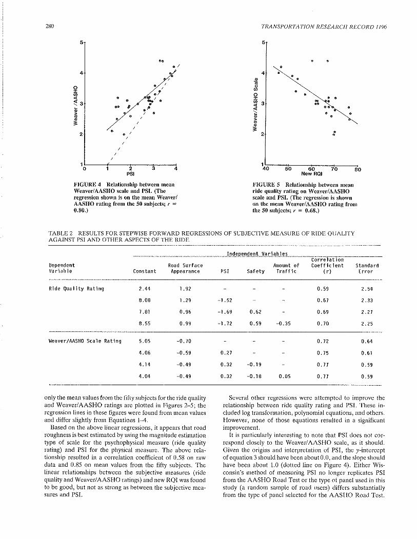
280 TRANSPORTATION RESEARCI.I RECORD I 196

FIGURE 5 Relationship between meanride quality rafing on Weaver/AASHOscale and PSI. (The regression is shorvnon the mean Weaver/AASHO rating fromthe 50 subjects; r = 0.68.)

.go(,(t,

otq,

oo(¡,

3

FIGURE 4 Relationship between meanWeaver/AASHO scale and PSI. (Theregression shown is on the mean Weaver/AASHO rating from the 50 subjects; r =0.80.)

TABLE 2 RESULTS FOR STEPWISE FORWARD REGRESSIONS OF SUBJECTIVE MEASURE OF RIDE QUALITYAGAINST PSI AND OTHER ASPECTS OF THE RIDE

CorreìatlonDependentVa ri abl e

Road SurfaceConstant Appearance PSI

Amount ofSafety Trafflc

Coefficlent(r)

Standa rdt rror

Rtde Quaìity Ratlns 2.44

8.08

7.81

8.55

I .92

| .?9

0.96

0.99

-t .52

-l .69

-l .72

0. 62

0. 59 -0. 35

0. 59

0.67

0.69

0. 70

2.54

2.33

2.21

2.25

Heaver/^^SHO Scale Ratlng 5 .05

4.06

4.14

4.04

-0. 70

-0. 59

-0. 49

-0.49

0.21

0 .32

0. 32

-0.19

-0.t8 0.0s

0.72

0.75

0.77

0.77

0. 64

0.6l

0.59

0. s9

only the mean values from the fifty subjects for the ride qualityand Weaver/AASHO ratings are plotted in Figures 2-5; theregression lines in these figures were found from mean valuesand differ slightly from Equations 1-4.

Based on the above linear regressions, it appears that roadroughness is best estimated by using the magnitude estimationtype of scale for the psychophysical measure (ride qualityrating) and PSI for the physical measure. The above rela-tionship resulted in a correlation coefficient of 0.58 on rawdata and 0.85 on mean values from the fifty subjects. Thelinear relationships between the subjective measures (ridequality and Weaver/AASHO ratings) and new RQI was foundto be good, but not as strong as between the subjective mea-sures and PSI.

Several other regressions were attempted to improve therelationship between ride quality rating and PSI. These in-cluded log transformation, polynomial equations, and others.However, none of those equations resulted in a significantimprovement.

It is particularly interesting to note that PSI does not cor-respond closely to the Weaver/AASHO scale, as it should.Given the origins and interpretation of PSI, the y-interceptof equation 3 should have been about 0.0, and the slope shouldhave been about 1.0 (dotted line on Figure 4). Either Wis-consin's method of measuring PSI no longer replicates PSIfrom the AASHO Road Test or the type oi panel used in thisstudy (a random sample of road users) differs substantiallyfrom the type of panel selected for the AASHO Road Test.

Garg et al.

On balance, subjects were fat'less willing than the Wisconsinl'oadmeter to rate a road as "poor."

Since appearance of the road surface, scenery, amount oftraffic, safety of the road, and importance of the road had

significant correlations with the subjective road roughness

ratings, forward stepwise linear regressions were performedbetween the subjective measures, these variables, and PSI.

A level of significance of 0.01 was used for inclusion of an

independent variable. The resulting regression equations aregiven in Table 2. It is clear from Table 2 that appearance ofthe road surface has a strong effect on the ride quality ratingand an even stronger effect on the Weaver/AASHO scale

rating. Road surface appearance and PSI explain 45 percentand 56 percent of the variation in ride quality rating and

Weaver/AASFIO rating, respectively. Thus, while PSI isimportant in determining subjective measures of ride quality,appearance of the road surface plays an equally importantrole.

The effect of road surface appearance on ride quality ratingsis readily seen in Figure 2. There are three cornparative seg-

ments that received particularly favorable ride quality ratings(about 3.0) but had PSI values of less than 4. These segments

deviate substantially from the regression line. All three seg-

ments had new surfaces (two portland cement and one bitu-minous concrete) at the time of the experiment. There wereno cracks, patches, discoloration, or any other evidence ofdeterioration. Objectively, howevet, there was some rough-ness to the surface.

The ride quality ratings show that subjects were significantlyinfluenced by the excellent appearance of the road. The effectof appearance is even more pronounced when the ride qualityrating is comparecl with new RQI (Figure 3).

Acceptability Measures

A series of linear regressions was performed to relate physical

measures of road roughness to acceptability measures (forexample, "money should be allocated"). Those regressionsincluded a number of subject background variables such as

seating comfort, use of seat belts, helpful road signs, per-centage of miles driven on highways, privacy in vehicle, years

of formal education, sex, weather, lack of construction, etc.

However, the contribution of a single background variablewas very small, and the number of variables was very large.By and large, little was learned from these regressions beyondthe information contained in Table 1. That is, both PSI and

new RQI are strongly related to the acceptability measures,with PSI providing a somewhat better fit. The fit could notbe substantially improved by inclusion of information aboutthe subjects' backgrounds. This result is important because itmeans that the results of this study (and similar studies) are

likely to be insensitive to the location from which the sample

is drawn.

Terminal Roughness

The major objective of this study was the determination of aterminal roughness, in other words, a value of PSI, that causes

a predictable percentage of drivers to become dissatisfied withthe road surface. In the past, this dissatisfaction has been

281

measured by asking the subjects to answer yes or no to a

question about spending tax dollars to improve the ride qualityof a given road. Some studies have used a third category ofundecided. In this study, however, a Likert scale ranging from1 (strongly agree) to 5 (strongly disagree) was used.

It is first necessary to establish a single criterion for dis-

satisfaction; in other words, which value on the Likert scale

should be used to represent the "money-should-be-allocated"level of dissatisfaction with road roughness. For example, thevalue can range from 1 (strong agreement with the statementthat "money should be allocated") to 3 (neutral point). Ide-ally, the cutoff value for "money should be allocated" shoulddepend upon several factors, such as percentage of driversdissatisfied, class of road (freeway versus local road), volumeof traffic served, importance of the road to the travellingpublic, resources available, and so on. For the following dis-

cussion the criterion for dissatisfaction is set at 2.5. A valueof 3.0 must be interpreted as ambivalent, and a value of 2.0

is too strict, considering the likelihood of central tendency inthe scale. A value of 2.5 can be interpreted as being in slightto moderate agreement with the idea of spending money toresurface the road.

The percentage of subjects with a rating of.2.5 or less for"money should be allocated" is plotted against PSI in Fig-ure 6. The linear correlation coefficient between the per-centage of subjects and PSI was 0.89. In addition to a linearregression, curvilinear regressions were also tried. The linearregression resulted in a slightly better fit. The following equa-

tions can be used to estimate percent dissatisfied (PD) fromPSI for a value of 2.5 for "money should be allocated."

PD = 72.49 - 19.74 PSI

(r : 0.89, SE = 8.2) (5)

PD=-19.81 +95.48/PSI

(r = 0.87, SE = 8.7) (6)

Equation 6 is recommended for determining the relation-ship between PSI and the percent of dissatisfied subjects.Equation 6 is recommended over equation 5 only because

FIGURE 6 Relationship betweenpercentage of subjects dissatislied withride quality based on a rating of 2.5 orless for "rnoney should be allocated"and PSI.

282 TRA NS PO RTA'N O N R ES EARCH R ECO R D I 1 96

TABLE 3 PSIs AS A FUNCTION OF PERCENTAGE OF RATERS DISSATISFIEDAND LEVEL OF DISSATISFACTION

Percent of Raters PSIDissatisfied

Í 2.5

50

45

40

35

30

25

20

t.36

1 ,47

r.60

I .74

I .9t

2.t3

2. 39

it appears to fit better at lower values of PSI (between 1

and 2).If desired, terminal roughness can easily be determined for

any percentage of subjects dissatisfied from the graph, fromEquations 5 and 6, or from Table 3. For example, the terminalroughness is 1.36 (PSI) for 50 percent of the Wisconsin driversto be dissatisfied (as estimated by a value of 2.5 or less onthe scale used for "money should be allocated"). This terminalroughness is considerably lower than those currently used bythe Wisconsin DOT (2.0 to 2.5).

Willingness To Spend Extra Time

Subjects were asked to estimate the amount of time theywould be willing to spend to avoid each segment, assumingthey were to make a 50-min trip. The results are summarizedin Figure 7. In addition, extra time may be computed fromthe following:

Extra time = 8.68 - 2.13 PSI

(r = 0.32, SE : 4.85) (7)

It is seen that the amount of extra time is small, but significant.For example, Equation 7 shows that subjects were willing to

PSI

FIGURE 7 Relationship betrveen extratime, in minutes, for a 50 min road tripand PSI.

spend 5.5 minutes (or 11 percent) more time to avoid a roadwith a PSI of 1.5.

These extra-time evaluations are analogous to time savingsbenefits. They can be converted to monetary units by usingaccepted values of time. Knowing the traffic volumes andspeeds on a road, and the rate of pavement deterioration, itwould be possible to compute total benefits of a new surfaceand to compare them with project costs.

CONCLUSIONS

Analysis of subjects' evaluations of ride quality leads to thefollowing conclusions.

A number of subjects' personal and background variableshad statistically significant effects on both the subjective mea-sures ofroad roughness and the acceptability ¡neasures. How-ever, these variables were found not to be of practical sig-nificance as they explained very little variation in either roadroughness or acceptability measures. This suggests that theresults of this study are generalizable; that is, they are notdependent on the location from which the sample is drawn.

Even though magnitude estimation is most easily accom-plished in a laboratory, it is possible to successfully use thistechnique for measuring ride quality.

PSI has a higher correlation with the rnagnitude estimationscale (ride quality rating) than with the Weaver/AASHO scale.The magnitude estimation scale appears to have a greaterpower of discrimination between various roads, and it is lessinfluenced by road surface appearance. Magnitude estimationis the preferred method of rneasuring subjective ride quality.

The best physical measure of road roughness appears to bePSI. PSI has the highest correlations with both the ride qualityrating and the Weaver/AASHO scale. In a completely hands-off comparison, the less expensive roadmeter was found tobe superior to the profilometer in predicting both subjectiveroad roughness and the acceptability of the road. However,both instruments failed to relate with subjective measures ofride quality for those segments judged to be very good by thesubjects.

Appearance of the road surface is extremely important tosubjects rating ride quality.

oo

.s

=oEi:(ú

xu.t

Gurg ct ul.

People are willing to spend approximately 1l percent (5.5minutes on a 50-min load trip) mol'e time to take a betterride quality road and avoid a road with PSI of 1.5. This rep-l'esents a significant t'esource expenditure. It is recommendedthat such time savings benefits be incorporated into evalt¡a-tions of road resurfacing plans.

PSI, as measured in Wisconsin, does not closely ap-proximate the We¿rver/AASHO scale. There can be twoexplanations:

1. The measurement of PSI has sornehow changed since itwas first established, or

2. The subjects in this experiment differ considerably fromthe subjects in the AASHO Road Test.

If the latter explanation is true, then it is likely that PSI,regardless of where it is currently being measured, is notproperly reflective of the opinions of roacl users.

A panel can provide detailed information about the needfor road resurfacing. In order to properly use this inforrnation,it is necessary to establish both a criterion level of dissatis-faction and a percentage of roacl users who would be sodissatisfied.

ACKNOWI,EDGMENTS

A number of people contributed both tirne and effort to bringthis study to completion. The authors are grateful to KarlDunn and his staff at WisDOT for their encoulagement, sug-gestions, cooperation, ancl assistance. A special note ofthanksis extended to the subjects without whose enthusiasm andcoopelation this project woulcl never have been cornpleted.

Professor Edward Beirnborn provided advice and encour-agement. Professor Urnesh Saxena macle valuable suggestionsin the statistical design and analysis of the experimental clata.

We are also appreciative of the efforts of the staffs of theHuman Perforrnance Labot'atory and the Center for UrbanTransportation Studies of the University of Wisconsin at Mil-waukee, among them: David Sincere and Richard Clark whocollected, coded, and stored the data in the computer; RanclalZakowski who provided graphical illustrations; and Tar.unGupta who performed all statistical analyses.

REFERENCES

l. L. F. Holbrook. Precliction of Subjective Response to RoadRoughness by Use of the Rapid Travet Plofilometer. ln Iligh-way Research Record ó9, HRB, National Research Council,Washington, D.C., 1969, pp. 21,2-226.

2. S. Mohan. Development of a System for the Evaluation ofPavements in Indiana. Joint Highway Research ProjectNo. C-36-63-G, Puldue University, Incl., 1978.

3. S. K. Nair and W. R. Hudson. Serviceability Prediction frornUser-Based Evaluations of Pavenrent Ride Quality. Presentedat the 65th Annual Meeting of the Transportation ResearchBoard, Washirrgton, D.C., 1986.

4. W. R. Hudson. Roacl Roughness: Its Elements and Measure-¡nents. In Transportation Research Record 836 ,TRB, NationalResearch Council, Washington, D.C., 1981, pp. l-7.

5. B. G. Hutchinson. Principles of Subjective Rating Scale Con-struction. ln Highway Research Record 4ó, HRB, NationalResearch Council, Washington, D.C., l9ó4, pp. 60-70.

283

6. M. S. Janoff and J. B. Nick. Evaluation and Quantifying UserPerceptiott of Pavement Serviceability. Report for Pennsylva-nia Departrnent of Transportation, Pennsytvania, 1983.

7. W. N. Carey and P. E. Irick. The Pavement ServiceabilityPerfor¡nance Concept. Bulletin 250, HRB, National ResearchCouncil, Washington, D.C., 19ó0, pp 40-50.

8. S. S. Stevens. On the Opelation Known as Juclgement. Arrer-ican Scientist. Vol. 54, 1966, pp. 385-401.

DISCUSSION

MrcHepl S. JeNoprJMJ Research, P.O. Box 144, Newtown, Pa. 18940.

This is a well written paper that presents potentially valuableinforrnation. However, because of some omissions, misinter-pretations, and possible mistakes, the results are not readilyapplicable. The authors have not considered the results ofrecent work by NCHRP ancl by Ohio DOT and have incor-rectly interpreted a number of their references.

1. The authors state that little infolmation is available todefine the relationship between ride quality and roughness.This is false. Studies conducted in Texas, Ohio, Louisiana,New Mexico, Michigan, New Jersey, and Pennsylvania definesuch relationships quite well (1-5). The data from Ohio, NewJersey, Michigan, New Mexico, and Louisiana also reveal thatthe relationship between roughness measured with a profi-lometer ancl subjective ratings of ride quality are nearly iden-tical for each of the five different states.

2. Perhaps the greatest problern in this paper. is the rela-tively poor correlations that the authors have found betweenphysical measures of pavernent roughness and subjective ridequality ratings. For profile-derived roughness measures theauthors have found correlations of at most .7 with (rnean)ride quality ratings, which are far lower than the col.relationsfound between profile measures of roughness and ride qualityratings in Ohio, New Jersey, Michigan, New Mexico, Loui-siana, and Texas. For four different models of profile-derivedroughness used in these other states, correlations between theroughness and ride quality ratings were always in excess of.9, and for the data from five states combined they were betterthan .93. A numbel' of explanations for the authors' low cor-relations can be suggested.

First, the instru¡nent used to collect profiles was the olderone-wheelpath unit of Michigan DOT, which is not as accuratein measuring profiles as the more common two-wheelpathvelsions used in the states mentioned above. Although theprofile frorn one wheelpath can be accurately used to predictrideability (3) the instrument used to collect this one-wheel-path profile must provide accurate data; it is suspected thatthe instrument used by \{isconsin DOT was not. In testsconducted as part of the NCHRP research (3, ó) the olderone-wheelpath profilometer yieldecl correlations between RQIand ride quality of .85, while for the two-wheelpath profilo-metel these correlations between RQI and ride quality rosero .93.

Second, the magnitude estimation scale, which the authorsbelieve is preferred to the similar interval scale, may not beyielding accurate and consistent rating data. As the authorspoint out, magnitude estimation is best suited to laboratory

284

research where the "standard" level can be presented to thetest subjects along with each test condition. Was this scale

pretested in any way to determine if it was suitable for such

ratings of ride quality? (It appears that the raw rating dataobtained with the magnitude estimation scale, as illustratedin their final report, appeared to have rather high ratervariability, indicating a lack of consistency in the ratingprocedure.)

Both Flolbrook (7) and Janoff and Nick (5) have shownthat the choice of rating scale has no effect on the quality ofthe subjective ratings. The analysis by Hutchinson that theauthors use to support their selection of the magnitude esti-mation scale as the preferred one was shown to be unimpor-tant in panel ratings of ride quality (5). Although I believethat Hutchinson is correct in theory, in application driverscan use almost any scale to accurately and consistently rateride quality, as demonstrated by Holbrook and by Janoff andNick.

The instructions to the raters could also have had a signif-icant effect on the quality of the ride quality ratings. In thepast research for Pennsylvania DOT (5) three different ratingscales were tested, and it was disclosed that with properinstructions to the raters either one could be used to deriveaccurate and consistent ratings of ride quality. This same resultwas also found by Holbrook. Did the authors test their instruc-tions in any way?

The authors' finding that surface appearance is affectingthe ratings of ride quality may also be a result of the instruc-tions; Holbrook showed that the use of blindfolds had noeffect on such subjective ratings, hence with proper instruc-tions appearance should have no effect on ride quality (7).

3. PSI is not a physical measure of roughness but a valuederived from a regression equation that relates a physicalmeasure of roughness (typically an RTRRMS inclex) with a

subjective rating of ride quality (such as mean panel ratingsor PSR). That the authors found a correlation of .35 betweentheir magnitude estimation scale and PSI and a correlationcoefficient of .9 between PSI and the Weaver/AASHO ratingis not unexpected. When RTRRMS data from New Jersey,Ohio, and Louisiana were compared to ride quality ratings a

correlation of .79 was found for the Weaver/AASHO scale,almost identical to the authors' results. Unless the surfacesare separately analyzed for each type (BC, PCC, composite)no better results can be expected.

The problem is that RTRRMS instruments do not provideroughness data that are highly correlated with ride qualityratings except for BC surfaces.(actually such instruments failto respond to all of the roughness frequencies present in PCCor composite surfaces). On surfaces other than BC, and whenthe range of ride quality is great, the correlations fall to verylow values. The authors should have analyzed the surfacetypes individually to disclose the effect of surface type on thecorrelations.

The authors' conclusion that PSI, therefore, no longerapproximates the Weaver/AASHO scale is conjecture only.A better explanation is that when RTRRMS are used, cor-relations of .8 to .85 are typical; to increase the correlationit is necessary to use profiles to measure roughness.

4. The Weaver/AASHO scale used bi, the authors (and

illustrated in their final report) is not the same scale that was

used by either Carey and Irick (8), Weaver (9), Janoff and

TRANSPORTA'ilON RESEARCI-I IìECOIì,D I 196

Nick (5), or NCHRP (2,3); it is a cornpletely different typeof scale. The Weaver/AASHO scale is a vertical line, typically5-in long, with major subdivisions at 1-in intervals (labelled0,'1,2,3, 4, and 5) and minor subdivisions at 7z-in pointslabelled "very poor" (at Vz-in) "poor" (at 1,Yz-in), "fair" (at2t/z-in), "good" (at3%-in), "very good" (at4%-in), "perfect"(at the top) and "impassable" (at the bottom). The authors'scale includes the word and number cues but not the verticalline. In addition, the instructions to the raters used by theauthors do not explain how to even mark this scale. In pastuses of the Weaver/AASHO scale the raters were told to placea horizontal rnark across the scale (in other words, across thevertical line) at the point that they feel best describes the ridequality ofthe test section. It appears that on the authors'scalethe subject is instead placing a mark into one of the categoriesdefined by the 7z-in divisions. This is completely differentfrom past applications and hence the data (that the authorsrefer to as Weaver/AASHO ratings) may be incomparable topast applications of this scale.

5. The authors use a five-point Likert scale instead of a

two-point yes versus no rating to indicate need for improve-ment, claiming that such a scale is better for the intended use.

Again no pretest or pilot results are shown, and it is suspectedthat the results may suffer the same problems as those relatedto the magnitude estimation scale.

6. In summary, the authors conclude that magnitude esti-mation is the preferred rating plocedure and that PSI (oractually RTRRMS indexes) are preferred to profile-derivedroughness for predicting ride quality. The opinion of this writeris that these conclusions are unsupported. The correlationsbetween the roughness and rating data are too low in com-parison to other recent ride quality research to draw such

conclusions and the authors' lack of attention to and misin-telpretation of past research sheds serious doubts on the valid-ity of their results.

REFERENCES

1. K. N. Sukumar and W. R. Hudson. Serviceability Predictionfrom User-Basecl Evaluations of Pavement Ride Quality. InTransportation Research Record I 084,'fR.B, National ResearchCouncil, Washington, D.C., 1986.

2. M. S. Janoff et al. Pavement Roughness and Rideaóilþ. NCHRPReport 275,1985.

3. M. S. Janolf. Pavement Roughness and Rideability FieldExperiment. NCHRP Project 1-23(2), Final Report, Dec. 1987.

4. J. McQuirk and E. Spangler. Use of the Inertial Profilometerin the Ohio DOT Pavement Management Syslen. ASTM Com-mittee E-17 Symposiurn, Columbus, Ohio, June 1985.

5. M. S. Janoff and J. B. Nick. Evaluating and Quantifying UserPerception of Pavement Serviceability. Penn-DOT, 1983.

6. M. S. Janoff. Quarterly Report on NCHRP Project l-23(2).Dec. 1986.

7. L. F. Holbrook. Prediction of Subjective Response to RoadRoughness by Use of the Rapid Travel Profilometer. In Éligå-way Research Recorcl ó9, HRB, National Research Council,Washington, D.C., 1963.

8. W. N. Carey and P. E. Irick. The Pavement ServiceabilityPerfor¡nance Concept. ln Highway Research Record 250, HRB,National Research Council, Washington, D.C., l9ó8.

9. R. J. Weaver. Quantífying Pavement Serviceability as It IsJudged by Hig,hway Useis. NYSDOT, 1978.

Carg el al.

AUTHORS'CLOSURE

The basis of Mr. Janoff's criticism is that our results are indisagreement with his own work. Such criticism is a two-edgedsword; it can raise doubts about the validity of Mr. Janoff'searlier efforts in measuring ride quality. Indeed, the principalreason for our conducting a ride quality experiment was dis-appointment with the experimental design of the NCHRPstudy to which Mr. Janoff refers. We chose not to make anissue of Mr. Janoff's work in our paper. However, we wereparticularly disturbed by the subject selection procedures,instructions to subjects, the way stimuli were presented, andthe rating scales in the NCHRP study. That the results of thetwo studies are different is unremarkable; we attempted tocorrect problems in the NCHRP study design that we believecould have skewed the results.

We believe the low correlations between subjective mea-sures of ride quality and physical measures of ride qualitystem from the "hands-off" nature of our study design. Wechose to take physical measures from other sources so thattheir transferability could be evaluated. The physical measurefrom the response-type instrument (PSI in our case) behavedas expected. The performance of the profilometer (new RQI)was much poorer than expected. Based on ¡nany earlier stud-ies (including Mr. Janoff's) we do ¡rot feel that the problemstemmed from the quality of either equipment or data anal-ysis. One-wheelpath profilometers have served quite nicelyin the past. Instead, it appears that cornplex transforrnationsof profilometer data are not applicable when there are sig-nificant variations in study design (for example, location, sub-ject selection, or stimuli presentation). A major lesson ofthese comparisons is that engineers cannot take any physicalmeasure of ride quality at face value; they must fully under-stand the conditions under which panel data were assembled.

Magnitude estimation is one of the most respected psycho-physical measurement techniques. Its use in ride quality mea-surement has been suggested by many authors, and an abbre-

285

viated version was tried by Holbrook with very encouragingresults. Mr. Janoff has seriously misrepresented Holbrook'sconclusions. Holbrook states, "'lhe equations predicting ridefrom physical input by means of magnitude estimation are tobe preferred" (Janoff's reference 7 , page 255). A magnitudeestimation scale is quite different from any of the three cat-egorical scales tested by Janoff and Nick. Their conclusionsare not relevant.

Our experience indicates Hutchinson's criticism of theWeaver/AASHO scale is correct in practice as well as in the-ory. It is unfortunate that Mr. Janoff decided to disregardHutchinson's advice.

We found intersubject variability to be about the same formagnitude estimation and for the Weave¡/AASHO scales. Wedid not address this issue in our paper because it is uninter-esting. Mr. Janoff's erred during his casual inspection of sum-mary data from our full report.

PSI is a physical measure of ride quality; its peculiar his-torical origins cannot alter the fact that only mechanical dataare used to cornpute it.

Our conclusion that Wisconsin's PSI no longer approxi-¡nates the V/eaver/AASHO scale is based on Figure 4 in ourpaper. Regardless ofsurface type, the regression line is plainlyat the wrong angle.

Mr. Janoff has apparently received incorrect informationabout our depiction of the Weaver/AASHO scale. It waspurposefully identical to the one used in his NCHRP study.In regard to another scaling issue, we are perplexed why Mr.Janoff believes an ad hoc 2-point scale of acceptability isinherently superior to a Likert scale-a standard tool ofpsychometrics.

We appreciate Mr. Janoff's interest in our research. How-ever, we do not feel that his discussion is helpful for eitherunderstanding or extending our work.

Publication of this paper sponsored by Committee on SurfaceP r op e r t ies-V e h ic Ie I nte ract io n.

286.I'

R A N S P O R'I' A7' I O N II F,S EA RC I I II EC O II D I I 96

Use of the Inertial Profilometer To CalibrateKentucky Department of HighwaysMays Ride Meter Systems

Ersou B. SreNcrnn, RoTANDS L. RIzrN¡ERGS, Jauns L. BuncuETT, ANDDoNaro C. Ro¡rNsoN

The National Bureau of Standards (NIIS), the Commonwealthof Kentucky Department of Highways (DOH), and SurfaceDynamics, Inc. joined in a project in the Colnrnonwealth ofKentucky to calibrate five Kentucky DOH vehicle-mountedMays Ride Meter (MRM) systems. In this project, an NBS-operated inertial profilometer system was used to measure theelevation profiles of selected pavement test sections. The mea-sured elevation profiles were used to compute the StandardMays Ritle Meter Index (SMRMI) values for each pavementtest section. The computed SMRMI values rvere then uscd as

reference values for the calibration of the actual KentuckyDOH MRM systems. The profilomctcr was used to identifysuitable pavement sections from test sites selected by the Ken-tucky DOH using an MRM systern. The site selection processincluded sr¡ffïcient repeat runs fo estal¡lish a meân SMRMIvalue for each ¡ravernent and a standard deviation from thatmean for thc repeat runs. Six pavement test sites with thedesired SMRMI values and lorv standard deviations rvereselected. Thc I'ive Kentucky DOH MRM systems rvcre thelrdriven over the selected test sites a number of tinres to deter-mine a mean rneasured value and a starrdard deviation abo¡ltthat ¡neasured mean value for each systetn on each pavementtest site. The test data frorn the profilorneter antl the fÏveKentucky DOH MRM systems rvere used to develop a cali-bration equation and expected standard deviation for each ofthe MRM systems. The resulfing calibration equations will beused by the Kentucky DOH to compute SMRMI vah¡es foreach system. Included in thc project was a correlation of theOhio Department of Transportation inertial profilometer withthe NBS-operated inertial profilometer to establish the validityof using another identically constructed inertial profilometerfor the same calibration procedure.

The inertial plofilorneter was developed in the early 1960s byElson Spangler and William Kelly at the General MotorsResearch Laboratory in Warren, Michigan. The profilonreter'was designed to be a research tool that woulcl allow pavementprofiles to be brought into the laboratory for use as computerinput data for vehicle suspension stuclies. The first presen-

tation of the inertial profilorneter was made by Spangler andKelly (1) at the Transportation Research Board Annual Meet-

E. B. Spangler, Surface Dynanics, Inc., 800 West Long LakeRoad, Suite 145, Bloomfield Hills, Mich., 48013. R. L. Rizen-bergs ancl J. L. Ilurchett, Kentucky Department of Highways,Roo¡n 701, Clinton and High Streets, Frankfort, Ky.40622. D.C. Robinson, National Bureau of Stanclarcls, Acoustics Mea-suring Group, Gaithersburg, Md. 20899.

ing in Washington, D.C., in 1965. Through the efforts of theGeneral Motors Corporation, the technology associated withthe inertial profilometer has been made available for use inthe highway testing comrnunity. Early inertial profilorneterirnplementations were used by Michigan (2), Pennsylvania,Kentucky (3), and Texas (4) and by Brazil as part of a WorlclBank project. Mol'e recent irnplernentations are in use in fivestates including Texas, West Virginia, Minnesota, Michigan,and Ohio and in Chile, as part of a Worlcl Bank ploject.

INTRODUCTION

The most recent irnplcrne¡rtation is an inertial plofilometerpurchased by the Fecleral Highway Administration (FtlWA)from K. J. Law Engincers, Inc., and was being evaluated bythe National Bureau of Standards (NBS) foL the FHWA dur'-ing the work reported in this paper. In May 1987, the NBS,the Comnronwealth of Kentucky Department of Iligltways(DOfl), the Ohio Departrnent of Transportation (DOT) andSurface Dynarnics, Inc. joined in a projcct in the Common-wealth of Kentucky to calibrate five Kentucky DOII vehicle-nrounted MRM systerns using an NBS-operated inertial pro-filonleter to perform this calibratiort. Fourtcen pavement testsections in the vicinity of Frankfort, Kentucky, were selectedas candidate sites for the calibration of Kentucky DOH MRMsystems. Seven of the pavement test sections wel'e portlanclcemcnt concrete ancl seven wele bituminous concrete.

PRO¡'ILOMBTBR MBASURBMENTS ANDANAI,YSIS

The elevation profiles of all the p¿ìveÍnerìt test sections weremeasured with an NBS-opelated ineltial profilometer mul-tiple times to evaluate the precision of the measuring rnethod.After the nrultiple measurer¡ìents of the elevation profilcs ofthe foul'teen paverìrer)t test sections, a SMRMI value was

conrputecl for each test section.The SMRMI value is a computecl output of a coluputet'

sinrulation of an MRM systern including the vehicle a¡rcl theMRM measuring instrument. The MRM vehicle parameters("Golden Car") used in the computer sirnulation are tlloseproposed in NCHRP Project l-18 (5), which are being definedfurther in a new proposed ASTM standard. The inputs to thecomputer simulation are the elevation profile rneasurentents

Kentucky Numbe! ofDOH lest Repeat

Spangler et al.

TABLE 1 INERTIAL PROFILOMETER MEASUREMENTS

287

six pavement test sites were chosen because they representeda range of desired SMRMI values and because they exhibitedlow standard deviations. Although there is a wide range ofstandard deviations for each test site, it is important to notethat the six calibration test pavements selected exhibited abouta L percent maximum standard deviation.

Test site 201, a smooth bituminous concrete pavement, wasthe site where the precision or repeatability of the NBS-oper-ated profilometer was evaluated in detail. Twenty test runswere conducted on this particular site. The results of twentytests runs are shown in Figure 1 as a plot of the computedSMRMI value (inches/mile) for each of the twenty runs. Thevariation in the computed SMRMI values can be attributedto three factors:

. Variation in the profilometer's elevation profile mea-suring performance,

o Variation in the path driven by the profilometer driver,and

. Transverse variations in the elevation profile of the testsite pavement.

It is suggested that a test site \l,ith little variation in com-puted SMRMI values (low standard deviation) would be atest site with little transverse variation in the elevation profile,and the computed SMRMI values would be less affected bythe path driven by the profilometer driver.

The computed cumulative mean SMRMI value (inches/mile)is shown in Figure 2 as a function of the number of test runsincluded in the computation. As would be expected, the com-puted mean becomes more stable as the number of includedtests runs increases. The cornputed standard deviation of thecomputed SMRMI values (inches/mile) as a function ofthe number of test runs is shown in Figure 3. Again, as wouldbe expected, the standard deviation is reduced as the nurnberof runs increases. Although some improvement is still occur-ring at test run twenty, the majority of the improvement hasoccurred by run ten and on the less variable sites, mea-suring stability appears possible with five test runs with theprofilometer.

Standardll€an l{Rll

StandardD€vlation

Site No. t¡teasurements Index Value_ lin/¡ni) (in/ni)

PCC

101t102103104 r10 5rr06107

75.082 .4

100.5103.014{.1151.4160.7

47 .l{9.463.35?.583.5

111. ¡¡

133.9

0.342.520.820.571.381.5?2.7L

0.560.450 .42I .040.93I .031 .38

9565955

BC

201 20202. 5203 5204 6205 52L6' l0207* 6

made with the inertial profilometer. Using this computer sim-ulation, the SMRMI value was computed for each of themultiple profile measurements. The computed mean SMRMIvalue and standard deviation for the multiple measurementsfor each of the fourteen Kentucky DOH test sites are shownin Table 1.

Although readings were taken every 0.1 mile, it was foundthat averaging readings over a longer test section improvedthe precision of SMRMI values computed from the profilo-meter measurements. It was determined that the precision ofthe measurements improved significantly as the length of thetest section was increased from 0.1 mile to 0.5 mile and con-tinued to improve as the test section length was increased toone mile. Where possible, all measurements were made overa test section length of one mile.

The asterisks beside the test site numbers in Table I indicatethe final six test pavements selected for the calibration study.Three of those sites were constructed with portland cementand the other three with bituminous concrete pavement. These

.:E

osoc

xt¡JôzÉ.L¡J

hUJoÉ.

U).<

ôÉ.

ôztsØ

48

47.5

47

46.5

46

45.5

RUN NUMBER

FIGURE I Conrputed standard MRM index value by run numl¡er.

1816141210

o o

o oo a

aoaO

'ooO'Ooo

o

22 24

288

RUN NUMBER

FIGURE 2 Computed mean standard MRM index value by run number.

TRANSPORTATION RESEARCH RECORD I 196

vehicle 2678 had a mean MRM index value of 136.2 inches/mile on test site No. 105 while vehicle 3664 had a mean MRMindex value of 184.8 inches/mile for the same site. Since theSMRMI value as established by the NBS inertial profilometerwas 144.1 inches/mile, vehicle 2678 was measuring 5 percenttoo low, and vehicle 3664 was measuring 28 percent too high.The measurements shown in Table 2 clearly show the problemassociated with using uncalibrated MRM measurements andemphasizes the need for good MRM calibration procedures.

The computed SMRMI values from the inertial profilo-meter were then used with the computed mean MRM indexvalue for each Kentucky DOH MRM system to compute theleast-squares best fit straight line relationship between thetwo data sets. This relationship is shown graphically in Fig-ure 4 for Kentucky DOH MRM vehicle No. 2678. For thedata set shown in Figure 4, we can compute the slope and y-

3ci 48.5øa)soci7 48Xt¡lôz¿É,

oã47ôztsu> 46.5zt946F5l

= 4s.s

o

o

o taaooo¡ooaaotooao

1 2 3 4 5 6 7 I I 10111213 141516171819202122232425

É.

ÕÉ.

ozf^'u,, oo'Ët¡J \lølo(L!>oo.:uEô -ì'o>E><k tiJ

ûzÕoÉ.

Õzts(n

ttaataolooooaaoooa

a

1 2 3 4 5 6 7 8 9 10111213 ',141516171819202122232425RUN NUMBER

FIGURE 3 Standard deviation of the mean standard MRM index value by run number.

Simultaneous to measuring the Kentucky DOH test sites

with the inertial profilometer, the five Kentucky DOH MRMvehicles were used to obtain MRM index values for each ofthe six test sites. Each of the test sites was measured at least

ten times by each Kentucky DOH MRM system. The repeatmeasurements were made to compute a mean MRM indexvalue and standard deviation about the mean for each MRMsystem for each test site. The computed mean MRM indexvalue (x) and standard deviation (o) in inches/mile foreach Kentucky DOH MRM system for each of the six Ken-tucky DOH test sites are shown in Table 2. Also shown inTable 2 are the computed SMRMI values (from Table 1)

computed from elevation profile measured with the inertialprofilometer.

The MRM index values in Table 2 show a wide range values

for the different MRM vehicles. For example, Kentucky DOH

Spangler et al. 289

¡(entucky Standard* l{ean {B{ Index Valug.(i) and Standaf4,Devtatlon 6) bv Kentuckv DOH Vehtcle No.DOH Test ¡lean !flU{ 2678 3664 _Slte llo. Index Value

TABLE 2 MEAN MAYS RIDE METER INDEX VALUES FOR KENTUCKY DOH MRM SYSTEMS

PCC

l0l

104

¡05

7 5.0

103.0

r44. I

70.3 3.98 98.3 2.83

98.1 4,22 139.3 t.44

136,2 4.25 t84.8 2.59

40.ó 3.14 69,2 4.5t

108.4 4,95 143,0 6.61

128.0 2,84 t63.0 3.53

72,9 r.47

t08.9 2,45

154. I 2,42

41.0 2.18

115.5 3.36

I 39. 6 3.77

76.2 0.85 77.7 2.78

t07.8 t.ó4 t04.1 3.19

150.3 t.73 t42.4 3.15

43.7 0.83 47.0 3.26

tot. r t.90 109.9 4.ót

127.4 2.34 t27.8 2.t4

BC

202

2t6

207

49.4

l¡t.4

133.9

Average Std. Dev. 3. 90 3. 58 3.32

* Conputed fron Proflloneter Meaaurenentt

(¡)

tØoso.€

l¡JfJ

xt¡lclzÉ.t¡J

hØIôÉ.ôzFØ

160

140

120

100

80

60

40

20

0

Ktr{Tr¡CXY DOH VEtCtE t¡O. 2678

std. MRM = 7.16 + .987 (2678 MRM)

Corr. (r) = 6.996

* PCC

oBc

o 20 40 60 80 100 120 140 160

ACTUAL MAYS MfrER TNDEX VALUE (inches/mite)

FIGURE 4 Calibration curve for Kentucky Mays Meter Vehicle No.2678.

intercept for the least-squares best fit line through the datapoints. The computed line slope and )-intercept can then beused to develop a transform or calibration equation betweenthe MRM Index values obtained with the Kentucky DOHMRM system and the SMRMI values computed from theinertial profilometer elevation profile measurements. The cal-ibration equation and the data set correlation coefficient (r)for Kentucky DOH MRM vehicle No. 2678 are shown inFigure 4.

Calibration equations and correlation coefficients for Ken-tucky DOH MRM vehicles Number 3664,3665, 4323, and

4325 were developed using the sa¡ne procedure shown in Fig-ure 4. The results for these four MRM systems are shown inFigures 5 through 8. The high correlation coefficients for thefive Kentucky DOH MRM systems is an indication that the"Golden Car" computer model used to compute the SMRMIvalues is an accurate representation of the actual MRM sys-tems. It is also an indication that the Kentucky DOH MRMsystems are in good condition and are functioning as expected.

The calibration equations for each of the five KentuckyDOH MRM systems are summarized in Table 3. Also shownin Table 3 are the average standard deviation for each of the

g 160tØ.3 140oc

r¡r 12Ol)> tooxtrlô280É.u960(t

É40oá20ôz'ln 0

* PCC

oBc

g 160E

i i4o().ç

; 120IS tooxl¡¡

2- BoÉ.UJb60U'l¿oôÈ. o^ôzáo

e 160E

E 140oc

; 120fJs 1ooXt¡J

280É.ulE60anì40ôÉ. t^ôzÉo

KE{nrcKY DO}l VE{C|.-E l,lo. gE64

Std. MRM = -8.47 + .857 (3664 MRM)

Corr. (r) = 0.995

20 40 60 80 100 120 140 160 180 200

ACTUAL MAYS ME-ÍER INDEX VALUE (inches,/mile)

Calibration curve for Kentucky Mays Meter Vehicle No.

KE{nrcKY DOft ì/ElCLE Mt. gE6õ

std. MRM = 13.57 + .847 (3665 MRM)

Corr. (r) = 0'999

o 20 40 60 B0 100 120 140 160

ACTUAL MAYS MFTER INDEX VALUE (inches/mile)

FIGURE 6 Calibration curve for Kentucky Mays Meter Vehicle No.3665.

KE{nffY DO}l VEICIE l{O. ¿1323

Std. MRM = 8.34 + .934 (4323 MRM)

Corr. (r) = o.985

FIGURE 74323.

20 40 60 B0 100 120 140 160

ACTUAL MAYS MEIER INDEX VALUE (inches/mile)

Calibration curve for Kentucky Mays Meter Vehicle No.

* Pcc

aBc

FIGURE 53664.

* PCC

oBC

Spangler et al. 29t

3 160E

i i4oo.c

; 120Js 1ooxt¡lôzB0É.trjh60UIà+oôx20ozS^'Øu

KEt{nrcKY DO}l VE{CLE 1,1O. 4{¡26

Std. MRM = -1.62 + 1.029 (4325 MRM)

Corr, (r) = o.997

o 20 40 60 B0 100 120 140 160

t< PCC

oBc

ACTUAL MAYS Mfl-ER INDEX VALUE (inches/mite)

FIGURE I Calibration curve for Kentucky Mays Meter Vehicle No. 4325.

TABLE 3 CALIBRATION EQUATIONS FOR KENTUCKY DOHMAYS RIDE METER VEHICLES

KentuckyDOH ¡IR¡|IVehicle No. Câlibratiôn Eduatiôns

2678 Ståndard URM - 7.16 + .987 (vehicle !lRl,l)

Àverage Std. Dev. - 3.90

3664 Standard l,lRl¡t = -8.47 + .837 (vehicle uru,l)

Àverage Std. Dev. - 3.58

3665 Standard MRM - 13.57 + ,847 (vehicle MRI|I)

Àverage std. Dev. = 2.61

4323 Standard ltRtt = 8.3{ + .934 (vehicle }tRü}

Average Std. Dev. - 1.55

4325 Standard t¡tRü = _1.62 - L.029 (vehicle üRM)

Àverage Std. Dev. - 3.32

five Kentucky DOH MRM systems (from Table 2). This aver- manufactured by K. J. Law Engineers, Inc., and to determineage standard deviation is probably the best that might be if equivalent MRM calibrations can be obtained from twoexpected for each system, since these values were computed identical inertial profilometers.for pavement test sites that were initially selected for their The measuring results for the NBS and Ohio DOT profi-low standard deviations when measured with the inertial lo¡neters are shown in Table 4 for the seven Kentucky DOHprofilometer. test sites. The SMRMI values for each profilometer are plot-

ted in Figure 9 for each of the seven sites. Also shown inFigure 9 is the best fit straight line for the data point pairs,

PROFILOMETER CORRELATION and the y-intercept, slope, and the correlation coefficient (ffor the best fit straight line. The high correlation coefficient

Although the NBS-operated inertial profilometer was used to of 0.99934 would support the interchangeable use of identicalestablish the SMRMI values for the Kentucky DOH calibra- inertial profilometers for the calibration of MRM systems.tion test sites, a second K. J. Law Engineers, Inc., inertialprofilometer, owned and operated by the Ohio Departmentof Transportation, was used to measure and compute theSMRMI values for seven of the Kentucky DOH test sites used DISCUSSIONin the calibration project. This simultaneous measurement ofseven test sites provided an excellent opportunity to compare The calibration procedure developed in this project providesthe measuring performance of the two inertial profilometers a method that can be used to convert MRM measurements

292 TRANSPORTATION RESEARCH RECORD I 196

TABLE 4 COMPUTED STANDARD MAYS RIDE METER DATA

NentuckyDOH TestSite No.

NBS Profilometer Ohio DOT Profilometer

Nu¡nber 1of Runs in/¡ni

Nu¡nberof Runs

a1n/mi

ioin/mi in/mi

PCC

r01

102

105

BC

4

5

4

20

4

4

4

7

5

9

20

5

5

5

75.1 0.15

85.7 0. ¡¡9

l¡13.1 O.26

{7.1 0.79

48.6 0.39

63,7 0.23

84,7 I .32

75. 1 0. 35

82. I 0.78

t41 . I 0.78

201

202

203

205

46.8 0.60

49. { 0.44

64,7 0.60

83. s 0,92

9 160E

3 140coci:i 12O

É,

oÉÉ80zl-u' 60U)(nzô40UJl-e20=.ooo

KY SITE 20

KY SITE IO

KY SITE 102

KI SITE 201

r00 120 140 1 60

COMPUTED OHIO STANDARD MRM (inches/mile)

FIGURE 9 Correlation of identical inertial profilometers.

Slope = 0.97331

Y lntercept = 1.36056

Corr. (r) = 0.99934

4020

made with individual MRM systems into SMRMI values. The

experiences gained in developing calibratio¡l procedure sug-

gest the following recommendations related to the calibrationand use of MRM systems, in particular, and to response-type

ride meters, in general:

o Due to the higher standard deviation values for MRMsystems compared to the profilometer, measurements should

be made by averaging multiple repeat measurements for each

test site. Ten repeat measurements would be desirable.o One calibration site for each pavement type should be

used periodically to confirm the calibration of individual MRMsystems. The confirmation would consist of computing the

standard mean MRM index value for ten repeat measure-

ments at each site. A deviation from the expected SMRMIvalue would indicate a change in the system and the need forrecalibration.

o A change in the measuring characteristics of an individual

MRM system would indicate the need for a full calibrationon all calibration sites. As in the original calibration, the mean

of ten repeat measurements would be used with the SMRMIvalue to compute a new calibration equation and correlationcoefficient.

o A reduction in the correlation coefficient computed inthe recalibration process might be an indication that the SMRMIvalue for one or more of the established calibration test sites

has changed. A significant reduction in the computed cor-relation coefficient would be an indication that the SMRMIvalues for the calibration test sites should be reestablishedusing an inertial profilometer.

Although it would be a significant task, it would be desir-able to monitor the time stability of calibration sites with an

inertial profilometer to develop a short-term (24-hour) and

long-term (daily, monthly and annually) time history for each

site. A research project in this area may be highly desirable.

Spangler el al.

CONCLUSION

o MRM systems can be effectively calibrated using an iner-tial profilometer.

o The observed variability between MRM systems supportsthe need for an accurate system calibration.

o Additional research is required to investigate the timestability of both the MRM systems and the pavement sectionsused in calibration.

REFERENCES

1. E. B. Spangler and tly'. J. Kelly. GMC Road Profilometer-A Method for Measuring Road Profile. ln Highway ResearchRecord.l2.l, HRB, National Research Council, Washington,D.C., 1966.

293

2. J. R. Darlington and P. Milliman. A Progress Report on theEvaluation and Application Study of the General Motors RapidTravel Road Profilometer. ln Highway Research Record2l4,HRB, National Research Council, \iVashington, D.C., 1968,pp. 50-67.

3. J. L. Burchett, R. L. Rizenbergs and T. A. Moore. SurfaceDynamics Profibmeter and Quarter-Car Simulator: Descríp-tion, Evaluation, and Adaptar¿o¿. Research Report 465, Ken-tucky Department of Transportation, Lexington, 1977.

4. W. R. Hudson. High-Speed Road Profile Equipment Evalu-ation. In Highway Research Record 189, HRB, NationalResearch Council, Washington, D.C., 1967 , pp. 150-163.

5. T. D. Gillespie, M. W. Sayers and L. Segel. NCHRP Report228: Calibratíon of Response-Type Road Roughness MeasuringSystems. TRB, National Research Council, Washington, D.C.,1980.

Publicatíon of this paper sponsored by the Committee on SurfaceP ro p e rties-V e hic le I nteraction.

294 TRANSPORTATION RESEARCI{ RECORD I ]96

Road Characteristics and Skid Testing

Javrns C. Wen¡¡orp

This paper reports the results of many years of skid tests andmacrotexture and microtexture measurements as well as newersets ofdata obtained during a mini-test conducted in connectionwith a Federal Highway Administration (FHWA) study todevelop a normalization procedure for seasonal effects. Themini-test was concerned mainly with the variation of skid num-ber as a function of placement on the pavement; both lateraland longitudinal placement were examined. It was found thatlongitudinal placement was not significant if the entire testsection was uniform; however, lateral placement is very impor-tant, as it can result in the skid numbers differing by morethan 10. All of the data available from this mini-test andprevious tests were used to correlate macrotexture (MTD),microtexture (BPN), speed gradient data (SNo and PNG), andribbed- and blank-tire skid numbers (SNA and SN'). Linearcorrelations between texture measurements and skid numbersand between speed gradient data and skid numbers were foundto be adequate in the normal range of measured skid numbers.Further work is needed before limiting values can be estab-lished.

Early in the project, a test plan was developed to study thevariation of skid number in both the lateral and longitudinalplacement on a test section. The data showed very little vari-ation in the longitudinal direction as long as the entire testsection was of the same construction and had no patching.

In the lateral direction, on the other hand, there was con-siderable variation. Figure 1 shows the variation in SN withlateral placement at four sites. Site 2 showed much wear (suchas rutting) compared with the others, which is reflected bythe SN. Site 4 was a fairly new road, while site I was a mucholder road than the rest of the sites. Site 3 is located in a

curved section.Figure 2 shows the variation of microtexture and macro-

texture (BPN and MTD) with lateral placement. The resultsare similar to those deterrnined from tests conducted in Swit-zerland (Figure 3) and presented by S. Huschek at a Per-manent International Association of Road Congresses meet-ing (1).

It can be concluded that lateral placement is critical andthat care must be taken in an ASTM E 274 test to positionthe test wheel at the lateral location desired (for example, inthe center of the left wheel track).

CORRELATIONS

An initial experiment (called a minitest) was conducted tocompare the correlation of the skid numl¡er (SN) from a blanktire (SN¡) with that from a ribbed tire (SNR) with texture andSNu (skid number at speed y). SNv is obtained from the

Pennsylvania Transportation Institute, The Pennsylvania StateUniversity, University Park, Pa. 16802.

following equation:

SNy = SNo e-PNclroo'v

where SNs and PNG are the regression coefficients givenbelow.

Similarly, texture was also correlated to SNo and PNG and,thus, indirectly, to SNr. Five sets of data were collected bythe Pennsylvania Transportation Institute (PTI) at the testtrack and at several sites around State College. Two sets werecollected by the Texas Transportation Institute (TTI) at itscalibration site. Table 1 lists the sites, their locations, and thetesting dates. Figure 4 shows ribbed- and blank-tire SNs forthe test track. The database included test data taken duringa previous project at Penn State in the fall of 1978 and springof. 1979, as reported by J. J. Henry (2). Mean texture depth(MTD) was measured for macrotexture (in milli-inches), andBritish pendulurn number (BPN) was the measure for micro-texture. All data given for skid number as a function of speed(SNu) are for the ribbed (ASTM E 501) tire.

SN' AND SNft VERSUS TEXTURE

The first correlation was performed for SNB and SN'ì withMTD and BPN. Linear and nonlinear regressions were per-

formed; in all, thirteen different forms were tried. The threemodels with the highest correlations and smallest standarddeviations are as follows:

Motlel R2 S

Al + 81 SNi* + Cl (SNR)',A2 + BT,SNB + C2 SNÂ

^43 + 83 SNRDl + EI (SNB/SNA) + Fl (SN',/SNR)'?D2 + Ez (SN" - SNR) + F2 (SN" - .SNn)'D3 + E3 SN' + F3 SNn

BPN =BPN =BPN =MTD =MTD =MTD =

.90 8.3

.86 9.6

.87 9.3

.88 10.2

.84 11.8

.83 t2.4

There were very few differences among these models foreither measurement. The following two equations are plottedin Figure 5.

BPN : 11.0 - 0.472 SNa + 1.59 SNR (2)

MTD : 40.9 + 1..77 SND - 1.20 SN/? (3)

SN¿, SNß VERSUS SNV

SNo and PNG were also correlated with SNB and SNÀ. Theresults of these regressions suggest the following models:

Model R2 S

= 5.6 + 1.8 SNR - 0.72 SN' .96 4.7

= 1.1 + 0.02 sN/? - 0.03 sN" .79 0.3SNoPNG

Watnbold 295

LOCKED WHEELCOEFFICIENTAT 37.MI/H(60 KM/H)

PEAKCOEFFICIENTAT 37 MI/H(60 KM/H)

BR IT ISHPENDULUMNUMEER

TRANSVERSEPROFILE (MM)

z(t>

rc/31 /44

srTE 2 lo/3t/84

FIGURE I Variation in skid number with lateralplacement.

LEFTWHEELTRACK

zÀ.I)

SNB =25.1i SNn =51.2i SNe=65.9' PNG=l'35

FIGURE 2 Variation in BPIV and MID withlateral placement.

DISTANCE FROM RIGHT LANE EDGE LINE (CM)

FIGURE 3 Transverse measurements in the right half of theright lane of an 8-yr-old heavily traveled asphalt pavement'PIARC tire, 0.ü)2-in (0.5-mm) water depth (I).

These equations are plotted and presented graphically in fig-

ure 6. Álthough the model for PNG can be improved to

Rz = .82 if (SNÃ)l/'? and 1(SN')t/2 are added, there are not

enough data points to ensure an improvement. In addition'

this change makes the relationship nonlinear.

TEXTURE VERSUS SNV

A similar set of correlations was performed to establish the

relations between SNo and PNG with MTD and BPN. The

regressions for PNG were good' indicating that MTD and

PÑG are highly correlated' SNo and BPN showed high cor-

relations within a given time period and region but not ìñ/hen

different times and regions were used. The best regression

model for PNG follows:

PNG: -0.26=0.tgA/ilmR2 = 0,92, S = 0.14 (4)

The regression model for SNo gives the following:

SNo = 9.1 + 0.95 BPN R2 : 0'32, S = 17.3 (5)

FARRIGHT

FARLEFT

RIGHTWHEELTRACK

]rl

þU'l¡JIozot-=

PASSENGER CARWHEEL TRACK-

296 TRANSPORTATION RESEARCH RECORD 1 196

TABLE 1 SITES FOR MINITEST

SÍteNumber DaÈe Loca t íon

PSI

PS2

8lt5l85

614186

614186

517186

5lt2/86

3127 l86

313U86

TesE Track,

PA Rr. 45E,and 3175

PA Rt. 45t{,and 3l7O

TesI Track,and 3. I

TesE Track,and 5.2

Section 2

between 3/70

between 3/75

between 3

between 4. I

PS3

PS4

PS5

TX6

ÎX7

SRS No.

SRS No.

5

7

I to-aCn Gtovôl

5 oonrcCf, 610{ol

t PCCgu?loD Orqc

PCCGroovôd

2 p-zLlmaslono

, ooaFcL¡múlonr

FJ. ILlmúldt ' FJ.I

Limcalona

SNaqR

FIGURE 4 PTI sk¡d test facility results.

when all the sites are used. If site PSI (earlier test) and sitesTX6 and TX7 (another region) are removed so that all thedata are for the same region and time frame, the regressionmodel becomes:

SNo = -68.+ + 2.41 BPN R2 = 0.98, S = 2.8 (6)

These results lead to the conclusion that, at a given timeand place, the two texture parameters (BPN and MTD) arehighly correlated to SN6 and PNG. However, the tire respondsto factors other than BPNand MTD; and, thus, the predictionof SN from texture cannot be used for different times andlocations. The ribbed- and blank-tire SN measurement methoddoes not have this limitation.

SNO AND PNG MEASUREMENTS

SNo and PNG are defined by a skid number/speed modelreferred to as the Penn State Model (3). SNo is related mainlyto microtexture, and PNG is related mainly to macrotexture.The model is used to calculate SNu, the skid number atvelocity 7:

.tNv = sNo e- PNGIø 'v (7)

If the logarithm of each side is taken, this relation becomes:

lnSNu = lnSNo - #" (8)

29"1Wambold

FIGURE 5 Constant SNo and PNG versus SNt and SNR.

FIGURE 6 Constant SN¡ and PNG versus SIV'and SNR.

If

lnSNo = y, lnSN6 = A, -# : B, and V = ¡

then equation 8 can be written as a linear regression:

y=A+Bx (9)

Thus,,it is possible to run a skid test at several speeds,

perform a linear regression of the ln SN with V, and obtain

the constants, A and B, of the regression.

Good results can be obtained by performing five skid tests

at 30, 40, and 50 mph. If a transient test is run, then the same

procedure is used except that SNT20, SNT30, SNT40, and

SNTSO for a 50-mph test or SNT20, SNT30, and SNT40 fora 40-mph test are used in place of SNro, SNrq, and SNae, where

'I'hen

SNo = ln-t14

PNG = -B x 102

(10)

(1 1)

298

New, GoodOense Groded

SN8=20

Old, Polished Povoments

30SNR . RI88ED TIRE (E5Ot)

FIGURE 7 Acceptance criteriâ (shaded ârea) using blank-tire skid numbers (SNfs).

SNTV is the skid numbeì'at speed Vobtained from a transienttest.

SUMMARY

A summary of the relationships developed is given in Figures7 through 11, which show lines of constant SNo and PNG ongraphs of SN' versus SNR. Also included is a line of constantBPN equal to 55 and a line of constant MTD equal to 0.03inch. These two values were suggested by Huschek and rep-resent the limits on microtexture and macrotexture (for 55mph) in Switzerland (1). Figures 7 through 11 illustrate var-

Open Groded

, GoodDense Groded

Old, Pol

SNR =35

sNR - RTBEEO TrRE (E5Ot)

FIGURE 8 Acceptance criteria using ribbed-tire skidnumbers (SNfn).

TRANSPORTATION RESEARCH RECORD I 196

sNR - RtBEED T|RE (E5Ot)

FIGURE 9 Acceptance criteria using both blank- andribbed-tire skid numbers (SNå and SNfo).

ious criteria for acceptable pavements. The limits of theacceptable regions, which are superimposed on data from a1978 study (2), are shown only as an example. For instance,if only blank-tire skid numbers (SNf) are available and thelevel of20 is chosen, the acceptable region will be above theline at SNfo : 20 in figure 7. On the other hand, if onlyribbed-tire skid numbers (SNfo) are available and the limit of35 is chosen, only the pavements to the right of the lineSNfo = 35 in Figure 8 will be acceptable. If data from bothtires are available and the same limits are chosen, the upperright quadrant of Figure 9 will contain acceptable pavements.If mean texture depth (MTD) and British pendulum numbers(.8PM) are available, the acceptable region will be to the right

Test Speed = 65 kmlh (4O mi.zh)

Open

l,lew, GoodDense Groded

T0:2.C3 mm

Old, Pol¡shed Povements

sNR - Rt88ED T|RE (E5Ot)

FIGURE f0 Acceptance criteria using sand-patch MTD andBPN.

mi/h

çN()l¡J

l¡Jfrt-YzJû)

I

d)zØ

\tNtf)l¡.1

l¡J(lt-YzJ.I¡I

c¡z.t)

çNlf)l¡J

l¡J

ct"-

Yz)(D

I

d¡zU'

(¡N()¡¡J

l¡JEt-:<zJd¡I

(Dzan

Tost Speed = 65 km/h (aO milh)

Test Speed =65 km/h (a0 mílh)

\tN()l¡J

l¡Jg1-

YzJ(I¡

toz

at,

Wambold

New, GoodGroded

SNR - RIBEED TIRE (EsOI)

FIGURE U Acceptance cr¡teria using skid number/speedintercept (SNq) and percent normal¡zed gradient (PNG).

of the BPN = 55 line and above the MTD = .030 line inFigure 10. Finally, if SNo and PNG data are used, the accept-

able region will be to the right of the sNo = 50 line and above

the PNG : 1.0 line in Figure 11. The levels of acceptabilityshown in the figures are not intended to be conclusive. Furtherresearch should be conducted to determine levels of accept-

ability from accident data. However, it is clear that the use

of any one or two of these parameters would delimit different

299

areas of acceptance, and, thus, some roads that are acceptable

on the basis of one criterion are unacceptable on the basis ofother criteria.

ACKNOWLDDGMENTS

Many of the statistical data calculations were performed byJacov Norman, a visiting scientist from Israel. Test data fromTexas were supplied by A. J. Stocker of the Texas Trans-portation Institute. The work was done as part of FederalHighway Administration Contract No. DTFH61-84-C-00078,"Pavement Friction Measurements Normalized for Opera-tional, Seasonal, and Weather Effects."

REFERENCES

1. S. Huschek. Recent Progress in the Measurement of SkidResistance and Improvement Procedures. Surface Character'¡s¡ics. Technical Committee Report No. 1, 18th World RoadCongress, Permanent International Association of Road Con'gresses, Paris, France, 1987, pp. 49 -60.

2. i. J. Henry. The Use of Blank and Ribbed Test Tires forEvaluating Wet Pavement Friction. ln Transportalion Research

Record 788, TRB, National Research Council, Washington,DC, 1981, pp.23-28.

3. J. J. Henry, K. Saito, and R. Blackburn. Predictor Model forSeasonal Variatiow in Skid Resistance, Report No. FHWA/RD-83/005, Federal Highway Administration, Washington,D.C., 1983.

Publicøtion of this paper sponsored by the Committee on SurfaceP rop e rties-V e hic I e I nte ract io n.

l

i,|,

i

{

Ií

(

I

I

f

I

300 I'RANSPORTATION RESEARCH IIECO RD I 19ó

Obtaining Skid Number at Ary Speed fromTest at Single Speed

]anrns C. WeMsoru

This paper reports the results of a set of tests from New York,Pennsylvania, Texas, and Florida that were used to correlateskid number measurements made with ASTM ribbed and blanktires with skid number (SN) data recorded at any speed [inother words, the calculation ofSN at any speed from the deter-mination of the skid number/zero speed intercept (SNo) andpercent normalized gradient (P¡yG)1. Correlations were madewith actual data at three or four speeds. Similarly, SNo andPNG were determined from transient tests of a ribbed.tire runat a single speed, and these results were correlated with theactual speed data. It was found that a transient skid test madewith a ribbed tire at 40 or 50 mph, or a locked-wheel test withboth the ribbed and blank tire at 40 mph, produced excellentresults. SN could be calculated over a rânge of 20 to 60 mphwith a correlation (l?'?) better than 0.96 and as high as 0.99.

Two methods stand out as lending thelnselves to a new skidtester design: the method employing a ribbed and a blank tirein combination, and the spinup method. A series of tests wasundertaken to determine the feasibility of these methods.With one minor exception no special equipment or instru-mentation was constructed or obtainecl. The available frictiontesters were used, and a large number of the tests were con-ducted as part of the overall testing program of this project.

The objective of the experiments was to determine if theresults of ribbed/blank tire tests and of spinup/spindown testscan be used to compute SNo and PNG, hence the SN/speedrelationship. The reference was the SNn and PNG obtainedfrom lockup tests with the ribbed ASTM E 501 tire at severalspeeds. Tests the results of which were to be compared weremade at the same locations and wheel tracks of public high-ways, or of the Pennsylvania'Iransportation Institute SkidResistance Research Facility, and as close together in time aspractical in order to eliminate as many extraneous variablesas possible from the comparisons.

The ribbed/blank tire comparisons were made in only one(left) wheel track, thus eliminating the effect of the possibledifferences between wheel tracks. This required changing thetires, or rather the wheels to which either a ribbed E 50i ora blank E 524 tire had been mounted. This procedure elim-inated errors that could be caused by differences in waterapplication and instrumentation of the two wheels of the two-wheel tester. Thus the results of the tests were kept free ofinfluences that might obscure the validity of the comparisons.

Department of Mechanical Engineering and Vehicle/SurfaceInteraction and Safety Program, Pennsylvania TransportationInstitute, The Pennsylvania State University, University Park,Pa.16802.

For the spinup/spindown investigations, the standard locked-wheel tests were used except that oscillograph chart speedwas set at the maximum to get optimutn resolution. The testwheel speed trace was quite free of noise, and the force tracewas smoothed visually. This permitted wheel speed and forceto be related, thereby obtaining the transient skid numbersfSNy.çD (spindown) and ZSN'SU (spinup). Examples of suchcharts are reproduced as Figure 1.

The following data sets were used:

SNro, SNoo, SNro, ancl SN.B, or SNro, SNrn, SN.,n, and SNofi,

and ISN"SU, TSN"SD

to calculate from either one of the first two sets of PNG andSNo by perforrning a least squares fit of the three points to

sNv = sN e-PNclroo'v (1)

This equation is referred to as the Penn State Model (1).Taking the log of each side:

ln SNu : ln SNn - #,If ln SN, = y,ln SNo = á, and PNGI100 : B then

y=A-BV (2)

A linear least-squares fit can then be used to calculate Aand B, from which SNo and PNG result. These are consideredthe actual or standard SNo and PNG to which everything elseis to be correlated.

In a similar manner, PNGSU, PNGSD, SN.SU, and SN.SD(SU and SD, referrirrg to spinup and spindown, respectively)can be calculated from the transient skid numbers ?nSNySUand TSNTSD. In addition, the following regressions wereperformed:

PNG = At + Bt SNfo + Cr SNI'0

= A2 + A, SNå + C, SNoBo

+ orr,Æffi + rrln,/SñTo

SNo = As * & SNÍ|, + C, SNj{,

= Aa + 86 SNå + Co SNfo

+ oorÆffi + r,on/SffiFor each pair of SNn and PNG calculated (test at three

speeds, spinup, spindown, and SN'and SNß), CSNro, CSNoo,

and CSNro could then be calculated (C inclicating the calcu-lated skid numbers).

Next, the correlations were obtained. The following com-

WITHOUT WEIGHTS

WITH WEIGHTS

TRACf IONFORCg

(L8¡

l.*

t

VELOCITY(r¡fl H)

FIGURE I Oscillograph charts illustrating spindown and spinup tests.

TABLE 1 CORRELATIONS OF SNO AND PNC FROM RIBBED/BLANK TIRE TEST

COEFFICIENTS

Eouation NY (ALL) NY (S) NY(C) NY(S) + FL

NY(S) +

FL+TX

A -0.582

B t.59

c 9.97

-0.704

1.77

6. 19

-0.8 172

1.9292

2.90 t

-0.80t

t.784

B. 571

-0.495 -0.851 -0.3ó5

I .48 2.03 t.32

ll.9 0.3 l2 .8

Q -0.0272

ß 0.0102

Y 1.23

-0.0303 -0.0254

0.0ts8 0.00ó26

l. l0 I .33

-0.04t9 -0.0173

0.0 r59 0.0032

1.44 1.057

-0.0336

0.0188

I .06

-0.0317

0.0175

1.0372

a -0.8s8

B -7.66

c 124.0

D -79

E -382

-1.53

t7 .2

188.0

-315

-53 7

-0.876

2.778

- 11 .29

- 19.0

45.5

-0. 682

2.894

-t2.75

24.7

3 5.4

-0.801 -0.73

-8.7 24.6

137.0 -293

-52 -227

-t+24 981

a -0.0204

ß -0. zeo

Y 3.99

õ 2.75

E -12.8

-0.0417 -0.0202 -0. r02

-0.4ó -0.307 0.43

6.41 4.2r -5.33

-4.86 3.12 -24.2

-19. r -13.14 24.8

-0.0t98

0.069

-0.680

4 .708

2.504

-0.0 1996

0.0t06

0.113

3.844

-0.49

¡2

Eouauion NY (ALL) NY (S) NY(C) FL Ny(S) + FL

NY(s) +

FL+TX

| 0.92

2 0.77

3 0.96

0.90

0.70

0.96

0.9ó

0.90

0.99

0.95

0. 89

0.99

0.90

0.99

0.99

*

*

0.99

0.85

0.95

0.8s

0.94

0.78

0.96

0.794 0.90 0.87 0.99

'i

I

*1oo fçw daca points co give five coefficientsEquations:

l. SNg = {r5¡B + B'SNR + C

2, P¡lÇ - sr5¡B + $r5¡R * y

3. SNO 3 A'SNB + 3r5¡R * ç

. 4. .PNc = ¡r5¡B + $r5¡R * y

./SNR+D//SNB+S

../SnR+ô/.,/SNB+e

Wambold

TABLE 2 R, VALUES OF SNO AND PNC WITH.tNfo AND SNfo

sn¿.oB sN4oR

sNo

PNG

.0s9

-.832

.869

-.lst

parisons were made to determine the correlation factor R2 (orR, if so noted):

SNo with SNgSU

sNosD

SNo from SNR and SN'

SNo from SNR, .SN', SNR, and l(SNB)v'z

PNG With PNGSU

PNGSD

PNG from SNR & SN'

PNG from SNÀ, SNB, SNR, and l/(SNa¡vz

303

What follows are the comparisons of CSN' with the measuredSNu for each of the four methods.

RESULTS OF RIBBED/BLANK TIRE METHOD

The results of the correlation of S1V6 and PNG are given inTable 1. In the case of the New York sites, straight and curvedsections were first combined [NY (all)] and then separated

[NY(S) and NY(C)]. When the New York sites were com-bined with the Texas and Florida sites, only the straight, ortangent, sites were used since the non-tangent sites producea poor correlation in calculating PNG.

The correlation coefficients (R'?) of Sl/o and PNG for thefour equations are given in Table 1. The R2 values N(S), FL,TX, and combined are excellent for SNo (R2 = 0.94 for allsites combined to R2 = .99 for the Texas sites). The corre-lations of PNG are also very good but less than for SNo. TheR2 values range from .778 for all sites combined to .99 for theTexas sites, and can be improved slightly by using (SNn¡vzand 1/(SNB)I/2. However, the improvement is not worth theadded complexity of the calculation.

Table2 shows the correlation, using all of the New Yorksites, between SNo and PNG, with SNfo and SNfo. This cor-relation shows that the ribbed tire is mostly sensitive to SNoand only mildly sensitive to PNG. The blank tire is sensitivemainly to PNG and has very little sensitivity to SNo.

TABLE 3 SNO AND PNG CORRELATIONS (R' VALUES) USING SPINUP AND SPINDOWNMETHOD, NEW YORK SITES

sNo sNoT40SD sNoT40SU SNgT5OSD SNqT50SU

sNo

sN9T40SD

SN6T40su

sN6T50sD

SN6150sU

.902

I

.890

.932

I

.898

.919

.933

I

.90t

.959

.955

.959

I

PNGT4OSD PNGT4OSU PNGT5OSD PNGT5OSU

PNG

PNGT4OSD

PNGT4OSU

PNGT5OSD

PNGT5OSU

*.208/ .8 to

I

o.zool.ott

.6 t6

I

n.Bt¿,/.90

.538

.495

I

o.603/ . B to

.730

. 531

.909

I

Note: *All. sices/tangent only sicesNumbers níÈhout, an asterisk represent, results for all siLes.

304 TRANSPOR'IATION RESEAI¿,CII RECORD I 196

TABLE 4 CORRELATTONS (N' VALUES) OF CALCULAI'ED CSNV FOR SPINDOWN ANDSPINUP TESTS WITH MEASURED SNY

CalculatedSN(Measured )

*sNg a PNc T5OSD T4OSD T5OSU T40SU S i t,e

sN3o

SN¿*O

sN5o

sN3o

sN4o

sN5o

.992

.994

.987

.995

.996

.994

.97 4

,97 |

.964

.987

.987

.984

.989

.991

.993

.978

.98I

.979

.980

.9Bs

.986

.989

.989

.985

NY

NY

NY

TX

TX

TX

*v"1,r." calculated from actual speed data.

vCSNV.SN6e-

RESULTS OF SPINUP/SPINDOWN METHOD

Two separate sets of spinup and spindown tests were per-formed. One set included all of the New York sites, the cal-ibration site at the Texas Transportation Institute, and theBryan, Texas, sites, Table 3 shows the correlations of SNoand PNG with the spinup and spindown tests run at both 40

mph and 50 mph on the New York sites. SNn correlates withall the tests with an R2 of about .9, showing very goodcorrelation.

Table 3 also shows the values of R2 when PNG is comparedwith the values of PNG computed from spinup and spindowntests. These tests showed lower correlations than those forSNo. However, the results at 50 mph were considerably betterthan those at 40 mph. When the curved sections are removed,all the R2 values improve-the 40 mph tests more than the50 mph tests. Once the curved sections were removed,the correlations were very good: R2 values ranged from .611to .90.

In summary, it may be said that good PNG correlationsare fairly easy to obtain, but very good SNo correlations canalso be obtained easily. This indicates that macrotexture isless homogeneous than microtexture.

The next set of correlations was performed by using theSNo and PNG values calculated from the various tests tocalculate CSNro, CSNoo, and CNSro. These were then corre-lated with the SNrn, SNon, SNrn values actually measured.Table 4 gives the correlation values (R2) for each speed forall the New York sites and for the Bryan and TTI sites. Whilethe SNo and PNG correlations were good, these results showthat when the SNo and PNG values were used to calculateCSN' the calculated values were excellent. For all the speeds

and methods, the lowest.R2 value was .964. In fact, the spin-down and spinup tests produced results almost as good as thevalues calculated directly for the curve fit to the actual speeddata.

Because these results were so good, calculated CSNro andCSNoo were also compared with those values calculated fromthe original speed data. Again, the same correlations werefound. The tests were then run at the PTI Skid ResistanceResearch Facility at speeds up to 60 mph, and again no sig-nificant degradation of results was found.

SUMMARY

The results of these tests show that the spinup or spindowntransient tests can be used to obtain skid number versus speeddata from 20 mph up to at least 60 mph from a single test atone speed. Similarly, a ribbed and blank tire can be used andsimilar results obtained.

It is recommended that where a standard SN cannot be

obtained at 40 mph a transient test be made. Frorn those dataan SN can be calculated for 40 mph so that all test data wouldbe reported at the same speed. If this method were alwaysused, then on the basis of the reported SNo and PNG onewould know whether the microtexture, o¡' the macrotexture,or both, needed corrective action.

ACKNOWLEDGMENT

This paper is based on research sponsored by the FederalHighway Administration, Contract No. DTFH61-84-C-00078,"Pavement Friction Measurements Normalized for Opera-tional, Seasonal, and Weather Effects. " Many of the statisticalcalculations were performed by Xioaying Ma, a visiting sci-entist from China. The test data from Texas were suppliedby A. J. Stocker of the Texas Transportation Institute, whomade the arrangements for obtaining the Florida data, which

PNG

loo

Wanbold

were supplied by Larry He$'ett of the Florida Department ofTransportation.

REFERENCE

1. J. J. Henry, K. Saito, and R. Blackburn, Predtaor Model forSeasonal Variatíons ín Skid Resistance. Report No. FHWA/

305

RD-83/005, Federal Highway Administration, U.S. Depart-ment of Transportation, \ryashington, D.C., 1983.

Publication of this pøper sponsored by the Cornmltße on SurføcePropertie*Vehícle Interaction.

306 TRANSPORTATION RESEARCLI RECO II,D I 196

Concrete Pavement Rehabilitation for theTexas State Department of Highways andPublic Transportation

Janans L. Bnowx

In order to formulate recommendations for rehabilitationstrategies that should be considered for concrete pavementsthe author has: (a) Reviewed the performance of differentsolutions used in Texas, (b) Revierved the performance of othermethodologies in other states, and (c) Examined costs ofseveralrecent projects in Texas and Kentucky. This paper surnmarizesthe findings and recommendations.

Historically, rehabilitation of concrete pavernents has con-sisted of (1) attempts to stabilize pumping with asphalt under-sealing, joint sealing, and grouting; (2) repairs varying fromspall repairs to joint replacement to full slab replacement;(3) leveling atternpts include grinding, mudjacking, ancl thinasphalt overlays; and (4) strengthening with thick asphaltoverlays, bonded and unbonded concrete overlays, and retro-fitted tied portland cement concrete (PCC) shoulders.

Recent work by the concrete paving industry has lumpedmany of these items into a program called concrete pavernentrestoration (CPR). The author feels this program, properlyapplied, is a viable approach to contracting for deferred main-tenance, and that CPR should often be used to restore thepavement to an acceptable operating condition. It is alsobelieved that the reason such maintenance is often deferredin Texas is the difficulty of performing such maintenance underheavy traffic. It is further believed that soon after completionof CPR there will again arise the need for maintenance andit will be again deferred. In other words, there comes a timein the life of all heavily trafficked concrete pavements wheneither strengthening or replacement is needed. This paperdeals with those situations.

The following types of PCC pavements have been built inTexas and are discussed hereafter. They are plain concretepavements (CPCD) with a variety of load transfer devices andactive joints from twenty to fifty feet; jointed reinforced con-crete pavements (JRCP), with 50- to 60Vz-ftjoint spacing; andcontinuously reinforced concrete pavements (CRCP).

The following rehabilitation solutions have beenconsidered:

1. Simple asphalt overlays,2. Asphalt overlays with crack relief layers,3. Asphalt overlays after cracking and seating the PCC,

Pavement Design Section, Highway Design Division, Texas StateDepartment of Highways and Public Transportation, llth andBrazos, Austin, Tex. 78701.

4. Bonded concrete overlays, and5. Unbonded concrete overlays.

Within certain limits it is believed all of the above solutionscan provide a viable extension of life of the existing pavement.It is also believed that a sixth solution, complete reconstruc-tion, will ultimately be necessary. The expected performanceof each type of rehabilitation for each type of pavement isdiscussed briefly below.

Reflected joints through simple asphalt overlays have usu-ally been the scourge of this solution for jointed PCC pave-ments. Water enters the broken asphalt at the reflection crack,and potholing, crack spalling, and stripping often follow.

Simple asphalt overlays should, therefore, be limited topavements with less traffic and good load transfer across thejoints. The only reasons that justify the need for such overlays,then, are slickness ancl loughness. In sum¡nary, a slick orrough, but sound, jointed PCC might be successfully overlaidwith asphalt concrete pavement (ACP). (Sawing of the ACPover the old joints is being researched in some states. Thismay be an improvernent on this technique.)

Texas'experience has indicated that sirnple asphalt overlayshave been very successful when placed over repaired CRCP.Based on the perforrnance of more than 20 such projectsranging in age from one to eighteen years, it appears con-servative to expect a ten-year life for such solutions (resultsof unpublished condition surveys conducted on asphalt over-lays of 8-in CRCP in Texas in 1986). Thickness of the asphaltoverlays has varied from 1 inch to 6% inches. Current rec-ommendations are to carefully repair the CRCP with full-depth, fully reinforced patches and place a 3Vz-in to Yz-in

ACP overlay.One asphalt overlay with a crack relief layer has been tried

in Texas. Several projects in Arkansas and other states havealso been built (/). Mixed success has been reported. Onefactor that has not been completely resolved with this tech-nique is how much joint movement-both horizontally andvertically--can be accommodated by what size aggregate inthe crack relief layer. Additionally, the crack relief layer actsas a drainage layer with all the attendant problems associatedwith outlets. In summary, enough success has been reportedwith this technique to not rule it out, but specific recommen-dations on optimizing the design are not possible.

Many projects using the "crack and seat" or "break andseat" technique followed by an asphalt overlay have beenbuilt in recent years. California and Kentucky (2) have beenleading states using this method. Existing PCCs in California

Brow¡t

are plain pavements without reinforcement and only aggre-gate interlock for loacl transfer. Stabilized subbases are usuallypresent. Kentucky, on the other hand, uses mesh reinforce-ment and dowels. The California overlays are approximately3%-in, plus a fabric reinforcement. The Kentucky overlaysare approximately 6Y2-in thick. Other states are also tryingthis technique.

Questions related to factors that should be optimized include:

1. How close should one be to crack the pavement?2. How thick should the ACP overlay be?

3. How much difference does reinforcement make?4. How should breaking or cracking and the seating oper-

ation be inspected?5. Is the fabric needed or beneficial?6. Is drainage necessary?7. What will the ultimate wearout and, thus, future reha-

bilitation be like?

Even with these uncertainties, it appears the technique usedin Kentucky is a viable one for rehabilitating CPCD and JRCPpavements.

Bonded concrete overlays are being tried more and moreon highway pavements. This technique, developed to strengthensound airfield pavements to handle heavier aircraft, was firstused in the highway field for bridge deck repair. Many proj-ects have been placed in the Midwest on jointed concretepavements (3). Two critical elements must be present, how-ever, for bonded concrete overlays to be successful. Mostengineers believe that bondii'rg to an existing pavement is aprocess that requires a sound existing pavement. Unfortu-nately, these same engineers will likely differ widely in whatthey determine to be a sound pavement. Second, bonded is

the critical word in bonded concrete overlay. Very carefulconstruction is necessary to achieve bonding.

Two full-scale bondecl PCC overlays of CRCP were builtin the late 1970s in Minnesota and Iowa, another in 1983-84in Wisconsin, and one in 198G1987 in Houston, Texas. Somedebonding is being experienced on the Houston project atthis time. As will be shown later, this technique has an eco-nomic advantage over unbonded PCC overlays in urban free-way construction if it performs well.

Unbonded PCC overlays (4) have been used many timesthroughout the United States. Provided the designer recog-nizes that the existing pavement provides only an excellentbase upon which to build a new PCC and, therefore, doesnot try to make the overlay too thin, unbonded PCC overlaysshould last as long as a new PCC pavement.

COST PERFORMANCE

In order to determine the cost-effectiveness of some of thepreviously mentioned techniques, fifteen full-scale Texas free-way rehabilitation projects were studied. Additionally Drake(2) provided data on 12 projects using the break and seat

technique. Table 1 summarizes the 27 projects. The projectsfrom Texas include two simple-asphalt overlays, one ACPoverlay plus extensive repairs, one bonded PCC over CRCP,six unbonded overlays, and five reconstruction projects. Twelvecrack and seat projects from Kentucky are shown. Five oftheTexas projects are capacity improvement projects: two change

307

from a six-lane freeway to an eight-lane freeway plus anauthorized vehicle lane (AVL); two change from a four-lanefreeway to an eight-lane freeway; and one changes from a

four- to a six-lane freeway. In Texas, three of the old pave-ments were plain, eight were jointed reinforced, and five wereCRCP. All the old Kentucky pavements were 25-ft, jointed,mesh-doweled pavements. Data on six "Texas ComparisonProjects" are also supplied. These were not PCC-rehabilita-tion projects and are not discussed. The data are provided so

the reader can make comparisons, if desired.Table2 summarizes bid prices for these projects. The col-

umn labeled "Unit Bid" shows the bid per square yard forall paving items used on the main lanes and shoulders. Thecolumn labeled "Total Cost of Paving" attempts to isolate allcosts associated with pavement rehabilitation. This columnincludes repairs, mobilization, traffic handling, and pavementmarkings for the Texas projects. It excludes drainage struc-tures, grading, and frontage roads except where upgradingthe frontage road was explicitly required for traffic handling.Figure 1 shows that the total cost of paving exceeds the unitbid by significant amounts.

In order to develop a better estimate for optimal solutions,estimates of pavement life were made as shown in Table 3.Thirty-year, life-cycle cost calculations were made using theseestimates and a discount rate of 5 percent. The column labeled"Net Present Worth" shows these results.

Note that the expected life estimates are the author's andare based only on very limited evidence for most of the tech-niques. Unfortunately, it is necessary to make decisions onenormous construction outlays based on limited data.

These calculations indicate tremendous advantages forsolutions that incorporate significant portions of the existingpavement into the new pavement, in other words the ACPoverlays, the ACP plus crack and seat, and the bonded PCCoverlay. Many engineers, including the author, believe anotherfactor, reliability, or the probability that the design will per-form as expected, should be considered (5). Reliability shouldbe high whenever the consequences of failure are critical. Thisfactor, as well as the cost ofdelay for rehabilitation construc-tion, has not been quantified but has subjectively influencedthe recommendations that follow.

Annual cost per-vehicle-mile, per-lane using present ADTfor the thirty-year cycle were computed and are also shownin Table 3. Texas State Department of Highways and PublicTransportation rehabilitation funds are currently allocated ona basis that is closely related to this number. The basis forallocation is 50 percent for lane-miles and 50 percent for vehi-cle-miles. Highways (or districts) with heavier traffic receivemore rehabilitation funds.

The recommendations that conclude this paper are basedon the following assumptions:

1. The previously stated assumptions about pavement life,interest rate, etc., are accurate enough to be useful.

2. There is not enough rehabilitation money available toselect the longer life/higher life-cycle cost solutions for ruralfreeway projects.

3. The potential cost savings for the bonded PCC overlayoutweighs the uncertainty associated with it.

4. The urban freeway capacity improvement projects arenot wholly funded with rehabilitation funds. Their excessivecosts must be balanced by the opportunity to effect user delay

TABLE 1 SUMMARY OF CONCRETE REHABILITATION PROJECTS_TEXAS PROJECTS

JO8 EXISTINC

I PAVEMENÎ

DBSCRIPTION

(B)

SHOULDBRS ÎIIPB I LAI¡88 ADl

(c)

LBNEM TOÎAL DATE

(MILBS) BID ¡.ET

( 106)

t

2

3

4

5

ó

7

8

9

t0

¡l12

t3

l4

¡5

cRcP 3' ACP 0.L.

CRCP&JRCP 4' ACP O.L.

JRCP 3- ACP O.L. & REPATRS (3.t)*

CRCP 4' BONDBI} CRCP O.L.

JRCP ¡0" CRCP O.L.

cPcD 10" cRcP o.L. (6.1)

cPcD l0' cPcD o.L. (7.1)

cRcP t0' cPcD 0.L. (8.1)

cPcD t3" cPcD RBCONSTR (9.r)

JRCP 13' CRCP RECONSTR

JRCP 10" CRCP O.L. (r¡.t)

JRCP lt" CRCP O.L. (r2.1)

JRCP 14" CRCP RECONSTR (T3.I)

cRcP 12" cRcP RECoNSTR (I4.1)

JRCP 13' CRCP RECoNSm (r5.r)

3" ACP O.L.

4' ACP O.L. û 15' WIDBN (I7.t)

CoMPLEIE ACP RECONSÎR (t8.1)

10" cRcP REcoNslR (19.1)

t2" cPcD

8" CRCP IIDBNTNG (21.1)

ÎEXAS COMPARISON PROJECTS

3" ACP RURAL 414

1.5"e4'ACP URBAN 416

2' ACP RURAL 414

IO" CRCP RI'RAL 416

12" cPcD RURÁL 414

8" CRCP URBA}I 618

4' ACP O/L

4'ACP

3" ACP O/L

4'ACP

l0" cRcP

I0" cRcP

8"eI0" cPcD

¡0" AcP

l" AcP

13'cRcP

10" cRcP

ll'cRcP

t4" cRcP

12' cRcP

¡3'CRCP

RTTRAL 414 t5,000

URBAN 818 80,000

RURAL 416 26,000

uRsAr{ 818 t65,000

RURAL 414 17,000

RURAL 414 15,000

RURAL 414 2¡,000

RLR.ÀL 414 16,000

URBAN 414 20,000

URBAN 418 r35,ooo

URBAN 6/8+ÀVL 127,000

URBAN 6/8+AVL ¡75,000

RURAL 416 2ó,000

URBA!{ 418 73,000

l,R8A¡¡ 818 73,000

t4. t

3.3

3.9

3.4

14.9

9.5

r0.7

6.3

6.5

2.7

lt -7

¡4,000 4,2

90,000 5.ó

r ¡,000 8.3

7,000 8.8

35,000 4.3

90,000 r.9

rr,000 r3.2

2t,000 19.¡

38,000 2.4

12,000 7.5

12,000 12.5

45,000 7.9

22,000 rt.3

¡3,000 15.4

19,000 14.5

30,000 16.3

2r,000 5.1

2r,000 rr.l22,000 rr.4

96.2 SEP 85

$6.3 ocr 83

920.5 SEP 86

$r0.8 APR 85

s21.2 APR 85

$t8.6 ocr 85

928.4 AUC 86

$t2.2 AUC 8s

$tó.4 ocr 85

$50.0 ocr 85

$34.1 APR 85

s70.0 JA¡r 8ó

$20.5 SEP 86

945.8 JA¡r 86

$68.9 l,lAR 87

4.1

1.5

3.4

2.5

L7 ACP

18 ACP

t9 ACP

20 NEt{

2t cRcP

I JRCP

2 JRCP

3 JRCP

4 JRCP

5 JRCP

ó JRCP

7 JßCP

8 JRCP

9 JRCP

IO JRCP

II JRCP

12 JRCP

AVERAGE:

93.4 r'rAR 87

$15.4 sBP 86

$ 8.6 MÀR 85

sll.2 sBP 86

$r8.5 NOV 85

$ló.6 AUC 86

ó.5' ÂCP U/ CRACK & SBAT

6.5" ACP Il/ CRACK T SEAT

6.5' ACP r{/ CRACK t SBAT

ó.5" ACP lrl CRACK & SBAÎ

6.5' ACP U/ CRACK e SBAÎ

ó.5" ACP l{/ CRACK t SEAT

ó.5' ACP ùIl CRACK E SEAÎ

ó.5" ACP ¡il CRACK & SEAT

ó.5' ACP U/ CPóCK T SEAT

6.5" ACP l.t/ CRÀCK t SEAT

6.5" ACP [l/ CRACK e SBÀ1

6.5" ACP t.l/ CRÀCK t SEAÎ

6.5" ACP W/ CRACK t SBAT

KtsNlUCKY PROJECTS

ó.5" ACP RUR.AL 414

ó.5" ACP RURAL 414

ó.5'ACP URBAN 414

6.5'ACP RURAL 414

6.5" ÀCP RURAL 414

ó.5'ACP URBAN 414

ó.5" ACP RURA¡, 414

6.5" ACP RURAL 414

6.5'' ACP RUR.AL 414

ó.5' ACP URTAN 414

6.5" ACP RI'RÁL 414

ó.5" ACP RURAL 414

414

$8.0 rEE 82

$9.3 JUL 82

91.5 ¡{AY 83

$4.9 JUN 83

s7.r JUN 83

$6.2 JUL 83

9ó.9 JUL 83

98.3 AUC 83

98.8 SEP 83

$8.ó SBP 83

$4.0 Nov 83

$6.8 JUN 84

î6.677,937.80

*S"" "Noa"" for lablesi' for addltlonôl Project 6Peclflc lnforûaÈlon'

TABLE 2 SUMMARY COSTS FOR CONCRETE REHABILITATION PROJECTS_TEXAS PROJECTS

JO8 EXISÎING

I PAVTMENÎ

DESCRIPlION

(A) (8)

UNIT BID UNIT COSÎ UNIÎ BID

($/sY) 0F PAVTNC UNlr cosl

( 9/sr)

(D)

COST/MILE

(4 LA¡IES)

I CRCP 3' ACP O.L.

2 CRCPEJRCP 4' ACP O.L.

3 JRCP 3" ACP O.L. & REPAIRS

4 CRCP 4" BONDED CRCP O.L.

5 JRCP 10" cRcP o.L.

6 CPCD 10" CRCP 0.L.

7 CPCD I0' CPCD O.L.

I CRCP 10" CPCD O.L.

9 CPCD 13" CPCD REC0NSÎR

rO JRCP 13" CRCP RECONSTR

lt JRCP 10" cRcP o.L.

t2 JRCP ll' CRCP O.L.

13 JRCP 14' CRCP RECONSÎR

14 CRCP ¡2" CRCP RECONSTR

15 JRCP 13' CRCP RßCONSTR

RURAL

URBAN

RURAL

I'RTAN

&I,RÂL

RURAL

RI'RAL

RURAL

UREAN

URBAN

URAAN

URBAN

RUR.AI,

URBAN

URBAN

5.s6

9.85

ó.03

17 .79

19. t3

r 5.96

20.44

23.94

33. l3

35.25

35.80

39.32

4r.77

38.8r

28.68

8 0.70

13 0.76

20 0.30

25 0.7r

25 0.77

34 0,47

36 0.57

38 0.63

4t 0.8t

55 0.64

56 0.64

57 0.69

57 0.73

ór (14,2) 0.64

65 0.44

7

t4

t8

24

48

58

357,000

580,000

892,000

I , I t5,000

1 ,1 15,000

r,5 16,000

I,605,000

r,ó94,000

I ,828,000

2,452,000

2,497,000

2,54 r ,000

2,54r,000

2,720,O0O

2,898,000

3 r2,000

624,000

803,000

I,070,000

2,140,000

2,586,000

TEXAS COMPARISON PROJECTS

16 ACP

t7 ÂcP

18 ACP

19 ACP

20 NEfl

2t cRcP

3" ACP O.L.

4' ACP O.L. û 15' t{rDEN

COMPLETE ACP RECSÎR

IO" CRCP RECONSTR

12" cPcD

8" CRCP UIDENING

6.5" ACP t{/ CRACK e SBAÎ

ó.5" ACP r{/ CRÁCK e SEAÎ

6.5" ACP r{/ CRACK t SEAT

ó.5" ACP til CRACK e SEAÎ

ó.5" ACP t{/ CRACK e SEÂT

6.5" ACP r{/ CRACK & SEAÎ

ó.5" ÀCP r{/ CRACK e SEAT

6.5' ACP r{/ CRÁCK t sDAl

6.5" ACP I{/ CRACK E SBAT

ó.5' ACP lll CRACK e SEAÎ

6.5" ACP n/ CRACK ó SBAÎ

6.5'' ACP H/ CRÂCK E SEAÎ

ó.5" ACP t{/ CRACK û SBAÎ

KBNÎUCKY PROJECÎS

RI'RAL 6.22

RURAL 7.79

TRDAN 9.6r

RURAL 8.33

RI,RÁL 7.74

URBAN 6,29

RI'RAL 6.36

RURÂL 6.67

RI'RAL 9.88

URBAI{ 6.4t

RI'RA¡ ó.87

RUTâL ó.93

7,42

RURAL

URBAN

RURAL

RURAL

RURAL

URBAN

4.0ó

I 1.45

t3.21

18.55

24.rO

38.05

0.58

0.82

0.73

0.77

0.50

0.66

I JRCP

2 JRCP

3 JRCP

4 JRCP

5 JRCP

6 JRCP

7 JRCP

8 JRCP

9 JRCP

¡O JRCP

¡T JRCP

12 JRCP

AVERAGB:

t4

ut5

t3

l3

t5

t2

t2

L7

Itló

t3

l4

0.44

0.7 t

0.64

0.64

0.ó0

0.42

0,53

0.56

0.58

0.58

_0.43

0.53

0.55

ó01,000

488,000

ó39,000

646,000

567,000

777,0OO

6to,00o

538,000

ó05,000

526,000

763,000

6r4,000

ót4 ,500

TABLE 3 COST ANALYSETTEXAS PROJECTS

JOB EXISÎING TYPE DßSCRIPTION

I PAVEMENT

EXPECTBD UNIT

LIFE BID

lOlAL NBl ANNUA¡.

cosT oF PRasENl COSÎ

PAVINC T{ORTH /LN I'iI

($/sY) $/sr)* /vEHtcLE

(198ó $)

ADT ADT

/LANE

¡ CRCP RI'RAL 3" ACP O.L.

2 CRCPôJRCP URBAN 4" ACP O.L.

3 JRCP RT'RAL 3'' ACP O.L. & REPAIRS

4 CRCP I,'R8A¡I 4' BONDED CRCP O.L.

5 JRCP RURAL IO' CRCP O.L.

6 CPCD RURAL IO" CRCP O.L.

7 CPCD RURAL TO' CPCD O.L.

8 CRCP RURAL ¡0" CPCD O.L.

9 CPCD UR¡AN 13" CPCD RBCONSÎR

TO JRCP I'RBAN 13" CRCP RECONSTR

II JRCP I'RBAN IO' CRCP O.L.

12 JRCP URBAN II" ORCP O.L.

13 JRCP RURAL 14' CRCP RBCONSTR

14 CRCP URSAN 12' CRCP RECONSTR

15 JRCP URBAN 13" CRCP RECONSÎR

tó ÀcP

17 ACP

18 ACP

19 ACP

20 NEt{

2t cRcP

l0 5.5ó

r0 9.85

r0 ó.03

15 t7.79

30 t9. t3

30 15.96

30 20,44

30 23.94

30 33. 13

30 35.28

30 35.80

30 39.32

30 4r.77

30 38.8¡

30 28.68

II3

20

25

25

34

36

38

4t

55

56

57

57

6¡

ó5

¡ó

26

40

37

25

34

36

38

4t

55

56

57

57

6r

65

1.00 15,000 3,750

0.6¡ 80,000 10,000

2.16 26,000 4,330

0,42 165,000 20,ó30

r.38 17,000 4,250

2,r3 15,000 3,750

r.ót 21,000 5,250

2.23 tó,000 4,000

t.92 20,000 5,000

0,76 t35,000 ró,880

0.93 127,000 14,¡¡0

0.69 r75,000 19,440

3.09 26,000 4,330

r.57 73,000 9,r30

r.67 73,000 9,130

ÎBXAS COMPARISON PROJECTS

RUR¡. 3' ACP O.L. t0 4.06

URBA¡I 4" ACP O.L.t¡5" r''rDEN ¡0 11.45

RURAL CC}MPLSÎE ACP RßCOSÎR 20 I3.2I

RURAL t0" CRCP RECONSÎR 30 t8.55

RURÀL t2'CPCD 30 24.10

URBAN 8' CRCP UIDENING 30 38.05

7

l4

t8

24

48

58

l4

28

27

24

4g

58

0.93 14,000 3,500

0.44 90,000 15,000

2,33 l¡,000 2,750

4.8t 7,000 t,¡70

1.29 35,000 8,750

r.2r 90,000 u,250

KENÎUCKI PROJECTS

I JRCP RI,RAL ó.5" ACP l{/ CR ô SEAÎ 15 ó

2 JRCP RURAL ó.5'' ACP I.U CR & SEAÎ 15 8

3 JRCP URBAN 6.5' ACP I.'/ CR T SEAT 15 IO

4 JRCP RURAL 6.5" ACP !'/ CR T SBAT 15 8

5 JRCP RUR^AL ó.5" ACP I{/ CR T SEAÎ 15 8

ó JRCP I'RB^N 6.5" ACP t{/ CR e SEÀÎ 15 6

7 JRCP RTTRAL 6.5" ACP lll CR & SEAT 15 6

8 JRCP RURAL ó.5" ACP I,'/ CR E SEAT ¡5 7

9 JRCP RI'RAL ó.5" ACP }¡/ CR ú SBAT T5 IO

lo JRcp URBAN 6.5" ACP l{/ CR ú SEAÎ 15 6

u JRCP RURAL 6.5" ACP W/ eR e SEAÎ ¡5 7

12 JRCP RUR¡L 6.5" ACP U/ CR E SEAT 15 7

¡4

IT

t5

t3

l3

l5

t2

t2

L7

llt6

l3

l4

2t

Tó

22

t9

l9

22

t8

l8

25

Tó

24

¡9

20

1,77 ¡t,000 2,750

0,73 2¡,000 5,250

0.55 38,ooo 9,500

r.5r 12,000 3,000

r.5¡ 12,000 3,000

0.4ó 45,000 rr,250

0.76 22,000 5,500

1.28 13,000 3,250

t,24 19,000 4,750

0.51 30,000 7,500

1.06 2r,000 5,250

0.86 2r,000 5,250

r.02 22,000 5,520AVEPÁCB: ó.5" ACP U/ CR 6 SEAÎ

Brown

savings by "fixing it right the first time" and by the need forgreater reliability in the design solution.

RECOMMENDATIONS

Various concrete rehabilitation strengthening solutions have

been discussed and costs compared. For Texas, the follo\t"ing

recommendations are made.

UNIT BIO '/SY

FIGURE I Total cost versus unit bid.

TABLE4 COSTANALYSES

311

1.. For non-freeway jointed pavements that must be over-

laid due only to slickness or roughness, uselYz'to3Vz-in ACP.2. For all rural CRCP pavements experiencing punchouts

or spalling, repair the punchouts, full depth, fully reinforced,and immediately overlay with3lz'to 4t/2'iÍ ACP.

3. For urban CRCP pavements, fully repair all structuraldistress and then overlay with 3t/z- to 4t/z-in ACP or bonded

CRCP.4. For rural JRCP or CPCD, either use the crack and seat

or combine the crack and seat with the Arkansas crack relieflayer.

5. For urban freeway capacity-improvement projects' con-

sider widening unbonded overlays now and in the future, as

well as unbonded overlays now.

Applying these recommendations to the projects reviewed,in retrospect, one sees in Table 4 that six of the Texas selected

solutions were acceptable, four were marginal, and five wouldnot have been recommended.

NOTES FOR TABLES

Tables I and 4

(3.1) The ACP O/L and CRCP work for this job have been

separated into two separate projects for this analysis. Also,the cost for the ACP O/L included $1,330,425.00 for repairingthe existing concrete Pavement.

vloo

=À¡rot-Øo(JJF.ot-

JOD EXISTING ÎYPE

I PAVEMENT

DESCRIPTION UNIT COST

OF PAVINC

( 9/sY)

NET

PRESENl

WORTH

($/sv)

ANNUAL

COST/LN MI

/VEHICLE

( 1986 S)

4 CRCP T'RBAN

2 CRCP URBAN

L2 JRCP URBAI{

IO JRCP URBAN

* JRCP/CPCD R OR U

II JRCP URBAN

r CRCP RI'RAL

¿" BONDED CRCP O.L. 25

4" ACP O.L. 13

rr" cRcP o.L. (r2.1) 57

13" CRCP R¡CoNSÎR 55

ó.5" ACP U/ CRACK ú SEAT* 14

lo" cRcP o.L. (rl.l) 56

3' ACP O.L. 8

0.42 165,000

0.61 80,000

0.69 175,000

0.76 r35,000

0.85 22,000

0.93 127,0oo

r.00 15,000

OK for use

0K for uee

OK for use

oK for u8e

0K for use

oK for use

0K for uae

1.38 17'000 narglnåI

t.57 73,000 Mrglnal

t.61 2l,000 mrglnal

1.67 73'000 úarglnål

L.9Z 20'000 not recoænded

2,13 15'000 not reco@ended

2.16 26'000 not reco@ended

2.23 ló,000 not recouended

3.09 26'000 not recomended

5 JRCP

t4 CRCP

7 CPCD

T5 JRCP

9 CPCD

6 CPCD

3 JRCP

8 CRCP

13 JRCP

RUPâL IO" CRCP O.L.

I'RBAN 12' CRCP RDCONSTR (T4.I)

RURÁL tO" CPCD O.L. (7.r)

URBAN 13" CRCP R3CONSÎR (15.t)

TRBAN t3' cPcD RECONSÎR (9.t)

RrrRÂL 10" cRcP o.L. (6.1)

RURAL 3' ACP O.L.E RBPAIRS (3.T)

RUnAL l0' cPcD o.L. (8.I)

RURA¡, t4" CRCP RECoNSÎR (13.1)

25

6l

36

65

4l

34

20

38

57

37

26

57

55

20

56

tó

25

6t

36

65

4l

34

40

38

37

I AVERACB VALI'ES FOR KENTUCKY PROJECTS

312

__(6.1)5 percenr of job is 13-inch CRCp Reconsrruction (22,173 sy).

(7.1) The project includes 8-inch CONC pAV for shouldersand l3-inch CONC PAV RECONSTRUCTION.

21 percent of job is CRCp Reconsrruction (57 ,674 sy). pri_mary Bid Item quantity does not include g1,312 sy óf eCshoulders.

(9.1) 10 feet of rhe old lO-inch pCC was left in place foroutside shoulder base.

(11.1) Added lO-inch CRCP AVL.(12.1) Added 1i-inch CRCP AVL, only 25 percent of bond

breaker/level up was included when calculating the costs forrehabilitating rhe roadway since only 4.451 MÍ was overlaidof the 16.012 miles leveled up. The bond breaker/level upwas let in DEC 83 as a separate O/L contract to WilliamsBros. Constr. Co, The table combines both projects togetherfor cost analysis.

(13.1) Same as Nore (3.1). The job included a weigh srationa-nd frontage road work, which was not inclucled when totalingthe costs for rehabilitating the roadway, the 10- and 12_inchconcrete paving were substantial amounts of concrete used inthe frontage roads.

(14.1) The ramps for the highway are constructed with g_

inch CRCP.(15.1) All 13-inch CRCP work was included while all g_

inch CRCP work was excluded. The project included a majorinterchange at IH 20 and IH 35.

(17.1) The project includes some inlays and variable thick_ness overlays.

(18.1) The description of COMpLETE ACp RECON_STRUCTION includes; 2-inch ACp surf (new), a fabricunderseal, S-inch hot recycled ACp,6-inch lime treated base,and 6-inch existing base. The project had a substantial amountof salvaging and treating of existing base and subgrade.

(19.1) The project included an immigration statìon, whichwas not included in the rehabilitation costs for the roadway.

TRANSPORTATION RES EARCH RECORD 1 19ó

(21.1) The project is an addition of new lanes (from 4 to 6lanes) to the highway without overlaying the existing lanes.

Table 2

(6.2) The ratio is low due to substantial costs for shoulderand fr. road work, which increased the UNIT COST FORPAVING, but was not included in the UNIT BID.

(14.2\The 8-inch CRCP cosr is included in the UNIT COSTOF PAVING but is not included in the UNIT BID.

REFERENCES

1. M. J. Hensley. Open Graded Asphalt Concrete Base for theControl of Reflective Cracking. Proceedings, Association ofAsphalt Paving Technologrsfs, February 1980.

2. E. B. Drake. Breaking and Seating of Existing Portland CementConcrete Pavement Prior to Bituminous Concrete Overlays inKentucky. Presentation to the Design Committee, Region II,Kentucky, 1986.

3. M. J. Knutson. A Ten Year Performance Summary of pCConcrete and Concrete Overlay Research in Green Countylowa. Proceedings of the Third International Conference inConcrete Pavement Design and Rehabilitation, purdue Uni-versity, 1985.

4. R. L. Hutchinson. Resurfacing with Portland Cement Con-crete. National Cooperative Highway Research program Syn-thesis of Highway Practice 99, TRB, National Reseai.ch Coun-cil, Washington, D.C., 1982.

5. Guide for the Design of Pavement Sttuctures. AASHTO,Washington, D.C., 1986.

Publicøtion of this paper sponsoretl by Committee on pavementRehabilitation.

TRANSPORTATION RESEARCH RECORD I 19ó 313

Relative Influence of Accelerometer andDisplacement Transducer Signals in Road

BoHpeN T. KurerowsKl, JoHx J. Hu¡nv, AND Jelrans C. Wenlnoro

Roughness Measurements

Highway agencies conduct regular testing programs to monitorroad roughness characteristics. Measurement of road rough'ness does not present an extremely challenging problem con-ceptually. On the other hand, the cost of the measuring equip'ment is signilïcant. In this paper, the possibility of evaluatingroad roughness without an accelerometer is considered. Theanalysis of the frequency characteristics of displacement trans'ducer and acceterometer signals indicates that the latter signalcarries very little additional profile-related information withinthe frequency range of interest in the measurement of roadroughness. The analytical conclusions are confirmed by sta-

tistical analysis of actual road roughness data.

Roughness is a property of pavement surface that affects not

only ride comfort but also highway safety and vehicle energy

consumption. Highway agencies conduct regular testing pro-grams to monitor road roughness characteristics' From a con-

ceptual standpoint, measurement of road roughness does not

present an extremely challenging problem. On the other hand,

the cost of the measuring equipment is a significant factor inthe evaluation of road roughness. The cost of commercially

available profilometers ranges from $35,000 to over $250,000'

The cost of response-type road roughness meters is signifi-

cantly lower, but these devices require periodic calibrationusing profilometers.

The technique most widely employed in the United States

for obtaining road profile data is measurement of accelerationand displacement between the test vehicle and the road sur-

face with an inertial profilometer (1). High-pass filtering ofthe accelerometer signal followed by double integration gives

a record of the absolute vertical position of the vehicle body.

The displacement signal is then subtracted from the integrated

accelerometer signal to produce the road profile record, which

can be further processed to obtain road roughness measures.

An alternative approach to determining road roughness was

proposed by V/atugala (2). In this method the calculation ofthe elevation profile is eliminated, and road roughness index

values are generated by the quarter-car model using the accel-

erometer and displacement transducer signals as the inputs.

This simplifies somewhat the data processing involved, but

the procedure is still relatively complex and costly.In this paper, the possibility of evaluating road roughness

without an accelerometer is considered. The analysis of the

frequency characteristics of displacement transducer and

accelerometer signals indicates that the latter signal carriesvery little additional profile-related information within thefrequency range of interest in the measurement of road rough-ness. The analytical conclusions are confirmed by statisticalanalysis of actual road roughness data.

FREQUENCY ANALYSIS OF THE QUARTER.CARMODEL

An objective measure of road roughness is based on the dynamic

response of the standard quarter-car model, which is shown

in Figure | (3, 4). The quarter-car dynamics is described by

the following equations:

M"2" + C"(2" - 2,) + K,(2" - 2,,) : 0

M,,2,, - C"(2" -2,,) - K,(2, - zu) = K,(w - 2,,) (2)

The road roughness index is expressed as

2,,)dl

The road profile, w, is calculated using the equatiolr

a

I*Ø = J a(r) drdr - x(t) (4)

*n"r" åtn the displacement transducer signal' x(t), and

the accelerometer signal, a(t), are recorded by an inertialprofilometer.

A transfer function block diagram of the quarter-car model

employed in road roughness analysis is shown in Figure 2.

Road profile, lV(s), is the input signal to the system. Thedisplacement transducer and accelerometer lesponses to the

input are generated through the transfer functions G*rr(s)and G*o(s), relating vehicle body displacement to road pro-

file, and body acceleration to road profile, respectively:

G*rr(s) =

and

G*o(s) =

Lf

Rn.= tlLJQ,-0

(1)

(3)

(s)11(s)

wG)

A(s)lv(s)

Pennsylvania Transportation Institute, The Pennsylvania StateUniversity, University Park, Pa. 16802.

(6)

Sprung Moss(Vehicle Body)

314

K"/M. = 623;2 Mq/Mr = Q.l5

K¡lM" = 653Oi2 CelM. : @.6e-l

FIGURE I Standard quarter-carmodel.

The relative displacement of the two masses y(t) = z"(t) -2,.(f) represents the system output. It is related to the dis-placement transducer and the accelerometer signals throughtransfer functions Gr,r(s) and Go"(s) so that

Y(s) = Gnr(s) .ä(s) + G,.r(s) + ,4(s) (7)

Using Equations L and 2, and noting that

11(s)=2"(s)-W(s) (8)

the detailed expression for G*¡(s) in terms of the quarter-car model parameters can be obtained as shown in the Appen-dix, Equation A1.

Also, taking the Laplace transform of equation 4 we have

1

w(s) = *¿trl - H(s) (e)

and hence the profile-acceleration transfer function can befound as

G*"(s) = s'[1 + G*,, (s)] (10)

A detailed expression for G*o(s) is also given in the Appen-dix, Equation A2.

The other two transfer functions, G,,"(s) and Go"(s), canalso be expressed in terms of the quarter-car model param-eters as shown in the Appendix, Equations A4 and 45. Inorder to compare the relative effects of the displacementtransducer and accelerometer signals on the output signalY(s), the power spectral densities of the two signals will beconsidered. First, the power spectral densities of l'l(7or) andA(jø) are related to the power spectral density of the inputprofile signal, W(ir), as follows:

S"(l'r) = S'(l'o)' lG*"(t'r)l'and

S"(7'o) = s*(/'.,r)' lG*"(i't)l'Next, the power spectral densities of the two components

of Y(7'<o), one due to I/(j<o) and the other due to A(io), are

TRANSPORTATION RESEARCH RECORD I 196

expressed as

S"'(ito) = S"(l'o) 'lG""(l'r)l'

S""(ir) = S"(t't¡) . lG""(lr)l'Combining Equation 11 with Equation 13, and Equation

12 with Equation 14, the expressions for the power spectraldensities of the relative body-suspension displacement com-ponents caused by the displacement transducer and acceler-ometer signals, S"r(l'r) and Srr(7<o), are found:

S""(l'r) : S*(lr) lG*¡¡(jor)l'zlG,r"(lr)l'

S"t(,1'<,r) = S*(7'o) | G*"(io) l'?l G""(7'to) l,

In order to evaluate the relative effects of the displacementtransducer and accelerometer signals on the relative axle-bodydisplacement the function G(to) is introduced defined as

(13)

(14)

(1s)

(16)

o(a):#B

, \ lG*"(,¡'o)l'?lGo"(l'r)l'o t o ) = ic* (/',Fiõ"f /'r) f-

(17)

Using equations 15 and 16, o(to) can be represented by

(1 1)

(12)

(18)

Employing previously derived equations for the transferfunctions on the right hand side of Equation 18, o(to) can beexpressed in terms of the quarter-car palameters, (see Equa-tion A6 in the Appendix).

The plot of o(co) is shown in Figure 3. Function o(o) , intro-duced above, represents a measure of the relative effect ofaccelerometer and displacement transducer signals on the axle-body displacement, which, in turn, is used to determine roadroughness, Equation 3. It can be observed from Figure 3 thato(or) decreases rapidly with the increasing wave number ofthe road profile. For profile wave number equal to approxi-mately 0.05 cycle/ft the power spectral density of the axle-body displacement related to the accelerometer signal con-stitutes only about 10 percent of the axle-body displacementcornponent related to the displacement transducer signal. Itcan therefore be concluded that for wave numbers equal toor greater than approximately 0.05 cycle/ft the dynamics ofthe axle-body displacement can be accurately represented bythe displacement transducer signal only. In a recent study (5)it was found that a subjective measure of road roughnesscorrelates best with the objective measure, represented bythe roughness index given by Equation 3, in the range offrequency from 0.125 to 0.63 cycles/ft. It can be seen in Figure3 that the contribution of the accelerometer signal to the roadroughness measure within this frequency range is negligiblein comparison with the displacement transducer signal. Thisanalytical conclusion will be verified by statistical analysis of

FIGURE 2 lllock diagram of the system generating relative axle-body displacement.

Kulakowski

WAVE NUMBER, cycles/ft

FIGURE 3 Function o(ct) representing relative effect ofâccelerat¡on and d¡splacement signals on axle'bodydisplacement.

actual road roughness data, which is presented in the next

section.

STATISTICAL ANALYSß

In order to validate the lesults of the analytical considerationspresented in the previous sectiorl, a statistical analysis of actual

data collected on 15 l'oad sites in Central Pennsylvania was

performed. The data were used to calibrate the Pennsylvania

DOT's Mays meters (ó).First, the roughness index values were calculatecl for a full

quarter-car model using Equation 3. Both the displacementtransducer and the accelerometer signals were used as inputs.Next, the accelerometer signal was rejected and only the dis-

placement transducer signal was used as the input to the quarter-

car model. This model, with a displacement transducer signal

only, will be referred to as the reduced model. The roughness

index values were averaged over 0.25-mi intervals. Each roadsite was 0.5 mi long, and the total number of data points was

30. A regression analysis was performed to yield the followingtwo equations for 25 mph and 40 mph:

Âo. : 3.68 + 1.58Råc at 25 mph

and

Âoc = 5.66 + 1.58Rðc at 4o mph (20)

where carets and asterisks are used to denote road roughness

index values obtained with the full and leduced models,

respectively.The standard deviation between the road roughness index

values obtained from the quarter-car model, Ro., and the

values predicted by equations 19 and 20, Roc was found to

be 8.51 in/mile and 8.53 in/mile, respectively. The correlation

INDEX FOR REDUCED MODEL,Rð", inches/rnile

FIGURE 4 Correlation between roughness index valuesobtained with standard and reduced quarter'car models at25 mph.

coefficients characterizing the relationship between the com-plete and the reduced model were 0.99 and 0.98, at 25 mphand 40 mph, respectively. Therefore, it can be concluded thatthe regression Equations 19 and 20 are statistically meaningfulat both speeds. These results are shown in Figures 4 and 5.

In order to further evaluate the usefulness of the reducedmodel, calibration of the Pennsylvania DOT's Mays meterwas performed using the reduced modél, and the results werecompared with those obtained usirrg a complete quarter-carmodel (ó).

The following formulas were obtained with the quartet-carmodel as the calibration standard:

Âo. = 9.62 + 0.7272RMM at 25 mph (21)

and

Âo. = 13.1 + 0.664RMM at 40 mph

ROUGHNESS INDEX FOR REDUCED MOOEL,Räc , inches/mile

FIGURE 5 Correlatiolr betrveen roughness index valuesobtained with standard and reduced quârter'car n¡odels af40 mph.

3r5

Jtdôo=JJ)L6<'Eqì90tL<ox.gt¡Jo-2o-o(EU'U)trJzI(9loÈ

3b

o30ROUGHNESS

(22)

jUJoo=JJfoL.-

Ec;trÊ

ox.El!

2tÉ,

U'U)t!zI('3oÈ.

(1e)

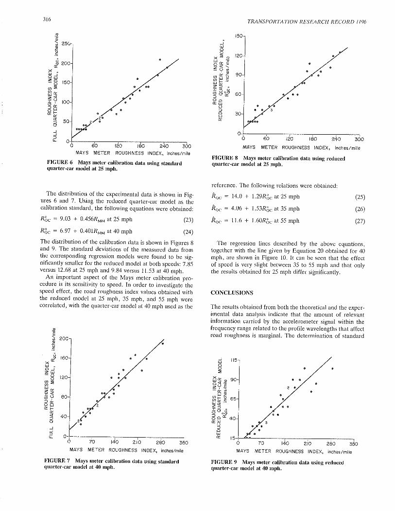
316 TRANSPOR'|ATION RESEARCH RECO RD t t9()

FICURE I Mays meter cal¡bration data using reducedquarter.car model at 25 mph.

reference. The following relations were obtained:

Âo" = 14.0 + 1..29R3c ar 25 rnph

Âo. = 4.06 + 1.53Rðc at 35 mph

Âo. : 11.6 + 1.60Råc at 55 mph

(2s)

(26)

(27)

jl¡lôo

*ãgHa ë5{:=(J øradEo:': oØH.c9etì oEõUOasü

Of,ÕUJÉ,

.9

€aEc.:Io

GxU:ed<ô-oaz,t'gz^\9riXUJdÞ

oJJlu-

MAYS METER ROUGHNESS |NDEX, ¡nches/mite

FIGURD 6 Mays meter calibration data using standardquarter-car model at 25 nph.

The distribution of the experimental data is shown in Fig-ures 6 and 7. Using the reduced quarter-car model as thecalibration standard, the following equations were obtained:

Rå. = 9.03 + 0.456RMM at 25 mph (23)

Rð. : 6.97 + 0.401RMM at 40 mph (24)

The distribution of the calibration data is shown in Figures gand 9. The standard deviations of the measured data fromthe corresponding regression models \ryere found to be sig-nificantly smaller for the reduced ¡nodel at both speeds: 7.g5versus 12.68 at 25 rnph and 9.84 versus 11.53 at 40 rnph.

An important aspect of the Mays meter calibration pro-cedure is its sensitivity to speed. In order to investigate thespeed effect, the road roughness index values obtainecl withthe reduced model at 25 mph, 35 mph, and 55 mph werecorrelated, with the qualter-car model at 40 mph used as the

MAYS METER ROUGHNESS tNOEX, inches/mite

FIGURE 7 Mays meter calibration data using standardquarter-car model at 40 mph.

The regression lines described by the above equations,togethel with the line given by Equation 20 obtained for 40mph, are shown in Figure 10. It can be seen that the effectof speed is very slight between 35 to 55 rnph and that onlythe results obtained for 25 mph differ silnificantly.

CONCLUSIONS

The results obtained from both the theoretical and the exper-imental data analysis indicate that the amount of relevantinformation carried by the accelerometer signal within thefrequency range related to the profile wavelengths that affectroad roughness is marginal. The determination of standard

o 70 t40 zto 280 3sO

MAYS METER ROUGHNESS tN0EX, inches/mile

FIGURB 9 Mays meter calibration data using reducedquarter-car ¡nodel at 40 mph.

Jt¡lÕoE

ñgs;(.)E-frËø)l- õ6;cllJä.-

=)ö o*gdotÈ91

:)oÙJ(r

gE

ofc.:oo

È.xtrj -ôJzw-ooE=9a=^<lÈoËGF

e

oJJf,ll-

MAYS METER ROUGHNESS lN0EX, inches,/mite

Kulakowski

ROUGHNESS INDEX VALUESto

[¡.T t

?l'.tnt ?,',#3 ot t'

FIGURE l0 Effect of speed on Mays metercalibration lines using rcduced quarter-cal'model.

road roughness measures can, therefore, be accomplished using

the body displacement data only. Elimination of the acceler-

ometer will certainly simplify the hardware of the road rough-ness measurement system; but, more important, it will also

allow the software necessary to generate the roughness indexto be limited to the processing of the displacement transducersignal. The computational process of calculating the roadroughness index without double integrating the accelerometersignal will thus become considerably less expensive.

The results of the analysis presented in this paper, whichwere obtained with actual displacement and acceleration data,confirm the feasibility of the proposed reduced quartel'-carmodel when used solely for the purpose of roughness indexdetermination.

REFERENCES

l. J. C. Wambold et al. The State of the Art of Measurementand Analysis of Highway Roughness. In Transportation Research

Record 83ó, TRB, National Research Council, Washington,D.C., 1981, pp.2t-29.

2. G. K. Watugala. Determination of Road Roughness from Iner'tial Profilometer Data. Ph.D. dissertation, The PennsylvaniaState University, 1984.

3. New Standard Practice for Simulating Vehicular Response toLongitudinal Profiles of a Vehicular Traveled Surface. áSTMBallot, September 1985.

4. T. D. Gillespie, M. W. Sayers, and L. Segel. NCHRP Report

317

228: Calibration and Correlation of Response:Iype RoadRoughness Measuring Systems. TRB, National ResearchCouncil, Washington, D.C., 1980.

5. M. S. Janoff et al. NCHRP Report 1-23: Pavement Roughnessand Ride Quality. TRB, National Research Council, Wash-ington, D.C., 1984.

6. B. T. Kulakowski. Correlation of Roacl Roughness Measure-ments Obtained with the 1962 Chevrolet Impala and with theStandard Quarter-Car Model. Final Report, PennsylvaniaDepartment of Transportation, Juty 1985.

APPENDIX

Combining Equations I and 2 and taking a Laplace transfor-mation, the transfer function G*r' (s) relating the displace-ment transducer signal to the road profile is obtained:

G*"(s) =

_sa + C,IM, + C,lM,,s3 + KJM, + K,/M,, + K,lM,,s2

B(s)(A1)

where the polynomial B(s) is

JUJoo=JJlr-

EtLEo)UOfç<.=

-å8,toz_

q>.J)t¡JzI('oÉ.

. K, . C"K, K,K,* ^'r,,t'

* -M¡7j

* -M¡r7,Substituting this for¡n into Equation 1 yields the following

expression for the transfer function G*^ (s):

/\ C,K,|M,M,,s3 + K,K,lMrM,,s2urve(s) = B(r)

B(s) = * * #,* *9,,r * #,* #,,

K,IM,, S2unv(s,l = B(r)

G,,',(s) = ry#

The transfer functions G,,r(s) and G"r(s) can also be obtainedfrom the model equations I and 2:

(^2)

(A3)

(A4)

(As)

Letting s : /b in Equations 41, A3, A4 and A5 and substi-tuting into Equation 18, the expression for o(to) is found as

follows:

o(ø)

(K,K,lM,M,,)2 * a2 (C"K,lM"M,,)2

,, l(-,' * #"* #,. u;,)'. *(#". t;,)'l

(46)

Publication of this paper sponsoreC by the Committee on SurfaceP rop erties-V e h icle I nte ractio n.