Optimizing Power, Heating, and Cooling Capacity on a Decision-Guided Energy Investment Framework

Optimizing Power, Heating, and CoolingCapacity on a Decision-Guided Energy

Investment Framework

Chun-Kit Ngan1(&), Alexander Brodsky1, Nathan Egge1,and Erik Backus2

1 Department of Computer Science, George Mason University, 4400 UniversityDrive, Fairfax, VA 22030, USA

{cngan,brodsky,negge}@gmu.edu2 Facilities Management Department, George Mason University,

4400 University Drive, Fairfax, VA 22030, [email protected]

Abstract. We propose a Decision-Guided Energy Investment (DGEI)Framework to optimize power, heating, and cooling capacity. The DGEIframework is designed to support energy managers to (1) use the analytical andgraphical methodology to determine the best investment option that satisfies thedesigned evaluation parameters, such as return on investment (ROI) andgreenhouse gas (GHG) emissions; (2) develop a DGEI optimization model tosolve energy investment problems that the operating expenses are minimal ineach considered investment option; (3) implement the DGEI optimizationmodel using the IBM Optimization Programming Language (OPL) with his-torical and projected energy demand data, i.e., electricity, heating, and cooling,to solve energy investment optimization problems; and (4) conduct an exper-imental case study for a university campus microgrid and utilize the DGEIoptimization model and its OPL implementations, as well as the analytical andgraphical methodology to make an investment decision and to measure trade-offs among cost savings, investment costs, maintenance expenditures,replacement charges, operating expenses, GHG emissions, and ROI for all theconsidered options.

Keywords: Decision guidance � Energy investment � Optimization model

1 Introduction

Sustainable enterprise development has been considered a significant and competitivestrategy of corporate growth in manufacturing and service organizations. A significantpart of sustainable development involves new technologies for local electricity,heating, and cooling generation. Making optimal decisions on planning and invest-ment of these technologies to support commercial and industrial facilities is aninvolved problem because of complex operational dependencies of these technologies.This is exactly the focus of this paper.

Currently, the existing approaches to support the optimization of energy plants canbe divided into two categories: (1) optimal operation of an energy system and (2)

� Springer International Publishing Switzerland 2014S. Hammoudi et al. (Eds.): ICEIS 2013, LNBIP 190, pp. 154–173, 2014.DOI: 10.1007/978-3-319-09492-2_10

a better plant-process design [1]. The former category is related to the optimizedscheduling of an electric power plant. Some researchers, such as Bojic and Stojanovic[2], proposed an optimization procedure based on a MILP solver [3] to provide anoperation diagram which allows users to find an optimum composition of energyconsumption that minimizes the operating expenses of an energy system [4–9].The latter approach includes the analysis of simulations carried out to determine themost suitable matching between a plant and its loads that could increase the plantpower output. Some researchers, e.g., Savola et al. [10], did extensive research topropose an off-design simulation and mathematical modelling of the operation at partloads and a Mixed-Integer Non-Linear Programming (MINLP) optimization model forincreasing power production [11, 12]. However, neither of the above approachesconsiders optimizing the complex interactions between the existing components andthe newly added energy equipment that would result in a higher operating cost, suchas the charges on electricity and gas consumptions, as well as significant environ-mental impacts, i.e., greenhouse gas (GHG) emissions, e.g., carbon dioxide (CO2) andmono-nitrogen oxide (NOx). Without considering such interactions for every timeinterval over an investment time horizon, it would be impossible to make optimalrecommendations on energy planning and investment.

Thus this paper focuses on addressing the above shortcomings. More specifically,the contributions of this paper are as follows. First, we propose a Decision-GuidedEnergy Investment (DGEI) Framework. Given electricity, heating, and cooling gen-eration processes, utility contracts, historical and projected demand, facility expan-sions, and Quality of Service (QoS) requirements, the DGEI framework is designed torecommend optimal settings of decision control variables. These decision controlvariables include the amount of electricity, heating, and cooling that is generated bythe supply of water and gas, which is inputted to each deployed component in everytime interval. The goal of the DGEI framework is to learn optimal values of thosedecision control variables in order to minimize the total operating cost within therequired quality of service and within the bound for GHG emissions, as well as to takeinto account all components’ interactions. Second, to support the DGEI framework,we develop a DGEI optimization model, i.e., a MILP formulation construct, to solvethe adjusted cost minimization problem. Furthermore, we implement the DGEIoptimization model by using the IBM Optimization Programming Language (OPL)[13, 14]. Third, we propose an analytical and graphical methodology to determine thebest available investment option based upon the evaluation parameters. The param-eters include investment costs, maintenance expenditures, replacement charges,operating expenses, cost savings, return on investment (ROI), and GHG emissions.Finally, we use the methodology and the DGEI framework to conduct an experimentalcase study on the microgrid at the Fairfax campus of George Mason University(GMU). This study has been conducted and used by the GMU Facilities ManagementDepartment (FMD) to make actual investment decisions.

The rest of the paper is organized as follows. Using the GMU Fairfax campusmicrogrid as an example, we describe its energy investment problem in Sect. 2. Weexplain our DGEI framework and optimization model in Sect. 3 and demonstrate theOPL implementation in Sect. 4. In Sect. 5, we present the analytical and graphicalmethodology to determine an optimal investment option. In Sect. 6, we conduct the

Optimizing Power, Heating, and Cooling Capacity on a DGEI Framework 155

experimental analysis on the GMU energy investment case and illustrate the rela-tionships among the investment costs, ROI, and GHG emissions of the various optionsin tabular and graphical formats. We also explain and draw the conclusion for theinvestment options from the graphs and tables in detail on the GMU energy invest-ment problem. In Sect. 7, we conclude and briefly outline the future work.

2 Problem Description of Real Case Study

Consider the real case study at GMU, in which the GMU Facilities ManagementDepartment (FMD) is planning to extend and or expand the existing energy equipmentin order to meet the current and future demand of electricity, heating, and coolingacross the expanding Fairfax campus in Virginia. Presently, the GMU existing energyfacilities at the Fairfax campus operate a centralized heating and cooling plant(CHCP) system and utilize the electricity purchased from the Dominion VirginiaPower Company (DVPC) to satisfy all the energy demand. Over the past 10 years, thecampus has experienced a significant growth on a square-foot basis in terms of landuse. Since the campus continues its expansion at a rapid rate, the existing CHCPsystem and the electricity consumption have reached a saturated point where thecurrent capacity and facilities will not be able to satisfy the future energy demand, i.e.,electricity, heating, and cooling. For these reasons, a study has been conducted todetermine the best available investment option, e.g., a new cogeneration (CoGen)plant, with regards to a possible methodology to meet the current and future elec-tricity, heating, and cooling demand, while also addressing the optimal operations ofthe newly added facility with the existing energy equipment.

The diagram in Fig. 1 depicts the GMU energy generation process which suppliesheating, cooling, and electricity to the entire Fairfax campus. The GMU energyfacilities have a CHCP system to supply the hot and cold water (see the red and blueresources) which are distributed across the facilities to the campus buildings to meetthe heating and cooling demand (see the upper two sub-processes on the right), i.e.,heating and air-conditioning to the buildings. To supply the heating and cooling to thecampus buildings, the CHCP system needs the inputs, i.e., natural gas (see the yellowresource on the left), water (see the light blue resource on the left), and electric power(see the green resource on the left). These resources come from the gas supply, i.e.,Washington Gas Light Company (WGLC), the water supply, i.e., Fairfax CountyWater Authority (FCWA), and the electricity supply, i.e., Dominion Virginia PowerCompany (DVPC), correspondingly. In addition, the facilities also need to satisfy theelectricity demand across the entire campus, where the electricity demand is beyondthe demand from the CHCP consumption. Any excessive electric power supply canalso be resold to the DVPC (see the electricity resell on the right). Furthermore, thefacilities also commit a curtailment demand (see the curtailment demand on the right)to the energy curtailment program through EnergyConnect (EC), Inc. Both the elec-tricity resell and the curtailment commitment can bring certain revenues and savingsto offset the overall operational costs on a monthly basis and the capital expendituresin the long run. The facilities also generate greenhouse gas (GHG) emissions, such ascarbon dioxide (CO2) (see the black resource at the bottom right).

156 C.-K. Ngan et al.

Given the expansion of the GMU Fairfax campus, in addition to the increasingelectricity demand, the heating and cooling demand is also expected to increase. TheCHCP system will not have enough capacity to meet the future need. The GMU planis to employ a procurement strategy, i.e., the deployment of the best availableinvestment option, which will satisfy projected demand and minimize investmentcosts, maintenance expenditures, replacement charges, operating expenses, and GHGemissions, as well as maximize cost savings and return on investment (ROI) at thesame time. The FMD managers are now considering some viable options. One of theconsiderable options is to integrate a new cogeneration (CoGen) plant (see the lowersub-process in the middle), i.e., the Combined Heating and Power (CHP) Plant [1, 15],into the existing facilities shown in Fig. 1. The new CoGen plant has turbines togenerate electricity to complement the electricity demand, uses the generated heat as aby-product to complement the heating demand, and collaborates with the ammoniaprocess technology [16] to supply the cooling demand. Now, the challenging questionis how to analytically determine the best investment option that satisfies all the energydemand, i.e., electricity, heating, and cooling, at the lowest operating costs.

3 Decision-Guided Energy Investment (DGEI) Frameworkand Optimization Model

To answer the above question, we propose the DGEI framework. This framework iscomposed of six energy-investment libraries, i.e., Energy Generation Process (EGP),Energy Contractual Utility (ECU), Energy Historical Demand (EHD), Energy FutureDemand (EFD), Energy Facility Expansion (EFE), Quality of Service (QoS)requirements, and a DGEI optimizer. The EGP is an extensible library that enablesdomain experts to construct an energy generation process to supply electricity,heating, and cooling. The ECU is a library that contains energy contractual terms forcalculating bill utilities, e.g., an electricity bill, a water bill, and a gas bill. The EHDand EFD are the libraries that store historical and projected energy demand

Fig. 1. Prospective heating, cooling, and electric power facilities at the GMU Fairfax campus.


respectively. The EFE library archives the facility expansion of an organization interms of square-footage increase. The QoS library stores the QoS requirements thatthe energy facilities of an organization need to meet, e.g., the maximal power inter-ruptions allowed per monthly pay period in an organization. The DGEI optimizersupports energy managers to utilize all the libraries, i.e., EGP, ECU, EHD, EFD, EFE,and QoS, as inputs to the decision optimization process, which minimizes operatingexpenses and maximize cost savings. This decision optimization process not onlyoptimizes the interactions between the existing and the considerable energy facilityoptions but also minimizes the environmental impacts on the surroundings, i.e.,minimizing the GHG emissions. In addition to the GHG emissions, energy managersalso utilize (1) return on investment (ROI), i.e., the gain return efficiency amongdifferent investments, (2) the investment costs, i.e., an amount spent to acquire a long-term asset, and (3) equipment expenses, i.e., maintenance expenditures plusreplacement charges, to evaluate all the available investments and then to determinethe best option.

To solve an energy investment optimization problem in terms of minimizing theoperating cost and the GHG emissions is to formulate a DGEI optimization model.This model optimally learns decision control variables, which require several inputdata sets, i.e., the historical and projected electricity, heating, and cooling demandover a time horizon, the electric and gas contractual utility, the operational parametersand capacity constraints of the existing and the new electric power plants, as well asthe energy aggregation of the supply and demand, e.g., electricity, gas, heating, andcooling, to minimize the entire operating expenses. Using the GMU energy invest-ment optimization problem over the 10-year time horizon as an example, we explainthe above terminologies used in this case study in the following subsections.

3.1 Electricity, Heating, and Cooling Demand Over a Time Horizon

The electricity, heating, and cooling demand over a time horizon is the input,including the usage of the historical and projected quantities, which are provided fromthe GMU Facilities Management Department, to the DGEI optimization model thatrequires the domain users to define all (i.e., past plus future), past, and future powerintervals over the 10-year time horizon respectively.

• AllPowerIntervals is a set of all powerIntervals, where each powerInterval is a tuplewhich includes several attributes, i.e., pInterval, payPeriod, year, month, day, hour,and weekDay. We use negative and zero integers to represent the past time horizonand positive integers to denote the future time horizon. For example, pInterval is anhourly time interval of the energy demand, where -8759 B pInterval B 78840.payPeriod is a monthly pay period of the energy demand, where -11 B payPeri-od B 108. Other attributes’ intervals include 2011 B year B 2020,1 B month B 12, 1 B day B 31, 0 B hour B 23, and 0 B weekDay B 6.

• PastPowerIntervals is a set of past powerIntervals of tuples, where -8759 B pIn-terval B 0, -11 B payPeriod B 0, year = 2011, 1 B month B 12, 1 B day B 31,0 B hour B 23, and 0 B weekDay B 6.


• FuturePowerIntervals is a set of future powerIntervals of tuples, where 1 B pIn-terval B 78840, 1 B payPeriod B 108, 2012 B year B 2020, 1 B month B 12,1 B day B 31, 0 B hour B 23, and 0 B weekDay B 6.

After declaring the power intervals, the quantities of electricity, heating, and coolingdemand can be stored in their arrays over their power intervals. These three quantitiesof demand are provided by the GMU Facilities Management Department.

• demandKw[AllPowerIntervals] C 0 is an array of electricity demand over theAllPowerIntervals. This array stores both the historical and the projected demandover the PastPowerIntervals and the FuturePowerIntervals respectively.

• demandHeat[FuturePowerIntervals] C 0 is an array of projected heating demandover the FuturePowerIntervals.

• demandCool[FuturePowerIntervals] C 0 is an array of projected cooling demandover the FuturePowerIntervals.

3.2 Electric and Gas Contractual Utility

To determine the total operating cost, we need to compute the consumption expensesof electricity and gas supply according to their utility contracts. The consumptionexpenses of electricity include both the peak demand charge and the total powerconsumption charge that are explained in detail as follows.

3.2.1 Peak Demand ChargeFor the electricity supply, utilityKw[AllPowerIntervals] C 0 is an array of electricitysupplied from the DVPC over the AllPowerIntervals.

historicUtilityKw[i] is an array of past electricity demand from the GMU, i.e.,historicUtilityKw[i] = demandKw[i], which satisfies the constraint, i.e.,

utilityKw[i] == historicUtilityKw[i], where i [ PastPowerIntervals.This constraint is to assure that the electricity consumed by the GMU in the past year,i.e., 2011, is equivalent to the supply from the DVPC.

payPeriodSupplyDemand[p] is the peak demand usage per future pay period (p).This peak demand usage meets the below contractual constraints (C1 and C2) and isdetermined based upon the highest of either (C1) or (C2):

C1: The highest average kilowatt measured in any hourly time interval of the currentbilling month during the on-peak hours of either between 10 a.m. and 10 p.m. fromMonday to Friday for the billing months of June through September or between 7 a.m.and 10 p.m. from Monday to Friday for all other billing months.

C2: 90 % of the highest kilowatt of demand at the same location as determined under(C1) above during the billing months of June through September of the precedingeleven billing months.


The logic constraints of both C1 and C2 can be expressed as follows:

AllPowerIntervals, p [ FuturePayPeriods, and 1 B FuturePayPeriods B 108. Usingthese logic constraints, we can determine the optimal peak demand usage per futurepay period, which consumes more than the expected electricity supply per powerIn-terval from the DVPC.

generationDemandCharge[p], i.e.,generationDemandCharge[p] = 8.124 *

payPeriodSupplyDemand[p];, is the Electricity Supply (ES) service charge, i.e.,the peak demand charge, where p [ FuturePayPeriods, and 8.124 is the dollar chargeper kW.

3.2.2 Total Power Consumption ChargepayPeriodKwh[p] is the total power consumption per future pay period, i.e., pay-

PeriodKwh[p] =P

utilitykW[i];, where i [ AllPowerIntervals, p [ Futur-ePayPeriods, and i.payPeriod = p.

payPeriodKwhCharge[p] is the total kWh charge per future pay period, i.e.,payPeriodKwhCharge[p] C 0, which satisfies the below contractual constraints:

where p [ FuturePayPeriods, 0.01174 is the dollar charge of the first 24000 kWhconsumed, 0.00606 is the dollar charge of the next 186000 kWh consumed, and0.00244 is the dollar charge of the additional kWh consumed. Note that ifpayPeriodSupplyDemand[p] is 1000 kW or more, 210 kWh for each peak demandusage over 1000 kW is added to the total power consumption to calculatepayPeriodKwhCharge[p].

3.2.3 Total Electricity CostThe total electricity cost per future pay period is the sum of payPeriodKwhCharge[p]and generationDemandCharge[p], i.e., electricCostPerFuturePayPeri-

od = (payPeriodKwhCharge[p] + generationDemandCharge[p]);,where p [ FuturePayPeriods.


The total electricity cost of all the FuturePayPeriods is the aggregations of all thetotal electricity costs per future pay period, i.e., electricCost =

P(pay-

PeriodKwhCharge[p] + generationDemandCharge[p]);, where p [FuturePayPeriods.

Table 1 summarizes the descriptions of all the constant values from the electricutility contract used in the DGEI optimization model for the GMU energy investmentproblem.

3.2.4 Total Gas Consumption ChargeRegarding the gas supply, utilityGas[FuturePowerIntervals] C 0 is an array of gassupplied from the WGLC over the FuturePowerIntervals. The total gas cost of all theFuturePowerIntervals is the aggregations of all the total gas utility per future powerinterval, i.e., gasCost = (

P(utilityGas[i]/btuPerDth)) *

gasPricePerDth;, where i [ FuturePowerIntervals, btuPerDth = 1000000 BTU,which is the amount of energy per decatherm, and gasPricePerDth = $6.5, which isthe gas charge per decatherm.

3.2.5 Total Operating CostThe total operating cost is the sum of the total electricity cost of all the future payperiods and the total gas cost of all the future power intervals, i.e.,totalCost = electricCost + gasCost;.

3.3 Operational Parameters and Capacity Constraints of the CHCPand the Cogen Plant

In addition to the supply and demand of gas and electricity, the operational parametersand the capacity constraints of the CHCP and the CoGen plant are also considered.

Table 1. Descriptions for the constant values in the DGEI optimization model of the GMUenergy investment problem.

Constant Description

0.9 Percentage of the highest kW of demand during the billing months of Junethrough September of the preceding 11 billing months

8.124 Amount ($) of Electricity Supply (ES) demand charged per kW

24000 First ES kWh

0.01174 Amount ($) of the first 24000 ES kWh charged per kWh

186000 Next ES kWh

0.00606 Amount ($) of the next 186000 ES kWh charged per kWh

210000 Sum of the first ES kWh and the next ES kWh

0.00244 Amount ($) of the additional ES kWh charged per kWh

210 kWh for each ES kW of demand over 1000 kW


3.3.1 The CHCP PlantFor the CHCP plant, gasIntoCHCP[FuturePowerIntervals] C 0 is an array of naturalgas input to the CHCP over the FuturePowerIntervals to generate the heat supply.kwIntoCHCP[FuturePowerIntervals] C 0 is an array of power input to the CHCP overthe FuturePowerIntervals to generate the cool supply. heatOutCHCP[FuturePower-Intervals] C 0 is an array of heat output from the CHCP over the FuturePowerIn-tervals to satisfy the partial heating demand. coolOutCHCP[FuturePowerIntervals] C

0 is an array of cool output from the CHCP over the FuturePowerIntervals to satisfythe partial cooling demand. The CHCP constraints include:

• heatOutCHCP[i] * gasPerHeatUnit B gasIntoCHCP[i];, i.e., the amountof gas consumed to generate the heat cannot be more than that of the gas input;

• coolOutCHCP[i] * kwhPerCoolUnit B kwIntoCHCP[i];, i.e., the amountof electric power consumed to generate the cool cannot be more than that of thepower input;

• heatOutCHCP[i] B chcpMaxHeatPerHr;, i.e., the amount of heat generatedcannot be more than the maximal heat output of the CHCP; and

• coolOutCHCP[i] B chcpMaxCoolPerHr;, i.e., the amount of cool generatedcannot be more than the maximal cool output of the CHCP, where i [ Future-PowerIntervals, gasPerHeatUnit = (1 /0.78), and kwhPerCoolUnit = (1 /0.94).

3.3.2 The CoGen PlantFor the CoGen plant, gasIntoCogen[FuturePowerIntervals] C 0 is an array of gasinput to the CoGen plant over the FuturePowerIntervals to generate the power supply.kwOutCogen[FuturePowerIntervals] C 0 is an array of power output from the CoGenplant over the FuturePowerIntervals to satisfy the partial electricity demand. hea-tOutCogen[FuturePowerIntervals] C 0 is an array of heat output from the CoGenplant over the FuturePowerIntervals to satisfy the partial heating demand. coolOut-Cogen[FuturePowerIntervals] C 0 is an array of cool output from the CoGen plantover the FuturePowerIntervals to satisfy the partial cooling demand. The constraints ofthe CoGen plant include:

• kwOutCogen[i] * cogenGasPerKwh B gasIntoCogen[i];, i.e., the amountof gas consumed to generate the power cannot be more than that of the gas input;

• kwOutCogen[i] B cogenMaxKw;, i.e., the amount of power generated cannotbe more than the maximal electricity output of the CoGen plant;

• heatOutCogen[i]BcogenHeatPerKwh*kwOutCogen[i];, i.e., theamount of heat generated cannot be more than the maximal heat supply that isrestricted by the power output of the CoGen plant;

• heatOutCogen[i] B cogenMaxHeatPerHr * (kwOutCogen[i]/co-

genMaxKw);, i.e., the amount of heat generated cannot be more than the maximalheat output of the CoGen plant;

• coolOutCogen[i] B (cogenMaxHeatPerHr * (kwOutCogen[i]/co-

genMaxKw) - heatOutCogen[i]) * cogenHeatToCoolRatio;, i.e., theamount of cool generated cannot be more than the maximal cool supply that isrestricted by the power and heat output of the CoGen plant; and


• coolOutCogen[i] B cogenMaxCoolPerHr;, i.e., the amount of coolgenerated cannot be more than the maximal cool output of the CoGen plant,

where i [ FuturePowerIntervals, cogenMaxKw = 7200 kW is the maximal poweroutput, cogenHeatPerKwh = 10300 kWh is the amount of heat generated per kWh,cogenHeatToCoolRatio = cogenMaxCoolPerHr/cogenMaxHeatPerHr is the ratio ofconverting heat to cool supply, cogenMaxHeatPerHr = 40000000 BTU is the maxi-mal heat supply of the CoGen plant per hour, cogenMaxCoolPerHr = 2400 Tons isthe maximal cool supply of the CoGen plant per hour, cogenGasPerKwh = gasB-TUPerGallon/kWhPerGallon/cogenGasToKwhEfficiency is the amount of natural gasconsumed per kWh, for gasBTUPerGallon = 114000 BTU is the amount of energygenerated per gallon of gas, kwhPerGallon = 33.41 is the amount of kWh generatedper gallon of gas, and cogenGasToKwhEfficiency = 0.33 is the efficiency of theCoGen plant to generate power from natural gas.

3.4 Energy Aggregations of Supply and Demand

The aggregations of energy supply and demand within the entire energy systeminclude:

• kwIntoCHCP[i] + demandKw[i] B utilityKw[i] + kwOutCogen[i];,i.e., the amount of power input to the CHCP and the power demand from the GMUcannot exceed the amount of power supply provided from the DVPC and the poweroutput generated from the CoGen plant, where i [ FuturePowerIntervals.

• demandReduction[i] B (utilityKw[i] + kwOutCogen[i]) - (kwInto

CHCP[i] + demandKw[i]);, i.e., the power supply reduction cannot exceed thedifference between the total power supply (utilityKw[i] + kwOutCogen[i]) and thetotal power demand (kwIntoCHCP[i] + demandKw[i]), where demandReduction[FuturePowerIntervals] C 0 is an array of extra power supply that canbe cut from the power inputs over the FuturePowerIntervals, and i [ FuturePowerIntervals.

• PdemandReduction[i] B maxKwReductionPerPayPeriod;, i.e., the

total power reductions over the future power intervals cannot exceed the allowablemaximal power interruptions per future pay period, where i [ FuturePowerInter-vals, p [ FuturePayPeriods, and i.payPeriod = p.

• utilityGas[i] C gasIntoCogen[i] + gasIntoCHCP[i];, i.e., the gasinput to the CoGen plant and to the CHCP cannot exceed the gas supply providedfrom the WGLC, where i [ FuturePowerIntervals.

• heatOutCogen[i] + heatOutCHCP[i] C demandHeat[i];, i.e., the heatdemand from GMU cannot exceed the heat supply generated from the CoGen plantand the CHCP, where i [ FuturePowerIntervals.

• coolOutCogen[i] + coolOutCHCP[i] C demandCool[i];, i.e., the cooldemand from GMU cannot exceed the cool supply generated from the CoGen plantand the CHCP, where i [ FuturePowerIntervals.


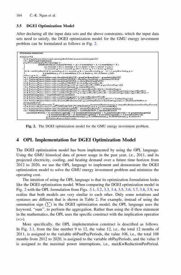
3.5 DGEI Optimization Model

After declaring all the input data sets and the above constraints, which the input datasets need to satisfy, the DGEI optimization model for the GMU energy investmentproblem can be formulated as follows in Fig. 2.

4 OPL Implementation for DGEI Optimization Model

The DGEI optimization model has been implemented by using the OPL language.Using the GMU historical data of power usage in the past year, i.e., 2011, and itsprojected electricity, cooling, and heating demand over a future time horizon from2012 to 2020, we use the OPL language to implement and demonstrate the DGEIoptimization model to solve the GMU energy investment problem and minimize theoperating cost.

The intuition of using the OPL language is that its optimization formulation lookslike the DGEI optimization model. When comparing the DGEI optimization model inFig. 2 with the OPL formulation from Figs. 3.1, 3.2, 3.3, 3.4, 3.5, 3.6, 3.7, 3.8, 3.9, werealize that both models are very similar to each other. Only some notations andsyntaxes are different that is shown in Table 2. For example, instead of using thesummation sign (

P) in the DGEI optimization model, the OPL language uses the

keyword, ‘‘sum’’, to perform the aggregation. Rather than using the if-then statementin the mathematics, the OPL uses the specific construct with the implication operatior(=[).

More specifically, the OPL implementation construct is described as follows.In Fig. 3.1, from the line number 9 to 12, the value 12, i.e., the total 12 months of2011, is assigned to the variable nbPastPayPeriods, the value 108, i.e., the total 108months from 2012 to 2020, is assigned to the variable nbPayPeriods, and the value 0is assigned to the maximal power interruptions, i.e., maxKwReductionPerPeriod.

Fig. 2. The DGEI optimization model for the GMU energy investment problem.


The FuturePayPeriods is ranged from 1 to 108. From the line number 15 to 23, wedeclare a tuple of a power interval that has the attributes, including pInterval, pay-Period, year, month, day, hour, and weekDay. The line number 25 to 27 declares andinitializes AllPowerIntervals that include both PastPowerIntervals and FuturePower-Intervals. The line number 30 to 32 declares and initializes the demandKw[AllPow-erIntervals], the demandHeat[FuturePowerIntervals], and the demandCool[FuturePowerIntervals] arrays.

Figure 3.2 declares the decision control variables, i.e., utilityKw[AllPowerInter-vals], payPeriodSupplyDemand[FuturePayPeriods], and payPeriodKwh[Futur-ePayPeriods], to compute payPeriodKwhCharge[FuturePayPeriods] and generation

Table 2. Differences between DGEI Optimization model and OPL formulation model.

DGEI optimization model OPL formulation model

Notation: Summation SignP

Example:P(demandKw[i] - kW[i]) B

2 * annualBound

Syntax: sumExample:sum(i in PowerIntervals : i.pInterval [= 1)(demandKw[i] - kW[i]) \= annualBound * 2

Notation: If-then StatementExample:if (payPeriodKwh[p] B 24000)payPeriodKwhCharge[p] =0.01174 * payPeriodKwh[p]

Syntax: =[Example:(payPeriodKwh[p] \= 24000) =[ (payPeriodKwhCharge[p] ==0.01174 * payPeriodKwh[p])

Notation: Where clauseExample: peakDemandBound[p] B

payPeriodSupplyDemand[p], wherep [ PayPeriods

Syntax: forallExample:forall (p in PayPeriods)peakDemandBound[p] \=payPeriodSupplyDemand[p]

Fig. 3.1. General and demand input data.


DemandCharge[FuturePayPeriods] that are summed together to determine the totalelectricity cost over all the future pay periods while satisfying the electric contractualconstraints.

Figure 3.3 declares the constants, i.e., gasPricePerDth and btuPerDth, and utili-tyGas[FuturePowerIntervals] to calculate the total gas cost over all the future powerintervals.

Figure 3.4 declares the objective function to minimize the total operating cost, i.e.,the total electricity cost plus the total gas cost.

Figure 3.5 declares the constants, i.e., gasPerHeatUnit, kwhPerCoolUnit,chcpMaxHeatPerHr, and chcpMaxCoolPerHr, and the arrays, i.e., gasIntoCHCP[Fu-turePowerIntervals], kwIntoCHCP[FuturePowerIntervals], heatOutCHCP[Future-PowerIntervals], and coolOutCHCP[FuturePowerIntervals], used in the CHCPcapacity constraints.

Fig. 3.2. Total electricity cost.

Fig. 3.3. Total gas cost.

Fig. 3.4. Total operating cost.

Fig. 3.5. Operational parameters and data structures of the CHCP plant.


Figure 3.6 declares the constants from the line number 71 to 79, and the arrays,i.e., gasIntoCogen[FuturePowerIntervals], heatOutCogen[FuturePowerIntervals],coolOutCHCP[FuturePowerIntervals], and kwOutCHCP[FuturePowerIntervals],which are used in the capacity constraints of the CoGen plant.

Figure 3.7 defines all the capacity constraints for the CHCP and the CoGen plant.

Figure 3.8 defines the contractual constraints for the electricity bill.

Figure 3.9 defines the constraints for the energy aggregations of electric power,gas, heat, and cool.

Fig. 3.6. Operational parameters and data structures of the CoGen plant.

Fig. 3.7. Capacity constraints of the CHCP and the CoGen plant.

Fig. 3.8. Contractual electricity utility constraints.

Fig. 3.9. Energy aggregations of supply and demand.


5 Analytical Methodology on Evaluation among EnergyInvestment Options

For domain experts being able to formulate and implement the above DGEI optimi-zation model to determine the best investment option, we propose an analyticalmethodology that guides the domain experts to achieve this goal. The methodologyincludes six steps.

STEP 1: Collect historical energy demand, such as electricity, heating, and cooling,from each building unit, and forecast those demands in terms of growth on a square-foot basis over the future time horizon.

STEP 2: Identify all the possible energy investment options, such as the expansion ofcurrent facilities and the procurement of cogeneration plants.

STEP 3: Formulate, implement, and execute the DGEI optimization model thatintegrates historical and projected energy demand, electric and gas contractual utility,operational parameters and capacity constraints of energy equipment, as well asenergy aggregations of supply and demand in each considered option under theassumption of optimal interactions among available resources.

STEP 4: Compute the annualized evaluation parameters for each option based uponthe results from the optimization process in STEP 3.

The parameters include the investment cost (Ii), equipment cost (Ei), i.e., main-tenance expenditure (Mi) plus replacement charge (Ri), operating expense (Ci), i.e.,the charges on electricity and gas consumptions, cost saving (Si), i.e., C0 – Ci, wherei C 0 denotes an investment option and C0 is the operating cost of a base investmentoption that the other available options compare with, and return on investment (ROIi),i.e., Si /(Ii – I0), as well as the GHG emissions (MTCDEi), i.e., Gi * 0.053 MTCDE/Million-Btu + Pi * 0.513 MTCDE/Million-Wh, shown in Table 3, against the variousinvestment options, where 0.053 and 0.513 are the factors, which are calculated fromthe historical data.

Note that the base investment option is the option that the current capacity of theexisting facilities is expanded without procuring any new energy equipment.

Using the ROI and GHG emissions, domain users and experts can plot the ana-lytical graphs to illustrate the relationships among the ROI, GHG emissions, andinvestment expenses, which enable the domain experts to determine the best invest-ment option among all of the options being considered.

STEP 5: Remove any option that is dominated by the other options in terms of theevaluation parameters.

STEP 6: Construct a trade-off graph to evaluate the options that are not dominatedamong others and then make a final decision.

Note that although STEP 1, 2, 4, 5, and 6 are typical processes of evaluations,STEP 3 is not typical at all as the problem that we solve is a non-trivial optimizationproblem.


6 Analytical Methodology on Experimental Case Study

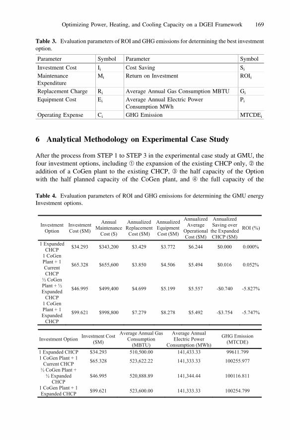
After the process from STEP 1 to STEP 3 in the experimental case study at GMU, thefour investment options, including � the expansion of the existing CHCP only, ` theaddition of a CoGen plant to the existing CHCP, ´ the half capacity of the Optionwith the half planned capacity of the CoGen plant, and ˆ the full capacity of the

Table 3. Evaluation parameters of ROI and GHG emissions for determining the best investmentoption.

Parameter Symbol Parameter Symbol

Investment Cost Ii Cost Saving Si

MaintenanceExpenditure

Mi Return on Investment ROIi

Replacement Charge Ri Average Annual Gas Consumption MBTU Gi

Equipment Cost Ei Average Annual Electric PowerConsumption MWh

Pi

Operating Expense Ci GHG Emission MTCDEi

Table 4. Evaluation parameters of ROI and GHG emissions for determining the GMU energyInvestment options.

Investment Option

Investment Cost ($M)

Annual Maintenance

Cost ($)

Annualized Replacement

Cost ($M)

Annualized Equipment Cost ($M)

Annualized Average

Operational Cost ($M)

Annualized Saving over

the Expanded CHCP ($M)

ROI (%)

1 Expanded CHCP $34.293 $343,200 $3.429 $3.772 $6.244 $0.000 0.000%

1 CoGen Plant + 1 Current CHCP

$65.328 $655,600 $3.850 $4.506 $5.494 $0.016 0.052%

½ CoGen Plant + ½ Expanded

CHCP

$46.995 $499,400 $4.699 $5.199 $5.557 -$0.740 -5.827%

1 CoGen Plant + 1 Expanded

CHCP

$99.621 $998,800 $7.279 $8.278 $5.492 -$3.754 -5.747%

Investment Option Investment Cost ($M)

Average Annual Gas Consumption

(MBTU)

Average Annual Electric Power

Consumption (MWh)

GHG Emission (MTCDE)

1 Expanded CHCP $34.293 510,500.00 141,433.33 99611.799 1 CoGen Plant + 1

Current CHCP $65.328 523,622.22 141,333.33 100255.977

½ CoGen Plant + ½ Expanded

CHCP $46.995 520,888.89 141,344.44 100116.811

1 CoGen Plant + 1 Expanded CHCP $99.621 523,600.00 141,333.33 100254.799


Option with the full planned capacity of the CoGen plant, have been chosen to beevaluated to meet the electricity, heating, and cooling demand of the Fairfax campusover the next 9 years from 2012 to 2020.

In STEP 4, using the evaluation parameters, i.e., ROI and GHG emissions, dis-cussed in Sect. 5 and the OPL to solve the GMU energy investment problem inSect. 4, we obtained Table 4 and Fig. 4 that can be used to determine the bestinvestment option.

In STEP 5, the Option ´ and ˆ are the dominated cases that can be removed fromour consideration list because of the negative ROI.

In STEP 6, according to the Table 4 and Fig. 4, we can conclude that the Option �

should be chosen because of the three observations. First, the GHG emissions and theequipment cost of the Option � are the lowest. Second, even though the ROI of theOption `, i.e., 0.052 %, is marginally better than that of the Option `, the GHGemissions of the Option ` is the highest among all the options being considered.Third, it is not economical at all for GMU to invest $31 million dollars, i.e., the Option` investment cost minus the Option � investment cost, more to earn only 0.052 %ROI in the next 9-year timeframe. Thus, the Option 1 is the best long-term option forGMU.

7 Conclusions and Future Work

In this paper, we propose a Decision-Guided Energy Investment (DGEI) Frameworkto optimize power, heating, and cooling capacity. The DGEI framework is designed tosupport energy managers to (1) use the analytical and graphical methodology todetermine the best investment option that satisfies the designed evaluation parameters,such as ROI and GHG emissions; (2) develop a DGEI optimization model to solveenergy investment problems that the operating expenses are minimal in each con-sidered investment option; (3) implement the DGEI optimization model using theIBM OPL language with historical and projected energy demand data, i.e., electricity,heating, and cooling, to solve energy investment optimization problems; and

Fig. 4. ROI (%) and GHG emissions (MTCDE) vs. investment cost ($M) across the fourinvestment options.


(4) conduct an experimental case study on the Fairfax campus microgrid at GeorgeMason University (GMU) and utilize the DGEI optimization model and its OPLimplementations, as well as the graphical and analytical methodology to make theinvestment decision and trade-offs among the cost savings, investment costs, main-tenance expenditures, replacement charges, operating expenses, GHG emissions, andreturn on investment (ROI) for all the considered options.

Technically, the core challenge is the development of the DGEI optimizationmodel that is very accurate in terms of the contractual terms and engineering con-straints, and yet efficient and scalable, which is done by the careful modelling ofmainly continuous decision variables and using constructs that avoid introduction ofcombinatorics, e.g., explicit or implicit binary variables, into the model. However, theDGEI optimization problem that we formulate is implemented by using the OPLlanguage. This OPL construct is then sent to the IBM CPLEX solver which is thebranch-and-bound-based algorithm with the exponential time complexity, i.e., O(k2N),where k is the number of decision control variables, and N is the size of the learningdata set. Thus the future research focus will develop a new algorithm that will be ableto solve the energy investment problems at a lower time complexity.

Concerning the real case study at George Mason University and its CHCP system,it is clear that GMU must develop and research other available options beyond thosediscussed in the analysis of this paper in order to meet the future needs of the Fairfaxcampus demand. Thus, the DGEI framework further developed will aid the GMUenergy decision makers to determine the optimal solutions that will satisfy the GMUshort- and long-term power, heating, and cooling demand. Note that our framework isapplicable to solve any energy investment problem in different domains of industry.Therefore, the future work includes the advanced development of the DGEI librariesand optimization models that enable domain users and experts to integrate more cleanand efficient energy equipment, such as geothermal electric power facilities, into theexisting plants optimally in order to support the continuous development of enter-prises and organizations.

Appendix: Abbreviation

Abbreviation Full Name Abbreviation Full Name

CHCP Centralized Heating andCooling Plant

ES Electricity Supply

CO2 Carbon Dioxide FCWA Fairfax County WaterAuthority

CoGen Cogeneration FMD Facilities ManagementDepartment

DGEI Decision-Guided EnergyInvestment

GHG Greenhouse Gas

DVPC Dominion Virginia PowerCompany

MILP Mixed Integer LinearProgramming

(continued)


References

1. Broccard, M., Girdinio, P., Moccia, P., Molfino, P., Nervi, M., Pini Prato, A.: Quasi staticoptimized management of a multinode CHP plant. J. Energy Convers. Manag. 51(11),2367–2373 (2010)

2. Bojic, M., Stojanovic, B.: MILP optimization of a CHP energy system. J. Energy Convers.Manag. 39(7), 637–642 (1998)

3. SAS Institute Inc.: SAS/OR(R) 9.22 User’s Guide: Mathematical Programming (2012)http://support.sas.com/documentation/cdl/en/ormpug/63352/HTML/default/viewer.htm#ormpug_milpsolver_sect001.htm. Accessed 29 April 2012

4. Brodsky, A., Wang. X.S.: Decision-guidance management systems (DGMS): seamlessintegration of data acquisition, learning, prediction, and optimization. In: Proceedings ofthe 41st Hawaii International Conference on System Sciences, Waikoloa, Big Island,Hawaii, USA (2008)

5. Brodsky, A., Bhot, M.M., Chandrashekar, M., Egge, N.E., Wang, X.S.: A decisions querylanguage: high-level abstraction for mathematical programming over databases. In:Proceedings of the 35th SIGMOD International Conference on Management of Data, RI,USA (2009)

6. Brodsky, A., Cherukullapurath, M., Awad, M., Egge, N.: A decision-guided advisor tomaximize ROI in local generation and utility contracts. In: Proceedings of the 2ndEuropean Conference and Exhibition on Innovative Smart Grid Technologies, Manchester,UK (2011)

7. Brodsky, A., Egge, N., Wang, X.S.: Reusing relational queries for intuitive decisionoptimization. In: Proceedings of the 44th Hawaii International Conference on SystemSciences, Koloa, Kauai, Hawaii, USA (2011)

8. Brodsky, A., Henshaw, S.M., Whittle, J.: CARD: a decision-guidance framework andapplication for recommending composite alternatives. In: Proceedings of the 2nd ACMInternational Conference on Recommender Systems, Lausanne, Switzerland (2008)

9. Brodsky, A., Alrazgan, A., Nagarajan, A., Egge, N.: Learning occupancy prediction modelswith decision-guidance query language. In: Proceedings of the 44th Hawaii InternationalConference on System Sciences, Koloa, Kauai, Hawaii, USA (2011)

10. Savola, T., Keppo, I.: Off-design simulation and mathematical modeling of small-scaleCHP plants at part loads. J. Appl. Therm. Eng. 25(8–9), 1219–1232 (1997)

11. Tuula Savola, T., Fogelholm, C.: MINLP optimization model for increased powerproduction in small-scale CHP plants. J. Appl. Therm. Eng. 27(1), 89–99 (2007)

12. Tuula Savola, T., Tveit, T., Fogelholm, C.: A MINLP model including the pressure levelsand multiperiods for CHP process optimization. J. Appl. Therm. Eng. 27(11–12),1857–1867 (2007)

(Continued)

EC EnergyConnect MINLP Mixed Integer Non-Linear Programming

ECU Energy Contractual Utility NOx Mono-Nitrogen Oxide

EFD Energy Future Demand OPL Optimization Programming Language

EFE Energy Facility Expansion QoS Quality of Service

EGP Energy Generation Process ROI Return On Investment

EHD Energy Historical Demand WGLC Washington Gas Light Company


http://support.sas.com/documentation/cdl/en/ormpug/63352/HTML/default/viewer.htm#ormpug_milpsolver_sect001.htm

http://support.sas.com/documentation/cdl/en/ormpug/63352/HTML/default/viewer.htm#ormpug_milpsolver_sect001.htm

13. Hentenryck, P.V.: The OPL Optimization Programming Language. MIT Press, Cambridge(1999)

14. The IBM Corporation: Optimization Programming Language (OPL) (2012). http://pic.dhe.ibm.com/infocenter/cosinfoc/v12r4/index.jsp?topic=%2Filog.odms.ide.help%2FOPL_Studio%2Fmaps%2Fgroupings_Eclipse_and_Xplatform%2Fps_opl_Language_1.html

15. Biezma, M., San Cristobal, J.: Investment criteria for the selection of cogeneration plants –a state of the art review. J. Appl. Therm. Eng. 26(5–6), 583–588 (2006)

16. American Electric Power Inc.: CCS front end engineering & design report Americanelectric power mountaineer CCS II Project Phase 1, Columbus, Ohio, USA (2012). http://cdn.globalccsinstitute.com/sites/default/files/publications/32481/ccs-feed-report-gccsi-final.pdf


http://pic.dhe.ibm.com/infocenter/cosinfoc/v12r4/index.jsp?topic=%2Filog.odms.ide.help%2FOPL_Studio%2Fmaps%2Fgroupings_Eclipse_and_Xplatform%2Fps_opl_Language_1.html



http://cdn.globalccsinstitute.com/sites/default/files/publications/32481/ccs-feed-report-gccsi-final.pdf



Optimizing Power, Heating, and Cooling Capacity on a Decision-Guided Energy Investment Framework

Documents

Transcript of Optimizing Power, Heating, and Cooling Capacity on a Decision-Guided Energy Investment Framework