PAPER www.rsc.org/jaas | Journal of Analytical Atomic Spectrometry

Dow

nloa

ded

by U

NIV

ER

SID

AD

E D

E S

AO

PA

UL

O o

n 22

Aug

ust 2

010

Publ

ishe

d on

17

June

201

0 on

http

://pu

bs.r

sc.o

rg |

doi:1

0.10

39/C

0036

20J

View Online

Optimization and validation of a LIBS method for the determination ofmacro and micronutrients in sugar cane leaves

Lidiane Cristina Nunes,ab Jez Willian Batista Braga,c Lilian Cristina Trevizan,b Paulino Florencio de Souza,b

Gabriel Gustinelli Arantes de Carvalho,b Dario Santos J�unior,d Ronei Jesus Poppie andFrancisco Jos�e Krug*b

Received 25th February 2010, Accepted 17th May 2010

DOI: 10.1039/c003620j

Laser induced breakdown spectrometry (LIBS) was applied for the determination of macro (P, K,

Ca, Mg) and micronutrients (B, Cu, Fe, Mn and Zn) in sugar cane leaves, which is one of the most

economically important crops in Brazil. Operational conditions were previously optimized by

a neuro-genetic approach, by using a laser Nd:YAG at 1064 nm with 110 mJ per pulse focused on

a pellet surface prepared with ground plant samples. Emission intensities were measured after 2.0 ms

delay time, with 4.5 ms integration time gate and 25 accumulated laser pulses. Measurements of

LIBS spectra were based on triplicate and each replicate consisted of an average of ten spectra

collected in different sites (craters) of the pellet. Quantitative determinations were carried out by

using univariate calibration and chemometric methods, such as PLSR and iPLS. The calibration

models were obtained by using 26 laboratory samples and the validation was carried out by using 15

test samples. For comparative purpose, these samples were also microwave-assisted digested and

further analyzed by ICP OES. In general, most results obtained by LIBS did not differ significantly

from ICP OES data by applying a t-test at 95% confidence level. Both LIBS multivariate and

univariate calibration methods produced similar results, except for Fe where better results were

achieved by the multivariate approach. Repeatability precision varied from 0.7 to 15% and 1.3 to

20% from measurements obtained by multivariate and univariate calibration, respectively. It is

demonstrated that LIBS is a powerful tool for analysis of pellets of plant materials for determination

of macro and micronutrients by choosing calibration and validation samples with similar matrix

composition.

1 Introduction

The high production of sugar cane and its subproducts (e.g.

sugar and ethanol fuel) make this crop one of the most important

for the Brazilian agro-industrial economy. Brazil has the highest

sugar cane growing area (i.e. 8.1 million hectares) and is the

world’s highest producer of sugar cane (i.e. 563 million tonnes in

2008/2009). The growing production and the improvement in

technology make the country the world’s largest exporter of

sugar and ethanol fuel. The Brazilian production of sugar and

ethanol fuel represents 45 and 37% of world consumption,

respectively.1–3 Because of the importance of sugar cane in the

Brazilian economy, researchers are looking for ways to improve

the sugar cane culture, making it more productive and resistant.3

aDepartamento de Qu�ımica, Universidade Federal de Sao Carlos, RodoviaWashington Lu�ıs, km 235, 13565-905 Sao Carlos, SP, BrazilbCentro de Energia Nuclear na Agricultura, Universidade de Sao Paulo, Av.Centen�ario 303, 13416-000 Piracicaba, SP, Brazil. E-mail: fjkrug@cena.usp.br; Fax: +55-19-34294610cInstituto de Qu�ımica, Universidade de Bras�ılia, Campus Universit�arioDarcy Ribeiro, 70904-970 Bras�ılia-DF, BrazildUniversidade Federal de Sao Paulo – UNIFESP, Rua Prof. Artur Riedel275, 09972-270 Diadema, SP, BrazileInstituto de Qu�ımica, Universidade Estadual de Campinas, Caixa Postal6154, 13084-971 Campinas, SP, Brazil

This journal is ª The Royal Society of Chemistry 2010

The concentration of nutrients in sugar cane leaves can change

according to the plant variety, age and soil type. The determi-

nation of macro (P, K, Ca, Mg) and micronutrients (B, Cu, Fe,

Mn and Zn) in crops of economical interest is commonly used for

the evaluation of nutritional status of plants, correction of

nutrients deficiencies, optimization of crop production and

evaluation of fertilizer requirements.4

A variety of analytical techniques have been applied to

determine the elements concentrations in plants samples such as

inductively coupled plasma optical emission spectrometry (ICP

OES),5–9 inductively coupled plasma mass spectrometry (ICP-

MS),10 and flame atomic absorption spectrometry (FAAS).11 In

general, these techniques require that samples should be dis-

solved prior to elements determination. Dry ashing and mainly

acid digestion are the most recommended procedures to this task,

but they are time and/or reagent consuming.

LIBS analysis of plant materials, aiming the determination of

macro and micronutrients, have been recently evaluated in our

laboratory by using univariate12,13 and multivariate14 calibration

with certified reference materials (CRMs). Pellets (test samples)

prepared from dried and ground laboratory samples were fixed in

an ablation chamber and the plasmas were induced in the pellet

surface by ns Nd:YAG laser pulses. Although there was a clear

indication that LIBS could be an alternative to the existing rec-

ommended methods (e.g. ICP OES, FAAS), some discrepant

J. Anal. At. Spectrom., 2010, 25, 1453–1460 | 1453

Table 1 Concentration range of analytes covered by the calibrationsamples

Dow

nloa

ded

by U

NIV

ER

SID

AD

E D

E S

AO

PA

UL

O o

n 22

Aug

ust 2

010

Publ

ishe

d on

17

June

201

0 on

http

://pu

bs.r

sc.o

rg |

doi:1

0.10

39/C

0036

20J

View Online

results were observed when different plants were analyzed

simultaneously. On the other hand, some applications of LIBS for

direct analysis of plant materials have been demonstrated.15–17

The reliability of LIBS as an analytical technique in various

applications involves the development and optimization of

robust statistical methods for analyzing complex spectra.

Multivariate calibration is a powerful approach for extracting

chemical information from analytical data and for performing

simultaneous determination of analytes. The most commonly

used multivariate methods for chemical analysis are partial least

squares (PLS)18 and principal component regression (PCR),19

where the factors related to variation in the response measure-

ments are regressed against the properties of interest. Ideally,

each factor added to the model would describe variation relevant

for predicting property values.20 An overview of multivariate

calibration methodologies is found elsewhere.21–24

The theoretical basis of the PLS algorithm has been presented

in relevant ref. 18,21,25–28 and some applications in LIBS

analysis of plant materials were mentioned in a previous publi-

cation.14 The application of multivariate analysis on LIBS data

has proven its usefulness in the discrimination capability of wood

furnish and wood polymer lignin,29 slag samples,30 qualitative

and quantitative analysis of soils,31 on-line monitoring of steel

processes.32 In this context, LIBS data management with suitable

chemometric methods has been a valuable combination for

analysis of different types of samples.

In LIBS analysis, the interaction between laser beam and

sample depends strongly on laser parameters and on physical and

chemical characteristics of the sample. In the case of ground

materials, large differences in particle size distribution and

particle composition between samples may also produce differ-

ences in the laser-sample interaction and can affect the quality of

the results. Differences in particle size distribution are generally

related to sample composition and it was frequently observed in

our laboratory after grinding sugar cane leaves, when compared

to other plant species.

In the multivariate approach applied for micronutrients

determination,14 for example, the calibration set was composed

by samples with different chemical compositions. Due to the

occurrence of inaccurate results, it was concluded that the

development of a specific calibration method for plant species

with similar matrix composition should be carried out.

In this work, the influence of some parameters for the simul-

taneous optimization of LIBS operational conditions for the

determination of macronutrients (Ca, Mg, K and P) and

micronutrients (B, Cu, Fe, Mn and Zn) in pellets of sugar cane

leaves was evaluated. Interval-PLS (iPLS) was used in order to

find the best spectral ranges for the determination of elements,

and partial least square regression as the chemometric strategy to

develop both calibration and prediction steps.

Element Concentration intervals (mg kg�1)

P 50–1740K 1380–14700Ca 1580–5220Mg 390–2040Mn 20–200Fe 70–210Zn 4–19B 6–38

2 Experimental setup

2.1 LIBS instrumentation

Experiments were carried out using a Q-switched Nd:YAG laser

(Brilliant, Quantel, France) at 1064 nm, generating 5 ns pulses up

to (365 � 3) mJ, in a 6 mm diameter beam with quality factor M2

smaller than 2, at 10 Hz repetition rate. The pulse energy was

1454 | J. Anal. At. Spectrom., 2010, 25, 1453–1460

measured with a pyroelectric sensor (Coherent, model Energy

Max J-50MB-YAG) coupled to a digital energy meter (Coherent,

model Field Max II-P).

Individual samples (i.e. 15 mm diameter pellet) were placed in

a manually controlled two-axes translation stage that was moved

in the plane orthogonal to the laser propagation direction. Argon

flowing at 1.0 L min�1 was continuously fed into the ablation

chamber by one entrance inlet positioned in the sample holder.

The laser pulse was focused on the sample pellet by a convergent

lens with 2.54 cm diameter and 20 cm focal length (Edmund

Optics, USA). The plasma emission was collected by a telescope

composed of 50 mm and 80 mm focal length fused silica lenses

(LLA Instruments GmbH, Germany) and coupled to the spec-

trometer optical fiber (1.5 m, 600 mm core). The telescope collec-

tion angle with respect to the laser optical axis was 25 degrees.

It was used a model ESA3000 spectrometer (LLA Instruments

GmbH, Germany) equipped with Echelle optics of focal length

of 25 cm with 1 : 10 numerical aperture, and a 24.5 � 24.5 mm2

flat image plane. This system assemblage is a compromise that

offers maximum resolution in the wavelength range between 200

and 780 nm with resolving power ranging from 10.000 to 20.000.

The linear dispersion per pixel ranges from 5 pm at 200 nm to

19 pm at 780 nm. The detector is an Intensified CCD-Array

Kodak KAF 1001 CCD array of 1024 � 1024 pixels full frame

(24 � 24 mm2) and a microchannel plate image intensifier of

25 mm diameter coupled to a UV-enhanced photocathode. The

image signals are digitalized in dynamic range of 16 bits and

further processed by an industrial computer using resident soft-

ware. The dark current of the ICCD was automatically sub-

tracted from the measured spectral data.

2.2 Samples and certified reference materials

A set of 6 CRMs and 41 samples of sugar cane leaves were used.

The experiments were made with sugar cane varieties (i.e. RB

855536, RB 855035, RB 855036, RB 855113, RB 845486, SP

813250) collected in Sao Paulo State.

Dried sugar cane leaves were ground without the central veins

as recommended for plant nutrition diagnosis.33 In this way, the

samples were homogenized by using a cryogenic mill (Spex model

6800) with a 5 min pre-cooling step followed by 20 grinding

cycles of 2 min each one. Four laboratory samples can be inde-

pendently ground and homogenized simultaneously. After

grinding, pellets were prepared in a Spex model 3624B X-Press

by transferring 0.5 g of powdered material to a 15 mm die set and

applying 8.0 ton cm�2 during 5 min. Pellets were approximately

2 mm thick.

This journal is ª The Royal Society of Chemistry 2010

Dow

nloa

ded

by U

NIV

ER

SID

AD

E D

E S

AO

PA

UL

O o

n 22

Aug

ust 2

010

Publ

ishe

d on

17

June

201

0 on

http

://pu

bs.r

sc.o

rg |

doi:1

0.10

39/C

0036

20J

View Online

Samples and CRMs were microwave-assisted acid digested in

triplicate. A closed vessel microwave oven (ETHOS 1600, Mile-

stone, Italy) was used according to the following procedure:

250 mg of ground material was accurately weighed in the TFM�

vessels and then 6.0 mL of 65% v/v HNO3 and 1.0 mL of 30% v/v

H2O2 were added. Thereafter, the residual solutions were trans-

ferred to 25 mL volumetric flasks and the volume made up with

high purity de-ionized water (resistivity 18.2 MU cm). The final

solutions were analyzed by a radially viewed ICP OES (Vista RL,

Varian, Australia).

The following CRMs were used for validation of the acid

decomposition procedure and ICP OES analysis: bush branches

and leaves (GBW 07603), spinach leaves (NIST 1570a), apple

leaves (NIST 1515), tomato leaves (NIST 1573), peach leaves

(NIST 1547), and pine needles (NIST 1575a).

The development of multivariate calibration models and its

validation were carried out by using sets of 26 and 15 samples of

sugar cane leaves, respectively. The samples chosen for calibra-

tion and validation were the same for univariate models. The

concentration range of each analyte covered by the calibration

samples is presented in Table 1.

LIBS measurements were performed at 30 different sites on the

pellet surface in order to minimize drawbacks related to sample

micro-heterogeneity. The number of accumulated laser pulses of

each site was optimized.

2.3 Simultaneous optimization of the laser parameters

The development of a LIBS method for multi-elemental analysis

of plant materials involved the optimization of delay time (tdelay),

integration time gate (tint), pulse energy (ep), number of accu-

mulated laser pulses (np), and lens-to-sample distance (LTSD).

The LTSD is defined as the distance between the focalization lens

and the sample surface. As pointed out by Multari et al.,34 the

LTSD parameter affects the laser fluence, the spot size, the

plasma volume, mass ablated, line emission intensities, signal to

background ratio, signal to noise ratio, and consequently the

method sensitivity.

The experimental levels chosen for the four studied factors are

presented in Table 2. Spinach leaves (NIST 1570a) were

employed as laboratory sample for optimization and Doehlert

design was applied for evaluation of the variables to each

element.

A Doehlert matrix consisting of a set of 31 experiments was

designed. The central point was performed in five replicates.

These replicates at the central point permit the model validation

by estimating of the experimental error variance.

Average spectra in the VUV region (200 to 780 nm) were

recorded for each experimental data point according to the

Table 2 Experimental domain for the determination of B, Ca, Cu, Fe, P,Mn, Mg, and Zn in pellets of plant materials by LIBS

Factor Unit Low level Upper level

lens-to-sample distance cm 16 18.5number of laser pulses — 10 30pulse energy mJ 50 130delay time ms 1.5 4integration time gate ms 3 8

This journal is ª The Royal Society of Chemistry 2010

Doehlert design. The analytical responses of each experimental

point of the Doehlert matrix were the emission peak areas of P I

214.914 nm, K I 404.414 nm, Ca I 315.895 nm, Mg I 277.983 nm,

Mn II 257.611 nm, Fe II 259.940 nm, Zn I 213.861 nm, B I

249.773 nm, and Cu I 324.755 nm.

Results obtained by Doehlert design were employed for

a quadratic polynomial model in the Bayesian Regularized

Artificial Neural Network (BRANN) training. The BRANN

training was performed with a tangent-sigmoidal transfer func-

tion in hidden layer and linear function in the output layer, five

neurons in the input layer (corresponding to the five operational

variables studied), and eleven neurons in the output layer

equivalent to elements evaluated. The BRANN architecture

optimization was performed by varying the number of neurons in

the intermediate layer from 1 to 20 and proceeding five replicates

to each network architecture generated.

The quality of the quadratic polynomial response surfaces was

evaluated through ANOVA tables. The BRANN model was

evaluated considering the Root Mean Square Error (RMSE) in

the net estimation of each element.

The neuro-genetic optimization was built by combining

BRANN and genetic algorithm (GA). The weight factors of the

loss-minimization function for each element utilized in GA were

defined as the ratio between the peak areas and the larger peak in

the set of the Doehlert design. More details on the simultaneous

optimization strategy based on a neuro-genetic approach can be

found in a previous publication.35

2.4 Univariate and multivariate calibration

Each site (i.e. crater) was obtained after 25 consecutive laser

pulses on pellet surface (test sample). Each test portion corre-

sponded to an average of 10 sites (i.e. 250 pulses). Three test

portions were analyzed (i.e. total of 750 pulses) and, in most

cases, this approach resulted in better precision repeatability.

For background (BG) correction, averaged emission signals of

independent spectral regions in the surroundings of the emission

line were estimated for each analyte. Corrected emission inten-

sities were obtained after subtraction of the calculated BG from

the maximum intensity of each selected emission line. Univariate

models were obtained from the regression of the corrected

maximum intensities of the analyte emission line against the

reference concentrations of the calibration samples by using

classical least squares regression model.36 P I 214.914 nm, K I

404.414 nm, Ca I 422.673 nm, Mg I 277.983 nm, Mn II 257.611

nm, Fe II 259.940 nm, Zn II 206.200 nm and B I 249.773 nm

emission lines were chosen for calibration taking into account

spectral selectivity and sensitivity.

When multivariate calibration is applied, a higher number of

calibration samples are generally required in order to contem-

plate the differences on matrix samples. The addition of new

samples makes the model more robust to new measurement

conditions and can often leads to better prediction results. For

the development of the calibration models 41 sugar cane leaves

samples were separated in two sets containing 26 and 15 samples,

which were used for calibration and validation, respectively.

These two sets were established based on the correlations

obtained by principal components analysis on LIBS spectra. The

quantitative determinations were carried out by using

J. Anal. At. Spectrom., 2010, 25, 1453–1460 | 1455

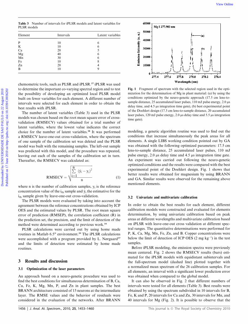
Table 3 Number of intervals for iPLSR models and latent variables forPLSR models

Element Intervals Latent variables

P 10 6K 10 6Ca 20 5Mg 40 6Mn 30 6Fe 10 8Zn 20 4B 10 9

Fig. 1 Fragment of spectrum with the selected region used in the opti-

mization for the determination of Mg in plant material: (a) by using the

conditions optimized by the neuro-genetic approach (17.5 cm lens-to-

sample distance, 25 accumulated laser pulses, 110 mJ pulse energy, 2.0 ms

delay time, and 4.5 ms integration time gate), (b) best experimental point

of the Doehlert design (17.3 cm lens-to-sample distance, 20 accumulated

laser pulses, 120 mJ pulse energy, 2.0 ms delay time and 5.5 ms integration

time gate).

Dow

nloa

ded

by U

NIV

ER

SID

AD

E D

E S

AO

PA

UL

O o

n 22

Aug

ust 2

010

Publ

ishe

d on

17

June

201

0 on

http

://pu

bs.r

sc.o

rg |

doi:1

0.10

39/C

0036

20J

View Online

chemometric tools, such as PLSR and iPLSR.37 iPLSR was used

to determine the important co-varying spectral region and to test

the possibility of developing an optimized local PLSR model

built on fewer variables for each element. A different number of

intervals were selected for each element in order to obtain the

best results with iPLSR.

The number of latent variables (Table 3) used in the PLSR

models was chosen based on the root mean square error of cross-

validation (RMSECV) values obtained for a trial number of

latent variables, where the lowest value indicates the correct

choice for the number of latent variables.38 It was performed

a RMSECV leave-one-out cross-validation, where the spectrum

of one sample of the calibration set was deleted and the PLSR

model was built with the remaining samples. The left-out sample

was predicted with this model, and the procedure was repeated,

leaving out each of the samples of the calibration set in turn.

Thereafter, the RMSECV was calculated as:

RMSECV ¼

ffiffiffiffiffiffiffiffiffiffiffiffiffiffiffiffiffiffiffiffiffiffiffiffiffiffiffiPi¼1

nðyi � yiÞ

2

n

vuuut(1)

where n is the number of calibration samples, yi is the reference

concentration value of the ith sample and yi the estimative for the

ith sample given by leave-one-out cross-validation.

The PLSR models were evaluated by taking into account the

agreement between the reference concentrations obtained by ICP

OES and the estimated values by PLSR. The root mean square

error of prediction (RMSEP), the correlation coefficient (R) in

the prediction set, the precision, and the limit of detection of the

method were determined according to previous work.14

PLSR calculations were carried out by using home made

routines in Matlab 6.5� environment.39 The iPLSR calculations

were accomplished with a program provided by L. Nørgaard37

and the limits of detection were estimated by home made

routines.

3 Results and discussion

3.1 Optimization of the laser parameters

An approach based on a neuro-genetic procedure was used to

find the best conditions for simultaneous determination of B, Ca,

Cu, Fe, K, Mg, Mn, P, and Zn in plant samples. The best

BRANN architecture consisted of 15 neurons at the intermediate

layer. The RMSE values and the behavior of residuals were

considered in the evaluation of the networks. After BRANN

1456 | J. Anal. At. Spectrom., 2010, 25, 1453–1460

modeling, a genetic algorithm routine was used to find out the

conditions that increase simultaneously the peak areas for all

elements. A single LIBS working condition pointed out by GA

was obtained with the following optimized parameters: 17.5 cm

lens-to-sample distance, 25 accumulated laser pulses, 110 mJ

pulse energy, 2.0 ms delay time and 4.5 ms integration time gate.

An experiment was carried out following the neuro-genetic

optimized conditions and the results were compared with the best

experimental point of the Doehlert design. Fig. 1 shows that

better results were obtained for magnesium by using BRANN

and GA. Similar results were observed for the remaining above

mentioned elements.

3.2 Univariate and multivariate calibration

In order to obtain the best results for each element, different

calibration models were constructed and evaluated for elements

determination, by using univariate calibration based on peak

areas at different wavelengths and multivariate calibration based

on iPLSR with leave-one-out cross validation at different spec-

tral ranges. The quantitative determinations were performed for

P, K, Ca, Mg, Mn, Fe, Zn, and B. Copper concentrations were

below the limit of detection of ICP OES (2 mg kg�1) in the test

samples.

Before iPLSR modeling, the emission spectra were previously

mean centered. Fig. 2 shows the RMSECV results (bars) esti-

mated for the iPLSR models with equidistant subintervals and

the full-spectrum model (dashed line) plotted together with

a normalized mean spectrum of the 26 calibration samples. For

all elements, an interval with a significant lower prediction error

was obtained when compared to the global model.

It can also be observed in Fig. 2 that different numbers of

intervals were tested for all elements (Table 3). Best results were

obtained by using the spectrum subdivided in 10 intervals for B,

Fe, K and P, 20 intervals for Ca and Zn, 30 intervals for Mn, and

40 intervals for Mg (Fig. 2). It is possible to observe that the

This journal is ª The Royal Society of Chemistry 2010

Fig. 2 Observed RMSECV values for iPLSR models for P, K, Ca, Mg, Mn, Fe, Zn and B divided in different subintervals, where the dotted line is the

RMSECV of the global model.

Dow

nloa

ded

by U

NIV

ER

SID

AD

E D

E S

AO

PA

UL

O o

n 22

Aug

ust 2

010

Publ

ishe

d on

17

June

201

0 on

http

://pu

bs.r

sc.o

rg |

doi:1

0.10

39/C

0036

20J

View Online

iPLSR models with the lowest RMSECV were obtained with the

interval numbers 1, 10, 19, 31, 18, 5, 1 and 2 for P, K, Ca, Mg,

Mn, Fe, Zn and B, respectively.

The numbers of latent variables selected in each spectral

interval for iPLSR modeling were 6, 6, 5, 6, 6, 8, 4 and 9 for P, K,

Ca, Mg, Mn, Fe, Zn and B, respectively. For Fe and B a rela-

tively high number of latent variables was necessary, which can

be justified by the high number of emission lines and the back-

ground variations to be modeled in the selected intervals.

This journal is ª The Royal Society of Chemistry 2010

Table 4 presents the average results of some figures of merit for

LIBS with PLSR and univariate regression. The standard devi-

ation of blank for each element, required for limits of detection

estimation, was assumed to be the standard deviation of a spec-

tral region that did not present emission signals and that was in

the selected interval for model development. Taking into account

the data presented in Table 1, it can be concluded that the limits

of detection obtained by univariate or PLSR model (Table 4) are

appropriate for P, K, Ca, Mg, Mn, Fe, Zn, and B in sugar cane

J. Anal. At. Spectrom., 2010, 25, 1453–1460 | 1457

Table 4 Average results of some figures of merit from univariate andPLSR calibrations

Element

Limit of detection(LOD) RMSEP a Mean Precision b

PLSR Univariate PLSR Univariate PLSR Univariate

P (g/kg) 0.03 0.02 0.07 0.07 0.05 0.08K (g/kg) 0.21 0.35 0.98 0.78 0.46 0.55Ca (g/kg) 0.08 0.08 0.30 0.39 0.16 0.22Mg (g/kg) 0.12 0.03 0.17 0.25 0.06 0.17Mn (mg/kg) 6.6 0.5 13 12 6.8 6.5Fe (mg/kg) 9.5 1.3 24 77 10 28Zn (mg/kg) 1.2 1.9 1.9 2.3 0.8 1.5B (mg/kg) 0.8 0.5 1.7 2.0 1.2 1.3

a Determined in analogy to the RMSECV (eqn (1)) but with thevalidation samples. b Estimated as the pooled standard deviation of thereplicates in the validation samples.

Dow

nloa

ded

by U

NIV

ER

SID

AD

E D

E S

AO

PA

UL

O o

n 22

Aug

ust 2

010

Publ

ishe

d on

17

June

201

0 on

http

://pu

bs.r

sc.o

rg |

doi:1

0.10

39/C

0036

20J

View Online

leaves. The RMSEP values showed that PLSR presented better

results than univariate regression for LIBS, with exception for K

and Mn. The most significant improvement in the results

obtained by PLSR was observed for Fe determination, where

better correlation between LIBS and ICP OES was obtained by

employing multivariate calibration (Fig. 3).

Table 4 shows that the mean precision results obtained by

PLSR model for LIBS were generally better than the univariate

model. When applying a F-test with 99% of confidence and 30

degrees of freedom, it was observed that the differences were

significant just for P, Mg, Fe and Zn, where PLSR was the most

precise method. It is important to note that, considering the

concentration ranges presented in Table 1 and the PLSR results,

the mean precision was lower than 5% for elements, excepting for

Fe and Zn.

The comparison of the prediction results of the validation

samples with LIBS and the reference values obtained by ICP

OES is shown in Fig. 4, where only the PLSR results for the LIBS

method are presented. In general, it can be observed that there

was a good agreement between PLSR results and ICP OES data.

Applying a paired t-test with all samples the calculated t-values

were 0.21 (P), 0.13 (K), 0.39 (Ca), 2.53 (Mg), 0.21 (Mn), 0.04

(Fe), 1.05 (Zn), and 0.94 (B). The critical values for the t-Student

distribution with 95 and 99% of confidence is 2.13 and 2.94,

respectively. Therefore, only for Mg there was a statistical

Fig. 3 Comparison of Fe results in sugar cane leaves obtained by ICP OES

PLSR calibrations. Dotted lines represent the best theoretical correlations be

1458 | J. Anal. At. Spectrom., 2010, 25, 1453–1460

difference between ICP OES and LIBS results at 95% confidence

level, but not at 99%.

It can be concluded that the success of LIBS for plant analysis

depends on the strategy chosen for appropriate calibration. It was

also evident that these results represent a significant improvement

on accuracy of LIBS over our recent contributions.12–14

4 Conclusions

There was a significant improvement over our previous contri-

butions, including sample preparation, optical setup optimiza-

tion (LTSD), development of global or matrix dependent

calibration models, choice of the appropriate regression model,

selection of variables and outliers identification.

The neuro-genetic optimization was efficient to maximize peak

areas of macro and micronutrients for simultaneous determina-

tions with appropriate sensitivities. In this context, integration

time gate, delay time, number of accumulated laser pulses, pulse

energy and lens-to-sample distance affected significantly the

results.

Data obtained confirm the good predictive ability of the PLSR

models based on calibration and validation samples composed

by the same plant specie, for avoiding or minimizing the occur-

rence of matrix effects suggested in previous work.14 The present

strategy makes possible the selection of the variables based on

the application of iPLSR with the full spectra, instead of the

manual selection of specific analyte lines.

By choosing calibration and validation samples with similar

chemical and physical matrix composition, good correlation

between LIBS and ICP OES results was obtained, which is

a good indication of better fitness for plant analysis and nutrient

diagnosis purposes.

Acknowledgments

Authors are thankful to CAPES (Coordenacao de Aperfeicoa-

mento de Pessoal de N�ıvel Superior), FAPESP (Fundacao de

Amparo �a Pesquisa do Estado de Sao Paulo, Process 04/15965-

2), CNPq (Conselho Nacional de Desenvolvimento Cient�ıfico e

Tecnol�ogico, Processes: 578728/2008-7, 550164/2009-0, 305913/

2009-3) for financial support and fellowships and to Ana Rita

Nogueira (EMBRAPA) for ICP OES analysis.

and (a) LIBS univariate at Fe II 259.940 nm and (b) LIBS multivariate

tween LIBS and ICP OES.

This journal is ª The Royal Society of Chemistry 2010

Fig. 4 Determination of P, K, Ca, Mg, Mn, Fe, Zn and B in pellets of sugar cane leaves after analysis of acid digests by ICP OES and LIBS multivariate

PLSR. Error bars represent �1 estimated standard deviation (n ¼ 3).

Dow

nloa

ded

by U

NIV

ER

SID

AD

E D

E S

AO

PA

UL

O o

n 22

Aug

ust 2

010

Publ

ishe

d on

17

June

201

0 on

http

://pu

bs.r

sc.o

rg |

doi:1

0.10

39/C

0036

20J

View Online

References

1 Industry Statistics: 2008 World Fuel Ethanol Production. RenewableFuels Association. <http://www.ethanolrfa.org/industry/statistics/#E>. Retrieved 01 February 2010.

2 Biofuels: The Promise and the Risks, in World Development Report2008. The World Bank. <http://go.worldbank.org/UK40ECPQ20>.Retrieved 01 February 2010.

3 Guia da Cana-de-ac�ucar. Conselho de Informacoes SobreBiotecnologia. <http://www.cib.org.br/pdf/guia_cana.pdf>.Retrieved 01 February 2010.

This journal is ª The Royal Society of Chemistry 2010

4 R. D. Reis and P. H. Monnerat, Pesq. Agropec. Bras., 2003, 38, 379–385.

5 G. C. L. Araujo, M. H. Gonzalez, A. G. Ferreira, A. R. A. Nogueiraand J. A. Nobrega, Spectrochim. Acta, Part B, 2002, 57, 2121–2132.

6 J. M. Frantz, J. C. Locke, L. Datnoff, M. Omer, A. Widrig, D. Sturtz,L. Horst and C. R. Krause, Commun. Soil Sci. Plant Anal., 2008, 39,2734–2751.

7 A. A. Momen, G. A. Zachariadis, A. N. Anthemidis and J. A. Stratis,Anal. Chim. Acta, 2006, 565, 81–88.

8 A. Sapkota, M. Krachler, C. Scholz, A. K. Cheburkin and W. Shotyk,Anal. Chim. Acta, 2005, 540, 247–256.

J. Anal. At. Spectrom., 2010, 25, 1453–1460 | 1459

Dow

nloa

ded

by U

NIV

ER

SID

AD

E D

E S

AO

PA

UL

O o

n 22

Aug

ust 2

010

Publ

ishe

d on

17

June

201

0 on

http

://pu

bs.r

sc.o

rg |

doi:1

0.10

39/C

0036

20J

View Online

9 N. S. Mokgalaka, R. I. McCrindle and B. M. Botha, J. Anal. At.Spectrom., 2004, 19, 1375–1378.

10 J. S. Alvarado, T. J. Neal, L. L. Smith and M. D. Erickson, Anal.Chim. Acta, 1996, 322, 11–20.

11 J. H. Baker and T. Grewelin, J. Agric. Food Chem., 1967, 15, 340.12 L. C. Trevizan, D. Santos, R. E. Samad, N. D. Vieira, C. S. Nomura,

L. C. Nunes, I. A. Rufini and F. J. Krug, Spectrochim. Acta, Part B,2008, 63, 1151–1158.

13 L. C. Trevizan, D. Santos, R. E. Samad, N. D. Vieira, L. C. Nunes,I. A. Rufini and F. J. Krug, Spectrochim. Acta, Part B, 2009, 64,369–377.

14 J. W. B. Braga, L. C. Trevizan, L. C. Nunes, I. A. Rufini, D. S. Juniorand F. J. Krug, Spectrochim. Acta, Part B, 2010, 65, 66–74.

15 V. Juve, R. Portelli, M. Boueri, M. Baudelet and J. Yu, Spectrochim.Acta, Part B, 2008, 63, 1047–1053.

16 J. Kaiser, M. Galiova, K. Novotny, R. Cervenka, L. Reale,J. Novotny, M. Liska, O. Samek, V. Kanicky, A. Hrdlicka,K. Stejskal, V. Adam and R. Kizek, Spectrochim. Acta, Part B,2009, 64, 67–73.

17 M. Pouzar, T. Cernohorsky, M. Prusova, P. Prokopcakova andA. Krejcova, J. Anal. At. Spectrom., 2009, 24, 953–957.

18 P. Geladi and B. R. Kowalski, Anal. Chim. Acta, 1986, 185, 1–17.19 J. G. Sun, J. Chemom., 1996, 10, 1–9.20 R. N. Feundale, N. A. Woody, H. W. Tan, A. J. Myles, S. D. Brown

and J. Ferre, Chemom. Intell. Lab. Syst., 2002, 64, 181–192.21 H. Martens and T. Naes, Multivariate Calibration, New York.

1989.22 B. R. Kowalski and M. B. Seasholtz, J. Chemom., 1991, 5, 129–145.

1460 | J. Anal. At. Spectrom., 2010, 25, 1453–1460

23 M. Forina, S. Lanteri and A. Casale, J. Chromatogr., A, 2007, 1158,61–93.

24 J. H. Kalivas, Anal. Lett., 2005, 38, 2259–2279.25 D. M. Haaland and E. V. Thomas, Anal. Chem., 1988, 60, 1193–1202.26 R. W. Gerlach, B. R. Kowalski and H. O. A. Wold, Anal. Chim. Acta-

Comp. Tech. Optimiz., 1979, 3, 417–421.27 K. R. Beebe and B. R. Kowalski, Anal. Chem., 1987, 59, 1007A–

1017A.28 B. Nadler and R. R. Coifman, J. Chemom., 2005, 19, 45–54.29 N. Labbe, I. M. Swamidoss, N. Andre, M. Z. Martin, T. M. Young

and T. G. Rials, Appl. Opt., 2008, 47, G158–G165.30 V. Sturm, H. U. Schmitz, T. Reuter, R. Fleige and R. Noll,

Spectrochim. Acta, Part B, 2008, 63, 1167–1170.31 M. E. Essington, G. V. Melnichenko, M. A. Stewart and R. A. Hull,

Soil Sci. Soc. Am. J., 2009, 73, 1469–1478.32 H. Balzer, S. Hoelters, V. Sturm and R. Noll, Anal. Bioanal. Chem.,

2006, 385, 234–239.33 E. Malavolta, Manual de Nutricao Mineral de Plantas, Editora

Agronomica Ceres Ltda, Sao Paulo. 2006.34 R. A. Multari, L. E. Foster, D. A. Cremers and M. J. Ferris, Appl.

Spectrosc., 1996, 50, 1483–1499.35 L. C. Nunes, G. A. da Silva, L. C. Trevizan, D. Santos, R. J. Poppi

and F. J. Krug, Spectrochim. Acta, Part B, 2009, 64, 565–572.36 K. Danzer and L. A. Currie, Pure Appl. Chem., 1998, 70, 993–1014.37 L. Nørgaard, A. Saudland, J. Wagner, J. P. Nielsen, L. Munck and

S. B. Engelsen, Appl. Spectrosc., 2000, 54, 413–419.38 E. V. Thomas, Anal. Chem., 1994, 66, A795–A804.39 B. S. Dayal and J. F. MacGregor, J. Chemom., 1997, 11, 73–85.

This journal is ª The Royal Society of Chemistry 2010