Heat Transfer—Asian Research, 43 (2), 2014

Optimal Homotopy Asymptotic Method for Heat Transfer inHollow Sphere with Robin Boundary Conditions

Fazle Mabood,1 Waqar A. Khan,

2 and Ahmad Izani Md Ismail

1

1School of Mathematical Sciences, Universiti Sains Malaysia, Penang, Malaysia

2Department of Engineering Sciences, National University of Sciences and Technology,

PNEC, Karachi, Pakistan

In this article, we have investigated heat transfer from a hollow sphere using

a powerful and relatively new semi-analytic technique known as the optimal homo-

topy asymptotic method (OHAM). Robin boundary conditions are applied on both

the inner and outer surfaces. The effects of Biot numbers, uniform heat generation,

temperature-dependent thermal conductivity, and temperature parameters on the

dimensionless temperature and heat transfer are investigated. The results of OHAM

are compared with a numerical method and are found to be in good agreement. It is

shown that the dimensionless temperature increases with an increase in Biot number

at the inner surface and temperature and heat generation parameters, whereas it de-

creases with an increase in the Biot number at the outer surface and the dimension-

less thermal conductivity and radial distance parameters. © 2013 Wiley Periodicals,

Inc. Heat Trans Asian Res 43(2): 124–133, 2014; Published online 20 June 2013 in

Wiley Online Library (wileyonlinelibrary.com/journal/htj). DOI 10.1002/htj.21067

Key words: OHAM, Robin boundary condition, heat transfer, hollow sphere

1. Introduction

Heat transfer is of importance in numerous applications in science and engineering [5, 12].

The study of heat transfer problems in hollow spheres has received considerable interest due to the

many possible applications. For example in biomedical ultrasonic imaging and underwater hy-

drophones, hollow sphere transducers may provide higher resolution due to smaller sphere sizes

than presently in use [1].

A discussion of standard solution techniques, both analytical and numerical, for heat conduc-

tion problems can be found in books such as Refs. 2 to 4. Some work on hollow shapes include that

of Jiang and Sousa [5] who derived an analytical expression for the temperature profile in a hollow

sphere with sudden temperature changes on its inner and outer surfaces. The authors also reported the

presence of hyperbolic anomalies inside the hollow sphere with the use of Dirichlet boundary

conditions.

© 2013 Wiley Periodicals, Inc.

124

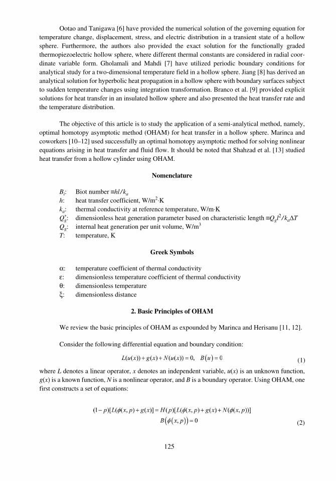
Ootao and Tanigawa [6] have provided the numerical solution of the governing equation for

temperature change, displacement, stress, and electric distribution in a transient state of a hollow

sphere. Furthermore, the authors also provided the exact solution for the functionally graded

thermopiezoelectric hollow sphere, where different thermal constants are considered in radial coor-

dinate variable form. Gholamali and Mahdi [7] have utilized periodic boundary conditions for

analytical study for a two-dimensional temperature field in a hollow sphere. Jiang [8] has derived an

analytical solution for hyperbolic heat propagation in a hollow sphere with boundary surfaces subject

to sudden temperature changes using integration transformation. Branco et al. [9] provided explicit

solutions for heat transfer in an insulated hollow sphere and also presented the heat transfer rate and

the temperature distribution.

The objective of this article is to study the application of a semi-analytical method, namely,

optimal homotopy asymptotic method (OHAM) for heat transfer in a hollow sphere. Marinca and

coworkers [10–12] used successfully an optimal homotopy asymptotic method for solving nonlinear

equations arising in heat transfer and fluid flow. It should be noted that Shahzad et al. [13] studied

heat transfer from a hollow cylinder using OHAM.

Nomenclature

Bi: Biot number ≡hl / ka

h: heat transfer coefficient, W/m2⋅Kka: thermal conductivity at reference temperature, W/m⋅KQg

∗: dimensionless heat generation parameter based on characteristic length ≡Qgl2

/ kaΔTQg: internal heat generation per unit volume, W/m3

T: temperature, K

Greek Symbols

α: temperature coefficient of thermal conductivity

ε: dimensionless temperature coefficient of thermal conductivity

θ: dimensionless temperature

ξ: dimensionless distance

2. Basic Principles of OHAM

We review the basic principles of OHAM as expounded by Marinca and Herisanu [11, 12].

Consider the following differential equation and boundary condition:

where L denotes a linear operator, x denotes an independent variable, u(x) is an unknown function,

g(x) is a known function, N is a nonlinear operator, and B is a boundary operator. Using OHAM, one

first constructs a set of equations:

(1)

(2)

125

where 0 ≤ p ≤ 1 is an embedding parameter, H(p) is a nonzero auxiliary function for p ≠ 0 and

H(0) = 0, φ(x, p) is an unknown function. For p = 0 and p = 1,

Thus, as p increases from 0 to 1, the solution φ(x, p) varies from u0(x) to the solution u(x), where

u0(x) is obtained from Eq. (2) for p = 0.

The auxiliary function H(p) is chosen in the form:

where C1, C2, . . . are constants which are to be determined.

Expanding φ(x, p, Ci) in a Taylor’s series about p, we obtain:

Substituting Eqs. (5) and (6) into Eq. (2), collecting the same powers of p, and equating each

coefficient of p to zero, we obtain the set of differential equations with boundary conditions. Solving

the differential equations and boundary conditions will result in the zeroth-, first-, second-order

solutions u0(x), u1(x, C1), u2(x, C1, C2), . . . being obtained.

Generally speaking, the approximate solution of Eq. (1) can be determined as

Substituting Eq. (7) in Eq. (1) results in the following residual:

If R(x, Ci) = 0, then u~ will be the exact solution, although for nonlinear problems generally this will

not be the case.

For determining Ci(i = 1, 2, . . . m), the method of least squares is used:

where a and b are chosen such that the optimum values for Ci are obtained from the condition:

With these constants, one can get the approximate solution of order m.

3. Problem Formulation

We consider a hollow sphere with inside radius r1, outside radius r2, which is made of a

material with temperature-dependent thermal conductivity k(T). The sphere undergoes a uniform

(3)

(4)

(5)

(6)

(7)

(8)

(9)

(10)

126

volumetric internal heat generation Qg. For our problem, we consider the case where the thermal

conductivity is a linear function of temperature T, i.e.,

where λ1 = Ta / Tf1 << 1 and ε = αTf1 and where ka is the thermal conductivity at the ambient

temperature and α is the thermal expansion coefficient. The governing equation for the hollow sphere

can be written as

The inside surface of the sphere is assumed to be in contact with a coolant at temperature Tf1 which

provides a convective heat transfer coefficient h1. The outside surface of the sphere is assumed to be

cooled by a fluid at temperature Tf2 providing a convective heat transfer coefficient h2, i.e.,

Assuming

The transformed equation can be written as

with boundary conditions

4. OHAM Solution for Heat Transfer in Hollow Sphere

Applying the mentioned method (OHAM) to Eqs. (15) and (16), we obtain for

Bi1 = 0.1, Bi2 = 0.5, λ = 1.2

Zeroth-order problem:

(11)

(12)

(13)

(14)

(15)

(16)

(17)

127

with boundary conditions:

Its solution is

First-order problem:

with boundary conditions:

Its solution is

Second-order problem:

with boundary conditions:

Its solution is

(18)

(19)

(20)

(22)

(24)

(23)

(21)

128

Using Eqs. (19), (22), and (25), the second-order approximate solution by OHAM for p = 1 can be

written as

We use the method of least squares to obtain the values of unknown C1, C2 convergent constants and

after substituting the values of C1, C2 in Eq. (26), we get the second-order approximate solution of

dimensionless temperature θ(ξ).

In particular, for Bi1 = 0.1, Bi2 = 0.5, Qg = 1, R = 2, λ = 1.2, o = −0.1.

The approximate solution is

where C1 = 0.7114, C2 = −3.2112.

5. Results and Discussion

Figure 1 shows the comparison of OHAM and numerical results of the dimensionless

temperature for the specific values of the controlling parameters. The OHAM results are found to be

in good agreement with the numerical results. Figure 2 shows the temperature distribution in a hollow

(25)

(26)

129

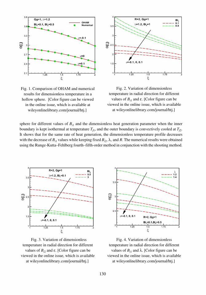
sphere for different values of Bi1 and the dimensionless heat generation parameter when the inner

boundary is kept isothermal at temperature Tf1, and the outer boundary is convectively cooled at Tf2.

It shows that for the same rate of heat generation, the dimensionless temperature profile decreases

with the decrease of Bi1 values while keeping fixed Bi2, λ, and R. The numerical results were obtained

using the Runge-Kutta–Fehlberg fourth–fifth-order method in conjunction with the shooting method.

Fig. 1. Comparison of OHAM and numerical

results for dimensionless temperature in a

hollow sphere. [Color figure can be viewed

in the online issue, which is available at

wileyonlinelibrary.com/journal/htj.]

Fig. 2. Variation of dimensionless

temperature in radial direction for different

values of Bi1 and ε. [Color figure can be

viewed in the online issue, which is available

at wileyonlinelibrary.com/journal/htj.]

Fig. 3. Variation of dimensionless

temperature in radial direction for different

values of Bi2 and ε. [Color figure can be

viewed in the online issue, which is available

at wileyonlinelibrary.com/journal/htj.]

Fig. 4. Variation of dimensionless

temperature in radial direction for different

values of Bi1 and λ. [Color figure can be

viewed in the online issue, which is available

at wileyonlinelibrary.com/journal/htj.]

130

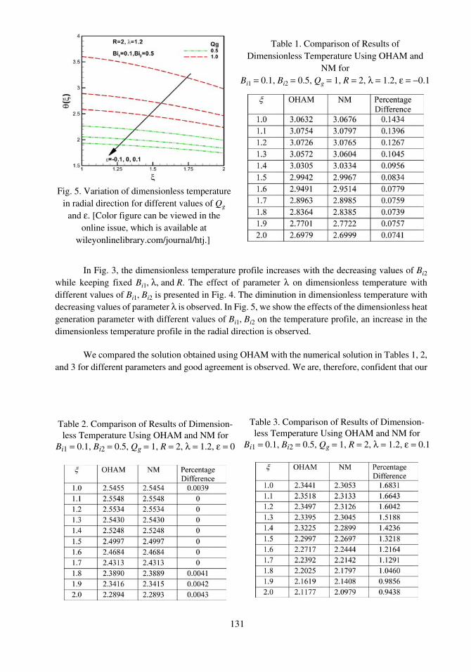
In Fig. 3, the dimensionless temperature profile increases with the decreasing values of Bi2

while keeping fixed Bi1, λ, and R. The effect of parameter λ on dimensionless temperature with

different values of Bi1, Bi2 is presented in Fig. 4. The diminution in dimensionless temperature with

decreasing values of parameter λ is observed. In Fig. 5, we show the effects of the dimensionless heat

generation parameter with different values of Bi1, Bi2 on the temperature profile, an increase in the

dimensionless temperature profile in the radial direction is observed.

We compared the solution obtained using OHAM with the numerical solution in Tables 1, 2,

and 3 for different parameters and good agreement is observed. We are, therefore, confident that our

Table 1. Comparison of Results of

Dimensionless Temperature Using OHAM and

NM for

Bi1 = 0.1, Bi2 = 0.5, Qg = 1, R = 2, λ = 1.2, ε = −0.1

Fig. 5. Variation of dimensionless temperature

in radial direction for different values of Qg

and ε. [Color figure can be viewed in the

online issue, which is available at

wileyonlinelibrary.com/journal/htj.]

Table 2. Comparison of Results of Dimension-

less Temperature Using OHAM and NM for

Bi1 = 0.1, Bi2 = 0.5, Qg = 1, R = 2, λ = 1.2, ε = 0

Table 3. Comparison of Results of Dimension-

less Temperature Using OHAM and NM for

Bi1 = 0.1, Bi2 = 0.5, Qg = 1, R = 2, λ = 1.2, ε = 0.1

131

results using OHAM are correct and accurate. Finally, the corresponding values of unknown

convergent constants C1, C2 in each figure are given in Table 4.

6. Conclusions

In this study, we have successfully applied the optimal homotopy asymptotic method for the

steady-state heat conduction with temperature-dependent thermal conductivity and uniform heat

generation in a hollow sphere. It is observed that the dimensionless temperature and heat transfer

depends on the uniform heat generation parameter, thermal conductivity, and Biot numbers. The

solution obtained using OHAM is consistent with the solution obtained using a numerical method for

variation of different parameters and thus confirms the effectiveness of OHAM.

Literature Cited

1. Cochran JK. Ceramic hollow sphere and their application. Current Opinion Solid State Mater

Sci 1998;3(5):474–479.

2. Ozisik MN. Heat conduction. Wiley; 1980.

3. Kreith F (editor). CRC handbook of thermal engineering. CRC Press; 2000.

4. Arpaci V. Conduction heat transfer. Addison-Wesley; 1966.

5. Jiang F, Sousa ACM. Analytical solution for hyperbolic heat propagation in a hollow sphere.

AIAA J Thermophys Heat Transf 2005;19:595–598.

6. Ootao Y, Tanigawa Y. Transient piezothermoelastic analysis for a functionally graded ther-

mopiezoelectric hollow sphere. Composite Structures 2007;81:540–549.

7. Gholamali A, Mahdi M. A temperature Fourier series solution for a hollow sphere. J Heat

Transf 2006;128:963–968.

8. Jiang F. Solution and analysis of hyperbolic heat propagation in hollow spherical objects. Heat

Mass Transf 2006;42:1083–1091.

9. Branco JF, Pinho CT, Figueiredo RA. Heat conduction in the hollow sphere with a power-law

variation of the external heat transfer coefficient. Int Comm Heat Mass Transf 2000;27:1067–

1076.

10. Marinca V, Herisanu N. Application of optimal homotopy asymptotic method for solving

nonlinear equations arising in heat transfer. Int Commun Heat Mass Transf 2008;35:710–715.

11. Marinca V, Herisanu N, Bota C, Marinca B. An optimal homotopy asymptotic method applied

to the steady flow of a fourth grade fluid past a porous plate. Appl Math Lett 2009;22:245–251.

Table 4. Values of Convergent Constants C1, C2 in Different Figures

132

12. Marinca V, Herisanu N, Nemes I. Optimal homotopy asymptotic method with application to

thin film flow. Central European J Phys 2008;6(3):648–653.

13. Shahzad A, Khan WA, Hussain AK. Heat transfer from hollow cylinder using optimal

homotopy asymptotic method. Heat Transf Asian Res 2012;41:114–126.

"F F F"

133