PAPER KIMIA UNSUR UNSUR LOGAM GOLONGAN TRANSISI GOLONGAN IIIB DAN IVB
Upload
khangminh22Category
view
0download
0
OPTICAL FIBER TE LE C 0 M M U N I CAT I
SYSTEMS AND IMPAIRMENTS


OPTICAL FIBER TELECOMMUNICATIONS IV B SYSTEMS AND IMPAIRMENTS


OPTICAL FIBER TELECOMMUNICATIONS IV B SYSTEMS AND IMPAIRMENTS
Edited by IVAN P. KAMINOW Bell Laboratories (retired) Kaminow Lightwave Technology Holmdel, New Jersey
TINGYE LI AT&T Labs (retired) Boulder, Colorado
ACADEMIC PRESS An Elsevier Science Imprint
San Diego San Francisco New York Boston London Sydney Tokyo

This book is printed on acid-free paper. @
Copyright @ 2002, Elsevier Science (USA). All rights reserved.
No part of this publication may be reproduced or transmitted in any form or by any means, electronic or mechanical, including photocopy, recording, or any information storage and retrieval system, without permission in writing from the publisher.
The appearance of the code at the bottom of the h s t page of a chapter in this book indicates the Publisher’s consent that copies of the chapter may be made for personal or internal use of speci6c clients. This consent is given on the condition, however, that the copier pay the stated per copy fee through the Copyright Clearance Center, Inc. (222 Rosewood Drive, Danvers, Massachusetts 01923), for copying beyond that permitted by Sections 107 or 108 of the U.S. Copyright Law. This consent does not extend to other kinds of copying, such as copying for general distribution, for advertising or promotional purposes, for creating new collective works, or for resale. Copy fees for pre-2001 chapters are as shown on the title pages. If no fee code appears on the title page, the copy fee is the same as for current chapters. $35.00.
Academic Press An Elsevier Science Imprint 525 B Street, Suite 1900, San Diego, California 92101-4495, USA http://www.academicpress.com
Academic Press Harcourt Place, 32 Jamestown Road, London NW17BY, UK http://www.academicpress.com
Library of Congress Control Number: 2001098830
International Standard Book Number: 0-12-395173-9
PRINTED IN CHINA 02 03 04 05 06 07 RDC 9 8 7 6 5 4 3 2 1

For Florence and Edith, with love


Contents
Contributors xi
Chapter 1 Overview
Ivan 19 Kaminow
Chapter 2 Growth of the Internet
Kerry G. Coflman and Andrew M. Odbzko
Chapter 3 Optical Network Architecture Evolution
John Strand
Chapter 4 Undersea Communication Systems
Neal S. Bergano
Chapter 5 High-Capacity, Ultra-Long-Haul Networks
John Zyskind, Rick Bany, Graeme Pendock, Michael Cahill, and Jinendra Ranka
1
17
57
154
198
Chapter 6 Pseudo-Linear Transmission of High-speed TDM Signals: 40 and 160 Gb/s
Red-Jean Essiambre, Gregory Raybon, and Benny Mikkelsen
232
vii

viii Contents
Chapter 7 Dispersion-Managed Solitons and Chirped Return to Zero: What Is the Difference? 305
Curtis R. Menyuk, Gary M. Carter; William L. Kath, and Ruo-Mei Mu
Chapter 8 Metropolitan Optical Networks
Nasir Ghani, Jin-B Pan, and Xin Cheng
Chapter 9 The Evolution of Cable TV Networks
Xiaolin Lu and OIeh Sneizka
Chapter 10 Optical Access Networks
Edward Harstead and Pieter H. van Heyningen
329
404
438
Chapter 11 Beyond Gigabit: Application and Development of High-speed Ethernet Technology 514
Cedric E Lam
Chapter 12 Photonic Simulation Tools
Arthur J. Lowery
Chapter 13 Nonlinear Optical Effects in WDM Transmission
Polina Bayvel and Robert Killey
564
61 1
Chapter 14 Fixed and Tunable Management of Fiber Chromatic Dispersion 642
Alan E. Willner and Bogdan Hoanca
Chapter 15 Polarization-Mode Dispersion
Herwig Kogelnik, Robert M. Jopson, and Lynn E. Nelson
725
Contents ix
Chapter 16 Bandwidth-Efficient Modulation Formats for Digital Fiber Transmission Systems 862
Jan Conradi
Chapter 17 Error-Control Coding Techniques and Applications 902
E! Vjay Kumar, Moe Z. Win, Hsiao-Feng Lu, and Costas N. Georghiades
Chapter 18 Equalization Techniques for Mitigating Transmission Impairments 965
Moe Z. Win, Jack H. Winters, and Giorgio M. Etetta
Index to Volumes IVA and IVB 999

Contributors
D. A. Ackerman (A:587), Agere Systems, 600 Mountain Avenue, Murray Hill,
Daniel Y. Al-Salameh (A295), JDS Uniphase Corporation, 100 Willowbrook
Rick Barry (B: 198), Sycamore Networks, 10 Elizabeth Drive, Chelmsford,
Polina Bayvel (B:61 l), Optical Networks Group, Department of Elec- tronic and Electrical Engineering, University College London (UCL), Torrington Place, London WCl E 7JE, United Kingdom
Neal S. Bergano (B: 154), Tyco Telecommunications, 250 Industrial Way West, Eatontown, New Jersey 07724-2206
Lee L. Blyler (A:17), OFS Fitel, LLC, 600 Mountain Avenue, Murray Hill, New Jersey 07974
Raymond K. Boncek (A: 17), OFS Fitel, LLC, 600 Mountain Avenue, Murray Hill, New Jersey 07974
Michael Cahil (B: 198), Sycamore Networks, 10 Elizabeth Drive, Chelmsford, Massachusetts 01824-41 11
Gary M. Carter (B:305), Computer Science and Electrical Engineering Department, TRC-20 1 A, University of Maryland Baltimore County, 1000 Hilltop Circle, Baltimore, Maryland 21250 and Laboratory for Physical Sciences, College Park, Maryland
Connie J. Chang-Hasnain (A:666), Department of Electrical Engineering and Computer Science, University of California, Berkeley, California 94720 and Bandwidth 9 Inc., 46410 Fremont Boulevard, Fremont, California 94538
Young-Kai Chen (A:784), Lucent Technologies, High Speed Electronics Research, 600 Mountain Avenue, Murray Hill, New Jersey 07974
Xin Cheng (B:329), Sorrento Networks Inc., 9990 Mesa Rim Drive, San Diego, California 921 2 1-2930
New Jersey 07974
Road, Bldg. 1 , Freehold, New Jersey 07728-2879
Massachusetts 01 824-41 11
xi

xu Contributors
Dominique Chiaroni (A:732), Alcatel Research & Innovation, Route de Nozay, F-9 146 1 Marcoussis cedex, France
Kerry G. Coffman (B:17), AT&T Labs-Research, A5-1D03, 200 Laurel Avenue South, Middletown, New Jersey 07748
Jan Conradi (B:862), Director of Strategy, Corning Optical Communications, Corning Incorporated, MP-HQ-Wl-43, One River Front Plaza, Corning, New York 14831
Santanu JL Das (A: 17), OFS Fitel, LLC, 600 Mountain Avenue, Murray Hill,
Emmanuel Desurvire (A:732), Alcatel Technical Academy, Villarceaux,
David J. DiGiovanni (A:17), OFS Fitel, LLC, 600 Mountain Avenue, Murray
Christopher R Doerr (A:405), Bell Laboratories, Lucent Technologies, 791
Adam Ellison (A:80), Corning, Inc., SP-FR-05, Corning, New York 14831
L. E. Eng (A:587), Agere Systems, Room 2F-204, 9999 Hamilton Blvd., Breinigsville, Pennsylvania 1803 1-9304
Turan Erdogan (A:477), Semrock, Inc., 3625 Buffalo Road, Rochester, New York 14624
RenkJean Essiambre (B:232), Bell Laboratories, Lucent Technologies, 79 1 Holmdel-Keyport Road, Holmdel, New Jersey 07733
Costas N. Georghiades (B:902), Texas A&M University, Electrical Engineer- ing Department, 237 Wisenbaker, College Station, Texas 77843-3 128
Nasir Ghani (B:329), Sorrento Networks Inc., 9990 Mesa Rim Drive, San Diego, California 92121-2930
Steven E. Golowich (A: 17), Bell Laboratories, Lucent Technologies, Room 2C-357,600 Mountain Avenue, Murray Hill, New Jersey 07974
Christoph S. Harder (A:563), Nortel Networks Optical Components, Binzstrasse 17, CH-8045 Zurich, Switzerland
Edward Harstead (B:438), Bell Laboratories, Lucent Technologies, 101 Crawford Corners Road, Holmdel, New Jersey 07733
Bogdan Hoanca (B:642), Phaethon Communications, Inc., Fremont, California 96538
New Jersey 07974
F-9 1625 Nozay cedex, France
Hill, New Jersey 07974
Holmdel-Keyport Road, Holmdel, New Jersey 07733
Contributors xiii
J. E. Johnson (A587), Agere Systems, 600 Mountain Avenue, Murray Hill, New Jersey 07974
Robert M. Jopson (B:725), Crawford Hill Laboratory, Bell Laboratories, Lucent Technologies, 79 1 Holmdel-Keyport Road, Holmdel, New Jersey 07733
Ivan P. Kaminow (A: 1 , B: l), Bell Laboratories (retired), Kaminow Lightwave Technology, 12 Stonehenge Drive, Holmdel, New Jersey 07733
Bryon L. Kasper (A:784), Agere Systems, Advanced Development Group, 4920 Rivergrade Road, Irwindale, California 91 706-1404
William L. Kath (B:305), Computer Science and Electrical Engineering Department, University of Maryland Baltimore County, 1000 Hilltop Circle, Baltimore, Maryland 21250 and Applied Mathematics Depart- ment, Northwestern University, 2145 Sheridan Road, Evanston, Illinois
L. J. P. Ketelsen (A:587), Agere Systems, 600 Mountain Avenue, Murray Hill, New Jersey 07974
P. A. Kiely (A:587), Agere Systems, 9999 Hamilton Blvd., Breinigsville, Pennsylvania 1803 1-9304
Robert Killey (B:61 l), Optical Networks Group, Department of Elec- tronic and Electrical Engineering, University College London (UCL), Torrington Place, London WClE 7JE, United Kingdom
Herwig Kogelnik (B:725), Crawford Hill Laboratory, Bell Laboratories, Lucent Technologies, 79 1 Holmdel-Keyport Road, Holmdel, New Jersey 07733
Steven K Korotky (A295), Bell Laboratories, Lucent Technologies, Room HO 3C-351,101 Crawfords Corner Road, Holmdel, New Jersey 07733-1900
P. Mjay Kumar (B:902), Communication Science Institute, Department of Electrical Engineering - Systems, University of Southern California, 3740 McClintock Avenue, EEBSOO, Los Angeles, California 90089-2565 and Scintera Networks, Inc., San Diego, California
Cedric E Lam (B:514), AT&T Labs-Research, 200 Laurel Avenue South, Middletown, New Jersey 07748
Bruno Lavigne (A:732), Alcatel CIT/ Research & Innovation, Route de Nozay, F-91461 Marcoussis cedex, France
Olivier Leclerc (A732), Alcatel Research & Innovation, Route de Nozay, F-91460 Marcoussis cedex, France
60208-3125
xiv Contributors
David S. Levy (A295), Bell Laboratories, Lucent Technologies, Room HO 3B-506, 101 Crawfords Corner Road, Holmdel, New Jersey 07733-3030
Arthur J. Lowery (B:564), VPIsystems Inc., Design Center Group, 17-27 Cotham Road, Kew, Melbourne 3101, Australia
Xiaolin Lu (B:404), Morning Forest, LLC, 8804 S. Blue Mountain Place, Highlands Ranch, Colorado 80126
Hsiao-Feng Lu (B:902), Communication Science Institute, Department of Electrical Engineering - Systems, University of Southern California, 3740 McClintock Avenue, EEBSOO, Los Angeles, California 90089-2565
Amaresh Mahapatra (A:258), Linden Corp., 10 Northbriar Road, Acton, Massachusetts 01720
T. G. B. Mason (A:587), Agere Systems, 9999 Hamilton Blvd., Breinigsville, Pennsylvania 1803 1-9304
Curtis R. Menyuk (B:305), Computer Science and Electrical Engineering Department, TRC-20 1 A, University of Maryland Baltimore County 1000 Hilltop Circle, Baltimore, Maryland 21250 and PhotonEx Cor- poration, 200 MetroWest Technology Park, Maynard, Massachusetts 0 1754
Benny Mikkelsen (B:232), Mintera Corporation, 847 Rogers Street, One Lowell Research Center, Lowell, Massachusetts 01 852
John Minelly (A:80), Corning, Inc., SP-AR-02-01, Corning, New York 14831
Osamu Muuhara (A:784), Agere Systems, Optical Systems Research, 9999 Hamilton Blvd., Breinigsville, Pennsylvania 1803 1
Stefan Mohrdiek (A:563), Nortel Networks Optical Components, Binzstrasse 17, CH-8045 Ziirich, Switzerland
Ruo-Mei Mu (B:305), Tyco Telecommunications, 250 Industrial Way West, Eatontown, New Jersey 07724-2206
Edmond J. Murphy (A:258), JDS Uniphase, 1985 Blue Hills Avenue Ext., Windsor, Connecticut 06095
Timothy 0. Murphy (A:295), Bell Laboratories, Lucent Technologies, Room HO 3D-516, 101 Crawfords Corner Road, Holmdel, New Jersey 07733- 3030
Lynn E. Nelson (B:725), OFS Fitel, Holmdel, New Jersey 07733
Andrew M. Odlyzko (B:17), University of Minnesota Digital Technology Center, 1200 Washington Avenue S., Minneapolis, Minnesota 5541 5
Contributors xv
Jin-Yi Pan (B:329), Sorrento Networks Inc., 9990 Mesa Rim Drive, San Diego, California 92121 -2930
Sunita 18. Pate1 (A:295), Bell Laboratories, Lucent Technologies, Room HO 3D-502,101 Crawfords Comer Road, Holmdel, New Jersey 07733-3030
Graeme Pendock (B: 198), Sycamore Networks, 10 Elizabeth Drive, Chelms- ford, Massachusetts 01824-41 11
Jinendra Ranka (B: 198), Sycamore Networks, 10 Elizabeth Drive, Chelms- ford, Massachusetts 01824-41 11
Gregory Raybon (B:232), Bell Laboratories, Lucent Technologies, 79 1 Holmdel-Keyport Road, Holmdel, New Jersey 07733
Gaylord W. Richards (A:295), Bell Laboratories, Lucent Technologies, Room 6L-219,2000 Naperville Road, Naperville, Illinois 60566-7033
Karsten Rottwitt (A:213), Orsted Laboratory, Niels Bohr Institute, University of Copenhagen, Universitetsparken 5, Copenhagen dk 2 100, Denmark
Bertold E. Schmidt (A: 563), Nortel Networks Optical Components, Binzs- trasse 17, Ch-8045 Zurich, Switzerland
Oleh Sniezko (B:404), Oleh-Lightcom, Highlands Ranch, Colorado 801 26
Leo H. Spiekman (A:699), Genoa Corporation, Lodewijkstraat 1 A, 5652 AC
Atul K. Srivastava (A:174), Onetta Inc., 1195 Borregas Avenue, Sunnyvale,
Andrew J. Stentz (A:213), Photuris, Inc., 20 Corporate Place South, Piscataway, New Jersey 08809
John Strand (B:57), AT&T Laboratories, Lightwave Networks Research Department, RoomA5-106,200 Laurel Avenue, Middletown, New Jersey 07748
Thomas A. Strassser (A:477), Photuris Inc., 20 Corporate Place South,
Yan Sun (A:174), Onetta Inc., 1195 Borregas Avenue, Sunnyvale, California
Eric S. Tentarelli (A:295), Bell Laboratories, Lucent Technologies, Room HO 3B-530,101 Crawfords Corner Road, Holmdel, New Jersey 07733-3030
Pieter H. van Heyningen (B:438), Lucent Technologies NL, PO. Box 18, Huizen 1270AA, The Netherlands
Eindhoven, The Netherlands
California 94089
Piscataway, New Jersey 08854
94089

xvi Contributors
Giorgio M. Vitetta (B:965), University of Modena and Reggio Emilia, Depart- ment of Information Engineering, Via Vignolese 905, Modena 41100, Italy
W. White (A:17), OFS Fitel, LLC, 600 Mountain Avenue, Murray Hill, New Jersey 07974
Alan E. Willner (B:642), University of Southern California, Los Angeles, California 90089-2565
Moe Z. Win (B:902, B:965), AT&T Labs-Research, Room A5-1D01, 200 Laurel Avenue South, Middletown, New Jersey 07748-1914
Jack H. Winters (B:965), AT&T Labs-Research, Room 4-147, 100 Schulz Drive, Middletown, New Jersey 07748- 19 14
Martin Zirngibl (A:374), Bell Laboratories, Lucent Technologies, 79 1 Holmdel-Keyport Road, Holmdel, New Jersey 07733-0400
John Zyskind (B: 198), Sycamore Networks, 10 Elizabeth Drive, Chelmsford, Massachusetts 0 1824-41 1 1
Ivan P. Kaminow Bell Laboratories (retired), Kaminow Lightwave Technology, Holmdel, New Jerscy
Introduction
Modern lightwave communications had its origin in the first demonstrations of the laser in 1960. Most of the early lightwave R&D was pursued by estab- lished telecommunications company labs (AT&T, NTT, and the British Post Office among them). By 1979, enough progress had been made in light- wave technology to warrant a book, Optical Fiber Telecommunications (OFlJ, edited by S. E. Miller and A. G. Chynoweth, summarizing the state of the art. Two sequels have appeared: in 1988, OFT 11, edited by S. E. Miller and I. P. Kaminow, and in 1997, OFT 111 (A & B), edited by I. P. Kaminow and T. L. Koch. The rapid changes in the field now call for a fourth set of books, OFTW (A & B).
This chapter briefly summarizes the previous books and chronicles the remarkably changing climates associated with each period of their publica- tion. The main purpose, however, is to summarize the chapters in OFT IV in order to give the reader an overview.
History
While many excellent books on lightwave communications have been pub- lished, this series has developed a special character, with a reputation for comprehensiveness and authority, because of its unique history. Optical Fiber Telecommunications was published in 1979, at the dawn of the revolution in lightwave telecommunications. It was a stand-alone work that aimed to collect all available information on lightwave research. Miller was Director of the Lightwave Systems Research Laboratory and, together with Rudi Kompfner, the Associate Executive Director, guided the system research at the Crawford Hill Laboratory of AT&T Bell Laboratories; Chynoweth was an Executive Director in the Murray Hill Laboratory, leading the optical fiber research. Many groups were active at other laboratories in the United States, Europe, and Japan. OFT, however, was written exclusively by Bell Laboratories authors, who nevertheless aimed to incorporate global results.
1 OPTICAL FIBER TELECOMMUNICATIONS, VOLUME IVB
Copyright 0 2002, Elsevier Science (USA). All rights of reproduction in any form reserved.
ISBN 0-12-395173-9

2 Ivan P. Kaminow
Miller and Chynoweth had little trouble finding suitable chapter authors at Bell Labs to cover practically all the relevant aspects of the field at that time.
Looking back at that volume, it is interesting that the topics selected are still quite basic. Most of the chapters cover the theory, materials, mea- surement techniques, and properties of fibers and cables (for the most part, multimode fibers). Only one chapter covers optical sources, mainly multi- mode AlGaAs lasers operating in the 800- to 900-nm band. The remaining chapters cover direct and external modulation techniques, photodetectors and receiver design, and system design and applications Still, the basic elements of the present day systems are discussed: low-loss vapor-phase silica fiber and double-heterostructure lasers.
Although system trials were initiated around 1979, it required several more years before a commercially attractive lightwave telecommunications system was installed in the United States. The AT&T Northeast Corridor System, operating between New York and Washington, DC, began service in January 1983, operating at a wavelength of 820 nm and a bit rate of 45 Mb/s in multi- mode fiber. Lightwave systems were upgraded in 1984 to 1310nm and 417 or 560 Mb/s in single-mode fiber in the United States as well as in Europe and Japan.
The year 1984 also saw the Bell System broken up by the court-imposed “Modified Final Judgment” that separated the Bell operating companies into seven regional companies and left AT&T as the long distance camer as well as a telephone equipment vendor. Bell Laboratories remained with AT&T, and Bellcore was formed to serve as the R&D lab for all seven regional Bell operat- ing companies (RBOCs). The breakup spurred a rise in diversity and competi- tion in the communications business. The combination of technical advances in computers and communications, growing government deregulation, and apparent new business opportunities all served to raise expectations.
Tremendous technical progress was made during the next few years, and the choice of lightwave over copper coaxial cable or microwave relay for most long- haul transmission systems was assured. The goal of research was to improve performance, such as bitrate and repeater spacing, and to find other applica- tions beyond point-to-point long haul telephone transmission. A completely new book, Optical Fiber Telecommunications 11, was published in 1988 to sum- marize the lightwave R&D advances at the time. To broaden the coverage, non- Bell Laboratories authors from Bellcore (now Telcordia), Corning, Nippon Electric Corporation, and several universities were represented among the contributors. Although research results are described in OFT 11, the emphasis is much stronger on commercial applications than in the previous volume.
The initial chapters of OFT 11 cover fibers, cables, and connectors, deal- ing with both single- and multimode fiber. Topics include vapor-phase methods for fabricating low-loss fiber operating at 13 10 and 1550 nm, understanding chromatic dispersion and nonlinear effects, and designing polarization-maintaining fiber. Another large group of chapters deals with
1.Overview 3
a range of systems for loop, intercity, interoffice, and undersea applications. A research-oriented chapter deals with coherent systems and another with possible local area network designs, including a comparison of time-division multiplexing (TDM) and wavelength division multiplexing (WDM) to effi- ciently utilize the fiber bandwidth. Several chapters cover practical subsystem components, such as receivers and transmitters and their reliability. Other chapters cover photonic devices, such as lasers, photodiodes, modulators, and integrated electronic and integrated optic circuits that make up the subsys- tems. In particular, epitaxial growth methods for InGaAsP materials suitable for 13 10 and 1550 nm applications and the design of high-speed single-mode lasers are discussed in these chapters.
By 1995, it was clear that the time had arrived to plan for a new volume to address recent research advances and the maturing of lightwave systems. The contrast with the research and business climates of 1979 was dramatic. Sophisticated system experiments were being performed utilizing the commer- cial and research components developed for a proven multibillion-dollar global lightwave industry. For example, 10,000-km lengths of high-performance fiber were assembled in several laboratories around the world for nonreturn-to-zero (NRZ), soliton, and WDM transmission demonstrations. Worldwide regula- tory relief stimulated the competition in both the service and hardware ends of the telecommunications business. The success in the long-haul market and the availability of relatively inexpensive components led to a wider quest for other lightwave applications in cable television and local access network mar- kets. The development of the diode-pumped, erbium-doped fiber amplifier (EDFA) played a crucial role in enhancing the feasibility and performance of long-distance and WDM applications. By the time of publication of OFT 111 in 1997, incumbent telephone companies no longer dominated the industry. New companies were offering components and systems and other startups were providing regional, exchange, and Internet services.
In 1996, AT&Tvoluntarily separated its long distance service and telephone equipment businesses to better meet the competition. The former kept the AT&T name, and the latter took on the name Lucent Technologies. Bell Labs remained with Lucent, and AT&T Labs was formed. Bellcore was put up for sale, as the consolidating and competing RBOCs found they did not need a joint lab.
Because of a wealth of new information, OFTIII was divided into two books, A and B, covering systems and components, respectively. Many topics of the previous volumes, such as fibers, cables, and laser sources, are updated. But a much larger list of topics covers fields not previously included. In A , for exam- ple, transceiver design, EDFAs, laser sources, optical fiber components, planar (silica on silicon) integrated circuits, lithium niobate devices, and photonic switching are reviewed. And in By SONET (synchronous optical network) standards, fiber and cable design, fiber nonlinearities, polarization effects, solitons, terrestrial and undersea systems, high bitrate transmission, analog

4 Ivan P. Kaminow
cable systems, passive optical networks (PONS), and multiaccess networks are covered.
Throughout the two books, erbium amplifiers and WDM are common themes. It is difficult to overstate the impact these two technologies have had in both generating and supporting the telecommunications revolution that coincided with their commercial introduction. The EDFA was first reported in about 1987 by researchers at Southampton University in the UK and at AT&T Bell Labs. In 1990, driven by the prospect of vast savings offered by WDM transmission using EDFAs, Bell Labs began to develop long-haul WDM sys- tems. By 1996, AT&T and Alcatel had installed the first transatlantic cable with an EDFA chain and a single 5 Gb/s optical channel. AT&T installed the first commercial terrestrial WDM system employing EDFAs in 1995. Massive deployment of WDM worldwide soon followed. WDM has made the expo- nential tratlic growth spurred by the coincident introduction of the Internet browser economically feasible. If increased TDM bitrates and multiple fibers were the only alternative, the enthusiastic users and investors in the Internet would have been priced out of the market.
Optical Fiber Telecommunications IV
BA CKGROWD
There was considerable excitement in the lightwave research community during the 1970s and early 1980s as wonderful new ideas emerged at a rapid pace. The monopoly telephone system providers, however, were less enthusiastic. They were accustomed to moving at their own deliberate pace, designing equipment to install in their own systems, which were expected to have a long economic life. The long-range planners projected annual telephone voice traffic growth in the United States at about 5-lo%, based on population and business growth.
Recent years, on the other hand, have seen mind-numbing changes in the communication business-especially for people brought up in the tele- phone environment. The Internet browser spawned a tremendous growth in data traillc, which in turn encouraged visions of tremendous revenue growth. Meanwhile, advances in WDM technology and its wide deployment synergisti- cally supported the Internet traffic and enthusiasm. As a result, entrepreneurs invested billions of dollars in many companies vying for the same slice of pie. The frenzy reached a peak in the spring of 2000 and then rapidly melted down as investors realized that the increased network capacity had already outstripped demand. As of October 2001, the lightwave community is waiting for a recovery from the current industry collapse.
Nevertheless, the technical advances achieved during these last five years will continue to impact telecommunications for years to come. Thus, we are proud to present a comprehensive and forward-looking account of these accomplishments.

1.Overview 5
Survey of O F T W A and B
Advances in optical network architectures have followed component innova- tions. For example, the low loss fiber and double heterostructure laser enabled the first lightwave system generation; and the EDFA has enabled the WDM generation. Novel components (such as tunable lasers, MEMS switches, and planar waveguide devices) are making possible more sophisticated optical net- works. At the same time, practical network implementations uncover the need for added device functionality and very low cost points. For example, 40 Gb/s systems need dynamic dispersion and PMD compensation to overcome system impairments.
We have divided OFTIV into two books: book A comprises the component chapters and book B the system and system impairment chapters.
BOOKA: COMPONENTS
Design of Optical Fibers for Communications Systems (Chapter 2)
Optical fiber has been a key element in each of the previous volumes of OFT. The present chapter by DiGiovanni, Boncek, Golowich, Das, Blyler, and White reflects a maturation of the field: fiber performance must now go beyond simple low attenuation and must exhibit critical characteristics to support the high speeds and long routes on terrestrial and undersea systems. At the same time, fiber for the metropolitan and access markets must meet demanding price points.
The chapter reviews the design criteria for a variety of fibers of current com- mercial interest. For the traditional long-haul market, impairments such as dispersion slope and polarization mode dispersion (PMD) that were negligible in earlier systems are now limiting factors. If improved fiber design is unable to overcome these limits, new components will be required to solve the problem. These issues are addressed again from different points of view in later systems and components chapters in O F T N A and B.
The present chapter also reviews a variety of new low-cost fiber designs for emerging metropolitan and access markets. Further down the network chain, the design of multimode glass and plastic fiber for the highly cost-sensitive local area network market are also explored. Finally, current research on hollow core and photonic bandgap fiber structures is summarized.
New Materials for Optical Amplifiers (Chapter 3)
In addition to transport, fiber plays an important role as an amplifying medium. Aluminum-doped silica has been the only important commercial host and erbium the major amplifying dopant. Happily, erbium is soluble in AI-silica and provides gain at the attenuation minimum for silica transmis- sion fiber. Still, researchers are exploring other means for satisfying demands

6 Ivan P. Kaminow
for wider bandwidth in the 1550 nm region as well as in bands that might be supported by other rare-earth ions, which have low efficiency in silica hosts.
Ellison and Minelly review research on new fiber materials, including fluo- rides, alumina-doped silica, antimony silicates, and tellurite. They also report on extended band erbium-doped fiber amplifiers (EDFAs), thulium-doped fiber amplifiers, and 980 nm ytterbium fiber lasers for pumping EDFAs.
Advances in Erbium-Doped Fiber Amplifiers (Chapter 4)
The development of practical EDFAs has ushered in a generation of dense WDM (DWDM) optical networks. These systems go beyond single frequency or even multifrequency point-to-point links to dynamic networks that can be reconfigured by adddrop multiplexers or optical cross-connects to meet vary- ing system demands. Such networks place new requirements on the EDFAs: they must maintain flatness over many links, and they must recover from sud- den drops or adds of channels. And economics drives designs that provide more channels and denser spacing of channels.
Srivastava and Sun summarize recent advances in EDFA design and means for coping with the challenges mentioned above. In particular, they treat long wave L-band amplifiers, which have more than doubled the conven- tional C-band to 84nm. They also treat combinations of EDFA and Raman amplification, and dynamic control of gain flatness.
Raman Amplification in Lightwave Communication Systems (Chapter 5)
Raman amplification in fibers has been an intellectual curiosity for nearly 30 years; the large pump powers and long lengths required made Raman amplifiers seem impractical. The advent of the EDFA appeared to drive a stake into the heart of Raman amplXers. Now, however, Raman amplifiers are rising along with the needs of submarine and ultralong-haul systems. More powerful practical diode pumps have become available; and the ability to provide gain at any wavelength and with low effective noise figure is now recognized as essential for these systems.
Rottwitt and Stentz review the advances in distributed and lumped Raman amplifiers with emphasis on noise performance and recent system experiments.
Electrooptic Modulators (Chapter 6)
Modulators put the payload on the optical carrier and have been a focus of attention from the beginning. Direct modulation of the laser current is often the cheapest solution where laser linewidth and chirp are not impor- tant. However, for high performance systems, external modulators are needed. Modulators based on the electrooptic effect have proven most versatile in meeting performance requirements, although cost may be a constraint.
1.Overview 7
Titanium-diffused lithium niobate has been the natural choice of material, in that no commercial substitutes have emerged in nearly 30 years. However, inte- grated semiconductor electroabsorption modulators are now offering strong competition on the cost and performance fronts.
Mahapatra and Murphy briefly compare electroabsorption-modulated lasers (EMLs) and electrooptic modulators. They then focus on titanium- diffused lithium niobate modulators for lightwave systems. They cover fab- rication methods, component design, system requirements, and modulator performance. Mach-Zehnder modulators are capable of speeds in excess of 40Gb/s and have the ability to control chirp from positive through zero to negative values for various system requirements. Finally, the authors survey research on polymer electrooptic modulators, which offer the prospect of lower cost and novel uses.
Optical Switching in Transport Networks: Applications, Requirements, Architectures, Technologies, and Solutions (Chapter 7)
Early DWDM optical line systems provided simple point-to-point links between electronic end terminals without allowing access to the intermedi- ate wavelength channels. Today’s systems carry over 100 channels per fiber and new technologies allow intermediate routing of wavelengths at add/drop multiplexers and optical cross-connects. These new capabilities allow “optical layer networking,” an architecture with great flexibility and intelligence.
AI-Salameh, Korotky, Levy, Murphy, Patel, Richards, and Tentarelli explore the use of optical switching in modern networking architectures. After reviewing principles of networking, they consider in detail various aspects of the topic. The performance and requirements for an optical cross connect (OXC) for opaque (with an electronic interface and/or electronic switch fabric) and transparent (all-optical) technologies are compared. Also, the applica- tions of the OXC in areas such as provisioning, protection, and restoration are reviewed. Note that an OXC has all-optical ports but may have internal electronics at the interfaces and switch fabric.
Finally, several demonstration OXCs are studied, including small opti- cal switch fabrics, wavelength-selective OXCs, and large strictly nonblocking cross connects employing microelectromechanical system (MEMS) technol- ogy. These switches are expected to be needed soon at core network nodes with 1000 x 1000 ports.
Applications for Optical Switch Fabrics (Chapter 8)
Whereas the previous chapter looked at OXCs from the point of view of the network designer, Zirngibl focuses on the physical design of OXCs with capaci- ties greater than 1 Tb/s. He considers various design options including MEMS switch fabrics, transparent and opaque variants, and nonwavelength-blocking

8 Ivan P. Kaminow
configurations He finds that transport in the backplane for very large capacity (bitrate x port number) requires optics in the interconnects and switch fabric.
He goes beyond the cross-connect application, which is a slowly recon- figurable circuit switch, to consider the possibility of a high-capacity packet switch, which, although schematically similar to an OXC, must switch in times short relative to a packet length. Again the backplane problem dictates an opti- cal fabric and interconnects. He proposes tunable lasers in conjunction with a waveguide grating router as the fast optical switch fabric.
Planar Lightwave Devices for WDM (Chapter 9)
The notion of integrated optical circuits, in analogy with integrated electronic circuits, has been in the air for over 30 years, but the vision of large-scale integration has never materialized. Nevertheless, the concept of small-scale planar waveguide circuits has paid off handsomely. Optical waveguiding pro- vides efficient interactions in lasers and modulators, and novel functionality in waveguide grating routers and Bragg gratings. These elements are often linked together with waveguides.
Doerr updates recent progress in the design of planar waveguides, start- ing with waveguide propagation analysis and the design of the star coupler and waveguide grating router (or arrayed waveguide grating). He goes on to describe a large number of innovative planar devices such as the dynamic gain equalizer, wavelength selective cross connect, wavelength adddrop, dynamic dispersion compensator, and the multifrequency laser. Finally, he compares various waveguide materials: silica, lithium niobate, semiconductor, and polymer.
Fiber Grating Devices in High-Performance Optical Communication Systems (Chapter 10)
The fiber Bragg grating is ideally suited to lightwave systems because of the ease of integrating it into the fiber structure. The technology for economically fabricating gratings has developed over a relatively short period, and these devices have found a number of applications to which they are uniquely suited. For example, they are used to stabilize lasers, to provide gain flattening in EDFAs, and to separate closely spaced WDM channels in adddrops.
Strasser and Erdogan review the materials aspects of the major approaches to fiber grating fabrication. Then they treat the properties of fiber gratings analytically. Finally, they review the device properties and applications of fiber gratings.
Pump Laser Diodes (Chapter 11)
Although EDFAs were known as early as 1986, it was not until a high-power 1480 nm semiconductor pump laser was demonstrated that people took notice.

1.Overview 9
Earlier, expensive and bulky argon ion lasers provided the pump power. Later, 980nm pump lasers were shown to be effective. Recent interest in Raman amplifiers has also generated a new interest in 1400 nm pumps. Ironically, the first 1480 nm pump diode that gave life to EDFAs was developed for a Raman amplifier application.
Schmidt, Mohrdiek, and Harder review the design and performance of 980 and 1480nm pump lasers. They go on to compare devices at the two wavelengths, and discuss pump reliability and diode packaging.
Telecommunication Lasers (Chapter 12)
Semiconductor diode lasers have undergone years of refinement to satisfy the demands of a wide range of telecommunication systems. Long-haul terrestrial and undersea systems demand reliability, speed, and low chirp; short-reach systems demand low cost; and analog cable TV systems demand high power and linearity.
Ackerman, Eng, Johnson, Ketelsen, Kiely, and Mason survey the design and performance of these and other lasers. They also discuss electroabsorp- tion modulated lasers (EMLs) at speeds up to 40 Gb/s and a wide variety of tunable lasers.
VCSELs for Metro Communications (Chapter 13)
Vertical cavity surface emitting lasers (VCSELs) are employed as low-cost sources in local area networks at 850nm. Their cost advantage stems from the ease of coupling to fiber and the ability to do wafer-scale testing to elimi- nate bad devices. Recent advances have permitted the design of efficient long wavelength diodes in the 1300-1600 nm range.
Chang-Hasnain describes the design of VCSELs in the 1310 and 1550 nm bands for application in the metropolitan market, where cost is key. She also describes tunable designs that promise to reduce the cost of sparing lasers.
Semiconductor Optical Amplifers (Chapter 14)
The semiconductor gain element has been known from the beginning, but it was fraught with difficulties as a practical transmission line amplifier: it was difficult to reduce reflections, and its short time constant led to unacceptable nonlinear effects. The advent of the EDFA practically wiped out interest in the semiconductor optical amplifier (SOA) as a gain element. However, new applications based on its fast response time have revived interest in SOAs.
Spiekman reviews recent work to overcome the limitations on SOAs for amplification in single-frequency and WDM systems. The applications of main interest, however, are in optical signal processing, where SOAs are used in wavelength conversion, optical time division multiplexing, optical phase

10 Ivan P. Kaminow
conjugation, and all-optical regeneration. The latter topic is covered in detail in the following chapter.
All-Optical Regeneration: Principles and WDM Implementation (Chapter 15)
A basic component in long-haul lightwave systems is the electronic regenera- tor. It has three functions: reamplifying, reshaping, and retiming the optical pulses. The EDFA is a 1R regenerator; regenerators without retiming are 2R; but a full-scale repeater is a 3R regenerator. A separate 3R electronic regen- erator is required for each WDM channel after a fixed system span. As the bitrate increases, these regenerators become more expensive and physically more difficult to realize. The goal of ultralong-haul systems is to eliminate or minimize the need for electronic regenerators (see Chapter 5 in Volume B).
Leclerc, Lavigne, Chiaroni, and Desurvire describe another approach, the all-optical 3R regenerator. They describe avariety of techniques that have been demonstrated for both single channel and WDM regenerators. They argue that at some bitrates, say 40 Gb/s, the optical and electronic alternatives may be equally difficult and expensive to realize, but at higher rates the all-optical version may dominate.
High Bitrate Tkansmitters, Receivers, and Electronics (Chapter 16)
In high-speed lightwave systems, the optical components usually steal the spotlight. However, the high bitrate electronics in the terminals are often the limiting components.
Kasper, Mizuhara, and Chen review the design of practical high bitrate (10 and 40 Gb/s) receivers, transmitters, and electronic circuits in three sepa- rate sections. The first section reviews the performance of various detectors, analyzes receiver sensitivity, and considers system impairments. The second section covers directly and externally modulated transmitters and modu- lation formats like return-to-zero (RZ) and chirped RZ (CRZ). The final section covers the electronic circuit elements found in the transmitters and receivers, including broadband amplifiers, clock and data recovery circuits, and multiplexers.
BOOK B: SYSTEMS AND IMPAIRMENTS
Growth of the Internet (Chapter 2)
The explosion in the telecommunications marketplace is usually attributed to the exponential growth of the Internet, which began its rise with the introduc- tion of the Netscape browser in 1996. Voice traffic continues to grow steadily, but data traffic is said to have already matched or overtaken it. A lot of self- serving myth and hyperbole surround these fuzzy statistics. Certainly claims of doubling data t r a c every three months helped to sustain the market frenzy.
1.Overview 11
On the other hand, the fact that revenues from voice traffic still far exceed revenues from data was not widely circulated.
Coffman and Odlyzko have been studying the actual growth of Internet traffic for several years by gathering quantitative data from service providers and other reliable sources. The availability of data has been shrinking as the Internet has become more commercial and fragmented. Still, they find that, while there may have been early bursts of three-month doubling, the overall sustained rate is an annual doubling. An annual doubling is a very powerful growth rate; and, if it continues, it will not be long before the demand catches up with the network capacity. Yet, with prices dropping at a comparable rate, faster traffic growth may be required for strong revenue growth.
Optical Network Architecture Evolution (Chapter 3)
The telephone network architecture has evolved over more than a century to provide highly reliable voice connections to a global network of hundreds of millions of telephones served by different providers. Data networks, on the other hand, have developed in a more ad hoc fashion with the goal of connecting a few terminals with a range of needs at the lowest price in the shortest time. Reliability, while important, is not the prime concern.
Strand gives a tutorial review of the Optical Transport Network employed by telephone service providers for intercity applications. He discusses the tech- niques used to satisfy the traditional requirements for reliability, restoration, and interoperability. He includes a refresher on SONET (SDH). He discusses architectural changes brought on by optical fiber in the physical layer and the use of optical layer cross connects. Topics include all-optical domains, protection switching, rings, the transport control plane, and business trends.
Undersea Communication Systems (Chapter 4)
The oceans provide a unique environment for long-haul communication systems. Unlike terrestrial systems, each design starts with a clean slate; there are no legacy cables, repeater huts, or rights-of-way in place and few international standards to limit the design. Moreover, there are extreme economic constraints and technological challenges For these reasons, sub- marine systems designers have been the first to risk adopting new and untried technologies, leading the way for the terrestrial ultralong-haul system designers (see Chapter 5).
Following a brief historical introduction, Bergano gives a tutorial review of some of the technologies that promise to enable capacities of 2Tbh on a single fiber over transoceanic spans. The technologies include the chirped RZ (CRZ) modulation format, which is compared briefly with NRZ, RZ, and dispersion-managed solitons (see Chapters 5,6, and 7 for more on this topic). He also discusses measures of system performance (the Q-factor), forward

12 Ivan P. Kaminow
error correcting (FEC) codes (see Chapters 5 and 17), long-haul system design, and future trends.
High Capacity, Ultralong-Haul Transmission (Chapter 5)
The major hardware expense for long-haul terrestrial systems is in electronic terminals, repeaters, and line cards. Since WDM systems permit traffic with various destinations to be bundled on individual wavelengths, great savings can be realized if the unrepeatered reach can be extended to 2000-5000 km, allow- ing traffic to pass through nodes without optical-to-electrical (O/E) conver- sion. As noted in connection with Chapter 4, some of the technology pioneered in undersea systems can be adapted in terrestrial systems but with the added complexities of legacy systems and standards. On the other hand, the terres- trial systems can add the flexibility of optical networking by employing optical routing in add/drops and OXCs (see Chapters 7 and 8) at intermediate points.
Zyskind, Barry, Pendock, and Cahill review the technologies needed to design ultralong-haul (ULH) systems. The technologies include EDFAs and distributed Raman amplification, novel modulation formats, FEC, and gain flattening. They also treat transmission impairments (see later chapters in this book) such as the characteristics of fibers and compensators needed to deal with chromatic dispersion and PMD. Finally, they discuss the advantages of optical networking in the efficient distribution of data using IP (Internet Protocol) directly on wavelengths with meshes rather than SONET rings.
Pseudo-Linear Transmission of High-speed TDM Signals: 40 and 160 Gb/s (Chapter 6)
A reduction in the cost and complexity of electronic and optoelectronic com- ponents can be realized by an increase in channel bitrate, as well as by the ULH techniques mentioned in Chapter 5. The higher bitrates, 40 and 160 Gb/s, present their own challenges, among them the fact that the required energy per bit leads to power levels that produce nonlinear pulse distortions. Newly discovered techniques of pseudo-linear transmission offer a means for deal- ing with the problem. They involve a complex optimization of modulation format, dispersion mapping, and nonlinearity. Pseudo-linear transmission occupies a space somewhere between dispersion-mapped linear transmission and nonlinear soliton transmission (see Chapter 7).
Essiambre, Raybon, and Mikkelsen first present an extensive analysis of pseudo-linear transmission and then review TDM transmission experiments at 40 and 160 Gb/s.
Dispersion Managed Solitons and Chirped RZ: What Is the Difference? (Chapter 7)
Menyuk, Carter, Kath, and Mu trace the evolution of soliton transmission to its present incarnation as Dispersion Managed Soliton (DMS) transmission
1.Overview 13
and the evolution of NRZ transmission to its present incarnation as CRZ transmission. Both approaches depend on an optimization of modulation format, dispersion mapping, and nonlinearity, defined as pseudo-linear trans- mission in Chapter 6 and here as “quasi-linear” transmission. The authors show how both DMS and CRZ exhibit aspects of linear transmission despite their dependence on the nonlinear Icerr effect. Remarkably, they argue that, despite widely disparate starting points and independent reasoning, the two approaches unwittingly converge in the same place.
Still, on their way to convergence, DMS and CRZ pulses exhibit different characteristics that suit them to different applications: For example, CRZ pro- duces pulses that merge in transit along a wide undersea span and reform only at the receiver ashore, while DMS produces pulses that reform periodically, thereby permitting access at intermediate adddrops.
Metropolitan Optical Networks (Chapter 8)
For many years the long-haul domain has been the happy hunting ground for lightwave systems, since the cost of expensive hardware can be shared among many users. Now that component costs are moderating, the focus is on the metropolitan domain where costs cannot be spread as widely. Metropolitan regions generally span ranges of 10 to 100 km and provide the interface with access networks (see Chapters 9, 10, and 11). SONETBDH rings, installed to serve voice traffic, dominate metropolitan networks today.
Ghani, Pan, and Chen trace the developing access users, such as Internet service providers, local area networks, and storage area networks. They discuss a number of WDM metropolitan applications to better serve them, based on optical networking via optical rings, optical adddrops, and OXCs. They also consider 1P over wavelengths to replace SONET. Finally, they discuss possi- ble economical migration paths from the present architecture to the optical metropolitan networks.
The Evolution of Cable TV Networks (Chapter 9)
Coaxial analog cable TV networks were substantially upgraded in the 1990s by the introduction of linear lasers and single-mode fiber. Hybrid Fiber Coax (HFC) systems were able to deliver in excess of 80 channels of analog video plus a wide band suitable for digital broadcast and interactive services over a distance of 60 km. Currently high-speed Internet access and voice-over-IP telephony have become available, making HFC part of the telecommunications access network.
Lu and Sniezko outline past, present, and future HFC architectures. In par- ticular, the mini fiber node (mFN) architecture provides added capacity for two-way digital as well as analog broadcast services. They consider a number of mFNvariants based on advances in RF, lightwave, and DSP (digital signal pro- cessor) technologies that promise to provide better performance at lower cost.

14 Ivan P. Kaminow
Optical Access Networks (Chapter 10)
The access portion of the telephone network, connecting the central office to the residence, is called the “loop.” By 1990 half the new loops in the United States were served by digital loop carrier (DLC), a fiber several miles long from the central office to aremote terminal in aneighborhoodthat connects to about 100 homes with analog signals over twisted pairs. Despite much anticipation, fiber hasn’t gotten much closer to residences since. The reason is that none of the approaches proposed so far is competitive with existing technology for the applications people will buy.
Harstead and van Heyningen survey numerous proposals for Fiber-in-the- Loop (FITL) and Fiber-to-the-X (FTTX), where X = Curb, Home, Desktop, etc. They consider the applications and costs of these systems. Considerable creativity and thought have been devoted to fiber in the access network, but the economics still do not work because the costs cannot be divided among a suflicient number of users. An access technology that is successful is Digital Subscriber Line (DSL) for providing high-speed Internet over twisted pairs in the loop. DSL is reviewed in an Appendix.
Beyond Gigabit: Development and Application of High-speed Ethernet Technology (Chapter 11)
Ethernet is a simple protocol for sharing a local area network (LAN). Most of the data on the Internet start as Ethernet packets generated by desktop computers and system servers. Because of their ubiquity, Ethernet line cards are cheap and easy to install. Many people now see Ethernet as the univer- sal protocol for optical packet networks. Its speed has already increased to 1000 Mb/s, and 10 Gb/s is on the way.
Lam describes the Ethernet system in detail from protocols to hard- ware, including 10 Gb/s Ethernet. He shows applications in LANs, campus, metropolitan, and long distance networks.
Photonic Simulation Tools (Chapter 12)
In the old days, new devices or systems were sketched on a pad, a prototype was put together in the lab, and its performance tested. In the present climate, physical complexity and the expense and time required rule out this brute- force approach, at least in the early design phase. Instead, individual groups have developed their own computer simulators to test numerous variations in a short time with little laboratory expense. Now, several commercial vendors offer general-purpose simulators for optical device and system development.
Lowery relates the history of lightwave simulators and explains how they work and what they can do. The user operates from a graphic user interface (GUI) to select elements from a library and combine them. The simulated device or system can then be run and measured as in the lab to determine

1.Overview 15
attributes like the eye-diagram or bit-error-rate. In the end, a physical proto- type is required because of limits on computation speed among other reasons.
THE PRECEDING CRAPTERS RAVE DEALT WITH SYSTEM DESIGN; THE REMAIMNG CHAPTERS DEAL WlTH SYSTEM IMPAIRMENTS AND METHODS FOR MITIGATING THEM
Nonlinear Optical Effects in WDM Systems (Chapter 13)
Nonlinear effects have been mentioned in different contexts in several of the earlier system chapters. The Kerr effect is an intrinsic property of glass that causes a change in refractive index proportional to the optical power.
Bayvel and Killey give a comprehensive review of intensity-dependent behavior based on the Ken effect. They cover such topics as self-phase mod- ulation, cross-phase modulation, four-wave mixing, and distortions in NRZ and RZ systems.
F%ied and "unable Management of Fiber Chromatic Dispersion (Chapter 14)
Chromatic dispersion is a linear effect and as such can be compensated by adding the complementary dispersion before any significant nonlinearities intervene. Nonlinearities do intervene in many of the systems previously discussed so that periodic dispersion mapping is required to manage them.
Willner and Hoanca present a thorough taxonomy of techniques for com- pensating dispersion in transmission fiber. They cover fixed compensation by fibers and gratings, as well as tunable compensation by gratings and other novel devices. They also catalog the reasons for incorporating dynamic as well as k e d compensation in systems.
Polarization Mode Dispersion (Chapter 15)
Polarization mode dispersion (PMD), like chromatic dispersion, is a linear effect that can be compensated in principle. However, fluctuations in the polar- ization mode and fiber birefringence produced by the environment lead to a dispersion that varies statistically with time and frequency. The statistical nature makes PMD difficult to measure and compensate for. Nevertheless, it is an impairment that can kill a system, particularly when the bitrate is large (> 10 Gb/s) or the fiber has poor PMD performance.
Nelson, Jopson, and Kogelnik offer an exhaustive survey of PMD cover- ing the basic concepts, measurement techniques, PMD measurement, PMD statistics for first- and higher orders, PMD simulation and emulation, sys- tem impairments, and mitigation methods. Both optical and electrical PMD compensation (see Chapter 18) are considered.
16 Ivan P. Kamhow
Bandwidth Efficient Formats for Digital Fiber Transmission Systems (Chapter 16)
Early lightwave systems employed NRZ modulation; newer long-haul systems are using RZ and chirped RZ to obtain better performance. One goal of system designers is to increase spectral efficiency by reducing the RF spectrum required to transmit a given bitrate.
Conradi examines a number of modulation formats well known to radio engineers to see if lightwave systems might benefit from their application. He reviews the theory and DWDM experiments for such formats as M-ary ASK, duo-binary, and optical single-sideband. He also examines RZ formats combined with various types of phase modulation, some of which are related to discussions of CRZ in the previous Chapters 4-7.
Error-Control Coding Techniques and Applications (Chapter 17)
Error-correcting codes axe widely used in electronics, e.g., in compact disc play- ers, to radically improve system performance at modest cost. Similar forward error correcting codes (FEC) are used in undersea systems (see Chapter 4) and are planned for ULH systems (Chapter 5).
Win, Georghiades, Kumar, and Lu give a tutorial introduction to coding theory and discuss its application to lightwave systems. They conclude with a critical survey of recent literature on FEC applications in lightwave systems, where FEC provides substantial system gains.
Equalization Techniques for Mitigating Transmission Impairments (Chapter 18)
Chapters 14 and 15 describe optical means for compensating the linear impair- ments caused by chromatic dispersion and PMD. Chapters 16 and 17 describe two electronic means for reducing errors by novel modulation formats and by FEC. This chapter discusses a third electronic means for improving perfor- mance using equalizer circuits in the receiving terminal, which in principle can be added to upgrade an existing system. Equalization is widely used in tele- phony and other electronic applications. It is now on the verge of application in lightwave systems.
Win, Vitetta, and Winters point out the challenges encountered in lightwave applications and survey the mathematical techniques that can be employed to mitigate many of the impairments mentioned in previous chapters. They also describe some of the recent experimental implementations of equalizers. Additional discussion of PMD equalizers can be found in Chapter 15.
2
Duty Cycle l O O % ( N g ) 50% 33% 20% 10%
40 Gbls Single channel
Distance of 80 km
TrueWave@ with
D = 4 ps/(km nm)
I -2-1 0 I 2 3 Eye Closure Penalty (dB)
-250 -125 0 -250 -125 0 -250 -125 0 -250 -125 0 -250 -12J 0
Pceromp Ipdnmm) kcamp (p4nml k r o m p (pshml Prccomp lpdnrni k c o m p lpdnrnl
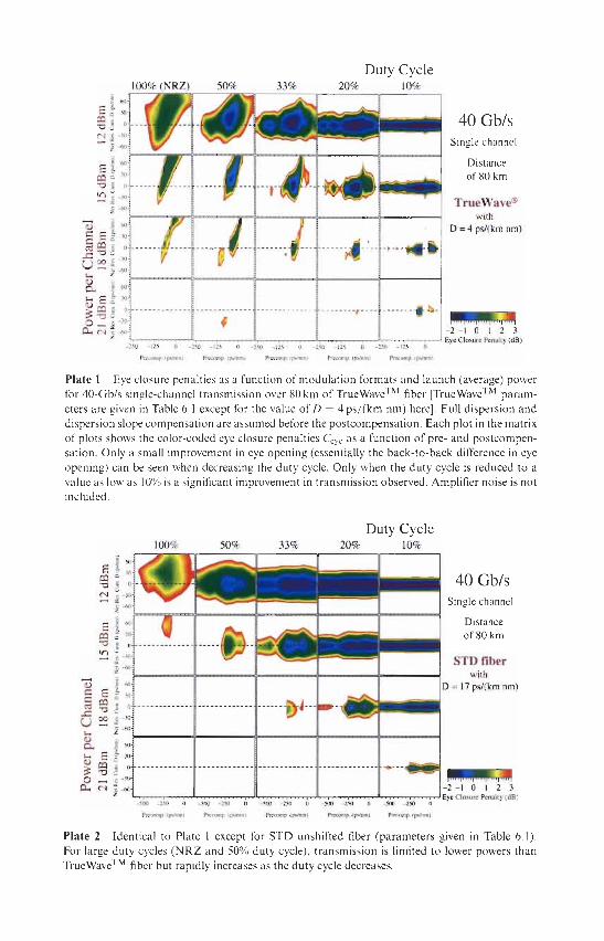
Plate 1 Eye closure penalties as a function of modulation formats and launch (average) power for 40-Gbh single-channel transmission over 80 km of TrueWaveTM fiber [TrueWaveTM param- eters are given in Table 6.1 except for the value of D = 4ps/(km nm) here]. Full dispersion and dispersion slope compensation are assumed before the postcompensation. Each plot in the matrix of plots shows the color-coded eye closure penalties Ceye as a function of pre- and postcompen- sation. Only a small improvement in eye opening (essentially the back-to-back difference in eye opening) can be seen when decreasing the duty cycle. Only when the duty cycle is reduced to a value as low as 10% is a significant improvement in transmission observed. Amplifier noise is not included.
5 Duty Cycle
33% 20% 10% ---
I I I
RFrornp lpdnm) F-omp lpdnml Rsomp lpdnml F-omp (~Jn,nm) R-mp Ipdoml
Plate 2 Identical to Plate 1 except for STD unshifted fiber (parameters given in Table 6.1). For large duty cycles (NRZ and 50% duty cycle), transmission is limited to lower powers than TrueWaveTM fiber but rapidly increases as the duty cycle decreases.
40 Gb/s Single channel
12 dBm 8 spans of 80 !un
TrueWaveTM/DSF with
D = 2 ps/(km nm)
- I O 1 2 3 4
Eye Closure Penalty (dB)
Recomp. (pdnm) Reeomp. (pdnm) Recomp. (pdnm) Recomp. (pdnm)
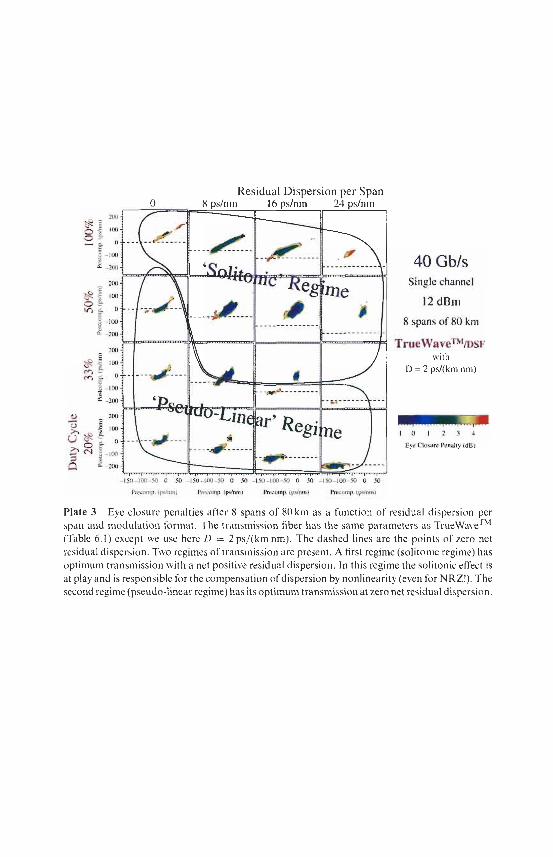
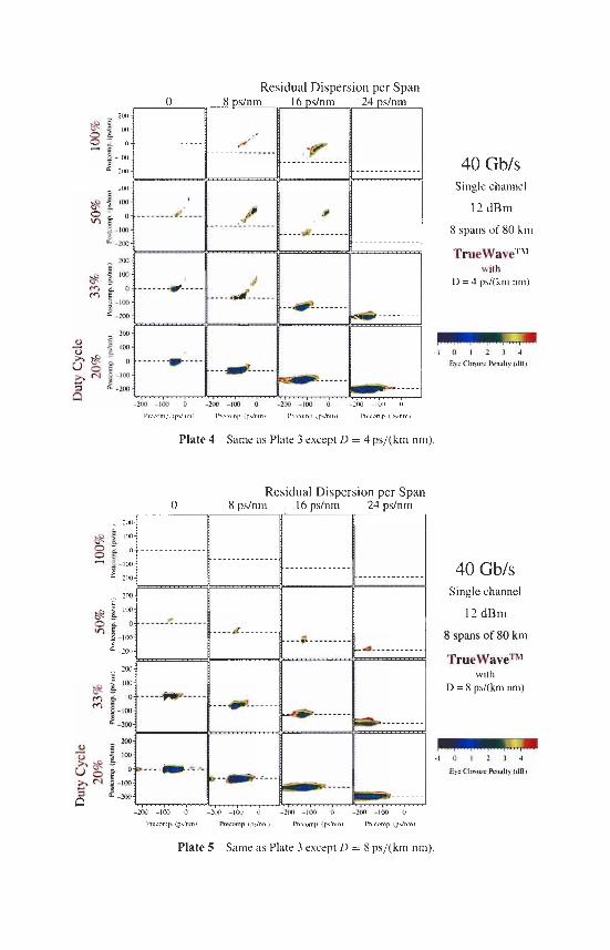
Plate 3 Eye closure penalties after 8 spans of 80 km as a function of residual dispersion per span and modulation format. The transmission fiber has the same parameters as TrueWaveTM (Table 6.1) except we use here D = 2 ps/(km nm). The dashed lines are the points of zero net residual dispersion. Two regimes of transmission are present. A first regime (solitonic regime) has optimum transmission with a net positive residual dispersion. In this regime the solitonic effect is at play and is responsible for the compensation of dispersion by nonlinearity (even for NRZ!). The second regime (pseudo-linear regime) has its optimum transmission at zero net residual dispersion.
Residual DisDersion per Span 0
- l a ,
-200
-200 -100 0
Reeomp. (pdnm)
0
I
a -100 0 -200 -100 0
Precomp. (pdnm) Reeomp (plnm)
40 Gb/s Single channel
12 dBm 8 spans of 80 km
TrueWavem with
D = 4 pd&m nm)
- 1 0 1 2 3 4 Eye Closure Penalty (dB)
Precomp. (pdnm)
Plate 4 Same as Plate 3 except D = 4ps/(km nm).
Residual Dispersion per Span 8 p s / m 16 ps/nm 24 pdnm
_ _ _ _ _ _ _ _ _ _ _ _ _ 40 Gb/s - _ _ _ _ _ _ _ _ _ _ _ _ _
Single channel
12 dBm 8 spans of 80 km
TrueWavem with
D = 8 pd&m nm)
M. , . . . . , -1 0 1 2 3 1
Eye Closure Penalty (dB)
m -100 o -200 -100 o -200 -100 o Recomp. (jdnm) PReomp (pdnm) Reeomp. (pslnm)
Plate 5 Same as Plate 3 except D = 8 ps/(km nm).
Residual Dispersion per Span
40 Gb/s Single channel
12 dBm
8 spans of 80 km
STD Unshifted Fiber
with D = 17 pd@m nm)
- 1 0 1 2 3 4
Eye Closure Penalty (dB)
Rsomp. (pS/nrnl Rsomp. (pslnml F’recomp. ( g n m l Pr~comp. (pdnm)
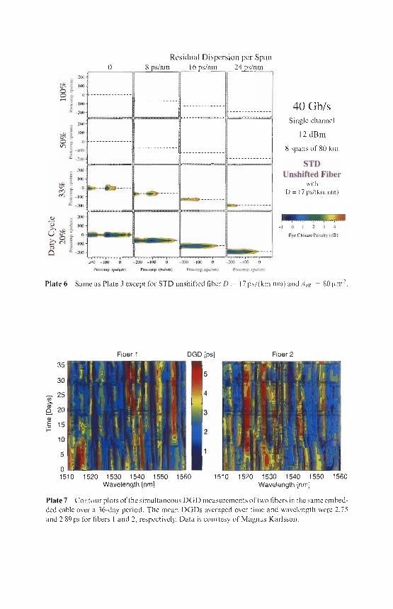
Plate 6 Same as Plate 3 except for STD unshifted fiber D = 17 ps/(km nm) and A,ff = 80 km2.
Fiber 1 Fiber 2
35 I .- 25‘ 2 g 20
15
10 F
15,J 1520 1530 1540 1550 1560 1510 1520 1530 1540 1550 1560 Wavelength [nm] Wavelength [nm]
Plate 7 Contour plots of the simultaneous DGD measurements of two fibers in the same embed- ded cable over a 36-day period. The mean DGDs averaged over time and wavelength were 2.75 and 2.89 ps for fibers 1 and 2, respectively. Data is courtesy of Magnus Karlsson.

Chapter 2
Kerry G. Coffman
Andrew M. Odlyzko AT&T Labs-Research, Middletown, New Jersey
University of Minnesota, Minneapolis, Minnesota
Growth of the Internet
Abstract
The Internet is the main cause of the recent explosion of activity in optical fiber telecommunications. The high growth rates observed on the Internet, and the popular perception that growth rates were even higher, led to an upsurge in research, development, and investment in telecommunications. The telecom crash of 2000 occurred when investors realized that transmission capacity in place and under construction greatly exceeded actual traffic demand. This chapter discusses the growth of the Internet and compares it with that of other communication services. It also presents speculations about future develop- ments. Internet traffic is growing, approximately doubling each year. There are reasonable arguments that it will continue to grow at this rate for the rest of this decade. If this happens, then in a few years we may have a rough balance between supply and demand.
1. Introduction
Optical fiber communication was initially developed for the voice phone sys- tem. The feverish level of activity that we have experienced since the late 199Os, though, was caused primarily by the rapidly rising demand for Internet con- nectivity. The Internet has been growing at unprecedented rates. Moreover, because it is versatile and penetrates deeply into the economy, it is affecting all of society, and therefore has attracted inordinate amounts of public attention.
The aim of this chapter is to summarize the current state of knowledge about the growth rates of the Internet, with special attention paid to the impli- cations for fiber optic transmission. We also attempt to put the growth rates of the Internet into the proper context by providing comparisons with other communications services.
The overwhelmingly predominant view has been that Internet traffic (as measured in bytes received by customers) doubles every 3 or 4 months.
17 OPTICAL FIBER TELECOMMUNICATIONS, VOLUME TVB
Copyright 0 2002, Elsevier Scienm (USA). ALI rights of reproduction in any form reserved.
ISBN &12-395173-9

18 Kerry G. Coffman and Andrew M. Odlyzko
Such unprecedented rates (corresponding to traffic increasing by factors of between 8 and 16 each year) did prevail within the United States during the crucial 2-year period of 1995 and 1996, when the Internet first burst onto the scene as a major new factor with the potential to transform the economy. However, as we pointed out in [CoffmanOl] (written in early 1998, based on data through the end of 1997), by 1997 those growth rates subsided to approx- imate the doubling of traffic each year that had been experienced in the early 1990s. A more recent study [CoffmanO2] provided much more evidence, and in particular more recent evidence, that traffic has about doubled each year since 1997. (We use a doubling of traffic each year to refer to growth rates between 70 and 150% per year, with the wide range reflecting the uncertainties in the estimates.)
Other recent observers also found that Internet traffic is about doubling each year. The evidence was always plentiful, and the only thing lacking was the interest in investigating the question. By 2000, though, the myth of Internet traffic doubling every 3 or 4 months was getting hard to accept. Very simple arithmetic shows that such growth rates, had they been sustained throughout the period from 1995 (when they did hold) to the end of 2000, would have produced absurdly high tr&c volumes. For example, at the end of 1994, traffic on the NSFNet backbone, which was well instrumented, came to about 15 TB/month. Had just that traffic grown at 1300% per year (which is what a doubling every 3 months corresponds to), by the end of 2000, there would have been about 250,000,000 TB/month of backbone traffic in the United States. If we assume there are 150 million Internet users in the United States, that would produce a data flow of about 5Mb/s for each user around the clock. The assumption of a doubling of traffic every 4 months produces traffic volumes that are only slightly less absurd.
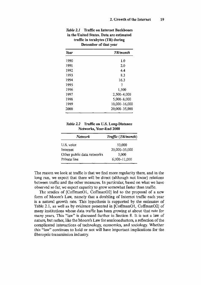
Table 2.1 shows our estimates for traffic on the Internet. The data for 1990 through 1994 is that for the NSFNet backbone, and therefore is very precise. It is incomplete only to the extent of neglecting what is thought to have been small fractions of traffic that went completely through other backbones. The data for 1996 through 2000 are our estimates, and the wide ranges reflect the uncertainties caused by the lack of comprehensive data.
Table 2.2 presents our estimates of the tr&c on various long-distance net- works at the end of 2000. The voice network still dominated, but it will likely be surpassed by the public Internet within a year or two. (For details of the measurements used to convert voice traffic to terabytes and related issues, see [CoffmanOl].) In terms of bandwidth, the Internet is already dominant. How- ever, it is hard to obtain good figures, since, as we discuss later, the bandwidth of Internet backbones jumps erratically. In terms of dollars, though, voice still provides the lion’s share (well over 80%) of total revenues. We concentrate in this chapter (as in our previous papers [CoffmanOl, CoffmanO21) on the growth rates in Internet tr&c, as measured in bytes. For many purposes, it is the other measures, namely bandwidth and revenues, that are more important.
2. Growth of the Internet 19
Table 2.1 Traffic on Internet Backbones in the United States. Data are estimated
traffic in terabytes (TB) during December of that year
Year TB/month
1990 1991 1992 1993 1994 1995 1996 1997 1998 1999 2000
1 .o 2.0 4.4 8.3
16.3 ?
1,500 2,5004,000 5,00&8,000
10,00&16,000 20,00&35,000
Tuble 2.2 Traffic on U.S. Long-Distance Networks, Year-End 2000
U.S. voice 53,000 Internet 20,00&35,000 Other public data networks 3,000 Private line 6,000-1 1,000
The reason we look at traffic is that we find more regularity there, and in the long run, we expect that there will be direct (although not linear) relations between traffic and the other measures. In particular, based on what we have observed so far, we expect capacity to grow somewhat faster than traffic.
The studies of [CoffmanOl, Coffman021 led to the proposal of a new form of Moore’s Law, namely that a doubling of Internet tr&c each year is a natural growth rate. This hypothesis is supported by the estimates of Table 2.1, as well as by evidence presented in [CoffmanOl, CoffmanO2] of many institutions whose data traffic has been growing at about that rate for many years. This “law” is discussed further in Section 8. It is not a law of nature, but rather, like the Moore’s Law for semiconductors, a reflection of the complicated interactions of technology, economics, and sociology. Whether this “law” continues to hold or not will have important implications for the fiberoptic transmission industry.
20 Kerry G. Coffman and Andrew M. Odlyzko
Much of this chapter, especially Sections 6 8 , is based on our earlier studies [CoffmanOl , CoffmanO2]. In Section 2, we present yet more evidence of how often popular perception and subsequent technology and investment decisions are colored by myths that are easy to disprove, but which nobody had bothered to disprove for an astonishingly long time. In Section 3, we look at historical growth rates of various communication services and how they compare to the much higher growth rate of the Internet. Section 4 is a brief review of the history of the Internet. Section 5 discusses some of the various types of growth rates that are relevant in different contexts. Section 6 presents the evidence about Internet traffic growth rates we have been able to assemble. Section 7 is devoted to new sources of traffic that might create sudden surges of demand, such as Napster. Section 8 discusses the conventional Moore’s Law and the analog we are proposing for data traffic. Section 9 suggests a way of thinking about data-traffic growth, based on an analogy with the computer industry. Finally, Section 10 presents our conclusions.
2. Growth Myths and Reality
Internet growth is an unusual subject, in that it has been attracting enormous attention but very little serious study. In particular, the general consensus has been that Internet traffic is doubling every 3 or 4 months. Yet no real evidence of that astronomical rate of growth was ever presented. As we discuss later, Internet traffic did grow at such rates in 1995 and 1996, but before and since it has been about doubling each year.
At this point, we would like to point out the need for careful quantitative data in evaluating any claims about growth rates. Some examples of public claims that do not match reality are presented in [Coffman02]. Here we discuss another case, this one concerning the widely held belief that any capacity that is installed will be quickly saturated. The British JANET network, which provides connectivity to British academic and research institutions, will be discussed in more detail later. What is important is that it is large (with three OC3 links across the Atlantic at the end of 2000), and has traffic statistics going back several years available at http://bill.ja.net/. A press release, available at http://~.ja.net/press_release/archive~nnounce/index.html as “Increase in Transatlantic Bandwidth-28 May 1998” (but actually dated 3 June 1998), described what happened when JANET’S transatlantic link was increased from a single T3 to two T3s:
With effect from Thursday 28 May 1998, JANET has been running a second T3 (45 Mbit/s) link to the North American Internet, bringing the total transatlantic bandwidth available to JANET to 90 Mbit/s. . . . Usage of the new capacity has been brisk, with the afternoon usage levels reaching in excess of 80 Mbit/s This is of course evidence of the suppressed demand imposed by the single T3 link
2. Growth of the Internet 21
operating previously. The fact that usage has risen so quickly on this occasion is also indicative of the improved domestic infrastructures. . . that now exist.
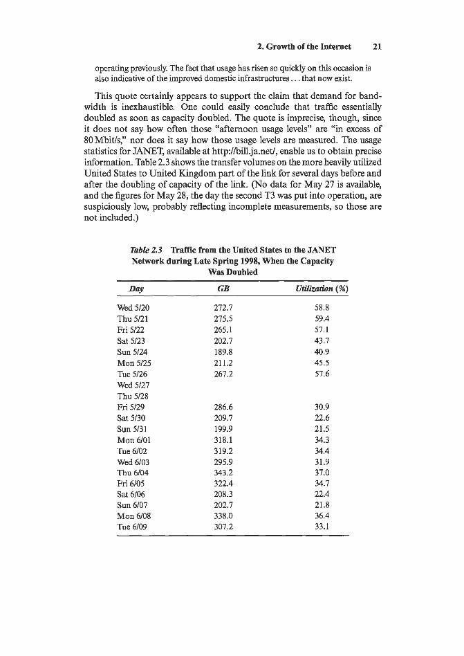
This quote certainly appears to support the claim that demand for band- width is inexhaustible. One could easily conclude that traffic essentially doubled as soon as capacity doubled. The quote is imprecise, though, since it does not say how often those “afternoon usage levels” are “in excess of 80 Mbit/s,” nor does it say how those usage levels are measured. The usage statistics for JANET, available at http://bill.ja.net/, enable us to obtain precise information. Table 2.3 shows the transfer volumes on the more heavily utilized United States to United Kingdom part of the link for several days before and after the doubling of capacity of the link. (No data for May 27 is available, and the figures for May 28, the day the second T3 was put into operation, are suspiciously low, probably reflecting incomplete measurements, so those are not included.)
Table 2.3 Traffic from the United States to the JANET Network during Late Spring 1998, When the Capacity
Was Doubled
Day GB UtiZizution (%)
Wed 5/20 Thu 5/21 Fri 5/22 Sat 5/23 Sun 5/24 Mon 5/25 Tue 5/26 Wed 5/27 Thu 5/28 Fri 5/29 Sat 5130 Sun 5/31 Mon 6/01 Tue 6102 Wed 6/03 Thu 6/04 Fri 6/05 Sat 6/06 Sun 6/07 Mon 6/08 Tue 6/09
272.7 275.5 265.1 202.7 189.8 211.2 267.2
286.6 209.7 199.9 318.1 319.2 295.9 343.2 322.4 208.3 202.7 338.0 307.2
58.8 59.4 57.1 43.7 40.9 45.5 57.6
30.9 22.6 21.5 34.3 34.4 31.9 37.0 34.7 22.4 21.8 36.4 33.1
22 Kerry G. Coffman and Andrew M. Odlyzko
What we observe is that although there was substantial growth in traffic after the capacity increase, suggesting that the transatlantic link had been a bottleneck, this increase was far more moderate than the popular Internet- growth mythology or the JANET press release would make one think. While capacity doubled, traffic increased by less than a third.
3. Growth Rates of Other Communication Services
Telecommunications has been a growth industry for centuries, but growth rates have generally been modest, except for a few episodes, such as the beginnings of the electric telegraph (see [Odlyzko2]). For example, the number of pieces of mail delivered in the United States grew by a factor of over 50,000 between 1800 and 2000, but that was a growth rate of about 5.6% per year. (If we adjust for population increase, we find a growth rate of about 3.5% in the mail volume per capita.) The number of phone calls in the United States grew by a factor of over 230 between 1900 and 2000, for a compound annual growth rate of 5.6%. (The per capita growth rate was 4.2% during this period.) Long-distance calls grew faster, about 12% per year between 1930 and 2000, and transatlantic calls faster yet. (There was just one voice circuit between the United States and Europe in 1927, when service was inaugurated. It used radio to span the ocean. This single low quality link grew to 23,000 voice circuits to Western Europe by 1995, for a compound annual growth rate of capacity of 16%.)
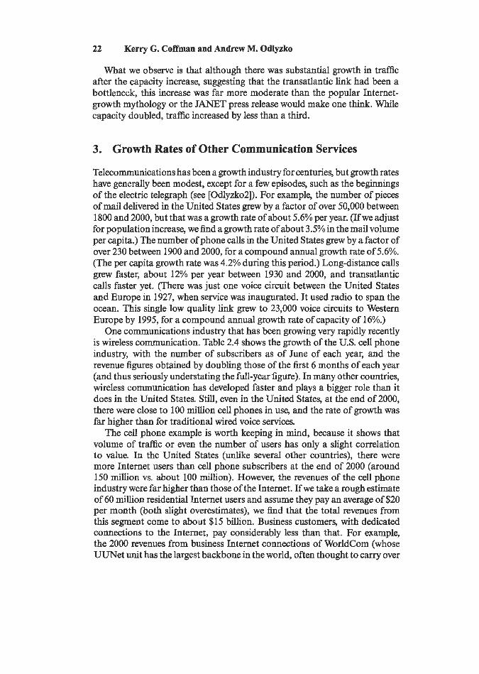
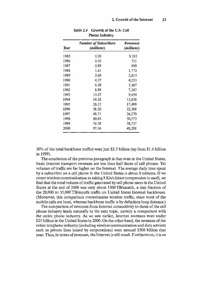
One communications industry that has been growing very rapidly recently is wireless communication. Table 2.4 shows the growth of the U.S. cell phone industry, with the number of subscribers as of June of each year, and the revenue figures obtained by doubling those of the fmt 6 months of each year (and thus seriously understating the full-year figure). In many other countries, wireless communication has developed faster and plays a bigger role than it does in the United States. Still, even in the United States, at the end of 2000, there were close to 100 million cell phones in use, and the rate of growth was far higher than for traditional wired voice services.
The cell phone example is worth keeping in mind, because it shows that volume of traffic or even the number of users has only a slight correlation to value. In the United States (unlike several other countries), there were more Internet users than cell phone subscribers at the end of 2000 (around 150 million vs. about 100 million). However, the revenues of the cell phone industry were far higher than those of the Internet. If we take a rough estimate of 60 million residential Internet users and assume they pay an average of $20 per month (both slight overestimates), we find that the total revenues from this segment come to about $15 billion. Business customers, with dedicated connections to the Internet, pay considerably less than that. For example, the 2000 revenues from business Internet connections of WorldCom (whose UUNet unit has the largest backbone in the world, often thought to carry over
2. Growth of the Internet 23
Table 2.4 Growth of the U.S. Cell Phone Industry
Number of Subscribers Revenues Year (miZlions) (millions)
1985 0.20 $352 1986 0.50 72 1 1987 0.89 959 1988 1.61 1,772 1989 2.69 2,813 1990 4.37 4,253 1991 6.38 5,307 1992 8.89 7,267 1993 13.07 9,639 1994 19.28 13,038 1995 28.15 17,499 1996 38.20 22,388 1997 48.71 26,270 1998 60.83 30,573 1999 76.28 38,737 2000 97.04 49,291
30% of the total backbone traffic) were just $2.5 billion (up from $1.6 billion in 1999).
The conclusion of the previous paragraph is that even in the United States, basic Internet transport revenues are less than half those of cell phones. Yet volumes of traffic are far higher on the Internet. The average daily time spent by a subscriber on a cell phone in the United States is about 8 minutes. If we count wireless communication as taking 8 Kb/s (since compression is used), we find that the total volume of traffic generated by cell phone users in the United States at the end of 2000 was only about 1500TB/month, a tiny fraction of the 20,000 to 35,000 TB/month traffic on United States Internet backbones. (Moreover, this comparison overestimates wireless traffic, since most of the mobile calls are local, whereas backbone traffic is by definition long distance.)
The comparison of revenues from Internet connectivity to those of the cell phone industry leads naturally to the next topic, namely a comparison with the entire phone industry. As we saw earlier, Internet revenues were under $25 billion in the United States in 2000. On the other hand, the revenues of the entire telephone industry (including wireless communication and data services such as private lines leased by corporations) were around $300 billion that year. Thus, in terms of revenues, the Internet is still small. Furthermore, it is so
24 Kerry G. Coffman and Andrew M. Odlyzko
intimately tied to the phone industry that it is difficult to see what its roleis. The basic technologies (fiber transmission, SONET, and so on) that are used for Internet transport were developed initially for voice telephony, but were easily adopted for data. (Some, such as SONET, will likely turn out to be redundant, but are still widely used.) At the transport level, voice has been carried as bits for a long time. What happened is that during the late 1990s, the long-distance telecommunications infrastructure changed. It used to be dominated by the demands of voice transport, and data was a small part of what it carried. Now, however, its development is driven by data, especially Internet data. For quite a long time, the volume of data was extremely small, so that even though the growth rate was higher than for voice, this did not affect the overall growth rate of the infrastructure. That was one reason the telecommunications industry was repeatedly surprised by the demand for bandwidth in the 1990s. Moreover, the transition from voice to data domination was complicated by the presence of several types of data, with substantially different growth rates. We discuss this in more detail below.
Another reason that the recent upsurge in demand for bandwidth was a sur- prise is that there had been several previous false predictions that data tralTic was about to explode. The excitement of the early 1990s about the “telecommu- nications superhighway” and “500 channels to the home,” to be accomplished through technologies such as hybrid fiber-coax, certainly led to large financial losses and serious disappointments (see Woll21). However, there were even earlier periods of extremely rapid growth followed by sudden deceleration. For example, the number of modems in the United States grew between 1965 and 1970 at about 60% per year, to over 150,000 at the end of that period [WalkerM]. Had that growth rate been maintained, we would have had about 200 billion modems in the United States by the end of 2000, clearly an absurd number. Instead, it appears that growth in the 1970s followed the projections made around 1970 (p. 297 of [WalkerM]), which predicted annual increases of 25 to 30%. It is interesting to read the speculations in [DunnL] about the sup- posedly rosy prospects for electronic cash, distance education, and other data services (as well as for Picturephone) that were supposed to power the growth of networks. In general, predicting what communications services society will accept and how it will use them has been difficult (see [Luckyl, Odlyzko2]). In particular, even recent history is littered with technologies that seemed extremely promising at one point, such as ISDN (see meinrock3, WuL]) or SMDS (Switched Multimegabit Data Services-a high speed packet switched WAN technology), but never attained more than a marginal role.
There are two aspects of the inability to forecast the prospects of communi- cations technologies that are worth discussing at greater length. One goes back to the earlier discussion of wireless telephony and how the mobility offered by cell phones appears to be more important for many people than broadband Internet access. Sometimes, though, higher bandwidth did prevail. In the early days of telephony, there was widespread lack of appreciation of how attractive
2. Growth of the Internet 25
it would eventually prove to be. The telephone was used primarily for business purposes, and the telegraph appeared to be adequate for that to many. Yet it was the phone that won, even though it appeared to use bandwith very waste- fully when compared to the telegraph, and even though it encouraged what was often dismissed as “idle chatter.” The attractions of instantaneous personal interactions turned out to be crucial in leading to an almost universal penetra- tion of the telephone in industrialized countries. In the last four decades of the twentieth century though, the telecommunications industry attempted several times to extend its success with the voice telephone by introducing videotele- phony. This service appeared to offer the attraction of an even deeper level of communication than voice. Yet prospective users have not only not embraced it, but have in many cases treated it with hostility. There is a growth of video- conferencing, but even that is far slower than its proponents had forecasted. For a variety of reasons that have not been completely explained, videotele- phony does not appeal to people for person-to-person communication. On the other hand, mobile narrowband voice flourishes.
The other aspect of the dismal record in forecasting the prospects of com- munications technologies that we now consider is that of the nature of traffic carried. Data networks, which in commercial settings go back about four decades, have spent essentially all this time in the shadow of the much larger voice telephone network. (They also benefited from being able to use the infra- structure of the phone network, and were also constrained by its limitations, but that is less relevant for us here.) It was therefore natural for network- ing experts to continuously think of voice traffic, and in particular of the possibility of eventually carrying it as data. Looking further out, to a stage where the progress of technology appeared to offer the possibility of data net- works becoming much larger than the phone networks, it was also natural to think of enriching the communications medium through the addition of video. (See the projections of Estill Green [Green, Lucky21 and Hough [Hough], for example.) Later, the huge volume of broadcast data (radio and especially tele- vision) offered further possibilities for traffic that could be carried on data networks. The key point is what was seen as eventually filling data network was streaming multimedia traffic. The Internet’s rise to dominance was a sur- prise for many reasons, but one of the main ones was that it did not fit this model. Although much current work on Internet technologies is devoted to streaming multimedia, there are good reasons, to be discussed later, why such traffic is not likely to dominate.
Althoughit has proven difficult to forecast which technologies will be widely adopted, once a service had been successfully introduced, it often showed reg- ular growth rates for extended periods of time [Odlyzko2]. The approximately 30% annual growth rate that had been projected in 1970 for data transmis- sion (or, to be more precise, for the proxy for actual transmission that is offered by the number of modems) appears to have held not just in the 1970s, but in the 1980s and most of the 1990s as well. There are no comprehensive

26 Kerry G. Coffman and Andrew M. Odlyzko
statistics (and there are measurement problems, in that private lines, whose bandwidth is often taken as a measure of the data traffic, can also be used for voice transmission). However, there are a few pieces of evidence support- ing those growth rates around 1980 in [deSolaPITH]. Those same growth rates appeared to also hold for long-distance private line transmission in the mid 1990s [CoffmanOl] and for local data bandwidth in the late 1980s and most of the 1990s [Galbi]. The comprehensive data summarized in [Galbi] is especially interesting. During the late 1980s and most of the 199Os, installed computer power came close to doubling each year, and the new “Informa- tion Economy” was taking root, but this was not reflected in the volume of data traffic. This low rate of growth in data transmission may have come from the high cost and poor quality of data transmission or from other causes, such as lack of uniform standards that would enable easy data communica- tion between companies. It may also have been caused to a large extent by the slow rate at which computation and communication technologies were adopted. Whatever the reasons, this low growth rate of approximately 30% a year (low by comparison to growth of computing power) in data transmis- sion was higher than that of voice networks. Hence by the mid 199Os, the bandwidth of long-distance data networks (primarily private lines used for intracompany communication) was already comparable to that of the voice network [CoffmanOl].
The Internet has historically had a growth rate of close to 100% per year in the traffic it carried. As Table 2.1 shows, it was growing with striking regularity in the early 1990s at this rate. Then it experienced a period of astronomical growth in 1995 and 1996, and then reverted to an approximate doubling each year in 1997, and has continued growing at about that rate through the end of 2000. The big question is how fast it will grow in the future. While the overwhelming preponderance of opinion all through the end of 2000 was that Internet traffic was doubling every 3 or 4 months, by early 2001 the consensus started changing. Some analysts even began projecting declines in the growth rates to the 50% per year range by around 2005. And indeed, some sources of growth did dry up. With the crash of telecom stocks (caused largely by the realization that expected demand and revenues were not materializing), investments slowed, and many dot-coms that had been busily filling transmis- sion pipes with their content disappeared. In a related development, corporate managements started asking for detailed justifications for new data network- ing expenditures instead of rushing to endorse any proposals that came along. At various enterprises, the growth rates of data traffic, which had been close to doubling every year in the late 199Os, began to slow down toward doubling every 18 or 24 months. It is not inconceivable that overall data traffic growth may be moving back to its historical rate of around 30% per year. We do not think this will occur, but before considering the reasons why (presented in detail in Sections 6 to 9), we look at the general history of the Internet and its growth rates.
2. Growth of the Internet 27
At this point we just remark that the dominant role of the Internet in communications, whether in terms of bandwidth of networks or popular consciousness, is a fairly recent phenomenon. There had been extensive dis- cussions of the “Information Superhighway” and the “National Information Infrastructure” for a long time. Leading thinkers foresaw the possibilities for much improved communication offered by new technologies, and there was tremendous effort devoted to various systems. However, the general expecta- tion was that the “Information Superhighway” would be composed of a very heterogeneous collection of (interconnected) networks. This was true even as late as the beginning of the Clinton presidency in 1993 and 1994 (see [NII]). It was only in the mid to late 1990s that the Internet was perceived as evolving toward an all-encompassing network, carrying all types of traffic.
4. Internet History
Over the past 5 to 10 years, we have witnessed not only an explosion of activ- ity, but the creation of entirely new sectors within the optical industry. As the concept of wavelength division multiplexing (WDM) began to emerge, many new companies developing WDM transport equipment came into existence. The newer enterprises pushed the older established equipment vendors to more aggressive deployment schedules, and a constant downward trend for the cor- responding prices of WDM transport equipment followed. In what appeared to be an almost insatiable demand for more bandwidth, a situation arose that allowed the creation of the new companies and the accompanying innovation. Not only did new equipment vendors emerge, but also new national-scale carriers were created. This trend is continuing as the concept of optical layer- inghetworking is gaining acceptance and new optical equipment companies are being formed on a regular basis. They deal not only with “traditional” WDM transport equipment, but also with terrestrial ultra long-haul systems, regional and metro optimized systems, and various incarnations of optical cross connects.
There were hundreds of developments and contributions enabling this burst of activity. Many of the technical innovations are described in this book and its predecessors. However, perhaps the greatest single factor that fueled this phenomena was the belief and perception that traffic, and hence needed capac- ity, were growing at explosive rates. This is a remarkable fact, especially when one recalls that around 1990 both the traditional carriers and most of their equipment vendors still expected the traffic demands to not vary much from the voice demand growths (which historically was around 10% per year). In fact, both carriers and equipment vendors were arguing that WDM would not be needed and that going to individual channel rates of at most 10 Gb/s would be adequate. Also, around 1995, the conventional wisdom was that 8-channel WDM systems would suffice well into the foreseeable future. Now it almost

28 Kerry G. Coffman and Andrew M. Odlyzko
appears as if the pendulum has swung the other way. Is too much capacity being deployed? Are many of the reported traffic growth rates correct? And if so, will they continue?
As we explained in the previous section, the early skepticism about the need for high-capacity optical transport was rooted in the reality of the telecommu- nications networks. Up until 1990, they were dominated by voice, which was growing slowly. Then, by the mid 1990s, they came to be dominated (in terms of capacity) by private lines, which were growing three or four times as fast. And then, in the late 1990s, they came to be dominated by the Internet, which was growing faster still.
Before we go through the analyses for the tr&c growth on the Internet, we must first at least define the Internet and describe its history and structure. This is paramount in helping put much of the later described growth analyses into perspective.
When one now speaks of the Internet, it is usually described as an evolution from ARPANET to NSFNet, and finally to the commercial Internet that now exists. Arguably, the phenomenal growth of the Internet started in 1986 (more than 17 years after its “birth”) with NSFNet. However, the path was very complicated and full of many twists and turns in its roughly 40-year history [Cerf, Hobbes, Leiner].
From the very early research in packet switching, academia, industry, and the U.S. government have been intertwined as partners. Ironically, the begin- nings of the Internet can trace itself back to the Cold War and specihlly to the launch of Sputnik in 1957. The U.S. government formed the Advanced Research Project Agency (ARPA; the name was later changed to DARPA, Defense Advanced Research Project Agency, and later back to ARPA) the year after the launch with the stated goal of establishing a U.S. lead in tech- nology and science (with emphasis on military applications). As ARPA was establishing itself, there were several pivotal works [Kleinrockl , Baran] in the early 1960s on packet switching and computer communications. These works and the efforts they spawned laid many of the foundations that enabled the deployment of distributed packet networks. J. C. R. Licklider (of MIT) [LickC] wrote a series of papers in 1962 in which he “envisioned a glob- ally interconnected array of computers which would enable ‘everything’ to easily access data and programs from any of the sites.” Generically speak- ing, this idea is not much diflterent from what today’s Internet has become. Of importance is the fact the Licklider was the first head of the computer research program at DARPA (beginning in 1962), and in this role he was instrumental in pushing his concept of networks. Kleinrock published both the first paper on packet switching and the first book on the subject. In addi- tion, Kleinrock convinced several key players of the theoretical feasibility of using packets instead of circuits for communications. One such person was Larry Roberts, one of the initial architects for the ARPANET. In the 1965 to 1966 time frame, ARPA sponsored studies on a “cooperative network of [users]

2. Growth of the Internet 29
sharing computers” [Leiner], and the first ARPANET plans were begun, with the first design papers on ARPANET being published in 1967. Concurrently, the National Physical Laboratory (NPL) in England deployed an experimen- tal network called the NPL Network that made use of packet switching. It utilized 768 Kb/s lines.
A year before the moon landing, in 1968, the first ARPANET requests for proposals were sent out, and the first ARPANET contracts were awarded. Two of the earliest contracts went to UCLA to develop the Network Measurement Center, and to Bolt, Beranek, and Newman (BBN) for the Packet Switch contract (to construct the Interface Message Processors or IMPs-effectively the routers).
Kleinrock headed the Network Measurement Center at UCLA and it was selected as the first node on the ARPANET. The first IMP was installed at UCLA and the first host computer was connected in September of 1969. The second node was at Stanford Research Institution (SRI). Two other nodes were added at UC Santa Barbara and in Utah, so that by the second half of 1969, just months past the lkst moon landing, the initial four-node ARPANET became functional. This was truly the initial ARPANET, and thus a case can be made that this was when the Internet was born. The first message carried over the network went from Kleinrock’s lab to SRI. Supposedly the first packet sent over ARPANET was sent by Charley Kline, and as he was trying to log in the system crashed as the letter “ G of “LOGIN” was entered.
One of the next major innovations for the fledgling Internet (i.e., ARPANET) was the introduction of the first host-to-host protocol, called Network Control Protocol, or NCP, which was first used in ARPANET in 1970. By 1972, all of the ARPANET sites had finished implementing NCP. Hence the users of ARPANET could finally begin to focus on the develop- ment of applications-another paramount driver for the phenomenal growth and sustained growth of the Internet. It was also in 1970 that the first cross- country link was established for ARPANET by AT&T between UCLA and BBN (at the blinding rate of 56 Kbh). By 1971, the ARPANET had grown to 15 nodes and had 23 hosts. However, perhaps the most influential work that year was the creation of an e-mail program that could send messages across a distributed network. (E-mail was not among the original design criteria for the ARPANET, and its success caught the creators of this network by surprise.) Ray Tomlinson of BBN developed this application, and his original program was based on two previous ones [Hobbes]. Tomlinson modified his program for ARPANET in 1972, and at that point its popularity quickly soared. In fact, it was at this time that the symbol “@,, was chosen. Arguably, Internet e-mail as we know it today can trace its origins directly to this work. Internet e-mail was clearly one of the key drivers for the popularity (and hence the phenom- enal traffic-growth demands) of the Internet and was the first “killer app” for the Net. It was every bit as critical to the Internet’s “success” as spreadsheet applications were to the popularization of the PC. Internet e-mail provided

30 Kerry G. Coffman and Andrew M. Odlyzko
a new model of how people could communicate with each other and alter the very nature of collaborations.
Although there was already considerable work being done on packet networks outside the United States, the first international connections to the ARPANET (to England via Norway) took place in 1973. To put the time frame in perspective, this was the same year that Robert Metcalfe did his PhD that described his idea for Ethernet. Also during this year, the num- ber of ARPANET c‘users” was estimated to be 2,000 and that 75% of all the ARPANET t r a c (in terms of bytes) was e-mail. One needs to note that in only 1 to 2 years from its introduction onto the Internet, e-mail became the predominant type of traffic. The same behavior took place several years later for HTML (Hypertext Markup Language) (i.e., Web traffic), and to a some- what lesser degree, this was seen for Napster-like traffic within many networks a few years later.
Several other key developments began to take place in the mid 1970s. The initial design specification for TCP (Transfer Control Protocol) was published by Vint Cerf and Bob Kahn in 1974 [CerfK]. The NCP protocol, which was being utilized at the time, tended to act like a device driver, whereas the future TCP (later TCP/IP) would be much more like a communications protocol. As is discussed later, the evolution from ARPANET’s NCP protocol to TCP (which in 1978 was split into TCP and IP (Internet Protocol)) was critical in allowing the future growth and scalability of today’s Internet. DARPA had three contracts to implement TCPLIP (at the time still called TCP), at Stanford (led by Cerf), BBN (led by Ray Tomlinson), and UCLA (led by Kirsten). Stanford produced the detailed specification and within a year there were three independent implementations of TCP that could interoperate.
It is noted that the basic reasons that led to the separation of TCP (which guaranteed reliable delivery) from IP actually came out of work that was done trying to encode and transport voice through a packet switch. It was found that a tremendous amount of bdering was needed in order to allow for the appro- priate reassembly after transmission was completed. This in turn led to trying to find a way to deliver the packets without requiring a guaranteed level of reliability. In essence, the UDP (User Datagram Protocol) was created to allow users to make use of IP. In addition, it was also in 1978 that the first commercial version of ARPANET came into existence when BBN opened Telenet.
In 198 1-1982, the first plans were made to “migrate” from NCP to TCP. It is claimed by some that it was this event (TCP was established as the protocol suite for ARPANET) was truly the birth of the InternetAefined as a connected set of networks, specifically those with TCP/IP. A few years later (in 1983) another major development occurred, which later enabled the Internet to scale with the “explosive” growth and popularity of the future Internet. This was the development of the name server, which evolved into the DNS [Cerf, Leiner]. The name server was developed at the University of Wisconsin [Hobbes]. This made it easy for people to use the network because hosts were assigned names

2. Growth of the Internet 31
and it was not necessary to remember numeric addresses. Much of the credit for the invention of the DNS (Domain Name Server) is given to Paul Mockapetris of USC/ISI [Cerfl.
The year 1983 was also the date for two other key developments on ARPANET. The first one was the cutover from NCP to TCP on the ARPANET. Secondly, ARPANET was split into ARPANET and MILNET. Although the road was convoluted, this split was one of the key bifurcation points that later allowed NSFNet to come into existence. Soon thereafter (in 1984), the number of hosts on ARPANET had grown to 1,000, and the next year in 1985 the first registered domain was assigned in March.
In 1985, NSFNet was created with a backbone speed of 56 Kb/s. Initially, there were five supercomputing centers that were interconnected. One of the paramount benefits of this was that it allowed an explosion of connections (most importantly from universities) to take place. Two years later in 1987, NSF agreed to work with MERIT Network to manage the NSFNet backbone. The next year (1988), the process of upgrading the NSFNet backbone to one based on T1 (Le., 1.5 Mb/s links) was begun. In 1987, the number of hosts on the Internet broke 10,000. Two years later in 1989, this had grown to around 100,000, and 3 years after that, in 1992, it reached the 1,000,000 value. It is noted that if you look at how the number of hosts had been growing from 1984 to 1992, that it was still pretty much tracking a growth curve that was less than tripling each year (i.e., doubling every 9 months). In the 1985-1986 time frame, a key decision was made that had very long-term impact: that TCP/IP would be mandatory for the NSFNet program.
In the 1988-1990 time frame, a conscious decision was made to connect the Internet to electronic mail carriers, and by 1992, most of the commercial e-mail carriers in the United States were “like the Internet.” This was still another development that cemented e-mail as the single most important application to take advantage of the Internet.
In 1990, the ARPANET ceased to exist, and arguably NSFNet was the essence of the Internet. The following year, commercial Internet Service Providers (ISPs) began to emerge (PSI, ANS, Sprint Link, to name a few), and the Commercial Internet Xchange (CIX) was organized in 1991 by com- mercial ISPs to provide transfer points for traffic. NSF’s lifting the restriction on the commercial use of the Net was again one of the pivotal decisions. This was again a key bifurcation point, in that this helped set the stage for the com- plete commercialization of the Net that would follow only a few years later. In 1991, the upgrading of the NSFNet backbone continued as the work to upgrade to a T3 (Le., 45 Mb/s links) began. It is also interesting to note that it was the next year, 1992, that the term “surfing the Internet” was first coined by Jean Armour Polly [Polly], only 2 years before the ARPANEThternet celebrated its 25th anniversary.
It was in the 1993-1995 time period that several major events seemed to emerge that fueled an almost explosive growth in the popularity of the Internet.

32 Kerry G. Coffman and Andrew M. Odlyzko
One of the key ones was the introduction of “browsers,” most notably Mosaic. This led to the creation of Netscape, which went public in 1995. Even as early as 1994, WWW (i.e., predominantly HTML) tr&c was increasing in volume on the Net. By then it was the second most popular type of traf- fic, surpassed only by FTP (File Transfer Protocol) tr&c. However, in 1995 WWW tra& surpassed FTP as the greatest amount of tr&c. In addition, the traditional online dial-up systems such as AOL (America Online), Prodigy, and CompuServe began to provide Internet access.
In 1996, the Net truly became public with the NSFNet being phased out. Soon thereafter, major infrastructure improvements were made within the transport part of the Internet. The Internet began to upgrade much of its backbone to OC3-0C12 (up to 622Mb/s) links, and in 1999, upgrades began for much of the Net to OC48 (2.5 Gb/s) links.
5. The Many Internet Growth Rates
The Internet is very hard to describe. By comparison, even the voice phone system, which is a huge enterprise, far larger in terms of revenues than the Internet, is much simpler. In the phone system, the basic service is well defined and simple to describe. The users have only limited ability to interact with the system. The Internet is completely different. Users interact with the system in a multiplicity of ways, on widely different time scales, and there are many complicated feedback loops. The paper [FloydP] is an excellent overview of the problems that arise in attempting to simulate the Internet.
The problems of measuring the Internet are also formidable. There are many different measures that are relevant. In this chapter, just as in the papers [CoffmanOl , CoffmanO2], we will concentrate on traffic as measured in bytes. For the optical fiber telecommunications industry, it is capacity that is most relevant. Unfortunately, there are numerous problems in measuring capacity. Much of the fiber is not lit, and even when it is lit, often only a few wavelengths are lit. Finally, much of the potential capacity is used for restoration, through SONET or other methods. In addition, even at the levels of links used for pro- viding IP traffic, it is hard to obtain accurate capacity measurements, because few carriers provide detailed data. Further, this type of capacity has a ten- dency to jump suddenly, as bandwidth is usually increased in large steps (such as going from OC3 to OC12, and then 0048, a phenomenon that contributes to the low utilization of data links [Odlyzkol]). Thus, there is little regularity in capacity growth figures. On the other hand, we do find astonishing regu- larity in traffic growth, which leads us to propose that a form of Moore’s Law applies. In the long run, we expect that capacity will grow slightly faster than traffic, as we explain later.
For many purposes other measures are important, such as the number of users, how they spend their time, how many and what types of commercial
2. Growth of the Internet 33
transactions they engage in, and so on. There are many sources of such data, and useful references can be found at [Cyberspace, MeekerMJ, Nua].
6. Internet Traffic and Bandwidth Growth
Whether Internet traffic doubles every 3 months or just once a year has huge consequences for network design as well as the telecommunications equipment industry. Much of the excitement about and funding for novel technolo- gies appears to be based on expectations of unrealistically high growth rates ([Bruno]). In this section we briefly examine avariety of examples in an attempt to understand the traffic-growth rates that the Internet has experienced over its lifetime. There are places where the traffic is growing at rates that exceed 100% per year. One such example is LINX (London Internet Exchange). Its online data, available at http://ochre.linx.net/, clearly shows a growth rate of about 300% from early 1999 to early 2001. There are also examples of even higher growth rates, although those tend to be for much smaller links or exchange points. However, there are also numerous examples of much more slowly grow- ing links. In this section we briefly present growth rates from avariety of sources and attempt to put them into context. In an earlier study [CoffmanOl] in 1997, we found that the evidence supported a traffic growth rate of about 100% per year (doubling annually). Four years later, the general conclusion is that Inter- net traffic still appears to be growing at about 100% per year. In other words, we have not found any substantial slowdown in the growth rate.
Some recent reports and projections conclude that Internet traffic is only about doubling each year, but claim that it was growing much faster until recently, and that its growth rate will continue to slow down. In that view, the telecom crash of 2000 was associated with a sudden decline in the growth rate of traffic. As far as we can tell, that is not accurate. The general rate of growth of traffic appears to have been remarkably stable throughout the period 1997- 2000. As one of the most convincing pieces confirming this claim, we cite the news story ([Cochrane]) based on official figures from Telstra, the dominant Australian telecommunications carrier. This story reports that Telstra’s IP traffic was almost exactly doubling each year between November 1997 and November 2000. (The printed version of this news story, but not the one available online at the URL listed in [Cochrane], shows a very regular growth, about 100% per year, from the beginning of 1997 to November 2000.) Hence our conclusion is that the problems the photonics industry is experiencing are not caused by any sudden slowdown in traffic, but rather by a realization that the astronomical growth rates that people had been assuming were fantasies.
Most of this section is drawn from the more detailed account in [Coffman02]. There are only a few new pieces of information. For exam- ple, the China Internet Network Information Center has statistics (at www.cnnic.net.cn/develst./e-index.shtm1) of the Internet bandwidth between
34 Kerry G. Coffman and Andrew M. Odlyzko
China and the rest of the world. It grew from 84.64Mb/s in June 1998 to 2,799 Mbls in December 2000, for a compound growth rate of 305% per year. Thus, even in a rapidly growing economy like that of China, where Internet penetration is low and is trying to catch up with the industrialized world, traffic is only doubling about every 6 months.
The comparison of the international bandwidth for Australia and China is instructive. In December 2000, Telstra had about 1,000 Mb/s to the rest of the world, about a third of Chinese bandwidth. Thus, making allowances for other Australian carriers, we can speculate that Australia may be exchang- ing half as much traffic with international destinations as China does, even though the latter has over 60 times the population. This shows the degree to which countries can differ in their intensity of Internet usage. The data in [Cochrane], showing that Telstra’s IP traffic in November 2000 reached about 270 TBlmonth, also shows that our general estimates for U.S. backbone traffic are reasonable, because the United States is not only larger than Australia, but also richer on aper capita basis and has a better developed telecommunications infrastructure.
In the remainder of this section we examine some of the data and trends from ISPs, exchange points, and residential traffic patterns, along with traffic from “stable sources,” such as corporate, research, and academic networks.
It is noted that the data for the first two sources (ISPs and exchange points) are not nearly as complete nor reliable as only a few years ago. However, much better data are available for the “stable sources,” and several are examined in much more detail later. As a brief note on conversion factors, traffic that averages 100 Mb/s is equivalent to about 30 TB/month. (It is 32.4 TB for a 30-day month, but such precision is excessive given the uncertainties in the data we have.)
Unfortunately, the largest ISPs do not release reliable statistics. This situa- tion was better even a couple of years ago. Much of the older data was used in previous studies ([CoffmanOl]). For example, MCI used to publish precise data about the traffic volumes on their Internet backbone. Even though they were among the first ISPs to stop providing official network maps, one could obtain good estimates of the MCI Internet backbone capacity from public presentations. These sources dried up when MCI was acquired by WorldCom, and the backbone was sold to Cable &Wireless. As was noted in [CoffmanOl], the traffic-growth rate for that backbone had been in the range of 100% a year before the change.
Today, one can obtain some idea of the sizes (but not trafEc) of various ISP networks through the backbone maps available from Boardwatch. However, even those are not too reliable. The only large ISP in the United States to pro- vide detailed network statistics is AboveNet, at http:lluww.above.netltrafficl. Therefore, we looked at this ISP in moderate detail. We have recorded the MRTG (Multi-Router Traffic Grapher) [MRTG] data for AboveNet for March 1999, June 1999, February 2000, June 2000, November 2000, and April 2001.
2. Growth of the Internet 35
The average utilizations of the links in the AboveNet long-haul backbone dur- ing those 4 months were 18, 16, 29, 12, 11, and lo%, respectively. (The large drop between February and June 2000 was caused by deployment of massive new capacity, including four OC48s. One of the reasons we concentrate on traffic and not network sizes in this chapter is that extensive new capacity is being deployed at an irregular schedule and is often lightly utilized. Thus, it is hard to obtain an accurate picture of the evolution of network capacity.) If one just adds up the volumes for each link separately, one finds that between March 1999 and April 2001, the total volumes of traffic increased at an annual growth rate of about 200%. However, this figure has to be treated with caution, as actual traffic almost surely increased less than 200%. During this period, AboveNet expanded geographically, with links to Japan and Europe, so that at the end it probably carried packets over more hops than before. Because we are interested in end-to-end traffic as seen by customers (which can be thought of as the ingress and/or egress traffic into and/or out of “the network”), we have to deflate the sum of traffic volumes seen on separate backbone links by the aver- age number of hops that a packet makes over the backbones (perhaps around three). Even when there is reliable data for a single carrier, such as AboveNet, some of the growth seen may be coming from gains in market share, both from gains within a geographical region and from greater geographical reach, and not from general growth in the market.
We next look at Internet exchange points. When the NSF Internet backbone was phased out in early 1995, it was widely claimed that most of the Inter- net backbone traffic was going through the Network Access Points (NAPs) (which are effectively interconnection vehicles), which tended to provide decent statistics on their traf3ic. Currently it is thought that only a small fraction of backbone traffic goes through the NAPs, while most goes through private peer- ing connections. Furthermore, NAP statistics are either no longer available or not as reliable. This is in sharp contrast to the situation in 1998 [CoffmanOl]. As documented elsewhere [CoffmanO2], there is very little that can be reli- ably concluded about current growth rates of Internet traffic by examining the statistics of the public NAPs in the United States.
However, the situation was slightly better when we examined a large num- ber of international exchange points. These included LINX, AMS-IX (the Amsterdam Internet exchange), the Slovak Internet exchange, HKIX (a com- mercial exchange created by the Chinese University of Hong Kong, BNIX (located in Belgium), the INEX (an Irish exchange), and FICX (the Finish exchange). Some of these show growth rates of only about doubling per year while others show much faster growth rates. Trafiic interchange statistics are hard to interpret, unless one has data for most exchanges, which is virtually impossible to obtain. Much of the growth one sees can come from ISPs mov- ing from one exchange to another, moving their traffic from one exchange to another, or coming to an exchange in preference to buying transit from another ISP. Consider the specific case of LINX. A large part of its growth
36 Kerry G. Coffman and Andrew M. Odlyzko
is almost surely caused by more ISPs exchanging their traffic there. Between March 1999 and March 2000, the ranks of ISPs that are members of LINX have grown by about two-thirds, based on the data on the LINX home page. Hence the average per-member traffic through LINX may have increased only around 120% during that year.
The traffic from residential U.S. customers will probably begin to increase at a faster rate in the near future. The growth in the number of users is likely to diminish as we reach saturation. (You cannot double the ranks of subscribers if more than half the people are already signed up!) However, broadband access, in the shape of cable modems and DSL (and to a lesser extent fixed wireless links), will stimulate usage. The evidence so far is that users who switch to cable modem or DSL access increase their time online by 50 to loo%, and the total volume of data they download per month by factors of five to ten. A five- or tenfold growth in data traEic would correspond to a doubling of traffic every 4 months if everyone were to switch to such broadband access in a year. However, that is not going to happen. At the end of 1999, there were about 3 million households in the United States with broadband access. The most ambitious projections for cable modem and DSL access call for about 13 mil- lion households to have such links in 2003, and between 5 M O million in the year 2007. That is approximately a doubling each year. (There was apparently almost a tripling in the ranks of households with broadband access in 2000, but the telecom crash that wiped out many of the ADSL providers has led to a slowdown in the pace of deployment in 2001 .) The traffic from a typical res- idential broadband customer is likely to grow beyond the level we see today as more content becomes available and especially as more content that requires high bandwidth is produced. Still, it is hard to see average traffic per customer among those with broadband connections growing at more than 50% a year. Together with a doubling in the ranks of such customers, this might produce a tripling of traffic from this source. Because the ranks of customers with reg- ular modems are unlikely to decrease much, if any, and because their traffic dominates, it appears that the most likely scenario will be for the total resi- dential customer traffic to grow no faster than 200% per year, and probably closer to 100% per year. (Access from information appliances, which are fore- cast to proliferate, is unlikely to have a major impact on total traffic, since the mobile radio link will continue to have small bandwidth compared to wired connections.)
We next consider traf€ic at various stable institutions-corporate, academic, and governmental. Growth in traffic can be broken down into growth in the number of traffic sources and growth in traffic per source. For LINX, much of the increase in traffic may be coming from an increase in member ISPs. For individual ISPs, much of the increase in traffic may also be com- ing from new customers. Yet in the end, that kind of growth is limited, as the market becomes saturated. The rest of this section focuses on rates of growth in traffic from stable sources. Now nothing is completely stable, as
2. Growth of the Internet 37
the number of devices per person is likely to continue growing, especially with the advent of information appliances and wireless data transmission. Hence we will consider growth in traffic from large institutions that are already well wired, such as corporations and universities. Most corporations do not publicize information about their network traffic, and many do not even collect it. However, there are some exceptions. For example, Lew Platt, the former CEO of Hewlett-Packard, used to regularly cite the HP intranet in his presentations.. The last such report, dated September 7, 1998, and available at http://www.hp.com/financials/textonly/personnel/ceo/~es.ht~, stated that this network carried 20 TB/month, and a comparison with pre- vious reports shows that this volume of traffic had been doubling each year for at least the previous 2 years. (As an interesting point of comparison, the entire NSFNet Internet backbone carried 15 TB/month at its peak at the end of 1994.) Several other corporations have provided data showing similar rates of growth for their Intranet trafllc, although some indicated their growth has slowed, and a few have had practically no recent growth.
Internal corporate tr&c appears to be growing much more slowly than public Internet traffic. Data for retail private lines as well as for Frame Relay and ATM (Asynchronous Transfer Mode) services show aggregate growth in bandwidth (and therefore most likely also traffic) in a range of 3040% per year. The growth is slow for retail private lines and fast for Frame Relay and ATM. These rates are remarkably close to the growth rate observed in the late 1970s in the United States, which was around 30% per year [deSolaPITH]. Thus, it is the corporate traffic to the public Internet that is growing at 100% per year. It is also important to note that in the year 2000, over two-thirds of the volume on the public Internet appeared to be business to business. Thus, the acceleration of the overall growth rate of data traffic to about 100% per year from the old 30% or so a year appears to be a consequence of the advantages of the Internet, with its open standards and any-to-any connectivity.
For the remainder of this section we concentrate on publicly available infor- mation, primarily about academic, research, and government networks. These might be thought of as unrepresentative of the corporate or private residential users. Our view is just the opposite, in that these are the institutions that are worth studying the most, since they normally already have broadband access to the Internet, tend to be populated by technically sophisticated users, and tend to try out new technologies first. The spread of Napster through universities is a good example of the last point. We believe that Napster and related tools, such as Gnutella and Wrapster, are just the forerunners of other programs for sharing of general information, and not just for disseminating pirated MP3 files. As we explained elsewhere, there is already much more digital data on hard disks alone than shows up on today’s Internet. Further, this situation is likely to continue.
The prevalent opinion appears to be that in data networks, “If you build it, they will fill it.” Our evidence supports this, but with the important
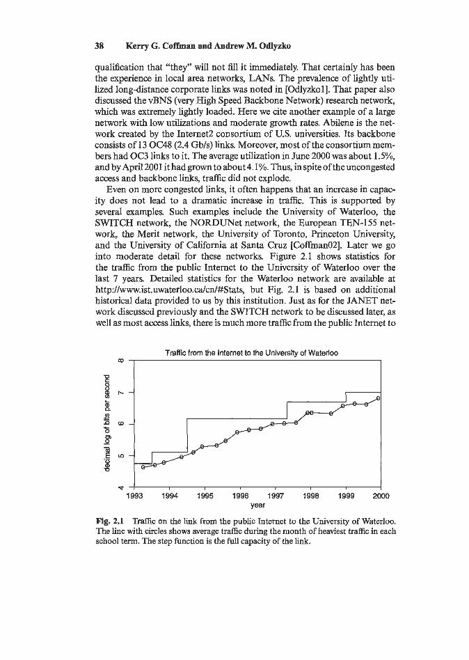
38 Kerry G. Coffian and Andrew M. Odlyzko
qualiiication that “they” will not fill it immediately. That certainly has been the experience in local area networks, LANs. The prevalence of lightly uti- lized long-distance corporate links was noted in [Odlyzkol]. That paper also discussed the vBNS (very High Speed Backbone Network) research network, which was extremely lightly loaded. Here we cite another example of a large network with low utilizations and moderate growth rates. Abilene is the net- work created by the Internet2 consortium of U.S. universities. Its backbone consists of 13 OC48 (2.4 Gb/s) links. Moreover, most of the consortium mem- bers had OC3 links to it. The average utilization in June 2000 was about 1.5%, and by April 2001 it had grown to about 4.1%. Thus, in spite of the uncongested access and backbone links, tr&c did not explode.
Even on more congested links, it often happens that an increase in capac- ity does not lead to a dramatic increase in traffic. This is supported by several examples. Such examples include the University of Waterloo, the SWITCH network, the NORDUNet network, the European TEN-155 net- work, the Merit network, the University of Toronto, Princeton University, and the University of California at Santa Cruz [CoffmanO2]. Later we go into moderate detail for these networks. Figure 2.1 shows statistics for the traffic from the public Internet to the University of Waterloo over the last 7 years. Detailed statistics for the Waterloo network are available at http://www.ist.uwaterloo.ca/cn/#Stats, but Fig. 2.1 is based on additional historical data provided to us by this institution. Just as for the JANET net- work discussed previously and the SWITCH network to be discussed later, as well as most access links, there is much more traffic from the public Internet to
Traffic from the Internet to the University of Waterloo 03
I I I I
1993 1994 1995 1996 1997 1998 1999 2000 year
Fig. 2.1 T r a c on the link from the public Internet to the University of Waterloo. The line with circles shows average traffic during the month of heaviest traffic in each school term. The step function is the full capacity of the link.

2. Growth of the Internet 39
the institution than in the other direction. Hence we concentrate on this more congested link, because it offers more of a barrier. We see that even substantial jumps in link capacity did not affect the growth rate much. Traffic has been about doubling each year for the entire 7-year period. (Overall, the growth rate at the University of Waterloo has slowed, about 55% from early 1999 to early 2000. This was at least partially the result of official limits on individual users that were imposed, limits we will discuss later.)
The same phenomenon of traffic doubling each year, no matter what happens to capacity, can be observed in the statistics for the SWITCH network, which provides connectivity for Swiss academic and research institu- tions. The history and operations of this network are described in [Harms, ReichlLS], and extensive current and historical data are available at http:// www.switch.ch/lan/stat/. The data used to prepare Fig. 2.2 was provided to us by SWITCH. As is noted in [ReichlLS], the transatlantic link has historically been the most expensive part of the SWITCH infrastructure, and at times was more expensive than the entire network within Switzerland. It is therefore not surprising that this link tends to be the most congested in the SWITCH net- work. Even so, increasing its capacity did not lead to a dramatic change in the growth rate of traffic. If we compare increases in volume of data received between November of one year and January of the following year, there was an unusually high jump (420/0) from November 1998 to January 1999. This was in response to extreme congestion experienced at the end of 1998, congestion that produced extremely poor service, with packet loss rates during peak peri- ods exceeding 20%. However, over longer periods of time, the growth rate has been rather steady at close to 100% per year and independent of the capacity
Capacity and traffic on SWITCH transatlantic link H I
1996 1997 1998 1999 2000 2001 year
1996 1997 1998 1999 2000 2001 year
32
Fig. 2.2 Capacity of link between the Swiss SWITCH network and the United States and traffic on it toward Switzerland.
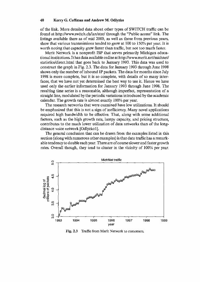
40 Kerry G. Coffman and Andrew M. Odlyzko
of the link. More detailed data about other types of SWITCH traffic can be found at http://www.switch.cMan/stat/ through the “Public access” link. The listings available there as of mid 2000, as well as those from previous years, show that various transmissions tended to grow at 100 to 150% per year. It is worth noting that capacity grew faster than traffic, but not too much faster.
Merit Network is a nonprofit ISP that serves primarily Michigan educa- tional institutions. It has data available online at http://www.merit.net/michnet/ statistics/direct.html that goes back to January 1993. This data was used to construct the graph in Fig. 2.3. The data for January 1993 through June 1998 shows only the number of inbound IP packets. The data for months since July 1998 is more complete, but it is so complete, with details of so many inter- faces, that we have not yet determined the best way to use it. Hence we have used only the earlier information for January 1993 through June 1998. The resulting time series is a reasonable, although imperfect, representation of a straight line, modulated by the periodic variations introduced by the academic calendar. The growth rate is almost exactly 100% per year.
The research networks that were examined have low utilizations. It should be emphasized that this is not a sign of inefficiency. Many novel applications required high bandwidth to be effective. That, along with some additional factors, such as the high growth rate, lumpy capacity, and pricing structure, contributes to the much lower utilization of data networks than of the long- distance voice network [Odlyzkol].
The general conclusion that can be drawn from the examples listed in this section (along with numerous other examples) is that data traffic has a remark- able tendency to double each year. There are of course slower and faster growth rates. Overall though, they tend to cluster in the Vicinity of 100% per year.
MichNet traffic
1993 1994 1995 1996 1997 1998 1999 year
Fig. 2.3 Traffic from Merit Network to customers
2. Growth of the Internet 41
To date, the authors have not seen any large institutions with traffic doubling anywhere close to every 3 or even 4 months.
The growth rates that are cited here are often affected strongly by restrictions imposed at various levels. As described elsewhere [CoffmanOl , CoffmanO2], some of the explicit limits are imposed by network administrators.
The arrival of Napster (discussed in Section 7) led many institutions to either ban its use or else limit traffic rates to some parts of the campus (typi- cally student dormitories). Push technologies were stifled at least partially because enterprise network administrators blocked them at their firewalls. E-mail often has size restrictions that block large attachments (and in some cases all attachments are still banned). Teleconferencing is only slowly being experimented with on corporate intranets, and even packetized voice sees very limited (although growing) use.
Similar constraints apply to most of the content seen on the Web. As long as a large fraction of potential users have limited bandwidth, such as through dial modems, managers of Web servers will have an incentive to keep individ- ual pages moderate in size. Thus, one can see that Internet traffic is subject to a variety of constraints at different levels. Some are applied by network managers, others by individual users, and the interaction of these constraints with the rising demands is fundamental in understanding what produces the growth rates observed.
The ability to sustain the high growth rate of Internet traffic will require the creation of new applications that will generate huge volumes of traffic. At current growth rates, by 2005 there will be eight times as much Internet as voice traffic (on the U.S. long-haul networks). If voice were packetized, in all likelihood the voice traffic would only account for about 3% of the Internet traffic. Thus, voice traffic will not fiU the pipes that are likely to exist, and neither will traditional Web surfing. This will create a dilemma for service providers, network administrators, and equipment suppliers: To sustain the growth rates that the industry has come to depend on, and to accommodate the progress in technology, new technologies are needed. Such applications will appear disruptive to network operations today, and as such, they often have to be controlled. However, in the long run, they must be encouraged.
7. Disruptive Innovation
It is often said that everything changes so rapidly on the Internet that it is impossible to forecast far into the future. The next “killer app” could disrupt any plans that one makes. Yet there have been just two “killer apps” in the history of the Internet: e-mail and the Web (or, more precisely, Web browsers, which made the Web usable by the masses). Many other technologies that had been widely touted as the next “killer app,” such as push technology have fizzled. (Push technology allows the sending of information directly to one’s

42 Kerry G. Coffman and Andrew M. Odlyzko
computer instead of the computer needing to actively go out and obtain it.) Furthermore, only the Web can be said to have been truly disruptive. From the first release of the Mosaic visual browser around the middle of 1993, it apparently took under 18 months before Web trafKc became dominant on Internet backbones. It appears overwhelmingly likely that it was the appear- ance of browsers that then led, in combination with other developments, to that abnormal spurt of a doubling of Internet trafKc every 3 or 4 months in 1995 and 1996.
What were the causes of the 100-fold explosion in Internet backbone traffic over the 2-year period of 1995 and 1996? We do not have precise data, but it appears that there were four main factors, all interrelated. Browsers passed some magic threshold of usability, so many more people were willing to use computers and online information services. Users of the established online services, primarily AOL, CompuServe, and Prodigy, started using the Internet. The text-based transmissions of those services, which probably averaged only a few hundred bits per second per connected user, were replaced by the graphics- rich content of the Web, so transmission rates increased to a few thousand bits per second. Finally, flat rate access plans led to a tripling of the time that individual users spent online [Odlyzko3], as well as faster growth in number of users.
The Internet was able to support this explosion in use because it was utilizing the existing infrastructure of the telephone network. At that time, the Internet was tiny compared to the voice network.It is likely that the data network that handles control and billing for the AT&T long-distance voice services by itself was carrying more traffic than the NSF Internet backbone did at its peak at the end of 1994. Today, by contrast, the public Internet is rapidly moving toward being the main network, so quantum jumps in traffic cannot be tolerated so easily.
In late 1999, a new application appeared that attracted extensive attention and led to many predictions that network traffic would see a major impact. It was Napster. At the time, numerous articles in the press cited Napster’s ability to “overwhelm Internet lines,” and have claimed that it has forced numerous universities to ban or limit its use. The impression one got from those press reports was that Napster was causing a quantum jump in Internet traffic, and was driving the traffic growth rates well beyond the normal range. However, upon close examination this does not appear to be completely accurate, and the use of Napster has not increased growth rates much beyond the annual doubling or tripling rates, even within university environments, where Napster is most popular. That is not to say that it has not resulted in huge amounts of traffic, nor that it has not had serious impact on several major networks.
Napster provides software that enables users connected to the Internet to exchange andor download MP3 music files. The Napster Web site matches users seeking certain music files with other users who have those files on their computer. The Napster system preferentially uses machines that have high
2. Growth of the Internet 43
bandwidth connections as sources of files. This means that universities are the primary sources, since other organizations with fast dedicated links, mainly corporations, do not allow such traffic. The result is that although college students are often cited as the greatest users of MP3 files, it is the traffic from universities that gets boosted the most. (Because that direction of traffic is typically much less heavily used than the reverse one, the impact of Napster is much less severe than if the dominant direction of traffic were reversed.) Regular modem users are usually not affected, because their connections are too slow. However, the proliferation of cable modems and DSL connections that have “always-onyy high-bandwidth connectivity is leading to problems for some residential users, especially since the uplink is the one that invariably has the more limited bandwidth.
A key reason that Napster is of great interest to us is that similar types of sharing applications effectively turn consumers of information into providers of information. u h e World Wide Web was designed for such information sharing, but for some types of files Napster and its kin are preferable.) These applications will effectively turn traditional consumer PCs into Internet servers that will output large amounts of traffic to other users. In Napster’s case this has been predominantly MP3 music files, but other programs, such as Gnutella, work with more general data. It is highly probable that such applications could be one of the key applications that fuel the continued annual doubling or tripling of data traffic.
Napster first became noticeable in the summer of 1999. Its share of the total Internet traffic on many of the university networks has grown from essentially nothing to around 25% of the total traffic by mid to late 2000. In [CoffmanO2] the traffic generated by Napster and its impact on various networks was examined. The amount of Napster traffic that is reported by several university networks (such as University of California at Santa Cruz, University of Michigan, University of Indiana, University of California at Berkeley, Northwestern University, and Oregon State University to name a few) ranges from around 20 to 50%. However, the reported numbers are often very preliminary, and in some cases they compare Napster traffic to total traffic, whereas in others it appears that the high values may represent a com- parison only to the out traffic. In any event, this is a phenomenal growth rate for any single application. Since it started from zero and our data only goes out to about a year from that time, it is risky to extrapolate this ini- tial explosion out indefinitely. In most cases [CoffmanO2], Napster has had a noticeable effect on the growth rate of traffic on this campus, but not an outlandish one.
Several networks, such as that of the University of Wisconsin-Madison that report Napster traflk making up as much as 30% of the total, are not doing anything to limit Napster because they claim that they still have plenty of bandwidth. Others have imposed limits on the total bandwidth available to the dormitories.

44 Kerry G. Coffman and Andrew M. Odlyzko
Aside from Napster, occasionally even a large institution will experience a local perturbation in its data traffic patterns caused by one particular application. For example, the SETI@home distributed computing project (http://setiathome.ssl.berkeley.edu) uses idle time on about three million PCs (as of mid 2001) to search for signs of extraterrestrial intelligence in signals collected by radio telescopes. This project is run out of the Space Sciences Insti- tute at the University of California at Berkeley, and within a year of inception it accounted for about a third of the outgoing campus traffic [McCredie]. (Moreover, this was extremely asymmetrical traffic, with large sets of data to be analyzed going out to the participating PCs and small final results coming back. That most of the data went away from campus made this application less disruptive than it would have been otherwise.) Its disruptive effect is mod- erated by limiting its transmission rate to about 20 Mb/s. At the University of California at Santa Cruz, a complete copy of the available genome sequence was made available for public download in early July 2000. This, combined with coverage in the popular press and on Slashdot, led to an immediate surge in traffic, far exceeding the effects of Napster. If the interest in this database continues, it will require reengineering of the campus network.
The SETI@home project is interesting for several reasons. It is cited in [McCredie] as a major new disruptive influence. Yet it contributes only about 20 Mb/s to the outgoing traffic. An increasing number of PCs and worksta- tions are connected at 100 Mb/s, and even Gigabit Ethernet (1,000 Mb/s) is coming to the desktop. This means that for the foreseeable future, a handful of workstations will, in principle, be capable of saturating any Internet link. Given the projections for bandwidth, a few thousand machines will continue to be capable of saturating all the links in the entire Internet. Thus control on user traffic will have to be exercised to prevent accidental as well as malicious disruptions of service. However, it seems likely that such control could be lim- ited to the edges of the network. In fact, such control will pretty much have to be exercised at the edges of the network. QoS (Quality of Service) will not help by itself, since a malicious attacker who takes control of a machine will be able to subvert any automatic controls.
Finally, after considering current disruptions from Napster and SETI@home, we go back and consider browsers and the Web again. They were cited as disruptive back in 1994 and 1995. (Mosaic was first released unofficially around the middle of 1993, officially in the fall of 1993, and took off in 1994.) However, when we consider the growth rates for the University of Waterloo, for MichNet [CoffmanOl], or for SWITCH (which apparently had regular growth throughout the 1990s according to [Harms]), we do not see anything anomalous, just the steady doubling of traffic each year or so. If we consider the composition of the traffic, there were major changes. For example, Fig. 2.4 shows the evolution of traffic between the University of Waterloo and the Internet. (It is based on analysis of traffic during the third week in each March, and more complete results

2. Growth of the Internet 45
are available at http://www.ist.uwaterloo.ca/cn/Stats/ext-prot.html.) The Web did take over, but much more slowly than on Internet backbones. There are no good data sets, but it has been claimed that by the end of 1994, Web traffic was more than half of the volume of the commercial back- bones. On the other hand, the data for the NSFNet backbone, available at http://www.merit.edu/merit/archive/nsfnet/statistics/index.html, show that Web traffic was only approaching 20% there by the end of 1994, a level similar to that for the University of Waterloo. Thus, at well-wired academic institu- tions such as the University of Waterloo and others that dominated NSFNet traffic, the impact of the Web was muted.
Perhaps the main lesson to be drawn from the discussion in this section is that the most disruptive factor is simply rapid growth by itself. A doubling of traffic each year is very rapid, much more rapid than in other communication services. Figure 2.4 shows e-mail and netnews shrinking as fractions of the traffic at the University of Waterloo, from a quarter to about 5%. Yet the byte volume of these two applications grew by a factor of 12 during the 6 years covered by the graph, for a growth rate of over 50% per year, which is very rapid by most standards. If we are to continue the doubling of traffic each year, new applications will have to keep appearing and assuming dominant roles. An interesting data point is that even at the University of Wisconsin in Madison, which analyzes its data traffic very carefully, about 40% of the transmissions escape classification. That is consistent with information from a few corporate networks, where the managers report that upwards of half of their traffic is of unknown types. (A vast majority of network managers do not even attempt to perform such analyses.) This shows how difficult coping with rapid growth is.
internet traffic at the University of Waterloo
0 m 0 E 9 - u - 0 o m a 0, m c p 0) n 0 cu
I I I I I I 1994 1995 1996 1997 1998 1999 2000
year
Fig. 2.4 Composition of traffic between the University of Waterloo and the Internet based on data collected in March of each year.
46 Kerry G. Coffman and Andrew M. Odlyzko
8. Moore’s Law for Data Traffic
The approximate doubling of transmission capacity of each fiber that is described in [CoffmanO2] is analogous to the famous Moore’s Law in the semiconductor industry. In 1965, Gordon E. Moore, then in charge of R&D at Fairchild Semiconductor, made a simple extrapolation from three data points in his company’s product history. He predicted that the number of transistors per chip would about double each year for the next 10 years. This prediction was fulfilled, but when Moore revisited the subject in 1975, he modified his projection for further progress by predicting that the doubling period would be closer to 18 months. (For the history and fuller discussion of Moore’s Law, see [Schaller].) Remarkably enough, this growth rate has been sustained over the past 25 years. There have been many predictions that progress was about to come to a screeching halt (including some recent ones), but the most that can be said is that there may have been some slight slowdown recently. (For example, according to the calculations shown in FlderingSE], the number of transistors in leading-edge microprocessors doubles every 2.2 years. On the other hand, the doubling period is lower for commodity memories.) Experts in the semiconductor area are confident that Moore’s 1975 prediction for rate of improvement can be fulfilled for at least most of the next decade.
Predictions similar to Moore’s had been made before in other areas, and in [Licklider] they were made for the entire spectrum of computing and com- munications. However, it is Moore’s Law that has entered the vernacular as a description of the steady and predictable progress of technology that improves at an exponential rate (in the precise mathematical sense).
Moore’s Law results from a complex interaction of technology, sociology, and economics. No new laws of nature had to be discovered, and there have been no dramatic breakthroughs. On the other hand, an enormous amount of research had to be carried out to overcome the numerous obstacles that were encountered. It may have been incremental research, but it required increasing ranks of very clever people to undertake it. Furthermore, huge investments in manufacturing capacity had to be made to produce the hardware. Perhaps even more important, the resulting products had to be integrated into work and lifestyles of the institutions and individuals using them. For further discussions of the genesis, operations, and prospects of Moore’s Law, see [ElderingSE, Schaller]. The key point is that Moore’s Law is not a natural law, but depends on a variety of factors. Still, it has held with remarkable regularity over many decades.
Although Moore’s Law does apply to a wide variety of technologies, the actual rates of progress vary tremendously among Merent areas For example, battery storage is progressing at a snail‘s pace’ compared to microprocessor improvements. This has signscant implications for mobile Internet access, limiting processor power and display quality. Display advances are more rapid than those in power storage, but nowhere near fast enough to replace paper
2. Growth of the Internet 47
as the preferred technology for general reading, at least not at any time in the next decade. (This implies, in particular, that the bandwidth required for a single video transmission will be growing slowly.) Dynamic Random Access Memories (DRAMS) is growing in size in accordance with Moore’s Law, but their speeds are improving slowly. Microprocessors are rapidly increasing their speed and size (which allows for faster execution through parallelism and other clever techniques), but memory buses are improving slowly. For some quantitative figures on recent progress, see [Grays]. From the standpoint of a decade ago, we have had tidal waves of just about everything: processing power, main memory, disk storage, and so on. For a typical user, the details of the PC on the desktop (MHz rating of the processor, disk capacity) do not matter too much. It is generally assumed that in a couple of years a nav and much more powerful machine will be required to run the new applications, and that it will be bought for about the same price as the current one. In the meantime, the average utilization of the processor is low (since it is provided for peak performance only), compression is not used, and wasteful encodings of information (such as 200 KB Word documents conveying a simple message of a few lines) are used. The stress is not on optimizing the utilization of the PC’s resources, but on making life easy for the user.
To make life easy for the end user, though, clever engineering is employed. Because the tidal waves of different technologies are advancing at differ- ent rates, optimizing user experience requires careful architectural decisions [Grays, HennessyP]. In particular, since processing power and storage capac- ity are growing the fastest, while communication within a PC is improving much more slowly, elaborate memory hierarchies are built. They start with magnetic hard disks and proceed through several levels of caches, invisibly to the user. The resulting architecture has several interesting implications, which are explored in [Grays]. For example, mirroring disks is becoming preferable to RAID (Redundant Arrays of Inexpensive Disks) fault-tolerant schemes that are far more efficient but slower.
The density of magnetic disk storage increased at about 30% per year from 1956 to 1991, doubling every 2; years [Economist]. (Total deployed storage capacity increased faster, as the number of disks shipped grew.) In the 1990s, the growth rate accelerated, and in the late 1990s increased yet again. By some accounts, t h ~ densities in disk drives are about doubling each year. For our purposes, the most relevant figure will be total storage of disk drives. Table 2.5 shows data from an IDC study, which shows storage capacity shipped each year just about doubling through the year 2000, and then slowing down. However, that study was prepared in 1998, and since then IDC has revised upwards its estimates for disk storage systems toward a continuation of the doubling trend. Similar projections from Disk/Trend (http://www.disktrend.com/) also suggest that the total capacity of disk drives shipped will continue doubling through at least the year 2002. Given the advances in research on magnetic storage, it seems that a doubling each year until the year 2010 might be achievable (with
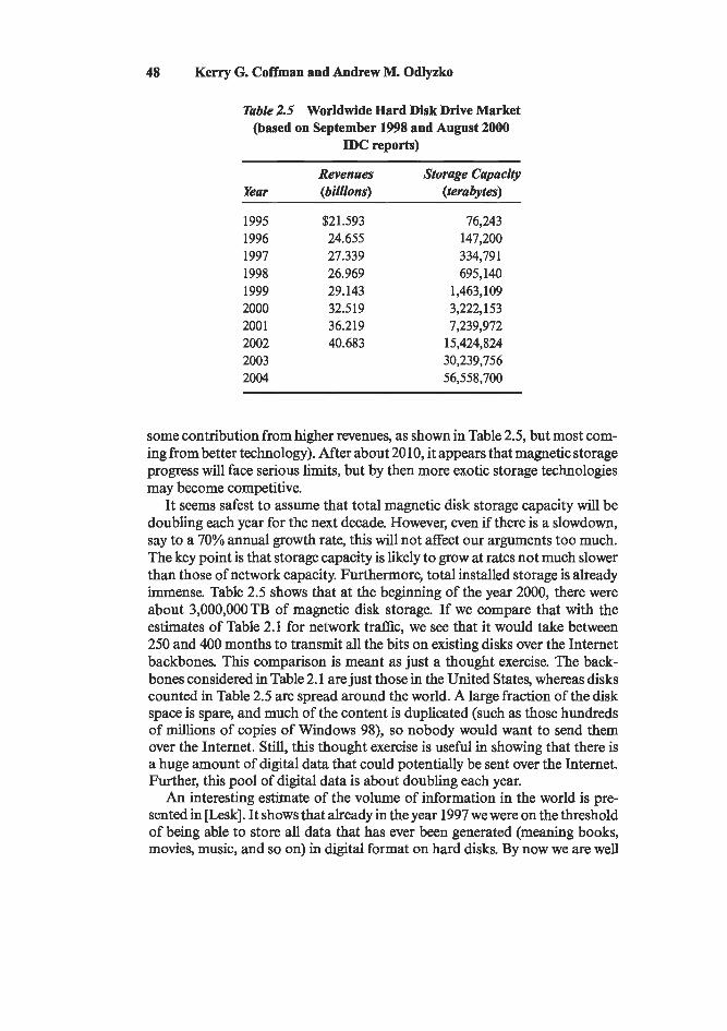
48 Kerry G. Coffman and Andrew M. Odlyzko
Table 2.5 Worldwide Hard Disk Drive Market (based on September 1998 and August 2000
IDC reports)
Revenues Storage Capacity Year (bizfions) (terabytes)
1995 $21.593 76,243 1996 24.655 147,200 1997 27.339 334,791 1998 26.969 695,140 1999 29.143 1,463,109 2000 32.519 3,222,153 200 1 36.219 7,239,972 2002 40.683 15,424,824 2003 30,239,756 2004 56,558,700
some contribution from higher revenues, as shown in Table 2.5, but most com- ing from better technology). After about 2010, it appears that magnetic storage progress will face serious limits, but by then more exotic storage technologies may become competitive.
It seems safest to assume that total magnetic disk storage capacity will be doubling each year for the next decade. However, even if there is a slowdown, say to a 70% annual growth rate, this will not affect our arguments too much. The key point is that storage capacity is likely to grow at rates not much slower than those of network capacity. Furthermore, total installed storage is already immense. Table 2.5 shows that at the beginning of the year 2000, there were about 3,000,000TB of magnetic disk storage. If we compare that with the estimates of Table 2.1 for network traffic, we see that it would take between 250 and 400 months to transmit all the bits on existing disks over the Internet backbones. This comparison is meant as just a thought exercise. The back- bones considered in Table 2.1 are just those in the United States, whereas disks counted in Table 2.5 are spread around the world. A large fraction of the disk space is spare, and much of the content is duplicated (such as those hundreds of millions of copies of Windows 98), so nobody would want to send them over the Internet. Still, this thought exercise is useful in showing that there is a huge amount of digital data that could potentially be sent over the Internet. Further, this pool of digital data is about doubling each year.
An interesting estimate of the volume of information in the world is pre- sented in [Lesk]. It shows that already in the year 1997 we were on the threshold of being able to store all data that has ever been generated (meaning books, movies, music, and so on) in digital format on hard disks. By now we are well

2. Growth of the Internet 49
past that threshold, so future growth in disk capacities will have to be devoted to other types of data that we have not dealt with before. Some of that capac- ity will surely be devoted to duplicate storage (such as a separate copy of an increasingly bloated operating system on each machine). Most of the storage, though, will have to be filled by new types of data. The same process that is yielding faster processors and larger memories is also leading to improved cameras and sensors These will yield huge amounts of new data that have not been available before. It appears impossible to predict precisely what type of data this will be. Much is likely to be video storage from cameras set up as security measures or ones that record our every movement. There could also be huge amounts of data from medical sensors on our bodies. What is clear, though, is that “[tlhe typical piece of information will never be looked at by a human being” [Lesk]. There will simply not be enough of the traditional “content” (books, movies, music) nor even enough of the less formal type of “content” that individuals will be generating on their own.
Huge amounts of data that is machine generated for machine use suggests that data networks will also be dominated by transfers of such data. This was already predicted in [deSolaPITH], and more recently in [Odlyzko2, StArnaud, StArnaudCFM]. Given an exponential growth rate in volume of data transfers, it was clear that at some point in the future most of the data flying through the networks would be neither seen nor heard by any human being. Thus, we can expect that streaming media with real-time quality requirements will be a decreasing fraction of total traffic at some point within the next decade.
There will surely be an increase in the raw volume of streaming real-time traffic, as applications such as videoconferencing move onto the Internet. However, as a fraction of total trafiic, such transmissions will not only decrease eventually, but may not grow much at all even in the intermediate future. (Recall that at the University of Waterloo over the last 6 years, the volume of e-mail grew about 50% a year, but as a fraction of total trafiic it is almost negligible now.) The huge imbalance in volume of storage and capacities of long-distance data networks means that even the majority of traditional “con- tent” will be transmitted as files, and not in streaming form. For more detailed arguments supporting this prediction, see [Odlyzko2]. This development, in which “content” is sent around as files for local storage and playback, is already making its appearance with MP3, Napster, and related programs.
The huge hard disk storage volumes also mean that most data will have to be generated locally. There will surely also be much duplication (such as operating systems, movies, and so on that would be stored on millions of computers). Aside from that, there will surely be huge volumes of locally generated data (e.g., from security cameras and medical sensors) that will be used (if at all) only in highly digested form.
The examples in [Coffman02] support the notion that there is a “Moore’s Law” for data traffic, with transmission volumes doubling each year. Even at large institutions that already have access to state-of-the art technology,
50 Kerry G. Cofitnan and Andrew M. Odlyzko
data traffic to the public Internet tends to follow this rule of doubling each year. This is not a natural law, but, like all other versions of Moore’s Law, reflects a complicated process, the interaction of technology and the speed with which new technologies are absorbed. A Moore’s Law for data traffic is different from those in other areas, since it depends in a much more direct way on user behavior. In semiconductors, consumer willingness to pay drives the research, development, and investment decisions of the industry, but the effects are indirect. In data traffic, though, changes can potentially be much faster. A residential customer with dial-up modem access to the Internet could increase the volume of data transfer by a factor of about five very quickly. All it would take would be the installation of one of the software packages that prefetch Web sites that are of potential interest and that fill in the slack between transmissions initiated by the user. Similarly, a university’s T3 connection to the Internet could potentially be filled by a single workstation sending data to another institution. Thus any Moore’s Law for data traflic is by nature much more fragile than the standard Moore’s Law for semiconductors, for example. Thus it is remarkable that we see so much regularity in growth rates of data transfers.
Links to the public Internet are usually the most expensive parts of a net- work, and are regarded as key choke points They are where congestion is seen most frequently at institutional networks. Yet the “mere” annual doubling of data traffic even at institutions that have plenty of spare capacity on their Inter- net links means that there are other barriers that matter. The obvious one is the public Internet itself. It is often (some would say usually) congested. A terabit pipe does not help if it is hooked up to a megabit link, and so providing a lightly utilized link to the Internet does not guarantee good end-to-end performance. Yet that is not the entire explanation either, since corporate Intranets, which tend to have adequate bandwidth and seldom run into congestion, tend to grow no faster than a doubling of traflic each year. There are other obstruc- tions, such as servers, middleware, and, perhaps most important, services and user interfaces People do not care about getting many bits. What they care about are the applications. However, applications take time to be developed, deployed, and adopted. To quote J. Licklider (who probably deserves to be called “the grandfather of the Internet” for his role in setting up the research program that led to the Internet’s creation):
A modern maxim says: “People tend to overestimate what can be done in one year and to underestimate what can be done in five or ten years.” Picklider]
“Internet time,” where everything changes in 18 months, has a grain of truth, but is largely a myth. Except for the ascendancy of browsers, most substantial changes take 5 to 10 years. As an example, it has been at least 4 years since voice over IP was first acclaimed as the ‘‘next big thing.” Yet its impact so far has been surprisingly modest. It is coming, but it is not here today, and it won’t be here tomorrow. People take time to absorb new technologies.
2. Growth of the Internet 51
What is perhaps most remarkable is that even at institutions with congested links to the Internet, traffic doubles or almost doubles each year. Users appear to find the Internet attractive enough that they exert pressure on their admin- istration to increase the capacity of the connection. Existing constraints, such as those on e-mail attachments, or on packetized voice or video, as well as the basic constraint of limited bandwidth, are gradually loosened. Note that this is similar to the process that produces the standard Moore’s Law for PCs. Intel, Micron, Toshiba, and the rest of the computer industry would surely produce faster advances if users bought new PCs every year. Instead, a typical PC is used for 3 to 4 years. On one hand there is pressure to keep expenditures on new equipment and software under control, and also to minimize the com- plexity of the computing and communications support job. On the other hand, there is pressure to upgrade, either to better support existing applications or to introduce new ones. Over the last three decades, the conflict between these two pressures has produced a steady progress in computers. Similar pressures appear to be in operation in data networking.
In conclusion, we cannot be certain that Internet t r a c will continue dou- bling each year. All we can say is that historically it has tended to double each year. Still, trends in both transmission and in other information technologies appear to provide both the demand and the supply that will allow a continuing doubling each year. Since betting against such Moore’s laws in other areas has been a loser’s game for the last few decades, it appears safest to assume that data traffic will indeed follow the same pattern, and grow at close to 100% per year.
9. Further Economic and Technical Considerations
A frequently asked question concerns the elasticity of demand for data trans- mission capacity. However, for long-range projections it might be more useful to think of analogies with the computer industry. In that industry, product managers clearly do think about elasticities in the short or intermediate terms. From a long-range perspective, though, what dominates are the effects of Moore’s Law. Table 2.6 (drawn from [FishburnO]) shows a dozen years from the history of Intel. The leading microprocessor sold for roughly a constant price all during this period. However, its power was increasing at the expo- nential rate given by Moore’s Law. Intel’s total revenues (and profits) grew, as more processors were being sold, but this growth rate was considerably more modest than that of the computing power. Users found the increasing compu- tational power of new PCs sufficiently attractive that they not only bought new PCs, but increased their total spending. They did this even though most of that power was sitting idle, and it was only the occasional bursts of recomputing a spreadsheet or bringing up a presentation package that mattered. A similar

52 Kerry G. Coffman and Andrew M. Odlyzko
Table 2.6 Intel and Its Microprocessors (each year lists the most powerful General Purpose Microprocessors Sold by Intel, Its Computing Power, Price at the End of the Year (in Dollars), and Intel’s Revenues and Profits for That Year
(in Millions of Dollars))
Revenue Net Profit Price (millions (millions
Year Processor Mips (dollam) of dollars) of dollars)
1986 386 DX (16MHz) 5 300 1,265 - 173 1987 386 DX (20 MHz) 6 1,907 248
1989 486 DX (25 MHz) 20 950 3,127 391 1990 486 DX (33 MHz) 27 950 3,922 650 1991 486 DX (50 MHz) 41 644 4,779 819 1992 DX2 (66 MHz) 54 600 5,844 1,067 1993 Pentium (66 MHz) 112 898 8,782 2,295 1994 Pentium (100MHz) 166 935 11,521 2,266 1995 Pentium Pro (200 MHz) 400 1,325 16,202 3,566 1996 20,847 5,157 1997 Pentium I1 (300 MHz) 600 735 25,070 8,945
1988 386 DX (25 MHz) 8 2,875 453
evolution might take place in networking. Total spending may (subject to busi- ness cycles) increase at a moderate pace, while the bandwidth and traffic grow at rates determined by technological progress. If that happens, we are likely to see traffic and capacity about doubling each year, with capacity growth faster than that of traffic.
10. Conclusions
Much of the almost hyperactivity within the optical fiber telecommunications industry over the past few years can be traced to the perceived and real growth of the traffic on the Internet. We maintain that the overall growth rate of the Internet for most of its existence (despite some excursions) was remarkably close to “doubling every year,” and we anticipate that this rate will continue into the foreseeable future. In effect, we see a type of Moore’s Law associated with the growth of data traffic. This type of growth rate is in sharp contrast to the historical growth rates of various methods of communications (including conventional mail, telegraph service, and traditional voice phone service) that tended to be no greater (and typically much less) than about 10Y0 per year. Still, even though a doubling each year represents very fast growth, it is only comparable to the rate of progress in transmission capacity. Hence we are

2. Growth of the Internet 53
unlikely to see the huge increases in spending on optical communication that many business plans had been based on.
Throughout the history of the Internet there have only been two “killer applications”: e-mail and the Web (including Web browsers). Several events conspired that allowed an unprecedented explosion (roughly 1 00-fold increase) in Internet traffic in the 1995-1996 time frame, and the Internet was able to handle this because it made use of the existing telephone industry infrastruc- ture. Because the Internet is quickly approaching the point at which it is the predominant network, it is very unlikely that such huge growth rates could be so easily supported in the future.
It also appears that, aside from short-range perturbations, there will be neither a “bandwidth glut” nor a “bandwidth shortage” in the foreseeable future, in that supply and demand will be growing at comparable rates. As such, it is very likely that pricing will begin to play an even more important role in the evolution of traffic. Throughout most of the 1990s, data transmission prices were increasing. However, there are recent signs that they are beginning to decrease, and in some cases, especially across the Atlantic and on major transcontinental routes in the United States, they have decreased dramatically. If they begin to decrease rapidly in general, then many of the constraints on usage that exist today may very likely start to ease. We are likely to see capacity growing somewhat faster than traffic, a continuation of the trend we have already seen in the last few years.
We also believe that “file” transfers, and not real-time streaming, will remain dominant on the network. Streaming real-time transmissions will undoubtedly grow in absolute terms, and as a fraction of the total traffic it may increase for a while. However, in all likelihood it will eventually begin to decline as the demand for this type of traffic will not grow as fast as network capacity. We foresee sharing applications as a likely candidate to fuel traffic growth. One of the first major examples of this was Napster, because it effectively turned consumers of information into providers of information. It is extremely likely that such file sharing applications will be some of the key applications that continue to fuel the annual doubling of data traffic.
References
[Abbate] [Baran]
[Boardwatch] [Bruno]
J. Abbate, Inventing the Internet, MIT Press, 1999. I? Baran, On distributed communications network, IEEE Trans. Comm. Systems, vol. 12, 1964, pp. 1-9. Boardwatch. Available at http://www.boardwatch.com. L. Bruno, Fiber optimism: Nortel, Lucent, and Cisco are bat- tling to win the high-stakes fiber-optics game, Red Herring, June 2000. Available at http://www.herring.com/mag/issue79/mag-fiber- 79.html.
54 Kerry G. Coffman and Andrew M. Odlyzko
1Cerf-I
[CerfKI
[Cochrane]
[CoffmanOl]
[Coffman02]
[CTIA]
[Cyberspace]
[deSolaPITH]
P W L I
[Economist] [ElderingSE]
[Fishburno]
FlOYdPI
[Galbi]
V. G. Cerf, A brief history of the Internet and related networks. Available at http://www.isoc.org/internethistory/cerf html. V. G. Cerf and R. E. Kahn, A protocol for packet network inter- connection, IEEE Trans. Comm. Tech., vol. COM-22, May 1974,
N. Cochrane, We’re insatiable: Now it’s 20 million million bytes a day, Melbourne Age, January 15, 2001. Available at http:llwww .it.fairfax.com.au/networking/200 10 1 15/A 13694-200 1 Jan1 5.html. K. G. Coffman and A. M. Odlyzko, The size and growth rate of the Internet, First Monday, October 1998. Available at http://fkstmonday.org/. Also available at http://www.dtc.umn.edu/ -0dlyzko. K. G. Coffman and A. M. Odlyzko, Internet growth: Is there a “Moore’s Law” for data traffic?, Handbook of Massive Data Sets, J. Abello, P. M. Pardalos, and M. G. C. Resende, eds, Kluwer, 200 1, in press. Available at http://www.dtc.umn.edu/-odlyzko. CTIA (Cellular Telecommunications Industry Association), Semi- Annual FEreleSs Industry Survey, June 1985 to June 2000. Available at http:l/www.wow-com.codwirelesssurvey/. Geography of Cyberspace Directoiy: Internet Trafic and Demo- graphic Statistics. Available at http://www.cybergeography.org/ statistics.html. I. de Sola Pool, H. Inose, N. Takasaki, and R. Hurwitz, Communica- tions Flows: A Census in the Unitedstates andJapan, North-Holland, 1984. D. A. Dunn and A. J. Lipinski, Economic considerations in computer-communication systems, pp. 37 1- 422 in Computer- Communication Networh, N. Abramson and F. F. Kuo, eda, Prentice-Hall, 1973. Not Moore’s Law, The Economist, July 12,1997. C. A. Eldering, M. L. Sylla, and J. A. Eisenach, Is there a Moore’s Law for bandwidth? IEEE Communications Magazine, October
I? C. Fishburn and A. M. Odlyzko, Dynamic behavior of dif- ferential pricing and Quality of Service options for the Internet, pp. 128-139 in Proc. First Intern. Con$ on Information and Com- putation Economies (ICE-98), ACM Press, 1998. Available at http://www.dtc.umn.edu/-odlyzko. S. Floyd and V. Paxson, Dimculties in simulating the Inter- net, IEEE/ACM Damactions on Networking, in press. Available at ht tp://www. aciri. orglfloydpapers. html. D. Galbi, Bandwidth use and pricing trends in the U.S., Telecom- munications Policy, vol. 24, no. 11, December 2000. Available at http://www.galbithink.org.
pp. 627-641.
1999, pp. 2-7.
2. Growth of the Internet 55
[Green]
[Harms]
[HennessyP]
[Hobbes]
[Houghl
[Kleinrockl]
[Kleinrock2]
[Kleinrock3]
[Leiner]
[Lesk]
[Licklider] [LickC]
[Lucky 11
[Lucky21
[McCredie]
[MeekerM J]
J. Gray and P. Shenoy, Rules of thumb in data engineering, Proc. 2000 ZEEE Intern. Con$ Data Engineering. Available at http://research.microsoft.com/-gray. E. E. Green, Communications spectra by the wholesage2012 A.D., Proc. IRE, vol. 50,1962, pp. 585-587. Reprinted in Proc. ZEEE, vol.
J. Harms, From SWITCH to SWITCH*-extrapolating from a case study, Proc. INET '94, pp. 341-1 to 341-6. Available at http:l/ info.isoc.org/iso~whatis/conferences/ine~94lpapers/index. html. J. L. Hennessy and D. A. Patterson, Computer Architecture: A Quantitative Approach, Morgan Kaufmann, 1990. Hobbes Internet Emeline. Available at http:/lwww.zakon.org/ robert/internet/timeline/. R. W. Hough, Future data traffic volume, ZEEE Computer, September-October 1970, pp. 6-12. L. Kleinrock, Information flow in large communications networks, RLE Quarterly Progress Report, July 1961, pp. 1-35. Available at http://www.lk.cs.ucla.edu/LK/Bib/REPORT/PhD. L. Kleinrock, Communication Nets; Stochastic Message Flow and Delay, McGraw-Hill, 1964. L. Kleinrock, ISDN-The path to broadband networks, Proc. ZEEE,
B. M. Leiner, V. G. Cerf, D. D. Clark, R. E. Kahn, L. Kleinrock, D. C. Lynch, J. Postel, L. G. Roberts, and S. Wolf€, A Brief His- tory of the Internet, Version 3.31, August 4, 2000. Available at http://www.isoc.org/internetlhistory/brief.html. M. Lesk, How much information is there in the world? 1997, unpub- lished paper. Available at http://www.lesk.com/mlesk/diglib.html. J. C. R. Licklider, Libraries of the Future, MIT Press, 1965. J. C. R. Licklider and W. Clark, On-Line Man Computer Communi- cations, August 1962. R. W. Lucky, New communications services-What does society want? Proc. ZEEE, vol. 85, 1997, pp. 15361543. R. W. Lucky, Through a glass darkly-Viewing communications in 2012 from 1961, Proc. IEEE, vol. 87, 1999, pp. 1296-1300. J. McCredie, UC Berkeley must manage campus network growth, The Daily Californian, March 14, 2000. Available at http://www.dailycal.org/article.asp?id= 19 12&ref=news M. Meeker, M. Mahaney, and D. Joseph, The Internet userlusage ecosystem framework, Morgan Stanley Dean Witter report, Jan- uary 24, 200 1. Available at http://www.msdw.com/techresearch/ index.htm1. The Multi-Router Traflc Grapher of Tobias Oetiker and Dave Rand, information and links to sites using it at http://ee-staff.ethz.ch/ -oetiker/webtools/mrtg/mrtg.html.
87,1999,1293-1295.
V O ~ . 79, 1991, pp. 112-117.

56 Kerry G. Coffman and Andrew M. Odlyzko
PI11
[Nolll]
[No1121
pol131
[Nual [OdlYZko 11
[Odlyzko2]
[Odlyzko3]
[ReichlLS]
[Schaller]
[StAmaud]
[StAmaudCFM]
[Standage]
U. S. Information Infrastructure Task Force, The NationalZnforma- tion Znffastructure. Available at http://www.ibiblio.orglniiltoc.html. A. M. Noll, Znhoduction to Telephones and Telephone Traflc, 2nd ed., Artech House, 1991. A. M. Noll, Highway of Dreams: A Critical Appraisal of the Commu- nications Superhighway, Lawrence Erlbaum Associates, 1997. A. M. Noll, Does data traffic exceed voice traffic? Comm. ACM, June 1999, pp. 121-124. Nua Internet Surveys. Available at http://www.nua.com. A. M. Odlyzko, Data networks are lightly utilized, and will stay that way. Available at http://m.dtc.umn.edu/-odlyzko. A. M. Odlyzko, The history of communications and its implications for the Intenet. Available at http://www.dtc.umn.edu/-odlyzko. A. M. Odlyzko, Internet pricing and the history of communications, Computer Networh, vol. 36, 2001, pp. 493-517. Also available at http://www.dtc.umn.edu/-odlyzko. J. A. Polly, Surfing the Internet: An introduction, Wilson Library Bulletin, June 1992, pp. 38-42. Available at http://www.netmom .com/about/surfing.shtml. P. Reichl, S. Leinen, and B. Stiller, A practical review of pricing and cost recovery for Internet services, Proc. 2nd Internet Economics Worhhop Berlin (IEW '99), Berlin, Germany, May 28-29, 1999. Available at http://www. tik.ee.ethz.ch/-cati/. R. R. Schaller, Moore's law: Past, present, and future, IEEE Spec- trum, vol. 34: no. 6, June 1997, pp. 52-59. Available through Spectrum online search at http://www.spectrum.ieee.org. B. St. Arnaud, The future of the Internet is NOT multimedia, Net- work World, November 1997. Available at http://www.canarie.ca/ -bstarn/publications. html . B. St. Arnaud, J. Coulter, J. Fitchett, and S. Mokbel, Architectural and engineering issues for building an optical Internet. Short ver- sion in Proc. SOC. Optical Engineering, 1998. Full version available at http://www.canet3.net. T. Standage, n e Kctorian Internet: n e Remarkable Story of the Telegraph and the Nineteenth Century 5. On-line Pioneers, Walker, 1998. S. Taggart, Telstra: The prices fight, Wired News, http://www.wired .com/news/politics/O, 1283,32961 ,OO.html. €? M. Walker and S. L. Mathison, Regulatory policy and future data transmission services, pp. 295-370 in Computer- Communication Networh, N. Abramson and F. E Kuo, eds, Prentice-Hall, 1973. W. W. Wu and A. Livne, ISDN A snapshot, Proc. ZEEE, vol. 79, 1 9 9 1 , ~ ~ . 103-111.
Chapter 3
John Strand AT&T Laboratories, Middletown, New Jersey
Optical Network Architecture Evolution
1. Introduction
An Optical Transport Network (OTN) is composed of interconnected network elements (NEs), plus software and operational processes that must function together to provide services. Ongoing advances in technology will cause sig- nificant changes in OTN architecture; however, equally important will be the growth and evolution of the services it transports, particularly the Internet. In addition, business changes in the telecommunications industry will be very crit- ical. This chapter tries to weave the technology, services, and business stories together to indicate how they are shaping the architecture of the emerging optical network. Because most of the readers of these volumes are primarily technologists, tutorial material has been included.
1.1.
The very definition of “Optical Transport Network” illustrates why these sto- nes are interrelated. All would agree that optical fiber will be the physical layer of an OTN. There is less agreement on whether a network making extensive use of electronics for regeneration and switching should be called an OTN. Most of the audience for this volume are presumably most interested in all-optical OTNs; however, for a variety of business and service-related reasons that will be discussed later, many of the first generation “optical cross- connects” perform electronics-based functions like multiplexing DS-3s and slower speed SONET OC-ns into OC-48s and OC-192s. From this perspective, SONET is an “opaque one-wavelength” optical network, as Green [47] pointed out, even though much of its characteristic functionality is implemented in electronics.
We will take a “broad church” approach to defining an OTN. Given the nature of this volume, we will concentrate primarily, when possible, on net- works built from optical components; however, when necessary we will use the term to include networks transporting STS-1 (52 Mb/s) and larger con- nections that have an optical physical layer. When necessary to be precise, we will use the term “photonic” instead of “optical” to indicate that an all-optical
WHAT IS AN OPTICAL TRANSPORTNETWORK?
The views expressed are those of the author and not necessarily those of AT&T.
57 OPTICAL FIBER TELECOMMUNICATIONS, VOLUME IVB
Copyright 0 2002, Elsevier Science (USA). AU rights of reproduction in any form reserved.
ISBN: 0-12-395173-9
58 John Strand
situation is being discussed. Thus, a “Photonic Transport Network” (PTN) will be an all-optical OTN, and “Photonic Cross-Connect” (PXC) and “Photonic Add/Drop Multiplexer” (PADM) will be used when all-optical equipment is under discussion.
We will call a communications channel through an OTN a “circuit.” It is frequently called a “wavelength” or a “lightpath,” but because of the possibility that a connection might be partially electronic, we will stick with “connection.” If it is all-optical, we will also use the term “optical channel” (OCh).
1.2. SCOPE OF THIS CHAPTER
Because other chapters in the current volume deal with submarine systems, metropolitan OTNs, and access OTNs, we will focus primarily on intercity networks. Because of the background of the author, most of the discussion will have a strong U.S. flavor: For example, I will use SONET rather than SDH terminology, and I will frequently discuss issues of most interest to networks with diameters of thousands of kilometers, even though such large networks are only relevant to a handful of countries.
To keep the material to be covered within bounds, only technology likely to be commercially available within the next few years is considered. Many interesting areas, such as optical packet switching, are therefore omitted.
The reader should keep in mind the large error bars surrounding this whole enterprise. As an example, the architecture of actual OTNs even a few years in the future depends profoundly on the Internet: If its growth were to slow, the rate of introduction of new architectures would certainly slow, and the func- tionality desired (and hence the underlying technologies) might well change.
2. Technology Advances and Trends
The important underlying optical technologies are for the most part discussed elsewhere in this volume; the reader interested in the technologies per se should turn to the relevant sections. Our purpose here is twofold: (1) identify and define at a system level the building blocks on which the OTN architecture rests, and (2) point out major system-level trends we need to deal with in our later architecture development.
2.1. SONETBDH REFRESHER
SONET/SDH is important for optical networking for several reasons: (1) The overwhelming proportion of connections in long-haul OTNs are SONET or SDH formatted, and (2) many aspects of OTN architectures have been mod- eled on SONET/SDH concepts. This section gives a very brief overview of a few key aspects of these protocols that we will need later. For more complete overviews, see [18,72,73].
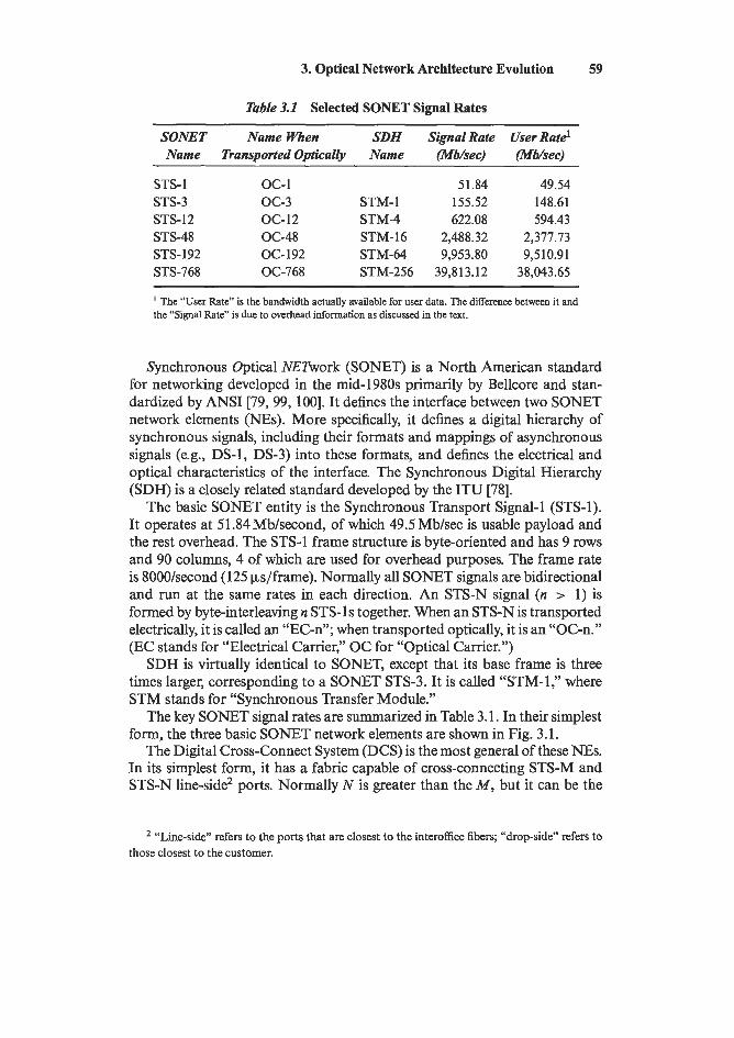
3. Optical Network Architecture Evolution 59
Table 3.1 Selected SONET Signal Rates
SONET Name When SDH Signal Rate User Rate’ Name Transported Optically Name (Mbhec) (IMb/sec)
STS-1 oc-1 51.84 49.54 STS-3 OC-3 STM- 1 155.52 148.61 STS-12 oc- 12 STM-4 622.08 594.43 STS-48 OC-48 STM-16 2,488.32 2,377.73 STS-192 OC- 192 STM-64 9,953.80 9,510.91 S T S - 7 6 8 OC-768 STM-256 39,813.12 38,043.65
’ The “User Rate” is the bandwidth actually available for user data. The difference between it and the “Signal Rate” is due to overhead information as discussed in the text.
Synchronous Optical NETwork (SONET) is a North American standard for networking developed in the mid-1980s primarily by Bellcore and stan- dardized by ANSI [79,99, 1001. It defines the interface between two SONET network elements (NEs). More specifically, it defines a digital hierarchy of synchronous signals, including their formats and mappings of asynchronous signals (e.g., DS-1, DS-3) into these formats, and defines the electrical and optical characteristics of the interface. The Synchronous Digital Hierarchy (SDH) is a closely related standard developed by the ITU [78].
The basic SONET entity is the Synchronous Transport Signal-1 (STS-1). It operates at 51.84Mb/secondY of which 49.5 Mb/sec is usable payload and the rest overhead. The STS-1 frame structure is byte-oriented and has 9 rows and 90 columns, 4 of which are used for overhead purposes. The frame rate is 8000/second (125 ps/frame). Normally all SONET signals are bidirectional and run at the same rates in each direction. An STS-N signal (n > 1) is formed by byte-interleaving n STS-1 s together. When an STS-N is transported electrically, it is called an “EC-n”; when transported optically, it is an c‘OC-n.y’ (EC stands for “Electrical Carrier,” OC for “Optical Carrier.”)
SDH is virtually identical to SONET, except that its base frame is three times larger, corresponding to a SONET STS-3. It is called “STM-1,” where STM stands for “Synchronous Transfer Module.”
The key SONET signal rates are summarized in Table 3.1. In their simplest form, the three basic SONET network elements are shown in Fig. 3.1.
The Digital Cross-Connect System (DCS) is the most general of these NEs. In its simplest form, it has a fabric capable of cross-connecting STS-M and STS-N line-side2 ports. Normally N is greater than the M , but it can be the
“Line-side” refers to the ports that are closest to the interoffice fibers; “drop-side” refers to those closest to the customer.

60 Johnstrand
STS-N
I k
I t- llloopll
STS-M Ports N : M
STS-N STS-M Fabric
(M<=N) E S I
STS-M Ports N : M
STS-N
s - E P A
S T
Digital Cross-Connect System AddlDrop Multiplexer ( D W (ADMI
Fig. 3.1 Generic SONET network elements.
STS-M Ports N : M
Multiplexer (“End Terminal”)
same. If N > M , an incoming STS-N is first demultiplexed into a number (N/M at most) of STS-Ms, which are switched through the STS-M fabric and reassembled into STS-N if they are continuing on or are dropped in the office as STS-Ms through the ports shown at the bottom. There could be many (thousands) of STS-N and STS-M ports on a single DCS.
The Add-Drop Multiplexer (ADM), shown in the middle of Fig. 3.1, is a special case of a DCS. It has only two pair of bidirectional line-side ports, which are often designated “east” and “west.” Each pair has a service STS-N (“S” in the figure), and also a protection STS-N (“P”) that is normally in standby mode until needed to recover from a failure. The protection capacity may also be used for “extra traffic”--connections that will be preempted in the event of a failure.
A basic multiplexer (see the right side of Fig. 3.1; often called an “end terminal”) is a further specialization. There is either a single line-side STS-N port (as shown) or a service/protection pair. It is used to multiplex a number of lower-speed signals into a single STS-N for transport through the network.
All three of these types of NEs are very widely deployed today and continue to be deployed in large volumes (billions of dollars per year in the United States alone). In intercity networks, a typical ADM installed today would likely have STS-48 or STS-192 line-side ports and a mix of STS-3 and STS-12 drop-side ports.
A number of specialized deployment configurations are also specified by the SONETEDH standards. The most important configuration is the Self-Healing Ring (SHR). One such SONET SHR configuration is called a “line-switched ring” for reasons that will become apparent shortly. In this configuration, up to 16 SONET ADMs are configured in a ring topology, as shown at the left in Fig. 3.2.

3. Optical Network Architecture Evolution 61
................
S
P=‘ !:? P O P
@I--- I
0 S
ADM At Office F
Fig. 3.2 SONET line-switched ring example.
The ADMs are labeled “A” through “F,” with the service and protection STS-Ns interconnecting them labeled “S” and “P,” respectively. A connection is shown entering at A, then passing through F and E before exiting the ring at D. (Solid line is also labeled “1.”) The right side shows this connection passing through the fabric from one service port to the other.
If the service connection between F and E fails, ADMs F and E would cooperate to reroute the connection over their protection connection. (Dashed line in the figure, also labeled “2.”) If there is a route failure that affects both S and P between F and E, the connection is rerouted the opposite way around the ring. (Dotted line, labeled “3.”) In both cases, the initial routing of the connection is reestablished at E.
These recovery mechanisms are triggered by standardized signaling mes- sages between F and E that are carried in the SONET overhead bytes mentioned earlier. The rerouting is done by the ADM switch fabrics as illus- trated at the right in Fig. 3.2. The specialized structure of the configuration allows very rapid reaction (50 ms on rings under 1200 km in circumference and with no extra traffic [79]. Sometimes 150-200 ms is used as a bound for an arbitrary ring.) In some cases the rigid restoration discipline generates convoluted restoration paths. For example, if for some reason an A-B connec- tion was routed the long way around the ring (A-F-E-D-C-B) and E-F failed, then the restored connection would be routed A-F-A-B-C-D-E-D-C-B, even though A-B would have restored the failed connection! This is done to keep the protocol and implementations more manageable.
The protection capacity is shared in this type of ring. This means that if a different link failed, the same protection capacity would be used for the connections affected. For this reason they are also called “Shared Protection Rings” (SPRING).
Another important type of SONET ring is called a “path-switched ring,” for reasons discussed below. In this type of ring each connection has dedicated protection capacity. In Fig. 3.2, if the A-F-E-D connection were protected in this manner, there would have been dedicated protection capacity for the
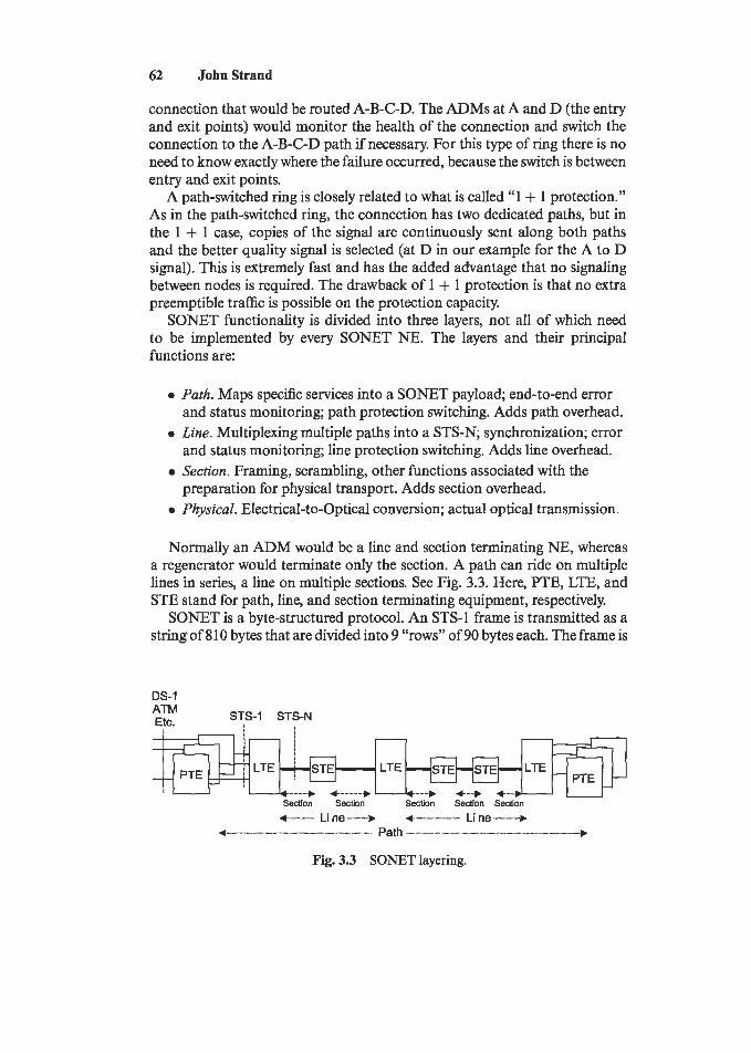
62 John Strand
connection that would be routed A-B-C-D. The ADMs at A and D (the entry and exit points) would monitor the health of the connection and switch the connection to the A-B-C-D path if necessary. For this type of ring there is no need to know exactly where the failure occurred, because the switch is between entry and exit points.
A path-switched ring is closely related to what is called “1 + 1 protection.” As in the path-switched ring, the connection has two dedicated paths, but in the 1 + 1 case, copies of the signal are continuously sent along both paths and the better quality signal is selected (at D in our example for the A to D signal). This is extremely fast and has the added advantage that no signaling between nodes is required. The drawback of 1 + 1 protection is that no extra preemptible traffic is possible on the protection capacity.
SONET functionality is divided into three layers, not all of which need to be implemented by every SONET NE. The layers and their principal functions are:
0 Path. Maps specific services into a SONET payload; end-to-end error and status monitoring; path protection switching. Adds path overhead.
0 Line. Multiplexing multiple paths into a STS-N; synchronization; error and status monitoring; line protection switching. Adds line overhead.
0 Section. Framing, scrambling, other functions associated with the preparation for physical transport. Adds section overhead.
0 Physical. Electrical-to-Optical conversion; actual optical transmission.
Normally an ADM would be a line and section terminating NE, whereas a regenerator would terminate only the section. A path can ride on multiple lines in series, a line on multiple sections. See Fig. 3.3. Here, PTE, LTE, and STE stand for path, line, and section terminating equipment, respectively.
SONET is a byte-structured protocol. An STS-1 frame is transmitted as a string of 810 bytes that are divided into 9 “rows” of 90 bytes each. The frame is
Fig. 3.3 SONET layering.
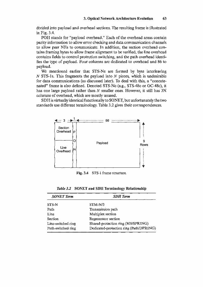
3. Optical Network Architecture Evolution 63
-
Overhead Section p
0
Line ,, Overhead
divided into payload and overhead sections. The resulting frame is illustrated in Fig. 3.4.
POH stands for “payload overhead.” Each of the overhead areas contain parity information to allow error checking and data communication channels to allow peer NEs to communicate. In addition, the section overhead con- tains framing bytes to allow frame alignment to be verified, the line overhead contains fields to control protection switching, and the path overhead identi- fies the type of payload. Four columns are dedicated to overhead and 86 to payload.
We mentioned earlier that STS-Ns are formed by byte interleaving N STS-1s. This fragments the payload into N pieces, which is undesirable for data communications (as discussed later). To deal with this, a “concate- nated” frame is also deked. Denoted STS-Nc (e.g., STS-48c or 0C-48~)~ it has one large payload rather than N smaller ones. However, it still has 3N columns of overhead, which are mostly unused.
SDH is virtually identical functionally to SONET, but unfortunately the two standards use different terminology. Table 3.2 gives their correspondences.
-1 A 9
Rows Payload
i
Fig. 3.4 STS-1 frame structure.
Table 3.2 SONET and SDH Terminology Relationship
SONET Term SDH Term
STS-N STM-N/3 Path Transmission path Line Multiplex section Section Regenerator section Line-switched ring Shared-protection ring (MSEPRING) Path-switched ring Dedicated-protection ring (PaWDPRING)

64 John Strand
Frequency registered Receivers transmitters
Fig. 3.5 Basic Optical Transport System (OTrS).
2.1.1. Multivendor Interworking
One of the goals of SONET and SDH was to define standards that would let equipment from multiple vendors interwork. This has been achieved in simple point-to-point configurations, but in more complex configurations, such as shared protection rings, progress has been frustratingly slow. Hardware inter- operability has by and large not been a serious problem; instead, software interworking has been limiting, particularly the exchange of state informa- tion between the ADMs and the handling of “operations, administration, and maintenance” functions. As a result, transport people tend to be suspicious of proposals for multivendor “mid-span meets.”
2.2. OPTICAL TRANSPORT SYSTEMS
A basic Optical Transport System (OTrS) is shown in Fig. 3.5. In its most basic form, it consists of an optical multiplexer and demultiplexer and a number of optical amplifiers (OAs) between them.3 OAs in terrestrial systems usually have a nominal spacing (span length) of about 25dB (roughly 80km after allowance for splices, etc., and assuming a nominal span loss of 0.25 dB/km). Wider spacings can significantly reduce the first costs of a route, but cause difficulties for 10 Gb/sec and faster connections and also impose limits on the number of wavelengths that can be supported, therefore most operators appear to be sticking with 80 km or shorter spacings. Impairments force regeneration after about 5-7 spans (400-560 km). This is a wavelength rather than an OTrS constraint, so that if a wavelength traversed two such systems in series without regeneration between the systems, the span limit would apply to the sum of the spans on the systems.
2.2.1. Capacity Trends
OTrS capacity has been increasing very rapidly. In fact, by some estimates the rate of increase is considerably faster than Moore’s Law for electronics
The system shown (and the underlying technology, usually) is unidirectional; however, they are normally deployed in pairs so as to support bidirectional SONET/SDH circuits.
3. Optical Network Architecture Evolution 65
Gbls
1996 1998 2000 2002 2004
Fig. 3.6 Capacity of a single fiber (derived from data in [SI) .
(see [54]). The underlying trends are analyzed in [55], from which Fig. 3.6 is derived. The years given are for commercial deployment (actual and pro- jected). Over the 1 0-year period shown, capacity doubles approximately eight times due to increases in the bits per channel, reductions in wavelength spacing, and increases in the total usable fiber bandwidth.
In a recent talk [104], Rick Barry of Sycamore used bandwidth times distance as a relevant metric. He traced the evolution of capacity from 120-160 Terabits/sec*km with conventional systems (e.g., 80 OC-48s over 600km or 40 OC-192s over 400km) to today's 160&2400Tb/sec*km (e.g., 80 OC-192 over 3000km) and projected a next generation providing 3200-4800 Tb/sec*km.
Important architectural implications from these trends:
0 The increase in wavelength counts make the introduction of some form of mechanized cross-connect a necessity if operations costs and complexity are to be kept under control.
0 Total OTrS costs are rising significantly more slowly than capacity. Hence unit cost ($/Gigabit) is declining.
0 The combination of these two trends-rapidly rising capacity and declining unit costs-have formed a synergistic relationship with the rapid growth of the Internet. Internet growth has allowed the new technologies to be economically justified, while the rapid capacity increases and cost decreases have been essential enablers for the growth of the Internet.
2.2.2. Ultra-Long-Haul Systems
The OTrS just described requires each wavelength to be regenerated roughly every 500 km. The optical-electrical-optical (OEO) functionality required for regeneration is quite expensive; if a transponder is put on each wavelength of the OTS shown in Fig. 3.5, their cost could exceed the total costs of all the
66 John Strand
MdDemux and OAs combined. Hence extending the regeneration distance is an appealing possibility. Raman amplification, strong forward error cor- rection (FEC), and advances in dynamic power management are making this possible. The resulting “ultra-long-haul” technology can support OTrS with dozens of 80-km spans, leading to regeneration distances of 3000 km or more. However, this comes at a cost: To get longer regeneration distances, the per- wavelength multiplexing, demultiplexing, and amplifications costs are likely to significantly exceed those of traditional systems. We can expect ultra-long-haul systems to be competitive, therefore, only for long systems where these per- wavelength costs can be counterbalanced by regeneration savings. A strawman ultra-long system based on 2000-2001 products is shown in Fig. 3.7.
This system shown in Fig. 3.7 illustrates a number of architecturally interesting features we shall return to in the architecture discussion.
a Adaptation. The boxes labeled “A” are adaptation functions. Using an OEO transponder function, they map one or more inputs (the a’s, typically standard short-reach signals) into a long-reach OCh or group of OCh‘s that will pass transparently to a distant adaptation function. Adaptation options include: a. Multiplexing. Either electrical or optical TDM may be used to
combine the inputs into a single wavelength. This is done to increase effective capacity. After multiplexing, the combined signal must be routed as a group to the distant adaptation function.
b. Adaptation grouping. In this technique, groups of k (e.g., 4) inputs are managed as a group (an “adaptation grouping,” increasingly called a “wave group”) within the system and normally must be addeddropped as a group. Tight spacing is used for wavelengths within a group, with larger guard bands between groups. Grouping is done to simplify power management. It may also be possible to largely contain nonlinear effects such as four-wave mixing within the groups. Wavelength spacing may vary between groups, as may the
X Y PADM PADM D AN IA
........................ T .............. F =a1 oak
Fig. 3.7 Strawman ultra-long-haul optical transport system (OAs not shown).
6 1 1
Olk
=Nl
=Nk

3. Optical Network Architecture Evolution 67
number of wavelengths in each group. Note that either option places limits on connectivity (which 0’s are delivered to which output port), because the inputs involved must be routed as a group to a compatible output adaptation function.
Photonic add-drop multiplexers (PADM). X and Y are “photonic add-drop multiplexers”-the all-optical analog to the SONET ADM discussed in Section 3.1. They allow economical dropping and insertion of limited numbers of adaptation groupings without requiring demultiplexing and remultiplexing all the other wavelengths. Depending on the filtering architecture, it may be possible to reuse frequencies so that, for instance, the same frequency could be used for a D to X grouping, an X to Y grouping, and a Y to E grouping.
0 “Domain oftransparency.” The dotted line encloses an all-optical “domain of transparency,” an all-optical subnetwork. The adaptation functions just discussed optically isolate the domain.
2.2.3. More Complex Domains of Transparency
Since the PADMs in Fig. 3.7 are all-optical, it is possible to build more complex all-optical domains, as shown in Fig. 3.8. In Fig. 3.8, the basic ultra-long system D-X-Y-E from Fig. 3.7 has had branches added at the PADM’s X and Y, with further branching at PADM U. In this configuration, there is an all-optical path, A-Y-X-U-Z, connecting A to Z . Transponders to optically isolate the domain would need to be present on the boundary of the domain and would serve to define the boundary of the domain.
There are no “loops” in Fig. 3.8. If a U-Y link were added, the domain would turn from a topological “tree” (only one path between any two points) into a more general “mesh.” The alternate paths that result might be useful for restoration, but they also might complicate considerably the management of impairments.
OPADM
Fig. 3.8 Larger domain of transparency (OAs not shown).
68 John Strand
2.3. RECONFIGURATION CAPABILITIES
2.3.1. Why Reconfigurability Is Important
Returning to the example given in Fig. 3.7, for fixed wavelengths, hk, and a fixed configuration of the PADMs, each input port is in effect hard-wired to some distant output port. The connectivity between ports is fixed. In fact, the set of transmitters and receivers that are tuned to a specific frequency can be thought of as a plane that cannot be interconnected within the domain to planes dehed by other frequencies. We will see later that this can be a serious problem in some situations.
In addition, the lack of reconfigurability can make it difficult to effectively use the capacity of a complex domain of transparency such as that in Fig. 3.8. In this figure, for example, if a specific frequency is in use between D and E, then this frequency cannot be used for the path A-Y-X-U-Z connecting A to Z-it is blocked on the X-Y link.
If it were possible to reconfigure this connectivity, the OTrS would in effect be turned into a distributed switch or cross-connect, which could be used for software controlled provisioning or for restoration after some types of failures. These types of functional capabilities are at the heart of the business rationale for deploying the optical network.
There are a number of ways in which reconfigurability may be achieved:
0 Laser/receiver tunability. The lasers producing the LR wavelengths (the Ai in Fig. 3.8) may have a fixed frequency, may be tunable over a limited range, or be tunable over the entire range of wavelengths supported by the DWDM. Tunability speeds may also vary. Tunability may give additional connectivity options, and allow ports that could not otherwise be connected to do so.
0 Wavelength conversion. Internal to a domain of transparency, it might be possible to change the frequency of a connection, thereby in effect interconnecting the planes described earlier. This could be done by converting to the electrical domain and then modulating a laser (fixed frequency or tunable) with the signal. However, this is apt to be quite expensive and may degrade the signal. Conversion in the optical domain has been the subject of considerable research but products with functionality, reliability, performance, and cost adequate to make them attractive are not yet available (see [5] and [13] for surveys).
0 Switch fabrics. A switching fabric could be placed in the PADM in Fig. 3.7 or a cross-connect could be inside a domain of transparency or be placed between two domains. This technology is discussed next.
0 Adaptation grouping adjustments. If the boundaries between groupings are dynamically adjustable, bandwidth could be moved between groupings.
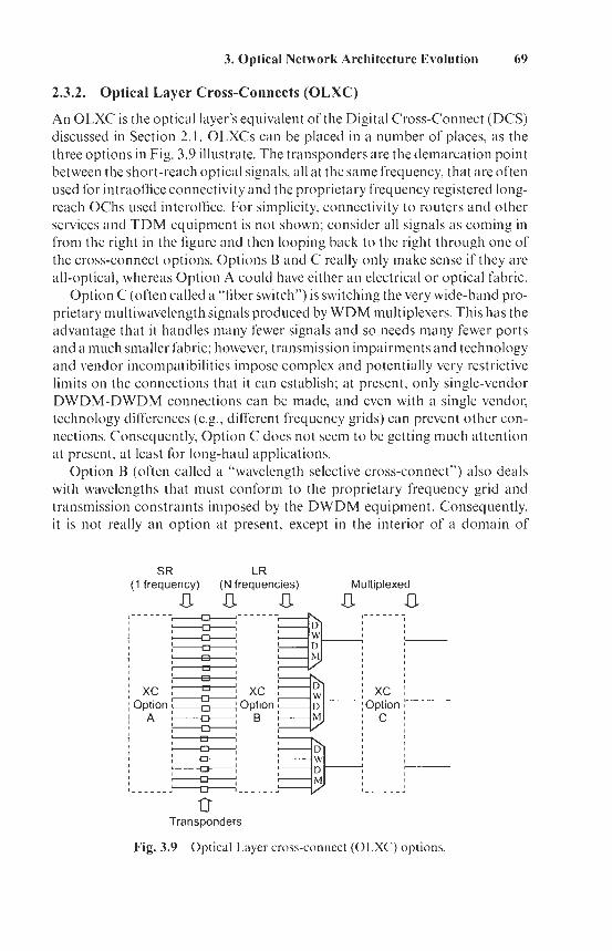
3. Optical Network Architecture Evolution 69
2.3.2. Optical Layer Cross-Connects (OLXC)
An OLXC is the optical layer’s equivalent of the Digital Cross-Connect (DCS) discussed in Section 2.1. OLXCs can be placed in a number of places, as the three options in Fig. 3.9 illustrate. The transponders are the demarcation point between the short-reach optical signals, all at the same frequency, that are often used for intraoffice connectivity and the proprietary frequency registered long- reach OChs used interoffice. For simplicity, connectivity to routers and other services and TDM equipment is not shown; consider all signals as coming in from the right in the figure and then looping back to the right through one of the cross-connect options. Options B and C really only make sense if they are all-optical, whereas Option A could have either an electrical or optical fabric.
Option C (often called a “fiber switch”) is switching the very wide-band pro- prietary multiwavelength signals produced by WDM multiplexers. This has the advantage that it handles many fewer signals and so needs many fewer ports and a much smaller fabric; however, transmission impairments and technology and vendor incompatibilities impose complex and potentially very restrictive limits on the connections that it can establish; at present, only single-vendor DWDM-DWDM connections can be made, and even with a single vendor, technology differences (e.g., different frequency grids) can prevent other con- nections. Consequently, Option C does not seem to be getting much attention at present, at least for long-haul applications.
Option B (often called a “wavelength selective cross-connect”) also deals with wavelengths that must conform to the proprietary frequency grid and transmission constraints imposed by the DWDM equipment. Consequently, it is not really an option at present, except in the interior of a domain of
SR LR (1 frequency) (N frequencies) Multiplexed
I
U Transponders
Fig. 3.9 Optical Layer cross-connect (OLXC) options.
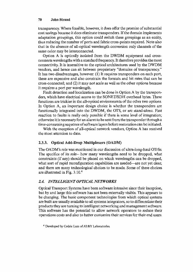
70 John Strand
transparency. Where feasible, however, it does offer the promise of substantial cost savings because it does eliminate transponders. If the domain implements adaptation groupings, this option could switch these groupings as an entity, thus reducing the number of ports and fabric cross-points required. Note also that in the absence of all-optical wavelength conversion only channels of the same color may be interconnected.
Option A is optically isolated from the DWDM equipment and cross- connects wavelengths with a standard frequency. It therefore provides the most connectivity. It is insensitive to the optical architectures used by the DWDM vendors, and hence can sit between proprietary “domains of transparency.” It has two disadvantages, however: (1) It requires transponders on each port, these are expensive and also constrain the formats and bit rates that can be cross-connected; and (2) it may not scale as well as the other options because it requires a port per wavelength.
Fault detection and localization can be done in Option A by the transpon- ders, which have electrical access to the SONET/SDH overhead bytes. These functions are trickier in the all-optical environments of the other two options. In Option A, an important design choice is whether the transponders are functionally integrated into the DWDM, the OTS, or are stand-alone. Fast reaction to faults is really only possible if there is some level of integration; otherwise it is necessary for an alarm to be sent from the transponder through a time-consuming sequence of software layers before restoration can be initiated.
With the exception of all-optical network vendors, Option A has received the most attention to date.
2.3.3. Optical Add-Drop Multiplexers (OADM)
The OADM’s role was mentioned in our discussion of ultra-long-haul OTrSs. The specifics of its rol+how many wavelengths need to be dropped, what constraints (if any) should be placed on which wavelengths can be dropped, what sort of rapid reconfiguration capabilities are needed-are not yet clear, and there are many technological choices to be made. Some of these choices are illustrated in Fig. 3.10.4
2.4. INTELLIGENT OPTICAL NETWORKS
Optical Transport Systems have been software intensive since their inception, but by and large this software has not been externally visible. This appears to be changing. The basic component technologies from which optical systems are built are usually available to all systems integrators, so to differentiate their products they are turning to intelligent networking and management software. This software has the potential to allow network operators to reduce their operations costs and also to better customize their services for their end users.
Developed by Cedric Lam of ATBET Laboratories.
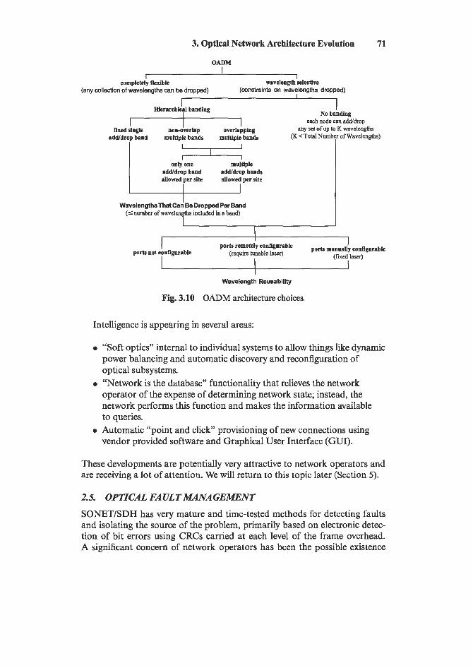
3. Optical Network Architecture Evolution 71
OADM
I multiple only one
adddrop band adddrop bands allowed per site allowed per site
I I completely flexible wavelength selective
(any collection of wavelengths can be dropped) (constraints on wavelengths dropped) I
I No banding
each node can add/dro~
WavelengthsThat Can Be Dropped PerBand (5 number of wavelengths included in a band)
I
(require tunable laser) Ports remotely configurable md!.r rn”*n..r.hlm
(tiwedlaser) ports not configurable
I I I I
Wavelength Reusability
Fig. 3.10 OADM architecture choices.
Intelligence is appearing in several areas:
0 “Soft optics” internal to individual systems to allow things like dynamic power balancing and automatic discovery and reconfiguration of optical subsystems.
0 “Network is the database” functionality that relieves the network operator of the expense of determining network state; instead, the network performs this function and makes the information available to queries.
0 Automatic “point and click” provisioning of new connections using vendor provided software and Graphical User Interface (GUI).
These developments are potentially very attractive to network operators and are receiving a lot of attention. We will return to this topic later (Section 5).
2.5. OPTICAL FAULT MANAGEMENT
SONET/SDH has very mature and time-tested methods for detecting faults and isolating the source of the problem, primarily based on electronic detec- tion of bit errors using CRCs carried at each level of the frame overhead. A significant concern of network operators has been the possible existence
12 JohnStrand
of failure modes that are difficult or perhaps impossible to isolate by optical means alone. One can envision monitoring optical power or signal-to-noise ratio, but these analog measurements will not detect pulse distortion arising from nonlinearity and dispersion, for example. Maeda [ 121 gives as an example an OLXC failure that resulted in the delivery to the proper port of a signal with the correct optical characteristics but incorrect digital content.
This is a serious matter, perhaps even a show-stopper, for network oper- ators, particularly as network growth and cost pressures continue to stretch operations resources ever thinner. A number of approaches are being tried to deal with the issue:
0 Persuasion. Green [47l points out that this issue was encountered when all-optical OAs replaced OEO regenerators that did electronic fault monitoring approximately every 40 miles. Anxious to realize the enormous economic and capacity benefits offered by OAs, operators were persuaded that pump power level and other optical parameters were adequate. Green hopes that history will repeat itself and make looking at the bits unnecessary.
0 SignaZ splitting. A small amount of the optical signal could be diverted and examined electronically.
0 Containment. All-optical subnetworks could be kept small and optically contained, with electronic monitoring of all connections entering/ leaving such a subnetwork. A related step would be to keep the topology of all-optical subnetworks simple-for example, require them to be topological “trees” without loops. (Fig. 3.8 is such a tree.)
2.6. FUNCTIONAL CONSOLIDATION
Advances in silicon technology have created the possibility of integrating trans- port functions that traditionally had been in discrete boxes. For example, in SONET/SDH networks cross-connects and add-drop multiplexers have tra- ditionally been physically separate network elements (NEs), as have DWDM terminals. However, it is now possible to implement a full ADM on a DCS line card. In the intercity network, so-called “optical layer cross-connects” have appeared: They have a large number (thousands) of OC-48/192 ports but an STS-1 fabric and the ability to do all the traditional ADM functions as well as provide an OC-48/192 cross-connect capability. In the metropolitan market, products (often called “multi-service provisioning platforms”) are appearing that carry this trend further, with optical ring functionality and the ability to groom individual DS-1 (1.5 Mb/sec) signals and even ATM switch and IP router capabilities added to the functionality mix in a single NE.
The drivers for this trend are compelling: Significant cost, power, and floor- space savings result from the elimination of the line cards and cabling necessary to interconnect network elements. In addition, maintenance costs tend to be

3. Optical Network Architecture Evolution 73
proportional to the number of NEs, and would therefore benefit from this trend.
When functions are integrated in the same NE, layer boundaries get blurred. In the case of the OTN, it is likely that it will be difficult to cleanly separate the management of the OTN from the other transport networks residing in the same NE. If OTN software and operations cannot be cleanly separated from the massive and complex multilayer legacy transport network, the introduction of new OTN technology and functionality will be significantly impeded.
3. Service and Business Trends
Changes and trends in the telecommunications services mix and also in the structure of the telecom industry will be critically important determinants of tomorrow's OTN architecture. In this section we will look at a few of the most important trends and their architectural implications.
3.1. SERVICE BASICS
The breakdown of bytes of U.S. long-distance traffic by major service grouping is summarized in Fig. 3.1 1. The two bars on the left show the service breakdown at the end of 1997 and 1999, respectively. The bar on the right shows the breakdown of the growth in this period. The predominance of voice traffic even at the end of 1999 may seem surprising to some; much of this is due to differences in utilization, which are discussed later. The Internet segment is clearly growing more rapidly; in [55] it is estimated that average annual growth rates for voice are about 109'0, for the Internet about loo%, and for private line about 30%. Because of this, Internet traffic is expected to exceed voice traffic by early 2002. Note that even in the 1997-1999 period, network growth was driven by the Internet segment. After 1999, Internet growth is expected to become increasingly dominant. From an architectural perspective, this means
DataNetworks
EOY 1997 EOY 1999 1997-99 Growth
Fig. 3.11 Traffic on U.S. long-distance networks, 1997-1999 (from [SI).
74 John Strand
that new investment will need to be pointed increasingly to the needs of Internet t r f ic .
The revenue perspective is quite different. A leading industry consult- ing group (RHK) estimates that voice revenue per megabit is seven times that for a T1 Internet connection; for the telecommunications industry as a whole, total voice revenues are projected to be much larger than data rev- enues for many years. Much of the voice revenue comes from a small number of very large corporate customers who are dependent on very sophisticated and complex software-based functionality in the legacy voice network, and therefore very hard to migrate to a new IP-based infrastructure without the same level of f~nctionality.~ This introduces conflicts into the strategic plan- ning process, particularly for carriers with a large embedded base of voice customers, because there is a constant tension between investing in the future and satisfying the current customer base.
3.1.1. Ethernet
We are focused on intercity transport, and so Local Area Networks (LANs) are out of scope. However, we should not lose sight of the fact that Ethernet is the dominant protocol in buildings and campuses, and that a large portion of data traffic is carried at least partly on Ethernet. Ethernet is a very rapidly evolving technology.6 It has benefited from enormous volumes and achieved unsurpassed fiber-port economies and is steadily extending its reach into metro and even long-haul networks, and therefore it bears careful watching as a potential service driver in the long-haul network in its own right, and even a technological competitor for some long-haul applications.
3.2. INTERNET TRAFFIC CHARACTERISTICS
Since Internet traffic will be the driver for network growth and architectural change, it is important to understand the nature of this t r f ic . In this section we will look at some of its important characteristics.
3.2.1. Connection Bandwidth
The size of the connections between routers will impact a number of aspects of the OTN architecture. For example, the necessity for leaving the optical
IBM, for example, has thousands of call center agents averaging 95 sales calls and rev- enues of $63,000 a minute [107]. Such an operation depends heavily on sophisticated network call-management software to balance loads between call centers, among other functions. This softwm works in coordination with IBM’s internal computer telephony integration product, which provides a customer history screen-pop when an incoming customer number is transferred to an mailable agent’s phone.
See Chapter 11 on Ethernet in this volume.
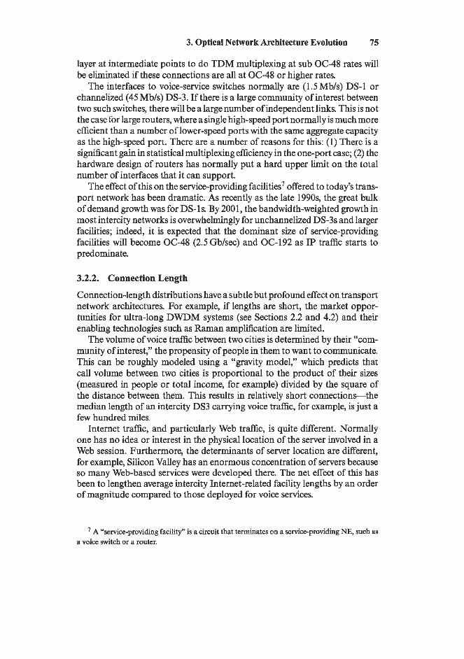
3. Optical Network Architecture Evolution 75
layer at intermediate points to do TDM multiplexing at sub OC-48 rates will be eliminated if these connections are all at OC-48 or higher rates.
The interfaces to voice-service switches normally are (1.5 Mb/s) DS-1 or channelized (45 Mb/s) DS-3. If there is a large community of interest between two such switches, there will be a large number of independent links. This is not the case for large routers, where a single high-speed port normally is much more efficient than a number of lower-speed ports with the same aggregate capacity as the high-speed port. There are a number of reasons for this: (1) There is a significant gain in statistical multiplexing efficiency in the one-port case; (2) the hardware design of routers has normally put a hard upper limit on the total number of interfaces that it can support.
The effect of this on the service-providing facilities7 offered to today’s trans- port network has been dramatic. As recently as the late 1990s, the great bulk of demand growth was for DS-1s. By 2001, the bandwidth-weighted growth in most intercity networks is overwhelmingly for unchannelized DS-3s and larger facilities; indeed, it is expected that the dominant size of service-providing facilities will become OC-48 (2.5 Gb/sec) and OC-192 as IP traffic starts to predominate.
3.2.2. Connection Length
Connection-length distributions have a subtle but profound effect on transport network architectures. For example, if lengths are short, the market oppor- tunities for ultra-long DWDM systems (see Sections 2.2 and 4.2) and their enabling technologies such as Raman amplification are limited.
The volume of voice traffic between two cities is determined by their “com- munity of interest,” the propensity of people in them to want to communicate. This can be roughly modeled using a “gravity model,” which predicts that call volume between two cities is proportional to the product of their sizes (measured in people or total income, for example) divided by the square of the distance between them. This results in relatively short connections-the median length of an intercity DS3 carrying voice traffic, for example, is just a few hundred miles.
Internet traffic, and particularly Web traffic, is quite different. Normally one has no idea or interest in the physical location of the server involved in a Web session. Furthermore, the determinants of server location are different, for example, Silicon Valley has an enormous concentration of servers because so many Web-based services were developed there. The net effect of this has been to lengthen average intercity Internet-related facility lengths by an order of magnitude compared to those deployed for voice services.
A “service-providing facility” is a circuit that terminates on a service-providing NE, such as a voice switch or a router.
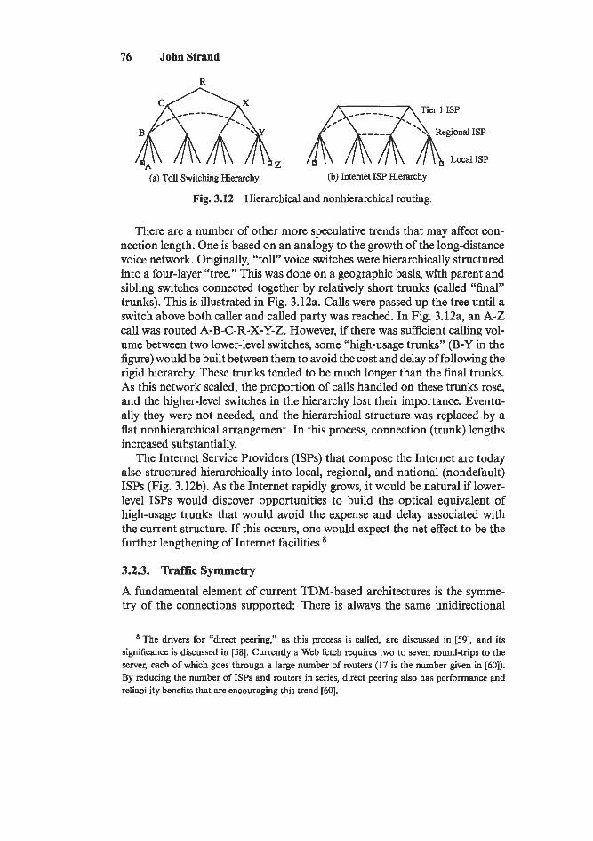
76 John Strand
R
Z (a) Toll Switching Hierarchy (b) Internet ISP Hierarchy
Fig. 3.12 Hierarchical and nonhierarchical routing.
There are a number of other more speculative trends that may affect con- nection length. One is based on an analogy to the growth of the long-distance voice network. Originally, “toll” voice switches were hierarchically structured into a four-layer “tree.” This was done on a geographic basis, with parent and sibling switches connected together by relatively short trunks (called “final” trunks). This is illustrated in Fig. 3.12a. Calls were passed up the tree until a switch above both caller and called party was reached. In Fig. 3.12a, an A-Z call was routed A-B-C-R-X-Y-Z. However, if there was sufficient calling vol- ume between two lower-level switches, some “high-usage trunks” (B-Y in the figure) would be built between them to avoid the cost and delay of following the rigid hierarchy. These trunks tended to be much longer than the final trunks. As this network scaled, the proportion of calls handled on these trunks rose, and the higher-level switches in the hierarchy lost their importance. Eventu- ally they were not needed, and the hierarchical structure was replaced by a flat nonhierarchical arrangement. In this process, connection (trunk) lengths increased substantially.
The Internet Service Providers (ISPs) that compose the Internet are today also structured hierarchically into local, regional, and national (nondefault) ISPs (Fig. 3.12b). As the Internet rapidly grows, it would be natural if lower- level ISPs would discover opportunities to build the optical equivalent of high-usage trunks that would avoid the expense and delay associated with the current structure. If this occurs, one would expect the net effect to be the further lengthening of Internet facilities.8
3.2.3. Tkaffic Symmetry
A fundamental element of current TDM-based architectures is the symme- try of the connections supported: There is always the same unidirectional
* The drivers for “direct peering,” as this process is called, are discussed in [59], and its sigmficance is discussed in [58]. Currently a Web fetch requires two to seven round-trips to the server, each of which goes through a large number of routers (17 is the number given in [60]). By reducing the number of ISPs and routers in series, direct peering also has performance and reliability benefits that are encouraging this trend [60].

3. Optical Network Architecture Evolution 77
bandwidth dedicated to A to Z traffic as there is no traffic in the reverse direction. This originates in the design of traditional voice circuits, which are 64-kb/sec full-duplex connections. If this were to change, there would be opportunities to build more economical networks if asymmetry were better supported.
There is no need for data traffic to be symmetric. A file transfer is unidirec- tional; on the Internet, the prevalent client-server architecture leads to large amounts of data sent from servers in response to small requests. Various stud- ies have found twice as much traffic flowing from the United States to other countries, and much larger imbalances in flows from ISPs that specialize in supporting servers to those that are residentially oriented (see [48] and [29]).
3.2.4. Utilization
By utilization, we mean the proportion of bandwidth that is actually used. Because there is hourly, daily, and seasonal variation in traffic intensity, it is appropriate to look at a time-averaged utilization. Odlyzko [40, 571 estimates that Internet backbones are about one-third as utilized as U.S. long-distance switched voice networks, and that private line data networks are only about 10% as utilized. There are many reasons for this that are discussed in the references; two of these provide opportunities for the OTN architecture to add value:
0 If it is possible to add capacity very rapidly, there is little reason for an ISP to keep a spare capacity buffer. However, if additions take a long time, it is prudent to order capacity so it is available well before it is likely to be needed to guard against unexpectedly rapid demand growth or unexpected delays in getting the capacity online. The higher the demand volatility or the more uncertain the capacity delivery process, the earlier a prudent manager will order new capacity. The Internet is noted for wild demand surges, and the time it takes to get an additional large (multi-megabidsecond) connection installed today is frequently measured in months, and there can be significant uncertainties, particularly when multiple operators are involved (e.g., a local telco and a long-distance telco). Hence early capacity ordering, which leads to low utilization on average, is standard operations procedure for many data network managers.
0 Intranets and other business-oriented private data networks have usage concentrated during business hours. Because these networks use dedicated private lines, there is little ability to use the idle bandwidth for other purposes during off hours. Conversely, ISPs catering to residential customers are likely to see their usage higher in the evenings and on weekends.

78 John Strand
3.3. INDUSTRY STRUCTURE
The US. telecommunications industry is changing in ways that are profoundly affecting OTN architecture. This section identifies a few of the changes that affect network architecture.
3.3.1. Additional Intercity Optical Networks
In the mid-1990s, there were basically three national scale OTNs in the United States, each vertically integrated into one of the major intercity service providers (AT&T, MCI, and Sprint). They accounted for about three-quarters of total intercity fiber deployment. By the end of the decade, however, they accounted for less than a third, with 39 new national carriers accounting for an equal amount [61]. This same source estimates that in 1999 there was a total of 400K route miles in long-haul networks, with an average of 46 fibers per cable.
This trend has a number of architectural implications:
0 The new OTNs can provide a facility underpinning for nonfacility based ISPs and other service providers. The resulting service competition puts pressure on vertically integrated service providers to keep the unit cost of their OTNs competitive, for example, by introducing new technologies faster than they would otherwise have done.
leading to a situation where competing OTN operators may share fiber in the same right of way or even the same fiber cable.
0 There are many opportunities for buying, selling, or swapping fiber,
3.3.2. Additional Local Networks
Hundreds of so-called “Competitive Local Exchange Companies” (CLECs) provide competition for the “Baby Bells.” Particularly in areas with a high density of telecom-intensive businesses such as lower Manhattan, these com- panies provide optical connectivity to many key customer locations. They have more incentive to introduce new architectures than the incumbent carriers. The long-term economic viability of many CLECs is hostage to politicdregulatory developments affecting their complex relationships with the “Baby Bells”
3.3.3. Web Hosting and Carrier Hotels
Facilities to meet the need of carriers, ISPs, and Internet content providers are changing the geographic structure of the industry:
0 “Carrier hotels” are buildings run by third parties that meet the needs of new carriers for a physical presence in some city. They provide a

3. Optical Network Architecture Evolution 79
telco-grade infrastructure, so all conduit, power, environmental, and security requirements are satisfied; provide an opportunity to share costs; and facilitate interconnection between CLECs, ISPs, and intercity carriers.
servers and routers deployed by Internet content providers. e Web hosting sites provide similar facilities for the enormous number of
These sites provide enormous concentrations of potential business and poten- tially make it easier for start-up OTNs to find the service volumes they need. The “dot-com” downturn in 2001 has hit a number of them very severely, however.
3.3.4. Bandwidth Trading
We mentioned earlier that carriers frequently lease dark fiber from each other. These deals are each separately negotiated by the parties to specify qual- ity of service, any penalties for contract nonfulfillment, and other details, and the physical implementation typically requires engineering and construc- tion to establish the physical connection. This process is time consuming and expensive.
This is in marked contrast with the situation in energy markets like gas, oil, and electricity where there are enormous markets to facilitate trading. These markets are based on standardizing the product’s physical characteristics and quality, specifying a clearing and settlement process for payments, and defining penalties for nonperformance. To facilitate trading, a “benchmark” product delivered at a specified location is used as a basis for establishing a price, and conversion factors are established to establish prices for other grades and physical delivery points. Once this is done, it is possible to establish forward markets that allow buyers and sellers to do financial risk management and also allow speculation. Markets that have been through this ‘ccommodification’y process have been profoundly changed, as anyone following the deregulation of the U.S. electricity industry is aware.
Many sophisticated and very well financed players are trying to commodify the bandwidth market: A Web search for “bandwidth trading” in January 2001 got 95,800 hits. A number of intermediaries have sprung up to help buyers and sellers of bandwidth to trade with each other efficiently. One approach is to act as a “matchmaker.” Many of these companies have Web sites where owners of underutilized capacity can post their offering^.^ A smaller number of players are actually deploying equipment to facilitate the process. A possible architecture is shown in Fig. 3.13.
An offering typically identifies the two end points, the type of circuit (OC-3, STM-1, etc.), and the price and availability date. Offerings can be either “Irrevocable Right to Use” (long-term or permanent) or on some sort of leasing arrangement, e.g., on a monthly basis.
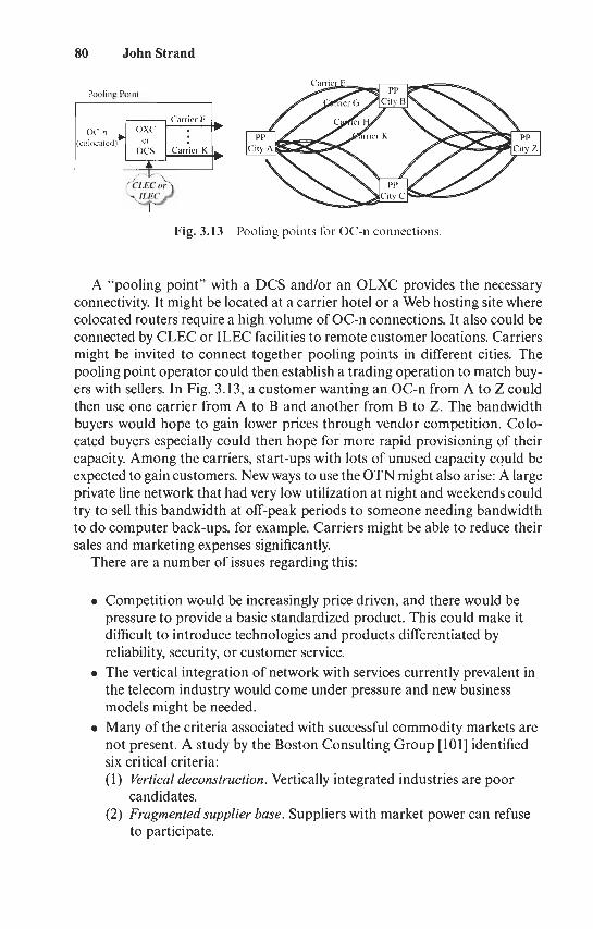
80 John Strand
Pooling Point
Carrier F
DCS CarrierK
CLEC or
Fig. 3.13 Pooling points for OC-n connections.
A “pooling point” with a DCS and/or an OLXC provides the necessary connectivity. It might be located at a carrier hotel or a Web hosting site where colocated routers require a high volume of OC-n connections. It also could be connected by CLEC or ILEC facilities to remote customer locations. Carriers might be invited to connect together pooling points in different cities. The pooling point operator could then establish a trading operation to match buy- ers with sellers. In Fig. 3.13, a customer wanting an OC-n from A to Z could then use one carrier from A to B and another from B to Z . The bandwidth buyers would hope to gain lower prices through vendor competition. Colo- cated buyers especially could then hope for more rapid provisioning of their capacity. Among the carriers, start-ups with lots of unused capacity could be expected to gain customers. New ways to use the OTNmight also arise: A large private line network that had very low utilization at night and weekends could try to sell this bandwidth at off-peak periods to someone needing bandwidth to do computer back-ups, for example. Carriers might be able to reduce their sales and marketing expenses significantly.
There are a number of issues regarding this:
Competition would be increasingly price driven, and there would be pressure to provide a basic standardized product. This could make it difficult to introduce technologies and products differentiated by reliability, security, or customer service. The vertical integration of network with services currently prevalent in the telecom industry would come under pressure and new business models might be needed. Many of the criteria associated with successful commodity markets are not present. A study by the Boston Consulting Group [loll identified six critical criteria: (1) Vertical deconstruction. Vertically integrated industries are poor
candidates. (2) Fragmented supplier base. Suppliers with market power can refuse
to participate.

3. Optical Network Architecture Evolution 81
(3) Fragmented customer base. If there are few buyers, they can be targeted by suppliers, eliminating the need for a market.
(4) Price volatility. Predictable prices reduce the need to hedge risk and reduce the incentives of market makers.
(5) Common unit ofexchange. Efficient trading environments require common units of exchange and settlement contracts to fuel liquidity.
(6) Delivery mechanism. A physical delivery mechanism is required to efficiently and quickly move commodities between buyers and sellers.
This study concluded that in most of these areas, the bandwidth market was not yet ripe for commodification but might be in a few years. They did see immediate opportunities in a few specific areas, especially for private lines on high-volume, capacity constrained routes.
In summary, bandwidth trading is not yet a significant factor for 0 7 3 s . However, it does appear that there are short-term opportunities and incen- tives for companies running carrier hotels and server farms, and also for some start-up carriers, to move in this direction. In the longer term, the prospects appear rosier. lo There are also significant architectural implications: Band- width trading would make rapid provisioning an essential network capability, would make it harder for both equipment vendors and carriers to establish proprietary product and service improvements not incorporated in the defini- tion of the standard traded product, and would make network interworking much more important.
3.4. OPTICAL NETWORK SERVICES
3.4.1. Services Overview
It should be clear from the discussion in Section 3.1, that OTN services in the future will be targeted primarily at meeting the needs of public and private data services, and particularly IP-based services. We will generically refer to the providers of these services as “ISPs.”
From an architectural perspective, an OTN architect must make a choice: (1) Build a network with premium features such as very fast restoration in the hope that it will command a premium price and profit margin; (2) build a network offering only the functionality required for “commodity” bandwidth and hope to get higher volumes and efficiencies; or (3) build a network that
lo The Web is the best place to do further research on bandwidth trading. Some market participants whose Web sites might be of interest are Band-X, Interxion, AIG, and Arbinet (all facilities based) and Ratexchange, Bandwidth Market, and Bandwidth.com (nonfacilities based).

82 Johnstrand
can offer both commodity and premium services. We expect that there will be network operators opting for each of these options.
A fruitful way to start thinking about the service/architecture interrelation- ship is to identify ISP needs, identify the functionalities that might possibly be provided by the network, and then match functionalities to needs.
3.4.2. ISP Needs
ISP needs axe as follows:
0 Price. The most important need is undoubtedly low price. 0 Availability. ISPs are struggling to keep up with exponential growth.
Therefore, the availability of bandwidth is a key need-whether it can be provided at all between the desired locations, and if so, how quickly.
desirable. By this we mean functionality provided by the OTN that will allow the ISP to reduce their internal costs. Some potential areas for this are: a. Reduce the cost of physical interfaces on routers. b. Provide bandwidth at the speeds optimal for the router. c. Assume some of the costs of reliability and failure recovery. d. Assume the responsibility for providing exactly the capacity required
e. Allow flexible peering with other ISPs. f. Provide network management capabilities that allow the ISP to be
0 ISP cost displacement. Displacement of internal ISP costs is also
when it is required.
aware of the state of their connections at all time and to reconfigure them as appropriate.
0 Additional revenue opportunities. Provision of capabilities that enable new services. For example, a highly reliable Virtual Private Network (VPN) offering conceivably might be based on an optical layer restoration capability. Coverage of special events might be facilitated by rapid OTN provisioning of extra bandwidth.
3.4.3. Possible Functionality Areas
Possible areas of functionality include the following:
0 Additional connection oflerings. Higher bit rates (e.g., OC-768); different formats (Ethernet, Digital Wrapper); more flexible bandwidth configurations, such as asymmetric or unidirectional connections; flexible concatenation of standard SDHBONET connections to provide additional bandwidth options; and inverse multiplexing.
0 More rupidprovisioning. Software control of optical cross-connects and other reconfigurable ONES. User-Network Interface (UNI) allowing

3. Optical Network Architecture Evolution 83
direct signaling by a router or customer controller requesting immediate additional connections. Larger network footprint. More ubiquitous connectivity can be provided by interworking between networks and by providing OTN access from more locations. Additional restoration options. A range of restoration speeds and threat coverage; assistance in dealing with service layer failures such as router or service outages.
3.4.4. Relating Needs and Possible Functionality
Table 3.3 attempts to identify possible relationships between needs and func- tionality. The justification for many of the entries can be found in the subsections of Section 3.4.
3.4.5. A Carrier Perspective on Service Functionality
The Carrier Working Group within the Optical Interworking Forum (OIF) recently produced an “Optical Services Framework and Associated Require- ments” document [43] that provides a good snapshot of current services thinking in the carrier community as it relates to optical networking and software control. What follows is excerpted from this document.’*
3.4.6. Value Statement Optical networking permits camers to provide new types of network services not available with other technologies, enabling sophisticated transport applications of (D)WDM based networks (featuring a variety of topologies such as point- to-point, ring and mesh). These new generation networks provide means for the improved use of network resources and the support of high-bandwidth services. Dynamic bandwidth allocation, fast restoration techniques and flow-through provisioning give birth to an assortment of services.
Intelligent OTNs contain distributed management capability and subsume many provisioning and data basing functions currently performed by carrier Opera- tions Systems (OS). This allows the rapid establishment and reconfiguration of connections, potentially reducing provisioning times from months to seconds, thus lowering operating costs and providing the means to set and guarantee SLAs12 and QoS configured on a per-connection basis to better meet customer’s specific needs.
I I The current author was the chair of the OIF group producing this report. It is a working
l2 SLA Service Level Agreement. Defines the details of the service to be provided, particularly text and not an official OIF Technical Report, and is not binding on the OIF or its members.
its availability and reliability.
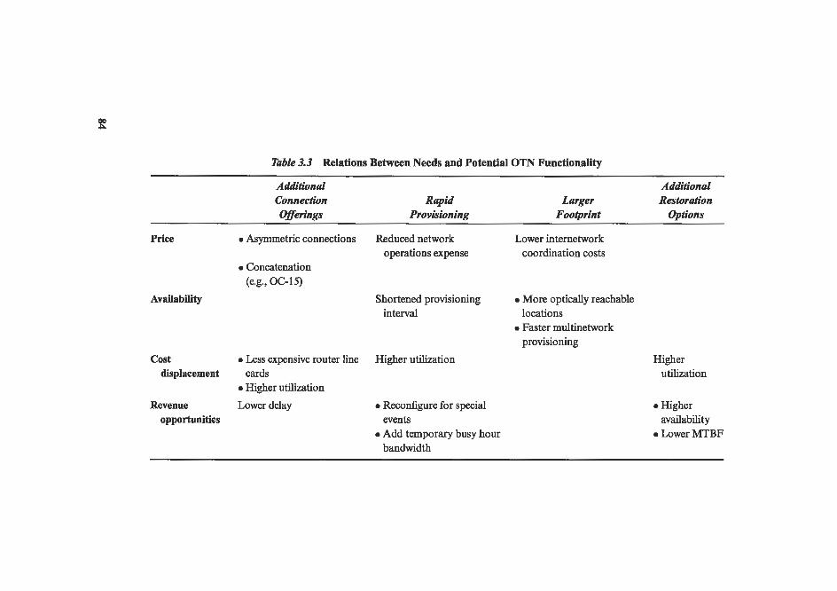
Table 3.3 Relations Between Needs and Potential OTN Functionality
Additional Additional Connection Rapid Larger Restoration Offerings Provisioning Footprint Options
Price 0 Asymmetric connections Reduced network Lower internetwork operations expense coordination costs
0 Concatenation (e.g., OC-15)
Availability Shortened provisioning 0 More optically reachable interval locations
0 Faster multinetwork provisioning
cost 0 Less expensive router line Higher utilization Higher displacement cards utilization
0 Higher utilization 0 Higher
0 Lower MTBF
Revenue Lower delay 0 Reconfigure for special opportunities events availability
0 Add temporary busy hour bandwidth

3. Optical Network Architecture Evolution 85
The large capacity and great flexibility of such networks enables the support of several degrees of transparency to user traffic at lower cost to the end customer. The new services expected to be enabled as aminimum are bandwidth on demand, point and click provisioning of optical connections, and optical virtual private networks.
The standardized interface between the optical layer and the higher layer data service layers such as IP, ATM, SONET/SDH enables the end-to-end internetworking of the optical channels for conveying user information of varying formats. The use of standardized protocols will make the benefits of the intelligent OTNs available end-to-end, even if several networks are involved.
This document also defined business models for three types of service offerings they hoped to see supported. These were:
Provisioned Bandwidth Service: Enhanced leaseaprivate line services. Provision- ing is done at the customer request by the network operator. . . . This is basically the “point and click” type of service currently proposed by many vendors.. . . Billing will be based on the bandwidth, restoration and diversity provided, ser- vice duration, quality of service, and other characteristics of the connection.. . . No customer visibility into the interior of the OTN is required; however, infor- mation on the health of provisioned connection and other technical aspects of the connection may in some circumstances be provided to the user network as a part of the service agreement. . . may involve multiple networks, e.g., both access networks and an intercity network. In this case provisioning may be initiated by whichever network has primary service responsibility. . .
Bandwidth-&-Demand Service: OC-n/STM-n and other facility connections are established and reconfigured in real time. Signaling between the user NE and the optical layer control plane initiates all necessary network activities. A real-time commitment for a future connection may also be established. A standard set of “branded” service options is available. . . .
Optical Ertual Private Network The customer contracts for specific network resources (capacity between OLXCs, OLXC ports, OLXC switching resources) and is able to control these resowces to establish, disconnect, and reconfigure optical connection connections. In effect they would have a dedicated optical sub- network under their control.. . . Billing will be based on the network resources contracted. Network connection acceptance would involve only a check to ensure that the request is in conformance with capacities and constraints specified in the OWN service agreement.. . . Real-time information about the state of all resources contracted for would be made available to the customer. Depending on the service agreement, this may include information on both in-effect connections and spare resources accessible to the customer.

86 Johnstrand
4. Optical Network Architectures
4.1. INTRODUCTION
4.1.1. Unit Costs
Architecture is basically about achieving a proper balance between costs and capabilities. A common mistake is to equate “cost” with equipment cost. This is far from the truth. For a typical traditional long-distance voice service, for example, a typical cost breakdown is as follows:
Access (paid to the local exchange carrier) 35% Network-related costs 15% Customer care, billing, miscellaneous 50%
The network-related costs typically divide roughly equally between the actual carrying costs associated with the equipment and the expenses associated with running the network. It is not unusual for the hardware cost of the NEs to be 10% or less of the total costs that need to be recovered. Thus it is cru- cial to always consider the non-hardware-cost implications of all architecture decisions. The revenue implications are also crucial.
4.2. TRANSPARENCY
In an optical network, “transparency” refers to whether, or to what degree, an optical signal passes through the network optically. In today’s (2001) so- called “optical” networks, there are actually many OEO conversions and a high degree of reliance on electronic processing. However, the vision of many optical networking researchers includes a much larger role for all-optical functionality.
In this section we will explore this issue, the outcome of which will have a large role in shaping the use of optical technology in future OTN architectures.
4.2.1. m e s of Transparency
There are many shades of transparency. A categorization used in the MONET project13 was:
Digital transparency. Transparency to intensity-modulated digital
Amplitude transparency. Transparency to intensity-modulated digital or
Strict transparency. Transparency to any optical signal.
signals of arbitrary bit rate, frame format, and protocol.
analog signals.
l3 MONET w a s an ARPA-sponsored project established to define and demonstrate how best to achieve multiwavelength optical networking of national scale. See www.bell-Iabs.com/ project/MONET or www.darpa.mil.

3. Optical Network Architecture Evolution 87
Even if there is optoelectronic regeneration, there are a number of levels of transparency possible [ 11:
0 Regeneration with retiming and reshaping (3R). This involves acquiring the clock of the regenerated signal, and thus makes it quite difficult to handle multiple frame formats.
a Regeneration with reshaping but without retiming (2R). This offers bit rate and format transparency, but allows jitter to accumulate, thus limiting the number of regenerations that can be done.
performance but can handle a wide variety of signals, both analog and digital.
0 Regeneration without retiming or reshaping (IR). This has the worst
We will use the word transparency to mean no optoelectronic conversions of any kind.
4.2.2. Potential Advantages of Transparency
The potential advantages of transparency fall into two major categories:
a Format independence. A transparent network is largely indifferent to the details of the signal being transported so long as the power levels and other optical characteristics are within bounds. This has the major advantage of allowing new protocols (and also legacy protocols such as PDH) to be easily handled.I4 Without this independence, potentially each new format or bit rate requires standards changes and hardware and software to be developed and deployed.
require expensive OEO functionality at intermediate nodes; electronics is bypassed by through wavelengths.
0 Less expense at intermediate nodes. A transparent network does not
4.2.3. Limitations on Transparency [30,45,46]
Unfortunately, transparency also has some serious problems:
Impairments accumulate. Various forms of dispersion, nonlinearities, polarization-dependent loss, multipath interference, misalignment of lasers and WDM filters all degrade optical signals, and many of them pose increasingly serious performance limitations as bit rates increases channel spacing gets tighter, and the number of channels increases. Individually, these limitations constrain the distance a wavelength can
l4 A thought-provoking example of this is quantum cryptography, an unbreakable form of cryptography that exploits the uncertainty principle of quantum theory, but requires the polarization of individual photons to be preserved. It has been demonstrated over 23 km of fiber [62].
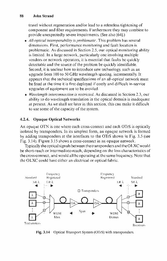
88 John Strand
travel without regeneration and/or lead to a relentless tightening of component and fiber requirements. Furthermore they may combine to provide unexpectedly severe impairments. (See also [64].)
e All-optical interoperability is problematic. This problem has several dimensions. First, performance monitoring and fault location is problematic. As discussed in Section 2.5, our optical monitoring ability is limited. In a large network, particularly one involving multiple vendors or network operators, it is essential that faults be quickly detectable and the source of the problem be quickly identifiable. Second, it is unclear how to introduce new technology, such as an upgrade from 100 to 50 GHz wavelength spacing, incrementally. It appears that the technical specifications of an all-optical network must be fixed at the time it is first deployed if costly and difficult in-service upgrades of equipment are to be avoided.
e Wavelength interconnection is restricted. As discussed in Section 2.3, our ability to do wavelength translation in the optical domain is inadequate at present. As we shall see later in this section, this can make it difficult to use some of the capacity of the system.
4.2.4. Opaque Optical Networks
An opaque OTN is one where each cross-connect and each OTrS is optically isolated by transponders. In its simplest form, an opaque network is formed by adding transponders at the interfaces to the OTrS shown in Fig. 3.5 (see Fig. 3.14). Figure 3.15 shows a cross-connect in an opaque network.
Typically the optical signals between the transponders and the OLXC would be short-reach or intermediate-reach, depending on the loss characteristics of the cross-connect, and would all be operating at the same frequency. Note that the OLXC could have either an electrical or optical fabric.
Frequency Standard Registered
S R h : L R h 4---;--+
Frequency Registered Standard
L R h S R h 4- -+ -- +
Receivers Trai
Transponders
Span
Mux
El El
Fig. 3.14 Optical Transport System (OTrS) with transponders.
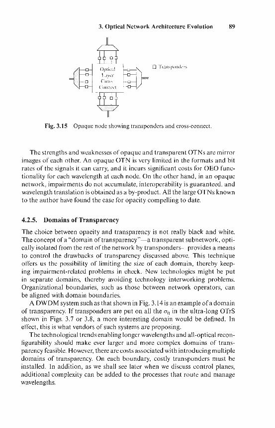
3. Optical Network Architecture Evolution 89
0 Transponders
Fig. 3.15 Opaque node showing transponders and cross-connect.
The strengths and weaknesses of opaque and transparent OTNs are mirror images of each other. An opaque OTN is very limited in the formats and bit rates of the signals it can carry, and it incurs significant costs for OEO func- tionality for each wavelength at each node. On the other hand, in an opaque network, impairments do not accumulate, interoperability is guaranteed, and wavelength translation is obtained as a by-product. All the large OTNs known to the author have found the case for opacity compelling to date.
4.2.5. Domains of Transparency
The choice between opacity and transparency is not really black and white. The concept of a “domain of transparency”-a transparent subnetwork, opti- cally isolated from the rest of the network by transponders-provides a means to control the drawbacks of transparency discussed above. This technique offers us the possibility of limiting the size of each domain, thereby keep- ing impairment-related problems in check. New technologies might be put in separate domains, thereby avoiding technology interworking problems. Organizational boundaries, such as those between network operators, can be aligned with domain boundaries.
A DWDM system such as that shown in Fig. 3.14 is an example of a domain of transparency. If transponders are put on all the q, in the ultra-long OTrS shown in Figs. 3.7 or 3.8, a more interesting domain would be defined. In effect, this is what vendors of such systems are proposing.
The technological trends enabling longer wavelengths and all-optical recon- figurability should make ever larger and more complex domains of trans- parency feasible. However, there are costs associated with introducing multiple domains of transparency. On each boundary, costly transponders must be installed. In addition, as we shall see later when we discuss control planes, additional complexity can be added to the processes that route and manage wavelengths.
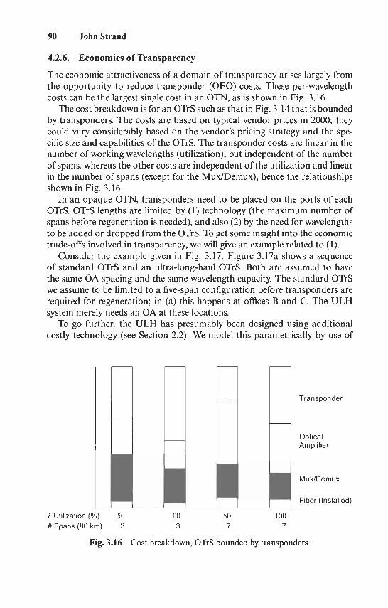
90 John Strand
4.2.6. Economics of Transparency
The economic attractiveness of a domain of transparency arises largely from the opportunity to reduce transponder (OEO) costs. These per-wavelength costs can be the largest single cost in an OTN, as is shown in Fig. 3.16.
The cost breakdown is for an OTrS such as that in Fig. 3.14 that is bounded by transponders. The costs are based on typical vendor prices in 2000; they could vary considerably based on the vendor’s pricing strategy and the spe- cific size and capabilities of the OTrS. The transponder costs are linear in the number of working wavelengths (utilization), but independent of the number of spans, whereas the other costs are independent of the utilization and linear in the number of spans (except for the MudDemux), hence the relationships shown in Fig. 3.16.
In an opaque OTN, transponders need to be placed on the ports of each OTrS. OTrS lengths are limited by (1) technology (the maximum number of spans before regeneration is needed), and also (2) by the need for wavelengths to be added or dropped from the OTrS. To get some insight into the economic trade-offs involved in transparency, we will give an example related to (1).
Consider the example given in Fig. 3.17. Figure 3.17a shows a sequence of standard OTrS and an ultra-long-haul OTrS. Both are assumed to have the same OA spacing and the same wavelength capacity. The standard OTrS we assume to be limited to a five-span configuration before transponders are required for regeneration; in (a) this happens at offices B and C. The ULH system merely needs an OA at these locations.
To go further, the ULH has presumably been designed using additional costly technology (see Section 2.2). We model this parametrically by use of
h Utilization (%) 50 100 # Spans (80 km) 3 3
n I I
50 7
Transponder
Optical Amplifier
100 7
Fig. 3.16 Cost breakdown, OTrS bounded by transponders.
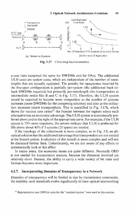
3. Optical Network Architecture Evolution 91
OTS Type
Standard
ULH
0 Transponder
b ULHlStandard
100 Cost Ratio
C Y
._
0 1 3 5 7 9
No. Of Standard OTS Systems (5 span) In Series
(a) Reference Systems (b) Domains Of Application
Fig. 3.17 Ultra-long-haul economics.
a cost ratio (assumed the same for DWDMs and for OAs). The additional ULH costs are system costs, which are independent of the number of wave- lengths that are actually equipped. The penalty for opaqueness incurred by the five-span configuration is partially per-system (the additional back-to- back DWDMs required) but primarily per-wavelength (the transponders at intermediate nodes like B and C in Fig. 3.17). Therefore, the ULH system would be expected to become more competitive as the number of systems increases (more DWDMs for the competing solution) and also as the utiliza- tion increases (more transponders). This is quantified in Fig. 3.17b, which shows for various cost ratios15 the frontier between the regions where each alternative has an economic advantage. The ULH system is economically pre- ferred above and to the right of the appropriate curve. For example, if the ULH system is 75% more expensive, the arrows indicate that ULH is preferred for fills above about 45% if 5 systems (25 spans) are needed.
If the topology of the subnetwork is more complex, as in Fig. 3.8, an all- optical solution has the additional advantage that transponders are not needed at the branch points. Evaluation of this benefit is more complex and will not be discussed further here. Unfortunately, we are not aware of any efforts to systematically look at this effect.
In metro areas, the economic issues are quite different. Normally OEO is not needed for transmission reasons, because the distances involved are relatively short. Instead, the ability to carry a wide variety of bit rates and formats becomes more important.
4.2.7. Incorporating Domains of Transparency in a Network
Domains of transparency will be limited in size by transmission constraints, the inability until standards evolve significantly to have optical interworking
l 5 Representative year 2000 list costs for the "standard system" were used in this exercise.

92 John Strand
Fig. 3.18 Express domain of transparency example.
between vendors, and by economics. In a long-haul network, a likely initial use of a domain of transparency would be to provide an express backbone on which longer connections would be routed. Shorter connections would be routed on an opaque technology that is more economic over shorter distances. This situation is illustrated in Fig. 3.18.
In this mesh network, two technologies are used, one all-optical (shown by dashed lines with squares showing offices with DWDMs or OADMs), the other one an opaque technology with electrical fabric OLXCs (circles) and with solid lines showing connectivity. On the left, the two technologies are shown with the topologies separate, and on the right, they are laid onto the conduit network used for both.
As just discussed, the all-optical technology is most cost-effective for longer distances. In this case, if we wished to route a connection from A to Z, the best route might be to go from A to J using the opaque technology (top plane in Fig. 3.18a), then go J-N-P-Q-L using the all-optical technology, and complete the route from L to Z using the opaque technology. This example suggests that introducing such a domain of transparency will raise new issues for routing and probably for other operational areas. We consider routing next.
4.2.8. Routing and Wavelength Assignment in a Domain of Transparency
Within an all-optical domain, “wavelength conversion” (changing the wave- length of a connection) is still expensive and not yet practical without an OEO conversion. Therefore, it is important to understand the architectural implica- tions of limited (or no) wavelength conversion. This requires us to look at what is called the “Routing and Wavelength Assignment (RWA) Problem” [l]: Given one or more connections that need to be established in an all-optical domain, determine the routes over which each connection should be routed and also assign each connection a color. If the routes are already known, the problem is called the “Wavelength Assignment (WA) Problem.”
The RWA problem has received extensive attention in the literature, mostly from a mathematical perspective. This literature is best approached through

3. Optical Network Architecture Evolution 93
a survey article (e.g., [l, 2, 14, 741). The underlying mathematical problem is very hard in general. The WA problem is easily seen to be equivalent to the problem of coloring the nodes of a graph so that no two nodes connected by an arc of the graph have the same color: Simply represent each connection by a node, and connect every pair of nodes whose corresponding connections ride on the same link (and so need to be assigned different wavelengths). This coloring problem is known to be NP-complete [75], which means that, in gen- eral, it is computationally intractable, but there are many fast but approximate (heuristic) algorithms for solving it.
Before discussing some of the architectural implications of this problem, it should be emphasized that the results in the literature frequently depend crucially on subtle points of the problem definition. The following definitional choices are particularly important:
0 Is there an accurate forecast of future connection requirements? If so the RWA process can take a more global approach to decision making.
0 What is the expected holding time of a connection? Some analyses assume that connections are permanent, while others assume that holding times are quite short.
demands are likely, this makes a major difference. 0 Is it possible to rearrange connections? In situations where unexpected
We feel that the most appropriate assumption at the present time is to assume that (1) we have minimal knowledge about future demands, there- fore each demand must be routed and assigned a wavelength when it appears without knowledge of future demands, and (2) that holding times are very long. With these assumptions, we simulated a number of RWA algorithms on a realistic model of the U.S. intercity network [76] without rearrangement or wavelength conversion and reached the following conclusions:
0 It is important to choose the route and do the wavelength assignment simultaneously. If routing is done first and then a wavelength is assigned, significantly suboptimal results are obtained (e.g., low utilization).
capacity penalty can be incurred if wavelength conversion is not available.
0 This penalty can be significantly mitigated if wavelength conversion is available at a small subset of nodes. In particular, half of the lack-of-wavelength-conversion penalty is removed if 21% of the nodes have conversion capabilities; 75% was removed if 35% of the nodes have conversion capabilities.
0 Even with simultaneous route and wavelength selection, a significant

94 John Strand
e Dual-OTrS scenarios, which provide two instances of each wavelength
A recent survey of the value of wavelength conversion [74] concluded that the performance improvements it offered depended on a number of factors, includ- ing the network topology and size. It further concluded that in networks with tunable transmitters and receivers, limited wavelength conversion provides improvements close to that achieved with ideal wavelength conversion.
on each link, reduced this penalty by only 6%.
4.2.9. Effect of Impairments on Routing in a Domain of Transparency [19,95]
As domains of transparency get larger, optical impairments such as amplifier spontaneous emission (ASE) and various types of dispersion may become an issue. Specifically:
e Polarization Mode Dispersion (PMD). PMD imposes a limit on the maximum wavelength length that is inversely proportional to the square of the bit rate of the signal. For typical installed fibers, the limits are 400 km and 25 km for bit rates of 10 Gb/s and 40 Gb/s, respectively. With newer fibers assuming PMD of 0.1 ps/,/km, the limits are 10,000 km and 625 km, respectively.
e AmpIiJier Spontaneous Emission (ASE). ASE imposes a constraint on the number of spans that is inversely proportional to its optical bandwidth.
e other polarization-dependent impairments. For example, many components have polarization-dependent loss (PDL) [ 11 that accumulates in a system with many components on the transmission path. The state of polarization fluctuates with time, and it is generally required to maintain the total PDL on the path to be within some acceptable limit.
impairments such as four-wave mixing cause more problems at a given launch power.
a Nonlinear impairments. As wavelengths get longer, nonlinear
These constraints are summarized in Fig. 3.19. The specific constraints required in a given situation will depend on the design and engineering of the domain of transparency. For example:
e The effect of nonlinear impairments depends on complex factors, e.g., on the order in which specific fiber types are traversed, the specific types of fiber involved, and the characteristics of the other active wavelengths (see, e.g., [46] or [64]).
e The impact of chromatic dispersion may depend on whether it has been dealt with on a per-link basis, and whether the domain is operating in a linear or nonlinear regime.

3. Optical Network Architecture Evolution 95
Launch Power (PL)
\ PMD Constraint
Bit Rate PMD Parameter Optical Bandwidth Minimum acceptable SNR at receiver
Length Of All-Optical Path ** L 6 t h e r
System Parameters
Fig. 3.19 Effect of impairments on wavelength muting.
4.2.10. Connectivity Limitations Associated with
The strawman ultra-long-haul system shown in Fig. 3.7 may be thought of as a large distributed switch. Depending on the configuration of the OADMs and the tunable lasersh-eceivers, the port-to-port connectivity of the a's will change. However, the connectivity is limited:
a Domain of Transparency
0 The adaptation function forces groups of input channels to be delivered together to the same distant adaptation function.
0 Only adaptation functions whose laserdreceivers are tunable to compatible frequencies can be connected.
0 The switching capability of the OADMs may also be constrained. For example: a. There may be some wavelengths that cannot be dropped at all. b. There may be a fixed relationship between the wavelength dropped
and the physical port on the OADM to which it is dropped. c. OADM physical design may put an upper bound on the number of
adaptation groupings dropped at any single OADM.
For a fixed configuration of the OADMs and adaptation functions, connec- tivity will be fixed: Each input port will essentially be hard-wired to some specific distant port. However, this connectivity can be changed by changing the configurations of the OADMs and adaptation functions. For example, an additional adaptation grouping might be dropped at an OADM or a tunable laser retuned. In each case, the port-to-port connectivity is changed. This capa- bility can be expected to be under software control. Today the control would rest in the vendor-supplied Element Management System (EMS), which in turn would be controlled by the operator's 0%.
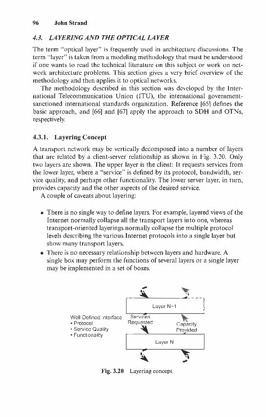
96 John Strand
4.3.
The term “optical layer” is frequently used in architecture discussions. The term “layer” is taken from a modeling methodology that must be understood if one wants to read the technical literature on this subject or work on net- work architecture problems. This section gives a very brief overview of the methodology and then applies it to optical networks.
The methodology described in this section was developed by the Inter- national Telecommunication Union (ITU), the international government- sanctioned international standards organization. Reference [65] defines the basic approach, and [66] and [67] apply the approach to SDH and OTNs, respectively.
LAYERING AND THE OPTICAL LAYER
4.3.1. Layering Concept
A transport network may be vertically decomposed into a number of layers that are related by a client-server relationship as shown in Fig. 3.20. Only two layers are shown. The upper layer is the client: It requests services from the lower layer, where a “service” is defined by its protocol, bandwidth, ser- vice quality, and perhaps other functionality. The lower server layer, in turn, provides capacity and the other aspects of the desired service.
A couple of caveats about layering:
0 There is no single way to define layers. For example, layered views of the Internet normally collapse all the transport layers into one, whereas transport-oriented layerings normally collapse the multiple protocol levels describing the various Internet protocols into a single layer but show many transport layers.
single box may perform the functions of several layers or a single layer may be implemented in a set of boxes.
0 There is no necessary relationship between layers and hardware. A
Well-Defined Interface Protocol - Service Quality Functionality
Requested Capacity
Layer N
Fig. 3.20 Layering concept.
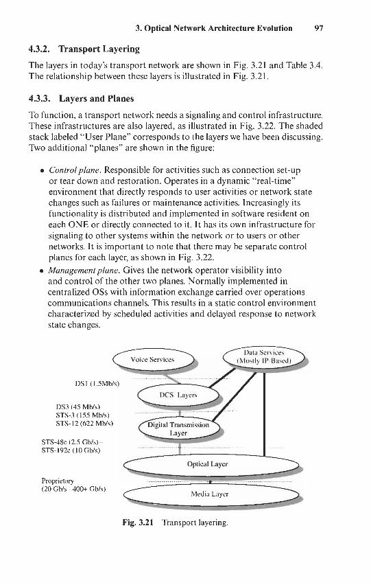
3. Optical Network Architecture Evolution 97
4.3.2. Transport Layering
The layers in today’s transport network are shown in Fig. 3.21 and Table 3.4. The relationship between these layers is illustrated in Fig. 3.21.
4.3.3. Layers and Planes
To function, a transport network needs a signaling and control infrastructure. These infrastructures are also layered, as illustrated in Fig. 3.22. The shaded stack labeled “User Plane” corresponds to the layers we have been discussing. Two additional “planes” are shown in the figure:
Control plane. Responsible for activities such as connection set-up or tear down and restoration. Operates in a dynamic “real-time” environment that directly responds to user activities or network state changes such as failures or maintenance activities. Increasingly its functionality is distributed and implemented in software resident on each ONE or directly connected to it. It has its own infrastructure for signaling to other systems within the network or to users or other networks. It is important to note that there may be separate control planes for each layer, as shown in Fig. 3.22. Management plane. Gives the network operator visibility into and control of the other two planes. Normally implemented in centralized OSs with information exchange carried over operations communications channels. This results in a static control environment characterized by scheduled activities and delayed response to network state changes.
DSl(1SMbls)
DS3 (45 Mbk)
STS-12 (622 Mb/S) igital Transmissio STS-3 (155 Mbk)
STS-48~ (2.5 Gb/S)- PTP 1 n?- fin P.I.L\ *,*-,7LL (‘VU”,>,
Proprietary (20 Gbk -400+ GbA)
Fig. 3.21 Transport layering.
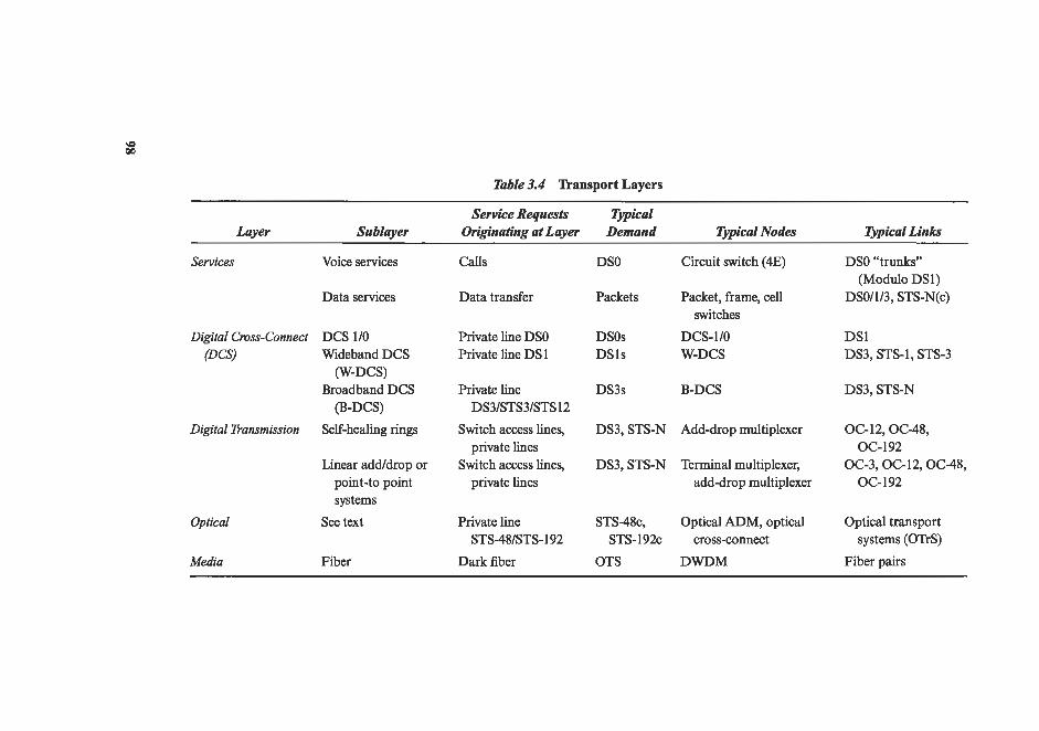
Table 3.4 Transport Layers
Service Requests Typical Layer Sublayer Originating at Layer Demand Typical Nodes Typical Links
Services Voice services
Data services
Digital Cross-Connect DCS 110 W S ) Wideband DCS
Broadband DCS
Digital Transmission Self-healing rings
(W-DCS)
(B-DCS)
Linear add/drop or point-to point systems
Optical See text
Media Fiber
calls
Data transfer
Private line DSO Private line DS 1
Private line
Switch access lines,
Switch access lines,
DS3/STS3/STS 12
private lines
private lines
Private line STS-48/STS-192
Dark fiber
DSO
Packets
DSOs DSls
DS3s
DS3, STS-N
DS3, STS-N
STS-48c,
OTS STS- 1 9 2 ~
Circuit switch (4E)
Packet, frame, cell switches
DCS-1/0 W-DCS
B-DCS
Add-drop multiplexer
Terminal multiplexer, add-drop multiplexer
Optical ADM, optical
DWDM cross-connect
DSO “trunks” (Modulo DS1)
DS0/1/3, STS-N(c)
DS 1 DS3, STS-I, STS-3
DS3, STS-N
OC-12,OC-48, OC- 192
OC-3,OG12,OC-48, OC-192
Optical transport systems (OTrS)
Fiber pairs

3. Optical Network Architecture Evolution 99
N
Layers
3 .: * ‘ < 5 < <
2
1
Physical Medium (fiber)
Fig. 3.22 Abstract layered network showing control and management planes.
4.3.4. Sublayers of the Optical Layer
The sublayers of SONET and SDH were described earlier (Section 3.1). The ITU is in the process of defining a very similar structure for what they call the “Optical Transport Network” (OTN). Starting from the top, the ITU’s layers are:
e Optical Channel (OCh) Layer. Provides end-to-end networking of optical channels for transparently conveying information of varying format such as SONET or G-Ethernet. In non-ITU circles, an OCh may be called by other names, of which “lightpath” seems to be the most popular. Today OCh’s typically carry STS-48 or STS-192 signals, with Gigabit- or 1 0-Gigabit Ethernet also receiving considerable attention along with STS-768. OLXCs provide cross-connect functionality for this sublayer.
multiwavelength optical signal that is passed between DWDMs. It also is responsible for wavelength shifting and management. A fiber switch (see Section 2.3) might provide cross-connect functionality for this sublayer.
e Optical Transmission Section (OTS) Layer. Provides basic transport functions for an OMS such as amplification and gain equalization.
Overlaying this structure on Fig. 3.1 one gets the system shown in Fig. 3.23. In SONET and SDH, at the terminations of the equivalents of each OCH,
OMS, and OTS, the signal is electrically accessible and so it is straightforward to add overhead bytes for management and signaling. This is not the case for the OMS and OTS, therefore the ITU is proposing an out-of-band optical “OTM Overhead Signal” (00s). In [69] the logical elements to be included are specified but the format is not. Since today OTSs are invariably single- vendor, the handling of OTS and OMS overhead is vendor proprietary. There is, however, some interest from carriers, particularly in Europe, for all-optical
e Optical Multiplex Section (OMS) Layer. Multiplexes OChs into the
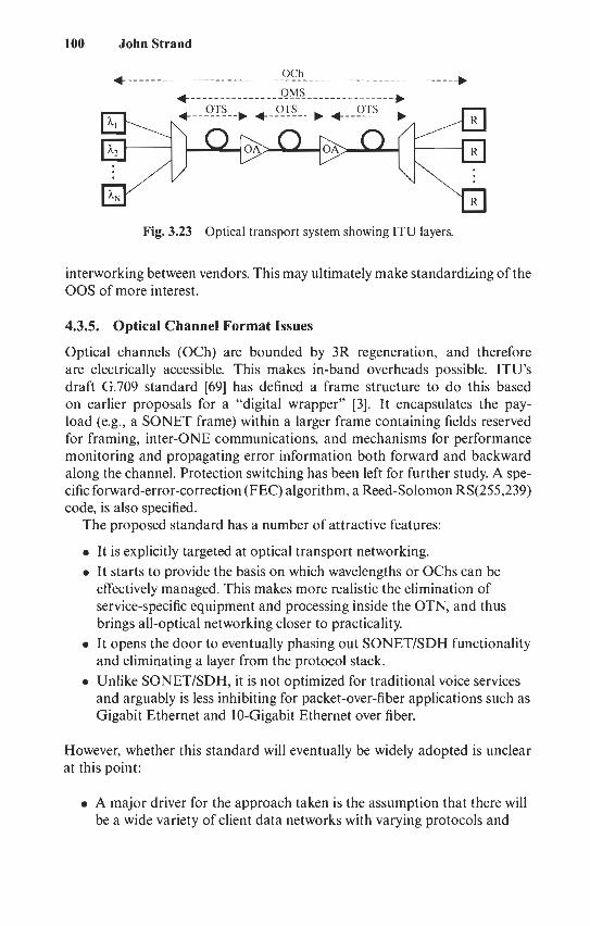
100 John Strand
interworking between vendors. This may ultimately make standardizing of the 00s of more interest.
4.3.5. Optical Channel Format Issues
Optical channels (OCh) are bounded by 3R regeneration, and therefore are electrically accessible. This makes in-band overheads possible. ITU’s draft G.709 standard [69] has defined a frame structure to do this based on earlier proposals for a “digital wrapper” [3]. It encapsulates the pay- load (e.g., a SONET frame) within a larger frame containing fields reserved for framing, inter-ONE communications, and mechanisms for performance monitoring and propagating error information both forward and backward along the channel. Protection switching has been left for further study. A spe- cific forward-error-correction (FEC) algorithm, a Reed-Solomon RS(255,239) code, is also specified.
The proposed standard has a number of attractive features:
0 It is explicitly targeted at optical transport networking. 0 It starts to provide the basis on which wavelengths or OChs can be
effectively managed. This makes more realistic the elimination of service-specific equipment and processing inside the OTN, and thus brings all-optical networking closer to practicality.
0 It opens the door to eventually phasing out SONETISDH functionality and eliminating a layer from the protocol stack.
0 Unlike SONETISDH, it is not optimized for traditional voice services and arguably is less inhibiting for packet-over-fiber applications such as Gigabit Ethernet and 10-Gigabit Ethernet over fiber.
However, whether this standard will eventually be widely adopted is unclear at this point:
0 A major driver for the approach taken is the assumption that there will be a wide variety of client data networks with varying protocols and
3. Optical Network Architecture Evolution 101
service needs [3]. The recommended approach is designed to allow a wide variety of client protocols (SONETEDH, ATM, IP, PDH, etc.) to be transported independent of their format. There are, however, many who argue that IP will become the common traffic convergence layer for all services. If this does indeed happen, the importance of flexibly handling a wide variety of protocols will decrease and a less general, IP-centric solution may emerge.
vendors are using strong FEC algorithms that require more FEC information than allowed in the standard. The timeliness of trying to standardize FEC now is therefore an issue.I6
intraoffice short-reach connections covered by SDH/SONET standards. In long-haul networks, vendors would be optically isolated from each other by transponders. In this architecture, FEC originates and is terminated by a single vendor, and therefore proprietary solutions are feasible and allow vendors to seek competitive advantage with innovative FEC solutions.
0 SONET/SDH can be used to encapsulate a wide range of protocols including IP, ATM, and Ethernet, thereby preserving the large investment in SONET/SDH transponders and 0%.
0 FEC needs have not yet stabilized. For example, ultra-long-haul
0 At present, optical interworking between vendors is limited to
This is not to say that the proposed G.709 standards will not be widely adopted eventually; however, their future seems most promising if multi- ple data protocols flourish, FEC technology stabilizes, practical multivendor all-optical standards emerge, and rapid growth (which would allow network operators to justify writing off their investment in SONET/SDH transpon- ders and line cards) continues. In the meantime, a vendor wanting some of the promised functionality might wish to use the proposed format within a single domain of transparency. This would avoid most of the objections listed previously, because at the boundary of the domain, an encapsulation of SONET/SDH into the new format could be done without necessarily affecting the larger network or service level interfaces.
4.4. EVOLVING ROLE OF THE OPTICAL LAYER 4.4.1. SONET/SDH and WDM
One of the most important functions performed by SONET/SDH has tradi- tionally been TDM-based intermediate multiplexing. This function is possible
l6 G.709 is sensitive to this issue. There is an appendix that discusses alternatives to the recommended approach.

102 John Strand
only if the SONET line rate is significantly larger than the data rate of the underlying service. For traditional 64-kb/sec voice services riding on 1.5-Mb/sec DS-ls, this is certainly t rue-a STS-48/STM-16 can carry 1344 DS-1s. However, this is not true for large IP backbone networks, where routers are increasingly connected with STS-48 or STS-192 connections. The situation is illustrated in Fig. 3.24, which shows the maximum available TDM rate (solid line), single-fiber WDM rate (dotted line), and IP router fabric capacities.
The gap between the line speed of IP routers and the maximum TDM-line rate represents the opportunity for TDM intermediate multiplexing. It has basically vanished and the prospects for it catching up again are uncertain at best. Because data trailic is driving network architecture evolution, this implies that SONET/SDH intermediate multiplexing capabilities will be of declining importance.
Because of this change, the SONET networking layers (the cross-connect and digital transmission layers in Table 3.4) cannot perform their traditional role for much of the bandwidth growth expected to be generated by IP-based services. Instead, their functions need to be distributed between the IP services layer and the optical layer, as illustrated in Fig. 3.25.
This redistribution will very likely have major impacts on equipment ven- dors as well as network operators. If the functionality largely goes into the IP layer, then vendors of IP equipment will be well positioned to control trans- port evolution and also to charge premium prices; if it largely goes into the optical layer, then the OTN vendors will be in the driver’s seat.
The rest of this chapter largely is devoted to spinning out the implications of this change. There are three major functionality groupings that must be studied:
100
8 lo
1
0.1
L
.. TDM Multiplexing 0pp-v
Fig. 3.24 The declining opportunity for TDM multiplexing.
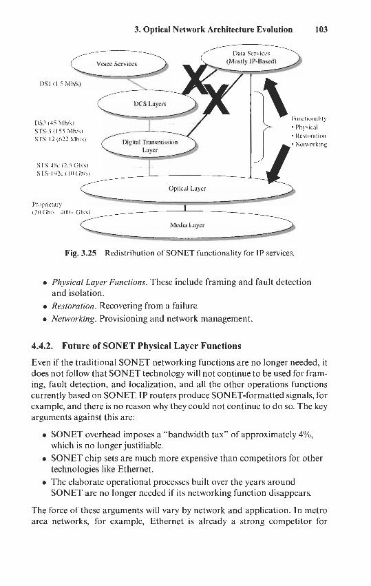
3. Optical Network Architecture Evolution 103
DS 1 (1 5 Mb/s)
- Restoration STS-12(622 Mbis) F D i g i t a l T r a n s m i s s i o x I I A . Netwnrkinn
I‘ rl STS-192c (10 Gb/s) x
Propnetary (2OGb/s--400+ G
Fig. 3.25 Redistribution of SONET functionality for IP services.
0 Physical Layer Functions. These include framing and fault detection
0 Restoration. Recovering from a failure. 0 Networking. Provisioning and network management.
and isolation.
4.4.2. Future of SONET Physical Layer Functions
Even if the traditional SONET networking functions are no longer needed, it does not follow that SONET technology will not continue to be used for fram- ing, fault detection, and localization, and all the other operations functions currently based on SONET. IP routers produce SONET-formatted signals, for example, and there is no reason why they could not continue to do so. The key arguments against this are:
0 SONET overhead imposes a “bandwidth tax” of approximately 4%,
0 SONET chip sets are much more expensive than competitors for other
0 The elaborate operational processes built over the years around
which is no longer justifiable.
technologies like Ethernet.
SONET are no longer needed if its networking function disappears.
The force of these arguments will vary by network and application. In metro area networks, for example, Ethernet is already a strong competitor for
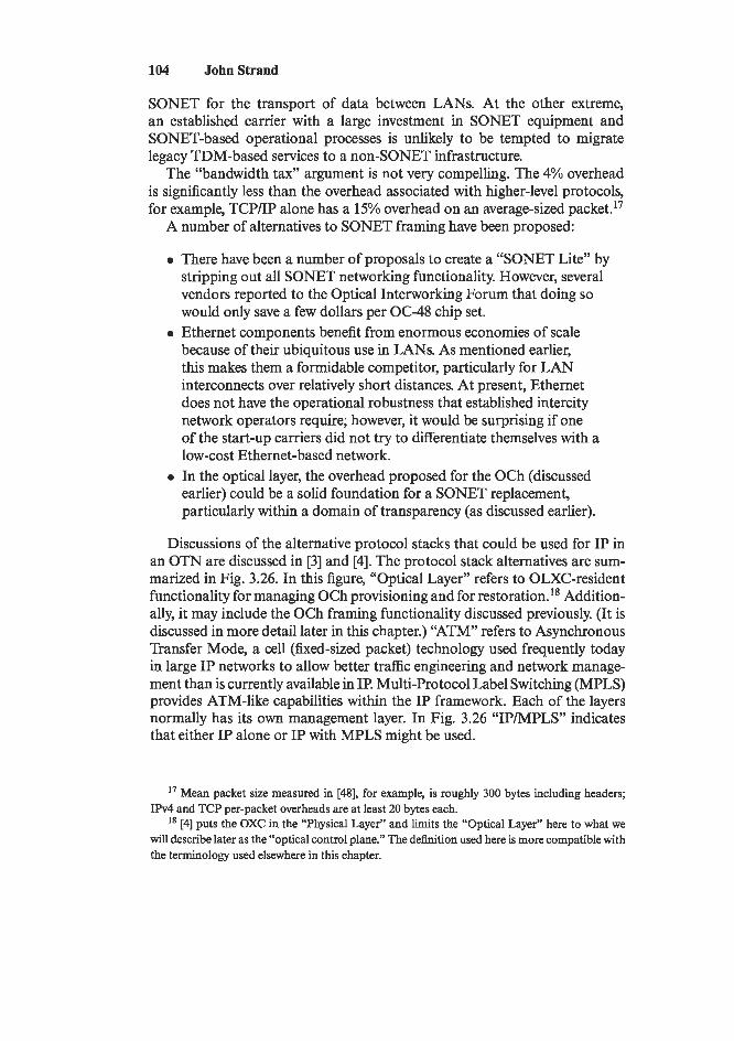
104 John Strand
SONET for the transport of data between LANs. At the other extreme, an established carrier with a large investment in SONET equipment and SONET-based operational processes is unlikely to be tempted to migrate legacy TDM-based services to a non-SONET infrastructure.
The “bandwidth tax” argument is not very compelling. The 4% overhead is significantly less than the overhead associated with higher-level protocols, for example, TCP/IP alone has a 15% overhead on an average-sized packet.17
A number of alternatives to SONET framing have been proposed:
0 There have been a number of proposals to create a “SONET Lite” by stripping out all SONET networking functionality. However, several vendors reported to the Optical Interworking Forum that doing so would only save a few dollars per OC-48 chip set.
0 Ethernet components benefit from enormous economies of scale because of their ubiquitous use in LANs. As mentioned earlier, this makes them a formidable competitor, particularly for LAN interconnects over relatively short distances. At present, Ethernet does not have the operational robustness that established intercity network operators require; however, it would be surprising if one of the start-up carriers did not try to differentiate themselves with a low-cost Ethernet-based network.
0 In the optical layer, the overhead proposed for the OCh (discussed earlier) could be a solid foundation for a SONET replacement, particularly within a domain of transparency (as discussed earlier).
Discussions of the alternative protocol stacks that could be used for IP in an OTN are discussed in [3] and [4]. The protocol stack alternatives are sum- marized in Fig. 3.26. In this figure, “Optical Layer” refers to OLXC-resident functionality for managing OCh provisioning and for restoration.18 Addition- ally, it may include the OCh framing functionality discussed previously. (It is discussed in more detail later in this chapter.) “ATM” refers to Asynchronous Transfer Mode, a cell (fixed-sized packet) technology used frequently today in large IP networks to allow better traffic engineering and network manage- ment than is currently available in IP. Multi-Protocol Label Switching (MPLS) provides ATM-like capabilities within the IP framework. Each of the layers normally has its own management layer. In Fig. 3.26 “IP/MPLS” indicates that either IP alone or IP with MPLS might be used.
l7 Mean packet size measured in [48], for example, is roughly 300 bytes including headers; IPv4 and TCP per-packet overheads are at least 20 bytes each. ’* [4] puts the OXC in the “Physical Layer” and limits the “Optical Layer” here to what we will describe later as the “optical control plane.” The definition used here is more compatible with the terminology used elsewhere in this chapter.
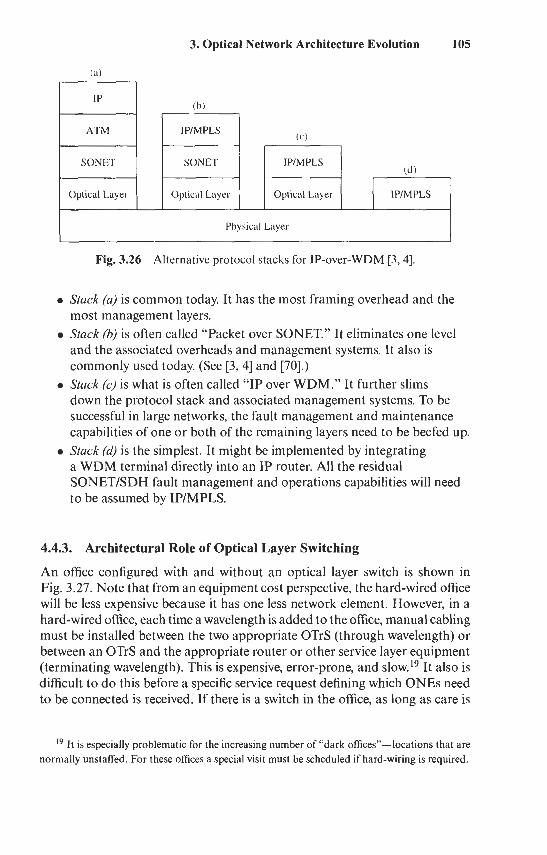
3. Optical Network Architecture Evolution
IP
ATM
SONET
Optical Layer
105
(b)
IPMPLS
SONET IPMPLS
(C)
(d)
Optical Layer Optical Layer IPMPLS
0 Stuck (a) is common today. It has the most framing overhead and the
0 Stuck (a) is often called “Packet over SONET.” It eliminates one level most management layers.
and the associated overheads and management systems. It also is commonly used today. (See [3,4] and [70].)
0 Stuck (c) is what is often called “IP over WDM.” It further slims down the protocol stack and associated management systems. To be successful in large networks, the fault management and maintenance capabilities of one or both of the remaining layers need to be beefed up.
a WDM terminal directly into an IP router. All the residual SONET/SDH fault management and operations capabilities will need to be assumed by IP/MPLS.
0 Stack (d) is the simplest. It might be implemented by integrating
4.4.3. Architectural Role of Optical Layer Switching
An office configured with and without an optical layer switch is shown in Fig. 3.27. Note that from an equipment cost perspective, the hard-wired office will be less expensive because it has one less network element. However, in a hard-wired office, each time a wavelength is added to the office, manual cabling must be installed between the two appropriate OTrS (through wavelength) or between an OTrS and the appropriate router or other service layer equipment (terminating wavelength). This is expensive, error-prone, and slow. l 9 It also is difficult to do this before a specific service request defining which ONES need to be connected is received. If there is a switch in the office, as long as care is
l 9 It is especially problematic for the increasing number of “dark offices”-locations that are normally unstaffed. For these offices a special visit must be scheduled if hard-wiring is required.

106 John Strand
n Service Layers
(a) Hard-Wired Office (b) Office With Switch
Fig. 3.27 Office configurations with and without a switch.
IP Router
(a) OLXC Office Architecture (b) “BFR Office Architecture
Fig. 3.28 Optical Layer switching alternatives-OLXC and “big fat router.”
taken to ensure that a spare connection is always available from each ONE to the switch, none of these difficulties arise-the software-controlled switch can establish the desired connectivity on demand. Arguments along these lines seem to have led most carriers to conclude that the option in Fig. 3.27b is desirable in larger offices at least.
In Section 2 we introduced optical layer cross-connects (OLXCs). These are certainly a candidate for use here. The principal competition for an OLXC-based architecture is likely to come from “big fat routers” (BFR; [80, 8 11). In this architecture, IP routers with line-side interfaces operating at the per-wavelength bit rate are directly connected to one another via point- to-point OTrS. The OTrS terminals might even be integrated into the IP router. Legacy services requiring constant bit-rate connections are supported with vir- tual leased-line services [84]. The two competing architectures are shown in Fig. 3.28.
The BFR approach is most appealing if IP-based traffic continues its dra- matic growth and dwarfs other types of traffic. In this scenario, it is argued that there is no need to interpose another layer between the OTrS and the IP routers. It is further argued that eliminating a layer of switching will simplify network management and will reduce capital costs by eliminating some “boxes.”
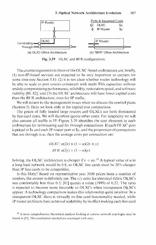
3. Optical Network Architecture Evolution 107
Ports 8, Assumed Costs E4 OLXC $x d IP Router $y
Terminating Through
(a) OLXC Office Architecture (b) "BFR Office Architecture
Fig. 3.29 OLXC and BFR configurations.
The counterarguments in favor of the OLXC-based architecture are, briefly, (1) non-IP-based services are expected to be very important to carriers for some time (see Section 3.1); (2) it is not clear whether router technology will be able to scale to port counts consistent with multi-Tb/s capacities without unduly compromising performance, reliability, restoration speed, and software stability [80, 821; and (3) the OLXC architecture will have lower capital costs than the BFR architecture, even for IP traffic.
We will return to the management issues when we discuss the control plane (Section 5) . Here we look only at the capital cost comparison.
The prices of fully loaded large routers and OLXCs are both dominated by line-card costs. We will therefore ignore other costs. For simplicity we will also assume all traffic is IP. Figure 3.29 identifies the cost elements in each architecture for terminating and for through connections. If each OLXC port is priced at $x and each IP router port at $y, and the proportion of connections that are through is a, then the average costs per connection are:
OLXC: a(2x) + (1 - a)(2x + y )
BFR: 4 2 ~ ) + (1 - a)b)
Solving, the OLXC architecture is cheaper if x < ay.'O A typical value of a in a long-haul network would be 0.8, so OLXC line cards must be 20% cheaper than IP line cards to be competitive.
Is this likely? Based on representative year 2000 prices from a number of vendors, the answer is definitely yes. The x/y ratio for electrical-fabric OLXCs was comfortably less than 0.5; [ l l] quotes a value (1999) of 0.22. The ratio is expected to become more favorable to OLXCs when transparent OLXCs appear. A technology comparison makes this relationship quite intuitive: In a transparent OLXC there is virtually no line card functionality needed, while IP router architects have achieved scalability by in effect making each line card
*O A more comprehensive theoretical analysis looking at various network topologies may be found in [83]. The conclusions reached are consistent with ours.
108 John Strand
a mini-router. We conclude that an OLXC is the most economic way of doing optical layer (OC-48/OC- 192) cross-connections.
4.5. SUR WABILITI: PROTECTION, AND RESTORATION
4.5.1. Background
Survivability-the ability to deal with and recover from failures-is a critical architectural consideration. In Fig. 3.25 each of the layers shown, except the Media Layer, have survivability capabilities Unless carefully designed, this functional overlap introduces additional costs and coordination issues.
The protection and restoration functions provided by SONET/SDH are critical to the survivability of today’s TDM-based transport networks. Before discussing how these functions relate to the IP and the Optical Layers, we will take a digression to introduce the general topic of survivability.
There are many types of failures that can occur in an optical network, but two are of particular importance: equipment failures and route failures. Equipment failures, primarily failures of individual components, such as a laser, are far more numerous than route failures. In “carrier class” equipment, normally there are no single points of failure; if a component such as a laser fails, automatic protection switching (APS, discussed later) is used to restore service.
Although much less frequent, route failures (also called fiber cuts) can have a much more devastating effect. The prototypical cause of a route failure is an errant backhoe that physically severs the fibers; other causes might be a natural disaster (flood, earthquake) or a train wreck. Normally all fibers in a cable will be affected. By electronic standards, these failures occur in slow motion. Initially fiber stretching might cause a period of transient errors; the actual severing of fibers can be spread out over a period of seconds. This can cause confusion and churning if a recovery process able to react in millisec- onds locks in on a restoration plan before the full magnitude of the failure is known.
The incidence of route failures varies widely. Rural areas have fewer prob- lems, as do cables run through concrete conduits. As a rough rule of thumb, one fiber cut per thousand route kilometers per year might be used; thus a national-scale network in the United States might expect, on average, a couple of incidents per month.21
Physical repair after a route failure requires dispatching a repair crew to the site, which may be quite distant, and then physically splicing the ruptured
In 1997, when the total intercity fiber in the United States was 59,000 route miles, 136 fiber cuts were reported by various US. carriers to the Federal Communications Commission [6, 711. Only cuts with serious service impacts are required to be reported, therefore the total number of cuts is no doubt somewhat higher.

3. Optical Network Architecture Evolution 109
fibers. The nominal time for doing this is on the order of 4 hours, but it may be much longer if there is a massive failure, for example, a building fire or an extensive wash-out. For many services, however, the overall availability requirements are on the order of 99.999% (6 minutedyear) or better. There- fore, additional survivability mechanisms must be provided. There are many possible mechanisms, some of which are appropriate for service restoration and some of which need to be resident in a transport layer.
Because of their importance in transport networks, we will focus on recovery from route failures in this section. Optical Layer mechanisms will be discussed first, then mechanisms appropriate for other layers will be introduced and related to the optical layer.
4.5.2. Protection and Restoration
Protection and restoration are both used in the process of recovering from a failure. A quick review of a few published articles found a number of dehitions, of which the most popular were as follows:
0 Protection refers to the primary recovery, whereas restoration refers to secondary methods that are invoked if the primary method fails.
0 Protection refers to methods whose operation is specified prior to a failure; restoration refers to methods that dynamically determine how to proceed. Protection reroutes onto preassigned spares; restoration makes use of a pool of spare resources that are dynamically assigned after a failure.
0 Protection refers to recovery from a component or subsystem failure by switching to a hot standby that is usually performed in a distributed way by the ONES. Recovery that requires rerouting facilities over a physically different route is called “restoration.”
0 Protection is triggered by “defects”-the physical layer’s detection of a problem, whereas restoration is triggered by ‘Lalarmsyy-messages generated by ONES to be sent to external managementlcontrol functions.
In general, “protectionyy has historically referred to deterministic methods that are very fast, whereas “restoration” referred to more complex methods whose precise behavior is determined at the time of failure, and which may be somewhat slower than protection. However, IP-inspired changes in the way transport networks are controlled are rapidly eroding this difference. In this section we will use “protection” to refer to preplanned methods using pre- assigned capacity and “restoration” for other methods. We will use the term “recovery” when we want to be generic.
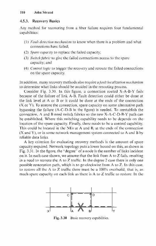
110 John Strand
4.5.3. Recovery Basics
Any method for recovering from a fiber failure requires four fundamental capabilities:
(1) Fault detection mechanism to know when there is a problem and what
(2) Spare capacity to replace the failed capacity; (3) Switchfabric to give the failed connections access to the spare
(4) Control logic to trigger the recovery and reroute the failed connections
connections have failed;
capacity; and
on the spare capacity.
In addition, many recovery methods also require a fault localization mechanism to determine what links should be avoided in the rerouting process.
Consider Fig. 3.30. In this figure, a connection routed X-A-B-Y fails because of the failure of link A-B. Fault detection could either be done at the link level at A or B or it could be done at the ends of the connection (X or Y). To restore the connection, spare capacity on some alternative path bypassing the failure (A-C-D-B in the figure) is needed. To reestablish the connection, A and B need switch fabrics so the new X-A-C-D-B-Y path can be established. Where this switching capability needs to be depends on the location of the spare capacity. Finally, there needs to be a control capability. This could be located in the NEs at A and B, at the ends of the connection (X and Y), or in some network management system connected to A and B by reliable data links.
A key criterion for evaluating recovery methods is the amount of spare capacity required. Network topology puts a lower bound on this, as shown in Fig. 3.31. In the figure, the “degree” of a node is the number of links incident on it. In each case shown, we assume that the link from A to Z fails, resulting in a need to reroute the A to Z traffic. In the degree 2 case there is only one possible restoration path, which is to go clockwise from A to Z. In this case, to restore all the A to Z traffic there must be a 100% overbuild, that is, as much spare capacity on each link as there is A to Z traffic to restore. In the
Fig. 3.30 Basic recovery capabilities.

3. Optical Network Architecture Evolution 111
Z
Degree 2 Nodes 100% Overbuild
Degree 3 Nodes Degree N Nodes 50% Overbuild l/(N-1) Overbuild
Fig. 3.31 Effect of topology on restoration capacity.
second (degree 3) case, there are two potential restoration paths from A to Z. Therefore, if there is a 50% overbuild on each restoration path, all the A-Z traffic can be restored. In general, in a network with all degree N nodes a 1/(N - 1) overbuild is required (last figure).
4.5.4. Taxonomy of Recovery Methods
Recovery can be done in many different ways, many of them proprietary to either a vendor or a network operator. It also can be done at different levels- service, SONET, or optical. When confronted with a new method, it is useful to determine how it provides the four basic capabilities listed previously:
(1) Fault detection. Is the fault localized before the recovery process starts or not? Localizing the failure can take time and be complex, but it allows the process to bypass only the failed elements, and thus may require less spare capacity. Without fault detection, the connection must be rerouted onto a diverse path end-to-end.
0 Is the capacity used for restoration dedicated to individual (2) Spare capacity.
connections or is it shared? If each connection to be restored has dedicated restoration capacity, the restoration process can be very fast and the control logic can be quite simple; however, much more restoration capacity is likely to be needed.
protection against a wider range of failures is provided; however, this comes at the cost of having to plan and coordinate across a wider geographical area involving more network elements.
( 3 ) Switchfabric. Are connections restored individually (this is normally called “path” restoration) or are connections restored in bulk (“link” restoration). Also of interest is where the switching is done.
0 Is the spare capacity diverse from the working capacity? If so,
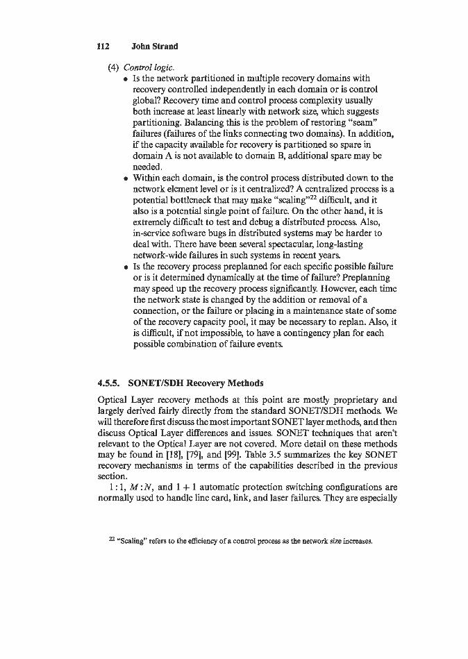
112 John Strand
(4) Control logic. 0 Is the network partitioned in multiple recovery domains with
recovery controlled independently in each domain or is control global? Recovery time and control process complexity usually both increase at least linearly with network size, which suggests partitioning. Balancing this is the problem of restoring “seam” failures (failures of the links connecting two domains). In addition, if the capacity available for recovery is partitioned so spare in domain A is not available to domain B, additional spare may be needed.
0 Within each domain, is the control process distributed down to the network element level or is it centralized? A centralized process is a potential bottleneck that may make “scaling”22 dficult, and it also is a potential single point of failure. On the other hand, it is extremely difficult to test and debug a distributed process. Also, in-service software bugs in distributed systems may be harder to deal with. There have been several spectacular, long-lasting network-wide failures in such systems in recent years.
0 Is the recovery process preplanned for each specific possible failure or is it determined dynamically at the time of failure? Preplanning may speed up the recovery process significantly. However, each time the network state is changed by the addition or removal of a connection, or the failure or placing in a maintenance state of some of the recovery capacity pool, it may be necessary to replan. Also, it is difficult, if not impossible, to have a contingency plan for each possible combination of failure events.
4.5.5. SONETISDH Recovery Methods
Optical Layer recovery methods at this point are mostly proprietary and largely derived fairly directly from the standard SONET/SDH methods. We will therefore first discuss the most important SONET layer methods, and then discuss Optical Layer differences and issues. SONET techniques that aren’t relevant to the Optical Layer are not covered. More detail on these methods may be found in [18], [79], and [99]. Table 3.5 summarizes the key SONET recovery mechanisms in terms of the capabilities described in the previous section.
1 : 1, M : N , and 1 + 1 automatic protection switching configurations are normally used to handle line card, link, and laser failures. They are especially
“Scaling” refers to the efficiency of a control process as the network size increases.

Table 3.5 SONET Recovery Methods
Typical Fault Dedicated Location of Diverse Multipre
Localization Recovery Switching Recovery Path or Recovery Control within Preplanned Needed Capacity Function Capacity Link Domains Each Domain or Dynamic
M:Nand No Yes Ubiquitous No Path Yes Distributed Preplanned
Path-switched No Possible ADM line Yes Path Yes Distributed Prcplanncd
Line-switched Yes No ADM Yes Link Yes Distributed Preplanned
Mesh No Possible DCS Yes Path Possible Centralized or Either
l + l A P S
rings card
rings
distributed
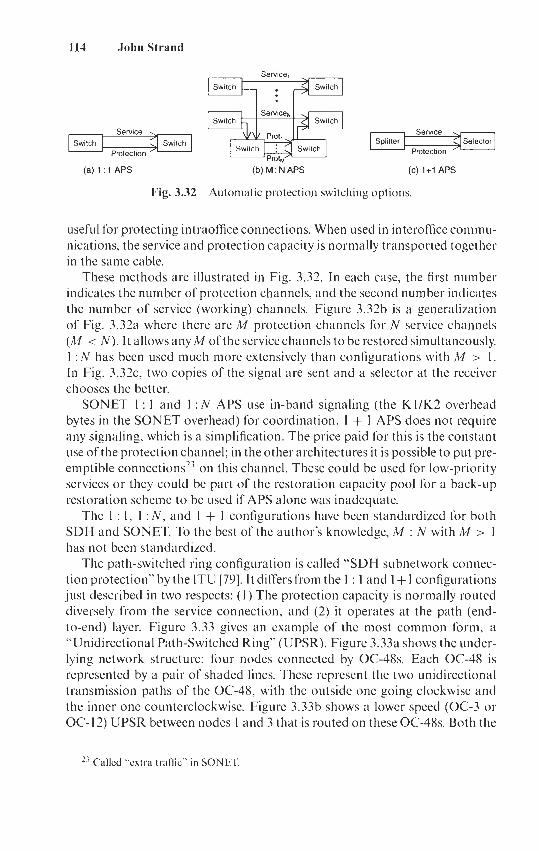
114 John Strand
Switch
(a) 1 : 1 APS
Fig. 3.32
I Switch SWI
(b) M: N APS (c) 1+1 APS
Automatic protection switching options.
useful for protecting intraoffice connections. When used in interoffice commu- nications, the service and protection capacity is normally transported together in the same cable.
These methods are illustrated in Fig. 3.32. In each case, the first number indicates the number of protection channels, and the second number indicates the number of service (working) channels. Figure 3.32b is a generalization of Fig. 3.32a where there are M protection channels for N service channels (M < N ) . It allows any M of the service channels to be restored simultaneously. 1 : N has been used much more extensively than configurations with M > 1. In Fig. 3.32c, two copies of the signal are sent and a selector at the receiver chooses the better.
SONET 1 : 1 and 1 : N APS use in-band signaling (the K1/K2 overhead bytes in the SONET overhead) for coordination. 1 + 1 APS does not require any signaling, which is a simplification. The price paid for this is the constant use of the protection channel; in the other architectures it is possible to put pre- emptible connection^^^ on this channel. These could be used for low-priority services or they could be part of the restoration capacity pool for a back-up restoration scheme to be used if APS alone was inadequate.
The 1 : 1, 1 : N , and 1 + 1 configurations have been standardized for both SDH and SONET. To the best of the author’s knowledge, M : N with M > 1 has not been standardized.
The path-switched ring configuration is called “SDH subnetwork connec- tion protection” by the ITU [79]. It differs from the 1 : 1 and 1 + 1 configurations just described in two respects: (1) The protection capacity is normally routed diversely from the service connection, and (2) it operates at the path (end- to-end) layer. Figure 3.33 gives an example of the most common form, a “Unidirectional Path-Switched Ring” (UPSR). Figure 3.33a shows the under- lying network structure: four nodes connected by OC-48s. Each OC-48 is represented by a pair of shaded lines. These represent the two unidirectional transmission paths of the OC-48, with the outside one going clockwise and the inner one counterclockwise. Figure 3.33b shows a lower speed (OC-3 or OC-12) UPSR between nodes 1 and 3 that is routed on these OC-48s. Both the
23 Called “extra traffic” in SONET.

3. Optical Network Architecture Evolution 115
(a) 4 Node OC-48 Ring (b) UPSR - Normal State (c) UPSR - Failure State
Fig. 3.33 Path-switched ring (OC-48-based UPSR example).
Fig. 3.34 Generic path-switched ring.
1-3 direction and the 3-1 direction are routed clockwise, on the outer trans- mission path. Thus the two directions are routed separately. At nodes 1 and 3 there is path termination equipment for the UPSR. Figure 3 . 3 3 ~ shows that if the service path from 4 to 1 fails, the 3-1 direction of the UPSR is rerouted onto the counterclockwise loop, thus restoring the connection. The switching is done at nodes 1 and 3, with no involvement by the other nodes. Only the failed direction (3-1) is rerouted.
There could be multiple UPSRs between different nodes riding on the same set of OC-48s. More general connecting networks are possible, as indicated in Fig. 3.34. Here the SONET network “cloud” could be composed of a mixture of SONET rings and linear structures. The protection switching is done at the terminations of the path. A line-switched ring configuration was discussed in conjunction with Fig. 3.2 in Section 2.1.
All of the recovery mechanisms described so far require that the network be divided into recovery domains with either ring or linear topologies4egree 2 topologies in Fig. 3.3 1. Planning and operating a network so divided is complex and frequently expensive, as we shall see shortly. Mesh recovery works in an arbitrary topology (degreeN in Fig. 3.31) without having to deal with the plan- ning and operational complexities of a multi-recovery-domain environment.

116 John Strand
Unfortunately, this flexibility makes it virtually impossible to standardize a mesh restoration method to the level that has been done with SONET rings. As a result, all mesh implementations are proprietary.
One mesh implementation that has been described in the public literature is AT&T’s FAST Automated Restoration (FASTAR@) [20]. Originally designed for a pre-SONET network, it has been extended for SONET. We will briefly describe how it works to give a flavor of mesh restoration.
FASTAR’s physical infrastructure consists of Restoration Network Con- trollers (RNCs) in each office; a centralized restoration controller [the Restora- tion and Provisioning Integrated Design (RAPID) system]; and a redundant data network to connect them together, and also to connect RAPID to the DCSs, which do the actual rerouting. When a failure occurs, each RNC col- lects alarms from the affected NEs in its office. After waiting for a brief period to allow all alarms to come in, and also to see if the problem is a transient, it then sends the alarms to RAPID.
The RAPID database contains information on all spare capacity available for restoration.24 When the first alarm arrives, RAPID opens up an “event window.” While the window is open,25 alarms are collected. After the window is closed, RAPID:
0 Determines what spare capacity has survived the failure. 0 Orders all the connections reported failed according to their restoration
priority. 0 Processes each connection in turn. For each, an alternate path with
spare capacity is computed, the spare capacity is committed, and commands are sent to the appropriate DCSs to implement the reroute.
FASTAR’s restoration speed is gated by the rate at which the DCS can do reroutes.26
As indicated in Table 3.5, there are many dimensions in which mesh methods may vary:
0 Recovery actions may be determined dynamically after the failure (like FASTAR) or can be preplanned. A number of levels of preplanning are
24 FASTAR depends critically on the timeliness and accuracy of this database. Keeping a centralized view of a network composed of many types of equipment and distributed around hundreds of nodes and links sufficiently accurate is probably the most difficult challenge a centralized-mesh-restoration developer faces.
25 It is closed when either a specified period elapses with no additional alarms or when a time specifying the maximum window period expires.
26 For a U.S. government description of FASTAR, including some restoration times, see http:/ l~ .ncsgov/n5_hp/InformationAssuraSec3. htm.

3. Optical Network Architecture Evolution 117
possible. For example, the reroute paths may be preplanned but the specific capacity to be used along the path for a specific connection may be determined dynamically.
the NEs.
constrained to stay near the site of the failure.
0 Control may be centralized (like FASTAR) or may be distributed to
0 Rerouting may be done end-to-end (which is allowed by FASTAR) or
Many of these alternatives are being vigorously pursued for Optical Layer restoration. We will discuss distributed mesh algorithms in Section 5.
4.5.6. Ring/Mesh Comparison
ITU and SONET standards specify that restoration should be completed within 50 ms in most cases,27 and 200 ms is an achievable upper bound for ring restoration. There are new mesh restoration schemes proposed for the optical layer, and also for IP-based networks, that may be competitive, but these are still mostly theoretical results. Centralized mesh algorithms are likely to take a minute or more to recover from a large failure.
Rings are required to have uniform capacity on each of their links. This can cause difficulties, as is illustrated in Fig. 3.35. Figure 3.35a shows a topological structure common in intercity networks-a set of paralleling north-south and east-west fiber routes. If there is a roughly equal amount of demand on each link, then the same amount of capacity is needed in the upper (e.g., A-B-C-D) and the lower (C-D-E-F) “window panes.” But this leads to double capacity on the middle route.
Figure 3.35b shows another example of the complexities introduced by the equal capacity constraint. Here, each dashed line shows the routing of some connections, each of which requires more than 50% of the capacity of a ring.
(a) Window Pane Network
Demands (25 DS3 Each): A-E F-L H-G H-L
Shortest Distance Routing (b) Effect Of Routing
Fig. 3.35 Ring examples.
I I I I
Optimized Routing On Ring Efficiency
*’ If a ring is more than 1200 km in circumference, or if it is carrying extra traffic, an extra 100 ms or so may be required.
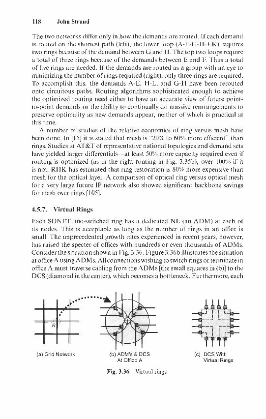
118 John Strand
The two networks differ only in how the demands are routed. If each demand is routed on the shortest path (left), the lower loop (A-F-G-H-J-K) requires two rings because of the demand between G and H. The top two loops require a total of three rings because of the demands between E and F. Thus a total of five rings are needed. If the demands are routed as a group with an eye to minimizing the number of rings required (right), only three rings are required. To accomplish this, the demands A-E, H-L, and G-H have been rerouted onto circuitous paths. Routing algorithms sophisticated enough to achieve the optimized routing need either to have an accurate view of future point- to-point demands or the ability to continually do massive rearrangements to preserve optimality as new demands appear, neither of which is practical at this time.
A number of studies of the relative economics of ring versus mesh have been done. In [15] it is stated that mesh is “20% to 60% more efficient” than rings. Studies at AT&T of representative national topologies and demand sets have yielded larger differentials-at least 50% more capacity required even if routing is optimized (as in the right routing in Fig. 3.35b), over 100% if it is not. RHK has estimated that ring restoration is 80% more expensive than mesh for the optical layer. A comparison of optical ring versus optical mesh for a very large future IP network also showed significant backbone savings for mesh over rings [105].
4.5.7. Virtual Rings
Each SONET line-switched ring has a dedicated NE (an ADM) at each of its nodes. This is acceptable as long as the number of rings in an office is small. The unprecedented growth rates experienced in recent years, however, has raised the specter of offices with hundreds or even thousands of ADMs. Consider the situation shown in Fig. 3.36. Figure 3.36b illustrates the situation at office A using ADMs. All connections wishing to switch rings or terminate in office A must traverse cabling from the ADMs [the small squares in (b)] to the DCS (diamond in the center), which becomes a bottleneck. Furthermore, each
(a) Grid Network (b) ADM’s & DCS (c) DCS With At Office A Virtual Rings
Fig. 3.36 Virtual rings.

3. Optical Network Architecture Evolution 119
ADM is physically cabled on the network side to specific physical facilities; recabling would be needed to change this.
Figure 3.36~ illustrates what is called a “virtual ring.” Here, a single DCS switch fabric replaces all the ADM fabrics. Any two DCS ports may be associ- ated together through the fabric to form the functional equivalent of an ADM. Ring interconnects also are made through this fabric and the line-switched ring-protection algorithm is implemented in the DCS control software. This has major advantages: (1) Intraoffice connections between rings no longer require intraoffice cabling to and from the DCS; (2) any two high-speed ports on the DCS can be made into a logical ADM via a software command; and (3) it is now physically possible for two virtual rings to share protection capacity.
Proprietary virtual ring implementations have been made by a number of DCS and OLXC vendors.
4.5.8. Diversity
For a ring to work properly, it is necessary that the links forming it are physi- cally diverse from each other, otherwise a single failure might cut it in two places and cause a total failure. To determine whether two lightpath routings are diverse, it is necessary to identify single points of failure in the interoffice plant. To do so, we will use the following terms: AJiber cabZeis a uniform group of fibers contained in a sheath. An OTrS will occupy fibers in a sequence of fiber cables. Each fiber cable will be placed in a sequence of conduits-buried honeycomb structures through which fiber cables may be pulled-or buried in a right ofway (ROW). It is worth noting that for economic reasons, ROWs are frequently obtained from railroads, pipeline companies, or thruways. Often several carriers may lease ROWs from the same source; this makes it common to have a number of carriers’ fiber cables in close proximity to each other. Similarly, in a metropolitan network, several carriers might lease duct space in the same RBOC conduit. As discussed in Section 3.3, carriers also trade capac- ity. In each of these situations, there is the opportunity for a single event to disrupt more than one carrier’s facilities simultaneously. Thus, relying on car- riers to be diverse from each other without detailed evaluation of the physical routings is chancy.
In a typical U.S. intercity facility network there might be on the order of lo2 major offices. To accurately capture diversity, however, a network with an order of magnitude more nodes is required. In addition to Optical Amplifier (OA) sites, these additional nodes include:
0 Places where fiber cables enterneave a conduit or right of way; 0 Locations where fiber cables cross; 0 Locations where fiber splices are used to interchange fibers between
fiber cables.
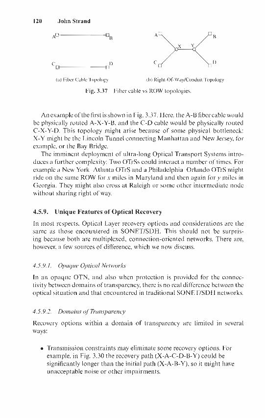
120 John Strand
A-B
(a) Fiber Cable Topology (b) Right-Of-WayKonduit Topology
Fig. 3.37 Fiber cable vs ROW topologies.
An example of the first is shown in Fig. 3.37. Here, the A-B fiber cable would be physically routed A-X-Y-B, and the C-D cable would be physically routed C-X-Y-D. This topology might arise because of some physical bottleneck: X-Y might be the Lincoln Tunnel connecting Manhattan and New Jersey, for example, or the Bay Bridge.
The imminent deployment of ultra-long Optical Transport Systems intro- duces a further complexity: Two OTrSs could interact a number of times. For example a New York-Atlanta OTrS and a Philadelphia-Orlando OTrS might ride on the same ROW for x miles in Maryland and then again for y miles in Georgia. They might also cross at Raleigh or some other intermediate node without sharing right of way.
4.5.9. Unique Features of Optical Recovery
In most respects, Optical Layer recovery options and considerations are the same as those encountered in SONETBDH. This should not be surpris- ing because both are multiplexed, connection-oriented networks. There are, however, a few sources of difference, which we now discuss.
4.5.9.1. Opaque Optical Networks
In an opaque OTN, and also when protection is provided for the connec- tivity between domains of transparency, there is no real difference between the optical situation and that encountered in traditional SONET/SDH networks.
4.5.9.2. Domains of Transparency
Recovery options within a domain of transparency are limited in several ways:
0 Transmission constraints may eliminate some recovery options. For example, in Fig. 3.30 the recovery path (X-A-C-D-B-Y) could be significantly longer than the initial path (X-A-B-Y), so it might have unacceptable noise or other impairments.
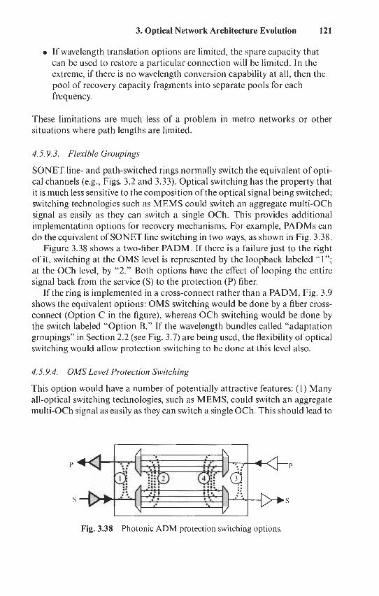
3. Optical Network Architecture Evolution 121
0 If wavelength translation options are limited, the spare capacity that can be used to restore a particular connection will be limited. In the extreme, if there is no wavelength conversion capability at all, then the pool of recovery capacity fragments into separate pools for each frequency.
These limitations are much less of a problem in metro networks or other situations where path lengths are limited.
4.5.9.3. Flexible Groupings
SONET line- and path-switched rings normally switch the equivalent of opti- cal channels (e.g., Figs. 3.2 and 3.33). Optical switching has the property that it is much less sensitive to the composition of the optical signal being switched; switching technologies such as MEMS could switch an aggregate multi-OCh signal as easily as they can switch a single OCh. This provides additional implementation options for recovery mechanisms. For example, PADMs can do the equivalent of SONET line switching in two ways, as shown in Fig. 3.38.
Figure 3.38 shows a two-fiber PADM. If there is a failure just to the right of it, switching at the OMS level is represented by the loopback labeled “1”; at the OCh level, by “2.” Both options have the effect of looping the entire signal back from the service (S) to the protection (P) fiber.
If the ring is implemented in a cross-connect rather than a PADM, Fig. 3.9 shows the equivalent options: OMS switching would be done by a fiber cross- connect (Option C in the figure), whereas OCh switching would be done by the switch labeled “Option B.” If the wavelength bundles called “adaptation groupings” in Section 2.2 (see Fig. 3.7) are being used, the flexibility of optical switching would allow protection switching to be done at this level also.
4.5.9.4. OMS Level Protection Switching
This option would have a number of potentially attractive features: (1) Many all-optical switching technologies, such as MEMS, could switch an aggregate multi-OCh signal as easily as they can switch a single OCh. This should lead to
P
S
Fig. 3.38 Photonic ADM protection switching options.
4 .* .. * P
S
P
S
Fig. 3.38 Photonic ADM protection switching options.

122 John Strand
economic savings. (2) Since there are fewer OMS than OCh, OMS restoration may scale better than OCh restoration. (3) Wavelength conversion is not an issue.
However, OMS restoration can only be done within a domain of trans- parency. Thus all the issues associated with transparency discussed in earlier sections,28 particularly transmission constraints, multivendor interoperabil- ity, and problems associated with the introduction of new technologies arise here. Therefore, most attention is currently focused on OCh-level restoration. However, OMS restoration can be effective in situations where these issues are not compelling, particularly in metro and access networks and when integrated into a single-vendor all-optical networking product such as the ultra-long-haul systems discussed in Section 2.2.
OMS protection switching does not protect against the failure of an indi- vidual signal before they are wavelength multiplexed. To gain this capability, it must be combined with an OCh-level mechanism, such as 1 : N protection switching, which is discussed next.
4.5.9.5. 1 :NAPS Protection Switching
Providing equipment protection for wavelength-specific components such as a transponder that is transmitting into a domain of transparency can be done in a number of ways. The setting is shown in Fig. 3.39.
As shown in Fig. 3.39, an incoming signal (from the left) is fed to a working transponder (with output wavelength hl in the example) and also to a protec- tion transponder (at bottom). Not shown are up to N - 1 other incoming signals that are sharing the same protection transponder. Two of the implementation approaches described in [ 151 are:
Transponders
Fig. 3.39 1 : N APS protection setting.
28 Sections 2.3 and 4.2 in particular.
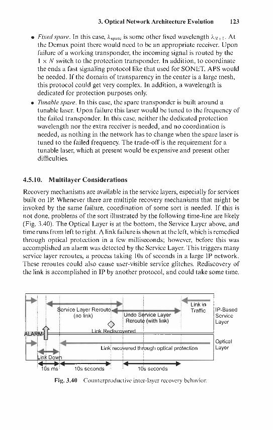
3. Optical Network Architecture Evolution 123
Fixed spare. In this case, Aspare is some other fixed wavelength AN+^. At the Demux point there would need to be an appropriate receiver. Upon failure of a working transponder, the incoming signal is routed by the 1 x N switch to the protection transponder. In addition, to coordinate the ends a fast signaling protocol like that used for SONET, APS would be needed. If the domain of transparency in the center is a large mesh, this protocol could get very complex. In addition, a wavelength is dedicated for protection purposes only.
0 Tunable spare. In this case, the spare transponder is built around a tunable laser. Upon failure this laser would be tuned to the frequency of the failed transponder. In this case, neither the dedicated protection wavelength nor the extra receiver is needed, and no coordination is needed, as nothing in the network has to change when the spare laser is tuned to the failed frequency. The trade-off is the requirement for a tunable laser, which at present would be expensive and present other difficulties.
4.5.10. Multilayer Considerations
Recovery mechanisms are available in the service layers, especially for services built on IP. Whenever there are multiple recovery mechanisms that might be invoked by the same failure, coordination of some sort is needed. If this is not done, problems of the sort illustrated by the following time-line are likely (Fig. 3.40). The Optical Layer is at the bottom, the Service Layer above, and time runs from left to right. A link failure is shown at the left, which is remedied through optical protection in a few milliseconds; however, before this was accomplished an alarm was detected by the Service Layer. This triggers many service layer reroutes, a process taking 10s of seconds in a large IP network. These reroutes could also cause user-visible service glitches. Rediscovery of the link is accomplished in IP by another protocol, and could take some time.
. . . . . . . . . . . . 10s seconds, 10s seconds ,
Fig. 3.40 Counterproductive inter-layer recovery behavior.
IP-Based Service Layer
Optical Layer

124 John Strand
When this finally happens, another period of service instability will ensue as the Service Layer reroutes are undone.
In addition to these effects, uncoordinated multilayer restoration is likely to lead to excessive capacity being provided for restoration. The problem here is that it is very difficult for layers to share this capacity; hence if both layers are provided with capacity to handle the same failure scenario, much of this expenditure is wasted.
It is thus important both for performance and economic reasons to apply the restoration capabilities of each layer to only the types of failures for which it is most suited. The remainder of this section tries to apply this principal to the Optical Layer and the IP Services layers.
The Optical Layer strengths in this respect are:
0 Line-curd costs. As discussed in Section 4.4, OLXC costs per unit capacity are expected to be significantly lower than those of an IP router.
0 Multiservice support. As long as there are multiple client services, a single restoration mechanism at the Optical Layer reduces the need for separate mechanisms with their associated capacity requirements and operational support costs.
0 Bundle size. The Optical Layer can restore in much larger bundles than can higher layers. Larger bundles implies fewer recovery reroutes need to be done, which should translate into faster overall recovery times.
Relying on the IP layer for recovery has advantages:
0 Much finer granularity restoration is possible. This means that “best effort” traffic (which comprises a large proportion of total Internet traffic) can be left unrestored, with corresponding restoration capacity savings.
0 IP layer restoration capacity may be provided to deal with router failures. If this capability is in place, the incremental capacity and complexity required to deal with all failures may be modest.
Doverspike et ul. [l 1, 851 have modeled a number of OLXC and IP-based architectures to study the economic trade-offs more closely. Their conclusion [l 11: “. . . generally, for single fiber failure, OLXC restoration tends to be less expensive than IP Layer restoration except when low fractions of IP traffic need restoration and the OLXC layer is omitted or, possibly, when we need to provide extra capacity to protect against IP layer node (router) failures.”
Rather than viewing the choice of restoration layer as an either/or choice, it is likely to be more profitable to look for hybrid strategies that make use of the

3. Optical Network Architecture Evolution 125
strengths of each layer. Gerstel and Ramaswami [15] have identified several cooperative strategies:
a Optical layer routing to enhance IP layer restoration. a. At its simplest level, this requires the OL to ensure that IP service
and protection capacity is kept physically diverse; more generally it requires that the IP layer understand its redundancy constraints and communicate these constraints to the OL when requesting new capacity. (See [19], [37], and [lo81 for more detail on diverse routing.)
b. Additional capacity efficiency can be obtained by treating some of the IP layer protection capacity as preemptible “extra traffic” connections in the OL. Careful design is required to ensure that these protection resources will be available when needed.
a Multilayerprotection. Recovery responsibility can be divided between layers in various ways. This requires an escalation strategy defining how layers interwork to provide recovery. Some of the building blocks for cooperation are: a. Hold-oftimes. The IP layer could allow a short interval for the OL to
execute its procedures before starting its own procedures. b. Controlplane coordination. As will be discussed in Section 5, a new
OL control mechanism based on IP protocols is being defined. Common protocols should facilitate interlayer communication.
c. Assign responsibility for each type offailure to a specijk layer. As a strawman, the OL might deal with single route failures while the IP layer deals with node failures of any type. Intraoffice (tie cable) failures can be efficiently dealt with in the OL using 1 + 1 APS.
0 Segregate protected and unprotected trafic. The IP layer could separate traffic requiring restoration onto specific OL connections and identify these connections to the OL. This would allow the OL to provide recovery capacity for these connections only.
We have mentioned strategies that use IP layer functionality to reroute around optical layer failures. It also may be possible to use the Optical Layer to recover from IP layer failures in some cases. We give one example here.29
In a large ISP central office, there are typically at least two backbone routers for redundancy in case of router hardware or software failures and to simplify software upgrades. These routers aggregate all the traffic to or from all the provider edge routers that connect to the customers. Figure 3.41 gives an example of such an IP network, with detailed office architecture shown for office B only.
29 See [lo21 for more details. To the author’s knowledge, this scheme has not yet been implemented by any vendor.
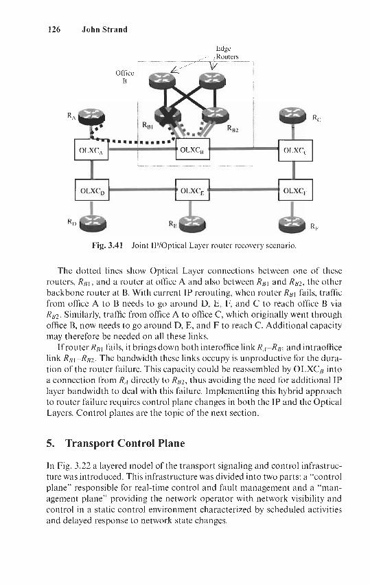
126 John Strand
Edge
Fig. 3.41 Joint IPlOptical Layer router recovery scenario.
The dotted lines show Optical Layer connections between one of these routers, R B I , and a router at office A and also between RBI and R B ~ , the other backbone router at B. With current IP rerouting, when router RBI fails, traffic from office A to B needs to go around D, E, F, and C to reach office B via R B ~ . Similarly, traffic from office A to office C, which originally went through office B, now needs to go around D, E, and F to reach C. Additional capacity may therefore be needed on all these links.
If router RB1 fails, it brings down both interoffice link RA-RBI and intraoffice link RBI-RB~. The bandwidth these links occupy is unproductive for the dura- tion of the router failure. This capacity could be reassembled by OLXCB into a connection from RA directly to Rsz, thus avoiding the need for additional IP layer bandwidth to deal with this failure. Implementing this hybrid approach to router failure requires control plane changes in both the IP and the Optical Layers. Control planes are the topic of the next section.
5. Transport Control Plane
In Fig. 3.22 a layered model of the transport signaling and control infrastruc- ture was introduced. This infrastructure was divided into two parts: a “control plane” responsible for real-time control and fault management and a “man- agement plane” providing the network operator with network visibility and control in a static control environment characterized by scheduled activities and delayed response to network state changes.

3. Optical Network Architecture Evolution 127
5.1. TRADITIONAL TRANSPORT NETWORK MANAGEMENT AND CONTROL
Legacy transport telecommunications services have evolved to be paragons of reliability, providing guaranteed quality of service regardless of network load. Much effort was directed at optimizing the use of what was then a very expensive resource, bandwidth. All this was accomplished in an era when intelligence could only be provided by centralized Operations Systems (0%). Communications between them was normally by faxed “work orders.”
In this environment, microprocessors first appeared in discrete, intelligent NEs communicating with the external world through ASCII-based “craft ter- minals.” Because intelligence was largely isolated, there was little value in conforming to standards; each network operator developed proprietary OSs, and the Element Management Systems (EMSs) embedded in NEs were largely vendor proprietary. The architecture is illustrated in Fig. 3.42.30
Two carriers, X and Y, are shown in Fig. 3.42. Within each are sepa- rate vendor “clouds,” each with one or more vendor-supplied EMSs that communicate with the individual NEs. The EMSs also communicate with a carrier-proprietary NMS (which actually is likely to be a large number of cooperating Operations Systems (OSs), each dedicated to a specific task like restoration, provisioning, or maintenance, and sharing network state information to some extent). Protocols like Common Management Informa- tion Protocol (CMIP), Simple Network Management Protocol (SNMP), and Common Object Request Broker Architecture (CORBA) have brought some level of standardization to these interfaces. Human operators track network status and apply controls through both the NMS and the EMS. Intercarrier
_ _ _ _ _ _ /--------.
.--_--_________---- NE: Network Element EMS: Element Management System NMS: Network Management System
Fig. 3.42 Traditional transport control structure.
30 See [86] for the next level of detail.

128 John Strand
management communications is likely to be between the human operators rather than between system^.^'
There is a nontrivial control plane in this structure. Each node in a SONET ring, for example, has state knowledge about the ring, and the nodes coop- erate to recover from failures. However, the general architecture puts most multinode functionality in the management plane (the EMS and NMS).
This structure has some serious deficiencies from a network operator’s perspective:
0 NMS software typically is large, complex, costly, and requires a major ongoing software development and maintenance effort. The introduction of a new technology, vendor, or service is frequently slowed down significantly by the need to wait for the necessary NMS software changes.
0 Creating a network-wide “database of record” containing accurate and up-to-date state information is greatly complicated by the proliferation of proprietary software at the EMS and NE level.
0 NEs have minimal ability to automatically determine their connectivity to other NEs. This forces reliance on expensive, error-prone manual inputs.
0 State change information may take some time to percolate up to the NMS level. This can cause problems when rapid action is required, for example, when there is a failure.
0 The ad hoc intervendor interfaces make rapid provisioning or recovery very difficult when multiple vendors are involved. Frequently months are required to establish a complex high-capacity connection.
0 Even when only a single vendor is involved, communications problems and data inconsistencies among all the OSs and EMSs involved in a provisioning introduces significant delays and errors.
Together, these deficiencies are a significant ongoing problem for transport network providers. Ever-increasing competition, together with the evermore volatile needs of customers, make costs, long provisioning intervals, and delays in introducing new services and technologies increasingly intolerable.
5.2. EMERGENCE OF ALTERNATIVE
The management and control planes for the Internet and for ATM data net- works were developed more recently and have avoided many of these problems.
CONTROL PLANE ARCHITECTURES
31 For voice services there is of course a rigorously standardized service-control plane that allows calls to be established and managed across carriers. We are talking only of the transport layers here.
3. Optical Network Architecture Evolution 129
Network elements are assumed to be intelligent and able to support a much “thicker” control plane, and thus require less NMS and EMS functionality. For someone aware of the problems discussed in the previous section, these new control planes have some very attractive features:
0 NEs could automatically discover their neighbors. 0 This information could be disseminated throughout the network,
and each node could build its own view of the entire network. As a byproduct, this process would generate much of the accurate, up-to-date state information needed by the NMS. This has come to be called “The Network as the Database.”
localization, and restoration functions to the NEs. In this approach, the necessary software would be provided by the equipment vendor; this spreads software development costs over all the vendor’s customers and reduces the possibility of network operator software development bottlenecks slowing down the introduction of new technologies and services.
0 This software would implement standardized, proven protocols derived from the Internet and ATM worlds. The standardization might allow multivendor interworking and even a degree of multicarrier interworking. Furthermore, public domain or commercially available implementations of the basic protocols are readily available, and programmers familiar with this software are also readily available. If this software proves to be adaptable to the needs of the Optical Layer, this all should greatly speed up the realization of the desired capabilities.
0 This information could be used to distribute provisioning, fault
From a carrier’s perspective, then, a vision of an alternative management and control structure has begun to emerge. In this vision, vendor-supplied OLXC control-plane software will automatically do some key NMS functions such as database creation, provisioning, and restoration, thereby allowing a lower-cost, streamlined NMS. Furthermore, the new control plane had the promise of supporting much more rapid provisioning and less painful inter- vendor and even intercarrier interworking. In the longer term, there is a hope that if the Optical Layer control plane is compatible with that used by the Internet, then additional ways to be responsive to the Internet’s needs will emerge.
OLXC vendors, particularly start-ups, were quick to see that they could inexpensively differentiate their hardware products by modifying existing implementations of the basic protocols. Today virtually every OLXC vendor claims to have a control plane based on this approach.
Additional support for the use of Internet protocols came from the Inter- net community. Anticipating the necessity of incorporating optical switching
130 John Strand
if they were to continue to scale to meet exploding demand, they greeted the possibility of common Internet-Optical Transport control protocols with enthusiasm. If the transport paradigm could be changed from one of fixed “pipes” that could only be reconfigured on a time scale of weeks to months to one of the transport network as a sort of giant distributed circuit switch with a dynamically reconfigurable backplane, new dimensions in traffic engi- neering might emerge. Vendors with substantial Internet equipment expertise were particularly enthusiastic, foreseeing the possibility of gaining a foothold in the massive telecom equipment market.
Both established and start-up network operators have shown considerable interest in these developments. The Carrier Working Group within the Optical Interworking Forum (OIF) recently produced an “Optical Services Frame- work and Associated Requirements” document [43] that provides a good snapshot of current services thinking in the carrier community as it relates to optical networking and software control. They articulated the following objectives for a new control plane.32
a Promote a standardized optical network control plane, with its associated inter$aces andprotocols. Ensure that intelligent optical networking (OTN) products from different vendors or employing different technologies can interwork at the control plane level. This is not meant to preclude vendor specific extensions so long as the extensions do not degrade total network performance. However, it is unacceptable to expect carriers to write software to conceal OL vendor or technology incompatibilities.
a Provide rapid automatic end-to-end provisioning within the optical network, including routing and signaling by the control plane. “End- to-end” is an important part of this objective; the value of rapid provisioning in the core network is greatly reduced if traditional provisioning intervals are encountered in metro and access networks. Hence interdomain interworking is viewed as being key to realizing many of the hoped-for benefits. It is recognized that rapid interdomain provisioning must be built upon rapid automatic provisioning within a single domain. In this document “provisioning” refers to network provisioning only and does not necessarily include other customer-facing aspects of provisioning like the establishment of a new account.
a Provide restoration, diverse routing, and other Quality of Service features within the control plane on a per-service-path basis. Per-connection
32 The current author was the chair of the OIF group producing this report. It is working text and not an official OIF Technical Report and is not binding on the OIF or its members.

3. Optical Network Architecture Evolution 131
control of these capabilities is important because of the anticipated diversity of needs of the OL users.
e Provide policy-based call acceptance and peering policies and support usage-based accounting based on start and termination time, bandwidth, and other resources requested. These capabilities are necessary to support a pay-for-service business model and otherwise safeguard carrier resources, which carriers expect to be basic to their OL plans.
e Oger carrier-spec@c “branded” services. A fundamental carrier business need is the ability to put together packages of features, quality of service, support, and pricing, which they can then market.
service disruption. In particular, deployment of a new vendor X capability should not depend on vendor Y’s willingness to upgrade their control plane software. It is recognized that the part of the network served by vendor Y equipment may not get the benefits of the new capability in this case.
e Protect the security and reliability of the optical layer, andparticularly the controlplane. The damage, which could be done if this is not accomplished, is beyond measure.
The carrier will control what network resources are wailable to individual services or users. Therefore, in the event of capacity shortages this ability will allow the carrier to ensure that critical and priority services get capacity.
e Reduce the need for carrier-written OS software through heavy use of open protocols and vendor and third-party software, particularly for network provisioning and restoration. Carrier OS software development bottlenecks frequently are on the critical path to technology and service innovation. Improvements in this area are at least as important to many carriers as is the prospect of very rapid provisioning. Note, however, that entire functions need to be off-loaded in most cases; if this is not done the carrier OS function remains, with the added requirement of interfacing with the new control plane software.
scalability are highly important in a carrier’s network: e Node scalability-the size of a single node is expected to be sized
anywhere between several hundred and several thousands optical terminations.
expected to be anywhere from several to hundred or thousands of nodes.
e Rapid deployment of new technologies and capabilities with no network
e Provide the ability for the carrier to control usage of its network resources.
e Ensure the scalability of the Optical Network. Several aspects of
e Network scalability-the size of an interconnected network is

132 John Strand
5.3. INTERNET PROTOCOL BACKGROUND
To understand the proposed control plane, some exposure to a few Internet concepts are necessary. We provide only the barest possible peek into this vast area. Readers interested in learning more could start with [87,88,89,90, or 911.
53.1. Internal Protocol (IP)
IP transmits blocks of data called packets from sources to destinations, where sources and destinations are hosts identified by fixed-length globally unique addresses. Each packet contains a destination address and is passed through a sequence of switches called “IP routers.” In a router, each packet is processed independently; IP has no concept of a “connection.” Its address is matched against entries in a forwarding table. The matched entry in this table specifies the output port through which the packet should be sent.
5.3.2. Domains
There are millions of IP addresses. Indeed, the 32-bit address space supported by the current version of IP (IPv4) is in danger of being exhausted. Further- more, the Internet is in a constant state of flux. Therefore, it is impossible and undesirable for any node to have an up-to-date entry in its forwarding table for each of these addresses-the signaling and processing overhead would over- whelm the Internet. Consequently, the Internet is divided into many thousands of domains (formally, “Autonomous Systems (ASS)”; also called “Routing Domains”). Each router keeps detailed forwarding table entries for addresses within its domain. Packets for other addresses are sent to a “border router” that communicates with its peers in other domains and handles the processing of packets entering or leaving the AS for other ASS. Each AS is under the con- trol of a single administrative entity and comprises a “domain of trust” within which state information is freely shared and routing decisions not questioned.
5.33. Open Shortest Path First (OSPF)
OSPF is a “routing protocol.” An instance of OSPF33 runs in each router, where it constantly communicates with its peers to keep an up-to-date view of the network topology. Whenever there is a change, OSPF modifies the forwarding table, which immediately modifies the way subsequent packets travel through the network. OSPF is an Interior Gateway Protocol (IGP), which means that it handles the routing within a single domain only.
33 Or an equivalent protocol lie IS-IS. Within an AS a single IGP needs to be used.

3. Optical Network Architecture Evolution 133
5.3.4. Link State Advertisements (LSAs)
OSPF routers send LSAs to all their peers in their domain. These define the “linksYy-onnections between adjoining routers. With this information, each router can maintain a complete and up-to-date picture (Link-State Database) of the global topology of the entire domain. It then runs an algorithm (a “Shortest Path First” algorithm, whence the name OSPF) that determines how to construct the forwarding table. Each time an LSA update is received, the algorithm is rerun.
5.3.5. Neighbor Discovery and Maintenance
Each OSPF router periodically (by default, every 10 seconds) sends a “Hello” message out of each of its ports. It learns of the existence of a neighboring router when it receives the neighbor’s OSPF “Hello” in turn. If too much time elapses between receipt of these messages (nominally 40 seconds), the router will stop advertising the unresponsive link and also will start routing packets around the failure. This time dominates “convergence time”-the time it takes all the forwarding tables in a domain to stabilize after a failure.
5.3.6. Border Gateway Protocol (BGP)
BGP4 is the interdomain routing protocol (commonly called an “Exterior Gateway Protocol”) currently used over the Internet. BGP nodes (called “speakers”) exchange summarized information about the addresses they can reach and the sequence of ASS through which the address would be reached. Trust between ASS is not assumed; each BGP speaker applies “policy-based controls” to determine which ASS it wishes to peer with and what traffic it is willing to accept from each peer. BGP does not do neighbor discovery; instead, peering relationships are manually configured. Unlike OSPF, where the ongi- nating router did its routing based on a global-link-state database, each BGP speaker keeps a summary list of distant addresses and the distance to each through each adjacent peer (the “distance vector”). Distance is normally mea- sured as a hop count. Then a speaker will normally route packets to a given destination through the peer that had advertised the fewest number of hops.
5.3.7. Multi Protocol Label Switching (MPLS) IP is a connectionless protocol, meaning that each packet is routed indepen- dently; thus if a block of data is broken up into multiple packets they might be routed independently. An analogy has been drawn to copying a novel onto a set of postcards. MPLS creates the equivalent of connections (called “Label Switched Paths,” or LSPs) by attaching an additional label to each packet in a flow. MPLS label processing is illustrated in Fig. 3.43.
In Fig. 3.43, a packet with IP address X is shown entering from the left. A table look-up in the first MPLS node results in the label “6” being appended

I In 1: IP 10; 1 ; I Label Address Label Interface
1 6 1 7 0 O I X I I Y
n 0
MPLS MPLS MPLS Ingress Router Node Egress Router
Fig. 3.43 MPLS label processing example.
3. Optical Network Architecture Evolution 135
at the front of the packet and the out interface 0 being used for the packet. In the second MPLS node the label 5 replaces the initial label and out interface 3 is chosen. In the final node, the MPLS label is “popped” off to reveal the initial packet, which is then routed over out interface 0. As long as the MPLS tables are unchanged, all packets with the same destination address that enter this ingress router will be routed in exactly the same fashion.
An LSP is a “virtual” connection. Unlike a TDM connection, creating an LSP does not commit bandwidth or use bandwidth when idle. MPLS can make use of this feature to set up numerous LSPs for restoration purposes without consuming bandwidth. To OSPF, an MPLS LSP can be considered as a link in its link state database.
MPLS has many other features of importance. One that should be men- tioned is the ability to have nested LSPs. This provides a sort of multiplexing capability that is of importance for our application because it will allow an optical connection to be treated as an LSP on which other LSPs are routed.
5.3.8. Label Distribution Protocol (LDP)
LDP allows MPLS routers to request that an LSP be set up to a specified address. This is done by sending a label request to the desired node. If no problems are encountered, a second message is passed back along the same path, assigning the labels and establishing the LSP.
5.3.9. Constraint-based Routing Label Distribution Protocol
This extension of LDP allows the LSP establishment process to be con- strained to a specific physical path. It also allows the reservation of resources (bandwidth) along the path. There is an alternative protocol called RSVP (Reservation Protocol) that performs essentially the same function.
(CR-LDP)
5.4. MPkS AND GENERALIZED MPLS (GMPLS)
GMPLS (closely related to MPhS, or ‘‘MP Lambda S”) is an extension of MPLS and related protocols to form the basis for a control plane for Optical Networks [24, 49, 921. In fact, it is more ambitious than this: The goal is to support devices that do packet switching and also switching in the time, wave- length, and space dimensions by enhancing the connection-oriented protocols used by MPLS and its traffic engineering extensions.
For Optical Networking, GMPLS:
0 Replaces the MPLS label discussed earlier with the wavelength frequency, which acts as an implicit label, thus treating an OTN
136 John Strand
connection as an LSP. An OXC is then analogous to an MPLS node and wavelength translation to a label swap. MPLS’s label-nesting capability allows the multiplexing of multiple SONET connections onto a single wavelength to be handled naturally.
0 Uses an extended IGP (e.g., OSPF) to advertise information about the OTN topology and resource availability (e.g., spare capacity). Its routing algorithm then also needs extension or replacement so that it can compute appropriate paths in the OTN.
0 Uses an enhanced CR-LDP or RSVP to set up connections.
GMPLS requires enhancements to the protocols used in MPLS to deal with peculiarities of OTNs:
0 Optical bandwidth comes in a few discrete sizes (OC-58, OC-192, etc.), whereas MPLS LSPs can be any size.
0 Optical bandwidth is real and physical, whereas MPLS LSPs are virtual and need not consume any bandwidth if idle. It is not possible to set up standby optical connections for restoration or other purposes without consuming bandwidth.
wavelengths on an OTrS is a hard constraint.
that will need to be advertised, for example, the acceptable formats (SONET, Ethernet) and bit rates (is OC-768 supported on the link). (This is discussed in detail below in Section 5.6.)
0 Optical connections are normally bidirectional while LSPs are unidirectional.
0 Labels are no longer abstract identifiers. They need to be mapped to specific wavelengths or time slots.
0 Fast fault detection and isolation is needed if restoration is to be supported.
0 Unlike normal data applications, control traffic cannot be directly inserted into the user data stream without an OEO conversion and other changes. Thus there needs to be a separate data communications infrastructure for the control plane.
impairments and connectivity constraints, need to be dealt with.
0 Overbooking optical capacity is not possible; the number of
0 Optical links have a number of other attributes that affect routing
0 All the routing complexities discussed in Section 4, particularly
One area where the challenges for GMPLS are likely to be particularly daunting is restoration. This area is discussed in [lo31 in more detail.
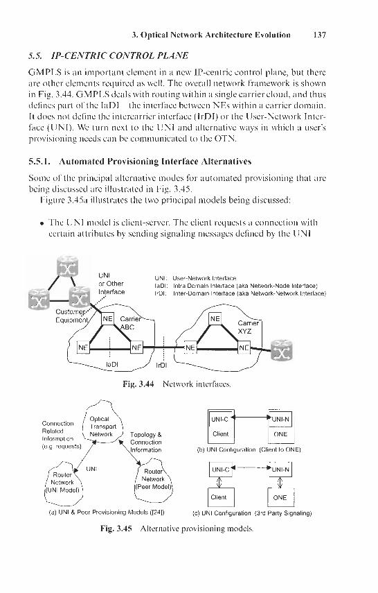
3. Optical Network Architecture Evolution 137
5.5. IP-CENTRIC CONTROL PLANE
GMPLS is an important element in a new IP-centric control plane, but there are other elements required as well. The overall network framework is shown in Fig. 3.44. GMPLS deals with routing within a single carrier cloud, and thus defines part of the IaDI-the interface between NEs within a carrier domain. It does not define the intercarrier interface (IrDI) or the User-Network Inter- face (UNI). We turn next to the UNI and alternative ways in which a user's provisioning needs can be communicated to the OTN.
5.5.1. Automated Provisioning Interface Alternatives
Some of the principal alternative modes for automated provisioning that are being discussed are illustrated in Fig. 3.45.
Figure 3.45a illustrates the two principal models being discussed:
0 The UNI model is client-server. The client requests a connection with certain attributes by sending signaling messages defined by the UNI
UNI. User-Network Interface IaDI. Intra Domain Interface (aka Network-Node Interface) lrDl Inter-Domain Interface (aka Network-Network Interface)
n
Fig. 3.44 Network interfaces.
Connection
Network Network
(a) UNI 8 Peer Provisioning Models ([24])
UNI-C UNI-N
Client
(b) UNI Configuration (Client to ONE)
UNI-C UNI-N
Client
(c) UNI Configuration (3rd Patty Signaling)
Fig. 3.45 Alternative provisioning models.
138 John Strand
standard, and the OTN responds with success and status information. Internal network topology and state information is not disseminated to the client.
network. Topology information (LSAs) and other state information necessary to do routing is shared. If a router wanted to establish a connection, it would compute the path itself and then send the appropriate CR-LDP/RSVP messages through the OTN to set up the connection.
0 In the peer model, routers are “peersyy of the ONES inside of the
The peer model was proposed first. It seems to be quite appealing to many Internet people, but has run into major resistance from the carriers because it seemingly does not allow carriers to control their resources34 The Optical VPN service concept proposed by the OIF Carriers Group (see Section 3.4 and [43]) is an attempt to meet the need without compromising network integrity.
Figures 3.45b and 3.4% give several variants on UNI. Here “UNI-CYy and “UNI-N represent the UNI client and network processes, respectively. In Fig. 3.45b the client device and the ONE directly interact across the UNI. In Fig. 3.4% the devices are not UNI-capable. Instead, separate client and net- work management entities negotiate the connection. This may be appropriate when one or both entities are SONET or other legacy equipment.
5.5.2. Connection Attributes
The proposed control plane would allow fixed-bandwidth connections to be requested, torn down, and modified. To establish a connection, the desired attributes of the connection must be specified. In [93] the major types of attributes to be supported were identified as:
0 IdentiJcation attributes. Source and destination nodes, when the connection is desired.
0 Basic connection type. Framing type (SONET, Ethernet, etc.), bandwidth, and directionality (unidirectional, bidirectional).
0 Priority, preemptibility, protection, and restoration requirements. 0 Routing constraints. This could include explicit routing or diversity
constraints.
34 An interested reader might want to compare the peer model with the OIF Carrier Group objectives outlined in Section 5.2. There are a number of discords: It is unclear how policy-based call acceptance or carrier-specific “branded” services would be supported, for example. Security issues and the ability of the carrier to control usage of its own resources also may be troublesome. These may not be show-stoppers, but at the least: refinement of the peer model and/or modification of carrier objectives will be needed.
3. Optical Network Architecture Evolution 139
5.5.3. Neighbor Discovery
This refers to the process that determines the port-to-port connectivity of the ONES. Both ONE-ONE connectivity within the OTN and client-ONE connectivity needs to be determined. Automation of this process is particularly important because of the hundreds or even thousands of fiber connections expected in a single office.
There are many types of interfaces currently in use in OTNs that differ in many respects, therefore a variety of methods are required to accom- plish this [24]. The basic functions, however, are similar to those discussed in Section 5.3.
5.5.4. Service Discovery
Those adjoining ONES and client devices connected to the OTN need to deter- mine what the capabilities of each of their links are, for example, whether both OC-48 and OC-192 are supported on the link.
5.5.5. Topology and Resource Discovery
OSPF extensions are needed to determine and globally disseminate informa- tion on spare bandwidth, multiplexing capabilities, and protection needed for route computations.
5.5.6. Standards Activities
There are four groups involved in standardslimplementation agreement work in the optical arena:
0 The International Telecommunications Union (ITU),35 and particularly its Telecommunication Standardization Sector (ITU-T), which is an international government-sanctioned group that has traditionally controlled telecommunications standards. The ITU-T has a reputation for being thorough, but slow; they are trying to speed up their process.
IP-over-Optical (IPO) working The IETF is the driver for all Internet-related standards and the nexus of IP-related activities. They tend to move rapidly. Before standardizing anything they require two working implementations. Their standards are called “Requests for Comments” (RFCs). Working papers are called “Internet Drafts.”
0 The Optical Domain Services Interconnect (ODSI)37 is an informal association of more than 100 companies, primarily equipment vendors.
0 The Internet Engineering Task Force (IETF), and particularly its
35 See itu.int. 36 See ietEorghtm.charters/ipo-charter.htm1. 37 See odsi-coalition.com.
140 John Strand
They have developed a functional definition of a mechanism that will allow electrical layer devices to automatically signal the optical network to establish high-speed bandwidth on demand. They anticipate turning their results over to formal standards activities.
over 300 members, both equipment vendors and carriers. Its goal is to foster the development and deployment of interoperable products and services for data switching and routing using optical networking technologies. The OIF is working on both physical layer and control plane (OIF) documents.
The Optical Interworking Forum (OIF)38 is an informal group with
The OIF and ODSI are not sanctioned standards groups. Instead, they are trylng to develop “implementation agreements”-specific focused specs that will allow implementation to move onward.
The relationships between all these bodies is confusing and there clearly are overlaps. Many people seem to be following the strategy of submitting their standards contributions to multiple bodies in the hope that somehow they will have the desired impact. The proper relationships among all these groups are unclear and controversial. There are some who would like to see all standards work carried out in the ITU. Others would like to see more specialization. This might lead the IETF to be the arena for dealing with protocols, for example, and the ITU the arena for dealing with physical layer standards and for detailing and formalizing the major standards. The author would like to see the carriers take a more active role in ensuring that the requirements driving the various bodies are consistent.
5.6. ROUTING COMPLEXITIES ARISING FROM DOMAINS OF TRQNSPARENCY
Plans for an IP-centric control plane have incorporated some of the idiosyncra- cies of optical technology. However, the work so far is principally relevant to opaque networks with OLXC nodes. This greatly simplifies the control-plane design. In this section we look at some of the additional considerations that arise if we wish to apply this control plane within a domain of transparency.
5.6.1. Routing Complications
Section 4.2 summarized the state of routing and wavelength assignment in large domains of transparency. Several issues for the control plane arise from this discussion:
0 Impairments cannot be ignored in large domains. Additional constraints will need to be imposed on routing. These constraints
38 see oiforum.com.
3. Optical Network Architecture Evolution 141
depend on additional physical parameters that will need to be determined and advertised, and the specific constraints required in a given situation may depend on the design and engineering of the domain.
0 Port-to-port connectivity across a domain of transparency will be limited by the level of wavelength translation supported within the domain. It will also be constrained by implementation specifics such as adaptation grouping capabilities. At a minimum, significantly more connectivity information will need to be advertised.
0 A number of additional software-controllable components (beyond the OLXC) that can change the internal connectivity of the domain can be expected. These include PADMs, tunable lasers and filters, and dynamic devices that allow changes in the bandwidth assigned to an adaptation grouping and the wavelength spacing within the grouping. At a minimum, information about the connectivity changes resulting whenever these components are reconfigured will need to be advertised. In addition, these components potentially could be configured by the control plane.
0 Because the route selected must have the chosen wavelength available on all links, this information needs to be considered in the routing process. This is discussed in [94], where it is concluded that advertising detailed wavelength availabilities on each link is not likely to scale. Instead they propose an alternative method that probes along a chosen path to determine which wavelengths (if any) are available. This would require a significant addition to the routing logic normally used in OSPF.
0 Choosing a path first and then a wavelength along the path is known to give adequate results in simple topologies such as rings and trees [74]. This does not appear to be true in large mesh networks under realistic provisioning scenarios, however. Instead, significantly better results are achieved if wavelength and route are chosen simultaneously [76]. This approach would, however, also have a significant affect on OSPF.
5.7. TRADING OFF THE CONTROL PLANE, SYSTEM DESIGN, AND CARRTER PLANNINGYENGINEERING
As domains of transparency become both larger and more software recon- figurable, these complexities become increasingly of concern. It is important to note that at present this evolution is largely technology driven. Vendors pushing the technology envelope are competing fiercely to provide solutions that have higher capacity, can go further all-optically, are more reconfigurable, and are more cost-effective. As vendors pursue their diverse visions, it is quite plausible that the Optical Layer of the future will be made up of heterogeneous technologies that differ significantly in their control-plane needs.

142 John Strand
Carriers will wish to take advantage of the new technologies; however, they are also going to want to gain the service and operational benefits offered by the new control plane concepts, which are made more difficult to achieve by this evolution. What are the choices? Alternative approaches that deserve consideration are:
Control-plane solutions. The control plane could be enhanced in a number of ways: a. All-encompassing intradomain protocols. GMPLS could attempt
to include the full range of technological options and constraints and evolve as these evolve. This will be, at best, a very challenging approach, in this author’s opinion, which will be made more difficult by the need to do periodic in-service software upgrades in a multivendor network.
b. Per-domain routing. In this approach, each domain could have its own tuned approach to routing. Interdomain routing would be handled by a multidomain or hierarchical protocol that allowed the hiding of local complexity. Single vendor domains might have proprietary intradomain routing strategies. This option is discussed further in [19], [36], and [37].
System architecture solutions. Vendor system designers could be less aggressive with respect to nonlinearities, and therefore somewhat suboptimal, in exchange for improved scalability, simplicity, and flexibility in routing and control-plane design. As a hypothetical example, if control-plane protocols did not deal with chromatic dispersion, carriers would require their vendors to provide transport systems engineered to keep this impairment from ever being binding.
a. Transmission engineers could be required to only deploy domains Transport planning/transmission engineering solutions.
where every possible route met all constraints not handled explicitly by the control plane, even if the cost penalties were severe.
b. At (selected) OLXCs within a domain of transparency, the control plane could insert O/E/O regeneration into routes with transmission problems. This might make all routes feasible again, but at the cost of additional cost and complexity, and with some loss of rate and format transparency.
The author is not aware of any studies that evaluate these alternatives generically.
5.8. HETEROGENEOUS TECHNOLOGIES AND
One of the approaches for dealing with the routing and control problems associated with complex domains of transparency that were identified in the
MULTIPLE DOMAINS
3. Optical Network Architecture Evolution 143
preceding section was to divide a network into multiple routing domains, each with relatively homogeneous technology (e.g., single vendor). Then a mul- tidomain protocol (the optical equivalent to BGP or multiarea OSPF for the Internet) would be used for multidomain interworking.
There are a number of other scenarios where multiple routing domains are likely to be needed. Two of these are:
e Metro-core interworking. Deployment of intelligent optical networking technology is planned or under way in both intercity (core) and metro portions of a number of carrier networks. It is essential that the metro and core subnetworks be able to interwork as soon as possible if we are to realize the fast provisioning potential of these deployments, because a large proportion of the anticipated connections will need to traverse both metro and core subnets.
established, opportunities and needs for routing optical connections over multiple competing carrier networks are presented. This is done today in the United States with private lines, many of which are routed through an intercity carrier network and one or more RBOC networks. Internationally also, multiple carriers are often involved. As the number of optical networks supporting rapid provisioning increases, the needs for this sort of interconnection can only increase.
e Multi-carrier interconnection. As optical networking becomes
More details on these applications and some initial requirements for amulti- domain optical protocol can be found in [97]. At the time of writing, work to define the necessary protocols is just starting (see, e.g., [96], [98]).
5.9. ALTERiVATIVE CONTROL-PLANE APPROACHES
The distributed, IP-inspired control-plane work described in the last few sec- tions is not the only possible approach to controlling and managing an optical network. In this section some dissenting opinions and alternative approaches will be mentioned.
Gerstel [22] argues that it would be a mistake to adopt Internet-style dis- tributed network control. He argues that a telecom-style network management interface augmented with a minimal control plane and a service-layer inter- face between management systems would be a better choice. The control plane would be distributed but would be limited to fault management. Connection setup would only be provided for automatic protection purposes. The key functions addressed by the control plane discussed in the previous sections would be performed by network management systems. There would be mul- tiple single-vendor domains, each with its own EMS; they would interoperate

144 John Strand
at the NMS level using a protocol based on the CORBA interface standards developed in the telecom industry.
d s l i Hjdmtjrsson and his collaborators [go], on the other hand, argue that a thorough-going integration of the IP and Optical layers is a better architecture. In this architecture, each node integrates a router and a PXC. Intelligence remains entirely in the router, which is responsible for all networking functions, including optical resource management. They argue that collapsing these two layers together would remove a major source of complexity. Their proposal is consistent with a strong form of the GMPLS peer model.
Mukherjee [lo51 summarizes an alternative control plane approach for domains of transparency that is not based on each node keeping a global Link-State Database. In this distributed-routing approach, routes are selected in a distributed fashion without knowledge of the overall network topology. Each node maintains a routing table that specifies the next hop and the cost associated with the shortest path to each destination on a given wavelength. The connection request is routed one hop at a time, with each node along the route independently selecting the next hop. If a node on the path is unable to reserve the desired wavelength on a link, it sends a negative acknowledg- ment back along the reverse path. Once the destination node is reached, an acknowledgment is sent back along the reverse path; this triggers OLXC con- figurations as it goes. This approach has the advantage of not requiring distant nodes to be cognizant of impairments in distant parts of the network, but has the disadvantage that it makes constraint-based routing, such as is required for diversity, more complex.
6. Summary
We have tried to emphasize the interconnections between technology, network structure, services, and economics. Low cost is critically important, but this does not imply that a vendor can focus strictly on hardware costs. Because most telecommunications costs are in operations rather than in hardware, the maintenance and provisioning costs associated with a design must always be a major consideration. Control-plane architects ignore the many unique aspects of optical technology at their peril. The unique aspects of IP-based services must be foremost in the minds of everyone.
Both network operators and equipment vendors will be struggling to dif- ferentiate their offerings. It appears that much of this struggle will focus on software-based fmctionality--"soft optics" and new control and manage- ment planes. Of critical importance will be the sorting out of functionality between the Optical and IP-based layers. Where should restoration be done? Who should be responsible for fault detection and management? Can a rapidly reconfigurable optical network compete with Tier 1 ISPs to provide IP connectivity?

3. Optical Network Architecture Evolution 145
In this context, some of the most interesting technological developments are those that make Optical Transport Systems more flexible and reconfigurable- software-reconfigurable OADMs, tunable lasers and receivers, and the like. They have the potential to turn an OTS into a sort of giant distributed optical cross-connect. Equally important are the developments in all-optical switching fabrics.
As optical technology matures, all-optical “domains of transparency” are likely to become more important. They promise considerable cost savings by reducing the need for expensive transponders, and they may offer additional advantages in the form of better scalability and service flexibility. Complex architectural and economic trade-offs will need to be made to get the right balance of domain diameter, unit cost, and operational complexity. Fault management in all-optical networks is a continuing concern. There is also a tension between optimizing the use of optical technology and unduly compli- cating the control plane that must determine in real-time how to configure and manage the network. It is likely that this tension will lead to domain-specific control with some sort of distributed or centralized interdomain network management.
The future of all-optical domains is complicated by another trend-the economic and operational improvements that can be attained by integrating layers. In one direction, IP vendors may see reasons to tightly couple opti- cal functionality into their routers while keeping the discrete optical layer as simple and “dumb” as possible. In another direction, particularly in metro networks multiservice provisioning, platforms integrating TDM , optical, and data fabrics into a single box are getting a lot of attention. Both of these trends couple optical network design with other worlds, and therefore may complicate the efforts to optimize the use of optical networking capabilities.
Changes in the structure of the industry are also of great importance for the evolution of optical network architecture. Of particular note is the fragmen- tation of the long-haul transport infrastructure as many new entrants appear. Also important is the structure of the Internet world-its preference for very large bandwidth connections, as well as the emergence of server farms and car- rier hotels, which may change the relationship between customers and their network providers and offer new business models, such as bandwidth trading, to get established.
Acronyms
ADM Adddrop multiplexer ANSI American National Standards Institute AS Autonomous system ATM Asynchronous transfer mode (protocol) BGP Border gateway protocol (Internet routing protocol)

146 John Strand
CLEC CRC DCS DPRING EMS EO EOY FEC GUI IaDI IGP ILEC IP IrDI ISP ITU ITU-T LAN LEC LR LSA LSP LSR MAN MPLS MTBF MTTR NE OA OADM
OCh OE OEO OH OL OLXC
OMS ONE OSPF OTN OTrS OTS
Competitive local exchange carrier Cyclic redundancy code Digital cross-connect system Dedicated protection ring (SDH terminology) Element management system Electrical-to-Optical (conversion) End of year Forward error correction Graphical user interface Intra-domain interface (ITU terminology) Interior gateway protocol Incumbent local exchange carrier Internet protocol (Internet layer 2 protocol) Inter-domain interface (ITU terminology) Internet service provider International telecommunication union Telecommunication standardization sector of the ITU Local area network Local exchange carrier Long reach (referring to lasers) Link state advertisement Label switched path (an MPLS connection) Label switched router (MPLS node) Metropolitan area network Multiprotocol label switching Mean time between failures Mean time to repair Network element Optical amplifier Optical add-drop multiplexer (either optical or electrical fabric) Optical channel (ITU terminology) Optical-to-Electrical (conversion) Optical-electrical-optical (as in a regenerator) Overhead (control information added to a packet or frame) Optical layer Optical layer cross-connect (may have optical or electrical fabric) Optical multiplex section (ITU terminology) Optical network element Open shortest path first (an Internet routing protocol) Optical transport network Optical transport system Optical transmission section (ITU terminology)
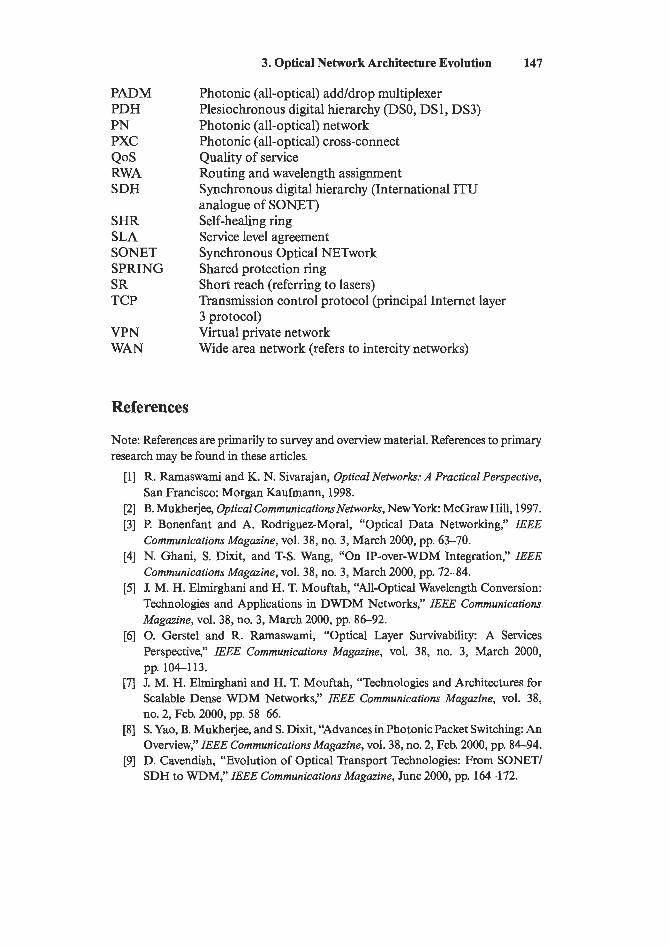
3. Optical Network Architecture Evolution 147
PADM PDH PN PXC QOS RWA SDH
SHR SLA SONET SPRING SR TCP
VPN WAN
Photonic (all-optical) adddrop multiplexer Plesiochronous digital hierarchy (DSO, DS1, DS3) Photonic (all-optical) network Photonic (all-optical) cross-connect Quality of service Routing and wavelength assignment Synchronous digital hierarchy (International ITU analogue of SONET) Self-healing ring Service level agreement Synchronous Optical NETwork Shared protection ring Short reach (referring to lasers) Transmission control protocol (principal Internet layer 3 protocol) Virtual private network Wide area network (refers to intercity networks)
References
Note: References are primarily to survey and overview material. References to primary research may be found in these articles.
[l] R. Ramaswami and K. N. Sivarajan, Optical Networks: A Practical Perspective, San Francisco: Morgan Kaufmann, 1998.
[2] B. Mukherjee, Optical Communications Networks, New York McGraw Hill, 1997. [3] P. Bonenfant and A. Rodriguez-Moral, “Optical Data Networking,” ZEEE
Communications Magazine, vol. 38, no. 3, March 2000, pp. 63-70. [4] N. Ghani, S. Dixit, and T-S. Wang, “On IP-over-WDM Integration,” IEEE
Communications Magazine, vol. 38, no. 3, March 2000, pp. 72-84. [5] J. M. H. Elmirghani and H. T. Mouftah, “All-Optical Wavelength Conversion:
Technologies and Applications in DWDM Networks,” IEEE Communications Magazine, vol. 38, no. 3, March 2000, pp. 86-92.
[6] 0. Gerstel and R. Ramaswami, “Optical Layer Survivability: A Services Perspective,” ZEEE Communications Magazine, vol. 38, no. 3, March 2000, pp. 104-113.
[7] J. M. H. Elmirghani and H. T. Mouftah, “Technologies and Architectures for Scalable Dense WDM Networks,” ZEEE Communications Magazine, vol. 38, no. 2, Feb. 2000, pp. 58-66.
[8] S. Yao, B. Mukherjee, and S. Dixit, “Advances in Photonic Packet Switching: An Overview,” IEEE Communications Magazine, vol. 38, no. 2, Feb. 2000, pp. 84-94.
[9] D. Cavendish, “Evolution of Optical Transport Technologies: From SONETI SDH to WDM,” IEEE Communications Magazine, June 2000, pp. 164-172.
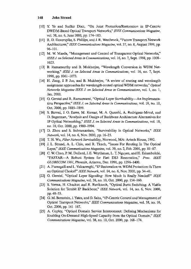
148 John Strand
[lo] Y Ye and Sudhir Dixit, “On Joint ProtectionRestoration in IP-Centric DWDM-Based Optical Transport Networks,” ZEEE Communications Magazine, vol. 38, no. 6, June 2000, pp. 174-183.
[l 11 R. D. Doverspike, S. Phillips, and J. R. Westbrook, “Future Transport Network Architectures,” IEEE Communications Magazine, vol. 37, no. 8, August 1999, pp. 96-101.
[12] M. W. Maeda, “Management and Control of Transparent Optical Networks,” ZEEEJ. on SelectedAreas in Communications, vol. 16, no. 7, Sept. 1998, pp. 1008- 1023.
[13] B. Ramamurthy and B. Mukherjee, “Wavelength Conversion in WDM Net- working,” IEEE J. on Selected Areas in Communications, vol. 16, no. 7, Sept.
[14] H. Zang, J. P. Jue, and B. Mukherjee, “A review of routing and wavelength assignment approaches for wavelength-routed optical WDM networks,” Optical Networks Magazine ZEEE J. on Selected Amas in Communications, vol. 1, no. 1, Jan. 2000.
[15] 0. Gerstel and R. Ramaswami, “Optical Layer Survivability-An Implementa- tion Perspective,” IEEE J. on Selected Areas in Communications, vol. 18, no. 10,
[ l a S. Baroni, J. 0. Eaves, M. Kumar, M. A. Qureshi, A. Rodriguez-Moral, and D. Sugerman, “Analysis and Design of Backbone Architecture Alternatives for IP Optical Networking,” IEEE J. on Selected Areas in Communications, vol. 18, no. 10, Oct. 2000, pp. 1980-1994.
[17] D. Zhou and S. Subramaniam, “Survivability in Optical Networks,” ZEEE Network, vol. 14, no. 6, Nov. 2000, pp. 16-23.
[18] T. H. Wu, Fiber NetworkSurvivability, Nonvood, MA: Artech House, 1992. [19] J. L. Strand, A. L. Chiu, and R. Tkach, “Issues For Routing In The Optical
Layer,” ZEEE Communications Magazine, vol. 39, no. 2, Feb. 2001, pp. 81-87. [20] C. W. Chao, P. M. Dollard, J. E. Weythman, L. T. Nguyen, and H. Eslambolchi,
“FASTAR-A Robust System for Fast DS3 Restoration,” Proc. ZEEE GLOBECOM1991, Phoenix, Arizona, Dec. 1991, pp. 1396-1400.
[21] A. Fumagalli and L. Valcarenghi, “IP Restoration vs. WDM Protection: Is There an Optimal Choice?’ ZEEE Network, vol. 14, no. 6, Nov. 2000, pp. 34-41.
[22] 0. Gerstel, “Optical Layer Signaling: How Much Is Really Needed?’ ZEEE Communications Magazine, vol. 38, no. 10, Oct. 2000, pp. 154-160.
[23] S. Verma, H. Chaskar, and R. Ravikanth, “Optical Burst Switching: A Viable Solution for Terabit IP Backbone,” IEEE Network, vol. 14, no. 6, Nov. 2000,
[24] G. M. Bernstein, J. Yates, and D. Saha, “IP-Centric Control and Management of Optical Transport Networks,” IEEE Communications Magazine, vol. 38, no. 10,
[25] A. Copley, “Optical Domain Service Interconnect: Defining Mechanisms for Enabling On-Demand High-speed Capacity from the Optical Domain,” ZEEE Communications Magazine, vol. 38, no. 10, Oct. 2000, pp. 168-174.
1998, pp. 1061-1073.
Oct. 2000, pp. 1885-1899.
pp. 48-53.
Oct. 2000, pp. 161-167.

3. Optical Network Architecture Evolution 149
[26] B. Rajagopalan, D. Pendarakis, D. Saha, R. S. h a m o o r t h y , and K. Bala, “IP Over Optical Networks: Architectural Aspects,” IEEE Communications Magazine, vol. 38, no. 9, Sept. 2000, pp. 94-103.
[27] C. Qiao, “Labeled Optical Burst Switching For IP-Over-WDM Integration,” IEEE Communications Magazine, vol. 38, no. 9, Sept. 2000, pp. 1041 15.
[28] D. K. Hunter and I. Andonovic, “Approaches to Optical Packet Switching,” IEEE Communications Magazine, vol. 38, no. 9, Sept. 2000, pp. 116-122.
[29] M. Listanti and R. Sabella, “Architectural and Technological Issues for Future Optical Internet Networks,” IEEE Communications Magazine, vol. 38, no. 9, Sept. 2000, pp. 82-92.
[30] R. Tkach, E. Goldstein, J. Nagel, and J. Strand, “Fundamental Limits of Optical Transparency,” Optical Fiber Communication ConJ, Feb. 1998, pp. 161-162.
[31] E. Modiano and A. Narula-Tam, “Mechanisms for Providing Optical Bypass in WDM-Based Networks,” OpticalNetworh Magazine, vol. 1, no. 1, Jan. 2000,
[32] H. Zang, J. P. Jue, and B. Mukherjee, “A Review of Routing and Wavelength Assignment Approaches for Wavelength-Routed Optical WDM Networks,” Optical Networks Magazine, vol. 1, no. 1, Jan. 2000, pp. 4740.
[33] C. P. Laresen and F! 0. Anderson, “Signal Quality Monitoring in Optical Networks,” Optical Networks Magazine, vol. 1, no. 4, Oct. 2000, pp. 17-23.
[34] G. Hjilmtjrsson, P. Sebos, G. Smith, and J. Yates, “Simple IP Restoration for IP/GbE/lO GbE Optical Networks,” Optical Fiber Communication ConJ, 2000, vol. 4,2000, pp. 275-277.
[35] S. Verma, H. Chaskar, and R. Ravikanth, “Optical Burst Switching: A Viable Solution for Terabit IP Backbone,” IEEE Network, vol. 14, no. 6, Nov. 2000,
[36] J. Strand, “Optical Layer Services Framework,” Optical Interworking Forum oif2000.108, May, 2000; available from the author.
[37] J. Strand and M. Lazer, “Some Routing Constraints,” Optical Interworking Forum oif 2000.109, May, 2000; available from the author.
[38] M. Eiselt, “The Quest For Optimum Transmission Capacity: Is There An Optimum Fiber Choice,” OFC 2000 tutorial.
[39] A. Odlyzko, “Internet Growth Myth and Reality, Use and Abuse,” iMP: Information Impacts Magazine, November 2000.
[40] A. Odlyzko, “The Internet and Other Networks: Utilization Rates and Their Implications,” Feb. 26, 2000. Available at http://www.research.att.com/-amo/ doc/complete. html.
[41] See http://www.canet2.net/library/papers.html. [42] B. Ramamurthy, H. Feng, D. Datta, J. P. Heritage, and B. Mukherjee, “Transpar-
ent vs. Opaque vs. Translucent Wavelength-routed Optical Networks,” Optical Fiber Communication Conference, 1999, and the International Conference on Inte- grated Optics and Optical Fiber Communication. OFC/IOOC ‘99. Technical Digest, vol. 1, 1999, pp. 5 M 1 .
pp. 11-18.
pp. 48-53.

150 John Strand
[43] OIF Carrier Group, Yong Xue, and Monica Lazer, eds, “Carrier Optical Ser- vices Framework and Associated Requirements for UNI,” Optical Interworking Forum oif2000.155, Sept. 13, 2000. Also available as working documents in TlX1.5 and the IETF.
[44] G. Mohan and C. S. R. Murthy, “Lightpath Restoration in WDM Optical Networks,” IEEE Network, vol. 14, no. 6, Nov./Dec. 2000, pp. 24-33.
[45] E. L. Goldstein, L. Y Lin, and R. W. Tkach, “Multiwavelength Opaque Optical- Crossconnect Networks,” IEICE Duns. Commun., vol. E82-B, no. 8, Aug. 1999,
[46] F. Bentivoglio and E. Iannone, “The Opaque Optical Network,” OpticaZ Networks, vol. 1, no. 4, Oct. 2000, pp. 24-31.
[47] P. Green, “Progress in Optical Networking,” IEEE Communications Magazine, vol. 39, no. 1, Jan. 2001, pp. 54-61.
[48] G. Miller, K. Thompson, and R. Wilder, “Wide-Area Internet Traffic Patterns and Characteristics,” IEEE Network, vol. 11, no. 6, Nov. 1997.
[49] A. Banerjee, J. Drake, J. F! Lang, B. Turner, K. Kompela, and Y Rekhter, “Generalized Multiprotocol Label Switching: An Overview of Routing and Management Enhancement,” IEEE Communications Magazine, vol. 39, no. 1, Jan. 2001, pp. 144-150.
[50] P. Ari js , B. van Caenegem, P. Demeester, F! LaGasse, W. Van Parys, and P. Achten, “Design of Ring- and Mesh-Based WDM Transport Networks,” Optical Networks, vol. 1, no. 3, July 2000, pp. 25-38.
[51] R. H. Cardwell, 0. J. Wasem, and H. Kobrinski, “WDM Architectures and Economics in Metropolitan Areas,” Optical Networks, vol. 1, no. 3, pp. 41-50.
[52] B. St. Amaud, “Overview of the Latest Developments in Optical Internets,” Optical Networks, vol. 1, no. 3, pp. 51-54.
[53] C. Blaizot, I. Cerutti, A. Fumagalli, M. Tacca, L. Valcarenghi, R. Jagannathan, A. Lardies, F. Masetti, and M. Garnot, “Design and Planning of Transport Net- works Based on SDH/SONET and WDM Optical Networks: Methods, Tools and Applications,” Optical Networks, vol. 1, no. 3, pp. 55-65.
[54] Vinod Khosla, “Terabit Tsunami,” Keynote Address at OFC 2000, Baltimore, MD, March 2000.
[55] K. G. Coffman and A. M. Odlyzko, “Internet Growth Is there a “Moore’s Law” for Data Traffic?” Preliminary version, 7/11/00. Available at: research.att.com/-amo.
[56] L. Xu, H. Perros, and G. Rouska, “Techniques for Optical Packet Switching And Optical Burst Switching,” IEEE Communications Magazine, vol. 39, no. 1, pp. 136-145.
[57] A. Odlyzko, “Data Networks Are Mostly Emptly And For Good Reason,” ITPro, MarcWAprill999, pp. 6749.
[58] B. St. Amaud, “Scaling Issues on Internet Networks” (draft), Canarie, Inc., Jan. 13,2001, available at www.canet2.nefflibraqdpapers.
pp. 1095-1104.
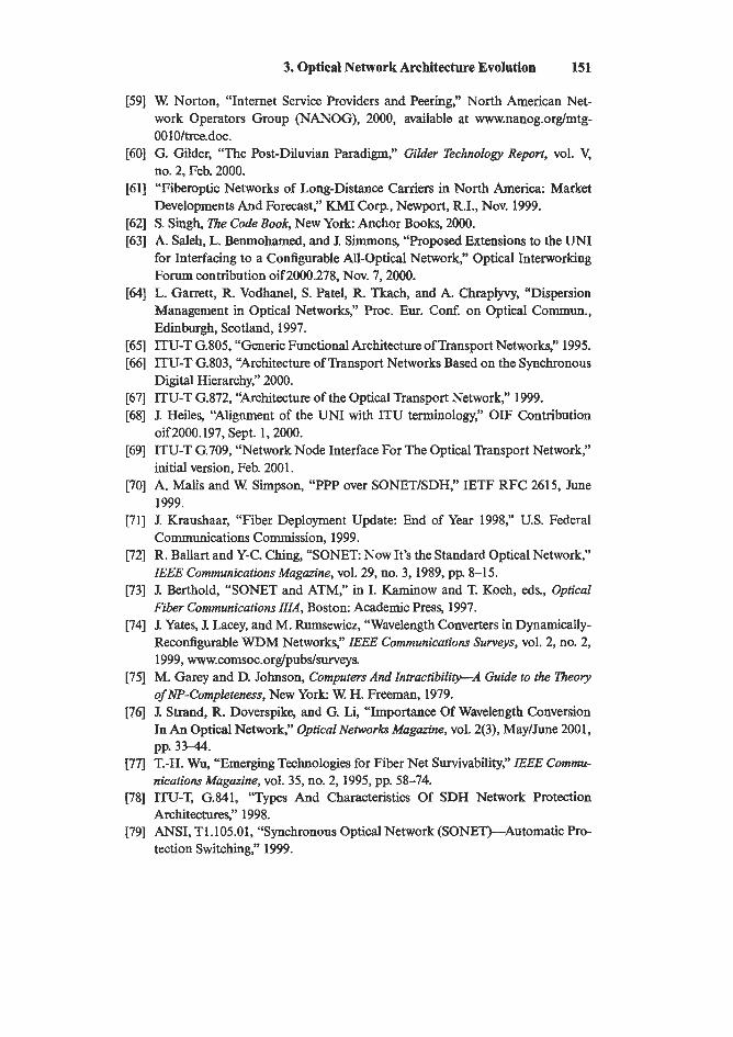
3. Optical Network Architecture Evolution 151
[59] W. Norton, “Internet Service Providers and Peering:’ North American Net- work Operators Group (NANOG), 2000, available at www.nanog.org/mtg- 00 1Oltree.doc.
[60] G. Gilder, “The Post-Diluvian Paradigm,” Gilder Technology Report, vol. V, no. 2, Feb. 2000.
[61] “Fiberoptic Networks of Long-Distance Carriers in North America: Market Developments And Forecast,” KMI Corp., Newport, R.I., Nov. 1999.
[62] S. Singh, The Code Book, New York: Anchor Books, 2000. [63] A. Saleh, L. Benmohamed, and J. Simmons, “Proposed Extensions to the UNI
for Interfacing to a Configurable All-Optical Network,” Optical Interworking Forum contribution oif 2000.278, Nov. 7,2000.
[64] L. Garrett, R. Vodhanel, S. Patel, R. Tkach, and A. Chraplyvy, “Dispersion Management in Optical Networks,” Proc. Eur. Cod. on Optical Comxnun., Edinburgh, Scotland, 1997.
[65] ITU-T G.805, “Generic Functional Architecture of Transport Networks,” 1995. [66] ITU-T G.803, “Architecture of Transport Networks Based on the Synchronous
Digital Hierarchy,” 2000. [67] ITU-T G.872, “Architecture of the Optical Transport Network,” 1999. [68] J. Heiles, “Alignment of the UNI with ITU terminology:’ OIF Contribution
oif2000.197, Sept. 1,2000. [69] ITU-T G.709, “Network Node Interface For The Optical Transport Network,”
initial version, Feb. 2001. [70] A. Malis and W. Simpson, “PPP over SONETlSDH,” IETF RFC 2615, June
1999. [71] J. Kraushaar, “Fiber Deployment Update: End of Year 1998,” U.S. Federal
Communications Commission, 1999. [72] R. Ballart and Y-C. Ching, “SONET: Now It’s the Standard Optical Network,”
IEEE Communications Magazine, vol. 29, no. 3, 1989, pp. 8-15. [73] J. Berthold, “SONET and ATM,” in I. Kaminow and T. Koch, eds, OpticaI
Fiber Communications IIIA, Boston: Academic Press, 1997. [74] J. Yates, J. Lacey, and M. Rumsewicz, “Wavelength Converters in Dynamically-
Reconfigurable WDM Networks,” IEEE Communications Surveys, vol. 2, no. 2, 1999, www.comsoc.org/pubs/surveys.
[75] M. Garey and D. Johnson, Computers And Intractibili-A Guide to the Theory of Np-Completeness, New York W. H. Freeman, 1979.
[76] J. Strand, R. Doverspike, and G. Li, “Importance Of Wavelength Conversion In An Optical Network,” Optical Networks Magazine, vol. 2(3), MaylJune 2001,
[77l T.-H. Wu, “Emerging Technologies for Fiber Net Survivability,” IEEE Commu-
[78] ITU-T, G.841, “Types And Characteristics Of SDH Network Protection
[79] ANSI, TI. 105.01, “Synchronous Optical Network (SONET)-Automatic Pro-
pp. 3344.
nications Magazine, vol. 35, no. 2, 1995, pp. 58-74.
Architectures,” 1998.
tection Switching,” 1999.
152 John Strand
[80] G. HjilmtJisson, J. Yates, S. Chaudhuri, and A. Greenberg, “Smart Routers- Simple Optics: an Architecture for the Optical Internet,” IEEE/OSA Journal of Lightwave Technology, Dec. 2000, pp. 37-50.
[81] B. Doshi, S. Dravida, P. Harshavardhana, and M. A. Qureshi, “A Comparison of Next-Generation IP-Centric Transport Architectures,” Bell Labs Tech. J . , vol. 3, no. 4,Oct.-Dec. 1998, pp. 137-143.
[82] M. Reardon and S. Saunders, “Terabit Trouble,” Data Communications,
[83] S. Chaudhuri and E. Goldstein, “On The Value of Optical-Layer Reconfigura- bility in IP-Over-WDM Lightwave Networks,” ZEEE Photonics Technology Letters, vol. 12, no. 8, Aug. 2000, pp. 1097-1099.
[84] B. Gleeson, A. Lin, J. Heinanen, G. Armitage, and A. Malis, “A Framework for IP-Based Virtual Private Networks,” RFC 2764, IETF, Feb. 2000.
[85] R. Doverspike, S. Phillips, and J. Westbrook, “Transport Network Architectures in an IP World,” Proc. INFOCOM-2000, March 2000, Tel-Aviv, Israel.
[86] 0. Gerstel, “Optical Layer Signaling: How Much Is Really Needed,” ZEEE Communications Magazine, vol. 38, no. 10, Oct. 2000, pp. 154-160.
[87l D. Comer, Internetworking with TCP/IR El. I : Principles, Protocols, and Architecture, Upper Saddle River, NJ: Prentice Hall, 1995.
[88] U. Black, ZP Routing Protocols: Ne OSPF: BGE P W I & Cisco Routing Protocols, Upper Saddle River, NJ: Prentice Hall, 2000.
[89] J. Moy, OSPF: Anatomy OfAn Internet Routing Protocol, Boston: Addison Wesley Longman, 1998.
[90] J. Stewart 111, BGP4: Inter-Domain Routing in the Internet, Boston: Addison- Wesley Longman, 1998.
[91] B. Davis and Y Rekhter, MPLS: Technology And Applications, San Francisco: Morgan Kaufmann, 2000.
[92] D. Awduche et al., “Multiprotocol Lambda Switching: Combining MPLS Traffic Engineering with Optical Crossconnects,” Internet draft, draft-awduche-mpls- te-optical-02.txt, March 2000, work in progress.
[93] L. McAdams and J. Yates, eds., “User to Network Interface Service Defini- tion and Connection Attributes,” Optical Interworking Fonun Contribution oif2000.061, Dec. 15,2000.
[94] S. Chaudhuri, G. HjPlmtJisson, and J. Yates, “Control of Lightpaths in an Optical Network,” work in progress, Internet draft, draft-chaudhuri-ip-olxc-control-
[95] A. Chiu, J. Strand, R. Tkach, and J. Luciani, “Features and Requirements for the Optical Layer Control Plane,” work in progress, Internet draft, draft-chiu- strand-unique-olcp.tt, Feb. 2001, available from the author also.
[96] M. Blanchet, E Parent-Viagenie, and B. St-knaud, “Optical BGP (OBGP): InterAS lightpath provisioning,” work in progress, Internet draft, draft-parent- obgp-OO.txt, Jan. 2001, available at www.canet2.netAibraxy/papers.
[97] J. Strand and Y Xue, “Routing for Optical Networks With Multiple Routing Domains,” Optical Interworking Forum Contribution oif 2001.046, Jan. 2001; available from the authors.
Aug. 1999, pp. 11-16.
OO.txt, 2000.

3. Optical Network Architecture Evolution 153
[98] G. Bernstein and B. Rajagopalan, “Optical Inter-Domain Routing Require- ments,” Internet draft, draft-bernstein-optical-bgp.txt, Feb. 2001, work in progress.
[99] Bellcore, “SONET Bidirectional Line-Switched Ring Equipment: Generic Criteria,” GR-1230-CORE, Issue 2, Nov. 1995.
[ 1001 Bellcore, “Synchronous Optical Network (SONET) Generic Criteria,” GR-253- CORE, Issue 1, Dec. 1994.
[loll Quoted by Russell McGuire, VP, Strategic Development Williams Corp., in a 12/3/1999 talk to the Risk Conference on Bandwidth Trading, New York.
[lo21 A. Chiu and J. Strand, “Joint IP/Optical Layer Restoration After a Router Failure,” OFC2001, Anaheim, vol. 1, March 2001, pp. MN5-1-MN5-2.
[lo31 R. Doverspike and J. Yates, “Challenges for MPLS in Optical Network Restoration,” IEEE Communications Magazine, vol. 39, no. 2, Feb. 2001, pp. 8%96.
[lo41 R. Barry, “Optical Networking Technologies: Driving the Evolution of the Public Network,” NFOEC, 1999.
[lo51 B. Mukherjee, “WDM Optical Communication Networks: Progress and Chal- lenges,” IEEE Journal on Selected Areas In Communications, vol. 18, no. 10, Oct. 2000, pp. 181CL1824.
11061 S. Baroni, J. Eaves, M. Kumar, M. Qureshi, A. Rodriguez-Moral, and D. Sugrarman, “Analysis and Design of Backbone Architecture Alternatives for IP Optical Networking,” IEEE Journal on Selected Areas In Communications, vol. 18, no. 10, Oct. 2000, pp. 198CL1994.
[lo71 E. Messmer, “Holding the Line on Call-Center Sprawl,” Network World, Apr. 2, 2001.
[ 1081 R. Bhandari, Survivable Networks--Algorithm for Diverse Routing, New York: Kluwer Academic Publishers, 1999.

Chapter 4
Neal S. Bergano l jco Telecommunications. Eatontown, New Jersey
Undersea Communication Systems
4.1 Introduction
In today’s Internet age information flows across continents as easily as it flows across the office. With so many “point and click” virtual connections, it is easy to forget that the world’s communications needs are made possible by real systems based on fiber-optic cables. ‘3’ This comes as no surprise to those of us in the optics community; however, many others underestimate the importance of undersea fiber-optic cables for intercontinental telecommunications. The earth‘s continents are connected with a web of undersea fiber-optic cables that join the world’s major population centers. Anyone who makes international phone calls, sends international faxes, or simply surfs the Web at sites in other continents uses undersea fiber-optic cables.
Although the debate regarding the merits of cable systems versus satellite systems for international communications ended many years ago, with cable systems the clear economic and technological winner, many people still assume that overseas communications occur via satellite. But consider this: since 1990 over 600,000 km of undersea fiber-optic cable has been installed across the world’s oceans. Today, the vast majority of international telecommunications is carried on undersea cable^.^
This chapter reviews concepts for the design of long-haul transmission sys- tems based on optical amplifier repeaters and wavelength division multiplexing (WDM) techniques. Important strides have been made in areas of dispersion management, gain equalization, and modulation formats, which have made possible the demonstration of capacities exceeding 2TB/s on a single fiber. This chapter includes sections on the history of undersea cable, the amplified transmission line, dispersion and nonlinearity management, transmission for- mats, measures of system performance, error correcting codes, polarization effects, long-haul system design, experimental techniques, and future trends in long-haul optical transmission systems.
4.2 A Rich History of Undersea Cables
Undersea cable has been in use for over 130 years. The installation of the first transatlantic telegraph cable was completed in 1858 (Fig. 4.1). Unfortunately,
154 OPTICAL FIBER TELECOMMUNICATIONS, VOLUME IVB
Copyright Q 2002, Elsevier Science (USA). All rights of reproduction in any form reserved.
ISBX 0-12-395173-9
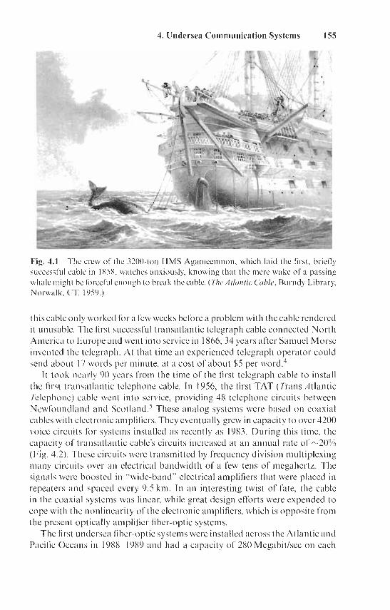
4. Undersea Communication Systems 155
Fig. 4.1 The crew of the 3200-ton HMS Agameemnon, which laid the first, briefly successful cable in 1858, watches anxiously, knowing that the mere wake of a passing whale might be forceful enough to break the cable. (The Atlantic Cable, Burndy Library, Norwalk, CT, 1959.)
this cable only worked for a few weeks before a problem with the cable rendered it unusable. The first successful transatlantic telegraph cable connected North America to Europe and went into service in 1866,34 years after Samuel Morse invented the telegraph. At that time an experienced telegraph operator could send about 17 words per minute, at a cost of about $5 per word.4
It took nearly 90 years from the time of the first telegraph cable to install the first transatlantic telephone cable. In 1956, the first TAT (Trans Atlantic Telephone) cable went into service, providing 48 telephone circuits between Newfoundland and Scotland.’ These analog systems were based on coaxial cables with electronic amplifiers. They eventually grew in capacity to over 4200 voice circuits for systems installed as recently as 1983. During this time, the capacity of transatlantic cable’s circuits increased at an annual rate of -20% (Fig. 4.2). These circuits were transmitted by frequency division multiplexing many circuits over an electrical bandwidth of a few tens of megahertz. The signals were boosted in “wide-band’’ electrical amplifiers that were placed in repeaters and spaced every 9.5 km. In an interesting twist of fate, the cable in the coaxial systems was linear, while great design efforts were expended to cope with the nonlinearity of the electronic amplifiers, which is opposite from the present optically amplifier fiber-optic systems.
The first undersea fiber-optic systems were installed across the Atlantic and Pacific Oceans in 1988-1989 and had a capacity of 280 Megabithec on each

156
1M -
100K-
10K-
1K-
100 -
Neal S. Bergano
TWO-WAY CABLE CIRCUITS
64Kbk Digital Circuits 3KHz Analoa Circuits > I 00% Annual
Growth
1960 1970 1980 1990 2000 1955 1965 1975 1985 1995 2005
YEAR
Fig. 4.2 The cumulative capacity that has been installed crossing the Atlantic Ocean over the past 4 decades. The capacity is given in 3-kHz circuits for the analog systems, and 64-kB/s circuits for the digital systems.
of three fiber pairs.6 These systems were actually hybrid optical systems in the sense that the repeaters converted the incoming signals from optical to electri- cal, regenerated the data with high-speed integrated circuits, and retransmitted the data with a local semiconductor laser. The transmission capacity of the regenerated fiber cables eventually increased to 2.5 Gigabidsec, and repeater spacing increased with the switch from 1.3 pm multifrequency lasers to 1.55 pm single-frequency laser diodes. These first undersea fiber systems revo- lutionized international telephony, bringing costs down and greatly expanding capacity and quality. However, the ability of the regenerator systems to exploit the large fiber bandwidth was limited by the capacity bottleneck in the high- speed electronics of undersea repeaters. Beginning in the mid- 1 9 9 0 ~ ~ undersea fiber-optic systems using erbium-doped fiber-amplifiers in the repeaters were deployed. These systems removed the electronic bottleneck and provided the first clear optical channel connectivity between the world’s continent^.^
Today’s undersea systems use erbium-doped fiber amplifiers (EDFAs) to compensate the attenuation in the optical fiber cable. These optical amplifiers are in repeaters that are typically spaced every 50 km along the cable and have an optical bandwidth that is wide enough to support many optical channels using WDM techniques. Data signals coming from the land-based systems (typically referred to as “terrestrialyy systems) are converted to an optical for- mat that is more robust for transmission over transoceanic distances. Systems being designed today for deployment in the next few years will support many
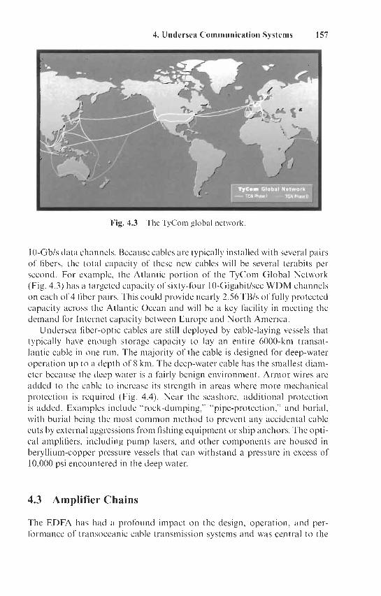
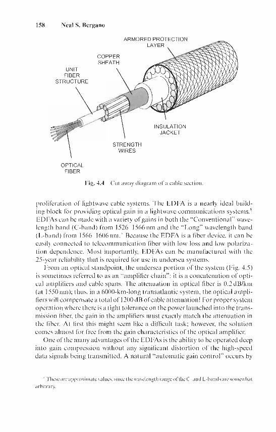
158 Neal S. Bergano
STRENGTH , * \ WIRES
OPTICAL FIBER
Fig. 4.4 Cut away diagram of a cable section.
proliferation of lightwave cable systems. The EDFA is a nearly ideal build- ing block for providing optical gain in a lightwave communications systems.8 EDFAs can be made with a variety of gains in both the “Conventional” wave- length band (C-band) from 1526-1566 nm and the “Long” wavelength band (L-band) from 1566-1606 nm.* Because the EDFA is a fiber device, it can be easily connected to telecommunication fiber with low loss and low polariza- tion dependence. Most importantly, EDFAs can be manufactured with the 25-year reliability that is required for use in undersea systems.
From an optical standpoint, the undersea portion of the system (Fig. 4.5) is sometimes referred to as an “amplifier chain”; it is a concatenation of opti- cal amplifiers and cable spans. The attenuation in optical fiber is 0.2 dB/km (at 1550 nm); thus, in a 6000-km-long transatlantic system, the optical ampli- fiers will compensate a total of 1200 dB of cable attenuation! For proper system operation where there is a tight tolerance on the power launched into the trans- mission fiber, the gain in the amplifiers must exactly match the attenuation in the fiber. At first this might seem like a difficult task; however, the solution comes almost for free from the gain characteristics of the optical amplifier.
One of the many advantages of the EDFAs is the ability to be operated deep into gain compression without any significant distortion of the high-speed data signals being transmitted. A natural “automatic gain control” occurs by
* These are approximate values, since the wavelength range ofthe C- and L-bands are somewhat arbitrary.
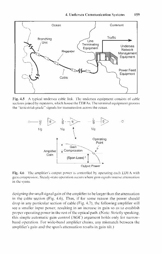
4. Undersea Communication Systems 159
Fig. 4.5 A typical undersea cable link. The undersea equipment consists of cable sections joined by repeaters, which house the EDFAs. The terminal equipment grooms the “terrestrial-grade” signals for transmission across the ocean.
t Operating Point
(Span Loss)-’ Gain
Output Power
Fig. 4.6 The amplifier’s output power is controlled by operating each EDFA with gain compression. Steady-state operation occurs where gain equals inverse attenuation in the spans.
designing the small signal gain of the amplifier to be larger than the attenuation in the cable section (Fig. 4.6). Thus, if for some reason the power should drop in any particular section of cable (Fig. 4.7), the following amplifier will see a smaller input power, resulting in an increase in gain so as to establish proper operating power in the rest of the optical path. (Note: Strictly speaking, this simple automatic gain control (AGC) argument holds only for narrow- band operation. For wide-band amplifier chains, any mismatch between the amplifier’s gain and the span’s attenuation results in gain tilt.)

160 Neal S. Bergano
Normal Output Power r - _ _ _ _ ____-------- ---- --- --- -
Repeater output Power r I, 71 ti f r r , _ _ _ _ _ _ _ _ _ _ _ _ _ _ _ ---- --- --- -
Position of Repeater in System
Fig. 4.7 Repeater output powers versus transmission distance. The repeater’s output power is controlled by gain compression in the amplifiers.
The real challenge is to equalize the power over a wide optical bandwidth to allow for many WDM channels. Here we are not as fortunate as with the total power control given by the EDFA gain compression. Most of the gain equal- ization is accomplished using passive gain-flattening filters placed along the length of the amplifier chain.9 These filters can be packaged with the individual amplifiers to provide the majority of the gain equalization. Depending on the required level of equalization, additional “clean-up” filters can be placed at regular intervals (i.e., once every 10-20 amplifiers) along the amplifier chain. Figure 4.8 shows the gain shape of a single-stage EDFA before and after gain equalization. This amplifier was designed to have usable gain throughout the entire C-band.
The amplified spontaneous emission (ASE) noise accumulation can be controlled by properly selecting the distance between amplifiers. In a long transmission line, ASE noise generated in the EDFAs can accumulate to power levels similar to the data-carrying signal. The accumulated noise can influence the system’s performance by reducing the level of the signal and signal-to- noise ratio. The noise power out of an optical amplifier is proportional to the amplifier’s gain and is given by:’O
where hv is photon energy, g is gain in linear units, nsp is the excess noise factor related to the amplifier’s noise figure, and Bo is optical bandwidth. For a chain of identical amplifier spans, the total accumulated ASE noise out of the N* amplifier is simply NPnoise (assuming no signal decay caused by noise accumu- lation). As a consequence, the spectral density of the accumulated noise at the end of the system depends on the repeater gain and fiber loss. Consider a linear system where we treat only noise accumulation, with a fiber loss of 0.2 dB/km.
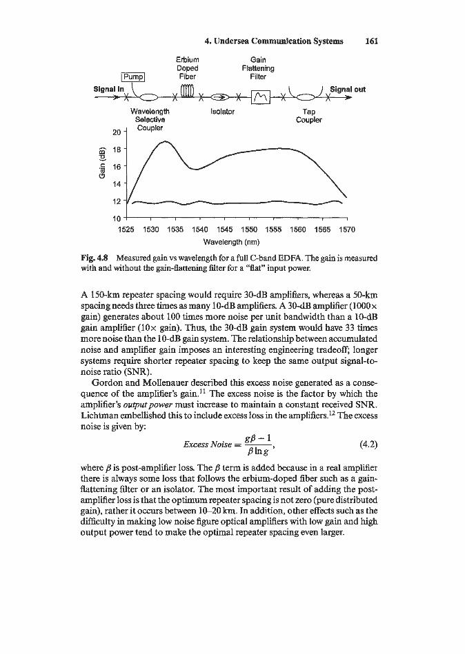
4. Undersea Communication Systems 161
Erbium Gain Doped Flattening Fiber Filter
Signal out V xmxwx *
Wavelength Isolator Tap Selective Coupler
*O 1 Coup’er
1525 1530 1535 1540 1545 1550 1555 1560 1565 1570
Wavelength (nm)
Fig. 4.8 Measured gain vs wavelength for a full C-band EDFA. The gain is measured with and without the gain-flattening filter for a “flat” input power.
A 150-km repeater spacing would require 30-dB amplifiers, whereas a 50-km spacing needs three times as many 1 0-dB amplifiers. A 30-dB amplifier (1000 x gain) generates about 100 times more noise per unit bandwidth than a 10-dB gain amplifier (lox gain). Thus, the 30-dB gain system would have 33 times more noise than the 10-dB gain system. The relationship between accumulated noise and amplifier gain imposes an interesting engineering tradeoff; longer systems require shorter repeater spacing to keep the same output signal-to- noise ratio (SNR).
Gordon and Mollenauer described this excess noise generated as a conse- quence of the amplifier’s gain.“ The excess noise is the factor by which the amplifier’s output power must increase to maintain a constant received SNR. Lichtman embellished this to include excess loss in the amplifiers.I2 The excess noise is given by:
g s - 1 B h g ’
Excess Noise = - (4.2)
where is post-amplifier loss. The /3 term is added because in a real amplifier there is always some loss that follows the erbium-doped fiber such as a gain- flattening filter or an isolator. The most important result of adding the post- amplifier loss is that the optimum repeater spacing is not zero (pure distributed gain), rather it occurs between 10-20 km. In addition, other effects such as the difficulty in making low noise figure optical amplifiers with low gain and high output power tend to make the optimal repeater spacing even larger.

162 Neal S. Bergano
The total accumulated noise power depends on the amount of noise gener- ated at each amplifier (Eq. 4.1) times the number of amplifiers in the system. As stated previously, the automatic control obtained through the amplifier’s gain saturation fixes the total output power. This total power contains both signal and accumulated noise. Because the total power is fixed and noise accu- mulates, then the signal’s power must decrease as the signal propagates down the amplifier chain.13 As an example, consider a 6000-km-long amplifier chain with 120 amplifiers spaced every 50 km. From Eq. 4.1 we know that a 10-dB net gain amplifier with nsp = 1.4 will generate about 16 p.W of noise power over the 40-nm C-band. Thus, at the end of the amplifier chain there is a total noise power of -2 mW (+3 dBm) of noise power.
A simple but useful estimate of the signal-to-noise ratio at the output of a chain of N amplifiers is:
PL NF ghu B,N ’
SNR, = (4.3)
where PL is the average optical power launched into the transmission spans, NF is noise figure, and g is the amplifier’s gain, and Bo is optical bandwidth in Hertz. Equation 4.3 assumes that all the amplifiers are identical, and that there is no signal decay from noise accumulation.
Wide-band EDFAs are not ideal amplifiers that have a simple gain shape. The actual output power over the amplifier’s optical bandwidth is somewhat dependent on the spectral distribution of input power, which is known as spectral h~le-burning’~ (SHB). The result of SHB is that the output power at any individual wavelength will be influenced by other signals within some characteristic spectral range, or “hole width.” The influence of SHB can be useful for gain equalization.
Unfortunately, it can also limit the ability to perform transmitter pre- emphasis15 to correct for unequal SNR in a WDM system. Figure 4.9 shows a measurement of SHB on an amplifier chain and the effect it can have on
1544 1548 1552 1556 Wavelength (nm)
01 .
-40 -301 1544 1548 1552 1556
Wavelength (nm)
Fig. 4.9 The influence of SHB is observed in the optical spectra at the output of a 6200-km amplifier chain. When pre-emphasis powers are changed, the SNR is altered for neighboring channels, but not for channels far away.
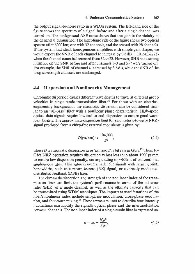
4. Undersea Communication Systems 163
the output signal-to-noise ratio in a WDM system. The left-hand side of the figure shows the spectrum of a signal before and after a single channel was turned on. The background ASE noise shows that the gain in the vicinity of the channel is diminished. The right-hand side of the figure shows two optical spectra after 6200 km; one with 32 channels, and the second with 28 channels. If the system had ideal, homogeneous amplifiers with simple gain shapes, we would expect the SNR of each channel to increase by 0.6 dB = 10 log(32/28) when the channel count is decreased from 32 to 28. However, SHB has a strong influence on the SNR before and after channels 1-3 and 5-7 were turned off. For example, the SNR of channel 4 increased by 3.6 dB, while the SNR of the long wavelength channels are unchanged.
4.4 Dispersion and Nonlinearity Management
Chromatic dispersion causes different wavelengths to travel at different group velocities in single-mode transmission fiber.16 For those with an electrical engineering background, the chromatic dispersion can be considered simi- lar to an “all-pass” filter with a nonlinear phase characteristic. High-speed optical data signals require low end-to-end dispersion to ensure good wave- form fidelity. The approximate dispersion limit for a nonreturn-to-zero (NRZ) signal produced from a chirp-free external modulator is given by:
104,000 D(ps/nm) = ~
B2 ’ (4.4)
where D is chromatic dispersion in ps/nm and B is bit rate in Gb/s.17 Thus, 10- Gb/s NRZ operation requires dispersion values less than about 1000 ps/nm to ensure low dispersion penalty, corresponding to -60 km of conventional single-mode fiber. This value is even smaller for signals with larger optical bandwidths, such as a return-to-zero (RZ) signal, or a directly modulated distributed feedback (DFB) laser.
The chromatic dispersion and strength of the nonlinear index of the trans- mission fiber can limit the system’s performance in terms of the bit error ratio (BER) of a single channel, as well as the ultimate capacity that can be transmitted using WDM techniques. The important manifestations of the fiber’s nonlinear index include self-phase modulation, cross-phase modula- tion, and four-wave mixing.’* These terms are used to describe how intensity fluctuations can modify the signal‘s optical phase and the intermodulation between channels. The nonlinear index of a single-mode fiber is expressed as:
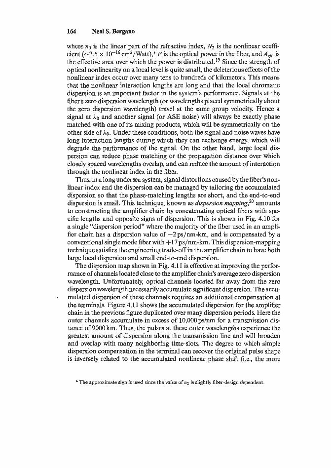
164 Neal S. Bergano
where no is the linear part of the refractive index, N2 is the nonlinear coeffi- cient (-2.5 x cm2/Watt),* P is the optical power in the fiber, and A@ is the effective area over which the power is distrib~ted.‘~ Since the strength of optical nonlinearity on a local level is quite small, the deleterious effects of the nonlinear index occur over many tens to hundreds of kilometers. This means that the nonlinear interaction lengths are long and that the local chromatic dispersion is an important factor in the system’s performance. Signals at the fiber’s zero dispersion wavelength (or wavelengths placed symmetrically about the zero dispersion wavelength) travel at the same group velocity. Hence a signal at A0 and another signal (or ASE noise) will always be exactly phase matched with one of its mixing products, which will be symmetrically on the other side of ho. Under these conditions, both the signal and noise waves have long interaction lengths during which they can exchange energy, which will degrade the performance of the signal. On the other hand, large local dis- persion can reduce phase matching or the propagation distance over which closely spaced wavelengths overlap, and can reduce the amount of interaction through the nonlinear index in the fiber.
Thus, in a long undersea system, signal distortions caused by the fiber’s non- linear index and the dispersion can be managed by tailoring the accumulated dispersion so that the phase-matching lengths are short, and the end-to-end dispersion is small. This technique, known as dispersion amounts to constructing the amplifier chain by concatenating optical fibers with spe- cific lengths and opposite signs of dispersion. This is shown in Fig. 4.10 for a single “dispersion period” where the majority of the fiber used in an ampli- fier chain has a dispersion value of -2ps/nm-km, and is compensated by a conventional single mode fiber with + 17 ps/nm-km. This dispersion-mapping technique satisfies the engineering trade-off in the amplifier chain to have both large local dispersion and small end-to-end dispersion.
The dispersion map shown in Fig. 4.11 is effective at improving the perfor- mance of channels located close to the amplifier chain’s average zero dispersion wavelength. Unfortunately, optical channels located far away from the zero dispersion wavelength necessarily accumulate significant dispersion. The accu- mulated dispersion of these channels requires an additional compensation at the terminals. Figure 4.1 1 shows the accumulated dispersion for the amplifier chain in the previous figure duplicated over many dispersion periods. Here the outer channels accumulate in excess of 10,000 pdnm for a transmission dis- tance of 9000 km. Thus, the pulses at these outer wavelengths experience the greatest amount of dispersion along the transmission line and will broaden and overlap with many neighboring time-slots. The degree to which simple dispersion compensation in the terminal can recover the original pulse shape is inversely related to the accumulated nonlinear phase shift (i.e., the more
* The approximate sign is used since the value of nz is slightly fiber-design dependent.

4. Undersea Communication Systems 165
10,000 -
t 0
a, a In
U a, m
.- $2 5,000-
6 0 --
c - 2 2 2 -5,000-
-1 0,000 -
Long wavelength channel
-500
-1 000 0 100 200 300 400 500
Length (krn)
-2ps/krn-nm +17ps/km-nrn -2pslkm-nm
Fig. 4.10 The accumulated dispersion along a 500-km amplifier chain. The “disper- sion map” consists of a dispersion value of -2 ps/nm-km for the majority of the fiber, compensated by a fiber with +17ps/nm-km.
I
...
Terminal’s Dispersion
Compensation
I dmap6
0 2000 4000 6000 8000 10000 Distance (km)
Fig. 4.11 Accumulated dispersion as a function of distance for several channels of a WDM transmission system. The average slope of the dispersion is 0.075 ps/km-nm*. The minimum and maximum wavelengths are f l 5 n m from the zero dispersion wavelength (ho).
linear the system, the more accumulated dispersion that can be tolerated in the transmission line). In practice, it has been found that the performance of long transmission lines can be improved by placing half of the needed disper- sion at the transmit end and half at the receiver21 (sometimes known as 50/50 compensation).

166 Neal S. Bergano
Trans. #3
ps Trans. #N-I
/ Trans. #2
Trans. #N
Fig. 4.12 Block diagram of a WDM transmitter using “pair-wise” orthogonal polarization launch.
The simplest method of reducing the deleterious effects of the fiber’s non- linear index is simply to reduce the operating power of the WDM channels.22 Unfortunately, reduced power leads to poorer SNR and potentially, degraded bit-error ratios. Poor bit-error ratio performance can be greatly reduced by using forward error correction codes in the terminals (see Section 4.7). These effects can also be reduced by wisely choosing the transmission format used at the transmitter (see next section on transmission formats). For example, synchronous phase modulation added at the transmitter allows operation at greater launch power, particularly for channels located far away from the amplifier chains zero dispersion wavelength.
One very effective method of reducing the interactions between WDM channels is to launch the even numbered channels orthogonally polarized with respect to the odd numbered channels (Fig. 4.12). This “pair-wise” orthogonal method23 greatly reduces nonlinear crosstalk from four-wave mixing and lin- ear crosstalk such as nonideal extinction in demultiplexing devices. Figure 4.13 shows an example of two-tone four-wave mixing through a 500-km amplifier chain.24 When two CW tones were launched in the same polarization, the two interacted to form many mixing products. However, the mixing was greatly reduced when the two were launched orthogonally p ~ l a r i z e d . ~ ~
4.5 Modulation Formats
The choice of modulation format has an important performancekconomic trade-off. From a performance standpoint, the best modulation format is dic- tated by many system parameters, such as system length, the fiber type, the dispersion management, and the optical bandwidth. For example, the chirped
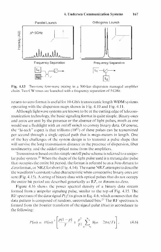
4. Undersea Communication Systems 167
- 3 - 9 A -
u) S
a - c
4-4 ._
Parallel Launch
1 Af-5GHz
Frequency Separation
Orthogonal Launch
Frequency Separation
Fig. 4.13 Two-tone four-wave mixing in a 500-km dispersion managed amplifier chain. Two CW tones are launched with a frequency separation of 5 GHz.
return-to-zero format is useful for lO-Gb/s transoceanic length WDM systems operating with the dispersion maps shown in Fig. 4.10 and Fig. 4.1 1.
Although lightwave systems are known to be at the cutting edge of telecom- munication technology, the basic signaling format is quite simple. Binary ones and zeros are sent by the presence or the absence of light pulses, much as one would use a flashlight with an on/off switch to convey binary data. Of course, the “hi-tech’’ aspect is that trillions (10l2) of these pulses can be transmitted per second through a single optical path that is mega-meters in length. One of the key challenges of the system design is to transmit a pulse shape that will survive the long transmission distance in the presence of dispersion, fiber nonlinearity, and the added optical noise from the amplifiers.
Transmission based on this simple on/off pulse scheme is referred to a unipo- lar pulse system.26 When the shape of the light pulse used is a rectangular pulse that occupies the entire bit period, the format is referred to as a Non-Return to Zero format, or NRZ for short (Fig. 4.14). The name NRZ attempts to describe the waveform’s constant value characteristic when consecutive binary ones are sent (Fig. 4.15). A string of binary data with optical pulses that do not occupy the entire bit period are described generically as RZ, or Return-to-Zero.
Figure 4.16 shows the power spectral density of a binary data stream formed from a unipolar signaling pulse, similar to the top of Fig. 4.15. The RF spectrum of the data signal P ( f ) is given in Eq. 4.6, which assumes that the data pattern is composed of random, uncorrelated bits.27 The R F spectrum is formed from the Fourier transform of the signal pulse H ( o ) in accordance to the following:
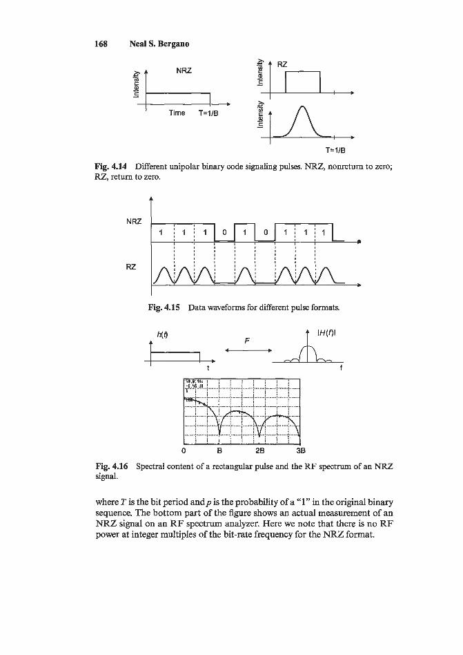
168
Fig. ’
Neal S. Bergano
T= 1 IB
Different unipolar binary C O ~ J signaling pulses. NRZ, nonreturn to zero; RZ, return to zero.
NRZ
Rz
I I I
t
Fig. 4.15 Data waveforms for different pulse formats.
- 0 B 2B 38
Fig. 4.16 Spectral content of a rectangular pulse and the RF spectrum of an NRZ signal.
where T is the bit period andp is the probability of a “1 ” in the original binary sequence. The bottom part of the figure shows an actual measurement of an NRZ signal on an RF spectrum analyzer. Here we note that there is no RF power at integer multiples of the bit-rate frequency for the NRZ format.
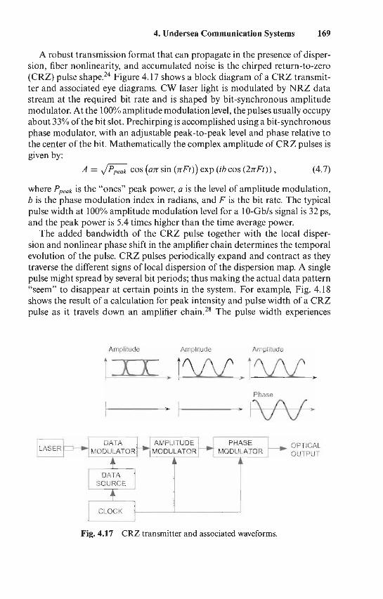
4. Undersea Communication Systems 169
A robust transmission format that can propagate in the presence of disper- sion, fiber nonlinearity, and accumulated noise is the chirped return-to-zero (CRZ) pulse shape.24 Figure 4.17 shows a block diagram of a CRZ transmit- ter and associated eye diagrams. CW laser light is modulated by NRZ data stream at the required bit rate and is shaped by bit-synchronous amplitude modulator. At the 100% amplitude modulation level, the pulses usually occupy about 33% of the bit slot. Prechirping is accomplished using a bit-synchronous phase modulator, with an adjustable peak-to-peak level and phase relative to the center of the bit. Mathematically the complex amplitude of CRZ pulses is given by:
A = & cos (an sin ( n ~ t ) ) exp (ib cos ( 2 n ~ t ) ) , (4.7)
where Pp& is the “ones” peak power, a is the level of amplitude modulation, b is the phase modulation index in radians, and F is the bit rate. The typical pulse width at 100% amplitude modulation level for a lO-Gb/s signal is 32 ps, and the peak power is 5.4 times higher than the time average power.
The added bandwidth of the CRZ pulse together with the local disper- sion and nonlinear phase shift in the amplifier chain determines the temporal evolution of the pulse. CRZ pulses periodically expand and contract as they traverse the different signs of local dispersion of the dispersion map. A single pulse might spread by several bit periods; thus making the actual data pattern “seem” to disappear at certain points in the system. For example, Fig. 4.18 shows the result of a calculation for peak intensity and pulse width of a CRZ pulse as it travels down an amplifier chain.28 The pulse width experiences
Amplitude Amplitude Amplitude
AMPLITUDE OPTICAL OUTPUT
LASER
DATA SOURCE
4 CLOCK
Fig. 4.17 CRZ transmitter and associated waveforms.
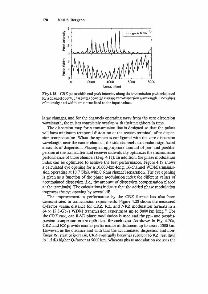
170 Neal S. Bergano
6 .- 0 $ 4
g 2
w c Y .-
n 0
g 8 5 - 8 4 l?
0 0 2000 4000 6000 8000
Length (km)
Fig. 4.18 CRZ pulse width and peak intensity along the transmission path calculated for a channel operating43 nm above the average zero dispersion wavelength. The values of intensity and width are normalized to the input values.
large changes, and for the channels operating away from the zero dispersion wavelength, the pulses completely overlap with their neighbors in time.
The dispersion map for a transmission line is designed so that the pulses will have minimum temporal distortion at the receive terminal, after disper- sion compensation. When the system is configured with the zero dispersion wavelength near the center channel, the side channels accumulate significant amounts of dispersion. Placing an appropriate amount of pre- and postdis- persion at the transmitter and receiver individually optimizes the transmission performance of these channels (Fig. 4.1 1). In addition, the phase modulation index can be optimized to achieve the best performance. Figure 4.19 shows a calculated eye opening for a lO,OOO-km-long, 16-channel WDM transmis- sion operating at 10.7 Gb/s, with 0.6 nm channel separation. The eye opening is given as a function of the phase modulation index for different values of accumulated dispersion (i.e., the amount of dispersion compensation placed at the terminals). The calculations indicate that the added phase modulation improves the eye opening by several dB.
The improvement in performance by the CRZ format has also been demonstrated in transmission experiments. Figure 4.20 shows the measured Q-factor versus distance for CRZ, RZ, and NRZ modulation formats in a 64 x 12.3-Gb/s WDM transmission experiment up to 9000 km long.29 For the CRZ case, one RAD phase modulation is used and the pre- and postdis- persion compensation are optimized for each case. As shown in Fig. 4.20a, CRZ and RZ provide similar performance at distances up to about 5000 km. However, as the distance and with that the accumulated dispersion and non- linear IS1 start to increase, CRZ eventually becomes superior to RZ, resulting in 1.5 dB higher Q-factor at 9000 km. Whereas phase modulation reduces the
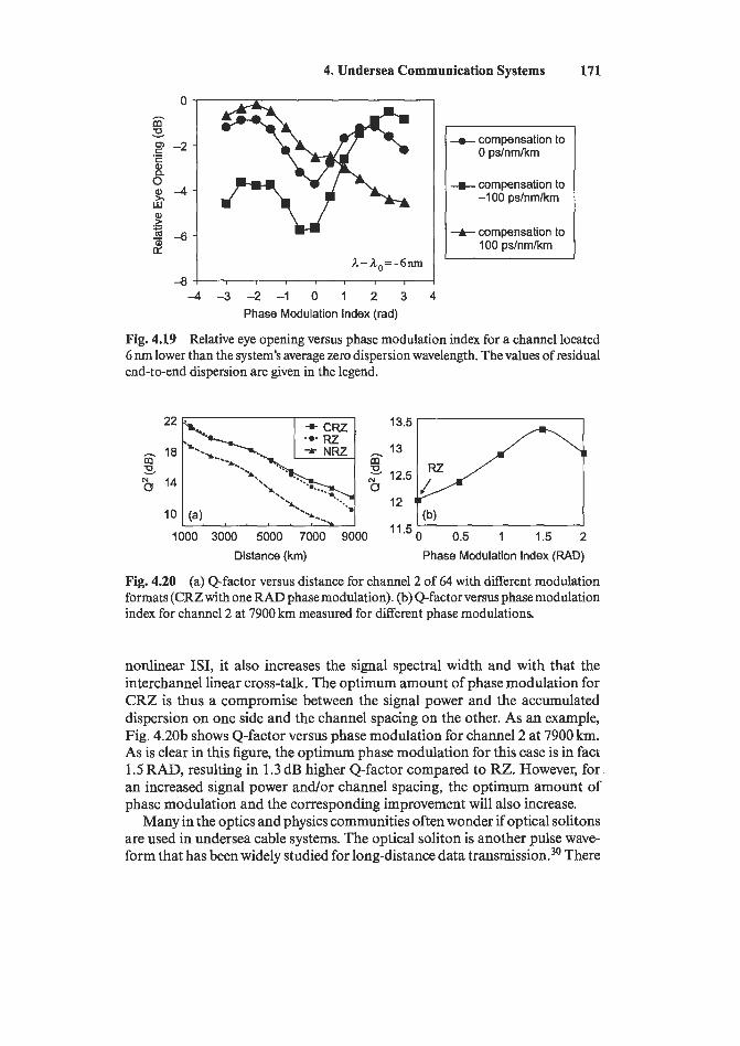
4. Undersea Communication Systems 171
5- p - 2 - -0 v
.- c a,
0" w ; -6-
W a, > .- e
rY
-8
0-
A - A =-6nm 0 I I I
w
+ compensation to 0 pslnmlkm
+ compensation to
t- compensation to I 100 pslnmlkm
-1 00 pslnmlkm
Fig. 4.19 Relative eye opening versus phase modulation index for a channel located 6 nm lower than the system's average zero dispersion wavelength. The values of residual end-to-end dispersion are given in the legend.
22
- 18 m
14 D v
10
1000 3000 5000 7000 9000 I (b)
0.5 1 1.5 2 11.5
Distance (km) Phase Modulation Index (RAD)
Fig. 4.20 (a) Q-factor versus distance for channel 2 of 64 with different modulation formats (CRZ with one RAD phasemodulation). (b) Q-factor versus phase modulation index for channel 2 at 7900 km measured for different phase modulations.
nonlinear ISI, it also increases the signal spectral width and with that the interchannel linear cross-talk. The optimum amount of phase modulation for CRZ is thus a compromise between the signal power and the accumulated dispersion on one side and the channel spacing on the other. As an example, Fig. 4.20b shows Q-factor versus phase modulation for channel 2 at 7900 km. As is clear in this figure, the optimum phase modulation for this case is in fact 1.5 RAD, resulting in 1.3 dB higher Q-factor compared to RZ. However, for an increased signal power and/or channel spacing, the optimum amount of phase modulation and the corresponding improvement will also increase.
Many in the optics and physics communities often wonder if optical solitons are used in undersea cable systems. The optical soliton is another pulse wave- form that has been widely studied for long-distance data transmis~ion.~~ There
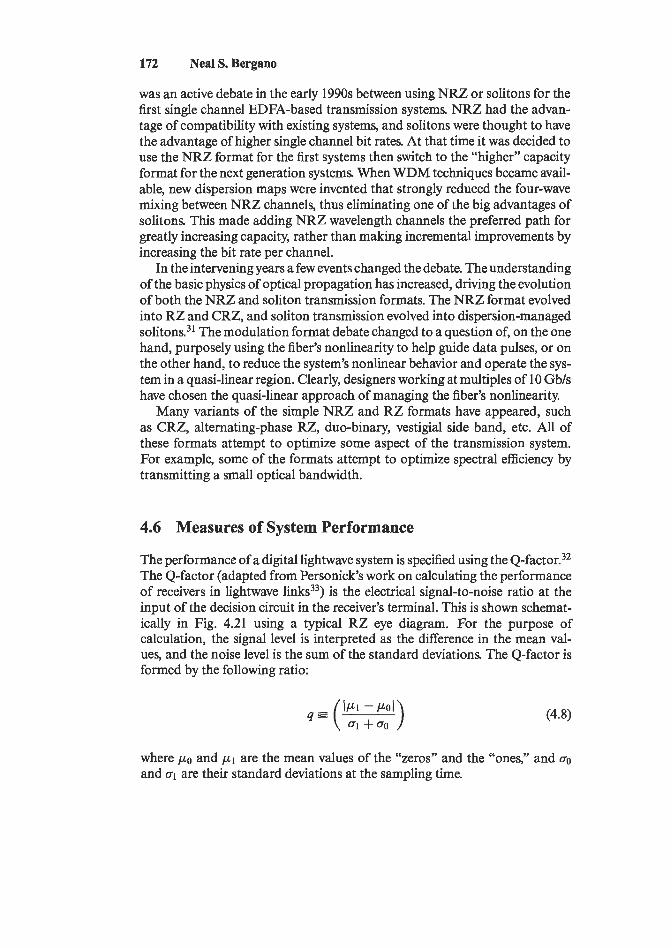
172 Neal S. Bergano
was an active debate in the early 1990s between using NRZ or solitons for the first single channel EDFA-based transmission systems. NRZ had the advan- tage of compatibility with existing systems, and solitons were thought to have the advantage of higher single channel bit rates. At that time it was decided to use the NRZ format for the first systems then switch to the “higher” capacity format for the next generation systems. When WDM techniques became avail- able, new dispersion maps were invented that strongly reduced the four-wave mixing between NRZ channels, thus eliminating one of the big advantages of solitons. This made adding NRZ wavelength channels the preferred path for greatly increasing capacity, rather than making incremental improvements by increasing the bit rate per channel.
In the intervening years a few events changed the debate. The understanding of the basic physics of optical propagation has increased, driving the evolution of both the NRZ and soliton transmission formats. The NRZ format evolved into RZ and CRZ, and soliton transmission evolved into dispersion-managed solitons.31 The modulation format debate changed to a question of, on the one hand, purposely using the fiber’s nonlinearity to help guide data pulses, or on the other hand, to reduce the system’s nonlinear behavior and operate the sys- tem in a quasi-linear region. Clearly, designers working at multiples of 10 Gbls have chosen the quasi-linear approach of managing the fiber’s nonlinearity.
Many variants of the simple NRZ and RZ formats have appeared, such as CRZ, alternating-phase RZ, duo-binary, vestigial side band, etc. All of these formats attempt to optimize some aspect of the transmission system. For example, some of the formats attempt to optimize spectral efficiency by transmitting a small optical bandwidth.
4.6 Measures of System Performance
The performance of a digital lightwave system is specified using the Q-fa~tor.~* The Q-factor (adapted from Personick’s work on calculating the performance of receivers in lightwave links33) is the electrical signal-to-noise ratio at the input of the decision circuit in the receiver’s terminal. This is shown schemat- ically in Fig. 4.21 using a typical RZ eye diagram. For the purpose of calculation, the signal level is interpreted as the difference in the mean val- ues, and the noise level is the sum of the standard deviations. The Q-factor is formed by the following ratio:
lPl - Pol 4 a1+a0)
where PO and p1 are the mean values of the “zeros” and the “ones,” and a0 and a1 are their standard deviations at the sampling time.

4. Undersea Communication Systems 173
Eye Diagram
” P1 Decision Level
.. Po
. ... . . ... . . .
a,
= ... gJ .. s
Sampling time ’ w
5 I
I3 Q
Fig. 4.21 A typical received RZ eye diagram for a lightwave system. A voltage his- togram is schematically shown to indicate the parameters that are included in the definition of Q-factor.
The Q-factor is related to the system’s bit error ratio through the comple- mentary error function, given by:*
M where
or in terms of the more standard error function erf( . ):
where
(4.10)
The Q-factor given in Eq. 4.8 is a unitless quantity expressed as a lin- ear ratio, or it can be expressed in decibels as 20log(q). The factor of 20 (or 10 log (q2)) is used to maintain consistency with the linear noise accumula- tion model. For example, a 3-dB increase in the average launch power in all of the spans results in a 3-dB increase in Q-factor (assuming signal-spontaneous beat noise dominates and ignoring signal decay and fiber nonlinearity). The
*Here I use the definition of erfC(n) as given in MATLAB@ rather than the definition originally given in reference [32]. (MATLAB@ is a product of The Mathworks Inc.)
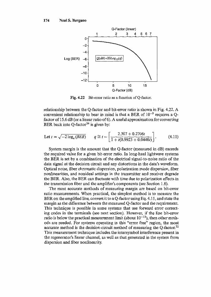
174 Neal S. Bergano
Q-Factor (linear)
Log (BER)
1 2 3 4 5 6 7 0-
-4-
-8-
-10-
-1 2 -_ 0 5 10 15
Q-Factor (dB)
Fig. 4.22 Bit-error ratio as a function of Q-factor.
relationship between the Q-factor and bit-error ratio is shown in Fig. 4.22. A convenient relationship to bear in mind is that a BER of requires a Q- factor of 15.6 dB (or a linear ratio of 6). A useful approximation for converting BER back into Q - f a ~ t o r ~ ~ is given by:
[ 2.307 + 0.2706t Let t = J-2 log, (BER)
System margin is the amount that the Q-factor (measured in dB) exceeds the required value for a given bit-error ratio. In long-haul lightwave systems the BER is set by a combination of the electrical signal-to-noise ratio of the data signal at the decision circuit and any distortions in the data’s waveform. Optical noise, fiber chromatic dispersion, polarization mode dispersion, fiber nonlinearities, and nonideal settings in the transmitter and receiver degrade the BER. Also, the BER can fluctuate with time due to polarization effects in the transmission fiber and the amplifier’s components (see Section 1.8).
The most accurate methods of measuring margin are based on bit-error ratio measurements. When practical, the simplest method is to measure the BER on the ampliiied line, convert it to a Q-factor using Eq. 4.1 1, and state the margin as the difference between the measured Q-factor and the requirement. This technique is possible in some systems that use forward error correct- ing codes in the terminals (see next section). However, if the line bit-error ratio is below the practical measurement limit (about 10-13), then other meth- ods are needed. For systems operating in this “error free” region, the most accurate method is the decision-circuit method of measuring the Q - f a c t ~ r . ~ ~ This measurement technique includes the intersymbol interference present in the regenerator’s linear channel, as well as that generated in the system from dispersion and fiber nonlinearity.
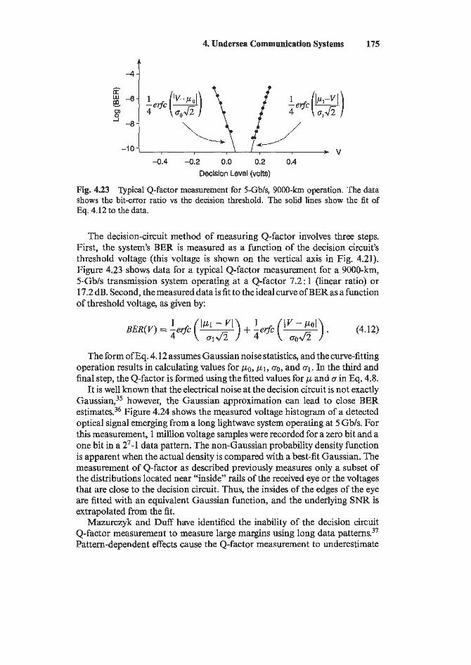
4. Undersea Communication Systems 175
* v -0.4 -0.2 0.0 0.2 0.4
Decision Level (volts)
Fig. 4.23 Typical Q-factor measurement for 5-Gb/s, 9000-km operation. The data shows the bit-error ratio vs the decision threshold. The solid lines show the fit of Eq. 4.12 to the data.
The decision-circuit method of measuring Q-factor involves three steps. First, the system’s BER is measured as a function of the decision circuit’s threshold voltage (this voltage is shown on the vertical axis in Fig. 4.21). Figure 4.23 shows data for a typical Q-factor measurement for a 9OOO-km, 5-Gb/s transmission system operating at a Q-factor 7.2: 1 (linear ratio) or 17.2 dB. Second, the measured data is fit to the ideal curve of BER as a function of threshold voltage, as given by:
The form of Eq. 4.12 assumes Gaussian noise statistics, and the curve-fitting operation results in calculating values for PO, ply 00, and q. In the third and final step, the Q-factor is formed using the fitted values for p and CJ in Eq. 4.8.
It is well known that the electrical noise at the decision circuit is not exactly Gaussian,35 however, the Gaussian approximation can lead to close BER estimates36 Figure 4.24 shows the measured voltage histogram of a detected optical signal emerging from a long lightwave system operating at 5 Gb/s. For this measurement, 1 million voltage samples were recorded for a zero bit and a one bit in a 27-1 data pattern. The non-Gaussian probability density function is apparent when the actual density is compared with a best-fit Gaussian. The measurement of Q-factor as described previously measures only a subset of the distributions located near “inside” rails of the received eye or the voltages that are close to the decision circuit. Thus, the insides of the edges of the eye are fitted with an equivalent Gaussian function, and the underlying SNR is extrapolated from the fit.
Mazurczyk and Duff have identified the inability of the decision circuit Q-factor measurement to measure large margins using long data Pattern-dependent effects cause the Q-factor measurement to underestimate
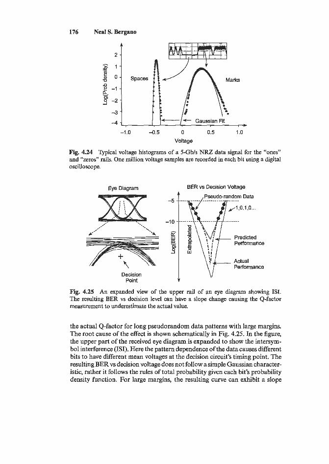
176 Neal S. Bergano
P -1 a,
-3
-4
I
r : t
a/+ Gaussian Fit * -1 .o -0.5 0 0.5 1 .o
Voltage
Fig. 4.24 Typical voltage histograms of a 5-Gb/s NRZ data signal for the “ones” and “zeros” rails. One million voltage samples are recorded in each bit using a digital oscilloscope.
Eye Diagram
-5 ’
-1 0 ‘.., %
Decision Point
Fig. 4.25 An expanded view of the upper rail of an eye diagram showing ISI. The resulting BER vs decision level can have a slope change causing the Q-factor measurement to underestimate the actual value.
the actual Q-factor for long pseudorandom data patterns with large margins. The root cause of the effect is shown schematically in Fig. 4.25. In the figure, the upper part of the received eye diagram is expanded to show the intersym- bo1 interference (ISI). Here the pattern dependence of the data causes different bits to have different mean voltages at the decision circuit’s timing point. The resulting BER vs decision voltage does not follow a simple Gaussian character- istic, rather it follows the rules of total probability given each bit’s probability density function. For large margins, the resulting curve can exhibit a slope

4. Undersea Communication Systems 177
change at BERs less than what is practical to measure, and the extrapolated BER (and Q-factor) is then underestimated. In practice, this is not a serious limitation to characterizing a working system, because typical values of begin- ning of life optical margins are less than 5 or 6 dB. A practical engineering fix to this problem is to measure the Q-factor for a series of word lengths.
It is often useful to know the ideal Q-factor as a starting place for system calculations. Marcuse described the ideal Q - f a ~ t o r ~ ~ considering only accumu- lated noise impairments in terms of the optical SNR. This formalism can be embellished to include other effects such as finite extinction ratio in the trans- mitter and other pulse shapes. For example, assuming a NRZ data format with extinction ratio (I), the ideal Q-factor is given as:
where
2(1 - y = [d],
where& andBE are the optical and electrical bandwidths in the receiver. Later in the section on system design (Section 4.9) we will use Eq. 4.13 to calculate the expected Q-factor using the SNR given by Eq. 4.3 as a starting point for the impairment budget.
4.7 Error Correcting Codes
Up to this point our discussion has focused on the generation of optical signals, propagating them over fiber cables, and detecting them at the far end; that is to say the physics of getting optical data bits across the system. The topic of forward error correction (FEC) codes approaches the subject of data trans- mission from a more classical communications channel perspective, where information is transmitted over a nonideal noisy channel.
FEC adds redundancy or extra information to the original input data before it is converted to an optical signal (Fig. 4.26). The decoder in the receiver uses this redundant information to identify and correct bit errors caused by the transmission channel. The result of this added information is that the actual transmitted bit rate is larger than the rate of the input data. For example, a 10-Gb/s system employing a 23% FEC overhead has a transmitted data rate of 12.3 Gb/s.
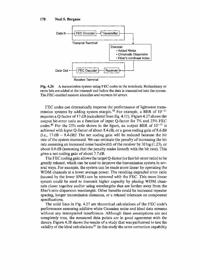
178 Neal S. Bergano
Data In 4 FEC Encoder Transiitter I-, , ......................................................................... Transmit Terminal
Channel: Added Noise Chromatic Dispersion Fiber's nonlinear index
.........................................................................
Data Out I : ........................................................................ ;
Receive Terminal
Fig. 4.26 A transmission system using FEC codes in the terminals. Redundancy or extra bits are added at the transmit end before the data is transmitted into the system. The FEC-enabled receiver identifies and corrects bit errors.
FEC codes can dramatically improve the performance of lightwave trans- mission systems by adding system margin.39 For example, a BER of lo-" requires a Q-factor of 17 dB (calculated from Eq. 4.1 1). Figure 4.27 shows the output bit-error ratio as a function of input Q-factor for 7% and 23% FEC codesa For the 23% code shown in the figure, an output BER of 1O-I' is achieved with input Q-factor of about 8.4 dB, or a gross coding gain of 8.6 dB (i.e., 17 dB - 8.4 dB)! The net coding gain will be reduced because the bit rate of the system increased. We can estimate the penalty of increasing the bit rate assuming an increased noise bandwidth of the receiver by 10 log (1.23)' or about 0.9 dB (assuming that the penalty scales linearly with the bit rate). This gives a net coding gain of about 7.7 dB.
The FEC coding gain allows the target Q-factor (or line bit-error ratio) to be greatly relaxed, which can be used to improve the transmission system in sev- eral ways. For example, the system can be made more linear by operating the WDM channels at a lower average power. The resulting degraded error ratio (caused by the lower SNR) can be removed with the FEC. This more linear system could be used to transmit higher capacity by placing WDM chan- nels closer together and/or using wavelengths that are farther away from the fiber's zero dispersion wavelength. Other benefits could be increased repeater spacing, longer transmission distances, or a relaxed tolerance on component specifications.
The solid lines in Fig. 4.27 are theoretical calculations of the FEC code's performance assuming additive white Gaussian noise and ideal data streams without any intersymbol interference. Although these assumptions are not completely true, the measured data points are in good agreement with the theory. Figure 4.28 shows the results of a study that was performed to test the validity of the ideal ca l~ula t ions~~ In this study the error correction capability
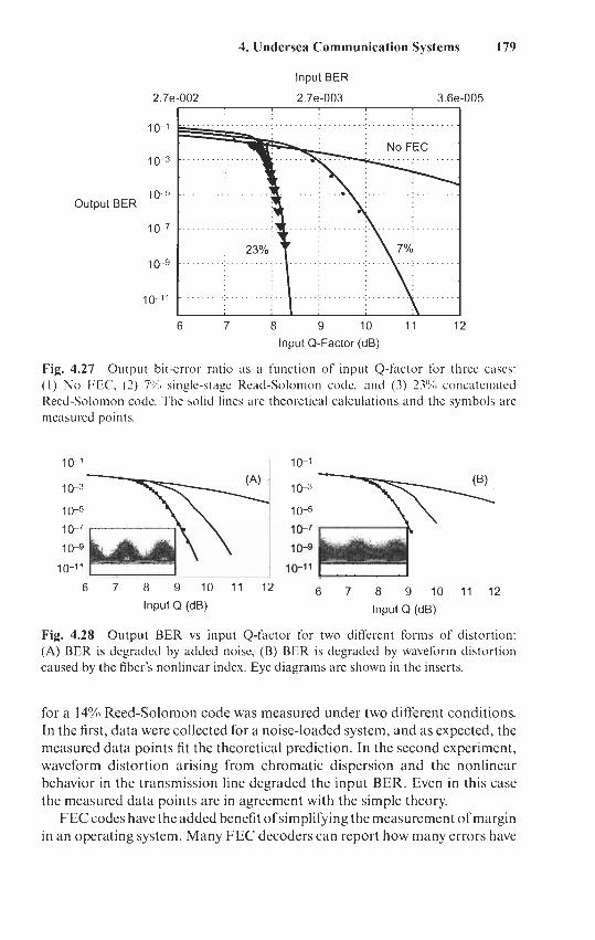
4. Undersea Communication Systems 179
Input BER 2.7e-002 2.7e-003 3.6e-005
I I
IO-‘
I 0-3
I 0-5
I 0-7
Output BER
I 0-9
IO-”
6 7 8 9 10 1 1 12 Input Q-Factor (dB)
Fig. 4.27 Output bit-error ratio as a function of input Q-factor for three cases: (1) No FEC, (2) 7% single-stage Read-Solomon code, and (3) 23% concatenated Reed-Solomon code. The solid lines are theoretical calculations and the symbols are measured points.
6 7 8 9 10 1 1 12 6 7 8 9 10 1 1 12 Input Q (dB) Input Q (dB)
Fig. 4.28 Output BER vs input Q-factor for two different forms of distortion: (A) BER is degraded by added noise, (B) BER is degraded by waveform distortion caused by the fiber’s nonlinear index. Eye diagrams are shown in the inserts.
for a 14% Reed-Solomon code was measured under two different conditions. In the first, data were collected for a noise-loaded system, and as expected, the measured data points fit the theoretical prediction. In the second experiment, waveform distortion arising from chromatic dispersion and the nonlinear behavior in the transmission line degraded the input BER. Even in this case the measured data points are in agreement with the simple theory.
FEC codes have the added benefit of simplifying the measurement of margin in an operating system. Many FEC decoders can report how many errors have
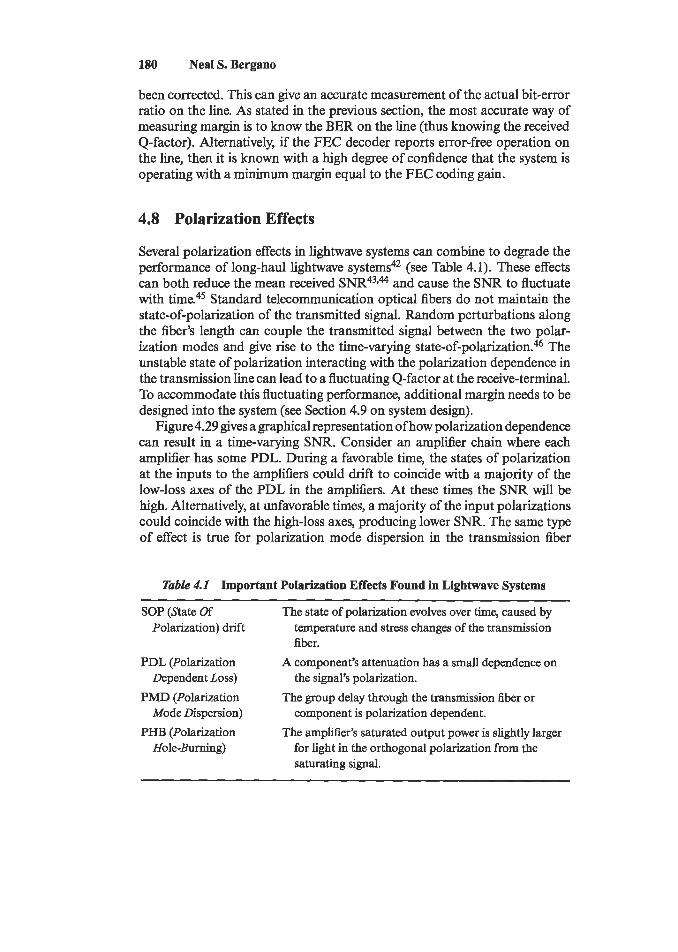
180 Neal S. Bergano
been corrected. This can give an accurate measurement of the actual bit-error ratio on the line. As stated in the previous section, the most accurate way of measuring margin is to know the BER on the line (thus knowing the received Q-factor). Alternatively, if the FEC decoder reports error-free operation on the line, then it is known with a high degree of confidence that the system is operating with a minimum margin equal to the FEC coding gain.
4.8 Polarization Effects
Several polarization effects in lightwave systems can combine to degrade the performance of long-haul lightwave systems42 (see Table 4.1). These effects can both reduce the mean received SNR43344 and cause the S N R to fluctuate with time.45 Standard telecommunication optical fibers do not maintain the state-of-polarization of the transmitted signal. Random perturbations along the fiber’s length can couple the transmitted signal between the two polar- ization modes and give rise to the time-varying state-of-p~larization.~~ The unstable state of polarization interacting with the polarization dependence in the transmission line can lead to a fluctuating Q-factor at the receive-terminal. To accommodate this fluctuating performance, additional margin needs to be designed into the system (see Section 4.9 on system design).
Figure 4.29 gives a graphical representation of how polarization dependence can result in a time-varying SNR. Consider an amplifier chain where each amplifier has some PDL. During a favorable time, the states of polarization at the inputs to the amplifiers could drift to coincide with a majority of the low-loss axes of the PDL in the amplifiers. At these times the SNR will be high. Alternatively, at unfavorable times, a majority of the input polarizations could coincide with the high-loss axes, producing lower SNR. The same type of effect is true for polarization mode dispersion in the transmission fiber
Table 4.1 Important Polarization Effects Found in Lightwave Systems
SOP (State Of Polarization) drift
PDL (Polarization Dependent Loss)
PMD (Polarization Mode Dispersion)
PHB (Polarization Hole-Burning)
~ ~~~~~~~
The state of polarization evolves over time, caused by temperature and stress changes of the transmission fiber.
A component’s attenuation has a small dependence on the signal‘s polarization.
The group delay through the transmission fiber or component is polarization dependent.
The amplifier’s saturated output power is slightly larger for light in the orthogonal polarization from the saturating signal.
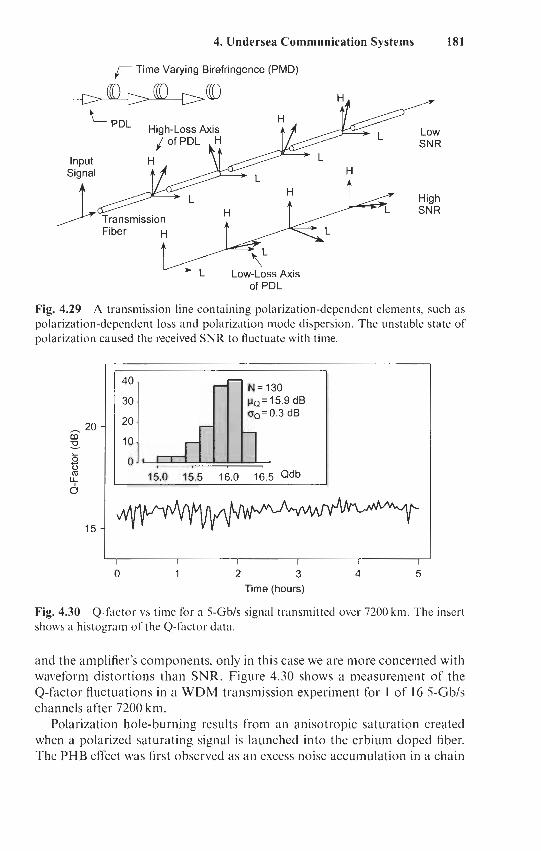
4. Undersea Communication Systems 181
Time Varying Birefringence (PMD)
~~ 'uL HFI+:: SNR Low
Input H Signal rl' A
A H T - .,. ,
- L ~ow-Loss~xis of PDL
Fig. 4.29 A transmission line containing polarization-dependent elements, such as polarization-dependent loss and polarization mode dispersion. The unstable state of polarization caused the received SNR to fluctuate with time.
I I 1 I I I
0 1 2 3 4 5 Time (hours)
Fig. 4.30 Q-factor vs time for a 5-Gb/s signal transmitted over 7200 km. The insert shows a histogram of the Q-factor data.
and the amplifier's components, only in this case we are more concerned with waveform distortions than SNR. Figure 4.30 shows a measurement of the Q-factor fluctuations in a WDM transmission experiment for 1 of 16 5-Gb/s channels after 7200 km.
Polarization hole-burning results from an anisotropic saturation created when a polarized saturating signal is launched into the erbium doped fiber. The PHB effect was first observed as an excess noise accumulation in a chain

182 Neal S. Bergano
of saturated EDFAs,~~ and was later isolated in a single amplifier and iden- tified as PHB.48 The gain difference caused by PHB is quite small in a single amplifier, with a typical value of about 0.07 dB for an amplifier with 3 dB of gain compression. Although PHB is a very small effect in a single EDFA, its effect on the overall performance of an optical amplifier transmission line can be several dBs in received Q-factor.
PHB can cause the amplified spontaneous emission noise to accumulate in the polarization orthogonal to the signal faster than along the parallel axis (Fig. 4.31). Noise accumulates faster than would be predicted by simple noise accumulation theory, and as a result, the signal decays at the expense of the noise. Fortunately, the deleterious effects of PHB can be avoided by depolarizing the total signal propagating in the amplifier chain at a rate faster than the EDFA’s gain recovery time. When the signal’s degree of polarization is low, there is no preferred polarization axis for the gain to be depleted, and the transmission performance returns to the expected value.
Depolarizing the total signal in a WDM system can be performed pas- sively by allowing channels to take on random SOPS or actively by modulating the channel’s polarizations. In a WDM system with many optical channels, the unavoidable PMD in the amplified line causes the different channels to disperse in polarization, which leads to a natural decrease in the degree of polarization. This process can be accelerated by purposely launching the channels in a “pair-wise” orthogonal manner.23
Actual Signal Decay with
Distance (km)
Rg. 4.31 PHB causes the noise in the orthogonal polarization to have an excess gain. If left unchecked, this could lead to noise accumulation faster than would be predicted with simple noise accumulation theory.

4. Undersea Communication Systems 183
Alternatively, the state of polarization can be actively modulated or “scram- bled” at the transmit end of the system. Because the dynamics of the EDFA gain are relatively polarization scrambling the signal at a rate faster than the EDFA can respond to eliminates any excess noise accumulation caused by PHB. The characteristic time constant associated with PHB is similar to the time contents that govern the large signal response of the EDFA, or about 130-200 ~sec.~O To reduce the negative effects of PHB on transmission systems, the SOP of the transmitted optical data signal should be scrambled at a rate that is high compared to the amplifier’s response time. Therefore, polarization scrambling should interchange the optical signal between orthogonal polar- izations at a frequency higher than 1 / 130 sec, or about 7 kHz. Polarization scrambling techniques were particularly important for the first single-channel optical amplifier systems where the degree of polarization launched into the system was potentially large. Performance improvements have been reported for slow-speed ~crambling~lg~~ (i.e., much lower than the bit rate), synchronous scrambling53 (equal to the bit rate), and high-speed ~ c r a m b l i n g ~ ~ . ~ ~ (faster than the bit rate).
4.9 System Design
Thus far, we have reviewed several aspects of optical amplifier transmis- sion technology used in undersea cable systems. This section attempts to put the pieces together by reviewing the design of a 32-channel by lO-Gb/s transatlantic 6000-km system. The goal of the system design is to have ade- quate end-of-life margin considering many of the factors presented thus far, such as degradations caused by optical noise, waveform distortions, Q-factor fluctuations, and system aging. Key design parameters are the repeater spac- ing, launch power, and the dispersion management of the amplified line (Table 4.2).
A 6000-km system will require about 120 repeaters spaced every 50 km. The term repeater is taken from the nomenclature of analog transmission systems. For our purposes, a repeater is the pressure vessel that houses the erbium- doped fiber amplifiers. In ow example the repeater’s EDFA will have a net gain of 10 dB, assuming an average cable attenuation of 0.2 dB/km. A total launch power of about 11 dBm (-4 dBm per channel) is required to produce enough margin. A system bandwidth of about 19 nm is required for 32 channels spaced every 75 GHz (-0.6nm at 1550nm). The dispersion map shown in Fig. 4.10 is used to limit the negative effects of the fiber’s nonlinear index, and each transmitter will use the chirped return to zero format.
The impairment budget (Table 4.3) is a design tool used to account for all of the expected impairments over the system’s lifetime. The starting point is the ideal Q-factor that is calculated considering only the received SNR, cal- culated for example using Eq. 4.3 and Eq. 4.13. From this starting point the
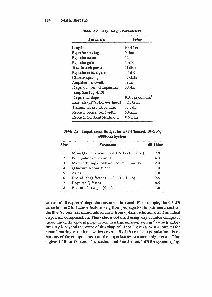
184 Neal S. Bergano
Table 4.2 Key Design Parameters
Parameter Value
Length Repeater spacing Repeater count Repeater gain Total launch power Repeater noise figure Channel spacing Amplifier bandwidth Dispersion period dispersion map (see Fig. 4.10)
Dispersion slope Line rate (23% FEC overhead) Transmitter extinction ratio Receiver optical bandwidth Receiver electrical bandwidth
6000 km 50 km 120 10 dB 11 dBm 4.5 dB 75 GHz 19nm 500 km
0.075 ps/km-nm2 12.3 Gbls 13.7dB 50 GHZ 8.6GHz
Table 4.3 Impairment Budget for a 32-Channel, 10-Gb/s, 6000-km System
~
Line Parameter ~~~
dB Value
1 2 Propagation impairment 3 Manufacturing variations and impairments 4 Q-factor time variations 5 Aging 6 7 Required Q-factor 8
Mean Q value (from simple SNR calculation)
End-of-life Q-factor (1 - 2 - 3 - 4 - 5)
End-of-life margin (6 - 7)
17.8 4.3 2.0 1 .o 1 .o 9.5 8.5 1 .o
values of all expected degradations are subtracted. For example, the 4.3-dB value in line 2 includes effects arising from propagation impairments such as the fiber’s nonlinear index, added noise from optical reflections, and nonideal dispersion compensation. This value is obtained using very detailed computer modeling of the optical propagation in a transmission system56 (which unfor- tunately is beyond the scope of this chapter). Line 3 gives a 2-dB allotment for manufacturing variations, which covers all of the realistic population distri- butions of the components, and the imperfect system assembly process. Line 4 gives 1 dB for Q-factor fluctuation, and line 5 allots 1 dB for system aging.

4. Undersea Communication Systems 185
The Q-factor target of 8.5 dB represents the FEC threshold value shown in Fig. 4.27. The values in the table were recalculated for different launch powers and span lengths until the 1 dB end-of-life figure was reached.
Much of the terminal transmission equipment for undersea systems differs significantly from equipment for terrestrial applications because of the large system-length differences. The transmission terminals include equipment to condition digital data for transmission undersea, power feed equipment to provide DC power to the undersea equipment, and line monitoring equipment to diagnose the location of undersea cable cuts and other undersea faults.
An important part of the undersea cable network's terminal is the power feed equipment used to supply electrical power to the optical amplifiers located in the undersea repeaters. The active components (such as pump lasers) are powered by running a DC current through the copper conductor in the cable. The power feed equipment at the shore terminals supply a constant current of about 1 Ampere at -lO,OOOvolts, where one side of the cable is biased with positive voltage and the other with negative voltage. Interestingly, having a cable conductor across the ocean allows one to determine the ground potential difference between continents, which is typically tens of volts, but can increase significantly during electrical or solar storms.
Figure 4.32 shows a diagram of a typical amplifier pair that is located in an undersea system. A maintenance system is used to identify the location of faults andor degraded components by monitoring the undersea equipment from the shore terminals. An optical monitoring signal is coupled back into the fiber in the reverse direction at a low optical power. The signal-to-noise ratio of this low-level signal is enhanced using signal correlation techniques to provide data on repeater gain, gain tilt, and span attenuation. This approach
Erbium Doped
WDM Fiber Isolator
U ' b

186 Neal S. Bergano
also is synergistic with the use of COTDR (Coherent Optical Time Domain Reflectometer) techniques to identify the location of a cable cut or other fault between repeaters.
4.10 Transmission Experiments
Most long-haul transmission experiments using optical amplifiers fall into one of three categories: circulating test bed^,^^ and special measurements performed on installed systems.59 Circulating-loop transmission measure- ments are by far the most important experimental technique. Circulating-loop techniques applied to an amplifier chain of modest length can provide an experimental platform to study a broad range of transmission phenomena for EDFA-based transmission systems.60
A loop experiment attempts to simulate the transmission performance of a multithousand-kilometer-long system by making multiple passes through an amplifier chain of modest length (Le., hundreds of kilometers). The loop transmission experiment (Fig. 4.33) contains most of the elements found in conventional experiments, such as an optical data transmitterlregenerator pair, a chain of amplifiedfiber sections, and diagnostic equipment such as a bit-error ratio test set (BERTS). In the loop experiment, optical switching is added to allow data to flow into the loop (the load state) and then to circulate (the loop state, Fig. 4.34). The data circuIates for a specified time, after which the state of the experiment toggles, and the Ioacfnoop cycle is repeated.
Load Switch
3dB Coupler BERTS
Clock Gate
-2.4 msec Load /round trip time
J + a i tchL-1 , >: I: I -,. State
hl , , Jnl , , ) Measurement
Gate
Fig. 4.33 Top: Block diagram for a circulating-loop transmission experiment. Bottom: Timing diagram for the experiment showing the optical switch states and the time gate for making measurements.
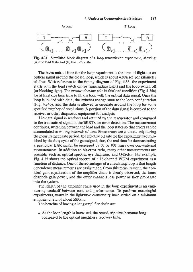
4. Undersea Communication Systems 187
A) Load B) Loop
Fig. 4.34 Simplified block diagram of a loop transmission experiment, showing: (A) the load state and (B) the loop state.
The basic unit of time for the loop experiment is the time of flight for an optical signal around the closed loop, which is about 4.89 wsec per kilometer of fiber. With reference to the timing diagram of Fig. 4.33, the experiment starts with the load switch on (or transmitting light) and the loop switch off (or blocking light). The two switches are held in this load condition (Fig. 4.34a) for at least one loop time to fill the loop with the optical data signal. Once the loop is loaded with data, the switches change state to the loop configuration (Fig. 4.34b), and the data is allowed to circulate around the loop for some specified number of revolutions. A portion of the data signal is coupled to the receiver or other diagnostic equipment for analysis.
The data signal is received and retimed by the regenerator and compared to the transmitted signal in the BERTS for error detection. The measurement continues, switching between the load and the loop states so that errors can be accumulated over long intervals of time. Since errors are counted only during the measurement gate period, the effective bit rate for the experiment is dimin- ished by the duty cycle of the gate signal; thus, the real time for demonstrating a particular BER might be increased by 50 or 100 times over conventional measurements. In addition to bit-error ratio, many other measurements are possible, such as optical spectra, eye diagrams, and Q-factor. For example, Fig. 4.35 shows the optical spectra of a 16-channel WDM experiment as a function of distance. One of the advantages of a circulating loop is that length dependence measurements are easily made. From this measurement, the non- ideal gain equalization of the amplifier chain is clearly observed; the inner channels gain power, and the outer channels lose power as they propagate into the system.
The length of the amplifier chain used in the loop experiment is an engi- neering tradeoff between cost and performance. To perform meaningful experiments, many in the lightwave community have settled on a minimum amplifier chain of about 500 km.
The benefits of having a long amplifier chain are:
0 As the loop length is increased, the round-trip time becomes long compared to the optical amplifier’s recovery time.
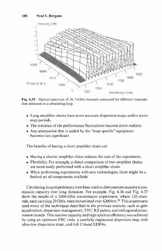
188 Neal S. Bergano
Intensity (dB) -
i 62
Distance (krn) 1558
i 5 5 6 ‘ 1554
1552 Wavelength (nrn) 0
Fig. 4.35 Optical spectrum of 16, 5-Gbls channels measured for different transmis- sion distances in a circulating loop.
0 Long amplifier chains have more accurate dispersion maps and/or more
0 The statistics of the performance fluctuations become more realistic. 0 Any attenuation that is added by the “loop specific” equipment
map periods.
becomes less significant.
The benefits of having a short amplifier chain are:
0 Having a shorter amplifier chain reduces the cost of the experiment. 0 Flexibility. For example, a direct comparison of two amplifier chains
0 When performing experiments with new technologies, there might be a are more easily performed with a short amplifier chain.
limited set of components available.
Circulating-loop experiments have been used to demonstrate massive trans- mission capacity over long distances. For example, Fig. 4.36 and Fig. 4.37 show the results of a 2400-Gb/s transmission experiment, where 120 chan- nels, each carrying 20 Gb/s, were transmitted over 6200 km.61 This experiment used many of the techniques described in the previous sections, such as gain equalization, dispersion management, FEC, RZ pulses, and orthogonal polar- ization launch. This massive capacity and high spectral efficiency was achieved by using an optimum FEC code, a carefully engineered dispersion map with ultra-low dispersion slope, and full C-band EDFAs.

4. Undersea Communication Systems 189
-20 y I I I I
1525 1535 1545 1555 1565 Wavelength (nrn)
Fig. 4.36 Optical spectrum of 120 channels, each carrying 20 Gb/s, measured in a circulating loop after propagating over 6200 km. The channel spacing was 42 GHz (AA. x 0.33 nm). Note that the channels near 1535 nm were purposely omitted because of insufficient BER performance caused by low SNR.
12
8 8 1525 1535 1545 1555 1565
Wavelength [nm]
Fig. 4.37 Q-factor of 120 channels, each carrying 20 Gb/s, measured in a circulating loop after propagating over 6200 km.
4.11 Future Trends in Long-Haul Optical Transmission Systems
The capacity of undersea fiber-optic systems will increase by using more opti- cal bandwidth and by using the available bandwidth more efficiently. The conventional pass-band of the EDFA (C-band) is about 40nm wide, in the wavelength range of roughly 1526 to 1566 nm, corresponding to optical fre- quencies of 196.5 to 191.4THz. Thus, the conventional erbium band has about 5 THz of bandwidth available for data transmission. The ultimate dig- ital capacity that can be “fit” into the EDFA’s C-band will depend on how efficiently this bandwidth can be used for data transmission. This spectral effi- ciency, expressed in (Bits/second)/Hz, is defined as the system’s average digital

190 Neal S. Bergano
" 'I.. j 0000 Total Capacity 0 .
capacity divided by the average optical bandwidth of the system. The best- reported spectral efficiencies in WDM transmission range from 1 .O bits/sec/Hz for very short (-100 km) distances, to roughly 0.5 bits/sec/Hz for transoceanic distance (Fig. 4.38). For example, the data shown in Fig. 4.36 represents a spectral efficiency of about 0.48 bits/sec/Hz. Assuming that this spectral effi- ciency could be achieved (with realistic margin) gives an upper limit on the C-band capacity of about 2.5TB/s on a single fiber. Table 4.4 gives some representative values for the optical bandwidth required to achieve a total transmission capacity for different spectral efficiencies.
in GBIs 0. .
e..: 9. 30;)' --. . *. -9.. *'..,f400 *'. ....
*e.. 9.
d- q o o *.. *-a..po , a. 0 . ***-*w.@oo
"'-.,. I000
9. *. 0..
# -3FEO =.. *. .3200 -. .. 180( **..
*. -9 . With FEC -1 0 Without FEC 6.8
- m
:,ooo -
1000 i: 0
v)
- g 0.2
I I I I I I I '
100 200 500 1,000 2,000 5,000 10,000
Transmission Distance (km)
Fig. 4.38 Spectral efficiency of recently published transmission experiments as a func- tion of transmission distance. The data points list the total capacities. Experiments that used FEC are displayed with a different symbol.
Table 4.4 The Relationship between Total Capacity, Spectral Efficiency, and Required Optical Bandwidth (The required
optical bandwidth is calculated assuming a center wavelength of 1545 nm. The missing entries calculate to a bandwidth that
is much larger than 80 nm.)
640 Gb/s 1280 Gb/s 2560 Gb/s 5120 Gb/s
0.1 (B/s)/Hz 50.9nm 102nm - - 0.3 (B/s)/Hz 16.7nm 34.2nm 67.6nm - 0.5 (B/s)/Hz 10.2nm 20.4nm 40.7nm 81.5nm 1.0 (B/s)/Hz 5.1 nm 10.2nm 20.3nm 40.7nm

4. Undersea Communication Systems
Cable “Repeater” Cable “Repeater”
Fig. 4.39 An amplifier chain with both EDFAs and Raman gain.
191
+
The performance of the C-band could also be improved by using a combina- tion of Raman gain with the EDFA as shown in Fig. 4.39. Here Raman gain in the transmission fiber is used to “assist” the EDFA gain, which lowers the accu- mulated noise, thus increasing the SNR. Alternatively, the same SNR could be achieved while lowering the signal power, thus reducing the nonlinear effects.62
The system’s total capacity could also be improved by increasing the number of optical fibers in the cable. This becomes an engineering challenge to make the optical amplifiers more efficient in physical space, given the limited amount of space in the pressure vessels, and require less electrical power, given the practical limits of electrical power transmission in the cable.
We can continue to use this bandwidthhpectral efficiency idea to estimate the ultimate capacity of a transoceanic-length system (practicality notwith- standing). The low attenuation window of typical telecommunications-grade optical fibers is about 120 nm wide and extends from approximately 1500 to 1620 nm, corresponding to -1 5 THz. Assuming the same 0.5 bits/sec/Hz spec- tral efficiency yields a potential capacity of about 7.5 TB/s. Erbium amplifiers can cover about 2/3 of this bandwidth by using both the C-band and the newer “Long” wavelength band (or L-band) in the wavelength range of about 1570 to 1610nm. The leading optical amplifier candidate for the remaining short wavelength band (S-band) is stimulated Raman gain, which would be accomplished by pumping the transmission fiber at - 1430 nm.
Commensurate with the required wide-band optical amplifier, is the need for wide-band transmission fibers that have a “flattened” chromatic disper- sion characteristic. Such fibers have been reported recently that extend the concept of dispersion mapping by alternating both the sign and the slope of the d i s p e r s i ~ n . ~ ~ , ~ The resulting fiber spans have relatively constant disper- sion value over a broad bandwidth (Fig. 4.40). Ultimately, one could envision using the entire pass-band of the transmission fiber from 1300 to 1700 nm, cor- responding to 55 THz. This would pose many challenges to fiber and system designers. For example, a very broadband optical amplifier would be needed (or combinations of amplifiers), and the added attenuation of the fiber at the shorter wavelengths would decrease the signal-to-noise ratios for WDM channels in that region.
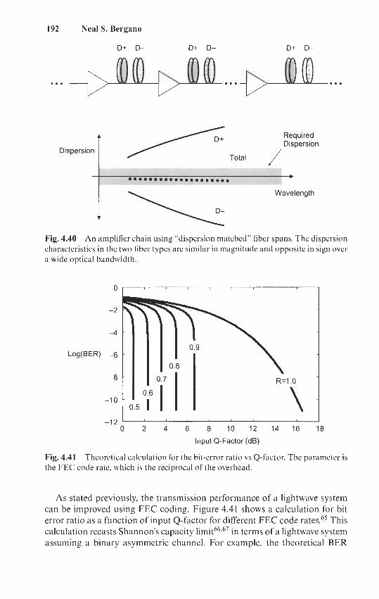
192 Neal S. Bergano
D+ D- D+ D- D+ D-
... ... ...
.................... b
Fig. 4.40 An amplifier chain using “dispersion matched” fiber spans. The dispersion characteristics in the two fiber types are similar in magnitude and opposite in sign over a wide optical bandwidth.
0
-2
-4
Log(BER) -6
-8
-1 0
0.8
0.7 R=l .O
\ -1 2
0 2 4 6 8 10 12 14 16 18
Input Q-Factor (dB)
Fig. 4.41 the FEC code rate, which is the reciprocal of the overhead.
Theoretical calculation for the bit-error ratio vs Q-factor. The parameter is
As stated previously, the transmission performance of a lightwave system can be improved using FEC coding. Figure 4.41 shows a calculation for bit error ratio as a function of input Q-factor for different FEC code rates.65 This calculation recasts Shannon’s capacity limit66,67 in terms of a lightwave system assuming a binary asymmetric channel. For example, the theoretical BER
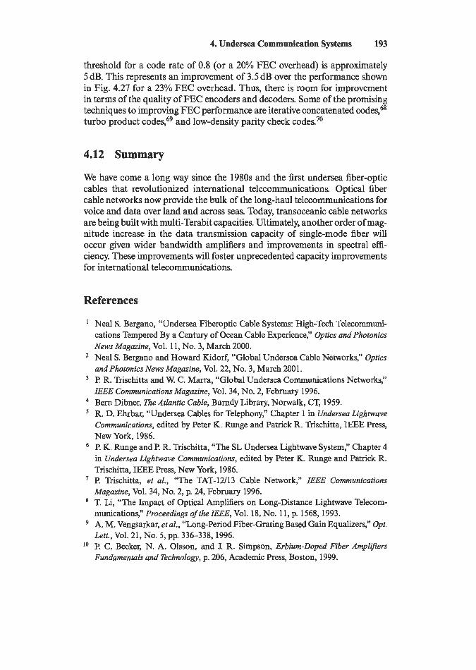
4. Undersea Communication Systems 193
threshold for a code rate of 0.8 (or a 20% FEC overhead) is approximately 5 dB. This represents an improvement of 3.5 dB over the performance shown in Fig. 4.27 for a 23% FEC overhead. Thus, there is room for improvement in terms of the quality of FEC encoders and decoders. Some of the promising techniques to improving FEC performance are iterative concatenated codesY6* turbo product codes,69 and low-density parity check codes.70
4.12 Summary
We have come a long way since the 1980s and the first undersea fiber-optic cables that revolutionized international telecommunications. Optical fiber cable networks now provide the bulk of the long-haul telecommunications for voice and data over land and across seas. Today, transoceanic cable networks are being built with multi-Terabit capacities. Ultimately, another order of mag- nitude increase in the data transmission capacity of single-mode fiber will occur given wider bandwidth amplifiers and improvements in spectral effi- ciency. These improvements will foster unprecedented capacity improvements for international telecommunications.
References
Neal S. Bergano, “Undersea Fiberoptic Cable Systems: High-Tech Telecomuni- cations Tempered By a Century of Ocean Cable Experience,” Optics and Photonics News Magazine, Vol. 11, No. 3, March 2000. Neal S. Bergano and Howard Kidorf, “Global Undersea Cable Networks,” Optics and Photonics News Magazine, Vol. 22, No. 3, March 2001. F! R. Trischitta and W. C. Marra, “Global Undersea Communications Networks,” IEEE Communications Magazine, Vol. 34, No. 2, February 1996. Bern Dibner, The Atlantic Cable, Burndy Library, Norwalk, CT, 1959. R. D. Ehrbar, “Undersea Cables for Telephony,” Chapter 1 in Undersea Lightwave Communications, edited by Peter K. Runge and Patrick R. Trischitta, IEEE Press, New York, 1986. P. K. Runge and P. R. Trischitta, “The SL Undersea Lightwave System,” Chapter 4 in Undersea Lightwave Communications, edited by Peter K. Runge and Patrick R. Trischitta, IEEE Press, New York, 1986. P. Trischitta, et al., “The TAT-12/13 Cable Network,” IEEE Communications Magazine, Vol. 34, No. 2, p. 24, February 1996.
* T. Li, “The Impact of Optical Amplifiers on Long-Distance Lightwave Telecom- munications,’’ Proceedings ofthe IEEE, Vol. 18, No. 11, p. 1568, 1993. A. M. Vengsarkar, et al., “Long-Period Fiber-Grating Based Gain Equalizers,” Opt. Lett., Vol. 21, No. 5, pp. 336-338, 1996.
lo P. C. Becker, N. A. Olsson, and J. R. Simpson, Erbium-Doped Fiber Amplijiers Fundamentals and Technology, p. 206, Academic Press, Boston, 1999.
194 Neal S. Bergano
l1 J. P. Gordon and L. F. Mollenauer, “Effects on Fiber Nonlinearities and Amplifier Spacing on Ultra-Long Distance Transmission,” Journal of Lightwave Communica- tion, Vol. 9, No. 2, p. 170, 1991.
l2 E. Lichtman, “Optimal Amplifier Spacing in Ultra-Long Lightwave Systems,” Electronics Letters, Vol. 29, p. 2058, 1993.
l3 C. R. a l e s and E. Desurvire, “Propagation of Signal and Noise in Concatenated Erbium-Doped Fiber Amplifiers,” Journal of Lightwave Technology, Vol. 9, No. 2, p. 147, 1991.
l4 A. K. Srivastava, et al., “Room Temperature Spectral Hole-Burning in Erbium- Doped Fiber Amplifiers,” in Proc. Optical Fiber Con$, p. 33, San Jose, CA, 1996.
l5 A. R. Chraplyvy, J. A. Nagel, and R. W. Tkach, “Equalization in Amplified WDM Lightwave Transmission Systems,” IEEE Photonics Technology Letters, Vol. 4, No. 8, August 1992.
l6 G. P. Agrawal, “Group-Velocity Dispersion,” Chapter 3 in Nonlinear Fiber Optics, edited by Ivan P. Kaminow and Thomas L. Koch, Academic Press, Boston, 1989.
l7 A. H. Gnauck and R. M. Jopson, “Dispersion Compensation for Optical Fiber Systems,” Chapter 7 in Optical Fiber Telecommunications IIU, edited by Ivan F? Kaminow and Thomas L. Koch, Academic Press, Boston, 1997.
’* G. P. Agrawal, Nonlinear Fiber Optics, Academic Press, Boston, 1989. l9 D. Marcuse, A. R. Chraplyvy, and R. W. Tkach, “Effects of Fiber Nonlinearity
on Long-Distance Transmission,” Journal of Lightwave Technology, Vol. 9, No. 1,
2o F. Forghieri, R. W. Tkach, and A. R. Chraplyvy, “Fiber Nonlinearities and Their Impact on Transmission Systems,” Chapter 8 in Optical Fiber Telecommunications IIIA, edited by Ivan P. Kaminow and Thomas L. Koch, Academic Press, Boston, 1997.
21 T. Naito, T. Terahara, T. Chikama, and M. Suyama, “Four 5-Gbith WDM Transmission Over 4760-km Straight-Line Using Pre- and Post-Dispersion Com- pensation and FWM Cross-Talk Reduction,” Optical Fiber Communications, OFC
22 A. Puc, F. W Kerfoot, A. Simons, and D. L. Wilson, “Concatenated FEC Exper- iment Over 5000-km-long Straight Line WDM Test Bed,” OFC ’99 Paper ThQ6, San Diego, CA.
23 Neal S. Bergano and C. R. Davidson, “Method and Apparatus for Improving Spectral Efficiency in Wavelength Division Multiplexed Transmission Systems,” United States Patent 6,134,033, issued October 17,2000.
z4 Neal S. Bergano, et al., “320 Gb/s WDM Transmission (64 x 5 Gb/s) over 7,200 km using Large Mode Fiber Spans and Chirped Return-to-Zero Signals,” OFC ’98, paper PD12, San Jose, CA, February 1998.
25 E. A. Golovchenko, Neal S. Bergano, and C. R. Davidson, “Four-Wave Mixing in Multispan Dispersion-Managed Transmission Links,” IEEE Photonics Technology Letters, Vol. 10, No. 10, October 1998.
26 Bell Telephone Laboratories, Transmission Systems for Communications, Fifth Edition, Chapter 30, p. 741, Bell Telephone Laboratories, Inc., 1982.
pp. 121-128,1991.
’96, pp. 182-183, 1996.
4. Undersea Communication Systems 195
27 Bell Telephone Laboratories, Transmission Systems for Communications, Fifth Edition, Chapter 30, p. 741, Bell Telephone Laboratories, Inc., 1982.
28 Ekaterina A. Golovchenko, Alexei N. Pilipetskii, and Neal S. Bergano, “Trans- mission Properties of Chirped Return-to-Zero Pulses and Nonlinear Intersymbol Interference in 10 Gbls WDM Transmission,” OFC 2000, paper FC3, Baltimore, MD, March 2000.
29 B. Bakhshi, M. Vaa, E. A. Golovchenko, W. W. Patterson, R. L. Maybach, and Neal S. Bergano, “Comparison of CRZ, RZ, and NRZ Modulation Formats in a 64 x 12.3 Gbls WDM Transmission Experiment Over 9000 km,” OFC 2001, paper WF4, Anaheim, CA, March 2001.
30 L. F. Mollenauer, J. P. Gordon, and P. V, Mamyshev, “Solitons in High Bit-Rate Long-Distance Transmission,” Chapter 12 in Optical Fiber Telecommunications IIIA, edited by Ivan P. Kaminow and T. L. Koch, Academic Press, Boston, 1997.
31 M. I. Suzuki, et al., “Reduction of Gordon-Haus Timing Jitter by Periodic Disper- sion Compensation in Soliton Transmission,” Electronics Letters, Vol. 3 1, No. 23, p. 2027, 1995.
32 Neal S. Bergano, E W. Kerfoot, and C. R. Davidson, “Margin Measurements in Optical Amplifier Systems,” IEEE Photonics Technology Letters, Vol. 5, No. 3, March 1993.
33 S. D. Personick, “Receiver Design for Digital Fiber Optic Communications Systems,” Bell System Technical Journal, Vol. 52, No. 6, pp. 843-886, 1973.
34 Cecil Hastings, Jr., Approximations for Digital Computers, Princeton University Press, Princeton, p. 191, 1955.
35 D. Marcuse, “Derivation of Analytical Expressions for the Bit-Error Probability in Lightwave Systems with Optical Amplifiers,” Journal of Lightwave Technology, Vol. 8, pp. 18161823, 1990.
36 P. A. Humblet and M. Azizoglu, “On the Bit Error Rate of Lightwave Systems with Optical Amplifiers,” JournaZ of Lightwave Technology, Vol. 9, pp. 15761582, 1991.
37 V, J. Mamczyk and D. G. Duf, “Effect of Intersymbol Interference on Signal-to- Noise Measurements,’’ Conference on Optical Fiber Communications, paper WQ1, 1995.
38 D. Marcuse, “Derivation of Analytical Expressions for the Bit-Error Probability in Lightwave Systems with Optical Amplifiers,’’ Journal of Lightwave Technology, Vol. 8, pp. 18161823, December 1990.
39 N. Ramanujam, et al., “Forward Error Correction (FEC) Techniques in Long- Haul Optical Transmission Systems,” Paper WE1 presented at the LEOS Annual Meeting, Vol. 2, p. 405,2000. C. R. Davidson, et al., “1800Gbls Transmission of One Hundred and Eighty 10 Gbls WDM Channels over 7,000 km using the Full EDFA C-Band,” Paper PD25 at the conference on Optical Fiber Communications OFC 2000, March 2000.
41 H. Kidorf, et al., “Performance Improvement in High-Capacity, Ultra-Long Distance, WDM Systems using Forward Error Correction Codes,” Paper ThS3 presented at the conference on Optical Fiber Communications OFC 2000, p. 274, March 2000.

196 Neal S. Bergano
42 C. D. Poole and J. Nagel, “Polarization Effects in Lightwave Systems,” Chapter 6 in Optical Fiber Telecommunications IIIa, edited by I. Kaminow and T. Koch, Academic Press, Boston, 1997.
43 E. Lichtmann, “Performance Degradation Due to Polarization Dependent Gain and Loss in Lightwave Systems with Optical Amplifiers,” Electronics Letters, Vol.
F. Bruyere and 0. Audouin, “Penalties in Long-Haul Optical Amplifier Systems Due to Polarization Dependent Loss and Gain,” IEEE Photon. Tech. Lett., Vol. 6, No. 5, pp. 654-656, 1994.
45 S. Yamamoto, N. Edagawa, H. Taga, Y. Yoshida, and H. Wakabayashi, “Obser- vation of BER Degradation Due to Fading in Long-Distance Optical Amplifier System,” Electronics Letters, Vol. 29, No. 2, pp. 209-210, 1993.
46 R. E. Wagner, C. D. Poole, H. J. Schulte, N. S. Bergano, V. P. Nathu, J. M. Amon, R. L. Rosenberg, and R. C. Alferness, “Polarization Measurements on a 147-km Lightwave Undersea Cable,” in Technical Digest of OFC ’86, Paper PDP7, Atlanta, GA, February 24-26,1986.
47 M. G. Taylor, “Observation of New Polarization Dependence Effect in Long-Haul Optically AmpUied System,” OFC ’93, Post-deadline paper, PDS, San Jose, CA, 1993.
48 V. J. Mazurczyk and J. L. Zyskind, “Polarization Hole-Burning in Erbium-Doped Fiber Amplifiers,” CLEO ’93, Post-deadline paper, CPD26, Baltimore, MD, 1993.
49 E. Desurvire, C. R. Giles, and J. R. Simpson, “Gain Saturation Effects in High- Speed, Multichannel Erbium-doped Fiber Amplifiers at h = 1.53 pm,” Journal of Lightwave Technology, Vol. 7, No. 7, pp. 2095-2104, December 12,1989.
50 Neal S. Bergano, “The Time Dynamics of Polarization Hole Burning in Erbium- Doped Fiber Amplifiers,” OFC ’94, San Jose, CA, 1994.
51 Neal S. Bergano, V. J. Mazurczyk, and C. R. Davidson, “Polarization Scrambling Improves SNR Performance in a Chain of EDFAs,” OFC ’94, San Jose, CA, 1994.
52 M. G. Taylor, “Improvement in Q with Low-Frequency Polarization Modulation on Transoceanic EDFA Link,” IEEE Photonics Technology Letters, Vol. 6, No. 7, pp. 860-862, July 1994.
53 Neal S. Bergano, C. R. Davidson, and F. Heismann, “Bit-Synchronous Polarization and Phase Modulation Scheme for Improving the Transmission Performance of Optical Amplifier Transmission System,” Electronic Letters, Vol. 32, No. 1, pp. 52-54, January 4,1996.
54 M. G. Taylor and S. J. Penticost, “Improvement in Performance of Long Haul EDFA Link Using High Frequency Polarization Modulation,” Electronics Letters, Vol. 30, No. 10, pp. 805-806, 1994.
55 Y. Fukada, T. Imai, and A. Mamoru, “BER Fluctuation Suppression in Optical In-Line Amplifier Systems Using Polarization Scrambling Technique,” Electronics Letters, Vol. 30, No. 5, pp. 432433, 1994.
56 E. A. Golovchenko, et al., “Modeling of Transoceanic Fiber-optic WDM Commu- nications Systems,” IEEE Journal of Selected Topics in Quantum Electronics, Vol. 6, No. 2, pp. 337-347, March/April2000.
29, NO. 22, pp. 1971-1972,1993.
4. Undersea Communication Systems 197
57 Neal S. Bergano, Jennifer Aspell, C. R. Davidson, P. R. Trischitta, B. M. Nyman, and F. W. Kerfoot, “A 9000-km 5 Gb/s and 21,000-km 2.4 Gb/s Feasibility Demon- stration of Transoceanic EDFA Systems Using a Circulating Loop,” Optical Fiber Communications Conference, PD-13, San Diego, CA, February 18-22,1991.
58 H. Taga, N. Edagawa, H. Tanaka, M. Suzuki, S. Yamamoto, H. Wakabayashi, N. Bergano, C. Davidson, G. Homsey, D. Kalmus, P. Trischitta, D. Gray, and R. Maybach, “10-Gb/s, 9,000-km IM-DD Transmission Experiments Using 274 Er-Doped Fiber Amplifier Repeaters,” Post-deadline Paper, OFC ’93.
59 J. C. Feggeler, et al., “10-Gb/s WDM Transmission Measurements on an Installed Optical Amplifier Undersea Cable System,” Electronics Letters, Vol. 31, No. 19, p. 1676, September 14,1995.
6o Neal S. Bergano and C. R. Davidson, “Circulating Loop Transmission Experiments for the Study of Long-Haul Transmission Systems Using Erbium-Doped Fiber- Amplifiers,” IEEEJournalofLightwave Technology, Vol. 13, No. 5, p. 879, May 1995.
61 J.-X. Cai, M. Nissov, A. N. Pilipetskii, A. J. Lucero, C. R. Davidson, D. Foursa, H. Kidorf, M. A. Mills, R. Menges, P. C. Corbett, D. Sutton, and N. S. Bergano, “2.4 Tb/s (120 x 20 Gb/s) Transmission over Transoceanic Distance with Optimum FEC Overhead and 48% Spectral Efficiency,” OFC 2001, PD-20, March 2001.
62 Balslev C. Clausen, et al., “Modeling and Experiments of Raman Assisted Ultra Long-haul Terrestrial Transmission Over 7500 km,” Paper We.F. 1.2 presented at the 27th European Conference on Optical Communications, Amsterdam, The Netherlands, 2001.
63 Stig Nissen Knudsen and Torben Veng, “Large Effective Area Dispersion Compen- sating Fiber for Cabled Compensation of Standard Single Mode Fiber,” OFC 2000, Paper TUGS, Baltimore, MD, March 2000.
64 M. Tsukitani, et al., “LOW-Loss Dispersion-Flattened Hybrid Transmission Lines Consisting of Low-Nonlinearity Pure Silica Core Fibres and Dispersion Compen- sating Fibers,” Electronics Letters, Vol. 36, No. 1,2000.
65 Y Cai, et al., “Performance Limit of Forward Error Correction Codes in Optical Fiber Communications,” Paper TuF2, presented at the Optical Fiber Communications Conference, Anaheim, CA, 2001.
66 C. E. Shannon, “A mathematical theory of communication,” Bell System Technical Journal, Vol. 27, pp. 379423 and 623-656, July and October, 1948.
67 W Weaver and C. E. Shannon, n e Mathematical Theory of Communication, University of Illinois Press, Urbana, Illinois: 1949, republished in paperback, 1963. 0. Ait Sab, “FEC Techniques in Submarine Transmission Systems,” Paper TuF1, presented at the Optical Fiber Communications Conference, Anaheim, CA, 2001.
69 R. M. Pyndiah, “Near-optimum decoding of product codes: block turbo codes,” IEEE Trans. on Communications, Vol. 46, No. 8, pp. 1003-1010, August 1998.
70 D. J. C. MacKay and R. M. Neal, “Near Shannon limit performance of low density parity check codes,” Electronics Letters, Vol. 32, No. 18, pp. 1645-1646, August 1996.
Chapter 5
John Zyskind, Rick Barry, Graeme Pendock, Michael Cahill, and Jinendra Ranka
High-Capacity, Ultra-Long-Haul Networks
Sycamore NetworkF, Chelmsford, Massachusetts
I. Introduction
The advent of optically amplified transmission and of Dense Wavelength Divi- sion Multiplexing (DWDM) technology has transformed the technology and also the economics of optical network deployments. In less than 10 years, the capacity of a single optical fiber equipped with commercial transmission equipment has increased from a single OC-48 signal, transmitting at a rate of 2.488 Gb/s, to 160 OC-192s signals, totaling 1600 Gb/s, a factor of close to 1000. The economics of DWDM are driving the development and deploy- ment of a new generation of ultra-long-haul DWDM systems for terrestrial networks that can carry these high-capacity data streams over thousands of kilometers. During the same period, driven by the growth of the Internet and other data-based services, the demand for new capacity has exploded and the requirements for the public network have changed dramatically. This chapter will discuss the challenges of high-capacity, ultra-long-haul terrestrial trans- mission systems, the advanced technologies required for such systems, and the architectures of optical networks based on ultra-long-haul transmission capability designed to meet these new demands.
In conventional time-division multiplexed (TDM) regenerated transmis- sion, prevalent until the mid-l990s, one signal was transmitted over its own fiber and, because of the attenuation of the fiber, the signal had to be opto- electronically regenerated approximately every 50 km by a dedicated, 13 IO-nm optoelectronic regenerator, comprising expensive, complex, and bit-rate spe- cific high-speed optical and electronic components, the bandwidth of which limited the capacity of the TDM signal. On the other hand, modern day DWDM systems can carry simultaneously on a single fiber numerous signals, each at the same bit rate as the aforementioned TDM signal, and each carried on a distinct optical wavelength. A single optical amplifier, which amplifies all the signal wavelengths simultaneously, is used periodically to overcome the fiber attenuation in place of the multitude of more complicated regenerators that would be required, one for each signal, in a regenerated TDM system. These technologies dramatically reduce the cost of long-haul transmission capacity, and this dramatic cost reduction has driven the development and
198 OPTICAL FIBER TELECOMMUNICATIONS, VOLUME N B
Copyright 8 2002, Elsevier Science (USA). All rights of repmduction in any form reserved.
ISBN 0-12-395173-9

5. High-Capacity, Ultra-Long-Haul Networks 199
widespread deployment of DWDM as the technology of choice for long-haul telecommunications networks.
Since the introduction of the first commercial DWDM systems in 1995, the capacity of such systems has grown explosively from 8 channels each carrying a DWDM OC-48 signal in the first systems to 160 DWDM channels or more each carrying an OC-192 channel in some recently announced systems. Until recently, these systems were typically able to carry the DWDM signals over dis- tances of 300-600 km without optoelectronic regeneration. As the capacity of such systems has exploded, the cost of terminals and regenerators has become an ever larger fraction of total system cost. Minimizing the number and the cost of regenerators is now a major economic driver in the design of new equipment and the design of carriers’ fiber networks. These economic factors are driving increased channel bit rates from OC-48 (2.488 Gb/s) to OC-192 (9.953 Gb/s) and, in the near future, to OC-768 (39.813 Gb/s) to minimize the number of regenerators, transmitters, and receivers. The demand to reduce system cost is also driving the demand for, and development of, ultra-long-haul terres- trial DWDM systems with reach between regenerators exceeding 2000 km. A hypothetical national-scale fiber network connecting major urban centers of the United States is shown in Fig. 5.1. A backbone network would connect such centers, and much of the traffic arriving at these network nodes would pass through destined for other nodes. The cost benefit lies in avoiding the necessity for expensive optoelectronic regenerators between these nodes and permitting optical pass through of express traffic destined for another node.
Fig. 5.1 Hypothetical national-scale, backbone long-haul network with nodes situated at major urban centers of the United States.
200 John Zyskind et al.
Managing the large bandwith and the large number of channels carried by high capacity DWDM systems represents an unprecedented challenge both for equipment suppliers and for carriers. Applying the conventional technol- ogy of switching and routing low-bit-rate tributaries, for example, at the STS-1 speed, requires very large and expensive switches, and the optical-to-electronic- to-optical (OEO) conversions required for such electronic switching is also increasingly expensive. Optical networking promises a solution to the chal- lenge of managing the immense bandwidth carried by such DWDM systems. The fact that the different signals are encoded on distinct optical wavelengths opens the possibility of optical manipulation, switching, and routing of each individual signal channel using optical filtering and switching technologies to which optics is naturally well suited. For such optical networking to be use- ful, it will be necessary to extend the unregenerated reach of DWDM optical transmission to support the extended optical path lengths that will result.
Transmission of high data rate channels (presently at lOGb/s as in the future at 40 Gbls) over unregenerated links with lengths of 1000 to 5000 km poses major challenges that cannot be met with conventional DWDM tech- nology. Foremost among these problems are the accumulation of optical noise and spectral gain nonuniformity arising from optical amplification, as well as distortion due to transmission effects (including chromatic dispersion, polarization mode dispersion, and optical nonlinearities).
These challenges were first addressed for undersea systems in which both fiber and optical amplifiers are placed under the water while terminals and regenerators are restricted to the shores at the ends of transoceanic links spanning thousands of kilometers (see, for example, Bergano 1997). The undersea elements of transoceanic systems must meet much more stringent reliability requirements than terrestrial systems because of the great expense that deep water ship repairs entail; the range of technologies that can be deployed is thereby strictly limited. However, each undersea deployment is a “green field” system in which the fiber spans, fiber type, and optical ampli- fier spacing can be specially tailored to the link length and designed capacity of that particular system. As a result, there is a great deal of latitude for opti- mization of each system’s design to meet the challenges of ultra-long-haul transmission.
In terrestrial systems, on the other hand, the fiber network is typically already installed, often with a very different system in mind, well before the ultra-long-haul system designer begins. The fiber type is usually already defined and is one of a number of widely deployed, distinct fiber types. The locations of optical amplifiers are predetermined by the locations of hut sites, selected based on the availability of rights of way and the economic incentive to support as few amplifier sites as possible, which as we shall see, is not con- ducive to overcoming the challenges of ultra-long-haul transmission. While terrestrial ultra-long-haul systems certainly have strong similarities to under- sea systems, the differences are significant, and the solutions to the problems

5. High-Capacity, Ultra-Long-Haul Networks 201
Deriodic channel Dower manaoement &
FEC FEC optional dispersion slope management
encoder dispersion decoder
OC192 Tx’s
Raman pump Raman pump
Fig. 5.2 Schematic of an ultra-long-haul transmission system illustrating the use of Raman amplification, FEC, and periodic dispersion slope compensation and power management with a reconfigurable gain-flattening filter.
of ultra-long-haul transmission are quite distinct. Figure 5.2 depicts some of the key features of a high-capacity, ultra-long-haul transmission system which will be discussed in this chapter.
11. Noise and Optical Amplification
A. NOISE IN OPTICALLYAMPLIFIED ULTRA-LONG-HA UL SYSTEMS
The management of optical amplifier noise and the management of transmis- sion distortions of the high-speed optical signals are the two most important considerations in the design of high-capacity, ultra-long-haul transmission systems. This section will focus on the management of amplifier noise, and in Section I11 we will turn to sources of distortion.
The advent of practical optical amplifiers capable of simultaneously ampli- fying multiple signal wavelengths that occupy an appreciable range of the optical spectrum was the key technological advance that ushered in the DWDM revolution. Optical amplifiers are used at the end of each fiber span to boost the power of the DWDM signal channels to compensate for fiber attenuation in the span. EDFAs designed to operate with high inversion pro- vide gain over a spectral range about 30 nm in width, from about 1530 nm to about 1560 nm. This spectral range can support roughly 40 DWDM signal channels with a separation of 100 GHz and 80 channels with a separation of 50 GHz, corresponding to 400 or 800 Gb/s, respectively, for 10 Gb/s OC-192 or STM-64 channels, and in the future, with 40-Gb/s channels, capacities of 1.6Tb/s (1600 Gb/s) for 100-GHz spaced channels. EDFAs designed to oper- ate with lower inversion can provide gain over an even wider spectral range, including the so-called L-band, starting at about 1570 nm, thus offering the opportunity to double the capacity on a single fiber through addition of an L-band EDFA. For a system transmitting over both the C- and L-bands, the

202 John Zyskind et al.
capacity can reach 1.6 Tb/s or more for lO-Gb/s channels spaced at 50 GHz or 3.2 Tb/s or more for 40-Gb/s channels spaced at 100 GHz.
Unfortunately, optical amplification is not possible without the generation of amplified spontaneous emission (ASE), and the noise resulting from this ASE constitutes perhaps the most severe impairment that limits the reach and capacity of such systems. Each optical ampljjier contributes ASE, and these contributions add cumulatively along the amplifier chain. This accumulated ASE gives rise to signal-spontaneous beat noise at the receiver, which is the fundamental noise limit in an optically amplified transmission system. Each EDFA contributes an amount of ASE:
where PME is the ASE power in an optical bandwidth Av, h is Planck’s con- stant, v is the optical frequency, nsp is the spontaneous emission factor, and G is the optical amplifier gain. The spontaneous emission factor, nsp, is deter- mined by the inversion of the amplifier’s Er ions. The contribution of each amplifier’s ASE to the accumulated ASE is characterized by the amplifier’s noise figure, which at high gain is well approximated by NF rz 2nsp.
The signal-spontaneous noise impairment can be characterized in terms of the Optical Signal to Noise Ratio (OSNR), defined as the ratio of the signal channel power to the power of the ASE in a specified optical bandwidth, usu- ally taken by convention to be 0.1 nm. This OSNR target must be sufficient to achieve the required system performance, which for commercial systems is today most often a bit-error rate (BER) of Le., effectively error free. The OSNR target must include sacient margin to provide for any impairments that may be encountered. These include transmission impairments arising, for example, from chromatic dispersion, nonlinearities, and PMD discussed in the following sections; distortions introduced by the transmitter and receiver; amplser gain ripple; manufacturing margin to provide for variances in perfor- mance of parts such as transmitters and receivers produced in a commercial manufacturing environment; and aging both of the system equipment and fiber plant during the expected life of the system. The target OSNR must theoretically increase by 6 dB for each factor of 4 increase in the channel bit rate in order to maintain equivalent noise performance. The actual increase in required OSNR with channel bit rate may be greater than this value due to the greater difficulty in achieving comparable transmitter and receiver perfor- mance at higher bit rates, and because of the greater severity of transmission impairments at higher bit rates, especially for rates as high as 40 Gb/s. As the length of a system increases, and the number of amplifiers contributing ASE increases, the OSNR at the end of the system decreases. The maximum unre- generated reach of an optically amplified system is the length of the system at which the OSNR at its end equals the target OSNR for acceptable system performance. However, the realization of this maximum length is contingent
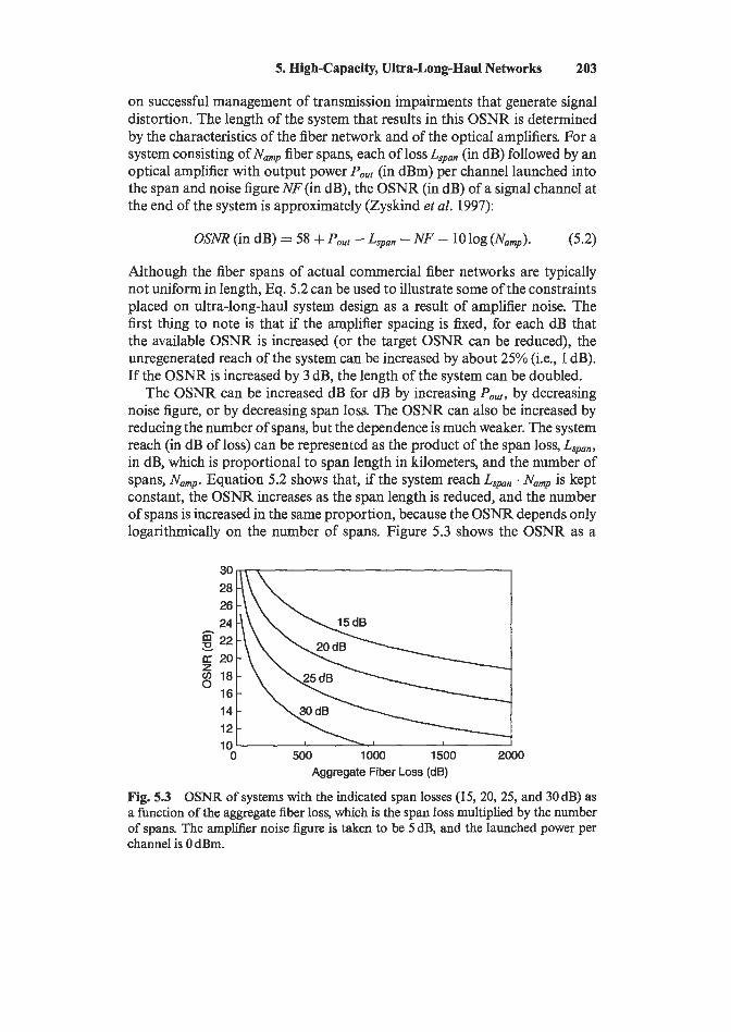
5. High-Capacity, Ultra-Long-Haul Networks 203
on successful management of transmission impairments that generate signal distortion. The length of the system that results in this OSNR is determined by the characteristics of the fiber network and of the optical amplifiers. For a system consisting of NaW fiber spans, each of loss LsPM (in dB) followed by an optical amplifier with output power Pout (in dBm) per channel launched into the span and noise figure NF (in dB), the OSNR (in dB) of a signal channel at the end of the system is approximately (Zyskind et al. 1997):
OSNR (in dB) = 58 + Pout - LsPw - NF - 10 log (Namp). (5.2)
Although the fiber spans of actual commercial fiber networks are typically not uniform in length, Eq. 5.2 can be used to illustrate some of the constraints placed on ultra-long-haul system design as a result of amplifier noise. The first thing to note is that if the amplifier spacing is fixed, for each dB that the available OSNR is increased (or the target OSNR can be reduced), the unregenerated reach of the system can be increased by about 25% (i.e., 1 dB). If the OSNR is increased by 3 dB, the length of the system can be doubled.
The OSNR can be increased dB for dB by increasing Pout, by decreasing noise figure, or by decreasing span loss. The OSNR can also be increased by reducing the number of spans, but the dependence is much weaker. The system reach (in dB of loss) can be represented as the product of the span loss, L,,,, in dB, which is proportional to span length in kilometers, and the number of spans, Namp. Equation 5.2 shows that, if the system reach Lspan . Namp is kept constant, the OSNR increases as the span length is reduced, and the number of spans is increased in the same proportion, because the OSNR depends only logarithmically on the number of spans. Figure 5.3 shows the OSNR as a
0 500 1000 1500 2000 0 500 1000 1500 2000 Aggregate Fiber Loss (dB)
Fig. 5.3 OSNR of systems with the indicated span losses (15, 20, 25, and 30dB) as a function of the aggregate fiber loss, which is the span loss multiplied by the number of spans The amplifier noise figure is taken to be 5 dB, and the launched power per channel is 0 dBm.
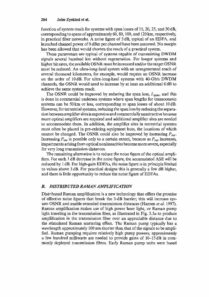
204 John Zyskind et al.
function of system reach for systems with span losses of 15,20,25, and 30 dB, corresponding to spans of approximately 60,80,100, and 120 km, respectively, in practical fiber networks. A noise figure of 5 dB, typical of an EDFA, and launched channel power of 0 dBm per channel have been assumed. No margin has been allowed that would shorten the reach of a practical system.
These parameters are typical of systems capable of transmitting DWDM signals several hundred km without regeneration. For longer systems and higher bit rates, the available OSNR must be increased and/or the target OSNR must be reduced. An ultra-long-haul system with an unregenerated reach of several thousand kilometers, for example, would require an OSNR increase on the order of 10dB. For ultra-long-haul systems with 4O-Gb/s DWDM channels, the OSNR would need to increase by at least an additional 6 dB to achieve the same system reach.
The OSNR could be improved by reducing the span loss, Lspan, and this is done in commercial undersea systems where span lengths for transoceanic systems can be 50 km or less, corresponding to span losses of about 10 dB. However, for terrestrial systems, reducing the span loss by reducing the separa- tion between amplifier sites is expensive and commercially unattractive because more optical amplifiers are required and additional amplifier sites are needed to accommodate them. In addition, the amplifier sites in terrestrial systems must often be placed in pre-existing equipment huts, the locations of which cannot be changed. The OSNR could also be improved by increasing Pout. Increasing Pour is possible only to a certain extent, because as Pour increases, impairments arising from optical nonlinearities become more severe, especially for very long transmission distances.
The remaining alternative is to reduce the noise figure of the optical ampli- fiers. For each 1 dB decrease in the noise figure, the accumulated ASE will be reduced by 1 dB. For high-gain EDFAs, the noise figure is in principle limited to values above 3 dB. For practical designs this is generally a few dB higher, and there is little opportunity to reduce the noise figure of EDFAs.
B. DISTRIBUTED RAlMAN AMPLIFICATION
Distributed Raman ampliiication is a new technology that offers the promise of effective noise figures that break the 3-dB barrier; this will increase sys- tem OSNR and enable extended transmission distances (Hansen et al. 1997). Raman amplification makes use of high power laser light, or Raman pump light traveling in the transmission fiber, as illustrated in Fig. 5 . 3 ~ to produce amplification in the transmission fiber over an appreciable distance due to the stimulated Raman scattering effect. The Raman pump typically has a wavelength approximately 100 nm shorter than that of the signals to be ampli- fied. Raman pumping requires relatively high pump powers; approximately a few hundred milliwatts are needed to provide gains of 10-15dB in com- monly deployed transmission fibers. Early Raman pump units were based
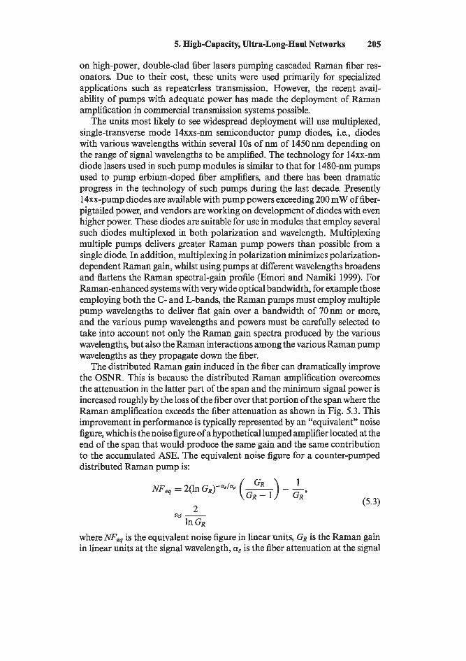
5. High-Capacity, Ultra-Long-Haul Networks 205
on high-power, double-clad fiber lasers pumping cascaded Raman fiber res- onators. Due to their cost, these units were used primarily for specialized applications such as repeaterless transmission. However, the recent avail- ability of pumps with adequate power has made the deployment of Raman amplification in commercial transmission systems possible.
The units most likely to see widespread deployment will use multiplexed, single-transverse mode 14xxs-nm semiconductor pump diodes, i.e., diodes with various wavelengths within several 10s of nm of 1450 nm depending on the range of signal wavelengths to be amplified. The technology for 14xx-nm diode lasers used in such pump modules is similar to that for 1480-nm pumps used to pump erbium-doped fiber amplifiers, and there has been dramatic progress in the technology of such pumps during the last decade. Presently 14xx-pump diodes are available with pump powers exceeding 200 mW of fiber- pigtailed power, and vendors are working on development of diodes with even higher power. These diodes are suitable for use in modules that employ several such diodes multiplexed in both polarization and wavelength. Multiplexing multiple pumps delivers greater Raman pump powers than possible from a single diode. In addition, multiplexing in polarization minimizes polarization- dependent Raman gain, whilst using pumps at different wavelengths broadens and flattens the Raman spectral-gain profile (Emori and Namiki 1999). For Raman-enhanced systems with very wide optical bandwidth, for example those employing both the C- and L-bands, the Raman pumps must employ multiple pump wavelengths to deliver flat gain over a bandwidth of 70nm or more, and the various pump wavelengths and powers must be carefully selected to take into account not only the Raman gain spectra produced by the various wavelengths, but also the Raman interactions among the various Raman pump wavelengths as they propagate down the fiber.
The distributed Raman gain induced in the fiber can dramatically improve the OSNR. This is because the distributed Raman amplification overcomes the attenuation in the latter part of the span and the minimum signal power is increased roughly by the loss of the fiber over that portion of the span where the Raman amplification exceeds the fiber attenuation as shown in Fig. 5.3. This improvement in performance is typically represented by an “equivalent” noise figure, which is the noise figure of a hypothetical lumped amplifier located at the end of the span that would produce the same gain and the same contribution to the accumulated ASE. The equivalent noise figure for a counter-pumped distributed Raman pump is:
2 In GR
%-
(5.3)
where NFeq is the equivalent noise figure in linear units, GR is the Raman gain in linear units at the signal wavelength, as is the fiber attenuation at the signal
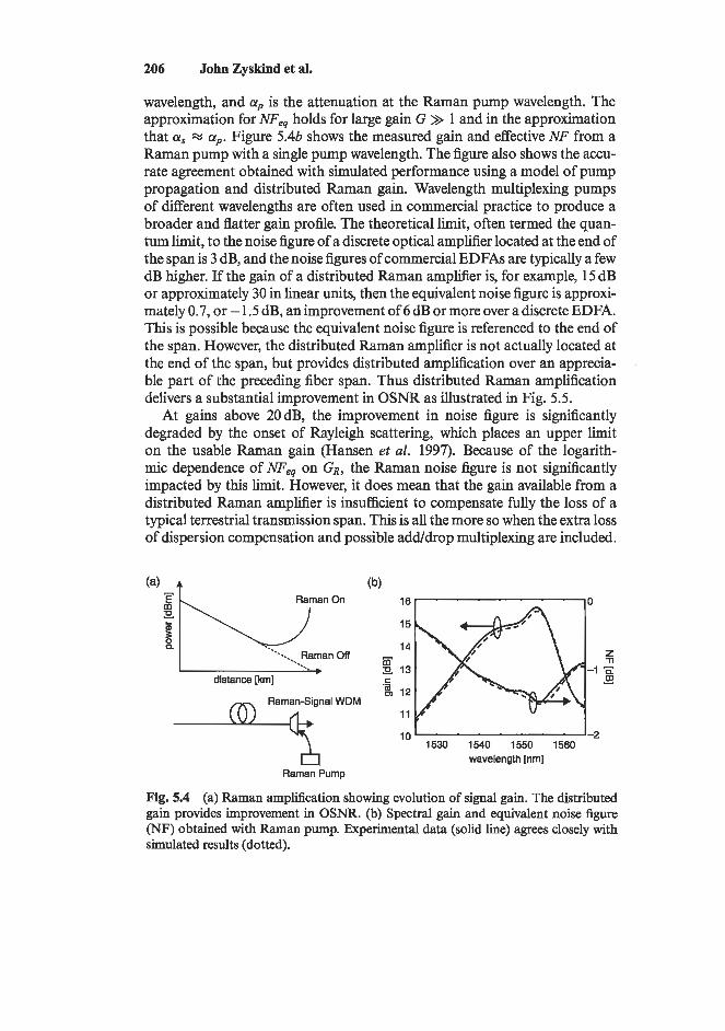
206 John Zyskind et al.
wavelength, and olP is the attenuation at the Raman pump wavelength. The approximation for NF,, holds for large gain G >> 1 and in the approximation that as x 9. Figure 5.4b shows the measured gain and effective NF from a Raman pump with a single pump wavelength. The figure also shows the a m - rate agreement obtained with simulated performance using a model of pump propagation and distributed Raman gain. Wavelength multiplexing pumps of different wavelengths are often used in commercial practice to produce a broader and flatter gain profile. The theoretical limit, often termed the quan- tum limit, to the noise figure of a discrete optical amplifier located at the end of the span is 3 dB, and the noise figures of commercial EDFAs are typically a few dB higher. If the gain of a distributed Raman amplifier is, for example, 15 dB or approximately 30 in linear units, then the equivalent noise figure is approxi- mately 0.7, or -1.5 dB, an improvement of 6 dB or more over a discrete EDFA. This is possible because the equivalent noise figure is referenced to the end of the span. However, the distributed Raman amplifier is not actually located at the end of the span, but provides distributed amplification over an apprecia- ble part of the preceding fiber span. Thus distributed Raman amplification delivers a substantial improvement in OSNR as illustrated in Fig. 5.5.
At gains above 20dB, the improvement in noise figure is significantly degraded by the onset of Rayleigh scattering, which places an upper limit on the usable Raman gain (Hansen et al. 1997). Because of the logarith- mic dependence of NF,, on GR, the Raman noise figure is not significantly impacted by this limit. However, it does mean that the gain available from a distributed Raman amplifier is insufficient to compensate fully the loss of a typical terrestrial transmission span. This is all the more so when the extra loss of dispersion compensation and possible adddrop multiplexing are included.
Raman On I
Raman On
a
distance [km]
Raman-Signal WDM 3 Raman Pump
IO' . . . - 1-2 1530 1540 1550 1560
wavelength [nm]
Fig. 5.4 (a) Raman amplification showing evolution of signal gain. The distributed gain provides improvement in OSNR. (b) Spectral gain and equivalent noise figure (NF) obtained with Raman pump. Experimental data (solid line) agrees closely with simulated results (dotted).
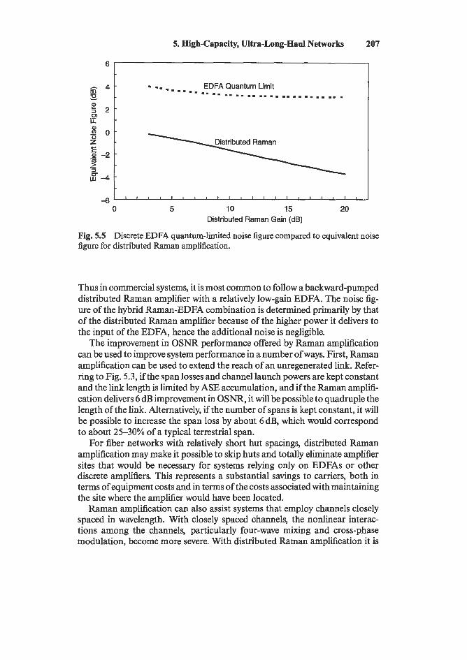
5. High-Capacity, Ultra-Long-Haul Networks 207
0 5 10 15 20 Distributed Raman Gain (dB)
Fig. 5.5 Discrete EDFA quantum-limited noise figure compared to equivalent noise figure for distributed Raman amplification.
Thus in commercial systems, it is most common to follow a backward-pumped distributed Raman amplifier with a relatively low-gain EDFA. The noise fig- ure of the hybrid Raman-EDFA combination is determined primarily by that of the distributed Raman amplifier because of the higher power it delivers to the input of the EDFA, hence the additional noise is negligible.
The improvement in OSNR performance offered by Raman amplification can be used to improve system performance in a number of ways. First, Raman amplification can be used to extend the reach of an unregenerated link. Refer- ring to Fig. 5.3, if the span losses and channel launch powers are kept constant and the link length is limited by ASE accumulation, and if the Raman amplifi- cation delivers 6 dB improvement in OSNR, it will be possible to quadruple the length of the link. Alternatively, if the number of spans is kept constant, it will be possible to increase the span loss by about 6 dB, which would correspond to about 25-30% of a typical terrestrial span.
For fiber networks with relatively short hut spacings, distributed Raman amplification may make it possible to skip huts and totally eliminate amplifier sites that would be necessary for systems relying only on EDFAs or other discrete amplifiers. This represents a substantial savings to carriers, both in terms of equipment costs and in terms of the costs associated with maintaining the site where the amplifier would have been located.
Raman amplification can also assist systems that employ channels closely spaced in wavelength. With closely spaced channels, the nonlinear interac- tions among the channels, particularly four-wave mixing and cross-phase modulation, become more severe. With distributed Raman amplification it is

208 John Zyskind et al.
possible to reduce launched channel powers in order to mitigate the nonlinear interactions while maintaining the link‘s OSNR performance.
Counterpropagating Raman pumping is preferred to copropagating Raman pumping, as this reduces the transfer of pump noise to the signal, as well as pump mediated cross-talk between the signals. Further improvements in OSNR may also be possible through the use of copropagating Raman amplification, and the development of Raman pump sources suitable for copumped distributed Raman amplifiers is an area of active research. The use of second-order Raman pumping in conjunction with first-order counter- pumping (Rottwitt et al. 2000; Dominic et al. 2001) has been proposed, as has the use of low-noise pump sources with a low degree of polarization (Dominic et al. 2001b).
C. FORWARD ERROR CORRECTION
An additional way of improving the system bit error rate without requiring an increase in the OSNR, is by making use of forward error correcting (FEC) codes. With FEC, extra bits are appended to the data by the FEC encoder at the transmitter. These extra bits help the FEC decoder at the receiver to detect and correct bits that become corrupted through transmission. Conse- quently, FEC enables the system to operate at a far lower received OSNR than would be possible without FEC, whilst maintaining an acceptable BER. The system’s target OSNR can be correspondingly reduced, which makes extended transmission distances possible.
The strength of the FEC in correcting errors is characterized in terms of the coding gain, which is the difference in the OSNR at which the system oper- ates with a specified bit error rate (BER) without and with FEC. The coding gain is usually defined at the system’s target BER, for example for many 10-Gb/s-based and 40-Gbh-based terrestrial systems. The serial addition of the extra bits with FEC increases the bit rate. There are penalties associated with the expanded serial bit rate of FEC-encoded signals. To maintain the same noise performance, the required OSNR increases by the ratio of the rate expansion, for example a 7% rate expansion requires a 0.3 dB increase in OSNR. Thus the coding gain is often quoted as a Net Equivalent Coding Gain, which is obtained by subtracting the linear noise penalty associated with the expanded serial rate from the raw coding gain. In addition, higher transmis- sion rates may, depending on the channel bit rate and the system design, entail greater transmission penalties from nonlinearities, dispersion, and PMD, and from limitations in transmitters and receivers. The higher bandwidth compo- nents required for the expanded rate may also be more expensive. Typically, for a given type of error correcting code, the stronger the FEC coding gain, the higher this overhead will be, but the better the FEC will be at correct- ing a severely corrupted signal. The most advantageous FEC encoding is that which requires the least rate expansion and delivers the greatest coding gain.
5. High-Capacity, Ultra-Long-Haul Networks 209
In fact, coding schemes have been found and implemented commercially that deliver very substantial coding gains with acceptable overhead. FEC is typ- ically implemented on one or more integrated circuits specially designed for this purpose. Beyond the rate expansion and the coding gain, the complex- ity of the encoding algorithm and the feasibility of implementing it on an integrated circuit (IC) are critical considerations in designing a FEC code for ultra-long-haul systems.
Some commercial optical communications systems placed the extra bits in the SONET overhead. This has the advantage that the aggregate bit rate transmitted is not increased, but the available overhead rate is relatively small and the FEC coding gain is correspondingly weak. In so-called “out of band of band” FEC, the serial bit rate carried on a wavelength is expanded above the rate required to carry the data. The most widely used FEC code is the ITU G.975 standard (ITU 1999), which is a Reed-Solomon (255,239). The RS(255,239) code increases the bit rate by 7%, from 9.95 Gb/s to 10.66 Gb/s, but is able to correct a BER of IO-’ down to a BER below lo-’’, correspond- ing to a coding gain of approximately 6 dB. This code was first adopted for commercial undersea systems where it was widely used. Single-chip codecs capable of providing G.975 FEC for terrestrial systems are now offered for OC-192 lO-Gb/s transmission by a number of commercial vendors of telecom- munications ICs, and codecs for 4O-Gb/s OC-768 transmission are currently under development. The ability to reduce OSNR requirements by up to 6 dB has a dramatic impact on system capabilities similar to that delivered by the OSNR improvement achieved with distributed Raman amplification. In a sys- tem limited by noise accumulation and not by transmission impairments, 6 dB of coding gain results in a quadrupling in the length of an unregenerated link.
Advanced FEC schemes that deliver even greater coding gain will be crit- ically important for future ultra-long-haul systems, and are the object of a great deal of work by equipment manufacturers and companies specializing in integrated circuits for the telecommunications industry. The most straight- forward improvement would be to use a stronger Reed-Solomon code, and Kidorf et al. (2000) have reported a further 1.2 dB increase in coding gain for a RS (255,223) code, but at the cost of increasing the rate expansion from 7% for the G.975 RS code to 14% for the RS(255,223) code.
More powerful FEC schemes can be designed by using other coding approaches. Concatenated FEC codes use two FEC codes, an inner code and an outer code, and at the transmitter the data is sequentially encoded with the outer code and then the inner code, and at the receiver sequentially decoded with the inner code and then the outer code. Concatenated codes can signifi- cantly increase the coding gain, but at the cost of greater complexity and, in many cases, greater rate expansion to support the FEC overhead. Ait et al. (1999) proposed concatenation of the RS(255,223) with the RS(255,239) code, which provides an additional 2 dB of coding gain relative to the RS(255,239) code alone with a rate expansion of about 25%. This approach, based as it is

210 John Zyskind et al.
on concatenation of the already commercially deployed Reed-Solomon codes, appears very attractive.
PUC et al. (1999) reported use of a Reed Solomon (255,239) code concate- nated with a soft-decision Viterbi convolutional code to produce a net coding gain of 10 dB. However, this coding scheme requires an overhead of 1 13% or an expanded rate 2.13 times greater than the rate of the payload data. For high-speed fiber-optics systems where rate expansion entails not only propor- tionately greater OSNR requirements for an ideal receiver, but also more severe nonlinear transmission impairments and bandwidth limitations of optoelec- tronic components, such dramatic rate expansion is likely not practical. Sab and Lemaire (2001) have reported results of the performance calculated for a block turbo-code, which is an interative, soft-decision code. This code should deliver a net coding gain of 10 dB with a more feasible rate expansion of 28%, but its implementation is likely to be complex.
Keeton et al. (2001) have proposed the use of BCH both in conjunction with Reed-Solomon codes in a concatenated scheme and for even greater cod- ing gain in a two-dimensional product code. In the product code the data are encoded with the BCH code in each dimension of a two-dimensional array. The product code can be decoded iteratively by iterating alternately on the product code in each dimension, resulting in higher coding gain while materi- ally increasing the overhead. Simulated results for these schemes indicate that they offer high net coding gain with modest rate expansion. Figure 5.6 shows
3 4 5 6 7 8 9 10 11 12 13 14 15 16 17 18 19 20 21 22 23 24 Q factor per information bit (dB)
Fig. 5.6 Simulated coding gains for three coding schemes: a RS(255,239) code, a BCH(239,223)-RS(255,239) concatenated code, and a BCH(255,239) product code. In each case the raw coding gain (dotted curve) and the Net Equivalent Coding Gain (solid curve) are shown. (From Keeton et al. 2001.)
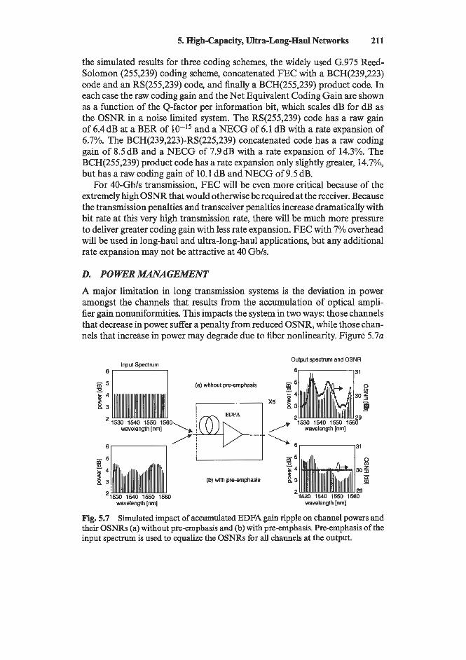
5. High-Capacity, Ultra-Long-Haul Networks 211
the simulated results for three coding schemes, the widely used G.975 Reed- Solomon (255,239) coding scheme, concatenated FEC with a BCH(239,223) code and an RS(255,239) code, and finally a BCH(255,239) product code. In each case the raw coding gain and the Net Equivalent Coding Gain are shown as a function of the Q-factor per information bit, which scales dB for dB as the OSNR in a noise limited system. The RS(255,239) code has a raw gain of 6.4dB at a BER of and a NECG of 6.1 dB with a rate expansion of 6.7%. The BCH(239,223)-RS(225,239) concatenated code has a raw coding gain of 8.5dB and a NECG of 7.9dB with a rate expansion of 14.3%. The BCH(255,239) product code has a rate expansion only slightly greater, 14.7%, but has a raw coding gain of 10.1 dB and NECG of 9.5 dB.
For 4O-Gb/s transmission, FEC will be even more critical because of the extremely high OSNR that would otherwise be required at the receiver. Because the transmission penalties and transceiver penalties increase dramatically with bit rate at this very high transmission rate, there will be much more pressure to deliver greater coding gain with less rate expansion. FEC with 7% overhead will be used in long-haul and ultra-long-haul applications, but any additional rate expansion may not be attractive at 40 Gb/s.
D. P O n R MANAGEMENT
A major limitation in long transmission systems is the deviation in power amongst the channels that results from the accumulation of optical ampli- fier gain nonuniformities. This impacts the system in two ways: those channels that decrease in power sufTer a penalty from reduced OSNR, while those chan- nels that increase in power may degrade due to fiber nonlinearity. Figure 5 . 7 ~
input Spectrum 6-
O@ut spectfum and OSNR
131
-5 $ - 5 (a) without pre-emphasis
b 4 b 4 30 5 z
5 s I
E 3 ..- x5
E 3 I 2 29 1530 1540 1550 1560 ‘1530 1540 1550 1560
I E 5 0 E i 5 E. E. s 4 s 4 30:
$ 3 (b) with pre-emphasis E 3 E I 2 29 1530 1540 1550 1560 ‘1530 1540 1550 1580
wavelength [nm] wavelength [nm]
Fig. 5.7 Simulated impact of accumulated EDFA gain ripple on channel powers and their OSNRs (a) without pre-emphasis and (b) with pre-emphasis. be-emphasis of the input spectrum is used to equalize the OSNRs for all channels at the output.
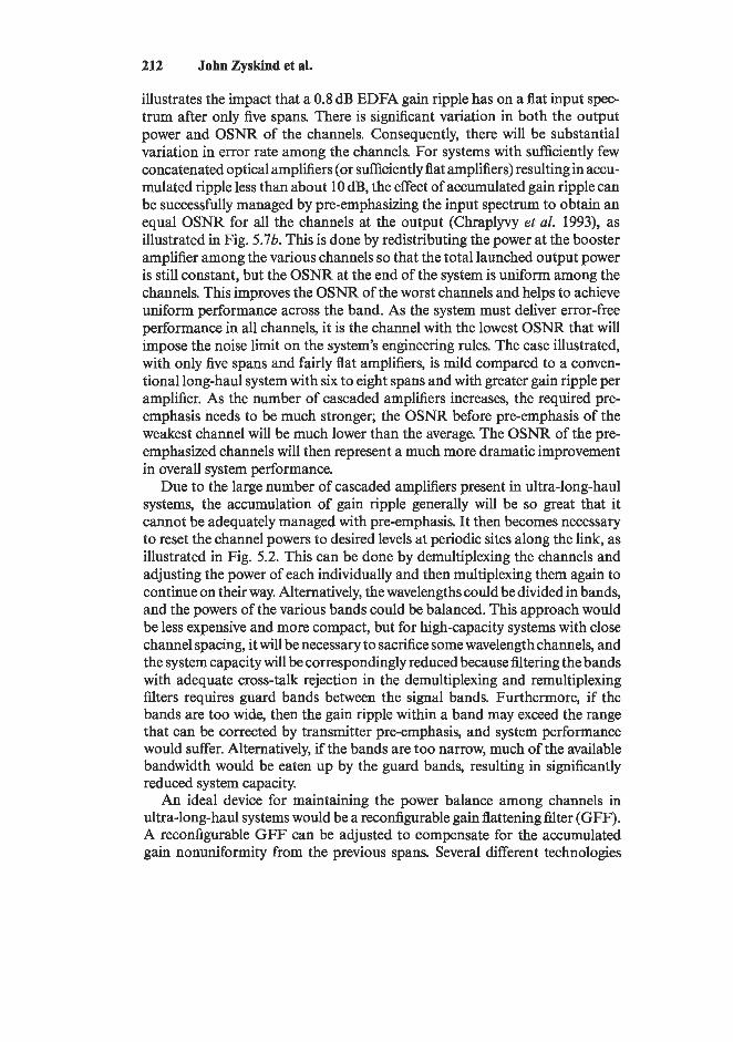
212 John Zyskind et al.
illustrates the impact that a 0.8 dB EDFA gain ripple has on a flat input spec- trum after only five spans. There is significant variation in both the output power and OSNR of the channels. Consequently, there will be substantial variation in error rate among the channels. For systems with sufliciently few concatenated optical amplifiers (or sufficiently flat amplifiers) resulting in accu- mulated ripple less than about 10 dB, the effect of accumulated gain ripple can be successfully managed by pre-emphasizing the input spectrum to obtain an equal OSNR for all the channels at the output (Chraplyvy et al. 1993), as illustrated in Fig. 5.7b. This is done by redistributing the power at the booster amplifier among the various channels so that the total launched output power is still constant, but the OSNR at the end of the system is uniform among the channels. This improves the OSNR of the worst channels and helps to achieve uniform performance across the band. As the system must deliver error-free performance in all channels, it is the channel with the lowest OSNR that will impose the noise limit on the system’s engineering rules. The case illustrated, with only five spans and fairly flat amplifiers, is mild compared to a conven- tional long-haul system with six to eight spans and with greater gain ripple per amplifier. As the number of cascaded amplifiers increases, the required pre- emphasis needs to be much stronger; the OSNR before pre-emphasis of the weakest channel will be much lower than the average. The OSNR of the pre- emphasized channels will then represent a much more dramatic improvement in overall system performance.
Due to the large number of cascaded amplifiers present in ultra-long-haul systems, the accumulation of gain ripple generally will be so great that it cannot be adequately managed with pre-emphasis. It then becomes necessary to reset the channel powers to desired levels at periodic sites along the link, as illustrated in Fig. 5.2. This can be done by demultiplexing the channels and adjusting the power of each individually and then multiplexing them again to continue on their way. Alternatively, the wavelengths could be divided in bands, and the powers of the various bands could be balanced. This approach would be less expensive and more compact, but for high-capacity systems with close channel spacing, it will be necessary to sacrifice some wavelength channels, and the system capacity will be correspondingly reduced because filtering the bands with adequate cross-talk rejection in the demultiplexing and remultiplexing filters requires guard bands between the signal bands. Furthermore, if the bands are too wide, then the gain ripple within a band may exceed the range that can be corrected by transmitter pre-emphasis, and system performance would suffer. Alternatively, if the bands are too narrow, much of the available bandwidth would be eaten up by the guard bands, resulting in significantly reduced system capacity.
An ideal device for maintaining the power balance among channels in ultra-long-haul systems would be a reconfigurable gain flattening filter (GFF). A reconfigurable GFF can be adjusted to compensate for the accumulated gain nonuniformity from the previous spans. Several different technologies
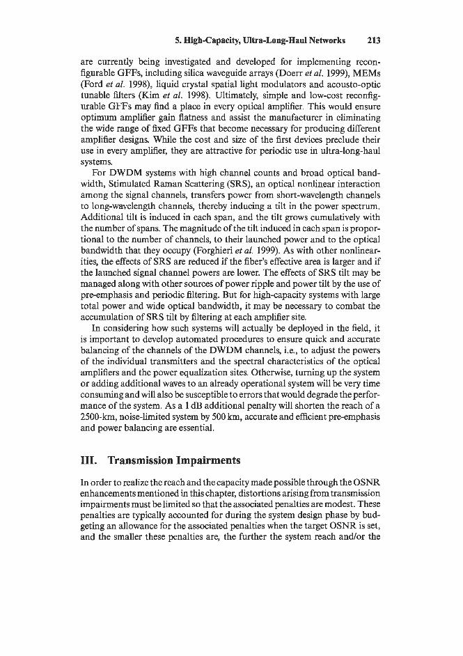
5. High-Capacity, Ultra-Long-Haul Networks 213
are currently being investigated and developed for implementing recon- figurable GFFs, including silica waveguide arrays (Doerr et al. 1999), MEMs (Ford et al. 1998), liquid crystal spatial light modulators and acousto-optic tunable filters (Kim et al. 1998). Ultimately, simple and low-cost reconfig- urable GFFs may find a place in every optical amplifier. This would ensure optimum amplifier gain flatness and assist the manufacturer in eliminating the wide range of fixed GFFs that become necessary for producing different amplifier designs. While the cost and size of the first devices preclude their use in every amplifier, they are attractive for periodic use in ultra-long-haul systems.
For DWDM systems with high channel counts and broad optical band- width, Stimulated Raman Scattering (SRS), an optical nonlinear interaction among the signal channels, transfers power from short-wavelength channels to long-wavelength channels, thereby inducing a tilt in the power spectrum. Additional tilt is induced in each span, and the tilt grows cumulatively with the number of spans. The magnitude of the tilt induced in each span is propor- tional to the number of channels, to their launched power and to the optical bandwidth that they occupy (Forghieri et QZ. 1999). As with other nonlinear- ities, the effects of SRS are reduced if the fiber’s effective area is larger and if the launched signal channel powers are lower. The effects of SRS tilt may be managed along with other sources of power ripple and power tilt by the use of pre-emphasis and periodic filtering. But for high-capacity systems with large total power and wide optical bandwidth, it may be necessary to combat the accumulation of SRS tilt by filtering at each amplifier site.
In considering how such systems will actually be deployed in the field, it is important to develop automated procedures to ensure quick and accurate balancing of the channels of the DWDM channels, i.e., to adjust the powers of the individual transmitters and the spectral characteristics of the optical amplifiers and the power equalization sites. Otherwise, turning up the system or adding additional waves to an already operational system will be very time consuming and will also be susceptible to errors that would degrade the perfor- mance of the system. As a 1 dB additional penalty will shorten the reach of a 2500-h, noise-limited system by 500 km, accurate and efficient pre-emphasis and power balancing are essential.
111. Transmission Impairments
In order to realize the reach and the capacity made possible through the OSNR enhancements mentioned in this chapter, distortions arising from transmission impairments must be limited so that the associated penalties are modest. These penalties are typically accounted for during the system design phase by bud- geting an allowance for the associated penalties when the target OSNR is set, and the smaller these penalties are, the further the system reach and/or the

214 John Zyskind et al.
higher its capacity. One of the objects in the design of high-capacity, ultra- long-haul systems is to minimize the impact of these penalties on the target OSNR and to ensure that the penalties for these impairments do not exceed their allocated penalties.
A. CHROMATIC DISPERSION AND OPTICAL NONLINEARITIES
Chromatic dispersion results from the dependence of the optical fiber’s index of refraction on optical wavelength and is the most important source of dis- tortion of high-speed signals. As a result of chromatic dispersion, different frequencies of light travel at different speeds. For on-off keyed data transmis- sion, where data 1s and Os are represented by the presence and absence of light, respectively, the pulses representing 1s contain a range of frequencies, and chromatic dispersion causes the pulses to spread as they propagate. Signal pulses corresponding to 1s will spread into the time slots for adjacent bits lead- ing to the generation of bit errors when the distorted data trains are detected after transmission. The dispersion length LD, corresponding to the distance after which a pulse has broadened by one bit interval, is:
1
where B is the bit rate, D is the dispersion, and AA is the spectral width of a pulse (Gnauck 1997). This length, which provides an estimate of the limit chromatic dispersion imposes on the length signals can be transmitted, is shorter when the bit rate is higher, when the dispersion is greater, or when the spectral width of the signal is greater. For high bit-rate long-haul transmission, external modulation of continuous wave diode lasers is used in preference to direct modulation of diode lasers because of the narrower spectrum that results. For signals produced by external modulation, the spectral width approximates the bit rate, B. The dispersion limit is then:
105 LD X -
D * B 2 ’ (5.5)
where LD is in km, D is in ps/nm. km, and B is Gb/s. The precise limit depends on the details of the modulation format and the design of the receiver circuitry, but Eq. 5.5 provides a reasonable approximation. The dispersion limit for externally modulated signals is inversely proportional to the square of the bit rate; for lO-Gb/s OC-192 signals on standard single mode fiber (SMF) with a dispersion of 17 ps/nm - km, it is about 60 km, corresponding to a residual dispersion of about 1000 ps/nm, and for 4O-Gb/s OC-768 signals, it is less than 4 km, corresponding to about 60 pdnm. These lengths are a great deal shorter than the link lengths permitted by noise accumulation, and techniques to compensate and manage the dispersion are essential for high-capacity, ultra- long-haul transmission.
5. High-Capacity, Ultra-Long-Haul Networks 215
Two complementary approaches are used to manage the fiber chromatic dis- persion: design of transmission fiber to reduce dispersion in the signal bands in the 1500-1600 nm spectral region, and the use of dispersion compensation to provide negative dispersion to compensate the accumulated positive disper- sion of transmission fiber. In a system with no nonlinear effects, transmission fibers designed to have no chromatic dispersion at about 1550 nm (so-called dispersion shifted fiber, or DSF) could be used, and the small residual disper- sion for channels whose wavelengths do not coincide with the zero dispersion wavelength could be compensated at any point in the link, as long as the final residual dispersion at the receiver is less than the dispersion limit. However, in typical high-capacity, ultra-long-haul-systems, it is desirable to launch the highest signal powers possible in order to maximize the OSNR (see Eq. 5.5), but as the launched power increases the impairments resulting from optical nonlinearities become more severe. The optimum launched signal power is therefore determined by the tradeoff between maximizing the launched power to maximize the OSNR and reducing the launch power to mitigate nonlineari- ties. At the optimal launch power, nonlinearities are sigdicant but not unduly severe, and the BER at the end of the system as a function of launch power is a minimum. In order to design the system with optimized launch power and thus the best system performance, it is not suEcient merely to control the residual dispersion at the end of the system. The local dispersion and the accumulated dispersion at each point along the length of the system are also important. Where dispersion compensation is used, both the amount of dis- persion compensation and its placement are also important; if the dispersion map is not properly designed, impairments from nonlinearities will be severe, resulting in stricter limits on the launched channel power.
Forghieri et al. (1997) have provided a comprehensive review of optical non- linearities and dispersion management. In this chapter we shall focus on some of the aspects that are of particular importance for high-capacity, ultra-long- haul systems. The effects of cross-phase modulation and self-phase modulation can be converted into amplitude modulation by chromatic dispersion if the accumulated dispersion is allowed to grow too large before compensation. The dispersion map must be designed so that either the dispersion of the transmission fiber is very low or its dispersion is compensated with sufficient frequency along the route to keep the accumulated dispersion sufficiently low at all points along the link.
Against this need for keeping the accumulated dispersion low is the need for local dispersion to be suf€iciently large in order to minimize nonlinear interactions among the channels. Four-wave mixing and cross-phase mod- ulation are especially severe when the local dispersion is low. Only fibers with substantial local dispersion are suitable for most DWDM applications. DSF with zero dispersion near 1550 nm is not suitable. Standard single mode fiber (SSMF), which has zero dispersion at 1310nm and a dispersion of 17 ps/nm . km at 1550 nm (sometimes also called nondispersion shifted fiber,
216 John Zyskind et al.
or NDSF), is well-suited to DWDM transmission in both the C- and L-bands but residual dispersion accumulates very quickly. Nonzero dispersion shifted fibers (NZDSF) have been designed to support transmission of high-data-rate DWDM channels. The dispersion of NZDSF in the signal band is designed to be large enough to avoid significant impairments from four-wave mixing for practical systems with channel spacing of 50 GHz (about 0.4 nm) or greater (typically about 4 ps/nm . km) but small enough that dispersion accumulates much more slowly with propagation distance than for NDSF. However, even for NZDSF, the dispersion limit is only about 240 km for lO-Gb/s signals at the center of the C-band and about 16 km for 40-Gbh signals. In fact, because the dispersion increases with wavelength, for transmission fibers the limit is even lower at the red end of the C-band and in the L-band. Thus, both NDSF and NZDSF require dispersion compensation for both 10-Gb/s and for 4O-Gb/s signal channels, but for NDSF much more is needed.
For transmission over more than a few spans in systems where the chan- nels cover a broad spectral range, careful attention must be given to matching the dispersion slope, defined as the derivative of dispersion D with respect to the wavelength, so that an acceptable dispersion map can be provided for all channels across the channel band. This requires matching the relative disper- sion slope (i.e., RDS, the ratio of the dispersion slope to the dispersion) of the transmission fiber and the dispersion compensation. A mismatch in the relative dispersion slope between the transmission fiber and dispersion com- pensation will cause a walk-off in the accumulated dispersion that varies across the channel band and increases with distance. Consequently, a small group of channels may have good transmission, whereas channels in the remainder of the band perform poorly.
Dispersion compensating fiber (DCF) is single mode fiber designed to have a large dispersion opposite in sign to that of the transmission fiber to be com- pensated, and is the technology most widely used to compensate dispersion. It is generally located between the stages of optical amplifiers, which are designed with two amplifying stages and access to the mid-stage region to accommodate the dispersion compensation and optical add/drop filters. DCF typically has a far lower RDS than transmission fibers This disparity is especially severe for the NZDSF fibers, which have been widely deployed for high-speed DWDM applications. NZDSF fiber designs tend to have a large RDS because of their low absolute dispersion. In recent years there has been a drive to address this problem by reducing the dispersion slope of transmission fibers and increas- ing it for DCF. The walk-off in accumulated dispersion across the C-band with transmission distance for two different fiber and DCF combinations is illustrated in Fig. 5.8. In these figures the accumulated dispersion is plotted for three wavelengths across the C-band (1530, 1546, and 1562 nm) for a sys- tem comprising twenty 100-km fiber spans with equal amount of dispersion compensation applied at the end of every span. Figure 5 . 8 ~ shows the accu- mulated dispersion for TrueWave Classic fiber, an early NZDSF, that has a

5. High-Capacity, Ultra-Long-Haul Networks 217
2500 r----
1000
-1 -2000 -~~~~~ 500 1530 - nm
0 500 1000 1500 2000 distance [km]
(b)
1562 nm 1500 1 /
p 1000 J 1546 nm f- 5 500
a c o 8 9 -500
7J 1530 n
I
4 -1000
-1 500
1000 1500 2000 -2000 '
0 500
Fig. 5.8 Dispersion maps illustrating the walk-off in accumulated dispersion across the band due to residual dispersion slope. The walk-off is large in case of (a) older TW-classic fiber that had a large slope, but is substantially smaller when using (b) TrueWave Reduced Slope fiber in conjunction with newer DCFs with greater slope. The far smaller walk-off allows the eyes to be recovered across the band.
high RDS (where D = 2.7 ps/nm/km at 1550 nm and S = 0.07 ps/nm2/km) compensated by an older DCF with negligible dispersion slope. The walk-off in accumulated dispersion across the band over 2000 km is 4000 pshm. It is tempting to try and use dispersion management at the end of the link on each channel independently to bring its accumulated dispersion to the optimum. Unfortunately, this works only for channels near the center of the band. This is illustrated by the simulated eye diagrams for the two channels at the edges of the band that, in addition to the common dispersion compensation at each optical amplifier, have been passed through a dispersion compensating fiber located before the receiver, the length of which is adjusted for optimum performance of that individual channel. The eyes cannot be recovered because the impact from fiber nonlinearity on the signals while they are substantially dispersed

218 John Zyskind et al.
cannot be undone using dispersion compensation at the end. This result is expected as the effects of dispersion and nonlinearity are not commutative.
Figure 5.8b plots the accumulated dispersion for a similar system with TrueWave RS fiber that has a much lower dispersion slope (where D = 4.4ps/nm/km at 1550nm and S = 0.045ps/nm2/km) compensated by a newer DCF having RDS S / D = 0.0067 ps/nm. Here the walk-off in accumu- lated dispersion has been reduced to around 1 100 ps/nm. In this case, by using appropriate per-channel dispersion adjustment of the channels at the end of the link, the eyes can be recovered across the band. With further improvements in slope-matched dispersion compensation, the need for end-of-the-system, per-channel dispersion adjustment can be minimized or even avoided.
The design of single mode DCF with sufficiently high dispersion slope to match that of NZDSFs is the object of intense work and is progressing rapidly. Single mode DCFs have been reported for two of the most widely deployed NZDSF fiber designs (Srikant 2001; Quang Le et al. 2001). However, the design and manufacturing of single mode DCFs with sufficiently high relative dispersion slope to match the NZDSFs with the highest relative dispersion is quite challenging and, at this writing, commercial single mode DCF solutions are not yet generally available for some of the widely deployed varieties of NZDSF with high dispersion slope.
Because of the importance of slope-matched dispersion compensation for ultra-long-haul systems at 10 Gb/s, and even more so at 40 Gb/s, other tech- nologies to provide slope-matched dispersion compensation for NZDSF have been proposed. One possible alternative technology that can provide high neg- ative dispersion slopes is higher-order mode dispersion compensation, first proposed in 1993 (Poole et al.) and presently the subject of revived inter- est to meet the need for slope-matched dispersion compensation for NZDSF (Gnauck et al. 2000; Ramachandran 2000). These are wideband devices that work across the C- or L-band. Signals are passed through amode converter and transformed into a higher mode that propagates through a length of specially designed higher-order mode fiber that has negative dispersion and high RDS for this transmitted mode. A second converter at the output end transforms the signals back to single mode to continue down the link. In addition to the possibility of higher relative dispersion slope, higher-order mode dispersion compensation also offers the possibility of lower losses and, because of the larger effective area of the higher-order mode fiber, reduced nonlinear impair- ments compared to single mode DCFs. The Virtually Imaged Phased Array (VIPA), another potential technology for slope-matched dispersion compen- sation for NZDSFs with high relative dispersion slope, is a resonant device. It works for a prescribed comb of wavelengths, and is thus more limited for use in wide optical bandwidth applications than single mode DCF or higher-order mode dispersion compensators (Ishikawa and Ooi 1998; Shirasaki and Cao 2001). Because it is based on bulk optics, the VIPA will avoid the nonlinear effects that are produced in single mode DCFs.

5. High-Capacity, Ultra-Long-Haul Networks 219
Without dispersion compensating modules that adequately match the dis- persion slope of transmission fiber, or to the extent that slope matching is imperfect, it may be necessary to perform dispersion slope equalization at periodic sites along the link (Zyskind et al. 2000), as shown in Fig. 5.2. This can be done either on a per-channel basis, which is expensive, bulky, and dif- ficult to manage, or it can be done on groups of channels or bands (Haxell et al. 2000). As with power balancing by bands, the use of bands is less attractive than broadband slope-matched dispersion compensation because elaborate filtering arrangements are required for compensation by band. Such band fil- tering entails a reduction in system capacity because of the necessity for dead bands in which no channels can be supported and because, compared to use of broadband slope-matched dispersion compensation, it is more expensive, complex, and bulky.
Nondispersion shifted single mode fiber has larger dispersion than NZDSF, and thus requires longer lengths of dispersion compensating fiber, which have higher loss. But the RDS of NDSF is smaller than that of NZDSF, and NDSF is the transmission fiber for which commercially available DCFs pro- vide the best slope compensation. NDSF also has the largest effective area, which permits higher launched signal powers and the largest local dispersion, which tends to minimize interchannel nonlinear effects, particularly four-wave mixing.
For 40-Gbls transmission where residual dispersion must be much smaller than for 10-Gbls, additional trimming will be required to compensate for imperfect dispersion slope compensation and for variations of dispersion aris- ing from temperature variations experienced by transmission fiber over the link (Kato 2000). Tunable dispersion compensation on a per-channel basis will be able to provide the required slope trimming, as well as adjust for temporal vari- ations. Tunable dispersion compensation may also be required for dynamically reconfigurable networks to compensate for differences in cumulative disper- sion a wavelength channel will experience when its path through the network is changed. Component suppliers are now working on developing such devices (see Eggleton 2001 for a review of work on tunable dispersion compensation) using a variety of approaches. Tunable dispersion compensation has been reported for dispersion compensating chirped-fiber Bragg gratings controlled by temperature or strain tuning (Eggleton 1999; Eggleton 2000; Willner 1999; Fells 2000); integrated all-pass filters (Madsen 1999; Horst 2000), which are planar deviGes based on ring resonators; and the virtually imaged phased array devices (Shirasaki 2000), which as described previously, are bulk optic devices based on resonant multipath reflections.
The ideal fiber span would have high local dispersion to mitigate nonlin- earities, but would have accumulated dispersion that is small and equal to the value for optimal transmission performance (depending on the modulation format). It has been proposed to create such spans by combining fibers having large positive dispersion with fibers having large negative dispersion (Reverse
220 John Zyskind et al.
Dispersion Fibers, RDF) in the same span. The positive dispersion fibers typ- ically have a large effective area-wbich reduces optical nonlinearities-and small RDS, so as to facilitate matching of dispersion slope of the positive dispersion and reverse dispersion fibers.
Such fiber spans would obviate the need for additional dispersion compen- sation at the amplifier sites In addition to the direct cost savings of dispensing with dispersion compensation, such fiber spans would be more suitable than currently deployed fiber networks for all Raman systems in which only dis- tributed Raman amplifiers are used. Without the need to compensate the loss of dispersion compensation at amplifier sites, it would be more practi- cal to compensate the fiber span loss with distributed Raman amplification, which would improve OSNR performance, reduce costs, as well as reduce the power transients that accompany changes in channel loading in EDFAs. Such fiber spans would also be well adapted to support dispersion-managed soliton transmission.
Such dispersion-managed spans are currently used for undersea systems where the fiber spans and the system equipment are designed together, and each fiber span is the same length. For terrestrial systems with nonuniform spacings between-amplifier huts, it would be necessary to tailor the lengths of the two fiber types for each individual span to the total length required for that span. Before such networks are deployed it will be necessary to meet these practical engineering challenges in the deployment of such fiber networks.
B. POLARIZATION EFFECTS
Polarization effects arise from three phenomena: polarization-mode dis- persion; polarization-dependent loss and polarization-dependent gain; or polarization hole-burning. Polarization-dependent losses and polarization hole-burning are effects that become important in systems where signals prop- agate over long distances through many optical amplifiers and other compo- nents. Polarization-mode dispersion (PMD) becomes increasingly important for higher data rates and the effect grows with the square root of the link length.
Polarization-dependent loss (PDL) arises from the fact that the optical components (such as isolators, filters, optical amplifiers, etc.) through which the signals pass have insertion loss that depends on the incident polarization. When the light impinges on a component in a polarization state with relatively less loss, the input power to subsequent optical amplifiers is raised and the OSNR improves. Conversely, when the light impinges on a component with a polarization state with relatively greater loss, the input power to subsequent optical amplifier is lowered and the OSNR is degraded. PDL manifests itself as a statistical impairment because of the random and variable evolution of the polarization state as light propagates over long distances in fiber; the PDL arising from each of many components is a random variable that varies with time. PDL is controlled in long systems by requiring that the PDL is small for
5. High-Capacity, Ultra-Long-Haul Networks 221
all components in the signal path. Components with sufficiently low PDL for terrestrial ultra-long-haul applications are commercially available.
Polarization-dependent gain (PDG) or polarization hole-burning (PHB) in the optical amplifiers arises from inhomogeneity in the saturation character- istics of the gain. Polarization hole-burning arises from the greater saturation experienced by erbium ions oriented so as to be preferentially saturated by light with the polarization of the signal. The result in a system with a long chain of optical amplifiers is that a strong saturating signal experiences more severe gain saturation than ASE with the orthogonal polarization because the signal always interacts most strongly with precisely those ions that will not be as deeply saturated for the polarization state that is orthogonal to that of the signal. This effect, unlike PDL, is deterministic, and the orthogonal ASE steals power from the signal at each optical amplifier as the signals propagate down the amplifier chain. But PHB is very weak, therefore it is only a problem for very long chains of amplifiers, such as are used in submarine systems. In addition, for DWDM systems with multiple channels, the polarization states of the different wavelength channels are independent and their PHB contribu- tions cancel each other. PDG also arises from the relative orientation of the pump light and the signal light. The system behavior of pump-induced PDG is similar to PDL, but, like PHB, it is very weak and in multistage EDFAs with multiple pumps the PDG tends to get washed out.
Polarization-mode dispersion (PMD) is the most important polarization effect for high-capacity, ultra-long-haul systems with high bit-rate channels. PMD arises from the birefringence in the fiber that gives rise to differential group delay between the two principal states of polarization. PMD is man- ifest as a time varying and statistical pulse broadening and pulse distortion because the perturbations to the fiber symmetry that give rise to the birefrin- gence vary randomly in orientation along the fiber and are also dependent on environmental variations, particularly temperature. For lengths of fiber longer than the correlation length for the birefringence, which is generally the case for a fiber span, PMD is characterized in terms of the differential group delay (DGD) between the two principal states of polarization after a given length of fiber. Because of the statistical nature of PMD, the differ- ential group delay increases with the square root of the length of the fiber and is expressed in units of p s / G . The PMD of a fiber span is typically specified in terms of a mean PMD, which is the average over time of its net DGD. The statistical distribution of DGD about this mean is determined by the physics of PMD and follows a Maxwellian distribution. Because of its statistical nature, the possibility of errors arising from PMD can never be totally eliminated, but the probability of an outage, defined as the prob- ability of a penalty greater than the OSNR margin assigned to PMD, can be calculated from the mean PMD and its statistical distribution. In prac- tice, a given amount of margin is allocated to PMD impairments, and the probability of an outage is defined as the probability that the instantaneous
222 John Zyskind et al.
DGD will exceed that value that induces a penalty equal to this margin allo- cation. When the DGD exceeds this value, the possibility of PMD-induced bit errors at the end of the system cannot be excluded. For modest DGD, the penalty due to PMD goes up quadratically with both the bit rate and with the DGD (Poole and Nagel 1997). This means that the acceptable mean PMD is inversely related to the bit rate, but that as the instantaneous PMD increases above the acceptable level, the penalty increases rapidly. It follows that the acceptable mean differential group delay is proportional to the bit period and is generally of the order of 10-15% of a bit period depending on the modulation format and other details of the system design and the permitted outage probability (Poole and Nagel 1997). In addition to DGD, or first-order PMD, second-order PMD must be considered when the PMD varies over the bandwidth of the source. Components of higher-order PMD tends to increase as first-order PMD increases (Shtengel et al. 2001), therefore higher-order PMD becomes relatively more important when the PMD is larger, and in fact becomes dominant for 10 Gb/s per second above about 20 ps of mean PMD (Taga et al. 1998).
For recently manufactured fiber with a mean PMD of 0.125 ps/& or less (Noutsias and Poirier 2001), PMD is not an obstacle to ultra-long-haul trans- mission at 10 Gb/s. However, for older fiber where PMD can be significantly larger or for 4O-Gb/s ultra-long-haul transmission, PMD can limit the reach of a system. For IO-Gb/s ultra-long-haul transmission on older vintage fiber and for 40-Gb/s ultra-long-haul transmission over a wide range of fibers, PMD compensation will be necessary. Because of the importance of higher-order PMD for larger PMD where compensation is needed, it is likely compensa- tion of second-order PMD, in addition to fist-order PMD, will be necessary in a useful compensator. The development of optical and electrical compo- nents to counteract the PMD is an area of active research and commercial development. See Penninckx and Lanne (2001) for a recent review.
C. MODULATIONFOR2MAT
The modulation format is also an important consideration in the design of ultra-long-haul systems. The most commonly used format in long haul optical communications is Nonreturn to Zero (NRZ) modulation, in which 1s are represented as rectangular pulses occupying the full bit period and Os by the absence of a pulse. N R Z pulses are normally formed either by directly modulating a semiconductor laser (for DWDM transmission gen- erally a single longitudinal mode Distributed Feedback Laser) to turn its power on for a data “1” and off for a “0,” or by using a continuous wave semiconductor laser followed by an external modulator (or sometimes by an integrated modulator on the same semiconductor chip with the diode laser) passing the laser’s optical power for a “1” and blocking it for a “0.”
5. High-Capacity, Ultra-Long-Haul Networks 223
In high bit rate (2.5 Gb/s per channel or greater), long-haul transmission, it is necessary to use external modulation. Direct modulation of semiconduc- tor lasers induces chirping, and the associated spectral broadening entails unacceptable dispersion penalties, as can be seen by reference to Eq. 5.4. External modulators for IO-Gb/s applications are commercially available and widely deployed. The two most widespread technologies are electro-optically controlled Mach-Zehnder interferometers fabricated in LiNbO3 and electro- absorption modulators fabricated in semiconductor-based devices. In fact, a modest amount of chirp of the proper sign (a chup parameter of approximately -0.7) results in improvement in performance because dispersion initially acts to narrow the c h q e d pulse (Agrawal 1992). LiNb03-based Mach-Zehnder modulators are commercially available that can provide properly prechirped NRZpulses.
Return to Zero (RZ) modulation uses pulses that are substantially nar- rower than a bit period to represent “ls,” so even for consecutive “1s” the power level returns to zero between successive pulses. For practical receiver designs, RZ modulation results in receiver performance superior to that for NRZ modulation by 1 to 2 dB (Boivin and Pendock 1999). With RZ modu- lation, systems can also be designed to be more robust against impairments such as self-phase modulation and polarization mode dispersion (Taga et al. 1998; Sunnerud et al. 2001). In fact, if the dispersion map and signal powers are appropriately managed and the input pulse is properly shaped to pro- duce solitons (Mollenauer 1997) or dispersion managed solitons (Suzuki et al. 1995; Smith et al. 1997; Cao and Yu 2001) the effects of dispersion and self-phase modulation can be held in balance. In this case, pulse spreading induced by dispersion is balanced by pulse narrowing induced by self-phase modulation so that, in the case of classical solitons, the pulse shape is main- tained for transmission over arbitrary distance, or so that, in the case of dispersion managed solitons, it returns to the same shape at the end of each span for an arbitrary number of spans. Carrier-suppressed RZ (Miyamoto et al. 1999; 2001) and chirped RZ (Bergano et al. 1997) modulation have also been proposed as modulation formats to further mitigate nonlinear interactions.
Although RZ modulation offers improved performance, transmitters for RZ modulation are more complex and expensive than those for NRZ modu- lation. Generally, two modulation stages are required, one to form the pulses and a second to modulate the pulses to imprint the data on the signals. For example, whereas NRZ modulation can be implemented with a single LiNbO3 Mach-Zehnder modulator, RZ modulation requires either two separate modu- lators or a two-stage modulator. For dispersion-managed soliton transmission, the dispersion map must generally be controlled more tightly than for NRZ transmission, which can pose a practical challenge for commercial systems deployed on carriers’ actual fiber networks with highly variable amplifier-hut separations.
224 John Zyskind et al.
IV. Optical Networking
A. CHANGING NETWORK NEEDS
The 1990s marked tremendous advances in optical networking. In particu- lar, the 1990s saw the widespread deployment of SONET systems. SONET, or Synchronous Optical Networking, was a tremendous step forward for the public telecommunications network infrastructure over the preceding plesiosynchronous system, enabling networks to be built that provided switch- ing granularity (down to a voice call), scalability (up to 40 Gb/s or beyond), and high availability though the use of automatic protection switching (APS) and ring-based restoration. In addition, the 1990s saw the widespread deploy- ment of point-to-point DWDM systems used for fiber multiplication. By the end of the 199Os, most major public telecommunications networks were pri- marily built by stacking SONET rings on top of one another through the use of DWDM.
The 1990s also saw an explosion in data traffic driven by both corporate and public demands. IP, driven by the Internet, corporate requirements, and the World Wide Web, became the dominant data networking technology by the end of the 1990s. The dominating trend of IP is continuing, with most tech- nologists agreeing that IP will within the next 10 years become the technology of choice to carry all traffic, including voice.
As IP traffic grew, IP routers grew in size, speed, and complexity, which drove fundamental changes in the way backbone IP and optical networks were constructed. At first, data growth helped spur the deployment of WDM as more and more SONET rings were stacked. However, as the speed of the backbone router ports increased, the core network evolved from a highly lay- ered one (e.g., IP over Frame Relay over ATM over SONET over DWDM) to a flat IP-over-wavelength architecture. The latter architecture, also known as an IP-over-glass architecture, was motivated, enabled, and in a large sense required when IP router ports started to run at the speed of a wavelength (first OC-48c, now OC-l92c, and moving to OC-768c). So dramatic was the fail- ure of SONET rings to respond to the high-speed service requirements on IP, that many backbone networks had bifurcated by early 2000, with the SONET network providing voice and lower-speed services, and the WDM network providing wavelengths to the IP layer, SONET layer, ATM layer, and for sale to external customers as “transparent unprotected wavelength services.” These customers in turn used these wavelengths to construct their IP, SONET, and ATM networks.
In summary, the core of the public network infrastructure is changing for three fundamental reasons. First, the service requirements are changing from voice to data, electrical to optical, and static to dynamic. Second, the exist- ing SONET-over-WDM infrastructure is insdlicient to meet those changing requirements. Third, new technologies and architectures are available to meet the new requirements in a far more economical and scalable fashion. For these
5. High-Capacity, Ultra-Long-Haul Networks 225
reasons, the first decade of the new millennium will see the maturation of the second phase of optical networking, the intelligent optical network, beginning with IP over wavelengths as the first step. The rest of this section will discuss the use of ULH transmission as a key enabler of this new architecture.
B. THE VALUE OF ULTRA-LONG-E4UL TRANSMISSION
Data networks are not the same as voice networks. There are many fundamen- tal differences, including the use of packet switching, statistical multiplexing, and the use of both connectionless data transfer and logical connection- oriented data transfer in data networks versus the use of circuit switching, time division multiplexing, and physical-connection-oriented bit transfers in voice networks. There are also fundamentally different traffic and service require- ments with data traffic being characteristically distance insensitive, dynamic, and unpredictable, and voice tr&c being characterized as more local, steady, and predictable. For these and other reasons, the SONET ring networks opti- mized for the voice network are no longer optimal, or even adequate, to continue to build the public data infrastructure.
Because of the different traffic requirements, the different underlying tech- nologies, and the different historical evolution of the two technologies (data being an unregulated and relatively new technology), data networks are not planned, engineered, or constructed the same way as voice networks. Two key attributes of an IP backbone are: (1) that it is typically an irregular mesh topology, often evolving in an organic and hard-to-predict fashion; and (2) the trunks of the mesh run at wavelength speeds (OC-48c/OC-192c/OC-768~). The design and optimization of an IP network is a complicated process, but ide- ally the trunks should be determined from the traffic requirements and not the physical layout of the fiber backbone. In fact, this is currently done with wavelength services criss-crossing the country interconnecting distant routers. This enables the construction of flatter IP networks whose topologies are bet- ter optimized to the traffic. Such a design has the benefits of using fewer IP router ports (which reduces costs and keeps the routers smaller) and reducing latency. In fact, the construction of long trunks is absolutely critical in the con- struction of a scalable optical Internet in that the IP layer traffic is essentially off-loaded to the more scalable optical layer.
Today, these trunks are constructed with the concatenation of shorter- reach WDM systems. For instance, a 5000-km, cross-continental trunk, for example, from New York to Los Angeles, might be required to cross 8-10 or more DWDM systems with a corresponding number of costly optical-to- electrical-to-optical (OEO) conversions along the way. It is the reduction of these intermediate OEO conversions by using optical bypass that saves money, space, and power and leads to a far more economical and manageable network.
Optical bypass and long trunks are not only useful in constructing IP net- works. In fact, one of the driving forces behind ULH transmission is the move away from an interconnected SONET ring-based architecture to an optical
226 John Zyskind et al.
mesh network. Similar to an IP network, the optical mesh network topol- ogy is optimized by considering the traffic demands, not the physical fiber topology.
Whether for express wavelengths for an IP-over-glass architecture, the construction of an optical mesh network, or for more narrow applications, ultra-long-haul transmission can greatly reduce costs by reducing the amount of required OEO conversions in the network. In general, the higher the bandwidth-distance requirements on the traffic, the more motivation there is for optical bypass and ULH transmission.
C. ALL-OPTICAL NETWORKS'
With the advent of ultra-long-haul transmission, it is now possible to con- struct IP and optical mesh networks with long express trunks with little or no intermediate OEO conversion. Such a technology has significant architectural implications on building the network, as has already been alluded to.
One of these implications is the ability to construct all-optical networks. An all-optical network is one in which the signal remains in the optical domain from the source to destination without any conversion to electronics within the network. The primary motivation for an all-optical network is that optics, and not electronics, is the most cost effective way to tap the multi-Tb/s capacity of the optical fiber, i.e., through the use of optical bypass and optical switching nodes. Another motivation is that fiber transparency provides an element of future proofing the network against advances in technology.
Two other architectural implications were already discussed: that long express wavelengths enable the construction of flatter IP and optical mesh net- works optimized to meet the traffic demands rather than on the physical layout of the fiber. With automation in the all-optical layer, these express trunks can be quickly brought into service and/or reconfigured to meet changing tr&c demands.
All-optical networks have been commercial for some time now, albeit in very limited form; linear and ring systems with intermediate wavelength-selective adddrop are widely deployed in long-haul as well as metropolitan networks. By slotting in a transponder card of the appropriate wavelength, the carrier can route the signal from the source node to the destination node without any conversion to electronics. The technologies that have enabled these static wavelength routing networks are well known and include DFB lasers, LiNbOs modulators, thin film filters, fiber Bragg gratings, etc. Tunable lasers and recon- figurable adddrop technologies promise to enable configurable versions of these systems.
ULH transmission enables the construction of larger networks, to the point that now linear or ring network topologies are insufficient to realize the full benefit of the transmission capabilities, i.e., the reach exceeds the normal distance between the major backbone junction nodes (a node with

5. High-Capacity, Ultra-Long-Haul Networks 227
a fiber-route degree greater than 2; typically 3 4 in a continental U.S. net- work, or sometimes even higher). Thus, having surpassed the unregenerated reach required to connect junction nodes without intermediate regeneration, carriers can now further reduce OEO conversion cost by building a ULH mesh network optically interconnecting many or all of these junction nodes.
These junction nodes may be manually patch-paneled or may contain all- optical switches. The choice of a manual versus automatically configurable node depends on the trade-off between the cost of the optical switches and the benefits of wavelength configuration. In fact, there are more detailed cost trade-offs involving levels of network configuration/automation dependent on such things as the tuning range of the transmitters, and in some cases the tunability of the dispersion compensation. Such trade-offs are complicated and time and business sensitive depending upon such considerations as the dynamic nature of the IP trunks, OXC trunks, or wavelength services, the predictability of such traffic, the potential lost opportunity costs, as well as the operational cost savings of the automatic node over the manual node, to name more than a few.
D. ALL-OPTICAL ISLANDS
ULH and all-optical mesh networks can greatly reduce the OEO conversion cost in the network. However, these cost savings do not come without potential drawbacks.
First, because of the lack of standards for optical midspan meet, the larger the mesh, the larger the portion of the network built from one vendor. Unlike the o/e/o intelligent optical networking interoperability standards that have been demonstrated several times and that are continuing to be addressed at various industry fora (IETF GMPLS, OIF UNI, ITU G.ASON, ODSI UNI), there is no current or expected activity to standardize the interfaces necessary to support an optical midspan meet. Thus, for the foreseeable future, all-optical networks will have to be interconnected through OEO.
Second, for a given technology at a certain point in time, the capacity (per lit fiber) of the optical mesh will decrease as the reach of the wavelengths is increased. If the supported capacity is sufficient, then the reduced OEO cost will result in reduced network cost. However, if more capacity is required, extra fibers will have to be lit, increasing the amplifier costs. Thus, infinitely extending reach (toward the goal of one optical hop across the core backbone) at the expense of capacity may or may not be the most cost effective way to build the network.
Third, although optical switching is maturing, the level of configuration/ automation in an all-optical junction node is less than in its OEO coun- terpart. For example, the OEO nodes typically support STS-1 grooming, fully automatic circuit setup, various protection and restoration mechanisms, logical dissociation between the client-side interfaces and the network-side interface/wavelength, client-side APS, rate adaptation (e.g., 10G to 40G),
228 John Zyskind et al.
conversion of transmission formats such as from NRZ to RZ or from FEC to SuperFEC, wavelength changing, etc. Thus, there is a balance to be made in the core backbone architecture between functionality and cost, and a car- rier may choose to make some nodes all OEO, others all or mostly OEO, and others hybrid.
For these and other reasons, larger backbone networks will continue to be built from an interconnection of all-optical networks, or islands. These islands are surrounded by OEO performing regeneration, wavelength changing, rate adaptation, format conversions, etc. These islands not only encompass the traditional static linear point-to-point systems, the emerging ULH meshes, but also newer, short fat-pipe OC-768 systems and future islands using as yet undeveloped technologies. Over time these islands will become larger, support more capacity, and become more sophisticated in their functionality. Future islands will likely support optical regeneration as well as wavelength changing.
Because of the OEO around the islands, multivendor and multitechnology networks are easily constructed. It also allows the use of different technologies in different parts of the network, for example, high-capacity, short fat-pipe systems in shorter distance, high density areas and longer skinnier ultra- long-haul pipes in more widely spaced, sparse parts of the network. The use of OEO switches ties this bandwidth together into a complete multivendor multitechnology mesh network.
V. Conclusions
Some of the most exciting technological advances in optical communications have made possible dramatically increased reach for high-capacity DWDM systems. The ability to extend high-capacity optical paths to thousands of kilometers between regenerators makes possible dramatic reductions in net- work cost as well as scalable network architectures, based on increased optical functionality, to support the rapid growth of data-based servies.
Acknowledgments
The authors would like to acknowledge useful conversations and fruitful collaborations with our colleagues at Sycamore Networks.
References
0. Ait Sab, “FEC Techniques in Submarine Transmission Systems,” Paper TuF1, Proceedings OFC 2001, OSA, Anaheim, California, 2001.
0. Ait Sab and V. Lemaire, “Block turbo code performances for long-haul DWDM optical transmission systems,” Proceedings of OFC 2000, Baltimore, MD, paper ThS5, pp. 280-282,2000.
5. High-Capacity, Ultra-Long-Haul Networks 229
N. Bergano, “Undersea Lightwave Systems Design,” in Optical Fiber Communications
N. Bergano, et al., Proceedings OFC 1997, Paper PD16, 1997. L. Boivin and G. Pendock, “Receiver Sensitivity for Optically Amplified RZ Signals
with Arbitrary Duty Cycle,” in OpticalAmpliJers and Their Applications, 1999, Nara, Japan: Paper ThB4, pp. 106-109 (Optical Society of America).
X. Cao and Y. Yu, “Ultra Long-Haul DWDM Transmission via Nonlinearity Man- agement,” Optical Amplifiers and Their Applications, OSA Trends in Optics and Photonics, vol. 44, A. Mecozzi, M. Shimizu, and J. L. Zyskind eds., Optical Society of America, Washington DC, 2001, pp. 203-210.
A. R. Chraplyvy, J. A. Nagel, and R. W. Tkach, “Equalization in Amplified WDM Lightwave Transmission Systems,” IEEE Photon. Technol. Lett., vol. 4, p. 920, 1992.
V. Dominic, A. Mathur, and M. Ziari, “Second-order Distributed Raman Amplifi- cation with a High-Power 1370-nm Laser Diode,” in O p t i d Amplijiers and Their Applications, 2001, Stresa, Italy, OMC6 (Optical Society of America).
V. Dominc, E. Mao, J. Zhang, B. Fidric, S. Sanders, and D. Mehuys, “Distributed Raman Amplification with Co-Propagating Pump Light,” in O p t i d AmpliJers and Their Applications, 2001, Stresa, Italy, OMC5 (Optical Society of America).
C. R. Doerr, et al., “Dynamic Wavelength Equalizer in Silica Using the Single-Filtered- Arm Interferometer,” IEEE Photon. Technol. Lett., vol. 11, pp. 581-583, 1999.
B. J. Eggleton, J. A. Rogers, P. B. Westbrook, and T. A. Strasser, “Electrically Tunable Power Efficient Dispersion Compensating Fiber Bragg Grating,” IEEE Photon. Technol. Lett., vol. 11, pp. 854-856, 1999.
B. J. Eggleton, A. Ahuja, P. S. Westbrook, J. A. Rogers, P. Kuo, T. N. Nielsen, and B. Mikkelsen, “Integrated Per-Channel Dispersion Compensating Bragg Gratings,” Journal of Lightwave Technology, v01. 18,2000.
B. J. Eggleton, “Dynamic Dispersion Compensation Devices for High-speed Trans- mission Systems,” Paper WH1, OFC 2001, Anaheim, California (Optical Society of America).
J. A. J. Fells, et al., “Twin Fiber Grating Adjustable Dispersion Compensator for 40 Gbith,” ECOC 2000, Munich, Germany, Postdeadline paper 2.4,2000.
Y. Emori and S. Namiki, “100-nm Bandwidth Flat Gain Raman Amplifiers Pumped and Gain-Equalized by 12-wavelength-channel WDM High-Power Laser Diodes,” OFC 1999, San Diego, CA, Postdeadline paper PD19.
J. E. Ford and J. A. Walker, “Dynamic Spectral Power Equalization Using Micro-Opto- Mechanics,” IEEE Photon. Technol. Lett., vol. 10, pp. 1440-1442, 1998.
F. Forghieri, R. W. Tkach, and A. R. Chraplyvy, “Fiber Nonlinearities and Their Impact on Transmission Systems,” in Opical Fiber Communications IIIA, Ivan P. Kaminow and Thomas L. Koch, eds, pp. 196264, Academic Press, San Diego, 1997.
L. D. Garrett, et al., “Demonstration of VIPA Device for Tunable Dispersion Com- pensation in 16 x 10-Gb/s WDM Transmission over 480 km Standard Fiber,” OFC 2000, Baltimore, Maryland (Optical Society of America).
A. H. Gnauck and R. M. Jopson, “Dispersion Compensation for Optical Fiber Sys- tems,” in Opical Fiber Communications IIIA, Ivan P. =now and Thomas L. Koch, eds., pp. 162-195, Academic Press, San Diego, 1997.
IIIA, I. P. Kaminow and T. L. Koch, eds., pp. 302- 335, Academic Press, 1997.

230 John Zyskind et al.
A. H. Gnauck, L. D. Garrett, Y. Danziger, U. Levy, and M. Shur, “Dispersion and Dispersion Slope Compensation of NZ-DSF for 40 Gbps Operation over the Entire C-band,” Technical Digest of OFC 2000, San Diego, CA, PD-8,2000.
P. B. Hansen, et al., “Capacity Upgrades of Transmission Systems by Raman Amplification,” IEEE Photon. Technol. Lett., vol. 9, pp. 262-264, 1997.
I. Haxell, et al., “2410 km All-Optical Network Field Trial with 10 Gb/s DWDM Transmission,” OFC 2000, Postdeadline paper PD41.
I. Haxell, M. Ding, A. Akhtar, H. Wang, and P. Farmgia, “52 x 12.3 Gbit/s DWDM Transmission over 3600 km of True Wave Fiber with 100 km Amplifier Spans,” Opti- cal Amplifiers and Their Applications, OSA Trends in Optics and Photonics, vol. 44, A. Mecozzi, M. Shimizu, and J. L. Zyskind, eds., Optical Society of America, Washington, DC, 2001, pp. 217-219.
F. Horst, “Tunable Ring Resonator Dispersion Compensators Realized in High- Refractive-Index Contrast SiON Technology,” ECOC, Munich, Germany, Postdead- line paper PD2.2,2000.
G. Ishikawa and H. Ooi, “Demonstration of Automatic Dispersion Equalization in 40 Gbps OTDM Transmission,” ECOC 1998, WdC-6, pp. 519-520,1998.
ITU-T G.975, November 1999, “Forward Error Correction for Submarine Appli- cations.”
T. Kato, Y. Koyano, and M. Nishimura, “Temperature Dependence of Chromatic Dispersion in Various Types of Optical Fiber,” Optics Letters, vol. 25, pp. 11 5 6 1 158, 2000.
S. Keeton, S. Sridharan, and M. Jarchit, “Enabling Next Generation Optical Networks with Forward Error Correction,” NFOEC 2001 Proceedings, pp. 54-59, Baltimore, Maryland, 2001.
H. Kidorf, et al., “Performance Improvement in High-Capacity, Ultra-Long-Distance, WDM Systems Using Forward Error Correction Codes,” OFC 2000, San Diego, CA, THS3, pp. 274-276.
H. S. Kim, et al., “Actively Gain Flattened Erbium-Doped Amplifier over 35 nm by Using All-Fiber Acousto-Optic Tunable Filters,” IEEE Photon. Technol. Lett., vol. 10, pp. 790-702,1998.
C. K. Madsen, et al., “Integrated All-Pass Filters for Tunable Dispersion and Dis- persion Slope Compensation,” IEEE Photon. Technol. Lett., vol. 11, pp. 1623-1625, 1999.
Y. Miyamoto, et ab, Electronics Letters, vol. 35, no. 23, pp. 2041-2042, 1999. Y. Miyamoto, S. Kuwahara, A. Hirano, Y. Tada, Y. Yamane, and H. Miyazawa,
“Reduction of nonlinear crosstalk of carrier-suppressed RZ format for 100 GHz- spaced Nx43-Gbith WDM in non-zero shifted band,” Proceedings of ECOC 2001, Paper Th.B.3,2001.
R. E. Neuhauser, P. M. Krummn ’ch, H. Bock, and C. Glingener, “Impact of Non- linear Pump Interactions on Broadband Distributed Raman Amplification,” Paper MA4-1, OFC 2001, OSA, Anaheim, California, 2001.
C. D. Poole, et al., “Elliptical-Core Dual Mode Fiber Dispersion Compensator,” IEEE Photon. Technol. Lett., vol. 5 , pp. 194-197, 1993.
5. High-Capacity, Ultra-Long-Haul Networks 231
P. Noutsios and S. Poirier, “PMD Assessment of Installed Fiber Plant for 40 Gb/s Trans- mission,” NFOEC 2001 Proceedings, pp. 1342-1 347, Baltimore, Maryland, 2001.
D. Penninckx and S. Lanne, “Reducing PMD Impairments,” Paper TuP1, OFC 2001, OSA, Anaheim, California, 2001.
A. Puc, E Kerfoot, A. Simons, and D. Wilson, OFC 1999, ThQ6, pp. 255-258. N. T. Quang Le, T. Vng, and L. Gruner-Nielsen, “New Dispersion Compensating Mod-
ule for Compensation of Dispersion and Dispersion Slope of Non-Zero Dispersion Fibres in the C-band,” Paper TuH5, OFC 2001, OSA, Anaheim, California, 2001.
S. Ramachandran, B. Mikkelsen, L. C. Cowsar, M. F. Yan, G. Raybon, L. Boivin, M. Fishteyn, W. A. Reed, P. Wisk, and D. Brownlow, “All-fiber, Grating-Based, Higher-Order-Mode Dispersion Compensator for Broadband Compensation and 1000-km Transmission at 40 Gbps,” ECOC 2000, PD-2.5,2000.
K. Rottwitt, A. Stentz, T. Nielsen, P. Hansen, K. Feder, and K. Walker, “Transparent 80-km Bidirectionally Pumped Distributed Raman Amplifier with Second-Order Pumping,” in European Conference on Optical Communications 2000, Nice, France, 11-14.
M. Shirasaki, et al., “Variable Dispersion Compensator Using the Virtually Imaged Phase Array (VIPA) for 40-Gbh WDM Transmission Systems,” ECOC 2000, Munich, Germany, Postdeadline paper 2.3,2000.
M. Shirasaki and S. Cao, “Compensation of Chromatic Dispersion and Dispersion Slope Using a Virtually Imaged Phased Array,” Paper TuS1, OFC 2001, OSA, Anaheim, California, 2001.
G. Shtengel, E. Ibragimov, M. Rivera, and S. Suh, “Statistical Dependence Between First and Second-Order PMD,” Paper MO-3, OFC 2001, OSA, Anaheim, California, 2001.
N. J. Smith, N. J. Doran, W Forysiak, and E M. Knox, “Soliton Transmission Using Periodic Dispersion Compensation,” Journal ofLightwave Technology, vol. 15, p. 1808, 1997.
V. Srikant, “Broadband Dispersion and Dispersion Slope Compensation in High Bit Rate and Ultra Long Haul Systems,” Paper TuHl, OFC 2001, OSA, Anaheim, California, 2001.
H. Sunnerud: M. Karlsson, and P. A. Andrekson, “A Comparison Between NRZ and RZ Data Formats with Respect to PMD-induced System Degradation,” Paper WT3, OFC 2001, OSA, Anaheim, California, 2001.
M. Suzuki: I. Morita, N. Edagawa, S. Yamamoto, H. Taga, and S. Akiba, Electronics Letters, vol. 31, p. 2027, 1995.
H. Taga, et al., “Polarization Mode Dispersion Tolerance of 10-Gbitls NRZ and RZ Optical Signals,” Electronics Letters, vol. 34, pp. 2098-2100, 1998.
J. L. Zyskind, J. Nagel, and H. D. Kidorf, “Erbium-Doped Fiber Amplifiers for Opti- cal Communications: in Optical Fiber Communications IIIB, I. P. Kaminow and T. L. Koch, eds., pp. 13-68, Academic Press, San Diego, 1997.
J. L. Zyskind, G. J. Pendock, M. J. L. Cahill, G. D. Bartolini, J. K. Ranka, and S. Y. Park, “High Capacity, Ultra-Long-Haul Transmission,” Pmc. of NFOEC 2000, Denver, CO, 2000.

Chapter 6
Renk-Jean Essiambre, Gregory Raybon, and Benny Mikkelsen* Bell Laboratories, Lucent Technologies. Holmdel, New Jersey
Pseudo-Linear Transmission of High-speed TDM Signals: 40 and 160 Gb/s
1. Introduction
High-capacity fiber-optic communication systems transport bits of informa- tion (optical pulses) by having them first time-division multiplexed (TDM) to form a channel centered at a given wavelength. Many channels at different wavelengths are then wavelength-division multiplexed (WDM) together and launched in an optical fiber for transport. A given capacity can be implemented through a large number of low-speed TDM channels or a reduced number of high-speed TDM channels. By July 2001, the highest bit rate per channel in state-of-the-art installed commercial WDM systems is 10 Gb/s. The next antic- ipated higher standard bit rates for the synchronous optical network (SONET) and synchronous digital hierarchy (SDH) standards are 40 Gb/s and 160 Gb/s. The deployment of transmission systems based on 40 Gb/s per channel and above (from here referred to as high-speed TDM systems) can be advantageous in many ways. Benefits include a reduced number of opto-electronic compo- nents used for transport such as lasers, modulators, and receivers. The size of optical networking components used for routing and switching, such as opti- cal add-drops and cross-connect, is also reduced dramatically for low channel count. Such reductions in component count, complexity, and size generally lead to a decrease in overall system size, cost, electrical power consumption, and channel sparing. Besides the advantages in hardware mentioned above, provisioning, operation, administration, and maintenance (POAM) are also simplified by the deployment of high-speed transport as the number of paths to monitor and restore in case of hardware failure or malfunction is reduced. Also, it is cheaper to spare a single high-speed transponder than several low- speed WDM transponders. Furthermore, as networks predominantly carry Internet protocol (IP) traffic, it is important to take into account that a few high-data-rate links perform better than many low-data-rate links in a packet- switched network. While offering many advantages, high-speed systems have not been deployed because they faced numerous challenges.
* Author’s present address: Mintera Corporation, Lowell, Massachusetts.
232 OPTICAL FIBER TELECOMMUNICATIONS, VOLUME IVB
Copyright 0 2002, Elsevier Science (USA). All rights of reproduction in any form reserved.
ISBN 0-12-395173-9
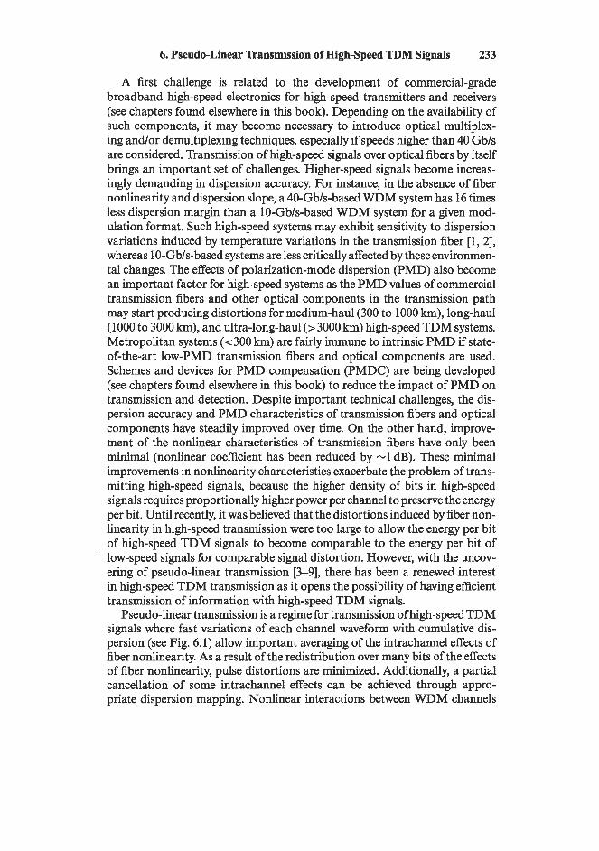
6. Pseudo-Linear Transmission of High-speed TDM Signals 233
A first challenge is related to the development of commercial-grade broadband high-speed electronics for high-speed transmitters and receivers (see chapters found elsewhere in this book). Depending on the availability of such components, it may become necessary to introduce optical multiplex- ing and/or demultiplexing techniques, especially if speeds higher than 40 Gb/s are considered. Transmission of high-speed signals over optical fibers by itself brings an important set of challenges. Higher-speed signals become increas- ingly demanding in dispersion accuracy. For instance, in the absence of fiber nonlinearity and dispersion slope, a 40-Gbls-based WDM system has 16 times less dispersion margin than a 10-Gb/s-based WDM system for a given mod- ulation format. Such high-speed systems may exhibit sensitivity to dispersion variations induced by temperature variations in the transmission fiber [l, 21, whereas 10-Gb/s-based systems are less critically affected by these environmen- tal changes. The effects of polarization-mode dispersion (PMD) also become an important factor for high-speed systems as the PMD values of commercial transmission fibers and other optical components in the transmission path may start producing distortions for medium-haul (300 to 1000 km), long-haul (1000 to 3000 km), and ultra-long-haul (>3000 km) high-speed TDM systems. Metropolitan systems (e300 km) are fairly immune to intrinsic PMD ifstate- of-the-art low-PMD transmission fibers and optical components are used. Schemes and devices for PMD compensation (PMDC) are being developed (see chapters found elsewhere in this book) to reduce the impact of PMD on transmission and detection. Despite important technical challenges, the dis- persion accuracy and PMD characteristics of transmission fibers and optical components have steadily improved over time. On the other hand, improve- ment of the nonlinear characteristics of transmission fibers have only been minimal (nonlinear coefficient has been reduced by -1 dB). These minimal improvements in nonlinearity characteristics exacerbate the problem of trans- mitting high-speed signals, because the higher density of bits in high-speed signals requires proportionally higher power per channel to preserve the energy per bit. Until recently, it was believed that the distortions induced by fiber non- linearity in high-speed transmission were too large to allow the energy per bit of high-speed TDM signals to become comparable to the energy per bit of low-speed signals for comparable signal distortion. However, with the uncov- ering of pseudo-linear transmission [3-91, there has been a renewed interest in high-speed TDM transmission as it opens the possibility of having efficient transmission of information with high-speed TDM signals.
Pseudo-linear transmission is a regime for transmission of high-speed TDM signals where fast variations of each channel waveform with cumulative dis- persion (see Fig. 6.1) allow important averaging of the intrachannel effects of fiber nonlinearity. As a result of the redistribution over many bits of the effects of fiber nonlinearity, pulse distortions are minimized. Additionally, a partial cancellation of some intrachannel effects can be achieved through appro- priate dispersion mapping. Nonlinear interactions between WDM channels

234 RedJean Essiambre et al.
h
4 6 0
8 0
40 E 20
300 -- -- --- -_ 0 -300 -200 ...----- 100
/-- _-_--- Time @s)
Time @s)
Fig. 6.1 The fast waveform evolution of rapidly dispersing pulses provide a redistribu- tion of the effects of fiber nonlinearity that is the basis for pseudo-linear transmission. The upper part of the figure shows the location of a 40-ps t h e window in the pulse train made of 5-ps pulses. The average power of the full train is 8 a.u. The lower part shows the waveform evolution in that time window after the pulses have been dispersed by 100 to 120 ps /m of cumulative dispersion by step of 5 pdnm. After such dispersion, pulses strongly overlap and any trace of the intensity proiile of individual pulses is lost. Note that each step of 5 pslnm corresponds to the cumulative dispersion of about 300 m of STD unshifted fiber.
(interchannel interactions) are generally much weaker than intrachannel non- linear interactions for pseudo-linear transmission. The evolution of the signal during propagation is generally characterized by important pulse overlap. In this regime, the optimum transmission is obtained when the net residual disper- sion at the end of the system is nearly zero, a characteristic common with trans- mission when fiber nonlinearity is negligible, i.e., when transmission is linear.
The origin of the term “pseudo-linear” transmission (pseudo means false, spurious, etc.) can be understood as follows The ultimate performance of a transport system is measured as the energy per bit it can transport at fixed signal distortion from fiber nonlinearity for a given spectral efficiency S (bits/s/Hz). It can be shown that the maximum energy per bit of a high- speed TDM signal transmitted in the pseudo-linear regime is on the order of the energy per bit of systems using lower bit rates (lOGb/s per channel and below) for high but practical spectral efficiencies of intensity-modulated signals (S = 0.2 to 0.4 bits/s/Hz). It follows that the transmission in the pseudo-linear regime is highly nonlinear since the energy per bit in this regime does not
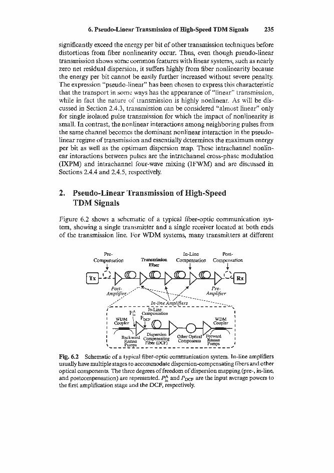
236 RenB-Jean Essiambre et al.
wavelengths are multiplexed together to form a WDM signal that is transmit- ted and demultiplexed before being detected by receivers. A number of spans made of transmission fibers are linked with discrete amplifiers that are used to periodically amplify the signal. In some instances, the transmission fiber can be Raman pumped to reduce the generation of amplified spontaneous emission (ASE) noise in the system. Typically dispersion compensation is applied at the amplification sites and is included within two stages of a multistage amplifier. This positioning inside an amplifier reduces the impact on ASE noise gener- ation associated with the introduction of a lossy element in the transmission line. Amplifiers linking two spans are referred to as in-line amplifiers, and dispersion compensation at these amplifier sites is referred to as in-line com- pensation. The amplifier following the transmitter is called a postamplifier (the prefix “post” is relative to the transmitter as the amplification is generally considered as an extension of the transmitter). The dispersion compensation at this amplification site is referred to as precompensation (the prefix “pre” is relative to the transmission line as the choice of dispersion compensation is dictated mainly by the transmission line ahead). Similarly, the amplifier just before the receiver is the preamplifier, and the associated dispersion com- pensation for this amplifier is the postcompensation. One should note that additional lossy elements might be present in the in-line amplifiers to perform other functions such as gain equalization, channel adddrop, channel cross- connect, performance monitoring, optical regeneration, polarization-mode dispersion (PMD) compensation, etc. Additional amplification stages may be inserted in the amplifiers to accommodate these additional elements.
A typical cumulative dispersion map is displayed in Fig. 6.3. It is generally desirable to have identical spans so as to minimize system complexity and cost. For such systems, the three parameters, pre-, in-line, and postcompensation, uniquely define the map. When convenient, in-line compensation is sometimes replaced by the residual dispersion per span and postcompensation by the net residual dispersion at the end of the link. Points of zero cumulative disper- sion are labeled ZO. In the absence of nonlinear effects and residual dispersion slope, the pulses at these points are identical to the pulses at the output of the transmitter. For pseudo-linear transmission, the pulses at zo are nearly transform-limited like those in linear transmission. Positions corresponding to launch points to the transmission fibers are labeled zin.
2.1 NOISE ACCUMULATION AND OPTICAL SIGNAL-TO-NOISE RATIO REQUIREMENTS
In optically amplified systems, the main source of noise is the accumulation of ASE of the optical amplifiers. The noise accumulation can easily be calculated for passive transmission fibers. The ASE noise generated in both polarization states by an individual amplifier (composed of multiple stages or not) measured
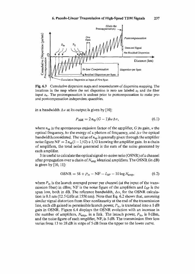
6. Pseudo-Linear Transmission of High-speed TDM Signals 237
(Undo the kcompensation) ,I
Zin
Postcompensation
Net Residual Dispersion
Dispersion per Span
Cumulative Dispersion at Input of First Span
Fig. 6.3 Cumulative dispersion maps and nomenclature of dispersion mapping. The locations in the map where the net dispersion is zero are labeled z0 and the fiber input zi,. The precompensation is undone prior to postcompensation to make pre- and postcompensation independent quantities.
in a bandwidth A u at its output is given by [lo]:
where nsp is the spontaneous emission factor of the amplifier, G its gain, u the optical frequency, hu the energy of a photon of frequency, and Au the optical bandwidth considered. The value of nsp is generally given through the amplifier noise figure NF = 2 nsp(l - 1/G) + 1/G knowing the amplifier gain. In a chain of amplifiers, the total noise generated is the sum of the noise generated by each amplifier.
It is useful to calculate the optical signal-to-noise ratio (OSNR) of a channel after propagation over a chain of Nap identical amplifiers. The OSNR (in dB) is given by [lo, 111:
where P i n is the launch averaged power per channel (at the input of the trans- mission fiber) in dBm; NF is the noise figure of the amplifiers and Lsp is the span loss, both in dB. The reference bandwidth, Au, for the OSNR calcula- tion is 0.1 nm (12.5 GHz at 1550nm). Note that Eq. 6.2 shows that, assuming similar signal distortion from fiber nonlinearity at the end of the transmission line, each dB gained in permissible launch power, P i n , is translated into a 1 dB gain in OSNR. Figure 6.4 displays the OSNR evolution with an increase in the number of amplifiers, Namp, in a link. The launch power, P i n , is OdBm, and the noise figure of each amplifier, NF, is 5 dB. The transmission fiber loss varies from 13 to 28 dB in steps of 5 dB from the upper to the lower curve.

238 Renk-Jean Essiambre et al.
I " " I " " l ~ " " ' " ' - 13 dg SpanLoss
--- 23 dB Span Loss . -.-. 28 dB Span Loss
....... 18 dB span Loss
.................. .................. ---------_ _ _
-.-.-.-.-._._._._,_.
0 10 20 30 40 50 Number of Amplifiers
Fig. 6.4 OSNR evolution as a function of the number of amplifiers Nmp. The launch power per channel is Pi, = 0 dBm and the noise figure of each amplifier is NF = 5 dB. At 40 Gbk, a typical OSNR requirement for bit-error-rate is 23 dB.
The required OSNR to achieve a given bit-error-rate (BER) depends in general on the nature of noise limiting detection, the type and distortions of the waveform being detected, and the receiver design. One can, however, derive an approximate expression for the required OSNR, assuming that the main source of noise results from the beating between the signal and the ASE noise and for large duty cycle intensity-modulated formats. Under these approximations, one can express the required OSNR, OSNRR, as [12],
Q2Be l + r OSNRR = - Bo ( 1 - a 2 '
where Bo is the optical reference bandwidth of 12.5 GHz and Be is the elec- trical Nter's bandwidth of the receiver. The transmitter extinction ratio, I, is defined as r = Izems/Iones, where Io, (Izems) is the instantaneous current at the sampling instant for a "1" ("0") bit. The parameter Q is given by [13]:
Iones - Izems
aones + azeros Q =
where cones (azems) is the standard deviation of Iones (Izems). At the opti- mum decision threshold, the parameter Q is related to the BER through the relation [ 131,
~ X P (-Q2/2) BER=-er$c - ($)% Q2/2;7 ' where erfc(x) = 2/fiLm exp (-u2)du is the complementary error function. A BER of corresponds to a value of Q = 6. The parameter Q is often quoted in dB by using 10 loge', giving 15.6dB for Q = 6. According to Eq. 6.3, the corresponding required OSNR is 19.4dB for an electrical filter bandwidth of Be = 30 GHz and an infinite extinction ratio (r = 0).

6. Pseudo-Linear Transmission of High-speed TDM Signals 239
Alternatively, one can estimate the OSNR requirement if the receiver sensitivity Prec is known using:
OSNRR = 58 + Pm - NF, (6.6)
where NF is the noise figure of the optically preamplified receiver. For such receivers the best (quantum-noise-limited) receiver sensitivity for an intensity-modulated format and direct detection corresponds to 38 photons per bit (NF = 3 dB), which gives an ideal OSNR requirement of 17.8 dB at 40Gb/s (infinite extinction ratio and ideal electrical filtering). This ideal OSNR requirement is 1.6 dB lower than the value given by the approximate expression of Eq. 6.3. For realistic transmitters and receivers with nonideal responses, the required OSNR is generally higher by more than 3 dB from the quantum limit. A direct measurement of receiver sensitivity can determine the required OSNR for a given transmitter-receiver pair by using Eq. 6.6.
One should also mention that 40-Gb/s systems using Reed-Solomon (239,255) forward-error correction (FEC) operate at a higher bit rate of 42.68 Gb/s and have a slightly higher OSNR requirement than systems operating without FEC (see chapters found elsewhere in this book).
One can estimate the impact on the noise figure of an in-line amplifier from the presence of an additional amplikation stage required to compensate for the loss of a dispersion-compensating fiber (DCF). Assuming the same noise figure NF for all amplification stages, the noise figure NFDC of an amplifier that includes a dispersion compensation module (DCM) of loss r] is approximately given by
where Pk is the average power at the input of the amplifier and PDCF is the average power at the input of the DCM (see Fig. 6.2). Let’s consider an example where the presence of a DCM significantly impacts the amplifier’s noise figure. For a 12-dB DCM loss ( r ] = 12 dB), a PDCF of -2 dBm to avoid nonlinearities in the DCF, and a Pk of - 16 dBm (launch power Pi, = 4 dBm and 20 dB span loss), the excess noise figure contribution is 2.1 dB. The impact of the presence of dispersion compensation can be minimized by using dispersion compensa- tion devices that have higher-power thresholds for nonlinearities or lower loss such as the higher-order mode (HOM) DCF described in Section 3.1.1.
2.2 INTENSITTY-MODULATED FORMATS AND SPECTRAL EFFICIENCY
Intensity-modulated direct-detection (IMDD) formats are the most com- monly used transmission formats in high-capacity fiber-optic communication systems (for alternative formats see chapters found elsewhere in this book).

240 RedJean Essiambre et al.
These formats generally lead to the simplest designs for transmitters and receivers. Such simplicity is desirable since the fabrication of commercial-grade high-speed receivers and transmitters is a challenge by itself. The IMDD for- mats are defined by the duty cycle and the pulse shape. The duty cycle d is defined as:
(6.8) d = - , TP TB
where Tp is the pulse full-width at half maximum (FWHM) and TB the bit period. The IMDD formats considered here are the non-return-to-zero (NRZ) format and the return-to-zero (RZ) format with Gaussian pulse shapes. Besides simplicity in transmitter and receiver designs, there are two important proper- ties determining the choice of optimum format for WDM transmission. The first is related to the spectral efficiency S defined as:
B S = - ,
Vch (6.9)
where B is the bit rate and Vch is the channel spacing. The spectral efficiency corresponds to the spectral density of information and is expressed in bits/s/Hz.
The spectra of various modulation formats differ in their bandwidths and shapes. Moreover, the intersymbol interference created by narrow optical or electrical filtering varies widely according to the modulation format. As a result, the ability to achieve high spectral efficiency by closely spacing WDM channels generally depends on the modulation format. Figure 6.5 shows an example of the differences between formats for demultiplexing a 40-Gbls signal from a WDM field with 100-GHz spacing. The fist two columns are the speo tra of an isolated channel and the WDM field, respectively. Third and fourth columns are the eye diagrams after demultiplexing for an isolated channel and from an arbitrary channel from the WDM field, respectively. For both cases, optical demultiplexing is performed using a 80-GHz FWHM Gaussian optical filter and a 28-GHz, 3-dB electrical Bessel filter included in the receiver. The upper row is the NRZ format, whereas from second to fourth row, the format is RZ (Gaussian pulses) with duty cycles of 50,33, and 20%, respectively. Single- channel eye diagrams clearly show minimal distortions, whereas eye diagrams of the demultiplexed WDM channel are distorted from coherent cross-talk. Coherent cross-talk originates from the overlap of the spectra of neighboring channels with the demultiplexed channel. The coherent cross-talk increases as the duty cycle decreases because the broader spectra of short pulses lead to greater spectral overlap. As a result, one should expect low-duty-cycle formats to be limited to lower spectral efficiencies than formats with larger duty cycles. Nonetheless, it is noticeable that for duty cycles as low as 20%, the eye dia- grams still show significant opening for the spectral efficiency of 0.4 bits/s/Hz of Fig. 6.5.
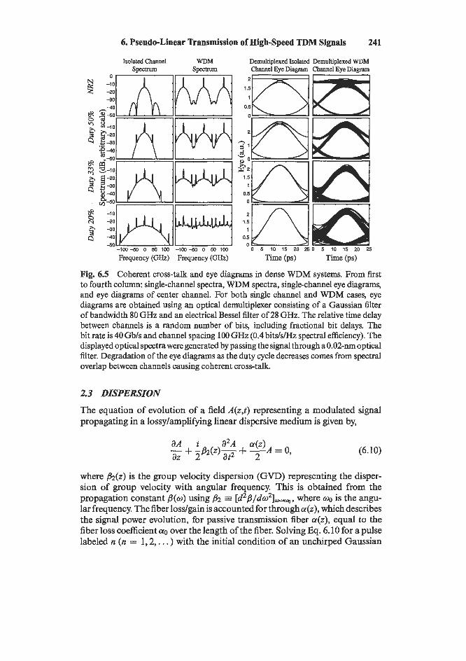
6. Pseudo-Linear Transmission of High-speed TDM Signals 241
Isolated Channel WDM speceum spectrum
Demultiplexed Isolated Demultiplexed WDM Channel Eye Diagram Channel Eye Diagram
2
1.5
1
0.5
0
2
- 1 z go v
!.I22 1.5
I 0.5
0
3 -30
4 0 do
0 5 10 15 20 250 5 10 15 20 25 -100 -50 0 50 100 -100 do 0 50 loo Frequency (GHz) Frequency (GHz) Time (ps) Time (ps)
Fig. 6.5 Coherent cross-talk and eye diagrams in dense WDM systems. From fmt to fourth column: single-channel spectra, WDM spectra, single-channel eye diagrams, and eye diagrams of center channel. For both single channel and WDM cases, eye diagrams are obtained using an optical demultiplexer consisting of a Gaussian filter of bandwidth 80 GHz and an electrical Bessel filter of 28 GHz. The relative time delay between channels is a random number of bits, including fractional bit delays. The bit rate is 40 Gbls and channel spacing 100 GHz (0.4 bitslslHz spectral efficiency). The displayed optical spectra were generated by passing the signal through a 0.02-nm optical filter. Degradation of the eye diagrams as the duty cycle decreases comes from spectral overlap between channels causing coherent cross-talk.
2.3 DISPERSION
The equation of evolution of a field A(z,t) representing a modulated signal propagating in a lossy/amplifying linear dispersive medium is given by,
aA i a2A a(z) - + -/32(z)- + -A = 0, aZ 2 at2 2
(6.10)
where BZ(Z) is the group velocity dispersion (GVD) representing the disper- sion of group velocity with angular frequency. This is obtained from the propagation constant B(w) using /32 = [d2B/d~2]0=00, where wo is the angu- lar frequency. The fiber loss/gain is accounted for through a(z), which describes the signal power evolution, for passive transmission fiber a(z), equal to the fiber loss coefficient a0 over the length of the fiber. Solving Eq. 6.10 for a pulse labeled n (n = 1 , 2, . . . ) with the initial condition of an unchirped Gaussian
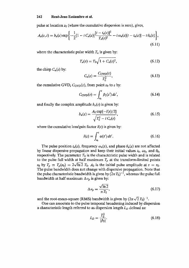
242 RenLTean Essiambre et al.
pulse at location zo (where the cumulative dispersion is zero), gives,
(6.1 1)
where the characteristic pulse width T, is given by:
the chirp C,(z) by: CGVD(Z) C,(Z) = -,
To2 the cumulative GVD, CGVD(Z), from point zo to z by:
and finally the complex amplitude b,(z) is given by:
where the cumulative losdgain factor Z(z) is given by:
Z(Z) = Jc,l .(z’)h’.
(6.13)
(6.14)
(6.15)
(6.16)
The pulse position t,(z), frequency w,(z), and phase &(z) are not affected by linear dispersive propagation and keep their initial values to, WO, and 00,
respectively. The parameter TO is the characteristic pulse width and is related to the pulse full width at half maximum Tp at the transform-limited points zo by Tp 3 TP(zo) = 2 m TO. A0 is the initial pulse amplitude at z = ZO.
The pulse bandwidth does not change with dispersive propagation. Note that the pulse characteristic bandwidth is given by (2nTo)-l, whereas the pulse full bandwidth at half maximum Av, is given by:
(6.17)
and the root-mean-square (RMS) bandwidth is given by ( 2 n a To)-’.
a characteristic length referred to as dispersion length LD defined as: One can associate to the pulse temporal broadening induced by dispersion
‘F2 10 L D = -. 1821
(6.18)
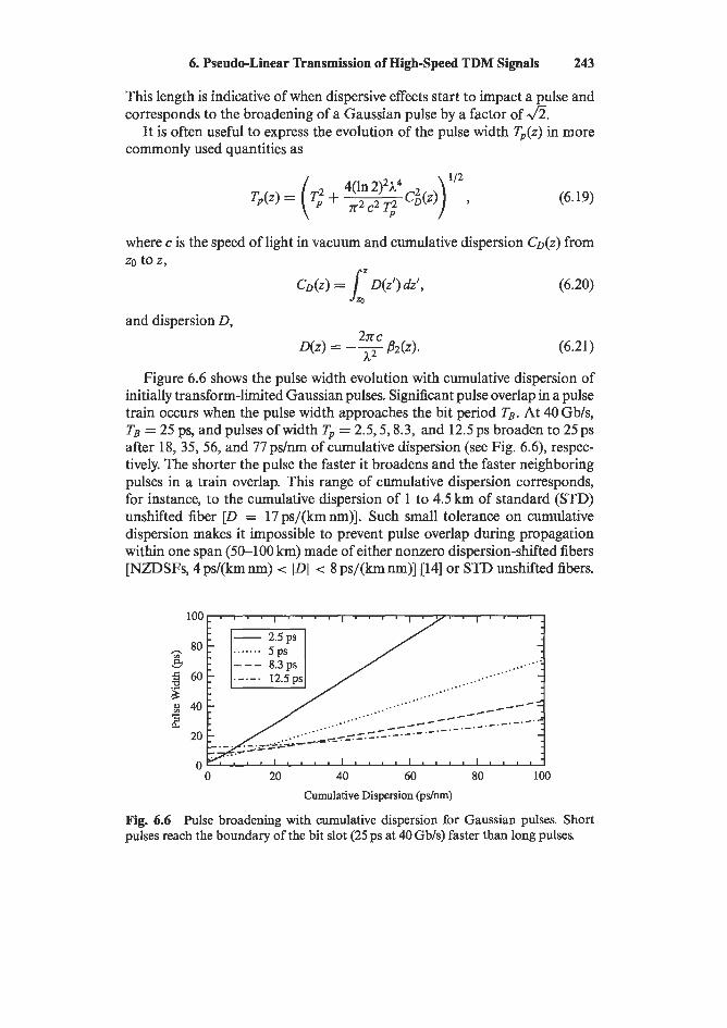
6. Pseudo-Linear Transmission of High-speed TDM Signals 243
This length is indicative of when dispersive effects start to impact a pulse and corresponds to the broadening of a Gaussian pulse by a factor of &.
It is often useful to express the evolution of the pulse width Tp(z) in more commonly used quantities as
(6.19)
where c is the speed of light in vacuum and cumulative dispersion C&) from 20 to z,
(6.20)
and dispersion D,
(6.21) h2
Figure 6.6 shows the pulse width evolution with cumulative dispersion of initially transform-limited Gaussian pulses. Significant pulse overlap in a pulse train occurs when the pulse width approaches the bit period TB. At 40 Gb/s, TB = 25 ps, and pulses of width Tp = 2.5,5,8.3, and 1 2 . 5 ~ s broaden to 25 ps after 18, 35, 56, and 77ps/nm of cumulative dispersion (see Fig. 6.6), respec- tively. The shorter the pulse the faster it broadens and the faster neighboring pulses in a train overlap. This range of cumulative dispersion corresponds, for instance, to the cumulative dispersion of 1 to 4.5 km of standard (STD) unshifted fiber [D = 17ps/(kmnm)]. Such small tolerance on cumulative dispersion makes it impossible to prevent pulse overlap during propagation within one span (50-100 km) made of either nonzero dispersion-shifted fibers [NZDSFs, 4ps/(kmnm) < ID1 < 8ps/(kmnm)] [14] or STD unshifted fibers.
2RC D(z) = -- B ~ ( z ) .
0 20 40 60 80 100
Cumulative Dispersion (pdnm)
Fig. 6.6 Pulse broadening with cumulative dispersion for Gaussian pulses. Short pulses reach the boundary of the bit slot (25 ps at 40 Gb/s) faster than long pulses.

244 RenC-Jean Essiambre et al.
However, the use of dispersion-shifted fibers [DSFs, 101 < Zps/(kmnm)] makes it possible to prevent pulse broadening for long pulses (Tp > lops). Alternatively, dispersion compensation on a short scale (a few kilometers) using segments of NZDSF or STD unshifted fibers can prevent the a m - mulation of dispersion. The impact of nonlinearity on high-speed TDM transmission using these low cumulative dispersion maps can be quite dif- ferent from the impact of nonlinearity in the pseudo-linear regime and will not be covered in this chapter (even though a glimpse of the effects of nonlin- earity on dispersion-shifted fibers (DSFs) for high-speed TDM signals can be seen in the upper part of Fig. 6.24).
Accumulating dispersion not only leads to pulse broadening, but also to pulse chirping. This can be understood by considering that dispersion leads to a spread in delays between the different frequency components of a pulse. As a result, in a medium having normal dispersion (negative D, positive &), the leading edge of a dispersed pulse becomes composed of the lowest-frequency components (“red”) of the pulse, whereas the trailing edge contains the highest- frequency components (“blue”). The opposite situation occurs for a medium having anomalous dispersion (positive D, negative 82). Because the phase of these frequency components evolve at different speeds, a chirp is created across the pulse.
The waveform evolution of a 40-Gbh pulse train made of 5-ps Gaussian pulses is shown in Fig. 6.7. As dispersion accumulates, the initially transform- limited pulses (Fig. 6.7a) broaden (Fig. 6.7b) until significant pulse overlap
0 0 1 0 0 1 0 0 1 1 0 1 1 0 1 0 1 1 0 1 (d) 30pdnm
60 60
40 40 20 20 n n
40
20
0 0 100 200 300 400 500 0 100 200 300 400 500
Time (ps) Time (ps)
Fig. 6.7 Waveform evolution of a 5-ps Gaussian-pulse train at 40 Gb/s with cumula- tive dispersion. The transform-limited pulses in (a) gradually broaden in (b) until there is significant overlap between nearest neighbors in (c)-(f). At large values of cumu- lative dispersion (100 ps/nm and above) a large number of pulses overlap in time and individual pulses are no longer identifiable.
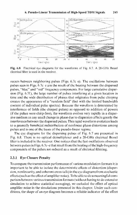
6. Pseudo-Linear Transmission of High-speed TDM Signals 245
10
0 5 10 15 20 2t 5 10 15 20 25
Time (ps) Time (ps)
Fig. 6.8 Electrical eye diagrams for the waveforms of Fig. 6.7. A 28-GHz Bessel electrical filter is used in the receiver.
occurs between neighboring pulses (Figs. 6.7c-e). The oscillations between pulses seen in Figs. 6.7c-e are the result of the beating between the dispersed pulses, “blue” and “red” frequency components. For large cumulative disper- sion (Fig. 6.7f), the large number of pulses interfering at a given location in time and the wide distribution of phases that originates from pulse chirping creates the appearance of a “random field” (but with the limited bandwidth content of individual pulse spectra). Because the waveform is determined by interference of fields (the chirped pulses) as opposed to addition of powers (if the pulses were chirp-free), the waveform evolves very rapidly in a disper- sive medium as any small change in phase due to dispersion affects greatly the interference between the dispersed pulses. This rapid waveform evolution leads to a generally beneficial redistribution of nonlinear phase distortions among pulses and is one of the bases of the pseudo-linear regime.
The eye diagrams for the dispersing pulses of Fig. 6.7 are presented in Fig. 6.8. There is no optical demultiplexer and a 28-GHz electrical Bessel filter is included in the receiver. One notices that the fast oscillations observed between pulses in Figs. 6.7c-e that result from the beating of the high-frequency components of the pulses are reduced as a result of electrical filtering.
2.3.1 Eye Closure Penalty
To compare the transmission performance of various modulation formats it is important to be able to isolate the deterministic effects of distortion (disper- sion, nonlinearity, and coherent cross-talk) in the eye diagrams from stochastic effects (such as the effect of amplifier noise). To be able to do a meaningful com- parison between various transmission formats (without having to do extensive simulation to achieve statistical averaging), we excluded the effect of optical amplifier noise in the simulations presented in this chapter. Under such con- ditions, the shape of an eye diagram becomes a reliable indicator of the effect

246 RenC-Jean Essiambre et al.
40
35
30 - + 25 m (u - 20
15
10
5 n 0 5 10 15 20 25 30 35
Time (ps)
Fig. 6.9 width 20% of the bit duration.
Example of the determination of the eye diagram closure using a box of
of transmission. One measure of distortions of an eye diagram is given by the eye closure penalty. It is calculated by first determining the height PR of the highest rectangle that can be fitted inside the eye opening. The rectangle width is 20% of the bit period TB. This width is chosen to include the effect of clock jitter on the decision sampling instant. The eye closure penalty (expressed in dB) is then given by:
Ceye = -1Olog ~
(2ppXe)’ (6.22)
where Pave is the signal average power. Note that twice the average power is equivalent to the height of the rectan-
gle for an unfiltered NRZ sequence having the same number of “zeros” and “ones.” A negative eye closure Ceye represents an eye more opened than the reference (the unfiltered NRZ signal), whereas a positive Ceye represents an eye more closed than the reference. Figure 6.9 shows a typical example of the positioning of the box for determining PR used in the eye closure calculation of Eq. 6.22. Note that the relation between eye closure penalty and receiver sensitivity penalty or BER penalty is not straightforward, as it depends on the nature of the noise and the type of waveform distortion.
2.3.2 Dispersion Margin and Modulation Formats
High-speed TDM systems based on intensity-modulated formats use closely- spaced short pulses that rapidly broaden and overlap (as seen in Fig. 6.7), causing intersymbol interference (ISI) [15]. This leads to much tighter require- ments on dispersion margins for high-speed TDM systems than for lower- speed systems. Dispersion margins are dependent on the modulation format. Figure 6.10 shows the eye closure as a function of the cumulative dispersion applied to transform-limited RZ and NRZ formats. One first notices that RZ formats have negative eye closure at the transform-limited point (0 pshm) that represents the fact that the eye opening is larger for RZ than unfiltered NRZ,
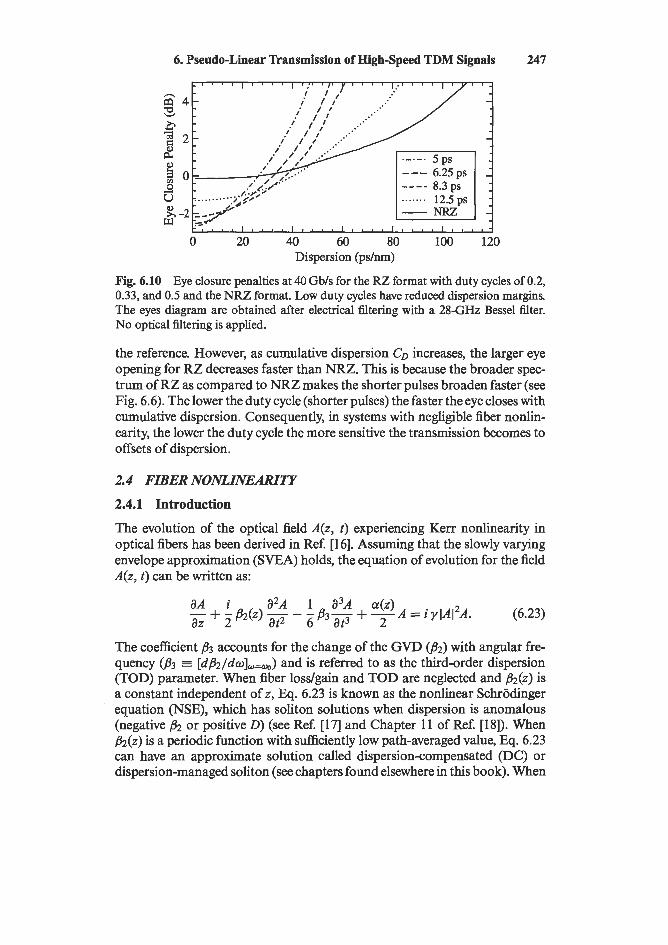
6. Pseudo-Linear Transmission of High-speed TDM Signals 247
I. ' ' ' ' I ' ' ' ' I ' ." ' I ' y ' ' ' ' I..' ' ' ' I ' y '
1 1 . . . . . . . 12.5 ps
I-NRZ
0 20 40 60 80 100 120 Dispersion (ps/nm)
Fig. 6.10 Eye closure penalties at 40 Gb/s for the RZ format with duty cycles of 0.2, 0.33, and 0.5 and the NRZ format. Low duty cycles have reduced dispersion margins. The eyes diagram are obtained after electrical filtering with a 28-GHz Bessel filter. No optical filtering is applied.
the reference. However, as cumulative dispersion CD increases, the larger eye opening for RZ decreases faster than NRZ. This is because the broader spec- trum of RZ as compared to NRZ makes the shorter pulses broaden faster (see Fig. 6.6). The lower the duty cycle (shorter pulses) the faster the eye closes with cumulative dispersion. Consequently, in systems with negligible fiber nonlin- earity, the lower the duty cycle the more sensitive the transmission becomes to offsets of dispersion.
2.4 FIBER NONLINEARITY 2.4.1 Introduction
The evolution of the optical field A(z, t ) experiencing Ken- nonlinearity in optical fibers has been derived in Ref [16]. Assuming that the slowly varying envelope approximation (SVEA) holds, the equation of evolution for the field A(z, t ) can be written as:
The coefficient 83 accounts for the change of the GVD ( 8 2 ) with angular fre- quency Cg3 [dp2/dw],=,) and is referred to as the third-order dispersion (TOD) parameter. When fiber losdgain and TOD are neglected and 82(z) is a constant independent of z, Eq. 6.23 is known as the nonlinear Schrodinger equation (NSE), which has soliton solutions when dispersion is anomalous (negative /32 or positive 0) (see Ref [17] and Chapter 11 of Ref [18]). When &(z) is a periodic function with suf€iciently low path-averaged value, Eq. 6.23 can have an approximate solution called dispersion-compensated (DC) or dispersion-managed soliton (see chapters found elsewhere in this book). When

248 RenC-Jean Essiambre et al.
any additional terms are included, Eq. 6.23 is referred to as a generalized nonlinear Schrodinger equation (GNSE).
The coefficient 83 of Eq. 6.23 is related to the more straightforwardly measurable quantity dispersion slope S through the following relation,
dD 4nc dh h3
S(2) = - = - p (6.24)
The coefficient y in Eq. 6.23 represents the effect of the Kerr nonlinearity and
(6.25) n 2 wo is defined as: y = -
where 122 is the nonlinear refractive index coefficient and A& is the effective mode area. Typical fiber parameter values for some common fibers are given in Table 6.1.
One can associate different length scales that are specific to nonlinear transmission. A first length scale is related to power only and is defined as:
cAeff ’
1 LNL=-,
YPP (6.26)
where LNL is the fiber length required to produce nonlinear phase rotation of one radian at a power Pp. When Pp is interpreted as a pulse peak power, LNL is related to the effect of self-phase modulation (SPM, see Section 2.4.3). A second length scale is related to the power evolution in fibers; for a passive fiber this is known as the effective length L,ff and is given by:
1 - exp (-a0 L) a0
Leff = Y (6.27)
where L is the length of the fiber segment considered. The effective length L,ff gives the length over which the power decreases by a factor of e in passive fibers. This length is related to most nonlinear effects but is perhaps most critical for SPM and cross-phase modulation (XPM) (see Chapter 8 of Ref. [18] and chapters found elsewhere in this book).
A third length scale is the walk-off length and is defined as:
TD L w = - DAV ’ (6.28)
where Av is the spacing between the two spectral components of interest and TO is a time delay. In WDM systems experiencing XPM (see Fig. 6.1 l), the relevant delay corresponds to 2 Tp (see Chapter 8 of Ref [18]), the delay nec- essary for two pulses from channels separated by Av to fully walk through each other. The time delay TD may have different values depending of the non- linear interaction of interest. Note that the dispersion length LD defined in

Table 6.1 Some Nominal Values of Fiber Parameters at 1550 nm of Different Commercial Fiber Brands. The Ratio Dispersion to Slope (RDS) Is Defined as S/D
D S RDS (110 Aefi PMD Manufacturer ps/(km nm) ps/(ltm nm2) nm-’ dBhm pm2 ps/& Fiber
TrueWaveTM RS Lucent 4.5 0.045 0.01 0.22 55 t o . 1 LEAFW Corning 4.2 0.09 0.021 0.22 12 t O . l
STD unshifted fiber Lucent, Coming, 16.9 0.055 0.0033 0.23 87 t o . 1
Submarine Lucent -3.1 0.05 -0.016 0.215 50 t o . 1 DeeplightTM Pi r e 11 i -2.2 t0.12 >-0.055 t0.23 70 to . 1 TeralightTM Alcatel 8 0.058 0.0073 t0.25 63 t0.08
DCF Lucent -100 -0.22 0.0022 0.5 20 t0.25 WB-DCF Lucent -95 -0.33 0.0035 0.5 19 t0.25 HS-DCF Lucent -100 -0.67 0.0067 0.68 15 t0.25
TeralightTM Ultra Alcatel 8 0.052 0.0065 t0.22 63 (0.04
Furukawa
Metro
N A W

250 RenkJean Essiambre et al.
Eq. 6.18 can be interpreted as a walk-off length within a pulse where the delay To = TO, the characteristic pulse width, and the spectral separation Au = -sgnm(B$t2/(ncTo).
The various length scales defined in Eq. 6.18 and Eqs. 6.26-6.28 character- ize different length scales for the effects of nonlinearity. In general, these length scales depend on channel bit rate, channel spacing, modulation format, fiber types, input powers, power evolution, dispersion mapping, amplifier spacings, system length, etc. It is difficult to determine a general rule that would deter- mine which scale is the most important for a given set of system parameters. Nonetheless, it is still instructive to define these length scales and, whenever possible, we will point out the scale relevant to nonlinear interactions specific to pseudo-linear transmission.
Equation 6.23 describes the evolution of the full field (which may include many WDM channels) with distance. In general, nonlinear interactions for the WDM field can be decomposed into more basic nonlinear interactions (see Fig. 6.1 1). These interactions are single-channel self-phase modulation, multiple-channel cross-phase modulation (XPM), and multiple-channel four- wave mixing (FWM). Cross-phase modulation and four-wave mixing are interchannel interactions that are the strongest for moderate- (-10 Gb/s) and low-speed (c 10 Gb/s) signals. Cross-phase modulation and four-wave mixing
Basic Nonlinear Interactions -- Single Channel Multiple Channels (WDM)
SingleChannel Modulation Four-Wave Cross-Phase Self-Phase Modulation Instability (MI) Mixing {FWM) Modulation JXPM)
Self-Phase Nonlinear Coherent Cross-talk Timing Jitter Modulation (SPM) Intersymbol and Pulse Distortion
-- -- -\ v v
(Soli:ons, etc.) Intefierence
/ \ Pulse Distortion
Intrachannel Intrachannel Cross-Phase Four-Wave Modulation Mixing
U m a I I F W M ) v
Timing Jitter Amplitude Jirrer ... 10 Gbls and Above 10 Gb/s and Below
Fig. 6.11 Distribution of inter- and intrachannel nonlinear impairment in a WDM system for different bit rates per channel. For high-speed TDM systems, the domi- nant nonlinear interactions are self-phase modulation (SPM), intrachannel cross-phase modulation (IXPM), and intrachannel four-wave mixing (IFWM).
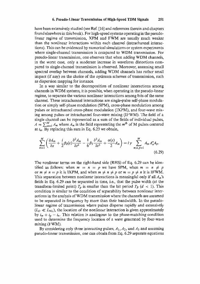
6. Pseudo-Linear Transmission of High-speed TDM Signals 251
have been extensively studied (see Ref [ 161 and references therein and chapters found elsewhere in this book). For high-speed systems operating in the pseudo- linear regime of transmission, XPM and FWM are usually much weaker than the nonlinear interactions within each channel (intrachannel interac- tions). This can be evidenced by numerical simulations or system experiments where single-channel transmission is compared to WDM transmission. For pseudo-linear transmission, one observes that when adding WDM channels, in the worst case, only a moderate increase in waveform distortions com- pared to single-channel transmission is observed. Moreover, assuming small spectral overlap between channels, adding WDM channels has rather small impact (if any) on the choice of the optimum schemes of transmission, such as dispersion mapping for instance.
In a way similar to the decomposition of nonlinear interactions among channels in WDM systems, it is possible, when operating in the pseudo-linear regime, to separate the various nonlinear interactions among bits of the same channel. These intrachannel interactions are single-pulse self-phase modula- tion or simply self-phase modulation (SPM), cross-phase modulation among pulses or intrachannel cross-phase modulation (IXPM), and four-wave mix- ing among pulses or intrachannel four-wave mixing (IFWM). The field of a single channel can be represented as a sum of the fields of individual pulses, A = zt=, A , where A , is the field representing the mth of M pulses centered at tm. By replacing this sum in Eq. 6.23 we obtain,
M
= i y A , A ; A ~ . m= I m,n,p=l
(6.29)
The nonlinear terms on the right-hand side (RHS) of Eq. 6.29 can be iden- tified as follows: when m = n = p we have SPM, when m = n # p or m # n = p it is IXPM, and when m # n # p or m = p # n it is IFWM. This separation between nonlinear interactions is meaningful only if all Am’s fields in Eq. 6.29 can be separated in time, Le., that the pulse width (at the transform-limited point) Tp is smaller than the bit period TB (d < 1). This condition is similar to the condition of separability between nonlinear inter- actions in the analysis of WDM transmission where the channels are assumed to be separated in frequency by more than their bandwidth. In the pseudo- linear regime of transmission where pulses disperse rapidly and extensively (Lo << LNL), the location of the nonlinear interaction is given approximately by tm + tp - tn. This relation is analogous to the phase-matching condition used to determine the frequency location of a wave generated by four-wave mixing (FWM).
By considering only three interacting pulses, A , , A2, and A3 and assuming pseudo-linear transmission, one can obtain from Eq. 6.29 separate equations
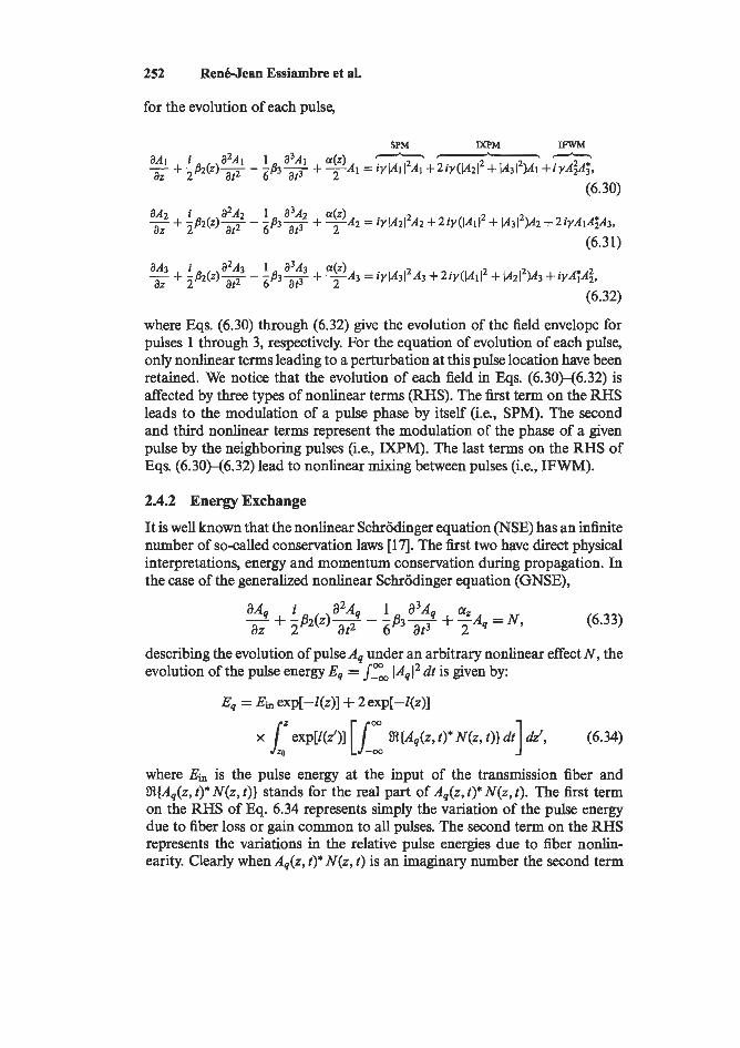
252 RedJean Essiambre et aL
for the evolution of each pulse,
SPM IXPM IFWM
aA2 i a 2 ~ 2 1 a 3 ~ 2 a(z) - + -82(z)- - -83- + -A2 = iylAzI2Az + 2iy(lA1I2 + IA312)A2 +2iyAlAtA3, az 2 at2 6 at3 2
(6.31) 3~~ i a * ~ ~ 1 a 3 ~ 3 a(z) a Z 2 at2 6 at3 2 - + -82(z)- - -83- + -A3 = iyIA3I2A3 +2iy(lAiI2 + IA212243 +iyA;Az,
(6.32)
where Eqs. (6.30) through (6.32) give the evolution of the field envelope for pulses 1 through 3, respectively. For the equation of evolution of each pulse, only nonlinear terms leading to a perturbation at this pulse location have been retained. We notice that the evolution of each field in Eqs. (6.30H6.32) is affected by three types of nonlinear terms (RHS). The first term on the RHS leads to the modulation of a pulse phase by itself (i.e., SPM). The second and third nonlinear terms represent the modulation of the phase of a given pulse by the neighboring pulses (i.e., IXPM). The last terms on the RHS of Eqs. (6.30H6.32) lead to nonlinear mixing between pulses (ie., IFWM).
2.4.2 Energy Exchange
It is well known that the nonlinear Schrodinger equation (NSE) has an infinite number of so-called conservation laws [17]. The fist two have direct physical interpretations, energy and momentum conservation during propagation. In the case of the generalized nonlinear Schrodinger equation (GNSE),
aA, i @A, 1 a3A, az - + 2/32(z)- - - 8 3 7 + -A, = N , az at2 6 at 2 (6.33)
describing the evolution of pulse A, under an arbitrary nonlinear effect N , the evolution of the pulse energy E, = f”, IA,I2 dt is given by:
E, = Ej,, exp[-Z(z)] + 2 exp[-l(z)]
where Eh is the pulse energy at the input of the transmission fiber and %{A,(z, t)* N(z, t ) ] stands for the real part of A,(z, t)* N(z, t). The first term on the RHS of Eq. 6.34 represents simply the variation of the pulse energy due to fiber loss or gain common to all pulses. The second term on the RHS represents the variations in the relative pulse energies due to fiber nonlin- earity. Clearly when A,(z, t)* N(z, t ) is an imaginary number the second term
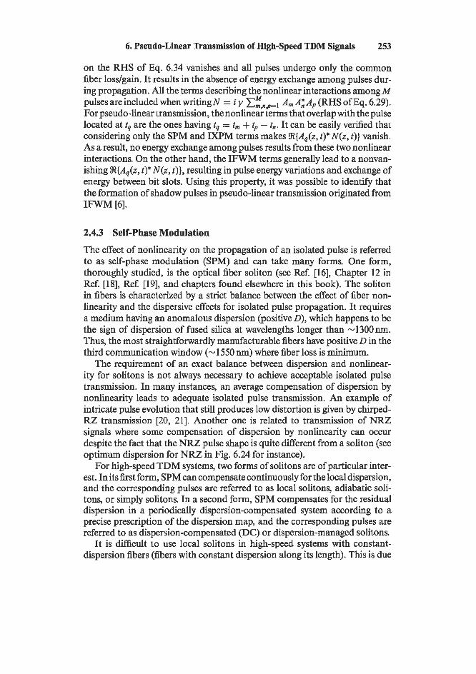
6. Pseudo-Linear Transmission of High-speed TDM Signals 253
on the RHS of Eq. 6.34 vanishes and all pulses undergo only the common fiber losdgain. It results in the absence of energy exchange among pulses dur- ing propagation. All the terms describing the nonlinear interactions among M pulses are included when writingN = i y CEn,=, A, A: Ap (RHS of Eq. 6.29). For pseudo-linear transmission, the nonlinear terms that overlap with the pulse located at tq are the ones having tq = t, + tp - tn. It can be easily verified that considering only the SPM and IXPM terms makes %{A4(z, t>* N(z , t)} vanish. As a result, no energy exchange among pulses results from these two nonlinear interactions. On the other hand, the IFWM terms generally lead to a nonvan- ishing %{A,(z, t)* N(z, t)}, resulting in pulse energy variations and exchange of energy between bit slots. Using this property, it was possible to identify that the formation of shadow pulses in pseudo-linear transmission originated from IFWM [6].
2.4.3 Self-Phase Modulation
The effect of nonlinearity on the propagation of an isolated pulse is referred to as self-phase modulation (SPM) and can take many forms. One form, thoroughly studied, is the optical fiber soliton (see Ref. [16], Chapter 12 in Ref. [18], Ref [19], and chapters found elsewhere in this book). The soliton in fibers is characterized by a strict balance between the effect of fiber non- linearity and the dispersive effects for isolated pulse propagation. It requires a medium having an anomalous dispersion (positive D), which happens to be the sign of dispersion of fused silica at wavelengths longer than -1300nm. Thus, the most straightforwardly manufacturable fibers have positive D in the third communication window (-1 550 nm) where fiber loss is minimum.
The requirement of an exact balance between dispersion and nonlinear- ity for solitons is not always necessary to achieve acceptable isolated pulse transmission. In many instances, an average compensation of dispersion by nonlinearity leads to adequate isolated pulse transmission. An example of intricate pulse evolution that still produces low distortion is given by chirped- RZ transmission [20, 211. Another one is related to transmission of NRZ signals where some compensation of dispersion by nonlinearity can occur despite the fact that the NRZ pulse shape is quite dif€erent from a soliton (see optimum dispersion for NRZ in Fig. 6.24 for instance).
For high-speed TDM systems, two forms of solitons are of particular inter- est. In its first form, SPM can compensate continuously for the local dispersion, and the corresponding pulses are referred to as local solitons, adiabatic soli- tons, or simply solitons. In a second form, SPM compensates for the residual dispersion in a periodically dispersion-compensated system according to a precise prescription of the dispersion map, and the corresponding pulses are referred to as dispersion-compensated (DC) or dispersion-managed solitons.
It is difficult to use local solitons in high-speed systems with constant- dispersion fibers (fibers with constant dispersion along its length). This is due
254 Red-Jean Essiambre et al.
to the large range of signal power experienced during propagation in the trans- mission fiber. This range is approximately 10 to 25 dB for passive transmission fibers. Self-phase modulation (SPM), the nonlinear effect that compensates the effects of dispersion also experiences the same range as the power evo- lution. To preserve the local soliton, the width of each local soliton would also experience the same range as the power evolution, and consequently, the spectral bandwidth of the local soliton would vary by 10 to 25dB [22-251. Such large variations in spectral bandwidth prevent efficient use of WDM techniques. It is possible, however, to preserve the balance of nonlinearity and dispersion required by local solitons without the spectral broadening by tai- loring the fiber dispersion along its length. For passive fibers, the dispersion should decrease exponentially along the length, and such fibers are referred to as dispersion-decreasing fibers (DDFs) [26-281. Even though interesting and manufacturable from a single fiber draw [29-331, DDFs impose some important constraints on system designs by forcing fixed values of powers (the local soliton power) for the signal evolution, as well as unidirectionality for individual fibers. Moreover, the wide dispersion range necessary to accom- modate the span loss (>20 dB) for large amplifier spacings (100 km) requires large values of dispersion at the input end of the fiber. Such a high dispersion value increases significantly the path-averaged dispersion and can lead to large timing jitter [34-371.
The other possibility for using the soliton effect in high-speed TDM sys- tems is to use DC solitons. The design of DC soliton links allows some pulse broadening but limited to the bit slot duration to prevent pulse overlap dur- ing transmission. As shown in Fig. 6.7, at 40 Gb/s the pulse overlap becomes significant when the cumulative dispersion reaches approximately f 10 ps/nm. For large amplifier spacings (-100 km), this requirement restricts the disper- sion of the transmission fiber to a range of ID1 c 2 ps/(km nm), assuming a precompensation of half the span cumulative dispersion. Dispersion-shifted fibers (DSFs) meet the requirement of low-dispersion values (over a limited bandwidth of -60nm however) and can support DC solitons [38-44]. Such low, local dispersion, however, makes WDM difficult due to four-wave mixing (FWM) [45] and limits the use of DSFs in high-capacity transport.
An alternative to DSFs is to use dispersion compensation on a short length scale (on the order of a few kilometers) [46-48]. Such short-scale dispersion compensation allows one to use fiber segments with relatively high dispersion and still have a low value of average dispersion and a low excursion of cumula- tive dispersion. As for the fabrication of DDFs, one can fabricate continuously dispersion compensating fibers (CDCFs) from a single fiber draw [49]. How- ever, the scale of dispersion compensation cannot be arbitrarily small because for too frequent dispersion compensation, the fiber starts to behave like a constant-dispersion fiber with a low average value of dispersion. As for DSF, such CDCF would suffer from FWM in WDM transmission [46]. As a result, an optimum scale of dispersion compensation may exist that will correspond

6. Pseudo-Linear Transmission of High-speed TDM Signals 255
to a tradeoff between the effects of pulse broadening and FWM. One should note that the design of such a CDCF is a priori bit rate and modulation format specific. Since the use of DSFs is likely to be limited by FWM, it suggests that the effective use of DC solitons in high-speed systems may require deployment of special transmission fibers.
In pseudo-linear transmission, the propagation of short pulses (Tp 10 ps) over dispersive fibers [ID1 > 2 ps/(km nm)] is dominated by dispersion (LD << LNL), and each pulse can broaden by up to several orders of magni- tude. As a result, the length scale over which the soliton dynamics start to play a significant role can increase considerably, reducing the importance of SPM in pseudo-linear transmission [50, 511. The effect of SPM is best seen by considering the bandwidth evolution of a short pulse transmitted in the pseudo-linear regime as depicted in Fig. 6.12 (from Ref. [SO]). The transform- limited pulse width is 5 ps, and each span is made of 100 km of large effective area STD unshifted fiber fully dispersion compensated at each amplifier. The parameters of the transmission fiber differ slightly from Table 6.1 and are
= -2Ops2/km [D = 15.75ps/(km nm)], (11 = 0.25 dB/km, A,ff = 108 pm2 and n2 = 3.2 x cm2/W. Three dispersion maps are represented. Curve (a) in Fig. 6.12 shows the bandwidth evolution when no precompensation is
Pulse RMS bandwidth evolution as a function of distance for transmission of-5-ps Gaussian pulse over multiple spans. Full dispersion compensation at each span is applied. The amplifier spacing is 100 km and the transmission fiber is a large effective area fiber with the following parameters, #32 = -20 ps2/km, ct = 0.25 dB/km, Aen = 108 pm2 and n2 = 3.2 x cm2/W. In case (a) there is no precompensation, (b) a precompensation of 2000 ps2/km (D = - 1575 ps/nm), equivalent to one span, and (c) a precompensation of 100 ps2 [D = -79 ps/(km nm)]. The input peak powers Pp are 35,20, and 50mW for (a), (b), and (c), respectively. From Ref. [50].
256 Renk-Jean Essiambre et al.
applied. Curve (b) is when a precompensation compensating for a full span is used (CpE = - 1575 ps/nm), whereas curve (c) is when 5% of the span dis- persion is precompensated (CpE = -79 ps/nm). When no precompensation is present [curve (a)], a sharp bandwidth decrease occurs where the pulse peaks up (at the beginning of each span), with negligible bandwidth evolution for the remainder of each span. When the precompensation is set to compensate a full span dispersion [curve (b)], the pulse peaks up at the very end of the span where the power is low and the effect of SPM is neghgible. For a moderate precompensation of 5% of the span [curve (c)], the pulse bandwidth experi- ences a rapid breathing just around the point of zero cumulative dispersion (points zo in Fig. 6.3) where the pulse is nearly transform-limited. This evolu- tion consists of a rapid spectral broadening just before zo followed by a rapid spectral narrowing (of nearly equal magnitude as the spectral broadening) just after zo. The net result is the generation of a small residual spectral broadening every time the pulse goes through a point zo in the transmission fiber. For a transmission fiber of opposite sign of dispersion, a net spectral narrowing is observed instead of a net spectral broadening.
Figure 6.12 also shows that the magnitude of the spectral narrowing after 13 spans is about 10% for the case of no precompensation [curve (a)], 2% when the precompensation is equal to 5% of the span [curve (c)], and virtually no change in pulse bandwidth when the precompensation is equal to the fidl span [curve (b)]. Because the chirp caused by SPM is a smooth function, the broadening or narrowing of the spectra observed in Fig. 6.12 is virtually equivalent to change in duty cycle of the pulses. The effect of SPM is identical for each pulse of a data sequence. The net result of SPM is to produce a train of identical pulses with a slightly different duty cycle than the original train. For the example of curve (c) of Fig. 6.12 that has a 2% spectral broadening after 13 spans, no significant degradation in the eye diagram and reception results from SPM in single-channel transmission. Even for larger spectral broadening (like a doubling of the spectrum bandwidth), no significant degradation is expected from SPM other than the difference in eye openings between various duty cycles (see Section 2.3.1). In the case of a 5% precompensation [curve (c) of Fig. 6.121, the spectral bandwidth doubles only after approximately 40,000 km. The most likely detrimental effect of SPM in the pseudo-linear transmission regime is to broaden the spectrum so much as to create coherent cross-talk from overlapping spectra in dense WDM.
It is clear that for pseudo-linear transmission of high-speed TDM signals, the effect of nonlinearity on isolated pulse transmission (the effect of SPM) is greatly reduced relative to lower bit rate systems. However, in pseudo-linear transmission, a large number of pulses belonging to the same channel simul- taneously overlap and interact through fiber nonlinearity. As mentioned in Section 1 , these intrachannel interactions among neighboring pulses are the main source of waveform distortions in pseudo-linear transmission.
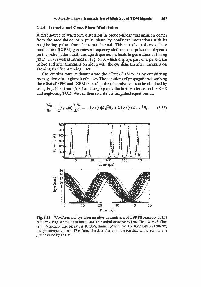
6. Pseudo-Linear mansmission of High-speed TDM Signals 257
2.4.4 Intrachannel Cross-Phase Modulation
A first source of waveform distortion in pseudo-linear transmission comes from the modulation of a pulse phase by nonlinear interactions with its neighboring pulses from the same channel. This intrachannel cross-phase modulation (IXPM) generates a frequency shift on each pulse that depends on the pulse pattern and, through dispersion, it leads to generation of timing jitter. This is well illustrated in Fig. 6.13, which displays part of a pulse train before and after transmission along with the eye diagram after transmission showing significant timing jitter.
The simplest way to demonstrate the effect of IXPM is by considering propagation of a single pair of pulses. The equations of propagation describing the effect of SPM and IXPM on each pulse of a pulse pair can be obtained by using Eqs. (6.30) and (6.31) and keeping only the first two terms on the RHS and neglecting TOD. We can then rewrite the simplified equations as,
(6.35)
0 50 100 150 200 Time @s)
16 14 12
0 8 $ 6
4 2 0
s 10 v
0 10 20 30 40 50
Time (ps)
Fig. 6.13 Waveform and eye diagram after transmission of a PRBS sequence of 128 bits consisting of 5-ps Gaussian pulses. Transmission is over 80 km ofTrueWaveTM fiber (D = 4 ps/nm). The bit rate is 40 Gb/s, launch power 18 dBm, fiber loss 0.21 d B h , and precompensation - 17 ps/nm. The degradation in the eye diagram is from timing jitter caused by IXPM.

258 RenHean Essiambre et al.
where we renormalized the amplitude A, to
Bn = A n exp[W/21, (6.36)
where n = 1 , 2 and s(z) = exp[-Z(z)] is the power evolution (normalized to the power at z = ZO). The second term on the RHS of Eq. 6.35 represents the effect of cross-phase modulation of one pulse on another and is the MPM effect.
A few methods have been used to evaluate analyt~cally the effects of MPM [52-61]. One approach consists of using the variational formulation [62]. The variational approach is particularly useful in nonlinear optics for describing the propagation of chirped pulses in nonlinear media. It was first used to describe pulse propagation in nonlinear diffractive media [63] and then in nonlinear dispersive media [64] such as optical fibers. Even though pertur- bative in nature, the variational method can be quite accurate even when the effect of nonlinearity is large [65,66]. The accuracy essentially depends on how well the ansatz chosen represents the evolution of the field experiencing non- linearity. It is known through numerical simulations that the pulse integrity is essentially preserved after nonlinear interactions [3-61 in the pseudo-linear regime and that dispersion dominates the waveform evolution. Let’s consider the following ansatz,
(6.37)
where the parameters B,, C,, T,, t,, w,, and e,, assumed real, are the nth pulse renormalized amplitude, chirp, characteristic width, position, frequency, and phase, respectively. All these parameters are assumed to be slowly varying functions of the distance z. Applying the variational method to Eq. 6.35 with the ansatz (6.37) gives [52, 541,
(6.38)
(6.39)
d a w - = E y s(z)(Ei + E2)P2 T exp (-T2/2) dz (6.41)
(6.42) dAt dz - = - B ~ ( z ) A ~ ,

6. Pseudo-Linear Transmission of High-speed TDM Signals 259
where n = 1 , 2, Aw = 01 - w2 is the relative angular frequency between pulses 1 and 2, and At = tl - tz the separation between the two pulses. The dummy parameters P = &/dm and T = PAt have been introduced for convenience. The equation of evolution of the phase 6, has been omitted here. From Eqs. 6.38 and 6.39, one can easily show that the renormalized energy per bit, E1,2 = f i B ; , z T ~ , z , is conserved (as one would expect for IXPM, as discussed in Section 2.4.2). From Eq. 6.36, the actual energy in the fiber, E,(z), is given by E&) = E~exp[-Z(z)], where EO is the energy of a pulse at z = zo or E n ( Z ) = Eh exp [-Z(z - in)], where Ein = f i B i T n = f i A : ( z = Zin)Tn(z = Zin) is the energy per pulse at the input of the span located at z = zh.
Equations 6.38-6.42 represent the evolution of the pulse parameters with distance. One can easily verify that in the absence of nonlinearity [ y = 01 one recovers the evolution of a pulse in a dispersive medium (Eqs. 6.1 1-6.15) except for the pulse amplitude B, that is given by:
B, = Bo/[l + C,(Z)~]~’~ = Ibnl. (6.43)
The latter equation means that the phase of the complex amplitude b, asso- ciated with a linearly dispersive pulse is not included in the choice of ansatz (Eq. 6.37) used in the variational method.
It is obvious from Eqs. 6.38-6.42 that IXPM affects all pulse parameters, B,, C,, T,, t,, and 0,. The chup is affected by both SPM (second term on the RHS of Eq. 6.40) and IXPM (third term on the RHS of Eq. 6.40). Chirping of a transform-limited pulse results in spectral broadening [16]. As discussed in Section 2.4.3, the spectral broadening caused by chirp induced by SPM is gen- erally small in the pseudo-linear regime, especially when a precompensation equivalent to a few kilometers of transmission fibers is used (see Fig. 6.12). Moreover, the pulse chirping induced by SPM is identical for all pulses and does not lead to significant closure of the eye, as all pulses have the same degree of broadening at a given point in the dispersion map. The pulse chirping effect of IXPM, however, depends on the presence or absence of neighboring pulses and creates a differential in pulse parameters that depends on the bit pattern. This effect of IXPM will create not only a differential in pulse bandwidth as the pulses propagate, but also in the value of net residual dispersion at which the pulses are transform-limited at the end of transmission. As a result, pulse chirping induced from IXPM can be responsible for some degree of amplitude jitter as pulses with different degrees of temporal broadening will be observed at a given point in the dispersion map. However, a potentially more dramatic effect of IXPM is the generation of timing jitter through the generation of frequency shifts (Eq. 6.41) that are converted into time shifts by dispersion (Eq. 6.42). For the case of a single pulse pair, the relative time shift induced by the nonlinear interaction between two pulses can be obtained by simultane- ously solving Eqs. 6.41 and 6.42. For the purpose of solving Eqs. 6.41 and 6.42,
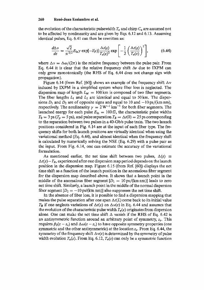
260 Renk-Jean Essiambre et al.
the evolution of the characteristic pulsewidth T,, and chirp C,, are assumed not to be affected by nonlinearity and are given by Eqs. 6.12 and 6.13. Assuming identical pulses, Eq. 6.41 can then be rewritten as:
where Au = Aw/(2n) is the relative frequency between the pulse pair. From Eq. 6.44 it is clear that the relative frequency shift Au due to IXPM can only grow monotonically (the RHS of Eq. 6.44 does not change sign with propagation).
Figure 6.14 (from Ref. [60]) shows an example of the frequency shift Au induced by IXPM in a simplified system where fiber loss is neglected. The dispersion map of length LM = lOOkm is composed of two fiber segments. The fiber lengths L1 and LZ are identical and equal to 50km. The disper- sions D1 and D2 are of opposite signs and equal to 10 and -1Ops/(kmnm), respectively. The nonlinearity y = 2 W-' km-' for both fiber segments. The launched energy for each pulse Ein = 100 fJ, the characteristic pulse widths TO = 3 ps (Tp = 5 ps), and pulse separation TB = At(0) = 25 ps corresponding to the separation between two pulses in a 4O-Gb/s pulse train. The two launch positions considered in Fig. 6.14 are at the input of each fiber type. The fre- quency shifts for both launch positions are virtually identical when using the variational method (Eq. 6.44), and almost identical when the frequency shift is calculated by numerically solving the NSE (Eq. 6.29) with a pulse pair as the input. From Fig. 6.14, one can estimate the accuracy of the variational formulation.
As mentioned earlier, the net time shift between two pulses, A(z) 3
At(z) - TB, experienced after one dispersion map period depends on the launch position in the dispersion map. Figure 6.15 (from Ref. [60]) displays the net time shift as a function of the launch position in the anomalous fiber segment for the dispersion map described above. It shows that a launch point in the middle of the anomalous fiber segment [Dl = lOps/(kmnm)] leads to zero net time shift. Similarly, a launch point in the middle of the normal dispersion fiber segment [D2 = -10 ps/(km nm)] also suppresses the net time shift.
In the absence of fiber loss, it is possible to find a dispersion mapping that makes the pulse separation after one span At(L) come back to its initial value TB if one neglects variations of At(z) on Au(z) in Eq. 6.44 and assumes that the evolution of the characteristic pulse width T,(z) originates from dispersion alone. One can make the net time shift A vanish if the RHS of Eq. 6.42 is an antisymmetric function around an arbitrary point of symmetry, 2,. This requires 82(z - z,) and Aw(z - z,) to have opposite symmetry properties (one symmetric and the other antisymmetric) at the location z,. From Eq. 6.44, the symmetry of the frequency shift Au(z) is determined by the symmetry of pulse width evolution T,,(z). From Eq. 6.12, T,(z) can only be a symmetric function
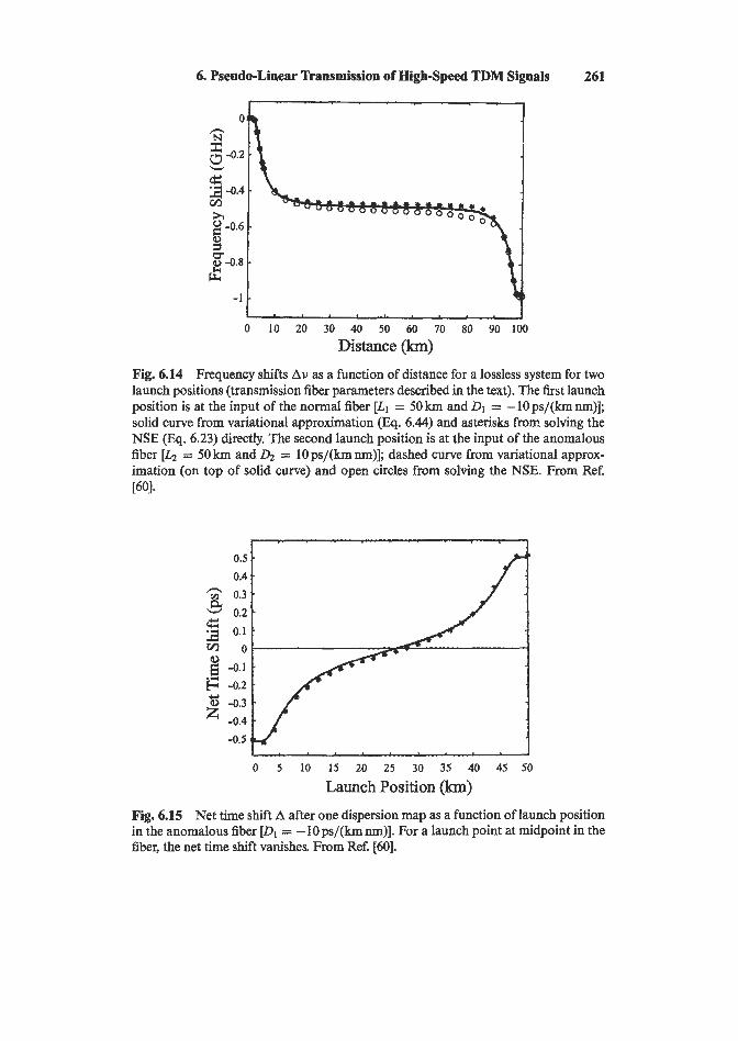
6. Pseudo-Linear Wansmission of High-speed TDM Signals 261
1
0 10 20 30 40 50 60 70 80 90 100
Distance (km)
Fig. 6.14 Frequency shifts Au as a function of distance for a lossless system for two launch positions (transmission fiber parameters described in the text). The first launch position is at the input of the normal fiber [Ll = 50 km and D1 = - 10 ps/(km nm)]; solid curve from variational approximation (Eq. 6.44) and asterisks from solving the NSE (Eq. 6.23) directly. The second launch position is at the input of the anomalous fiber [Lz = 50 km and 4 = IOps/(km nm)]; dashed curve from variational approx- imation (on top of solid curve) and open circles from solving the NSE. From Ref. f601-
I ' 1 0.5
0.4
-0.1 b -0.2 .rl
+, Q -0.3 ' -0.4
-0.5
0 5 10 15 20 25 30 35 40 45 50
Launch Position (km)
Fig. 6.15 Net t h e shift A after one dispersion map as a function of launch position in the anomalous fiber [Dl = -lOps/(kmnm)]. For a launch point at midpoint in the fiber, the net time shift vanishes. From Ref. [60].

262 RenUean Essiambre et al.
if the cumulative dispersion map is either symmetric or antisymmetric around zo, i.e., ICGW(Z -zo)l = ~CGW(ZO -.)I where zo is the point of zero cumulative dispersion. Such a map makes the RHS of Eq. 6.44 a symmetric function and, after integration overz, makes Au(z) an antisymmetric function (see Fig. 6.14). The net time shift A(z) will then vanish when the dispersion map &(z - ZO) is a symmetric function. This condition is fulfilled when zo coincides with the middle of a fiber segment.
Realistic systems differ in a few ways from the rather idealized symmetric system considered above. First the dispersion map is generally made of a long monotype lossy transmission fiber. Fiber nonlinearity cannot be avoided in this fiber as the launch power Pin should be maximum to maximize the link OSNR (see Eq. 6.2). The dispersion compensation is generally performed using a DCF having a much larger magnitude of dispersion than the transmission fiber so as to make it short enough to ease its insertion inside the in-line amplifiers and minimize its loss. The maximum power launched in the DCF is generally set to minimize any additional nonlinear signal distortions to the distortions already present from propagation in the transmission fiber. The degradation of the N F of the in-line amplifier from the presence of the DCF is set by this maximum power value. Depending on the type of transmission fiber, the type of DCF and whether or not these fibers are active (by using Raman pumping for instance), the impact of the presence of the DCF on the NF of the in-line amplifiers (see Eq. 6.7) and the link budget (see Eq. 6.2) can vary greatly.
Let's consider a system with the following parameters: pSpan = -5 ps2/km, ~ D C F = 20 ps2/km, L,,, = 100 km, LDCF = 25 km (the length LM of the dispersion map is 125 km), a0 = 0.21 dB/km in the transmission fiber with a nonlinearity coefficient y = 2 W-I km-' while the DCF is considered as having no significant nonlinearity for simplicity. Note that the relatively low value for the dispersion of the DCF has been chosen to facilitate visu- alization in Fig. 6.17. The cumulative dispersion of the transmission fiber Cspan = - 5 0 0 ~ s ~ . Figure 6.16 shows the frequency and net time shifts after one dispersion map period LM as a function of precompensation (see Fig. 6.2). Even though it is clear from Fig. 6.16 that there is always a frequency shift associated with IXPM, there is a precompensation length L,, that leads to zero net time shift. From Fig. 6.16 this value of L, = 3 km or a cumulative dispersion C,, = 60 psz.
The mechanism allowing a zero net time shift for the optimum launch point (LpE = 3 km) can be understood by considering the evolution of the pulse parameters with distance as displayed in Fig. 6.17. The launch point of transform-limited pulses is at z = zo = 0 km. Besides the launch point, the pulses go through only one other point of zero net cumulative dispersion zo at z = 15 km during the first map period. As the pulses propagate they broaden and recompress (Fig. 6.17d) according to the cumulative GVD (Fig. 6.17b). The pulses initially have their relative frequency Au(z) = 0 at z = 0 km. As

6. Pseudo-Linear Transmission of High-speed TDM Signals 263
2 0 I - j
i .-, , , , . , , , , , , I -2oof .
F Y
0 3 5 10 15 20 25 Precompensation (km)
Fig. 6.16 Frequency shift Au and net time shift A after one dispersion period in a lossy system (described in the text) as a function of the length of DCF before the transmission fiber. Despite a nonvanishing frequency shift, it is possible to induce a zero net time shift with proper precompensation. In this exmple, the precompensation that minimizes the net time shift corresponds to 3 km of DCF.
the pulses enter the transmission fiber at zin = 3 km, their relative frequency gradually shifts (3 km < z < 10 km) as the pulses start to compress as they approach zo = 15 km. No significant frequency shift occurs when pulses are close to the point of zero cumulative GVD (10 km < z 20 km) because of their negligible temporal overlap near ZO. An additional frequency shift occurs when pulses have passed the point z = 20 km where they start to overlap again. This process leaves a nonvanishing frequency shift at the end of the transmis- sion fiber and a net time shift from the continuous conversion of the frequency shift Au(z) by the dispersion of the transmission fiber. Then, the remainder of the dispersion compensation (-Cspan - Cp, = 440 ps’) is applied using 22 km of DCF (103 km < z < 125 km) to bring back the cumulative GVD to zero (pseudo-linear transmission). It is worth remembering that there is no addi- tional frequency shift generated in the DCF because nonlinearity is neglected in this fiber. The accumulated frequency shift at the end of the transmission fiber translates into a time shift in the DCF that is opposite in sign to the one generated in the transmission fiber (because of the opposite sign of dispersion of the DCF). Under certain conditions these two net time shifts can cancel exactly. Using the relation A(z = L,) = 2n s,”- Bz(z)Au(z)dz, the requirement for timing cancellation can be written,
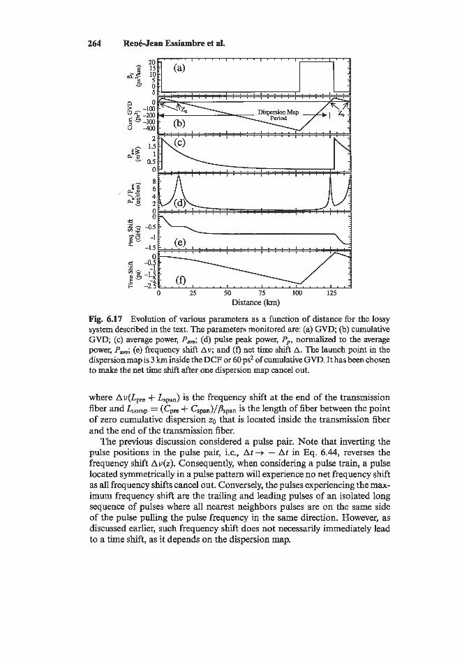
264 RenkJean Essiambre et al.
Distance (km)
Fig. 6.17 Evolution of various parameters as a function of distance for the lossy system described in the text. The parameters monitored are: (a) GVD; @) cumulative GVD; (c) average power, Pm; (d) pulse peak power, Pp, normalized to the average power, P,; (e) frequency shift Au; and (f) net time shift A. The launch point in the dispersion map is 3 km inside the DCF or 60 ps2 of cumulative GVD. It has been chosen to make the net time shift after one dispersion map cancel out.
where Au(Lpre + Lspan) is the frequency shift at the end of the transmission fiber and Lcomp = (CPE + Cspm)/j?span is the length of fiber between the point of zero cumulative dispersion zo that is located inside the transmission fiber and the end of the transmission fiber.
The previous discussion considered a pulse pair. Note that inverting the pulse positions in the pulse pair, Le., At + - At in Eq. 6.44, reverses the frequency shift Au(z). Consequently, when considering a pulse train, a pulse located symmetrically in a pulse pattern will experience no net frequency shift as all frequency shifts cancel out. Conversely, the pulses experiencing the max- imum frequency shift are the trailing and leading pulses of an isolated long sequence of pulses where all nearest neighbors pulses are on the same side of the pulse pulling the pulse frequency in the same direction. However, as discussed earlier, such frequency shift does not necessarily immediately lead to a time shift, as it depends on the dispersion map.

6. Pseudo-Linear Transmission of High-speed TDM Signals 265
2.4.5 Intrachannel Four-Wave Mixing
The second type of nonlinear interaction occurring among rapidly dispers- ing pulses in the pseudo-linear regime is intrachannel four-wave mixing (IFWM) [6, 71. This nonlinear interaction among pulses leads to generation of small pulses (shadow pulses) that can have positive or negative delays with respect to the original pulses. Observation of shadow pulses due to Kerr non- linearity in fibers has been reported as early as 1992 [67] in the context of an experiment on an ultrashort (-90 fs) pair of pulses. IFWM in fibers has simi- larities with the phenomena of photon echoes in inhomogeneously broadened media and stimulated photon echoes in transient four-wave mixing [68].
One way to understand the mechanism of IFWM is as follows. Dispersed pulses that experience nonlinearity can see a small portion of their field shifted by a discrete frequency value [69] as a result of FWM occurring between different spectral components of overlapping pulses. After propagation in a dispersive medium followed by full dispersion compensation, the discrete fre- quency shift is translated in a discrete time shift that, for sufficiently high dispersion, localizes the shifted field near the middle of a neighboring bit slot. If the bit slot is empty, the shifted field appears as a pulse of small ampli- tude referred to as “shadowy’ pulse. If there is a pulse in the bit slot where the field localizes, the two fields beat together, creating variations in main pulse amplitude. Figure 6.18 shows an example of how IFWM affects transmis- sion. The eye diagram shows that the eye closure comes from amplitude jitter and shadow pulse generation. Pseudo-linear transmission usually operates at sufficiently high values of dispersion that result in having the shadow pulses localized near the middle of a bit slot.
Let us consider the nonlinear interaction between two pulses propagating in a highly dispersive medium shown in Fig. 6.19. Four power levels separated by 3 dB are displayed. The difference in power between the first-order shadow pulses (seen on each side of the pulse pair) is 9 dB. This power difference is proportional to the product of three times the original pulse power and is identical to the power scaling of sidebands generation in well-known FWM between channels. The second-order shadow pulses located further away from the pulse pair are separated by 15 dB, consistent with FWM scaling for the dominant IFWM product (twice the pulse pair power and one time the first- order shadow pulse) that leads to the second-order shadow pulse.
A variety of analytic methods have been used to describe IFWM [5541,70, 711. They can be divided into three groups: small field perturbations [55, 56, 61, 711, nonlinear evolution in a dispersive frame [58, 591, and the varia- tional method [57, 701. These different approaches have different advantages and drawbacks. The small-field-perturbation method has the advantage that it is not limited to a particular type of interaction between pulses, as it encom- passes all types of nonlinear interactions. However, it is not clear how accurate the analysis becomes for large perturbation, especially when the timing jitter
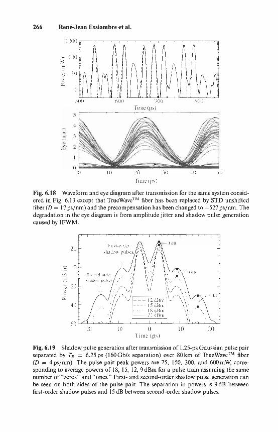
266 RenC-Jean Essiambre et al.
1000
F loo E 5 10 v
5 a 1
500 600 700 800 Time (ps)
4 + v $ 3 0
$ 2
1
0 0 I O 20 3 0 40 50
Time (ps)
Fig. 6.18 Waveform and eye diagram after transmission for the same system consid- ered in Fig. 6.13 except that TrueWaveTM fiber has been replaced by STD unshifted fiber (D = 17 ps/nm) and the precompensation has been changed to -527 ps/nm. The degradation in the eye diagram is from amplitude jitter and shadow pulse generation caused by IFWM.
Time (ps)
Fig. 6.19 Shadow pulse generation after transmission of 1.25-ps Gaussian pulse pair separated by TB = 6.25 ps (160 Gb/s separation) over 80 km of TrueWaveTM fiber (D = 4ps/nm). The pulse pair peak powers are 75, 150, 300, and 600mW, corre- sponding to average powers of 18, 15, 12, 9dBm for a pulse train assuming the same number of "zeros" and "ones." First- and second-order shadow pulse generation can be seen on both sides of the pulse pair. The separation in powers is 9dB between first-order shadow pulses and 15 dB between second-order shadow pulses.
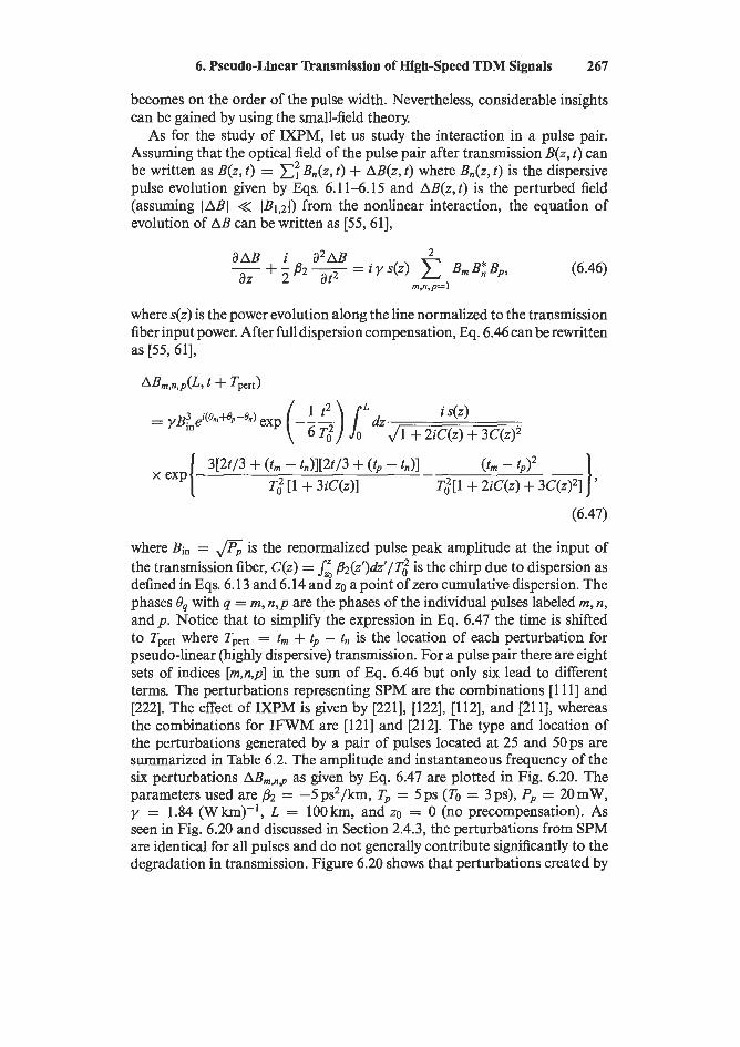
6. Pseudo-Linear Transmission of High-speed TDM Signals 267
becomes on the order of the pulse width. Nevertheless, considerable insights can be gained by using the small-field theory.
As for the study of IXPM, let us study the interaction in a pulse pair. Assuming that the optical field of the pulse pair after transmission B(z, t ) can be written as B(z, t ) = B,(z, t ) + AB(z, t ) where Bn(z, t ) is the dispersive pulse evolution given by Eqs. 6.11-6.15 and AB(z,t) is the perturbed field (assuming ]AB1 << IB1,21) from the nonlinear interaction, the equation of evolution of AB can be written as [55,61],
where s(z) is the power evolution along the line normalized to the transmission fiber input power. After full dispersion compensation, Eq. 6.46 can be rewritten as [55, 611,
(6.47)
where Bin = & is the renormalized pulse peak amplitude at the input of the transmission fiber, C(z) = B~(z')dz'/Ti is the chirp due to dispersion as defined in Eqs. 6.13 and 6.14 and zo a point of zero cumulative dispersion. The phases 0, with q = m, n,p are the phases of the individual pulses labeled m, n, andp. Notice that to simplify the expression in Eq. 6.47 the time is shifted to TFrt where Tpert = tm + tp - tn is the location of each perturbation for pseudo-linear (highly dispersive) transmission. For a pulse pair there are eight sets of indices [m,n,p] in the sum of Eq. 6.46 but only six lead to different terms. The perturbations representing SPM are the combinations [ 1 1 11 and [222]. The effect of IXPM is given by [221], [122], [112], and [211], whereas the combinations for IFWM are [121] and [212]. The type and location of the perturbations generated by a pair of pulses located at 25 and 50ps are summarized in Table 6.2. The amplitude and instantaneous frequency of the six perturbations AB,,,n, as given by Eq. 6.47 are plotted in Fig. 6.20. The parameters used are /32 = -5ps2/km, Tp = 5ps (TO = 3ps), Pp = 20mW, y = 1.84 (Wkm)-', L = 100km, and zo = 0 (no precompensation). As seen in Fig. 6.20 and discussed in Section 2.4.3, the perturbations from SPM are identical for all pulses and do not generally contribute significantly to the degradation in transmission. Figure 6.20 shows that perturbations created by
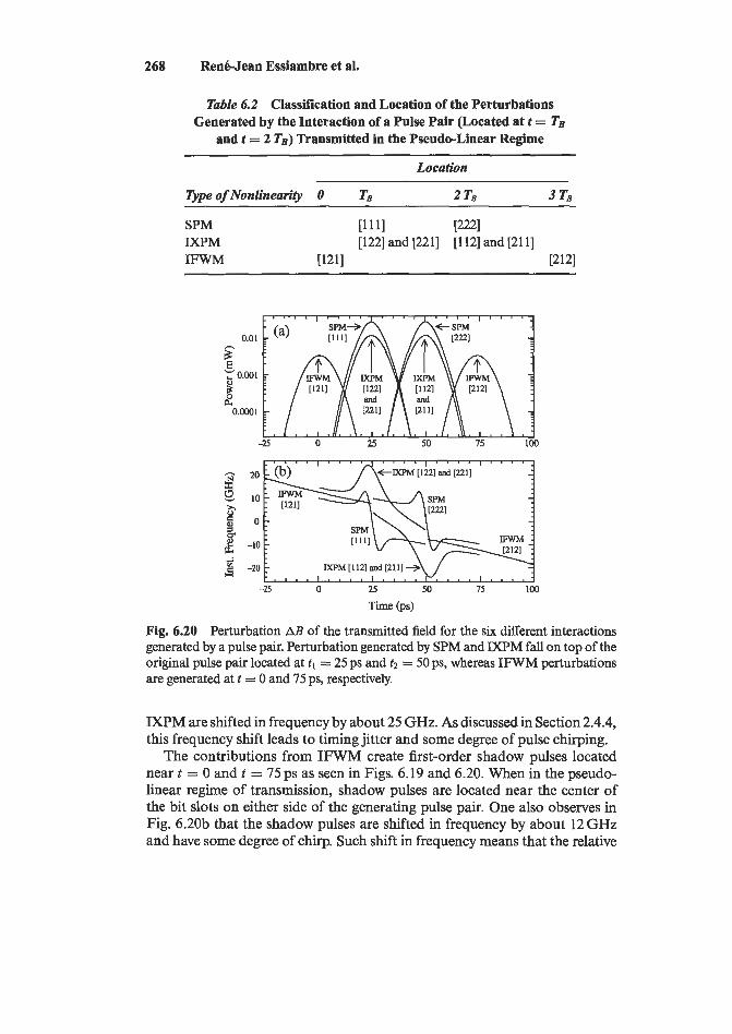
268 RenUean Essiambre et al.
Table 6.2 Classification and Location of the Perturbations Generated by the Interaction of a Pulse Pair (Located at t = TB
and t = 2 TB) Transmitted in the Pseudo-Linear Regime
Location
Type of Nonlineariq 0 TE 2 TE 3 TE
SPM [1111
IFWM 11211 W I IXPM [122] and [221] [112] and [211]
0.01
5 ; 0.001
&
E
B
0.m1
-25 0 25 50 75 100
-25 0 25 50 15 100
Time @s)
Fig. 6.20 Perturbation AB of the transmitted field for the six different interactions generated by a pulse pair. Perturbation generated by SPM and IXPM fall on top of the original pulse pair located at tl = 25 ps and t2 = 50 ps, whereas IFWM perturbations are generated at t = 0 and 75 ps, respectively.
IXPM are shifted in frequency by about 25 GHz. As discussed in Section 2.4.4, this frequency shift leads to timing jitter and some degree of pulse chirping.
The contributions from IFWM create first-order shadow pulses located near t = 0 and t = 75 ps as seen in Figs. 6.19 and 6.20. When in the pseudo- linear regime of transmission, shadow pulses are located near the center of the bit slots on either side of the generating pulse pair. One also observes in Fig. 6.20b that the shadow pulses are shifted in frequency by about 12 GHz and have some degree of chirp. Such shift in frequency means that the relative

6. Pseudo-Linear Transmission of High-speed TDM Signals 269
position of the shadow pulses changes with dispersion. Interestingly, for condi- tions such as Lo - LNL (for short dispersion map periods or for low-dispersion fibers), the shadow pulses are located closer to the pulse pair [71]. However, this condition generally falls outside the scope of pseudo-linear transmission.
Equation 6.47 can help to predict the effect of dispersion mapping on IFWM and how it impacts amplitude jitter. As mentioned before, the system impact of IFWM is to create shadow pulses in the “zeros” and amplitude varia- tions in the “ones” as a result of the beating between the shadow pulses and the “ones.” The amplitude variations in the “ones” are maximum when shadow pulses and “ones” are in phase (in-phase cross-talk). This produces the max- imum power variations (a zlB,(L, t)lABmrp(L, t)l) in the “ones.” Conversely, when the shadow pulses and the “ones” are in quadrature (quadrature cross- talk) only to small amplitude variations (a lAB,,np(L, t)I2) appear. When the “ones” from the pulse train have identical phases = the difference of phase between the perturbation t ) and the pulse B&, t ) at the end of transmission is given by the phase of the integral on the RHS of Eq. 6.47. When the power distribution is symmetric [s(z) = s(-z)], it is easily verified that the real part of ABm,ng(~, t ) (the in-phase cross-talk) vanishes for a symmetric dis- persion map (zo = L/2) whereas it is not possible to make the imaginary part of AB,,, vanish with a specific dispersion mapping. A symmetric map will thus make the in-phase cross-talk disappear but keep the quadrature component. Since the amplitude jitter created by the in-phase cross-talk is the dominant source of distortion introduced by IFWM, a symmetric dispersion map is very efficient to reduce the effect of IFWM on the “ones” for a symmetric power distribution. Figure 6.21 (from Ref. [61]) illustrates the strong reduction of the effects IFWM for a symmetric dispersion map compared to a nonsymmetric map. The dispersion map is shown in the inset. The only difference between the dispersion maps of Figs. 6.21a and 6.21b is that the first occurrence of dispersion compensation is applied halfway in the transmission in Fig. 6.21b instead of as a precompensation in Fig. 6.21a. The small fluctuations in the “zeros” and beating in the “ones” in Fig. 6.21b come from the nonvanishing quadrature component of the perturbed field AB that does not disappear for a symmetric dispersion map.
2.4.6 Dispersion Mapping When the effects of fiber nonlinearity are negligible (at low power levels), the waveform distortions observed at the end of a link depend only on the resid- ual dispersion and dispersion slope at the center wavelength of each channel. However, to maximize the OSNR, operation at the highest possible power pro- ducing minimal waveform distortions becomes necessary. Unlike transmission at low powers, transmission at high powers suffers from the effects of fiber non- linearity that strongly depend on the details of the dispersion maps. We present
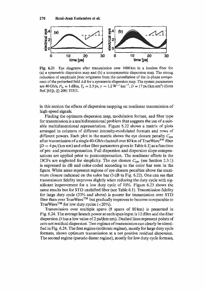
270 RedJean Essiambre et al.
s 4 (a) 3 2 ~ f : 1 0 t o
0 10 20 30 0 10 20 30 time [PSI time [PSI
Fig. 6.21 Eye diagrams after transmission over 1600km in a lossless fiber for (a) a symmetric dispersion map and (b) a nonsymmetric dispersion map. The strong reduction of amplitude jitter originates from the cancellation of the in-phase compo- nent of the perturbed field AB for a symmetric dispersion map. The system parameters are 40 Gb/s, Pin = 1 dBm, Tp = 2.5 ps, y = 1.2 W-I km-' , D = 17 ps/(km nmz) (from Ref. [61]), @ 2001 IEEE.
in this section the effects of dispersion mapping on nonlinear transmission of high-speed signals.
Finding the optimum dispersion map, modulation format, and fiber type for transmission is a multidimensional problem that suggests the use of a suit- able multidimensional representation. Figure 6.22 shows a matrix of plots arranged in columns of different intensity-modulated formats and rows of different powers. Each plot in the matrix shows the eye closure penalty Ceye
after transmission of a single 40-Gbh channel over 80 km of Ti-ueWaveTM fiber [D = 4 ps/(lun nm) and other fiber parameters given in Table 6.11 as a function of pre- and postcompensation. Full dispersion and dispersion slope compen- sations are applied prior to postcompensation. The nonlinear effects in the DCFs are neglected for simplicity. The eye closure C,, (see Section 2.3.1) is expressed in dB and color-coded according to the color bar seen in the figure. White areas represent regions of eye closure penalties above the maxi- mum closure indicated on the color bar (3 dB in Fig. 6.22). One can see that transmission fidelity improves slightly when reducing the duty cycle with sig- nificant improvement for a low duty cycle of 10%. Figure 6.23 shows the same results but for STD unshifted fiber (see Table 6.1). Transmission fidelity for large duty cycle (33% and above) is poorer for transmission over STD fiber than over TmeWaveTM but gradually improves to become comparable to Ti-ueWaveTM for low duty cycles (~20%).
Transmission over multiple spans (8 spans of 80km) is presented in Fig. 6.24. The average launch power at each span input is 12 dBm and the fiber dispersion D has a low value of 2 ps/(km nm). Dashed lines represent points of zero net residual dispersion. Two regimes of transmission can clearly be identi- fied in Fig. 6.24. The first regime (solitonic regime), mostly for large duty cycle formats, shows optimum transmission at a net positive residual dispersion. The secohd regime (pseudo-linear regime), mostly for low duty cycle formats,
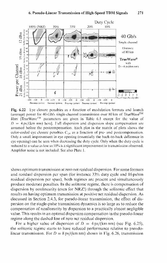
6. Pseudo-Linear Transmission of High-speed TDM Signals 271
Duty Cycle lOO%(NRZ) 50% 33% 20% 10%
preeornp (pdnm) Rccornp (pslnrn) precomp (pslnm) Rccornp (pdnrn) Pnecornp (pshrn)
Fig. 6.22 Eye closure penalties as a function of modulation formats and launch (average) power for 40-Gb/s single-channel transmission over 80 km of TrueWaveTM fiber [TrueWaveTM parameters are given in Table 6.1 except for the value of D = 4ps/(km nm) here]. Full dispersion and dispersion slope compensation are assumed before the postcompensation. Each plot in the matrix of plots shows the color-coded eye closure penalties Ceye as a function of pre- and postcompensation. Only a small improvement in eye opening (essentially the back-to-back difference in eye opening) can be seen when decreasing the duty cycle. Only when the duty cycle is reduced to a value as low as 10% is a significant improvement in transmission observed. Amplifier noise is not included. See also Plate 1.
shows optimum transmission at zero net residual dispersion. For some formats and residual dispersion per span (for instance 33% duty cycle and 16 pshm residual dispersion per span), both regimes are present and simultaneously produce moderate penalties. In the solitonic regime, there is compensation of dispersion by nonlinearity (even for NRZ!) through the solitonic effect that results on having optimum transmission at positive net residual dispersion. As discussed in Section 2.4.3, for pseudo-linear transmission, the effect of dis- persion on the single-pulse transmission dynamics is so large as to reduce the compensation of nonlinearity by dispersion to a practically almost negligible value. This results in an optimal dispersion compensation in the pseudo-linear regime along the dashed line of zero net residual dispersion.
For a higher value of dispersion of D = 4ps/(kmnm) (see Fig. 6.25), the solitonic regime starts to have reduced performance relative to pseudo- linear transmission. For D = 8 ps/(km nm) shown in Fig. 6.26, transmission

272 Red-Jean Essiambre et al.
Duty Cycle 100% 50% 33% 20% 10%
D = 17 ps/(km nm)
-5w -250 n -sw -250 n sw 250 o sw 250 n -5w 250 o Precomp (pdnm) Precomp (pslnm) Precomp (pdnm) Precamp (pslnm) Precomp (p”nm)
Fig. 6.23 Identical to Fig. 6.22 except for STD unshifted fiber (parameters given in Table 6.1). For large duty cycles (NRZ and 50% duty cycle), transmission is limited to lower powers than TrueWaveTM fiber but rapidly increases as the duty cycle decreases. See also Plate 2.
performance is clearly better for pseudo-linear transmission. Finally, for STD unshifted fiber (Fig. 6.27), pseudo-linear transmission with low duty cycle is the only regime that allows transmission fidelity.
It is clear from Figs. 6.246.27 that optimum transmission is achieved by proper choice of precompensation. For the solitonic regime (Fig. 6.24) over low-dispersion fibers, there is a range of optimal values of precompensation that can be quite large, especially for the NRZ format. For pseudo-linear transmission, a more precise value of precompensation leads to optimum transmission, as evident from Figs. 6.24-6.27. Observations of the type of distortions for nonoptimum precompensation reveals that the eye diagram closes mostly due to timing jitter in these cases. As described in Section 2.4.4, the main source of timing jitter originates from IXPM.
In the absence of fiber loss, the timing jitter can be minimized choosing a precompensation that makes the dispersion map symmetric (see Figs 6.14 and 6.15 for the single-span case). For a single span, the precompensation that makes the map symmetric is -Lspan Dspan/2 where Lspan is the span length. When many spans are concatenated, one should add half of the sum of the residual dispersion per span, or -N Cre,/2 where C,,, is the net residual disper- sion per span. When fiber losses are included, the single-span precompensation should be shorter since the power distribution is concentrated at the beginning of the span (see Fig. 6.16) [6, 72, 731. The optimal precompensation can be

6. Pseudo-Linear Transmission of High-speed TDM Signals 273
Residual Dispersion per Span 0 8 oslnm 16 vslnm 24 uslnm
40 Gb/s Single channel
12 dBm 8 spans of 80 km
TrueWaveTM/DSF with
D = 2 p s / ( h nm)
m
s m m
-I 0 I 2 3 4
Eye Closure Penalty (dB)
Fig. 6.24 Eye closure penalties after 8 spans of 80 km as a function of residual disper- sion per span and modulation format. The transmission fiber has the same parameters as TrueWaveTM (Table 6.1) except we use here D = 2 ps/(km nm). The dashed lines are the points of zero net residual dispersion. Two regimes of transmission are present. A first regime (solitonic regime) has optimum transmission with a net positive residual dispersion. In this regime the solitonic effect is at play and is responsible for the compen- sation of dispersion by nonlinearity (even for NRZ!). The second regime (pseudo-linear regime) has its optimum transmission at zero net residual dispersion. See also Plate 3.
expressed by the following semi-empirical relation [74],
It is easily verified that this relationship approximately describes the optimum value of precompensation for pseudo-linear transmission limited by IXPM in Figs. 6.24-6.27.
For systems operating at higher powers per channel, such as those in Figs. 6.22 and 6.23, IFWM can become the dominant nonlinear interaction. This can be easily understood as an increase in the “ones” pulses, peak power Pp followed by a much faster increase of the shadow pulses, peak power (c( Pj , see Fig. 6.19. In contrast, the frequency shift associated to IXPM increases linearly with Pp (E1 and E2 in Eq. 6.41 are linearly proportional to Pp). As

274 Red-Jean Essiambre et al.
0 8 pshm Residual Dispersion per Span
-200 -100 0 -200 -100 0 Preeomp (psinm) k o m p (pdnm)
0 -100 0 -200 -100 0 Precomp (pdnm) Precomp (psinm)
40 Gb/s Single channel
12 dBm
8 spans of 80 km
TrueWaveTM with
D = 4 ps/(km nm)
- 1 0 1 2 3 4
Eye Closure Penalty (dB)
Fig. 6.25 Same as Fig. 6.24 except D = 4ps/(km nm). See also Plate 4.
Residual Dispersion per Span
40 Gb/s Single channel
12 dBm
8 spans of 80 km
TrueWaveTM with
D = 8 ps/(km nm)
1 0 1 2 3 4
Eye Closure Penalty (dB)
Precomp. (pdnm) Precomp. (pdnm) Reeomp. (pslnm) Precomp. (pdnm)
Fig. 6.26 Same as Fig. 6.24 except D = 8 ps/(km nm). See also Plate 5.

6. Pseudo-Linear Transmission of High-speed TDM Signals 275
Residual Dispersion per Span 0 8 pslnm 16 pslnm 24 pshm
e 200
Single channel
12 dBm
8 spans of 80 km
STD Unshifted Fiber
D = 17 ps/(km nm)
- 200 E
p -100
5 100
0 ............... ...............
Z " ' O o
............... ............... -200
- 2w
with 5 ; 0 ~~-L*-.--- +--<-% .......
m g 100 =;--. ___ ....... -?.4r-.......... 0. -200 -
- 200 W E - s IO0 1 0 1 2 3 4
U O ? O
n
Ks2 Eye Closure Penalty (dB)
r-4 B I 0 0 .... s 2 200
-200 100 0 200 -100 0 -200 -100 0 -200 -100 0
Precomp. (pslnm) Precomp (pdnm) Precomp. (pdnm) Precomp. (pslnm)
Fig. 6.27 Same as Fig. 6.24 except for STD unshifted fiber D = 17 ps/(km nm) and A,E = 80 km2. See also Plate 6.
a result, the importance of IFWM relative to IXPM grows as the power per channel increases.
For transmission limited by IFWM, multiple optimum values of precom- pensation can be found, as is obvious in Fig. 6.23, for low duty cycle and high powers. These multiple optimal values of precompensation originate from the recurrence of FWM that results from periodic generation and reabsorption of FWM products. Such phenomenon in the case of FWM between channels in WDM systems has been described in Ref. [75]. A similar phenomenon occurs with creation and reabsorption of shadow pulses for IFWM. The number of optimal values increases with the channel bit rate and the transmission-fiber dispersion.
3. High-speed TDM Pseudo-Linear Transmission Experiments
Commercial systems operating at 40 Gb/s are expected to be installed by the beginning of 2002. Although high-capacity (3.08 Tb/s) long-span (100 km) 40-Gbk-based long-haul transmission over 1200 km has been demonstrated [76] using the NRZ format [with the added advantage of forward error
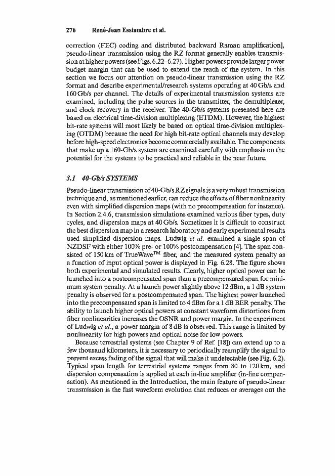
276 RedJean Essiambre et al.
correction (FEC) coding and distributed backward Raman amplification], pseudo-linear transmission using the RZ format generally enables transmis- sion at higher powers (see Figs. 6.22-6.27). Higher powers provide larger power budget margin that can be used to extend the reach of the system. In this section we focus our attention on pseudo-linear transmission using the RZ format and describe experimentalhesearch systems operating at 40 Gb/s and 160 Gb/s per channel. The details of experimental transmission systems are examined, including the pulse sources in the transmitter, the demultiplexer, and clock recovery in the receiver. The 4O-Gb/s systems presented here are based on electrical time-division multiplexing (ETDM). However, the highest bit-rate systems will most likely be based on optical time-division multiplex- ing (OTDM) because the need for high bit-rate optical channels may develop before high-speed electronics become commercially available. The components that make up a 16O-Gb/s system are examined carefully with emphasis on the potential for the systems to be practical and reliable in the near future.
3.1 40-Gbh SYSTEMS
Pseudo-linear transmission of 4O-Gb/s RZ signals is a very robust transmission technique and, as mentioned earlier, can reduce the effects of fiber nonlinearity even with simplified dispersion maps (with no precompensation for instance). In Section 2.4.6, transmission simulations examined various fiber types, duty cycles, and dispersion maps at 40 Gb/s. Sometimes it is difficult to construct the best dispersion map in a research laboratory and early experimental results used simplified dispersion maps. Ludwig et al. examined a single span of NZDSF with either 100% pre- or 100% postcompensation [4]. The span con- sisted of 150km of Ti-ueWaveTM fiber, and the measured system penalty as a function of input optical power is displayed in Fig. 6.28. The figure shows both experimental and simulated results. Clearly, higher optical power can be launched into a postcompensated span than a precompensated span for mini- mum system penalty. At a launch power slightly above 12 dBm, a 1 dB system penalty is observed for a postcompensated span. The highest power launched into the precompensated span is limited to 4 dBm for a 1 dB BER penalty. The ability to launch higher optical powers at constant waveform distortions from fiber nonlinearities increases the OSNR and power margin. In the experiment of Ludwig et al., a power margin of 8 dB is observed. This range is limited by nonlinearity for high powers and optical noise for low powers.
Because terrestrial systems (see Chapter 9 of Ref [18]) can extend up to a few thousand kilometers, it is necessary to periodically reamplify the signal to prevent excess fading of the signal that will make it undetectable (see Fig. 6.2). Typical span length for terrestrial systems ranges from 80 to 120km, and dispersion compensation is applied at each in-line amplifier (in-line compen- sation). As mentioned in the Introduction, the main feature of pseudo-linear transmission is the fast waveform evolution that reduces or averages out the
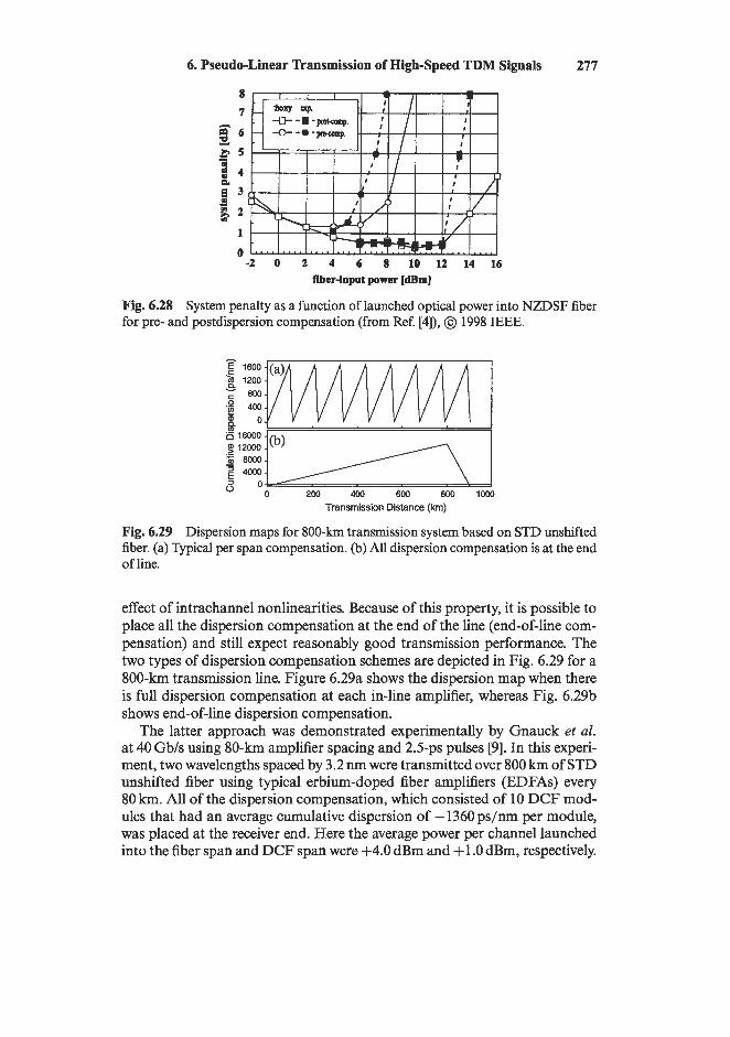
I I
I - - - I . -G--l-polt.ooap. ; I
-O--.-pR&mp. - , , I
1
0 -2 0 2 4 6 8 10 12 1 4 7 6
fiber-input power [am]
Fig. 6.28 System penalty as a function of launched optical power into NZDSF for pre- and postdispersion Compensation (from Ref [4]), @ 1998 IEEE.
1600 -g 1200
.- E 400
- 800
D O
6 16000 :: 9 12000 s 8000
0
._ -
0 200 400 600 800 101 I
fiber
Transmission Distance (km)
Fig. 6.29 Dispersion maps for 800-km transmission system based on STD unshifted fiber. (a) Typical per span compensation. (b) All dispersion compensation is at the end of line.
effect of intrachannel nonlinearities. Because of this property, it is possible to place all the dispersion compensation at the end of the line (end-of-line com- pensation) and still expect reasonably good transmission performance. The two types of dispersion compensation schemes are depicted in Fig. 6.29 for a 800-km transmission line. Figure 6.29a shows the dispersion map when there is full dispersion compensation at each in-line amplifier, whereas Fig. 6.2913 shows end-of-line dispersion compensation.
The latter approach was demonstrated experimentally by Gnauck et al. at 40 Gb/s using 80-km amplifier spacing and 2.5-ps pulses [9]. In this experi- ment, two wavelengths spaced by 3.2 nm were transmitted over 800 km of STD unshifted fiber using typical erbium-doped fiber amplifiers (EDFAs) every 80 km. All of the dispersion compensation, which consisted of 10 DCF mod- ules that had an average cumulative dispersion of - 1360 ps/nm per module, was placed at the receiver end. Here the average power per channel launched into the fiber span and DCF span were +4.0 dBm and +1 .O dBm, respectively.
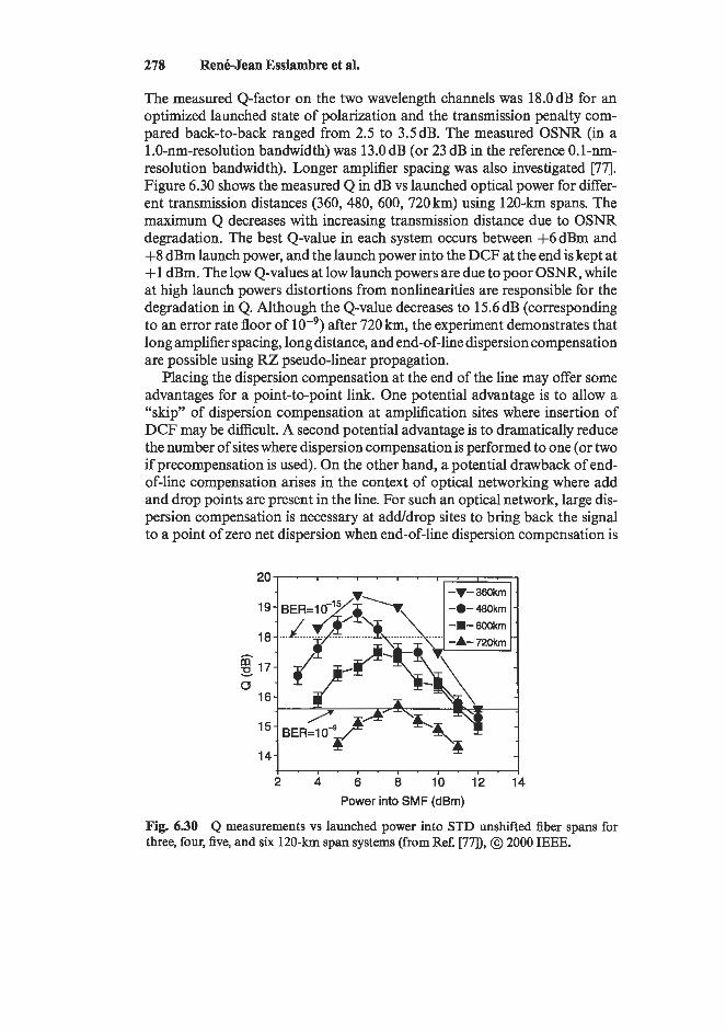
278 Renk-Jean Essiambre et al.
The measured Q-factor on the two wavelength channels was 18.0dB for an optimized launched state of polarization and the transmission penalty com- pared back-to-back ranged from 2.5 to 3.5dB. The measured OSNR (in a 1.0-nm-resolution bandwidth) was 13.0 dB (or 23 dB in the reference 0.1-nm- resolution bandwidth). Longer amplifier spacing was also investigated [77]. Figure 6.30 shows the measured Q in dB vs launched optical power for differ- ent transmission distances (360, 480, 600, 720 km) using 120-km spans. The maximum Q decreases with increasing transmission distance due to OSNR degradation. The best Q-value in each system occurs between +6dBm and +8 dBm launch power, and the launch power into the DCF at the end is kept at +1 dBm. The low Q-values at low launch powers are due to poor OSNR, while at high launch powers distortions from nonlinearities are responsible for the degradation in Q. Although the Q-value decreases to 15.6 dB (corresponding to an error rate floor of after 720 km, the experiment demonstrates that long amplifier spacing, long distance, and end-of-line dispersion compensation are possible using RZ pseudo-linear propagation.
Placing the dispersion compensation at the end of the line may offer some advantages for a point-to-point link. One potential advantage is to allow a “skip” of dispersion compensation at amplification sites where insertion of DCF may be difficult. A second potential advantage is to dramatically reduce the number of sites where dispersion compensation is performed to one (or two if precompensation is used). On the other hand, a potential drawback of end- of-line compensation arises in the context of optical networking where add and drop points are present in the line. For such an optical network, large dis- persion compensation is necessary at adddrop sites to bring back the signal to a point of zero net dispersion when end-of-line dispersion compensation is
20 -v-3360km . -0-480km - -B- 600km .
14
2 4 6 8 10 12 14
Power into SMF (dBm)
Fig. 6.30 Q measurements vs launched power into STD unshifted fiber spans for three, four, five, and six 120-km span systems (from Ref [77]), @ 2000 IEEE.

6. Pseudo-Linear Transmission of High-speed TDM Signals 279
used. In contrast, for in-line compensation, a more modest cumulative disper- sion is necessary at adddrop sites to bring the signal to a value of dispersion where it can be detected.
3.1.1 ETDM Long-Haul Pseudo-Linear Transmission
Maintaining high OSNR is important for any communication system, but it is especially critical for 40-Gb/s-based systems because of the high density of bits. Today’s receivers require typically at least 24 dB OSNR (measured in 0. l-nm- resolution bandwidth) in order to achieve bit error rate (BER) performance better than lop9.
For noise accumulation purposes, the transmission line can be considered as a chain of amplifiers with lossy elements inserted between them. Because one wants to minimize the number of in-line amplifiers for a given transmission line, the span loss is generally the most lossy element in the line. As a result of limitation of launch power to the transmission fiber because of fiber non- linearity, the amplifiers in the chain receiving the lowest input powers are the in-line amplifiers. Consequently, the degradation of OSNR arises primarily from the in-line amplifiers and is related to their NE However, the presence of DCF inside the in-line amplifiers may also add to the degradation of OSNR by increasing the NF of the in-line ampuer (see Section 2.4.4). The degradation of NF from the presence of DCF can be decreased by reducing the DCF loss and by increasing the input power to the DCF. However, the input power to the DCF is limited by its small effective area of 15-22 vm2 (see Table 6.1).
To improve the performance, alternative methods of providing dispersion compensation are being examined. Recently, Ramachandran et al. described a dispersion compensation module that is based on higher-order mode (HOM) fiber that has an effective area, A,r of 65 pm2 [78]. Such effective area is much larger than conventional DCFs and reduces the nonlinear effects in the fiber. A schematic of the module is shown in Fig. 6.3 1. The device consists of a 2-km spool of HOM fiber spliced to two long-period gratings (LPGs) written using ultraviolet light. The LPG converts the linearly polarized mode, LPol, into the LP02 mode at the input and then back to the LPol at the output. Up to 99% mode conversion over a bandwidth of 40 nm has been demonstrated.
2 km EOM-JXF
LPG LPG lull \/ 11111
11 4 u 1 + Lp,, LP, LPOl
Fig. 6.31 Schematic of higher-order-mode dispersion compensation module (HOM-DCM). Block arrows represent propagation of dominant mode. LPG- long period grating, X fusion splice.
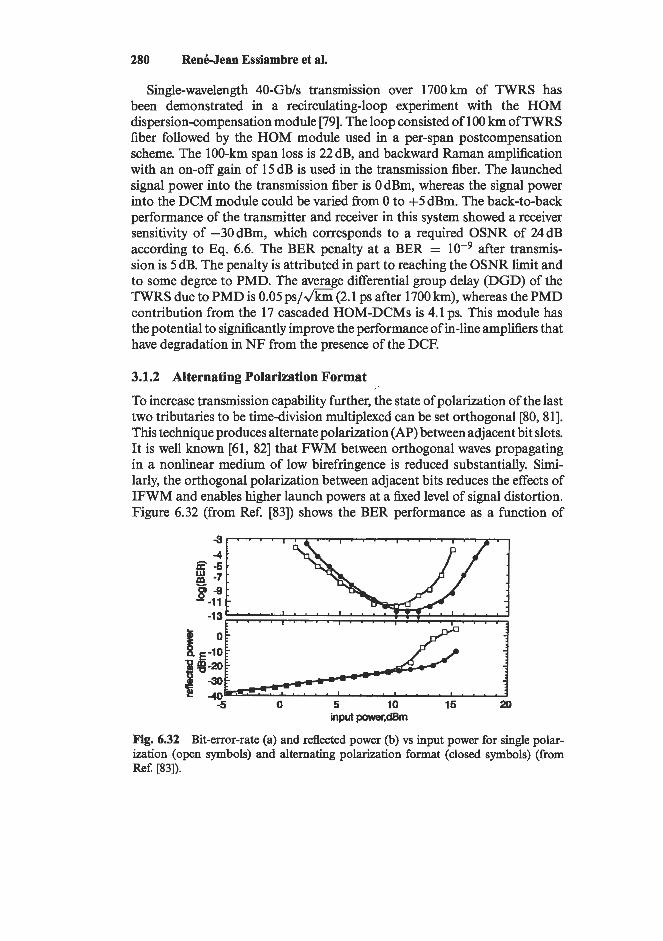
280 Renuean Essiambre et al.
Single-wavelength 4O-Gb/s transmission over 1700 km of TWRS has been demonstrated in a recirculating-loop experiment with the HOM dispersion-compensation module [79]. The loop consisted of 100 km of TWRS fiber followed by the HOM module used in a per-span postcompensation scheme. The 100-km span loss is 22 dB, and backward Raman amplification with an on-off gain of 15 dB is used in the transmission fiber. The launched signal power into the transmission fiber is 0 dBm, whereas the signal power into the DCM module could be varied from 0 to +5 dBm. The back-to-back performance of the transmitter and receiver in this system showed a receiver sensitivity of -30 dBm, which corresponds to a required OSNR of 24 dB according to Eq. 6.6. The BER penalty at a BER = after transmis- sion is 5 dB. The penalty is attributed in part to reaching the OSNR limit and to some degree to PMD. The average differential group delay (DGD) of the TWRS due to PMD is 0.05 ps/& (2.1 ps after 1700km), whereas the PMD contribution from the 17 cascaded HOM-DCMs is 4.1 ps. This module has the potential to significantly improve the performance of in-line amplifiers that have degradation in NF from the presence of the DCF.
3.1.2 Alternating Polarization Format
To increase transmission capability further, the state of polarization of the last two tributaries to be time-division multiplexed can be set orthogonal [80,81]. This technique produces alternate polarization (AP) between adjacent bit slots. It is well known [61, 821 that FWM between orthogonal waves propagating in a nonlinear medium of low birefringence is reduced substantially. Simi- larly, the orthogonal polarization between adjacent bits reduces the effects of IFWM and enables higher launch powers at a fixed level of signal distortion. Figure 6.32 (from Ref. [83]) shows the BER performance as a function of
-5 0 5 10 15 20 input power,dBm
Fig. 6.32 Bit-error-rate (a) and reflected power (b) vs input power for single polar- ization (open symbols) and alternating polarization format (closed symbols) (from Ref [83]).
6. Pseudo-Linear Transmission of High-speed TDM Signals 281
launched optical power for a 40-Gb/s transmission experiment over a single span of 240 km of STD unshifted fiber. Two curves are plotted; one for the AP format and one for single polarization (SP). By going from SP to AP, an additional 2 dB of launch power is possible, extending the ultimate span length of the system. Furthermore, the AP format reduces the effect of stimulated Brillouin scattering in the fiber (the Brillouin gain is polarization dependent), thus enabling higher launch powers to be achieved. This technique is also used in later sections to achieve long-distance transmission of 160 Gbk
3.2 IdO-Gb/s OTDMSYSTEMS
To keep pace with the increasing demand for capacity in the backbone network, fiber transmission systems with high TDM bit rates are becoming increasingly important. Long-haul system evolution has historically occurred in four-fold increases in bit rate because of the SONET and SDH standards. Economics have determined that the cost per bit can almost be cut in half if the bit rate increases by a factor of four. High TDM bit rates are attractive because a sin- gle wavelength can accommodate a higher-capacity payload. Already there are applications that require a high serial data rate. One such application involves the aggregation of data from a high resolution radio telescope that consists of 13,000 dipole antenna elements [84]. Each antenna produces digitized data at 2.O-Gb/s rates and the antennas are grouped into stations of 78 antennas, resulting in an aggregate data rate of 160 Gb/s for each group. Consequently, the interest for the next generation TDM bit rate of 160Gb/s is emerging rapidly [85-871. However, the speed of electronic circuits currently limits the possible TDM data rate to -40 Gb/s. Therefore, OTDM techniques have to be applied today to construct serial data rates of 160 Gb/s. This section examines the progress toward TDM rates of 160Gb/s based on OTDM. In particu- lar, the focus is on practical implementation, fiber transmission limitations at 160 Gb/s, and the possible channel spacing for WDM systems.
3.2.1 16O-Gb/s OTDM Transmitter and Receiver
Optical time-division multiplexing (OTDM) is a well-known technique that allows very high serial data rates to be obtained while using lower bit-rate electronics. This multiplexing technique is often used in research laboratories to explore high bit-rate transmission before electronic components are avail- able [88]. In order to realize a 160-Gbh TDM system, optical multiplexing and demultiplexing of lower-rate tributaries must be used at the transmitter and receiver ends. Figure 6.33 shows a schematic of a 16O-Gb/s OTDM system including the most important building blocks.
To minimize the complexity of the transmitter, the highest possible tribu- tary/ electronic data rate should be used, Le., 40 Gb/s at present. The optical multiplexing can be performed by either bit-interleaving four 4O-Gb/s RZ sig- nals with the SP or with AP where adjacent bits have orthogonal polarization.
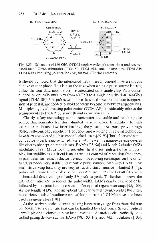
282 RenCJean Essiambre et al.
160 Gbls Transmitter:
Ootical MUX
160 Gbls Receiver:
Ootical DeMUX
Gbls RZ
4 x 40 Gbls ETDM 40 GH7
40 Gb/s ETDM
Fig. 6.33 Schematic of 160-Gb/s OTDM single wavelength transmitter and receiver based on 40-Gbit/s tributaries. TDM-SP TDM with same polarization. TDM-AP TDM with alternating polarization (AP) format. CR: clock recovery.
It should be noted that the interleaved tributaries in general have a random relative carrier phase. This is also the case when a single pulse source is used, unless the four data modulators are integrated on a single chip. As a conse- quence, to optically multiplex from 40 Gb/s to a single polarization 16O-Gb/s signal (TDM-SP), 2-ps pulses with more than 30 dB extinction ratio (suppres- sion of pedestal) are needed to avoid coherent beat-noise between adjacent bits. Multiplexing by alternating polarization (TDM-AP) considerably relaxes the requirements to the RZ pulse-width and extinction ratio.
Clearly, a key technology at the transmitter is a stable and reliable pulse source that generates transform-limited narrow pulses. In addition to high extinction ratio and low insertion loss, the pulse source must provide high SNR, well-controlled repetition frequency, and wavelength. Several techniques have been considered such as mode-locked lasers [89-931 (both fiber and semi- conductor types), gain-switched lasers [94], as well as gatingkarving devices like electro-absorption modulators (EAMs) [95-981 and Mach-Zehnder (MZ) modulators [99]. Mode locking provides the shortest pulses (< 1 ps is possi- ble), but stability is a critical issue as well as control of repetition frequency, in particular for semiconductor devices. The carving technique, on the other hand, provides very stable and versatile pulse sources. Although EAMs have intrinsic carving loss, they are very attractive since transform-limited 3-4 ps pulses with more than 20 dB extinction ratio can be realized at 40 GHz with a sinusoidal drive voltage of only 5 V peak-to-peak. To further improve the extinction ratio and to reduce the pulse width, EAMs can be cascaded or be followed by an optical compression and/or optical regenerator stage [98, 1001. A short length of DSF and an optical filter can very efficiently realize the latter, but various kinds of nonlinear optical loop mirrors (NOLMs) have also been used as regenerators [loll.
At the receiver, optical demultiplexing is necessary to go from the serial rate of 160 Gb/s to a data rate that can be handled by electronics. Several optical demultiplexing techniques have been investigated, such as electronically con- trolled gating devices such as EAMs [98, 100, 1021 and MZ modulators [103],
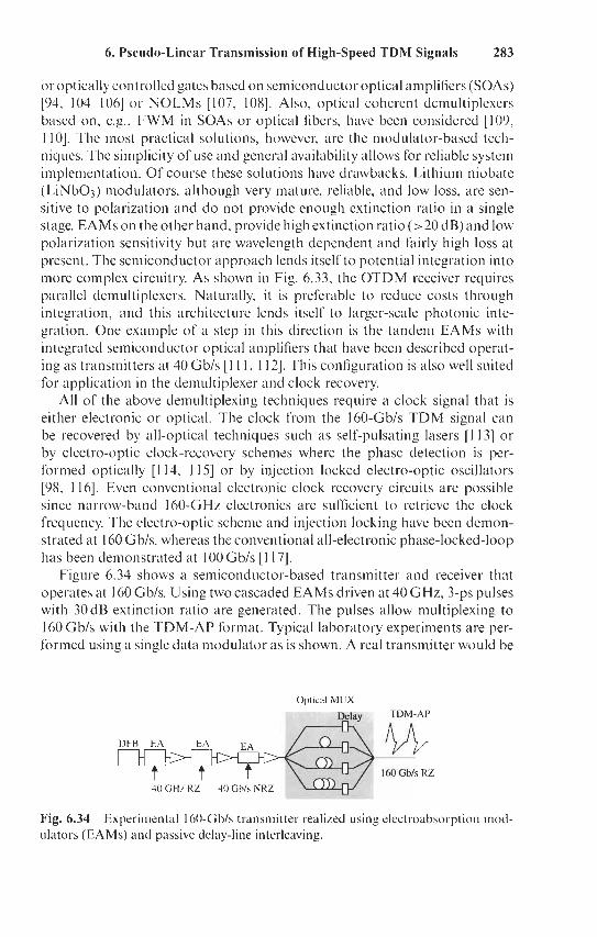
6. Pseudo-Linear Transmission of High-speed TDM Signals 283
or optically controlled gates based on semiconductor optical amplifiers (SOAs) [94, 104-1061 or NOLMs [107, 1081. Also, optical coherent demultiplexers based on, e.g., FWM in SOAs or optical fibers, have been considered [109, 1 lo]. The most practical solutions, however, are the modulator-based tech- niques. The simplicity of use and general availability allows for reliable system implementation. Of course these solutions have drawbacks. Lithium niobate (LiNb03) modulators, although very mature, reliable, and low loss, are sen- sitive to polarization and do not provide enough extinction ratio in a single stage. EAMs on the other hand, provide high extinction ratio (>20 dB) and low polarization sensitivity but are wavelength dependent and fairly high loss at present. The semiconductor approach lends itself to potential integration into more complex circuitry. As shown in Fig. 6.33, the OTDM receiver requires parallel demultiplexers. Naturally, it is preferable to reduce costs through integration, and this architecture lends itself to larger-scale photonic inte- gration. One example of a step in this direction is the tandem EAMs with integrated semiconductor optical amplifiers that have been described operat- ing as transmitters at 40 Gb/s [l 1 1, 1121. This configuration is also well suited for application in the demultiplexer and clock recovery.
All of the above demultiplexing techniques require a clock signal that is either electronic or optical. The clock from the 160-Gb/s TDM signal can be recovered by all-optical techniques such as self-pulsating lasers [ 1 131 or by electro-optic clock-recovery schemes where the phase detection is per- formed optically [114, 1151 or by injection locked electro-optic oscillators [98, 1 161. Even conventional electronic clock recovery circuits are possible since narrow-band 160-GHz electronics are sufficient to retrieve the clock frequency. The electro-optic scheme and injection locking have been demon- strated at 160 Gb/s, whereas the conventional all-electronic phase-locked-loop has been demonstrated at 100 Gb/s [ 1 171.
Figure 6.34 shows a semiconductor-based transmitter and receiver that operates at 160 Gb/s. Using two cascaded EAMs driven at 40 GHz, 3-ps pulses with 30dB extinction ratio are generated. The pulses allow multiplexing to 160 Gb/s with the TDM-AP format. Typical laboratory experiments are per- formed using a single data modulator as is shown. A real transmitter would be
Optical MUX
Fig. 6.34 ulators (EAMs) and passive delay-line interleaving.
Experimental 160-Gb/s transmitter realized using electroabsorption mod-

284 Red-Jean Essiambre et al.
implemented using at least four modulators, as shown previously in Fig. 6.33. To achieve appropriate decorrelation of the 40-Gb/s tributaries, several meters of fiber are used in each arm of the multiplexer, providing sufficient delay. To generate pulses that can be multiplexed to 160 Gb/s with the TDM-SP format, further reduction of pulse width and improved extinction ratio are necessary. A simple fiber regenerator based on self-phase modulation in optical fiber can achieve sufficient improvement to multiplex in single polarization [118]. In this case, less than 2-ps pulses with higher than 30 dB extinction ratio are generated. The optically preamplified receiver shown in Fig. 6.35 consists of two concatenated EAMs, one being driven at 40 GHz, the other at 10 GHz [119]. Consequently, optical demultiplexing from 160 to 10 Gb/s is performed. This allows BER testing to be performed at 10 Gb/s, where electronic testing equipment is widely available. Future implementations would most likely be based on 40-Gb/s tributaries to reduce the number of demultiplexers required. The clock recovery is realized by an injection locking technique, using compo- nents very similar to the demultiplexer. The clock recovery is also a series of concatenated EAMs that perform TDM demultiplexing from 160 to 10 Gb/s. This tributary is detected and then filtered using an electronic filter with a very high Q (900-1000). The oscillator is formed by amplifying the 10-GHz component and driving the EAMs with this signal. Electronic phase adjust- ment can be used to control which time slot or tributary is demultiplexed. This approach can also be used to provide add/drop functionality. One advantage of this approach is that the reconfiguration of the demultiplexer can be achieved on a very fast time scale. Tong et al. demonstrated 4-11s reconfiguration of a similar EAM-based demultiplexer [ 1201. Taking advantage of optical demulti- plexing to 10 Gb/s, the bandwidth required at the receiver is less than 10 GHz. For most of the experimental results described, back-to-back receiver sensi- tivity at 160 Gb/s is approximately -26 dBm, which corresponds to a required OSNR of 28 dB according to Eq. 6.6. Receiver sensitivity is measured before the optical demultiplexer.
160 Gb/s Rz
CR
,@Phase shifter
-lOGb/s
Fig. 6.35 demultiplexing and electro-optic clock recovery.
Experimental 160-Gb/s receiver with electro-absorption-modulator-based

6. Pseudo-Linear Transmission of High-speed TDM Signals 285
3.2.2 Single-Channel Transmission
A transmission experiment using a single channel at 160Gb/s was demon- strated. The 160 Gb/s transmitter and receiver are similar to those described in Figs. 6.34 and 6.35 except that the baseband modulation rate is at 20 Gb/s, which requires an extra passive optical multiplexer. In addition, the 16O-Gb/s signal was multiplexed in a single polarization. The link is assembled similar to the typical system layout shown in Fig. 6.3. It consists of four, 100-km spans of TmeWaveTM reduced slope (TWRS) with a measured dispersion of 3.5 ps/(km nm) and an average loss of 0.2 dB/km. The dispersion is compen- sated at each amplifier site using DCF to nearly 100% compensation. PMD measurements on the fiber show PMD values of less than 0.06 ps/d&. The launch power into the transmission span is +8 dBm while the launch power into the DCF is +3 dBm. Figure 6.36 shows the measured BER vs received power for 0 and 300 km. Bit error rate is plotted for two arbitrarily chosen 10-Gb/s tributaries. The receiver sensitivity for the 160-Gb/s transmission, measured at a BER = is -21.5 dBm after 300 km. Compared to back- to-back (0 km), the BER penalty is 3.5 dB. The penalty is mainly attributed to PMD and IXPM, which occurs in NZDSF as described in Section 2.4.4.
To extend the reach further, an experiment with an improved system, displayed in Fig. 6.37 has been performed [ 1211. In this system, Raman amplifi- cation is used to compensate for the span loss of 22 dB and no in-line amplifiers are required. This enables an improvement in OSNR to be achieved through both lower NF of the Raman amplifiers and by removing EDFAs and DCF throughout the span. As described earlier in Section 3.1, placing the DCMs
-4
-5
E-6 B -0 -7
-8
-9
-1 0.
0,
3 2 3 0 -28 -26 -24-22 -20 -18 -'
Received Power (dBm) 6
Fig. 6.36 BER vs received power for two arbitrarily chosen lO-Gb/s tributaries after 300-km transmission compared to back-to-back.

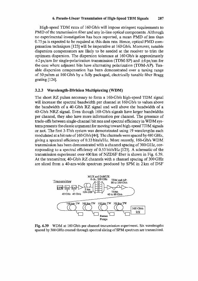
6. Pseudo-Linear Transmission of High-speed TDM Signals 287
High-speed TDM rates of 160 Gb/s will impose stringent requirements to PMD of the transmission fiber and any in-line optical components. Although no experimental investigation has been reported, a mean PMD of less than 0.75 ps is expected to be required at this data rate. Hence, optical PMD com- pensation techniques [ 1231 will be imperative at 160 Gb/s. Moreover, tunable dispersion compensators are likely to be needed at the receiver to trim the optimum dispersion. The dispersion tolerance at 160 Gb/s is approximately f 2 ps/nm for single-polarization transmission (TDM-SP) and f 6 ps/nm for the case where adjacent bits have alternating polarization (TDM-AP). Tun- able dispersion compensation has been demonstrated over a tuning range of 50 pshm at 160 Gb/s by a fully packaged, electrically tunable fiber Bragg grating [ 1241.
3.2.3 Wavelength-Division Multiplexing (WDM)
The short RZ pulses necessary to form a 160-Gb/s high-speed TDM signal will increase the spectral bandwidth per channel at 160 Gb/s to values above the bandwidth of a 4O-Gb/s RZ signal and well above the bandwidth of a 4O-Gb/s NRZ signal. Even though 16O-Gb/s signals have larger bandwidths per channel, they also have more information per channel. The presence of trade-offs between single-channel bit rate and spectral efficiency in WDM sys- tems presents the classic argument for moving toward high-speed TDM signals or not. The first 3-Tb/s system was demonstrated using 19 wavelengths each modulated at a bit rate of 160 Gb/s [44]. The channels were spaced by 480 GHz, giving a spectral efficiency of 0.33 bits/s/Hz. More recently, 16O-Gb/s WDM transmission has been demonstrated with a channel spacing of 300 GHz, cor- responding to a spectral efficiency of 0.53 bit/s/Hz [125]. A schematic of the transmission experiment over 400 km of NZDSF fiber is shown in Fig. 6.39. At the transmitter, 4O-Gb/s RZ channels with a channel spacing of 300 GHz are sliced from a 40-nm-wide spectrum produced by SPM in 2km of DSF
MUX and D m 6 Ch., 300 GHz TDM ~ p : Transmitter
Pumps
Fig. 639 WDM at 160 Gb/s per channel transmission experiment. Six wavelengths spaced by 300 GHz created through spectral slicing of SPM spectrum are transmitted.
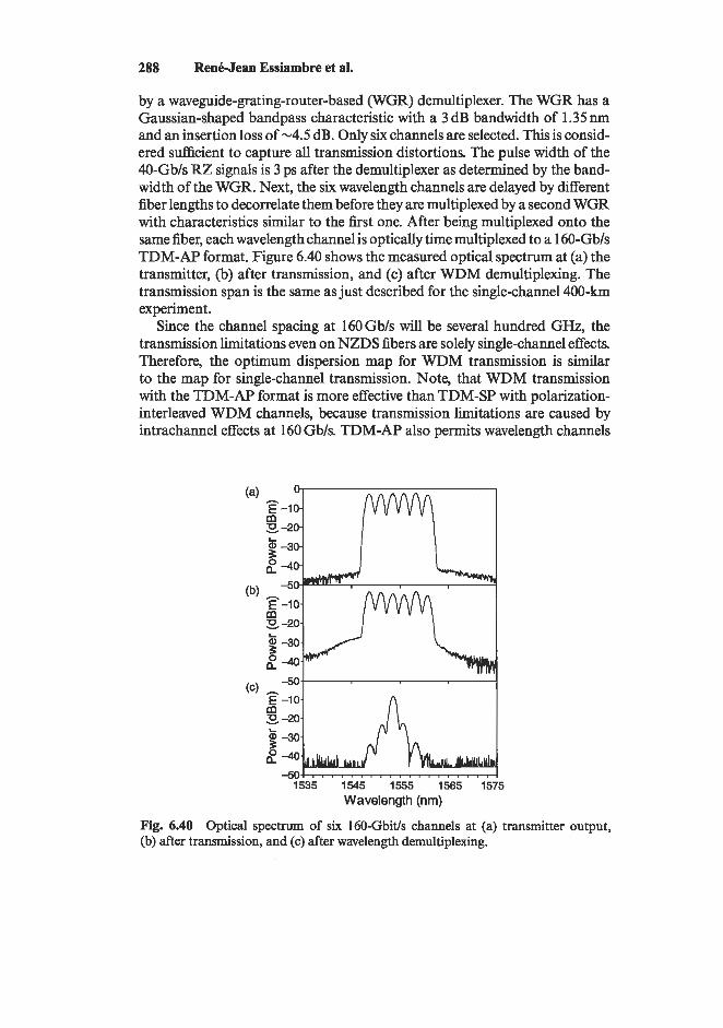
288 RedJean Essiambre et al.
by a waveguide-grating-router-based (WGR) demultiplexer. The WGR has a Gaussian-shaped bandpass characteristic with a 3 dB bandwidth of 1.35 nm and an insertion loss of -4.5 dB. Only six channels are selected. This is consid- ered sutlicient to capture all transmission distortions. The pulse width of the 4O-Gb/s RZ signals is 3 ps after the demultiplexer as determined by the band- width of the WGR. Next, the six wavelength channels are delayed by different fiber lengths to decorrelate them before they are multiplexed by a second WGR with characteristics similar to the first one. After being multiplexed onto the same fiber, each wavelength channel is optically time multiplexed to a 160-Gb/s TDM-AP format. Figure 6.40 shows the measured optical spectrum at (a) the transmitter, (b) after transmission, and (c) after WDM demultiplexing. The transmission span is the same as just described for the single-channel 400-km experiment.
Since the channel spacing at 160 Gb/s will be several hundred GHz, the transmission limitations even on NZDS fibers are solely single-channel effects. Therefore, the optimum dispersion map for WDM transmission is similar to the map for single-channel transmission. Note, that WDM transmission with the TDM-AP format is more effective than TDM-SP with polarization- interleaved WDM channels, because transmission limitations are caused by intrachannel effects at 160 Gb/s. TDM-AP also permits wavelength channels
f -30 2 4 0
-50 1535 1545 1555 1565 1575
Wavelength (nm)
Fig. 6.40 Optical spectrum of six 16O-Gbivs channels at (a) transmitter output, (b) after transmission, and (c) after wavelength demultiplexing.

6. Pseudo-Linear Transmission of High-speed TDM Signals 289
-4-
-5-
- -6-
g -7-
- -8-
-9 - -10- -1 1 '
U w
m 0
back-tpbmk 0 ch 3, po1-l14W km WDM 0 ch3,pol-2.400kmWDM 0 ch 4 pd-1,400 km WDM W ch4 pol-2 4M)lrmWDM A alngie chainel pol.i,m B A aingie channel pol-2.400 kn
*. fi 4. P *:e
W
a@
* B B
' ' ' ' ' . ' ' ' . ' ' . . ' ' ' '
to be dropped and added without the need for polarization tracking. Fur- thermore, TDM-AP allows for a high spectral efficiency because this format tolerates broader RZ pulses.
The measured BER performance after transmission is shown in Fig. 6.41. For comparison, back-to-back BER (no transmission fiber) is also shown for wavelength channel three (1556nm) for the case where only channel three is being multiplexed (squares). The difference in sensitivity between the squares and circles gives the combined penalty for allocating 160Gb/s on a 300- GHz grid and transmitting the six channels over 400 km over fiber. As seen, the penalty is less than 0.2 dB, confirming that the cross-talk from adjacent wavelength channels is very small. Furthermore, the change in measured receiver sensitivity is less than 0.5 dB when varying the launched power per channel between - 1.4 and +7.6 dBm (power limited by EDFA), demonstrat- ing the large power margin of the pseudo-linear transmission regime.
4. Conclusions
A description of high-speed TDM systems operating at 40 and 160 Gbls per channel has been presented. We first discussed and described a new regime of transmission, the pseudo-linear regime. Such a regime allows transmission of high-power, high-speed TDM signals over fibers with relatively high dis- persion [ID1 > 2ps/(kmnm)], the type of fiber composing the vast majority of the installed and currently deployed networks. The pseudo-linear regime of transmission is characterized by a rapid pulse broadening that results in a dramatic reduction of the solitonic effect (compensation of dispersion by
290 RenCJean Essiambre et al.
nonlinearity) on each pulse. As a result, full dispersion compensation is used in this regime. We described two new forms of nonlinear interactions between rapidly dispersing pulses, intrachannel cross-phase modulation (IXPM) and intrachannel four-wave mixing (IFWM). These two intrachannel effects are the most important nonlinear interactions in pseudo-linear transmission and determine the dispersion mapping even for wavelength-division multiplexed (WDM) systems. Both effects limit the maximum power that can be transmit- ted. It was shown that the most important effect of IXPM is the generation of timing jitter, whereas for IFWM it is the generation of amplitude jitter and the creation of shadow pulses. The effects of dispersion mapping on the reduction of the effects of DLPM and IFWM has been discussed.
In the second part of the chapter, the semiconductor-based technologies enabling the development of stable and reliable high-speed transmitters and receivers have been described. Long-distance error-free transmission at 40 and 160Gb/s per channel has been demonstrated with the return-to-zero (RZ) format. Both electronic time-division multiplexing (ETDM) and optical time-division multiplexing (OTDM) systems have been demonstrated. Finally, transmission of a WDM signal based on 160 Gb/s per channel with 300-GHz channel spacing (spectral efficiency of 0.53 bits/s/Hz) has been demonstrated.
Acknowledgments
We would like to thank Andrew Chraplyvy, Daniel Fishman, Lisa Wickham, Taras Lakoba, Alan Gnauck, Peter Winzer, Vadim Zharninsky, Diego Grosz, Bob Jopson, Jau Tang, and Colin McInstrie for interesting discussions and/or their comments on the manuscript.
List of Symbols
Symbol Meaning
Av Av
rl Y
AVP
Fiber loss at the signal wavelength Gadloss coefficient at the signal wavelength Constant of propagation Group-velocity dispersion (GVD) parameter Third-order dispersion (TOD) parameter Temporal separation between two pulses relative to the
bit period Spectral width Spectral separation Pulse full-spectral width at half maximum Loss of a dispersion-compensating module Nonlinear coefficient

6. Pseudo-Linear Transmission of High-speed TDM Signals 291
D Dspan EO Ein G h Iones
L Lcotn,
Signal wavelength Signal optical frequency Channel spacing in WDM systems Angular frequency of the nth pulse Pulse initial angular frequency Standard deviation of Iones Standard deviation of Izeroh Phase of the n* pulse Pulse initial phase Complex pulse amplitude of the nth pulse Effective area of the fiber transverse mode Field amplitude of the nth pulse Bit rate 3-dB electrical filter bandwidth Renormalized electric field of the n* pulse Full width at half maximum optical filter bandwidth Speed of light in vacuum Pulse chirp Initial pulse chirp Cumulative dispersion Eye closure penalty Cumulative group-velocity dispersion Cumulative dispersion precompensation Net residual dispersion per span Dispersion Dispersion of the fiber making a span Energy of pulse at a point zo Pulse energy at the input of a span Amplifier gain Planck constant Current at the sampling instant in a “one” bit Current at the sampling instant in a “zero” bit Cumulative losslgain factor Length of the communication link Fiber length from the point zo inside the transmission fiber
Length of the nth fiber segment Length of fiber used as precompensation Soliton period (= n L D / 2 ) Length of the transmission fiber making a span span loss Dispersion length (= T;/lj321) Dispersion map period
to the fiber end

292 RenBJean Essiambre et al.
Nonlinear refractive index Spontaneous emission factor Number of amplifiers Noise figure of an amplifier Noise figure of an optical amplifier with mid-stage
dispersion compensation Required OSNR to achieve a given bit error rate Noise power in a given bandwidth Au Average signal power Average power at the input of the dispersion compensating fiber Average power at the input of a transmission fiber Average power at the input of the first stage of a
multistage amplifier Peak power of a pulse Height of the rectangle fitting inside the eye diagram Receiver sensitivity Q- factor Extinction ratio between “zeros” and “ones” Power evolution normalized to the power at the fiber input Spectral efficiency Dispersion slope Time Timing of the nth pulse Bit period Characteristic width of a transform-limited pulse Full width at half maximum of the nth pulse Full width at half maximum of a pulse Evolution of Tp with cumulative dispersion Distance where the net cumulative dispersion is zero Distance corresponding to the input of the transmission fiber Point@) of symmetry of a dispersion map Propagation distance
List of Useful Relations
PASE = 2ns,(G - 1) hu Au
OSNR = 58 + Pi, - NF - Lsp - 10 10gNmp
Q 2 B e l f r OSNRR = - B o (1 -a2
Iones - Leros
nones + ozeros Q =

6. Pseudo-Linear Transmission of High-speed TDM Signals 293
OSNRR = 58 + Prec - NF
2 K C
A= D = - - p 2
2Jrc 83
2
83 = (%) ( : D + S )
Ti LD = - 1821
1 Lm=- YPP
1 - exp (-aoL) a 0
Leff =
TD
DAv Lw= -

294 RenCJean Essiambre et al.
List of Acronyms
AP APT ASE BER CDCF DC DCF DCM DDF DGD DSF EAM ETDM EDFA FEC FWHM FWM GNSE GVD HOM IFWM IMDD IP IS1 IXPM LEAF LHS LPG MZ NF NRZ NSE NZDSF NOLM OSNR OTDM PMD PMDC POAM PRBS RDS RZ
Alternate polarization Adiabatic perturbation theory Amplified spontaneous emission Bit error rate Continuously dispersion-compensating fiber Dispersion-compensated or dispersion compensation Dispersion-compensating fiber Dispersion compensation module Dispersion-decreasing fiber Differential group delay Dispersion-shifted fiber Electro-absorption modulator Electrical time-division multiplexing Erbium-doped fiber amplifier Forward error correction Full width at half maximum Four-wave mixing Generalized nonlinear Schrodinger equation Group-velocity dispersion Higher-order mode Intrachannel four-wave miXing Intensity-modulated direct-detection Internet protocol Intersymbol interference Intrachannel cross-phase modulation Large effective area fiber Left-hand side Long-period grating Mach-Zehnder Noise figure Nonreturn-to-zero Nonlinear Schrodinger equation Nonzero dispersion-shifted fiber Nonlinear optical loop mirror Optical signal-to-noise ratio Optical time-division multiplexing Polarization-mode dispersion Polarization-mode dispersion compensation Provisioning, operation, administration, and maintenance Pseudo-random bit sequence Ratio dispersion to slope Re turn-to-zero

6. Pseudo-Linear Transmission of High-speed TDM Signals 295
RHS SDH SNR SOA SONET SP SPM STD SVEA TDM TWRS TOD WDM WGR XPM
Right-hand side Synchronous digital hierarchy Signal-to-noise ratio Semiconductor optical amplifier Synchronous optical network Single polarization Self-phase modulation Standard unshifted fiber Slowly-varying-envelope approximation Time-division multiplexing TrueWavem reduced slope Third-order dispersion Wavelength-division multiplexing Waveguide grating router Cross-phase modulation
References
[ 1 ] K. S. Kim and M. E. Lines, “Temperature Dependence of Chromatic Dispersion in Dispersion-Shifted Fibers: Experiment and Analysis,” Appl. Phys. Left. 73,
[2] K. Yonenaga, A. Hirano, S. Kuwahara, Y Miyamoto, H. Toba, K. Sato, and H. Miyazawa, “Temperature-independent 8O-Gbit/s OTDM Transmission Experiment Using Zero-Dispersion-Flattened Transmission Line,” Electron. Lett. 36, pp. 343-345 (2000).
[3] D. Breuer and K. Petermann,“Comparison of NRZ- and RZ-Modulation For- mat for 4O-Gbls TDM Standard-Fiber Systems,” ZEEE Photon. Technol. Lett. 9, pp. 398-400 (1997).
[4] D. Breuer, H. J. Ehrke, F. Kiippers, R. Ludwig, K. Petermann, H. G. Weber, and K. Weich, “Unrepeatered 40-Gb/s RZ Single-Channel Transmission at 1.55 pm Using Various Fiber Types,” ZEEE Photon. Technol. Lett. 10, pp. 822-824 (1998).
[5] K. Ennser, R. I. Laming, and M. N. Zervas, “Analysis of 40-Gb/s TDM- Transmission over Embedded Standard Fiber Employing Chirped Fiber Grating Dispersion Compensators,” J. Lightwave Technol. 16, pp. 807-81 1 (1998).
[6] R.-J. Essiambre, B. Mikkelsen, and G. Raybon, “Intrachannel Cross-Phase Modulation and Four-Wave Mixing in High-speed TDM Systems,” Electron. Left. 35, pp. 1576-1578 (1999).
[7] P. V. Mamyshev and N. A. Mamysheva, “Pulse-Overlapped Dispersion- Managed Data Transmission and Intrachannel Four-Wave Mixing,’’ Opt. Left. 24, pp. 1454-1456 (1999).
[8] C. M. Weinert, R. Ludwig, W. Pieper, H. G. Weber, D. Breuer, K. Petermann, and E Kiippers, “40Gb/s and 4 x 40Gb/s TDM/WDM Standard Fiber Transmission,” J. Lightwave Technol. 17, pp. 2276-2284 (1999).
pp. 2069-2074 (1993).

296 ReneJean Essiambre et al.
[9] A. H. Gnauck, Sang-Gyu Park, J. M. Wiesenfeld, and L. D. Garrett, “Higbly Dispersed Pulses for 2 x 40 Gbit/s Transmission over 800 km of Conventional Single-Mode Fiber,” Electron. Lett. 35, pp. 2218-2219 (1999).
[lo] I?. C. Becker, N. A. Olsson, and J. R. Simpson, Erbium-Doped Fiber Amplij?ers, Fundamentab and Technology (Academic Press, San Diego, 1999).
[ll] I. Kaminow and T. Koch (Editors), Optical Fiber Telecommunications IIIB (Academic Press, San Diego, 1997), Chap. 2.
[12] N. A. Olsson, “Lightwave Systems With Optical Amplifiers,” J. Lightwave Technol. 7 , pp. 1071-1082 (1989).
[13] G. I? Agrawal, Fiber-optic Communication Systems, 2nd Edition (Academic Press, San Diego, 1997).
[14] A. R. Chraplyvy, R. W. Tkach, and K. L. Walker, “Optical Fiber for Wavelength Division Multiplexing,” U.S. Patent 5,327,516, July 5, 1994.
[15] H. Meyr, M. Moeneclaey, and S. A. Fechtel, Digital Communication Receivers: Synchronization, Channel Estimation, and Signal Processing (Wiley, New York, 1997).
[16] G. P. Agrawal, Nonlinear Fiber Optics, 3rd Edition (Academic Press, San Diego,
[17] P. G. Drain and R. S. Johnson, Solitons: An Introduction (Cambridge University Press, UK, 1989).
[18] I. Kaminow and T. Koch (Editors), Optical Fiber Telecommunications IIIA (Academic Press, San Diego, 1997).
[19] R.-J. Essiambre and G. I?. Agrawal, “Soliton Communication Systems” in P r o p s s in Optics, Vol. XXXVII (North Holland, Amsterdam, 1997).
[20] E. Golovchenko, A. Pilippetskii, and N. S. Bergano, “Transmission Properties of Chirped Return-to-Zero Pulses and Nonlinear Intersymbol Interference in 10 Gb/s WDM Transmission,” OFC’OO, Baltimore, USA, paper FC3, pp. 38-40 (2000).
[21] A. Pilippetskii, E. Golovchenko, and S. G. Evangelides Jr., “Nonlinear Interac- tion of Signal and Noise in 10-Gbls Long-Distance RZ Transmission,” OFC‘OO, Baltimore, USA, paper FC1, pp. 41-43 (2000).
[22] T. C. Damen, P. B. Hansen, H. A. Haus, and R. H. Stolen, “Applications of Solitons in Transmission Systems Employing High Launch Powers,” U.S. Patent 5,737,460, April 7, 1998.
[23] M. L. Dennis, T. E Carruthers, W. I. Kaechele, R. B. Jenkins, J. U. Kang, and I. N. Duling 111, “Long Span Repeaterless Transmission Using Adiabatic Solitons,” IEE Photon. TechnoZ. Lett. 11, pp. 478-480 (1999).
[24] M. L. Dennis, W. I. Kaechele, L. Goldberg, T. E Carruthers, and I. N. Duling 111, “Wavelength-Division Multiplexing of Adiabatic Solitons for Repeaterless Transmission,” Electron. Lett. 35, pp. 1003-1004 (1999).
[25] M. L. Dennis, W. I. Kaechele, L. Goldberg, T. E Carruthers, and I. N. Duling 111, “Wavelength-Division Multiplexed 4 x 10 Gb/s Adiabatic Soliton Transmission Over 235km,” IEEE Photon. Technol. Lett. 11, pp. 1680-1682 (1999).
2001).
6. Pseudo-Linear Transmission of High-speed TDM Signals 297
[26] K. Tajima, “Compensation of Soliton Broadening in Nonlinear Optical Fibers with Loss,” Opt. Le#. 12, pp. 54-56 (1987).
[27] H. H. Kuehl, “Solitons on an axially nonuniform optical fiber,” J. Opt. SOC. Am. B. 5, pp. 709-713 (1988).
[28] Q. Ren and H. Hsu, “Solitons in Dispersion-Compensated Optical Fiber with Loss,” IEEE J. Quantum Electron. 24, pp. 2059-2062 (1988).
[29] V. A. Bogatyrev, M. M. Bubnov, E. M. Dianov, A. S. Kurkov, I? V. Mamyshev, A. M. Prokhorov, S. D. Rumyantsev, V. A. Semenov, A. A. Sysoliatin, S. V. Chernikov, A. N. Gur’yanov, G. G. Devyatykh, and S. I. Miroshnichenko, “A Single-Mode Fiber with Chromatic Dispersion Varying Along the Length,” J. Lightwave Technol. 9, pp. 561-566 (1991).
[30] A. J. Stentz, R. W. Boyd, and A. F. Evans, “Dramatically Improved Transmis- sion of Ultrashort Solitons Through 40 km of Dispersion-Decreasing Fiber,” Opt. Lett. 20, pp. 1770-1772 (1995).
[3 11 V. A, Bogatyrjov, M. M. Bubnov, E. M. Diabov, and A. A. Sysoliatin, “Advanced Fibres for Soliton Systems,” Pure Appl. Opt. 4, pp. 345-347 (1995).
[32] D. J. Richardson, R. P. Chamberlin, L. Dong, and D. N. Payne, “High-Quality Soliton Loss-Compensation in 38-km Dispersion-Decreasing Fibre,” Electron. Lett. 31, pp. 1681-1682 (1995).
[33] D. J. Richardson, L. Dong, R. I? Chamberlin, A. D. Ellis, T. Widdowson, and W. A. Pender, ‘‘Periodically Amplified System Based on Loss Compensating Dispersion-Decreasing Fibre,” Electron. Lett. 32, pp. 373-374 (1 996).
[34] J. D. Moores, W S. Wong, and H. A. Haus, “Stability and Timing Maintenance in Soliton Transmission and Storage Rings,” Opt. Commun. 113, pp. 153-175 (1 994).
[35] D.-M. Baboiu, D. Mihalache, and N.-C. Panoiu, “Combined Influence ofAmpli- fier Noise and Intrapulse Raman Scattering on the Bit Rate Limit of Optical Fiber Communication Systems,” Opt. Le#. 20, pp. 2282-2284 (1995).
[36] R.-J. Essiambre and G. P. Agrawal, “Timing Jitter Analysis for Optical Commu- nication Systems Using Ultrashort Solitons and Dispersion-Decreasing Fibers,” Opt. Commun. 131, pp. 274-278 (1996).
[37l R.-J. Essiambre and G. I? Agrawal, “Timing Jitter of Ultrashort Solitons in High-speed Communication Systems. I. General Formulation and Application to Dispersion-Decreasing Fibers,” J. Opt. SOC. Am. B 14, pp. 314-322 (1997).
1381 T. Morioka, S. Kawanishi, H. Takara, and 0. Kamatani, “Penalty-Free, 100 Gbith Optical Transmission of t 2 ps Supercontinuum Transform-Limited Pulses over 40km,” Electron. Lett. 31, pp, 124-125 (1995).
[39] T. Morioka, S. Kawanishi, H. Takara, 0. Kamatani, M. Yamada, T. Kanamori, K. Uchiyama, and M. Saruwatari, “lOOGbit/s x 4ch, l 0 O h Repeaterless TDM-WDM Transmission Using a Single Supercontinuum Source,” Electron. Le#. 32, pp. 468-470 (1996).
[40] S. Kawanishi, H. Takara, 0. Kamatani, T. Morioka, and M. Saruwatari, “100 Gbit/s, 560 km Optical Transmission Experiment with 80-km Amplifier
298 Renuean Essiambre et al.
Spacing Employing Dispersion Management,” Electron. Lett. 32, pp. 470-471 (1996).
[41] T. Morioka, H. Takara, S. Kawanishi, 0. Kamatani, K. Takiguchi, K. Uchiyama, M. Saruwatari, H. Takahashi, M. Yamada, T. Kanamori, and H. Ono, “1 Tbitls (100 Gbit/s x 10 channel) OTDMWDM Transmission Using a Single Supercontinuum WDM Source,” Electron. Lett. 32, pp. 906-907 (1996).
[42] S. Kawanishi, H. Takara, K. Uchiyama, I. Shake, 0. Kamatani, and M. Saruwatari, “ 1.4 Tbitls (200 Gbit/s x 7 ch) 50 km Optical Transmission Experiment,” Electron. Lett. 33, pp. 1716-1717 (1997).
[43] J. Hansryd, B. Bakhshi, B. E. Olsson, P. A. Andrekson, J. Brentel, and E. Kolltveit, “80 Gbitls Single Wavelength Soliton Transmission over 172 km Installed Fibre,” Electron. Lett. 35, pp. 313-315 (1999).
[44] S. Kawanishi, H. Takara, K. Uchiyama, I. Shake, and K. Mori, ‘‘3TbitIs (160 Gbit/s x 19 channel) Optical TDM and WDM Transmission Experiment,” Electron. Lett. 35, pp. 826827 (1999).
[45] A. R. Chraplyvy, “Limitations on Lightwave Communications Imposed by Optical-Fiber Nonlinearities,” J. Lightwave Technol. 8, pp. 1548-1 557 (1990).
[46] R. W. Tkach, A. R. Chraplyvy, E Forghieri, A. M. Gnauck, and R. M. Derosier, “Four-Photon Mixing and High-speed WDM Systems,” J. Lightwave Technol. 13, pp. 841-849 (1995).
[47l D. Marcuse and C. Menyuk, “Simulation of Single-Channel Optical Systems at 100 Gb/s,” J. Lightwave Technol. 17, pp. 564-569 (1999).
[48] S. K. Turitsyn, M. P. Fedoruk, and A. Gornakova, “Reduced-Power Optical Solitons in Fiber Lines with Short-Scale Dispersion Management,” Opt. Lett.
[49] H. Anis, G. Berkey, G. Bordogna, M. Cavallari, B. Charbonnier, A. Evans, I. Hardcastle, M. Jones, G. Pettitt, B. Shaw, V. Srikant, and J. Wakefield, “Continuous Dispersion-Managed Fiber for Very High Speed Soliton Systems,” ECOC’99, Nice, France, pp. 230-231 (1999).
[SO] M. Zitelli, E Matera, and M. Settembre, “40-Gbitls Transmission in Dispersion- Management Links with Step-Index Fiber and Linear Compensation,” Opt. Lett. 24, pp. 1169-1171 (1999).
[Sl] M. Zitelli, F. Matera, and M. Settembre, “Single-Channel Transmission in Dis- persion Management Links in Conditions of Very Strong Pulse Broadening: Application to 4O-Gb/s Signals on Step-Index Fibers,” J. Lightwave Technol. 17,
[52] M. Matsumoto, “Analysis of Interaction Between Stretched Pulses Propagating in Dispersion-Managed Fibers,” IEEE Photon. Technol. Lett. 10, pp. 373-375 (1998).
[53] S. Kumar, M. Wald, E Lederer, and A. Hasegawa, “Soliton Interaction in Strongly Dispersion-Managed Optical Fibers,” Opt. Lett. 23, pp. 1019-1021 (1998).
24, pp. 869-871 (1999).
pp. 2498-2505 (1999).
6. Pseudo-Linear Transmission of High-speed TDM Signals 299
I541 T. Inoue, H. Sugahara, A. Maruta, and U. Kodama, “Interactions Between Dispersion Managed Solitons in Optical-Time-Division-Multiplexed System,” ZEEE Photon. Technol. Lett. 12, pp. 299-301 (2000).
[55] A. Mecozzi, C. B. Clausen, and M. Shtaif, “Analysis of Intrachannel Nonlinear Effects in Highly Dispersed Optical Pulse Transmission,” IEEE Photon. Technol. Lett. 12, pp. 392-394 (2000).
1561 A. Mecozzi, C. B. Clausen, and M. Shtaif, “System Impact of Intra- Channel Nonlinear Effects in Highly Dispersed Optical Pulse Transmission,” IEEE Photon. Technol. Lett. 12, pp. 1633-1635 (2000).
[571 T. Inoue and A. Maruta, “Prespread RZ Pulse Transmission for Reducing Intra- channel Nonlinear Interactions,” LEOS’OO, Puerto Rico, USA, Paper MJ3
[58] F. Merlaud and S. K. Turitsyn, “Intrachannel Four-Wave Mixing and Ghost Pulses ‘Generation: Time Domain Approach,” ECOC’OO, Munich, Germany, Paper 7.2.4, pp. 39-40 (2000).
[59] M. J. Ablowitz and T. Hirooka, “Resonant Nonlinear Intrachannel Interac- tions in Strongly Dispesion-Managed Transmission Systems,” Opt. Lett. 25, pp. 1750-1752 (2000).
[60] J. MBrtensson, A. Berntson, M. Westlund, A. Danielsson, P. Johannisson, D. Anderson, and M. Lisak, “Timing Jitter Owing to Intrachannel Pulse Inter- actions in Dispersion-Managed Transmission Systems,” Opt. Lett. 26, pp. 55-57
[61] A. Mecozzi, C. B. Clausen, M. Shtaif, S.-G. Park, and A. H. Gnauck, “Cancella- tion of Timing and Amplitude Jitter in Symmetric Links Using Highly Dispersed Pulses,” ZEEE Photon. Technol. Left. 13, pp. 441-447 (2001).
[62J H. Goldstein, ClassicalMechanics, 2nd Edition (Addison Wesley, Massachusetts, 1980).
[63] W. J. Firth, “Propagation of Laser Beams Through Inhomogeneous Media,” Upt. Cornmun. 22, pp. 226-320 (1977).
[&I] D. Anderson, “Variational Approach to Nonlinear Pulse Propagation in Optical Fibers,” Phys. Rw. A 27, pp. 313.5-3145 (1983).
[65l D. Anderson, M. Lis& and T. Reichel, “Approximate Analytical Approaches to Nonlinear Pulse Propagation in Optical Fibers: a Comparison,” Phys. Rev. A.
[66] M. Desaix, D. Anderson, and M. Lisak, “Accuracy of an Approximate Variational Solution Procedure for the Nonlinear Schrodinger Equation,”
[67] M. K. Jackson, G. R. Boyer, J. Paye, M. A. Franco, and A. Mysyrowicz, “Tem- poral Diffraction by Nonlinear Interaction in Optical Fibers,” Opt. Len. 17, pp. 1770-1772 (1992).
[68] Y. R. Shen, The Principles of Nonlinear Optics (Wiley, New York, 1984), Chaps. 21.3 and 21.4.
(2000).
(2001).
38, pp. 1618-1620 (1988).
Phys. Rw. A. 40, pp. 2441-2445 (1 989).
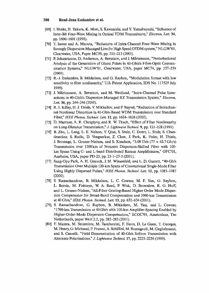
300 Renk-Jean Essiambre et al.
[69] I. Shake, H. Takara, K. Mori, S. Kawanishi, and Y. Yamabayashi, “Influence of Inter-Bit Four-Wave Mixing in Optical TDM Transmission,” Electron. Lett. 34, pp. 1600-1601 (1998).
[70] T. Inoue and A. Maruta, “Reduction of Intra-Channel Four-Wave Mixing in Strongly Dispersion-Managed Line for High Speed OTDM system,” NLGWO1, Clearwater, USA, Paper MC59, pp. 211-213 (2001).
[71] P. Johannisson, D. Anderson, A. Berntson, and J. Mfirtensson, “Perturbational Analysis of the Generation of Ghost Pulses in 40-Gbids Fibre-Optic Commu- nication Systems,” NLGWO1, Clearwater, USA, paper MC74, pp. 257-259
[72] R.-J. Essiambre, E. Mikkelsen, and G. Raybon, “Modulation format with low sensitivity to fiber nonlinearity,” U.S. Patent Application, IDS No. 117529 July 1999).
[73] J. Mhtensson, A. Berntson, and M. Westlund, “Intra-Channel Pulse Inter- actions in 40-Gbids Dispersion-Managed RZ Transmission system,” Electron. Lett. 36, pp. 244246 (2000).
[74] R. I. Killey, H. J. Thiele, V. Mikhailov, and P. Bayvel, “Reduction of Intrachan- ne1 Nonlinear Distortion in 40-Gbh-Based WDM Transmission over Standard Fiber,” IEEE Photon. Technol. Lett. 12, pp. 1624-1626 (2000).
[75] D. Mamse, A. R. Chraplyvy, and R. W. Tkach, “Effect of Fiber Nonlinearity on Long-Distance Transmission,” J. Lightwave Technol. 9, pp. 121-128 (1991).
[76] B. Zhu, L. Leng, L. E. Nelson, Y. Qian, S. Stulz, C. Doerr, L. Stulz, S. Chan- drasekar, S. Radic, D. Vengsarkar, Z. Chen, J. Park, K. Feder, H. Thiele, J. Bromage, L. Gruner-Nielsen, and S. Knudsen, “3.08 Tb/s (77 x 42.7 Gb/s) Transmission over 1200 km of Nonzero Dispersion-Shifted Fiber with 100- km Spans Using C- and L-band Distributed Raman Amplification: OFC‘O1, Anaheim, USA, paper PD-23, pp. 23-1-23-3 (2001).
[77] Sang-Gyu Park, A. H. Gnauck, J. M. Wiesenfeld, and L. D. Garrett, “4O-Gb/s Transmission Over Multiple 120-km Spans of Conventional Single-Mode Fiber Using Highly Dispersed Pulses,” IEEE Photon. Technol. Left. 12, pp. 1085-1087
[78] S. Ramachandran, B. Mikkelsen, L. C. Cowsar, M. E Yan, G. Raybon, L. Boivin, M. Fishteyn, W. A. Reed, P. Wisk, D. Brownlow, R. G. Huff, and L. Gruner-Nielsen, “All-Fiber Grating-Based Higher Order Mode Disper- sion Compensator for Broad-Band Compensation and 1000-km Transmission at 40 Gb/s,” IEEE Photon. Technol. Lett. 13, pp. 632-634 (2001).
[79] S. Ramachandran, G. Raybon, B. Mikkelsen, M. Yan, and L. Cowsar, “1700-km Transmission at 40 Gb/s with 100-km Amplifier-Spacing Enabled by Higher-Order-Mode Dispersion-Compensation,” ECOC‘O1 , Amsterdam, The Netherlands, paper We.F.2.2, pp. 282-283 (2001).
[SO] E Matera, M. Settembre, M. Tamburrini, E Favre, D. Le Guen, T. Georges, M. Henry, G. Michaud, F? Franco, A. Schiffini, M. Romagnoli, M. Gugliehwci, and S. Cascelli, “Field Demonstration of 40-Gb/s Soliton Transmission with Alternate Polarizations,” J. Lightwave Technol. 17, pp. 2225-2234 (1999).
(2001).
(2000).
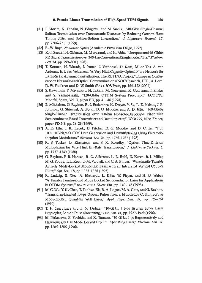
6. Pseudo-Linear Transmission of High-speed TDM Signals 301
[81] I. Morita, K. Tanaka, N. Edagawa, and M. Suzuki, “40-Gb/s Single-Channel Soliton Transmissioii over Transoceanic Distances by Reducing Gordon-Haus Timing Jitter and Soliton-Soliton Interaction,” J. Lightwave Technol. 17, pp. 2506-2511 (1999).
[82] R. W. Boyd, Nonlinear Optics (Academic Press, San Diego, 1992). I831 K.-I. Suzuki, N. Ohkawa, M. Murakami, and K. Aida, “Unrepeatered40-Gbitls
RZ Signal Transmission over 240-km Conventional Singlemode Fibre,” Electron. Lett. 34, pp. 799-800 (1998).
[84] T. Koonen, H. Waardt, J. Jennen, J. Verhoosel, D. Kant, M. de Vos, A. van Ardenne, E. J. van Velduizen, “A Very High Capacity Optical Fibre Network for Large-Scale Antenna Constellations: The RETINA Project,” European Confer- ence on Networks and Optical Communications (NOC) Ipswitch, U.K.: A. Lord, D. W. Faulkner and D. W. Smith (Eds.), 10s Press, pp. 165-172 (2001).
[85] S. Kawanishi, Y Miyamoto, H. Takara, M. Yoneyama, K. Uchiyama, I. Shake, and Y Yamabayashi, “120-Gbitls OTDM System Prototype,” ECOC’98, Madrid, Spain, Vol. 3, paper PD, pp. 41-46 (1998).
[86] E. Mikkelsen, G. Raybon, R.-J. Essiambre, K. Dreyer, Y Su, L. E. Nelson, J. E. Johnson, G. Shtengel, A. Bond, D. G. Moodie, and A. D. Ellis, “160-Gbit/s Single-Channel Transmission over 300-km Nonzero-Dispersion Fiber with Semiconductor-Based Transmitter and Demultiplexer,” ECOC’99, Nice, France, paper PD 2-3, pp. 28-29 (1999).
[87] A. D. Ellis, J. K. Lucek, D. Pitcher, D. G. Moodie, and D. Cotter, “Full 10 x 10 Gbit/s OTDM Data Generation and Demultiplexing Using Electroab- sorption Modulators,” Electron. Lett. 34, pp. 17661767 (1998).
I881 R. S. Tucker, G. Eisenstein, and S. K. Korotky, “Optical Time-Division Multiplexing for Very High Bit-Rate Transmission,” J. Lightwave Technol. 6 ,
[89] G. Raybon, I? B. Hansen, R. C. Alferness, L. L. Buhl, U. Koren, B. I. Miller, M. G. Young, T. L. Koch, J.-M. Verdiell, and C. A. Burrus, “Wavelength-Tunable Actively Mode-Locked Monolithic Laser with an Integrated Vertical Coupler Filter,” Opt. Lett. 18, pp. 1335-1336 (1993).
[90] R. Ludwig, S. Diez, A. Ehrhardt, L. Kller, W. Pieper. and H. G. Weber, “A Tunable Femtosecond Mode Locked Semiconductor Laser for Applications in OTDM Systems,” ZEZCE Trans. Electz E81, pp. 140-145 (1998).
[91] M. C. Wu, Y K. Chen, T. Tanbun-Ek, R. A. Logan, M. A. Chin, and G. Raybon, “Transform-Limited 1.4-ps Optical Pulses from a Monolithic Colliding-Pulse Mode-Locked Quantum Well Laser,” Appl. Phjx Lett. 57, pp. 759-761 (1990).
[92] T. F. Carruthers and I. N. Duling, “IO-GHz, 1.3-ps Erbium Fiber Laser Employing Soliton Pulse Shortening,” Opt. Lett. 21, pp. 1927-1929 (1996).
[93] M. Nakazawa, E. Yoshida, and K. Tmura, “IO-GHz, 2-ps &generatively and Harmonically FM Mode Locked Erbium Fiber Ring Laser,” Electron. Lett. 32, pp. 1285-1286 (1996).
pp. 1737-1749 (1988).

302 Renk-Jean Essiambre et al.
[94] M. Vaa, B. Mikkelsen, K. S. Jepsen, K. E. Stubkjaer, M. Schilling, K. Daub, E. Lach, G. Laube, W. Idler, K. Wunstel, S. Bouchoule, C. Kazmierski, and D. Mathoorasing, “A Bit-Rate Flexible and Power Efficient All-Optical Demul- tiplexer Realised By Monolithically Integrated Michelson Interferometer,” ECOC‘96, Oslo, Norway, paper PD-ThB3.3, pp. 11-14 (1996).
[95] E Devaux, N. Souli, A. Ougazzaden, F. Huet, and M. Carre, “High Speed Tandem of MQW Modulators for Coded Pulse Generation with 14-dB Fiber to Fiber Gain:’ IEEE Photon. Technol. Lett. 8, pp. 218-219 (1996).
[96] M. Suzuki, H. Tanaka, K. Utaka, N. Edagawa, and Y Matsushima, “Trans- form-Limited 14-ps Optical Pulse Generation with 15GHz Repetition Rate by InGaAsP Electroabsorption Modulator,” Electron. Left. 28, pp. 1007-1008 (1992).
[97] D. G. Moodie, P. J. Cannard, A. J. Dann, D. D. Marcenac, C. W. Ford, J. Reed, R. T. Moore, J. K. Lucek, and A. D. Ellis, “Low Polarisation Sensi- tivity Electroabsorption Modulators for 160-Gbitls Networks,” Electron. Lett.
[98] G. Raybon, B. Mikkelsen, R.-J. Essiambre, J. E. Johnson, K. Dreyer, and L. E. Nelson, “100-Gbitls Single-channel Transmission over 200-km True- Wave and 160-km Conventional Fiber with EAM Source and Demultiplexer,” ECOC‘99, Nice, France, paper WeC2.5, pp. 92-93 (1999).
[99] J. J. Veselka, S. K. Korotky, P. V. Mamyshev, A. H. Gnauck, G. Raybon, and N. M. Froberg, “A Soliton Transmitter Using a CW Laser and an NRZ Driven Mach-Zehnder Modulator,” ZEEE Photon. Technol. Lett. 8, pp. 950-952 (1996).
[loo] B. Mikkelsen, G. Raybon, R.-J. Essiambre, J. E. Johnson, K. Dreyer, and L. E Nelson, “Unrepeatered Transmission over 150 km of Nonzero-Dispersion Fibre at 100 Gbitls with Semiconductor-Based Pulse Source, Demultiplexer, and Clock Recovery,” Elechon. Lett. 35, pp. 1866-1868 (1999).
[loll I. Y Khrushchev, J. D. Bainbridge, J. E. A. Whiteaway, I. H. White, and R. V. Penty, “Multiwavelength Pulse Source for OTDMMDM Applications Based on Arrayed Waveguide Grating,” ZEEE Photon. Technol. Lett. 11,
[lo21 D. D. Marcenac, A. D. Ellis, and D. G. Moodie, ‘%O-Gbit/s OTDM Using Electroabsorption Modulators,” Electron. Lett. 34, pp. 101-103 (1998).
[lo31 M. L. Dennis et al., “Eight-to-One Demultiplexing of 100-Gbitls TDM Data Using LiNbOs Sagnac Interferometer Modulators,” OFC‘98, San Jose, CA, USA, pp. 110-112 (1998).
[lo41 S. Diez, R. Ludwig, and H. G. Weber, “Gain-Transparent SOA-Switch for High-Bitrate OTDM Add/Drop Multiplexing,” ZEEE Photon. Technol. Lett. 11, pp. 60-62 (1999).
[I051 M. Vaa, B. Mikkelsen, K. S. Jepsen, K. E. Stubkjaer, R. Hess, M. Duelk, W. Vogt, E. Gamper, E. Gini, P. A. Besse, H. Melchior, and S. R. Bouchoule, “Bit Error Rate Assessment of 80-Gbls All-Optical Demultiplexing by a Mono- lithically Integrated Mach-Zehnder Interferometer with Semiconductor Optical Amplifiers,” ECOC‘97, Edinburgh, Scotland, Vol. 3, pp. 31-34 (1997).
33, pp. 2068-2070 (1997).
pp. 1659-1661 (1999).
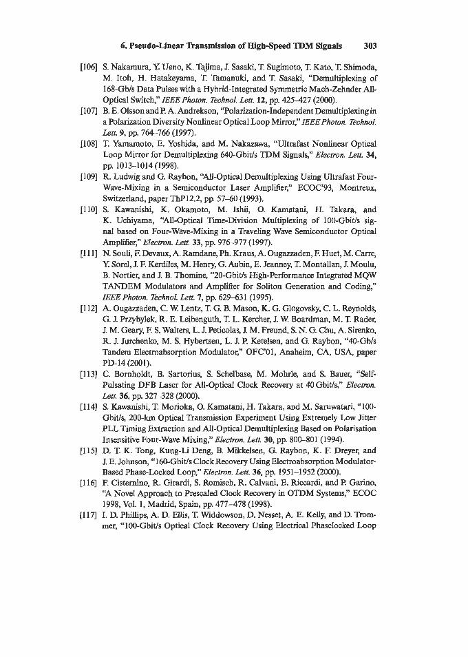
6. Pseudo-Linear Transmission of High-speed TDM Signals 303
[lo61 S. Nakamura, Y Ueno, K. Tajima, J. Sasaki, T. Sugimoto, T. Kato, T. Shimoda, M. Itoh, H. Hatakeyama, T. Tamanuki, and T. Sasaki, “Demultiplexing of 168-Gbls Data Pulses with a Hybrid-Integrated Symmetric Mach-Zehnder All- Optical Switch,” IEEE Photon. Echnol. Lett. 12, pp. 425427 (2000).
[lo71 B. E. Olsson and P. A. Andrekson, “Polarization-Independent Demultiplexing in a Polarization Diversity Nonlinear Optical Loop Mirror,” IEEE Photon. Techno!. Lett. 9, pp. 764-766 (1997).
[lo81 T. Yamamoto, E. Yoshida, and M. Nakazawa, “Ultrafast Nonlinear Optical Loop Mirror for Demultiplexing 64O-Gbit/s TDM Signals,” Electron. Lett. 34,
[lo91 R. Ludwig and G. Raybon, “All-Optical Demultiplexing Using Ultrafast Four- Wave-Mixing in a Semiconductor Laser Amplifier,” ECOC’93, Montreux, Switzerland, paper ThP12.2, pp. 57-60 (1993).
[110] S. Kawanishi, K. Okamoto, M. Ishii, 0. Kamatani, H. Takara, and K. Uchiyama, “All-Optical Time-Division Multiplexing of lOO-Gbit/s sig- nal based on Four-Wave-Mixing in a Traveling Wave Semiconductor Optical Amplifier,” Electron. Lett. 33, pp. 976-977 (1997).
[l 1 I] N. Souli, E Devaux, A. Ramdane, Ph. Kraus, A. Ougazzaden, F. Huet, M. Carre, Y Sod , J. E Kerdiles, M. Henry, G. Aubin, E. Jeanney, T. Montallan, J. Moulu, B. Nortier, and J. B. Thomine, “20-Gbit/s High-Performance Integrated MQW TANDEM Modulators and Amplifier for Soliton Generation and Coding,” IEEE Photon. Technol. Lett. 7 , pp. 629-631 (1995).
[112] A. Ougazzaden, C. W. Lentz, T. G. B. Mason, K. G. Glogovsky, C. L. Reynolds, G. J. Przybylek, R. E. Leibenguth, T. L. Kercher, J. W. Boardman, M. T. Rader, J. M. Geary, F. S. Walters, L. J. Peticolas, J. M. Freund, S. N. G. Chu, A. Sirenko, R. J. Jurchenko, M. S. Hybertsen, L. J. P. Ketelsen, and G. Raybon, “40-Gb/s Tandem Electroabsorption Modulator,” OFC‘O1, Anaheim, CA, USA, paper
[113] C. Bornholdt, B. Sartorius, S. Schelbase, M. Mohrle, and S. Bauer, “Self- Pulsating DFB Laser for All-Optical Clock Recovery at 40Gbit/s,” Electron. Lett. 36, pp. 327-328 (2000).
[114] S. Kawanishi, T. Morioka, 0. Kamatani, H. Takara, and M. Saruwatari, “100- Gbit/s, 200-km Optical Transmission Experiment Using Extremely Low Jitter PLL Timing Extraction and All-Optical Demultiplexing Based on Polarisation Insensitive Four-Wave Mixing,” Electron. Lett. 30, pp. 800-801 (1994).
[115] D. T. K. Tong, Kung-Li Deng, B. Mikkelsen, G. Raybon, K. E Dreyer, and J. E. Johnson, “160-Gbith Clock Recovery Using Electroabsorption Modulator- Based Phase-Locked Loop,” Electron. Lett. 36, pp. 1951-1952 (2000).
[l lq E Cisternino, R. Girardi, S. Romisch, R. Calvani, E. Riccardi, and F! Garino, “A Novel Approach to Prescaled Clock Recovery in OTDM Systems,” ECOC 1998, Vol. 1, Madrid, Spain, pp. 477-478 (1998).
[117] I. D. Phillips, A. D. Ellis, T. Widdowson, D. Nesset, A. E. Kelly, and D. Trom- mer, “lOO-Gbit/s Optical Clock Recovery Using Electrical Phaselocked Loop
pp. 1013-1014 (1998).
PD-14 (2001).
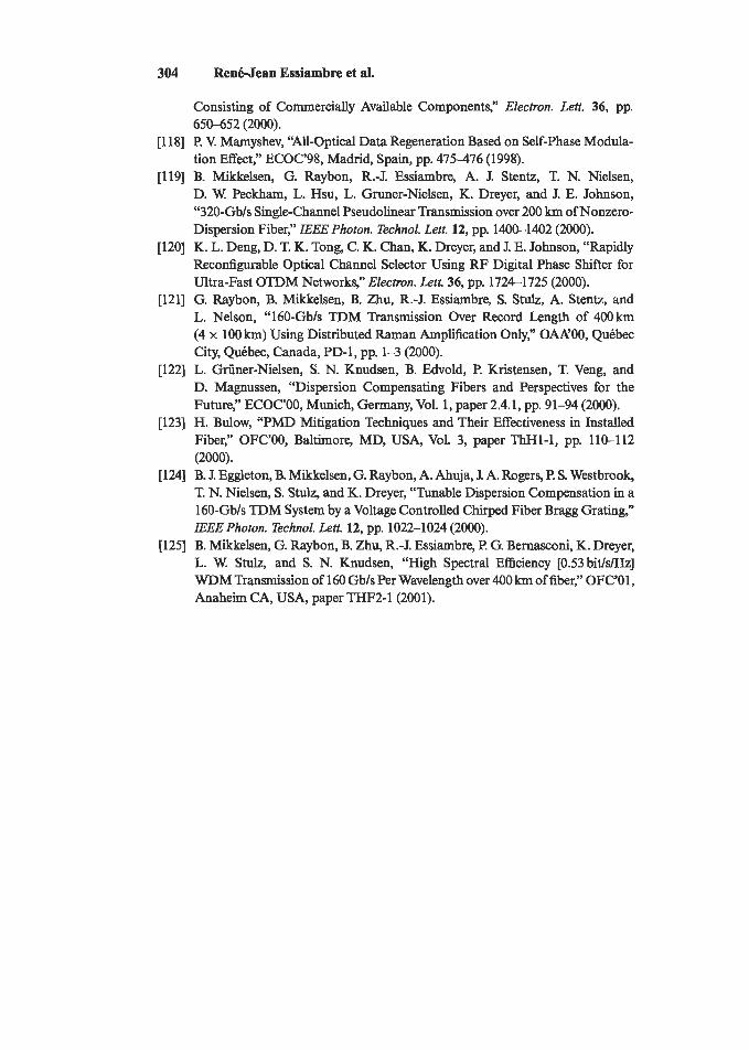
304 RenMean Essiambre et al.
Consisting of Commercially Available Components,” Electron. Lett. 36, pp. 65M52 (2000).
[118] P. V. Mamyshev, “All-Optical Data Regeneration Based on Self-phase Modula- tion Effect,” ECOC‘98, Madrid, Spain, pp. 475476 (1998).
[119] B. Mikkelsen, G. Raybon, R.-J. Essiambre, A. J. Stentz, T. N. Nielsen, D. W. Peckham, L. Hsu, L. Gruner-Nielsen, K. Dreyer, and J. E. Johnson, “320-Gbls Single-Channel Pseudolinear Transmission over 200 km of Nonzero- Dispersion Fiber,” IEEE Photon. Technol. Le t . 12, pp. 1400-1402 (2000).
[120] K. L. Deng, D. T. K. Tong, C. K. Chan, K. Dreyer, and J. E. Johnson, “Rapidly Reconfigurable Optical Channel Selector Using RF Digital Phase Shifter for Ultra-Fast OTDM Networks,” Electron. Lett. 36, pp. 1724-1725 (2000).
[121] G. Raybon, B. Mikkelsen, B. Zhu, R.-J. Essiambre, S. Stulz, A. Stentz, and L. Nelson, “160-Gbls TDM Transmission Over Record Length of 400km (4 x 100 km) Using Distributed Raman Amplification Only,” OAA’OO, Qukbec City, Qukbec, Canada, PD-1, pp. 1-3 (2000).
[122] L. Griiner-Nielsen, S. N. Knudsen, B. Edvold, P. Kristensen, T. Veng, and D. Magnussen, “Dispersion Compensating Fibers and Perspectives for the Future,” ECOC‘OO, Munich, Germany, Vol. 1, paper 2.4.1, pp. 91-94 (2000).
[123] H. Bulow, “PMD Mitigation Techniques and Their Effectiveness in Installed Fiber,” OFC‘OO, Baltimore, MD, USA, Vol. 3, paper ThH1-1, pp. 110-112
[124] B. J. Eggleton, B. Mikkelsen, G. Raybon, A. Ahuja, J. A. Rogers, P. S. Westbrook, T. N. Nielsen, S. Stulz, and K. Dreyer, “Tunable Dispersion Compensation in a 160-Gbls TDM System by a Voltage Controlled Chirped Fiber Bragg Grating,” IEEE Photon. TechnoZ. Lett. 12, pp. 1022-1024 (2000).
[125] B. Mikkelsen, G. Raybon, B. Zhu, R.-J. Essiambre, P. G. Bernasconi, K. Dreyer, L. W. Stulz, and S. N. Knudsen, “High Spectral Efficiency [0.53bit/s/Hz] WDM Transmission of 160 Gb/s Per Wavelength over 400 km of fiber,” OFC‘O1, Anaheim CA, USA, paper THFZl(2001).
(2000).
Chapter 7
Curtis R. Menyuk Computer Science and Electrical Engineering Department, University of Ma ryland Baltimore County, Baltimore, Maryland and Photon& Corporation, Maynard, Massachusetts
Gary M. Carter Computer Science and Electrical Engineering Department, University of Maryland Baltimore Coun& Baltimore, Maryland and Laboratory for Physical Sciences, College Park, Maryland
William L. Kath Computer Science and Electrical Engineering Department, University of h4atyhnd Baltimore County, Baltimore, Maryland and Applied Mathematics Department, Northwestern University, Evanston. Illinois
Ruo-Mei Mu QCO Telecommunications, Eatontown, New Jersey
Dispersion-Managed Solitons and Chirped Return to Zero: What Is the Difference?
I. Historical Overview
Once upon a time, a long time ago-at least as time is counted in the telecom- munications industry-there was a place called AT&T Bell Laboratories. At this remarkable place, it was possible for great scientists to do long-term research-research that might take many years to affect the development of telecommunications products. In 1973, Akira Hasegawa, who was then at AT&T Bell Laboratories, published a paper with Fred Tappert that contained three important contributions [l]. First, it showed that in an idealized optical fiber, with just second-order dispersion and the Kerr nonlinearity, the wave envelope of the light obeys the nonlinear Schrodinger equation, which may be written:
au pii a2u 2
az 2 at2 i- - -- + ylUl U = 0,
where U is the complex wave envelope, z is the distance along the optical fiber, is the second-order dispersion coefficient, and y is the nonlinear coefficient
due to the Kerr effect. The quantity t = t - z/vg is referred to as retarded time, where t is physical time and vg is the group velocity. Second, this paper
305 OPTICAL FIBER TELECOMMlJKICATIONS VOLUME IVB
Copyright 0 2002, Elrevier Science (USA). All rights of reproduction in any form reserved.
ISBN 0-12-395173-9
306 Curtis R Menyuk et al.
showed that when p” c 0, Eq. 7.1 has a soliton solution,
where T is an arbitrary parameter indicating the soliton pulse duration. Third, they showed that Eq. 7.1 can be solved using the split-step Fourier trans- form method. Equation 7.1 neglects the effects of higher-order dispersion, the Raman and Brillouin nonlinearities, device impairments along the transmis- sion line, amplified spontaneous emission (ASE) noise, and fiber birefringence. However, in the succeeding quarter century, a large number of scientists have contributed to amend Eq. 7.1 to include the missing effects [2]. To this day, almost all modeling of optical fiber transmission is based on Eq. 7.1, its amend- ments, and its reductions. Moreover, almost all numerical solutions of Eq. 7.1 and its amendments are based on the split-step method.
At the time that Eq. 7.1 was first written down, the notion of using solitons in communications systems seemed farfetched. Optical fiber losses were still too large in the anomalous dispersion regime where p” < 0 for nonlinear prop- agation to be practical, and no sources that could produce the needed powers at these long wavelengths, h > 1.3 pm, existed [2]. By 1980, however, fibers with losses almost as low as 0.2 dB/km at h = 1.5 pm had been fabricated, and color center lasers that could produce short, high-intensity pulses at 1.5 wm had been perfected. In that year, a scientist at AT&T Bell Laboratories named Linn Mollenauer, along with his colleagues Roger Stolen and Jim Gordon, demonstrated that it was possible to transmit solitons in optical fibers [3]. While a large number of scientists have contributed to the development of optical fiber solitons since 1980, Hasegawa and Mollenauer have been tireless advocates of their use in optical fiber communications systems.
The interest in using solitons stems from their remarkable property- apparent in Eq. 7.2-that they do not spread in the time domain due to dispersion or in the frequency domain due to nonlinearity. A single soliton pulse in an ideal, lossless fiber is completely stable. Moreover, solitons that are in different wavelength channels do not change their shape after a collision. The central times just shift slightly [2,4]. At an early stage, it was thought that it might be possible to actually use the nonlinearity to compensate for disper- sion [5]; however, it soon became apparent that it is more fruitful to view the dispersion as compensating for the nonlinearity. Any communications system is impaired by noise in the transmission line and the receiver. Optical fiber transmission systems are no exception. To ensure a reasonable signal-to-noise level, some nonlinearity is inevitable. However, it was already apparent in the early 1980s that the nonlinearity was too small to matter in the communica- tions systems of the day in which the signal was typically regenerated every 40 km or less. Thus, soliton advocates began in the early 1980s to explore the possibility of replacing repeaters with amplifiers. Raman amplification
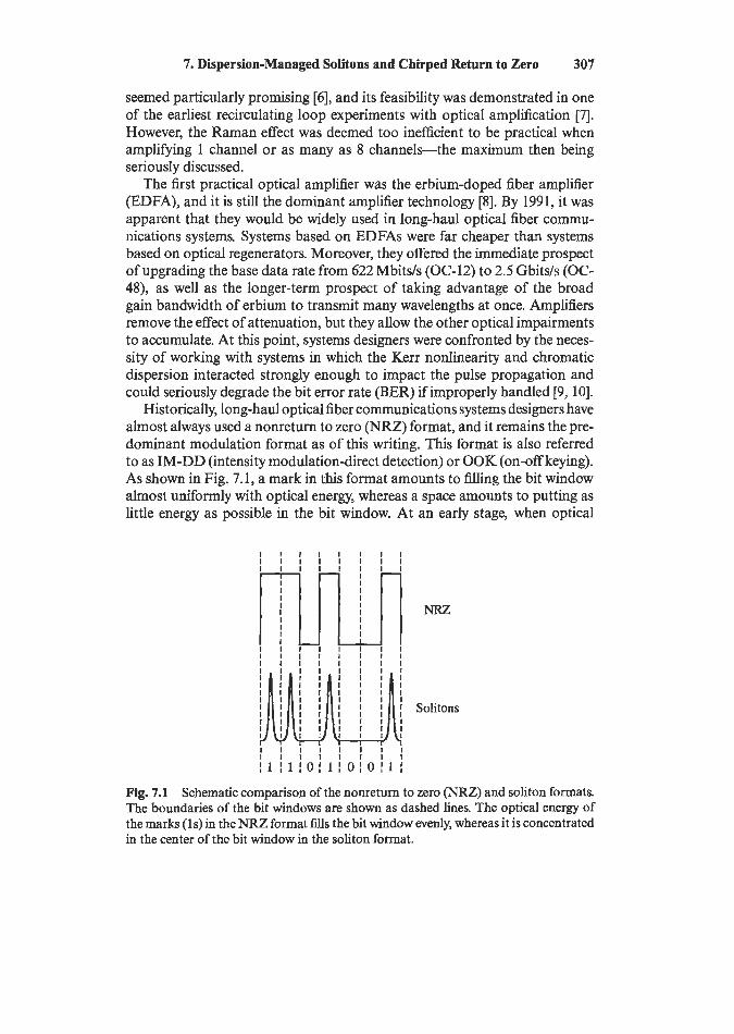
7. Dispersion-Managed Solitons and Chirped Return to Zero 307
seemed particularly promising [6], and its feasibility was demonstrated in one of the earliest recirculating loop experiments with optical amplification [7]. However, the Raman effect was deemed too inefficient to be practical when amplifying 1 channel or as many as 8 channels-the maximum then being seriously discussed.
The first practical optical amplifier was the erbium-doped fiber amplifier (EDFA), and it is still the dominant amplifier technology [8]. By 1991, it was apparent that they would be widely used in long-haul optical fiber commu- nications systems. Systems based on EDFAs were far cheaper than systems based on optical regenerators. Moreover, they offered the immediate prospect of upgrading the base data rate from 622 Mbitsh (OC-12) to 2.5 Gbitsh (OC- 48), as well as the longer-term prospect of taking advantage of the broad gain bandwidth of erbium to transmit many wavelengths at once. Amplifiers remove the effect of attenuation, but they allow the other optical impairments to accumulate. At this point, systems designers were confronted by the neces- sity of working with systems in which the Kerr nonlinearity and chromatic dispersion interacted strongly enough to impact the pulse propagation and could seriously degrade the bit error rate (BER) if improperly handled [9, 101.
Historically, long-haul optical fiber communications systems designers have almost always used a nonreturn to zero (NRZ) format, and it remains the pre- dominant modulation format as of this writing. This format is also referred to as IM-DD (intensity modulation-direct detection) or OOK (on-off keying). As shown in Fig. 7.1, a mark in this format amounts to filling the bit window almost uniformly with optical energy, whereas a space amounts to putting as little energy as possible in the bit window. At an early stage, when optical
NRZ
Solitons
Fig. 7.1 Schematic comparison of the nonreturn to zero (NRZ) and soliton formats. The boundaries of the bit windows are shown as dashed lines. The optical energy of the marks (1s) in the NRZ format fills the bit window evenly, whereas it is concentrated in the center of the bit window in the soliton format.

308 Curtis R. Menyuk et al.
communications systems used multimode fibers and light emitting diode (LED) transmitters, this format became dominant because it required s h - pler device technology than any of the alternatives [ll]. Later, when laser diodes replaced LEDs, the NRZ format also had the advantage of a smaller bandwidth than a return-to-zero (RZ) format at the same data rate [12]. Prior to the deployment of EDFAs, transmission impairments were dominated by attenuation and dispersion; therefore, it was important to reduce the impact of dispersion. As of 1990, practical NRZ sources based on distributed feedback lasers were available [13]. By contrast, solitons were generated by color-center lasers, which were too expensive and bulky for use in systems [14]. Moreover, receivers were optimized for the NRZ format [ 131.
The challenge posed by nonlinearity to the NRZ format-particularly in transoceanic systems where signals are required to propagate all-optically for thousands of kilometers-was quite serious. Unless the fiber’s dispersion is close to zero, the NRZ pulses spread unacceptably, leading to a large inter- symbol interference at the receiver. If, however, the dispersion is zero, the ASE noise from the amplifier is pumped through a resonant four-wave mix- ing interaction and grows exponentially, leading to severe distortion of the signal [15]. The solution to this problem in undersea systems was dispersion management. In one example of this approach, one alternates sections of stan- dard fiber that have a dispersion of 17 ps/nm-km at 1.55 pm with sections of dispersion-shifted fiber that have a dispersion of -2 ps/nm-km at 1.55 p,m [16]. Doing so, one keeps the average dispersion close to zero, which minimizes the spreading, while mitigating the resonant four-wave mixing. Dispersion man- agement is not as critical in terrestrial systems, but as the single-channel rates have increased to 10 Gbits/s and distances between repeaters have increased, it has become increasingly important. A typical dispersion-managed config- uration in a terrestrial setting alternates sections of standard fiber that have a dispersion of 17 ps/nm-km at 1.55 p,m and are already in the ground with sections of higher-dispersion fiber, at perhaps -85 ps/nm-km, that are placed in the amplifier huts or are part of the amplifier design [17,18].
After the invention of the EDFA, the next great step forward was the devel- opment of wavelength-division multiplexing (WDM) systems in which many wavelengths are transmitted at once. The earliest experiments came before 1990, and by 1993 there had been several important field trials [19]. As early as 1993, Chraplyvy et al. [20] had demonstrated the transmission of 8 channels in the NRZ format over distances that were relevant for terrestrial communi- cations at 10 Gbits/s per channel. By 1996, Mollenauer et al. [21] had demon- strated the transmission of 6 and 7 channels of solitons using sliding-guiding filters over transoceanic distances at 10 Gbitds per channel. Also by 1996, Bergano and Davidson [22] had demonstrated the transmission of 20 channels in the NRZ format, using bit-synchronous polarization and phase modula- tion, over transoceanic distances at 5Gbitds. At around this time, AT&T began to massively deploy WDM transmission systems in their networks.
7. Dispersion-Managed Solitons and Chirped Return to Zero 309
In 1996, the situation stood as follows: Soliton sources had finally been invented that used laser diodes and LiNbOs modulators, much like in the NRZ systems [23]. Testbed experiments had demonstrated the feasibility of long-haul WDM transmission at 10 Gbits/s using both the NRZ format and the soliton format. The NRZ experiments had used dispersion management with all the wavelength channels in the normal dispersion regime. The soliton experiments had used constant dispersion with all the wavelength channels in the anomalous dispersion regime. The NRZ systems avoided the bad effects of a sizable average dispersion by setting it close to zero, while accepting the residual nonlinear impairments. The soliton systems avoided the nonlinear impairments by using a sizable dispersion, but the dispersion combined with ASE noise led to a large timing jitter [24,25].
At this point, the NRZ and soliton formats appeared completely different. Experiments up to this time to study these formats were done on separate testbeds. Since the leading protagonists of the different formats did not work cooperatively with each other, it was almost impossible for an outside observer to judge among the competing claims. But things were about to change!
Soliton systems evolved dramatically in the next few years. Suzuki et al. [26] and Carter et al. [27] showed that it is advantageous to combine dispersion management with a soliton system. The nonlinearity of the system is effectively lowered by the spreading of the solitons, leading to a substantial reduction of the timing jitter [28, 291. While these dispersion-managed solitons are no longer stationary, they are at least periodically stationary in that they return to the same pulse shape after every period. By contrast, in the later experiments of Favre et al. [30] and Tsurutani et al. [31], this is no longer true. Here, the initial RZ pulses, which are simply raised-cosine pulses, have an initial chirp, which is related to the entire dispersion in the transmission line. While in the case of Favre et QI. [30] they continue to refer to their format as a disperslon- managed soliton (DMS) format, Tsurutani et al. [31] refer to their format as simply an RZ format.
At the same time, the NRZ format also evolved dramatically. Bergano et al. [32] first introduced phase modulation in order to reduce the degree of polarization of the signal stream and, consequently, the effect of polarization hole-burning. They observed that the optimal phase modulation led to pulse compression by the end of the propagation, so that the marks appeared as clearly distinguishable RZ pulses. They later observed that this effect could be enhanced and better performance obtained by using an initial amplitude mod- ulation as well as an initial phase modulation [33-351. Using this approach, they successfully transmitted wavelength channels on both sides of the zero dispersion point over transoceanic distances. The initial pulses in this case are raised-cosine pulses, and they are referred to by Bergano et al. [34] as chirped return to zero (CRZ) pulses.
It is our contention that the NRZ and soliton formats have effectively con- verged. The result is a new format, which some call DMS and others call
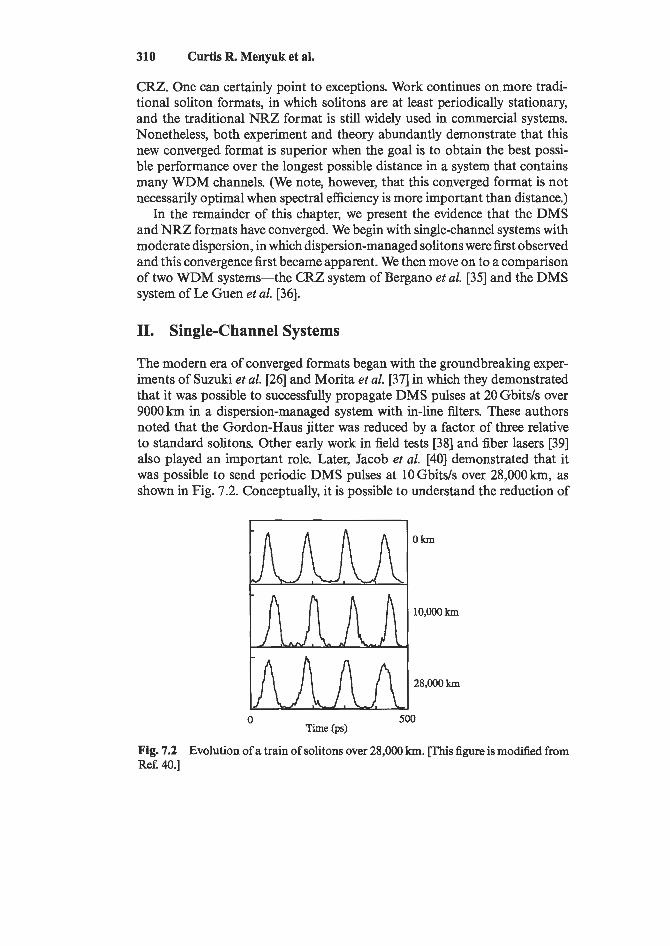
310 Curtis R. Menyuk et al.
CRZ. One can certainly point to exceptions. Work continues on,more tradi- tional soliton formats, in which solitons are at least periodically stationary, and the traditional NRZ format is still widely used in commercial systems. Nonetheless, both experiment and theory abundantly demonstrate that this new converged format is superior when the goal is to obtain the best possi- ble performance over the longest possible distance in a system that contains many WDM channels. (We note, however, that this converged format is not necessarily optimal when spectral efficiency is more important than distance.)
In the remainder of this chapter, we present the evidence that the DMS and NRZ formats have converged. We begin with single-channel systems with moderate dispersion, in which dispersion-managed solitons were first observed and this convergence first became apparent. We then move on to a comparison of two WDM systems-the CRZ system of Bergano et al. [35] and the DMS system of Le Guen et al. [36].
11. Single-Channel Systems
The modern era of converged formats began with the groundbreaking exper- iments of Suzuki et al. [26] and Morita et al. [37] in which they demonstrated that it was possible to successfully propagate DMS pulses at 20 Gbitsls over 9000 km in a dispersion-managed system with in-line filters. These authors noted that the Gordon-Haus jitter was reduced by a factor of three relative to standard solitons. Other early work in field tests [38] and fiber lasers [39] also played an important role. Later, Jacob et al. [40] demonstrated that it was possible to send periodic DMS pulses at 10 Gbitsls over 28,000 km, as shown in Fig. 7.2. Conceptually, it is possible to understand the reduction of
10,000 km rii.n.n.n 0 500
Time @)
Fig. 7.2 Evolution of a train of solitons over 28,000 km. mis figure is modified from Ref. 40.1
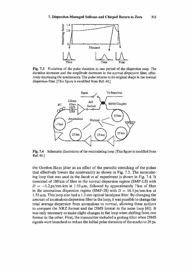
7. Dispersion-Managed Solitons and Chirped Return to Zero 311
E 1.4 e 1.0
B
g m o
I Distance
Ln Time Time Time
Fig. 7.3 Evolution of the pulse duration in one period of the dispersion map. The duration increases and the amplitude decreases in the normal dispersion fiber, effec- tively decreasing the nonlinearity. The pulse returns to its original shape in the normal dispersion fiber. phis figure is modified from Ref. 40.1
To Receiver To Receiver InputJ4 /-
Fig. 7.4 Ref. 40.1
Schematic illustration of the recirculating loop. [This figure is modified from
the Gordon-Haus jitter as an effect of the periodic stretching of the pulses that effectively lowers the nonlinearity as shown in Fig. 7.3. The recirculat- ing loop that was used in the Jacob et al. experiment is shown in Fig. 7.4. It consisted of 100 km of fiber in the normal dispersion regime (SMF-LS) with D = - 1.2 ps/nm-km at 1.55 pm, followed by approximately 7 km of fiber in the anomalous dispersion regime (SMF-28) with D = 16.5 ps/nm-km at 1.55 Fm. This loop also had a 1.2-nm optical bandpass filter. By changing the amount of anomalous dispersion fiber in the loop, it was possible to change the total average dispersion from anomalous to normal, allowing these authors to compare the NRZ format and the DMS format in the same loop [41]. It was only necessary to make slight changes in the loop when shifting from one format to the other. First, the transmitter included a grating filter when DMS signals were launched to reduce the initial pulse duration of the marks to 20 ps.
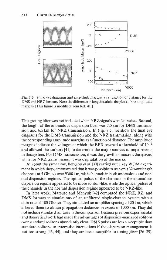
312 Curtis R. Menyuk et al.
I DMS t v,h
200
0
o o o O 9 E - -200 c
r
E 9
6 0 20000
0, $
w"
m
a, e,
L ._
N RZ 4 0
0 10000 Distance (krn)
Fig. 7.5 Final eye diagrams and amplitude margins as a function of distance for the DMS and NRZ formats. Note the difference in length scale in the plots of the amplitude margins. [This figure is modified from Ref. 41 .]
This grating filter was not included when NRZ signals were launched. Second, the length of the anomalous dispersion fiber was 7.5 km for DMS transmis- sion and 6.5 km for NRZ transmission. In Fig. 7.5, we show the final eye diagrams for the DMS transmission and the NRZ transmission, along with the corresponding amplitude margins as a function of distance. The amplitude margins indicate the voltages at which the BER reached a threshold of and allowed the authors [41] to determine the major sources of impairments in this system. For DMS transmission, it was the growth of noise in the spaces, while for NRZ transmission, it was degradation of the marks.
At about the same time, Bergano et al. [33] carried out a key WDM experi- ment in which they demonstrated that it was possible to transmit 32 wavelength channels at 5 Gbits/s over 9300 km, with channels in both anomalous and nor- mal dispersion regimes. The optical pulses of the channels in the anomalous dispersion regime appeared to be more soliton-like, while the optical pulses of the channels in the normal dispersion regime appeared to be NRZ-like.
In later work, Marcuse and Menyuk [42] compared the NRZ, RZ, and DMS formats in simulations of an unfiltered single-channel system with a data rate of 100 Gbitsh. They simulated an amplifier spacing of 20 km, which allowed them to obtain propagation distances in excess of 1000 km. They did not include standard solitons in the comparison because previous experimental and theoretical work had made the advantages of dispersion-managed solitons over standard solitons abundantly clear. DMS pulses are less susceptible than standard solitons to interpulse interactions if the dispersion management is not too strong [43, 441, and they are less susceptible to timing jitter [26-291.
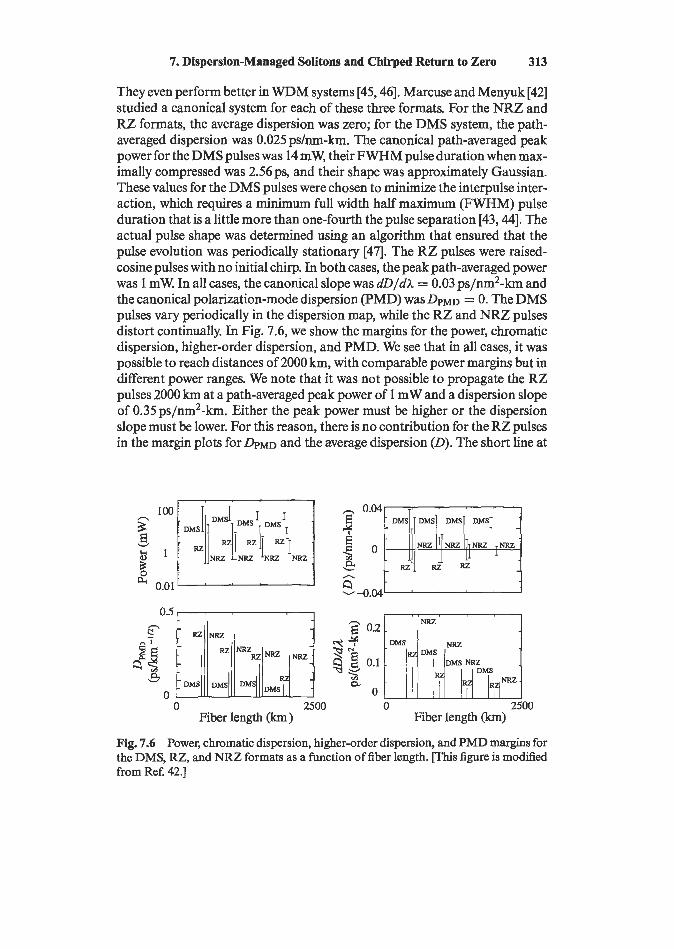
7. Dispersion-Managed Solitons and Chirped Return to Zero 313
They even perform better in WDM systems [45,46]. Marcuse and Menyuk [42] studied a canonical system for each of these three formats. For the NRZ and RZ formats, the average dispersion was zero; for the DMS system, the path- averaged dispersion was 0.025 ps/nm-km. The canonical path-averaged peak power for the DMS pulses was 14 mW, their FWHM pulse duration when max- imally compressed was 2.56 ps, and their shape was approximately Gaussian. These values for the DMS pulses were chosen to minimize the interpulse inter- action, which requires a minimum full width half maximum (FWHM) pulse duration that is a little more than one-fourth the pulse separation [43,44]. The actual pulse shape was determined using an algorithm that ensured that the pulse evolution was periodically stationary [47]. The RZ pulses were raised- cosine pulses with no initial chirp. In both cases, the peak path-averaged power was 1 mW. In all cases, the canonical slope was dD/dh = 0.03 ps/nm2-km and the canonical polarization-mode dispersion (PMD) was &MD = 0. The DMS pulses vary periodically in the dispersion map, while the RZ and NRZ pulses distort continually. In Fig. 7.6, we show the margins for the power, chromatic dispersion, higher-order dispersion, and PMD. We see that in all cases, it was possible to reach distances of 2000 km, with comparable power margins but in different power ranges. We note that it was not possible to propagate the RZ pulses 2000 km at a path-averaged peak power of 1 mW and a dispersion slope of 0.35ps/nm2-km. Either the peak power must be higher or the dispersion slope must be lower. For this reason, there is no contribution for the RZ pulses in the margin plots for &MD and the average dispersion (D). The short line at
Fig. 7.6 Power, chromatic dispersion, higher-order dispersion, and PMD margins for the DMS, RZ, and NRZ formats as a function of fiber length. phis figure is modified from Ref 42.1

314 Curtis R. Menyuk et al.
1' 8
2000 km on the margin plot for Dpm is a tic mark, not an indication of RZ pulses.
There is no fundamental distinction between the RZ pulses and the DMS pulses. As we raise the powers of the RZ pulses, we find that the pulses begin to oscillate in the dispersion map and that the overall dispersion must become anomalous. The NFU pulses do not evolve continually into DMS pulses unless they are modulated with a phase chirp. In that case, Bergano et aZ. [33] showed that they do evolve into pulses that are like DMS pulses. Schematically, a picture like the one that we show in Fig. 7.7 emerges from these considerations. It is possible to successfully transmit pulses with a wide range of combinations of the path-averaged peak power and the average chromatic dispersion over a length L. The interior of the oval marked Lj indicates the combinations that are possible over that length. High-power pulses require an average dispersion that is slightly anomalous and a shape that is soliton-like for optimal performance. At lower powers, the pulses should be more like RZ pulses. At even lower powers, the pulses should be more like NRZ pulses. As the length L increases from L1 to LZ to L3 to L4, the range of possible parameter values decreases, and the power and chromatic dispersion become tightly coupled. However, a range of power values is still possible as long as one chooses the appropriate chromatic dispersion to match each power value.
This convergence has not been universally accepted to date by the strongest advocates of the soliton and NRZ formats. It is certainly possible to question whether DMS pulses are really solitons. After all, solitons were first defined as stationary solutions to partial differential equations that had the additional property of passing through each other unscathed in collisions except for a time shift [48], as, for example, the solution to Eq. 7.1 given in 7.2. DMS pulses are far from stationary. They oscillate in amplitude due to spatially varying gain
RZ-like ~~
NRZ-like I

7. Dispersion-Managed Solitons and Chirped Return to Zero 315
and loss; they oscillate in pulse duration due to dispersion; and, finally, they do not have the standard hyperbolic-secant shape given by Eq. 7.2. One could respond that the DMS pulses are at least periodically stationary, and that is true if they are launched with a precisely correct combination of pulse duration, pulse power, and shape. Moreover, in filtered systems, a fairly broad set of initial pulses will ultimately evolve into periodically-stationary DMS pulses after a transient period. A periodically-stationary DMS pulse will ultimately emerge even in unfiltered systems, but, unless the initially launched pulse shape is close to the required pulse shape, a large amount of continuum radiation is created as well, leading to an unacceptable level of intersymbol interference. That said, when NRZ pulses are launched with an initial chirp, Bergano and his coworkers showed that they can ultimately evolve into pulses that are at least reminiscent of solitons. Should they be called solitons? While this question is still actively debated in scientific meetings, it is one that in OUT view has little scientific content at this point and is largely a matter of semantics. It is apparent that the new formats that we have described here have evolved substantially from the standard soliton and NRZ formats. The advocates of both the soliton and NRZ formats have contributed significantly to this development.
111. Wavelength-Division Multiplexed Systems
There is a serious problem with using the periodically stationary DMS mod- ulation format in WDM systems-at least with currently available fibers and dispersion-compensation techniques. To understand this problem, the reader should turn to Fig. 7.8, where we show the interaction length as a function of the dispersion map strength, y = 2(/3;’L1 - /3;Lz)/tO, where /3;’ and are the second-order dispersion in the first and second legs of the dispersion map,
50
0 0 3 6
Y = 2( p;L,-p;L,)/~,2
Fig. 7.8 Interaction length vs the map strength y. The larger curve with dots corre- sponds to a pulse separation of four times the maximally compressed FWHM, whereas the lower curve with squares corresponds to a separation of three times the maximally compressed FWHM. phis figure is modified from Ref. 43.1

316 Curtis R Menyuk et al.
respectively, L1 and L2 are the corresponding lengths, and to is the FWHM pulse duration at the point of minimum compression for the soliton. The inter- action length is the length scale on which two neighboring solitons attract each other, leading to a transmission error. Therefore, a longer interaction length is better. Here, we normalize the interaction length to the soliton’s character- istic nonlinear length scale [2]. We see that as the map strength increases, the interaction length increases up to a point, indicating that DMS pulses perform better than standard solitons, as noted earlier. However, beyond y = 3, the interaction length rapidly plunges and becomes worse than for standard soli- tons. This precipitous degradation is related to the increased stretching of the solitons. When the solitons stretch enough to begin to interact significantly, the mutual nonlinear interaction ultimately destroys them. Later work confirmed that periodically stationary DMS pulses cannot tolerate any significant inter- pulse interaction [49]. As a consequence, it is not possible to use periodically stationary DMS pulses in a WDM system unless a strong form of soliton con- trol is used like frequency sliding [50] or active amplitude modulation [51 , 521. The reason is that the third-order dispersion in today’s optical fibers implies that some channels in a WDM system that uses more than 10 nm of bandwidth must experience large dispersion, so that the pulses in the channels with large dispersion will stretch by large factors. In modern-day systems, it is common- place to have 30 nm of bandwidth, and systems have been demonstrated with more than 80nm [53]. Even when slope-compensating fiber is used inside one map period, so that there is no large change in the average dispersion from channel to channel, the spread within one map period is typically large. More- over, it is desirable to keep the residual dispersion large in order to minimize the nonlinear interchannel interactions that occur due to cross-phase modula- tion. As systems are upgraded from 10 Gbits/s to 40 Gbitsls, the stretching will become even larger. The response to this dilemma has been to lower powers in the soliton systems until the mutual interactions are at a tolerable level and to add an initial chirp [30,36]. In this case, the pulses are no longer periodically stationary. Instead, they change shape throughout their propagation along the entire transmission line. With a properly chosen initial chirp, their pulse durations at the end are smaller than at the beginning. This new kind of DMS system closely resembles the CRZ system of Bergano et al. [35]. We will show that these systems resemble each other far more closely than either resembles a single-channel, periodically stationary DMS system.
We show a schematic illustration of the first system that we are studying in Fig. 7.9. The dispersion map has L1 = 160km and L2 = 20km, while B;’ = -2.125 ps/nm-km and l?; = 17ps/nm-km at 1.55 km, so that the aver- age dispersion is zero at 1.55 bm. The dispersion slope is 0.075 ps/nm2-km, and the total propagation length is 5040 km. Each channel in the simulation has an average power of 0.3mW at the point of largest amplification and contains a 64-bit, pseudo-random stream with 32 marks and 32 spaces. The pulses have a raised-cosine pro€ile; so the FWHM pulse duration is 50ps.

7. Dispersion-Managed Solitons and Chirped Return to Zero 317
Channel &-chirp Post-compensation
1 & compensation 1
n -1 n
n -1 n
.d
L, L, Fig. 7.9 Schematic illustration of the simulated CRZ system. This system resembles the experimental system in Ref. 35.
Channel Pre-chwp Post-compensation 1
n -1 n -1 n n
Fig. 7.10 Schematic illustration of the simulated DMS system. This system resembles the experimental system in Ref. 36.
Each period of the dispersion map contains four amplifiers, spaced 45km apart. The pulses in each wavelength channel are prechirped, and the chro- matic dispersion in each channel can be compensated at both the beginning and the end of the transmission. Symmetric compensation is superior to either just precompensation or just postcompensation [54, 551. This system resem- bles the experimental system of Bergano et al. [35], although these authors used alternating polarizations in neighboring channels, while we used a single polarization so that Eq. 7.1 applies, They also used large-effective-area fiber, and we did not. We will refer to this system as the CRZ system.
We show a schematic illustration of the second system that we study in Fig. 7.10. In this case, the dispersion map has L1 = 102km and LZ = 17.3km, while B;’ = 16.4ps/nm-km and = -85ps/nm-km at 1.55km. The dispersion in the first leg corresponds to SMF (single-mode fiber)
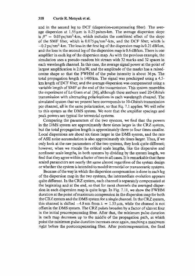
318 Curtis R Menyuk et al.
and in the second leg to DCF (dispersion-compensating fiber). The aver- age dispersion at 1.55 pm is 0.25ps/nm-km. The average dispersion slope is p”’ = 0.03ps/nm2-km, which includes the combined effect of the slope of the SMF fiber, which is 0.075ps/nm2-km, and the DCF fiber, which is -0.2 ps/nm2-km. The loss in the first leg of the dispersion map is 0.21 dB/km, and the loss in the second leg of the dispersion map is 0.6 dB/km. There is one amplifier in each leg of the dispersion map. As with the previous example, the simulation uses a pseudo-random bit stream with 32 marks and 32 spaces in each wavelength channel. In this case, the average signal power at the point of largest amplification is 2.0 mW, and the amplitude of the marks has a raised- cosine shape so that the FWHM of the pulse intensity is about 36ps. The total propagation length is 1400 km. The signal was prechirped using a 4.5- km length of DCF fiber, and the average dispersion was compensated using a variable length of SMF at the end of the transmission. This system resembles the experiment of Le Guen et al. [36], although these authors used 20-Gbitds transmission with alternating polarizations in each wavelength channel. The simulated system that we present here corresponds to 10-Gbits/s transmission per channel, all in the same polarization, so that Eq. 7.1 applies. We will refer to this system as the DMS system. We note that the amplifier spacings and peak powers are typical for terrestrial systems.
Comparing the parameters of the two systems, we find that the powers in the DMS system are approximately three times larger in the CRZ system, but the total propagation length is approximately three to four times smaller. Local dispersions are about six times larger in the DMS system, and the rate of ASE noise accumulation is also approximately six times larger. Thus, if we only look at the raw parameters of the two systems, they look quite different; however, when we rescale the critical scale lengths, like the dispersive and nonlinear scale lengths, in both systems by dividing by the system length, we find that they agree within a factor of two in all cases. It is remarkable that these scaled parameters are nearly the same almost regardless of the system design or whether the system is intended to model terrestrial or transoceanic systems.
Because of the way in which the dispersion compensation is done in each leg of the dispersion map in the two systems, the intermediate evolution appears quite different. In the CRZ system, each channel is separately compensated at the beginning and at the end, so that for most channels the averaged disper- sion in each dispersion map is quite large. In Fig. 7.1 1, we show the FWHM duration at the point of maximum compression in the dispersion map for both the CRZ system and the DMS system for a single channel. In the CRZ system, this channel is shifted -4.8 nm from h = 1.55 pm, while the channel is not offset in the DMS system. The CRZ pulses broaden by a factor of almost four in the initial precompensating fiber. After that, the minimum pulse duration in each map decreases up to the middle of the propagation path, at which point the minimum pulse duration increases once again, reaching a maximum right before the postcompensating fiber. After postcompensation, the final
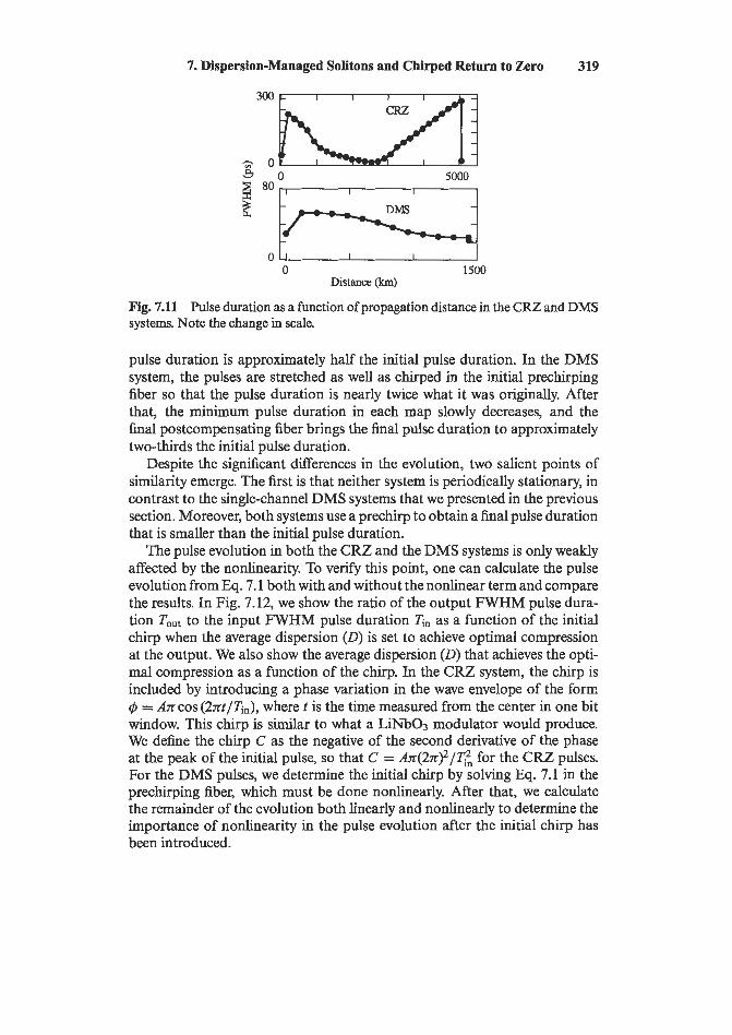
7. Dispersion-Managed Solitons and Chirped Return to Zero 319
5000
Ii 0 0 1500
Distance (km)
Fig. 7.11 Pulse duration as a function of propagation distance in the CRZ and DMS systems. Note the change in scale.
pulse duration is approximately half the initial pulse duration. In the DMS system, the pulses are stretched as well as chirped in the initial prechirping fiber so that the pulse duration is nearly twice what it was originally. After that, the minimum pulse duration in each map slowly decreases, and the k a l postcompensating fiber brings the final pulse duration to approximately two-thirds the initial pulse duration.
Despite the significant differences in the evolution, two salient points of similarity emerge. The first is that neither system is periodically stationary, in contrast to the single-channel DMS systems that we presented in the previous section. Moreover, both systems use a prechirp to obtain a final pulse duration that is smaller than the initial pulse duration.
The pulse evolution in both the CRZ and the DMS systems is only weakly affected by the nonlinearity. To verify this point, one can calculate the pulse evolution from Eq. 7.1 both with and without the nonlinear term and compare the results. In Fig. 7.12, we show the ratio of the output FWHM pulse dura- tion Tout to the input FWHM pulse duration Ti, as a function of the initial chirp when the average dispersion (0) is set to achieve optimal compression at the output. We also show the average dispersion (0) that achieves the opti- mal compression as a function of the chirp. In the CRZ system, the chirp is included by introducing a phase variation in the wave envelope of the form q5 = A n cos (2nt/Tin), where t is the time measured from the center in one bit window. This chirp is similar to what a LiNbOs modulator would produce. We define the chirp C as the negative of the second derivative of the phase at the peak of the initial pulse, so that C = An(27r))2/qi for the CRZ pulses. For the DMS pulses, we determine the initial chirp by solving Eq. 7.1 in the prechirping fiber, which must be done nonlinearly. After that, we calculate the remainder of the evolution both linearly and nonlinearly to determine the importance of nonlinearity in the pulse evolution after the initial chirp has been introduced.
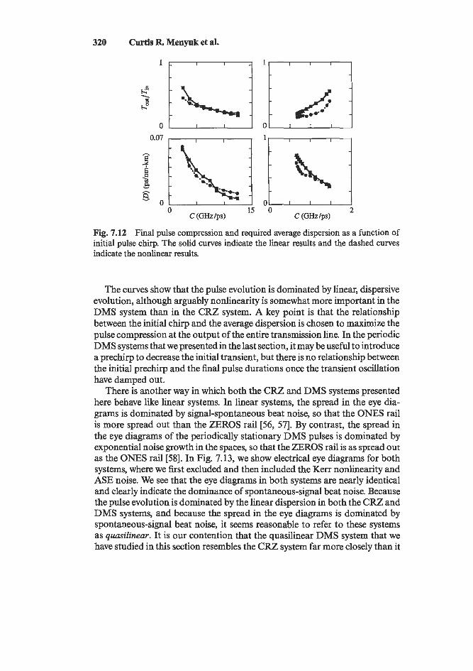
320 Curtis R Menyuk et al.
0.07
s _a E pq-/;pq %
--*
0 15 0 2 8 0
C (GHz Ips) C (GHz /ps)
Fig. 7.12 Final pulse compression and required average dispersion as a function of initial pulse chirp. The solid curves indicate the linear results and the dashed curves indicate the nonlinear results.
The curves show that the pulse evolution is dominated by linear, dispersive evolution, although arguably nonlinearity is somewhat more important in the DMS system than in the CRZ system. A key point is that the relationship between the initial chirp and the average dispersion is chosen to maximize the pulse compression at the output of the entire transmission line. In the periodic DMS systems that we presented in the last section, it may be useful to introduce a prechirp to decrease the initial transient, but there is no relationship between the initial prechirp and the final pulse durations once the transient oscillation have damped out.
There is another way in which both the CRZ and DMS systems presented here behave like linear systems. In linear systems, the spread in the eye dia- grams is dominated by signal-spontaneous beat noise, so that the ONES rail is more spread out than the ZEROS rail [56, 571. By contrast, the spread in the eye diagrams of the periodically stationary DMS pulses is dominated by exponential noise growth in the spaces, so that the ZEROS rail is as spread out as the ONES rail [58]. In Fig. 7.13, we show electrical eye diagrams for both systems, where we first excluded and then included the Kerr nonlinearity and ASE noise. We see that the eye diagrams in both systems are nearly identical and clearly indicate the dominance of spontaneous-signal beat noise. Because the pulse evolution is dominated by the linear dispersion in both the CRZ and DMS systems, and because the spread in the eye diagrams is dominated by spontaneous-signal beat noise, it seems reasonable to refer to these systems as quasilinear. It is our contention that the quasilinear DMS system that we have studied in this section resembles the CRZ system far more closely than it
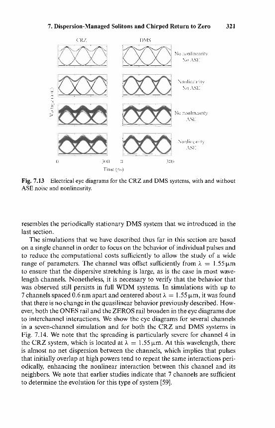
7. Dispersion-Managed Solitons and Chirped Return to Zero 321
CRZ
No nonlinearity No ASE
Nonlinearity No ASE
Q)
No nonlineanty ASE
,-? ? v
c 2 8 e
Nonlinearity ASE
0 300 0 300 Time (ps)
Fig. 7.13 Electrical eye diagrams for the CRZ and DMS systems, with and without ASE noise and nonlinearity.
resembles the periodically stationary DMS system that we introduced in the last section.
The simulations that we have described thus far in this section are based on a single channel in order to focus on the behavior of individual pulses and to reduce the computational costs sufficiently to allow the study of a wide range of parameters. The channel was offset sufficiently from h = 1.55 km to ensure that the dispersive stretching is large, as is the case in most wave- length channels. Nonetheless, it is necessary to verify that the behavior that was observed still persists in full WDM systems. In simulations with up to 7 channels spaced 0.6 nm apart and centered about h = 1.55 km, it was found that there is no change in the quasilinear behavior previously described. How- ever, both the ONES rail and the ZEROS rail broaden in the eye diagrams due to interchannel interactions. We show the eye diagrams for several channels in a seven-channel simulation and for both the CRZ and DMS systems in Fig. 7.14. We note that the spreading is particularly severe for channel 4 in the CRZ system, which is located at h = 1.55 km. At this wavelength, there is almost no net dispersion between the channels, which implies that pulses that initially overlap at high powers tend to repeat the same interactions peri- odically, enhancing the nonlinear interaction between this channel and its neighbors. We note that earlier studies indicate that 7 channels are sufficient to determine the evolution for this type of system [59].
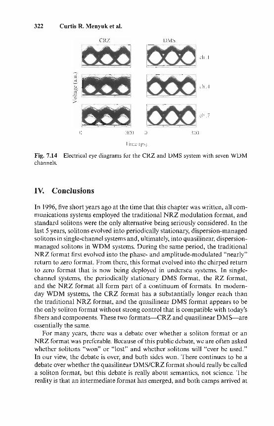
322 Curtis R. Menyuk et al.
CRZ DMS
ch.1
ch .I
0 300 0 300
Time (ps)
Fig. 7.14 Electrical eye diagrams for the CRZ and DMS system with seven WDM channels.
IV. Conclusions
In 1996, five short years ago at the time that this chapter was written, all com- munications systems employed the traditional NRZ modulation format, and standard solitons were the only alternative being seriously considered. In the last 5 years, solitons evolved into periodically stationary, dispersion-managed solitons in single-channel systems and, ultimately, into quasilinear, dispersion- managed solitons in WDM systems. During the same period, the traditional NRZ format first evolved into the phase- and amplitude-modulated “nearly” return to zero format. From there, this format evolved into the chirped return to zero format that is now being deployed in undersea systems. In single- channel systems, the periodically stationary DMS format, the RZ format, and the NRZ format all form part of a continuum of formats. In modern- day WDM systems, the CRZ format has a substantially longer reach than the traditional NRZ format, and the quasilinear DMS format appears to be the only soliton format without strong control that is compatible with today’s fibers and components. These two formats-CRZ and quasilinear DMS-are essentially the same.
For many years, there was a debate over whether a soliton format or an NRZ format was preferable. Because of this public debate, we are often asked whether solitons “won” or “lost” and whether solitons will “ever be used.” In our view, the debate is over, and both sides won. There continues to be a debate over whether the quasilinear DMS/CRZ format should really be called a soliton format, but this debate is really about semantics, not science. The reality is that an intermediate format has emerged, and both camps arrived at

7. Dispersion-Managed Solitons and Chirped Return to Zero 323
this format almost simultaneously, starting from different points. This inter- mediate format is remarkably robust and effective. Like Juliet, when she is bemoaning the hostility between the Capulets and the Montagues, we can conclude, “What’s in a name? That which we call a rose, by any other name would smell as sweet.. . .” [60].
Acronyms
ASE BER CRZ DMS EDFA FWHM IM-DD LED NRZ OOK PMD Rz SMF WDM
Amplified spontaneous emission Bit error rate Chirped return to zero Dispersion managed soliton Erbium-doped fiber amplifier Full-width half-maximum Intensity modulated-direct detection Light emitting diode Nonreturn to zero On-off keying Polarization-mode dispersion Return-to-zero Single mode fiber Wavelength-division multiplexing
References
[ 11 A. Hasegawa and E Tappert, “Transmission of stationary nonlinear optical pulses in dispersive dielectric fibers. I. Anomalous dispersion,” Appl. Phys. Lett., vol. 23, pp. 142-144 (1973).
[2] ’ Ibo general references that contain copious further references to the literature on soliton communications are: A. Hasegawa and Y. Kodama, Solitons in Optical Communications, Clarendon: Oxford, UK (1995) and G. P. Agrawal, Nonlinear Fiber Optics, Academic Press: San Diego, CA (1995).
[3] L. E Mollenauer, R. H. Stolen, and J. I? Gordon, “Experimental observation of picosecond pulse narrowing and solitons in optical fibers,” Phys. Rm. Lett.,
[4] The original paper that demonstrates this property for soliton solutions of the nonlinear Schrodinger equation is: V. E. Zakharov and A. E. Shabat, “Exact theory of two-dimensional self-focusing and one-dimensional self-modulation of waves in nonlinear media,” Sov. Phys.-JETP, vol. 34, pp. 62-69 (1972) [Original RussianZh. Ehp. Teol: Fiz., vol. 61, pp. 118-134 (1971)].
[5] A. Hasegawa and Y Kodama, “Signal transmission by optical solitons in monomode fiber,” Proc. IEEE, vol. 69, pp. 1145-1 150 (1981).
V O ~ . 45, pp. 1095-1098 (1980).
324 Curtis R Menyuk et al.
[6] A. Hasegawa and Y Kodama, “Amplification and reshaping of optical solitons in a glass fiber-IV Use of the stimulated Raman process,” Opt. Lett., vol. 8, pp. 650-652 (1983).
[7] L. E Mollenauer and K. Smith, “Demonstration of soliton transmission over more than 4000 km in fiber with loss periodically compensated by Raman gain,” Opt. Lett., vol. 13, pp. 675-677 (1988).
[8] Historical discussions and discussions of systems applications may be found in: E. Desurvire, Erbium-Doped Fiber AmpliJers: Principles and Applications, Wiley: New York, NY (1994) and P. C. Becker, N. A. Olsson, and J. R. Simpson, Erbium-Doped Fiber Amplifzers: Fundamentals and Technology, Academic Press: San Diego, CA (1999).
[9] E Forghieri, R. W. Tkach, and A. R. Chraplyvy, “Fiber nonliiearities and their impact on transmission systems,” in Optical Fiber Telecommunications IIIA, I. P. Kaminow and T. L. Koch, eds., Academic Press: San Diego, CA (1997). Contains an extensive set of references to the key literature.
[lo] A. R. Chraplyvy, “Limitations on lightwave communications imposed by optical- fibernon-linearities,” J. Lightwave Technol., vol. 8, pp. 1548-1 557 (1990). Contains a lucid review of the physical effects.
[ll] See, e.g., the discussions in L. Kazovsky, S. Benedetto, and A. Wdner, Opti- cal Fiber Communication Systems, Artech Boston, MA (1996), Chap. 3.1 and S. Gowar, Optical Communication Systems, Prentice-Hall New York, NY (1993), Chap. 7.3.
[12] G. P. Agrawal, Fiber-optic Communication Systems, Wiley: New York, NY (1997), Chap. 1.2.3. See also the historical discussion at the beginning of E Heismann, S. K. Korotky, and J. J. Veselka, “Lithium niobate integrated optics: Selected contemporary devices and systems applications,” in Optical Fiber Telecommuni- cations IIIB, I. P. Kaminow and T. L. Koch, eds., Academic Press: San Diego, CA (1997).
[13] D. A. Fishman and B. S. Jackson, “Transmitter and receiver design for amplified lightwave systems,” in Optical Fiber Telecommunications IIIB, I. P. Kaminow and T. L. Koch, eds, Academic Press: San Diego, CA (1997).
[14] K. Smith and L. E Mollenauer, “All-optical long-distance soliton-based trans- mission systems,” in Optical Solitons--Theory and Experiment, J. R. Taylor, ed., Cambridge: Cambridge, UK (1992).
[15] D. Marcuse, “Single-channel operation in very long nonlinear fibers with optical amplifiers at zero dispersion,” J. Lightwave Technol., vol. 9, pp. 356-361 (1991).
[16] N. S. Bergano, “Undersea amplified lightwave systems design,” in OpticaZ Fiber Telecommunications IIU, I. P. Kaminow and T. L. Koch, eds., Academic Press: San Diego, CA (1997).
1171 A. H. Gnauck and R. M. Jopson, “Dispersion compensation for optical fiber systems,” in OpticaIFiber Telecommunications IIIA, I. P. Kaminow and T. L. Koch, eds., Academic Press: San Diego, CA (1997).
7. Dispersion-Managed Solitons and Chirped Return to Zero 325
[I81 J. L. Zyskind, J. A. Nagel, and H. D. Kidorf, “Erbium-doped fiber amplifiers for optical communications,” in OpticalFiber Telecommunications IIIB, I. P. Kaminow and T. L. Koch, eda, Academic Press: San Diego, CA (1997).
[19] R. Gi!es and T. Li, “Optical amplifiers transform long-distance lightwave telecommunication^" Proc. IEEE, vol. 84, pp. 87-83 (1996).
[ZO] A. R. Chraplyvy, A. H. Gnauck, R. W. Tkach, and R. M. Derosier, “8 x 10 Gb/s transmission through 280 km of dispersion-managed fiber,” ZEEE Photon. Technol. Lett., vol. 5, pp. 1233-1235 (1993).
[21] L. E Mollenauer, I? V. Mamyshev, and M. J. Neubelt, “Demonstration of soliton WDM transmission at 6 and 7 x 10 Gbit/s, error-free over transoceanic distances,” Electron. Lett., vol. 32, pp. 471-473 (1996).
[22] N. S. Bergano and C. R. Davidson, “Wavelength division multiplexing in long- haul transmission systems,” J. Lightwave Technol., vol. 14, pp. 1299-1307 (1996).
[23] P. V. Mamyshev, “Dual-wavelength source of high-repetition-rate, transform- limited optical pulses for soliton transmission,” Opt. Lett., vol. 19, pp. 2074-2076 (1994).
[24] J. P. Gordon and H. A. Haus, “Random walk of coherently amplified solitons in optical fiber,” Opt. Lett., vol. 11, pp. 665-667 (1986).
[25] H. A. Haus, “Quantum noise in a solitonlike repeater system,” J. Opt. SOC. Am. B,
[26] M. Suzuki, I. Morita, N. Edagawa, S. Yamamoto, H. Taga, and S. Akiba, “Reduc- tion of Gordon-Haus timing jitter by periodic dispersion compensation in soliton transmission,” Electron. Lett., vol. 31, pp. 2027-2029 (1995).
[27] G. M. Carter, J. M. Jacob, C. R. Menyuk, E. A. Golovchenko, and A. N. Pilipetskii, “Timing-jitter reduction for a dispersion-managed soliton system: Experimental evidence,” Opt. Lett., vol. 22, pp. 513-515 (1997).
[28] N. J. Smith, W. Forysiak, and N. J. Doran, “Reduced Gordon-Haus jitter due to enhanced power solitons in strongly dispersion managed systems,” Electron. Lett., vol. 32, pp. 2085-2086 (1996).
[29] R.-M. Mu, V. S. Grigoryan, C. R. Menyuk, E. A. Golovchenko, and A. N. Pilipetskii, “Timing-jitter reduction in a dispersion-managed soliton system,” Opt Lett., vol. 23, pp. 936932 (1998).
[30] E Favre, D. Le Guen, M. L. Moulinard, M. Henry, and T. Georges, “320 Gbit/s soliton WDM transmission over 1300 km with 100 km dispersion-compensated spans of standard fibre,” Electron Lett., vol. 33, pp. 2135-2136 (1997).
[31] T. Tsurutani, K. Imai, N. Edagawa, and M. Suzuki, “340Gbit/s (32 x 10.66 Gbit/s) WDM transmission over 6054 km using hybrid fibre spans of large core fibre and dispersion shifted fibre with low dispersion slope,” Electron. Lett., vol. 35, pp. 646-647 (1999). It is difficult to do justice to the wide scope of the work of Suzuki, Edagawa, and their colleagues at KDD with any single ref- erence. In a series of publications that appeared mostly in Electronics Letters, they have examined all of the major formats that are being considered for use in transoceanic systems at different data rates and with different numbers of chan- nels. The work just cited uses initial raised-cosine pulses with an initial chirp, just
V O ~ . 8, pp. 1122-1 126 (1991).

326 Curtis R. Menyuk et al.
like the work by Favre et al. cited in Ref. [31]. In other work, H. Taga, K. Imai, N. Takeda, M. Suzuki, S. Yamamoto, and S. Akiba, “10 WDM 10 Gbitfs recir- culating loop transmission experiments using dispersion slope compensator and non-soliton RZ pulse,” Electron. Lett., vol. 33, pp. 2058-2059 (1997) study an RZ format with unchirped raised-cosine pulses. An experiment based on more traditional soliton-like pulses is described in K. Tanaka, I. Morita, M. Suzuki, N. Edagawa, and S. Yamamoto, “400 Gbit/s (20 x 20 Gbit/s) dense WDM soliton- based RZ signal transmission using dispersion flattened fibre,” Electron. Lett., vol.
[32] N. S. Bergano, C. R. Davidson, and F. Heismann, “Bit-synchronous polarisation and phase modulation scheme for improving the performance of optical amplifier transmission systems,” Electron. Lett., vol. 32, pp. 52-54 (1996).
[33] N. S. Bergano, C. R. Davidson, M. A. Mills, P. Corbett, S. G. Evangelides, B. Pedersen, R. Menges, J. L. Zyskind, J. W. Sulhoff, A. K. Srivastava, C. Wolf, and J. Judkins, “Long-haul WDM transmission using optimal channel modu- lation: A 160Gb/s (32 x 5Gb/s) 9,500km demonstration,” OFC ’97 Technical Digest (Dallas, TX), Feb. 1997, postdeadline paper PD16.
[34] N. S. Bergano, C. R. Davidson, M. Ma, A. N. Pilipetskii, S. G. Evangelides, H. D. Kidorf, J. M. Darcie, E. A. Golovchenko, K. Rottwitt, P. C. Corbett, R. Menges, M. A. Mills, E. Pedersen, D. Peckham, A. A. Abramov, and A. M. Vengsarkar, “320 Gb/s WDM transmission (64 x 5 Gb/s) over 7,200 km using large mode fiber spans and chirped return-to-zero signals,” OFC ’98 Technical Digest (San Jose, CA), Feb. 1998, postdeadline paper PD12.
[35] N. S. Bergano, C. R. Davidson, C. J. Chen, B. Pedersen, M. A. Mills, N. Ramanujam, A. B. Kidorf, H. D. PUC, M. D. Levonas, and H. Abdelkader, “640 Gb/s transmission of sixty-four 10 Gb/s WDM channels over 7,200 km with 0.33 (bits/s)/hz spectral efficiency,” OFC ’99 Technical Digest (San Diego, CA), Feb. 1999, postdeadline paper PD2.
[36] D. Le Guen, S. D. Burgo, M. L. Moulinard, D. Grot, M. Henry, E Favre, and T. Georges, “Narrow band 1.02Tbit/s (51 x 20Gbit/s) soliton DWDM trans- mission over 1000 km of standard fiber with 100 km amplifier spans,” OFC ’99 Technical Digest (San Diego, CA), Feb. 1999, postdeadline paper PD4.
[37] I. Morita, M. Suzuki, N. Edagawa, S. Yamamoto, H. Taga, and S. Akiba, “20- Gb/s single-channel soliton transmission over 9000 km without inline filters,” IEEE Photon. Technol. Lett., vol. 8, pp. 1573-1574 (1996).
[38] M. Nakazawa, Y. Kimura, K. Suzuki, H. Kubota, T. Komukai, E. Yamada, T. Sugawa, E. Yoshida, T. Yamamoto, T. Imai, A. Sahara, H. Nakazawa, 0. Yamauchi, and M. Umezawa, “Field demonstration of soliton transmission at 10 Gbitls over 2000 km in Tokyo metropolitan optical loop network,” Electron Lett., vol. 31, pp. 992-994 (1995).
[39] H. A. Haus, K. Tamura, L. E. Nelson, and E. P. Ippen, “Stretched-pulse additive pulse mode-locking in fiber ring lasers: Theory and experiment,” J. Quantum Electron., vol. 31, pp. 591-598 (1995).
34, pp. 2257-2258 (1998).
7. Dispersion-Managed Solitons and Chirped Return to Zero 327
[40] J. M. Jacob, E. A. Golovchenko, A. N. Pilipetskii, G. M. Carter, and C. R. Menyuk, “Experimental demonstration of soliton transmission over 28 Mrn using mostly normal dispersion fiber,” IEEE Photon. Technol. Lett., vol. 9, pp. 130-132 (1997).
[41] J. M. Jacob, E. A. Golovchenko, A. N. Pilipetskii, G. M. Carter, and C. R. Menyuk, “10Gb/s transmission of NRZ over 10,000krn and solitons over 13,500 km error-free in the same dispersion-managed system,” ZEEE Photon. Technol. Lett., vol. 9, pp. 1412-1414 (1997).
[47] D. Marcuse and C. R. Menyuk, “Simulation of single-channel optical systems at 100Gb/s,” J. Lightwave Technol., vol. 17, pp. 564-569 (1999).
[43] T. Yu, E. A. Golovchenko, A. N. Pilipetskii, and C. R. Menyuk, “Dispersion- managed soliton interaction in optical fibers,” Opt. Lett., vol. 22, pp. 793-795 (1 997).
[44] N. J. Smith, N. J. Doran, W. Forysiak, and E M. Knox, “Soliton transmission using periodic dispersion compensation,” J. Lightwave Technol., vol. 15, pp. 1808- 1822 (1997).
[45] E. A. Golovchenko, A. N. Pilipetskii, and C. R. Menyuk, “Collision-induced timing jitter reduction by periodic dispersion management in soliton WDM transmission,” Electron. Lett., vol. 33, 735-737 (1997).
[46] E. A. Golovchenko, A. N. Pilipetskii, and C. R. Menyuk, “Periodic disper- sion management in soliton wavelength-division multiplexing transmission with sliding filters,” Opt. Lett., vol. 22, 1156-1 158 (1997).
[47] J. H. B. Nijhof, W. Forysiak, and N. J. Doran, “The averaging method for finding exactly periodic dispersion-managed solitons,” IEEE J. Select. Topics Quantum Electron., vol. 6, pp. 330-336 (2000).
[48] N. J. Zabusky and M. D. Kruskal, “Interaction of solitons in a collisionless plasma and the recurrence of initial states,” Phys. Rev Lett., vol. 15, pp. 240-243 (1965).
[49] V S. Grigoryan, G. M. Carter, and C. R. Menyuk, “Tolerance of dispersion- managed soliton transmission to the shape of the input pulses,” IEEE Photon. Technol. Lett., vol. 12, pp. 1165-1167 (2000).
[50] L. E Mollenauer, J. P. Gordon, and S. G. Evangelides, “The sliding-frequency guiding filter: An improved form of soliton jitter control,” Opt. Lett., vol. 17,
E511 M. Nakazawa, E. Yamada, H. Kubota, and K. Suzuki, “lOGbit/s soliton data transmission over one million kilometres,” Electron Lett., vol. 27, pp. 1270-1272
[52] E. Desurvire, 0. Leclerc, and 0. Audouin, “Synchronous in-line regeneration of wavelength-division multiplexed solitons signals in optical fibers,” Opt. Lett., vol. 21, pp. 1026-1028 (1996).
[53] Y Sun, J. W. Sulhoff, A. K. Srivastava, J. L. Zyskind, T. A. Strasser, J. R. Pedraz- zini, C. Wolf, J. Zhou, J. B. Judkins, R. P. Espindola, and A. M. Vengsarkar, “80 nm ultra-wideband erbium-doped silica fibre amplifer,” Electron Lett., ~01.33,
pp. 1575-1577 (1992).
(199i).
pp. 1965-1967 (1997).

328 Curtis R Menyuk et al.
[54] L. Ding, E. A. Golovchenko, A. N. Pilipetskii, C. R. Menyuk, and P. K. A. Wai, “Modulated NRZ signal transmission in dispersion maps,” OS4 Trends in Optics and Photonics, vol. 12, System Technologies, A. E. Willner and C. R. Menyuk, eds. Optical Society of America: Washington, DC, pp. 204-206 (1997).
[55] M. I. Hayee and A. E. Willner, “Pre- and post-compensation of dispersion and nonlinearities in 10-Gb/s WDM systems,” IEEE Photon. Technol. Lett., vol. 9,
[56] D. Marcuse, “Derivation of analytical expressions for the bit-error probability in lightwave systems with optical amplifiers,” J. Lightwave Technol., vol. 8, pp. 1816- 1822 (1990).
[57] P. A. Humblet and M. Azizoglu, “On the bit error rate of lightwave systems with optical amplifers,” J. Lightwave Technol., vol. 9, pp. 1576-1582 (1991).
[58] R.-M. Mu, V. S. Grigoryan, C. R. Menyuk, G. M. Carter, and J. M. Jacob, “Comparison of theory and experiment for dispersion-managed solitons in a recirculating fiber loop,” Select. Topics Quantum Electron., vol. 6, pp. 248-251
[59] T. Yu, W. M. Reimer, V. S. Grigoryan, and C. R. Menyuk, “A mean field approach for simulating wavelength-division multiplexed systems,” IEEE Photon. Technol.
pp. 1271-1273 (1997).
(2000).
Lett., vol. 12, pp. 4 4 3 4 5 (2000). [60] W. Shakespeare, Romeo and Juliet, Act 2, Scene 2.
Chapter 8
Nasir Ghani, Jin-Yi Pan, and Xin Cheng Sorrento Networh Inc., San Diego, California
Metropolitan Optical Networks
1. Introduction
The modem telecommunications age has created an unprecedented growth in networking infrastructures. With the recent explosion of Internet data com- munications, Internet Protocol (IP) data traffic volumes have surpassed voice and are projected to be over 75% of total network traflic within the next 2 years [60,65]. It is often stated that Internet traffic is experiencing “exponen- tial” growth rates, and whilst the exact values are very case specific, it is safe to say that data growth is much larger than circuit voice growth [42]. Moreover, it is also well known that data traffic characteristics are very different from voice, exhibiting highly bursty and unpredictable behaviors, see [60, 1591. As the user base grows and more content-rich applications emerge, undoubtedly capacity demands will increase further. These fundamental trends are already having a profound impact on the overall networking space.
Telecommunications networks are usually segmented in a three-tier hier- archy: access, metropolitan, and long haul (further delineations also are possible [65]). Long-haulbackbone networks span interregional/global dis- tances (1000 km or more) and provide large tributary connectivity between regional and metro domains. Backbone networks are optimized for transmis- sion, and related costs have been dominated by expensive line equipment, for example, regeneration gear [64, 731. On the other end of the hierarchy are access networks, providing connectivity to a plethora of customers within close proximity. Access networks use a very broad range of technologies/protocoIs and represent a continual flux. Straddled in the middle are metropolitan (metro) networks, averaging regions between 10-100h [22, 641 and inter- connecting access and long-haul networks. Metro networks today are based upon synchronous optical network (SONET)/synchronous digital hierarchy (SDH) ring architectures. Namely, smaller tributary rings, for example, OC- 3/STM-1(155 Mb/s) or OC-12/STM-4(622 Mb/s), aggregate trafficonto larger core interoffice (IOF) [64] rings that interconnect central office (CO) loca- tions at higher bit rates, for example, OC-48/STM-16 (2.5 Gb/s). Overall, SONET/SDH has been very successful in delivering the first wave of end-user connectivity, namely voice.
329 OPTICAL FIBER TELECOMMUNICATIONS, VOLUME N B
Copyright 0 2002, Elscvier Science (USA). All rights of repduction in any form m d .
ISBN: &12-395173-9

330 Nasir Ghani et al.
Internet traffic growth has significantly altered the networking domains bordering the metro. Long-haul networks felt the Internet crunch first and have undergone large-scale expansions using optical dense wavelength-division multiplexing (DWDM) technology [64] (note that herein, the terms DWDM and WDM are used interchangeably). DWDM yields the best backbone costkapacity tradeoff [41,71], and many backbone networks now boast ter- abit capacities. Meanwhile, access networks have also seen their share of progress. Residential cable and digital subscriber loop (DSL) modems have increased user access rates from kilobits to megabits, and other advanced tech- nologies promise to further this trend. Also, large corporate customers are now deploying advanced switchinglrouting gear capable of direct line-rate inputs to the metro core, for example, concatenated OC-48~4192~~ lO-Gb/s Ethernet interfaces. Collectively, these increased access rates are blurring traditional access boundaries and beginning to stifle legacy “voicecentric” metro archi- tectures. Many SONETEDH rings are experiencing capacity exhaust at even OC-48/192 rates [62, 65, 1421, and costly ring (fiber) expansion is becoming overly slow and expensive. Furthermore, as market expansion and deregula- tion take form, increased competition is forcing operators to support a highly dynamic, increasingly diverse mixtures of client protocols, both legacy and asynchronous data [61-65, 871. Examples include IP, ATM (Asynchronous Transfer Mode), SONETBDH, Ethernet (10/100 Mb/s, 1.0/10 Gb/s), multi- plexed TDM voice (DS-n), and other more specialized data protocols such as FDDI (Fiber Distributed Data Interface), ESCON (Enterprise System Con- nectivity), FICON (Fiber Connectivity Channel), Fibre Channel, cable video, etc. (see Fig. 8.1, adapted from [158]). Again, legacy SONET/SDH networks are proving extremely restrictive here, exhibiting high bandwidth inefficiencies and overly complex, cumbersome provisioning procedures [ 141, 1421.
Clearly new metro solutions are required that offer superior price/ performance alternatives to legacy SONET/SDH expansion, and from the above, a host of necessary features can be derived. For example, new platforms must offer high bandwidth scalability and carry multiple protocols over a com- mon infrastructure to reduce costs [46]. Rapid, intelligent services provisioning and survivability are also crucial, as operators look to compete via service dif- ferentiation and not just pricing [65], Le., advanced service level agreements (SLA). Moreover, given current infrastructure investments, new schemes must provide backwards compatibility, i.e., legacy support [22,44], to enable more cost-effective, staged migrations. Undoubtedly, DWDM technology meets many of these requirements, and given its success in the long-haul space, is being increasingly touted in the metro domain [22, 35-57, 61-65]. Declining costs are making this technology very cost competitive with SONET/SDH, and even though increased bit rate TDM solutions are emerging, for exam- ple, 40 Gb/s OC-768/STM-256, DWDM is much more scalable from a pure capacity perspective, Le., terabitdfiber. Moreover, DWDM provides gen- uine bit rate/protocol transparency, a very compelling advantage in the
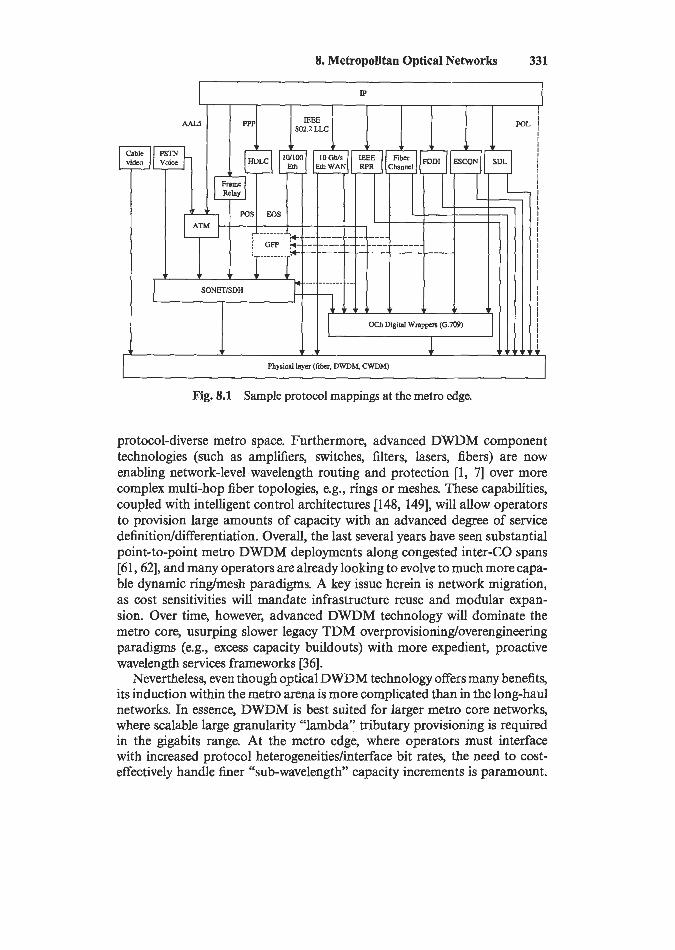
8. Metropolitan Optical Networks 331
I rP I
Physical layer (fiber, DWDM CWDM) I Fig. 8.1 Sample protocol mappings at the metro edge.
protocol-diverse metro space. Furthermore, advanced DWDM component technologies (such as amplifiers, switches, filters, lasers, fibers) are now enabling network-level wavelength routing and protection [ 1 , 71 over more complex multi-hop fiber topologies, e.g., rings or meshes. These capabilities, coupled with intelligent control architectures [148, 1491, will allow operators to provision large amounts of capacity with an advanced degree of service definitioddifferentiation. Overall, the last several years have seen substantial point-to-point metro DWDM deployments along congested inter-CO spans [61 , 621, and many operators are already looking to evolve to much more capa- ble dynamic rindmesh paradigms. A key issue herein is network migration, as cost sensitivities will mandate infrastructure reuse and modular expan- sion. Over time, however, advanced DWDM technology will dominate the metro core, usurping slower legacy TDM overprovisioningloverengineering paradigms (e.g., excess capacity buildouts) with more expedient, proactive wavelength services frameworks [36].
Nevertheless, even though optical DWDM technology offers many benefits, its induction within the metro arena is more complicated than in the Iong-haul networks. In essence, DWDM is best suited for larger metro core networks, where scalable large granularity “lambda” tributary provisioning is required in the gigabits range. At the metro edge, where operators must interface with increased protocol heterogeneitieshnterface bit rates, the need to cost- effectively handle finer “sub-wavelength” capacity increments is paramount.
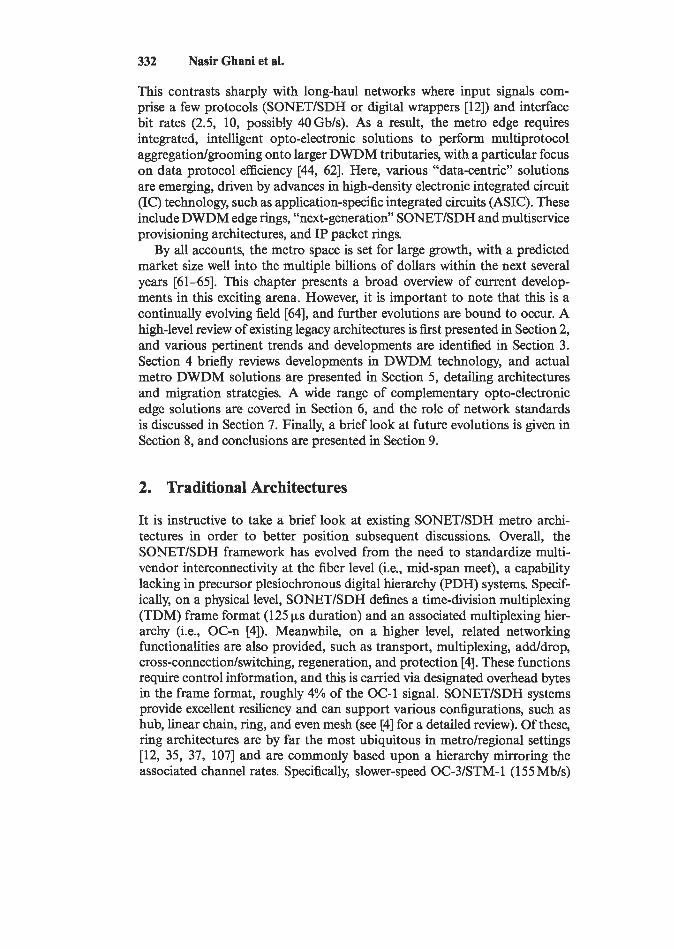
332 Nasir Ghani et al.
This contrasts sharply with long-haul networks where input signals com- prise a few protocols (SONETlSDH or digital wrappers [12]) and interface bit rates (2.5, 10, possibly 4OGbls). As a result, the metro edge requires integrated, intelligent opto-electronic solutions to perform multiprotocol aggregation/grooming onto larger DWDM tributaries, with a particular focus on data protocol efficiency [44, 621. Here, various “data-centric” solutions are emerging, driven by advances in high-density electronic integrated circuit (IC) technology, such as application-specific integrated circuits (ASIC). These include DWDM edge rings, “next-generation” SONETlSDH and multiservice provisioning architectures, and IP packet rings.
By all accounts, the metro space is set for large growth, with a predicted market size well into the multiple billions of dollars within the next several years [61-651. This chapter presents a broad overview of current develop- ments in this exciting arena. However, it is important to note that this is a continually evolving field [64], and further evolutions are bound to occur. A high-level review of existing legacy architectures is first presented in Section 2, and various pertinent trends and developments are identified in Section 3. Section 4 briefly reviews developments in DWDM technology, and actual metro DWDM solutions are presented in Section 5, detailing architectures and migration strategies. A wide range of complementary opto-electronic edge solutions are covered in Section 6, and the role of network standards is discussed in Section 7. Finally, a brief look at future evolutions is given in Section 8, and conclusions are presented in Section 9.
2. Traditional Architectures
It is instructive to take a brief look at existing SONETlSDH metro archi- tectures in order to better position subsequent discussions. Overall, the SONETlSDH framework has evolved from the need to standardize multi- vendor interconnectivity at the fiber level (i.e., mid-span meet), a capability lacking in precursor plesiochronous digital hierarchy (PDH) systems. Specif- ically, on a physical level, SONETlSDH defines a time-division multiplexing (TDM) frame format (125 ps duration) and an associated multiplexing hier- archy (i.e., OC-n [4]). Meanwhile, on a higher level, related networking fimctionalities are also provided, such as transport, multiplexing, add/drop, cross-connectionlswitching, regeneration, and protection [4]. These functions require control information, and this is carried via designated overhead bytes in the frame format, roughly 4% of the OC-1 signal. SONETlSDH systems provide excellent resiliency and can support various configurations, such as hub, linear chain, ring, and even mesh (see [4] for a detailed review). Of these, ring architectures are by far the most ubiquitous in metrolregional settings [12, 35, 37, 1071 and are commonly based upon a hierarchy mirroring the associated channel rates. Specifically, slower-speed OC-3lSTM- 1 (1 55 Mbls)
8. Metropolitan Optical Networks 333
RegronaVlong-haul
e m (IOF) SONET/SDH B U R ring (oc-19YSTM-64)
Mem (IOF) SONET/SDH B U R nng \ (OC-48/STM- 16)
Edge UPSR nng
Enterprise routed swtches (leased line TDM interfaces)
Fig. 8.2 Traditional SONETISDH ring hierarchy in metropolitan region.
or OC-l2/STM-4 (622 Mb/s) metro edge rings (or loops) are used to aggregate customer traffic onto larger OC-48/STM-16 (2.5 Gb/s) or OC-192/STM-64 (10 Gb/s) metro core rings [3,35, 37,641. A sample overview of this hierarchy is shown in Fig. 8.2 and details follow. As will be seen, these current metro architectures will have a large impact on future evolutions, with similar edge and core delineations being carried forward (Sections 5 and 6).
2.1 METRO EDGE RINGS
The metro edge is commonly defined as the space between high-speed (metro core) CO locations and customer access facilities [35, 651. Most metro edge rings span 20-65 km (average span lengths of 1040 km) [64], and collect traffic between several customer sites [35] (under lo), running at either OC- 3/STM-1 or OC-12/STM-4 rates. (Note that these rings are equivalent to the junction layer defined in [4]). The key network element in metro edge rings is the add/drop multiplexer (ADM) node, which aggregates traffic from low/moderate-speed interfacedfacilities in the access layer (i.e., rates such as DS1, DS3, up to lOO’sMb/s). Metro edge ADM devices are usually linked to customer premise (CP) networks that groom client traffic onto TDM tribu- taries [4]. Examples can include digital loop carrier (DLC) setups, enterprise networks (Le., T1 leased lines), telephony public branch exchanges (PBX), etc. As the boundary between the metro edge and customer access continues

334 Nasir Ghani et al.
to blur, many ADM nodes are also providing aggregation capabilities for smaller DSO rates. Such “edge” aggregation significantly reduces required port counts versus more centralized “back-hauling” configurations [ 1341 (detailed subsequently), i.e., “multiplexer mountain.”
Because most edge traffic is usually outbound from the immediate local- ized region, metro edge rings exhibit strongly hubbed tratXc-demand patterns [35, 541, and hence are well-suited (bandwidth efficient) for SONET/SDH unidirectional path-switched ring (UPSR) [8] designs. UPSR schemes use dual counterrotating rings and perform 1 + 1 receiver bridging [4, 51 to reduce the need for more complex (expensive) protection signaling. Metro edge ring tratXc is routed onto larger metro core rings at appropriate IOF CO hub locations [64]. Ring interconnection can be done in several ways [4]. A simple means is via direct connection of the associated ADM nodes (i.e., metro edge and core rings). Alternatively, more advanced (expensive) synchronous switching digital cross-connect (DCS) functionalities (Fig. 8.2) can also be used to perform fine-granularity time-slot interchange (TSI) and spatial switching [5]. In other words, DCS nodes basically perform as band- width managers, providing tributary termination, segregation, and grooming (i.e., multiplexing/demultiplexing) capabilities at various levels, namely VT1.5 (1.544Mb/s) or STS-1 (51.84Mb/s). Namely, incoming tributaries are fully demultiplexed (e.g., into STM-1 streams [3]), even if they are “pass-through,” and these are either dropped locally or cross-connectedhegroomed with other tributaries onto larger outbound tributaries. Such centralized DCS-based processing is commonly called “back-ha~ling~’ [4]. Also note that DCS- based ring interconnection can be done either via directly subtending ADM nodes on to a separate DCS (nonintegrated) node or by a more advanced integrated DCS node [2, 1341 with added ADM functionality. Note that the latter approach saves the cost of two ADM nodes [134] and reduces equipment cost, footprint space, and management complexity. However, inte- grated DCS nodes increase network vulnerability, as a failure can affect both rings.
There are two types of DCS nodes, namely wideband DCS (W-DCS) and broadband DCS (B-DCS) [4, 5, 1341, largely discerned by their grooming granularities. W-DCS nodes handle tributary rates down to DSlNT1.5 levels and therefore enable fine granularity bandwidth control [4, 51. As such, they are well-suited for metro edge ring bandwidth management, where tributary rates are smaller due to closer customer proximity. Meanwhile, B-DCS nodes can cross-connect signals from DS-3 (Mb/s) up to OC-48 (2.5 Gb/s) and have granularities of STS-1 [91]. As such, these nodes are much better suited for metro core networks handling larger increments andlor interfaces over OC-1. In general, given the complexity of SONETISDH standards and the differen- tiating augmentations added in many vendor solutions, multivendor network element interoperability is rather difficult. This makes it more likely that a single vendor’s solution will be deployed in a ring, and DCS nodes used to

8. Metropolitan Optical Networks 335
independently groom traffic between rings [134]. For more details on DCS designs, refer to [4, 51.
Traditional metro networks have employed a “multilayering” [38] approach for asynchronous data transport, where enterprise customers use leased- line services (Tl, T3, OC-n) to interconnect their private networks. In essence, this approach has evolved from a gradual layering of data network- ing protocols onto voice-based infrastructures. Specifically, data protocols are mapped onto SONET frames via intermediate “adaptationyy protocols (equipment) such as ATM or frame relay (switches). As a result, differ- ent “layersyy are used to implement a complete “service” definition, for example, SONETEDH for protectiordtransport, ATM for t&c/bandwidth engineering, IP for connectivityh-outing. More recently, however, direct packet over SONET (POS) interfaces have also been defined, where IP packets are mapped to the high-level data link control (HDLC) protocol and then framed into SONET/SDH [ll , 121. In fact, today, many upper- end gigabit routers/switches provide high-speed concatenated POS interfaces, namely 2.5 Gb/s (OC-48c/STM-l6c) and 10 Gb/s (OC-192c/STM-64c), capa- ble of directly interfacing to larger metro core rings [7, 651. Furthermore, as edge boundaries continue to blur, newer ADM designs are even provid- ing direct “non-TDM” native data interfaces with SONET/SDH mappings [4] (see also Section 6.2). Nevertheless, multilayering increases overall port costkomplexity significantly since more protocol layers are involved (i.e., implementation, maintenance, etc.). Although this was acceptable in past “voice-centric” networks, its viability in increasingly “data-centric” scenarios is highly questionable.
2.2 METRO CORE RZNGS
The core fiber plant of many established metro operators is very dense, and this infrastructure is typically provisioned as a series of metro core rings running through major CO hub locations, i.e., the core layer [4]. These rings are then usually interconnected as meshes using DCS nodes. Metro core rings (also termed as IOF or collector rings [3, 851) naturally represent a higher level of aggregation, and their boundaries are marked by larger tributary rates. OC- 48/STM-16 (2.5 Gb/s) has been widely used, although recently, the demand for OC-192/STM-64 systems is growing rapidly, with deployment set to double over the coming years [142]. These rings interconnect large CO (ADM) loca- tions across a metropolis, and feed into larger regional and long-haul networks for cross-regiordglobal transport, for example, between service provider points of presence (POP) or inter-exchange COS. Ring sizes can vary anywhere from 50-250 km, with average spans of 40-80 km [64]. Note that SONET/SDH per- forms per-hop regeneration, and hence transmission impairment concerns for most metro distances do not arise [47].
336 Nasir Ghani et al.
Due to larger geographic spread and customer base, traflic demands in metro core rings are much more meshed (versus edge rings), i.e., “any-to- any” between arbitrary CO ADM locations. In such scenarios, bidirectional line-switched ring (BLSR) designs [9] are well-suited, allowing for improved bandwidth efficiency via timeslot reuse [75]. Two- and four-fiber BLSR ring designs are available, performing loopback span switching for logical (two-fiber) and physical (four-fiber) rings, respectively [5]. In a typical large metropolis there can be well over 10 IOF rings, and hence ring interconnection is also required. Due to the increased scale of traffic, larger IOF rings are usu- ally connected via reliable dual ring interworking @RI)/drop-and-continue [4,9,74] schemes (also termed dual homing [5]). These schemes prevent against major outages from all single-hubhnterface failures and a number of dual fail- ures [74]. However, these schemes come at a price, namely more equipment complexity and fiber requirements. Simpler variants are also possible, such as a single DCS node between two subtending ADM rings, etc. [74, 1341. Note that BLSR-UPSR interconnection is also specsed [9], applicable for edge/core ring interconnection.
In some cases, DCS (W-DCS) nodes are also used to interconnect metro core rings in larger “mesh” network topologies across a large metropolis. Mesh networks are typically deployed when internode fiber connectivity is signifi- cantly higher than that in rings (e.g., beyond degree two). DCS mesh networks provide path-level mesh restoratiodprotection capabilities (logical layer recov- ery [5]), and generally, these schemes are usually much more efficient in terms of spare capacity utilization due to higher oversubscription [74]. Both dis- tributed and centralized DCS recovery schemes are possible [SI, but most solutions are proprietary vendor-based offerings (see also [ 10,741). However, DCS mesh restoration schemes require more complex software (versus self- healing rings) and very careful capacity preplanning. Hardware complexity also increases significantly, and intermediate demultiplexing is very ineffi- cient for handling larger-tributary pass-through operations. Moreover, mesh recovery timescales are usually much longer (seconds to minutes) [5], and therefore most stringent services must still rely upon ring protection. Over- all this gives a three-tiered survivability hierarchy [5] for large metrohegional networks (i.e., ring protection switching, DCS mesh restoration, and manual operator control).
3. Emerging Trends
As stated previously, there are various technological and commercial factors driving today’s metro arena, such as increasing traffic demands, improving access technologies, and industry deregulation. A very brief review is pre- sented here to highlight the growing disconnect with legacy SONET/SDH metro architectures and to better qualify further discussion on solutions and
8. Metropolitan Optical Networks 337
migration strategies. Interested readers are referred to the related references for complete details [22,42, 61-65].
3.1 DEMAND GROWTH
Undoubtedly, rapid growth in network traffic volumes is one of the key drivers for optical networking solutions. In particular, there are various aspects of this growth that are of significance in the metro space, and some details are now presented.
3.1.1 Internet Applications
Residential Internet has produced sustained data traffic growth, with close to half of the households in North America now having Internet connec- tivity [42]. Meanwhile, penetration rates are also growing significantly in Europe and Asia [65]. Applications such as e-mail, FTP, Telnet, and Web are commonplace and other advanced “content-rich” (bandwidth-intensive) applications are also emerging (e.g.. “real-time” applications such as Inter- net telephony, video-on-demandvideo streaming, Internet gaming, etc.). More futuristic offerings such as multidimensional virtual reality are also envisioned. On the corporate side, many businesses are heavily utilizing existing Internet applications and busy developing new possibilities. For example, Internet teleconferencingkelecommuting is commonplace and Web hostinglmirroring and e-commerce are growing rapidly (incorporating more graphics, sounds, and video content). Other, more distant possibilities such as telemedicine and remote sensing are also being studied. Overall, unlike tra- ditional “delay-insensitive” applications, many newer applications have much more stringent (guaranteed) bandwidth needs.
Apart from applicationhandwidth growth, the number of simultaneous peered sessions is also increasing rapidly, further accelerating volumes [60]. In all, the combination of increased user populations, applications, and cconliney’ times is boosting capacity demands tremendously, with compound annual growth rates (CAGR) of over 35% [43]. Also, many studies indicate that Internet traffic exhibits highly bursty (some argue nonstationary), asymmet- ric behaviors [159], and overall customer demands can be more difficult to predict as compared to legacy voice [22, 601. This contrasts with long-haul networks, where the degree of traffic aggregation is much higher @e., between large population centers), and consequently, traffic fluctuations are more grad- ual. Furthermore, as communication distances expand, larger proportions of end-user traffic, roughly 80%, are destined for wider communities of interest (unlike legacy voice), averaging over 400 km [22, 521, @e., 80-20 rule). Over- all, these traffic characteristics are very challenging, and metro networks must scale to handle them properly (see [60] for details).

338 Nasir Ghani et al.
3.1.2 VirtuaVTransparent LANs
As corporate clients expand to diverse geographic locations, the concept of transparenthirtual LAN (TLANNLAN) services is gaining strong favor, pro- viding seamless LAN interconnection between selected enterprise and remote locations [38] (via port grouping). This will allow enterprise clients to main- tain the “LAN-like” feel of their networks, yet scale across larger geographic areas. Note that this is not a novel concept, and some existing protocols such as ATM or frame relay already support LAN emulation capabilities, albeit these are costly and provide limited bandwidth [64, 1331. A key difference today is the use of lower-cost native Ethernet interfaces. Native VLANs repre- sent a very large, emerging metro market given the predominance of Ethernet interfaces [133] (Le., over 80% of enterprise tr&c originates in Ethernet form [46] and low-speed Ethernet (10/100 Mb/s) dominates the desktop). Overall, VLAN services may become subsets of more generalized optical virtual private network (0-VPN) services [65].
More recently, there have also been significant efforts to extend Ethernet protocol standards to gigabit rates, namely 10 Gb/s Ethernet (10 GbE) [159, 1601. Specifically, new standards are being defined for both for both LAN (short reach) and WAN (long reach) applications (IEEE 802.3 working group), and these are expected to dominate the high-speed router interface market as components arrive on the market [47]. Note that the WAN interface type will reuse SONET/SDH OC-192c framing and require synchronization [158, 1601, making if significantly different from the short-reach interface. Overall, gigabit Ethernet interfaces will significantly increase enterprise tra& volumes in the metro. As an aside, such bit rates will also help reduce port counts on high-throughput Ethernet switches.
3.1.3 Storage Area Networks
As information volumes expand, corporations are looking at storage area networks (SAN) for reliable back-up/recovery capabilities. This market has emerged recently, driven by falling storage and bandwidth costs, and is poised for significant growth [64]. SANs utilize various storage protocols (Fibre Channel, ESCON, and recently Gigabit Ethernet), to provide reliable, high- speed, native connectivity between large storage sites in a metro area [65]. Namely, these sites interconnect servers and backup storage devices using SAN hublswitch nodes. Since many large corporations have on the order of petabytes worth of stored data [59], clearly, very large transport capacities are required. Additionally, SANs can also play a key role in disaster recovery applications (see [59] for a detailed deployment study).
3.1.4 Virtual Line Services
Given the broad range of client protocols, many operators are looking to provide bit-rate-independent services, also termed “lambda servi~es.’~ These
8. Metropolitan Optical Networks 339
offerings are particularly attractive for enterprise clients wanting to build optical VPNs [155] to interconnect multiple locations via a full variety of interfacedprotocols (e.g., Gigabit Ethernet, SONET, frame relay, ATM, etc.). Also, in the future more advanced services such as bandwidth leasindtrading can also be leveraged hereof Unlike legacy leased-line services, virtual-line services will provide genuine transparency (e.g., even for SONET/SDH over- heads), enabling customers to manage their own networks [68]. See [44, 64, 65, 1411 for more details.
3.1.5 Legacy Voice
Despite data traffic growth, the legacy voice business is not in decline. On the contrary, private-line telephony service continues to exhibit steady linear growth, with some studies indicating rates up to 7-25% per year [42,65]. This represents a strong, sizable revenue stream for most incumbent operators. Since many operators have yet to deploy “packet-voice” services (e.g., technological, standardization, operational issues), this growth will likely remain for the next several years. Moreover, many users may opt to stay with legacy voice services, unless operators offer compelling, competitive value-adds to their “packet-voice” offerings [65].
3.2 IMPRO MNG ACCESS TECHNOLOGIES
With growing application bandwidth demands, there is strong push to bring broadband capacities closer to end-users. Many new (high-speed) access tech- nologies have emerged, such as cable and digital subscriber loop (DSL) modems, high-speed wireless, air fiber, and more advanced optical offerings. The economics of these solutions are key factors here, because end-users are very cost-sensitive and access infrastructures are difficult to amortize over mul- tiple subscribers (as with core infrastructures). Nevertheless, research shows that average access rates will increase in the coming years, with the exact values contingent upon technology type (see [65]). As these new access technologies undergo deployment, the commensurate need for high-capacity metro network solutions will strengthen. Some of these solutions are briefly reviewed.
3.2.1 Cable and Digital Subscriber Loop Modems
Residential Internet access is still largely based upon copper-plant modem technology, with bit rates limited to under 56 kb/s. However, DSL technol- ogy is now available, utilizing signal processing techniques to boost copper line rates to over 2.0 Mb/s. Many residentidsmall business DSL solutions use an ATM link-layer, and DSL access multiplexers (DSLAMs) help aggre- gate customers onto larger TDM-based access tributaries (e.g., ATM DS-3 and OC-3 rates). ATM offers good latency control, and hence, some have also proposed c‘voice-over-DSLyy for packaging data and voice services [65].

340 Nasir Ghani et al.
Meanwhile, cable is another widely deployed “last-mile” solution that offers relatively high access bandwidth. Cable modem technology allows for bidi- rectional data transmission using radio frequency (RF) separation [19], and typical access rates are in the megabits. Most cable operators are deploying two-way services using hybrid fiber-coax (HFC) networks, and standards are emerging for data over cable [64]. Overall, cable operators have a strong, grow- ing customer base and many have successfully rolled out bundled datahoice services. Market research predicts that both the DSL and cable markets will grow by nearly an order of magnitude over the next few years [65].
3.2.2 High-speed Wireless Technologies
High-speed wireless technologies present a good alternative for many new entrants who lack ownership of fiber/copper/cable plants. For example, many wireless operators are moving to deploy “next-generation” wireless solutions (e.g., 3G wireless), with proposed bit rates of up to 2.0Mb/s. Additionally, ultra-high-bandwidth local multipoint distribution service (LMDS) technol- ogy is also available. LMDS occupies a higher spectrum range (24-39 Ghz) and yields about 1 Ghz bandwidth for a range of between 1-3 miles (as limited by precipitation and other effects) [MI. This is usually best suited for business customers in dense metropolitan districtslindustrial parks, providing a mix of voice and data services (Tl/OC-3). Other wireless solutions use various “line- of-sight” communication techniques between end-users and hub nodes. For example, multichannel multipoint distribution system (MMDS) offers about 200Mhz bandwidth and ranges between 5-35 miles. This is well-suited for residentiahmall business customers and provides an alternative to cable/DSL access. Meanwhile, in dense, fiber-constrained business settings, “air fiber” solutions also offer high-capacity, localized transmissions for distances under 10 km. Specifically, these schemes use carefully aligned high-launch-power semiconductor lasers. However, air-fibex systems must contend with many transmission limitations, such as atmospheric loss, scatteringhefraction (via rain, fog, mist, even snow), etc. Although back-up microwave transmission techniques can be utilized, transmission rates will be much lower. Overall, these techniques are less ubiquitous due to the line-of-sight requirement, even though availability levels of over 99% have been stated [23].
3.2.3 Optical Access Technologies
As bandwidth growth continues, there is a strong push to deploy fiber closer to end-users [20,22] in order to overcome capacity and distance limitations of aging copper plants. Much research has been done on “optical” access archi- tectures such as fiber-to-the-home (FTTH) and fiber-to-the-curb (FTTC) [19]. In particular, many solutions based upon passive optical networks (PONS) [2, 3, 191 have been investigated. Earlier PON schemes used power-splitting setups with time-slotted multi-access (TDMA) protocols, but these designs

8. Metropolitan Optical Networks 341
suffer from excessive power loss and ranging limitations [58]. With the emergence of cost-effective DWDM mudde-mux devices and amplifiers, higher-capacity DWDM PON architectures have now emerged [58,168] direct- ing wavelengths to end-user terminals (e.g., via wavelength gratings [19]). DWDM PON solutions provide enhanced security since optical channels are passively routed to receivers and not broadcasted. A lot of research has been done on different PON architectures (e.g., combining TDM and DWDM PONS) [5, 19, 21, 1681, and commercial offerings are even available. With improving economics these architectures will dramatically improve access rates (gigabits range).
Code-division multiplexing (CDM) is an asynchronous spread-spectrum technique that has been widely applied in satellite, wireless, cable, and more recently, optical networks. Optical CDM permits bandwidth sharing by dis- tinguishing signals via distinct spectral or temporal codes and can be applied to shared medium access networks (e.g., passive star coupler configurations [3, 171). Code switching can be done using low-cost passive (linear) optical devices (spectral filters) and only requires a single optical carrier frequency (see [ 181). Additionally, the added signal processing capabilities may also enable consistent operation over a whole range of fiber types (e.g., single mode, disper- sion shifted, even older polarized mode) [44], a capability difficult to achieve in high-speed TDM systems (10 Gb/s or beyond). There are many emerging advances in coding devices and code design [ lq , and this technology may soon come on the market.
3.3 INDUSTRY DEREGULATION
Competitive pressures and new regulations have resulted in a global push to privatize and deregulate telecommunications markets. Deregulation has progressed rapidly in North America and Europe, and other markets (Asia, Latin America) will likely follow suit. Within the metro arena, the effects of deregulation are very acute, as entry costs tend to be lower than those in long-haul markets. This has created an abundance of operators, ranging from incumbent local exchange carriers (LECs), newer competitive local exchange carriers (CLECs), cable operators, and even (traditionally long haul) inter- exchange carriers (IXC) and utilities corporations. Given this large operator pool, undoubtedly competition is stiff [133]. For example, many IXC compa- nies are actively expanding into the metro/access markets to feed expanded capacities on their long-haul DWDM buildouts. Meanwhile, CLECs are aggressively buying/leasing/laying dark fiber to build out their infrastructures [65]. Also, a growing number of utility companies are entering the telecom market in order to diversify and increase their revenue base (usually as “car- riers’ carriers” [64]). These outfits own “right-of-way” into most metro areas, a crucial advantage that allows them to lay new fiber routes. Most utilities with telecom operations are leasing out dark fiber, and this is also expediting

342 Nasir Ghani et al.
market entry for many other nonincumbent operators. Moreover, utilities can also leverage their large regional customer bases and extensive service and construction capabilities. In all, deregulation has driven down bandwidth costs significantly [62], and operators are increasingly competing via advanced service differentiation capabilities. For further details, refer to [62,64,65].
3.4 CHALLENGES AND REQUIREMENTS
In light of the above trends/developments, legacy metro networks are now facing many limitations With increasing demands and improving access tech- nologies, capacity exhaust on metro rings is a major issue [5, 41, 62, 681 for OC-48/STM-16 and in some cases even OC-19USTM-64 bit rates. In fact, market research indicates that OC-48L3TM-16 is fast becoming the new unit of cunrency among carriers, replacing lower DS3 rates [63, 641. Now SONET/SDH technology really only offers two lengthy solutions to capacity exhaust, either increase single-channel TDM rates (e.g., OC-192,OC-768) or deploy new rings (i.e., “stacked rings”). Neither of these are particularly scal- able, and hence are aptly termed “fork-lift” upgrades [64, 1411. The former is expensive, requiring equipment upgrades on all ring nodes, and usually gives only fourfold capacity increases. Meanwhile, the latter is even more expen- sive, requiring complex forecasting [68] and new fiber routes and TDM gear at ring add/drop points (although fewer nodes can be deployed initially to reduce costs [SI). Fiber expansion costs are dominated by right-of-way and construction costs, and albeit high, can vary significantly (see [45, 62, 711). Although it is relatively cheaper to pull fiber through existing conduits [22], in many cases conduit exhaust is also occurring. Additionally, electronic cross- connects must still demultiplex large incoming tributaries (e.g., OC-48) down to the STM-1 levels and switch/recombine on the outbound side [3]. This increases electronic switching fabric complexity and power consumption and is not scalable in the least for multiple ring hops. Overall, these unscalabilities present a huge capacity bottleneck between increasingly higher-speed end- users and abundant long-haul DWDM bandwidth, often termed the “metro gap” [36], see Fig. 8.3.
Apart from capacity limitations, the SONET/SDH “multilayering’y paradigm is overly outdated for dynamic, data-centric settings For exam- ple, IP volumes are surpassing legacy voice levels and Ethernet ports easily source most Internet data traflic. Yet at the same time, data interface rates are highly incongruent with SONET/SDH TDM hierarchies, and resultant mappings yield large bandwidth inefficiencies and consume more ports for a given data throughput (see Section 6.2). This has accelerated capacity exhaust and proven very challenging for operators, especially as bandwidth costs decline [66]. For example, from a revenue standpoint, (lower-volume) voice still earns more “per-bit” transmitted than data, yet data growth requires much more expenditures. Moving forward, metro operators must also contend with

8. Metropolitan Optical Networks 343
Access-to-lonp-haul “metro-pad’ .Mainly SONET/SDH-based infrastructures *Low provisioning flexibility, scalability *Abundant core capacity left stranded
......................
.10-100 Mb/s, 1 Gbls Ethernet ,,”’ Metro core e1 Gbls Fiber Channel / TributaryRates ,200 Mbls ESCON / .OC-48,OC-192,oC-728 *Cable video (DI) .xDSL traffic
Solution Technologies
.DWDM edge rings ‘%\ .DWDM OXC meshes ,,,“ -“Next-generation” SONETISDH ‘-..\
.I,IOGbls Ethernet
: Solution Technologies ‘\ .DWDM transmission
.SONET/SDH (0(3-12/481192) ‘s,, ,DWDM oADM rings ,
‘\\\ -MSPP platforms ‘-.. *Resilient packet rings
----_______.__-----
Fig. 8.3 Metro coreledge network taxonomy.
rapid traffic variations (e.g., volumes, geographical locations, client protocols). Again, legacy TDM architectures are very restrictive here, as (re)provisioning across multiple SONET/SDH rings requires careful capacity planning and usu- ally takes weeks [ 1421. Moreover, supporting “specialized” high-speed SAN data protocols, such as ESCON (200 Mb/s), FICON (1.06 Gb/s), or Fibre Channel (1 .O Gb/s), is even more difficult as no standardized mappings exist [141] and related bit rates do not fit well with SONET/SDH tributaries [64,141] (see also Section 6.2). Traditionally, dedicated fibers are provisioned here and this is very inefficient [64]. Finally, SONET/SDH provides very little latitude in service definitions (e.g., fixed bit rates, full protection overheads). Overall, it is becoming increasingly evident that SONET/SDH “multilayering” is not an ideal solution for the metro market and suffers from the “lowest common denominator” effect, i.e., where one layer (particularly SONET/SDH) limits the scalability of the entire network [154].
Undoubtedly, the requirements for new metro solutions/platforms are plentiful (e.g., see [44, 1411). Perhaps paramount is the need for abundant bandwidth to “future proof” networks for unexpected demand growth. How- ever, as cost is usually an overriding concern in the metro, newer solutions must reuse existing fiber infrastructures and allow for more cost-effective, modu- lar capacity expansions (Le., “pay-as-you-grow” [22]). Here, a related crucial requirement is bandwidth transparency, Le., the ability to support multiple protocols/signals over a single platform [44], unlike SONET/SDH. Bandwidth- transparent metro platforms can significantly reduce operations and manage- ment costs [22]. More importantly, transparency enables continued support for
344 Nasir Ghani et al.
legacy equipment (e.g., voice, private line), and does not require operators to forgo their investments in SONET/SDH gear (i.e., “backwards compatibility” for cost-effective migration). Still, pure capacity expansion will hardly suf- fice, as operators need intelligent “network-level” provisioning capabilities to support a full range of client protocols and applications (i.e., “bandwidth-on- demand” [64]). Specifically, metro platforms must efficiently allocate capacity resources and at the same time provide very selective handling in order to enable competitive services (SLA) differentiation. Service differentiation can be achieved in many facets, such as turn-up speed, channel quality, priority, protection levelshpeed, etc. [156]. In particular, service protection is a key discerning factor, and SONETlSDH timescales must be matched. Overall, it has even been argued that transparency and rapid, intelligent service cre- ation capabilities are even more important than raw capacity and equipment consolidation [64,65]. Additionally, with increased fiber leasing at dense mul- ticarrier colocation points, new solutions have to address floorspace/footprint and power consumption concerns [45, 1331. Finally, given the plethora of competing vendors, standards-based interoperable network control and man- agement will become more important as operators gradually induct differing gears. Ideally, the highest degree of interoperability would be multivendor interconnection at the mid-span meet level (hardware and software levels) [22].
Optical DWDM technology can meet many of the above requirements for the metro space. On a very high level, the salient features of DWDM include scalable capacity, transparent carriage/legacy support, efficient large- tributary switching, rapid “payload-agnostic” survivability, modular expan- sion, reduced footprints, etc. On a more detailed level, however, the metro environment also poses challenges for DWDM applicability, ranging from market-related cost/migration concerns to more detailed technical groom- inglinterworking issues. The overall induction of DWDM technology into the metro, therefore, is significantly more complicated than in the long-haul market. In general, metro DWDM costs will tend to lie more in advanced net- work elements and not expensive line transmission systems (as in the long-haul space) [40, 621. Metro DWDM solutions are now discussed in detail.
4. Enabling Component Technologies
Continuing advances in optical component technologies and declining costs are making metro DWDM increasingly viable. These “enabling” technolo- gies include lasers, amplifiers, filters, fibers, and switching devices. From a market standpoint, it is projected that the collective effects of increased production capacities, improved fabrication techniques, and competitive pressures will yield annual price erosions of 8-20% [61]. As a result, key net- working functions, traditionally performed in the electronic (SONET/SDH) domain, are now possible optically, such as dynamic channel add/drop,
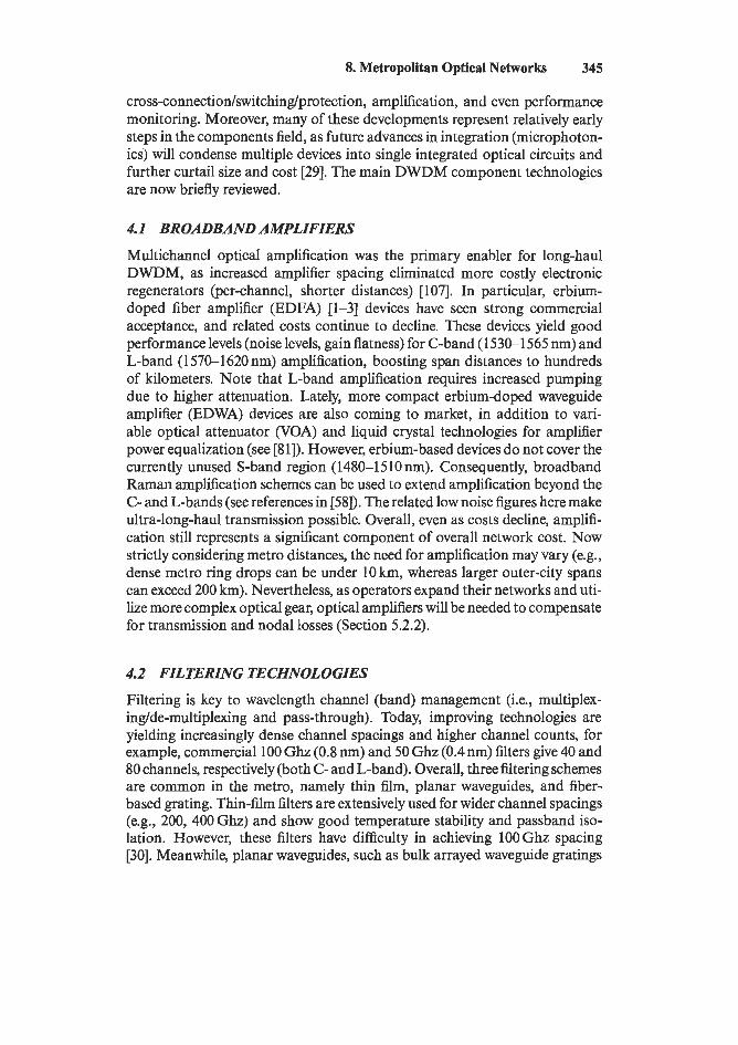
8. Metropolitan Optical Networks 345
cross-connection/switching/protection, amplification, and even performance monitoring. Moreover, many of these developments represent relatively early steps in the components field, as future advances in integration (microphoton- ics) will condense multiple devices into single integrated optical circuits and further curtail size and cost [29]. The main DWDM component technologies are now briefly reviewed.
4.1 BROADBAND AMPLIFIERS
Multichannel optical amplification was the primary enabler for long-haul DWDM, as increased amplifier spacing eliminated more costly electronic regenerators (per-channel, shorter distances) [ 1071. In particular, erbium- doped fiber amplifier (EDFA) [ 1-31 devices have seen strong commercial acceptance, and related costs continue to decline. These devices yield good performance levels (noise levels, gain flatness) for C-band (15361 565 nm) and L-band (1 570-1620 nm) amplification, boosting span distances to hundreds of kilometers. Note that L-band amplification requires increased pumping due to higher attenuation. Lately, more compact erbium-doped waveguide amplifier (EDWA) devices are also coming to market, in addition to vari- able optical attenuator (VOA) and liquid crystal technologies for amplifier power equalization (see [81]). However, erbium-based devices do not cover the currently unused S-band region (1480-1 5 10 nm). Consequently, broadband Raman amplification schemes can be used to extend amplification beyond the C- and L-bands (see references in [%I). The related low noise figures here make ultra-long-haul transmission possible. Overall, even as costs decline, amplifi- cation still represents a significant component of overall network cost. Now strictly considering metro distances, the need for amplification may vary (e.g., dense metro ring drops can be under 10 km, whereas larger outer-city spans can exceed 200 km). Nevertheless, as operators expand their networks and uti- lize more complex optical gear, optical amplifiers will be needed to compensate for transmission and nodal losses (Section 5.2.2).
4.2 FILTERLNG TECHNOLOGIES
Filtering is key to wavelength channel (band) management (Le., multiplex- ing/de-multiplexing and pass-through). Today, improving technologies are yielding increasingly dense channel spacings and higher channel counts, for example, commercial 100 Ghz (0.8 nm) and 50 Ghz (0.4 nm) filters give 40 and 80 channels. respectively (both C- and L-band). Overall, three filtering schemes are common in the metro, namely thin film, planar waveguides, and fiber- based grating. Thin-film filters are extensively used for wider channel spacings (e.g., 200, 400 Ghz) and show good temperature stability and passband iso- lation. However, these filters have difficulty in achieving 100 Ghz spacing [30]. Meanwhile, planar waveguides, such as bulk arrayed waveguide gratings
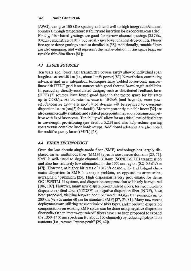
346 Nasir Ghani et al.
(AWG), can give 100-Ghz spacing and lend well to high integratiordchannel counts (although temperature stability and insertion losses concerns can arise). Finally, fiber-based gratings are good for narrow channel spacings (25 Ghz, 0.4 nm demonstrated [30]), but usually give lower channel drop counts Newer free-space dense gratings are also detailed in [58]. Additionally, tunable filters are also emerging, and will represent the next evolution in this space (e.g., see tunable thin-film filters [Sl]).
4.3 LASER SOURCES
Ten years ago, lower laser transmitter powers rarely allowed individual span lengths to exceed 40 km (i.e., about 1 mW power) [SS]. Nevertheless, continuing advances and new integration techniques have yielded lower-cost, narrow- linewidth ITU-T grid laser sources with good thermal/wavelength stabilities. In particular, directly-modulated designs, such as distributed feedback laser (DFB) [3] sources, have found good favor in the metro space for bit rates up to 2.5 G/bs. As bit rates increase to 10 Gb/s (and beyond), more pow- erfullexpensive externally modulated designs will be required to overcome dispersion issues (see [3] for details). More importantly, tunable lasers [32] are also commercially available and related pricepoints may soon become compet- itive with fixed laser costs. Tunability will allow for an added level of flexibility in wavelength provisioning (see Section 5.2.3) and also help reduce sparing costs versus complete laser bank setups. Additional advances are also noted for multifrequency lasers (MFL) [28].
4.4 FIBER TECHNOLOGY
Over the last decade single-mode fiber (SMF) technology has largely dis- placed earlier multimode fiber (MMF) types in most metro domains [25,71]. SMF is well-tuned to single channel 1310-nm (SONETKDH) transmission and also has relatively low attenuation in the 1550 nm region (0.2-0.3 db/km [47]). However, at higher bit rates of 10 Gb/s or more, C- and L-band chro- matic dispersion in SMF is a major problem, as opposed to attenuation, averaging 17ps/km/nm [25]. High dispersion is very problematic for dense OC-192/STM-64 systems, and dispersion compensation will likely be required [ 106, 1071. However, many new dispersion-optimized fibers, termed non-zero dispersion shifted fiber (NZDSF) or negative dispersion fiber (NDF), have been proposed, yielding longer uncompensated IO-Gb/s transmissions up to 200 km (versus under 60 km for standard SMF) [37,53,81]. Many new metro deployments are utilizing these optimized fiber types, and moreover, dispersion compensation on existing SMF spans can be done using negative-dispersion fiber coils. Other “metro-optimized” fibers have also been proposed to expand the 1350-1450 nm spectrum (to about 100 channels) by reducing hydroxil ion contents (i.e., remove “water-peak” [25,42]).
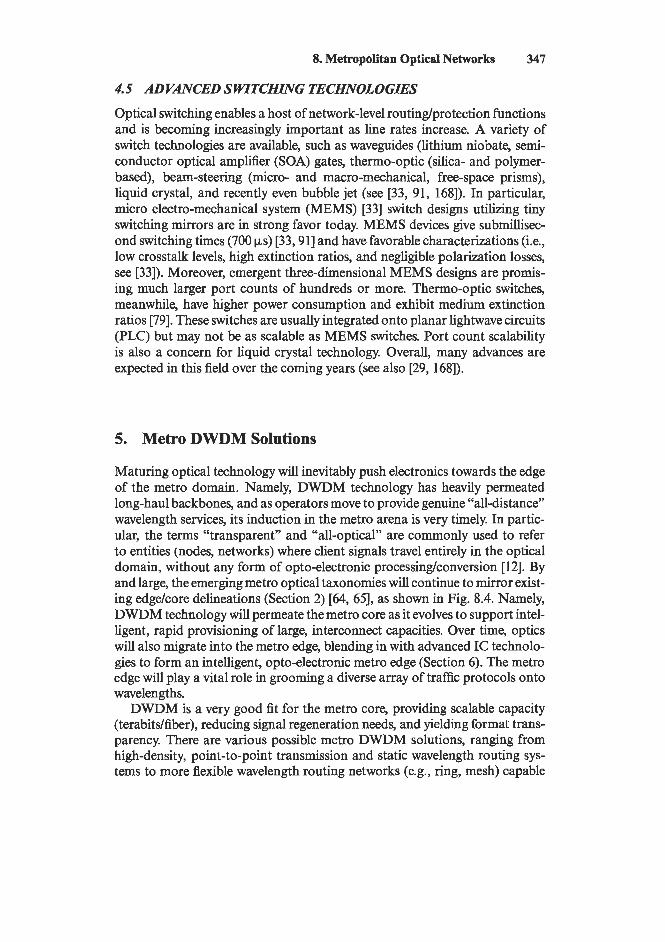
8. Metropolitan Optical Networks 347
4.5 ADVANCED SWITCHING TECHNOLOGIES
Optical switching enables a host of network-level routinglprotection functions and is becoming increasingly important as line rates increase. A variety of switch technologies are available, such as waveguides (lithium niobate, semi- conductor optical amplifier (SOA) gates, thermo-optic (silica- and polymer- based), beam-steering (micro- and macro-mechanical, free-space prisms), liquid crystal, and recently even bubble jet (see [33, 91, 1681). In particular, micro electro-mechanical system (MEMS) [33] switch designs utilizing tiny switching mirrors are in strong favor today. MEMS devices give submillisec- ond switching times (700 ps) [33,91] and have favorable characterizations (ie., low crosstalk levels, high extinction ratios, and negligible polarization losses, see [33]). Moreover, emergent three-dimensional MEMS designs are promis- ing much larger port counts of hundreds or more. Thermo-optic switches, meanwhile, have higher power consumption and exhibit medium extinction ratios [79]. These switches are usually integrated onto planar lightwave circuits (PLC) but may not be as scalable as MEMS switches. Port count scalability is also a concern for liquid crystal technology. Overall, many advances are expected in this field over the coming years (see also [29, 1681).
5. Metro DWDM Solutions
Maturing optical technology will inevitably push electronics towards the edge of the metro domain. Namely, DWDM technology has heavily permeated long-haul backbones, and as operators move to provide genuine “all-distance” wavelength services, its induction in the metro arena is very timely. In partic- ular, the terms “transparent” and “all-optical’’ are commonly used to refer to entities (nodes, networks) where client signals travel entirely in the optical domain, without any form of opto-electronic processinglconversion [ 121. By and large, the emerging metro optical taxonomies will continue to mirror exist- ing edgekore delineations (Section 2) [64, 651, as shown in Fig. 8.4. Namely, DWDM technology will permeate the metro core as it evolves to support intel- ligent, rapid provisioning of large, interconnect capacities. Over time, optics will also migrate into the metro edge, blending in with advanced IC technolo- gies to form an intelligent, opto-electronic metro edge (Section 6). The metro edge will play a vital role in grooming a diverse array of traffic protocols onto wavelengths.
DWDM is a very good fit for the metro core, providing scalable capacity (terabitdfiber), reducing signal regeneration needs, and yielding format trans- parency. There are various possible metro DWDM solutions, ranging from high-density, point-to-point transmission and static wavelength routing sys- tems to more flexible wavelength routing networks (e.g., ring, mesh) capable
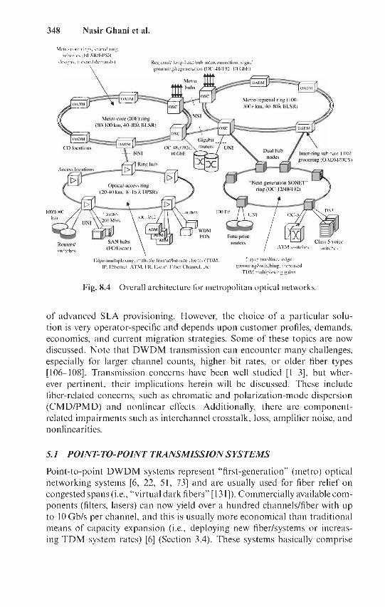
348 Nasir Ghani et al.
Metro core nngs. T h u d nng scheme$ (BLSFUBPSR
decigns meshed demands)
Metro-regional nng (100-
“Next-generation SONET’ nng (oC-12/48/192)
I rnbda loo
Edge-multiplexing, multiple formathit-rate clients (TDM. IP, Ethernet, ATM. FR, Escon, Fiber Channel etc)
Layer twolthree edge graommglswitchmg. increased
TDM multiplexing gams
Fig. 8.4 Overall architecture for metropolitan optical networks.
of advanced SLA provisioning. However, the choice of a particular solu- tion is very operator-specific and depends upon customer profiles, demands, economics, and current migration strategies. Some of these topics are now discussed. Note that DWDM transmission can encounter many challenges, especially for larger channel counts, higher bit rates, or older fiber types [106108]. Transmission concerns have been well studied [l-31, but wher- ever pertinent, their implications herein will be discussed. These include fiber-related concerns, such as chromatic and polarization-mode dispersion (CMD/PMD) and nonlinear effects. Additionally, there are component- related impairments such as interchannel crosstalk, loss, amplifier noise, and nonlinearities.
5.1 POINT-TO-POINT TRANSMISSION SYSTEMS
Point-to-point DWDM systems represent “first-generation” (metro) optical networking systems [6, 22, 51, 731 and are usually used for fiber relief on congested spans (i.e., “virtual dark fibers” [ 13 13). Commercially available com- ponents (filters, lasers) can now yield over a hundred channeldfiber with up to 10 Gb/s per channel, and this is usually more economical than traditional means of capacity expansion (i.e., deploying new fiberhystems or increas- ing TDM system rates) [6] (Section 3.4). These systems basically comprise

8. Metropolitan Optical Networks 349
client interface cards, wavelength transponderheceiver pairs, filter modules, and wavelength mudde-mux devices, as shown in Fig. 8.5. The transponders perform wavelength modulation (from short-reach client interfaces, typically 13 10 nm) for client signals. The corresponding wideband receivers translate received wavelengths, outputting at either 13 10 or 850 nm. Alternatively, newer SONET/SDH devices and even IP routers can be equipped with ITU-T com- pliant lasers (1 550-nm band) and wideband receivers, allowing for “direct” DWDM interfacing. Overall, these elements will allow different protocols to traverse the fiber and can eliminate separate dark fiber requirements for “non- TDM mapped” payloads (e.g., ESCON, Fibre Channel, cable video). Note that Ethernet interfaces (1 .O, 10 Gb/s) may require added receiver-side buffer- ing to handle flow-control features over larger distances, depending upon level of buffering at client gears.
Various setups can be used for the filtering modulehtage in Fig. 8.5. For example, operators who want to modularly expand their channel counts can use channel interleaving and banding filtering techniques. Specifically, band filters add/drop sets of wavelengths, and subsequently, interleavers (with appropriate offsets) and filter cascades achieve closer channel spacings [3 13. The latter is a very appealing solution since wider channel spacing technology is more mature and less costly [30]. Thin-film filters are in wide use today [64], and well-suited for band filtering (Le., dropping channel sets). A sample setup is shown in Fig. 8.6, where two “coarse” (thin-film) 200-Ghz filters are used to generate 100-Ghz spacing. Alternatively, serial add-drop combinations are also possible, albeit these are usually more disruptive (see [89]). For larger drop counts (i.e., more channel density), meanwhile, single high-channel count fil- tering devices are more attractive [89] (e.g., wavelength gratings [80] or AWG
Wavelength laser transponders
Passive splitter ( l+ l protection) or 1x2 switch \ (I:l protection)
Standard short-reach interfaces (I330 nm)
Fiber span (OMS) protection ( l + l , l:l,or 1:Nvariants)
,_____._..........._~~~~~~~....
. I
Wideband receivers
Optional \ filter modules
(banding, interleaving)
Fig. 8.5 Point-to-point DWDM transmission.
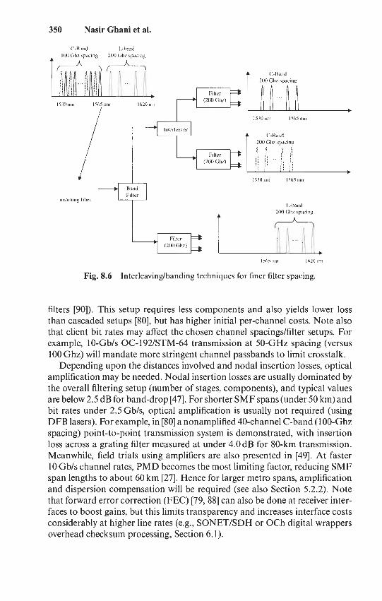
350 Nasir Ghani et al.
C-Band L-hand 100 Ghz spacing 200 Ghz spacing
200 Ghz spacing
I530 nm 1565 nm
I530 nrn 1565 nm
L-hand
1565 nm 1620 nm
Fig. 8.6 Interleavindbanding techniques for finer filter spacing.
filters [90]). This setup requires less components and also yields lower loss than cascaded setups [SO], but has higher initial per-channel costs. Note also that client bit rates may affect the chosen channel spacingdfilter setups. For example, 10-Gb/s OC- 192/STM-64 transmission at 50-GHz spacing (versus 100 Ghz) will mandate more stringent channel passbands to limit crosstalk.
Depending upon the distances involved and nodal insertion losses, optical amplification may be needed. Nodal insertion losses are usually dominated by the overall filtering setup (number of stages, components), and typical values are below 2.5 dB for band-drop [47]. For shorter SMF spans (under 50 km) and bit rates under 2.5 Gb/s, optical amplification is usually not required (using DFB lasers). For example, in [80] a nonamplified 40-channel C-band (100-Ghz spacing) point-to-point transmission system is demonstrated, with insertion loss across a grating filter measured at under 4.0 dB for 80-km transmission. Meanwhile, field trials using amplifiers are also presented in [49]. At faster 10 Gb/s channel rates, PMD becomes the most limiting factor, reducing SMF span lengths to about 60 km [27]. Hence for larger metro spans, amplification and dispersion compensation will be required (see also Section 5.2.2). Note that forward error correction (FEC) [79,88] can also be done at receiver inter- faces to boost gains, but this limits transparency and increases interface costs considerably at higher line rates (e.g., SONETISDH or OCh digital wrappers overhead checksum processing, Section 6.1).
8. Metropolitan Optical Networks 351
Given the large increase in per-fiber traffic, various protection schemes have been proposed for point-to-point transmission systems (see [40,96, loll). Specifically, these include optical multiplex section (i.e., fiber span) or opti- cal channel (OCh) level protection setups. Fiber protection can be done in a dedicated 1 + 1 manner [2, 40, 96, 100, 1011 and requires passive splitters to bridge all wavelengths onto two fibers. This is a simple setup and pre- cludes any (head-to-tail) protection signaling [75], Fig. 8.5. Meanwhile, more complex “nondedicated” 1 : 1 or 1 : N protection schemes are also possible [40], and these are usually more resource efficient (since protection resources can be shared by multiple working fibers or lower priority traffic [96]). Still, 1 : 1/1: N protection requires active switching devices at the sender and fast pro- tection signaling and additional electronics to exploit fiber reuse [103]. Overall, fiber-level protection can reduce the need for electronic (client) protection equipment significantly (e.g., optical fiber protection with 1 : N SONET/SDH (electronic) protection is found to be very efficient [22, 40, loll). This find- ing will likely hold for more advanced optical ring and mesh networks also. Meanwhile, for optical channel protection in point-to-point systems, bridg- inglswitching is most commonly used to provide selective 1 + 1 protection (not shown in Fig. 8.5). Although this is a simple approach, it requires more hard- ware (splitters, switches) and wavelengths than corresponding fiber protection, especially if all demands are to be protected.
5.2 O P T I C . RING NETWORKS Given the success of initial point-to-point DWDM deployments, multihop (wavelength) lightpath [ 1, 21 provisioning is gaining strong favor. Specif- ically, the goal is to maintain large tributary signals within the optical domain as much as possible, thereby exploiting the transparency and cost- per-bit advantages of DWDM. Since ring topologies are ubiquitous within the metro space, multihop DWDM rings will clearly represent a logical pro- gression towards multihop wavelength networks (from simpler point-to-point setups). DWDM rings draw strongly from SONET/SDH concepts, essentially replacing timeslots with wavelengths and performing “optically equivalent” channel operations (i.e., add-drop, pass-through, protection). However, unlike SONET/SDH, these rings offer high-capacity scalability and transparency and permit multiple data rates. In particular, optical bypass eliminates the need for detailed electronic knowledge of, or even access to, client signals [6] and yields significant cost savings over traditional ADM/DCS nodes [3] (e.g., 40% or more in ADM costs [68, 1361). For example, in high bit rate TDM rings, traffic add/drop ratios are typically 25% [89, 1321, yet full electronic multi- plexingldemultiplexing of all (concatenated) tributaries is still required and is very unscalable [92]. Many different DWDM ring architectures have been pro- posed, varying from simpler static setups (i.e., fixed nodes) to more advanced

352 Nasir Ghani et al.
sharing schemes @e., dynamic nodes) [92]. Details are now presented along with considerations for the metro space.
5.2.1 Static Rings
In many cases, metro demands are relatively long standing, with holding times of 3 months or more [56]. Moreover, edge ring networks wiU continue to show very “hubbed” demands, since data traffic exhibits larger communities of interest (Section 3.1 .l) (i.e., communication remains “fixed” between access locations and central outbound gatewayshubs). Carefully note that there is a linear relation between node count and required wavelengths for supporting hubbed traffic patterns in optical rings [3, 541. Given that metro edge rings typically have lower node counts (between two and six [35]) collectively, the above implies that lower-cost static/passive WDM rings [5] with moderate channel counts (e.g., 16-32 wavelengths) are very amenable solutions [62] (i.e., (‘second-generation” optical networks). In particular, optical UPSR schemes, i.e., dedicated protection rings (OCh-DPRINGs) [73,75], are very efficient for hubbed traffic patterns and lend well to static realizations. OCh-DPRINGs use two unidirectional fibers, working and protection, with counterpropagating directions. Channel protection is done using dedicated 1 + 1 setups, requir- ing head-end bridging (via an optical splitter) and receiver-based switching (e.g., based upon received power levels) [132]. Specifically, in case of a link or node failure, receivers switch to bridge traffic along the protection route (see Fig. 8.10). This is a relatively simple, robust architecture and does not require any complex protection-signaling protocols. Moreover, path switching also precludes any (optical) performance monitoring inside the ring, unlike more complex bidirectional designs (Section 5.2.2) (see [73,75] for full details). Now since user routes are essentially predetermined for hubbed demands, channel routing and wavelength assignment (RWA) [l , 21 can be greatly simplified [35]. Specifically, by allocating a unique, fixed set of wavelengths (band) to each node, as per projected demand, wavelength blocking can be avoided (see [56]). Note also that more robust dual-hub rings are also possible [83, 1371. Never- theless, UPSR rings are very inefficient for meshed demands, largely limiting metro core applicability, see Section 5.2.2.
The basic building block of an optical ring is the optical ADM (OADM) node [67]. Generically, a static-ring OADM node is basically a “back-to- back” configuration of point-to-point (DWDM) transmission systems [35, 851 (note that “back-to-back” interconnection has been routinely done in ear- lier SONETISDH and PDH networks [4]). Static OADM nodes use passive optical filters to implement their k e d wavelength relations. A generic overview of a static two-fiber UPSR ring OADM is given in Fig. 8.7, comprising band and mudde-mux filters and optional amplifiers. Here, various passive filter- ing technologies can be used, such as thin-film filters, fiber Bragg gratings, Mach-Zehnder filters, AWG devices, and diffraction gratings (see [SS, 90,921).

8. Metropolitan Optical Networks 353
\ Wideband 9 9 9 I receivers I
Incoming east (working)
I
Outgoing east (protection)
Incoming west (protection)
k
.9..3.;$. transmitters Laser I
Fig. 8.7 Fixed-wavelength OADM node.
Akin to the point-to-point case (Section 5. l), varying filteringhterleaving setups can also be used, depending upon the application desired. This is com- monly termed “right-sizing’’ [35]. For example, given large add/drop ratios, as required in UPSR hub nodes (Fig. 8.8), it is more economical to fully muxlde- mux all channels via a single device [89] (e.g., AWG). Meanwhile, for remote “nonhub” nodes, thin-film band filters (Fig. 8.8) can be much more economi- cal for isolating a required wavelength band, usually under eight wavelengths [35]. Band filtering lowers insertion losses considerably (about 1-2 dB [47]), and thereby significantly improves link budgets. Moreover, this technique also prevents channel passband-narrowing effects [8 11 associated with full- spectrum filters, i.e. , since multihop filter concatenations (spectral function multiplication) induce time-domain signal distortion [88] (e.g., 25% reduction in 3-dB bandwidth for four filters [Sl]). Note also that modular interleav- ing techniques can also be used to selectively increase channel densities (e.g., Fig. 8.6).
In general, static OADM devices do not use advanced optical subsystems, and thus exhibit lower through-loss and design complexities than correspond- ing dynamic OADM or OXC nodes [56]. However, optical transmission impairments can still reduce the shorter distance advantages of metro domains. For example, even though amplifiers may not be required for distances under 80 km, signal attenuation concerns can still arise if the number of ring nodes is sufficiently large. Here, “built-in” amplification uses preamplifiers to com- pensate for transmission losses and postamplifiers to compensate for node
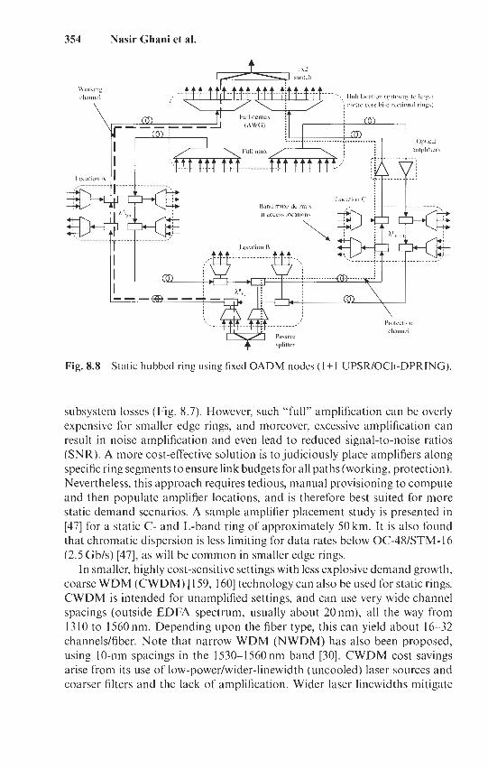
354 Nasir Ghani et al.
J\, 1x2 switch
Working
Band mud de-mux at access locations
Fig. 8.8 Static hubbed ring using fixed OADM nodes (1+1 UPSRIOCh-DPRING).
subsystem losses (Fig. 8.7). However, such “full” amplification can be overly expensive for smaller edge rings, and moreover, excessive amplification can result in noise amplification and even lead to reduced signal-to-noise ratios (SNR). A more cost-effective solution is to judiciously place amplifiers along specific ring segments to ensure link budgets for all paths (working, protection). Nevertheless, this approach requires tedious, manual provisioning to compute and then populate amplifier locations, and is therefore best suited for more static demand scenarios. A sample amplifier placement study is presented in [47] for a static C- and L-band ring of approximately 50 km. It is also found that chromatic dispersion is less limiting for data rates below OC-48/STM- 16 (2.5 Gb/s) [47], as will be common in smaller edge rings.
In smaller, highly cost-sensitive settings with less explosive demand growth, coarse WDM (CWDM) [159, 1601 technology can also be used for static rings. CWDM is intended for unamplified settings, and can use very wide channel spacings (outside EDFA spectrum, usually about 20nm), all the way from 1310 to 1560 nm. Depending upon the fiber type, this can yield about 16-32 channelshber. Note that narrow WDM (NWDM) has also been proposed, using 10-nm spacings in the 1530-1560nm band [30]. CWDM cost savings arise from its use of low-powedwider-linewidth (uncooled) laser sources and coarser filters and the lack of amplification. Wider laser linewidths mitigate

8. Metropolitan Optical Networks 355
(center-wavelength) temperature drift concerns and relax filter stringencies. However, unamplified transmission distances are usually limited to 40 km, and per-channel bit rates are strictly below 2.5 Gb/s. Additionally, it has also been proposed to combine CWDM with (lower) rate-adaptive transceivers to derive some gain from older, higher-loss fiber infrastructures that would other- wise be incapable of supporting high-speed DWDM transmission [159]. This would be particularly appealing in very low-cost settings, giving acceptable capacity improvements without expensive fiber upgrades. Nevertheless, this lower “first-cost” advantage is likely to disappear as EDFA-based DWDM system pricepoints decline [ 1591. Note that lower launch powers and broader wavelength bands require full opto-electronic processing, which is expensive, to map CWDM channels across larger metro core rings (i.e., signal regenera- tion, relaunch on ITU-T lasers). Hence, CWDM is best suited for smaller domains requiring simple point-to-point or static ring configurations, for example, low-cost interconnection of gigabit routers.
Note that from an architectural standpoint, static OADM rings primar- ily expand capacity and provide large tributary bypass functions. As such, they may not be viable as stand-alone metro edge solutions, especially for smaller client tributaries (see Section 5.4). Instead, these static OADM plat- forms are best integrated with various “subwavelength-rate” opto-electronic aggregation solutions to improve wavelength efficiency (e.g., DWDM edge rings, Section 6.1).
5.2.2 Dynamic Rings
Tr&c demands between metro core CO locations are much heavier and more “meshed” as compared to metro edge rings [38, 54, 871, and there- fore the required wavelength counts will be much higher, easily exceeding 50 channels [88]. With increasing customer dynamics, static unidirectional rings (Section 5.2.1) will become very limiting, requiring complex manual wavelength planning and yielding reduced wavelength efficiencies [54]. Here, reconfigurability is a key issue (in addition to scalability), and dynamic OADM rings are very amenable solutions (i.e., “third-generation” optical networks). These architectures use various filtering and switching techniques [56, 921 to implement wavelength programmability (Le., selective channel adddrop). Optical protection is central to OADM rings given the large degree of fibedwavelength multiplexing. Dynamic optical rings are commonly based upon wavelength sharing [73] paradigms, yielding improved wavelength effi- ciencies and more advanced protection definitions (versus static rings). The former is particularly important in metro cores, as the wavelengthhode-count relation grows quadratically for meshed demands [54]. Overall, the market for such gear is expected to grow considerably [67l, as operators look to deploy more cost-effective architectures with broader service offerings. Optical

356 Nasir Ghani et al.
rings can either be opaque (wavelength convertible) or transparent (wave- length inconvertible) [ 151, although various results indicate only modest gains with wavelength conversion (see Section 5.2.3). The latter offers a common “payload-agnostic’’ transport/protection framework, and related standardiza- tion efforts have also emerged [ 15,751. This reduces overlapping functionalities in electronic layers (IP, SONETBDH) essentially “delayering” existing “multi- layered” setups and reducing equipment/maintenance costs [40]. In particular, service survivability can be offered for native “non-TDM mapped” data pro- tocols, such as Ethernet and Fibre Channel, a crucial advantage [47]. Details are now discussed.
Dynamic OADM nodes [67, 851 are the building blocks of a flexible metro core and logical counterparts of dynamic TDM ADM nodes. These elements provide dynamic “on-demand” wavelength add/drop, along with advanced signaling (setup, protection). An overview of a sample dynamic OADM node is presented in Fig. 8.9, comprising incoming/outgoing transport (i.e., mux/de- mux, filters, amplifiers), an add/drop stage, intelligent signaling/control, and optional subrate DCS grooming. Further generalizations are also possible in which a subset of demultiplexed wavelengths are manually provisioned (very cost effective for significant numbers of static connections). There are several ways to implement OADM add-drop stages (Fig. 8.9). In transparent nodes,
Channel setup, maintenance. and protection (APS) signaling
osc Optionalpnd bypass T-----+----------------------------------------l control
I r--lL------------___---------------------- 7 1 I 1
Mux I I Optical I I $’ Channel bypassladd- I 1
Direct wavelength outputs (to wideband receivers)
Direct ITU wavelength inputs (e g , IO GbE)
Recewerltransponder bank (addldrop channels)
Sub-rate m M Sub-rate TDM
Optional DCS stage (integrated or sub-tended)
@-
Fig. 8.9 Sample integrated OADMlDCS node (two-fiber design).

8. Metropolitan Optical Networks 357
static filtering can be coupled with active switching devices (i.e., switch arrays [67, 77, 901 or complete fabrics [85]). For example, MEMS or thermo-optic technologies (Section 4.5) can yield under 5 ms switching times [77]. Because OADM nodes have smaller switch requirements (i.e., two or four fiber ports), MEMS technology provides a very good fit as pricepoints continue to decline. Additionally, Mach-Zender and liquid crystal switches have also been tested [88]. Another means of flexible optical adddrop is via tunable fiber Bragg gratings [56, 57, 851, although this requires a filter per dropped channel [56]. Meanwhile, in opaque OADM designs, dynamic add-drop is done electroni- cally via electronic cross-point switches (EXC) or large DCS fabrics [45, 1321. EXC devices use IC technology, such as gallium arsenide (GaAs) [38j, and commercial offerings with high-port counts can process native bit rate chan- nels up to 3.5 Ghz [26]. Although opaque designs can offer varying levels of regeneration (two, three) and possibly even efficient subrate switching (DCS only), scalability to 10 Gb/s and beyond is difficult. As a cost-effective trade- off, optical and electronic technologies can be coalesced into “hybrid’ OADM designs (with intermediate receivers/transponders) (Fig. 8.9), to exploit the benefits of both domains. These issues are discussed more completely in Section 5.2.3. More generally, both transparent and opaque nodes can fully leverage bandingfinterleaving techniques [89] (Section 5. l), for example, band filters [5q, AWG devices [go], and diffraction gratings [88]. Note that larger metro core channel counts will mandate L-band transmission. As an aside, by appropriately expanded switch-based adddrop stage, local tributary intercon- nection can also be done (e.g., add-tributary/drop-tributary cross-connection, “hair-pinning” [56]).
For amplified all-optical (OADM) nodes, gain equalization is an integral requirement as amplifier behaviors can perturb nonparticipating wavelengths during channel setup/takedown/protection switching [26,93]. With increasing metro customer dynamics (site changes, demand variations), gain flatness must be maintained over wide input dynamic ranges [79]. This is usually done using output amplifier feedback control (Fig. 8.9), and the related settling times will inevitably determine switchingfprotection timescales. Various hardware- based equalization schemes have been demonstrated with good results [55, 79, 88, 931. For example, in a severe condition test (i.e., 32 to 1 channel drop, fibercut) millisecond settling times are achieved, with surge levels under 2 dB. Moreover, subsecond network stabilization times have been claimed [88], and as these techniques improve, they will find increasing favor in dynamic metro cores. As important, dynamic gain equalization will also prove invaluable in simplifying installation procedures, precluding operations staff from complex manual tuningkesting procedures.
Using the above dynamic OADM designs, various dynamic DWDM self- healing ring (SHR) architectures are possible. These solutions draw heavily from SONET/SDH concepts and include both dedicated &e., unidirectional) and more complex shared (i.e., bidirectional) rings [l-3,73,96]. Although the
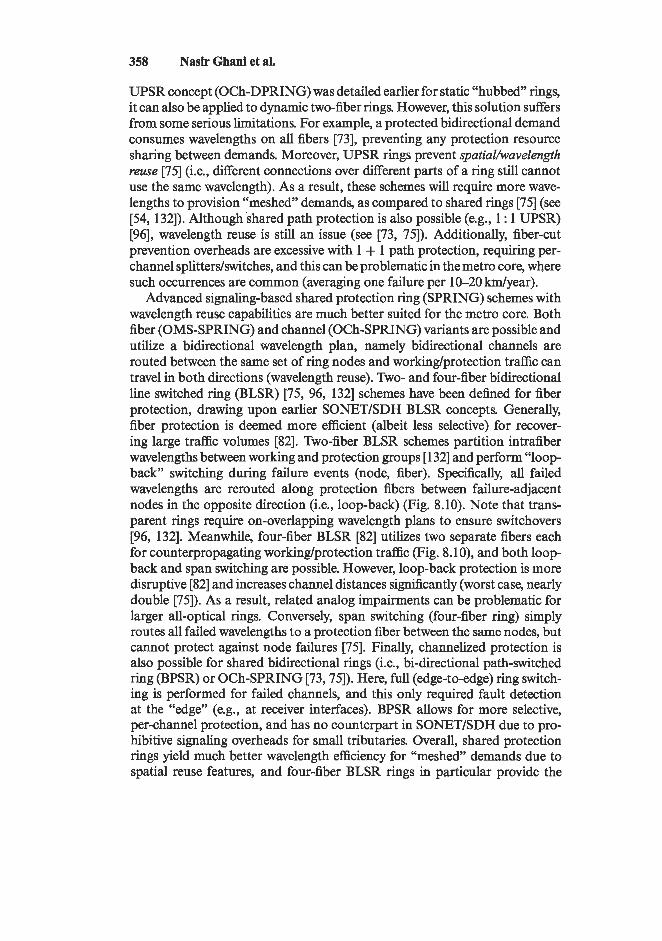
358 Nasir Ghani et al.
UPSR concept (OCh-DPRING) was detailed earlier for static “hubbed)) rings, it can also be applied to dynamic two-fiber rings. However, this solution suffers from some serious limitations. For example, a protected bidirectional demand consumes wavelengths on all fibers [73], preventing any protection resource sharing between demands. Moreover, UPSR rings prevent spatialhavelength reuse [75] (i.e., different connections over different parts of a ring still cannot use the same wavelength). As a result, these schemes will require more wave- lengths to provision “meshed)) demands, as compared to shared rings [75] (see [54, 1321). Although shared path protection is also possible (e.g., 1 : 1 UPSR) [96], wavelength reuse is still an issue (see [73, 751). Additionally, fiber-cut prevention overheads are excessive with 1 + 1 path protection, requiring per- channel splitters/switches, and this can be problematic in the metro core, where such occurrences are common (averaging one failure per 10-20 kndyear).
Advanced signaling-based shared protection ring (SPRING) schemes with wavelength reuse capabilities are much better suited for the metro core. Both fiber (OMS-SPRING) and channel (OCh-SPRING) variants are possible and utilize a bidirectional wavelength plan, namely bidirectional channels are routed between the same set of ring nodes and workinglprotection traffic can travel in both directions (wavelength reuse). Two- and four-fiber bidirectional line switched ring (BLSR) [75, 96, 1321 schemes have been defined for fiber protection, drawing upon earlier SONETISDH BLSR concepts. Generally, fiber protection is deemed more efficient (albeit less selective) for recover- ing large traffic volumes [82]. Two-fiber BLSR schemes partition intrafiber wavelengths between working and protection groups [ 1321 and perform “loop- back” switching during failure events (node, fiber). Specifically, all failed wavelengths are rerouted along protection fibers between failure-adjacent nodes in the opposite direction (i.e., loop-back) (Fig. 8.10). Note that trans- parent rings require on-overlapping wavelength plans to ensure switchovers [96, 1321. Meanwhile, four-fiber BLSR [82] utilizes two separate fibers each for counterpropagating workinglprotection traiEc (Fig. 8. lo), and both loop- back and span switching are possible. However, loop-back protection is more disruptive [82] and increases channel distances significantly (worst case, nearly double [75]). As a result, related analog impairments can be problematic for larger all-optical rings. Conversely, span switching (four-fiber ring) simply routes all failed wavelengths to a protection fiber between the same nodes, but cannot protect against node failures [75]. Finally, channelized protection is also possible for shared bidirectional rings (i.e., bi-directional path-switched ring (BPSR) or OCh-SPRING [73,75]). Here, full (edge-to-edge) ring switch- ing is performed for failed channels, and this only required fault detection at the “edge” (e.g., at receiver interfaces). BPSR allows for more selective, per-channel protection, and has no counterpart in SONETISDH due to pro- hibitive signaling overheads for small tributaries. Overall, shared protection rings yield much better wavelength efficiency for ccmeshed” demands due to spatial reuse features, and four-fiber BLSR rings in particular provide the
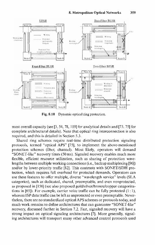
8. Metropolitan Optical Networks 359
WorXing wavelengths
Two-Fiber BLSR
Faher
Four-Fiber BLSR Two-Fiber BPSR
............ pTotefeCll0” span
. . . . . . FTotcet,on
Protection fibers (Inner)
Working wavelengths
Fihcr
Fig. 8.10 Dynamic optical ring protection.
most overall capacity (see [3, 54, 78, 1191 for analytical details and [73, 751 for complete architectural details). Note that optical ring interconnection is also required, and this is detailed in Section 5.3.
Shared ring schemes require real-time distributed protection signaling protocols, termed “optical APS” [75], to implement the above-mentioned protection schemes (fiber, channel). Most likely, operators will demand “SONET-like” recovery times (50 ms). Signaled recovery enables much more flexible, efficient resource utilization, such as sharing of protection wave- lengths between multiple working connections (Le., backup multiplexing [96]) and/or by lower-priority traffic [82]. This contrasts with SONET/SDH pro- tection, which requires full overhead for protected demands. Operators can use these features to offer multiple, diverse “wavelength service” levels (SLA categories), such as dedicated, shared, preemptable, and even nonprotected, as proposed in [ 1561 (see also proposed gold/silver/bronze/copper categoriza- tions in [65]). For example, carrier voice traffic can be fully protected (1 : l), whereas ISP data traffic can be left as unprotected or even preemptable. Never- theless, there are no standardized optical APS schemes or protocols today, and much work remains to define architectures that can guarantee “SONET-like” recovery, discussed further in Section 7.2. Fast, signaled recovery will have a strong impact on optical signaling architectures [7]. More generally, signal- ing architectures will transport many other advanced control protocols used
360 Nasir Ghani et al.
in dynamic ring provisioning (e.g., resource/topology autodiscovery, channel setup/maintenance, management, see Section 7). Here, two related architeo tures are possible, namely inband and outband control [3, 7, 161. The former is used in opaque OADM rings, where control information is carried on data wavelengths via designated overhead bytes in “opaque” framing formats, for example, SONET/SDH [9] or OCh (digital wrappers) framing [12, 13, 1451. Both of these framing formats reserve specialized bytes for APS switching, ensuring protection signaling bandwidth. Meanwhile, transparent networks more clearly decouple control/data planes using outband [2, 71 control. The most common approach here is via an optical supervisory channel (OSC) [2,7] on the 1510-nm wavelength, and this requires per-fiber filters, receivers, and lasers (Fig. 8.9). Note that typical OSC filters can add roughly 1.5 dB loss and this needs to be incorporated in the network design. Clearly, outband OSC control standards are strong prerequisites for interoperable all-optical rings (see early discussions in [16, 1451).
Dynamic optical rings pose many practical engineering concerns, as high- lighted by various studies [38, 49, 50, 51, 54-57, 77-79, 82, 85-89]. In [56], two dynamic OADM designs with differing add-drop stages are compared, one using tunable fiber Bragg grating cascades and the other using an AWG demux and 2 x 2 switch arrays. The latter technique requires more switches and internal fibers and yields higher crosstalk. However, both adddrop stages yield roughly equal add/drop attenuation (2-3.5 dB). In [77], a four-fiber “bridge- and-switch” (1 : 1 shared) path-protection OADM design using 32-channel Gband AWG filters and 2 x 2 mechanical switch arrays is presented. Measure- ments for varying “intra-OADM” working/protection paths indicate insertion loss fluctuations between 2-6 dB, stressing the need for dynamic gain equal- ization. In an all-optical node cascade test (transmission span losses of 10 dB, about 40 km), results through six nodes show average losses of 11.5dB and good BER performance for up to 5-Gb/s transmissions (positive simulation results for large OADM cascades are also reported in [3]). Meanwhile, lO-Gb/s transmission is found to suffer from PMD effects and temperature control issues with the AWG filters therein. Because C-band dispersion will limit such transmission to under about 60 km on SMF [27] (and intraband disper- sion can vary), electronic regeneration (of TDM payloads only) andor DCF modules will be required. Here, detailed analyses are required for optimiz- ing distributed DCF placement in optical rings (e.g., demand, channel routes, etc.), and increased laser powers may also be of concern (i.e., nonlinearities [ 1061). Note that advanced MEMS-based dispersion compensation techniques are also being studied [26]. Additionally, [79] demonstrates a 32-channel L-band UPSR (1 + 1 protection) OADM node with dynamic gain control using (PLC-integrated) thermo-optic 2 x 2 switch arrays. System performance was verified for lO-Gb/s transmission over 240 km of DCF through two nodes (dis- tances with SMF would likely be less). In-band FEC is also performed at the receiver interface (via modified SDH frame format), providing about 2-3 dB

8. Metropolitan Optical Networks 361
improvement. Finally, a four-fiber BLSR ring with protection fiber reuse via low priority traffic is also demonstrated in [82], yielding under 50 ms recovery. Overall, larger metro networks will require careful planning and analyses to ensure user performance levels (see other studies in [49, 57,87,92]).
Because many SONET/SDH tributariedrings will be carried over wave- lengths (e.g., stacked SONET rings, “path-in-lambda” [39]), protection inter- working is a big concern as timescales can easily overlap. Particularly, signaled BLSR schemes can exhibit cascaded APS behaviors [98] between the two layers, prolonging recovery intervals well beyond 50 ms. For example, 8 1.2-ms DS3 recovery times are measured in [lo41 for a stacked TDMDWDM BLSR ring, where the SONET/SDH layer attempts both span and ring switches. These values violate the SONET/SDH 50-ms bound, but may still be acceptable for data services. Meanwhile, nonsignaled 1 + 1 UPSR (OCh-DPRING) recovery is usually much faster than BLSR (5 ms or less), and may limit APS cascading behaviors. Overall, coordinating interlayer recovery falls under the broader topic of multilayer (protocol) escalation strategies [loo] (see Section 7.2). As far as SONET/SDH is concerned, the simplest practical solution may be an “all or nothing” approach [SI, where protection on one layer is disabled, for example, [ 1041 proposes SONET/SDH carriage on unprotected wavelengths (or bands).
5.2.3 Transparency Considerations
There has been much debate on the pros and cons of optical transparency. Opaque networks perform per-hop opto-electronic conversions and map all client signals to standardized frame formats, for example, SONET/SDH or OCh digital wrappers [12]. Although this precludes full transparency, frame mappings allow for per-hop signal regeneration and detailed performance monitoringlfault isolation [ 12, 1051. This largely mitigates analog impairment concerns (e.g., loss, dispersion, crosstalk) for most metro networks with spans under 100 km. Additionally, opaque networks allow for wavelength conver- sion [l-3, 1151 to reduce call-blocking rates. Although many findings indicate that wavelength conversion yields good blocking probability improvements in mesh topologies (10-30%), it is not as effective in rings, as connectivity is limited (yielding high load correlation on subsequent links) [113, 114, 116, 117, 122-1261. More interestingly, judicious placement of ring wavelength conversion shows very good blocking performances (i.e., relatively close to full wavelength-conversion). For example, results in [116] indicate a signifi- cant reduction in the ratio of averaged blocking rates for longer-path versus shorter-path connections for larger multiring networks (1 3 nodes) where only 10-20% of the nodes can perform full wavelength conversion (see also [117]). Blocking reduction in smaller rings is less dramatic, and moreover, wavelength conversion at ring boundaries (Le., via OXC/DCS nodes, Section 5.3) yields almost the full benefits of wavelength conversion [116, 117, 1241. In other
362 Nasir Ghani et al.
studies, increased wavelengths are found to be more effective than wavelength converters [ 122, 1261, particularly for increased traffic peakedness (peawmean ratios) [122]. As an aside, note that all-optical wavelength conversion (and regeneration) techniques may become available soon, for example, four-wave mixing and cross-modulation [120, 121, 124, 1271. Most likely, these offerings will not perform full range conversion (i.e., wavelength dependence between inputloutput). Regardless, architectural studies are still very promising, indi- cating that a relatively small degree of dependent wavelength conversion (25% of full range) can yield ring blocking close to that of full range conversion [ 121 , 1241 (similar to partial wavelength conversion). It is important to note that the findings are affected by ring channel RWA algorithms, discussed subsequently.
Apart from limited wavelength conversion gains, opaque OADM rings present many other limitations. Clearly, footprints will be much larger and power consumption higher, as transpondersh-eceivers (and related electronic control hardware) are required for all fiber wavelengths [53, 541. Likely, transponder costs alone will be excessive for metro systems with large channel counts and bit rates over 10 Gb/s [88]. Furthermore, laser transponders present added reliability concerns and require sparing (further cost and complexity). Another huge limitation is that multirate wavelengths are difficult to provision, as payloads must be mapped onto a common TDM framing formatdrates, usu- ally OC-48/STM-16. As in legacy SONETEDH networks, such mappings will inhibit transparency and complicate support for various data protocols (see Section 3.4). With increasing channel rateddemands, opaque OADM nodes will require complete laser bank upgrades, which are very restrictive to future growth. The actual wavelength tributary processing, meanwhile, will require complex DCS switching fabrics that must scale to handle large wavelength channel counts, for example, thousands of DS3 or STM-1 ports [3], further increasing costs. Overall, suchfuZZ opto-electronic regeneration is more crucial in long-haul networks, where attenuation concerns are much more severe.
In transparent networks, meanwhile, performance monitoring is a crucial concern, as standards and (to an extent) advanced features are lacking. Optical monitoring solutions use nonintrusive monitoring techniques to analyze such parameters as fibedwavelength power and optical signal-to-noise ratios (0- SNR), and other factors such as Q-factors are being studied [94, 1051. Power monitoring, however, can only detect hard failures (node faults, fiber cuts) and not degenerative system faultskonditions, such as increased BER [91]. Moreover, costlpackaging restrictions still prohibit dedicated power monitor- ing for larger wavelength counts. As such, optical monitoring will suffice for BLSR-type schemes, and optical path-level protection (BPSR, UPSR) can use end-point (optical or electronic) detection [75]. Nevertheless, emerging advances in packaging techniques [29] and integrated monitoring capabilities will likely mitigate these concerns in the future (e.g., MEMS photodetectors [33], power detector arrays, 0-SNR [SO]). Moving forward, it is expected that there will be a reduced need for “complete” bit-level information at all nodal
8. Metropolitan Optical Networks 363
locations, akin to the trend of optical amplifiers usurping digital regenerators. Overall, optical monitoring will find good applicability in metro cores, where there is a premium on transparency.
All-optical rings use intelligent RWA algorithms [l-3,7] to determine chan- nel routedwavelength assignments. Ideally, if demands are known a priori, static (offline) RWA can optimize routes, and some algorithms are shown to largely mitigate the need for any wavelength conversion (i.e., 0.25% wavelength gain [114]). Note also that a priori demand knowledge can be used for virtual topology [l] design before the actual RWA phase (see [A). Nevertheless, real- istically, metro connection arrivalddepartures will occur in succession over many timescales, requiring dynamic (online) [2] RWA algorithms. Here, exist- ing connections most likely cannot be disrupted (i.e., rerouted, preempted) to improve wavelength utilizations (even though various virtual topology “migra- tionhuning” algorithms have been studied for slowly/periodically readjusting circuit assignments, see [l, 1361 for details). Dynamic RWA is usually done in two steps, namely route resolution and wavelength selection, and various algo- rithms have been proposed for each, for example, shortestllongestneast-loaded path selection, and randodfirst-availablefleast-used wavelength selection, etc. (see [113, 122, 1281 for details). Note that wavelength selection is not an issue in opaque rings, and simpler SONET/SDH ring algorithms can be used [ 114, 1221. Overall results for dynamic all-optical ring RWA are good, for example, [114] shows 90% of utilization of static “a priori” RWA and only 5% below full wavelength conversion RWA (see also [113]). Theoretical details of opti- cal ring RWA are also considered in [119, 1231. Dynamic RWA algorithms will require ring resource information (e.g., wavelength usages/values, con- nection maps, etc.), and emerging standards are addressing these concerns (Section 7.1). Note that transponder sources must be “matched” to assigned wavelengths, and new tunable laserdater designs can be very advantageous here, precluding manual line-card changes.
However, transparency poses further routing implications in larger metro networks, as impairment concerns can arise [106,108]. A simple solution here may be to enforce geographic bounds on channels, such as distances or hop- counts (e.g., enforced homogeneity [ 1061). However, as operators progressively expand their networks or provision higher bit rates (1 0 Gb/s or more), this is not feasible. Now, most RWA algorithms strictly focus on “logical” resource control (e.g., wavelengths, converters, channel delays, etc.) and assume perfect analog conditioning (e.g., flat amplifier gains, no losskrosstalkldispersion). Consequently, such “idealized” algorithms accept more calls (i.e., yield lower blocking probabilities) than may be practically possible for a given channel BER threshold [108]. For example, consider amplifier saturation, where sim- ulation results for nine nodes indicate that heavier meshed demands reduce span lengths by 30% over lighter hubbed traffic [54], even if wavelengths are available. Consequently, physical layer concerns may have to be incorporated into the RWA phase [106, 108-1101. In a sample proposal, [110] presents a
364 Nasir Ghani et al.
two-phase logical/physical RWA scheme that incorporates transmission loss, crosstalk, and amplifier saturation (see additional work in [108, 1091 also). In another solution, translucent routing (Le., partial wavelength conversion) is considered, where signals are transmitted optically “as far as possible” before signal degradation mandates opto-electronic regeneration [ 1 181. This is especially appealing in the metro space, as transparency is very important. Specifically, a translucent routing algorithm (modeling componentlfiber loss and crosstalk) is presented and results for a metro-sized multiring indicate good gains for larger crosstalk values (see [l 181). Overall, the computed complexities of such advanced “optical-layer” routing algorithms are sigdcant, making them more suited for centralized control architectures [lo61 (Section 7.1). Note that translucent routing requires subtending opto-electronic stages, and DCS fabrics can be used here (i.e., “hybrid” OADM, Fig. 8.9).
Carefully note that using DCS switching fabrics for wavelength conver- sion/translucent routing also offers another key benefit, namely edge subrate TDM grooming [48, 651 between metro core and access rings. Namely, bun- dled subrate TDM tributaries (DS3,0C-3/12) emanating from different access rings can be unbundled and rearranged onto larger core wavelengths to improve efficiency. Such subrate grooming has also been studied more broadly under the SONETLDWDM circuit-wavelength grooming (e.g., “stacked” SONET rings) [68, 1361. Specifically, studies have focused on demand group- ing and lightpath routing to minimizing network-wide electronic ADM/DCS costs for a given OADM design (i.e., exploit optical bypassing). For example, [ 1391 derives bounds and presents results for various intelligent grooming (cir- cle construction) algorithms for uniform and nonuniform traflic. Simulations indicate significant ADM cost savings in both uni- and bidirectional dynamic rings (from 30 to 60%). Detailed discussions and analytical bounds for arbi- trary traffic patterns are also presented in [140] (Le., primitive ring grooming). Additionally, [137, 1381 also study various OADM-DCS ring combinations for static OADM designs, for example, point-to-point, single/dual-hub con- figurations. Again, cross-connection is found to lower overall network-wide ADM costs for dynamic demand conditions. This is an important area, and related findings can be exploited to help appropriately size subtending DCS stages on dynamic OADM rings, such as dropped wavelength counts, DCS port counts/types, etc.
5.3 OPTICAL HY3MDMESHNETWORg;S
Metro topologies are rarely homogenous and usually comprise a meshed inter- connection of many IOF rings, up to 20 in larger areas [143] (commonly termed hybrid topologies [75,76]). Now, due to larger communities of interest, user demands must be routed/protected between multiple rings, requiring ring gateway interconnection [43, 541. Alternatively, in the future, operators may choose to move to mesh routing paradigms (either “greenfield” builds or via

8. Metropolitan Optical Networks 365
selective ring fiberplant expansions) in order to improve resource efficiencies further. In these hybrid/mesh networks, optical cross-connect switch (OXC) nodes will be the central elements, handling increased spatial (fiber) connec- tivities and serving in an advanced generalization of the role performed by SONET/SDH DCS nodes. Overall, “mesh” optical switching has emerged from the long-haul space [6, 91-93], and first-generation switch designs used electronic DCS switching fabrics [58,91, 1321 (Le., electronic wavelength cross- connects [2]). Specifically, a DCS fabric functioned as a bandwidth manager [48], performing subwavelength grooming/aggregation and full signal regener- ation for long spans [93]. However, akin to OADM evolutions (Section 5.2.3), associated opto-electronic fabric costs proved prohibitive for large-tributary switching, and hence optical switching technologies (Section 4.5) gained favor. Nevertheless, since multiple, diverse add-drop systems can converge at large metro switching interchange locations, extensive bandwidth manage- ment capabilities will still be required, ranging from subrate TDM streams to large-granularity optical wavelengths. Consequently, integrated OXC/DCS nodes [46, 64, 91, 1681 are most germane here (Fig. 8.11), comprising both optical and electronic switching cores. In these “hybrid” designs, optical switching of larger tributaries will significantly reduce required DCS fabric
(adddrop channels) filtenng
Sub-rate TDM Sub-rate TDM
Electmnic DCS grwmmg. channel adddrop stage
Fig. 8.11 Integrated OXC/DCS node.

366 Nasir Ghani et al.
sizes, yet DCS fabrics will still permit subrate terminatiodgrooming andlor interdomain regeneratiordmanagement functions.
OXC cores can use a variety of switching technologies (Section 4.5), although MEMS is most common today [33]. Currently, 16 x 16 two- dimensional MEMS modules have been demonstrated [33] and are com- mercially available, whereas a practical limit of 32 x 32 is stated in [26]. Nevertheless, future metro switch fabric requirements will clearly increase further, driven by denser channel counts and larger multiring interconnec- tions. For example, port counts are proportional to the square of wavelength channels for multiring interconnection [58]. Therefore, switch fabric expan- siodscalability is a major issue [91]. One solution here is to use multistage interconnection [34] of multiple smaller switches, for example, Clos architec- tures [3, 91, 1681. Here, nonblocking configurations are highly desirable, as transparent networks already suffer from wavelength blocking. However, com- plex multistage connections increase insertion loss/crosstalk between stages, and ideally a large single stage is most desirable [3,91]. Although dense three- dimensional MEMS switches are being studied [33] (256 x 256 and beyond), cost concerns will likely preclude metro application for the next several years. Consequently, a more immediate and scalable solution is to use band filters (Section 5.2.1) to perform coarser wavelength band switching [46]. This reduces port count requirements significantly, as a single MEMS port can switch a whole band, even fiber. Note, however, that band switching has various higher-layer provisioning implications, and therefore is best applied to traflic with similar characteristics, for example, routes, application types, protection levels, etc. [93]. Apart from switching, note that many considerations for the transport stage (filtering, amplification) are also similar to those for dynamic OADM nodes.
Ring tributary interconnection will likely be the fist application of inte- grated OXC/DCS designs [ 1 131. Now in many cases, multivendor rings using differing optical gear will interface via standardized interfaces (e.g., OC-48/192 at 13 10 nm) at administrative boundaries. Most likely, bit-level monitoring will be necessary at these interchange points in order to monitor cross- connecting signals (e.g., security concerns, SLA BER monitoring, etc.) [105]. Moreover, operators will want cleaner interdomain hand-offs, fully regener- atinghormalizing incoming wavelength tributaries before transmission across their own networks. For example, long-haul networks use standardized pay- loads (SONET/SDH, OCh digital wrappers) and require relaunching via more powerful lasers. Hence for the foreseeable future, ring interconneo tion will be done opto-electronically via DCS devicedfabrics (Fig. 8.1 l), even for larger tributaries. Moving forward, however, optical ring interconnection via OXC switches will also become important, especially in single-operator domains [56]. Such “clear-channel” interconnection [58] can extend the reach of “non-SONET/SDH mapped” services (not possible with DCS interconnec- tion). Although no standards currently exist for optical ring interconnection,
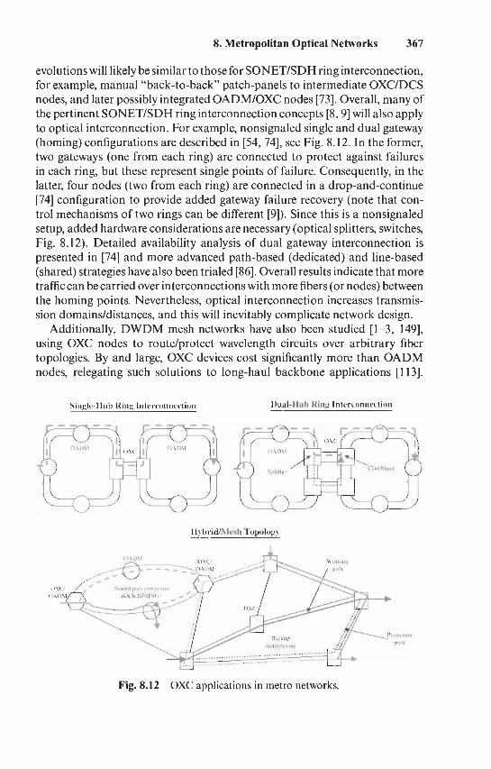
8. Metropolitan Optical Networks 367
evolutions will likely be similar to those for SONET/SDH ring interconnection, for example, manual "back-to-back'' patch-panels to intermediate OXC/DCS nodes, and later possibly integrated OADM/OXC nodes [73]. Overall, many of the pertinent SONET/SDH ring interconnection concepts [8,9] will also apply to optical interconnection. For example, nonsignaled single and dual gateway (homing) configurations are described in [54,74], see Fig. 8.12. In the former, two gateways (one from each ring) are connected to protect against failures in each ring, but these represent single points of failure. Consequently, in the latter, four nodes (two from each ring) are connected in a drop-and-continue [74] configuration to provide added gateway failure recovery (note that con- trol mechanisms of two rings can be different [9]). Since this is a nonsignaled setup, added hardware considerations are necessary (optical splitters, switches, Fig. 8.12). Detailed availability analysis of dual gateway interconnection is presented in [74] and more advanced path-based (dedicated) and line-based (shared) strategies have also been trialed [86]. Overall results indicate that more traffic can be carried over interconnections with more fibers (or nodes) between the homing points. Nevertheless, optical interconnection increases transmis- sion domains/distances, and this will inevitably complicate network design.
Additionally, DWDM mesh networks have also been studied [l-3, 1491, using OXC nodes to route/protect wavelength circuits over arbitrary fiber topologies. By and large, OXC devices cost significantly more than OADM nodes, relegating such solutions to long-haul backbone applications [ 1 131.
Single-Hub Ring Interconnection Dual-Hub Ring Interconnection
HvbridMesh Touologv
Fig. 8.12 OXC applications in metro networks.
368 Nasir Ghani et al.
Nevertheless, as costs decline and metro operators expand their fiber plants, mesh or hybrid (ring-mesh) topologies (Fig. 8.12) will gain importance. Many theoretical results indicate that mesh topologies are usually more wavelength efficient than rings (assuming larger connectivities) (i.e., rings need more wavelengths to route a given demand set, see [113, 1321). A whole range of mesh RWA algorithms have been developed, including online/offline and/or distributed/centralized computation schemes, see [128] for a survey. Many mesh survivability mechanisms have also been tabled, broadly classified as restoration and protection schemes [7, 961. The former refers to more active, postfault signaled recovery (usually path level), whereas the latter refers to pre- designed protection (link or path level) [7, 1131. Restoration schemes are very wavelengthkber efficient, but protection schemes are by far the most studied, and many variations are possible, for example, nonsignaled and signaled ded- icated/shared schemes, etc. [7, 95-97, 155, 1561. Although further details are beyond the scope herein, results show that shared protection over increased mesh connectivity can yield significant capacity/efficiency improvements (see references in [96,97]). A more ominous concern with DWDM mesh protection (and restoration) is recovery timescales, as topologies can be arbitrary. Typical values are larger than those for ring protection (i.e., hundreds of milliseconds [48, 96, 97,991). Nevertheless, these values are very adequate for many Inter- net data services [159], and overall, mesh networks can offer very rich service definition capabilities (similar to those mentioned for advanced bidirectional rings, Section 5.2.2). As an aside, given these larger recovery timescales, slower optical sampling and/or spectrum scanning techniques [93, 1051 can be con- sidered for monitoring/fault localization. Meanwhile, standardized control architectures are also emerging for optical mesh networks, and detailed pro- tection protocols have been tabled (Section 7). Overall, transparent DWDM mesh routing will face many of the same challenges as dynamic OADM nodes (i.e., attenuation/dispersion, performance monitoring).
As per previous discussions, rings present ubiquitous, fast protection mech- anisms to which operators are very well-accustomed [76]. Consequently, many operators may still want to provision rings over expanded hybrid (mesh ring) topologies (see also migration issues, Section 5.5). In particular “virtual ring” emulation may become a key requirement, allowing operators to define arbi- trary ring topologies on top of mesh plants, traversing a mix of OADM and OXC nodes. Over time, these requirements will likely blur the lines between OXC and OADM designs, as integrated OADM/OXC/DCS nodes (Fig. 8.12) collapse mesh routing and UPSR/BLSR ring protocol functions onto a com- mon platform [85]. Various techniques have been studied to resolve ring overlays onto mesh topologies, termed ring covers [3], and [73,97,113] present surveys. For example, rings can be grouped via “communities of interest” to minimize interring traffic. Alternatively, rings can also be defined to help “localizey~ recovery domains, ensuring that network faults do not disrupt t r a c in other parts of a larger hybrid network [97]. In [84], the ring-covers problem
8. Metropolitan Optical Networks 369
is solved using an optimization formulation to resolve “optimal” ring sets and ensuing connection routes (hierarchical, nonhierarchical rings). Meanwhile, [97l presents a simulated annealing solution. Some early standardization dis- cussions on ring-mesh interworking have also appeared, for example, ring identifier extensions to mesh routing protocols [76].
5.4 ECONOMIC CONSIDERATIONS: TDM VS. D WDM
Several years ago, DWDM technology was largely considered as a long- haul solution, as optical amplifiers provided better economics over new fiber builds (and opto-electronic regenerators). At the time, the viability of metro DWDM was questionable, since related subsystem costs could not justify applications over smaller unamplified distances. For example, in [71], for very modest demand growth (1 2 STS- 1 circuits/year), OC- 192 TDM yielded better economics than DWDM (at OC-48 rates). Similar results were pre- sented in [41, 511. Nevertheless, recent studies are indicating a reversal of this trend, especially for bit rates over OC-IUSTM-4. Most current studies com- pare DWDM node (and possibly amplifier) costs against higher-rate TDM systems with increased fiber counts, commonly termed as space division mul- tiplexing (SDM) [49]. For example, in [54], metro core dimensioning shows good cost reduction using DWDM for larger STM-16/64 tributaries (3549%). Smaller access networks, however, give a much closer tradeoff, with DWDM approaching cost parity for more aggressive demand scenarios (see studies in [51] also). Meanwhile, results for point-to-point spans [49] find DWDM more economical than OC-192 for capacity expansion up to eight OC-48 channels (assuming no amplification). Most likely, it will also be more cost effective to transport OC-192 signals via DWDM than SONETISDH (e.g., no per-hop complexity) [3]. Additionally, in a comprehensive study [40], three different metro (two-fiber ring) network scenarios show over 20% cost savings in capacity exhaust scenarios for both moderate and aggressive demands. Fur- thermore, findings for direct OC-12 tributary transport indicate near parity in cost between SONET OC-48, OC-192, and 24-wavelength systems [40]. The authors even hint at direct OC-3 cost parity in the future as costs decline. In general, market research also confirms overall DWDM cost effectiveness for bit rates over OC-lUSTM-4 [62,65]. Other discussions are presented in [3,5 11.
Overall, many of these techno-economic analyses are very encouraging, especially as DWDM component prices continue to decline. Moreover, in the studies, cost modeling was largely done for equipment/infrastructure. Many crucial operator-related benefits of DWDM systems are more difficult to incor- porate, whose inclusion, nonetheless, would further enhance the DWDM value proposition. These include rapid provisioning, advanced service defini- tions, transparent routing/protection of “non-TDM mapped” payloads, and likely reduced operations costs (e.g., power consumption, floorspace). For example, cost studies for rapid provisioning in regionalllong-haul networks

370 Nasir Ghani et al.
show significant revenue potential over slower legacy provisioning [72]. As the TDM-DWDM metro debate abates, -the two technologies are now seen as more complementary, with focus shifting on when to deploy and achieving the right mix between the two for transition purposes (e.g., TDM edge multiplex- inglswitching, see Section 6) [22, 641. Generally speaking, transport-related functionalities will migrate to the optical layer, and SONET/SDH will serve as an aggregation/framing (sub)layer [6] closer to the edge.
5.5 MIGRATIONSTRATEGIES
Despite the many advantages of DWDM technology in the metro core, it is unrealistic to expect immediate, full-scale deployments. Instead, a more grad- ual, cost-effective migration is likely, as operators pair added expenditures with expanded revenue growth. Moreover, many metro operators have invested (and continue to invest) heavily in SONETISDH technology [46,63,142] and may be unwilling to undertake further expenditures without realizing signifi- cant returns thereof. Additionally, DWDM represents a new technology, and most operators will first want to gain valuable field/market experience with smaller-scale deployments. Most operators will look for strategies that offer low “firstcost” and economical lifecycle costs [22]. In particular, a migration path that reuses existing fiber infrastructures/equipment will help improve ini- tial costs significantly. Overall, it is expected that metro DWDM will evolve from less costly point-to-poindring deployments to more advanced dynamic rindmesh (hybrid) optical networking solutions offering wavelength services [22,49, 50,731, as shown in Fig. 8.13.
For most incumbent metro operators, fiber-reliefkapacity expansion is the first likely application of DWDM technology. In cases where there is still available conduit space, it is usually more economical to simply pull more fiber through [22]. However, in many largeddenser cities, conduit space may be lacking and laying new fiber can be expensive and very time consuming (involv- ing lengthy right-of-way concerns). Moreover, such spatial expansion may not meet projected demand increases, and DWDM offers the best price/bandwidth return. In fact, initial linear point-to-point fiber-relief deployments are well underway in the metro, see [22, 37, 49, 501 for deployment details. DWDM- enabled spans offer a large number of “clear-channels” (is., 32 wavelengths and beyond), with which operators can easily address immediate capacity concerns and further expand “non-TDM” client services (e.g., Fiber Channel, Escon, etc.). Note here that band-filteringhterleaving techniques (Section 5.1) will also permit modularly wavelength expansion, helping to lower initial costs.
In order to minimize disruptions for existing clients, metro DWDM can be phased in with existing SONET/SDH infrastructures by using inexpen- sive 131 0/1550-nm broadband (mux/de-mux) filters to create two “virtual fibers” [70] (Fig. 8.14). Specifically, legacy SONET/SDH interfaces can con- tinue to use the lower 1310-nm region, whereas the upper 1550-nm region

8. Metropolitan Optical Networks 371
SONET/SDH Ring Hierarchy SONET/SDH w. Partial WDM
Inter-nng DCS hub
Increased WDM penetration
Hybrid (Ring-Mesh) Networks
Hybrid ringlmeshes. J Multiple Programmable Optical Rings
High capacity, fast rotection witchi virtual overlay nngs
Network expansion/ \\ lambda3
w
Fig. 8.13 High-level overview of metropolitan (core) network migration phases.
DWDM Edge sub-rate TDM
mudde-mux
Fig. 8.14 Wavelength-band filtering for SONETBDH-DWDM coexistence.

312 Nasir Ghani et al.
(C-, L-bands) can be used by DWDM transmission (note that filters are required at all nodes under 1 dB loss). This filtering technique is very cost effective and expedient since it reuses existing fiberplants. Moreover, it also allows a more staged DWDM induction on a hop-basis, for example, DWDM transmission only added on two “capacity-exhaust” spans (Fig. 8.14). As the traffickonnectivity profiles develop, more advanced OADM devices can be subtended, allowing for TDM/DWDM ring coexistance. A detailed economic analysis of this technique is done in [70], and results show improved cost effectiveness over counterpart SONET-ring upgrades for larger-rate tributaries (e.g., from OC-12 to OC-48 and from OC-48 to OC-192). Larger ring sizes are also found to favor the DWDM-based solution [70]. Alternatively, many newer SONETKDH systems can be equipped with 15 1 0-nm band interfaces, allowing for more direct integration with optical transmission gear.
As metro point-to-point DWDM penetration increases and larger por- tions of ring topologies become wavelength capable, the next logical step is a move to genuine optical ring architectures (Fig. 8.13). In fact, many opera- tors are already at this evolution point, effectively migrating SONET/SDH out of the metro core. Meanwhile, many upstart operators building new “greenfield” networks are also utilizing ring topologies for various reasons, for example, most transport gear (TDM, DWDM) is specialized for rings. Optical rings will extend “clear channel” services across multiple CO hops, allowing for “network-level” wavelength services provisioning. For many car- riers’ carriers, this is becoming much more profitable than directly leasing dark fiber [64]. Overall, many factors will determine the types and sizes of optical rings deployed, for example, cost, trafEc types, service require- ments, projected growth, etc. [78]. In highly cost-sensitive areas with moderate growth and/or hubbed traffic patterns, operators will likely choose simpler static UPSR designs. For example, in [35] it is stated that eight wavelengths will suffice for most small (metro edge) rings. Conversely, for larger-growth regions with dynamic demand patterns, advanced BLSR/BPSR rings will be more scalable, for example, advanced service definitions, better capacity uti- lization/reuse, etc. Over time, integrated OADM/OXC/DCS nodes will also replace SONETBDH DCS nodes at ring interconnection points. However, a precursor requirement for these advanced ring architectures is the need for detailed architecturalkignaling standards. Although still evolving, these are expected to mature over the next several years (Section 7).
Finally, migration to hybrid/mesh metro core topologies may also occur in larger markets, where marketldemand growth can justify the associated OXC-based costs. For example, it is conceivable that after several years, some operators may experience congestion in their optical ring architectures, for example, at interconnection gateways (interring traffic) or at specific ring nodes (intraring traffic). As a result, they may be forced to deploy new fiber routes to essentially “break” existing ring topologies to even demand distribution [45,76], for example, fiber routes between nonadjacent ring nodes, additional
8. Metropolitan Optical Networks 373
intergateway fiber routehodes (see findings in [86l). Alternatively, opera- tors may experience unpredictable demand growth in altogether new areas, requiring added fiber builds from existing ring plants. In these scenarios, oper- ators will deploy a mix of OADM and advanced OXC gear, depending upon the fiber build and economic conditions. Nevertheless, most locations terminat- ing higher fiber counts will utilize more costly, integrated OADM/OXC/DCS gear. In these topologies, mesh-ring interworking (Section 5.3) will be crucial from a services point of view, in order to minimize service disruption. Overall, much more defining studies are required for planning migration from ring to hybrid topologies.
6. Metro Edge Solutions
Similar to traditional taxonomies, the metro edge will continue to represent a merging between the core interoffice and the client-access spaces. Here it is becoming increasingly evident that SONETKDH is not the best unifying layer [42]. Conversely, since DWDM is bandwidth-inefficient for subgigabit line- rates, advanced electronic multiplexing technologies are needed to aggregate diverse end-user protocols onto large-granularity optical (DWDM) tributaries [46]. Dense IC technologies are finding particular favor here, helping collapse legacy multiplexing hierarchies (i.e., “system-on-a-shelfkard” [141]) and fur- ther blurring traditional access boundaries. Many new metro edge solutions, broadly termed as optical edge devices (OED) [63], have been proposed, includ- ing DWDM edge rings, next-generation SONET/multiservice provisioning, and IP routindpacket rings. Some details are now presented.
6.1 D WDM EDGE RINGS
In Section 5.2.1 it was stated that low-cost passive optical rings are generally well-suited for hubbed traffic patterns and can serve as metro edge solutions, Le., metro DWDM access [64,65]. However, a key issue is mapping client pro- tocols onto the underlying wavelengths, and several solutions are possible (see Fig. 8.15). A straightforward, transparent approach is to assign a complete wavelength to each client signal, regardless of bit rate (termed “protoc01- per-lambda”). This works well for low demandnode counts and sac ien t wavelength channels. For example, [87] proposes to back-haul individual sub- rate client tributaries (DSI, DS3,0C-3) across a dual-homed DWDM (access) ring to a CO for aggregationhermination. Nevertheless, given the propensity of metro-edge DSl/DS3 subrate tributaries, this approach cannot scale in wavelengths and is very costkapacity inefficient for rates below the “break- even” OC-IUSTM-4 value, see Section 5.4. Clearly, edge aggregation must be coupled with static DWDM rings in order to improve efficiency and reduce wavelength port requirements, as shown in Fig. 8.4.

374 Nasir Ghani et al.
Sub-rate TDM multiplexing (line cards)
Fixed wavelength/
Fiber Channel
Ethernet switch
Fig. 8.15 Generic overview of metro edge DWDM ring node (single direction).
A variety of subrate “circuit” multiplexing schemes can be implemented. For legacy TDM support, dense IC chipsets can reduce many multiplex- ing hierarchies onto line cards, e.g., 4 : 1 OC-3 to OC-12, and even OC-12 to OC-48 (Fig. 8.15). These “integrated SONET/DWDM” interfaces [40], also termed “thin mux” [51], can combine the benefits of both technologies and further improve cost effectiveness. For example, in [40], integration of SONET/SDH line termination functionality with DWDM transport is found to yield significant savings in electronic protection overheads. The availabil- ity of newer software-programmable SONET/SDH transceivers (OC-3/12/48) further improves flexibility, as line rates can be adjusted per demand, eliminat- ing the need for constant line card upgrades. In some cases, a complete subrate DCS switching unit can also be added to aggregate multiple flows. However, SONET/SDH multiplexing is only amenable for legacy voice/leased-line traffic and not native packet interfaces (e.g., 10/100 Mb/s, 1 Gb/s Ethernet). The latter require expensive “telecom adapter” (mapping) interfaces, more than quadru- pling overall interface costs (electronics, labor) and yielding high bandwidth inefficiencies [46, 1331, see also Section 6.2.
More flexible TDM multiplexing techniques can also be used for metro edge-aggregation. For example, proprietary “asynchronous” multiplexing can combine multiple subrate circuits onto a higher-bit-rate time-division carrier. The resultant protocol concurrencies can be much more efficient and can include a mixture of SONET/SDH and other alternate data trib- utaries (e.g., 155 Mb/s OC-3, 200 Mb/s ESCON, 1 Gb/s Ethernet). Recent
8. Metropolitan Optical Networks 375
developments in digital wrapper standards [12,13] will also facilitate more flex- ible TDM multiplexing schemes. Digital wrappers define client-independent overheads for transport and management of payload bit streams across opti- cal domains, for example, bytes for management, monitoring, protection signaling, even FEC (about 6% FEC overhead [145]). These overheads are pro- cessed at “electronic” (opaque) monitoring points, such as boundaries between access/core rings/domains. Currently, several “wavelength” rates are defined, namely 2.5, 10, and 40 Gb/s, albeit subrate multiplexing hierarchies are not defined [12, 1451. Conceivably, a full variety of protocols can be multiplexed into the payload section, unlike rigid SONET hierarchies, although there can be FEC implications (see [ 1451). Nevertheless, digital wrappers will inevitably entail similar overhead processing complexity as SONET/SDH and related chipset costs will likely relegate this technology to long-haulhegional trans- port and/or for larger (metro) interdomain interfacing functionality for the nearlmedium term.
Optical frequency division multiplexing (0-FDM) has also been proposed for edge multiplexing, using a single laser to modulate “subrateyy carriers (ie., client channels) within a spectral band. Specifically, all signals undergo quadrature amplitude modulation (QAM) and are subsequently frequency- multiplexed onto a fibedwavelength (i.e., 0-FDM/DWDM ring combination). 0-FDM is genuinely bit rate transparent and can improve spectral efficiency over on-off keying (OOK) modulation schemes used in SONET/SDH or Giga- bit Ethernet encoding (between 20-50%, 20 Gb/s per wavelength possible). 0-FDM transmission is also more dispersion tolerant, and can work well on older fibers, for example, high-PMD types: unlike 10- or 4O-Gb/s TDM [44]. Additionally, related electronic costs are lower, since speeds need only match slower subcarrier channels. Studies for moderate demand scenarios show 0-FDM to be more fiber efficient than OC-48 andmore capacity efficient than OC-192 [44]. Nevertheless, DWDM-induced transmission impairments for 0-FDM transmission may be problematic, and this needs proper charac- terization. Note that only DWDM technology can transport 0-FDM signals in their native formats.
6.2 “NEXT-GENERATION99 SONETMULTISER WCE PRO VISIONING PARADIGMS
Even though legacy TDM technology has many shortcomings (Section 3.4), it will continue to play a significant role in the convergence of data and opti- cal networks at the metro edge. Demand for short-haul SONETBDH gear is still high and may continue to grow for the next several years [63,65]. A large part of this market comprises larger OC-48/STM-16 and OC- 192/STM-64 sys- tems, although smaller OC-3/STM-1 and OC-12/STM-4 systems Will also see increased deployments (see [63]). Moreover, many existing routershwitches have SONET/SDH interfaces (e.g., POS, AALS), and recent efforts to define

376 Nasir Ghani et al.
a broader generic framing protocol (GFP) [ 141 (for mapping “nonstandard” data protocols) may further propagate the ubiquity of such framing [158]. In light of this, many proposals have sought to “enhance” SONETLSDH paradigms to better suit data traffic needs [130, 131, 133-135, 141-1441. Although these proposals have appeared under different names (e.g., “super SONET” [63], “data-aware SONET” [130]), herein the term “next-generation SONET” (NGS) is chosen (Fig. 8.4). Overall, all these solutions share two main features, namely efficient data tributary mappings and integrated higher layer (twokhree) protocol functionalities, as shown in Fig. 8.16. Concurrently, these solutions also leverage ubiquitous SONET/SDH performance monitor- ing, protection switching, and network management capabilities. Some details are presented.
SONET/SDH mapping of smaller packet interfaces (10, 100 Mb/s Ether- net) is usually done in “coarse” STM-1 increments and the resultant bit-rate incongruencies usually yield large amounts of stranded bandwidth [129, 1441 (e.g., lO-Mb/s Ethernet allocated a full STS-1, 80% unused capacity). Bursty data profiles can further exacerbate bandwidth inefficiencies. Nevertheless, advanced IC technologies are permitting high-density switching fabrics with much finer TDM granularities, particularly at smaller/fractional VTl.5 levels [141, 1581. By combining finer tributaries, for example, virtual concatena- tion [158] (wideband packet-over-SONET [130]), native packet interface rates
“NextGeneration” SONETBDH Node Tributary switching, addldmp, protection
_______....... I _ _ _ _ _ _ _ _ _ _ _ _ _ _ I
Input buffcrs Output buffcrs
MultiService Provisioning Platform (MSpPr Scndcr side Rmiver ride
Fig. 8.16 “Next-generation” SONETKDH and MSPP.
8. Metropolitan Optical Networks 377
can now be matched much more closely (e.g., lO-Mb/s Ethernet via seven VT1.55). Multiple “matched” tributaries can then be more efficiently packed into existing standardized tributaries, and this will help collapse multiplexing (equipment) hierarchies. Switching designs can also use multilevel DCS fab- rics to assign capacities in both VTl.5 and larger STM-1 increments to better scale electronic complexities [129] (Fig. 8.16). Overall, advanced DCS designs will extend ubiquitous TDM tributary add-drop/switching/protection func- tions to cover a full range of combined streams, in addition to intenvorking with legacy streams (i.e., from ADM, W-DCS, B-DCS gears). Furthermore, more advanced renditions are possible that dynamically adjust allocations to “match” bursty loads on incoming interfaces (albeit layer two/three buffer- ing/processing and end-to-end signaling are required here). Along these lines, there have been notable developments in the link capacity adjustment scheme (LCAS) [172] mechanism. LCAS defines a control protocol that allows for “hitlessly” increasing/decreasing the number of “trails” (e.g., STS- 1 circuits) assigned to a connection. Moreover, each circuit trail can be diversely routed to improve resiliency and failed trails can be removed altogether. Additionally, connection asymmetry also can be achieved by assigning a different number of trail counts to a given connection direction. Overall, LCAS defines a very powerful new capability for exploiting virtual concatenation techniques and improving capacity utilization (see [172] for more details).
To further improve data efficiency/scalability, NGS designs intend to pro- vide a full range of higher-layer “non-SONET/SDH” protocol functionalities (i.e., “data-aware” TDM interfaces). Examples include IP routing, ATM switching, LAN switching, and even frame-relay aggregation, see [4, 130, 133, 135, 142, 1441. Namely, intelligent layer two/three cell/packet process- ing (e.g., bfiering, scheduling, switching, routing, Fig. 8.16) capabilities are used to increase capacity oversubscription ratios (e.g., statistical multiplex- ing gains) between multiple customer ports [143], a step beyond “circuit” aggregation. Many designs also ,provide direct data (Ethernet) packet inter- faces, eliminating the need for more expensive “telecom adapter” private-line interfaces at client switches/routers. Additionally, line-termination capabilities can also be added to extract and process payloads from existing private- line data interfaces [ 1301. This essentially “decouples” link interfaces from their associated data payloadprotocols, an important step in extending the benefits of oversubscription to private-line traffic (Fig. 8.16). Traffic mul- tiplexing coupled with tributary concatenation achieves aggregation closer to the edge, leaving more free capacity inside the ring and yielding very good bandwidth efficiencies. For example, three 10-Mb/s Ethernet streams averaging 3 Mb/s can be edge-buffered and packed into six VT1.5 circuits versus three OC-1 legacy interfaces, a bandwidth savings of 94%. Note that edge-multiplexing of multiple packet interfaces also reduces port counts and the need for complex, costly centralized back-hauling setups [13 11.
378 Nasir Ghani et al.
Overall, integrating formerly distinct packetkell and SONET/SDH pro- tocols onto a common platform removes multiple subtending aggregation gears (routers, switches, ADMs) and their associated management systems. This reduction can yield significant operational cost/provisioning complex- ity improvements and reduce footprint space/complex cabling considerably. Moreover, the emerging generalized MPLS framework (Section 7.1) presents a comprehensive control setup for NGS systems, Le., edge equivalence mappings between circuit and packet labels and more recently, even provi- sioning of concatenated SONETlSDH tributaries (see [153]). As an aside, note that some earlier schemes proposed using ATM as the primary mul- tiservice SONETEDH aggregation layer [4, 1441. However, these designs suffered from high bandwidth inefficiency (about 20% [l58]) and hardware scalabilitykost concerns, and have been largely usurped by improving IP paradigms [65].
Despite its capacity improvements, NGS still reuses rigid, synchronized electronic payload framinglencapsulation formats. As a result, this solution is not truly capacity scalable (i.e., electronic bit rate and cost limitations) and is much better suited to improving time-slot packing on existing rings (OC-3, OC-12) and/or for areas with limited demand growth or high fiber count [65l. SONETBDH framing again precludes transparency, making it difficult to support data protocols such as Fibre Channel, ESCON, or FICON without proprietary handling [51, 1411 (until the formalization of GFP at least [14]). Moreover, the associated functionalities of such protocols may be too special- ized, still mandating the use of subtending gear. A more ominous concern with NGS is that its associated packet/cell functionalities/features likely may not match those of “best-in-class” solutions offered by specialized routerhwitch vendors [65]. Here, many operators already have (or plan to deploy) sepa- rate “best-in-class” geadmanagement systems and will be unwilling to accept single-vendor solutions. Consequently, more generalized multiservice provi- sioning platforms (MSPP) attempt to address these limitations by further integrating DWDM functionality to boost transparency/scalability. In essence, MSPP solutions combine NGS with DWDM (ring) technology (Section 6.1), and have also been more aptly termed as integrated metro DWDM [64,65]. An overview of an MSPP node is given in Fig. 8.16, where added passive DWDM transport/ring functions are shown. To lower costs and increase flexibility, many MSPP designs intend to add “optical” functionalities (multiplexing, transport, filtering) in a modular fashion via line-card additions. Again, “all- in-one” MSPP solutions may be overly expensive and impractical, especially if the existing base of legacy TDM and/or “best-in-class” routing/switching infrastructures is large (see also Section 6.4).
On the subject of SONETlSDH enhancements, recent advances have pro- posed increasing SONETBDH line rates to 40 Gb/s (OC-768/STM-256), further propagating existing TDM-paradigms. Currently, 40-Gbh trans- mission is usually done by optically interleaving [2] four 10-Gb/s streams

8. Metropolitan Optical Networks 379
(channelized), as commercial availability of electronic SONET/SDK overhead processing/clock recovery circuitry at direct 4O-Gb/s rates is still a ways off (i.e., OC-768c concatenated interfaces). Regardless of the interface type, dispersion (slope) effects at these bit rates will restrict transmission distances significantly (e.g., chromatic dispersion at 40 Gb/s is 16 times larger than at 10 Gb/s, yield- ing a dispersion limit of about 25 kni [106, 1121). This will hinder applicability beyond small metro domains, and usually extensive dispersion compensation and fiber characterization considerations will be necessary (as used in most studies, see [I 111). Moreover, bandwidth scalability at these increased bit rates still falls well short of those yielded by DWDM. Furthermore, mapping OC- 768/STM-256 tributaries onto wavelengths (e.g., for transmission across core metro rings) will likely require larger 100-Ghz spacings (and not 50 Ghz) due to interchannel crosstalk limitations. To an extent, this mitigates the gains of increasing the channel bit rate. Overall, 4O-Gb/s OC-768/STM-256 solutions have yet to be deployed, and related technical and cost concerns will adversely affect or delay their applicability in the highly cost-sensitive metro edge [88]. When they do emerge, such large TDM interfaces will likely interface with larger metro core wavelength routing gears. Moreover, it is also conceivable that cheaper multiplexed 4O-Gb/s Ethernet router interfaces will emerge first. Namely, these interfaces will simply multiplex four lO-Gb/s Ethernet streams together, thereby avoiding many complexities associated with genuine 4O-Gb/s TDM clock recovery and/or header processing.
6.3 PACKET-BASED SOLUTIONS
Although DWDM rings provide significant improvements over TDM rings, as discussed previously, they still embody a circuit-switching paradigm. It is well known that circuit switching is generally less bandwidth efficient than packet switching [4], and bandwidth utilization oncircuit-multiplexed DWDM rings can be very low for bursty data profiles [60, 1661. Nevertheless, the emergence of ‘cnext-generation’y packet-switching devices (Ethernet switches, IP routers) is helping resolve many of these data inefficiencies. Specifically, advanced hardware-based packet filtering [ 1641 and switching technologies [168] can now support line-rate inputloutput switching at full “wavelength” tributary rates (0C-48c/192cy lO-Gb/s Ethernet) (e.g., via custom high-speed ASIC solutions or even generalized network-processor chips). Hence these nodes can serve as direct (POP) aggregation boxes for metro edge, even core, DWDM rings, completely collapsing inefficient, legacy “leased-lineyy data hierarchies (e.g., “evolutionary delayering,” see Fig. 8.18). There have also been significant improvements in the overall IP routing framework to support “TDM-style” guarantees (bandwidth, delay, loss, etc.), namely the multiproto- col label switching (MPLS) framework and its associated resource reservation protocol (RSVP). Overall, this emergent framework can support very fine quality of service (QOS) levels via the integrated services model (Intserv)
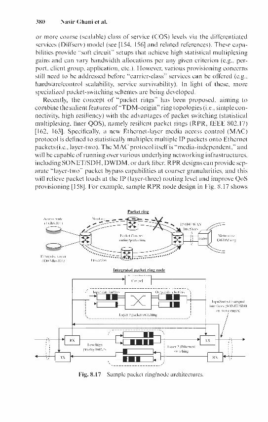
380 Nasir Ghani et ai.
or more coarse (scalable) class of service (COS) levels via the differentiated services (Diffserv) model (see [154, 1561 and related references). These capa- bilities provide “soft circuit” setups that achieve high statistical multiplexing gains and can vary bandwidth allocations per any given criterion (e.g., per- port, client group, application, etc.). However, various provisioning concerns still need to be addressed before “carrier-class’’ services can be offered (e.g., hardware/control scalability, service survivability). In light of these, more specialized packet-switching schemes are being developed.
Recently, the concept of “packet rings” has been proposed, aiming to combine the salient features of “TDM-origin” ring topologies (i.e., simple con- nectivity, high resiliency) with the advantages of packet switching (statistical multiplexing, finer QOS), namely resilient packet rings (RPR, IEEE 802.17) [162, 1631. Specifically, a new Ethernet-layer media access control (MAC) protocol is defined to statistically multiplex multiple IP packets onto Ethernet packets (Le., layer-two). The MAC protocol itself is “media-independent,’’ and will be capable of running over various underlying networking infrastructures, including SONETEDH, DWDM, or dark fiber. RPR designs can provide sep- arate “layer-two’’ packet bypass capabilities at coarser granularities, and this will relieve packet loads at the IP (layer-three) routing level and improve QoS provisioning [ 1.581. For example, sample RPR node design in Fig. 8.17 shows
Packet ring
\ 10GhEWAN interface?
4 M Metro core nng
Enterpnqe router (100Mb/sEth)
Integrated packet ring node
Fig. 8.17 Sample packet ringlnode architectures.

8. Metropolitan Optical Networks 381
two data priorities, or COS categories. Additionally, packet rings will also provide a rapid “layer-twoyy protection signaling protocol, designed to match the 50-ms timescales yielded by SONET/SDH [158]. The current RPR frame- work focuses on two (i.e., dual) counterpropagating “ringsyy that can both carry working traffic (i.e., no reserved protection bandwidth for bandwidth efficiency). All control messages are carried “in-stream,” making the control strictly in-band. Additionally, (layer-two) destination stripping is performed for unicast flows, unlike earlier source-stripping FDDI rings, permitting spa- tial reuse of bandwidth (note that multicast and broadcast still require source stripping, however). Collectively, the above features significantly improve ring capacity utilizatiodthroughput (i.e., bandwidth multiplication, see [ 1581 for details). Currently, a spatial reuse protocol (SRP) framework has been tabled for standardization and is commercially available (amongst others), aiming to provide all RPR features (e.g., protection switching, topology discovery, band- width fairness, etc.). In particular, the related protection switching protocol, termed the intelligent protection switching (IPS) protocol, is an architectural counterpart to the SONET/SDH K 1-K2 byte protocol.
Nevertheless, since packet rings have emerged from enterprise LAN require- ments, they clearly cannot support legacy TDM trafh (without proprietary mappings). Moreover, since RPR nodes must perform “electronic” packet pro- cessing operations, realistically, their scalability to high speeds (10 Gb/s and beyond) and large node counts needs to be proven [ 1581. As such, they are most suitable for new IP-based carriers [65], at least initially, providing very low-cost metro solutions. Most likely3 initial deployments will run over smaller-scale metro edge rings, and here, packet ring/optical ring interworking will become an important issue (see [75] for early discussions on this topic). Nevertheless, it is likely that future advances in optical packet switching (Section 8) will be leveraged to design substantially faster terabit packet rings. Overall, this is an evolving area, and more work will emerge (i.e., standardization, design, and performance evaluation).
6.4 MIGRATION STRATEGIES
Metro edge evolution will likely exhibit high variability due to the diversity of subrate client protocols and available solutions. Ultimately, any chosen solution will depend very much upon existing infrastructures, economic con- siderations, and clientloperational needs. Many metro edge networks still run at lower TDM bit rates (OC-3/STM-l, OC-12/STM-4), and therefore, rel- atively large capacity expansions can be cost effectively achieved by simply upgrading to higher bit rate TDM systems [54]. This is especially true for moderate demand growth and smaller tributary rates (DS3, OC-3/STM- 1) and/or fiber-rich scenarios. Meanwhile, newer operators with littlelno existing gear and more constrained fiber counts may prefer compact “data-efficient” NGSiMSPP platforms to rapidly provision a full range of services (TDM and

382 Nasir Ghani et al.
layer two/three). Furthermore, those incumbents with costly “best-in-class” routinglswitching gear may adopt a more cautious strategy towards NGS, choosing to deploy full solutions only for highly compelling price/performance alternatives. Still other incumbents may prefer NGS, given its strong origins from existing paradigms and finer-capacity allocation capabilities. Mean- while, for native Ethernet traffic, clearly packet-ring technology will be much more cost-effective than solutions using “telecom adapter” interfaces (SONETEDH, NGS). Moving forward, this will likely be the solution of choice for newer data-centric operators without legacy clients. For example, packet rings will offer very low-cost aggregation between residential (Internet) cable and DSL hubs.
Although the above alternatives may prevent immediate deployment of DWDM technology in the metro edge, in the longer term it remains the most scalable and complementary solution [63, 641. Namely, DWDM rings can agnostically support all other solutions (e.g., by reserving different wave length sets for SONET/SDH, NGS, and IP routing solutions) and will clearly decouple operators from continuing fluctuations in technology directions. More importantly, DWDM rings will allow operators to easily expand ser- vice offerings (e.g., legacy TDM voice/private line to data or vice versa). Most likely, many larger operators with existing legacy gear and diverse, specialized “higher-layer” systems (IP routers, ATM switches, Fibre Chan- nel hubs, telephony switches) will deploy passive DWDM rings with flexible edge aggregation interfaces to consolidate their architectures [35]. This will ensure abundant capacities for any future demand “spikes,” and also address the growing “wavelength services” market (gigabits to customer edge [62, 641). Other operators who choose NGS gear may also move to modularly add DWDM capabilities in the future (e.g., flexible MSPP solutions). A key planninglcosting activity will be choosing when to cross over to optical ring architectures (see also Section 5.4). For example, some operators may move from OC-48/STM-4 rings to DWDM rings rather than upgrade to less- scalable OC- 192/STM- 16 systems. Clearly, metro edge evolution requires more defining studies, see [63-651 for market-related considerations
7. Network Standards
Interoperable standards are a key factor in ensuring the success and adop- tion of next-generation metro optical networking solutions. Standards help to properly formalize both features and functionality, and will also help insu- late operators from single-vendor solutions. The key components of optical interoperability are now beginning to emerge. At the physical and link layers, many interface standards are well-defined, for example, SONET/SDH con- catenated formats, ITU-T wavelength grids, IEEE Ethernet interfaces, OIF interfaces, etc. Increasingly, higher-layer control and architectural issues are

8. Metropolitan Optical Networks 383
Data Plane ATM AALS mapping to SONETISDH frames Gigabit Ethernet framing,
LAN and WAN standards Packet-over-
I , . I IP packet routing IP, ATM traffic engineennglresource management, SONETlSDH protechon switching IP/MPLS routing and traffic 7 switching Setup signaling, resource/traffic
SONETISDH Packet, wavelength, fiber rouhng.
engineenng, rotechodrecovery P \
Trends ~ .........................
Physical opticslfiber layer
Fig. 8.18 IP over optics: data and control plane “delayering.”
now being considered, and the ITU-T optical transport network (OTN) archi- tecture defines three layers of transport (channel, multiplex, transport) [ 12, 1451. Meanwhile the IETF and OIF are beginning to tackle more detailed net- work signaling/protocols issues [157] and the ANSI TlXl is studying optical ring frameworks. Perhaps the most notable development is the multiproto- col lambda switching (MPAS) [148, 149, 1571 framework, superseded recently by the more generalized (emerging) multiprotocol label switching (GMPLS) framework [150, 1541. GMPLS represents a strong push to increase horizon- tal control plane integration (data and optical) by extendingheusing existing data networking concepts/protocols. The overall aim is to replace the features of multiple protocol layers in traditional multilayered models (e.g., separate addressing schemes, SONET/SDH protection, ATM traffic engineering) with a more unified solution, as shown in Fig. 8.18. A brief summary is presented here (refer to related references for details).
7.1 CHANNEL PROVISIONING
There are several major required components for dynamic channel provi- sioning and advanced SLA management in metro optical networks, namely setup signaling, resource discovery, and constraint-based routing [7]. GMPLS implements all of these requirements by extending MPLS signaling and
384 Nasir Ghani et al.
resource discovery protocols and defining multiple link-specific abstractions of the original MPLS label-swapping paradigm (ie., “implicit labels” for time- slots, wavelengths, and fibers), see [148,149,153,154]. Thesedefinitionscan be further coupled with hierarchical label-stacking schemes to exploit scalability (e.g., packet labels into TDM circuit labels into lambda labels). In particular, this ubiquity make GMPLS an ideal control framework for multiservice metro edge platforms (Sections 6.1 and 6.2).
First, optical channel setup signaling is accomplished by extensions to MPLS signaling protocols, namely RSVP-TE (RSVP traffic engineering) and CR-LDP (constraint-routing label distribution protocol) (see [ 148, 1541 and references therein). Here, the explicit-routing (ER) capability [ 1491 is used to indicate the channel route and reserve resources. Meanwhile, actual route computation (Le., RWA, Section 5.2.3) is done via constrained routing/path computation (Le., constraint-based routing (CBR) [ 1481). Moreover, CBR can also incorporate advanced trafiic/resource engineering algorithms for dynamic ring/mesh networks. Finally, route computation requires network topologi- cal/resource information (i.e., self-inventory capability), and this is propagated via extensions to pertinent routing protocols, namely open-shortest path fist (OSPF) and intermediate-system to intermediate-system (IS-IS) (see [154] for full details). Examples include fiber-types, wavelength counts, wavelength con- version resources, and possibly even analog metrics. More recently, resource diversity information has also been proposed to explicitly capture risk asso- ciations (physical, logical) [106, 1551, and this can help channel-routing algorithms improve the “disjointedness” between working/protection paths.
A key concern is provisioning architectures, namely centralized or dis- tributed architectures [7]. Data routing traditionally uses distributed control (signaling, routing), whereas optical ring/mesh routing is much more amenable to centralized implementations [7, 106, 1551. For example, many shared pro- tection schemes (Sections 5.2.2 and 5.3) require advanced optical ring/mesh RWA algorithms with global per-connection state. Distributinghlooding such information to all nodes is clearly unscalable. In other cases, if transmission impairments are incorporated, the resulting computations themselves are less amenable to distributed renditions. Nevertheless, many distributed shortest- path heuristic RWA algorithms are still possible, and possible future advances (components, algorithms) may permit more feasible distributed renditions (see [l , 7,1281). Regardless, the GMPLS framework can be applied for either model (e.g., appropriate LSA extensions (distributed) and/or policylroute servers (centralized) 11611).
7.2 PROTECTION SIGNALING
Dynamic optical rings, and likely even hybrid/mesh architectures (Sections 5.2.2 and 5.3), must provide fast optical protection signaling pro- tocols in order to match the capabilities of SONET/SDH APS (i.e., 50-ms
8. Metropolitan Optical Networks 385
recovery). Moreover, these protocols are necessary to implement advanced service definitions (e.g., multilevel resource sharing, Section 5.2.2). Various standardization efforts for optical protection are underway [15,75,95], but no signaling standards currently exist. However, early proposals for fast optical protection signaling in GMPLS have appeared [75, 951. For example, [75, 941 discusses extending existing MPLS LSP protection signaling or defin- ing an altogether new optical A P S protocol. Initially, APS protocol(s) can be defined for rings (ie., leveraging on SONETEDH concepts), but subse- quent generalizations to hybrid ring-mesh networks can also be considered. Meanwhile, [95] presents a new “lightweight” restoration signaling proto- col in lieu of RSVP/CR-LDP signaling. In general, until such standards are dehed, metro operators will continue to rely upon SONET/SDH protection, ultimately delaying the introduction of dynamic optical services provisioning.
Assuming that fast optical protection signaling schemes will emerge, inter- layer protection coordination becomes an issue. Many metro-area protocols have their own recovery mechanisms, operating across multiple domains (e.g., optical channel protection, SONET APS, MPLS LSP protection switching, IP flow rerouting), and the simultaneous interference of such functionalities can be very detrimental. Specifically, problems can include reduced resource utilization, increased recovery times, or routing instabilities [96, 100,102, 1031 (e.g., prolonged SONETISDH recovery times, Section 5.2.2). DWDM can also compromise higher-layer survivability, as the high degree of multiplex- ing can lower higher-layer connectedness without proper preplanning [ 1021. Additionally, replicated (excessive) protection functionality across layers can be very inefficient [98]. To date, no standards exist for multilayer protection interworking, and this is largely done via careful preplanning, see [ 1021 for a detailed study. Moving forward, more formalized mechanisms are needed for coordinating interlayer recovery actions between the packet/wavelength/fiber levels, termed escalation strategies [94, 100, 1031. Various escalation strate- gies are possible, such as bottom-uphop-down [7, 1001 or serial/parallel[103], and these will require complex interlayer signaling and hold-off timer mech- anisms. In particular, metro edge (NGS, MSPP) platforms handling many protocols and their associated control/monitoring functions present some very unique protection coordination possibilities. For example, routing diversity information can be used to ensure higher-layer workinglprotection resource separation. Overall, this is a complex area that requires much more work [98].
7.3 DOMAIN INTERFACING
Edge clients will need intelligent interfaces in order to automatically requesthelease “optical” bandwidth (i.e.,“bandwidth-on-demand” applica- tions. Here, several interworking models have been defined to propagate routing/connectivity information between the data (IP) and optical routing domains, namely overlay, peer, and integrated models [154, 1551. The overlay

386 Nasir Ghani et aL
model achieves maximum separation using separate routinglsignaling pro- tocols in each domain and defining an intermediate optical user network interface (0-UNI) [146, 147, 1511. Conversely, the peer model achieves max- imum integration running the same (extended) routinglsignaling protocols in both domains. However, this proves overly complex/cumbersome, requiring routers (optical nodes) to maintainlprocess optical (data) routing informa- tion. The integrated model strikes a balance between the above two schemes, running different instances of the same protocols (e.g., signaling, routing with extensions) and using gateway protocols for end-point exchange (see [155] for full details). In the near term, however, the overlay model will see most favor since related UNI standards are available and proprietary optical con- trol protocols can be accommodated. Moreover, this model provides better multiservice support, not just IP, and thus is well-suited for the metro space.
At the core of "optical" channel provisioning is the concept of a service def- inition, as extended via an 0-UNI or elementhetwork management system (EMS/NMS) interface. The 0-UNI is intended improve vertical integration between layers by allowing automated service discovery along with bandwidth signaling functions (e.g., request/release/modify operations). In addition, a set of generic signaled attributes are defined that can be mapped to subsequent channel requests (e.g., RSVP/CR-LDP, Section 7.1; framing type; bit rate; protection type; priority; etc.) [147, 151, 157. These mappings can cover a broad range of underlying capabilities (e.g., ring protection, mesh restora- tion, etc.) [94]. Signaled attributes will help facilitate multiple service levels for differing customer requirements, a necessary requirement in metro net- works. Overall, 0-UNIs are very germane to metro edge platforms, and even metro core nodes with direct wavelength interfaces. Several 0-UNI defini- tions have been tabled for standardization of which both the ODSI interface [147] and OIF standard [146] have been completed. Meanwhile, interdomain channel routing and protection coordination between operator networks will require (optical) network-to-network interface (0-NNI) definitions and early considerations are also underway here [ 152, 1551.
7.4 NETWORKMANAGEMENT As metro network elements continue to integrate many more diverse inter- faceskapabilities, especially at the metro edge, integrated network manage- ment is obviously a major requirement [22]. Network management is a very large focus area in its own right, and here only a brief discussion is provided due to scope limitations. In general, the well-accepted telecommunication network management (TMN) framework defines a hierarchical management model comprising vendor element management systems (EMS) entities inter- facing with multivendor network management systems (NMS). Although most early metro (DWDM) systems only provided proprietary EMS support for point-to-point transport nodes [156], more advanced solutions are now
8. Metropolitan Optical Networks 387
being offered. Optical channel (and link) visibility is of particular concern here, and is complicated by the fact that there are still no standards for related parameters. As an interim, detailed SONET/SDH B 1/JO overhead byte mon- itoring (or digital wrappers equivalent) can be used at ‘ ‘ ~ p a q u e ~ ~ points to measure bit-level performance (e.g., errored/severely-enored seconds, etc.). These “opaque” points can either be inside opaque nodes and/or at “edge” interfaces in transparent networks. Note that some vendors are also beginning to offer various (proprietary) sets of optical monitoring parameters, such as laser powers/current/temperature, amplifier power, etc. [68].
Meanwhile, with metro networks supporting many more protocols, advanced NMS solutions will be the key enablers for “end-to-end” services management operating across multiple vendors’ equipment [22]. Ideally, NMS solutions should provide operators with a full range of functionalities that are derived across multiple protocol domains, such as remote configuration, performance monitoring, rapid fault detection/alarm processing, failure iso- lation, diagnostics testing, and comprehensive logginglreporting, well-defined graphical interfaces, etc. [43]. However, genuine multivendor services manage- ment requires widescale adoption of standardized management frameworks, and overall this area is still in its infancy. Going forward, the common approach here will likely be to adapt TMN concepts and develop appropriate management information models between EMS and NMS systems [156].
8. Future Directions
As data t r a c volumes continue to increase, packet-switching paradigms will gain increasing favor, owing to their inherent statistical efficiencies [7, 165- 1681. Particularly, optical packet switching (OPS) designs are under study, utilizing optical techniques to perform as much of the packet-routing oper- ations as possible (e.g., switching, buffering, even processing, i.e., “fourth generation” optical networks). On the transport level, data packets are sent directly over wavelength channels (i.e., “packet-over-lightwave” (POL), Fig. 8.1). OPS nodes intend to achieve ultra-high packet throughputs, in the multiterabits range, largely surpassing current gigabit router designs. Even though all packet-switchinglrouting functions are difficult to perform opti- cally (and may remain so for the foreseeable future), various multifaceted opto-electronic designs are being studied, and inevitably this work will lead to significant improvements in packet-routing performance. In particular, the three main functionalities pertaining to OPS are buffering, switching, and header processing (i.e., label lookup) [2, 1681. Some brief details are reviewed, and readers are referred to related references for more complete treatments.
By and large, OPS nodes have the same architecture as electronic packet switches (i.e., input buffering, space switching, output buffering [168,169], see Fig. 8.19). In packet switching, contention can occur if multiple packets are

388 Nasir Ghani et al.
Metropolitan hybrid packetkircuit routing network
Integrated opticallelectronic packetkircuit switching node Header extraction (electmnic. possihly optical logic)
: Coupleror space -
Fig. 8.19 Hybrid metro optical packet/circuit switching networkhode.
routed to the same output port [165], and resolution is commonly achieved via buffering. Most OPS designs use fiber delay line buffers, and recently, the use of fast tunable laserskonverters has also been proposed to exploit the wave- length dimension to store multiple (wavelength) packets in a given delay line [167]. However, fiber delay line buffers constrain packets to multiples of a fixed length, as there is no means to retrieve packets before minimum buffer delays. Furthermore, large buffer sizes become costly/bulky (requiring complex shar- ing setups), and additionally, fiber attenuation concerns will limit the number of “circulations,” (usually under 100 [165]). Hence, as a tradeoff, a mixture of electronic memory and delay line buffering can be utilized [166]. Note that there are also very interesting, early developments in all-optical memories (e.g., molecular transistors, see references in [ 1671). OPS switching fabrics, mean- while, can also exploit the wavelength dimension to reduce contention and boost throughputs by orders of magnitude. However, nanosecond timings are needed for packet transfers between switch ports, and this can be problem- atic for MEMS technology. SOA gate technology has been considered here, although careful design is necessary to control crosstalk [I 661. Another switch- ing setup couples ultra-fast tunable lasers and wavelength converters with passive wavelength routing devices (e.g., AWG) [ 1691. As component tunabil- ity performances improve and integration technologies mature, this approach
8. Metropolitan Optical Networks 389
may become very feasible. Finally, carefully note that unlike circuit switching, OPS is still linked to the bit rate of the client signal, at least the header. Specif- ically, even though payload flow is optically transparent, electronic header processing/synchronization (and subsequent control of switchinglbuffering resources) must be done electronically, as “all-optical” processing is not cur- rently feasible (see [ 1681). Clearly, electronic costhcalability concerns can arise for high-wavelengtldfiber count systems and/or very small packet sizes, and this may limit the complexity/range of label processing/packet filtering oper- ations performed. Consequently, various bit-serial packet-coding techniques and/or guard-band schemes have been proposed to reduce electronic process- ing bottlenecks [169]. Note also that transparent payload sections will suffer from multi-hop optical degradations (loss, crosstalk), and this may require all-optical regeneration to maintain transmission distances.
Overall, OPS will provide a good match for limited metro distances and can reuse much of the existing packet-switching (MPLS, DiffServ) protocol suites [156, 166, 1671. Moreover, metro OPS will prove highly complemen- tary to emerging packet-based PON access solutions. Most likely, future metro packet switching solutions will evolve towards hybrid opto-electronic switching architectures (Fig. 8.19). Specifically, electronic switchinglbuffering will be utilized for finer-granularity/more complex label-processing “edge” operations, whereas OPS will implement less complex label-swapping func- tionalities, achieving higher throughputs for more “aggregated” packet flows (e.g., 10Tb/s stated in [166]). This delineation potentially lends well to “optical” packet rings, where more “coarse” stages (layer two COS) can be implemented using OPS. Even more germane to the metro arena, optical packet- and circuit-switching paradigms can be integrated onto a common platform, as the packet switches are still optically transparent to data pay- loads [167]. Namely, lightpaths can be switched over the same OPS switching fabric by simply “decoupling” the switching state from header-processing con- trol logic @e., bypass control logic and apply zero delay lines, Fig. 8.19). This optical circuit bypassing will permit transparent legacy support (in exactly the same manner as current DWDM systems, Section 5): and when applied to the packet domain, will further improve scalability (Le., eliminate per-node processing of large transithabeled packet flows). Overall, OPS is an exciting new frontier, and future advances in optical processing/buffering will undoubt- edly yield fundamental conceptual evolutions in the metro domain. Note also that slotted DWDM rings have also been proposed for accesdmetro data trans- port, utilizing fast tunable transmitters and/or receiver devices and fixed slot timings [170, 1711. Here, no optical buffering is performed inside the ring, and instead, advanced multiaccess (MAC) protocols are used to arbitrate DWDM channel slots in a fair manner between multiple users/traffic classes. These rings require edge packet buffering but can yield improved efficiencies ver- sus circuit-provisioned rings, as the wavelengths are shared between multiple source/destination points. A sample, advanced design using subcarrier sensing
390 Nasir Ghani et al.
techniques is studied in [171]. However, fixed slot timings arevery inefficient for variable-length IP packets, and proposed protocol amendments (e.g., multi- ple slot sizes, backoff schemes [171]) entail further desigrdprotocol complexity. Moreover, access-control protocol timings may adversely affect scalability over larger metro core distances.
9. Conclusions
Metropolitan networks occupy a strategic place in the overall network hier- archy, bridging end-users with abundant long-haul capacities. Traditionally, hierarchical SONET/SDH architectures have dominated the metro landscape, with slower speed access rings interconnecting to larger, faster metro core rings. However, as metro operators look to the future, many foresee surging band- width demands, primarily driven by data traffic, and a plethora of diverse clients with differing protocols and service requirements. As competition intensifies, legacy multilayered architectures are proving overly sluggish and unsalable in meeting complex, stringent service requirements. Clearly, metro operators are in urgent need of scalable, flexible, multiservice bandwidth provi- sioning solutions that allow for achieving a high level of service differentiation.
DWDM technology provides many benefits in the metro arena, including scalable capacity, transparency, and survivability. Moreover, many techno- economic studies have confirmed the cost-effectiveness of DWDM for bit rates beyond OC- lUSTM-4, bolstered further by falling component pricepoints As a result, DWDM technology has gained strong favor as a metro core solution, and various architectures are possible (ranging from simpler point-to-point transmission systems to dynamic wavelength-routing ring and mesh networks). Nevertheless, given the large existing base of (SONETEDH) fiber rings in the metro area, network migration is a key issue. Very likely, the first step in this migration will be a move to point-to-point DWDM “fiber-relief” applications, and then onwards to more advanced optical ringlhybrid architectures Mean- while, metro edge networks are evolving to represent a merging of the optical and electronic domains, aggregating many user protocols onto large metro core wavelength tributaries Many metro edge solutions have been proposed, ranging from DWDM edge rings, next-generation SONETEDH, and multi- service provisioning platforms, to “IP-based” packet rings. The choice of edge solution will clearly depend upon an individual operator’s needs, but over time, those incorporating DWDM technology will be most beneficial and hence will likely gain prominence.
Acknowledgments
The authors are indebted to the editors, Dr. Tingye Li and Dr. Ivan Kaminow, for their support, guidance, and overall patience in the preparation of

8. Metropolitan Optical Networks 391
this manuscript. The authors would also like to thank Mrs. Amber Alam, Mr. Mohamed Haiba, Mr. Paul Bonenfant, Dr. Hongxing Dai, Dr. De Yu Zang, Dr. James Fu, Dr. Zhensheng Zhang, Dr. Xinyi Liu, Mr. Ajay Sarkar, Dr. Xinhong Wang, Dr. Zhijian Wang, Mr. Bill Berry, and Mr. Don Buell for their invaluable feedback and discussions. Additionally, the authors are extremely thankful to Mrs. Rozsa Punkosti and Dr. Ti-Shiang Wang for their assistance with related references.
Abbreviations
ADM ASIC ATM AWG
BLSR BPSR CAGR CDM CLEC CMD co cos CP CWDM DCS DFB DifTServ DLC DPRING DRI DSL DSLAM DWDM EDFA EDWA EMS ESCON EXC FDDI FEC FICON FTTC
B-DCS
Add-drop multiplexer Application-specific integrated circuit Asynchronous transfer mode Arrayed waveguide grating Broadband digital cross-connect Bidirectional line-switched ring Bidirectional path-switched ring Compound annual growth rate Code-division multiplexing Competitive local exchange carrier Chromatic mode dispersion Central office Class of service Customer premise Coarse WDM Digital cross-connect Distributed feedback laser Differentiated services Digital loop carrier Dedicated protection ring Dual-ring interconnection Digital subscriber loop DSL access multiplexer Dense WDM Erbium-doped fiber amplifier Erbium-doped waveguide amplifier Element management system Enterprise system connectivity Electronic cross-point switch Fiber distributed data interface Forward error correction Fiber connectivity channel Fiber to the curb
392 Nasir Ghani et al.
FTTH GaAs GFP GMPLS HDLC HFC IC IntServ IOF IP IS-IS IXC LCAS LEC LMDS MAC MEMS MFL MMDS MMF MPLS MSPP NDF NGS NMS NWDM NZDSF OADM OCh OED
OMS 0-NNI OOK OPS osc 0-SNR OSPF OTN
0-FDM
0-UNI 0-VPN oxc PBX PDH
Fiber to the home Gallium arsenide Generic framing protocol Generalized MPLS High-level data link control Hybrid fiber coax Integrated circuit Integrated services Interoffice fiber Internet protocol Intermediate-system to intermediate-system Interexchange carrier Link capacity adjustment scheme Local exchange carrier Local multipoint distribution service Media access control Micro electro-mechanical system Multifrequency laser Multichannel multi-point distribution system Multimode fiber Multiprotocol label switching Multiservice provisioning platform Negative dispersion fiber Next-generation SONET Network management system Narrow WDM Non-zero dispersion shifted fiber Optical add-drop multiplexer Optical channel Optical edge device Optical frequency division multiplexing Optical multiplex section Optical network-to-network interface On-off keying Optical packet switching Optical supervisory channel Optical signal-to-noise ratio Open-shortest path first Optical transport network Optical user network interface Optical virtual private network Optical cross-connect Public branch exchange Plesiochronous digital hierarchy

8. Metropolitan Optical Networks 393
PLC PMD POL PON POP POS QAM QOS RF RPR RSVP RWA SAN SDH SDM SHR SLA SMF SNR SOA SONET SPRING TDM TDMA TLAN TMN TSI UPSR VLAN VPN W-DCS WDM
Planar lightwave circuit Polarization-mode dispersion Packet over lightwave Passive optical network Provider points of presence Packet over SONET Quadrature amplitude modulation Quality of service Radio frequency Resilient packet ring Resource reservation protocol Routing and wavelength assignment Storage area network Synchronous digital hierarchy Space division multiplexing Self-healing ring Service level agreement Single mode fiber Signal-to-noise ratio Semiconductor optical amplifier Synchronous optical network Shared protection ring Time-division multiplexing Time-slotted multiaccess Transparent local area network Telecommunication Management Network Time-slot interchange Unidirectional path-switched ring Virtual local area network Virtual private network Wideband digital cross-connect Wavelength division multiplexing
References
[I] B. Mukherjee, Optical Communications Networks, McGraw-Hill, New York, NY,
[2] R. Ramaswami, K. Sivarajan, Optical Networks: A Practical Perspective, Morgan
[3] T. E. Stern, K. Bala, Multiwavelength Optical Networks: A Layered Approach,
1997.
Kaufmann Publishers, San Francisco, CA, 1998.
Addison-Wesley, Reading, MA, 1999.
394 Nasir Ghani et al.
[4] M. Chow, Understanding SONET/SDH: Standards and Applications, Andan
[5] T. H. Wu, Fiber Network Service Survivability, Artech House, Boston, 1992. [6] R. Alferness, et al., “A Practical Vision for Optical Transport Networking,” Bell
Labs Technical Journal, Vol. 4, No. 1, January-March 1999, pp. 3-18. [7] N. Ghani, et al., “On IP Over WDM Integration,” IEEE Communications
Magazine, Vol. 38, No. 3, March 2000, pp. 72-84. [8] GR-1400-CORE, SONET Dual-Fed Unidirectional Path Switched Ring (UPSR)
Equipment Generic Criteria, Bellcore, Issue 1, Revision I , October 1995. [9] GR-1230-CORE, SONET Bi-directional Line-Switched Ring Equipment Generic
Criteria, Issue 4, December 1998. [ 101 J. Sosnosky, “Service Applications for SONET DCS Distributed Restoration,”
IEEE Journal on Selected Areas in Communications, Vol. 12, January 1994, pp.
[ l l] A. Mali% “PPP over SONETEDH,” Internet Engineering Task Force (IETF)
[ 121 P. Bonenfant, A. Moral, “Optical Data Networking,” IEEE Communications
[13] “Draft ITU-T Rec. G. 709,” ANSI TlX1.5/2000-246, October 2000. [ 141 “GFP Draft Specification-Revision 2,” ANSI TlX1.5/2001-024, January 2001. [15] M. Souillere, “Proposed ITU-T Contribution on Transparent OCh SPRings,”
ANSI TlX1.5/20OI-027, January 2001. [ 161 L. Szerenyi, “Approach to OSC Standardization,” ANSI T1X1.5/2001-002,
January 200 1. [17] A. Stok, E. Sargent, “Lighting the Local Area: Optical Code-Division Multiple
Access and Quality of Service Provisioning,” IEEE Network, Vol. 14, No. 6, NovemberDecember 2000, pp. 4246.
[18] T. Mossberg, M. Raymer, “Optical Code-Division Multiplexing,” Optics & Photonics News, Vol. 12, No. 3, March 2001, pp. 50-54.
[19] N. J. Frigo, “A Survey of Fiber Optics in Local Access Architectures,” in Optical Fiber Telecommunications IIZA, Academic Press, San Diego, CA, 1997,
[20] I. P. Kaminow, “Advanced Multiaccess Lightwave Networks,” in Optical Fiber Telecommunications IIIA, Academic Press, San Diego, CA, 1997, pp. 560-593.
[21] J. Senior, M. Handley, M. Leeson, “Developments in Wavelength Division Mul- tiple Access Networking,” IEEE Communications Magazine, Vol. 36, No. 12, December 1998, pp. 28-36.
[22] P. V. Hatton, F. Cheston, “WDM Deployment in the Local Exchange Network,” IEEE Communications Magazine, Vol. 36, No. 2, February 1998, pp. 5661.
[23] D. J. T. Healty, et al., “Optical Wireless: The Story So Far,” IEEE Communications Magazine, Vol. 36, No. 12, December 1998, pp. 72-82.
[XI H. Salloum, “How Does Local Multipoint Distribution Service (LMDS) Com- pare to Fiber to the Home (FTTH),” National Fiber Optic Engineers Conference (NFOEC) 1998, Orlando, FL, September 1998.
Publisher, New Jersey, 1995.
59-68.
Request for Comments (RFC) 2615, June 1999.
Magazine, Vol. 38, No. 3, pp. 63-70, March 2000.
pp. 461-522.
8. Metropolitan Optical Networks 395
[25] J. Refi, “Optical Fibers for Optical Networking,” Bell Labs Technical Journal, Vol. 4, No. 1, January-March 1999, pp. 24G261.
[26] E. Goldstein, L. Lin, J. Walker, “Lightwave Micromachines for Opti- cal Networks,” Optics & Photonics News, Vol. 12, No. 3, March 2001, pp. 60-65.
[27] Y. Danziger, D. Askegard, “High-Order-Mode Fiber,” Optical Networks Maga- zine, Vol. 2, No. 1, Januarymebruary 2001, pp. 40-50.
[28] M. Zirngibl, “Multi-Frequency Laser and Applications in WDM Net- works,” IEEE Communications Magazine, Vol. 37, No. 2, February 1999, pp. 39-41.
[29] P. Fairley, “The Microphotonics Revolution,” Technology Review, July/August
[30] J. Bautista, “Multiplexers Bring DWDM to Metro/Access Markets,“ WDM Solutions, February 2000, pp. 11-14.
[3 11 C. Huang, et al., “Ultra-Low Loss, Temperature-Insensitive 16-channel 100-Ghz Dense Wavelength Division Multiplexers Based on Cascaded AU-Fiber Unbal- anced Mach-Zehnder Structure,” Optical Fiber Communications Conference (OFC) 1999, San Diego, CA, February 1999.
[32] B. Broberg, et al., “Widely Tunable Semiconductor Lasers,” Optical Fiber Communications Conference (OFC) 1999, San Diego, CA, February 1999.
[33] L. Lin, “Free-Space Micromachined Optical-Switching Technologies and Archi- tectures,” Optical Fiber Communications Conference (OFC) 1999, San Diego, CA, February 1999.
[34] Y. Pan, et al., “Optical Multi-Stage Interconnection Networks,” IEEE Communi- cations Magazine, Vol. 37, No. 2, February 1999, pp. 50-56.
[35] Y. Chen, et al., “Metro Optical Networking,” Bell Labs Technical Joirrnal, Vol. 4, No. 1, January-March 1999, pp. 163-186.
[36] X. Cheng, “Beyond Transport: Creating the Metro Network,” Telephony, May 22,2000.
[37] T. Thakur, “Deploying Metro DWDM Systems,” National Fiber Optic Engineers Conference (NFOEC) 2000, Denver, CO, August 2000.
[38] E. Almstrom, et al., “Requirements and Solutions For Reconfigurable Metro WDM Networks,” National Fiber Optic Engineers Conference (NFOEC) 2000, Denver, CO, August 2000.
[39] T. E. Adams, et al., “Metropolitan Area Optical Networking,” National Fiber Optic Engineers Conference (NFOEC) 1998, Orlando, FL, September 1998.
[40] R. H. Cardwell. 0. J. Wasem, H. Kobrinski, “WDM Architectures and Eco- nomics in Metropolitan Areas.” Optical Networks Magazine, Vol. 1, No. 3, July
[41] R. Cardwell, et al., “WDM Network Economics,” National Fiber Optic Engineers Conference (NFOEC) 1997, San Diego, CA, September 1997.
[42] R. Boncek, et al., “Fiber and Systems for Metropolitan Optical Networks,” National Fiber Optic Engineers Conference (NFOEC), Orlando, FL, September 1998.
2000, pp. 38-44.
2000, pp. 41-50.
396 Nasir Ghani et sl.
[43] C. D. Webb, T. D. Krause, “Drivers and Enabling Technologies for Wavelength- Based Services in The All Optical Network,” National Fiber Optic Engineers Conference (NFOEC) 1998, Orlando, FL, September 1998.
[44] S. Wilkinson, “Metropolitan Area Transport Requirements,” National Fiber Optic Engineers Conference (NFOECJ 2000, Denver, CO, August 2000.
[45] l? Wong, “Network Architectures in the Metro DWDM Environment,” National Fiber Optic Engineers Conference (NFOEC) 2000, Denver, CO, August 2000.
[46] M. Simcoe, “A Layered Architecture for Metro Optical Networks,” National Fiber Optic Engineers Conference (NFOEC) 2000, Denver, CO, August 2000.
[47] M. Daoust, B. Lavallee, “Designing and Planning Metropolitan DWDM Solu- tions,” National Fiber Optic Engineers Conference (NFOEC) 2000, Denver, CO, August 2000.
[48] M. Wendel, R. Ward, M. Jary, “Transparent Optical Networking: Future Trends in Design and Deployment,” National Fiber Optic Engineers Conference (NFOEC) 2000, Denver, CO, August 2000.
[49] S. Greenholtz, et al., “Deployment of Dense Wave Division Multiplexing (DWDM) Technology in the Bell Atlantic Network,” National Fiber Optic Engineers Conference (NFOEC) 1998, Orlando, FL, September 1998.
[50] M. Williams, D. Klepp, “Introduction of DWDM Technology in BellSouth,” National Fiber Optic Engineers Conference (NFOEC) 1998, Orlando, FL, Septem- ber 1998.
[51] G. Ocakoglu, N. Wauters, P. Falcao, “The Technical Issues in the Selection and Deployment of WDM Systems in a Pan-European Carriers’ Carrier Net- work,” National Fiber Optic Engineers Conference (NFOEC) 1998, Orlando, FL, September 1998.
[52] S. Nathan, “Overcoming the Challenges of Designing, Planning, and Building an Optical Global Network That Will Support the Smooth Migration Towards the Intelligent Optical Network,” EuroForum: Intelligent Optical Networks, May 2000.
[53] M. Estep, “Deploying Advanced Optical Fiber Solutions for Metropolitan Networks,” EuroForum: Intelligent Optical Networks, May 2000.
[54] S. Johansson, et al., “A Cost Effective Approach to Introduce an Optical WDM Network in the Metropolitan Environment,” IEEE Journal on Selected Areas in Communications, Vol. 16, No. 7, September 1998, pp. 1109-1122.
[55] L. D. Garrett, et al., “The MONET New Jersey Network Demonstrator,” IEEE Journal on Selected Areas in Communications, Vol. 16, No. 7, September 1998,
[56] D. Stoll, et al., “Metropolitan DWDM: A Dynamically Configurable Ring for the KomNet Field Trial in Berlin,” IEEE Communications Magazine, Vol. 39, No. 2, February 2001, pp. 106-113.
[57] A. Richter, et al., “Germany-Wide DWDM Field Trial: Transparent Connec- tion of a Long-Haul Link and a Multichannel Metro Network,” Optical Fiber Communications Conference (OFC) 2001, Anaheim, CA, March 2001.
pp. 1199-1219.

8. Metropolitan Optical Networks 397
[58] A. Stavdas, “Architectural Solutions Towards a 1,000 Channel Ultra-Wideband WDM Network,” Optical Networks Magazine, Vol. 2, No. 1, JanuarylFebruary 2001, pp. 5140.
[59] C. Decusatis, “Dense Wavelength Division Multiplexing for Parallel Sysplex and Metropolitan/Storage Area Networks,” Optical Networks Magazine, Vol. 2, No. 1, JanuaryRebruary 2001, pp. 6!%80.
[60] B. St. Amaud, “Current Optical Network Designs May Be Flawed,” Optical Networks Magazine, Vol. 3, No. 2, March/April2000, pp. 21-28.
[61] “WDM and Optical Networks-Metro WDM: Market Forecast and Analysis,” Ryan Hankin Kent W K ) Report, February 2001.
[62] D. Cooperson, “Short-Haul WDMlOptical Networking: Is It (Finally) for Real?” National Fiber Optic Engineers Conference (NFOEC) 2000, Denver, CO, August 2000.
[63] “SONET Transport and DCS-Metro WDM: Market Forecast and Analysis,“ Ryan Hankin Kent (RHK) Report, March 2001.
[64] “Metro Optical Networks: Metro DWDM and the New Public Network,” Pioneer Consulting Report, 1999.
[65] “Optical Edge Networks: Market Opportunities for Integrated Optical Network Solutions in Metro Networks,” Pioneer Consulting Report, July 2000.
[66] J. P. Ryan, T h e Golden Age of Telecommunications?” Ryan Hankin Kent ( M K ) STARTRAX2OOO Conference, Palm Springs, CA, November 2000.
[67] J. Montgomery, “Optical AddlDrop Multiplexers Match Network Growth,” WDMSolutions, February 2000, pp. 4-8.
[68] K. Struyve, et al., “Application, Design, and Evolution of WDM in GTS’s Pan- European Transport Network,” IEEE Comrniinications Magazine, Vol. 38, No. 3, March 2000, pp. 114-121.
[69] G. Ocakoglu, K. Struyve, P. Falcao, “The Business Case for DWDM Metro Sys- tems in a Pan-European Carrier Environment,’’ National Fiber Optic Engineers Conference (NFOEC) 2000, Denver, CO, August 2000.
[70] 0. Gerstel, R. Ramaswami, “Upgrading SONET Rings with WDM Instead of TDM: An Economic Analysis,” Optical Fiber Comrniinications Conference (OFC) 1999, San Diego, CA, February 1999.
[71] G. Redifer, “DWDM vs. TDM In Metro and Long Haul Applications,” National Fiber Optic Engineers Conference (NFOEC) 1997, San Diego, CA, September 1997.
[72] L. Nederlof, et al., “Value Proposition for Configurable Optical Network Ele- ments,” Optical Fiber Communications Conference (OFC) 2001, Anaheim, CA, March 2001.
[73] P. Arijs, et aZ., “Design of Ring and Mesh Based WDM Transport Networks,” Optical Networks Magazine, Vol. 1, No. 3, July 2000, pp. 2540.
[74] W. Grover, “High Availability Path Design in Ring-Based Optical Net- works,” IEEE/ACM Transactions on Networking, Vol. 7, No. 4, August 1999, pp. 558-574.

398 Nasir Ghani et al.
[75] N. Ghani, et al., “Architectural Framework for Automatic Protection Provision- ing In Dynamic Optical Rings,” Internet Draj?, draft-ghani-optical-rings-01. txt, March 2001.
[76] D. Guo, et d., “Hybrid Mesh-Ring Optical Networks and Their Routing Information Distribution Using Opaque LSA,” Internet Draj?, draj?-guo-optical- mesh-ring-OO.txt, December 2000.
[77] T. Miyazaki, T. Kato, S. Yamamoto, “A Demonstration of an Optical Switch Cir- cuit with ‘Bridge-and-Switch’ Function in WDM Four-Fiber Ring Networks,” ZEICE Transactions on Communications, Vol. E82-B, No. 2, February 1999, pp. 326-334.
[78] N. Nagatsu, et al., “Flexible OADM Architecture and Its Impact on WDM Ring Evolution for Robust and Large-Scale Optical Transport Networks,” IEZCE Transactions on Communications, Vol. E82-B, No. 8, August 1999, pp. 1105-1 114.
[79] S. Kuwano, H. Uematsu, “Two-Fiber Uni-Directional OADM Ring System for L-Band,” National Fiber Optic Engineers Conference (NFOEC) 2000, Denver, CO, August 2000.
[80] W. Emkey, “Transparent DWDM Network with Optical Management,” National Fiber Optic Engineers Conference (NFOEC) 2000, Denver, CO, August 2000.
[8 11 N. Antoniades, “Engineering the Performance of DWDM Metro Networks,” National Fiber Optic Engineers Conference (NFOEC) 2000, Denver, CO, August 2000.
[82] R. Iraschko, et al., “An Optical 4-Fiber Bi-Directional Line-Switched Ring,” Optical Fiber Communications Conference (OFC) 1999, San Diego, CA, February 1999.
[83] W. Zhong, “New Bi-Directional WDM Ring Networks with Dual Hub Nodes,” IEEE Global Communications Conference (GLOBECOM’97), Phoenix, AZ, 1997. OBECOM’97.
[84] A. Zolfghari, “A Self-Healing Ring Network Topology Optimization Method,” National Fiber Optic Engineers Conference (NFOEC) 2000, Denver, CO, August 2000.
[85] C. R. Giles, M. Spector, “The Wavelength Add/Drop Multiplexer for Lightwave Communication Networks,” Bell Labs Technical Journal, Vol. 4, No. 1, January-
[86] G. Ellinas, et al., “Architecture Considerations in Merging Multi-Vendor WDM Rings for the MONET Washington D.C. Network,” Uptical Fiber Communications Conference (OFC) 1999, San Diego, February 1999.
[871 A. DiMichele, “Building High Capacity Broadband Metro Networks Using Optical Add-Drop Multiplex Systems,” National Fiber Optic Engineers Confer- ence (NFOEC) 1999, Chicago, IL, 1999.
[88] S. Ferguson, “Meeting OADM Performance Goals,” National Fiber Optic Engineers Conference (NFOEC) 2000, Denver, CO, August 2000.
[89] W. J. Tomlinson, “Comparison of Approaches and Technologies for Wave- length AddIDrop Network Elements,” National Fiber Optic Engineers Conference (NFOEC) 1998, Orlando, FL, September 1998.
March 1999, pp. 207-229.
8. Metropolitan Optical Networks 399
[90] G. E. Bodeep, et al., “16 Channel Reconflgurable Optical AddlDrop Multiplexer: An Engineering Model,” National Fiber Optic Engineers Conference (NFOEC) 1998, Orlando, FL, September 1998.
[91] N. A. Jackman, et al., “Optical Cross Connects for Optical Networking,” Bell Labs Technical Journal, Vol. 4, No. 1, January-March 1999, pp. 262-281.
[92] P. Jaggi, H. Onaka, S. Kuroyanagi, “Optical ADM and Cross Connects: Recent Technical Advancements and Future Optimal Architectures,” National Fiber Optic Engineers Conference (NFOEC) 1998, Orlando, FL, September 1998.
[93] J. Gruber, P. Roorda, F. LaLonde, “The Photonic SwitcWCross-Connect (PSX)-Its Role in Evolving Optical Networks,” National Fiber Optic Engineers Conference (NFOEC) 2000, Denver, CO, August 2000.
[94] N. Ghani, “Survivability Provisioning in Optical MPLS Networks,” 5th European Conference on Networks and Optical Communications (NOC ZOOO), June 2000.
[95] B. Rajagopalan, et al., “Signaling for Fast Restoration in Optical Mesh Networks,” Internet Draj?, draj?-bala-restoration-signcrling-OO.~t, February 2001.
[96] D. Zhou, S. Subramaniam, “Survivability in Optical Networks,” IEEE Network Magazine, Vol. 14, No. 6, November/December 2000, pp. 16-23.
[97] A. Fumagalli, L. Valcarenghi, “IP Restoration vs WDM Protection: Is There an Optimal Choice?” ZEEE NetworkMagazine, Vol. 14, No. 6, NovembedDecember 2000, pp. 34-41.
1981 S. Ayandeh, P. Veitch, “Dynamic Protection and Restoration in Multi-Layer Networks,” Optical Internetworking Forum, OIF2001.166, April 200 1.
[99] R. Doverspike, et al., “Fast Restoration in a Mesh Network of Optical Cross- Connects,” Optical Fiber Communications Conference (OFC) 1999, San Diego, February 1999.
[loo] P. Demeester, et al., “Resilience in Multilayer Networks,” IEEE Communications Magazine, Vol. 37, No. 8, August 1999, pp. 44-51.
[loll R. Batchellor, “Optical Layer Protection: Benefits and Implementation,” National Fiber Optic Engineers Conference (NFOEC) 1998, Orlando, FL, Septem- ber 1998.
[ 1021 J. Sosnosky, Z. Lin, “Planning for Broadband Multilayer Survivability,” NationaZ Fiber Optic Engineers Conference (NFOEC) 1998, Orlando, FL, September 1998.
[ 1031 J. Manchester, P. Bonenfant, “Fiber OpticNetwork Survivability: SONET/Optical Protection Layer Intenvorking,” National Fiber Optic Engineers Conference (NFOEC) 1996, Denver, CO, 1996.
[lo41 R. Iraschko, et al., “Interoperability of SONET and Optical Layer Protection,” National Fiber Optic Engineers Conference (NFOEC) 1999, Chicago, IL, 1999.
[lo51 C. Larsen, I? Anderson, “Signal Quality Monitoring in Optical Networks,” Optical Networks Magazine, Vol. 1, No. 4, October 2000, pp. 17-23.
[lo61 J. Strand, A.Chiu, “Issues for Routing in the Optical Layer,’’ IEEE Commuizica- tions Magazine, Vol. 39, No. 2, February 2001, pp. 81-87.
[lo71 C. Fan, J. P. Kunz, “Terrestrial Amplified Lightwave System Design,” in Opfi- cal Fiber 22iecornrnunications IIU, Academic Press, San Diego, CA, 1997, pp. 265-30 1.
400 Nasir Ghani et al.
[lo81 B. Ramamurthy, et al., “Impact of Transmission Impairments on the Teletraffic Performance of Wavelength-Routed Optical Networks,” IEEE/OSA Journal of Lightwave Technology, Vol. 17, No. 10, October 1999, pp. 1713-1723.
[lo91 D. Datta, et al., “BER-based Call Admission in Wavelength-Routed Optical Networks,” OpticaI Fiber Communications Conference (OFC’98), San Jose, CA, February 1998.
[110] M. Ali, B. Ramamurthy, J. Deogun, “A Genetic Algorithm for Routing in WDM Optical Networks with Power Considerations, Part I: Unicast Case,” 8” IEEE International Conference on Computer Communications and Network (ICCCN’99), Boston, MA, October 1999.
[l 1 11 L. Nelson, “Challenges of 40 Gb/s WDM Transmission,” Optical Fiber Commu- nications Conference (OFC) 2001, Anaheim, CA, March 2001.
[112] S. Wilkinson, S. Sasaki, Y Nakano, “Technological Advances Towards OC- 768 Transmission,” National Fiber Optic Engineers Conference (NFOEC) 1998, Orlando, FL, September 1998.
[113] D. Marcenac, “Benefits of Wavelength Conversion in Optical Ring-Based Networks,” Optical Networks Magazine, Vol. 1 No. 2, April 2000, pp. 23-29.
[114] D. Marcenac, C. Felicite, “Practical Benefits of 4 Fiber WDM Rings With Real- istic Ti-aEc,” Optical Fiber Communications Conference (OFC) 1999, San Diego, CA, February 1999.
[115] B. Ramamurthy, B. Mukherjee, “Wavelength Conversion in WDM Networks,” IEEE Journal on Selected Areas in Communications, Vol. 1, No. 7, September
[116] K. Bala, “The Benefits of Minimal Wavelength Interchange in WDM Rings,” Optical Fiber Communications (OFC) Conference 1997, Dallas, TX, February 1997.
[117] E. Bouillet, K. Bala, “The Benefits of Wavelength Interchange in WDM Rings,” IEEE International Conference on Communications (ICC), June 1997, pp. 41 1 4 5 .
[ 1 181 B. Ramamurthy, “Transparent vs. Opaque vs. Translucent Wavelength-Routed Optical Networks,” Optical Fiber Communications Conference (OFC) 1999, San Diego, CA, February 1999.
[119] 0. Gerstel, R. Ramaswami, G. H. Sasaki, “Fault-Tolerant Multi-Wavelength Optical Rings with Limited Wavelength Conversion,” IEEE Journal on Selected Areas in Communications, Vol. 16, No. 7, September 1998, pp. 1166-1 178.
[ 1201 J. Elmirghani, H. Mouftah, “All-Optical Wavelength Conversion: Technologies and Applications in DWDM Networks,” IEEE Communications Magazine, Vol. 38, No. 3, March 2000, pp. 8692.
[121] J. Yates, et al., “Limited-Range Wavelength Translation in All-Optical Net- works,” IEEEINFOCOM, Vol. 3, March 1996, pp. 954-961.
[122] G. Maier, et al., “Performance of WDM Rings With Wavelength Conversion Under Non-Poisson Tralk,” IEEE International Conference on Communications (ICC’99), Vancouver, B.C., June 1999.
1998, pp. 1061-1073.
8. Metropolitan Optical Networks 401
[123] 0. Gerstel, S. Kutten, “Dynamic Wavelength Allocation in All-Optical Ring Net- works,” IEEE International Conference on Communications (ICC’97), Montreal, Canada, June 1997.
[ l a ] J. Yates, M. Rumsewicz, J. Lacey, “Wavelength Converters in Dynamically- Reconfigurable WDM Networks,” IEEE Communications Surveys, Vol. 2, No. 2, 2nd Quarter, 1999 (available at http://www.comsoc.org/pubs/surveys).
[125] M. Kovacevic, A. Acampora, “Benefits of Wavelength Translation in All-Optical Clear-Channel Networks,” IEEE Journal on Selected Areas in Communications, Vol. 14, No. 5, June 1996, pp. 868-880.
[126] S. Subramaniam, M. Azizoglu, A. Somani, “AU-Optical Networks with Sparse Wavelength Conversion,” IEEE Journal on SelectedAreas in Communications, Vol. 4, No. 4, August 1996, pp. 544556.
[127] M. Stephens, et al., “All-Optical Regeneration and Wavelength Conversion in an Integrated Semiconductor Optical Amplifier/Distributed Feedback Laser’’ Optical Fiber Communications Conference (OFC) 1999, San Diego, CA, February 1999.
[128] H. Zang, J. Jue, B. Mukherjee, “Review of Routing and Wavelength Assignment Approaches for Wavelength-Routed Optical WDM Networks,” Optical Networks Magazine, Vol. 1, No. 1, January 2000, pp. 47-60.
[139] G. A. Young, “Planning SONET Architectures for Improved Capacity Utiliza- tion,” National Fiber @tic Engineers Confemce (NFOEC) 1998, Orlando, FL, September 1998.
[130] A. Repech, “Architecting Data-Aware SONET Networks,” National Fiber Optic Engineers Conference (NFOEC) 1999, Chicago, IL, 1999.
[131] D. O’Connor, “Internet Optimized SONET ADM,” National Fiber Optic Engineers Confermce (NFOEC) 1998, Orlando, FL, September 1998.
[132] K. Bala, “WDM Optical Network Architectures for a Data-Centric Environ- ment,“ National Fiber Optic Engineers Conference (NFOEC) 1998, Orlando, FL, September 1998.
[133] E Moore, ”Extending the LAN to the Transport Network,” National Fiber Optic Engineers Conference (NFOEC) 2000, Denver, CO, August 2000.
[134] D. K. Gordon, “Broadband Digital Cross Connect Application Guidelines,” National Fiber Optic Engineers Conference (NFOEC) 1998, Orlando, FL, Septem- ber 1998.
[135] R. Goudreault, et al., “Impact of Integrated Architecture for Bandwidth Man- agement in a Broadband Network Infrastructure,” Bel1 Labs Technical Journal, Vol. 4, No. 1, January-March 1999, pp. 19-41.
11361 E. Modiano, A. Nola-Tam, “Mechanisms for Providing Optical Bypass in WDM-Based Networks,” Optical Networks Magazine, Vol. 1, No. 1, January
[137] 0. Gerstel, R. Ramaswami, G. Sasaki, “Cost-Effective Traffic Grooming in WDM Rings,” IEEWACM Transactions on Networking, Vol. 8, No. 5, October 2000, pp. 618630.
2000, pp. 11-18.

402 Nasir Ghani et al.
[138] G. Sasaki, 0. Gerstel, “Minimal Cost WDM SONET Rings That Guarantee No Blocking,” Optical Networks Magazine, Vol. 1, No. 4, October 2000, pp. 51-57.
[139] X. Zhang, “An Effective and Comprehensive Approach for Traffic Grooming and Wavelength Assignment in SONETlWDM Rings,” IEEEIACM Transactions on Networking, Vol. 8, No. 5, October 2000, pp. 608-617.
[140] P. Wan, et al., “Grooming of Arbitrary TraEic in SONETlWDM BLSRs,” IEEE Journal on Selected Arem in Communications, Vol. 18, No. 10, October 2000, pp. 1995-2003.
[141] L. Castellon, T. Rado, “The Future of SONET,” National Fiber Optic Engineers Conference (NFOEC) 2000, Denver, CO, August 2000.
[142] A. Shivji, “SONET Gear for the Optical Generation,” National Fiber Optic Engineers Conference (NFOEC) 2000, Denver, CO, August 2000.
[143] N. Sayer, S. Donnelly, G. Winslow, “Positioning for Automated Provisioning of Broadband Services Over SONET,” National Fiber Optic Engineers Conference (NFOEC) 1998, Orlando, FL, September 1998.
[144] R. Newman, A. Dobrushin, S. White, “Effects of Data and New Access Tech- nologies on Optical Access Networks,” National Fiber Optic Engineers Conference (NFOEC) 1998, Orlando, FL, September 2000.
[145] L. Steinhorst, “Enabling the Optical Transport Network Through Digital Wrap- pers,” National Fiber Optic Engineers Conference (NFOEC) 2000, Denver, CO, August 2000.
[146] L. McAdams, J. Yates, K. Bala, “User to Network Interface (UNI) Service. Defjnition and Lightpath Attributes,” OIF Forum, OIF2000.061, September 2000.
[147] K. Arvind, et al., “Optical Domain Service Interconnect (ODSI) Signaling Control Specification,” Version 1 A.5, ODSI Coalition, November 2000.
[148] D. Awduche, Y Rekhter, “Multiprotocol Lambda Switching: Combining MPLS Trallic Engineering Control with Optical Crossconnects,” ZEEE Communications Magazine, Vol. 39, No. 3, March 2001, pp. 11 1-116.
[149] N. Ghani, “Lambda-Labeling: A Framework for IP over WDM Using MPLS,” Optical Networks Magazine, April 2000.
[150] Y Xu, et al., “Generalized MPLS Control Plane Architecture for Automatic Switched Transport Network,” Internet Draft, drafr-xu-mpls-ipo-gmpls-arch- OOM, November 2000.
[ 15 11 Y. Xue, et al., “Carrier Optical Services Framework and Associated UNI Require- ments,” Internet Draft, draft-many-cam‘er-framavork-uni-00. at, November 2000.
[152] D. Papadimitriou, et al., “Optical Network-to-Network Interface Framework and Signaling Requirements,” Internet Draft, draft-papadimihiou-onni-ffame- Ol.brt, November 2000.
[153] G. Bernstein, E. Mannie, V. Sharma, “Framework for MPLS-based Control of Optical SDWSONET Networks,” IETF Draft, draft-bms-optical-sdhsonet-mpls- contml-Jimwrk-00. at, November 2000.
8. Metropolitan Optical Networks 403
[154] A. Banerjee, et al., “Generalized Multiprotocol Label Switching: An Overview of Routing and Management Enhancements,” IEEE Communications Magazine, Vol. 39, No. 1, January 2001, pp. 144-150.
[155] B. Rajagopalan, et al., “IP Over Optical Networks: Architectural Aspects,” IEEE Communications Magazine, Vol. 39, No. 9, September 2000, pp. 94-102.
[156] N. Golmie, T. Ndousse, D. Su, “A Differentiated Optical Services Model for WDM Networks,” IEEE Communications Magazine, Vol. 38, No. 2, February
[157] D. H. Su, D. W. Griffith, “Standards: Standards Activities for MPLS Over WDM Networks,” Optical Networks Magazine, Vol. 1, No. 3, July 2000, pp. 6b-69.
[158] P. Bonenfant, A. Moral, “Framing Techniques for IP Over Fiber,” IEEE Network Mugmine: Vol. 15, No. 4, JulylAugust 2001, pp. 12-18.
[159] B. St. Amaud, “Overview of the Latest Developments in Optical Internets,” Optical Networks Magazine, Vol. 1, No. 3, July 2000, pp. 51-54.
[160] D. H. Su, “Standards: The IEEE P802.3ae Project for 10GbIs Ethernet,“ Optical Networks Magazine, Vol. 1, No. 4, October 2000, pp. 58-59.
[161] N. Ghani, et al., “COPS Usage for ODSI,” Optical Domain Service Interconnect (ODSI) Coalition, Policy/Accounting Specification, January 200 1.
[162] A. Herrera, et al., “A Framework for IP Over Resilient Packet Rings,” Internet Draj?, draft-ietf-iporpr-framework-OO.Lxt, February 2001.
[163] IEEE 802.1 7 Resilient Packet Ring Working Group, http://www.ieee802.org/17/. 11641 P. Gupta, N. McKeown, “Algorithms for Packet Classification,” IEEE Network
Magazine, Vol. 15, No. 2, MarcldApril2001, pp. 24-32. [165] B. Li, et al., “Photonic Packet Switching: Architectures and Performance,”
Optical Networks Magazine, Vol. 2, No. 1, January/February 2001, pp. 27-39. [166] A. Jourdan, etal., “The Perspective of Optical Packet Switching in IP-Dominant
Backbone and Metropolitan Networks,” IEEE Communications Magazine, Vol. 39, No. 3, March 2001, pp. 136141.
[167] S. Yao, B. Mukhejee, “All-Optical Packet Switching for Metropolitan Area Networks: Opportunities and Challenges,” IEEE Communications Magazine, Vol.
[168] A. Pattavina, et al., “Techniques and Technologies Towards All-Optical Switch- ing,” Optical Networks Magazine, Vol. 1, No. 2, April 2000, pp. 75-92.
[169] L. Xu, “Techniques for Optical Packet Switching and Optical Burst Switching,” IEEE Communications Magazine, Vol. 39, No. 1, January 2001, pp. 136143.
[170] M. Marsan, et al., c‘All-Optical WDM Multi-Rings with Differentiated QOS,” IEEE Communications Magazine, Vol. 36, No. 12, February 1999, pp. 58-66.
[171] K. Shrikhande, et al., “HORNET A Packet-Over-WDM Multiple Access Metropolitan Area Ring Network,” IEEE Journal on SelectedAreas in Communi- cations, Vol. 18, No. 10, October 2000, pp. 2004-2016.
[172] N. Jones, H. Helvoort, T. Wilson, “Proposed Text on Link Capacity Adjustment Scheme (LCAS) for SDH Virtually Concatenated VCs to be contributed to ITU- T SG-15,” ANSI TlX1.5/2001429, January, 2001.
2000, pp. 68-73.
39, NO. 3, March 2001, pp. 142-148.

Chapter 9
Xiaolin Lu Morning Forest, Highlands Ranch, Colorado
Oleh Sniezko Oleh-Lightcom, Highlands Ranch, Colorado
The Evolution of Cable TV Networks
1. Introduction
The telecommunications industry is facing tremendous challenges and new opportunities brought about by deregulation, competition, and advanced technologies and services The opportunities in broadband subscriber access and its promise of eliminating the bottleneck that has limited progress towards a global information infrastructure have been stimulating large-scale business efforts and technology evolution. Network operators and service providers must upgrade their “embedded infrastructure” in order to protect their cur- rent revenue while searching for new market potentials. This becomes more critical as the existing services (telephone, broadcast analog TV) are reaching the saturation point, while the emergence of new service opportunities requires different network characteristics (asynchronous vs synchronous, switched vs broadcast, broadband vs narrowband, etc.). Depending on the economic situ- ation and projected revenue potential, different network operators and service providers may choose different network upgrade paths and business strategies involving different technologies [ 141.
Historically, communication networks have been established to support specific services and their related business models. Therefore, each type of network has its own characteristics that serve special needs. With entertain- ment and communication being the two major and distinguished services, at least historically, the access networks can be categorized as broadcast-based (point-to-multipoint) and switch-based (point-to-point). Examples include tree-and-branch-based network topology used by the cable industry and twisted-pair-based star architecture used by the telephony industry.
The cable industry’s primary business is broadcasting multichannel video to subscribers’ homes. The notion of “pushingyy information to customers and allowing them to choose naturally leads to the use of the tree-and-branch architecture and coaxial cable (broadband capacity) for signal distribution utilizing radio frequency (RF) subcarrier multiplexing technique. Although the pros and cons of this architecture versus that of the star architecture con- tinue to be debated, the use of tree-and-branch topology with tapped coaxial
404 OPTICAL FIBER TELECOMMUNICATIONS VOLUME IVB
Copyright 0 2002, Elsevier Science (USA). All rights of reproduetion in any form reserved.
ISBN 0-12-395173-9
9. The Evolution of Cable TV Networks 405
bus provides the cable industry the most cost-effective way of building and operating the network for two reasons.
First, in the United States, residential houses are constructed based on a typical grid topology, which resembles the bus architecture. The tapped coax- ial bus allows cable operators to easily connect and disconnect customers and provision potential growth in certain areas without overbuilding or under- building the network. For example, along a typical coaxial bus, one can easily provision many taps (within certain limitations defined by the signal qual- ity requirements). Each tape can have many different numbers of ports for connecting customers (customer activation), and the number of ports can be larger than the current number of customers in that area, therefore leaving room for growth.
Second, multiple system operators (MSOs) can extend the network reach by extending the coaxial bus @e., adding coaxial amplifiers), as long as the signal level requirements are met.
The use of Frequency Division Multiplexing (FDM) or Subcarrier Mul- tiplexing (SCM) schemes throughout the network also makes the network transparent to signal formats. Any change (e.g., bandwidth requirement) can be made by modifying the headend equipment and customer premise equipment (CPE), therefore simplifying the operation.
Armed with the advent of linear lightwave technology, the advanced RF modem, and DSP technology, cable network operators have embarked on extensive upgrades and on the transition to hybrid fiber coax (HFC) architec- tures in the past 2 decades. The main goal has been to evolve the infrastructure from a broadcast-type trunk-and-branch plant to a high-capacity two-way network with superior quality and reliability that is ready to deliver advanced telecommunications services.
This chapter will discuss cable network evolution and related technology innovations, and their impacts on business and operations. Instead of dis- cussing all the physical and engineering details, we will try to provide an intuitive view of this evolution. Section 2 provides a general overview of the conventional coaxial cable network and its migration to the HFC archi- tecture. Section 3 discusses the commonly used modern broadband cable infrastructure, including the metro networks, secondary hub networks, and the Fiber-to-the Serving Area (FSA) distribution networks. Section 4 discusses the further evolution of the HFC network based on deep fiber penetration and digital technology. Section 5 provides background on some of the technology advances that continually drive the network evolution.
2. Historical Overview
In 1998, the cable television industry celebrated its fiftieth anniversary. The first cable television system in the United States was built with twin-lead
406 Xiaolin Lu and Oleh Sniezko
symmetrical antenna wires and without ampliliers [5-6]. At approximately the same time, similar systems were also built in London, England and Ontario, Canada. Soon after these first, amplificationless systems, tube ampwers and then later silicon-based ampliliers were added to extend the reach on the coax- ial distribution systems. A drive towards increased bandwidth in the cable television distribution systems led to the deployment of 400+-MHz systems with 54+ analog video channels by the end of the 1970s. This expansion was made possible by significant strides in semiconductor technology that created push-pull amplifiers, feed-forward amplifiers, and power-doubling amplifiers. Further improvement in these basic technologies resulted in forward band- width being expanded to 550 MHz by the end of the 1990s and to 750-4360 MHz by the end of the century. This also allowed for 25 and more amplifiers being cascaded while still meeting the minimal regulatory end-of-line performance requirements.
At the end of the 1970s and the beginning of the 1980~~ two-way cable TV systems became operational, although the wide deployment of two-way broadband systems did not start until early in the 1990s when the technol- ogy innovation broke the tech-economic barrier and enabled cable operators to support public demand for broadband telecommunication services. In a modern two-way cable system, 5-42MHz is typically used for upstream transmission, and 50 MHz and above is used for downstream transmission, in which 50 -500 MHz is used for carrying broadcast analog video and the upper-frequency band (550 MHz) is used for emerging digital services.
In the late 1980% linear fiber-optic technology achieved the level of per- formance suitable for analog cable TV applications. The deployment of this technology allowed for improved quality and reliability of cable television sys- tems by shortening the cascades of active devices. In the 1990% affordable linear reverse lasers became available. Both these contributed to an unprecedented architectural progress, which eventually converted traditional tree-and-branch coaxial architecture into a node-based HFC architecture.
2.1 TRADITIONAL COAXIAL SYSTEM
Traditionally, the majority of television sets were built to receive AM-VSB (analog modulation-vestigial sideband) signals. The most cost-effective way to deliver those signals to customers was to maintain the same format and avoid the cost of format conversion. Therefore, the AM-VSB signals were fre- quency multiplexed and transmitted over coaxial cable with multiple coaxial amplifiers in cascade [5-71. At the end of these cascades, the signals had to maintain a minimal level of performance (noise and distortions) to meet reg- ulatory requirements and customer satisfaction. The minimal performance requirements changed over time with increased subjective perceptibility of the video impairments brought about by customer education, larger TV screens, and high-quality alternative means of video content reproduction (e.g., DVD
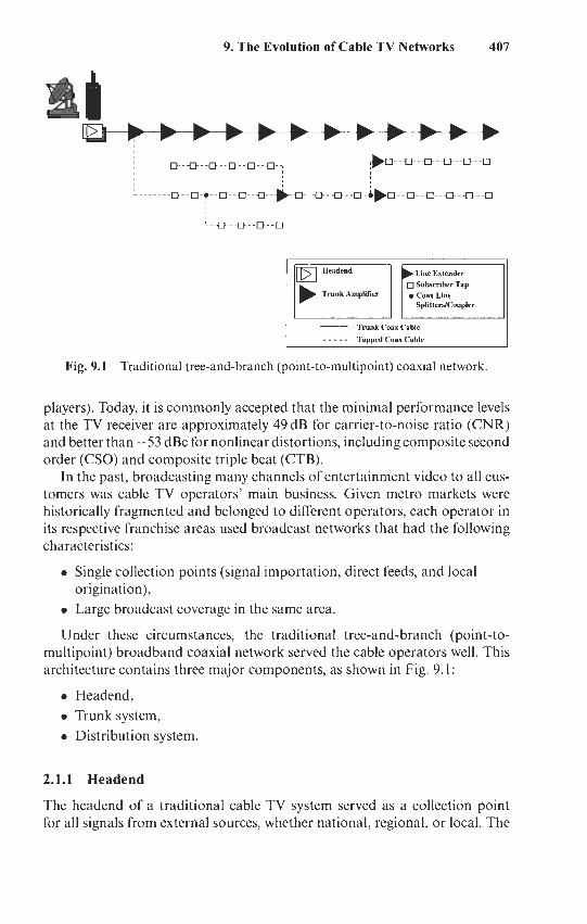
9. The Evolution of Cable TV Networks 407 ,,,,,,,, Line Extender
- Trunk Coax Cable _ _ _ _ _ TaDwd Coax Cable
Fig. 9.1 Traditional tree-and-branch (point-to-multipoint) coaxial network.
players). Today, it is commonly accepted that the minimal performance levels at the TV receiver are approximately 49 dB for carrier-to-noise ratio (CNR) and better than -53 dBc for nonlinear distortions, including composite second order (CSO) and composite triple beat (CTB).
In the past, broadcasting many channels of entertainment video to all cus- tomers was cable TV operators’ main business. Given metro markets were historically fragmented and belonged to different operators, each operator in its respective franchise areas used broadcast networks that had the following characteristics:
0 Single collection points (signal importation, direct feeds, and local
0 Large broadcast coverage in the same area.
Under these circumstances, the traditional tree-and-branch (point-to- multipoint) broadband coaxial network served the cable operators well. This architecture contains three major components, as shown in Fig. 9.1:
origination),
0 Headend, 0 Trunk system, 0 Distribution system.
2.1.1 Headend
The headend of a traditional cable TV system served as a collection point for all signals from external sources, whether national, regional, or local. The
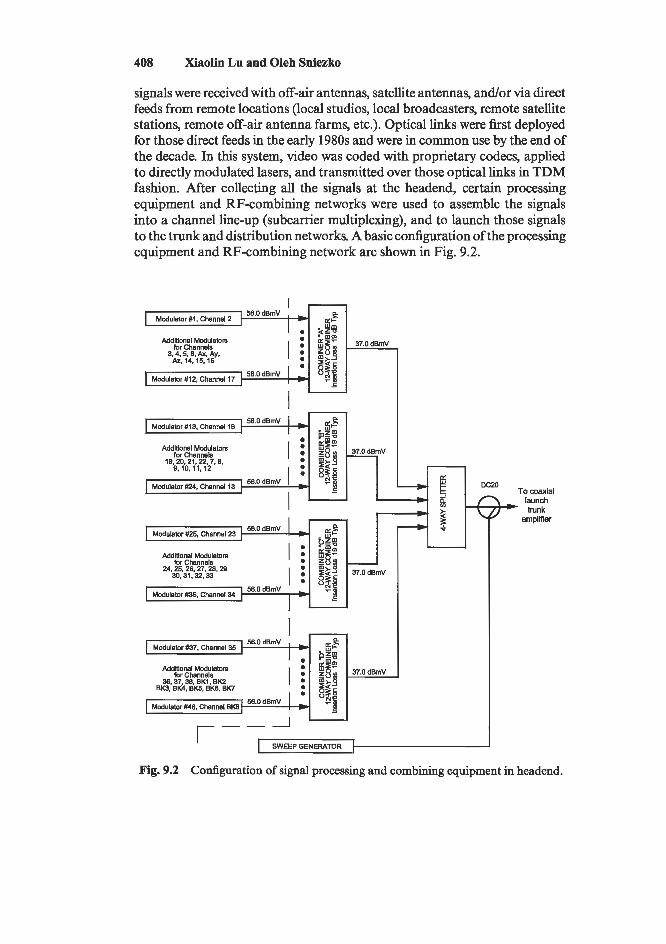
408 Xiaolin Lu and Oleh Sniezko
signals were received with off-air antennas, satellite antennas, and/or via direct feeds from remote locations (local studios, local broadcasters, remote satellite stations, remote off-air antenna farms, etc.). Optical links were fist deployed for those direct feeds in the early 1980s and were in common use by the end of the decade. In this system, video was coded with proprietary codecs, applied to directly modulated lasers, and transmitted over those optical links in TDM fashion. After collecting all the signals at the headend, certain processing equipment and RF-combining networks were used to assemble the signals into a channel line-up (subcarrier multiplexing), and to launch those signals to the trunk and distribution networks. A basic configuration of the processing equipment and RF-combining network are shown in Fig. 9.2.
AddMonal Modulators for Channels
3,4.5.6. Ax. AY,
Addltlonal Modulators for Channeb
19.20,21,22. 7,8 , 9, io, I t 1 2 4 Modulator W, Channel 13 56'o dBmV
37.0 dBmV
1 1
DC20
amplifier t
Fig. 9.2 Con6guration of signal processing and combining equipment in headend.
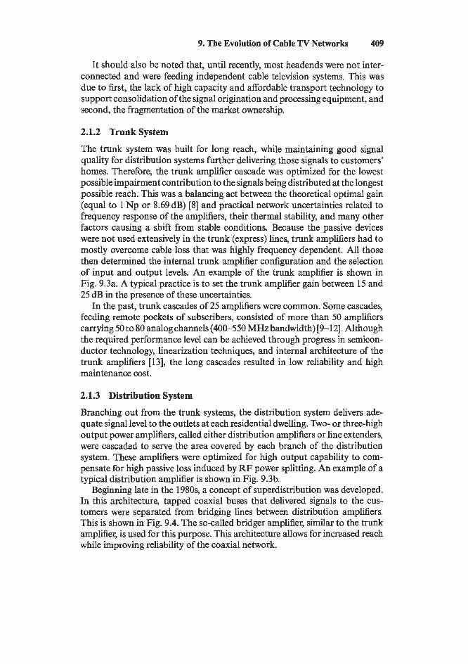
9. The Evolution of Cable TV Networks 409
It should also be noted that, until recently, most headends were not inter- connected and were feeding independent cable television systems. This was due to first, the lack of high capacity and affordable transport technology to support consolidation of the signal origination and processing equipment, and second, the fragmentation of the market ownership.
2.1.2 Trunk System
The trunk system was built for long reach, while maintaining good signal quality for distribution systems further delivering those signals to customers’ homes. Therefore, the trunk amplifier cascade was optimized for the lowest possible impairment contribution to the signals being distributed at the longest possible reach. This was a balancing act between the theoretical optimal gain (equal to 1 Np or 8.69 dB) [8] and practical network uncertainties related to frequency response of the amplifiers, their thermal stability, and many other factors causing a shift from stable conditions. Because the passive devices were not used extensively in the trunk (express) lines, trunk amplifiers had to mostly overcome cable loss that was highly frequency dependent. All those then determined the internal trunk amplifier configuration and the selection of input and output levels. An example of the trunk amplifier is shown in Fig. 9.3a. A typical practice is to set the trunk amplifier gain between 15 and 25 dB in the presence of these uncertainties.
In the past, trunk cascades of 25 amplifiers were common. Some cascades, feeding remote pockets of subscribers, consisted of more than 50 amplifiers carrying 50 to 80 analog channels (400-550 MHz bandwidth) [9-121. Although the required performance level can be achieved through progress in semicon- ductor technology, linearization techniques, and internal architecture of the trunk amplifiers [13], the long cascades resulted in low reliability and high maintenance cost.
2.1.3 Distribution System
Branching out from the trunk systems, the distribution system delivers ade- quate signal level to the outlets at each residential dwelling. Two- or three-high output power amplifiers, called either distribution amplifiers or line extenders, were cascaded to serve the area covered by each branch of the distribution system. These amplifiers were optimized for high output capability to com- pensate for high passive loss induced by RF power splitting. An example of a typical distribution amplifier is shown in Fig. 9.3b.
Beginning late in the 1980s, a concept of superdistribution was developed. In this architecture, tapped coaxial buses that delivered signals to the cus- tomers were separated from bridging lines between distribution amplifiers. This is shown in Fig. 9.4. The so-called bridger amplifier, similar to the trunk amplifier, is used for this purpose. This architecture allows for increased reaGh while improving reliability of the coaxial network.
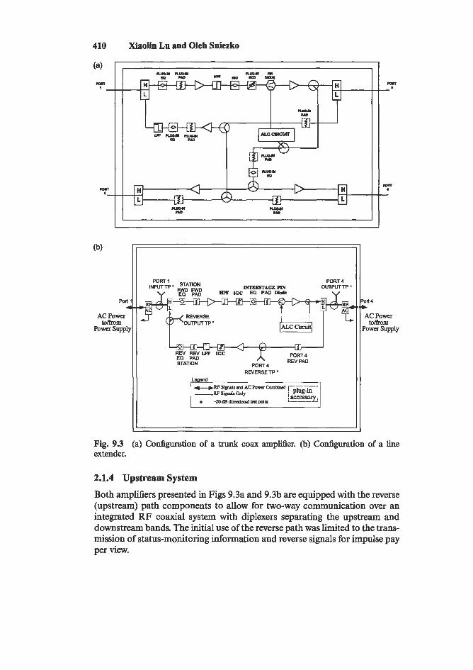
Xiaolin Lu and Oleh Sniezko
I
m
AC Power toniwm
Powa suppl:
PORT 4 INTERSTAGE PIN
EPF IDC E9 PAD Diode
REV REVLPF IGC E9 PAD STATION WRT 4 . .
REVERSE TP *
*rI 4 b AC Power
tolfmm Power Supply
Fig. 9.3 (a) Configuration of a trunk coax amplifier. (b) Contiguration of a line extender.
2.1.4 Upstream System
Both amplifiers presented in Figs 9.3a and 9.3b are equipped with the reverse (upstream) path components to allow for two-way communication over an integrated RF coaxial system with diplexers separating the upstream and downstream bands. The initial use of the reverse path was limited to the trans- mission of status-monitoring information and reverse signals for impulse pay per view.
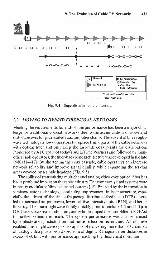
9. The Evolution of Cable TV Networks 411
Trunk and Super-D Coax Cable
Fig. 9.4 Superdistribution architecture.
2.2 MOVING TO HYBRID FIBEWCOAX NETWORKS
Meeting the requirements for end-of-line performance has been a major chal- lenge for traditional coaxial networks due to the accumulation of noise and distortion over long, cascaded coax amplifier chains. The advent of linear light- wave technology allows operators to replace trunk parts of the cable networks with optical fiber and only keep the last-mile coax plants for distribution. Pioneered by ATC (part of today's AOWTime Warner) and followed by many other cable operators, the fiber-backbone architecture was developed in the late 1980s [14-171. By shortening the coax cascade, cable operators can increase network reliability and improve signal quality, while expanding the serving areas covered by a single headend (Fig. 9.5).
The ability of transmitting multichannel analog video over optical fiber has had a profound impact on the cable industry. The commonly used systems were intensity modulated/direct detected systems [ 181. Enabled by the innovation in semiconductor technology, continuing improvement in laser structure, espe- cially the advent of the single-frequency-distributed-feedback (DFB) lasers, led to increased output power, lower relative-intensity noise (RIN), and better linearity. The linear lightwave family quickly grew to include 1.3 and 1.5 km DFB lasers, external modulators, and erbium-doped fiber amplifiers (EDFAs) to further extend the reach. The system performance was also enhanced by sophisticated predistortion and noise reduction techniques. All of these enabled linear lightwave systems capable of delivering more than 80 channels of analog video plus a broad spectrum of digital-RF signals over distances in excess of 60 km, with performance approaching the theoretical optimum.

412 Xiaolin Lu and Oleh Sniezko
1000 900 800 700 600 500 400 300 200
- N I 3 5 .- U
U S s m m
w---
- Optical Fiber Cable ___ Trunk Coax Cable
Fig. 9.5 Fiber backbone architecture.
100 I 1 0 1 I I I I
1962 1967 1972 1977 1982 1987 1992 1997 2002 Years
Fig. 9.6 Bandwidth expansion of cable network.
3. An End-to-End HFC Network
Linear lightwave technology not only enables the cable operator to replace coaxial trunk with optical fiber to achieve high capacity, quality, and reliabil- ity, but also allows for the interconnection of many distribution networks to increase network flexibility and to further reduce operating costs.
The total bandwidth in a cable network has expanded exponentially over the past 35 years, initially enabled by technology innovations in R F devices and further accelerated by the deployment of fiber-optics (Fig. 9.6). Most recently,

9. The Evolution of Cable TV Networks 413
Metro Network Secondary Ring Access Network
Fig. 9.7 A modern hybrid fiberlcoax cable network.
emerging interactive services, always-on applications, and therefore substan- tially increased network usage increase the demand for further bandwidth expansion per user in both downstream and upstream directions. Compet- itive pressures, on the other hand, motivated network evolution toward cost reduction and operating savings. All of these, as well as increased cus- tomer expectation for quality and reliability, led to technology innovations in transforming the traditional broadcast cable network into a broadband two- way infrastructure, and further to an end-to-end digital platform with wide implementation of the advances in lightwave and digital technologies.
In North America, a modern cable network typically consists of three major sections, as shown in Fig. 9.7:
1. Metro network, 2. Secondary ring, 3. Access network.
3.1 METRO MARKET ARCHITECTURE
In the late 1980s and early 1990s, metro market consolidation (or clustering) among cable TV operators accelerated significantly. In parallel with this trend, new services and changes in the competitive landscape increased pressure on the cable TV industry to develop the capacity to deliver a multitude of services at a much larger scale and serve those clustered areas in a more cost-effective way. Pioneered by engineers of Rogers Cablesystems in Canada, a metro fiber ring architecture to interconnect clustered HFC distribution networks was established and was later adopted by CableLabs as a recommended metro market architecture for the North America cable industry [19, 201.
Today, most of the metro networks in markets exceeding 100,000 homes resemble ring configurations (single or dual rings). Numerous so-called mater headends, sometimes operated by different multiple system operators (MSOs),

414 Xiaolin Lu and Oleh Sniezko
are connected by the metro rings with full redundancy and survivability. These mater headends typically serve as the primary signdcontent sources, and potentially also serve as interconnection points with other service providers (ISPs, ILECs, and CLECs) for high-speed data and telecommunication ser- vices. Traditional separated (stand-alone) headends are consolidated into a so-called primary hub, which are interconnected by the market rings with the mater headends and serve as furtber signal distribution points. These primary hubs typically serve 60,000 to 100,000 homes.
In the past, the choice of transmission technology over the metro ring was based mostly on the requirements for signal quality and on technology availability (including its cost). Also, the transport systems in the metro mar- kets were historically built to meet the requirements of certain services at that time. Since the headend consolidation began when broadcast video ser- vices dominated, the transport systems were therefore optimized for these signals. An analysis of the video transport systems used in metro markets is shown in Table 9.1, which reflects the results of several studies performed by major MSOs.
It should be noted that the deployment of the SONET-based systems in the cable industry was slow in the past because video distribution over the metropolitan rings had been monopolized by the cost-effective, proprietary, linear PCM systems. However, these systems provided only limited support for transport of voice and data services.
This situation changed in the mid-1990s when high-speed data, digital video, and digital telephony services were introduced. To support delay- sensitive voice service, as well as high-speed data services, operators started deploying SONET rings in parallel to the embedded proprietary systems. Recently, the increasing need for a common IP infrastructure to support integrated services with reduced OAM&P (operation, administration, and pro- vision) cost further stimulated the integration of the layered protocol stack. AU these resulted in a mixed transport system being deployed in the metro markets, therefore imposing a big challenge to metro network migration. Any new metro network infrastructure has to support not only legacy services, but also emerg- ing services, both of which employ a wide variety of formats and protocols.
These requirements demand the capability of multiplexing and demultiplex- ing to DSl level, while being able to perform optical aggregation at OC-48, OC- 192, and even higher speeds. The metro network needs to support standard interfaces for MPEG-2 video service, as well as native Ethernet interface for data service. It also needs to accommodate many different protocols for net- working and management purposes, such as 802.1 p/Q Layer 2 protocol, Border Gateway Protocol (BGP), Open Shortest Path First (OSPF) Layer 3 protocols, as well as emerging multiprotocol label switching (MPLS)-types of protocols.
In addition, efficient trafEc protection and recovery mechanisms continue to be a critical feature in the new transport platforms. Preeminent among
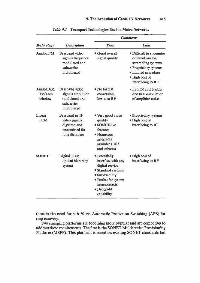
9. The Evolution of Cable TV Networks 415
Table 9.1 Transport Technologies Used in Metro Networks
Comments
Technology Description pros Cons
Analog FM Baseband video signals frequency modulated and subcarrier multiplexed
Analog AM Baseband video 1550-nm signals amplitude window modulated and
subcarrier multiplexed
Linear Baseband or IF PCM video signals
digitized and transmitted for long distances
SONET Digital TDM optical hierarchy system
Good overall Difficult to encounter
scrambling systems Proprietary systems Limited cascading High cost of interfacing to RF
signal quality different analog
SONET-like interfacing to RF features Numerous interfaces available (DS3 and subsets)
Proprietary systems
Potentially High cost of interface with any digital service Standard systems Survivability Perfect for system interconnects Dropladd capability
interfacing to RF
these is the need for sub-50-ms Automatic Protection Switching (APS) for ring recovery.
Two emerging platforms are becoming more popular and are competing to address these requirements. The first is the SONET Multiservice Provisioning Platform (MSPP). This platform is based on existing SONET standards but
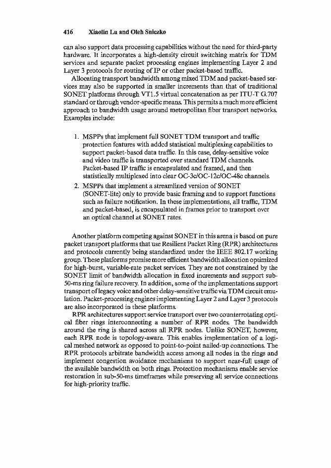
416 Xiaolin Lu and Oleh Sniezko
can also support data processing capabilities without the need for third-party hardware. It incorporates a high-density circuit switching matrix for TDM services and separate packet processing engines implementing Layer 2 and Layer 3 protocols for routing of IP or other packet-based traffic.
Allocating transport bandwidth among mixed TDM and packet-based ser- vices may also be supported in smaller increments than that of traditional SONET platforms through VT1.5 virtual concatenation as per ITU-T G.707 standard or through vendor-specific means. This permits a much more efficient approach to bandwidth usage around metropolitan fiber transport networks. Examples include:
1. MSPPs that implement full SONET TDM transport and traffic protection features with added statistical multiplexing capabilities to support packet-based data traffic. In this case, delay-sensitive voice and video traffic is transported over standard TDM channels. Packet-based IP traffic is encapsulated and framed, and then statistically multiplexed into clear OC-3c/OC-12c/OC-48~ channels.
(SONET-lite) only to provide basic framing and to support functions such as failure notification. In these implementations, all trafEc, TDM and packet-based, is encapsulated in frames prior to transport over an optical channel at SONET rates.
2. MSPPs that implement a streamlined version of SONET
Another platform competing against SONET in this arena is based on pure packet transport platforms that use Resilient Packet Ring (RPR) architectures and protocols currently being standardized under the IEEE 802.17 working group. These platforms promise more efficient bandwidth allocation optimized for high-burst, variable-rate packet services. They are not constrained by the SONET limit of bandwidth allocation in fixed increments and support sub- 50-ms ring failure recovery. In addition, some of the implementations support transport of legacy voice and other delay-sensitive t r a c via TDM circuit emu- lation. Packet-processing engines implementing Layer 2 and Layer 3 protocols are also incorporated in these platforms.
RPR architectures support service transport over two counterrotating opti- cal fiber rings interconnecting a number of RPR nodes. The bandwidth around the ring is shared across all RPR nodes. Unlike SONET, however, each RPR node is topology-aware. This enables implementation of a logi- cal meshed network as opposed to point-to-point nailed-up connections. The RPR protocols arbitrate bandwidth access among all nodes in the rings and implement congestion avoidance mechanisms to support near-full usage of the available bandwidth on both rings. Protection mechanisms enable service restoration in sub-50-ms timeframes while preserving all service connections for high-priority t r a c .
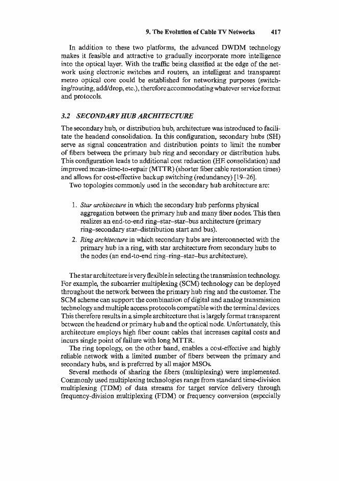
9. The Evolution of Cable TV Networks 417
In addition to these two platforms, the advanced DWDM technology makes it feasible and attractive to gradually incorporate more intelligence into the optical layer. With the t r a c being classified at the edge of the net- work using electronic switches and routers, an intelligent and transparent metro optical core could be established for networking purposes (switch- ing/routing, adddrop, etc.), therefore accommodating whatever service format and protocols.
3.2 SECONDARY HUB ARCHITECTURE
The secondary hub, or distribution hub, architecture was introduced to facili- tate the headend consolidation. In this configuration, secondary hubs (SH) serve as signal concentration and distribution points to limit the number of fibers between the primary hub ring and secondary or distribution hubs. This configuration leads to additional cost reduction (HE consolidation) and improved mean-time-to-repair (MTTR) (shorter fiber cable restoration times) and allows for cost-effective backup switching (redundancy) [ 19-26].
Two topologies commonly used in the secondary hub architecture are:
1. Star architecture in which the secondary hub performs physical aggregation between the primary hub and many fiber nodes. This then realizes an end-to-end ring-star-star-bus architecture (primary ring-secondary star-distribution start and bus).
primary hub in a ring, with star architecture from secondary hubs to the nodes (an end-to-end ring-ring-star-bus architecture).
2. Ring architecture in which secondary hubs are interconnected with the
The star architecture is very flexible in selecting the transmission technology. For example, the subcarrier multiplexing (SCM) technology can be deployed throughout the network between the primary hub ring and the customer. The SCM scheme can support the combination of digital and analog transmission technology and multiple access protocols compatible with the terminal devices. This therefore results in a simple architecture that is largely format transparent between the headend or primary hub and the optical node. Unfortunately, this architecture employs high fiber count cables that increases capital costs and incurs single point of failure with long MTTR.
The ring topology, on the other hand, enables a cost-effective and highly reliable network with a limited number of fibers between the primary and secondary hubs, and is preferred by all major MSOs.
Several methods of sharing the fibers (multiplexing) were implemented. Commonly used multiplexing technologies range from standard time-division multiplexing (TDM) of data streams for target service delivery through frequency-division multiplexing (FDM) or frequency conversion (especially
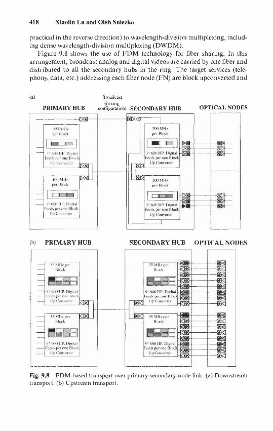
418 Xiaolin Lu and Oleh Sniezko
- - -
- - -
practical in the reverse direction) to wavelength-division multiplexing, includ- ing dense wavelength-division multiplexing (DWDM).
Figure 9.8 shows the use of FDM technology for fiber sharing. In this arrangement, broadcast analog and digital videos are carried by one fiber and distributed to all the secondary hubs in the ring. The target services (tele- phony, data, etc.) addressing each fiber node (FN) are block upconverted and
200 MHz per Block
3* 600 HP Digital Feeds per one Block
Up Converter
200 MHz per Block
3* 600 HP Digital Feeds per one Block
Up Converter
(a) Broadcast (in ring
PRIMARY HUB configuration) SECONDARY HUB OPTICAL NODES
(b) PRIMARY HUB
3' 600 HP Digital
3* 600 HP Digital Feeds per one Block
SECONDARY HUB OPTICAL NODES
E* 600 HP Digita 'eed, per one Bloc
Fig. 9.8 FDM-based transport over primary-secondary-node link. (a) Downstream transport. (b) Upstream transport.

9. The Evolution of Cable TV Networks 419
combined at the primary hub and transmitted to the secondary hub over a separate fiber. They are then downconverted to the original frequency at the secondary hub, and are directed to each fiber node accordingly. The upstream transmission uses the same principle.
DWDM technology has been considered a very desirable solution, but has matured to support SCM signals in the cable TV environment only in recent years. As shown in Fig. 9.9, instead of multiplexing target services (addressing each FN) over RF frequency (as in the FDM case), these signals are multiplexed over optical wavelength [26]. With the fast-paced DWDM
(a) PRIMARY HUB SECONDARY HUB
(b) PRIMARY HUB SECONDARY HUB OPTICAL NODES I
1~~~~~~~~~~~~~~~~~~~~
I I I I I I I I I I I I I I I I I I I I I I I I I I I I I I I I I I I I I I I I I I
I I I I I 1 I--------;
( _ _ _ _ _ _ _ _ _ _ _ _ _ _ _ _ _ _ _ _ _ _ _ _ _
I I 1 I I I
I I I I
I I I I I I I I I I I I I I I I I I I I I I I I I I I I I I I I I
I I
I I I I I I I I I I
I I I
I I I I
I I I
I I
I I I I I I I I
Fig. 9.9 DWDM-based transport over primary-secondary-node link. (a) Down- stream transport. (b) Upstream transport.
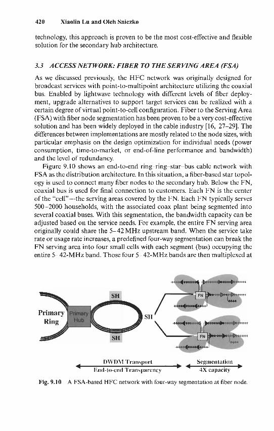
420 Xiaolin Lu and Oleh Sniezko
technology, this approach is proven to be the most cost-effective and flexible solution for the secondary hub architecture.
3.3 ACCESS NETWORK: FIBER TO THE SERVING AREA (FSA)
As we discussed previously, the HFC network was originally designed for broadcast services with point-to-multipoint architecture utilizing the coaxial bus. Enabled by lightwave technology with different levels of fiber deploy- ment, upgrade alternatives to support target services can be realized with a certain degree of virtual point-to-cell configuration. Fiber to the Serving Area (FSA) with fiber node segmentation has been proven to be a very cost-effective solution and has been widely deployed in the cable industry [16, 27-29]. The differences between implementations are mostly related to the node sizes, with particular emphasis on the design optimization for individual needs (power consumption, time-to-market, or end-of-line performance and bandwidth) and the level of redundancy.
Figure 9.10 shows an end-to-end ring-ring-star-bus cable network with FSA as the distribution architecture. In this situation, a fiber-based star topol- ogy is used to connect many fiber nodes to the secondary hub. Below the FN, coaxial bus is used for final connection to customers. Each FN is the center of the “cell”-the serving areas covered by the FN. Each FN typically serves 500 -2000 households, with the associated coax plant being segmented into several coaxial buses. With this segmentation, the bandwidth capacity can be adjusted based on the service needs. For example, the entire FN serving area originally could share the 5-42 MHz upstream band. When the service take rate or usage rate increases, a predefined four-way segmentation can break the FN serving area into four small cells with each segment (bus) occupying the entire 5-42-MHz band. Those four 5-42-MHz bands are then multiplexed at
4 b 4 DWDM Transport Segmentation
End-to-end Transparency 4~ capacity
Fig. 9.10 A FSA-based HFC network with four-way segmentation at fiber node.

9. The Evolution of Cable TV Networks 421
FN using DWDM technology. This effectively increases the upstream band- width by a factor of four without adding new fibers and still maintaining the end-to-end transparency.
4. Photonic Moore’s Law and Deep Fiber Penetration
The innovation in and implementation of photonic technology has occurred at a much faster rate than Moore projected for the computer industry. The linear laser made it possible for optical transport technology to be introduced into the cable industry’s networks. This, in turn, created tremendous opportunities for advanced services delivery that otherwise would be difficult over conventional twisted-pair-based telephony networks or purely coaxial R F networks.
The aggressive deployment of lightwave technology, especially in access networks, has resulted in a decrease in the price of photonic components and systems at a rate of 1.5 times that of electronics and digital signal processing (DSPs). This trend has accelerated deeper fiber penetration and the widespread deployment of photonic technology [29].
All these changes enable new architecture alternatives and different ways of operating the networks and lead to the industry’s continuous efforts in defining and redefining architectural solutions to capture the ever-changing landscape of service demand and affordability (costlbenefit ratio) of new technological solutions.
4.1 MINI FIBER NODE FOR FIBER OVERLAY
To resolve upstream limitations (ingress noise and bandwidth) and to simplify terminal operation, mini fiber node (mFN) technology was proposed [30, 3 11. Using emerging lightwave technology, the existing network is overlaid with a fiber-to-the-bridger architecture to exploit the large ingress-free bandwidth at high frequency for two-way digital services. As shown in Fig. 9.1 1, independent of existing systems, the mFNs couple directly into the passive coax legs (with drop taps) after each distribution coax amplifier (i.e., line extender). Each
New Services I
Fig. 9.11 The mini fiber node fiber overlay architecture.

422 Xiaolin Lu and Oleh Sniezko
mFN contains a low-cost laser and a low-cost PIN receiver, and is connected to the hub with separate fiber.
Based on this strategy, the mFNs subdivide the FN serving areas into small cells (e.g., 50 HHP/mFN) and exploit the clean and large bandwidth at high frequency for both upstream and downstream transmission. The mFN there- fore creates a new path for digital services without affecting analog TV services carried by conventional FN/amplified-coax paths. All services are then merged over passive coax distribution legs.
By exploiting the clean and large bandwidth, this strategy increases overall system bandwidth beyond current coax amplifier limitations for new digital services without replacing coax amplifiers and changing amplifier spacing. It also eliminates the need for complex noise avoidance (e.g., frequency hopping) and signal conditioning techniques (FEC, interleaving, and so on) deployed to increase the immunity of the upstream signals to interference commonly encountered in the traditional 5- 42-MHz upstream band. This simplifies system operation and reduces the cost of the terminal equipment.
Also, because mFNs only carry digital subcarrier signals over a clean high- frequency band, low-cost, low-power consumption and space-saving optical and RF components can be used in the mFNs and also at the headend.
4.2 LIGHTWIRETM FOR DEEP FIBER PENETRATION
Bringing fiber deeper into the network incurs certain incremental costs. Reduc- ing the cost of fibering (material and labor) then becomes critical. The mFN strategy simplifies system operation for new services and reduces related ter- minal costs. However, it would be more compelling if the front-end costs can be justified by operational savings over the entire network, both embedded and mFN overlay.
To achieve this goal and to establish a platform that can improve the per- formance of the embedded system while also evolving to meet future needs and simplify operations across the entire network, the baseline mFN configu- ration was transformed into a LightWireTM architecture [27-291. As shown in Fig. 9.12, instead of overlaying over the existing coaxial amplifiers, mFNs
Fig. 9.12 The LightWirem architecture.

9. The Evolution of Cable TV Networks 423
eliminate all the coaxial amplifiers (typically one mFN will eliminate two to three coaxial amplifiers). Between each mFN and the customers, passive coaxial plant is used to carry both legacy and new services.
Fibers connecting multiple mFNs are terminated at the MuxNode that resides either at the original fiber node location or at a location that “con- solidates” multiple FNs. As its name implies, the MuxNode performs certain concentration and distribution functions It “multiplexes” the upstream sig- nals and sends them to the primary hub through the secondary hubs. It also “demultiplexes” the downstream signals received from the PH-SH fiber trunks and distributes them to m F N s .
One of the interesting features of this architecture is that it maintains the characteristics of conventional HFC networks of being transparent to dif- ferent signal formats and protocols, therefore fully supporting the existing operation for current services. One preferred approach is to transmit down- stream broadcast signals, including analog and digital video, over dedicated fiber from the primary hub to the secondary hub. The existing narrowcast and switched signals, such as telephony and high-speed data using DOCSIS-based cable modems and set-top boxes will be DWDM multiplexed at the PH and transmitted over another fiber to the secondary hub. After DWDM demulti- plexing, the narrowcast and switched signals will be optically combined with the broadcast signals (in a different RF band) and transmitted to the MwrNode over optical fiber.
At the MuxNode, those combined downstream signals will be optically ampliiied and distributed to multiple mFNs over optical fiber. Given the short distance between the MuxNode and the mFN, it is also feasible to move the EDFA from the MuxNode to the secondary hub and only keep the optical splitter at the MuxNode, therefore simplifying the MuxNode. Other options, such as relasing at the MuxNode, are also promising.
The mFN performs the same function as that of a typical FN. It receives downstream signals and distributes them to customers over passive coax cable. In the upstream direction, the mFN combines upstream signals from all the coax branches it serves and transmits them to the MuxNode over optical fiber.
The MuxNode further performs O/E conversion to those upstream signals from the mFNs, RF combines them, and transmits to the secondary hub using a wavelength-speczed laser. Upstream signals from multiple MuxNodes will then be DWDM multiplexed at the SH and transmitted to the PH. Besides DWDM multiplexing, another option is to relase upstream signals at the SH.
To expand capacity of the system, one can frequency shift the upstream signals at each mFN such that when they are combined at the MuxNode, they will be at separate RF bands. If the relasing option is used at the SH, the frequency stacking could also be deployed at the MuxNode. With the passive coax distribution system, this architecture can also support bandwidth expansion at higher frequency range (800-1000 MHz), similar to that of the original mFN overlay architecture.

424 Xiaolin Lu and Oleh Sniezko
Fig. 9.13 Active component reduction in LightWireTM network. (a) Conventional FSA-based HFC network. (b) LightWireTM network.
4.2.1 Life Cycle Cost
One of the biggest advantages of this architecture is the elimination of all the coax amplifiers. This results in substantial reduction in active components, and therefore reduction in overall network power consumption (Fig. 9.13). In addition, sweeping and maintenance of active components in the field will be reduced, which leads to further operation savings. It is estimated that annual operation savings, including reduction in customer calls, etc., could reach $1 l/HHP.
Due to a significant reduction in the number of active devices and the progress in RF active component technology, the power consumption of the network elements will be decreased by at least 50%. This will allow.for powering architecture optimization and for less challenging powering of the customer terminal devices.
4.3 OXiomTM FOR COST-EFFECTIVE NETWORK EXPANSION
One challenge the industry is facing is to provide flexibility for future expansion and growth provisioning while minimizing the incremental cost and service interruption. Also, bringing fiber deeper into the network incurs certain capi- tal costs and also potentially increases the needs of fiber handling. To address this need, a so-called OXiomTM architecture was proposed (Fig. 9.14) [28, 291. While maintaining the same passive coax plant as in the LightWireTM architec- ture, the mFNs, based on their geographic locations, are daisy chained together with three fibers: one carrying downstream broadcast signals, one carrying the remaining downstream narrowcast signals, and one carrying upstream signals. This therefore implements an optical bus (physical), whereas the pre- vious LightWireTM architecture is a physical star. The advantages are the reduced fiber handling and the lower cost associated with it, and the flexibility for future expansion and growth (the optical bus can be further expanded to
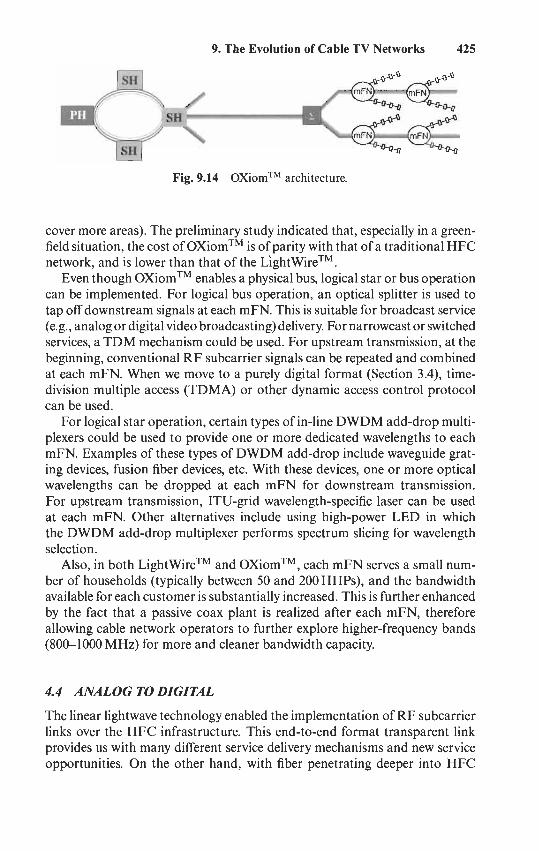
9. The Evolution of Cable TV Networks 425
Fig. 9.14 OXiomTM architecture.
cover more areas). The preliminary study indicated that, especially in a green- field situation, the cost of OXiomTM is of parity with that of a traditional HFC network, and is lower than that of the LightWireTM.
Even though OXiomTM enables a physical bus, logical star or bus operation can be implemented. For logical bus operation, an optical splitter is used to tap off downstream signals at each mFN. This is suitable for broadcast service (e.g., analog or digital video broadcasting) delivery. For narrowcast or switched services, a TDM mechanism could be used. For upstream transmission, at the beginning, conventional R F subcarrier signals can be repeated and combined at each mFN. When we move to a purely digital format (Section 3.4), time- division multiple access (TDMA) or other dynamic access control protocol can be used.
For logical star operation, certain types of in-line DWDM add-drop multi- plexers could be used to provide one or more dedicated wavelengths to each mFN. Examples of these types of DWDM add-drop include waveguide grat- ing devices, fusion fiber devices, etc. With these devices, one or more optical wavelengths can be dropped at each mFN for downstream transmission. For upstream transmission, ITU-grid wavelength-specific laser can be used at each mFN. Other alternatives include using high-power LED in which the DWDM add-drop multiplexer performs spectrum slicing for wavelength selection.
Also, in both LightWireTM and OXiomTM, each mFN serves a small num- ber of households (typically between 50 and 200 HHPs), and the bandwidth available for each customer is substantially increased. This is further enhanced by the fact that a passive coax plant is realized after each mFN, therefore allowing cable network operators to further explore higher-frequency bands (800-1 000 MHz) for more and cleaner bandwidth capacity.
4.4 ANALOG TO DIGITAL
The linear lightwave technology enabled the implementation of R F subcarrier links over the HFC infrastructure. This end-to-end format transparent link provides us with many different service delivery mechanisms and new service opportunities. On the other hand, with fiber penetrating deeper into HFC

426 Xiaolin Lu and Oleh Sniezko
networks, the proliferation of RF technology, together with the power of DSP, motivates using the ultimate transmission format over optical fiber and distributing certain control functions into the networks to simplify opera- tion and improve network scalability. Terminating RF subcarrier links at the fibedmetallic transition point and enabling a pure digital platform over the optical link therefore makes more sense, if not just from a cost reduction point of view.
One of the first steps towards the digital platform is to digitize the entire upstream band at the FN or mFN location [32], sending the digital signals to the headend at which the original signal format is reassumed. By doing so, the high-quality linear upstream laser can be replaced by a low-cost digital laser, therefore reducing the cost of upstream transport.
Beyond digitizing the upstream RF bands, a complete “demarcation” func- tion can be performed at the mFN or FN location [27-311. The upstream RF subcarrier signals from the coax plant are demodulated to digital baseband for transmitting over the optical fiber to the headend, while the downstream signals from the headend are carried over the optical fiber in native digital baseband format and modulated to the RF carriers at the mFN or FN for further distribution over the coax plant. In addition, the unique position of each mFN enables a considerable simplification in defining media access control (MAC) protocols. Each mFN can perform local policing and resolve upstream contention within its serving area without involving other parts of the networks. This can be accomplished by using any standard MAC pro- tocol, such as DOCSIS [33]. Other options include incorporating a simple out-of-band signaling loopback scheme such that users know the upstream channel status prior to transmission. This enables the use of standard, but full-duplex, Ethernet protocol (CSMAICD), and therefore the use of stan- dard and lowcost terminals (modified Ethernet transceiver, Ethernet bridger and Ethernet card). No ranging is needed, and the headend becomes virtually operation-free. The relative small roundtrip delay between each user and the mFN (-2000 ft) also substantially increases bandwidth efficiency and reduces contention delay.
The typical headend equipment can therefore be distributed into the network. In the case discussed here, the RF interface (modulator and demodulator) and MAC functions are placed at mFNs or FNs, and the multi- plexing/demultiplexing functions can be placed at the secondary hub [27-3 11. By doing this, the current RF optical transmitters and receivers can be replaced by digital ones, and passive optical network (PON) technology, such as the spectrum slicing technique with high-power LED and DWDM adddrop at each mFN or FN, can be utilized. This further simplifies the transport net- work, reduces its cost, improves service performance, and enhances network flexibility and scalability.

9. The Evolution of Cable TV Networks 427
5. Technology Enablers
All the architectural evolutions in building modern cable networks have been facilitated by the advances in lightwave, RF, and DSP technologies. In this section, we will describe some of the fundamental technologies that enabled today's broadband HFC network and some of their impacts on system operation.
5.1 RF TECHNOLOGY
The bandwidth of the broadband coaxial network has expanded exponentially over the last 35 years, facilitated by the progress in RF-active device technology that provides the capability of accommodating higher loss at higher frequency while maintaining the same level of performance at the subscriber outlet. As a result of this progress, the number of active devices per mile increased mini- mally, whereas the bandwidth increased more than three times, as shown in Table 9.2. This was achieved by several RF amplifier techniques described below [lo, 19, 34-38].
5.1.1 Push-Pull Hybrids
The first important achievement in the RF amplifier technology was the intro- duction of the push-pull hybrids. These addressed second-order distortion problems that occurred during expansion of the cable TV network bandwidth over one octave. As shown in Fig. 9.15a' if the phase shift in both arms of the amplification block is exactly 180", the even harmonics of the output signal will be eliminated, whereas odd harmonics will not be affected.
5.1.2 Power-Doubling Hybrids
The push-pull block effectively reduced second-order and other even-order nonlinear distortions. However, with further bandwidth expansion and with
Table 9.2 Actives Per Mile vs. Forward Bandwidth Expansion
Bandwidth A ctivesRMile
250 M H z (50-300) 4.0 350 M H z (50-400) 4.2 400 M H z (50-450) 4.5 500 M H z (5Cb550) 4.7 700+ MHz (50-870) 5.2

428 Xiaolin Lu and Oleh Sniezko
9. The Evolution of Cable TV Networks 429
increased numbers of carriers, third-order distortions in the form of compos- ite triple beats (CTBs) became the dominant limiting factor. Power-doubling techniques resolved this issue.
In the configuration shown in Fig. 9.15b, the output level of each ampli- fier (in itself built in push-pull configuration) arm is lower by three dB with respect to the total output level of the amplification block. Therefore, even though the total output level remains the same, the "doubling" mechanism, in which each arm contributes 3 dB less gain, results in 3 dB less second-order distortion overall and 6 dB less third-order distortion. This configuration can be further extended into a quad configuration where power-doubling blocks were used in both arms. However, further improvements with this method- ology were limited by exponential increases in power consumption, doubled for each power-doubling configuration. Therefore, the single power-doubling configuration is commonly used today.
5.1.3 Feed-Forward Technology
In order to improve the linearity of the amplification block by a sizeable amount, a feed-forward amplification technique was introduced [34-361. As shown in Fig. 9 . 1 5 ~ ~ the signal was split to feed main and error arms. The signal in the error arm is shifted 180" and combined with a portion of the original signal directed from the main arm. Under the assumption of accu- rate level balancing, the input signal would be eliminated and only nonlinear distortions from the main arm would be present at the input of the error ampli- fier. After ampucation and phase shifting by 180", these distortions would be added to the main arm signal. Theoretically, with perfect phase and gain balance over the entire bandwidth, the distortions would be completely elim- inated. Practically, the improvement or cancellation factor was not infinite, but was significantly higher than in the power-doubling configuration. In the past, the feed-forward technique was commonly used in trunk amplifiers for bandwidths up to 550 MHz. Due to the increasing difficulty of balancing the main and error arms with increased bandwidth, and the introduction of light- wave technologies that eliminated long trunk amplifier cascades, the use of this technique has been substantially reduced.
5.1.4 New Developments
The most recent progress in RF amplifiers occurs in several areas. One is the use of GaAs technology. Amplifiers using this technology have significantly improved output level capacity for the same level of nonlinear distortion with slightly lower power consumption.
Other areas of focus are the predistortion and linearization techniques commonly used in lightwave technologies for laser transmitter linearization. The continual cost reduction of the linearization techniques allows for their wide deployment in RF amplifier devices. Further, maturity and cost reduction

430 Xiaolin Lu and Oleh Sniezko
in certain RF technologies initially used in wireless communication make it fea- sible for its applications in the cable network. All of these continually improve coax network performance, increase its bandwidth capacity, and enhance its reliability.
5.2 LIGHT WAKE TECHNOLOGY
5.2.1 Linear Lightwave
As we discussed previously, linear lightwave technology has been one of the foundations of the modern cable network (HFC). Typical lightwave links used in RF SCM systems consist of transmitters, fiber runs, and receivers The performance of these links is determined by the performance of both active and passive components, including different phenomena occurring in fiber runs “stimulated” by the light. The lightwave link performance can be quantified by CNR and second- and third-order distortions (CSO and CTB), which directly determine the quality of the analog AM-VSB signals received at the customer premise equipment (e.g., TV set) [18, 39-60].
Excluding fiber effects, the CNR at the receiver is given by
The signal power per channel is ( m I 0 ) ~ / 2 , where m is the Optical Modulation Depth (OMD) per channel, and IO is the average received photocurrent. The denominator consists of several noise factors and the& is the noise bandwidth (4 MHz for NTSC channels). The thermal noise of the receiver is Ben;, and the shot noise is 2BeeIo, where e is the electron charge. The laser’s relative intensity noise is RlN (dB/Hz).
The noise and quantum efficiency of the receiver determines the necessary received optical power to satisfy the CNR requirement. The received optical power is related to the photocurrent by:
where tiv is the photon energy and is the quantum efficiency of the photodi- ode. From Eqs 9.1 and 9.2, one can determine the necessary optical power to achieve the desired CNR.
Besides noise, when multiple RF signals are multiplexed (FDM), the second-order and third-order distortion products that are generated within the multichannel multioctave band will affect the signal quality. For a simple (memoryless) nonlinear characteristic, the optical power can be expressed as a Taylor-series expansion of the electrical signal:
P C( xo(i + X + + bx3 + . . .), (9.3)
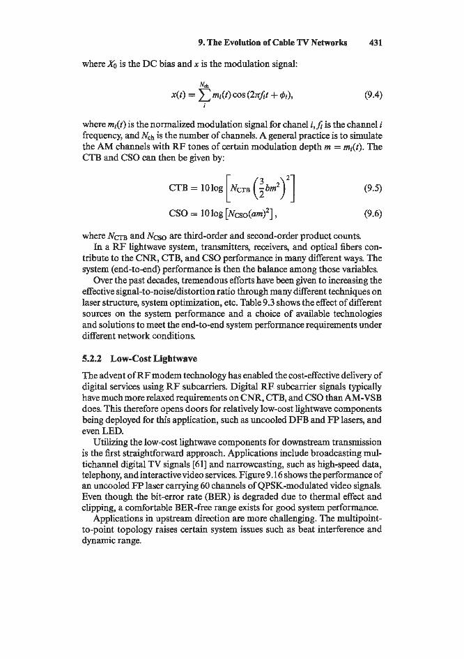
9. The Evolution of Cable TV Networks 431
where X, is the DC bias and x is the modulation signal:
where mi(t) is the normalized modulation signal for chanel i,J is the channel i frequency, and Nch is the number of channels. A general practice is to simulate the AM channels with RF tones of certain modulation depth m = mi(t). The CTB and CSO can then be given by:
cso = 10 log [Ncso(am)2] , (9.6)
where NCTB and N C ~ O are third-order and second-order product counts. In a RF lightwave system, transmitters, receivers, and optical fibers con-
tribute to the CNR, CTB, and CSO performance in many different ways. The system (end-to-end) performance is then the balance among those variables.
Over the past decades, tremendous efforts have been given to increasing the effective signal-to-noise/distortion ratio through many different techniques on laser structure, system optimization, etc. Table 9.3 shows the effect of different sources on the system performance and a choice of available technologies and solutions to meet the end-to-end system performance requirements under different network conditions.
5.2.2 Low-Cost Lightwave
The advent of RF modem technology has enabled the cost-effective delivery of digital services using RF subcarriers. Digital RF subcarrier signals typically have much more relaxed requirements on CNR, CTB, and CSO than AM-VSB does. This therefore opens doors for relatively low-cost lightwave components being deployed for this application, such as uncooled DFB and FP lasers, and even LED.
Utilizing the low-cost lightwave components for downstream transmission is the first straightforward approach. Applications include broadcasting mul- tichannel digital TV signals [61] and narrowcasting, such as high-speed data, telephony, and interactive video services. Figure 9.16 shows the performance of an uncooled FP laser carrying 60 channels of QPSK-modulated video signals. Even though the bit-error rate (BER) is degraded due to thermal effect and clipping, a comfortable BER-free range exists for good system performance.
Applications in upstream direction are more challenging. The multipoint- to-point topology raises certain system issues such as beat interference and dynamic range.
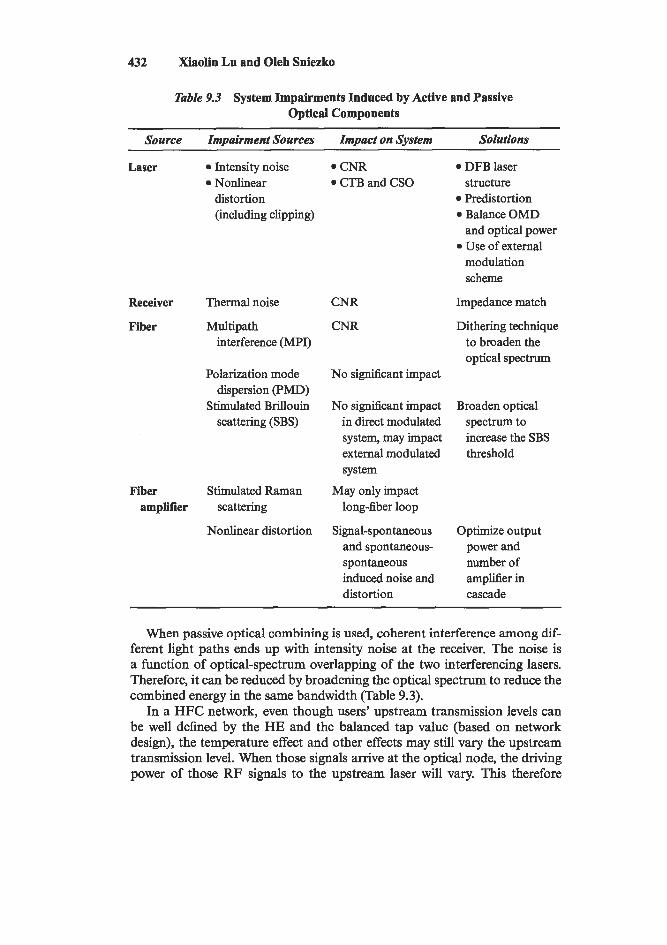
432 Xiaolin Lu and Oleh Sniezko
Table 9.3 System Impairments Induced by Active and Passive Optical Components
~
Source Impairment Sources Impact on System Solutions
Laser Intensity noise CNR DFB laser Nonlinear CTB and CSO structure distortion
Use of external and optical power
modulation scheme
Receiver Thermal noise CNR Impedance match
Fiber Multipath CNR Dithering technique interference (MPI) to broaden the
optical spectrum Polarization mode No significant impact
dispersion (PMD) Stimulated Brillouin No significant impact Broaden optical
scattering (SBS) in direct modulated spectrum to system, may impact external modulated threshold system
increase the SBS
Fiber Stimulated Raman May only impact amplifier scattering long-fiber loop
Nonlinear distortion Signal-spontaneous Optimize output and spontaneous- power and spontaneous number of induced noise and amplifier in distortion cascade
When passive optical combining is used, coherent interference among dif- ferent light paths ends up with intensity noise at the receiver. The noise is a function of optical-spectrum overlapping of the two interferencing lasers. Therefore, it can be reduced by broadening the optical spectrum to reduce the combined energy in the same bandwidth (Table 9.3).
In a HFC network, even though users’ upstream transmission levels can be well defined by the HE and the balanced tap value (based on network design), the temperature effect and other effects may still vary the upstream transmission level. When those signals arrive at the optical node, the driving power of those RF signals to the upstream laser will vary. This therefore
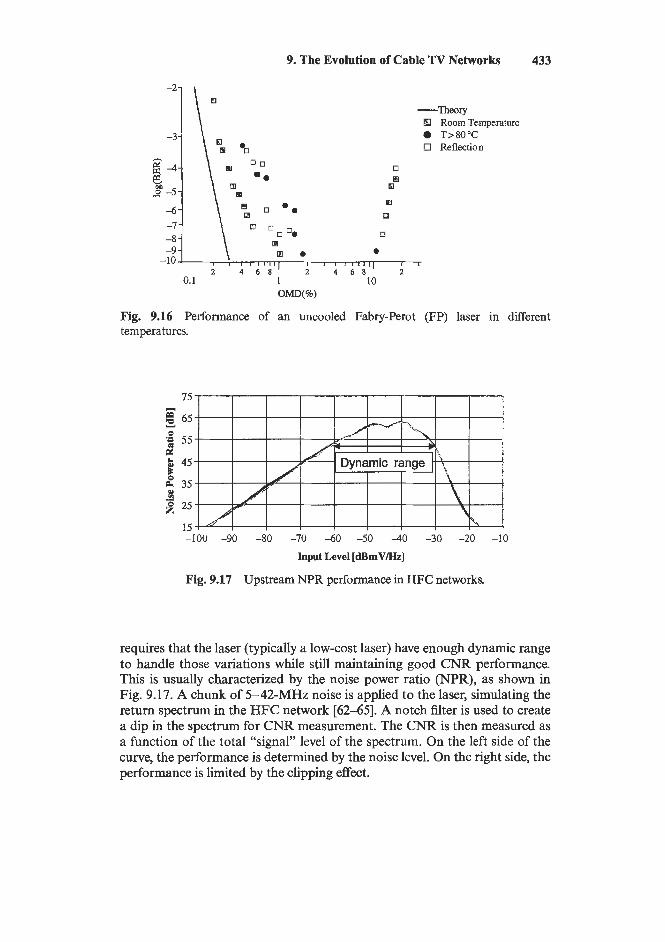

434 Xiaolin Lu and Oleh Sniezko
6. Summary
Enabled by advances in RF, lightwave, and DSP technology, cable net- works were transformed from clustered, one-way coaxial networks for analog video broadcasting to a well-interconnected, fiber-based, two-way broadband infrastructure capable of delivering a wide variety of services.
Fiber-optics has had a profound impact on the industry since the advent of linear laser. It provided a backward compatible and format transparent plat- form for cable operators to accommodate multiservice needs, and will continue to drive the evolution to a digital broadband era and platform convergence.
References
[l] T. E. Darcie, “Broadband Subscriber Access Architectures and Technologies,” OFC‘96 tutorial, 1996.
[2] N. J. Frigo, “A Survey of Fiber Optics in Local Access Architecture,” in Optical Fiber Telecommunications IIU, Academic Press, San Diego, CA, 1977.
[3] X. Lu, “Broadband Access: Technologies and Opportunities,” Globecom’99 tutorial, 1999.
[4] X. Lu, “RF Subcarrier Links in Local Access Networks,” in RF Links, Academic Press, San Diego, CAY 2001.
[5] W. S. Ciciora, Cable Television in the United States, an Overvim. CableLabs, Louisville, CO, 1995.
[a K. Simons, Technical Handbook for Cable Television Systems, 3rd Edition, Jerrold Electronics Corporation, 1968.
[A S. Dukes, “Next Generation Cable Network Architecture,” 1995 NCTA Convention Technical Papers, NCTA, Washington, D.C., pp. 8-29.
[8] G. Hart and N. Hamilton-Piercy, “Rogers Fiber Architecture,” 1989 NCTA Convention Technical Papers, NCTA, Dallas, TX, pp. 104-1 13.
[9] 0. Sniezko, “Video and Data Transmission in Evolving HFC Network,” OFC‘98, San Jose, CA, pp. 131-132.
[lo] J. C. Pavlic, “Some Consideration for Applying Several Feedforward Gain Block Models to CATV Distribution Amplifiers,” 1983 NCTA Convention Technical Papers, NCTA.
[l 11 J. €! Preschutti, “Limitations and Characteristics of Broadband Feedforward Amplifiers,” 1984 NCTA Convention Technical Papers, pp. 109-1 17.
[12] A. Prochazka, €! Lancaster, R. Neumann, “Amplifier Linearization by Com- plementary Pre- or Post-Distortion,” 1976 NCTA Convention Technical Papers, NCTA, Dallas, TX, pp. 58-66.
[ 131 K. M. Casey, “The Evolution of Cable Television Delivery Systems,” Communica- tions Engineering and Design, September 1990.
9. The Evolution of Cable TV Networks 435
[14] J. A. Chiddix, H. Laor, D. M. Pangrac, L. D. Williamson, R. W. Wolfe, “AMVideo on Fiber in CATV Systems, Need and Implementation,” J. Selet. Area Commun., 8 (1990).
[15] J. A. Chiddix, J. A. Vaughan, R. W. Wolfe, “The Use of Fiber Optics in Cable Communication Networks,” J. Lightwave Tech., 11(1), 154-166 (1993).
[16] A. E. Werner and 0. J. Sniezko, “HFC Optical Technology: Ten Years of Progress and Today’s Status, Choices and Challenges,” CED, September 1998.
[ 171 T. E. Darcie, “Subscriber Multiplexing for Multiple-Access Lightwave Networks,” IEEE J. Lightwave Tech., LT-5, 1103-1 110 (1987).
E181 M. R. Phillips and T. E. Darcie, “Lightwave Analog Video Transmission,” in Optical Fiber Telecommunications IIIA, Academic Press, San Diego, CA, 1997.
[19] A. E. Werner, “Regional and Metropolitan Hub Architecture Consideration,” SCTE Conference on Emerging Technology, 1995.
[20] T. G. Elliot and 0. J. Sniezko, “Transmission Technologies in Secondary Hub Rings-SONET versus FDM Once More,” NCTA Technical Papers, 1996.
[21] R. Balsdon, “Rogers Implements Regional Hub Fiber Network,” Lightwave Journal, August 1993.
[22] J. A. Chiddix and D. M. Pangrac, “Fiber Backbone: A Proposal for an Evolutionary CATV Architecture,” 1988 NCTA Convention Technical Papers.
[23] F! Rogan, R. B. Stelle 111, L. Williamson, “A Technical Analysis of a Hybrid FiberKOaxial Cable Television System,” 1988 NCTA Convention Technical Papers.
[24] 0. J. Sniezko and A. E. Werner, “Invisible Hub or End-to-End Transparency,” 1998 NCTA Technical Papers (1998).
[25] 0. J. Sniezko, “Video and Data Transmission in Evolving HFC Network,” OFC‘98,1998.
[26] J. W. Neil and E. Sandino, “Design and Implementation of DWDM-Based Transport Networks,” CED, September 1998.
[27] 0. Sniezko, T. Werner, D. Combs, E. Sandino, X. Lu, T. Darcie, A. Gnauck, S. Woodward, B. Desai, “HFC Architecture in the Making,” NCTA Technical Papers, 1999.
[28] 0. Sniezko and X. Lu, “HOW much ‘F’ and ‘C‘ in HFC,” ET2000,2000. [29] 0. Sniezko and X. Lu, “Beyond Moore’s Law,” 2000 NCTA Convention Technical
[30] X. Lu, T. E. Darcie, A. H. Gnauck, S. L. Woodward, B. Desai, X. Qiu, “Low-Cost
[31] X. Lu, “Broadband Access Over HFC Network,” Proceeding, OFC’97,1997. [32] D. Sipes and B. Loveless, “Deep Fiber Networks: New, Ready-to-Deploy
Architectures Yield Technical and Economic Benefits,” 1999 NCTA Technical Papers.
Papers.
Cable Network Upgrade for Two-way Broadband,” ET’98,1998.
[33] “Data Over Cable Service Interface Specifications,” Cable Labs, July 1998. [34] K. A. Simons, “Optimum Gain for CATV Line Amplifier, Communications
Engineering and Design,” Proceeding of IEEE, Special Issue on Cable Television, 58(7) (1970).
436 Xiaolin Lu and Oleh Sniezko
[35] N. Slater and D. McEwen, “Limiting Nonlinear Distortions in 400+MHz Systems,” 1984 CCTA Convention Papers.
[36] N. J. Slater and D. J. McEwen, “Composite Second Order Distortions,” 1984NCTA Convention Technical Papers, pp. 129-1 34.
[37] R. Pidgeon, Jr., “Performance of a 400MHz, 54 Channel, Cable Television Distribution System,” 1982 NCTA Convention Technical Papers, pp. 60-65.
[38] A. Prochazka and R. Neumann, “Design of a Wideband Feedforward Distribu- tion Amplifier,” IEEE Transaction on Cable Television, CATV-5, pp. 72-79 (1980).
[39] K. Y Lau and A. Yariv, “Intermodulation Distortion in a Directly Modulated Semiconductor Injection Laser,” Appl. Phys. Lett., 45 (1984).
[40] R. Olshasky, V. Lanzisera, P. Hill, “Design and Performance of Wideband Subcarrier Multiplexed Lightwave Systems,” ECOC‘88, 1988.
[41] T. E. Darcie, R. S. Tucker, G. J. Sullivan, “Intermodulation and Harmonic Distortion in GaAsP lasers,” Elect. Lett., 21 (1984).
[42] G. P. Agrawal and N. K. Dutta, Long- Wavelength SemiconductorLasers, New York, Van Nostrand Reinhold, 1986.
[43] M. Nazarathy, J. Berger, A. J. Ley, I. M. Levi, Y. Kagan, “Progress in externally modulated AM CATV transmission systems,” J. Lightwave Tech, 11 (1993).
[44] A. Gnauck, T. Darcie, G. Bodeep, “Comparison of direct and external modulation for CATV lightwave transmission at 1.55 Fm wavelength,” Electron. Lett., 28, (1992).
[45] N. Frigo, M. Phillips, G. Bodeep, “Clipping Distortion in Lightwave CATV Systems: Model, Simulation, and Measurements,” IEEE J. Lightwave Tech., 11 (1993).
[46] A. Saleh, “Fundamental Limit of Number of Channels in Subcarrier Multiplexed Lightwave CATV System,” Electron. Lett., 25 (1989).
[47] U. Cebulla, J. Bouayad, H. Haisch, M. Klenk, G. Laube, H. Mayer, R. Weinmann, E. Zielinski, “1.55-mm Strained Layer Quantum Well DFB Lasers with Low Chirp and Low Distortions for Optical Analog CATV Distribution Systems,” Proceedings of Conference on Lasers and Electron-Optics, 1993.
[48] E Koyama and K. Iga, “Frequency Chirping in External Modulators,” J. Lightwave Tech., 6 (1988).
[49] A. Judy, “The Generation of Intensity Noise from Fiber Rayleigh Back- Scattering and Discrete Reflections,” Proceeding of European Conference on Optical Communications, 1989.
[50] T. Darcie, G. Bodeep, A. Saleh, “Fiber-Reflection Induced Impairments in Lightwave AM-VSB CATV Systems,” IEEE J. Lightwave Tech., 9 (1991).
[51] S. Woodward and T. Darcie, “A Method for Reducing Multipath Inteference Noise,” IEEE Photon. Tech. Lett., 6 (1 994).
[52] M. Phillips, T. Darcie, D. Marcuse, G. Bodeep, N. Frigo, “Nonlinear Distortion Generated by Dispersive Transmission of Chirped Intensity-Modulated Signals,” IEEE Photon. Tech. Lett., 3 (1991).
[53] C. Poole and T. Darcie, “Distortion Related to Polarization-Mode Dispersion in Analog Lightwave Systems,” J. Lightwave Tech., 11 (1993).
9. The Evolution of Cable TV Networks 437
[54] M. Phillips, G. Bodeep, X. Lu, T. Darcie, “64QAM BER Measurements in an Analog Lightwave Link with Large Polarization-Mode Dispersion,” Proceedings of Conference on Optical Fiber Communication, 1994.
[55] A. Chraplyvy, “Limitation on Lightwave Communication Imposed by Optical- Fiber Nonlinearities,” J. Lightwave Tech., 8 (1990).
[56] X. Mao, G. Bodeep, R. Tkach, A. Chraplyvy, T. Darcie, R. Derosier, “Brillouin Scattering in Externally Modulated Lightwave AM-VSB CATV Tansmission Systems,” IEEE Photon. Tech. Lett., 4 (1992).
[57] X. Mao, Q Bodeep, R. Tkach, A. Chraplyvy, T. Darcie, R. Derosier, “Sup- pression of Brillouin Scattering in Externally Modulated Lightwave AM-VSB CATV Transmission Systems: Proceedings of Conference on Optical Fiber Communication, 1 993.
[58] G. Agrmal, Nonlinear Fiber Optics, Academic Press, San Diego, CA, 1989. [59] A. Saleh, T. Darcie, R. Jopson, “Nonlinear Distortion Due To O p t i d Amplifiers
in Subcarrier-Multiplexed Lightwave Communications Systems,” Electron. Lett., 25 (1989).
[60] E. Desurvire, Erbium-Doped Fiber Aamplijiers: Principles and Applications, Wiley, New York, 1994.
[61] S. L. Woodward and G. E. Bodeep, “Uncooled Fabry-Perot Lasers for QPSK Transmission,” IEEEPhot. Tech. Lett., 7,558 (1995).
[62] 0. J. Sniezko, “Reverse Path for Advanced Services-Architecture and Technol- ogy,” NCTA Technical Papers, 1999.
[63] 0. J. Sniezko and T. Werner; “Return Path Active Components Test Methods and Performance Comparison,” 1997 Conference on Emerging Technologies, January 8-10, 1997, Nashville, Tennessee.
[64] 0. J. Sniezko and T. Werner, “Signal Level Optimization in Reverse Path Coax- ial and Optical Transmission Systems,” Technical Papers, 46” Annual NCTA Convention and International Exposition, New Orleans, Louisiana, 1997.
[65l R. L. Howald, “Advancing Return Technology . . . Bit by Bit,” 1999 NCTA Technical Papers, 1999.
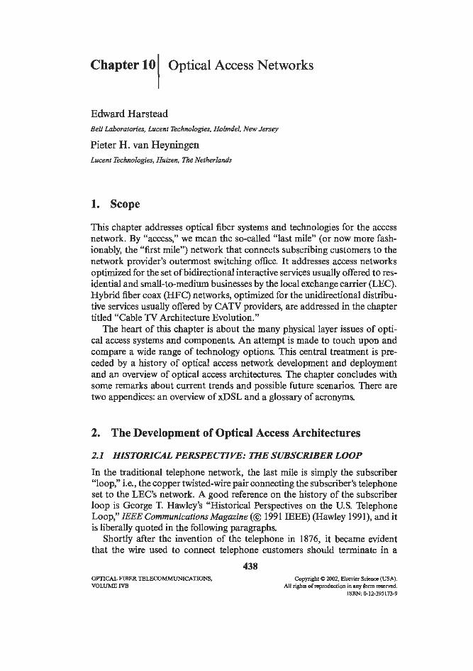
Chapter 10
Edward Harstead
Pieter H. van Heyningen
Bell Laboratories, Lucent Technologies, Holmdel, New Jersey
Lucent Technologies, Huizen, The Netherlands
Optical Access Networks
1. Scope
This chapter addresses optical fiber systems and technologies for the access network. By “access,” we mean the so-called “last mile” (or now more fash- ionably, the “fist mile”) network that connects subscribing customers to the network provider’s outermost switching office. It addresses access networks optimized for the set of bidirectional interactive services usually offered to res- idential and small-to-medium businesses by the local exchange carrier (LEC). Hybrid fiber coax (HFC) networks, optimized for the unidirectional distribu- tive services usually offered by CATV providers, are addressed in the chapter titled “Cable TV Architecture Evolution.”
The heart of this chapter is about the many physical layer issues of opti- cal access systems and components. An attempt is made to touch upon and compare a wide range of technology options. This central treatment is pre- ceded by a history of optical access network development and deployment and an overview of optical access architectures. The chapter concludes with some remarks about current trends and possible future scenarios. There are two appendices: an overview of XDSL and a glossary of acronyms.
2. The Development of Optical Access Architectures
2.1 HISTORICAL PERSPECTWE: THE SUBSCRIBER LOOP
In the traditional telephone network, the last mile is simply the subscriber ccloop,” i.e., the copper twisted-wire pair connecting the subscriber’s telephone set to the LEC‘s network. A good reference on the history of the subscriber loop is George T. Hawley’s “Historical Perspectives on the U.S. Telephone Loop,” IEEE Communications Muguzine (@ 1991 IEEE) (Hawley 1991), and it is liberally quoted in the following paragraphs.
Shortly after the invention of the telephone in 1876, it became evident that the wire used to connect telephone customers should terminate in a
438 OPTICAL FIBER lELECOMMUNICATIONS, VOLUME IVB
Copyright 0 2002, Elsevier Science (USA). All rights of reproduction in any form resmed.
ISBN 0-12-395173-9

10. Optical Access Networks 439 ~
- -
RT co a. Single star (SS+traditional subscriber loop. ~
- d. Active double star (ADS).
b. Digital loop carrier (DLC).
e. Passive double star (PDS or PON).
Fig. 10.1 Copper and fiber-in-the-loop access architectures.
centrally located telephone company offic-the central office ( 0 ) . Primi- tive batteries in customer’s homes were soon replaced by a power sowce in the CO that powered the telephones over the copper wires. Within about 10 years after the invention of the telephone, the basic shape of the loop plant, which was to last into the second half of the twentieth century, was in place (Fig. l0.la). Although it was refined over the years, the loop eventually became a technological backwater.
Carrier systems, which reduce costs by multiplexing multiple voice calls onto a single wire, were deployed in the long-distance trunk (core) network starting in the 1920s. The cost of carrier technology fell over the years, but it was not until the early 1970s that T1 carrier became economical in the loop, and then only for very long loops. This was the beginning of the digital loop carrier (DLC). Up to 80 customers were connected via short loops, called the “distribution,” to a remote terminal (RT). A 24-line T1 carrier connected the RT to the CO and was called the “feeder.” (The economics of DLC were enhanced by concentration.) The cost of the remote electronics in the RT and electronic repeaters in the feeder were offset by the savings accrued from the large reduction in the number of pairs needed to connect the RT to the CO. This reduction is called “pair gain.” The distance at which DLC breaks even is called the “prove-in distance.” In early applications it was 75 Ut,’ which represented less than 1% of the United States loops (copper loop lengths in the United States are significantly longer than in Europe and Japan and explain why
’ Kilofeet; 1 km equals 3.028 kft. Kft is the traditional unit of measure in the United States loop plant, and is used in this section to preserve the historical flavor. Kilometers aie used in the rest of the chapter.
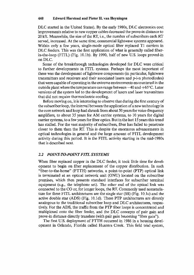
440 Edward Harstead and Pieter H. van Heyningen
DLC started in the United States). By the early 1980s, DLC electronics cost improvements relative to new copper cables decreased the prove-in distance to 20 kft. Meanwhile, the size of the RT, i.e., the number of subscribers each RT served, increased. At the same time, commercial lightwave systems appeared. Within only a few years, single-mode optical fiber replaced T1 carriers in DLC feeders. This was the first application of what is generally called fiber- in-the-loop (FITL) (Fig. 10.lb). By 1990, half of new U.S. loops proved-in on DLC.
Some of the breakthrough technologies developed for DLC were critical to further developments in FITL systems. Perhaps the most important of these was the development of lightwave components (in particular, lightwave transmitters and receivers and their associated lasers and p-i-n photodiodes) that were capable of operating in the extreme environments encountered in the outside plant where the temperature can range between -40 and +65”C. Later versions of the system led to the development of lasers and laser transmitters that did not require thermoelectric cooling.
Before moving on, it is interesting to observe that during the first century of the subscriber loop, the interval between the application of a new technology in the core network and loop had shrunk from about 50 years for voice-frequency amplifiers, to about 35 years for AM carrier systems, to 10 years for digital carrier systems, to a few years for fiber optics. But in the last 15 years this trend has stalled. For the vast majority of subscribers, fiber has failed to penetrate closer to them than the RT. This is despite the enormous advancements in optical technologies in general and the large amount of FITL development activity during this period. It is the FITL activity starting in the mid-1980s that is described next.
2.2 POINT-TO-POINT FITL SYSTEMS
When fiber replaced copper in the DLC feeder, it took little time for devel- opment to begin on fiber replacement of the copper distribution. In such “fiber-to-the-home” (FTTH) networks, a point-to-point (PTP) optical link is terminated at an optical network unit (ONU) located on the subscriber premises, which then presents standard interfaces for subscriber terminal equipment (e.g., the telephone set). The other end of the optical link was connected to the CO or, for longer loops, the RT. Commonly used nomencla- ture for these FITL architectures are the single star (SS) (Fig. 10.1~) and the active double star (ADS) (Fig. 1O.ld). These PTP architectures are directly analogous to the traditional subscriber loop and DLC architectures, respec- tively. For the ADS, the t r a c from the PTP fiber loops is concentrated and multiplexed onto the fiber feeder, and the DLC concepts of pair gain and prove-in distance directly translate (with pair gain becoming “fiber gain”).
The first U.S. deployment of FTTH occurred in 1986 in a housing devel- opment in Orlando, Florida called Hunters Creek. This field trial system,
10. Optical Access Networks 441
developed by AT&T's equipment arm (now Lucent Technologies), was deployed by Southern Bell (now BellSouth). It delivered switched digital video (SDV) service that replicated CATV over an ADS system. The system, crude by today's technology and intended primarily as a field trial, incorporated the fundamental architecture used in modern switched digital video systems.
Another early trial, also conducted by Southern Bell in a Florida develop- ment (Heathrow), used equipment designed by Bell-Northern Research (now Nortel) (Balmes et al. 1990). This was a technically advanced system using a SS architecture to deliver SDV and ISDN for voice. The substitution of ISDN for plain old telephone service (POTS) had its own set of problems, such as house wiring issues and the inability to deal with extension phones. The last version of this system added POTS over an ADS.
Although from a technical point of view these trials were a success, three important issues were uncovered. The first was that from a regulatory and marketing basis the telephone companies were not prepared to enter the video delivery business. Second, it became clear that the cost structure of deliv- ering a CATV-like service digitally over fiber could not, in the foreseeable future, compete with analog delivery over a coaxial cable bus architecture. And finally, the distribution of switched video within the subscriber residence was difficult and expensive. Even today, these issues have not yet been fully resolved. The real goal of the LECs, then and now, was to have a differentiated service such as video on demand (VOD) where SDV makes more functional and economic sense. But in the meantime, the focus shifted to narrowband services.
AT&T was the first to commercialize a FTTH system by offering 1.544 Mb/s one-fiber PTP optical plug-ins on their widely deployed DLC RT (Bohn et al. 1992). The system offered POTS and narrowband specials services only, with a story for upgrading to broadband later. It was deployed in several trials starting in 1988.
2.3 PASSIVE OPTICAL NETWORKS (PONS)
It was realized from the start that the cost of FTTH systems was going to be a major barrier to deployment. Fiber gain was necessary for the economics of FTTH networks, but the short low-bandwidth PTP links of the ADS archi- tecture clearly did not take advantage of the capabilities of optical fiber. Work began to exploit these capabilities to further lower costs. The most important focused on point-to-multipoint (PTM) architectures with fiber gain that eco- nomically connected all subscribers to the CO without the need for an RT. Because there were no active remote electronics required in the outside plant between the CO and the subscriber, these architectures were called passive optical networks (PONs). The most important PTM architecture is the tree- and-branch topology, of which the simplest type is the passive double star (PDS) (Fig. 10.le). The PDS architecture is analogous to the ADS, but with a
442
passive optical splitter/combiner in place of an RT.2 PONS are multiple access networks in which the feeder fiber and optical interface at the CO are shared by multiple subscribers.
The first PON proposal was made by British Telecom in 1987 (Stem et al. 1987). Typical of most PONS to follow, it broadcast a baseband time- division multiplexing (TDM) signal from the CO to all the ONUs, and used a time-division multiple access (TDMA) protocol to control ONU baseband transmission back to the CO. It was called telephony over PON (TPON). A laboratory demonstrator was built with a 20.48 Mb/s line rate capable of 294 64 kb/s channels optically split up to 128 ways. British Telecom later did a PON trial at Bishops Stortford. It used PON equipment manufactured by Fulcrum (Faulkner et al. 1989). Perhaps the most pioneering PON vendor was Raynet (Engineer 1990), whose PON was originally designed as an optical bus architecture.
The PDS architecture is a special case of the tree-and-branch topology where all branching is lumped at one point. The special case at the other end is the passive bus, where a fiber distribution cable runs past all subscribers and an optical tap is used to connect each subscriber’s fiber drop to the distribution. The bus requires the least amount of fiber, but wastes optical power unless the taps are tuned (complicating installation). As such, the bus topology has been abandoned.
For the remainder of the chapter, the term “PON” will be used to denote all optical tree-and-branch PTM topologies (including the PDS) with the exception of the bus. This is in line with common usage of the term.
Edward Harstead and Pieter H. van Heyningen
2.4 THE FTTH PROBLEM, AND THE BEGINNING OF FTTx
As already discussed, in some early lab and field trials the LECs dabbled with video services. But in the late 1980s and early 1990~~ for various regulatory, economic, and technological reasons, the only services the LECs were going to deploy on a wide scale were narrowband telephony services. Obviously, fiber was not required for that, but for new build and for rehabilitation of the old copper plant, it was attractive to lay in future-proof fiber to be ready for and to enable future broadband ~ervices.~ However, the LEC business case did not account for the revenue of these future services. For ubiquitous deployment, the goal for FTTH was “copper parity,” Le., the installed first cost of the FTTH system must come down to that of copper, around $1000 (U.S.) per line.
Some overzealous claims that the RT was actually “replaced” by the optical splitter did not account for “conservation of functionality,” i.e., the fact that much of the RT functionality (e.g., concentration, the switch interface) was merely moved back to the CO.
An analogy was made to the electrification of households: electricity was delivered for lighting without my knowledge of the myriad uses that it would ultimately be put to.
10. Optical Access Networks 443
It became apparent early on that for the delivery of telephony services, FTTH systems, whether PON or PTP, were not going to attain copper parity in the near term. Another problem for FTTH was powering. The subscriber telephone set was powered from the CO or RT via the copper loop. That meant powering was not a concern of the subscriber, and that the telephone service worked during a power failure: the so-called “lifeline” service. Powering tele- phones with optical power over fiber was (and still is) impractical. This meant that for FTTH, either a separate metallic power network must be deployed to every home in addition to the fiber (expensive) or the telephone must be powered by the subscriber’s own AC power. In the latter case, to maintain lifeline service, there would need to be backup batteries, which would need to be periodically replaced by either the LEC (expensive) or the subscriber (who may not be willing to do so).
The solution to the cost and power problems was fiber-to-the-curb (FTTC). It was proposed that the ONU be located at the corner of four properties and serve four living units over copper drops. This sharing of the ONU reduced the per-subscriber cost of the optical network. Also, it made the powering problem more manageable. The ONUs powered the telephones over the copper drops. A power network and backup batteries were still needed, but for a much smaller number of ONUS. When copper parity was still not quickly attained, ONUs became larger to increase cost sharing, serving more subscribers (anywhere between 12 and 96). The larger the number of subscribers per ONU, the further the ONU was located from the subscribers, spawning variants like FTTBuild- ing (i.e., multidwelling unit, MDU), FTTExchange, etc., which collectively came to be called FTTx. These systems began to resemble small DLC systems.
FTTC came with its own problems. Now, instead of siting, powering, and maintaining an active remote terminal in the outside plant for every 1000 subscribers or so (DLC), there were many more smaller active terminal^.^ Still, FTTC was widely trialed, and by the mid-1990s it was claimed that FTTC had achieved copper parity BellSouth then made deployment of Rel-Tec (now Marconi) PTP FTTC equipment standard for new build (Kettler et al. 2000). But as we shall see, FTTC deployment has been sporadic at best, and the concept of FTTC has failed to bring about widespread deployment of FITL. Work continues on FTTCabinet and FTTBuilding, neither of which require the establishment of new outside ONU sites or new power grids.
2.5 FITL STmARDIZATION
Standardization efforts in the United States and Europe began in the early 1990s. Bellcore (now Telcordia) released TA-909 in 1990, which addressed all aspects of narrowband FTTC systems. It allowed one- and two-fiber PTP
Advocates for PON made much of elimination of the active electronics and optics in the RT, and so when PON switched from FTTH to FTTC, it seemed a little strange.
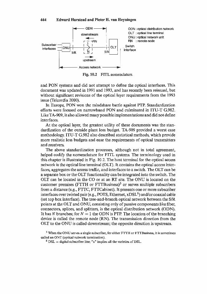
444 Edward Harstead and Pieter H. van Heyningen
ODN : optical distribution network OLT : optical line terminal ONU : optical network unit
S u b s c r i b e r a interfaces
Access network
Fig. 10.2 FITL nomenclature.
and PON systems and did not attempt to define the optical interfaces. This document was updated in 1991 and 1993, and has recently been reissued, but without significant revisions of the optical layer requirements from the 1993 issue (Telcordia 2000).
In Europe, PON won the mindshare battle against PTP. Standardization efforts were focused on narrowband PON and culminated in ITU-T G.982. Like TA-909, it also allowed many possible implementations and did not define interfaces.
At the optical layer, the greatest utility of these documents was the stan- dardization of the outside plant loss budget. TA-909 provided a worst case methodology. ITU-T G.982 also described statistical methods, which provide more realistic loss budgets and ease the requirements of optical transmitters and receivers.
The above standardization processes, although not in total agreement, helped codify the nomenclature for FITL systems. The terminology used in this chapter is illustrated in Fig. 10.2. The host terminal for the optical access network is the optical line terminal (OLT). It contains the optical access inter- faces, aggregates the access traffic, and interfaces to a switch. The OLT can be a separate box or the OLT functionality can be integrated into the switch. The OLT can be located in the CO or at an RT site. The ONU is located on the customer premises (FTTH or FTTBusiness)’ or serves multiple subscribers from a distance (e.g., FITC, FTTCabinet). It presents one or more subscriber interfaces over twisted pair (e.g., POTS, Ethernet, xDSL6) andor coaxial cable (set top box interface). The tree-and-branch optical network between the S/R points at the OLT and ONU, consisting only of passive components like fiber, connectors, splices, and splitters, is the optical distribution network (ODN). It has N branches; for N = 1 the ODN is PTP. The location of the branching device is called the remote node (RN). The transmission direction from the OLT to the ONU is called downstream; the opposite direction is upstream.
When the ONU serves a single subscriber, for either FTTH or FTTBusiness, it is sometimes
DSL = digital subscriber line; “x” implies all the varieties of DSL. called an ONT (optical network termination).
10. Optical Access Networks 445
2.6 NARROWBAND PONDEPLOYMENT
In the early 1990s, long-range plans were made for wide-scale residential deployment of PON systems designed to provide existing narrowband ser- vices (with the possibility to optically overlay a broadcast video service; see Section 4.8). The most aggressive activity occurred in Germany and Japan.
After the reunification of Germany, the Deutsche Bundespost (now Deutsche Telekom) was faced with rehabilitation of the obsolete telecommu- nications infrastructure in the Eastern states. Rather than install new copper systems, which might soon become obsolete, a decision was made to deploy FITL. Then began a series of trials and deployments called OPAL (optical access line). PON systems, at least initially, were favored. The early vendor was Raynet, and trials started in the early 1990s (Tenzer 1991). A flexible set of requirements to accommodate other PON vendors were drawn up (Orth 1992) and significant deployment of mostly FTTC and some FTTH occurred in the mid-1990s. But PON deployments tapered off soon after.
While the rest of the world moved to FTTC, NTT, the Japanese telco, stayed the course, believing that Japan’s high population density favored FTTH. In Japan there is less space for outdoor cabinets, and nearly all distribution and drop cables are aerial cables which are relatively easy to switch to fiber. In the early 1 9 9 0 ~ ~ NTT architected a FTTH PON system and contracted vendors to develop them. NTT initially ran around the lifeline POTS problem by propos- ing narrowband ISDN-only systems (Miki et al. 1991). Initially, these had a 28.8 Mb/s line rateY7 and were trialed in Tachikawa (Harikae 1995).
But soon NTT also realized that more time was required for the cost of FTTH to drop. They adapted their narrowband PON into a FTTC system, increased the line rate to 49 Mb/s, and called it n-PON (Harikae et al. 1998). Limited commercial deployment of this system began in the late 1990s.
Still planning for FTTH, NTT adapted the n-PON for FTTH, with Inter- net access added (a lobase-T Ethernet interface). They were still striving for copper panty (Amemiya et al. 1997) with this system, but now it appears that this system will not be deployed.
2.7 ATM PON
By about the mid-l990s, it became clear to many that the paradigm of deploy- ing FITL to carry only existing services that could be more easily carried by copper and coaxial systems was a dead end. FITL would not be widely deployed until new broadband services demanded it. While narrowband FITL struggled for commercial viability, vendors and network operators also worked on marrying the new ATM technology to FITL, and in particular to PON.
’ This was a time-compression multiplexing system, so there was only about 12 Mb/s in each direction; see Section 3.3.3.
446 Edward Harstead and Pieter H. van Heyningen
Thus ATM PON (also called APON) became a fertile area for research and trials, and the result was the concept of the full service access network. And before there was a World Wide Web, the new broadband service was VOD, and it would be carried by SDV. VOD allows for viewing of movies stored on a remote video server that emulates VCR command functions. As with the early FTTH trials, conventional CATV service was also provided by indi- vidually digitizing the full stack of channels and remotely switching them at the OLT via channel changing commands from the subscriber’s set-top box. Unlike symmetrical circuit-switched services, the bandwidth asymmetry of the video services prompted some of the ATM PON systems to have downstream bit rates higher than upstream rates.
An ATM PON project called BAF (Broadband Access Facilities) started with the RACE I1 program8 in 1992 (van Heyningen et al. 1992; Killat et al. 1996). Typical of ATM PONS to follow, the BAF PON used TDM/TDMA, and the time slots contained ATM cells. It was both a FITC and FTTH system with a line rate of 622Mb/s in each direction over separate fibers. It delivered El and optical ATM155 services to small business and residen- tial subscribers. The general aim of this project was to improve the common understanding of the conceptual, technical, and application levels of full ser- vice access networks to enable the timely introduction of broadband services throughout the EC.
One European vendor, Alcatel, developed its own ATM PON system, with 622 or 155 Mb/s downstream and 155 Mb/s upstream. It supported POTS and VOD, and was deployed in several residential FTTH trials starting in 1994 (Van der Plas et al. 1995). In the United States, Broadband Technologies commercialized a FTTC ATM PON system that carried POTS, VOD, and CATV services. This also was an asymmetric PON with a downstream bit rate of about 800 Mb/s and upstream rate of 51.84 Mb/s. The digital video signals were delivered to the home over copper pairs using VDSL.9
In Japan, concurrent with their narrowband PON work, NTT pushed a similar development of ATM PON. They architected and then contracted several vendors to develop a 155 Mb/s ATM PON FTTH system that carried ISDN, CATV, and VOD services to residential users. Trials occurred between 1995-1997 (Terada et al. 1996).
* In Europe, precompetitive R&D cooperation among vendors, operators, and users is sub- sidized by the European Commission (EC). RACE (Research and technology development in Advanced Communication technologies in Europe) was a framework for EGsponsored research for the introduction of integrated broadband communications into the community. It involved organizations established in different member states and between equipment vendors, operators, and users RACE I1 ws the second RACE phase, it covered the period from January 1992 to December 1995.
Refer to Section 9 for an overview of DSL technologies

10. Optical Access Networks 447
2.8 FSAN
In 1995, six European national telephone operators (“ te lco~~~) plus NTT formed an industry forum initially named the “G7,” then the “Gx,” and now FSAN (for full service access networks). They invited leading vendors to help them define common standards for broadband access networks. Later, more telcos and vendors joined. In the first phase of this work ATM PON was identified as the core transport technology, and some minimum require- ments were established (FSAN 1996). To satisfy all participants, all flavors of FTTx were allowed. The next phase, starting in 1996, accomplished, for the first time, the standardization of the PON interface. Both the physical layer, approved as ITU-T G.983.1 in 1998 (ITU-T 1998), and the management chan- nel, approved as ITU-T G.983.2 in 2000 (ITU-T 2000), were standardized.’O ITU-T G.983.1 describes a TDM/TDMA PON but allows for several imple- mentations. Bidirectional 155 Mb/s is aimed at FTTH applications; 622 Mb/s downstread155 Mb/s upstream is aimed at FTTCabinetNDSL (Cooper et aZ.
The objectives of this standardization were to drive up the volumes of com- mon components, leading to lower prices; to ensure vendors that they could sell their products into all markets; and, ultimately, to allow for multivendor interoperability between the OLT and ONU. Vendors working on pre-FSAN ATM PONS have generally abandoned those efforts to join the standard.
NTT was the first telco to begin trials of FSAN-compliant systems (from more than one vendor) in 1999. By then the difficulty of making money on VOD was clear, and NTT took the novel approach of asking for ATM PON systems that delivered leased-line services for small-to-medium businesses (Ueda et aZ. 1999). An argument (e.g., Harstead, 2000) can be made that ATM PON is the lowest-cost vehicle for the delivery of all business access services for subscriber bandwidth requirements exceeding a few DSl/E 1s (typically deliv- ered by HDSL”) and less than an OC-1 (typically delivered by SONET/SDH). On the other hand, BellSouth is trialing the joint LucentlOki ATM PON as a data overlay in an existing and primarily aerial residential neighborhood (Kettler et al. 2000). A separate fiber to each home carries analog CATV, and telephony is provided by the embedded copper network.
Despite the lack of widespread deployment of FSAN systems, a new effort was initiated by the telcos in 2000 to extend the existing standards. The extensions are aimed at allowing a dense wavelength-division multiplexing (DWDM) andor broadcast CATV overlay on the ATM PON, increasing the efficiency of the upstream path for noncontinuous bit-rate services by using dynamic bandwidth allocation; and standardizing protection architectures.
2000).
lo The lead authors of ITU-T G.983.1 were NTT, Alcatel, and Fujitsu; the lead author for ITU-T G.983.2 was Lucent Technologies
Refer to Section 9 for an overview of DSL technologies.

448 Edward Harstead and Pieter H. van Heyningen
Some of the new PON start-up vendors are now participating and taking active roles.
2.9 ETHERNETAND PTP
PON dominated FITL activity in the 1 9 9 0 ~ ~ but with the emergence of Ethernet as the convergence layer in the access network, this might change. Ethernet conquered the LAN market, and in the process evolved from a coaxial cable bus topology to PTP. As speeds increase from the original 10 Mb/s to 100 Mb/s (Fast Ethernet) to 1 Gb/s (Gigabit Ethernet) to 10 Gb/s, the medium of choice changes from twisted pair to multimode fiber to single-mode fiber. If Ethernet moves into last mile access, the PTP architecture is likely to capitalize first.
3. Optical Transmission
The relatively short lengths and modest bandwidth requirements of access systems allow them to be designed in the linear and nondispersive regime of optical fibers, and without the need for regeneration. Consequently, nonlinear effects, dispersion maps, and optical amplification are not considered.
3.1 FIBER
It could be argued that the use of multimode fiber would be adequate to the bandwidth-distance requirements of access systems, and yield the lowest cost solution. But an access provider willing to take on the expense of deploying new media in the last mile will not be willing to deploy a media that might be obsolete in the near future. Therefore, the multimode argument has never gained acceptance.
The fiber of choice has been standard single-mode fiber (SSMF). Consider- ing the reach and optical power levels in access systems, there is no need to pay a premium for any of the varieties of dispersion-shifted fibers optimized for DWDM systems. All of the systems described in this chapter are SSMF-based systems.
3.2 OPTICAL WAVELENGTH WIND0 WS
With SSMF, the obvious choices for transmission are the 1.3 and 1.5 pm opti- cal wavelength windows. However, it might be worth mentioning that shorter wavelength transmission is also an alternative for point-to-point systems operating over modest lengths. Such a strategy was proposed in the 1980s (Soderstrom et al. 1986; Stern et al. 1987). At that time telecommunications lasers were still relatively expensive, while 780-nm lasers were being mass produced for consumer products (CD players). Bidirectional transmission at
10. Optical Access Networks 449
780 nm also spared both the 1.3- and 1.5-pm bands, leaving them available for future uses.
Such short wavelength transmission in SSMF will occur below the fiber cutoff wavelength, Am, resulting in bimodal propagation of both the funda- mental LPol and LPll modes. Depending on A,, and the actual transmitted wavelength, additional third-order LP02 and LP21 modes may or may not sur- vive. In the worst case that they do, modal dispersion will limit the fiber to only 66 MHz . km (Engineer 1990). Trimodal transmission must also be accounted for when specifying component performance and making system loss budget calculations (Refi et aZ. 1990). With only a handful of modes, modal noise is potentially a major problem (Das 1988; Suto et al. 1992). Reducing the source’s coherence length by dithering or designing for self-sustained oscil- lation (Poh 1985) can mitigate impairments. Further, the fiber loss, due to increased Rayleigh scattering, is about 3 dBkm. All these factors eliminate short wavelength transmission for mainstream access applications; however, it might still be useful, for example, for overlay of low speed (e.g., telemetry) signals on a PTP link.
Above hco, the 1.3-pm window has the lowest chromatic dispersion on SSMF (not exceeding about 5 pshm-km), which allows for the use of inex- pensive uncooled Fabry-Perot lasers even for very long loop lengths and reasonably high bit rates. The 1.5-pm window has higher dispersion, so bandwidth-distance requirements may require the use of more costly single longitudinal mode (SLM) lasers, such as the distributed feedback (DFB) laser. The cost of applying DFB lasers is kept reasonably low since they can be directly modulated and uncooled.
There is a fiber identical to SSMF, except that it has little or no OH absorption in between the 1.3- and 1.5-pm bands (Refi 1999). It is called low- water-peak fiber, and it allows for transmission across a much wider optical band. Although low-cost components in the 1.4-pm band are not yet avail- able, it might be a good choice to deploy such a future-proof fiber in access networks where the cables are expected to last 25 years or more. The extra spectrum would allow greater flexibility for service upgrades and overlays. (Refer to the chapter on “Communication Fiber.”)
3.3 BIDIRECTIONAL TRANSMISSION
Methods of achieving bidirectional transmission for interactive services on optical mess networks have been the subject of debate and study over the years. There are two sometimes conflicting goals. One is to minimize initial first costs while meeting bandwidth and distance requirements. The other is min- imizing the consumption of optical spectrum, leaving more usable spectrum for other signals carrying other services (e.g., broadcast video) or for future upgrades. Several directional multiplexing methods that have found practical use in optical access systems are described and compared in this section.
450 Edward Harstead and Pieter H. van Heyningen
3.3.1 Space-Division Multiplexing (SDM)
SDM is simply the transmission of each direction over a separate fiber, usually at 1.3 pm. This is the most straightforward implementation from the equip- ment maker’s perspective, but doubles the number of fibers, splices, connectors, and splitters (for PON) in the ODN. On the other hand, a single fiber system, although leaner in the outside plant, requires 1 : 2 devices of some type at each end of the fiber to couple the transmitter and receiver. FSAN studied the overall installed first costs of one- and two-fiber systems and determined that one-fiber systems are more economical. Similar results have been found for point-to-point systems (e.g., Baskerville 1989). Although two fibers would be more future-proof than one, network providers have asked the vendor community for one-fiber solutions.
3.3.2 Full Duplex
Full duplex refers to the simultaneous bidirectional transmission over a single optical fiber without taking any special measures to separate the two signals in time, the optical or electrical frequency domains. Typically, this means both directions of transmission are in the same wavelength window. A 1 : 2 optical power splittinglcombining coupler at each end provides access to the fiber for both the transmitter and the receiver. One significant side effect is the added insertion loss of a pair of couplers, about 3.5 dB each (3 dB intrinsic loss plus about 0.5dB excess loss). Another is the creation of a near-end cross-talk (NEXT) path between them. Interference results when the near-end trans- mitted optical signal is reflected back into the receiver. Performance can be maintained if the optical signal-to-interference (OSIR) ratio meets a relatively modest value, about 10 dB for a 0.5 dB penalty (because the interferer is a reflected signal and not Gaussian noise, it is bounded) (Bohn et al. 1987). The OSIR requirement puts a return loss requirement on the ODN and the far-end transceiver.
For low loss ODNs, such as a point-to-point link, the return loss require- ment can be easily attained because the received signal is relatively strong. For higher loss systems, such as PONS, the ODN return loss requirement becomes stringent. For example, TPON was initially proposed as full duplex, and fusion splices were expected to keep return loss high. However, it was realized that guaranteeing such a high return loss on massively deployed low cost net- works would be impractical, and subsequent PON developments abandoned full duplex.
The previous discussion assumes incoherent crosstalk, i.e., the signal and interferer add on a power basis. If the two signals are coherent, they will beat on the square-law photodetector at the difference of the two optical frequencies. If the two optical frequencies are close enough, the difference frequency, or beat, will fall within the electrical signal bandwidth, resulting in optical beat interference (OBI) noise and increased bit-error rate. The spectral width of

10. Optical Access Networks 451
OBI noise is determined by a convolution of the power spectral densities of the optical fields incident on the detector. If a transmitter has a Lorentzian lineshape, as is typically assumed for lasers, the resulting beat note has a spectral width equal to the sum of the spectral width of the two sources.
The magnitude of this effect depends on the relative magnitudes of the sig- nal bandwidth, B, and the optical spectrum linewidth, Av. For large Av, the OBI noise will be spread over a wide spectrum, reducing the fraction of the noise power that is within the signal bandwidth. Chirp from direct modula- tion will help this spread. For small B, there is less noise within the signal band. When B / A v = 0.01, the penalty is not significantly different from the incoherent case; for B / A v = 0.1, the OSIR requirement becomes lOdB more stringent, about 20dB; for B / A v = 1 (more or less transform-limited), the OSIR must be 30 dB (Das et al. 2001).
With access system bit rates increasing (100 Mb/s to 1 Gb/s; maybe even 10 Gb/s in the future), OBI from NEXT can become a problem for SLM lasers, especially those with low chirp such as vertical-cavity surface-emitting lasers (VCSELs) and quantum-dot lasers. One idea is to split the wavelength window into two parts, with the downstream transmitter occupying one half and the upstream transmitter the other (this is not the same as coarse WDM discussed in Section 3.3.5; there is no separation of the wavelengths anywhere, and the receiver cannot differentiate between them). An optical spectrum budget must account for laser batch wavelength variation and the temperature dependence of the uncooled laser's wavelength. This split-band approach could be enabled by a current effort in the ITU-T Study Group 15 to standardize a coarse wave- length grid, with about 20-nm channel spacings, which would provide enough guard band to allow the use of uncooled DFB lasers (Eichenbaum 2001).
As discussed in Section 3.2, low-cost multilongitudinal mode (MLM) lasers, like the Fabry-Perot (FP) laser, are preferred in the 1.3-pm wavelength win- dow. In this case, each of the individual modes of the far- and near-end sources beat against each other, creating a large number of beats, but whose sum is less than that for SLM lasers since all the individual beats then add on a power rather than amplitude basis. This lessens the coherence effect. For example, for a FP laser with five modes of equal power and linewidth, the OBI-related OSIR improvement with respect to a SLM laser is about 7 dB (Das et al. 2001). Therefore, a FP laser should be workable up to 1 Gb/s (i.e., B / A v = 0.1) on full duplex systems.
Note that it is not practical to put (uncooled) Fabry-Perot lasers on the coarse ITU grid since their temperature dependence is about OSnm/"C, and their manufacturing tolerance is about 10-20 nm.
3.3.3 Time-Compression Multiplexing (TCM)
A workaround that allows single-fiber, single-wavelength transmission on high-loss ODNs is time-compression multiplexing (TCM), also known as
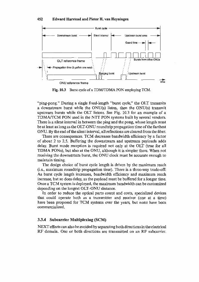
452 Edward Harstead and Pieter H. van Heyningen
k- Bunt cycle -4 Downstreambunt 1 Silent Interval r z m ~ ~ r l
n I I I I ! I I I I I I I I I I , ,’ ,’ Bursts from other ONUS
, I , I
I , I , I ,
, I I , I ,
, I I I .
b time ONU reference frame
Fig. 10.3 Burst cycle of a TDMRDMA PON employing TCM.
“ping-pong.” During a single fixed-length “burst cycle,” the OLT transmits a downstream burst while the ONU(s) listen, then the ONU(s) transmit upstream bursts while the OLT listens. See Fig. 10.3 for an example of a TDMA/TCM PON used in the NTT PON systems built by several vendors. There is a silent interval in between the ping and the pong, whose length must be at least as long as the OLT-ONU roundtrip propagation time of the farthest ONU. By the end of the silent interval, all reflections are cleared from the fiber.
There are consequences. TCM decreases bandwidth efficiency by a factor of about 2 to 2.5. Buffering the downstream and upstream payloads adds delay. Burst mode reception is required not only at the OLT (true for all TDMA PONS), but also at the ONU, although it is simpler there. When not receiving the downstream burst, the ONU clock must be accurate enough to maintain timing.
The design choice of burst cycle length is driven by the maximum reach (i.e., maximum roundtrip propagation time). There is a three-way trade-off: As burst cycle length increases, bandwidth efficiency and maximum reach increase, but so does delay, as the payload must be buffered for a longer time. Once a TCM system is deployed, the maximum bandwidth can be customized depending on the longest OLT-ONU distance.
In order to reduce the optical parts count and costs, specialized devices that could operate both as a transmitter and receiver (one at a time) have been proposed for TCM systems over the years, but none have been commercialized.
3.3.4 Subcarrier Multiplexing (SCM)
NEXT effects can also be avoided by separating both directions in the electrical RF domain. One or both directions are transmitted on an RF subcarrier.

10. Optical Access Networks 453
Prefiltering at the transmitters to limit the RF signal spectrum may be required to limit crosstalk into the other direction. This method introduces linearity requirements and RF componentry with their associated cost and complexity into both ends of the system. It is also necessary to consider the coherent NEXT effect described in Section 3.3.2.
3.3.5 Diplex, or Wavelength-Division Multiplexing (WDM)
Instead of separation in the RF domain, downstream and upstream signals can be separated in the optical frequency domain using a 1 : 2 WDM (wavelength- division multiplexing) coupler instead of a power splittingkombining coupler. (An optical rejection filter at the receiver may also be required to obtain ade- quate isolation from reflections.) Proposals in the early 199Os, when 1.5-pm sources were still relatively exotic, called for dividing the 1.3-pm window into so-called 1.3+ and 1.3- ranges, one for each direction. The optical spectrum budget must now also account for the multiplexing guard band, in addition to the sources' wavelength variation discussed in Section 3.3.2. At that time, laser suppliers did not have processes set up to control the wavelengths, 1.3 +/1.3- multiplexing couplers did not exist, and if they did, their narrower separation would make them more costly than standard 1.3/1.5 couplers. Then and today it is generally thought that multiplexing the 1.3- and 1.5-pm windows is more practical and cost-effective. Since the wavelength bands are so far apart, this is usually referred to as coarse WDM (CWDM).
A CWDM coupler has excess loss of only about 1 dB or less, and so there is significantly less system loss compared to the one-fiber methods that use a power coupler.
3.3.6 Summary
A comparison of the techniques is shown in Table 10.1.
Table 10.1 Comparison of Directional Multiplexing Methods
No. of X No. of Fibers Bandwidth Added windows Consumed
Method Required Eficiency Loss (By @er@er)
SDM 2 1 0 1 Full duplex 1 1 7 1 TCM 1 -0.40.5 7 1 SCM 1 1 7 1 WDM (1.3/1.5) 1 1 1 2
Assumes a 0.5 dB excess for the coupler at each end of the link.
454 Edward Harstead and Pieter €I. van Heyningen
If ODN costs are not a driving issue, the simplicity, spectral frugality, and low implementation loss of SDM make it an easy choice (e.g., SONETISDH systems). However, the consensus for access systems is that one-fiber systems are cheaper. The simplest one-fiber method is full duplexing, a good choice for low-loss point-to-point systems. For higher-loss point-to-multipoint topolo- gies there are three practical choices. TCM and SCM both conserve optical spectrum, but their 1 : 2 couplers consume precious dBs. TCM is a good low-cost choice for narrowband PONS where bit rates are modest, and the 1.5-pm window can be used for broadband services (e.g., broadcast video: see Section 4.8.2). But for broadband PONs with higher bit rates and higher required receiver input power, the preference is for WDM. A low-cost 1.3-pm FP laser goes in the ONU, and the more expensive 1.5-pm DFB laser is shared in the OLT. The major downside of WDM directional multiplexing is the con- sumption of both standard wavelength windows, if there is no wavelength control on the sources. FSAN is currently studying the partition of the 1.5-pm window into a more restricted band for the downstream source, leaving a band around the peak erbium wavelengths for DWDM upgrades andor video over- lays. Another spectrum strategy is to use the 1.4-pm band in low-water-peak fibers.
4. PON: Power-Splitting PONs
Because they are point-to-multipoint, PONS are more complex than PTP systems, and so in this section we delve into PONS in more detail. A miffing topological characteristic of all types of PONS is that upstream transmissions from all ONUS are passively multiplexed in the tree-and-branch ODN and arrive at the OLT on a single fiber where they must be demultiplexed. How- ever, no ONU has access to the upstream transmission of any other ONU. On the other hand, there are two fundamentally different ways to distribute down- stream signals in the ODN. In this section we will consider the class of PONs we call “power-splitting P O N (PSPON). In a PSPON, the downstream signal is power split at every branching point, with the result that it is broadcast to all ONUS, and each ONU is responsible for extracting its payload from the aggregate signal. There is another class of PONs, wavelength routing PONS, or WDM PONs, where wavelength routing replaces power splitting. WDM PONs allocate one or more private downstream wavelength(s) to each O W , while retaining fiber gain. Wavelength-routing WDM PONs are considered in Section 5.
4.1 SPLITTING STRATEGIES
PSPONs are tree-and-branch PTM networks. The simplest ODN is one where all the splitting is lumped in one location. To minimize fiber, the lumped

10. Optical Access Networks 455
splitter for each ODN is placed at the centroid of the ONUS that are connected to it. Another strategy is to colocate splitters of several PONS at a single accessible maintenance point. This lengthens some of the distribution fibers, but allows for flexible rearrangement of OLT-ONU connectivity. For example, if one PON’s capacity is nearing exhaustion an O W can be moved over to another PON’s splitter. The limiting case that maximizes flexibility and simplilies maintenance is to sacrifice all fiber gain by installing all the splitters at the OLT, a case which is addressed in Section 4.6.5.
Splitting can also be cascaded in stages, for example, a 1 x 8 splitter could be installed at the end of a feeder route, and 1 x 4 splitters could be installed at the corner of every 4 living units (LUs) for a total split of 1 : 32. There could be more than two stages of splitting (in the limiting case the ODN could be a topological bus). Splitting can be distributed in a way such that ONUS on the same PON can “see” different split ratios.
Flexible splitting also allows for a relatively graceful upgrade of PON sys- tems. If the bandwidth requirements of the ONUS on a PON start to exceed the PON capacity, a second splitter can be installed beside the first splitter, some of the ONUS can be moved over to the second splitter (service-affecting), and the second splitter can be connected over a second feeder fiber to a new OLT PON interface. If a dark feeder fiber had already been installed, this bandwidth upgrade can be implemented with no changes to the ONUS or the fiber plant.
4.2 OPTIC’ SPLITRATIO
When deployed, PONS allow for a range of optical splitting, from no splitting at all (PON collapses to a PTP system) up to a maximum determined by the optical loss budget and the PON protocol. PSPON capacity is shared, and so the larger the optical split ratio, the less average bandwidth available per O W . Also, as splitting loss increases, there is less optical power budget left for cable, and system reach is reduced. But the primary reason for PON is to share the cost of the feeder fiber and the OLT optical interface and, as splitting increases, the cost of these system components decreases. However, overall system cost does not asymptotically decrease as split ratio increases; there are two less obvious effects that become significant as the savings from increased splitting bring diminishing returns. The first is that for a given maximum system reach, the higher the optical split ratio, the more demanding are the requirements on the opto-electronic components, which increases cost. Secondly, and less obvious, is that for a single, lumped splitter deployed as close to ONUS as possible, the larger the split ratio, the longer the average drop lengths between the splitter and the ONUs. This also begins to drive up distribution fiber cost as split ratio increases.
Accounting for all these effects yielded an economic optimum around 16 to 32, with no justification for larger values (Harstead et al. 1992). Although

456 Edward Harstead and Pieter H. van Heyningen
3
g 1 k 6 9 S 0.75 '0 C m
$' 0.5 '0 a, N .- 3 0.25
z E 0
0.
\ \ '. . Normalized cost per LL 40
30 0
v 3-
52 J
20 8 h
10
0 1 2 4 8 16 32 64
Optical split ratio
Fig. 10.4 Optical split ratio trade-offs.
this cost study is dated, requirements on PON systems have generally hovered around a maximum split ratio of 32 (although FSAN continues to consider requiring up to 64). Figure 10.4 shows the trade-offs between average band- width per ONU, maximum system reach, and cost as splitting ratio is varied. The system reach curve is for a FSAN-compliant, class B 155-Mbh symmetri- cal PON (see Section 6.1. l), computed using a standardized statistical method (ITU-T G.982) and standardized statistical loss values (ETSI 1997); the cost curve is one taken from Harstead et al. (1992) and is shown for qualitative purposes only. Considering the trade-offs, the optimal value of splitting is generally in the range of 16; lower values may be better when larger amounts of bandwidth are required per ONU (e.g., FTTBusiness or FTTC); perhaps higher values for F n H , especially for low take.
There is a distinction between the maximum optical split ratio and the max- imum number of active ONUS connected to the PON. The ITU-T G.983.1 PON protocol can support up to 32 active ONUS per PON. It is okay if 32 active ONUS are attached to, for example, a 1 : 48 ODN, where the excess optical splitting is to deal with service breakage and less than 100% take rate. In other words, the limitation on optical splitting is the optical power budget, and the limitation on the number of active ONUS is the PON protocol.
4.3 DO WSTREAM MULTIPLEXING
In a PSPON, all downstream traffic on the PON is multiplexed onto the feeder fiber and broadcast to all ONUS via the ODN. Multiplexing can be done in the electrical or the optical domain. In the electrical domain, the simplest and
10. Optical Access Networks 457
least costly method is TDM. The only requirement for the ONU is to time demultiplex its payload from the aggregate signal.
For optical multiplexing, the technique of DWDM can be used on a PSPON. Each ONU is assigned a unique downstream wavelength and must optically filter it from the broadcast DWDM signal. A problem with this is that each ONU must have a relatively expensive wavelength-specific receiver, which impacts installation and inventory procedures. For example, for a PON that supports up to 32 ONUs, 32 different ONU codes must be stocked and carried on truck-rolls, and upon installation care must be taken to connect the correct ONU codes on the PON. (An alternative is a wavelength-generic ONU that accepts craft-installable optical filters.)
DWDM will greatly increase the capacity of the PSPON, but at greater cost and complexity. Currently the use of downstream DWDM is a subject of study in FSAN in the context of future upgrades of a TDM PSPON (ITU-T 2001). If one were to deploy a PON system that used DWDM from the start, then a wavelength-routing WDM PON architecture might be more attrac- tive. This solves the ONU-type problem since each ONU receives only its allocated wavelength and no optical demultiplexing is required. Wavelength routing has another advantage in that the insertion loss of the wavelength router is less than that for a power-splitter. WDM PON is considered in Section 5 .
4.4 UPSTREAM MULTIPLE ACCESS
In a tree-and-branch network all upstream transmissions from the ONUS are multiplexed onto the root fiber at the optical branching devices and must be demultiplexed at the OLT receiver. How the ONUs successfully contend for the resources of the OLT receiver is accomplished through a multiple access technique. The three most practical, TDMA, subcarrier multiple access (SCMA), and wavelength-division multiple access (WDMA) are described in this section.
4.4.1 TDMA
In TDMA systems, the ONUs buffer upstream tr&c and then transmit it in baseband bursts. Since the OLT baseband receiver can only accept one burst at a time, the ONUS must share the receiver’s bandwidth. Contention techniques are not practical on PON systems. For example, ALOHA is too inefficient as there are relatively few ONUS on a PON, and they will often be transmitting on a regular basis. Carrier sense multiple access (CSMA) doesn’t work because ONUS cannot sense other ONU’s upstream transmission. For PONS it makes more sense to use a token (or “grant”) scheme where ONUS are assigned timeslots, and collisions are prevented.
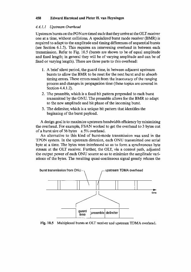
458 Edward Harstead and Pieter H. van Heyningen
guard time
4.4.1.1 Upstream Overhead
Upstream bursts on the PON are timed such that they arrive at the OLT receiver one at a time, without collisions. A specialized burst mode receiver (BMR) is required to adapt to the amplitude and timing differences of sequential bursts (see Section 6.1.3). This requires an intervening overhead in between each transmission. Refer to Fig. 10.5 (bursts are shown to be of equal amplitude and fixed length; in general they will be of varying amplitude and can be of fixed or varying length). There are three parts to this overhead:
1. A brief silent period, the guard time, in between adjacent upstream bursts to allow the BMR to be reset for the next burst and to absorb timing errors. These errors result from the inaccuracy of the ranging process and changes in propagation time (these topics are covered in Section 4.4.1.2).
transmitted by the ONU. The preamble allows for the BMR to adapt to the new amplitude and bit phase of the incoming burst.
3. The delimiter, which is a unique bit pattern that identifies the beginning of the burst payload.
2. The preamble, which is a fixed bit pattern prepended to each burst
preamble delimiter
A design goal is to maximize upstream bandwidth efficiency by minimizing the overhead. For example, FSAN worked to get the overhead to 3 bytes out of a burst size of 56 bytes-a 5% overhead.
An alternative to this kind of burst-mode transmission was used in the TPON system. In the upstream direction, each ONU transmitted one serial byte at a time. The bytes were interleaved so as to form a synchronous byte stream at the OLT receiver. Further, the OLT, via a control path, adjusted the output power of each ONU source so as to minimize the amplitude vari- ations of the bytes. The resulting quasi-continuous signal greatly relaxes the
burst transmission from ONU upstream TDMA overhead
10. Optical Access Networks 459
requirements on the OLT receiver. However, the complexity of fine control and the later development of very good burst-mode receivers has pushed this technique out of favor.
4.4. I .2 Ranging
The finite speed of light in optical fiber (about 2 x lo8 m/s) becomes a factor in the upstream timeslot-assignment protocol. For example, in the ITU-T G.983.1 protocol, the OLT issues “grants” to ONUs that correspond to time- slots at the OLT receiver. To prevent collisions, in each frame each ONU is instructed to transmit its burst(s) after waiting a designated amount of time after a reference point in the received downstream frame. Because the ONUS can be varying distances from the OLT, the point in time in which the downstream frame is received will also vary. On practical PONS, the variation in propagation time is of such a degree that if not accounted for, collisions will result. To quantify this variation, the OLT initiates the process of roundtrip delay measurement, or “ranging,” during ONU initialization. The OLT will then add more waiting time to closer ONUS and less waiting time to farther ONUS, so that all ONUs “appear” to be the same distance from the OLT, i.e., the maximum possible distance.
Maximum PON reach is constrained by the lesser of the optical power bud- get and the “logical” reach. Logical reach is the maximum possible OLT-ONU distance independent of the optical loss budget, and it is usually determined by the ranging protocol. ITU-T G.983.1 requires a minimum logical reach of 20 km. A good design principle is to ensure that the logical reach is never the limiting factor.
As mentioned previously, ranging is performed upon ONU initialization, before the ONU is permitted to transmit any upstream bursts. But once is not enough, as propagation delay can change over time. The propagation time in an optical fiber depends on both its length and its index of refraction, both of which are slightly temperature dependent. The variation of the propagation time is significant when considering the timing of upstream bursts on a TDMA PON. Differential effects can be seen on the same PONY as ONUS can be at different fiber distances, and different branch fibers can experience different environmental effects (aerial cables in particular). The magnitude of the effect, i.e., the change in propagation time on a fiber in bit unit intervals, is
b = A t x L x R x A T , (10.1)
where A t is the fiber propagation delay temperature coefficient (ns/km/”C), L is the roundtrip length of the fiber (km), R is the bit rate (Gbh), and AT is the temperature change of fiber (“C).
A t values of 0.220 (Hoppit et al. 1989), 0.125 (Hartog et al. 1979), and 0.037 (Carr et al. 1990) have been reported. For A t = 0.220, L = 20km,

460 Edward Harstead and Pieter H. van Heyningen
and R = 0.155 Gb/s, the temperature drift is about 0.68 unit intervals per “C, obviously a nonnegligible amount.
The guard time can be increased to accommodate the worst case differential drift. This will impact bandwidth efficiency, so generally the preferred solution is periodic “ h e ” ranging, which can be realized simply by monitoring the arrival time of a normal upstream burst with respect to the expected time. If the deviation is larger than some bit intervals, the OLT will correct the ONU. For a realistic worst case rate of differential temperature change, fine ranging should be done at least every 15 minutes or so.
Out-of-Band Ranging. Out-of-band ranging is a ranging procedure that does not interrupt the user traffic. This implies that the ranging signal uses a differ- ent format or modulation method than the user traffic. The accuracy obtained by out-of-band ranging is usually worse than several bit intervals, therefore, it is sometimes called coarse ranging. A fine in-band ranging step has to imme- diately follow the out-of-band ranging, but with special precautions to prevent upstream collisions. If the coarse ranging accuracy is, for example, within one burst slot, the ONU can transmit a special short burst, containing only the preamble and no payload, placed in the center of the reserved slot for that ONU. The OLT opens the preamble-detection window during the whole slot to iind this special ranging burst, and measures the round-trip time with an accuracy of about one bit interval (Killat et al. 1996). Out-of-band ranging need only be performed during initialization of an ONU. During normal ONU operation, fine ranging is used.
Three out-of-band ranging methods are discussed here. They usually discriminate the ranging signal and user signal in the electrical frequency spectrum. The commonly used naming convention is low-frequency ranging, high-frequency ranging, and spread-spectrum ranging, with the ranging signal frequencies lying respectively, below, above, and in the user signal frequency spectrum.
Low-frequency ranging can be done, for example, by means of the ONU transmitting a sine-wave signal at a frequency lower than the lowest frequency of the data signal (van Heyningen et al. 1995). When the OLT wants to range a certain ONU, it activates the ranging signal of that ONU by a start-ranging command. The ONU ranging signal has a h e d start phase, and on arrival at the OLT the phase of the ranging signal is measured with respect to the start- ranging command. From the phase delay, the total network round-trip time is measured. With some processing, for example, digital averaging, the roundtrip time can be measured with sufficient accuracy. This method is implemented in a European-trial ATM PON system (Killat et al. 1996).
High-frequency ranging can be performed by transmitting a signal from the ONU to be ranged to the OLT in the first or the second nulls in the power spectral density point of the sine(x)/x data spectrum. That signal should be
10. Optical Access Networks 461
coded in some way to make accurate signal detection and determination of the round-trip time possible. Processing actions in the OLT and ONU are similar to the low-frequency ranging method. In Quayle (1995), this method is described as part of a hybrid-ranging system for a SuperPON.
Spread-spectrum ranging is a method where a low-level digital ranging signal, coded in, for example, a pseudo-random sequence, is transmitted by the ONU to be ranged. The OLT receives such a signal superimposed on the data signal of other ONUS. The ranging signal should be of sufficiently low power to prevent disturbing the detection of the user traffic in the OLT receiver. The ranging signal, being much smaller than the data signal, should be detected by means of correlation techniques comparable to code division multiple access (CDMA) systems. Because the level difference between ranging and user signal can be very large, correlation can take a long time.
In-Band Ranging. With in-band ranging, the ranging signal is of the same type as the user signal. This implies that the user tr&c has to be interrupted if ranging is performed. The length of this interruption, or silent interval, is determined by the uncertainty of the OLT-ONU distances on the PON, i.e., the difference between the minimum and maximum possible distances. If a priori knowledge about the locations of ONUS on a particular PON is known, the operator has the ability to minimize the silent interval by provisioning, through the management system, the expected minimum and maximum dis- tances. For every kilometer of differential distance,lO ps of silent interval is required. If a priori knowledge is not available, the silent interval will corre- spond to the specified minimum and maximum distances. For example, for an ITU-T G.983.1 specified minimum length of 0 km and maximum length of 20 km, the silent interval is 200 ps.
The duration of the silent interval contributes directly to delay and delay variation of the upstream signals Its effect is dependent on the application of the PON. For real-time services, the ranging silent interval causes nonnegligible jitter on the synchronous bit stream. If repair is needed, it can be accomplished by adding buffers in the ONU and OLT to smooth out the traffic interruption, a technique comparable to t r a c shapers in, for example, ATM networks. For data traffic, the ranging interruption has in general no consequences for the quality of the user t r a c . The interruption time is on the same order as the cell delay variation in ATM networks, and the ATM protocols are capable of handling such a delay variation.
With the ITU-T standardized ranging, two options for ranging new ONUS are possible: human activated on-demand ranging and periodic automatic ranging. With the first option, the instances of ranging are minimized, therefore the total interruption time is the lowest, and negligible with respect to the PON bandwidth. With periodic ranging, needed for plug-and-play installation of ONUS, ranging will decrease the bandwidth available for user
462 Edward Harstead and Pieter H. van Heyningen
traffic. The PON should allow all options so that the choice is up to the operator.
Comparison of Out-of-Band and In-BandRanging. Out-of-band ranging meth- ods have been proposed in the literature and implemented in trial systems, but none have been implemented in commercial PON products The reason is that the complexity of the out-of-band ranging electronics, combined with the rel- atively minor interruption time due to in-band ranging, does not justify the implementation of out-of-band ranging. The complexity is caused by the fact that the ranging signal and the user signals must be separated at the OLT receiver. To achieve small power penalties on the detection of the user signal, the ranging signal must always arrive at the OLT at a level much lower rel- ative to the user signal. On the other hand, the ranging detection and time measurement must have a certain accuracy, which sets a lower limit to the ranging signal level. These requirements must be fulfilled over a differential OLT-ONU loss range of 15 dB on a given PON (typical requirement, and specified in ITU-T G.983.1). Moreover, there is a risk of OBI because two ONU lasers are transmitting simultaneously. All these issues lead to the pref- erence for in-band ranging, which has been the usual choice in commercial systems.
Special Case: In-Band Ranging in a TCM TDMRDMA System. The narrow- band PON systems deployed in Japan used a TCM TDMD'DMA protocol (Miki et al. 1995). In this protocol, the silent interval required by TCM is not necessarily wasted; ranging can be performed during this time. At the ONU, at the end of the reception of the downstream burst, the ONU transmits a ranging burst upstream (refer again to Fig. 10.3). But this burst may arrive at the OLT receiver at the same time as reflected downstream bursts, causing the following potential scenarios.
A ranging burst may collide with a reflection from a point further than the ONU being ranged. However, for an ODN with only one optical splitting point, the potentially interfering reflection must make a round-trip through the splitter, which the ranging burst passes through only once. This ensures enough OSIR if all optical components, including the ONU transceivers, are not excessively reflective. But for distributed splitting, with ONUS seeing vary- ing amounts of splitting, the one-way loss of the ranged ONU could be more than the round-trip loss seen by a further reflection, resulting in an inadequate OSIR. For example, in Fig. 10.6, a reflection in front of O W 8 may experience relatively little round-trip loss through 1 x 2 splitter A, while the closer ONU4 must transmit one-way through an aggregate 1 x 32 splitting.
In this case, all ONUS on the distributed PON are provisioned to wait an additional amount of time, equal to the round-trip propagation of the differen- tial distance, before transmitting the ranging burst. This allows all reflections
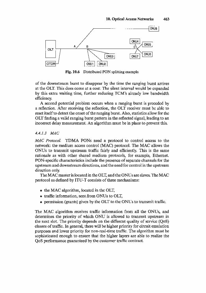
10. Optical Access Networks 463
OLT
OTDR
Fig. 10.6 Distributed PON splitting example.
of the downstream burst to disappear by the time the ranging burst arrives at the OLT. This does come at a cost: The silent interval would be expanded by this extra waiting time, further reducing TCM’s already low bandwidth efficiency.
A second potential problem occurs when a ranging burst is preceded by a reflection. After receiving the reflection, the OLT receiver must be able to reset itself to detect the onset of the ranging burst. Also, statistics allow for the OLT finding a valid ranging burst pattern in the reflected signal, leading to an incorrect delay measurement. An algorithm must be in place to prevent this.
4.4.1.3 MAC
MAC Protocol. TDMA PONS need a protocol to control access to the network the medium access control (MAC) protocol. The MAC allows the ONUs to transmit upstream traffic fairly and efficiently. This is the same rationale as with other shared medium protocols, for example, Ethernet. PON-specific characteristics include the presence of separate channels for the upstream and downstream directions, and the need for control in the upstream direction only.
The MAC master is located in the OLT, and the ONUs are slaves. The MAC protocol as defined by ITU-T consists of three mechanisms:
0 the MAC algorithm, located in the OLT, 0 traffic information, sent from ONUs to OLT, 0 permission (grants) given by the OLT to the ONUS to transmit traffic.
The MAC algorithm receives traffic information from all the ONUs, and determines the priority of which ONU is allowed to transmit upstream in the next slot. The priority depends on the different quality of service (QoS) classes of traffic. In general, there will be higher priority for circuit emulation purposes and lower priority for non-real-time traffic. The algorithm must be sophisticated enough to ensure that the higher layers are able to realize the QoS performance guaranteed by the customer traffic contract.

464 Edward Harstead and Pieter H. van Heyningen
When two different users are connected to the same ONU, and both deliver traffic with the same QoS class, special measures should be taken either to provide fair access to the PON, or at least to prevent that one user experiences starvation due to the traffic offered by the other user. Several measures can be taken, for example, policing per user in the ONU (expensive) or granting permission per user interface instead of per ONU. The traffic of the differ- ent users should be stored in different ONU queues to make such measures possible.
There are two principally Merent MAC protocols: static bandwidth allo- cation and dynamic bandwidth allocation. A static MAC allocates bandwidth to ONUS by manual provisioning. The bandwidth is determined by the traffic contract, regardless of the momentarily offered traffic. This MAC is always needed to provide the guaranteed minimum bandwidth for any traffic flow, and is sufficient by itself for constant bit-rate services (CBR), where the required bandwidth is known and does not change during the connection time.
Dynamic bandwidth allocation (DBA) allocates bandwidth adaptively, based on the varying amount of traffic offered by the ONUS. If the PON has to transfer statistically variable traffic like non-CBR ATM or IP, a flexible bandwidth allocation for each ONU is desirable. Each ONU should be able to ask for and to get a part of the bandwidth of the PON. Compared to the static MAC, DBA will increase the network efficiency because a higher statistical multiplexing gain can be obtained.
ITU-T G.983.1 only standardized some aspects of the MAC protocol, such that only a static MAC can be guaranteed in a multivendor environment. FSAN is currently working on a specscation for a communications channel, used to communicate traffic conditions in the ONU to the OLT, and the priority classes of tr&c upon which the MAC operates. The container for traffic information transfer from ONU to OLT, standardized in ITU-T G.983.1, is the so-called mini-slot, which is of programmable length, but always shorter than cells. The contents of the mini-slot could signify, for example, the length of the queues in the ONU butTers. The format and coding of the mini-slot contents requires standardization. This will enable multivendor operation of DBA, and it is the objective of FSAN that a new ITU-T Recommendation on this issue will be published. The MAC algorithm itself in the OLT, which uses this information to generate grants, is outside the scope of standardization, is not required for multivendor interoperability, and is an area for vendor innovation and differentiation.
Traffic using DBA may be oversubscribed in two ways. Either the s u m of the maximum bandwidths of all subscribers is higher than the PON bandwidth, or the sum of the guaranteed bandwidths is higher than the PON bandwidth (Devadhar 2000). The first case is usually called statistical multiplexing, with a multiplexing gain that is the quotient of the users’ maximum bandwidth and the bandwidth that is allocated to these users. The second case is usually called overbooking. Overbooking is based on the phenomenon, observed by
10. Optical Access Networks 465
operators, that the long-term average utilization of networks is below 3040%. To improve this, the operators might want to have the ability to decide on a certain overbooking, i.e., the bandwidth of the PON is considered higher than it physically is.
The actual situation in FSAN (as of December 2000) calls for a MAC at the transmission convergence layer. Various types of traffic containers are defined. Such a container is essentially a pipe that connects the O W to the OLT. A single container is able to carry connections with different higher layer QoS classes. One O W can support one or more traffic containers. For shared ONUS, it should also be possible to allocate a container for each user of that ONU. The container allocation depends on the service situation, and is done via manual provisioning. The ONU reports the status of the container bufTers to the OLT. The OLT issues grants to containers, each grant directed to only one container. Concerning the traffic types, a bandwidth priority hier- archy will probably be defined that has four bandwidth classes. From highest to lowest priority, these classes are guaranteed fixed bandwidth, guaranteed assured bandwidth, additional nonassured bandwidth, and additional best- effort bandwidth. The mapping of the bandwidth classes on the container types is being standardized. At this moment five container types are consid- ered, of which some have a mixture of bandwidth classes. The mapping of ATM traffic classes on the various types of containers will also be standardized.
lMAC Algorithm and Statistical Multiplexing Gain. The MAC algorithm must guarantee the customers’ QoS, while satisfying the operator’s desire for maxi- mum network efficiency. For statistically behaving cell or packet trafEc loads, these tasks are in conflict with each other. The operator wants high statistical multiplexing gain, which implies a certain risk that the QoS of the connections is below the agreed value.
In general, to design a MAC, a split is made between real-time traffic and non-real-time trafEc. For real-time traffic, the traffic characteristics should be maintained, which means fast access to the network without a noticeable delay. For non-real-time traffic, a low momentary access speed is tolerated, but buffers in the ONU are required to store the traffic. Combining the various requirements in an efficient way is the task of the MAC. Numerous studies and simulations to design efficient MAC algorithms can be found in the liter- ature, for example, in Killat et al. (1 996), where various MAC algorithms are proposed and analyzed for an ATM PON.
However, it must be realized that simulations of MAC performance are dependent on assumed traffic behavior of the sources. In the past, commonly used network traffic modeling was based on a Poisson or Markovian distribu- tion of the arriving packets or cells. The characteristics of such distributions leads to smoothing the overall traffic load by averaging over a large number of users and a long enough timescale. But measurements of real, modern network
466 Edward Harstead and Pieter H. van Heyningen
traffic such as TCP/IP or multimedia traffic indicate that this assumption is not valid. A significant traffic variance is present even on aggregated t r a c . This phenomenon is called self-similarity. The self-similar behavior of such traffic is affirmed by various theoretical studies based on real-world source modeling, which better describes the real-trac statistics (Sahinoglu et al. 1999; Tsy- bakov et al. 1998; Veres et al. 2000). The consequence of this self-similarity for network design is that previously expected statistical multiplexing gain factors cannot be realized.
The statistical multiplexing gain that can be obtained on a PON with DBA does not differ significantly from other statistical multiplexing systems. The differences, which have a minor influence, are the presence of upstream queue length messages, which take some percents of the bandwidth, and the phys- ical delay in the PONY which causes some extra delay variation. Simulations based on on-off bursty traffic with a mean burst size of 10 cells (Markovian t r a c statistics, so not self-similar) showed, as a best situation, that a gain up to 7.5 at an average PON load of 68% is possible with an acceptable QoS performance (Killat et al. 1996). Statistical multiplexing gain that can be real- ized when multiplexing self-similar traffic is still a subject of investigation. One of these investigations is given in Bashforth et al. (1998), where a detailed simulation study is reported for self-similar traffic multiplexing with MPEG traffic in a general, non-PONY multiplexing situation. The conclusion is that a moderate statistical multiplexing gain can be achieved. A generally applicable number to quantify such gain is not given; too many parameters are involved. But as an example, the best situation achieves an average network load of 63% with a statistical multiplexing gain of about 1.5, with an acceptable QoS performance.
4.4.2 SCMA
The previous discussions on burst-mode transmission, ranging, and MAC all pertain to TDMA. Another upstream multiple access method that has received considerable research attention is subcarrier multiple access (SCMA). Instead of partitioning the time domain, the ONUS transmit simultane- ously but on different, assigned RF carriers. Each ONU’s upstream data modulates the RF carrier, i.e., a subcarrier, which then modulates the opti- cal source. At the OLT receiver, after optical-to-electrical (O/E) conversion, the upstream signals are demultiplexed in the electrical domain and sent to separate demodulatordreceivers.
To minimize crosstalk between channels, there needs to be adequate filtering in the electrical domain on both transmit and receive sides. Also, there needs to be adequate linearity of the transmitter and receiver components, including the laser, or the signal bandwidth will spread. If nonlinearity generates higher- order harmonics, it can interfere with higher-frequency subcarriers, unless the subcarriers are restricted to a single octave. There are several modulation

10. Optical Access Networks 467
techniques, but the category that places the easiest requirements on linearity are constant envelope techniques, where the envelope of modulation remains constant even during transitions from one symbol to the next. These are frequency shift keying (FSK) techniques, and there are several kinds that mini- mize the signal bandwidth. Bandwidth efficiency is important if the subcarriers are to be restricted to a single octave, and in general because higher-frequency components will cost more.
Crosstalk is an issue because there may be a soft signal in the presence of loud signals. Therefore, to minimize adjacent channel interference, the frequency guard bands will need to be sized to the optical dynamic range requirements of PONY impacting bandwidth efficiency.
ONUs will need to be assigned different carrier frequencies upon con- nection to the PONY requiring ONU frequency agility. This is relatively straightforward, but to vary the bandwidth allocation (RF spectrum) more complicated RF filter control will be required.
Because the signals from many ONUs will be incident simultaneously on the OLT square-law photodetector, SCMA is susceptible to OBI. The dis- cussion on OBI in Section 3.3.2 now applies more generally with a plurality of interferers. The penalty from OBI will be most severe on a PON when the beat notes from many strong channels interfere with the signal from a weak channel. Therefore, OBI has the potential to significantly limit the PON optical dynamic range, and aggressive measures to broaden the source optical spectrum have been undertaken. Results with lasers designed for self-sustained oscillation have been reported (Bates et al. 1991), but only at short optical wave- length. Very high laser modulation index at the subcarrier frequency (Wood et al. 1993; Feldman et al. 1996) or at an out-of-band frequency (Woodward et al. 1996; Lin 1997; Yamamoto et al. 1999) improves OBI, but clipping increases harmonics. An amplified light emitting diode (LED) has been used as a source (Feldman et al. 1996b), but LEDs have speed limitations and a low-cost amplified commercial device does not yet exist.
Comparing SCMA against TDMA, the main attraction of SCMA is that the ONUS can operate at their own (and possibly different) bit rates, not the much higher aggregate TDMA rate (however, assuming that the down- stream signal is TDM, the downstream part of the ONU will already be operating at the downstream aggregate rate, which will equal or exceed the upstream rate). Buffers can be smaller and delay reduced. Ranging is not required, which greatly simplifies logic design, and ranging-induced delay and delay variation on upstream traffic is avoided. But SCMA has not been used on any commercial PONs. The reason for this is that for the kind of bit rates required in upstream PONs, the digital electronics required by TDMA are less expensive and can be highly integrated, while SCMA requires addi- tional RF components of nonnegligible costs that are not easily integrated. Finally, there is the difficulty in flexible bandwidth allocation and the OBI problem.

468 Edward Harstead and Pieter H. van Heyningen
4.4.3 WDMA
The technique of (dense) wavelength-division multiple access (WDMA) can be used on a PSPON. In the upstream direction, each O W sends its traffic on a unique wavelength, all the wavelengths are power-combined in the ODN, wavelength demultiplexed at the OLT, and sent to a receiver array. However, similar to downstream DWDM (Section 4.3) ONUS with fixed-wavelength transmitters will impact operations, and tunable transmitters are more costly. In either case, wavelength control adds considerable cost to the ONU com- pared to a TDMA. Methods of achieving WDMA without ONU wavelength control are covered in Section 5.3.
4.5 SECURITYAND PRIVACY
The point-to-multipoint nature of PONs introduces concerns when the fiber is run all the way to the customer premises, as in FTTBusiness and FTTH.
4.5.1 Privacy
Privacy is the end-user’s concern that his or her communications can be listened to by another party on the same PON. All PSPONs broadcast the down- stream signal to end-users, potentially allowing one end-user to eavesdrop on another end-user’s payload. There is at least one level of protection against this: The PON protocol itself would need to be emulated. A second level of protection is to encrypt the downstream signals. An example of this is the so-called “churning” specified in ITU-T G.983.1, a relatively light encryption mechanism. The standard was written with the understanding that if greater protection were required, more sophisticated encryption should be provided at a higher layer.
There is also the possibility that upstream signals reflected back from the upstream side of the splitter can be intercepted at another end-user location. However, it is generally accepted that the necessary magnitudes and combina- tion of reflections and splitter losses will rarely, if ever, occur, and so upstream signals are often transmitted in the clear (as in ITU-T G.983.1).
4.5.2 Security
Security is the network provider’s concern that the network may be subject to unauthorized use or sabotage. On PONs, there is the potential for mis- chief whenever someone can gain access to the fiber (e.g., an unused drop). A “pirate” can connect an ONU and steal service. Piracy can be thwarted with a password protocol (called “verification” in ITU-T G.983. l), but this would require that the OLT has a priori knowledge of each ONU’s ID number and password before installation, a logistical challenge. It is more simple for the ONU, at first initialization, to communicate its password to the OLT, which

10. Optical Access Networks 469
assumes it to be legitimate and stores it. Later, the OLT is then able to chal- lenge the ONU for its password to ensure that a masquerading ONU has not been connected to the network when the legitimate ONU is in power-down mode. At any rate, since passwords are only sent upstream, they should not be interceptable.
Sabotage is the more problematic possibility where someone maliciously injects an upstream signal with the intention to interfere with or block upstream transmissions. Countermeasures include alarming of the ONU housing to detect unauthorized entry and remote detection of fiber breaks (see Section 4.6). However, it is impossible to quantify the risk, and sabotage has generally not aroused much concern.
4.5.3 Conclusion
The question is not whether PON networks are perfectly invulnerable, but whether an acceptable level of privacy and security can be guaranteed. A widely held view is that with the simple measures described above, PONS will be at least as good as today’s twisted pair and SONET/SDH ring networks (when a SONET/SDH node is deployed on business premises).
4.6 FAULT LOCATION TECHNIQUES FOR PONs
As with other fiber-optic systems, it is desirable to monitor PON fibers and to detect and locate faults when they occur. Aspects of this problem peculiar to PONs are discussed here.
There is a kind of built-in fault location capability in PON networks. The OLT can localize fiber cuts to a particular segment by correlating the loss of signals from ONUS. For example, the PON in Fig. 10.6 has three splitting points, A, B, and C. If the OLT suddenly lost upstream signals from ONUS 4, 5, 6, and 7 (only), it could infer a fiber cut in the segment between splitters B and C. But it cannot locate the fault within the segment. Furthermore, if the fault is on the drop segment, it cannot distinguish between a cut in the drop and an ONU failure. Optical time-domain reflectometry (OTDR) techniques, on the other hand, are well-suited for both of these. Ideally, the OTDR would be colocated with the OLT where it could continuously monitor the fiber network and troubleshoot faults. So as not to interfere with working signals, OTDR wavelengths above 1600nm have been proposed. Blocking filters would be required at the ONU receivers. But when a conventional OTDR is used to analyze a point-to-multipoint network, it must have the dynamic range to cope with the large, lumped splitter losses. Even more problematic is the fact that reflections and backscatter from the optical branches after the splitter(s) are superimposed, making it difficult to resolve features on any particular branch. Various schemes have been proposed to overcome this. A brief survey of some of these solutions follows.
470 Edward Harstead and Pieter H. van Heyningen
4.6.1 Comparison with Reference Traces
This method requires an OTDR backscatter trace from the root of the ODN at installation. Then, employing various techniques to associate each PON branch end reflection with an ONU, a reference trace is created. Such tech- niques include computation of predicted backscatter traces from a priori known OLT-ONU path lengths and the installation of wavelength-selective reflectors at each ONU (passes signal wavelengths and reflects the OTDR wavelength) to increase visibility of the branch end point.
A future backscatter trace can be made, and this can be compared with the reference trace. If there is a change due to a fault, it has been claimed that algorithms have been developed that can determine which distribution fiber has been affected, and where the fault is (Takeda et al. 1994; Wuilmart et al. 1996; Araki et al. 1998).
There are installation and equipment costs associated with this method. Each ONU requires an additional optical component, whose insertion loss must be accounted for. Also, if the difference between any two or more OLT- ONU paths is less than the OTDR resolution, different length patch cords will need to be installed at the ONUS to remove the ambiguity.
4.6.2 WDM-Based OTDR
Instead of plain power combiner-splitters in the ODN, a passive device that is a splitter-combiner at the signal wavelengths and is a wavelength router at OTDR wavelengths is deployed. In this way, each of the distribution fibers can be individually addressed depending upon the wavelength. The OTDR employs a tunable laser that can then diagnose each branch individually (Tanaka et al. 1996).
4.6.3 Polarization OTDR
Analogous to this WDM-based OTDR is the polarization-based OTDR. At each downstream splitter port, an out-of-band linear fiber polarizer is installed, with each port having a different angle of polarization. The output from a conventional OTDR is passed through a polarization controller. In this way, the OTDR can be tuned to analyze each branch individually.
4.6.4 Diagnosis in the Field
All of these schemes involve at least one of the following: enhanced OTDRs, manipulation of the outside plant so as to make distribution fibers “different” from each other, and comparison of OTDR plots before and after faults. Although decreasing maintenance costs by performing fiber monitoring and fault location from the OLT is a worthy goal, significant installed first costs are incurred through customized ODN installation and specialized equipment.
10. Optical Access Networks 471
The straightforward alternative is for a technician to disconnect the faulty branch from the working network at a splitter andor ONU location and probe the single piece of fiber with an OTDR. This is made easier if splitters and ONUS are connectorized. Because that fiber segment has been isolated, the OTDR can even operate at conventional wavelengths. If the splitter is spliced, it might be assumed that it is OK to probe upstream from the ONU. Since the fiber is presumably broken, other working upstream transmissions should not be affected.
The downside to field diagnosis is the added expense of sending technicians into the field to perform fault analysis.
4.6.5 Central Office Splitter Placement
For characterization of each PON leg with a conventional OTDR located in the CO without tricks, there is a simple solution: Move all splitting to the CO. Of course the PON’s fiber gain is lost, and it could be argued that the simplicity of a PTP network would be preferred. However, NTT has calculated that a PON with or without fiber gain can still be more cost-effective than a PTP system, and furthermore, when maintenance costs are factored in, a PON with its splitter in the CO is more cost-effective than one with the splitter located near customers for short loop lengths (Nakao et al. 1996). Since distances in Japan are short, NTT has installed systems with splitters in the CO.
4.6.6 Conclusion
Due to the immaturity of the advanced OTDR techniques described previ- ously, and the resulting first costs the networks incur, diagnosis in the field or central office splitter placement are likely to be the standard fault location techniques for PON in the near term. For a more detailed discussion on this topic, refer to Caviglia et al. (1999).
4.7 PROTECTION
Reliability and availability are important aspects for network operators. Reli- ability is commonly expressed by the mean time between failure and availability by the up time per year per user. Availability depends on the reliability of the fiber and equipment, the repair time (including time for maintenance), and deployment of redundancy. Implementation of redundancy in the system architecture, combined with automatic protection switching, is important for protecting the user traffic against network and/or equipment failures.
Compared to ring networks as used in SONET/SDH, the PON tree-and- branch structure is more vulnerable to single points of failures due to its topology and the lack of an alternative redundant path.
This has been recognized by ITU-T, therefore, in an appendix of ITU-T G.983.1 , several redundant network architectures are proposed for
472 Edward Harstead and Pieter H. van Heyningen
ATM PONs. However, no details on the mechanisms and protocols to apply protection switching are standardized. This means that multivendor inter- operability cannot be realized based on this standard. Because the operators in FSAN have expressed their wish that multivendor interoperability should be possible, further standardization is under study in FSAN and may lead to a specific ITU-T Recommendation on protection switching for ATM PONs. A possible outcome of the FSAN work will be that protection switching will take place in the transmission convergence layer, with protection switch-over times that are comparable to SONET/SDH times (50 ms). An alternative and more lenient switch-over time requirement can be that connections are not lost, which depends on the signalling protocol applied for a particular con- nection (e.g., the POTS signalling protocol requires a shorter switch-over time than ATM signalling protocols). The standardization of hitless switching (ie., no bits are lost) will probably also be taken into consideration, but because of additional costs associated with such switching, it is questionable if it will be standardized.
Availability is a key issue for business customers. To assess the need for protection in PONs in terms of unavailability figures, a detailed study has been performed (de Groote et al. 1999). The mean downtime is a combination of reliability and repair time. The repair time was assumed to be 2 hours for the OLT (located at the CO) and 24 hours for the fiber and the ONUS. In that example, a mean PON downtime of about 350 minutedyear is calculated, which is far more than 53 minutedyear (99.99% availability), which is con- sidered a requirement for a multiservice access network. The major cause of downtime is fiber breaks. To improve the availability, at least the OLT and the feeder fiber (option B in ITU-T G.983.1) have to be duplicated. This is depicted in Fig. 10.7 (upper diagram). But even then the 53 minutedyear cannot be real- ized; the downtime is slightly more, about 90 minutedyear. Full duplication, which includes the OLT, the ONU, and the complete outside plant fiber (option C in ITU-T G.983.1) (see Fig. 10.7, lower diagram), provides a much better availability, but at higher costs.
Because of the point-to-multipoint topology of the PONY the physical layer is shared and does not allow for simple point-to-point physical layer protection as in SONET or SDH. The shared medium leads to PON-specific protection architectures, and to specific issues, such as whether a mixture of protected and unprotected ONUs on one PON should be possible. Moreover, issues such as switch-over time and sanity checks are more complicated. The sanity check is needed to determine the quality of the redundant path before the switch-over to that path takes place. Plus, before switch-over, the redundant ONUS must be ranged on the redundant path, which in general will be of different length than the working path. This will lead to increased switch-over times compared to nonshared networks.
The PON shared medium topology also asks for special measures in the upstream direction if extra t r a c has to be supported. The protection path

10. Optical Access Networks 473
~
7
- -
ONU #1
R Fig. 10.7 ITU-T G.983.1 PON protection configurations.
is available to carry extra tr&c as long as the working path is up. Extra traffic will increase the overall network efficiency of the working PON plus protection PONY because the extra traffic uses the protection capacity of a protected O W . There are several issues related with extra traffic as there is a need for an automatic protection switching protocol. Moreover, as long as the working PON is not fully loaded with protected traffic, the protection PON can have a mixture of extra traffic and regular nonprotected traffic. The MAC has to take this issue into account.
In de Groote et aZ. (1999), a method is described how both the sanity check and the ranging of the ONUs over the redundant path can be performed. This is done by application of physical layer operations and maintenance (PLOAM) cells over the stand-by equipment, without causing interference on the user traffic on the working path. It is shown that switch-over performance can be obtained comparable to SONET/SDH requirements (50 ms switch-over time).
A deficiency of protection switching methods, such as those mentioned in ITU-T G.983.1 option C and de Groote et al. (1999), is that in a mixed situ- ation, with protected and unprotected ONUS on the same PONY unprotected ONUs on the working PON are disconnected in case of switch-over to the redundant PON. Because it is expected that such mixed situations occur reg- ularly, such a solution is unattractive for operators. A better method provides logical point-to-point protection from the OLT to each ONU on the PON. This can be realized by applying simultaneous transmission (bridging) on both the working path and the protection path at both sources (OLT and ONU). The
474 Edward Harstead and Pieter H. van Heyningen
selection of the good connection takes place at both sink ends. In the upstream direction, the ONU bridges its traffic flow in a timeslot in each of the PONS. Such a method is generally known as 1 + 1 unidirectional switching, and is attractive because a protocol is not needed, because every sink can switch on its own. Consequently, development and multivendor interoperability would be easier to achieve. Switch-over times can be very short because there is no exchange of protocol information between ONU and OLT.
If PON protection is to be standardized, several issues need be addressed. These include protocol definition, 1 + 1 vs 1 : 1 architecture, revertive and nonrevertive switching, bi- and unidirectional switching, and extra t r a c . The 1 + 1 bidirectional switching discussed in the previous paragraph does not allow extra traflic, which is a disadvantage. A 1 : 1 PON protection architecture allows for extra traffic, but if the take rate of protected service is not high, it may not be worthwhile to undertake the complexity of standardization and implementation of 1 : 1 protection. All these issues are under discussion in FSAN, with the objective to standardize PON protection in a future ITU-T Recommendation. Such a standard is considered important for large-scale PON deployment for business access.
4.8 OPTICAL BROADCAST
When adding a unidirectional broadcast service, specifically CATV, the broad- cast nature of a PSPON can be used to advantage. The primary requirement is to provide entertainment video at a level at least comparable (number of chan- nels, picture. quality, and end-user interface) to that of the CATV providers. There are two ways to achieve this: true broadcasting (either analog, digital, or both) and integrated “broadcast replication.”
4.8.1 Broadcast Replication
Instead of broadcasting all channels to all subscribers for local selection at the set-top box (STB), a “zapping” protocol between the STB and a remote channel server enables remote channel selection. Since only those channels requested by the users on the PON are broadcast (digitally), the required downstream bandwidth may be within the capabilities of a conventional ATM PON, depending on service take rate. Both the channels and the protocol are integrated into the main PON traffic. The FTTC SDV systems used broadcast replication to solve the bottleneck of the twisted-pair medium used in the VDSL drop. For FTTH, this constraint disappears, and there seems to be little reason to implement its complex protocols, and risk disappointing the customer with inferior channel selection performance, and to then be faced with an enormous upgrade challenge when high-definition television (HDTV) becomes ubiquitous.
10. Optical Access Networks 475
4.8.2 True Broadcasting of the Stack of Frequency-Division Multiplexed (FDM) Channels
Probably the most practical solution to provide CATV service, even over fiber, is to deliver the full stack of channels to the customer’s home for local selec- tion. This solution will meet all customer expectations and meet or exceed all the capabilities of the CATV HFC network. Further minimizing overall costs of providing video services, this solution works with existing high-volume dig- ital STBs (with little or no modification), associated handheld controllers, and existing digital head-end equipment. True broadcast can be carried over FTTH or FTTC (with a coaxial cable connecting the ONU to the home). A funda- mental decision is whether channels must be delivered to the home in analog format or if it is acceptable to deliver digitized channels only, with conversion to analog in the home. This is in part a customer acceptance issue, as owners of cable-ready televisions may not like to have a digital STB on top of every set.
The most straightforward approach is to transmit a standard 50 MHz to 550 (or 750) MHz analog AM-VSB (amplitude modulation vestigial sideband) or mixed analoddigital signal over a tree-and-branch PON. This can be done on a separate fiber from the fiber(s) used for bidirectional baseband signals (e.g., Kettler 2000), or the interactive services can also be carried in passband, i.e., an HFC system with fiber extended all the way to the curb or home (Wood et al. 1999). To achieve a satisfactory carrier-to-noise-ratio (CNR) for analog channels, the ONU receiver requires a very high optical input power, which in turn requires optical amplification somewhere upstream. As with HFC systems, this is typically done with an erbium-doped fiber amplifier (EDFA), but in FTTC or FTTH systems the cost of the EDFA will be shared by relatively few users, especially for low video take rate. Such systems will be costly until such time that EDFAs become much less expensive on a costImW basis.
Most work has attempted to overlay the CATV signal onto the same fiber as the bidirectional baseband signals. There are separate optical sources for the downstream passband video signal and the downstream baseband interactive signal. To eliminate the loss of a 1 : 2 coupler, the digital video passband signal can be carried on a dedicated feeder fiber and optically inserted at a second input port at the first splitter. Different wavelengths can be used for the downstream signals so that they can be demultiplexed at the O W . NTT, in laboratory and field trial environments, evaluated various 1.5 Fm window video overlays to their 1.3 km bidirectional narrowband PON (Omiya 1997; Ogura et al. 1997). The ONU has a WDM (e.g., Fig. 10.1 1) for directing the video signal to a separate video receiver. In this way modular ONUS can be designed so that for a less than 100% video take rate, only subscribers to the video service need to pay for the hardware associated with it. Some channel formats contained AM channels, but to keep the optical power low, the number of AM channels was small. The remaining channels were either FM (also an analog signal but with a much lower CNR requirement) or digital format.
476 Edward Harstead and Pieter H. van Heyningen
In contrast to NTT's narrowband PONS, broadband PONS now generally use WDM for directional multiplexing, occupying both of the 1.3 and 1.5 pm windows, and making it harder to use WDM for the video overlay. So it has been proposed to use the 1.5 pm window for both of the downstream signals, still originating from separate (1.5 pm) sources, but with both detected by a single optical receiver in the ONU. Demultiplexing is now done solely in the RF domain, which means that the video signal must reside completely in the RF passband above the broadband baseband signal. This is a problem for conventional CATV signals, which start at 50 MHz and whose analog channels have much higher CNR and power requirements than the baseband signal.
The problem can be solved if the full stack of channels is transmitted in digital format with conversion to analog in the home, and a higher RF fre- quency plan is used. This approach has been demonstrated to work with DBS (direct broadcast satellite) format QPSK (quadrature phase shift keying) mod- ulated 30 MHz-spaced carriers (Chand et al. 1999a) and MMDS (multichannel multipoint distribution service) format 64-QAM (quadrature amplitude mod- ulation) modulated 6 MHz-spaced carriers (Chand et al. 1999b). In either case existing terminal equipment can still be used at both ends of the PON. Broad- cast capabilities of 1 Gb/s or greater are realized, suilicient to support HDTV as it becomes available. With the cost of video compressioddecompression dropping this is an attractive approach from a technological point of view.
This sharing of the 1.5 pm window between an all-digital CATV signal and the downstream baseband signals is being addressed in FSAN, which is defining a new, narrower wavelength range for the downstream baseband transmitter. This is to ensure that the two downstream signals are sufficiently far apart in optical frequency to avoid OBI effects.
4.8.3 Integrated Baseband Broadcast
If the downstream baseband bit rate is high enough, it is possible, of course, to multiplex the stack of digital channels into the baseband signal with the other services, doing away with all the additional hardware required in an overlay and the potential OBI issues. Originally 622 Mb/s was thought to be adequate for this purpose, but the quantity of channels offered by CATV providers has now climbed too high. A 2.5Gb/s rate has been proposed in so-called gigabit-to-the-home (GTTH) systems (Shibutani et al. 1997), which use 1.5 pm downstream and 1.3 pm 155 Mb/s upstream. Such downstream bandwidth can simultaneously carry the services usually associated with ATM PON, plus 200 digital video programs in MPEG2 format (6 Mb/s per channel).
The 2.5 Gb/s speed can be realized with common existing technologies, but the challenge is to do so at very low size and cost, especially since every sub- scriber must pay for a 2.5-Gbh ONU whether video service is subscribed to or not (optical components for PON are covered in Section 6, but work specif- ically aimed at GTTH is mentioned here). Essential to reach these goals is a
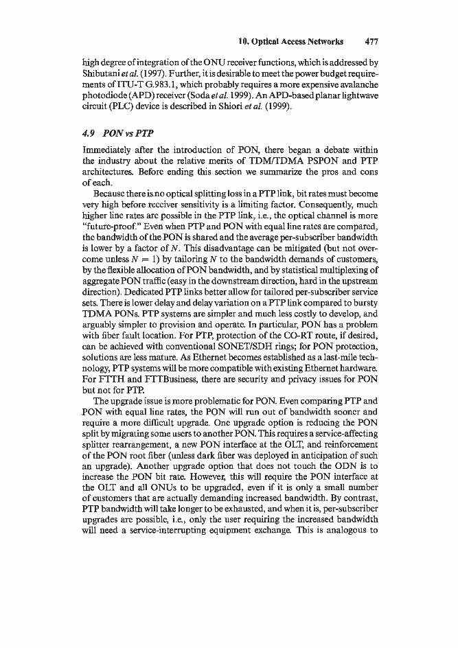
10. Optical Access Networks 477
high degree of integration of the ONU receiver functions, which is addressed by Shibutani et al. (1997). Further, it is desirable to meet the power budget require- ments of ITU-T G.983.1 , which probably requires a more expensive avalanche photodiode (APD) receiver (Soda etal. 1999). An APD-based planar lightwave circuit (PLC) device is described in Shiori et al. (1999).
4.9 PON vs PTP Immediately after the introduction of PONY there began a debate within the industry about the relative merits of TDM/TDMA PSPON and PTP architectures. Before ending this section we summarize the pros and cons of each.
Because there is-no optical splitting loss in a PTP link, bit rates must become very high before receiver sensitivity is a limiting factor. Consequently, much higher line rates are possible in the PTP link, i.e., the optical channel is more “future-proof.~y Even when PTP and PON with equal line rates are compared, the bandwidth of the PON is shared and the average per-subscriber bandwidth is lower by a factor of N . This disadvantage can be mitigated (but not over- come unless N = 1) by tailoring N to the bandwidth demands of customers, by the flexible allocation of PON bandwidth, and by statistical multiplexing of aggregate PON traf3ic (easy in the downstream direction, hard in the upstream direction). Dedicated PTP links better allow for tailored per-subscriber service sets. There is lower delay and delay variation on a PTP link compared to bursty TDMA PONS. PTP systems are simpler and much less costly to develop, and arguably simpler to provision and operate. In particular, PON has a problem with fiber fault location. For PTP, protection of the CO-RT route, if desired, can be achieved with conventional SONET/SDH rings; for PON protection, solutions are less mature. As Ethernet becomes established as a last-mile tech- nology, PTP systems will be more compatible with existing Ethernet hardware. For FTTH and FTTBusiness, there are security and privacy issues for PON but not for PV.
The upgrade issue is more problematic for PON. Even comparing PTP and PON with equal line rates, the PON will run out of bandwidth sooner and require a more difficult upgrade. One upgrade option is reducing the PON split by migrating some users to another PON. This requires a service-affecting splitter rearrangement, a new PON interface at the OLT, and reinforcement of the PON root fiber (unless dark fiber was deployed in anticipation of such an upgrade). Another upgrade option that does not touch the ODN is to increase the PON bit rate. However, this will require the PON interface at the OLT and all ONUS to be upgraded, even if it is only a small number of customers that are actually demanding increased bandwidth. By contrast, PTP bandwidth will take longer to be exhausted, and when it is, per-subscriber upgrades are possible, i.e., only the user requiring the increased bandwidth will need a service-interrupting equipment exchange. This is analogous to

478 Edward Harstead and Pieter H. van Heyningen
Ethernet LAN% where autosensing interfaces allow an Ethernet hub to adapt to individual users upgrading from 10 Mb/s to 100 Mb/s on the same LAN.
But PONS have built-in fiber gain, which means that they have amuch longer prove-in distance than PTP systems. In other words, PTP systems will likely require many more remotely located OLTs, with their associated powering and maintenance issues, whereas PONS will require fewer or maybe none. Another view is to compare PON and PTP when the OLT is located in the CO for both. PON’s fiber gain, after the cost of the splitter is accounted for, can result in lower cost ODN for longer loops. Sharing of the OLT optical interface, after accounting for the increased cost of optical components and PON logic, may save costs. PON also has built-in distributed multiplexing, which requires less multiplexing at the OLT. PTP systems will have a large number of fibers homing into an OLT, which might pose a physical congestion problem; PON pushes the connections out to the splitter sites. PON is a more natural topology for the overlay of broadcast services. PON allows for splicing in new unplanned subscribers without the need to reinforce the entire ODN.
There is no right answer, although some general remarks can be made. If the figure of merit is cost per subscriber, then PON has the potential for being the lower-cost system. Examples of this case are FTTH and fiber to the small-to-medium business.
If the figure of merit is cost per unit bandwidth delivered to the sub- scriber, then PTP is likely to be lower cost. An example of this case is fiber to the medium-to-large business (where PTP will compete with more reliable SONETISDH rings). Another example are FTTx cases where shared ONUS aggregate bandwidth from multiple subscribers. Here, there is already a large sharing factor of everything upstream of the ONU, and the cost benefit of further sharing from PON is greatly diluted.
4.10 SUPERPONS
Another kind of PSPON that has been the subject of research is the Super- PONY a TDM/TDMA PON with considerably more users and covering a longer distance than the typical PONS with a maximum of 32-64 users and a maximum length of 20 km. The concept of the SuperPON was developed in the mid- 1990s and was justified by two scenarios. First, the need to have an all- optical FTTH upgrade scenario ready for FlTC/Cabinet PONS: Only if such an upgrade scenario was available and proven to be feasible, it was argued, would FTTC be deployed on a large scale. Second, central office consolidation would greatly increase the distances between OLT and ONU.
In Mestdagh et al. (1996), the design of a SuperPON is thoroughly described. Proposed is a TDM/TDMA system for 100 km, a splitting factor of 1024 or 2048, and bit rates of 2.5 Gbls downstream and 31 1 Mb/s upstream. It is theoretically shown that the losses of the optical signal that occur in a SuperPON can be overcome satisfactorily with optical amplification. The main
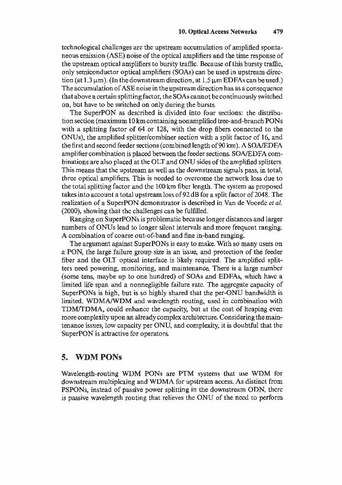
10. Optical Access Networks 479
technological challenges are the upstream accumulation of amplified sponta- neous emission (ASE) noise of the optical amplifiers and the time response of the upstream optical amplifiers to bursty traffic. Because of this bursty traffic, only semiconductor optical amplifiers (SOAs) can be used in upstream direc- tion (at 1.3 pm). (In the downstream direction, at 1.5 pm EDFAs can be used.) The accumulation of ASE noise in the upstream direction has as a consequence that above a certain splitting factor, the SOAs cannot be continuously switched on, but have to be switched on only during the bursts.
The SuperPON as described is divided into four sections: the distribu- tion section (maximum 10 km containing nonamplified tree-and-branch PONS with a splitting factor of 64 or 128, with the drop fibers connected to the ONUS), the amplified splitterkombiner section with a split factor of 14 and the first and second feeder sections (combined length of 90 km). A SONEDFA amplifier combination is placed between the feeder sections. SONEDFA com- binations are also placed at the OLT and ONU sides of the amplified splitters. This means that the upstream as well as the downstream signals pass, in total, three optical amplifiers. This is needed to overcome the network loss due to the total splitting factor and the 100 km fiber length. The system as proposed takes into account a total upstream loss of 92 dB for a split factor of 2048. The realization of a SuperPON demonstrator is described in Van de Voorde et al. (2000), showing that the challenges can be fulfilled.
Ranging on SuperPONs is problematic because longer distances and larger numbers of ONUS lead to longer silent intervals and more frequent ranging. A combination of coarse out-of-band and fine in-band ranging.
The argument against SuperPONs is easy to make. With so many users on a PON, the large failure group size is an issue, and protection of the feeder fiber and the OLT optical interface is likely required. The amplified split- ters need powering, monitoring, and maintenance. There is a large number (some tens, maybe up to one hundred) of SOAs and EDFAs, which have a limited life span and a nonnegligible failure rate. The aggregate capacity of SuperPONs is high, but is so highly shared that the per-ONU bandwidth is limited. WDMANDM and wavelength routing, used in combination with TDM/TDMA, could enhance the capacity, but at the cost of heaping even more complexity upon an already complex architecture. Considering the main- tenance issues, low capacity per ONU, and complexity, it is doubtful that the SuperPON is attractive for operators.
5. WDMPONs
Wavelength-routing WDM PONS are PTM systems that use WDM for downstream multiplexing and WDMA for upstream access. As distinct from PSPONs, instead of passive power splitting in the downstream ODN, there is passive wavelength routing that relieves the ONU of the need to perform
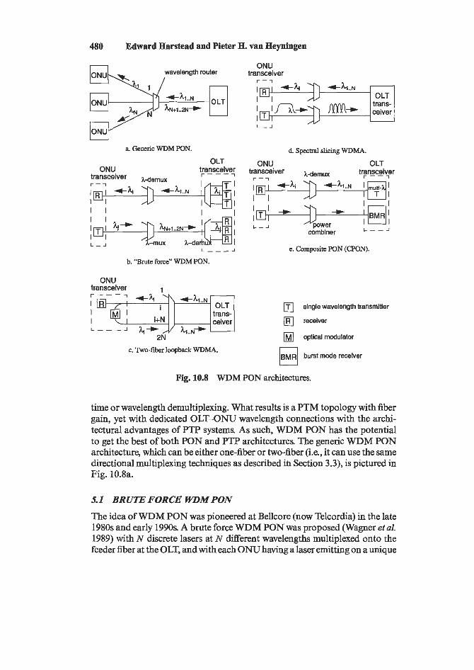
480 Edward Harstead and Pieter H. van Heyningen
- wavelength router
-
44 0
I R I IO1
;m; *
b. “Brute force” WDM PON.
‘I t h l . . N I I
-BMR I
I T 1 I - I -
‘1
ONU. transcewer 1
L - - - A
2N
c. Two-fikr loopback WDMA.
single wavelength transmitter
receiver
optical modulator
burst mode receiver
Fig. 10.8 WDM PON architectures.
time or wavelength demultiplexing. What results is a PTM topology with fiber gain, yet with dedicated OLT-ONU wavelength connections with the archi- tectural advantages of PTP systems. As such, WDM PON has the potential to get the best of both PON and PTP architectures. The generic WDM PON architecture, which can be either one-fiber or two-fiber (i.e., it can use the same directional multiplexing techniques as described in Section 3.3), is pictured in Fig. 10.8a.
5.1 BRUTE FORCE WDlM PON
The idea of WDM PON was pioneered at Bellcore (now Telcordia) in the late 1980s and early 1990s A brute force WDM PON was proposed (Wagner et al. 1989) with N discrete lasers at N different wavelengths multiplexed onto the feeder fiber at the OLT, and with each O W having a laser emitting on a unique
10. Optical Access Networks 481
upstream wavelength. A two-fiber version is shown in Fig. 10.8bY although a one-fiber WDM directional multiplexing version can be made by splitting the DWDM spectrum into downstream and upstream halves. Such a WDM PON allows for the sharing of the feeder fiber, but each ONU is burdened by the cost of two wavelength-controlled sources, one in the ONU and one in the OLT.
An especially significant effort in developing and evaluating techniques to reduce this cost was carried out at Bell Laboratories (now split between Lucent Technologies and AT&T) in the mid-1990s (largely summarized in Feldman et al. 1998). Upstream WDMA schemes that do not require wavelength control in the ONU are discussed in Section 5.3. Shared multiwavelength sources have the potential to reduce the per-ONU cost of the OLT transmitter and are discussed in Section 5.4.
5.2 THE WAVELENGTH ROUTER AND TEMPERATURE
The preferred embodiment of the wavelength router is the wavelength grating router (WGR), also known as an arrayed waveguide grating (AWG) or an opti- cal phased array (PHASAR) (see Smit 1988; Dragone et al. 1991; Takahashi et al. 1992).12 In addition to straight 1 x N wavelength multiplexing and demul- tiplexing, WGRs can be designed to exhibit periodicity, i.e., they can operate over multiple free spectral ranges. This property allows the same 1 x N WGR input/output ports to simultaneously operate over separate optical bands, per- mitting WDM directional multiplexing and the overlay of extra wavelengths for additional services.
WGRs can be made using planar waveguide silica-based technology, the same as that used in power splitters with large split ratios. They are currently more expensive than splitters, but the price difference should diminish as WGR volume is driven up by other DWDM applications. The cost gap may never be eliminated, however, because the WGR is a larger device and fewer can be made on a single substrate.
The WGR is deployed at the RN, where it is assumed that there is no electrical power available, and consequently, that there is no active temperature control. The temperature sensitivity of silica WGRs is about 0.01 1 nm/T, and so over a range of -40 to+85"C, there is a passband wavelength drift of nearly 1.4 nm. This is of the same magnitude as a typical DWDM channel spacing of 100 GHz (which corresponds to 0.8 nm in the 1550-nm band). Because the RN passband centers must be aligned with the sources and with the wavelength demultiplexer at the OLT receiver, this is a problem. There are at least three methods of dealing with this.
l2 For a more complete description of this device, refer to the chapter in this book entitled "Planar Lightwave Devices for WDM."
482 Edward Harstead and Pieter H. van Heyningen
5.2.1 Wavelength Tracking
One solution is to tune all source wavelengths and the OLT receiver demulti- plexer (which itselfcan be a WGR) into alignment with the RN WGR Gaussian passband centers. This can be done at the OLT by tuning the downstream source array to maximize the optical power from one of the RN output ports (Mayweather et al. 1996). Measuring this power back at the OLT can involve a separate monitoring channel and a return path from the RN to the OLT, which is accomplished by reflection (Giles et al. 1997) or separate loopback fiber (Monnard et al. 1997). The demultiplexer can then be tuned to the array.
Tuning will be simplified if the number of degrees of freedom, or “knobs,” is limited. In the brute force WDM PONY each of the 2N sources plus the OLT multiplexer and demultiplexer will need to be individually tuned, a total of 2N + 2 knobs. All downstream source alternatives in Section 5.4 poten- tially replace N of those with single-knob tuning. The WDMA alternatives in Section 5.3 remove the need for all N knobs in the ONUS. Further, the ONUS can participate in wavelength tracking and remove the need for returning power from the RN back to the OLT.
5.2.2 Set-and-Forget
If the channel spacings are wide enough and the optical sources are tuned to the middle of the WGR temperature range, wavelength tracking can be eliminated. Called “set-and-forget,” this strategy requires channel spacings on the order of 400GHz. Such spacings limit the channel density (e.g., 16 channels would occupy 48 nm of the 1550-nm window), and if EDFAs are used anywhere within the system, this limitation could become important. Since the signal will be drifting across the WGR passband, set-and-forget would benefit from WGR passbands with flatter tops and steeper skirts than the standard Gaussian passband, although such routers normally have higher insertion loss (Dragone et al. 1997).
5.2.3 Temperature-Insensitive Routers
There are now new, advanced WGR designs that use passive techniques to decrease temperature sensitivity (e.g., Kaneko 2000). This functionality comes with a cost premium when compared with a conventional uncompensated device.
5.3 UPSTREAM N?IIMA ALTERNATIWS
5.3.1 Optical Loopback
Wavelength control and the ONU source itself can be eliminated by opti- cal loopback. Some of the downstream light can be tapped in front of the

10. Optical Access Networks 483
ONU receiver, modulated with upstream data, and looped back upstream (Frigo et al. 1994), as shown in Fig. 10.8~ (this figure shows one of many possible loopback transceiver configurations). This elegantly solves the wave- length control problem in the ONU, and is attractive if a modulator can be commercialized at or below the cost of a FabryPerot laser. Micro- electromechanical systems (MEMS) technology has been proposed for such a modulator (Goossen et al. 1994). An additional built-in advantage of opti- cal loopback is that a drop fiber break and an ONU power failure can be distinguished by the OLT (assuming that the modulator is designed to fail in the “on” position), a nice maintenance feature. Another advantage is that the loopbacked power can be used for wavelength tracking of the downstream sources to the WGR (Mayweather et al. 1996).
The major drawback is that optical loopback increases the burden of the downstream source, which now must provide enough power to drive not only the downstream path, but also the round-trip upstream path. Furthermore, a kind of TCM approach is required, where the downstream light is divided into upstream and downstream parts, unless some kind of overmodulation tech- nique is used, which will introduce other penalties, or a separate downstream wavelength is provided solely for upstream modulation (doubling the number of wavelengths). Put together, the required power at the OLT for reasonably high bit rates cannot be achieved without optical amplification (e.g., semicon- ductor optical amplger) at either the OLT or the ONU (Feldman et al. 1998). MEMS technology, if used in the ONU modulator, will also limit upstream bit rates.
Another drawback of this approach is that the upstream and downstream comb of wavelengths are identical, so separate downstream and upstream fibers are required to avoid unacceptable interference levels due to coherent Rayleigh backscattering (Wood et al. 1988), unless the OLT sources are incoherent (Feldman et al. 1998b).
5.3.2 Spectral Slicing
Another WDMA method that does not impose wavelength control on the ONU is spectral slicing (Wagner et al. 1988; Lee et al. 1993; Zirngibl et al. 1995). When a broad optical spectrum source is connected to an input port of a WGR, a fraction of the emitted light will match the optical passband corresponding to that port. The exact portion of the ONU source’s spectrum that passes will depend on which router port it is attached to. As each ONU is attached to a different port, each ONU has a uniquely sliced spectrum that passes through the router. A two-fiber ODN is shown in Fig. 10.8d, but a one-fiber system can be implemented with the usual directional multiplexing, for example, DWDM downstream in the 1550-nm band and spectral slicing upstream in the 13 1 0-nm band. Spectral slicing is attractive because a relatively low-cost LED qualiiies as a potential broad optical spectrum source. If the

484 Edward Harstead and Pieter H. van Heyningen
wavelength router is a WGR, its periodicity property can be used to relax the center wavelength requirement of the source.
If wavelength tracking of the WGR is used, it might be easier to use the upstream path for tuning. An approach has been proposed whereby the total received power before and after the OLT demultiplexer can be compared, and the demultiplexer tuned to minimize the difference (Jung et al. 2000). The OLT source grid is then tuned to the OLT receiver demultiplexer.
Unfortunately, slicing losses are very high, even higher than the 1/N loss of a power splitter, especially when taking into consideration the combined passband filtering of the router and the wavelength demultiplexer in the OLT receiver when they are not perfectly aligned (Feldman 1997). Achiev- ing reasonably high bit rates will require power levels beyond the capability of conventional LEDs, so either high-powered, high-cost LEDs or optical amplification at the ONU may be required. The possibility and performance limitations of using a Fabry-Perot laser broadened by clipping has also been investigated (Woodward et al. 1998).
Because each ONU source blankets the entire optical spectrum of the mul- tiplexing and demultiplexing routers, optical crosstalk is a serious issue for spectrally sliced WDMA. It can only be overcome by low-crosstalk compo- nents, close alignment of the wavelength multiplexer and demultiplexer, and control of ONU sources to equalize the received powers at the OLT receivers (Feldman 1997).
Probably a more practical use of spectral slicing is its ability to broadcast a downstream signal over a WDM PON network (see Section 5.5.2).
5.3.3 CPON (Composite PON)
While elegant solutions to the ONU wavelength control problem, both optical loopback and spectral slicing WDMA techniques have significant limitations due to high loss and crosstalk, which can only be overcome with a combination of advanced and unavailable optical components. A compromise approach between WDM PON and PSPON is to use a composite WDM PON down- stream and a PSPON upstream, which we call composite PON (CPON) (Lin et al. 1989; Feldman et al. 1998). Again, a two-fiber approach is shown in Fig. 10.8e, with separate wavelength routing on the downstream fiber and power combining on the upstream fiber. A one-fiber version can be obtained using the 1550-nm band for DWDM downstream and the 13 10-nm band for upstream, although this will require one CWDM component on the upstream side of the router/combiner and N of them on the downstream side. A labo- ratory device that monolithically integrates the WGR, power combiner, and the N + 1 CWDMs is described in Li (1996). A WGRhplitter device proposed in Inoue et al. (1995) can be adapted with the addition of one CWDM. Such devices, if commercialized, would provide a major boost to CPON as a viable
10. Optical Access Networks 485
PON architecture. Another routerkombiner has been implemented with a conventional power splitter. N - 1 fiber grating rejection filters are W-exposed onto each of the N outputs, allowing only the single desired downstream wave- length and the upstream optical spectrum to pass (Giles et al. 1996). With a simple power splitter at its heart, it may be easier to commercialize, but unlike a real router its insertion loss scales with N .
With dedicated downstream wavelengths and shared upstream bandwidth, CPON is particularly well-suited for the asymmetric bandwidth demands typical of the residential application. Furthermore, wavelength routing downstream defuses the PSPON privacy issue, and can be made to work with the wavelength-selectable OTDR for remote fault location of branch fibers (Section 4.6.2). All this is obtained without the ONU even being “aware” of being on a WDM network, i.e., at the optical layer a CPON ONU and TDMEDMA PSPON ONU are indistinguishable. In the OLT, the wavelength demultiplexer and receiver array are replaced by a single BMR.
Wavelength tracking is simplified in a CPON. Only the OLT source grid need be tuned, and the loopback of power from the RN is replaced by optical power monitoring at the ONU. A possible start-up protocol is: The OLT lights one downstream wavelength at a time until an O W responds with an acknowledgment (if there is no response to any channels, the OLT concludes that channel misalignment was maximum and repeats the procedure after moving the source grid one-half channel spacing). The OLT then varies the source frequency until power is maximized. Since the ONU must only measure relative power, such a function can be added at minimal cost.
5.4 DOWVSTREAM SOURCE ALTERNATIVES
The downstream transmitter of the brute force WDM PON consists of a wave- length multiplexer (or power combiner) plus N discrete sources, each of which must be wavelength tuned. The economics might be improved by adopting some of the devices described in this section, which combine some of the following characteristics: shared components, high levels of integration, and single-knob tuning of the downstream optical frequency comb.
5.4.1 Spectral Slicing
An array of N broad optical sources at the OLT can be individually modulated and then spectrally sliced and multiplexed onto the feeder fiber by a WGR (Reeve 1988; Jung et al. 2000b). Then only the OLT WGR need be tuned to the RN WGR. As with upstream spectral slicing, the potential for greater simplicity and lower cost is balanced against high slicing losses or mitigated by the use of optical amplification.
486 Edward Harstead and Pieter H. van Heyningen
5.4.2 Integrated Array
Monolithic integration of N simultaneously lasing optical sources at N differ- ent wavelengths is another avenue toward cost reduction and also single-knob wavelength tuning. Arrays of DFB or distributed Bragg reflector lasers have been integrated with a power combiner. More novel is the multifrequency laser (MFL) (Zirngibl2000), which is a 1 x N WGR integrated onto active InP with N individually modulated SOAs on the back facet and a common SOA on the single output port. Such a device has high channel spacing accuracy and does not require a power combiner. However, this device is relatively large and complex and has yet to be ~ommercialized.’~
5.4.3 Tunable Lasers
A tunable laser can serially step through the assigned downstream wavelengths, one packet at a time (Frigo et al. 1994). Like PSPON, the ONU receiver must operate at the aggregate TDM bit rate. Although some of the attributes of WDM PON are preserved (privacy, lower loss through the RN), these are not likely to be enough reason to abandon the lower-cost components of PSPON.
5.4.4 Bit-Interleaved WDM
Another serial approach, but one that does not require the ONU to operate at the aggregate TDM bit rate, is to generate a bit-interleaved (rather than packet-interleaved) WDM signal. A novel way of generating such a signal is described in Nuss et al. (1996). An optical source produces a train of very short low duty cycle pulses at the per-ONU bit rate. Each pulse has a very wide optical bandwidth, for example, a 70 femtosecond transform-limited Gaussian pulse has an optical bandwidth of 6.4 THz, enough for 32 channels spaced at 200 GHz. These pulses are launched into a dispersive fiber, which imposes a linear frequency chirp onto the pulse while stretching the pulse out in time so that it nearly fills the entire bit period. Consequently, each WDM channel occupies a unique position in time and can be modulated (carved) sequentially with a single optical modulator operating at N times the pulse repetition rate when N WDM channels are needed. This bit-interleaved WDM signal is launched onto the feeder fiber and demultiplexed at the RN. Each ONU receives a low duty cycle signal at the per-ONU rate. Single-knob tuning is accomplished just by adjusting the delay of the modulator drive signal. Flexibility and scaleability result from a smooth trade-off between the number of channels and the data rate per channel (for a given modulator rate).
The short pulses are generated by, for example, a mode-locked fiber ring laser. Such a device, plus the dispersive fiber, will be expensive, even when
l3 For a more complete description of this device, refer to the chapter in this book entitled “Planar Lightwave Devices for WDM.”
10. Optical Access Networks 487
shared by all users on the PON. But these components can be shared over many PONs. An EDFA can be used to boost the power of the chirped pulses and a 1 x M power splitter is then used to supply the unmodulated pulses to A4 different PONS (Stark et al. 1997). In this way, the source, chirping fiber, the EDFA, and the 1 x M splitter are shared byM WDM PONs, and the only major per-PON optical component is the modulator. On the other hand, the very large sharing of the source leads to a large failure group size and high start-up costs.
There are a number of technical issues associated with this technique:
1. the synchronization of the TDM modulator drive signal and the optical input must be precise; errors cause mistuning of the optical comb, leading to power and crosstalk penalties;
2. reasonable values for N and downstream data rates lead to high modulator speeds;
3. the optical spectrum of the short pulse source needs to be stable over its lifetime;
4. set-and-forget combined with the EDFA will limit the channel count, while wavelength tracking may be impaired by power fluctuations caused by ripple or some other structure in the source optical spectrum.
An alternative to the continuously optically chirped pulse is a discretely chirped pulse generated by an array of discrete or integrated sources (Giles et al. 1997b). This bit-interleaved WDM source uses less exotic components and might be simpler to implement.
5.5 WDM PON VARIATIONS
5.5.1 Distributed Routing
Up until now, only lumped wavelength routing has been considered in the WDM PON ODN. However, analogous to distributed splitting in PSPON, it is possible to cascade the WGRs in the ODN to distribute the wavelength multiplexing and demultiplexing. Maier et al. (2000) make such a proposal for the purpose of improving WDM PON scaleability. This may or may not be worthwhile, but at any rate, PSPON splitting remains far more flexible.
5.5.2 Broadcast
PSPONs are naturally disposed to support broadcast services by power splitting, whereas WDM PONS with a WGR naturally support PTP wave- length connections. But if a broad optical signal is launched onto the feeder fiber, it will be spectrally sliced at the RN and broadcast to the ONUS. By virtue of its periodicity, the WGR can simultaneously support one or more combs of PTP services and one or more broadcast signals (e.g., Reichmann et al. 1998).
488 Edward Harstead and Pieter H. van Heyningen
5.5.3 Mixed PS and WDM PON
To reduce the requirements, and therefore the risks and costs of WDM compo- nents, a mixture of PSPON and WDM PON can be considered (Wagner et al. 1989; Frigo et al. 1998). Subsets of ONUS on a PON are grouped into wave- length groups, with each group sharing a wavelength via TDM. The ODN will be a cascade of a splitting and wavelength routing. Perhaps this kind of compromise can provide a viable stepping stone for the adoption of full WDM PON.
5.6 COMPARSONS OF WDM PON AGAINST ESTABLISHED TECHNOLOGIES
Although much research has been invested in WDM PON throughout the 1990s, it has not yet found its way into commercially available products. From the previous discussion, the reader has probably surmised why. Looking to the comparison of PTP and PSPON in Section 4.9, it is clear that WDM PON can claim most of the advantages of PTP systems while also claiming the fiber gain of PTM systems. But when WDM PON is compared to established PTP and PSPON systems, these advantages are outweighed by the preponderance of costly and unavailable WDM components, crosstalk and loss impairments, and complexity. The bottom line is cost, and whether the figure of merit is cost per subscriber or cost per bandwidth, in the near future, for residential and small-medium business access, WDM PON falls sh01-t.'~
This is particularly true of the upstream side: WDM looks farmore practical when WDMA is replaced with TDMA, and so if WDM PON were to be deployed in the near term, it is likely that CPON would be its first incarnation.
6. Optical Components
This section covers the optical components for the two broadband optical access systems that seem to have the most promise for wide deployment in the near future, namely one-fiber FSAN-compliant TDMEDMA PONS, as standardized in ITU-T G.983.1, and one-fiber Ethernet-based PTP systems.
6.1 ONE-FIBER FSAN-COMPLIANT TDiWTDMA PONS
6.1.1 Requirements
End-of-life (EOL) transmitter and receiver requirements are given in ITU-T G.983.1. The signal format on the fiber is non-return-to-zero (NRZ), with
l4 It can be argued that a WDM PON network is more future-proof, but the NFV of future proofness is a di&ult sell.

10. Optical Access Networks 489
Table 10.2 ITU-T 6.983.1 Optical Power Requirements (am) for TDM/TDMA PON
155Mb/s Down and Up 622Mb/s Down
Parameter ClassB Class C ClassB Class C
Min. mean launched power -4 -2 -2 -2 Max. mean launched power +2 +4 +4 +4 Receiver sensitivity at BER -30 -33 -28 -33 Receiver overload at 10-lo BER -8 -11 -6 -11
intensity modulation of the source and direct detection at the receiver (IM-DD system). Downstream speeds are 155 and 622 Mb/s, and the upstream speed is 155 Mb/s. The one-fiber PON uses the 1.5-pm wavelength window for down- stream and the 1.3-pm window for upstream. The main optical requirements at the S/R points are given in Table 10.2.
The beginning-of-life (BOL) receiver sensitivity should be about 3 dB better than mentioned. The BOL transmitter level should be in the center of its range. The difference between EOL and BOL parameters is needed to cope with aging of optical components and connector variations. The maximum optical path penalty allowed in all cases is 1 dB. Taking this into account, class B can handle 10 to 25 dB optical path loss and class C 15 to 30 dB. Class B has lower equipment costs than class C because of the less demanding requirements on optical output power and receiver sensitivity. On the other hand, class C will allow more splitting and a longer optical path length than class B.
An ideal PON transceiver would cover both class B and C simultane- ously, i.e., have a receiver with class B overload and class C sensitivity and a transmitter with class C minimum power and class C maximum power.
In the next sections a short overview is given of the most relevant issues.
6.1.2 TDM/TDMA PON Transmitters
The transmitter EOL output power requirements are given in Table 10.2. Con- sidering dispersion and the output power requirements, only lasers can be used as the optical transmitter source. Lasers are extensively described in the literature (e.g., Mestdagh 1995).
Feasible laser types include MLM (typically Fabry-Perot) and SLM (typ- ically DFB) lasers, and explicit requirements for both are given in ITU-T G.983.1. Where possible, the cheaper MLM laser is used, but this is constrained by spectral width requirements. For MLM lasers, the RMS spectral width is specified by the maximum root-mean square width under standard operating conditions (with only the modes with levels of 0-20 dB down from the peak

490 Edward Harstead and Pieter H. van Heyningen
mode taken into account). MLM lasers can be used for the 155 Mb/s 1310 nm upstream channel, but due to higher chromatic dispersion in the 1550 nm window, the MLM spectral width requirement for the 155 Mb/s downstream channel is maximum 1 .E nm. This is not practical in commercial systems and implies the use of a DFB laser. For 622 Mb/s, the use of an MLM laser is not foreseen in the standard, only SLM lasers. The SLM spectral width is specified as the width of the single wavelength peak, measured at the 20 dB points down from the maximum amplitude. Required is a maximum width of 1 nm for all PON configurations Laser side mode suppression, which is the level of side modes that are still present in the spectrum, is specified to be better than 30 dB for all configurations.
The requirements above are reasonably easy to meet with conventional lasers. Further, both FP and DFB laser types can easily obtain modulation speeds in the GHz range, so speed is not an issue. It is worth noting that the required PSPON output power levels lead to a higher laser price compared to lasers with output powers in the - 10 dBm range, as might be used in a FTP link.
A special requirement for the transmitter in the ONU is the ability to handle the upstream burst mode character of the traffic as required by the TDM/TDMA protocol. In between these bursts the transmitter must be com- pletely silent. It is even not allowed to leave the laser at its prebias “0”-bit level, which is (for conventional continuous transmission) above the laser’s thresh- old current. The aggregate off-level light power levels of 31 upstream lasers transmitting at that regular “0”-bit level can induce so much shot noise in the OLT receiver photodiode that the required receiver sensitivity might not be obtained.
Switching a laser on from zero-drive current to the “l”-bit level current will induce a certain switch-on delay time for the first rising edge. Depending on the laser characteristics, this delay can deteriorate the bits; essentially, the “l”-bits are shortened and the “O”-bits are extended in time. Because this laser is used in the ONU, dedicated, very fast laser types are not wanted for cost reasons, so a conventional Fabry-Perot laser should be used, and that type shows the switch-on delay.
Several switch-on delay compensation techniques are possible. Some tech- niques are described in the literature (van Bremen et al. 1997; Solina et al. 1994). One method is to apply zero bias modulation, driving the laser with zero current for all “0”-bits. Bit predistortion of the laser drive current has to be applied to all bits to compensate for switch-on delay. This can only be applied if the laser switch-on delay is really constant as a function of temper- ature and aging. A second method is to switch on the prebias level directly at the start of the burst. Only the first bit of the burst is distorted then, and only the first bit has to be corrected with the laser current predistortion.
However, the ITU-T standard requires that all transmitted bits, including the preamble bits, must comply to a certain eye pattern mask. This means
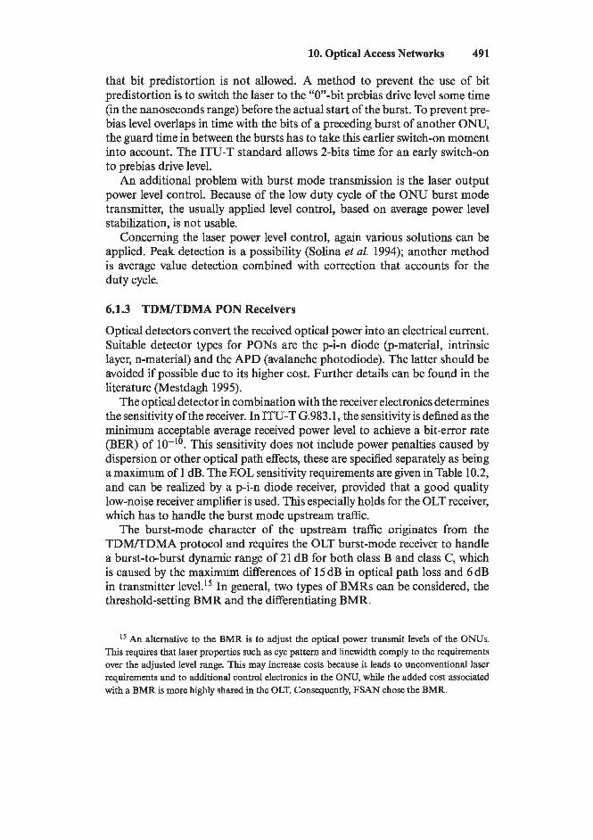
10. Optical Access Networks 491
that bit predistortion is not allowed. A method to prevent the use of bit predistortion is to switch the laser to the “0”-bit prebias drive level some time (in the nanoseconds range) before the actual start of the burst. To prevent pre- bias level overlaps in time with the bits of a preceding burst of another O W , the guard time in between the bursts has to take this earlier switch-on moment into account. The ITU-T standard allows 2-bits time for an early switch-on to prebias drive level.
An additional problem with burst.mode transmission is the laser output power level control. Because of the low duty cycle of the ONU burst mode transmitter, the usually applied level control, based on average power level stabilization, is not usable.
Concerning the laser power level control, again various solutions can be applied. Peak detection is a possibility (Solina et al. 1994); another method is average value detection combined with correction that accounts for the duty cycle.
6.1.3 TDIWTDMA PON Receivers
Optical detectors convert the received optical power into an electrical current. Suitable detector types for PONS are the p-i-n diode @-material, intrinsic layer, n-material) and the APD (avalanche photodiode). The latter should be avoided if possible due to its higher cost. Further details can be found in the literature (Mestdagh 1995).
The optical detector in combination with the receiver electronics determines the sensitivity of the receiver. In ITU-T G.983.1, the sensitivity is defined as the minimum acceptable average received power level to achieve a bit-error rate (BER) of loplo. This sensitivity does not include power penalties caused by dispersion or other optical path effects, these are specified separately as being a maximum of 1 dB. The EOL sensitivity requirements are given in Table 10.2, and can be realized by a p-i-n diode receiver, provided that a good quality low-noise receiver amplifier is used. This especially holds for the OLT receiver, which has to handle the burst mode upstream traffic.
The burst-mode character of the upstream traffic originates from the TDMRDMA protocol and requires the OLT burst-mode receiver to handle a burst-to-burst dynamic range of 21 dB for both class B and class C, which is caused by the maximum differences of 15 dB in optical path loss and 6 dB in transmitter 1e~el. l~ In general, two types of BMRs can be considered, the threshold-setting BMR and the differentiating BMR.
l5 An alternative to the BMR is to adjust the optical power transmit levels of the ONUS. This requires that laser properties such as eye pattern and linewidth comply to the requirements over the adjusted level range. This may increase costs because it leads to unconventional laser requirements and to additional control electronics in the ONU, while the added cost associated with a BMR is more highly shared in the OLT. Consequently, FSAN chose the BMR.
492 Edward Harstead and Pieter H. van Heyningen
With the threshold-setting BMR, the decision level is reset to the minimum after the end of the burst and set to the optimal level at the start of a new burst. The setting of the decision level can be done via detection of the incoming signal level, followed by setting the decision level at half the peak value of the incoming bit level. This must be done within the fist one or two bits of the burst. In Ota et aZ. (1992) such a receiver is described. Another method for adaptive level setting is by means of a special pattern that can be delivered by upstream PLOAM cells. The optimum level is stored in the BMR memory, to be used for the user cells arriving after such a PLOAM cell. Setting the decision level on the basis of network knowledge obtained during initialization is another possibility, but this is not as accurate as adaptive setting.
With the differentiating BMR, the DC component of the bursty signal is removed by differentiation of the incoming signal. This results in a 1.5-dB loss of sensitivity (Killat et aZ. 1996). Because the DC level is removed, further processing in an automatic gain controlled amplilier, followed by a regular decision circuit, is relatively easy (de Blok et al. 1993).
After the right level decision is taken, bit-phase alignment has to be obtained. This is done via synchronization on the preamble in the burst over- head. The main functions of such an alignment system are similar for all burst synchronization methods, although the implementation details may dif- fer. In van Bremen et al. (1997), the burst overhead signal is sampled at 8 bit phases until the preamble is detected. That is, the sampler produces for each of the 8 bit phases a binary output stream. All eight output streams are correlated with the preamble bit pattern that is stored in the OLT memory. A minimum correlation result is required, otherwise a signal loss indication is generated. The stream with the highest correlation result indicates the optimum bit-phase clock. The sampler is clocked at 8 bit phases, coming from an 8-phase clock generator, and realized by a tapped delay line. This clock generator delivers eight clock signals having the frequency of the OLT bit clock, on which the ONU has synchronized, but with eight different clock phases equally spaced (~/4) over the 2~ phase interval. The optimum phase clock is used for the detection of all following bits of the burst.
In van Bremen et al. (1997), the byte clock, which is an indication of the beginning of the burst payload, is also determined by this method, because the preamble position with respect to the byte boundaries is known. In the FSAN PONY a separate delimiter in the overhead is available to identify the beginning of the burst payload.
6.1.4 Splitters
In a passive optical network, the main outside plant components are the fibers and the optical splitters. Splitters are optical couplers, which are recip- rocal devices having a splitting function in the downstream direction and a combining function in upstream direction.
10. Optical Access Networks 493
The splitters in a PON using WDM directional multiplexing have to be achromatic (wavelength independent), i.e., they should behave equally at 1.3 and 1.5 Fm.
Two splitter technologies can be considered for PON applications: fused couplers and planar couplers (Kashima 1993).
Fused couplers are produced by fusing a number of fibers together and stretching the fibers over the length that is fused. The stretching decreases the diameter of the fibers and causes mutual coupling between the electromagnetic fields of the fibers. Such fused couplers are available in a large variety of input and output configurations. The coupling loss is approximately 3.5 dB per factor-two splitting: 3 dB intrinsic loss and about 0.5 dB excess loss. Coupling uniformity is not very good, which means that there is a difference between the output branches of some tenths of a dB. The reflection and directivity of fused couplers can be very good: both can be 50 dB or better.
Planar couplers are built on a substrate of an optical guiding material. The substrate contains optical waveguides having a different refractive index than the substrate. Coupling can be based on various principles, for example Y- branch or multimode interference (MMI) coupling, which are realized by the waveguide structures. These couplers have good uniformity; other properties are strongly dependent on the principle applied.
The price per port of the couplers is dependent on the split ratio. Fused fiber couplers are generally cheaper for small port count, and planar devices prove-in for larger port counts.
6.2 ONE-FIBER ETHERNETBASED PTP SYSTEMS
6.2.1 Requirements
One-fiber Ethernet has no standardized requirements at this time. The major- ity of the actually deployed optical lOO-Mb/s Ethernet, 100Base-FX, is realized as a multimode two-fiber system, as standardized in IEEE-802.3. Such sys- tems are mostly applied as in-building networks, and the choice between one- or two-fiber systems has little influence on the costs. The IEEE-802.3 standard for optical Gigabit Ethernet, 1000Base-SX or -LX, does not imply any par- ticular implementation, so either one- or two-fiber is possible. However, for access networks, having longer link lengths, one-fiber systems are preferred for cost reasons.
Ethernet in FITL systems will probably be addressed in the IEEE (see Section 7.2). We assume here that the most likely optical standard will be based on a one-fiber, full-duplex 100-Mbh Ethernet operating over SSMF in the 1.3-pm window.
6.2.2 Ethernet Point-to-Point Transmitters
A rough estimate for the power budget required for a 10-km PTP link over SSM fiber, including splices and connectors, is about 7dB. The distance of

494 Edward Harstead and Pieter H. van Heyningen
10 km is chosen because an active double star architecture is assumed, with the remote terminal, in this case, an Ethernet switch. The 7 dB budget allows for the use of low-power transmitters, estimated at about - 10 dBm output power, combined with relatively low-sensitivity receivers of -17 dbm. Compared to the PON requirements of 0 dBm transmitter output and -30 dBm receiver sensitivity, a PTP link has a far less demanding power budget, resulting in lower-cost components.
For full duplex (Section 3.3.2), the 1 : 2 optical coupler adds a loss of about 3.5 dB at both the transmit and receive locations. This means that, to obtain the above S and R values, the coupled laser output power must be -6.5 dBm and the receiver sensitivity -20.5 dBm. These values are still considerably more relaxed than for PON.
Dispersion is negligible, because of the 1.3-pm wavelength and the maximum length of the network of about 10 km.
Because the requirements on the laser are very relaxed, a very low-cost Fabry-Perot laser is usable for both directions.
6.2.3 Ethernet Point-to-Point Receivers
As mentioned previously, the requirement on the receiver sensitivity is about -20dBm. A simple receiver with a regular low-cost p-i-n photodiode will easily suffice.
6.3 BIDIRECTIONAL MODULES
Bidirectional transceivers are needed for one-fiber systems to split the upstream and downstream tr&c. This can be implemented with discrete compo- nents. A bidirectional module, which integrates the optical functions (laser, photodiode, and 1 :2 coupler) into a single package, is a lower-cost solu- tion. State-of-the-art modules contain the laser driver and receiver front-end electronics.
Functionally, there are two different bidirectional module types depending upon the directional multiplexing used. For full duplex, TCM, or SCM, the 1 : 2 coupler provides wavelength-independent coupling from fiber to laser and photodiode. For WDM directional multiplexing, the coupler provides a WDM coupling function. More complex modules can also combine both functions (e.g., a 1 .5-~m overlay of a 1.3-pm duplex system).
The principal setup of the bidirectional module is depicted in Fig. 10.9. A monitor diode can be added for laser output level detection and stabilization. A major concern for the bidirectional module is an additional NEXT path internal to the module itself, in addition to reflections and backscatter from the ODN. The WDM module can be equipped with an optical blocking filter in front of the photodiode to mitigate this effect, but this is not possible with the wavelength-independent module.

10. Optical Access Networks 495
photodiode
fiber - -
4 -
Pin
Pout
._ - - - - - ._ - - - - -
-
laser
-
Fig. 10.10 Free-space optics bidirectional module.
As described in Section 3.3.2, an OSIR of lOdB is required to obtain a penalty of 0.5 dB for a p-i-n diode receiver and noncoherent interference (for coherent interference the requirement can be much heavier; again refer to Section 3.3.2). This means that the FSAN PON system, with about 30dB transmitter-receiver level difference, requires a crosstalk loss of at least 40 dB. PTP systems with about 10 dB transmitter-receiver level difference require at least 20 dB crosstalk loss. The 40 dB crosstalk loss requirement is the reason that the one-fiber FSAN PON uses WDM directional multiplexing. The more relaxed isolation requirement for PTP allows for full duplex.
Some practical realizations of modules are discussed next. Modules can be built up in free-space optics or in a planar lightwave circuit (PLC) technology.
The free-space optic module is based on a free-beam optic technique, and uses a thin-film wavelength-independent semitransparent mirror for full duplex or a thin-film filter mirror for WDM. Figure 10.10 shows the minimal setup of the free-space optics bidirectional module.
The incoming light from the single fiber is reflected toward the photo- diode by the mirror, which is placed at a 45-degree angle with the optical beams. The laser transmitted light is passed through the mirror to the fiber. Additional focusing lenses are needed to adapt the optical beams to the free- space optics. The good optical performance of this type of module makes it suitable for broadband PONS. When a network extension is needed with a third wavelength, for example, for video broadcast overlay, the module can be extended with an additional WDM and photodiode (Althaus et al. 1994).

496 Edward Harstead and Pieter H. van Heyningen
photodiode 1.5 rnrn 1.5prn
-w Fiber - - 4- -+
1.3 prn
Fig. 10.11 1.3/1.5-pm bidirectional PLC module for ONU.
A PLC module can be designed with various levels of integration, for exam- ple, it can consist of a laser and a photodiode mounted on a silica planar lightwave circuit with an integrated coupler. For a WDM system, the WDM filter can be mounted on the PLC (Inoue et al. 1997). A PLC bidirectional module configuration for bidirectional 1.3-pm traffic and 1.5-pm unidirec- tional downstream tratlic (for CATV overlay signal) is shown in Fig. 10.11. In this example, in the ONU bidirectional module, the received 1.5-~m sig- nal is reflected by the WDM filter to the 1.5-pm photodiode. At 1.3-pm, the bidirectional signals pass through the WDM filter and the module functions as described with Fig. 10.9. This module has been advocated for narrow- band PON using TCM for directional multiplexing, but also can be used for bidirectional PTP Ethernet at 1.3 pm and broadcast tratlic at 1.5 pm.
Important for low-cost realization of the module is an accurate but sim- ple alignment of the optical components to the planar waveguides. A special technique, called spot-size conversion (Itaya et al. 1997), has been developed for lasers to make low-cost alignment possible. The spot-size converter is a part of the laser device structure, additional to the regular structure, to match the optical field of the laser to the waveguide field. The photodiode can be directly fabricated in a matching waveguide structure. With such lasers and photodiodes, passive alignment can be used, i.e., alignment based on mechan- ical procedures only without active feedback, i.e., without alignment based on optical measurements.
The use of a polymer technology also appears promising because it will allow for mass production and lower cost (Id0 et aZ. 1999).
Considering the not too stringent optical budget requirements for PTP Ethernet, the use of PLC modules for that application is easily possible. The more demanding broadband PON requirements have also been realized (Yoshida 1997; Kimura et al. 1998). However, PON PLCs have not been com- mercialized yet. The cost savings of PLC will be realized at large volumes, which have not yet materialized.
7. Current Trends and Possible Future Scenarios
In this section we close with a discussion of the future of FTTH and the optical architecture(s) that might be employed. The section reflects the fact that the
10. Optical Access Networks 497
activity surrounding FTTH is predominantly occurring in the United States as of early 200 1.
7.1 FIBER-TO-THE-HOME 7.1.1 The Emergence of Broadband Metallic Media
VOD proved to be yet another false start, and the last years of the 1990s were dark for FITL. Not only was its killer app discredited, but the new killer app, broadband Internet access, was going to be successfully carried by multiple system operators (MSOs) over existing coaxial cable and by incumbent LECs (ILECs) over existing copper using ADSL. (For more information on cable modems, see the chapter titled “Cable TV Architecture Evolution”. For more information on DSL, see Section 9.) In this light, it is more understandable why ATM PON might be first deployed for business access.
However, DSL and HFC are not the “enemies” but rather the enablers of FlTH. Users will use the larger bandwidths, more applications on the World Wide Web will involve streaming audio and video, and the demand for even more bandwidth will follow. Yet as the take rate of cable modems increases, the shared HFC bandwidth will throttle users. As the take rate of ADSL increases, cable binder groups will fill up with ADSL pairs and far-end crosstalk (FEXT) will limit further additional subscribers. These trends will drive fiber closer to the customer in both HFC and DSL networks, and ultimately lead to a true end-user demand (rather than an industry push) for FTTH.
Conversely, if the services provided by cable modems and ADSL fail to gain wide acceptance, FTTH will likely not happen.
7.1.2 Fiber-to-the-Home Scenarios and Issues
Despite numerous claims throughout the 1990s that FTTC had achieved cost parity with copper, with few exceptions (BellSouth, NTT) there has been little sustained deployment. Since copper parity was FTTC’s raison d’etre, this can be viewed as a failure. It may get another chance: As residential bandwidth demands push ADSL bit rates higher toward VDSL, it will force shorter loop lengths, which can only be served by fiber-fed terminals close to the customers, and ultimately, perhaps FTTC.
It remains to be seen whether FTTH will happen before that. BellSouth, the leading deployer of FTTC, recently estimated that ATM PON FlTH is currently 1.5 times more expensive than FTTC, but is expected to achieve cost parity with other full service architectures in the near future (Kettler et al. 2000). “Full service” are the key words here: FTTH will benefit from the abandonment of the copper cost parity paradigm and the inclusion of revenues from new services in the business case.
On the demand side, increased competition is reviving interest in FTTH in the United States. The ILECs are looking for a solution that can surpass

498 Edward Harstead and Pieter H. van Heyningen
HFC networks in the delivery of voice, entertainment video, and high-speed data. Facilities-based competitive LECs (CLECs), including utilities, looking to beat both ILECs and MSOs, perhaps have even more incentive to deploy FTTH since they have no existing infrastructure to milk and have a greater need to differentiate themselves. It may be the case, and history supports this, that ILECs will not deploy FTTH until they are forced to, and CLEC deployment of FTTH could provide the impetus. A different business model is one in which municipalities deploy and operate FTTH as a public service, and allow any service provider to retail its services to subscribers.
7.1.3 Overbuild and New Build
One view of the itccess world is that it is divided into three parts: existing buried plant, existing aerial plant, and new build (whether buried or aerial). It has long been assumed by many that FTTH will be widely deployed first in new-build applications. In new build, fiber would be deployed to every home, and in addition to broadband, it must deliver legacy narrowband services.
Another scenario is that the ONU will adopt the “set top box business model.” That is, the ONU is placed indoors, is AC-powered, has no require- ment for back-up power, and is deployed only when broadband service is subscribed to. For broadband take rates significantly lower than loo%, this is the lowest-cost model for FTTH, and therefore may allow for the earliest deployment. The principal application for this model is overbuild, Le., where a copper “lifeline” POTS network already exists. Aerial plant, of which there is a significant amount in the United States, is the most practical place to start overbuild because there is no digging required, only the hanging of new cables.
In addition to cost reasons, there are other reasons why overbuild may come first. New-build applications raise powering, service, and regulatory issues that are not present in overbuild applications.
7.1.3.1 Powering
The new-build ONU will also be AC-powered, but we assume back-up power must be available for lifeline POTS, at least as an option. It is tempting to assume that the subscriber will maintain a back-up battery, as they already do for cordless and mobile phones, or that mobile phones even take the place of wired phones. However, customer expectations and/or regulatory constraints may prove otherwise. If the LEC is forced to bear the cost of maintaining batteries, it may decide that an outdoor-mounted ONU may be necessary for craft access. This is a trade-off between lower maintenance cost and the higher cost of the environmentally hardened ONU.
l6 Recently there have been proposals to run fiber through sewer systems (!).

10. Optical Access Networks 499
7.1.3.2 Services
In new build, the FTTH system must find a practical and cost-effective way to deliver a wide range of legacy services. This means more than POTS, for example, specials like coin and automatic teller machine. Supporting all these services from the start will require major up-front investments from vendors.
7.1.3.3 Regulatory Issues
First, it needs to be verified that local powering with battery back-up is an acceptable substitute for network powering. This may be a gating issue for new build, as network powering might be cost-prohibitive.
Another potential regulatory issue is service uniformity. In a distribution area, new build deployment is often surrounded by existing customers served by legacy systems. Is it allowed to have some customers in this area served by a system with different performance during long power outages, or a system with better data throughput that could not be offered at any price to nearby neighbors that will be served by, say, ADSL?
Unbundling may be another important issue as both regulated and unregulated services are supported via the same access system.
The complexity of the above regulatory issues may be multiplied if they must be negotiated on a case-by-case basis with different state public utility commissions.
7.1.3.4 Summary of New Buildoverbuild Discussion
We believe that the first and most cost-effective widely deployed ONU will be based on the set top box model, and will only need to provide a core set of service interfaces, namely high speed data, probably video, and perhaps second line (not lifeline) voice. Its first application is likely to be overbuild, whose deployment does not hinge on the resolution of complex regulatory issues or the burden of delivering a large range of legacy services. This ONU will benefit from the early overbuild volumes and will serve as the building block on which later FTTH ONUS targeted at new builds will be built.
When will this happen? One of the authors has a coffee mug on his desk commemorating the deployment of the first commercial FTTH system that reads “FIBER TO THE HOME, FIRST SERVICE, AUGUST 5 1988.” Prognosticators take care.
7.2 SYSTEM ARCHITECTURES
7.2.1 FTTH Topology
Nothing in the last 10+ years has changed the basic arguments re: point- to-point vs point-to-multipoint (PON). At about seven to eight cents (US)

500 Edward Harstead and Pieter H. van Heyningen
per fiber meter, the cost of cabled feeder fiber is still too expensive to ignore for large scale deployment of FTTH and FTTBusiness. That is, the prove-in distance for PTP systems will still be short enough to require many remotely located and remotely powered active multiplexers. Or, a PON solution will be chosen. The argument tipped in favor of PONS during the 199Os, but the ascendancy of Ethernet as a networking technology and the availability of cheap Ethernet components is reenergizing interest in PTP systems. It is not clear at this time which might see large-scale deployment.
7.2.2 Ethernet
In November 2000, the IEEE 802.3 Working Group, which has been respon- sible for standardizing 10Base-T (10 Mb/s), Fast Ethernet (100 Mb/s), Gigabit Ethernet, and 10-Gigabit Ethernet, announced a new study group called “Ethernet in the First Mile” (EFM). Its charter is to apply Ethernet to the residentialhmall business access space. Although all media are under con- sideration, there is detectable enthusiasm for FTTH and FTTC. An obvious subject for the traditional Ethernet community to standardize is a single-fiber PTP optical interface. Since the OLT laser is not shared, it will be impor- tant that lasers on both ends of the link are low cost. Today, this means Fabry-Perot lasers, which means both directions of transmission must be in the 1.3-pm window to avoid dispersion penalties on SSMF. This limits the choice of directional multiplexing to either full duplex (Section 3.3.2) or TCM (Section 3.3.3). Gigabith speed will push on the coherent NEXT problem of full duplex and the bandwidth inefficiency of TCM, which adds impetus to selection of the lower cost Fast Ethernet speed.
Although less familiar to this group, PON is also under serious considera- tion. While ATM PON currently has the largest support among large network providers, vendors, and the standards, its deployment has been disappoint- ingly slow, leaving it vulnerable to competing PON technologies. ATM PONS reliance on ATM at layer 2, which adds protocol conversion costs to the ONU, is a vulnerability that IP adherents are exploiting. An Ethernet PON could be designed to carry the same services as ATM PONY with the probable excep- tion of legacy services with strict timing requirements, like leased-line El/DSl service.
If the study group addresses PONY it could reuse the physical medium- dependent requirements and ranging protocol of ITU-T G.983.1. The trans- mission convergence layer would need to be redone, with fixed length cells most likely replaced by variable length packets. An iconoclast in this group could argue that it is not worth the delay and effort to standardize and develop a new PON interface when ATM PON can also carry Ethernet. Ethernet has no inherent advantages at the physical layer (in fact the TDMA protocol for variable length upstream packets will be more complicated), the ATM cell tax is not so large, and the ATM layer could be hidden from the operator if

10. Optical Access Networks 501
necessary. The main motivation for an Ethernet PON must be the elimination of the EthernedATM protocol conversion cost.
This group is not experienced in PONY nor the last mile problem that the Telecom industry has wrestled with for the past 15 years. But they might make up for it with IPIEthernet fervor. If they don’t, an industry forum is purportedly being organized, along lines analogous to FSAN, to specifically accelerate the standardization of Ethernet PON.
7.2.3 If You Do PON: WDM PON vs PSPON
There are advocates of WDM PON who argue that PSPON is not adequate to the bandwidth challenge. Here is one view: It is cheaper to push the electronics until you get to the steep part of their cost curve, which is now between 2.5 and 10 GbIs, before you resort to WDM.17 It’s not easy to imagine how (or when) 16 or 32 residential users, TDM’ed, can push this limit (business users at this bandwidth level are unlikely to be served by PON). Another necessary develop- ment for WDM PON is the commoditization of low-cost WDM components, lirst used in the core and metro segments. Among today’s rapidly maturing DWDM technologies that could be applied to WDM PONY DFB lasers on the ITU-T grid and temperature-insensitive WGRs are probably the most impor- tant. If they become cheap, then WDM PON (or CPON) is at least in the running. Both these developments will take some time, and by then dropping fiber prices might be a tough moving target for any kind of PON.
8. Acknowledgments
The authors would like to thank Peter Bohn and Santanu Das for the benefit of their long experience in this field.
9. Appendix: Brief Overview of Digital Subscriber Line (DSL) Systems
The twisted-copper pair loops running to residential and business users were designed to support a voice frequency (VF) spectrum of 3 kHz. Dial-up modems utilize this audio frequency band for data transfer speeds up to 56 k b k To increase the data rate further, the latent bandwidth of “good” loops beyond 3 kHz must be mined with highly efficient digital encoding tech- niques. Services delivered with such techniques are generally denoted as digital subscriber line (DSL), or xDSL, where “xyy stands for various flavors of DSL.
l7 At least in the downstream direction. Very high-speed burst mode receivers may present a major technical challenge, if upstream bandwidth requirements also become extremely large.
502 Edward Harstead and Pieter H. van Heyningen
The first DSL technology was Basic Rate ISDN, which transports a 16 kb/s sig- nalling “D” channel and two 64 kb/s “B” payload channels, which are switched through the telephony network. Subsequent higher-speed symmetric data rate DSLs, like high-speed DSL (HDSL and HDSL2) and single-pair high-speed DSL (SHDSL), backhaul channelized voice and narrowband nonvoice t r f i c to the circuit-switched network. These services are aimed at business users, with speeds in the Tl/El range and unrepeatered ranges of a few km.
However, for high-speed residential data access the data signal must be diverted from the telephony network, whose class 5 VF switches will not allow rates beyond 56 kb/s, into a high-speed data network. Data traffic carried on residential loops using asymmetric DSL (ADSL), at anywhere from 0.5 to 6 Mb/s downstream (and considerably less upstream), bypasses the telephony switch at the CO. ADSL is beginning to be deployed now on a massive scale in the United States. Similarly, very high-speed DSL (VDSL) carries asym- metric traffic, but at downstream speeds up to 50 Mb/s, and is foreseen to be a potential vehicle for residential video service delivery.
9.1 STANDARDIZATION EFFORTS
xDSL was fist proposed by Bellcore (now Telcordia) during the late 1980s and spent many years in the laboratory, while FITL was in vogue, before being taken seriously. The DSL Forum was established in 1994 to promote xDSL and facilitate its development and standardization. ANSI and ETSI have also played a role in DSL standards. Around 1997 standardization work was taken up by ITU-T. Recommendations G.991.1 (HDSL), G.991.2 (G.shdsl), G.992.1 (G.dmt, ADSL), G.992.2 (G.lite/ADSL lite) have developed techniques for transmitting a range of bit rates over the existing copper local network from relatively short distances at high bit rates and to long distances at relatively lower bit rates. Recommendations G.994.1, G.996.1, and G.997.1 support G.992.1 and G.992.2 by providing common handshake, management, and testing procedures. These Recommendations include mandatory requirements, recommendations, and options.
9.2 TRANSMISSION TECHNIQUES
All xDSL systems apply transmission methods based on special modula- tion and encoding techniques. The techniques applied are discrete multitone (DMT) modulation, carrier-less amplitude-phase (CAP) modulation, quadra- ture amplitude modulation (QAM), and 2B1Q encoding. TC-PAM (trellis- coded pulse amplitude modulation) is the scheme used for G.shds1 (ITU-T) and HDSL2 (ANSI). We can differentiate between DSL technologies that are based on baseband (i.e., 2B1Q for SDSL and TC-PAM for HDSL and SHDSL) vs passband (i.e., CAP, QAM, or DMT for ADSL and VDSL).

10. Optical Access Networks 503
Passband schemes allow DSL to be used on a loop that is also carrying a base- band telephony signal such as POTS or Basic Rate ISDN, unlike baseband DSL schemes which do not.
Self-adaptation techniques are applied to obtain the best signal-to-noise ratio over the copper medium by minimizing the consequences of several trans- mission impairments. Because unshielded copper lines are used, special care is needed to limit the influence of crosstalk. No further details will be given here because an extensive literature exists on xDSL (see e.g., Hawley et al. 1997; Kim et al. 1995; Palm 2000; Zimmerman 1997). In the next sections ADSL, HDSL, and VDSL are discussed in more detail.
9.3 ADSL
ADSL uses DMT modulation. Peak speeds often mentioned are 6 Mbls down- stream and up to 800 kb/s upstream, but actual achievable bit rates are limited by loop characteristics such as length, wire gauge, gauge changes, crosstalk, the presence and characteristics of bridge taps, and noise presence. A typical maximum downstream speed on a 5 km loop is roughly 2 Mb/s.
Separation from the POTS signal is provided by a splitter at both ends of the loop, which isolates a DC to 4 kHz band. G.lite is aimed at splitterless installation at the end-user premises. The tradeoff is somewhat reduced band- width and momentary disruption of the data signal during POTS events like ringing and off-hook.
The number of users connected to ADSL worldwide is about three million (end of 2000).
9.4 HDSL
HDSL enables the transmission of bidirectional 1.512 Mb/s. Different trans- mission measures are required with respect to ADSL because of this higher upstream speed and the full duplex service. Transmission improvement mea- sures are echo cancellation and 2B1Q encoding (two binary bits encoded in one quaternary symbol). A maximum distance of about 4 km can be covered.
The standards for HDSL (not just in ITU-T, but also ETSI and ANSI) fall short in being able to achieve multivendor interoperability. G.shds1 is com- prehensive enough to achieve multivendor interoperability and is based on more modern (i.e., more advanced processing) DSL mechanisms to achieve better bit rate vs loop characteristics than the 2BlQ-based DSL. G.shds1 also improves the spectral “friendliness” of DSL, i.e., the effect it has on other pairs in the cable.
9.5 W S L
VDSL can support downstream speeds up to 50 Mbls, and so is seen as the ulti- mate copper-based technique to deliver high-end broadband to the residential

504 Edward Harstead and Pieter H. van Heyningen
user. The modulation is CAP, multilevel QAM or DMT. The length of the copper loop is limited to some hundreds of meters, which means that VDSL must be fed from ONUs deployed within that distance from the subscribers. Using ATM PON to feed VDSL ONUs in a FTTCabinet architecture has received particular attention in FSAN (e.g., Cooper et al. 2000), but for rea- sonable take rates the VDSL bandwidth demand will limit PON to small split ratios, and therefore PTP links are probably better suited. There has been spotty commercial deployment of VDSL over the years, but widescale sustained deployment has remained elusive.
9.6 xDSL IMPLEMENTATION AND SERVICES
ADSL is used for high-speed data access (with the potential to supply multiple voice lines and maybe some very limited video service delivery). ATM has become the exclusive “layer 2” over the ADSL, although all the data tr&c over the-ATM over ADSL is certainly IP. On the other hand, symmetric DSLs have a history of being used to transport leased-line (DSl/El or N x 64 kb/s), circuit-switched voice (i.e., N x 64 kb/s), frame relay, or ATM.
Deployment of DSLs carrying ATM or Frame Relay are via the use of DSLAMs (DSL access multiplexers). These DSLAMs provide statistical bandwidth concentration for the traffic transmittedlreceived over the DSL. TDM or leased-line transport over symmetric DSLs use transmission gear similar to that used for T1 or DLC/pair-gain systems. DSL is deployed by the network operator wherever the copper loop is served, via the cen- tral office/exchange, via outside plant cabinet enclosures, vaults, or huts, or on-site in multitenant/dwelling units.
10. Acronyms
ADS ADSL
APD APON ASE AWG BER BMR BOL CAP CBR CDMA CLEC
AM-VSB
Active Double Star Asymmetric Digital Subscriber Line Amplitude Modulation Vestigial SideBand Avalanche PhotoDiode ATM Passive Optical Network Amplified Spontaneous Emission Arrayed Waveguide Grating Bit-Error Rate Burst-Mode Receiver Beginning of Life Carrier-less Amplitude-Phase Constant Bit Rate Code Division Multiple Access Competitive Local Exchange Carrier
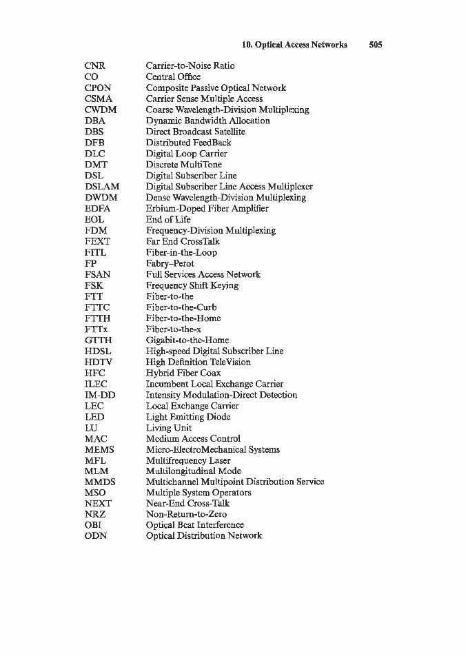
10. Optical Access Networks 505
CNR co CPON CSMA CWDM DBA DBS DFB DLC DMT DSL DSLAM DWDM EDFA EOL FDM FEXT FITL FP FSAN FSK FTT FTTC FTTH FTTx GTTH HDSL HDTV HFC ILEC
LEC LED LU MAC MEMS MFL MLM MMDS MSO NEXT NRZ OBI ODN
IM-DD
Carrier-to-Noise Ratio Central Office Composite Passive Optical Network Carrier Sense Multiple Access Coarse Wavelength-Division Multiplexing Dynamic Bandwidth Allocation Direct Broadcast Satellite Distributed FeedBack Digital Loop Carrier Discrete MultiTone Digital Subscriber Line Digital Subscriber Line Access Multiplexer Dense Wavelength-Division Multiplexing Erbium-Doped Fiber Amplifier End of Life Frequency-Division Multiplexing Far End CrossTalk Fiber-in-the-Loop Fabry-Per0 t Full Services Access Network Frequency Shift Keying Fiber-to-the Fiber-to-the-Curb Fiber-to-the-Home Fiber-to-the-x Gigabit-to-the-Home High-speed Digital Subscriber Line High Definition Television Hybrid Fiber Coax Incumbent Local Exchange Carrier Intensity Modulation-Direct Detection Local Exchange Carrier Light Emitting Diode Living Unit Medium Access Control Micro-ElectroMechanical Systems Multifrequency Laser Multilongitudinal Mode Multichannel Multipoint Distribution Service Multiple System Operators Near-End Cross-Talk Non-Return-to-Zero Optical Beat Interference Optical Distribution Network
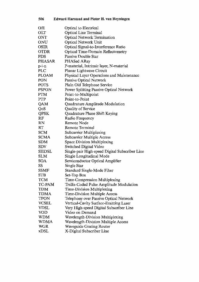
506 Edward Harstead and Pieter H. van Heyningen
O/E OLT ONT ONU OSIR OTDR PDS PHASAR p-i-n PLC PLOAM PON POTS PSPON PTM PTP QAM QOS QPSK RF RN RT SCM SCMA SDM SDV SHDSL SLM SOA ss SSMF STB TCM
TDM TDMA TPON VCSEL VDSL VOD WDM WDMA WGR xDSL
TC-PAM
Optical to Electrical Optical Line Terminal Optical Network Termination Optical Network Unit Optical Signal-to-Interference Ratio Optical Time-Domain Reflectometry Passive Double Star PHASed ARay P-material, Intrinsic layer, N-material Planar Lightwave Circuit Physical Layer Operations and Maintenance Passive Optical Network Plain Old Telephone Service Power Splitting Passive Optical Network Point-to-Multipoint Point-to-Point Quadrature Amplitude Modulation Quality of Service Quadrature Phase Shift Keying Radio Frequency Remote Node Remote Terminal Subcarrier Multiplexing Subcarrier Multiple Access Space Division Multiplexing Switched Digital Video Single-pair High-speed Digital Subscriber Line Single Longitudinal Mode Semiconductor Optical Amplifier Single Star Standard Single-Mode Fiber Set-Top Box Time-Compression Multiplexing Trellis-Coded Pulse Amplitude Modulation Time-Division Multiplexing Time-Division Multiple Access Telephony over Passive Optical Network Vertical-Cavity Surface-Emitting Laser Very High-speed Digital Subscriber Line Video on Demand Wavelength-Division Multiplexing Wavelength-Division Multiple Access Waveguide Grating Router X-Digital Subscriber Line

10. Optical Access Networks 507
References
Althaus, L. et al. 1994, “Bidirectional transmission in the optical subscriber network,” Siemens Rev., v. 61, pp. 24-26.
Amemiya, M., Maekawa, T., Haga, K., Tamaki, N., 1997, “Low-cost FTTH system based on PDS architecture,” h c . Global Telecom. Conf GLOBECOM’97, v. 2, pp. 878-882.
Araki, N., Enomoto, Y, Tomita, N., 1998, “Improvement of fault identification per- formance using nearal networks in passive double star optical networks,” OFC’98 Tech. Digest, pp. 223-224.
Balmes, M., Bourne, J., Mar, J., 1990, “Fiber to the home: the technology behind Heathrow,” IEEE LCS, v. 1, no. 3, pp. 2549.
Bashforth, B. N., Williamson, C. L., 1998, “Statisticalmultiplexing of self-similar video streams: simulation study and performance results,” Proc. Sixth Int. Sym. on Modeling, Analysis and Simulation of Computer and Telecommunication Systems, pp. 119-126.
Baskerville, L., 1989, “Two fibers or one? (a comparison of two-fiber and one-fiber star architectures for fiber-to-the-home applications),” J. Lightwave Tech., v. 7, no.
Bates, R., Walker, S., 1991, “450 Mbit/s BPSK and 1 Gbit/s QPSK throughout subcar- rier multiple-access networks using 790 nm self-pulsation laser transmitter network for computer applications,” Elect. Lett., v. 27, pp. 1014-1016.
Bohn, P., Das, S., 1987, “Return loss requirements for optical duplex transmission,” J. Lightwave Tech., v. 5, pp. 243-254.
Bohn, P., Kania, M., Nemchik, J., Purkey, R., 1992, “Fiber in the loop,” AT&T Tech. J., Jan.lFeb. 1992, pp. 3145.
Carr, J., Saikkonen, S., Williams, D., 1990, “Refractive index measurements on single- mode fiber as functions of product parameters, tensile stress, and temperature,” Fiber and Integrated Optics, v. 9, pp. 393-396.
Caviglia, E, Di Biase, V., Gnazzo, A., 1999, “Optical maintenance in PONS,” Optical Fiber Tech., v. 5, no. 4, pp. 349-362.
Chand, N. et al. 1999a, “Delivery of digital video and other multimedia services (> 1 Gbps bandwidth) in passband above the 155 Mbps baseband services on a FTTx full service access network,” J. Lightwave Tech., v. 17, no. 12, pp. 2449-2460.
Chand, N. et al. 1999b, “Adding 64-QAM broadcast digital video to FTTH ATM Passive Optical Network,” Proc. ECOC’99, post-deadline paper, Nice, France.
Cooper, I., Bramhall, M., 2000, “ATM passive optical networks and integrated VDSL,” IEEE Comm. Mag., v. 39, pp. 174-179.
Das, S . , 1988, “Modal noise due to short-wavelength (78S900nm) transmission in single-mode fibers optimized for 1300 nm,” Applied Optics, v. 27, no. 3, pp. 552-556.
Das, S., Harstead, E. “Beat interference penalty in optical duplex transmission,” J. Lightwave Tech., to be published Feb. 2002, vol. 20, no 2.
de Blok, C. M. et al. 1993, “Fast low cost feed-forward burst mode optical receiver for 622 Mbitls,” Proc. EFOCH.93, pp. 256-260.
11, pp. 1733-1740.

508 Edward Harstead and Pieter H. van Heyningen
de Groote, J. L. et al. 1999, “Redundancy and protection switching in APON systems,” Pmc. E F O C W 9 9 , pp. 1 19-126.
Devadhar, S., Ryan, K., 2000, “Dynamic bandwidth allocation over passive optical networks,” Lightwave Mug., Nov. 2000, pp. 138-142.
Dragone, C., Edwards, C., Kistler, R., 1992, “Integrated optics N x N multiplexer on silicon,” IEEE Photonics Tech. Lett., v. 4, pp. 896-899.
Dragone, C. et al. 1997, “Waveguide grating router with maximally flat passband produced by spatial filtering,” Elect. Lett., v. 33, pp. 1312-1313.
Eichenbaum, B., 2001, “Proposal for a frequency plan for optical communications networks optimized for sources where the emission wavelength may drift by several nanometers,” ITU submission B01-01-17, SG 15, Jan. 2001.
Engineer, C., 1990, “Fiber in the loop: an evolution in services and systems,” Proc. SPIE Fiber Optics in the Subscriber Loop, v. 1363, pp. 19-29.
ETSI, 1997, ETS 300 681, Transmission and Multiplexing (TM); @tical Distribution Network (ODN) for Optical Access Network (OAN,).
Faulkner, D. W., Payne, D. B., Stern, D. B., Ballance, J. W., 1989, “Optical networks for local loop applications,” J. Lightwave Tech., v. 7, no. 11, pp. 1741-1751.
Feldman, R., Liou, K., Raybon, G., Austin, R., 1996, “Reduction of optical beat interference in a subcarrier multiple access passive optical network through the use of an amplified light emitting diode,” IEEE Photonics Tech. Lett., v. 8, pp. 116-118.
Feldman, R., Wood, T., Raybon, G., Austin, R., 1996b, “Effect of optical beat inter- ference on the dynamic range of a subcarrier multiple access passive optical network using Fabry-Perot lasers,” J. Lightwave Tech., v. 14, no. 5, pp. 71 1-715.
Feldman, R., 1997, “Crosstalk and loss in wavelength division multiplexed systems employing spectral slicing,” J. Lightwave Tech., v. 15, no. 1 1, pp. 1823-1 83 1.
Feldman, R. et al. 1998, “An evaluation of architectures incorporating wavelength division multiplexing for broad-band fiber access,” J. Lightwave Tech., v. 16, no. 9, pp. 1546-1559.
Feldman, R. et al. 1998b, “In-service signaling and fault identification in a passive optical network using a reflective modulator and a broad spectrum optical source: Proc. ECOC’98, pp. 703-704, Madrid.
Frigo, N. et al. 1994, “A wavelength-division multiplexed passive optical network with cost-shared components,” IEEE Photonics Tech. Lett., v. 6, no. 11, pp. 1365-1367.
FSAN, 1996, h c . FSANConJ, London, 20 June 1996. Giles, C. et al. 1996, “Access PON using downstream 155Onm WDM routing and
upstream 1300 nm SCMA combining through a fiber-grating router,” IEEEPhotonics Tech. Lett., v. 8, pp. 154%1551.
Giles, C., Jiang, S., 1997, “Fiber-grating sensor for wavelength tracking in single-fiber WDM access PON’s,” IEEE Photonics Tech. Lett., v. 9, no. 4, pp. 523-525.
Giles, C., Zimgibl, M., Joyner, C., 1997b, “1 152-subscriber WDM access PON archi- tecture using a sequentially pulsed multifrequency laser,” IEEE Photonics Tech. Lett., v. 9, no. 9, pp. 1283-1284.

10. Optical Access Networks 509
Goossen, K., Walker, J., Amey, S., 1994, “Silicon modulator based on mechanically- active anti-reflection layer with 1 Mbitlsec capability for fiber-in-the-loop applica- tions,” IEEE Photonics Tech. Lett., v. 6, pp. 11 19-1 121.
Harikae, K., 1995, “Optical access system technology to support multimedia service field trials,” NTTReview, v. 7, no. 6, pp. 7479.
Harikae, K., Shibata, Y, Nakashima, Y, 1998, “New optical access system (rr-system),” NTTReview, v. 10, no. 2, pp. 69-76.
Harstead, E., Ocenasek, J., 199 1, “Short wavelength transmission over single-mode fiber optimized for long wavelengths,” SPIE OE/Fibers, Boston, 1991.
Harstead, E., Bohn, P., Kallenberg, P., 1992, “Optimal split ratio and channel capacity of poht-to-multipoint networks for FITL,” Proc. IEEE 4th Workshop on Optical Local Networks, Versailles, France.
Harstead, E., 2000, “ATM PON as a business access technology, with migration path to FTTH,” Proc. wTc/ISSZOOO, Birmingham, U.K., May 2000.
Hartog, A. H., Conduit, A. J., Payne, D. N., 1979, “Variation of pulse delay with stress and temperature in jacketed and unjacketed optical fibres,” Optical & Quantum Elechonics, v. 11, pp. 265-273.
Hawley, G., 1991, “Historical perspectives on the U.S. telephone loop,” IEEE Comm. Mag., March 199 1, pp. 24-28.
Hawley, T., 1997, “System Considerations for the Use of xDSL Technologies for Data Access,” IEEE Comm. Mag., v. 35, pp. 56-60.
Hoppit, C. E., Clarke, D. E. A., 1989, “The provision of telephony over passive optical networks,” Bs Telecom Tech. J., v. 7, no. 2.
Iannone, P., Frigo, N., Darcie, T., 1995, “A WDMPON architecture with bidirectional optical spectral slicing,” Proc. OFC’95, San Diego, CA, paper TuK2.
Ido, T. et al. 1999, “A simple low-cost polymer PLC platform for hybrid integrated modules,” OFC/IOOC’99 Tech. Digest, pp. PD41-1-PD41-2.
Inoue, Y et al. 1995, “Silica-based arrayed-waveguide grating circuit as optical splitterhouter,” Elect. Lett., v. 31, no. 9, pp. 726727.
Inoue, Y et al. 1997, “PLC Hybrid Integrated WDM Transceiver Module for Access Networks,” NTTReview, v. 9, no. 6, pp. 5544.
Itaya, Y. et al. 1997, “Optical Semiconductor Devices for Hybrid Modules,” NTT Review, v. 9, no. 6, pp. 65-74.
ITU-T, 1996, Recommendation G.982, Optical access networks to support services up to the ISDNprimaiy rate or equivalent bit rates.
ITU-T, 1998,, Recommendation G.983.1, Broadband optical access systems based on Passive Optical Networks (POW.
ITU-T, 2000, Recommendation G.983.2, ONT management and control inte~ace specijkation for ATM PON.
ITU-T, 2001, Recommendation G.983.3, A broadband optical access system with increased service capability by wavelength allocation.
Jung, D. et al. 2000, “Wavelength-tracking technique for spectrum-sliced WDM passive optical network,” IEEE Photonics Tech. Left., v. 12, no. 3, pp. 338-340.
510 Edward Harstead and Pieter H. van Heyningen
Jung, D., 2000b, “Spectrum-sliced bidirectional WDM PON,” Proc. OFC’2000, v. 2, pp. 160-162.
Kaneko, A. et al. 2000, “Athermal silica-based arrayed-waveguide grating (AWG) multUdemultiplexers with new low loss groove design,” Elect. Lett., v. 36, no. 4,
Kashima, N., 1993, @tical Dansmission for the Subscriber Loop, Artech House, Boston. Kettler, D., Kafka, H., Spears, D., 2000, “Driving fiber to the home,” IEEE Comm.
Killat, U. et al. 1996, Access to B-ISDN via PONS, John Wiley C Sons, NewYork. Kim, H., Yim, C., 1995, “ADSLHDSL Technologies and Application in VoD and
Multimedia Services,” International Broadcasting Convention IBC‘95. Kimura, H. et al. 1998, “A low-crosstalk optical module design on PLC platform
for realizing LDPD full-duplex operation in ATM systems,” Pmc. ECOC’98, v. 1, pp. 481432.
Lee, J., Chung, Y, DiGiovanni, D., 1993, “Spectrum-sliced fiber amplifier light source for multichannel WDM applications,” IEEEPhotonics Tech. Lett., v. 5, pp. 1458-1461.
Li, Y et al. 1996, “Demonstration and application of a monolithic two-PONS-in-one device,” Proc. ECOC’96, Oslo, Norway, paper TuC.3.4.
Lin, W., 1997, “Reducing multiple optical carriers interference in broad-band passive optical networks,” IEEE Photonics Tech. Lett., v. 9, no. 3, pp. 368-370.
Lin, Y, Spears, D., 1989, “Passive optical subscriber loops with multiaccess,” J. Lightwave Tech., v. 7, pp. 1769-1777.
Maier, G. et al. 2000, “Design and cost performance of the multistage WDM-PON access networks,” J. Lightwave Tech., v. 18, no. 2, pp. 125-143.
Mayweather, D. et al. 1996, “Wavelength tracking of a remote WDM router in a passive optical network,” IEEE Photonics Tech. Lett., v. 8, no. 9, pp. 1238-1240.
Mestdagh, D. J. G., 1995, Fundamentals of Multiaccess Optical Fibre Networh, Artech House, Boston.
Mestdagh, D. J. G., Martin, C. M., 1996, “The Super-PON concept and its tech- nological challenges,” Proc. of International IFIP-IEEE Con$ on Broadband Comm,
Miki, T., Komiya, R., 1991, “Japanese subscriber loop network and fiber optic loop deployment,” IEEE Comm. Mag., pp. 60-67.
Monnard, R. et al. “Demonstration of a 12 x 155 Mb/s WDM PON under outside plant temperature conditions,” IEEEPhotonics Tech. Lett., v. 9, no. 12, p p 1655-1657.
Nakao, N., Enomoto, T., Kuroiwa, M., 1996, “Splitter positions and testingwavelength for optical fiber access networks,” Pmc. ECOC’96, Oslo, Norway.
Nuss, M., Knox, W., Koren, U., 1996, “Scaleable 32 channel chirped-pulse WDM source,” Elect. Lett., v. 32, pp. 13 1 1-1 3 12.
Ogura, H. etal. 1997, “Launch of CATV distribution service over FTTH,” NTTReviao, v. 9, no. 6, pp. 1W112.
Omiya, I., 1997, “NTT’s joint utilization tests of multimedia communications- utilization tests for CATV and VOD over FlTH,” Multimedia Tools andApplications, v. 5, no. 2, pp. 85-91.
pp. 318-319.
Mag., v. 38, no. 11.
pp. 33s345.

10. Optical Access Networks 511
Orth, B., 1992, “FITL specification in Germany; PON system for interactive services,”
Ota, Y., Swartz, R. G., 1992, “DC-lGb/s Burst-Mode Compatible Receiver for Optical
Palm, S., 2000, “xDSL Tutorial and Standards Update,” Internntional Conference on
Poh, B. S., 1985, “Prediction of self-sustained oscillations in buried-heterostructure
Quayle, J. A., 1995, “Ranging on AdvancedPONs,” Proc. ofEFOCdlN’95, pp. 154-157. Reeve, M. et al. 1988, “LED spectral slicing for single-mode local loop applications,”
Refi, J. J., Swiderski, M. J., 1990, “System requirements and installation testing for
Refi, J., 1999, “Low-water-peak singlemode-fiber standards proposal,” Lightwave Mag. Reichmann, K., Iannone, P., Frigo, N., “Operational demonstration and filter align-
ment study of multiple broadcast video delivery on a WDM passive opticalnetwork,” IEEE Photonics Tech. Lett., v. 10, no. 9, pp. 1331-1333.
Sahinoglu, Z., Tekinay, S., 1999, “On multimedia networks: self-similar traffic and network performance,” IEEE Comm. Mag., v. 37, no. 1, pp. 48-52.
Shibutani, M. et al. 1997, “A Gigabit-To-The-Home (GTTH) system for future broad- band access infrastructure,” IEEE Con$ Communications ICC’97, Montreal, Canada, pp. 1004-1008.
Shiori, S. et al. 1999, “A 2.5 Gb/s high speed PLC module for Gigabit-To-The-Home (GTTH) system,” Tech. Digest Optical Fiber Communication Con$ OFC/IOOC’99,
Smit, M., 1988, “New focussing and dispersive planar component based on an optical phased array,” Elect. Lett., v. 24, pp. 385-386.
Soda, M. et al. 1999, “A 2.5 Gb/s one-chip receiver module for Gigabit-To-The-Home (GTTH) system,” Proc. of the IEEE Custom Integrated Circuits, pp. 273-276.
Soderstrom, R. L., Block, T. R., Karst, D. L., Lu, T., 1986, “The compact disc (CD) laser as a low-cost, high performance source for fiber optic communication,” Tech. Digest, FOC/LAN 86, Orlando, p. 263.
Solina, P., Valvo, M., 1994, “Novel burst mode optical transmitter for a 622 Mbitls TDMA PON,” h c . ECOC’94, Florence, Italy.
Stark, J. et al. 1997, “Cascaded WDM passive optical network with a highly shared source,” IEEEPhotonics Tech. Lett., v. 9, no. 8, pp. 1170-1172.
Stem, J. et al. 1987, “Passive optical local networks for telephony applications and beyond,” Elect. Lett., v. 23, n. 24, pp. 1255-1257.
Stern, M., Way, W. I., Shah, V., Romeiser, M. B., Young, W. C., Krupsky, J. W., 1987, “800-nm digital transmission in 1300-nm optimized single-mode fiber,” Tech. Digest, Optical Fiber Communication Con$, Washington, D.C., paper MD2.
Suto, K., Yoneda, E., Hayakawa, T., Tuchiya, T., 1992, “0.78-p-m digital transmission characteristics using 1.3-mm optimized single-mode fiber for a subscriber loop,” Electronics and Communications in Japan Pt. I , v. 75, no. 2, pp. 3847.
5th Con$ on Optical/Hybrid Access Networks.
Bus Applications,” J. Lightwave Tech.; v. 10, no. 2, pp. 244-249.
Consumer Electronics ICCE 2000, pp. 68-69.
stripe lasers,” IEE Proc., v. 132, no. 1, pp. 29-33.
Elect. Lett., v. 24, no. 7, pp. 389-390.
fiber-to-the-subscriber,” Proc. of Int? wire and Cable Sym., pp. 730-734.
V. 3, pp. 188-190.

512 Edward Harstead and Pieter H. van Heyningen
Takahashi, H., Hibino, Y, Nishi, I., 1992, “Polarization-insensitive arrayed waveguide grating wavelength multiplexer on silicon,” Opt. Lett., v. 3, pp. 491-501.
Takeda, K., Koga, H., 1994, “Fault location in optical lines of passive double star net- works by pattern matching of OTDR waveforms,” Electronics and Communications in Japan, Pt. I , v. 77, no. 7, pp. 1-3.
Tanaka, K., Tateda, M., 1996, “Measuring the individual attenuation distribution of passive branched optical networks,” IEEE Photonics Tech. Lett., v. 8, no. 7, pp. 915-917.
Telcordia, 2000, GR-909-CORE Issue I, Generic Criteria for Fiber in the Loop Systems. Tenzer, T., 1991, “The introduction of optical fiber in the subscriber loop in the
telecommunication networks of DBP Telekom,” IEEE Comm. Mag., pp. 36-49. Terada, N. et al. 1996, “An MPEG2-based digital CATV and VOD system using ATM-
PON architecture,” Pmc. of IEEE Multimedia ’96, Los Alamitos, CA, pp. 522-53 1. Tsybakov, B., Georganas, N. D., 1998, “Self-similar processes in communications
networks,” IEEE Trans. on Information f i e o y , v. 44, no. 5, pp. 1713-1725. Ueda, H., Maekawa, E., 1999, “Development of an ATM subscriber system
(model C),” NTTReview, v. 11, no. 6, pp. 27-32. van Bremen, J. et al. 1997, “Asynchronous transfer mode over a passive optical network:
the realization of a high speed demonstrator system,” Int. J . Optoelectronics, v. 11, no. 1, pp. 71-84.
Van der Plas, G. et al. 1995, “Demonstration of an ATM-based passive optical net- work in the FTTH trial on Bermuda,” Proc. Global Telecom. Con$ GLOBECOM95,
van Heyningen, P. et al. 1992, “Optical network for broadband services in the subscriber loop,” Electronics & Communication Engineering Journal, v. 4, pp. 405411.
van Heyningen, P. et al. 1995, “A novel ranging method for ATM over PON systems,” Pmc. EFOCHV’95, pp. 150-1 53.
Van de Voorde, I., Martin, C. M., Vandewege, J., Qiu, X. Z., 2000, “The Super- PON demonstrator: An exploration of possible evolution paths for optical access networks,” IEEE Comm. Mag., v. 38, pp. 74-82.
Veres, A., Boda, M., 2000, “The chaotic nature of TCP congestion control,” Pmc. INFOCOM 2000 Con$ IEEE Computer and Commun. SOC., v. 3, pp. 17 15-1 725.
Wagner, S. et al. 1988, “Experimental demonstration of a passive optical subscriber loop architecture,” Elect. Lett., v. 24, pp. 344346.
Wagner, S., Lemberg, H., 1989, “Technology and system issues for a WDM-based fiber loop architecture,” J. Lightwave Tech., v. 7, no. 11, pp. 1759-1768.
Wood, T. et al. 1988, “Observation of coherent Rayleigh noise in single-source bidirectional optical fiber systems,” J. Lightwave Tech., v. 6, pp. 346-352.
Wood, T., Shankaranarayanan, N., 1993, “Operation of a passive optical network with subcarrier multiplexing in the presence of optical beat interference,” J. Lightwave Tech., v. 11, pp. 1632-1640.
pp. 988-992.

10. Optical Access Networks 513
Wood, T., Wilson, G., Feldman, R., Stiles, J., 1999, “Fibervista: a cost-effective fiber- to-the-home (FTTH) system providing broad-band data over cable modems along with analog and digital video,” ZEEE Photonics Tech. Lett., v. 1 1, no. 4, pp. 475477.
Woodward, S., Lu, X., Darcie, T., Bodeep, G., 1996, “Reduction of optical-beat interference in subcarrier networks,’’ ZEEE Photonics Tech. Lett., v. 8, no. 5, pp. 694-696.
Woodward, S. et al. 1998, “A spectrally sliced PON employing Fabry-Perot lasers,” ZEEE Photonics Tech. Lett., v. 10, no. 9, pp. 1337-1339.
Wuilmart, L. et al. 1996, “A PC-based method for the localisation and quantization of faults in passive tree-structured optical networks using the OTDR technique,” Proc.
Yamamoto, H., Morikura, S., Utsumi, K., Fujito, K., 1999, “Increasing acceptable number of signals in subcarrier multiple access optical networks in the presence of high optical beat interference,” J. Lightwave Tech., v. 17, no. 9, pp. 1525-1 53 1.
Yoshida, J., 1997, “Low-cost optical transceivers for access networks,” Proc. OFC’97,
Zimmerman, G., 1997, “Achievable rates vs. Operating Characteristics of Local Loop Transmission: HDSL, HDSL2, ADSL and VDSL,” Conference Recordofthe llirty- First Asilomar Conference on Signals, @stems and Computers, pp. 573-577.
Zirngibl, M. et al. 1995, “LARNet, a local access router network,” ZEEE Photonics Tech. Lett., v. 7, pp. 215-217.
Zirngibl, M., 1998, “Multifrequency lasers and applications in WDM networks,” ZEEE Comm. Mag., v. 36, no. 12, pp. 39-41.
IEEE LEOS’96, pp. 122-123.
pp. 275-276.
Chapter 11
Cedric E Lam AT&T Labs Research, Middletown, New Jersey
Beyond Gigabit: Application and Development of High-speed
Introduction
With the advent of the World Wide Web 0 in the early 1990s, the demand for bandwidth has been rapidly increasing. The Internet has revolu- tionized the telecommunication industry. Web content has quickly developed from simple text-based static pages into multimedia-based interactive applica- tions containing data, audio, high-resolution images, and motion pictures over the last few years. As a result of the 1996 Telecommunications Act, which deregulated the telecommunication industry, service providers are rac- ing to provide network infrastructures capable of transporting voice, data, and video at the same time. Traditional public switched telephone networks (PSTNs) for voice communications are based on time-division multiplexing (TDM) and circuit switched technology. On the other hand, the Internet is built upon packet-switched technology employing Internet Protocol (IP). As IP services proliferate, it is desirable to create a network infrastructure that is IP friendly and efficient in handling IP packets, yet also able to accommodate circuit-switched trailic.
Since its invention in 1973 at Xerox Corporation in Palo Alto, California [METC1976; METC19771, Ethernet has become the most popular local area network (LAN) technology, connecting hundreds of millions of com- puters, printers, servers, telephone switches, lab equipment, etc. world- wide [KAPL2001]. Low cost is a major reason for Ethernet popularity. A 100BASE-T networkinterfacecard (NIC) running at 100 Mb/s now costs aslit- tle as $15. Most of today’s network data tr&c is generated from Ethernet inter- faces. In fact, it is not an exaggeration to say that nearly all IP tr&c consists of Ethernet packets. The large volume of Ethernet deployment in turn generates the economy of scale, which helps to keep the price of Ethernet devices low.
Another reason for Ethernet popularity besides its low cost is the ease of installation and configuration, which makes the technological barrier to entry very small. Ethernet is very simple. Ethernet does not require a central controller. Each workstation has the same fair access to the shared bandwidth. The auto negotiation feature allows seamless interconnection of different speed Ethernet interfaces and eliminates human errors.
514 OPTICAL FIBER TUECOMYUNICATIONS, VOLUME WB
Copyright 0 2002, Elsevier Science (USA). All rights of reproduction in any form reserved.
ISBN 0-12-395173-9

11. High-speed Ethernet Technology 515
1000000 h v) 2 100000 E g 1000
10000 U a,
0) - a, 100 E a, 10 5
1 W
1985 1990 1995 2000 2005 2010 2015 Year
Fig. 11.1 Development of Ethernet speed and medium. UTP, unshielded twisted pair; MMF, multimode fiber; SMF, single-mode fiber; WWDM, wide wavelength-division multiplexing. Note: '10 Mb Ethernet using coaxial cables was developed in the 1980s. Ethernet becomes very popular after 10BASE-T was invented in 1990.
Traditionally, Ethernet has been deployed as a LAN technology for con- necting desktop devices. LANs are interconnected using campus backbones, metropolitan area networks (MANS), and wide area networks (WANs). FDDI (fiber distribution digital interconnect), Frame Relay, ATM (asynchronous transfer mode), and SONET (synchronous optical network) have been used to aggregate and switch LAN traffic, as well as provide LAN interconnection.
As the technology has evolved, the data rate transported by Ethernet has changed from 10 Mb/sl to 1000 Mb/s in the latest standard. Figure 11.1 shows the development of Ethernet rates in the 1990s. During that period, the Ethernet medium changed from the original shared coaxial bus in the first generation to dedicated point-to-point fiber-optic links. The medium access has also changed from half-duplex to full-duplex. This change removed the distance limitation imposed by the medium access control (MAC) protocol and enabled Ethernet packets to travel extended distances in their native for- mat. The changes in bandwidth and medium access control opened the path for Ethernet to penetrate from LANs into backbones and WANs.
Despite all the changes, the format of Ethernet frames has been kept invariant in all the Ethernet variations. An end-to-end Ethernet solution elim- inates a lot of the format conversion inefficiencies when different technologies such as SONET and ATM are used for backbone transport. Unlike SONET and ATM technologies, which tend to be vendor-implementation dependent, Ethernet products from various vendors are highly compatible. Although
The original version of Ethernet developed at Xerox Lab was running at 3 Mbls. There was also a 1 Mb version developed by the IEEE 802.3 standard group, but it was never popular.
516 Cedric E Lam
management issues and quality of service (QoS) in Ethernet are still insuf- ficient for time-sensitive traffic, the IEEE is working diligently on relevant standards to deal with these issues. Nonetheless, it is quite clear that Ethernet is rapidly emerging as a replacement for traditional backbone technologies.
Circuit Switching vs Packet Switching
Telecommunication networks can be classified as “connection oriented” or “connectionless” The telephone system is a typical connection-oriented sys- tem. In a connection-oriented network, a call setup procedure is initiated for each communication session. The bandwidth requirement is specified at the call setup and a circuit reserved along the communication path. When the ses- sion is hished, the circuit is released to make the resources available to the system again. A circuit may be a permanent physical connection or a virtual circuit made up of packets that follow the same path in the network. A call is admitted when the required resources are available along the communication path. The reserved bandwidth cannot be shared by other users until the cur- rent session is terminated, even though the transmitter may be idle most of the time. Nevertheless, the bandwidth and the quality of the call is guaranteed for the users. A connectionless network uses packets to carry information, and the packets are individually routed through the network. There is no call setup and tear down procedure for two network entities to communicate. Ethernet is a connectionless network. A packet network can also be connection oriented, using virtual circuits that can be either permanently or dynamically set up. During a call setup, users have the flexibility of specifying constant or variable bit rate of the requested virtual circuit. ATM (Asynchronous Transfer Mode) is such an example.
Ethernet Naming Convention
Ethernet uses a n-signal-phy nomenclature [SEIF1998]. In this notation, n represents the link speed in megabits per second, signaZ represents the physical layer signaling scheme, and phy indicates the physical layer technology. In early versions of Ethernet, the last field, phy, represents the maximum link distance in hundreds of meters, so that lOBASE5 means 500m maximum link distance.2 Thus, a 10BASE2 system signifies a link speed of 10 Mb/s using baseband modulation and a link distance of 185 m (i.e., approximately 200 m). Except for 10BROAD36, which uses three channels of a broadband CATV system in each direction for modulation, all existing Ethernet systems use
The maximum link distance for 10BASE2 is actually 185m, i.e., approximately equal to 200 m.

11. High-speed Ethernet Technology 517
Application layer
Presentatior layer
Session layer
Transport layer
Network layer
Data Link layer
baseband modulation. Later versions of Ethernet use this last phy field (with a hyphen in the front) to represent the transmission medium and/or coding schemes. For example, 10BASE-T and 10BASE-F use unshielded twisted pair and optical fiber as the transmission medium, respectively. 100BASE-X is the generic name for 100 Mb/s Ethernet using 4B5B codes for line encoding. 1 OOBASE-TX and 1 OOBASE-FX are flavors of 100BASE-X systems using twisted pair and optical fiber as the transmission medium, etc. The 100 Mb/s Ethernet is also commonly called Fast Ethernet and lOOOMb/s Ethernet is commonly called Gigabit Ethernet.
1'
Ethernet Architecture and the OS1 Reference Model
Modern telecommunication systems follow the layered network principle [KESH1997]. An important example is the OS1 (Open Systems Interconnec- tion) reference model developed by the International Standard Organization (ISO). The OS1 model consists of the seven layers described in Fig. 11.2. Each layer specifies a different level of abstraction and performs a well-defined func- tion. The layered design encapsulates the unnecessary details of lower layer from the upper layers so that the system designer can better concentrate on the functions within the particular layer of interest.
Ethernet is developed by the IEEE 802.3 Working Group in the IEEE 802 Standard Committee, which is chartered with the development of local and metropolitan area network standards. Ethernet basically covers the physical
Medium access Medium access + -------------- logical link control
Actual data transmission path Actual data transmission path - End Intermediate End
System System System
Fig. 11.2 The OS1 reference model.
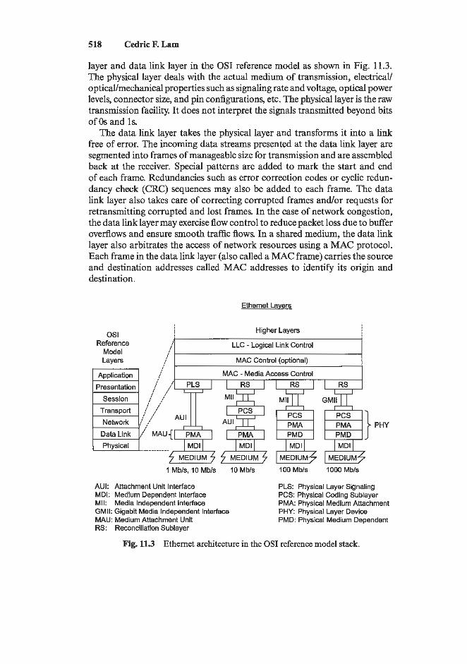
518 Cedric F. Lam
layer and data link layer in the OS1 reference model as shown in Fig. 11.3. The physical layer deals with the actual medium of transmission, electrical/ optical/mechanical properties such as signaling rate and voltage, optical power levels, connector size, and pin configurations, etc. The physical layer is the raw transmission facility. It does not interpret the signals transmitted beyond bits of Os and 1s.
The data link layer takes the physical layer and transforms it into a link free of error. The incoming data streams presented at the data link layer are segmented into frames of manageable size for transmission and are assembled back at the receiver. Special patterns are added to mark the start and end of each frame. Redundancies such as error correction codes or cyclic redun- dancy check (CRC) sequences may also be added to each frame. The data link layer also takes care of correcting corrupted frames and/or requests for retransmitting corrupted and lost frames. In the case of network congestion, the data link layer may exercise flow control to reduce packet loss due to bf ier overflows and ensure smooth traffic flows. In a shared medium, the data link layer also arbitrates the access of network resources using a MAC protocol. Each frame in the data link layer (also called a MAC frame) carries the source and destination addresses called MAC addresses to identify its origin and destination.
Ethernet Lavers
Higher Layers
Reference
1 Mbls, 10 Mbls 10 Mb/s 100 Mbls 1000 Mbls
AUI: Attachment Unit Interface PLS: Physical Layer Signaling MDI: Medium Dependent Interface PCS: Physical Coding Sublayer MII: Media Independent Interface PMA: Physical Medium Attachment GMII: Gigabit Media Independent Interface PHY: Physical Layer Device MAU: Medium Attachment Unit PMD: Physical Medium Dependent RS: Reconciliation Sublayer
Fig. 11.3 Ethernet architecture in the OS1 reference model stack.
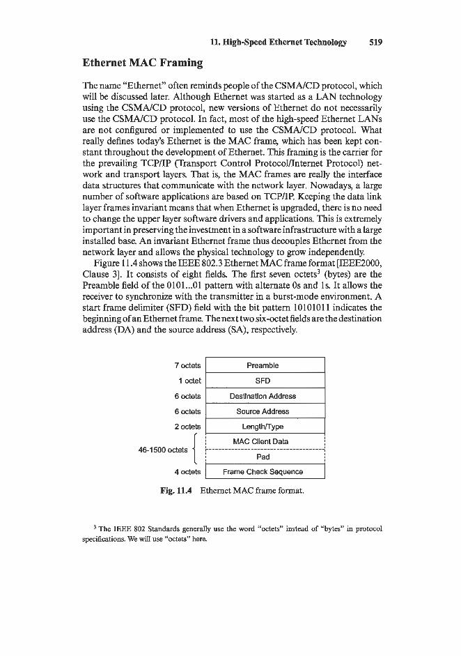
11. High-speed Ethernet Technology 519
7 octets
Ethernet MAC Framing
Preamble
The name “Ethernet” often reminds people of the CSMMCD protocol, which will be discussed later. Although Ethernet was started as a LAN technology using the CSMMCD protocol, new versions of Ethernet do not necessarily use the CSMA/CD protocol. In fact, most of the high-speed Ethernet LANs are not configured or implemented to use the CSMMCD protocol. What really defines today’s Ethernet is the MAC frame, which has been kept con- stant throughout the development of Ethernet. This framing is the carrier for the prevailing TCP/IP (Transport Control ProtocoVInternet Protocol) net- work and transport layers. That is, the MAC frames are really the interface data structures that communicate with the network layer. Nowadays, a large number of software applications are based on TCP/IP. Keeping the data link layer frames invariant means that when Ethernet is upgraded, there is no need to change the upper layer software drivers and applications. This is extremely important in preserving the investment in a software infrastructure with a large installed base. An invariant Ethernet frame thus decouples Ethernet from the network layer and allows the physical technology to grow independently.
Figure 1 1.4 shows the IEEE 802.3 Ethernet MAC frame format [IEEE2000, Clause 31. It consists of eight fields. The first seven octets3 (bytes) are the Preamble field of the 0101 ... 01 pattern with alternate Os and 1s. It allows the receiver to synchronize with the transmitter in a burst-mode environment. A start frame delimiter (SFD) field with the bit pattern 10101011 indicates the beginning of an Ethernet frame. The next two six-octet fields are the destination address (DA) and the source address (SA), respectively.
2 octets LengthKype
MAC Client Data
Pad
4 octets Frame Check Sequence
I octet I SFD I 6 octets I Destination Address I 6 octets I Source Address I
Fig. 11.4 Ethernet MAC frame format.
The IEEE 802 Standards generally use the word “octets” instead of “bytes” in protocol specifications. We will use “octets” here.
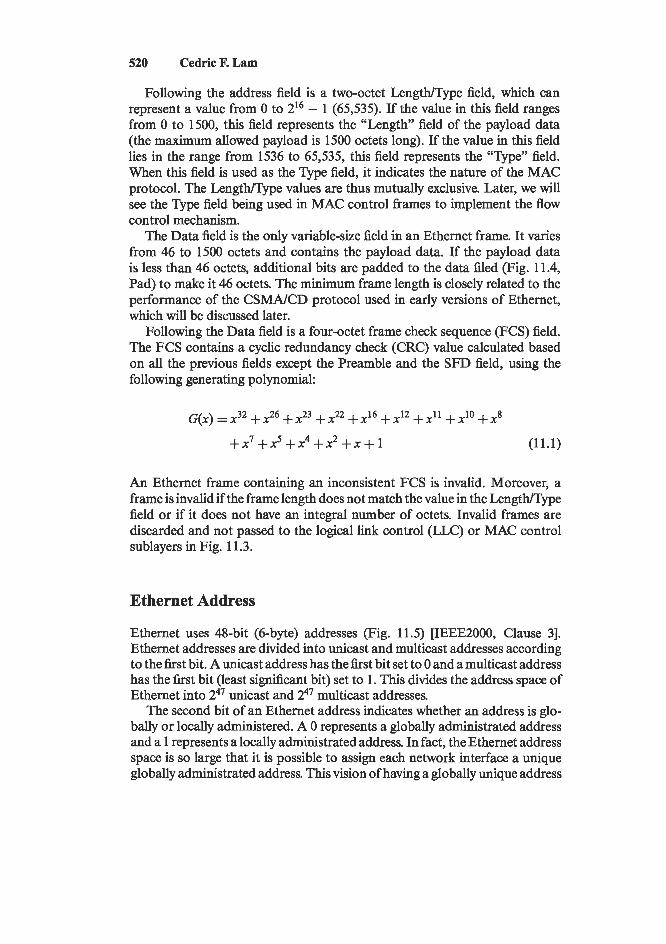
520 Cedric E Lam
Following the address field is a two-octet LengWType field, which can represent a value from 0 to 216 - 1 (65,535). If the value in this field ranges from 0 to 1500, this field represents the “Length” field of the payload data (the maximum allowed payload is 1500 octets long). If the value in this field lies in the range from 1536 to 65,535, this field represents the ‘‘TypeYY field. When this field is used as the Type field, it indicates the nature of the MAC protocol. The LengtWType values are thus mutually exclusive. Later, we will see the Type field being used in MAC control frames to implement the flow control mechanism.
The Data field is the only variable-size field in an Ethernet frame. It varies from 46 to 1500 octets and contains the payload data. If the payload data is less than 46 octets, additional bits are padded to the data filed (Fig. 11.4, Pad) to make it 46 octets. The minimum frame length is closely related to the performance of the CSMNCD protocol used in early versions of Ethernet, which will be discussed later.
Following the Data field is a four-octet frame check sequence (FCS) field. The FCS contains a cyclic redundancy check (CRC) value calculated based on all the previous fields except the Preamble and the SFD field, using the following generating polynomial:
+x7 +x5 +x4 +1 + x + 1 (11.1)
An Ethernet frame containing an inconsistent FCS is invalid. Moreover, a frame is invalid if the frame length does not match the value in the LengtWType field or if it does not have an integral number of octets. Invalid frames are discarded and not passed to the logical link control (LLC) or MAC control sublayers in Fig. 11.3.
Ethernet Address
Ethernet uses 48-bit (6-byte) addresses (Fig. 1 1.5) [IEEE2000, Clause 31. Ethernet addresses are divided into unicast and multicast addresses according to the fist bit. Aunicast address has the first bit set to 0 and a multicast address has the first bit (least significant bit) set to 1. This divides the address space of Ethernet into 247 unicast and 247 multicast addresses.
The second bit of an Ethernet address indicates whether an address is glo- bally or locally administered. A 0 represents a globally administrated address and a 1 represents a locally administrated address. In fact, the Ethernet address space is so large that it is possible to assign each network interface a unique globally administrated address. This vision of having a globally unique address
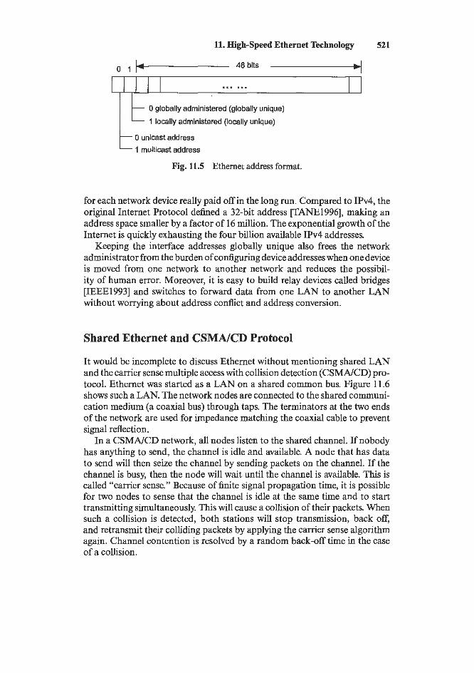
11. High-speed Ethernet Technology 521
, b- 46 bits -4 ... ...
0 globally administered (globally unique)
1 locally administered (locally unique)
0 unicast address 1 multicast address
Fig. 11.5 Ethernet address format.
for each network device really paid off in the long run. Compared to IPv4, the original Internet Protocol dehed a 32-bit address pANE19961, making an address space smaller by a factor of 16 million. The exponential growth of the Internet is quickly exhausting the four billion available IPv4 addresses.
Keeping the interface addresses globally unique also frees the network administrator from the burden of configuring device addresses when one device is moved from one network to another network and reduces the possibil- ity of human error. Moreover, it is easy to build relay devices called bridges [IEEE1993] and switches to forward data from one LAN to another LAN without worrying about address conflict and address conversion.
Shared Ethernet and CSMNCD Protocol
It would be incomplete to discuss Ethernet without mentioning shared LAN and the carrier sense multiple access with collision detection (CSMNCD) pro- tocol. Ethernet was started as a LAN on a shared common bus. Figure 11.6 shows such a LAN. The network nodes are connected to the shared communi- cation medium (a coaxial bus) through taps. The terminators at the two ends of the network are used for impedance matching the coaxial cable to prevent signal reflection.
In a CSMNCD network, all nodes listen to the shared channel. If nobody has anything to send, the channel is idle and available. A node that has data to send will then seize the channel by sending packets on the channel. If the channel is busy, then the node will wait until the channel is available. This is called “carrier sense.” Because of finite signal propagation time, it is possible for two nodes to sense that the channel is idle at the same time and to start transmitting simultaneously. This will cause a collision of their packets. When such a collision is detected, both stations will stop transmission, back off, and retransmit their colliding packets by applying the carrier sense algorithm again. Channel contention is resolved by a random back-off time in the case of a collision.
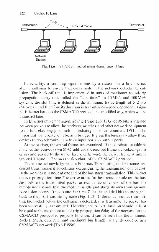
522 Cedric F. Lam
Taps Terminator Coaxial Cable Terminator
Network Station
Fig. 11.6 A LAN connected using shared coaxial bus.
In actuality, a jamming signal is sent by a station for a brief period after a collision to ensure that every node in the network detects the col- lision. The back-off time is implemented in units of maximum round-trip propagation delay time called the “slot time.” In 10Mb/s and 100Mb/s systems, the slot time is defined as the minimum frame length of 512 bits (64 bytes), and therefore its duration is transmission-speed dependent. Giga- bit Ethernet handles the CSMA/CD protocol in a modified way, which will be discussed later.
In Ethernet implementation, an interframe gap (IFG) of 96 bits is inserted between packets to allow the receivers, switches, and other network equipment to do housekeeping jobs such as updating statistical counters. IFG is also important for repeaters, hubs, and bridges. It gives the leeway to allow these devices to resynchronize data from input ports to output ports.
At the receiver, the arrival frames are examined. If the destination address matches the receiver’s own MAC address, the received frame is checked against errors and passed to the upper layers. Otherwise, the arrival frame is simply ignored. Figure 11.7 shows the flowchart of the CSMA/CD protocol.
There is no acknowledgement in Ethernet. Transmitting nodes assume suc- cessful transmission if no collision occurs during the transmission of a packet. In the worst case, a node at one end of the bus starts transmission. This packet takes a propagation time T to arrive at the furthest remote node on the bus. Just before the transmitted packet arrives at the other end of the bus, the remote node senses that the medium is idle and starts its own transmission. A collision occurs. It takes another time T for the collided bits to propagate back to the first transmitting node (Fig. 11.8). If the node finishes transmit- ting the packet before the collision is detected, it will assume the packet has been successfully transmitted. Therefore, the packet duration should at least be equal to the maximum round-trip propagation delay of the network for the CSMA/CD protocol to properly function. It can be seen that the minimum packet length, data rate, and maximum bus length are tightly coupled in a CSMA/CD network [TANE1996].

11. High-speed Ethernet Technology 523
Frame Transmission
wait for IFG + c send jam
start transmission
compute backoff
Done:Transmit OK
Frame Reception
[ Receive Frame ]
no
-r" lengthltype? 1 C ves I &
,&,,-I Fig. 11.7 CSMA/CD protocol for frame transmission and reception.
frame generated at time t=O
frame about to reach node B at time t=T4
b I - - - - - - _ _ _ _ _ _ _ _ _ _ - - - - - I----
L"PJ
Node A Node B
collision detected collision occurred 'fF% at time t=T 4 _ _ _ _ _ _ _ _ - - - - - - - - - _ - - - - - pqm
Node A Node B
Fig. 11.8 It takes as much as the round-trip propagation delay time to detect a collision.
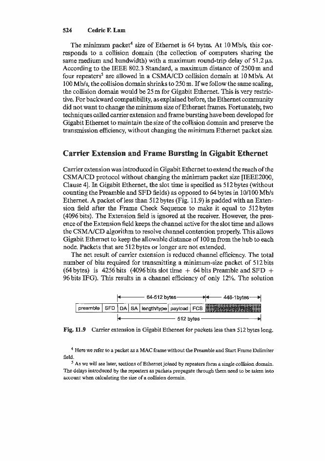
524 Cedric F. Lam
The minimum packet4 size of Ethernet is 64 bytes. At 10 Mb/s, this cor- responds to a collision domain (the collection of computers sharing the same medium and bandwidth) with a maximum round-trip delay of 5 1.2 ps. According to the IEEE 802.3 Standard, a maximum distance of 2500 m and four repeaters5 are allowed in a CSMA/CD collision domain at 10 Mb/s. At 100 Mb/s, the collision domain shrinks to 250 m. If we follow the same scaling, the collision domain would be 25 m for Gigabit Ethernet. This is very restric- tive. For backward compatibility, as explained before, the Ethernet community did not want to change the minimum size of Ethernet frames. Fortunately, two techniques called carrier extension and frame bursting have been developed for Gigabit Ethernet to maintain the size of the collision domain and preserve the transmission efficiency, without changing the minimum Ethernet packet size.
Carrier Extension and Frame Bursting in Gigabit Ethernet
Carrier extension was introduced in Gigabit Ethernet to extend the reach of the CSMA/CD protocol without changing the minimum packet size [IEEE2000, Clause 41. In Gigabit Ethernet, the slot time is specified as 512bytes (without counting the Preamble and SFD fields) as opposed to 64 bytes in 10/100 Mb/s Ethernet. A packet of less than 512 bytes (Fig. 11.9) is padded with an Exten- sion field after the Frame Check Sequence to make it equal to 512bytes (4096 bits). The Extension field is ignored at the receiver. However, the pres- ence of the Extension field keeps the channel active for the slot time and allows the CSMA/CD algorithm to resolve channel contention properly. This allows Gigabit Ethernet to keep the allowable distance of 100 m from the hub to each node. Packets that are 512 bytes or longer are not extended.
The net result of carrier extension is reduced channel efficiency. The total number of bits required for transmitting a minimum-size packet of 512bits (64 bytes) is 4256 bits (4096 bits slot time + 64 bits Preamble and SFD + 96 bits IFG). This results in a channel efficiency of only 12%. The solution
p- 64-512 bytes- 448-1bytes--+
512 bytes -4 Fig. 11.9 Carrier extension in Gigabit Ethernet for packets less than 512 bytes long.
Here we refer to a packet as a MAC frame without the Preamble and Start Frame Deliiter field.
As we will see later, sections of Ethernet joined by repeaters form a single collision domain. The delays introduced by the repeaters as packets propagate through them need to be taken into account when calculating the size of a collision domain.

11. High-speed Ethernet Technology 525
Baseline Average 0 1.5k Bursting Average IS 1.5k Bursting 95%
E l Baseline 95%
v) 8k Bursting Average I23 8k Bursting 95%
p 150
n $ 100
- 0
W 0 ‘ 50
0 30% load 40% load 50% load
Fig. 11.10 Mean and 95th percentile of access delay. (Reproduced from M. Molle et al., “Frame Bursting: A Technique for Scaling CDMNCD to Gigabit Speeds,” IEEE Network, JulyIAugust 1997, pp. 6-15.)
to this problem is called “frame bursting.” In a properly configured network, once a station has finished sending the first frame (with or without carrier extension) successfully, the station is sure that it has control of the channel. If there are still packets in its transmit queue, the station is allowed to burst up to a total of 8 192 bytes.
Frame bursting not only improves the channel efficiency, but also helps to reduce the “capture effect” in Ethernet [RAMA1994]. In a CSMNCD net- work, a station that transmits successfully after a collision has a higher chance of transmitting new frames than stations that lost in the collision resolution. In a busy network, this results in a station having a long period of transmission while other stations have to wait a long time. The capture effect induces long delay variance and is undesirable for delay-sensitive applications.
Surprisingly, simulation results show frame bursting helps to alleviate the capture effect [MOLL1997; MOLL1997al. Figure 11.10 shows the mean and 95th percentile of access delay with and without frame bursting. The reason for the improved performance is that only the first frame of the burst can potentially experience collision. Frame bursting allows a host to empty its transmit queue much faster and reduces the number of collisions experienced by individual stations so that their back-off delays do not increase much in a heavily loaded network.
Hubbed Ethernet and Full Duplex Operation
In the 1980s, structured wiring became popular as digital telephone systems took off. Structured wiring is a physical star architecture. All the connections terminate at a common wiring closet where a switching hub or concentrator is
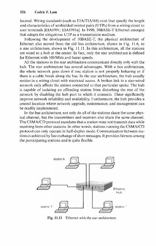
526 Cedric F. Lam
located. Wiring standards (such as EIAlTIA568) exist that specify the length and characteristics of unshielded twisted pairs (UTPs) from a wiring closet to user terminals [EIA1991; EIA1991al. In 1990, 10BASE-T Ethernet emerged that adopts the ubiquitous UTP as a transmission medium.
Following the development of 1 OBASE-T, the physical architecture of Ethernet also moved from the old bus architecture, shown in Fig. 11.6, to a star architecture, shown in Fig. 11.11. In this architecture, all the stations are wired to a hub at the center. In fact, only the star architecture is defined for Ethernet with 100 Mb/s and faster speeds.
All the stations in the star architecture communicate directly only with the hub. The star architecture has several advantages. With a bus architecture, the whole network goes down if one station is not properly behaving or if there is a cable break along the bus. In the star architecture, the hub usually resides in a wiring closet with restricted access. A broken link in a star-wired network only affects the station connected to that particular spoke. The hub is capable of isolating an offending station from disturbing the rest of the network by disabling the hub port to which it connects. These significantly improve network reliability and availability. Furthermore, the hub provides a central location where network upgrade, maintenance, and management can be readily implemented.
In the bus architecture, not only do all of the stations share the same phys- ical channel, but the transmitters and receivers also share the same channel. The CSMNCD protocol mandates that a station must not transmit data while receiving from other stations. In other words, stations running the CSMNCD protocol can only operate in half-duplex mode. Communication between sta- tions is achieved by fast exchange of short messages. It provides fairness among the participating stations and is quite flexible.
Fig. 11.11 Ethernet with the star architecture.

11. High-speed Ethernet Technology 527
In the star architecture, there is no intermediate drop between the hub and an end station. All the stations are connected to a hub, with sepa- rate channels dedicated for transmission and reception, respectively (using either twisted pairs or optical fibers). This opens the possibility of running Ethernet in full-duplex mode, Le., transmitting and receiving simultaneously. The throughput is at least doubled in full-duplex mode compared to half- duplex mode. Full-duplex Ethernet is sometimes called switched Ethernet, which will become clear later. Of course, the CSMNCD protocol no longer applies to full-duplex mode.
However, not all star-wired Ethernets support full-duplex operation. Although all lOOMb/s and faster Ethernet adopt a physical star archi- tecture, the CSMNCD protocol has been defined and implemented for 10/100/1000 Mb/s Ethernet. A hub running the CSMNCD protocol is called a repeater hub.
Repeaters
A repeater is a physical layer device [IEEE2000, Clauses 9, 27, and 411. Figure 11.12 shows the 100 Mb/s repeater relationship relative to the OS1 pro- tocol stack. Repeaters for other speed Ethernet are located similarly in the protocol stack. As can be seen in Fig. 11.12, a repeater terminates at the top of the physical layer. An explicit implementation of the Medium Independent Interface (MII) is optional. (More detailed discussion of the physical layer- PHY implementation is given in a later section.) The function of the repeater is to forward the MAC frames from one PHY entity to another. The repeater
Ethernet Layers
~ Higher Layers
10Mb/s 100Mb/s
MEDIUM MEDIUM
1 OOMb/s 100Mb/s
Fig. 11.12 Location of repeaters in the OS1 reference model (using 100 Mb/s repeater as an example).

528 Cedric F. Lam
does not examine the content in the MAC frame. In other words, it does not do any MAC processing of the data and should not be costly to build.
Repeaters usually have more than two ports (Le., multiple PHYs). They can be used to connect different media such as optical fiber and twisted pair to form a single LAN or to extend the reach of a link beyond its physical constraint (Fig. 1 1.13). For example, in a coaxial bus network, the CSMNCD protocol allows a transmission distance of 2500 m. However, physical impairments such as noise, attenuation, and interference impose a limit to the distance that actual bits can propagate in the medium. According to the IEEE 802.3 Standard, this distance is 185m for the 10BASE2 system and 500m for 10BASE5. So if a lOBASE2 network has a physical distance longer than 185 m, it must be broken into sections smaller than 185 m and joined with repeaters.
A repeater reproduces the data presented at one port to another with proper line coding for the destination PHY It restores preamble bits consumed in clock recovery and the signal levels at the output. It also removes noise accu- mulation and timing jitters. Besides, if a collision is detected at one repeater port, the repeater will send jamming signals to other ports.
In a star configuration, a repeater hub simulates the CSMNCD protocol by propagating the received signal from one port to all other ports. A repeater hub usually can have 4 to 24 ports. When the receiver detects simultaneous transmission from different hosts (collision), it sends out the jamming sig- nal to all the stations connected to the hub. Although each station may have separate transmit and receive channels, only half-duplex operation is allowed using the CSMNCD protocol. One important characteristic is that all the stations connected together using repeaters form a single collision domain and its total size should obey the limit imposed by the CSMNCD proto- col. Moreover, in the case where multiple sections are joined with repeaters, there should be no loops (ring topology) formed for subtle reasons to avoid deadlock in the CSMNCD protocol [KADA1998]. When calculating the
_..- _____.--------_..________
'\\. I OBASE-T ,/" -- -_..__..___._.____- -------
/.." Single Collision Domain -*--..__ -----_.__._--
Fig. 11.13 Repeaters are used to extend the LAN reach, join different media, and act as a hub station. All the stations connected by repeaters form a single collision domain.
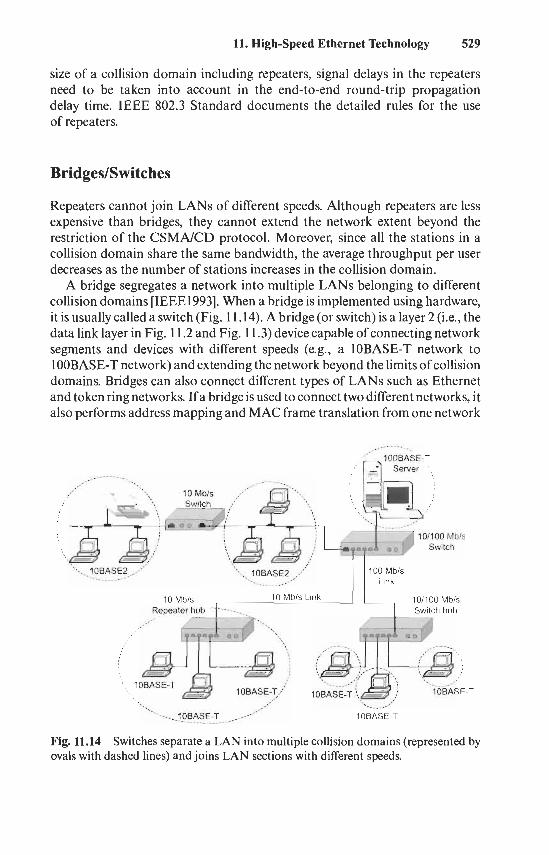
11. High-speed Ethernet Technology 529
size of a collision domain including repeaters, signal delays in the repeaters need to be taken into account in the end-to-end round-trip propagation delay time. IEEE 802.3 Standard documents the detailed rules for the use of repeaters.
BridgesBwitches
Repeaters cannot join LANs of different speeds. Although repeaters are less expensive than bridges, they cannot extend the network extent beyond the restriction of the CSMNCD protocol. Moreover, since all the stations in a collision domain share the same bandwidth, the average throughput per user decreases as the number of stations increases in the collision domain.
A bridge segregates a network into multiple LANs belonging to different collision domains [IEEE1993]. When a bridge is implemented using hardware, it is usually called a switch (Fig. 1 1.14). A bridge (or switch) is a layer 2 (i.e., the data link layer in Fig. 11.2 and Fig. 11.3) device capable of connecting network segments and devices with different speeds (e.g., a 10BASE-T network to 1 OOBASE-T network) and extending the network beyond the limits of collision domains. Bridges can also connect different types of LANs such as Ethernet and token ring networks. If a bridge is used to connect two different networks, it also performs address mapping and MAC frame translation from one network
10/100 Mbls Switch
Mbls Repeater hub I-------.. hub
10 Mbls Link I 10 Mbls
_/'
(BJ '<\ 10BASE-T
,,. -._._-, --.. ----%JoEAsE;T .___ __-----**' IOBASE-T
Fig. 11.14 Switches separate a LAN into multiple collision domains (represented by ovals with dashed lines) and joins LAN sections with different speeds.
530 Cedric F. Lam
to another. If the destination network has a smaller maximum packet size than the source network, a bridge also needs to perform packet segmentation.
We will only discuss Ethernet switches in this section. Because a switch separates a network into individual collision domains, it improves the overall network performance. A switch hub replaces a repeater hub in full-duplex Ethernet. In this case, the transmitter and receiver use a separate channel for communication and carrier sense is disabled. Because dedicated links exist between each port of the switch hub and an end station, there is no contention for the channel. Moreover, the hub switch hub performs media access control so there is no collision to detect. Another way of looking at this is that each station forms its own collision domain.
Stations are connected to a switch at switch ports, each of which has a port identifier. An Ethernet switch works in promiscuous mode. It examines the Destination Address of each incoming packet to decide what action to take. When a packet arrives at a switch port, and the Destination Address belongs to the subnetwork attached to the same switch port, then the switch simply discards that packet. Otherwise, the switch uses an address lookup table to decide to which port the packet should be forwarded. Each address in the address table has an associated port identifier. If the Destination Address is in the address table, the switch will forward the packet to the appropriate port. Otherwise, the switch will flood the packet to all the ports except the one it comes from.
The address table is built dynamically. A switch learns how to associate an address with a port by examining the Source Address field of the incoming packets and periodically refreshing the address lookup table. To account for the possibilities that a network interface may be moved from one location to another location during network maintenance and configuration, a timer is set for each entry in the address table. If a particular address table entry is inactive for too long, it is purged from the address table.
Unlike a repeater, multiple ports of a switch may be active at the same time. In fact, a switch is basically a circuit concept. Nevertheless, it is used to describe devices providing similar functions in a packet world. Figure 11.15 shows the concept of an N x N nonblocking circuit switch made up of an array of crossbar switches. A switch connects the input ports to output ports. A nonblocking switch is a switch that can connect from any input to any output in an arbitrary fashion, provided there are no two inputs contending for the same output port simultaneously. A blocking switch is cheaper than a nonblocking switch. However, certain connections may not be possible in a blocking switch even though both the input and output ports are available, depending on the existing switch configuration [HUI1999; TANE19961.
A switching fabric is required in a packet switch (Fig. 11.15). This switch- ing fabric can be made up of memory blocks connected to a common bus or electronic crossbar gates. In a nonblocking switch, the bandwidth of the switching fabric should be at least the sum of the bandwidths of all individual
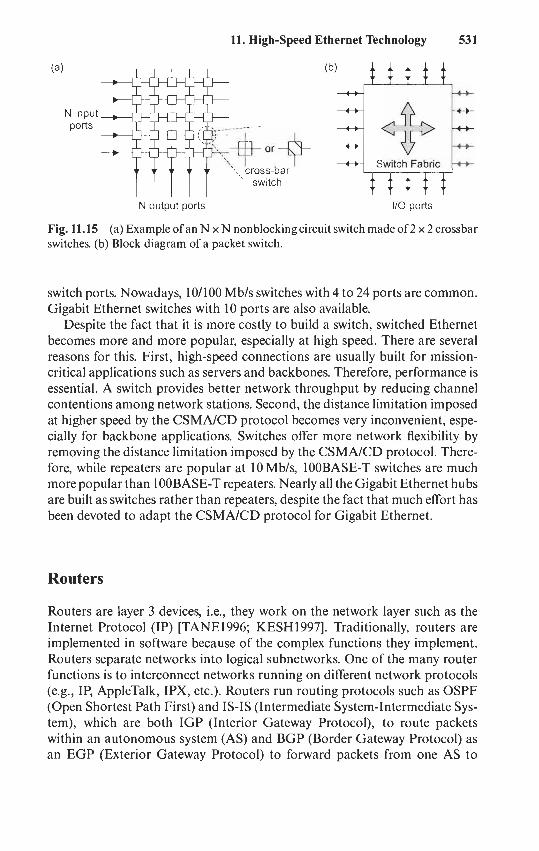
11. High-speed Ethernet Technology 531
(4
N input ports
+or+ '\\\ cross-bar
' switch
N output ports
Switch Fabric
110 ports
Fig. 11.15 (a) Example of an N x N nonblocking circuit switch made of 2 x 2 crossbar switches. (b) Block diagram of a packet switch.
switch ports. Nowadays, 10/100 Mb/s switches with 4 to 24 ports are common. Gigabit Ethernet switches with 10 ports are also available.
Despite the fact that it is more costly to build a switch, switched Ethernet becomes more and more popular, especially at high speed. There are several reasons for this. First, high-speed connections are usually built for mission- critical applications such as servers and backbones. Therefore, performance is essential. A switch provides better network throughput by reducing channel contentions among network stations. Second, the distance limitation imposed at higher speed by the CSMA/CD protocol becomes very inconvenient, espe- cially for backbone applications. Switches offer more network flexibility by removing the distance limitation imposed by the CSMA/CD protocol. There- fore, while repeaters are popular at 10 Mb/s, 100BASE-T switches are much more popular than 100BASE-T repeaters. Nearly all the Gigabit Ethernet hubs are built as switches rather than repeaters, despite the fact that much effort has been devoted to adapt the CSMA/CD protocol for Gigabit Ethernet.
Routers
Routers are layer 3 devices, Le., they work on the network layer such as the Internet Protocol (IP) [TANE1996; KESH19971. Traditionally, routers are implemented in software because of the complex functions they implement. Routers separate networks into logical subnetworks. One of the many router functions is to interconnect networks running on different network protocols (e.g., IP, AppleTalk, IPX, etc.). Routers run routing protocols such as OSPF (Open Shortest Path First) and IS-IS (Intermediate System-Intermediate Sys- tem), which are both IGP (Interior Gateway Protocol), to route packets within an autonomous system (AS) and BGP (Border Gateway Protocol) as an EGP (Exterior Gateway Protocol) to forward packets from one AS to

532 Cedric F. Lam
another. Routers exchange information such as network reachability informa- tion, topology, link cost, link state, routing distance, etc., with each other. These parameters are used to build the routing tables for routing decisions. Routing algorithms not only have to ensure routing correctness, but also the system stability and optimality. Security functions such as firewalls are part of a router’s function. Besides, routers also perform network management func- tions using SNMP (Simple Network Management Protocol) and configuration function using DHCP (Dynamic Host Configuration Protocol), etc.
In recent years, router technology has advanced considerably. As Inter- net use becomes more widespread, new protocols such as RSVP (Resource Reservation Protocol) [ZHAN1993] have been developed to enable resource allocation along the routing path. Multiprotocol label switching (MPLS) [DAVI2000] was originally designed to speed up routing decisions. It makes use of technologies developed for ATM and circuit switching to direct traffic to certain paths in the network to enable traffic engineering, as well as other applications such as network-based virtual private network OrpN). In MPLS, packets are attached with switching labels, which control the routing path. MPLS and RSVP provide ways to enable Internet quality of service (QoS).
In the last few years, there has been a trend of merging the functions of layer 2 switches and layer 3 routers into a single box. In fact, silicon techno- logy has improved so much that more and more router functions can be built into switches using hardware. From an economic viewpoint, as IP becomes the single dominating network protocol, it makes more sense to implement IP routing in hardware. New-generation IP routers will implement time-critical routing functions such as address decode and look up and packet valida- tion and forwarding in hardware, while other complicated but less frequently used functions such as network management can be implemented in software without sacrificing the cost and performance.
Flow Control in Ethernet
When a switch or a station is overloaded, it may not have enough resources to process the arriving packets at their incoming speed. As a result, its buffer may become full (buffer overflow), causing packets to be dropped. Dropping pack- ets may degrade the performance of upper-layer protocols. For instance, TCP relies on a positive acknowledgment and retransmission mechanism to ensure reliable packet transmission and correct packet sequence. A lost packet would cause TCP to time out. All the subsequent packets would be delayed (to ensure proper packet sequence). This represents a severe performance penalty. Flow control is a mechanism to throttle the packet arrival rate to prevent packets from being dropped due to buffer overflow.
In half-duplex Ethernet, back pressure can be used to slow the transmitting stations. One way of doing this is to generate collisions by sending jamming
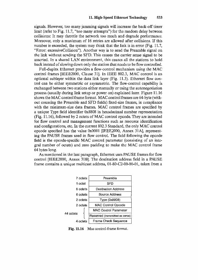
11. High-speed Ethernet Technology 533
signals. However, too many jamming signals will increase the back-off timer limit (refer to Fig. 11.7, “too many attempts”) for the random delay between collisions: It may throttle the network too much and degrade performance. Moreover, only a maximum of 16 retries are allowed after collisions. If this number is exceeded, the system may think that the link is in error (Fig. 1 1.7, “Error: excessiveCollision”). Another way is to send the Preamble signal on the link without sending the SFD. This causes the carrier sense signal to be asserted. In a shared LAN environment, this causes all the stations to hold back instead of slowing down only the station that needs to be flow controlled.
Full-duplex Ethernet provides a flow-control mechanism using the MAC control frames [IEEE2000, Clause 311. In IEEE 802.3, MAC control is an optional sublayer within the data link layer (Fig. 11.3). Ethernet flow con- trol can be either symmetric or asymmetric. The flow-control capability is exchanged between two stations either manually or using the autonegotiation process (usually during link setup or power on) explained later. Figure 1 1.16 shows the MAC control frame format. MAC control frames are 64-byte (with- out counting the Preamble and SFD fields) fixed-size frames, in compliance with the minimum-size data frames. MAC control frames are specified by a unique Type field identifier Ox8808 in hexadecimal number representation (Fig. 1 1.16), followed by 2 octets of MAC control opcode. They are intended for flow control and management functions such as resource identification and configuration% etc. In the current 802.3 Standard, the only MAC control opcode specified has the value Ox0001 [IEEE2000, Annex 31A], represent- ing the PAUSE frames used in flow control. The field following the opcode field is the opcode-specific MAC control parameter (consisting of an inte- gral number of octets) and zero padding to make the MAC control frame 64 bytes long.
As mentioned in the last paragraph, Ethernet uses PAUSE frames for flow control [IEEE2000, Annex 31Bl. The destination address field in a PAUSE frame contains a unique multicast address, 01-80-C2-00-00-01 , taken from a
7 octets I Preamble I I octet I SFD I
6 octets
2 octets
j MAC Control Parameter j :----------------------------------- + j Reserved (transmitted as zeros) j
44 octets
Fig. 11.16 Mac control-frame format.
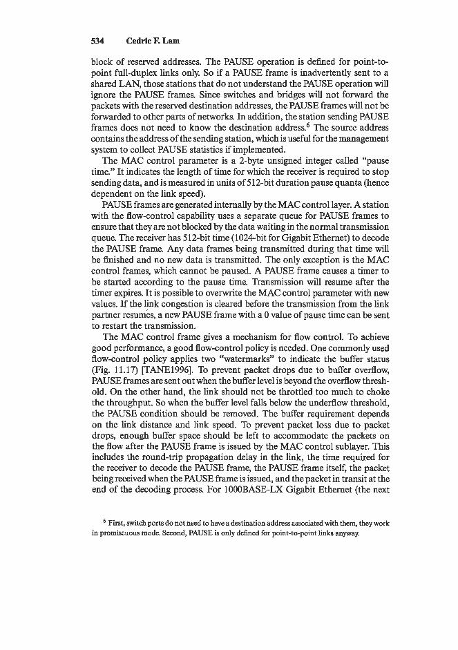
534 Cedric F. Lam
block of reserved addresses. The PAUSE operation is defined for point-to- point full-duplex links only. So if a PAUSE frame is inadvertently sent to a shared LAN, those stations that do not understand the PAUSE operation will ignore the PAUSE frames. Since switches and bridges will not forward the packets with the reserved destination addresses, the PAUSE frames will not be forwarded to other parts of networks. In addition, the station sending PAUSE frames does not need to know the destination address6 The source address contains the address of the sending station, which is useful for the management system to collect PAUSE statistics if implemented.
The MAC control parameter is a 2-byte unsigned integer called “pause time.” It indicates the length of time for which the receiver is required to stop sending data, and is measured in units of 5 12-bit duration pause quanta (hence dependent on the link speed).
PAUSE frames are generated internally by the MAC control layer. A station with the flow-control capability uses a separate queue for PAUSE frames to ensure that they are not blocked by the data waiting in the normal transmission queue. The receiver has 512-bit time (1024-bit for Gigabit Ethernet) to decode the PAUSE frame. Any data frames being transmitted during that time will be finished and no new data is transmitted. The only exception is the MAC control frames, which cannot be paused. A PAUSE frame causes a timer to be started according to the pause time. Transmission will resume after the timer expires. It is possible to overwrite the MAC control parameter with new values. If the link congestion is cleared before the transmission from the link partner resumes, a new PAUSE frame with a 0 value of pause time can be sent to restart the transmission.
The MAC control frame gives a mechanism for flow control. To achieve good performance, a good flow-control policy is needed. One commonly used flow-control policy applies two “watermarks” to indicate the buffer status (Fig. 11.17) [TANE1996]. To prevent packet drops due to buffer overflow, PAUSE frames are sent out when the buffer level is beyond the overflow thresh- old. On the other hand, the link should not be throttled too much to choke the throughput. So when the buffer level falls below the underflow threshold, the PAUSE condition should be removed. The buffer requirement depends on the link distance and link speed. To prevent packet loss due to packet drops, enough buffer space should be left to accommodate the packets on the flow after the PAUSE frame is issued by the MAC control sublayer. This includes the round-trip propagation delay in the link, the time required for the receiver to decode the PAUSE frame, the PAUSE frame itself, the packet being received when the PAUSE frame is issued, and the packet in transit at the end of the decoding process. For 1000BASE-LX Gigabit Ethernet (the next
First, switch ports do not need to have a destination address associated with them, they work in promiscuous mode. Second, PAUSE is only defined for point-to-point links anyway.
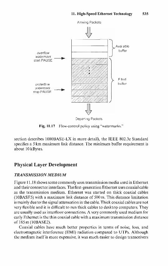
11. High-speed Ethernet Technology 535
Arriving Packets
overflow watermark -
start PAUSE
underf/ow watermark -
stop PAUSE
+ Filled buffer
a Departing Packets
Fig. 11.17 Flow-control policy using “watermarks.”
section describes 1000BASE-LX in more detail), the IEEE 802.32 Standard specifies a 5 km maximum link distance. The minimum buffer requirement is about 10 kBytes.
Physical Layer Development
TRANSMISSION MEDIUM
Figure 1 1.18 shows some commonly seen transmission media used in Ethernet and their connector interfaces. The first-generation Ethernet uses coaxial cable as the transmission medium. Ethernet was started on thick coaxial cables (10BASE5) with a maximum link distance of 500 m. This distance limitation is mainly due to the signal attenuation in the cable. Thick coaxial cables are not very flexible and it is difficult to run thick cables to desktop computers. They are usually used as interfloor connections. A very commonly used medium for early Ethernet is the thin coaxial cable with a maximum transmission distance of 185 m (10BASE2).
Coaxial cables have much better properties in terms of noise, loss, and electromagnetic interference (EMI) radiation compared to UTPs. Although the medium itself is more expensive, it was much easier to design transceivers

536 Cedric E Lam
Fig. 11.18 Some commonly seen Ethernet media and connectors (MDI).
for coaxial cables in the early days. Structured wiring using Category 3 UTP cables became popular in the early 1990s. At the same time, advancement in silicon technology, signal processing, and signal conditioning has reached the stage to allow economical design of lO-Mb/s Ethernet running on UTP called 10BASE-T. The ubiquity, low cost, and ease of wiring of UTP wiring has made 10BASE-T Ethernet the most popular local area technology. There are two observations to be made about the evolution of Ethernet since 10BASE-T. First, Ethernet has adopted point-to-point link design and a star architecture. There is no more bus architecture as in the coaxial designs. Second, all the systems (from 10 Mb/s to 1000 Mb/s) using UTP as the transmission medium have specified a common maximum point-to-point distance of 100 m.
When 100BASE-T was designed, the UTP medium was also upgraded from Category 3 to Category 5 with better cable quality. 100BASE-TX runs on two pairs of Category 5 cables. On the other hand, 100BASE-T2 and 100BASE-T4 are designed to run on two pairs and four pairs of Category 3 cables, respectively, using different line coding schemes other than that used in 100BASE-TX. Although optical fiber has been specified as the medium for 10BASE-F, its use in lO-Mb/s Ethernet was never popular. One of the functions (at least initially) of lOO-Mb/s Ethernet is for traffic aggregation and backbone transport. Optical fiber has the advantage of having low loss and high bandwidth for long-distance transmission. 100BASE-FX uses Light Emitting Diodes (LEDs) as the light source and multimode fiber (MMF) as the transmission medium (Fig. 1 1.18). It specifies a maximum distance of 2 km.
MMF has been widely used in FDDIs for campus backbone connection. The physical layer design for 100BASE-X is actually borrowed from FDDI

11. High-speed Ethernet Technology 537
[JAIN1994]. For low-speed and short-distance applications, LEDs are cheaper than laser diodes in general. However, it is more difficult to couple LED output into optical fibers because of the incoherent nature of light from LEDs. MMF has a larger core area, and hence it is easier to couple light into MMF. Commonly used MMF has core diameters of 50 or 62.5 Vm. However, the large core of MMF supports multiple modes of light, each propagating at a different speed. Therefore, if a pulse stream is launched into MMF, various modes will arrive at the receiver at different times, causing distortion of the signal. This is called modal dispersion. Modal dispersion limits the bit-rate distance product that signals can be transported [GREE1993].
1000BASE-X Ethernet was first created with optical fiber as the medium. The 1000BASE-SX standard uses short-wavelength (850 nm) lasers as trans- mitters, and 1000BASE-LX uses long-wavelength (1310 nm) lasers. The 1000BASE-T standard specified four pairs of Category 5 cables as the medium. It was finished the year after the 1000BASE-SX and 1000BASE-LX standards were finished. Lasers and single-mode fiber (SMF) were adopted for the first time in 1000-Mbh Ethernet standards. 1000BASE-LX allows a maximum transmission distance of 5-km using single-mode fiber. Standard SMF has a core diameter of 10 Vm. Because light can only propagate in one mode in a SMF, there is no bandwidth and distance limitation due to modal dispersion. SMF is used in all long-distance fiber communication systems.
Tables 11.1 and 11.2 list some of the physical layer characters and trans- mission distance specified for 1000BASE-SX and 1000BASE-LX Ethernet in IEEE 802.32 Standard (IEEE2000, Clause 38).
The lO-Gb/s Ethernet standard is still being drafted and is expected to be finished in 2002. Like 1000-Mb/s Ethernet, both MMF and SMF will be used as the transmission medium. In addition, coarse WDM (wavelength-division multiplexing) is being included as a physical layer implementation in the draft standard. Since IO-Gb/s Ethernet is expected to be mainly a backbone tech- nology, the transmission distance will be increased to several 10s of kilometers in some physical layer implementations.
LINE CODING
The data link layer processes data as bits, which are digits of binary numbers. However, the actual electrical voltages and optical pulses that the physical layer sees are analog signals, and they suffer degradations from impairments such as noise and timing jitters as they propagate in the transmission medium. The frequency content in the actual physical signal is important for implementing clock recovery and transformer coupling in some designs. Digital signals are demodulated using threshold decisions at time intervals indicated by a clock. To correctly demodulate the signal, the clock signal needs to be synchronized with the symbols in the received data. One way of obtaining the clock is to use a clock recovery circuit, usually made up of a phase locked loop (PLL),
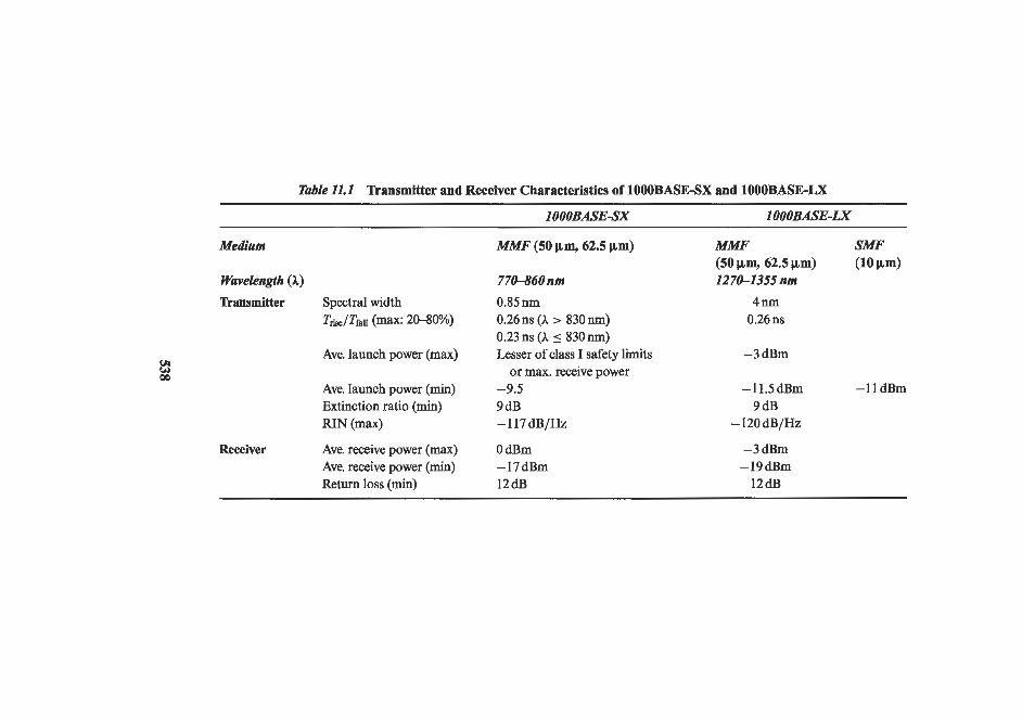
Table 11.1 Transmitter and Receiver Characteristics of 1000BASE-SX and 1000BASE-LX
1 OOOBASESX 1 OOOBASE-LX
Medium
Wavelength ( I )
MMF (50 pm, 62.5 pm) MMF SMF
770-860 nm 12 70-1355 nm (50 pm, 62.5 pm) (10 pm)
Transmitter Spectral width 0.85 nm 4 nm T'/Tf," (max: 2&80%) 0.2611s (A > 830nm) 0.26 ns
0.23 ns (h 5 830 nm) Ave. launch power (max) Lesser of class I safety limits -3 dBm
or max. receive power Ave. launch power (min) -9.5 - 11.5 dBm -11 dBm Extinction ratio (min) 9 dB 9 dB RIN (rnax) - 117 dB/Hz - 120 dB/Hz
Receiver Ave. receive power (max) 0 dBm -3 dBm Ave. receive power (min) -17dBm -19dBm Return loss (min) 12 dB 12 dB
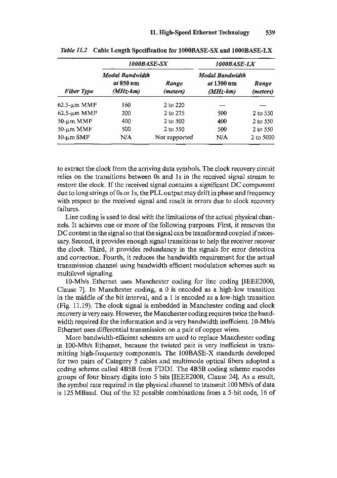
11. High-speed Ethernet Technology 539
Table 11.2 Cable Length Specification for 1000BASE-SX and 1000BASE-LX
1 OOOBASE-SX
Modal Bandwidth at 850 nm Range
Fiber Type (nHz.km) (metem)
62.5-pmMMF 160 2 to 220 62.5-pmMMF 200 2 to 275 50-pm MMF 400 2 to 500 50-pm MMF 500 2 to 550 10-pm SMF N/A Not supported
1 OOOBASE-LX Modal Bandwidth
at 1300 nm WHPknr)
- 500 400 500 N/A
Range (meters)
-
2 to 550 2 to 550 2 to 550 2 to 5000
to extract the clock from the arriving data symbols. The clock recovery circuit relies on the transitions between Os and 1s in the received signal stream to restore the clock. If the received signal contains a significant DC component due to long strings of Os or Is, the PLL output may drift in phase and frequency with respect to the received signal and result in errors due to clock recovery failures.
Line coding is used to deal with the limitations of the actual physical chan- nels. It achieves one or more of the following purposes. First, it removes the DC content in the signal so that the signal can be transformed coupled if neces- sary. Second, it provides enough signal transitions to help the receiver recover the clock. Third, it provides redundancy in the signals for error detection and correction. Fourth, it reduces the bandwidth requirement for the actual transmission channel using bandwidth efficient modulation schemes such as multilevel signaling.
lO-Mb/s Ethernet uses Manchester coding for line coding [IEEE2000, Clause 71. In Manchester coding, a 0 is encoded as a high-low transition in the middle of the bit interval, and a 1 is encoded as a low-high transition (Fig. 11.19). The clock signal is embedded in Manchester coding and clock recovery is very easy. However, the Manchester coding requires twice the band- width required for the information and is very bandwidth inefficient. lO-Mb/s Ethernet uses differential transmission on a pair of copper wires.
More bandwidth-efficient schemes are used to replace Manchester coding in 100-Mb/s Ethernet, because the twisted pair is very inefficient in trans- mitting high-frequency components. The 1 OOBASE-X standards developed for two pairs of Category 5 cables and multimode optical fibers adopted a coding scheme called 4B5B from FDDI. The 4B5B coding scheme encodes groups of four binary digits into 5 bits [IEEE2000, Clause 241. As a result, the symbol rate required in the physical channel to transmit 100 Mb/s of data is 125 MBaud. Out of the 32 possible combinations from a 5-bit code, 16 of

540 Cedric E Lam
I
-
- - -
I - - I I
non-return-to zero (uncoded) data
-
! Manchester i coded signal
them are used to represent the 4-bit information. The rest of the code words can be used as control code groups to represent the channel idle signal: start of data stream delimiters, etc. Adopting the coding scheme used in FDDI not only helped to speed up the development of lOO-Mb/s Ethernet, but also leveraged on the components developed for a mature technology and lowered the development cost.
100BASE-T4 and 100BASE-T2 were designed for operation on Category 3 cables. Since Category 3 cables have much worse frequency responses than the Category 5 cable, very bandwidth-efficient coding schemes have been used. The 100BASE-T4 Ethernet uses four pairs of Category 3 cables (Channel 1 to Channel 4). Channel 1 is used for unidirectional data symbol transmis- sion and collision resolution. Channel 2 is used as unidirectional input for data symbol receiving and collision detection when transmitting. Channel 3 and Channel 4 are bidirectional channels for transmission and/or reception. 100BASE-T4 uses a coding scheme called 8B6T in which 8 binary symbols are encoded into a string of 6 ternary symbols with values {+1 , 0, - 1) [IEEE2000, Clause 231. As a result of the cable arrangement and 8B6T encoding, the sym- bol rate on each pair of the cables to transmit 100 Mbps data on 100BASE-T4 is 25 MBaud. The 8B6T coding also has error detection capability. 100BASE- T2 uses an even more bandwidth-efficient encoding scheme called PAM5 x 5 to support transmission of 100 Mb/s on a pair of Category 3 cables simultane- ously [TEEE2000, Clause 321. The PAM5 scheme encodes a pulse-amplitude modulated (PAM) signal with 5 levels {-2, -1, 0, +1, +2} on each copper pair (represented as A, and B, in Fig. 11.20). Both pairs of copper wires are bidirectional. Each symbol in Fig. 11.20 can represent four bits of information (plus some redundancy for control and error detection). As a result of this, the symbol rate required on each pair is also 25 Mbaud.
10-Mb Ethernet uses burst-mode receivers. The receiver synchronizes its clock to the incom- ing data using the alternate Os and 1s provided by the Preambles. 100-Mb and faster receivers do not use burst-mode receivers anymore. There are idle symbols in the physical layer to keep the receiver clock always synchronized when there is no data to transmit.

11. High-speed Ethernet Technology 541
=-2 =-I =I =2 4 -1 0 0
0 0 1 - 2 . 0
Fig. 11.20 Signal constellation of the PAM5 x 5 encoding scheme used in 100BASE-T2 (0 IEEE, reproduced with permission).
1000BASE-X Ethernet uses a line coding called 8B10B. The 8B10B code was invented for the Fiber Channel technology by IBM wIDM1983; FCA19941. It is so far the most widely used line coding scheme for high- speed data communication. This again shortened the development of Gigabit Ethernet and lowered its cost. As its name implies, the 8B10B scheme encodes 8 binary digits into 10 digits. As a result of this, the raw symbol rate for trans- mitting 1000 Mb/s becomes 1250 MBaud. The 8B10B scheme selects 256 code words out of the 1024 possible 10-bit combinations to represent the 8 data bit. There are no streams of more than 5 continuous 1s or Os in the 8B10B codes. Moreover, the running disparity (difference in the number of Os and 1s in the transmitted symbols) is at most 1. As in other coding schemes, certain code groups are used to represent control and management information such as idle symbols, carrier extension, start of data delimiter, etc. The 8B10B encoding scheme also provides error detection capability.
It can be imagined that encoding for 1000BASE-T is no simple feat. 1000BASE-T systems use 4 pairs of Category 5 cables simultaneously for full-duplex transmission and reception. The line coding scheme used in 1000BASE-T is called 8BlQ4 [IEEE2000, Clause 401. It encodes eight bits into a four-dimensional quinary symbol { -2, - 1 , 0, 1, 2) carried on the four pairs of cables. The baud rate on each cable pair is 125 MBaud. Interested readers should refer to the IEEE 802.3ab Standards.
PHYSICAL LAYER ARCHITECTURE
Figure 11.3 shows the IEEE 802.3 Standards architecture for 10/100/1000- Mb/s Ethernet. It is reproduced again as Fig. 11.21 for easy reference. Figure 11.21 also lists the physical layer components in 1000BASE-LX and 1000BASE-SX Ethernet systems. Ethernet has followed the principle of lay- ered design. The bottom layer of the Ethernet architecture is the physical medium, which represents the coaxial cable, unshielded twisted pairs, or

542 Cedric E Lam
Ethernet Lavers
\ Higher Layers I
1 LLC - Loaical Link Control os1
Refrence
corresponding comwnents in
1000BASE-WSX
88108 ncoder/decoder
serialized deserialiir
aser transmitter/ photo detector
ber connector
1 MWs, IOMbls 10 Mbls 100 Mbls
AUI: Attachment Unit Interface PLS: Physical Layer Signaling MDI: Medium Dependent Interface PCS: Physical Coding Sublayer MII: Media Independent Interface PMA: Physical Medium Attachment GMII: Gigabit Media Independent Interface PHY Physical Layer Device MAU: Medium Attachment Unit PMD: Physical Medium Dependent R S Reconciliation Sublayer
Fig. 11.21 Ethernet architecture in the OS1 reference model.
optical fibers used to connect the Ethernet switches and network interfaces, etc. The medium-dependent interface (MDI) specifies the connector type and dimension used to attach the Ethernet transmitters and receivers to the actual medium (some of them are shown in Fig. 1 1.18).
Figure 1 1.22 shows some of the Ethernet devices used in the actual world. In lO-Mb/s Ethernet, a medium attachment unit (MAU) is used to attach the network interface to the medium. The MAU forms the physical-medium attachment (PMA) layer in IO-Mb/s Ethernet. The MAU can be implemented as a separate entity or as an integral part of the network interface card (NIC). Most of the NICs seen today have the MAU integrated onboard. Some NICs may even include multiple MAUs for different media (for example, the one shown in Fig. 1 1.22). The MAU is basically an analog driver to transmit and receive a signal from the medium. It is separated from the upper-layer digital portion of the network interface using an attachment unit interface (AUI). 10- Mb/s Ethernet specifies a 15-pin IEC 60807-2 connector with a maximum of 50 m as the AUI interface. The AUI decoupled the physical layer and allowed the reuse of a common MAC design. For 10BASE5, the AUI also enables the desktop and the inflexible thick coaxial cable to be physically separated.8 An exposed AUI is not required if the MAU is integrated on the NIC.
* This was in fact the original reason for inventing AUI. It also explains why AUIs are not commonly seen anymore.

11. High-speed Ethernet Technology 543
Fig. 11.22 Some common Ethernet devices.
The physical layer signaling sublayer (PLS) in lO-Mb/s Ethernet receives the transmit data from the MAC layer and Manchester encodes the data [IEEE2000, Clause 71. It also passes the received data and carrier sense to the MAC layer. Another function of the PLS layer is to sense if the MAU is operational by examining the “Signal Quality Error Test” signal generated by the MAU.
lOO-Mb/s and 1000-Mb/s Ethernet architectures are very similar. A Media- Independent Interface (MII) or Gigabit Media-Independent Interface (GMII) is used to decouple the MAC layer design from the physical layer in a way similar to the way that the AUI has been used in lO-Mb/s Ethernet. The only difference is that a 40-pin MI1 connector interface with 0.5 m range has been defined for lOO-Mb/s-Ethernet [IEEE2000, Clause 221, whereas GMII is purely a logical interface with no physical implementation defined [IEEE2000, Clause 351. This is due to the difficulty in implementing the very high-speed digital interface that Gigabit Ethernet requires. One can also regard the GMII as a reference model for chip, board, or device-level interconnect. Figure 11.22 shows an external MI1 implementation of an 100BASE-T Ethernet PHY (physical) attachment unit. An external implementation of MI1 is even more rarely seen than the lO-Mb/s external AUI.
The Reconciliation Sublayer (RS) between the MI1 or GMII and the MAC layer is an artificial layer that defines the mapping of the primitives between MAC and PHY to the signals in the MIUGMII interface. Primitives are mes- sages passed between protocol layers to achieve certain functional behaviors such as indicating data is ready on the transmit bus, receiving channel is clear for new data, etc.

544 Cedric E Lam
The MI1 and GMII have several functions. They pass transmit data from the MAC layer to the PHY layer and the received data back to the MAC layer. They also pass the controls from the MAC layer to the PHY and indicate carrier sense and collision detection to the MAC layer. To reduce the speed requirement for digital electronics, transmit and receive data are handled in groups of four bits called nibbles at the MI1 interface in lOO-Mb/s Ethernet. Gigabit Ethernet uses an eight-bit-wide data path for GMII.
MI1 and GMII also contain the management interface to pass the manage- ment information between a management entity and a managed PHY The management information is transported using the MDIO (management data input/output) and MDC (management data clock) signals in MI1 or GMII. The management information is stored in the MI1 management register set (Table 1 1.3). The basic registers are mandated by the standard in the implemen- tation of Ethernet PHY, whereas the extended registers are optional. A PHY implementing MI1 is required to maintain the basic register set containing Control (Register 0) and Status (Register 1) registers. A PHY implement- ing GMII is required to maintain the extended basic register set containing Control (Register 0), Status (Register l), and Extended Status (Register 15) registers. MI1 management registers are used to store system abilities such as link speed(s) supported, half-dupledfull-duplex capability; flow-control
Table 11.3 MII Management Register Set (IEEE 802.3,2000 Edition, Clause 22.2.4,O IEEE, reproduced with permission)
Basic @)/Extended (E)
Register Address Register Name MII GMII
0 1 293 4 5
6 7 8
9 10 11 through 14 15 16 through 31
Control Status PHY identifier Auto negotiation advertisement Auto negotiation link partner
Auto negotiation expansion Auto negotiation next page transmit Auto negotiation link partner
MASTER-SLAVE control register MASTER-SLAVE status register Reserved Extended status Vendor specific
base page ability
received next page
E E E
E E E Reserved E
E E E
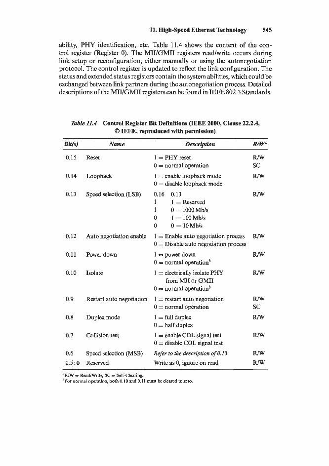
11. High-speed Ethernet Technology 545
ability, PHY identification, etc. Table 11.4 shows the content of the con- trol register (Register 0). The MII/GMII registers read/write occurs during link setup or reconfiguration, either manually or using the autonegotiation protocol. The control register is updated to reflect the link configuration. The status and extended status registers contain the system abilities, which could be exchanged between link partners during the autonegotiation process. Detailed descriptions of the MIUGMII registers can be found in IEEE 802.3 Standards.
Table 11.4 Control Register Bit Definitions (IEEE 2000, Clause 22.2.4, 0 IEEE, reproduced with permission)
Bit(s) Name Description ma 0.15
0.14
0.13
0.12
0.11
0.10
0.9
0.8
0.7
0.6
0.5 : 0
Reset
Loopback
Speed selection (LSB)
Auto negotiation enable
Power down
Isolate
Restart auto negotiation
Duplex mode
Collision test
Speed selection (MSB) Reserved
1 = PHY reset 0 = normal operation
1 = enable loopback mode 0 = disable loopback mode
0.16 0.13 1 1 =Reserved 1 0 = lOOOMb/s 0 1 = 100Mb/s 0 0 = 10Mb/s
1 = Enable auto negotiation process 0 = Disable auto negotiation process
1 = power down O = normal operationb
1 = electrically isolate PHY from MI1 or GMII
O = normal operationb
1 = restart auto negotiation 0 = normal operation
1 = full duplex 0 = half duplex
1 = enable COL signal test 0 = disable COL signal test
Refer to the description of 0.13
Write as 0, ignore on read
R/w sc RIW
R/w
R/w
RIW
RIW
R/w sc RIW
RIW
RIW RIW
"WW = ReaWrite, SC = Self-Clearing. *For normal operation, both 0.10 and 0.1 1 must be cleared to zero.
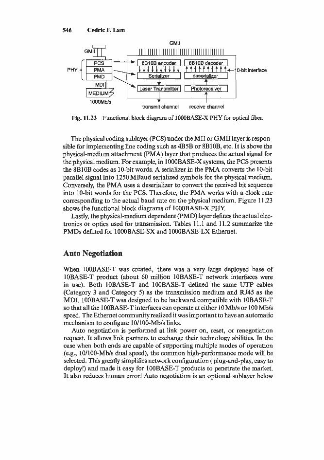
546 Cedric F. Lam
& ? * & I Laser Transmitter Photoreceiver - 1000Mb/s
transmit channel receive channel
Fig. 11.23 Functional block diagram of 1000BASE-X PHY for optical fiber.
The physical coding sublayer (PCS) under the MI1 or GMII layer is respon- sible for implementing line coding such as 4B5B or 8B10B, etc. It is above the physical-medium attachment (PMA) layer that produces the actual signal for the physical medium. For example, in 1000BASE-X systems, the PCS presents the 8BlOB codes as 10-bit words. A serializer in the PMA converts the 10-bit parallel signal into 1250 MBaud serialized symbols for the physical medium. Conversely, the PMA uses a deserializer to convert the received bit sequence into 10-bit words for the PCS. Therefore, the PMA works with a clock rate corresponding to the actual baud rate on the physical medium. Figure 1 1.23 shows the functional block diagrams of 1000BASE-X PHY
Lastly, the physical-medium dependent (PMD) layer defines the actual elec- tronics or optics used for transmission. Tables 11.1 and 11.2 summarize the PMDs defined for 1000BASE-SX and 1000BASE-LX Ethernet.
Auto Negotiation
When 100BASE-T was created, there was a very large deployed base of 10BASE-T product (about 60 million IOBASE-T network interfaces were in use). Both IOBASE-T and 100BASE-T defined the same UTP cables (Category 3 and Category 5) as the transmission medium and RJ45 as the MDI. 100BASE-T was designed to be backward compatible with IOBASE-T so that all the 100BASE-T interfaces can operate at either 10 Mb/s or 100 Mb/s speed. The Ethernet community realized it was important to have an automatic mechanism to configure 10/100-Mb/s links.
Auto negotiation is performed at link power on, reset, or renegotiation request. It allows link partners to exchange their technology abilities. In the case when both ends are capable of supporting multiple modes of operation (e.g., 10/100-Mb/s dual speed), the common high-performance mode will be selected. This greatly simplifies network configuration ( plug-and-play, easy to deploy!) and made it easy for 100BASE-T products to penetrate the market. It also reduces human error! Auto negotiation is an optional sublayer below
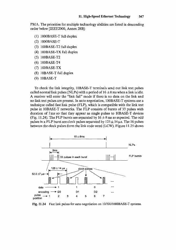
11. High-speed Ethernet Technology 547
... 33 pulses in each burst
PMA. The priorities for multiple technology abilities are listed in descending order below [IEEE2000, Annex 28Bl:
FLP bursts ...
(1) 1000BASE-T full duplex
(3) 1 OOBASE-T2 full duplex (4) 100BASE-TX full duplex
(2) 1000BASE-T
(5) 100BASE-T2 (6) 100BASE-T4 (7) 100BASE-TX (8) 10BASE-T full duplex (9) 10BASE-T
To check the link integrity, IOBASE-T terminals send out link test pulses called normal link pulses (NLPs) with a period of 16 f 8 ms when a link is idle. A receiver will enter the “link fail” mode if there is no data on the link and no link test pulses are present. In auto negotiation, 100BASE-T systems use a technique called fast link pulse (FLP), which is compatible with the link test pulse in IOBASE-T networks. The FLP consists of bursts of 33 pulses with duration of 2ms so that they appear as single pulses to IOBASE-T devices (Fig. 1 1.24). The FLP bursts are separated by 16 f 8 ms as expected. The odd pulses in a FLP burst are clock pulses separated by 125 f 14 ps. The 16 pulses between the clock pulses form the link code word (LCW). Figure 11.25 shows
k 16 f 8rns 4 I I NLPs
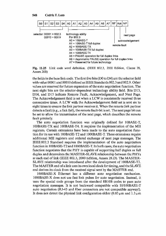
548 Cedric F. Lam
selector: 00001 = 802.3 technology ability 00010 = 802.9 For 802.3:
A0 = IOBASE-T
I SO I S I I S2 1 S3 I S4 I A0 I AI I A2 I A3 I A4 I A5 I A6 I A7 1 RF IAckI NP
I nextpage
acknowledgement

11. High-speed Ethernet Technology 549
optics are not compatible, misconnecting one technology to another will cause a link fail!). The auto negotiation function in 1000BASE-X basi- cally exchanges information such as half/full-duplex modes and flow-control capabilities between the two link partners.
Beyond Gigabit: Continuing Development of Ethernet
10-Gbh ETHERNET
At the time of this writing, lO-Gb/s Ethernet is still being worked on by the IEEE 802.3ae Standards group DEEE20011. The actual standard will not be finished until 2002. For the time being, lO-Gb/s Ethernet will be deployed mainly as backbone connections for high-performance server applications.
lO-Gb/s Ethernet will preserve the 802.3 Ethernet MAC frame format. There will be no CSMA/CD mechanism defined for 10-Gb/s Ethernet. Since only full-duplex mode will be supported, carrier extension and frame bursting will not be applicable to lO-Gb/s Ethernet.
Figure 11.26 shows the lO-Gb/s Ethernet architecture [IEEE2001]. It is not an easy task to design a PHY working at 10 Gb/s. To reduce the bandwidth requirement for the MAC circuits, the XGMII in Fig. 11.26 uses a 4-octet (32-bit) wide data path. The medium for 10-Gb/s Ethernet will be optical fiber. The goal of 10-Gb/s Ethernet is to increase the speed of Gigabit Eth- ernet by 10 times without increasing the price by 10 times. There are three flavors of 10-Gb/s Ethernet: the 10GBASE-W WAN interface, IOGBASE-R LAN interface using 64B66B encoding, and 10GBASE-X LAN interface using 8B10B encoding.
Higher Layers
Reference
IOGBASE-W IOGBASE-R IOGBASE-X
Fig. 11.26 IO-Gb/s Ethernet Architecture.
550 Cedric E Lam
In order to meet the cost requirement, there will be separate LAN PHYs and WAN PHYs. LAN PHYs will handle data in the native Ethernet format and will likely use low-cost optics. WAN PHYs will take advantage of the existing SONET deployment for WANs. Current SONET-OC192 systems are running at 9.953 Gb/s A WAN interface sublayer (WIS) will be added in the WAN PHYs for encapsulating 10-Gb/s Ethernet data into SONET/SDH compatible formats so that they can be transported across SONET/SDH networks.
Moreover, parallel technologies such as VCSEL arrays with parallel fiber ribbons or wide WDM (WWDM) could be used to carry lO-Gb/s Ethernet data. Agilent has developed a technology to carry lO-Gb/s Ethernet on 4 parallel wavelengths separated by 25 nm in the 1.3 pm wavelength window [LEM02000]. The 10GBASE-LX4 PHY specifies four lanes (Le. four parallel data paths) LO to L3 with wavelengths LO: 1269.0-1282.4nm, L1: 1293.5- 1306.9nm, L2: 1318.&1331.4nmY and L3: 1342.5-1355.9nm in the draft standard [IEEE2001]. Currently, the Optical Internetworking Forum (OIF) is also working on low-cost solutions for short distance interconnections. These efforts could influence the development of 10-Gb/s Ethernet PHY
10-Gb/s Ethernet will support both multimode fiber (MMF) and single mode fiber (SMF). Single mode fiber and 1.5 pm lasers will be used for con- nections up to 40 km. 1.5 pm optics have been used in long haul DWDM applications. The fiber loss is smaller at 1.5 pm than at 0.85 pm and 1.3 pm. 1.5 pm also corresponds to the wavelength range where optical amplification technology is mature and readily available [GREE1993].
A new coding scheme, 64B66B, has been developed for IO-Gb/s Ethernet. The 8B10B code used for Gigabit Ethernet has an extra overhead of 25%. This will increase the transmission speed of a lO-Gb/s channel to 12.5 Gbaud. With the 64B66B encoding, the actual channel speed will be 10.3125 Gbaud, making it easier to leverage on the existing 10 Gb/s optoelectronic technolo- giesg developed for OC-192 speed SONET/SDH systems. In fact, the 8B10B codes will continue to be used in 10GBASE-LX4. Each lane will be running at 3.125 Gbaud after 8B10B encoding.
lO-Gb/s Ethernet Standard also defined an optional XGMII Extender as shown in Fig. 1 1.27. As its name implies, the XGMII Extender is used to extend the operational distance of the XGMII. It consists of an RS end XGXS, a XAUI and a PHY end XGXS. The chip-to-chip reach that XGMII provides is approximately 7 cm on a circuit board. The XGMII Extender allows distances up to roughly 50 cm.
The XGMII Extender also reduces the number of interface signals (Fig. 11.28). XGMII uses four lanes to pass data and control in each direc- tion. Each lane consists of a one-octet wide data path and a control signal.
At the moment, 10-Gb/s transmission systems are still the state-of-the-art technology. Pushing the (raw) bit rate from 10Gb/s to 12.5 Gb/s still requires a lot of effort.
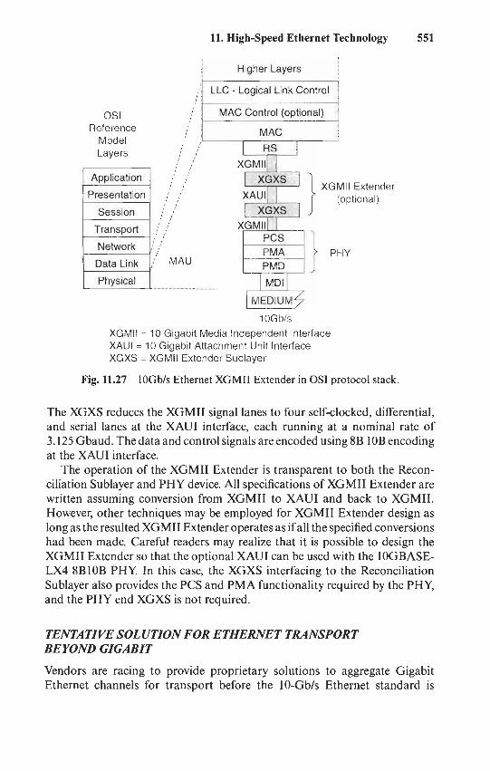
11. High-speed Ethernet Technology 551
! Higher Layers
Reference Model Layers
XGMll
PHY PMD
X’ MEDIUM
10GbIs XGMll = 10 Gigabit Media Independent Interface XAUI = 10 Gigabit Attachment Unit Interface XGXS = XGMll Extender Sublayer
Fig. 11.27 10Gb/s Ethernet XGMII Extender in OS1 protocol stack.
The XGXS reduces the XGMII signal lanes to four self-clocked, differential, and serial lanes at the XAUI interface, each running at a nominal rate of 3.125 Gbaud. The data and control signals are encoded using 8B 10B encoding at the XAUI interface.
The operation of the XGMII Extender is transparent to both the Recon- ciliation Sublayer and PHY device. All specifications of XGMII Extender are written assuming conversion from XGMII to XAUI and back to XGMII. However, other techniques may be employed for XGMII Extender design as long as the resulted XGMII Extender operates as if all the specified conversions had been made. Careful readers may realize that it is possible to design the XGMII Extender so that the optional XAUI can be used with the 10GBASE- LX4 8B10B PHY In this case, the XGXS interfacing to the Reconciliation Sublayer also provides the PCS and PMA functionality required by the PHY, and the PHY end XGXS is not required.
TENTATIVE SOLUTION FOR ETHERNET TRANSPORT BEYOND GIGABIT
Vendors are racing to provide proprietary solutions to aggregate Gigabit Ethernet channels for transport before the lO-Gb/s Ethernet standard is

552 Cedric F. Lam
Fig. 11.28 XGXS inputs and outputs.
completed. Gigachannel is such an example. It was a research project con- ducted at Lucent Technologies in late 1990. It is an electronic multiplexer for Gigabit Ethernet. The Gigachannel takes eight Gigabit Ethernet inputs and electronically multiplexes them into a single channel for transmission [WOOD2000]. The data streams from individual inputs are bit interleaved at the multiplexer and deinterleaved into individual channels at the receiving end. Elastic buffers and inter-frame gaps (IFG) are used to adjust for the clock differences in the input data streams. There are two fundamental differences between Gigachannel and 10-Gb/s Ethernet. First, the actual data throughput in the optical link speed is only 8 Gb/s. Second, the individual port speed is still 1 Gb/s per port on each end of the link. Lucent also tested Gigachannel on a 16-wavelength WaveStarTM DWDM system [WOOD2000a].
Application of High-speed Ethernet
UPGRADE EXISTING LOCAL AREA NETWORKS
10/100-Mb/s Ethernet are mainly used for desktop connections. In fact, lO-Mb/s connection was an overdesign at the time it was invented. The original idea of Ethernet was a high-performance communication channel achieved by fast exchange of short bursts of data with low latency. Even by

11. High-speed Ethernet Technology 553
100BASE-7 Q Server 1 - 1 7 -
Ethernet/ FDDl bridge
100BASE-T Links Switch
to FDDl campus
backbone
IOBASE-T
P’ L-\,-J \-’ i
Department A Department B Department C
Fig. 11.29 Common view of a LAN in a mid-size campus.
today’s standard, 1 OBASE-T (especially in full-duplex mode) provides a lot of bandwidth. It is more than 170 times faster than 56k dial-up modems. A MPEG3 video stream requires about 4 Mb/s bandwidth. For ordinary desktop applications, 10BASE-T will exist for a while.
A hierarchical structure is required to build scalable networks. A com- mon scenario is to use 100BASE-T to interconnect departments with multiple 10BASE-T stations and as server connections, as shown in Fig. 11.29. A nat- ural use of high-speed Ethernet is to upgrade existing networks. For example, the connections to individual desktops will be upgraded from 10BASE-T to 100BASE-T. Furthermore, as new network applications proliferate, and as the number of network users and individual user’s bandwidth increases, the server capacity and server bandwidths will need to be upgraded in order to meet the demand. One way of providing more server capacity is to install multiple servers on the existing network so that the server load can be distributed. However, most of the time, communication bandwidth is the bot- tleneck in a clientherver environment. We have seen that Gigabit Ethernet has been adopted for server applications. Figure 1 1.30 shows a possible upgrade scenario for the network shown in Fig. 1 1.29.
BACKBONE UPGRADE
LANs are usually interconnected with a campus backbone, which is in turn connected to the WAN backbone. Figure 11.28 shows a LAN connected to
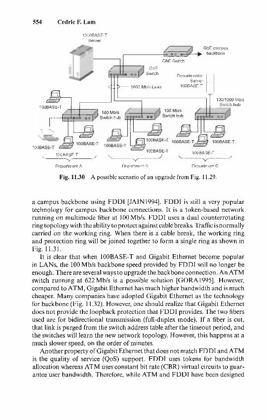
554 Cedric F. Lam
1000BASE-T Server
GbE Switch
Department A Department B Department C
Fig. 11.30 A possible scenario of an upgrade from Fig. 11.29.
a campus backbone using FDDI [JAIN1994]. FDDI is still a very popular technology for campus backbone connections. It is a token-based network running on multimode fiber at 100 Mb/s. FDDI uses a dual counterrotating ring topology with the ability to protect against cable breaks. Traffic is normally carried on the working ring. When there is a cable break, the working ring and protection ring will be joined together to form a single ring as shown in Fig. 11.31.
It is clear that when 100BASE-T and Gigabit Ethernet become popular in LANs, the 100 Mb/s backbone speed provided by FDDI will no longer be enough. There are several ways to upgrade the backbone connection. An ATM switch running at 622Mb/s is a possible solution [GORA1995]. However, compared to ATM, Gigabit Ethernet has much higher bandwidth and is much cheaper. Many companies have adopted Gigabit Ethernet as the technology for backbone (Fig. 11.32). However, one should realize that Gigabit Ethernet does not provide the loopback protection that FDDI provides. The two fibers used are for bidirectional transmission (full-duplex mode). If a fiber is cut, that link is purged from the switch address table after the timeout period, and the switches will learn the new network topology. However, this happens at a much slower speed, on the order of minutes.
Another property of Gigabit Ethernet that does not match FDDI and ATM is the quality of service (QoS) support. FDDI uses tokens for bandwidth allocation whereas ATM uses constant bit rate (CBR) virtual circuits to guar- antee user bandwidth. Therefore, while ATM and FDDI have been designed
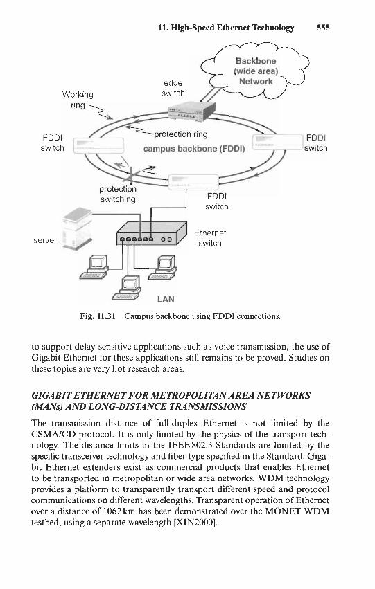
11. High-speed Ethernet Technology 555
Backbone (wide area)
edge Network 7 Wnrkinn switch
FDDl %protection ring FDDl
Ethernet switch server
LAN pJ
Fig. 11.31 Campus backbone using FDDI connections.
to support delay-sensitive applications such as voice transmission, the use of Gigabit Ethernet for these applications still remains to be proved. Studies on these topics are very hot research areas.
GIGABIT ETHERNET FOR METROPOLITAN AREA NETWORKS (MANS) AND LONG-DISTANCE TMNSMISSIONS
The transmission distance of full-duplex Ethernet is not limited by the CSMNCD protocol. It is only limited by the physics of the transport tech- nology. The distance limits in the IEEE802.3 Standards are limited by the specific transceiver technology and fiber type specified in the Standard. Giga- bit Ethernet extenders exist as commercial products that enables Ethernet to be transported in metropolitan or wide area networks. WDM technology provides a platform to transparently transport different speed and protocol communications on different wavelengths. Transparent operation of Ethernet over a distance of 1062 km has been demonstrated over the MONET WDM testbed, using a separate wavelength [XIN2000].
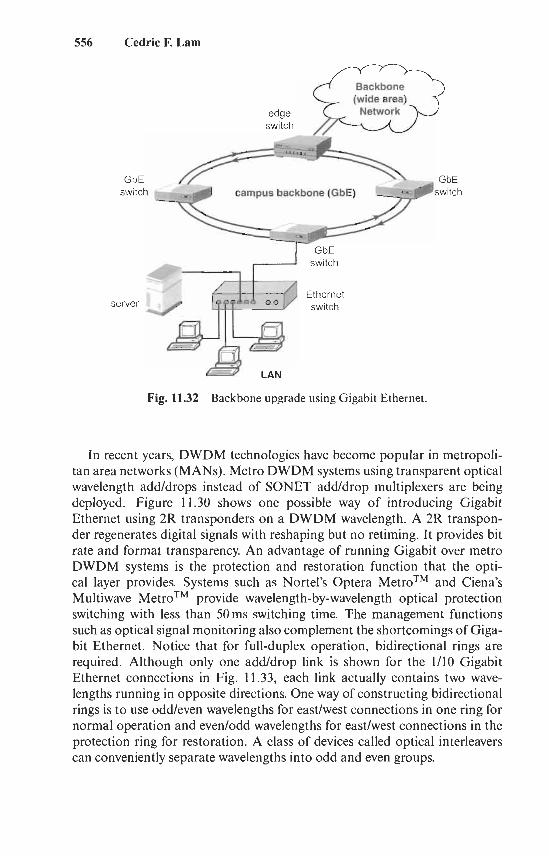
556 Cedric E Lam
campus backbone (GbE)
Fig. 11.32 Backbone upgrade using Gigabit Ethernet.
In recent years, DWDM technologies have become popular in metropoli- tan area networks (MANS). Metro DWDM systems using transparent optical wavelength add/drops instead of SONET addldrop multiplexers are being deployed. Figure 11.30 shows one possible way of introducing Gigabit Ethernet using 2R transponders on a DWDM wavelength. A 2R transpon- der regenerates digital signals with reshaping but no retiming. It provides bit rate and format transparency. An advantage of running Gigabit over metro DWDM systems is the protection and restoration function that the opti- cal layer provides. Systems such as Nortel’s Optera MetroTM and Ciena’s Multiwave MetroTM provide wavelength-by-wavelength optical protection switching with less than 50 ms switching time. The management functions such as optical signal monitoring also complement the shortcomings of Giga- bit Ethernet. Notice that for full-duplex operation, bidirectional rings are required. Although only one add/drop link is shown for the 1/10 Gigabit Ethernet connections in Fig. 11.33, each link actually contains two wave- lengths running in opposite directions. One way of constructing bidirectional rings is to use odd/even wavelengths for east/west connections in one ring for normal operation and even/odd wavelengths for east/west connections in the protection ring for restoration. A class of devices called optical interleavers can conveniently separate wavelengths into odd and even groups.
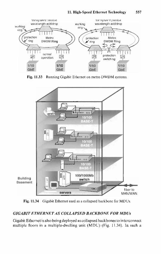
11. High-speed Ethernet Technology 557
transparent passive transparent passive wavelength addldrop working wavelength addldrop
Fig. 11.33 Running Gigabit Ethernet on metro DWDM systems.
Building Basement
I
Fig. 11.34 Gigabit Ethernet used as a collapsed backbone for MDUs.
GIGABIT ETHERNET AS COLLAPSED BACKBONE FOR MDUs
Gigabit Ethernet is also being deployed as collapsed backbones to interconnect multiple floors in a multiple-dwelling unit (MDU) (Fig. 11.34). In such a

558 Cedric E Lam
configuration, each floor of the MDU is served by a 10/100-Mb/s LAN that is connected to a 100/1000-Mb/s switch hub in the building basement. In most of today’s MDUs, the connections from each level to the Gigabit Ethernet switch in the basement is usually achieved using multimode fibers The basement provides a convenient location where servers and the backbone 100/1000-Mb/s Ethernet switch are colocated and easily managed. In the case of FDDI campus backbone, the switches are distributed around the ring, which makes services more dficult. Gigabit Ethernet also provides more bandwidth than FDDI and ATM switches.
l/lO-Gb/s Ethernet: A Disruptive Technology?
The Ethernet community has adopted the price and performance model of the PC industry. Although there existed a 1-Mb/s version Ethernet specifica- tion, Ethernet was first widely deployed in the lO-Mb/s version. For each new generation, the speed of Ethernet is improved by 10-fold with a targeted price increase of only three to four times.
Traditionally, the high-bandwidth and long-distance backbone connections have been served using the SONET technology [BLAC1997]. The removal of the CSMNCD protocol in high-speed Ethernet has enabled Ethernet to go long distance. Gigabit products are now widely available at much more &or- dable prices than SONET and ATM products with comparable performance. Conventional SONET equipment has a very rigid time-division multiplex- ing (TDM) hierarchy. To compete with Ethernet, next-generation SONET boxes will implement TDM with statistical multiplexing to gain efficiency and lightweight SONET functions to make them much more cost-effective.
Nonetheless, the world of telecommunications is moving into packet switching, and Ethernet frames are really the dominating format in data communications SONET and ATM equipment being designed for circuit switching does not provide an efficient platform for carrying the ubiquitous Ethernet traffic. The goal of lO-Gb/s Ethernet is to eventually enable native Ethernet frames to be carried over metro and long-distance networks, without using SONET for transport. We already see aggressive new operators such as Yipes, Sigma Networks, Teleson, etc., selling Gigabit Ethernet services as metro services to Internet service providers (ISPs) and enterprise users. These operators are leveraging on the existence of dark fibers from fiber infrastructure overbuilds.
However, l/lO-Gb/s Ethernets still do not provide the fast protection and restoration capability that SONET provides. IEEE has recently formed the 802.17 Workgroup on resilient packet rings to address this issue. Pro- tection and restoration can be provided by higher layers such as IP, and has been demonstrated and actively researched [HJAL2000, SONG2000, SONG2000al. Current Ethernet does not support quality of service (QoS).

11. High-speed Ethernet Technology 559
But IETF (Internet Engineering Task Force) has been working on these issues. Ethernet also lacks the rich SONET administration and management func- tions such as performance monitoring, remote provisioning, alarm collection, and fault location, etc. These properties have been demanded by traditional incumbent carriers. These carriers understand SONET better than Ethernet. However, ISPs corning from a data communication background usually do not demand the level of reliability that incumbent carriers do. Cost-effectiveness has always been a primary concern in data communications. There are also more people in the data communication world who understand Ethernet but do not understand SONET. Whether Ethernet will eventually become a dis- ruptive technology displacing SONET will be proven by time. A failure in a backbone connection carrying huge amounts of data is a serious consequence. High-speed 1/10-Gigabit Ethernet must address the reliability issue before it will become truly ubiquitous in both LANs and WANs.
Useful Web Sites
0 IEEE 802 LAN/MAN Standard Committee, http://www.ieee802.orgl 0 Search for IEEE Standards,
0 IEEE 802.3 CSMA/CD (ETHERNET) http://www.ieee802.org/3/ 0 IEEE P802.3ae lO-Gb/s Ethernet Task Force, http://grouper.ieee.orgl
0 Gigabit Ethernet Alliance, http://www.gigabit-ethernet.org/ 0 1 0-Gigabit Ethernet Alliance, http://www. 10gea.orglindex.htm 0 Online tutorial of Ethernet, http://wwwhost.ots.utexas.edu/ethemet/
0 Optical Internetworking Forum, http://www.oiforum.com
http://ieeexplore.ieee. orgApdocs/epic03/standards.htm
groups/802/3/ae/index. html
ethernet-home.html
Acronyms
AS ATM AUI BGP CRC CSMNCD DA DHCP EGP EIA
Autonomous system Asynchronous Transfer Mode Attachment unit interface Border Gateway Protocol Cyclic redundancy check Carrier sense multiple access with collision detection Destination address Dynamic Host Codiguration Protocol Exterior Gateway Protocol Electronic Industries Association

560 Cedric F. Lam
FCS FDDI FLP GMII IEEE IETF IFG IGP IP IPv4 IS-IS IS0 ISP LAN LCW LED LLC LSB MAC MAN MAU MDI MDU MI1 MMF MONET MPEG MPLS MSB NIC NLP OIF os1 OSPF PAM PCS PHY PLL PLS PMA PMD PSTN
RS QOS
Frame check sequence Fiber distribution digital interconnect Fast link pulse Gigabit medium independent interface Institute of Electronics and Electrical Engineering Internet Engineering Task Force Inter-frame gap Interior Gateway Protocol Internet Protocol Internet Protocol version 4 Intermediate system-intermediate system International standard organization Internet service provider Local area network Link code word Light emitting diode Logical link control Least significant bit Medium access control Metropolitan area network Medium attachment unit Medium dependent interface Multiple dwelling unit Medium independent interface Multimode fiber Multiwavelength optical network Moving picture experts group Multiprotocol label switching Most significant bit Network interface card Normal link pulse Optical Internetworking Forum Open system interconnection Open shortest path first Pulse amplitude modulation Physical coding sublayer PHYsical Layer Device Phase locked loop Physical layer signaling Physical medium attachment Physical medium dependent Public switched telephone network Quality of service Reconciliation sublayer
11. High-speed Ethernet Technology 561
RSVP SA SDH SFD SMF SNMP SONET TCP TDM UTP VPN WAN WDM WIS www
References
[BLAC1997]
[CARO2000]
PAm2000]
[EL419911
VIA1 99 1 a]
[FCA1994]
[GORA1995]
[GREEl993]
[HJAL2000]
[HUI 19991
[IEEE1993]
Resource Reservation Protocol Source address Synchronous digital hierarchy Start frame delimiter Single-mode fiber Simple Network Management Protocol Synchronous optical network Transport Control Protocol Time-division multiplexing Unshielded twisted pair Virtual private network Wide area network Wavelength-division multiplexing Wan interface sublayer World Wide Web
Black, U. and S. Waters, SONET & TI: Architectures for Digital Transport Networks, Prentice-Hall, New Jersey, 1997. Caro, R. H., “Ethernet Wins Over Industrial Automation,” IEEE Spectrum, January 2000, p. 114. Davie, B. S. and Y. Rekhter, MPLS: Technologv and Applications, Morgan Kaufmann Publishers, California, 2000. EWTIA Standard 568, Commercial Building Telecommunications Mring Standard, July 199 1. EWTIA Bulletin TSB-36, Additional Cable Specifications for Unshielded Pair Cables, November 1991. Fibre Channel Association, Fibre Channel: Connection to the Future, 1994. Goralski, W. J., Introduction to ATM Networking, McGraw-Hill, New York, 1995. Green, I? E., Jr., Fiber Optic Networks, Prentice-Hall, New Jersey, 1993. Hjalmtysson, G., P. Sebos, G. Smith, and J. Yates, “Simple IP Resto- ration for IP/GbE/lOGbE Optical Networks,” OFC 2000 Technical Digest, vol. 4, pp. 275-277,2000. Hui, J., Switching and Traffi. Theoly for Integrated BroadbandNetworks, Kluwer Academic Press, Massachusetts, 1990. IEEE Standard 802.1, Information technology-telecommunications and information exchange between systems-Local area networks Media access control (MAC) bridges, 1993.

[IEEE2000]
vEEE200 11 [JAIN1994] F(ADA19981
[KAPL2001]
[KESH1997]
[KUMA1996]
[LEM02000]
[MCKE1997]
[METC1976]
[METC1977]
[MOLL19971
[MOLL1997a]
[RAMA1994]
[SEIF1998] [SONG20001
[SONG2000a]
[TANE 19961
562 Cedric F. Lam
I
New Jersey, 1996.
IEEE Standard 802.3, Carrier sense multiple access with collision detec- tion (CSMMCD) access method and physical layer speciJications, 2000 Edition. IEEE Draft P802.3ae/D3.2, August, 2001. Jain, R., FDDI Handbook, Addison-Wesley, Massachusetts, 1994. Kadambi, J., I. Crayford, and M. Kalkunte, Gigabit Ethernet: Migrat- ing to High-Bandwidth LANs, Prentice Hall, New Jersey, 1998. Kaplan, G., “Ethernet’s Winning Ways,” IEEE Spectrum, January
Keshav, S., An Engineering Approach to Computer Networking: ATM Networks, the Internet, and the Telephone Network, Addison-Wesley, Massachusetts, 1997. Kumar, B., Broadband Communications, McGraw-Hill, New York, 1996. Lemoff, B. E., “Technology Alternatives for 10-Gbit/s LANs,” OFC 2000, Tutorial WI1-1, Baltimore, 2000. McKeown, N., et al., “The Tiny Tera: A Packet Switch Core,” IEEE Micro, vol. 17, no. 1, pp. 26-33, 1997. Metcalfe, R. M. and D. R. Boggs, “Ethernet: Distributed Packet Switching for Local Computer Networks,” Communications of the ACMvol. 19, no. 7, July 1976, pp. 395-404. Metcalfe, R. M., D. R. Boggs, C. P. Thacker, and B. W. Lampson, Multipoint data communication system with collision detection, U.S. Patent 4,063,220, assigned to Xerox Corporation. Molle, M., M. Kalkunte, and J. Kadambi, “Frame Bursting: A Technique for Scaling CSMNCD to Gigabit Speeds,” IEEE Network, July/August 1997, pp. 6-15. Molle, M., M. Kalkunte, and J. Kadambi, “Scaling CSMNCD to 1Gb/s with Frame Bursting,” Proceedings of 22nd Local Computer Networks, pp. 211-219,1997. Ramakrishnan, K. K. and H. Yang, “The Ethernet Capture Effect: Analysis and Solution,” 19th IEEE Local Computer Networks Confer- ence, Minneapolis, MN, October 1994, pp. 228-240. Seifert, R., Gigabit Ethernet, Addison-Wesley, Massachusetts, 1998. Song, S., J. Huang, l? Kappler, R. Freimark, J. Gustin, and T. Kozlik, “Fault Tolerant Ethernet for IP-based Process Control: A Demonstration,” Proceedings of 2000 IEEE International Conference on Dependable Systems and Networks, pp. 361-366,2000. Song, S., J. Huang, P. Kappler, R. Freimark, and T. Kozlik, “Fault- Tolerant Ethernet Middleware for IP-base Process Control Networks,” Proceedings of 25th IEEE Annual Conference on Local Computer Networks, pp. 116-125,2000. Tanenbaum, A. S., Computer Networks, Third Edition, Prentice-Hall,
2000, pp. 113-115.

11. High-speed Ethernet Technology 563
pOLL2000]
[WHIT20001
[WIDM1983]
[WOOD20001
Tolley, B., “Moving the Decimal Point: 10-Gigabit Ethernet Appli- cations and Market Opportunity,” Proceedings of IEEE LEOS 13th Annual Meeting: Puerto Rico, paper TuT1, vol. 1, November 2000,
Whitlock, B. K., “Modeling and Simulation Issues with 10-Gigabit Ethernet,” Proceedings of IEEE LEOS 13th Annual Meeting, Puerto Rico, paper TuBB3, vol. 1, November 2000, pp. 352-353. Widmer, A. X. and F! A. Franaszek, “A DC-Balanced, Partitioned- Block, 8B/10B Transmission Code,” IBMJ. Res. Develop, vol. 27, no. 5, September 1983, pp. 440-451. Woodward, T. K., A. L. Lentine, J. D. Fields, G. Giaretta, and R. Limacher, “A System for Native Ethernet Optical Transport at IOGbls,” OFC 2000 Technical Digest, vol. 2, pp. 154-156, Baltimore, 2000.
pp. 288-289.
[WOOD2000a] Woodward, T. K., A. L. Lentine, J. D. Fields, G. H. Smith, D. Baner- jee, M. C. Nuss, R. Limacher, G. Giaretta, and M. Chou, “lOGb/s Native Ethernet Transport Over Campus, MAN, and WAN distances,” Proceedings of IEEE LEOS 13th Annual Meeting, Puerto Rico, vol. 1, November 2000, pp. 350-351. Xin, W., G. K. Chang, and T. T. Gibbons, “Transport of Gigabit Ethernet Directly Over WDM for 1062 km in the MONET Washing- ton D.C. network:” 2000 Digest of IEEE LEOS Summer TopicalMeeting on Broadband Optical Networh, Aventura, FL, July 2000, pp. 9-10. Zhang, L., S. Deering, D. Estrin, S. Shenker, and D. Zappala, “RSVP: A New Resource Reservation Protocol,” IEEE Network, vol. 7, no. 5, September 1993, pp. 8-18.
pIN20001
[ZHAN1993]
Chapter 12
Arthur J. Lowery vplsystem, Design Center Group, Melbourne, Australia
Photonic Simulation Tools
Abstract
Simulation of photonic systems has become a necessity due to the complex interactions within and between components, and the need for rapid design cycles using the latest technologies to meet the growth in bandwidth demand while utilizing legacy plant. Tools have evolved from in-house code, developed for a single purpose, to commercial simulation environments that cover almost all simulation tasks and provide additional functionality to speed the design process, such as the ability to automate the design process and to capture expert knowledge.
The move to an electronic design environment, from laboratory prototypes, provides many advantages that are not immediately obvious. The simulator and its libraries becomes a standard design platform, so that individuals, teams, and companies can communicate their designs electronically. This can speed interactions. It also ensures that information is passed in a standard format (the parameters of the models), and is essential for design reuse: Part of an existing design can be pasted into a simulation far more easily than part of a laboratory prototype.
This chapter introduces the key elements of photonic simulation tools for designing the photonic physical layer. First, the evolution of photonic simula- tion tools over the last few years is traced. This history introduces Graphical User Interfaces (GUIs), how photonic signals are represented in a photonic environment, and how a common language is useful for data exchange between customer and vendor. The ingredients of a photonic simulator are then dis- cussed, including considerations when developing a component model; the abstraction level of a model; and a study of how to simulate the key elements in a photonic system, from transmitter to bit error ratio (BER) estimator. Fea- tures that enhance design productivity are then reviewed, including hierarchy, automatic sweeps of parameters, models and topologies, parameterization and optimization, and automated synthesis from network-level specifications. To illustrate automated synthesis, the design process of a 24-channel 40-Gbith per channel wavelength-division multiplexed (WDM) system is examined, including verification of power budget, optical signal-to-noise ratio (OSNR), linear and nonlinear impairments, and polarization-mode dispersion VMD)
564 OPTICAL FIBER TELECOMMUNICATIONS, VOLUME IVB
W g h t 0 2002, Elsevier science (USA). AU rightp of reproduction in any form reserved.
ISBN 0-12-395173-9
12. Photonic Simulation Tools 565
compensation. Finally, the application of simulation to analog photonic system design is touched upon.
I. Introduction
As is obvious from the scope of this book, designing high-capacity photonic networks is not a trivial task. The performance of each component must be considered, which in itself requires a broad understanding of many technolo- gies, and the interactions of the many components forming a link or an optical network must be understood. As the previous chapters have shown, compo- nent interactions are complex, and can be highly nonlinear in nature. For this reason alone, computer simulation has become an essential part of the design process of optical fiber systems.
There have been many papers written on the use of computer simulations to design specific photonic systems or to investigate particular phenomena in systems. Computer simulations are used particularly when analytical solu- tions are difficult or impossible to formulate without excessive approximation (Duff 1984), for example, when modeling the interaction of the dynamics of lasers with fibers (Koch and Corvini 1988; Stephens 1994, 1995; Lowery 1997a), when studying statistical noise in complex systems (Djupsjobacka 1984; Jacobsen 1998), when optimizing modulation format for long-haul transmission (Caspar 1999), when investigating dispersion and its compen- sation (Elrefaie 1988a; Caspar 2000), exploring nonlinear effects in fibers (Gnauck 1993; Tkach 1995; Hui 1997), when comparing fiber types (e.g., Breuer 1998), and in understanding the impact of PMD (Elbers 1997) and forward error correction (Ho and Lin 2000).
However, there are other benefits of using computers in the design pro- cess that are not immediately obvious. These include the ability to capture the physics of components’ behavior in numerical models in such a way that the effects of interactions of components can be predicted, for almost any topol- ogy. Simulation also imposes a standardization of language onto the industry: Parameter names, data file formats, definitions, and units have been standard- ized. Moreover, simulations require all details of a device to be specified, this enforces precision and prevents omission of important characteristics.
Simulation also allows knowledge to be leveraged-designs captured in a simulator can be reused, copied, distributed, discussed, and modified elec- tronically. But more powerfully, simulators can leverage expert knowledge by synthesizing designs given basic specifications, this means that standard design rules can be applied consistently and automatically to meet diverse customer requirements by teams who need not themselves be experts in systems design. This is important because the number of engineers with long experience in photonics is fixed in an industry that is growing rapidly and avoids standard designs in order to extract maximum capacity from networks.
566 Arthur J. Lowery
A. SCOPE OF THIS CHAPTER
It is essential to start any review with an apology, as a short chapter cannot hope to include references to the thousands of people that have contributed to the development of simulation tools, both in-house and commercial. Further- more, this review cannot include details of the physical understanding and numerical techniques that are the core of a simulator. As proof, the manu- als for a commercial simulator may run into several thousand pages covering hundreds of individual modules and hundreds of application examples. For- tunately, some of these techniques are detailed in this book, and others have been summarized in focused texts on particular devices.
Simulation tools are used for many layers of telecommunications network design, from demand forecasting, service provisioning, and transport net- work optimization, through equipment, component and device design, to the details of band-engineering and material design. In line with this book, this work concentrates on the simulation of photonic systems and components from an electrical-engineering perspective (the “physical layer”). Readers are referred to books on network design and planning and on integrated optics for information on other tools.
This chapter introduces the subject of systems and component simulation. Section I1 describes the development of photonic simulation platforms, and introduces their technological features that are required to support efficient photonic simulation on a platform. Section I11 highlights the need for mul- tiple levels of abstraction when describing photonic components, and then covers the challenges when modeling key photonic components. Section IV introduces features of photonic simulation platforms that considerably speed the design process, including optimization, parameterization, and automated synthesis and analysis. A 960-Gbith long-haul system using 4O-Gbit/s chan- nels is used to illustrate the synthesis and analysis process. The simulation of analog fiber systems is discussed briefly in Section V. Finally, conclusions are drawn from the chapter.
11. Evolution of Photonic Simulation Tools
Figure 12.1 illustrates the numerous technical challenges of optical systems design arranged on a chart with three axes: optical bandwidth, capacity per channel, and channel density. The volume contained within the axes is the capacity of the transmission system in Gbit/s. Some challenges map along the axes, for example, a large optical bandwidth requires broadband (or multi- band) amplifiers and wideband dispersion compensation. Other challenges map onto planes; for example, good filter technology is required for high- bandwidth channels at a high channel density. The most difficult challenges, such as fiber nonlinearity, map onto the volume.

12. Photonic Simulation Tools 567
Dispersion Compensation Bandwidth
Modulai Modulator
Rprpivpr Rai
Filter Sharpness .- kl ‘ c
for Bandwidth Driver Bandwidth
Fig. 12.1 Challenges for optical systems design arranged on three orthogonal axes.
From Fig. 12.1 it is obvious that there are numerous considerations when designing optical systems. Although some challenges can be met by treating them as separate tasks, others interact in a complex and nonlinear manner. A well-known example is the interaction of fiber dispersion and nonlinearity, which can support soliton pulses, thus two negative effects can act together to cancel one another. Even linear problems can be complex to analyze by hand. For example, the penalties of modulation format on pulse propagation in dispersive fibers with PMD.
Simulation has always been a powerful research tool, particularly for indi- vidual devices, and many simulation tools have been developed in the quest to design better components or understand unusual component behavior. Semiconductor laser dynamics (Amann and Buus 1998; Carroll 1998) are a particularly good example of this as semiconductor lasers have highly com- plex behavior due to dynamic interactions of electron and photon populations within a waveguide whose index is dependent on the electron population. Semiconductor laser modeling has been the subject of hundreds of papers, workshops, conference sessions, and conferences themselves, as well as government initiatives such as the European Union’s COST-240 initiative (Guekos 1999).
Even in a Fabry-Perot laser, where the electron and photon populations can usually be averaged over space, a numerical solution is required to find the power dynamics and the frequency “chirping” that occurs during modulation. However, models become much more complex when periodic structures are added to the waveguide, such as in the Distributed Feedback (DFB) laser, and more recently, tunable lasers. In these cases, the lasing modes of the waveguide must be found simultaneously with the spatial distributions of the electrons

568 Arthur J. Lowery
and photons. If this is done correctly, unexpected phenomena, such as self- pulsation, can be predicted, and devices can be optimized.
In-house simulation has also been applied to passive devices, and is fundamental to designing passive structures, from couplers to multiplex- ers/demultiplexers for WDM systems and optical switches and cross-connects (e.g., Guekos 1999). Although most of these problems are linear, the mul- tidimensional nature of light propagation makes numerical simulation a necessity.
Most early in-house simulation [apart from some examples, such as Ahamed and Lawrence (1989)l has no GUI, it relies on object code reading data from files and writing to files. This is not a drawback, as the code is normally written for a specific device that is the subject of intensive study by an individual researcher. This gives the flexibility of being able to compile modified code with new algorithms, and a GUI has little use if there is only one component to connect to input and output files.
A. GRAPHICAL USER INTERFACES
GUIs became a necessity as simulation tasks moved outside the boundaries of a single device. This is because the topology of the “photonic circuit” becomes as important as the components themselves. In evolutionary terms, once components have been developed, then circuits (including links) become important. A GUI enables complex topologies to be assembled quickly and with visual error checking. This is a basic GUI, more advanced features will be discussed later.
GUIs have also been used extensively for device simulation, where two- and three-dimensional problems are naturally candidates for graphical entry. In electronic systems simulation, GUIs are commonplace for representing the signal flow between components (Balaban 1984), and early commercial photonic simulators grew from electronic simulation tools (Tageman 1994; Gay 1995a,b). One of the first photonic simulators offering a GUI to link detailed models of photonic components was OPALS, released in March 1996.l This developed from the need to interconnect semiconductor laser models to external components such as optical resonators to simulate devices such as mode-locked lasers, wavelength converters, and tunable lasers (Lowery 1997b). OPALS used the LabVIEw graphical interface and the power of LabVIEWs control and analysis functions to enhance its library of photonic models (lasers, fibers, filters, instrumentation) (Fig. 12.2).
However, OPALS was not designed to model systems, particularly wide- bandwidth systems (Lowery and Gurney 1998). Its primary application was
OPALS (Optoelectronic, Photonic, and Advanced Laser Simulator): Virtual Photonics Ry.
LabVIEW is a registered trademark of National Instruments, Inc. Ltd. (now VPIsystems).
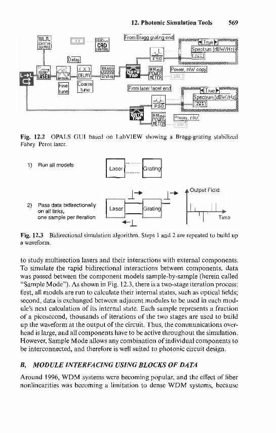
12. Photonic Simulation Tools 569
Fig. 12.2 OPALS GUI based on LabVIEW showing a Bragg-grating stabilized Fabry-Perot laser.
1) Run all models _.. ._ _ _ _ _
Output Field
2) Pass data bidirectionally on all links, one sample per iteration +L
Fig. 12.3 Bidirectional simulation algorithm. Steps 1 and 2 are repeated to build up a waveform.
to study multisection lasers and their interactions with external components. To simulate the rapid bidirectional interactions between components, data was passed between the component models sample-by-sample (herein called “Sample Mode”). As shown in Fig. 12.3, there is a two-stage iteration process: first, all models are run to calculate their internal states, such as optical fields; second, data is exchanged between adjacent modules to be used in each mod- ule’s next calculation of its internal state. Each sample represents a fraction of a picosecond, thousands of iterations of the two stages are used to build up the waveform at the output of the circuit. Thus, the communications over- head is large, and all components have to be active throughout the simulation. However, Sample Mode allows any combination of individual components to be interconnected, and therefore is well suited to photonic circuit design.
B. MODULE INTERFACING USING BLOCKS OF DATA
Around 1996, WDM systems were becoming popular, and the effect of fiber nonlinearities was becoming a limitation to dense WDM systems, because

570 Arthur J. Lowery
...... .. I.. w 1) Run First Model (e.g. transmitter)
2) Pass data forward, as a block representing a section of time
3) Run Next Model (e.g. fiber)
Fig. 12.4 Passing data unidirectionally simplifies calculations and allows data to be processed efficiently in blocks.
four-wave mixing (FWM) induced crosstalk quadruples when the channel density was doubled (Forghieri 1996). Simulators capable of predicting the per- formance of many-channel, long-haul WDM systems were required. Two early candidates were GOLD (Gigabit Optical Link De~igner)~ and BroadNED (Broadband Network De~igner).~ GOLD was developed using LabVIEW as an interface and operated by passing blocks of data in a “forward” direc- tion, from transmitter to receiver (herein called “Block Mode”). As shown in Fig. 12.4:
0 the signal source (usually the data generator or transmitter) is run first; this generates a block of data representing a signal waveform or its spectrum;
0 the block of data is then passed to the next module, such as the fiber; 0 the next module is then run to process the data, 0 and so on, until the receiver or instrumentation is reached.
This scheme greatly eases the communications overhead (Pendock 1997), and means that modules are only active for a short portion of the simulation time. Furthermore, data had periodic boundaries, which is essential for fiber modeling without latency (Lowery and Gurney 1997).
BroadNED was developed using Ptolemy’ as a scheduler to allow com- plex topologies to be simulated. Ptolemy fires the models in the required order for the simulation to proceed. In 1998, BroadNED, GOLD, and OPALS were merged into one platform, using the Ptolemy scheduler for both
Released by Virtual Photonics, Melbourne, Australia, 1998. Released by BNeD, Berlin, Germany, 1998. Ptolemy was developed by the University of California at Berkeley.

12. Photonic Simulation Tools 571
6 ,.: 100 l;m 3 ? i t ) 320 Channel h 10 GbUs
I I.nmmls
___ -
- - - - ,.sa %.*A N X I d *It1
- ?
Y * $ >, V I ) 5 .< .",- 1
. -~ A3
Fig. 12.5 VPltransmissionMakerTM and VPIcomponentMakerlM simulation envi- ronment.
sample-by-sample (Sample Mode) data passing and block-by-block (Block Mode) data passing. Figure 12.5 shows the resulting simulation environment.
C. MULTIPLE SIGNAL REPRESENTATIONS
The challenge with simulating large channel count, dense, long WDM systems is the computational task of modeling the fiber. The most direct method is to represent all channels by a single optical field (the total field method), which is essentially a sum of modulated sine waves, each representing a WDM channel. The complex envelope representation is used to represent all channels, as this allows the sampling rate to be lowered to close to the overall bandwidth of the WDM channels, rather than twice the highest optical frequency, as would be required using conventional sampling (PCM).
As the utilized bandwidth of fibers increases, the sample rate in simulations must also increase. This leads to a large number of samples within a block if a significant number of bits is to be represented. One solution is to break the simulation into smaller blocks, each containing tens rather than hundreds of bits, then averaging statistics over a number of blocks. Another is to rep- resent only some of the channels by sampled signals, and then represent the remaining channels by their average power and extinction ratio (herein called
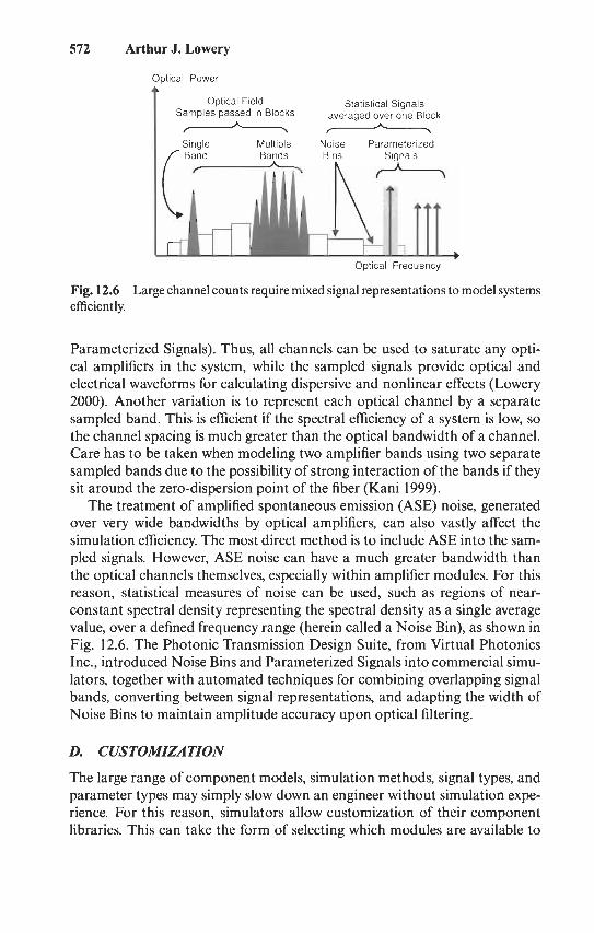
572 Arthur J. Lowery
Optical Power
Optical Field Statistical Signals Samples passed in Blocks averaged over one Block ** Single Multiple Noise Parameterized
f Band Bands Bins Signals
Optical Frequency
Fig. 12.6 Large channel counts require mixed signal representations to model systems efficiently.
Parameterized Signals). Thus, all channels can be used to saturate any opti- cal amplifiers in the system, while the sampled signals provide optical and electrical waveforms for calculating dispersive and nonlinear effects (Lowery 2000). Another variation is to represent each optical channel by a separate sampled band. This is efficient if the spectral efficiency of a system is low, so the channel spacing is much greater than the optical bandwidth of a channel. Care has to be taken when modeling two amplifier bands using two separate sampled bands due to the possibility of strong interaction of the bands if they sit around the zero-dispersion point of the fiber (Kani 1999).
The treatment of amplified spontaneous emission (ASE) noise, generated over very wide bandwidths by optical amplifiers, can also vastly affect the simulation efficiency. The most direct method is to include ASE into the sam- pled signals. However, ASE noise can have a much greater bandwidth than the optical channels themselves, especially within amplifier modules. For this reason, statistical measures of noise can be used, such as regions of near- constant spectral density representing the spectral density as a single average value, over a defined frequency range (herein called a Noise Bin), as shown in Fig. 12.6. The Photonic Transmission Design Suite, from Virtual Photonics Inc., introduced Noise Bins and Parameterized Signals into commercial simu- lators, together with automated techniques for combining overlapping signal bands, converting between signal representations, and adapting the width of Noise Bins to maintain amplitude accuracy upon optical filtering.
D. CUSTOMIZATION
The large range of component models, simulation methods, signal types, and parameter types may simply slow down an engineer without simulation expe- rience. For this reason, simulators allow customization of their component libraries. This can take the form of selecting which modules are available to
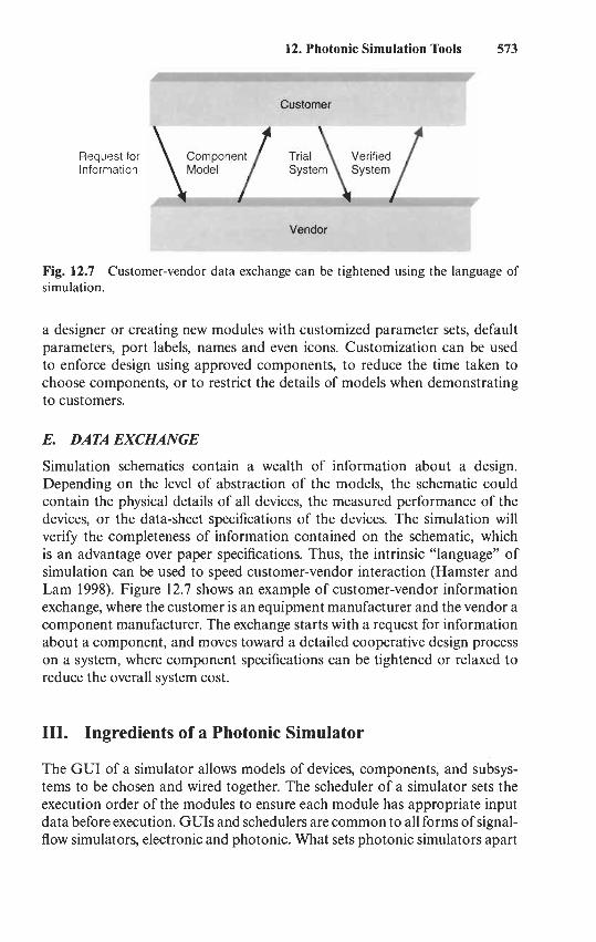
12. Photonic Simulation Tools 573
Customer
Request for Information
Fig. 12.7 Customer-vendor data exchange can be tightened using the language of simulation.
a designer or creating new modules with customized parameter sets, default parameters, port labels, names and even icons. Customization can be used to enforce design using approved components, to reduce the time taken to choose components, or to restrict the details of models when demonstrating to customers.
E. DATA EXCHANGE
Simulation schematics contain a wealth of information about a design. Depending on the level of abstraction of the models, the schematic could contain the physical details of all devices, the measured performance of the devices, or the data-sheet specifications of the devices. The simulation will verify the completeness of information contained on the schematic, which is an advantage over paper specifications. Thus, the intrinsic “language” of simulation can be used to speed customer-vendor interaction (Hamster and Lam 1998). Figure 12.7 shows an example of customer-vendor information exchange, where the customer is an equipment manufacturer and the vendor a component manufacturer. The exchange starts with a request for information about a component, and moves toward a detailed cooperative design process on a system, where component specifications can be tightened or relaxed to reduce the overall system cost.
111. Ingredients of a Photonic Simulator
The GUI of a simulator allows models of devices, components, and subsys- tems to be chosen and wired together. The scheduler of a simulator sets the execution order of the modules to ensure each module has appropriate input data before execution. GUIs and schedulers are common to all forms of signal- flow simulators, electronic and photonic. What sets photonic simulators apart

574 Arthur J. Lowery
is their libraries of photonic components, into which a great deal of design and implementation effort is put.
A. CONSIDERATIONS WHEN DEVELOPING A MODEL
A model of a component in a simulator contains a large amount of intellec- tual property. During its development, many details have to be considered and techniques developed. This is illustrated in Fig. 12.8. First, a decision to create a model has to be made based on a thorough knowledge of current and likely simulation tasks and component developments. The model parameters then have to be decided upon and defined unambiguously with due consideration to the level of abstraction of the model, which is discussed later. The physics of the device then has to be considered before appropriate numerical algo- rithms are developed. The algorithms must solve the problem efficiently and consider all types of signals that are to be processed. The complete specifica- tion of the model must then be implemented and tested, including real-world comparisons. Topical application examples are then developed to help users understand and apply the models most efficiently. The module and its appli- cations must be thoroughly documented, and training examples developed. Finally, a database of support questions and answers will evolve, and this can be used to define future developments to the model.
B. ABSTRACTION LEVEL OF COMPONENT MODELS
When defining a new model, its application, and hence its level of abstraction, is a prime consideration. The intrinsic trade-off is detail versus computa- tion speed. A secondary consideration is that detailed models require detailed
Parameter
Field & Current
Computational Documentation co Efficiency
Topical Applications Examples
Software Implementation
Testing and Comparison with
Real world
Fig. 12.8 Considerations when developing a model.

12. Photonic Simulation Tools 575
Model Type
Physical Model
I
Measured Model
Parameters
Dimensions and Material Characteristics
e.g.: length = 10pm index = 3.4
Measurements at Multiole
e.g.: rise time = 10 ps bandwidth = 12 GHz
Operating Points u Measurements at
x p e r a t i n g Point
Applications
Designing components and sub-systems and relating component design to systems performance
Systems simulation over a wide range of operating points (e.9. amplifier saturations)
Modeling of linear components in systems (e.g. filters), or packaged components (Transmitter Modules)
Relating specifications and parameterized measurements (e.g. risetime, bandwidth, SMSR) to systems performance
Fig. 12.9 Types of models (levels of abstraction), from physical to data sheet.
parameters; whereas behavioral models can be used to set specifications based on easily measured characteristics or data from data sheets. Figure 12.9 illustrates four levels of abstraction that can be used to categorize models:
At one extreme, each component could be represented by a detailed physical model based on material and structural parameters of the device. However, these parameters may be difficult to obtain, being proprietary, or difficult to derive from external measurements of a packaged device. The advantage of detailed physical models is that they can be used to predict the performance of new devices and design devices themselves. Their disadvantage is that they require intensive computation, especially if they include nonlinear effects or interactions of electrons and photons (Lowery 1996). Some devices are well suited to representation by a Black Box model. This model is based on the physics of the device, but has parameters that can be derived solely from external measurements on the device. An example is the Black Box EDFA model (Bonnedal 1996; Burgmeier 1998). This uses the physics of the device to derive interpolation schemes for the gain spectra for any input spectrum. The advantage over a physical model is that only external measurements (from input port to output port) are required on the device, therefore no proprietary information is needed. Furthermore, if the physics is sufficiently generic, a large-signal model can be derived from simple measurements. A disadvantage is that a Black Box model is only useful at a systems level of modeling, it cannot be used to design the device itself.
576 Arthur J. Lowery
Linear devices (such as optical and electrical filters) or well-specified devices (such as transmitters with a digital input) can be represented by their measured performance. For example, a filter’s characteristic can be imported into a simulation as a data file or the output of a transmitter module can be measured, digitized, stored, and replayed into the simulation. Again, novel devices cannot be designed using measured models, but the systems performance of a module is easily and accurately assessed using this method.
0 Datu sheets often give performance data as a series of parameters fitted to measurements, such as rise time, spectral width, wavelength sensitivity to temperature, etc. Although such data is often gathered using long-term measurements (spectra, averaged or sampling- scope measured transients), its wide availability makes it useful for systems-level simulation. Care must be taken because the long-term averages misrepresent the worst cases. For example, a side-mode suppression ratio for a laser of 30 dB may appear acceptable, but is not acceptable ifthe laser spends just 1 in lo9 of its time with an output dominated by the side mode.
C. COMPONENT SIMULATION CHALLENGES
Some photonic components require far more simulation effort than others. For this reason, a short discussion of the main challenges in developing models in a simulator follows. Unfortunately, there is not enough space for a detailed discussion. Reasonably complete descriptions of the models within a simulator would run to several thousand pages in length. However, the other chapters of this book and its predecessors give an excellent background on the physics of components and their likely interactions in systems and networks.
1. Optical Sources
If a system relies on a directly modulated laser as a transmitter, the transmis- sion distance is likely to be limited by the chirp of the laser. Indeed, some of the k s t systems simulations were developed to estimate this effect (Corvini and Koch 1987; Cartledge and Burley 1989). In essence, a laser will chirp from bluer to redder wavelengths during each of its transient peaks (dynamic chirp), and will generally shift to bluer wavelengths during extended trains of ones (adiabatic chirp). Because blue wavelengths travel faster than red in stan- dard fibers, chirping will result in pulse spreading. The exact fohn of the chirp waveform depends on the design of the laser. For Fabry-Perot lasers, chirp is unimportant compared with their multimode spectrum. For DFB lasers, longitudinal spatial hole-burning adds a third form of chirp, with wavelength shifts on nanosecond timescales, causing timing wander or even hysteresis and self-pulsation. For such systems, it is advisable to either use a very detailed
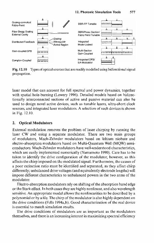
12. Photonic Simulation Tools 577
1 1 DBR-FP Tunable f
1 1 1 DBWPhase Section/ Fabry Perot Tunable
Integrated
Grating-controlled Fabry-Perot
Fiber Bragg Grating External Cavlty
Distributed Feedback /Grating 1 1 1 -Waveguide ‘Active Region Mode-Locked t
Multi-Section Gain-Coupled
Integrated DFB/ EA-Modulator
Fig. 12.10 Types of optical sources that are readily modelled using bidirectional signal propagation.
laser model that can account for full spectral and power dynamics, together with spatial hole-burning (Lowery 1996). Detailed models based on bidirec- tionally interconnected sections of active and passive material can also be used to design novel active devices, such as tunable lasers, ultra-short clock sources, and integrated laser modulators. A selection of such devices is shown in Fig. 12.10.
2. Optical Modulators
External modulation removes the problem of laser chirping by running the laser CW and using a separate modulator. There are two main groups of modulators, Mach-Zehnder modulators based on lithium niobate and electro-absorption modulators based on Multi-Quantum Well (MQW) semi- conductors. Mach-Zehnder modulators have well-understood characteristics, which are easily implemented numerically (Yamamoto 1990). Care has to be taken to identify the drive configuration of the modulator, however, as this affects the chirp imposed on the modulated signal. Furthermore, the causes of a poor extinction ratio must be identified and separated, as they affect chirp differently; unbalanced drive voltages (and equivalently electrode lengths) will impose different characteristics to unbalanced powers in the two arms of the modulator.
Electro-absorption modulators rely on shifting of the absorption band edge or the Stark effect. In both cases they are highly nonlinear, and also wavelength sensitive. An appropriate model allows the nonlinearities to be described by a polynomial or by a file. The chirp of the modulator is also highly dependent on the drive conditions (Fells 1994a,b). Good characterization of the real device is essential to match simulation results.
The drive conditions of modulators are as important as the modulators themselves, and there is an increasing interest in maximizing spectral efficiency

578 Arthur J. Lowery
(On0 1999) and minimizing the effects of dispersion (Smith 1997) using novel modulation formats (see Chapter 16 of this book). Commercial simulators include a variety of signal sources and signal processing modules (such as mul- tilevel code generators and Hilbert transforms) that allow novel modulation formats to be studied.
3. Passive Components
Passive components account for the majority of the components in systems, yet they require the least simulation effort if they are linear in nature. However, their effect on system performance can be dramatic, and their characteristics should be considered within a system simulation (Garcia and Uttamchanani 1997). Examples of system impact include dispersion compensation using chirped Bragg gratings (Mason 1995) and optimizing demultiplexing filter group delay characteristics (Lenz 1998).
Optical demultiplexers can be modeled as physical networks of components such as Bragg gratings within interferometers, measured Characteristics of lab- oratory devices, or as parameterized characteristics from data sheets (such as spectral width, insertion loss, and rejection). Physical models will automati- cally show the phase and amplitude characteristics of a component and allow for optimization. Measured characteristics allow prototype components with manufacturing imperfections to be assessed in a systems context. Care should be taken when using parameterized information on components, as it may not necessarily be complete. For example, few optical filter specifications give details on dispersion or group delay, though these become critical in systems with high spectral efficiency.
Optical add-drop multiplexers (OADMs) and optical cross-connects (OXCs) can be built from elementary components using hierarchical descrip- tions found in most simulators. Imperfections such as crosstalk and switching speed can be globally defined by statistical spreads. Often, only the worst-case paths through OADMs and OXCs need be considered, which considerably speeds simulation. However, care has to be taken to properly describe the effects of crosstalk, because they are strongly dependent on the wavelength difference between signal and interferer.
4. Optical Fibers
The behavior of optical fibers is detailed in other chapters. For WDM systems where nonlinear effects are of concern (Tkach 1995; Agrawal1995), the simu- lation of the fiber takes most of the computational effort (Tkach and Forghieri 1996), followed by the simulation of optical ampliiiers. Thus it is important to use efficient methods of computation, such as the split-step Fourier method (Agrawall995). With the adoption of distributed Raman amplification (DRA) in long-haul systems, fiber simulation has become yet more complex, as the interaction of backward-traveling pump waves with bidirectional noise, and

12. Photonic Simulation Tools 579
perhaps bidirectional signals, requires intensive computation. Fortunately, the rapid walk-off (movement of different wavelength pulses through one another) between pump and signals means that the interactions can be solved in terms of power rather than optical field. This vastly reduces the computational task while retaining critical interactions.
To model fiber nonlinearities, the split-step Fourier method is most often used. This splits the fiber into a large number of longitudinal subsections along which the signal is passed. Each section contains a calculation of fiber dispersion, then a calculation of the nonlinear phase shift. The dispersion is best implemented in the frequency domain (a convolution in the time domain becomes multiplication in the frequency domain, which is efficient for long impulse responses), whereas nonlinear phase shift has to be implemented in the time domain (Agrawal 1995). Thus, fast Fourier transforms (FFT) are used to translate between the time and frequency domains.
The computation time of a FFT is proportional to N ( log2 N ) , where N is the number of samples in the time or frequency array, which itself is proportional to the optical bandwidth and the number of bits simulated. Thus, the Total Field method may not be the optimum solution for all applications. For this reason, different optical signal representations have been developed.
0 The mean-field method (Yu 2000) shows that only a few neighboring channels need be represented by sampled signals when calculating nonlinear impairments on a given channel. This results in very large reductions in computational effort for systems with high channel counts.
0 Semianalytical methods can also be used for particular classes of systems. For example, frequency decomposition (Agrawall995) offers considerable savings when modeling cross-phase modulation (XF’M) and self-phase modulation (SPM) in systems with low spectral efficiency, because each channel is represented by its own sampled band (Lowery 1999). This saves modeling regions of the optical spectrum with little signal power within them.
0 For WDM return-to-zero (RZ) systems where XPM dominates timing jitter, semianalytical methods give 100-fold savings in computation time (Richter and Grigoryan 1999).
PMD is by nature random in its effect on transmission systems, because the polarization state within the fiber evolves along the fiber length (see Chapter 15 in this book), and the exact evolution depends on the fiber’s environment, which changes over days and seasons. Thus a simulation using a specific evolution path will only sample the performance of the fiber at one time. Furthermore, PMD states that cause severe degradation are rare, but impor- tant, events. Thus many simulation runs are required to assess the outage

580 Arthur J. Lowery
of a system due to PMD. To solve this problem, the system can be biased to give worst-case PMD states. Alternatively, PMD emulators can be used to dial-up a worst-case PMD state with a known probability (Francia 2000). There is considerable debate on whether such techniques give an accurate rep- resentation of the effects on the strong wavelength-dependence of PMD when high-bandwidth optical channels are used.
Figure 12.11 illustrates the variety of distortion that can occur due to PMD. The two runs correspond to two “states” of a coarse-step PMD model (Marcuse 1997). The range of pulse shapes within each run are due to the rota- tion of the polarization state of the input pulse, which changes the distribution of power between the fast and slow Principal States of Polarization (PSPs). Run 1 shows a large differential group delay (DGD) of 8 ps, and maximum pulse broadening occurs when the input power is divided equally between the PSPs. Run 2 shows a much smaller DGD. To get a true picture of the effect of DGD requires many thousands of runs of the coarse-step fiber, in order that the worst-case DGDs occur. The simulation task may be reduced by biasing the simulation towards worst cases, called “Importance Sampling” (Biondini 2001). Alternatively, far simpler models of PMD can be used with dial-up PMD characteristics. However, these may not be able to predict com- plex interactions such as “high-order” PMD causing dispersion on further pulse splitting.
3
Time [ps]
Fig. 12.11 Illustration of the effect of PMD on a RZ pulse. Two states of the fiber are shown consecutively. The variation within each state is due to the rotation of input polarization.
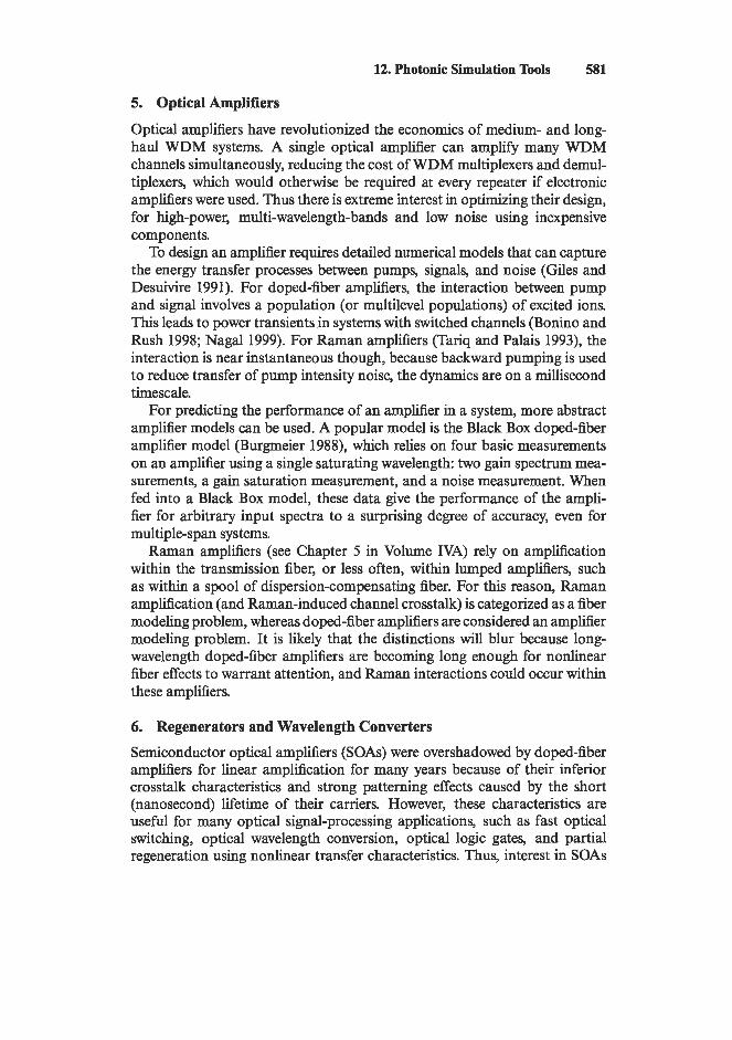
12. Photonic Simulation Tools 581
5. Optical Amplifiers
Optical amplifiers have revolutionized the economics of medium- and long- haul WDM systems. A single optical amplifier can amplify many WDM channels simultaneously, reducing the cost of WDM multiplexers and demul- tiplexers, which would otherwise be required at every repeater if electronic amplifiers were used. Thus there is extreme interest in optimizing their design, for high-power, multi-wavelength-bands and low noise using inexpensive components.
To design an amplifier requires detailed numerical models that can capture the energy transfer processes between pumps, signals, and noise (Giles and Desuivire 1991). For doped-fiber amplifiers, the interaction between pump and signal involves a population (or multilevel populations) of excited ions. This leads to power transients in systems with switched channels (Bonino and Rush 1998; Nagal 1999). For Raman amplifiers (Tariq and Palais 1993), the interaction is near instantaneous though, because backward pumping is used to reduce transfer of pump intensity noise, the dynamics are on a millisecond timescale.
For predicting the performance of an amplifier in a system, more abstract amplifier models can be used. A popular model is the Black Box doped-fiber amplifier model (Burgmeier 1988), which relies on four basic measurements on an amplifier using a single saturating wavelength two gain spectrum mea- surements, a gain saturation measurement, and a noise measurement. When fed into a Black Box model, these data give the performance of the ampli- fier for arbitrary input spectra to a surprising degree of accuracy, even for multiple-span systems.
Raman amplifiers (see Chapter 5 in Volume IVA) rely on amplification within the transmission fiber, or less often, within lumped amplifiers, such as within a spool of dispersion-compensating fiber. For this reason, Raman amplification (and Raman-induced channel crosstalk) is categorized as a fiber modeling problem, whereas doped-fiber amplifiers are considered an amplifier modeling problem. It is likely that the distinctions will blur because long- wavelength doped-fiber amplifiers are becoming long enough for nonlinear fiber effects to warrant attention, and Raman interactions could occur within these ampliiiers.
6. Regenerators and Wavelength Converters Semiconductor optical amplifiers (SOAs) were overshadowed by doped-fiber amplifiers for linear amplification for many years because of their inferior crosstalk characteristics and strong patterning effects caused by the short (nanosecond) lifetime of their carriers. However, these characteristics are useful for many optical signal-processing applications, such as fast optical switching, optical wavelength conversion, optical logic gates, and partial regeneration using nonlinear transfer characteristics. Thus, interest in SOAs

582 Arthur J. Lowery
is in resurgence, and tools for simulating photonic circuits made from inter- connected SOAs have been developed.6 Some sectors of industry have also experimented with using SOAs for linear amplification based on gain control, highly dispersed pulses, novel modulation formats, and large channel counts.
7. Optical Receivers
The sensitivity of optical receivers used to be a critical design issue for optical communication systems, and this prompted research into coherent systems to give a valuable few-dB improvement in sensitivity. However, much greater improvement in optical receiver sensitivity can be gained by using an optical preamplifier than by using a coherent receiver. For this reason, most receivers use direct detection, rather than coherent detection, and this is achieved using PIN or avalanche photodiodes (APDs).
For simulation purposes, the receiver model should include all noise sources and also electrical frequency (and phase) response. For PIN-diode receivers, the noise sources include shot noise on detection and the thermal noise of any electronics, plus noise generated by the beating of signal and ASE, of ASE and ASE, and of the signal with source relative intensity noise (RIN). For APD receivers, there is additional noise due to the randomness of avalanche mul- tiplication. In systems using multiple signal representations, ASE represented by Noise Bins is converted to a random optical field before mixing with the electrical signal.
Modules representing electrical signal-processing functions can be used to model electronic forms of signal restoration within a photonic simulator. The simulation challenge is the large discrepancy in sample rates between optical and electronic parts of a simulation. Resampling waveforms after photodetec- tion can mitigate this. However, the practical limitation may be providing the electronic part of simulation with sufficiently long data streams to test coding schemes with long coding lengths.
8. BER Estimation
One of the ultimate goals of simulation is to produce performance results that can be compared with real systems and the performance requirements placed on a real system. For communication systems this means BER. In the real world, systems are almost “error free” (less than one error per day). This is difficult to measure to any coniidence (at least 10 days would be required for a measurement on a single channel, given a single BER test set), unless extrapo- lation techniques are used (Bergano 1993). For simulations, it is impossible to
For example, VPIcomponentMakermActive Photonics.
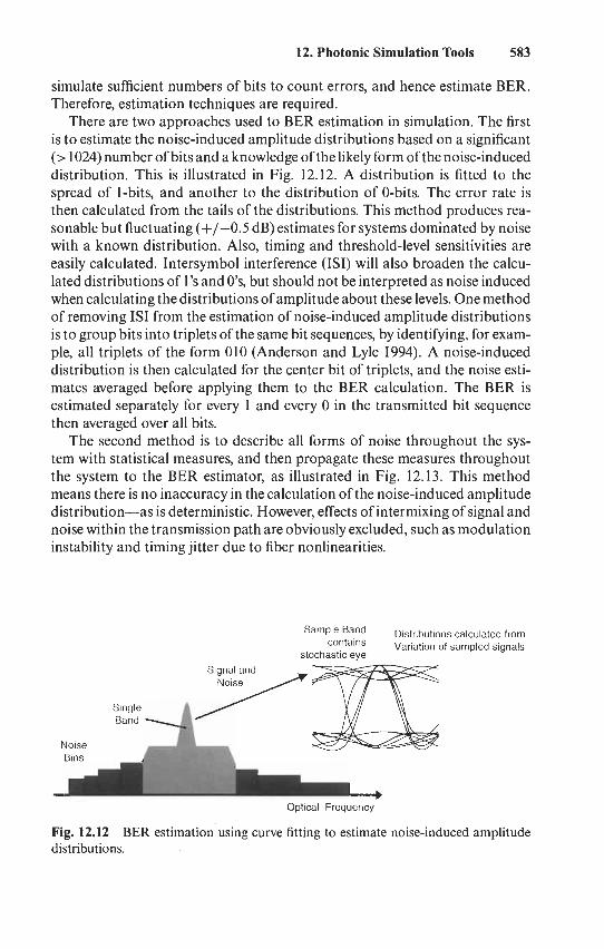
12. Photonic Simulation Tools 583
simulate sufficient numbers of bits to count errors, and hence estimate BER. Therefore, estimation techniques are required.
There are two approaches used to BER estimation in simulation. The first is to estimate the noise-induced amplitude distributions based on a significant (> 1024) number of bits and a knowledge of the likely form of the noise-induced distribution. This is illustrated in Fig. 12.12. A distribution is fitted to the spread of 1-bits, and another to the distribution of 0-bits. The error rate is then calculated from the tails of the distributions. This method produces rea- sonable but fluctuating (+/-0.5 dB) estimates for systems dominated by noise with a known distribution. Also, timing and threshold-level sensitivities are easily calculated. Intersymbol interference (ISI) will also broaden the calcu- lated distributions of 1’s and 03, but should not be interpreted as noise induced when calculating the distributions of amplitude about these levels. One method of removing IS1 from the estimation of noise-induced amplitude distributions is to group bits into triplets of the same bit sequences, by identifying, for exam- ple, all triplets of the form 010 (Anderson and Lyle 1994). A noise-induced distribution is then calculated for the center bit of triplets, and the noise esti- mates averaged before applying them to the BER calculation. The BER is estimated separately for every 1 and every 0 in the transmitted bit sequence then averaged over all bits.
The second method is to describe all forms of noise throughout the sys- tem with statistical measures, and then propagate these measures throughout the system to the BER estimator, as illustrated in Fig. 12.13. This method means there is no inaccuracy in the calculation of the noise-induced amplitude distribution-as is deterministic. However, effects of intermixing of signal and noise within the transmission path are obviously excluded, such as modulation instability and timing jitter due to fiber nonlinearities.
Sample Band Distributions calculated from of sampled signals
Optical Frequency
Fig. 12.12 BER estimation using curve fitting to estimate noise-induced amplitude distributions.
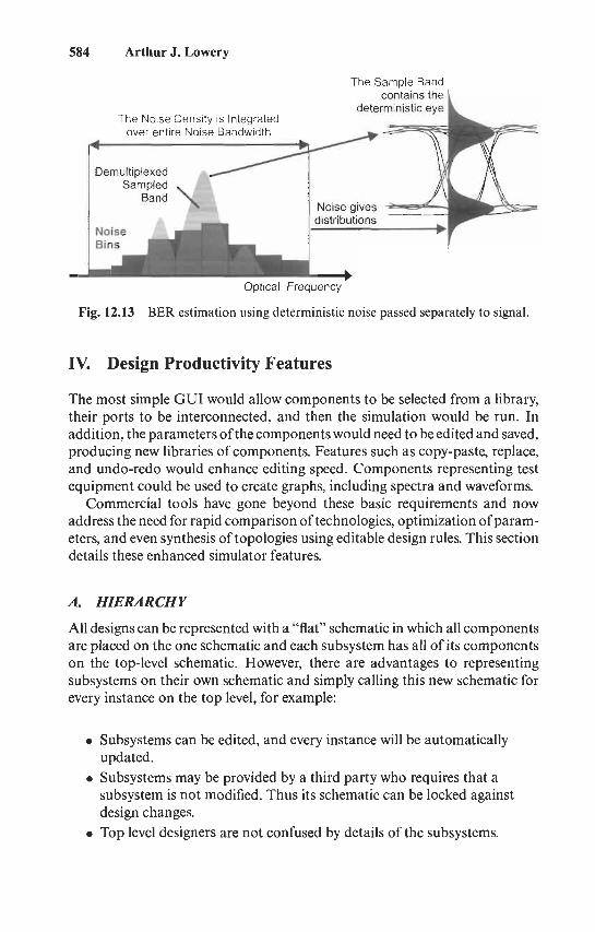
584 Arthur J. Lowery
The Sample Band
deterministic eye
Optical Frequency
Fig. 12.13 BER estimation using deterministic noise passed separately to signal.
IV. Design Productivity Features
The most simple GUI would allow components to be selected from a library, their ports to be interconnected, and then the simulation would be run. In addition, the parameters ofthe components would need to be edited and saved, producing new libraries of components. Features such as copy-paste, replace, and undo-redo would enhance editing speed. Components representing test equipment could be used to create graphs, including spectra and waveforms.
Commercial tools have gone beyond these basic requirements and now address the need for rapid comparison of technologies, optimization of param- eters, and even synthesis of topologies using editable design rules. This section details these enhanced simulator features.
A. HIERARCHY
All designs can be represented with a “flat” schematic in which all components are placed on the one schematic and each subsystem has all of its components on the top-level schematic. However, there are advantages to representing subsystems on their own schematic and simply calling this new schematic for every instance on the top level, for example:
0 Subsystems can be edited, and every instance will be automatically
0 Subsystems may be provided by a third party who requires that a updated.
subsystem is not modified. Thus its schematic can be locked against design changes.
0 Top level designers are not confused by details of the subsystems.

12. Photonic Simulation Tools 585
0 Interfaces between the top layer and the subsystems can represent physical interfaces between equipment, which helps comparisons with the physical equipment and tests these specifications.
0 Space is saved on the top-level schematic, making it more clear.
Most commercial simulators allow hierarchy. Some include detailed param- eter passing from one level to another, allowing many instances of the same schematic to have their parameters controlled at the top level of the schematic. This is similar to feeding performance settings into lower-level equipment. Figure 12.14 shows three levels of hierarchy in an optical cross-connect. The lowest level contains wavelength converters (illustrated) and individual switches; the mid-level contains the internal connections of the switch itself, and the top level is a test setup for the switch. As an example of parameter passing, the crosstalk levels of the lowest-level switches are controlled by a single parameter at the top level.
B. HIGHER-ORDER FUNCTIONS
Designs contain repetitive features, for example, WDM systems have many similar transmitters, parallel fibers connecting to multiplexers, and multiple spans each comprising an amplifier, fiber, and perhaps dispersion compensa- tion. Rather than represent each source and modulator in a transmitter by a separate module (icon), higher-order functions can be used that take one instance of the transmitter and automatically create an array of instances. This is similar to a FOR loop in text programming. The output of the trans- mitter array will be many parallel fibers connected to a multiplexer. Rather than having to draw multiple fibers on the schematic, a single connection (a bus) can be used, as shown in Fig. 12.15. Similarly, a loop construct can be used to represent multiple spans by a single span.
C. SIMULATION CONTROL
Software should reduce all repetitive tasks to one action, thus capturing the design process. For this reason, scripting languages are often used to control a simulation in a very flexible and precise way. For example, a simulation can be run multiple times with a simple script, and multiple parameters can be changed on each run. Furthermore, outputs can be monitored and actions taken, such as for optimization. However, although scripts are powerful, they can also be difficult for new users, therefore interfaces are often developed to generate commonly used scripts such as sweeps, optimization, and simulation control.
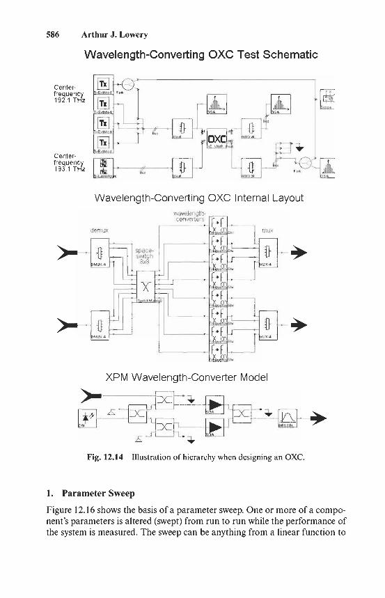
586 Arthur J. Lowery
Wavelengt h-Converting OXC Test Schematic
Center- frequenc 192.1 d z
Center- frequenc 193.1 T&
Wavelength-Converting OXC Internal Layout
demux
XPM Wavelength-Converter Model
Fig. 12.14 Illustration of hierarchy when designing an OXC.
1. Parameter Sweep
Figure 12.16 shows the basis of a parameter sweep. One or more of a compo- nent’s parameters is altered (swept) from run to run while the performance of the system is measured. The sweep can be anything from a linear function to

12. Photonic Simulation Tools 587
Source + Model b
+ b
Array Construct M ux
Loop Construct Connection
Fig. 12.15 Higher-order functions simplify the schematic: array, bus, and loop constructs are ideal for multispan WDM system simulation.
Y Instrumentation 4 XY plots
Instrumentation
X sweep
a logarithmic function or a random number with a given distribution. Multi- dimensional sweeps are also useful, most commonly for sweeping the test conditions while sweeping the parameter, for example:
0 Sweeping the input power of a regenerator while sweeping a design parameter to obtain a power-idpower-out transfer. Characteristics for a number of designs.
before the receiver) while sweeping a system parameter (e.g., fiber length) to obtain the degradation in receiver sensitivity.
0 Sweeping the input power into a receiver (usually using an attenuator
The results are usually plotted on an x-y graph. The y trace is usually a single performance measure, such as BER, Q, or eye opening, whereas the x-axis can be derived from the sweep or from an independent measurement (commonly received power for sensitivity measurements). Because of their utility, parameter sweeps are available in most commercial tools.
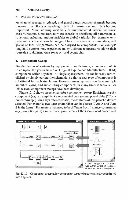
588 Arthur J. Lowery
a. Random Parameter Variations
As channel spacing is reduced, and guard bands between channels become narrower, the effects of wavelength drift of transmitters and filters become important. Manufacturing variability or environmental factors can cause these variations. Simulators now are capable of specifying all parameters as functions, including random variables or global variables. For example, tem- perature dependence can be assigned to all parameters in simulators, and global or local temperatures can be assigned to components. For example long-haul systems may experience many different temperatures along their route due to differing time zones or local geography.
2. Component Sweep
For the design of systems by equipment manufacturers, a common task is to compare the performance of Original Equipment Manufacturer (OEM) components within a system. In a single-span system, this can be easily accom- plished by simply editing the schematic, so that a new type of component is substituted for each simulation. However, many systems now have multiple amplified spans, and substituting components in many times is tedious. For this reason, component sweeps have been developed.
Figure 12.17 shows the schematic for a component sweep. Each instance of a component (e.g., an amplifier) is represented by a generic placeholder (“Com- ponent Sweep”). On a separate schematic, the contents of this placeholder are selected. For example, two types of amplifier can be chosen (Type A and Type B in the figure). Parameters that need to be different from instance-to-instance (e.g., amplifier gain) can be made parameters of the Component Sweep and
S
Fig. 12.17 Component sweeps allow component types to be automatically substituted into a system.

12. Photonic Simulation Tools 589
picked up from the individual instances of the Component Sweep. The simu- lation will automatically run for each type of amplifier within the component, and results can be plotted on separate traces of the same graph. An example result of a component sweep for different filter types within an add-drop multi- plexer (ADM) is shown in Fig. 12.18. A great advantage of component sweeps is that the parameters of the types of components can be altered simply by edit- ing the Component Sweep-all instances will be automatically updated. Note that the components themselves can be subsystems. This allows systems with dispersion compensating fiber (DCF) and standard single-mode fiber (S-SMF, SMF) fiber to be compared with systems with nonzero dispersion-shifted fiber (NZDFS) using component sweeps.
3. Topology Sweep
If two or more systems with widely different topologies have to be compared, such as a direct detection system versus a coherent system, then a topology sweep is required, as shown in Fig. 12.19. The easiest method is to place both topologies on the same schematic. The scheduler will run one, then the other. Results can be plotted onto the same graph, as shown in Fig. 12.20. In this case, the graceful degradation of differential phase-shift keyed (DPSK) modulation with fiber length is demonstrated.
D. OPTIMIZATION AND PARAMETERIZATION
Design, rather than testing, inherently uses optimization. The most simple and often-used form of optimization is to run a parameter sweep, and then look for the best performance in the results. However, this may be very time- consuming, and may produce many wasted simulations whose results are far from the optimum. Furthermore, it requires user interaction, which is wasteful of human resources.
1. Automated Optimization
As shown in Fig. 12.21, automated optimization examines the result of a trial simulation and compares this with a design goal or multiple goals. The opti- mization engine then adjusts parameters to drive the simulation towards the design goal. Very sophisticated algorithms are available from the area of con- trol theory that speed the optimization process by minimizing the number of simulation runs required. The risk is that a local optimum will be found, rather than a global optimum. Therefore, the optimization process requires testing by a skilled designer before being included in a “mass-production” process.
2. Automated Parameterization
In order to model a system effectively, the parameters of the models of each component in the system should match those in reality. For behavioral models,

Power [dBrn] OSA
.35
-60
- - ,-.. 42 4 -35 -30 -25 -20 -15 -10 -5 0 5 10 15 20 25 30 35 24
Optical Frequencyrelative to 193 I THZ [GHz]
Phase [ I e3degreesl
r -.. 0
- I I
42 4 -35 -30 -25 -20 -15 -10 -5 c 5 10 15 20 25 30 35 142 4 Optical Frequency relative to 193 1 THz [GHz]
Delay Ips1 207
200
100
-
I -
r r . 42 4 -35 -30 -25 -20 -15 -10 -5 0 5 10 15 20 25 30 35 142 4
Outical Freauency relative to I 93 I THZIGHZI
Dispersion [ns/nm]
Optical Frequency relative to 193 1 THz [GHz]
Fig. 12.18 Comparison of cascaded filter responses in an ADM using component sweeps with two types of filters.
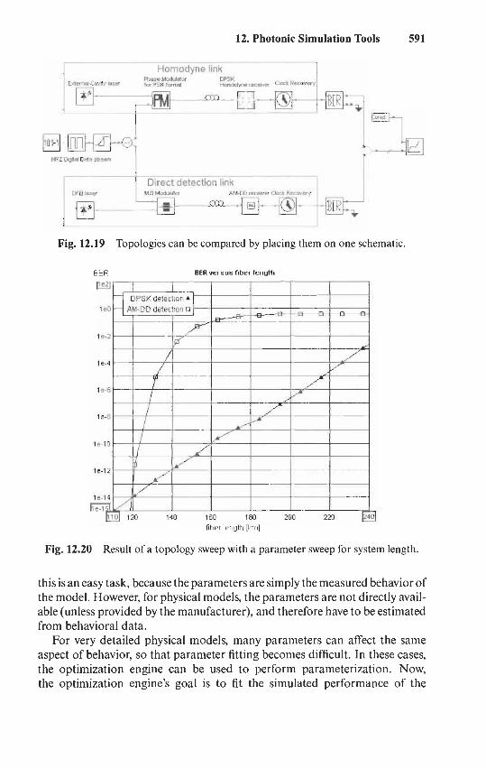
12. Photonic Simulation Tools 591
DFB laser
I Homodyne link I
Direct detection link MZI Modulator AM-DD receiver Clock Recovery
4 m *- w- Fig. 12.19 Topologies can be compared by placing them on one schematic.
-#E&-
BER BER versusfiber length
fiber length [km]
Fig. 12.20 Result of a topology sweep with a parameter sweep for system length.
this is an easy task, because the parameters are simply the measured behavior of the model. However, for physical models, the parameters are not directly avail- able (unless provided by the manufacturer), and therefore have to be estimated from behavioral data.
For very detailed physical models, many parameters can affect the same aspect of behavior, so that parameter fitting becomes difficult. In these cases, the optimization engine can be used to perform parameterization. Now, the optimization engine’s goal is to fit the simulated performance of the

592 Arthur J. Lowery
Fig. 12.21 Optimization includes a feedback loop to control parameter settings.
Laboratory Characterization
-7-
1 mponent + LabOrato~ Test + Source Instrumentation
Simulation to fit Parameters
U Fig. 12.22 Parameterization of a measured component using an optimization engine.
component to the measured behavior of the component by adjusting the component model’s parameters. Figure 12.22 shows the arrangement of the optimization engine to perform this task. The real laboratory instrumenta- tion provides the measured behavior. Parameterization using a commercial optimizer/parameter extractor7 is shown in Fig. 12.23. This has been set the task of fitting a transfer characteristic of a regenerator by adjusting a design parameter of an active device. It is also capable of fitting multiple parameters given multiple design goals.
’ VPIparameterExtractorTM is jointly developed with Mathematical Systems Incorporated, Tokyo, and NTT, Japan.

12. Photonic Simulation Tools 593
Close 1 Fig. 12.23 Demonstration of an optimization tool that has found the value of a parameter so that the transfer characteristic of a regenerator matches the required goal.
E. AUTOMATED SYNTHESIS
Building a simulation traditionally involved choosing each component from a library, placing it, setting its parameters, and linking it to adjacent compo- nents. Using computer tools, all “no-brainer” tasks ought to be automated. Similarly, basic calculations should also be automated, such as power bud- gets and dispersion-compensation schemes. Furthermore, users should only be asked to enter data once.
These requirements lead to a requirement that the GUI have some degree of automation. At the lowest level, this could take the form of macros, which capture common tasks and perform them with a single-keystroke command. However, a much more powerful tool would have wizards that interac- tively communicate with the designer until enough information is gained to
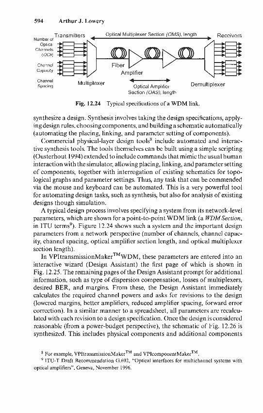
594 Arthur J. Lowery
Number of Optical
Channels ( O W
Channel Capacity
Multiplexer - Optical Amplifier Demultiplexer Section (OAS), length
Fig. 12.24 Typical specifications of a WDM link.
Channel Spacing
synthesize a design. Synthesis involves taking the design specifications, apply- ing design rules, choosing components, and building a schematic automatically (automating the placing, linking, and parameter setting of components).
Commercial physical-layer design tools’ include automated and interac- tive synthesis tools. The tools themselves can be built using a simple scripting (Ousterhout 1994) extended to include commands that mimic the usual human interaction with the simulator, allowing placing, linking, and parameter setting of components, together with interrogation of existing schematics for topo- logical graphs and parameter settings. Thus, any task that can be commended via the mouse and keyboard can be automated. This is a very powerful tool for automating design tasks, such as synthesis, but also for analysis of existing designs though simulation.
A typical design process involves specifying a system from its network-level parameters, which are shown for a point-to-point WDM link (a WDMSection, in ITU terms9). Figure 12.24 shows such a system and the important design parameters from a network perspective (number of channels, channel capac- ity, channel spacing, optical amplifier section length, and optical multiplexer section length).
In VPItransmissionMakerTMWDM, these parameters are entered into an interactive wizard (Design Assistant) the first page of which is shown in Fig. 12.25. The remaining pages of the Design Assistant prompt for additional information, such as type of dispersion compensation, losses of multiplexers, desired BER, and margins. From these, the Design Assistant immediately calculates the required channel powers and asks for revisions to the design (lowered margins, better amplifiers, reduced amplifier spacing, forward error correction). In a similar manner to a spreadsheet, all parameters are recalcu- lated with each revision to a design specification. Once the design is considered reasonable (from a power-budget perspective), the schematic of Fig. 12.26 is synthesized. This includes physical components and additional components
* For example, VPItransmissionMakerTM and VPIcomponentMakerTM. ITU-T Draft Recommendation (3.692, “Optical interfaces for multichannel systems with
optical amplifiers”, Geneva, November 1996.

12. Photonic Simulation Tools 595
Fig. 12.25 First page of a Design Assistant wizard for specifying a link design.
Fig. 12.26 Automatically synthesized link design schematic. All parameters are set.
to control the type of signals in the simulation (shown in gray) during the analysis process.
E AUTOMATED ANALYSIS
The design process also involves testing the effects of component changes and verifying the operation of a design at each change. This can be achieved “by hand” by running through a list of tests for each change. However, this can become tedious, especially if testing involves setting up new instrumentation around the system for each type of test.

596 Arthur J. Lowery
Design Assistants can be used to automate (and implicitly standardize) the testing process of a design. Automation also takes care of setting up a numer- ical simulation to achieve optimum simulation efficiency, for example, using statistical measures to test power budgets, linear simulation techniques to ver- ify dispersion maps, then full nonlinear models for h a l verifications. Because the enhanced tcl (tool control language) (Ousterhout 1994) can interrogate topologies, it can automatically place appropriate instrumentation and set physical and numerical parameters for each test. This vastly speeds designs by removing repeated operations and by selecting optimum numerical techniques.
A worthwhile advantage of using automated synthesis and analysis tools is that the design process is captured electronically. It can then be distributed company-wide or to suppliers and customers. This has the effect of leveraging expert knowledge, and also enforcing standards in a benign manner. With current skills shortages in photonics, particularly high-end design, this is a huge benefit to companies and their customers.
The following sections walk through an automated analysis process for a 24-channel40-Gbith per channel WDM system transmitting over 650 km using 50-km spans with fiber dispersion compensators at the reamplib- tion sites. Design changes are made throughout the analysis process due to unacceptable degradation.
1. Power Budget
One of the first sanity tests is to simulate the optical power in each channel throughout the system. If amplifier models including gain saturation are used, the effects of gain tilt will be seen to build-up from amplifier to amplifier. To speed simulation, statistical measures of power (Parameterized Signals) and noise (Noise Bins) can be used, for example, signal power and noise spectral density. The noise is required as it may dominate the saturation of the ampli- fiers, particularly if optical flters are not used in the system. Instrumentation is placed along the system to probe the optical power. This can be achieved automatically in advanced simulators. The same instrumentation can be used to monitor the ASE noise spectrum, and hence calculate the OSNR.
The initial synthesized system suffered from a build-up of ASE to dom- inance at the gain peak of the erbium-doped fiber amplifiers (EDFAs). Figure 12.27 shows the optical spectrum before the h a 1 optical demultiplexer. The optical spectrum analyzer (OSA) also gives a tabulated display of signal, noise, and OSNR for each channel. At this stage, all are acceptable, although the variation of channel powers is undesirable.
2. Optical Signal-to-Noise Ratio
Placing optical filters with a 3-THz passband after every four amplifiers cured the ASE build-up. Figure 12.28 shows the evolution of channel powers and OSNR for the best and worst channels in the automatically synthesized system,
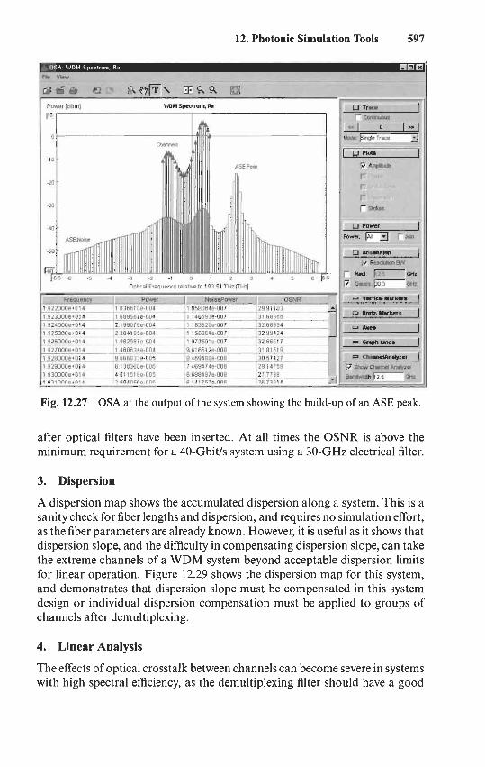
12. Photonic Simulation Tools 597
Fig. 12.27 OSA at the output of the system showing the build-up of an ASE peak.
after optical filters have been inserted. At all times the OSNR is above the minimum requirement for a 40-Gbit/s system using a 30-GHz electrical filter.
3. Dispersion
A dispersion map shows the accumulated dispersion along a system. This is a sanity check for fiber lengths and dispersion, and requires no simulation effort, as the fiber parameters are already known. However, it is useful as it shows that dispersion slope, and the difficulty in compensating dispersion slope, can take the extreme channels of a WDM system beyond acceptable dispersion limits for linear operation. Figure 12.29 shows the dispersion map for this system, and demonstrates that dispersion slope must be compensated in this system design or individual dispersion compensation must be applied to groups of channels after demultiplexing.
4. Linear Analysis
The effects of optical crosstalk between channels can become severe in systems with high spectral efficiency, as the demultiplexing filter should have a good
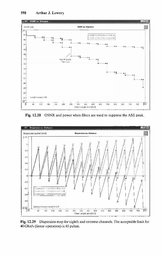
598 Arthur J. Lowery
OSNR (dB)
B O
44
42 - -
40
38
36-
34-
32 - 30-
28-
26-
24 - 22 . Lcnrfh includes DCF
- -
Filer Loss
E 50 100 150 200 2 M 300 350 400 450 500 550 600 650 700 750
Fiber Length (km) [le31
Fig. 12.28 OSNR and power when filters are used to suppress the ASE peak.
Dispersion (pslnrn) [l e31 DlSPerSlO" "8.01818"Ee
50 100 (50 200 250 300 350 4GU 450 500 550 600
bstana includes iensth of DCF
Fig. 12.29 Dispersion map for eighth and extreme channels. The acceptable limit for 40 Gbit/s (linear operation) is 65 ps/nm.
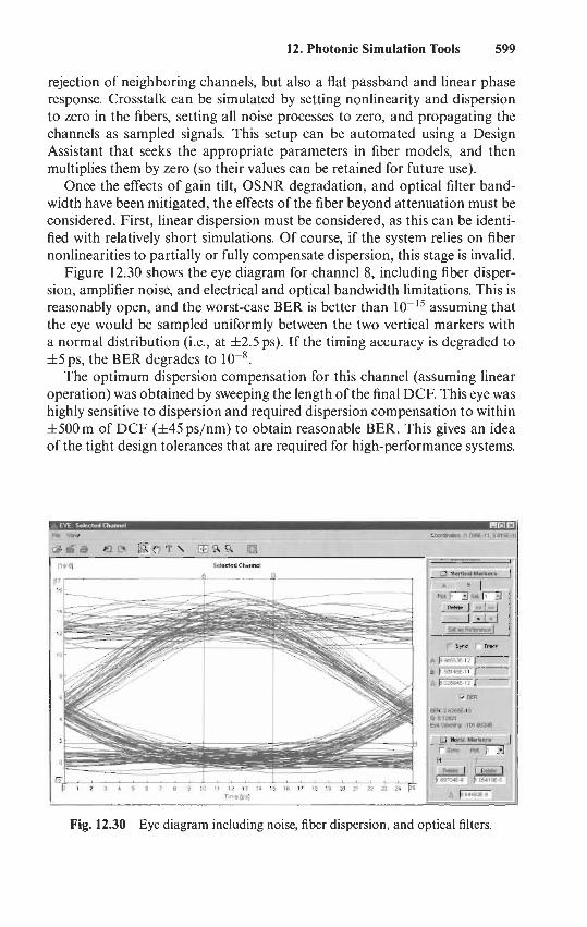
12. Photonic Simulation Tools 599
rejection of neighboring channels, but also a flat passband and linear phase response. Crosstalk can be simulated by setting nonlinearity and dispersion to zero in the fibers, setting all noise processes to zero, and propagating the channels as sampled signals. This setup can be automated using a Design Assistant that seeks the appropriate parameters in fiber models, and then multiplies them by zero (so their values can be retained for future use).
Once the effects of gain tilt, OSNR degradation, and optical filter band- width have been mitigated, the effects of the fiber beyond attenuation must be considered. First, linear dispersion must be considered, as this can be identi- fied with relatively short simulations. Of course, if the system relies on fiber nonlinearities to partially or fully compensate dispersion, this stage is invalid.
Figure 12.30 shows the eye diagram for channel 8, including fiber disper- sion, amplifier noise, and electrical and optical bandwidth limitations. This is reasonably open, and the worst-case BER is better than assuming that the eye would be sampled uniformly between the two vertical markers with a normal distribution (i.e., at f 2 . 5 ps). If the timing accuracy is degraded to f 5 ps, the BER degrades to lo-*.
The optimum dispersion compensation for this channel (assuming linear operation) was obtained by sweeping the length of the final DCF. This eye was highly sensitive to dispersion and required dispersion compensation to within f500 m of DCF ( f 4 5 ps/nm) to obtain reasonable BER. This gives an idea of the tight design tolerances that are required for high-performance systems.
Fig. 12.30 Eye diagram including noise, fiber dispersion, and optical filters.
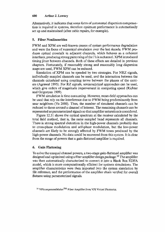
600 Arthur J. Lowery
Alternatively, it indicates that some form of automated dispersion compensa- tion is required in systems, therefore optimum performance is automatically set up and maintained (after cable repairs, for example).
5. Fiber Nonlinearities
FWM and XPM are well-known causes of system performance degradation and were the focus of numerical simulation over the last decade. FWM pro- duces optical crosstalk in adjacent channels, which behaves as a coherent interferer, producing strong patterning of the 1’s in achannel. XPM introduced timing jitter between channels. Both of these effects are detailed in previous chapters. Fortunately, if reasonably strong and reasonably long dispersion maps are used, FWM XPM can be reduced.
Simulation of XPM can be speeded by two strategies. For NRZ signals, individually sampled channels can be used, and the interaction between the channels calculated using coupling terms between the phases of the carri- ers (Agrawal 1995). For RZ signals, semianalytical approaches can be used, which give orders of magnitude improvement in computing speed (Richter and Grigoryan 1999).
FWM simulation is time consuming. However, mean-field approaches can be used that rely on the interference due to F W M being predominantly from near neighbors (Yu 2000). Thus, the number of simulated channels can be reduced to those around a channel of interest. The remaining channels can be represented as parameterized signals so that amplifier saturation is considered.
Figure 12.31 shows the optical spectrum at the receiver calculated by the total field method, that is, the same sampled band represents all channels. There is strong spectral distortion in the high-power channels probably due to cross-phase modulation and self-phase modulation, but the low-power channels are likely to be strongly affected by FWM tones produced by the high-power channels. No data could be recovered from this system. It is clear from the range of powers that a gain-flattened amplifier is required.
6. Gain Flattening
To solve the unequal channel powers, a two-stage gain-flattened amplifier was designed and optimized using a fiber amplifier design package.1° The amplifier was then automatically characterized to convert it into a Black Box EDFA model, which is more computationally efficient for systems simulations. The amplifier characteristics were then imported into the system simulation by file reference, and the performance of the amplifier chain verified for overall flatness using parameterized signals.
lo VPIcomponentMakerTM Fiber Amplifier from VPI Virtual Photonics.
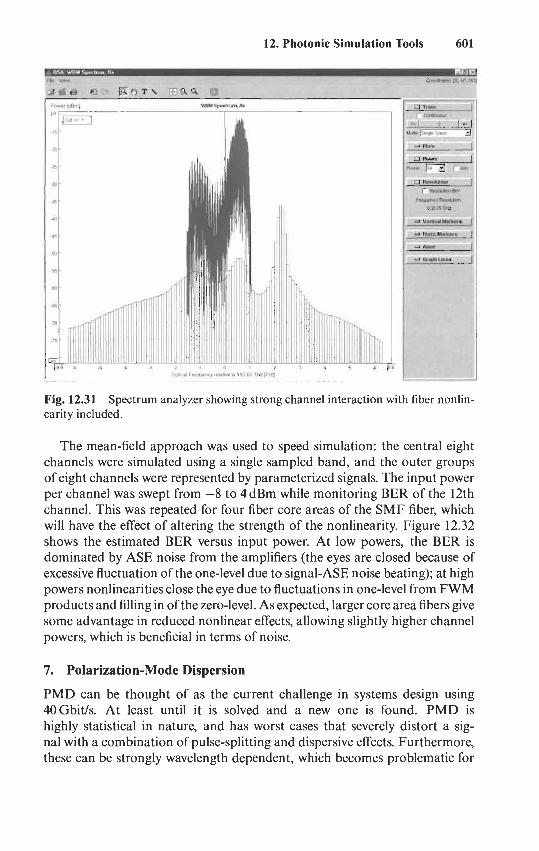
12. Photonic Simulation Tools 601
Fig. 12.31 earity included.
Spectrum analyzer showing strong channel interaction with fiber nonlin-
The mean-field approach was used to speed simulation: the central eight channels were simulated using a single sampled band, and the outer groups of eight channels were represented by parameterized signals. The input power per channel was swept from -8 to 4 dBm while monitoring BER of the 12th channel. This was repeated for four fiber core areas of the SMF fiber, which will have the effect of altering the strength of the nonlinearity. Figure 12.32 shows the estimated BER versus input power. At low powers, the BER is dominated by ASE noise from the amplifiers (the eyes are closed because of excessive fluctuation of the one-level due to signal-ASE noise beating); at high powers nonlinearities close the eye due to fluctuations in one-level from FWM products and filling in of the zero-level. As expected, larger core area fibers give some advantage in reduced nonlinear effects, allowing slightly higher channel powers, which is beneficial in terms of noise.
7. Polarization-Mode Dispersion
PMD can be thought of as the current challenge in systems design using 40GbitIs. At least until it is solved and a new one is found. PMD is highly statistical in nature, and has worst cases that severely distort a sig- nal with a combination of pulse-splitting and dispersive effects. Furthermore, these can be strongly wavelength dependent, which becomes problematic for
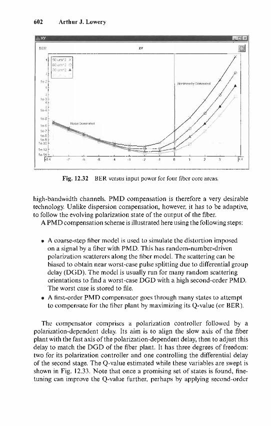
602 Arthur J. Lowery
Fig. 12.32 BER versus input power for four fiber core areas.
high-bandwidth channels. PMD compensation is therefore a very desirable technology. Unlike dispersion compensation, however, it has to be adaptive, to follow the evolving polarization state of the output of the fiber.
A PMD compensation scheme is illustrated here using the following steps:
0 A coarse-step fiber model is used to simulate the distortion imposed on a signal by a fiber with PMD. This has random-number-driven polarization scatterers along the fiber model. The scattering can be biased to obtain near worst-case pulse splitting due to differential group delay (DGD). The model is usually run for many random scattering orientations to find a worst-case DGD with a high second-order PMD. The worst case is stored to file.
0 A first-order PMD compensator goes through many states to attempt to compensate for the fiber plant by maximizing its Q-value (or BER).
The compensator comprises a polarization controller followed by a polarization-dependent delay. Its aim is to align the slow axis of the fiber plant with the fast axis of the polarization-dependent delay, then to adjust this delay to match the DGD of the fiber plant. It has three degrees of freedom: two for its polarization controller and one controlling the differential delay of the second stage. The Q-value estimated while these variables are swept is shown in Fig. 12.33. Note that once a promising set of states is found, fine- tuning can improve the Q-value further, perhaps by applying second-order
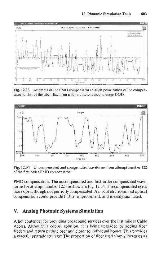
12. Photonic Simulation Tools 603
Fig. 12.33 Attempts of the PMD compensator to align polarization of the compen- sator to that of the fiber. Each run is for a different second-stage DGD.
Fig. 12.34 Uncompensated and compensated waveforms from attempt number 122 of the first order PMD compensator.
PMD compensation. The uncompensated and first-order compensated wave- forms for attempt number 122 are shown in Fig. 12.34. The compensated eye is more open, though not perfectly compensated. A mix of electronic and optical compensation could provide further improvement, and is easily simulated.
V. Analog Photonic Systems Simulation
A hot contender for providing broadband services over the last mile is Cable Access. Although a copper solution, it is being upgraded by adding fiber feeders and return paths closer and closer to individual homes. This provides a graceful upgrade strategy: The proportion of fiber used simply increases as
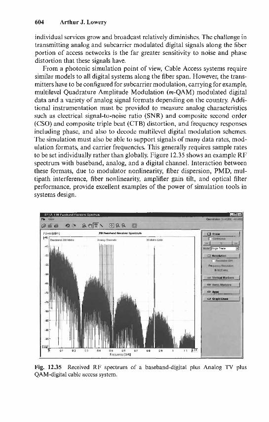
604 Arthur J. Lowery
individual services grow and broadcast relatively diminishes. The challenge in transmitting analog and subcarrier modulated digital signals along the fiber portion of access networks is the far greater sensitivity to noise and phase distortion that these signals have.
From a photonic simulation point of view, Cable Access systems require similar models to all digital systems along the fiber span. However, the trans- mitters have to be configured for subcarrier modulation, carrying for example, multilevel Quadrature Amplitude Modulation (m-QAM) modulated digital data and a variety of analog signal formats depending on the country. Addi- tional instrumentation must be provided to measure analog characteristics such as electrical signal-to-noise ratio (SNR) and composite second order (CSO) and composite triple beat (CTB) distortion, and frequency responses including phase, and also to decode multilevel digital modulation schemes. The simulation must also be able to support signals of many data rates, mod- ulation formats, and carrier frequencies. This generally requires sample rates to be set individually rather than globally. Figure 12.35 shows an example RF spectrum with baseband, analog, and a digital channel. Interaction between these formats, due to modulator nonlinearity, fiber dispersion, PMD, mul- tipath interference, fiber nonlinearity, amplifier gain tilt, and optical filter performance, provide excellent examples of the power of simulation tools in systems design.
Fig. 12.35 Received RF spectrum of a baseband-digital plus Analog TV plus QAM-digital cable access system.

12. Photonic Simulation Tools 605
VI. Conclusions
Simulation of photonic systems has become a necessity due to the complex interactions within and between components, and the need for rapid design cycles using the latest technologies to meet the growth in bandwidth demand while utilizing legacy plant. Tools have evolved from in-house code, developed for a single purpose, to commercial simulation environments that cover almost all simulation tasks and provide additional functionality to speed the design process, such as the ability to automate the design process and to capture expert knowledge.
The move to an electronic design environment, from laboratory prototypes, provides many advantages that are not immediately obvious. The simulator and its libraries becomes a standard design platform, so that individuals, teams, and companies can communicate their designs electronically. This can speed interactions. It also ensures that information is passed in a standard format (the parameters of the models), and is essential for design reuse: Part of an existing design can be pasted into a simulation far more easily than part of a laboratory prototype.
Simulation does have some intrinsic disadvantages over laboratory proto- types: A Tbit/s system prototype will always be able to generate information at a greater rate than the fastest computer. However, simulation also has advan- tages, for one, parameters can be set and adjusted with far more certainty than in reality, and measurement errors can be eliminated by removing reflections, unknown losses, and even noise in some cases. Any design process using novel components should include laboratory prototypes, at least until the simulation is verified for these components. However, as is shown in the electronic world, designs using standard processes need not be prototyped at all.
The future of simulation tools will follow the development of other informa- tion technology tools: They are purchased with specific tasks in mind (e.g., as the word-processor replaced the typewriter), then subconsciously become an integral part of the working environment until they replace conventional forms of communication and effortlessly impose standards (e.g., word-processors produce documents that are distributed electronically, contain other informa- tion, have hyperlinks, and also impose standards of spelling, layout, grammar, and backup). Thus the value of simulation will subtly shift from investigation of unusual effects to standardizing and facilitating communications between parties. With this in mind, it is preferable for standards of data exchange to be set at an early stage.
Acknowledgments
Numerous people and institutions have contributed to the development of simulation tools. I should like to thank them all. Those more directly involved

606 Arthur J. Lowery
in this chapter are the VPI software development teams at Minsk, Melbourne, and Berlin for providing software; members of the VPI Optical Systems Group, training group, and support group for providing examples; the Optical Net- work Group at VPI Holmdel for developing transport-transmission simulation interoperability; MSI and NTT (Japan) for developing the optimization tool; VPI’s OSG Scientific Advisory Board (Professors Palle Jeppersen, Curtis Menyuk, Klaus Petermann, and Alan Winner); VPI’s partners and cus- tomers for discussing their needs and requirements; the Australian Photonics CRC; Heinrich Hertz Institute; Deutsch Telecom; Telstra (Australia); and the Technical University of Berlin, and the University of Nottingham for ini- tial research. Honorable mentions go to Dr. Graeme Pendock for developing GOLD, and Dr. Phil Gurney (VPI) for developing OPALS, and Dr. Igor Koltchanov and Dr. Olaf Lenzmann (VPI) for developing and implementing multiple-signal representations.
References
Agrawal, G. l? (1995) Nonlinear Fiber Optics. Academic Press, San Diego. Ahamed, S. V. and Lawrence, V. B. (1989) “A PC-based CAD environment for fiber
optic simulations,” GLOBECOM ’89. IEEE Global Telecommunications Conference and Exhibition. (Cat. No.89CH2682-3), 2,696-701.
Am-, M.-C. and Buus, J. (1998) finable h e r Diodes. Artech House, Boston. Anderson, C. J. and Lyle, J. A. (1994) “Technique for evaluating system performance
using Q in numerical simulation exhibiting intersymbol interference,” Electronics Letters, 30(1), 71-72.
Balaban, l?, Shanmugam, K. S., and Stuck, B. W. (1984) “Computer-aided modeling, analysis, and design of communication systems: introduction and issue overview,” IEEE Journal on Selected Areas in Communications, SAC-2(1), 1-8.
Bergano, N. S., Kerfoot, E W., and Davidson, C. R. (1993) “Margin measurements in optical amplifier systems,” Photonics Technology Letters, 5(3), 304-306.
Biondini, G., Kath, W. L., and Menyuk, C. R. (2001) “Non-maxwellian DGD distri- butions of PMD emulators,” Technical Digest of OFC 2001, Anaheim, California.
Bonnedal, D. (1 996) “EDFA gain described with a Black Box model,” OSA %rids in Optics and Photonics: Optical Amplifiers and Their Applications, 5, 5S56.
Bononi, A. and Rush, L. A. (1998) “Doped-fiber amplifier dynamics: A system perspective,” Journal of Lightwave Technology, 16(5), 945-956.
Breuer, D., Ehrlce, H. J., Kiippers, E, Ludwig, R., and Petermann, K. (1998) “Unre- peated 4O-Gb/s RZ single-channel transmission at 1.55 pm using various fiber types,” Photonics Technology Letters, lo(@, 822-824.
Burgmeier, J., Cords, A., Marz, R., Schaffer, C., and Strummer, B. (1998). “A Black Box model of EDFA’s in WDM systems,” Journal of Lightwave Technology, 1 6 0 , 1271-1275.

12. Photonic Simulation Tools 607
Carroll, J., Whiteaway, J., and Plumb, D. (1998) Distributed Feedback Semiconductor Lasers. SPIE Press, Washington.
Cartledge, J. C. and Burley, G. S. (1989) “The effect of laser chirping on lightwave system performance,” Journal of Lightwave Technology, 7,568-573.
Caspar, C., Foisel, H.-M., Gladisch, A., Hanik, N., Kuppers, F., Ludwig, R., Mattheus, A., Pieper, W., Streubel, B., and Weber, H. G. (1999) “RZ versus NRZ modulation format for dispersion compensated SMF-based 10-Gb/s transmission with more than 100-km amplifier spacing,” IEEE Photonics Technology Letters, 11,481483.
Caspar, C., Freund, R., Hanik, N., Molle, L., and Peucheret, C. (2000) “Using nor- malised sections for the design of all optical networks,” Proceedings of the Optical Network Design and Modeling Conference (ONDM ZOOO), Athens.
Corvini, I? J. and Koch, T. L. (1987) “Computer simulation of high-bit-rate optical fiber transmission using single-frequency lasers,” Journal of Lightwave Technology,
Damle, R., Freund, R., and Breuer, D. (1999) “Outside-in evaluation of commercial WDM systems,” National Fiber Optic Engineering Conference (NFOEC), Florida.
Djupsjobacka, A. (1998) “Prechirped duobinary modulation,” Photonics Technology Letters, 10(8), 115P-1161.
Duff, D. G. (1984) “Computer-aided design of digital lightwave systems,” IEEEJournal on SelectedAreas in Communications, SAC-2(1), 171-185.
Elbers, J. P., Glingener, C., Duser, M., and Voges, E. (1997) “Modeling of polarization mode dispersion in single-mode fibers,” Electronics Letters, 33,1894-1895.
Elrefaie, F., Wagner, R. E., Atlas, D. A., and Daut, D. G. (1988a) “Chromatic disper- sion limitations in coherent lightwave systems,” Journal of Lightwave Technology, 6, 704-709.
Elrefaie, A. E, Townsend, J. K., Romeiser, M. B., and Shanmugam, K. S. (1988b) “Computer simulation of digital lightwave links,” IEEE Journal of Selected Areas in Communications, 6(1), 94-105.
Fells, J. A. J., White, I. H., Penty, R. V., Gibbon, M. A., andThompson, G. H. B. (1994) “Optimisation of the chirp performance of electroabsorption modulators using a numerical system model,” Technical Digest of the 20th European Conference on Optical Communication, 1,403406.
Fells, J. A. J., Gibbon, M. A., White, I. H., Thompson, G. H. B., Penty, R. V., Armistead, C. J., Kimber, E. M., Moule, D. J., and Thrush, E. J. (1994) “Transmis- sion beyond the dispersion limit using a negative chirp electroabsorption modulator,” Electronics Letters, 30, 1168-1 169.
Forghieri, F. (1996) “Modeling the performance of WDM lightwave systems,” Proceedings of Integrated Photonics Research (lPR’96), 572-575.
Francia, C., Bruykre, E, Penninckx, D., and Chbat, M., (1998) “PMD second-order effects on pulse propagation in single-mode optical fibers,” Photonics Technology Letters, 10(12), 1739-1741.
Garcia, M. M. and Uttamchanani, D. (1997) “Influence of the dynamic response of the Fabry-Perot filter on the performance of an OFDM-DD network,” Journal of Lightwave Technology, 15(10), 1778-1783.
5, 1591-1595.
608 Arthur J. Lowery
Gay, E., Guillard, E, Ligne, M. L., and Hui Bon Hoa, D. (1995a) “A computer program for the simulation of telecommunication systems: Application to optical transmission systems,” Annales des Telecommunications, 50,379-388.
Gay, E., Le Ligne, M., and Hui Bon Hoa, D. (1995b) “An example of the use of the Comsis Software: Simulation of an optical network which uses wavelengthmultiplex- ing, FSK modulation format, and direct detection,” Annales des Telecommunications, 50,38940.
Giles, C. R. and Desurvire, E. (1991) “Modeling erbium-doped fiber ampmers,” Journal of Lightwave Technology, 9(2), 271-283.
Gnauck, A. H., Tkach, R. W., and Mazurczyk, M. (1993) “Interplay of chirp and self phase modulation in dispersion-limited optical transmission systems,” Proceedings of European Conference on Optical Communications, Tuesday Volume, 105-108.
Guekos, G. (Ed.) (1999) Photonic Devices for Telecommunications. Springer Verlag, Berlin.
Hamster, H. and Lam, J. (1998) “PDA: Challenges for an Emerging Industry,” Lightwave,
Ho, K. P. and Lin, Ch. (2000) “Performance analysis of optical transmission system with polarization-mode dispersion and forward error correction,” ZEEE Photonics Technology Letters, 9(9), 1288-1290.
Hui, R., O’Sullivan, M., Robinson, A., and Taylor, M. (1997) “Modulation insta- bility and its impact in multispan optical amplified IMDD systems: Theory and experiments,” Journal of Lightwave Technology, 15(7), 1071-1082.
JQE Feature Issue (1998) “Fundamental challenges in ultrahigh-capacity optical fiber communications systems,” ZEEE Journal of Quantum Electronics, 34(11), 2053-2103.
JLT Feature Issue (1 988) “Factors Affecting Data Transmission Quality,” Journal of Lightwave Technology, 60,609-738.
Kani, J.-I. et al. (1999) “Interwavelength-band nonlinear interaction their suppres- sion in multi-wavelength-band WDM transmission systems,” Journal of Lightwave Technology, 17(11), 2249-2260.
Koch, T. L. and Corvini, P. J. (1988) “Semiconductor laser chirping-induced dispersive distortion in high-bit-rate optical fiber communications systems,” IEEE International Conference on Communications ’88: Digital Technology-Ypanning the Universe, 2, 584-587.
Lenz, G., Eggleton, B. J., Madsen, C. K., Giles, C. R., andNykolak, G. (1998) “Optimal dispersion of optical jilters for WDM systems,” IEEE Photonics Technology Letters,
Lowery, A. J. (1997) “Computer-aided photonics design,” ZEEE Spectrum, 34(4), 2631. Lowery, A. J. (1997a) “Semiconductor device and lightwave system performance
Lowery, A. J. (1997b) “Computer-aided design of photoniccircuits and systems,” Digest
Lowery, A. J. and Gurney, P. C. R. (1998) “Two simulators for photonic computer-aided
10(4), 567-569.
modelling,” Technical Digest of OFC 97,6,267-268.
of OECC’97, Seoul, Korea, 9E2-1,260-261.
design,” Applied Optics, 37(26), 60666077.
12. Photonic Simulation Tools 609
Lowery, A. J. et al. (2000) “Photonic design automation: the photonic transmission design suite,” Technical Digest of Designcon ’2000, Santa Clara, California.
Lowery, A. J., Gurney, P. C. R., Wang, X-H., Nguyen, L. V. T., Chan, Y-C., and Premaratne, M. (1996) “Time-domain simulation of photonic devices, circuits, and systems,” Technical Digest of Physics and Simulation of Optoelectronic Devices IV, San Jose, California, 2693,624-635.
Lowery, A. J., Lenzmann, O., Koltchanov, I., Moosburger, R., Freund, R., Richter, A., Georgi, S., Breuer, D., and Hamster, H. (2000) “Multiple signal representation simulation of photonic devices, systems, and networks,” IEEE J. Selected Topics Quantum Electronics, 6(2), 282-296.
Marcuse, D., Menyuk, C. R., and Wai, P. K. A. (1997) “Application of the Manakov- PMD equation to studies of signal propagation in optical fibers with randomly varying birefringence,” IEEE Journal of Lightwave Technology, 15(9), 1735-1745.
Mason, P. L., Penty, R. V., and White, I. H. (1995) “Extendingthe transmission distance of a directly modulated laser source using Bragg grating dispersion,” IEE Colloquium on “OpticalFibre Gratings and TheirApplications,” Digest No.1999017, paper 12/1-5.
Morthier, G. and Vankwikelberge, P. (1997) Handbook of Distributed Feedback Lasers. Artech House, Boston.
Nagal, J. (1999) “Dynamic behavior of amplified systems,” Technical Digest of OFC’99, San Diego, California, Thursday Volume, 3 19-320.
Ono, T. (1999) “Approaching 1 bit/s/Hz spectral efficiency,” Technical Digest of OFC’99, San Diego, California, Friday Volume, 41041 1.
Ousterhout, J. K. (1994) An Introduction to tcl and tk. Addison-Wesley, Redwood City, California.
Pendock, G. J. (1997) “WDM Transmission Simulator,” Digest of OECC’97, Seoul, Korea, Paper 9EP-9,296-297.
Poole, C. D, Winters, J. H., and Nagal, J. A. (1991) “Dynamical Equation for Polarization Dispersion,” Optics Letters, 16(6), 372-374.
Richter, A. and Grigoryan, V. S. (1999) “Efficient approach to estimate collision- induced timing jitter in dispersion-managed WDM RZ systems,” Technical Digest of OFC’99, San Diego, California, Wednesday Volume, 292-294.
Shen, Y K. Lu. and Gu, W. (1999) “Coherent and incoherent crosstalk in WDM optical networks,” Journal of Lightwave Technology, 17(5), 759-764.
Smith, G. H., Novak, D., and Ahmed, A. (1997) “Technique for optical SSB genera- tion to overcome dispersion penalties in fibre-radio systems,” Electronics Letters, 33, 7475.
Stephens, T., Hinton, K., Anderson, T., and Clarke, B. (1995) “Laser turn-on delay and chirp noise effects in Gb/s intensity-modulated direct-detection systems,” Journal of Lightwave Technology, 13,666-674.
Stephens, T. D. (1994) “Modelling and analysis of high bit rate systems,” Proceedings of the 19th Australian Conference on Optical Fibre Technology (ACOFT ’94), 20.
Tageman, 0. (1994) “Models of optical fibre transmission for HSpice,” Elektronik, 43, 118-120 and 122-126.
610 Arthur J. Lowery
Tariq, S. and Palais, J. C. (1993) “A computer model of non-dispersion-limited stimu- lated Raman scattering in optical fiber multiple-channel communications,” Journal OfLightwme Technology, 11, 1914-1924.
Tkach, R. and Forghieri, E (1996) “Lightwave system limitations of nonlinear optical effects,” Proceedings of ECOC’96, 6.25-6.63.
Tkach, R. W., Chraplyvy, A. R., Forghieri, E, et al. (1995) “Four photon mixing and high-speed WDM systems,” Journal of Lightwave Technology, 13(5), 841449.
Yamamoto, S., Taga, H., and Wakabayashi, H. (1990) “Computer simulation of signal transmission characteristics in optical fiber communication system using LiNbO3 Mach-Zehnder modulator,” Transactions of the Institute of Electronics, Information and Communication Engineers E, E73,481484.
Yu, C. X., Wang, W.-K., and Brorson, S. D. (1998) “System degradation due to multi- path coherent crosstalk in WDM network nodes,” Journal of Lightwave Technology, 16(8), 1380-1386.
Yu, T., Reimer, W. M., Grigoriyan, V. S., and Menyuk, C. R. (2000) “A mean-field approach for simulating wavelength division multiplexed systems,” IEEE Photonics Technology Letters, 12(4), 443-445.
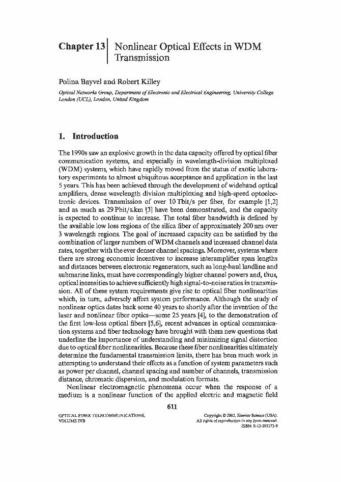
Chapter 13
Polina Bayvel and Robert Killey Optical Networks Group, Department of Electronic and Electrical Engineering, University College London (UCL), London, United Kingdom
Nonlinear Optical Effects in WDM Transmission
1. Introduction
The 1990s saw an explosive growth in the data capacity offered by optical fiber communication systems, and especially in wavelength-division multiplexed (WDM) systems, which have rapidly moved from the status of exotic labora- tory experiments to almost ubiquitous acceptance and application in the last 5 years. This has been achieved through the development of wideband optical amplifiers, dense wavelength division multiplexing and high-speed optoelec- tronic devices. Transmission of over 10Tbit/s per fiber, for example [1,2] and as much as 29Pbit/s.lun [3] have been demonstrated, and the capacity is expected to continue to increase. The total fiber bandwidth is defined by the available low loss regions of the silica fiber of approximately 200 nm over 3 wavelength regions. The goal of increased capacity can be satisfied by the combination of larger numbers of WDM channels and increased channel data rates, together with the ever denser channel spacings. Moreover, systems where there are strong economic incentives to increase interamplifier span lengths and distances between electronic regenerators, such as long-haul landline and submarine links, must have correspondingly higher channel powers and, thus, optical intensities to achieve sufliciently high signal-to-noise ratios in transmis- sion. All of these system requirements give rise to optical fiber nonlinearities which, in turn, adversely affect system performance. Although the study of nonlinear optics dates back some 40 years to shortly after the invention of the laser and nonlinear fiber optics-some 25 years [4], to the demonstration of the first low-loss optical fibers [5,6], recent advances in optical comunica- tion systems and fiber technology have brought with them new questions that underline the importance of understanding and minimizing signal distortion due to optical fiber nonlinearities. Because these fiber nonlinearities ultimately determine the fundamental transmission limits, there has been much work in attempting to understand their effects as a function of system parameters such as power per channel, channel spacing and number of channels, transmission distance, chromatic dispersion, and modulation formats.
Nonlinear electromagnetic phenomena occur when the response of a medium is a nonlinear function of the applied electric and magnetic field
611 OPTICAL FIBER TELECOMMUNICATIONS, VOLUME IVB
Commght 0 2002, Elsevier Science (USA). All rights of nproduction in any form reserved.
ISBN. 0-12395173-9
612 Polina Bayvel and Robert Killey
amplitudes. The nonlinearities are inherently described by Maxwell’s equa- tions by including the nonlinear polarization term. Fiber nonlinearities can be classified into two types: stimulated scattering and intensity-dependent refractive index [7,8]. Stimulated scattering leads to intensity-dependent gain or loss. The most detrimental of the scattering effects is stimulated Raman scattering (SRS), in which interactions between the photons and the silica leads to the transfer of the light intensity from shorter to longer wavelengths, as the photons transfer energy to the silica molecules (optical phonons). It can be used to provide broadband amplification in optical fiber, and the SRS gain in silica has a wide bandwidth on the order of 12 THz (-1OOnm around A. = 1.5 pm) due to its amorphous structure. The application is described in detail in Chapter 5, OFT IVA, and a good review of SRS is given in [7-91. However, it can also limit the performance of multichannel communication systems through the transfer of energy between the channels separated by the frequency offsets within the Raman gain spectrum, leading to wavelength- dependent loss, with short wavelengths losing power to the longer wavelengths. SRS can also result in nonlinear cross-talk between WDM channels across a wide wavelength range.
In contrast, the second type of effect, known as the Kerr effect, is due to the intensity dependence of the refractive index which, in turn, gives rise to an intensity-dependent phase shift of the optical field. This leads to the effects of self-phase modulation (SPM), cross-phase modulation (XPM), and four- wave mixing (FWM). This chapter is devoted to this second category and its aim is to describe how these nonlinearities impair transmission perfor- mance, describe their interaction with chromatic dispersion, as well as review recently developed techniques to characterize and attempts to suppress their effects.
The refractive index of the silica, n, increases with the optical power P:
n = no + n2-Y P Aeff
(13.1)
where no is the linear refractive index at low powers, and A,ff is the effective area of the optical mode in the fiber, which in typical single-mode fibers is 50-80 pm2. It is clear that one of the most direct ways of reducing the nonlin- ear refractive index dependence is to increase the fiber effective area, see for example [lo]. Much research has been focused on optimizing the effective area and chromatic dispersion characteristics [see Chapter 2, OFT IVA]. The coef- ficient n2 is typically -2.6 x lo-” mZ/W in standard single-mode fiber, with measured values varying over the range of 2.2-3.4 10-20m2/W, depending on fiber type and measurement technique [7].
The propagation of short optical pulses in single-mode fibers subject to nonlinearities is described well by the equation, referred to as the nonlinear

13. Nonlinear Optical Effects in WDM Transmission 613
Schrodinger equation (NLSE) [7]:
au i aZu u az 2 at2 2 - + -82- + -u = iylu12u, (13.2)
where u is the pulse amplitude, assumed to be normalized so that luI2 repre- sents the optical power; u is the fiber loss, and the group velocity (or chromatic) dispersion of the single mode fiber (SMF), 8 2 = - h 2 D s ~ ~ / 2 n c . The fiber nonlinear coefficient y is defined (in W-lkm-') as
(13.3)
where 00 is the optical carrier frequency of the pulse. It can clearly be seen from Eq. 13.2 that the nonlinearity-induced intensity distortion is the result of an interaction between nonlinear refraction and the fiber chromatic dispersion. The exact nature of this interaction depends on the magnitude and sign of the fiber dispersion, and is key to the understanding of the fiber nonlinearities in WDM transmission.
The NLSE is a nonlinear partial differential equation and, in most cases, must be solved numerically, typically using the split-step Fourier method. First proposed by Tappert in 1973, it is one of the fastest numerical techniques for the solution of the NLSE and has now become the technique of choice for the analysis and understanding of pulse propagation in single- and multichan- nel optical fiber systems. Throughout this chapter the simulation results have been obtained using the split-step Fourier method, typically using sequences with 128bits and a step size of lOOm and the nonlinear fiber coefficient y = 1.2 W-lkm-'.
2. Self-phase Modulation
The first effect of the nonlinear refractive index that must be considered in both single- and multichannel transmission is self-phase modulation, that is, the change of the optical phase of a channel by its own intensity. The high peak power of the signal pulses increases the refractive index of the silica, leading to a lower group velocity. Solving Eq. 13.2 shows that an optical phase shift, A&PM, results after propagation over distance L, given by
where the effective length L,ff takes the fiber loss into account, and is defined as
1 - exp( - a!L) Leff =
a! (13.5)
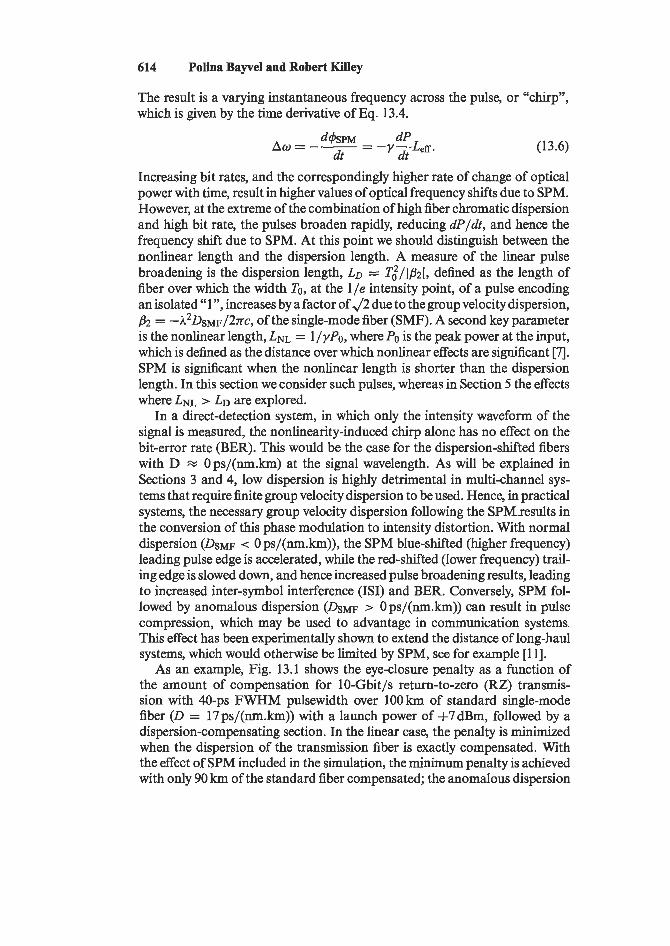
614 Polina Bayvel and Robert Killey
The result is a varying instantaneous frequency across the pulse, or “ c h q ” , which is given by the time derivative of Eq. 13.4.
d&PM dP dt dt
AW = -- = -y-L,r. (13.6)
Increasing bit rates, and the correspondingly higher rate of change of optical power with time, result in higher values of optical frequency shifts due to SPM. However, at the extreme of the combination of high fiber chromatic dispersion and high bit rate, the pulses broaden rapidly, reducing dP/dt, and hence the frequency shift due to SPM. At this point we should distinguish between the nonlinear length and the dispersion length. A measure of the linear pulse broadening is the dispersion length, LO = T;/Ipzl, defined as the length of fiber over which the width TO, at the l /e intensity point, of a pulse encoding an isolated “1 ”, increases by a factor of ,/2 due to the group velocity dispersion, 8 2 = - h 2 D s ~ ~ / 2 n c , of the single-mode fiber (SMF). A second key parameter is the nonlinear length, L m = 1/ yP0, where PO is the peak power at the input, which is defined as the distance over which nonlinear effects are significant [A. SPM is significant when the nonlinear length is shorter than the dispersion length. In this section we consider such pulses, whereas in Section 5 the effects where L m > LD are explored.
In a direct-detection system, in which only the intensity waveform of the signal is measured, the nonlinearity-induced chirp alone has no effect on the bit-error rate (BER). This would be the case for the dispersion-shifted fibers with D = Ops/(nm.km) at the signal wavelength. As will be explained in Sections 3 and 4, low dispersion is highly detrimental in multi-channel sys- tems that require finite group velocity dispersion to be used. Hence, in practical systems, the necessary group velocity dispersion following the SPM..results in the conversion of this phase modulation to intensity distortion. With normal dispersion (DSMF < 0 ps/(nm.km)), the SPM blue-shifted (higher frequency) leading pulse edge is accelerated, while the red-shifted (lower frequency) trail- ing edge is slowed down, and hence increased pulse broadening results, leading to increased inter-symbol interference (ISI) and BER. Conversely, SPM fol- lowed by anomalous dispersion (DSMF =- Ops/(nm.km)) can result in pulse compression, which may be used to advantage in communication systems. This effect has been experimentally shown to extend the distance of long-haul systems, which would otherwise be limited by SPM, see for example [l 11.
As an example, Fig. 13.1 shows the eye-closure penalty as a function of the amount of compensation for 10-Gbit/s return-to-zero (RZ) transmis- sion with 40-ps FWHM pulsewidth over 100 km of standard single-mode fiber (D = 17 ps/(nm.km)) with a launch power of +7 dBm, followed by a dispersion-compensating section. In the linear case, the penalty is minimized when the dispersion of the transmission fiber is exactly compensated. With the effect of SPM included in the simulation, the minimum penalty is achieved with only 90 km of the standard fiber compensated; the anomalous dispersion

13. Nonlinear Optical Effects in WDM Transmission 615
4/
65 3 3 - c 7 '\
/ 0 - I I ' \-,/' , I
70 80 90 100 110 120 130 Dispersion compensation (%)
Fig. 13.la Calculated eye-opening penalty due to dispersion and SPM for a 100-km link of standard SPM (D = 17 ps/(nm-km)) versus value of post-compensation at the receiver. Low power linear transmission (dashed line), 7 dBm launch power (solid line).
65- E 3 - c $ 2 Q m C
a Q 0
'E 1 7 0 5 10 15
Number of spans
I I I I
I - 100 ps
Fig. 13.lb Top: Calculated SPM-induced eye closure vs transmission distance with NRZ signal format and 13 dBm launch power, without (circular markers) and with (square markers) optimized anomalous dispersion at the receiver for 10-Gbit/s mul- tispan transmission with exact inline span compensation. Bottom: Experimental (le@) and simulated (right) eye diagrams after 8 spans with 8 dBm launch power and exact dispersion compensation, showing SPM-induced pulse broadening.
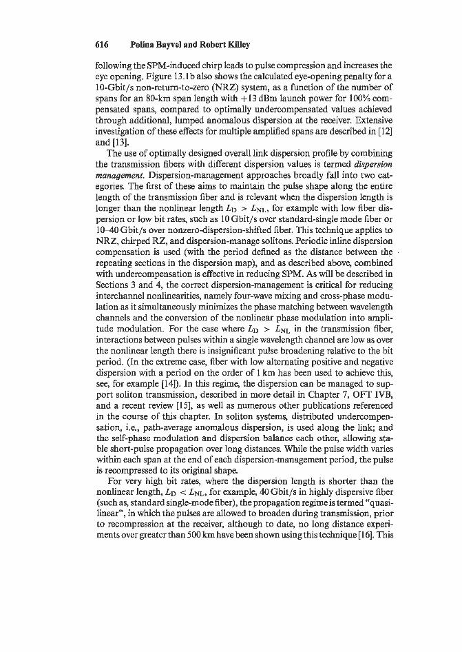
616 Polina Bayvel and Robert Killey
following the SPM-induced chirp leads to pulse compression and increases the eye opening. Figure 13.1 b also shows the calculated eye-opening penalty for a 10-Gbit/s non-return-to-zero (NRZ) system, as a function of the number of spans for an 80-km span length with + 13 dBm launch power for 100% com- pensated spans, compared to optimally undercompensated values achieved through additional, lumped anomalous dispersion at the receiver. Extensive investigation of these effects for multiple amplified spans are described in [12] and [13].
The use of optimally designed overall link dispersion profile by combining the transmission fibers with different dispersion values is termed dispersion management. Dispersion-management approaches broadly fall into two cat- egories. The first of these aims to maintain the pulse shape along the entire length of the transmission fiber and is relevant when the dispersion length is longer than the nonlinear length LD > LNL, for example with low fiber dis- persion or low bit rates, such as 10 Gbit/s over standard-single mode fiber or 1040 Gbit/s over nonzero-dispersion-shifted fiber. This technique applies to NRZ, chirped RZ, and dispersion-manage solitons. Periodic inline dispersion compensation is used (with the period defined as the distance between the repeating sections in the dispersion map), and as described above, combined with undercompensation is effective in reducing SPM. As will be described in Sections 3 and 4, the correct dispersion-management is critical for reducing interchannel nonlinearities, namely four-wave mixing and cross-phase modu- lation as it simultaneously minimizes the phase matching between wavelength channels and the conversion of the nonlinear phase modulation into ampli- tude modulation. For the case where LD > LNL in the transmission fiber, interactions between pulses within a single wavelength channel are low as over the nonlinear length there is insignificant pulse broadening relative to the bit period. (In the extreme case, fiber with low alternating positive and negative dispersion with a period on the order of 1 km has been used to achieve this, see, for example [14]). In this regime, the dispersion can be managed to sup- port soliton transmission, described in more detail in Chapter 7, OFT IVB, and a recent review [15], as well as numerous other publications referenced in the course of this chapter. In soliton systems, distributed undercompen- sation, i.e., path-average anomalous dispersion, is used along the link; and the self-phase modulation and dispersion balance each other, allowing sta- ble short-pulse propagation over long distances. While the pulse width varies within each span at the end of each dispersion-management period, the pulse is recompressed to its original shape.
For very high bit rates, where the dispersion length is shorter than the nonlinear length, LD < LNL, for example, 40 Gbit/s in highly dispersive fiber (such as, standard single-mode fiber), the propagation regime is termed “quasi- linear”, in which the pulses are allowed to broaden during transmission, prior to recompression at the receiver, although to date, no long distance experi- ments over greater than 500 km have been shown using this technique [16]. This

13. Nonlinear Optical Effects in WDM 'Ikansmission 617
approach aims to minimize both inter- and intrachannel effects due to the low peak power of the broadened pulses, and works best with very short RZ pulses, as these rapidly disperse. However, the broad spectra associated with them limits the channel spacing and, hence, the spectral efficiency in WDM systems.
A further complication arises in wideband WDM systems due to the dispersion slope, dDldh, which may not be exactly compensated by the com- pensating fiber, and this leads to positive and negative values of accumulated dispersion for channels at the extreme wavelengths of the WDM spectrum. This can lead to a variation in the performance across the channels. If neces- sary, the use of additional dispersion on a channel-by-channel basis between the demultiplexer and receiver can be used to improve the performance [17].
In summary, distributed dispersion compensation to achieve low anoma- lous path-average dispersion over the link helps mitigate SPM-induced distortions for the case of LD > LNL. Fortunately, this is also compatible for combating multichannel nonlinearities, as will be described in the following sections.
3. Four-Wave Mixing
In multichannel transmission the beating between light at different frequen- cies leads to the phase modulation of the channels and hence generation of modulation sidebands at new frequencies, termed four-wave mixing [8, 18-24]. If three components copropagate at frequencies J, A and fk, a new wave is generated at frequencyJyk , where,
f. -f yk - I (13.7)
This causes penalties if the frequency J jk is equal or close to the frequency of an existing WDM channel, so that the resulting interferometric noise falls within the bandwidth of the receiver.
To predict the effect of FWM, an expression predicting the efficiency, 9, of the FWM process has been derived (see e.g., [SI). The power of the generated new signal is given by [9],
Pijk = (dF yL)2PiPjPke-ffLT), (13.8)
where the degeneracy factor dF = 1 when i = j , dF = 2 when i # j . The FWM efficiency is given by,
1 - exp( - [a + A/3]L) ' = I (a+iA/3)L (13.9)
assuming the original channels are copolarized. The quantity Aj3 in Eq. 13.9 is the difference in the propagation constant between the channels due to the

618 Polina Bayvel and Robert KiJley
fiber dispersion
AS = pi + pj - p k - &k = bZ(wi - wk)(aj - ak), (13.10)
where D is the dispersion at the signal wavelength A andA,J, andfk are the optical frequencies of channels i , j , and k. Equation 13.9 predicts that the FWM efficiency is largest when AB is low and the phase matching between the channels is high, for example in systems with close channel spacing and dispersion-shifted fiber at wavelengths close to the zero dispersion wavelength, LO. The FWM efficiency as a function of channel spacing with two values of fiber dispersion is plotted in Fig. 13.2, showing the increased efficiency with low dispersion. In WDM systems based on low-dispersion fiber, an effective tech- nique to minimize crosstalk due to FWM is to use unequal channel spacing [25], so that the FWM components are not generated at frequencies corre- sponding to the channel frequencies. In practical WDM systems, installed over existing fiber, the implementation of this would be to use a subset of the transmitter wavelengths, even though the standard transmitter wavelengths (current systems are equipped with as many as 160 wavelength channels) have a constant wavelength/frequency spacing.
However, the most effective technique to avoid FWM crosstalk is the use of transmission fiber with high local dispersion, so that the phase matching between WDM channels is minimized. Periodic dispersion compensation can be used to maintain a low accumulated dispersion-all part of optimizing the dispersion-management of the link. Although the use of high local dispersion is effective at suppressing interchannel FWM in WDM transmission systems, its detrimental impact in limiting transmission distances of very high channel
0 50 100 150 200 Channel spacing Af (GHz)
Fig. 13.2 Plot of the four-wave mixing efficiency r] (normalized to the efficiency with perfectly phase matched channels), calculated for standard single-mode and dispersion-shifted fiber links of length 100 lan and loss a! = 0.21 dB/km.
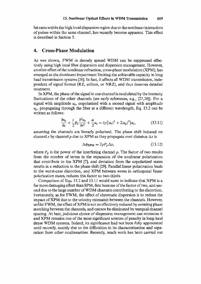
13. Nonlinear Optical Effects in WDM Transmission 619
bit rates within the high local dispersion region due to the nonlinear interaction of pulses within the same channel, has recently become apparent. This effect is described in Section 5.
4. Cross-Phase Modulation
As was shown, FWM in densely spaced WDM can be suppressed effec- tively using high local fiber dispersion and dispersion management. However, another effect of the nonlinear refraction, cross-phase modulation (XPM), has emerged as the dominant impairment limiting the achievable capacity in long haul transmission systems [26]. In fact, it affects all WDM transmission, inde- pendent of signal format (RZ, soliton, or NRZ), and thus deserves detailed treatment.
In XPM, the phase of the signal in one channel is modulated by the intensity fluctuations of the other channels (see early references, e.g., [27,28]). For a signal with amplitude us, copolarized with a second signal with amplitude up, propagating through the fiber at a different wavelength, Eq. 13.2 can be written as follows:
(13.11) aus i a2us (11 - + -B2- + -us = iy(lus12 + 21~,1~)u,, az 2 at2 2
assuming the channels are linearly polarized. The phase shift induced on channel s by channelp due to XPM as they propagate over distance Az is
A h M = 2YP,Az, (1 3.12)
where Pp is the power of the interfering channel p. The factor of two results from the number of terms in the expansion of the nonlinear polarization that contribute to the XPM [7], and deviation from the copolarized states results in a reduction in the phase shift [29]. Parallel linear polarization leads to the worst-case distortion, and XPM between waves in orthogonal linear polarization states, reduces this factor to two-thirds
Comparison of Eqs. 13.2 and 13.1 1 would seem to indicate that XPM is a far more damaging effect than SPM, first because of the factor of two, and sec- ond due to the large number of WDM channels contributing to the distortion. Fortunately, as for FWM, the effect of chromatic dispersion is to reduce the impact of XPM due to the velocity mismatch between the channels. However, unlike FWM, the effect of XPM is not so effectively reduced by avoiding phase matching between the channels, and cannot be eliminated by unequal channel spacing. At best, judicious choice of dispersion management can minimize it and XPM remains one of the most significant sources of penalty in long-haul dense WDM systems. Indeed, its significance had not been fully appreciated until recently, mainly due to the difficulties in its characterization and sepa- ration from other nonlinearities. Recently, much work has been carried out
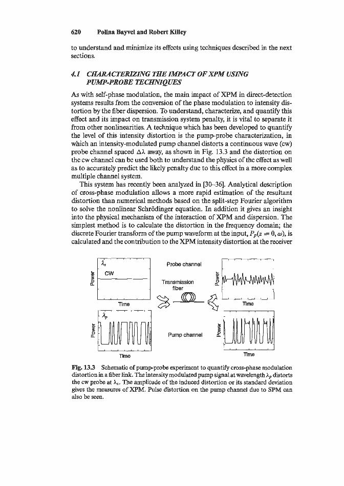
620 Polina Bayvel and Robert KiUey
to understand and minimize its effects using techniques described in the next sections.
4.1 CRARA CTERLZING THE IMPACT OF XPM USING PUMP-PROBE TECHNIQUES
As with self-phase modulation, the main impact of XPM in direct-detection systems results from the conversion of the phase modulation to intensity dis- tortion by the fiber dispersion. To understand, characterize, and quantify this effect and its impact on transmission system penalty, it is vital to separate it from other nonlinearities A technique which has been developed to quantify the level of this intensity distortion is the pump-probe characterization, in which an intensity-modulated pump channel distorts a continuous wave (cw) probe channel spaced AA away, as shown in Fig. 13.3 and the distortion on the cw channel can be used both to understand the physics of the effect as well as to accurately predict the likely penalty due to this effect in a more complex multiple channel system.
This system has recently been analyzed in [30-361. Analytical description of cross-phase modulation allows a more rapid estimation of the resultant distortion than numerical methods based on the split-step Fourier algorithm to solve the nonlinear Schrodinger equation. In addition it gives an insight into the physical mechanism of the interaction of XPM and dispersion. The simplest method is to calculate the distortion in the frequency domain; the discrete Fourier transform of the pump waveform at the input, Pp(z = 0, o), is calculated and the contribution to the XPM intensity distortion at the receiver
7 1 Probechannel
z s 0 Transmission Q
Time
Pump channel 2 5 2
Time Time
Fig. 13.3 Schematic of pump-probe experiment to quantify cross-phase modulation distortion in a fiber link. The intensity modulated pump signal at wavelength AP distorts the cw probe at As. The amplitude of the induced distortion or its standard deviation gives the measures of XPM. Pulse distortion on the pump channel due to SPM can also be seen.

13. Nonlinear Optical EffeeQ in WDM Transmission 621
is obtained for each sinusoidal frequency component. These contributions are combined to give the resulting probe spectrum, and the inverse Fourier transform of the probe signal is then calculated to obtain the total probe distortion in the time domain in the following way.
Key to the characterization of XPM is the concept of the walk-off between channels, delined as the distan-dependent relative temporal position of the channels, in units of ps/km, which arises as a result of the different group velocities us and up of the probe and pump,
(1 3.1 3)
The walk-off parameter, d
the fiber:
results in the phase shift of the pump modulation component Pp(z, o) = Iup T I relative to the probe as they co-propagate through
h ( z r 0 = 2Y i= lup(0, t + dspd)[2 e4&. (1 3.14)
The walk-off between the channels reduces the magnitude of the total phase modulation of the probe f37. In the analysis of the intensity distortion due to XPM, the phase modulation of the probe over inhitesimal lengths, L, of the transmission fiber is calculated and the resulting sinusoidal intensity modulation, dPs(o), at the receiver due to the dispersion of the follow- ing fiber is estimated, using the equation describing the phase-to-intensity conversion [38]:
(13.15)
where dPs(z,o) is the power modulation, normalized to the average probe power, and /?z(re~) is the residual accumulated dispersion,
(13.16)
between the position of the nonlinear phase distortion at distance z and the d v e r at distance L. It can be seen that reducing the value of #3qm) results in lower intensity distortion because of a less efficient phaeto-amplitude conversion. This can be achieved through inline dispersion compensation and is one of the techniques for nonlinearity-suppressing dispersion management.
Integrating Eq. 13.15 over the full length of the link, the total distortion due to XPM is given by [38]:

622 Polina Bayvel and Robert Killey
where AP, is the probe modulation depth at the output, normalized to the average probe power at frequency w, and Hsp(w) is the XPM transfer fmction.
1 - exp (-a + ibi) Hsp(w) = 2yi exp (i4) [ ( a-ibl
1 - exp (-a + ib2) a! - ib2
- exp (- i4)
where
4 = i&,,p2, bi = (dspw - B2w2/2) L and b2 = (dspw + &w2/2) L. (13.19-13.21)
The probe waveform in the time domain is given by the inverse Fourier trans- form of AP,. For multispan systems, the total distortion is the sum of the distortion components generated from each span.
From Eq. 13.18, it can be seen that the XPM-distorted probe waveform at the output resembles a high-pass filtered version of the pump input wave- form, with the filter transfer function given by Hsp, so that the distortion of the cw probe is significant only at high frequencies. By way of an exam- ple, the calculated transfer functions, I Hsp I , of dispersion-compensated 60-km spans are shown in Fig. 13.4 for channel spacing of Ah = 0.4nm, comparing the XPM distortion in SMF and non-zero dispersion-shifted fiber (NZ-DSF, D = 4ps/(nm/km)). In both links, the dispersion was compensated at the receiver, and a fiber nonlinear coefficient of y = 1.2 W-lkm-' was assumed. Despite the large difference in dispersion between the links, the magnitude of the transfer functions are similar. The phase modulation in the NZDSF
O . O o 3 V 0.002
0.000 L d L 0 1 2 3 4 5
Frequency (GHz)
0.0°3 r----
Frequency (GHz)
Fig. 13.4 XPM transfer function, Hsp, of 6 0 h fiber spans, with channel spacing of AA = 0.4ps, in SMF (D = 17ps/(nm/km)) (left) and non-zero dispersion-shifted fiber (NZ-DSF, D = 4ps/(nm/km)) (right), both with dispersion compensation at the receiver. Values calculated from Eq. (13.17) (lines) and by split-step Fourier simulations (markers). See ref [45].

13. Nonlinear Optical Effects in WDM Transmission 623
is greater; however, the conversion of this phase modulation to intensity dis- tortion is lower due to the lower fiber dispersion. This trend was confirmed in experimental pump-probe measurements comparing XPM in the two fiber types, each with a span length of 80km [39]. The XPM-induced intensity distortion was found to be approximately two times larger in the dispersion- shifted fiber, due to the smaller effective area of 55 ,urn2 compared with the 80 ,urn* of the standard fiber.
Equation 13.18 predicts areduction in intensity distortion as the wavelength spacing is increased due to the increase in the walk-off between the chan- nels, dsp = D ~ M F A ~ , which appears in the denominator terms of the transfer function, Hsp. Pump-probe experiments have been carried out by a number of groups confirming the inverse relationship between channel spacing and XPM distortion. Figure 13.5 shows the experimental result of pump-probe measure- ments [40] over a two-span, dispersion-compensated standard fiber link, also shown in Fig. 13.5. The standard deviation of the detected probe level, CTX~M,
is plotted as a function of wavelength spacing, Ah, exhibiting the reduction with increasing spacing predicted by Eq. 13.18,.with C T X ~ M = 0.1 (normalized to the average detected probe power) with 0.4-nm spacing, reducing to < 0.02 for 2 nm and above.
An experimentally measured probe waveform at the output of this two-span, standard single-mode fiber (DSMF = 17 ps/(nm/km)) is shown in the inset of Fig. 13.5. The XPM high-pass filtering effect can be observed as the peaks in the distortion arising from the pulse edges in the PRBS pump waveform. In a practical system this would have the effect of causing additional noise on the “lyy-rail and, hence, increase the bit-error rate. This is further addressed in the next section.
Pattern generator 10 GbiW
DCF1 Probe E b
0 0.5 1 1.5 2 Wavelength spacing (nrn)
Fig. 13.5 Left: Pump-probe experiment, over a two span link with standard single- mode fiber (D = 17 ps/(nm/km)) and pre- and post-dispersion compensation. Channel launch powers: 13 dBm in the first span, 9 dBm in the second. Right: Standard deviation of the probe distortion with a PRBS modulated pump signal, as a function of channel spacing, experimental values (markers) and simulations, with parallel and orthogonal polarization states (lines). Inset: Measured distorted probe waveform. See ref [40].
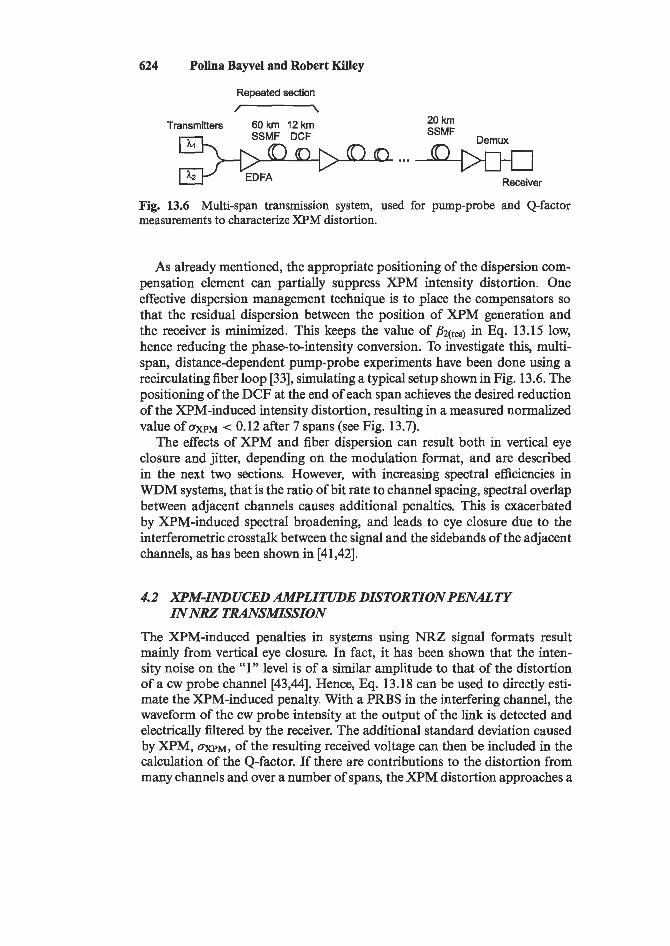
624 Polina Bayvel and Robert Killey
Repeated section - Transmitters 60 krn 12km
SSMF DCF
ODOCn.
20 krn SSMF
Demux
Receiver
Fig. 13.6 Multi-span transmission system, used for pump-probe and Q-factor measurements to characterize XPM distortion.
As already mentioned, the appropriate positioning of the dispersion com- pensation element can partially suppress XPM intensity distortion. One effective dispersion management technique is to place the compensators so that the residual dispersion between the position of XPM generation and the receiver is minimized. This keeps the value of &res) in Eq. 13.15 low, hence reducing the phase-to-intensity conversion. To investigate this, multi- span, distance-dependent pump-probe experiments have been done using a recirculating fiber loop [33], simulating a typical setup shown in Fig. 13.6. The positioning of the DCF at the end of each span achieves the desired reduction of the XPM-induced intensity distortion, resulting in a measured normalized value of ~ Q M < 0.12 after 7 spans (see Fig. 13.7).
The effects of XPM and fiber dispersion can result both in vertical eye closure and jitter, depending on the modulation format, and are described in the next two sections. However, with increasing spectral efficiencies in WDM systems, that is the ratio of bit rate to channel spacing, spectral overlap between adjacent channels causes additional penalties. This is exacerbated by XPM-induced spectral broadening, and leads to eye closure due to the interferometric crosstalk between the signal and the sidebands of the adjacent channels, as has been shown in [41,42].
4.2 PM-INDUCED AMPLITUDE DISTORTION PENALTY IN NRZ TRANSMISSION
The XPM-induced penalties in systems using NRZ signal formats result mainly from vertical eye closure. In fact, it has been shown that the inten- sity noise on the “1” level is of a similar amplitude to that of the distortion of a cw probe channel [43,44]. Hence, Eq. 13.18 can be used to directly esti- mate the XPM-induced penalty. With a PRBS in the interfering channel, the waveform of the cw probe intensity at the output of the link is detected and electrically filtered by the receiver. The additional standard deviation caused by XPM, q p ~ , of the resulting received voltage can then be included in the calculation of the Q-factor. If there are contributions to the distortion from many channels and over a number of spans, the XPM distortion approaches a
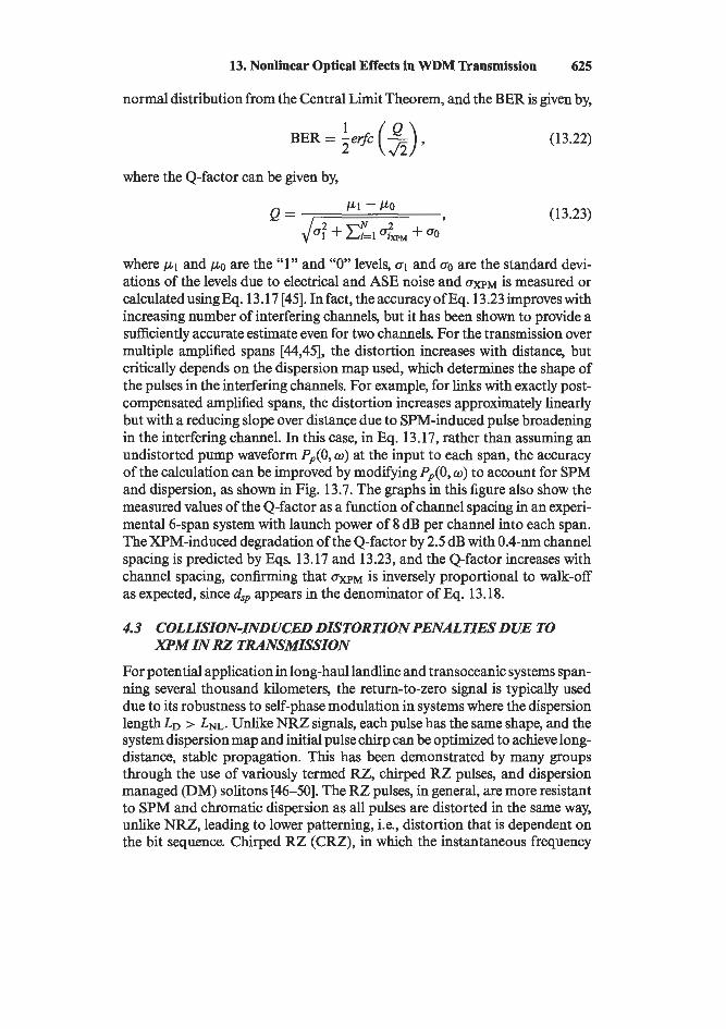
13. Nonlinear Optical Effects in WDM Transmission 625
normal distribution from the Central Limit Theorem, and the BER is given by,
1 2
BER = -e$c (-$) , where the Q-factor can be given by,
(1 3.22)
(1 3.23)
where and po are the “1” and “0” levels, a1 and a0 are the standard devi- ations of the levels due to electrical and ASE noise and a x p ~ is measured or calculated using Eq. 13.17 [45]. In fact, the accuracy of Eq. 13.23 improves with increasing number of interfering channels, but it has been shown to provide a sufficiently accurate estimate even for two channels. For the transmission over multiple amplified spans [44,45], the distortion increases with distance, but critically depends on the dispersion map used, which determines the shape of the pulses in the interfering channels. For example, for links with exactly post- compensated amplified spans, the distortion increases approximately linearly but with a reducing slope over distance due to SPM-induced pulse broadening in the interfering channel. In this case, in Eq. 13.17, rather than assuming an undistorted pump waveform Pp(O, w ) at the input to each span, the accuracy of the calculation can be improved by modifying Pp(O, w) to account for SPM and dispersion, as shown in Fig. 13.7. The graphs in this figure also show the measured values of the Q-factor as a function of channel spacing in an experi- mental 6-span system with launch power of 8 dB per channel into each span. The XPM-induced degradation of the Q-factor by 2.5 dB with 0.4-nm channel spacing is predicted by Eqs. 13.17 and 13.23, and the Q-factor increases with channel spacing, confirming that axp~ is inversely proportional to walk-off as expected, since dsp appears in the denominator of Eq. 13.18.
4.3 COLLISION-INDUCED DISTORTION PENALTIES DUE TO XPM IN RZ TRQNSMISSION
For potential application in long-haul landline and transoceanic systems span- ning several thousand kilometers, the return-to-zero signal is typically used due to its robustness to self-phase modulation in systems where the dispersion length LD > LNL. Unlike NRZ signals, each pulse has the same shape, and the system dispersion map and initial pulse chirp can be optimized to achieve long- distance, stable propagation. This has been demonstrated by many groups through the use of variously termed RZ, chirped RZ pulses, and dispersion managed (DM) solitons [46-501. The RZ pulses, in general, are more resistant to SPM and chromatic dispersion as all pulses are distorted in the same way, unlike NRZ, leading to lower patterning, Le., distortion that is dependent on the bit sequence. Chirped RZ (CRZ), in which the instantaneous frequency
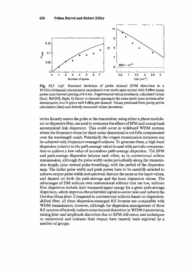
626 Polina Bayvel and Robert Killey
0.15
0.05
10
9
7
6
0 0 1 2 3 4 5 6 7 0.5 1 1.5 2 2.5 3
Number of spans ~ i f i (nm-')
Fig. 13.7 Lej?: Standard deviation of probe channel XPM distortion in a 10 Gbit/s/channel transmission experiment over multi-span system with 8 dBm pump power and channel spacing of 0.4 nm. Experimental values (markers), calculated values (line). Ref [45]. Right: Q-factor vs channel spacing in the same multi-span systems after transmission over 6 spans with 8 dBm per channel. Values predicted from pump-probe calculation (line) and directly measured values (markers).
varies linearly across the pulse at the transmitter, using either a phase modula- tor or dispersive fiber, are used to overcome the effects of SPM and nonoptimal accumulated link dispersion. This could occur in wideband WDM systems where the dispersion slope (or third-order dispersion) is not fully compensated over the wavelength comb. Potentially the longest transmission instances can be achieved with dispersion-managed solitons. To generate these, a high local dispersion (relative to the path-average value) is used with periodic compensa- tion to achieve a low value of anomalous path-average dispersion. The SPM and path-average dispersion balance each other, as in conventional soliton transmission, although the pulse width varies periodically along the transmis- sion length, (also termed pulse-breathing), with the period of the dispersion map. The initial pulse width and peak power have to be carefully selected to achieve output pulse width and spectrum that are the same as the input values, and depend on both the path-average and the local dispersion values. The advantages of DM solitons over conventional solitons that use low, uniform fiber dispersion include their increased signal energy for a given path-average dispersion, which improves the achievable signal-to-noise ratio and reduces the Gordon-Haus jitter. Compared to conventional solitons based on dispersion- shifted fiber, all these dispersion-managed RZ formats are compatible with WDM transmission; however, although the dispersion management of these RZ systems effectively reduces interchannel distortion in WDM transmission, timing jitter and amplitude distortion due to XPM still occur, and techniques to understand and evaluate their impact have recently been explored by a number of groups.

13. Nonlinear Optical Effects in WDM Transmission 627
With multichannel transmission, the pulses in different channels propa- gate at different velocities due to the high local dispersion of the fiber, and consequently, collisions between pulses (i.e., two or more pulses at different wavelengths, spatially overlapping and walking through each other) occur dur- ing transmission, leading to nonlinear crosstalk. To minimize the nonlinear crosstalk, extremely low channel powers are required [50], limiting the trans- mission distance to a maximum (to date) of 4500 km for 32 WDM channels at 40 Gbit/s [51]. The effect of XPM during the collisions is not only to distort the pulse amplitude as in NRZ systems, but also to vary the arrival times of the pulses at the receiver. This contributes to the total timing jitter defined as the standard deviation of the timing shifts of all the pulses. Both of these impairments are described in Fig. 13.8. Much work has focused on charac- terizing the XPM-induced timing jitter in dispersion-managed RZ systems, and optimizing the dispersion map to minimize this effect. The timing shift of a probe pulse arises from the shift of its carrier frequency, Aws, due to a collision with a pump pulse. Applying the soliton perturbation method to the nonlinear Schrodinger equation [52], the XPM-induced frequency shift of the probe pulse, Ams, and timing separation of the peaks of the pump and probe pulses, AT,, are given by,
d(Aw,) -2y(z) O0 aP, dz - EO 100ps%-dt’ (13.24)
(13.25)
L dP AmmM = loL*& = - 2 y L d z
0 dt
Power at 4
Power at
I A . Velocity change, giving timing jitter: “ =AmXPMN&es)
Chirp-induced amplitude distortion
Fiber time
AwXPMata, I $ .dispersion
N-number of spans following XPM &,,-residual dispersion per span
Fig. 13.8 Schematic of the process of pulse collisions and the effect of interchannel cross-phase modulation, explaining the mechanism for the resultant pulse amplitude distortion and timing jitter.
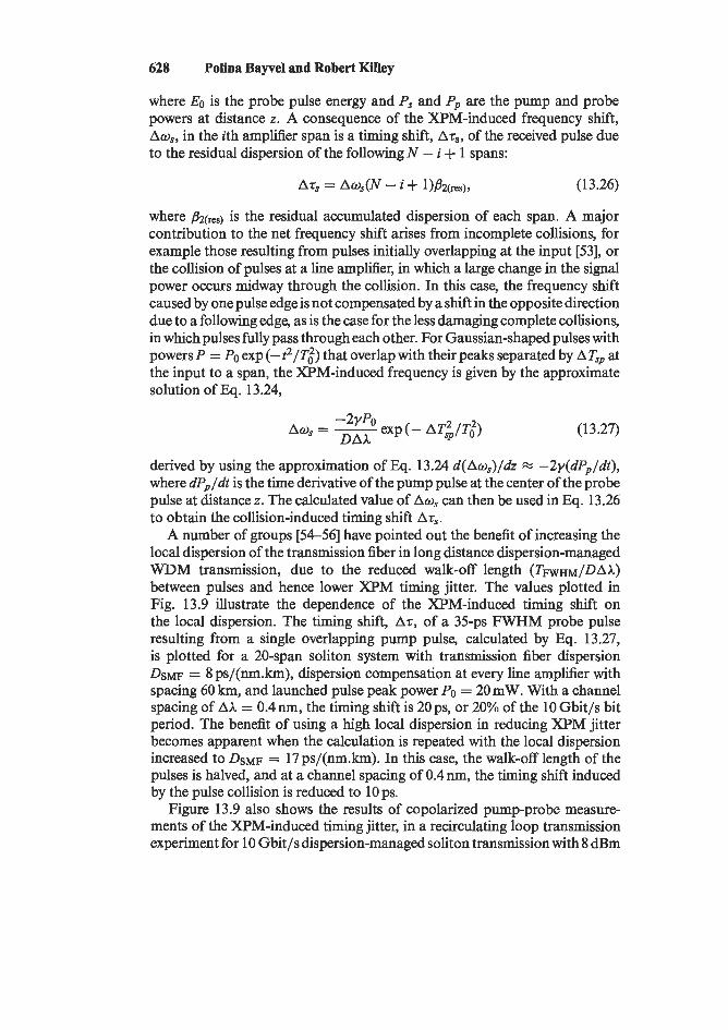
628 Polina Bayvel and Robert Killey
where EO is the probe pulse energy and P, and Pp are the pump and probe powers at distance z. A consequence of the XPM-induced frequency shift, Ams, in the ith amplifier span is a timing shift, At,, of the received pulse due to the residual dispersion of the following N - i + 1 spans:
ATs = Aws(N - i + 1)BZ(reS), (13.26)
where is the residual accumulated dispersion of each span. A major contribution to the net frequency shift arises from incomplete collisions, for example those resulting from pulses initially overlapping at the input [53], or the collision of pulses at a line amplifier, in which a large change in the signal power occurs midway through the collision. In this case, the frequency shift caused by one pulse edge is not compensated by a shift in the opposite direction due to a following edge, as is the case for the less damaging complete collisions, in which pulses f d y pass through each other. For Gaussian-shaped pulses with powers P = PO exp (- t2/T;) that overlap with their peaks separated by ATsp at the input to a span, the XPM-induced frequency is given by the approximate solution of Eq. 13.24,
(1 3.27)
derived by using the approximation of Eq. 13.24 d(Aw,)/dz FZ -2y(dFp/dt), where dPp/dt is the time derivative of the pump pulse at the center of the probe pulse at distance z. The calculated value of Aw, can then be used in Eq. 13.26 to obtain the collision-induced timing shift At,.
A number of groups [5&56] have pointed out the benefit of increasing the local dispersion of the transmission fiber in long distance dispersion-managed WDM transmission, due to the reduced walk-off length (TFWHMIDAh) between pulses and hence lower XPM timing jitter. The values plotted in Fig. 13.9 illustrate the dependence of the XPM-induced timing shift on the local dispersion. The timing shift, AT, of a 35-ps FWHM probe pulse resulting from a single overlapping pump pulse, calculated by Eq. 13.27, is plotted for a 20-span soliton system with transmission fiber dispersion D ~ M F = 8 ps/(nm.km), dispersion compensation at every line amplifier with spacing 60 km, and launched pulse peak power PO = 20 mW. With a channel spacing of Ah = 0.4 nm, the timing shift is 20 ps, or 20% of the 10 Gbit/s bit period. The benefit of using a high local dispersion in reducing XPM jitter becomes apparent when the calculation is repeated with the local dispersion increased to DSMF = 17ps/(nm.km). In this case, the walk-off length of the pulses is halved, and at a channel spacing of 0.4 nm, the timing shift induced by the pulse collision is reduced to 10 ps.
Figure 13.9 also shows the results of copolarized pump-probe measure- ments of the XPM-induced timing jitter, in a recirculating loop transmission experiment for 10 Gbit/s dispersion-managed soliton transmission with 8 dBm
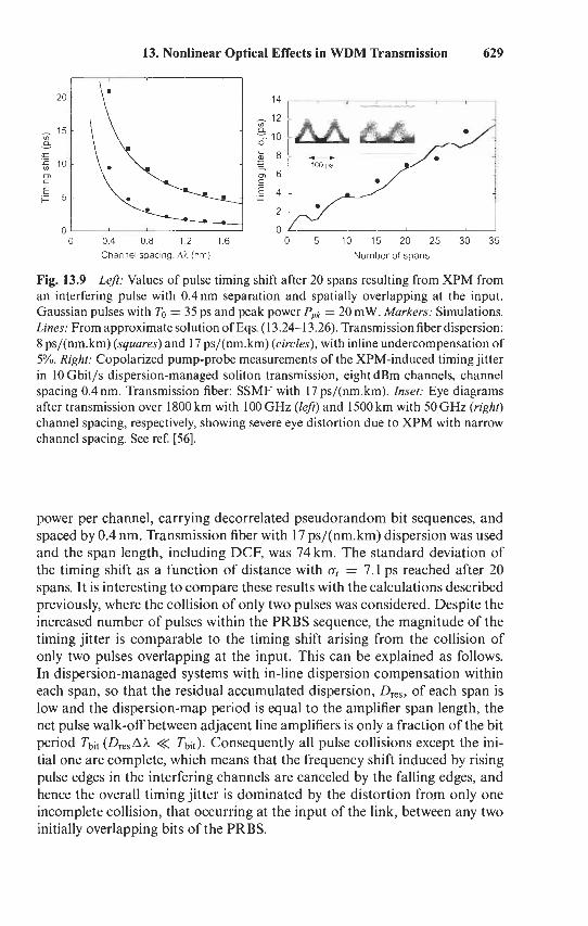
13. Nonlinear Optical Effects in WDM Transmission 629
2o t \
0 I
14 I 12
10 a v
._ B .- c n 6
.E 4
._
I- t ./ 1 td 1 2
o v 1 I 0 0.4 0.8 1.2 1.6 0 5 10 15 20 25 30 35
Channel spacing, AX (nm)
Fig. 13.9 Left: Values of pulse timing shift after 20 spans resulting from XPM from an interfering pulse with 0.4nm separation and spatially overlapping at the input. Gaussian pulses with To = 35 ps and peak power Ppk = 20 mW. Markers: Simulations. Lines: From approximate solution of Eqs. (1 3.24-1 3.26). Transmission fiber dispersion: 8 ps/(nm.km) (squares) and 17 ps/(nm.km) (circles), with inline undercompensation of 5%. Right: Copolarized pump-probe measurements of the XPM-induced timing jitter in 10 Gbit/s dispersion-managed soliton transmission, eight dBm channels, channel spacing 0.4 nm. Transmission fiber: SSMF with 17 ps/(nm.km). Inset: Eye diagrams after transmission over 1800 km with 100 GHz (Zeft) and 1500 km with 50GHz (right) channel spacing, respectively, showing severe eye distortion due to XPM with narrow channel spacing. See ref. [56].
Number of spans
power per channel, carrying decorrelated pseudorandom bit sequences, and spaced by 0.4 nm. Transmission fiber with 17 ps/(nm.km) dispersion was used and the span length, including DCF, was 74 km. The standard deviation of the timing shift as a function of distance with at = 7.1 ps reached after 20 spans. It is interesting to compare these results with the calculations described previously, where the collision of only two pulses was considered. Despite the increased number of pulses within the PRBS sequence, the magnitude of the timing jitter is comparable to the timing shift arising from the collision of only two pulses overlapping at the input. This can be explained as follows. In dispersion-managed systems with in-line dispersion compensation within each span, so that the residual accumulated dispersion, D,,, of each span is low and the dispersion-map period is equal to the amplifier span length, the net pulse walk-off between adjacent line amplifiers is only a fraction of the bit period rbit (DresAh. << &). Consequently all pulse collisions except the ini- tial one are complete, which means that the frequency shift induced by rising pulse edges in the interfering channels are canceled by the falling edges, and hence the overall timing jitter is dominated by the distortion from only one incomplete collision, that occurring at the input of the link, between any two initially overlapping bits of the PRBS.
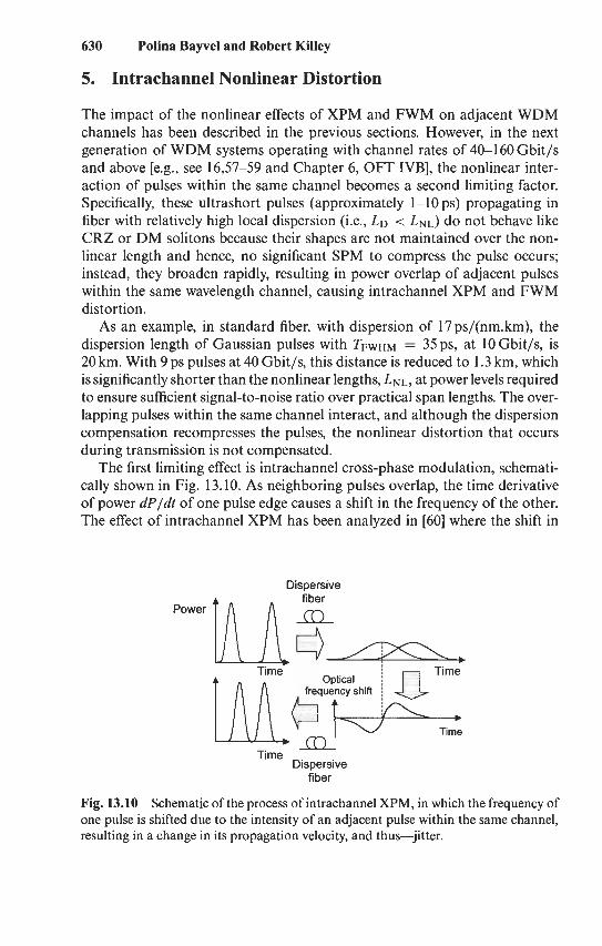
630 Polina Bayvel and Robert Killey
5. Intrachannel Nonlinear Distortion
The impact of the nonlinear effects of XPM and FWM on adjacent WDM channels has been described in the previous sections. However, in the next generation of WDM systems operating with channel rates of 40-160 Gbit/s and above [e.g., see 16,57-59 and Chapter 6, OFT IVB], the nonlinear inter- action of pulses within the same channel becomes a second limiting factor. Specifically, these ultrashort pulses (approximately 1-1 0 ps) propagating in fiber with relatively high local dispersion (i.e., LD < LNL) do not behave like CRZ or DM solitons because their shapes are not maintained over the non- linear length and hence, no significant SPM to compress the pulse occurs; instead, they broaden rapidly, resulting in power overlap of adjacent pulses within the same wavelength channel, causing intrachannel XPM and FWM distortion.
As an example, in standard fiber, with dispersion of 17 ps/(nm.km), the dispersion length of Gaussian pulses with TFWHM = 35 ps, at 10 Gbit/s, is 20 km. With 9 ps pulses at 40 Gbit/s, this distance is reduced to 1.3 km, which is significantly shorter than the nonlinear lengths, LNL, at power levels required to ensure sufficient signal-to-noise ratio over practical span lengths. The over- lapping pulses within the same channel interact, and although the dispersion compensation recompresses the pulses, the nonlinear distortion that occurs during transmission is not compensated.
The first limiting effect is intrachannel cross-phase modulation, schemati- cally shown in Fig. 13.10. As neighboring pulses overlap, the time derivative of power dP/dt of one pulse edge causes a shift in the frequency of the other. The effect of intrachannel XPM has been analyzed in [60] where the shift in
Dispersive
Power fiber
T r n L Time 1 Time
G u e L - ,,,’, Dispersive
fiber
-cn Time
Fig. 13.10 Schematic of the process of intrachannel XPM, in which the frequency of one pulse is shifted due to the intensity of an adjacent pulse within the same channel, resulting in a change in its propagation velocity, and thus-jitter.

13. Nonlinear Optical Effects in WDM Transmission 631
I I I I I I I I I - - - -
-
-
0 1 2 3 4 5 6 7 8 9 10 Normalised pulse width, V l
Fig. 13.11 Dimensionless function F(t/T) describing the XPM-induced frequency shift of two interacting Gaussian pulses as a function of the pulse width normalized to the pulse separation. [Redrawn from ref. [60], with permission from the Optical Society of America.]
the optical carrier frequency of each pulse is given by,
YE0 dz T2
dAfXPM = ~kO.l5---F(t /T) (13.28)
for Gaussian pulses of width t (FWHM), which varies with distance, energy EO, and bit period T. In this expression, F(t/T) is a numerically calculated function plotted in Fig. 13.1 1. When t -= 0.4T, there is negligible distortion, as the pulses do not overlap, and hence F ( t / T ) is low. A maximum frequency shift occurs when t x T, while for t >> T, the effect becomes small, as the pulse power is low due to the large broadening. It would appear that allowing the pulses to broaden out during transmission, and only using dispersion compensation at the receiver, so that t >> T during transmission, would be an effective technique to minimize intrachannel XPM. This technique, termed “quasi-linear” propagation has been successfully demonstrated with 160-320- Gbit/s transmission experiments [58,59].
However, for pulse widths in the range t / T =- 1, a second intrachannel nonlinear effect occurs [60], namely four-wave mixing between the frequency components of adjacent, now overlapping pulses, within the same wavelength channel, which results in the depletion of the pulse energies and power transfer into the “zero” bit slots, schematically shown in Fig. 13.12. The result is an increase in the noise on the “zero” and “one” rails, 00 and cq in Eq. 13.23, as can be seen in Fig. 13.13, and a corresponding reduction in the Q-factor. Intrachannel FWM has been experimentally observed [61] in NZDSF and
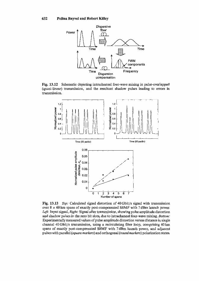
632 Polina Bayvel and Robert Kiuey
DisDersive
Time- Time
t
Time Frequency Dispersion
compensation
Fig. 13.12 Schematic depicting intrachannel four-wave mixing in pulse-overlapped (quasi-linear) transmission, and the resultant shadow pulses leading to errors in transmission.
Time (50 pddv) Time (50 pddiv)
0.03 ::r---- 0.01 0.02 .
rn
0 1 2 3 4 5 6 7 Number of spans
F'ig. 13.13 Top: Calculated signal distortion of 40 Gbit/s signal with transmission over 8 x 60 lan spans of exactly post-compensated SSMF with 7 dBm launch power. Lej?: Input signal, Right: Signal after transmission, showing pulse amplitude distortion and shadow pulses in the zero bit slots, due to intrachannel four-wave mixing. Bottom: Experimentally measured values of pulse amplitude distortion versus distance in single channel 40Gbit/s transmission, using a recirculating fiber loop, comprising 60km spans of exactly post-compensated SSMF with 7dBm launch power, and adjacent pulses with parallel (square markers) and orthogonal (roundmarkers) polarization states.
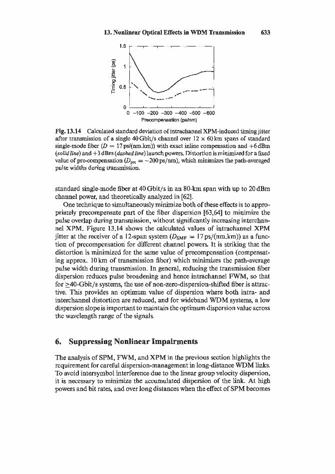
13. Nonlinear Optical Effects in WDM Transmission 633
1.5 I I
0 ' I I I 0 -100 -200 -300 -400 600 -600
Precompensation (pdnm)
Fig. 13.14 Calculated standard deviation of intrachannel XPM-induced timing jitter after transmission of a single 40 Gbit/s channel over 12 x 60 km spans of standard single-mode fiber (D = 17 ps/(nm.km)) with exact inline compensation and +6 dBm (solid line) and +3 dBm (dashed line) launch powers. Distortion is minimized for a fixed value of pre-compensation (DPE = -200 ps/nm), which minimizes the path-averaged pulse widths during transmission.
standard single-mode fiber at 40 Gbit/s in an 80-km span with up to 20 dBm channel power, and theoretically analyzed in [62].
One technique to simultaneously minimize both of these effects is to appro- priately precompensate part of the fiber dispersion [63,64] to minimize the pulse overlap during transmission, without significantly increasing interchan- ne1 XPM. Figure 13.14 shows the calculated values of intrachannel XPM jitter at the receiver of a 12-span system (DSMF = 17ps/(nm.km)) as a func- tion of precompensation for different channel powers. It is striking that the distortion is minimized for the same value of precompensation (compensat- ing approx. 10 km of transmission fiber) which minimizes the path-average pulse width during transmission. In general, reducing the transmission fiber dispersion reduces pulse broadening and hence intrachannel FWM, so that for >40-Gbit/s systems, the use of non-zero-dispersion-shifted fiber is attrac- tive. This provides an optimum value of dispersion where both intra- and interchannel distortion are reduced, and for wideband WDM systems, a low dispersion slope is important to maintain the optimum dispersion value across the wavelength range of the signals.
6. Suppressing Nonlinear Impairments
The analysis of SPM, FWM, and XPM in the previous section highlights the requirement for careful dispersion-management in long-distance WDM links. To avoid intersymbol interference due to the linear group velocity dispersion, it is necessary to minimize the accumulated dispersion of the link. At high powers and bit rates, and over long distances when the effect of SPM becomes

634 Polina Bayvel and Robert Killey
significant, a small anomalous path-average dispersion is desirable to avoid the pulse broadening that occurs when the SPM chirping is followed by normal dispersion, D < 0 ps/(nm.km). Hence, for high-speed single-channel trans- mission, independent of format, fiber with a low, uniform value of dispersion is sufficient for good performance, such as dispersion-shifted fiber (DSF), with dispersion, 0 < DDSF < lps/(nm.km) at the operating wavelength, h = 1.55pm.
However, in dense WDM transmission, more complex dispersion man- agement is needed to minimize inter and intrachannel effects simultaneously. Non-zero dispersion fiber, Le., with sufliciently high values to suppress interchannel FWM and XPM, must be used, and the fiber dispersion is com- pensated, either using spans of transmission fiber with alternating sign of dispersion (sometimes called reverse-dispersion compensation) or by using periodic lumped compensators, such as dispersion compensating fiber (DCF), DDCF M -100 ps/(nm.km) or dispersion-compensating fiber gratings, as shown in Fig. 13.15, and the positioning of these dispersion compensators afTects the performance of the system.
-500 1 0 50 100 150 200 250
Distance (km)
F'ig. 13.15 Accumulated dispersion of two typical dispersion managed system maps. Top: Spans of standard single-mode fiber, with dispersion compensation at the ampli- fiers: local dispersion is kept high to minimize interchannelnonlinearities, whilst the low overall anomalous path-averaged dispersion minimizes SPM-induced pulse broaden- ing. Bottom: Spans of alternating positive and negative dispersion NZDSF optimized to maintain the pulse shape in ultra-high channel bit-rate systems.
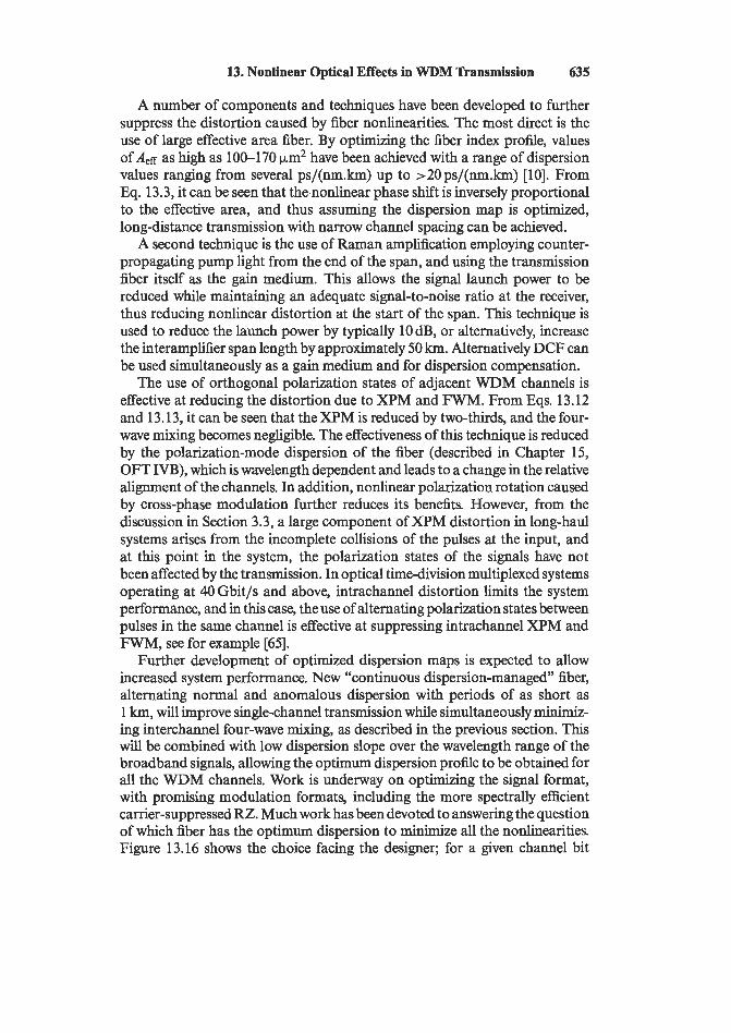
13. Nonlinear Optical Effects in WDM Transmission 635
A number of components and techniques have been developed to further suppress the distortion caused by fiber nonlinearities. The most direct is the use of large effective area fiber. By optimizing the fiber index profile, values of A,ff as high as 100-170 p,m2 have been achieved with a range of dispersion values ranging from several ps/(nm.km) up to >20ps/(nm.km) [lo]. From Eq. 13.3, it can be seen that the nonlinear phase shift is inversely proportional to the effective area, and thus assuming the dispersion map is optimized, long-distance transmission with narrow channel spacing can be achieved.
A second technique is the use of Raman amplification employing counter- propagating pump light from the end of the span, and using the transmission fiber itself as the gain medium. This allows the signal launch power to be reduced while maintaining an adequate signal-to-noise ratio at the receiver, thus reducing nonlinear distortion at the start of the span. This technique is used to reduce the launch power by typically 10 dB, or alternatively, increase the interamplifier span length by approximately 50 km. Alternatively DCF can be used simultaneously as a gain medium and for dispersion compensation.
The use of orthogonal polarization states of adjacent WDM channels is effective at reducing the distortion due to XPM and FWM. From Eqs. 13.12 and 13.13, it can be seen that the XPM is reduced by two-thirds, and the four- wave mixing becomes negligible. The effectiveness of this technique is reduced by the polarization-mode dispersion of the fiber (described in Chapter 15, OFT IVB), which is wavelength dependent and leads to a change in the relative alignment of the channels. In addition, nonlinear polarization rotation caused by cross-phase modulation further reduces its benefits. However, from the discussion in Section 3.3, a large component of XPM distortion in long-haul systems arises from the incomplete collisions of the pulses at the input, and at this point in the system, the polarization states of the signals have not been affected by the transmission. In optical time-division multiplexed systems operating at 40 Gbit/s and above, intrachannel distortion limits the system performance, and in this case, the use of alternating polarization states between pulses in the same channel is effective at suppressing intrachannel XPM and FWM, see for example [65].
Further development of optimized dispersion maps is expected to allow increased system performance. New “continuous dispersion-managed” fiber, alternating normal and anomalous dispersion with periods of as short as 1 km, will improve single-channel transmission while simultaneously minimiz- ing interchannel four-wave mixing, as described in the previous section. This will be combined with low dispersion slope over the wavelength range of the broadband signals, allowing the optimum dispersion profile to be obtained for all the WDM channels. Work is underway on optimizing the signal format, with promising modulation formats, including the more spectrally efficient carrier-suppressed RZ. Much work has been devoted to answering the question of which fiber has the optimum dispersion to minimize all the nonlinearities. Figure 13.16 shows the choice facing the designer; for a given channel bit
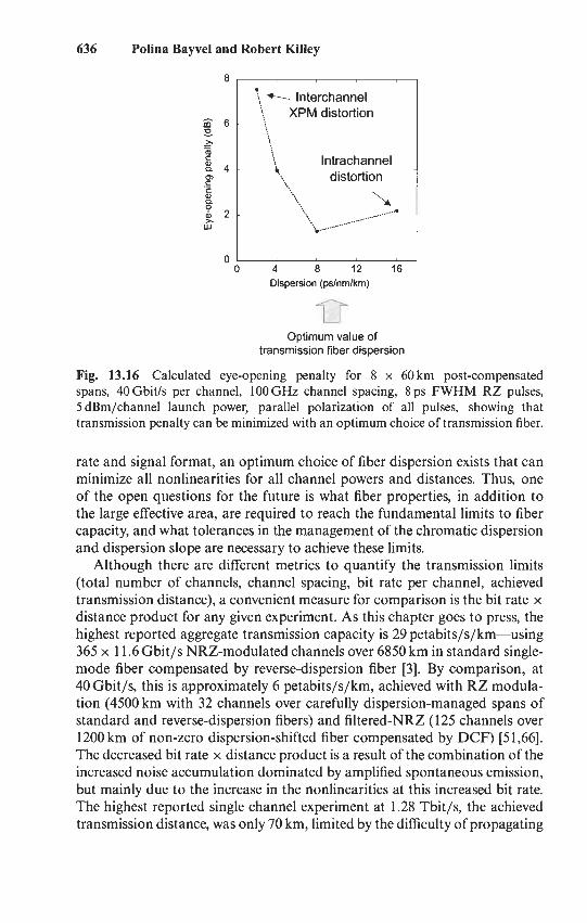
636 Polina Bayvel and Robert Killey
m - 0
g 4 -
8 2 2 -
c rn ._
2. w
8 ,
lntrachannel distortion
\ ...... _.._... . ___... __...-
i..
k--""
I -- lnterchannel
01 0 4 8 12 16
Dispersion (pslnmlkm)
Optimum value of transmission fiber dispersion
Fig. 13.16 Calculated eye-opening penalty for 8 x 60 km post-compensated spans, 40Gbit/s per channel, 100GHz channel spacing, 8ps FWHM RZ pulses, 5 dBm/channel launch power, parallel polarization of all pulses, showing that transmission penalty can be minimized with an optimum choice of transmission fiber.
rate and signal format, an optimum choice of fiber dispersion exists that can minimize all nonlinearities for all channel powers and distances. Thus, one of the open questions for the future is what fiber properties, in addition to the large effective area, are required to reach the fundamental limits to fiber capacity, and what tolerances in the management of the chromatic dispersion and dispersion slope are necessary to achieve these limits.
Although there are different metrics to quantify the transmission limits (total number of channels, channel spacing, bit rate per channel, achieved transmission distance), a convenient measure for comparison is the bit rate x distance product for any given experiment. As this chapter goes to press, the highest reported aggregate transmission capacity is 29 petabits/s/km-using 365 x 1 1.6 Gbit/s NRZ-modulated channels over 6850 km in standard single- mode fiber compensated by reverse-dispersion fiber [3]. By comparison, at 40 Gbit/s, this is approximately 6 petabits/s/km, achieved with RZ modula- tion (4500 km with 32 channels over carefully dispersion-managed spans of standard and reverse-dispersion fibers) and filtered-NRZ (1 25 channels over 1200 km of non-zero dispersion-shifted fiber compensated by DCF) [5 1,661. The decreased bit rate x distance product is a result of the combination of the increased noise accumulation dominated by amplified spontaneous emission, but mainly due to the increase in the nonlinearities at this increased bit rate. The highest reported single channel experiment at 1.28 Tbit/s, the achieved transmission distance, was only 70 km, limited by the difficulty of propagating

13. Nonlinear Optical Effects in WDM Transmission 637
such short pulses [67J The future research in this area will attempt to identify what is practically achievable at bit rates higher than 40 Gbit/s (80-320 Gbit/s per channel), the optimal modulation formats as well as in optimizing the fiber properties and increasing the dispersion tolerances. The future research aims to continue to investigate and combat the nonlinearities in order to propagate and route the largest possible capacities over long distances, and the under- standing of the fundamental limits to fiber transmission are likely to drive the development of this exciting, rapidly changing and competitive field of optical networking in the Coming years.
It should be noted that throughout this chapter, residual or residual accumu- Zated dispersion Ips/nm] is &fined as the fiber chromatic dispersion integrated over distance between two specified positions along the link. Path-average dispersion [ps/(nm.km)] is used for dispersion-managed links with repeating sections of positive and negative dispersion with period L. Dehed as the resid- ual accumulated dispersion over N periods of the dispersion map, divided by NL, where N is an integer.
Acknowledgments
The authors would like to thank their colleagues Hans Jorg Thiele, Vitaly Mikhailov, and other members of the Optical Networks Group (UCL) for their contributions to the modelling, experiments, and discussions that have been included in this paper, as well as for critical reading of this paper. Alan Robinson of Nortel Networks (Harlow, UK) and Chris Park of Agilent Tech- nologies (Ipswich, UK) are also thanked for their comments. Support from the Engineering & Physical Sciences Research Council and the Royal Society is gratefully acknowledged.
References
[l] K. Fukuchi, T. Kasamatsu, M. Morie, R. Ohhira, T. Ito, K. Sekiya, D. Ogasa- hara, T. Ono, “10.92 Tbit/s (273 x 40 Gbith) triple-band/ultra-dense WDM optical repeated transmission experiment,” OFC2001, Postdeadline paper, PD24, Anaheim, CA, March 2001
[2] S. Bigo, etal., “10.2Tbit/s (256 x 42.7Gbit/s) PDM x WDM transmission over 1000 km Teralight fiber with 1.28 bits/s/Hz spectral efficiency,” Pmc. OFC 2001 Postdeadline paper, PD24, Anaheim, CA, March 2001
[3] G. Vareille, E Pitel, J. E Marceau, “3.65Tbit.h (365 x 11.6Gbit/s) transmis- sion experiment over 6850 km using 22.2 GHz channel spacing in NRZ format,” Post deadline paper, 27th European Conference on Optical Communications, ECOC2001, September 2001, Amsterdam, paper PD.M.1.7
[4] N. Bloembergen, “Nonlinear optics: past, present, and future,” IEEE Journal of Selected Topics in Quantum Electronics 6 , 876 (2000)
638 Polina Bayvel and Robert Wley
[5] W. A. Gambling, “The rise and fall of optical fibem,” IEEE Journal of Selected lbpics in Quantum Electronics 6, 1085 (2000)
[a J. E. Midwinter, ‘“The start of optical fiber communications as seen from the UK perspective,” IEEE Journal of Selected Topics in Quantum Electronics 6, 1307 (2000)
[7] G. P. Agrawal, Nonlinear Fiber optic^, Academic Press, 2001 [8] F. Forghieri, R. W. Tkach, A. R. Chraplyvy, “Fiber nonlinearities and their impact
on transmission systems,” Chapter 8, in Optical Fiber Telecommunications ZIIA, eds. I. P. Kaminow and T. L. Koch, Academic Press, 1997
[9] G. P. Agrawal, Fiber nonlinearities and their applications, Academic Press, 2000 [lo] T. Miyakawa, I. Morita, K. Tanaka, H. Sakata, N. Edagawa, “2.56Tbit/s
(40 Gbitls x 64 WDM) unrepeatered 230 km transmission with 0.8 bit/s/Hz spec- tral efficiency using low-noise fiber Raman amplifer and 170 bm2 - & fiber,” OFC2001, PD26 Postdeadline paper, PD24, Anaheim, CA, March 2001
[l 13 G. Bellotti, A. Bertaina, S. Bigo, “Impact of residual dispersion on SPM-related power margins in 10 Gbit/s-based systems using standard SMF,” h c . ECOC ’98, vol. 1, pp. 681682
[12] N. Kikuchi, S. Sasaki, “Analytical evaluation technique of self-phase modulation effect on the performance of cascaded optical amplier systems,” J. Lightwave Tech. 13,868, 1995
[13] R. J. Nuyts, Y Park, “Dispersion equalization of a 10 Gbls repeatered transmis- sion system using dispersion compensating fiber,” J. Lightwave Tech. 15,1,3 1-42, 1997
[ 141 H. Anis, et al., “Continuous dispersion-managed fiber for very high speed soliton systems,” Pmc. ECOC ’99, vol. 1, pp. 230-231, Nice, France 1999
[15] M. Nakazawa, “Solitons for breaking barriers to terabitlsecond WDM and OTDM transmission in the next millennium,” ZEEE Journal on Selected Topics in Quantum Electronics 6, 1332 (2000)
[16] B. Mikkelsen, G. Raybon, B. Zhu, R. J. Essiambrq P. G. Bernasconi, K. Dreyer, L. W. Stilz, S. N. Knudsen, “High spectral efficiency (0.53 bit/s/Hz) WDM trans- mission of 160 Gbit/s per wavelength over 400 km of fibeq” Proc. OFC 2001, paper ThF2, Anaheim, CA, March 2001
[17] J. A. J. Fells, P. J. Bennett, R. Feced, P. Ayliffe, J. Wakefield, H. E M. fiddle, V. Baker, S. E. Kanellopoulos, C. Boylan, S. Sahil, W. S. Lee, S. J. Clements, “Widely tunable twin fiber grating dispersion compensator for 80 Gbit/s,” Optical Fiber Communication Conference and Exhibit, 2001. Pmc. OFC 2001, 2001, Postdeadline paper, paper PDll
[IS] K. 0. Hill, D. C. Johnson, B. S. Kawasaki, R. I. MacDonald, “CW three-wave mixing in single-mode optical fibers,” J. Appl. Phys. 49,5098 (1978)
[19] R. G. Waarts, R. l? Braun, “System limitations due to four-wave mixing in single- mode optical fibers,” Electron. Lett. 22,873 (1986)
PO] N. Shibata, R. P. Braun, R. G. Waarts, “Phase-mismatch dependence of efficiency of wave generation through four-wave mixing in a single mode optical fiber,” .I Quantum Electron QE-23,1205 ( 1 987)
13. Nonlinear Optical Effects in WDM Transmission 639
[21] K. Inoue, “Phase-mismatching characteristic of four-wave mixing in fiber lines with multi stage optical amplifiers,” Optics Lett. 17,801 (1992)
[22] W. Zeiler, E Di Pasquale, P. Bayvel, J. E. Midwinter, “Modeling of four-wave mixing and gain peaking in amplified WDM optical communication systems and networks,” J. Lightwave Tech. 14, 1933 (1996)
[23] M. Eiselt, ‘‘Limits on WDM systems due to four-wave mixing: a statistical approach,” J. Lightwuve Tech. 17,11,2261-2267 (1999)
[24] K. Inoue, K. Nakanishi, K. Oda, H. Toba, “Crosstalk and power penalty due to fiber four-wave mixing in multi channel transmission,” J. Lightwave Tech. 12, 1423 (1 994)
[25] E Forghieri, R. W. Tkach, A. R. Chraplyvy, “WDM systems with unequally spaced channels,”J. Lightwave Tech. 13,889 (1995)
[26] P. P. Mitra, J. B. Stark, “Nonlinear limits to the information capacity of optical fiber communications,” Nature 411,1027 (2001)
[27] M. N. Islam, L. E Mollenauer, R. H. Stolen, J. R. Simpson, H. T. Shang, “Cross- phase modulation in optical fibers,” Optics Lett. 12,625 (1987)
[28] R. R. Alfano, P. L. Baldeck, E Raccah, P. P. Ho, “Cross-phase modulation measured in optical fibers,” Appl. Optics 26,17,3491(1987)
[29] S. V. Chernikov, J. R. Taylor, “Measurement of normalization factor for n 2 for random polarization in optical fibers,” Optics Lett. 21, no. 19, 1559 (1996)
[30] L. Rapp, “Experimental investigation of signal distortions induced by cross-phase modulation combined with dispersion,” Photon. Tech. Lett. 9, 1592 (1997)
[31] H. J. Thiele, R. I. Killey, P. Bayvel, “Influence of fiber dispersion and bit-rate on cross-phase modulation induced distortion in amplified optical fiber links,” Electron. Lett. 34,2050 (1998)
[32] G. Bellotti, M. Varani, C. Francia, A. Bononi, “Intensity distortion induced by cross-phase modulation and chromatic dispersion in optical-fiber transmissions with dispersion compensation,” Photon. Tech. Lett. 10, 1745 (1998)
[33] H. J. Thiele, R. I. Killey, P. Bayvel, “Influence of transmission distance on XPM- induced distortion in dispersion managed amplified fiber links,” Electron. Lett. 35, 15,408409,1999
[34] A. V T. Cartaxo, “Cross-phase modulation in intensity modulation-direct detection WDM systems with multiple optical amplifiers and dispersion com- pensators,” J. Lightwave Tech. 17, 178 (1999)
[35] M. Shtaif, “Analytical description of cross-phase modulation in dispersive optical fibers,” OpticsLeft. 23,15, 1191-1193, 1998
[36] M. Shtaif, M. Eiselt, “Analysis of intensity interference caused by cross-phase modulation in dispersive fibers,” Photon. Tech. Lett. 10, 12,979-981, 1998
[37] N. Kikuchi, K. Sekine, S. Sasaki, “Analysis of cross-phase modulation (XPM) effect on WDM transmission performance,” Electron. Lett. 33,8,65-54, 1997
[38] J. M. Wang, K. Petermann, “Small-signal analysis for dispersive optical fiber communication systems,” J. Lightwave Tech. 10,96 (1992)
[39] M. Shtaif, L. Eiselt, D. Garrett, “Cross-phase modulation distortion measure- ments in multispan WDM systems,” Photon. Tech. Lett. 12, 1,88-90,2000
640 Polina Bayvel and Robert Killey
[40] H. J. Thiele, R. I. Killey, P. Bayvel, “Investigation of XPM distortion in transmission over installed fiber,” Photon. Tech. Lett. 12,669 (2000)
[41] V. Mikhailov, R. I. Killey, H. J. Thiele, J. Prat, P. Bayvel, “Limitation to WDM transmission distance due to cross-phasemodulation induced spectral broadening in dispersionGompensated standard fiber systems,” Photon. Tech. Lett. 11, 994 (1 999)
[42] K.-P. Ho, H. Yu, L.-K. Chen, E Tong, “High-resolution measurement and spec- tral overlap of cross-phase modulation induced spectral broadening,” Photon. Tech. Lett. 12,11,1534-1536,2000
[43] M. Eiselt, M. Shtaif, L. D. Garrett, “Contribution of timing jitter and amplitude distortion to XPM system penalty in WDM systems,” Photon. Tech. Lett. 11,748 (1999)
[44] H. J. Thiele, R. I. Killey, P. Bayvel, “Simple technique to determine cross-phase modulation induced penalties in WDM transmission,” Pmc. OFC 2000, paper ThM2, Baltimore, MD, March 2000
[45] R. I. Killey, H. J. Thiele, V. Mikhailov, P. Bayvel, “Prediction of transmission penalties due to cross-phase modulation in WDM systems using a simplified technique,” Photon. Tech. Lett. 12,7 (2000)
[46] N. S. Bergano, C. R. Davidson, “Wavelength division multiplexing in long-haul transmission systems,” J. Lightwave Tech. 14, 1299-1308,1996
[47] M. Suzuki, I. Morita, N. Edagawa, S. Yamamoto, H. Taga, S. Akiba, “Reduction of Gordon-Haus timing jitter by periodic dispersion compensation in soliton transmission,” Electron. Lett. 31,23,2027-2029,1995
[48] N. J. Smith, E M. Knox, N. J. Doran, K. J. Blow, I. Bennion, “Enhancedpower solitons in optical fibers with periodic dispersion management,” Electron. Lett. 32, 1,5455,1996
[49] T. Yu, E. A. Golovchenko, A. N. Pilipetskii, C. R. Menyuk, “Dispersion-managed solitons interactions in optical fibers,” Optics Lett. 22,793 (1997)
[50] M. Suzuki, N. Edagawa, “Technical challenges to multi-terabit transoceanic systems,’’ Pmc. Optical Fiber Communication, OFC2001, vol. 3,2001, paper WF2
[51] J. X. Cai, et al., “1.28 Tbit/s (32 x 40Gbit/s) transmission over 4500km,” Proc. 27th European Conference on Optical Communications, ECOC2001, October 2001, Amsterdam, PD.M.1.2
[52] A. Hasegawa, Y. Kodama, Solitons in optical communications, Oxford University Press, Oxford, 179-183, 1995
[53] D. J. Kaup, B. A. Malomed, J. Yang, “Interchannel pulse collision in a wavelength- division-multiplexed system with strong dispersion management,” Optics Lett. 23, 20,1600-1602, 1998
[54] V. S. Grigoryan, A. Richter, “Efficient approach for modelling collision-induced timing jitter in WDM return-to-zero dispersion-managed systems,” J. Lightwave Tech. 18,8,1148-1154,2000
[55] J. E L. Devaney, W. Forysiak, A. M. Niculae, N. J. Doran, “Soliton collisions in dispersion-managed wavelength-division-multiplexed systems,’’ Optics Lett. 22, 22, 1695-1697, 1997
13. Nonlinear Optical Effects in WDM Transmission 641
[56] V. Mikhailov, H. J. Thiele, R. I. Killey, P. Bayvel, “Experimental investigation of collision-induced timing jitter and pulse distortion in WDM return-to-zero dispersion-managed systems,” Proc. OFC 2001, vol. 2, pp. TuN4.1-TuN4.3, Anaheim, CAY March 2001
[57] S. Kawanishi, H. Takara, K. Uchiyama, I. Shake, K. Mori, “3Tbit/s (160Gbit/s x 19 channel) optical TDM and WDM transmission experiment,” Electron Lett. 35,826 (1999)
[58] G. Raybon, B. Mikkelsen, R.-J. Essiambre, A. J. Stentz, T. N. Nielsen, D. W. Pekham, L. Hsu, L. Gruner-Nielsen, K. Dreyer, J. E. Johnson, “320 Gbit/s single- channel, pseudo-linear transmission over 200 km of nonzero-dispersion fiber,” Photon. Tech. Lett. 12, 1400 (2000)
[59] R. Ludwig, U. Feiste, S. Diez, C. Schubert, C. Schmidt, H. J. Ehrke, H. G. Weber, “Unrepeatered 160 Gbit/s RZ singlechannel transmission over 160 km of standard fiber at 1.55 bm with hybrid MZI optical demultiplexer,” Electron. Lett. 36, 1405 (2000)
[60] P. V. Mamyshev, N. A. Mamysheva, “Pulse-overlapped dispersion-managed data transmission and intrachannel four-wave mixing,” Optics Lett. 24,21, 1454-1456, 1999
[61] R.-J. Essiambre, B. Mikkelsen, G. Raybon, “Intra-channel cross-phase modula- tion and four-wave mixing in high-speed TDM systems,” Ekctmn. Lett. 35, 18, 1999
[62] A. Mecozzi, C. B. Clausen, M. Shtaif, “Analysis of intrachannel nonlinear effects in highly dispersed optical pulse transmission,” Photon. Tech. Lett. 12,4,392-394, 2000
[63] P. Harper, S. B. Alleston, I. Bennion, N. J. Doran, “40 Gbit/s dispersion managed soliton transmission over 116Okm in standard fiber with 75km span length,” Electmn. Lett. 35,24, 1999
[64] R. I. Killey, H. J. Thiele, V. Mikhailov, P. Bayvel, “Reduction of intrachannel distortion in 4O-Gb/s-based WDM transmission over standard fiber,” Photon. Tech. Lett. 12, 12, 1624-1626,2000
[65] E Matera, et al., “Field demonstration of 40Gb/s soliton transmission with alternate polarizations,” J. Lightwave Tech. 17,2225 (1999)
[66] S. Bigo, et al., “Transmission of 125 WDM channels at 42.7Gbit/s (5Tbit/s capacity over 12 x 100 km of Teralight Ultra fibre,” Proc 27th European Confer- ence on Optical Communications, ECOC2001, October 2001, Amsterdam, paper PD.M. 1.1
[67l M. Nakazawa, T. Yamamoto, K. R. Tamura, “1.28 Tbit/s-70km OTDM trans- mission using third- and fourth-order simultaneous dispersion compensation with a phase modulator,” Electron. Lett. 36,2027 (2000)

Chapter 14
Alan E. Willner
Fixed and Tunable Management of Fiber Chromatic Dispersion
University of Southern California, Los Angeles, California and Phaethon Communications, Inc.. Fwmont, California
Bogdan Hoanca Phaethon Communications, Inc., Fwmont, California
I. Introduction
In 1993, Linn Mollenauer of Bell Laboratories mentioned to us a simple thought that we think puts this chapter into perspective. He said, “One can transmit infinite bandwidth over zero distance.” Unless the fiber issues of chromatic dispersion and nonlinearities are managed in a transmission link, propagation of high-speed signals over nontrivial distances may be impractical.
As recently as 1998, a debate was raging as to whether 10-Gbids systems were needed given the simplicity of deploying more 2.5-Gbith wavelength- division-multiplexed (WDM) channels. At 2.5 Gbids, the optics and electron- ics were fairly straightforward to implement. In what seemed like the blink of an eye, the debate ended in 1999 when Nortel was able to successfully sell -$6 billion of lO-Gbit/s equipment. Although 2.5-Gbids equipment still accounts for a sizable fraction of the optical communications market, we are now squarely in the lO-Gbit/s phase of deployment. The new debate now raging concerns the timing of 40-Gbids systems deployment.
When progressing from 2.5- to 10-Gbids systems, most technical challenges are less than four times as complicated and the cost of components is usually much less than four times as expensive. One critical exception to this “rule” is the deleterious time-spreading effect that optical-fiber-induced chromatic dispersion has on the transmission of a data bit stream; chromatic dispersion can be illustratively thought of as the effect that each photon within a single bit exists at a slightly different frequency and travels down the fiber at a slightly different speed. When increasing the bit rate by a factor of 4, the effect of chromatic dispersion increases by a staggering factor of 16! Furthermore, chromatic dispersion effects increase linearly with transmission distance.
To put this transmission problem in perspective, we can compare the longest distance that a data channel can be transmitted over conventional single-mode fiber. Whereas dispersion limits a 2.5-Gbit/s channel to roughly 900 km (1 dB power penalty), a 10- and 40-Gbids channel would be limited to approximately
642 OITICAL FIBER TELECOMMUNICATIONS, VOLUME IVB
Copyright 0 2002, Elscviu Science (USA). All rights of reproduction in any form r e ~ e ~ e d .
ISBN 0-12395173-9

14. Fixed and Tunable Management 643
60 and 4 km, respectively. Some method of dispersion compensation must be employed for a system to operate beyond these distance limits. Although this was not much of an issue for 2.5-Gbit/s systems, it is crucial for transmitting more than 10 Gbit/s.
Chromatic dispersion is one of the most basic characteristics of fiber. Although it is possible to manufacture fiber that induces zero chromatic dis- persion, it should be emphasized that such fiber is incompatible with the deployment of WDM systems since harmful nonlinear effects would be gener- ated. As long as WDM is dominant in the marketplace, chromatic dispersion must exist, and therefore must be compensated.
In theory, compensation of chromatic dispersion for high-speed or long- distance systems can be fixed in value if each link’s dispersion value is known. However, there are several important aspects of optical systems and networks that make tunable dispersion compensation solutions attractive, including: (1) it significantly reduces the inventory of different required types of compen- sation modules, (2) it tunes to adapt to routing path changes in a reconfigurable network, (3) it tracks dynamic changes in dispersion due to environment, and (4) it achieves a high degree of accuracy necessary for 4O-Gbit/s channels.
Dispersion compensation enables robust optical systems that can accom- modate longer distances, higher speeds, and/or network reconfigurability. This chapter will address the issues surrounding the compensation of chromatic dispersion in high-performance optical systems. We will describe the effects of dispersion, various k e d compensation techniques, the need for tunable compensation and its potential solutions, and also techniques for monitoring accumulated dispersion.
11. Chromatic Dispersion and Its Effects on Optical Fiber Systems
ILa. FUNDMENTM CONCEPTS
In any medium other than a vacuum and in any waveguide structure, different electromagnetic frequencies propagate at different speeds. This is the essence of chromatic dispersion. Chromatic dispersion in optical fibers is due to the frequency-dependent nature of the propagation characteristics for both the material (the refractive index of glass) and the waveguide structure [l]. Using a Taylor-series expansion of the value of the refractive index n as a function of the wavelength h, the speed v of a particular wavelength will be:
(14.1) ,.. Cn
’ no(A0) + where co is the speed of light in vacuum, ho is a reference wavelength, and the terms in anp i and a2n/ah2 are associated with the chromatic dispersion
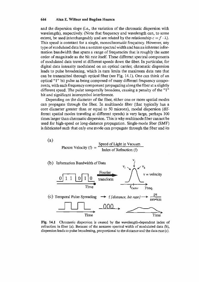
644 Alan E. Willner and Bogdan Hoanca
and the dispersion slope (Le., the variation of the chromatic dispersion with wavelength), respectively. (Note that frequency and wavelength can, to some extent, be used interchangeably and are related by the relationship c =f . A). This speed is constant for a single, monochromatic frequency. However, any type of modulated data has a nonzero spectral width and has an inherent infor- mation bandwidth that spans a range of frequencies that is roughly the same order of magnitude as the bit rate itself. These different spectral components of modulated data travel at different speeds down the fiber. In particular, for digital data intensity modulated on an optical carrier, chromatic dispersion leads to pulse broadening, which in turn limits the maximum data rate that can be transmitted through optical fiber (see Fig. 14.1). One can think of an optical “Iy7 bit pulse as being composed of many different frequency compo- nents, with each frequency component propagating along the fiber at a slightly different speed. The pulse temporally broadens, causing a penalty of the “1 ” bit and significant intersymbol interference.
Depending on the diameter of the fiber, either one or more spatial modes can propagate through the fiber. In multimode fiber (that typically has a core diameter greater than or equal to 50 microns), modal dispersion (dif- ferent spatial modes traveling at different speeds) is very large, perhaps 100 times larger than chromatic dispersion. This is why multimode fiber cannot be used for high-speed or long-distance propagation. Single-mode fiber (SMF) is fabricated such that only one mode can propagate through the fiber and its
Speed of Light in Vacuum Index of Refraction (f)
(a) Photon Velocity (f) =
3 (b) Information Bandwidth of Data
v = velocity Fourier om o m 0 I U L
Time
(C) Temporal Pulse Spreading
r
Time
Fig. 14.1 Chromatic dispersion is
PS --+ f [distance, bit rate] + - n m * h - n,
Time
caused by the wavelength-dependent index of refraction in fiber (a). Because of the nonzero spectral width of modulated data (b), dispersion leads to pulse broadening, proportional to the distance and the data rate (c).
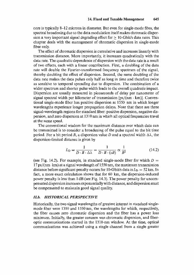
14. Fixed and Tunable Management 645
core is typically 8-12 microns in diameter. But even for single-mode fiber, the spectral broadening due to the data modulation itself makes chromatic disper- sion a very important signal degrading effect for 2 10-Gbit/s data rates. This chapter deals with the management of chromatic dispersion in single-mode fiber only.
The effect of chromatic dispersion is cumulative and increases linearly with transmission distance. More importantly, it increases quadratically with the data rate. The quadratic dependence of dispersion with the data rate is a result of two effects, each with a linear contribution. First, a doubling of the data rate will double the Fourier-transformed frequency spectrum of the signal, thereby doubling the effect of dispersion. Second, the same doubling of the data rate makes the data pulses only half as long in time and therefore twice as sensitive to temporal spreading due to dispersion. The combination of a wider spectrum and shorter pulse width leads to the overall quadratic impact. Dispersion are usually measured in picoseconds of delay per nanometer of signal spectral width per kilometer of transmission Lps/(nm . km)]. Conven- tional single-mode fiber has positive dispersion at 1550 nm in which longer wavelengths experience longer propagation delays. Note that there are three signal-wavelength regions for standard fiber: positive dispersion, negative dis- persion, and zero dispersion at 13 10 nm in which all optical frequencies travel at the same speed.
The conventional wisdom for the maximum distance over which data can be transmitted is to consider a broadening of the pulse equal to the bit time period. For a bit period By a dispersion value D and a spectral width Ah, the dispersion-limited distance is given by
1 D - B - A h D . B . ( c B ) B2
0:- 1 - - 1
L D = (14.2)
(see Fig. 14.2). For example, in standard single-mode fiber for which D = 17 ps/(nm. km) at a signal wavelength of 1550 nm, the maximum transmission distance before significant penalty occurs for 10-Gbit/s data is LD = 52 km. In fact, a more exact calculation shows that for 60 km, the dispersion-induced power penalty is less than 1 dB (see Fig. 14.3). The power penalty for uncom- pensated dispersion increases exponentially with distance, and dispersion must be compensated to maintain good signal quality.
1I.h HISTORICXL PERSPECTIVE
Historically, the two signal wavelengths of greatest interest in standard single- mode fiber were 13 10 and 1550 nm, the wavelengths for which, respectively, the fiber causes zero chromatic dispersion and the fiber has a power loss minimum. Initially, the greater concern was chromatic dispersion, and fiber- optic communications started in the 1310-nm window. At the time, optical communications was achieved using a single channel from a single greater
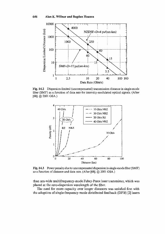
646 Alan E. Willner and Bogdan Hoanca
Fig. fiber. [68]. @ 2001 OSA.)
4 [ . ' . , I I
3
1
10 Gbls NRZ 20 Gbls NRZ 20 Gb/s RZ 40 Gbls NRZ . . . . . . .
, / *
40Gbls I I
c-!O Gbls-y;> . _____-___ , - ....__-- -,,
10 Gbls I I I
i I i l
* / -
,/*
0 20 40 60 80 100 Distance (km)
Fig. 14.3 Power penalty due to uncompensated dispersion in single-mode fiber (SMF) as a function of distance and data rate. (After [68]. @ 2001 OSA.)
than nm-wide multifrequency-mode Fabry-Perot laser transmitter, which was placed at the zero-dispersion wavelength of the fiber.
The need for more capacity over longer distances was satisfied first with the adoption of single-frequency-mode distributed feedback (DFB) [2] lasers

14. Fixed and Tunable Management 647
20
1 16 \
W & 12
TeraLight PureGuide E-LEAF ................. TrueWave RS TrueWave Classic DSF
---.
-..-..
-4 1510 1530 1550 1570 1590 1610
Wavelength (nm)
Fig. 14.4 Chromatic dispersion values for several commercially available types of transmission fiber.
and later with the advent of erbium-doped fiber amplifiers (EDFA) [3]. The EDFA enabled several independent wavelength channels to be transmitted over a single fiber and amplified economically in a single device, thereby open- ing the low-loss 1550-nm window to WDM. Unfortunately, SMF has a fairly large chromatic dispersion value of 17 ps/(nm . km) for this wavelength range (Fig. 14.4). The first WDM systems were not terribly concerned with chro- matic dispersion since the data rates used were OC-48 (2.5 Gbids) and lower, accommodating over 600 km of transmission before dispersion compensation was required.
It is important to emphasize that early 2.5-GbWs system integrators needed to address the issue of optical modulation. A DFB laser may lase in a sin- gle frequency, but its spectrum is “chirped” and spread across a much wider bandwidth when the optical power is modulated by directly turning the laser’s current ON and OFF. This additional chirping of the signal can be as large as 10 GHz, and will increase the deleterious effects of dispersion. In order to avoid this additional problem, external optical modulators were used. These modulators, such as lithium niobate Mach-Zehnder [4] and on-chip semi- conductor electroabsorption [5] types, tend to not introduce a chirping of the signal. External modulators are used in many 2.5-Gbids systems and in almost all 1 0-Gbit/s systems.
With the deployment of the first OC-192 systems, it became apparent that dispersion would become a severe limitation. At OC-192, dispersion-limited distances in SMF are as short as 60km. An instructive simulated view of signal degradation is shown in Fig. 14.5 in which a lO-Gbit/s signal is severely distorted after being transmitted over 100 km of standard fiber, whereas a 2.5 Gbit/s signal is not affected at all by dispersion over the same distance.
Over the course of the 1980s, another parallel track was taking place. Fiber manufacturers saw value in fabricating an optical fiber whose zero dispersion wavelength point coincided with the loss minimum of the fiber. The reasoning
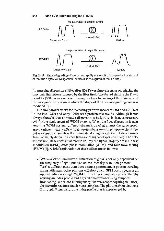
648 Alan E. Willner and Bogdan Hoanca
No distortion of output bit stream
Distance = 0 km 100 km
Large distortion of output bit stream
Distance = 0 km 100 km
Fig. 14.5 Signal-degrading effects occur rapidly as a result of the quadratic nature of chromatic dispersion (dispersion increases as the square of the bit rate).
for pursuing dispersion-shifted fiber (DSF) was simple in terms of reducing the two main limitations imposed by the fiber itself. The feat of shifting the D = 0 point to 1550 nm was achieved through a clever balancing of the material and the waveguide dispersion in which the shape of the fiber waveguiding core was modified [6].
The two parallel tracks for increasing performance of WDM and DSF met in the late 1980s and early 1990s with problematic results. Although it was always thought that chromatic dispersion is bad, it is, in fact, a necessary evil for the deployment of WDM systems. When the fiber dispersion is near zero in a WDM system, different channels travel at almost the same speed. Any nonlinear mixing effects that require phase matching between the differ- ent wavelength channels will accumulate at a higher rate than if the channels travel at widely different speeds (the case of higher-dispersion fiber). The dele- terious nonlinear effects that tend to destroy the signal integrity are self-phase modulation (SPM), cross-phase modulation (XPM), and four-wave mixing (FWM) [7]. A brief explanation of these effects are as follows:
0 S P M a n d P M . The index of refraction of glass is not only dependent on the frequency of light, but also on the intensity. A million photons “see” a different glass than does a single photon, and a photon traveling along with many other photons will slow down. SPM occurs because an optical pulse on a single WDM channel has an intensity profile, thereby causing an index profile and a speed differential causing temporal broadening. When considering many channels copropagating in a fiber, the scenario becomes much more complex. The photons from channels 2 through N can distort the index profile that is experienced by
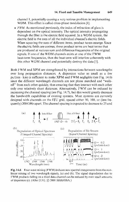
14. Fixed and Tunable Management 649
channel 1, potentially causing a very serious problem in implementing WDM. This effect is called cross-phase modulation [I].
dependent on the optical intensity. The optical intensity propagating through the fiber is the electric field squared. In a WDM system, the electric field is the sum of all the individual channel’s electric fields. When squaring the sum of different items, product terms emerge. Since the electric fields are cosines, these product terms are beat terms that are produced at various sum and difference frequencies of the original signals. If one of the WDM channels exists at one of the FWM beat-term frequencies, then the beat term will interfere coherently with this other WDM channel and potentially destroy the data [l].
0 FWM. As mentioned previously, the index of refraction of glass is
Both FWM and XPM are strengthened by interactions between wavelengths over long propagation distances. A dispersion value as small as a few ps/(nm . km) is sufficient to make XPM and FWM negligible (see Fig. 14.6) since the different wavelength channels are not phase matched and “walk- off” from each other quickly, thus ensuring that they interact with each other only over relatively short distances. Alternatively, FWM can be reduced by increasing the channel spacing (see Fig. 14.7), but this would greatly decrease the bandwidth capabilities of existing systems. Most systems are currently designed with channels on the ITU grid, spaced either 50, 100, or (less fre- quently) 200 GHz apart. The channel spacing is expected to decrease to 25 and
(a) t t I n t o i b e r OutofFib; t t ~
b f f l f2 DSF(D -0) 2 fl-f2 f, f2 2 f2-fl
Degradation of Optical Spectrum (‘) Degradation of Bit Stream (Equal Channel Spacing)
(b )
(Unequal Channel Spacing)
D = -0.2
D=-1 (ps/(nm.km))
(ps/(nm.km)) 1542 1544 1546 1548 H
Wavelength (nm) 2ns Time(ns)
Fig. 14.6 Four-wave mixing (FWM) induces new spectral components from the non- linear mixing of two wavelength signals, (a) and (b). The signal degradation due to FWM products falling on a third data channel can be reduced by even small amounts of dispersion (c). (After [ 13 11. @ 2001 IEEE/OSA.)
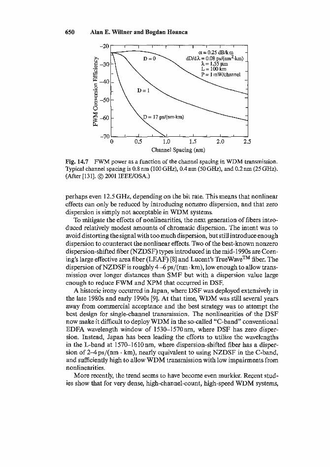
650 Alan E. Willner and Bogdan Hoanca
Channel Spacing (nm)
Fig. 14.7 FWM power as a function of the channel spacing in WDM transmission. Typical channel spacing is 0.8 nm (100 GHz), 0.4 nm (50 GHz), and 0.2 nm (25 GHz). (After 11311. @ 2001 IEEE/OSA.)
perhaps even 12.5 GHz, depending on the bit rate. This means that nonlinear effects can only be reduced by introducing nonzero dispersion, and that zero dispersion is simply not acceptable in WDM systems.
To mitigate the effects of nonlinearities, the next generation of fibers intro- duced relatively modest amounts of chromatic dispersion. The intent was to avoid distorting the signal with too much dispersion, but still introduce enough dispersion to counteract the nonlinear effects. Two of the best-known nonzero dispersion-shifted fiber (NZDSF) types introduced in the mid-1 990s are Corn- ing’s large effective area fiber (LEAF) [8] and Lucent’s TrueWaveTM fiber. The dispersion of NZDSF is roughly 4-6 ps/(nm. km), low enough to allow trans- mission over longer distances than SMF but with a dispersion value large enough to reduce FWM and XPM that occurred in DSF.
A historic irony occurred in Japan, where DSF was deployed extensively in the late 1980s and early 1990s [9]. At that time, WDM was still several years away from commercial acceptance and the best strategy was to attempt the best design for single-channel transmission. The nonlinearities of the DSF now make it difficult to deploy WDM in the so-called “C-band” conventional EDFA wavelength window of 1530-1570nmY where DSF has zero disper- sion. Instead, Japan has been leading the efforts to utilize the wavelengths in the L-band at 1570-1610nmY where dispersion-shifted fiber has a disper- sion of 2 4 ps/(nm km), nearly equivalent to using NZDSF in the C-band, and sufficiently high to allow WDM transmission with low impairments from nonlinearities.
More recently, the trend seems to have become even murkier. Recent stud- ies show that for very dense, high-channel-count, high-speed WDM systems,
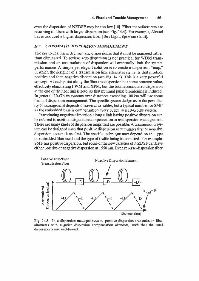
14. Fixed and Tunable Management 651
even the dispersion of NZDSF may be too low [lo]. Fiber manufacturers are returning to fibers with larger dispersion (see Fig. 14.4). For example, Alcatel has introduced a higher dispersion fiber VeraLight, 8ps/(nm km)].
I . c . CHROMATIC DISPERSION MANAGEMENT
The key to dealing with chromatic dispersion is that it must be managed rather than eliminated. To review, zero dispersion is not practical for WDM trans- mission and an accumulation of dispersion will eventually limit the system performance. A simple yet elegant solution is to create a dispersion "map," in which the designer of a transmission link alternates elements that produce positive and then negative dispersion (see Fig. 14.8). This is a very powerful concept: At each point along the fiber the dispersion has some nonzero value, effectively eliminating FWM and XPM, but the total accumulated dispersion at the end of the fiber link is zero, so that minimal pulse broadening is induced. In general, 10-Gbit/s systems over distances exceeding 100 km will use some form of dispersion management. The specific system design as to the periodic- ity of management depends on several variables, but a typical number for SMF as the embedded base is compensation every 80 km in a 10-Gbit/s system.
Introducing negative dispersion along a link having positive dispersion can be referred to as either dispersion compensation or as dispersion management. There are many kinds of dispersion maps that are possible. A transmission sys- tem can be designed such that positive dispersion accumulates first or negative dispersion accumulates first. The specific technique may depend on the type of embedded fiber used and the type of traffic being transmitted. For example, SMF has positive dispersion, but some of the new varieties of NZDSF can have either positive or negative dispersion at 1550 nm. Even reverse-dispersion fiber
Positive Dispersion Transmission Fiber
Negative Dispersion Element
f
h E A = J D $2 g .El z g
- - J C
.- P
Distance (km)
Fig. 14.8 In a dispersion-managed system, positive dispersion transmission fiber alternates with negative dispersion compensation elements, such that the total dispersion is zero end-to-end.
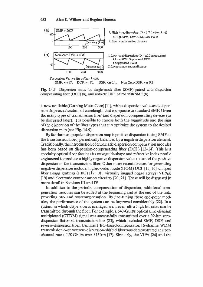
652 Alan E. Willner and Bogdan Hoanca
1. High local dispersion: (D - 1 7 (ps/(nm.km)) High SPM, Low XPM, Low FWM
2. Short compensation distance
100 200 300
(b) 1. Low local dispersion: (D - H).2ps/(nm.km)) Low SPM, Suppressed XPM, Suppressed FWM -D
Distance (km)
lo00 zoo0 3000
2. Long compensation distance
Dispersion Values (in ps/(nm.km)): SMF: - +17, DCF - -85, DSP: <f 0.1, Non-Zero DSF - & 0.2
Fig. 14.9 Dispersion maps for single-mode fiber (SMF) paired with dispersion compensating fiber (DCF) (a), and nonzero DSF paired with SMF (b).
is now available (Corning Metrocore) [l 11, with a dispersion value and disper- sion slope as a function of wavelength that is opposite to standard SMF. Given the many types of transmission fiber and dispersion compensating devices (to be discussed later), it is possible to choose both the magnitude and the sign of the dispersion of the fiber types that can optimize the system to the desired dispersion map (see Fig. 14.9).
By far the most popular dispersion map is positive dispersion (using SMF as the transmission fiber) periodically balanced by a negative dispersion element. Traditionally, the introduction of chromatic dispersion compensation modules has been based on dispersion-compensating fiber (DCF) [12-141. This is a specialty optical fiber that has its waveguide shape and refractive index profile engineered to produce a highly negative dispersion value to cancel the positive dispersion of the transmission fiber. Other more recent devices for generating negative dispersion include: higher-order mode (HOM) DCF [15, 161, chirped fiber Bragg gratings (FBG) [17, 181, virtually imaged phase arrays (VIPAs) [19] and electronic compensation circuitry [20,21]. These will be discussed in more detail in Sections I11 and IV.
In addition to the periodic compensation of dispersion, additional com- pensation modules can be added at the beginning and at the end of the link, providing pre- and postcompensation. By fine-tuning these end-point mod- ules, the performance of the system can be improved considerably [22]. In a system in which dispersion is managed well, even ultra-high bit rates can be transmitted through the fiber. For example, a 640-Gbith optical time-division multiplexed (OTDM) signal was successfully transmitted over a 92-km zero- dispersion-flattened transmission line [23], which included SMF, DSF, and reverse-dispersion fiber. Using an FBG-based compensator, 16-channel WDM transmission over nonzero dispersion-shifted fiber was demonstrated at a per- channel rate of 20Gbit/s over 315 km [17]. Similarly, the VIPA [24] and the

14. Fixed and Tunable Management 653
HOM fiber [25] have been shown to provide good dispersion compensation in system demonstrations at 40 Gbit/s.
ILd. DISPERSION COMPENSATION IN THE PRESENCE OF OPTICAL NONLINEARITIES
Chromatic dispersion is a linear process. Therefore, as a first-order approxima- tion, dispersion maps can be understood as linear systems. Yet nonlinearities play a major role in many real systems and can dramatically affect the choice of a dispersion map. The existence of nonlinear effects in fiber communication systems can be due to any number of factors, including the high signal power levels required for transmission at higher bit rates, large propagating opti- cal power in WDM systems having a large number of channels, EDFAs that produce large output powers, very dense channel spacing in WDM systems, and the larger-than-normal nonlinear coefficient of DCF. Furthermore, if too much chromatic dispersion is allowed to accumulate before compensation, the data bits will evolve into odd shapes, potentially creating narrow spikes of very high peak power.
In this section, we will consider three consequences of the interaction between chromatic dispersion and nonlinearities: (1) the importance of the dispersion map in controlling nonlinear effects, (2) the nonlinear corrections to simple, linear, dispersion-compensation schemes, and (3) the potential of extreme^^ dispersion maps in which pulses experience significant time dispersal before compensation occurs.
A topic that we will not address is that of special data formats that are resistant to dispersion or that make use of dispersion for stable transmission. Perhaps the most well-known data format that is related to dispersion is the optical soliton, an optical data pulse of particular shape and energy, for which chromatic dispersion uniquely cancels the nonlinear self-phase modulation [26]. Such pulses have long been a focal point for researchers, but are still not widely deployed commercially. Additionally, several types of data formats have been shown to be either resistant to dispersion or have been shown to rely on dispersion itself for transmission. Such data formats include: (1) chirped pulses, in which the prechirping of a pulse gives a phase shift to the opti- cal signal with the negative value of the transmission fiber [27, 28, 1291; (2) return-to-zero (RZ) format, which is more susceptible to chromatic dispersion than is the non-return-to-zero (NRZ) format but is more robust to nonlin- ear effects [29]; (3) dispersion-managed solitons [30]; (4) dispersion-assisted transmission, in which an initial phase modulation tailored to the transmis- sion distance leads to a full scale amplitude modulation at the receiver due to the dispersion [31]; and (5) duobinary coding for which alternating phase modulation is used on “1” symbols [32]. The reader is encouraged to pursue the reference material on these fascinating topics.
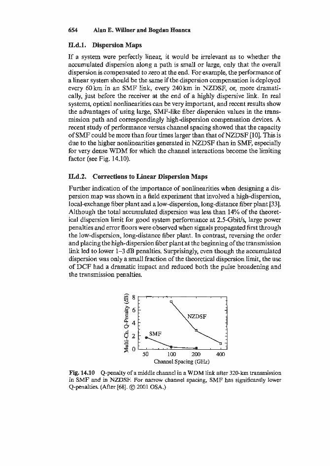
654 Alan E. Willner and Bogdan Hoanca
II.d.1. Dispersion Maps
If a system were perfectly linear, it would be irrelevant as to whether the accumulated dispersion along a path is small or large, only that the overall dispersion is compensated to zero at the end. For example, the performance of a linear system should be the same if the dispersion compensation is deployed every 60 km in an SMF link, every 240 km in NZDSF, or, more dramati- cally, just before the receiver at the end of a highly dispersive link. In real systems, optical nonlinearities can be very important, and recent results show the advantages of using large, SMF-like fiber dispersion values in the trans- mission path and correspondingly high-dispersion compensation devices. A recent study of performance versus channel spacing showed that the capacity of SMF could be more than four times larger than that of NZDSF [lo]. This is due to the higher nonlinearities generated in NZDSF than in SMF, especially for very dense WDM for which the channel interactions become the limiting factor (see Fig. 14.10).
II.d.2. Corrections to Linear Dispersion Maps
Further indication of the importance of nonlinearities when designing a dis- persion map was shown in a field experiment that involved a high-dispersion, local-exchange fiber plant and a low-dispersion, long-distance fiber plant [33]. Although the total accumulated dispersion was less than 14% of the theoret- ical dispersion limit for good system performance at 2.5-Gbit/s, large power penalties and error floors were observed when signals propagated first through the low-dispersion, long-distance fiber plant. In contrast, reversing the order and placing the high-dispersion fiber plant at the beginning of the transmission link led to lower 1-3 dB penalties. Surprisingly, even though the accumulated dispersion was only a small fraction of the theoretical dispersion limit, the use of DCF had a dramatic impact and reduced both the pulse broadening and the transmission penalties.
50 100 200 400 Channel Spacing (GHz)
Fig. 14.10 Q-penalty of a middle channel in a WDM link after 320-km transmission in SMF and in NZDSF. For narrow channel spacing, SMF has significantly lower Q-penalties. (After [68]. @ 2001 OSA.)

14. Fixed and ’hnable Management 655
Another intriguing issue due to the interaction of dispersion and nonlinear- ities is that low-dispersion fiber may require higher-than-expected compensa- tion when including the effect of nonlinearities Even if a truly linear link would allow use of NZDSF without any dispersion compensation, realistic channel power levels as required in terrestrial systems with a certain inter-EDFA dis- tance will make dispersion compensation mandatory. For example, consider the transmission of eight 5-dBm, 10-Gbit/s channels spaced 200 GHz apart over 5 spans of 100 km each. The authors of a recent paper [34] compared the relative performance of three types of NZDSF systems, in which disper- sion accumulates relatively slowly: (1) systems using fiber with only positive dispersion, (2) systems with fiber of only negative dispersion, and (3) sys- tems alternating positive and negative NZDSF with relatively equal lengths. The single-type systems [cases (1) and (2)] used optimized compensation at the transmitter and receiver sites as well as in-line compensation, whereas the alternating system (case 3) required only pre- and postcompensation; in-line compensation was not required, due to the alternating signs of NZDSF. The best performance was obtained in decreasing order, with alternating signs NZDSF; positive NZDSF (3.0 ps/(nm - km), 2-dB power penalty); and neg- ative NZDSF (-2.3 ps/(nm a km), 4-dB power penalty). Moreover, when no compensation was used, error floors as high as
A critical conclusion of these studies is that not all dispersion compensation maps are created equal. A simple calculation of the dispersion compensation to cancel the overall dispersion value does not lead to optimal dispersion map designs.
were detected.
II.d.3. Extreme Dispersion Maps
Dispersion compensation is traditionally performed periodically, with the most desirable location being in the midsection of each EDFA span. In a truly linear system, there should be no difference between periodic dispersion compensation and dispersion compensation done only once at the transmitter or the receiver end. In fact, this extreme approach is possible and may have some advantages, including: (1) no midspan access to the fiber is required, and (2) allowing pulses to first become highly dispersed may minimize the nonlin- earities because the spectrum is broader and the peak powers can be tailored to be lower. Very highly dispersed 40-Gbith RZ data pulses were transmitted over up to 6 fiber spans, each 120 km long (see Fig. 14.1 1) [35]. Very low duty cycle pulses were used at the transmitter so that they would disperse very quickly. Such pulses have broad spectra, which reduce nonlinear effects, allowing much longer transmission distances than if using NRZ pulses (see Fig. 14.12). The authors chose to name such pulses tedons, from the verb “to ted,” a syn- onym of “to scatter; to dissipate.” The demonstration included dispersion compensation at widely spaced points (120 km), well in excess of the traditional compensation distance corresponding to 1 dB power penalty (4 km).

656 Alan E. Willner and Bogdan Hoanca
H 20 ps
Fig. 14.11 Eye diagrams for transmitted (a) and received (b) tedon pulses at 40 Gbit/s through six spans of 120 km apiece. Launch power is 8 dBm. (After [35]. @ 2000 IEEE.)
Transmitted A
h
Y .* E:
c
, 80'
60
40
20
0
Received
0
15
10
5
Q
a
0 10 20 30 40 50 0 10 20 30 40 50 ps
Fig. 14.12 Simulations of tedon and NRZ pulse transmission over six 120-km spans of SMF, launch power is 7 dBm for (a) transmitted NRZ, (b) transmitted tedons, (c) received NRZ, (d) received tedons. A 30-GHz electrical filter was used in the receiver. (After [35]. @ 2000 IEEE.)
One issue that seems to arise in all of these results is that nonlinearities are extremely important in analyzing dispersion-managed systems. As the number of data channels increases in future WDM systems, the total power in the fiber increases as well, and nonlinearities change. This is only one of the reasons
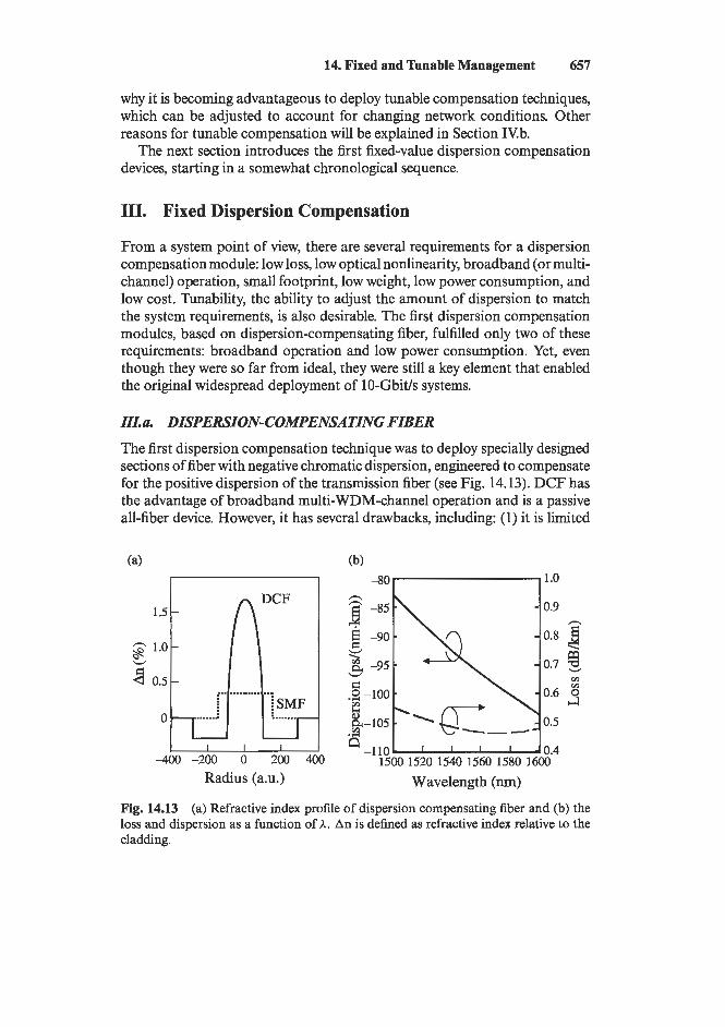
14. Fixed and Thnable Management 657
why it is becoming advantageous to deploy tunable compensation techniques, which can be adjusted to account for changing network conditions. Other reasons for tunable compensation will be explained in Section 1V.b.
The next section introduces the first fixed-value dispersion compensation devices, starting in a somewhat chronological sequence.
111. Fixed Dispersion Compensation
From a system point of view, there are several requirements for a dispersion compensation module: low loss, low optical nonlinearity, broadband (or multi- channel) operation, small footprint, low weight, low power consumption, and low cost. Tunability, the ability to adjust the amount of dispersion to match the system requirements, is also desirable. The first dispersion compensation modules, based on dispersion-compensating fiber, fulfilled only two of these requirements: broadband operation and low power consumption. Yet, even though they were so far from ideal, they were still a key element that enabled the original widespread deployment of 10-Gbit/s systems.
IILa DISPERSION-COMPENSATINGFIBER
The first dispersion compensation technique was to deploy specially designed sections of fiber with negative chromatic dispersion, engineered to compensate for the positive dispersion of the transmission fiber (see Fig. 14.13). DCF has the advantage of broadband multi-WDM-channel operation and is a passive all-fiber device. However, it has several drawbacks, including: (1) it is limited
- 0.9
cl -110 I I I I 0.4 1500 1520 1540 1560 1580 1600
Radius (a.u.) Wavelength (nm)
Fig. 14.13 (a) Refractive index profile of dispersion compensating fiber and (b) the loss and dispersion as a function of 1. An is defmed as refractive index relative to the cladding.

658 Alan E. Willner and Bogdan Hoanca
to a fixed compensation value, and (2) it has a much smaller cross-section, 19 p,m2 as compared to the 85 pm2 of standard single-mode fiber, leading to higher nonlinearity from the higher power density, higher splice losses, and higher bending losses. Furthermore, the length of DCF required to compen- sate for SMF dispersion is rather long, approximately one-fifth the length of transmission fiber for which the module is designed to compensate. Thus, the modules induce loss, and they are relatively bulky and heavy. The bulk is partly due to the mass of fiber, but also due to the resin that is used to hold the fiber securely in place to avoid vibrations. One other contribution to the size of the module is the higher bending loss associated with the smaller cross-section; this limits the radius of the DCF loop to 6-8 inches, as opposed to the min- imum bend radius of 2 inches for SMF. Another key limitation is that in the first generations of DCF, the negative dispersion as a function of wavelength did not match the inverse of the positive dispersion as a function of wavelength of the transmission fiber itself This means that only one central WDM chan- nel could be compensated exactly, with shorter-wavelength channels having a residual positive dispersion and longer-wavelength channels having a residual negative dispersion. This problem is known as “dispersion slope mismatch” and will be covered in greater detail in Section V.
Traditionally, DCF-based dispersion compensation modules are deployed at amplifier sites, with common amplifiers usually being composed of two EDFA stages. The optimal choice is to place the DCF in the midsection of a two-section amplifier. Deployment near EDFA sites serves several purposes. First, amplifier sites offer relatively easy access to the fiber, without any dig- ging and unbraiding of the cable. Second, DCF has high loss, so a gain stage is required before the DCF module to avoid excessively low signal levels. Third, DCF has a cross-section four times smaller then SMF, hence a higher nonlin- earity, which limits the maximum launch power into a DCF module. Placing the DCF before the second stage of the amplifier ensures that the optical power into the DCF module will not induce excessive amounts of nonlinear effects. This way, the second EDFA stage amplifies the dispersion compensated sig- nal to a power level suitable for launching in the fiber. This power level is usually much higher than DCF would tolerate. Note that some of the newer dispersion compensation devices have lower loss and lower nonlinearities than DCF and may not necessitate being deployed in the EDFA midsection. Still, the convenience of easy access to fiber may lead to continued deployment of dispersion compensating modules at amplifier sites.
IILb. CHIXPED FIBER BMGG GRATINGS
Fiber Bragg gratings have emerged as a powerful technology for dispersion compensation because of their potential for low loss, small footprint, and low optical nonlinearity. Bragg gratings are sections of single-mode fiber in which the refractive index of the core is modulated in a periodic fashion as a function
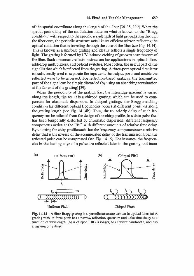
14. Fixed and Tunable Management 659
of the spatial coordinate along the length of the fiber [36-38, 1301. When the spatial periodicity of the modulation matches what is known as the “Bragg condition” with respect to the specific wavelength of light propagating through the fiber core, the periodic structure acts like an efficient mirror, reflecting the optical radiation that is traveling through the core of the fiber (see Fig. 14.14). This is known as a uniform grating and ideally reflects a single frequency of light. The grating is formed by UV-induced etching of grooves near the core of the fiber. Such a resonant reflection structure has applications in optical filters, adddrop multiplexers, and optical switches. Most often, the useful part of the signal is that which is reflected from the grating. A three-port optical circulator is traditionally used to separate the input and the output ports and enable the reflected wave to be accessed. For reflection-based gratings, the transmitted part of the signal can be simply discarded (by using an absorbing termination at the far end of the grating) [39].
When the periodicity of the grating (Le., the interridge spacing) is varied along the length, the result is a chirped grating, which can be used to com- pensate for chromatic dispersion. In chirped gratings, the Bragg matching condition for different optical frequencies occurs at different positions along the grating length (see Fig. 14.14b). Thus, the round-trip delay of each fre- quency can be tailored from the design of the chirp profile. In a data pulse that has been temporally distorted by chromatic dispersion, different frequency components arrive at the FBG with different amounts of relative time delay. By tailoring the chirp profile such that the frequency components see a relative delay that is the inverse of the accumulated delay of the transmission fiber, the reflected pulse can be compressed (see Fig. 14.15). For instance; the frequen- cies in the leading edge of a pulse are reflected later in the grating and incur
(a) Uniform FBG Chirped FBG
+I If Uniform Pitch Chirped Pitch
Fig. 14.14 A fiber Bragg grating is a periodic structure written in optical fiber. (a) A grating with uniform pitch has a narrow reflection spectrum and a flat time delay as a function of wavelength. (b) A chirped FBG is longer, has a wider bandwidth, and has a varying time delay.

660 Alan E. Willner and Bogdan Hoanca
Incident 0 0 - .n Reflected
Fig. 14.15 Chirped gratings reflect different frequency components at different loca- tions within the grating. They can be used for dispersion compensation when the time delay for the grating is the inverse of the delay caused by dispersion.
a long time delay, whereas the frequencies in the trailing edge of the pulse are reflected in the earlier part of the grating and incur a shorter time delay. The negative dispersion induced by the grating can be characterized by the slope of the time delay when plotted as a function of wavelength, which is related to the grating chirp. The chirp, in turn, is the rate of change of the spatial frequency as a function of position along the grating. This time vs wavelength slope is in units of pshm, which is the same as the fiber chromatic dispersion.
As mentioned previously, dispersion-compensating FBGs are very attrac- tive for system designers because of their low nonlinearity, low loss, and compact footprint. A key technical challenge of gratings is that the amplitude- reflection and phase-delay spectral profile have some nonuniformity, com- monly known as “ripple.” Ideally, the amplitude profile of the grating should have a flat or smoothly rounded top in the passband, and the phase profile should vary as a smooth function according to the periodicity written into the grating, such that the profile is a straight line for linearly chirped gratings or a polynomial for nonlinearly chirped gratings. The grating ripple is the deviation from the ideal profile shape (see Fig. 14.16). In general, the ripple is random, with both deterministic and random causes. When ripple is mentioned, it usu- ally refers to the phase ripple, which is significantly more problematic than the amplitude ripple.
One source of ripple is the edge effects at the beginning and end of the grating. Because the grating has a finite length, sharp transitions at the edges of the grating induce oscillations in the spectrum, which lead to ripple. The straightforward solution is to apodize the grating by smoothing out the grating edges such that the ripple is minimized [40].
Another source of ripple is stitching error. Gratings can be written by shin- ing UV light through a phase mask, and masks are fabricated by scanning an electron etching beam across a glass substrate [41]. When scanning the beam along the mask, it may be necessary to reposition the mask relative to the electron beam source so as to write over larger fields. This repositioning can introduce alignment (“stitching”) errors, which are much higher than the writ- ing errors due to the positioning of the electron beam alone. As several sections of the mask are written, the repeated repositioning events lead to increasing

14. Fixed and Tunable Management 661
0 2500 h CQ 3 -5 2000
1500
h .E? 2 -10 3. 2
B 1000 8 B 5 -20
3 2 -15
.d
B
2 E -25 500
0 1
1558.6 1558.7 1558.8
-30! I I I I , I I m
Wavelength (nm)
Fig. 14.16 Plot of the amplitude and time delay, including ripple, for a linearly chirped FBG. The ripple is oscillatory and random and should be minimized for best system performance.
amounts of stitching error. The effect of the stitching error can be quanti- fied by comparing the performance of electron-beam-written masks with the performance of holographically written masks for which no repositioning or stitching error occurs. One possible way to mitigate the stitching problem is by repeated exposures of the e-beam phase mask that tends to average out the writing imperfections. Experimental data indicates that a four-times- overwritten phase mask has ripple comparable with that of gratings obtained using a holographically written phase mask [42].
The two ripple sources mentioned here are deterministic in the sense that such errors are fixed at the time of mask fabrication. Other sources of rip- ple that may introduce nondeterministic errors include: (1) laser phase noise, (2) variations in the grating diameter due to variations in the original fiber in which the grating is written, (3) laser beam pointing error in the writing process, (4) dust particles in an unclean environment, and (5) various random mechanical effects in the grating writing stage.
Considerable effort has been expended on reducing the ripple. From the first gratings that were plagued by more than 100 ps of ripple, the published results have improved to present-day values close to f 3 ps [43].
Ripple is random, “noisy,” and can be decomposed into various frequency components containing slower and faster varying contributions. The effects of ripple on the signal are bit rate dependent, with the highest power penalty occurring when the largest frequency component of the ripple matches the bit rate [44]. In this case, the random slope of the ripple can be in the completely wrong direction and be relatively constant across the entire signal bandwidth, hence inducing the highest penalty (see Fig. 14.17). A ripple period that is smaller than the data rate averages out over the signal bandwidth, whereas a
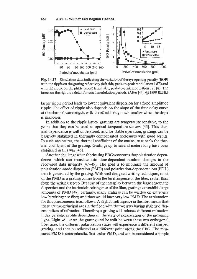
662 Alan E. Willner and Bogdan Hoanca
0.30 - 8
8
b 0.20 a 8 9 0.10
0.00 M
40 80 120 160 200 240 260
5
0 0 200 400 600 800 1000
Period of modulation [pm]
Fig. 14.17 Simulation data indicating the variation of the eye opening penalty (EOP) with the ripple on the grating reflectivity (left side, peak-to-peak modulation 1 dB) and with the ripple on the phase profile (right side, peak-to-peak modulation 120 ps). The insert on the right is a detail for small modulation periods. (After [44]. @ 1998 IEEE.).
Period of modulation [pm]
larger ripple period leads to lower equivalent dispersion for a fixed amplitude ripple. The effect of ripple also depends on the slope of the time delay curve at the channel wavelength, with the effect being much smaller when the slope is shallower.
In addition to the ripple issues, gratings are temperature sensitive, to the point that they can be used as optical temperature sensors [45]. This ther- mal dependence is well understood, and for stable operation, gratings can be passively stabilized in thermally compensated enclosures with good results. In such enclosures, the thermal coefficient of the enclosure cancels the ther- mal coefficient of the grating. Gratings up to several meters long have been stabilized in this way [46].
Another challenge when fabricating FBGs concerns the polarization depen- dence, which can translate into time-dependent random changes in the recovered data integrity [47-491. The goal is to minimize the amount of polarization-mode dispersion (PMD) and polarization-dependent loss (PDL) that is generated by the grating. With well-designed writing techniques, most of the PMD in a grating comes from the birefringence of the fiber, rather than from the writing set-up. Because of the interplay between the large chromatic dispersion and the intrinsic birefringence of the fiber, gratings can exhibit large amounts of PMD [47]; certainly, many gratings can be written on extremely low birefringence fiber, and thus would have very low PMD. The explanation for this phenomenon is as follows: A slight birefringence in the fiber means that there are two principal axes in the fiber, with the two axes having slightly differ- ent indices of refraction. Therefore, a grating will induce a different refraction index periodic profile depending on the state of polarization of the incoming light. Light will enter the grating and be split between these two orthogonal fiber axes, the different polarization states will experience a different chirped grating, and thus be reflected at a different point along the FBG. The mea- sured PMD is deterministic, first-order PMD, and can be considered a simple

14. Fixed and Tunable Management 663
differential group delay (DGD) that does not change appreciably over time if the grating is well stabilized thermally. For cases in which this DGD exists and must be compensated, a simple DGD element (i.e., a length of polarization- maintaining fiber) that provides the exact opposite DGD can be spliced directly onto the FBG [50]. It should be noted that good grating-writing techniques use a symmetrical writing set-up, which can reduce the PMD of the resulting gratings to less than a few picoseconds.
PDL is another phenomenon that concerns system designers. Devices with PDL induce a different amount of insertion loss depending on the state of polarization of the signal. In a system this can induce unacceptable power fluctuations, as well as more complex pulse distortions due to the interaction among several PDL elements or interaction among several PMD and PDL sources. Traditionally, the PDL of FBGs has not been a concern due to the symmetry of the device.
Several system demonstrations have shown that FBGs are very robust and can deliver performance superior to other dispersion compensation solutions. WDM 10- and 40-GbitIs transmission has been demonstrated over distances up to 480 km [17] and 109 km [5 11, respectively. As explained previously, FBG- based dispersion compensators have inherently lower nonlinearity than DCF. Simulations of the power penalty for transmitting 40-Gbit.h RZ data using DCF, idealized DCF with zero nonlinearity, and FBGs showed that the per- formance of the FBG is close to the idealized linear DCF systems. Because real DCF has sizeable nonlinearity, FBGs have the potential to allow much higher performance [74].
Not to be neglected is the capability of FBGs to perform other func- tions simultaneously with dispersion compensation. Several approaches have been proposed that would use an FBG to flatten the gain of an EDFA [52] or to function as an optical add-drop multiplexer [53] while simultaneously compensating for link dispersion.
III.b.1. Single-Channel Linearly Chirped Gratings
Some early chirped gratings were fabricated with a linear chirp [54]. For a lin- early chirped grating, the slope of the FBG time delay curve as a function of wavelength is constant and chosen to be equal to the negative of the amount of accumulated fiber dispersion to be compensated. Such centimeters-long grat- ings are intended for fixed compensation, but were not very cost effective since they could only compensate for a single WDM channel. The most interest- ing recent developments are towards multiple-channel gratings and towards tunability, or a combination of the two.
III.b.2. Multiple-Channel Bragg Gratings
Conceptually, there are presently four ways to achieve multiple-channel opera- tion: (1) concatenating gratings in series, (2) concatenating gratings in parallel, (3) fabricating long, broadband gratings, and (4) fabricating short, sampled

664 Alan E. Willner and Bogdan Hoanca
gratings. The first two approaches are expensive, do not scale well, introduce large losses, and may even create a nonuniform amplitude reflection between the WDM channels. The third and fourth methods are potentially more practical since multiple-channel operation is achieved in a single grating. His- torically, the first multiple-channel gratings were made using longer gratings, with recent results indicating that gratings up to 10 meters are feasible [55-571.
III. b. 2. i. Long-Length Broadband Gratings
A chirped FBG can provide negative dispersion over a wide wavelength range if the grating itself can be written over a long enough fiber. Traditionally, writ- ing meters-length gratings for broadband operation has been difficult due to the large ripple induced by the accumulated stitching errors when reposition- ing the grating to the writing stage. The breakthrough in making very long broadband gratings with low ripple was to use constant velocity writing, with the grating fiber wrapped around a large rotating spindle (see Fig. 14.18). It is possible to stabilize and control the velocity to better than 1 ppm [58] by using a large weight to create rotational momentum on a spool that is very carefully trued to a precision of 250 nm. Meters-long gratings manufactured with this technique can have as little as f20ps ripple [58].
Broadband linearly chirped compensation gratings have been used for transmission of 32 10-Gbitls NRZ channels over 375 km [59]. Each ampli- fier site was spaced 75 km apart and contained three broadband gratings, one
Velocity Control
UV beam
1 I Velocity A.O. c-I1 t+ Function
generation I I
tn
Fig. 14.18 Writing of very long FBG structures using a constant velocity stage, with the fiber on a rotating spool. “Infinitely long” (tens of meters long) gratings can potentially be written this way. A.0.-acousto-optic. (After [%I. @ 2000 Pennwell Corp.)
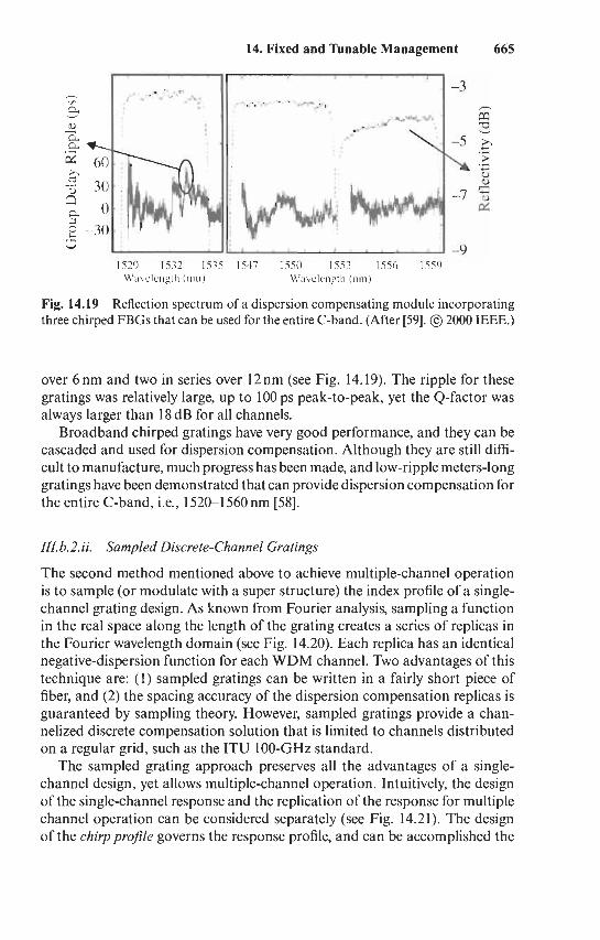
14. Fixed and Tunable Management
1529 1532 1535 1547 1550 1553 1556 1559 Wavelength (nm) Wavelength (nm)
Fig. 14.19 Reflection spectrum of a dispersion compensating module incorporating three chirped FBGs that can be used for the entire C-band. (After [59]. @ 2000 IEEE.)
over 6 nm and two in series over 12 nm (see Fig. 14.19). The ripple for these gratings was relatively large, up to 100 ps peak-to-peak, yet the Q-factor was always larger than 18 dB for all channels.
Broadband chirped gratings have very good performance, and they can be cascaded and used for dispersion compensation. Although they are still diffi- cult to manufacture, much progress has been made, and low-ripple meters-long gratings have been demonstrated that can provide dispersion compensation for the entire C-band, Le., 1520-1560 nm [58].
III. b.2.ii. Sampled Discrete-Channel Gratings
The second method mentioned above to achieve multiple-channel operation is to sample (or modulate with a super structure) the index profile of a single- channel grating design. As known from Fourier analysis, sampling a function in the real space along the length of the grating creates a series of replicas in the Fourier wavelength domain (see Fig. 14.20). Each replica has an identical negative-dispersion function for each WDM channel. Two advantages of this technique are: (1) sampled gratings can be written in a fairly short piece of fiber, and (2) the spacing accuracy of the dispersion compensation replicas is guaranteed by sampling theory. However, sampled gratings provide a chan- nelized discrete compensation solution that is limited to channels distributed on a regular grid, such as the ITU 100-GHz standard.
The sampled grating approach preserves all the advantages of a single- channel design, yet allows multiple-channel operation. Intuitively, the design of the single-channel response and the replication of the response for multiple channel operation can be considered separately (see Fig. 14.21). The design of the chirp profile governs the response profile, and can be accomplished the
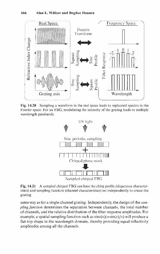
666 Alan E. Willner and Bogdan Hoanca
Real Space \
1-4
Grating axis
Fourier Transform
I Wavelength
Fig. 14.20 Sampling a waveform in the real space leads to replicated spectra in the Fourier space. For an FBG, modulating the intensity of the grating leads to multiple wavelength passbands.
UV light
Sinc periodic sampling - Chirped phase mask
Sampled chirped FBG
Fig. 14.21 A sampled chirped FBG can have the chirp profile (dispersion character- istics) and sampling function (channel characteristics) set independently to create the grating.
same way as for a single-channel grating. Independently, the design of the sam- pling function determines the separation between channels, the total number of channels, and the relative distribution of the filter response amplitudes. For example, a spatial sampling function such as sinc(x)(=sin(x)/x) will produce a flat-top shape in the wavelength domain, thereby providing equal reflectivity amplitudes among all the channels.


668 Alan E. Willner and Bogdan Hoanca
For an N channel grating, the refractive index is modulated only in 1/N of the grating length (i.e., the duty cycle of the grating is l/N), therefore the reflectivity is reduced by the same factor, A clever way of increasing the efficiency is to interleave several grating designs into the same general space, such that each grating’s modulation of reflectivity falls in the areas where other gratings have no reflectivity modulation [61]. This technique allows an N channel grating to be written as f i interleaved gratings, each with f i channels. The decrease in reflectivity of each grating is then corresponding to only l / f i , even though the total grating can service N channels.
III.b.3. FBG Dispersion Compensators in Transmission Mode
FBG-based dispersion compensators are typically used in the reflection mode, thus requiring a circulator to separate the input and output signals. It may be more cost effective to use gratings in the transmission mode [39] for which the compensated signal is input from one side of the grating and is output from the other side, thereby eliminating the need for the circulator. Transmission gratings typically have a grating periodicity that is much longer than reflection gratings, thus they are also referred to as long-period gratings. Such gratings could potentially reduce the cost, footprint, and loss. Additionally, the grat- ing phase ripple could be considerably smaller because the gratings would be weaker per unit length. Given the attractive features of transmission gratings, research groups have already demonstrated the feasibility of dispersion com- pensation with such devices [62]. The demonstration involved transmission of 470-fs pulses (corresponding to 112 Gbit/s RZ) over 3.9 km of DSF or 260 m of SMF. The results also show good performance with cascaded transmission gratings.
From a practical point of view, transmission gratings are difficult to deploy since: (1) they are very sensitive to temperature because they are operated near the temperature-dependent resonance wavelength, and (2) they are limited to narrow bandwidth operation. The grating length can also be rather long, requiring greater thermal stability. Simulations indicate that a 50-cm grating is required to compensate for 100 km of SMF [39]. For comparison, a 15-cm length is sufficient for the same function if using a reflection grating. The challenge of using transmission gratings is to thermally compensate a long grating without bending or spooling it.
IILc. HIGHER-ORDER-MODEDISPERSION COMPENSATION FIBER
One of the challenges of designing standard DCF is that high negative disper- sion is hard to achieve unless the cross-section of the fiber is small, thereby leading to high nonlinearity and high loss. One method to reduce both the nonlinearity and the loss is to use a higher-order-mode (HOM) fiber, which
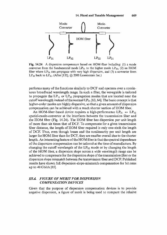
14. Fixed and Tunable Management 669
Mode- Mode- Converter Converter
Fig. 14.24 A dispersion compensator based on HOM fiber including: (1) a mode converter from the fundamental mode LPol to the higher mode LP02, (2) an HOM fiber where LPo2 can propagate with very high dispersion, and (3) a converter from LP02 back to LPol. (After [132]. @ 2000 Lasercomm Inc.)
performs many of the functions similarly to DCF and operates over a contin- uous broadband wavelength range. In such a fiber, the waveguide is tailored to propagate the LPll or LP02 propagation modes that are located near the cutoff wavelength instead of the normal LPol[63,64]. The basic concept is that higher-order modes are highly dispersive, so that a given amount of dispersion compensation can be achieved with a much shorter section of HOM fiber.
An HOM-fiber-based device requires a high-performance LPol -e LP02 spatial-mode-converter at the interfaces between the transmission fiber and the HOM fiber (Fig. 14.24). The HOM fiber has dispersion per unit length of more than six times that of DCF. To compensate for a given transmission fiber distance, the length of HOM fiber required is only one-sixth the length of DCF. Thus, even though losses and the nonlinearity per unit length are larger for HOM fiber than for DCF, they are smaller overall due to the shorter length. An interesting feature of the HOM fiber is that the spectral dependence of the dispersion compensation can be tailored at the time of manufacture. By changing the cutoff wavelength of the LP02 mode or by changing the length of the HOM fiber, a dispersion slope across a wide wavelength range can be achieved to compensate for the dispersion slope of the transmission fiber or the dispersion slope mismatch between the transmission fiber and DCF. Published results have shown full dispersion-slope-mismatch compensation for bit rates up to 40 Gbit/s [65].
IILd FIGURE OF MERIT FOR DISPERSION COMPENSATION DE WCES
Given that the purpose of dispersion compensation devices is to provide negative dispersion, a figure of merit is being used to compare the relative
670 Alan E. Willner and Bogdan Hoanca
performance among the different solutions. This figure of merit is defined as
FOM = D/a, (14.3)
which is the ratio of the dispersion of the device to its insertion loss. Because both the loss and the dispersion of DCF increase as the length increases, the FOM is relatively constant and independent of the dispersion value of the module. A similar behavior applies to HOM fiber. On the other hand, FBG- based devices have a loss essentially independent of dispersion, and therefore have the capability of achieving much larger FOM values for large dispersion compensation.
IV. Tunable Dispersion Compensation
I k h TIME-DEPENDENT EFFECTS IN OPTICAL NETWORKS
Chromatic dispersion historically has been considered predominantly a time- invariant phenomenon. As such, fixed compensation of signal impairments in a “set-and-forget” approach at the time of manufacture and deployment would be expected to perform uniformly well over time. This is certainly the case for relatively low (52.5-Gbids) signals for which dispersion compensation is most often not needed. In scenarios that do not require either accurate com- pensation or dynamic network conditions, fixed and/or coarse compensation can be considered adequate.
The first OC-48 systems involved only a small number of WDM channels and the system was expected to operate undisturbed and unchanged, except for catastrophic network failure events. This static view is challenged more and more as the performance of systems continues to rise and the timescale of system changes continues to decrease. The shrinking system margins are due to three key systems advances: (1) higher bit rates, (2) more wavelength chan- nels, and (3) the migration to more complex, time varying network topologies. Thus, small changes that used to be insignificant when compared to the design power margins are now becoming very significant. These changes must now be compensated for to keep the systems operating. In addition, events that used to be viewed as catastrophic, such as restoration in case of failure, are becom- ing more common as the networks become truly reconfigurable. Therefore, it is not surprising that control of signal impairments in fiber-optic systems has acquired the new dimension of time, and that dispersion compensation has gained tunability as a highly desirable function [66-681.
For every SONET-based, four-fold bit-rate upgrade, the deleterious effect of chromatic dispersion increases by a factor of 16. Effects that could be safely ignored for OC-48 systems become critical for OC-192 and above. Issues such as component aging and environmental effects do not affect the performance of a low-bit-rate system. This isnot the case for high-bit-rate systems, where these
14. Fixed and 'hnable Management 671
issues may have a severe impact on the system performance unless changes are tracked and compensated. For example, thermal drift of the chromatic dispersion is insignificant for data rates below 40-Gbit.h signals, but must be continuously tracked for systems at 40 Gbit/s and above [69].
The effect of increasing channel counts also contributes to making the net- work h e dependent. In a two-wavelength system, little change is expected, unless a catastrophic failure occurs. However, in a system with tens of wavelength channels, it is much more likely that some channels may be dropped or added, with the associated changes in the power level in the fiber that would affect the dispersion map. Furthermore, a k e d dispersion map does not allow a network to gracefully deploy more channels in any future upgrade.
Of course, the most intuitive time dependence is induced in circuit-switched reconfigurable networks Such networks are expected to increase the efficiency of bandwidth usage. A study showed that for the same blocking probability, a reconfigurable WDM network with 20 nodes could support up to 6 times the traffic load compared to a network with a static topology [70]. Most often, reconfigurable networks are based on complex mesh topologies, where several possible paths exist between any s o w and destination. Depending on the state of the reconfigurable network, establishing a connection between the same two points at two different instances may result in a totally different signal path as the network management attempts to balance the traffic load and bypass unavailable sections.
In order to achieve the expected efficiency gains in such reconfigurable networks, signal paths must be set up and torn down in seconds or frac- tions of seconds. Channels are added and dropped, and wavelengths may follow time-dependent paths, all to achieve higher efficiency of the network's resources. As fiber paths change, chromatic dispersion will change accord- ingly, and compensation devices will have to adjust on the fly to accommodate the changes. Examples of signal path changes are: (a) reconligurable WDM adddrop multiplexing nodes. (b) SONET rings that must redirect traffic to the protection path in case of a fiber break, and (c) fdly-recordigurable WDM crossconnects.
It is conceivable that tunable compensation for recordigurable optical net- works will not be necessary if one assumes that each fiber link in the entire network has been internally dispersion compensated. In such a scenario, path changes located at network nodes do not incur any changes in accumulated chromatic dispersion. However, this can be quite problematic because: (1) it may be unlikely that each and every fiber link in the entire network has been internally compensated or would remain so in the face of periodic maintenance, and (2) it limits the scalability and modularity that is an essential ingredient of flexible and high-performance networks [71].
For the more distant future, there is talk about packet-switched opti- cal networks. Unlike circuit-switched networks, in packet-switched networks

672 Alan E. Willner and Bogdan Hoanca
paths are set up for only the duration of a packet. This avoids all the over- head of circuit-switched paths, which require handshake signals and which guarantee the bandwidth availability. In a packet-switched network, smaller chunks of data (packets) are sent over paths that are allocated dynamically. No guarantee is made for bandwidth availability, so packets may be lost or dropped. Conversely, there is no expensive overhead to set up the path. Overall, packet switching is much more demanding on the speed of switch- ing elements. It is not clear if and whether optical packet switching will be feasible, but when available it will put a tremendous strain on the switch- ing speed of optical components, including tunable dispersion-compensation modules.
Because of all the time-dependent effects, such as component changes, environmental changes, or network-induced path changes, it may become important that compensation of signal degrading effects allow not only for tunability, but also for adaptability. For changes that occur on the order of milliseconds or faster, a global management system that would tune the com- pensator remotely may be too slow to react. Instead, each device may require a local dispersion-monitor-control feedback loop to adapt to new network con- ditions. At present, dynamically self-tunable dispersion compensators have yet to be deployed commercially.
IKb. THE NEED FOR TUNABLE DISPERSION COMPENSATION
In general, fixed dispersion maps are suitable only for relatively low-speed, static systems. Otherwise, compensation devices must be tunable for several reasons, as described below:
1. Inventory management. Even in a static network, distances between dispersion compensation points will vary, depending on the geography of the region and on the traffic requirements. Each‘ fiber link will have a different length, and the chromatic dispersion value of the deployed fiber is only accurate to within some nonzero factory specification. As such, dispersion compensation modules must cover a wide range of compensation values. Any systems integration company would need to stock many different models of a given dispersion compensation module to account for the many values of accumulated chromatic dispersion. When considering inventory reduction, it is highly attractive to stock modules that can be tuned to the desired value, and then deployed interchangeably in a “set-and-forgetyy fashion. The alternative is to have a large stock of devices covering the whole range of required discrete compensation values or a source for custom devices to match the deployment needs. Similar considerations apply to the management of backup devices for an existing system.

14. Fixed and anable Management 673
Tunable Compensator
0 40 80 120 160 Distance (km)
Fig. 14.25 Through the use of a tunable compensator, the power penalty can be reduced across a wide range of transmission distances at 10 Gbitlsec. The k e d 80-km compensator is good in a specific range and at t40km is worse than having no compensation.
2. Accuracy for ZlO-Gbith systems. The required accuracy in dispersion compensation increases dramatically with the signal bit rate. Whereas the amount of residual dispersion that is tolerable at 10-Gbit/s in a partially-compensated link is approximately 1000 pshm (see Fig. 14.25), this margin shrinks to only 60 pshm for 40-Gbit/s systems (see Fig. 14.26). It is clear that providing highly accurate compensation would require either tunable or custom modules. Otherwise, increasing amounts of residual dispersion will accumulate over cascaded stages of imperfect partial dispersion compensation (see Fig. 14.27). The use of tunable modules seems to be the only practical solution for compensating accumulated dispersion with a manageable inventory of modules.
3 . Changes in the path length. In a reconfigurable network, as signals are rerouted to avoid traffic congestion or faulty sections, the distance and type of fiber may change. The chromatic dispersion-compensation unit at the receiver must follow these changes. It is important to note that even if the fiber spans are compensated periodically, span-by-span, the pervasive use of compensation at the transmitter and receiver suggests that optimization and tunability based on the path will still be needed. Moreover, the span length itself is constantly modified by rework of the network in the form of splicing in case of fiber breakage and repair.
4. Environmental eflects. Temperature changes can lead to variations in dispersion that may be significant enough to impact the system. In

674 Alan E. Willner and Bogdan Hoanca
No,Compensation
fT-7 : 40GbiVs I Fixed 80 km Compensator
0 20 40 60 80 100 120 140 160 Distance (km)
Fig. 14.26 A tunable compensator allows for a wide range of transmission distances at 40 Gbitkec. The 80-km fixed compensator case offers too small a range to be practical.
Single channel
accumulated chromatic dispersion
40 Gbit/s limit b
50% compensation
\ / / \ compensation
Distance
Fig. 14.27 The tolerance of 40-GbiVs systems to chromatic dispersion is 16 times lower than that of 10-Gbit/s systems. Approximate compensation by fixed in-line disper- sion compensators for a single channel may lead to rapid accumulation of unacceptable levels of residual chromatic dispersion.
fiber, the zero-dispersion wavelength changes with temperature, at a rate of 0.03 nm/"C (see Fig. 14.28). Thus, the relative change in dispersion is proportional to the magnitude of the slope of the fiber and to the thermal change [69]. Given a temperature change of AT = 25"C, a distance of L = 500 km, and an SMF dispersion slope of D(2) = 0.08 ps/(nm2 . km), the thermally induced variation in dispersion is AD = 30 ps/nm, which corresponds to the accumulated dispersion of 2 km of SMF or 7.5 km of NZDSF. This amount is relatively insignificant for IO-Gbit/s systems, but is becoming significant for 4O-GbitIs systems, where the 1-dB tolerance is at

14. Fixed and Tunable Management 675
100 \ " ' . ' . ' . ' . ' . ' \
NRZ40 GWs Limit . \ ......................................... \
\ 50 "'. \
'. \ - . . - .>\ '. 6
M
-.. -.. '.\ * u p
1.. -..-: g G = 0 - $:.-.. \'., 5 .2 23 0 2 a
\ '.<
123 I-\ k200km
\ +=SO0 km . 3 :Dispersion Slope - 0.08 ps/(nmZkm) \ \. dhddT - 0.03 nmPC Q -50 -
.3
\ ............................................ ' NRZ 40 Gb/s Limit \
L=1oookm\ '
\ . -100 ' I " . ' " " " ' ' ,'
-60 ps/nm. Figure 14.29 shows that a not-uncommon 50°C variation along a 1000-km 40-Gbids link would produce significant degradation.
5 . Wavelength drift andfilterpassband shape. It is quite possible that in any WDM network, various components, such as lasers, aters, and (de)multiplexers will experience wavelength drift. Particularly in the case of SONET rings, there could potentially be many demuxlmux pairs that must be traversed by a signal. Now let's consider the filter passband shape of flters and (de)muxes. In any filter, there is a phase change induced on the transmitted signal if the signal is located off

676 Alan E. Willner and Bogdan Hoanca
(a) Ideal Hat Tap (b) A/ Nophase
change (A@ =0)
t' filter . channel
Sloping Tails
Phase change
I \ I \
I
Fig. 14.30 A channel centered within a flat-top filter undergoes no phase changes (a). A channel on the sloping edge of a filter gains an induced chirp, resulting in dispersion 0).
peak and on the sloping roll-off edges of the filter passband function (see Fig. 14.30). A phase change can be thought of as a time shift, in picoseconds. This change is taking place across the spectral bandwidth of the signal itself, as measured in nm. Therefore, a signal that passes through a filter but is not located at the peak will suffer from frequency-dependent phase delay (i.e., dispersion), which will then interact with the fiber chromatic dispersion and degrade the signal. Note that this is also a key reason why filter manufacturers diligently strive to produce flat-top response shapes for their customers.
6. Changes in the signalpower. As channels are added/dropped in a network or if the transmitter power changes over time, the total power in the fiber will change, thereby changing the effect due to fiber nonlinearities [72]. As the power changes, the optimal dispersion-compensation map may also change, requiring tunability of the dispersion. For 24O-Gbith signals, even self-phase modulation will change the dispersion map sufficiently to require tunable dispersion compensation [73].
when using nontraditional data formats in a system. For example, it has been shown that RZ transmission at 40 Gbit/s can extend the distance by a factor of two as compared to NRZ [74]. (Moreover, the RZ format is more sensitive to chromatic dispersion.) For this reason, RZ systems may require dynamically adaptive dispersion compensation even when NRZ formats may not.
7. High per$ormance data formats. Tunability may be quite important
Each of these changes occw on a very different timescale. Path-length changes can be moderately fast, on the order of a few milliseconds for SONET
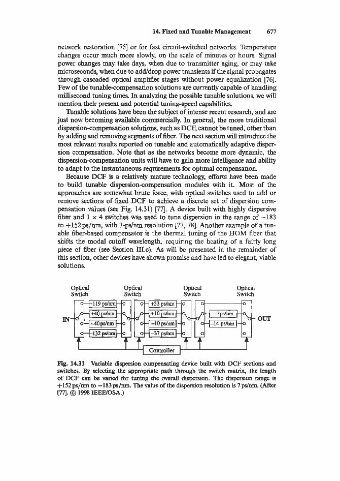
14. Fixed and Tunable Management 677
network restoration [75] or for fast circuit-switched networks. Temperature changes occur much more slowly, on the scale of minutes or hours. Signal power changes may take days, when due to transmitter aging, or may take microseconds, when due to adddrop power transients if the signal propagates through cascaded optical amplifier stages without power equalization [7q. Few of the tunable-compensation solutions are currently capable of handling millisecond tuning times. In analyzing the possible tunable solutions, we will mention their present and potential tuning-speed capabilities.
Tunable solutions have been the subject of intense recent research, and are just now becoming available commercially. In general, the more traditional dispersioncompensation solutions, such as DCF, cannot be tuned, other than by adding and removing segments of fiber. The next section will introduce the most relevant results reported on tunable and automatically adaptive disper- sion compensation. Note that as the networks become more dynamic, the dispersion-compensation units will have to gain more intelligence and ability to adapt to the instantaneous requirements for optimal compensation.
Because DCF is a relatively mature technology, efforts have been made to build tunable dispersion-compensation modules with it. Most of the approaches are somewhat brute force, with optical switches used to add or remove sections of fixed DCF to achieve a discrete set of dispersion com- pensation values (see Fig. 14.31) [77]. A device built with highly dispersive fiber and 1 x 4 switches was used to tune dispersion in the range of -183 to +152ps/nm, with 7-pslnm resolution [77, 781. Another example of a tun- able fiber-based compensator is the thermal tuning of the HOM fiber that shifts the modal cutoff wavelength, requiring the heating of a fairly long piece of fiber (see Section 1II.c). As will be presented in the remainder of this section, other devices have shown promise and have led to elegant, viable solutions.
IN
optical optical Optical Optical Switch Switch Switch Switch
OUT
Fig. 14.31 Variable dispersion compensating device built with DCF sections and switches. By selecting the appropriate path through the switch matrix, the length of DCF can be varied for tuning the overall dispersion. The dispersion range is + 152 ps/nm to - 183 ps/nm. The value of the dispersion resolution is 7 pdnm. (After [77l. @ 1998 IEEWOSA.)

678 Alan E. Willner and Bogdan Hoanca
I l k . SINGLE-CHANNEL TUNABLE FIBER BRAGG GRATINGS
IV.c.1. Single-Channel Tunable Gratings
To achieve dispersion-compensation tunability in an FBG, the slope of the delay curve as a function of wavelength must be altered. Several ways to do this have been reported.
IV.c.2. Grating Tuning with Nonuniform Mechanical Strain
The first idea for demonstrating dispersion tunability was to use a multiple dif- ferential stretching of a uniform grating [79]. A uniform grating was mounted on a stretcher with 21 piezoelectric sections (see Fig. 14.32). By applying volt- ages ramping up linearly from zero to a maximum value across the piezo stages, the induced dispersion could be varied from 940 pshm with maximum strain to 8770pshm with no strain. The concept is that eadh section induces a different amount of stretching, which increases linearly along the grating. The effect is to change the grating periodicity and the chirp rate, thereby changing the dispersion. The tuning speed can be on the order of -20ms.
Uniform FBG
2 1 Discrete Piezoelectric Stretchers
100 , I, I , I , I , , ,I ,I ,I ,I , I , I , I, I, I, I, , I , , , , ,I
0 2 1 6 8 IO 12 14 16 18 20 Segment
Fig. 14.32 By attaching a linearly chirped grating to a stack of 21 independent stretchers (top), the slope of the chirp (Le., the dispersion) can be changed. Asymmetric stretching is the key to this tuning scheme. The bottom figure shows the percentage of full-scale voltage applied to each of the 21 sections for 4 different stretching amounts, A, B, C, and D (increasing dispersion). (After [79]. @ 1997 OSA.)

14. Fixed and Tunable Management 679
Unintended consequences as the grating was tuned from no strain to maxi- mum strain included: (a) the reflectivity of the grating decreased by more than 3 dB, (b) the passband increased by a factor of two, (c) the center wavelength shifted by about 0.2 nm, and (d) the ripple increased considerably.
Another approach is to induce differential stretching with a single stretching element. This can be accomplished by attaching the grating to a cantilever beam and bending the beam. Because the strain distribution in such a beam is nonlinear, the slope of the chirp induced on the grating can be changed by varying the amount of beam bending [SO]. To avoid the shift of the center wavelength, the cantilever beam can be mounted to prevent rotations [S 11. A simple method to realize this general technique relies upon the use of a plastic sleeve enclosing a 10-cm-long linearly chirped FBG and a metal rod of similar length (see Fig. 14.33). The rod diameter was 1.5 mm and the total beam diameter 3.0 mm. The grating pitch can be varied to give positive, negative, or even zero chirp by simply bending the beam in the right direction. A key issue was to rigidly hold the end of the beam, so that no rotation would occur. The authors reported a dispersion tuning range from -791 ps/nm to +932 ps/nm with a 10-mm bend [Sl]. The center wavelength shift of the FBG was as small as 0.09 nm over the dispersion tuning range, but the grating passband changed considerably, from 0.5 to 2.0 nm. A key element for this method is a very good bond between the grating and the substrate in order to ensure that the strain profile is accurately transferred from the substrate to the grating.
.* 3 0 2
h
B 800 v
1550.5 1551.0 1551.5 1552.0 Wavelength (nm)
-z=O mm - - - z = 5 mm h
?? .2-20 .* -
4o 1549 1550 1551 1552 1553 Wavelength (nm)
Fig. 14.33 Tunable dispersion compensation with a linearly chirped FBG mounted on a cantilever.beam (a). Time-delay curve showing linear tunable slope as a function of displacement (b). Reflectivity curve showing no shift of the center wavelength, but only a change in passband width (c). (After [SO]. @ 1998 IEEE.)

680 Alan E. Willner and Bogdan Hoanca
0 0.0 2 4 6
Position Along Fiber (cm) i
Fig. 14.34 Thermally tuned FBG using a tapered metal film. Temperature profile varies along the fiber length (due to the tapered film thickness, top), inducing a variable dispersion. Cross sections of the fiber show the variable thickness of the metallic layer (bottom). (After [82]. @ 1999 IEEE.)
IV.c.3. Grating Tuning with Nonuniform Thermal Gradients
Another tunable method is based on differential heating of the substrate and, consequently, the grating (see Fig. 14.34). In general, the grating response shifts to longer wavelengths under an increase in the local temperature. An electrically controlled thermal gradient induced along an FBG will chirp the FBG response and produce a tunable dispersion compensator [82]. This ther- mal gradient is produced by varying the thickness of a thermal heating element deposited around and along the length of the grating. For a 7.5-cm grating, the power consumption was only 1 W, the tuning range was -300 to - 1350 ps/nm, and the ripple was lops peak-to-peak (see Fig. 14.35). The thermally tuned grating has a major advantage: no moving parts. However, the disadvantages include: (1) slow tuning that is limited to large fractions of seconds, (2) require- ment for accurate deposition of a thin film of tapered thickness, and (3) large power consumption. The thermally tuned grating has been used for com- pensation of 40-Gbith data [73]. The purpose was to fine-tune dispersion to compensate for the effects of SPM, rather than for large accumulated dis- persion. Thus, the system included static dispersion compensation and used relatively large launched signal power (see Fig. 14.36).
Moreover, the thermally tuned grating can handle even higher data rates [83]. A grating that was used for 160-Gbit/s compensation had a tun- ing range of 50pdnm (-130 to -8Ops/nm) and a ripple of less than 5ps
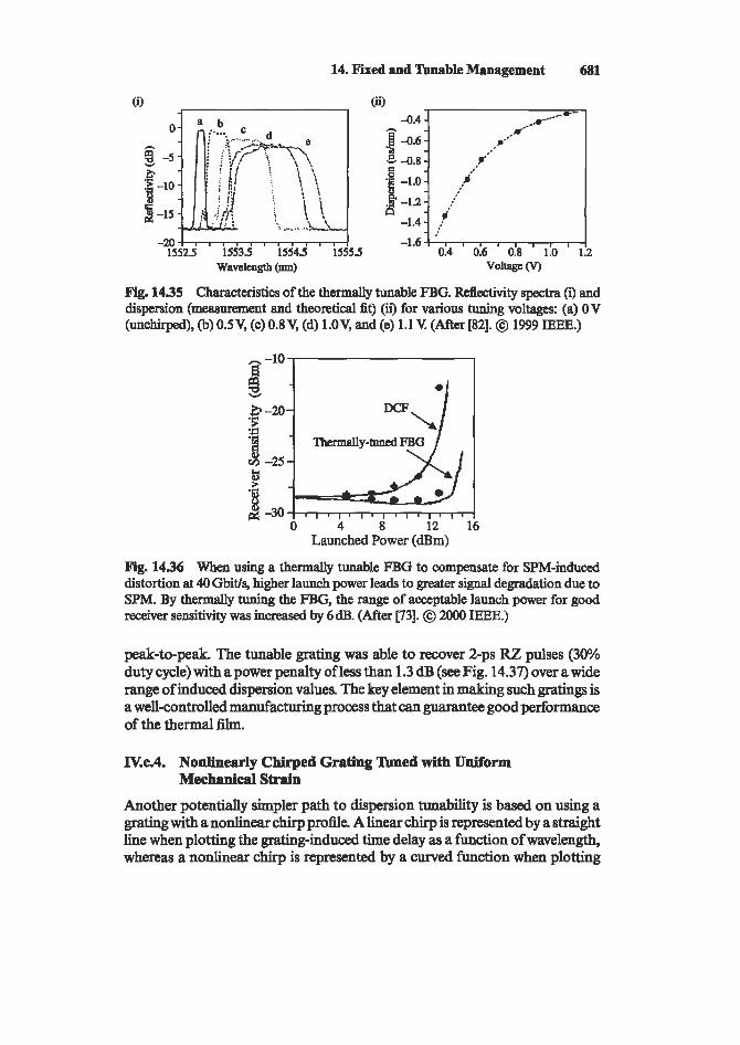
14. F'ixed and Tunable Management 681
- .-....-*-- ~
#.--- -0.4 - $ -0.6: ,.*-
.e B -1.0 - ,, 4''
f -1.2: /* -0.8 - #Ye
-1.4- i -1.6 I I I I ,
-30 0 4 8 12
Launched Power (dBm)
Fig. 1436 When using a thermally tunable FBG to compensate for SPM-induced distortion at 40 Gbitk, higher launch power leads to greater signal degradation due to SPM. By thermally tuning the FBG, the range of acceptable launch power for good receiver sensitivity was increased by 6 dB. (After [73]. @ 2000 IEEE.)
peak-to-peak. The tunable grating was able to recover 2-ps F U pulses (30% duty cycle) with apower penalty of less than 1.3 dB (see Fig. 14.37) over a wide range of induced dispersion values The key element in making such gratings is a well-controlled manufacturing process that can guarantee good performance of the thermal film.
JXcA. Nonlinearly Chirped Grating Tuned with Uniform Mechanical Strain
Another potentially simpler path to dispersion tunability is based on using a grating with a nonlinear chirp proiile. A linear chirp is represented by a straight line when plotting the grating-induced time delay as a function of wavelength, whereas a nonlinear chirp is represented by a curved function when plotting
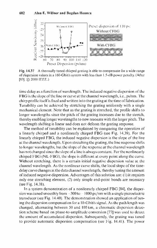
682 Alan E. Willner and Bogdan Hoanca
E Without CFBG
2 -25 W
.1, -27
d 60 70 80 90 100 110 120 $ -28
Preset Dispersion (pshm)
Preset dispersion of 110 ps: Without CFBG
With CFBG
Fig. 14.37 A thermally tuned chirped grating is able to compensate for a wide range of dispersion values in a 160-Gbit/s system with less than 1.5-dB power penalty. (After [83]. @ 2000 IEEE.)
time delay as a function of wavelength. The induced negative dispersion of the FBG is the slope of the line or curve at the channel wavelength, Le., ps/nm. The chirp profile itself is fixed and written into the grating at the time of fabrication. Tunability can be achieved by stretching the grating uniformly with a single mechanical element. Note that as the grating is stretched, the profile shifts to longer wavelengths since the pitch of the grating increases due to the stretch, thereby enabling longer wavelengths to now resonate with the larger pitch. The wavelength shifting is linear and does not deform the grating response.
The method of tunability can be explained by comparing the operation of a linearly chirped and a nonlinearly chirped FBG (see Fig. 14.39). For the linearly chirped FBG, the induced negative dispersion is the slope of the line at the channel wavelength. Upon stretching the grating, the line response shifts to longer wavelengths, but the slope of the response at the channel wavelength has not changed since the slope of a line is always constant. For the nonlinearly chirped FBG (NL-FBG), the slope is different at every point along the curve. Without stretching, there is a certain initial negative dispersion value at the channel wavelength. As the nonlinear curve shifts, the local slope of the time- delay curve changes at the data channel wavelength, thereby tuning the amount of induced negative dispersion. Advantages of this solution are: (1) it requires only one stretching element, (2) only simple end-point bonds are necessary (see Fig. 14.38).
In a system demonstration of a nonlinearly chirped FBG [84], the disper- sion was tuned smoothly from -300 to - 1000 ps/nm with a single piezoelectric transducer (see Fig. 14.40). The demonstration showed an application of tun- ing the dispersion compensation for a lO-Gbit/s signal. As the path length was changed, alternating between 50 and 105 km, a chromatic dispersion detec- tion scheme based on phase-to-amplitude conversion [77] was used to detect the amount of accumulated dispersion. Subsequently, the grating was tuned to provide automatic dispersion compensation (see Fig. 14.41). The power
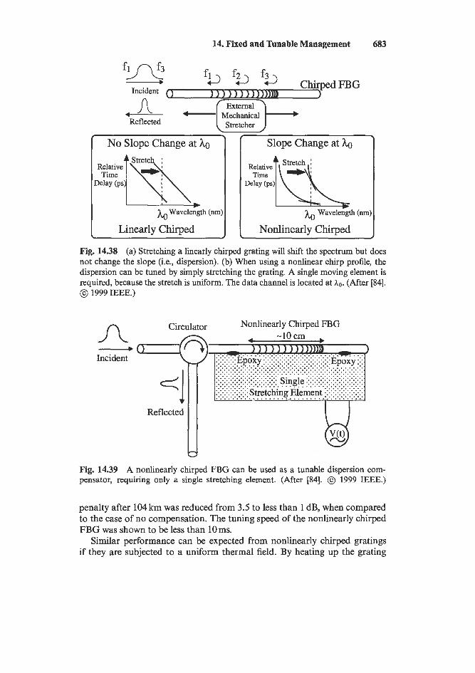
14. Fixed and Tunable Management 683
No Slope Change at LO
R;grly\. Delay (PSI
Lo Wavelength (nm)
Linearly Chirped
Slope Change at &,
Reh:~lp&
Delay (PSI
&, Wavelength (nm
Nonlinearly Chirped
Fig. 14.38 (a) Stretching a linearly chirped grating will shift the spectrum but does not change the slope (i.e., dispersion). (b) When using a nonlinear chirp profile, the dispersion can be tuned by simply stretching the grating. A single moving element is required, because the stretch is uniform. The data channel is located at ho. (After [84]. @ 1999 TEEE.)
Circulator Nonlinearly Chirped FBG n L
Incident . . . . . . . . . . . . . . . . . . . . . . . . . . . . . . . . . . . . . . . . . . . . . . . . . . . . . . . . . . . . . . . . . . . . . . . . . . . . . . . . . . . . . . . . . . . . . . . . . . . . . . . . . ................
Fig. 14.39 A nonlinearly chirped FBG can be used as a tunable dispersion com- pensator, requiring only a single stretching element. (After [84]. @ 1999 IEEE.)
penalty after 104 km was reduced from 3.5 to less than 1 dB, when compared to the case of no compensation. The tuning speed of the nonlinearly chirped FBG was shown to be less than 10 ms.
Similar performance can be expected from nonlinearly chirped gratings if they are subjected to a uniform thermal field. By heating up the grating

684 Alan E. Willner and Bogdan Hoanca
500." " 1 ' ' " I ' i " I ' " ' I ' " ' I ' " ' _
1000 : 0 v - - pslnm 300V - 1
400 500V -+ 1
4 I001
m - F
0:
pslnm
1550.5 1551 1551.5 1552 1552.5 1553 1553.5 Wavelength (nm)
Fig. 14.40 Channel dispersion in the nonlinearly chirped FBG can be tuned from 300 pslnm to 1000 ps/nm with a single stretching element. The voltage range to achieve this tuning range is 0-1OOOV. (After [84]. @ 1999 IEEE.)
of conventional fiber
! I I Fig. 14.41 Eye diagrams showing dispersion compensation of 10 Gbit/s in a recon- figurable network: baseline (top), uncompensated after 50 km (middle, left), uncom- pensated after 104 km (middle, right), compensated after 50 km (bottom, left), and compensated after 104 km (bottom, right). (After [84]. @ 1999 IEEE.)
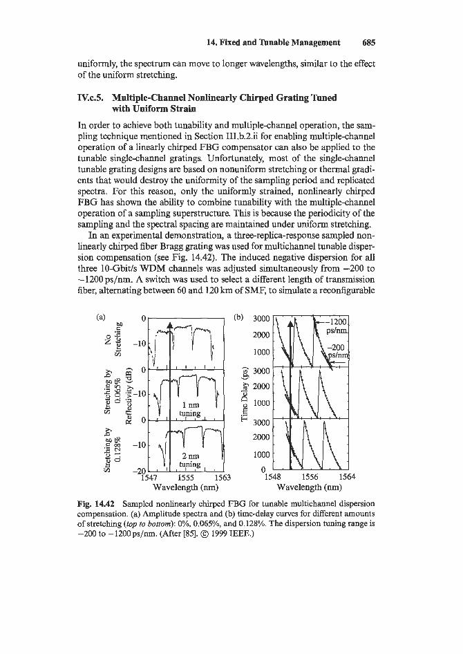
14. Fixed and finable Management 685
uniformly, the spectrum can move to longer wavelengths, similar to the effect of the uniform stretching.
IV.c.5. Multiple-Channel Nonlinearly Chirped Grating Tuned with Uniform Strain
In order to achieve both tunability and multiple-channel operation, the sam- pling technique mentioned in Section III.b.2.ii for enabling multiple-channel operation of a linearly chirped FBG compensator can also be applied to the tunable single-channel gratings. Unfortunately, most of the single-channel tunable grating designs are based on nonuniform stretching or thermal gradi- ents that would destroy the uniformity of the sampling period and replicated spectra. For this reason, only the uniformly strained, nonlinearly chirped FBG has shown the ability to combine tunability with the multiple-channel operation of a sampling superstructure. This is because the periodicity of the sampling and the spectral spacing are maintained under uniform stretching.
In an experimental demonstration, a three-replica-response sampled non- linearly chirped fiber Bragg grating was used for multichannel tunable disper- sion compensation (see Fig. 14.42). The induced negative dispersion for all three 10-Gbit/s WDM channels was adjusted simultaneously from -200 to - 1200 ps/nm. A switch was used to select a different length of transmission fiber, alternating between 60 and 120 km of SMF, to simulate a reconfigurable
(a)
Wavelength (nm)
3000
2000
1000
3000
2000
1000
3000
2000
1000
0 1548 1556 1564
Wavelength (nm)
Fig. 14.42 Sampled nonlinearly chirped FBG for tunable multichannel dispersion compensation. (a) Amplitude spectra and (b) time-delay curves for different amounts of stretching (top to bottom): 0%: 0.065%, and 0.128%. The dispersion tuning range is -200 to -1200ps/nm. (After [SI. @ 1999 IEEE.)

686 Alan E. Willner and Bogdan Hoanca
10 Gbit/s Eye Diagrams
60 km wlo compensation
60 km wl compensation
\ a: 1551 nm b: 1555 nm c: 1559nm 1 Fig. 14.43 Tunable multichannel dispersion compensation using a sampled non- linearly chirped FBG. Eye diagrams of the three channels for 60 km (top) and 120 km (bottom), with and without compensation. (After [MI. @ 1999 IEEE.)
network. A dispersion monitor detected the amount of dispersion compensa- tion needed, and this signal was used to control the compensator, which tuned all of the three channels simultaneously (see Fig. 14.43) [85].
IV.c.6. Tunable Grating Compensators Exhibiting Low Third-Order Dispersion
One recent refinement of the grating-based dispersion compensator was to reduce the effects of the third-order dispersion, D(3). In general, chromatic dispersion is considered second-order dispersion and is measured in units of ps/(nm . km). However, if there is any deviation from linearity in the time delay of an element as a function of wavelength for the frequency range of the channel itself, then higher-order dispersion will result. A typical quadratic function will give rise to a third-order dispersion component, and this will degrade the signal since different dispersion is being applied to different spectral portions of the data channel. In a nonlinearly chirped grating, the dispersion changes across the bandwidth of each data channel. This dispersion slope [Le., the third-order dispersion as measured in ps/(nm2 . km)] is usually not a problem for optical fiber, where the slope is very low, on the order of 0.1 ps/(nm2 . km). In chirped gratings, D(3) can be appreciably larger, in the range of thousands of ps/(nm2 . km). Third-order dispersion tends to cause power penalties mainly for 240- Gbit/s signals, especially for modules with relatively large tuning ranges (see Fig. 14.44).

14. Fixed and Tunable Management 687
7
10000 20000 30000 40000 50000 60000 70000 10Gbit/s 1 1 1 D(3) (pslnm *)
Fig. 14.44 Influence of the D(3) value on the eye opening penalty, for both 10-Gbit/s and 40-Gbith data rates. (R. K. Hosravani, Phaeton Communications Inc., private communication, 2001 .)
40 Gbit/s
__ - NL-FBGA _-
Wavelength
Fig. 14.45 Two nonlinearly chirped fiber Bragg gratings (NL-FBG) (a) with equal and opposite D(3) values can together achieve a linear chirp profile (b). The dispersion can still be tuned via stretching one or both gratings. (After [87]. @ 2001 OSA.)
By combining two nonlinearly chirped gratings with opposite dispersion slopes, it is possible to achieve tunable compensation with significantly reduced third-order dispersion (see Fig. 14.45). A dual-grating-based dispersion com- pensation device was used to demonstrate tunable compensation of 40-Gbith data over distances of 500 km [86]. The signal enters one grating from the long- grating-period side and enters the second grating at the short-grating-period side, giving rise to the opposite third-order dispersion contribution. The grat- ings may have different center wavelengths or different dispersion values. The
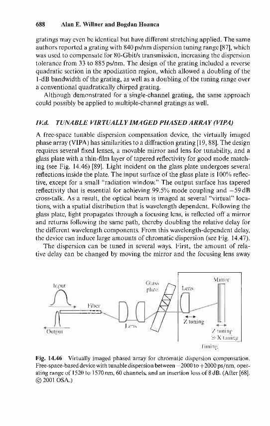
688 Alan E. Willner and Bogdan Hoanca
gratings may even be identical but have different stretching applied. The same authors reported a grating with 840 pshm dispersion tuning range [87], which was used to compensate for 80-Gbith transmission, increasing the dispersion tolerance from 33 to 885 pshm. The design of the grating included a reverse quadratic section in the apodization region, which allowed a doubling of the 1-dB bandwidth of the grating, as well as a doubling of the tuning range over a conventional quadratically chirped grating.
Although demonstrated for a single-channel grating, the same approach could possibly be applied to multiple-channel gratings as well.
IKd. TUNABLE VIRTUALLY IMAGED PHASED ARRAY (VIPA)
A free-space tunable dispersion compensation device, the virtually imaged phase array (VIPA) has similarities to a diffraction grating [19,88]. The design requires several fixed lenses, a movable mirror and lens for tunability, and a glass plate with a thin-film layer of tapered reflectivity for good mode match- ing (see Fig. 14.46) [89]. Light incident on the glass plate undergoes several reflections inside the plate. The input surface of the glass plate is 100% reflec- tive, except for a small “radiation window.” The output surface has tapered reflectivity that is essential for achieving 99.5% mode coupling and -59 dB cross-talk. As a result, the optical beam is imaged at several “virtual” loca- tions, with a spatial distribution that is wavelength dependent. Following the glass plate, light propagates through a focusing lens, is reflected off a mirror and returns following the same path, thereby doubling the relative delay for the different wavelength components. From this wavelength-dependent delay, the device can induce large amounts of chromatic dispersion (see Fig. 14.47).
The dispersion can be tuned in several ways. First, the amount of rela- tive delay can be changed by moving the mirror and the focusing lens away
Mirror
Z tuning 0 X tuning
Tuning
Fig. 14.46 Virtually imaged phased array for chromatic dispersion compensation. Free-space-based device with tunable dispersion between -2000 to +2000 ps/nm, oper- ating range of 1520 to 1570 nm, 60 channels, and an insertion loss of 8 dB. (After [68]. @ 2001 OSA.)

14. Fixed and Tunable Management 689
1500
EL 2 1000
a"
v
3
.e 2 500
\ I
I....I....I 1550.4
0
s -10 g
I;
-20 g 5 2
v)
cl
.-
-30 - 4 0
1568.8 Wavelength (nm)
Fig. 14.47 Group delay and insertion loss plots for a central channel and two outer edge channels of the VIPA. (After [68]. @ 2001 OSA.)
from the glass plate in the same plane as the optical propagation. Second, the dispersion can be changed by varying the profile of the mirror. By using a three-dimensional (3D) mirror with a curvature that changes in a direction perpendicular to the direction of propagation of the light, the dispersion can be changed by translating the mirror in the plane perpendicular to the beam propagation. Moreover, if the curvature of the mirror changes from concave to convex, the dispersion may be tuned across both positive and negative values.
An advantage of the VIPA is that the dispersion can be tuned from positive to negative values, which is useful for fine-tuning the residual dispersion at the end of a transmission link. Currently, however, the device has a fairly large insertion loss due to the free-space design. Although a similar approach can be achieved using diffraction gratings instead of the Fabry-Perot interferometer, the dispersion capabilities would be greatly diminished because of the lower dispersion of the gratings.
IKe.
A host of other dispersion compensation techniques have been proposed in recent years. Some of these ideas have potential to become viable technologies.
OTHER TUNABLE AND NONTUNABLE SOLUTIONS
IV.e.1. Integrated Tunable Dispersion-Compensation Devices
Several types of dispersion-compensation devices can be integrated on an opti- cal or electronic chip. Such integration has long-term promise for low cost and high performance. The options will be treated with brevity in this section, and the reader is encouraged to find more information from the references.
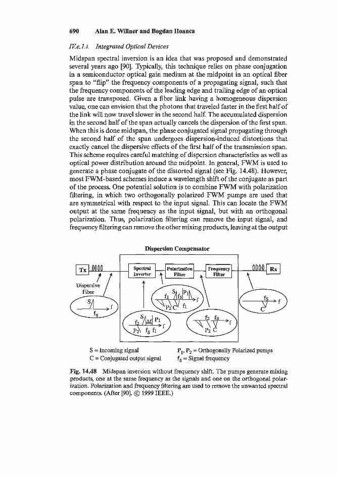
690 Alan E. Willner and Bogdan Hoanca
I r e . 1.i. Integrated Optical Devices
Midspan spectral inversion is an idea that was proposed and demonstrated several years ago [go]. Typically, this technique relies on phase conjugation in a semiconductor optical gain medium at the midpoint in an optical fiber span to “flip” the frequency components of a propagating signal, such that the frequency components of the leading edge and trailing edge of an optical pulse are transposed. Given a fiber link having a homogeneous dispersion value, one can envision that the photons that traveled faster in the first half of the link will now travel slower in the second half. The accumulated dispersion in the second half of the span actually cancels the dispersion of the first span. When this is done midspan, the phase conjugated signal propagating through the second half of the span undergoes dispersion-induced distortions that exactly cancel the dispersive effects of the first half of the transmission span. This scheme requires careful matching of dispersion characteristics as well as optical power distribution around the midpoint. In general, FWM is used to generate a phase conjugate of the distorted signal (see Fig. 14.48). However, most FWM-based schemes induce a wavelength shift of the conjugate as part of the process. One potential solution is to combine FWM with polarization filtering, in which two orthogonally polarized FWM pumps are used that are symmetrical with respect to the input signal. This can locate the FWM output at the same frequency as the input signal, but with an orthogonal polarization. Thus, polarization filtering can remove the input signal, and frequency filtering can remove the other mixing products, leaving at the output
Dispersion Compensator
Rx Tx F n f r 0 0 0 0
I Dispersive
P2 f, f l
S = Incoming signal C = Conjugated output signal
P,, Pz = Orthogonally Polarized pumps f, = Signal frequency
Fig. 14.48 Midspan inversion without frequency shift. The pumps generate mixing products, one at the same frequency as the signals and one on the orthogonal polar- ization. Polarization and frequency filtering are used to remove the unwanted spectral components. (After [go]. @ 1999 IEEE.)

14. Fixed and Tunable Management 691
only the phase conjugate signal, with no wavelength shift. The experimental validation shows negligible power penalty for transmission of 2.5-Gbit/s data from a directly modulated laser over 120 km; note that the power penalty without the spectral inverter is more than 3 dB for even 60 km; for 120 km, an error floor is encountered.
Several other techniques include Gires-Tournois interferometers (or all- pass filters, in general) [9 11; tunable ring resonators [92]; arrayed-waveguide devices [93]; Mach-Zehnder interferometers with thermal phase tuning [94]; chirp tuning of electroabsorption modulators for analog systems [95], and spectral holography in which dynamic holograms can adaptively change to compensate for dispersion [96]. A more detailed description of some of these techniques follows.
Phase-only filters have the capability of integrating dispersion compensa- tion on a chip. Several architectures are possible, whether using ring resonators, Mach-Zehnder structures, or cavity resonators (see Fig. 14.49). A sixth-order structure with ring resonators having a small 3.3-mm diameter can be built on a 7 x 26 mm2 chip and can compensate for up to 15,000 pslnm of dispersion, equivalent to 880 km of SMF [97]. The key limitation is that the free spectral range (FSR) limits the channel spacing to 10 GHz or less. This spacing can be increased by reducing the diameter of the resonator ring, but this would tend to increase the insertion loss of the device. The solution is to use materials
Out & -Resonant reflectors
I, 111 111 Resonant 111 111 111 Ht- reflectors
out 4 Fig. 14.49 Architectures of phase-only filter structures for chromatic dispersion compensation. (a) Ring resonator cascade, (b) ring lattice, (c) folded Mach-Zehnder (suitable for cascading) and (d) resonant cavity lattice with input circulator.
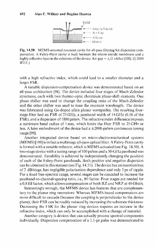
692 Alan E. Willner and Bogdan Hoanca
Silicon Nitride Air Gap Silicon Mirror
Fig. 14.50 MEMS-actuated resonant cavity for all-pass filtering for dispersion com- pensation. A Fabry-Perot cavity is built between the silicon nitride membrane and a highly reflective layer in the substrate of the device. Air gap = h/2. (After [loo]. @ 2000 IEEE.)
with a high refractive index, which could lead to a smaller diameter and a larger FSR.
A tunable dispersion-compensation device was demonstrated based on an al,l-pass architecture [98]. The device included four stages of Mach-Zehnder structures, each with two thermo-optic chromium phase-shift elements. One phase shifter was used to change the coupling ratio of the Mach-Zehnder and the other shifter was used to tune the resonant wavelength. The device was fabricated using Ge-doped silica planar waveguides. The resulting four- stage filter had an FSR of 25 GHz, a passband width of 14 GHz (0.56 of the FSR), and a dispersion of 1800 p h m . The refractive index difference imposes a minimum bend radius of 1 mm, which limits the filter FSR to 25 GHz or less. A later embodiment of the device had a f2000-ps/nm continuous tuning range [99].
Another integrated device based on micro-electro-mechanical systems (MEMS) [loo] is in fact a multistage all-pass optical filter. A Fabry-Perot cavity is formed with a tunable reflector, which is MEMS actuated (see Fig. 14.50). A two-stage device with a tuning range of 100 pdnm and a 50-GHz passband was demonstrated. Tunability is achieved by independently changing the position of each of the Fabry-Perot passbands. Both positive and negative dispersion can be obtained in this manner (see Fig. 14.5 1). The device has an insertion loss of 2 dB/stage, has negligible polarization dependence and only 3 ps of ripple. For a fixed free-spectral range, several stages can be cascaded to increase the passband-to-channel-spacing ratio, i.e., fill factor. Four stages are needed for a 0.8 fill factor, which allows compensation of both RZ and NRZ at 40 Gbit/s.
Interestingly enough, the MEMS device has features that are complemen- tary to the planar ring resonators: Whereas MEMS-based compensators are more difficult to cascade (because the coupling is perpendicular to the device plane), their FSR can be readily reduced by increasing the substrate thickness. Decreasing the FSR for the planar ring devices requires an increase in the refractive index, which can only be accomplished with a change of material.
Another category is devices that can actually process spectral components individually. Dispersion compensation of a 1.1 -ps pulse was demonstrated in
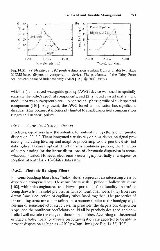
14. Fixed and Tunable Management 693
1550.0 1550.4 1550.8 1550 0 1550.4 1550.8 Wavelength (nm) Wavelength (nm)
Fig. 14.51 (a) Negative and (b) positive dispersion resulting from a tunable two-stage MEMS-based dispersion compensation device. The passbands of the Fabry-Perot sections can be tuned independently. (After [loo]. @ 2000 IEEE.)
which: (1) an arrayed waveguide grating (AWG) device was used to spatially separate the pulse’s spectral components, and (2) a liquid crystal spatial light modulator was subsequently used to control the phase profile of each spectral component [loll. At present, the AWG-based compensator has significant disadvantages because it is generally limited to small dispersion compensation ranges and to short pulses.
N e . l . i i . Integrated Electronic Devices
Electronic equalizers have the potential for mitigating the effects of chromatic dispersion [20,2 11. These integrated circuits rely on post-detection signal pro- cessing, including filtering and adaptive processing, to sharpen the distorted data pulses. :Because optical detection is a nonlinear process, the function of compensating for the linear distortions of chromatic dispersion is some- what complicated. However, electronic processing is potentially an inexpensive solution, at least for < lO-Gbit/s data rates.
IV.e.2. Photonic Bandgap Fibers
Photonic bandgap fibers (i.e., “holey fibers”) represent an interesting class of dispersion compensators. These are fibers with a periodic hollow structure [102], with holes engineered to achieve a particular functionality. Instead of being drawn from a solid preform as with conventional fibers, holey fibers are drawn from a collection of capillary tubes fused together. The properties of the resulting structure can be tailored in a manner similar to the bandgap engi- neering of semiconductor structures. In principle, the dispersion, dispersion slope, and the nonlinear coefficients could all be precisely designed and con- trolled well outside the range of those of solid fiber. According to theoretical estimates, holey fibers for dispersion compensation are expected to be able to provide dispersion as high as -2000 ps/(nm. km) (see Fig. 14.52) [103].
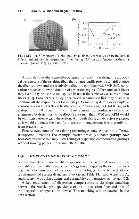
694 Alan E. Willner and Bogdan Hoanca
(b) h E 500 A
-500
e-1500
5 -2500 !2 0.4 0.6 0.8 1 1.2 1.4 6 Core Diameter (pm)
v . 0 .-
Fig. 14.52 (a) SEM image of a photonic crystal fiber. A core exists where the central hole is omitted. (b) Net dispersion of the fiber at 1550nm as a function of the core diameter. (After [133]. @ 1999 IEEE.)
Although holey fibers can offer outstanding flexibility in designing the opti- cal parameters of the resulting fiber, they do not readily provide tunability once the fiber is drawn and are relatively difficult to combine with SMF. Still, fabri- cation processes allow production of km-scale lengths of fiber, and such fibers may eventually be cleaved and spliced in much the same way as conventional fibers [103]. Long term, a holey-fiber-based transmission link may be able to combine all the requirements for a high performance system. For example, a zero-dispersion fiber is theoretically possible for wavelengths 1.3-1.8 Km, with a slope of only 0.01 ps/(nm2 . km). Furthermore, the nonlinearity could be engineered by designing a large effective area such that FWM and XPM would be eliminated even at zero dispersion. Although this is an attractive scenario, as it would eliminate the need for dispersion management, it is presently far from practicality.
Finally, even some of the existing technologies may evolve into different, unexpected directions. For example, electro-optically tunable gratings have been demonstrated that may allow tuning of dispersion compensation gratings without moving parts and thermal effects [104].
IK’’ COMPENSATION DE VICE SUMMARY
Several tunable and nontunable dispersion compensation devices are now available commercially. No one technology has emerged as the definitive win- ner, partly because none of the existing technologies is able to meet all the requirements of system designers. Two tables, Table 14.1 and Appendix A, summarize the popular commercially available compensation techniques [68].
A key requirement of dispersion compensators is the slope matching between the wavelength dependence of the transmission fiber and that of the dispersion compensation device. This matching will be covered in the next section.
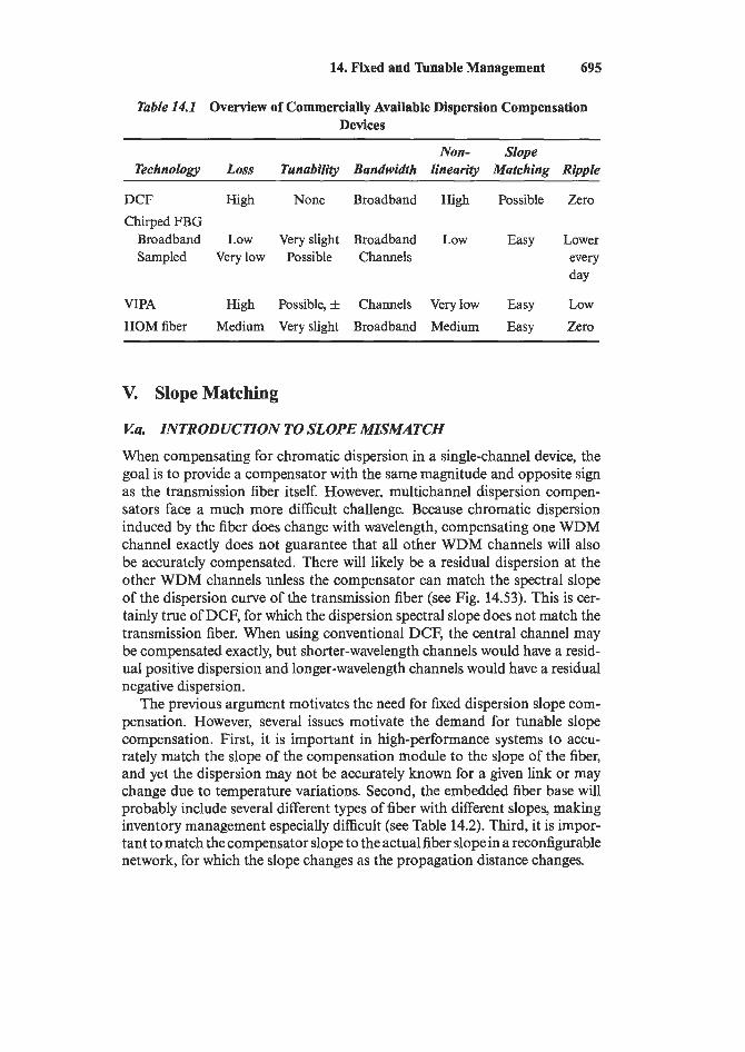
14. Fixed and Tunable Management 695
Table 14.1 Overview of Commercially Available Dispersion Compensation Devices
Technology Loss
DCF High Chirped FBG
Broadband Low Sampled Very low
VIPA High HOM fiber Medium
Non- Tunability Bandwidth linearity
None Broadband High
Very slight Broadband Low Possible Channels
Possible, f Channels Very low Very slight Broadband Medium
Slope Matching Ripple
Possible Zero
Easy Lower every day
Easy Low Easy Zero
V. Slope Matching
Ka. INTRODUCTION TO SLOPE MISMATCH
When compensating for chromatic dispersion in a single-channel device, the goal is to provide a compensator with the same magnitude and opposite sign as the transmission fiber itself. However, multichannel dispersion compen- sators face a much more difficult challenge. Because chromatic dispersion induced by the fiber does change with wavelength, compensating one WDM channel exactly does not guarantee that all other WDM channels will also be accurately compensated. There will likely be a residual dispersion at the other WDM channels unless the compensator can match the spectral slope of the dispersion curve of the transmission fiber (see Fig. 14.53). This is cer- tainly true of DCF, for which the dispersion spectral slope does not match the transmission fiber. When using conventional DCF, the central channel may be compensated exactly, but shorter-wavelength channels would have a resid- ual positive dispersion and longer-wavelength channels would have a residual negative dispersion.
The previous argument motivates the need for fixed dispersion slope com- pensation. However, several issues motivate the demand for tunable slope compensation. First, it is important in high-performance systems to accu- rately match the slope of the compensation module to the slope of the fiber, and yet the dispersion may not be accurately known for a given link or may change due to temperature variations. Second, the embedded fiber base will probably include several different types of fiber with different slopes, making inventory management especially difficult (see Table 14.2). Third, it is impor- tant to match the compensator slope to the actual fiber slope in a reconfigurable network, for which the slope changes as the propagation distance changes.
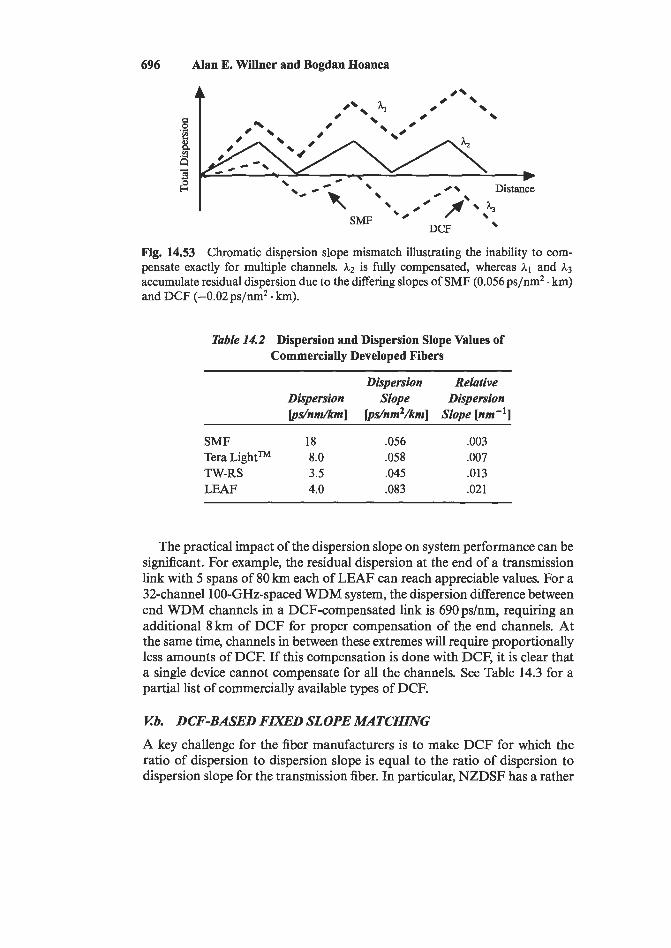
696 Alan E. Willner and Bogdan Hoanca
Fig. 14.53 Chromatic dispersion slope mismatch illustrating the inability to com- pensate exactly for multiple channels. J.2 is fully compensated, whereas A.1 and J.3
accumulate residual dispersion due to the differing slopes of SMF (0.056ps/nm2. km) and DCF (-0.02ps/nm2 o h ) .
Table 14.2 Dispersion and Dispersion Slope Values of Commercially Developed Fibers
Dispersion Relative Dispersion Slope Dispersion [~dnni/km] Ipdnm2/km] slope [nm-'I
SMF 18 .056 .003 Tera LightTM 8.0 .058 .007 TW-RS 3.5 .045 .013 LEAF 4.0 .083 .021
The practical impact of the dispersion slope on system performance can be significant.. For example, the residual dispersion at the end of a transmission link with 5 spans of 80 km each of LEAF can reach appreciable values. For a 32-channel 100-GHz-spaced WDM system, the dispersion difference between end WDM channels in a DCF-compensated link is 690ps/nm, requiring an additional 8 km of DCF for proper compensation of the end channels. At the same time, channels in between these extremes will require proportionally less amounts of DCF. If this compensation is done with DCF, it is clear that a single device cannot compensate for all the channels. See Table 14.3 for a partial list of commercially available types of DCF.
Kb. DCF-BASED FlXED SLOPE MATCHING
A key challenge for the fiber manufacturers is to make DCF for which the ratio of dispersion to dispersion slope is equal to the ratio of dispersion to dispersion slope for the transmission fiber. In particular, NZDSF has a rather

14. Fixed and Tunable Management 697
Table 14.3 Commercially Available DCF Types and Their Characteristics [lo51
Characteristics Standard Wideband High-Slope at 1550nm Unit DCF DCF DCF
Relative slope nm-' 0.0022 0.0035 0.0067 FOM ps/(nm. dB) 200 190 150 Attenuation dBlkm 0.50 0.50 0.68 Dispersion ps/(nm . km) - 100 -95 -100 Mode field diameter km 5.2 5.1 4.5 PMD ps . km-'.' 0.08 0.08 0.08
DCF w/o slope comp. /
1530 nm
1540 nm
1545 nm I I
1550 nm
1560 nm 1530 1540 1550 1.560
Wavelength (nm)
Fig. 14.54 (a) Slope matching with HOM fiber showing wavelength dependence of the measured Q-factor for DCF and for HOM fiber and (b) eye diagrams of 40-Gbith data channels after HOM slope compensation. (After [15]. @ 2000 OSA.)
large ratio of dispersion to dispersion slope, thus leading to difficult slope compensation (Table 14.2). Recent efforts have led to the fabrication of DCF with a dispersion slope nearly matched to conventional transmission fiber [lo6 -1081. These fibers are then used to assemble dispersion-flattened modules by combining transmission fiber with such slope-matched DCF [109, 1101. The higher-order-mode dispersion compensators are also designed for very good slope matching (see Fig. 14.54) [15]. The above mentioned techniques are solutions for fixed dispersion slope compensation.
Ec. FBGs FOR FIXED SLOPE MATCHING
Because the dispersion can be tailored fairly precisely, broadband fiber Bragg gratings have been used to compensate for the dispersion slope of transmis- sion fiber. For example, a 1-m long grating was designed to compensate for 627 km of TrueWaveTM fiber [l 1 1, 1121. The deviation from the ideal parabolic
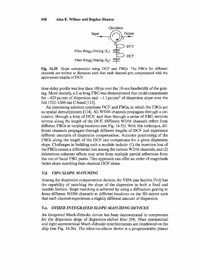
698 Alan E. Wlllner and Bogdan Hoanca
Circulator
DCF
% DCF Fiber Bragg Grating (A,)
Fiber Bragg Grating (&)
Fig. 14.55 Slope compensator using DCF and FBGs. The FBGs for different channels are written at distances such that each channel gets compensated with the appropriate lengths of DCF.
time-delay profile was less than loops over the IO-nm bandwidth of the grat- ing. More recently, a 2-m long FBG was demonstrated that could compensate for -629 ps/nm of dispersion and - 1.1 ps/nm2 of dispersion slope over the full 1532-1560-nm C-band [113].
An interesting solution combines DCF and FBGs, in which the FBGs act as spatial demultiplexers [114]. All WDM channels propagate through a cir- culator, through a loop of DCF, and then through a series of FBG sections written along the length of the DCF. Different WDM channels reflect from different FBGs at varying locations (see Fig. 14.55). With this technique, dif- ferent channels propagate through different lengths of DCF and experience different amounts of dispersion compensation. Accurate positioning of the FBGs along the length of the DCF can compensate for a given dispersion slope. Challenges in building such a module include: (1) the insertion loss of the FBGs causes a differential loss among the various WDM channels, and (2) deleterious coherent effects may arise from multiple partial reflections from the out-of-band FBG peaks. This approach can offer an order of magnitude better slope matching than classical DCF alone.
Kd. VIPA SLOPE MATCHING
Among the dispersion compensation devices, the VIPA (see Section 1V.d) has the capability of matching the slope of the dispersion in both a fixed and tunable fashion. Slope matching is achieved by using a diffraction grating to focus different WDM channels at different locations on the 3D mirror such that each channel experiences a slightly different amount of dispersion.
Re. OTHER INTEGRATED SLOPE MATCHING DEVICES
An integrated Mach-Zehnder device has been demonstrated to compensate for the dispersion slope of dispersion-shifted fiber [94]. Nine symmetrical and eight asymmetrical Mach-Zehnder interferometers are interleaved on the chip (see Fig. 14.56). The silica-on-silicon device is a programmable planar

14. Fixed and Tunable Management 699
Thermo-optic Tunable Phase Shifter
Input
Waveguide 02 \ U
output
Si Substrate (974 x 88 mm) \
Fig. 14.56 Planar lightwave circuit for dispersion and slope compensation. The device is a phase-only filter with nine symmetrical and eight asymmetrical Mach-Zehnder stages, each with one thermoelectric phase shifter. AL is the differential length. 4 and 8 represent different phase shift values. (After [94]. @ 1998 IEEE/OSA.)
(a) Phase Shifter (b) (C) Ri
Reso f c- i
Waveguide
Fig. 14.57 (a) Ring resonator with fixed coupling ratio, and two configurations with tunable coupling ratios: symmetrical (b) and asymmetrical (c). (After [98]. @ 1999 IEEE.)
lightwave circuit, and the dispersion-inducing phase shift is achieved using chromium thermoelectric heaters. Experimental evaluation of the device shows a 4-dB improvement in power penalty for the transmission of a 200-Gbith sig- nal over 100 km. The limitation of the device is in achieving small channel spacing. For a 200-GHz spacing, the length difference between the arms of the interferometers is 1 mm. This length would increase proportionally with a decrease in the channel spacing, reaching impractical values of several mm for I 100-GHz channel spacings. Similarly, the insertion loss increases for lower channel spacings: from I 1.4 dB at 300-GHz spacing to 15.5 dB for 200 GHz spacing.
Phase-only filters are also powerful candidates for dispersion slope compen- sation (see Figs. 14.57,14.58) [98]. As introduced in Section 1V.e. 1, such devices are limited to small channel spacing due to the limitation on the bend radius
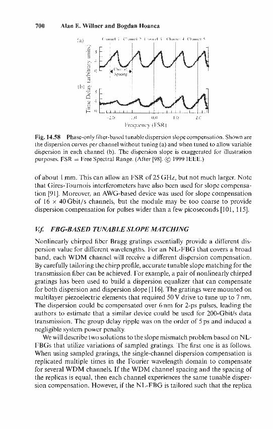
700 Alan E. Willner and Bogdan Hoanca
Channel 1 Channel 2 Channel 3 Channel 4 Channel 5
h v1 * (a)
.a 8 s A 4
.s 0
2
z (b) 2
a"
s v
- 8
2 4 'c; 0 -2.0 -1.0 0.0 1 .o 2.0
Frequency (FSR)
Fig. 14.58 Phase-only filter-based tunable dispersion slope compensation. Shown are the dispersion curves per channel without tuning (a) and when tuned to allow variable dispersion in each channel (b). The dispersion slope is exaggerated for illustration purposes. FSR = Free Spectral Range. (After [98]. @ 1999 IEEE.)
i- Spacing i
of about 1 mm. This can allow an FSR of 25 GHz, but not much larger. Note that Gires-Tournois interferometers have also been used for slope compensa- tion [91]. Moreover, an AWG-based device was used for slope compensation of 16 x 40Gbit/s channels, but the module may be too coarse to provide dispersion compensation for pulses wider than a few picoseconds [101, 1151.
KJ FBG-BASED TUNABLE SLOFE MATCHING
Nonlinearly chirped fiber Bragg gratings essentially provide a different dis- persion value for different wavelengths. For an NL-FBG that covers a broad band, each WDM channel will receive a different dispersion compensation. By carefully tailoring the chirp profile, accurate tunable slope matching for the transmission fiber can be achieved. For example, a pair of nonlinearly chirped gratings has been used to build a dispersion equalizer that can compensate for both dispersion and dispersion slope [116]. The gratings were mounted on multilayer piezoelectric elements that required 50 V drive to tune up to 7 nm. The dispersion could be compensated over 6 nm for 2-ps pulses, leading the authors to estimate that a similar device could be used for 200-Gbit/s data transmission. The group delay ripple was on the order of 5 ps and induced a negligible system power penalty.
We will describe two solutions to the slope mismatch problem based on NL- FBGs that utilize variations of sampled gratings. The first one is as follows. When using sampled gratings, the single-channel dispersion compensation is replicated multiple times in the Fourier wavelength domain to compensate for several WDM channels. If the WDM channel spacing and the spacing of the replicas is equal, then each channel experiences the same tunable disper- sion compensation. However, if the NL-FBG is tailored such that the replica
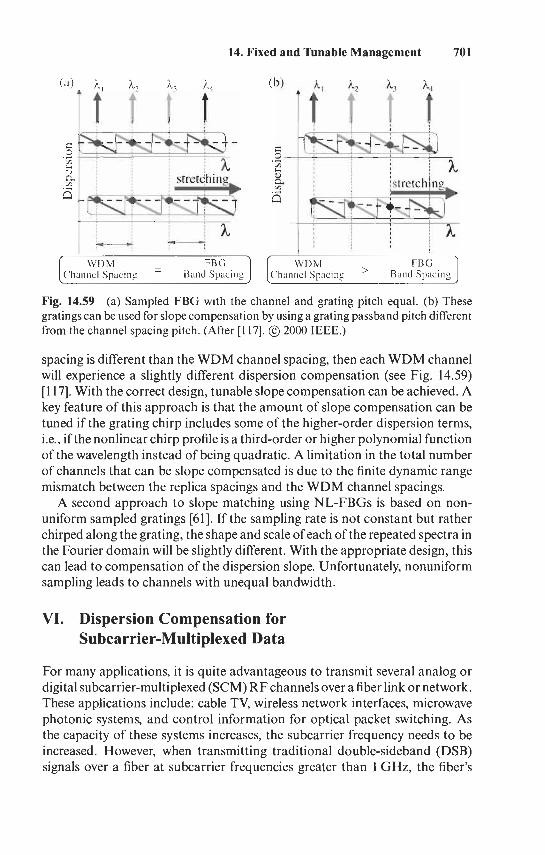
14. Fixed and Tunable Management 701
WDM - FB G WDM FB G Channel Spacing - Band Spacing Channel Spacing ' Band Spacing
Fig. 14.59 (a) Sampled FBG with the channel and grating pitch equal. (b) These gratings can be used for slope compensation by using a grating passband pitch different from the channel spacing pitch. (After [117]. @ 2000 IEEE.)
spacing is different than the WDM channel spacing, then each WDM channel will experience a slightly different dispersion compensation (see Fig. 14.59) [117]. With the correct design, tunable slope compensation can be achieved. A key feature of this approach is that the amount of slope compensation can be tuned if the grating chirp includes some of the higher-order dispersion terms, i.e., if the nonlinear chirp profile is a third-order or higher polynomial function of the wavelength instead of being quadratic. A limitation in the total number of channels that can be slope compensated is due to the finite dynamic range mismatch between the replica spacings and the WDM channel spacings.
A second approach to slope matching using NL-FBGs is based on non- uniform sampled gratings [61]. If the sampling rate is not constant but rather chirped along the grating, the shape and scale of each of the repeated spectra in the Fourier domain will be slightly different. With the appropriate design, this can lead to compensation of the dispersion slope. Unfortunately, nonuniform sampling leads to channels with unequal bandwidth.
VI. Dispersion Compensation for Subcarrier-Multiplexed Data
For many applications, it is quite advantageous to transmit several analog or digital subcarrier-multiplexed (SCM) R F channels over a fiber link or network. These applications include: cable TV, wireless network interfaces, microwave photonic systems, and control information for optical packet switching. As the capacity of these systems increases, the subcarrier frequency needs to be increased. However, when transmitting traditional double-sideband (DSB) signals over a fiber at subcarrier frequencies greater than 1 GHz, the fiber's
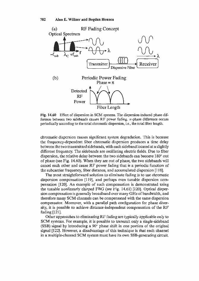
702 Alan E. Willner and Bogdan Hoanca
(a) RF Fading Concept Optical Spectrum
Receiver Dispersive Fiber
Periodic Power Fading Phase = 71: DeEdm Power Fiber Length
Fig. 14.60 Effect of dispersion in SCM systems. The dispersion-induced phase dif- ference between two sidebands causes RF power fading. n-phase difference occurs periodically according to the total chromatic dispersion, i.e., the total fiber length.
chromatic dispersion causes significant system degradation. This is because the frequency-dependent fiber chromatic dispersion produces a time delay between the two transmitted sidebands, with each sideband located at a slightly different frequency. The sidebands are oscillating electric fields. Due to fiber dispersion, the relative delay between the two sidebands can become 180" out of phase (see Fig. 14.60). When they are out of phase, the two sidebands will cancel each other and cause RF power fading that is a periodic function of the subcarrier frequency, fiber distance, and accumulated dispersion [118].
The most straightforward solution to eliminate fading is to use chromatic dispersion compensation [119], and perhaps even tunable dispersion com- pensation [120]. An example of such compensation is demonstrated using the tunable nonlinearly chirped FBG (see Fig. 14.61) [120]. Optical disper- sion compensation is generally broadband over many GHz of bandwidth, and therefore many SCM channels can be compensated with the same dispersion compensator. Moreover, with a parallel path configuration for phase diver- sity, it is possible to achieve distance-independent compensation of the RF fading [121].
Other approaches to eliminating RF fading are typically applicable only to SCM systems. For example, it is possible to transmit only a single-sideband (SSB) signal by introducing a 90" phase shift in one portion of the original signal [122]. However, a disadvantage of this technique is that each channel in a multiple-channel SCM system must have its own SSB-generating circuit.

14. Fixed and Tunable Management 703
( 4 After 40 km (b) After 80 km
E: 5 F " " " " " " ' " 1 " ' I E 5 m ? 2 0
a -10
d 5 -15 .- N w/o compensation 3 -20 E 8 -25
d)
2 4 6 8 10 12 s p 3 O 2 4 6 8 10 12 Carrier Frequency (GHz) Carrier Frequency (GHz)
Fig. 14.61 Tunable RF power-fading compensation using a nonlinearly chirped FBG. Less than 5-dB RF power deviation was obtained after compensation, whereas 25-dB power fading occurs without compensation. (After [120]. @ 1999 OSA.)
Another reported approach uses a two-mode laser that heterodynes in the receiver 11231, but the subcarrier frequency is not easily tunable.
Tunable dispersion compensation is, in the end, the most powerful tech- nique for SCM systems, because it allows compensation of multiple subcarrier channels simultaneously (as long as they arrive from the same distance). The distance restriction itself can be removed with a parallel path configuration for phase diversity, with which it is possible to achieve distance-independent compensation of the fading [121].
VII. Chromatic Dispersion Monitoring
There are systems scenarios in which a dynamic feedback loop may be required for dispersion compensation. Such a feedback loop would track the changes in the accumulated dispersion of a signal and drive a tuning element that would compensate for the dispersion. Scenarios that may require dynamic compensa- tion include: (1) a reconfigurable network for which fiber path changes occur, and (2) temperature changes for >40-Gbit/s channels. A key element of a dynamic dispersion compensator is a chromatic dispersion monitor in the feedback loop that can measure the required compensation while the data is being transmitted through the optical link. This is quite different from the more traditional chromatic dispersion measurement techniques in which dark fiber is usually measured off-line.
Chromatic dispersion monitoring can be performed at the receiving end, where the Q-factor, eye diagram, or bit-error rate of the received data would be monitored to assess the accumulated dispersion. As data rates increase or if inline monitoring is needed, it may be highly desirable to monitor dispersion
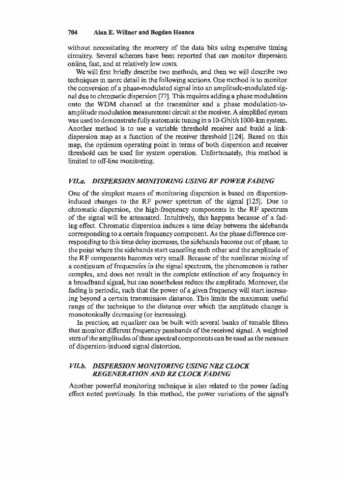
704 Alan E. Wdlner and Bogdan Hoanca
without necessitating the recovery of the data bits using expensive timing circuitry. Several schemes have been reported that can monitor dispersion online, fast, and at relatively low costs.
We will first briefly describe two methods, and then we will describe two techniques in more detail in the following sections. One method is to monitor the conversion of a phase-modulated signal into an amplitude-modulated sig- nal due to chromatic dispersion [77]. This requires adding a phase modulation onto the WDM channel at the transmitter and a phase modulation-to- amplitude modulation measurement circuit at the receiver. A simplified system was used to demonstrate fully automatic tuning ina lO-Gbit/s 1000-km system. Another method is to use a variable threshold receiver and build a link- dispersion map as a function of the receiver threshold [124]. Based on this map, the optimum operating point in terms of both dispersion and receiver threshold can be used for system operation. Unfortunately, this method is limited to off-line monitoring.
VILa. DISPERSION MONITORING USING RF POWER FADING
One of the simplest means of monitoring dispersion is based on dispersion- induced changes to the RF power spectrum of the signal [125]. Due to chromatic dispersion, the high-frequency components in the RF spectrum of the signal will be attenuated. Intuitively, this happens because of a fad- ing effect. Chromatic dispersion induces a time delay between the sidebands corresponding to a certain frequency component. As the phase difference cor- responding to this time delay increases, the sidebands become out of phase, to the point where the sidebands start canceling each other and the amplitude of the RF components becomes very small. Because of the nonlinear mixing of a continuum of frequencies in the signal spectrum, the phenomenon is rather complex, and does not result in the complete extinction of any frequency in a broadband signal, but can nonetheless reduce the amplitude. Moreover, the fading is periodic, such that the power of a given frequency will start increas- ing beyond a certain transmission distance. This limits the maximum useful range of the technique to the distance over which the amplitude change is monotonically decreasing (or increasing).
In practice, an equalizer can be built with several banks of tunable filters that monitor different frequency passbands of the received signal. A weighted sum of the amplitudes of these spectral components can be used as the measure of dispersion-induced signal distortion.
VILb. DISPERSION MONITORING USING NRZ CLOCK REGENERATIONAND RZ CLOCKFADING
Another powerful monitoring technique is also related to the power fading effect noted previously. In this method, the power variations of the signal’s

14. Fixed and Tunable Management 705
Back to Back Clock Tone -76.17dBm 9.96 GHz
20 km SMF 40 km SMF 55 km SMF
T o n e b
Fig. 14.62 Effect of dispersion on the clock component and eye diagram in lO-Gbit/s NRZ systems. Greater dispersion leads to greater distortion and generates higher RF clock power. (After [ 1341. 0 2001 OSA.)
clock frequency component is monitored [126]. It is well known that the power spectrum of an NRZ signal does not contain any power at the clock frequency (i.e., a 10-Gbit/s data rate stream will not contain any power at 10 GHz where there is a null in the Fourier spectrum). The effect of dispersion is to regenerate the clock and to induce an increase in the power at the clock frequency (see Fig. 14.62). Within a range of values of signal dispersion, the clock power is proportional to the amount of accumulated dispersion. Beyond this distance, the clock power fades, but will continue to increase and decrease periodically with transmission distance (see Fig. 14.63). A chromatic dispersion monitor can be built, albeit limited to the first range of monotonic behavior. A similar approach was used to automatically compensate for dispersion in a 40-Gbit/s system over 200 km [78].
For RZ data, the technique can be used with a similar monitoring approach, but with the opposite phenomenon. The clock component in RZ data is relatively strong, but it fades and decreases under the effect of dispersion. Dispersion is inversely proportional to the power spectral density at the clock frequency over some finite range of dispersion values. Similar techniques can be used for optically time-division-multiplexed data [ 1271.
By combining the two monitoring techniques presented above, the RF power monitoring and the clock power monitoring, the maximum distance can be substantially extended beyond the limits of using either of the two methods alone.
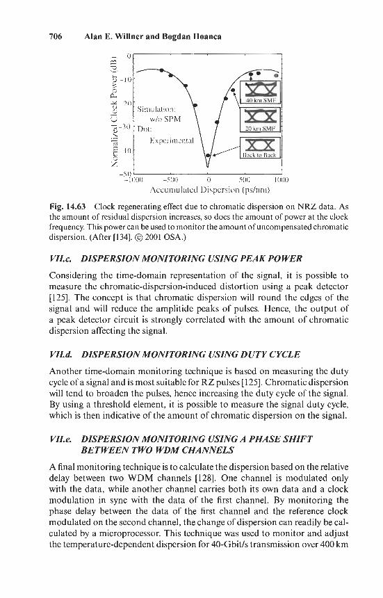
706 Alan E. Willner and Bogdan Hoanca
- o r 1
N 1 Experimental \ / m
z / Back 10 Hack v 4
1 0 500 1000
-50’ -1000 -500
Accumulated Dispersion (pshm)
Fig. 14.63 Clock regenerating effect due to chromatic dispersion on NRZ data. As the amount of residual dispersion increases, so does the amount of power at the clock frequency. This power can be used to monitor the amount of uncompensated chromatic dispersion. (After [134]. @ 2001 OSA.)
VILc. DISPERSION MONITORING USING PEAK POWER
Considering the time-domain representation of the signal, it is possible to measure the chromatic-dispersion-induced distortion using a peak detector [125]. The concept is that chromatic dispersion will round the edges of the signal and will reduce the amplitide peaks of pulses. Hence, the output of a peak detector circuit is strongly correlated with the amount of chromatic dispersion affecting the signal.
VII.d. DISPERSION MONITORING USING DUTY CYCLE
Another time-domain monitoring technique is based on measuring the duty cycle of a signal and is most suitable for RZ pulses [125]. Chromatic dispersion will tend to broaden the pulses, hence increasing the duty cycle of the signal. By using a threshold element, it is possible to measure the signal duty cycle, which is then indicative of the amount of chromatic dispersion on the signal.
VILe. DISPERSION MONITORING USING A PHASE SHIFT BETWEEN TWO WDM CHANNELS
A final monitoring technique is to calculate the dispersion based on the relative delay between two WDM channels [128]. One channel is modulated only with the data, while another channel carries both its own data and a clock modulation in sync with the data of the first channel. By monitoring the phase delay between the data of the first channel and the reference clock modulated on the second channel, the change of dispersion can readily be cal- culated by a microprocessor. This technique was used to monitor and adjust the temperature-dependent dispersion for 40-Gbith transmission over 400 km

14. Fired and ’Ihnable Management 707
of SMF. The change in the zero-dispersion wavelength was measured to be 30 pm/”C, and the dispersion slope changed by 27 ps/nm2. The dispersion- tuning mechanism consisted of tuning the wavelength of the transmission lasers to track the changes in the zero-dispersion wavelength of the fiber. Tem- perature variations between 0°C and 40°C induced large power penalties for the uncompensated case, but no observable power penalty was observed when the monitoring and compensation loop was operating.
The importance of monitoring techniques continues to rise, just as tunable dispersion solutions become more mature. When both technologies develop suiliciently, the natural symbiosis of online monitoring and fast tunable chromatic dispersion devices will lead to adaptive compensation modules.
VIII. Summary
Chromatic dispersion is a phenomenon with profound implications for optical fiber communications systems. It has negative pulse-broadening effects, but it also helps reduce the effects of fiber nonlinearhies For this reason, managing dispersion, rather than trying to eliminate it altogether, is the key. Several fixed compensation solutions exist, and several tunable solutions have also emerged. Tunable dispersion components may be needed to fully optimize a system, and such tunable modules should have low loss, low nonkearity, and be cost effective.
Although several technologies have emerged that meet some or most of the above requirements, no technology is a clear Winner at present. There is a trend away from the static, passive fiber devices towards tunable devices that will allow system designers to cope with the shrinking system margins and with the rapidly emerging reconfigurable optical networks.
For a long time, tunable dispersion compensation has been an interesting research topic. With the rapid deployment of 10-Gbit/s systems and the poten- tial for future reconfigurable networks, tunable compensation is ready for commercial deployment. In fact, the future emergence of 40-Gbit/s signals will depend on an understanding and development of robust solutions for tunable chromatic dispersion compensation.
IX. Acknowledgments
The authors wish to acknowledge the kind help and insight of the following individuals, listed in alphabetical order: Anna Babayan, Dr. Pat Chou, Dr. Kaiming Feng, Dr. Steve Havstad, Dr. Reza Khosramni, Dr. Tingye Li, Dr. Yao Li, John McGeehan, Zhongqi Pan, Yong-Won Song, Lianshan Yan, and Dr. Qian Yu. Special appreciation goes to Lara Garrett of Celion for her gracious assistance and advice.
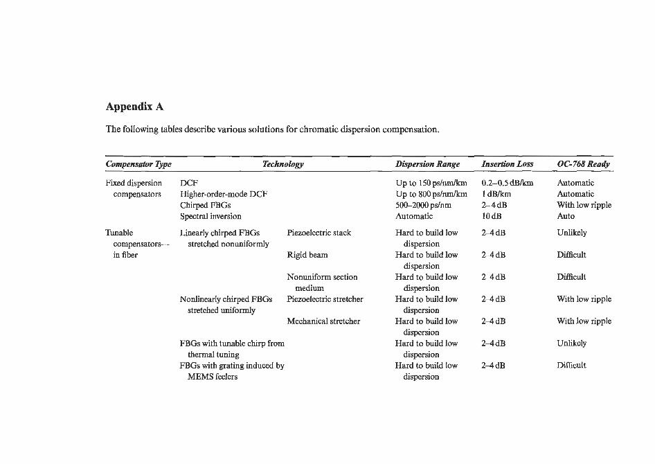
Appendix A
The following tables describe various solutions for chromatic dispersion compensation.
~ ~~
Compensator Type Technology Dispersion Range Insertion Loss OC- 768 Ready
Fixed dispersion DCF compensators Higher-order-mode DCF
Chirped FBGs Spectral inversion
Tunable Linearly chirped FBGs Piezoelectric stack compensator+ stretched nonuniformly in fiber Rigid beam
Nonuniform section medium
Nonlinearly chirped FBGs Piezoelectric stretcher
Mechanical stretcher stretched uniformly
FBGs with tunable chirp from
FBGs with grating induced by thermal tuning
MEMS feelers
Up to 150 pslnmkm Up to 800 pslnmlkm 500-2000 pslnm Automatic
Hard to build low
Hard to build low
Hard to build low
Hard to build low
Hard to build low
Hard to build low
Hard to build low
dispersion
dispersion
dispersion
dispersion
dispcrsion
dispersion
dispersion
0.2-0.5dBh 1 dBkm 2-4dB 10dB
2-4 dB
2 4 dB
2 4 dB
2 4 dB
2-4 dB
2-4 dB
2 4 dB
Automatic Automatic With low ripple Auto
Unlikely
Diilicult
Difficult
With low ripple
With low ripple
Unlikcly
Difficult
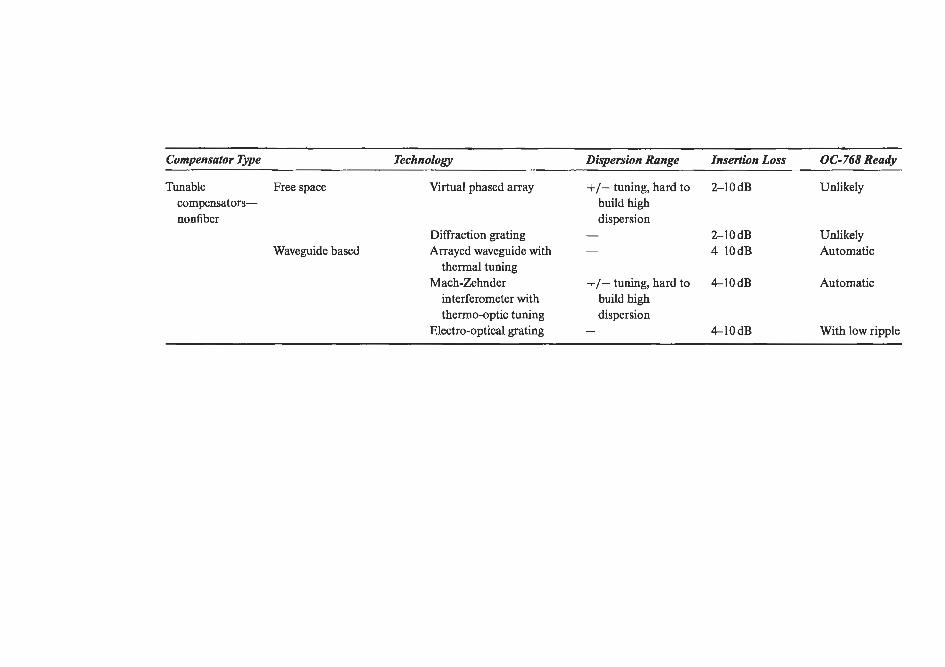
Compensator Type Technology Dispersion Range Insertion Loss 0 6 7 6 8 Ready
Tunable Free space Virtual phased army +/- tuning, hard to 2-1 0 dB Unlikely compensators- build high
dispersion nonfiber - Unlikely 2-1 0 dB
Waveguide based Arrayed waveguide with - 4 lOdB
Mach-Zehnder +/- tuning, hard to 4 1 0 dB
Diffraction grating
thermal tuning
interferometer with build high thermo-optic tuning dispersion
Automatic
Automatic
Electro-optical grating -. 4-1OdB With low ripple
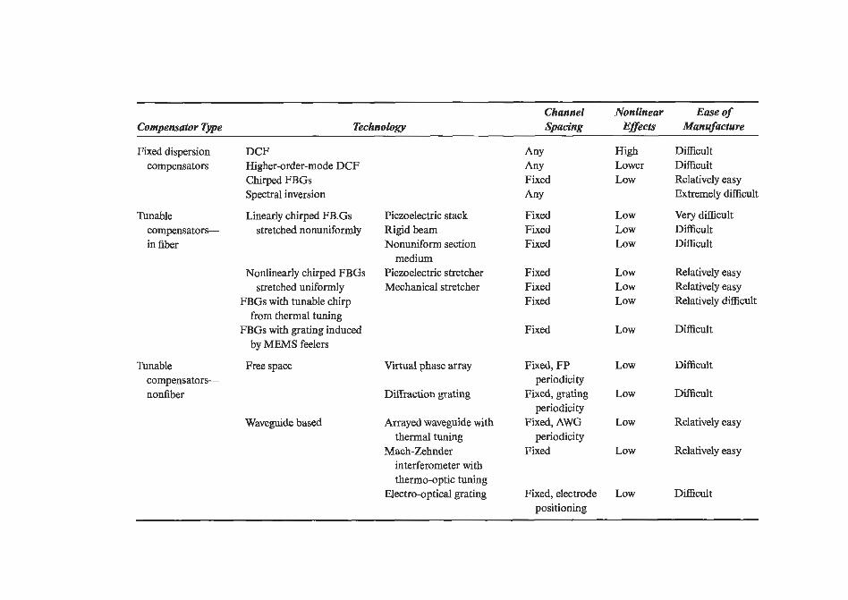
-~
Channel Nonlinear Ease of Compensator Type Technology Spacing Effects Manufacture
Fixed dispersion compensators
DCF Higher-order-mode DCF Chirped FBGs Spectral inversion
Linearly chirped FB.Gs stretched nonuniformly
Any Any
h Y Fixed
Fixed Fixed Fixed
High Lower Low
Difficult Difficult Rclatively easy Extremely difficult
Low Low Low
Very difficult Difficult Difficult
Tunable compensators- in fiber
Piezoelectric stack Rigid beam Nonuniform section
medium Piezoelectric stretcher Mechanical stretcher
Relatively easy Relatively easy Relatively difficult
Nonlinearly chirped FBGs stretched uniformly
FBGs with tunable chirp from thermal tuning
FBGs with grating induced by MEMS feelers
Free space
Fixed Fixed Fixed
Low Low Low
Difficult Fixed Low
Virtual phase array Fixed, FP periodicity
Fixed, grating periodicity
Fixed, AWG periodicity
Fixed
Low Difficult Tunable compensators- nodiber Difficult Diffraction grating Low
Waveguide based Arrayed waveguide with
Mach-Zehnder thermal tuning
interferometer with thermo-optic tuning
Electro-optical grating
Low Relatively easy
Relatively easy Low
Fixed, electrode positioning
Low Difficult

Packaging Compensator Type Technohgy Complexity Slope Matching Tuning Speed
Fixed dispersion compensators
DCF Avoid PMD,
Avoid bending loss bending loss
Can be done Not tunablc
Not tunable
Not tunable
Not tunable
1 ms lOOms
Higher-order-mode
Chirped FBGs DCF
Can be done
Thermal
Extreme stabilization
Can be done
Spectral inversion Automatic
Very difficult May not be done Tunable
compensators- in fiber
Linearly chirped FBGs stretched nonuniformly
Piezoelectric stack Rigid beam
Stack control Adhesive uniformity
uniformity Adhesivc
Low
Nonuniform section
Piezoelectric stretcher medium
May not be done 100 ms
Nonlinearly chirped FBGs stretched uniformly
FBGs with tunable chirp from thermal tuning
Can be done 1 ms
1 ms 100ms
10 ms
Mechanical stretcher Low Low
Can be done May not be done
Can be done FBGs with grating induced by MEMS feelers
Free space Virtual phase array Diffraction grating
Waveguide based Arrayed waveguide with thermal tuning
interferometer with thermo-optic tuning
Electro-optical grating
Mach-Zehnder
Tunable compensator+ nodiber
Complex Complex Low
May be done May be done
Can be done
lOms Not tunable 100 ms
Low Can be done 100 ms
Low Can be done
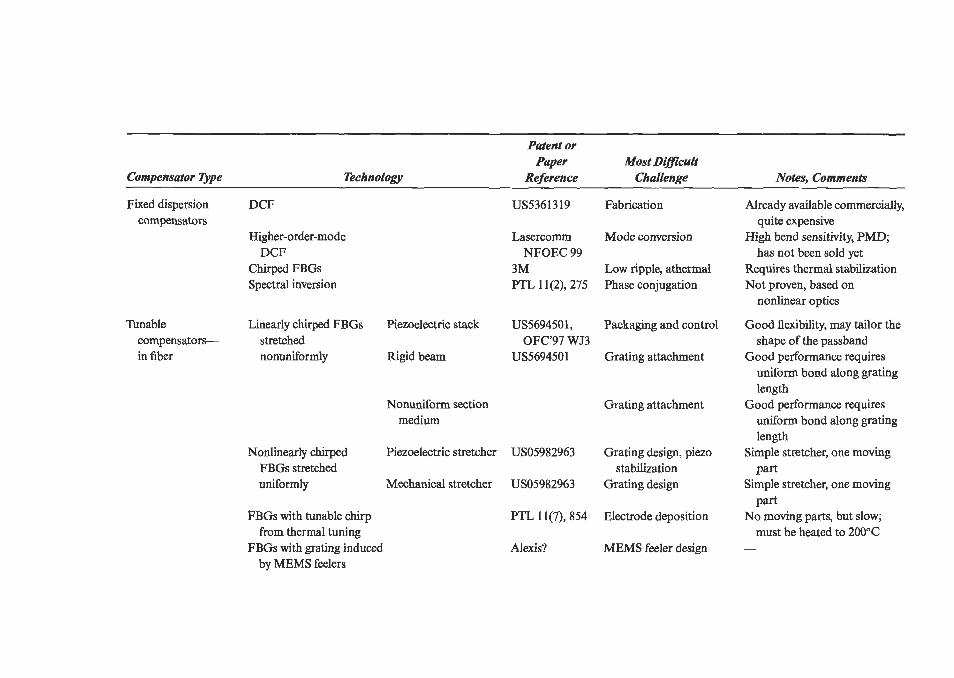
Patent or Paper Most Diflcult
Compensator Type Technology Reference Challenge Notes, Comments
Fixed dispersion DCF compensators
Higher-order-mode
Chirped FBGs Spectral inversion
DCF
Tunable Linearly chirped FBGs compensators- stretched in fiber nonuniformly
Nonlinearly chirped FBGs stretched uniformly
FBGs with tunable chirp from thermal tuning
FBGs with grating induced by MEMS feelers
US5361319 Fabrication
Lasercomm Mode conversion
3M Low ripple, athermal PTL 11(2), 275 Phase conjugation
NFOEC 99
Piezoelectric stack US5694501, Packaging and control OFC'97 WJ3
Rigid beam US5694501 Grating attachment
Nonuniform section medium
Grating attachment
Piezoelectric stretcher US05982963 Grating design, piezo stabilization
Mechanical stretcher US05982963 Grating design
PTL 11(7), 854 Electrode deposition
Alexis? MEMS feeler design -
Already mailable commercially,
High bend sensitivity, PMD;
Requires thermal stabilization Not proven, based on
nonlinear optics
quite expensive
has not been sold yet
Good flexibility, may tailor the shape of the passband
Good performance requires uniform bond along grating length
uniform bond along grating length
part
Good performance requires
Simple stretcher, one moving
Simple stretcher, one moving Pad
No moving parts, but slow; must be heated to 200°C
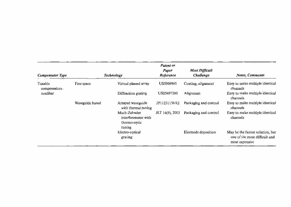
Patent or Paper Most DlSCUit
Compensator Type Technology Reference Challenge Notes, Comments
Tunable Free space compensators nonfiber
Virtual phased array US5969865 Coating, alignment
Diffraction grating US05497260 Alignment
Waveguide based Arrayed waveguide JP1123 1156A2 Packaging and control
Mach-Zehnder JLT 14(9), 2003 Packaging and control with thermal tuning
interferometer with thcrmo-optic tuning
grating Electro-optical Electrode deposition
Easy to make multiple identical
Easy to make multiple identical
Easy to make multiple identical
Easy to make multiple identical
channels
channels
channels
channels
May be the fastest solution, but one of the most difficult and most expensive

714 Alan E. Willner and Bogdan Hoanca
References
[ 11 G. P. Agrawal, Nonlinear Fiber Optics, 2nd Edition, Academic Press, San Diego, 1997.
[2] G. P. Agrawal and N. K. Dutta, Semiconductor Lasers, Chapman and Hall, New York, 1993.
[3] E. Desurvire, Erbium-Doped Fiber Amplijers: Principles and Applications, John Wiley & Sons, New York, 1994.
[4] R. C. Alferness, in Guided- Wive Optoelectronics, T. Tamir, ed., Springer Verlag, New York, 1989.
[5] A. Ougazzaden, C. W. Lentz, T. G. B. Mason, K. G. Glogovslq, C. L. Reynolds, G. J. Przybylek, R. E. Leibenguth, T. L. Kercher, J. W. Boardman, M. T. Rader, J. M. Geary, F. S. Walters, L. J. Peticolas, J. M. Freund, S. N. G. Chu, A. Sirenko, and R. J. Jurchenko, “4OGbis tandem electro-absorption modulator,” Optical Fiber Communication Con$, vol. 4, pp. PD14-1-PD14-3,2001.
[6] G. F! Agrawal, Fiber Optic Communications Systems, John Wiley & Sons, New York, 1992.
[7] D. Marcuse, A. R. Chraplyvy, and R. W. Tkach, “Dependence of cross- phase modulation on channel number in fiber WDM systems,” IEEE Journal ofLightwave Technology, vol. 12, no. 5, pp. 885-890, May 1994.
[8] S. N. Knudsen and T. Veng, “Large effective area dispersion compensating fiber for cabled compensation of standard single mode fiber,” Optical Fiber Communication Con$2000, vol. 1, pp. 9&100,2000.
[9] M. Fukui, K. Shimano, A. Umeda, T. Sakamoto, S. Aisawa, and K. Oda, “Influ- ence of dispersion fluctuation of installed dispersion-shifted fiber on four-wave mixing induced degradation in WDM transmission system,” European Con$ on Optical Communications, vol. 1, pp. 142-145, 1997.
[lo] M. Eiselt, L. D. Garrett, and R. W. Tkach, “Experimental comparison of WDM system capacity in conventional and nonzero dispersion-shifted fiber,” IEEE Photon. Tech. Letters, vol. 11, no. 2, pp. 281-283, February 1999.
[l 11 C.-C. Wang, I. Roudas, I. Tomkos, M. Sharma, and R. S. Vodhanel, “Negative dispersion fibers for uncompensated metropolitan networks,” European Con$ on Optical Communication 2000, Paper 2.4.3,2000.
[12] A. J. Antos and D. K. Smith, “Design and characterization of dispersion com- pensating fiber based on the LPol mode,” IEEE Journal of Lightwave Technology,
[13] A. M. Vengsarkar, A. E. Miller, M. Haner, A. H. Gnauck, W A. Reed, and K. L. Walker, “Fundamental-mode dispersion-compensating fibers: Design con- siderations and experiments,” Optical Fiber Communication Con$ 1994, Paper
[14] R. J. Nuyts, Y K. Park, and F! Gallion, ‘‘Performance improvement of 10-Gbith standard fiber transmission system by using the SPM effect in the dispersion compensating fiber,” IEEE Photon. Tech. Letters, vol. 10, pp. 1406-1408, 1996.
pp. 1739-1745,1994.
ThK2, pp. 225-227,1994.
14. Fixed and Tunable Management 715
[15] A. H. Gnauck, L. D. Garrett, Y. Danziger, U. Levy, and M. Tur, “Dispersion and dispersion-slope compensation of NZDSF for 40 Gbit/s operation over the entire C-band,” Optical Fiber Communication Con$ 2000, vol. 4, pp. 190-192, 2000.
I161 C. D. Poole, J. M. Wiesenfeld, D. J. DiGiovanni, and A. M. Vengsarkar, “Opti- cal fiber-based dispersion compensation using higher order modes near cutoff,” IEEE Journal of Lightwave Technology, vol. 12, no. 10, pp. 17461758, October 1994.
[17] A. H. Gnauck, L. D. Garrett, F. Forghieri, V. Gusmeroli, and D. Scarano, “8 x 20 Gb/s 3 15-km, 8 x 10 Gb/s 480-km WDM transmission over conventional fiber using multiple broad-band fiber gratings,” IEEE Photon. Tech. Letters, vol. 10, no. 10, pp. 1495-1497, October 1998.
[18] A. H. Gnauck, J. M. Wiesenfeld, L. D. Garrett, M. Eiselt, E Forghieri, L. Arcangeli, B. Agogliata, V. Gusmeroli, and D. Scarano, “16 2O-Gbit/s, 400- km WDM transmission over NZDSF using a slope-compensating fiber grating module,” IEEE Photon. Tech. Letters, vol. 12, no. 4, pp. 437439, April 2000.
[ 191 M. Shirasaki, “Chromatiedispersion compensator using virtually imaged phased array,” IEEE Photon. Tech. Letters, vol. 9, no. 11, pp. 1598-1600, 1997.
[20] J. H. Winters and R. D. Gitlin, “Electrical signal processing techniques in long-haul fiber-optic systems,” IEEE Trans. on Communications, vol. 38, no. 9, pp. 1439-1453, September 1990.
[21] J. H. Winters,“Equalization in coherent lightwave systems using a fractionally spacedequalizer,” IEEE Journal ofLightwave Technology, vol. 8, no. 10, pp. 1487- 1491, October 1990.
[22] M. I. Hayee and A. E. Willner, “Pre- and post-compensation of dispersion and nonlinearities in 10 Gbit/s WDM systems,” IEEE Photon. Tech. Letters, vol. 9, pp. 1271-1273,1997.
[23] T. Yamamoto, E. Yoshida, K. R. Tamura, K. Yonenaga, and M. Nakazawa “640- Gbit/s Optical TDM transmission over 92 km through a dispersion-managed fiber consisting of single-mode fiber and reverse-dispersion fiber,” IEEE Photon. Tech. Letters, vol. 12, no. 3, pp. 353-355, March 2000.
[24] L. D. Garrett, A. H. Gnauck, M. H. Eiselt, R. W. Tkach, C. Yang, C. Mao, and S. Cao, “Demonstration of virtually-imaged phased-array device for tun- able dispersion compensation in 16 x 10 Gb/s WDM transmission over 480 km standard fiber,” Optical Fiber Communication Con$ 2000, vol. 4, pp. 187-189, 2000.
[25] A. H. Gnauck, L. D. Garrett, Y. Danziger, U. Levy, and M. Tur, “Dispersion and dispersion-slope compensation of NZDSF for 40 Gbit/s operation over the entire C-band,” Optical Fiber Communication Con$ 2000, vol. 4, pp. 190-192, 2000.
[26] L. E Mollenauer, E. Lichtman, M. J. Neubelt, and G. T. Harvey, “Demonstra- tion, using sliding-frequency guiding filters, of error-free soliton transmission over more than 20 Mm at 10Gbit/s, single channel, and over more than 13 Mm
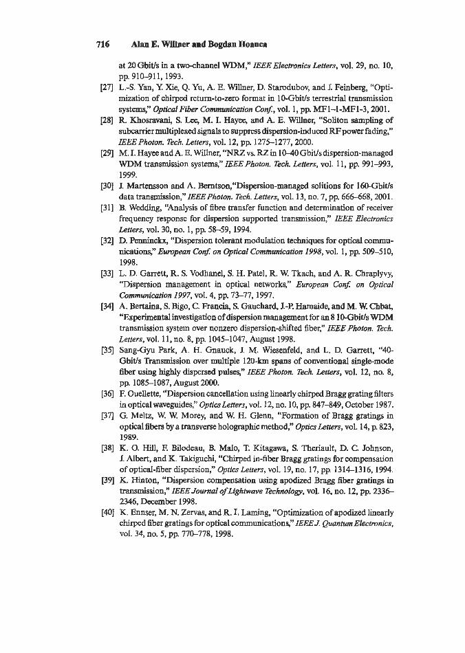
716 Alan E. W h e r and Bogdan Hoanca
at 20 Gbit/s in a two-channel WDM,” ZEEE Electronics Letters, vol. 29, no. 10, pp. 910-911,1993.
[27] L.-S. Yan, Y Xie, Q. Yu, A. E. Willner, D. Starodubov, and J. Feinberg, “Opti- mization of chirped return-to-zero format in lO-GbitIs terrestrial transmission systems,” Optical Fiber Communication Con$, vol. 1, pp. MFl-l-MF1-3,2001.
[28] R. Khosravani, S. Lee, M. I. Hayee, and A. E. Willner, “Soliton sampling of subcarrier multiplexed signals to suppress dispersion-induced RF power fading,” IEEE Photon. Tech. Letters, vol. 12, pp. 1275-1277,2000,
[29] M. I. Hayee and A. E. Willner, “ N U vs. RZ in 1040 Gbit/s dispersion-managed WDM transmission systems,” ZEEE Photon. Tech. Letters, vol. 11, pp. 991-993, 1999.
[30] J. Martensson and A. Berntson,“Dispersion-managed solitions for 160-Gbith data transmission,” IEEEPkoton. Tech. Letters, vol. 13, no. 7, pp. 666468,2001.
[31] B. Wedding, “Analysis of fibre transfer function and determination of receiver frequency response for dispersion supported transmission,” IEEE Electronics Letters, vol. 30, no. 1, pp. 58-59, 1994.
[32] D. Penninckx, “Dispersion tolerant modulation techniques for optical commu- nications,” European Con$ on @tical Communication 1998, vol. 1, pp. 509-510, 1998.
[33] L. D. Garrett, R. S. Vodhanel, S. H. Patel, R. W. Tkach, and A. R. Chraplyvy, “Dispersion management in optical networks,” European Con$ on Optical Communication 1997, vol. 4, pp 73-77,1997.
[34] A. Bertaina, S. Bigo, C. Francia, S. Gauchard, J.-I? Hamaide, and M. W. Chbat, “Experimental investigation of dispersion management for an 8 lO-Gbit/s WDM transmission system over nonzero dispersion-shifted fiber,” IEEE Photon. Tech. Letters, vol. 11 , no. 8, pp. 1045-1047, August 1998.
[35] Sang-Gyu Park, A. H. Gnauck, J. M. Wiesenfeld, and L. D. Garrett, “40- Gbitls Transmission over multiple 120-km spans of conventional single-mode fiber using highly dispersed pulses,” ZEEE Photon. Tech. Letters, vol. 12, no. 8, pp. 1085-1087, August 2000.
[36] F. Ouellette, “Dispersion cancellation using linearly chirped Bragg grating filters in optical waveguides,” Optics Letters, vol. 12, no. 10, pp. 847-849, October 1987.
[37] G. Meltz, W. W. Morey, and W. H. Glenn, “Formation of Bragg gratings in optical fibers by a transverse holographicmethod,” OpticsLetters, vol. 14, p. 823, 1989.
[38] K. 0. Hill, E Bilodeau, B. Malo, T. Kitagawa, S. Theriault, D. C. Johnson, J. Albert, and K. Takiguchi, “Chirped in-fiber Bragg gratings for compensation of optical-fiber dispersion,” Optics Letters, vol. 19, no. 17, pp. 13 1 4 1 3 16, 1994.
[39] K. Hinton, “Dispersion compensation using apodized Bragg fiber gratings in transmission,’’ ZEEE Journal of Lightwave Technology, vol. 16, no. 12, pp. 2336- 2346, December 1998.
[a] K. Ennser, M. N. Zervas, and R. I. Laming, “Optimization of apodized linearly chirped fiber gratings for optical communications,” IEEEJ. Quantum Electronics, vol. 34, no. 5, pp. 77C778, 1998.

14. Fixed and ’hnable Management 717
[41] S. J. Mihailov, E Bilodeau, K. 0. Hill, D. C. Johnson, J. Albert, D. Stryckman, and C. Shu, “Comparison of fiber Bragg grating dispersion-compensators made with holographic and E-beam written phase masks,” IEEE Photon. Tech. Letters, vol. 11, no. 5, pp. 572-574, 1999.
[42] T. Komukai, T. Inui, and M. Nakazawa, “Group delay ripple reduction and reflectivity increase in a chirped fiber bragg grating by multiple-overwriting of a phase mask with an electron-beam,” IEEE Photon. Tech. Letters, vol. 12, no. 7, pp. 816818, July 2000.
[43] T. Komukai, T. Inui, and M. Nakazawa, “Very low group delay ripple character- istics of fibre Bragg grating with chirp induced by an S-curve bending technique,” IEEE Electronics Letters, vol. 37, no. 7, pp. 449451,2001.
[44] K. Ennser, M. Ibsen, M. Durkin, M. N. Zervas, and R. I. Laming, “Influence of nonideal chirped fiber grating characteristics on dispersion cancellation,” IEEE Photon. Tech. Letters, vol. 10, no. 10, pp. 14761478, October 1998.
[45] Y. J. Rao, P. J. Henderson, D. A. Jackson, L. Zhang, and I. Bennion, “Simul- taneous strain, temperature and vibration measurement using a multiplexed in- fibre-Bragg-gratinglfibre-Fabry-Perot sensor system,” IEEE Electronics Letters, vol. 33, no. 24, pp. 2063-2064,1997.
[46] Nortel Networks, announcement regarding 2.4 m dispersion compensating grating: http://www.nortelnetworks.comlcorporate/tec~olo~/techfeatures/ ipinitiativesthpush. html .
[47] E. Ciaramella, E. Riccardi, and M. Schiano, “System penalties due to polar- ization mode dispersion of chirped gratings,” European Conf on Optical Communication 1998, pp. 515-516,1998.
[48] M. Rochette? l? Cortes, S. Larochelle, M. Guy, and J. Lauzon, “Polarisa- tion mode dispersion compensation of chirped Bragg gratings,” Optical Fiber Communication Conf, vol. 2, pp. 254-256, 2000.
[49] Y. Zhu, E. Simova, P. Berini, and C. P. Grover, “A comparison of wavelength dependent polarization dependent loss measurements in fiber gratings,” ZEEE Transactions on Instrumentation and Measurements, vol. 49, no. 6, pp. 123 1-1239, 2000.
[50] M. Rochette, P. Cortes, S. LaRochelle, M. Guy, and J. Lauzon, “Polarisa- tion mode dispersion compensation of chirped Bragg gratings,” Optical Fiber Communications Conf 2000, vol. 2, pp. 254256,2000.
[51] L. Dong, M. J. Cole, A. D. Ellis, R. I. Laming, and T. Widdowson, “40Gbit/s 1.55 km RZ transmission over 109 km of non-dispersion shifted fiber with long continuously chirped fiber gratings,” ZEEE Electronics Letters, vol. 33, pp. 156% 1565,1997.
[52] M. Ibsen, M. K. Durkin, M. N. Zervas, A. B. Grudinin, and R. I. Laming, “Custom design of long chirped Bragg gratings: application to gain-flattening filter with incorporated dispersion compensation,” IEEE Photon. Tech. Letters, vol. 12, no, 5, pp. 498-500, May 2000.
[53] A. D. Ellis, R. Kashyap, I. Crisp, D. J. Malyon, and J. P. Hueting, “Demon- stration of an 80 Gbitls throughput, reconfigurable dispersion compensating
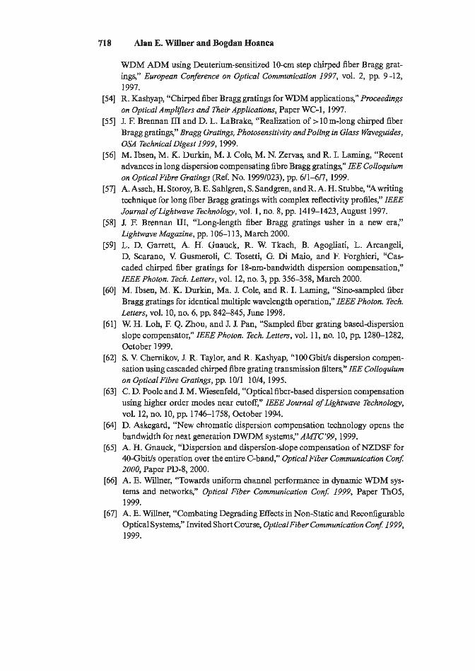
718 Alan E. Willner and Bogdan Hoanca
WDM ADM using Deuterium-sensitized 10-cm step chirped fiber Bragg grat- ings,” European Conference on Optical Communication 1997, vol. 2, pp. 9-12, 1997.
[54] R. Kashyap, “Chirped fiber Bragg gratings for WDM applications,” Proceedings on Optical AmpliJiers and Their Applications, Paper WC-1, 1997.
[55] J. E Brennan I11 and D. L. LaBrake, “Realization of > 10 m-long chirped fiber Bragg gratings,” Bragg Gratings, Photosensitivity and Poling in Glass Waveguides, OSA Technical Digest 1999, 1999.
[56] M. Ibsen, M. K. Durkin, M. J. Cole, M. N. Zervas, and R. I. Laming, “Recent advances in long dispersion compensating fibre Bragg gratings,” IEE Colloquium on Optical Fibre Gratings (Ref No. 19991023), pp. 611-617, 1999.
[57] A. Asseh, H. Storoy, B. E. Sahlgren, S. Sandgren, andR. A. H. Stubbe, “Awriting technique for long fiber Bragg gratings with complex reflectivity profiles,” IEEE Journal OfLightwave Technology, vol. 1, no. 8, pp. 1419-1423, August 1997.
[58] J. E Brennan 111, “Long-length fiber Bragg gratings usher in a new era,” Lightwave Magazine, pp. 106-1 13, March 2000.
[59] L. D. Garrett, A. H. Gnauck, R. W. Tkach, B. Agogliati, L. Arcangeli, D. Scarano, V. Gusmeroli, C. Tosetti, G. Di Maio, and E Forghieri, “Cas- caded chirped fiber gratings for 18-nm-bandwidth dispersion compensation,” IEEE Photon. Tech. Letters, vol. 12, no. 3, pp. 356-358, March 2000.
[60] M. Ibsen, M. K. Durkin, Ma. J. Cole, and R. I. Laming, ‘‘Sinesampled fiber Bragg gratings for identical multiple wavelength operation,” IEEE Photon. Tech. Letters, vol. 10, no. 6, pp. 842-845, June 1998.
[61] W. H. Loh, E Q. Zhou, and J. J. Pan, “Sampled fiber grating based-dispersion slope compensator,” IEEE Photon. Tech. Letters, vol. 11, no. 10, pp. 1280-1282, October 1999.
[62] S. V. Chernikov, J. R. Taylor, and R. Kashyap, “100 Gbitls dispersion compen- sation using cascaded chirped fibre grating transmission filters,” IEE Colloquium on Optical Fibre Gratings, pp. 1011-1014, 1995.
[63] C. D. Poole and J. M. Wiesenfeld, “Optical fiber-based dispersion compensation using higher order modes near cutoff,” IEEE Journal of Lightwave Technology, vol. 12, no. 10, pp. 1746-1758, October 1994.
[&I] D. Askegard, “New chromatic dispersion compensation technology opens the bandwidth for next generation DWDM systems,” AMTC’99, 1999.
[65] A. H. Gnauck, “Dispersion and dispersion-slope compensation of NZDSF for 40-Gbitls operation over the entire C-band,” Optical Fiber Communication Con$ 2000, Paper PD-8,2000.
[66] A. E. Willner, “Towards uniform channel performance in dynamic WDM sys- tems and networks,” Optical Fiber Communication Con$ 1999, Paper ThO5, 1999.
[67] A. E. Willner, “Combating Degrading Effects in Non-Static and Reconfigurable Optical Systems,” Invited Short Course, OpticalFiber Communication ConJl999, 1999.
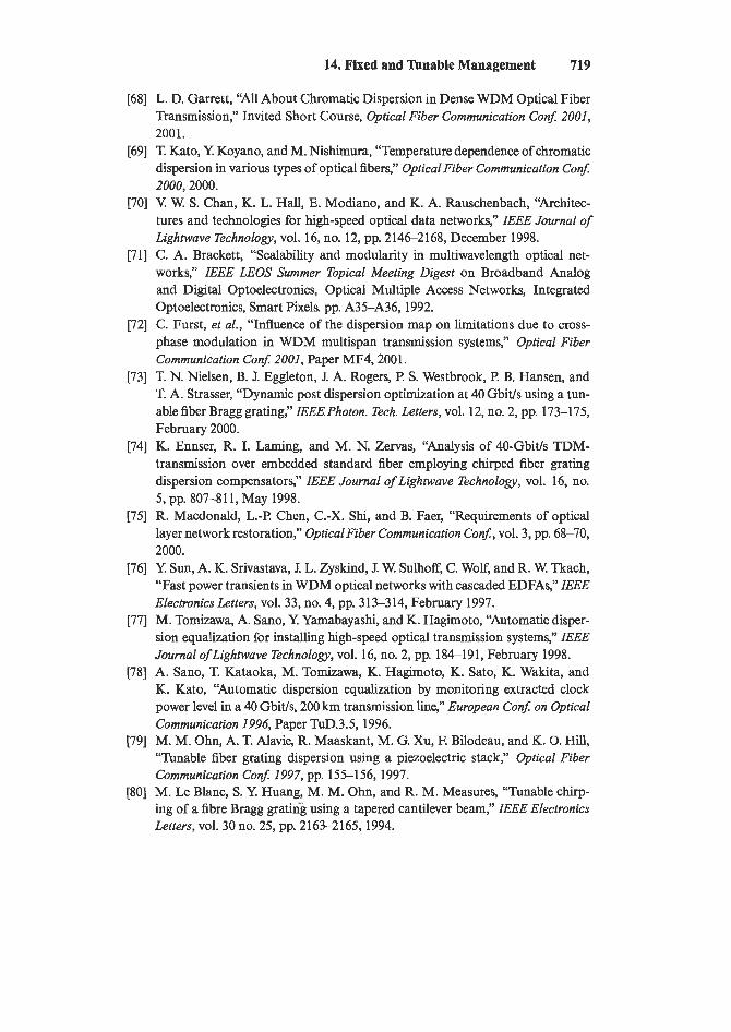
14. Fixed and Tunable Management 719
[68] L. D. Garrett, “All About Chromatic Dispersion in Dense WDM Optical Fiber Transmission,” Invited Short Course, Optical Fiber Communication Conf 2001: 200 1.
[69] T. Kato, Y. Koyano, and M. Nishimura, “Temperature dependence of chromatic dispersion in various types of optical fibers,” Optical Fiber Communication Con$ 2000,2000.
[70] V. W. S. Chan, K. L. Hall, E. Modiano, and K. A. Rauschenbach, “Architec- tures and technologies for high-speed optical data networks,” IEEE Journal of Lightwave Technology, vol. 16, no. 12, pp. 2146-2168, December 1998.
[71] C. A. Brackett, “Scalability and modularity in multiwavelength optical net- works,” ZEEE LEOS Summer Topical Meeting Digest on Broadband Analog and Digital Optoelectronics, Optical Multiple Access Networks, Integrated Optoelectronics, Smart Pixels. pp. A35-A36, 1992.
[72] C. Furst, et al., “Influence of the dispersion map on limitations due to cross- phase modulation in WDM multispan transmission systems,” Optical Fiber Communication Conf2001, Paper MF4,2001.
[73] T. N. Nielsen, B. J. Eggleton, J. A. Rogers, P. S. Westbrook, P. B. Hansen, and T. A. Strasser, “Dynamic post dispersion optimization at 40 Gbitls using a tun- able fiber Bragg grating,” ZEEE Photon. Tech. Letters, vol. 12, no. 2, pp. 173-175, February 2000.
[74] K. Ennser, R. I. Laming, and M. N. Zervas, “Analysis of 40-Gbitls TDM- transmission over embedded standard fiber employing chirped fiber grating dispersion compensators,” IEEE Journal of Lightwave Technology, vol. 16, no. 5, pp. 807-81 1, May 1998.
[75] R. Macdonald, L.-P. Chen, C.-X. Shi, and B. Faer, “Requirements of optical layer network restoration,” Optical Fiber Communication Conf, vol. 3, pp. 68-70, 2000.
[76] Y. Sun, A. K. Srivastava, J. L. Zyskind, J. W. Sulhoff, C. Wolf, and R. W. Tkach, “Fast power transients in WDM optical networks with cascaded EDFAs,” IEEE Electronics Letters, vol. 33, no. 4, pp. 313-314, February 1997.
[77] M. Tomizawa, A. Sano, Y. Yamabayashi, and K. Hagimoto, “Automatic disper- sion equalization for installing high-speed optical transmission systems,” ZEEE Journal ofLightwave Technology, vol. 16, no. 2, pp. 18k191, February 1998.
[78] A. Sano, T. Kataoka, M. Tomizawa, K. Hagimoto, K. Sato, K. Wakita, and K. Kato, “Automatic dispersion equalization by monitoring extracted clock power level in a 40 Gbitls, 200 km transmission line,” European Con$ on Optical Communication 1996, Paper TuD.3.5, 1996.
[79] M. M. Ohn, A. T. Alavie, R. Maaskant, M. G. Xu, F. Bilodeau, and K. 0. Hill, “Tunable fiber grating dispersion using a piezoelectric stack,” Optical Fiber Communication Confl997, pp. 155-156,1997.
[80] M. Le Blanc, S. Y. Huang, M. M. Ohn, and R. M. Measures, “Tunable chirp- ing of a fibre Bragg grating using a tapered cantilever beam,” ZEEE Electronics Letters, vol. 30 no. 25, pp. 2163-2165, 1994.

720 Alan E. Willner and Bogdan Hoanca
[81] T. Imai, T. Komukai, and M. Nakazawa, “Dispersion tuning of a linearly chirped fiber B r a g grating without a center wavelength shift by applying a strain gradient,” IEEE Photon. Tech. Letters, vol. 10, no. 6, p. 845, June 1998.
[82] B. J. Eggleton, J. A. Rogers, P. S. Westbrook, and T. A. Strasser, “Elec- trically tunable power efficient dispersion compensating fiber Bragg grat- ing,”IEEE Photon. Tech. Letters, vol. 11, no. 7, pp. 854-856, July 1999.
[83] B. J. Eggleton, B. Mikkelsen, G. Raybon, A. Ahuja, J. A. Rogers, P. S. Westbrook, T. N. Nielsen, S. Stulz, and K. Dreyer, “Tunable dispersion compensation in a 160-Gbitls TDM system by a voltage controlled chirped fiber Bragg grating,” IEEE Photon. Tech. Letters, vol. 12, no. 8, pp. 1022-1024, August 2000.
[84] K.-M. Feng, J.-X. Cai, V. Grubsky, D. S. Starodubov, M. I. Hayee, S. Lee, X. Jiang, A. E. Willner, and J. Feinberg, “Dynamic dispersion compensation in a 10-Gbit.h optical system using a novel voltage tuned nonlinearly chirped fiber Bragg grating,” IEEE Photon. Tech. Letters, vol. 11, no. 3, pp. 373-375, March 1999.
[85] J.-X. Cai, K.-M. Feng, A. E. Willner, V. Grubsky, D. S. Starodubov, and J. Feinberg, “Simultaneous tunable dispersion compensation of many WDM channels using a sampled nonlinearly chirped fiber Bragg grating,” IEEE Photon. Tech. Letters, vol. 11, no. 11, pp. 1455-1457, November 1999.
[8s] J. A. J. Fells, S. E. Kanellopoulos, P. J. Bennett, V. Baker, H. E M. Priddle, W. S. Lee, A. J. Collar, C. B. Rogers, D. P. Goodchild, R. Feced, B. J. Pugh, S. J. Clements, and A. Hadjifotiou, ‘‘Twin fibre grating adjustable dispersion compensator for 40 Gbitls,” European Conf on Optical Communication 2000, Paper PD 2.4,2000.
[87] J. A. J. Fells, P. J. Bennett, R. Feced, P. Ayliffe, J. Wakefield, H. F. M. Priddle, V. Baker, S. E. Kanellopoulos, C. Boylan, S. Sahil, W. S. Lee, S. J. Clements, and A. Hadjifotiou, “Widely tunable twin fiber grating dispersion compensator for 80Gbit/s,” Optical Fiber Communication Conf 2001, vol. 4, pp. PD11-1-
[88] M. Shirasaki, “Chromatic dispersion compensator using virtually imaged phased array,” IEEE Photon. Tech. Letters, vol. 9, no. 12, pp. 1598-1600, December 1997.
[89] M. Shirasaki, A. N. Akhter, and C. Lin, “Virtually imaged phased array with graded reflectivity,” IEEE Photon. Tech. Letters, vol. 11, no. 11, pp. 1443-1445, November 1999.
[go] A. Corchia, C. Antonini, A. D’Ottavi, A. Mecozzi, F. Martelli, P. Spano, G. Guekos, and R. Dall’Ara, “Midspan spectral inversion without frequency shift for fiber dispersion compensation: a system demonstration,” IEEE Photon. Tech. Letters, vol. 11, no. 2, pp. 275-277, February 1999.
[91] C. K. Madsen and G. Lenz, “A multichannel dispersion slope compensating optical all-pass filter,” Optical Fiber Communication Conf 2000, Paper WF5, 2000.
PDll-3,2001.

14. Fixed and ’hnable Management 721
[92] E Horst, C. Berendsen, R. Beyeler, G.-L. Bona, R. Germann, H. W. M. Salemink, and D. Wiesmann, “Tunable Ring Resonator Dispersion Compen- sators Realized in High Refractive Index Contrast SiON Technology” European Conf on Optical Communication 2000, Paper PD2.2,2000.
[93] H. Takenouchi, T. Goh, and T. Ishii, “2 x 40-channel dispersion slope compen- sator for 40 Gbit/s WDM transmission systems covering entire C- and L-bands,” Optical Fiber Communication Conf2001, Paper TuS2,2001.
[94] K. Takiguchi, S. Kawanishi, H. Takara, A. Himeno, andK. Hattori, “Dispersion slope equalizer for dispersion shifted fiber using a lattice-form programmable optical filter on aplanar lightwave circuit,” IEEEJournal OfLightwave Technology, vol. 16, no. 9, pp. 1647-1656, September 1998.
[95] V. Polo, J. Marti, E Ramos, and D. Moodie, “Mitigation of chromatic disper- sion effects employing electroabsorption modulator-based transmitters,” IEEE Photon. Tech. Letters, vol. 11, no. 7, pp. 883-885, July 1999.
[96] K. E. Anderson and K. H Wagner, “Chromatic and polarization mode dispersion compensation using spectral holography,” Optical Fiber Communication Con$ 2001, Paper TuH2,2001.
[97l C. K. Madsen and G. Lenz, “Optical all-pass filters for phase response design with applications for dispersion compensation,” IEEE Photon. Tech. Letters, vol. 10, no. 7, pp. 994-996, July 1998.
[98] C. K. Madsen, G. Lenz, A. J. Bruce, M. A. Cappuzzo, L. T. Gomez, and R. E. Scotti, “Integrated all-pass filters for tunable dispersion and dispersion slope compensation,” IEEE Photon. Tech. Letters, vol. 11, no. 12, pp. 1623-1625, December 1999.
[99] C. K. Madsen, S. Chandrasekar, E. J. Laskowsky, K. Bogart, M. A. Cappuzzo, A. Paunescu, L. W. Schultz, and L. T. Gomez, “Compact integrated tunable chromatic dispersion compensator with a 4000 ps/nm tuning range,” Optical Fiber Communication Conf2001, Paper PD9: 2001.
[loo] C. K. Madsen, J. A. Walker, J. E. Ford, K. W. Goossen, T. N. Nielsen, and G. Lenz, “A tunable dispersion compensating MEMS all-pass filter,” IEEE Photon. Tech. Letters, vol. 12, no. 6, pp. 651-653, June 2000.
[loll H. Tsuda, T. Kurokawa, K. Okamoto, T. Ishii, K. Naganuma, Y. Inoue, and H. Takenouchi, “Second- and third-order dispersion compensation using a high resolution arrayed waveguide grating,” European Conf on Optical Communication 1998, vol. 1, pp. 533-534, 1998.
[lo21 T. M. Monro, P. J. Bennett, N. G. R. Broderick, and D. J. Richardson, “New possibilities with holey fibers,” Optical Fiber Communication Conf2000, pp. 1 0 6 108,2000.
[lo31 D. J. Richardson, T. M. Monro, and N. G. R. Broderick, “Holey fibres - a review of recent developments in theory, fabrication and experiment,” European Con$ on Optical Communication 2000, Paper 10.2.2,2000.
[lo41 B. Srinivasan and R. K. Jain, “First demonstration of thermally poled electro- optically tunable fiber Bragg gratings,” IEEE Photon. Tech. Letters, vol. 12, no. 2, pp. 170-172, February 2000.
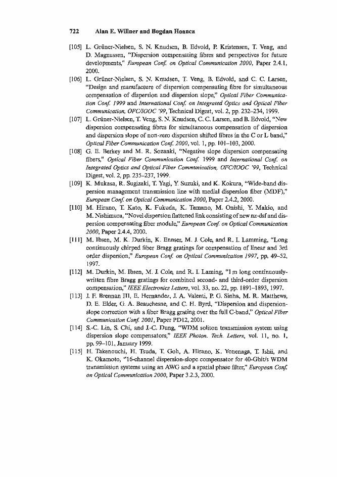
722 Alan E. Willner and Bogdan Hoanca
[lo51 L. Griiner-Nielsen, S. N. Knudsen, B. Edvold, P. Kristensen, T. Veng, and D. Magnussen, “Dispersion compensating fibres and perspectives for future developments,” European ConJ on Optical Communication 2000, Paper 2.4.1, 2000.
[I061 L. Griiner-Nielsen, S. N. Knudsen, T. Veng, B. Edvold, and C. C. Larsen, “Design and manufacture of dispersion compensating fibre for simultaneous compensation of dispersion and dispersion slope,” Optical Fiber Communica- tion Con$ 1999 and International Con$ on Integrated Optics and Optical Fiber Communication, OFC/IOOC ’99, Technical Digest, vol. 2, pp. 232-234, 1999.
[lo71 L. Griiner-Nielsen, T. Veng, S. N. Knudsen, C. C. Larsen, and B. Edvold, “New dispersion compensating fibres for simultaneous compensation of dispersion and dispersion slope of non-zero dispersion shifted fibres in the C or L band,” Optical Fiber Communication ConJ2000, vol. 1, pp. 101-103,2000.
[lo81 G. E. Berkey and M. R. Sozanki, “Negative slope dispersion compensating fibers,” Optical Fiber Communication Con$ 1999 and International Con$ on Integrated Optics and Optical Fiber Communication, OFC/IOOC ’99, Technical Digest, vol. 2, pp. 235-237, 1999.
[lo91 K. Mukasa, R. Sugizaki, T. Yagi, Y Suzuki, and K. Kokura, “Wide-band dis- persion management transmission line with medial dispersion fiber (MDF),” European Con$ on Optical Communication 2000, Paper 2.4.2,2000.
[110] M. Hirano, T. Kato, K. Fukuda, K. Tamano, M. Onishi, Y Makio, and M. Nishimura, “Novel dispersion flattened link consisting of new nz-dsf and dis- persion compensating fiber module,” European Con$ on Optical Communication 2000, Paper 2.4.4,2000.
[ l l l ] M. Ibsen, M. K. Durkin, K. Ennser, M. J. Cole, and R. I. Lamming, “Long continuously chirped fiber Bragg gratings for compensation of linear and 3rd order dispersion,” European Conf on Optical Communication 1997, pp. 49-52, 1997.
[I 121 M. Durkin, M. Ibsen, M. J. Cole, and R. I. Laming, “1 m long continuously- written fibre Bragg gratings for combined second- and third-order dispersion compensation,” IEEE Electronics Letters, vol. 33, no. 22, pp. 1891-1893, 1997.
[113] J. E Brennan 111, E. Hernandez, J. A. Valenti, P. G. Sinha, M. R. Matthews, D. E. Elder, G. A. Beauchesne, and C. H. Byrd, “Dispersion and dispersion- slope correction with a fiber Bragg grating over the full C-band,” Optical Fiber Communication Con$2001, Paper PD12,2001.
[114] S.-C. Lin, S. Chi, and J.-C. Dung, “WDM soliton transmission system using dispersion slope compensators,” IEEE Photon. Tech. Letters, vol. 11, no. 1, pp. 99-101, January 1999.
[115] H. Takenouchi, H. Tsuda, T. Goh, A. Hirano, K. Yonenaga, T. Ishii, and K. Okamoto, “16-channel dispersion-slope compensator for 4O-Gbit/s WDM transmission systems using an AWG and a spatial phase filter,” European Con$ on Optical Communication 2000, Paper 3.2.3,2000.

14. Fixed and anable Management 723
[116] T. Inui, T. Komukai, and M. Nakazawa, “A wavelength-tunable dispersion equalizer using a nonlinearly chirped fiber Bragg grating pair mounted on mul- tilayer piezoelectric transducers,” IEEE Photon. Tech. Letters, vol. 12, no. 12, pp. 1668-1 670, December 2000.
[117] Y. Xie, S. Lee, Z. Pan, J.-X. Cai, A. E. Willner, V. Grubsky, D. S. Staro- dubov, E. Salik, and J. Feinberg, “Tunable compensation of the dispersion slope mismatch in dispersion-managed systems using a sampled nonlinearly chirped FBG,” IEEE Photon. Tech. Letters, vol. 12, no. 10, pp. 1417-1419, October 2000.
[118] H. Schmuck, “Comparison of optical millimeter-wave system concepts with regard to chromatic dispersion,” IEEE Electronics Letters, vol. 31, no. 21,
[119] J. Marti, J. M. Fuster, and R. I. Laming, “Experimental reduction of chro- matic dispersion effects in lightwave microwave/millimeter-wave transmissions using tapered linearly chirped fiber gratings,” ZEEE Electronics Letters, vol. 33, pp. 1170-1171,1997.
[120] H. Sun, M. Cardakli, J. X. Cai, K. M. Feng, H. Long, M. I. Hayee, and A. E. Willner, “Tunable compensation of dispersion-induced RF power degradation in multiple-channel SCM transmission by nonlinearly-chirped FBGs,” ZEEE Conf on Lasers and Elecho-Optics 1999, Paper CWK2, 1999.
[121] S. A. Havstad, A. B. Sahin, 0. H. Adamczyk, Y. Xie, and A. E. Willner, “Distance-independent microwave and millimeter-wave power fading compen- sation using a phase diversity configuration,” IEEEPhoton. Tech. Letters, vol. 12, no. 8, pp. 1052-1054, August 2000.
[122] G. H. Smith, D. Novak, and Z. Ahmed, “Overcoming chromatic-dispersion effects in fiber-wireless systems incorporating external modulators,” IEEE Microwave Theory and Techniques, vol. 45, no. 8, pp. 1410-1415, 1997.
[123] C. Lim, D. Novak, and G. H. Smith, “Implementation of an upstream path in a millimeter-wave fiber-wireless system,” Optical Fiber Communication Conf1998; Paper TuC3, pp. 1617,1998.
[ 1241 K. Yonenaga, A. Sano, M. Yoneyama, S. Kuwahara, Y. Miyamoto, and H. Toba, “Automatic dispersion equalization using bit-error-rate monitoring in a 4O-gbit/s transmission system,” European Conf on Optical Communication 2000, Paper 3.2.5,2000.
[l25] T. Ihara, and Y. Oikawa, US patent 5,999,289, Detection oJ; and compensation fol; waveform change due to chromatic dispersion assigned to Fujitsu, Ltd., Dec
[126] G. Ishikawa, H. Ooi, and N. Kuwatya, US patent 6,081,360, Method and appa- ratus for optimizing dispersion in an optical fiber transmission line in accordance with an optical sigrralpower level assigned to Fujitsu, Ltd., June 27,2000.
[127] G. Ishikawa and H. Ooi, “Demonstration of automatic dispersion equalization in 40 GbitJs OTDM transmission,” European Conf on Optical Communication
pp. 1848-1849,1995.
7,1999.
1998, V O ~ . 1, pp. 519-520, 1998.
724 Alan E. Willner and Bogdan Hoanca
[128] A. Sano, Y Miyamoto, S. Kuwahara, and H. Toba, “Adaptive dispersion equal- ization by monitoring relative phase shift between spacing-fixed WDM signals,” IEEE Journal of Lightwave Technology, vol. 19, no. 3, pp. 336-344, March 2001.
[129] B. Bakhsbi, M. Vaa, E. A. Golovehenko, W. W. Patterson, R. L. Maybach, and N. S. Bergano, “Comparison of CRZ, RZ and NRZ modulation formats in a 64 x 12.3 Gb/s WDM transmission experiment over 9000 km,” Optical Fiber Communication Con$, vol. 3, pp. WF4-1-WF4-3,2001.
[130] R. Kashyap, Fiber Bragg Gratings, New York: Academic (1999). [131] R. W. Tkach, A. R. Chraplyvy, F. Forghieri, A. H. Gnauck, andR. M. Derosier,
“Four-photon mixing and high-speed WDM systems,” J. Lightwave Technol., vol. 13, no. 5, pp. 841-849, 1995.
[132] h t tp : / /www. la se rcomm- inc . com/med ia lWP_Fu-28-2000 .pdf
[133] T. A. Birks, D. Mogilevtsev, J. C. Knight, and P. St. J. Russell, “Dispersion compensation using single-material fibers,” IEEE Photon. Technol. Lett., vol. 11, no. 6, pp. 674676, 1999.
[134] Z. Pan, Q. Yu, Y Xie, S. A. Havstad, A. E. Willner, D. S. Starodubov, and J. Feinberg, “Chromatic dispersion monitoring and automated compensation for NRZ and RZ data using clock regeneration and fading without adding signaling,” Optical Fiber Communication Conf, vol. 3. pp. wh5-1-wh5-3,2000.

Chapter 15 Polarization-Mode Dispersion
Herwig Kogelnik and Robert M. Jopson
Lynn E. Nelson
Crawford Hill hboratory, Bell Laboratories, Lucent Technologies, Holmdel, New Jersey
OFS Fitel, Holmdel, New Jersey
1. Introduction
As the bit rate and distance of optical fiber transmission systems continue to increase, the understanding of polarization-mode dispersion (PMD) and its system impairments and mitigation are becoming ever more important. In an ideal circularly symmetric fiber, the two orthogonally polarized modes have the same group delay. In reality, fibers have some amount of birefringence due to imperfections in the manufacturing process and/or mechanical stress on the fiber after manufacture. PMD has its origins in this optical birefringence and the random variation of the birefringent axes orientation along the fiber length. PMD causes different delays for different polarizations, and when the difference in the delays approaches a significant fraction of the bit period, pulse distortion and system penalties occur. Environmental changes, including temperature and stress, cause the fiber PMD to vary stochastically in time, making PMD particularly difficult to manage. In addition, although amplifiers or other components such as add-drop multiplexers in an optical system may have constant birefringence, variable polarization rotations between them due
Fig. 0 Flip movie of changes in the DGD spectrum of a 110-km test span having a mean DGD of 41 ps (Nagel et al. 2000). The signal passed through a 55-km span, was amplified, and returned over a second fiber in the same cable. This cable was buried for much of its length but passed over a river on an automobile bridge at one point and traveled near railroad tracks at another point. The horizontal axis represents a 0.20 nm range of wavelength, centered at 155Onm, while the vertical axis displays the DGD and ranges from 0 ps at the bottom to 80 ps at the top. Successive measurements were made at approximately 9.3-minute intervals. The number in each frame indicates time in units of 9.3 minutes; hence, the movie spans about 21 hours. J. A. Nagel, currently of Terraworx, P. D. Magill and Misha Brodsky of AT&T Labs Research provided the movie, which appears courtesy of AT&T Labs.
OPTICAL mBER TELECOMMUNICATIONS, VOLUME IVB
Copyright 0 2002, Elsevier Science (USA). All rights of reproduction in any form reserved. ISBN 0-12-395173-9
725
726 H. Kogelnik et al.
to the environment cause these components to randomly add to the PMD of the total system. PMD therefore differs from group-velocity dispersion (GVD). While GVD also causes pulse broadening, GVD is basically constant over time (or at least predictable if the temperature changes significantly or the received signal’s route changes due to add-drop), and compensation can be set once and forgotten.
This chapter is modeled after the classic review of Poole and Nagel (1997) and attempts to update and complement their work. It is written for the practicing researcher and engineer designing transmission systems. For a detailed discussion of the theoretical background of PMD, we refer the reader to Gordon and Kogelnik (2000), which can be accessed at www.pnas.org. We adopt their notation throughout this chapter, with the exception of minor changes listed in Appendix A summarizing our notation. We refer the interested reader to Poole and Nagel (1997) for historical information on PMD.
Proposals for deployment of commercial systems at 40 Gb/s and 80 Gb/s over installed fiber have fueled a resurgence of interest in PMD phenomena over the last three years. In 1997, the Poole and Nagel review listed about 90 publications relevant to PMD, of which about 25 had appeared by the end of 1986, the year marking the concept of the Principal States Model. An indication of the rapidly growing interest in the field over the past three years is the fact that this chapter’s reference list contains over 401) publications, and this list is incomplete. With the growth of interest in the field, this could be the last comprehensive book chapter on PMD. Subsequent reviews will have to divide the material and specialize on particular aspects of PMD or present the material in a book-length manuscript.
In Section 2 we focus on fundamental concepts of PMD. Measurement techniques are discussed in Section 3, with most attention devoted to recently developed techniques far PMD vector measurement and single-ended PMD measurements. Section 4 contains an outline of PMD statistics, including higher-order PMD. Simulation and emulation of PMD are addressed in Section 5, followed by Section 6 on PMD systems impairments, with some focus on higher-order PMD. Finally, in Section 7 we review PMD mitiga- tion strategies, both optical and electrical, and include a discussion of PMD monitoring. Four appendices summarize notation, key rotation matrices, and acronyms.
2. Fundamental Concepts
This section focuses on basic concepts of PMD, beginning with birefrin- gence and polarization-mode coupling, the short- and long-length regimes of

15. Polarization-Mode Dispersion 727
PMD, and the Principal States Model. More advanced concepts include the PMD vector, second-order PMD, and the bandwidth of the principal states. The concatenation rules of Section 2.7 are usefully applied in PMD simulation, statistics, and compensation, as discussed in later sections.
2.1 BIREFMNGENCE
PMD has its origins in optical birefringence. Although telecommunications fibers are often called “single mode,” even in an ideal circularly symmetric fiber, there are two orthogonally polarized HE11 modes. In a perfect fiber, these modes have the same group delay. However, in reality, fibers have some amount of asymmetry due to imperfections in the manufacturing pro- cess andor mechanical stress on the fiber after manufacture. The asymmetry breaks the degeneracy of the orthogonally polarized HE11 modes, resulting in birefringence-a difference in the phase and group velocities of the two modes. Even very small amounts of birefringence can cause evolution of the polarization state as light propagates through fiber.
Optical fiber birefringence is caused by both intrinsic and extrinsic per- turbations. Imperfections in the manufacturing process set up permanent, intrinsic perturbations in the fiber. Form (geometric) birefringence arises due to a noncircular waveguide, whereas stress birefringence is due to forces set up by a noncircular core. Since less than 1% core ellipticity and the associated stress can result in significant birefringence, much work in fiber manufactur- ing has focused on reducing deviations in the circularity of the fiber preform. When fiber is spooled, cabled, or embedded in the ground, birefringence can be induced from a number of extrinsic perturbations, including lateral stress, bending, or twisting. These perturbations will change as the fiber’s external environment changes.
In a short section of fiber, the birefringence can be considered uniform. The difference between the propagation constants of the slow and fast modes can be expressed as:
where w is the angular optical frequency, c is the speed of light, and An = n, -nf is the differential effective refractive index between the slow (s) and fast (0 modes. Except for fiber twist, which creates circular birefringence (Ulrich and Simon 1979), the perturbations discussed in the previous paragraph generally create linear birefringence where there are two linearly polarized waveguide modes whose electric field vectors are aligned with the symmetry axes of the fiber.
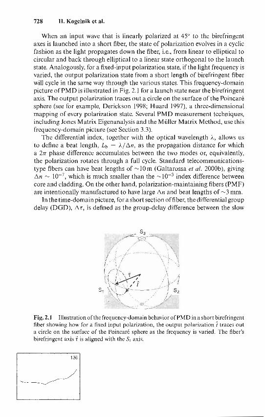
728 H. Kogelnik et al.
When an input wave that is linearly polarized at 45" to the birefringent axes is launched into a short fiber, the state of polarization evolves in a cyclic fashion as the light propagates down the fiber, i.e., from linear to elliptical to circular and back through elliptical to a linear state orthogonal to the launch state. Analogously, for a fixed-input polarization state, if the light frequency is varied, the output polarization state from a short length of birefringent fiber will cycle in the same way through the various states. This frequency-domain picture of PMD is illustrated in Fig. 2.1 for a launch state near the birefringent axis. The output polarization traces out a circle on the surface of the PoincarC sphere (see for example, Derickson 1998; Huard 1997), a three-dimensional mapping of every polarization state. Several PMD measurement techniques, including Jones Matrix Eigenanalysis and the Muller Matrix Method, use this frequency-domain picture (see Section 3.3).
The differential index, together with the optical wavelength A, allows us to define a beat length, Lb = A,/An, as the propagation distance for which a 2n phase difference accumulates between the two modes or, equivalently, the polarization rotates through a full cycle. Standard telecommunications- type fibers can have beat lengths of -10m (Galtarossa et al. 2000b), giving An - lop7, which is much smaller than the -lop3 index difference between core and cladding. On the other hand, polarization-maintaining fibers (PMF) are intentionally manufactured to have large An and beat lengths of -3 mm.
In the time-domain picture, for a short section of fiber, the differential group delay (DGD), AT, is defined as the group-delay difference between the slow
Fig. 2.1 Illustration of the frequency-domain behavior of PMD in a short birefringent fiber showing how for a fixed input polarization, the output polarization 2 traces out a circle on the surface of the PoincarC sphere as the frequency is varied. The fiber's birefringent axis ? is aligned with the SI axis.
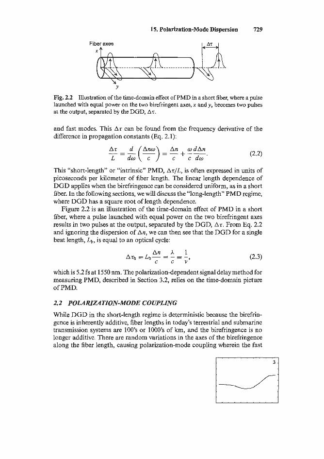
15. Polarization-Mode Dispersion 729
Fiber axes v4 n
Y
Fig. 2.2 Illustration of the time-domain effect of PMD in a short fiber, where a pulse launched with equal power on the two birefringent axes, x and y , becomes two pulses at the output, separated by the DGD, AT.
and fast modes. This AT can be found from the frequency derivative of the difference in propagation constants (Eq. 2.1):
(2.2) L dw
This “short-length” or “intrinsic” PMD, AT/L, is often expressed in units of picoseconds per kilometer of fiber length. The linear length dependence of DGD applies when the birefringence can be considered uniform, as in a short fiber. In the following sections, we will discuss the “long-length” PMD regime, where DGD has a square root of length dependence.
Figure 2.2 is an illustration of the time-domain effect of PMD in a short fiber, where a pulse launched with equal power on the two birefringent axes results in two pulses at the output, separated by the DGD, A t . From Eq. 2.2 and ignoring the dispersion of An, we can then see that the DGD for a single beat length, Lb, is equal to an optical cycle:
which is 5.2 fs at 1550 nm. The polarization-dependent signal delay method for measuring PMD, described in Section 3.2, relies on the time-domain picture of PMD.
2.2 POLARIZATION-MODE COUPLING
While DGD in the short-length regime is deterministic because the birefrin- gence is inherently additive, fiber lengths in today’s terrestrial and submarine transmission systems are 100’s or 1000’s of km, and the birefringence is no longer additive. There are random variations in the axes of the birefringence along the fiber length, causing polarization-mode coupling wherein the fast

730 H. Kogelnik et al.
and slow polarization modes from one segment each decompose into both the fast and slow modes of the next segment. Polarization-mode coupling results from localized stress during spooling/cabling/deployment, from splices and components, from variations in the fiber drawing process, and from intentional fiber “spinning” during drawing, which induces mode coupling at “meter” lengths (Judy 1994). Long fibers are often modeled as a concatenation of bire- fringent sections whose birefringence axes (and magnitudes) change randomly along the fiber, as shown in Fig. 2.3.
Due to mode coupling, the birefringence of each section may either add to or subtract from the total birefringence, and therefore the DGD does not accumulate linearly with fiber length. In fact, it has been shown that in long fiber spans, the DGD accumulates as a three-dimensional random-walk, and on average increases with the square root of distance (Poole 1988a; Poole and Nagel 1997). Although mode coupling helps to reduce the DGD of a fiber span, because the mode coupling is determined by the fiber’s environment, variations in, for example, external stresses will change the mode coupling and thus the fiber’s DGD. Therefore, a statistical approach for PMD must be adopted, as discussed in Section 4.
The categorization of a fiber in the short- or long-length regime is deter- mined by a parameter called the correlation length L,, also referred to as the coupling length (Kaminow 198 1). This parameter describes weak random coupling between two waveguides or the equivalent random coupling between the two polarization modes of a fiber with mostly uniform birefringence sub- ject to random perturbations. One considers the evolution of the polarizations as a function of length in an ensemble of fibers with statistically equivalent perturbations. While the input polarization is fixed, it is equally probable to observe any polarization state at large lengths. The evolution is characterized by the difference (p , ) - (p,,) of the ensemble averages of the power in the x and y polarizations. Assuming (p , ) = 1 and (p,,) = 0 at the input, this difference evolves from a value of 1 at the input to a value of zero at large lengths. L, is defined as that length where the power difference has decayed
Fig. 2.3 Model of a long fiber as a concatenation of birefringent sections with birefringence axes (and magnitudes) that change randomly along the fiber length.

15. Polarization-Mode Dispersion 731
to (p , ) - by) = l/e2 (for further detail see Poole and Nagel 1997). Correla- tion lengths can be less than 1 m when fiber is spooled (due to large amounts of polarization-mode coupling); conversely, L, can be -1 km when fiber is cabled. The actual fiber behavior can be affected by fiber “spinning” dur- ing draw, temperature, spool diameter and tension, cable design, installation conditions, and fiber relaxation.
The correlation length then defines the two different PMD regimes. When the fiber transmission distance L satisfies L << L,, the fiber is in the short-length regime and the mean DGD increases linearly with distance. When L >> L,, the fiber is considered to be in the long-length regime and the mean DGD, AT, increases with the square root of distance. Transmission systems are gen- erally in the long-length regime, so fiber PMD is often specified using a PMD coefficient having units of ps/(km)’/2. While fibers manufactured today can have mean PMD coefficients less than 0.1 ps/(km)’l2, “legacy” fibers installed in the 1980s may exhibit PMD coefficients higher than 0.8 ps/(km)ll2 (Peters et ~ l . 1997).
The statistical theory of PMD (Foschini and Poole 1991; Wai and Menyuk 1996) has provided an elegant expression linking the mean square DGD of the fiber to Lb and L,, valid for both regimes and also the transition region between them:
-
For L << L,, the above relation Simplifies to Jm = Arms = AtbL/Lb, whereas for L >> L,, Atms = ( A t b / L b ) m , reflecting the length depen- dence discussed earlier. In Section 3.6 we will discuss how single-ended backscattering measurement techniques can determine birefringence (Lb) and the mean square DGD. Then the correlation length (L,) can be inferred from the fundamental Eq. 2.4 relating the three quantities.
2.3 PRlNCIPAL STATES MODEL
The propagation of a pulse through a long length of fiber is very complicated due to random mode coupling and pulse splitting at every change in the local birefringence axes. But a (perhaps) surprising aspect of PMD is that even for long fibers, one can still find two special orthogonal polarization states at the fiber input that result in an output pulse that is undistorted to first order. An example is shown in Fig. 2.4, where a lO-Gb/s, 50% duty-cycle return-to-zero signal was launched with various polarizations through a 48-km fiber with large PMD. The figure shows an output pulse for each of two polarization
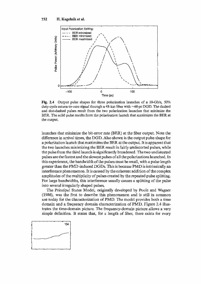
732 H. Kogelnik et al.
Input Polarization Setting: BER minimized BER minimized ,'-\ - BER maximized I
'\ /-\ 3 P E 9 s. I?
- 8
-
= a
0
-100 0 100 Time (ps)
Fig. 2.4 Output pulse shapes for three polarization launches of a 10-Gbh, 50% duty-cycle return-to-zero signal through a 48-km fiber with -60 ps DGD. The dashed and dot-dashed pulses result from the two polarization launches that minimize the BER. The solid pulse results from the polarization launch that maximizes the BER at the output.
launches that minimize the bit-error rate (BER) at the fiber output. Note the difference in arrival times, the DGD. Also shown is the output pulse shape for a polarization launch that maximizes the BER at the output. It is apparent that the two launches minimizing the BER result in fairly undistorted pulses, while the pulse from the third launch is signzcantly broadened. The two undistorted pulses are the fastest and the slowest pulses of all the polarizations launched. In this experiment, the bandwidth of the pulses must be small, with a pulse length greater than the PMD-induced DGDs. This is because PMD is intrinsically an interference phenomenon. It is caused by the coherent addition of the complex amplitudes of the multiplicity of pulses created by the repeated pulse splitting. For large bandwidths, this interference usually causes a splitting of the pulse into several irregularly shaped pulses.
The Principal States Model, originally developed by Poole and Wagner (1986), was the first to describe this phenomenon and is still in common use today for the characterization of PMD. The model provides both a time domain and a frequency domain characterization of PMD. Figure 2.4 illus- trates the time-domain picture. The frequency-domain picture allows a very simple definition. It states that, for a length of fiber, there exists for every

15. Polarization-Mode Dispersion 733
frequency a special pair of polarization states, called the Principal States of Polarization (PSPs). A PSP is defined as that input polarization for which the output state of polarization is independent of frequency to first order, i.e., over a small frequency range.
In the absence of polarization-dependent loss, the PSPs are orthogonal. For each pair of input PSPs, there is a corresponding pair of orthogonal PSPs at the fiber output. The input and output PSPs are related by the fiber's trans- mission matrix, just as any input polarization is related to a polarization at the fiber output. Using the common Stokes vector description of polarization (for more detail see Appendix A), any output polarization, 3, is related to its input polarization, 5, by the 3 x 3 Muller rotation matrix, R, via ? = %. The unit Stokes vectors,j, of the input PSP a n d j of the output PSP, are similarly related, i.e.,j = Rj,.
2.4 PMD VECTOR
Using the Principal States Model, PMD can be characterized by the PMD vector:
? = AT$, (2.5)
a vector in three-dimensional Stokes space, where the magnitude, AT, is the DGD. The unit vector, j, points in the direction of the slower PSP, whereas the vector -j indicates the orthogonal faster PSP. The latter is 180" from? in Stokes space. Note that the definition used here is in right-circular Stokes space (Yith S3 denoting right-circular polarization), whereas the original PMD vector $2 of Poole et al. (1988b) was defined in left-circular Stokes space. See Appendix B for further explanation of the relation between the two.
The PMD vector at the fiber input ?, is related to the output PMD vector ? by 3 = R?,. One can then show that the frequency derivative of? = % leads directly to the law of infinitesimal rotation:
d? dw
t - - = t x t ,
where ? x = R,RT and RT is the transpose ofR. Here, the PMD vector describes how, for a fixed input polarization, the output polarization ? will precess around ? as the frequency is changed. The direction of? relative to ? deter- mines the angle of precession, whereas the magnitude, AT, determines the rate at which ? precesses around ?. For example, if 3 is launched with equal power along the PSPs, ? x will have its largest value, and the largest change in the output polarization will occur for a frequency change Aw. The precession has

734 H. Kogelnik et al.
magnitude 4 = A t A o , where 4 is the rotation angle on the PoincarC sphere. If 2 is aligned with &?, then there is no precession and no change of the output polarization with frequency. This is, of course, the postulate for a PSP. The rotation law, Eq. 2.6, thus provides a precise mathematical definition of the PSP and of its length, At , the DGD. The law also says that there are only two PSPs corresponding to the two possible alignments, 1 aligned with &?.
A length of polarization-maintaining fiber (PMF) has a constant PMD vector whose length, the DGD, and directionj do not change with frequency. For this simple case, the output vector 2 will trace out a circle on the Poincare sphere as the frequency is varied. This is illustrated in Fig 2.1. In real fibers, however, both the magnitude and the direction of 2 change with frequency, as shown in Fig. 2.5. The rotation law still applies locally in this case, describing l (w) as a circular arc for a small range of frequencies. In this range, charac- terized by first-order PMD, the behavior of the real fiber resembles that of the PMF. The DGD at an instant in time for such a range is often called the “instantaneous DGD” to distinguish it from a mean DGD obtained by aver- aging over time or frequency. The longer-range motion of ?(w) around ?(w) is more complicated, reflecting higher-order PMD. This is illustrated in Fig. 2.6.
Now return to the time-domain picture of Fig. 2.4. Whereas the frequency domain provides a continuous wave, single-frequency view of PMD, the time
0 1540 1545 1550 1555 1560
Wavelength (nm) - - 0.1 nm
Fig. 2.5 Measurement of the PMD vector 7 for a 14.7-ps mean DGD fiber. (a) Mag- nitude of T’ (the DGD, AT) plotted as a function of wavelength. (b) Direction of T’ (the slow PSP, j) plotted on the PoincarC sphere as a function of wavelength. The markers indicate 0.1-nm intervals.
133
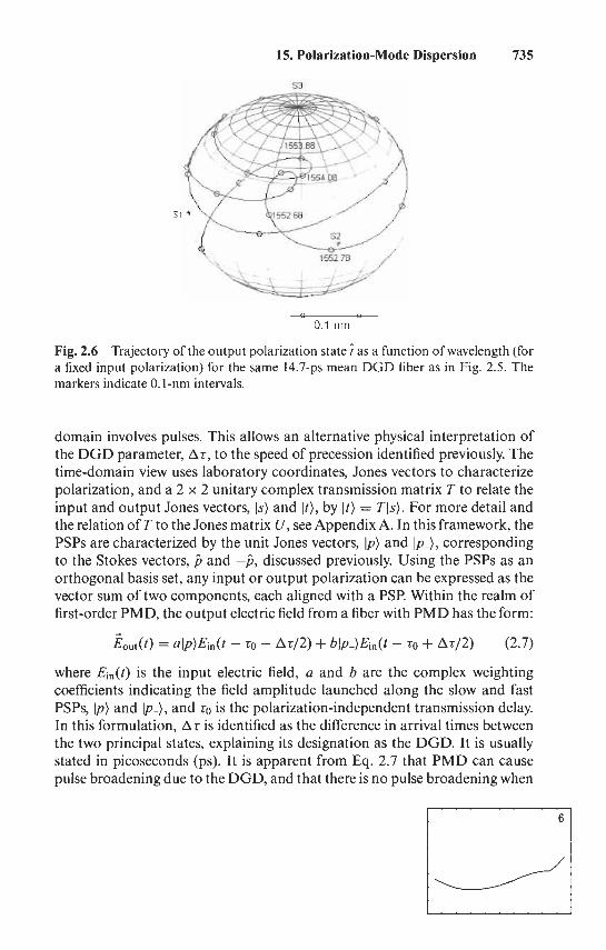
15. Polarization-Mode Dispersion 735
0.1 nm
Fig. 2.6 Trajectory of the output polarization state ? as a function of wavelength (for a fixed input polarization) for the same 14.7-ps mean DGD fiber as in Fig. 2.5. The markers indicate 0.1-nm intervals.
domain involves pulses. This allows an alternative physical interpretation of the DGD parameter, A t , to the speed of precession identified previously. The time-domain view uses laboratory coordinates, Jones vectors to characterize polarization, and a 2 x 2 unitary complex transmission matrix T to relate the input and output Jones vectors, Is) and It), by It) = TIS). For more detail and the relation of T to the Jones matrix U , see Appendix A. In this framework, the PSPs are characterized by the unit Jones vectors, lp) and lp-), corresponding to the Stokes vectors, j-j and -j, discussed previously. Using the PSPs as an orthogonal basis set, any input or output polarization can be expressed as the vector sum of two components, each aligned with a PSP. Within the realm of first-order PMD, the output electric field from a fiber with PMD has the form:
Eout(t) = alp)Ei,(t - to - At/2) + blp-)Ein(t - to + At/2) (2.7)
where Ein(t) is the input electric field, a and b are the complex weighting coefficients indicating the field amplitude launched along the slow and fast PSPs, lp) and Ip-), and to is the polarization-independent transmission delay. In this formulation, A t is identified as the difference in arrival times between the two principal states, explaining its designation as the DGD. It is usually stated in picoseconds (ps). It is apparent from Eq. 2.7 that PMD can cause pulse broadening due to the DGD, and that there is no pulse broadening when
I . . . . . . . . . I
736 H. Kogelnik et aL
the input is aligned with a PSP, Le., when a or b is zero. Note that the simple PMD Stokes vector, ?, does not have a vector analog in the laboratory frame where Eq. 2.7 separates the DGD from the PSP polarizations.
Section 3 gives themathematical background for a precise definition of PSPs and DGD in the time domain. It is based on the polarization-dependent signal delay, defined by the first moments of the transmitted pulses. This time-domain definition identifies the PSPs as those input polarizations that maximize or minimize the signal delay. This definition turns out to be equivalent to the earlier frequency-domain definition.
The traditional Jones Matrix Eigenanalysis (JME) approach (discussed in Section 3) provides yet another equivalent definition bridging the time and frequency domain. Haus (1999) observes that the Hermitian appearing in the JME is connected to the energy of the light stored in the fiber. The light in the slow PSP spends more time in the fiber and maximizes the stored energy, whereas transmission along the fast PSP minimizes the stored energy.
The evolution of the PMD vector with fiber length is described by the dynamical equation for PMD (Poole et al. 199 1 b),
--- d? dz do
relating the PMDvector to the microscopic birefringence. Herez is the position along the fiber. #3 is the three-dimensional, local birefringence vector of the fiber (Eickhoff et al. 1981) pointing in the direction of the birefringence axis with a magnitude A#3 proportional to An (see Gordon and Kogelnik 2000). This equation is the basis for the statistical theory of PMD (Foschini and Poole 1991).
2.5 SECOND-ORDER PMD
Because the fiber PMD vector varies with optical angular frequency, a, a Taylor-series expansion of ?(w) with Am about the carrier frequency 00 is typically used for larger signal bandwidths (Foschini and Poole 1991; Gleeson et al. 1997; Biilow 1998b),
So-called second-order PMD is then described by the derivative,
(2.10)
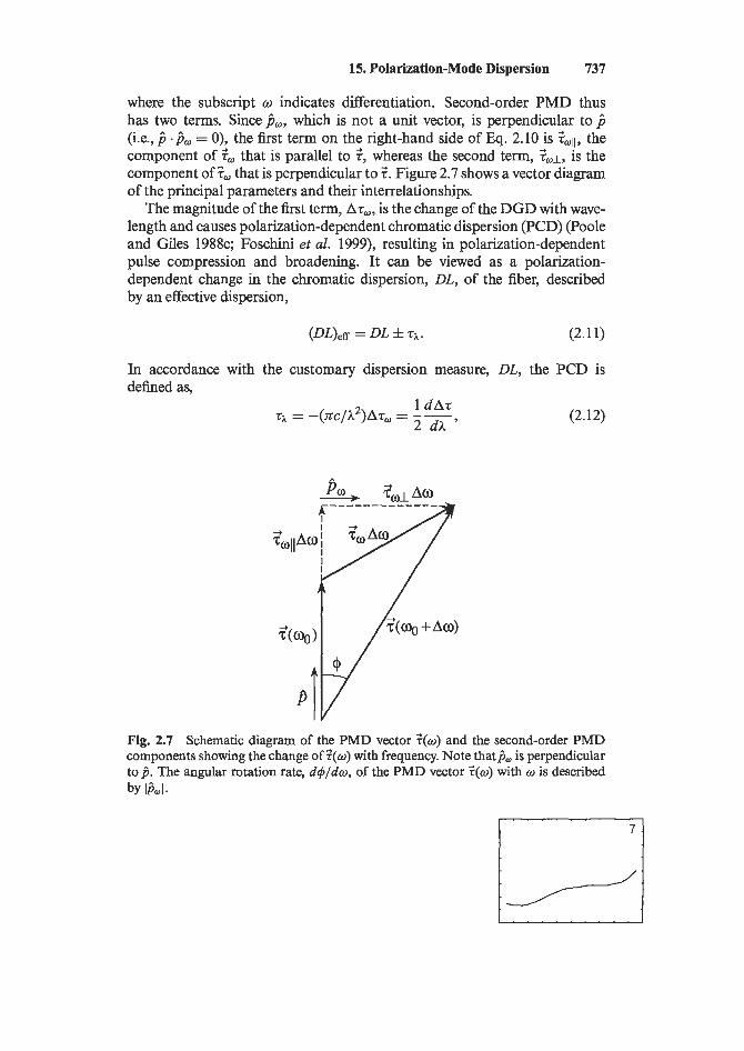
15. Polarization-Mode Dispersion 737
where the subscript w indicates differentiation. Second-order PMD thus has two terms. Since j,, which is not a unit vector, is perpendicular to j @e., j .j, = 0), the first term on the right-hand side of Eq. 2.10 is 5,11, the component of 2, that is parallel to 5, whereas the second term, ?,l, is the component of 2, that is perpendicular to 5. Figure 2.7 shows a vector diagram of the principal parameters and their interrelationships.
The magnitude of the first term, At,, i s the change of the DGD with wave- length and causes polarization-dependent chromatic dispersion (PCD) (Poole and Giles 1988c; Foschini et al. 1999), resulting in polarization-dependent pulse compression and broadening. It can be viewed as a polarization- dependent change in the chromatic dispersion, DL, of the fiber, described by an effective dispersion,
In accordance with the customary dispersion measure, DL, the PCD is defmed as,
1 d A t ti = - (nc/h2)At - -- " - 2 d c
(2.12)
Fig. 2.7 Schematic diagram of the PMD vector ?(a) and the second-order PMD components showing the change of ?(w) with frequency. Note thatj- is perpendicular to 5. The angular rotation rate, d4/dw, of the PMD vector ?(w) with w is described bY @ w l -

738 H. Kogelnik et al.
50
where c is the velocity of light, h is the wavelength, and ti is usually expressed in ps/nm. The PCD is proportional to the wavelength derivative of the DGD spectrum. The plus and minus signs in Eq. 2.11 correspond to alignment with the two PSPs. Note that the magnitudes of ?,I, and At, are equal and At, = z,ll has a sign that is negative when ?,,I points in the direction opposite t o j . Figure 2.8 shows the PCD of the fiber from Fig. 2.5. The DGD data were numerically differentiated to obtain the PCD. It is apparent that PCD causes the effective dispersion to fluctuate rapidly with wavelength.
The second term, AT&,, describes PSP depolarization, a rotation of the PSPs with frequency. As shown in Fig. 2.7, the angular rate of rotation, dcp/dw = & I, of the PMD vector ?(w) is measured by the magnitude E, I, which we express in ps. Note that d@/dv [mradGHz] = 2nE,l[ps], where v is the optical carrier frequency and w = 27cv. We have already seen in Fig. 2.5 the rapid motion of j for the 14.7-ps mean DGD fiber. Figure 2.9 is a plot of Eml for this same fiber and wavelength range. As discussed in Section 6, pulse distortions caused by depolarization include overshoots and generation of satellite pulses. PSP depolarization can also have a detrimental effect on ht-order PMD compensators.
- PCD = -( nc / l i? )A~~ [pdnm]
-50 1540 1545 1550 1555 1560
Wavelength (nrn)
Fig. 2.8 Plot of the polarization-dependent chromatic dispersion (PCD) for the 14.7-ps mean DGD fiber from Fig. 2.5. To obtain the PCD, the DGD data in Fig. 2.5 were numerically differentiated.
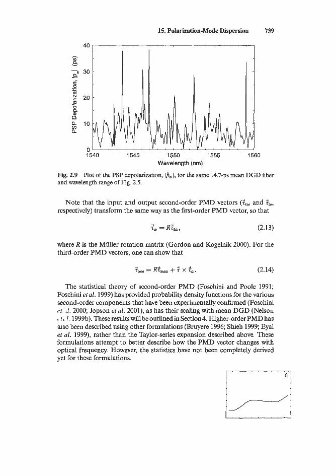
15. Polarization-Mode Dispersion 739
0 1540 1545 1550 1555 1560
Wavelength (nm)
Fig. 2.9 Plot of the PSP depolarization, &,,I, for the same 14.7-ps mean DGD fiber and wavelength range of Fig. 2.5.
Note that the input and output second-order PMD vectors and zu, respectively) transform the same way as the first-order PMD vector, so that
?* = R& (2.13)
where R is the Muller rotation matrix (Gordon and Kogelnik 2000). For the third-order PMD vectors, one can show that
?mm = R?- + + + t x tu. (2.14)
The statistical theory of second-order PMD (Foschini and Poole 1991; Foschini et al. 1999) has provided probability density functions for the various second-order components that have been experimentally confirmed (Foschini ct il. 2000; Jopson et al. 2001), as has their scaling with mean DGD (Nelson
t, 1.1999b). These results will be outlined in Section 4. Higher-order PMD has ais0 been described using other formulations (Bruyere 1996; Shieh 1999; Eyal et al. 1999), rather than the Taylor-series expansion described above. These formulations attempt to better describe how the PMD vector changes with optical frequency. However, the statistics have not been completely derived yet for these formulations.

740 H. Kogelnik et al.
2.6 THE BAND WIDTH OF THE PRINCIPAL STATES
The bandwidth of the principal state is an important concept providing guidance on the change of the PMD vector ?(o) of the fiber with frequency (or wavelength). It is the bandwidth, Awpsp = kAupsp, or the corresponding wavelength range, AApsp, over which the PMD vector is reasonably constant. Examples of the utility of this concept include the frequency-domain mea- surement of PMD vectors (covered in Section 3) and the measurement of PMD statistics. Consider, for example, the determination of the PMD vector at the different wavelengths, A I , h2, and A3, as sketched in Fig. 2.10. As will be explained in Section 3, for each of these determinations, measurements of polarization rotations at two or more frequencies are required. These frequen- cies have to be confined to the range AApsp as indicated in order to reduce inaccuracy caused by higher-order PMD. In statistical PMD measurements, on the other hand, measured samples of ?(A) are deemed to be statistically independent if their wavelengths are at least 6Ahpsp apart. This is indicated in Fig. 2.10, where ?(LO) and ?(h6) are considered statistically independent. Thus, measurements over a spectral range from Amin to A,, will yield a number of statistically independent samples, Nsamples, given by
While varying constants are reported in the literature (Betti et al. 1991; Bruyere 1996), studies of the accuracy of measurements of PMD provide a
I I
Fig. 2.10 Diagram showing the important wavelength (or frequency) intervals for measurements of the PMD. For PMD vector measurements, the wavelength inter- val should be smaller than Akpsp to avoid inaccuracy from higher-order PMD. For PMD statistics, in order to consider the measured samples statistically independent, the wavelength interval should be at least 6Ak.p~.
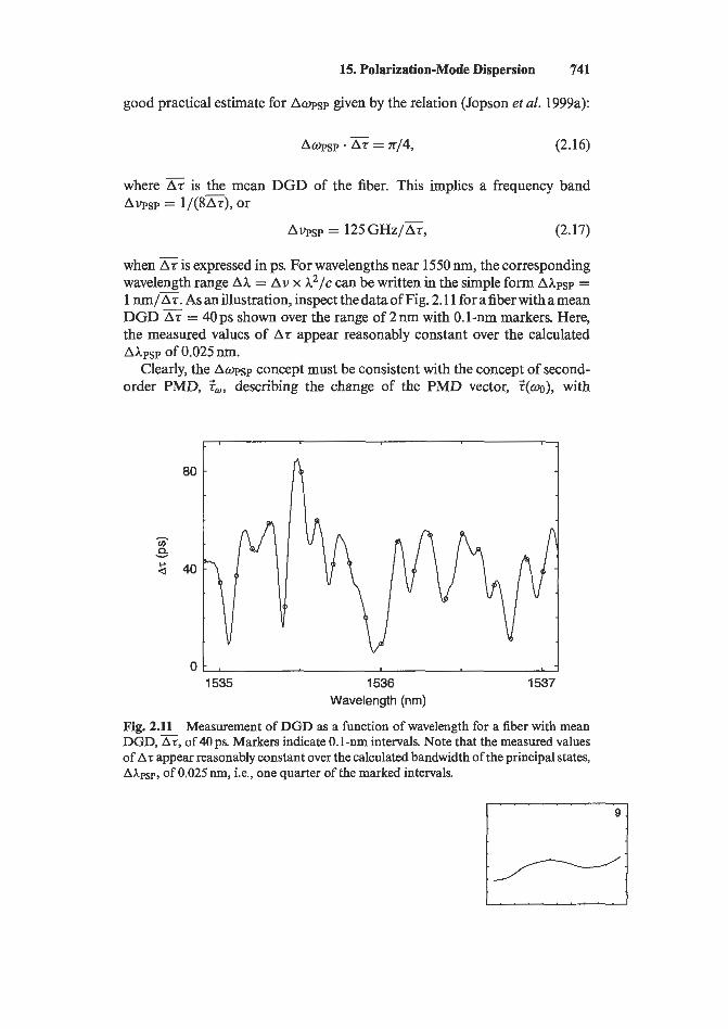
15. Polarization-Mode Dispersion 741
good practical estimate for Aopsp given by the relation (Jopson et al. 1999a):
where S is the mean DGD of the fiber. This implies a frequency band Aupsp = 1/(8=), or
Avpsp = 125GHz/S, (2.17)
when is expressed in ps. For wavelengths near 1550 nm, the corresponding wavelength range Ah = Au x A2/c can be written in the simple form AApsp = 1 n m / z . As an illustration, inspect the data of Fig. 2.1 1 for a fiber with a mean DGD = 40ps shown over the range of 2nm with 0.1-nm markers. Here, the measured values of AT appear reasonably constant over the calculated
Clearly, the Awpsp concept must be consistent with the concept of second- describing the change of the PMD vector, ?(@), with
AApsp of 0.025 nm.
order PMD,
1535 1536 1537 Wavelength (nrn)
Fig. 2.11 Measurement of DGD as a function of wavelength for a fiber with mean DGD, %, of 40 ps Markers indicate 0.1-nm intervals. Note that the measured values of AT appear reasonably constant over the calculated bandwidth of the principal states, AA-psp, of O.O25nm, i.e., one quarter of the marked intervals.
742 H. Kogelnik et al.
frequency. At ~0 f Awpsp the PMD vector is
(2.18) 1 2
?(wg f AupspI2) = ?(mo) f -AOPSP . Zm.
Using the above expression for Aupsp and the known relation (Foschini and Poole 1991) I?m:wlrms = . (nE2/8), one finds that the root-mean-square (rms) magnitude ofthe change (?(q+Aopsp/2)-?(wo)) equals 0.267dz. This relatively large value may seem to imply that the Awpsp values are somewhat too large. However, on average, the vector 2w is perpendicular to ? (Foschini et al. 1999) as discussed in Section 4. In this case, there is only a small (3%) change in the magnitude of? accompanied by a rotation of the PSP by about 15" in Stokes space (Le., 7.5" in the laboratory for linear polarization).
The correlation function of the PMD vectors ?(mg) and ?(* + Am) recently reported by Karlsson and Brentel (1999) and Shtaif et al. (2000b) (and discussed further in Section 4) provides an elegant confirmation and inter- pretation of the Awpsp concept and its practical implications. Figure 2.12 shows a (normalized) plot of this correlation as a function of the frequency separation, Av = Aw/2n, for a mean DGD of = 1.25 ps. For this value, the bandwidth of the PSP is Avpsp = 1OOGHz. At this frequency spacing the correlation is seen to drop from 1 to 0.89, supporting the idea that ? is essentially constant over the 100-GHz width. At 6Aupsp = 600 GHz, the cor- relation drops to 0.1 1 , indicating that PMD vectors at that frequency spacing are essentially uncorrelated.
2.7 CONCATENATION OF PMD VECTORS The total PMD vector of a series of two or more elements with known PMD vectors can be determined using the simple, but powerful concatenation rules (Curti et al. 1990; Poole et al. 1991b; Foshini and Poole 1991; Gisin and Pellaux 1992; Mollenauer and Gordon 1994; Gordon and Kogelnik 2000). The concatenation rules have been used in the analysis of how the PMD vector grows with fiber length (Curti et al. 1990) and for statistical PMD modeling (Foschini and Poole 1991). They are also useful for PMD simulation and in the design of multisection PMD compensators. Although the concatenation rules have appeared in sum, differential, and integral formulations for both first- and second-order PMD vectors, this section will concentrate on the sum rules See Gordon and Kogelnik (2000) for the other formulations.
The concatenation rule for first-order PMD is similar to that for transmission-line impedances: To obtain the PMD vector of an assembly, transform the PMD vectors of each individual section to a common reference
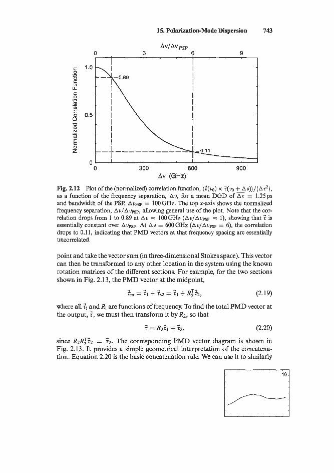
15. Polarization-Mode Dispersion 743
AVlAVPSP 0 3 9
I
0 ; 0 300 600 900
Av (GHz)
Fig. 2.12 Plot of the (normalized) correlation function, (?(uo) x ?(UO + Av))/(At2), as a function of the frequency separation, Au, for a mean DGD of = 1.25 ps and bandwidth of the PSP, Aupsp = 100 GHz. The top x-axis shows the normalized frequency separation, Au/Al)p~p, allowing general use of the plot. Note that the cor- relation drops from 1 to 0.89 at Au = 100GHz (Au/Aupsp = l), showing that ? is essentially constant over Aupsp. At Au = 600GHz (Au/Aup~p = 6), the correlation drops to 0.11, indicating that P M D vectors at that frequency spacing are essentially uncorrelated.
point and take the vector sum (in three-dimensional Stokes space). This vector can then be transformed to any other location in the system using the known rotation matrices of the different sections. For example, for the two sections shown in Fig. 2.13, the PMD vector at the midpoint,
(2.19)
where all ?i and Ri are functions of frequency. To iind the total PMD vector at the output, 2, we must then transform it by R2, so that
- + + tm = tl + 2 s2 = +R:&,
? = Rztl + 22, (2.20)
since R2RT?2 = 22. The corresponding PMD vector diagram is shown in Fig. 2.13. It provides a simple geometrical interpretation of the concatena- tion. Equation 2.20 is the basic concatenation rule. We can use it to similarly
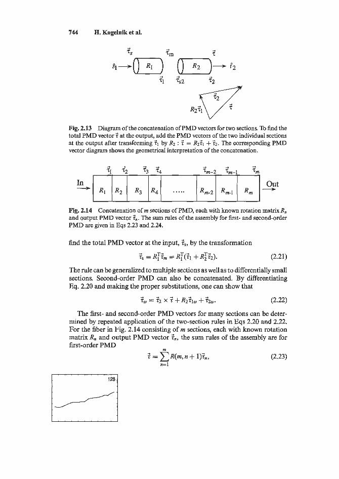
744 H. Kogelnik et al.
Fig. 2.13 Diagram of the concatenation of PMD vectors for two sections. To find the total PMD vector ? at the output, add the PMD vectors of the two individual sections at the output after transforming ?I by R2 : ? = Rz?~ + 6 . The corresponding PMD vector diagram shows the geometrical interpretation of the concatenation.
Fig. 2.14 Concatenation of m sections of PMD, each with known rotation matrix R,, and output PMD vector ?,,. The sum rules of the assembly for first- and second-order PMD are given in Eqs 2.23 and 2.24.
find the total PMD vector at the input, ?,, by the transformation
zs = RT?,,, = RT(?i + Rz?2). (2.21)
The rule can be generalized to multiple sections as well as to differentially small sections. Second-order PMD can also be concatenated. By differentiating Eq. 2.20 and making the proper substitutions, one can show that
?,,,, = ?2 x i + R& + ?h. (2.22)
The first- and second-order PMD vectors for many sections can be deter- mined by repeated application of the two-section rules in Eqs 2.20 and 2.22. For the fiber in Fig. 2.14 consisting of m sections, each with known rotation matrix R, and output PMD vector in, the sum rules of the assembly are for first-order PMD ,.. ...
? = R(m, n + l)?,, n= 1
(2.23)
15. Polarization-Mode Dispersion 745
and for second-order PMD
(2.24)
where we define the rotation matrix of the last m - n + 1 sections as R(m, n) = R,,,R,-l. . R,, where R(m, m) = R, and R(m, m + 1) is the identity matrix. The differential concatenation rule for PMD shows how ?(z) changes due to the differential addition of length Az (Gordon and Kogelnik 2000) and is equivalent to Eq. 2.8, the dynamical PMD equation.
3. Measurement Techniques
A considerable number of techniques for the measurement of PMD have been proposed. Several have been extensively tested and standardized. Some of these measure the (scalar) instantaneous DGD, others determine the mean DGD, and a few allow measurement of the instantaneous PMD vectors as a function of frequency. Some methods operate in the time domain by sensing pulse delays, whereas others employ frequency-domain concepts detecting changes of polarization with frequency. Measurement capabilities of various instruments range from around 1 fs to about 100 ps of DGD. The smaller ranges are needed for the measurement of the (instantaneous) DGD of optical components or short pieces of fiber, whereas the larger ranges are used to characterize long communication spans.
Our discussion will cover five techniques: interferometric techniques allow- ing rapid determination of the DGD, optical time-domain reflectometry (OTDR) methods convenient for in-field measurements where only one end of an installed fiber line is accessed, and three methods permitting the char- acterization of PMD vectors, the polarization-dependent signal delay (PSD) method, and the closely related Jones Matrix Eigenanalysis (JME) and Miiller Matrix Methods (MMM). For broader reviews the reader is referred to Poole and Nagel (1997) and Hernday in Derickson (1998). These reviews also cover the PoincarC sphere method (Andresciani et al. 1987; Bergano et al. 1987), the fixed analyzer method (Poole 1989; Poole and Favin 1994) and the modulation phase-shift method used for the measurement of dispersion and scalar DGD (Costa et al. 1982; Williams et al. 1998; Williams 1999b).
I . . . . . . . .

746 H. Kogelnik et al.
3.1 INTERFEROMETRIC TECHNIQUES
A variety of interferometric techniques for PMD measurement (Mochizuki et al. 1981; Thevenaz et al. 1989; Gisin et al. 1991b; Namihira et al. 1993a,b) have been developed into compact field instruments that can make a DGD measurement in as little as 30s. With modifications, these instruments can measure the instantaneous DGD of optical components or short fibers to an accuracy better than 1 fs (Oberson et al. 1997; Simova et al. 2000).
A schematic of a typical interferometric system is shown in Fig. 3.1. The method usually employs a Michelson interferometer, as shown in the figure, or a Mach-Zehnder interferometer. Often the interferometer is implemented using a fiber-directional coupler constructed with PM fiber. The interferome- ter has a ked-mirror arm and an arm with a scanning mirror. The maximum scanning range of the latter determines the maximum DGD that can be mea- sured. In some variations on this method additional components are inserted. Examples are the use of bias birefringent plates following the fiber under test or the insertion of a quarter-wave plate in the fixed-mirror arm.
Fixed mirror
Fiber Polarization under test
LED Control
A2
Polarizer 8 4 Scanning mirror
Detector
Fig. 3.1 Typical interferometric measurement system. The example of a Michelson interferometer is shown using a fixed and a scanning mirror arm. The system uses a broadband light-emitting diode (LED), polarization control, and a polarizer analyzer. The scan range is Az.

15. Polarization-Mode Dispersion 747
The conventional implementation for low-coherence interferometry employs an unpolarized broadband source of light, such as an LED, pro- viding a spectral width of about 100 nm. The coherence length of this source determines the smallest PMD that can be measured for optical components. For long fibers, the method provides the mean DGD averaged over the spectral width of the source.
The light from the source is sent through the fiber and split into two parts in the interferometer. The two parts are delayed relative to each other by a time delay, AT, proportional to the scan distance, Az, from interferometer balance,
where c is the speed of light. The delayed parts are recombined for interference at the detector. Scanning of the mirror distance creates a fringe pattern at the detector from which DGD information is extracted. As an example, consider first the fringe pattern generated by a narrowband pulse with polarizations properly adjusted. The fiber under test splits the pulse into two parts, delayed by the DGD, At. When the interferometer is balanced, there is a central inter- ference peak. As the mirror is scanned away from balance, the fringe pattern shows two side peaks when AT = &At, providing DGD information. For broadband light there are complex fringe patterns and correlation peaks that have been modeled and analyzed. A typical fringe pattern is shown in Fig. 3.2. The mean DGD is extracted from this fringe pattern by such methods as deter- mining the second moment, a,, of the fringe distribution (Gisin 1994a; Perny et al. 1996) or the Gaussian fit shown. The mean square DGD is approximately equal to this moment, i.e., (At’) % a,.
The polarization controller and polarizer shown in Fig. 3.1 are, in some designs, used to ensure that the desired interference takes place, as orthogonal polarizations at the detector will not interfere.
AT = ~ A z / c , (3.1)
3.2 THE POLARIZATION-DEPENDENT SIGNAL DELAY METHOD
The polarization-dependent signal delay (PSD) method (Jopson et al. 1999b; Nelson et al. 2000a,c) is a time-domain technique for the measurement of PMD vectors. The method uses conventional phase-detection instruments, such as network analyzers, that have been perfected to measure the phase delay of periodic signals with great accuracy. These instruments, also used in the modulation phase-shift method mentioned at the beginning of this section, can, for example, determine the delay of a sinusoidal 100-MHz signal to an accuracy of 1 ps. The PSD method exploits the polarization dependence of the propagation delay of light passing through a fiber possessing PMD.
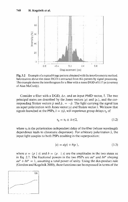
748 H. Kogelnik et al.
-0.8 -0.4 0.0 0.4 0.8
Displacement (ps)
Fig. 3.2 Example of a typical fringe pattern obtained with the interferometricmethod. Information about the mean DGD is extracted from this pattern by signal processing. The example shows the interferogram for a fiber with a mean DGD of 0.17 ps (courtesy of Alan McCurdy).
Consider a fiber with a DGD, AT, and an input PMD vector, ?. The two principal states are described by the Jones vectors lp) and lp-), and the cor- responding Stokes vectors j and $- = -$. The light carrying the signal has an input polarization with Jones vector Is) and Stokes vector 3. We know that signals launched at the PSPs, i = ztj, will experience group delays tg of
where TO is the polarization-independent delay of the fiber (whose wavelength dependence leads to chromatic dispersion). For arbitrary polarization 3, the input light couples to both PSPs resulting in the superposition:
where a = ( p I s) and b = ( p - I s) are the amplitudes in the two states as in Eq. 2.7. The fractional powers in the two PSPs are aa* and bb* obeying aa* + bb* = 1, assuming a total power of unity. Using the dot-product rule (Gordon and Kogelnik 2000), these functions can be expressed in terms of the
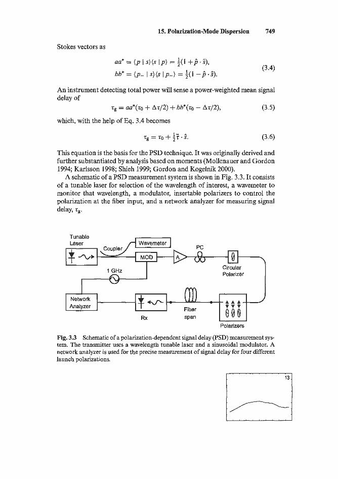
15. Polarization-Mode Dispersion 749
Stokes vectors as
uu* = ( p I s)(s Ip) = ;(l +j m i ) ,
bb* = ( p - I s)(s Ip-) = ;(l -j .i). (3.4)
An instrument detecting total power will sense a power-weighted mean signal delay of
tg = uu*(ro + At/2) + bb*(to - At/2), (3.5)
which, with the help of Eq. 3.4 becomes
This equation is the basis for the PSD technique. It was originally derived and further substantiated by analysis based on moments (Mollenauer and Gordon 1994; Karlsson 1998; Shieh 1999; Gordon and Kogelnik 2000).
A schematic of a PSD measurement system is shown in Fig. 3.3. It consists of a tunable laser for selection of the wavelength of interest, a wavemeter to monitor that wavelength, a modulator, insertable polarizers to control the polarization at the fiber input, and a network analyzer for measuring signal delay, rg.
I - I GHz
Tunable Laser Wavemeter
PC
MOD \ Circular Polarizer
I 1
8 0 8 Fiber span
Network Analyzer
Rx Polarizers
Fig. 3.3 Schematic of a polarization-dependent signal delay (PSD) measurement sys- tem. The transmitter uses a wavelength tunable laser and a sinusoidal modulator. A network analyzer is used for the precise measurement of signal delay for four different launch polarizations.
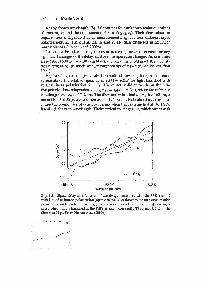
750 H. Kogelnik et al.
At any chosen wavelength, Eq. 3.6 contains four unknown scalar quantities of interest, to and the components of 2 = (tl, t2, q). Their determination requires four independent delay measurements, tgi, for four different input polarizations, i i . The quantities, to and ?, are then extracted using linear matrix algebra (Nelson et al. 2000~).
Care must be taken during the measurement process to correct for any significant changes of the delay, to, due to temperature changes. As to is quite large (about 500 ~.l.s for a 100-km fiber), such changes could mask the accurate measurement of the much smaller components o f ? (which can be less than
Figure 3.4 depicts in open circles the results of wavelength-dependent mea- surements of the relative signal delay t&) - to (h0) for light launched with vertical linear polarization, = i l . The central solid curve shows the rela- tive polarization-independent delay, TOR = to(h) - to(ho), where the reference wavelength was ho = 1542 nm. The fiber under test had a length of 62 km, a mean DGD of 35 ps, and a dispersion of 124pshm. Note also the curves indi- cating the boundaries of delay, occurring when light is launched at the PSPs, j and -j, for each wavelength. Their vertical spacing is At, which varies with
lops).
100 r I
50
-50
-1 00
1541.5 1542.0 1542.5 Wavelength (nm)
Fig. 3.4 Signal delay as a function of wavelength measured with the PSD method with 31 used as launch polarization (open circles). Also shown is the measured relative polarization-independent delay, toR, and the maxima and minima of the delays, mea- sured when light is launched at the PSPs at each wavelength. The mean DGD of the fiber was 35 ps. From Nelson et ~ l . (2000~).
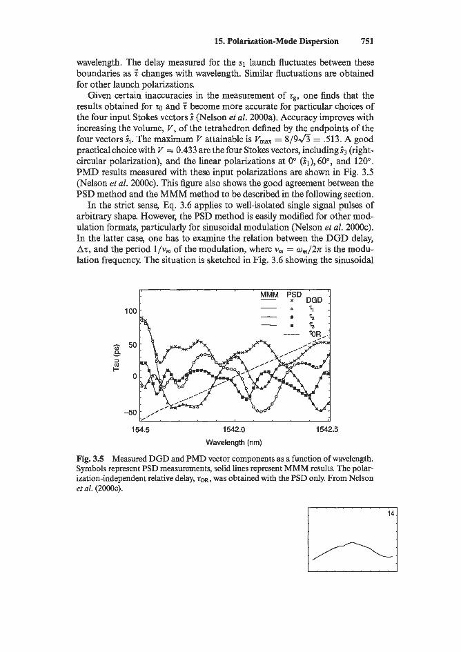
15. Polarization-Mode Dispersion 751
wavelength. The delay measured for the SI launch fluctuates between these boundaries as ? changes with wavelength. Similar fluctuations are obtained for other launch polarizations.
Given certain inaccuracies in the measurement of tg, one finds that the results obtained for TO and 2 become more accurate for particular choices of the four input Stokes vectors ? (Nelson et al. 2000a). Accuracy improves with increasing the volume, V , of the tetrahedron defined by the endpoints of the four vectors &. The maximum V attainable is V,, = 8/9& = .513. A good practical choice with V = 0.433 are the four Stokes vectors, including ?3 (right- circular polarization), and the linear polarizations at 0" (&), 60°, and 120". PMD results measured with these input polarizations are shown in Fig. 3.5 (Nelson et al. 2000~). This figure also shows the good agreement between the PSD method and the MMM method to be described in the following section.
In the strict sense, Eq. 3.6 applies to well-isolated single signal pulses of arbitrary shape. However, the PSD method is easily modified for other mod- ulation formats, particularly for sinusoidal modulation (Nelson et al. 2000~). In the latter case, one has to examine the relation between the DGD delay, AT, and the period l/vm of the modulation, where v, = wm/2n is the modu- lation frequency. The situation is sketched in Fig. 3.6 showing the sinusoidal
154.5 1542.0 1542.5
Wavelength (nm)
Fig. 3.5 Measured DGD and PMD vector components as a function of wavelength. Symbols represent PSD measurements, solid lines represent MMM results. The polar- ization-independent relative delay, tOR, was obtained with the PSD only. From Nelson et al. (2000~).
I " 14 1
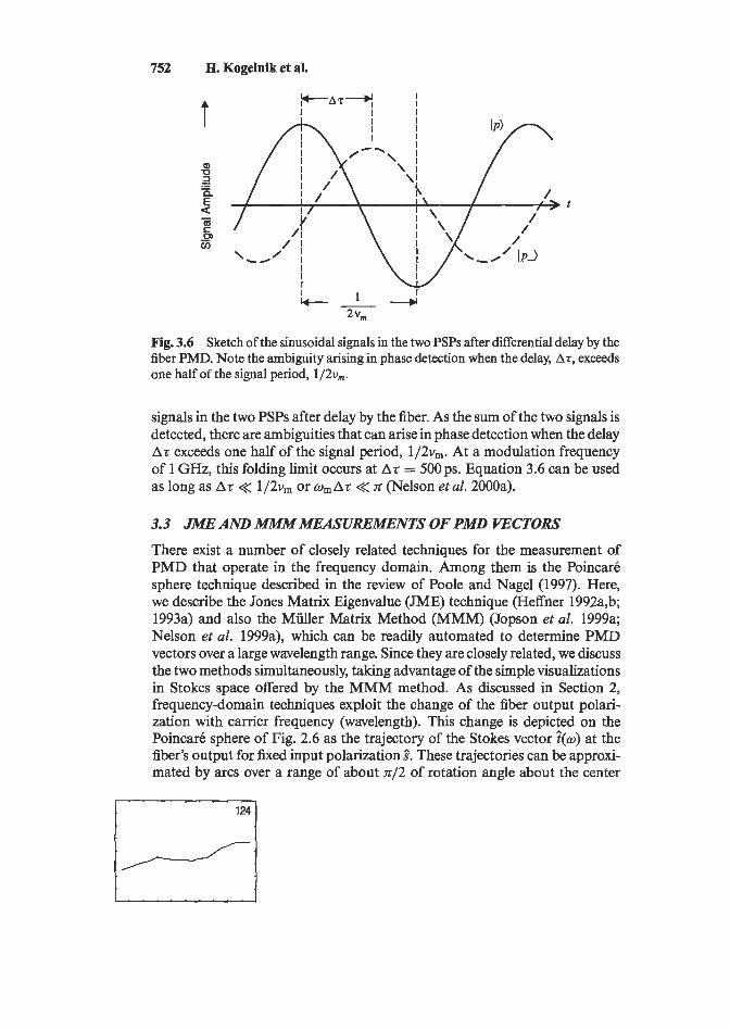
752 H. Kogelnik et al.
t
Fig. 3.6 Sketch of the sinusoidal signals in the two PSPs after differential delay by the fiber PMD. Note the ambiguity arising in phase detection when the delay, Ar, exceeds one half of the signal period, 1/2vm.
signals in the two PSPs after delay by the fiber. As the sum of the two signals is detected, there are ambiguities that can arise in phase detection when the delay At exceeds one half of the signal period, 1/2vm. At a modulation frequency of 1 GHz, this folding limit occurs at At = 500ps. Equation 3.6 can be used as long as At << 1/2vm or @,At << n (Nelson et al. 2000a).
3.3 JME AND MMMMEASUXEMENTS OF PMD VECTORS
There exist a number of closely related techniques for the measurement of PMD that operate in the frequency domain. Among them is the Poincar6 sphere technique described in the review of Poole and Nagel (1997). Here, we describe the Jones Matrix Eigenvalue (JME) technique (Heffner 1992a,b; 1993a) and also the Miiller Matrix Method (MMM) (Jopson et al. 1999a; Nelson et al. 1999a), which can be readily automated to determine PMD vectors over a large wavelength range. Since they are closely related, we discuss the two methods simultaneously, taking advantage of the simple visualizations in Stokes space offered by the MMM method. As discussed in Section 2, frequency-domain techniques exploit the change of the fiber output polari- zation with carrier frequency (wavelength). This change is depicted on the Poincark sphere of Fig. 2.6 as the trajectory of the Stokes vector i(o) at the fiber's output for k e d input polarization i. These trajectories can be approxi- mated by arcs over a range of about n/2 of rotation angle about the center

15. Polarization-Mode Dispersion 753
of the arc. The law of infinitesimal rotation (Eq. 2.6) describes the differential motion of? as a function of the output PMD vector t:
d? A . + A
= to = t x t. do - (3.7)
This indicates that the magnitude, Aip, of the rotation angle is related to the DGD, A t , by
Aip = A o A t , (3.81
when the frequency changes from o = wo to o = wo + Aw. Several methods have used Eq. 3.7 for the extraction of PMD information from measured ?(w) trajectories.
The JME and MMM techniques provide an additional feature: They deter- mine the fiber’s 2 x 2 Jones matrix, U , or the corresponding 3 x 3 Muller rotation matrix, R. These matrices connect the fiber output polarizations It), ? to the input polarizations Is) , i via
(see Section 2), where U is related to the transmission matrix by T = e-j4OU and det ( U ) = 1. In MMM Stokes space language, R describes the rotation of the input Stokes vector to the Stokes vector at the fiber output. For any given frequency, R has three degrees of freedom, two for the Stokes vector of the rotation axis and one for the rotation angle. Thus, the determination of R requires the measurement of at least two different output vectors, i, for two independent inputs, $. More polarizations can be used to improve accu- racy or to determine effects related to polarization-dependent loss (PDL). The schematic for the measurement system is shown in Fig. 3.7. It consists of a tunable laser to generate the desired wavelengths (or carrier frequencies), polarization controllers and insertable polarizers to assure the desired input polarization to the fiber, and a polarimeter to measure the Stokes vectors of the corresponding output polarizations. The MMM uses these Stokes vectors directly to determine R, while the JME needs to first convert the measured Stokes vectors to the corresponding output Jones vectors and then determines the Jones matrix U .
The JME and MMM determine the output PMD vector ? from the measured matrix data: Eqs. 3.7 and 3.9 can be used to obtain
? X = R,R+, (3.10)

754 H. Kogelnik et al.
Polarizer
- - Polarimeter - Fiber span
where x denotes the crossproduct operator and the dagger indicates the Hermitian conjugate. The corresponding relation for the Jones matrix is
ttS---/ 8 0 8
Equation 3.1 1 is equivalent (Gordon and Kogelnik 2000) to the classical Jones matrix eigenvector equation of Poole and Wagner (1986),
used as the basis for the JME. Both relations (3.10 and 3.12) derive from the frequency-domain definition of PSPs given in Section 2. They suggest that ? can be determined from two R (or U ) matrices measured at two closely spaced frequencies to obtain the derivatives. However, great accuracy would be required in the polarimeter as well as in the frequency measurement. Rather than infinitesimal rotations, the two methods use finite rotations in order to obtain the best signal-to-noise ratio. The frequency spacing, Am, should be close to the bandwidth of the PSP, Aupsp, but not exceed it to avoid undue influence of higher-order PMD. A reasonable requirement is that
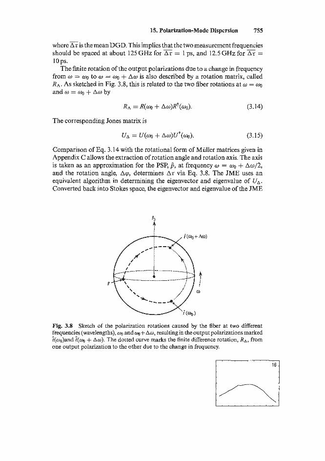
15. Polarization-Mode Dispersion 755
where at is the mean DGD. This implies that the two measurement frequencies should be spaced at about 125 GHz for = 1 ps, and 12.5 GHz for at =
The finite rotation of the output polarizations due to a change in frequency from w = wo to w = w-, + Aw is also described by a rotation matrix, called RA. As sketched in Fig. 3.8, this is related to the two fiber rotations at w = w-, and w = 00 + Aw by
10 ps.
R A = R(w0 + Aw)R+(w-,). (3.14)
The corresponding Jones matrix is
UA = U ( W 0 + Aw)u'(kh)). (3.15)
Comparison of Eq. 3.14 with the rotational form of Muller matrices given in Appendix C allows the extraction of rotation angle and rotation axis. The axis is taken as an approximation for the PSP, j, at frequency w = 00 + Aw/2, and the rotation angle, Ap, determines At via Eq. 3.8. The JME uses an equivalent algorithm in determining the eigenvector and eigenvalue of UA. Converted back into Stokes space, the eigenvector and eigenvalue of the JME
Fig. 3.8 Sketch of the polarization rotations caused by the fiber at two different frequencies (wavelengths), mo and COO + A+ resulting in the output polarizations marked ?(wo)and ?(w, + Am). The dotted curve marks the finite difference rotation, Ra, from one output polarization to the other due to the change in frequency.
756 H. Kogelnik et al.
are isomorphic to the rotation axis and rotation angle since a vector launched in alignment with the rotation axis exits in alignment with it.
A minor difficulty arises with the JME when automated data are taken over a range of frequencies (see e.g., JSarlsson et al. 2000a). The problem is best explained by reference to the relation between R and U (Gordon and Kogelnik
RG = U'GU. (3.16)
Inspection of this equation makes it evident that on transition from Stokes to Jones space, the algebraic sign of U is left undefined. The JME algorithm has to make a choice of sign on the transition from the measured Stokes vectors, and care must be taken to make this choice in a consistent manner at all frequencies. The MMM algorithm remains entirely in Stokes space and does not have to deal with this particular issue.
Figure 3.5 shows data for the PMD vectors of a 62-km fiber with a mean DGD of 35ps measured with the MMM technique. Comparison with data obtained using the PSD method (Nelson et al. 2000c) shows good agreement. Reported comparisons of JME and MMM results also agree well (Nelson etal. 1999a), as expected.
2000),
3.4 INTERLEAVING
The simple technique of interleaving (Jopson et al. 1999a) resolves a seeming contradiction inherent in measurement techniques such as the JME and the MMM. The contradiction appears because of two conflicting requirements:
1. To obtain accurate data for a PMD vector ?, two rotation matrices, R(@) and R(w + Am), must be measured at frequencies spaced at the relatively large MMM step size Ao 5 Awpsp.
2. For adequate resolution of the wavelength dependence of the measured ?(o), one requires frequency intervals smaller than the MMM step size. An example where this resolution is essential is the numerical differentiation used to obtain second-order PMD vectors.
The interleaving technique, sketched in Fig. 3.9, resolves this conflict and delivers accurate data with good spectral resolution. Consider that the R matri- ces are measured at frequencies w1, wz, 03, etc., and 01 + Am, wz + Am, etc., as indicated on the upper line of the figure. The matrix pair at m1 and w1+ Am is used in the MMM algorithm to determine the PMD vector ? at 01 + A 4 2 as indicated in the second line, and similarly for wz, w3, etc. To produce good
I
15. Polarization-Mode Dispersion 757
MMM step size
+ A m ___j(
R ( a ) : qTJ--;;\a ~
a 2 0 3 I I ~ , + A w +a
?(a) : .. n v n " n
/ \ w , + A w I ~ 0 2 + A 0 1 2
Fig. 3.9 Sketch of the interleaving technique. The upper rail shows the frequencies at which the rotation matrix, R, is measured. The frequency pairs (ml ,ml + Am), (02, m2 + Am), etc., are used to determine the PMD vectors at m1+ A 4 2 , q + Am/2, etc. as shown on the lower rail. Interleaving allows the frequency spacing between the measured PMD vectors to be arbitrarily smaller than the MMM step size Am.
resolution, the frequency spacing (02 - w1) of the final data series can be chosen to be smaller than Aw. Typical interleaving ratios used in practice are 3 or 4. The results obtained with this technique are in good agreement with results measured with the PSD technique, which does not employ interleaving.
3.5 SECOND-ORDER PMD WCTOR MEASUREMENT The experimental determination of second-order PMD vectors ?m requires the availability of error-free, high-resolution experimental data for the first- order PMD vector ?(w). Typically these are interleaved JME or MMM results as discussed previously or data obtained with the PSD technique. See, for example, Fig. 3.5. In accordance with its definition given in Eq. 2.10, the vector ?m is then determined by numerical differentiation,
using the ? vectors measured at two neighboring frequencies, w1 and 0 2 (Jopson et QZ. 1999a; Nelson et QZ. 1999a).
The second-order PMD data contain two key parameters required for the understanding of second-order PMD effects and associated systems impair- ments (see Sections 2 and 6). They are the polarization-dependent chromatic
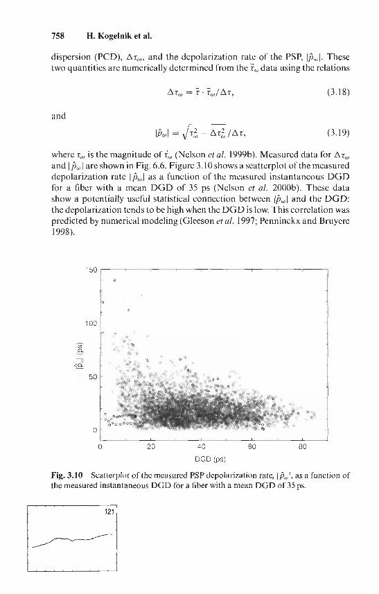
758 H. Kogelnik et al.
dispersion (PCD), At, , and the depolarization rate of the PSP, l@,l. These two quantities are numerically determined from the ?, data using the relations
A t , = T . ? w / A t , (3.18)
and
Ijwl = Jti - A t ; / A t , (3.19)
where t, is the magnitude of (Nelson et al. 1999b). Measured data for A t , and I @, I are shown in Fig. 6.6. Figure 3.10 shows a scatterplot of the measured depolarization rate lj,l as a function of the measured instantaneous DGD for a fiber with a mean DGD of 35 ps (Nelson et al. 2000b). These data show a potentially useful statistical connection between @,I and the DGD: the depolarization tends to be high when the DGD is low. This correlation was predicted by numerical modeling (Gleeson et al. 1997; Penninckx and Bruyere 1998).
0 20 40 60 80
DGD (PS)
Fig. 3.10 the measured instantaneous DGD for a fiber with a mean DGD of 35 ps.
Scatterplot of the measured PSP depolarization rate, lj3wl, as a function of
121
15. Polarization-Mode Dispersion 759
-
3.6 BA CKSCATTEMNG TECHNIQUES
There are three attributes that make backscattering techniques for measuring PMD particularly appealing:
- ... . . . . i:i optional t i ! mirror . . ::: -
1. The fiber under test is accessed from one end only. 2. Local mean DGD variations can be sensed as a function of location in
the fiber. 3. The beat length L b of the fiber can be measured.
As some PMD vector information is lost on the return path of the light, the methods measure mean DGD information only. A general schematic for these techniques is shown in Fig. 3.11. Most of them use polarimetric optical time- domain reflectometry (POTDR) with a pulsed laser source (Bebbington et al. 1997; Sunnerud et al. 1998; Corsi et al. 1998). The polarized light passes through a beam splitter or directional coupler and is backscattered by the fiber under test. The beam splitter directs the backscattered light to a detector for time-resolved OTDR analysis. In the figure, the detector is preceded by a
Polarization
or polarimeter t Detector
Fig. 3.11 Schematic for measurement systems using backscattering. The mirror at the far end of the fiber is optional as Rayleigh backscattering in the fiber itself is used by most techniques. In most cases one uses pulsed laser sources and OTDR analysis of the detected signals.
760 H. Kogelnik et al.
polarization analyzer. However, in simple implementations a single polarizer is inserted at the input to the fiber under test, thus combining the input polarizer and output analyzer functions. The polarization of the backscattered light, i ~ , changes with the round-trip time delay, A T ,
AT = 2zn/c, (3.20)
where z is the scattering location in the fiber and n is the effective fiber index. The scattering location is, thus, identified by the timing of the OTDR. After passing through the analyzer, the detected signal, T(z), is proportional to
where io is the setting of the analyzer. A conceptually simple backscattering method for the measurement of mean
DGD is a modification of Poole and Favin's (1994) fixed analyzer method. Here, only one polarizer is used as mentioned earlier, and the OTDR timing is set for the fiber location, z, of interest (e.g., z = L for the full fiber length). The laser source is tuned over a frequency range, A o , and the analyzer signal, T(z = const, w), is determined as a function of frequency. From the fluctua- tions of T , one determines the number of extrema, ne^, or the number of mean level crossings. The (single-pass) mean DGD, 5, of the fiber is related to the extrema count ne^ of the backreflected signal by (Galtarossa et al. 1999a,b):
- A t = 1.56 * N e ~ / A w . (3.22)
This compares to the single-pass Poole/Favin formula - A t = 2.58 ' N,/Aw, (3.23)
where Ne is the extrema count for a single pass through the fiber. Both formulas above assume that the fiber length, L, is much larger than the beat length Lb and the coupling length Lc discussed in Section 2, i.e., L >> Lc,Lb.
The constant in Eq. 3.22 is smaller than that expected from a simple 1/2 scaling of Eq. 3.23 to allow for the double length of fiber traversed by the return signal. The fundamental reason for this is a change of the polarization statistics of the return signal as compared to that of the single-pass signal. The single-pass DGD obeys a Maxwellian density distribution whereas the DGD of the return signal follows a Rayleigh distribution. A detailed discussion of the study of this effect by theory, simulation, and experiment is reported in
15. Polarization-Mode Dispersion 761
Corsi et QZ. (1998). They also show that the mean DGD of the backscattered signal, (ATB), is related to the conventional mean DGD, at, of the fiber by
n- (Atg) = - A t ,
2 (3.24)
The relation of Eq. 3.24 has also been confirmed by experiments with con- tinuous wave (cw) lasers (Corsi et QZ. 1999b; Galtarossa et aZ. 1999a,b). In this modified technique only the backreflection from the facet (or mirror) at the far end of the fiber is used, limiting fiber lengths to about 40 km. The cw techniques use the polarization controller option shown in Fig. 3.1 1 and the polarimeter at the detector port. With this arrangement, conventional meth- ods such as the JME, MMM, or PoincarC sphere technique can be used to determine the DGD as a function of frequency for the backreflected signal, and its mean, (Atg) .
The beat length, Lb, can also be measured using the OTDR fixed analyzer configuration with a single inputloutput polarizer. Consider the analyzer sig- nal of Eq. 3.21, T(z, w = const) for a fixed laser wavelength as a function of delay or scattering location, z. It has been shown (Corsi etaZ. 1999c; Galtarossa et QZ. 2000c) that the characteristics of T(z) can be simply related to Lb. One key result is the relation
Lb = 4 f i / n ( v ) , (3.25)
linking L b to the mean level crossing rate n(u) per unit distance for a given level u of T ranging from 0 to 1. Lb can also be obtained from the variance of the mean power spectral density of T(z). The authors report measurements of L b values ranging between 5 and 25 m depending on fiber type.
As a simple illustration, compare the statistical formula (Eq. 3.25) with the fixed analyzer signal T = i(1 + cos(4m/Lb)) for a polarizer set at 51 and a PMF fiber set at 45" in the lab (i.e., 52). This periodic signal exhibits no = 4/Lb crossings of v = 1/2 per unit length.
Finally, we should remark on the possibility of determining the coupling length L,. Because the statistical relation (Eq. 2.4) connects Lb, L, and at, this equation can be used to determine L, once at and Lb are measured by the above techniques.
3.7 ACCURACY OF THE MEASURED MEAN DGD
The earlier sections on the PSP, JME, and MMM methods explain the mea- surement of the wavelength dependence of the instantaneous DGD. The wavelength range of these measurements is typically limited to about 100 nm.
I . . . . . . . . . I

762 H. Kogelnik et al.
The mean DGD of the fiber is then determined as the average over this spectral interval, Ah. As the number of statistically independent samples, N , in this interval is also limited, a question arises concerning the confidence intervals of such a measurement. The answer is rooted in the concept of the bandwidth of the PSP discussed in Section 2.
We know that the DGD follows a Maxwellian distribution (for more detail see Section 4) with variance, a2 = (At2) - (At)2, and the standard deviation for a single measurement of
cr = 0.422%. (3.26)
For N statistically independent measurements the deviation, a ~ , narrows to
ON = 0.422=/&. (3.27)
From the discussion of the bandwidth of the PSP in Section 2.6 it follows that N is determined by the spectral range and by Ahpsp as
N = Ah/BAhpsp. (3.28)
This allows us to express the standard deviation of the measurement as approximately
aN = JZ, (3.29) where ar~ and AT are expressed in ps and Ah in nm. The limited spectral interval, therefore, imposes an accuracy limit o f f lOO/d= percent on the measurement of the mean DGD. For a 100-nm interval, for example, one gets accuracies of 3% for 10 ps, 10% for 1 ps, and 30% for 0.1 ps mean DGDs.
Detailed studies and numerical simulations of this accuracy issue are reported in Gisin et al. (1 996) and Cameron et al. (1 999).
3.8 FURTHER READING
Comparisons of measurement methods can be found in Schiano (1998), Galtarossa et al. (1996), Gisin et al. (1994a), and Namihira and Maeda (1992a,b). Madsen (2001) describes a new measurement method.
4. Statistics
4.1 INTRODUCTION
PMD differs from many lightwave system properties in that the impairment caused by PMD usually changes stochastically with wavelength and also with

15. Polarization-Mode Dispersion 763
time. This means that one cannot predict the impairment of the system at any particular wavelength and time, but must instead resort to a statistical description. It also means that, in general, one cannot characterize the PMD of a system to arbitrary accuracy, since a measurement will sample only a portion of the statistical ensemble. Most other impairments, such as those due to chromatic dispersion, system attenuation, or self-phase modulation, will have some uncertainty caused by manufacturing tolerances, imprecise wavelength control, aging, and the like. However, in most cases, the probability densities for these impairments will vanish beyond some value, allowing a system to be designed to tolerate the worst-case impairment. Tolerance of worst-case impairment is rarely possible when PMD is a significant source of impairment. The probability densities for PMD in most situations have asymptotic tails extending to unacceptably large impairment. Hence, the system cannot be designed to handle the worst-case PMD impairment, and must instead be designed for a specified outage probability. For similar reasons, the goal of PMD compensation cannot be to eliminate the impairment, but rather to reduce the PMD outage probability. To understand and predict system outage probabilities, to design PMD compensators, and to accurately measure PMD in systems, one must understand the statistics of the phenomena associated with PMD.
Interesting statistical characteristics of PMD include the probability den- sities of first- and higher-order PMD, the scaling of PMD phenomena with changes in the mean DGD, various correlation functions, and characteris- tics associated with the accuracy of PMD measurements. The first statistical property of PMD to attract interest was the mean DGD (Poole and Wagner 1986; Andresciani et ai. 1987). Since the DGD usually changes quite slowly with time, it is difficult to obtain an accurate estimate of the mean DGD by repeatedly measuring the DGD at one wavelength. Instead, the DGD is aver- aged over wavelength and the result is assumed to be equal to the time average. This assumption is of crucial importance. Although some data has been taken covering a broad span of time and wavelength (Poole et al. 1991a; Karlsson etal. 2000a), the issue has not been fully explored. Instead, this equality, upon which the accuracy of much experimental PMD work relies, is assumed.
However; caution must be applied when assuming equivalence between time averaging and wavelength averaging, particularly for large (> 10 nm) wavelength scans. The wavelength dependence of the DGD may include a systematic variation in addition to the stochastic variation that is statistically similar to the variation with time. Such systematic variation may occur as a result of dispersion in the fiber birefringence. Once the validity of wavelength scanning is assumed, experimental attention can be focused on probability
764 H. Kogelnik et al.
densities. Measurements, together with simulation results (see Section 5), can be used to establish the veracity of analytic derivations of probability densities and the validity of the PMD models. The densities are then combined with an understanding of PMD-induced system penalties (see Section 6) to predict system outage probability. Powerful scaling laws emerge from the densities and their derivation. With these laws, one can obtain extensive understanding of the statistical properties of the PMD in a particular system through the measurement of a single system characteristic, the mean DGD.
4.2 PROBABILITY DENSITIES
Probability densities and scaling rules can be obtained from an analytic model developed by Foschini and Poole (1991). This model, like most models used to obtain analytic results for PMD statistics, assumes the ideal, perfectly random, fiber birefringence. It should be borne in mind that real systems are not perfectly random and real densities presumably do not exhibit the asymptotic tails extending to inhity that are found in densities obtained ana- lytically. The Foschini-Poole analysis starts with a model for fiber birefringence having a frequency independent differential delay that is independent of dis- tance and a frequency-independent rotation that fluctuates with distance as three-dimensional white Gaussian noise in Stokes space. Physically, the first term provides the delay and the second term randomizes the orientation. The model leads to the characteristic function (Foschini and Shepp 1991) of the six-dimensional normalized vector (2, ;l,),
= sech . exp --
from which many PMD probability densities have been obtained. Here, E is the expectation operator, which is an integral weighted by the six-dimensional probability density p ~ , ; ~ . F denotes the six-dimensional Fourier transform of a function of (>,+tL, into a function of its conjugate vector, (Z, 5). The normalized vector, (try tl,), is obtained from the six-dimensional vector (?, c) according to

15. Polarization-Mode Dispersion 765
As discussed below, the normalization allows results obtained from Eq. 4.1 to be generalized to systems having any mean DGD. We will see in Table 4.1 that the normalization constant, atmy is the rms value (standard deviation) of a first-order PMD component. Although the six-dimensional characteristic function may be difficult to derive, once it is known, one can apply pow- erful techniques to obtain a variety of probability densities and moments. For instance, the characteristic function of a single variable can be obtained from the six-dimensional function by setting the uninteresting conjugate vari- ables to zero. This can be easily seen from the second expression in Eq. 4.1, which then merely becomes an integral over P ? , ? ~ for these variables, leaving only the Fourier transform over the remaining variable@). In this way, the Gaussian characteristic function for a first-order component, rx for example, is found trivially from Eq. 4.1 by settingz,, z,, and to zero. An inverse Fourier transform can be used to provide the desired density, which is also Gaussian. The density for a second-order component, tu,, for example, is also easily retrieved, this time by setting 2, &, and TZ to zero in Eq. 4.1. This leaves the sech. Since a sech, like the Gaussian, is its own Fourier transform, the densi- ties of the second-order components are hyperbolic secants. With more effort, one can derive the familiar Maxwellian dependence of the DGD density and obtain the density for the magnitude of the second-order PMD. Impairment arising from second-order PMD is conveniently understood by considering separately, ?,l, the component of 2, perpendicular to ?, and polarization- dependent chromatic dispersion, l?l,, which is the component of parallel to 2 (see Section 2). Thus, the densities of these two components are of interest and have been derived from Eq. 4.1 (Foschini et al. 1999; Foschini et al. 2000; Nelson et al. 1999b; Jopson et al. 2001). Penalties caused by ?,l are often understood through the use of the closely related quantity, the PSP depolari- zation term, 5, = ?,l/At, so its density has also been derived. While most of the densities are available in closed form, those for 2 , ~ and &, are known in integral form.
Once the densities are known, they can be used to obtain the mean and mean square (or second moment or variance) of each of the variables of inter- est. Table 4.1 summarizes results obtained from Eq. 4.1. The normalization imposed on Eq. 4.1 has been removed for this table, so the dependence on DGD is shown explicitly. For simplicity, t rather than at is used in the table to represent the mean DGD.
Before trusting the results shown in Table 4.1, they should be compared to experimental and simulated results. The Maxwellian has received a lot of attention (Curti et al. 1990; Poole et al. 1991b) and various efforts have addressed some of the other predictions (Foschini and Poole 1991; Ciprut

766 H. Kogelnik et al.
Table A I Densitypx(x) 2 0, j-”, dxpx(x) = 1
0 2
t i - e-(2x/32/n, Gaussian nt
soliton amplitude
t
0
2G - t2 n
0; x t o
\?lo = A Ato -sech’(:), 2 t 2
soliton intensity
I t l I x sech(a)(a tanha)’/’
0
(i)’ t4 = cr4
n 3 ( i)2 t4 = 3$
1 K Z 4 1 , 3 ( 8 ) t = y
3 ( 8 ) 8 n Z 4 t 8 ,
~ ~ ~ ~ ~ ~ ~
Probability densities of a component of lirst-order PMD (ri), the magnitude of fist-order PMD (l?l), a component of second-ord PMD (r&). the magnitude of second-order PMD (I?J), the second-order PMD component associated with PCD = A?& the perpendicular second-order component (l?mll), and the depolarization (If&,]) all scaled to the mean DGD, 5, denoted he by r. Catalan’s constant, G, is 0.915965.. ., JO is the zero-order cylindrical Bessel function, and IF, is the standard hypergeometr function

15. Polarization-Mode Dispersion 767
et al. 1998). Data obtained from measurement of the PMD vector ?(w) of a fiber with a mean DGD of AT = 14.7 ps over a spectral range of 120 nm have provided a verification of all the densities in Table 4.1 (Foschini et al. 1999; Foschini et al. 2000; Nelson et al. 1999b; Jopson et al. 2001). The measurement used the Miiller Matrix Method (see Section 3.3) to obtain the spectrum of ?. From this, 2, could be obtained by numerical differentiation. The broad scan width and relatively high mean DGD provided more than 6000 data points estimated to include about 300 statistically independent samples. Figure 4.1 shows the experimentally derived densities together with the analytic predic- tions of Table 4.1. The measured densities have been scaled as outlined below to a mean DGD of 1 .O ps. It can be seen that the predictions appear to agree well with measured results, but a rigorous statistical analysis of the agreement has not been performed.
Since a larger number of statistical samples is hard to obtain in the labora- tory, simulation (see Section 5) must be used to explore the asymptotic tails of the densities. The tail is often the region of greatest importance because it is the large values of PMD that impose system outage. The markers in Fig. 4.1 show densities obtained by simulation. The simulation employed a concatenation of 1200 randomly oriented, linearly birefringent sections providing a mean DGD of 14.7 ps and produced 260,000 statistically independent realizations. Once again, the results have been scaled to a mean DGD of 1 .O ps and once again, the analytic predictions appear to agree with the simulation results.
The estimation of system outage probabilities often requires complemen- tary cumulative probability distributions, which are CC( y) = iym dxp,(x),, where p,(x) could be one of the densities in Table 4.1. These integrals provide the probability exceeding some value, y, which is typically the threshold for unacceptable impairment. Figure 4.2 shows the complementary cumulative probability distribution together with the cumulative probability distribution for the DGD, once again using a mean DGD of 1 ps. The markers show results from the simulation described previously. The deviation of the simulation from theoretical predictions for AT > 3.1 ps is probably a result of the small number of realizations (5) that generated a DGD larger than 3.1 ps.
4.3 SCALING
A remarkable feature of the results shown in Fig. 4.1 is that only one param- eter, the mean DGD, is needed to predict all the PMD densities of a fiber with perfectly random birefringence. This feature follows from the scaling rule of Eq. 4.2, which removes all physical parameters from the characteristic equation. Examination of Table 4.1 reveals simple rules for scaling densities
t 22
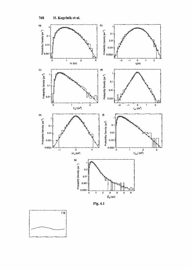
768 H. Kogelnik et al.
0 1 2
L " " " " " " " " " " " " ' 1 1
0.1
0.01
0.001
-2 -1 0 1 2
(e) 1
v; n w-
; - b 0.1 P 0.1
; 0.01 G C .- .-
x
6 0.001
0.01 I .- - B n
B 0.001
t a 0.0001 0.0001
-1 0 1 0 1 2 3
0 1 2 3 4 5 6
l i i l (PSI
Fig. 4.1
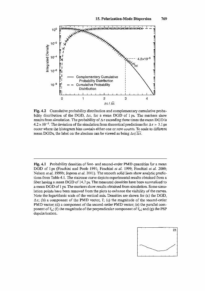
15. Polarization-Mode Dispersion 769
1 00
~ 10-2
p 10-4
c .- en c al n
F c
m a E 10-6
10-8
- Complementary Cumulative Probability Distribution - - Cumulative Probability Distribution
I I I I I I I I I I L
I I L L
0 1 2 3 4 AT I A<
Fig. 4.2 Cumulative probability distribution and complementary cumulative proba- bility distribution of the DGD, At, for a mean DGD of 1 ps. The markers show results from simulation. The probability of At exceeding three times the mean DGD is 4.2 x The deviation of the simulation from theoretical predictions for At > 3.1 ps occur where the histogram bins contain either one or zero counts. To scale to different mean DGDs, the label on the abscissa can be viewed as being At/=.
Fig. 4.1 Probability densities of first- and second-order PMD quantities for a mean DGD of 1 ps (Foschini and Poole 1991; Foschini et al. 1999; Foschini et al. 2000; Nelson et al. 1999b; Jopson et al. 2001). The smooth solid lines show analytic predic- tions from Table 4.1. The staircase curve depicts experimental results obtained from a fiber having a mean DGD of 14.7 ps. The measured densities have been normalized to a mean DGD of 1 ps. The markers show results obtained from simulation. Some simu- lation points have been removed from the plots to enhance the visibility of the curves. Note the logarithmic scale of the vertical axis. Densities are shown for (a) the DGD, Ar; (b) a component of the PMD vector, ?; (c) the magnitude of the second-order PMD vector; (d) a component of the second-order PMD vector; (e) the parallel com- ponent of ?m; (f) the magnitude of the perpendicular component o f t ; and (g) the PSP depolarization.

770 H. Kogelnik et al.
obtained for one to densities for another an. For first-order densities, multiply the density P by and the outcome x , by At2/Atl. The scal- ing of second-order densities is performed similarly except (At1 /At2)~ is used instead of Aq/At2 and correspondingly for the outcome. Note that as jjw is the ratio of a second-order quantity and a first-order quantity, it scales as first-order PMD. The scaling rules for the means and the mean squares of PMD quantities follow from the scaling of the densities. The mean square of first-order PMD quantities increases quadratically with mean DGD, as does the mean of second-order PMD quantities. The mean square of second-order PMD quantities increases as the fourth power of mean DGD.
Some of these scaling predictions have been compared to results obtained by experiment and simulation. One measurement used a selection of 11 differ- ent fibers with mean DGD values between 1.3 and 3 6 . 0 ~ ~ ~ and a wavelength range of 1460 to 1580 nm for most of the fibers. This provided 30 to 300 inde- pendent samples (depending on the fiber mean DGD) for the rms values of Ifiwl, l?wll and Atw (Nelson 1999b; Jopson etal. 2001). The same quantities were evaluated by a simulation using 600 delay elements that obtained 29,000 independent realizations for each of 13 mean DGDs. The results are shown in Fig. 4.3. The lines are predictions from Table 4.1 that contain no free parame- ters whereas the markers show results from experiment and simulation. It can
-- --
--
1000
1
1 2 5 10 20 50 Mean DGD (ps)
Fig. 4.3 Scaling of therms values of l&.,,l, Aq,, (denoted Q2,11, and I?2,toll, for fibers with different mean DGD. The lines are theoretical predictions and the markers represent results obtained by experiment and simulation.

15. Polarization-Mode Dispersion 771
be seen, as expected, that the rms of l ? l w and the rms liwll scale quadratically with mean DGD whereas the rms
Examination of the expressions in Table 4.1 reveals many interesting rela- tionships. For instance, the densities of the first-order components, ti, are equal, showing that no axis is favored. As mentioned earlier, all of the delay in the analytic model used to derive the densities lies along the first component of Stokes space. The symmetry in the first-order densities shows that this bias is removed by the frequency-independent rotation term. The rms of the second- order magnitude, I ? w l , is l /& the value of the mean square of the first-order magnitude, A t , and it is split quite unevenly between the PCD or parallel component and the perpendicular components. Indeed, the mean square of I?wl I accounts for 8/9 of the total mean square second-order whereas the mean square of the parallel component consumes the remaining 1/9. Summarizing:
I scales linearly with mean DGD.
= 3(?:) = 27{At:). (4.3)
Thus, as stated in Section 2, changes in ? are much more likely to take the form of a change in a direction than a change in length, information important to the designers of second-order compensators.
One very useful scaling relationship that has not received much explicit experimental attention links bit rate and mean DGD: The allowable in a system scales inversely with bit rate. This scaling is not constrained to sys- tems with purely first-order PMD, but it does assume that other sources of impairment are either absent or scaled appropriately. Its usefulness is that it allows results from PMD experiments performed at low bit rates to be applied to higher bit rates where experiments might be more difficult to control. This scaling follows from the model of Eq. 5.6 as illustrated in Fig. 2.3, which pre- dicts that if the element delays, At,,, and the bit rate are changed in a manner that preserves their product, any particular output waveform will also scale with the bit rate.
4.4 CORRELATION FUNCTIONS
An alternate, powerful description of PMD statistics is provided by auto- correlation functions, which contain the effects of all PMD orders in simple, compact form. They provide information about the means or expectation values of products of PMD vectors or states of polarization (SOPS) cor- responding to different frequencies or different times. An example is the spectral autocorrelation of the PMD vectors recently derived by Karlsson and Brentel(1999a) and Shtaif et al. (2000b). It applies to the PMD vectors

772 H. Kogelnik et al.
at the frequencies m1 and w;! = m1+ A m and has the form:
This correlation function has been used in Section 2 for the characterization of the bandwidth of the PSP; it impacts the inherent uncertainty in measuring the mean DGD, an issue discussed in Section 3.7. The spectral correlation between output SOPS, ( f (w1) - $(w;!)), is given in Eq. 6.24. It is used in Section 6.6 to analyze the effect of PMD on the FWM efficiency in the fiber and in Section 6.7 to determine the PMD effect on polarization-dependent gain in fiber Raman amplifiers. The corresponding temporal correlation functions both for the SOPS and the PMD vectors are given in Eqs. 7.1 and 7.2 where they are used to discuss the time response required for PMD mitigation.
4.5 FURTHER READING
For additional information on the evolution of PMD with distance, see Poole (1988a), Pooleetal. (1988b), Bettietal. (1991), FoschiniandPoole(1991), and Karlsson (200la). Information on joint probability densities can be found in Penninckx and Bruyere (1998), Shtengel etal. (2001), and Jopson et al. (2001).
5. Emulation and Simulation
5.1 PURPOSE
Although lightwave systems are typically specified to have outage probabilities of less than testing system robustness to PMD-induced outage to these levels is rarely practical in the field. A three-pronged attack employing anal- ysis, numerical simulation, and experimental emulation can be used instead. Analytic derivation of probability densities, described in Section 4, provides the best information about asymptotic behavior, but these derivations are not easily undertaken and require assumptions about the nature of birefringence in fiber. As described in Section 4, analytic solutions to first- and second-order PMD quantities have been obtained for the Taylor-series expansion model of PMD. Simulation of PMD can be used to verify statistical predictions derived analytically, to make statistical predictions that have not been derived analyt- ically, to test assumptions made about the behavior of fiber birefringence, and to incorporate PMD into a system simulation. Laboratory emulation is used to corroborate results obtained through analysis or simulation, to study system impairment caused by PMD, and to test compensators of PMD impairment.
15. Polarization-Mode Dispersion 773
Emulators are of crucial importance in the latter role since numerical simu- lation cannot be trusted to mimic all the vagaries of physical components. In addition, emulation can be faster than numerical simulation. Since thousands or millions of PMD realizations may be needed to obtain usable statistics on system performance, emulation may offer the only practical way to obtain this information. However, one must ensure that the model used to construct an emulator or simulator mimics the system properties of interest.
5.2 COMPARISON OF MODELS
The total PMD of a system contains contributions from fiber and from dis- crete components. The PMD arising from a random combination of small amounts of birefringence from a large number of sources is well understood. This includes the PMD of most fiber spans and also includes the PMD of sys- tems wherein the birefringence of each component is much smaller than the total system PMD. The most common model used in numerical simulations is a concatenation of linear birefringent elements oriented at random angles (illustrated in Fig. 2.3) that are chosen randomly over the range 0 to n (Poole and Nagel 1997). Other models use linearly birefringent elements, but restrict the orientation of the elements in various ways that reduce the average change in orientation between successive elements. The statistics of the simulated first- and second-order PMD do not appear to depend on the details of the model so long as a sufficient number of birefringent elements are used in the simula- tion. However, the number of such elements required for a desired statistical accuracy will depend on the details of the model (Prola et al. 1997; Dal Forno et al. 2000; Lima et al. 2000; Khosravani et al. 200 1 a).
The densities plotted in Fig. 4.1 show remarkable agreement between experi- ment, theory, and simulation even though the underlying models used to generate the curves differ significantly. As will be discussed in detail below, the simulation used a large number of small sections of linear birefringence that were longer than a birefringent beat length. These sections provided polariza- tion rotation about the Stokes SI axis. They were rotated relative to each other by a random angle between 0 and IT radians. First- and second-order PMD were determined at a single frequency by calculating the transmission matrix in Jones space for several closely-spaced frequencies and taking derivatives. In contrast, the theory combines infinitesimally small sections of linear bire- fringence with infinitesimally small, random rotations about the Stokes space. The PMD was evaluated at a single frequency using Stokes space differential concatenation rules for ? and zm. For both simulation and theory, the statisti- cal variation was determined by changing the random rotations between the
774 H. Kogelnik et al.
sections. The birefringence of the fiber used in the experiments was probably similar to that of the theoretical model except that the sections of linear bire- fringence and the rotations were not infinitesimally small. In addition, there was random variation in the birefringence of the linear sections. The experi- mentally derived densities were obtained by averaging over frequency rather than orientation of fiber birefringence, thus for the experimental densities, the orientations of the birefringent axes were frozen. The randomness was prob- ably introduced by the frequency dependence of the s1 rotation in the linear sections. These three different models appear to lead to similar statistics. This can be understood for 2 from the concatenation rule, Eq. 2.23. The statistics of ? arise from the vector sum at the end of the fiber of the transformed random birefringences. Any model that creates this vector sum should generate similar statistics.
The DGD density obtained from most emulator models does deviate at high DGD values from most theoretically derived densities. This is a consequence of the finite number of sections available in practical emulators. Consider a fiber with an rms DGD of Y. This fiber can be modeled using N randomly oriented birefringent sections, each having a birefringence T/&. The maxi- mum PMD in the model, obtained by perfect alignment of the birefringence in each section, is N times the section birefringence or T a . Thus theories employing an infinite number of sections include the possibility of arbitrar- ily large PMD (with small probability), whereas the DGD density obtained from emulation or simulation will truncate at a DGD value determined by the number of birefringent sections used in the model. Similar deviations between theory and simulation are also seen in the densities of other first- and second- order PMD components. While schemes may be devised to bypass this limit, they are unlikely to provide a better model of fiber PMD. Real fiber PMD itself arises from a finite number of birefringent elements; hence, the densities of some PMD quantities for real fibers are expected to be truncated.
5.3 EMULATION OF FIRST-ORDER PMD
First-order PMD emulation is important, not only for testing system perfor- mance, but also as a key component of several of the PMD compensation techniques in Section 7. The most easily implemented emulator of first-order PMD is a length of polarization-maintaining fiber. One obtains about 2 ps/m of delay from most commercially available PMFs. The usefulness of PMF as a hst-order emulator is limited to applications for which the delay need not be adjustable. For these applications, PMF is the lowest cost, most stable method for providing first-order PMD.
I
15. Polarization-Mode Dispersion 775
Figure 5.1 shows a method commonly used in commercial instruments to provide adjustable first-order PMD. This bulk-optics design uses a polariza- tion beam splitter to separate an input signal into two orthogonally polarized beams. A variable optical delay is applied to one of the polarized beams prior to the recombination of the beams in a second polarization beam splitter. The design, like a length of PMF, provides pure first-order PMD without higher-order PMD. However, the output polarization depends on the optical phase difference between the two orthogonally polarized beams at the point of recombination. Since the variable and fixed delays in the emulator rarely are interferometrically stable, the polarization of the output beam fluctuates. This polarization fluctuation usually occurs with a time scale of 10’s to 1000’s of milliseconds and limits the placement of bulk-optic emulators to locations downstream of all polarization-dependent components in a system. Note that a length of PMF also requires interferometric stability in the two signal paths if polarization fluctuation is to be avoided at the output. However, since the two signal paths are in the same fiber, the necessary stability can be easily achieved by temperature control and isolation from external mechanical stress. Taping a jacketed fiber to a table in the open air usually provides sufficient stability to increase the time scale of polarization fluctuations to minutes or hours.
The second design, shown in Fig. 5.2, uses the concatenation rule, Eq. 2.20. Two lengths of PMF are connected through a polarization controller. The PMD at the midpoint (input to the second length of PMF) will be the vector sum in Stokes space of the second section’s PMD and the first section’s PMD as rotated by the polarization controller. (For simplicity, we neglect the PMD of the polarization controller, which is always less than 6 fs for 4 quarter-wave retarders at 1550 nm.) The polarization controller adjusts the angle, 8, between
PBS PBS
OUT
Fig. 5.1 polarization beam splitters.
Bulk-optics method of providing adjustable first-order PMD. PBS refers to
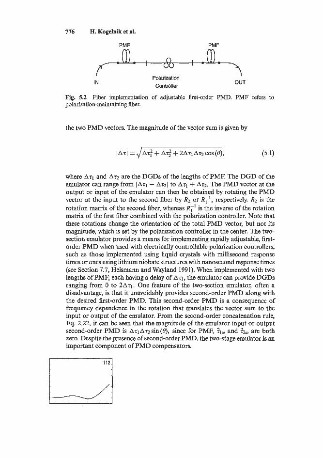
776 H. Kogelnik et al.
PMF PMF
I
IN Polarization
Controller
I
OUT
Fig. 5.2 Fiber implementation of adjustable first-order PMD. PMF refers to polarization-maintaining fiber.
the two PMD vectors. The magnitude of the vector sum is given by
where At1 and At2 are the DGDs of the lengths of PMF. The DGD of the emulator can range from l A q - At21 to At1 + At2. The PMD vector at the output or input of the emulator can then be obtained by rotating the PMD vector at the input to the second fiber by R2 or R;', respectively. RZ is the rotation matrix of the second fiber, whereas R,' is the inverse of the rotation matrix of the first fiber combined with the polarization controller. Note that these rotations change the orientation of the total PMD vector, but not its magnitude, which is set by the polarization controller in the center. The two- section emulator provides a means for implementing rapidly adjustable, first- order PMD when used with electrically controllable polarization controllers, such as those implemented using liquid crystals with millisecond response times or ones using lithium niobate structures with nanosecond response times (see Section 7.7, Heismann and Wayland 1991). When implemented with two lengths of PMF, each having a delay of At1 , the emulator can provide DGDs ranging from 0 to 2 A q . One feature of the two-section emulator, often a disadvantage, is that it unavoidably provides second-order PMD along with the desired first-order PMD. This second-order PMD is a consequence of frequency dependence in the rotation that translates the vector sum to the input or output of the emulator. From the second-order concatenation rule, Eq. 2.22, it can be seen that the magnitude of the emulator input or output second-order PMD is AtlAt2 sin (e), since for PMF, ?lo and ?h are both zero. Despite the presence of second-order PMD, the two-stage emulator is an important component of PMD compensators.

15. Polarization-Mode Dispersion 777
5.4 EMULATION OF FIBER PMD
A full understanding of PMD can be gained only by emulating all orders of PMD. A useful PMD emulator should be able to reach all combinations of first- and higher-order PMD present in the optical fiber being emulated; it should mimic the PMD spectrum of an optical fiber; it should be stable over measurements lasting hours to days; and it should be possible to both predict the emulator PMD for a given instrument setting and to predict the instrument setting required to obtain a desired PMD. It would also be useful if the emulator could easily mimic the complex statistics of fiber PMD. One approach that can be viewed as laboratory emulation of fiber PMD is to use a short fiber with high PMD (Jopson et al. 1999~). This approach can provide PMD with statistics similar to those encountered in the field; however, the PMD is not adjustable and the fiber may add additional impairments such as loss, dispersion, or nonlinearity.
A multiplate emulator can be used to obtain adjustable PMD (Damask 2000; Williams 1999a). Light passing through a multiplate emulator transits a series of birefringent elements sandwiched between random interelement polarization coupling. The birefringent elements are often crystalline wave- plates, but PMF is also common. Orienting the axes of successive birefringent elements at random angles can provide the random polarization coupling. An alternative is to use polarization controllers. Adjustment of the emulator PMD can be obtained by changing the polarization coupling between elements, by changing the amount of birefringence in each element, or by changing both. The former course is usually chosen. Since the emulator PMD is sensitive to small changes in the birefringence of its components, it is difficult to adjust a multiplate emulator to a desired state of PMD and it is difficult to predict the PMD obtained from a known setting. However, a group of random settings of the emulator will provide a sample of PMDs that match the statistical variation of fiber PMD. The statistical match is not perfect. While a fiber may effectively consist of hundreds or thousands of birefringent sections (Galterossa et al. 2000b), multiplate emulators generally have less than 20 sections or elements. As mentioned previously, the peak DGD is roughly the root-mean-square DGD times the square root of the number of elements. Thus, for a given mean DGD, the peak DGD achievable by an emulator is considerably less than that possible in a fiber. This limitation causes a truncation of the emulator’s proba- bility density for DGD and other PMD values. Figure 5.3 shows the deviation from theoretical predictions of the densities expected from a 12-plate emulator for the magnitude and one Stokes component of both first- and second-order PMD, as well as the parallel and perpendicular components of second-order
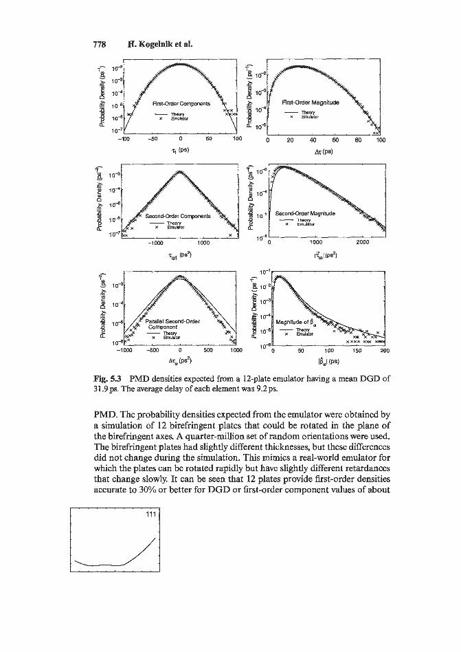
€3. Kogelnik et al.
1 04
109
104
1 0 4 First-Order Components
104 x Emulator
I 0-7
lo4I 109
104
1 0 4 First-Order Components
104 x Emulator
I 0-7 -XI0 -50 0 50 100
, , x, 0 20 40 60 8 0 '
h 109 I
.2 2 104
d .- 1 0 4 B 2 106 e n
I 0-7
- ond-Order Componen
x Emulalor
-1 000 1000
-1000 4 0 0 0 500 1OW x x x x X%
50 100 150 200
ATm ( P d 18,l (PSI
Fig. 5.3 PMD densities expected from a 12-plate emulator having a mean DGD of 3 1.9 ps. The average delay of each element was 9.2 ps.
PMD. The probability densities expected from the emulator were obtained by a simulation of 12 birefringent plates that could be rotated in the plane of the birefringent axes A quarter-million set of random orientations were used. The birefringent plates had slightly different thicknesses, but these differences did not change during the simulation. This mimics a real-world emulator for which the plates can be rotated rapidly but have slightly different retasdances that change slowly. It can be seen that 12 plates provide first-order densities accurate to 30% or better for DGD or first-order component values of about
15. Polarization-Mode Dispersion 779
3 times their rms value. However, the second-order densities obtained from the 12-plate emulator are inaccurate.
5.5 NUMERICAL SIMULATION OF PMD
When simulating PMD numerically, one usually follows the approach used for PMD emulation: A series of birefringent elements are sandwiched between polarization adjustment. Simulations usually use more sections than emula- tors and can use more sophisticated polarization adjustment than emulators. Emulators most commonly adjust polarization by physically rotating the bire- fringent elements as described previously. The polarization adjustment options in simulators include, in addition, three-axis polarization controllers and ran- dom orientation over all of Stokes space for the birefringence in the delay elements. Simulation can be used to explore the behavior of system perfor- mance in the presence of PMD (see Section 6), to understand the behavior of PMD monitors or compensators (see Section 7), and to provide insight into the statistics of PMD (see Section 4). The flexibility inherent in numerical cal- culation allows randomness to be achieved more easily than in emulators. For instance, adjustments to the retardation of birefringent elements are difficult in an emulator and trivial in a simulator. Although simulation is usually per- formed in Jones space (see Section 2), it is also done in Stokes space. The PMD concatenation rules (see Section 2, Gordon and Kogelnik 2000) can be applied sequentially for each birefringent element in the simulation. Figure 2.13 shows two birefringent elements with first-order PMD 21 and 22 together with rota- tion matrices R1 and Rz, respectively. The rotation matrices contain, in addition to the rotation matrix of the element, the intraelement polarization adjust- ment preceding it. As discussed in Section 2, the PMD at the output of the two sections is given by:
As birefringent elements R3, R4, and so on are added as illustrated in Fig. 2.14, this rule can be cascaded. The result is a sum of the PMD of each of the birefringent elements in the simulation, each rotated by the product of the rotation matrices of the birefringent elements following it:
? = 22 + R2t;. (5.2)
This becomes a sum of PMD vectors having magnitudes corresponding to the PMD of the birefringent elements but with a nearly random orien- tation. A deviation from randomness occurs for the last few birefringent elements: The vector corresponding to the final element is not rotated by any
I . . . . . . . . . I
780 H. Kogelnik et aL
succeeding elements; hence, it retains its orientation. The angle between that vector and the vector corresponding to the penultimate element will retain its original value. For a good statistical sample of first-order PMD, one can use a sum of randomly oriented PMD vectors and dispense with the rotation matri- ces in Eq. 5.3. However, the rotation matrices are needed if the wavelength dependence of the PMD is of interest. Second-order PMD can be obtained (see Section 2, Gordon and Kogelnik 2000) by cascading the expression for the second-order PMD of the two sections shown in Fig. 2.13:
Second-order components as well as higher-order components can also be obtained by using Eq. 5.2 for closely spaced wavelengths and calculating the PMD using one of the methods described in Section 3.
Simulations are often performed in Jones space, perhaps because they are usually done by experimentalists who appreciate the intuitive correspondence between Jones matrices and real-world components and angles. One simple approach, similar to many PMD emulators, is to cascade linear retarders with the birefringent axes oriented at random angles This is illustrated in Fig. 2.3. In the simulation, each plate becomes a linear retardation matrix sandwiched between two rotation matrices. The rotation matrices, which effectively orient the retarder at a random angle, correspond to a rotation of first -8 and then 8, where 8 is chosen randomly. Thus, a two-element simulation would have a transmission matrix given by:
wherej = and the V(8,) are matrices for rotation about the z axis They rotate the orientation of linear polarization states through an angle of 8, in the laboratory, and are given as U3 in Table C1 of Appendix C, with p/2 = 8,. Notice that these rotations are independent of w, the angular optical frequency. Birefringent element n has a delay of tn. Immediately after the rotation oper- ation 81 we rotate by -6% in Eq. 5.5. Since both of these angles are chosen randomly, the two rotations can be replaced by a single rotation through a randomly chosen angle, &. The two-element simulation now becomes:
15. Polarization-Mode Dispersion 781
where we have added the rotation through 03 to decrease the correlation between the simulated output PMD and the orientation of the final birefrin- gent element. From the transmission matrix, one can determine the PMD that it represents. One of the disadvantages of working in Jones space is the need to convert transmission matrices in Jones space to PMD vectors in Stokes space. This can be accomplished by simulating one of the measurement techniques that are described in Section 3. If the DGD is all that is needed, it can be obtained from the determinant of the frequency derivative of the transmission matrix (Gordon and Kogelnik 2000):
where T, = [T(m + Am) - T(w)] / A m for a small frequency step, Am. The tn should have different values if realistic PMD spectra are desired.
The lowest curve in Fig. 5.4 shows the spectrum of the DGD obtained from a 100-element simulation when the tn all have the same value. It can be seen that the spectrum is periodic, with a period of l/tn. This is the frequency interval over which the arguments of the exponentials in the delay matrix change by n. The lowest curve in Fig. 5.4 was obtained using one-tenth of the rms DGD for the tn: 109 fs. Thus, the repetition period is 9.2THz. In addition to the periodicity, there are also mirror symmetries visible in Fig. 5.4, and a plot of the spectra of the first-order components will reveal an inversion symmetry in addition to those present in the DGD. Repetition can be avoided in any desired spectral range by making the delay elements sufficiently small such that the repetition period exceeds the spectral range of interest. However, the spectral range may still include symmetry points for injudicious choices of tn. A common approach to reducing the problems presented by periodicity is to add some randomness to the t,,. One should avoid large scatter in the values of the tn, lest the distribution chosen to implement this scattering color the probability densities obtained from the simulation. A common choice is to add variation to the values of the tn with a Gaussian distribution having a width of 20% the mean value (Prola et ul. 1997). The upper curves in Fig. 5.4 show the effect of adding randomness to the delays used in the simulation for the lowest curve. The U(0,) remained unchanged for all curves in Fig. 5.4. As the amount of scatter in the tn increases, the periodicity and symmetries decrease. The curves for a scatter of 0.1 optical cycles are quite similar to the lowest curve. Although 0.5 cycles of scatter modify the spectrum significantly, the periodicity is readily apparent. The curves obtained using a scatter of five optical cycles show greatly diminished periodicity. A scatter of 5 optical cycles means that the 109 fs nominal delay for each element has been spread over 26 fs,
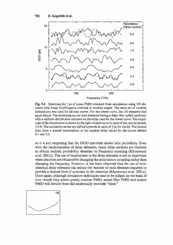
782 H. Kogelnik et al.
Retardation 15 Dither (cycles)-
-
5.0
2.0
1 .o 10 - -
Y
190 200 Frequency (THz)
Fig. 5.4 Spectrum for 1 ps of mean PMD obtained from simulations using 100 ele- ments with linear birefringence oriented at random angles. The same set of random orientations was used for all nine curves. For the lowest curve, the 100 elements had equal delays. The remaining curves used elements having a delay that varied randomly with a uniform distribution centered on the delay used for the lowest curve. The ampli- tude of the distribution is shown to the right of each curve in units of the optical period, 5.2 fs. The successive curves are shifted upwards in units of 2 ps for clarity. The dashed lines show a second instantiation of the random delay values for the curves labeled 0.1 and 5.0.
so it is not surprising that the DGD spectrum shows little periodicity. Even with the randomization of delay elements, many delay sections are required to obtain realistic probability densities by frequency scanning (Khosravani et al. 2001a). The use of randomness in the delay elements is not as important when densities are obtained by changing the polarization coupling rather than changing the frequency. However, it has been observed that the use of non- identical delay elements can reduce the number of such elements required to provide a desired level of accuracy in the densities (Khosravani et al. 2001a). Once again, although simulation techniques tend to be judged on the basis of how closely they mimic purely random PMD, actual fiber PMD and system PMD will deviate from this analytically tractable “ideal.”
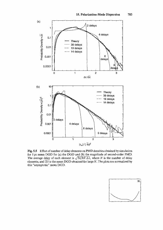
(a)
1
'2 .- 2.
.- 2. a n g 0.001 a
x 0.1 m c
0" 0.01 - m
15. Polarization-Mode Dispersion
k " " " " " " " " '
4 delays
0.0001 11 , , , , , , , I , ,
0 1 2 AT
3
1 N-
'2 v
:
; 0.001
X
m C
0 0.1
0 0.01 a n
.-
.- - m
0.0001
783
0 1 2 3
IrmlI ( a' Fig. 5.5 Effect of number of delay elements on PMD densities obtained by simulation for 1 ps mean DGD for (a) the DGD and (b) the magnitude of second-order PMD. The average delay of each element is J W G , where N is the number of delay elements, and is the mean DGD obtained for large N . The plots are normalized by this "asymptotic" mean DGD.
784 H. Kogelnik et al.
Much effort has been devoted to determining the influence of both the number of delay elements used in a simulation and the method used to couple between them (Prola et aI. 1997; Dal Forno et al. 2000; Lima et al. 2000; Khosravani et al. 2001a). Figure 5.5 illustrates the changes in several PMD probability densities as the number of delay elements used in the simulation is increased. These simulations used the algorithm based on Eq. 5.6. It can be seen that agreement with theory becomes better as the number of delay elements increases; the value at which the densities truncate increases as the number of delay elements increases; and, accuracy in second-order densities require more delay elements than the same degree of accuracy in first-order densities. The number of delay elements required for a particular application depends on the degree of accuracy required.
5.6 FURTHER READING
The importance of importance sampling in PMD simulation is demonstrated by Menyuk et al. (2001) and Lima et al. (2001), particularly for the densi- ties of finite element models near the truncation. Karlsson (2001a) provides exact probability densities for 3-D PMD models with finite number of delay elements.
6. System Impairments Due to PMD
Fiber PMD causes a variety of impairments in optical fiber transmission sys- tems. First of all there is the intersymbol interference (ISI) impairment of a single digital transmission channel. The IS1 impairment is caused by the differential group delay, A t , between the two pulses propagating in the fiber when the input polarization, & of the signal does not match the PSP of the fiber, j. In this first-order PMD effect the fractional powers launched into thePSPsarey= {s I p ) ( p I s ) = ; ( l + j . E ) a n d ( l - y ) = i ( 1 - j . ? ) . Systems impairments due to second- and higher-order PMD occur for larger signal bandwidths, particularly when these PMD components combine with chromatic fiber dispersion or signal chirp.
PMD impairments due to interchannel effects occur in polarization- multiplexed transmission systems. Examples are WDM systems where adja- cent wavelength channels are launched with orthogonal polarizations in order to suppress nonlinear impairments such as cross-phase modulation (XPM) or four-wave mixing (FWM). PMD destroys the orthogonality of these polariza- tions. A related PMD effect is the decorrelation between the polarizations of

15. Polarization-Mode Dispersion 785
pump and probe in Raman fiber amplifiers reducing polarization-dependent gain. Another example is a system wherein polarization multiplexing is used for close packing of WDM channels in order to achieve high bandwidth effi- ciency. Here, PMD induces coherent cross-talk between multiplexed channels leading to system impairments.
The above impairments of digital systems are described in the succeeding sections. For reviews of the impact of PMD on analog systems, the reader is referred to Poole and Nagel (1997) and to Ciprut et al. (1998). Literature discussing system impairments because of polarization-dependent loss (PDL) is listed in Section 6.8; the following sections assume absence of PDL.
6.1 POWER PENALTIES DUE TO FIRSTORDER PMD
In the first-order picture, PMD splits the input signal entering the fiber into two orthogonally polarized components that are delayed by At relative to each other during transmission. The impairment caused by this effect can be expressed as a power penalty E of the form (Poole et al. 1991)
&(dB) = (A/T2)At2y(l - y ) = A(At/2T)* sin’ 8, (6.1)
where the penalty, expressed in dB, is assumed to be small. Here, T is the bit interval, 0 5 y 5 1 is the power-splitting ratio, and 8 is the angle between the input polarization, ?, and the input PSP, h. The y(1 - y ) dependence shown in this expression has been verified by experiment in Kim et al. (2001a). The dimensionless A-parameter depends on pulse shape, modulation format, and specific receiver characteristics such as the detailed response of the electrical filter and whether optical or thermal noise predominates. For pin receivers the reported values for A range from 10 to 40 for NRZ and from 20 to 40 for RZ, whereas the A ranges for optically preamplified receivers are 10 to 70 for NRZ and 10 to 40 for RZ.
Jopson et al. (1999~) report the penalty measurements, emulations, and sim- ulations for optical preamplifiers shown in Fig. 6.1. For these specific receiver types, the data for NRZ transmission show a good fit to the penalty formula (6.1) for an A-parameter of about 60 to 70. For RZ transmission the measured A parameters range from about 15 to 25. Sunnerud et al. (2001a) used a differ- ent approach, reporting simulations for PMD-induced RZ and NRZ system degradation.
The DGD value, At, appearing in Eq. 6.1 is the “instantaneousyy DGD value, assumed to be constant during the penalty measurement. For polarization-maintaining fibers (PMFs), often used as PMD emulators, this constancy is assured. However, in communication fibers, the DGD and the
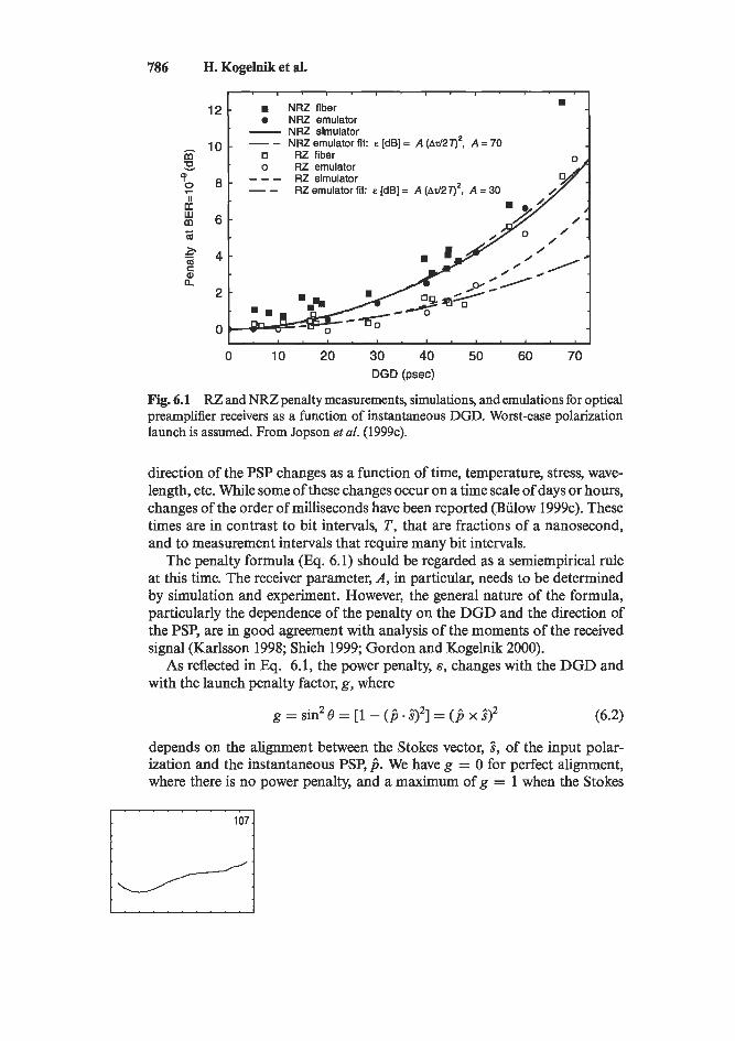
786 H. Kogelnik et al.
NRZ simulator NRZ emulator fit: E [de] = A ( A T I ~ ~ ' , A = 70
RZ fiber RZ emulator RZ simulator RZ emUlatOr fit: E [dB] = A (Ad2n2, A = 30
2
0 10 20 30 40 50 60 70 DGD (psec)
Fig. 6.1 RZ and NRZ penalty measurements, simulations, and emulations for optical preamplifier receivers as a function of instantaneous DGD. Worst-case polarization launch is assumed. From Jopson et al. (1999~).
direction of the PSP changes as a function of time, temperature, stress, wave- length, etc. While some of these changes occur on a time scale of days or hours, changes of the order of milliseconds have been reported (Biilow 1999~). These times are in contrast to bit intervals, T , that are fractions of a nanosecond, and to measurement intervals that require many bit intervals.
The penalty formula (Eq. 6.1) should be regarded as a semiempirical rule at this time. The receiver parameter, A, in particular, needs to be determined by simulation and experiment. However, the general nature of the formula, particularly the dependence of the penalty on the DGD and the direction of the PSP, are in good agreement with analysis of the moments of the received signal (Karlsson 1998; Shieh 1999; Gordon and Kogelnik 2000).
As reflected in Eq. 6.1, the power penalty, E , changes with the DGD and with the launch penalty factor, g , where
(6.2) 2 g = sin e = [I - (j .i)7 = (j x i)2
depends on the alignment between the Stokes vector, i, of the input polar- ization and the instantaneous PSP, j. We have g = 0 for perfect alignment, where there is no power penalty, and a maximum of g = 1 when the Stokes
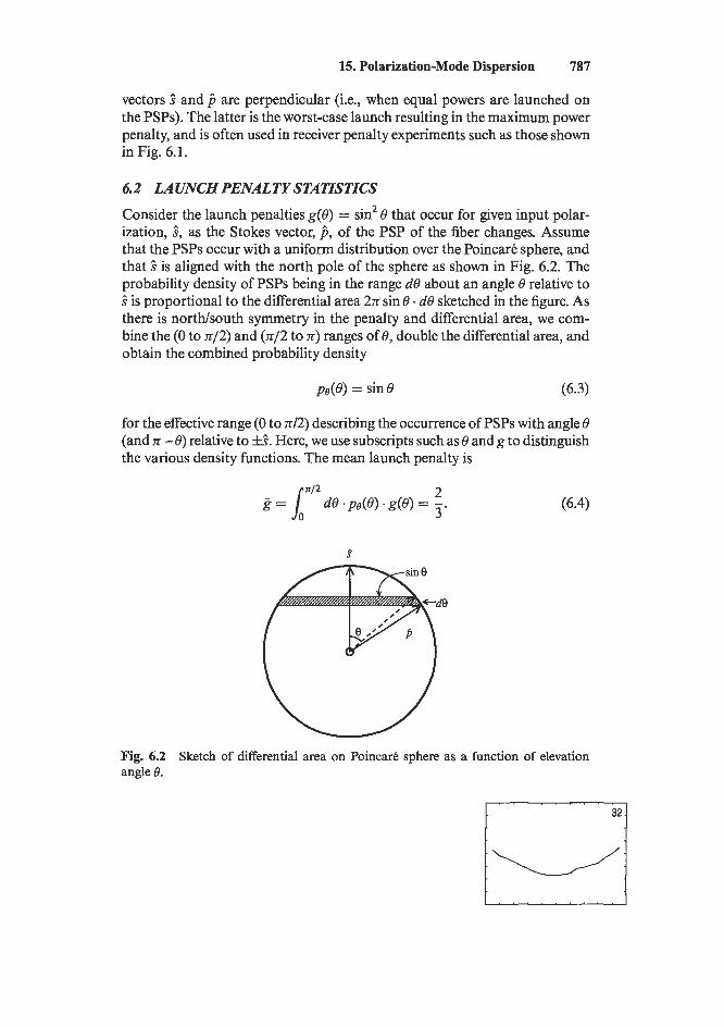
15. Polarization-Mode Dispersion 787
vectors ; and j are perpendicular (i.e., when equal powers are launched on the PSPs). The latter is the worst-case launch resulting in the maximum power penalty, and is often used in receiver penalty experiments such as those shown in Fig. 6.1.
6.2 LAUNCH PENALTY STATISTICS
Consider the launch penalties g(8) = sin2 8 that occur for given input polar- ization, ;, as the Stokes vector, f i , of the PSP of the fiber changes. Assume that the PSPs occur with a uniform distribution over the Poincart sphere, and that P is aligned with the north pole of the sphere as shown in Fig. 6.2. The probability density of PSPs being in the range d8 about an angle 8 relative to ; is proportional to the differential area 2n sin 8. d8 sketched in the figure. As there is northhouth symmetry in the penalty and differential area, we com- bine the (0 to n/2) and (n/2 to n) ranges of 8, double the differential area, and obtain the combined probability density
ps(8) = sin 8 (6.3)
for the effective range (0 to n/2) describing the occurrence of PSPs with angle 8 (and 7t - 8) relative to hi. Here, we use subscripts such as 8 and g to distinguish the various density functions. The mean launch penalty is
Fig. 6.2 Sketch of differential area on Poincart sphere as a function of elevation angle 0.
788 H. Kogelnik et al.
This mean value is relatively large compared to the maximum of g = 1 as there is more area for PSPs near the equator than there is near the pole.
The probability density for the occurrence of a launch penalty g is
P ~ W =Pe(eW * dQ/dg = ;/G- (6.5)
Integrating this density one finds the cumulative probability of a penalty g exceeding the value G as
Inserting G = 0.75, we find that for 50% of the possible PSPs, the launch penalty exceeds 75% of the maximum penalty of 1. This means that for one- half of the PSPs occurring in a fiber as time changes, the launch penalties are almost as large as those obtained in worst-case tests.
6.3 SYSTEM OUTAGE DUE TO PMD
Outage specifications for optical fiber transmission systems depend on the application. Usually one requires the power penalty contributions of PMD to be less than 1 dB for all but a specified cumulative probability. This speci- fication ranges between outage probabilities of and Disregarding the potentially large PMD correlation times (see the 19 hours mentioned in Section 7), this is commonly translated to average cumulative outages ranging from fractions of a second to 60 minutes per year. To specify this limit one requires knowledge of the probability density, P,(E), for the occurrence of a power penalty E. The penalty formula (6.1) shows that E is proportional to the product of the launch penalty g and a DGD term, At2. The probability den- sity of g for uniform distribution over the Poincart sphere is given in Eq. 6.5. The density of A t is Maxwellian (see Table 4.1) from which the density of the DGD term can be derived. From the densities for g and the DGD term, one can deducep,(s) using standard probability theory for the density of a product (Poole and Nagel 1997).
However, we follow another, more direct, approach shedding further light on the mechanisms of PMD penalty statistics. In view of A t 2 ( j x i)2 = (2 x i)2 = (21 x i)2 = At: we can rewrite the first-order penalty formula as
E = (A/4T2)Ati, (6.7)
where 21 is the component of 2 perpendicular to i, and A t 1 is its magnitude. The penalty E is caused only by the components of the PMD vector 2 that are perpendicular to i. The statistics of the two components of 21 are described by

15. Polarization-Mode Dispersion 789
two independent Gaussians. The magnitude A t l , therefore, follows a Rayleigh distribution, with the probability density
where
and is the mean DGD. The mean penalty parameter is, therefore, oc
(6.10) E = Jd dx. E ( X ) . P A ~ ~ ( X ) = Aa2/2T2 = (nA/16T 2 ) A t -2 .
One can now transform the Rayleigh density for AT^ to the density for E and obtain the known exponential (Boltzmann) distribution:
~ E ( E ) - = P A ~ - ( A T ~ ( E ) ) . dArl /dE = (l/E) . e-'/'. (6.11)
Figure 6.3 shows a test of the exponential density predicted by Eq. 6.11 using computer simulation (Poole and Nagel 1997). Here, the frequency of occurrence for penalties was calculated far 10,000 fibers, each modeled as a concatenation of 1000 birefringent fiber sections with random orientation. Good agreement was found between the simulated data and the predictions.
From Eq. 6.11 follows the outage probability, Pout, i.e., the probability for the penalty to exceed N dB,
(6.12)
where the penalty limit, N , is usually specified as 1 or 2 dB. The mean penalty associated with the specification of an outage probability, Pout, is
E =N/ln(l/Pout). (6.13)
Inserting Eq. 6.10 we can formulate this condition as a requirement for the mean DGD of the fiber:
A ~ / T = 4 . &/Jn A . In (l/Pout), (6.14)
where A is the receiver parameter discussed earlier. Figure 6.4 shows a plot of this requirement for three values of the parameter AIN covering the men- tioned range of values encountered in NRZ and RZ systems. Note that for

790 H. Kogelnik et al.
0
-1
h
VI C
C -2 = CI)
B
6 3
-3
-4
Simulation Results
- Exponential Fit with A = 25
0.0 0.5 1 .o 0.5 2.0 Power Penalty E in (dB)
Fig. 6.3 Test of the exponential distribution of the power penalty,p,(s), by computer simulation. From Poole and Nagel (1 997).
an outage probability of (3 seconds/year), a typical RZ system (A = 30, N = 1) requires a At/T ratio of 10% whereas the corresponding typical NRZ system (A = 70, N = 1) requires At/T to be less than 7% (assuming receivers with optical preamplifers). We should reemphasize that A values are strongly dependent on pulse shape and receiver chracteristics and must be determined for each specific system.
Some workers find it convenient to express this requirement in terms of the DGD value, A ~ L , that characterizes a worst-case-launch PMD penalty measurement in the laboratory, such as that shown in Fig. 6.1. Here, ATL is the 1-dB intercept, i.e., the instantaneous DGD value causing a 1-dB PMD penalty. The intercept ATL follows from Eq. 6.1 by setting E = 1 and y = 1/2. The requirement for the mean fiber DGD becomes
A t / a t ~ = 2.&/,/n-ln(l/POut) (6.15)
Figure 6.5 shows a graph of this requirement for two outage criteria (N = 1 dB and N = 2dB). For an outage probability of loe5 and N = 1, the required
-
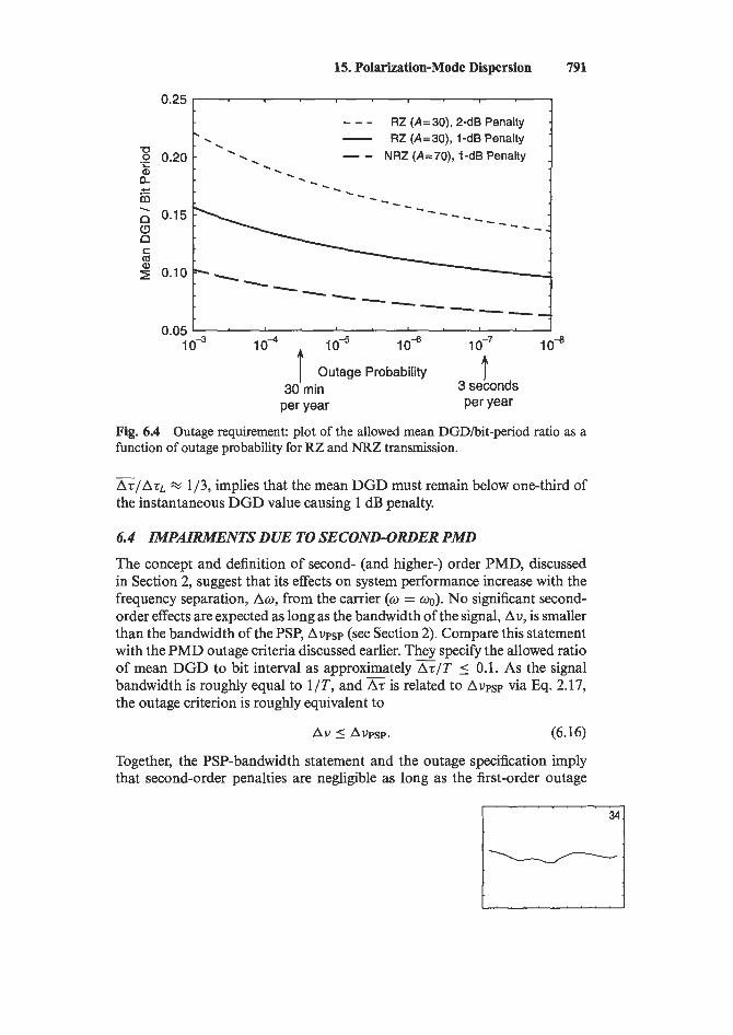
15. Polarization-Mode Dispersion 791
0.25 - - - RZ (A=30), 2-dB Penalty . - RZ (A=30) , 1-dB Penalty - - NRZ (A=70), I-dB Penalty
.r
. \ \
. . . . . . m .- 0 0.20 - & a - - .- c - -_ m - - - - -
- - - _ . - - - - - - -
--- -- 0.05
- A t / A q the instantaneous DGD value causing 1 dB penalty.
113, implies that the mean DGD must remain below one-third of
6.4 IMPAIRMENTS DUE TO SECOND-ORDER PMD
The concept and definition of second- (and higher-) order PMD, discussed in Section 2, suggest that its effects on system performance increase with the frequency separation, Aw, from the carrier (w = wo). No significant second- order effects are expected as long as the bandwidth of the signal, Au, is smaller than the bandwidth of the PSP, Aupsp (see Section 2). Compare this statement with the PMD outage criteria discussed earlier. They specify the allowed ratio of mean DGD to bit interval as approximately Z / T 5 0.1. As the signal bandwidth is roughly equal to 1/T, and at is related to Aupsp via Eq. 2.17, the outage criterion is roughly equivalent to
AU 5 A~psp . (6.16)
Together, the PSP-bandwidth statement and the outage specification imply that second-order penalties are negligible as long as the first-order outage
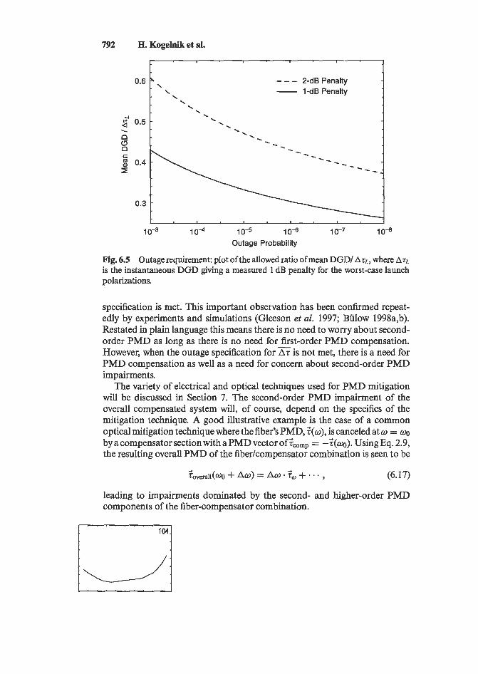
792 H. Kogelnik et al.
t 1
\
- - - 2-dB Penalty - 1-dB Penalty
. n x
0.3
1 09 1 o4 I 0-5 1 04 10-7 10-8 Outage Probability
Fig. 6.5 Outage requirement: plot of the allowed ratio ofmean DGDI ArL, where ArL is the instantaneous DGD giving a measured 1 dB penalty for the worst-case launch polarizations.
specification is met. This important observation has been confirmed repeat- edly by experiments and simulations (Gleeson et al. 1997; Biilow 1998a,b). Restated in plain language this means there is no need to worry about second- order PMD as long as there is no need for first-order PMD compensation. However, when the outage specification for is not met, there is a need for PMD compensation as well as a need for concern about second-order PMD impairments.
The variety of electrical and optical techniques used for PMD mitigation will be discussed in Section 7. The second-order PMD impairment of the overall compensated system will, of course, depend on the specifics of the mitigation technique. A good illustrative example is the case of a common optical mitigation technique where the fiber’s PMD, ?(w), is canceled at w = q by a compensator section with a PMD vector of 2comp = -?(wg). Using Eq. 2.9, the resulting overall PMD of the fiberkompensator combination is seen to be
Zo-l1(~o + Am) Am * 2, + * . . , (6.17)
leading to impairments dominated by the second- and higher-order PMD components of the fiber-compensator combination.
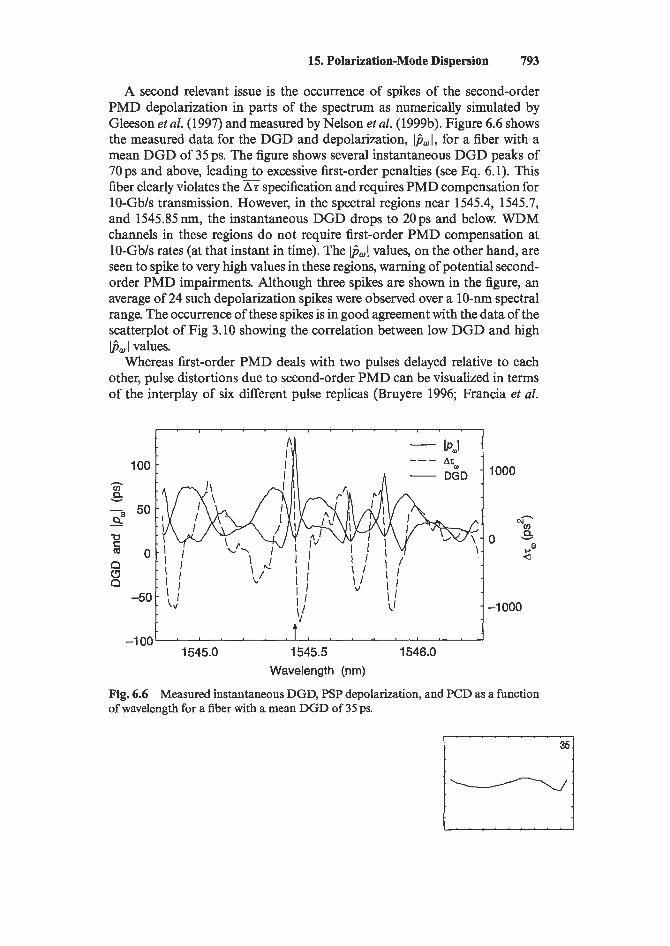
15. Polarization-Mode Dispersion 793
A second relevant issue is the occurrence of spikes of the second-order PMD depolarization in parts of the spectrum as numerically simulated by Gleeson et al. (1997) and measured by Nelson et al. (1999b). Figure 6.6 shows the measured data for the DGD and depolarization, pwl, for a fiber with a mean DGD of 35 ps. The figure shows several instantaneous DGD peaks of 70 ps and above, leading to excessive first-order penalties (see Eq. 6.1). This fiber clearly violates the at specification and requires PMD compensation for 10-Gb/s transmission. However, in the spectral regions near 1545.4, 1545.7, and 1545.85nm7 the instantaneous DGD drops to 20ps and below. WDM channels in these regions do not require first-order PMD compensation at 10-Gb/s rates (at that instant in time). The $J values, on the other hand, are seen to spike to very high values in these regions, warning of potential second- order PMD impairments. Although three spikes are shown in the figure, an average of 24 such depolarization spikes were observed over a 10-nm spectral range. The occurrence of these spikes is in good agreement with the data of the scatterplot of Fig 3.10 showing the correlation between low DGD and high $ w l values.
Whereas first-order PMD deals with two pulses delayed relative to each other, pulse distortions due to second-order PMD can be visualized in terms of the interplay of six different pulse replicas (Bruyere 1996; Francia et al.
1000
-1 000
Wavelength (nm)
Fig. 6.6 Measured instantaneous DGD, PSP depolarization, and PCD as a function of wavelength for a fiber with a mean DGD of 35 ps.

794 H. Kogelnik et al.
1998). These mechanisms result in pulse overshoots and the generation of satellite pulses. For higher PMD orders, Leppla and Weiershausen (2000) suggest distortion mechanisms involving a number of pulses proportional to AV/A*SP.
The simplest second-order impairment mechanism is polarization- dependent chromatic dispersion (PCD) first pointed out by Poole and Giles (1988c,d). As explained in Section 2, PCD is caused by the ;, component parallel to the PSI? It is described by the PCD measure TA defined in Eq. 2.12. Given a fiber chromatic dispersion, DL, the PCD impairment is equivalent to that of an effective chromatic dispersion of the transmission system,
(DL)eff = DL f TA, (6.18)
that is different for the two PSPs as the plus/minus signs indicate. While PCD is a simple mechanism, it is a relatively minor component of the second-order PMD vector since 2, has a statistical tendency to point away from the PSP (see Section 4). The dominant impairment mechanism is due to the depolarization component perpendicular to the PSP that is proportional to Pm I .
Statistical analyses and numerical simulations of system impairments indi- cate a strong interaction between chromatic dispersion in the fiber and the second-order PMD in general (Bruykre 1996; Penninckx and Bruybre 1998). Similarly, it has been found that chirp in the transmitted signal has a significant impact on second-order PMD impairments (Biilow 1998b).
Recent PMD vector measurements have enabled the correlation of system penalties to measured instantaneous first- and second-order PMD vectors (Nelson et al. 2000b). In these experiments, signal launch polarizations were known and controlled relative to the PSP and the second-order PMD vector. Impairments were found to be dependent on chirp and chromatic dispersion, and to be highly dependent on launch polarization. Measurements of the impairment of IO-Gb/s NRZ signals were made near the depolarization spike at 1545.45 nm of the fiber with 35 ps mean DGD (Fig. 6.6). Care was taken to ensure a dispersion-free system, however, signal chirp was known to be present and is thought to be responsible for the large penalties that were observed. As an illustration, Fig. 6.7 shows the output bit patterns and eye diagrams for the three launch polarizations with the largest impairments. These launches were perpendicular in Stokes space, with +pa, indicating a polarization aligned with j,, -p indicating alignment with the fast PSP and -pp designating a launch perpendicular to these two. Pulse overshoots in the output bit patterns are evident. Large optical-receiver penalties were measured for these three launches reaching as high as 4 dB for thep, alignment. Launch polarizations
I
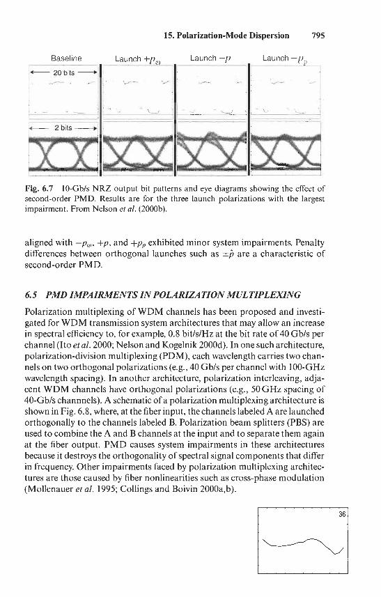
15. Polarization-Mode Dispersion 795
Fig. 6.7 lO-Gb/s NRZ output bit patterns and eye diagrams showing the effect of second-order PMD. Results are for the three launch polarizations with the largest impairment. From Nelson et al. (2000b).
aligned with -pw, +p, and +pp exhibited minor system impairments. Penalty differences between orthogonal launches such as =tj are a characteristic of second-order PMD.
6.5 PMD IMPAIRMENTS IN POLARIZATION MULTIPLEXING
Polarization multiplexing of WDM channels has been proposed and investi- gated for WDM transmission system architectures that may allow an increase in spectral efficiency to, for example, 0.8 bit/s/Hz at the bit rate of 40 Gb/s per channel (It0 etal. 2000; Nelson and Kogelnik 2000d). In one such architecture, polarization-division multiplexing (PDM), each wavelength carries two chan- nels on two orthogonal polarizations (e.g., 40 Gb/s per channel with 100-GHz wavelength spacing). In another architecture, polarization interleaving, adja- cent WDM channels have orthogonal polarizations (e.g., 50 GHz spacing of 40-Gb/s channnels). A schematic of a polarization multiplexing architecture is shown in Fig. 6.8, where, at the fiber input, the channels labeled A are launched orthogonally to the channels labeled B. Polarization beam splitters (PBS) are used to combine the A and B channels at the input and to separate them again at the fiber output. PMD causes system impairments in these architectures because it destroys the orthogonality of spectral signal components that differ in frequency. Other impairments faced by polarization multiplexing architec- tures are those caused by fiber nonlinearities such as cross-phase modulation (Mollenauer et al. 1995; Collings and Boivin 2000a,b).
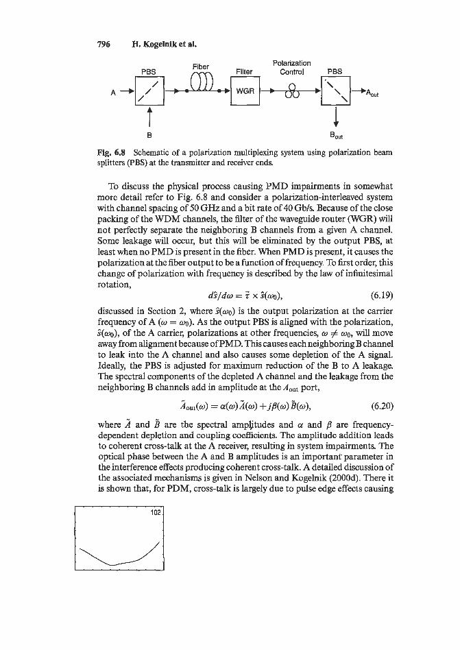
796 H. Kogelnik et al.
Polarization Fiber A +,/P;/ ,-, Filter , Control
WGR e D
t B
?J ‘ +Ao”t
1 BO,
Fig. 6.8 Schematic of a polarization multiplexing system using polarization beam splitters (PBS) at the transmitter and receiver ends.
To discuss the physical process causing PMD impairments in somewhat more detail refer to Fig. 6.8 and consider a polarization-interleaved system with channel spacing of 50 GHz and a bit rate of 40 Gb/s. Because of the close packing of the WDM channels, the a te r of the waveguide router (WGR) will not perfectly separate the neighboring B channels from a given A channel. Some leakage will occur, but this will be eliminated by the output PBS, at least when no PMD is present in the fiber. When PMD is present, it causes the polarization at the fiber output to be a function of frequency. To first order, this change of polarization with frequency is described by the law of inkitesimal rotation,
&/dw = ? x i(wg), (6.19) discussed in Section 2, where i(w0) is the output polarization at the carrier frequency of A (w = wg). As the output PBS is aligned with the polarization, i(wg), of the A carrier, polarizations at other frequencies, w # wg, will move away from alignment because of PMD. This causes each neighboring B channel to leak into the A channel and also causes some depletion of the A signal. Ideally, the PBS is adjusted for maximum reduction of the B to A leakage. The spectral components of the depleted A channel and the leakage from the neighboring B channels add in amplitude at the A,,, port,
A O U t b ) = a(w)A(w) +jP(w) my (6.20)
where A and 8 are the spectral ampljtudes and a and are frequency- dependent depletion and coupling coefficients. The amplitude addition leads to coherent cross-talk at the A receiver, resulting in system impairments. The optical phase between the A and B amplitudes is an important parameter in the interference effects producing coherent cross-talk. A detailed discussion of the associated mechanisms is given in Nelson and Kogelnik (2000d). There it is shown that, for PDM, cross-talk is largely due to pulse edge effects causing
J
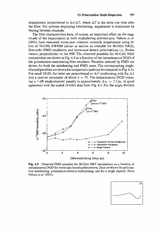
15. Polarization-Mode Dispersion 797
impairments proportional to A t / A T , where AT is the pulse rise time after the filter. For systems employing interleaving, impairment is dominated by beating between channels.
The filter characteristics have, of course, an important effect on the mag- nitude of the impairments in both multiplexing architectures. Nelson et al. (200 1) have measured worst-case coherent crosstalk impairments using fil- ters of 50-GHz FWHM (about as narrow as tolerable for 4O-Gb/s NRZ), first-order PMD emulation, and worst-case launch polarizations, i.e., Stokes vectors perpendicular to the PSP. The observed penalties for 4O-Gb/s NRZ transmission are shown in Fig. 6.9 as a function of the instantaneous DGD of the polarization-maintaining-fiber emulator. Penalties induced by PMD are shown for both the interleaving and PMD cases. The corresponding single- channel penalties are shown for comparison (and can be compared to Fig. 6.1). For small DGD, the latter are proportional to A t 2 conforming with Eq. 6.1 and a receiver parameter of about A = 70. The instantaneous DGD induc- ing a 1-dB single-channel penalty is approximately ATL = 7 . 5 ~ ~ ~ in good agreement with the scaled lO-Gb/s data from Fig. 6.1. For the single 4O-Gb/s
- Polarization Interleaved v- - + Single Channel
3 2 0 2 4 6 8 10
Differential Group Delay (ps)
Fig. 6.9 Observed PMD penalties for 4O-Gb/s NRZ transmission as a function of instantaneous DGD for worst-case launch polarizations. Data are shown for polariza- tion interleaving, polarization-division multiplexing, and for a single channel. From Nelson et al. (2001).
798 H. Kogelnik et al.
channel, the penalty statistics of Section 6.3 translates this ATL value into an allowable mean fiber DGD of (see Eq. 6.15).
We note in the figure that the penalties for the two polarization multiplex- ing cases are about equal and that they are also nearly proportional to A t 2 . However, here the instantaneous DGD for a 1-dB penalty is A ~ L = 1.5 ps, a factor of 5 less than in the single-channel case. For the interleaving case this value agrees with the measurements of Ito et al. (2000). This suggests that the polarization-multiplexed systems with high spectral efficiency considered here are about a factor of five more sensitive to PMD impairments than a single-transmission channel. While detailed outage statistics for polarization- multiplexed systems have yet to be developed, we note some close similarities between the single-channel case (whose statistics are described in Section 6.3) and the case of polarization multiplexing: In both cases the penalties depend quadratically on A t , and in both cases the underlying mechanisms seem to depend on the perpendicular component ATL only (see, e.g., Eq. 6.19). One would, therefore, expect that the allowable mean fiber DGD for the mentioned polarization-multiplexed 40-Gbh systems is about 0.5 ps for a 1 dB-outage of 1 O-5.
= 2.5ps for a 1 dB-penalty outage of
6.6 PMD EFFECT ON THE REDUCTIONOF F W A N D X P M B Y POLARIZATION INTERLEAVING
Four-wave mixing (FWM) and cross-phase modulation (XPM) are two effects caused by fiber nonlinearities that result in considerable system impairments in WDM long-haul and ultra-long-haul transmission (Forghieri et al. 1997). System designs attempt to minimize these impairments by maximizing the WDM wavelength spacing and by judicious management of local power lev- els and local fiber dispersion, the technique called dispersion management. As the FWM and XPM effects are strongly dependent on the relative polarization between the relevant WDM channels, the technique of polarization interleav- ing has been proposed and explored for the reduction of these effects (Hill et al. 1978; Mahon 1990; Inoue 199 1 ; Evangelides et al. 1992). The system layout for this technique is similar to the one sketched in Fig. 6.8, with two notable differ- ences: (1) the optical filters of the WDM channels are chosen narrow enough compared to the wavelength separation so that no coherent crosstalk occurs (as opposed to Section 6.5), (2) the output PBS is usually not present (for an exception note Mahon et al. 1996). Polarization interleaving can reduce the power level of some of the important FWM components generated in the fiber by a factor of four and eliminate other important FWM components (Inoue
I
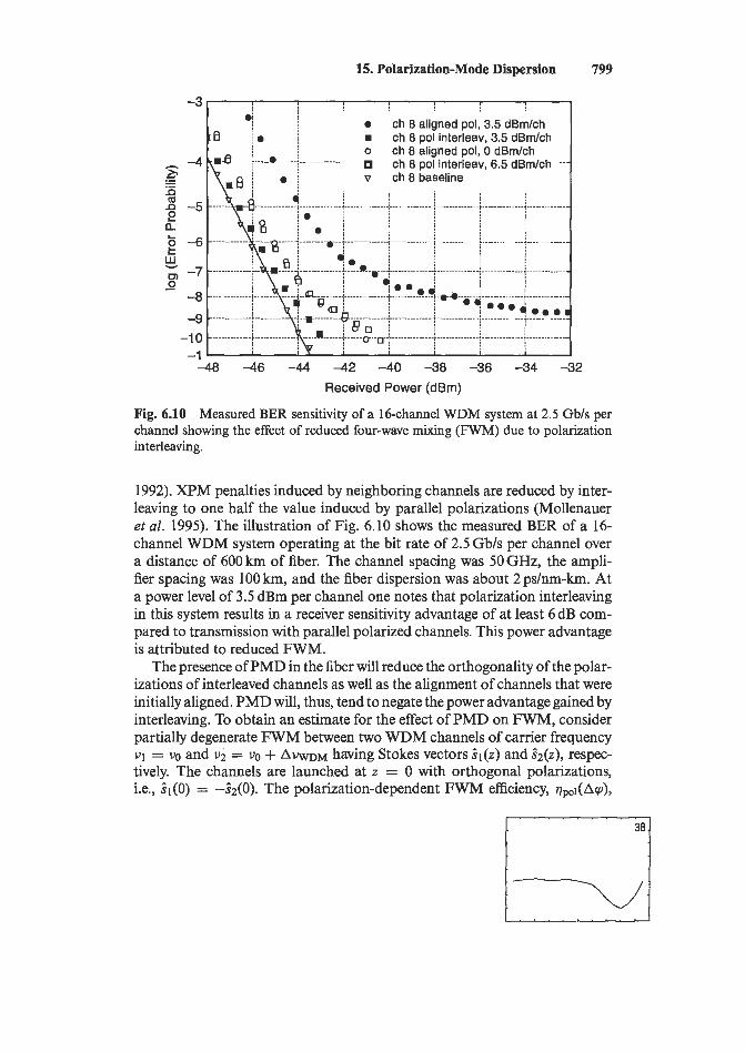
15. Polarization-Mode Dispersion 799
w ch 8 pol interleav, 3.5 dBm/ch o ch 8 aligned pol, 0 dBrn/ch
ch 8 pol interleav, 6.5 dBrn/ch -
-48 -46 -44 -42 -40 -38 -36 -34 -32 Received Power (dBm)
Fig. 6.10 Measured BER sensitivity of a 16-channel WDM system at 2.5 Gb/s per channel showing the effect of reduced four-wave mixing (FWM) due to polarization interleaving.
1992). XPM penalties induced by neighboring channels are reduced by inter- leaving to one half the value induced by parallel polarizations (Mollenauer et al. 1995). The illustration of Fig. 6.10 shows the measured BER of a 16- channel WDM system operating at the bit rate of 2.5 Gb/s per channel over a distance of 600 km of fiber. The channel spacing was 50 GHz, the ampli- fier spacing was 100 km, and the fiber dispersion was about 2 ps/nm-km. At a power level of 3.5 dBm per channel one notes that polarization interleaving in this system results in a receiver sensitivity advantage of at least 6 dB com- pared to transmission with parallel polarized channels. This power advantage is attributed to reduced FWM.
The presence of PMD in the fiber will reduce the orthogonality of the polar- izations of interleaved channels as well as the alignment of channels that were initially aligned. PMD will, thus, tend to negate the power advantage gained by interleaving. To obtain an estimate for the effect of PMD on FWM, consider partially degenerate FWM between two WDM channels of carrier frequency u1 = uo and v2 = uo + AWDM having Stokes vectors &(z) and i2(z), respec- tively. The channels are launched at z = 0 with orthogonal polarizations, i.e., 51 (0) = -52(0). The polarization-dependent FWM efficiency, qpol(Aq),
l " " " " ' l 38

800 H. Kogelnik et al.
depends on the Stokes angle, Ap(z), of the misalignment of iz(z) relative to the ideal orthogonal alignment, -&(z). (Note that, with this notation, the two polarizations become parallel when the misalignment reaches Ap = n.) This alignment changes with the frequency spacing, AWM, and the prop- agation distance, z, in the fiber. The efficiency is qpol(0) = 0 for orthogonal polarizations and qpol(n) = 1 for parallel polarizations. For reasonably small misalignments we have, using the results of Inoue (1992),
qp0dAd = ;AVO2. (6.21)
PMD causes the misalignment, Ap(z), to change randomly with position, z, in the fiber. Within the bandwidth of the PSP, Aupsp = 1/(8=), the misalign- ment is determined by the law of infinitesimal rotation of the output Stokes vectors (Eq.2.6)as Ap = 2 n . A t . s i n I 3 . A ~ ~ ~ ~ whereAt(z)isthelocalDGD, and e(z) is the angle between i 2 and the local PSF? In our above experiment, for example, where the mean DGD was = 2.4 ps and Aupsp = 50 GHz, angular shifts as large as A&) = 30" were measured at the fiber output
The overall FWM efficiency (qpol) of the system represents a weighted average over the local efficiencies qpol(z) throughout the length, L, of the transmission system. Assuming a uniform distribution of the relative PSP angles I3 over the Poincark sphere, we have, according to Eq. 6.4, that (sin28) = 2/3. The model further assumes that the local instantaneous DGDs, At(z), fluctuate around the mean DGD. The mean square DGD, (At2(z)), grows linearly with z, leading to a distance-averaged DGD term of (1/2)(At2(L)) = (3n/16)z2. Thus, we obtain an overall FWM efficiency of
(z = L).
(6.22)
Since random polarizations will lead to an FWM efficiency of qpol = 1/2, we judge interleaving to be effective as long as the FWM efficiencies are below about 1/4. This happens as long as
AWDM 5 1/(4G) = 2Avpsp. (6.23)
Note that this rule of thumb depends on the mean DGD of the transmission line only. It should, therefore, be the same for all WDM channels, regardless of instantaneous DGD fluctuations with frequency.
Now compare the rule of thumb for the effkctiveness of interleaving with the single-channel outage criterion as stated in Eq. 6.16 in terms of the signal bandwidth Au. Recall that for closely packed WDM we have, approximately,
I
15. Polarization-Mode Dispersion 801
AWDM = 2Au. For this case it follows that interleaving should be effective in suppressing FWM in closely packed WDM systems as long as the single channels do not require first-order PMD compensation.
While rule (6.23) requires further testing, it is consistent with our exper- imental results of Fig. 6.10 where A ~ M was suf€iciently small to prevent PMD effects, and those of Hansryd et al. (2000), as well as the results of Kovsh et al. (2001), who have found the same rule by numerical simulation of a transoceanic system.
Hansryd et al. (2000) also discuss the correlation function, (& . 52), derived by Karlsson et al. (2000a), providing a compact description of the scrambling of polarizations occurring when the frequency spacings, Aw = ~ ~ A V W D M , exceed the bandwidth of the PSP. The correlation function is
(& -&) = ?," exp(-Ad(At2)/3), (6.24)
for the dot product of the output Stokes vectors, 51 (9) and &(w + Aw), at two different frequencies for given input Stokes vectors, Sp. Equation 6.24 tells us that polarizations get totally scrambled for large frequency spacings and large distances, leading to their uniform distribution over the Poincark sphere. The correlation drops to one half for A w G = ,/- or A W D M ~ = 0.21, defining the correlation length used in Section 6.7. At large spacings the expected angle between the Stokes vectors of two frequencies is n/2 (i.e., ( i 1 . i 2 ) = 0). Both initially parallel alignments (i'p = i:) and initially orthog- onal polarizations (5: = -i?) will diffuse to this n/2 value. At this point FWM and XPM become the same for both parallel and orthogonal polar- ization launches. We find that the application of the correlation function also leads to rule (6.23).
Finally, we should mention that PMD is not the only effect that can destroy the initial alignment of signal polarizations carried by two (or more) different frequencies in a fiber. There is another effect, sometimes called "power- dependent PMD," which is a second aspect of XPM. This nonlinear process causes the two Stokes vectors i l (w0) and iz(w0 + Aw) to precess around one another (Mollenauer et al. 1995). Due to the nonlinearity, the infinitesimal rotation law for the change of a Stokes vector after traversal of a short section, dz, of fiber assumes the generalized form
(6.25)
governing the above precession, where p~ = 2nn2P2/hteff is the normal- ized power level of channel 2, A,ff is the effective area of the fiber, n2 is the
802 H. Kogelnik et al.
polarization-averaged nonlinear index, and P2 is the power in channel 2 (the differential rotation for & is obtained by interchanging indices). The birefrin- gence vector 3 appears also in the dynamical PMD equation (Eq. 2.8), whose relation to the linear rotation law (for p2 = 0) is detailed in Gordon and Kogelnik (2000). The power-dependent PMD effect associated with Eq. 6.25 can accelerate the scrambling or depolarization of the WDM channels beyond the rate caused by PMD alone. Collings and Boivin (2000a) have reported quantitative results of this depolarization in an interleaved WDM transmis- sion system measuring impairments for power levels ranging from 0 to 10 dBm per channel. Further, they have shown that the depolarization can change from bit to bit, making compensation of associated impairments in interleaved sys- tems very difficult. Even without interleaving, WDM channels can interact to induce power-dependent PMD and depolarization in each individual chan- nel. This effect creates an obstacle to optical PMD mitigation as discussed by Moller et al. (~OOOC), Moller et al. (2001) and Khosravani et al. (2001b). Section 7 also discusses the PMD resistance of solitons, another manifestation of the interaction of fiber nonlinearities and PMD.
6.7 PMD EFFECTS ON POLARIZATION-DEPENDENT GAIN IN RAMAN AMPLIFIERS
The gain in fiber Raman amplifiers is known to depend on the relative alignment between the pump and signal polarizations. When the two polar- izations are aligned, the gain can be as much as 10 times larger than the gain for orthogonal polarizations. This effect is a relative of PDL and is called polarization-dependent gain (PDG). There is no PDG when a depolarized pump is used (Zhang et al. 2000). The presence of PMD in the fiber will scram- ble the relative alignment of the polarizations to various degrees and reduce PDG. When the pump is counterpropagating, the scrambling is so strong that PDG is minimized. PDG is strongest when a polarized copropagating pump is used, and the following discussion addresses this case. Consider a Raman pump spaced Au from the optical carrier frequency and an effective Raman interaction length, L, in the fiber. The correlation between the pump and sig- nal polarizations in the presence of PMD is described by Eq. 6.24 discussed in Section 6.6. As the mean DGD in the fiber grows with the square root of the distance, =(z) = =(L) m, one can determine the correlation length, L,,, for the two polarizations from the condition AuEmrr = 0.21 mentioned in Section 6.6. Thus we can visualize the Raman interaction as N statistically independent interactions in N sections of fiber of constant relative

15. Polarization-Mode Dispersion 803
polarizations between pump and signal. The number of these sections is
N = L/L,,,, % 22Au2z2, (6.26)
where nt = At(L) is the mean DGD of the interaction length. For large N , the relative polarizations in the sections can be assumed to be uniformly dis- tributed over the Poincart: sphere. Their mean determines the mean gain. The PDG is related to the standard deviation, which scales like l / a , predicting a PDG inversely proportional to the mean DGD of the interaction length.
An illustrative example is a typical pump frequency spacing of 100 nm, i.e., Au = 12.5THzY and a mean DGD of 0.1 ps. For this case one gets N = 35 independent interactions. For more detail refer to Mahgerefteh et al. (1997) who report experimental investigations of the PDG of Raman amplifiers as a function of PMD. Ebrahimi et al. (2001) study the statistics of PDG in fiber Raman amplifiers due to PMD by simulation and experiment. Their results show that a mean DGD of 0.66 ps is enough to reduce the mean PDG to 10% of the average gain.
A -
6.8 FURTHER READING
More information on PMD system impairments can be found in Beltrame et al. (2000), Cameron et al. (2000), Chowdhury et al. (2000), Lee et al. (2000), Shieh (2000a), Bruyere and Audouin (1994a), Zhou and O’Mahoney (1994), and Yamamoto et al. (1989).
Literature on PDL system impairments includes Wang and Menyuk (200 l), Haunstein and Kallert (2001a), Kim et al. (2001b), Yan et al. (2001), Bessa dos Santos et al. (2000), Huttner et al. (2000), Gisin (1995), and Bruyere and Audouin (1994b).
Second-order PMD impairments are discussed in Watley et al. (1999b), Ciprut et al. (1998), and Bruyere et al. (1997).
More information on polarization multiplexing can be found in Him et al. (2001), Yeniay et al. (2000), Zheng et al. (2000), and Bergano et al. (1998).
7. PMD Mitigation
Increased understanding of PMD and its system impairments, together with a quest for higher transmission bandwidths, has motivated considerable recent work on PMD mitigation. One of the primary objectives has been to enable sys- tem upgrades from 2.5-Gb/s to lO-Gb/s or from lO-Gb/s to 40-Gb/s on older, embedded, high-PMD fibers. PMD compensation techniques must reduce the

804 H. Kogelnik et al.
impact of first-order PMD and should reduce higher-order PMD effects or at least not increase the higher-order PMD. The techniques should also be able to rapidly track changes in PMD, including changes both in the DGD and the PSPs. Other desired characteristics of PMD mitigation techniques are low cost and small form factor to minimize the impact on existing system architectures. In addition, mitigation techniques should have a small number of control parameters to enable manageable feedback algorithms.
In this section we will review various methods of PMD mitigation, from the simple methods, which include deploying low-PMD fiber or using a PMD- tolerant modulation format, to more complex optical or electrical PMD compensation techniques that may be implemented at the transmitter or the receiver. As the compensation techniques must follow the temporal varia- tions of PMD, we will also outline several monitoring techniques that provide information for the feedback loops and algorithms controlling the PMD com- pensators. Note that, as no uniform standard to measure the effectiveness of the various compensation schemes currently exists, we quote the DGD values of the compensated systems as reported in the literature. The reader is advised to consult the cited references for further detail.
7.1 TIME RATE OF CHANGE OF PMD
The required speed of PMD compensators depends on the time rate of change of the PMD in installed fiber links. A number of groups have made long- term PMD measurements, and the consensus is that temperature changes in embedded fibers are slow in general and cause slow PMD variations, Le., on the time scale of hours (Bulow and Veith 1997; Cameron et al. 1998b; Taka- hashi et al. 1993) to days (Gleeson et al. 1997; Karlsson et al. 1999b, 2000a). In fact, the DGD versus wavelength spectrum for an embedded cable can be quite stable over intervals as long as several weeks (Gleeson et al. 1997). A detailed, long-term study with simultaneous measurements of two fibers in the same embedded cable showed that drift averaged over wavelength was 96% correlated between the two fibers for both the DGD and PSPs (Karlsson et al. 1999b, 2000a). Figure 7.1 shows contour plots of the DGD spectra for the two fibers over a 36-day period. A strong correlation between changes in the DGD and PSP was observed, and the study also confirmed that the rate of temporal change of the PMD increased with the cable length and the mean DGD.
In another comprehensive study, Nagel et al. (2000) measured the DGD of a 41-ps mean DGD embedded fiber every 5 to 10 minutes over a 70-day period. All observed large amplitude, rapid DGD fluctuations were caused by human activity. They found that the measured DGD values at a given wavelength

15. Polarization-Mode Dispersion 805
Fiber 1 DGD [PSI Fiber 2
1510 1520 1530 1540 1550 1560 1510 1520 1530 1540 1550 1560 Wavelength [nm] Wavelength [nm]
Fig. 7.1 Contour plots of the simultaneous DGD measurements of two fibers in the same embedded cable over a 36-day period. The mean DGDs averaged over time and wavelength were 2.75 and 2.89 ps for fibers 1 and 2, respectively. Data is courtesy of Magnus Karlsson. See also Plate 7.
did in fact follow a Maxwellian distribution over long times, with average correlation times of 19 hours for DGD and 5 hours for PSPs, indicating that the PSPs are changing more rapidly. From their measurements, they predicted that the DGD would exceed three times the mean DGD at an average rate of once every 3.5 years, for a duration of 13 minutes.
An example of the temporal change of DGD in an embedded fiber is shown by the small figures in the lower corner of each page. These measurements are a subset of the data collected for the long-term study described previously (Nagel et al. 2000). The figures are part of the flip movie of Fig. 0 described in greater detail in the Introduction.
In addition to slow temperature variations in embedded cable, human oper- ation in huts, mechanical vibrations, or wind for aerial fibers can cause state of polarization (SOP) variations on the Poincart sphere of up to 50 revolutions per second (Bulow et al. 1999~). Bulow et al. (1999~) measured the fastest PMD fluctuations to take place in a timescale of 6 to 13 ms on a 52-km, 7.3-ps mean DGD embedded cable, presumedly due to moving of the fiber pigtails in the central office. Measurements of aerial cables have also been reported, where larger strain and temperature changes can occur. In one study where the interferometric technique was used to measure the -9-ps mean DGD (over a 70-nm wavelength range) of a 96-km aerial cable, temperature alone caused mean DGD fluctuations on a time scale of about 5 minutes (Cameron et al. 1998a). Another study measured the upper limit of SOP changes to be
806 H. Kogelnik et al.
1.8 seconds (Waddy et al. 2001) on a 12.7-ps mean DGD aerial fiber, seem- ingly a contradiction to the faster PMD fluctuations measured by Biilow et al. (1999~). Further investigation of these fast perturbations to PMD and SOP is still warranted.
Information about the required speed of the different optical compensation methods can be gleaned from the autocorrelation functions for the SOP :(a, t ) and PMD vector ?(w,t) (Karlsson et al. 2000a). The temporal correlation function for two polarization states (SOPS) at the same frequency was shown to be
(7.1) where IAt( = t l - t2 and td = 2to/(302(At2)) is the typical drift time for the polarization states with o the carrier frequency and to a measure of the drift time of the index difference of the birefringent elements of the fiber. td must be measured for each fiber. The temporal correlation function for the PMD vector (at the same frequency) is
(%tl) ’ i(t2)) = exp(-lAtl/td),
From Eqs 7.1 and 7.2, we can see that the PMD vector correlation function has a slower decay. By setting the expectation values equal to 0.5 and solving for the correlation times, fpmd and tsop, one can show that tpmd 2.3 tsop, implying that the PMD vector changes more slowly than the SOP.
7.2 LO W-PMD TRANSMISSION FIBERS
The simplest and potentially least costly way of reducing PMD impairments is to deploy fiber having very low PMD. For example, fiber routes having mean DGD of less than 2% of the current bit rate would have sufliciently low PMD for current systems, as well as next-generation systems, assuming that bit rates will increase by a factor four. Fiber manufacturers are (painfully) well aware of the burden of producing fibers with the lowest possible PMD, and PMD is routinely measured on every spool of fiber before cabling. Note that there can be large differences in the PMD of spooled versus cabled single-mode fibers (Passy et al. 1991; Gisin et al. 1991d; de Lignie et al. 1994), depending on how the spooling and cabling conditions affect the mode coupling length and birefringence. A more recent study has found that the PMD values of the edge fibers in a high-count ribbon cable on the reel correlate well to the PMD values in the deployed configuration (Jackson et al. 2001).
Advances in fiber manufacturing techniques (Norman et al. 1979; Chiang 1985a, 1985b; Barlow et al. 1981; Vengsarkar et al. 1993a) initially led to lower
15. Polarization-Mode Dispersion 807
intrinsic fiber birefringence, and spinning of the fiber during draw (Judy 1994; Li and Nolan 1998; Li et al. 1999) has enabled lower PMD in each new genera- tion of fiber. Spin profiles can be constant or variable, with variable and higher spin rates generally showing lower PMD. Simple theoretical explanations of the benefits of spinning consider birefringent fiber lengths short compared to the correlation length, L,, where the DGD increases linearly with length in the absence of spinning. One conceptual (but impractical) way to reduce PMD in this regime is a periodic abrupt 90" rotation of adjacent fiber sections lead- ing to a periodic change of the fiber DGD with length. Spin profiles treated theroretically include uniform spin, sinusoidal spin, and frequency modulated spin. For the common sinusoidal profile, the fiber designer needs to consider, in addition to the beat length Lb, the maximum spin rate (usually several turns per Lb) and the spin period. It has been reported that a balance between these three parameters can produce phase matching of coupled modes leading to strong reduction of PMD (Li and Nolan 1998). The achievement of periodic DGD variations with distance, recently observed in simultations by Galtarossa et al. (2001a), requires spin profiles having only odd harmonics and spin rates much faster than Lb. By obtaining periodic DGD for short fiber lengths, the maximum DGD can be reduced both in the absence of random mode coupling as well as in the long-length regime.
Today, fibers typically have PMD coefficients less than 0.1 ~s/(km) ' /~ on the spool. Fiber manufacturers also use another parameter to specify fiber PMD, the "link design value" (LDV), which defines the maximum value of the PMD coefficient in terms of the probability Q for links with at least N concatenated sections, where typically Q = lop4 and N 2 20 (IEC SC 86A/WGl). The LDV serves as a statistical upper bound for the PMD coefficient of the con- catenated fibers comprising an optical cable link. This specification allows for small variations of the PMD coefficient from section to section. Some manu- facturers have recently specified LDVs as low as O.O4p~/(km)'/~. Referring to Fig. 6.4 and allowing a 1-dB penalty for 30 mirdyear, a 4O-Gb/s NRZ (A = 70) signal could be transmitted over 2500 km of fiber with LDV of 0.04 ps/(km)'/2, compared to 400km of fiber with LDV of 0.1 ps/(km)'/2. As the bit rate and system reach continue to increase, fiber manufacturers will continue to search for methods to reduce the PMD of cabled fibers.
7.3 ALTERNATm MODULATION FORMATS
The impact of first-order PMD on unchirped, non-return-to-zero (NRZ) systems has been fairly well characterized (Poole et al. 1991a; Zhou and O'Mahony 1994; Morkel et al. 1994), as discussed in Section 6. However,
808 H. Kogelnik et al.
diflterent modulation formats may be more or less sensitive to the pulse distor- tion caused by PMD. Experiments using a PMD emulator (Taga et al. 1998) and high-PMD fiber (Jopson et al. 1999c) have shown return-to-zero (RZ) modulation to be more tolerant to first-order PMD than NRZ in systems with an optically preamplified receiver (see Fig. 6.1). Since the pulse energy is more confined to the center of each bit slot for RZ, even after transmission, power in isolated zeros rises more quickly for NRZ signals than for RZ sig- nals as the PMD is increased. This power, in combination with the change in signal on the ones, leads to a greater penalty for NRZ modulation when using an optically preamplified receiver. Further numerical simulations com- paring NRZ and RZ (Sunnerud et al. 200la) have shown that the shorter the pulse width, the more robust to PMD, whereas simulations of other modu- lation formats have indicated that chirped RZ can be more tolerant to PMD compared to RZ and NRZ (Khosravani and Willner 2000b). Note that the optical and electrical filter bandwidths are important issues when comparing modulation formats. Without PMD, the optimum optical filter bandwidth is approximately two times the bit rate for both formats, whereas electrical band- widths of approximately 0.6 to 0.7 times the bit rate are optimum for NRZ and already good for RZ (whose sensitivity improves only slightly for higher band- widths). Filter bandwidths of this magnitude were used in the experiments of Jopson et al. (1999~) as well as in most other models and experiments testing PMD sensitivity. Note also that comparing modulation format sensitivity to PMD using a PIN receiver may yield different results, because PIN receivers are sensitive to eye closure instead of power in the zeros.
The PMD tolerance of single-sideband modulation (Woodward et al. 2000) has also been tested and compared to that of NRZ..In an experiment, a 5-Gbls single-sideband modulated signal could be transmitted through a fiber with an instantaneous DGD of 380 ps (mean DGD of 187 ps) by launching on the PSP. Presumably, the narrower optical spectrum of single-sideband modula- tion reduces pulse impairments from higher-order PMD. In other experiments, phase-shaped binary modulation format in combination with optical PMD compensation has shown an extension of the PMD limit beyond that attainable using NRZ modulation (Lanne et al. 2000a). Note that these more compli- cated modulation formats can suffer from reduced back-to-back sensitivity when compared to NRZ or RZ due to the stringent requirements on the high-bit-rate electronics. One must therefore evaluate how much advantage in overall receiver sensitivity can be gained in the presence of PMD.
The resistance of classical solitons to PMD has been well known for over a decade (Mollenauer et al. 1989; Wai et al. 1991). Just as the fiber nonlin- earity interacts with anomalous dispersion to prevent pulse broadening, .in
15. Polarization-Mode Dispersion 809
a medium with constant birefringence, the nonlinear attraction between the two polarization components can prevent birefringence-induced breakup of the pulse, sometimes referred to as soliton self-trapping. (Menyuk 1989; Islam et al. 1989). In a fiber with multiple sections of randomly oriented birefringence (Le.¶ PMD), the solitons are unstable and emit dispersive-wave radiation into the orthogonal polarization (Wai et al. 1991). Although the power loss could appear to be small, it causes broadening having az1I2 dependence (Matsumoto et al. 1997; Xie et al. 2000a; Xie et al. 2000b). Soliton-control methods such as sliding-frequency filters can cancel the growth of this dispersive radiation (Matsumoto et al. 1997), but may not be practical. In an experimental compar- ison between classical solitons and RZ linear pulses, Bakhishi and coworkers found that solitons were more robust to PMD even without inline soliton control (Bakhishi et al. 1999a).
The question of dispersion-managed (DM) solitons’ tolerance to PMD has also been addressed through numerical simulation (Xie et al. 2001a) and experiments (Sunnerud et al. 2000b). Through the same mechanism as classical solitons, DM soliton pulses can hold together in the presence of birefringence. Detailed experiments (Sunnerud et al. 2001b) have quantified the robustness of dispersion-managed solitons to PMD and have shown that dispersion- managed solitons can be even more robust to PMD than conventional solitons. The robustness is dependent on the average dispersion and dispersion-map strength, S = JB;’Ll - B!&I/t,2, where By, B;’ are the dispersions of fibers with corresponding lengths L1 , Lz and rs is the pulse width. DM solitons show enhanced robustness over linear pulses for 0 .e S < 10. For lower average dispersion (e.g., 0.1 pslnm-km vs 1.0pslnm-km), a higher map strength (e.g., S M 6 vs S 2) is required for optimum robustness to PMD (Nishioka et al. 2000; Sunnerud et al. 2001b).
7.4 OPTICAL COMPENSATION TECHNIQUES
The goal of compensating PMD in the optical domain is to reduce the total PMD impairment caused by the transmission fiber plus the compensator. Numerous techniques have been proposed and demonstrated in the literature, and Penninckx and Lanne (2001) and Karlsson et al. (2000b) serve as good general reviews. The analytical theory of optical PMD compensation has also been addressed (see Section 7.7). In general, optical compensation consists of an adaptive counter-element, a feedback signal, and a control algorithm, as shown in Fig. 7.2. In this section we will cover the three main types of optical first-order PMD compensation, as well as outline several other techniques.

810 H. Kogelnik et al.
Fiber Transmitter Receiver
Adaptive Counter-Element
I I I I
Fig. 7.2 General scheme for optical PMD compensation consisting of an adaptive counter-element, a monitor providing a feedback signal, and a control algorithm.
Fiber Transmitter Receiver
pc // 3
*- I I I
d = Bs Fig. 7.3 Optical PMD compensation by transmitting on a PSP. The polarization controller, PC, at the fiber input is adjusted to match the input state of polarization Q(wO, t ) to the fiber’s input PSPj,(oo, t ) at the carrier frequency WO.
PSP Transmission
Transmission on a PSP using polarization control at the fiber input (Ono et al. 1994) was the first optical PMD compensation technique to be demonstrated. A schematic is shown in Fig. 7.3. The simple equation that describes this technique is
$ =A, (7.3)
where 3 is the polarization of the launched signal andli, is the PSP at the fiber input. When the PSPs vary with frequency, this technique can compensate for fist-order PMD only. It also requires special hardware at both the transmitter and receiver, and the compensation speed is limited by the round-trip delay
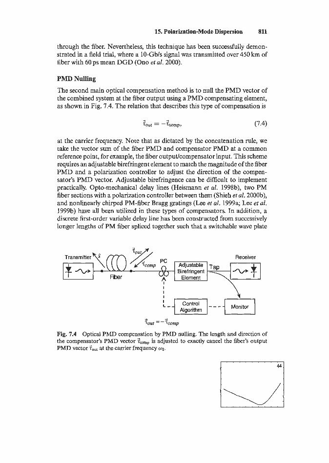
15. Polarization-Mode Dispersion 811
through the fiber. Nevertheless, this technique has been successfully demon- strated in a field trial, where a lO-Gb/s signal was transmitted over 450 km of fiber with 60 ps mean DGD (On0 et al. 2000).
PMD Nulling
The second main optical compensation method is to null the PMD vector of the combined system at the fiber output using a PMD compensating element, as shown in Fig. 7.4. The relation that describes this type of compensation is
at the carrier frequency. Note that as dictated by the concatenation rule, we take the vector sum of the fiber PMD and compensator PMD at a common reference point, for example, the fiber outputkompensator input. This scheme requires an adjustable birefringent element to match the magnitude of the fiber PMD and a polarization controller to adjust the direction of the compen- sator’s PMD vector. Adjustable birefringence can be difficult to implement practically. Opto-mechanical delay lines (Heismann et al. 1998b), two PM fiber sections with a polarization controller between them (Shieh et al. 2000b), and nonlinearly chirped PM-fiber Bragg gratings (Lee et al. 1999a; Lee et al. 1999b) have all been utilized in these types of compensators. In addition, a discrete first-order variable delay line has been constructed from successively longer lengths of PM fiber spliced together such that a switchable wave plate
Transmitter\ Receiver
% o q T~~ ‘0“ Adjustable Birefringent
Element ? Fiber
Fig. 7.4 Optical PMD compensation by PMD nulling. The length and direction of the compensator’s PMD vector &,mp is adjusted to exactly cancel the fiber’s output PMD vector at the carrier frequency 00.

812 H. Kogelnik et al.
operating as either a half- or full-wave plate between each PM fiber pair can add or subtract the various sections of DGD (Sobiski et al. 2001).
Fixed DGD
A third optical compensation scheme that has been extensively investigated is shown in Fig. 7.5. This simple and dynamic compensator consists of an adjustable polarization controller and a single element with fixed DGD, often a PM fiber of fixed length (Takahashi et al. 1994; Roy et al. 1999; Francia et al. 1999). There are two possible modes of operation for this compensator. The first mode is to adjust the polarization controller so that the combination of the fiber plus the compensator has a PSP that is aligned with the input
PM fiber Receiver
I I I
Fig. 7.5 (a) Optical PMD mitigation using a fixed DGD compensator. (b) The two modes of operation are indicated by PMD vector diagrams, where R-' zc,, is indicated by a dashed vector. For mode 1 there are two possible orientations for R-l&,mp to minimize first-order PMD.
15. Polarization-Mode Dispersion 813
polarization, as described by
5 = &in + ~-'?comp), (7.5)
where a is a scalar constant and where the concatentation rule was invoked to sum ?in and icOmp at the fiber input. As shown in Fig. 7.5, for this mode of operation, the compensator's fixed DGD must be sufficiently large such that I?comp I > I?in - sin +I , where 4 is the angle between the launch state, 5, and the fiber's input PMD vector ?b. Note also that the polarization controller can be adjusted for two possible orientations for R-'?co, to satisfy Eq. 7.5. The second operation mode, applicable when (?camp( < I Q . sin 41, is to adjust the polarization controller to minimize the penalty resulting from the combined PMD vector of the fiber and compensator,
(7.6)
where 8 is the angle between the launch state, 5, and the vector ?in + R-'?comp. The compensator of Fig. 7.5 is often implemented using degree-of-polarization (DOP) monitoring (discussed in Section 7.6). In maximizing the DOP of the compensated signal, it is irrelevant which operation mode is in use at any particular point in time. This compensator with DOP monitoring was used in several 10-Gb/s field trials with fibers having mean DGDs of more than 30 ps (Chbat et al. 1999; Lanne et al. 2000c; Nagel et al. 2000). Adaptive PMD compensation at 40 Gb/s has also been demonstrated (Lanne et al. 2001).
In reality, the PMD nulling compensator (and fixed DGD compensator) may not operate exactly according to the above first-order principles, and their detailed operation depends on the monitor and feedback algorithm. Recent studies have shown that these optical compensators may show optimal BER performance (or maximization of the DOP) when the compensator does not completely cancel the first-order PMD vector. In fact, the PMD nulling com- pensator (as well as the fixed DGD compensator) may be able to mitigate some higher-order PMD (Karlsson et al. 2001b; Lanne et al. 2001 ; Nagel et al.
2.3 tsop from Section 7.1 provides some information on the required speed of the PSP trans- mission and fixed DGD compensators. PSP transmission compensators need only operate on the timescale of tpmd, since they track changes of the PSP at the fiber input. Fixed DGD compensators, on the other hand, must operate on the timescale of tsop, since the R-l?comp changes on the timescale of an SOP. Therefore, PSP transmission compensators can operate a factor of 2.3 slower than fixed DGD compensators.
min I (?h + R-' ?camp) . sin el ,
2000). When applied to PMD compensation, the relation tpmd
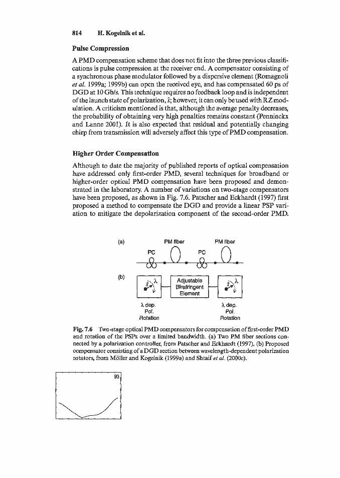
814 H. Kogelnik et al.
Pulse Compression
A PMD compensation scheme that does not fit into the three previous classifi- cations is pulse compression at the receiver end. A compensator consisting of a synchronous phase modulator followed by a dispersive element (Romagnoli et al. 1999a; 1999b) can open the received eye, and has compensated 60 ps of DGD at 10 Gb/s. This technique requires no feedback loop and is independent of the launch state of polarization, $; however, it can only be used with RZ mod- ulation. A criticism mentioned is that, although the average penalty decreases, the probability of obtaining very high penalties remains constant (Penninckx and Lanne 2001). It is also expected that residual and potentially changing chirp from transmission will adversely affect this type of PMD compensation.
Higher Order Compensation
Although to date the majority of published reports of optical compensation have addressed only first-order PMD, several techniques for broadband or higher-order optical PMD compensation have been proposed and demon- strated in the laboratory. A number of variations on two-stage compensators have been proposed, as shown in Fig. 7.6. Patscher and Eckhardt (1997) first proposed a method to compensate the DGD and provide a linear PSP vari- ation to mitigate the depolarization component of the second-order PMD.
PM fiber PM fiber
(b) F;'.̂H-HXl Adjustable pi Birefringent Element
h dep. Pol.
Rotation
h dep. Pol.
Rotation
Fig. 7.6 Two-stage optical PMD compensators for compensation of first-order PMD and rotation of the PSPs over a limited bandwidth. (a) Two PM fiber sections con- nected by a polarization controller, from Patscher and Eckhardt (1997). (b) Proposed compensator consisting of a DGD section between wavelength-dependent polarization rotators, from Moller and Kogelnik (1999a) and Shtaif et al. (2000~).
15. Polarization-Mode Dispersion 815
The compensator consisted of two PM fiber lengths connected by a polariza- tion controller, resulting in a circular sweep of the compensator’s PSP on the PoincarC sphere. The compensator could thus be adjusted to mitigate PSP depolarization over a bandwidth where the fiber’s PSP trajectory can be approximated by a single arc on the Poincark sphere. Moller and Kogelnik (1999a) and Shtaif et Q I . (2000~) also have proposed compensators consist- ing of a DGD section between wavelength-dependent polarization controllers (Fig. 7.6b) for compensation of first-order PMD and rotation of the PSPs over a limited bandwidth. For this type of device, compensation for first-order PMD is decoupled from the PSP rotation and can be controlled indepen- dently. Simulations of a two-stage PMD compensator consisting of the fixed DGD compensator followed by a polarization rotator and a variable differen- tial delay line have indicated that the maximum tolerable mean DGD is 50% higher than when only a fixed DGD compensator is used (Yu et al. 2001). Note that an important issue in all compensation schemes consisting of more than one differential delay is that the delays must remain stable on the order of a sin- gle wavelength. A subwavelength variation of the differential delay of the first stage rotates the polarization of the signal entering the second stage (Shtaif et al. 2000~)~ or equivalently, rotates the input PMD vector of the compensator.
Multi-Section Compensators
Compensators consisting of multiple birefringent sections (sometimes referred to as distributed PMD equalizers) that potentially can compensate broadband andlor higher-order PMD have also been proposed and demonstrated in the laboratory. The operation principle is that a large number of short DGD sections separated by polarization transformers can be adjusted so that the PMD vector profile of the compensator follows the profile of the transmission fiber, in reversed order, as shown in Fig. 7.7. Three PM fiber sections with polarization controllers were used to compensate 30 ps of DGD from a PMD emulator (Sandel et al. 1998b). Noe et al. (1998) then proposed a fiber-based distributed equalizer consisting of a long length of PM fiber pulled through the hollow axes of 64 stepper motors to form 16 endless polarization trans- formers and DGD sections. Compensation of 60ps of emulated DGD for 40-GHz pulses was demonstrated (Sandel et al. 1999). A distributed equalizer was later integrated in X-cut, Y-propagation Ti:LiNbOs (Noe et ~ l . 1999a), and could compensate up to 43 ps of DGD. With fifty lithium niobate sections, this distributed equalizer demonstrated compensation of 20-ps DGD for 6-ps, 40-GHz pulses (Him et al. 1999b). Tests of these distributed compensators are incomplete, since to date all demonstrations have used PMD emulators with

816 H. Kogelnik et al.
(a) PC DGD PC DGD PC DGD 0
unused compensator elements
Fig. 7.7 (a) Schematic of compensators consisting of multiple birefringent sections for potential broadband and/or higher-order PMD compensation. (b) PMD proiile of the transmission fiber span (solid arrows) and perfect equalization (dashed arrows) shown in three-dimensional normalized Stokes space, adapted from Noe etal. (1999b).
three or less PM fiber sections A potential problem with these distributed equalizers is that they require a large number of control parameters [e.g., 246 control voltages in Noe etal. (1999a)l. In addition, another critical issue is that the compensation for the various orders is coupled and has to be done simul- taneously (Shtaif et al. 2000~). Further details on the theory and operation of these compensators is provided in Noe et al. (1999b).
Multi-Channel Compensators
The possibility of simultaneous PMD compensation of multiple channels has been explored also. Khosravani et al. (2000a) demonstrated simultaneous PMD mitigation of four WDM channels by adjusting the single compen- sating module to optimize overall system performance. The experiment used feedback information about the total degradation of the combined WDM channels, and the PMD compensator was adjusted to minimize the DGD for the worst of the four WDM channels, since that channel dominated the overall system degradation. PMD mitigation using variable equalizing optical
15. Polarization-Mode Dispersion 817
circuits has also been proposed (Ozeki et al. 1994) and extended to broadband compensation (Moller 2000a; 2000b) and multichannel PMD equalization (Yamada et al. 2001).
7.5 ELECTRICAL PMD COMPENSATION TECHNIQUES
Although optical PMD compensation could, in principle, perfectly restore the optical pulse shape because the phase information is not lost, compensating PMD in the electrical domain before the receiver has a number of advan- tages, including potential low cost, small size, and simultaneous mitigation of intersymbol interference (ISI) from a variety of transmission impairments. The possibility of integrating a PMD mitigator into the receiver electronics is also an advantage, particularly if each channel must be compensated individu- ally. There are three main categories for electrical compensators: linear filters, nonlinear filters, and more complex signal processing techniques.
PMD causes linear distortion in the received electrical signal, since the orthogonal signals on the two PSPs add in power at the receiver (Le., in ampli- tude in the electrical domain). Therefore, a linear filter can be used to equalize PMD as long as the received signal eye is not closed (Winters and Gitlin 1990a). The Transversal Filter (TF), an electrical analog tapped delay line shown in Fig. 7.8a, is the most common linear filter and is also referred to as a Feed-Forward Equalizer. The TF divides the signal, delays the copies by constant delay stages AT, and superimposes the differentially delayed signals at the output port. Note that the delays are often set to be multiples of the bit period T and the tap weights (Coy C1, C2, etc.) are adjusted to maximize the received signal quality. A two-tap, manually adjustable TF of discrete coaxial components was first used for PMD compensation at 1.1 Gb/s by Winters and Santoro (1990b). Further work has resulted in demonstrations of PMD and chromatic dispersion compensation at 10 Gb/s using a TF of coaxial compo- nents (Schlump et al. 1998) or a five-tap discrete prototype TF (Frazer et al. 2000), as well as adaptive PMD mitigation using a voltage tunable, four-tap TF on an SiGe integrated electronic circuit (Biilow et QZ. 1999b). In the demon- stration of Bulow et al. (1999b), the tap weights were adjusted using feedback from an eye monitor (to be discussed in Section 7.6), and the TF reduced the penalty by 5-dB for 80-ps of emulated first-order DGD. It was also found that the TF is “blind” to PMD distortions when y = 0.5 and when AT > T, at which point nonlinear equalization is required.
The decision feedback equalizer (DFE), shown in Fig. 7.8b, is a nonlinear filter for adaptive nonlinear cancellation of IS1 and was first demonstrated for PMD compensation at 1.7 Gb/s by Winters and Kasturia (1992b). The basic
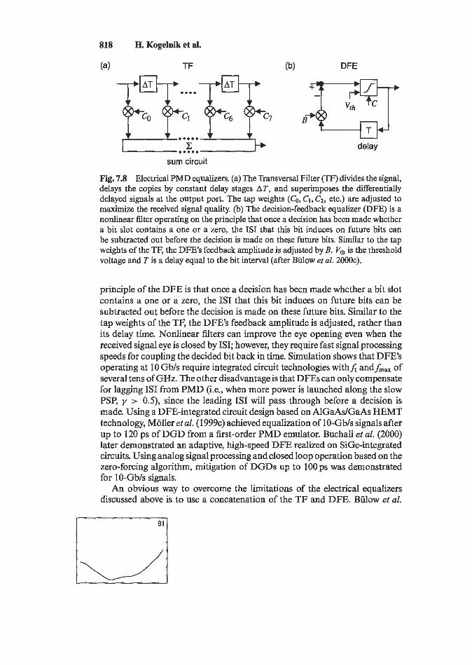
818 H. Kogelnik et al.
(a) TF FT::FTc7 r : : i : =
sum circuit
(b) DFE
B 4.3 delay
Fig. 7.8 Electrical PMD equalizers. (a) The Transversal Filter (TF) divides the signal, delays the copies by constant delay stages AT, and superimposes the differentially delayed signals at the output port. The tap weights (Co, Cl, Cz, etc.) are adjusted to maximize the received signal quality. (b) The decision-feedback equalizer (DFE) is a nonlinear filter operating on the principle that once a decision has been made whether a bit slot contains a one or a zero, the IS1 that this bit induces on future bits can be subtracted out before the decision is made on these future bits. Similar to the tap weights of the TF, the DFE’s feedback amplitude is adjusted by B. Glth is the threshold voltage and T is a delay equal to the bit interval (after Biilow et al. 2000~).
principle of the DFE is that once a decision has been made whether a bit slot contains a one or a zero, the IS1 that this bit induces on future bits can be subtracted out before the decision is made on these future bits. Similar to the tap weights of the TF, the DFE’s feedback amplitude is adjusted, rather than its delay time. Nonlinear filters can improve the eye opening even when the received signal eye is closed by ISI; however, they require fast signal processing speeds for coupling the decided bit back in time. Simulation shows that DFE’s operating at 10 Gb/s require integrated circuit technologies withJ andfmax of several tens of GHz. The other disadvantage is that DFEs can only compensate for lagging IS1 from PMD (Le., when more power is launched along the slow PSP, y > 0.5), since the leading IS1 will pass through before a decision is made. Using a DFE-integrated circuit design based on AlGaAdGaAs HEMT technology, Moller et al. (1999~) achieved equalization of 10-Gb/s signals after up to 120 ps of DGD from a first-order PMD emulator. Buchali et al. (2000) later demonstrated an adaptive, high-speed DFE realized on SiGe-integrated circuits. Using analog signal processing and closed loop operation based on the zero-forcing algorithm, mitigation of DGDs up to loops was demonstrated for 10-Gb/s signals.
An obvious way to overcome the limitations of the electrical equalizers discussed above is to use a concatenation of the TF and DFE. Biilow et al.

15. Polarization-Mode Dispersion 819
(2000~) compared the measured receiver sensitivity of a TF, DFE, and com- pound equalizer (TF + DFE) for 10-Gb/s signals in the presence of first-order PMD. Both the seven-tap TF and DFE having 100-ps delay were realized on SiGe-integrated circuits, with tap weights, feedback weight coefficient, and decision threshold level determined (manually) by external voltages applied to electrodes on the chip. Not surprisingly, the compound equalizer outper- forms the TF and DFE alone. The advantage of the TF + DFE was clearest in the high DGD range ( ~ 7 0 ps), and a penalty of only 3 dB at 80 ps DGD was measured. Experiments at 10Gb/s have also shown that using a com- pound equalizer in addition to a fixed DGD optical compensator can result in significant reductions in PMD penalties (Bulow et al. 2000d).
One of the more complex signal processing techniques for electronic PMD mitigation is phase diversity detection, proposed and demonstrated by Hakki (1997). After propagation through PMD, a received signal can be separated into its two PSPs by maximizing the measured phase difference between the two data streams. By inferring the DGD from the measured phase difference, the two signals can be resynchronized by introducing appropriate delay in their paths before recombining the signals. Experiments at 10 Gb/s demonstrated mitigation of up to 42 ps of DGD. Maximum likelihood sequence estimation (MLSE) (Winters and Gitlin 1990a) is another signal processing technique. MLSE is based on the correlation of a complete (undistorted) signal sequence with an estimate of the received sequence over many bits. Selection of the sequence and maximization of the correlation determine the decision for each individual bit. Although not yet experimentally demonstrated for 10-Gb/s PMD compensation, several recent papers have simulated its performance and asserted that it should be superior to the TF, DFE, or compound TF + DFE (Haunstein et al. 2000; Haunstein et al. 2001b; Bulow et al. 2001). At 10 Gb/s, MLSE could be realized as a digital processor using a Viterbi algorithm for correlation after analog-to-digital (AD) conversion. An analog-matched filter placed between the detector and the AD converter can be adapted to the actual signal distortion to improve equalization performance (Bulow et al. 2001).
Whereas forward-error correction (FEC) is generally used for extending the reach of transmission systems limited by optical signal-to-noise ratio, FEC has also been considered for PMD compensation. The performance of FEC has been experimentally studied in PMD-limited systems without compensation, and the PMD tolerance was shown to be limited to a mean DGD of -30 ps in lO-Gb/s systems using Reed-Solomon (255/239) FEC code (Ho and Lin 1997; Tomizawa et al. 2000). However, several recent PMD mitigation schemes have utilized FEC in addition to other compensation techniques. Simulations have shown that polarization scrambling along with FEC and a linear equalizer

820 H. Kogelnik et al.
at the receiver can enhance PMD tolerance (Wedding and Haslach 2001b). If the polarization is scrambled at a rate sutlicient to make the power ratio y vary between 0 and 1 within one FEC frame, the number of bits affected by PMD per FEC frame is limited, and the FEC can then correct the resulting bit errors. Combining FEC with an optical k e d DGD compensator has been shown to increase the PMD tolerance to a mean DGD of more than 40 ps at 10 Gb/s (Xie et al. 200 1 b).
7.6 MONITORING TECHNIQUES
All PMD compensation schemes, whether optical or electrical, rely on some kind of monitoring technique to provide information for the feedback loop and algorithm controlling the compensator. Important characteristics of the monitoring technique are (1) sensitivity to PMD, Le., how much does the signal from the monitor change when the PMD changes; (2) correlation with the BER; and (3) response time (Penninckx and Lanne 2001). If acompensator is expected to react to PMD fluctuations of a certain rate, then the monitor must provide a feedback signal at a faster rate so the algorithm can process the information and adjust the compensator within the allowed time interval. In general, the feedback signal is a compromise between accuracy and response time. This section will review several monitoring techniques proposed and demonstrated in the literature.
RF Spectrum
After propagation through PMD, the strength of the RF signal received by a photodiode is a function of the DGD, launch power ratio y, and RF frequency. It is well known that the pulse broadening induced by PMD results in “spectral hole burning,” i.a, the RF spectrum has a minimum where the DGD is equal to one-half the RF cycle,ffin = 1/(2At), where the two RF components carried by the two PSPs add out of phase. In fact, Bahsoun et al. (1990) proposed a PMD measurement technique based on measuring the strength of the RF signal as a function of the RF frequency and identifyingffi,. The narrowing of the RF spectrum that occurs as a result of the spectral hole can also be used as a monitor for PMD compensators. To assess the electrical spectral width, narrow bandwidth measurements at several frequencies are performed on the detected signal (Takahashi et al. 1994; Ishikawa and Ooi 1998; Sandel et al. 1998b). The bandpass filters often are centered at 0.5/T, 0.25/TY and 0.125/T, where T is the bit period, for example, for 40 Gb/s, the bandpass filters are at 20, 10, and 5 GHz (Sandel et al. 1998b), as shown in Fig. 7.9a. This choice of filters allows unambiguous detection of DGDs above one bit period. The

15. Polarization-Mode Dispersion 821
(4 40 Gbls Rx
PMD Compensator
N GHz
RF Bandpass Filters
0 25 50 75 100
(PSI + Fig. 7.9 Monitoring using the shape of the RF spectrum. (a) Narrow bandwidth measurements of the detected signal are performed at several RF frequencies. For example, for 40 Gb/s, bandpass filters can be centered at 20, 10, and 5 GHz. (b) Signals from the bandpass filters centered at 20, 10, and 5 GHz as a function of DGD. The receiver can switch between the signals (bold sections of curves) from the three bandpass filters according to whether the signal is above or below certain threshold levels (dashed lines), thus providing unambiguous detection of DGDs above one bit period T , while still retaining good sensitivity for small DGDs (adapted from Sandel et al. 1998b).
feedback algorithm can adjust the PMD compensator to maximize the signals derived from these narrow bandwidth measurements or to maximize a suitable linear combination of the three signals. Alternatively, the receiver could switch between the three bandpass filter signals when the signals are above or below certain threshold levels. As shown in Fig. 7.9b, these thresholds can be set to

822 H. Kogelnik et al.
detect DGDs up to 4T, while still retaining good sensitivity for small DGDs (Sandel et al. 1998b).
RF Power
A monitor signal for PMD compensation can also be extracted from a mea- surement of the total RF power of the detected signal. Since hole burning due to PMD results in reduction of the RF spectral power, the feedback algorithm can maximize the RF power at the compensator output (Biilow et al. 1999b). The RF power can be measured by a microwave power meter or by automatic gain control to normalize the output voltage from the compensator followed by a signal-squarer integrated circuit. Disadvantages of this method are the difficulty in measuring electrical power over a wide spectrum and its coarse sensitivity (Biilow et al. 1999b).
Eye Monitor
Several groups have proposed and demonstrated measurement of the open- ing in the eye pattern as a useful monitoring technique (Biilow et al. 2000b; Frazer et al. 2000). Estimates of the BER can be achieved by analyzing the eye using error measurements at suboptimal decision thresholds, also called pseudo-error rates. The eye monitor consists of two decision circuits in par- allel. The first acts as the simple decision gate in a conventional receiver, and the second functions as a monitor gate with variable threshold to character- ize the edges of the eye at variable phase. Choice of the suboptimal decision threshold determines the level of the pseudo-error rate, which again is a trade- off between response time and sensitivity. (Higher error rates provide faster response times, but have less sensitivity to changes in PMD.) Biilow et al. (2000b) reported an adaptive electrical PMD mitigator containing an eight- tap TF and an eye monitor circuit, both integrated on SiGe. Here the eye opening was measured by a monitor decision gate at 3 x BER level, and the tap voltages were tuned consecutively into the direction of an increasing eye opening by a dithering technique. In addition, excellent correlation between the BER and eye opening has been shown to BERs < and adaptive optical PMD compensation using a fast eye monitor has been demonstrated at 10 Gb/s (Buchali et al. 2001).
Other Electrical Monitoring Methods
Fast adaptive control of a TF using a continuous-time implementation of the Least Mean Squares algorithm has also been proposed and demonstrated at
15. Polarization-Mode Dispersion 823
10 Gb/s (Wedding et al. 2001a). In this technique, subtracting the regenerated signal at the receiver from the TF output generates an error signal e(t). The adaptive control block then calculates the correlation between the input signal to the TF and e(t) and minimizes the overall error due to distortion and noise. The uncorrected BER before forward-error correction has also been proposed as a monitor for PMD compensation.
Degree of Polarization
The concept of the degree of polarization (DOP) characterizes the average polarization state of light over a broad spectral range. For time-dependent signals it is also defined as an average over a specified time period. The def- inition of DOP is based on the Stokes parameters routinely measured by a polarimeter-based instrument (containing polarhers and four photodiodes) or DOP monitor.
A coherent sinusoidal optical carrier (or a narrow spectral component) has a well-defined polarization, described by a unit Stokes vector denoted by a lowercase 5 in the body of this text. The spectrally averaged Stokes param- eters, Si, are denoted by capital letters, where SO is the total intensity of the light. The other three parameters are the differences between the measured intensities of pairs of orthogonal polarizations, with 5'1 referring to the verti- calhorizontal polarizations, S2 to the f45" polarizations, and S, to right/left circular polarizations. The definition of the DOP is
DOP = ,/st + s,2 + $/so. (7.7)
A narrow spectral component then has DOP = 1. If the filter of the monitor passes several WDM channels (or spectral components), the measured inten- sity is the sum of all channel intensities for any given analyzer setting. The monitor, therefore, measures Stokes parameters that are the sum of the Stokes parameters of the individual WDM channels. For the illustrative example of two channels with equal power, one finds DOP = J(1+ .52)/2 = cos (#J/2), where 51 and i 2 are the unit Stokes vectors of the two channels and #J is the Stokes angle between the two channels. If the channels have parallel polarizations, the DOP = 1; for antiparallel polarizations, the DOP = 0.
Assume, now, that 51 and Ez are the polarizations at the output of a fiber with a DGD, At, when the two channels (or spectral components) are launched with equal polarizations, and the channel (or spectral) spacing is Am. The fiber PMD rotates 22 relative to &, reducing the measured DOP at the output. The law of inlinitesimal rotation (Eq. 2.6) characterizes this relative
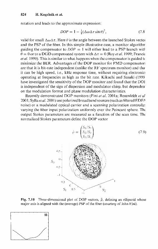
824 H. Kogelnik et al.
rotation and leads to the approximate expression:
DOP = 1 - $(AwAtsin8)2, (7.8
valid for small AwAt . Here 8 is the angle between the launched Stokes vectoi and the PSP of the fiber. In this simple illustrative case, a monitor algorithn guiding the compensator to DOP = 1 will either lead to a PSP launch wit1 8 = 0 or to a DGD compensated system with A t = 0 (Roy et al. 1999; Francis et al. 1999). This is similar to what happens when the compensator is guided tc minimize the BER. Advantages of the DOP monitor for PMD Compensator: are that it is bit-rate independent (unlike the R F spectrum monitor) and thai it can be high speed, i.e., kHz response time, without requiring electronic: operating at frequencies as high as the bit rate. Kikuchi and Sasaki (1999 have investigated the sensitivity of the DOP monitor and found that the DO€ is independent of the sign of dispersion and modulator chirp, but dependeni on the modulation format and phase modulation characteristics.
Recently demonstrated DOP monitors (Fini et al. 2001a; Rosenfeldt et al 2001; Sylla et al. 2001) use polarized broadband sources (such as filtered EDFP noise) or a modulated optical carrier and a scanning polarization controllei varying the fiber input polarization uniformly over the Poincart sphere. Tht output Stokes parameters are measured as a function of the scan time. Tht normalized Stokes parameters define the DOP vector
0.5
0
-0 5
-1
s3
Fig. 7.10 Three-dimensional plot of DOP vectors, ;, defining an ellipsoid whose major axis is aligned with the (average) PSP of the fiber (courtesy of John Fini).

15. Polarization-Mode Dispersion 825
whose magnitude equals the DOP. A three-dimensional plot of vectors pro- duced by the scan defines an ellipsoid whose major axis is aligned with the (average) PSP of the fiber. An example is shown in Fig. 7.10. The parameters of the ellipsoid also allow the determination of other PMD information, such as the spectral average of the DGD, when a broadband source is used. This measurement can be performed in fractions of a second with a sufficiently fast polarization scanner.
7.7 FURTHER READING
Information on soliton and dispersion-managed soliton resistance to PMD can be found in Matera and Settembre (1995a); Zhang et al. (1998a); Lakoba and Kaup (1997); Chen and Haus (2000); Nishioka et al. (2000); and Lakoba
Literature on theory and comparison of PMD compensators includes Sunnerud et al. (2000a); Karlsson et al. (2000b); Kudou et al. (2000); Madsen (2000); Yu and Willner (2001); Fini and Haus (2001b); and Sunnerud et al.
Limitations of first-order PMD compensation are discussed in Mahgerefteh and Menyuk (1999); Bulow (1999a); and Penninckx and Lanne (2000). Polar- ization controllers for optical PMD compensation are discussed in Heismann and Wayland (1991) and Heismann (1994) (lithium niobate); Shimuzu et al. (1991) and Ono et al. (1993) (fiber squeezing); and Sobiski et al. (2001) (PM fiber as variable phase plates).
(2000).
(2001c).
Acknowledgments
It is a pleasure to thank our colleagues at Bell Labs for extensive discussions on this subject and for their comments on the manuscript, particularly Herbert Haunstein, Art Judy, Heiko Kallert, Kavita Ramanan, Peter Winzer, and Weiguo Yang. We also thank Elsa Thomas for invaluable assistance in the preparation of the manuscript.
Appendix A: Notation
We have attempted to keep our notation simple and transparent while linking to the notation already established as much as possible. The following is an abbreviated listing.
I " ' . " ' 51 1
826 H. Kogelnik et al.
X , Y , Z Fiber coordinates: z is the direction of propagation; x , y are the transverse coordinates, i.e., those of Jones space. Continuous wave traveling in the z direction:j is the imaginary unit, 00 is the angular carrier frequency, t is time, and p is the propagation constant. Electric field vectors: &(o) is the Fourier transform of the complex transverse (x , y ) electric-field vector E(t) and has a complex amplitude e such that
ei(mt-flz)
E Y E
i
The vector of the real electric field is Re(Edm'). Deviation from the angular carrier frequency 9 of the light. The optical frequency is (00 + Am). 2D complex Jones (column) ket vector,
Is) = ( ; ) The bra (SI indicates the corresponding complex conjugate row vector, i.e., (SI = (sz,s,*). The bra-ket notation is used to distinguish Jones vectors from Stokes vectors. Our Jones vectors are all of unit magnitude, i.e., (sls) = szsx f s;sY = 1, as we assume coherent light (except as noted). 3D Stokes vector of unit length indicating the polarization of the field and corresponding to Is). The components of B are the Stokes parameters:
s1 = sxs; - s s*
s2 = s,s; + s,sy s3 =j(s,s,* - s,"sy).
Y Y (A.3)
By this definition, SI = 1 for linear polarization aligned with the x axis, s2 = 1 for linear polarization at 45" to this axis, and sg = 1 for right-circular polarized light (sy =js,) conforming with the traditional optics definition. However, left-circular

15. Polarization-Mode Dispersion 827
I
T
definitions are also used in the literature. We always use the same letter symbols for corresponding Jones and Stokes vectors. Note that a common phase shift of both components of Is) does not change 2. 2 x 2 or 3 x 3 identity matrix. The distinction should be clear from the context. 2 x 2 unitary transmission matrix in Jones space. Relates output to input via
We use the symbols s and t when necessary for clarity to designate respective input and output quantities, as illustrated in Fig. Al. 2 x 2 Jones matrix, with det (U) = 1. Related to T by
where $0 is the common phase. 3 x 3 orthogonal rotation matrix in Stokes space isomorphic to U . Relates output to input via
3 = Ri. (-4.6)
2 x 2 Pauli spin matrices, for our purposes defined as
0 -j 0 -1
(A.7) Pauli spin vector in Stokes space, 2 = (cq, 0 2 ~ 0 3 ) .
2 x 2 matrix in Jones space, j. 2 = Blul + B 2 a 2 + B3a3 .
Fig. A.l Block diagram of optical fiber under test.
I . . . . . . . . .

828 H. Kogelnik et al.
3D birefringence vector in Stokes space describing local fiber properties. Output PMD vector in Stokes space. Its length, At , is the differential group delay (DGD), and its direction is that of the Stokes vector of the slow principal state.
Unit Stokes vectors: $ is sometimes used to describe the polarization of the slow principal state, whereas f is used for a rotation axis. Indicates differentiation, i.e., dsldw = s,. Mean or expectation value. Sometimes denoted as E(. ) .
s ?
- A t Mean DGD of the fiber, k (At) .
h, i
Subscript w
(*)
Appendix B: Relation between PMD vectors and 6 In the main body of this text we have defined the PMD vector 2 to characterize the fiber. To conform with most of the optics literature and the available mea- surement instrumentation, we are using ccright-circular’y Stokes space, where the Stokes parameter
s3 = (s I 0 3 I s) (B.1)
is unity and positive fSr right-handed circular polarization. The PMD vector SZ defined and introduced by Poole and Wagner (1986)
is widely used in the PMD literature, and this appendix serves to connect 2 and h.
The vectors ? and d are different in two respects. The first is that d is dehed in “left-circular” Stokes space, where the s3 Stokes parameter is unity and positive for left-handed circular polarization (and - 1 for right-circular light).
The second distinction is that ? is defined to point into the direction of the slow PSP with group delay
tg = to + At/2, (B.2)
whereas 6 is defined to point into the direction of thefast PSP with group delay
These two differences combine to ensure that the basic law_of infinitesimal rotation (Eq. 2.6) has the same form and sign for both 2 and SZ. However, the
tg =-to - At/2. (B.3)

15. Polarization-Mode Dispersion 829
Stokes vectors of the two spaces are not the same, and the relation between the PMD vectors is given by
where 2 is in right-circular Stokes space and 6 is in left-circular Stokes space. Our birefringence vector $, defined in Eq. 2.8, and the birefringence vector I?', often used in the literature (Ulrich 1997), are related in a similar way as ? and a. We have
with E in right-circular and 6' in left-circular Stokes space.
Appendix C: Rotational Forms of the Jones and Miiller Matrices
For the convenience of the reader, we list here the rotational expressions for both the Jones matrix and the 3 x 3 Muller matrix of a fiber. These expressions explicitly exhibit the rotation axis f and the rotation angle qo in Stokes space. For derivations and a more detailed discussion we refer to Gordon and Kogelnik (2000). The expressions refer to loss-less fibers in the absence of PDL.
C.1 ROTATIONAL FORMS OF THE JONES MATRlx
General rotation: U = I cos qo/2 - j f sin 912, (C. 1)
(C.2) Exponential form: U = e-j(P/')'''.
The matrix operator F.6 appearing in the exponent is explained in Appendix A.
C.2 ROTATIONAL FORMS FOR THE MULLER MATRlx
General rotation: R = cos p . I + (1 - cos qo)ff + sin qo f x , (C.3)
= f f + sinqofx - cosqo(Px)(fx),
830 €3. Kogelnik et al.
where the 3D dyadic ii is the projection operator and i x is the cross-product operator:
Exponential form: R = ep('x)m (C. 5)
C.3 ELEMENTARY ROTATIONS
Elementary rotations in Stokes space are those special cases that rotate the Stokes vectors around the axes El, 22, and E3 of the Poincar6 sphere. The expressions for = 1 , 2,3 are
The elements of U, and Ri are listed in Table C. 1. Note that U1 and R1 describe the rotation caused by a birefringent phase
plate with the slow principal axis aligned with x axis in Jones space. U2 and R2 correspond to a phase plate set at a 45" angle in Jones space. U3 and R3 describe a rotation by p0/2 around the z axis.
Table C.1 Elementary Rotations
Rotation Axis Jones Matrix Stokes Space Rotation
cos q1/2 -j sin p/2 ) R2=( COSY, 0 0 1 S i n Y , 0 )
-sinp 0 COSY,
i 2

15. Polarization-Mode Dispersion 831
Appendix D: Acronyms
BER DFE DGD DOP EDFA FEC FWHM FWM GVD
IS1 JME MLSE MMM NRZ OTDR PBS PC PCD
PDG PDL PMF
PMD PSD PSP RF rms RZ SOP TF XPM
Bit error rate Decision feedback equalizer Differential group delay, At. Degree of polarization Erbium-doped fiber amplifier Forward-error correction Full width at half maximum Four-wave mixing Group-velocity dispersion, also called fiber chromatic
Intersymbol interference Jones matrix eigenanalysis method Maximum likelihood sequence estimation Miiller matrix method Non-return-to-zero modulation Optical time-domain reflectometry Polarization beam splitter Polarization controller Polarization-dependent chromatic dispersion Probability density function Polarization-dependent gain Polarization-dependent loss Polarization-maintaining fiber, also called
high-birefringence fiber Polarization-mode dispersion Polarization-dependent signal delay method Principal state of polarization, lp), j Radio frequency Root mean square Return-to-zero modulation State of polarization Transversal a ter Cross-phase modulation
dispersion
832 H. Kogelnik et al.
References
Adamczyk, 0. H., A. B. Sahin, Q. Yu, S. Lee, and A. E. Willner. 2001. “Statistics of PMD-induced power fading for double sideband and single sideband subcarrier- multiplexed signals,” Proc. Optical Fiber Communication Conference, OFC’Ol. Paper M05.
Anderson, K. E. and K. H. Wagner. 2001. “Chromatic and polarization mode disper- sion compensation using spectral holography,” Proc. Optical Fiber Communication Conference, OFC’Ol. Paper TuH2.
Andresciani, D., E Curti, E Matera, and B. Daino. 1987. “Measurement of the group- delay dxerence between the principal states of polarization on a low-birefringence terrestrial fiber cable,” Opt. Lett. 123846846.
Aso, O., I. Ohshima, and H. Ogoshi. 1994. “Study on a conservation quantity in PMD measurements,” Pmc. Symp. Opt. Fiber Measurements, SOFM’94.159-162.
Aso, 0. 1998. “Measurement of a parameter limiting the analysis of the first-order PMD effect,” Opt. Lett. 23:1102.
Bahsoun, S., J. Nagel, and C. Poole. 1990. “Measurement of temporal variations in fiber transfer characteristics to 20 GHz due to polarization-mode dispersion,” Proc. European Conference on Optical Communication, ECOC’90,1003. Postdeadline paper.
Bakhshi, B., J. Hansryd, P. Andrekson, J. Brentel, E. Kolltveit, B.-E. Olsson, and M. Karlsson. 1999a. “Experimental observation of soliton robustness to polarization dispersion pulse broadening,” Elect. Lett. 35:65-66.
Bakhshi, B., J. Hansryd, €? Andrekson, J. Brentel, E. Kolltveit, B.-E. Olsson, and M. Karlsson. 1999b. “Measurement of the differential group delay in installed optical fibers using polarization multiplexed solitons,” IEEE Photon. Technol. Lett. 1 1:593.
Barlow, A. J., J. J. Ramskov-Hansen, and D. N. Payner. 1981. “Birefringence and polarization mode-dispersion in spun single-mode fibers,” Appl. Opt. 20:2962-2968.
Bebbington, D. H. O., J. G. Ellison, R. E. Schuh, X. Shan, A. S. Siddiqui, and S. D. Walker. 1997. “Fully polarimetric optical time-domain reflectometer with 1 -m spatial resolution,” Proc. Optical Fiber Communication Conference, OFC ’97. Technical Digest. 185-186.
Beltrame, D., E Matera, M. Settembre, A. Galtarossa, A. Pizzinat, E Favre, D. Le Guen, and M. Henry. 2000. “Statistical behavior of the Q-factor in optical transmis- sion systems due to the polarization mode dispersion,” Proc. European Conference on Optical Communication, ECOC 2000.2:95-96.
Bergano, N. S., C. D. Poole, and R. E. Wagner. 1987. “Investigation of polarization dispersion in long lengths of single-mode fiber using multilongitudinal mode lasers,” IEEEJ. Lightwave Technol. LT- 5:1618-1622.
Bergano, N. S. 1994. “Time dynamics of polarization hole burning in an EDFA,” Optical Fiber Communication Conference, OFC’94. Technical Digest. 305-306.

15. Polarization-Mode Dispersion 833
Bergano, N. S., C. R. Davidson, M. Ma, A. Pilipetskii, S. G. Evangelides, H. D. Kidorf, J. M. Darcie, E. Golovchenko, K. Rottwitt, P. C. Corbett, R. Menges, M. A. Mills, B. Pedersen, D. Peckham, A. A. Abramov, and A. M. Vengsarkar. 1998. “320 Gb/s WDM transmission (64 x 5 Gb/s) over 7,200 km using large mode fiber spans and chirped return-to-zero signals,” Proc. Optical Fiber Communication Conference, OFC’98. Paper PD12.
Bessa dos Santos, A., A. 0. Dal Forno, M. Lacerda Rocha, A. Paradisi, and J. P. von der Weid. 2000. “Fading in 2.5 Gb/s IM-DD optical transmission due to PMD and PDL,” Proc. European Conference on Optical Communication, ECOC2000.1: 145-146.
Betti, S., F. Curti, B. Daino, G. De Marchis, E. Iannone, and E Matera. 1991. “Evolu- tion of the bandwidth of the principal states of polarization in single-mode fibers,” Opt. Lett. 16:467469.
Biondini, G. and W. L. Kath. 2001. “Non-Maxwellian DGD distributions of PMD emulators,” Proc. Optical Fiber Communication Conference, OFC’Ol. Paper ThA5.
Bononi, A. and A. Vannucci. 2001. “Statistics of the Jones matrix of fibers affected by polarization mode dispersion,” Opt. Lett. 26:675-677.
Bruyere, E, J. Guillon, and J. J. Bernard. 1991. “Polarization dispersion of the con- stituents of an erbium-doped fiber amplified link,” Proc. European Conference on Optical Communication, ECOC’91. 645.
Bruyere, E and 0. Audouin. 1994a. “Assessment of system penalties induced by polar- ization mode dispersion in a 5 Gbls optically amplified transoceanic link,” IEEE Photon. Technol. Lett. 6443-445.
Bruyere, E and 0. Audouin. 1994b. “Penalties in long-haul optical amplifier systems due to polarization dependent loss and gain,” IEEE Photon. Technol. Lett. 6:654-656.
Bruyere, E, 0. Audouin, V. Letellier, G. Bassier, and P. Marmier. 1994c. “Demonstra- tion of an optimal polarization scrambler for long-haul optical amplifier systems,” IEEE Photon. Technol. Lett. 6:1153-1155.
Bruyere, E 1996. “Impact of first- and second-order PMD in optical digital transmis- sion system,” Opt. Fiber Technol. 2:269-280.
Bruyere, E, L. Pierre, J. P. Thiery, and B. Clesca. 1997. “Penalties induced by higher-order PMD at 10 Gbitls in nondispersion-shifted fibers,” Proc. Optical Fiber Communication Conference, OFC ’97. 113-1 14.
Buchali, E, H. Biilow, and W. Kuebart. 2000. “Adaptive decision feedback equal- izer for 10 Gbitls dispersion mitigation,” Proc. European Conference on Optical Communication, ECOC 2000.2101-102.
Buchali, E, S. Lanne, J.-P. Thikry, and H. Biilow. 2001. “Fast eye monitor for 10 Gbith and its application for optical PMD compensation,” Proc. Optical Fiber Communication Conference, OFC’Ol. Paper TUPS.
Biilow, H. 1995. “Operation of digital optical transmission system with minimal degradation due to polarization mode dispersion,” Elect. Lett. 31:214-215.

834 H. Kogelnik et al.
Biilow, H. and G. Veith. 1997. “Temporal dynamics of error-rate degradation induced by polarization mode dispersion fluctuation of a field fiber link,” h c . European Conference on Optical Communication, ECOC’97. 1:115-118.
Biilow, H. 1998a. “Analysis of system outage induced by second order PMD in the pres- ence of chromatic dispersion,” Proc. European Conference on Optical Communication, ECOC’98. Paper WdCS.
Biilow, H. 1998b. “System outage probability due to first- and second-order PMD,” IEEE Photon. Technol. Lett, 10:696-698.
Biilow, H., D. Schlump, J. Weber, B. Wedding, and R. Heidemann. 1998c. “Elec- tronic equalization of fiber PMD-induced distortion at 10 Gbls,” Proc. Optical Fiber Communication Conference, OFC’98. Technical Digest. 2: 15 1-1 52.
Bulow, H. 1999a. “Limitation of optical first-order PMD compensation,” Proc. Optical Fiber Communication Conference, OFC’99. Technical Digest. 2:74-76.
Biilow, H., R. Ballentin, W. Baumert, G. Maisonneuve, G. Thielecke, and T. Wehren. 1999b. “Adaptive PMD mitigation at 10 Gbls using an electronic SiGe equalizer IC,” Pmc. European Conference on Optical Communication, ECOC’99,2: 138-139.
Biilow, H., W. Baumert, H. Schmuck, E Mohr, T. Schulz, E Kuppers, and W. Weiershausen. 1999c. “Measurement of the maximum speed of PMD fluctua- tion in installed field fiber,” Pmc. Optical Fiber Communications Conference, OFC’99. Technical Digest. W:83-85.
Biilow, H. 2000a. “PMD mitigation techniques and their effectiveness in installed fiber,” Proc. Optical Fiber Communication Conference, OFC 2000. 110-1 12.
Biilow, H., W. Baumert, E Buchali, and W Kuebart. 2000b. “Adaptation of an electronic PMD mitigator by maximization of the eye opening,” Proc. European Conference on Optical Communication, ECOC 2000. 3~209-210.
Biilow, H., E Buchali, W. Baumert, R. Ballentin, and T. Wehren. 2000c. “PMD mitiga- tion at 10 Gbitls using linear and nonlinear integrated electronic equalizer circuits,” Electron. Lett. 36: 163-164.
Biilow, H., E Buchali, and G. Thielecke. 2000d. “Electronically enhanced optical PMD compensation,” h c . European Conference on Optical Communication, ECOC 2000. 2:39-40.
Biilow, H. and G. Thielecke. 2001. “Electronic PMD mitigation-from linear equal- ization to maximum-likelihood detection,” Proc. Optical Fiber Communication Conference, OFC’OI. Paper WAA3.
Bums, W. K. and R. I? Moeller. 1983a. “Measurement ofpolarization-mode dispersion in high- birefringence fibers,” Pmc. Topical Meeting on Optical Fiber Communication, OFC’83. Paper TUA3.
Burns, W. K., R. I? Moeller, and C. Chen. 1983b. “Depolarization in a single-mode optical fiber,” iEEE J. Lightwave Technol. LT-1~44-49.
15. Polarization-Mode Dispersion 835
Cameron, J., X. Bao, and J. Stears. 1998a. “Time evolution of polarization mode dis- persion for aerial and buried cables,” Proc. Conference Optical Fiber Communication, OFC’98. Paper WM51:249-250.
Cameron, J., L. Chen, X. Bao, and J. Stears. 1998b. ‘‘Time evolution of polarization mode dispersion in optical fibers,” IEEE Photon. Technol. Lett. 10: 1265-1267.
Cameron, J., L. Chen, X. Bao, and J. Stears. 1999. “Uncertainty in the measurement of PMD,” Proc. European Conference on Optical Communication, ECOC’99. 1:308.
Cameron, J., L. Chen, and X. Bao. 2000. “Impact of chromatic dispersion on the system limitation due to PMD,” IEEE Photon. Technol. Lett. 12:47.
Chausse, E., N. Gisin, and C. Zimmer. 1995. “POTDR, depolarization and detection of sections with large PMD,” Proc. Symp. Optic. Fiber Measurements, SOFM’95. Technical Digest. VIII.3.
Chbat, M., W. J.-P. Soigne, S. Lame, et al. 1999. “Long-term field demonstration of optical PMD Compensation on an installed OC-192 link,” Proc. Optical Fiber Communication Conference, OFC’99. Postdeadline paper PD12.
Chen, L., J. Cameron, and X. Bao. 1999. “Statistics of polarization mode dispersion in presence of the polarization dependent loss in single mode fibers,” Opt. Comm.
Chen, L., M. Yafiez, C. Huang, and X. Bao. 2001. “Pulsewidth compression in optical components with polarization mode dispersion using polarization controls,” IEEE J. Lightwave Technol. 19:830-836.
Chen, Y. and H. A. Haus. 2000. “Solitons and polarization mode dispersion,” Opt. Lett. 25:290-292.
Chiang, K. S. 1985a. “Conditions for obtaining zero polarization-mode dispersion in elliptical-core fibres,” Elect. Lett. 21592-593.
Chiang, K. S. 1985b. “Linearly birefringent fibres with zero polarization-mode dispersion,” Elect. Lett. 21:916-917.
Chojetzki, C., H. Schmitzer, J. Vobian, and W. Dultz. 1992. “Four interferometric methods for the determination of the birefringence and polarization dispersion of polarization maintaining optical fibers,” Pmc. a m p . Opt. Fiber Measurements,
Chowdhury, D., E. Brarens, S. Nipple, A. Zainul, and T. Hanson. 2000. “Statistical impact of EDFA polarization mode dispersion on long-haul optical systems,” Proc. European Conference on Optical Communication, ECOC 2000.3: 147-148.
Chraplvyvy, A. R., R. W. Tkach, L. L. Buhl, and R. C. Alferness. 1986. “Phase modulation to amplitude modulation conversion of CW laser light in optical fibres,” Elect. Lett. 22:409411.
Ciprut, P., B. Gisin, N. Gisin, R. Passy, J. P. von der Weid, E Prieto, and C. Zimmer. 1998. “Second-order PMD: impact on analog and digital transmissions,” IEEE J. Lightwave Technol. 16:757-771.
169:69-73.
SOFM ’92.155-158.

836 H. Kogelnik et al.
Clesca, B., J.-F! Thiery, L. Pierre, V. Havard, and E Bruykre. 1995. “Impact of polar- ization mode dispersion on 10 Gbit/s terrestrial systems over nondispersion-shifted fiber,” Elect. Lett. 31:1594-1595.
Collings, B. C. and L. Boivin. 2000a. “Nonlinear polarization evolution induced by cross phase modulation and its impact on transmission systems,” ZEEE Photon. Technol. Lett. 12:1582-1584.
Collings, B. C. and L. Boivin. 2000b. “Nonlinear polarization evolution on the time scale of a single bit period in a fiber optic transmission line,” Proc. European Conference on Optical Communication, ECOC 2000. 3:43-44.
Corsi, E, A. Galtarossa, and L. Palmieri. 1998. “Polarkation mode dispersion char- acterization of single-mode optical fiber using backscattering technique,” IEEE J. Lightwave Technol. 16:1832-1843.
Corsi, E, A. Galtarossa, and L. Palmieri. 1999a. “Analytical treatment ofpolarization- mode dispersion in single-mode fibers by means of the backscattered signal,” J. Opt. SOC. Am. A. 16:574-583.
Corsi, E, A. Galtarossa, and L. Palmieri. 1999b. “Beat length characterization based on backscattering analysis in randomly perturbed single-mode fibers,” IEEE J. Lightwave Technol. 17:1172-1178.
Corsi, E, A. Galtarossa, L. Palmieri, M. Schiano, and T. Tambosso. 1999c. “Continuous-wave backreflection measurement of polarization mode dispersion,” IEEE Photon. Technol. Lett. 11 :45 1453.
Costa, B., D. Mazzoni, M. Puleo, and E. Vezzoni. 1982. “Phase shift technique for the measurement of chromatic dispersion in optical fibers using LED’s,” IEEE J. Quantum Elect. QE-18: 150!&1515.
Craig, R. M., S. L. Gilbert, and P. D. Hale. 1998a. “Accurate polarization dependent loss measurement and calibration standard development,” h c . Symp. Opt. Fiber Measurements, SOFM’98. Technical Digest. 5-8.
Craig, R. M., S. L. Gilbert, and F? D. Hale. 1998b. “High-resolution, nonmechanical approach to polarization-dependent transmission measurements,” IEEE J. Lightwave Technol. 16: 1285-1294.
Curti, E, B. Daino, Q. Mao, E Matera, and C. G. Someda. 1989. “Concatenation of polarization dispersion in single-mode fibres,” Elect. Lett. 25:290-292.
Curti, E, B. Daino, G. De Marchis, and E Matera. 1990. “Statistical treatment of the evolution of the principal states of polarization in single-mode fibers,” IEEE J. Lightwave Technol. LT-8:1162-1166.
Cyr, N., A. Girard, and G. Schinn. 1999. Stokes parameter analysis method, the consolidated test method for PMD measurements. h c . NFOEC’99,23.
Dal Forno, A. O., A. Paradisi, R. Passy, and J. F! von der Weid. 2000. “Experimental and theoretical modeling of polarization-mode dispersion in single-mode fibers,” IEEE Photon. Technol. Lett. 12:296-298.
15. Polarization-Mode Dispersion 837
Damask, J. N. 2000. “A programmable polarization-mode dispersion emulator for systematic testing of 10 Gb/s PMD compensators,” Trends in Optics and Photonics.
Darcie, T. and C. D. Poole. 1992. “Polarization-induced performance variables,” Communications Engineering and Design.
De Angelis, C., A. Galtarossa, G. Gianello, E Matera, and M. Schiano. 1992. “Time evolution of polarizationmode dispersion in long terrestrial links,” IEEEJ. Lightwave Technol. LT- 10: 552-555.
de Lignie, M. C., H. G. J. Nagel, and M. 0. van Deventer. 1994. “Large polarization mode dispersion in fiber optic cables,” IEEE J. Lightwave Technol. LT-12: 1325-1329.
Derickson, D. 1998. Fiber Optic Test and Measurement. Prentice Hall, New Jersey. Djupsjobacka, A. 2001a. “Calculation of signal outage due to polarization mode
dispersion.” IEEE Photon. Technol. Lett. 13:66&662. Djupsjobacka, A. 2001 b. “On differential group-delay statistics for polarization-mode
dispersion emulators,” IEEE J. Lightwave Technol. 19:285-290. Ebrahimi, P., M. C. Hauer, Q. Yu, R. Khosravani, D. Gurkan, D. W. Kim, D. W. Lee,
and A. E. Willner. 2001. “Statistics of polarization dependent gain in Raman fiber amplifiers due to PMD,” Proc. Con$ Lasers and Electro-optics, CLEO 2001.143-144.
Eickhoff, W., Y Yen, and R. Ulrich. 1981. “Wavelength dependence of birefringence in single-mode fiber,” Appl. Opt. 20:3428-3435.
Elamari, A., N. Gisin, B. Perny, H. Zbinden, and Ch. Z m e r . 1996. “Polarization dependent loss of Concatenated passive optical components,” Proc. Symp. Optic. Fiber Measurements, SOFM96. Technical Digest. 163-166.
El Amari, A., N. Gisin, B. Perny, H. Zbinden, and C. W. Zimmer. 1998. “Statistical prediction and experimental verification of concatenations of fiber optic components with polarization dependent loss.” IEEE J. Lightwave Technol. 16:332-339.
Eleftherianos, C. A., D. Syvridis, Th. Sphicopoulos, and C. Caroubalos. 1998. “Max- imum transmission distance of 40 Gb/s soliton systems in the presence of PMD,” Elect. Lett. 34688489.
Ellison, J. G. and A. S. Siddiqui. 1998a. “A fully polarimetric optical time-domain reflectometer,” IEEE Photon. Technol. Lett. 10:24&248.
Ellison, J. G. and A. S. Siddiqui. 1998b. “Estimation of linear birefringence suppression in spun fiber using polarimetric optical time-domain reflectometry,” Con$ Lasers and Electro-optics, CLE0’98.426421.
Ellison, J. G. and A. S. Siddiqui. 1998c. “Spun fibre parameter extraction using polari- metric optical time domain reflectometry,” Proc. Symp. Optic. Fiber Measurements, SOFM’98. Technical Digest. 109-1 12.
Evangelides, S. G., L. E Mollenauer, J. P. Gordon, and N. S. Bergano. 1992. “Polarization multiplexing with solitons,” IEEE J. Lightwave Technol. 10:28-35.
3:28-30.

838 H. Kogelnik et al.
Eyal, A. and M. Tur. 1998. “A modified Poincare sphere technique for the determina- tion of polarization-mode dispersion in the presence of differential gainnoss,” Proc. Optical Fiber Communication Conference, OFC ’98. 340.
Eyal, A., W. Marshall, M. Tu, and A. Yariv. 1999. “Representation of second-order PMD,” Elect. Lett. 35:1658-1659.
Eyal, A., 0. Dimenstein, M. Tur, M. Zaidman, A. Green, and S. Gali. 2001. “Polar- ization mode dispersion in radio-frequency interferometric embedded fiber-optic sensors,” IEEE J. Lightwave Technol. 19:504-511.
Fini, J. M., P. C. Chou, and H. A. Haus. 2001a. “Estimation of polarization dis- persion parameters for compensation with reduced feedback,” Proc. Optical Fiber Communication Conference, OFC ’01. Paper WAA6.
Fini, J. M. and H. A. Haus. 2001b. “Accumulation of polarization-mode dispersion in cascades of compensated optical fibers,” IEEE Photon. Technol. Lett. 13: 124-126.
Forghieri, F., R. W. Tkach, and A. R. Chraplyvy. 1997. “Fiber nonlinearities and their impact on transmission systems,” in Optical Fiber telecommunications IIIA, I. €? Kaminow and T. L. Koch, eds., Academic Press, CA. pp. 196-264.
Foschini, G. J. and C. D. Poole. 1991. “Statistical theory of polarization dispersion in single mode fibers,” IEEE J. Lightwave Technol. LT-9: 1439-1456.
Foschini, G. J. and L. A. Shepp. 1991. “Closed form characteristic functions for certain random variables related to Brownian motion,” in Stochastic Analysis Liber Amicorum for Moshe Zakai, Academic Press, CA. pp. 169-187.
Foschini, G. J., R. Jopson, L. Nelson, and H. Kogelnik. 1999. “The statistics of PMD- induced chromatic fiber dispersion,” IEEE J. Lightwave Technol. 17: 1560-1565.
Foschini, G. J., L. E. Nelson, R. M. Jopson, and H. Kogelnik. 2000. “Probability densi- ties of second-order polarization mode dispersion including polarization dependent chromatic fiber dispersion,” IEEE Photon. Technol. Lett. 12:293-295.
Francia, C., E Bruyere, D. Penninckx, and M. Chbat. 1998. “PMD second-order effects on pulse propagation in single-mode fibers,” IEEE Photon. Technol. Lett.
Francia, C., E Bruyere, J. P. Thiery, and D. Penninckx. 1999. “Simple dynamic polarization mode dispersion compensator,” Elect. Lett. 35:414-415.
Frazier, G. L., M. W. Goodwin, K. E. Leonard, J. €? Moffatt, and F. Zhang. 2000. “Static and dynamic performance of an adaptive receiver for 10 Gbps optical transmission,” Proc. European Conference on @tical Communication, ECOC’2000. 11:113-114.
Frigo, N. J. 1986. “A generalized geometrical representation of coupled mode theory,” IEEEJ. Quantum Electron. QE-2232131-2140.
Gabitov, I., B. Hein, E Kiippers, M. Miiller, andW Weiershausen. 1998. “Experimen- tal and numerical investigation of ps-pulse transmission in presence of PMD,” Proc. Optical Fiber Communication Conference, OFC ’98.342-343.
10: 1739-1 741.
15. Polarization-Mode Dispersion 839
Galtarossa, A., M. Schiano, C. G. Someda, B. Daino, E Matera, R. Zaninello, and E Bergamin. 1991. “Two different methods for measuring polarization mode disperison in singlemode fibres,” Elect. Lett. 27:2292-2293.
Galtarossa, A. and M. Schiano. 1993. “Polarization mode dispersion in high-density ribbon cables,” Proc. Optical Fibre Measurement Conference, 181-184.
Galtarossa, A., G. Gianello, and M. Schiano. 1994. “Comparison of polarization OTDR and PMD for stress analysis of an optical-fiber ribbon cable,” Proc. Optical Fiber Communication Conference, OFC’94. Technical Digest. 229-230.
Galtarossa, A., G. Gianello, C. G. Someda, and M. Schiano. 1996. “In-field com- parison among polarization-mode dispersion measurement techniques,” IEEE J. Lightwave Technol. LT-1442-49.
Galtarossa, A., E Corsi, and L. Palmieri. 1998a. “Experimental investigation of polarization-mode dispersion properties in single-mode fibers using a new backscat- tering technique,” Proc. Optical Fiber Communication Conference, OFC’98. Technical Digest. 343.
Galtarossa, A. and L. Palmieri. 1998b. “Relationship between pulse broadening due to polarization mode dispersion and differential group delay in long single mode fibers,” Elect. Lett. 34:492-493.
Galtarossa, A., L. Palmieri, and M. Schiano. 1999a. “Polarization-sensitive reflecto- metric techniques for PMD measurements,” Proc. European Conference on Optical Communication, ECOC’99. 2 2 .
Galtarossa, A., L. Palmieri, M. Schiano, and T. Tambosso. 1999b. “Single-end polar- ization mode dispersion measurement using backreflected spectra through a linear polarizer,” IEEE J. Lightwave Technol. 17:1835-1842.
Galtarossa, A., L. Palmieri, A. Pizzinat, M. Schiano, and T. Tambosso. 2000a. “Distributed birefringence characterization in installed single-mode fibers,” Proc. European Conference on Optical Communication, ECOC 2000.1:13%141.
Galtarossa, A., L. Palmieri, A. Piuinat, M. Schiano, and T. Tambosso. 2000b. “Mea- surement of local beat length and differential group delay in installed single-mode fibers,” IEEE J. Lightwuve Technol. 18: 1389-1394.
Galtarossa, A., L. Palmieri, M. Schiano, and T. Tambosso. 2000c. “Measurements of beat length and perturbation length in long single-mode fibers,” Opt. Lett. 25:38&386.
Galtarossa, A., L. Palmieri, A. Pizzinat, G. Roba, and D. Sarchi. 2001a. “Ultra low PMD fibers for long-haul high-capacity systems,” Proc. Optical Fiber Communication Conference, OFC’OI. Paper ThA8.
Galtarossa, A., L. Palmieri, M. Schiano, and T. Tambosso. 2001b. “PMD in single- mode fibers: Measurements of local birefringence correlation length,” Proc. Optical Fiber Communication Conference, OFC’OI. Paper ThA2.
Gisin, N. 1991a. Solutions of the dynamical equation for polarization dispersion. Opt. Comm. 86:371-373.

840 H. Kogelnik et al.
Gisin, N., R. Passy, B. Perny, A. Galtarossa, C. Someda, E Bergamin, M. Schi- ano, and E Matera. 1991b. “Experimental comparison between two different methods for measuring polarization mode disperion in singlemode fibres,” Elect. Lett. 27:2292-2293.
Gisin, N., J. P. Pellaux, and J. P. von der Weid. 1991c. “Polarization mode dispersion for short and long single-mode fibers,” IEEE J. Lightwave Technol. 92321427.
Gisin, N., B. Perny, and R. Passy. 1991d. “Polarization mode dispersion measurements in optical fibers, cables, installed terrestrial cables and fiber ribbons,” Proc. Optical Fibre Measurement Conference, 85-88.
Gisin, N., J. P. von der Weid, and J. Pellaux. 1991e. “Polarization mode dispersion of short and long single-mode fibers,” IEEE J. Lightwave Technol. LT-9921-827.
Gisin, N. and J. P. Pellaux. 1992. “Polarization mode dispersion: Time versus frequency domains,” Opt. Comm. 89:31&323.
Gisin, R., R. Passy, J. C. Bishoff, and B. Perny. 1993a. “Experimental investigations of the statistical properties of polarization mode dispersion in single mode fibers,” IEEE Photon. Technol. Lett. 5:819-821.
Gisin, N., U. Salama, and M. 0. Hongler. 1993b. “Polarization mode dispersion for single-mode fibers with polarization dependent losses,” Opt. Comm. 101:333.
Gisin, N. 1994a. “Polarization mode disperison: definitions, measurements and statistics,” Proc. Symp. Opt. Fiber Measurements, SOFM’94. 149-1 53.
Gisin, N. 1994b. “The statistics of polarization dependent losses,” Proc. Symp. Opt. Fiber Measurements, SOFM’94. 193-196.
Gisin, N., R. Passy, and J. P. von der Weid. 1994c. “Definitions and measurements of polarization mode dispersion: Interferometric versus fixed analyzer methods,” IEEE Photon. Technol. Lett. 6:730-732.
Gisin, N. 1995. “Statistics of polarization dependent loss,” Opt. Comm. 114399-405. Gisin, N., B. Gisin, J. P. von der Weid, and R. Passy. 1996. “How accurately can one
measure a statistical quantity like PMD?” IEEE Photon. Technol. Lett. 8:1671-1673. Gisin, N. and B. Huttner. 1997. “Combined effects of polarization mode dispersion
and polarization dependent loss in optical fibers,” Opt. Comm. 142:119-125. Gleeson, L., E. Sikora, and M. J. O’Mahoney. 1997. “Experimental and numerical
investigation into the penalties induced by second-order polarization mode disper- sion at 10 Gbls,” Proc. European Conference on Optical Communication, ECOC’97.
Glingener, C., A. Schopflin, A. Farber, G. Fischer, R. Nok, D. Sandel, S. Hinz, M. Yoshida-Dierolf, V. Mirvoda, G. Feise, H. Herrmann, R. Ricken, W. Sohler, and E Wehrmann. 1999. “Polarization Mode dispersion compensation at 20 Gb/s with a compact distributed equalizer in LiNbOs,” Pmc. Optical Fiber Communication Conference, 0FCJ99/OPPC’99. Postdeadline paper PD29.
15-18.
15. Polarization-Mode Dispersion 841
Gordon, J. P. and H. Kogelnik. 2000. “PMD Fundamentals: Polarization mode dis- persion in optical fibers,” Proceedings of the National Academy of Sciences USA. 97:4541-4550.
Greer, E. J., D. J. Lewis, and W. M. Macauley. 1994. “Polarization dependent gain in erbium-doped fibre amplifiers,” Elect. Lett. 30:4647.
Hakki, B. W. 1996. “Polarization mode dispersion in a single mode fiber,” IEEE J. Lightwave Technol. 14:2202-2208.
Hakki, B. W. 1997. “Polarization mode dispersion compensation by phase diversity detection,” IEEE Photon. Technol. Lett. 9: 121-123.
Hall, D. W., R. A. Haas, W. E Krupke, and M. J. Weber. 1983. “Spectral and polarization hole burning in neodymium glass lasers,” IEEE J. Quantum Electron.
Hamidi, S., N. H. Taylor, and W. D. Cornwell. 1999. “System penalty due to polar- ization mode dispersion in 10 Gbitls systems,” IEEE Colloquium on High-speed and Long-Distance Transmission. 17: 1-4.
Hansryd, J., H. Sunnerud, P. A. Andrekson, and M. Karlsson. 2000. “Impact of PMD on four-wave-mixing-induced crosstalk in WDM systems,” IEEE Photon. Technol. Lett. 12:1261-1263.
Haunstein, H., K. Sticht, A. Dittrich, M. Lorang, W. Sauer-Greff, and R. Urbansky. 2000. “Implementation of near optimum electrical equalization at 10 Gb/s:” Pmc. European Conference on Optical Communication, ECOC’2000. 3:223-224.
Haunstein, H. E and H. M. Kallert. 2001a. “Influence of PMD on the perfor- mance of optical transmission systems in the presence of PDL,” Proc. Optical Fiber Communication Conference, OFC’OI. Paper WT4.
Hamstein, H. E, K. Sticht, A. Dittrich, W. Sauer-Greff, and R. Urbansky. 2001b. “Design of near optimum electrical equalizers for optical transmission in the presence of PMD,” Proc. Optical Fiber Communication Conference, OFC’OI. Paper WAA4.
Haus, H. A. 1999. “Group velocity, energy, and polarization mode dispersion,” J. Opt. SOC. Am. B. 16:1863.
Heffner, B. L. 1992a. “Automated measurement of polarization mode dispersion using Jones matrix eigenanalysis,” IEEE Photon. Technol. Lett. 4: 1066-1069.
Heffner, B. L. 1992b. “Deterministic, analytically complete measurement of polarization-dependent transmission through optical devices,” IEEE Photon. Technol. Lett. 4:451-454.
Heffner, B. L. 1993a. “Accurate, automated measurement of differential group delay dispersion and principal state variation using Jones matrix eigenanalysis,” IEEE Photon. Technol. Lett. 5:814-817.
Heffner, B. L. 1993b. “Attosecond-resolution measurement of polarization mode dispersion in short sections of optical fiber,” Opt. Lett. 18:2102-2104.
QE-19: 1704-1717.
842 H. Kogelnik et al.
Heffner, B. L. 1994. “Single-mode propagation of mutual temporal coherence: Equiv- alence of time and frequency measurements of polarization-mode dispersion,” Opt. Lett. 19:1104-1106.
Heffner, B. L. 1995. “Analysis of interferometric PMD measurements: Relation to prin- cipal states model for highly mode-coupled fibers,” Symp. Opt. Fiber Measurements, SOFM’95. Technical Digest.
Heffner, B. L. 1996a. “Compensation formula for noise threshold bias of interfero- metric PMD measurement,” Symp. Opt. Fiber Measurements, SOFM’96. Technical Digest. 135-1 38.
Heffner, B. L. 1996b. “Influence of optical source characteristics on the measurement of polarization-mode dispersion of highly mode-coupled fibers,” Opt. Lett. 21 : 1 13-1 15.
Heismann, E and W S. Wayland. 1991. “Broadband reset-free automatic polarization controller,” Elect. Lett. 27:377-379.
Heismann, F. 1994. “Analysis of reset-free polarization controller for fast automatic polarization stabilization in fiberoptic transmission systems,” IEEE J. Lightwave Technol. 12:690-699.
Heismann, E 1998a. “Polarization mode dispersion: Fundamentals and impact on optical communication systems,” Proc. European Conference on Optical Communica- tion, ECOC’98. Technical Digest. 2:51-79.
Heismann, E, D. A. Fishman, and D. L. Wilson. 1998b. “Automatic compensation of first-order Polarization mode dispersion in a 10 Gb/s transmission system,” Proc. European Conference on Optical Communication, ECOC’98.529-530.
Hentschel, C. 1998. “Polarization-dependent loss measurements with the Mueller method,” Lightwave. 61-62.
Hill, K. O., D. C. Johnson, B. S. Kawasaki, and R. I. MacDonald. 1978. “Cw three-wave mixing in single-mode optical fibers,” J. Appl. Phys. 49:5098-5106.
Hinz, S., D. Sandel, M. Yoshida-Dierolf, et al. 1999a. “Distributed fiberoptic PMD compensation of a 60ps differential group delay at 40Gbit./s,” Proc. European Conference on Optical Communication, ECOC’99.2 136-137.
Hinz, S., D. Sandel, M. Yoshida-Dierolf, et al. 1999b. “Polarization mode dispersion compensation for 6 ps, 40 Gb/s pulses using distributed equalizer in LiNbOs,” Elect. Lett. 35:1185-1186.
Hinz, S., D. Sandel, M. Yoshida-Dierolf, V. Mirvoda, R. Noe, T. Weyrauch, L. Beresnev, and W Haase. 1999c. “10 Gb/s PMD compensation using ferroelectric liquid crystals and several PMD penalty signals,” SHE-The International Society for Optical Engineering. 3666:488491.
Hinz, S., D. Sandel, E Wust, and R. No6.2001. “Polarizationmultiplexed2 x20 Gbit/s RZ transmission using interference detection,” Proc. Optical Fiber Communication Conference, OFC’OI. Paper WM4.

15. Polarization-Mode Dispersion 843
Ho, K.-P. and C. Lin. 1997. “Performance analysis of optical transmission system with polarization mode dispersion and forward error correction,” Photon. Technol. Lett. 9~1288-1290.
Huard, S. 1997. Polarization of Light. John Wiley. Hurwitz, H. and R. C. Jones. 1941. “Anew calculus for the treatment of optical systems
11,” J. Opt. SOC. Am. 31:493499. Huttner, B. and N. Gisin. 1997. “Anomalous pulse spreading in birefringent optical
fibers with polarization-dependent losses,” Opt. Left. 22504-506. Huttner, B., J. Reecht, N. Gisin, R. Passy, and J. P. von der Weid. 1998a. “Local
birefringence measurements in single-mode fibers with coherent optical i’requency- domain reflectometry,” IEEE Photon. Technol. Lett. 10: 1458.
Huttner, B., J. Reecht, N. Gisin, R. Passy, and J. P. von der Weid. 1998b. “Polarization OFDR for measurements of birefringence and polarization mode coupling lengths in optical fibers,” OFMC’98. 101-103.
Huttner, B., B. Gisin, and N. Gisin. 1999a. “Distributed PMD measurement with a polarization OTDR in optical fibers,” IEEE J. Lightwave Technol. 17:1843.
Huttner, B., G. Gisin, and N. Gisin. 1999b. “Distributed PMD measurement with a polarization-OTDR,” Proc. European Conference on Optical Communication, ECOC’99. 2:14.
Huttner, B., C. Geiser, and N. Gisin. 2000. “Polarization-induced distortions in optical fiber networks with polarization-mode dispersion and polarization-dependent loss,” J. of Selected Topics in Quantum Elechonics. 6:317-329.
Iannone, E., E Matera, A. Galtarossa, G. Gianello, and M. Schiano. 1993. “Effect of polarization dispersion on the performance of IM-DD communication systems,” IEEE Photon. Technol. Left. 5:1247-1249.
Inoue, K. 1991. “Arrangement of orthogonal polarized signals for suppressing fiber four-wave mixing in optical multichannel transmission systems,” IEEE Photon. Technol. Lett. 33560-563.
Inoue, K. 1992. “Polarization effect on four-wave mixing efficiency in a single-mode fiber,” IEEE J. Quantum Electron. 28983-894.
Ishikawa, G. and H. Ooi. 1998. “Polarization-mode dispersion sensitivity and mon- itoring in 40-Gbitls OTDM and 10-Gbitls NRZ transmission experiments,” Proc. Optical Fiber Communication Conference, OFC ’98. 1 17-1 19.
Islam, M. N., C. D. Poole, and J. P. Gordon. 1989. “Soliton trapping in birefringent optical fibers,” Opt. Lett. 14:lOll-1013.
Ito, T., K. Fukuchi, K. Sekiya, D. Ogasahara, R. Ohhira, and T. Ono. 2000. “6.4Tbls (160 x 40 Gb/s) WDM transmission experiment with 0.8 bitls/Hz spectral efficiency,” Proc. European Conference on Optical Communication, ECOC 2000. Paper PD1 .l.
844 El. Kogelnik et al.
Jackson, K. W., A. Bhat, V. Chandraiah, R. E. Fangmann, L. R. Dunn, A. E Judy, J. Kim, H. Ly, and S. C. Mettler. 2001. “Polarization mode dispersion in high fiber count outside plant cable,” Proc. NFOEC 2001. Paper C8- 1.
Jones, R. C. 1941. “A new calculus for the treatment of optical systems I,” J. Opt. SOC. Am. 3 1 :488-503.
Jones, R. C. 1947. “A new calculus for the treatment of optical systems VI: Experimental determination of the matrix,” J. Opt. SOC. Am. 37:110-112.
Jones, R. C. 1948. “A new calculus for the treatment of optical systems VI1 Properties of the N-matrices,” J. Opt. SOC. Am. 38:671-685.
Jopson, R., L. Nelson, and H. Kogelnik. 1999a. “Measurement of second-order PMD vectors in optical fibers,” IEEE Photon. Technol. Lett. 11: 1153-1 155.
Jopson, R., L. Nelson, H. Kogelnik, and J. Gordon. 1999b. “Vector measure- ment of polarization-mode dispersion using the polarization-dependent signal delay method,” IEEE LEOS’99. Postdeadline papers.
Jopson, R., L. Nelson, G. J. Pendock, and A. H. Gnauck. 1999c. “Polarization- mode dispersion impairment in return-to-zero and nonreturn-to-zero systems,” Proc. Optical Fiber Communication Conference, OFC ’99. Paper WE3.
Jopson, R., L. E. Nelson, H. Kogelnik, and G. J. Foschini. 2001. “Probability densities of depolarization associated with second-order PMD in optical fibers,” Proc. Optical Fiber Communication Conference, OFC ’01. Paper ThA4.
Judy, A. E, W. T. Greene, and J. B. Haber. 1993. “PMD characterization of production cables for critical lightwave systems,” Proc. International lEm & Cable Symposium. 630.
Judy, A. F. 1994. “Improved PMD stability in optical fibers and cables,” Pmc. ofthe 43“‘ International Wre & Cable Symposium, 658-664.
Kaminow, I. P. 1981. “Polarization in optical fibers,” IEEE J. Quantum Electron. QE-
Kasturia, S. and J. H. Winters. 1991. “Techniques for high-speed implementation of nonlinear cancellation,” J. on Select. Areas Comm. 9:711-717.
Karlsson, M. 1998. “Polarization mode dispersion-induced pulse broadening in optical fibers,” Opt. Lett. 23:688490.
Karlsson, M. and J. Brentel. 1999a. “Autocorrelation function of the polarization-mode dispersion vector,” Opt. Lett. 24:939.
Karlsson, M., J. Brentel, and P. Andrekson. 1999b. “Simultaneous long-term mea- surement of PMD on two installed fibers,” Proc. European Conference on Optical Communication, ECOC’99. 2: 12.
Karlsson, M., J. Brentel, and F! Andrekson. 2000a. “Long-term measurement of PMD and polarization drift in installed fibers,” IEEE J. Lightwave Technol. 18:941-951.
17: 15-22.

15. Polarization-Mode Dispersion 845
Karlsson, M., H. Sunnerud, and F? A. Andrekson. 2000b. “A comparison of dif- ferent PMD-compensation techniques,” Proc. European Conference on Optical Communication, ECOC 2000. 2:33-35.
Karlsson, M. 2001a. “Probability density functions of the differential group delay in optical fiber communication systems,” IEEE J. Lightwave Technol. 19:324-33 1.
Karlsson, M., C. Xie, H. Sunnerud, and P. A. Andrekson. 2001b. “Higher-order polar- ization mode dispersion compensator with three degrees of freedom,” Proc. Optical Fiber Communication Conference, OFC’OI. Paper Mol .
Kawakami, S. and M. Ikeda. 1978. “Transmission characteristics of a two-mode optical waveguide,” IEEE J. Quantum Electron. QE-14608614.
Khosravani, R., S. A. Havstad, Y. W. Song, P. Ebrahimi, and A. E. Willner. 2000a. “Simultaneous PMD compensation of multiple WDM channels using a single compensator,” Proc. European Conference on Optical Communication, ECOC 2000. 2:4546.
Khosravani, R. and A. E. Willner. 2000b. “Comparison of different modulation for- mats in terrestrial systems with high polarization mode dispersion,” Proc. Optical Fiber Communication Conference, OFC 2000. Paper WL5.
Khosravani, R., I. T. Lima, Jr., P. Ebrahimi, E. Ibragimov, A. E. Willner, and C. R. Menyuk. 2001a. “Time and frequency domain characteristics of polarization- mode dispersion emulators,” IEEE Photon. Technol. Lett. 13: 127-129.
Khosravani, R., Y. Xie, L.-S. Yan, Y. W. Song, A. E. Willner, and C. R. Menyuk. 2001b. “Limitations to first-order PMD compensation in WDM systems due to XPM- induced PSP changes: Proc. Optical Fiber Communication Conference, OFC’OI. Paper WAA5.
Kikuchi, N. and S. Sasaki. 1999. “Polarization-mode dispersion detection sensitivity of degree of polarization method for PMD compensation,” Proc. European Conference on Optical Communication, ECOC’99.218-9.
Kikuchi, N. 2001. “Analysis of signal degree of polarization degradation used as control signal for optical polarization mode dispersion compensation,” IEEE J. Lightwave Technol. 19:480486.
Kikushima, K., K. Suto, H. Yoshinaga, and E. Yoneda. 1994. “Polarization dependent distortion in AM-SCM video transmission systems,” IEEE J. Lightwave Technol.
Kim, C . H., E. C. Burrows, and R. M. Jopson. 2001a. “Polarization dependence of polarization mode dispersion penalties,” private communication.
Kim, N. Y., D. Lee, H. Yoon, and N. Park. 2001b. “Analysis on the limitation of PMD compensator in the 10 Gbps transmission system with polarization-dependent loss,” Proc. Optical Fiber Communication Conference, OFC’OI. Paper WT6.
Kogelnik, H., L. E. Nelson, J. P. Gordon, and R. M. Jopson. 2000. “Jones matrix for second-order polarization mode dispersion,” Opt. Lett. 25: 19-21.
LT-12:650-657.

846 H. Kogelnik et al.
Kovsh, D. I., S. G. Evangelides, Jr., and A. N. Pilipetskii. 2001. “The impact of PMD on nonlinear interchannel crosstalk in DWDM transoceanic systems,” Proc. Optical Fiber Communication Conference, OFC’OI. Paper WT1.
Kudou, T., M. Iguchi, M. Masuda, and T. Ozeki. 2000. “Theoretical basis of polar- ization mode dispersion equalization up to the second order,” IEEE J. Lightwave Technol. 18:614-617.
Lakoba, T. I. and D. J. Kaup, “Perturbation theory for the Manakov soliton and its applications to pulse propagation in randomly birefringent fibers,” Phys. Rev. E 56:61474165.
Lakoba, T. I. 2000. “Enhanced robustness of dispersion-managed solitons with respect to polarization mode dispersion,” Opt. Lett. 25: 1789-1791.
Lanne, S., D. Penninckx, J.-P. ThiCry, and J.-P. Hamaide 2000a. “Extension of polarization-mode dispersion limit using optical mitigation and phase-shaped binary transmission,” Proc. Optical Fiber Communication Conference, OFC 2000. Paper ThH3.
Lanne, S., D. Penninckx, J.-P. ThiCry, and J .2 Hamaide. 2000b. “Impact of chirping on polarization-mode dispersion compensated systems,” IEEE Photon. Technol. Lett.
Lanne, S., J.-P. Thikry, D. Penninckx, J.-P. Hamaide, J.-P. Soigne, B. Desthieux, J. Le Briand, L. Ma&, and €? Gavignet. 2000c. “Field optical PMD compensation at 10Gbls over installed fibre totaling 35ps of PMD,” Pmc. European Conference on Optical Communication, ECOC 2000. 3:207-208.
Lanne, S., W. Idler, J.-P. ThiCry, and J . 2 Hamaide. 2001. “Demonstration of adaptive PMD compensation at 40 Gbls,” Proc. Optical Fiber Communication Conference, OFC’OI. Paper TuP3.
Lee, J. H. and Y. C. Chung. 2001. “An improved OSNR monitoring technique based on polarization-nulling method,” Proc. Optical Fiber Communication Conference, OFC’OI. Paper TuP6.
Lee, S., R. Khosravani, J. Peng, et al. 1999a. “Adjustable compensation of polarization mode dispersion using a high-birefringence nonlinearly chirped fiber Bragg grating,” IEEE Photon. Technol. Lett. 11:1277-1279.
Lee, S., R. Khosravani, J. Peng, et al. 1999b. “High-birefringence nonlinearly-chirped fiber Brag grating for tunable compensation of polarization mode dispersion,” Proc. Optical Fiber Communications Conference, OFC’99. Technical Digest. 1:272-274.
Lee, S., Y Xie, 0. H. Adamczyk, and A. E. Willner. 2000. “Penaltydistributioncompar- ison for different data formats under high PMD values” Proc. European Conference on Optical Communication, ECOC’ZOOO. 293-94.
Lee, S., Q. Yu, L-S. Yan, Y. Xie, 0. H. Adamczyk, and A. E. Willner. 2001. “A short recirculating fiber loop testbed with accurate reproduction of Maxwellian PMD statistics,” Proc. Optical Fiber Communication Conference, OFC ’01. Paper WT2.
12: 1492-1494.
15. Polarization-Mode Dispersion 847
Lefevre, H., G. LeBoudec, et al. 1996. “Simple optimization of the interferometric measurement of PMD,” Proc. Optical Fiber Communication Conference, OFC’96. 150-15 1.
Leppla, R. and W. Weiershausen. 2000. “A new point of view regarding higher order PMD pulse distortion: Pulse spreading interpreted as multi path propagation,” Proc. European Conference on Optical Communication, ECOC 2000.3:211-212.
Li, M. J. and D. A. Nolan. 1998. “Fiber spin designs for producing fibers with low polarization mode dispersion,” Opt. Lett. 23: 1659-1661.
Li, M. J., A. F. Evans,. D. W. Allen, and D. A. Nolan. 1999. “Effects of lzteral load and external twist on PMD of spun and unspun fibers,” Pmc. European Conference on Optical Communication, ECOC’99. 2:6243.
Li, Y , A. Eyal, E-0. Hedekvist, and A. Yariv. 2000. “Measurement of High-Order Polarization Mode Dispersion,” IEEE Photon. Technol. Lett. 12:861-863.
Lichtman, E. 1995a. “Limitations imposed by polarization-dependent gain and loss on all-optical ultralong communication systems,” IEEE J. Lightwave Technol.
Lichtman, E. 1995b. “Performance limitations imposed on all-optical ultralong lightwave systems at the zero-dispersion wavelength,” IEEE J. Lightwave Technol.
Lima, I., R. Khosravani, P. Ebrahimi, E. Ibragimov, A. E. Willner, and C. R. Menyuk. 2000. “Polarization mode dispersion emulator,” Proc. Optical Fiber Communication Conference, OFC 2000. Paper ThB4.
Lima, Jr., I. T., G. Biondini, B. Marks, W. L. Kath, and C. R. Menyuk. 2001. “Analysis of polarization-mode dispersion compensators using importance sampling,” Proc. Optical Fiber Communication Conference, OFC’OI. Paper M04.
Lu, P., L. Chen, and X. Bao. 2001a. “Polarization mode dispersion and polariza- tion dependent loss for a pulse in single-mode fibers,” ZEEE J. Lightwave Technol. 19:856-860.
Lu, P., L. Chen, and X. Bao. 2001b. ‘‘Pulse width dependence of polarization mode dispersion and polarization dependent loss for a pulse and their impacts on pulse broadening,” Proc. Optical Fiber Communication Conference, OFC’OI. Paper ThA6.
Madsen, C. K. 2000. “Optical all-pass filters for polarization mode dispersion compensation,” Opt. Lett. 25:878-880.
Madsen, C. K. 2001. “Chromatic and polarization mode dispersion measurement tech- nique using phase-sensitive sideband detection,” Proc. Optical Fiber Communication Conference, OFC’OI. Paper M06.
Mahgerefteh, D., H.-Y Yu, D. L. Butler, J. Goldhar, D. Wang, E. Golovchenko, A. N. Pilipetskii, C. R. Menyuk, and L. J. Joneckis. 1997. “Effect of randomly varying birefringence on the Raman gain in optical fibers,” Proc. Con$ Lasers and Electro-optics, CLEO’97.447.
LT-13:906-913.
LT-13:898-905.
848 H. Kogelnik et al.
Mahgerefteh, D. and C. R. Menyuk. 1999. “Effect of first-order PMD compensation on the statistics of pulse broadening in a fiber with randomly varying birefringence,” IEEE Photon. Technol. Lett. 11:340-342.
Mahon, C. J. 1990. “Carrier frequency allocation schemes for minimizing fiber four- wave mixing crosstalk in multi-channel coherent optical communication systems,” Proc. ConJ Lasers and Electro-optics, CLEO ’90.414-41 5.
Mahon, C. J., L. Olofsson, E. Bodtker, and J. Jacobsen. 1996. “Polarization alloca- tion schemes for minimizing fiber four-wave mixing crosstalk in wavelength division multiplexed optical communication systems,” IEEE Photon. Technol. Lett. 8:575-577.
Marcuse, D. 1972. “Pulse propagation in multimode dielectric waveguides,” Bell Syst. Technol. J. 51:1199-1232.
Martin, €?, G. LeBoudec, E. Tauilieb, and H. Lefevre. 1996. “Optimized polarization mode dispersion measurement with ‘p-shifted’ white light interferometry,” Opt. Fiber Technology. 2:207-212.
Masuda, M., Y. Yasutome, K. Yamada, S. Tomioka, T. Kudou, and T. Ozeki. 2000. “A novel polarization mode dispersion equalizers using quasi-phase matched SHG,” Proc. European Conference on Optical Communication, ECOC 2000. 1: 137-138.
Matera, F. and C. G. Someda. 1992. “Concatenation of polarization dispersion in single-mode fibers: A Monte-Carlo simulation,” Opt. Comm. 3:289-294.
Matera, E and M. Settembre. 1995a. “Compensation of polarization mode dispersion by means of the Kerr effect for nonreturn-to-zero signals,” Opt. Lett. 20:28-30.
Matera, E and M. Settembre. 1995b. “Performance evaluation of optical systems operating on long fibre links,” Optical and Quantum Electron. 27:831-846.
Matsumoto, M., Y. Akagi, and A. Hasegawa. 1997. “Propagation of solitons in fibers with randomly varying birefringence: Effects of soliton transmission control,” IEEE J. Lightwave Technol. 15584-589.
Mazurczyk, V. J. and C. D. Poole. 1994a. “The effect of birefringence on polariza- tion hole burning in erbium doped fiber amplifiers,” In Proceedings of the Optical AmpliJiers Topical Meeting. Paper THB3.
M m c z y k . V. J. and J. L. Zyskind. 1994b. “Polarization dependent gain in erbium doped fiber amplifiers,” IEEE Photon. Technol. Lett. 6:616-618.
Mechels, S. E., J. B. Schlager, and D. L. Franzen. 1997. “Accurate measurements of zero-disersion wavelength in optical fibers,” J. Research Nat. Inst. Stand. Technol.
Mecozzi, A., M. Shtaif, and J. A. Nagel. 2000. “Frequency autocorrelation of the differential group delay in optical fibers,” Proc. European Conference on Optical Communication, ECOC 2000.2:91-92.
Mekada, N., A. AL-Hamdan, T. Murakami, and M. Miyoshi. 1994. “New direct measurement technique of polarization dependent loss with high resolution and repeatability,” Proc. Symp. Opt. Fiber Measurements, SOFM’94. 189-192.
102:333-346.
15. Polarization-Mode Dispersion 849
Menyuk, C. R. 1989. “Pulse propagation in an elliptically birefringent Kerr medium,” IEEE J. Quantum Electron. 252674-2682.
Menyuk, C. R. and P. K. A. Wai. 1994. ”Polarization evolution and dispersion in fibers with spatially varying birefringence,” J. Opt. SOC. Am. B. 11:1288-1296.
Menyuk, C. R., D. Wang, and A. N. Pilipetskii. 1997. “Repolarization of polarization- scrambled optical signals due to polarization dependent loss,” IEEE Photon. Technol. Lett. 9:1247-1249.
Menyuk, C. R. 1999. “Application of multiple-length-scale methods to the study of optical fiber transmission,” J. Engineering Mathematics. 36: 1 13-1 36.
Menyuk, C. R., R. Holzloehner, and I. T. Lima, Jr. 2001. “New approaches for model- ing high data rate optical fiber communication system,” OSA Annual Meeting 2001. Paper ThFF1.
Meslener, G. J. 1984. “Chromatic dispersion induced distortion of modulated monochromatic light employing direct detection,” IEEE J. Quantum Electron.
Mochizuki, K., Y Namihira, and H. Wakabayashi. 1981. “Polarization mode dispersion measurements in long single mode fibres,” Elect. Lett. 17: 153-154.
Mollenauer, L. E, K. Smith, and J. P. Gordon. 1989. “Resistance of solitons to the effects of polarization dispersion in optical fibers,” Opt. Lett. 141219-1221.
Mollenauer, L. F. and J. P. Gordon. 1994. “Birefringence-mediated timing jitter in soliton transmission,” Opt. Lett. 19:375-377.
Mollenauer, L. F., J. l? Gordon, and E Heismann. 1995. “Polarization scattering by soliton-soliton collisions.” Opt. Lett. 20:2060-2062.
Mollenauer, L. E, J. P. Gordon, and P. V. Mamyshev. 1997. Solitons in high bit-rate, long-distance transmission. In Optical Fiber Telecommunications ZIIA, I. P. Kaminow and T. L. Koch, eds, Academic Press, CA. pp. 373460.
Moller, L. and H. Kogelnik. 1999a. “PMD emulator restricted to first- and second-order PMD generation,” Proc. European Conference Optical Communication, ECOC’99. 2:64-65.
Moller, L., A. Thiede, S. Chandrasekhar, W. Benz, M. Lang, T. Jakobus, and M. Schlechtweg. 1999b. “Error free recovery ofPMD distorted 10 Gbls NRZ signals by means of an analog decision feedback loop,” IEEE LEOS 1999. Paper PD1.3.
Moller, L., A. Thiede, S. Chandrasekhar, W. Benz, M. Lang, T. Jakobus, and M. Schlechtweg. 1999c. “IS1 mitigation using decision feedback loop demonstrated with PMD distorted 10 Gbit/s signals,” Elect. Lett. 35:2092-2093.
Moller, L. 2000a. “Broadband PMD compensation in WDM systems,” Proc. European Conference on Optical Communication, ECOC 2000. 3: 159-160.
Moller, L. 2000b. “Filter synthesis for broad-band PMD compensation in WDM systems,” IEEE Photon. Technol. Lett. 12: 1258-1260.
QE-20: 1208-1216.
850 H. Kogelnik et al.
Moller, L., L. Boivin, S. Chandrasekhar, and L. L. Buhl. 2000~. “Impact of cross- phase modulation on PMD compensation,” Proc. IEEE LEOS Annual Meeting 2000. Paper PD 1.2.
MoJler, L. and L. L. Buhl. 2000d. “Spectral resolved PMD vector monitoring using a scanning Fabry-Perot a ter and a polarimeter,” ZEEE LEOS 2000.220-221.
Moller, L., L. Boivin, S. Chandrasekhar, and L. L. Buhl. 2001. “Setup for demon- stration of cross channel-induced nonlinear PMD in WDM system,” Elect. Lett. 37: 306308.
Morkel, €! R., V. Syngal, D. J. Butler, and R. Newman. 1994. “PMD-induced BER penalties in optically-amplified IM/DD lightwave systems,” Elect. Lett. 30:806807.
Nagel, J. A., M. W. Chbat, L. D. Garrett, J. P. Soignb, N. A. Weaver, B. M. Desthieux, H. Biilow, A. R. McCormick, and R. M. Derosier. 2000. ‘‘Long-term PMD mitiga- tion at 10 Gbls and time dynamics over high-PMD installed fiber,” Proc. European Conference on Optical Communication, ECOC 2000.2:3 1.
Nakazawa, M. 1983. “Theory of backward Rayleigh scattering in polarization- maintaining single-mode fibers and its application to polarization optical time domain reflectometry,” IEEE J. Quantum Electron. QE-19:854-861.
Namihira, Y and H. Wakabayashi. 1991. “Fiber length dependence of polarization mode dispersion measurements in long-length optical fibers and installed optical submarine cables,” J. Opt. Comm. 121-8.
Namihira, Y, T. Kawazawa, and H. Wababayashi. 1992a. “Polarization mode dispersion measurements in 1520 km EDFA system,” Elect. Lett. 28:881-883.
Namihira, Y and J. Maeda. 1992b. “Polarization mode dispersion measurements in optical fibers,’’ Proc. Symp. Opt. Fiber Measurements, SOFM’92. 145-150.
Namihira, Y, K. Nakajima, and T. Kawazawa. 1993a. “Fully automated interfero- metric PMD measurements for active EDFAs, fiber optic devices and optical fibers,” Elect. Left. 29:1649-1650.
Namihira, Y, K. Nakajima, and T. Kawazawa. 1993b. “Fully automated interfero- metric PMD measurements for active EDFAs, fiber optic devices and optical fibers,” Proc. Optical Fibre Measurement Conference. 189-192.
Nelson, L., R. Jopson, and H. Kogelnik. 1999a. “Muller matrix method for determin- ing polarization-mode dispersion vectors,” Proc. European Conference on Optical Communication, ECOC’99.2: 10.
Nelson, L., R. Jopson, H. Kogelnik, and G. Foschini. 1999b. “Measurement of depo- larization and scaling associated with second-order PMD in optical fibers,” IEEE Photon. Technol. Lett. 11:16141616.
Nelson, L., R. Jopson, and H. Kogelnik. 2000a. “Influence ofmeasurement parameters on polarization mode dispersion measurements using the signal delay method,” Proc. European Conference on Optical Communication, ECOC 2000. 1: 143-144.
I

15. Polarization-Mode Dispersion 851
Nelson, L., R. Jopson, and H. Kogelnik. 2000b. “Polarization mode dispersion penal- ties associated with rotation of principal states of polarization in optical fiber,” Proc. Optical Fiber Communication Conference, OFC 2000. Paper ThB2.2S27.
Nelson, L., R. Jopson, H. Kogelnik, and J. l? Gordon. 2000c. “Measurement of polarization mode dispersion vectors using the polarization-dependent signal delay method,” Opt. Express. 6:158-167.
Nelson, L. E. and H. Kogelnik. 2000d. “Coherent crosstalk impairments in polariza- tion multiplexed transmission due to polarization mode dispersion,” Opt. Express. 7:35&36 1.
Nelson, L. E., T. N. Nielsen, and H. Kogelnik. 2001. “Observation of PMD-induced coherent crosstalk in polarization-multiplexed transmission,” IEEE Photon. Technol. Lett. 13:738-740.
Nielsen, C. J. 1982. “Influence of polarization-mode coupling on the transmission bandwidth of single-mode fibers,” J. Opt. SOC. Am. 72:1142-1146.
Nielsen, C. J. 1983. “Impulse response of single-mode fibers with polarization-mode coupling,”J. Opt. SOC. Am. 73:1603-1611.
Nishioka, I., T. Hirroka, and A. Hasagawa. 2000. “Effect of map strength on polariza- tion mode dispersion in dispersion-managed soliton systems,” IEEE Photon. Technol. Lett. 12:148&1482.
Noe, R., D. Sandel, M. Yoshida-Dierolf, S. Him, C. Glingener, C. Scheerer, A. Schopflin, and G. Fischer. 1998. Polarization mode dispersion compensation at 20 Gbls with fiber-based distributed equalizer,” Elect. Lett. 34:2421-2422.
Noe, R., D. Sandel, S . Hinz, et al. 1999a. “Integrated optical LiNbOs distributed polarization mode dispersion compensator in 20 Gbitls transmission system,” Elect. Lett. 35:652-654.
Noe, R., D. Sandel, M. Yoshida-Dierolf, et al. 1999b. “Polarization mode disper- sion compensation at 10, 20, and 40 Gbls with various optical equalizers,” IEEE J. Lightwave Technol. 17: 1602-1 616.
Norman, S. R., D. N. Payne, M. J. Adams, and A. M. Smith. 1979. “Fabrication of single-mode fibres exhibiting extremely low polarization birefringence,” Elect. Left.
Nyman, B. M. and G. Wolter. 1993. “High-resolution measurement of polarization dependent loss,” IEEE Photon. Technol. Lett. 5:817-818.
Nyman, B., D. L. Favin, and G. Wolter. 1994. “Automated system for measur- ing polarization-dependent loss,” Proc. Optical Fiber Communication Conference, OFC’94. Technical Digest. 230-231.
Oberson, P., K. Julliard, N. Gisin, R. Passy, and 3. F! von der Weid. 1997. “Inter- ferometric PMD measurements with femtosecond sensitivity,” ZEEE J. Lightwave Technol. 15: 1852.
24:309-311.

852 H. Kogelnik et al.
Olsson, B.-E. and D. J. Blumenthal. 2000. “Pulse width restoration and PMD sup- pression using fiber self-phase modulation,” Proc. European Conference on Optical Communication, ECOC 2000.3: 127-128.
Ono, T., S. Yamazaki, M. Morie, Y Suemura, Y Yano, E. Emura, S. Aria, and K. Kokura. 1993. “Highly reliable, small size fiber squeezer polarization controller using metal-coated fiber,” Proc. Optical Fiber Communications Conference, OFC’93. Paper ThH5.
Ono, T., S. Yamazaki, H. Shimizu, and K. Emura. 1994. “Polarization control method for suppressing polarization mode dispersion influence in optical transmission systems,” IEEE J. Lightwave Technol. 12:891-898.
Ono, T., Y Yano, L. D. Garrett, J. A. Nagel, M. J. Dickerson, and M. Cvijetic. 2000. “10 Gb/s PMD compensation field experiment over 452 km using principal state transmission method,” Proc. Optical Fiber Communication Conference, OFC 2000.
Ooi, H., Y Akiyama, and G. Ishikawa. 1999. “Automatic polarization-mode disper- sion compensation in 40 Gbith transmission,” Proc. Optical Fiber Communication Conference, OFC’99. Technical Digest. 2:86-88.
Oskar van Deventer, M. 1993. “Polarization properties of Rayleigh backscattering in single-mode fibers,” IEEE J. Lightwave Technol. 11: 1895-1899.
Ozeki, T. and T. Kudo. 1993. “Adaptive equalization of polarization mode dispersion,” Proc. Optical Fiber Communication Conference, OFC’93. 143-144.
Ozeki, T., M. Yoshimura, T. Kudo, and H. Ibe. 1994. “Polarization-mode disper- sion equalization experiment using a variable equalizing optical circuit controlled by a pulse-waveform-comparison algorithm,” Proc. Optical Fiber Communication Conference, OFC’94. 62-64.
Passy, R., B. Perny, A. Galtarossa, C. Someda, E Bergamin, M. Schiano, and E Matera. 1991. “Relationship between polarization dispersion measurements before and after installation of optical cables,” Elect. Lett. 27:595-596.
Patscher, J. and R. Eckhardt. 1997. “Component for second-order compensation of polarization-mode dispersion,” Elect. Lett. 33: 1 157-1 159.
Penninckx, D. and E Bruyere. 1998. “Impact of the statistics of second-order PMD on system performance,” Proc. Optical Fiber Communication Conference, OFC’98, Technical Digest. 34CL342.
Penninckx, D. and V. Morknas. 1999. Jones matrix of polarization mode dispersion. Opt. Lett. 24:875-877.
Penninckx, D. and S. Lanne. 2000. “Ultimate limits of optical polarization-mode dis- persion compensators,” Proc. European Conference on Optical Communication, ECOC
Penninckx, D. and S. Lanne. 2001. “Reducing PMD impairments,” Proc. Optical Fiber
PD-44.
2000. 3:205-206.
Communication Conference, OFC’OI. Paper TUP1 .
15. Polarization-Mode Dispersion 853
Perny, B., C. Zimmer, E Prieto, and N. Gisin. 1996. “Polarization mode disper- sion: large scale comparison of Jones matrix eigenanalysis against interferometric measurement techniques,” Elect. Lett. 32680-68 1.
Personick. S. D. 197 1. “Time dispersion in dielectric waveguides,” Bell S’st. Technol. J.
Peters, J., A. Dori, and E Kapron. 1997. “Bellcore’s fiber measurement audit of existing cable plant for use with high bandwidth systems,” NFOEC’97. 19-30.
Phillips, M. R., T. E. Darcie, D. Marcuse, G. E. Bodeep, andN. J. Frigo. 1991. “Nonlin- ear distortion generated by dispersive transmission of chirped intensity-modulated signals,” IEEE Photon. Technol. Lett. 3:48 1-483.
Phillips, M. R., G. E. Bodeep, X. Lu, and T. E. Darcie. 1994. “64-QAM BER measure- ments in an analog lightwave link with large polarization-mode dispersion,” Proc. Optical Fiber Communication Conference, OFC’94. Paper WH6.
Pierre, L. and J.-P. Thiery. 1997. “Comparison of resistance to polarization mode dispersion of NRZ and phase-shaped binary transmission formats at 10 Gbitls,” Elect. Lett. 33:40243.
Ping, L.-P. and C.-X. Shi. 2000. “Experimental comparison of transmission sys- tem penalty of lOGbit/s RZ and NRZ optical signals due to polarization-mode dispersion,” Microwave and Optical Technology Letters. 25:297-300.
Poirrier, J., A. Gnauck, and J. Winters. 2000. “Experimental nonlinear cancellation of polarization-mode dispersion,” Proc. Optical Fiber Communication Conference. OFC
Poole, C. D. and R. E. Wagner. 1986. “Phenomenological approach to polarization dispersion in long single-mode fibres,” Elect. Lett. 22: 1029-1030.
Poole, C. D. , N. S. Bergano, H. J. Schulte, R. E. Wagner, V. P. Nathu, J. M. Amon, and R. L. Rosenberg. 1987. “Polarization fluctuations in a 147 km undersea lightwave cable during installation,” Elect. Lett. 23: 1 113-1 114.
Poole, C. D. 1988a. “Statistical treatment of polarization dispersion in single-mode fiber,” Opt. Lett. 13:687-689.
Poole, C. D., N. S. Bergano, R. W. Wagner, and H. J. Schulte. 1988b. “Polarization dis- persion and principal states in a 147-km undersea lightwave cable,” IEEEJ. Lightwave Technol. LT-6:1185-1190.
Poole, C. D. and C. R. Giles. 1988c. “Polarization-dependent pulse compression and broadening due to polarization dispersion in dispersion-shifted fiber,” Opt. Lett.
Poole, C. D. and C. R. Giles. 1988d. “Polarization-dependent pulse compression and broadening due to Polarization dispersion in dispersion-shifted fiber,” Proc. Optical Fiber Communication Conference, OFC’88. Technical Digest. Paper WA2.
Poole, C. D. 1989. “Measurement of polarization-mode dispersion in single-mode fibers with random mode coupling,” Opt. Lett. 14:523-525.
50~843-859.
2000. 119-121.
13: 155-157.
854 H. Kogelnik et al.
Poole, C. D., R. W Tkach, A. R. Chraplyvy, and D. A. Fishman. 1991a. “Fading in lightwave systems due to polarization-mode dispersion,” ZEEE Photon. Technol. Lett.
Poole, C. D., J. H. Winters, and J. A. Nagel. 1991b. “Dynamical equation for polarization dispersion,” Opt. Lett. 16:372-374.
Poole, C. D. and T. E. Darcie. 1993. “Distortion related to polarization-mode dispersion in analog lightwave systems,” ZEEE J. Lightwave Technol. LT-11:1749-1759.
Poole, C. D. and D. L. Favin. 1994. “Polarization-mode dispersion measurements based on transmission spectra through a polarizer,” IEEE J. Lightwave Technol.
Poole, C. D. and J. A. Nagel. 1997. “Polarization effects in lightwave systems,” in Optical Fiber Telecommunications ZZIA. I. P. Kaminow and T. L. Koch, eds., Academic Press, CA. pp. 114-161.
Prola, Jr., C. H., J. A. Pereira da Silva, A. 0. Dal Forno, R. Passy, J. P. von der Weid, and N. Gisin. 1997. “PMD emulators and signal distortion in 2.48-Gb/s IM-DD lightwave systems,’’ IEEE Photon. Technol. Lett. 9:842-844.
Rashleigh, S. C. and R. Ulrich. 1978. “Polarization mode dispersion in single-mode fibers,” Opt. Lett. 3:60-62.
Rashleigh, S. C., W. K. Burns, R. F! Moeller, and R. Ulrich. 1982. “Polarization holding in birefringent single mode fibers,” Opt. Lett. 7:40-42.
Rashleigh, S. C. 1983. “Origins and control of polarization effects in single-mode fibers,” IEEE J. Lightwave Technol. LT-1:312-331.
Rogers, A. J. 1980. “Polarization-optical time domain reflectometry,” Elect. Lett. 16:489490.
Rogers, A. J. 198 1. “Polarization-optical time domain reflectometry: A technique for the measurement of field distributions,” Applied Optics 20: 1060-1074.
Rogers, A. J., Y R. Zhou, and V. A. Handerek. 1998. “Computational Polarization - Optical time domain reflectometry for measurement of the spatial distribution of PMD in optical fibres,” Symp. Optic. Fiber Measurements, SOFM98. Technical Digest. 126-129.
Romagnoli, M., F! Franco, R. Corsini, A. Schiffini, and M. Midrio. 1999a. “Tme- domain Fourier optics for polarization-mode dispersion compensation,” Opt. Lett.
Romagnoli, M., P. Franco, R. Corsini, A. Schifii, and M. Midrio. 1999b. “Real- time PMD compensation,” Proc. European Conference on Optical Communication, ECOC’99.2:18-19.
Rosenfeldt, H., R. Ulrich, U. Feiste, R. Ludwig, H. G. Weber, and A. Ehrhardt. 1999. “First-order PMD Compensation in a 10 Gb/s NRZ field experiment using a polarimetric feedback signal,” Proc. European Conference on Optical Communication, ECOC’99.2: 134-135.
3:68-70.
LT- 12~9 1 7-929.
24:1197-1199.

15. Polarization-Mode Dispersion 855
Rosenfeldt, H., C. Knothe, and E. Brinkmeyer. 2000. “Component for optical PMD- compensation in a WDM environment,” Proc. European Conference on Optical Communication, ECOC 2000. 1: 135-136.
Rosenfeldt, H., C. Knothe, R. Ulrich, E. Brinkmeyer, U. Feiste, C. Schubert, J. Berger, R. Ludwig, H. G. Weber, and A. Erhardt. 2001. “Automatic PMD compensation at 40 Gbit/s and 80 GbitJs using a 3-dimensional DOP evaluation for feedback,” Proc. Optical Fiber Communication Conference, OFC’OI. Paper PD27.
Roy, F., C. Francia, F. Bruyere, and D. Penninckx. 1999. “A simple dynamic polar- ization mode dispersion compensator,” Optical Fiber Communication Conference, OFC’99. Technical Digest. 1:275-278.
Sahara, A., H. Kubota, and M. Nakazawa. 1999. “Ultra-high speed soliton trans- mission in the presence of polarization mode dispersion using in-line synchronous modulation,” Elect. Lett. 35:76-78.
Sakai, J. and T. Kimura. 1981. “Birefringence and polarization characteristics of single-mode optical fibers under elastic deformations,” IEEE J. Quantum Electron.
Sanchez Garcia, J., A. Galindo Gonzalez, and M. Larraz Iribas. 1996. “Polarization mode dispersion power penalty; influence of rise/fall times, receiver Q and amplifier noise,” IEEE Photon. Technol. Lett. 8:1719-1721.
Sandel, D., S. Hinz, M. Yoshida-Dierolf, et al. 1998a. “lOGb/s PMD compensation using deformed- helical ferroelectric liquid crystals,” Proc. European Conference on Optical Communication, ECOC’98. 1 : 5 5 5-5 56.
Sandel, D., M. Yoshida-Dierolf, R. Noe, et al. 199813. “Automatic polarization mode dispersion compensation in 40 GbitJs optical transmission system,” Elect. Lett.
Sandel, D., S. Hinz, M. Yoshida-Dierolf, et al. 1999. “Optical polarization-mode dis- persion compensation of 2.4 bit durations of differential group delay at 40 Gbit/s,” Elect. Lett. 351365-1367.
Sandel, D., S. Hinz, R. No&, and E Wust. 2000. “Practical 2 x 10Gbit/s polariza- tion division multiplex Transmission system,” Proc. European Conference on Optical Communication, ECOC 2000.3: 103-104.
Sarkimukka, S., A. Djupsjobacka, A. Gavler, and G. Jacoben. 2000. “Mitigation of polarization-mode dispersion in optical multichannel systems,” IEEE J. Lightwave Technol. 18: 1374-1380.
Savory, S. J. and E P. Payne. 2001. “Pulse propagation in fibers with polarization-mode dispersion,” IEEE J. Lightwave Technol. 19:356357.
Schiano, M. 1998. “Comparison between interferometric and polarimetric PMD mea- surement techniques based on fiber impulse response,” Proc. Symp. Opt. Fiber Measurements, SOFM’98.4144.
Schlump, D., B. Wedding, and H. Bulow. 1998. “Electronic equalization of PMD and chromatic dispersion induced distortion after 1OOkm standard fiber
QE-17:1041-1051.
34~2258-2259.

856 H. Kogelnik et al.
at 10 Gbls,” Proc. European Conference on Optical Communication, ECOC’98.
Schuh, R. E., J. G. Ellison, L. M. Gleeson, E. S. R. Sikora, A. S. Siddiqui, N. G. Walker, and D. H. 0. Bebbington. 1996a. “Theoretical analysis and measurement of the effect of fiber twist on the polarization OTDR of optical fibers,” Proc. Optical Fiber Communication Conference, OFC’96. Technical Digest. 297-298.
Schuh, R. E., J. G. Ellison, A. S. Siddiqui, and D. H. 0. Bebington. 1996b. “Polar- ization OTDR measurements and theoretical analysis on fibres with twist and their implications for estimation of PMD,” Elect. Lett. 32:387-388.
Schuh, R. E. and A. S. Siddiqui. 1996c. “Measurement of SOP evolution along a linear birefringent fibre with twist using polarization OTDR,” Symp. Opt. Fiber Measurements, SOFM’96. Technical Digest. 159-162.
Schuh, R. E., A. Altuncu, X. Shan, and A. S. Siddiqui. 1997a. “Measurements and theoretical modeling of polarization mode dispersion in distributed erbium doped fibers,” Proc. European Conference on Optical Communication, ECOC’97.3:203-206.
Schuh, R. E., X. Shan, A. S. Siddiqui, and E. S. R. Sikora. 1997b. “Measurement and analysis of PMD in spun fibres with different linear birefringence and spinning parameters,” Symp. Opt. Fiber Measurements, SOFM’97. Technical Digest. 122-125.
Shieh, W. 1999. “Principal states of polarization for an optical pulse,” IEEE Photon. Technol. Lett. 11:677-679.
Shieh, W. 2000a. “Accelerated outage probability testing for PMD induced impair- ment,” IEEE Photon. Technol. Lett. 12:1364-1366.
Shieh, W., H. Haunstein, B. Mckay, D. Fishman, A. Golubchdc, J. Diubaldi, C. Martell, V. Arya, R. Lee, and H. Choudhury. 2000b. “Dynamic polarization- mode-dispersion compensation in WDM systems,” Proc. European Conference on Optical Communication, ECOC 2000.2:41-43.
Shieh, W and H. Kogelnik. 2001. “Dynamic eigenstates of polarization,” IEEEPhoton. Technol. Lett. 13:4&42.
Shimizu, H., S. Yamazaki, T. Ono, and K. Emura. 1991. “Highly practical fiber squeezer polarization controller,” IEEE J. Lightwave Technol. 9:1217-1224.
Shin, S., I. Yeo, H. Song, J. Park, Y Park, and B. Jo. 2001. “Real-time endless polar- ization tracking and control system for PMD compensation,” h e . Optical Fiber Communication Conference, OFC’O1. Paper TuP7.
Shlyagin, M. G., A. V. Khomenko, and D. Tentori. 1995. “Birefringence dispersion measurement in optical fibers by wavelength scanning,” Opt. Lett. 20:869-871.
Shtaif, M. and A. Mecozzi. 2000a. “Study of the frequency autocorrelation of the differential group delay in fibers with polarization mode dispersion,” Opt. Lett. 25:707-709.
Shtaif, M., A. Mecozzi, and J. Nagel. 2000b. “Mean-square magnitude of all orders of PMD and the relation with the bandwidth of the principal states,” IEEE Photon. Technol. Left. 12:53-55.
535-536.
15. Polarization-Mode Dispersion 857
Shtaif, M., A. Mecozzi, M. Tur, and J. A. Nagel. 200012. “A compensator for the effects of high-order polarization mode dispersion in optical fibers,” IEEE Photon. Technol. Lett. 12:434-436.
Shtengel, G., E. Ibragimov, M. Rivera, and S. Suh. 2001. “Statistical depen- dence between first and second-order PMD,” Proc. Optical Fiber Communication Conference, OFC’Ol. Paper M03.
Simova, E., I. Powell, and C. Grover. 2000. “Measurement of femtosecond polarization mode dispersion (PMD) using biased n-shifted low-coherence interferometry,” Opt. Express 7:22&236.
Sobiski, D., D. Pikula, J. Smith, C. Henning, D. Chowdhury, E. Murphy, E. Kolltveit, and E Annunziata. 2001. “Fast first-order PMD compensation with low insertion loss for 10 Gbit/s system,” Elect. Lett. 37:4&48.
Song, S. 2001. “The impact of polarization-mode dispersion on four-wave mixing in WDM systems,” Proc. Optical Fiber Communication Conference, OFC’Ol. Paper ThA7.
Srivastma, A. K., S. Banerjee, B. R. Eichenbaum, C. Wolf, Y. Sun, J. W. Sulhoff, and A. R. Chraplyvy. 2000. “A polarization multiplexing technique to mitigate WDM crosstalk in SOAs,” IEEE Photon. Technol. Lett. 12:1415-1416.
Suetsugu, Y., T. Kato, and M. Nishimura. 1995. “Full characterization ofpolarization- mode dispersion with random-mode coupling in single-mode optical fibers,” ZEEE Photon. Technol. Lett. 7:887-889.
Sunnerud: H., B. E. Olson, and F’. A. Andrekson. 1998. “Technique for characterization of polarization mode dispersion accumulation along optical fibers,” Electron. Lett. 34: 397-398.
Sunnerud, H., B. Olsson, and P. Andrekson. 1999a. “Measurement of polarization mode dispersion accumulation along installed optical fibers,” ZEEE Photon. Technol. Lett. 11:86&862.
Sunnerud, H., B. Olsson, M. Karlsson, and P. Andrekson. 1999b. “Techniques for measurement of PMD accumulation along installed optical fibers,” Proc. European Conference on Optical Communication, ECOC’99. 2:6.
Sunnerud, H., M. Karlsson, andP. A. Andrekson. 2000a. “Analytical theory for PMD- compensation,” IEEE Photon. Technol. Lett. 12:5&52.
Sunnerud, H.: J. Li, P. A. Andrekson, and C. Xie. 2000b. “Experimental quantification of soliton robustness to polarization-mode dispersion,” Proc. European Conference on Optical Communication, ECOC 2000. 3:253-254.
Sunnerud, H., M. Karlsson, and P. A. Andrekson. 2001a. ”A comparison between NRZ and RZ data formats with respect to PMD-induced system degradation,” Proc. Optical Fiber Communication Conference, OFC’Ol. Paper WT3.
Sunnerud, H., J. Li, P. A. Andrekson, and C. Xie. 2001b. “Experimental quantifica- tion of soliton robustness to polarization-mode dispersion in dispersion-managed systems,” IEEE Photon. Technol. Lett. 13: 118-120.
I “ ’ - ’ ’ ’ / 67

858 H. Kogelnik et al.
Sunnerud, H., C. Xie, M. Karlsson, R. Samuelsson, and P. A. Andrekson. 2001~. “A comparison between different PMD compensation techniques,” Submitted to ZEEE J. Lightwave Technol.
Sylla, P. M., C. J. K. Richardson, M. VanLeuwen, M. Saylors, and J. Goldhar. 2001. “A technique for characterization and visualization PMD,” Proc. Con$ Lasers and Electro-optics, CLEO 2001.476.
Taga, H., M. Suzuki, and Y Namihira. 1998. “Polarization mode dispersion tolerance of 10Gbit/s NRZ and RZ optical signal,” Elect. Lett. 34:2098-2100.
Takahasi, T., T. Imai, and M. Aiki. 1993. “Time evolution of polarization mode dispersion in 120 km installed optical submarine cable,” Elect. Lett. 20:1605-1606.
Takahashi, T., T. Imai, and M. Aiki. 1994. “Automatic compensation technique for time-wise fluctuating polarization mode dispersion in in-line amplifier systems,” Elect. Lett. 30:348-349.
Tardy, A., M. Jurczyszyn, F. Bruyere, M. Hertz, and J. L. Lang. 1995. “Fiber PMD analysis for optical-fiber cable using polarization OTDR,” Proc. Optical Fiber Communication Conference, OFC’95. Technical Digest. 236-239.
Taylor, M. G. 1993a. “Observation of new polarization dependence effect in long haul optically amplified systems,” IEEE Photon. Technol. Lett. 5: 1244-1246.
Taylor, M. G. 1993b. “Observation of new polarization dependence effect in long haul optically amplified system,” Proc. Optical Fiber Communication Conference, OFC’93. Paper PD5.
Thevenaz, L., J. Pellaux, N. Gisin, and J. von der Weid. 1989. ‘‘Birefringence measure- ments in fibers without polarizer,” IEEE J. Lightwave Technol. LT-7:1207-1212.
Thevenaz, L., M. Nikles, and P. Robert. 1992. “Interferometric loop method for polar- ization dispersion measurements,” Proceedings of the Symposium on Optical Fiber Measurement. 15 1-1 54.
Tomizawa, M., Y Kisaka, T. Ono, Y Miyamoto, and Y Tada. 2000. “FEC performance in PMD limited high-speed optical transmission systems,” Proc. European Conference on Optical Communication, ECOC 2000.2:97-99.
Tsubokawa, M. and M. Ohashi. 1991. “A consideration of polarization dispersion determining from a Stokes parameter evaluation,” IEEE J. Lightwave Technol. LT-
Ulrich, R. 1977. “Representation ofcodirectional coupled waves,” Opt. Lett. 1:10%111. Ulrich, R. and A. Simon. 1979. “Polarization optics of twisted single-mode fibers,”
Applied Optics. 18:2241-225 1. Ulrich, R., S. C. Rashleigh, and W. Eickhoff 1980. “Bending-induced birefringence in
single-mode fibers,” Opt. Lett. 5:273-275. van Laere, A. R., A. H. E. Breuls, R. Geertman, and G. Kuyt. 1995. “Powerful
measurement tools to control PMD,” Symp. Opt. Fiber Measurements, SOFM’95. Technical Digest, 11.2.
9:948-951.

15. Polarization-Mode Dispersion 859
Vassalo, C. 1995. “PMD pulse deformation,” Elect. Lett. 31:1597-1598. Vengsarkar, A. M. and L. G. Cohen. 1993a. “Polarization optical time domain reflec-
tometry for statistical evaluation of polarization mode dispersion,” Elect. Lett. 29:848-850.
Vengsarkar, A. M., A. H. Moesle, L. G. Cohen, and W. L. Mammel. 1993b. “Polariza- tion mode dispersion in dispersion shifted fibers: An exact analysis,” Proc. Optical Fiber Communication Conference, OFC/IOOC’93.209-210.
Villuendas, E, J. Pelayo, and P. Blasco. 1995. “Polarization-mode transfer function for the analysis of interferometric PMD measurements,” ZEEE Photon. Technol. Lett. 7:807409.
Waddy, D., P. Lu, L. Chen, and X. Bao. 2001. “The measurement of fast state of polarization changes in aerial fiber,” Proc. Optical Fiber Communication Conference, OFC’Ol. Paper ThA3.
Wagner, R. E. and A. E Elrefaie. 1988. “Polarization dispersion limitations in lightwave systems,” Proc. Optical Fiber Communication Conference, OFC’88. Paper TU16.
Wai, P. K. A., C. R. Menyuk, and H. H. Chen. 1991. “Stability of solitons in randomly varying birefringent fibers,” Opt. Lett. 16:1231-1233.
Wai, P. K. A. and C. R. Menyuk. 1994. “Polarization decorrelation in optical fibers with randomly varying birefringence,” Opt. Lett. 19:1517-1519.
Wai, P. K. A. and C. R. Menyuk. 1996. “Polarization mode dispersion, decorrela- tion, and diffusion in optical fibers with randomly varying birefringence,” IEEE J. Lightwave Technol. 14:14&157.
Wang, D. and C. R. Menyuk. 2001. “Calculation of penalties due to polarization effects in a long-haul WDM system using a Stokes parameter model,” IEEE J. Lightwave Technol. 19:487-494.
Watley, D. A., K. S. Farley, B. J. Shaw, et al. 1999a. “Compensation of polarization- mode dispersion exceeding one bit period using single high-birefringence fibre,” Elect. Lett. 35:1094-1095.
Watley, D.A., L. M. Gleeson, K. S. Farley, E. S. R. Sikora, W. S. Lee, andA. Hadjfotiou. 1999b. “Measurement of higher-order polarization mode dispersion effects on 10 Gb/s system over installed non-dispersion-shifted fiber,” Elect. Lett. 35: 148&1481.
Wedding, B., A. Chiarotto, W. Kuebart, and H. Biilow. 2001a. “Fast adaptive control for electronic equalization of PMD,” Proc. Optical Fiber Communication Conference, OFC’Ol. Paper TuP4.
Wedding, B. and C. N. Haslach. 2001b. “Enhanced PMD mitigation by polariza- tion scrambling and forward error correction,” Proc. Optical Fiber Communication Conference, OFC’OI. Paper WAAl.
Widdowson, T., A. Lord, and D. J. Malyon. 1994. “Polarization guiding in ultralong distance soliton transmission,” Elect. Lett. 30:879-880.
860 H. Kogelnik et al.
Williams, P. A. and P. R. Hernday. 1995. “Anomalous relation between time and fre- quency domain PMD measurements,” Symp. Opt. Fiber Measurements, SOFM’95. Technical Digest. p.I.2.
Williams, P. A. 1996. “Accuracy issues in comparisons of time- and frequency-domain polarization mode dispersion measurements,” Symp. Opt. Fiber Measurements, SOFM’96. Technical Digest. 125-129.
Williams, P. A., A. J. Barlow, C. Mackechnie, and J. E. Schlager. 1998. “Narrowband measurements of polarization-mode dispersion using the modulation phase shift technique,” Symp. Opt. Fiber Measurements, SOFM’98. Technical Digest. 23:26.
Williams, P. A. 1999a. “Mode-coupled artifact standard for polarization-mode dispersion: design, assembly, and implementation,” Applied Optics. 38:64984507.
Williams, P. 1999b. “Modulation phase-shift measurement of PMD using only four launched polarization states: a new algorithm,” Elect. Lett. 351578.
Winters, J. H. and R. D. Gitlin. 1990a. “Electrical signal processing techniques in long-haul fiber-optic systems,” IEEE Trans. Comm. 38:1439-1453.
Winters, J. H. and M. A. Santoro. 1990b. ‘‘Experimental equalization of polarization dispersion,” IEEE Photon. Technol. Lett. 2591-593.
Winters, J. H., Z . Haas, M. A. Santoro, and A. H. Gnauck. 1992a. “Optical equaliza- tion of polarization dispersion,” Proc. SOC. Photo-Opt. ImtK Eng. 1787:34&357.
Winters, J. H. and S. Kasturia. 1992b. “Adaptive nonlinear cancellation for high-speed fiber-optic systems,” IEEE J. Lightwave Technol. LT-10:971-977.
Woodward, S. L., A. H. Gnauck, J. A. Nagel, and C. E Lam. 2000. “PMD Miti- gation via single-sideband modulation and principal-state launch,” Proc. European Conference on Optical Communication, ECOC 2000.2:37-38.
Wysocki, I? E and I? Mazurczyck. 1994. “Polarization hole-burning in erbium-doped fiber amplifiers with birefringence,” Proceedings of the Optical Amplifiers Topical Meeting. Paper THB4.
Wysocki, l? E and P. Mazurczyck. 1996. “Polarization dependent gain in erbium-doped fiber amplifiers: Computer model and approximate formulas,” IEEE J. Lightwave Technol. LT- 14:572-584.
Xie, C., M. Karlsson, P. A. Andrekson, and H. Sunnerud. 2000a. “Statistical analysis of soliton propagation in fibers with polarization-mode dispersion,” Proc. European Conference on Optical Communication, ECOC 2000.3:217-219.
Xie, C., M. Karlsson, and I? A. Andrekson. 2000b. “Soliton robustness to polarization- mode dispersion in optical fibers,” IEEE Photon. Technol. Lett. 12301-803.
Xie, C., M. Karlsson, I? A. Andrekson, and H. Sunnerud. 2001a. “Robustness of dispersion-managed solitons to the polarization-mode dispersion in optical fibers,” IEEE Photon. Technol. Lett. 13:121-123.
Xie, Y , Q. Yu, L.-S. Yan, 0. H. Adamczyk, Z . Pan, S. Lee, A. E. Willner, and C. R. Menyuk. 2001 b. “Enhanced PMD mitigation using forward-error-correction coding
1 “ ” ” ” ’ l 70

15. Polarization-Mode Dispersion 861
and a first-order compensator,” Proc. Optical Fiber Communication Conference, OFC’OI. Paper WAA2.
Yamada, K., T. Kudou, and T. Ozeki. 2001. “Simultaneous multi-channel PMD equal- ization for WDM systems,” Proc. Optical Fiber Communication Conference, OFC’OI. Paper TuP2.
Yamamoto, S., N. Edagawa, H. Taga, Y. Yoshida, and H. Wakabayashi. 1989. “Obser- vation of BER degradation due to fading in long distance optical amplifier system,” Elect. Lett. 29:209-210.
Yamashita, S., T. Baba, and Y. Namihira. 2000. “Measurement of polarization mode dispersion (PMD) with a multiwavelength fiber laser,” Proc. European Conference on Optical Communication, ECOC 2000. 3: 151-1 52.
Yan, L.-S., Q. Yu, Y. Xie, and A. E. Willner. 2001. “Statistical measurement of the combined effect of PMD and PDL using a 10-Gbls recirculating loop testbed,” Proc. Optical Fiber Communication Conference, OFC’OI. Paper WT5.
Yeniay, A., J.-M. Delavaux, and J. Toulouse. 2000. “Polarization multiplexing tech- nique for SBS suppression,” Proc. European Conference on Optical Communication,
Yu, Q., L. Yan, S. Lee, Y. Xie, M. Hauer, Z. Pan, and A. E. Willner. 2000. “Enhanced higher-order PMD compensation using a variable time delay between polarizations,” Proc. European Conference on Optical Communication, ECOC 2000. 2:4748.
Yu, Q., and A. E. Willner. 2001. “Comparison of optical PMD compensation using a variable and fixed differential group delays,” Proc. Optical Fiber Communication Conference, OFC’OI. Paper M02.
Zhang, J., V. Dominic, M. Misey, S. Sanders, and D. Mehuys. 2000. “Dependence of Raman polarization dependent gain on pump degree of polarization at high gain levels,” Proc. Optical AmpliJiers and their Applications, OAA 2000. 13-1 5.
Zhang, X., M. Karlsson, P. A. Andrekson, and K. Bertilsson. 1998a. “Soliton stability in optical fibers with polarization mode dispersion,” IEEE Photon. Technol. Lett. 10:376378.
Zhang, X., M. Karlsson, P. A. Andrekson, and E. Koltveit. 1998b. “Polarization- division multiplexed solitons in optical fibers with polarization-mode dispersion,” IEEE Photon. Technol. Lett. 10: 1742-1744.
Zheng, X., E Liu, J. Yu, D. Wolfson, A. Koch, and T. Fjelde. 2000. “Simultaneous interferometric crosstalk suppression in WDM channels using polarization multi- plexing technique and SOA,” Proc. European Conference on Optical Communication,
Zhou, J. and M. J. O’Mahony. 1994. “Optical transmission system penalties due to fiber polarization mode dispersion,” IEEE Photon. Technol. Lett. 6: 1265.
Zou, N., M. Yoshida, Y Namihira, and H. Ito. 2001. “Measurement of polarization mode dispersion based on optical frequency domain reflectometry technique,” Proc. Optical Fiber Communication Conference, OFC’OI. Paper ThAl.
ECOC 2000.3:91-92.
ECOC2000.3:169-170.
Chapter 16
Jan Conradi Corning Incorporated, Corning, New York
Bandwidth-Efficient Modulation Formats for Digital Fiber Transmission Systems
1. Introduction
As the time-division multiplexed (TDM) bit rates of fiber-optic systems have increased from the early systems operating at DS-3 [l] to modern commercial rates of 9.95328 Gb/s (OC- 192/SDH-64) over single-mode fibers, attention has turned to the deleterious effects of chromatic dispersion in nondisper- sion shifted single-mode fiber (NDSF). For instance, a system operating at 2.48832Gbh (OC-48/SDH-16) using a wavelength in the region of minimum loss (-1550nm) sees a chromatic dispersion coefficient close to 17pdkm- nm, which results in a 1 dB eye-closure penalty at a distance around 700 km when the signal is transmitted chirp free, such as can be accomplished with a LiNb03 modulator driven in push-pull configuration. Because the chromatiedispersion-limited distance varies approximately inversely as the bit rate squared [2], this distance is reduced by a factor of about 16 at OC-192 compared with OC-48. With a bit of prechirping at the transmitter [3], this distance can be improved to -100 km at 10 Gb/s, a distance that is quite com- parable to practical loss-limited distances at this bit rate. However, with the advent of the erbium-doped fiber amplifier (EDFA), dramatic increases in loss-limited transmission distances became possible, with the result that most terrestrial long-haul systems have a degree of dispersion-limited performance, which depends on the type of modem fiber used and the nature of the disper- sion compensation technique used to reverse the chromatic dispersion of the fiber [see 4,5].
As the push for higher capacity and longer reach continues, TDM rates and the number of wavelength-division multiplexed (WDM) channels continue to increase, causing WDM channel spacings to decrease, thereby placing added emphasis on the impact of dispersion as well as intra- and interchannel nonlin- earities. One technology that could improve system performance is the use of transmission formats that provide better immunity to dispersion and/or non- linear fiber impairments as well as allowing higher channel density or spectral efficiency. The interplay of these items is often somewhat mutually exclusive in that nonlinear impairments as well as spectral filtering requirements in opti- cal demultiplexers get more difficult to handle as channel separation decreases.
862 OPTICAL FIBER TELECOMMUNICATIONS, VOLUME IVB
Copyright 0 2002, Elsevier Scienm (USA). All rights ofreproduction in any form rewed.
ISBN 0-12-395173-9
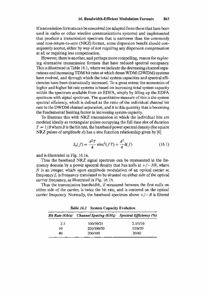
16. Bandwidth-Efficient Modulation Formats 863
If transmission formats can be conceived (or adapted from those that have been used in radio or other wireline communications systems) and implemented that produce a transmission spectrum that is narrower than the commonly used non-return-to-zero (NRZ) format, some dispersion benefit should con- sequently accrue, either by way of not requiring any dispersion compensation at all or requiring less compensation.
However, there is another, and perhaps more compelling, reason for explor- ing alternative transmission formats that have reduced spectral occupancy. This is illustrated in Table 16.1 , where we indicate the decreasing channel sepa- rations and increasing TDM bit rates at which dense WDM (DWDM) systems have evolved, and through which the total system capacities and spectral effi- ciencies have been dramatically increased. To a great extent the economics of higher and higher bit rate systems is based on increasing total system capacity within the spectrum available from an EDFA, simply by filling up the EDFA spectrum with signal spectrum. The quantitative measure of this is the system spectral efficiency, which is defined as the ratio of the individual channel bit rate to the DWDM channel separation, and it is this quantity that is becoming the fundamental limiting factor in increasing system capacity.
To illustrate this with NRZ transmission in which the individual bits are modeled ideally as rectangular pulses occupying the full time slot of duration T = 1/B whereB is the bit rate, the baseband power spectral density (for square NRZ pulses of amplitude A) has a sinc function relationship given by [6]
(16.1) A= T A2
4 4 &(f) = - sinc2(fT) + --S(f)
and is illustrated in Fig. 16.la. Thus the baseband NRZ signal spectrum can be represented in the fre-
quency domain by a power spectral density that has nulls at +/- NB, where N is an integer, which upon amplitude modulation of an optical carrier at frequencyf, is frequency translated to be situated on either side of the optical carrier frequency, as illustrated in Fig. 16.1 b.
Thus the transmission bandwidth, if measured between the first nulls on either side of the carrier, is twice the bit rate, and is centered on the optical carrier frequency. Normally, the baseband spectrum above +/- B is filtered
Table 16.1 System Capacity Evolution ~~~~ ~ ~
Bit Rate (Gb/s) Channel Spacing (GHZ) Spectral Eficiency (%)
2.5 100/50/25 2.5/5/10 10 200/100/50 5110120 40 2001 100 20140

864 Jan Conradi
1 Weight 0.5 t weight $
Frequency
Fig. 16.1 (a) Baseband power spectral density for N R Z and (b) power spectral density of an NRZ signal amplitude modulated onto a carrier at& (only positive frequencies shown).
out, which results in practical pulses with nonzero rise and fall times, which also substantially reduces the frequency content of the signal spectrum above the h s t nulls in the spectrum at the bit rate B. This also reduces spectral overlap between adjacent optical channels in a DWDM configuration, which can be placed at frequency intervals of 2B without incurring interchannel interference or cross-talk, and thus the maximum spectral efficiency for NRZ is 50% with this simple approximation. In a practical sense a spectral efficiency of 40% is realistic.
Thus for 10 and 40 Gb/s, the channel separations at 40% spectral efficiency are 25 and 100 GHz, respectively, which falls conveniently on the ITU spec- tral grid. It is worth noting that increasing the bit rate beyond 40 Gb/s cannot increase system capacity in the sense shown by the evolution in spectral effi- ciency illustrated in Table 16.1. What does result is a coarser channel plan that could have benefit in DWDM networks since a smaller number of wavelengths need to be managed.
Additionally, because interchannel nonlinear effects such as four-wave mix- ing (FWM) and cross-phase modulation (XPM) vary inversely with channel separation, reduced interchannel FWM and XPM penalties do occur as the bit rate is increased while keeping spectral efficiency fixed. Going to closer chan- nel spacings at lower bit rates, while keeping spectral efficiencies in the 40% range, presents difficult challenges from both an optical filtering perspective as well as from the standpoint of fiber nonlinearities and will require further research.
Thus, what is required if greater spectral efficiency, and hence system capacity, is to be achieved, are transmission formats that occupy a narrower spectrum while at the same time not causing other system impairments to increase.

16. Bandwidth-Efficient Modulation Formats 865
Various formats have been explored over the years, largely driven by the wireless business where spectrum is more at a premium than has hitherto been the case for fiber systems. Many communications engineering texts have extensive chapters devoted to this subject [see 6-91. Those formats that have received some attention for their potential application to optical communi- cations include multilevel signaling or M-ary ASK [lo], various forms of duo-binary signaling [l l-221 (which is a subset of partial response codes), and Optical Single Sideband (OSSB) [23-281.
Additionally, much attention has been focused recently on the use of return- to-zero (RZ) signaling [29] because of its demonstrated improved immunity to fiber nonlinearities relative to NRZ. If rectangular pulses were generated with a pulse width of half the bit time, their spectral occupancy would be twice that of NRZ, as the first nulls in the frequency domain would occur at +/- 2B, relative to the optical carrier, and their potential spectral efficiency would be one half that of NRZ signals. With pulse shaping, however, 40% spectral efficiency at 40 Gb/s has been demonstrated [30]. Therefore, it is fruitful to examine whether the nonlinearity improvements associated with FU signaling can be combined with more bandwidth-efficient formats to achieve still greater system performance.
The theme of this chapter, then, is to explore and review some of the work on transmission formats that would permit (or inhibit) increasing spectral efficiency, dispersion immunity, and interchannel nonlinearities. Much of this work has now progressed to the point where some reasonable statements as to future directions can and will be made.
The emphasis of this chapter will be on transmission formats that first and foremost have spectral occupancy or a transmission bandwidth on the fiber that is less than that of the true and tried (well loved?) NRZ format. It will be shown that such formats, by and large, are more immune to fiber disper- sion, but that other considerations and impairments need close attention. The emphasis will be on the fundamentals of generating and transmitting these signals, with a treatment founded in the theory of linear signals familiar to communications engineers, but possibly less familiar to the optical physics community.
It is also worth noting that in this electrical engineering communications context, fiber-optic systems are classified as classical bandpass systems to which well-developed electrical engineering modulation theory applies. The distinguishing differences between optical and radio/microwave systems lies in the carrier frequency (-200 THz vs several GHz) and in the nature of avail- able optical components that can generate or modulate these signals such that a direct comparison with theory can be made.
The balance of this chapter is organized as follows. Section 2 develops some basic background in modulation theory that is needed to understand how different modulation formats have different spectral occupancies and how these may be practically developed, as well as how optical modulators shape or
866 Jan Conradi
distort the input signal spectra before they are launched into optical fibers. We also examine how the commonly used PIN photodiode, which responds to the optical power and hence squares the time-dependent modulated electric field, significantly impacts both the time domain waveform and the spectrum of the square-law-detected signal, relative to the modulating signal at the modulator input, and the spectrum of the optical electric field at the detector input, all of which can be different.
Section 3 then examines the spectra associated with several bandwidth- efficient modulation formats; specifically M-ary ASK and poly-binary sig- naling with an emphasis on duo-binary and Optical Single Sideband formats where experimental work has been done to permit an assessment of their potential. Present-day understanding of the transmission characteristics of these signals, with an emphasis on the performance of single-channel 10-Gb/s transmission over NDSF, in the 1550-m low-loss spectral region is covered in Section 4, more as an illustration of how formats behave than to claim superiority of a particular format or for a particular optical fiber.
Section 5 looks at DWDM experiments that utilize these formats and also examines various formats that combine RZ with various other forms of signal manipulation, in particular some added phase modulation, to achieve improved transmission performance. Section 6 concludes with some suggestions for potential future research.
As a general rule, papers listed in the References section contain either the first or particularly illustrative results; other papers of interest are listed in the Bibliography.
2. Amplitude Modulation and Detection
2.1 AMPLITUDE-MODULATED SIGNAL REPRESENTATION1
Fiber-optic transmission systems, where the optical carrier frequency is in the 200-THz region and where the information to be transmitted occupies significantly less bandwidth than the optical carrier frequency, can be classified as bandpass signals. The desired outcome of an amplitude modulation process is to multiply, in the time domain, an information signal a(t) (which may or may not contain a dc component) with a continuous carrier wave represented by cos (2793) to produce a linearly amplitude-modulated signal given by
s(t) = a(t) cos (2Xf,t), (16.2)
wheref, is the optical carrier frequency.
Excellent material on the time and fkquency domain representation of modulated signals can be found in [6-lo].

16. Bandwidth-Efficient Modulation Formats 867
If we represent a(t) by 40 = a0 + a&), (16.3)
where a0 is a dc component and a&) is the information signal, then the Fourier transforms of these signals give the frequency domain representation of the baseband and modulated signals, respectively, as
and
Therefore, the desired outcome of this linear modulation process is the up- shifting of the frequency spectrum of the baseband signal to be centered on the optical carrier frequency, as illustrated in Fig. 16.1. Implicit in this is that the optical carrier can be represented by a pure sinusoid such that it is a delta function in the frequency domain, an approximation to which is that the linewidth of the optical source be much narrower than the bandwidth of the signal to be modulated onto the carrier.
It is important to note that it is the optical electn'cjeld spectrum that is represented by an up-shifted version of the baseband signal. It should also be noted that if no dc component is included in the information signal represented by Eq. 16.2, there is no unmodulated carrier present in the final modulated signal, whereas if a dc component is present, so is an unmodulated carrier. This has particular importance when a PIN photodiode detects the signal.
Distortion of the signal results from a large number of imperfections in an optical system. The most fundamental of these are:
(1) Modulators that, except in various small signal approximations, are
(2) The commonly used PIN semiconductor detector, which responds rarely linear in the sense of Eq. 16.2.
to the optical power and hence it squares the time representation of the modulated optical electric field. This in turn results in time and frequency representations of the detected signal that are quite different from those of the signal applied to the modulator.
(3) Dispersion in optical fibers, which introduces a differential time delay across the various frequency components of the modulated signal, which in turn is equivalent to a frequency-dependent phase shift [31].
These various impairments make it difficult to advantageously imple- ment modulation formats other than the tried-and-true intensity modulated approaches using either NRZ or RZ formats. Progress has nevertheless been

868 Jan Conradi
made, and in what follows we discuss this progress and outline where neces- sary, how current implementation capabilities impose limitations on progress and how improvements can be made.
2.2 MODULATOR CHAM CTERISTICS
Of the various approaches to modulating optical signals, really only three have seen significant adoption, namely
(1) direct modulation of semiconductor lasers by modulating their drive
(2) electroabsorption (EA) modulators [33]; (3) Mach-Zehnder (MZ) modulators [34].
current [32];
The directly modulated semiconductor laser and the electroabsorption modulator result in the opticdpower being modulated in response to an input modulating signal, usually with some accompanying phase modulation that can be either beneficial or detrimental to the transmission of the signal [35]. The MZ modulator, on the other hand, can be a quite flexible device that is capable of performing a variety of modulation functions on the light, and it has been used successfully in creating a variety of modulated signals that are not purely NRZ binary amplitude or intensity modulated signals.
Specilically, it has been used to create both duo-binary [13-161 and optical single-sideband signals [25,26,36,37], but invariably with some accompanying distortion in the output signal such that the transmitted signal spectrum is not an undistorted, frequency up-shifted version of the spectrum of the baseband signal. This is, undoubtedly, one of the main reasons why the potential of modulation formats other than NRZ have not fulfilled their potential.
Because the modulated output from the semiconductor laser and the EA modulator correspond to intensity modulation (with some added phase modulation), modulation formats requiring electric modulation as described by Eq. 16.2 cannot be used with these devices, and they will not be addressed further. We will examine how the MZ modulator can and has been used to generate modulated signals other than binary amplitude shift keyed (ASK) or intensity modulated (IM) signals
Figure 16.2 is a schematic representation of a MZ modulator. The input optical electric field is represented as Ein = lEol eiocr, where in this instance we adopt the exponential representation of the time-varying part of the opti- cal electric field. This unmodulated signal propagates in a waveguide at the modulator input where it is split into two separate waveguides, with a split ratio that ideally is 50%. Electrodes, to which signal voltages v1 ( t ) and vz(t) are applied, modulate the propagation constant within each waveguide, resulting in a phase modulation of the signal propagating in each arm. When these two signals are combined at the modulator output, the result is a modulated output

16. Bandwidth-Efficient Modulation Formats
Fig. 16.2 Schematic representation of a Mach-Zehnder modulator.
electric field given by
The electric field transfer function of the device is
where u, is the modulator extinction voltage,
& - 1 &+ 1
y = -
869
(16.6)
(16.7)
(16.8)
and S equals the dc extinction ratio of the modulator.
that To simplify, consider an ideal modulator with infinite extinction ratio such
S + o a or y = l .
Then,
To avoid chirp, the time-varying portions of v1 and v2 are often chosen such that vl(t) = -vz(t), and then

870 Jan Conradi
and the output optical electric field is
and the output optical power is
This is the usual way in which MZ modulator transfer functions are represented.
Figure 16.3 shows both the optical power and electric field transfer functions of the MZ modulator.
To look at the effect of a relative bias between the arms retaining chirpless modulation, let vz(t) = vdc - vl(t). Then Eq. 16.9 becomes
\y(vl(t), vdC) = cos (2vl(t) - vdc) ej(nv&12vr) ( 1 6.1 3)
t 1
t Modulation Constant
Term Phase Shift
Fig. 16.3 Normalized optical electric field and power transfer functions of a Mach-Zehnder modulator.

16. Bandwidth-Efficient Modulation Formats 871
(a) "Normal" bias Vd, = V,/2
amplitude to each arm as a fraction of V,. Then, vl(t) = ma(t)V, with a(t) = +/-1 for a digital signal, m = electrical drive
(Ignoring the constant phase shift).
(16.14)
To simplify let's invoke the small-signal condition such that nma(t) << 1. Then
'u(a(t), VJ2) = cos n ma(t) - - [ ( :>I (16.15)
n n = cos (nma(t)) cos - + sin (nma(t)) sin - 4 4 x -[1 1 + nma(t)]
2/2
The output optical electric field then becomes:
Ein
z/z 2 5 -[1 + 2nma(t)]eJ"'
t t Unmodulated Modulated
Carrier Carrier
The optical power transfer function is then given by
"I2 (16.17) = [cos (nma(t)) cos - + sin (nma(t)) sin - n 4 4
1 2
r3 -[1 + nma(t)]2.
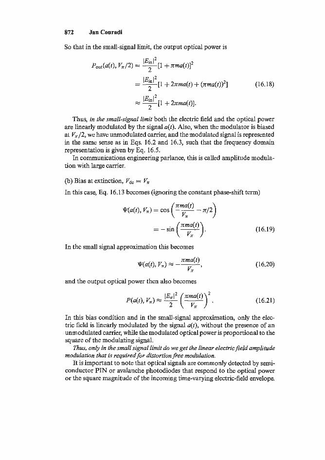
872 Jan Conradi
So that in the small-signal limit, the output optical power is
Thus, in the small-signal limit both the electric field and the optical power are linearly modulated by the signal a(t). Also, when the modulator is biased at V,/2, we have unmodulated carrier, and the modulated signal is represented in the same sense as in Eqs. 16.2 and 16.3, such that the frequency domain representation is given by Eq. 16.5.
In communications engineering parlance, this is called amplitude modula- tion with large carrier.
(b) Bias at extinction, vdc = V,
In this case, Eq. 16.13 becomes (ignoring the constant phase-shift term)
Q(a(t), V,) = cos
nma(t) - - -sin(T).
In the small signal approximation this becomes
nma(t) Q(a(t), Vn) e -- T, 9
v ,
and the output optical power then also becomes
(16.19)
(1 6.20)
(16.21)
In this bias condition and in the small-signal approximation, only the elec- tric field is linearly modulated by the signal a(t), without the presence of an unmodulated carrier, while the modulated optical power is proportional to the square of the modulating signal.
Thus, only in the small signal limit do we get the linear electric$eld amplitude modulation that is required for distortion f i e modulation.
It is important to note that optical signals are commonly detected by semi- conductor PIN or avalanche photodiodes that respond to the optical power or the square magnitude of the incoming time-varying electric-field envelope.
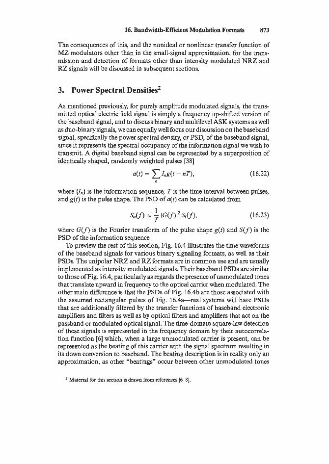
16. Bandwidth-Efficient Modulation Formats 873
The consequences of this, and the nonideal or nonlinear transfer function of MZ modulators other than in the small-signal approximation, for the trans- mission and detection of formats other than intensity modulated NRZ and RZ signals will be discussed in subsequent sections.
3. Power Spectral Densities’
As mentioned previously, for purely amplitude modulated signals, the trans- mitted optical electric field signal is simply a frequency up-shifted version of the baseband signal, and to discuss binary and multilevel ASK systems as well as duo-binary signals, we can equally well focus our discussion on the baseband signal, specifically the power spectral density, or PSD, of the baseband signal, since it represents the spectral occupancy of the information signal we wish to transmit. A digital baseband signal can be represented by a superposition of identically shaped, randomly weighted pulses [38]
(16.22)
where {In) is the information sequence, T is the time interval between pulses, and g(t) is the pulse shape. The PSD of a(t) can be calculated from
(16.23)
where G O is the Fourier transform of the pulse shape g(t) and S(f) is the PSD of the information sequence.
To preview the rest of this section, Fig. 16.4 illustrates the time waveforms of the baseband signals for various binary signaling formats, as well as their PSDs. The unipolar NRZ and RZ formats are in common use and are usually implemented as intensity modulated signals. Their baseband PSDs are similar to those of Fig. 16.4, particularly as regards the presence of unmodulated tones that translate upward in frequency to the optical carrier when modulated. The other main difference is that the PSDs of Fig. 16.4b are those associated with the assumed rectangular pulses of Fig. 16.4a-real systems will have PSDs that are additionally filtered by the transfer functions of baseband electronic amplifiers and filters as well as by optical filters and amplifiers that act on the passband or modulated optical signal. The time-domain square-law detection of these signals is represented in the frequency domain by their autocorrela- tion function [6] which, when a large unmodulated carrier is present, can be represented as the beating of this carrier with the signal spectrum resulting in its down conversion to baseband. The beating description is in reality only an approximation, as other “beatingsyy occur between other unmodulated tones
1 s a ~ ) = T IGCf>12SCf),
Material for this section is drawn from references [&SI.
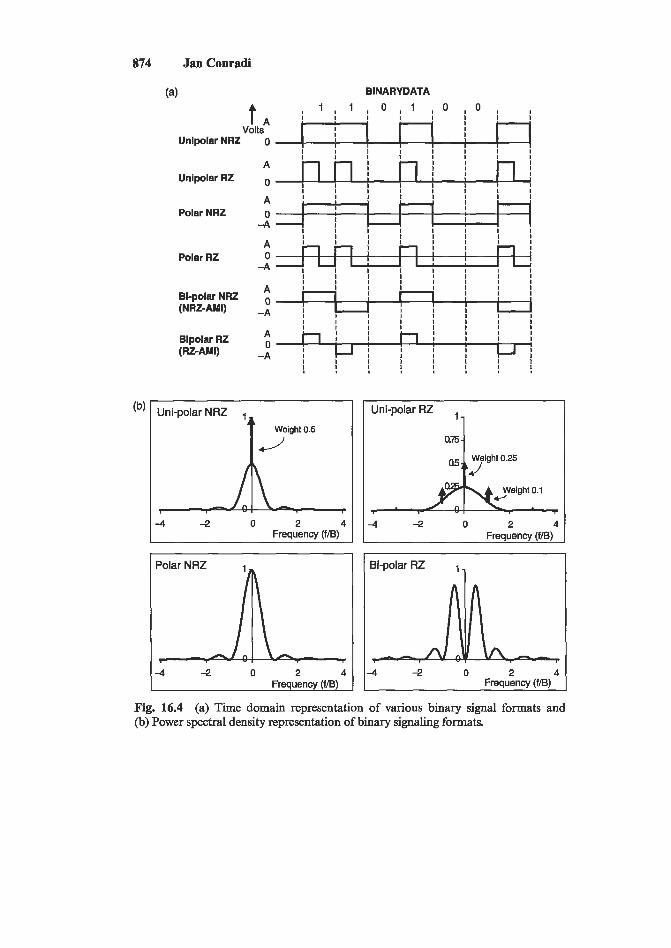
874 Jan Conradi
- - I I
Unlpolar NRZ 0 I
A ' 0
I
I
I -A -4 !I
Unipolar RZ
I - I - I
I Polar NRZ
A Polar RZ
I I I I I I I I
o-x+- I
Bi-polar NRZ (NRZ-AMI)
-A-
Bipolar RZ (RZ-AMI)
' 1 I I I
I I I I
I I I
1
I I 1 1 I I
A 0
I I 1 I I I I 1
I I I
I 1 I I 1
A O h b l I I
I I
-A I I I I I ! ! ! ! ! ! ! !
-4 -2 0 2 4 Frequency (f/B)
-2 0 2 4 Frequency (f/B)
, . ,A;- Weight 0.1
4 -2 0 2 4 Frequency (WB)
'1 Bi-polar RZ
-2 0 2 4 Freauencv If/BI
Fig. 16.4 (a) Time domain representation of various binary signal formats and (b) Power spectral density representation of binary signaling formats
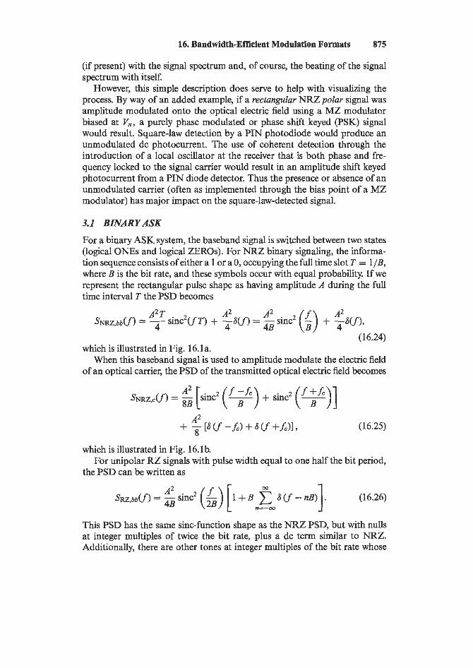
16. Bandwidth-Efficient Modulation Formats 875
(if present) with the signal spectrum and, of course, the beating of the signal spectrum with itself.
However, this simple description does serve to help with visualizing the process. By way of an added example, if a rectangular NRZ polar signal was amplitude modulated onto the optical electric field using a MZ modulator biased at V,, a purely phase modulated or phase shift keyed (PSK) signal would result. Square-law detection by a PIN photodiode would produce an unmodulated dc photocurrent. The use of coherent detection through the introduction of a local oscillator at the receiver that is both phase and fre- quency locked to the signal carrier would result in an amplitude shift keyed photocurrent from a PIN diode detector. Thus the presence or absence of an unmodulated carrier (often as implemented through the bias point of a MZ modulator) has major impact on the square-law-detected signal.
3.1 BAYARYASK
For a binary ASK system, the baseband signal is switched between two states (logical ONES and logical ZEROS). For NRZ binary signaling, the informa- tion sequence consists of either a l or a 0, occupying the full time slot T = 1/B, where B is the bit rate, and these symbols occur with equal probability. If we represent the rectangular pulse shape as having amplitude A during the full time interval T the PSD becomes
(1 6.24) which is illustrated in Fig. 16.la.
When this baseband signal is used to amplitude modulate the electric field of an optical carrier, the PSD of the transmitted optical electric field becomes
(16.25)
which is illustrated in Fig. 16.1 b.
the PSD can be written as For unipolar RZ signals with pulse width equal to one half the bit period,
This PSD has the same sinc-function shape as the NRZ PSD, but with nulls at integer multiples of twice the bit rate, plus a dc term similar to NRZ. Additionally, there are other tones at integer multiples of the bit rate whose

876 Jan Conradi
amplitudes are determined by the sinc function, resulting in tones at odd integer multiples of the bit rate. This is the PSD of RZ signals with ideal- square pulses, but with spectral shaping through various modulator stages, this spectrum can be substantially reduced and shaped.
3.2 MULTILEVEL AMPLITUDE SHIFTKEYING (n-av ASK) 1101 In this format, binary signal bits are converted into a binary code word where N bits are converted into a multilevel signal whose number of amplitude levels isM = P.
If we use the aggregate bit rate B of the final signal as our bit-rate reference, then effectively, instead of transmitting bits of a single amplitude of time duration T at a rate By we transmit symbols of time duration T = N/B at a rate BIN with amplitudes ranging from zero to M = 2N.
A generalization of Eq. 16.1 for the baseband power-spectral density of a square-pulse M-ary signal is
SW) (M2 - 1)A2T (M - 1)2A2
4 saw)= 12 sinc2UT) +
For a given level of encoding, the amplitudes of the symbols are given by the equivalent binary representation of the word it represents, and each symbol carries N = log,(M) bits of information. Since the symbol time has been extended from T = 1/B to T = N/B, the transmission bandwidth (measured between the first nulls in the spectrum) has been reduced from 2B to 2B/N = 2B/10g2 (Ad). Table 16.2 is a simple illustration of the diminishing return.
In order to construct and to detect these signals, complex linear analog circuitry is required. A relatively simple implementation for a 4-ary system is shown in Fig. 16.5.
This signal format is best transmitted as a four-level intensity-modulated signal, in that if equal amplitudes were used to modulate the electric field, the
Table 16.2 Equivalent Transmission Bandwidth of M-ary ASK
Number of Levels 0 Equivalent Transmission Bandwidth
2 4 8
16 32 64
+/ -B +/-I312 + / -B /3 + / -B /4 + / -B /5 + / -B/6
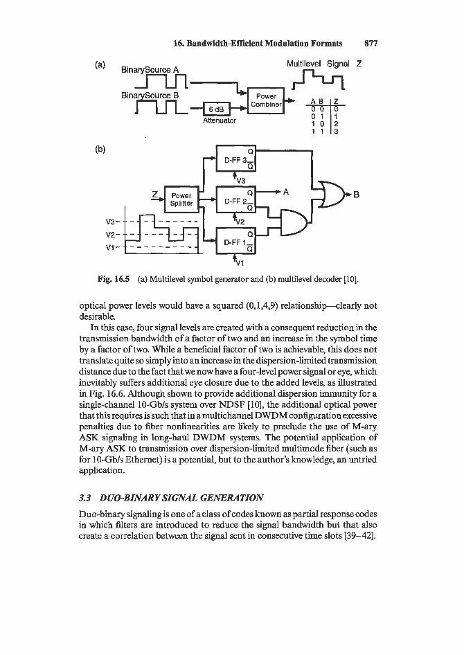
16. Bandwidth-Efficient Modulation Formats 877
v3 - v2 - v1-
Multilevel Signal Z
fi BinarySource A i n 1
- - -
Attenuator
D-FF 3- G U I I 1 0 12 1 1 13
1 B
t l
Fig. 16.5 (a) Multilevel symbol generator and (b) multilevel decoder [lo].
optical power levels would have a squared (0,1,4,9) relationship-clearly not desirable.
In this case, four signal levels are created with a consequent reduction in the transmission bandwidth of a factor of two and an increase in the symbol time by a factor of two. While a beneficial factor of two is achievable, this does not translate quite so simply into an increase in the dispersion-limited transmission distance due to the fact that we now have a four-level power signal or eye, which inevitably suffers additional eye closure due to the added levels, as illustrated in Fig. 16.6. Although shown to provide additional dispersion immunity for a single-channel 10-Gb/s system over NDSF [lo], the additional optical power that this requires is such that in a multichannel DWDM configuration excessive penalties due to fiber nonlinearities are likely to preclude the use of M-ary ASK signaling in long-haul DWDM systems. The potential application of M-ary ASK to transmission over dispersion-limited multimode fiber (such as for 10-Gb/s Ethernet) is a potential, but to the author’s knowledge, an untried application.
3.3 DUO-BINARY SIGNAL GENERATION
Duo-binary signaling is one of a class of codes known as partial response codes in which filters are introduced to reduce the signal bandwidth but that also create a correlation between the signal sent in consecutive time slots [39-421.
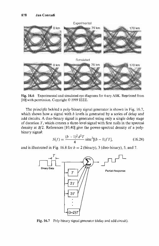
878 Jan Conradi
Exnerimental
Simulated
Fig. 16.6 Experimental and simulated eye diagrams for 4-ary ASK. Reprinted from [lo] with permission. Copyright 0 1999 IEEE.
The principle behind a poly-binary signal generator is shown in Fig. 16.7, which shows how a signal with b levels is generated by a series of delay and add circuits. A duo-binary signal is generated using only a single delay stage of duration T , which creates a three-level signal with first nulls in the spectral density at B/2. References [10,40] give the power-spectral density of a poly- binary signal:
sinc2[(b - l)fT], (1 6.28) (b - 1)2A2T W ) =
and is illustrated in Fig. 16.8 for b = 2 (binary), 3 (duo-binary), 5, and 7.
Binary Data i”m-
Partial-Response
Fig. 16.7 Poly-binary signal generator (delay and add circuit).
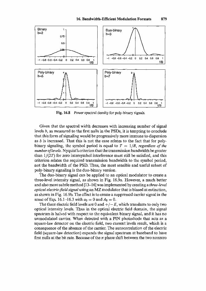
16. Bandwidth-Efficient Modulation Formats 879
Duo-binary ' 1 Binary b=2 I I "-" 0.75 1
-1 -0.6 -0.6 -0A -0.2 0 02 OA 0.6 0.8 1 WB ;';- nreh- , , ,
i/B -1 -0fl -0.6 -0.4 -02 0 02 0.4 0.6 0.8 1
Poly-binary
bL -1 -0.6 -0.6 -0.4 -0.2 0 0.2 0.4 0.6 0.8 1
WB
Fig. 16.8 Power spectral density for poly-binary signals.
Given that the spectral width decreases with increasing number of signal levels b, as measured to the first nulls in the PSDs, it is tempting to conclude that this form of signaling would be progressively more immune to dispersion as b is increased. That this is not the case relates to the fact that for poly- binary signaling, the symbol period is equal to T = 1/B, regardless of the number of levels. Nyquist's criterion that the transmission bandwidth be greater than 1/(2T) for zero intersymbol interference must still be satisfied, and this criterion relates the required transmission bandwidth to the symbol period, not the bandwidth of the PSD. Thus, the most sensible and useful subset of poly-binary signaling is the duo-binary version.
The duo-binary signal can be applied to an optical modulator to create a three-level intensity signal, as shown in Fig. 16.9a. However, a much better and also more subtle method [13-161 was implemented by creating a three-level optical electric-jeld signal using an MZ modulator that is biased at extinction, as shown in Fig. 16.9b. The effect is to create a suppressed carrier signal in the sense of Eqs. 16.1-16.3 with uo = 0 and& = 0.
The three electric field levels are 0 and + / - E , which translates to only two optical intensity levels. Thus in the optical electric field domain, the signal spectrum is halved with respect to the equivalent binary signal, and it has no unmodulated carrier. When detected with a PIN photodiode that acts as a square-law detector on the electric field, two current levels result, which is a consequence of the absence of the carrier. The autocorrelation of the electric field (square-law detection) expands the signal spectrum at baseband to have first nulls at the bit rate. Because of the n phase shift between the two nonzero
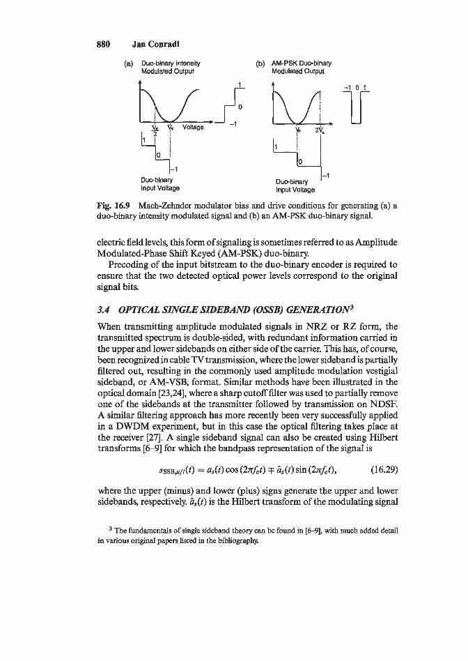
880 Jan Conradi
(a) Duo-binary Intensity (b) AM-PSK Duo-binary Modulated Output Modulated Output
i Duo-binary Input Voltage
1, lo I I
-1 Duebinary Input Voltage
u Fig. 16.9 Mach-Zehnder modulator bias and drive conditions for generating (a) a duo-binary intensity modulated signal and (b) an AM-PSK duo-binary signal.
electric field levels, this form of signaling is sometimes referred to as Amplitude Modulated-Phase Shift Keyed (AM-PSK) duo-binary.
Precoding of the input bitstream to the duo-binary encoder is required to ensure that the two detected optical power levels correspond to the original signal bits.
3.4 OPTICAL SINGLE SIDEBAND (OSSB) GENERATION3
When transmitting amplitude modulated signals in NRZ or RZ form, the transmitted spectrum is double-sided, with redundant information carried in the upper and lower sidebands on either side of the carrier. This has, of course, been recognized in cable TV transmission, where the lower sideband is partially filtered out, resulting in the commonly used amplitude modulation vestigial sideband, or AM-VSB, format. Similar methods have been illustrated in the optical domain [23,24], where a sharp cutoff filter was used to partially remove one of the sidebands at the transmitter followed by transmission on NDSF. A similar filtering approach has more recently been very successfully applied in a DWDM experiment, but in this case the optical filtering takes place at the receiver [271. A single sideband signal can also be created using Hilbert transforms [6-91 for which the bandpass representation of the signal is
where the upper (minus) and lower (plus) signs generate the upper and lower sidebands, respectively. &(t) is the Hilbert transform of the modulating signal
The fundamentals of single sideband theory can be found in [6-91, with much added detail in various original papers listed in the bibliography.
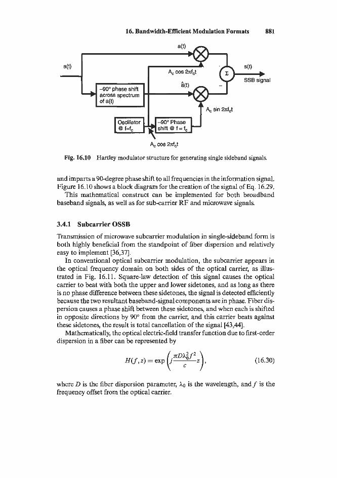
16. Bandwidth-Efficient Modulation Formats 881
SSB signal
a(t)
-90" phase shift + across spectrum
A, cos 2nfJ
Fig. 16.10 Hartley modulator structure for generating single sideband signals.
and imparts a 90-degree phase shift to all frequencies in the information signal. Figure 16.10 shows a block diagram for the creation of the signal of Eq. 16.29.
This mathematical construct can be implemented for both broadband baseband signals, as well as for sub-carrier RF and microwave signals.
3.4.1 Subcamer OSSB
Transmission of microwave subcarrier modulation in single-sideband form is both highly beneficial from the standpoint of fiber dispersion and relatively easy to implement [36,37].
In conventional optical subcarrier modulation, the subcarrier appears in the optical frequency domain on both sides of the optical carrier, as illus- trated in Fig. 16.11. Square-law detection of this signal causes the optical carrier to beat with both the upper and lower sidetones, and as long as there is no phase difference between these sidetones, the signal is detected efficiently because the two resultant baseband-signal components are in phase. Fiber dis- persion causes a phase shift between these sidetones, and when each is shifted in opposite directions by 90" from the carrier, and this carrier beats against these sidetones, the result is total cancellation of the signal [43,44].
Mathematically, the optical electric-field transfer function due to first-order dispersion in a fiber can be represented by
H c f , z ) = exp j - ( nD2f2z)y (16.30)
where D is the fiber dispersion parameter, ho is the wavelength, and f is the frequency offset from the optical carrier.

882 Jan Conradi
t
Fig. 16.11 Illustration of double sidebands associated with subcarrier modulation (only positive frequencies shown).
If a double sideband sinusoidal signal at modulation frequency& accord- ing to Eq. 16.3 propagates down a fiber whose transfer function is given by Eq. 16.30, the frequency domain representation of the optical electric field at distance z down the fiber is
x exp ( j F z ) . (1 6.3 1)
The square-law-detected signal is the Fourier transform, F, of the squared envelope operator in the time domain (i.e., the autocorrelation of the Fourier transform of the electric field) and is given by
F (IE(t)l2) = 7 FEWFf! cf + 6) df = 47- (0 .
If we consider only the fundamental term in Aff at& resulting from Eq. 16.32, we get:
(1 6.32) --bo
(16.33)

16. Bandwidth-Efficient Modulation Formats 883
If we take the inverse Fourier transform of Eq. 16.33 and then take the real part of this, we get the frequency dependence of the detected photocurrent as
z +cos 2n&t - n- I ( t ) oc 2n2 [ ( cos 2n&t + n- nDAz C ) ( nDAiL;z)l C
oc cos (2nf,t) cos (n*z) (1 6.34)
Thus the detectedwpower at the subcarrier frequency will vary with distance and subcarrier frequency according to
(16.35)
If one of the sidebands is removed, detector output current becomes
I(t) oc cos 2n.J + It- ( nDAiA:z) C Or
as in single-sideband modulation, the
2Rfsct-lT- nDAiL’z) C , (16.36)
depending on which sideband is removed. Note that both terms in Eq. 16.36 are constant in power as a function of fiber length.
Since most microwave subcarrier transmission occurs with relatively nar- rowband information signals, the result is that only dispersion across the narrow information spectrum is of relevance, and this is small for the distances that subcarrier systems have been implemented.
To implement an R F OSSB system using the modulator structure of Fig. 16.10, the sine and cosine carriers can be simply generated in an MZ modulator through the application of a differential dc bias voltage equal to V,/2 to the two arms, which creates a 90-degree phase shift between the opti- cal carriers in the two arms of the MZ modulator. The two arms of the MZ modulator are then modulated by the subcarrier, with a differential time delay between the drives to the arms corresponding to a n/2 phase shift of the sub- carrier frequency. Given that the information signal is narrow band, this also adequately Hilbert transforms the information signal.
Two illustrations of the impact of OSSB on the dispersion-limited trans- mission of a 17-GHz subcarrier on NDSF are illustrated in Fig. 16.12 [37]. Figure 16.12a compares the detected RF power of a 17.16-GHz subcarrier when transmitted at 1550 nm over NDSF using conventional double sideband modulation and OSSB as implemented previously. Figure 16.12b illustrates performance at 17.16 GHz when using the MZ modulator in two significantly nonlinear configurations.
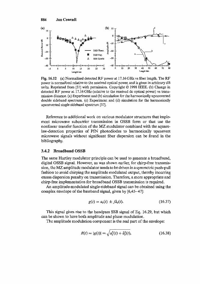
884 Jan Conradi
0 5 10 15 20 25 30
1 10
0
-10
-20
(a) 10
1 -30
-40 -5
Length h ;I h n s t h h
Fig. 16.12 (a) Normalized detected RF power at 17.16 GHz vs fiber length. The RF power is normalized relative to the received optical power, and is given in arbitrary dB units. Reprinted from [37] with permission. Copyright 0 1998 IEEE. @) Change in detected RF power at 17.16GHz (relative to the received dc optical power) vs trans- mission distance. (a) Experiment and @) simulation for the harmonically upconverted double sideband spectrum. (c) Experiment and (d) simulation for the harmonically upconverted single sideband spectrum [37].
-40 -30 0 10 20 30 40 50 M) 70 80
Reference to additional work on various modulator structures that imple- ment microwave subcarrier transmission in OSSB form or that use the nonlinear transfer function of the MZ modulator combined with the square- law-detection properties of PIN photodiodes to harmonically upconvert microwave signals without significant fiber dispersion can be found in the bibliography.
3.4.2 Broadband OSSB
The same Hartley modulator principle can be used to generate a broadband, digital OSSB signal. However, as was shown earlier, for chirp-free transmis- sion, the MZ amplitude modulator needs to be driven in a symmetric push-pull fashion to avoid chirping the amplitude modulated output, thereby incurring excess dispersion penalty on transmission. Therefore, a more appropriate and chirp-free implementation for broadband OSSB transmission is required.
An amplitude-modulated single-sideband signal can be obtained using the complex envelope of the baseband signal, given by [6,45-471:
This signal gives rise to the bandpass SSB signal of Eq. 16.29, but which
The amplitude modulation component is the real part of the envelope: can be shown to have both amplitude and phase modulation.
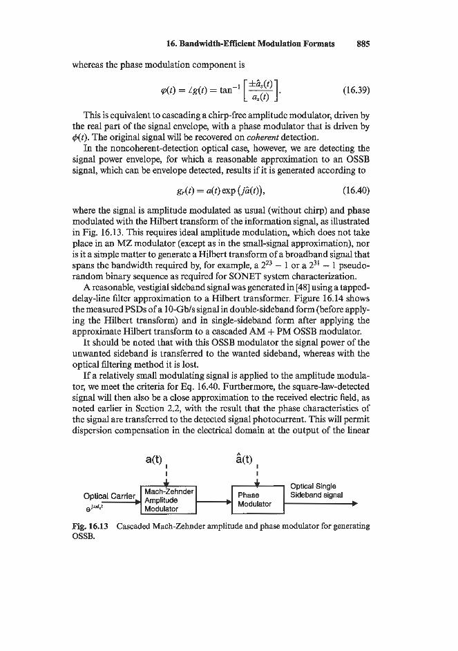
16. Bandwidth-Efficient Modulation Formats 885
Mach-Zehnder Phase Optical Carrier Amplitude
elZ&i Modulator Modulator
whereas the phase modulation component is
Sideband signal b
(16.39)
This is equivalent to cascading a chirp-free amplitude modulator, driven by the real part of the signal envelope, with a phase modulator that is driven by @(t). The original signal will be recovered on coherent detection.
In the noncoherent-detection optical case, however, we are detecting the signal power envelope, for which a reasonable approximation to an OSSB signal, which can be envelope detected, results if it is generated according to
g&) = ~ X P (jW)), (16.40)
where the signal is amplitude modulated as usual (without chirp) and phase modulated with the Hilbert transform of the information signal, as illustrated in Fig. 16.13. This requires ideal amplitude modulation, which does not take place in an MZ modulator (except as in the small-signal approximation), nor is it a simple matter to generate a Hilbert transform of a broadband signal that spans the bandwidth required by, for example, a 223 - 1 or a 231 - 1 pseudo- random binary sequence as required for SONET system characterization.
A reasonable, vestigial sideband signal was generated in [48] using a tapped- delay-line filter approximation to a Hilbert transformer. Figure 16.14 shows the measured PSDs of a 10-Gb/s signal in double-sideband form (before apply- ing the Hilbert transform) and in single-sideband form after applying the approximate Hilbert transform to a cascaded AM + PM OSSB modulator.
It should be noted that with this OSSB modulator the signal power of the unwanted sideband is transferred to the wanted sideband, whereas with the optical atering method it is lost.
If a relatively small modulating signal is applied to the amplitude modula- tor, we meet the criteria for Eq. 16.40. Furthermore, the square-law-detected signal will then also be a close approximation to the received electric field, as noted earlier in Section 2.2, with the result that the phase characteristics of the signal are transferred to the detected signal photocurrent. This will permit dispersion compensation in the electrical domain at the output of the linear

886 Jan Conradi
Frequency (GHz)
0
-30-
-10 -5 fo +5 +10 -60
Frequency (GHz)
Fig. 16.14 Experimental optical spectra for (a) DSB and (b) OSSB signals at 10 Gb/s [48].
portion of the optical receiver. In a sense, we have created a “self-homodyne” coherent detection system, and it is interesting to contemplate whether a full coherent detection system would permit large signal modulation at the trans- mitter with a reduction in the initial eye opening penalty associated with the small modulation depth. Alternatively, if a suppressed carrier OSSB signal is transmitted, and this signal is coherently detected at the receiver, it should be possible to perform dispersion compensation quite accurately at the output of the linear portion of the receiver, provided the received signal has not been corrupted by nonlinear effects in the fiber.
4. Single-Channel Transmission Results
4.1 M-ary ASK TRANSMISSION [lo]
The simulations in Fig. 16.15 show how the dispersion-induced reduction in receiver sensitivity (at a bit error ratio of varies with fiber length for sev- eral ASK formats for NDSF at an aggregate bit rate of 10 Gb/s at a wavelength in the 1550-nm window. Clearly, the dispersion limitation has been improved in all cases. In the case of the 4-ary signal, because of the need to detect the signal with a given bit error ratio (BER), the signal-to-noise ratio within each of the three eyes needs to be essentially the same as for the equivalent two-level
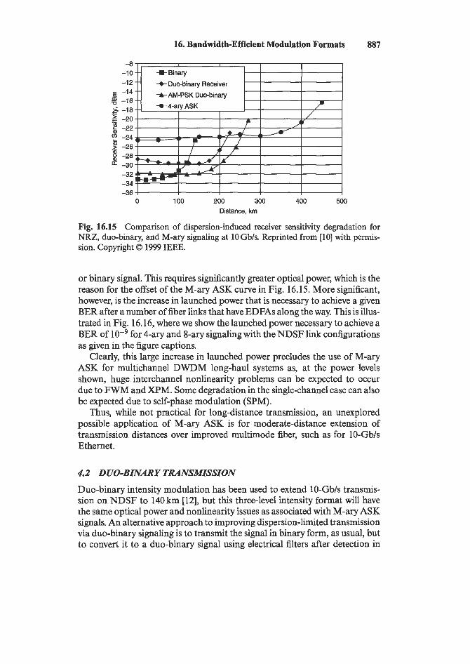
16. Bandwidth-Efficient Modulation Formats 887
-36 ! I I I I 0 100 200 300 400 500
I Distance, km
Fig. 16.15 Comparison of dispersion-induced receiver sensitivity degradation for NRZ, duo-binary, and M-ary signaling at 10 Gbk Reprinted from [lo] with permis- sion. Copyright 0 1999 IEEE.
or binary signal. This requires significantly greater optical power, which is the reason for the offset of the M-ary ASK curve in Fig. 16.15. More significant, however, is the increase in launched power that is necessary to achieve a given BER after a number of fiber links that have EDFAs along the way. This is illus- trated in Fig. 16.16, where we show the launched power necessary to achieve a BER of for 4-ary and 8-ary signaling with the NDSF link configurations as given in the figure captions.
Clearly, this large increase in launched power precludes the use of M-ary ASK for multichannel DWDM long-haul systems as, at the power levels shown, huge interchannel nonlinearity problems can be expected to occur due to FWM and XPM. Some degradation in the single-channel case can also be expected due to self-phase modulation (SPM).
Thus, while not practical for long-distance transmission, an unexplored possible application of M-ary ASK is for moderate-distance extension of transmission distances over improved multimode fiber, such as for 10-Gb/s Ethernet.
4.2 D UO-BINARY TRANSMISSION
Duo-binary intensity modulation has been used to extend 10-Gb/s transmis- sion on NDSF to 140 km [12], but this three-level intensity format will have the same optical power and nonlinearity issues as associated with M-ary ASK signals. An alternative approach to improving dispersion-limited transmission via duo-binary signaling is to transmit the signal in binary form, as usual, but to convert it to a duo-binary signal using electrical filters after detection in

888 Jan Conradi
0
-1 0
-20
E? $ -30 5 -40 s
-50
-60
-70 I' I \ I I \ I I \
5 10 15 20 Launched Optical Power, dBm
0
-1 0
-20 a $ -30 5 9 -40
+320 km (40 krn links) -50
-60
-70 5 10 15 20
Launched Optical Power, dBm
Fig. 16.16 Launched power necessary to achieve a lod9 BER for various M-ary ASK formats at 10 Gb/s over NDSF. Reprinted from [lo] with permission. Copyright 0 1999 IEEE.
the receiver. Improvement in transmission distance at 10 Gb/s on NDSF to - 160 km was achieved by this means [ 1 11. The best duo-binary single-channel transmission results have been obtained
using AM-PSK duo-binary signaling where distances up to -225km at lOGb/s at 1550nm over NDSF have been reported [13-161.
One important item to note is that in order to achieve improved dispersion- limited transmission with this format, it is necessary to provide extra filtering after the delay-and-add filter in order to remove those parts of the baseband signal spectrum that occur at frequencies above B/2 [17]. This is because the delay-and-add filter is in fact periodic in frequency, and does not continuously attenuate frequencies above B/2. These higher-frequency components of the signal, which are present at sufficient power, undergo sufficient dispersion to substantially reduce the signal eye opening, as illustrated in Fig. 16.17. The
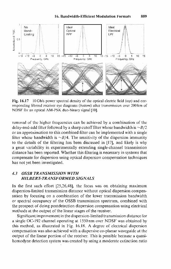
16. Bandwidth-Efficient Modulation Formats 889
-15 -10 -5 0 5 10 15 Frequency, GHz
Ideal Optical
-15 -10 Frequency, -5 0 GHz 5 10 15
Ideal Electrical
-15 -A -10 Frequency, -5 0 GHz 5 10 15
Fig. 16.17 10Gb/s power spectral density of the optical electric field (top) and cor- responding filtered receiver eye diagrams (bottom) after transmission over 200 km of NDSF for an optical AM-PSK duo-binary signal [lo].
removal of the higher frequencies can be achieved by a combination of the delay-and-add filter followed by a sharp cutoff filter whose bandwidth is -B/2 or an approximation to this combined filter can be implemented with a single filter whose bandwidth is -B/4. The sensitivity of the dispersion immunity to the details of the filtering has been discussed in [17], and likely is why a great variability in experimentally extending single-channel transmission distance has been reported. Whether this filtering is necessary in systems that compensate for dispersion using optical dispersion compensation techniques has not yet been investigated.
4.3 OSSB TRANSMISSION WITH HILBERT-TRANSFORMED SIGNALS
In the first such effort [25,26,48], the focus was on obtaining maximum dispersion-limited transmission distance without optical dispersion compen- sation by focusing on a combination of the lower transmission bandwidth or spectral occupancy of the OSSB transmission spectrum, combined with the prospect of doing postdetection dispersion compensation using electrical methods at the output of the linear stages of the receiver.
Significant improvement in the dispersion-limited transmission distance for a single OC-192 channel operating at 1550nm over NDSF was obtained by this method, as illustrated in Fig. 16.18. A degree of electrical dispersion compensation was also achieved with a dispersive co-planar waveguide at the output of the linear portion of the receiver. This is possible because a quasi- homodyne detection system was created by using a moderate extinction ratio
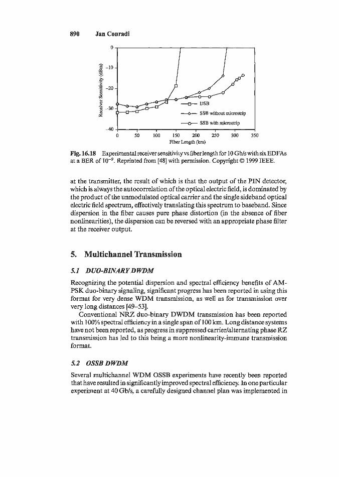
890 Jan Conradi
0
h
E -10
b
I
.-
v1
.- --b SSB without microstrip 3 -30
-40 0 50 100 150 200 250 300
Fiber Length (km) 0
Fig. 16.18 Experimentalreceiver sensitivityvsfiberlengthfor 10 Gb/s withsixEDFAs at a BER of lop9. Reprinted from [48] with permission. Copyright 0 1999 IEEE.
at the transmitter, the result of which is that the output of the PIN detector, which is always the autocorrelation of the optical electric field, is dominated by the product of the unmodulated optical carrier and the single sideband optical electric field spectrum, effectively translating this spectrum to baseband. Since dispersion in the fiber causes pure phase distortion (in the absence of fiber nonlinearities), the dispersion can be reversed with an appropriate phase filter at the receiver output.
5. Multichannel Transmission
5.1 DUO-BINARY DWDM
Recognizing the potential dispersion and spectral efficiency benefits of AM- PSK duo-binary signaling, significant progress has been reported in using this format for very dense WDM transmission, as well as for transmission over very long distances [49-531.
Conventional NRZ duo-binary DWDM transmission has been reported with 100% spectral efficiency in a single span of 100 km. Long distance systems have not been reported, as progress in suppressed carrierhlternating phase RZ transmission has led to this being a more nonlinearity-immune transmission format.
5.2 OSSBDWDM
Several multichannel WDM OSSB experiments have recently been reported that have resulted in significantly improved spectral efficiency. In one particular experiment at 40 Gbls, a carefully designed channel plan was implemented in

16. Bandwidth-Efficient Modulation Formats 891
which the signals were transmitted in double-sideband form using RZ modu- lation, allowing overlap of the transmitted signals to occur [27]. Portions of the overlapping spectra were subsequently filtered out at the receiver by optical means to create alternating upper and lower vestigial sideband signals. Spectral efficiencies of 66% were obtained with transmission over 300 km of NZ-DSF. Doing the filtering at the transmitter does not provide as much immunity to nonlinear impairments as filtering at the receiver, as nonlinear products appar- ently fill the filtered spectrum. Whether performing such filtering at both the transmitter and at the receiver would provide benefit has not yet been explored.
As pointed out in [48], electrical dispersion compensation with OSSB detec- tion is possible, but the effectiveness depends on the modulation depth of the OSSB signal in that it relies on the creation of what was called a “self-homo- dyne” detection capability. Combining this capability with VSB generation through optical filtering at the receiver also remains unexplored.
A recent comparison [54] of nonlinear impairments of NRZ, RZ, and OSSB (as implemented using Hilbert transforms) indicated no strong advantage for OSSB generated in this way. This would appear to be quite consistent with the underlying physical mechanisms that have resulted in significant progress made to indicate that chirped RZ and alternating phase RZ do indeed seem to be the formats that are most immune to nonlinearities that have been implemented and tested to date.
5.3 MODIFIED RZ D WDM
Of recent efforts, probably the most significant single practical advance in the use of modulation techniques has been in the application of added phase mod- ulation in conjunction with RZ transmission. Many groups have reported [29] on the application of added phase modulation by the application of a half-bit- rate clock to a second MZ modulator biased at V,, which is added in series to a conventional NRZ data modulator. This results in the generation of RZ bits with alternating phase, and it also results in suppressing the unmodulated carrier. It also adds tones at odd integers of +/- B / 2 away from the carrier fre- quency. The formalisms developed earlier in this chapter are directly applicable to analyzing such cascaded structures.
Although improvements in signal quality only in the 1-dBQ range have been achieved, this is very significant in ultra-long-haul systems, particularly when used in conjunction with forward error correction (FEC). Figure 16.19 illus- trates the power spectral densities obtained in this way, for which a 0.6-dBQ improvement was reported [ S I . In a comparison of N U , RZ, and chirped RZ at 12.3 Gb/s, Bakhshi and colleagues at Tyco [56] concluded that chirped RZ with a phase modulation index close to n/2 at a phase modulation frequency equal to the bit rate provided improvement over RZ in a very long system, but that careful balancing of nonlinear effects and spectral broadening from the chirping was essential.
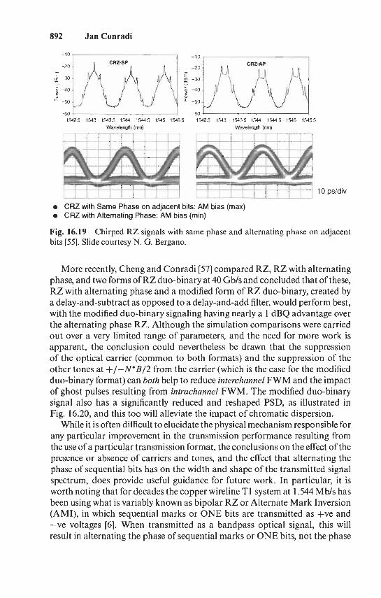
892 Jan Conradi
-1 0
-20
5 -30 - - G -40 B a -50
-60 5 15425 1543 15435 1544 15445 1545 15455
Wavehgth (nm)
0 CRZ with Same Phase on adjacent bits: AM bias (max) 0 CRZ with Alternating Phase: AM bias (min)
Fig. 16.19 Chirped RZ signals with same phase and alternating phase on adjacent bits [55] . Slide courtesy N. G. Bergano.
More recently, Cheng and Conradi [57] compared RZ, RZ with alternating phase, and two forms of RZ duo-binary at 40 Gb/s and concluded that of these, RZ with alternating phase and a modified form of RZ duo-binary, created by a delay-and-subtract as opposed to a delay-and-add filter, would perform best, with the modified duo-binary signaling having nearly a 1 dBQ advantage over the alternating phase RZ. Although the simulation comparisons were carried out over a very limited range of parameters, and the need for more work is apparent, the conclusion could nevertheless be drawn that the suppression of the optical carrier (common to both formats) and the suppression of the other tones at +/-N*B/2 from the carrier (which is the case for the modified duo-binary format) can both help to reduce interchannel FWM and the impact of ghost pulses resulting from intrachannel FWM. The modified duo-binary signal also has a significantly reduced and reshaped PSD, as illustrated in Fig. 16.20, and this too will alleviate the impact of chromatic dispersion.
While it is often difficult to elucidate the physical mechanism responsible for any particular improvement in the transmission performance resulting from the use of a particular transmission format, the conclusions on the effect of the presence or absence of carriers and tones, and the effect that alternating the phase of sequential bits has on the width and shape of the transmitted signal spectrum, does provide useful guidance for future work. In particular, it is worth noting that for decades the copper wireline T1 system at 1.544 Mb/s has been using what is variably known as bipolar RZ or Alternate Mark Inversion (AMI), in which sequential marks or ONE bits are transmitted as +ve and -ve voltages [6]. When transmitted as a bandpass optical signal, this will result in alternating the phase of sequential marks or ONE bits, not the phase
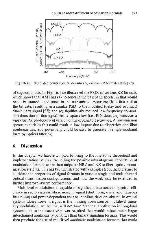
16. Bandwidth-Efficient Modulation Formats 893
-80 -40 0 40 80 Frequency(GH2)
Fig. 16.20 Simulated power spectral densities of various RZ formats (after [57]).
of sequential bits. In Fig. 16.4 we illustrated the PSDs of various RZ formats, which shows that AMI has (a) no tones in the baseband spectrum that would result in unmodulated tones in the transmitted spectrum; (b) a first null at the bit rate, resulting in a similar PSD to the modified (delay and subtract) duo-binary signal [57]; and (c) significantly reduced low-frequency content. The detection of this signal with a square law (Le., PIN detector) produces a unipolar RZ photocurrent version of the original bit sequence. A transmission spectrum such as this could result in low impact due to dispersion and fiber nonlinearities, and potentially could be easy to generate in single-sideband form by optical filtering.
6. Discussion
In this chapter we have attempted to bring to the fore some theoretical and implementation issues surrounding the possible advantageous application of modulation formats other than unipolar NRZ and RZ to fiber-optic commu- nication systems. This has been illustrated with examples from the literature to elucidate the properties of signal formats in various single and multichannel optical transmission configurations, and how the work may be extended to further improve system performance.
Multilevel modulation is capable of significant increases in spectral effi- ciency in radio systems where noise in signal (shot noise, signal-spontaneous beat noise) and power-dependent channel nonlinearities are absent. In optical systems where noise in signal is the limiting noise source, multilevel inten- sity modulation, we believe, will not have practical application in long-haul systems due to the excessive power required that would induce much larger interchannel nonlinearity penalties than binary signaling formats. This would then preclude the use of multilevel amplitude modulation formats that could
894 Jan Conradi
otherwise improve spectral efficiency beyond what has already been demon- strated through the combined use of polarization-division multiplexing and such formats as chirped or alternating phase RZ, modified duo-binary RZ, OSSB, and potentially AMI.4 The potential application of multilevel signaling to data transmission systems on multimode fiber remains an open issue.
However, it is intriguing to speculate whether with improvements in optical source stability now being required by closely spaced DWDM channels, if coherent transmission might just become practical. If this were practical from the standpoint of optical source stability, both for transmission lasers as well as for the phase andor frequency-locked local oscillator lasers needed at the receiver, then a whole host of additional possibilities open up. For instance, with the lower launched powers that distributed Raman amplifiers offer, the fiber portion of the transmission link is now very much closer to operating free of nonlinear distortions due to SPM, FWM, and XPM. Then the combination of OSSB with coherent detection might permit adaptive electrical dispersion compensators to be used based on, for example, electrical tapped delay line filters. If this were the case, then most of the needed dispersion compensation could be implemented using the usual very broadband optical means such as dispersion-compensating fiber, but that fine-tuning of the signal eye could be done electrically.
Additionally, coherent detection of phase modulated channels might take advantage of the constant envelope of phase modulated channels to reduce the impact of nonlinear impairments resulting from FWM and XPM since amplitude fluctuations, other than those induced by dispersion, would be absent. This too, might allow the application of multilevel PSK formats that have narrow signal spectra, thereby permitting the increased spectral efficiency denied by fiber nonlinearities in multilevel ASK formats. (Note the power levels in Fig. 16.16.)
Acknowledgments
The summary of work presented in this chapter would not have been pos- sible without the work carried out by many graduate students with whom I have had the pleasure of working both as colleague and supervisor during my tenure as NSERC/Nortel/TRLabs Industrial Research Chair at TRLabs and the University of Alberta in Edmonton, Alberta, Canada. Specifically, in chronological order, Greg May, Sheldon Walklin, Mike Sieben, Bob Davies,
This is in contradiction to a recent paper in Nu&=. P. P. Mitra and J. B. Stark, “Nonlinear limits to the information capacity of optical fibre communications,” Nature, vol. 41 1, pp. 1027- 1030,28 June 2001.
16. Bandwidth-Efficient Modulation Formats 895
and Sing Cheng contributed original work on the various modulation for- mats that is summarized here and in their publications. Additionally, I would like to acknowledge Prof. David Dodds of TRLabs and the University of Saskatchewan for his contributions and collaboration in the evolution of the work on optical single-sideband modulation.
Andrew Ellis and Roe Hemenway of Corning Incorporated are gratefully acknowledged for their comments on and suggestions for improving the clarity of the manuscript-any lack of success for which they are entirely exonerated. Becki Rappleye provided valuable assistance with the manuscript.
References
[l] Bell System Technical Journal issue devoted to the Atlanta Fiber System Experiment, BSTJ, vol. 57, July-August, 1976.
[2] Henry, P. S., “Lightwave Primer,” IEEE Journal of Quantum Electronics, vol. QE-21, No. 12, pp. 1862-1879, December 1985.
[3] Cartledge, J. C. and R. G. McJSay, “Performance of 10 Gbls Lightwave Systems Using an Adjustable Chirp Optical Modulator and Linear Equalization,” IEEE Photonics Technology Letters, vol. 4, no. 12, pp. 1394-1397, December 1992.
[4] Jopson, B. and A. Gnauck, “Dispersion Compensation for Optical Fiber Systems,” IEEE Communications Magazine, vol. 33, pp. 96102, June 1995.
[5] Gnauck, A. H. and R. M. Jopson, “Dispersion Compensation for Optical Fiber Systems,” in Optical Fiber Telecommunications IIIA, Edited by Ivan P. Kaminow and Thomas L. Koch, Academic Press, San Diego, 1997.
[6] Couch, L. W. 11, Digital and Analog Communication Systems, Fifth Edition, Prentice Hall, Upper Saddle River, New Jersey, 1997.
[7] Lahti, B. P., Modern Digital and Analog Communications Systems, Second Edition, Holt, Rinehart, and Winston, Inc., Orlando, Florida, 1989.
[8] Proakis, J. G., Digital Communications, Second Edition, McGraw-Hill, New York, 1989.
[9] Haykin, S., Communications Systems, Third Edition, John Wiley & Sons, New York, 1994.
[lo] Waklin, S. and J. Conradi, “Multilevel Signaling for Increasing the Reach of 10 Gb/s Lightwave Systems,” Journal of Lightwave Technology, vol. 17, pp. 2235- 2248,1999.
[l 11 May, G., A. Solheim, and J. Conradi, “Extended 10 Gbls Fiber Transmission Distance at 1538 nm Using a Duobinary Receiver,” IEEE Photonic Technology Letters, vol. 6, no. 5, pp. 648-650, May 1994.
[12] Gu, X., et al., “10 Gbitls, 138 km Uncompensated Duobinary Transmission Over Installed Standard Fiber,” Electronics Letters, vol. 30, no. 23, pp. 1953-1954, 1994.
[ 131 Yonenaga, K., et al., “Optical Duobinary Transmission System With No Receiver Sensitivity Degradation,” Electronics Letters, vol. 31, no. 4, pp. 302-304, 1995.

896 Jan Conradi
[14] Kuwano, S., et al., “lOGbit/s Repeaterless Transmission Experiment of Optical Duobinary Modulated Signal,” Electronics Letters, vol. 31, no. 16, pp. 135%1361, 1995.
[15] Price, A. J. and N. Le Mercier, “Reduced Bandwidth Optical Digital Intensity Modulation with Improved Chromatic Dispersion Tolerance,” Electronics Letters, vol. 31, no. 1, pp. 58-59, 1995.
[16] Price, A. J., et d., “210Km Repeaterless lOGb/s Transmission Experiment Through Nondispersion-Shifted Fiber Using Partial Response Scheme,” IEEE Photonics Technology Letters, vol. 7, no. 10, pp. 1219-1221, 1995.
[17] Walklin, S. and J. Conradi, “On the Relationship Between Chromatic Dispersion and Transmitter Filter Response in Duobinary Optical Communication Systems,” IEEE Photonics Technology Letters, vol. 9, no. 7, pp. 1005-1007, July 1997.
[18] Yano, Y, et al., “WDM Transmission Experiment Using Optical Duobinary Coding,” ECOC ’96, vol. 5, Postdeadline paper ThB.3.1, September 1996.
[19] Ito, T., et al., “Feasibility Study On Over 1 BitMHz High Spectral Efficiency WDM With Optical Duobinary Coding and Polarization Interleave Multiplex- ing,” OFC ’97, Paper TuJ1, pp. 4345,1997.
[20] Ono, T. and Y Yano, “Key Technologies for TerabitlSecond WDM Systems with High Spectral Efficiency of Over 1 bitlHz,” IEEE J. Quantum Electron., vol. 34, pp. 2080-2088, November 1998.
[21] Ono, T., Y. Yano, K. Fukuchi, T. Ito, H. Yamazaki, M. Yamaguchi, and K. Emura, “Characteristics of Optical Duobinary Signals in Terabith Capac- ity, High-Spectral Efficiency WDM Systems,” Journal OfLightwave Technology, vol. 16, no. 5, pp. 788-797, 1998.
[22] Miyamoto, Y, K. Yonenaga, A. Hirano, H. Toba, K. Murata, and H. Miyazawa, “Duobinary Carrier-Suppressed Return-to-Zero Format and Its Application to 100 GHz-spaced 8 x 43-Gb/s DWDM Unrepeatered Transmission over 163 km,” OFC 2001, Paper TU 1141.
[23] Yonenaga, K. and N. Takachio, “A Fiber Chromatic Dispersion Compensation Technique With An Optical SSB Transmission In Optical Homodyne Detection Systems,” IEEE Photonics Technology Letters, vol. 5, no. 8, pp. 949-951, August 1993.
[24] Yonenaga, K. and N. Takachio, “Dispersion Compensation for Homodyne Detection Systems Using a 10 Gb/s Optical PSK-VSB Signal,” IEEE Photonics Technology Letters, vol. 7 , no. 8, pp. 929-931, August 1995.
[25] Conradi, J., B. Davies, M. Sieben, D. Dodds, and S. Walklin, “Optical Single Side- band (OSSB) Transmission for Dispersion Avoidance and Electrical Dispersion Compensation in Microwave Subcarrier and Baseband Digital Systems,” OFC ’97, Postdeadline paper PD-29, Dallas, TX, February 1997.
[2q Sieben, M., J. Conradi, D. Dodds, B. Davies, and S. Walklin, “lOGb/s Optical Single Sideband System,” Electronic Letters, vol. 33, no. 11, pp. 971-973, 1997.
[27] Bigo, S., A. Bertaina, Y. Frignac, S. Borne, L. Lorcy, D. Hamoir, D. Bayart, J . 2 Hamaide, W. Idler, E. Lach, B. Franz, G. Veith, F! Sillard, L. Fleury, P. Guenot, and F! Nouchi, “5.12 Tb/s (128 x 40 Gb/s WDM) Transmission over
16. Bandwidth-Efficient Modulation Formats 897
3 x lOOkm of TeraLightm Fibre,” ECOC 2000, Postdeadline paper PD. 1.1, Munich, Germany, 2000.
[28] Kobayashi, Y , K. Kinjo, K. Ishida, T. Sugihara, S. Kajiya, N. Suzuki, and K. Shimizu, “A Comparison Among Pure-RZ, CS-RZ, and SSB-RZ Format, in 1 Tls (50 x 20 Gb/s, 0.4 nm spacing) WDM Transmission over 4,000 km,” ECOC 2000, Postdeadline paper 1.7, Munich, Germany, 2000.
[29] See OFC 2001 and ECOC 2001 conference proceedings. [30] Lee, W. S., et al., “4 x 40 Gbit/s RZ ETDM transmission over 520 km of NDSF
at 120 and 160km span lengths with Raman pre-amplification,” Electron. Lett., vol. 36, pp. 736736,2000.
[31] Elrefaie, A. F., R. E. Wagner, D. A. Atlas, and D. G. Daut, “Chromatic Disper- sion Limitations in Coherent Lightwave Transmission Systems,” IEEE Journal of Lightwave Technology, vol. 6, no. 5, pp. 704-709, 1988.
[32] Petermann, K., Laser Diode Modulation and Noise, Kluwer Academic Publishers, Holland, 1988.
[33] Moodie, D. G., et al., “4OGbit/s Modulator with Low Drive Voltage and High Optical Output Power,” Paper We.F.3.2, Proc. ECOC 2001, Amsterdam, vol. 33,
[34: Koyama, F. and K. Iga, “Frequency Chirping in External Modulators,” Journal of Lightwave Technology, vol. 6, pp. 87-93, 1998.
[35] Gnauck, A. H., S. K. Korotky, J. J. Veselka, J. Nagel, C. T. Kemmerer, W. J. Minford, and D. T. Moser, “Dispersion Penalty Reduction Using an Optical Modulator with Adjustable Chirp,” IEEE Photonics Technology Letters, vol. 3, no. 10, pp. 916-918,1991.
[36] Smith, G. H., D. Novak, and Z. Ahmed, “Technique for Optical SSB Generation to Overcome Dispersion Penalties in Fibre-Radio Systems,” Electronics Letters, vol. 33, no. 1, pp. 7675, 1997.
1371 Davies, B. and J. Conradi, “Hybrid Modulator Structure for Subcarrier and Har- monic Subcarrier Optical Single Sideband,” Photonics Technology Letters, vol. 10, no. 4, pp. 600-602, April 1998.
[38] Smith, R. G. and S. Personick, “Receiver Design for Optical Fiber Commu- nication Systems,” in Semiconductor Devices for Optical Communication, 2nd Edition, H. Kressel, ed., vol. 39, pp. 89-160, Springer Verlag, New York, 1982.
[39] Lender, A., “Correlative Digital Communication Techniques,” IEEE Transactions on Communications Technology, vol. COM-12, pp. 128-135, 1964.
[40] Lender, A., “Correlative Level Coding for Binary-Data Transmission,” IEEE Spectrum, vol. 3, pp. 104-115, 1966.
[41] Kabal, P. and S. Pasupathy, “Partial-Response Signaling,” IEEE Transaction on Communications, vol. Com-23, pp. 921-934, 1975.
[42] Haykin, S., Chapter 7, Communications Systems, Third Edition, John Wiley & Sons, 1994.
[43] Hakki, B. W., “Dispersion of Microwave-Modulated Optical Signals,” Journal of Lightwave Technology, vol. 11, no. 3, pp. 474-480, March 1993.
pp. 332-333.
898 Jan Conradi
[44] Schmuck, H., “Comparison of Optical Millimeter Wave Systems Concepts with Regard to Chromatic Dispersion,” Electronics Letters, vol. 31 pp. 1848-1849, 1996.
[45l Kahn, L. R., “Compatible Single Sideband,” Proceedings of the IRE, vol. 49, pp. 1503-1527,1961.
[46] Voelcker, H., “Demodulation of Single-Sideband Signals via Envelope Detec- tion,” IEEE Transactions on Communication Technology, vol. COM-14, pp. 20-30, February 1966.
[47] Voelcker, H., “Toward A Unified Theory of Modulation-Part 1: Phase-Envelope Relationships,” Proceedings of the IEEE, vol. 54, no. 3, pp. 340-353, March 1966.
[48] Sieben, M., J. Conradi, and D. E. Dodds, “Optical Single Sideband Transmission at 10 Gbls Using Only Electrical Dispersion Compensation,” JournaI ofLightwuve Transmission, vol. 17, pp. 1742-1749, 1999.
[49] Yano, Y , et al., “WDM Transmission Experiment Using Optical Duobinary Coding,” ECOC ’96, vol. 5, Postdeadline paper ThB.3.1, September 1996.
[SO] Ito T., etal., “Feasibility Study On Over 1 BitldHz High Spectral Efficiency WDM With Optical Duobinary Coding and Polarization Interleave Multiplexing,” OFC ’97, Paper T U , pp. 4345,1997.
[51] Ono, T., Y Yano, K. Fukuchi, T. Ito, H. Yamazaki, M. Yamaguchi, and K. Emura, “Characteristics of Optical Duobinary Signals in Terabitls Capac- ity, High-Spectral Efficiency WDM Systems,” Journal OfLightwave Technology, vol. 16, no. 5, pp. 788-797, 1998.
[52] Ono, T. and Y. Yano, “Key Technologies for TerabitdSecond WDM Systems with High Spectral Efficiency of Over 1 bitlsHz,” IEEE J. Quantum Electronics, vol. 34, pp. 2080-2088,1998.
[53] Asiawa, S., J. Kani, M. Fukui, T. Sakamoto, M. Jinno, S. Norimatsu, H. Ono, and K. Oguchi, “A 1580-nm Band WDM Transmission Technology Employing Optical Duobinary Coding,” Journal OfLightwave Technology, vol. 17, pp. 191- 198,1999.
[54] Kobayashi, Y., K. Kinjo, K. Ishida, T. Sugihara, S. Kajiya, N. Suzuki, and K. Shimizu, “A Comparison Among Pure-RZ, CS-RZ, and SSB-RZ Format, in 1 Tb/s (50 x 20 G/s, 0.4 nm spacing) WDM Transmission Over 4,000 km,” ECOC 2000, Postdeadline paper 1.7, Munich, Germany, September 2000.
[55] Nissov M., et al., “32 x 20 Transmission over Trans Atlantic Distance (6,200 km) with 31% Spectral Efficiency,” OFC 2000, Postdeadline paper PD-30.
[56] Bakhshi, B., M. Vaa, E. E. Golovchenko, W. W. Patterson, R. L. Maybach, and N. S. Bergano, “Comparison of CRZ, RZ, and NRZ Modulation Formats in a 64 x 12.3 Gb/s WDM Transmission Experiment over 9000 km,” OFC 2000,” Paper WF4, Anaheim, California, March 2000.
[57] Cheng, K. S. and J. Conradi, “Reduction of Pulse-to-Pulse Interaction Using Alternative RZ Formats in 40 Gbls Systems,” Photonics Technology Letters, in press.
16. Bandwidth-Efficient Modulation Formats 899
Bibliography
D UO-BINARY
Ennser, K., et aZ., “Phase-Encoded Duobinary Transmission Over Non-Dispersion Shifted Fiber Links Using Chirped Grating Dispersion Compensators,” Electronics Letters, vol. 33, no. 1, pp. 72-74, 1997.
Fukuchi, K., et al., “10 Gbitls-120 km Standard Fiber Transmission Employing a Novel Optical Phase-Encoded Intensity Modulation for Signal Spectrum Compres- sion,” OFC ’97 Technical Digest, Paper ThH3, pp. 270-271, 1997.
Gu, X. and L. C. Blank, “10 Gbit/s Unrepeatered Three-Level Optical Transmission Over l O O k m of Standard Fiber, Electronics Letters, vol. 29, no. 25, pp. 2209-2211, 1993.
Lender, A., “Correlative Digital Communication Techniques,” IEEE Transactions on Communications Technology, vol. COM-12, pp. 128-135, 1964.
Lender, A., “Correlative Level Coding for Binary-Data Transmission,” IEEE Spectrum, vol. 3, pp. 104-115, 1966.
Loh, W. H., et al., “Dispersion Compensated 10 Gbitls Transmission Over 700km of Standard Single Mode Fiber with 10 cm Chirped Fiber Grating and Duobinary Transmitter,” OFC ’96, Postdeadline paper PD30,1996.
Nakhla, M., “Error Probability for Multilevel Digital Systems in Presence of Intersym- bo1 Interference and Additive Noise,” IEEE Transactions on Communications, vol. 42, no. 7, pp. 2380-2383,1994.
Ono, T., et al., “Demonstration of High-Dispersion Tolerance of 20 Gbitls Optical Duobinary Signal Generated by a Low-Pass Filtering Method,” OFC ’97 Technical Digest, Paper ThH1, pp. 268-269, 1997.
Wuth, T., W. Kaiser, and W. Rosenkranz, “Impact of Self-Phase Modulation on Bandwidth Efficient Modulation Formats,” OFC 2001, Paper MM6,2001.
SINGLE SIDEBAND
Bedrosian, E., “A Product Theorem For Hilbert Transforms,” Proceedings ofthe IEEE, pp. 8684369, May 1963.
Kahn, L. R., “Compatible Single Sideband,” Proceedings ofthe IRE, vol. 49, pp. 1503- 527,1961.
Lockhart, G. B., “A Spectral Theory for Hybrid Modulation,” IEEE Transactions on Communications, vol. COM 21, no. 7, pp. 790-800, 1973.
Logan, B. F. and M. R. Schroeder, “A Solution to the Problem of Compatibility Single-Sideband Transmission,” IRE Transactions on Information Theoly, vol. IT-8,
Powers, K. H., “The Compatibility Problem in Single-Sideband Transmission,” Proceedings ofthe IRE, vol. 48, pp. 1431-1435, 1960.
Voelcker, H., “Demodulation of Single-Sideband Signals via Envelope Detection,” IEEE Transactions on Communication Technology, vol. COM-14, pp. 20-30, February 1966.
pp. S 252-S 259,1962.

900 Jan Conradi
Voelcker, H., “Toward A Unified Theory of Modulation-Part 1: Phase-Envelope Relationships,” Proceedings of the IEEE, vol. 54, no. 3, pp. 340-353, March 1966.
Weaver, D. K. Jr., “A Third Method of Generation and Detection of Single Sideband Signals,” Proceedings of the IRE, vol. 44, pp. 1703-1705, 1956.
Zaid, M. A., “Envelope Detection and Correction of SSB,” Electronics Letters, vol. 20, no. 22, pp. 901-902,1984.
RF AND MICRO WAVE: SSB AND OTHER TECHNIQUES
Davies, B. and J. Conradi, “Hybrid Modulator Structure for Subcarrier and Harmonic Subcarrier Optical Single Sideband,” Photonics Technology Letters, vol. 10, no. 4, pp. 600-602,1998.
Davies, B. and J. Conradi, “Hybrid Harmonic Subcarrier Optical Single Sideband With Phase Predistortion,” Electronics Letters, vol. 34, no. 17, pp. 1673-1675, 1998.
Hakki, B. W., “Dispersion of Microwave-Modulated Optical Signals,” Journal of Lightwave Technology, vol. 11, no. 3, pp. 474-480, 1993.
IEICE Transactions on Communications, Special Issue on Fiber-optic Microcellu- lar Radio Communication Systems and Their Technologies, vol. E76-B, no. 9, September 1993.
Makoto, S., T. Kanai, W. Domom, K. Emura, and J. Namiki, “Optical Fiber Feeder for Microcellular Mobile Communication Systems,” IEEE Journal on Selected Areas of Communications, vol. 11, no. 7, pp. 1118-1126,1993.
Motamedi, A. and R. Vahldeick, “Generation of Fourth Harmonic Microwave Sig- nals Using Mach-Zehnder Modulators,” Optical Fiber Conference OFC-97 Technical Digest, pp. 354-355, 1997.
O’Reilly, J. J. and I? M. Lane, “Fiber-Supported Optical Generation and Delivery of 60 GHz Signals,” Electronics Letters, vol. 30, no. 16, pp. 1329-1330, 1994.
Olshansky, R., “Optical Modulator For Cancellation of Second-Order Intermod- ulation Products In Lightwave Systems,” U.S. Patent no. 5,239,401, August 1993.
Olshansky, R., “Single Sideband Optical Modulator for Lightwave Systems,” U.S. Patent No. 5,301,058, 1994.
Recent special issues(s) of IEEE Transactions on Microwave lleory and Techniques. Schmuck, H., “Comparison of Optical MiUimeter Wave Systems Concepts with Regard
to Chromatic Dispersion,” Electronics Letters, vol. 31, no. 21, pp. 1848-1849, 1996. Smith, G. H., D. Novak, and Z. Ahmed, “Technique for Optical SSB Generation to
Overcome Dispersion Penalties in Fibre-Radio Systems,” Electronics Letters, vol. 33, no. 1, pp. 74-75, 1997.
Smith, G. H. and D. Novak, “Broadband Millimeter-Wave (38 GHz) Fiber-Wireless Transmission System Using Electrical and Optical SSB Modulation to Overcome Dispersion Effects,” IEEE Photonics Technology Letters, vol. 10, no. 1, pp. 141-143, 1998.
16. Bandwidth-Enicient Modulation Formats 901
Smith, G. H., D. Novak, and Z. Ahmed, “Overcoming Chromatic-Dispersion Effects in Fiber-Wireless Systems Incorporating External Modulators,” ZEEE Transactions on Microwave Theory And Techniques, vol. 45, no. 8, pp. 1410-1415, 1997.
Wake, M., R. G. Walker, and C. Edge, “Single Sideband Modulator in GaAs Integrated Optics For Microwave Frequency Operation,” Integrated Photonics Research, OSA Technical Digest Series, 10, Postdeadline paper PD-8, 1992.
Walker, N. G., D. Wake, and I. C. Smith, “Efficient Millimeter-Wave Signal Generation Through FM-IM Conversion In Dispersive Optical Fiber Links:” EZectronics Letters, vol. 28, no. 21, pp. 2027-2028, 1992.
Young, T., J. Conradi, and W. Tinga, “Generation and Transmission of FM and lrf4 DQPSK Signals at Microwave Frequencies Using Harmonic Generation and Opto- Electronic Mixing in Mach-Zehnder Modulators,” IEEE Transactions on Microwave Theoly and Techniques, vol. 44, no. 2, pp. 446453, 1996.
Zaheer, A., D. Novak, R. B. Waterhouse, and H.-F. Liu, “37-GHZ Fiber-Wireless System For Distribution of Broadband Signals,” ZEEE Transactions on Microwave Theory and Techniques, vol. 45, no. 8, pp. 1431-1435, 1997.

Chapter 17
€? Vijay Kumar University of Southern California, Los Angeles, California and Scintera Network, Inc.. San Jose, California
Moe Z . Win
Hsiao-Feng Lu
Costas N. Georghiades
AT&T Labs-Research, Middletown, New Jersty
University of Southern California, Los Angela, California
T a m A&iU University, College Station, Texas
Error-Control Coding Techniques and Applications'
17.1
17.1.1
Introduction
CHAPTER OVERVIEW
11. FECcodes
communication
In this chapter, the forward error correction (FEC) codes relevant to the establishment of reliable communication over the fiber-optic communication channel are presented and discussed. Opinions expressed in this chapter are those of the authors and should not be construed as being universally held,
This work was supported in part by the U.S. National Science Foundation under Grant
902
NSF-CCR-0073555.
OPTICAL FIBER TELECOMMUNICATIONS, VOLL'ME N B
Copyright 0 2002, Elsevier Science (LJSA). AU rights of reproduction in any form reserved.
ISBN: 0-12-395173-9
17. Error-Control Coding Techniques and Applications 903
as the study of FEC design for optical communication has yet to mature. The accompanying flowchart provides an overview of the chapter and indi- cates the linkage between different sections. The reader wishing to obtain a quick overview of the topic of FEC for the fiber-optic channel can get by with just reading Sections 17.1 and 17.11. Sections 17.2 through 17.10 discuss the principles underlying the various FEC codes of interest.
Section 17.1.2 discusses how imperfections in the fiber-optic channel distort the transmitted signal. The role of FEC in overcoming some of these impair- ments is discussed in Section 17.1.3. The coding gain of an FEC code is a quantitative measure of the energy savings resulting from use of the code. The final section, Section 17.11, discusses the various FEC codes used or proposed for use on the optical channel, as well as the coding gains provided by these codes. Bounds on the maximum achievable coding gain are also provided here.
Sections 17.2 through 17.10 present the principles of error correction and provide background material on most of the FEC codes used or proposed for use for optical fiber communication. General binary error correcting codes are introduced in Section 17.2 followed in Section 17.3 by a discussion of a commonly used class of binary codes, namely, cyclic codes. The codes most often proposed for optical channel error correction are a class of nonbinary codes known as Reed-Solomon (RS) codes, and these codes are introduced in Section 17.5. RS codes are best described in the language of finite fields and Section 17.4 provides the relevant background. It is possible to combine a pair of codes to yield a third code through a process known as concatenation. In the typical construction of concatenated codes, one of the two constituent codes is a RS code. Concatenated codes are described in the latter part of Section 17.5. The largest and most well-known family of binary cyclic codes is the family of Bose, Ray-Chaudhuri, and Hocquenghem (BCH) codes. As with RS codes, the most natural description of these codes is in terms of finite fields, and Section 17.6 contains such a description. Product codes, like concatenated codes, are also constructed by combining a pair of codes. The product codes that appear in the optical communication literature are constructed from a pair of BCH codes. The discussion on product codes appears in Section 17.6.
The input to the optical fiber communication channel may be regarded as being binary, as the most common modulation scheme employed is on-off key- ing (OOK). It is convenient to break up the optical receiver into two blocks. The first block can either be a symbol estimator or else, a symbol detector. The symbol estimator puts out a positive real number x whose magnitude reflects the likelihood of a pulse having been transmitted at that time instant. The symbol detector consists of the symbol estimator described above fol- lowed by a threshold circuit that outputs one or zero depending upon whether the output of the symbol estimator exceeds or does not exceed an appropri- ate threshold. The choice of symbol estimator or symbol detector depends upon the type of FEC decoder used. A hard-decision decoder [44] is capable only of processing {0,1} inputs and therefore must be preceded by a symbol
904 P. Vijay Kumar et aL
detector. FEC decoders that are capable of processing the output of the sym- bol estimator without first quantizing this output to two levels, are called soJ-decision decoders. Whereas most binary codes discussed in the litera- ture possess a hard-decision decoding algorithm of reasonable complexity, the class of codes possessing a low-complexity, soft-decision decoding algorithm is much smaller. Hard-decision decoding is typically simpler to implement, but can result in an energy penalty on the order of one or two decibels (dB). Most decoders used or proposed for use on the optical fiber channel are hard- decision decoders, although recently, soft-decision decoders have begun to attract attention, see [ 11 for instance.
The three classes of codes discussed in Sections 17.7, 17.9, and 17.10, namely convolutional, turbo and low-density parity-check (LDPC) codes possess an efficient, low-complexity, soft-decision decoding algorithm. The low-complexity decoding algorithm comes about because these codes have a graphical representation that can be exploited by a decoder. Section 17.8 explains how one can obtain a graphical representation for these classes of codes and also shows how this representation leads to an efficient soft-decision decoding algorithm. The material presented in Sections 17.8-17.10 is of recent origin and is taken mostly from journal articles.
17.1.2 SIGNAL IMPMRMENTS INTRODUCED BY THE OPTICAL CHANNEL
There are several causes for degradation of the optical signal as it progresses from transmitter to receiver. The three principal phenomena that affect the optical signal are attenuation, dispersion, and distortion due to noise [20].
Attenuation
Attenuation is the loss of optical energy, measured in dB/km, as the signal travels from transmitter to receiver.
Dispersion
Dispersion refers to the spreading of the optical signal in time during its passage down the fiber. There are two principal causes of dispersion in a single-mode fiber. Chromatic dispersion is pulse spreading caused by variation of the propa- gation constant of the electromagnetic light wave as a function of wavelength. The amount of dispersion increases linearly with distance and varies with wavelength. The dispersion is typically around 17ps/ldm at a wavelength of 1550 nm for conventional single-mode fibers, but is much lower (on the order of 2-6 ps/kmfnm) in the case of recently installed non-zero-dispersion-shifted fibers. This dispersion can vary with time.

17. Error-Control Coding Techniques and Applications 905
The second principal type of dispersion is polarization-mode dispersion (PMD) that arises because even in single-mode fibers, there are two modes of propagation distinguished by their polarization. The two modes travel with different group velocities because of fiber birefringence resulting once again, in pulse spreading. The amount of spreading in a commercial fiber varies as the square root of the length of the fiber. PMD also varies with time and wavelength.
A third cause of dispersion, internodal dispersion, occurs only in multimode fibers. This is caused by the fact that the different modes of propagation are associated with different propagation constants. Multimode fibers are gen- erally used to span short distances, such as those deployed in a local area network.
Dispersion of any of the types discussed above leads to inter-symbol interference (ISI), i.e., causes the channel output to depend not just on the corresponding input pulse, but also on adjacent pulses as well.
Noise
There are three principal sources of noise on an optical channel [18,20]. Shot noise is the quantum noise due to the fact that the received signal at the output of a photodetector is a series of electrons with the number of electrons in a symbol interval having a Poisson distribution even when the incident light is of uniform intensity. Thermal noise is produced at the receiver and is typically modeled as an additive white Gaussian noise (AWGN). The third source of noise is umplfied spontaneous emission (ASE) noise, which is generated when the signal is amplified using an optical amplifier. ASE noise can be modeled as being additive and Gaussian.
The most common form of detection is direct detection. Here, the incoming optical signal is converted to an electrical current proportional to the power of the incoming signal. In the absence of an optical amplifier, the major source of noise in a direct detection system is thermal noise. In the presence of an optical amplifier, the dominant source of noise is ASE [47].
In the case of coherent detection, the received signal is added to a local oscillator signal and the two signals are then converted to an electrical signal at a microwave frequency by a photodiode. This conversion makes it possible to process the converted signal using the array of signal-processing techniques developed for the microwave channel. However, coherent detection is harder to implement in practice and is not commonly employed.
The signal-to-noise-ratio (SNR) is the ratio of the average energy of the signal component of the input to the optical receiver to that of the noise present in the optical link. A precise definition of S N R appears in 17.1 1. The SNR has a direct relationship to the bit error rate (BER), with higher SNR leading to lower BER.
906 P. Vijay Kumar et al.
Other Sources of Distortion
There are several other sources of signal distortion. Chirping, self-phase modulation (SPM), stimulated Brillouin and Raman scattering are due to nonlinearities in the transmitting laser and fiber. A commonly-used technique to increase the rate of information transfer across an optical fiber is to use wavelength-division multiplexing (WDM). In WDM systems, fiber nonlineari- ties can give rise to additional sources of signal distortion known as cross-phase modulation and four-wave mixing.
17.1.3 THE ROLE OF FEC IN OPTICAL FIBER COMMUNICATION
There has been a recent upsurge in interest in using FEC [l, 17,39,46,49] for communication over WDM fiber-optic channels. Forward error correcting codes tag extra redundant symbols to the message that can be exploited by the receiver to correct errors introduced by the optical channel. At the present time, FEC codes are designed and chosen primarily based on their ability to combat the additive ASE noise present on the WDM optical link. Although these codes can overcome to some extent the other sources of signal distortion discussed above, it is desirable that alternative means be used to combat these. For instance, equalization, either in the optical or electronic domain is an effective means of dispersion compensation. Equalization is discussed in greater detail elsewhere in this book.
to [17] axe desirable, so when we speak of reliable communication, we will
mean communication with BER in this region. The bit-rate distance product, i.e., the product of the length of fiber over which reliable transmission can be achieved times the data rate guaranteed on that length of fiber is an effective means of judging the impact of a technological innovation on the optical communication capability.
The error correction capability of an FEC code enables reliable commu- nication at reduced energy levels, Le., at reduced values of SNR. This SNR margin can be spent to improve the bit-rate distance product, for example by allowing the signal to reliably traverse a longer distance. Alternately, the SNR margin can be used to operate at a lower power level, thereby reducing nonlinear effects.
As mentioned previously, the codingguin of an FEC code is a quantitative measure of the savings in energy afforded by the code. A detailed discussion of coding gain appears in Section 17.1 1. The coding gains of some specific codes appear in this section, together with a discussion on the maximum-achievable coding gain.
We end with a few words on channel models. Consider an optical communi- cation system in which the modulation is OOK and in which the first block in
In current optical WDM networks, bit error rates in the region

17. Error-Control Coding Techniques and Applications 907
1-P
Fig. 17.1 The binary symmetric channel model.
the receiver is a symbol detector. The combination of optical fiber communica- tion channel, and symbol detector effectively present to the hard-decision FEC decoder, a binary-input, binary-output channel (Fig. 17.1). It turns out that there is reasonable justification for assuming that the transition probabilities 0 + 1, 1 + 0 of this binary channel are equal. This topic is treated in greater detail in 17.1 1. As a result, the FEC decoder sees a symmetric binary-input binary-output channel known as the binary symmetric channel (BSC).
The next nine subsections are devoted to a discussion of the principles of error correction. Many of the codes discussed in these sections are designed to combat errors on the BSC.
17.2 Binary Codes in General
An excellent introduction to error correcting codes may be found in numerous textbooks [4,6,9,24,26,3 1 , 36,41,44]. A bZock code of length n is simply any subset of the set F! of all binary n-tuples. Here we use F2 to denote the set {O, 1). The elements of a code are called codewords. Each codeword is associated with a unique message. The size of a block code equals the number of codewords contained within the code. An example code is presented in Table 17.1.
To explain how the code accomplishes error correction we introduce the concept of Hamming weight and Hamming distance. The Hamming weight, ~(uJ of a codeword g is the number of 1’s in the n-tuple E. The weight distribution {A,lO 5 w 5 n} of a code lists the number, A,, of codewords of
Table 17.1 An Example Code
Codeword Hamming Weight
( 0 0 0 0 0 ) 0 ( 0 1 1 1 0 ) 3 ( 1 0 1 0 1 ) 3 ( 1 1 0 1 1 ) 4
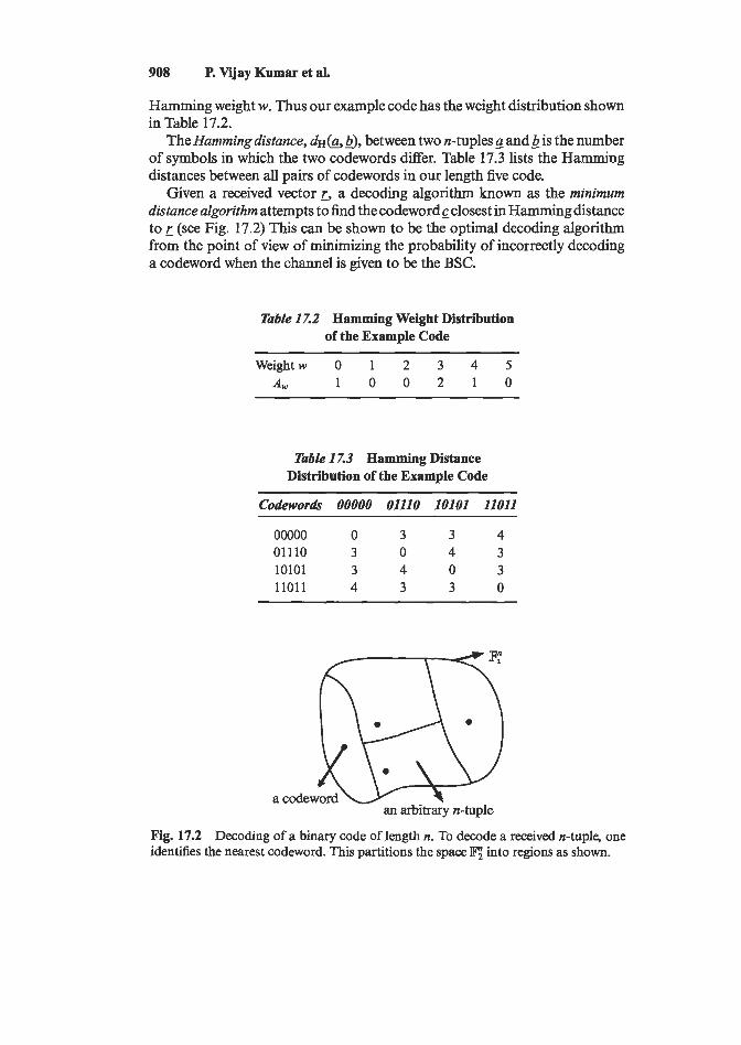
908 P. Vijay Kumar et aL
Hamming weight w. Thus our example code has the weight distribution shown in Table 17.2.
The Hamming distance, d&, bJ, between two n-tuples andb is the number of symbols in which the two codewords differ. Table 17.3 lists the Hamming distances between all pairs of codewords in our length five code.
Given a received vector E, a decoding algorithm known as the minimum distance algorithm attempts to find the codewordc closest in Hamming distance to (see Fig. 17.2) This can be shown to be the optimal decoding algorithm from the point of view of minimizing the probability of incorrectly decoding a codeword when the channel is given to be the BSC.
Table 17.2 Hamming Weight Distribution of the Example Code
Weightw 0 1 2 3 4 5 A, 1 0 0 2 1 0
Table 17.3 Hamming Distance Distribution of the Example Code
Codewords 00000 01110 10101 11011
00000 0 3 3 4 01 110 3 0 4 3 10101 3 4 0 3 11011 4 3 3 0
Fig. 17.2 Decoding of a binary code of length n. To decode a received n-tuple, one identifies the nearest codeword. This partitions the space IF! into regions as shown.

17. Error-Control Coding Techniques and Applications 909
The minimum distance, dmh, of a code is the smallest Hamming distance between a pair of distinct codewords within the code. Thus the minimum distance of our length five code equals 3. Whereas the exact error correc- tion capability of a code depends generally upon the distance distribution between pairs of codewords, an estimate of this error correction capability can be obtained from knowledge of &in as discussed below.
A code is said to be tc error correcting and td error detecting, td 2 to if the code can correct any error patterns that contain i t c errors, and in addition, is able to detect any pattern off errors, tc < t 5 td . For brevity we will refer to a tc error correcting, td error detecting, td 2 tc, code as a (tc, td)-code. It turns out that a code having minimum distance dmin can be a (fc, td)-COde if and only if dmin z tc + td + 1. The decoding algorithm that makes this possible is called the bounded-distance decoding algorithm and runs as follows:
Given a receivedvector L. the decoder searches to see if a codeword is present within Hamming distance fc of the received vector. If this is the case, then the decoder declares that codeword to be the decoded codeword. If this is not the case, the decoder declares an uncorrectable error.
We explain why the decoding algorithm works. The Hamming distance function satisfies the triangle inequality which states that
(17.1)
for any three binary n-tuples &,y, z_. The triangle inequality together with the condition dmin 1 tc + fd + 1 can-be used to show that the balls
of radius tc centered around any codeword c are disjoint, Le,, if c,, g2 are distinct codewords,
~k~ , tc> n Bk27 tc> = 4, (17.3)
where 4 denotes the empty set (see Fig. 17.3). This explains how the code is able to recover if the number of errors is i t c . If
the number of errors t lies in the range tc < t 5 td, then the received vector will not belong to any of the balls of radius tc centered around codewords and the decoder will declare an uncorrectable error. Finally, when t > td, it is possible for the received vector to lie in the ball of radius tc surrounding a different codeword from that transmitted causing the decoder to decode incorrectly.
When a block code is used purely for the purpose of error correction, we have fc = td , so the requirement on dmin changes to dmin 2 2tc + 1. Given a block code of length n and minimum distance dmin satisfying dmin ?- 2tc + 1, the probability Pcwe of incorrectly decoding a codeword using the minimum distance decoding algorithm, over a BSC having crossover probabilityp, can
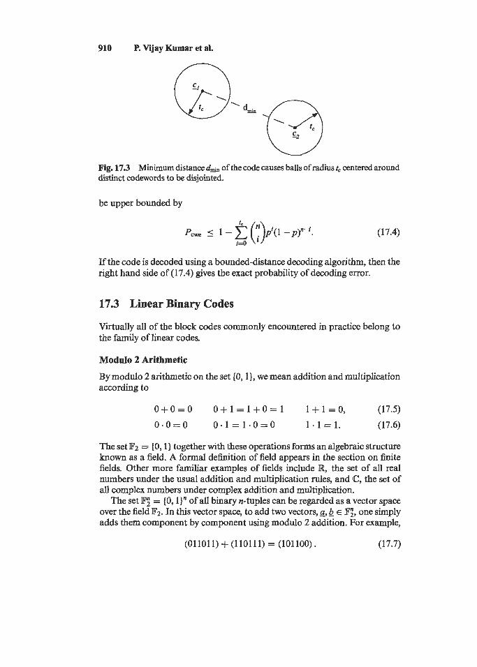
910 P. Vijay Kumar et al.
Fig. 17.3 Minimum distanced- of the code causes balls of radius tc centered around distinct codewords to be disjointed.
be upper bounded by
P , 5 1 - 2 (“)p’(l - p y 1 i=O
(17.4)
If the code is decoded using a bounded-distance decoding algorithm, then the right hand side of (17.4) gives the exact probability of decoding error.
17.3 Linear Binary Codes
Virtually all of the block codes commonly encountered in practice belong to the family of linear codes.
Modulo 2 Arithmetic
By modulo 2 arithmetic on the set {0, I}, we mean addition and multiplication according to
o + o = o 0 + 1 = 1 + 0 = 1 1 + 1 = 0 , (17.5)
o . o = o 0 . 1 = 1 . 0 = 0 1 . 1 = 1 . (17.6)
The set IF2 = IO, 1) together with these operations forms an algebraic structure known as a field. A formal definition of field appears in the section on bite fields. Other more familiar examples of fields include I[$, the set of all real numbers under the usual addition and multiplication rules, and @, the set of all complex numbers under complex addition and multiplication.
= IO, 1)” of all binary n-tuples can be regarded as a vector space over the field IF2. In this vector space, to add two vectors, a, b E IF!, one simply adds them component by component using modulo 2 addition. For example,
The set
(011011) + (110111) = (101100). (17.7)
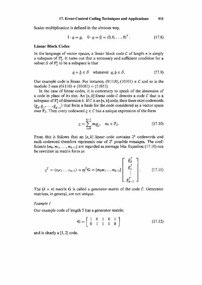
17. Error-Control Coding Techniques and Applications 911
Scalar multiplication is defined in the obvious way,
1 - g = g , O * g = Q = ( O , O ,...) o f . (17.8)
Linear Block Codes
In the language of vector spaces, a linear block code C of length n is simply a subspace of IF;. It turns out that a necessary and s a c i e n t condition for a subset S of IF; to be a subspace is that
- a + b E S whenever a,b E S. (17.9)
Our example code is linear. For instance, (OlllO), (10101) E C and so is the modulo 2 sum (01110) +(10101) = (11011).
In the case of linear codes, it is customary to speak of the dimension of a code in place of its size. An [n, k] linear code C denotes a code C that is a subspace of IF! of dimension k. If C is an [n, k] code, then there exist codewords &,gl,.. . ,%-1} that form a basis for the code considered as a vector space over IF2 . Then every codeword c E C has a unique expression of the form
k- 1
(17.10)
From this it follows that an [n,k] linear code contains 2k codewords and each codeword therefore represents one of 2' possible messages. The coef- ficients jmo, ml, . . . , mk-l} are regarded as message bits. Equation (17.10) can be rewritten in matrix form as
cT = (coq . . . cn-l) = cTG = [mom1 . . . mk-11 [ f I. (17.11)
&-1
The (k x n) matrix G is called a generator mutrzk of the code C. Generator matrices, in general, are not unique.
Enample I
Our example code of length 5 has a generator matrix:
(17.12)
and is clearly a [5,2] code.

912 P. %jay Kumar et al.
Example 2
Consider the [7,1] code having generator matrix:
G = [1111111]. (17.13)
Here each codeword consists of seven repetitions of a single message symbol, and for this reason such a code is commonly called a repetition code.
Example 3
Our final example is the [7,4] code having generator matrix:
This code is capable of correcting a single error and is an example of a family of codes known as Hamming codes.
Minimum Distance
The third important parameter of a linear code is the minimum distance, dmh. The Hamming distance d~ (E, b) between two binary n-tuples a, b equals the Hamming weight of their modulo 2 difference, i.e.,
(1 7.15)
It follows that the minimum distance of a linear code C equals the minimum Hamming weight of a nonzero codeword in C. Using this observation, it can be determined that the minimum distances of our example codes are as given in Table 17.4. Also shown in Table 17.4 are the ( t c , t d ) pairs for which the respective code can function as a tc error correcting, td error detecting code. When it is desired to include the minimum distance dmh in the description of a linear code C of length n and dimension k, we will refer to the code as an [n, k, &,in] code.
Table 17.4 Parameters of the Example Codes
Code dmi. Possible (tc, td) Pair

17. Error-Control Coding Techniques and Applications 913
1 1 0 1 1 0 0 1 0 1 1 0 1 0 0 1 1 1 0 0 1
Parity Check Matrix
The parity check (PC) matrix H of an [n, k] linear code C is any ((n - k) x n) matrix of rank (n - k) whose nullspace is precisely the k-dimensional vector space that is the code C .
If the [n, k] code C has generator matrix of the form
- - 1 0
1 = &+&+b+& = 0, (17.19)
1 0
I : - -
(1 7.1 6)
for some (k x (n - k)) matrix P, the code is said to be systematic. It can be verified that in the case of systematic codes,
(17.17)
is a valid PC matrix for the code.
corresponding PC matrices appear below: The generators of all our three example codes are systematic. The
1 0 0 0 1 0 0
1 1 0 0 0 0 0 1 0 1 0 0 0 0 1 0 0 1 0 0 0
1 0 0 0 0 1 0 1 0 0 0 0 0 1
1 1 1 0 0 H = 0 1 0 1 0
[ 1 0 0 0 1 1 9 H = [
(Length 5 Code) (Repetition Code)
1 0 1 1 0 1 0 . 1 1 0 1 1 0 0
H = [ 0 1 1 1 0 0 1 I
(Hamming Code)
(17.18)
dmin fromH
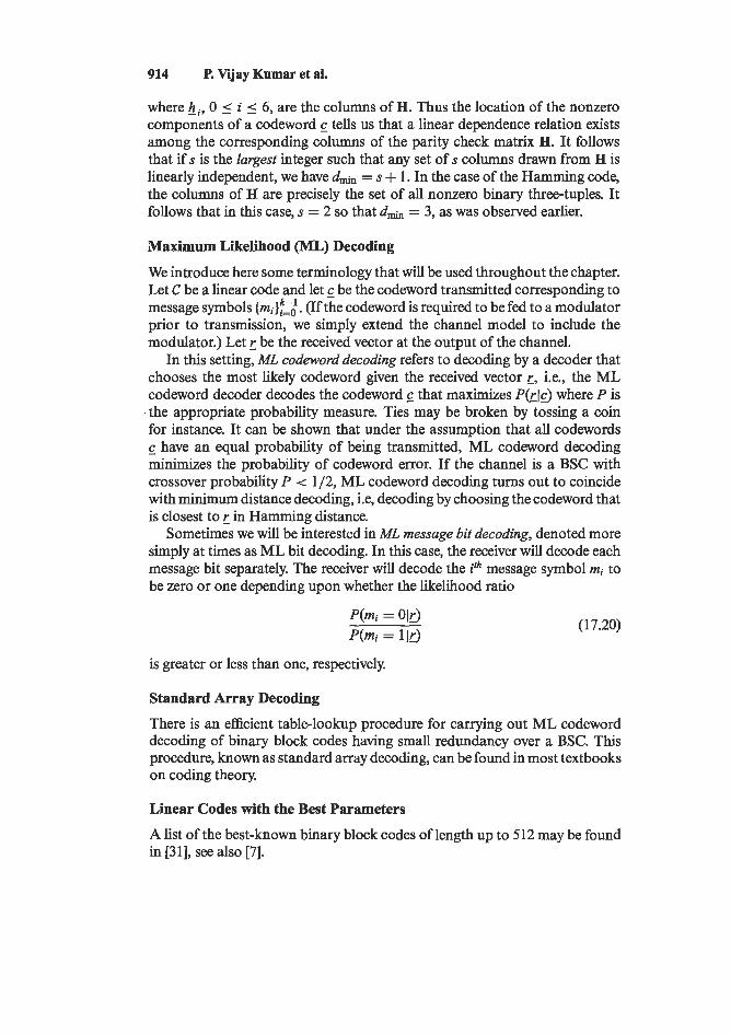
914 P. Vijay Kumar et al.
where hi, 0 5 i 5 6, are the columns of II. Thus the location of the nonzero components of a codeword c tells us that a linear dependence relation exists among the corresponding columns of the parity check matrix H. It follows that if s is the largest integer such that any set of s columns drawn from H is linearly independent, we have dmin = s + 1. In the case of the Hamming code, the columns of H are precisely the set of all nonzero binary three-tuples. It follows that in this case, s = 2 so that dmin = 3, as was observed earlier.
Maximum Likelihood (ML) Decoding
We introduce here some terminology that will be used throughout the chapter. Let C be a linear code and let c be the codeword transmitted corresponding to message symbols (mi};:;. (If the codeword is required to be fed to a modulator prior to transmission, we simply extend the channel model to include the modulator.) Let r: be the received vector at the output of the channel.
In this setting, ML codeword decoding refers to decoding by a decoder that chooses the most likely codeword given the received vector I-, i.e., the ML codeword decoder decodes the codeword c that maximizes PklcJ where P is the appropriate probability measure. Ties may be broken by tossing a coin for instance. It can be shown that under the assumption that all codewords - c have an equal probability of being transmitted, ML codeword decoding minimizes the probability of codeword error. If the channel is a BSC with crossover probability P c 1/2, ML codeword decoding turns out to coincide with minimum distance decoding, i.e, decoding by choosing the codeword that is closest to in Hamming distance.
Sometimes we will be interested in ML message bit decoding? denoted more simply at times as ML bit decoding. In this case, the receiver will decode each message bit separately. The receiver will decode the ith message symbol mi to be zero or one depending upon whether the likelihood ratio
P(mi = Old P(mi = llr>
(17.20)
is greater or less than one, respectively.
Standard Array Decoding
There is an efficient table-lookup procedure for carrying out ML codeword decoding of binary block codes having small redundancy over a BSC. This procedure, known as standard array decoding, can be found in most textbooks on coding theory.
Linear Codes with the Best Parameters
A list of the best-known binary block codes of length up to 512 may be found in [31], see also [7].

17. Error-Control Coding Techniques and Applications 915
17.3.1 THE GENERAL HAMMING CODE
Let m 2 3 be an integer and let H be an (m x (2" - 1)) matrix such that the columns of H precisely comprise, the set of all nonzero m-tuples. Clearly this matrix has rank m. Arguing as in the case of the example Hamming code discussed earlier, we see that the code C having H as parity check matrix is a [n = 2" - 1 , k = 2" - 1 - m, dmin = 31 linear block code. Any such code C is called a Hamming code.
Hamming codes are optimal with respect to a bound known appropriately enough as the Hamming bound, which states that the maximum size A(n, dmin) of a code of block length n and minimum distance &in satisfies:
(17.21)
Codes whose sizes achieve the Hamming bound with equality are known as perfect codes.
Hamming codes are perfect because:
(17.22)
Hamming codes turn out to have the property of being cyclic, and for this reason they also appear in the next section.
17.3.2 CYCLIC CODES
The most commonly used linear block codes belong to a class of codes known as cyclic codes. Examples of cyclic binary codes include Hamming codes, the Golay code, and BCH codes. Reed-Solomon codes on the other hand, are cyclic but nonbinary. Cyclic binary codes are most naturally described in terms of polynomials.
Given a vector
- c = (COY ~ 1 7 . . ., cn-1) (17.23)
by cyclic shift of c, we will mean any vector 6 of the form
- c' = (cry cr+1 , . . . , cn- 1 , co, . . . , cr- 1) , 0 -= t 5 n - 1. (1 7.24)
A binary linear code C is said to be cyclic if whenever a codeword c belongs to C, so does every cyclic shift g' of c. Given a cyclic code C and a codeword - c = (coy c1, . . . , ~"-1) we associate with the codeword, the code polynomial
n-1 c(x) = CiXi (17.25)
i=O

916 P. Vijay Kumar et al.
Example 4
Consider the code C having generator matrix
0 1 0 1 1 1 0 . (1 7.26) 1 0 1 1 1 0 0
G = [ 0 0 1 0 1 1 1 1
This code contains the eight codewords tabulated in Table 17.5. It can be verified that the code is cyclic. We will alternatively regard a cyclic
code C as a collection of code polynomials. It turns out that in every binary cyclic code the set of code polynomials has the property that it contains a unique nonzero polynomial g(x) of minimum degree. This polynomial is called the generating polynomial. Our example cyclic code thus has the generating polynomial
g(x) = x4 +x3 +2 + 1. (17.27)
The generating polynomial in any [n,k] cyclic code has the following properties:
(1) g(x) has degree = n - k. (2) g(x) I x" + 1 (i.e., g(x) divides X + 1) (3) A polynomial over IF2 of degree 5 n - 1 is a code polynomial if and
only if it can be expressed in the form c(x) = m(x)g(x) for some polynomial m(x) of degree 5 k - 1.
Table 17.5 Codewords and Code Polynomial in an Example Cyclic Code
Code Codeword Po&nomial Degree m(x)
0 0 0 0 0 0 0 0 1 0 1 1 1 0 0 x 4 + 2 + x 2 + 1 0 1 0 1 1 1 0 2 + X 4 + X 3 + X
0 0 1 0 1 1 1 x6+x5+x4+x2 1 1 1 0 0 1 0 x5+x2+x+1 1 0 0 1 0 1 1 x6+x5 +x3 + 1 0 1 1 1 0 0 1 x6+x3+2+x 1 1 0 0 1 0 1 x b + P + x + l
-m 4 5 6 5 6 6 6
0 1
2 1 + x 1 +2 x +x2 1+x+x*
X

17. Error-Control Coding Techniques and Applications 917
Example 5
Our example [7,3] code C has g(x) = x4 + x3 + x2 + 1 of degree = n - k = 7-3 =4.Alsog(x)lx7+1 sincex7+1 = ( x ~ + x ~ + x ~ + ~ ) ( x ~ + x ~ + ~ ) . E ~ ~ ~ code polynomial C(X) E C is expressible in the form c(x) = m(x)g(x). For each code polynomial the associated polynomial m(x) is displayed in Table 17.5.
From this it follows that a cyclic code of length n is completely specified once the generator polynomial g(x) is given. Also, the (k x n) matrix G, whose rows are code vectors in C associated to the code polynomials {x'g(x)lO 5 i I k - 1 } can be verified to be avalid generator matrix for the code. The generator matrix G provided in (17.26) for our example [7,3] code is so constructed.
Cyclic Hamming Code
We have seen previously that the general Hamming code has parameters of the form:
and that these codes are most easily described in terms of a parity check matrix H of size (m x 2" - 1) whose columns are precisely all nonzero binary m-tuples arranged in some order. It turns out that given an integer m 2 3, setting g(x) to be a primitive polynomial of degree m and n = 2" - 1 results in a cyclic Hamming code. Primitive polynomials are discussed in Section 17.4.
Cyclic Golay Codes
Apart from Hamming codes, the only other interesting perfect binary code is the Golay code. The Golay code is a [n = 23, k = 12, dmin = 71 linear code. Moreover the code is cyclic corresponding to choice of generator polynomial:
or
g(x) = x ' l +x9 +x7 +x6 +x5 + x + 1.
17.4 Finite Fields
(17.29)
The material in this section is essential for a good understanding of Reed- Solomon and BCH codes, discussed in Sections 17.5 and 17.6, respectively. Most textbooks on coding theory provide an introduction to finite fields.
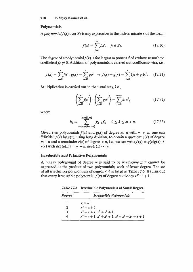
918 P. Vijay Kumar et al.
Polynomials
Apolynornialf(x) over IF2 is any expression in the indeterminate x of the form:
n
f ( x ) = c f ; x ' , 3 E Pz. (17.30) i=O
The degree of a polynomialf(x) is the largest exponent d ofx whose associated coefficient& # 0. Addition of polynomials is carried out coefficient-wise, i.e.,
Multiplication is carried out in the usual way, i.e.,
(17.32)
where min(k,m]
hk = C gk-ih O s k s m + n . (17.33) i=max(O,k-n]
Given two polynomialsf(x) and g(x) of degree my n with in > n, one can "divide"f(x) by g(x), using long division, to obtain a quotient q(x) of degree in - n and a remainder r(x) of degree < n, i.e., we can writef(x) = q(x)g(x) + r(x) with deg(q(x)) = m - n, deg(r(x)) < n.
Irreducible and Primitive Polynomials
A binary polynomial of degree in is said to be irreducible if it cannot be expressed as the product of two polynomials, each of lesser degree. The set of all irreducible polynomials of degree 5 4 is listed in Table 17.6. It turns out that every irreducible polynomialf(x) of degree in divides xZ"'-l + 1.
Table 17.6 Irreducible Polynomials of Small Degree
Degree Irreducible Polynomials
1 x , x + 1 2 x2+x+l 3 + + 1, x 3 + xz + I 4 x4+x+ i 3 + x 3 + 1 , ~ + x 3 + x 2 + x + 1

17. Error-Control Coding Techniques and Applications
Example 6
m = 2 , f ( x ) = x 2 + x + 1
f ( x ) I x3 + 1 since (x3 + 1 ) = (x + 1)(x2 + x + 1).
m = 4,f(x) = x" + x3 + x2 + x + 1
f(~)lx'~ + 1 since (x15 + 1) = (x4 + x3 + x2 + x + 1 )
x (x"+x'O+x6+x5+x+1) .
919
(17.34)
(1 7.3 5)
An irreducible polynomialf(x) of degree m is said to be primitive if the smallest degree polynomial of the form x' + 1 thatf(x) divides is x2"-l + 1.
Example 7
f ( x ) = x4 + x3 + x2 + x + 1 is not primitive asf(x)1x5 + 1 since
+ 1 = (x + 1)(~4 + + x2 + + 1). (17.36)
However, the remaining degree 4 irreducible polynomials x4 + x + 1 and x4 + x3 + 1 can be verified to be primitive.
Afield is a set F of elements together with two operations, addition (+) and multiplication ( . ), mapping pairs in F back to F , which satisfy the following three axioms:
( 1 ) The addition operation is associative and commutative and there is an additive identity element 0, called "zero" such that a + 0 = a for all a E F . Also, every element a has an unique additive inverse denoted by (-a) that satisfies a + ( -a) = 0.
there is a multiplicative identity element called "1" such that a . 1 = a for all a E F . Also, every nonzero element a has an unique multiplicative inverse, denoted by a-l , that satisfies a . a-l = 1.
(2) The multiplication operation is associative and commutative and
(3) The distributive law holds, Le.,
a . ( b + c ) = a - b + U . C . (1 7.37)
for all triples (a, b, e) in F .
For simplicity, we will often write ab in place of a b. AJiniteJield is simply a field containing a h i t e number of elements. Finite
fields containing IF2 relate to IF2 in much the same way as the field C of complex numbers relates to the field B of real numbers. To obtain C from B, one
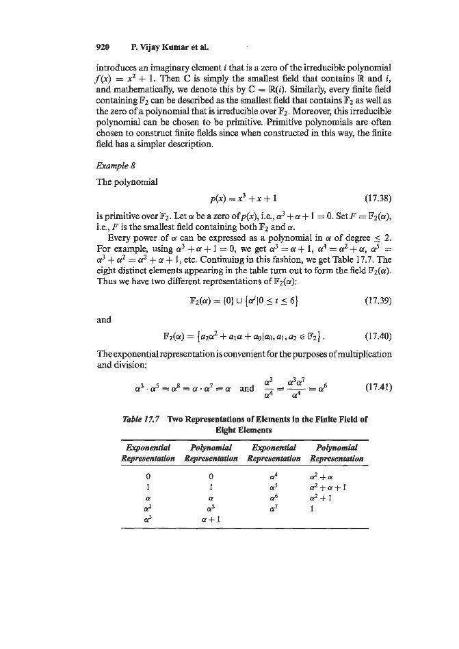
920 P. Vijay Kumar et al.
introduces an imaginary element i that is a zero of the irreducible polynomial f ( x ) = x2 + 1. Then C is simply the smallest field that contains R and i, and mathematically, we denote this by C = R(i). Similarly, every finite field containing F2 can be described as the smallest field that contains F2 as well as the zero of a polynomial that is irreducible over F2. Moreover, this irreducible polynomial can be chosen to be primitive. Primitive polynomials are often chosen to construct finite fields since when constructed in this way, the finite field has a simpler description.
Exumple 8
The polynomial
p(x) = 2 + x + 1 (17.38)
is primitive over F2. Let a! be a zero ofp(x), i.e., a3 +a! + 1 = 0. Set F = F2(01), i.e., F is the smallest field containing both F2 and a.
Every power of a! can be expressed as a polynomial in a! of degree 5 2. For example, using a3 +a + 1 = 0, we get a!3 = a! + 1, a4 = a2 +a, as = a3 + a2 = 2 + a! + 1, etc. Continuing in this fashion, we get Table 17.7. The eight distinct elements appearing in the table turn out to form the field Pz(a!). Thus we have two different representations of F2(a!):
F2(a!) = IO} U {a'lO 5 i 5 6} (17.39)
and
F2(.) = { u 2 2 + u,a + aoluo, U l , a2 E F2}. (1 7.40)
The exponential representation is convenient for the purposes of multiplication and division:
(17.41)
Table 17.7 Two Representations of Elements in the Finite Field of Eight Elements
Exponential Polynomial Exponential Polynomial Representation Representation Representation Representation
0 0 a4 a2+a
1 1 a5 d + a + l a a a6 a2 + 1 a2 a2 a7 1 a3 a + l
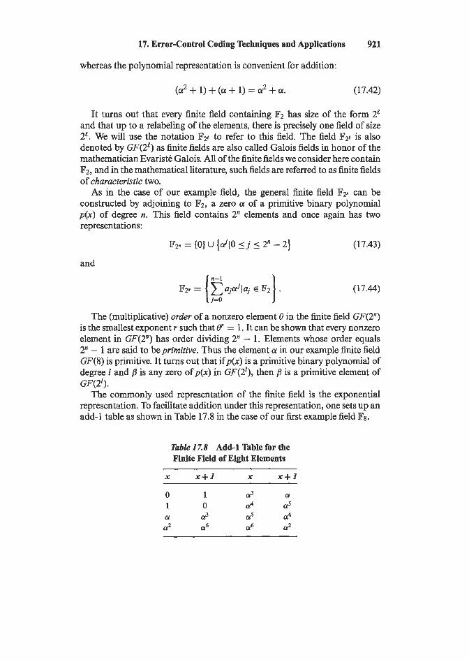
17. Error-Control Coding Techniques and Applications 921
whereas the polynomial representation is convenient for addition:
(a2 + 1) +(a! + 1) = a2 +a. (17.42)
It turns out that every finite field containing IF2 has size of the form 2l and that up to a relabeling of the elements, there is precisely one field of size 2e. We will use the notation P ~ c to refer to this field. The field PZC is also denoted by GF(2e) as finite fields are also called Galois fields in honor of the mathematician Evaristb Galois. All of the finite fields we consider here contain F2, and in the mathematical literature, such fields are referred to as finite fields of characteristic two.
As in the case of our example field, the general finite field F2. can be constructed by adjoining to IFz, a zero a of a primitive binary polynomial p(x) of degree n. This field contains 2" elements and once again has two representations:
P2" = {O} u (dl0 r j 5 2" - 2} (17.43)
and
(17.44)
The (multiplicative) order of a nonzero element 8 in the finite field GF(2") is the smallest exponent r such that 8' = 1. It can be shown that every nonzero element in GF(2") has order dividing 2" - 1. Elements whose order equals 2" - 1 are said to be primitive. Thus the element a! in our example finite field GF(8) is primitive. It turns out that if&) is a primitive binary polynomial of degree I and B is any zero of p(x) in GF(2'), then B is a primitive element of GF(2').
The commonly used representation of the finite field is the exponential representation. To facilitate addition under this representation, one sets up an add-1 table as shown in Table 17.8 in the case of our first example field IFg.
Table 17.8 Add-1 Table for the Finite Field of Eight Elements
X x + l X x + l
0 1 a3 a 1 0 d4 a5 a! a3 a5 a 4
a* a6 a6 a2

922 P. =jay Kumar et al.
With the aid of the add-I table, we can for instance, add
a3 + as + a6 = a3 (1 + a2 (1 + a)) = a3 (1 + ."a">) .3 + .5 + .6 = (2,3(1 + (.5) = ~4 = a7 = 1.
(1 7.45)
(1 7.46)
17.5 Reed-Solomon Codes
With this background in finite fields, we are now in a position to study the Reed-Solomon (RS) code. RS codes are in widespread use, for example in optical fiber communication [17], compact disks (CDs) [29] and deep-space communication [45]. In contrast to the codes discussed thus far, these codes are nonbinary.
Parallel to the binary case, a block code C of length n over the finite field F,, q = 2m, m > 1, is said to be linear if whenever c1 , 5 E C implies that every linear combination
Again as in the binary case, a code C over IF, is said to be cyclic if C is linear and if in addition, whenever (coy c1, . . . , cn-l) is a codeword, so is ( c5 , cT+~, ..., cn-l,co,c~,...,cr-~),forO< t s n - I .
DeJinition 1
Let q = 2m, m 1 and n be an integer dividing q - 1 and (Y an element in I?, of order n. Then a RS code C having parameters [n, k] over P, can be defined as
1. (17.48) ci =f(a') for some polynomial f ( x ) over F, of degree 5 k - 1
RS codes can be shown, using the definition given in Eq. (17.48), to be both linear and cyclic.
Minimum Distance
As in the binary case, we define the Hamming weight of an n-tuple over IFq to be the number of nonzero symbols in the n-tuple. Similarly, the Hamming distance between the pair of n-tuples a, b E equals the number of symbols in which the two vectors disagree. The Hamming distance d&z,bJ between two n-tuples g , b over F,, once again equals the Hamming weight of their difference, i.e.,
dH(% bJ = WH(E - b). (1 7.49)

17. Error-Control Coding Techniques and Applications 923
It follows that the minimum distance of a linear code C over IFq equals the minimum Hamming weight of a nonzero codeword in C. Since a polynomial of degree I k - 1 can have at most k - 1 zeros in lF,, the number of zeros in a nonzero codeword of an [n, k] RS code cannot exceed k - 1. On the other hand, the polynomial
k-1 n (x - ai> (17.50)
has exactly k - 1 zeros in IF,. It follows that the minimal Hamming weight of a nonzero codeword in an [n, k] Reed-Solomon code equals n - k + 1. By our previous observation, this must also be the minimum distance of the code. Thus, Reed-Solomon codes have parameters of the form [n, k, n - k + 1 1 . The Singleton bound states that a block code C of length n over an alphabet of size q having minimum distance dmin has size M upper bounded by
Codes achieving the Singleton bound with equality are said to be maximum distance separable (MDS). Thus RS codes are MDS.
Generator Matrix
A linear code of length n over IF, is a subspace of F;. The dimension of a linear code is the dimension of this subspace. As with binary codes, the notation [n, k, 4 refers to a code of length n, dimension k, and minimum distance d .
The notions of generator and parity-check matrices also carry over from the binary case. The generator matrix of any [n, k, dl code over F, is any (k x n) matrix whose rows form a basis for the code. Similarly, the parity-check matrix is any ((n - k) x n) matrix whose nullspace is the [n, k , d ] code.
The generator matrix G shown in Eq. (17.52) follows directly from the definition of a RS code
If g(x) is a polynomial of degree 5 n - 1 over GF(q) satisfying g(0) = 0, then it can be shown that g(a!') = 0. Setting g(x) = x'f(x), 1 5 i I n - k,
924 P. Vijay Knmar et a].
leads to the following parity-check matrix H of an RS code
since H has the right rank and Hc = 0 for any codeword c in the RS code.
Probability of Codeword Error
Let us assume that an [n, k, d ] RS code of length n = 2m - 1 is used to transmit information over a BSC having crossover probabilityp. Let d = 2t, + 1. To transmit information over the binary channel, each symbol ct E Fp of a codeword is converted into m binary digits. The probability Ps that any such symbol is received in error over the BSC is given by
P, = 1 - ( 1 - p y . (17.54)
Then following the argument used in the case of a general binary code in Section 17.2 to obtain an upper bound on the codeword error probability, we can upper bound the probability Pwe of codeword error in the case of the RS code by
Pme 5 1 - 2 &(l - P y . i=O
(17.55)
Burst Error Correction
RS codes excel in burst error correction. Consider for example an [255,239,17] RS code over GF(256). Prior to transmission, each symbol in GF(256) is converted to a string of eight binary digits, and these are transmitted in sequence. This effectively makes the RS code a binary code of length 8 * 255 = 2,040. Since the RS code can correct up to eight symbol errors, the code will correctly decode even in the presence of a contiguous stream of up to 1 + 7 x 8 = 57 erroneous binary digits, since such a string of errors will cause at most eight symbols over GF(256) to be in error. Of course this burst error correction capability carries over to any nonbinary code with symbols in GF(256). However, in comparison with other nonbinary codes of the same length over GF(256). RS codes offer the largest minimum distance for given dimension.

17. ErroA!ontrol Coding Techniques and Applications 925
Outer [N,K,D] code K m z oVerGF(zk) N code
Changing the Length of a RS Code
Given an [n,k,d] RS code Cy it is possible to “shorten” the code to an [n - a, k - a, d] code c,h by considering the set A of all the codewords in C whose last a symbols equal zero and then deleting the last a symbols from each codeword to obtain the code Csh. We note that it is possible to define RS codes in a more general setting than what we have done here (see [26]).
Inner [n,k,dl binary code Nn bEary
Decoding
There are several efficient algorithms, such as the Berlekamp-Massey, Welch- Berlekamp, and Euclidean algorithms, for the decoding of RS codes, all with complexity on the order of the square of the length n of the code or less. Details can be foundinmost texts oncoding theory, for example in [6,26,36,41,44], see also [4b, 221. Under certain circumstances, it is possible to decode beyond the minimum distance of the RS code using a procedure known as list decoding, see [14b].
17.5.1 CONCATENATED CODES
Concatenated codes are linear binary codes that are constructed from two component codes called the outer and inner code. In the classical construction of concatenated codes as shown in Fig. 17.4, the outer code is typically a RS code and the inner binary code, a short block code. We illustrate with an example.
Example 9
Consider an [255,244,12] RS code over GF(256). Each symbol in this code corresponds to an 8-bit string. Replacing each 8-bit string by the correspond- ing 12-bit codeword in the [12,8,3] single parity-check code yields a binary code with parameters [12.255,244.8,1 361. In general if the outer and inner codes have parameters [ N , K , D] and [n, k, d ] , respectively, the concatenated code will have parameter [Nn,Kk, 2 Dd] (Fig. 17.4).
Concatenated codes have large length and good minimum distance. The outer and inner codes have properties that complement each other. The RS code by itself, is vulnerable to isolated bit errors since each bit error can poten- tially cause a different code symbol to be in error. The inner code serves to

926 P. Vijay Kumar et al.
protect the RS code against isolated errors by providing an ability to either detect or correct them. Concatenated codes inherit from RS codes the ability to correct burst errors.
Whereas the complexity of decoding a block code of large length is high, concatenated codes are easily decoded using a suboptimal decoding algorithm (in relation to ML codeword decoding) in which the inner binary code is decoded first, followed by the decoding of the outer nonbinary code.
Although the outer code is typically a RS code, this is not essential and the RS code can be replaced by any efficient code with symbols lying in GF(29, such as, for example, nonbinary BCH codes [26] or else algebraic-geometric codes [31]. Other means of concatenating two codes also exist, as we shall shortly see.
17.6 BCH Codes
BCH codes are a family of binary cyclic codes that are very flexible in terms of allowing a trade-off to be made between dimension and minimum distance. Also, for code lengths up to a few thousand, these codes are very efficient in terms of the performance trade-off that they offer.
Let n be a divisor of 2P - 1 for some integer p 2 3. We assume that p is the smallest integer for which n divides 2* - 1. Let y be a primitive element of GF(2p) and set a! = y(2P-1)/n. Then a has order n.
Definition 2
Let n,p, a! be as above. A t-error correcting BCH code C of length n is the set of all binary n-tuples that lie in the null-space of the (t x n) matrix
Note that if JV denotes the nullspace of the above matrix over GF(29, then theBCHcodeC = NnF;.
Example IO Consider the singIe and double error correcting BCH codes of length n = 15. Here t E { 1,2},p = 4, n = 15. Let y be a primitive element of GF( 16) satisfying

17. Error-Control Coding Techniques and Applications 927
y4 + y + 1 = 0. Here, since n = 24 - 1, we have a = y. The double-error- correcting BCH code is the set of binary 15-tuples that lie in the null-space of the matrix:
1 4 2 . . . . . . H = [ 1 a3 . . . . . .
For example, since
(17.57)
(17.58)
satisfies a(.) = a(a3) = 0, we have that [10001011 1000OOO]T is a codeword in the BCH code. In the case of the single-error-correcting BCH code, the matrix H is given by
H = [ 1 a a 2 . . . . . . a14 1 . (17.59)
A more conventional (but less convenient) description of the BCH code can also be obtained. Each element a1 in the matrices has a unique representation in terms of the basis { 1, a, a2, a3} for the four-dimensional vector space P16 over Pz. Let the element a1 in the H matrix be replaced by its corresponding column vector. If this is done, in the case of the single-error-correcting BCH code, we will obtain the binary matrix
0 0 1 0 0 1 1 0 1 0 1 1 1 1 0 0 0 0 1 0 0 1 1 0 1 0 1 1 1 1
-(17.60) I [ 1 0 0 0 1 0 0 1 1 0 1 0 1 1 1 I H b i n = 0 1 0 0 1 1 0 1 0 1 1 1 1 0 0
The fifth column of this matrix equals fool 1IT since it corresponds to a4 = 0 - a3 + 0 . a2 + 1 a! + 1 . 1. It can be shown that the BCH code can also be described as the set of all binary 15-tuples that belong to the null- space of this matrix. Since the columns of this (4 x 15) matrix comprise all distinct nonzero 4-tuples, this makes the single-error-correcting BCH code a cyclic Hamming code. This is always the case. For any length n = 2 p - 1, the single-error-correcting BCH code is a cyclic Hamming code.
It can be shown that the t-error correcting BCH code, as the name suggests, has minimum distance dfin > 2t + 1. When the channel over which the code- word is transmitted is the BSC, BCH codes can be decoded using techniques very similar to those used to decode RS codes, see [6,26,36,41,44].
Because BCH codes are cyclic, they can be described in terms of a generator polynomial. It turns out that the generator polynomial of the BCH code is the smallest degree polynomial that has zeros
3 ..... a21-1 ... a2t-l (17.61) a,a Y Y

928 P. Vijay Kumar et al.
Example 11
The single-error-correcting BCH code of length n = 15 has generator polynomial
g ( x ) = x 4 + x + 1 , (17.62)
since this is the smallest-degree polynomial of which the (Y in the example is a zero. The double-error-correcting BCH code of length n = 15 has, for the same reasons, the generator polynomial
~ ( x ) = ( x ~ + x + ~ ) ( x ~ + x ~ + x ~ - ~ x + ~ ) = ~ ~ + ~ ~ + x ~ + x ~ + ~ . (17.63)
Tables providing the parameters of BCH codes of lengths up to 1023 may be found, for example in [24].
17.6.1 PRODUCT CODES
Let C1 and C2 be [nl , kl, dl] and [nz, kz, d2] systematic codes respectively. The product code C = C1 x C2 is a code having parameters [111n2, klk2, dldz] and may be constructed as follows.
Let the k1k2 information symbols be arranged in the form of a (k1 x k2) matrix A. Then construct an (nl x n2) matrix B such that the matrix in the upper-left comer of B is precisely A (see Fig. 17.5). In addition, we require that the first k1 rows of B are codewords in C2 and that the first k2 columns represent codewords in C1. Then let the remaining ((nl - kl) x (n2 - k2)) submatrix in the lower-right corner of B be chosen such that the last (nl - kl) rows of B are also codewords in CZ. (Alternately, the ((nl - k1) x ( n ~ - k2)) matrix in the lower-right corner of B could be chosen in such a way that the last (n2 - k2) columns in B are codewords in C1. It can be shown that either method yields the same ((nl - k1) x (n2 - k2)) submatrix.) A straightforward argument shows that the minium distance d of C satisfies d = dl dz.
I
I Check on A i columns
Check I C i e Z , on on
rows ' checks
- - - - - -
Fig. 17.5 An [nlnz, klk2] product code.

17. Error-Control Coding Techniques and Applications 929
As with concatenated codes, product codes offer a means of constructing a block code of large length. Again there is a simple suboptimal decoding algorithm for product codes. One first decodes the rows of the code matrix B using a decoding algorithm for code C 2 to obtain the (121 x 122) matrix B1. Next one decodes the columns ofthe matrix B1 using code C1, resulting in the (121 x 122) matrix B 2 . The second decoding step thus attempts to correct errors resulting from incorrect decoding of rows by code C 2 . The ( k ~ x k 2 ) matrix in the upper-left comer of B 2 constitutes the decoded information bits. This procedure can be iterated to improve error correcting capability.
17.7 Convolutional Codes
Convolutional codes [9,19,24,31,36,4244] are examples of tree codes. The distinction between block and tree codes is that in the case of a block code it is possible to partition the input and output of the encoder into finite blocks in such a way that the ith output block is a function only of the ith input block. With tree codes, such a partition is, in general, not possible. Instead, it is possible for a particular output bit to be a function of all previous input bits. Convolutional codes are a special class of tree codes in which the input-output relation is given by a convolutional relation. We begin with an example.
Example 12
In the convolutional encoder shown in Fig. 17.6 there is one input stream { u t } z 0 and two output streams { v ~ ’ } ~ ~ and related by
vjl’ -
VI“’ = Ut + Ut-2 ,
(17.64) t z 0
t z 0. (1 7.65)
- U t + Ut-1 + U t - 2 ,
It is assumed that the convolutional encoder is initialized with U - 1 = 24-2 = 0. The h a 1 output of the encoder is the multiplexed stream {vr’, vf’, vy’, vy’, . . .}.
Fig. 17.6 An example convolutional encoder.

930 P. Vijay Kumar et aL
In the general case, there are k inputs and n outputs related by:
(1 7.66)
where u is the memory of the convolutional code. Thus our example encoder has memory u = 2. The convolutional code is said to have rate k /n , thus our example convolutional code is of rate 1 /2.
Consider the case when the inputs {u?} to the convolutional encoder are finite strings of length N + u with the last u bits on each string equal to 0. The outputs {vy)} of the convolutional encoder are then finite strings as well. By multiplexing these output strings one obtains a vector
vectors may be regarded as codewords in the convolutional code and in this way we may regard the convolutional code as a block code of large block length n(N + u). The minimum distance between codewords as N +. 00 is called the minimum free distance, dfm, of the convolutional code. Our example code turns out to have df,, = 5.
A simplified description of the input-output relationship in a convolutional code can be obtained through the use of power series. Let us define
(vo (1) ).. .,vo (n) ,VI (1) ,...)VI (4 ,. ..,.. . ) v ~ - ~ + " , (1) . . . v ~ ~ ~ + , > . The collection ofthese
Then the convolutional relation in (17.66) is replaced by
k
vQ(D) = c u q D ) g y D ) , 1 sj 5 n, (17.68) i= 1
Example 13
In the case of our example code we have
[v(')(D) d2)(D)] = [u(D)] [g'l'(D) g(Z)(D)] , (1 7.69)
where g(')(D) = 1 + D + 02 and g(2)(D) = 1 + 02. The matrix
(17.70) g('J)(D) g(',Z)(D) . . . g(1JqD)
g(kJ)(D) g(Q)(D) . . . g ' y D ) G(D) =

17. Error-Control Coding Techniques and Applications 931
Fig. 17.7 State diagram of example code.
is called thepoZynomiuZgenerutor matrix (PGM) of the code. In the case of the example code above, we have
G(D) = [ 1 +D+D2 1 +D2 1. (17.71)
An alternate description of the convolutional code is in terms of a state diugrum. The state diagram of our example convolutional encoder is shown in Fig. 17.7. In the state diagram, the two symbols that form the label of each vertex are (ui-l ~ ~ - 2 ) . The solid edges correspond to input bits equal to 0 and the dotted edges represent input bits equal to 1. The label on each edge represents the output of the encoder corresponding to the input associated with the particular edge.
Recursive Systematic Convolutional Code
The conventional convolutional encoders considered thus far have finite impulse response. Consider a convolutional encoder with one input {ut} and two outputs {vi')}, {v;')} whose associated power series u(D) = C z O u t D t , v(')(D) = E,"=, vil)Dt, d2)(D) = xEo vj2)Dt, are related by
v(')(D) = u(D) (1 7.72)
(17.73)
One method of implementing such an encoder is to introduce the auxiliary power series
(17.74)
We then have u(D) = s(D)[l +D+D2 +D3 +D4], v(')(D) = u(D) and d2)(D) = s(D)[1 + 041 leading to the time domain relations: uf = st + st-' + s ~ - ~ + st-3 + st-4, vj') = ut, vf2' = st + ~ - 4 . This leads to the encoder shown in Fig. 17.8.
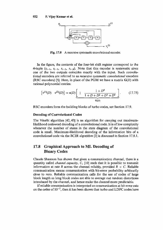
932 P. Vijay Kumar et al.
V/*)
Fig. 17.8 A recursive systematic convolutional encoder.
In the figure, the contents of the four-bit shift register correspond to the 4-tuple ( ~ ~ - 1 , ~ ~ - 2 , s+3, ~ ~ - 4 ) . Note that this encoder is systematic since one of the two outputs coincides exactly with the input. Such convolu- tional encoders are referred to as recursive systematic convolutional encoders (RSC encoders) [5]. Here, in place of the PGM we have a matrix G(D) with rational polynomial entries:
1. (17.75) 1 + 0 4
1 + D + D ~ + D ~ +04 [v(’)(D) V(Z)(D)] = u(D) [ 1
\ I
W)
RSC encoders form the building blocks of turbo codes, see Section 17.9.
Decoding of Convolutional Codes
The Viterbi algorithm [42,43] is an algorithm for carrying out maximum- likelihood codeword decoding of a convolutional code. It is of low complexity whenever the number of states in the state diagram of the convolutional code is small. Maximum-likelihood decoding of the information bits of a convolutional code via the BCJR algorithm [3] is discussed in Section 17.8.1.
17.8 Graphical Approach to ML Decoding of Binary Codes
Claude Shannon has shown that given a communication channel, there is a quantity called channeZ capacity, C , [lo] such that it is possible to transmit information at rate R across the channel reliably, provided R < C . Reliable communication means communication with bit-error probability arbitrarily close to zero. Reliable communication calls for the use of codes of large block length as long block codes are able to average out random distortions introduced by the channel, and hence make the channel more predictable.
If reliable communication is interpreted as communication at bit error rate on the order of then it has been shown that turbo and LDPC codes have

17. Error-Control Coding Techniques and Applications 933
come extremely close (within fractions of a dB) of achieving capacity on the AWGN channel.
A second feature that both turbo and LDPC codes share in common is that in both cases, decoding is accomplished by passing messages iteratively around in a graph that represents the code. Efforts are currently underway at explaining the superlative performance of such a decoding scheme.
Here we content ourselves with showing how the distributive law, applied in a more general setting, can be used to provide a heuristic justification for the use of message passing in a graph to approximate ML decoding of a code.
17.8.1 ML DECODllvG VIA THE DISTRIBUTNE LAW
In this rather long section, we lay down some principles that underline the decoding of turbo [5] and low-density parity-check codes [13]. The principal reference for the material in this section is the paper by Aji and McEliece [2], see also [8,23].
The Distributive Law
The distributive law may be viewed as a rule that allows a savings in computation. For example, the distributive law
ab1 + ab2 = a(b1 + b2) (17.76)
reduces three operations down to two. A second example is given in Example 14.
Example 14
Let A be a set of size q and let f and g be real-valued functions defined on 3-tuples and 2-tuples from A, respectively. Suppose it is desired to compute
F(xlsx4) = f (xl ,xZ,X4)g(Xl~X3)- (17.77) XZ,x3&
Direct computation would require q2[q2(1) + (q2 - l)] = 2q4 - q2 operations. However, the distributive law can be used to reorganize the computation as
F ( x l ~ X 4 ) = Cf(xl~x29x4) c g ( x l ~ x 3 ) = /%l,X4h’(xl)~ (17.78) X2 €A x3 4
where B(xl,x4) = Ex2e,4f(X1 7x2, x4) and ?&l) = zx3& g(X1 Y x3). Computing ~ ( ~ 1 ~ x 4 ) for all (q,x4) pairs requires q2(q - 1) operations.
Computing y(q) requires q(q - 1) operations. Thus a total of
q2(4 - 1) + 4(4 - 1) + 4” = q3 + q2 - 4 (17.79)

934 P. Vijay Kumar et al.
operations is now required, which could be a significant saving in com putation.
The MPF Problem and ML Decoding
We next present the problem of marginalizing a product function (MPF) and show how the generalized distributive law (GDL) can be used to present an efficient solution.
Let x1 , x2, . . . , x,, be variables taking on values from the set A1 , A2, . . . , A,, respectively. Let qi be the size of A i . Let
and let SI, S2, . . . , SM be subsets of S, not necessarily distinct. Each set Si will be called a local domain. We associate to each local domain
Si a local kernel ai : Si + B where B denotes the set of all real numbers and introduce a global kernel B(xl , x2, . . . ,xn) given by
By the Si-marginalization of B(K) we will mean the sum
(1 7.82)
and we will refer to this sum as the ifh objective function. (The notation S\Si is a reference to the subset of the elements in S that do not belong to Si.) Thus the MPF problem aims to efficiently compute the Si-marginalization of the product function p(.). Our earlier example can be recast in this notation.
Example I5
The computation
can be viewed as the marginalization of a global kernel as follows: Set
and introduce the local kernels:
Ul(S1) =f(x1,x2,x4), az(S2) = g(x1,x3), a3(S3) = 1. (1 7.85)

17. Error-Control Coding Techniques and Applications 935
Then since
it is the &-marginalization of the global kernel
For our second example, we consider the decoding of a simple binary linear code.
Example 16 (ML code symbol decoding of a block code)
Let C be the binary linear code having panty-check matrix
0 0 1 1 0 1 0 . (17.88) 1 1 0 1 0 0 0
H = [ 0 0 0 1 1 0 1 1
Consider the problem of decoding the code over a BSC. Let x_ be the transmitted codeword, g the error pattern introduced by the BSC, andy - the received vector given by
y=x_+g. (17.89)
The goal under ML code symbol decoding is to find the ith codeword symbol, xi E P2, i = 1,2,. . . , 7, such that P(xily) is a maximum. Although this goal does not correspond to either ML codeword decoding or to ML message-bit decoding, it is sometimes easier to formulate, and it can be shown that under reasonable assumptions, this decoding technique will, with high probability, pick the code symbols of the transmitted codeword.
-
Assuming all the codewords are equally likely, we can rewrite
where the indicator function xc is given by:
and where the cx sign indicates that we have ignored scale factors ( P o ) - in this case) that are independent of the symbol a.
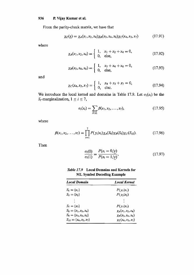
936 P. Vijay Kumar et al.
From the parity-check matrix, we have that
and
(17.92)
(17.93)
(17.94)
We introduce the local kernel and domains in Table 17.9. Let q ( x i ) be the Si-marginalization, 1 5 i 5 7,
(17.95)
where
Then
Table 17.9 Local Domains and Kernels for ML Symbol Decoding Example
Local Domain Local Kernel
(17.97)

17. Error-Control Coding Techniques and Applications 937
and thus the problem of ML code symbol decoding of the [7,4,2] block code can be viewed as an instance of the MPF problem. Iff = (21 , 22, . . . , 27) is the decoded codeword, we set
[ 1, ifq(1) s ai@), xi = 0, else.
Our next example considers the problem of ML decoding of a binary convolutional code.
Example 17 (ML message-bit decoding of a convolutional code)
Let [ui}Lil, [si}Lil, and [ y i } L i l denote the sequence of inputs of a convo- lutional encoder, the sequence of states of the convolutional encoder and the sequence of channel outputs respectively. For simplicity, we assume that the convolutional encoder is of rate R = l /n and memory u. Thus each ui is binary, each state si represents a binary u-tuple, and each output yi is an n-tuple. For ML message-bit decisions, we need to compute
Figure 17.9 presents a graph known as a Bayesian network that depicts the statistical relationship between the various random variables.
...
...
...
a @ YN.2 Y N - I
Fig. 17.9 Bayesian network of a convolutional code.

938 P. Vijay Kumar et al.
Table 17.10 Local Domains and Kernels for ML Decoding of the Convolutional Code
Local Domain Local Kernel
ML message-bit decisions are made according to
With local domains and kernels as shown in Table 17.10 and consequent global kernel
we see that the problem of ML message-bit decoding of a convolutional code can once again be recast as an MPF problem.
Junction Trees
The first step in applying the distributive law to solve the MPF problem is to set up a labeled graph known as a junction tree, in which each node in the graph is associated to a local domain. If it is not possible to organize the local domains into a junction tree then one has to modify this approach. When it is possible to organize the local domains into a junction tree, an algorithm known as Primm’s greedy algorithm (see footnotes on p. 359 of [2]) may be employed to construct the junction tree. The label for a node in the graph is just the set of variables making up the local domain associated to that node.
A tree may be defined as a graph in which there is a unique path between any two vertices. A junction tree satisfies the additional constraint that the subgraph consisting of all vertices whose label includes a fixed variable, say xl , is connected. Alternately, a junction tree can be characterized by the property that if nl belongs to the label of vertices vi and c it also belongs to the label of every vertex lying on the unique path between vi and 5.

17. Error-Control Coding Techniques and Applications 939
Table 17.11 Local Domains and Kernels of Example 18
Local Domain Local Kernel
Example 18
Consider the MPF problem of S1 -marginalization of the global kernel
given by B(SI) = &, B(xI,x~,x~,x~), where S = Ix~,x~,x~,x~} and the local domains and kernels are as shown in Table 17.1 1. The local domains can be organized into a junction tree as shown below:
Let us ignore for the moment the arrows along the edges. To verify that the graph is indeed a junction tree, note that the subgraph consisting of vertices containing the variable, xi, 1 5 i 5 4, are all connected, for instance, in case i = 1 , we obtain the connected graph
2
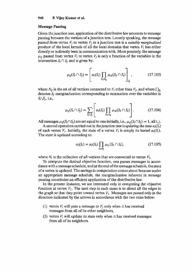
940 P. Vijay Kumar et al.
Message Passing
Given the junction tree, application of the distributive law amounts to message passing between the vertices of a junction tree. Loosely speaking, the message passed from vertex V;: to vertex 5 in a junction tree is a suitabZy marginalized product of the local kernels of all the local domains that vertex V;: has either directly or indirectly been in communication with. More precisely, the message pij passed from vertex V;: to vertex 5 is only a function of the variables in the intersection Si n 4 and is given by:
where Nu is the set of all vertices connected to V;: other than 5, and where [ Isj denotes +marginalization corresponding to summation over the variables in
(1 7.104)
All messages pv(Sins,) are set equal to one initially, i.e., &Sins,) = 1, all i , j . A second operation carried out in the junction tree is updating the state crj(Si)
of each vertex 6. Initially, the state of a vertex V;: is simply its kernel ai(&). The state is updated according to:
( 1 7.1 05)
where Ni is the collection of all vertices that are connected to vertex V;:. To compute the desired objective function, one passes messages in accor-
dance with a message schedule, and at the end of the message schedule, the state of a vertex is updated. The savings in computation comes about because under an appropriate message schedule, the marginalization inherent in message passing constitutes an efficient application of the distributive law.
In the present instance, we are interested only in computing the objective function at vertex V I . The next step in such cases is to direct all the edges in the graph so that they point toward vertex V I . Messages are passed only in the direction indicated by the arrows in accordance with the two rules below:
(1) vertex fi will pass a message to 5 only when it has received
(2) vertex V;: will update its state only when it has received messages messages from all of its other neighbors,
from all of its neighbors.

17. Error-Control Coding Techniques and Applications 941
When these rules are applied to our example, the sequence of messages passed reads as follows:
Phase 1
Phase 2
(1 7.106)
(1 7.107)
(1 7.108)
(1 7.109)
(1 7.1 10)
Phase 3
All the computations that comprise Phase 1 of the computation can be carried out simultaneously. However, the computations in Phase 1 must be completed prior to carrying out any computation that is part of Phase 2, etc.
The objective function computed given by cq(S1), when spelled out, reads as:
(17.112)
Clearly the computation when expressed in this fashion can be seen to make most efficient use of the distributive law.
Suppose next, that in the same example, we were interested in computing the objective functions at more than one, perhaps all of the vertices VI , V2, . . . , V5. In this case it takes more effort to describe what constitutes an appropriate message schedule. We begin with some notation:
Let E denote the set of all edges in the junction tree. We will distin- guish between edges (iJ) and (j,i) since reference to an edge ( i , j ) will

942 P. Vijay Kumar et al.
indicate our interest in passing a message from vertex V;: to vertex 5. In our example:
(17.113)
A message schedule is a sequence of subsets of E, such as E1 =
With each message schedule we associate a message trellis. The trellis associ- ated to message schedule {El, Ez) is shown in Fig. 17.10. Each vertical column of vertices in the message trellis corresponds to the vertex V;: of the graph at suc- cessive time instants beginning with time t = 0. We use V;:(t) to denote vertex V;: at time t. In the message trellis, we connect the pair of vertices (V;:(t - l), c(t)) if and only if (1) i = j or (2) ( i , j ) E Et.
We say that vertex &(t) knows c(0) if there is a path in the message trellis connecting Q(0) to V;:(t). In our example message trellis we see that Vz( 1) knows V4(0) and Vs(O), but not Vl(0). Also, Vl(2) knows V;:(O) for all i, 1 5 i 5 5. It can be shown that a vertex V,(t) is ready to compute its objective function pi(&) if K( t ) knows Q(O), allj.
Thus given that it is desired to compute the objective functions {pi (Si) I 1 5 i 5 M ) , setting up an appropriate message schedule can be accom- plished by using the message trellis to check that at the desired time instant t , the vertices { V;:(t), i = 1,2, . . . , M ) all know { c(O), allj}.
We next show how the GDL can help solve the MPF problem associated to ML decoding of our example [7,4,2] code.
I(4, a, (5,213 (3,1>1 and E2 = I(2, 111.
Fig. 17.10 Message trellis.

17. Error-Control Coding Techniques and Applications 943
Example 19 (ML code symbol decoding of the [7,4,2] code (continued))
Here we are interested in computing for all i = 1 , 2, . . . , 7, and xi = 0, l the following objective function:
(1 7.1 14)
We assume that the communication channel is a BSC having crossover prob- ability E , E e 1/2. Thus for given b 1 , y 2 , . . . ,y7), P(yiIxJ E 11 - E , E). Our decisions will be based on the ratio /&(O)//$(l). The MPF nature of the prob- lem is apparent. It will be found convenient to scale each local kernel P(yilxi) by the constant (1 - E ) (this will not affect the decision).
Let us assume that the received vector y = (0110100) in a instance of transmission across the BSC. The local kernzl a1 ( S I ) is then given by:
x1 = 0, Ql(S1) = - - p ( y l ' x l ) 1 - E - I E / 1 19 - E , x1 = 1. (1 7.1 15)
Let 8 = ~ / 1 - E , then 8 e 1. Set
We similarly obtain gi = [ L ] for i = 4,6,7 and gi = [ y ] for i = 2,3,5. We will use VA, V g , VC to denote the vertices corresponding to the local domains 11,2,4}, {3,4,6), and {4,5,7}, respectively. Figure 17.11 shows the local domains organized into a junction tree. We are interested here in com- puting the objective functions at all vertices 6, i = 1,. . . , 7. With regard to the message schedule, we will adopt an inward-outward schedule in which the outlying vertices send their messages inward first. Once the innermost vertex V4 has acquired knowledge of all the local kernels, the outward phase of mes- sage passing begins. The validity of this message schedule can be verified with the aid of a message trellis ifdesired. The messages passed are as follows:
Phase 1
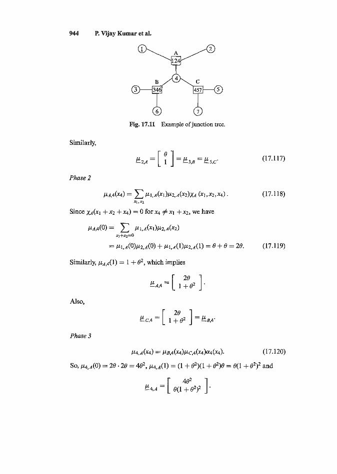
944 P. Vijay Kumar et al.
Fig. 17.11 Example of junction tree.
Similarly,
Phase 2
(1 7.1 17)
(1 7.1 18)
Similarly, p ~ , ~ ( 1 ) = 1 + 8', which implies
Also,
Phase 3
P4,A (x4) = P~P(X4>PC,4(~4)~4(40. (1 7.120)
SO, P ~ J ( O ) = 28.28 = 402, ~ ~ , ~ ( l ) = (1 + e2)(1 + e2)8 = e(1 + e2)2 and
4ez

17. Error-Control Coding Techniques and Applications 945
Similarly,
Phase 4
and
e2(i + e2)2 + 4.e2 - E A , 2 = [ 4e3 + e(i + e2)2 1 - - E B . 3 - EC.5'
Phase 5
Similarly, al(l) = Q3(l + 02)2 + 403, so that
(17.125)

946 P. Vijay Kumar et al.
Similarly,
(1 7.126)
(1 7.127)
Note that a, could have been computed in Phase 3.
Phase 6 (Decisions)
Since u1 (0) = 403 + e( 1 + e*)‘ > 01 (1) = e3( 1 + €J2)2 + 403, we conclude that
P(Xl = Oly) > P(x1 = lk). ( 17.128) - -
Denoting the decoded codeword as before by 2 = (21 , i z , . . . , 27), we therefore declare $1 = 0. Similarly, we get 26 = $7 = 0 and 22 = G = & = $5 = 1. It can be verified that [Ol 1 1 lWIT is a valid codeword.
Example 20 (ML message bit decoding of convolutional codes (continued))
The local domains corresponding to the MPF problem in this case can be organized into a junction tree as shown in Fig. 17.12.
The linear nature of the junction tree coupled with the fact that it is desired to compute the objective functions at vertices ui, i = 0,1,2,3 results in a message passing schedule that could be viewed as consisting of a forward wave of message passing and a second backward propagating wave.
Part 1. Passing on A Priori Probabilities
3
4 7 10
6 9
SO 2
Fig. 17.12 Junction-tree representation of maximum-likelihood bit decoding of convolutional codes,
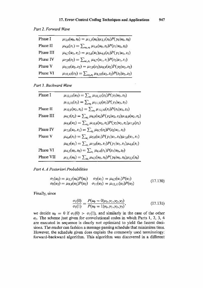
17. Error-Control Coding Techniques and Applications 947
Part 2. Forward Wave
Part 3. Backward Wave
Part 4. A Posteriori Probabilities
Finally, since
(17.130)
(17.131)
we decide uo = 0 if q(0) > el(l), and similarly in the case of the other cj. The scheme just given for convolutional codes in which Parts 1, 2, 3, 4 are executed in sequence is clearly not optimized to yield the fastest deci- sions. The reader can fashion a message passing schedule that minimizes time. However, the schedule given does explain the commonly used terminology: forward-backward algorithm. This algorithm was discovered in a different
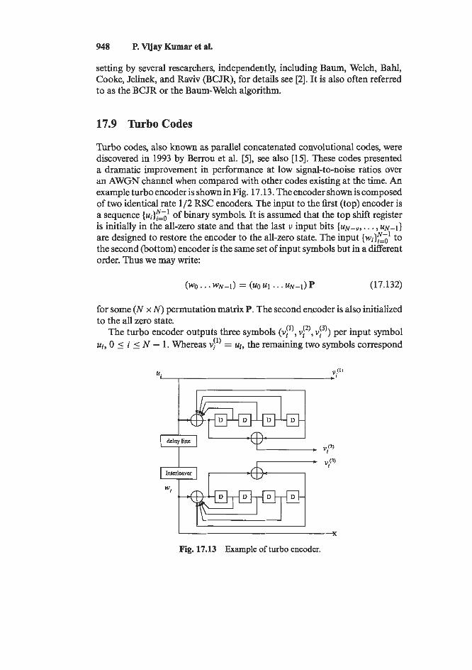
948 P. Vijay Kumar et al.
setting by several researchers, independently, including Baum, Welch, Bahl, Cooke, Jelinek, and Raviv (BCJR), for details see [2]. It is also often referred to as the BCJR or the Baum-Welch algorithm.
17.9 Turbo Codes
Turbo codes, also known as parallel concatenated convolutional codes, were discovered in 1993 by Berrou et al. [5], see also [15]. These codes presented a dramatic improvement in performance at low signal-to-noise ratios over an AWGN channel when compared with other codes existing at the time. An example turbo encoder is shown in Fig. 17.13. The encoder shown is composed of two identical rate 1/2 RSC encoders. The input to the first (top) encoder is a sequence {ui}Li’ of binary symbols. It is assumed that the top shift register is initially in the all-zero state and that the last u input bits {uN-”, . . . , UN-~} are designed to restore the encoder to the all-zero state. The input {wj}Ei’ to the second (bottom) encoder is the same set of input symbols but in a different order. Thus we may write:
(wo.. . WN-1) = (UO u1 . . . U N - 1 ) P (17.132)
for some (N x N ) permutation matrix P. The second encoder is also initialized to the all zero state.
ui, 0 5 i 5 N - 1. Whereas vi‘” = uj, the remaining two symbols correspond The turbo encoder outputs three symbols (vi (1) , vi (9 , vi (3) ) per input symbol
r.
Fig. 17.13 Example of turbo encoder.

17. Error-Control Coding Techniques and Applications 949
to outputs of the top and bottom encoder. Thus the overall rate of the code is one-third.
The input-output power series relationship of the two encoders may be expressed in the form
] (17.133) 1 + 0 4
1 + 0 + 0 2 + 0 3 + ~ 4
The turbo encoder incorporates three novel features: (1) the use of two convolutional encoders to encode scrambled versions of the same input data, (2) the use of RSC encoders in place of conventional convolutional encoders and, (3) the use of a message passing decoding algorithm [23,28] that employs an iterative message-passing schedule. It is this decoder that gives the code its name.
We explain with a simple example where N = 4, wo = u2, WI = U I , wz = 1.43, andw3 = UO. Consider MLmessage-bit decoding of u2. Let { X ~ , ~ ~ , Z ~ } ; = ~ denote
respectively. Then the received symbols corresponding to the output streams {vi (1) , vi (2) , vi (3) }i=o, 3
p (u2IIxi,yi,ziI~=o) a p (tui,si,qi,xi,yi,zi}Lo) (17-135) uom 9% Iqi);=o
[ 3 i=O 1 3
x n 1% Isi-1 ui-l)p(qi Iqi-lwi-~)] n p( yi I uisi)p(zi IWiqi) , (1 7.137) i= 1
where si, qi denote respectively, the state of the top and bottom encoder. At this point, one should, strictly speaking, identify the local domains
and kernels associated with this computation and then set up a junction tree. However, the turbo decoder operates using the graph shown in Fig. 17.14. The reader will observe that this graph is not a tree as it is possible to identify several pairs of nodes with each pair connected by two or more paths.
Despite this, however, message passing is used for decoding, and the sched- ule runs as follows. It is evident that the graph is composed of two sections. The top section is the junction tree associated with the top encoder and similarly with the bottom section. The two sections are linked by edges designated by a dotted line.
To begin with, let us pretend that the dotted edges are absent. The upper section employs message passing using a forward-backward schedule and con- cludes by updating the states ai(uj) of the vertices labeled uo,u1,u2 and u3.
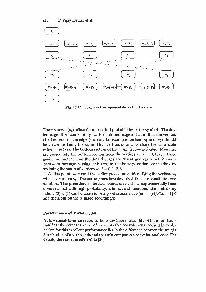
950 P. Vijay Kumar et aL
Fig. 17.14 Junction-tree representation of turbo codes.
These states q ( u i ) reflect the aposteriori probabilities of the symbols. The dot- ted edges then come into play. Each dotted edge indicates that the vertices at either end of the edge (such as, for example, vertices u3 and wz) should be viewed as being the same. Thus vertices u3 and w2 share the same state 4 u 3 ) = q(w2). The bottom section of the graph is now activated. Messages are passed into the bottom section from the vertices wi, i = 0, 1,2,3. Once again, we pretend that the dotted edges are absent and carry out fonvard- backward message passing, this time in the bottom section, concluding by updating the states of vertices wi, i = 0, 1,2,3.
At this point, we repeat the earlier procedure of identifying the vertices wi with the vertices ui. The entire procedure described thus far constitutes one iteration. This procedure is iterated several times. It has experimentally been observed that with high probability, after several iterations, the probability ratio ai(0)/ai(l) can be taken to be a good estimate of P(ui = Oly)/P(ui - = 1 ly) - and decisions on the ui made accordingly.
Performance of Turbo Codes
At low signal-to-noise ratios, turbo codes have probability of bit error that is significantly lower than that of a comparable convolutional code. The expla- nation for this excellent performance lies in the difference between the weight distribution of a turbo code and that of a comparable convolutional code. For details, the reader is referred to [30].
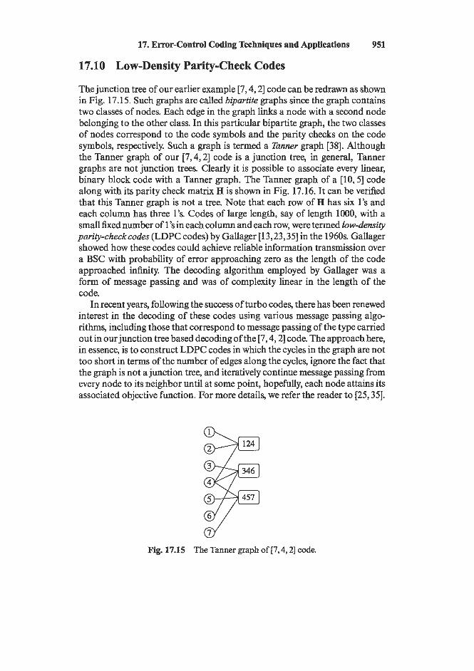
17. Error-Control Coding Techniques and Applications 951
17.10 Low-Density Parity-Check Codes
The junction tree of our earlier example [7,4,2] code can be redrawn as shown in Fig. 17.15. Such graphs are called bipartite graphs since the graph contains two classes of nodes. Each edge in the graph links a node with a second node belonging to the other class. In this particular bipartite graph, the two classes of nodes correspond to the code symbols and the parity checks on the code symbols, respectively. Such a graph is termed a Tanner graph [38]. Although the Tanner graph of our [7,4,2] code is a junction tree, in general, Tanner graphs are not junction trees. Clearly it is possible to associate every linear, binary block code with a Tanner graph. The Tanner graph of a [lo, 51 code along with its parity check matrix H is shown in Fig. 17.16. It can be verified that this Tanner graph is not a tree. Note that each row of H has six 1’s and each column has three 1’s Codes of large length, say of length 1000, with a small fixed number of 1’s in each column and each rowy were termed lowdensit): parity-check codes (LDPC codes) by Gallager [ 13,23,35] in the 1960s. Gallager showed how these codes could achieve reliable information transmission over a BSC with probability of error approaching zero as the length of the code approached infinity. The decoding algorithm employed by Gallager was a form of message passing and was of complexity linear in the length of the code.
In recent years, following the success of turbo codes, there has been renewed interest in the decoding of these codes using various message passing algo- rithms, including those that correspond to message passing of the type carried out in our junction tree based decoding of the [7,4,2] code. The approach here, in essence, is to construct LDPC codes in which the cycles in the graph are not too short in terms of the number of edges along the cycles, ignore the fact that the graph is not a junction tree, and iteratively continue message passing from every node to its neighbor until at some point, hopefully, each node attains its associated objective function. For more details, we refer the reader to [25, 351.
d Fig. 17.15 The Tanner graph of [7,4,2] code.
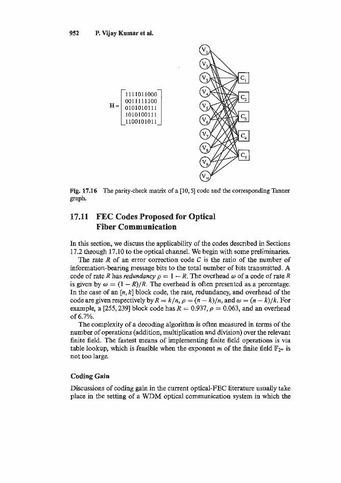
952 P. Vijay Kumar et al.
1111011000 0011111100
= 01010101 11 1010100111 [ I 1100101011
Fig. 17.16 The parity-check matrix of a [lo, 51 code and the corresponding Tanner graph-
17.11 FEC Codes Proposed for Optical Fiber Communication
In this section, we discuss the applicability of the codes described in Sections 17.2 through 17.10 to the optical channel. We begin with some preliminaries.
The rate R of an error correction code C is the ratio of the number of information-bearing message bits to the total number of bits transmitted. A code of rate R has redundancy p = 1 - R. The overhead w of a code of rate R is given by w = (1 - R)/R. The overhead is often presented as a percentage. In the case of an [n, k] block code, the rate, redundancy, and overhead of the code are given respectively by R = k /n , p = (n - k)/n, and w = ( n - k)/k. For example, a [255,239] block code has R = 0.937, p = 0.063, and an overhead of 6.7%.
The complexity of a decoding algorithm is often measured in terms of the number of operations (addition, multiplication and division) over the relevant finite field. The fastest means of implementing finite field operations is via table lookup, which is feasible when the exponent m of the finite field Fp is not too large.
Coding Gain
Discussions of coding gain in the current optical-FEC literature usually take place in the setting of a WDM optical communication system in which the
17. Error-Control Coding Techniques and Applications 953
dominant source of noise is the ASE noise introduced by the optical amplifiers present along the optical fiber. The modulation is assumed to be OOK and the receiver can be modeled as a symbol detector (see 17.1.3) followed by a hard-decision FEC decoder. The symbol detector consists of a direct-detection photodetector followed by an integrate-and-dump filter with integration-time interval T chosen to capture most of the energy of the incoming pulse. The output x of the integrate-and-dump filter is fed to a threshold circuit which declares the transmitted message bit to be a “1” or a “0” depending upon whether x exceeds or does not exceed, a threshold Xth. The output of the threshold circuit is fed to the input of the FEC decoder.
All distortions of the optical signal except that caused by the ASE noise are ignored. Thus an implicit assumption is made that the intersymbol interference caused by the various sources of pulse dispersion has been reduced to negligible levels through some form of optical or electronic equalization.
The ASE noise can be assumed to be modeled as colored Gaussian noise obtained by passing additive white Gaussian noise through a bandpass filter whose single-sided bandwidth equals Bo, the bandwidth of the optical ampli- fier. Using this fact it is shown in [16] that statistically, x is a random variable having a probability distribution known as the chi-square distribution [32] with the exact distribution depending upon whether the transmitted bit is a ”1” or a “0”. The authors of [16] then go on to to show how one can determine the optimal threshold setting Xth that minimizes bit error probability (BEP) p and how this minimum BEPp can be computed.
It is common in practice however, to assume that x has a Gaussian distri- bution. It is shown in [16], that while this assumption leads to an incorrect determination of the thresholdxth, it does yield an expression for a B E P j that is close to the true value p . Since it is the BEP that is of primary interest in this chapter, we will throughout use the approximation j for p given by the Gaussian assumption, Le.,
( 1 7.1 38)
where Q is called the Q-factor and turns to be given by [I61
(1 7.139)
where y = E/No is the SNR, i.e., the ratio of average signal energy E (per message bit) to the single-sided power density NO of the colored noise within the optical bandwidth Bo, and where Be = 1/T is the electrical bandwidth of the signal. The Q-factor is often expressed in terms of a quantity termed as
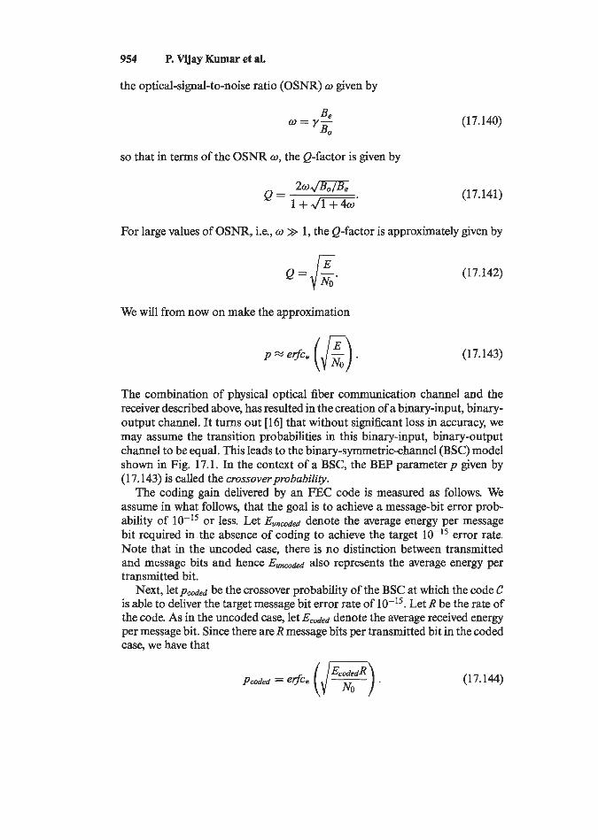
954 P. Vijay Kumar et aL
the optical-signal-to-noise ratio (OSNR) w given by
Be w = y - BO
so that in terms of the OSNR o, the Q-factor is given by
(1 7.140)
(1 7.141)
For large values of OSNR, Le., w >> 1, the Q-factor is approximately given by
We will from now on make the approximation
( 1 7.142)
(1 7.143)
The combination of physical optical fiber communication channel and the receiver described above, has resulted in the creation of a binary-input, binary- output channel. It turns out [ 161 that without significant loss in accuracy, we may assume the transition probabilities in this binary-input, binary-output channel to be equal. This leads to the binary-symmetric-channel (BSC) model shown in Fig. 17.1. In the context of a BSC, the BEP parameterp given by (17.143) is called the crossoverprobabiZity.
The coding gain delivered by an FEC code is measured as follows. We assume in what follows, that the goal is to achieve a message-bit error prob- ability of 10-l~ or less. Let Euncoded denote the average energy per message bit required in the absence of coding to achieve the target error rate. Note that in the uncoded case, there is no distinction between transmitted and message bits and hence E-ded also represents the average energy per transmitted bit.
Next, ktpcoded be the crossover probability of the BSC at which the code C is able to deliver the target message bit error rate of Let R be the rate of the code. As in the uncoded case, let Ecded denote the average received energy per message bit. Since there are R message bits per transmitted bit in the coded case, we have that
(17.144)
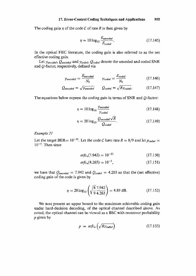
17. Error-Control Coding Techniques and Applications 955
The coding gain r] of the code C of rate R is then given by
(1 7.145) ~ u n c o d e d r] = lolog,, -.
Ecoded
In the optical FEC literature, the coding gain is also referred to as the net effective coding gain.
Let yiulcoded Quncoded and ycoded , Qcoded denote the uncoded and coded SNR and Q-factor, respectively, defined via
Euncoded Ecoded ycoded = -
No Yuncoded = ~ NO
(1 7.146)
The equations below express the coding gain in terms of SNR and @factor:
(1 7.148) hncoded
ycoded r] = lolog,, __
(17.149)
Example 21
Let the target BER= 10-j. Then since
Let the code C have rate R = 8/9 and letproded =
erfc,(7.942) =
e@..,(4.265) =
(17.150)
(17.151)
we have that Qimcoded = 7.942 and Qc&d = 4.265 so that the (net effective) coding gain of the code is given by
8 7.942 r] = 20 log,, (Am) = 4.89 dB. ( 1 7.1 52)
We next present an upper bound to the maximum achievable coding gain under hard-decision decoding, of the optical channel described above. As noted, the optical channel can be viewed as a BSC with crossover probability p given by
(17.1 53)

956 P. Vijay Kumar et al.
Table 17.12 Maximum Achievable Coding Gain on
the BSC
Maximum Achievable Coding Gain (BSC) (dB) Rate R
0.85 11.17 0.90 10.59 0.95 9.69
where R is the rate of the code. It is possible using information theory [lo] to determine the smallest value of S N R required to guarantee reliable communication at rate R. This value is obtained by solving the equation
R = -p log, p - (1 - p ) log, (1 - p) , where p = (Jx). (1 7.154)
Let as before, Yuncoded denote the SNR needed to achieve reliable commu- nication in the absence of coding. Interpreting reliable communication as communicating with BEP we can determine l/w,c&ed by solving
erf* (JG;;) = 1045 (17.155)
Then lOlog,, (YuncodedlYmin) is the maximum achievable coding gain at rate R. The maximum achievable coding gains at rates R = 0.85,O.g and 0.95 are tabulated in Table 17.12.
By replacing hard-decision decoding with soft-decision decoding, it may be possible to gain something on the order of an additional 1-2 dB depending upon the rate R of the code.
BCH Codes (Section 17.6)
BCH codes fall into the class of cyclic binary codes. From an optical stand- point, these codes offer certain advantages. They are efficient in having small overhead for given error correction capability, and are flexible in that they offer a trade-off to be made between overhead and error correction capabil- ity. When operated over a BSC, the codes can be decoded by a hard-decision decoding algorithm of reasonable complexity. If the BCH code has length n and is capable of correcting t errors, then decoding can be accomplished using roughly 4nt + 4t2 finite field operations, for details see [24].
A tabular listing of the coding overheadcoding gain trade-off offered by BCH codes is provided in Table 17.13. In deriving the coding gain of the BCH

17. Error-Control Coding Techniques and Applications 957
Table 17.13 Lower Bound on Coding Gain of Some BCH Codes
Length n t Rate R Overhead o (99) Coding Gain (d3B)
2047 27 0.85 17.64 8.02 2047 18 0.90 11.11 7.41 2047 9 0.95 5.26 6.17 4095 51 0.85 17.64 8.60 4095 34 0.90 11.11 8.09 4095 17 0.95 5.26 7.03 2047 1 0.99 0.60 1.59
codes, it was assumed that the bit error probability at the output of the BCH decoder is equal to the probability given in (17.4) of incorrectly decoding the transmitted codeword using the bounded-distance decoding algorithm. This assumption is equivalent to saying that whenever a codeword is incorrectly decoded, all the message bits are erroneously decoded. For this reason, the “coding gain” entries in Table 17.13 are lower bounds on the actual coding gain realized by the respective BCH code. Application of the bounded-distance decoding algorithm requires knowledge of the minimum distance of the code. In this case, the minimum distance was set equal to the value given by the BCH bound, see [26].
The lengths of the BCH codes were chosen to be 2047 and 4095. The first length is comparable to that of the binary code in the ITU G.975 Recom- mendation, which involves a length 255 RS code, which upon conversion to bits, results in a binary code of overall length 8 * 255 = 2040. At both lengths, three sample codes are presented, corresponding to the code rates in the range 0.85-0.95. The bottom entry in the table corresponds to a BCH code with parameter t = 1, which corresponds as indicated in Section 17.6, to a single-error-correcting, cyclic Hamming code of length 2047.
In the optical communication literature, BCH codes have appeared as con- stituent codes in the construction of product codes (see below). Hamming codes were proposed for use on the fiber-optic channel in an early paper by Grover [ 141.
Product Codes (Section 17.6.1)
Product codes offer the benefits of large block length combined with ease of decoding. However, if it is desired to construct a product code C of high rate R, this forces the constituent codes C1 and Cz to have even higher rates. Typically in such cases the minimum distance d = dldz of the resulting product code will be low.
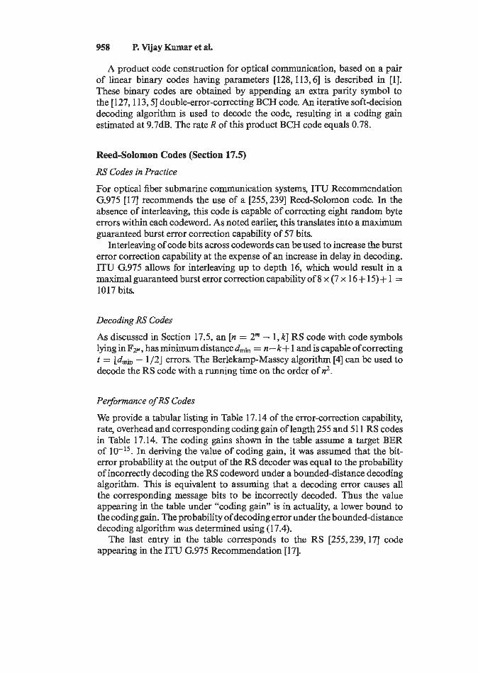
958 P. Vijay Kumar et al.
A product code construction for optical communication, based on a pair of linear binary codes having parameters [128,113,6] is described in [l]. These binary codes are obtained by appending an extra parity symbol to the [ 127,113,5] double-error-correcting BCH code. An iterative soft-decision decoding algorithm is used to decode the code, resulting in a coding gain estimated at 9.7dB. The rate R of this product BCH code equals 0.78.
Reed-Solomon Codes (Section 17.5)
RS Codes in Practice
For optical fiber submarine communication systems, ITU Recommendation G.975 [17] recommends the use of a [255,239] Reed-Solomon code. In the absence of interleaving, this code is capable of correcting eight random byte errors within each codeword. As noted earlier, this translates into a maximum guaranteed burst error correction capability of 57 bits.
Interleaving of code bits across codewords can be used to increase the burst error correction capability at the expense of an increase in delay in decoding. ITU G.975 allows for interleaving up to depth 16, which would result in a maximal guaranteed burst error correction capability of 8 x (7 x 16+ 15) + 1 = 1017 bits.
Decoding RS Codes
As discussed in Section 17.5, an [n = 2m - 1, k] RS code with code symbols lying in Fp, has minimum distance dmin = n-k+ 1 and is capable of correcting t = L&in - 1/2J errors. The Berlekamp-Massey algorithm [4] can be used to decode the RS code with a running time on the order of n2.
Peformance of RS Codes
We provide a tabular listing in Table 17.14 of the error-correction capability, rate, overhead and corresponding coding gain of length 255 and 51 1 RS codes in Table 17.14. The coding gains shown in the table assume a target BER of In deriving the value of coding gain, it was assumed that the bit- error probability at the output of the RS decoder was equal to the probability of incorrectly decoding the RS codeword under a bounded-distance decoding algorithm. This is equivalent to assuming that a decoding error causes all the corresponding message bits to be incorrectly decoded. Thus the value appearing in the table under “coding gain” is in actuality, a lower bound to the coding gain. The probability of decoding error under the bounded-distance decoding algorithm was determined using (17.4).
The last entry in the table corresponds to the RS [255,239,17] code appearing in the ITU G.975 Recommendation [17].

17. Error-Control Coding Techniques and Applications 959
Table 17.14 Lower Bound on the Coding Gain of Some RS Codes
Length n t Rate R Overhead o (%) Coding Gain (dB)
255 19 0.85 17.64 7.42 255 13 0.90 11.11 6.70 255 6 0.95 5.26 5.40 511 38 0.85 17.64 8.04 511 25 0.90 11.11 7.53 511 13 0.95 5.26 6.56 255 17 0.937 6.72 5.99
Concatenated Codes (Section 17.5.1)
The discussion here is restricted to the technique of concatenating codes presented in Section 17.5.1. Concatenated codes offer the benefits of large length and the ability to handle isolated errors as well as error bursts. Large code lengths improve performance as these tend to average out distortions introduced by the channel, making them more predictable, and hence more correctable. As pointed out earlier, the overall rate of the concatenated codes is the product of the rates of the outer and inner codes.
There is a downside to the use of concatenated codes. With concatenated codes, the dimension of the inner code equals the number of bits in one bit of the outer code and thus is typically around the value 8. At dimension 8, the maximum rate of a block code equals 8/9. To construct a concatenated code of overall high rate, one is forced to use a very high-rate RS code, which drives down the overall error correction capability.
RS Codes in the Literature
It is shown in [21] that an increase in coding gain of about 1.2dB is observed when the ITU-recommended [255,239] RS code is replaced by the more powerful [255,223] RS code having 14.3% overhead.
Most of the error correction schemes discussed in OFC 2001 were based on the Reed-Solomon code. In [l], an FEC scheme featuring a pair of concate- nated RS codes with an interleaver in between is examined (see Fig. 17.17). Note that the method of code concatenation described in [l] is different from that discussed in Section 17.5.
Two different example RS code pairs are considered. The first pair consists of two identical [255,239] RS codes. The overhead of the concatenated code in this case is 13.8% and a 7.2dB coding gain was estimated at a BER of
when the interleaver depth equaled 32 bytes. In the second example, the RS codes have parameters [255,239] and [255,223], resulting in an overall
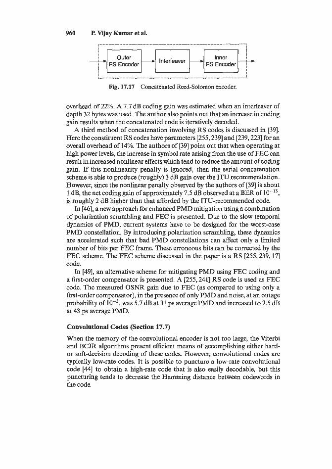
960 P. Vijay Kumar et al.
overhead of 22%. A 7.7 dB coding gain was estimated when an interleaver of depth 32 bytes was used. The author also points out that an increase in coding gain results when the concatenated code is iteratively decoded.
A third method of concatenation involving RS codes is discussed in [39]. Here the constituent RS codes have parameters [255,239] and [239,223] for an overall overhead of 14%. The authors of [39] point out that when operating at high power levels, the increase in symbol rate arising from the use of FEC can result in increased nonlinear effects which tend to reduce the amount of coding gain. If this nonlinearity penalty is ignored, then the serial concatenation scheme is able to produce (roughly) 3 dB gain over the ITU recommendation. However, since the nonlinear penalty observed by the authors of [39] is about 1 dB, the net coding gain of approximately 7.5 dB observed at a BER of is roughly 2 dB higher than that afforded by the ITU-recommended code.
In [46], a new approach for enhanced PMD mitigation using a combination of polarization scrambling and FEC is presented. Due to the slow temporal dynamics of PMD, current systems have to be designed for the worst-case PMD constellation. By introducing polarization scrambling, these dynamics are accelerated such that bad PMD constellations can &ect only a limited number of bits per FEC frame. These erroneous bits can be corrected by the FEC scheme. The FEC scheme discussed in the paper is a RS [255,239,17] code.
In [49], an alternative scheme for mitigating PMD using FEC coding and a first-order compensator is presented. A [255,241] RS code is used as FEC code. The measured OSNR gain due to FEC (as compared to using only a first-order compensator), in the presence of only PMD and noise, at an outage probability of was 5.7 dB at 31 ps average PMD and increased to 7.5 dB at 43 ps average PMD.
Convolutional Codes (Section 17.7)
When the memory of the convolutional encoder is not too large, the Viterbi and BCJR algorithms present efficient means of accomplishing either hard- or soft-decision decoding of these codes. However, convolutional codes are typically low-rate codes. It is possible to puncture a low-rate convolutional code [44] to obtain a high-rate code that is also easily decodable, but this puncturing tends to decrease the Hamming distance between codewords in the code.

17. Error-Control Coding Techniques and Applications 961
A discussion on the use of a convolutional code as an FEC scheme for a pulse-position modulation-based optical fiber communication system may be found in [ 121.
Turbo Codes (Section 17.9)
Turbo codes are also known as parallel concatenated convolutional codes. These codes tend to have low rates and also low values of minimum distance. Although these codes perform excellently at low SNR, at high SNR, the low minimum distance of these codes tends to degrade performance. It is also possible to iteratively decode convolutional codes that are serially concate- nated [8,15] and these tend to have larger minimum distance and may therefore be better suited to the optical channel where very low bit errors are desired. Thus, it is desirable to identify serially concatenated convolutional codes, that in addition to having large minimum distance, also offer high rate.
Low-Density Parity-Check Codes (Section 17.10)
LDPC codes are potentially of interest in optical channels. Of course, one does need to identify suitable high-rate LDPC codes that also possess large minimum distance. Nonbinary LDPC codes [25] could also be of interest.
Acknowledgment
The authors would like to thank Habong Chung, Manini Shah, Ted Darcie, and Jack Winters for some very useful discussions.
References
[l] 0. Ait Sab, “FEC techniques in submarine transmission systems,” OFC 2001,
[2] S. Aji and R. J. McEliece, “The generalized distributive law,” IEEE Trans. Inform. neory , vol. 46, no. 2, pp. 325-343, March 2000.
[3] L. R. Bahl, J. Cocke, E Jelinek, and J. Raviv? “Optimal decoding of linear codes for minimizing symbol error rate,” IEEE Zkuns. Inform. Theory, vol. 20, pp. 284-287, March 1974.
[4] E. R. Berlekamp, Algebraic Coding Theory, Aegean Park Press, Laguna Hills, 1984.
[4b] E. R. Berlekamp, “Bounded distance +1 soft-decision ReedSolomon decod- ing,” IEEE Trans. Inform. Theory, vol. 42, pp. 704-720, May 1996.
[5] G. Berrou, A. Glavieux, and P. Thitimajshima, “Near Shannon limit error correcting coding: Turbo codes,” in Proc. 1993 Znt. ConJ: Commun., Geneva, Switzerland, pp. 1064-1070, May 1993.
V O ~ . 2, pp. T~Fl.l-T~F1.3,2001.
962 P. Vijay Kumar et al.
[6] R. Blahut, Theory andpractice ofEmr Control Codes, Addison-Wesley, Reading, Massachusetts, 1983.
[7] A. E. Brouwer and T. Verhoeff, “An updated table of minimum-distance bounds for binary linear codes,” IEEE Duns. Inform. Theory, vol. 39, no. 2, pp. 662476, March 1993.
181 K. Chugg, A. Anastasopoulos, and X. Chen, Iterative Detection, Kluwer Academic Publishers, Boston, 2001.
[9] G. Clark and J. Cain, Error-Correction Coding for Digital Communications, Plenum Press, New York, 198 1.
[lo] T. M. Cover and J. A. Thomas, Elements ofhformation Theory, John Wiley, New York, 199 1.
[ 1 11 E. Desurvire, Erbium-Doped Fiber Ampl$ers-Principles and Applications, John Wiley & Sons, Inc., New York, 1994.
[12] E. Forestieri, R. Ganaopadhyay, and G. Prati, “Performance of convolutional codes in a direct-detection optical PPM channel,” IEEE Trans. Comm., vol. 37, no. 12, pp. 1303-1317, December 1989.
[ 131 R. G. Gallager, “Low-density parity-check codes,” IRE Trans. Inform. Theory,
[14] W. D. Grover, “Forward error correction in dispersion-limited lightwave systems,” J. Lightwave Tech., vol. 6, pp. 643654, May 1988.
[14b] V. Guruswami and M. Sadan, “Improved decoding of ReedSolomon and algebraic-geometry codes,” IEEE Trans. Inform. Theory, vol. 45, no. 6, pp. 1757- 1767, September, 1999.
[ 151 C. Heegard and S. Wicker, lttrbo Coding, Kluwer Academic Publishers, Boston, 1998.
[16] P. A. Humblet and M. Azizoglu, “On the bit error rate of lightwave systems with optical amplifiers,”J. Lightwave Tech., vol. 9, no. 11, pp. 1576-1582, November 1991.
[17] International Telecommunication Union Telecommunication Standardization Sector (ITU-T), Series G: Transmission Systems and Media, Digital Systems and Networks, G.975.
[18] G. Jacobsen, Noise in Digital Optical Transmission Systems, Artech House, Norwood, MA, 1994.
[19] R. Johannesson and K. Sh. Zigangirov, Fundamentals of Convolutional Coding, IEEE Press, New York, 1998.
[20] L.G. Kazovsky, S. Benedetto, and A. Willner, Optical Fiber Communication Systems, Artech House Publishers, Boston, October 1996.
[21] H. Kidorf, N. Ramanujam, I. Hayee, M. Nissov, J. X. Cai, B. Pedersen, A. Puc and C. Rivers, “Performance improvement in high capacity, ultra-long distance, WDM systems using forward error correction codes,” OFC ’00, vol. 3, pp. 274- 276,2000.
[22] R. Kotter, “A fast parallel implementation of a Berlekamp-Massy algorithm for algebraiegeometry codes,” IEEE Trans. Inform. Theory, vol. 44, no. 4, pp. 1353- 1368, July 1998.
V O ~ . 8, pp. 21-28, January 1962.
17. Error-Control Coding Techniques and Applications 963
[23] F. R. Kschischang, B. J. Frey and H.-A. Loeliger, “Factor graphs and the sum- product algorithm,” LEEE Trans. Inform. %ov, vol. 47, no. 2, p p 498-519, February 2001.
[24] S. Lin and D. J. Costello Jr., Error Conml Coding: Fundamentals andApplications, Prentice-Hall, Englewood Cliffs, New Jersey, 1983.
[25] D. J. C. Mackay and M. Davey, “Evaluation of Gallager codes for short block length and high rate applications,” in IMA Workrrhop on Codes, Systems and Graphical Models, 1999.
[26] E J. MacWilliamS and N. J. A. Sloane, The lIeo7-y of Emr-Comcting Codes, Amsterdam, North Holland, 1977.
[27] D. Marcuse, “Derivation of analytical expression for the bit-error probability in lightwave systems with optical amplsers,” J. Lightwave Tech., vol. 8 , no. 12, pp. 1816-1823, December 1990.
[28] R. J. McEliece, D. J. C. Mackay, and J.-E Cheng, “Turbo decoding as an instance of Pearl’s belief propagation algorithms,” IEEE J. Select Areas Comm., vol. 16, pp. 140-152, February 1998.
1291 J. B. H. Peek, “Communications aspects of the compact disc digital audio system,” IEEE Comm. Mag., vol. 23, no. 2, pp. 7-15, February 1985.
[30] L. C. Perez, J. Seghers, and D. J. Costello, “A distance spectrum interpretation of turbo codes,” IEEE Trans. Inform. Theory, vol. 42, no. 6, pp. 1698-1709, November 1996.
[3 11 V. S. Pless and W. C. Huf€man, Handbook of Coding Theory, Elsevier, New York, 1998.
[32] J. K. Proakis, Digital Communications, 4th edn., McGraw-Hill, Boston, 2000. [33] A. Puc, E m o o t , A. Simons, and D. Wilson, “Concatenated FEC experiment
over 5000 km long straight line WDM test bed,” OFC ’99, vol. 3, pp. 255-258, 1999.
[34] R. Rarnaswami and N. Sivarajan, Optical Networks: A Practical Perspective, 2nd edn., Morgan Kaufmann Publishers, San Francisco, 2002.
[35] T. J, Richardson and R. L. Urbanke, “The capacity of low-density parity-check codes under message-passing decoding,” IEEE Trans. Inform. Theory, vol. 47, no. 2, pp. 599-618, February 2001.
[36] I. S. Reed and X . Chen, Error-Conirol Coding for Data Networks, Kluwer Academic Publishers, Amsterdam, Netherlands, 2000.
[37] 0. Sab and J. Fang, “Concatenated forward error correction schemes for long- haul DWDM optical transmission systems,” in Tech. Dig., 25th European Conf. on Optical Comm. (ECOC’99), Nice, France, Paper Th C2.4.
[38] R. M. Tanner, “A recursive approach to low complexity codes,” IEEE Trans. Inform. Theory, vol. 27, pp. 533-547, September 1981.
[39] H. Taga, H. Yarnauchi, T. Inoue, K. Goto, N. Edagawa, and M. Suzuki, “Perfor- mance improvement of highly nonlinear long distance optical fiber transmission system using novel high gain forward error correcting code,” OF% 2001, vol. 2, pp. T~F3.1-TuF3.3,2001.

964 P. Vijay Kumar et al.
[40] M. Tomizawa, Y Yamabayashi, K. Murata, T. Ono, Y Kobayashi, and K. Hagimoto, “Forward error correcting codes in synchronous fiber optic transmission systems,” J. Lightwave Tech., vol. 15, no. 1, pp. 43-52, January 1997.
[41] S. A. Vanstone and l? C. Van Oorschot, An Introduction to Error Correcting Codes with applications, Kluwer Academic Publishers, Boston, 1989.
[42] A. J. Viterbi, “Convolutional codes and their performance in communication systems,” ZEEE Trans. Comm., vol. 19, pp. 751-772, Oct. 1971.
[43] A. J. Viterbi and J. K. Omura, Principles of Digital Communication and Coding, McGraw-Hill, New York, 1979.
[44] S. B. Wicker, E m r Control Systems for Digital Communication and Storage, Prentice-Hall, Englewood Cliff$ New Jersey, 1995.
[45] S. B. Wicker and V. K. Bhargava, Reed-Solomon Codes and n e i r Applications, IEEE Press, New York, June 1994.
[46] B. Wedding and C. N. Haslach, “Enhanced PMD mitigation by polarization scrambling and forward error correction,” OFC 2001 , vol. 2, pp. WAA1.1- WAA1.3,2001.
[47] J. Winters, R. Gitlin, and S. Kasturia, “Reducing the effects of transmission impairments in digital fiber optic systems,” ZEEE Comm. Mag., pp. 68-76, June 1993.
[48] J. -H. Wu and J. Wu, “Performance of Reed-Solomon codes in CPFSK coherent optical communications,” J. Opt. Comm., vol. 13, pp. 19-22, March 1992.
[49] Y Xie, 0. Yu, L.-S Yan, Q. H. Adamczyk, Z. Pan, S. Lee, A. E. Willner, and C. R. Menyuk, “Enhanced PMD mitigation using forward-error-correction coding and afirst-order compensator,” OFC2001, vol. 2, pp. WAA2.1-WAA2.3, 2001.
Chapter 18
Moe Z. Win and Jack H. Winters AT&T Labs-Research, Middletown, New Jersey
Giorgio M. Vitetta University of Modena and Reggio Ernilia, Modena, Italy
Equalization Techniques for Mitigating Transmission Impairments
18.1 Introduction
Most current multi-gigabit-per-second digital fiber-optic systems use simple modulation and detection techniques such as on-off keying with matched-filter receiver techniques. However, more complex techniques such as equalization, error control coding, and/or multilevel signaling can be used in lightwave systems to significantly increase the data rate and/or reduce the effect of trans- mission impairments and improve performance, and, in many cases, can be easily implemented [l].
There are numerous sources of transmission impairments in lightwave sys- tems. These include chromatic dispersion and polarization-mode dispersion (PMD) in the fiber, laser and fiber nonlinearities, nonideal receiver response, echo, and distortion caused by semiconductor optical amplifiers. Fortunately, there are also numerous techniques to reduce these impairments, including error control coding, equalization, and modulation techniques with multi- level signaling. These techniques can be used for upgrading existing systems (e.g., reducing chromatic dispersion and PMD in systems with previously installed fiber) or as an alternative to the use of more costly transmitters and receivers (e.g., using coding to permit less stringent laser specifications [2]).
The purpose of this chapter is to provide an overview of equalization tech- niques, which become increasingly important as device technology matures, in which case substantial increases in performance (especially for already installed systems) may only be achieved through these techniques.' We will examine the prospects for the application of digital equalization techniques to overcome these impairments, where the improvement is large and the implementation is relatively simple.
Error control coding techniques are discussed in Chapter 17 of this volume.
965 OPTICAL FIBER TELECOMMUNICATIONS, VOLUME IVB
Copyright Q 2002, Elsevier Science (USA). All rights of reproduction in any form reserved.
ISBN 0-12-395173-9
966 Moe Z. Win, Jack H. Winters, and Giorgio M. Vitetta
18.2 Transmission Impairments in Lightwave Systems
Here we classify the transmission impairments in lightwave systems into three categories: (1) signal distortion with a single signal, (2) signal distortion between multiple signals, and (3) noise. These impairments are discussed in the following text.
Signal distortion (with a single signal) refers to those impairments that distort and broaden the width of pulses, resulting in intersymbol interference (ISI) that limits the maximum bit rate. The key feature of signal distortion is that it is deterministic (can be calculated directly from the impairment), i.e., the distortion is bit-pattern dependent with the distortion for a given fixed pattern (or slowly varying). This distortion results in a narrowing or closing of the received signal eye in the vertical direction (a pattern-dependent signal level at the detector sampling time) and/or the horizontal direction (a pattern-dependent timing jitter). The most extensively analyzed distortion is chromatic dispersion (see, e.g. [3,4]) in long-haul systems. This is material dispersion in the fiber which causes a delay in the received signal spectrum that varies with frequency. The dominant delay distortion is a linear delay of about 17 p s k d n m at a wavelength of 1.55 p.m in a standard fiber. Thus, the delay variation is linear with distance, but is fixed for a given length of fiber, i.e., it doesn’t vary significantly with time. A second source of distortion is PMD in long-haul systems (see, e.g. [4--71). PMD is generated by signal delays that are polarization dependent. These delays increase with distance and also vary slowly with time (due to temperature and other variations) [6,8-lo]. At a given frequency, two orthogonal polarizations have different delays. Thus, a pulse with a sufficiently narrow frequency spectrum can be received as two pulses with a time delay between them. For a study of the combined effects of chromatic and polarization dispersion in lightwave systems, see [l 11. We group laser nonlinearities and receiver bandwidth limitations as the third source of distortion. Note that this impairment is independent of distance, and varies only due to aging. A fourth possible source of dispersion is a semiconductor optical amplifier [ 121 (fiber optical amplifiers have negligible distortion), and a fifth source is fiber nonlinearities [13,14].
The previous impairments all increase in severity with the signal bandwidth. This bandwidth is lower bounded by the data rate, but may be much larger than this because of other factors. For a multimode laser, both mode evolution and mode hopping [15,16] increase the bandwidth of the signal to several nanometers. For an analysis of equalization techniques in multimode fiber systems, see [ 171. For a single-frequency (mode) laser, the laser linewidth (due to phase noise) and chirping or relaxation oscillation (with direct modulation of the laser) increase the bandwidth of the signal. A single-frequency laser has a nonzero linewidth because of random variations in the phase of the laser (phase noise), as discussed below. Chirp is the variation in carrier frequency
18. Equalization Techniques 967
of the laser caused by changes in drive-signal amplitude. Similarly, relaxation oscillation is the variation (undesired oscillation) in amplitude of the laser caused by changes in drive-signal amplitude. Note that chirp (and relaxation oscillation) can be avoided if the laser itself is used in the cw mode with the modulation being done with an external modulator.
The second impairment is interference between multiple signals in different frequency bands on the same fiber. This can be due to nonlinearities in the fiber [13,14] or in semiconductor optical amplifiers [12]. In addition, in duplex systems, echo also can degrade performance. Note that these distortions are deterministic.
The third class of transmission impairment we consider is noise, which varies randomly from bit to bit. Noise in the received signal consists of shot noise, thermal noise, and, with optical amplifiers, amplified spontaneous emission (ASE) noise. Shot noise is the quantum noise due to the fact that the received signal is actually a series of photons. The number of photons received during each symbol interval has a Poisson distribution and, therefore, the received signal level vanes randomly from symbol to symbol. Thermal noise is introduced by the receiver preamplifier, and is usually assumed to be additive, white Gaussian noise. ASE is additive Gaussian noise in the optical signal that increases with the gain of the amplifiers. Although ASE is random, with direct detection the electrical signal at the receiver con- tains a noise times signal component, and thus the ASE noise level in the received electrical signal is signal-level dependent. Without optical ampli- fiers, thermal noise is the major limitation with direct detection, whereas shot noise is the major limitation with coherent detection if the local oscil- lator power is large enough. With large local oscillator power, however, the high-intensity shot noise can also be modeled as additive, white Gaussian noise. With optical amplifiers, ASE usually dominates the shot and thermal noise.
Another source of noise is phase noise, which, as discussed previously, is the random variation in phase of the transmitting laser. The main parameter of interest with phase noise is the width of the phase-noise spectrum relative to the data rate. Wider spectra (or linewidths) result in more signal dispersion as discussed earlier. Also, wider linewidths require wider receive filters (if all the signal energy in the received signal is to be detected), which results in higher thermal noise. However, wider linewidths (if wide enough) can have beneficial effects. In particular, with multimode lasers the distortion caused by PMD is fixed, rather than time varying as with single-frequency lasers, where the worst-case dispersion is significantly greater than the fixed value. Also, with multimode lasers, the distortion due to chromatic dispersion is linear in the received electrical signal rather than nonlinear with direct detection of a single-frequency laser signal. Both of these effects can make compensation of the distortion much easier.
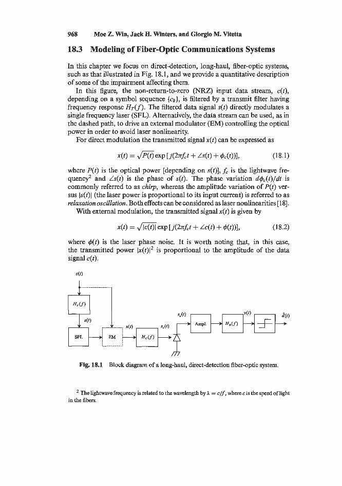
968
18.3 Modeling of Fiber-optic Communications Systems
Moe Z. Win, Jack H. Winters, and Giorgio M. Vitetta
In this chapter we focus on direct-detection, long-haul, fiber-optic systems, such as that illustrated in Fig. 18.1 , and we provide a quantitative description of some of the impairment affecting them.
In this figure, the non-return-to-zero (NRZ) input data stream, c(t), depending on a symbol sequence { c k } , is filtered by a transmit filter having frequency response H ~ c f ) . The filtered data signal s(t) directly modulates a single frequency laser (SFL). Alternatively, the data stream can be used, as in the dashed path, to drive an external modulator (EM) controlling the optical power in order to avoid laser nonlinearity.
For direct modulation the transmitted signal x( t ) can be expressed as
x ( t ) = m e x p [j(2nfct + LsO) + 4c(t)ll, (18.1)
where P(t) is the optical power [depending on 491, fc is the lightwave fre- quency’ and Ls(t ) is the phase of s(t). The phase variation d&(t)/dt is commonly referred to as chirp, whereas the amplitude variation of P(t) ver- sus Is(t)l (the laser power is proportional to its input current) is referred to as relaxation oscillation. Both effects can be considered as laser nonlinearities [ 181.
With external modulation, the transmitted signal x ( t ) is given by
where $(t) is the laser phase noise. It is worth noting that, in this case, the transmitted power Ix(t)l’ is proportional to the amplitude of the data signal c(t).
w c.. Fig. 18.1 Block diagram of a long-haul, direct-detection fiber-optic system.
The lightwave frequency is related to the wavelength by a = c / f , where c is the speed of light in the fibers.
18. Equalization Techniques 969
The transmitted optical signal feeds a fiber, having frequency response H c ( f ) , which can introduce chromatic dispersion and PMD [18-201.
Chromatic dispersion will have a significant impact on system performance if the laser frequency is different from that of zero dispersion of the fiber [corresponding to a wavelength equal to 1.3 Fm in a standard single-mode fiber (SMF)]. In this case, the main portion of the chromatic dispersion is linear delay distortion, and the frequency response of the fiber is
where
1 2 = TCD-L,
C (18.4)
where L is the fiber length, D is the chromatic dispersion parameterY3 c is the speed of the light in the fiber, and h(=c/f) is the wavelength. Then, in the presence of chromatic dispersion, the optical received signal is expressed by
where hc(t) is the channel impulse response of the fiber, and it is the inverse Fourier transform of H&) given in Eq. 18.3; and 03 denotes convolution operation.
With direct detection, the electrical signal se(t) at the photodetector output is related to so(t) as
s e ( f ) = a o e Iso(t)l 2 9 (18.6)
where aoe is the conversion constant between the optical and the electrical signals.
The PMD can be characterized in terms of first- and higher-order (in fi-e- quency) effects. The first-order effect can be simply represented as a delay in the signal in one polarization relative to the delay in the signal in the other one. Thus, with first-order polarization dispersion and direct detection, the electrical signal se(t) at the photodetector output is given by
where a, is the ratio of the signal strengths in the two polarizations and t is the time delay between propagation in the two polarizations.
For example, D = 17 ps/km/nm for a SMF and D = 2.6 ps/km/nm for non-zero-dispersion- shifted (NZDS) fiber at A. = 1.55 Fm.
970 Moe Z. Win, Jack H. Winters, and Giorgio M. Vitetta
The electrical signal se(t) at the photodetector output is amplijied and filtered [the frequency response HRcf) incorporates the characteristics of fre- quency selectivity of both the amplijier and the receive filter] to increase the signal-to-noise ratio of the decision variable. This produces the output signal
where hR(t) is the inverse Fourier transform ofHRcf). The signal v(t) is detected by comparing the signal level to a decision threshold during a short time interval at the peak opening of the eye in the received digital signal. The quality of data decisions can be seriously afTected by ISI, i.e., by interference coming from data transmitted in adjacent bit intervals.
As will become clear in the following sections, a key issue in the effective- ness of equalization techniques against intersymbol interference is the lineariiy of the intersymbol interference, i.e., the linear dependence of the data signal applied to the decision device on the transmitted data. In the communication system of Fig. 18.1, linear distortions include the receiver frequency response HR(J) and first-order PMD. Chromatic dispersion is a linear distortion in the optical fiber; however, whether this distortion produces a linear dependence on the transmitted data at the detector input [i.e., on v(t)] depends on the transmission and detection techniques used. Specifically, chromatic disper- sion appears as linear distortion in a coherent receiver, but as long as the laser linewidth is smaller than the data rate, this form of dispersion appears as non- linear in a direct detection system. This is a critical point and we concentrate on this below, for both direct and external modulation systems.
In a direct detection system using external modulation, the transmitted and the received optical signals are expressed by Eqs. 18.2 and 18.5, respectively. Then, after direct detection, the received electrical signal se(t) is (see Eqs. 18.5 and 18.6)
se(t) = aoe ~x( t ) 8 hc(t11' 3 (18.9)
and the filtered received signal v(t) is
or, in baseband notation,
If we consider long-haul systems operating at a data rate of several Gbps the phase noise bandwidth is typically below 50 MHz, so that the phase noise dis- tortion exp [ j4( t ) ] can be deemed approximately constant over the memory

18. Equalization Techniques 971
of the channel impulse response hc(t). Under this assumption Eq. 18.11 simplifies as
2 v(t) 21 a o e I ~ ~ x P [ ~ - u ~ ) I ~9 hc(t)[ ~9 hR(t). (1 8.12)
The last result shows that the IS1 in the electrical signal at the input of the decision device is the square of the IS1 in the optical signal so that the overall distortion is nonlinear. However, even with this nonlinearity, linear equalization can be partially effective in reducing ISI. In general, linear equali- zation will not improve performance with quadratic distortion. However, in lightwave systems, if the signaling is binary, on-off keying is used and the major portion of the IS1 is due to a single adjacent symbol, a linear equalizer can still be effective. In fact, under these assumptions, it can be shown that the IS1 consists of a linear component and a nonlinear component, with the former larger than the latter, if the IS1 is reasonably small (see [21], pp. 720-721).
If the laser is directly modulated and the nonlinear amplitude variations in the laser output signal are negligible, the transmitted signal (Eq. 18.1) can be rewritten as
x(t> m e x p [ j + 4) + 4C(t))l , (1 8.13)
where the phase distortion expL&(t)] is mainly due to the chirp effect. Substituting Eq. 18.13 into 18.10 produces
In this case, the chirp variations are not slow as the chirp bandwidth of lasers is typically larger than that of the data signal [21]. Then the simplification leading fromEq. 18.11 to 18.12cannotbeappliedtoEq. 18.14. However, for arapidly varying &(t) it can be easily shown that Eq. 18.14 may be approximated as
v(t> a o e IS(~)I ~9 I ~ ~ ( o I ’ ~9 ~ t ) . (18.15)
The last result shows that the IS1 in the electrical signal at the input of the decision device is the sum of the squares of the IS1 in the optical received signal. The distortion described by Eq. 18.15 may be viewed as due to a linear system having impulse response Ihc(t)12 and fed by Is(t)l. The insight provided by Eq. 18.15 is still not accurate. In fact, the chirp effect in the transmitted signal is caused by the signal level changes and, therefore, does not result in fast phase variations over the entire duration of each symbol. In addition, symbols surrounded by identical symbols may not experience chirp. Therefore, in general, in direct modulation systems, the IS1 is a combination of linear (Eq. 18.15) and nonlinear distortion (Eq. 18.1 1). This explains why, in direct detection systems employing direct modulation, linear equalization techniques can only be partially effective in reducing ISI.

972
18.4 Equalization Algorithms and Their Applications
Mae Z. Win, Jack H. Winters, and Giorgio M. Vitetta
In this section we delve into the field of equalization algorithms for digital communications and illustrate the application of some of them in the field of optical communications systems. Throughout this section we assume that
1. data decisions are based on the sequence of samples {Vk A v(kT)} (T being the symbol interval equal to the sample interval) of the electrical signal v( t ) in Fig. 18.1;
2. the dependence of { V k } on the symbol sequence {dk} is linear and the noise4 samples Ink} form an additive, white Gaussian noise (AWGN) sequence, i.e.,
(18.16)
where {ql} is the discrete-time overall channel impulse response (CIR) and Ink} is a sequence of iid (independent identical distributed) Gaussian random variables having zero mean and variance ai. The channel symbols, in general, belong to an M-ary alphabet, but in lightwave systems M = 2 is commonly used. Nonetheless, in this scenario multilevel signaling could be used to decrease the symbol rate by a factor log, M, this would entail a reduction in the amount of dispersion and decrease the noise power in the detector.
18.4.1 MLSD
It is known from the Equalization theory that, if the CIR is known, maximum likelihood sequence detection (MLSD) is the optimum sequence detection technique because it minimizes the error probability in making a decision on the transmitted data sequence. The ML sequence detector for the symbol sequence c = [CO, c1, . . . , ~ ~ - 1 1 ~ evaluates the Euclidean distance metric [22] A
k=O
for each possible trial sequence C, where the quantity
(18.17)
(1 8.18)
Thermal noise when direct detection is employed.

18. Equalization Techniques 973
A - depends on the data sequence through the vector E::-L+l - - [Cm-L+1, Z , , - L + ~ , . . . , &IT of L consecutive data symbols only, with the convention that Ci = 0 for i < 0 or i > N . The metric A(E) in Eq. 18.17 can be also rewritten as
N-1
(18.19) k=O
where
(18.20)
and Xk is the integer representation of the symbol vector ( Z ~ - L + I , Z ~ - L + Z , . . . , &I), consisting of (L - 1) consecutive data symbols. Equations 18.19, 18.20 express the optimal metric as a summation of partial metrics {h(xk,x~+l)}. The k-th of these terms, A(xk,xk+l), depends on Xk and xk+l, Le., on the vectors of consecutive trial symbols (C~-L+I, Zk-L+2, . . . , Zk-1) and ( Z R - L + ~ , Zk-~+3, . . . , Zk), respectively. These considerations suggest a recursive formula for the evaluation of A@). In fact, if we define the recursive relation
2 A.(X&,Xk+l) = IVk - Zk(E)l ,
N E k ) = N E k - 1 ) + A. (Xk ,Xk+l ) , (18.21)
with Ei A [Eo, Z1, . . . , Zi] EN-^ = E ) and A(E0) = 0, then we have
A(E) = A(&-1) (1 8.22)
after N iterations. A geometrical representation to the problem of searching over the optimal
metric can be given as follows. A trellis diagram with N, = ML-' states is drawn, as illustrated in Fig. 18.2 for M = 2 and L = 3. In the k-th interval
I I I I I +
k-2 k- 1 k &+l time
Fig. 18.2 Four-state trellis (M = 2 is assumed).
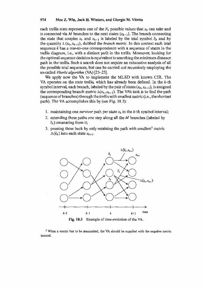
974 Moe Z. Win, Jack H. Winters, and Giorgio M. Vitetta
each trellis state represents one of the N, possible values that Xk can take and is connected via M branches to the next states {xk+1}. The branch connecting the state that couples Xk and Xk+l is labeled by the trial symbol zk and by the quantity h (xk,xk+l), dubbed the brunch metric. In this context each trial sequence E has a one-to-one correspondence with a sequence of states in the trellis diagram, Le., with a distinct path in the trellis. Moreover, looking for the optimal sequence decision is equivalent to searching the minimum distance path in the trellis. Such a search does not require an exhaustive analysis of all the possible trial sequences, but can be carried out recursively employing the so-called Eterbi algorithm (VA) [23-251.
We apply now the VA to implement the MLSD with known CIR. The VA operates on the state trellis, which has already been defined. In the k-th symbol interval, each branch, labeled by the pair of states (Xk, x~+I), is assigned the corresponding branch metric h(xk,xk+l). The VAS task is to find the path (sequence of branches) through the trellis with smallest metric (i.e., the shortest path). The VA accomplishes this by (see Fig. 18.3):
1. maintaining one suwivor path per state Xk in the k-th symbol interval; 2. extending these paths one step along all the M branches (labeled by
3. pruning these back by only retaining the path with smallest5 metric E,) emanating from it;
A(&) into each state x~+I.
I I I I I I *
k-2 k-1 k k+l time
Fig. 18.3 Example of time evolution of the VA.
When a metric has to be maximized, the VA should be supplied with the negative metric instead.

18. Equalization Techniques 975
In the k-th symbol interval, then, the Viterbi algorithm keeps track only of the one path (the so-called survivor) leading to each state Xk. Such a path, denoted as 2(xk), is the sequence of consecutive states belonging to the path, and it is characterized by an accumulated metric A(xk).
The VA procedure can be summarized in the following steps (k denotes the time variable):
1. Set
k = 0, ~ ( x o ) = (xo), A(XO) = 0
to initialize the algorithm; 2. Repeat steps 3-7 until k = N ; 3. Extend path metrics according to Eq. 18.22, that is
(18.23)
for d l the allowed state transitions X k + xk+l;
incoming path over all the previous states 4. For each destination state xk+l , find the best (minimum metric)
2k = arg min A(x,+l) (1 8.25) xk
5. Update and store survivor paths as
6. Store the new survivor metrics as
7. Set k = k + 1 (increment time counter); 8. Detect the ML decision for the symbol sequence as that associated
with the survivor path ~ ( x N ) with minimum metric A ( q ) (termination).
It is worth noting that (a) branch metrics evaluated for state transitions inconsistent with known (i.e., training or pilot) symbols are set to a large value (virtually inilnite), and (b) in any real implementation data estimates are generated by the VA with a fixed decision delay, K [23] by tracing back from the survivor with instantaneously best metric. In practice, however, there is little degradation if the final decisions are taken after a decision delay of about 5-10 L.
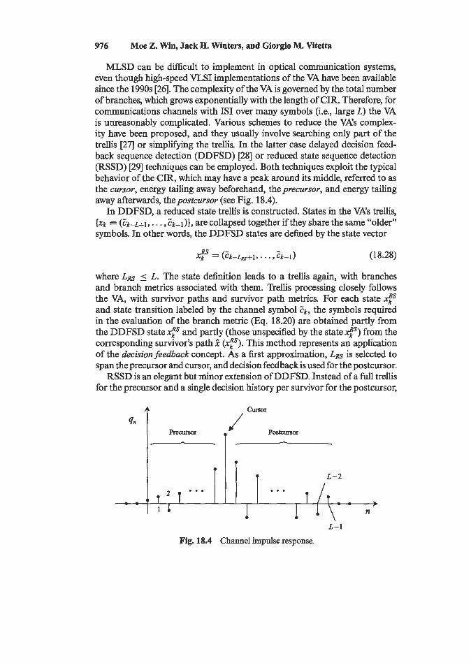
976 Moe 2. Win, Jack H. Winters, and Giorgio M. Vitetta
1 r 1
0
2 1 ' * '
MLSD can be difficult to implement in optical communication systems, even though high-speed VLSI implementations of the VA have been available since the 1990s [26]. The complexity of the VA is governed by the total number of branches, which grows exponentially with the length of CIR. Therefore, for communications channels with IS1 over many symbols @e., large L) the VA is unreasonably complicated. Various schemes to reduce the VA's complex- ity have been proposed, and they usually involve searching only part of the trellis [27] or simplifying the trellis. In the latter case delayed decision feed- back sequence detection (DDFSD) [28] or reduced state sequence detection (RSSD) [29] techniques can be employed. Both techniques exploit the typical behavior of the CIR, which may have a peak around its middle, referred to as the cursor, energy tailing away beforehand, the precursor, and energy tailing away afterwards, the postcursor (see Fig. 18.4).
In DDFSD, a reduced state trellis is constructed. States in the VA's trellis, {xk = (Z,+L+~, . . . ,&-I)), are collapsed together if they share the same "older" symbols. In other words, the DDFSD states are defined by the state vector
4 S = ( L m + l , . . ., Zk-1) (18.28)
r A - 0
0 L - 2
... k
where Lm 5 L. The state definition leads to a trellis again, with branches and branch metrics associated with them. Trellis processing closely follows the VA, with survivor paths and survivor path metrics. For each state 4' and state transition labeled by the channel symbol Ek, the symbols required in the evaluation of the branch metric (Eq. 18.20) are obtained partly from the DDFSD state xf and partly (those unspecified by the state 4') from the corresponding survivor's path i (e). This method represents an application of the decision feedback concept. As a first approximation, LRS is selected to span the precursor and cursor, and decision feedback is used for the postcursor.
RSSD is an elegant but minor extension of DDFSD. Instead of a full trellis for the precursor and a single decision history per survivor for the postcursor,

18. Equalization Techniques 977
set partitioning principles [30] are applied to steadily reduce the number of hypothesized symbols as more of the received pulse arrives The general idea behind it is to gracefully degrade performance with decreasing LRs.
Another way of working around a large L is to adaptively prefilter the signal to obtain shorter duration of the overall impulse response by using a linear equalizer [31,32] or a decision feedback equalizer [33-351. A MLSD based on the VA is then applied to this prefiltered signal. However, the prefilter colors the additive noise, thereby reducing performance if noise correlation is not taken into account.
There are also other techniques to implement simplified, approximate ver- sions of MLSD that may be practical in optical systems operating at high data rates, if the sequence length N is small. One of these is a block-oriented ML detector [36] which aims at determining the bits of a short block of length N , based on N consecutive received signal samples. Specifically, the detector compares blocks of N received signal samples to each of the 2N (M = 2 is assumed) possible (stored) signal sample vectors, each corresponding to one of the possible 2N bit vectors. The performance of this detector is degraded by the edge effects of ISI. In fact, since ML detection makes decisions on block of N bits from N signal samples referring to these bits, bits at the edge of the block are more likely to be detected in error because of the IS1 coming from bits outside the block.
18.4.2 DECISION FEEDBACK EQUALIZATION
The decision feedback equalizer (DFE) can be viewed as the prefilter plus DDFSD, where LRS = 1 so that 4' is an empty state vector. The trellis com- prises one state with M branches, each returning to the same state. However, the DFE has a preeminent role in communications due to its nice balance between complexity and performance. Therefore we study it as a separate structure [37-391.
In the DFE terminology, the prefilter is the feedforward filter (FFF), and the decision feedback of DDFSD is implemented via a feedback filter (FBF), as illustrated in Fig. 18.5. Since a DFE's trellis has one state, a memoryless quantizer is used as a decision device. As a simplification the FFF in an Lf- tap T-spaced FIR filter reduces precursor ISI, whereas the FBF an Ld-tap T-spaced FIR filter reduces the resulting postcursor ISI.
The impulse responses of the FFF and the FBF are given by
(18.29)
and
(18.30) cIA [&,4, . . . ,&d-~] , respectively. The feedback filter is always symbol spaced (i.e., the tap spac- ing is equal to the symbol interval), whereas the feedforward filter may be
T
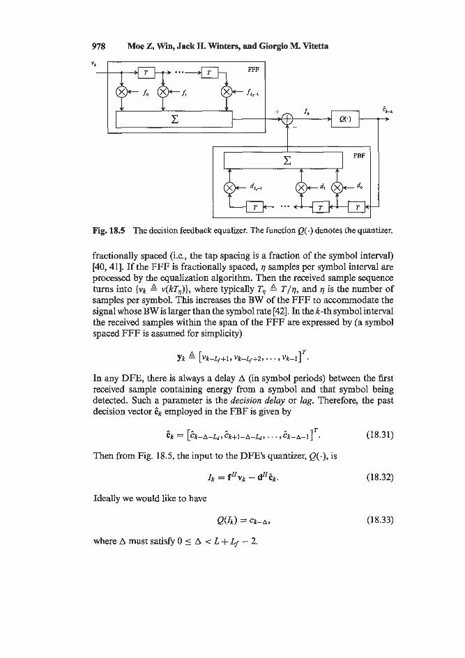
978 Moe Z. Win, Jack H. Winters, and Giorgio M. Vitetta
I
c I FBF I I I
... I I
Fig. 18.5 The decision feedback equalizer. The function Q( a ) denotes the quantizer.
fractionally spaced (i.e.y the tap spacing is a fraction of the symbol interval) [40, 411. If the FFF is fractionally spaced, r] samples per symbol interval are processed by the equalization algorithm. Then the received sample sequence turns into {Vk A v(kT,,)}, where typically T,, 4 T/r], and r] is the number of samples per symbol. This increases the BW of the FFF to accommodate the signal whose BW is larger than the symbol rate [42]. In the k-th symbol interval the received samples within the span of the FFF are expressed by (a symbol spaced FFF is assumed for simplicity)
A T 3 v k - 1 ] - y k = [vk-LJ+l , vk-LJ+Zy
In any DFE, there is always a delay A (in symbol periods) between the first received sample containing energy from a symbol and that symbol being detected. Such a parameter is the decision delay or lag. Therefore, the past decision vector 4 employed in the FBF is given by
(18.3 1) T e k = [;k-A-Ld, ;k+l -A-&, . . . Y Z k - A - l ] -
Then from Fig. 18.5, the input to the DFE's quantizer, e(-), is
I k = fHVk - dH&. (18.32)
Ideally we would like to have
(1 8.33)
where A must satisfy 0 5 A .e L + Lf - 2.
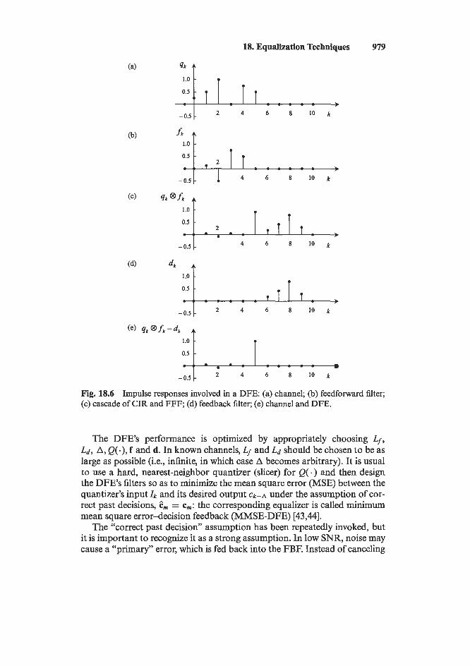
18. Equalization Techniques 979
0.5 2
>* - 0.5
1.0
0.5 . - ::
4 6 8 1 0 k -0.5 1 Fig. 18.6 Impulse responses involved in a DFE: (a) channel; (b) feedfoward filter; (c) cascade of CIR and FFF; (d) feedback filter; (e) channel and DFE.
The DFE’s performance is optimized by appropriately choosing Lf , Ld, A, e(.), f and d. In known channels, Lf and L d should be chosen to be as large as possible (i.e., infinite, in which case A becomes arbitrary). It is usual to use a hard, nearest-neighbor quantizer (slicer) for Q( . ) and then design the DFE’s filters so as to minimize the mean square error (MSE) between the quantizer’s input Ik and its desired output Ck-A under the assumption of cor- rect past decisions, &, = c,,,: the corresponding equalizer is called minimum mean square error-decision feedback (MMSE-DFE) [43,44].
The “correct past decision” assumption has been repeatedly invoked, but it is important to recognize it as a strong assumption. In low SNR, noise may cause a “primary” error, which is fed back into the FBF. Instead of canceling
980 Moe Z. Win, Jack H. Winters, and Giorgio M. Vitetta
the postcursor, the FBF can actually enhance it; in turn, this increases the likelihood of subsequent, “secondary” errors [45,46].
Since the beginning of the 199Os, DFE techniques have been proposed for use in long-haul direct-detection fiber-optic systems where it was shown that they can have more than double the maximum data rate of gigabit-per-second (Gbps) lightwave systems by canceling postcursors’ IS1 [47]. In this context, DFE can be implemented by the more general technique known as nonlinear cancellation (NLC) [47]. NLC can handle IS1 that arises from a variety of impairments, such as transmit laser chirp, chromatic dispersion, PMD, and nonideal receiver frequency response. The first implementation techniques for this equalization strategy are illustrated in [48]. Here, the proposed solution is based on a bank of 2 L d threshold detectors (where L d is the number of bits fed back), each having a difTerent threshold level that depends on the hypothesized postcursor ISI. The selection of the detector corresponding to the vector of selected symbols occurs after threshold detection. This is accomplished by choosing the output of the detector corresponding to the correct threshold rather than switching analog signals at the data rate in the feedback loop [47]. Since at high data rates, the propagation delay of the detector can exceed one symbol, another advantage of NLC is that the propagation delay of the detector is not an issue. Even if not shown in [48], a nonlinear canceler can also incorporate a feedforward section to mitigate the precursor IS1 (see, for instance, [21], p. 713).
Due to the progress in high-speed integrated cicuits (ICs) [49], the reali- zation of tunable analog linear and nonlinear filter functions has become feasible for high bit rates [50]. The electronic IC system for decision feedback equalization of 10-Gbps signals is described in [50]. It is based on an eight-tap transversal filter (FFF) and a one-tap feedback section, and its tap weights are adjusted by external tuning voltages. It is interesting to note that in such a device (as in all the other linear and nonlinear electrical equalizers designed until now for optical communications), the FFF is an analog transversal filter, i.e., the input signal of the decision device is
I (1 8.34)
where {fk} are the tap coefficients, T,, is the delay introduced by each stage in the tapped delay line (in [50], T,, = 55 ps, whereas the bit period is T = 100 ps). The analog signal i( t) is sampled every T sec (ideally at the instant of maximum eye opening) in the decision circuit and each bit decision is fed back in a unique stage of the FBF. The equalizer, consisting of two ICs (one for the feedforward section and the other one for the feedback section), has been successfully tested in transmission experiments using standard SMF. It has been shown that the power penalties of long-distance links, mainly induced by the chromatic dispersion, can be substantially reduced.
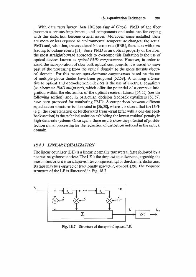
18. Equalization Techniques 981
With data rates larger than 10Gbps (say 40Gbps), PMD of the fiber becomes a serious impairment, and components and solutions for coping with this distortion become crucial issues. Moreover, since installed fibers are more or less exposed to environmental temperature changes, the actual PMD and, with that, the associated bit error rate (BER), fluctuates with time leading to outage events [51]. Since PMD is an optical property of the fiber, the most straightforward approach to overcome this limitation is the use of optical devices known as optical PMD compensators. However, in order to avoid the incorporation of slow bulk optical components, it is useful to move part of the processing from the optical domain to the more flexible electri- cal domain. For this reason opto-electronic compensators based on the use of multiple photo diodes have been proposed [52,53]. A winning alterna- tive to optical and opto-electronic devices is the use of electrical equalizers (as electronic PMD mitigators), which offer the potential of a compact inte- gration within the electronics of the optical receiver. Linear [54,55] (see the following section) and, in particular, decision feedback equalizers [56,57], have been proposed for combating PMD. A comparison between different equalization structures is illustrated in [56,58], where it is shown that the DFE (e.g., the concatenation of feedforward transversal filter with a one-tap feed- back section) is the technical solution exhibiting the lowest residual penalty in high-data-rate systems. Once again, these results show the potential of postde- tection signal processing for the reduction of distortion induced in the optical domain.
18.4.3 LINEAR EQUALIZATION
The linear equalizer (LE) is a linear, normally transversal filter followed by a nearest-neighbor quantizer. The LE is the simplest equalizer and, arguably, the most intuitive as it is an adaptive filter compensating for the channel distortion. Its taps may be T-spaced or fractionally spaced (T,-spaced) [39]. The T-spaced structure of the LE is illustrated in Fig. 18.7.
Fig. 18.7 Structure of the symbol-spaced LE.
982 Moe Z. Win, Jack H. Winters, and Giorgio M. Vitetta
LEs are also distinguished according to their design criteria. In applications, two criteria are usually considered zero forcing6 (ZF) and minimum mean square error (MMSE). The ZF method neglects the presence of the chan- nel noise and minimizes the IS1 contribution in the equalizer time span. This is undesirable since the communication channel may be characterized by multiple, deep notches in frequency. In inverting these, a ZF equalizer inevitably causes undue considerable noise amplification (noise enhacement) and a degraded BER. For this reason MMSE is usually a better design criterion, where the combination of noise and IS1 are minimized.
In the k-th symbol interval, the received samples within the span of an Lf-tap LE are expressed by (a symbol spaced LE is assumed for simplicity)
Then the input to the quantizer of LE is given by
where f is defined in (Eq. 18.29). Then a ZF LE is designed according to
and MMSE LE is designed according to
(18.37)
(1 8.38)
where E{-} denotes expectation operator, i and A are trial values of f and A, respectively, and Zk is the useful component of v k . At high data rates, symbol delays can be implemented by short transmission lines, and the taps can be implemented by variable gains amplifiers. Linear equalizers can be used inserted between the receiver filter and the threshold detector of an optical receiver [42,54,59,60].
In any practical application the coefficients of an LE or a DFE must be adapted to the channel state.
Equalizer tap weights can be adapted using either a single-step technique such as direct matrix inversion (DMI) or a gradient search algorithm (GSA) [21,61]. Although GSAs are much slower to converge than the DMI technique, they are generally suitable for fiber-optic systems since their computational
The ZF criterion can be also applied in the design of the DFE equalizers In this case the noise contribution in Eq. 18.32 must be neglected.
18. Equalization Techniques 983
complexity is much lower, while the impairment changes with rate much less than the transmission rate.
GSAs include both blind algorithms (see the following section) such as the constant modulus algorithm (CMA) and the least-mean-square (LMS) algorithm [62] or the zero-forcing algorithm [63] in conjunction with a training sequence. It is worth noting that the ZF algorithm minimizes the so-called peak distortion (ie., maximizes the opening of the eye diagram in the absence of thermal noise), whereas the MMSE algorithm minimizes the variance of the error signal. With modest amounts of linear IS1 and thermal noise, both equalizers produce distortion-free outputs and provide performance close to the optimum.
To understand the technical problems associated with the use of adaptive LEs in optical systems, let us focus on the celebrated LMS and on the ZF algorithms. They can be expressed as [39] (real signals are assumed here)
and
(18.39)
(18.40)
respectively, where f k is the tap vector in the k-th signaling interval, I is the step size (controlling the convergence speed and the stability of the algorithm), Ck = ICk-A-1, ck-A-2,. . . , Ck-A-L, l T is a past data vector, and
is the error signal. In order to compute (Eqs. 18.39 and 18.40) the data sym- bols or very reliable estimates of them have to be available. This is generally achieved by initially using a known sequence to train the equalizer and, after the acquisition period of the equalizer, switch to data decision. In long-haul optical systems operating at high data rates, generating analog samples of the signals may be costly, and therefore may not be desirable. Thus single-bit accu- racy samples (corresponding to h l ) should be used wherever possible. Then an alternative to Eq. 18.39 is provided by the so-called sgn-sgn least mean square algorithm,
fLMS k f l = fLMS k - s&ekl sgn[vkl, (1 8.42)
and the modified zero-forcing algorithm,
ffT1 = fF - h Sgn[ek]ck. (18.43)
Quantizing the signal samples reduces the rate of convergence of the algorithm. This is not a major concern, since channel impairments are expected to change
984 Moe Z. Win, Jack H. Winters, and Giorgio M. Vitetta
very slowly on optical channels. Of more concern, however, especially for the sgn-sgn LMS, are the steady-state weights. In fact, since the direction of the correction term sgn[vk] in Eq. 18.42 is different from that for the LMS (vk in Eq. 18.39), the equalizer taps may settle at different values in the two cases. On the other hand, the same considerations do not apply to the quantized version of the ZF algorithm (Eq. 18.43). In fact, the direction of the correction term in Eq. 18.43 is the same as for the unquantized algorithm (Eq. 18.40), and the former algorithm converges to the same weights as the latter when the eye diagram of the received signal is open (neither algorithm, however, works when the eye is closed).
As already stated previously, the (unquantized) MMSE algorithm outper- forms the ZF one when thermal noise is present and the improvement of MMSE increases with the noise power. Furthermore, unlike the ZF algo- rithm, when supplied with a training sequence the LMS algorithms can also work when the eye of the receiver is closed. However, the implementation prac- ticalities of Gpbs operation can preclude analog sampling of the signal and, as already mentioned, the quantized version of the LMS is not guaranteed to converge to the correct weights.
In the DFE section it has been pointed out that modern advances in elec- tronic technology have changed the perspective in the implementation of the equalizers. Linear electronic equalization can overcome the link-length limi- tation imposed by chromatic dispersion over more than 100-km SMF [60, 64-66]. An electronic LE compensating for PMD and chromatic dispersion after 100-km SMF at 10 Gbps is illustrated in [67]. In this case, a three-tap LE is realized with commercially available coaxial components, power splitters, tunable phase shifters, and broadband amplifiers and is preceded by an elec- trical low-pass filter using the dispersion supported transmission method to compensate for the chromatic dispersion of the fiber [65]. The magnitude of the tap weights in the LE is adjusted by the coaxial attenuator. This seemingly simple solution is shown to reduce the power penalty due to transmission via very high PMD fiber by 8.2 dB. A similar equalization scheme with the same penalty reduction is illustrated in [55].
More recently, advances in SiGe technology [68] have made it possible to implement integrated circuits, that can realize electronic processing functions for 1040-Gbps optical transmission systems. In particular, it has been possi- ble to implement IC LEs using the continuous time LMS algorithm (Eq. 18.39) for tap adaptation [69]. This solution exhibits excellent properties in terms of speed of convergence as it can accommodate both the slow environmental tem- perature changes (acting on the PMD properties) and the fast events (within a time scale of a few milliseconds) due to patch-cord moving or mechanical vibrations [57].
Further applications of SiGe tunable electronic equalizers in optical communications over SMF are illustrated in [70].
18. Equalization Techniques 985
18.5 Other Equalization Algorithms
In the previous section the most important linear (LE) and nonlinear (MLSD, DFE) equalization techniques for optical communications have been described. In this section we briefly describe other classes of equalization algorithms that might be used in future optical systems.
18.5.1 MAPSD
All previous equalization strategies can be easily incorporated in the receiver structure of Fig. 18.1. Whatever the selected solution, the detector will make a decision on each symbol of the sequence {ck} without providing any information about the reliability of the decision itself to a decoder. Reli- ability information can be extremely useful if channel coding is employed [71], since it can substantially improve the error performance of the system.
[coy c1, . . . , cnr-11~ is processed by the receiver, reliability (or SOB) information about the transmitted data is produced if the a posteriori probabilities (APPs)
If a vector v depending on the data vector symbol sequence c
P ( ~ k = C~V), k = 0,1, ..., N - 1 (18.44)
are evaluated for any possible choice of the symbol 2. These probabilities can be generated resorting to the so-called maximum a posteriori symbol detection (MAPSD) strategy which represent the optimum symboZ detection technique since it minimizes the probability of taking a wrong decision on each transmitted symbol.
When the MAP criterion replaces the ML criterion, the MAP forward- backward algorithm (MAP-FBA) replaces the VA [72]. The forward-backward procedure operates on the same state trellis as the VA, but it efficiently calcu- lates the MAP symbol probabilities, instead of just finding the ML sequence. The forward-backward algorithm requires the complete vector v of received samples to be available before decisions can be made. If a large decision delay is to be avoided, a near-optimal, Jixed-Zag (forward-only) MAP (MAP-FLA) strategy can be adopted [73]. However, both the FB and FL MAP algorithms work with likelihoods rather than log-likelihoods, so that their branch metrics are generally more expensive to compute and their operations are multiplica- tion and addition instead of the addition and minimization characterizing the Viterbi algorithm. Much work on reduced complexity implementations has been undertaken (see [22] and references therein), but this is outside the scope of this chapter.
Let us now briefly describe the MAP algorithms mentioned above.
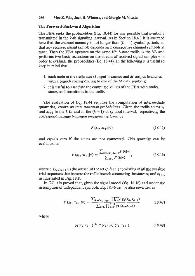
986 Moe Z. Win, Jack H. Winters, and Giorgio M. Vitetta
The Forward-Backward Algorithm
The FBA seeks the probabilities (Eq. 18.44) for any possible trial symbol Z. transmitted in the k-th signaling interval. As in Section 18.4.1 it is assumed here that the channel memory is not longer than (L - 1) symbol periods, so that any received signal sample depends on L consecutive channel symbols at most. Then the FBA operates on the same ML-'-state trellis as the VA and performs two basic recursions on the stream of received signal samples v in order to evaluate the probabilities (Eq. 18.44). In the following it is useful to keep in mind that:
1. each node in the trellis has M input branches and M output branches,
2. it is useful to associate the computed values of the FBA with nodes, with a branch corresponding to one of the A4 data symbols;
states, and transitions in the trellis.
The evaluation of Eq. 18.44 requires the computation of intermediate quantities, known as state transition probabilities. Given the trellis states xk and xk+1 in the k-th and in the (k + 1)-th symbol interval, respectively, the corresponding state transition probability is given by
and equals zero if the states are not connected. This quantity can be evaluated as
(18.46)
where C (xk, xk+l) is the subset (of the set C { E } ) consisting of all the possible trial sequences that traverse the trellis branch connecting the statesxk andxk+l , as illustrated in Fig. 18.8.
In [22] it is proved that, given the signal model (Eq. 18.16) and under the assumption of independent symbols, Eq. 18.46 can be also rewritten as
where
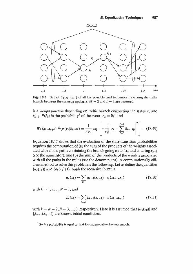
18. Equalization Techniques 987
J 0 0 0 0 0 0 0 0 0 4 oXk-l 0 0
I I I I I I I
k-2 k-1 k Hl k+2 k+3 time
Fig. 18.8 Subset Ck(xk,xk+l) of all the possible trial sequences traversing the trellis branch between the states x k and x k + l . M = 2 and L = 2 are assumed.
is a weightfunction depending on trellis branch connecting the states Xk and Xk+l, p(&,) is the probability7 of the event (Ck = &} and
Equation 18.47 shows that the evaluation of the state transition probabilities requires the computation of (a) the sum of the products of the weights associ- ated with all the paths containing the branch going out of Xk and entering Xk+l (see the numerator), and (b) the sum of the products of the weights associated with all the paths in the trellis (see the denominator). A computationally effi- cient method to solve this problem is the following. Let us define the quantities {a!k(Xk)] and (Bk(Xk)] through the recursive formula
ak(xk) = ~ak-1(xk-1) ' yk(xk-l,xk) ( 1 8.50) xk
withk= 1y2y... ,N- 1,and
Pk(xk) = Bk+I(xk+l) ' yk(xk,xk+l) (18.51)
with k = N - 2, N - 3, ..., 0, respectively. Here it is assumed that {ao(xo)) and {/~N-~(XN-I)} are known initial conditions.
Xk+l
Such a probability is equal to 1/M for equiprobable channel symbols.
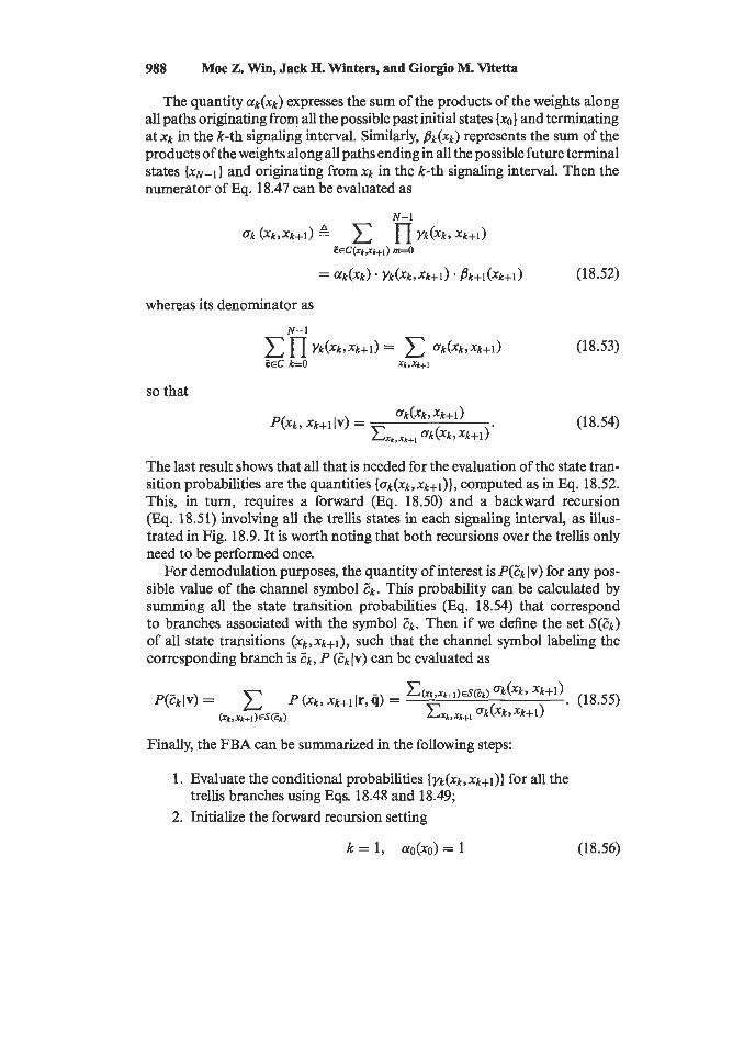
988 Moe Z. Win, Jack €I. Winters, and Giorgio M. Vitetta
The quantity a&) expresses the sum of the products of the weights along all paths originating from all the possible past initial states { X O } and terminating at Xk in the k-th signaling interval. Similarly, /?k(Xk) represents the sum of the products of the weights along all paths ending in all the possible future terminal states {XN-l} and originating from Xk in the k-th signaling interval. Then the numerator of Eq. 18.47 can be evaluated as
N-1
whereas its denominator as
so that
(18.53)
(1 8.54)
The last result shows that all that is needed for the evaluation of the state tran- sition probabilities are the quantities (a,&k, xk+l)}, computed as in Eq. 18.52. This, in turn, requires a forward (Eq. 18.50) and a backward recursion (Eq. 18.51) involving all the trellis states in each signaling interval, as illus- trated in Fig. 18.9. It is worth noting that both recursions over the trellis only need to be performed once.
For demodulation purposes, the quantity of interest is P(& Iv) for any pos- sible value of the channel symbol &. This probability can be calculated by summing all the state transition probabilities (Eq. 18.54) that correspond to branches associated with the symbol Ek. Then if we define the set S(&) of all state transitions (xk,xk+l), such that the channel symbol labeling the corresponding branch is &, P (Zklv) can be evaluated as
Finally, the FBA can be summarized in the following steps:
1. Evaluate the conditional probabilities { yk(xk, xk+l)} for all the
2. Initialize the forward recursion setting trellis branches using Eqs 18.48 and 18.49;
k = 1, ao(x0) = 1 (18.56)

18. Equalization Techniques 989
I I 1 I I I I
. I I I I
4 5 6 7 (c) k
a,@> y,(o,o) P&) o-o- 0-
0 1: (4 /
o,(O,o)=a,(O).Y 3(0,0>. P4(0>
?ig. 18.9 Application of the FBA to a two-state trellis (a) (A4 = 2, L = 1). The pantities {ak(xk)J and (Bk(xk)) are computed recursively in the forward (b) and in he backward (c) recursion, respectively, using the branch probabilities {yk(xk, xk+l)). ;inally, (d) the state transition probabilities {q(xk,xk+l)J are evaluated according to 3q. 18.52.
3. Repeat steps 4-5 until k = N ; 4. Compute and store the forward path probabilities (ak(xk) ) using
Eq. 18.50; 5 . Set k = k + 1; 6. Initialize the backward recursion setting
(18.57)

990 Moe Z. Win, Jack H. Winters, and Giorgio M. Vitetta
7. Repeat steps 8-9 until k = 0; 8. Compute and store the backward path probabilities {Pk(Xk)} using
Eq. 18.51; 9. Se tk=k- 1;
Eq. 18.52;
of Eq. 18.55.
10. For each trellis branch compute the quantity uk (&&+I) using
11. Evaluate the a posteriori symbol probabilities {P (Zklv)} by means
Fixed-Lag MAPSD
The forward-backward algorithm is suited to short burst transmission because, otherwise, its delay and storage requirements are unsatisfactory. The MAP ked-lag algorithm (MAP-FLA) detector [73,74] makes decisions at a fixed lag of Lfl symbols from the current received samples, as
(1 8.58)
where the notation x,” denotes the vector [xa,xn+l,. . . ,xblT. The parameter Lfl is akin to the decision delay in the VA, and so, for effectively optimal performance, it is expected to be as high as 5L or 7L. The decision rule may be implemented via two good algorithms, both requiring a single forward pass only. The newer one, dubbed soft-output algorithm (or OSA) [75], has a smaller computational complexity than the older one [73], since the number of quantities to be stored and recursively updated increases linearly, rather than exponentially, with the decision delay.
A description of the MAP-FLA is not provided here. However, it is impor- tant, at this stage, to make some comments about the VA, the MAP-FLAY and the MAP-FBA. Each of these algorithms can be employed for the detection of data sequences in the presence of ISI. Among these algorithms, however, the VA has the smallest complexity and this makes it the most reasonable choice in uncoded communication systems where soft output information is not required. The MAP algorithms have the following relevant disadvan- tages: (1) they require the knowledge of the noise variance; and (2) they have large memory and computation requirements. In particular, as already stated, MAP algorithms accomplish computations in the probability, instead of the logarithm domain and, consequently, require a large number of multiply and exponential operations. The MAP-FBA detector performs two recursions and, consequently, it operates in block mode. It memorizes all the received signal samples of each block and afterwards processes them. Its memory requirement grows linearly with the sequence length so that only short data sequences should be processed. The MAP-FLA requires only a forward recursion, so that it can operate in continuous-mode. Both the memory and computational

18. Equalization Techniques 991
requirements, however, grow exponentially with the decision delay so that this parameter should be kept to minimum. For this reason the FBA may have smaller computational requirements than the FLA.
18.5.2 BLIND TECHNIQUES AND CMA
The LE and the DFE equalization algorithms are commonly derived assuming a known CIR. In practice, such equalization algorithms learn the channel state in the training period during which a known data sequence is transmitted. An alternative to this approach is represented by blind equalization techniques.
An equalizer can compensate for channel distortion even in the absence of known symbols, by using one of a number of blind deconvolution algorithms. These may be classiiied into four classes: algorithms explicitly using higher order statistics (HOS), subspace algorithms, Bussgang algorithms, and joint data detection and channel estimation techniques. Here we shortly discuss only Bussgang algorithms. Such algorithms employ a gradient descent algorithm that attempts to restore some property of the input data that was destroyed by the frequency selective channel [76,77]. Let us consider a linear equalizer with contents V k , coefficients f k , and quantizer input Ik defined by Eqs. 18.29,18.35 and 18.36, respectively, and update equation (see Eq. 18.39)
where h is the step size and the error factor e( -) is a nonlinear, memoryless mapping that characterizes each Bussgang variant. There are two important variants for e( .) in the family of blind equalizers: (a) the Sat0 algorithm [76] and (b) the constant modulus algorithm (CMA) [77].
As we have previously shown with LMS-DFE, the error factor is evalu- ated as
(1 8.60)
where Q( -) is the nearest neighbor quantizer. Given reliable (ideally correct) decisions, this choice minimizes the residual mean square error between the input and output of the quantizer, and thus it is well-suited to tracking. It is unsuitable for acquisition since typically many incorrect decisions are fed back initially, and the equalizer may converge to a closed-eye setting (i.e., the cost function has many local minima). For this reason, common practice is to use another blind algorithm until the eye diagram is opened and then operation is switched to decision-directed mode.
Sato's algorithm pioneered the field of blind equalization. Given a real constellation and real received samples, it uses
e ( I , ) Ik - sgn(Ik). (18.61)
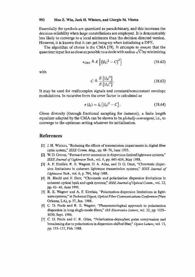
992 Moe Z. Win, Jack H. Winters, and Giorgio M. Vitetta
Essentially the symbols are quantized as pseudobinary, and this increases the decision reliability when large constellations are employed. It is demonstrably less likely to converge to a local minimum than the decision directed version. However, it is known that it can get hung-up when initializing a DFE.
The algorithm of choice is the CMA [78]. It attempts to ensure that the quantizer input lies as close as possible to a circle with radius f i by minimizing
with
(1 8.62)
(1 8.63)
It may be used for reaVcomplex signals and constantlnonconstant envelope modulations. In recursive form the error factor is calculated as
Given diversity (through fractional sampling for instance), a linite length equalizer adapted by the CMA can be shown to be globally convergent, i.e., to converge to the optimum setting whatever its initialization.
References
J. H. Winters, “Reducing the effects of transmission impairments in digital fiber optic system,” IEEE Comm. Mag., pp. 68-76, June 1993. W. D. Grover, “Forward error correction in dispersion-limited lightwave systems,” IEEE Journal ofLightwave Tech., vol. 6, pp. 643-654, May 1988. A. F. Elrefaie, R. E. Wagner, D. A. Atlas, and D. G. Daut, “Chromatic disper- sion limitations in coherent lightwave transmission systems,” IEEE Journal of Lightwave Tech., vol. 6, p. 704, May 1988. H. Bischl and F. Derr, “Chromatic and polarization dispersion limitations in coherent optical bpsk and qpsk systems,” IEEE Journal of Optical Comm., vol. 12, pp. 42-46, June 1991. R. E. Wagner and A. F. Elrefaie, “Polarization-dispersion limitations in light- wave systems,” in Technical Digest, Optical Fiber Communications Conference (New Orleans, LA), p. 37, Jan. 1988. C. D. Poole and R. E. Wagner, “Phenomenological approach to polarisation dispersion in long single-mode fibres,” IEE Electronics Letters, vol. 22, pp. 1029- 1030, Sept. 1986. C. D. Poole and C. R. Giles, “Polarization-dependent pulse compression and broadening due to polarization in dispersion-shifted fiber,” Optics Letters, vol. 13, pp. 155-157, Feb. 1988.
18. Equalization Techniques 993
[8] J. H. Winters, M. A. Santoro, and Z. Haas, “On the experimental measurement of pmd effects,” in Proc. of SPIE OE/Fibers’92, p. 1784.05, Sept. 1992.
[9] C. D. Poole, R. W. Tkach, A. R. Chraplyvy, and D. A. Fishman, “Fading in light- wave systems due to polarization-mode dispersion,” IEEE Photonics Technology Letters, vol. 3, pp. 68-70, Jan. 1991.
[lo] C. D. Angelis, A. Galtarossa, G. Gianello, E Matera, and M. Schiano, “Time evolution of polarization mode dispersion in long terrestrial links,” IEEE Journal OfLightwave Tech., vol. 10, pp. 552-555, May 1992.
[l 11 M. Tsubokawa, M. Ohashi, and Y Sasaki, “Waveform degradation due to disper- sion effects in an optical cpfsk system,” IEEE Journal of Lightwave Tech., vol. 8, pp. 775-779, May 1990.
[12] A. A. M. Saleh, R. M. Jobson, and T. E. Darcie, “Compensation of nonlinearity in semiconductor optical amplifiers,” IEE Electronics Letters, vol. 15, pp. 950-952, July 1988.
[13] W. J. Tomlinson and R. H. Stolen, “Nonlinear phenomena in optical fibers,” IEEE Communicationsibfag., vol. 26, pp. 36-44, April 1988.
[14] A. R. Chraplyvy, “Limitations on lightwave communications imposed by optical- fiber nonlinearities,” IEEE Journal of Lightwave Tech., vol. 9, pp. 1548-1557, Oct. 1990.
[15] R. Giles and J. Conradi, “Laser mode partitioning and mode evolution effects in high-speed fiber-optic transmission,” in Technical Digest of OFC’86, pp. 110-1 11, 1986.
[16] K. Ogawa, “Analysis of mode partition noise in laser transmission system,” IEEE Journal of Quantum Electronics, vol. QE-18, pp. 849-855, May 1982.
[17] B. L. Kasper, “Equalization ofmultimode optical fiber systems,” BellSyst. Tech. J., vol. 61, pp. 1367-1388, Sept. 1982.
[18] L. Kazosky, S. Benedetto, and A. Willner, Optical Fiber Communication Systems. London: Artech House, 1996.
[19] R. E. Wagner and A. F. Elrefaie, “Polarization-dispersion limitations in coherent lightwave systems,” in Technical Digest, Optical Fiber Communications Conference (New Orleans, LA), p. 37, Jan. 1988.
[20] A. E Elrefaie, R. E. Wagner, D. A. Atlas, and D. G. Daut, “Chromatic dispersion limitations in coherent lightwave systems,” IEEE JournaI of Lightwave Tech., vol. 6, pp. 704-709, May 1988.
[21] R. D. Gitlin, J. E Hayes, and S. B. Weinstein, Data Communications Principles. New York: Kluwer AcademicPlenum Publishers, 1992.
[22] A. E Molisch, Wideband wireless Digital Communications. Upper Saddle River, New Jersey: Prentice Hall, 2001.
[23] D. G. Forney, Jr., “Maximum-likehood sequence estimation of digital sequences in the presence of intersymbol interference,” IEEE Trans. In$ Eheory, vol. 18, pp. 363-378, May 1972.
[24] D. G. Forney, Jr., “The Viterbi algorithm,” Proc. IEEE, vol. 61, pp. 268-278, Mar. 1973.

994 Moe Z. Win, Jack H. Winters, and Giorgio M. Vitetta
[25] J. A. Heller and I. M. Jacobs, “Viterbi decoding for satellite and space coII1II1un- cation,” IEEE Trans. Commun. Tech., vol. COM-19, pp. 835-848, Oct. 1971.
[26] G. Fettweiss and H. Meyr, “High speed parallel Viterbi decoding: Algorithm and VLSI-architecture,” IEEE Communications Magazine, vol. 29, pp. 46-55, May 1991.
[27l J. B. Anderson, “Sequential coding algorithms: A survey and cost analysis,” IEEE Trans. Comm., vol. 32, pp. 169-176, Feb. 1984.
[28] A. D. Hallen and C. Heegard, “Delayed decision-feedback sequence estimation,” IEEE Trans. Comm., vol. 37, pp. 428-436, May 1989.
[29] M. V. Eyuboglu and S. U. H. Qureshi, “Reduced-state sequence estimation with set partitioning and decision feedback,” IEEE Trans. Comm., vol. 36, pp. 13-20, Jan. 1988.
[30] G. Ungerboeck, “Channel coding with MultilevelPhase signals,” IEEE Trans. In$ Theory, vol. 28, pp. 55-67, 1982.
[31] S. U. H. Qureshi and E. E. Newhall, “An adaptive receiver for data transmission over time-dispersive channels,” IEEE Trans. In$ Theory, vol. 19, pp. 448-457, July 1973.
[32] D. D. Falconer and F. R. Magee, “Adaptive channel memory truncation for maximum-likelihood sequence estimation,” Bell Syst. Tech. J., vol. 52, pp. 1541-1562, Nov. 1973.
[33] W. U. Lee and E Hill, “A maximum-likelihood sequence estimator with decision- feedback equalisation,” IEEE Trans. Comm., vol. 25, pp. 971-979, Sept. 1977.
[34] Y. Gu and T. Le-Ngoc, “Adaptive combined DFEMLSE techniques for IS1 channels,” IEEE Trans. Comm., vol. 44, pp. 847-857, July 1996.
[35] K. Wesolowski, “An efficient DFE & ML suboptimum receiver for data transmis- sion over dispersive channels using two-dimensional signal constellation,” IEEE Trans. Comm., vol. 35, pp. 337-339, March 1987.
[36] J. H. Winters and S. Kasturia, “Constrained maximum likelihood detection for high-speed fiber-optic systems,” in Proc. Globecom ’91, pp. 1574-1 579, Dec. 199 1.
[37l M. Austin, “Decision feedback equalization for digital communication over dis- persive channels,” MIT Research Laboratory of Electronics Technical Report 461, Aug. 1967.
[38] C. A. Belfiore and J. H. Park, “Decision feedback equalization,” Proc. IEEE,
[39] S. U. H. Qureshi, “Adaptive equalization,” Proc. ZEEE, vol. 73, pp. 1349-1387, Sept. 1985.
[40] R. D. Gitlin and S. B. Weinstein, “Fractionally-spaced equalization: An improved digital transversal equalizer,” BelZSyst. Tech. J., vol. 60, pp. 856-864, Feb. 1981.
[41] G. Ungerboeck, “Fractional tap-spacing equaliser and consequences for clock recovery in data modems,” IEEE Trans. Comm., vol. 24, pp. 856-864, Aug. 1976.
[42] J. H. Winters, “Equalization in coherent lightwave systems using a fractionally- spaced equalizer,” IEEE Journal of Lightwave Tech., vol. 8, pp. 1487-1491, Oct. 1990.
V O ~ . 67, pp. 1143-1 156, Aug. 1979.

18. Equalization Techniques 995
[43] J. Salz, “Optimum mean-square decision feedback equalization,” Bell Syst. Tech.
[44] D. D. Falconer and G. J. Foschini, “Theory of minimum mean-square error QAM systems employing decision feedback equalization,” Bell Syst. Tech. J., vol. 52, pp. 1821-1849, Dec. 1973.
[45] D. L. Duttweiler, J. E. Mazo, and D. G. Messerschmitt, “An upper bound on the error probability in decision-feedback equalisation,” ZEEE Dam. ZnJ: Theory, vol. 20, pp. 490-497, July 1974.
[46] R. A. Kennedy, B. D. 0. Anderson, and R. R. Bitmead, “Tight bounds on the error probabilities of decision feedback equalizers,” ZEEE Trans. Comm., vol. 35,
[47l J. H. Winters and R. D. Gitlin, “Electrical signal processing techniques in long- haul fiber-optic systems,” ZEEE Trans. Comm., vol. 38, pp. 1439-1453, Sept. 1990.
[48] S. Kasturia and J. H. Winters, “Techniques for high-speed implementation of nonlinear cancellation,”ZEEEJ. Sel. Areas Comm., vol. 9, pp. 711-717, June 1991.
[49] A. Schiippen, H. Dietrich, U. Seiler, H. V. D. Ropp, and U. Erben, “A SiGe RF technology for mobile communication systems,” Microw. Eng. Europe, pp. 39-46, 1998.
[50] E Buchali, H. Biilow, W. Baumert, R. Ballentin, and T. Wehreu, “Reduction of the chromatic dispersion penalty at 10 Gbitls by integrated electronic equalisers,” in Optical Fiber Communication Conference, 2000, vol. 3, pp. 268-270, March 2000.
[51] H. Biilow, “System outage probability due to first- and second-order PMD,” ZEEE Photon. Technol. Left., vol. 10, pp. 696-698, May 1998.
[52] H. Biilow, “Equalization of bit distortion induced by polarkition mode disper- sion,” in Proc. NOC’97, 1997.
[53] B. W. Hakki, “Polarization mode dispersion compensation by phase diversity detection,” ZEEE Photon. Technol. Lett., vol. 9, pp. 121-123, Jan. 1997.
[54] J. H. Winters, “Experimental equalization of polarization dispersion,” IEEE Photon. Technol. Lett., vol. 2, pp. 591-593, Oct. 1990.
[55] H. Biilow, D. Schlump, J. Weber, B. Wedding, and R. Heidemann, “Electronic equalization of fiber PMD-induced distortion at 10 Gbitls,” in Optical Fiber Com- munication Conference and Exhibit, 1998 (OFC ’98), Technical Digest, vol. 2, pp. 151-152, Feb. 1998.
[56] H. Biilow, F. Buchali, W. Baumert, R. Ballentin, and T. Wehren, “PMD mitigation at 10 Gbit/s using linear and nonlinear integrated electronic equaliser circuits,” Electron. Lett., vol. 36, pp. 163-164, Jan. 2000.
[57] H. Biilow, “PMD mitigation techniques and their effectiveness in installed fiber,” in Optical Fiber Communication Conference, 2000, v01. 3, pp. 110-112, March 2000.
[58] J. Poirrier, A. Gnauck, and J. Winters, “Experimental nonlinear cancellation of polarization-mode dispersion,” in Optical Fiber Communication Conference, 2000,
J . , V O ~ . 52, pp. 1341-1373, OCt. 1973.
pp. 1022-1029, Oct. 1987.
V O ~ . 3, pp. 119-121,2000.

996 Moe Z. Win, Jack H. Winters, and Giorgio M. Vitetta
[59] D. G. Messerschmitt, “Minimum MSE equalization of digital fiber optic systems,” IEEE Pans. Comm., vol. 16, pp. 1110-1118, July 1978.
[60] J. H. Winters and M. A. Santoro, “Experimental equalization of polarization diversity,” IEEE Photon. Technol. Lett., vol. 2, pp. 591-593, Aug. 1990.
[61] J. G. Proakis, Digital Communications. New York, New York McGraw-Hill, Inc., Fourth ed., 2001.
[62] B. Widrow, J. McCool, M. Larimore, and C. Johnson, “Stationary and non- stationary learning characteristics of the LMS adaptive filter,” Proc. IEEE, vol.
[63] R. W. Lucky, “Automatic equalization for digital communications,” Bell Syst. Tech. J . , vol. 44, pp. 547-588, April 1965.
[64] D. Schlump, K. Koffers, W. Pohlmann, H. Reichelt, and B. Wedding, “10 Gbitfs dispersion supported transmission field trial over 123 km standard single mode fibre for HDTV studio interconnection,” Electron. Lett., vol. 31, pp. 1854-1855, Oct. 1995.
[65l B. Wedding, €3. Franz, and B. Junginger, “10-Gb/s optical transmission up to 253 km via standard single-mode fiber using the method of dispersion-supported transmission,” IEEE JournaIofLightwave Tech., vol. 12, pp. 1720-1727, Oct. 1994.
[66] T. Takahashi, T. Imai, and M. Aiki, “PMD mitigation at 10 Gbitfs using linear and nonlinear integrated electronic equaliser circuits,” Electron. Lett., vol. 30, pp. 348-349, Feb. 1994.
[67] D. Schlump, B. Wedding, and H. Biilow, “Electronic equalisation of PMD and chromatic dispersion induced distortion after 100 km standard fibre at 10 Gbitfs,” in 24th European Conference on Optical Communication, vol. 1, pp. 535-536, Sept. 1998.
[68] €3. Wedding, W. Pohlmann, D. Schlump, E. Schlag, and R. Ballentin, “SiGe circuits for high bit-rate optical transmission systems,” in Proc. of the 1999 IEEE International Sjmposium on Circuits and Systems (ISCAS ‘99), vol. 2, pp. 492-495, May 1998.
[69] B. Wedding, A. Chiarotto, W. Kuebart, and H. Biilow, “Fast adaptive control for electronic equalization of PMD,” in Optical Fiber Communication Conference and Exhibit, 2001 (OFC 2001), vol. 2, pp. TuP4.1-TuP4.3, March 1988.
[70] H. Biilow, F. Buchali, and V. Nicolas, “Dispersion mitigation using a fiber-bragg- grating sideband filter and a tunable electronic equalizer,” in Optical Fiber Commu- nication Conference and Exhibit, 2001 (OFC 2001), vol. 3, pp. wdd34.1-wdd34.3, Jan. 2001.
[7 11 W. D. Grover, “Forward error correction in dispersion-limited lightwave systems,” IEEE JournalofLightwave Tech., vol. 6, pp. 643-654, Oct. 1988.
[72] R. W. Chang and J. C. Hancock, “On receiver structures for channel having memory,” IEEE Dam. In$ Theory, vol. 12, pp. 463-468, Oct. 1966.
[73] K. Abend and B. D. Fritchman, “Statistical detection for communication channels with intersymbol interference,” Proc. IEEE, vol. 58, pp. 779-785, May 1970.
64, pp. 1151-1 162, Aug. 1976.

18. Equalization Techniques 997
[74] K. Abend, T. J. Hartley, B. D. Fritchman, and C. Gumacos, “On optimum receivers for channels having memory,” IEEE Trans. In$ Theory, vol. 14,
[75] Y. Li, B. Vucetic, and Y. Sato, “Optimum soft-output detection for channels with intersymbol interference,” IEEE Trans. Inz neory, vol. 41, pp. 704-713, May 1995.
[76] Y. Sato, “A method of self-recovering equalisation for multilevel amplitude- modulation systems,” IEEE Trans. Comm., vol. 23, pp. 679-682, June 1975.
[77] D. N. Godard, “Self-recovering equalisation and carrier tracking in two- dimensional data communication systems,” IEEE Tram. Comm., vol. 28,
[78] R. Johnson, P. Schniter, T. J. Endres, J. D. Behm, D. R. Brown, and R. A. Casas, “Blind equalization using the constant modulus criterion: A review,” IEEE Proc., vol. 10, pp. 1927-1950, Oct. 1998.
pp. 152-157, NOV. 1968.
pp. 1867-1875, NOV. 1980.


Index to Volumes IVA and IVB
1 : 1 protection, A324, B:112, 113, 114 1 :Nprotection,B:112,113,114
1 + 1 protection, A322,323, B62; 112,113,114 1.3 micron VCSELs, A671474 1.5micron VCSELs
APS protection switching in, B122-123
AlGaAsSb DBR approach to, A675-676 dielectric mirror approach to, A674675 metamorphic DBR approach to; A676677 wavelength-tunable, A677478
10Gbit/s standard, B:537 characteristics of, B549-550 fibers in, B:550 future of, B:558-559 need for, B:642,647 optional features of, B:55&551 XGMII Extender in, B:550-551
directly modulated lasers in, A6l.9425 evolution of Ethernet standard, A52-57
compatibility issues of, B:546547 userbase of, B:546
10 Gigabit transmission, A45
IOBASE-T: B:517,526,536
100BASE-T4 and -T2, B540 100BASE-T, B:536
1000BASE-LX Ethernet, B:538,539 1000BASE-SX Ethernet, B:538,539 1000BASE-X Ethernet, B:537 1310nm analog lasers, A605
applications of, A:605, 612 distortion by, A:605412
1480 nm lasers characteristics of, A572-574 construction of, A:573-574 in EDFA pumping, A:575-576
demultiplexing in, B:283 OTDM in, B:281-284 practicability of, B:289-290 receiver for, B:282-284 sample system, B:283-284 single-channel transmission experiment,
B:285-287 transmitter for, B:281-282 WDM in, B:287-289
backward compatibility of, B:546-547
160 Gbit/s systems
16800GX, A:314 2R signal regeneration, A:720 3R signal regeneration
clock recovery block for, A735-736,741-742 electrooptic vs. all-optical, A:771-775 hardware for, A:736741 implementation of, A:736744 input adaptation for, A:742-744 need for, A:73?-734 by nonlinear gates, A735756
SOA-MZI based, A744-748 by synchronous modulation, A:747-771
alternating polarization format in, B:280-28 1 dispersion compensation in, B:278-279 ETDM pseudo-linear transmission in, B:279-280 experiments in, B:276-279 reamplification in, B:276277
40 Gbit/s systems
8B10B coding, B:541 8B6T coding, B:540 980 nm lasers
beam characteristics of, A565-568 design of, A568-570 in EDFA pumping, A575-576 emissions spectra of, A:579-580 light output of, A57&572 mirror passivation in, A:564-565 waveguides for, 569-570
Abilene network, B:38 AboveNet, B:34-35 Access networks
architectures for, E439 carrier systems in, B:439 described, A:36 dispersion compensation and reach in, A 3 9 4 0 fiber capacity limitations in, A 4 0 4 1 fiber choice for, A45 fiber economics for, A 4 3 4 l fiber requirements for, A 3 6 3 9 fiber use in, B:42&421,43b506. See also
Optical access networks 1400 nm market in, A 4 2 4 3 future trends in fiber use, A:44 history of, B:438440 SOAs in, A:722-723 1300 nm market in, A:42
Acoustooptic filters, A467468 Adaptation grouping, B:6M7
and reconfigurability, B:68 Add/drop filters, A541-543 Add/drop multiplexers, B:6041
photonic B:58,67, 121 Addresses, Internet, B: 132 Adiabatic couplers, A427428 ADSL, B:503
Al/Ge/Si glasses in xDSL, E504
advantages of, A109-110 applications of, A 1 17-1 18 compositions of, A 1 1&112 in EDFAs, A130 erbium doping of, A: 11 0 fiber losses in, A 1 15-1 I6 fiber fabrication of, A: 1 1 4 1 15 fiber strength of, A 1 1 6 1 17 impurities in, A115-116
999

1000 Index
A1 f Ge f Si glasses, continued phosphorus doping of, A 1 12 reliability of, A 1 17 synthesis of, A112-114
Alcatel Crosslight, A386 AlGaAs lasers
design of, A568-570 mirror passivation in, A564565 waveguide patterns for, A566-567
All-optical islands, B:227-228 All-optical networks
characteristics of, B226 feasibility of, B226 future of, B227
All-optical regeneration beyond 40 Gbit f s, A770-771 challenges facing, A:774-775 clock recovery block for, A735-736,741-742 electrooptic VL, A:771-775 experiments in, A769-770 hardware for, A736741 implementation of, A736-744 mechanism for, A748-749 need for, A733-734 by nonlinear gates, A735-756 prerequisites for, A773-774 regenerator configurations for, A768-769 by saturable absorbers, A749-756 by synchronous modulation, A:757-771 in WDM, A732-733, A767-771
cross-gain modulation, A 7 17-71 8 cross-phase modulation, A718-719 four-wave mixing, A719-720 optical time-division multiplexing (OTDM),
signal regeneration, A720. See also All-optical
transmission speed using, A 8 2 2 wavelength conversion, A 7 17-720
All-pass dispersion compensation, B691,692-693 Alumina-doped silica EDFAs, A 8 0 Aluminosilicates
All-optical signal processing
A720-722
regeneration
advantages of, AlO9-110 applications of, A117-118 compositions of, A.110-I12 in EDFAs, A 130 erbium doping of, A.110 fiber lossesin, A115-116 fiber fabrication of, A l l 4 1 1 5 fiber strengthof, A l l 6 1 1 7 impuritiesin, All5-116 phosphorus doping of, A:ll2 reliability of, A 1 17 synthesis of, A112-I14
in fluoride glasses, A107-108 in oxideglasses, A:108-118
B160-161,201,905 accumulation of, B:236237 in an EDFA, A229-230, B202 excess, B161 filtering of, A540 in a passive fiber, A228-229 in a passive fiber followed by an amplifier, A230 in a Raman amplifier, A231-232 in a Raman amplifier followed by an EDFA,
Aluminum
Amplified spontaneous emission (ASE), A225,
A:233-234
reduction of, B236 simulation of, B:572 source of, A705
Amplifier chains, length of, B:187-189 Amplifiers
materials characteristics for, A.81-83 materials limitations for, A 8 4 8 8 pump schemes for, A82,83
Amplitude modulation (AM) in metro networks, B:415 modulator characteristics for, B:868-873 signal distortion in, BS67-868 signal representation in, B866-868
Amplitude transparency, defined, B86 Amplitude-modulated-nonreturn-to-zero
(AM-NRZ) modulation, A276 Amplitude-modulated-return-to-xro (AM-R
modulation, A276 Analog lasers
history of, A601603 impairments of, A:60>604
Analog systems laser sources for, A595 SOAs in, A71 1
Analog-to-digital conversion, for cable systec B:42-26
Annealed proton exchange, A262 Anti-Stokes scattering, A216 Antimony silicates
applications of, A:128 in C-band EDFAs, A132-135 composition of, A124-125 fiber fabrication of, A126128 history of, A124 in L-band EDFAs, 137-139 rare earths in, A125 synthesis of, A125-126 thulium-doped, A 145-149
Apodization in fiber gratings, A495 in nonunifom gratings, A513
ARPA (Advanced Research Project Agency), ARPANET, B:28-29
end of, B31 growth of, B30-31
Arrayed wavelength grating (AWG), B481 Arrayed-waveguide devices, B691 AT&T
divestitures by, A.3, B:3 evolution of, A2, B:2
AT&T Northeast Corridor System, A2, B:2 ATM PON (APON), B446 Attenuation, defined, B:904 Attenuators
midstage, A186188 in optical crossconnects, A338
Australia, Internet growth in, B:33, B34 Automated provision, modes for, B137-138 Autonegotiation
evolution of, B548-549 importance of, B:546547 and link integrity, B547-548
Avalanche photodiodes (APDs), A790-791 sensitivity of receiver using, A795796 simulation of, B582
Backscattering hardware for measuring, B759 to measure PMD, B759-761
B:28

Index 1001
Band filling, for index tuning, A65&652 Bandgap shrinkage, for index tuning, A650-652 Bandwidth trading, B:7%81 Bandwidth-on-demand service, B:85 BCH codes, B:915
for lightwave communications, B956-957 mathematics of, B:926928 product codes, B928-929
Beam-steering spatial cross-connects, A458-461 Beat noise, A.226 Bell System, breakup of, A2, B 2 Bellcore, founding of, A2, B:2 Beryllium fluoride, glass formation from, A:108-109 BFR (big fat routers), B:106 Bias voltage drift: A277 Bidirectional transmission
achievement of, B:449 free-space optic modules, B:494-495 fullduplex, B 4 5 N 5 1 in optical access networks, B:494-496 PLC-based, B:495-496 using SCM, B:452453 using SDM, B450 using TCM, B451-452 using WDM, E453454
Binary ASK systems power spectral densities in, B:875-876 single-channel transmission simulations in,
B:887489
described, B907-910 linear, B:9 10-917 ML decoding of, B:932-948
causes of, A:483484, B:727 characteristics of, B72G729 circular, B:727 magnitude of, A:484-485
Biterror rate (BER), A685697 estimation of, B:582-584 measurement of, B174177 and OSNR, B:238 related to Q-factor, B:173-174
Bit-interleaved WDM, B:486487 Bitrate distance product, B906 Black box EDFA model, B:575,581 Black-box optical regenerator (BBOR) systems,
Binary codes
Birefringence
A764-765 advantages of, A765 characteristics of, A765-767 concerns regarding, A:767 for WDM application, A769-770
defined, B:907 linear, B:911-917
Block codes
Border Gateway Protocol (BGP), B:133 Boron, as dopant, A483 Bounded-distance decoding algorithm, B:909 B r a g gratings See also Fiber gratings
chirped, B:659469 coupled-mode theory on, A501-506 coupling in, A502-505 dispersion by, A:504-506 for fixed slope matching, B:69&699 illustrated, B:659 optics of, A498499 planar, A453454 for tunable slope matching, B:700-702
Bridges, function of, B:529
Broadband, metallic media for, B:497 Broadband access facilities (BAF), B:446 Broadband amplifiers
high bitrate, A824430 in MANS, B:345 need for, A:824825 transimpedance amplifier (TU), A826827 traveling-wave ampliier (TWA), A827430
Broadband OSSB, B : 8 W 8 6 BroadNED (Broadband Network Designer), B:570 Bromine, in tellurite glasses: A122 Bubble switches, A33%340 Burst error correction, B:924 Bursty data, amplification of, A:716 Bus architecture, compared to grid topology, B:405 Butt-joint growth, A599
C-band ampliien aluminosilicates in, A130 antimony silicates in, A132-135 fluorozirconates in, A:13&131 tellurites in, A123
Cable modems, B339 Cable TV systems
coaxial bus system, B:406410 digitization in, B425-426 future of, E421425 history of, B:40546 hybrid fiber/coax networks, B:411-421 linear lightwave technologies in, B:430-431 low-cost lightwave technologies in, B:431-433 RF technologies in, B:415,427-430 simulation of: B603-604 SONET systems in, B:414,415 topology of, B:404-405
Carrier extension, in Gigabit Ethernet, B:524 Carrier hotels, B:78-79 Carrier Sense Multiple Access with Collision
Carrier systems, B:439 Carrier-suppressed RZ modulation, A:816-818 Cascaded Raman fiber lasers, AM7-248 Cell phone industry, growth rate of, B:22-23 Cerium, as dopant, A:483 Channel capacity, B:932 Channel protection, A202-203
Detection (CSMA/CD), B:521-524
laser control, A205-206 link control, A20S205 pump control, A203
history of, A:112-113 modified,A:113, 114: 115
Chemical vapor deposition (CVD)
China, Internet growth in, B:33-34 Chirp, B:968
calculation of, B242 in direct-modulated lasers, 409 in fiber gratings, A49-96 in nonuniform gratings, A:513 simulation of, B576-577 uses of, A509-510 wavelength, A:69&692
advantages of, B:660 illustrated, B:659 multiple-channel, B:664-668 nonlinearly chirped, B682-686 polarization dependence of, B:662-663
Chirped fiber Bragg gratings (chirped FBGs)

1002 Index
Chirped fiber Bragg gratings (chirped FBGs), continued
ripple in, B66C-662 robustness of, B663 single-channel linearly chirped, B:664 single-channel tunable, B678488 temperature sensitivity of, B:662 tuning of, B:660 versatility of, B:663
advantages of, B:169-171 compared with DMS, B:309-310,322-323 described, B:169 and WDM, B:315-322
compensation of. See Dispersion compensation cumulative effect of, B645 defined, B:904 effect of, B:645 figures for commercial fibers, B:647 historical perspective on, B545-651 importance of, B:708 linearity of, B:653 management of, B:215-220,651453 mathematics of, B:648 monitoring of, B:704-708 physics of, B64-5 time behavior of, B67M72 universalities of, B:643
Ciena CoreDirector, A386 Circuit switching, vs packet switching, B:516 Cladding pumping, A151
Clamping, A708-709 Clipping, A604
Clock and data recovery (CDR) circuits, high bitrate
Chirped return-to-zero (CRZ) pulse system, A815
Chromatic dispersion, B214,979
with broadstripe lasers, A151-152
in cable systems, B:432
components of, A83C-831 function of, A832433 physical manifestation of, A835-836 using multiple-phase clocks, A83S834
mechanism of, A:741-742 types of, A742
effects on gain, A:87 minimization of, A87-88
Coaxial bus system, B:405 characteristics of, B:407 described, B:40M07 distribution system of, B:409 evolution of, B411 headend of, B:40749 trunk system in, B409 upstream system of, B:410
Clock recovery block, A735-736
Clustering
Coaxial cable, properties of, B:535-536 Code-division multiplexing, B341 Codewords, defined, B:907 Coding
Coding gain, B:208,906
Coherent detection, defined, B905 Coherent optical time-domain reflectometer
(COTD), B:186 Collision detection, B522,523 Commercial Internet Xchange (CIX), B31
error-control. See Error-control coding for Ethernet, B537,539-541
for lightwave communications, B:952 mathematics of, B:953-956
Communications technology, predictions about,
Compensation for PMD B24-25
electrical, B:817-820,981 higher-order, B814-815 multichannel, B816817 multisection, B:81%816 optical, B809-817,981
Complex amplitude, calculation of, B242 Composite PONS (CPONs), B:484485 Concatenated codes, B:925-926,959-960 Conduits, B119 Connection attributes, B 138 Consolidation, B:72
Constraint-based Routing Label Distribution
Containment, in fault management, B:72 Control logic, for failure recovery, B: 110,111 Control plane, B97,99
alternative approaches to, B:143-144 alternative architectures for, B:128-131 enhancements to, B:142
Control register bit definitions, in Ethernet, B545 Convolutional codes, B:929
decoding of, B932 in lightwave communications, B:960-961 mathematics of, B:929-931 parallel concatenated, B948-950 recursive systematic, B93 1-932
bandwidth management in, A302-303
and Bragg gratings, A501-506 and nonuniform gratings, 509-519 and tilted gratin& A51%522 and transmission gratings, A506509
in Bragg grating, A524-525 to cladding modes, A.522-525 radiation-mode, A:527-530 in transmission grating, A:525-526
architectures of, A312-315 beam-steering spatial, A 4 5 8 4 1 electrical, A314-315,385-389 optical. See Optical cross-connects port count and, A303-305
reasons for, B:72-73
hotowl (CR-LDP), B:135
Core network, A30lL302
Coupled-mode theory, to analyze fiber gratings, A499-500
coupling
Crossconnects
Cross-gain modulation (XGM), SOAs in, A717-718 Cross-phase modulation (XPM), A21,282
amplitude distortion penalty induced by, B:624625
collision-induced, B:625-629,635 compensation for, B:262-264 described, B548-649 effect of, B:257-261 intrachannel, B:257-264,629433 mathematics of, B:257-259,618 minimization through polarization interleaving,
in NRZ systems, B:624425 pump-probe measurements of, B518-624 in RZ systems, B625629 simulation of, B:600 SOAs in, A71M19
avoiding, A712-713 control of, A350-351,355,35%362
E798402
Crosstalk

Index 1003
ganged per-stage control in, A:360-362 interchannel, A238-239,712-716 nonlinear, A25-26 and optical fiber design, A26 in optical switches, A:335-336 propagation of, A:352-355 pump-signal, A:240 in Raman amplifiers, A238-241 signal-pump-signal, A241 simulation of, B:599 suppression of, A713-716
Cyclic codes, B:915-917 BCH codes, B:915,92&929,957 generating polynomial of, B:916 Golay codes: B:915,917 Hammingcodes, B:915,917
Cyclic shift, B915
DARPA (Defense Advanced Research Project Agency), B:28
Data modulator, for wavelength switching, A398 Data rates, evolution of, A19 Data sheets, B:576 Data transmission
growth rate of, B26 Moore’s law applied to, B:49-50 predictions about, B:25-26
Decision block for SOA-MZI-based 3R regeneration,
A744745 for 3R regeneration, A:736-741
Decision feedback equalizer (DFE), B:817-819,
Degree of polarization
Demultiplexers
Deuterium loading, to increase photosensitivity,
Dielectric mirrors, for VCSELs, A674675 Differential group delay (DGD), B:221-222,725,
measured mean, B:761-762 polarization-mode coupling and, B:730-73 1 to predict PMD densities, B767 pulse broadening due to, B:735-736 simulation of, B:580
fiber, A63
B:977-981
described, B:823424 to monitor PMD, B:824-825
high bitrate, A836 simulation of, B:578
A482
728-729
Differential mode attenuation (DMA), in plastic
Differential operation mode (DOM), A740-741 Digital Access and Cross-Connect Systems (DACS),
Digital cross-connect switch/system (DCS), A377,
A.309,311 evolution of, A:312-313
B 5 W in MANS B:334 types of nodes based on, B:334335
ADSL, B:503 described, B501-502 growth of, B:339-340 HDSL, B:503 standardization of, B:502 transmission techniques in, B:502-503
Digital loop carrier (DLC), B:439 Digital subscriber line (DSL)
VDSL, B:503-504 xDSL, B:502,504
Digital transmission, SOAs in, A710-711 Digital transparency, defined, B86 Dimension, of code, B:911 Diplex, B453 Direct detection, defined, E905 Direct matrix inversion, B:982 Direct modulation, in Ah4 transmission, B:868 Direct peering, B:76 Directional couplers, A:269,427; 428
types of, A270 Directly modulated distributed feedback (DFB)
lasers arrays of, E486 in DWDM systems, A:618619 modulation efficiency of, A621 need for, A613 oscillation frequency of, A621 performance analysis of, A614618 in 10 Gbit/s transmission, A:619625
density of, B:47 innovations enabled by, B:4849 trends in, B:48
calculation of, B:241-242,243 consequences of, B:163-165 cumulative effects of, B:244-245 deiined, B:163,904-905 leading to pulse broadening and chirping, B:244 simulation of, B:597,598
dynamic, A452453 figure of merit for, B:670 fixed, B657-670 in metro and access systems, A 3 9 4 0 with optical nonlinearities, B653457 slope matching, B:69&702 for subcarrier-multiplexed data, B:702-704 tunable, B:670496 using chirped FBGs, B659669 using dispersionxompensating fiber, B657459,
669-670 using FBGs in transmission mode, B:668669 wideband, A23-25
Dispersion length, B:214 calculation of, B242
Dispersion limit, B:214 formula for, B 163
Dispersion management, A:2&29, B:651453,
for land systems, A35 for undersea systems, A33-35 in WDM transmission, B633434
corrections to, B:654655 extreme, B:655657 optimization of, B:270-272 and precompensation choice, B:271-273,275
Dispersion monitoring, B:704 using duty cycle, B:707 using NRZ clock regeneration and RZ clock
fading, B:705-706 using peak detection, B707 using phase shift, B707-708 using RZ power fading, B:705
Directly modulated laser transmitters, A808409 Disk storage
Dispersion
Dispersion compensation, A:23-25, B:236,652, 709-714
798
Dispersion mapping, B164165, B269-270, B:654

1004 Index
Dispersion-compensating fiber (DCF), B216-218 adaptation to tunable compensators, B:677-678 characteristics of, B:657458 design of, B:218 higher-order, B:669-670 sites of application of, B:658459 slope matching based on, B:697498
Dispersion-compensating modules (DCM), A24 alternatives to, A25
Dispersion-compensation filters, A:543-546 Dispersion-managed soliton (DMS), B247-248
compared with CRZ, B309-310,322-323 PMD resistance of, B809 in singlechannel systems, B310-315 in WDM systems, B316-322
disadvantages of, B650
attenuation, B:904 dispersion, B904-905 dispersion management of, A26-29 limiting effects of, A25 miscellaneous sources of, B906 nonlinear, in cable systems, B432 between multiple signals, B967 noise, B905,967. See also Noise single-signal, B:966-967 types of, A28 1
AlGaAsSb for, A675476 characteristics of, A592 construction of, A591,64&641 function of, A641-642 metamorphic, A676477 variations of, A645-648
advantages of, A640 characteristics of, A592 disadvantages of, A639640 mechanism of, A608 nonlinearities of, A609-610
advantages of, A251, B:207 current research in, A:25&251 hardware for, B205 history of, B:204-205 to improve OSNR, B20S206 spontaneous emission in, A23 1-234
architectures for, B417 multiplexing techniques for, B417-420
Distributive law, B933-934 DNS, origin of, B30-31 Domains, Internet, B:132 Domains of transparency, B67,89
Dispersion-shifted fiber (DSF), A281, B:648
Distortion
Distributed Bragg reflector (DBR) lasers, A:398,462
Distributed feedback (DFB) lasers, A590-591
Distributed photodetectors, A788-789 Distributed Raman amplification (DRA), A29-30
Distribution hubs
complex, B:67 connectivity limitations associated with, B95 impairments and, 94-95 and networks, B:91-92 recoveryin, B:120-121 routing complications associated with, B: l a 1 4 1 routing and wavelength assignment in, B:92-94
Double-sideband suppressed carrier (DSSC)
DSL (digital subscriber line) modulation, A276
ADSL, B:503 described, B:501-502 growth of, B:339-340
HDSL, B503 standardization of, B502 transmission techniques in, B502-503 VDSL, B:503-504 xDSL, B502,504
DWDM, B:890 power spectral densities in, B:877-880
calculation of, B240 dispersion monitoring using, B:707
systems, A18 advantages of, B:390 characteristics of, A298 cost efficiency of, B330 difficulties in, A281 duo-binary, B:890 early, A298-299 economic issues of, B369-370 edge rings, B373-375 eye diagrams of, B241 history of, B198-199 laser use in, A:593 in MANS, B331-332,344,347-373,556 in metropolitan environments, A666 migration to, B:370-373 modem, A299 modified RZ, B891493 optical hybrid/mesh networks using, B:364369 optical switching in, A299-300 OSSB, B89&891 point-to-point systems, B224,348-351 in secondary hub architectures, B:419-420 simulation tools for, B571-572 spectra of, B241 subcarrier OSSB, B881-884 technologies enabled by, B:198 technologies enabling, B201 transparency of, B:330-331 use on PSPONs, B:457 wavelength budget of, A618419 wideband. See Wideband DWDM
Duobinary coding, A816 Duobinary signaling, B865
Duty cycle
DWDM (dense wavelength-division multiplexed)
Dynamic dispersion compensators, A:452453 Dynamic gain equalization filters, A433435 Dynam!c passband shape compensators, A451452 Dynanuc rings
engineering problems of, B36&361 indications for, B35M56 OADM nodes in, B356-357 self-healing, B:357-358 SPRING, B:358-359
E-mail, origin of, B29-30 EDFAs (erbium-doped fiber ampliiers)
advantages of, A128,174, B159-160 Al/Ge/Siandvariants in,A:117-118 applications of, A179 ASE noise from, B:202 circuit noise in, A80M01 control of, A181-182,202-206 conventional-band, A13&135 described, A176179 for DWDM, B:201 for dynamic WDM systems, A197-206 effect of optical filter bandwidth on, A79W00 erbium amplifier bands in, A:128-130

Index 1005
extinction ratio of, 801-803 gain dynamics of, A198-200 gain flatness of, A180-182 gain tilt in, A182 for high-capacity systems, A:183-197 history of, A176, B307 intersymbol interference in, A:803-805 L-band, 135-139,188-191 materials requirements for, A80 midstage attenuators for, A:186188 noise calculations for, A 178-179 noise sources in, Al97-799 OSNR of, A179-180 physical parameters for, A177-178 p e r adjustment for, A:182 power transient behavior of, A198,200-202 reliability of, B 158 S-band, A140-158 sensitivity limit of, A:799 sensitivity of receiver using, A796805 SHB in, A185-186 signal photocurrent in, A796797 simulation of, B575,581 super-band, A139-140 ultrawideband, A191-193 use in undersea communication, B156163 versatility of, B: 158
Electrical cross-connects, A314 advantages of, A314315 disadvantages of, A 3 15 examples of, A:386 history of, A385 interconnections among, A388-389 scalability of, A387-389,391 state-of-the-art, A386
Electrical signal-to-noise ratio, A226,227 Electroabsorption (EA) modulators (EAMs),
A:259-260, B:223 in AM transmission, B:868 chirp tuning of, B:691 simulation of, B:577
A809-810 Electroabsorption modulator transmitters,
Electroabsorption-modulated laser (EML), A259 described, A625 design of, A632434 elements of, A:626 fabrication of, A:634 interactions with modulators, A634437 parameters for, A:626-629 performance of, A637-638 physics of, A629434
Elextrooptic effect, A:260 Electrooptic modulators
compared with electroabsorption modulators, A259-260
lithium niobate, A260-278 need for, A:258 nonlinearity issues, A 2 8 1 performance assessment of, A279,281 polymeric, A283-288 system requirements for, A:278-282
dekice fabrication using, A285 photobleaching property of, A287
Electrooptic switches, 34&341,343 Equalization
algorithms for, B:972-992 decision feedback, B977-981
Electrooptic polymers, A284
for high bitrate applications, A837-841 linear, B:981-984 need for, B965 using gain-flattening filters, B160
amplifier bands of, A128-130 spectra of, A119-120
Erbiumdoped fiber amplifiers (EDFAs) advantages of, A128,174, B159-160 AI/Ge/Si and variants in, A:] 17-1 I8 applications of, A179 ASE noise from, B:202 circuit noise in, A800401 control of, A181-182,202-206 conventional-band, A:130-135 described, A176179 for DWDM, B201 for dynamic WDM systems, A:197-206 effect of optical lilter bandwidth on, A799-800 erbium ampliier bands in, A:128-130 extinction ratio of, 801-803 gain dynamics of, A:19M00 gain flatness of, A180-182 gain tilt in, A 182 for highcapacity systems, A183-197 history of, A176, B307 intersymbol interference in, A803-805
materials requirements for, A 8 0 midstage attenuators for, A:186188 noise calculations for, A:178-179 noise sources in, A797-799 OSNR of, A:179-180 physical parameters for, A177-178 power adjustment for, A 182 power transient behavior of, A198,200-202 reliability of, B: 158 S-band, A:14&158 sensitivity limit of, A:799 sensitivity of receiver using, A:796805 SHB in, A185-186 signal photocurrent in, A796797 simulation of, B:575? 581 super-band, A:139-140 ultrawideband, A 191-193 use in undersea communication, B156163 versatility of, B:158
Erbium-doped fiber lasers, A104 Emr-control coding
binary codes, B907-915 block codes, B911-917 convolutional codes: B:929-932,960-961 cyclic codes, B:91%917 lowdensity parity-check code& B951-952,961 need for, B:904-907 Reed-Solomon codes, B922-926,958 tree codes, B929-932 turbo codes, B:948-958,961
in access networks, B:448,500-501 addressing in, B:520-521 applications of, B:552-553 architecture of, B517-518,525-527 auto negotiation in, B:546551 bridges in, B:529-530 data rate supported by: B:515 development of, B:515 flow control in, B532-535
Equipment failures, B:108 Erbium
L-band, 135-139,188-191
Ethernet, B:74

1006 Index
Ethernet, continued and FTTH, B500-501 full duplex operation in, B:526527 future of, B:551-559 Gigabit, A45,51-52,334, B52&525,553-559 history of, B:514 hubbed, B:525-527 line coding for, B:537,539-541 nomenclature of, B516-517 one-fiber, B493494 packet size of, B:524 physical architecture of, B:541-546 physical layer of, B:535-546 repeaters in, B527-529 routers in, B531-532 shared, B:521-524 sublayers of, B:542-546 switches in, B530-531 transmission media for, B535-537 upgrade issues of, B:553-555
Extinction ratio, 801603 Eye closure penalty, B24S246
illustrated, B273,274,275 Eye monitor, of PMD, E822
Fably-Perot guiding filters, A:540-541 Fabry-Perot lasers
c o d p a t i o n of, A:589 mirrors of, A569 oscillation characteristics of, A 6 2 4 4 2 5 properties of, A590
protection and restoration from, A321-326, BlW-110
recovery from, Bl10-126 types of, B108-109
Fast Ethernet, A45 Fast link pulse (FLP), B:547 FASTAR@, B: 11 6 1 17 Fault detection, B 110,111 Fault localization, B110, B469
in central office, B471 in the field, B470-471 OTDR methods, B470 reference traces for, B:470 TDM/TDMA, B489492
cables, B:119-120 large-effective-area, B:635 in lasers, A549-550 simulation of behavior of, B:578-580 speed of light in, B:459
dispersion compensation in, A23-25 dispersion management in, A2629 economic issues in, A43 future of, A44 for long-haul systems, A18,20-23 for metro and access systems, A 3 U 5 of microstructured fibers, A:67-70 for multimode applications, A:45-57 optical nonlinearities and, A2529 of plastic fiber, A:57-67 PMD and, A31-32 span loss and, A22-23 for trunk lines, A18 for undersea systems, A:18,33-35 wideband amplification and, A29-31
Failure
Fiber
Fiber cuts, B:108 Fiber design
Fiber gratings annealing of, A487489 applications of, A478,537-551,579-580 birefringence in, A:48?-485 coupling by, A.522-530 creating apodiiation and chirp in, A:494495 described, A477 diffraction in, A496-499 fabrication of, A489495 fiber photosensitivity and, A480439 history of, A:478480
index modulation in, A495496 lifetime of, A:485487 limitations of, A478 in MANS, B:346 nonuniform, A509-519
properties of, A533-537 strain effects on, A533-535 synthesis of, 530-533 temperature effects on, A:486,533-535 tilted, A519-522 types of, A:497499,501-522 versatility of, A477478 waveguide design for, A:535-537
Fiber nonlinearity, B247-248 dispersion mapping of, B:269-275 energy exchange and, B:252-253 intrachannel cross-phase modulation, B257-264 intrachannel four-wave mixing, B:265-269 mathematics of, B248,250-252 precompensation for, B:271-273,275 self-phase modulation, B:253-257
Fiber switches, B:69 Fiber-in-the-loop (FITL) systems, B:440
point-to-point, B44C-441 standardization of, B : 4 4 3 4
Fiber-to-the-curb (arc), B:443 Fiber-to-the-Exchange (FTTx), B:443 Fiber-to-the-home (FTTH) networks, B:440-441
importance of, A477
optics of, A495-533
assimilation of existing services by, B499 concerns regarding, BM2-443 Ethernet in, B50&501 future of, B497498 media for, B:497 overbuild vs new-build issues, B:498,499 powering of, E498 regulatory issues, B499 topologies for, B:499-500
Field-effect transistors, A822623 Filters
See also Specific types of filter in MANS B:345-346 simulation of, B:576
defined, B:919 importance of, B:917 mathematics of, B:918-922
Fixed DGD, to control PMD, B:812-813 Fixed spare protection, B:123 Fixed-lag MAPSD, B990-991 Flow control
Finite fields
in full-duplex Ethernet, B533-534 in half-duplex Ethernet, B:532-533 MAC framing in, B533-535
fluoroaluminates, A 107-108 fluoroberyllates, A 108-109
Fluoride glasses

Index 1007
fluorodrconates, A:89-106 optical characteristics of, A88-89
Fluorine, in tellurite glasses, A121-122 Fluoroaluminates
applications of, A108 composition of, A107 fiber fabrication, A 108 history of, A:107 synthesis of, A:107-108
Fluoroberyllates, A 108-109 Fluorozirconates
applications of, A 104106 compositions of, A90-91 devitrification of, A95 durability of, A103-104 in EDFAs, A130-131 fiber fabrication of, A:9>99 fiber losses of, A:99-103 fiber strength in, A103 impurities in, 100-103 reliability of, A104 studies of, A89-90, 106 synthesis and purification of, A91-93 thulium doping in, A:141-142
Forward error correction (FEC) advanced schemes of, B209-211 advantages of, B:178-180, 192,193 burst, 924 codes in, B:906 features of, B:177 importance of, B:90&907 mechanisms of, B:208-209 and optical channels, B:100, 101 in optical communication, B952-961 to suppress PMD, B:819-820
Forward-backward algorithm (FBA), B:98&990 Four-port couplers, A427428 Four-wave mixing (FWM), A22,40
calculation of efficiency of, B:800 described, B265,266,649 dispersion mapping and, B:269 effects of, A41,281 intrachannel, B:265-269 mathematics of, B:267-269,61&617 mechanism of, B:265 minimization through polarization interleaving,
B798-802 simulation of, B:570, 600 SOAs in, A719-720 sources of, A707-708 studies of, A:191 suppression of, B617 uses of, A719-720
Frame bursting, B:525 Franz-Keldysh effect, A259 Free-carrier absorption, A650 Free-space optic modules, B:494495 Frequency chirp, A:69&692 Frequency modulation (FM) transmission, in metro
networks, B415 Frequencydivision multiplexing (FDM), B:405
in secondary hub architectures, B:417,418 Friss formula, A231 Full duplex transmission, B:450
Ethernet; B:52&527 implementation of, B:451 issues in, B:450451
between-channels design of; A438-439 Full wavelength-selective crossannects
employing 2 x 2 switches, A438 interleave chirped design of, A 4 3 9 4 1
Full-service area networks (FSAN), B447-448 Fused couplers, B:493
GaAs, use in RF technology, B:429 GaAsSb, in VCSELs, A:673 Gain
confinement factor and, A701 importance of, A700
Gain clamping, A708-709 Gain compression, A706-707
Gain control, in wideband amplifiers, A:183-188 Gain flatness
recovery from, 706
filters to achieve, A181-182 importance of, A:180-181
Gain ripple, A701-702 effects of, B:211-212 management of, B:212-213
Gain tilt, A182 control of, A186-I88
Gain-flattening filters, A537-539, B:160, B:212-213 simulation of, B600-601
Gain-shifted pumping, in TDFAs, 142-145 Gain-transparent switch, A721 GaInNAs, in VCSELs, A671472 Gas film levitation, A93 GCSR laser, A:644-645 Generalized distributive law (GDL), B934 Generalized Label Distribution Protocol (GMPLS)
characteristics of, B:135-136 requirements of, B:136
Generator matrix, of code, B:911 Germanosilicates
photosensitivity of, A480482 Raman gain in, A218-219
for backbone upgrade, B:553-555 carrier extension in, B:5Z frame bursting in, B:525 future of, B558-559 history of, A51-52 long-distance use of, B:556 in MANs, B:55>556 in multidwelling units, B:557-558 specifications for, A334 standard for, A45
Gigabit media-independent interfaces (GMII),
Gigachannel, B:552 Gires-Tournois interferometers, B:69 1
Glass systems
Gigabit Ethernet
B:543,544-546
for slope matching, E700
antimony silicates, A 124128 fluoride glasses, A88-109 oxides, A109-124
Gnutella, B37 Golay code& B:915,917 GOLD (Gigabit Optical Link Designer),
Gradient search algorithm (GSI), B982-983 Grating synthesis, A530-533
layer-peeling techniques of, A:532-533 matrix propagation techniques of, A531
Grating writing of complex structures, A530-533 using CW lasers, A:490
B:570

1008 Index
Grating writing, continued interferometer method, A491 phase mask method, A491494 using pulsed lasers, A:489490
Grating-assisted codirectional coupler (GACC)
Grid topology, E405 Grooming, OXCs in, A321 Group velocity dispersion (GVD), A282, B:726
laser, A643644
calculation of, B242
Hammingcodes, B915 cyclic nature. of, 917
Hamming distance, B:908 Hamming weight, B907 HDSL, B:503 Hierarchical networks, A30C-302 High saturation current photodiodes
design of, A791-793 need for, A791 uni-traveling-carrier (UTC), A793-794
High-bitrate electronics analog and mixed-function applications,
A824-830 ASIC technologies for, A819424 broadband amplifiers, A:824-830 CDR circuits, A830436 demultiplexers, A836 equalizers, A:837-841 future of, A841 multiplexers, A836-837
High-bitrate receivers experimental data on, A805407 need for, A:78&785 sensitivity of, A:7%807 ultrawide-bandwidth photodetectors in,
A.785-79 1 High-bitrate transceivers
hardware for, A819-821 high-speed IC technologies for, A:822-824 issues in, A821
carrier-suppressed RZ modulation in, A816-818 chirped return-to-zero modulation in, A815 design issues in, A81b819 directly modulated laser, A808409 duobinary coding in, A816 electroabsorption modulator, A809-8 10 lithium niobate, A:81&814 need for, A807-808 return-to-zero, A814815 types of, A 8 0 8
challenges posed by, B:199-200 features of, B200-201 FEC in, B:208-211 noise issues in, B:201-204 optical networking in, B224-228 power issues in, B:211-213 prerequisites for, B 198 transmission impairments in, B:213-223 value of, B225226
fiber nonlinearity and, B:247-275 pseudo-linear transmission of signals, B233-236,
sources of distortion, B:242-247 Higher-order compensation, for PMD, B:814815 Holmium-doped fiber lasers, A104
High-bitrate transmitters
High-capacity, ultralong-haul networks
High-speed TDM
275-289
HTML (HyperText Markup Language), B30 Hybrid fiber/coax (HFC) networks
advantages of, B:412413 described, B:413421 evolution of, B411
Hydrogen loading, to increase photosensitivity, A482
Hydroxyl ion in Al/Ge/Si fibers, A 1 16 optical behavior of, A84-87
Impairment budget, B183-184 In-band ranging, B:461462
compared with out-of-band ranging, B462 in TCM TDM/TDMA system, B:462463
In-fiber gratings. See Fiber gratings Index tuning
band filling and bandgap shrinkage for, A65Ck-652 bandgap independence of, A653 carrier-induced, A650 field effects for, A649450 free-carrier absorption, A.650 recombination, A554 thermal, A653
Index-guided microstmtured fibers, A6748 Indium phosphide waveguides
advantages of, A:466 structure of, A457458 uses of, A.457465
Infinitesimal rotation, law of, B:733 InGaAs
InGaAsP, lasers based on, A:572-573 Inner vapor deposition (IVD), A:ll3
InP, nonlinearities in, A 4 6 4 6 6 Intel, financial figures for, B52 Intensity modulation, A278 Intensity noise, in cable systems, B:432 Intensity-modulated direct-detection (IMDD)
transmission formats, B:239-241 Intercarrier interface (IrDI), B:137 Interchannel
quantum dots active region of, A673 in VCSELs, A674
limitations of, A 1 14
crosstalk, A238-239 Raman gain, A239
for grating writing, A491 Mach-Zehnder. See Mach-Zehnder
interferometers to measure PMD, B 7 6 7 4 7 Michelson, A738,739 types of, A492,738-740
Interferometers
Intermodal dispersion, defined, B:905 International Telecommunications Union (rrv),
Internet and optical standards, B:139
bandwidth for, B:7&75 bandwidth predictions for, B:53 connection length issues, B75-76 corporate traffic of, B:37 dominance of, B:27 and growth of metro networks, B:337 history of, B27-32 institutional traffic of, B:36-37 international exchange points of, B:35-36 killer applications in, B53 residential traffic of, B36 revenues from, B:23-24

Index 1009
timing of changes of, B50 traffic figures for, B:18, B:19 traffic symmetry in, B7677 utilization issues, B:77
standards, B:139
aspects of, B:32-33 bandwidth growth, B:3341 causes of, B:42 disruptive innovation in, B:41-45 factors in, B32 issues in, B:20-22 predictions about, B:26 rate of, B17-19, B:51 traffic composition in, B:44-45 trends in, B:36-41
Internet protocol (IP), B:132 support for use of, B129-130
Intern&, B:38 Intersymbol interference (ISI), A:23
in optical preamplifier, A:803-805 linearity of, B:970
Intrachannel distortion, B:629 minimization of, B:631,633 W M , B:629-633
Internet Engineering Task Force (IETF), and optical
Internet growth
Ion-pair formation, A:87 IP (Internet Protocol), B:30 IP layer, recovery in, B:124 IP routers, evolution of, B:224 IP-over-glass architecture, B:224 IP-over-wavelength architecture, B:224 IP-over-WDM, protocol stacks for, B:104105
JANET, traffic figures for, B:20: B:21 Jones matrix, rotational forms of, B829 Jones Matrix Eigenanalysis (JME), B:736
concerns regarding, B:756 hardware for, B754 interleaving and, B:756-757 mathematics of, B:752-755
Junction trees, B:938439
Kerr coefficient, A650 Kerr effect, A:30, B:612 Kink, in lasers, A572
L-band amplifiers advantages of, A18&190 antimony silicates in, A137-139 characteristics of, A136137 nonlinearities in, A190-191 tellurites in, A123, 139
Label Distribution Protocol (LDP), B:135 Generalized (GMPLS), B135-137
Label switched paths (LSPs), B:133,135 Lambda services, B:338-339 Large strictly nonblocking cross-connects
architectures of, A363-365 described, A363 performance of, A365 prototypes of, A.366 to restore mesh network, A.366368 using beam steering, A365-366
analog, A601412 Lasers
birth of, A l , B:l catastrophic failure of, A564-565 and control of EDFAs, A20S206 directly modulated digital, A:613-625 distributed Bragg reflector (DBR), A:398,462,
591,592,64&642,645448,675-677 distributed feedback, A590-591, 502, 608410;
639-640 electroabsorption-modulated, A625-639 Fabry-Perot, A569, 589-590,624625 fast tunable, A461465 fiber grating technology in, A549-550 1480nm, A572-576 for grating writing, A489490 linewidth of, A:689-690 multifrequency, A462465 980 nm, A:564-572,575-576 1310nm, A605-612 pump, A564-583, B205-206 tunable, A397-398,599,638455,667468,
677478, B:346,486 use in telecommunications, A587-656. See also
Telecommunication lasers VCSEL, A:601,668-697
Latching, A337-338 Layering
ambiguities regarding, B:96 basics of, B:96 and planes, B:97,99 transport, B97,98
Lightwave communications capacity growth of, A 174 capacity trends for, A309-311 cumulative dispersion in, B:236,237 design challenges in, B:567 equalization techniques for, B:965-992 FEC codes for, B952-961 and growth of MANs, B:340-341 history of, A 2 4 B:24 modeling of, B968-971 origin of, A l , B:l recent history of, A:4, B:4 schematic of, A20, B:235 time-de endent effects in, B:67&672
LightWireqM , B:422-424 costs of, B:424
Line coding, B:537 function of, B:539 types of, B539-540
Line-switched rings, B:113,115 Linear analysis, in photonic simulation, B597,
599-600 Linear binary codes
block, B:911-912 choice of, B:914 concatenation of, B:925-926 cyclic, B:915-917 Hamming, B915 ML decoding, B914 minimumdistance of, B913414 modulo 2 arithmetic for, B:91&911 parity check matrix of, B:913 standard array decoding, B914
Linear electrooptic effect, A260 Linear equalization, B:981-984 Linear lightwave technology, use in cable systems,
Linear PCM, in metro networks, B:415 Linewidth, A:689490
B:430431

1010 Index
Link control, of EDFAs, A203-205 Link state advertisements (LSAs), B:133 LINX (London Internet Exchange), growth rate
Liquid crystal switches, A34Q-341 Liquid-phase epitaxy (LPE), A:596 Lithium niobate
B:33
electrooptic effect in, A260 etching of, A267-269 optical properties of, A260-261 titanium diffusion in, A261,262
Lithium niobate amplitude modulators bias stability of, A277 buffer layers for, A273 crystal orientation for, A272-273 directional couplers, A269 lumped-capacitance, 271-272 Mach-Zehnder, A269 modulation efficiency of, A273-277 modulation formats for, A276 temperature performance of, A278 traveling-wave, A271
Lithium niobate modulator transmitters lOGbit/s, A810 40Gbit/s, A811414
drive voltage for, A266-267 electrode fabrication for, A:262-263 electrooptic effect in, A260 manufacture of, A264-265 pigtailing and packaging of, A265-266 testing of, A266 waveguide fabrication for, A261-262
Lithium niobate switch arrays, A349-350 Lithium niobate waveguides
advantages of, A468 structure of, A466 uses of, A46-68
Lithium niobate optical modulators
Local -networks (LANs), speed trends in, A Long-distance telephone service
historical growth rates of, B22 Internet as fraction of, B73-74 revenue issues, B:74
Long-haul systems, A19, B:65-67 See also Ultralong-had networks hierarchy of, A300-301 impairments in, A21-22 OXCs in, A300-306 performance requirements for, A18 span loss in, A22-23 trafficfiguresfor,B18,B:19 typical link in, A20-22
Long-period gratings See Transmission gratings Loss-gain factor, calculation of, E242 Lowdensity parity-check codes, B:951-952
in lightwave communications, B961 Low-water peak fiber (LWPF), A37
LPoz mode dispersion compensation,
Lucent
advantages of, A45
A54a-549
founding of, A3, B:3 Lambdarouter product of, A386
Lumped-capacitance amplitude modulators, 271-272
M-ary ASK systems B865 equivalent transmission bandwidth of, B876 power spectral densities in, B876-877
of,
:46
single-channel transmission simulations in, B:88&887
MAC framing in Ethernet, B519-520,533-535 in flow control, B:533-535 in TDMA, E463466
in AM transmission, B:868473 cascaded, A42-3 1 described, A270-271 simulation of, B:577 for slope matching, B:699-700 switches using, A432433 with thermal phase tuning, B:691 in 3R signal regeneration, A73&739,744-748
Mach-Zehnder interferometers (MZI), A269, B:223
Mail service, historical growth rates of, B:22 Management plane, B97,99 Manchester coding, B539, 540 Margin, measurement of, B174-175 Marginalization, of product function (MPF),
Maximum a posteriori symbol detection (MAF'SD),
Maximum likelihood (ML) decoding, B914
B934938
B985 fixed-lag, B:990-991
via distributive law, B933-9 junction trees in, B:938-939 message passing in, B:!XCb948 MPF problem and, B:934-938
Maximum likelihood sequence detection (MLSD), B:972-977
Media-independent interfaces (MII), B:543,544546 Medium access control
algorithm for, B465 mechanisms of: B:463 protocols of, B463465 statistical multiplexing gain in, B:461-466
Moore's law applied to, B:47 trends in, B52
MEMS (microelectromechanical systems) technology, A341-343,390
for dispersion compensation, B693 for MANs, B347
Merit Network, B38, B40 Mesh topologies
described, A343-344 andfailurerecovery, B:113,115-116 compared to ring topologies, B:l17-118 hybrids with ring topologies, B364-369 and restoration, A327 restoration using OXCs, A366368
Message passing, B940-948 Metamorphic DBR, A67&677 Metro communications systems
Memory chips
described, A36 dispersion compensation and reach in, A3940 evolution of, A666 fiber capacity limitations in, A w l fiber choice for, A45 fiber economics for, A 4 3 4 fiber requirements for, A3639 future trends in fiber usq A44 1400 nm market in, A4243 13OOnm market in, A42 performance requirements for, A667668 VCSELs for, A668469
Metro core rings, B:335-336 Metro edge rings, B:333-335

Index 1011
DWDM, B:373-375 migration strategies for, B:38 1-382
access technologies for, B:339-341 architecture of, B:348-349,413-417 asynchronous data transport in, E335 capacity issues, B342 channel provisioning in, B:383-384 component technologies for, 9344-347 domain interfacing in, B:385-386 DWDM in, B331-332,344,347-373,556 economic issues of, B:369-370 future of, B387-390 Gigabit Ethernet in, B:557 growing demands on, B:330-332,337-339 interoperability issues in, B:382-383 migration strategies for, B:370-373 network management for, B386-387 optical hybrid/mesh networks in, B364-369 packet switching in, B:379-381 protection in, B556,384-385 protocols for, B:414 regulatory issues, B341-342 requirements for growth of, B:343-344 RF technologies in, B415 traditional architectures for, B:332-336 transport technologies in, B:414-417
Metro-core internetworking, and multiple routing
Michelson interferometers, A:738,739 Microelectromechanical systems (MEMS),
for dispersion compensation, B:693 for MANS, B:347
Microstructured optical fibers design of, A67 index-guided, A67-68 photonic bandgap, A:6!%70
Midspan spectral inversion, B69C-691 Midstage attenuators, A:186188 MILNET, B:31 Minifiber node (MFN) technology, B:421422 Minimum distance
calculation of, B:912 defined, B:909
Minimum distance algorithm, B:908 Minimum mean square error (MMSE), B:982,984 Modified chemical vapor deposition (MCVD),
Modified return-to-zero DWDM, B:891-893 Modulation
Metro networks (metropolitan area networks, MANS), B329-330
domains, B:143
A341-343,390
A113,114,115
direct, A808-809 duobinary coding in, A816 electroabsorption and, A 8 0 W 1 0 lithium niobate and, A81&814 retum-to-zero, A:814-815 simulation of, B:577-578
Modulation formats, A276 choice of, 3:166-172 need for alternative, B362-866
Molecular beam epitaxy (MBE), A596,597 Moore's law
application to photonics, B:421 background of, B:46 for data traffic, B46-51 effects of, B:51 proposed application to Internet, B19, B:32
Mosaic, B:32
MP Lambda S, B:135 Miieller matrix method (MMM),
B752-I56 .~ hardware for, B:754 interleaving and, B:756-757 rotational forms of, B329-830
Multi protocol label switching (MPLS), B133-135 Multicarrier interconnection, and multiple routing
Multichannel compensation, for PMD, B:816-317 Multifrequency lasers, A:462465,648-649
in PONS, B486 Multilevel signaling
duo-binary DWDM, B:890 efficiency gained by, B:893494
modified RZ DWDM, B891493 OSSB DWDM, B:890-891
Multimode fiber (MMF), A45 characteristics of, 4-7 fiber and source characterization of, A:49-51 mechanism of, A:47-49 use in Ethernet, B:536-537
domains, B:143
M - q ASK, B:865,87&877,88M87
Multimode interference couplers, A:428 Multipath interference (MPI), in cable systems,
Multiple access B:432
subcanier, B:46&l67 time-division, B:457466 wavelength-division, B:468
Multiplechannel Bra& gratings, B:664 long-length, B:664665 sampled discretechannel, B:66&668
Multiplexed semiconductor lasers, A:246 Multiplexing
high bitrate, A:836-337 methods of, B:417420. See also specific types of
multiplexing
B:415416
Multisection compensation, for PMD, B:815-816 Multiservice Provisioning Platform (MSPP),
Napster, B:37, B41 described, B:4243 history of, B:43
NCP protocol, B:30 Negative dispersion fiber (NDF): A37
advantages of, A:45 Neighbor discovery and maintenance, B:132, 139 Neodymium, in tellurite glasses, A 1 18 Neodymium-doped fiber amplifiers, A104,105 Neodymium-doped fiber devices, Al/Ge/Si and
variants in, A117-118 Neodymium-doped fiber lasers, A:104 Netscape, B:32 Network Access Points, statistics on, B:35 Network management, B:386
for metro systems, B387 Noise
assessment of, B:162-163
905 detection of, B905 excess, E161 sources of, B:905 total, B162 in ultralong-haul systems, B:201-204
ME, A:225,228-234,705, B:160-161,201-202,

1012 Index
Noise figure calculation of, A227,705, B239 defined, A225-226 effective, A 2 2 8
Non-CVD (chemical vapor deposition) glasses, A80 Nonblocking connectivity, issues with, A:344 Nonlinear distortion, in cable systems, B:432 Nonlinear gates, in 3R regeneration, A735756 Nonlinear index
reduction of, B166 of single-mode fiber, B 1 6 H 6 4
generalized, B:247
and analog lasers, A604405 cross-phase modulation. See Cross-phase
modulation (XPM) fiber-based, B:247-275 four-wave mixing. See Four-wave mixing (FWM) intrachannel distortion, B629433 mathematics of, B612-613 origins of, B611412 self-phase modulation. See Self-phase modulation
simulation of, B:579,600 suppression of, B:63%36 types of, B:250
B:222-223,865 enhancements to, A281 and PMD modulation, B807 in undersea applications, B:172 XPM-induced amplitude distortion in, B624625
apodization in, A513 applications of, A509 spectrum calculation of, A510-519
advantages of, A45
Nonlinear optical loop mirrors (NOLMs), A738 Nonlinear Schrodinger equation, B305
Nonlinearities
(SPM)
Nonreturn-to-zero (NRZ) modulation, A278,
Nonuniform gratings
Nonzero dispersion fiber (NZDF), A37,38
Nonzero-dispersion-shifted fibers (NZDSF),
dispersion in, A:23,2425,281, B216,218 NPL network, B29 NRZ clock regeneration, dispersion monitoring
NRZ format
B:215-216,650,651
using, B:705-706
evolution of, B309 history of, B:307 and nonlinearities, B:308
NSFNet, B:28, B:31 Null fiber couplers, A 5 4 8
OADMs (optical add-drop multiplexers), A 174, B:70
architecture choices for, B:71 in networks, A381 simulation of, B578 in dynamic rings, B356-357 in static rings, B352-354 technologies for, A.382-383
OAMBtP (organization, administration,
OC48 interface specifications, A.334 OG192 interface specifications, A334 On-off keying (OOK), A278 One-fiber Ethernet
point-to-point receivers for, B:494
maintenance, and provisioning), A312
requirements for, B493 transmitters for, B493-494
benefits of, A:31C317 issues with, A317
advantages of, B:361 disadvantages of, B362 recovery in, B120 wavelength conversion in, B361
LSAs and, B132 neighbor discovery and maintenance, B132
bidirectional transmission issues, B449-454, 494-496
current state of the art of, B496-498 DSL in, B501-504 Ethernet, B:448 fiber-in-the-loop systems, BW1,443-444 FTTx systems, B:44243,497-498 full-service area networks, B:44748 future of, B:498499 multiplexing in, B:450-454 optical components for, B:488496 PONS, B:44142,445 PSPONs in, B:454479 m, B448 system architectures for, B499-501 transmission fiber for, B:448 wavelengths for, B:44849 WDM PONS in, B:479-488
OPALS simulation tool, B:568,569 Opaque interfaces
Opaque optical networks, B8WO
Open Shortest Path First (OSPF), B 132
Optical access networks, B420-421
Optical add-drop multiplexers (OADMs), A 174, B70
architecture choices for, B:71 in networks, A381 simulation of, B:578 in dynamic rinm B356-357 in static rings, B:352-354 technologies for, A.382-383
OptLal amplifiers, simulation of, B:581 Optical channel layer, B99 Optical channel monitoring, A:S46-547 Optical channels
characteristics of, B100 proposed standard for, B10CM01
applications of, A321-330 crosstalk in, A.335-336 evolution of, A306-309 features of, A307,311-312,389-391 fiber interface for, A337 granularity of, A331 internetworking of, A347 latching of, A337 in long-haul transport, A30C306 multivendor operation, A312 nonlinear effects and, A338 and OAMM features, A312 in optical hybrid/mesh networks, B365 optical performance properties of, A330-339 optical switching for, A295-300 performance features of, A:338-339 polarization-mode dispersion in, A336 port count and, A330 positioning of, A329 power issues with, A337 power loss and, A333,335
Optical cross-connects (OXCs), A174-175,315-321

Index 1013
reliability issues of, A338 scaling and, A.331 simulation of, B:578 size issues with, A:337 small optical switch fabrics, A:343-347 strictly nonblocking, A363-368 switch technologies for, A339-343, B:36 switching frequency and, A332-333 switching speed of, A332 wavelength dependence of, A.337 wavelength-selective, A347-363
optical standards, B:139 Optical Domain Services Interconnect (ODST), and
Optical fibers nonlinearity of, B:247-275 parameters of commercial products, B:249 performance requirements of, A17-18,19,
technologies for, A390-391
standards, B:139
ambiguities regarding, B96 basics of, B:96 and planes, B:97,99 recovery in, B:124,125 role of? B:101-108 sublayers of, B99-100
advantages of, B:107-108 types of, B:69-70
Optical layer switching, B:105-106 alternatives for, B:105-106
Optical loopback, B482-483 optical multiplex section (OMS) layer, B:99 Optical network architectures
389-390
Optical Internetworking Forum (OIF), and optical
Optical layer
Optical layer crossconnects (OLCCS, OLXCS), B:106
transparency or opacity of, B 8 a 9 unit costs of, B86
Optical network services advantages to be offered by, B:82-85 growth of, B.224-225 ISP needs, B:82 issues in, B:81-82 types of, B:85
Optical packet switch, A:393-394 Optical phased array (PHASAR), B:481 Optical preamplifiers
circuit noise in, A80&801 effect of optical filter bandwidth on: A799-800 extinction ratio of, 801-803 intersymbol interference in, A803405 noise sources in, A:797-799 sensitivitylimit of, A:799 sensitivity of receiver using, A796805 signal photocurrent in, A796-797
Optical receivers, simulation of, B582 Optical signal-to-noise ratio (OSNR), B202-203
calculation of, A Z O , 179-180, B:237,239 effects of, A180-181 improvement of, B:203-204,20%206 relation to bit-ermr rate, B:238
Optical single-sideband (OSSB) generation, B:865 broadband, B884886 DWDM, B:89C-391 with Hilbert-transformed signals, B:889490 power spectral densities in, B88C-386 single-channel transmission simulations in,
B:88!9-890
subcarrier, B881-884 Optical switching fabric
advantages of, A319-320 cross-connects with, A:315-316 disadvantages of, A:320 need for, A374 with opaque interfaces, A316-317 requirements and technologies of, A329-343 with transparent interfaces: A31&319
in 16OGbit/s systems, B281-284 SOAs in, A720-722 for ultrahigh data transmission rates, A818
Optical timedomain reflectometry (OTDR), B:470 polarization, B:471 WDM-based, B471
Optical transmission section (OTS) layer, B:99 Optical transport systems
advantages of, B:83 capacity trends of, B : M 5 defined, B57 described, B:64 domains of transparency in, B:91-92 failure management in, B71-72,109-126 intelligent, B:70-71, 83 intercity, E78 layering of, 96101 local, B:78 multivendor internetworking in, B:64 opaque, B88-90 polarization effects in, B180-183 reconligurability of, B68-70 recovery in, B120-123 relationship between needs and functionality, B84 service issues for, B:73-74 signaling formats of, B 167 SONET and SDH, B:5743 standards for, B:139-140 testing of PMD-induced problems in, B772-784 transparent, B 8 N 8 types offailures in, B:108-109
Optical TDM
Optical virtual private networks, B85 Optoelectronic transceivers, high bitrate, A819424 Optomechanical switches, 343 Organic nonlinear optical (NLO) polymers, A:283 Organometallic vapor-phase epitaxy (OMVPE),
Orthogonal polarization A:596,597,598-600
pairwise, B:166 to suppress distortion, B:635
Oscillation frequency calculation of, A621 minimum requirements for 10 Gbit/s
transmission, A:621-625
model, B:517-518 Ethernet architecture in, B:542 repeaters in, B527-529
Out-of-band ranghg, B:46C461 compared with in-band ranging, B:462
Outcoupling devices for optical channel monitoring, A546547 for polarization monitoring, A547-548
Outer vapor deposition (OVD), A 1 13 Oxide glasses
A/Ge/Si, A:109-118 characteristics of, A109
OXiomm, B424-425
OS1 (Open Systems Interconnection) reference

1014 Index
P-I-N diodes, simulation of, B:582 Packet rings, B38C381 Packet switch, A:377, B:530
application of, A391 capacity of, A392 vs. Circuit switching, A:37M76 optical, A394395 schematic diagram of, A393 state-of-the-art, A:391-393 switch fabrics for, A394
vs Circuit switching, B:516 future of, B387-389 in metro networks, B379-381 optical, B:387-389
Packet switching
Pairwise orthogonal polarization, B:166 PAM 5 x 5 coding, B:540,541 Parallel concatenated convolutional codes,
B948-950 Parity check matrix, of code, B:913 Passive bus, B:442 Passive double star (PDS), B:441,442 Passive optical networks (PONS), B:44142
ATM, B445-446 availability issues of, B:472 broadcast replication in, B474 channel broadcasting on; B475476 compared to WDM PONS, B:487 composite (CPON), B:484485 fault location in, B:469471 hybridized with WDM PONs, B488 integrated baseband broadcast on, B 4 7 U 7 7 narrowband, B445 one-fiber FSAN-compliant, B 4 8 8 4 9 power-splitting, B:454479 privacy issues in, B468 protection for, B:471474 vs point-to-point, B:477478 reliability of, B471-472 security issues in, B468-479 splitters in, B492-493 SuperPONs, B:478-479 WDM, B:479488
Path-switchedrings, B:6142,113,114-115 PAUSE frames, B:533-534 Payload overhead (POH), B63 Peak detection, dispersion monitoring using, B:707 Peak distortion, B:983 Perfect codes, B:915 Persuasion, in fault management, B:72 PFBVE fiber, A.58
applications of, A 6 5 4 7 attenuation of, A m 1 bandwidth of, A 6 1 4 3 differential mode attenuation in, A:63 geometry of, A:5%59 mode coupling in, A 6 2 4 3 reliability of, A.63-64
Phase diversity detection, B:819 Phase masks
properties of, A493494 to write gratings, A:491-493
dispersion monitoring using, B:707-708 Pockels effect and, A:431-432 use of, A510
Phase-modulated (PM) modulation, A276 Phase-only filters, B:692
for slope matching, B699-700
Phase shift
Phosphorus, as dopant, A483 Phosphosilicate fibers, in cascaded Raman fiber
lasers, A:247-248 Photodetectors, A785
distributed, A:78%789 efficiency issues, A786787 structure of, A785
avalanche, A:790-791 high saturation c u m t , A791-794 resonant cavity, A789-790 saturation currents of, A794 waveguide, A:787-788
recovery in, 121
Photodiodes
Photonic add/drop multiplexers (PADM), B:58,67
Photonic bandgap fibers, A:69-70, B:694-695 Photonic cross-connects, B58 Photonic integrated circuits, A:599 Photonic simulation
advantages and disadvantages, B:605 analog, B603-604 automated analysis in, B:595403 automated optimization of, B:589 automated parameterization of, B:589,591-592 automated synthesis in, B:59M95 benefits of, B:565 BER estimation, B:584 black box model for, B:575 component sweep, B:588-589,590,592 control of, B:585-589 customization of, B:572-573 data exchange in, B573 Design assistants in, 595, 596, 599 evolution of, B566-568 graphical user interfaces for, B568-569,57>574 hierarchy in, B584585 of higher-order functions, E585 model development for, B574-576 of modulators, B:577-578 module interfacing for, B569-571 multiple signal representations in, B571-572 need for, B:605 of optical amplifiers, B581 of optical receivers, B:582 of optical sources, B:576-577 parameter sweep, B586588 of passive components, B578 physical model for, B:575 of regenerators and wavelength converters,
of topologies, B:589,591 uses of, B:566
Photonic transport networks, B58 Photosensitivity
B:581-582
birefringence, A483485 boron-induced, A483 ceriumbinduced, A483 hydrogen-induced, A482 in germanosilicate glass, A480482 in phosphorus-doped silicates, A483 tin-induced, A483 type 11, A:481 to UV light, A481482
Ping-pong multiplexing, B:451 Planar Bragg gratings, A453454 Planar couplers, B493 Planar lightwave circuitry, in bidirectional modules,
Planar waveguide filters, B:345-346 B:495496

Index 1015
Plastic optical fibers applications of, A:6S67 attenuation of, A:5!9-51 bandwidth of, A61-63 chemistry of, A:59 connectability of, A 6 4 6 5 geometry of, A58-59 history of, A57 reliability of, A:63-64
PMD nulling, B811412 Pockels effect, A260,649
for index tuning, A:649 phase shifters based on, A:431432
FITL systems, B:440-441 metro systems, B:348-351 vs PONs, B:477478
Point-to-point transmission systems
Polarization hole-burning (PHB), B:180, 181-182, 221
counteracting, B:183 illustrated, B182
Polarization interleaving, B:798-802 Polarization monitoring, A 547-548 Polarization multiplexing
PMD impairments to, B:795-798 polarization beam splitters for, B:796
Polarization-dependent chromatic dispersion (PCD),
Polarization-dependent gain (PDG), B:220,221
Polarization-dependent loss (PDL), B 180, B220,
Polarization-dependent signal delay method,
B737-738,794
in Raman amplifiers, B:802403
B:663
B:747-749 hardware for, B:749 issues in, B:75&752 mathematics of, B:749
Polarization-mode coupling, B:729-730 correlation length and, B:730-731
Polarization-mode dispersion (PMD), A31, B:180, 182! 220-221.233
backscattering measurements of, B759-761 birefringence and, B:727-729 calculation of, A:32 causes of, A:336 characteristics of, B:725726 correlation functions for, B:771-772 defined, B:905 distinguished from GVD, B:726 electrical compensation for, B817420,981 emulation of fiber-based, B:777-779 emulation of first-order, B:774-776 emulation of second-order, B:776 fibers low in, B:80M07 frequency-domain behavior of, B:728 gain effects of: B:802403 higher-order, B:222, B739 impairment due to fist-order, B:784-785 impairment due to second-order, B:791-795 interferometric measurement of, B:746-747 intrinsic or short-length, B:729 JME analysis of, B:752-757 launch penalties from, B787-788 measurements of: B740-742 mitigation of, B:803425 models of, B:773-774 modulation formats and, B:807-809 monitoring of, B820-825 numerical simulation of, B779-784
optical compensation for, B809-817,981 origins of, B:725 and polarization interleaving, B:798402 in polarization multiplexing, B:795-798 power penalties from fist-order, B:78S787 Principal States model of, B:731-733 probability densities of, B:763,764-767,
PSD measurement of, B:747-752 in Raman amplifiers, B:802-803 relation between vectors of, B828-829 scaling of, B:767-771 second-order, B:736-739 simulation of, B:579-580,601603 statistical issues regarding, B:762-764 statistical theory of, B:730,731 system outages due to, B:788-791 time-domain behavior of, B:728-729,804-806
768-769
Polarization-mode dispersion (PMD) vectors, B:733-736
characterization of, B745-762 concatenation of, B:742-745 correlation functions of, B:742 second-order, B736-742 second-order measurement of, B:757-758
advantages of, A:455 structure of, A454 uses of, A454455
design of, A284285 manufacture of, A285-288
Polymer waveguides
Polymeric electrooptic modulators, A:283
Polymethylmethacrylate (PMMA), optical characteristics of, A284
Polynomials defined, B:918 degree of, defined, B918 irreducible, B:918-9 19 operations on, B:918 primitive, B:920-922
Port count, A:303-304 approximation of, A:305
Positive dispersion, B:652 Power management
for long-haul networks, B:Zll-212 simulation of power budget, B:596,598
Power scaliig optimal fiber for, A 155-1 58 tapered multimode oscillators in, A152-154 Yb transitions and, A:149-152
Power spectral densities, B:873475 in binary ASK systems, B:875476 in duo-binary systems, B:877480 in multilevel ASK systems, B:876-877 in OSSB systems, B:880-886
in EDFAs, A.198 in EDFA chains, A20C-202
distinguished from WDM PONs, B:479-480, 501 downstream multiplexing in, B:456457 optical split ration in, B:455456 splitting strategies for, B:454455 upstream multiple access of, B:457468
Praseodymium, in tellurite glasses, A 1 18 Praseodymium-doped fiber lasers, A 105 Principal states of polarization (PSP), B:732-733
Power splitters, for OX&, A:338-339 Power transients
Power-splitting PONs (PSPONs), B454
bandwidth of, B:74C-742

1016 Index
Principal states of polarization (FSP), continued depolarization of, B738
Privacy, in access networks, B468 Processor speed, Moore's law applied to, B:47 Product codes, B:928-929
for lightwave communications, B:957-958 Protection, B:109
events covered by, A325-326 importance of, A321-322 OMS-level, B:121-122 of PONS, B:471474 signaling of, B:384385 types of, A:322-325
Provision, automated, B:137-138 Provisioned bandwidth service, B:85 Provisioning, OXCs in, A:321 Pseudo-linear transmission, B:233-234
defined, B:234-235 experiments in, E275289 in 40 Gbit/s systems, B276281 need for, B:235-236 in 160Gbit/s OTDM systems, B:281-289 precompensation and, B:271-273,275 propagation of short pulses in, B:255-256
PSP transmission, to control PMD, B:81&811 F'TP (point-to-point), in access networks, B:448 Pulse broadening, B244 Pulse chirping, B:244 Pulse compression, to control PMD, B814 Pulse system
CRZ, B:169-171 NRZ, B172 optical solitons, B171-172 unipolar, B167-168
Pulse width, calculation of, B:242,243 Pump control, of EDFAs, A203 Pump depletion, in Raman amplifier, A237 Pump lasers
equivalent noise figures for, B:205-206 history of, A563-564 invention of, A:563 980nm, A564-572 980 vs 1480nm, A575-576 packaging of, A581-583 reliability of, A576578 wavelength and power stabilization in, A:578-581
Q-factor and bit-error rate, B:17>174 formula for, B: 172 limitations of, B:176-177
Quantum well disordering, A599 Quasi-phase matched wmlength conversion, A 4 6 8
Radiation-mode coupling, A527-530 suppression of, A529
Radio frequency. See R F Raman amplification
advantages of, A213-214 benefits of, A194197 cascaded Raman fiber lasers in, A247-248 constraints of, A236241 counterpropagating vs copropagating, B208 crosstalk in, A238-241 discrete, A249-250 distributed (DRA), A29-30,231-234,251,
B:204-207
gain characteristics of, A194 in high-bitrate receiver, A807 history of, AZ48-249, B206205 to improve SNR, 207 multiplexed semiconductor lasers in, A246 noise in, A:225-236 path-averaged power of, A23S235 polarization-dependent gain in, B:802-803 pump depletion in, A237 rate equations for, A219-223 Rayleigh scattering and, A:241-244 signal effective length of, A236235 simulation of, B:581 speed of, A580 spontaneous emission in, A228-234 to suppress distortion, B635 temperature dependence of, A244246 theory behind, A21%224 undepleted pump approximation of, A223- and undersea communications, B:191
calculation of, A193 coefficient of, A.30,217 in single-mode fiber, A216-219
technology in, A550
Raman gain
Raman lasers and amplifiers, fiber grating
Raman scattering, A213 physics of, A:215-216
Ranging, B:459-460 in-band, B:461462
Rayleigh scattering, A223 characteristics of, A241-242 noise caused by, A.225,242-244 and Raman amplification, B206207
Reamplification, SOAs in, A720
out-of-band, B:460461
Receiiers high bitrate, A784407, B:282-284 for onefiber Ethernet, B494 simulation of, B:582 TDMA PON, B491-492 tunability of, B68 using avalanche photodiodes, A795-796 using EDFAs, A796405 for wavelength switching, A398-399
importance of, B:68 methods of ensuring, B:68 multiplexing and, B70 OLXCs and, B69
conceptsof,BllO-111 methods of, B:lll-117 multilayer considerations in, B:123-126 options in optical networks, B:12&123 topologyand, B:ll&lll
burst error correction using, B:924 changing length of, B:925 codeword error probability, B:924 coding gain of, B:959 concatenation of, B:959-960 decoding of, B925,958 generator matrix for, B:923-924 for lightwave communications, B:958 minimum distance in, B922-923 performance of, B958 uses of, B:922
Reflection filters
Reconfigurability
Recovery, B:109
Reed-Solomon codes
-224

Index 1017
addldrop, A541-543 dispersion-compensation, A543-546 Fabry-Perot guiding, A:540-541
Reflection gratings. See Bragg gratings Refractive index, modulation of, in fiber gratings,
Relative intensity noise (RIN), A:687-689 Relaxation oscillation, B968 Repeaters
characteristics of, B528 in Ethernet, B:527-529 in star topology, B:528
Reservoir channel, A715 Reshaping of signal, SOAs in, A720 Resilient packet ring (RPR), 416 Resonant cavity photodiodes, A789-790 Resource discovery, B 139 Restoration, B:109
A:495496
failure scenario and recovery, A:328 network node and cross-connects, A327 topology and, A327, B:l10-111
Restoration and Provisioning Integrated Design
Return-to-zero (RZ) modulation, A282,814815, (RAPID), B116
B:223 carrier-suppressed, A816-8 18 chirped, A 8 15 collision-induced distortion in, B62M29 and PMD modulation, B:808
Reverse dispersion fibers (RDF): B:219 R F power, use to monitor PMD, B822 R F power fading, dispersion monitoring using,
R F spectrum, use to monitor PMD, B:82&822 R F technology
B:705
feed-forward hybrids, B428,429 future of, 429430 GaAs technology in, 429 power-doubling hybrids, B:427429
Right-of-way topology, B l l 9 , 120 Ring gateway interconnection, B364 Ring resonators, tunable, B:691 Ring topologies
advantages of, B:368-369 compared to mesh topologies, Bll7-118 described, A343-344 diversity in, BI19-I20 dynamic, B355-361 examples of, E 1 17 hybrids with mesh topologies, B366369 in metro networks, B:351-364,413414 self-healing, B357-358 SPRING, B358-359 static, B352-355 transparency issues, B:361-364 using OXC fabrics, A348 virtual, B l l b 1 1 9
push-pull hybrids, B:427,428
Ring tributary interconnection, B366 Ripple, B660
characteristics of, B662 multipl-hannel, E664668 sources of, B66(M61
Route failures, B:108 Routers, A 3 0 0
described, B:531 function of, B:531-532 modem advances in, B532 ports of, A344
transparency of, A383
effects of impairments on, B:9495 hierarchical vs. nonhierarchical, B:76
Routing
Routing and wavelength assignment problem,
RWA algorithms, in all-optical rings, B363-364 RZ clock fading, dispersion monitoring using,
B:92-93
B705-706
S-band amplifiers gain-shifted pumping in, A 142-145 power scaling in, A149-158 thulium-doped, A14&149
in optical regeneration, A74%750 properties of, A752.754 and regeneration of pulse marks, A752-754 technologies of, A750-752 in 2R regeneration, A:756756
Schawlow-Tomes linewidth, A689 Schottky's formula, A226 SDH (Synchronous Digital Hierarchy), B59
See also SONET contrasted with SONET, B:63
Secondary hubs architectures for, B417 multiplexing techniques for, B:417420
Security, of access networks, B:468469 Selective area growth (SAG), A599 Self-healing ring? (SHRs), B60,357-358 Self-phase modulation (SPM), A21, 282, B253-257
Sampled-grating DBR (SG-DBR) laser, A645-647 Saturable absorbers
described, B:648 illustrated, B:615 mathematics of, B613-614
in access networks, A722-723 advantages of, A724 in all-optical signal processing, A:716722 applications of, A710-723,739-740 future of, A723-724 gain in, A700-702,706-709 history of, A699 mechanism of, A699-700 noise figures of, A705-706 output power of, A703-705 phase shift in, A739 polarization properties of, A:703 simulation of, B581-582 in 3R regeneration, A744748
of avalanche photodiode, A795-796 of optical preamplifier, A796-805 of p-i-n detector, A794795
Semiconductor optical amplifiers (SOAs), A:461
Sensitivity
Service discovery, B:139 Service layer, recovery in, B12S124 Set partitioning, B976977 Set-and-forget strategy, B:482 SETIBhome, B:44 sgn-sgn least mean square algorithm, B983 Shared protection, A:324,325-325
in SOSFs, A347 Shared protection rings (SPRING), B:358-359 Short-haul systems, lasers in, A594595 Short-period gratings. See Bragg gratings Short-wave VCSELs, A45 Shot noise, A226, B905

1018 Index
Signal regeneration all-optical, A732-775. See also All-optical
regeneration SOAs in, A720 3R, A733-775 2R, A:720
Signal splitting, in fault management, B:72 Signal-to-noise ratio (SNR)
dehed, B905 estimation of, B:162-163 optical (OSKR), A20,179-181, B:202-203,
simulation of, B:59&597 types of, A226227
Signaling formats, B187 Silica waveguides
advantages of, A454 dynamic dispersion compensators, A452453 dynamic gain equalization filters, A433435 dynamic passband shape compensators,
planar Bragg gratings, A453454 Pockels-based phase shifters, A431432 structure of, A406-4Q9 topology of, A409-413 using Mach-Zehnder interferometers, A429430,
vertical tapers and segmentation of, A416418 waveguide grating routers in, A42W23 wavelength add-drops, A444-451 wavelength-selective cross-connects, A 4 3 5 4 4
advantages of, A457 structure of, A456 uses of, A 4 5 U 5 7
analog transmission, A71 1 digital transmission, A710-711
chromatic dispersion in, B:644-645 in MANS, B:346 nonlinear index of, B:163-164
Single-sideband modulation optical use of, B:865,880-891 PMD tolerance of, B:808
Size, of code, B:907
237-239
A451452
432-433
Silicon-on-insulator waveguides
Single sideband (SSB) modulation, A276 Single-channel amplification
Single-mode fiber
Slope matching DCF-based, B:697-698 FBG-based, B:698-699,700-702 Mach-Zehnder-based. B:699 need for, B69&697 using Gires-Tournois interferometers, B:700 using phase-only filters, B699 VIPAIbased, B:699
described. A345-347 Small-scale optical switch fabrics (SOSFs)
and intemetworking, A347 and protection, A347
Small-signal modulation (SSM), A:682-685 SOA-MZI-based 3R regeneration
decision block for, A:744-745 mechanism of, A:747 transmission properties and, A:745-747
Soda-lime glasses, A109 Sol-gel processing, of fluorozirconates, A92-93 Solitons
DC, B:254 dispersion-managed, B247-248,30%323
evolution of systems using, B:309 history of, B305-310 mathematics of, B306 nonlinearities and, B614 PMD resistance of, B80W09 SPM and, B:253-254 in undersea systems, B:171-172
See also SDH (Synchronous digital hierarchy) advantages and disadvantages of, B:342-343 alternatives to, B:lM characteristics of, B62-63 components of, B:59-62 contrasted with SDH, B:63 described, B:332-333 future of physical layer functions, B:103-105 history of, B224 interface specifications, A:334 and IP services, B102-103 layers of functionality of, E62 in metro networks, B332-333,414: 415 multiplexing issues in, B:101-103 next-generation, B:375-379 recovery mechanisms for, B:61,112-117 signal rates in, B:59 survivability features of, B108
SONET-based systems
SONET (Synchronous optical network), B57
features of, A345 in metro networks, B:414 in secondary hub architecture, B417
Space-division multiplexing (SDM), B:450 Span length
Span loss, A22-23 Span protection, A322,323 Spare capacity, for failure recovery, B: 110,111 Spatial mode conversion devices
and power consumption, AZO-22
fiber lasers, A549-550 LPOZ mode dispersion compensation,
null fiber couplers, A548 Raman lasers and amplifiers, A:550
consequences of, A185-186,6G9-611
A548-549
Spectral efficiency, B:240 Spectral hole burning, A185
Spectral holography, B692 Spectral sampling, A:424427 Spectral slicing
downstream, B:485 upstream, B:483484
in fault management, B:72 fused couplers, B493 for OXCs, A:338-339 planar couplers, B:493
Splitters, B:492493
Square mesh network, A:3M Standard array decoding, B:914 Standard single-mode fiber (SSMF), A37
advantages of, A45 Star coupler, A414416
size of, A418420 use of, A417
Star topology, B:404 in Ethernet, B:525-527 repeaters and, B528 in secondary hub architecture, B:417
State-of-polarization (SOP) drift, B:180 Static rings
components of, B:352-353

Index 1019
OADM nodes in, B:352-354 WDM in, B354-355
Step-index PMMA fibers, A57 production of, A58
Stimulated Brillouin scattering (SBS), A281 in cable systems, B:432
Stimulated Raman scattering (SRS) in cable systems, B:432 in EDFAs, A193-197 effect of, A29, 193 efficiency of, A29 equation for, A29 in power management, B:213
Stimulated scattering, B:612 Stitching error, B:661 Stokes scattering, A:215,216
Storage area networks (SANS), B338 Strict transparency, defined, B86 STS-I (Synchronous Transport Signal-1), B:59 Subcarrier multiple access (SCMA), B:46&467 Subcarrier multiplexing (SCM), B:405, B:452453
Subrate TDM grooming, B364 Super-band amplifiers, A139-140 SuperFQNs, B:47M79 Superstructure-grating DBR (SSG-DBR) laser,
A 5 4 5 4 8 Survivability: B108
OXCs in, A:321 protection, A:321-326 restoration, A:327-329
mechanism of, A219
dispersion compensation in, E702-704
Switch fabric, for failure recovery, B:lIO, 11 1 Switch technologies, for MANs, B347 SWITCH network, B:38, B39 Switches, A295-300; 344-368
circuit vs. packet, A375-376 in Ethernet, B530-531 function of, B:529,530 future of, A308-309 need for, A296-300 technologies for, A339-343
crosstalk control in, A350-351,355,359-362 crosstalk propagation in, A352-355 destination addresses of level-o and level-1 sign2
A355-357 discussed, A351 LN, A349-350 output leaf addresses, A357-359
Switching fabrics, B:530-531 and reconfigurability, B:68
Switching nodes functionalities of, A378 types of, A376-378
Sycamore SN16000, A386 Synchronous modulation
black-box optical regenerator approach to: A:764-761
optimization of systems, A761-764 principles of, A757-759 in singlechannel transmission, A7.59-761
System design, for undersea communications,
Switching arrays
B183-186
Tapered multimode oscillators, A152-154
TCP (Transfer Control Protocol), B:30 threshold power of, A153
TDFAs (thulium-doped fiber ampliiers), A121-122 antimony silicate, A145149 gain-shifted pumping in, A142-145 S-band, 140-142
decline of, B:102 described, B:198 economic issues of, B:369-370 evolution of, E862463 high-speed, B232-295. See also
Pseudo-linear transmission history of, B:232 increasing efficiency of, B:863-865 in secondary hub architectures, B:417 SOAs in, A:720-122
TDM grooming, subrate, B:364 TDM/TDMA PON
power requirements for, B:489 receivers, B:491492 transmitters, B:489-491
Telecommunication lasers analog, A:601-612 applications of, A592-595 design of, A589-591 directly modulated digital, A613425 electroabsorption-modulated, A:625439 fabrication of, A595401 factors affecting evolution of, A:655 function of, A590-591 history of, A587-588 importance of, A587 tunable, A638455 in WDM systems, A 5 8 8
TDM (time-division multiplexing), A19, B:66
Telecommunications industry, structure of,
Telephone service B:78-81
compared to telegraph service, B25 historical growth rates of, B22
applications of, A123-124 composition of, A: 11 b l 2 2 fiber fabrication of, A123 history of, A118 introduction of halides into, A121-122 in L-band EDFAs, 139 limitations of, A120 in super-band amplifiers, A139-140 synthesis of, A122
Tellium Aurora, A386 Tellurite glasses
Tellurium, as codopant, A121 Telstra, growth rate of, B:33, B:34 Thermal noise, A.226, B:905
in cable systems, B:432 Thermooptic switches, 343 Thin-film filters, B:345 Thulium
as dopant, A121-122 spectra of, A119-120
Thulium-doped fiber lasers, A105 Tilted gratings
characteristics of, A519-521 coupling in, A529 uses of, A522
described, B:457 MAC in, B463466 ranging, B459-460 upstream overhead in, B:458459
Time-compression multiplexing (TCM), B:451452 Time-division multiple access (TDMA)

1020 Index
Time-division multiplexing (TDM), A19, B:66 decline of, B:102 described, B:198 economic issues of, B:369-370 evolution of, B:862-863 high-speed, B:232-295. See also
Pseudo-linear transmission history of, B232 increasing efficiency of, B863-865 in secondary hub architectures, B:417 SOAs in, A720-722
Tin, as dopant, A483 Titan 6500. A:314 Topology dkovew, B139 Transceivers
high bitrate, A819-824 in optical access networks, B:494-496
capacitance of, A825 field-effect, A822423 frequency response of, A825
Translucent routing, B364 Transmission Hters
ASE, A540 gain-flattening, A537-539
Transmission gratings coupled-mode theory on, A506-509 coupling in, A505-506 optics of, A498
Transmission impairments, B:213-224
chromatic dispersion, B:214 classifications of, B966967 effects of, B:94-95 from polarization, B22CL222 related to modulation formats, B222-223
directly modulated, A808409 electroabsorption modulator, A809410 high bitrate, A807-819, B281-282 for one-fiber Ethernet, B:494495 TDMA PON, B489-491
advantages of, B:87 defined, B86 domains of, B:89 economic issues regarding, B90-91 hitations on, B87-88 types of, B86
Transparent interfaces benefits of, A318 issues with, A318-319
Transparent LANs PLANS), B:338 Transparent networks
advantages of, B:362-363 disadvantages of, B36M64
Transport control plane, B126 need for, B:127-128 objectives for, B130-131
Transport layering, B97,98 Transport management
alternative architectures for, B:128-131 concerns regarding, B:128 enhancements to, B142 protocols related to, B127 traditional view of, B127-128
Transversal filters PF), B:817-819 Traveling-wave amplifier W A )
Transimpedance ampliier (TTA), A82M27 Transistors
CBUS~S Of, B213-214,784-785,795-798,965
Transmitters
Transparency
advantages of, A.828-829 application of, A:827 concept behind, A827428
Traveling-- amplitude modulators, A271 Tree codes, B92%932 Tree-and-branch topology, B404,407 Triangular mesh network, A,304 Trunk lines, performance requirements for, A18 Tunability, of lasers and receivers, B:68 Tunable dispersion compensation, B:709-714
need for, B673-678 using electronic integrated devices, B694 using integrated optical devices, B690-694 using singlechannel tunable FBGs, B:678488 using VPA, B:689-690
with low third-order dispersion, B:686488 multiple&annel nonlinearly chirped, B685486 nonlinearly chirped, B:682485 single-channel, B678 using nonuniform mechanical strain, B678-680 using thermal gradients B:680-682
cantilever-VCSEL, A678 fast, A461465 index tuning in, A649454 and MANs, B:346 in PONs, B486 for reconfigurable networks, A667468 structure of, A599 types of, A639-649 uses of, A638-639 VCSEL, A677478 and wavelength switching, A397-398
l h a b l e FBGs
Tunable lasers
Tunable ring resonators, B:691 Tunable spare protection, B:l23 Tunable virtually imaged phase array (VIPA),
B689-690 for slope matching, B699
llubo codes, B:94&950 in lightwave communications, B961
Ultrafast nonlinear interferometer (UNI), A739 Ultralong-haul networks, A19, B:65-67
challenges posed by, B199-200 features of, B:200-201 FEC in, B:208-211 noise issues in, B201-204 optical networking in, B22&228 power issues in, B211-213 prerequisites for, B:198 transmission impairments in, B213-223 value of, B:225-226
Ultrawide-band wid^ photodetectors, A785 avalanche photodiodes, A79CL791 distributed, A788-789 efficiency issues, A786787 high saturation current photodiodes, A791-794 resonant cavity photodiodes, A78%790 structure of, A.785 waveguide photodiodes, A787-788
Ultrawideband EDFAs A191-193 Undersea communications
dispersion issues in, A33-35, B163-I66 EDFAs in, B:156163 equipment for, B:185-186 future trends in, B189-193 history of, B:154-157,200

Index 1021
modulation formats for, B:166-172 performance assessment of, B172-177 performance improvement of, B204 performance requirements for, A18 polarization effects in, B18C183 Raman gain and, E191 system design for, B18~186,191-192 temperature conditions in, A:578 transmission experiments in, B186-189,190
Uni-traveling-carrier (UTC) photodiodes,
Unipolar pulse system, defined, B167-168 User-network interface (UNI), B137-138
A793-794
Vapor-phase epitaxy (VPE), A596 VCSELs (vertical cavity surface emitting
lasers), A601 advantages of, A669 bit-error rate of, A685497 chirp in, A690692 continuous tuning of, A678481 described, A668-669 design issues, A669471 developments in, A681482 history of, A692493 linewidth of, A689490 materials for, A670 1.5 micron, 674682 1.3 micron, A571474 relative intensity noise of, A687489 small-signal modulation (SSM) response in,
SONET specifications for, A686 transmission characteristics of, A.682492 tunable cantilever, A678 tuning speed and, A681 wavelength locking of, A 6 8 1 wavelength-tunable, A677478
A682485
VDSL, B503-504 Vernier effect, A398 Vestigial sideband (VSB), A604 Virtual LANs (VLANs), B:338 Virtual line services, B338-339 Virtual private networks, optical, E85 Virtual rings, B:118-119 Virtually imaged phase array (VIPA), B:689490 Viterbi algorithm, B932,974 Voice telephony, growth trends in, B:339 VPI simulation environments, B571,594
Waveguide grating multiplexer, NxN arrayed, A396-397
Waveguide grating router as mux/demux, A420-422
spectral sampling by, A424427 Waveguide photodiodes, A787-788 Waveguides
fabrication-robust arrays of, A:42%424 four-port couplers and, A427428 index tuning in, A649454 indications for use of, A405 indium phosphide, A457466 lithium niobate, 466-468 polymer, A455-456 silica, A405454
N1 x N2, A422423
silicon-on-insulator, A456 star coupler in, A414416,417420 structure of, A4064409 topology of, A409413
difEculties of, A450-45 1 large-channel-count, A446-45 1 smallchannelcount, A446
Wavelength assignment problem, B:92,93 Wavelength blockers, A 4 4 1 4 2
advantages of, A442 experiments on, A443 refinements of, A 4 4 2 4 3
wavelength chirp, A690692 Wavelength conversion
and reconligurability, B:68 SOAs in, A717-720
components for, 39C399 demonstration of, A399 theory behind, A395-396
Wavelength tracking, B:482 Wavelength-division multiple access (WDMA),
Wavelength-division multiplexing (WDM)
Wavelength add-drops (WADS), A.444-445
Wavelength grating router (WGR), B481482 Wavelength switching
B468
advantages of, A174 bit-interleaved, B48-87 capacity growth in, A174-175,732 concatenation of systems, B:225 described, B:453454 dispersion management in, B633434 EDFAs in, A197-206 evolution of, B:862-863 gain-equaliid, A183-188 growth of, B:611 history of, B:224,308 increasing efficiency of, B363-865 and Internet, B27 lasers foq A588, 593 nonlinearities in, B:611436 in 160 Gbit/s system, B287-289 planar lightwave devices for, A 4 0 5 4 9 in secondary hub architectures, B418 simulation tools for, B:569-571
applications of, A383,385 system boundaries for, A384
A37C377, B:69-70
Wavelength-interchanging crossconnect (WIC), A377
Wavelength-selectable lasers. See Tunable lasers Wavelength-selective cross-connects (WSC),
advantages of, A379 architecture of, A347,348,37%379,435437 and crosstalk control, A350-351 described, A435437 drawbacks of, A37S380 examples of, A381 full, A438-441 optical add/drop as, A381-383 small lithium niobate switch arrays, A34%350 wavelength blockers and, A4414M
Wavestar, A309,314,315 WDM (wavelength-division multiplexing)
bit-interleaved, B486-487 capacity growth in, A174-175,732 concatenation of systems, B225 described, B453454
advantages of, A 174

1022 Index
WDM (wavelength-division multiplexing), continue dispersion management in, B633-634 EDFAs in, A197-206 evolution of, B862-863 gain+qualiized, A183-188 growth of, B611 history of, B224,308 increasing efficiency of, B863-865 and Internet, B27 lasers for, A588, 593 nonlinearities in, B:611-636 in 160 Gbit/s system, B:287-289 planar lightwave devices for, A405469 in secondary hub architectures, B:418 simulation tools for, B569-571
WDM amplification, SOAs in, A712-716 WDM PONS
alternatives to WDMA in, B:482484 architectures of, B480 assessment of, B:488 brute folce, B:480481 distinguished from PSPONs, B:479480,501 distributed routings in, B487 s o m alternatives for, B:485487 temperature issues, B:482 variations of, B487-488 wavelength muter for, B481482
Web hosting sites, B:79 Weight distribution, of code, B:908 Wideband
ampliication, A29-31,191-193 DWDM, A19
and growth of MANs, B:340-341 historical growth rates of, B:22
Wireless
Wrapster, B:37
xDSL, B:502
XGXS implementation of, B:504
inputs and outputs of, B:552 in 10 Gbit/s Ethernet, B:549-550
d XPM (crossphase modulation), A21,282 amplitude distortion penalty induced by,
collision-induced, B625429,635 compensation for, B262-264 described, B:648-649 effect of, B:257-261 intrachannel, B:257-264,629633 mathematics of, B257-259,618 minimization through polarization
interleaving, B:7984302 in NRZ systems, B:624425 pumpprobe measurements of, B518-624 in RZ systems, B525-629 simulation of, B600 SOAs in, A718-719
B624-625
Y-branch couplers, A428 Ytterbium
BS codopant in tellurite glasses, A 1 18-1 19 doubleclad fiber for 980nm, A15S158 electronic configuration of, A 150 978nm behavior of, A150-155 980nm transition of, A149,15>158
Ytterbiumdoped fiber lasers, A104-105
ZBLANs applications of, A104-106 compositions of, A90-91 devitrification of, A95 durability of, A103-104 in EDFAs, A13&131 fiber fabrication of, A93-99 fiber losses of, A9%103 fiber strength in, A 103 impurities in, 100-103 reliability of, A104 studies of, A89-90, 106 synthesis and p d c a t i o n of, A91-93
Zero forcing equalization (ZFE), B982,983 modified, B:983
Zirconium, in fluoride glasses, A89-106


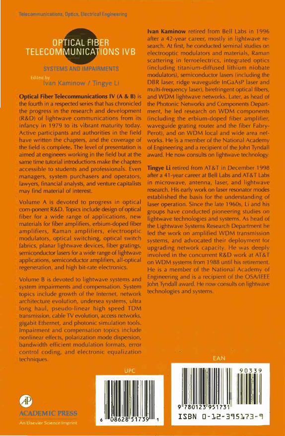
Copyright © 2022 FDOKUMEN